University of Groningen

Controlling omitted variables and measurement errors by means of constrainedautoregression and structural equation modelingSuparman, Yusep

IMPORTANT NOTE: You are advised to consult the publisher's version (publisher's PDF) if you wish to cite fromit. Please check the document version below.

Document VersionPublisher's PDF, also known as Version of record

Publication date:2015

Link to publication in University of Groningen/UMCG research database

Citation for published version (APA):Suparman, Y. (2015). Controlling omitted variables and measurement errors by means of constrainedautoregression and structural equation modeling: Theory, simulations and application tomeasuringhousehold preference forin-house piped water in Indonesia. University of Groningen.

CopyrightOther than for strictly personal use, it is not permitted to download or to forward/distribute the text or part of it without the consent of theauthor(s) and/or copyright holder(s), unless the work is under an open content license (like Creative Commons).

The publication may also be distributed here under the terms of Article 25fa of the Dutch Copyright Act, indicated by the “Taverne” license.More information can be found on the University of Groningen website: https://www.rug.nl/library/open-access/self-archiving-pure/taverne-amendment.

Take-down policyIf you believe that this document breaches copyright please contact us providing details, and we will remove access to the work immediatelyand investigate your claim.

Downloaded from the University of Groningen/UMCG research database (Pure): http://www.rug.nl/research/portal. For technical reasons thenumber of authors shown on this cover page is limited to 10 maximum.

Download date: 22-03-2022

  

53  

Chapter 3 Controlling for Time-Varying Omitted

Variables in Panel Data Models:

Evidence from a Monte-Carlo

Simulation

Abstract

Based on Monte-Carlo simulations, this paper presents evidence on the

performance of latent fixed effects regression, demeaning, first order differencing,

autoregression and constrained autoregression as methods to control for time-varying

omitted variables in panel data models. The data are generated from a standard regression

model with three explanatory variables, three time periods and one thousand cross

sectional units. From the bias, the standard error and the mean squared error of the

estimators of the regression coefficients of the included variables, we conclude that

constrained autoregression (Suparman et al., 2014) outperforms the alternative omitted

variables correction procedures. Regression of the log-transformed absolute bias on the

log- transformed simulation parameters identifies the main determinants of the bias of

each correction procedure.

Keywords: omitted variable bias, constrained autoregression, latent fixed effect,

demeaning, first order differencing, autoregression, Monte-Carlo simulation

1. Introduction

An important, but often ignored problem in applied social science research is the

omission of systematic explanatory variables from a regression model. If the omitted

variables are correlated with the included controls - which is usually the case in the social

sciences - ordinary least square (OLS) and standard maximum likelihood (ML) are biased

54  

and inconsistent. This even holds if only one omitted variable is correlated with one

control and the included controls are correlated.

The problem of omitted variable bias has been well addressed in standard text

books like Greene (2003) and Wooldridge (2002). The problem can be identified by

means of specification tests such as Ramsey’s (1969), Hausman’s (1978), Chamberlain’s

(1982), Angrist and Newey’s (1991) and Ahn and Low’s (1996). Omitted variables can

be controlled for by means of instrumental variables methods or panel data methods.

The present paper is restricted to panel data methods. Below we briefly summarize the

main panel data approaches. Details are presented in the next section.

Two types of panel data approaches to omitted variables can be distinguished. The

first type relates to time-invariant omitted variables, the second to time-varying omitted

variables. The time-invariant approaches comprise:

1. The fixed effect approach (FE) which models the omitted variables by means of a

dummy variable for each cross sectional unit (see e.g. Baltagi, 2005 and Greene,

2003).

2. The latent fixed effect model (LFE) which represents the omitted variables by means

of a latent variable whose variance and covariances with the explanatory variables at

each time point are estimated (Bollen, 2008).

3. First order differencing (FOD) which removes the omitted variables from the model

by means of differencing and performs the analysis in terms of first order differences

of the included variables (Wooldridge, 2002).

4. Demeaning (DR) which also removes the omitted variables from the model by way of

differencing and performs the regression in terms of the included variables with their

means subtracted (Baltagi, 2005).

  

55  

Most empirical studies routinely adopt a time-invariant approach to control for omitted

variables. See amongst others Brückner (2013), Kim (2014) and Sobel (2012). However,

application of a time-invariant approach is invalid, if the omitted variables evolve over

time. Suparman et al. (in press) illustrates that such application leads to another type of

bias.

Two types of time-varying approaches to control for omitted variables can be

distinguished. The first, the autoregressive approach (AR), captures the omitted variables

by the one-period lagged dependent variable (Wooldridge, 2002). Since the lagged

dependent variable is taken as a proxy for the omitted variables, it is subject to

approximation error. If the approximation error is correlated with the controls, OLS is

biased. The second time-variant approach, constrained autoregression model (CAR), is

based on the assumption that the omitted variables evolve according to an autoregression

model. Accordingly, the omitted variables are captured by the lagged dependent and the

lagged independent variables subject to constraints on the corresponding parameters.

Note that CAR could also be subject to approximation bias. Applications of CAR are still

very rare and no assessments of its relative performance have been undertaken.

In this study, we conduct a Monte-Carlo simulation study to evaluate the

performance of the above mentioned methods to reduce the bias and the mean squared

error due to the omission of a time-varying systematic variable in a regression model with

three explanatory variables. Note that we exclude FE from the study since its estimates

are identical to the DR estimates (Baltagi, 2005; Greene, 2003). In addition, we restrict

our simulation to a large cross sectional sample for the following reasons. First, the focus

of this paper is on bias reduction. A large sample size reduces the standard error and thus

provides better insight into each method’s bias reduction potential. Secondly, since we

use the maximum likelihood (ML) method to estimate the models, a large sample is

56  

required to achieve its consistency and efficiency properties (Casella and Berger, 2002).

Thirdly, many micro panel data sets like the Indonesia Family Life Survey (IFLS) (

Suparman, 2014 ) and Interuniversitair Steunpunt Politieke Opinie-onderzoek (ISPO)

(Angraeni et al., 2014 ) are based on large cross sectional samples.

2. A synopsis of methods to control for time-varying omitted

variables in panel data models

Consider the regression model

it

b

kkitk

a

jjitjit zxy

110 . (1)

for unit Ni ,,2,1 and wave Tt ,,2,1 , with it an independent-identically-

distributed (iid) random error satisfying the zero conditional mean assumption. Suppose

the variables kz , for any ,2,1b , are omitted from (1) such that the omitted variables

model

it

a

jjitjit xy

10 (2)

is estimated. Generally, the ordinary least square (OLS) estimator of the coefficients j

is biased (omitted variable bias).1

                                                            1 For a=1, b=1 and zxz xz 101 11

(the regression of the omitted variable on the included control

variable), the bias of the OLS estimator of 1 is 11 . For a>1, b=1, the bias of the OLS estimator of each

j is not only determined by k and jk xz but also by the covariances between the included variables and

the covariances between the omitted variable and the included controls. In the case of several omitted variables, the previous set of covariances needs to be expanded to also include the covariances among the omitted variables (Wooldridge, 2002).

  

57  

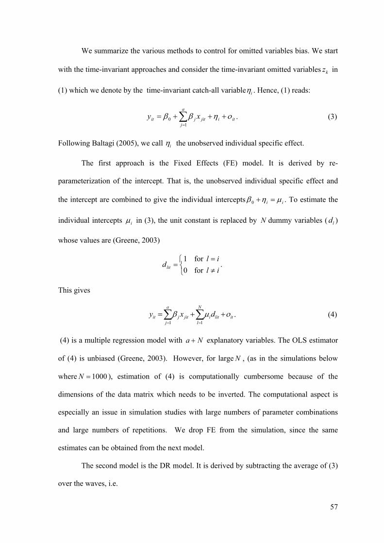
We summarize the various methods to control for omitted variables bias. We start

with the time-invariant approaches and consider the time-invariant omitted variables kz in

(1) which we denote by the time-invariant catch-all variable i . Hence, (1) reads:

iti

a

jjitjit xy

10 . (3)

Following Baltagi (2005), we call i the unobserved individual specific effect.

The first approach is the Fixed Effects (FE) model. It is derived by re-

parameterization of the intercept. That is, the unobserved individual specific effect and

the intercept are combined to give the individual intercepts ii 0 . To estimate the

individual intercepts i in (3), the unit constant is replaced by N dummy variables ( ld )

whose values are (Greene, 2003)

il

ildlit for 0

for 1.

This gives

it

N

lliti

a

jjitjit dxy

11

. (4)

(4) is a multiple regression model with Na explanatory variables. The OLS estimator

of (4) is unbiased (Greene, 2003). However, for large N , (as in the simulations below

where 1000N ), estimation of (4) is computationally cumbersome because of the

dimensions of the data matrix which needs to be inverted. The computational aspect is

especially an issue in simulation studies with large numbers of parameter combinations

and large numbers of repetitions. We drop FE from the simulation, since the same

estimates can be obtained from the next model.

The second model is the DR model. It is derived by subtracting the average of (3)

over the waves, i.e.

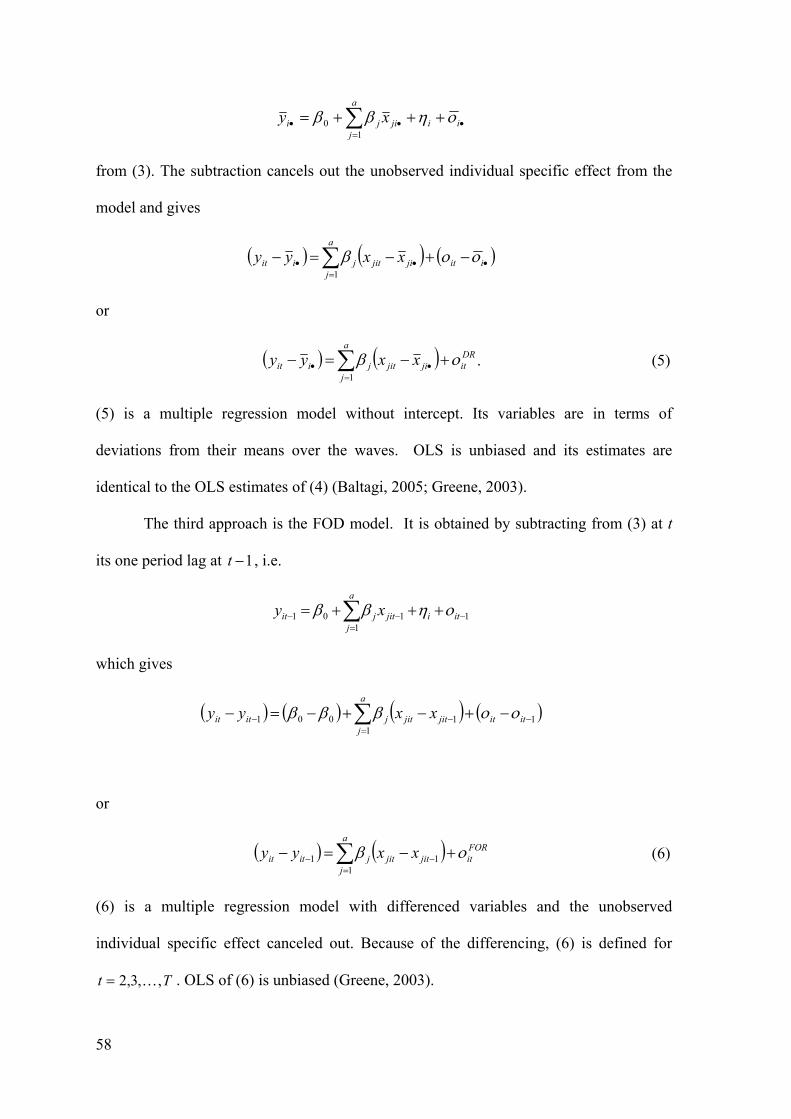
58  

ii

a

jjiji xy

10

from (3). The subtraction cancels out the unobserved individual specific effect from the

model and gives

iit

a

jjijitjiit xxyy

1

or

DRit

a

jjijitjiit xxyy

1

. (5)

(5) is a multiple regression model without intercept. Its variables are in terms of

deviations from their means over the waves. OLS is unbiased and its estimates are

identical to the OLS estimates of (4) (Baltagi, 2005; Greene, 2003).

The third approach is the FOD model. It is obtained by subtracting from (3) at t

its one period lag at 1t , i.e.

11

101

iti

a

jjitjit xy

which gives

11

1001

itit

a

jjitjitjitit xxyy

or

FORit

a

jjitjitjitit xxyy

111 (6)

(6) is a multiple regression model with differenced variables and the unobserved

individual specific effect canceled out. Because of the differencing, (6) is defined for

Tt ,,3,2 . OLS of (6) is unbiased (Greene, 2003).

  

59  

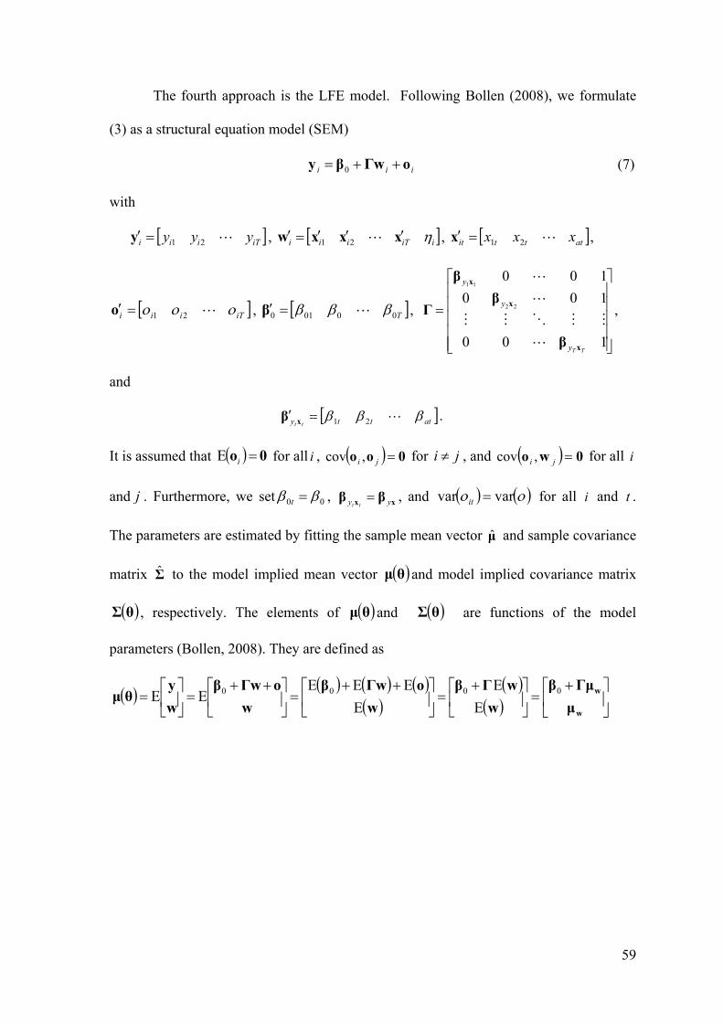
The fourth approach is the LFE model. Following Bollen (2008), we formulate

(3) as a structural equation model (SEM)

iii οΓwβy 0 (7)

with

iTiii yyy 21y , iiTiii xxxw 21 , atttit xxx 21x ,

iTiii 21ο , T00010 β ,

100

100

100

22

11

TTy

y

y

x

x

x

β

β

β

Γ

,

and

attty tt 21 xβ .

It is assumed that 0ο iE for all i , 0οο ji ,cov for ji , and 0wο ji ,cov for all i

and j . Furthermore, we set 00 t , xx ββ yy tt , and varvar it for all i and t .

The parameters are estimated by fitting the sample mean vector μ̂ and sample covariance

matrix Σ̂ to the model implied mean vector θμ and model implied covariance matrix

θΣ , respectively. The elements of θμ and θΣ are functions of the model

parameters (Bollen, 2008). They are defined as

w

w

μ

Γμβ

w

wΓβ

w

οΓwβ

w

οΓwβ

w

yθμ 0000

E

E

E

EEEEE

60  

wwww

wwοοww

ΣΓΣ

ΓΣΣΓΓΣ

ww,οw,Γww,

wο,wΓw,οο,ΓwΓw,

ww,οΓwβw

wοΓwβοΓwβοΓwβ

ww,yw,

w,yyy,wy

w

yθΣ

covcovcov

covcovcovcov

cov,cov

,cov,cov

covcov

covcov,cov

0

000

wμ and wwΣ are the mean vector and covariance matrix of the covariates in w . οοΣ is

the covariance matrix of the error terms. The covariances between i and the other

elements of w are given in the last row and column of wwΣ . The maximum likelihood

estimator (ML) of (7) is consistent (Jöreskog and Sörbom, 1996).

Now, we turn to the time-variant case. The first, the AR approach, uses the lagged

dependent variable as an approximation to the unobserved individual specific effect

(Wooldridge, 2002). Inclusion of the lagged dependent variable into model (2) gives the

following autoregression model

ARit

a

jjitjit

ARit xyy

110 . (8)

Reduction of omitted variable bias by means of (8) depends on the relationship between

ity and it . This relationship can be written as

ititity 101

with it the error term. For 2T , OLS of (8) gives a consistent estimator of j , if it is

uncorrelated with itx1 , …, aitx and 1ity . For 2T , OLS is inconsistent, if the errors ARit

follow an AR(1) because in that case the lagged dependent variable 1ity which is

  

61  

correlated with the error term ARit 1 at 1t ,is correlated with the current errors. Baltagi’s

(2005) ML is a consistent estimator of (8) in this case.

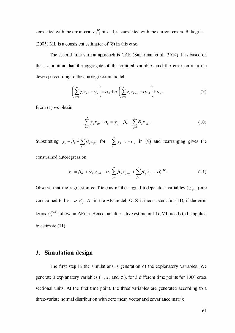
The second time-variant approach is CAR (Suparman et al., 2014). It is based on

the assumption that the aggregate of the omitted variables and the error term in (1)

develop according to the autoregression model

itit

b

kkitkit

b

kkitk zz

1

1110

1

. (9)

From (1) we obtain

a

jjitjitit

b

kkitk xyz

10

1

. (10)

Substituting

a

jjitjit xy

10 for it

b

kkitk z

1

in (9) and rearranging gives the

constrained autoregression

CARit

a

jjitj

a

jjitjittit xxyy

1111110 . (11)

Observe that the regression coefficients of the lagged independent variables ( 1jtx ) are

constrained to be j1 . As in the AR model, OLS is inconsistent for (11), if the error

terms CARit follow an AR(1). Hence, an alternative estimator like ML needs to be applied

to estimate (11).

3. Simulation design

The first step in the simulations is generation of the explanatory variables. We

generate 3 explanatory variables ( v , x , and z ), for 3 different time points for 1000 cross

sectional units. At the first time point, the three variables are generated according to a

three-variate normal distribution with zero mean vector and covariance matrix

62  

1,cov,cov

1,cov

1

zxzv

xvΣ .

At the second and third time point, the variables are generated according to the process

uitituit uu 1 with 21,0~ u

uit N , for zxvu ,, and 3,2t . The following

observations apply. First, we impose the standard restriction 0,cov 1 uititu . Secondly,

to keep the variance of the dependent variable constant over time and thus to stabilize the

standard errors over time, we impose 21var uuit . This restriction keeps the variances

of the variables fixed at 1: uititu

uitituit uuu ,cov2varvarvar 11

2

11 22 uu

for 3,2t .

For xv,cov , zv,cov and zx,cov as well as for u , we take the values 0.1,

0.3, 0.5, 0.7 and 0.9. Note that some of the combinations of the parameter values,

particularly those with the value of 0.9, produce non-positive definite Σ s. Since data

generation of multinormally distributed variables requires a positive definite Σ , we

exclude these combinations from the simulations. With the five values of each of the six

simulation parameters ( xv,cov , zv,cov , zx,cov , v , x , and z ), we have

56=15,625 combinations of the parameters values. Subtraction of the non-positive definite

Σ cases gives 13,000 combinations.

Next, given the explanatory variables and error term, we generate the dependent

variable according to the true model

yititzitxitvit zxvy ,

with 2,0~ yNyit

for 3,2,1t , and with values of v and x equal to 0.3, z equal to

1.0, and 2y

equal to 0.1.

  

63  

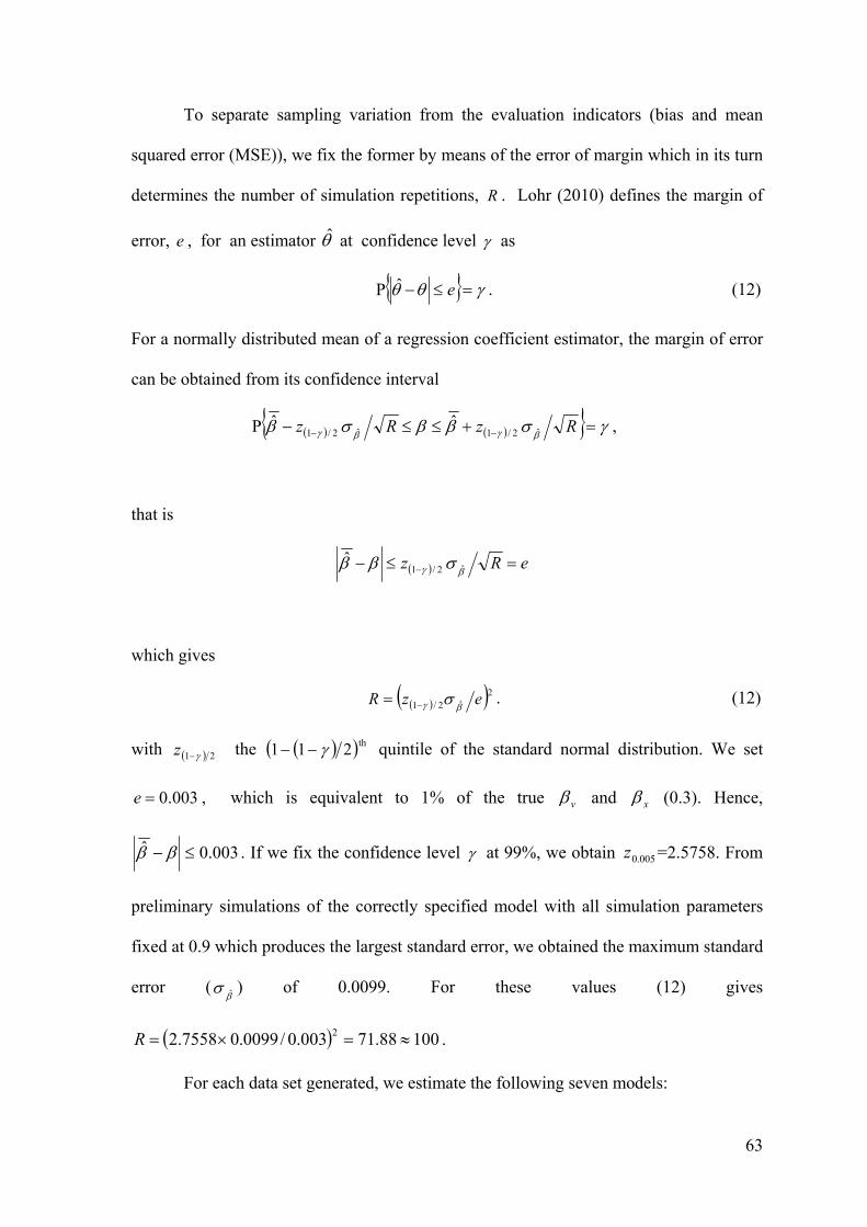
To separate sampling variation from the evaluation indicators (bias and mean

squared error (MSE)), we fix the former by means of the error of margin which in its turn

determines the number of simulation repetitions, R . Lohr (2010) defines the margin of

error, e , for an estimator ̂ at confidence level as

eˆP . (12)

For a normally distributed mean of a regression coefficient estimator, the margin of error

can be obtained from its confidence interval

RzRz ˆ2/1ˆ2/1ˆˆP ,

that is

eRz ˆ2/1ˆ

which gives

2ˆ2/1 ezR . (12)

with 21 z the th211 quintile of the standard normal distribution. We set

003.0e , which is equivalent to 1% of the true v and x (0.3). Hence,

003.0ˆ . If we fix the confidence level at 99%, we obtain 005.0z =2.5758. From

preliminary simulations of the correctly specified model with all simulation parameters

fixed at 0.9 which produces the largest standard error, we obtained the maximum standard

error (

ˆ ) of 0.0099. For these values (12) gives

10088.71003.0/0099.07558.2 2 R .

For each data set generated, we estimate the following seven models:

64  

1. The correctly specified model (CR)

000000 ititzitxitvit zxvy ,

for 3,2,1t . CR is estimated to evaluate the data generation process. Specifically, we

compare the mean of the bias of 0x to the margin of error of 0.003. A bias, which is

equal to or a smaller than 0.003, indicates an adequate data generation process. Note

that we only present the bias and individual MSE for one regression coefficient, i.e.

x , because the results for the other regression coefficient are the same due to equal

values of the regression coefficients and identical simulation parameters.

2. The under-specified regression model (UR):

11110 ititxitvit xvy

for 3,2,1t . UR is estimated without correction for the omitted variable tz . Hence, it

provides insight into omitted variable bias. Note that if UR produced the smallest

bias, the correction approaches presented in section 2 would be inadequate to correct

for omitted variables.

3. The latent individual effect model (LFE):

22220 ititxitvit xvy ,

for 3,2,1t .

4. The demeaned regression model (DR):

33330 itiitxiitviit xxvvyy ,

for 3,2,1t .

5. The first order difference model (FOD):

41

41

4401 itititxititvitit xxvvyy ,

for 3,2t .

6. The autoregression model (AR):

  

65  

51

55550 itititxitvit yxvy ,

for 3,2t ;

7. The constrained autoregression model (CAR):

61

661

661

66660 ititxitvititxitvit xvyxvy , (1)

for 3,2t .

The above models are estimated by means of the OpenMx maximum likelihood

procedure (Boker et al., 2011) in R. The seven models are formulated as covariance

structure models (SEM). The simulation syntax is available at Appendix 3.1.

The performance of the seven models is evaluated by means of the bias, standard

error, and mean squared error. That is, for model j and x we calculate

jx

R

r

jxr

jx R

1

ˆˆb ,

R

R

r

jx

jxr

jx

1

2ˆˆ

ˆse

withR

R

r

jx

jx

1

ˆˆ

, and

22 ˆseˆbˆmse jx

jx

jx x .

In addition, to get insight into their impacts on the bias, we regress jx̂b on the

covariances among the included controls, the covariances among the included controls

and the omitted variable, and the autoregression parameters of the included and excluded

explanatory variables 2:

jjjj

zj

xj

vjjj

x

zxzvxv

,covln,covln,covln

lnlnlnˆbln

654

3210, (13)

                                                            2 In a panel data model, the autoregression parameters determine the covariances among the variables in different waves which in their turn affect the omitted variable bias. Hence, the autoregression coefficient of the omitted variable affects the performance of the seven models presented above.

66  

for 6,,2,1 j . We estimate a lnln model because of the non-linear relationship

between the bias and its determinants.

4. Results

The complete set of outcomes of the evaluation indicators (bias, standard error,

MSE) for x ordered by the simulation parameters ( xv,cov , zv,cov , zx,cov , v ,

x , and z ) for the seven models is available from the author upon request. In Table 3.1

we present summary statistics (minimum, maximum, mean, and standard deviation) for

each model over all values of the simulation parameters.

Before going into detail, we observe that the estimation procedure converged for

every data set. Furthermore, from Table 3.1 it follows that the maximum absolute bias of

the correctly specified model (CR) is 0.002 which is well below the a priori fixed

benchmark margin of error of 0.003 (see section 3). These features indicate the adequacy

of the data generation process and of the number of replications.

We first evaluate the seven models according to the mean x̂b and the mean

x̂mse . Table 1 shows that CR performs best and UR worst, as expected. It furthermore

shows that the CAR results are closest to the CR outcomes. On average, CAR reduces

98.4% of the bias in UR. Furthermore, the CAR MSE is 86.2 times smaller than the UR

MSE. Next closest to the CR outcomes are the AR results. It reduces 66.7% of the UR

bias and its MSE is 8.5 times smaller than the UR outcomes.

The time-invariant approaches perform substantially less than the time-variant

approaches, as expected. DOF reduces 52.3% of the UR bias while its MSE is 4.8 times

smaller. The LFE bias reduction is about 52.2% and its MSEs is 3.2 times smaller than

  

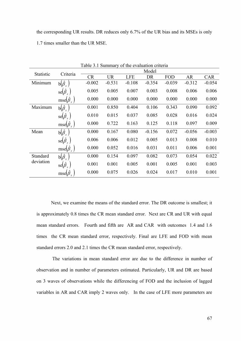
67  

the corresponding UR results. DR reduces only 6.7% of the UR bias and its MSEs is only

1.7 times smaller than the UR MSE.

Table 3.1 Summary of the evaluation criteria

Statistic Criteria Model

CR UR LFE DR FOD AR CAR Minimum x̂b -0.002 -0.531 -0.108 -0.354 -0.039 -0.312 -0.054

x̂se 0.005 0.005 0.007 0.003 0.008 0.006 0.006

x̂mse 0.000 0.000 0.000 0.000 0.000 0.000 0.000

Maximum x̂b 0.001 0.850 0.404 0.106 0.343 0.090 0.092

x̂se 0.010 0.015 0.037 0.085 0.028 0.016 0.024

x̂mse 0.000 0.722 0.163 0.125 0.118 0.097 0.009

Mean x̂b 0.000 0.167 0.080 -0.156 0.072 -0.056 -0.003

x̂se 0.006 0.006 0.012 0.005 0.013 0.008 0.010

x̂mse 0.000 0.052 0.016 0.031 0.011 0.006 0.001

Standard deviation

x̂b 0.000 0.154 0.097 0.082 0.073 0.054 0.022

x̂se 0.001 0.001 0.005 0.001 0.005 0.001 0.003

x̂mse 0.000 0.075 0.026 0.024 0.017 0.010 0.001

Next, we examine the means of the standard error. The DR outcome is smallest; it

is approximately 0.8 times the CR mean standard error. Next are CR and UR with equal

mean standard errors. Fourth and fifth are AR and CAR with outcomes 1.4 and 1.6

times the CR mean standard error, respectively. Final are LFE and FOD with mean

standard errors 2.0 and 2.1 times the CR mean standard error, respectively.

The variations in mean standard error are due to the difference in number of

observation and in number of parameters estimated. Particularly, UR and DR are based

on 3 waves of observations while the differencing of FOD and the inclusion of lagged

variables in AR and CAR imply 2 waves only. In the case of LFE more parameters are

68  

estimated (i.e. the covariances between the latent individual effect and the independent

variables) than in the case of UR and DR which tends to increase its mean standard error.

Table 3.2 Percentage smallest bias, standard error and MSE. Model Criterion

x̂b x̂se x̂mse

UR 4.4 100.0 6.8 LFE 10.8 0.00 10.0 DR 0.00 0.00 3.5 FOD 13.0 0.00 9.9 AR 19.6 0.00 17.2 CAR 52.2 0.00 52.7

Table 3.3 The determinants of x̂bln

Coefficient / Regressor

Model

UR LFE DR FOD AR CAR

0 /Unit constant -0.778 -2.659 -1.357 -2.900 -2.597 -4.176 (0.200) (0.027) (0.170) (0.220) (0.220) (0.021)

1 / xln -0.056 0.016 0.038 0.044 0.009 0.015 (0.008) (0.011) (0.007) (0.009) (0.009) (0.009)

2 / xln 0.246 0.136 0.453 -0.015 0.472 0.103 (0.008) (0.011) (0.007) (0.009) (0.009) (0.009)

3 / zln 0.220 -0.577 0.285 -0.716 0.388 -0.195 (0.008) (0.011) (0.007) (0.009) (0.009) (0.009)

4 / xv,covln -0.138 -0.027 -0.012 -0.020 0.187 0.057 (0.008) (0.011) (0.007) (0.009) (0.009) (0.009)

5 / zv,covln -0.134 -0.296 0.251 -0.291 0.238 -0.097 (0.008) (0.011) (0.007) (0.009) (0.009) (0.009)

6 / zx,covln 1.361 1.095 -0.456 1.310 -0.611 0.105 (0.008) (0.011) (0.007) (0.009) (0.009) (0.009)

R2 0.69 0.51 0.48 0.68 0.43 0.07 Note: Standard errors within brackets.

Next, in Table 3.2, we compare the six models on the basis of the percentage of

smallest bias, standard error and MSE scored over all simulation parameters. That is,

Table 3.2 shows how well a given model estimates x in comparison to the other

models. Table 3.2, column 2, presents the percentage of smallest bias scored. It shows

  

69  

that both time-varying approaches outperform the time-invariant approaches with CAR

performing best. Table 3.2, columns 3, shows that UR outperforms the other approaches

in terms of standard error. The MSE results (Table 3.2 column 4) are similar to the bias

results: CAR and AR are superior to the time-invariant approaches with CAR performing

best.

We finally discuss for each model the determinants of the bias of the estimator of

the regression coefficient x . The estimated regression model (13) is presented in Table

3.3. Before going into detail, we note that that all the estimates are significant at 1% level.

Table 3.3, column 3, shows that for the under-specified model UR. 16̂ is the largest

coefficient. It means that the correlation between the omitted and the included variable (

zx,cov ) has the largest positive impact on omitted variable bias with an elasticity of

1.36%. The autocorrelation coefficients of x and of z ( 12̂ =0.25 and 1

3̂ =0.22,

respectively) also have positive impacts, though substantially smaller than zx,cov .

From column 4, it follows that also for LFE the covariance between x and z ( 26̂ =1.10)

has the largest impact, although it is substantially smaller than in the case of UR. For

LFE, the autocorrelation coefficient of the omitted variable and zv,cov have

mitigating impacts: 23̂ =-0.58 and 2

5̂ =-0.30, respectively. All other parameters have

minor impacts. Colum 5 shows that in the case of DR zx,cov and the autoregression of

x ( 36̂ =-0.46 and 3

2̂ =0.45) have the largest impacts in absolute value with the former

having a negative sign. In addition, the autoregression of the omitted variable and

zv,cov have quite large positive impacts ( 33̂ =-0.28 and 3

5̂ =0.25). In the case of FOD,

shown in column 6, xv,cov has the largest impact: 46̂ =1.31. The autocorrelation

coefficient z and zv,cov have mitigating impacts: 43̂ =-0.72 and 4

5̂ =-0.29. In the

70  

case of AR, column 7, the autoregression of the included variable has the largest impact (

52̂ =0.47), followed by z ( 5

3̂ =0.39) and zv,cov ( 55̂ =0.24). Column 8 shows that

in the case of CAR none of the simulation parameters has a substantial impact on the bias.

From the discussion of Table 3.3 it follows that the covariance between the

regressor and the omitted variable has the largest positive impact on omitted variable bias

in the case of UR, LFE, FOD, and CAR, although for the latter the impact is substantially

smaller than for the other methods. For DR and AR the impacts are negative.

Interestingly, the covariances between the omitted variable and the two included variables

have opposite signs. However, there are alternations. Cov(z,v) is negative in the case of

UR, LFE, FOD and CAR and positive for DR and AR. Moreover, the magnitudes in

absolute value of the impacts of these covariances differ. In addition, the autoregression

of the regressor and of the omitted variable have quite large impacts in absolute value.

In conclusion, for the time-invariant correction procedures and for AR, the bias

left in the estimator of a regression coefficient after controlling for the omitted variable, is

a complicated function of notably the covariances among the included variables and the

omitted variable, the autoregression coefficient of the omitted variable, and the

autoregression coefficient of the regressor, Only in the case of CAR, the impacts of the

determinants on x̂b are very small.

5. Conclusion

Omitted variables form a serious problem in social science research because they

lead to biased and inconsistent estimators. Two kinds of omitted variables can be

distinguished: time-invariant and time-variant. In line with this distinction the approaches

to control for omitted variables can be grouped into two categories. The first category

  

71  

consisting of the latent fixed effect model, the demeaned regression model and the first

order difference regression model, apply to time-invariant omitted variables. The second

category consisting of the autoregressive and the constrained autoregressive model has

been developed to control for time-varying omitted variables. In spite of their application

design to time-invariant omitted variables, the former group has been frequently used to

correct for time-varying omitted variables.

The main objective of this paper was the comparison of the above mentioned

methods to control for time-variant omitted variables in panel data models by means of

Monte Carlo simulations. The main finding is that the time-variant approaches

outperform the time-invariant methods in terms of bias and mean squared error. Another

finding is that autoregression is inferior to constrained autoregression for virtually all

simulation parameters values.

Analysis of the impacts of the simulation parameters on x̂b showed that for the

time-invariant correction procedures and the AR model the bias left in the estimator of a

regression coefficient after controlling for the omitted variable, is a complicated function

of notably the covariances among the included variables and the omitted variable, and of

the autoregression coefficients of the omitted variable and of the regressor. Only in the

case of CAR, the impacts of the determinants on x̂b are very small.

The constrained autoregression model was recently introduced (Suparman et al.,

2014a). Consequently, applications of it are still very limited (Suparman et al., 2014b

only). Hence, more empirical studies are needed to establish its usefulness. In addition,

further theoretical developments are required to adapt it to application in various

specialized areas of regression, e.g. spatial and state space regression.

72  

References

Ahn, S. C., & Low, S. (1996). A reformulation of the Hausman test for regression models

with pooled cross-setional time-series data. Journal of Econometrics, 71, 309-319.

Angrist, J. D., & Newey, W. K., (1991). Over-identification tests in earnings function

with fixed effects. Journal of Business and Economic Statistics, 9, 317-323.

Baltagi, H. B. (2005). Econometric analysis of panel data (3rd ed.). Chichester: John

Wiley and Sons.

Boker, S., Neale, M., Maes, H., Wilde, M., Spiegel, M., Brick, T., Spies, J., Estarbrook,

R., Kenny, S., Bates, T., Mehta, P., & Fox, J. (2011). OpenMx: An open source

extended structural equation modeling framework. Psychometrika, 76(2), 306-

317. DOI: 10.1007/S11336-010-9200-6.

Bollen, K. A. & Brand, J. E. (2010). A General panel model with random and fixed

effects: A structural equations approach. Social Force, 89(1), 1-34. DOI:

10.1353/sof.2010.0072.

Brückner, M. (2013). On the simultaneity problem in the aid and growth debate. Journal

of Applied Econometrics, 28, 126-150. DOI: 10.1002/jae.1259.

Casella, G., & Berger, R. L. (2002). Statistical inference. Duxbury.

Chamberlain, G. (1982). Multivariate regression models for panel data. Journal of

Econometrics, 18, 5-46.

Greene, W. (2003). Econometrics analysis (5th ed.). New Jersey: Prentice Hall.

Hausman, J. A. (1978). Specification tests in econometrics. Econometrica, 46, 1251-

1271.

Jöreskog, K. & Sörbom, D. (1996). LISREL 8: User’s reference guide. Chicago, IL:

Scientific Software International.

  

73  

Kim, D. & Oka, T. (2014). Divorce law reforms and divorce rate in the USA: An

interactive fixed-effects approach. Journal of Applied Econometrics, 29, 231-245.

DOI: 10.1002/jae2310.

Lohr, S. L. (2010). Sampling: Design and Analysis (2nd ed.). Boston, MA: Brooks/Cole.

Ramsey, J. B. (1969). Test for specification error in classical linear least-square analysis.

Journal of the Royal Statistical Association, Seri B, 71, 350-371.

Sobel, M. E. (2012), Does marriage boost men’s wages?: Identification on treatment

effects in fixed effect regression models for panel data. Journal of the American

Statistical Association, 107(498), 521-529. DOI: 10.1080/01621459.2011.646917

Suparman, Y., Folmer, H., & Oud, J. H. L. (2014). Hedonic price models with omitted

variables and measurement errors: a constrained autoregression-structural

equation modeling approach with application to urban Indonesia. Journal of

Geographical Systems, 16(1), 49-70. DOI: 10.1007/s10109-013-0186-3

Suparman, Y., Folmer, H., & Oud, J. H. L. (in press). The willingness to pay for in-house

piped water in urban and rural Indonesia. Papers in Regional Science. DOI:

10.1111/pirs.12124.

Wooldridge, J. M. (2002). Introductory econometrics: A modern approach (2nd ed.).

South-Western.

 

74  

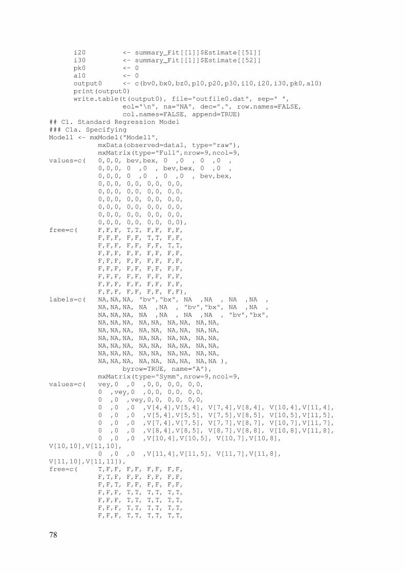
Appendix 3.1 Simulation Syntax (Bias Evaluation)

# Simulation # Constrained Autoregression # Spatial Lag-Autoregression setwd("D:/0sim5/") require(mvtnorm) require(OpenMx) # A. Simulation setting and Population Parameters for (av in 0:3) { for (ax in 0:av) # 0-4 { for (az in 0:0) # 0-4 { for (r in 0:0) # 0-4 { for (s in 0:0) { for (t in 0:0) { #for (b in 1:1) #{ set.seed(-3) # Initial random number seed K <- 100 # Number of simulation replication N <- 1000 # sample size ## parameters vx1 <- 1 #var(x1) vz1 <- 1 #var(z1) vv1 <- 1 #var(v1) cvx <- (1+2*r)/10 #cor(x1,z1) cvz <- (1+2*s)/10 #cor(v1,x1) cxz <- (1+2*t)/10 #cor(v1,z1) alv <- (1+2*av)/10 #autoregression v alx <- (1+2*ax)/10 #autoregression x alz <- (1+2*az)/10 #autoregression z vev <- 1-alv^2 #autoregression v error variance vex <- 1-alx^2 #autoregression x error variance vez <- 1-alz^2 #autoregression z error variance bev <- 0.3 #be(v->y) bex <- 0.3 #be(x->y) bez <- 1.0 #be(z->y) By <- matrix(c(bev,bex,bez),nrow=1,ncol=3) vey <- .1 #var(ey) # B. Data Generation ## Generating V1, X1 and Z1 Sxz <- matrix(c(vv1,cvx,cvz, cvx,vx1,cxz, cvz,cxz,vz1), nrow=3,ncol=3, byrow=TRUE) Mxz <- matrix(c(0,0,0),nrow=3, ncol=1) XZ1 <- rmvnorm(N,Mxz,Sxz) ## Generating V2, X2 and Z2 Sexz <- matrix(c(vev,0 ,0 , 0 ,vex,0 , 0 ,0 ,vez), nrow=3,ncol=3, byrow=TRUE) Mexz <- matrix(c(0,0,0),nrow=3, ncol=1)

  

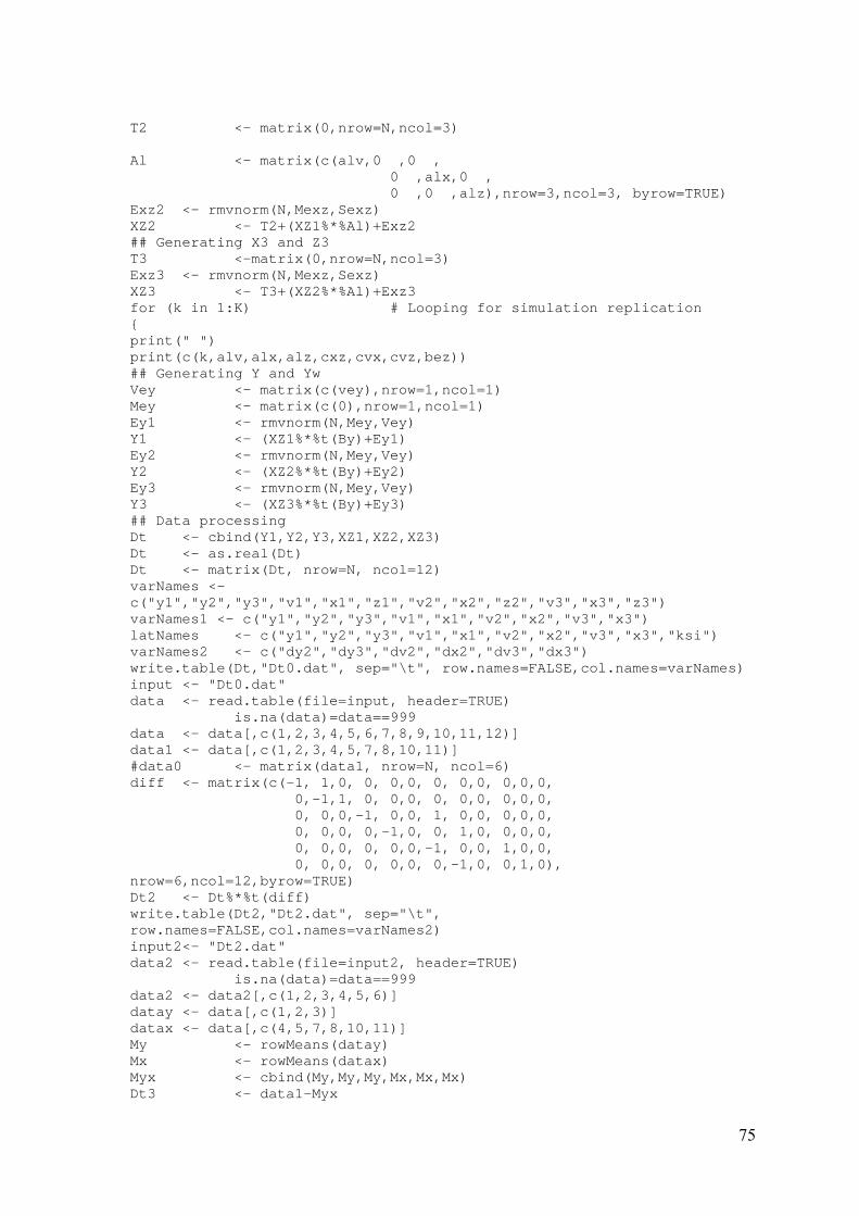
75  

T2 <- matrix(0,nrow=N,ncol=3) Al <- matrix(c(alv,0 ,0 , 0 ,alx,0 , 0 ,0 ,alz),nrow=3,ncol=3, byrow=TRUE) Exz2 <- rmvnorm(N,Mexz,Sexz) XZ2 <- T2+(XZ1%*%Al)+Exz2 ## Generating X3 and Z3 T3 <-matrix(0,nrow=N,ncol=3) Exz3 <- rmvnorm(N,Mexz,Sexz) XZ3 <- T3+(XZ2%*%Al)+Exz3 for (k in 1:K) # Looping for simulation replication { print(" ") print(c(k,alv,alx,alz,cxz,cvx,cvz,bez)) ## Generating Y and Yw Vey <- matrix(c(vey),nrow=1,ncol=1) Mey <- matrix(c(0),nrow=1,ncol=1) Ey1 <- rmvnorm(N,Mey,Vey) Y1 <- (XZ1%*%t(By)+Ey1) Ey2 <- rmvnorm(N,Mey,Vey) Y2 <- (XZ2%*%t(By)+Ey2) Ey3 <- rmvnorm(N,Mey,Vey) Y3 <- (XZ3%*%t(By)+Ey3) ## Data processing Dt <- cbind(Y1,Y2,Y3,XZ1,XZ2,XZ3) Dt <- as.real(Dt) Dt <- matrix(Dt, nrow=N, ncol=12) varNames <- c("y1","y2","y3","v1","x1","z1","v2","x2","z2","v3","x3","z3") varNames1 <- c("y1","y2","y3","v1","x1","v2","x2","v3","x3") latNames <- c("y1","y2","y3","v1","x1","v2","x2","v3","x3","ksi") varNames2 <- c("dy2","dy3","dv2","dx2","dv3","dx3") write.table(Dt,"Dt0.dat", sep="\t", row.names=FALSE,col.names=varNames) input <- "Dt0.dat" data <- read.table(file=input, header=TRUE) is.na(data)=data==999 data <- data[,c(1,2,3,4,5,6,7,8,9,10,11,12)] data1 <- data[,c(1,2,3,4,5,7,8,10,11)] #data0 <- matrix(data1, nrow=N, ncol=6) diff <- matrix(c(-1, 1,0, 0, 0,0, 0, 0,0, 0,0,0, 0,-1,1, 0, 0,0, 0, 0,0, 0,0,0, 0, 0,0,-1, 0,0, 1, 0,0, 0,0,0, 0, 0,0, 0,-1,0, 0, 1,0, 0,0,0, 0, 0,0, 0, 0,0,-1, 0,0, 1,0,0, 0, 0,0, 0, 0,0, 0,-1,0, 0,1,0), nrow=6,ncol=12,byrow=TRUE) Dt2 <- Dt%*%t(diff) write.table(Dt2,"Dt2.dat", sep="\t", row.names=FALSE,col.names=varNames2) input2<- "Dt2.dat" data2 <- read.table(file=input2, header=TRUE) is.na(data)=data==999 data2 <- data2[,c(1,2,3,4,5,6)] datay <- data[,c(1,2,3)] datax <- data[,c(4,5,7,8,10,11)] My <- rowMeans(datay) Mx <- rowMeans(datax) Myx <- cbind(My,My,My,Mx,Mx,Mx) Dt3 <- data1-Myx

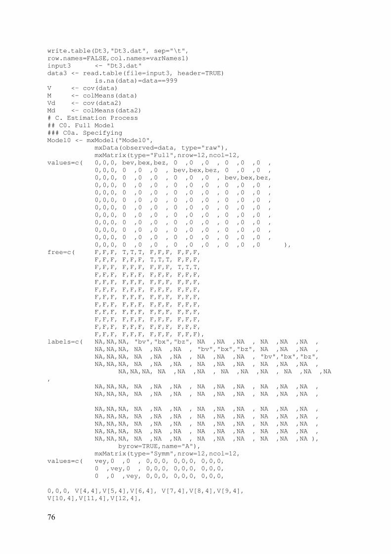
76  

write.table(Dt3,"Dt3.dat", sep="\t", row.names=FALSE,col.names=varNames1) input3 <- "Dt3.dat" data3 <- read.table(file=input3, header=TRUE) is.na(data)=data==999 V <- cov(data) M <- colMeans(data) Vd <- cov(data2) Md <- colMeans(data2) # C. Estimation Process ## C0. Full Model ### C0a. Specifying Model0 <- mxModel("Model0", mxData(observed=data, type="raw"), mxMatrix(type="Full",nrow=12,ncol=12, values=c( 0,0,0, bev,bex,bez, 0 ,0 ,0 , 0 ,0 ,0 , 0,0,0, 0 ,0 ,0 , bev,bex,bez, 0 ,0 ,0 , 0,0,0, 0 ,0 ,0 , 0 ,0 ,0 , bev,bex,bez, 0,0,0, 0 ,0 ,0 , 0 ,0 ,0 , 0 ,0 ,0 , 0,0,0, 0 ,0 ,0 , 0 ,0 ,0 , 0 ,0 ,0 , 0,0,0, 0 ,0 ,0 , 0 ,0 ,0 , 0 ,0 ,0 , 0,0,0, 0 ,0 ,0 , 0 ,0 ,0 , 0 ,0 ,0 , 0,0,0, 0 ,0 ,0 , 0 ,0 ,0 , 0 ,0 ,0 , 0,0,0, 0 ,0 ,0 , 0 ,0 ,0 , 0 ,0 ,0 , 0,0,0, 0 ,0 ,0 , 0 ,0 ,0 , 0 ,0 ,0 , 0,0,0, 0 ,0 ,0 , 0 ,0 ,0 , 0 ,0 ,0 , 0,0,0, 0 ,0 ,0 , 0 ,0 ,0 , 0 ,0 ,0 ), free=c( F,F,F, T,T,T, F,F,F, F,F,F, F,F,F, F,F,F, T,T,T, F,F,F, F,F,F, F,F,F, F,F,F, T,T,T, F,F,F, F,F,F, F,F,F, F,F,F, F,F,F, F,F,F, F,F,F, F,F,F, F,F,F, F,F,F, F,F,F, F,F,F, F,F,F, F,F,F, F,F,F, F,F,F, F,F,F, F,F,F, F,F,F, F,F,F, F,F,F, F,F,F, F,F,F, F,F,F, F,F,F, F,F,F, F,F,F, F,F,F, F,F,F, F,F,F, F,F,F, F,F,F, F,F,F, F,F,F, F,F,F, F,F,F), labels=c( NA,NA,NA, "bv","bx","bz", NA ,NA ,NA , NA ,NA ,NA , NA,NA,NA, NA ,NA ,NA , "bv","bx","bz", NA ,NA ,NA , NA,NA,NA, NA ,NA ,NA , NA ,NA ,NA , "bv","bx","bz", NA,NA,NA, NA ,NA ,NA , NA ,NA ,NA , NA ,NA ,NA , NA,NA,NA, NA ,NA ,NA , NA ,NA ,NA , NA ,NA ,NA , NA,NA,NA, NA ,NA ,NA , NA ,NA ,NA , NA ,NA ,NA , NA,NA,NA, NA ,NA ,NA , NA ,NA ,NA , NA ,NA ,NA , NA,NA,NA, NA ,NA ,NA , NA ,NA ,NA , NA ,NA ,NA , NA,NA,NA, NA ,NA ,NA , NA ,NA ,NA , NA ,NA ,NA , NA,NA,NA, NA ,NA ,NA , NA ,NA ,NA , NA ,NA ,NA , NA,NA,NA, NA ,NA ,NA , NA ,NA ,NA , NA ,NA ,NA , NA,NA,NA, NA ,NA ,NA , NA ,NA ,NA , NA ,NA ,NA ), byrow=TRUE,name="A"), mxMatrix(type="Symm",nrow=12,ncol=12, values=c( vey,0 ,0 , 0,0,0, 0,0,0, 0,0,0, 0 ,vey,0 , 0,0,0, 0,0,0, 0,0,0, 0 ,0 ,vey, 0,0,0, 0,0,0, 0,0,0, 0,0,0, V[4,4],V[5,4],V[6,4], V[7,4],V[8,4],V[9,4], V[10,4],V[11,4],V[12,4],

  

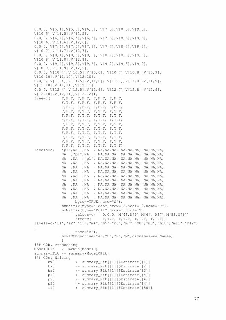
77  

0,0,0, V[5,4],V[5,5],V[6,5], V[7,5],V[8,5],V[9,5], V[10,5],V[11,5],V[12,5], 0,0,0, V[6,4],V[6,5],V[6,6], V[7,6],V[8,6],V[9,6], V[10,6],V[11,6],V[12,6], 0,0,0, V[7,4],V[7,5],V[7,6], V[7,7],V[8,7],V[9,7], V[10,7],V[11,7],V[12,7], 0,0,0, V[8,4],V[8,5],V[8,6], V[8,7],V[8,8],V[9,8], V[10,8],V[11,8],V[12,8], 0,0,0, V[9,4],V[9,5],V[9,6], V[9,7],V[9,8],V[9,9], V[10,9],V[11,9],V[12,9], 0,0,0, V[10,4],V[10,5],V[10,6], V[10,7],V[10,8],V[10,9], V[10,10],V[11,10],V[12,10], 0,0,0, V[11,4],V[11,5],V[11,6], V[11,7],V[11,8],V[11,9], V[11,10],V[11,11],V[12,11], 0,0,0, V[12,4],V[12,5],V[12,6], V[12,7],V[12,8],V[12,9], V[12,10],V[12,11],V[12,12]), free=c( T,F,F, F,F,F, F,F,F, F,F,F, F,T,F, F,F,F, F,F,F, F,F,F, F,F,T, F,F,F, F,F,F, F,F,F, F,F,F, T,T,T, T,T,T, T,T,T, F,F,F, T,T,T, T,T,T, T,T,T, F,F,F, T,T,T, T,T,T, T,T,T, F,F,F, T,T,T, T,T,T, T,T,T, F,F,F, T,T,T, T,T,T, T,T,T, F,F,F, T,T,T, T,T,T, T,T,T, F,F,F, T,T,T, T,T,T, T,T,T, F,F,F, T,T,T, T,T,T, T,T,T, F,F,F, T,T,T, T,T,T, T,T,T), labels=c( "p1",NA ,NA , NA,NA,NA, NA,NA,NA, NA,NA,NA, NA ,"p1",NA , NA,NA,NA, NA,NA,NA, NA,NA,NA, NA ,NA ,"p1", NA,NA,NA, NA,NA,NA, NA,NA,NA, NA ,NA ,NA , NA,NA,NA, NA,NA,NA, NA,NA,NA, NA ,NA ,NA , NA,NA,NA, NA,NA,NA, NA,NA,NA, NA ,NA ,NA , NA,NA,NA, NA,NA,NA, NA,NA,NA, NA ,NA ,NA , NA,NA,NA, NA,NA,NA, NA,NA,NA, NA ,NA ,NA , NA,NA,NA, NA,NA,NA, NA,NA,NA, NA ,NA ,NA , NA,NA,NA, NA,NA,NA, NA,NA,NA, NA ,NA ,NA , NA,NA,NA, NA,NA,NA, NA,NA,NA, NA ,NA ,NA , NA,NA,NA, NA,NA,NA, NA,NA,NA, NA ,NA ,NA , NA,NA,NA, NA,NA,NA, NA,NA,NA), byrow=TRUE,name="S"), mxMatrix(type="Iden",nrow=12,ncol=12,name="F"), mxMatrix(type="Full",nrow=1,ncol=12, values=c( 0,0,0, M[4],M[5],M[6], M[7],M[8],M[9]), free=c( T,T,T, T,T,T, T,T,T, T,T,T), labels=c("i1","i2","i3","m4","m5","m6","m7","m8","m9","m10","m11","m12"), name="M"), mxRAMObjective("A","S","F","M",dimnames=varNames) ) ### C0b. Processing Model0Fit <- mxRun(Model0) summary_Fit <- summary(Model0Fit) ### C0c. Writing bv0 <- summary_Fit[[1]]$Estimate[[1]] bx0 <- summary_Fit[[1]]$Estimate[[2]] bz0 <- summary_Fit[[1]]$Estimate[[3]] p10 <- summary_Fit[[1]]$Estimate[[4]] p20 <- summary_Fit[[1]]$Estimate[[4]] p30 <- summary_Fit[[1]]$Estimate[[4]] i10 <- summary_Fit[[1]]$Estimate[[50]]

78  

i20 <- summary_Fit[[1]]$Estimate[[51]] i30 <- summary_Fit[[1]]$Estimate[[52]] pk0 <- 0 al0 <- 0 output0 <- c(bv0,bx0,bz0,p10,p20,p30,i10,i20,i30,pk0,al0) print(output0) write.table(t(output0), file="outfile0.dat", sep=" ",

eol="\n", na="NA", dec=".", row.names=FALSE, col.names=FALSE, append=TRUE)

## C1. Standard Regression Model ### C1a. Specifying Model1 <- mxModel("Model1", mxData(observed=data1, type="raw"), mxMatrix(type="Full",nrow=9,ncol=9, values=c( 0,0,0, bev,bex, 0 ,0 , 0 ,0 , 0,0,0, 0 ,0 , bev,bex, 0 ,0 , 0,0,0, 0 ,0 , 0 ,0 , bev,bex, 0,0,0, 0,0, 0,0, 0,0, 0,0,0, 0,0, 0,0, 0,0, 0,0,0, 0,0, 0,0, 0,0, 0,0,0, 0,0, 0,0, 0,0, 0,0,0, 0,0, 0,0, 0,0, 0,0,0, 0,0, 0,0, 0,0), free=c( F,F,F, T,T, F,F, F,F, F,F,F, F,F, T,T, F,F, F,F,F, F,F, F,F, T,T, F,F,F, F,F, F,F, F,F, F,F,F, F,F, F,F, F,F, F,F,F, F,F, F,F, F,F, F,F,F, F,F, F,F, F,F, F,F,F, F,F, F,F, F,F, F,F,F, F,F, F,F, F,F), labels=c( NA,NA,NA, "bv","bx", NA ,NA , NA ,NA , NA,NA,NA, NA ,NA , "bv","bx", NA ,NA , NA,NA,NA, NA ,NA , NA ,NA , "bv","bx", NA,NA,NA, NA,NA, NA,NA, NA,NA, NA,NA,NA, NA,NA, NA,NA, NA,NA, NA,NA,NA, NA,NA, NA,NA, NA,NA, NA,NA,NA, NA,NA, NA,NA, NA,NA, NA,NA,NA, NA,NA, NA,NA, NA,NA, NA,NA,NA, NA,NA, NA,NA, NA,NA ), byrow=TRUE, name="A"), mxMatrix(type="Symm",nrow=9,ncol=9, values=c( vey,0 ,0 ,0,0, 0,0, 0,0, 0 ,vey,0 ,0,0, 0,0, 0,0, 0 ,0 ,vey,0,0, 0,0, 0,0, 0 ,0 ,0 ,V[4,4],V[5,4], V[7,4],V[8,4], V[10,4],V[11,4], 0 ,0 ,0 ,V[5,4],V[5,5], V[7,5],V[8,5], V[10,5],V[11,5], 0 ,0 ,0 ,V[7,4],V[7,5], V[7,7],V[8,7], V[10,7],V[11,7], 0 ,0 ,0 ,V[8,4],V[8,5], V[8,7],V[8,8], V[10,8],V[11,8], 0 ,0 ,0 ,V[10,4],V[10,5], V[10,7],V[10,8], V[10,10],V[11,10], 0 ,0 ,0 ,V[11,4],V[11,5], V[11,7],V[11,8], V[11,10],V[11,11]), free=c( T,F,F, F,F, F,F, F,F, F,T,F, F,F, F,F, F,F, F,F,T, F,F, F,F, F,F, F,F,F, T,T, T,T, T,T, F,F,F, T,T, T,T, T,T, F,F,F, T,T, T,T, T,T, F,F,F, T,T, T,T, T,T,

  

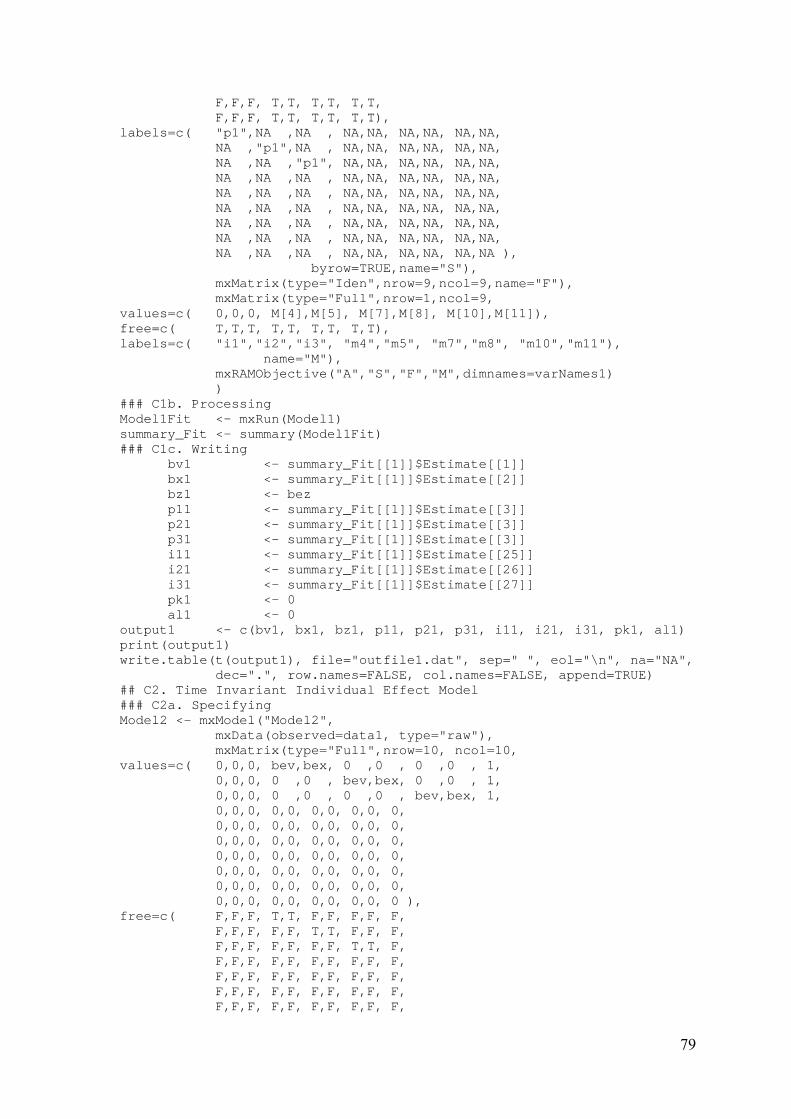
79  

F,F,F, T,T, T,T, T,T, F,F,F, T,T, T,T, T,T), labels=c( "p1",NA ,NA , NA,NA, NA,NA, NA,NA, NA ,"p1",NA , NA,NA, NA,NA, NA,NA, NA ,NA ,"p1", NA,NA, NA,NA, NA,NA, NA ,NA ,NA , NA,NA, NA,NA, NA,NA, NA ,NA ,NA , NA,NA, NA,NA, NA,NA, NA ,NA ,NA , NA,NA, NA,NA, NA,NA, NA ,NA ,NA , NA,NA, NA,NA, NA,NA, NA ,NA ,NA , NA,NA, NA,NA, NA,NA, NA ,NA ,NA , NA,NA, NA,NA, NA,NA ), byrow=TRUE,name="S"), mxMatrix(type="Iden",nrow=9,ncol=9,name="F"), mxMatrix(type="Full",nrow=1,ncol=9, values=c( 0,0,0, M[4],M[5], M[7],M[8], M[10],M[11]), free=c( T,T,T, T,T, T,T, T,T), labels=c( "i1","i2","i3", "m4","m5", "m7","m8", "m10","m11"), name="M"), mxRAMObjective("A","S","F","M",dimnames=varNames1) ) ### C1b. Processing Model1Fit <- mxRun(Model1) summary_Fit <- summary(Model1Fit) ### C1c. Writing bv1 <- summary_Fit[[1]]$Estimate[[1]] bx1 <- summary_Fit[[1]]$Estimate[[2]] bz1 <- bez p11 <- summary_Fit[[1]]$Estimate[[3]] p21 <- summary_Fit[[1]]$Estimate[[3]] p31 <- summary_Fit[[1]]$Estimate[[3]] i11 <- summary_Fit[[1]]$Estimate[[25]] i21 <- summary_Fit[[1]]$Estimate[[26]] i31 <- summary_Fit[[1]]$Estimate[[27]] pk1 <- 0 al1 <- 0 output1 <- c(bv1, bx1, bz1, p11, p21, p31, i11, i21, i31, pk1, al1) print(output1) write.table(t(output1), file="outfile1.dat", sep=" ", eol="\n", na="NA",

dec=".", row.names=FALSE, col.names=FALSE, append=TRUE) ## C2. Time Invariant Individual Effect Model ### C2a. Specifying Model2 <- mxModel("Model2", mxData(observed=data1, type="raw"), mxMatrix(type="Full",nrow=10, ncol=10, values=c( 0,0,0, bev,bex, 0 ,0 , 0 ,0 , 1, 0,0,0, 0 ,0 , bev,bex, 0 ,0 , 1, 0,0,0, 0 ,0 , 0 ,0 , bev,bex, 1, 0,0,0, 0,0, 0,0, 0,0, 0, 0,0,0, 0,0, 0,0, 0,0, 0, 0,0,0, 0,0, 0,0, 0,0, 0, 0,0,0, 0,0, 0,0, 0,0, 0, 0,0,0, 0,0, 0,0, 0,0, 0, 0,0,0, 0,0, 0,0, 0,0, 0, 0,0,0, 0,0, 0,0, 0,0, 0 ), free=c( F,F,F, T,T, F,F, F,F, F, F,F,F, F,F, T,T, F,F, F, F,F,F, F,F, F,F, T,T, F, F,F,F, F,F, F,F, F,F, F, F,F,F, F,F, F,F, F,F, F, F,F,F, F,F, F,F, F,F, F, F,F,F, F,F, F,F, F,F, F,

80  

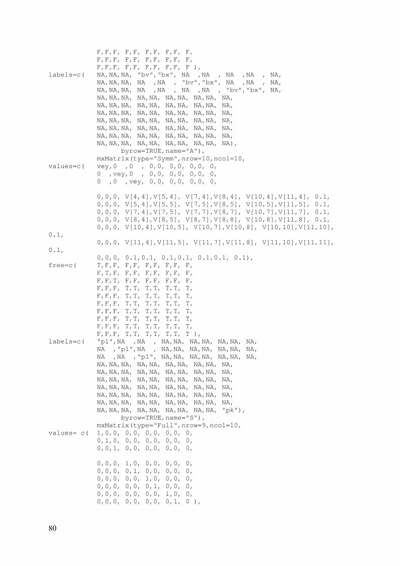
F,F,F, F,F, F,F, F,F, F, F,F,F, F,F, F,F, F,F, F, F,F,F, F,F, F,F, F,F, F ), labels=c( NA,NA,NA, "bv","bx", NA ,NA , NA ,NA , NA, NA,NA,NA, NA ,NA , "bv","bx", NA ,NA , NA, NA,NA,NA, NA ,NA , NA ,NA , "bv","bx", NA, NA,NA,NA, NA,NA, NA,NA, NA,NA, NA, NA,NA,NA, NA,NA, NA,NA, NA,NA, NA, NA,NA,NA, NA,NA, NA,NA, NA,NA, NA, NA,NA,NA, NA,NA, NA,NA, NA,NA, NA, NA,NA,NA, NA,NA, NA,NA, NA,NA, NA, NA,NA,NA, NA,NA, NA,NA, NA,NA, NA, NA,NA,NA, NA,NA, NA,NA, NA,NA, NA), byrow=TRUE,name="A"), mxMatrix(type="Symm",nrow=10,ncol=10, values=c( vey,0 ,0 , 0,0, 0,0, 0,0, 0, 0 ,vey,0 , 0,0, 0,0, 0,0, 0, 0 ,0 ,vey, 0,0, 0,0, 0,0, 0, 0,0,0, V[4,4],V[5,4], V[7,4],V[8,4], V[10,4],V[11,4], 0.1, 0,0,0, V[5,4],V[5,5], V[7,5],V[8,5], V[10,5],V[11,5], 0.1, 0,0,0, V[7,4],V[7,5], V[7,7],V[8,7], V[10,7],V[11,7], 0.1, 0,0,0, V[8,4],V[8,5], V[8,7],V[8,8], V[10,8],V[11,8], 0.1, 0,0,0, V[10,4],V[10,5], V[10,7],V[10,8], V[10,10],V[11,10], 0.1, 0,0,0, V[11,4],V[11,5], V[11,7],V[11,8], V[11,10],V[11,11], 0.1, 0,0,0, 0.1,0.1, 0.1,0.1, 0.1,0.1, 0.1), free=c( T,F,F, F,F, F,F, F,F, F, F,T,F, F,F, F,F, F,F, F, F,F,T, F,F, F,F, F,F, F, F,F,F, T,T, T,T, T,T, T, F,F,F, T,T, T,T, T,T, T, F,F,F, T,T, T,T, T,T, T, F,F,F, T,T, T,T, T,T, T, F,F,F, T,T, T,T, T,T, T, F,F,F, T,T, T,T, T,T, T, F,F,F, T,T, T,T, T,T, T ), labels=c( "p1",NA ,NA , NA,NA, NA,NA, NA,NA, NA, NA ,"p1",NA , NA,NA, NA,NA, NA,NA, NA, NA ,NA ,"p1", NA,NA, NA,NA, NA,NA, NA, NA,NA,NA, NA,NA, NA,NA, NA,NA, NA, NA,NA,NA, NA,NA, NA,NA, NA,NA, NA, NA,NA,NA, NA,NA, NA,NA, NA,NA, NA, NA,NA,NA, NA,NA, NA,NA, NA,NA, NA, NA,NA,NA, NA,NA, NA,NA, NA,NA, NA, NA,NA,NA, NA,NA, NA,NA, NA,NA, NA, NA,NA,NA, NA,NA, NA,NA, NA,NA, "pk"), byrow=TRUE,name="S"), mxMatrix(type="Full",nrow=9,ncol=10, values= c( 1,0,0, 0,0, 0,0, 0,0, 0, 0,1,0, 0,0, 0,0, 0,0, 0, 0,0,1, 0,0, 0,0, 0,0, 0, 0,0,0, 1,0, 0,0, 0,0, 0, 0,0,0, 0,1, 0,0, 0,0, 0, 0,0,0, 0,0, 1,0, 0,0, 0, 0,0,0, 0,0, 0,1, 0,0, 0, 0,0,0, 0,0, 0,0, 1,0, 0, 0,0,0, 0,0, 0,0, 0,1, 0 ),

  

81  

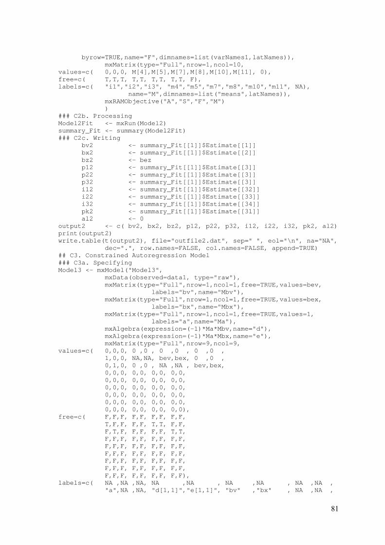
byrow=TRUE,name="F",dimnames=list(varNames1,latNames)), mxMatrix(type="Full",nrow=1,ncol=10, values=c( 0,0,0, M[4],M[5],M[7],M[8],M[10],M[11], 0), free=c( T,T,T, T,T, T,T, T,T, F), labels=c( "i1","i2","i3", "m4","m5","m7","m8","m10","m11", NA), name="M",dimnames=list("means",latNames)), mxRAMObjective("A","S","F","M") ) ### C2b. Processing Model2Fit <- mxRun(Model2) summary_Fit <- summary(Model2Fit) ### C2c. Writing bv2 <- summary_Fit[[1]]$Estimate[[1]] bx2 <- summary_Fit[[1]]$Estimate[[2]] bz2 <- bez p12 <- summary_Fit[[1]]$Estimate[[3]] p22 <- summary_Fit[[1]]$Estimate[[3]] p32 <- summary_Fit[[1]]$Estimate[[3]] i12 <- summary_Fit[[1]]$Estimate[[32]] i22 <- summary_Fit[[1]]$Estimate[[33]] i32 <- summary_Fit[[1]]$Estimate[[34]] pk2 <- summary_Fit[[1]]$Estimate[[31]] al2 <- 0 output2 <- c( bv2, bx2, bz2, p12, p22, p32, i12, i22, i32, pk2, al2) print(output2) write.table(t(output2), file="outfile2.dat", sep=" ", eol="\n", na="NA",

dec=".", row.names=FALSE, col.names=FALSE, append=TRUE) ## C3. Constrained Autoregression Model ### C3a. Specifying Model3 <- mxModel("Model3", mxData(observed=data1, type="raw"), mxMatrix(type="Full",nrow=1,ncol=1,free=TRUE,values=bev, labels="bv",name="Mbv"), mxMatrix(type="Full",nrow=1,ncol=1,free=TRUE,values=bex, labels="bx",name="Mbx"), mxMatrix(type="Full",nrow=1,ncol=1,free=TRUE,values=1, labels="a",name="Ma"), mxAlgebra(expression=(-1)*Ma*Mbv,name="d"), mxAlgebra(expression=(-1)*Ma*Mbx,name="e"), mxMatrix(type="Full",nrow=9,ncol=9, values=c( 0,0,0, 0 ,0 , 0 ,0 , 0 ,0 , 1,0,0, NA,NA, bev,bex, 0 ,0 , 0,1,0, 0 ,0 , NA ,NA , bev,bex, 0,0,0, 0,0, 0,0, 0,0, 0,0,0, 0,0, 0,0, 0,0, 0,0,0, 0,0, 0,0, 0,0, 0,0,0, 0,0, 0,0, 0,0, 0,0,0, 0,0, 0,0, 0,0, 0,0,0, 0,0, 0,0, 0,0), free=c( F,F,F, F,F, F,F, F,F, T,F,F, F,F, T,T, F,F, F,T,F, F,F, F,F, T,T, F,F,F, F,F, F,F, F,F, F,F,F, F,F, F,F, F,F, F,F,F, F,F, F,F, F,F, F,F,F, F,F, F,F, F,F, F,F,F, F,F, F,F, F,F, F,F,F, F,F, F,F, F,F), labels=c( NA ,NA ,NA, NA ,NA , NA ,NA , NA ,NA , "a",NA ,NA, "d[1,1]","e[1,1]", "bv" ,"bx" , NA ,NA ,

82  

NA ,"a",NA, NA ,NA ,"d[1,1]","e[1,1]", "bv","bx", NA,NA,NA, NA,NA, NA,NA, NA,NA, NA,NA,NA, NA,NA, NA,NA, NA,NA, NA,NA,NA, NA,NA, NA,NA, NA,NA, NA,NA,NA, NA,NA, NA,NA, NA,NA, NA,NA,NA, NA,NA, NA,NA, NA,NA, NA,NA,NA, NA,NA, NA,NA, NA,NA ), byrow=TRUE,name="A"),

mxMatrix(type="Symm",nrow=9,ncol=9, values=c( V[1,1],0 ,0 , V[4,1],V[5,1], V[7,1],V[8,1], V[10,1],V[11,1], 0 ,vey,0 , 0 ,0 , 0 ,0 , 0 ,0 , 0 ,0 ,vey, 0 ,0 , 0 ,0 , 0 ,0 , V[4,1],0,0, V[4,4],V[5,4], V[7,4],V[8,4], V[10,4],V[11,4], V[5,1],0,0, V[5,4],V[5,5], V[7,5],V[8,5], V[10,5],V[11,5], V[7,1],0,0, V[7,4],V[7,5], V[7,7],V[8,7], V[10,7],V[11,7], V[8,1],0,0, V[8,4],V[8,5], V[8,7],V[8,8], V[10,8],V[11,8], V[10,1],0,0,V[10,4],V[10,5], V[10,7],V[10,8], V[10,10],V[11,10], V[11,1],0,0,V[11,4],V[11,5], V[11,7],V[11,8], V[11,10],V[11,11]), free=c( T,F,F, T,T, T,T, T,T, F,T,F, F,F, F,F, F,F, F,F,T, F,F, F,F, F,F, T,F,F, T,T, T,T, T,T, T,F,F, T,T, T,T, T,T, T,F,F, T,T, T,T, T,T, T,F,F, T,T, T,T, T,T, T,F,F, T,T, T,T, T,T, T,F,F, T,T, T,T, T,T), labels=c( "p1",NA ,NA , NA,NA, NA,NA, NA,NA, NA ,"p2",NA , NA,NA, NA,NA, NA,NA, NA ,NA ,"p3", NA,NA, NA,NA, NA,NA, NA ,NA ,NA , NA,NA, NA,NA, NA,NA, NA ,NA ,NA , NA,NA, NA,NA, NA,NA, NA ,NA ,NA , NA,NA, NA,NA, NA,NA, NA ,NA ,NA , NA,NA, NA,NA, NA,NA, NA ,NA ,NA , NA,NA, NA,NA, NA,NA, NA ,NA ,NA , NA,NA, NA,NA, NA,NA ), byrow=TRUE,name="S"), mxMatrix(type="Iden",nrow=9,ncol=9,name="F"), mxMatrix(type="Full",nrow=1,ncol=9, values=c( M[1],0,0, M[4],M[5], M[7],M[8], M[10],M[11]), free=c( T,T,T, T,T, T,T, T,T), labels=c( "m1","i2","i3", "m4","m5", "m7","m8", "m10","m11"), name="M"), mxRAMObjective("A","S","F","M",dimnames=varNames1) ) ### C3b. Processing Model3Fit <- mxRun(Model3) summary_Fit <- summary(Model3Fit) ### C3c. Writing bv3 <- summary_Fit[[1]]$Estimate[[1]] bx3 <- summary_Fit[[1]]$Estimate[[2]] bz3 <- bez p13 <- 0.0 p23 <- summary_Fit[[1]]$Estimate[[5]] p33 <- summary_Fit[[1]]$Estimate[[6]] i13 <- 0.0

  

83  

i23 <- summary_Fit[[1]]$Estimate[[35]] i33 <- summary_Fit[[1]]$Estimate[[36]] pk3 <- 0 al3 <- summary_Fit[[1]]$Estimate[[3]] output3 <- c( bv3, bx3, bz3, p13, p23, p33, i13, i23, i33, pk3, al3) print(output3) write.table(t(output3), file="outfile3.dat", sep=" ",eol="\n", na="NA", dec=".", row.names=FALSE, col.names=FALSE, append=TRUE) ## C4. Time Lagged Dependent Model ### C4a. Specifying Model4 <- mxModel("Model4", mxData(observed=data1, type="raw"), mxMatrix(type="Full",nrow=9,ncol=9, values=c( 0,0,0, 0,0, 0 ,0 , 0 ,0 , 1,0,0, 0,0, bev,bex, 0 ,0 , 0,1,0, 0,0, 0 ,0 , bev,bex, 0,0,0, 0,0, 0,0, 0,0, 0,0,0, 0,0, 0,0, 0,0, 0,0,0, 0,0, 0,0, 0,0, 0,0,0, 0,0, 0,0, 0,0, 0,0,0, 0,0, 0,0, 0,0, 0,0,0, 0,0, 0,0, 0,0), free=c( F,F,F, F,F, F,F, F,F, T,F,F, F,F, T,T, F,F, F,T,F, F,F, F,F, T,T, F,F,F, F,F, F,F, F,F, F,F,F, F,F, F,F, F,F, F,F,F, F,F, F,F, F,F, F,F,F, F,F, F,F, F,F, F,F,F, F,F, F,F, F,F, F,F,F, F,F, F,F, F,F), labels=c( NA ,NA ,NA, NA,NA, NA ,NA , NA ,NA , "a",NA ,NA, NA,NA, "bv","bx", NA ,NA , NA ,"a",NA, NA,NA, NA ,NA , "bv","bx", NA,NA,NA, NA,NA, NA,NA, NA,NA, NA,NA,NA, NA,NA, NA,NA, NA,NA, NA,NA,NA, NA,NA, NA,NA, NA,NA, NA,NA,NA, NA,NA, NA,NA, NA,NA, NA,NA,NA, NA,NA, NA,NA, NA,NA, NA,NA,NA, NA,NA, NA,NA, NA,NA ), byrow=TRUE,name="A"), mxMatrix(type="Symm",nrow=9,ncol=9, values=c( V[1,1],0 ,0 , V[4,1],V[5,1], V[7,1],V[8,1], V[10,1],V[11,1], 0 ,vey,0 , 0 ,0 , 0 ,0 , 0 ,0 , 0 ,0 ,vey, 0 ,0 , 0 ,0 , 0 ,0 , V[4,1],0,0, V[4,4],V[5,4], V[7,4],V[8,4], V[10,4],V[11,4], V[5,1],0,0, V[5,4],V[5,5], V[7,5],V[8,5], V[10,5],V[11,5], V[7,1],0,0, V[7,4],V[7,5], V[7,7],V[8,7], V[10,7],V[11,7], V[8,1],0,0, V[8,4],V[8,5], V[8,7],V[8,8], V[10,8],V[11,8], V[10,1],0,0,V[10,4],V[10,5], V[10,7],V[10,8], V[10,10],V[11,10], V[11,1],0,0,V[11,4],V[11,5], V[11,7],V[11,8], V[11,10],V[11,11]), free=c( T,F,F, T,T, T,T, T,T, F,T,F, F,F, F,F, F,F, F,F,T, F,F, F,F, F,F, T,F,F, T,T, T,T, T,T, T,F,F, T,T, T,T, T,T,

84  

T,F,F, T,T, T,T, T,T, T,F,F, T,T, T,T, T,T, T,F,F, T,T, T,T, T,T, T,F,F, T,T, T,T, T,T), labels=c( "p1",NA ,NA , NA,NA, NA,NA, NA,NA, NA ,"p2",NA , NA,NA, NA,NA, NA,NA, NA ,NA ,"p3", NA,NA, NA,NA, NA,NA, NA ,NA ,NA , NA,NA, NA,NA, NA,NA, NA ,NA ,NA , NA,NA, NA,NA, NA,NA, NA ,NA ,NA , NA,NA, NA,NA, NA,NA, NA ,NA ,NA , NA,NA, NA,NA, NA,NA, NA ,NA ,NA , NA,NA, NA,NA, NA,NA, NA ,NA ,NA , NA,NA, NA,NA, NA,NA), byrow=TRUE, name="S"), mxMatrix(type="Iden",nrow=9,ncol=9, name="F"), mxMatrix(type="Full",nrow=1,ncol=9, values=c( M[1],0,0, M[4],M[5], M[7],M[8], M[10],M[11]), free=c( T,T,T, T,T, T,T, T,T), labels=c( "m1","i2","i3", "m4","m5", "m7","m8", "m10","m11"), name="M"), mxRAMObjective("A","S","F","M",dimnames=varNames1) ) ### C4b. Processing Model4Fit <- mxRun(Model4) summary_Fit <- summary(Model4Fit) ### C4c. Writing bv4 <- summary_Fit[[1]]$Estimate[[2]] bx4 <- summary_Fit[[1]]$Estimate[[3]] bz4 <- bez p14 <- 0.0 p24 <- summary_Fit[[1]]$Estimate[[5]] p34 <- summary_Fit[[1]]$Estimate[[6]] i14 <- 0.0 i24 <- summary_Fit[[1]]$Estimate[[35]] i34 <- summary_Fit[[1]]$Estimate[[36]] pk4 <- 0 al4 <- summary_Fit[[1]]$Estimate[[1]] output4 <- c( bv4, bx4, bz4, p14, p24, p34, i14, i24, i34, pk4, al4 ) print(output4) write.table(t(output4), file="outfile4.dat", sep=" ", eol="\n", na="NA",

dec=".", row.names=FALSE, col.names=FALSE, append=TRUE) ## C5. Differencing Model ### C5a. Specifying Model5 <- mxModel("Model5", mxData(observed=data2, type="raw"), mxMatrix(type="Full",nrow=6,ncol=6, values=c( 0,0, bev,bex, 0 ,0 , 0,0, 0 ,0 , bev,bex, 0,0, 0,0, 0,0, 0,0, 0,0, 0,0, 0,0, 0,0, 0,0, 0,0, 0,0, 0,0), free=c( F,F, T,T, F,F, F,F, F,F, T,T, F,F, F,F, F,F, F,F, F,F, F,F, F,F, F,F, F,F, F,F, F,F, F,F), labels=c( NA,NA, "bv","bx", NA ,NA , NA,NA, NA ,NA , "bv","bx",

  

85  

NA,NA, NA,NA, NA,NA, NA,NA, NA,NA, NA,NA, NA,NA, NA,NA, NA,NA, NA,NA, NA,NA, NA,NA), byrow=TRUE,name="A"), mxMatrix(type="Symm",nrow=6,ncol=6, values=c( vey,0 , 0,0, 0,0, 0 ,vey, 0,0, 0,0, 0 ,0 , V[1,1],V[1,2], V[1,3],V[1,4], 0 ,0 , V[1,2],V[2,2], V[2,3],V[2,4], 0,0, V[1,3],V[2,3], V[3,3],V[3,4], 0,0, V[1,4],V[2,4], V[3,4],V[4,4]), free=c( T,F, F,F, F,F, F,T, F,F, F,F, F,F, T,T, T,T, F,F, T,T, T,T, F,F, T,T, T,T, F,F, T,T, T,T), labels=c( "p2",NA ,NA,NA, NA,NA, NA ,"p2",NA,NA, NA,NA, NA,NA, NA,NA, NA,NA, NA,NA, NA,NA, NA,NA, NA,NA, NA,NA, NA,NA, NA,NA, NA,NA, NA,NA), byrow=TRUE,name="S"), mxMatrix(type="Iden",nrow=6,ncol=6,name="F"), mxMatrix(type="Full",nrow=1,ncol=6, values=c( 0,0, Md[3],Md[4],Md[5],Md[6]), free=c( T,T, T,T, T,T), labels=c( "i2","i3", "md2","md3","md5","md6"), name="M"), mxRAMObjective("A","S","F","M",dimnames=varNames2) ) ### C4b. Processing Model5Fit <- mxRun(Model5) summary_Fit <- summary(Model5Fit) ### C4c. Writing bv5 <- summary_Fit[[1]]$Estimate[[1]] bx5 <- summary_Fit[[1]]$Estimate[[2]] bz5 <- bez p15 <- 0.0 p25 <- summary_Fit[[1]]$Estimate[[3]] p35 <- summary_Fit[[1]]$Estimate[[3]] i15 <- 0.0 i25 <- summary_Fit[[1]]$Estimate[[14]] i35 <- summary_Fit[[1]]$Estimate[[15]] pk5 <- 0.0 al5 <- 0.0 output5 <- c( bv5, bx5, bz5, p15, p25, p35, i15, i25, i35, pk5, al5) print(output5) write.table(t(output5), file="outfile5.dat", sep=" ", eol="\n", na="NA", dec=".", row.names=FALSE, col.names=FALSE, append=TRUE) ## C6. Deviance Regression Model ### C6a. Specifying Model6 <- mxModel("Model6", mxData(observed=data3, type="raw"), mxMatrix(type="Full",nrow=9,ncol=9, values=c( 0,0,0, bev,bex, 0 ,0 , 0 ,0 , 0,0,0, 0 ,0 , bev,bex, 0 ,0 , 0,0,0, 0 ,0 , 0 ,0 , bev,bex, 0,0,0, 0,0, 0,0, 0,0,

86  

0,0,0, 0,0, 0,0, 0,0, 0,0,0, 0,0, 0,0, 0,0, 0,0,0, 0,0, 0,0, 0,0, 0,0,0, 0,0, 0,0, 0,0, 0,0,0, 0,0, 0,0, 0,0), free=c( F,F,F, T,T, F,F, F,F, F,F,F, F,F, T,T, F,F, F,F,F, F,F, F,F, T,T, F,F,F, F,F, F,F, F,F, F,F,F, F,F, F,F, F,F, F,F,F, F,F, F,F, F,F, F,F,F, F,F, F,F, F,F, F,F,F, F,F, F,F, F,F, F,F,F, F,F, F,F, F,F), labels=c( NA,NA,NA, "bv","bx", NA ,NA , NA ,NA , NA,NA,NA, NA ,NA , "bv","bx", NA ,NA , NA,NA,NA, NA ,NA , NA ,NA , "bv","bx", NA,NA,NA, NA,NA, NA,NA, NA,NA, NA,NA,NA, NA,NA, NA,NA, NA,NA, NA,NA,NA, NA,NA, NA,NA, NA,NA, NA,NA,NA, NA,NA, NA,NA, NA,NA, NA,NA,NA, NA,NA, NA,NA, NA,NA, NA,NA,NA, NA,NA, NA,NA, NA,NA ), byrow=TRUE,name="A"), mxMatrix(type="Symm",nrow=9,ncol=9, values=c( vey,0 ,0 , 0,0, 0,0, 0,0, 0 ,vey,0 , 0,0, 0,0, 0,0, 0 ,0 ,vey, 0,0, 0,0, 0,0, 0 ,0 ,0 , V[4,4],V[5,4], V[7,4],V[8,4], V[10,4],V[11,4], 0 ,0 ,0 , V[5,4],V[5,5], V[7,5],V[8,5], V[10,5],V[11,5], 0 ,0 ,0 , V[7,4],V[7,5], V[7,7],V[8,7], V[10,7],V[11,7], 0 ,0 ,0 , V[8,4],V[8,5], V[8,7],V[8,8], V[10,8],V[11,8], 0 ,0 ,0 ,V[10,4],V[10,5], V[10,7],V[10,8], V[10,10],V[11,10], 0 ,0 ,0 ,V[11,4],V[11,5], V[11,7],V[11,8], V[11,10],V[11,11]), free=c( T,F,F, F,F, F,F, F,F, F,T,F, F,F, F,F, F,F, F,F,T, F,F, F,F, F,F, F,F,F, T,T, T,T, T,T, F,F,F, T,T, T,T, T,T, F,F,F, T,T, T,T, T,T, F,F,F, T,T, T,T, T,T, F,F,F, T,T, T,T, T,T, F,F,F, T,T, T,T, T,T), labels=c( "p1",NA ,NA , NA,NA, NA,NA, NA,NA, NA ,"p1",NA , NA,NA, NA,NA, NA,NA, NA ,NA ,"p1", NA,NA, NA,NA, NA,NA, NA ,NA ,NA , NA,NA, NA,NA, NA,NA, NA ,NA ,NA , NA,NA, NA,NA, NA,NA, NA ,NA ,NA , NA,NA, NA,NA, NA,NA, NA ,NA ,NA , NA,NA, NA,NA, NA,NA, NA ,NA ,NA , NA,NA, NA,NA, NA,NA, NA ,NA ,NA , NA,NA, NA,NA, NA,NA), byrow=TRUE,name="S"),

mxMatrix(type="Iden",nrow=9,ncol=9,name="F"), mxMatrix(type="Full",nrow=1,ncol=9, values=c( 0,0,0, M[4],M[5], M[7],M[8], M[10],M[11]), free=c( T,T,T, T,T, T,T, T,T), labels=c( "i1","i2","i3", "m4","m5", "m7","m8", "m10","m11"), name="M"),

  

87  

mxRAMObjective("A","S","F","M",dimnames=varNames1) ) ### C6b. Processing Model6Fit <- mxRun(Model6) summary_Fit <- summary(Model6Fit) ### C6c. Writing bv6 <- summary_Fit[[1]]$Estimate[[1]] bx6 <- summary_Fit[[1]]$Estimate[[2]] bz6 <- bez p16 <- summary_Fit[[1]]$Estimate[[3]] p26 <- summary_Fit[[1]]$Estimate[[3]] p36 <- summary_Fit[[1]]$Estimate[[3]] i16 <- summary_Fit[[1]]$Estimate[[25]] i26 <- summary_Fit[[1]]$Estimate[[26]] i36 <- summary_Fit[[1]]$Estimate[[27]] pk6 <- 0 al6 <- 0 output6 <- c(bv6, bx6, bz6, p16, p26, p36, i16, i26, i36, pk6, al6 ) print(output6) write.table(t(output6), file="outfile6.dat", sep=" ", eol="\n", na="NA",

dec=".", row.names=FALSE, col.names=FALSE, append=TRUE) file.remove("Dt0.dat") file.remove("Dt2.dat") file.remove("Dt3.dat") } # D. Results Analysing ## D0. Full Model out0 <- read.table(file="outfile0.dat",header=FALSE,sep=" ",dec=".") is.na(out0)=out0==999 ME0 <-colMeans(out0) ME0 <-matrix(ME0,nrow=1,ncol=11) PV <-matrix(c(bev,bex,bez,vey,vey,vey,0,0,0,0,0),nrow=1,ncol=11) BE0 <-ME0-PV SE0 <-sqrt(diag(cov(out0))) SE0 <-matrix(SE0,nrow=1,ncol=11) ID0 <-matrix(c(0,N,alv,alx,alz,cvx,cvz,cxz,bez),nrow=1,ncol=9) Re0 <-cbind(ME0,BE0,SE0,ID0) write.table(Re0, file="outfile100.dat", sep=" ", eol="\n", na="NA", dec=".", row.names=FALSE, col.names=FALSE,

append=TRUE) file.remove("outfile0.dat") ## D1. Standard Spatial Autoregression Model out1 <- read.table(file="outfile1.dat",header=FALSE,sep=" ",dec=".") is.na(out1)=out1==999 ME1 <-colMeans(out1) ME1 <-matrix(ME1,nrow=1,ncol=11) PV <-matrix(c(bev,bex,bez,vey,vey,vey,0,0,0,0,0),nrow=1,ncol=11) BE1 <-ME1-PV SE1 <-sqrt(diag(cov(out1))) SE1 <-matrix(SE1,nrow=1,ncol=11) ID1 <-matrix(c(1,N,alv,alx,alz,cvx,cvz,cxz,bez),nrow=1,ncol=9) Re1 <-cbind(ME1,BE1,SE1,ID1) write.table(Re1, file="outfile100.dat", sep=" ", eol="\n", na="NA", dec=".", row.names=FALSE, col.names=FALSE,

append=TRUE) file.remove("outfile1.dat") ## D2. Time Invariant Individual Effect Model

88  

out2 <- read.table(file="outfile2.dat",header=FALSE,sep=" ",dec=".") is.na(out2)=out2==999 ME2 <-colMeans(out2) ME2 <-matrix(ME2,nrow=1,ncol=11) PV <-matrix(c(bev,bex,bez,vey,vey,vey,0,0,0,0,0),nrow=1,ncol=11) BE2 <-ME2-PV SE2 <-sqrt(diag(cov(out2))) SE2 <-matrix(SE2,nrow=1,ncol=11) ID2 <-matrix(c(2,N,alv,alx,alz,cvx,cvz,cxz,bez),nrow=1,ncol=9) Re2 <-cbind(ME2,BE2,SE2,ID2) write.table(Re2, file="outfile100.dat", sep=" ", eol="\n", na="NA", dec=".", row.names=FALSE, col.names=FALSE,

append=TRUE) file.remove("outfile2.dat") ## D3. Constrained Autoregression Model out3 <- read.table(file="outfile3.dat",header=FALSE,sep=" ",dec=".") is.na(out3)=out3==999 ME3 <-colMeans(out3) ME3 <-matrix(ME3,nrow=1,ncol=11) PV <-matrix(c(bev,bex,bez,vey,vey,vey,0,0,0,0,0),nrow=1,ncol=11) BE3 <-ME3-PV SE3 <-sqrt(diag(cov(out3))) SE3 <-matrix(SE3,nrow=1,ncol=11) ID3 <-matrix(c(3,N,alv,alx,alz,cvx,cvz,cxz,bez),nrow=1,ncol=9) Re3 <-cbind(ME3,BE3,SE3,ID3) write.table(Re3, file="outfile100.dat", sep=" ", eol="\n", na="NA", dec=".", row.names=FALSE, col.names=FALSE,

append=TRUE) file.remove("outfile3.dat") ## D4. Time Lagged Dependent Model out4 <- read.table(file="outfile4.dat",header=FALSE,sep=" ",dec=".") is.na(out4)=out4==999 ME4 <-colMeans(out4) ME4 <-matrix(ME4,nrow=1,ncol=11) PV <-matrix(c(bev,bex,bez,vey,vey,vey,0,0,0,0,0),nrow=1,ncol=11) BE4 <-ME4-PV SE4 <-sqrt(diag(cov(out4))) SE4 <-matrix(SE4,nrow=1,ncol=11) ID4 <-matrix(c(4,N,alv,alx,alz,cvx,cvz,cxz,bez),nrow=1,ncol=9) Re4 <-cbind(ME4,BE4,SE4,ID4) write.table(Re4, file="outfile100.dat", sep=" ", eol="\n", na="NA", dec=".", row.names=FALSE, col.names=FALSE,

append=TRUE) file.remove("outfile4.dat") ## D5. Differencing Model out5 <- read.table(file="outfile5.dat",header=FALSE,sep=" ",dec=".") is.na(out5)=out5==999 ME5 <-colMeans(out5) ME5 <-matrix(ME5,nrow=1,ncol=11) PV <-matrix(c(bev,bex,bez,vey,vey,vey,0,0,0,0,0),nrow=1,ncol=11) BE5 <-ME5-PV SE5 <-sqrt(diag(cov(out5))) SE5 <-matrix(SE5,nrow=1,ncol=11) ID5 <-matrix(c(5,N,alv,alx,alz,cvx,cvz,cxz,bez),nrow=1,ncol=9) Re5 <-cbind(ME5,BE5,SE5,ID5) write.table(Re5, file="outfile100.dat", sep=" ", eol="\n", na="NA", dec=".", row.names=FALSE, col.names=FALSE,

  

89  

append=TRUE) file.remove("outfile5.dat") ## D6. Deviance Regression Model out6 <- read.table(file="outfile6.dat",header=FALSE,sep=" ",dec=".") is.na(out6)=out6==999 ME6 <-colMeans(out6) ME6 <-matrix(ME6,nrow=1,ncol=11) PV <-matrix(c(bev,bex,bez,vey,vey,vey,0,0,0,0,0),nrow=1,ncol=11) BE6 <-ME6-PV SE6 <-sqrt(diag(cov(out6))) SE6 <-matrix(SE6,nrow=1,ncol=11) ID6 <-matrix(c(6,N,alv,alx,alz,cvx,cvz,cxz,bez),nrow=1,ncol=9) Re6 <-cbind(ME6,BE6,SE6,ID6) write.table(Re6, file="outfile100.dat", sep=" ", eol="\n", na="NA", dec=".", row.names=FALSE, col.names=FALSE,

append=TRUE) file.remove("outfile6.dat") } } } } } }