Embed Size (px)
Citation preview

University of Groningen Groningen Growth and Development Centre
Lifetimes of Machinery and Equipment.��Evidence from Dutch Manufacturing
Research Memorandum GD-87 Abdul Azeez Erumban RESEARCH MEMORANDUM
Lifetimes of Machinery and Equipment. Evidence from Dutch Manufacturing Research Memorandum GD-87 Abdul Azeez Erumban
Groningen Growth and Development Centre July 2006
2
Lifetimes of Machinery and Equipment. Evidence from Dutch Manufacturing
Abdul Azeez Erumban•
Groningen Growth and Development Centre
Faculty of Economics
University of Groningen
July 2006
Abstract This paper estimates service lifetimes for capital assets in Dutch manufacturing industries, using information on asset retirement patterns. A Weibull distribution function is estimated using a non-linear regression technique to derive service lifetimes for three selected asset types: transport equipment, machinery and computers. For this purpose the benchmark capital stock surveys for different two digit industries are linked to annual discard surveys. On average the estimated lifetimes are respectively 6, 9 and 26 years for transport equipments, computers and machinery. However, these estimates vary across industries. A comparison of our estimates with Canadian, US and Japanese estimates shows notable differences in the lifetimes of all the asset types, with machinery showing the largest difference.
•This research builds upon earlier efforts within Statistics Netherlands (CBS) to study the issue of asset lifetimes. It could not have been undertaken without the help of many people at the CBS for which the author is grateful. In particular, discussions with George van Leeuwen, Mark de Haan, and Gerard Meinen on different aspects of the data were very helpful. The suggestions and directions by Myriam Horsten on various aspects of the capital stock and discard databases and the comments by Myriam, Dirk van den Bergen and Erik Veldhuizen on the paper were highly beneficial. Nevertheless, the views and results in the paper do not reflect the position of the CBS, and the author is solely responsible for the contents. The comments by Marcel Timmer and Bart Los are highly acknowledged. Correspondence: Abdul Azeez Erumban, Groningen Growth and Development Centre, www.ggdc.net, Faculty of Economics, University of Groningen, P.O.Box 800, 9700 AV, Groningen, The Netherlands, e-mail: [email protected]
3
1. Introduction It is essential to have proper measures of inputs and output in order to unearth the contribution of inputs and productivity to output growth (see for e.g. Denison, 1969; Jorgenson and Griliches, 1967 & 1972 among others). Consequently, accurate measurement of inputs, especially the capital input and hence the capital depreciation, has gained much attention in economic literature (Jorgenson and Griliches, 1967; Hulten and Wykoff, 1981). Ever since the appearance of Goldsmith (1951), economists and statisticians have relied on capital stock data derived using the Perpetual Inventory Method (PIM) to illustrate changes in the productive contribution of capital. In the perpetual inventory method, the present capital stock is considered to be equal to the sum of past investment, after allowing for an ‘appropriate’ depreciation rate. Therefore, depreciation measures assume vital importance in productivity analysis, especially, multifactor productivity (MFP) analysis, which depends, inter alia, on the growth of capital stock and services.1 Capital goods are viewed as carriers of capital services which constitute the actual input in the production process. Therefore, if the depreciation of capital is not accurately measured, the estimated capital services and productivity will be biased.2 Recently there has been an urge towards inclusion of capital services into the national accounts (Schreyer, Diewert and Harrison, 2005), further highlighting the need for better measures of depreciation. Also the recent revamping of an old debate on gross versus net concepts, both in terms of capital stock measurement as well as output in productivity and welfare analysis signifies the importance of depreciation (Hulten, 2004; Oulton, 2004). BiØrn, HolmØy and Olsen (1989) have empirically illustrated the importance of distinguishing between gross and net measures of capital stock. Similarly, it has been recently argued that net output is more appropriate for welfare analysis (Oulton, 2004).3 The difference between net and gross output (capital) is nothing but the depreciated amount of capital. Depreciation is also important in the macro economic and tax policy models, as tax policies related to depreciation allowances can have serious implications for incentives to invest in various types of assets (Hwang, 2003; Hulten and Wykoff, 1981; Coen, 1975).
Despite the growing importance of depreciation in economic measurement, empirical evidence on depreciation patterns is scarce. Geometric depreciation4 rates have been derived in the literature either by using information on used asset prices (Baldwin et al 2005; Hulten and Wykoff, 1981) or on asset lifetimes (Fraumeni, 1997; Hulten and Wykoff, 1981). Hulten and Wykoff (1981) have demonstrated how one can estimate depreciation using information on market prices (of used assets), based on the pillars of microeconomics.5 Nevertheless, this approach is feasible only if there is substantial amount of information available on used asset prices. This is not true in most countries, with possible exceptions of the United States and Canada. Therefore, researchers and national statistical institutes (NSIs) rely on estimates of lifetimes, and combine these with a particular depreciation pattern to derive depreciation rates. However, it is hard to find estimates of service lives derived using the statistical information regarding the retiring pattern of capital assets. This is largely
1 See Oulton (1995) for a discussion on the role of depreciation, obsolescence and capital in growth accounting. Also see OECD (2001) for discussions on the concepts of depreciation, obsolescence, discards and lifetimes of capital. 2 For a detailed discussion on the components of capital service and their measurement see Erumban (2004). 3 Also see Jorgenson and Griliches (1972), Denison (1985), Jorgenson (1989) and Fraumeni (1997). 4 For a detailed discussion on various forms of depreciation patterns, see OECD (2001). 5 The idea behind using used asset price models is that the component unit cost associated with the aging of assets, i.e. the depreciation, can be isolated by comparing prices of assets of different ages. Also see Hwang (2003) and Baldwin et al (2005) for two recent studies in this line.

4
because firm do not have any incentive to keep record of their asset discard, which makes it difficult to arrive at reliable estimates of asset lifetimes (West, 1998). The general practice of NSIs is to rely on expert advices, information form tax authorities, or company records (OECD, 2001). These sources, however, may provide biased estimates of lifetimes. For instance, it is quite possible that the lifetimes and depreciation measures provided by tax authorities are manipulated for stimulating investment. In this milieu, this paper aims to analyze the discard pattern of capital assets to estimate expected lifetimes of these assets in the Netherlands, using information on directly observed capital stock and retirement patterns of assets. Information on actual retirement patterns helps one derive the expected service lives of assets. Statistics Netherlands (CBS) is one of the few statistical agencies in the world which collects data on capital stock and discards on a continuous basis (Meinen, 1998; Smeets et al, 1994). These two databases-capital stock and discard- in combination are used to estimate the asset lifetimes for three asset types – transport equipment, computers and machinery- in different industrial sectors. The estimated lifetimes for the Netherlands are presented in comparison with estimates for the United States, Canada and Japan.
It may be noted that there have been attempts in the past to estimate the service lifetimes of
capital assets in the Dutch manufacturing sector, utilizing the capital stock and discard data (Bergen et al 2005; Meinen 1998; Meinen et al, 1998). The present paper is an addition to these existing studies and differs from earlier work in its methodology. We feed more discard information into the estimation of lifetimes than before and hence provide better estimates. That is we monitor the discard pattern of each vintage over three consecutive years, and consider the average pattern over three different vintages for a given age (see section 2 for more detailed discussion). Earlier studies have considered only one vintage for a given age. Considering a single vintage as representative for a given age for all vintages may result in biased estimates if the selected vintage is not representative enough. Moreover, like investments, firm-level discards sometimes follow a spiky pattern with positive discards in one year, followed by zero discards in subsequent years. Therefore, a single discard year may need not necessarily a good representation of actual discard pattern. This problem is eased, to some extent, in this study by analyzing more vintages for a single age, including discard data for up to 3 years, rather than 1 (see Figure 1 and the following discussion in section 3). Indeed, we observe that the estimated survival function fits better to actual data when we incorporate more discard information, thereby providing better parameter estimates.
The remaining of the paper is organized in five sections. Section 2 presents the methodology
used in the present study in estimating lifetimes of assets. Section 3 provides a discussion on data and variables and section 4 provides the empirical results. The last section concludes the paper.
5
2. Estimating Survival functions and Asset lifetimes: The Methodology As mentioned earlier, we estimate service lifetime of assets using actual information on capital stock and discard, which can be used to derive estimates of depreciation. In order to derive consistent estimates of lifetime of capital assets, we analyze the discard pattern of these assets, which gives insights into the survival function. The survival function is the cumulative distribution of the probability that an asset survives until a given age and it helps us derive average service life of the capital asset.
While estimating the survival distribution, one faces the problem of selecting an appropriate functional form. There have been a number of approaches suggested in the literature on duration models to analyze survival functions. OECD (2001) has shown that most distributions except delayed linear and bell-shaped distributions are clearly unrealistic.6 Also earlier studies have emphasized that survival functions with longer tail like the Weibull or delayed linear are more realistic (OECD 2001; Meinen et al, 1998). In most empirical studies, due to the nice properties they have, researchers generally opt to use an exponential or Weibull distribution for lifetime distribution. However, when the lifetime is assumed to be distributed according to the exponential distribution, then the hazard rate is a constant, independent of time. A constant hazard rate implies that the probability of scrapping during the next time interval does not depend upon the duration spent in the initial state (Verbeek, 2004). The Weibull distribution, on the other hand, does not assume a constant hazard rate (see Pitman, 1992);7 it is a parametric distribution which includes decreasing, constant and increasing hazard rates. The Weibull specification requires only two parameters, and also it captures distributions that are skewed. Hence, in our estimation, in line with earlier studies (Bergen et al, 2005; Nomura 2005; Meinen, 1998), we also assume a Weibull distribution to describe the discard pattern.
The Weibull distribution has two parameters, α and β, where the former is the shape
parameter and the latter is the scale parameter. The lifetime distribution or the probability density (mortality) function, f(x), of the Weibull can be written as
α
βα
ββα ⎟⎟
⎠
⎞⎜⎜⎝
⎛−
−
⎟⎟⎠
⎞⎜⎜⎝
⎛=
x
exxf1
)( for x ≥ 0, (1)
where x is the age of the asset. This function is helpful in calculating the percentage of asset
of a given vintage that is discarded at different ages. The exponential distribution is a special case of Weibull where α takes the value 1, hence a single parameter distribution with constant retirement. Thus Weibull is the exponential distribution of the power transformed age, and is therefore more flexible than the exponential. From (1) the survival function S(x)-the probability that an asset of any
6 Other distributions include simultaneous exit and linear (see OECD, 2001). While the former assumes all the assets to be retired from capital stock at the moment they reach their average service life, the latter assumes that the surviving assets are reduced by a constant amount each year. The delayed linear is a variant of linear one in that it also assumes retirement of assets in equal parts until the entire vintage is fully scrapped, but the retirement starts later than in the linear case and finish sooner. The bell-shaped distributions, on the other hand, assumes a gradual retirement which starts some years after the year of installation, reaches the maximum around its average service life, and then starts lowering some years after average lifetime. 7 Also see Bekker (1991) for detailed discussion on the properties of Weibull distribution and Mudholkar, Srivastava, and Kollia (1996) for a generalized Weibull family of distributions for survival studies.
6
vintage survives until the age x- can be written as 1-F(x), where F(x) is the cumulative density function, i.e. the cumulative distribution of lifetime distribution f(x), i.e.
α
β ⎟⎟⎠
⎞⎜⎜⎝
⎛−
∫ −==xx
edyyfxF0
1)()( (2)
and the survival function S(x) is, α
β ⎟⎟⎠
⎞⎜⎜⎝
⎛−
=−=x
exFxS )(1)( (3)
where S(0)=1, S(∝)=0 and S(1/λ)=e-1, independently of the value of α. For notational simplicity assume λ=1/β. Then introducing the an additive error term u with
standard assumptions, one can specify an estimable non-linear equation, where survival function8 is a function of age, as
uexS x += − αλ )()( (4)
Given the Weibull distribution parameters, α and λ, the nth moment of Weibull probability
density function is given by
⎟⎟⎠
⎞⎜⎜⎝
⎛+Γ⎟
⎠⎞
⎜⎝⎛=
αλµ nn
n 11 (5)
where )(nΓ is the Gamma function of the shape parameter n, ∫∞
−−=Γ0
1)( dyeyn yn
Following (5) the first moment or the mean of the two parameter Weibull, which is by definition the expected average service life (Bekker, 1991; Nomura, 2005), E(x), is given by,9
⎟⎠⎞
⎜⎝⎛ +Γ==
αλµ 111)(1 xE (6)
The values of α and λ estimated using equation (4) are inserted in (6) to obtain the expected
lifetime estimates of assets.
8 Some previous studies have used hazard function instead of survival function to derive asset lifetimes (e.g. Meinen, 1998). Survival function and hazard rate are closely related concepts, the latter is nothing but a simple transformation of the former. The hazard function can be expressed as )()()( xSxfxh = , where f(x) is the lifetime distribution, and S(x) is the survival function. The hazard function describes the conditional probability that the asset is scrapped at a given age, given that it has survived up to that age. For the Weibull it can be
derived as 1)(
)(1
)()()( −
−
−−
== αλ
λα
λαλλαλα
α
xe
exxhx
x
.
9 The median and mode are respectively 1/λ[(ln2)1/α] and 1/λ[1-(1/α)1/α]. See Bekker (1991) for detailed discussion on the properties of Weibull distribution.

7
3. Data and Variables The survival function and asset lifetime estimation in this paper are conducted for 22 two-digit manufacturing industries in the Netherlands. However, in some cases several two-digit industries are clubbed together, based on the technology/product characteristics of such industries. For instance, different two-digit groups under textile products are clubbed into one. This was done in order to ensure sufficient numbers of observations to perform the regression analysis. Effectively, we have 15 industry groups in the final sample. Table 1 presents the list of industries considered in the present study along with the corresponding ISIC codes. The data is taken from two distinctive micro-economic surveys conducted by the Statistics Netherlands (CBS)-the capital stock survey and the discard survey. Therefore, it was essential to link these two to construct a comparable database.10 We discuss these two surveys below in short.
Table 1: Industries considered in the study ISIC Industry 15+16 Food, beverages & tobacco 17 to19 Textile & leather pdts. 20+33+36 Wood & wood pdcts, medical & optical eqpt & Other mfg. 21 Paper and paper products 22 Publishing and printing 23 Petroleum products; cokes, and nuclear fuel 24 Basic chemicals and man-made fibers 25 Rubber and plastic products 26 Other non-metallic mineral products 27 Basic metals 28 Fabricated metal products 29 Machinery and equipment n.e.c. 30+32 Office machinery & computers, radio, TV & communication eqpt. 31 Electrical machinery n.e.c. 34+35 Transport equipment
The capital stock surveys have been conducted on a rolling basis since 1993 in such a way
that each 2 digit industry will be surveyed once in five years.11 The survey contains information on all fixed assets that are used by enterprises in their production process, whether the assets are owned, rented or obtained through a leasing contract. More importantly, it provides the vintage year of each asset.12 Because of its rolling nature one or two benchmarks are available for each two-digit industry during the period 1993-2001. Therefore it was essential to consider one benchmark year for each industry and match it with subsequent discard years.
10 See Bergen et al (2005) and Meinen (1998) for previous studies who have used these surveys in combination. 11 See Lock (1985) for a documentation of the experiment by the CBS to arrive at directly observed measures of capital stock. 12 In some cases, especially for very older vintages, the exact year in which the asset was purchased is not available. But there is an average range of period available for such vintages, and hence the mid year is selected as the vintage year. Also, it is not clear whether the vintage years reported by firms for assets which are leased or purchased in the second hand market are exact vintage years. For instance, they could be the year in which the firm has bought the asset in the second hand market. Nevertheless, the presence of such cases is significant only in asset type transport equipment.
8
The data on discards13 in the manufacturing industry has been collected since 1992 in the Netherlands (see Smeets and van den Hove, 1997) and is publicly available till 2001. The survey provides information on all fixed assets which are no longer used in the production process. That is, it comprises all capital goods removed from the production process during the course of a particular year. However, this data is quite limiting due to the low response rate to this survey, as the information is gathered through mailed questionnaires.14 The information available includes the value of asset withdrawn from the production process both in historic and current prices and the destination to which the withdrawn asset goes to, i.e. whether the asset is scrapped, sold in the second hand market or returned to the lease company (the last option was added only recently).
Both capital stock and discard surveys cover only firms with 100 employees or more. They
provide firm level information on these variables in historic price at different vintages for eight asset types (see Appendix 1), among which we consider three-external transport equipments, machinery and equipments including internal means of transport (excluding computers), and computers and associated equipments (data processing machines that are freely programmable including peripheral devices; computers printers etc).
Appendix Tables 1 and 2 provide the number of firms reported to various benchmark capital
stock surveys and annual discard surveys during 1993-2001. There are 1354 manufacturing firms who have responded to at least one benchmark capital stock survey and a maximum of 1245 firms who have responded to various discard surveys during 1994-2001. Nevertheless, we have not included all these firms in our final dataset as we had to delete a number of firms during the cleaning process. Since our methodology to estimate asset lifetimes includes the use of both capital stock and discard data, we have made a combined dataset, consisting of firms reported to capital stock and discard surveys.
The historic value of capital stock in year t-1 (as on 31 December) is linked to the historic
value of discards in years t, t+1 and t+2 for each firm. Earlier studies have linked the benchmark capital stock in year t-1 to only one discard year, say t (Bergen et al, 2005), as they have used only single year discard information in the estimation of lifetimes. As mentioned before, in difference with earlier studies, the present study intends to incorporate more discard information into the estimation of lifetimes. Hence the benchmark capital stock data is linked to three discard years. The data is linked for each asset type and vintage year. That is the capital stock data for a particular asset bought in a particular year is linked to the same firm’s discard data for the same asset type of the same vintage. In the next step, we have deleted all the firms who have not reported to capital stock surveys, but to the discard surveys. This is because, since our analysis requires estimates of survival rates, which are the percentage of capital survived over years, it is meaningful only to include those firms who have reported to capital stock surveys. Also all those firms who have not reported discard value for at least one vintage are dropped from the sample. That is even if a firm has reported discards only in n vintages with reported capital stock in more than n vintages it is included in the sample. For the
13 Discards are also known as disinvestments or the withdrawal of assets from the production process. We use the concept “discard” throughout this paper. 14 Nevertheless, the data is quite reliable as the reported information is subjected to further scrutiny and reconfirmation in cases unbelievable or extreme information is found.
9
reported vintages, the actual discard values are used, while for the non-reported vintages, the discard is assumed to be zero. This assumption is based on the premise that there is no reason for a firm to report discard in certain vintages while not report discard in other vintages, other than not having a discard in that particular vintage. Those firms, who have no reported discard value in any vintage, are dropped, as we do not have any idea whether they have made any positive discard or not. Their inclusion may result in an exaggeration of capital stock, if we attribute zero discards to such firms.
All those cases where the reported discard values are higher than the capital in the given
vintage are deleted from the sample.15 All other cases, i.e. discard just equal to capital stock, where we assume a full discard of the asset; discard is zero, where we assume the entire capital is survived; and the discard is less than capital stock are included in the sample. Thus finally we had a sample in which the number of firms is much lower than the actual number of responding firms. We end up with 969 firms when we link the capital stock in year t-1 to the discard in year t which has further declined to 592 when added two more discard years (i.e. when we consider three discard years, t and t+1 and t+2). This decline is to be expected because, in the first case we include all those firms who have reported at least one vintage discard in the first year, however, in the second case, they are included in the sample only if they have responded to discard surveys in second and third years. This decline in the number of firms, however, is observed to have only marginal effect on the number of observation (vintages) in our regression analysis. As previously mentioned, for most industries there are two benchmarks capital stock surveys available (see Appendix Table 1). However, we have considered only the first round benchmark surveys in the current analysis, as the second round will not allow us to include up to three discard years, as the discard data is not available since 2001. This is also the reason why we limit the number of discard years into three; the recent benchmarks do not allow us to use more than three discard years.
We have aggregated this linked dataset to the 2 digit industry level across each vintage for
each asset separately. This aggregation is performed in order to ensure sufficient number of firms in the sample. This leaves us with the final dataset for each 2 digit industry, for different asset types and vintages. That means in our regression analysis, for each asset type, the degrees of freedom will be the number of vintages in that particular asset rather than the number of firms. Therefore, as mentioned before, the decline in the number of firms caused by the inclusion of more discard years into the model has only negligible effect on the degrees of freedom in our regression model. For each industry we have a series of data on historic value of capital stock and discards across various vintage years, which are used to construct the variables entering to our regression equation in (4). In what follows we explain each of the variables and their construction.
Survival function (S): The dependent variable in our Weibull specification (4) is the survival
function, which is calculated as the cumulative distribution of survival rate. It implies the probability that an asset is not discarded before the age x. In order to calculate survival rate we exploit data on capital stock and discard. Capital stock is the historic value of asset i of vintage j for industry k, taken
15 While excluding such firms, we have allowed for a margin of error of 2 per cent. That is even if the discard is greater than capital by 2 per cent of capital at firm level, we have included them, assuming that it will be a reporting error. However, they are subjected to further scrutiny in that if the discard is greater than capital stock even after aggregating to industry level (for each vintage) we drop such cases from the original sample.
10
as such from the capital stock survey, and discard is the historic value of asset i of vintage j for industry k, taken from the discard survey. The survival rate for a particular asset of particular vintage j at time t (or at age x where x is measured as t-j), is calculated as the historic value of capital in year t-1 minus historic value of discard in year t divided by historic value of capital in year t-1. Specifically, provided that the benchmark capital stock is available for the year t-1 and discard data is available for the year t, the survival rate for an asset of age x in year t can be calculated as16,
1,
,1,)(−
− −=
tj
tjtjtj K
DKxs (8)
where )(xs tj is the survival rate of an asset of vintage j at the age x at time t. The age of an
asset of a particular vintage is calculated as the discard year (year when it was discarded) minus its vintage year (year when it was purchased); i.e. x=t-j. K is the historic value of capital stock and D is the historic value of discard of an asset of jth vintage in year t. Since we use both capital stock and discard of same vintage to derive survival rates, we consider them in historic prices. The results will remain the same even if we use current or constant price figures, as both these variables will be inflated (deflated) by the same price indices, and as we take the ratios. Assuming that the survival rate for an asset of all vintages are equal for a given age x, i.e. sj(x)=s(x), (8) provides us the probability that an asset of any vintage survives until the age x, under the condition that it has survived until the age x-1. This is a standard, but strong, assumption, needed to make empirical estimation possible with the available data. Otherwise, one requires obtaining the information on capital stock and discards in all vintages over a long span of time, which is not practically possible. The capital that is reported in year t-1 is assumed to be the capital as existed on December 31st in year t-1 and therefore, Dj for year t-1 in (8) is assumed to be zero.
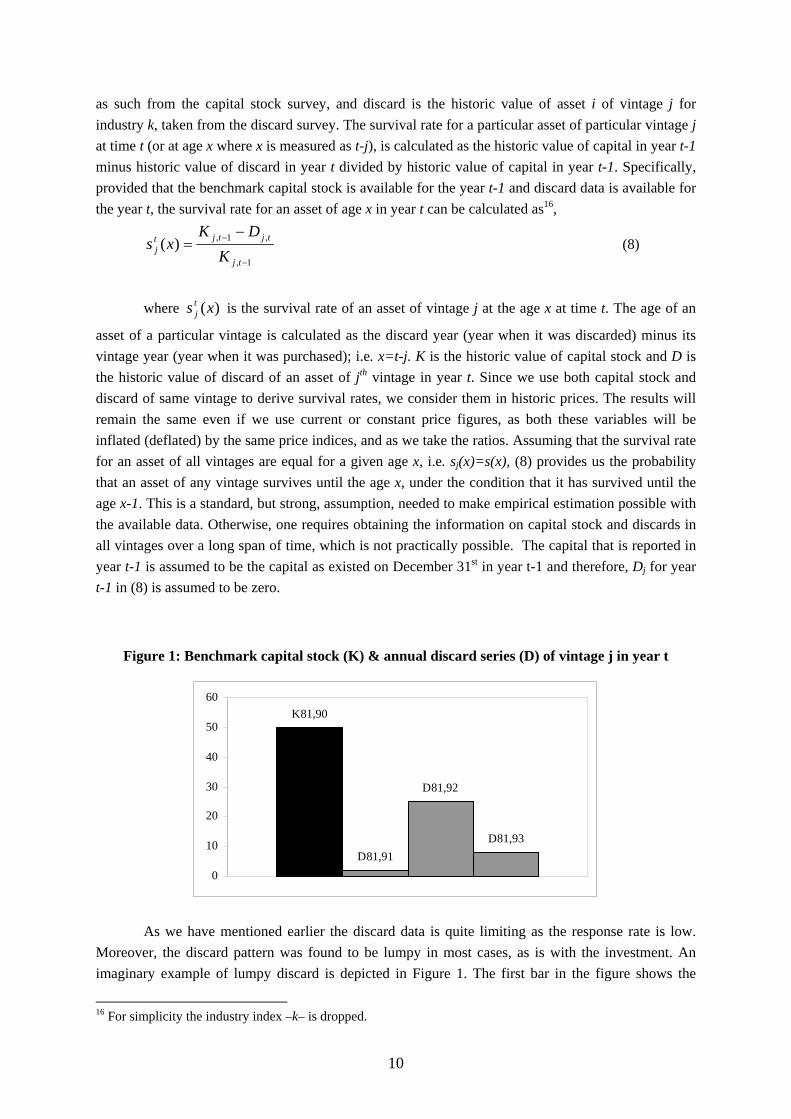
Figure 1: Benchmark capital stock (K) & annual discard series (D) of vintage j in year t
K81,90
D81,91
D81,92
D81,93
0
10
20
30
40
50
60
As we have mentioned earlier the discard data is quite limiting as the response rate is low.
Moreover, the discard pattern was found to be lumpy in most cases, as is with the investment. An imaginary example of lumpy discard is depicted in Figure 1. The first bar in the figure shows the
16 For simplicity the industry index –k– is dropped.
11
capital stock of vintage 1981 existed in the year 1990 (that is of age 9), and the second, third and fourth bars respectively show the value of discarded capital of the same vintage in years 1991, 1992, and 1993 (that is at age 10, 11 and 12). It is obvious from the figure that the discard pattern is lumpy with almost no discard at age 10 and a large amount of discard at age 11. However, if we consider the total discard over the three consecutive years, we see that almost 70 per cent of capital is discarded during the three years. According to the abovementioned methodology, the first two bars can be used to calculate the survival rate of an asset of age 10. And following the assumption sj(x)=s(x), the survival rate calculated using the first two bars can be considered representative of the survival rate of asset of any vintage at the age 10. Hence, as we observe very low discard in the first year, which will result in a very high survival rate at the age 10, attributing the same survival rate calculated using a single year’s discard information (as in 8) for all vintages does not seem to be an appropriate one. Though the particular vintage, considered as the representative vintage for the given age, say 10, have shown such a tendency, it may not hold for all vintages. More over the same vintage has shown a bulky discard in the next year, indicating that considering a single discard pattern may result in biased estimate of survival rate. Therefore, if one considers the single year discard information, taking a single vintage as representative of a particular age may affect the estimated survival rate for that particular age for all vintages, if the representative vintage has shown a very large or small discard. It can be argued that this lumpiness may disappear in some cases, when aggregating across vintages at two digit industry level. However, the problem of considering a single vintage as representative for all vintages at a given age still prevails. It is not necessary that all vintages have a similar discard behavior at any given age. That is, as mentioned earlier, the assumption of sj(x)=s(x) need not hold in complete sense. For instance the survival pattern of an asset of age 10 of vintage 1997 may be different from an asset of age 10 of vintage 1999. However, in order to incorporate this heterogeneity completely into the model, as we stated before, we need to have discard information throughout the lifetime of each asset, which is not practically possible. Therefore, given the data constraints, we suggest examining more vintages for the same age and consider an aggregate or average discard behavior of these different vintages at any particular age. In doing this we have considered three discard years for each vintage, which will help us calculate the survival rate for a particular vintage at three different ages. This will help us make the assumption sj(x)=s(x) less strong, though not completely relaxed. Thus, unlike the earlier studies (Bergen et al, 2005), who consider only the first year discard information, the present approach has the advantage of feeding more information on discard pattern of different vintages into the estimation of lifetime. More specifically, assuming that there is no second hand investment in any particular asset of a given vintage, the survival rate for any particular asset of age x in years t+1 and t+ 2 are given by
tjtj
tjtjtjtj DK
DDKxs
,11,1
1,1,11,111 )(
+−+
+++−+++ −
−−=
1,2,21,2
2,21,2,21,222 )(
+++−+
+++++−+++ −−
−−−=
tjtjtj
tjtjtjtjtj DDK
DDDKxs (9)
As before, we assume that sj(x)=s(x) for all vintages, i.e. survival rate for any given age is
constant over time, but less strongly. The assumption is less strong because the current approach incorporates more information on the discard behavior of firms at each age. This is because, when we
12
incorporates more information on the discard behavior of firms at each age. This is because, when we take into account only 1 year of discard data, our estimate of the survival rate of a particular asset (say machinery), of a particular age (say 10 years) in a given industry, would be based only on the discards of machinery of vintage t in year t+10. However, by also considering discards in years t+11 and t+12, the survival rate of age 10 is also based on observations of vintage t+1 and t+2, discarded in respectively t+11 and t+12. Then we take an average of these three survival rates for a given age as our preferred survival rate, which contains information of three different vintages for the given age.17 This average survival rate provides us the survival rate of an asset of a specific age regardless of its vintage.
Note that (9) assumes that there is no second hand investment in the vintage j. This is
because, only in the absence of second hand investment capital stock in year t for any particular vintage j can be calculated using information on capital stock in year t-1 and discard in year t as Kj,t-1 - Dj,t. If there exists second hand investments in the given vintage j, the capital stock in year t will be K
j,t-1 –Dj,t + SKj,t, where SKj,t is the second hand purchases of the same vintage j. Hence the survival rate will be higher than what is actually obtained assuming there is no second hand investment. We do not attribute much significance to this problem, as it is expected to have only negligible effect on our results, as second hand investments typically constitute a very tiny portion of total investment, especially in the asset types which we consider.
Once the survival rate is calculated, the survival function (S) is calculated as the cumulative
distribution of survival rates. That is,
∏=
=x
i
isxS1
)()( (10)
17 We have also calculated the survival rate using the total capital stock in three years (t-1, t and t+1) and total discards in three years (t, t+1 and t+2). The total capital stock is calculated by summing the constant price capital stock at any given age, say x, existed during three years, where the annual capital stock is calculated as the difference between previous year’s capital stock and current year’s discard. Similarly the total discard at any given age is calculated by summing the three years constant price discard for the given age. Then the survival rate at age x is calculated as the total capital stock of age x during the three years (t-1, t and t+1) – total discards of age x during the three years (t, t+1 and t+2)/ total capital stock of age x during the three years (t-1, t and t+1). The results remain to be the same as the ones obtained using average survival rates.
13
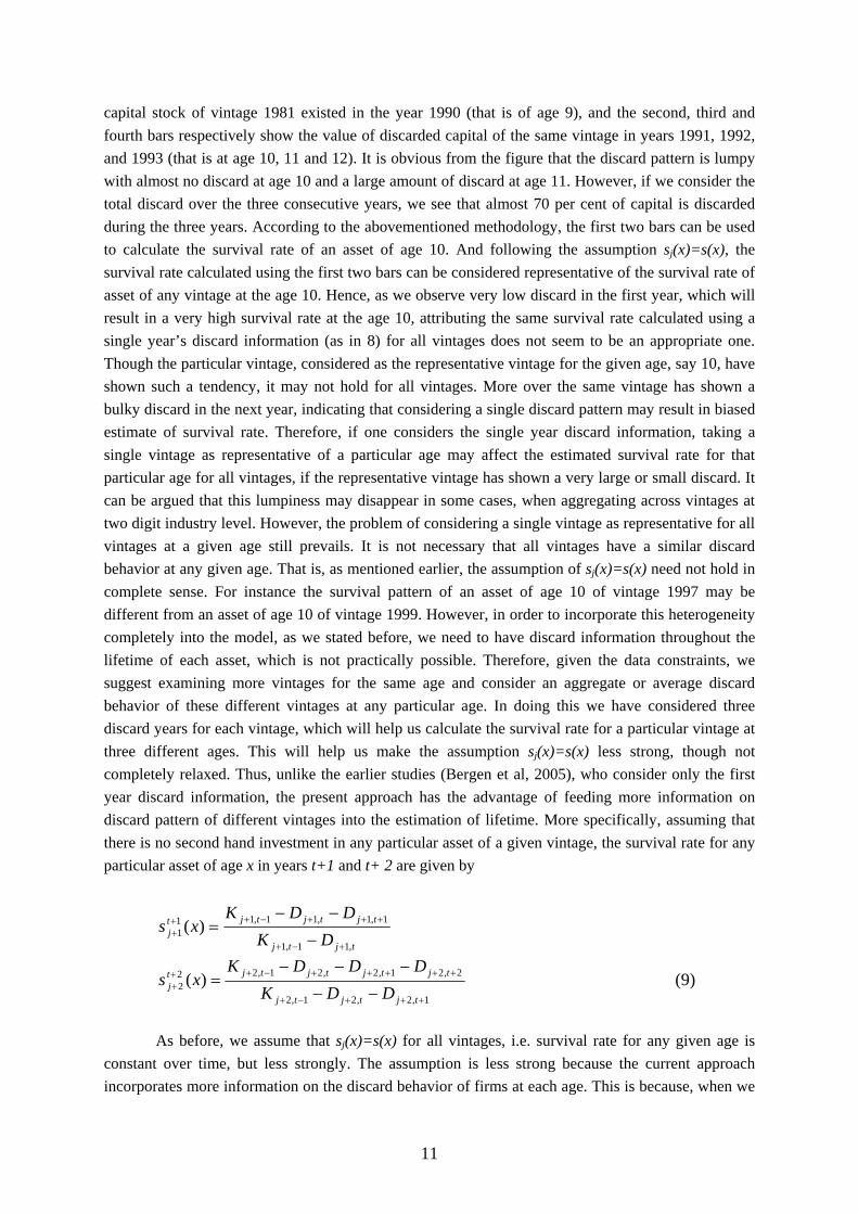
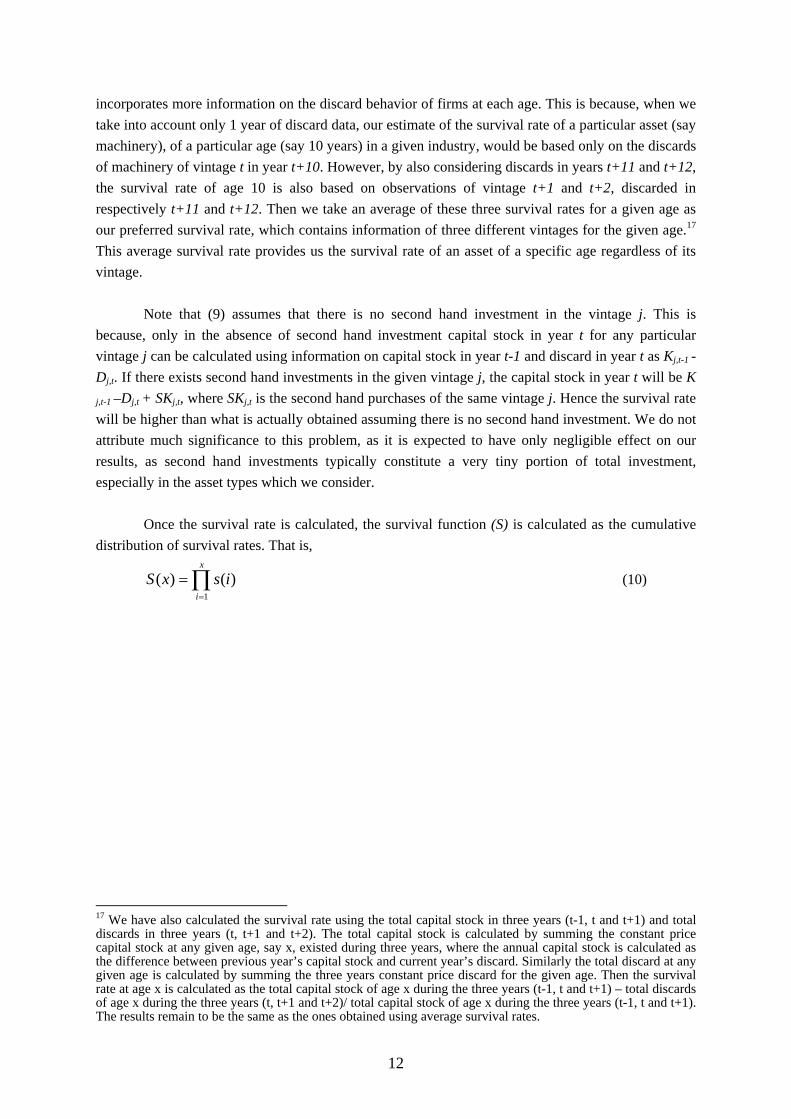
4. Empirical Results We have estimated equation (4), where we regresses the actual survival function, calculated using (10), on the age of the asset.18 Since the Weibull specification is non-linear in parameters, we have used a non-linear regression method. It is, however, possible to estimate the equation using a linear model by transforming the data into log form (e.g. Meinen, 1998). Nevertheless, the non-linear estimation is assumed to be more realistic and robust. In the linear transformed model, the parameter values are determined in such a way that they minimize the squared residuals for the transformed function rather than the original function. Hence, the estimated parameters may not produce the best fit of the original function to the data. Comparisons of estimated survival function with actual survival data have shown that the non-linear results are more close to actual data, compared to the linear ones (see Appendix Figure 1). Hence, we opt for non-linear regression estimation using a sequential quadratic programming algorithm, as provided in SPSS. The estimation is performed both for single discard year as well as 3 discard years case for purpose of comparison. In the former case, all firms who have reported at least one vintage in the first discard year are included in the sample, while in the latter case only firms who have reported zero or positive discard in at least one vintage in all the three years are included. The estimated parameters α and λ are then used to derive the expected service lifetimes of capital, using equation (6). While performing the regression, we have faced the problem of exaggerated tails, caused by the continuous lack of discard reporting in some of the older vintages. Such longer tails affects the variability and hence the regression estimation. Therefore, we have excluded such large tails from our regression, nevertheless, after allowing for a maximum of three vintages after the oldest vintage with positive discard.
Table 2: Estimated Regression Coefficients-Transport Equipments (3 Years Discard) ISIC α SE LC UC λ SE LC UC R2 DF 15+16 1.14 0.03 1.08 1.21 0.15 0.002 0.15 0.16 0.994 28 17 to19 1.00 0.17 0.63 1.37 0.16 0.016 0.12 0.19 0.856 17 20+33+36 1.22 0.13 0.94 1.49 0.18 0.010 0.15 0.20 0.937 17 21 1.12 0.13 0.85 1.39 0.20 0.013 0.17 0.23 0.929 17 22 2.18 0.18 1.81 2.55 0.23 0.006 0.22 0.24 0.983 20 23 1.00 0.08 0.83 1.17 0.11 0.006 0.10 0.12 0.926 30 24 1.00 0.11 0.77 1.23 0.08 0.005 0.07 0.09 0.843 23 25 1.00 0.14 0.70 1.30 0.14 0.011 0.12 0.16 0.864 16 26 1.16 0.16 0.82 1.50 0.20 0.016 0.17 0.24 0.899 19 27 1.80 0.11 1.56 2.04 0.11 0.003 0.11 0.12 0.984 16 28 1.27 0.12 1.02 1.52 0.19 0.009 0.17 0.21 0.953 20 29 1.12 0.17 0.75 1.49 0.18 0.016 0.15 0.22 0.895 13 30+32 1.38 0.11 1.14 1.61 0.21 0.009 0.20 0.23 0.968 22 31 1.05 0.14 0.73 1.37 0.15 0.011 0.12 0.17 0.920 11 34+35 1.00 0.11 0.78 1.22 0.12 0.007 0.11 0.14 0.904 16 Notes: SE is the standard error of estimate. LC and UC are respectively lower and upper confidence interval at 95 %s and DF is the degrees of freedom. All the coefficients are significant at 1 %. 18 Note that while performing the regression, we have faced the problem of exaggerated tails, caused by the continuous lack of discard reporting in some of the older vintages. We have excluded such large tails from our regression, nevertheless, after allowing for a maximum of three vintages after the oldest vintage with positive discard.
14
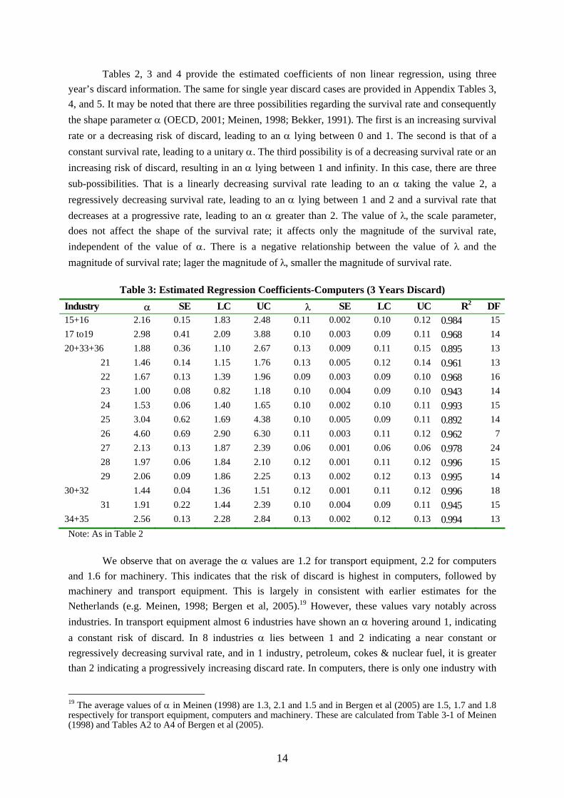
Tables 2, 3 and 4 provide the estimated coefficients of non linear regression, using three year’s discard information. The same for single year discard cases are provided in Appendix Tables 3, 4, and 5. It may be noted that there are three possibilities regarding the survival rate and consequently the shape parameter α (OECD, 2001; Meinen, 1998; Bekker, 1991). The first is an increasing survival rate or a decreasing risk of discard, leading to an α lying between 0 and 1. The second is that of a constant survival rate, leading to a unitary α. The third possibility is of a decreasing survival rate or an increasing risk of discard, resulting in an α lying between 1 and infinity. In this case, there are three sub-possibilities. That is a linearly decreasing survival rate leading to an α taking the value 2, a regressively decreasing survival rate, leading to an α lying between 1 and 2 and a survival rate that decreases at a progressive rate, leading to an α greater than 2. The value of λ, the scale parameter, does not affect the shape of the survival rate; it affects only the magnitude of the survival rate, independent of the value of α. There is a negative relationship between the value of λ and the magnitude of survival rate; lager the magnitude of λ, smaller the magnitude of survival rate.
Table 3: Estimated Regression Coefficients-Computers (3 Years Discard) Industry α SE LC UC λ SE LC UC R2 DF 15+16 2.16 0.15 1.83 2.48 0.11 0.002 0.10 0.12 0.984 15 17 to19 2.98 0.41 2.09 3.88 0.10 0.003 0.09 0.11 0.968 14 20+33+36 1.88 0.36 1.10 2.67 0.13 0.009 0.11 0.15 0.895 13
21 1.46 0.14 1.15 1.76 0.13 0.005 0.12 0.14 0.961 13 22 1.67 0.13 1.39 1.96 0.09 0.003 0.09 0.10 0.968 16 23 1.00 0.08 0.82 1.18 0.10 0.004 0.09 0.10 0.943 14 24 1.53 0.06 1.40 1.65 0.10 0.002 0.10 0.11 0.993 15 25 3.04 0.62 1.69 4.38 0.10 0.005 0.09 0.11 0.892 14 26 4.60 0.69 2.90 6.30 0.11 0.003 0.11 0.12 0.962 7 27 2.13 0.13 1.87 2.39 0.06 0.001 0.06 0.06 0.978 24 28 1.97 0.06 1.84 2.10 0.12 0.001 0.11 0.12 0.996 15 29 2.06 0.09 1.86 2.25 0.13 0.002 0.12 0.13 0.995 14
30+32 1.44 0.04 1.36 1.51 0.12 0.001 0.11 0.12 0.996 18 31 1.91 0.22 1.44 2.39 0.10 0.004 0.09 0.11 0.945 15
34+35 2.56 0.13 2.28 2.84 0.13 0.002 0.12 0.13 0.994 13 Note: As in Table 2
We observe that on average the α values are 1.2 for transport equipment, 2.2 for computers
and 1.6 for machinery. This indicates that the risk of discard is highest in computers, followed by machinery and transport equipment. This is largely in consistent with earlier estimates for the Netherlands (e.g. Meinen, 1998; Bergen et al, 2005).19 However, these values vary notably across industries. In transport equipment almost 6 industries have shown an α hovering around 1, indicating a constant risk of discard. In 8 industries α lies between 1 and 2 indicating a near constant or regressively decreasing survival rate, and in 1 industry, petroleum, cokes & nuclear fuel, it is greater than 2 indicating a progressively increasing discard rate. In computers, there is only one industry with
19 The average values of α in Meinen (1998) are 1.3, 2.1 and 1.5 and in Bergen et al (2005) are 1.5, 1.7 and 1.8 respectively for transport equipment, computers and machinery. These are calculated from Table 3-1 of Meinen (1998) and Tables A2 to A4 of Bergen et al (2005).
15
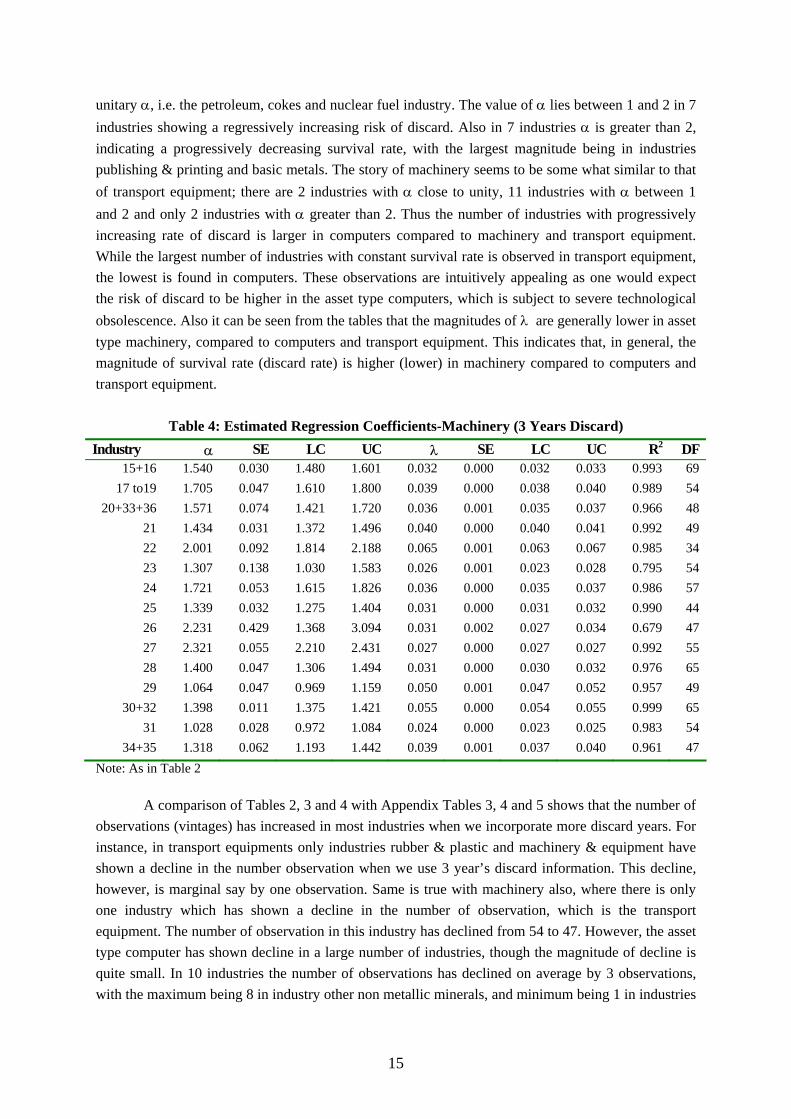
unitary α, i.e. the petroleum, cokes and nuclear fuel industry. The value of α lies between 1 and 2 in 7 industries showing a regressively increasing risk of discard. Also in 7 industries α is greater than 2, indicating a progressively decreasing survival rate, with the largest magnitude being in industries publishing & printing and basic metals. The story of machinery seems to be some what similar to that of transport equipment; there are 2 industries with α close to unity, 11 industries with α between 1 and 2 and only 2 industries with α greater than 2. Thus the number of industries with progressively increasing rate of discard is larger in computers compared to machinery and transport equipment. While the largest number of industries with constant survival rate is observed in transport equipment, the lowest is found in computers. These observations are intuitively appealing as one would expect the risk of discard to be higher in the asset type computers, which is subject to severe technological obsolescence. Also it can be seen from the tables that the magnitudes of λ are generally lower in asset type machinery, compared to computers and transport equipment. This indicates that, in general, the magnitude of survival rate (discard rate) is higher (lower) in machinery compared to computers and transport equipment.
Table 4: Estimated Regression Coefficients-Machinery (3 Years Discard)
Industry α SE LC UC λ SE LC UC R2 DF 15+16 1.540 0.030 1.480 1.601 0.032 0.000 0.032 0.033 0.993 69
17 to19 1.705 0.047 1.610 1.800 0.039 0.000 0.038 0.040 0.989 54 20+33+36 1.571 0.074 1.421 1.720 0.036 0.001 0.035 0.037 0.966 48
21 1.434 0.031 1.372 1.496 0.040 0.000 0.040 0.041 0.992 49 22 2.001 0.092 1.814 2.188 0.065 0.001 0.063 0.067 0.985 34 23 1.307 0.138 1.030 1.583 0.026 0.001 0.023 0.028 0.795 54 24 1.721 0.053 1.615 1.826 0.036 0.000 0.035 0.037 0.986 57 25 1.339 0.032 1.275 1.404 0.031 0.000 0.031 0.032 0.990 44 26 2.231 0.429 1.368 3.094 0.031 0.002 0.027 0.034 0.679 47 27 2.321 0.055 2.210 2.431 0.027 0.000 0.027 0.027 0.992 55 28 1.400 0.047 1.306 1.494 0.031 0.000 0.030 0.032 0.976 65 29 1.064 0.047 0.969 1.159 0.050 0.001 0.047 0.052 0.957 49
30+32 1.398 0.011 1.375 1.421 0.055 0.000 0.054 0.055 0.999 65 31 1.028 0.028 0.972 1.084 0.024 0.000 0.023 0.025 0.983 54
34+35 1.318 0.062 1.193 1.442 0.039 0.001 0.037 0.040 0.961 47 Note: As in Table 2
A comparison of Tables 2, 3 and 4 with Appendix Tables 3, 4 and 5 shows that the number of
observations (vintages) has increased in most industries when we incorporate more discard years. For instance, in transport equipments only industries rubber & plastic and machinery & equipment have shown a decline in the number observation when we use 3 year’s discard information. This decline, however, is marginal say by one observation. Same is true with machinery also, where there is only one industry which has shown a decline in the number of observation, which is the transport equipment. The number of observation in this industry has declined from 54 to 47. However, the asset type computer has shown decline in a large number of industries, though the magnitude of decline is quite small. In 10 industries the number of observations has declined on average by 3 observations, with the maximum being 8 in industry other non metallic minerals, and minimum being 1 in industries
16
paper & paper products, office machinery, computers, TV & radio manufacturing. In all other industries, for all the three asset types, the number of observation has increased, on average by 4 observations in transport equipment, 2 in computers and 5 in machinery.
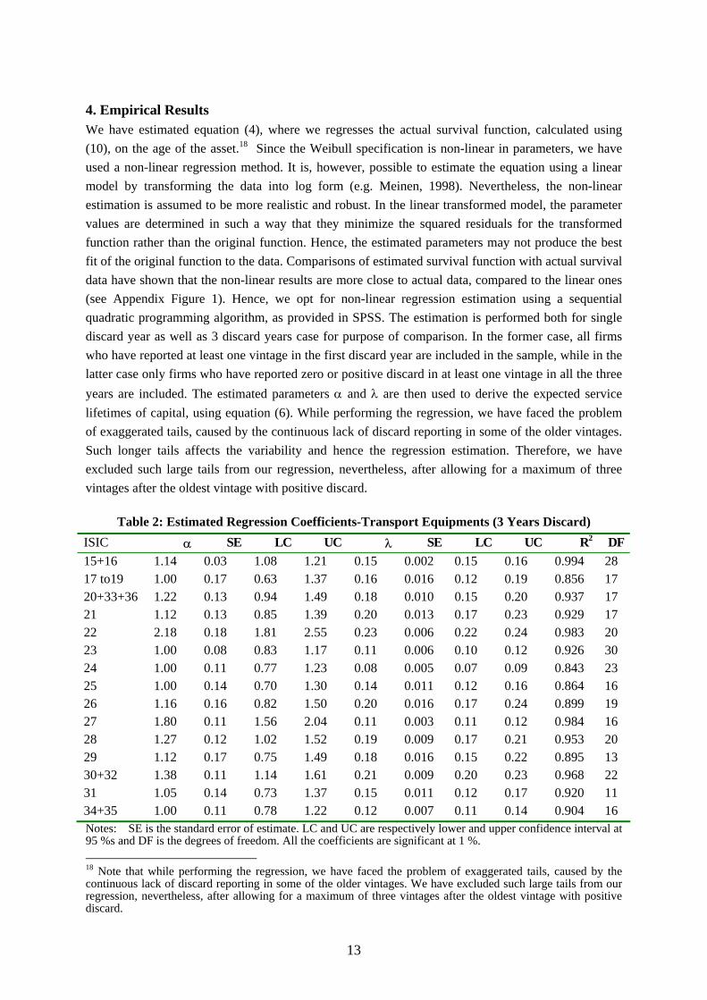
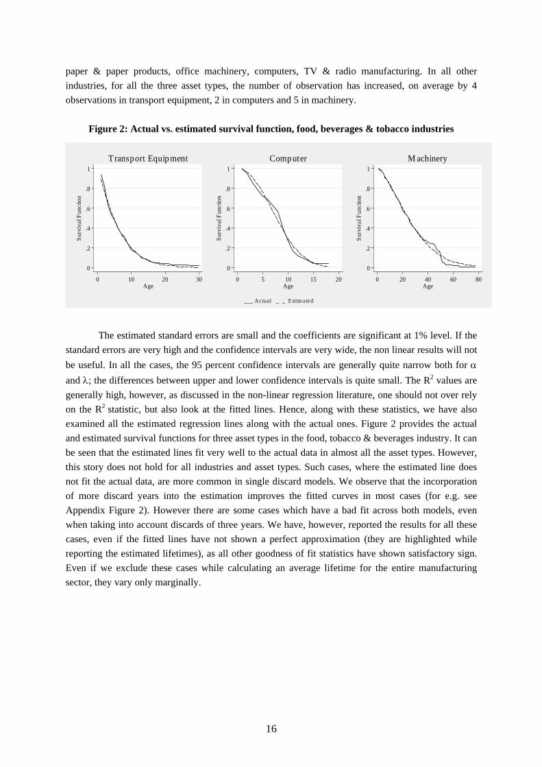
Figure 2: Actual vs. estimated survival function, food, beverages & tobacco industries
0
.2
.4
.6
.8
1
Surv
ival
Fun
ctio
n
0 10 20 30Age
Transport Equip ment
0
.2
.4
.6
.8
1
Surv
ival
Fun
ctio
n
0 5 10 15 20Age
Comp uter
0
.2
.4
.6
.8
1
Surv
ival
Fun
ctio
n
0 20 40 60 80Age
M achinery
___ A c tual _ _ Estim a te d The estimated standard errors are small and the coefficients are significant at 1% level. If the
standard errors are very high and the confidence intervals are very wide, the non linear results will not be useful. In all the cases, the 95 percent confidence intervals are generally quite narrow both for α and λ; the differences between upper and lower confidence intervals is quite small. The R2 values are generally high, however, as discussed in the non-linear regression literature, one should not over rely on the R2 statistic, but also look at the fitted lines. Hence, along with these statistics, we have also examined all the estimated regression lines along with the actual ones. Figure 2 provides the actual and estimated survival functions for three asset types in the food, tobacco & beverages industry. It can be seen that the estimated lines fit very well to the actual data in almost all the asset types. However, this story does not hold for all industries and asset types. Such cases, where the estimated line does not fit the actual data, are more common in single discard models. We observe that the incorporation of more discard years into the estimation improves the fitted curves in most cases (for e.g. see Appendix Figure 2). However there are some cases which have a bad fit across both models, even when taking into account discards of three years. We have, however, reported the results for all these cases, even if the fitted lines have not shown a perfect approximation (they are highlighted while reporting the estimated lifetimes), as all other goodness of fit statistics have shown satisfactory sign. Even if we exclude these cases while calculating an average lifetime for the entire manufacturing sector, they vary only marginally.
17
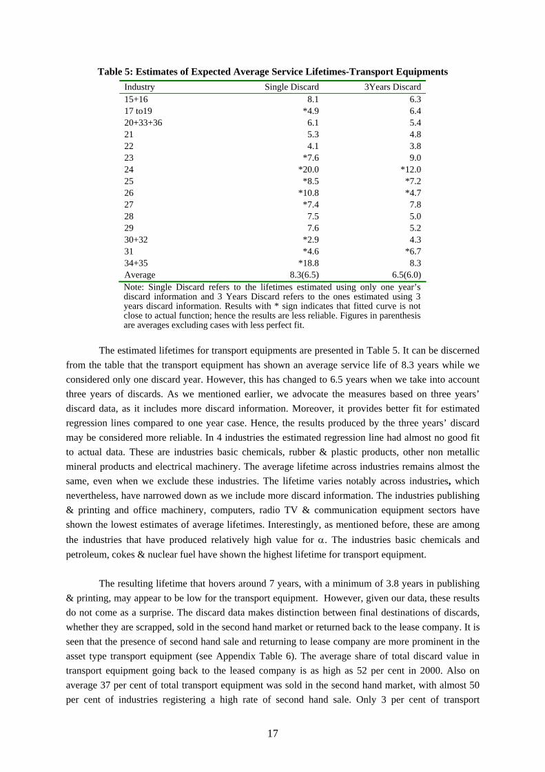
Table 5: Estimates of Expected Average Service Lifetimes-Transport Equipments Industry Single Discard 3Years Discard 15+16 8.1 6.3 17 to19 *4.9 6.4 20+33+36 6.1 5.4 21 5.3 4.8 22 4.1 3.8 23 *7.6 9.0 24 *20.0 *12.0 25 *8.5 *7.2 26 *10.8 *4.7 27 *7.4 7.8 28 7.5 5.0 29 7.6 5.2 30+32 *2.9 4.3 31 *4.6 *6.7 34+35 *18.8 8.3 Average 8.3(6.5) 6.5(6.0) Note: Single Discard refers to the lifetimes estimated using only one year’s discard information and 3 Years Discard refers to the ones estimated using 3 years discard information. Results with * sign indicates that fitted curve is not close to actual function; hence the results are less reliable. Figures in parenthesis are averages excluding cases with less perfect fit.
The estimated lifetimes for transport equipments are presented in Table 5. It can be discerned
from the table that the transport equipment has shown an average service life of 8.3 years while we considered only one discard year. However, this has changed to 6.5 years when we take into account three years of discards. As we mentioned earlier, we advocate the measures based on three years’ discard data, as it includes more discard information. Moreover, it provides better fit for estimated regression lines compared to one year case. Hence, the results produced by the three years’ discard may be considered more reliable. In 4 industries the estimated regression line had almost no good fit to actual data. These are industries basic chemicals, rubber & plastic products, other non metallic mineral products and electrical machinery. The average lifetime across industries remains almost the same, even when we exclude these industries. The lifetime varies notably across industries, which nevertheless, have narrowed down as we include more discard information. The industries publishing & printing and office machinery, computers, radio TV & communication equipment sectors have shown the lowest estimates of average lifetimes. Interestingly, as mentioned before, these are among the industries that have produced relatively high value for α. The industries basic chemicals and petroleum, cokes & nuclear fuel have shown the highest lifetime for transport equipment.
The resulting lifetime that hovers around 7 years, with a minimum of 3.8 years in publishing
& printing, may appear to be low for the transport equipment. However, given our data, these results do not come as a surprise. The discard data makes distinction between final destinations of discards, whether they are scrapped, sold in the second hand market or returned back to the lease company. It is seen that the presence of second hand sale and returning to lease company are more prominent in the asset type transport equipment (see Appendix Table 6). The average share of total discard value in transport equipment going back to the leased company is as high as 52 per cent in 2000. Also on average 37 per cent of total transport equipment was sold in the second hand market, with almost 50 per cent of industries registering a high rate of second hand sale. Only 3 per cent of transport
18
equipment was fully scrapped. This suggests the strong presence of leased assets and a large second hand market for the asset type transport equipment. In almost all the industries with lower lifetime estimates for transport equipment, we observe that the share of assets going back to lease company and second hand sale is more than 80 per cent. The story is quite different in the case of computers and machinery. On average 45 per cent of computers are fully scrapped, while 12 per cent are sold in the second hand market. Similarly, machinery has shown almost 42 percent scrap, while 35 percent is sold in the second hand market.
The average duration of a lease contract is probably shorter than the average age of owned
transport equipment, which will therefore cause to result a shorter lifetime estimate (Bergen et al 2005). The larger share of second hand sale indicates that this asset is sold for reuse and hence not used by the firm until the end of its actual service life, which will also reduce the lifetime estimate. Nevertheless, we make no adjustment for the presence of second hand market and leased assets in our study. As we have mentioned before, discard in our analysis is defined to include any withdrawal of an asset from the production process. Since the discard of an asset implies that it is no more profitable to keep (or efficiently usable) it in the production process in that particular industry, it is reasonable to expect that no competitive firm will be willing to use an asset discarded by another firm in the same industry, as it might adversely affect its efficiency and hence competitiveness. Similarly, as regard to the return to lease company, we assume that the economic life of that asset to this particular industry is over, and hence it is being discarded from that industry. Since most of the leased assets are found to be in transport assets, this assumption may be valid, as most discarded automobiles (or sold in the second hand market) are generally going to final consumers.
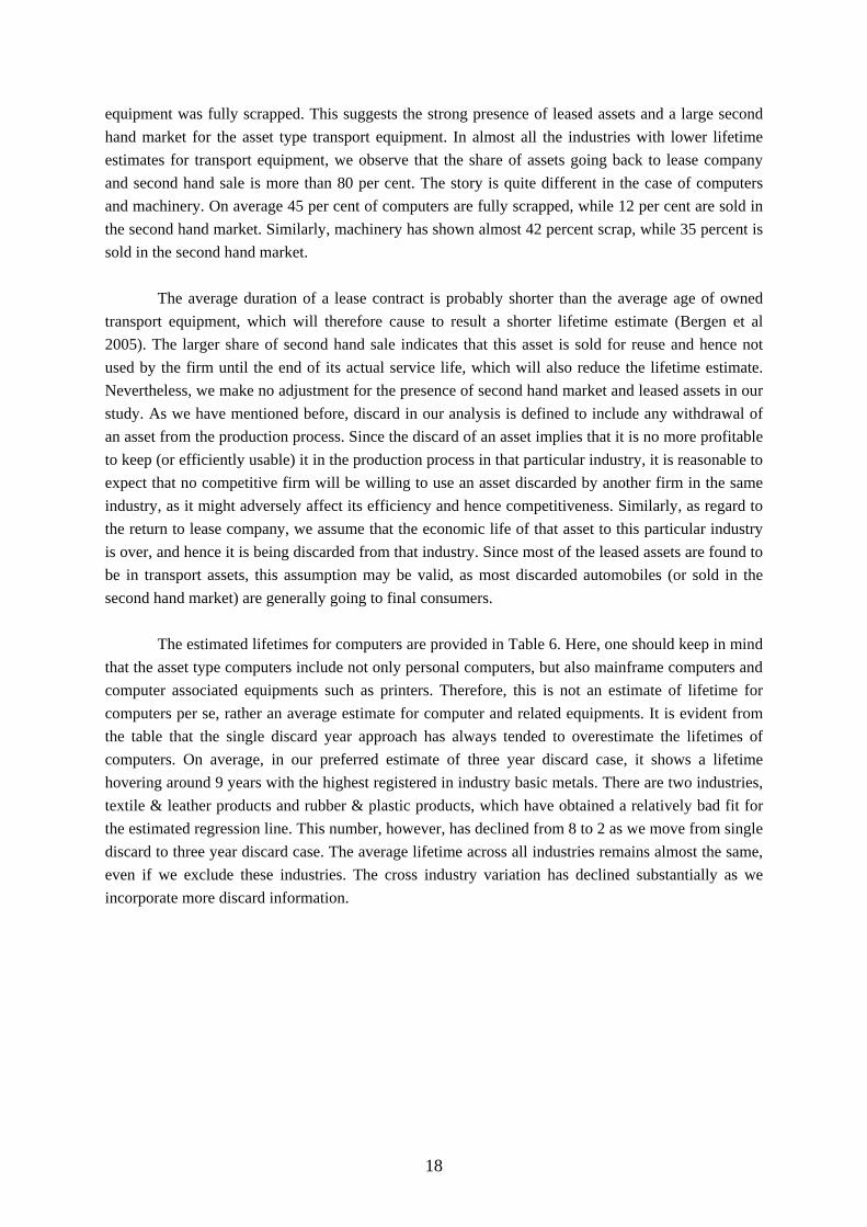
The estimated lifetimes for computers are provided in Table 6. Here, one should keep in mind
that the asset type computers include not only personal computers, but also mainframe computers and computer associated equipments such as printers. Therefore, this is not an estimate of lifetime for computers per se, rather an average estimate for computer and related equipments. It is evident from the table that the single discard year approach has always tended to overestimate the lifetimes of computers. On average, in our preferred estimate of three year discard case, it shows a lifetime hovering around 9 years with the highest registered in industry basic metals. There are two industries, textile & leather products and rubber & plastic products, which have obtained a relatively bad fit for the estimated regression line. This number, however, has declined from 8 to 2 as we move from single discard to three year discard case. The average lifetime across all industries remains almost the same, even if we exclude these industries. The cross industry variation has declined substantially as we incorporate more discard information.
19
Table 6: Estimates of Expected average lifetimes, Computers Industry Single Discard 3Years Discard 15+16 19.0 8.1 17 to19 *26.7 *9.0 20+33+36 *13.7 6.9 21 *12.5 6.9 22 16.8 9.7 23 *16.3 10.4 24 28.1 8.7 25 *24.1 *9.1 26 *23.7 8.0 27 *17.4 15.0 28 9.0 7.6 29 13.7 6.9 30+32 6.8 7.8 31 *26.8 8.9 34+35 9.8 6.9 Average 17.6(15.9) 8.7(8.6) Note: as in Table 5.
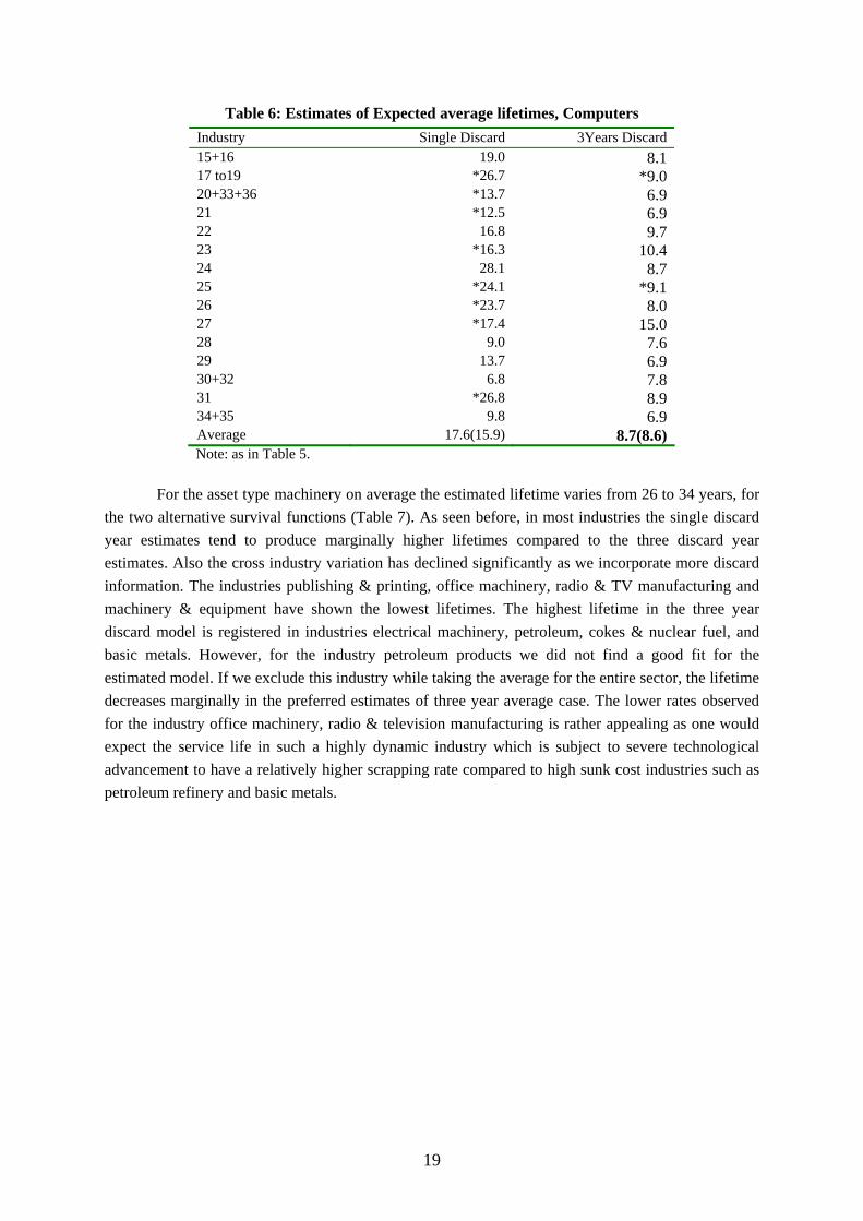
For the asset type machinery on average the estimated lifetime varies from 26 to 34 years, for
the two alternative survival functions (Table 7). As seen before, in most industries the single discard year estimates tend to produce marginally higher lifetimes compared to the three discard year estimates. Also the cross industry variation has declined significantly as we incorporate more discard information. The industries publishing & printing, office machinery, radio & TV manufacturing and machinery & equipment have shown the lowest lifetimes. The highest lifetime in the three year discard model is registered in industries electrical machinery, petroleum, cokes & nuclear fuel, and basic metals. However, for the industry petroleum products we did not find a good fit for the estimated model. If we exclude this industry while taking the average for the entire sector, the lifetime decreases marginally in the preferred estimates of three year average case. The lower rates observed for the industry office machinery, radio & television manufacturing is rather appealing as one would expect the service life in such a highly dynamic industry which is subject to severe technological advancement to have a relatively higher scrapping rate compared to high sunk cost industries such as petroleum refinery and basic metals.
20
Table 7: Estimates of Expected average lifetimes, Machinery
Industry Single Discard 3Years Discard 15+16 31.2 27.9 17 to19 28.4 22.8 20+33+36 34.7 24.9 21 *51.5 22.5 22 22.6 13.6 23 *59.8 *36.0 24 30.0 24.7 25 34.7 29.5 26 35.8 28.7 27 *52.8 33.0 28 28.5 29.2 29 24.5 19.6 30+32 13.6 16.7 31 *28.8 41.0 34+35 39.9 23.7 Average 34.5(29.4) 26.2(25.5)
Note: Note: as in Table 5.
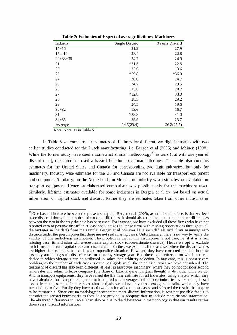
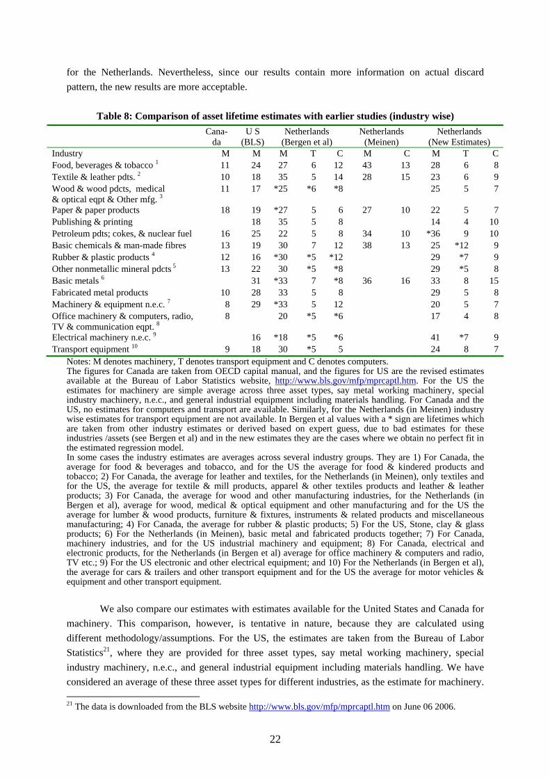
In Table 8 we compare our estimates of lifetimes for different two digit industries with two
earlier studies conducted for the Dutch manufacturing, i.e. Bergen et al (2005) and Meinen (1998). While the former study have used a somewhat similar methodology20 as ours (but with one year of discard data), the latter has used a hazard function to estimate lifetimes. The table also contains estimates for the United States and Canada for corresponding two digit industries, but only for machinery. Industry wise estimates for the US and Canada are not available for transport equipment and computers. Similarly, for the Netherlands, in Meinen, no industry wise estimates are available for transport equipment. Hence an elaborated comparison was possible only for the machinery asset. Similarly, lifetime estimates available for some industries in Bergen et al are not based on actual information on capital stock and discard. Rather they are estimates taken from other industries or
20 One basic difference between the present study and Bergen et al (2005), as mentioned before, is that we feed more discard information into the estimation of lifetimes. It should also be noted that there are other differences between the two in the way the data has been used. For instance, we have excluded all those firms who have not reported zero or positive discard in at least one vintage (i.e. those firms with missing observations throughout all the vintages in the data) from the sample. Bergen et al however have included all such firms assuming zero discards under the presumption that these are not real missing cases. Unfortunately, there is no way to verify the validity of this underlying assumption. The problem is that if this assumption is not true, i.e. if it is a real missing case, its inclusion will overestimate capital stock (underestimate discards). Hence we opt to exclude such firms both from capital stock and discard data. Further, we exclude all those cases where the discard values are higher than capital stock, as it is an impossible situation. However, they have corrected the data in these cases by attributing such discard cases to a nearby vintage year. But, there is no criterion on which one can decide to which vintage it can be attributed to, other than arbitrary selection. In any case, this is not a severe problem, as the number of such cases is quite negligible in all the three asset types we have considered. The treatment of discard has also been different, at least in asset type machinery, where they do not consider second hand sales and return to lease company (the share of latter is quite marginal though) as discards, while we do. And in transport equipments, they have raised the life time estimate for all industries, using a factor which they have calculated for transport equipment in food products, beverages and tobacco industries by excluding leased assets from the sample. In our regression analysis we allow only three exaggerated tails, while they have included up to five. Finally they have used two bench marks in most cases, and selected the results that appear to be reasonable. Since our methodology incorporates more discard information, it was not possible for us to consider the second benchmarks as they do not provide us adequate data to include more discard information. The observed differences in Table 8 can also be due to the differences in methodology in that our results carries three years’ discard information.
21
derived based on expert guesses, as they could not obtain robust results for these industries (such cases are marked by a * in Table 8). Hence, a strict comparison is meaningful only for industries for which robust estimates are available.
A comparison of our results with the previous estimates for the Netherlands shows that our
estimates are generally slightly higher than Bergen et al for transport equipment. The exceptions for this are industries wood, wood products & other manufacturing and publishing & printing where our estimates are one year less, and paper & paper products where they are the same. For machinery, our estimates lie in between Bergen et al and Meinen in 2 out of 6 industries for which estimates are available in these two studies. Our estimates are generally lower than Meinen's estimates in all the industries for which comparable figures are available, except in petroleum, cokes & nuclear fuel, where they are slightly higher, say by 2 years. Similarly new estimates are lower than Bergen et al for 10 industries. In industries, wood & wood products and basic metals they are the same, while in industries petroleum cokes & nuclear fuel and electrical machinery they are notably higher. Among these, the result in Bergen et al for industry electrical machinery is not robust. In computers, our estimates are higher than Bergen et al in 7 industries, lower in 6 industries and same in 2 industries. However, in 4 out of 8 industries where our estimates are higher, the estimates provided by Bergen et al are estimates borrowed from other industries or guesstimates. And our estimates are always lower than Meinen’s estimates for computers, say by 1 to 5 years.
In general, for machinery and computers, our estimates are relatively lower than the estimates
by Meinen. The differences between our estimates and Meinen’s estimates are on average 7(3) years for machinery(computers), while the new estimates differ from Bergen et al’s estimate on average by 7 (3, 1) year(s) for machinery (computer, transport equipment). These, however, vary across industries. In machinery, for instance, our results have shown substantial differences with that of Meinen’s estimate in food, beverages & tobacco and basic chemicals industries. In both these cases, Meinen have obtained unduly large lifetime estimates. Similarly, for computers, our results are quite lower than Meinen in food, beverages & tobacco, and textiles & leather industries. Our results tend to differ only marginally in transport equipment from Bergen et al, with the largest differences being in industries petroleum, coke & nuclear fuel, and basic chemicals. In these industries they have shown a lower lifetime compared to the new estimates. For the machinery, our results have shown large differences from Bergen et al in industries electrical machinery, printing & publishing, petroleum, cokes & nuclear fuel, textile & leather and machinery & equipment. It may be noted that the estimates for electrical machinery and machinery & equipment available in Bergen et al are not based on analysis of the discard data. For the other industries, our estimates are lower for publishing & printing and textiles & leather, while they are higher for petroleum, cokes & nuclear fuel. As we mentioned earlier, our results for petroleum, cokes & nuclear fuel industry is, however, less satisfactory as the estimated regression fit is not good. For computers, our estimates are higher in industries basic metals, electrical machinery, transport equipment, paper & paper products, petroleum, cokes & nuclear fuel, publishing & printing, and office machinery, computers, radio, TV & communication equipment. Again the results for Bergen et al for industries electrical machinery, basic metals, non metallic minerals and office machinery, computers, radio, TV & communication equipment are not robust. Moreover, our estimates for computers seem to be more appealing. Thus we observe some differences-in some cases substantial and in others trivial- between the new estimates and earlier ones
22
for the Netherlands. Nevertheless, since our results contain more information on actual discard pattern, the new results are more acceptable.
Table 8: Comparison of asset lifetime estimates with earlier studies (industry wise)
Cana- da
U S (BLS)
Netherlands (Bergen et al)
Netherlands (Meinen)
Netherlands (New Estimates)
Industry M M M T C M C M T C Food, beverages & tobacco 1 11 24 27 6 12 43 13 28 6 8 Textile & leather pdts. 2 10 18 35 5 14 28 15 23 6 9 Wood & wood pdcts, medical & optical eqpt & Other mfg. 3
11 17 *25 *6 *8 25 5 7
Paper & paper products 18 19 *27 5 6 27 10 22 5 7 Publishing & printing 18 35 5 8 14 4 10 Petroleum pdts; cokes, & nuclear fuel 16 25 22 5 8 34 10 *36 9 10 Basic chemicals & man-made fibres 13 19 30 7 12 38 13 25 *12 9 Rubber & plastic products 4 12 16 *30 *5 *12 29 *7 9 Other nonmetallic mineral pdcts 5 13 22 30 *5 *8 29 *5 8 Basic metals 6 31 *33 7 *8 36 16 33 8 15 Fabricated metal products 10 28 33 5 8 29 5 8 Machinery & equipment n.e.c. 7 8 29 *33 5 12 20 5 7 Office machinery & computers, radio, TV & communication eqpt. 8
8 20 *5 *6 17 4 8
Electrical machinery n.e.c. 9 16 *18 *5 *6 41 *7 9 Transport equipment 10 9 18 30 *5 5 24 8 7
Notes: M denotes machinery, T denotes transport equipment and C denotes computers. The figures for Canada are taken from OECD capital manual, and the figures for US are the revised estimates available at the Bureau of Labor Statistics website, http://www.bls.gov/mfp/mprcaptl.htm. For the US the estimates for machinery are simple average across three asset types, say metal working machinery, special industry machinery, n.e.c., and general industrial equipment including materials handling. For Canada and the US, no estimates for computers and transport are available. Similarly, for the Netherlands (in Meinen) industry wise estimates for transport equipment are not available. In Bergen et al values with a * sign are lifetimes which are taken from other industry estimates or derived based on expert guess, due to bad estimates for these industries /assets (see Bergen et al) and in the new estimates they are the cases where we obtain no perfect fit in the estimated regression model. In some cases the industry estimates are averages across several industry groups. They are 1) For Canada, the average for food & beverages and tobacco, and for the US the average for food & kindered products and tobacco; 2) For Canada, the average for leather and textiles, for the Netherlands (in Meinen), only textiles and for the US, the average for textile & mill products, apparel & other textiles products and leather & leather products; 3) For Canada, the average for wood and other manufacturing industries, for the Netherlands (in Bergen et al), average for wood, medical & optical equipment and other manufacturing and for the US the average for lumber & wood products, furniture & fixtures, instruments & related products and miscellaneous manufacturing; 4) For Canada, the average for rubber & plastic products; 5) For the US, Stone, clay & glass products; 6) For the Netherlands (in Meinen), basic metal and fabricated products together; 7) For Canada, machinery industries, and for the US industrial machinery and equipment; 8) For Canada, electrical and electronic products, for the Netherlands (in Bergen et al) average for office machinery & computers and radio, TV etc.; 9) For the US electronic and other electrical equipment; and 10) For the Netherlands (in Bergen et al), the average for cars & trailers and other transport equipment and for the US the average for motor vehicles & equipment and other transport equipment.
We also compare our estimates with estimates available for the United States and Canada for
machinery. This comparison, however, is tentative in nature, because they are calculated using different methodology/assumptions. For the US, the estimates are taken from the Bureau of Labor Statistics21, where they are provided for three asset types, say metal working machinery, special industry machinery, n.e.c., and general industrial equipment including materials handling. We have considered an average of these three asset types for different industries, as the estimate for machinery. 21 The data is downloaded from the BLS website http://www.bls.gov/mfp/mprcaptl.htm on June 06 2006.
23
Similarly for Canada, the figures are taken from OECD capital manual, which are available for different industries. However, in both these cases we have no information about the components of machinery (more importantly whether transport equipments are included or not). This is important because, a comparison is meaningful only if the same cohorts of assets are included in all the estimates. Nevertheless, we do compare them as we do not have a better estimate to compare with. Interestingly the Canadian estimates are quit smaller than both the US and all the earlier and current estimates for the Netherlands in all industries. This is surprising. For instance, the US and the Canada share not only geographical proximity, but also many economic characteristics, which make it less probable to have such huge differences in their asset lives. Hence, it may be an indication of differences in asset composition. Of course, one could argue that the discard decision and consequently the lifetimes of asset depends on many factors including tax policy, innovation, output growth and input prices, among others, which can vary across countries leading to differences in lifetimes. This is an issue that warrants further research, though. However, even if one gives allowance for such issues, one would not expect to have such huge lifetime differences, especially between countries of similar economic condition. When compared the US figures with the Dutch estimates, it is seen that the machinery in the Netherlands lives more than the US in almost all industries except in publishing & printing and machinery & equipment, where it is less respectively by 4 and 9 years. The difference between the estimates, on average is 6 years with the largest difference being in electrical machinery. These differences may either be real, or a reflection of the asset composition.
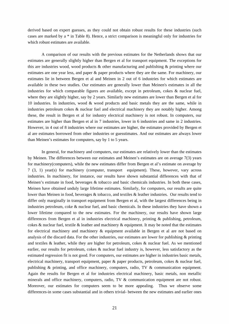
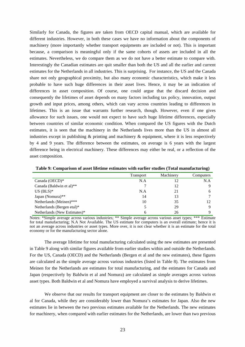
Table 9: Comparison of asset lifetime estimates with earlier studies (Total manufacturing) Transport Machinery Computers Canada (OECD)* N.A 12 N.A Canada (Baldwin et al)** 7 12 9 US (BLS)* N.A 21 6 Japan (Nomura)** 14 13 7 Netherlands (Meinen)*** 10 35 12 Netherlands (Bergen etal)* 5 29 9 Netherlands (New Estimates)* 6 26 9
Notes: *Simple average across various industries; ** Simple average across various asset types; *** Estimate for total manufacturing; N.A Not Available. The US estimate for computers is an overall estimate; hence it is not an average across industries or asset types. More over, it is not clear whether it is an estimate for the total economy or for the manufacturing sector alone.
The average lifetime for total manufacturing calculated using the new estimates are presented
in Table 9 along with similar figures available from earlier studies within and outside the Netherlands. For the US, Canada (OECD) and the Netherlands (Bergen et al and the new estimates), these figures are calculated as the simple average across various industries (listed in Table 8). The estimates from Meinen for the Netherlands are estimates for total manufacturing, and the estimates for Canada and Japan (respectively by Baldwin et al and Nomura) are calculated as simple averages across various asset types. Both Baldwin et al and Nomura have employed a survival analysis to derive lifetimes.
We observe that our results for transport equipment are closer to the estimates by Baldwin et
al for Canada, while they are considerably lower than Nomura’s estimates for Japan. Also the new estimates lie in between the two previous estimates available for the Netherlands. The new estimates for machinery, when compared with earlier estimates for the Netherlands, are lower than two previous

24
estimates though relatively closer to the estimates by Bergen et al, and quite lower than Meinen. Nevertheless they are still larger than the Japanese and the Canadian estimates though relatively closer to the US estimates. This is true with two earlier studies for the Netherlands as well. As we mentioned earlier, these differences could either be due to the differences in asset composition, or due to the differences in the factors that determine the scrapping behavior of firms. For computers, our estimates are same as Canadian estimates, but higher than US and Japanese estimates. It is also same as Bergen et al’s estimates for the Netherlands but lower than Meinen’s estimate. The US estimates for computer is quite low, but it is not clear whether these are estimates only for manufacturing. This is very important as it is also possible that the share of personal computers which are subjected to more rapid technological obsolescence is lower in manufacturing industries compared to service sectors. In the manufacturing sector computer equipments may largely consists of mainframe computers or highly customized numerically controlled machines, which may not be replaced as quick as personal computers may.
25
5. Conclusion In this paper we present estimates of average service life for three different asset types- transport equipment, computers, and machinery- for the manufacturing industries in the Netherlands. For this purpose, we exploit a unique firm level dataset on directly observed capital stock and discard of these asset types. A Weibull distribution function is estimated using a non-linear regression estimation procedure, where the survival function of select asset is regressed on its age. The Weibull parameters are then used to calculate the expected service life of the assets. In the measurement of lifetimes, unlike earlier studies, we have incorporated more information on discard behavior of each vintage and hence better approximation of survival rates at each age.
The estimated regression coefficients are found to have a good fit in general, and it has further
improved when we incorporate more discard information into estimation. Moreover, the number of observation has increased in most industries when more discard years are added into the model. On average the transport equipment have shown a lifetime of 6 years while the machinery and computers have respectively shown 26 and 9 years. While our estimates for transport equipments are quite close to estimates for Canada, they are significantly lower than that of Japan. A comparison of our estimates with that of earlier estimates for the Netherlands indicates that they lie in between the estimates provided by two previous studies. The asset transport equipment seems to have a lower lifetime in our estimate, at least in some industries, which may be attributed to the large share of leased assets and second hand sale in transport equipment component, with possibly lower length of lease contract. This point, however, needs further substantiation looking at the share of these factors in other countries, like Japan for instance. For machinery, our estimates are different from both Japan and Canada, but closer to the previous estimates for the Netherlands and to some extend closer to the US. These differences could either be due to compositional differences or due to differences in determinants of scrapping across countries. In the latter case, it warrants further research unearthing the determinants of scrapping behavior of firms. Computers, however, have produced a lifetime that is almost same as Canadian estimates, but slightly higher than the US and Japanese estimates.
It may be noted that there is wide variation in asset lifetimes across industries. The cross
industry variation is seen to be decreasing as we incorporate more discard information. However they still do exist. The difference is observed despite the fact that we have considered a relatively high level aggregation, where one might expect to have similar estimates. Nevertheless, apart from the technological specificities, which may be countered by the high level aggregation we have used, we have no explanation for this. The observed difference may either be a reality, or indicate noise. It is a worthwhile topic for future research. Similarly, since there is observed differences across different countries in terms of their lifetimes, especially in machinery, if it is a reality, it is also important to examine the determinants of scrapping by firms. This is particularly important from the perspective of the relationship between innovation and investment/discard behavior, particularly in the milieu of increasing technological obsolescence.
26
Appendix 1. The data
As mentioned in the text, the data used in this study are taken from two distinct surveys conducted by the Statistics Netherlands (CBS) - the capital stock survey and the discard survey. The capital stock data is collected since 1993 till 200322 for manufacturing firms coming under ISIC 2 digit level. Each year one or more 2 digit industries have been surveyed, and the same industry will be subjected to a second survey after five years. The information on existing capital stock, with vintage structure is available for 8 asset types, they are, 1. Land and sites (only purchase and sale of sites) 2. Industrial buildings (offices, shops, etc.) 3. Civil engineering works (including site improvements-roads, pipelines etc.) 4. External transport equipments (excavators, drudging machines etc.) 5. Internal means of transport (cranes, pulleys etc.) 6. Computers and associated equipments (computers, printers etc.) 7. Machinery and Equipments, and 8. Other tangible fixed assets (furniture, freight containers etc.)
In the present analysis, we consider only asset types 4 to 7. We have further merged internal
means of transport (5) with machinery and equipments (7), as the capital stock survey provide information on these assets together, though the discard survey provides them separate.
As mentioned in the paper the capital stock in year t-1 is merged for each vintage to the
discard in years t, t+1 and t+2. Prior to merging the two databases, we have deleted all firms reported more than once (for same asset, vintage and ownership type causing double counting and hence an exaggeration of actual data), i.e. firms with double reporting in both surveys. Tables 1 and 2 below provide the number of firms reported to various surveys on capital stock and discard respectively. It can be read from the table that the number of manufacturing firms reported to capital stock survey is 1354 in the first round and 1108 in the second round. The number of firms varies from 10 (7) in petroleum, coke and nuclear fuel industry to 247 (234) in food processing industry in the first (second) round. As is evident from the Table 2 the number of manufacturing firms reported to various discard surveys during 1993-2001 varies over years. The number has varied over years, the highest response rate being in 1997 and the lowest in 1996. As was observed in the case of capital stock survey, the largest number of firms reported is found to be in the food processing industry throughout the period, while the lowest number is observed in petroleum, coke and nuclear fuel industry. Note that all the firms reported in these tables are not considered in our final sample, as we had to apply a number of cleansing rules to clean up the data, which resulted in elimination of a number of firms from the sample (see text).
22 Practically, for our analysis the data on both capital stock and discard are available only till 2001, as the data after that are yet to be officially released.
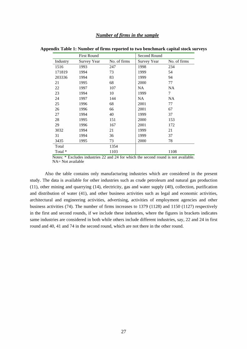
27
Number of firms in the sample
Appendix Table 1: Number of firms reported to two benchmark capital stock surveys
First Round Second Round Industry Survey Year No. of firms Survey Year No. of firms 1516 1993 247 1998 234 171819 1994 73 1999 54 203336 1994 83 1999 94 21 1995 68 2000 77 22 1997 107 NA NA 23 1994 10 1999 7 24 1997 144 NA NA 25 1996 68 2001 77 26 1996 66 2001 67 27 1994 40 1999 37 28 1995 151 2000 153 29 1996 167 2001 172 3032 1994 21 1999 21 31 1994 36 1999 37 3435 1995 73 2000 78 Total 1354 Total * 1103 1108
Notes: * Excludes industries 22 and 24 for which the second round is not available. NA= Not available
Also the table contains only manufacturing industries which are considered in the present
study. The data is available for other industries such as crude petroleum and natural gas production (11), other mining and quarrying (14), electricity, gas and water supply (40), collection, purification and distribution of water (41), and other business activities such as legal and economic activities, architectural and engineering activities, advertising, activities of employment agencies and other business activities (74). The number of firms increases to 1379 (1128) and 1150 (1127) respectively in the first and second rounds, if we include these industries, where the figures in brackets indicates same industries are considered in both while others include different industries, say, 22 and 24 in first round and 40, 41 and 74 in the second round, which are not there in the other round.
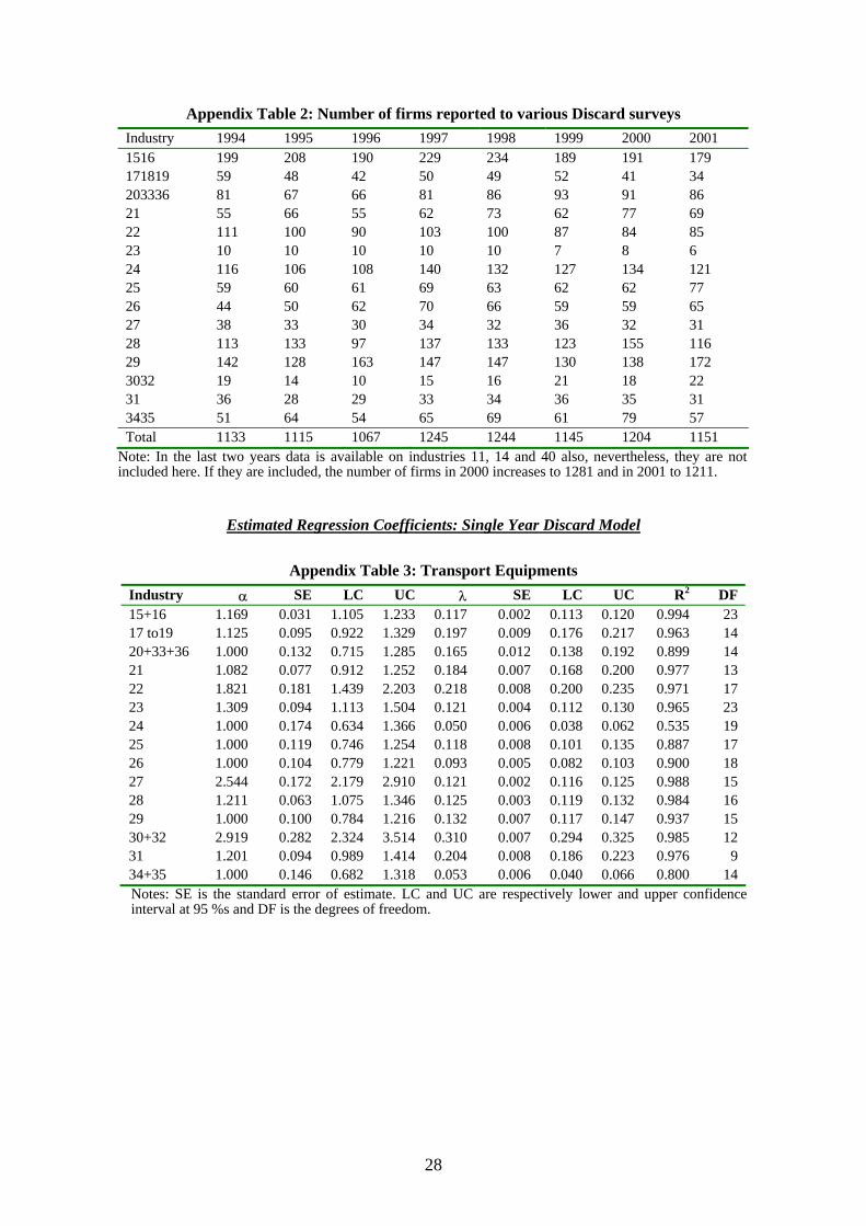
28
Appendix Table 2: Number of firms reported to various Discard surveys Industry 1994 1995 1996 1997 1998 1999 2000 2001 1516 199 208 190 229 234 189 191 179 171819 59 48 42 50 49 52 41 34 203336 81 67 66 81 86 93 91 86 21 55 66 55 62 73 62 77 69 22 111 100 90 103 100 87 84 85 23 10 10 10 10 10 7 8 6 24 116 106 108 140 132 127 134 121 25 59 60 61 69 63 62 62 77 26 44 50 62 70 66 59 59 65 27 38 33 30 34 32 36 32 31 28 113 133 97 137 133 123 155 116 29 142 128 163 147 147 130 138 172 3032 19 14 10 15 16 21 18 22 31 36 28 29 33 34 36 35 31 3435 51 64 54 65 69 61 79 57 Total 1133 1115 1067 1245 1244 1145 1204 1151
Note: In the last two years data is available on industries 11, 14 and 40 also, nevertheless, they are not included here. If they are included, the number of firms in 2000 increases to 1281 and in 2001 to 1211.
Estimated Regression Coefficients: Single Year Discard Model
Appendix Table 3: Transport Equipments
Industry α SE LC UC λ SE LC UC R2 DF 15+16 1.169 0.031 1.105 1.233 0.117 0.002 0.113 0.120 0.994 23 17 to19 1.125 0.095 0.922 1.329 0.197 0.009 0.176 0.217 0.963 14 20+33+36 1.000 0.132 0.715 1.285 0.165 0.012 0.138 0.192 0.899 14 21 1.082 0.077 0.912 1.252 0.184 0.007 0.168 0.200 0.977 13 22 1.821 0.181 1.439 2.203 0.218 0.008 0.200 0.235 0.971 17 23 1.309 0.094 1.113 1.504 0.121 0.004 0.112 0.130 0.965 23 24 1.000 0.174 0.634 1.366 0.050 0.006 0.038 0.062 0.535 19 25 1.000 0.119 0.746 1.254 0.118 0.008 0.101 0.135 0.887 17 26 1.000 0.104 0.779 1.221 0.093 0.005 0.082 0.103 0.900 18 27 2.544 0.172 2.179 2.910 0.121 0.002 0.116 0.125 0.988 15 28 1.211 0.063 1.075 1.346 0.125 0.003 0.119 0.132 0.984 16 29 1.000 0.100 0.784 1.216 0.132 0.007 0.117 0.147 0.937 15 30+32 2.919 0.282 2.324 3.514 0.310 0.007 0.294 0.325 0.985 12 31 1.201 0.094 0.989 1.414 0.204 0.008 0.186 0.223 0.976 9 34+35 1.000 0.146 0.682 1.318 0.053 0.006 0.040 0.066 0.800 14 Notes: SE is the standard error of estimate. LC and UC are respectively lower and upper confidence interval at 95 %s and DF is the degrees of freedom.
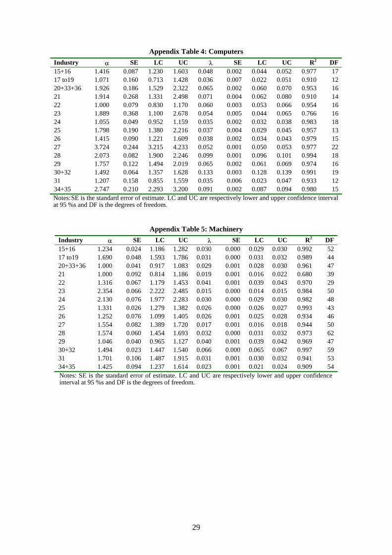
29
Appendix Table 4: Computers Industry α SE LC UC λ SE LC UC R2 DF 15+16 1.416 0.087 1.230 1.603 0.048 0.002 0.044 0.052 0.977 17 17 to19 1.071 0.160 0.713 1.428 0.036 0.007 0.022 0.051 0.910 12 20+33+36 1.926 0.186 1.529 2.322 0.065 0.002 0.060 0.070 0.953 16 21 1.914 0.268 1.331 2.498 0.071 0.004 0.062 0.080 0.910 14 22 1.000 0.079 0.830 1.170 0.060 0.003 0.053 0.066 0.954 16 23 1.889 0.368 1.100 2.678 0.054 0.005 0.044 0.065 0.766 16 24 1.055 0.049 0.952 1.159 0.035 0.002 0.032 0.038 0.983 18 25 1.798 0.190 1.380 2.216 0.037 0.004 0.029 0.045 0.957 13 26 1.415 0.090 1.221 1.609 0.038 0.002 0.034 0.043 0.979 15 27 3.724 0.244 3.215 4.233 0.052 0.001 0.050 0.053 0.977 22 28 2.073 0.082 1.900 2.246 0.099 0.001 0.096 0.101 0.994 18 29 1.757 0.122 1.494 2.019 0.065 0.002 0.061 0.069 0.974 16 30+32 1.492 0.064 1.357 1.628 0.133 0.003 0.128 0.139 0.991 19 31 1.207 0.158 0.855 1.559 0.035 0.006 0.023 0.047 0.933 12 34+35 2.747 0.210 2.293 3.200 0.091 0.002 0.087 0.094 0.980 15 Notes: SE is the standard error of estimate. LC and UC are respectively lower and upper confidence interval at 95 %s and DF is the degrees of freedom.
Appendix Table 5: Machinery Industry α SE LC UC λ SE LC UC R2 DF 15+16 1.234 0.024 1.186 1.282 0.030 0.000 0.029 0.030 0.992 52 17 to19 1.690 0.048 1.593 1.786 0.031 0.000 0.031 0.032 0.989 44 20+33+36 1.000 0.041 0.917 1.083 0.029 0.001 0.028 0.030 0.961 47 21 1.000 0.092 0.814 1.186 0.019 0.001 0.016 0.022 0.680 39 22 1.316 0.067 1.179 1.453 0.041 0.001 0.039 0.043 0.970 29 23 2.354 0.066 2.222 2.485 0.015 0.000 0.014 0.015 0.984 50 24 2.130 0.076 1.977 2.283 0.030 0.000 0.029 0.030 0.982 48 25 1.331 0.026 1.279 1.382 0.026 0.000 0.026 0.027 0.993 43 26 1.252 0.076 1.099 1.405 0.026 0.001 0.025 0.028 0.934 46 27 1.554 0.082 1.389 1.720 0.017 0.001 0.016 0.018 0.944 50 28 1.574 0.060 1.454 1.693 0.032 0.000 0.031 0.032 0.973 62 29 1.046 0.040 0.965 1.127 0.040 0.001 0.039 0.042 0.969 47 30+32 1.494 0.023 1.447 1.540 0.066 0.000 0.065 0.067 0.997 59 31 1.701 0.106 1.487 1.915 0.031 0.001 0.030 0.032 0.941 53 34+35 1.425 0.094 1.237 1.614 0.023 0.001 0.021 0.024 0.909 54 Notes: SE is the standard error of estimate. LC and UC are respectively lower and upper confidence interval at 95 %s and DF is the degrees of freedom.
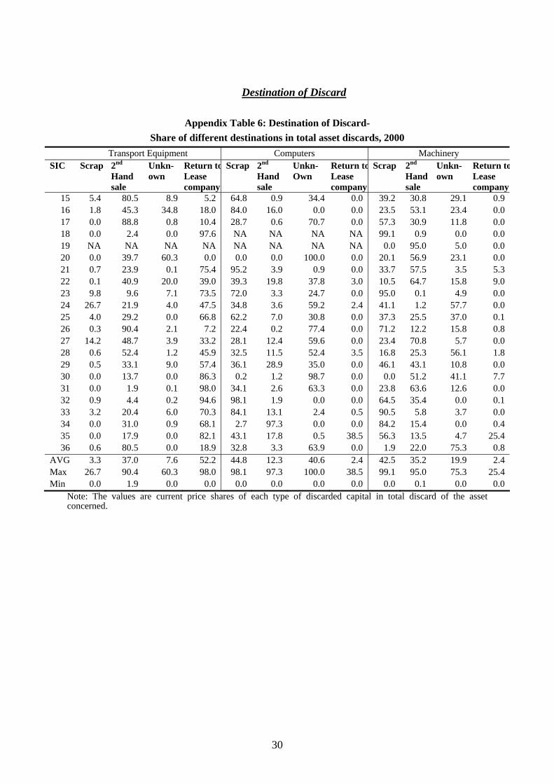
30
Destination of Discard
Appendix Table 6: Destination of Discard-
Share of different destinations in total asset discards, 2000 Transport Equipment Computers Machinery SIC Scrap 2nd
Hand sale
Unkn- own
Return toLease company
Scrap 2nd Hand sale
Unkn- Own
Return toLease company
Scrap 2nd Hand sale
Unkn- own
Return toLease company
15 5.4 80.5 8.9 5.2 64.8 0.9 34.4 0.0 39.2 30.8 29.1 0.9 16 1.8 45.3 34.8 18.0 84.0 16.0 0.0 0.0 23.5 53.1 23.4 0.0 17 0.0 88.8 0.8 10.4 28.7 0.6 70.7 0.0 57.3 30.9 11.8 0.0 18 0.0 2.4 0.0 97.6 NA NA NA NA 99.1 0.9 0.0 0.0 19 NA NA NA NA NA NA NA NA 0.0 95.0 5.0 0.0 20 0.0 39.7 60.3 0.0 0.0 0.0 100.0 0.0 20.1 56.9 23.1 0.0 21 0.7 23.9 0.1 75.4 95.2 3.9 0.9 0.0 33.7 57.5 3.5 5.3 22 0.1 40.9 20.0 39.0 39.3 19.8 37.8 3.0 10.5 64.7 15.8 9.0 23 9.8 9.6 7.1 73.5 72.0 3.3 24.7 0.0 95.0 0.1 4.9 0.0 24 26.7 21.9 4.0 47.5 34.8 3.6 59.2 2.4 41.1 1.2 57.7 0.0 25 4.0 29.2 0.0 66.8 62.2 7.0 30.8 0.0 37.3 25.5 37.0 0.1 26 0.3 90.4 2.1 7.2 22.4 0.2 77.4 0.0 71.2 12.2 15.8 0.8 27 14.2 48.7 3.9 33.2 28.1 12.4 59.6 0.0 23.4 70.8 5.7 0.0 28 0.6 52.4 1.2 45.9 32.5 11.5 52.4 3.5 16.8 25.3 56.1 1.8 29 0.5 33.1 9.0 57.4 36.1 28.9 35.0 0.0 46.1 43.1 10.8 0.0 30 0.0 13.7 0.0 86.3 0.2 1.2 98.7 0.0 0.0 51.2 41.1 7.7 31 0.0 1.9 0.1 98.0 34.1 2.6 63.3 0.0 23.8 63.6 12.6 0.0 32 0.9 4.4 0.2 94.6 98.1 1.9 0.0 0.0 64.5 35.4 0.0 0.1 33 3.2 20.4 6.0 70.3 84.1 13.1 2.4 0.5 90.5 5.8 3.7 0.0 34 0.0 31.0 0.9 68.1 2.7 97.3 0.0 0.0 84.2 15.4 0.0 0.4 35 0.0 17.9 0.0 82.1 43.1 17.8 0.5 38.5 56.3 13.5 4.7 25.4 36 0.6 80.5 0.0 18.9 32.8 3.3 63.9 0.0 1.9 22.0 75.3 0.8
AVG 3.3 37.0 7.6 52.2 44.8 12.3 40.6 2.4 42.5 35.2 19.9 2.4 Max 26.7 90.4 60.3 98.0 98.1 97.3 100.0 38.5 99.1 95.0 75.3 25.4 Min 0.0 1.9 0.0 0.0 0.0 0.0 0.0 0.0 0.0 0.1 0.0 0.0
Note: The values are current price shares of each type of discarded capital in total discard of the asset concerned.
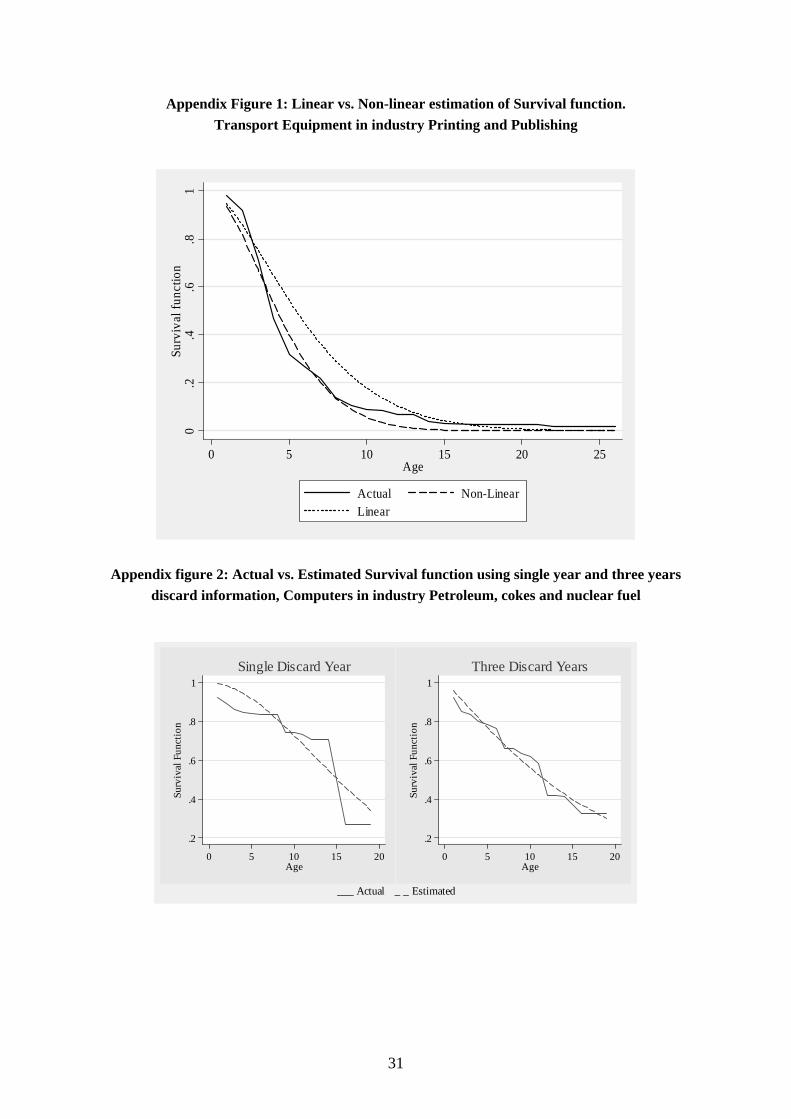
31
Appendix Figure 1: Linear vs. Non-linear estimation of Survival function. Transport Equipment in industry Printing and Publishing
0.2
.4.6
.81
Surv
ival
func
tion
0 5 10 15 20 25Age
Actual Non-LinearLinear
Appendix figure 2: Actual vs. Estimated Survival function using single year and three years discard information, Computers in industry Petroleum, cokes and nuclear fuel
.2
.4
.6
.8
1
Surv
ival
Fun
ctio
n
0 5 10 15 20Age
Single Discard Year
.2
.4
.6
.8
1
Surv
ival
Fun
ctio
n
0 5 10 15 20Age
Three Discard Years
___ Actual _ _ Estimated
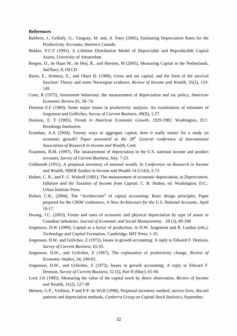
32
References Baldwin, J., Gellatly, G., Tanguay, M. and, A. Patry (2005), Estimating Depreciation Rates for the
Productivity Accounts, Statistics Canada. Bekker, P.C.F (1991), A Lifetime Distribution Model of Depreciable and Reproducible Capital
Assets, University of Amsterdam. Bergen, D., de Haan M., de Heij, R., and Horsten, M (2005), Measuring Capital in the Netherlands,
Std/Naes, 8, OECD BiØrn, E., HolmØy, E., and Olsen Ø. (1989), Gross and net capital, and the form of the survival
function: Theory and some Norwegian evidence, Review of Income and Wealth, 35(2), 133-149.
Coen, R (1975), Investment behaviour, the measurement of depreciation and tax policy, American Economic Review 65, 59–74.
Denison E.F (1969), Some major issues in productivity analysis: An examination of estimates of Jorgenson and Grilliches, Survey of Current Business, 49(II), 1-27.
Denison, E. F (1985), Trends in American Economic Growth, 1929-1982, Washington, D.C: Brookings Institution.
Erumban, A.A (2004), Twenty ways to aggregate capital, does it really matter for a study on economic growth? Paper presented at the 28th General conference of International Association of Research in Income and Wealth, Cork
Fraumeni, B.M. (1997), The measurement of depreciation in the U.S. national income and product accounts, Survey of Current Business, July, 7-23.
Goldsmith (1951), A perpetual inventory of national wealth, In Conference on Research in Income and Wealth, NBER Studies in Income and Wealth 14 (1143), 5-73
Hulten, C. R., and F. C. Wykoff (1981), The measurement of economic depreciation, in Depreciation, Inflation and the Taxation of Income from Capital, C. R. Hulten, ed. Washington, D.C.: Urban Institute Press.
Hulten, C.R., (2004), The “Architecture” of capital accounting: Basic design principles, Paper prepared for the CRIW conference, A New Architecture for the U.S. National Accounts, April 16-17.
Hwang, J.C. (2003), Forms and rates of economic and physical depreciation by type of assets in Canadian industries, Journal of Economic and Social Measurement, 28 (3), 89-108
Jorgenson, D.W (1989), Capital as a factor of production, in D.W. Jorgenson and R. Landau (eds.), Technology and Capital Formation, Cambridge, MIT Press, 1-35.
Jorgenson, D.W. and Griliches, Z (1972), Issues in growth accounting: A reply to Edward F. Denison, Survey of Current Business, 65-93.
Jorgenson, D.W., and Griliches, Z (1967), The explanation of productivity change, Review of Economic Studies, 34, 249-83.
Jorgenson, D.W., and Griliches, Z (1972), Issues in growth accounting: A reply to Edward F. Denison, Survey of Current Business, 52 (5), Part II (May), 65-94.
Lock J.D (1985), Measuring the value of the capital stock by direct observation, Review of Income and Wealth, 31(2), 127-38
Meinen, G.P., Verbiest, P and P.P. de Wolf (1998), Perpetual inventory method, service lives, discard patterns and depreciation methods, Canberra Group on Capital Stock Statistics, September.

33
Meinen, G.W (1998), Lives of capital goods, Paper presented at the 2nd meeting of the Canberra Group on Capital Stock Statistics, OECD, Paris.
Mudholkar, G.S., Srivastava, D.K., and G.D. Kollia (1996), A generalization of the Weibull distribution with applications to the analysis of survival data. Journal of American Statistical Association, 91, 1575-1583.
Nomura, K (2005), Examination of directly observed discard data in Japan, KEO Discussion Paper No.99
OECD (2001), Measuring Capital- A Manual on the Measurement of Capital Stocks, Consumption of Fixed Capital and Capital Services, OECD, Paris
Oulton, N. (1995), Depreciation, obsolescence and the role of capital in growth accounting, Bulletin of Economic Research, 47(1), 21-33.
Oulton, N. (2004), Productivity versus welfare; or GDP versus Weitzman’s NDP, Review of Income and Wealth, 50(3), 329-55.
Pitman, J (1992), Probability, Springer-Verlag Schreyer, P., W.E. Diewert and A. Harrison (2005), Cost of capital services and the national accounts,
paper presented at the Fifth Meeting of the Canberra II Group on the Measurement of Non-Financial Assets, Canberra, March 29-April 1
Smeets H.H and N.H.L.van den Hove (1994), Disinvestments, Statistics Netherlands, Voorburg. Verbeek, 2004, A Guide to Modern Econometrics, Weiley West, P. (1998), The direct observation of asset lives, paper for the 2nd meeting the Canberra group
on capital stock statistics.
34
Papers issued in the series of the Groningen Growth and Development Centre
Papers marked * are also available in pdf-format on the internet: http://www.ggdc.net/ Hardcopies of other papers can be ordered (as long as available) from [email protected]
536 (GD-1) Maddison, Angus and Harry van Ooststroom, The International Comparison of Value
Added, Productivity and Purchasing Power Parities in Agriculture (1993) 537 (GD-2) Mulder, Nanno and Angus Maddison, The International Comparison of Performance
in Distribution: Value Added, Labour Productivity and PPPs in Mexican and US Wholesale and Retail Trade 1975/7 (1993)
538 (GD-3)* Szirmai, Adam, Comparative Performance in Indonesian Manufacturing, 1975-90 (1993)
549 (GD-4) de Jong, Herman J., Prices, Real Value Added and Productivity in Dutch Manufacturing, 1921-1960 (1993)
550 (GD-5) Beintema, Nienke and Bart van Ark, Comparative Productivity in East and West German Manufacturing before Reunification (1993)
567 (GD-6)* Maddison, Angus and Bart van Ark, The International Comparison of Real Product and Productivity (1994)
568 (GD-7) de Jong, Gjalt, An International Comparison of Real Output and Labour Productivity in Manufacturing in Ecuador and the United States, 1980 (1994)
569 (GD-8) van Ark, Bart and Angus Maddison, An International Comparison of Real Output, Purchasing Power and Labour Productivity in Manufacturing Industries: Brazil, Mexico and the USA in 1975 (1994) (second edition)
570 (GD-9) Maddison, Angus, Standardised Estimates of Fixed Capital Stock: A Six Country Comparison (1994)
571 (GD-10)* van Ark, Bart and Remco D.J. Kouwenhoven, Productivity in French Manufacturing: An International Comparative Perspective (1994)
572 (GD-11) Gersbach, Hans and Bart van Ark, Micro Foundations for International Productivity Comparisons (1994)
573 (GD-12)* Albers, Ronald, Adrian Clemens and Peter Groote, Can Growth Theory Contribute to Our Understanding of Nineteenth Century Economic Dynamics (1994)
574 (GD-13)* de Jong, Herman J. and Ronald Albers, Industrial Output and Labour Productivity in the Netherlands, 1913-1929: Some Neglected Issues (1994)
575 (GD-14) Mulder, Nanno, New Perspectives on Service Output and Productivity: A Comparison of French and US Productivity in Transport, Communications Wholesale and Retail Trade (1994)
576 (GD-15) Maddison, Angus, Economic Growth and Standards of Living in the Twentieth Century (1994)
577 (GD-16) Gales, Ben, In Foreign Parts: Free-Standing Companies in the Netherlands around the First World War (1994)
578 (GD-17) Mulder, Nanno, Output and Productivity in Brazilian Distribution: A Comparative View (1994)
579 (GD-18) Mulder, Nanno, Transport and Communication in Mexico and the United States: Value Added, Purchasing Power Parities and Productivity (1994)
35
580 (GD-19) Mulder, Nanno, Transport and Communications Output and Productivity in Brazil and the USA, 1950-1990 (1995)
581 (GD-20) Szirmai, Adam and Ren Ruoen, China's Manufacturing Performance in Comparative Perspective, 1980-1992 (1995)
GD-21 Fremdling, Rainer, Anglo-German Rivalry on Coal Markets in France, the Netherlands and Germany, 1850-1913 (December 1995)
GD-22* Tassenaar, Vincent, Regional Differences in Standard of Living in the Netherlands, 1800-1875, A Study Based on Anthropometric Data (December 1995)
GD-23* van Ark, Bart, Sectoral Growth Accounting and Structural Change in Postwar Europe (December 1995)
GD-24* Groote, Peter, Jan Jacobs and Jan Egbert Sturm, Output Responses to Infrastructure in the Netherlands, 1850-1913 (December 1995)
GD-25* Groote, Peter, Ronald Albers and Herman de Jong, A Standardised Time Series of the Stock of Fixed Capital in the Netherlands, 1900-1995 (May 1996)
GD-26* van Ark, Bart and Herman de Jong, Accounting for Economic Growth in the Netherlands since 1913 (May 1996)
GD-27* Maddison, Angus and D.S. Prasada Rao, A Generalized Approach to International Comparisons of Agricultural Output and Productivity (May 1996)
GD-28 van Ark, Bart, Issues in Measurement and International Comparison of Productivity - An Overview (May 1996)
GD-29* Kouwenhoven, Remco, A Comparison of Soviet and US Industrial Performance, 1928-90 (May 1996)
GD-30 Fremdling, Rainer, Industrial Revolution and Scientific and Technological Progress (December 1996)
GD-31 Timmer, Marcel, On the Reliability of Unit Value Ratios in International Comparisons (December 1996)
GD-32 de Jong, Gjalt, Canada's Post-War Manufacturing Performance: A Comparison with the United States (December 1996)
GD-33 Lindlar, Ludger, “1968” and the German Economy (January 1997) GD-34 Albers, Ronald, Human Capital and Economic Growth: Operationalising Growth
Theory, with Special Reference to The Netherlands in the 19th Century (June 1997) GD-35* Brinkman, Henk-Jan, J.W. Drukker and Brigitte Slot, GDP per Capita and the
Biological Standard of Living in Contemporary Developing Countries (June 1997) GD-36 de Jong, Herman, and Antoon Soete, Comparative Productivity and Structural Change
in Belgian and Dutch Manufacturing, 1937-1987 (June 1997) GD-37 Timmer, M.P., and A. Szirmai, Growth and Divergence in Manufacturing Performance
in South and East Asia (June 1997) GD-38* van Ark, B., and J. de Haan, The Delta-Model Revisited: Recent Trends in the
Structural Performance of the Dutch Economy (December 1997) GD-39* van der Eng, P., Economics Benefits from Colonial Assets: The Case of the
Netherlands and Indonesia, 1870-1958 (June 1998) GD-40* Timmer, Marcel P., Catch Up Patterns in Newly Industrializing Countries. An
International Comparison of Manufacturing Productivity in Taiwan, 1961-1993 (July 1998)
36
GD-41* Ark, Bart van, Economic Growth and Labour Productivity in Europe: Half a Century of East-West Comparisons (October 1999)
GD-42* Smits, Jan Pieter, Herman de Jong and Bart van Ark, Three Phases of Dutch Economic Growth and Technological Change, 1815-1997 (October 1999)
GD-43* Fremdling, Rainer, Historical Precedents of Global Markets (October 1999) GD-44* Ark, Bart van, Lourens Broersma and Gjalt de Jong, Innovation in Services. Overview
of Data Sources and Analytical Structures (October 1999) GD-45* Broersma, Lourens and Robert McGuckin, The Impact of Computers on Productivity
in the Trade Sector: Explorations with Dutch Microdata (October 1999, Revised version June 2000)
GD-46* Sleifer, Jaap, Separated Unity: The East and West German Industrial Sector in 1936 (November 1999)
GD-47* Rao, D.S. Prasada and Marcel Timmer, Multilateralisation of Manufacturing Sector Comparisons: Issues, Methods and Empirical Results (July 2000)
GD-48* Vikström, Peter, Long term Patterns in Swedish Growth and Structural Change, 1870-1990 (July 2001)
GD-49* Wu, Harry X., Comparative labour productivity performance in Chinese manufacturing, 1952-1997: An ICOP PPP Approach (July 2001)
GD-50* Monnikhof, Erik and Bart van Ark, New Estimates of Labour Productivity in the Manufacturing Sectors of Czech Republic, Hungary and Poland, 1996 (January 2002)
GD-51* van Ark, Bart, Robert Inklaar and Marcel Timmer, The Canada-US Manufacturing Gap Revisited: New ICOP Results (January 2002)
GD-52* Mulder, Nanno, Sylvie Montout and Luis Peres Lopes, Brazil and Mexico's Manufacturing Performance in International Perspective, 1970-98 (January 2002)
GD-53* Szirmai, Adam, Francis Yamfwa and Chibwe Lwamba, Zambian Manufacturing Performance in Comparative Perspective (January 2002)
GD-54* Fremdling, Rainer, European Railways 1825-2001, an Overview (August 2002) GD-55* Fremdling, Rainer, Foreign Trade-Transfer-Adaptation: The British Iron Making
Technology on the Continent (Belgium and France) (August 2002) GD-56* van Ark, Bart, Johanna Melka, Nanno Mulder, Marcel Timmer and Gerard Ypma, ICT
Investments and Growth Accounts for the European Union 1980-2000 (September 2002)
GD-57* Sleifer, Jaap, A Benchmark Comparison of East and West German Industrial Labour Productivity in 1954 (October 2002)
GD-58* van Dijk, Michiel, South African Manufacturing Performance in International Perspective, 1970-1999 (November 2002)
GD-59* Szirmai, A., M. Prins and W. Schulte, Tanzanian Manufacturing Performance in Comparative Perspective (November 2002)
GD-60* van Ark, Bart, Robert Inklaar and Robert McGuckin, “Changing Gear” Productivity, ICT and Services: Europe and the United States (December 2002)
GD-61* Los, Bart and Timmer, Marcel, The ‘Appropriate Technology’ Explanation of Productivity Growth Differentials: An Empirical Approach (April 2003)
GD-62* Hill, Robert J., Constructing Price Indexes Across Space and Time: The Case of the European Union (May 2003)
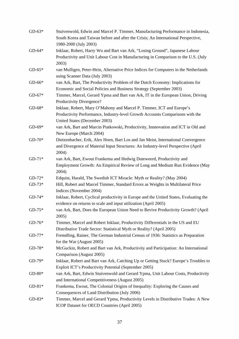
37
GD-63* Stuivenwold, Edwin and Marcel P. Timmer, Manufacturing Performance in Indonesia, South Korea and Taiwan before and after the Crisis; An International Perspective, 1980-2000 (July 2003)
GD-64* Inklaar, Robert, Harry Wu and Bart van Ark, “Losing Ground”, Japanese Labour Productivity and Unit Labour Cost in Manufacturing in Comparison to the U.S. (July 2003)
GD-65* van Mulligen, Peter-Hein, Alternative Price Indices for Computers in the Netherlands using Scanner Data (July 2003)
GD-66* van Ark, Bart, The Productivity Problem of the Dutch Economy: Implications for Economic and Social Policies and Business Strategy (September 2003)
GD-67* Timmer, Marcel, Gerard Ypma and Bart van Ark, IT in the European Union, Driving Productivity Divergence?
GD-68* Inklaar, Robert, Mary O’Mahony and Marcel P. Timmer, ICT and Europe’s Productivity Performance, Industry-level Growth Accounts Comparisons with the United States (December 2003)
GD-69* van Ark, Bart and Marcin Piatkowski, Productivity, Innnovation and ICT in Old and New Europe (March 2004)
GD-70* Dietzenbacher, Erik, Alex Hoen, Bart Los and Jan Meist, International Convergence and Divergence of Material Input Structures: An Industry-level Perspective (April 2004)
GD-71* van Ark, Bart, Ewout Frankema and Hedwig Duteweerd, Productivity and Employment Growth: An Empirical Review of Long and Medium Run Evidence (May 2004)
GD-72* Edquist, Harald, The Swedish ICT Miracle: Myth or Reality? (May 2004) GD-73* Hill, Robert and Marcel Timmer, Standard Errors as Weights in Multilateral Price
Indices (November 2004) GD-74* Inklaar, Robert, Cyclical productivity in Europe and the United States, Evaluating the
evidence on returns to scale and input utilization (April 2005) GD-75* van Ark, Bart, Does the European Union Need to Revive Productivity Growth? (April
2005) GD-76* Timmer, Marcel and Robert Inklaar, Productivity Differentials in the US and EU
Distributive Trade Sector: Statistical Myth or Reality? (April 2005) GD-77* Fremdling, Rainer, The German Industrial Census of 1936: Statistics as Preparation
for the War (August 2005) GD-78* McGuckin, Robert and Bart van Ark, Productivity and Participation: An International
Comparison (August 2005) GD-79* Inklaar, Robert and Bart van Ark, Catching Up or Getting Stuck? Europe’s Troubles to
Exploit ICT’s Productivity Potential (September 2005) GD-80* van Ark, Bart, Edwin Stuivenwold and Gerard Ypma, Unit Labour Costs, Productivity
and International Competitiveness (August 2005) GD-81* Frankema, Ewout, The Colonial Origins of Inequality: Exploring the Causes and
Consequences of Land Distribution (July 2006) GD-83* Timmer, Marcel and Gerard Ypma, Productivity Levels in Distributive Trades: A New
ICOP Dataset for OECD Countries (April 2005)

38
GD-86* Frankema, Ewout, and Jutta Bolt, Measuring and Analysing Educational Inequality: The Distribution of Grade Enrolment Rates in Latin America and Sub-Saharan Africa (April 2006)

39
Groningen Growth and Development Centre Research Monographs Monographs marked * are also available in pdf-format on the internet: http://www.ggdc.net/ No. 1* van Ark, Bart, International Comparisons of Output and Productivity: Manufacturing
Productivity Performance of Ten Countries from 1950 to 1990 (1993) (http://www.eco.rug.nl/GGDC/ThesisArk.html)
No. 2 Pilat, Dirk, The Economics of Catch-Up: The Experience of Japan and Korea (1993) No. 3 Hofman, André, Latin American Economic Development. A Causal Analysis in
Historical Perspective (1998) No. 4 Mulder, Nanno, The Economic Performance of the Service Sector in Brazil, Mexico
and the United States (1999) No. 5* Smits, Jan-Pieter, Edwin Horlings and Jan Luiten van Zanden, Dutch GNP and Its
Components, 1800-1913 (2000) (http://www.eco.rug.nl/GGDC/PUB/dutchgnp.pdf)