Embed Size (px)
Citation preview
UNIVERSITY OF ECONOMICS PRAGUE
Faculty of Finance and Accounting
Department of Banking and Insurance
Post-Crisis Valuation of Derivatives
Doctoral Thesis
Author: Mgr. Jaroslav Baran
Supervisor: doc. RNDr. Jiří Witzany, Ph.D.
Study programme: Finance and accounting
Field of study: Finance
Prague 2016
Declaration
I declare that I wrote this doctoral thesis independently and that all external sources and
literature are acknowledged in the text.
Prague, February 15, 2016 Jaroslav Baran
Acknowledgement
I wish to thank my supervisor doc. RNDr. Jiří Witzany, Ph.D. for our many encounters,
discussions, his guidance, valuable advice and patience with this thesis and throughout my
studies. I am also grateful to my parents and my girlfriend Katka for their encouragement, love
and support which made this thesis possible.
Abstract
In this study we analyse relationship between classical approach to valuation of linear interest
rate derivatives and post-crisis approach when the valuation better reflects credit and liquidity
risk and economic costs of the transaction on top of the risk-free rate. We discuss the method
of collateralization to diminish counterparty credit risk, its impact on derivatives pricing, and
how overnight indexed swap (OIS) rates became market standard for discounting future
derivatives’ cash flows. We show that using one yield curve to both estimating the forward
rates and discounting the expected future cash flows is no longer possible in arbitrage free
market. We review in detail three fundamental interest rate derivatives (interest rate swap,
basis swap and cross-currency swap) and we derive discount factors used for calculating the
present value of expected future cash flows that are consistent with market quotes. We also
investigate drivers behind basis spreads, in particular, credit and liquidity risk, and supply and
demand forces, and show how they impact valuation of derivatives. We analyse Czech swap
rates and propose an estimation of CZK OIS curve and approximate discount rates in case of
cross-currency swaps. Finally, we discuss inflation markets and consistent valuation of inflation
swaps.
Keywords: swap spreads, overnight indexed swap, basis swap, cross-currency swap, basis
spread, discount factor, collateral
JEL Classification: D53, G01
Abstrakt
V této práci se zabýváme vztahy mezi klasickým přístupem k oceňování lineárních úrokových
derivátů a postkrizovým přístupem, který kromě diskontování bezrizikovou křivkou rovněž
zohledňuje kreditní a likviditní riziko a ekonomické náklady transakce. Pojednáme o tom jak lze
pomocí kolateralizace snížit kreditní riziko protistrany, jaký vliv má kolateralizace na oceňování
derivátů a jak se OIS sazby stali tržním standardem pro diskontování budoucích peněžních toků
derivátových transakcí. Ukážeme, že používání jedné křivky pro odhad forwardových sazeb a
zároveň pro diskontování očekávaných peněžních toků již není možné na bezarbitrážním trhu.
Podrobně rozebereme tři základní úrokové deriváty (úrokový swap, bazický swap a meziměnový
swap) a odvodíme diskontní faktory používané k výpočtu současné hodnoty očekávaných
budoucích plateb, které jsou konzistentní s tržními kotacemi. Dále zkoumáme bazické přirážky
z pohledu kreditního a likviditního rizika a nabídky a poptávky a ukážeme, jak tyto přirážky
ovlivňují oceňování derivátů. Analyzujeme swapové sazby na českém trhu a ukážeme, jak lze
odhadnout korunové OIS sazby a aproximovat diskontní sazby pro ocenění meziměnových
swapů. Nakonec prodiskutujeme inflační trhy a oceňování iniflačních swapů.
Klíčová slova: swapové přirážky, overnight indexed swap, bazický swap, meziměnový swap,
bazické přirážky, diskontní faktor, kolaterál
JEL Klasifikace: D53, G01
5
Contents
1. Introduction .......................................................................................................................... 7
2. Valuation adjustments for derivatives ............................................................................... 11
2.1. Credit valuation adjustment (CVA) .................................................................................. 12
2.1.1. Modelling counterparty exposure .......................................................................... 13
2.1.2. Regulatory CVA ....................................................................................................... 14
2.2. Debit valuation adjustment (DVA) .................................................................................. 16
2.3. Funding valuation adjustment (FVA) ............................................................................... 16
2.4. Other valuation adjustments ........................................................................................... 18
2.4.1. Capital valuation adjustment (KVA) ....................................................................... 18
2.4.2. Initial Margin Valuation Adjustment (MVA) ........................................................... 19
3. Valuation of interest rate derivatives ................................................................................ 20
3.1. Interest Rate Swap ........................................................................................................... 21
3.1.1. Classical bootstrapping using discount factors ...................................................... 22
3.1.2. OIS rates, collateralization, and OIS discounting.................................................... 24
3.1.3. Collateralized interest rate swap ............................................................................ 27
3.1.4. Discount curve defined by spread to a reference rate .......................................... 28
3.2. Basis swap ........................................................................................................................ 29
3.2.1. Collateralized basis swap ........................................................................................ 30
3.3. Cross-currency swap ........................................................................................................ 31
3.3.1. Collateralized cross-currency swap ........................................................................ 33
3.3.2. Cross-currency swap collateralized in the currency of the second leg .................. 34
3.4. Approximation of discount curves of cross-currency swaps ........................................... 35
3.4.1. Credit and liquidity risks between two currencies ................................................. 36
3.4.2. Cross-currency OIS basis swap (float-float) ............................................................ 37
3.4.3. Currency of collateral and indirect quotes ............................................................. 39
4. Cross-currency and OIS market in Czech koruna ............................................................... 41
4.1. CZK Interest rate swap ..................................................................................................... 41
4.2. Estimation of CZK OIS curve above 10 years ................................................................... 41
6
4.3. Approximation of discount rates of cross-currency swap ............................................... 42
4.4. CZK discount curve implied from EUR/CZK cross-currency swap ................................... 43
4.5. EUR/CZK Cross-currency OIS swap .................................................................................. 45
5. Analysis of Cross-Currency Basis Swaps ............................................................................. 48
5.1. Cross-currency basis spread determinants ..................................................................... 50
5.1.1. Supply and demand ................................................................................................ 50
5.1.2. Short-end of the curve ........................................................................................... 54
5.1.3. Long-end of the curve............................................................................................. 54
5.1.4. Regression analysis of EUR/USD cross-currency basis swap spreads ………………....56
5.2. Arbitrage-free boundaries for basis swap spreads ......................................................... 60
5.2.1. EUR/USD cross-currency basis swap ...................................................................... 60
5.2.2. EUR/CZK FX swap .................................................................................................... 63
6. Valuation of Zero-coupon Inflation Swaps ......................................................................... 66
6.1. Inflation Market ............................................................................................................... 67
6.1.1. Measuring Inflation ................................................................................................ 68
6.1.2. Inflation-Linked Bond ............................................................................................. 69
6.1.3. Breakeven inflation rate ......................................................................................... 71
6.2. Zero-coupon inflation swaps ........................................................................................... 72
6.2.1. Valuation of zero-coupon inflation swap ............................................................... 72
6.2.2. Construction of zero coupon inflation swap curve ................................................ 74
Conclusion ..................................................................................................................................... 79
References .................................................................................................................................... 82
List of figures ................................................................................................................................. 87
List of tables .................................................................................................................................. 88
List of notations ............................................................................................................................ 89

7
1. Introduction
Risk-free rates are the essential input in calculation of present value of expected future cash
flows and in general, for pricing of financial instruments. In practice, to calculate a risk-free
yield curve, proxies such as government bond yields and short-term interbank deposit interest
rates (see Málek et. al (2007)) have been used. For valuation of derivative instruments using
quoted forward rates (FRA, Forward Rate Agreement) and swap rates (IRS, Interest Rate Swap)
have been a standard approach in the past.
The basis of these instruments is the exchange of fixed for floating rate cash flows. The floating
rate is usually the 3-month or 6-month IBOR (interbank offered rate) and reflects the unsecured
interbank funding rate for this maturity. IBOR rates therefore also include the average risk
premium of the given interbank market or respective reference banks. This risk premium is also
a part of the quoted swap rates and is thus reflected in the swap curve. Under normal market
conditions, the risk embedded in short-term interbank loans is considered very low and the
swap curve has been used as a proxy of a risk free curve; however, this no longer holds,
especially during market stress.
The increase in interbank risk has become a major issue during financial crisis with a direct
impact on banks’ liquidity management. We perceive interbank risk mainly as credit and
liquidity risk that are integral components of unsecured interbank loans. IBOR market reference
rates which reflect the interbank risk are one of the main channels of monetary transmission
mechanism and serve as a benchmark for wide range of financial products, i.e. financial
derivatives, mortgages, loans, or savings accounts. Since the breakout of recent financial crisis,
it has been shown that these rates are not adequate proxies for risk-free rates, see for example
Bianchetti (2008) or Bianchetti and Carlicchi (2012).
The risk premium in quoted IBOR rates is incorporated into quoted FRA and IRS rates, and is
therefore reflected in the yield curve derived from these instruments. According to Collin-
Dufresne and Solnik (2001), the swap rate is characterized as fixed rate equivalent of a
continuous short-term borrowing by banks of high credit rating (the average rating of IBOR
panel banks). If a rating of a certain bank deteriorates, the bank will be replaced by another
highly rated bank. During normal market conditions, the risk premium in interbank rates has
been considered as negligible and IBOR swap rates were therefore used as a proxy to construct
a risk-free yield curve. At the same time, IBOR swap rates were a good proxy for banks’ funding
costs. Nevertheless, IBOR swap rates are not risk-free anymore nor they approximate banks’
funding costs any longer.
8
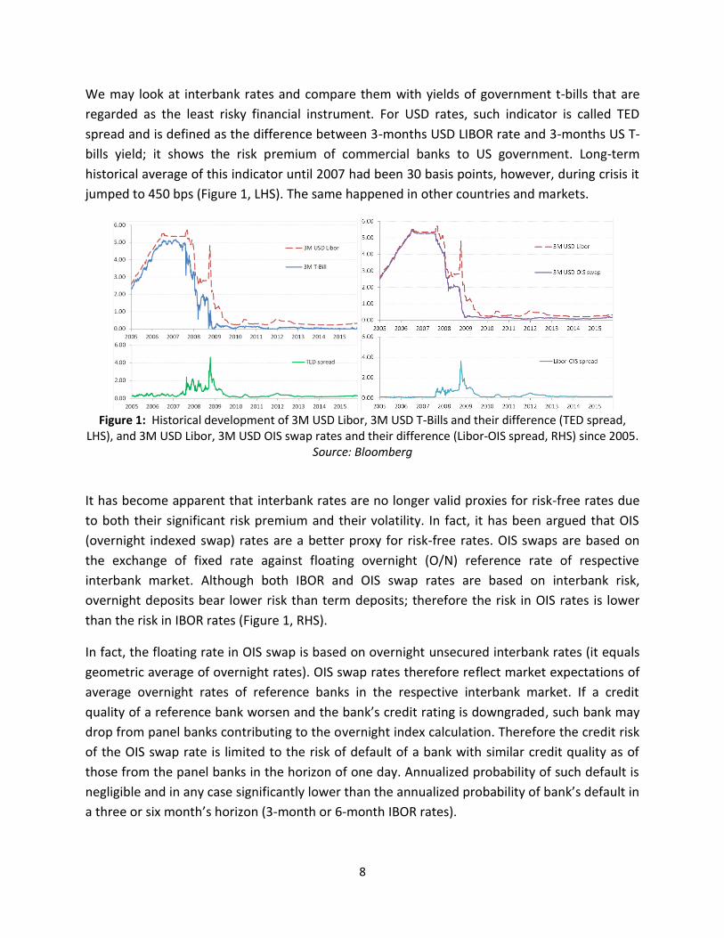
We may look at interbank rates and compare them with yields of government t-bills that are
regarded as the least risky financial instrument. For USD rates, such indicator is called TED
spread and is defined as the difference between 3-months USD LIBOR rate and 3-months US T-
bills yield; it shows the risk premium of commercial banks to US government. Long-term
historical average of this indicator until 2007 had been 30 basis points, however, during crisis it
jumped to 450 bps (Figure 1, LHS). The same happened in other countries and markets.
Figure 1: Historical development of 3M USD Libor, 3M USD T-Bills and their difference (TED spread,
LHS), and 3M USD Libor, 3M USD OIS swap rates and their difference (Libor-OIS spread, RHS) since 2005. Source: Bloomberg
It has become apparent that interbank rates are no longer valid proxies for risk-free rates due
to both their significant risk premium and their volatility. In fact, it has been argued that OIS
(overnight indexed swap) rates are a better proxy for risk-free rates. OIS swaps are based on
the exchange of fixed rate against floating overnight (O/N) reference rate of respective
interbank market. Although both IBOR and OIS swap rates are based on interbank risk,
overnight deposits bear lower risk than term deposits; therefore the risk in OIS rates is lower
than the risk in IBOR rates (Figure 1, RHS).
In fact, the floating rate in OIS swap is based on overnight unsecured interbank rates (it equals
geometric average of overnight rates). OIS swap rates therefore reflect market expectations of
average overnight rates of reference banks in the respective interbank market. If a credit
quality of a reference bank worsen and the bank’s credit rating is downgraded, such bank may
drop from panel banks contributing to the overnight index calculation. Therefore the credit risk
of the OIS swap rate is limited to the risk of default of a bank with similar credit quality as of
those from the panel banks in the horizon of one day. Annualized probability of such default is
negligible and in any case significantly lower than the annualized probability of bank’s default in
a three or six month’s horizon (3-month or 6-month IBOR rates).
9
When we look at cross-currency derivatives, we notice another interesting phenomenon; the
existence of cross-currency basis spread to a floating rate of one currency vs. the other. This
spread can be explained by different liquidity and credit risk of interbank market in one
currency vs. the other, and by demand and supply imbalances. We discuss the existence of
credit and liquidity risk premiums on top of risk-free rates in Baran and Witzany (2014). The
existence of basis swap spreads itself leads to discrepancies in their interpretation. According to
Chang and Schlogl (2012), basis swap spreads are inconsistent with a classical arbitrage
argument between spot and forward market. On the other hand, Bianchetti and Carlicchi
(2012) note that it is consistent with arbitrage-free market with the consequence that the
valuation of such derivatives needs multiple curve input for estimating forward rates and
discounting future cash flows. In fact, when we change the discount curve, we change the
market value of the derivative. The concept of using one curve to both estimate the forward
rates and discount future cash flows thus needs to be reassessed.
And this is the aim of our study. In this work, we analyse relationship between classical
approach to valuation of linear interest rate derivatives and post-crisis approach that requires
further assumptions to reflect the risk of the transaction, for example counterparty credit risk.
We discuss the method of collateralization to diminish counterparty credit risk and its impact
on derivatives’ pricing. We also analyse credit and liquidity risks, and supply and demand forces
and their impact on valuation of derivatives, in particular, interest rate swaps, basis swaps and
cross-currency swaps. We show that using one yield curve for both estimating forward rates
and discounting expected future cash flows is no longer possible in arbitrage free market. We
present valuations of three fundamental interest rate derivatives (interest rate, basis and cross-
currency swaps) step by step and we derive discount factors used to calculate the present value
of expected future cash flows that are consistent with market quotes.
This work is organized into six chapters. Each chapter starts with an introduction and a review
of relevant literature. The second chapter discusses recent changes and trends in derivatives’
valuation when different adjustments are needed to reflect risks and costs of a transaction, for
example, counterparty credit risk, funding costs, or capital charges. We discuss valuation
methodologies when future cash flows are discounted with risk free rates and such valuation is
then adjusted to take into account all economic costs of the transaction. The topic of valuation
adjustment is still evolving and as we discuss later, not without controversy.
The third chapter is the core chapter of the thesis. In this chapter we discuss derivatives’
discounting in detail. We explain how OIS rates became a market standard for discounting
future cash flows due to being both a good proxy to risk-free rates and due to the fact that they
are linked to interest paid on collateral for collateralized transactions. OIS discounting takes the
centre stage but we also discuss other discount curves. The aim of this chapter is to derive
10
discount factors and forward rates that are consistent with market prices. In this respect, we
also show how basis swap spreads impact the valuation. We focus in detail on valuation of
interest rate swaps, basis swaps and cross-currency swaps. We show that we can no longer
work with one curve but use multiple curves to estimate forward rates and to discount future
cash flows. Concluding section of this chapter deals with approximations of discount curves
implied from cross-currency market quotes and the discount curve of the base currency. Apart
from technical derivations, we also further investigate the relationship between discounting
and forwarding curves of both legs of cross-currency swap and discuss potential implications
and applications.
Fourth chapter is more practical and targets the Czech derivative market. We discuss how CZK
OIS curve could be estimated even if not all OIS quotes are available. We also analyse EUR/CZK
cross-currency basis swap spreads by decomposing them into individual components and
investigate if they are driven mainly by different credit and liquidity risk between EUR and CZK
interbank rates or by relative demand of one currency versus the other. We also show how we
can use such breakdown to approximate implied discount rates of the second leg of the cross-
currency swap.
Fifth chapter analyses cross-currency basis swap spreads from a different angle. We discuss
credit and liquidity risk and supply and demand pressure of one currency versus another one.
We then build a multiple regression model and explain drivers behind EUR/USD basis swap
spreads. We construct boundaries within which there should not be an arbitrage opportunity,
however, by testing these boundaries we discover that supply and demand imbalances may
push basis spreads outside these boundaries creating arbitrage opportunities for market
participants able to raise unsecured funding in one currency and swapping it into another
currency. We illustrate this on the example of EUR/USD and EUR/CZK FX swap markets.
The last, sixth, chapter differs slightly by focusing on inflation market and inflation derivatives.
One of the reasons to include this topic is that inflation markets do not enjoy such spotlight as
other market although they are quite sizeable and new valuation methods apply to them as
well as to other derivatives. That is why the aim of this chapter remains the same; to present a
consistent valuation approach to zero-coupon inflation swaps reflecting the risk of its future
cash-flows. However, we also provide a general overview on functioning of inflation markets,
and we discuss inflation measurement, real yields and nominal yields, and the construction of
inflation curve from zero coupon inflation swaps taking into account inflation seasonality.
Some results of the thesis were published in journals or presented at conferences, in particular,
chapters 3 and 4 were published together with J. Witzany in journal Politická ekonomie: teorie
modelování, aplikace (2014. sv. 62, č. 1, s. 67-99) and presented at the 6th CSDA International
Conference on Computational and Financial Econometrics (CFE 2012) in 2012 in Oviedo, Spain.
11
2. Valuation adjustments for derivatives
IBOR rates were in the past a good proxy for valuing derivatives for being close enough to risk-
free rates and also reflecting interbank risk. Recent years have changed the valuation of
derivatives as other risks have emerged from being negligible to being impactful to pricing. The
presence of these risks brought several adjustments to risk-neutral valuation of derivatives.
Derivatives are transacted between counterparties that are not risk-free. They bear, for
example, counterparty risk as either party may default during the life of the trade. Moreover,
derivative positions need to be funded and such funding costs are often reflected in the pricing.
On top of that, banks do not shy away from passing on capital charges to their clients.
Derivatives are thus being increasingly priced including all their economic costs. One way to
reduce these costs is to increase collateralization of trades. In fact, proper calculation of market
values of fully collateralized derivatives is the main focus of this thesis but without this chapter,
the thesis would not be complete.
In this chapter we discuss recently introduced valuation adjustments made to the value of
derivatives to adjust for their economic costs, in particular credit risk, funding costs, or capital
costs. Namely, we will discuss credit valuation adjustment (CVA), debit valuation adjustment
(DVA), funding valuation adjustment (FVA), capital valuation adjustment (KVA), and initial
margin valuation adjustment (MVA). All valuation adjustments are covered by a collective term
XVA introduced by Carver (2013). As we discuss below, most of these adjustments are linked to
either uncollateralized derivative transaction or the uncollateralized part of the derivative
transaction.
From an organizational point of view, XVA valuations function sometimes stays on the trading
desk and sometimes with the treasury department but the current trend seems to be that
banks set up centralized XVA desks that manage all valuation adjustments to derivatives in
addition to their risk-free fair value. XVA desk calculates counterparty credit risk, capital costs,
and other charges to each derivative trade to capture its real costs. It then allocates these costs
to different desks. Despite their different meaning, the XVA valuation adjustments follow
similar valuation principles. Recently published book by Gregory (2015) discusses latest market
practice on XVA valuation adjustments and tackles most of actual issues from the practitioner’s
point of view.
12
2.1. Credit valuation adjustment (CVA)
CVA quantifies the counterparty credit risk; it is the difference between the market value of a
derivative contract with counterparty with specific credit risk and the market value of the same
derivative with a risk-free counterparty. With unilateral CVA calculation we only take into
account credit risk of the counterparty and assume we are risk-free. CVA thus serves both to
calculate the fair value of the transaction (risk-free valuation plus the counterparty credit risk)
and by building a CVA buffer it also serves as a form of insurance against the counterparty
credit risk and its volatility.
CVA price depends on both credit spread of the counterparty as well as other market risk
factors that may impact the value of the derivative. A common approach to calculate credit
adjustments is to simulate future value of the derivative and calculate the expected exposure
over its life. The following text is based on Zhu and Pykhtin (2007) to illustrate the calculation of
the CVA.
Taking into account counterparty credit risk means calculating the discounted expected loss if
counterparty defaults. The discounted loss in case of counterparty’s default before the maturity
date and after recovering percentage R can be written as
( ) (2.1)
where τ is the time of counterparty’s default, is the counterparty exposure at time τ, and
is the risk-free discount factor to calculate present value of the loss. The CVA is then the risk-
neutral expectation of the discounted loss from (2.1) conditional on counterparty’s default
occurring at time t, in other words, an integral over the whole life of the transaction of the
discounted expected exposure conditional on counterparty’s default and multiplied by the
probability of default at time t and by one minus recovery rate R
( )∫ ( | )
(2.2)
where ( | ) is the expected discounted exposure conditional on counterparty’s
default at time t, is the risk neutral probability of counterparty’s default between time 0
and t, and T is the final maturity date of the transaction. A liquid CDS market can be used to
extract these probabilities from CDS spreads of the counterparty at different maturity dates. If
CDS market does not exist, a rating proxy can be used. The formula simplifies if there is no
correlation between exposure and counterparty’s credit risk
( )∫
(2.3)
13
The expected exposure is numerically simulated for each future date, and (2.3) thus in practice
becomes the sum
( )∑ . (2.4)
where is the probability of default between dates and , and is the expected
exposure at date .
In the above formulas we have used the term risk-neutral probability. For the purpose of
valuation of derivatives, it is often assumed that the present value of a derivative equals the
future expected payoff that is discounted at the risk-free rate and there is no arbitrage.
Therefore it is assumed that neither counterparty will default.
2.1.1. Modelling counterparty exposure
A credit exposure to counterparty in a single derivative is either zero in case of negative market
value or the positive market value of the derivative. Let represent this exposure at time t
[ ]
where is the market value of a single derivative at time t. For a portfolio including netting,
the total exposure is then the net portfolio value or zero, if the net portfolio value is negative
[∑ ]
where is the market value of derivative i at time t. At time t we only know the current
exposure. To calculate counterparty credit risk and the required regulatory capital we need to
model the potential future exposure.
Future exposure is uncertain and is usually modelled via Monte Carlo simulation of the
evolution of market risk factors (e.g. interest rates, FX rates) at each future date , because the
default can occur at any date in the future. If exposure is independent of counterparty’s credit
risk and there are no collateral agreements, then based on the generated values of market risk
factors we calculate the market value of each derivative at each future date , the
portfolio value ∑ , and exposure to counterparty [ ]. Discounted
expected exposure is then calculated as the average of a large number of such scenarios at
each future date . For N scenarios this leads to expected exposure at date
∑
(2.5)
and CVA is then calculated as in (2.4)
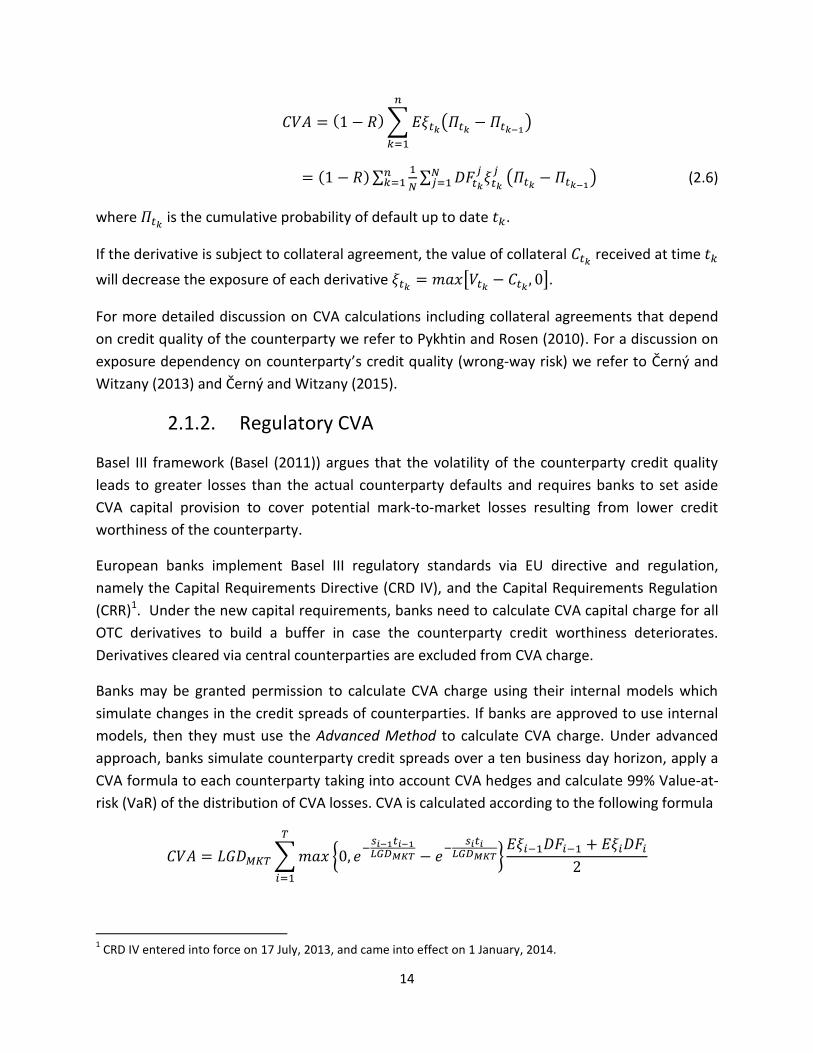
14
( )∑ ( )
( )∑
∑
( ) (2.6)
where is the cumulative probability of default up to date .
If the derivative is subject to collateral agreement, the value of collateral received at time
will decrease the exposure of each derivative [ ].
For more detailed discussion on CVA calculations including collateral agreements that depend
on credit quality of the counterparty we refer to Pykhtin and Rosen (2010). For a discussion on
exposure dependency on counterparty’s credit quality (wrong-way risk) we refer to Černý and
Witzany (2013) and Černý and Witzany (2015).
2.1.2. Regulatory CVA
Basel III framework (Basel (2011)) argues that the volatility of the counterparty credit quality
leads to greater losses than the actual counterparty defaults and requires banks to set aside
CVA capital provision to cover potential mark-to-market losses resulting from lower credit
worthiness of the counterparty.
European banks implement Basel III regulatory standards via EU directive and regulation,
namely the Capital Requirements Directive (CRD IV), and the Capital Requirements Regulation
(CRR)1. Under the new capital requirements, banks need to calculate CVA capital charge for all
OTC derivatives to build a buffer in case the counterparty credit worthiness deteriorates.
Derivatives cleared via central counterparties are excluded from CVA charge.
Banks may be granted permission to calculate CVA charge using their internal models which
simulate changes in the credit spreads of counterparties. If banks are approved to use internal
models, then they must use the Advanced Method to calculate CVA charge. Under advanced
approach, banks simulate counterparty credit spreads over a ten business day horizon, apply a
CVA formula to each counterparty taking into account CVA hedges and calculate 99% Value-at-
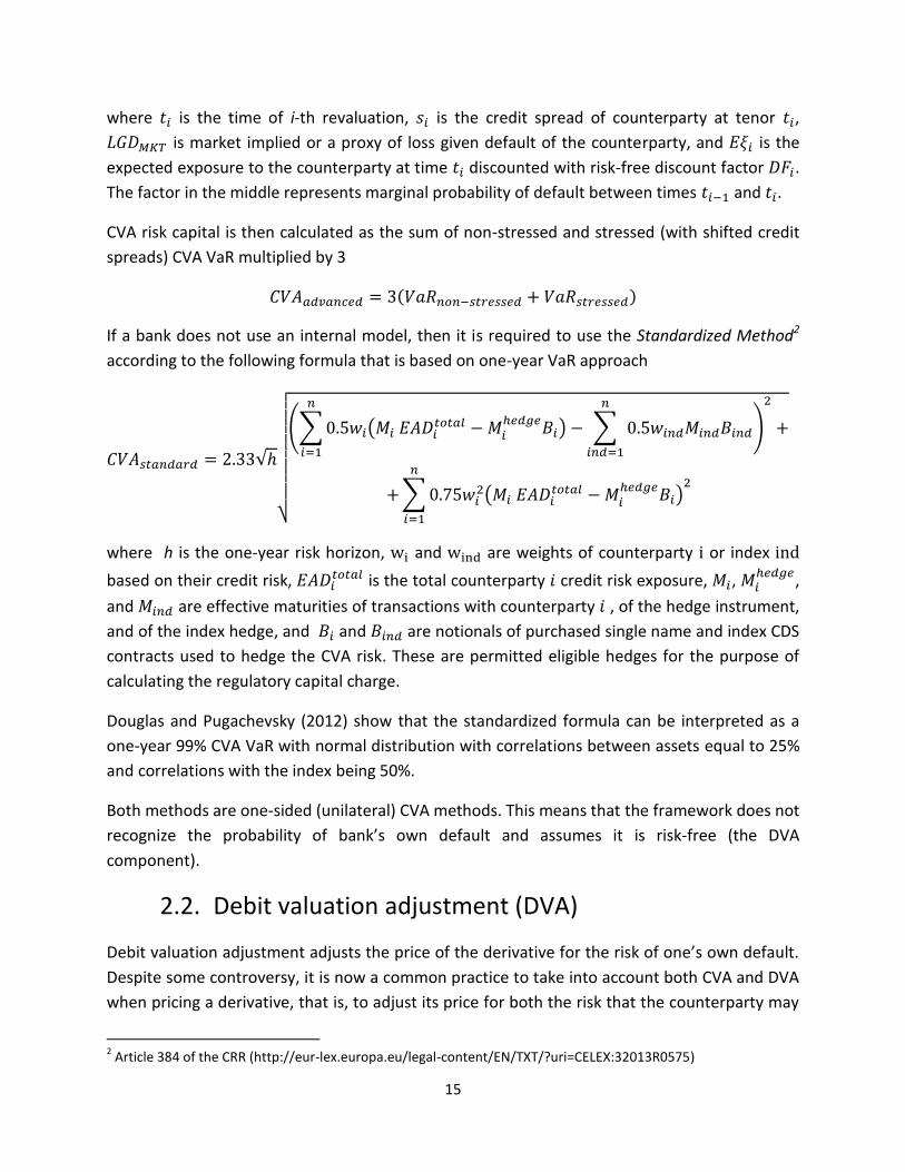
risk (VaR) of the distribution of CVA losses. CVA is calculated according to the following formula
∑ {
}
1 CRD IV entered into force on 17 July, 2013, and came into effect on 1 January, 2014.
15
where is the time of i-th revaluation, is the credit spread of counterparty at tenor ,
is market implied or a proxy of loss given default of the counterparty, and is the
expected exposure to the counterparty at time discounted with risk-free discount factor .
The factor in the middle represents marginal probability of default between times and .
CVA risk capital is then calculated as the sum of non-stressed and stressed (with shifted credit
spreads) CVA VaR multiplied by 3
( )
If a bank does not use an internal model, then it is required to use the Standardized Method2
according to the following formula that is based on one-year VaR approach
√
√
(∑ (
)
∑
)
∑ (
)
where h is the one-year risk horizon, and are weights of counterparty or index
based on their credit risk, is the total counterparty credit risk exposure, ,
,
and are effective maturities of transactions with counterparty , of the hedge instrument,
and of the index hedge, and and are notionals of purchased single name and index CDS
contracts used to hedge the CVA risk. These are permitted eligible hedges for the purpose of
calculating the regulatory capital charge.
Douglas and Pugachevsky (2012) show that the standardized formula can be interpreted as a
one-year 99% CVA VaR with normal distribution with correlations between assets equal to 25%
and correlations with the index being 50%.
Both methods are one-sided (unilateral) CVA methods. This means that the framework does not
recognize the probability of bank’s own default and assumes it is risk-free (the DVA
component).
2.2. Debit valuation adjustment (DVA)
Debit valuation adjustment adjusts the price of the derivative for the risk of one’s own default.
Despite some controversy, it is now a common practice to take into account both CVA and DVA
when pricing a derivative, that is, to adjust its price for both the risk that the counterparty may
2 Article 384 of the CRR (http://eur-lex.europa.eu/legal-content/EN/TXT/?uri=CELEX:32013R0575)
16
default and the risk of one’s own default. The controversy comes from the accounting
recognition of DVA gains if one’s own credit quality deteriorates (and DVA increases).
While in the case of CVA we calculate the positive expected exposure in case the counterparty
defaults, in the case of DVA we calculate the negative expected exposure in case of our own
default. The probabilities of default in case of CVA or DVA are likely to be different, too.
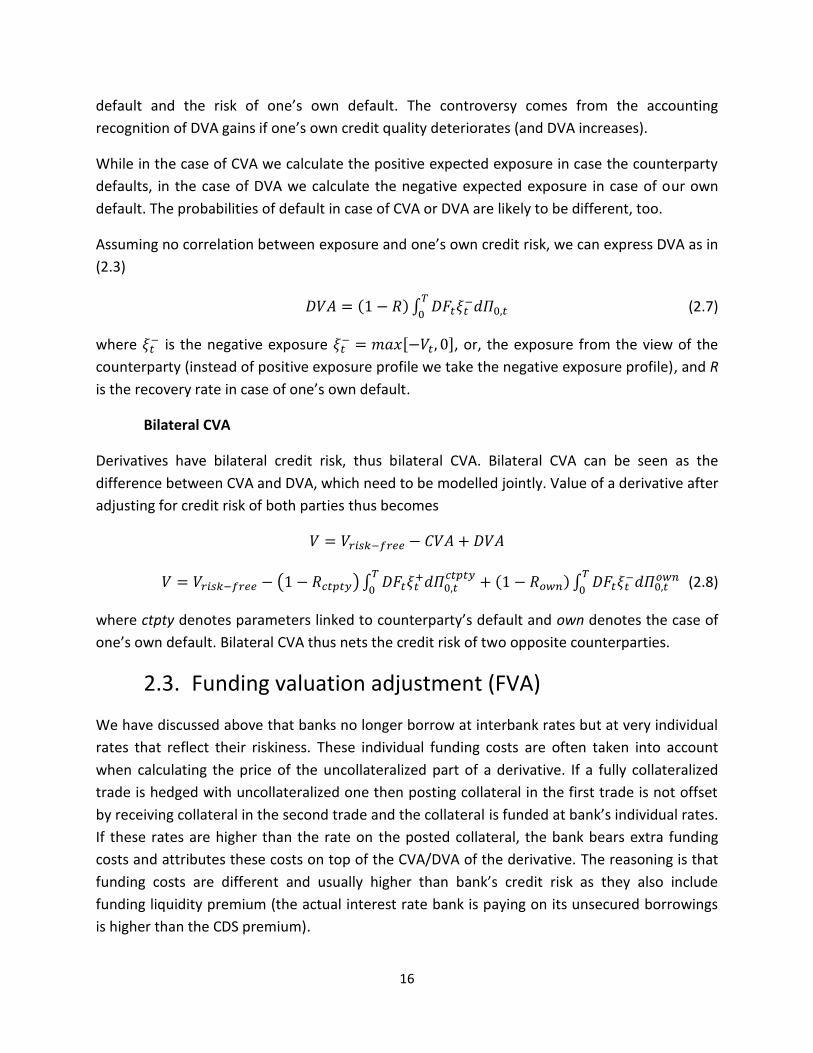
Assuming no correlation between exposure and one’s own credit risk, we can express DVA as in
(2.3)
( )∫
(2.7)
where is the negative exposure
[ ], or, the exposure from the view of the
counterparty (instead of positive exposure profile we take the negative exposure profile), and R
is the recovery rate in case of one’s own default.
Bilateral CVA
Derivatives have bilateral credit risk, thus bilateral CVA. Bilateral CVA can be seen as the
difference between CVA and DVA, which need to be modelled jointly. Value of a derivative after
adjusting for credit risk of both parties thus becomes
( ) ∫
( ) ∫
(2.8)
where ctpty denotes parameters linked to counterparty’s default and own denotes the case of
one’s own default. Bilateral CVA thus nets the credit risk of two opposite counterparties.
2.3. Funding valuation adjustment (FVA)
We have discussed above that banks no longer borrow at interbank rates but at very individual
rates that reflect their riskiness. These individual funding costs are often taken into account
when calculating the price of the uncollateralized part of a derivative. If a fully collateralized
trade is hedged with uncollateralized one then posting collateral in the first trade is not offset
by receiving collateral in the second trade and the collateral is funded at bank’s individual rates.
If these rates are higher than the rate on the posted collateral, the bank bears extra funding
costs and attributes these costs on top of the CVA/DVA of the derivative. The reasoning is that
funding costs are different and usually higher than bank’s credit risk as they also include
funding liquidity premium (the actual interest rate bank is paying on its unsecured borrowings
is higher than the CDS premium).
17
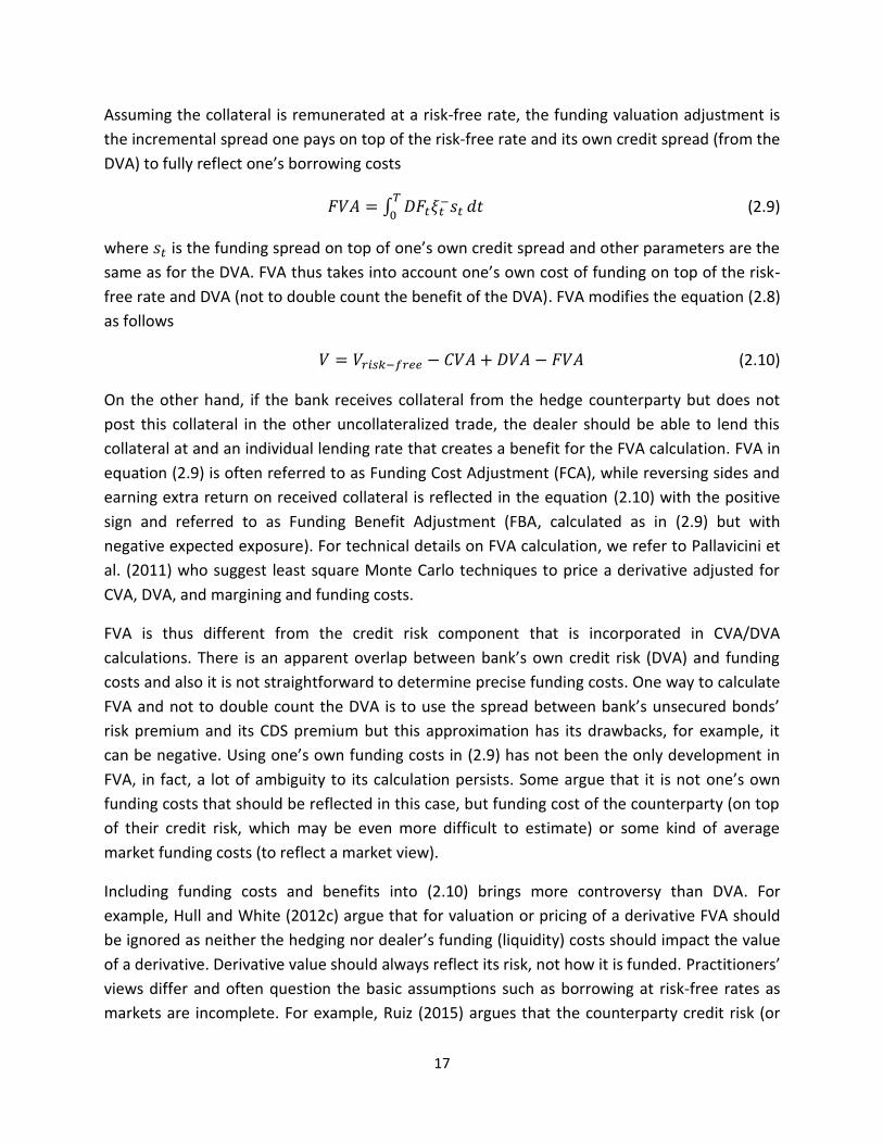
Assuming the collateral is remunerated at a risk-free rate, the funding valuation adjustment is
the incremental spread one pays on top of the risk-free rate and its own credit spread (from the
DVA) to fully reflect one’s borrowing costs
∫
(2.9)
where is the funding spread on top of one’s own credit spread and other parameters are the
same as for the DVA. FVA thus takes into account one’s own cost of funding on top of the risk-
free rate and DVA (not to double count the benefit of the DVA). FVA modifies the equation (2.8)
as follows
(2.10)
On the other hand, if the bank receives collateral from the hedge counterparty but does not
post this collateral in the other uncollateralized trade, the dealer should be able to lend this
collateral at and an individual lending rate that creates a benefit for the FVA calculation. FVA in
equation (2.9) is often referred to as Funding Cost Adjustment (FCA), while reversing sides and
earning extra return on received collateral is reflected in the equation (2.10) with the positive
sign and referred to as Funding Benefit Adjustment (FBA, calculated as in (2.9) but with
negative expected exposure). For technical details on FVA calculation, we refer to Pallavicini et
al. (2011) who suggest least square Monte Carlo techniques to price a derivative adjusted for
CVA, DVA, and margining and funding costs.
FVA is thus different from the credit risk component that is incorporated in CVA/DVA
calculations. There is an apparent overlap between bank’s own credit risk (DVA) and funding
costs and also it is not straightforward to determine precise funding costs. One way to calculate
FVA and not to double count the DVA is to use the spread between bank’s unsecured bonds’
risk premium and its CDS premium but this approximation has its drawbacks, for example, it
can be negative. Using one’s own funding costs in (2.9) has not been the only development in
FVA, in fact, a lot of ambiguity to its calculation persists. Some argue that it is not one’s own
funding costs that should be reflected in this case, but funding cost of the counterparty (on top
of their credit risk, which may be even more difficult to estimate) or some kind of average
market funding costs (to reflect a market view).
Including funding costs and benefits into (2.10) brings more controversy than DVA. For
example, Hull and White (2012c) argue that for valuation or pricing of a derivative FVA should
be ignored as neither the hedging nor dealer’s funding (liquidity) costs should impact the value
of a derivative. Derivative value should always reflect its risk, not how it is funded. Practitioners’
views differ and often question the basic assumptions such as borrowing at risk-free rates as
markets are incomplete. For example, Ruiz (2015) argues that the counterparty credit risk (or
18
CDS spread if it is liquid) can be different from bank’s cost of borrowing and cost of collateral.
Burgard and Kjaer (2013) show how different funding strategies and spreads may create
different values of derivative positions. Interestingly, Hull and White (2014) admit that one may
defend adjusting the valuation for the liquidity component of bank’s credit spread but continue
to argue that FVA may result in different estimates of market value by different counterparties
with different funding costs. Authors continue to advocate a single price for any derivative that
can be reached by properly calibrated and incorporated CVA and DVA, but not FVA, and further
provide an example of arbitrage if FVA valuations are taken into account. Nevertheless, there
seems to be a trend that banks include FVA both in pricing new trades and valuation for
accounting purposes. This may be linked to a fact that derivatives’ dealers are being charged
bank’s funding costs by their treasury or XVA desk and not the risk-free rate. This is why Hull
and White (2014) propose that treasury should lend funds to trading desks at the risk-free rate.
Nevertheless, if banks include FVA into their pricing, then those banks with higher credit quality
and lower funding costs may be more competitive to price uncollateralized derivatives that
require funding. Banks currently do not have to recognize FVA in terms of fair value accounting
nor there are any regulatory requirements for FVA and the FVA discussions continue but yet
without an agreement on how to exactly determine funding costs.
2.4. Other valuation adjustments
Other add-ons are being increasingly included in derivative’s value alongside CVA, DVA or FVA.
They are calculated in a similar manner. We discuss two of them that we consider the most
important, namely, Capital valuation adjustment and Margin valuation adjustment.
2.4.1. Capital valuation adjustment (KVA)
Regulatory changes for banks’ capital requirements have recently driven banks to include these
capital requirements into the valuation of derivatives. KVA adjustment calculates the cost of
such regulatory capital that would act as a buffer for unexpected losses and requires estimating
capital needs of a derivative over its life. In practice, usually treasury charges capital costs to
the dealer’s desk. This term was introduced and formalized by Green et al. (2014) to whom we
also refer for details on technical computational details. KVA usually comes as a cost charged to
a counterparty and thus modifies the formula (2.10) as follows
(2.11)
A complete price thus includes its risk-free valuation (or fully collateralized valuation),
counterparty credit risk, one’s own credit risk, unsecured funding costs and capital charges.
19
Sherif and Chambers (2015) conducted a survey on KVA in July 2015 showing interesting results
that most of banks now price KVA at least partially into trades and banks identify KVA to be the
biggest from the XVA valuation adjustments, larger than CVA or FVA.
2.4.2. Initial Margin Valuation Adjustment (MVA)
MVA reflects the cost of funding of the initial margin requirements on top of other valuation
adjustments. It is, too, being increasingly passed on to the end-client. Initial margin
requirement is often based on Value-at-Risk (VaR) or Expected Shortfall (ES) approaches. To
calculate MVA one must estimate expected profile of the initial margin over the life of the trade
or portfolio of trades.
MVA is charged to the counterparty and modifies the equation (2.11) as follows
(2.12)
To calculate the expected profile of the initial margin one needs to simulate multiple VaR/ES
scenarios for each future date, which is computationally intensive. Green and Kenyon (2015)
propose a more efficient approach using specific regression technique that allows fast
recalculation of the portfolio value. In fact, Basel Committee and International Organization of
Securities Commissions (Basel/IOSCO (2015)) published a revised framework for margin
requirements for OTC derivatives with the objective of reducing systemic risk and motivating
market participants to move to central clearing. The framework requires initial and variation
margin to be exchanged between counterparties and puts limits on thresholds of these
margins. Only institutions with over €8 billion of notional outstanding of OTC derivatives will be
subject to initial margin requirements, and the largest derivatives dealers (notional outstanding
over €3 trillion) will have to start posting initial margin for new transactions from September
2016 (smaller dealers later on and the requirements will be phased-in). If MVA adjustments are
then passed on to end customers and are sizable, then it may have a significant impact on
pricing and liquidity of derivatives.
20
3. Valuation of interest rate derivatives
In this chapter, we discuss discounting future cash flows of interest rate derivatives in detail.
We start from the definition that the present value of cash flows of one leg of the swap equals
the present value of cash flows of the other leg of the swap. OIS discounting takes the centre
stage but we discuss other discount curves, too. The aim of this chapter is to derive discount
factors and forward rates that are consistent with market prices. It is no longer plausible to use
one curve to both estimate the forward rates and discount future cash flows given the
prerequisite of arbitrage free market. We focus in detail on valuation of interest rate swaps,
basis swaps and cross-currency swaps but first, we review relevant existing literature.
One of the first pre-crisis papers that address the issue of collateralization of derivatives is
Johannes and Sundaresan (2003). The authors correctly note that collateralization as a way to
eliminate counterparty credit risk bears additional costs and that the rate of the collateral
impacts discount factors. In Johannes and Sundaresan (2007), the authors point to the impact
of collateralization on swap rates and introduce formula to price collateralized contracts. They
also show that if the collateral rate is continuous, then the rate of the collateral should be used
to discount future cash flows even if such rate is not equal to the risk-free rate. Authors further
present an empirical study of the US dollar swap rates dynamics. Many papers that followed
refer to their ideas.
Pulman (2003), as one of the first authors, warns that it is not suitable to construct the yield
curve from deposit, FRA/futures and swap rates. The author focuses on the short-end of the
curve and shows that, for example, by using 1-month deposit rate to construct a 3-month swap
curve (fixed swap rates against floating 3-month IBOR rates) one neglects the lower credit risk
in the 1-month rate. Ametrano and Bianchetti (2009) introduce a model that focuses on
segmentation of the market and uses the bootstrapping method to derive swap rates for each
tenor respectively. The authors thus assume multiple discounting curves in one currency, this
however does not eliminate arbitrage. Authors also ignore collateralization and cross-currency
effects.
The paper of Boenkost and Schmidt (2005) is among the first to clearly focus on valuation of
interest rate and cross-currency swaps including the effect of basis spreads and authors
introduce the idea of two discount factors. Kijima et al. (2009) derive consistent pricing of
USD/JPY cross-currency swaps, where they consider USD LIBOR as risk-free rate and calculate
the JPY discount rate. Chibane et al. (2009) highlight the existence of basis spreads and show
that valuation using one curve creates arbitrage opportunities between interest rate and
currency swaps. Therefore they introduce new method of arbitrage-free pricing incorporating
21
basis spreads. Authors work only with IBOR-based swap rates and do not consider
collateralization, or counterparty credit risk.
Fujii et al. (2010) extend the work of Johannes and Sundaresan (2007) for swaps where
collateral is posted in different currency and construct arbitrage-free arguments for
collateralized and uncollateralized interest rate and cross-currency swaps including quoted
basis swap spreads. Mercurio (2010) suggests constructing discount curves using OIS swap
rates, similar to Fujii et al. (2010). The impact of collateralization on derivatives pricing is
discussed also in Piterbarg (2010) where the author modifies Black-Scholes valuation formula
for collateralized options.
Hull and White (2013) consider OIS rates as currently the best proxy of risk-free rates and argue
that they should be used as risk-free rates for valuation of all derivatives under risk-neutral
measure. For completeness we list other relevant studies: Chibane (2012), Henrard (2009),
Morini (2009), Tuckman and Porfirio (2003), Kijima et al. (2009).
3.1. Interest Rate Swap
An interest rate swap is a contract in which one party exchanges regular fixed interest rate cash
flows in return for floating interest rate cash flows tied to a respective index, i.e. IBOR rate. The
market value of an interest rate swap is thus the difference in present values of future cash
flows of the fixed and floating rate leg. As for any other swap, at inception the present value of
the fixed leg equals the present value of the floating leg
∑ ∑
(3.1)
where are implied forward reference rates of the floating leg at times t-1 to t,
is the
year fraction for period between t-1 and t for i-th leg (i=1,2), is the actual number of days
between t-1 and t, B is the number of days in a year according to the day count convention for
the respective currency (e.g. for EUR, USD or CZK B=360), is the quoted swap rate and
are discount factors (present values of one unit payment that will be received in time t) and
usually there are different interest rate periods (i.e. m≠n).
The value of the floating leg depends on discount factors and implied forward rates .
The swap rate that makes the net present value equal zero is then derived as
∑
∑
(3.2)
22
With given swap rates and discount factors , we can calculate respective implied
forward rates. In the following text, we discuss how to determine the discount curves (discount
factors that are used to calculate present value of future cash flows).
3.1.1. Classical bootstrapping using discount factors
A derivative position is valued using zero coupon yield curves. Movements in interest rates are
reflected in discount factors that are used to obtain the present value of future derivative cash
flows. The discount factors are derived recursively by what is called a bootstrapping process.
Discount factors (and the time structure of spot interest rates) are derived from available
market prices of instruments in money market and swap market. First, we derive the initial
discount factor for the shortest (overnight) tenor
, (3.3)
where is the overnight (ON) money market cash rate. The remaining discount factors in the
short end of the curve are derived consecutively from the shortest to the longest from already
derived discount factors and money market and forward rate agreement (FRA) rates
, (3.4)
where is discount factor for tomorrow next (tom-next, TN, meaning for one day starting
tomorrow) money market rate. Every other money market deposit is settled in two business
days (T+2).
Quoted swap rates are used to derive discount factors in the long end of the curve and the
classical approach assumes that the present value of the swap’s floating rate leg cash flows
equals 100%.
∑ . (3.5)
Using quoted swap rates we can recursively calculate discount factors from (3.5)
∑
. (3.6)
Here we assumed that forward rates in (3.1) are implied from discount factors
23
(
) (3.7)
After obtaining a set of discount factors from available specific market data, we need to use
some form of interpolation to get discount factors for all other maturities (i.e. at dates between
two dates with known discount factors). We can either interpolate on discount factors or
convert discount factors into zero coupon (spot) rates and interpolate on the spot rates. Widely
used market practice includes exponential interpolation on the discount factors and cubic
splines or linear interpolation on the zero coupon curve. For a review of interpolation methods,
we refer to Hagan and West (2006).
From the discount curve we can then construct a zero coupon curve, a par swap curve and as
already shown, forward curves.
Swap rate which makes the net present value equal zero (par swap rate) is then
∑ (
)
∑
∑
(3.8)
Equation (3.8) is a classical approach to valuation of interest rate swaps where we use one
curve both to calculate forward rates and to discount future cash flows.
This approach can be found perhaps in almost every textbook on financial mathematics. It is
based on the assumption that forward rates are implied from discount factors . This
assumption is however not valid in the case when are calculated from the risk-free rates.
Then from (3.7) forward rates are also considered risk-free rates but they are in fact IBOR
rates that include credit and liquidity risk of interbank market. Therefore also equation (3.5)
does not hold. One can however recursively calculate forward rates implied from discount
factors and quoted swap rates from (3.1) as
∑ ∑
(3.9)
For completeness we derive the last case when discount factors and forward rates are
given. Then swap rate which makes the net present value equal zero becomes
∑
∑
(3.10)
Therefore we always need two sets of factors from , and to calculate the third one.
24
In the following section we focus on determining risk-free discount factors and we further
develop the concept of multiple curves.
3.1.2. OIS rates, collateralization, and OIS discounting
Overnight indexed swap (OIS) is an interest rate swap in which one party exchanges fixed rate
for floating rate, which equals geometric average of overnight ONIA3 rates during the life of the
contract. ONIA rates reflect weighted average of market rates of unsecured overnight (O/N)
deposits and loans transacted by reference banks in the respective interbank market, where
the weights are sizes of individual transactions. These overnight rates are in close relationship
with central banks’ deposit rates, which are used to direct evolution of interest rates in the real
economy.
Market participants can thus use OIS swaps to hedge against changes in central banks’ rates,
and vice versa, OIS swap rates reflect market expectation about central banks’ rates. For
example, if OIS rates are lower than current overnight rates then market signalizes incoming
easing of monetary policy. These market expectations are, of course, priced in other interest
rate instruments (FRAs, futures, interest rate swaps) but these include higher credit and
liquidity risk and can thus distort information about expected central bank rates. OIS rates can
be also distorted during times of low liquidity and at that time it can be problematic to use
them for estimating future monetary policy steps. However, the underlying reference rate in
OIS swaps is based on actual market transactions; therefore, OIS swaps better reflect market
conditions and expectations.
Derivatives in OTC markets are commonly transacted and cleared bilaterally under ISDA4
master agreement. The decrease in confidence and trust in the interbank markets led banks to
search for ways to mitigate credit risk exposure from derivatives transactions. Today, it is
common practice that part of ISDA agreement is the CSA annex5, which specifies rules and
conditions for credit support and collateral for mutual derivative transactions. It also agrees on
steps to be taken in case of failure to make the required payment, posting a collateral, or a
default of either of the counterparty. Derivatives are thus collateralized; they are secured by
liquid financial collateral that offsets the credit exposure of one party vs. the other. A party that
is in the money thus receives the collateral.
3 ONIA – OverNight Index Average, i.e. EONIA for EUR, Federal funds effective rate for USD and CZEONIA (Czech
OverNight Index Average) for CZK. 4 ISDA - International Swaps and Derivatives Association master agreement, Czech banks also use Czech master
agreement for financial transactions (CMA) published by Czech banking association and its respective product annex no. 5 for derivative transactions. 5 CSA – Credit support annex, in case of CMA it is the product annex no. 11 Margin maintenance annex.
25
According to ISDA Margin Survey 2015 (ISDA (2015)), the use of collateral is extensive: in 2014
89% of non-cleared fixed-income derivatives and 97% of non-cleared credit derivatives were
collateralized with CSA agreement, more than 80% of derivatives portfolios with more than
2500 trades are reconciled daily, and the use of cash or government securities accounts for
over 90% of total collateral. These numbers have had an increasing trend over past years.
OTC derivatives market is gradually moving from bilateral clearing to clearing via central
counterparty (CCP), which steps between the buyer and the seller and becomes counterparty
to each of them. CCP then introduces additional techniques to mitigate and monitor
counterparty credit risk (initial and variation margins, default fund contributions). When one of
the members fails to post the required collateral, the member defaults and his positions are
closed out.
The role of a CCP is to improve management of counterparty credit risk and increase
transparency (availability of data). New regulation for both bilaterally or centrally cleared
derivatives will require banks to post higher amounts of collateral, mainly in cash or liquid high
quality securities. In this sense, a shift from managing counterparty credit risk towards
managing liquidity risk of collateral outflow can be expected, see Finger (2012). By estimating
short term volatility of market value of open derivative contracts or for different stress
scenarios, one can estimate expenses for additional liquidity outflow (in the form of additional
margin call sent to a CCP), i.e. by a quantile based models. As we discuss below, due to daily
cash margining, CCPs have adopted OIS discounting.
As we discussed in Chapter 2 different valuation adjustment that were mainly focused on the
uncollateralized part of the derivative, it may happen that derivatives prices may be different
also when using central counterparties. In other words, it may happen that the same derivative
will have a different price if it is being cleared at a different central counterparty, and this price
would again depend on the collateralization rules being applied.
EU and the central counterparties
In 2009, G-20 leaders agreed to regulate OTC derivatives to decrease their credit and
operational risks. The regulation deals mainly with derivatives trading, clearing, and reporting.
To meet this agreement, the European Commission proposed and the Council of the EU and the
European Parliament then adopted following legislation:
On 4 July 2012, a Regulation on OTC derivatives, central counterparties and trade
repositories6, which specifies requirements for clearing and reporting for OTC
6 EMIR - European Market Infrastructure Regulation: http://eur-lex.europa.eu/legal-
content/EN/TXT/PDF/?uri=CELEX:32012R0648&from=EN
26
derivatives and requirements for activities of central counterparties and trade
repositories.
On 19 December 20127, regulatory technical standards and details on their
implementation which among other things further specify requirements for
central counterparties (including capital requirement), clearing obligation,
indirect clearing arrangements, risk mitigation techniques for derivatives not
cleared by a CCP, and data to be reported to trade repositories.
On 6 August 20158, a Regulation on central clearing for interest rate derivatives
that make central clearing of interest rate derivatives mandatory. It covers plain
vanilla interest rate swaps, FRAs, OIS swaps and basis swaps in major currencies.
OIS discounting
Using OIS curve to discount derivative cash flows gained a lot of traction in both academia and
among market professionals. In fact, discounting cash flows with OIS rates has become a
market standard. Collateral used is most frequently cash which is accrued at overnight ONIA
rate and collateralized portfolios are revalued daily, that is, margin call is calculated every day.
With perfect hedging, collateral value is equal to market value of swap at maturity T, that is, the
net interest payment at time T. The overnight rate accrued on the collateral is traded in the OIS
swap market and is equivalent to fixed OIS rate for respective maturity. The value of the
collateral and the market value of the interest rate swap are equal only if interest payments are
discounted with OIS curve. For these reasons the valuation of derivatives has changed, and
both banks and central counterparties started discounting at the OIS curve. One of the direct
implications is the separation of discounting curve (OIS swaps) and forwarding curve (forward
rates derived from the quoted fixed swap rates vs. IBOR) and as we show below, the implied
forward rates are not the same if we use classical IBOR discounting or if we use OIS discounting.
For more detailed discussion regarding valuation of collateralized trades and the choice of the
risk free curve, we refer to Piterbarg (2010) and Fujii et al. (2010).
The floating rate r of the OIS swap is calculated as annual effective interest rate from the
overnight ONIA rates for respective interest period
(∏ (
)
)
where is the overnight ONIA rate valid at time t and for a given currency, is a number of
days for which is valid (usually , during weekends etc.), is number of
business days for the given period (that is, number of rates ) and n is the total number of days
7 Press release: http://europa.eu/rapid/press-release_IP-12-1419_en.htm?locale=en
8 Draft: http://ec.europa.eu/finance/financial-markets/docs/derivatives/150806-delegated-act_en.pdf
27
in the interest rate period9. In other words, the floating rate payment equals swap notional
repeatedly invested at overnight ONIA rate (compounded interest).
From quoted OIS swap rates we can calculate discount factors; for one period (one fixed vs.
floating payment) we can write
For multiple periods we proceed analogically as in (3.6)
∑
(3.11)
We use single OIS curve to derive the discount factors and implied forward OIS rates. The
implied forward OIS rate and OIS par swap rate then become
∑ ∑
(
)
∑
∑
∑
(3.12)
3.1.3. Collateralized interest rate swap
Here we restrict ourselves to collateralized interest rate swap with zero thresholds, daily
margining, and symmetric cash collateral which pays the ONIA rate. In such case, OIS rates
should be used to discount future cash flows. If quoted swap rates are collateralized, then we
derive implied forward rates from quoted swap rates and already derived OIS discount factors.
Using OIS discounting, implied forward rates become
∑ ∑
(3.13)
One of the implications of changing the discounting curve is that the implied forward rate of
the collateralized swap is different than in (3.7). The swap rate , which makes the NPV zero at
inception, is then equal to
∑
∑
(3.14)
9 Number of days in a year is given by money market day count convention for the respective currency.
28
3.1.4. Discount curve defined by spread to a reference rate
We can generalize previous cases by using implied forward reference rates plus a spread
(IBOR + spread) to discount future cash flows. An arbitrage-free relation must hold for such
unsecured financing
∑ ( ) (3.15)
By using we treat all cases in the same manner; for example, for OIS discounting we set
(which can be negative) and we get (3.11). However, we need a quoted swap
market with reference rate to determine and
∑ ∑
(3.16)
Such market exists only if other subjects reflect the same risk of , what is not the case,
therefore, need to be approximated by existing swap market, for example, quoted swap
market from (3.8). Then
∑ ∑
(3.17)
We then obtain discount factors by plugging (3.17) into (3.15)
( )∑
( ), (3.18)
And forward rates
∑ ∑
. (3.19)
One of the reasons to mention this generalization of discounting with is that the time
structure of spreads shows the spread of the discount curve to forward curve in a similar way
that basis spreads determine the level of one forward curve to another one. However, such
discount curve can only be used if both parties reflect the same risk over the life of the swap.
This is very rarely the case. In fact, as we discussed in Chapter 2, what has become a standard
market practice is that cash flows are discounted at a proxy of a risk-free rate (most commonly
OIS rates or sometimes repo rates if government bonds are used as collateral) and risk
premiums of each of the swap counterparty are separately added on top of that.
29
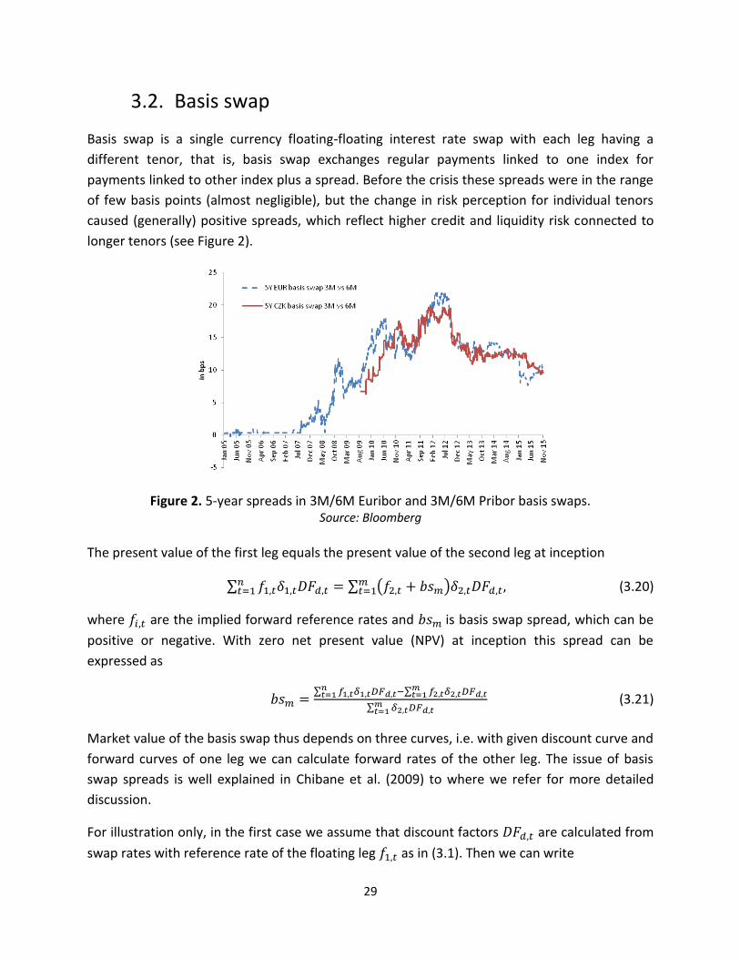
3.2. Basis swap
Basis swap is a single currency floating-floating interest rate swap with each leg having a
different tenor, that is, basis swap exchanges regular payments linked to one index for
payments linked to other index plus a spread. Before the crisis these spreads were in the range
of few basis points (almost negligible), but the change in risk perception for individual tenors
caused (generally) positive spreads, which reflect higher credit and liquidity risk connected to
longer tenors (see Figure 2).
Figure 2. 5-year spreads in 3M/6M Euribor and 3M/6M Pribor basis swaps. Source: Bloomberg
The present value of the first leg equals the present value of the second leg at inception
∑ ∑ ( )
(3.20)
where are the implied forward reference rates and is basis swap spread, which can be
positive or negative. With zero net present value (NPV) at inception this spread can be
expressed as
∑ ∑
∑
(3.21)
Market value of the basis swap thus depends on three curves, i.e. with given discount curve and
forward curves of one leg we can calculate forward rates of the other leg. The issue of basis
swap spreads is well explained in Chibane et al. (2009) to where we refer for more detailed
discussion.
For illustration only, in the first case we assume that discount factors are calculated from
swap rates with reference rate of the floating leg as in (3.1). Then we can write
30
∑ ∑
and we can calculate discount factors
∑
forward rates
(
)
and plugging this into (3.20) we calculate forward rates of the second leg
( ∑
∑
∑
) (3.22)
3.2.1. Collateralized basis swap
Now we assume our central case, a basis swap as in (3.20), which is fully collateralized. Discount
factors are derived from the OIS swap curve as in (3.11). We also assume that swap
rates are exchanged against reference rate , and to simplify notation we assume for the
swap same interest rate payment frequency for both fixed and floating leg (same for
both fixed and floating leg). Then according to (3.13) we can write
∑ ∑
where is the quoted swap rate for maturity n. Now we can recursively calculate forward
rates according to (3.22)
(∑
∑
∑
)
We see that basis spread enters the equation as an independent variable that cannot be
omitted.
31
3.3. Cross-currency swap
Cross-currency swap (CCS) is an interest rate swap that exchanges periodic interest payments in
different currencies and exchange rate used to fix initial and final notional is determined at
inception. For more detailed explanation of the mechanism of cross-currency and basis swaps
we refer the reader to Tuckman and Porfirio (2003).
A classical approach assumes that both legs of either cross-currency or basis swap trade
without a spread, that is, it abstracts from credit and liquidity risks and assumes that each
counterparty reflects the interbank risk of IBOR rates (and thus funds at swap rates), which was
somewhat true until summer 2007. Present value of each leg of the swap was equal to its
notional and the spread on one leg of the swap was in the range of several basis points (bps)
what used to be neglected for valuation purposes. Today, the costs associated with funding in
one currency versus funding in another are not negligible anymore. Temporary transfer of
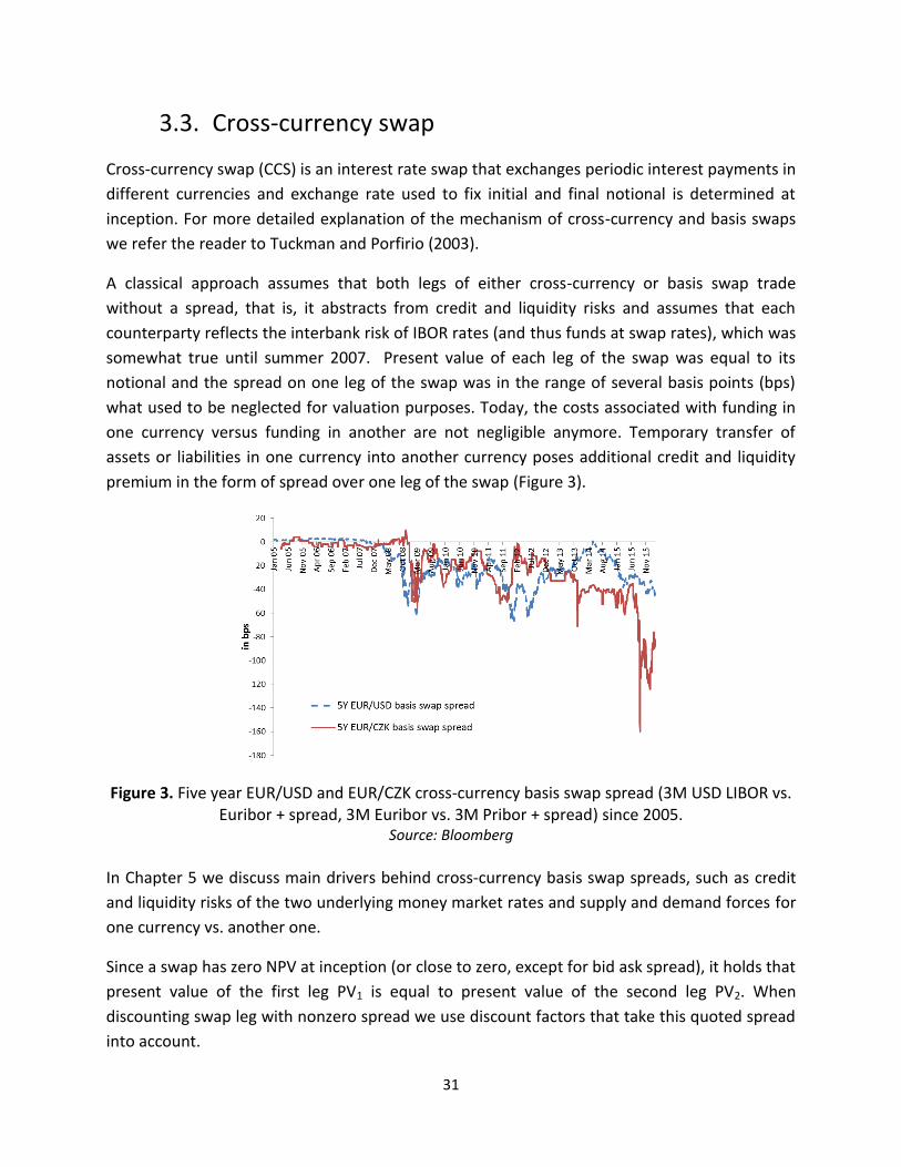
assets or liabilities in one currency into another currency poses additional credit and liquidity
premium in the form of spread over one leg of the swap (Figure 3).
Figure 3. Five year EUR/USD and EUR/CZK cross-currency basis swap spread (3M USD LIBOR vs. Euribor + spread, 3M Euribor vs. 3M Pribor + spread) since 2005.
Source: Bloomberg In Chapter 5 we discuss main drivers behind cross-currency basis swap spreads, such as credit
and liquidity risks of the two underlying money market rates and supply and demand forces for
one currency vs. another one.
Since a swap has zero NPV at inception (or close to zero, except for bid ask spread), it holds that
present value of the first leg PV1 is equal to present value of the second leg PV2. When
discounting swap leg with nonzero spread we use discount factors that take this quoted spread
into account.
32
∑ ∑ ( )
(3.23)
where is forward reference rate for period from t-1 to t,
is year fraction, is
the discount factor for currencies j=1,2 and is the agreed basis spread (we expect that the
spot fx rate equals the fx rate of the cross-currency swap at inception so we omit this term for
simplicity). Discount factors are calculated so that the equality (3.23) holds.
To simplify notation we assume that in (3.23) and further the frequency of interest payment is
the same for both legs.
Again, for illustration only, let us assume that discount factors are calculated from the
swap rates with reference rate of the floating leg then the following equality holds
∑ ∑
. (3.24)
Plugging (3.24) into (3.23) yields
∑ ( ) . (3.25)
Similarly, we can write for the second leg
∑ ∑
. (3.26)
Plugging (3.26) into (3.25) we can write
( )∑ (3.27)
from there we separate discount factors .
For the first period we have
( ) ,
where is the spot rate for the first period (i.e. IBOR), is the basis swap spread for the
first period (i.e. 3 months) and is the first period’s year fraction. Each following discount
factor is calculated recursively from the previous discount factors using (3.27)
( )∑
( ) . (3.28)
Forward rates can be calculated from (3.26)
∑
∑
. (3.29)
33
To value cross-currency swap with nonzero basis spread BS we have to use two different
curves, for discounting the cash flows of the first leg and for estimating and
discounting the second leg’s cash flows. Although assumption of discounting at swap rates does
not hold anymore, we did so to illustrate how quoted basis spread impacts the calculation of
discount factors and .
3.3.1. Collateralized cross-currency swap
We now assume full collateralization with overnight ONIA cash rate in the currency of the first
leg and therefore we use this rate to discount cash flows of the first leg. The present value of
the first leg equals the present value of the second leg, but that is not equal par any longer
(forward rates of the first leg are calculated from the quoted swap rates and discounted with
OIS curve, which is different and generally lower than the swap curve).
∑ ∑ ( )
(3.30)
Discount factors of the first leg are calculated from the OIS swap curve according to
(3.11). We assume that market quotes fixed swap rate against floating rates , then
according to (3.13) we can write
∑ ∑
We also assume that market quotes fixed swap rate against floating rates
∑ ∑
.
Plugging this into (3.30) we get
∑ ( )∑
and we can isolate discount factors .
For the first period we have
( )
( )
where is the spot rate for the first period (i.e. IBOR), is the OIS discount factor for
the first period, is the year fraction in day count convention of the first leg for the first
interest rate period. For each following discount factor we can write
34
∑ ( )∑
( ) (3.31)
Basis swap spread changes discount factors of the second leg. We also notice that the
present value of neither leg in (3.30) equals par.
3.3.2. Cross-currency swap collateralized in the currency of
the second leg
We assume that the cross currency swap is now fully collateralized in the currency of the
second leg of the swap
∑ ∑ ( )
(3.32)
We also assume that the OIS swap market of the currency of the second leg and the swap
market with reference rates exist, so we can calculate discount factors from (3.11)
and forward rates from (3.13). We also need a swap market for
∑
∑
Plugging this into (3.32) we get
∑
∑( )
And we can isolate discount factors
∑ ( ) ∑
(3.33)
Changing the currency of the collateral was the last case we wanted to illustrate. We have
shown how to incorporate basis spreads into the valuation of basis swaps and cross-currency
basis swaps, and we looked at the impact of collateralization on the discount factors and
forward rates. In other words, we have looked into how to price interest rate, basis, and cross-
currency swaps consistently with market quotes. We first illustrated the approach for the
classical case of uncollateralized IBOR discounting but we mainly focused on collateralized
derivatives (cash collateralization using OIS discounting).
35
For uncollateralized trades we also showed a general case of incorporating risk spreads into the
calculation and discounting, and for collateralized trades, we discussed the impact of the
currency of the collateral in case of cross-currency swaps.
We have seen that in the absence of arbitrage it is no longer possible to use one curve to both
estimate forward rates and to discount future cash flows and we have introduced the concept
of multiple curves.
3.4. Approximation of discount curves of cross-currency
swaps
In this section we derive discount curves implied from cross-currency market quotes and the
discount curve of the base currency. We follow Wu (2011) who explored relationship between
discount curve implied from CCS basis spread quotes and LIBOR and OIS curves. His findings
offer several interesting practical applications, for example, the discount curve of the second
leg of the CCS can be approximated from both CCS IBOR basis swap and CCS OIS basis swap, or
that the decomposition of CCS spread into OIS basis spread and spread reflecting credit and
liquidity risk between two currencies can have a direct implication on the choice of currency for
collateral posting.
The idea of such approximation is to express basis spread in terms of swap rates used to
calculate forwards rates, and swap rates used to discount cash flows. Let be the quoted
swap rate of j-th leg (j=1,2) for maturity n, from which the forward IBOR rates are derived and
let be the swap rate of j-th leg corresponding to discount factors (for example, OIS
discount factors). If the day count convention and interest payment frequency is the same, then
according to (3.1) and (3.8) we can write
∑ ∑
∑
∑
, (3.34)
∑ ,
∑
. (3.35)
Substituting (3.34) and (3.35) into (3.23) we get
( )∑ ( )∑
, (3.36)
And we can express as
36
( )∑
∑
( )
( )∑
∑
( ) (3.37)
The equation (3.37) will serve as a basis of the analysis as we further decompose basis spread
into its credit and liquidity element and supply and demand element . In
the following section we also use (3.37) to derive an approximate formula for selected types of
cross-currency basis swaps according to Wu (2011).
3.4.1. Credit and liquidity risks between two currencies
When we compare present values of two collateralized (OIS discounted) floating legs in two
different currencies we can approximate credit and liquidity risk of the two currencies
, or credit and liquidity risk of one currency vs. another one.
∑
∑( )
Combining (3.37), (3.34), and (3.35) we get
( )∑
∑
( )
where
∑
∑
∑
By rounding the ratio ∑
∑
to 1 we get an approximate relationship for spread
( ) ( ) (3.38)
Cross-currency credit and liquidity risk can thus be approximated as the difference between
interbank risk (IBOR and OIS spreads) in two currencies.
Likewise we can approximate swap rates used for discounting implied from quoted
IBOR-based basis spreads and from
37
( ) ( )
( )
( ) (3.39)
Swap rates implied from basis spreads can thus be approximated as IBOR swap rates
shifted by basis spread and reduced by IBOR-OIS spread of the first leg, or alternatively, as OIS
rates shifted by factor ( ). It is worth noting that only in case
that ( ) is negligible. This means that it is not possible to estimate OIS swap
rates of the second leg using only .
3.4.2. Cross-currency OIS basis swap (float-float)
Floating to floating cross-currency OIS basis swap temporarily transfers liquidity in one currency
in exchange for liquidity in another currency. During the life of the trade one party pays
periodic interest payments linked to overnight reference rates (ONIA) plus a spread (payments
occur for example every 3 months) and receives interest payments linked to overnight
reference rates in another currency10.
For those currencies for which OIS cross-currency market exists, we can estimate swap rates
used for discounting in a similar fashion as in (3.39)
∑ ∑ ( )
, (3.40)
where forward rates
(
) are calculated from OIS discount factors and
therefore the left side equals 1. Using (3.38) and (3.39) we get an approximation
( )
( ) ( )
(3.41)
OIS basis spread therefore represents the difference between the discount rate
implied from discount factors of the second leg and market OIS rate of the second leg and can
be approximated as IBOR basis spread reduced by basis spread that reflect
credit and liquidity risk between the two currencies.
10
For example, in case of EUR/USD it is a basis swap EUR EONIA + spread vs. Fed funds effective rate.
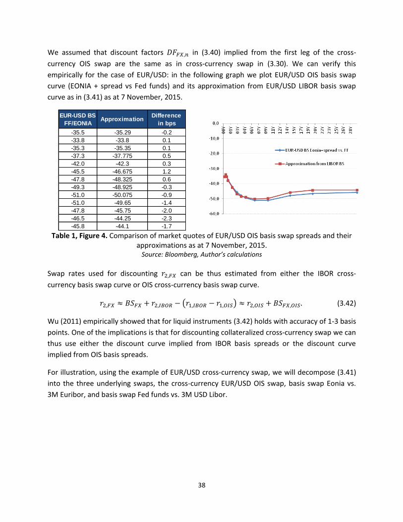
38
We assumed that discount factors in (3.40) implied from the first leg of the cross-
currency OIS swap are the same as in cross-currency swap in (3.30). We can verify this
empirically for the case of EUR/USD: in the following graph we plot EUR/USD OIS basis swap
curve (EONIA + spread vs Fed funds) and its approximation from EUR/USD LIBOR basis swap
curve as in (3.41) as at 7 November, 2015.
Table 1, Figure 4. Comparison of market quotes of EUR/USD OIS basis swap spreads and their approximations as at 7 November, 2015.
Source: Bloomberg, Author’s calculations Swap rates used for discounting can be thus estimated from either the IBOR cross-
currency basis swap curve or OIS cross-currency basis swap curve.
( ) (3.42)
Wu (2011) empirically showed that for liquid instruments (3.42) holds with accuracy of 1-3 basis
points. One of the implications is that for discounting collateralized cross-currency swap we can
thus use either the discount curve implied from IBOR basis spreads or the discount curve
implied from OIS basis spreads.
For illustration, using the example of EUR/USD cross-currency swap, we will decompose (3.41)
into the three underlying swaps, the cross-currency EUR/USD OIS swap, basis swap Eonia vs.
3M Euribor, and basis swap Fed funds vs. 3M USD Libor.
EUR-USD BS
FF/EONIAApproximation
Difference
in bps
-35.5 -35.29 -0.2
-33.8 -33.8 0.1
-35.3 -35.35 0.1
-37.3 -37.775 0.5
-42.0 -42.3 0.3
-45.5 -46.675 1.2
-47.8 -48.325 0.6
-49.3 -48.925 -0.3
-51.0 -50.075 -0.9
-51.0 -49.65 -1.4
-47.8 -45.75 -2.0
-46.5 -44.25 -2.3
-45.8 -44.1 -1.7
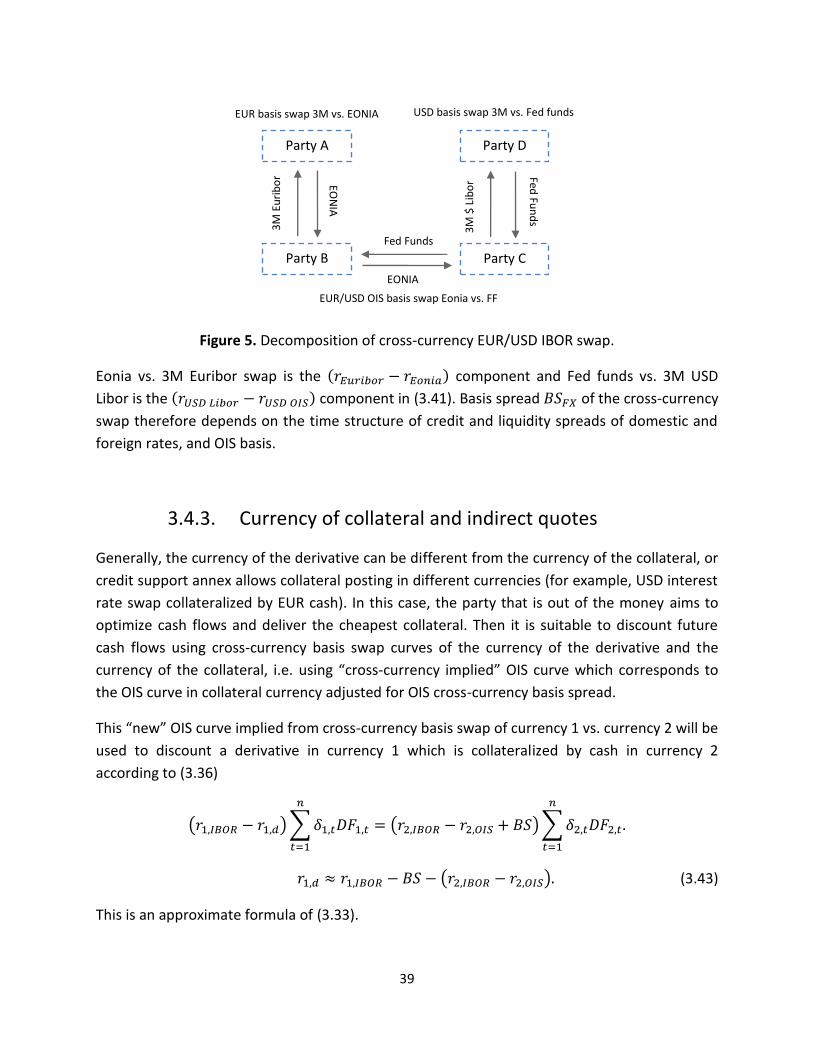
39
Figure 5. Decomposition of cross-currency EUR/USD IBOR swap.
Eonia vs. 3M Euribor swap is the ( ) component and Fed funds vs. 3M USD
Libor is the ( ) component in (3.41). Basis spread of the cross-currency
swap therefore depends on the time structure of credit and liquidity spreads of domestic and
foreign rates, and OIS basis.
3.4.3. Currency of collateral and indirect quotes
Generally, the currency of the derivative can be different from the currency of the collateral, or
credit support annex allows collateral posting in different currencies (for example, USD interest
rate swap collateralized by EUR cash). In this case, the party that is out of the money aims to
optimize cash flows and deliver the cheapest collateral. Then it is suitable to discount future
cash flows using cross-currency basis swap curves of the currency of the derivative and the
currency of the collateral, i.e. using “cross-currency implied” OIS curve which corresponds to
the OIS curve in collateral currency adjusted for OIS cross-currency basis spread.
This “new” OIS curve implied from cross-currency basis swap of currency 1 vs. currency 2 will be
used to discount a derivative in currency 1 which is collateralized by cash in currency 2
according to (3.36)
( )∑
( )∑
( ) (3.43)
This is an approximate formula of (3.33).
Party A Party D
Party C Party B 3
M E
uri
bo
r
3M
$ L
ibo
r
Fed Fu
nd
s
EON
IA
EONIA
Fed Funds
EUR basis swap 3M vs. EONIA
EUR/USD OIS basis swap Eonia vs. FF
USD basis swap 3M vs. Fed funds
40
For currency pairs without direct quotes, indirect quotes against a common currency need to
be used (for example for USD/CZK cross-currency swap we will use quoted spreads of EUR/USD
and EUR/CZK cross-currency swaps). We will use formula (3.36) and adjust the first leg for the
quoted spread
( )∑ ( )∑
( ) (3.44)
We conclude this chapter by revisiting the simplifying assumption in (3.38) about equality of
annuities ∑ meaning that the two swap curves are close to each other and their
discount factors have similar values. This may not hold for all currencies and especially not for
longer maturities. Wu (2012) suggests a simple approximation assuming a flat curve: for a given
swap rate we construct a flat curve whose discount factors form a geometric series
∑
∑
where is the year fraction unadjusted for business days.
41
4. Cross-currency and OIS market in Czech
koruna
In this chapter we discuss possible ways how to estimate OIS curve for the currency without the
liquid OIS market in all tenors. We focus on Czech market that has only recently started to
quote CZK OIS rates but results hold without loss of generality. We also decompose spread of
the cross-currency swap into individual components that reflect credit and liquidity risk
between the two currencies and relative demand of one currency versus the other. There is a
straightforward application of such breakdown, it can be used to approximate implied discount
rates of the second leg of the cross-currency swap and to estimate OIS rates in another
currency (in our case CZK OIS rates, which reflect market expectations about central bank rates
freed from credit and liquidity risk of Czech interbank rates). CZK OIS rates can be then used to
discount derivatives denominated in CZK and collateralized with CZK cash.
4.1. CZK Interest rate swap
In case of CZK interest rate swap that is collateralized in CZK cash we can write according to
(3.14)
∑ ∑
(4.1)
where are discount factors from CZK OIS rates CZK OIS rates are quoted up to
10 years but maturities above 1 year have started to be quoted only recently, since the 4Q
2013. For maturities above 10 years some form of approximation using available market data is
needed.
4.2. Estimation of CZK OIS curve above 10 years
One possible way to estimate CZK OIS curve above 10 years is to define the discount curve by
spread to reference rates as in (3.18). We set the reference rate as CZK swap rates and thus
define the spread as the difference between the 10-year swap rate (fix vs. 3-
month Pribor) and the 10-year OIS rate
(4.2)
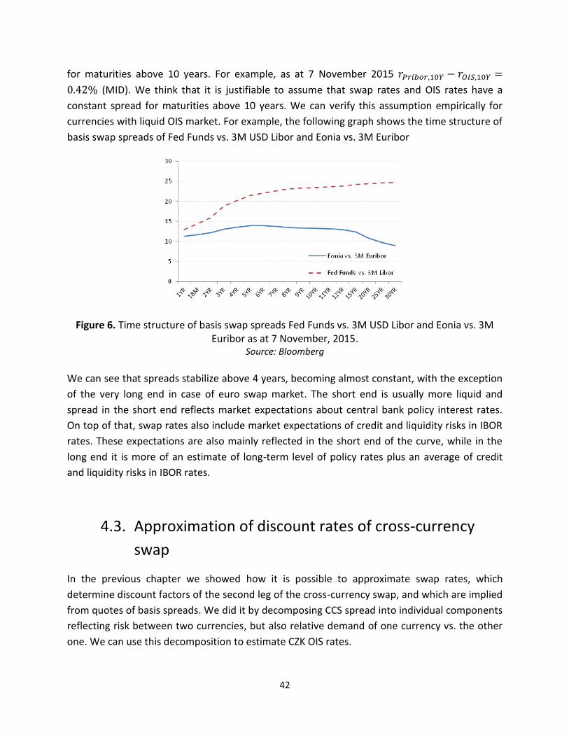
42
for maturities above 10 years. For example, as at 7 November 2015
(MID). We think that it is justifiable to assume that swap rates and OIS rates have a
constant spread for maturities above 10 years. We can verify this assumption empirically for
currencies with liquid OIS market. For example, the following graph shows the time structure of
basis swap spreads of Fed Funds vs. 3M USD Libor and Eonia vs. 3M Euribor
Figure 6. Time structure of basis swap spreads Fed Funds vs. 3M USD Libor and Eonia vs. 3M Euribor as at 7 November, 2015.
Source: Bloomberg We can see that spreads stabilize above 4 years, becoming almost constant, with the exception
of the very long end in case of euro swap market. The short end is usually more liquid and
spread in the short end reflects market expectations about central bank policy interest rates.
On top of that, swap rates also include market expectations of credit and liquidity risks in IBOR
rates. These expectations are also mainly reflected in the short end of the curve, while in the
long end it is more of an estimate of long-term level of policy rates plus an average of credit
and liquidity risks in IBOR rates.
4.3. Approximation of discount rates of cross-currency
swap
In the previous chapter we showed how it is possible to approximate swap rates, which
determine discount factors of the second leg of the cross-currency swap, and which are implied
from quotes of basis spreads. We did it by decomposing CCS spread into individual components
reflecting risk between two currencies, but also relative demand of one currency vs. the other
one. We can use this decomposition to estimate CZK OIS rates.
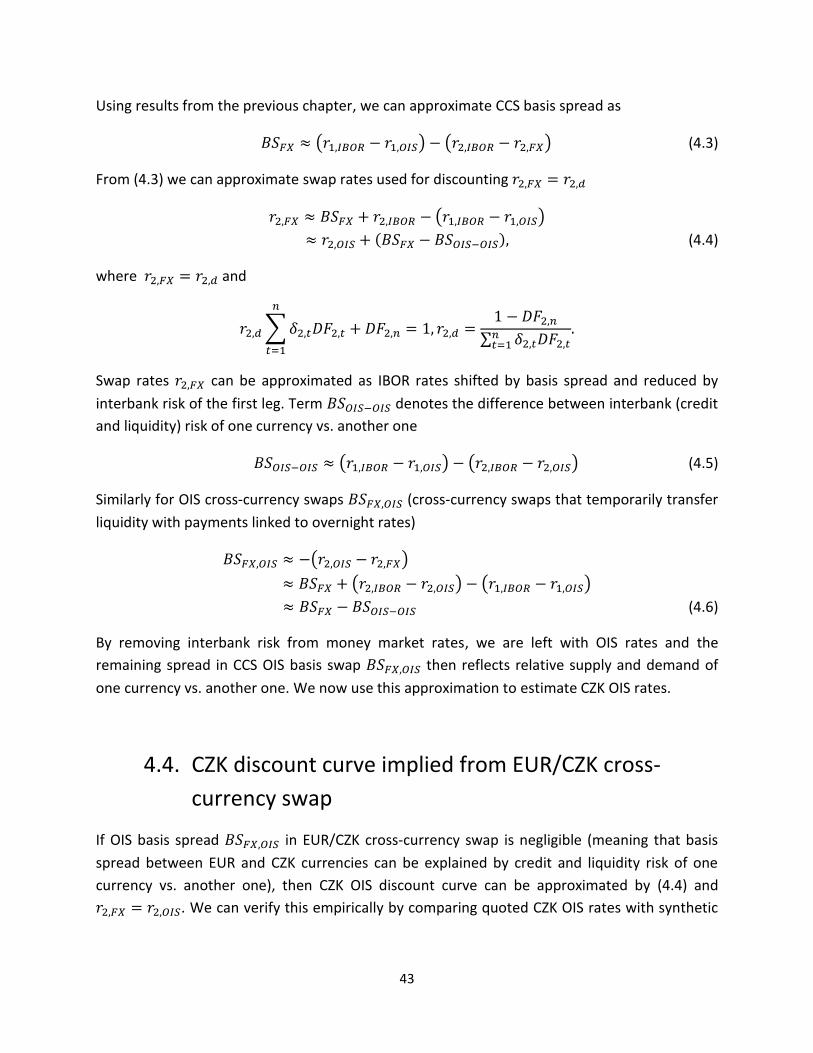
43
Using results from the previous chapter, we can approximate CCS basis spread as
( ) ( ) (4.3)
From (4.3) we can approximate swap rates used for discounting
( )
( ) (4.4)
where and
∑
∑
Swap rates can be approximated as IBOR rates shifted by basis spread and reduced by
interbank risk of the first leg. Term denotes the difference between interbank (credit
and liquidity) risk of one currency vs. another one
( ) ( ) (4.5)
Similarly for OIS cross-currency swaps (cross-currency swaps that temporarily transfer
liquidity with payments linked to overnight rates)
( )
( ) ( )
(4.6)
By removing interbank risk from money market rates, we are left with OIS rates and the
remaining spread in CCS OIS basis swap then reflects relative supply and demand of
one currency vs. another one. We now use this approximation to estimate CZK OIS rates.
4.4. CZK discount curve implied from EUR/CZK cross-
currency swap
If OIS basis spread in EUR/CZK cross-currency swap is negligible (meaning that basis
spread between EUR and CZK currencies can be explained by credit and liquidity risk of one
currency vs. another one), then CZK OIS discount curve can be approximated by (4.4) and
. We can verify this empirically by comparing quoted CZK OIS rates with synthetic
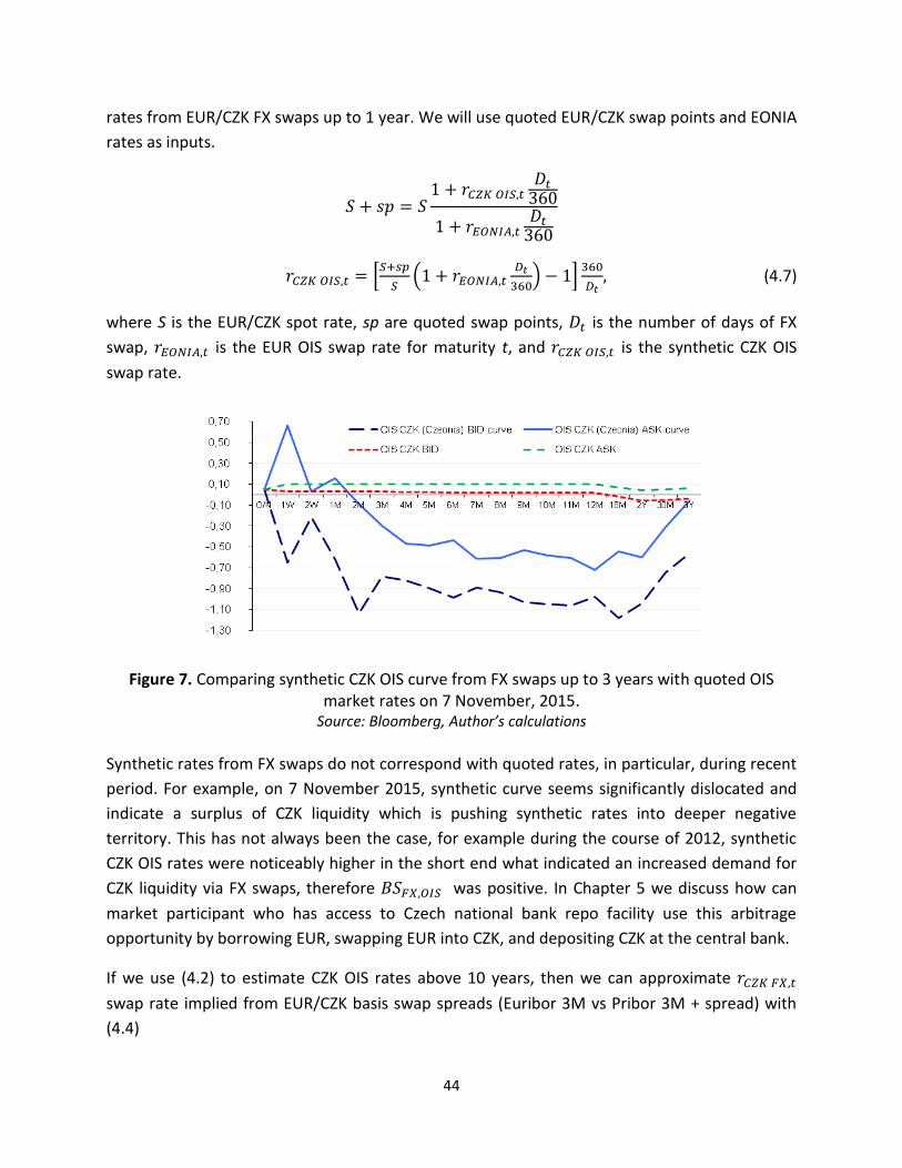
44
rates from EUR/CZK FX swaps up to 1 year. We will use quoted EUR/CZK swap points and EONIA
rates as inputs.
[
(
) ]
(4.7)
where S is the EUR/CZK spot rate, sp are quoted swap points, is the number of days of FX
swap, is the EUR OIS swap rate for maturity t, and is the synthetic CZK OIS
swap rate.
Figure 7. Comparing synthetic CZK OIS curve from FX swaps up to 3 years with quoted OIS market rates on 7 November, 2015.
Source: Bloomberg, Author’s calculations Synthetic rates from FX swaps do not correspond with quoted rates, in particular, during recent
period. For example, on 7 November 2015, synthetic curve seems significantly dislocated and
indicate a surplus of CZK liquidity which is pushing synthetic rates into deeper negative
territory. This has not always been the case, for example during the course of 2012, synthetic
CZK OIS rates were noticeably higher in the short end what indicated an increased demand for
CZK liquidity via FX swaps, therefore was positive. In Chapter 5 we discuss how can
market participant who has access to Czech national bank repo facility use this arbitrage
opportunity by borrowing EUR, swapping EUR into CZK, and depositing CZK at the central bank.
If we use (4.2) to estimate CZK OIS rates above 10 years, then we can approximate
swap rate implied from EUR/CZK basis swap spreads (Euribor 3M vs Pribor 3M + spread) with
(4.4)
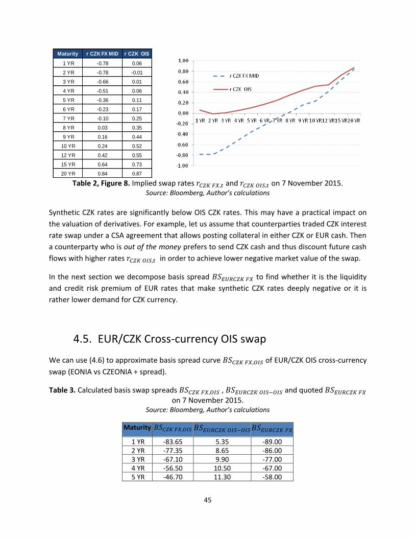
45
Table 2, Figure 8. Implied swap rates and on 7 November 2015.
Source: Bloomberg, Author’s calculations Synthetic CZK rates are significantly below OIS CZK rates. This may have a practical impact on
the valuation of derivatives. For example, let us assume that counterparties traded CZK interest
rate swap under a CSA agreement that allows posting collateral in either CZK or EUR cash. Then
a counterparty who is out of the money prefers to send CZK cash and thus discount future cash
flows with higher rates in order to achieve lower negative market value of the swap.
In the next section we decompose basis spread to find whether it is the liquidity
and credit risk premium of EUR rates that make synthetic CZK rates deeply negative or it is
rather lower demand for CZK currency.
4.5. EUR/CZK Cross-currency OIS swap
We can use (4.6) to approximate basis spread curve of EUR/CZK OIS cross-currency
swap (EONIA vs CZEONIA + spread).
Table 3. Calculated basis swap spreads , and quoted on 7 November 2015.
Source: Bloomberg, Author’s calculations
Maturity
1 YR -83.65 5.35 -89.00 2 YR -77.35 8.65 -86.00 3 YR -67.10 9.90 -77.00 4 YR -56.50 10.50 -67.00 5 YR -46.70 11.30 -58.00
Maturity r CZK FX MID r CZK OIS
1 YR -0.78 0.06
2 YR -0.78 -0.01
3 YR -0.66 0.01
4 YR -0.51 0.06
5 YR -0.36 0.11
6 YR -0.23 0.17
7 YR -0.10 0.25
8 YR 0.03 0.35
9 YR 0.16 0.44
10 YR 0.24 0.52
12 YR 0.42 0.55
15 YR 0.64 0.73
20 YR 0.84 0.87
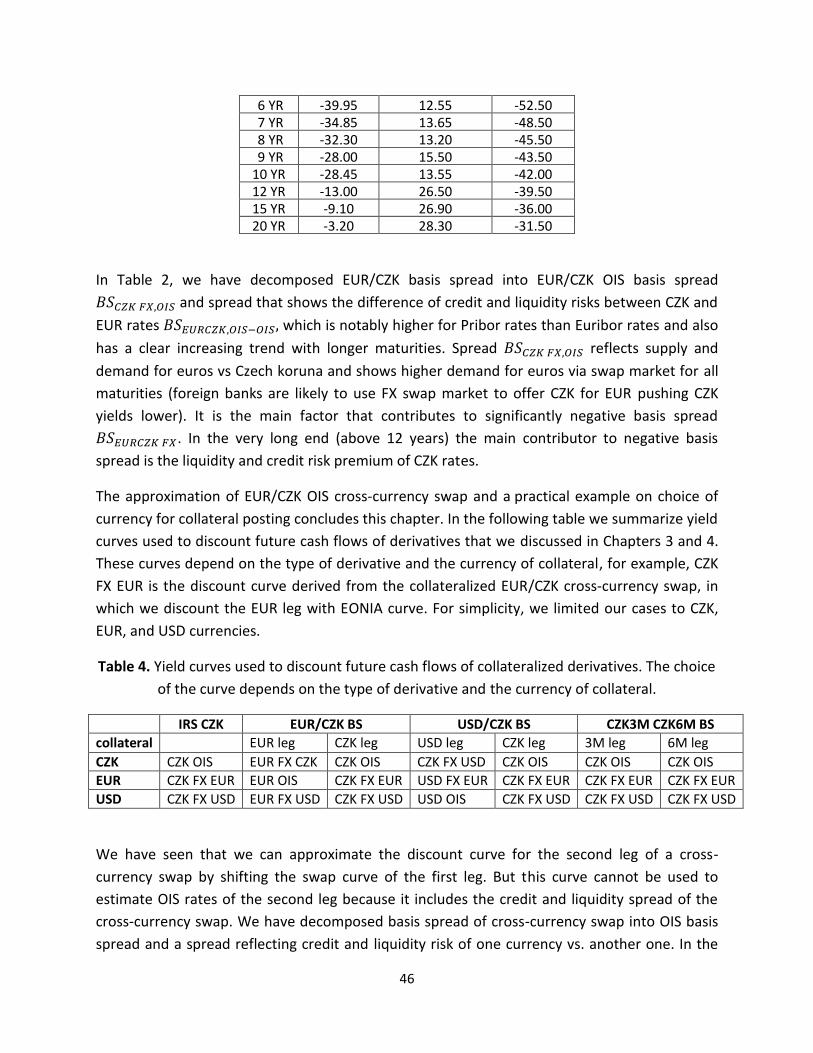
46
6 YR -39.95 12.55 -52.50 7 YR -34.85 13.65 -48.50 8 YR -32.30 13.20 -45.50 9 YR -28.00 15.50 -43.50 10 YR -28.45 13.55 -42.00 12 YR -13.00 26.50 -39.50 15 YR -9.10 26.90 -36.00 20 YR -3.20 28.30 -31.50
In Table 2, we have decomposed EUR/CZK basis spread into EUR/CZK OIS basis spread
and spread that shows the difference of credit and liquidity risks between CZK and
EUR rates which is notably higher for Pribor rates than Euribor rates and also
has a clear increasing trend with longer maturities. Spread reflects supply and
demand for euros vs Czech koruna and shows higher demand for euros via swap market for all
maturities (foreign banks are likely to use FX swap market to offer CZK for EUR pushing CZK
yields lower). It is the main factor that contributes to significantly negative basis spread
. In the very long end (above 12 years) the main contributor to negative basis
spread is the liquidity and credit risk premium of CZK rates.
The approximation of EUR/CZK OIS cross-currency swap and a practical example on choice of
currency for collateral posting concludes this chapter. In the following table we summarize yield
curves used to discount future cash flows of derivatives that we discussed in Chapters 3 and 4.
These curves depend on the type of derivative and the currency of collateral, for example, CZK
FX EUR is the discount curve derived from the collateralized EUR/CZK cross-currency swap, in
which we discount the EUR leg with EONIA curve. For simplicity, we limited our cases to CZK,
EUR, and USD currencies.
Table 4. Yield curves used to discount future cash flows of collateralized derivatives. The choice
of the curve depends on the type of derivative and the currency of collateral.
IRS CZK EUR/CZK BS USD/CZK BS CZK3M CZK6M BS
collateral EUR leg CZK leg USD leg CZK leg 3M leg 6M leg
CZK CZK OIS EUR FX CZK CZK OIS CZK FX USD CZK OIS CZK OIS CZK OIS
EUR CZK FX EUR EUR OIS CZK FX EUR USD FX EUR CZK FX EUR CZK FX EUR CZK FX EUR
USD CZK FX USD EUR FX USD CZK FX USD USD OIS CZK FX USD CZK FX USD CZK FX USD
We have seen that we can approximate the discount curve for the second leg of a cross-
currency swap by shifting the swap curve of the first leg. But this curve cannot be used to
estimate OIS rates of the second leg because it includes the credit and liquidity spread of the
cross-currency swap. We have decomposed basis spread of cross-currency swap into OIS basis
spread and a spread reflecting credit and liquidity risk of one currency vs. another one. In the
47
previous chapter we also discussed the case when there is no market for the two respective
currencies and direct quotes against a common currency must be used.
We have focused on CZK market and have shown possible way how to derive CZK OIS curve and
have decomposed spread of the EUR/CZK cross-currency spread into individual elements
reflecting relative supply and demand and the difference between credit and liquidity risks of
CZK and EUR rates. In markets where OIS quotes do not yet exist for all maturities, some
assumptions and subjectivity are needed, but the assumptions should be consistent with the
requirement of arbitrage-free pricing. Due to increased collateralization, one could expect
higher market activity in less liquid OIS markets, including CZK, with more market participants
being involved, which could lead to tighter spreads and quotes for longer maturities.
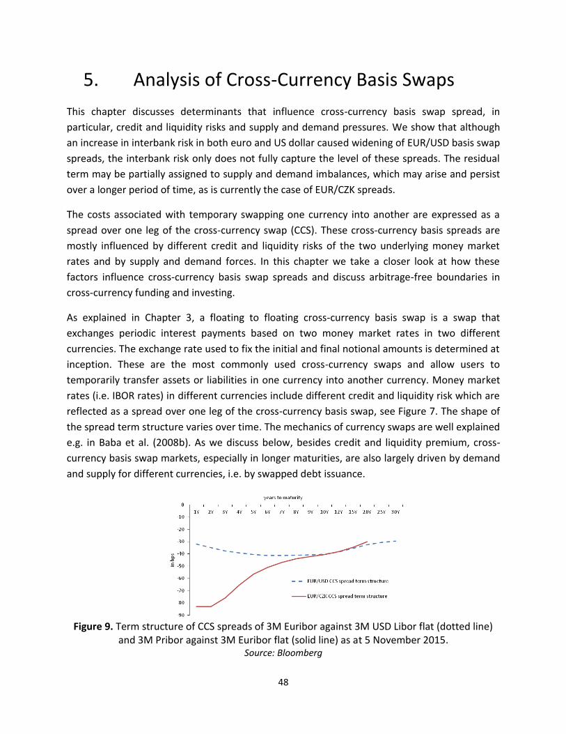
48
5. Analysis of Cross-Currency Basis Swaps
This chapter discusses determinants that influence cross-currency basis swap spread, in
particular, credit and liquidity risks and supply and demand pressures. We show that although
an increase in interbank risk in both euro and US dollar caused widening of EUR/USD basis swap
spreads, the interbank risk only does not fully capture the level of these spreads. The residual
term may be partially assigned to supply and demand imbalances, which may arise and persist
over a longer period of time, as is currently the case of EUR/CZK spreads.
The costs associated with temporary swapping one currency into another are expressed as a
spread over one leg of the cross-currency swap (CCS). These cross-currency basis spreads are
mostly influenced by different credit and liquidity risks of the two underlying money market
rates and by supply and demand forces. In this chapter we take a closer look at how these
factors influence cross-currency basis swap spreads and discuss arbitrage-free boundaries in
cross-currency funding and investing.
As explained in Chapter 3, a floating to floating cross-currency basis swap is a swap that
exchanges periodic interest payments based on two money market rates in two different
currencies. The exchange rate used to fix the initial and final notional amounts is determined at
inception. These are the most commonly used cross-currency swaps and allow users to
temporarily transfer assets or liabilities in one currency into another currency. Money market
rates (i.e. IBOR rates) in different currencies include different credit and liquidity risk which are
reflected as a spread over one leg of the cross-currency basis swap, see Figure 7. The shape of
the spread term structure varies over time. The mechanics of currency swaps are well explained
e.g. in Baba et al. (2008b). As we discuss below, besides credit and liquidity premium, cross-
currency basis swap markets, especially in longer maturities, are also largely driven by demand
and supply for different currencies, i.e. by swapped debt issuance.
Figure 9. Term structure of CCS spreads of 3M Euribor against 3M USD Libor flat (dotted line)
and 3M Pribor against 3M Euribor flat (solid line) as at 5 November 2015. Source: Bloomberg
49
CCS basis spreads were traditionally close to zero (apart from bid ask spreads) based on the
assumption of banks’ continuous access to interbank market financing at IBOR rates. This
assumption was widely questioned as spreads have blown in 2007 and practically became an
independent market risk factor.
The existing literature discussing cross-currency basis spreads is still somewhat limited.
However, factors influencing CCS spreads are often similar to factors influencing single currency
swap spreads. There have been a number of papers investigating determinants of interest rate
swap spreads, i.e. the differences between government bond yields and interest rate swap
levels. For example, Cortes (2006) uses principal component analysis to find that the term
structure of swap spreads in different markets move together and are upward sloping in the
two to ten year part of the curve due to the existence of a default term premium (a premium
reflecting the uncertainty about future interest rates and the risk of systemic failure of the
banking sector in the future) and global expectations of government bond issuance (the higher
net borrowing, the steeper the yield curve).
Huang et al. (2002) investigated whether liquidity and credit contribute to fluctuations in
spreads between 10-year US Treasuries and 10-year USD swaps using vector autoregression
method. Their results show that liquidity has a significant negative effect on the swap spreads
(swap spreads fall with increased supply and steeper treasury curve). The authors further argue
that swap spreads should be mainly regarded as an indicator of market liquidity, and that credit
determines the swap spread over longer horizons.
An interesting study was conducted by Heppke-Falk and Hüfner (2004) who analysed if
expected budget deficit impact swap spreads in France, Germany and Italy. Using a monthly
deficit forecast during the sample period of 1994-2004 they concluded that expected deficit has
no significant impact on swap spreads. However, this is contradicted by i.e. Caceres et al. (2010)
who show on the recent data that sovereign bond yields rise versus swap yields, when budget
deficits increase.
Swap spreads vary considerably over time, and some of this variation has occurred
internationally but their term structures also appear to move independently in each market.
Also, there might be other specific factors influencing swap spreads such as different liquidity
preferences and supply and demand forces.
Ando (2012) presents a study that focuses on EUR/JPY respectively EUR/USD market of cross-
currency swaps and investigates reasons for existence of basis swap spreads. Author concludes
that the volatility of basis swap spreads is caused by stress in unsecured interbank money
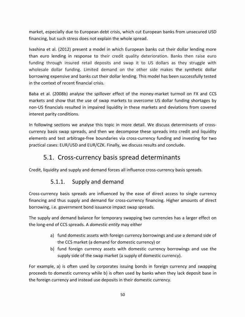
50
market, especially due to European debt crisis, which cut European banks from unsecured USD
financing, but such stress does not explain the whole spread.
Ivashina et al. (2012) present a model in which European banks cut their dollar lending more
than euro lending in response to their credit quality deterioration. Banks then raise euro
funding through insured retail deposits and swap it to US dollars as they struggle with
wholesale dollar funding. Limited demand on the other side makes the synthetic dollar
borrowing expensive and banks cut their dollar lending. This model has been successfully tested
in the context of recent financial crisis.
Baba et al. (2008b) analyse the spillover effect of the money-market turmoil on FX and CCS
markets and show that the use of swap markets to overcome US dollar funding shortages by
non-US financials resulted in impaired liquidity in these markets and deviations from covered
interest parity conditions.
In following sections we analyse this topic in more detail. We discuss determinants of cross-
currency basis swap spreads, and then we decompose these spreads into credit and liquidity
elements and test arbitrage-free boundaries via cross-currency funding and investing for two
practical cases: EUR/USD and EUR/CZK. Finally, we discuss results and conclude.
5.1. Cross-currency basis spread determinants
Credit, liquidity and supply and demand forces all influence cross-currency basis spreads.
5.1.1. Supply and demand
Cross-currency basis spreads are influenced by the ease of direct access to single currency
financing and thus supply and demand for cross-currency financing. Higher amounts of direct
borrowing, i.e. government bond issuance impact swap spreads.
The supply and demand balance for temporary swapping two currencies has a larger effect on
the long-end of CCS spreads. A domestic entity may either
a) fund domestic assets with foreign currency borrowings and use a demand side of
the CCS market (a demand for domestic currency) or
b) fund foreign currency assets with domestic currency borrowings and use the
supply side of the swap market (a supply of domestic currency).
For example, a) is often used by corporates issuing bonds in foreign currency and swapping
proceeds to domestic currency while b) is often used by banks when they lack deposit base in
the foreign currency and instead use deposits in their domestic currency.
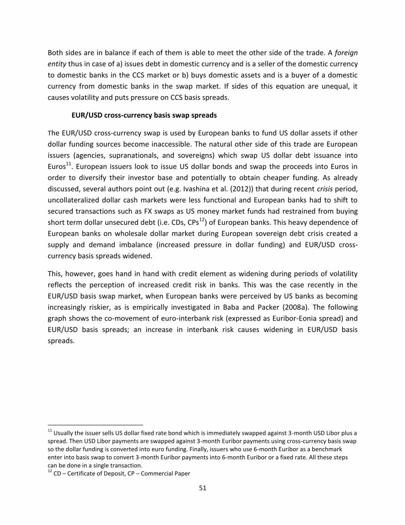
51
Both sides are in balance if each of them is able to meet the other side of the trade. A foreign
entity thus in case of a) issues debt in domestic currency and is a seller of the domestic currency
to domestic banks in the CCS market or b) buys domestic assets and is a buyer of a domestic
currency from domestic banks in the swap market. If sides of this equation are unequal, it
causes volatility and puts pressure on CCS basis spreads.
EUR/USD cross-currency basis swap spreads
The EUR/USD cross-currency swap is used by European banks to fund US dollar assets if other
dollar funding sources become inaccessible. The natural other side of this trade are European
issuers (agencies, supranationals, and sovereigns) which swap US dollar debt issuance into
Euros11. European issuers look to issue US dollar bonds and swap the proceeds into Euros in
order to diversify their investor base and potentially to obtain cheaper funding. As already
discussed, several authors point out (e.g. Ivashina et al. (2012)) that during recent crisis period,
uncollateralized dollar cash markets were less functional and European banks had to shift to
secured transactions such as FX swaps as US money market funds had restrained from buying
short term dollar unsecured debt (i.e. CDs, CPs12) of European banks. This heavy dependence of
European banks on wholesale dollar market during European sovereign debt crisis created a
supply and demand imbalance (increased pressure in dollar funding) and EUR/USD cross-
currency basis spreads widened.
This, however, goes hand in hand with credit element as widening during periods of volatility
reflects the perception of increased credit risk in banks. This was the case recently in the
EUR/USD basis swap market, when European banks were perceived by US banks as becoming
increasingly riskier, as is empirically investigated in Baba and Packer (2008a). The following
graph shows the co-movement of euro-interbank risk (expressed as Euribor-Eonia spread) and
EUR/USD basis spreads; an increase in interbank risk causes widening in EUR/USD basis
spreads.
11
Usually the issuer sells US dollar fixed rate bond which is immediately swapped against 3-month USD Libor plus a spread. Then USD Libor payments are swapped against 3-month Euribor payments using cross-currency basis swap so the dollar funding is converted into euro funding. Finally, issuers who use 6-month Euribor as a benchmark enter into basis swap to convert 3-month Euribor payments into 6-month Euribor or a fixed rate. All these steps can be done in a single transaction. 12
CD – Certificate of Deposit, CP – Commercial Paper
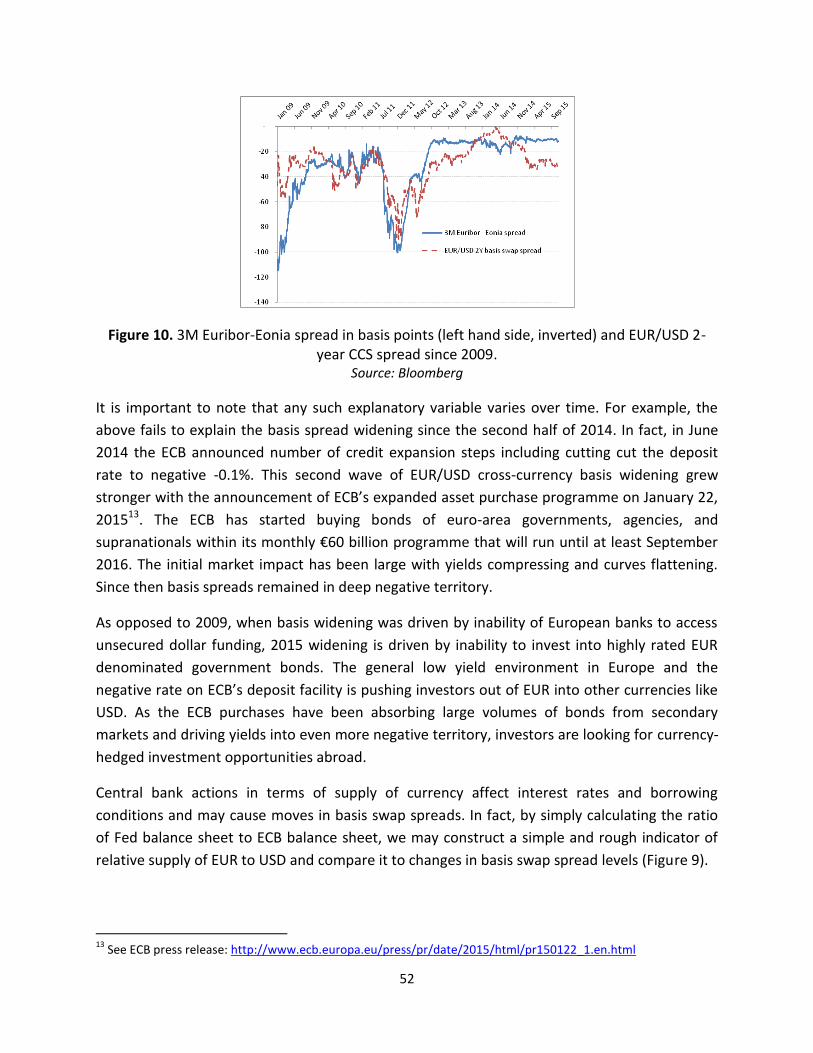
52
Figure 10. 3M Euribor-Eonia spread in basis points (left hand side, inverted) and EUR/USD 2-year CCS spread since 2009.
Source: Bloomberg
It is important to note that any such explanatory variable varies over time. For example, the
above fails to explain the basis spread widening since the second half of 2014. In fact, in June
2014 the ECB announced number of credit expansion steps including cutting cut the deposit
rate to negative -0.1%. This second wave of EUR/USD cross-currency basis widening grew
stronger with the announcement of ECB’s expanded asset purchase programme on January 22,
201513. The ECB has started buying bonds of euro-area governments, agencies, and
supranationals within its monthly €60 billion programme that will run until at least September
2016. The initial market impact has been large with yields compressing and curves flattening.
Since then basis spreads remained in deep negative territory.
As opposed to 2009, when basis widening was driven by inability of European banks to access
unsecured dollar funding, 2015 widening is driven by inability to invest into highly rated EUR
denominated government bonds. The general low yield environment in Europe and the
negative rate on ECB’s deposit facility is pushing investors out of EUR into other currencies like
USD. As the ECB purchases have been absorbing large volumes of bonds from secondary
markets and driving yields into even more negative territory, investors are looking for currency-
hedged investment opportunities abroad.
Central bank actions in terms of supply of currency affect interest rates and borrowing
conditions and may cause moves in basis swap spreads. In fact, by simply calculating the ratio
of Fed balance sheet to ECB balance sheet, we may construct a simple and rough indicator of
relative supply of EUR to USD and compare it to changes in basis swap spread levels (Figure 9).
13
See ECB press release: http://www.ecb.europa.eu/press/pr/date/2015/html/pr150122_1.en.html
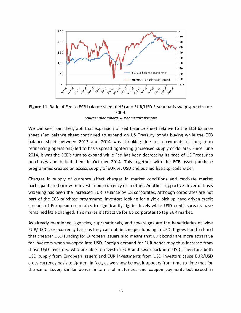
53
Figure 11. Ratio of Fed to ECB balance sheet (LHS) and EUR/USD 2-year basis swap spread since 2009.
Source: Bloomberg, Author’s calculations
We can see from the graph that expansion of Fed balance sheet relative to the ECB balance
sheet (Fed balance sheet continued to expand on US Treasury bonds buying while the ECB
balance sheet between 2012 and 2014 was shrinking due to repayments of long term
refinancing operations) led to basis spread tightening (increased supply of dollars). Since June
2014, it was the ECB’s turn to expand while Fed has been decreasing its pace of US Treasuries
purchases and halted them in October 2014. This together with the ECB asset purchase
programmes created an excess supply of EUR vs. USD and pushed basis spreads wider.
Changes in supply of currency affect changes in market conditions and motivate market
participants to borrow or invest in one currency or another. Another supportive driver of basis
widening has been the increased EUR issuance by US corporates. Although corporates are not
part of the ECB purchase programme, investors looking for a yield pick-up have driven credit
spreads of European corporates to significantly tighter levels while USD credit spreads have
remained little changed. This makes it attractive for US corporates to tap EUR market.
As already mentioned, agencies, supranationals, and sovereigns are the beneficiaries of wide
EUR/USD cross-currency basis as they can obtain cheaper funding in USD. It goes hand in hand
that cheaper USD funding for European issuers also means that EUR bonds are more attractive
for investors when swapped into USD. Foreign demand for EUR bonds may thus increase from
those USD investors, who are able to invest in EUR and swap back into USD. Therefore both
USD supply from European issuers and EUR investments from USD investors cause EUR/USD
cross-currency basis to tighten. In fact, as we show below, it appears from time to time that for
the same issuer, similar bonds in terms of maturities and coupon payments but issued in
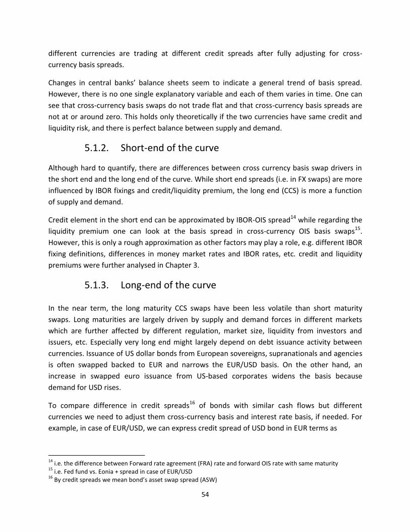
54
different currencies are trading at different credit spreads after fully adjusting for cross-
currency basis spreads.
Changes in central banks’ balance sheets seem to indicate a general trend of basis spread.
However, there is no one single explanatory variable and each of them varies in time. One can
see that cross-currency basis swaps do not trade flat and that cross-currency basis spreads are
not at or around zero. This holds only theoretically if the two currencies have same credit and
liquidity risk, and there is perfect balance between supply and demand.
5.1.2. Short-end of the curve
Although hard to quantify, there are differences between cross currency basis swap drivers in
the short end and the long end of the curve. While short end spreads (i.e. in FX swaps) are more
influenced by IBOR fixings and credit/liquidity premium, the long end (CCS) is more a function
of supply and demand.
Credit element in the short end can be approximated by IBOR-OIS spread14 while regarding the
liquidity premium one can look at the basis spread in cross-currency OIS basis swaps15.
However, this is only a rough approximation as other factors may play a role, e.g. different IBOR
fixing definitions, differences in money market rates and IBOR rates, etc. credit and liquidity
premiums were further analysed in Chapter 3.
5.1.3. Long-end of the curve
In the near term, the long maturity CCS swaps have been less volatile than short maturity
swaps. Long maturities are largely driven by supply and demand forces in different markets
which are further affected by different regulation, market size, liquidity from investors and
issuers, etc. Especially very long end might largely depend on debt issuance activity between
currencies. Issuance of US dollar bonds from European sovereigns, supranationals and agencies
is often swapped backed to EUR and narrows the EUR/USD basis. On the other hand, an
increase in swapped euro issuance from US-based corporates widens the basis because
demand for USD rises.
To compare difference in credit spreads16 of bonds with similar cash flows but different
currencies we need to adjust them cross-currency basis and interest rate basis, if needed. For
example, in case of EUR/USD, we can express credit spread of USD bond in EUR terms as
14
i.e. the difference between Forward rate agreement (FRA) rate and forward OIS rate with same maturity 15
i.e. Fed fund vs. Eonia + spread in case of EUR/USD 16
By credit spreads we mean bond’s asset swap spread (ASW)
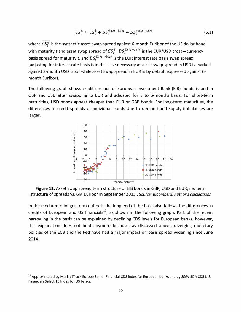
55
(5.1)
where is the synthetic asset swap spread against 6-month Euribor of the US dollar bond
with maturity t and asset swap spread of ,
is the EUR/USD cross—currency
basis spread for maturity t, and is the EUR interest rate basis swap spread
(adjusting for interest rate basis is in this case necessary as asset swap spread in USD is marked
against 3-month USD Libor while asset swap spread in EUR is by default expressed against 6-
month Euribor).
The following graph shows credit spreads of European Investment Bank (EIB) bonds issued in
GBP and USD after swapping to EUR and adjusted for 3 to 6-months basis. For short-term
maturities, USD bonds appear cheaper than EUR or GBP bonds. For long-term maturities, the
differences in credit spreads of individual bonds due to demand and supply imbalances are
larger.
Figure 12. Asset swap spread term structure of EIB bonds in GBP, USD and EUR, i.e. term
structure of spreads vs. 6M Euribor in September 2013 . Source: Bloomberg, Author’s calculations
In the medium to longer-term outlook, the long end of the basis also follows the differences in
credits of European and US financials17, as shown in the following graph. Part of the recent
narrowing in the basis can be explained by declining CDS levels for European banks, however,
this explanation does not hold anymore because, as discussed above, diverging monetary
policies of the ECB and the Fed have had a major impact on basis spread widening since June
2014.
17
Approximated by Markit iTraxx Europe Senior Financial CDS index for European banks and by S&P/ISDA CDS U.S. Financials Select 10 Index for US banks.
-40
-30
-20
-10
0
10
20
30
40
50
-4 -2 0 2 4 6 8 10 12 14 16 18 20 22 24
6-m
on
th a
sse
t sw
ap s
pre
ad in
EU
R
Years to maturity
EIB EUR bonds
EIB USD bonds
EIB GBP bonds
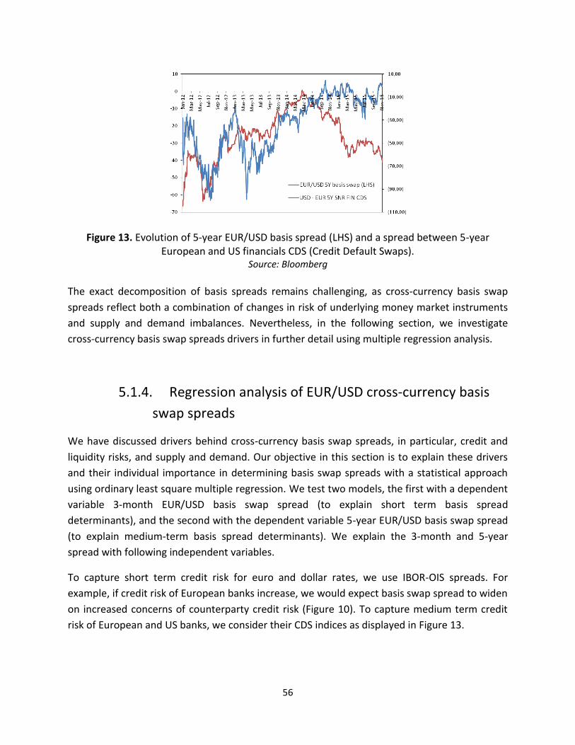
56
Figure 13. Evolution of 5-year EUR/USD basis spread (LHS) and a spread between 5-year European and US financials CDS (Credit Default Swaps).
Source: Bloomberg
The exact decomposition of basis spreads remains challenging, as cross-currency basis swap
spreads reflect both a combination of changes in risk of underlying money market instruments
and supply and demand imbalances. Nevertheless, in the following section, we investigate
cross-currency basis swap spreads drivers in further detail using multiple regression analysis.
5.1.4. Regression analysis of EUR/USD cross-currency basis
swap spreads
We have discussed drivers behind cross-currency basis swap spreads, in particular, credit and
liquidity risks, and supply and demand. Our objective in this section is to explain these drivers
and their individual importance in determining basis swap spreads with a statistical approach
using ordinary least square multiple regression. We test two models, the first with a dependent
variable 3-month EUR/USD basis swap spread (to explain short term basis spread
determinants), and the second with the dependent variable 5-year EUR/USD basis swap spread
(to explain medium-term basis spread determinants). We explain the 3-month and 5-year
spread with following independent variables.
To capture short term credit risk for euro and dollar rates, we use IBOR-OIS spreads. For
example, if credit risk of European banks increase, we would expect basis swap spread to widen
on increased concerns of counterparty credit risk (Figure 10). To capture medium term credit
risk of European and US banks, we consider their CDS indices as displayed in Figure 13.
57
To capture changes in supply of each currency, we investigate Fed’s and ECB’s balance sheets.
As hinted in Figure 11, when the Fed balance sheet expands relative to the ECB balance sheet,
the basis spread tends to tighten (increased supply of dollars).
We also add EUR/USD spot rate to see if FX spot market affects CCS basis spreads. We could
expect that if the depreciation of Euro against dollar causes forward buying of Euro by
corporates, it may cause also widening of the CCS basis spread due to a risen need to hedge
these forwards by banks.
Independent variables in regression equation are thus the following
(in %)
– (in %)
(Markit iTraxx Europe Senior Financial CDS index) (in
bps)
(S&P/ISDA CDS U.S. Financials Select 10 Index) (in bps)
To detrend the data we calculate for each variable their weekly changes. Data sample consists
of 223 observations between September 2011 and December 2015, and data are taken from
Bloomberg (data for US financials CDS index are only available since September 2011). We
regress weekly changes in 3-month and 5-year EUR/USD basis swap spreads against weekly
changes in the above selected drivers. Our regression equation is
(5.2)
Regression results are summarized in the following tables.
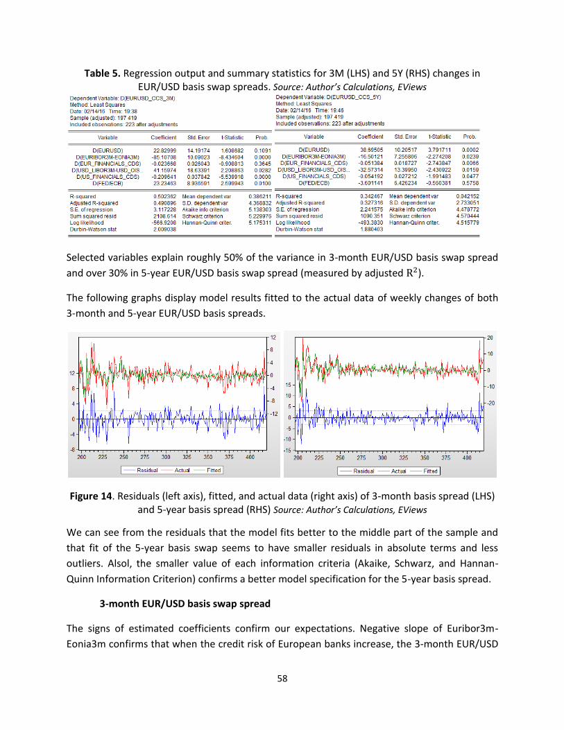
58
Table 5. Regression output and summary statistics for 3M (LHS) and 5Y (RHS) changes in EUR/USD basis swap spreads. Source: Author’s Calculations, EViews
Selected variables explain roughly 50% of the variance in 3-month EUR/USD basis swap spread
and over 30% in 5-year EUR/USD basis swap spread (measured by adjusted ).
The following graphs display model results fitted to the actual data of weekly changes of both
3-month and 5-year EUR/USD basis spreads.
Figure 14. Residuals (left axis), fitted, and actual data (right axis) of 3-month basis spread (LHS) and 5-year basis spread (RHS) Source: Author’s Calculations, EViews
We can see from the residuals that the model fits better to the middle part of the sample and
that fit of the 5-year basis swap seems to have smaller residuals in absolute terms and less
outliers. Alsol, the smaller value of each information criteria (Akaike, Schwarz, and Hannan-
Quinn Information Criterion) confirms a better model specification for the 5-year basis spread.
3-month EUR/USD basis swap spread
The signs of estimated coefficients confirm our expectations. Negative slope of Euribor3m-
Eonia3m confirms that when the credit risk of European banks increase, the 3-month EUR/USD
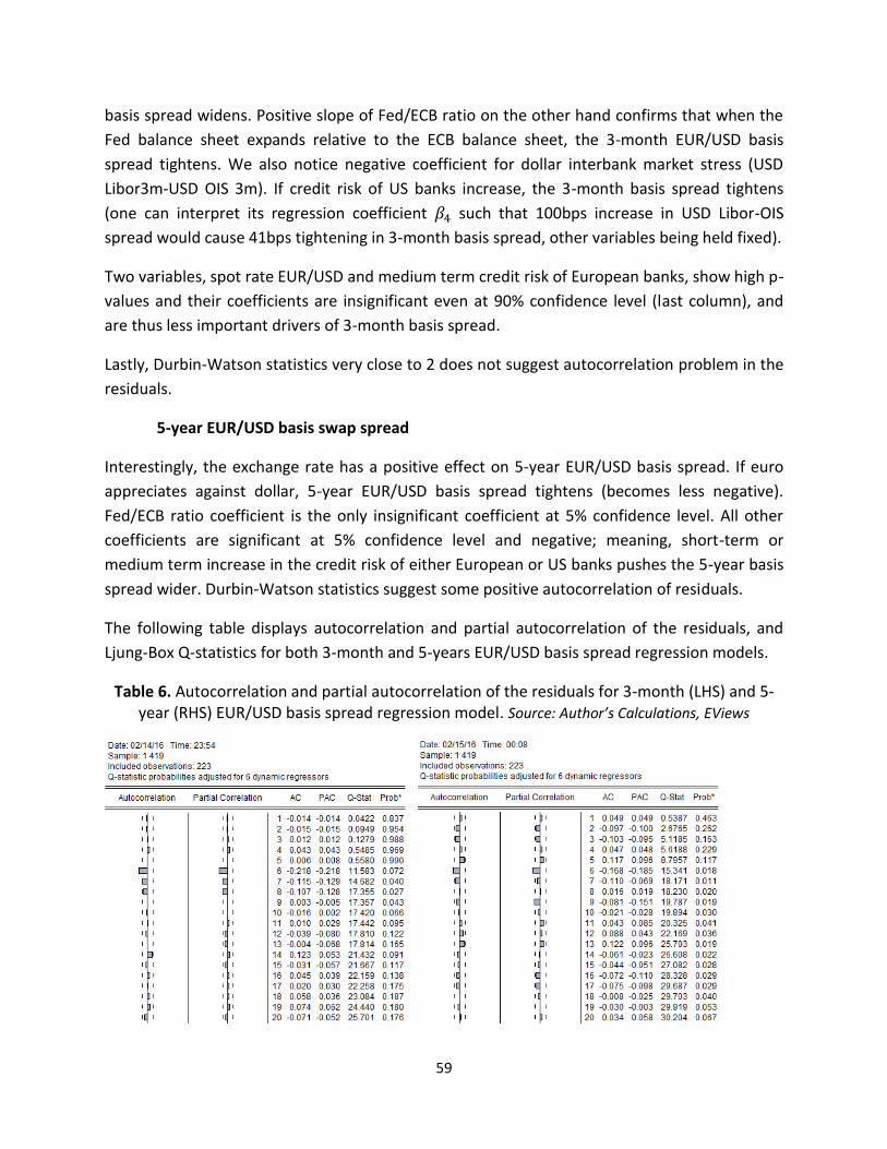
59
basis spread widens. Positive slope of Fed/ECB ratio on the other hand confirms that when the
Fed balance sheet expands relative to the ECB balance sheet, the 3-month EUR/USD basis
spread tightens. We also notice negative coefficient for dollar interbank market stress (USD
Libor3m-USD OIS 3m). If credit risk of US banks increase, the 3-month basis spread tightens
(one can interpret its regression coefficient such that 100bps increase in USD Libor-OIS
spread would cause 41bps tightening in 3-month basis spread, other variables being held fixed).
Two variables, spot rate EUR/USD and medium term credit risk of European banks, show high p-
values and their coefficients are insignificant even at 90% confidence level (last column), and
are thus less important drivers of 3-month basis spread.
Lastly, Durbin-Watson statistics very close to 2 does not suggest autocorrelation problem in the
residuals.
5-year EUR/USD basis swap spread
Interestingly, the exchange rate has a positive effect on 5-year EUR/USD basis spread. If euro
appreciates against dollar, 5-year EUR/USD basis spread tightens (becomes less negative).
Fed/ECB ratio coefficient is the only insignificant coefficient at 5% confidence level. All other
coefficients are significant at 5% confidence level and negative; meaning, short-term or
medium term increase in the credit risk of either European or US banks pushes the 5-year basis
spread wider. Durbin-Watson statistics suggest some positive autocorrelation of residuals.
The following table displays autocorrelation and partial autocorrelation of the residuals, and
Ljung-Box Q-statistics for both 3-month and 5-years EUR/USD basis spread regression models.
Table 6. Autocorrelation and partial autocorrelation of the residuals for 3-month (LHS) and 5-year (RHS) EUR/USD basis spread regression model. Source: Author’s Calculations, EViews
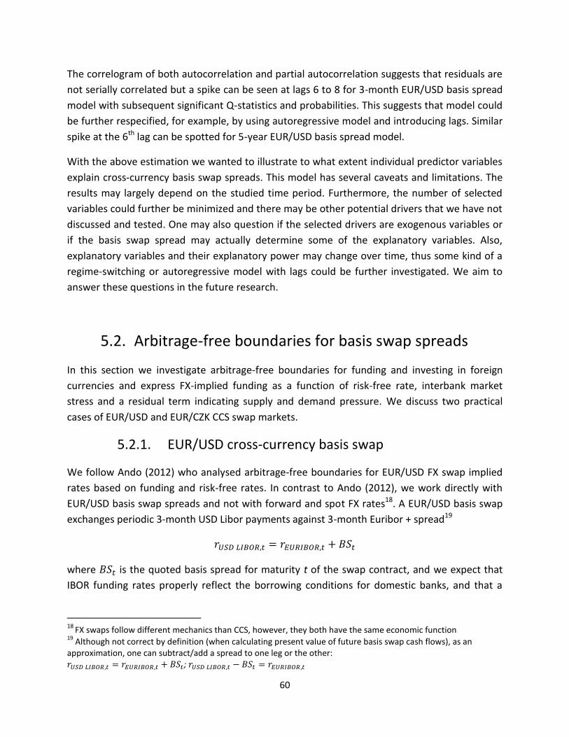
60
The correlogram of both autocorrelation and partial autocorrelation suggests that residuals are
not serially correlated but a spike can be seen at lags 6 to 8 for 3-month EUR/USD basis spread
model with subsequent significant Q-statistics and probabilities. This suggests that model could
be further respecified, for example, by using autoregressive model and introducing lags. Similar
spike at the 6th lag can be spotted for 5-year EUR/USD basis spread model.
With the above estimation we wanted to illustrate to what extent individual predictor variables
explain cross-currency basis swap spreads. This model has several caveats and limitations. The
results may largely depend on the studied time period. Furthermore, the number of selected
variables could further be minimized and there may be other potential drivers that we have not
discussed and tested. One may also question if the selected drivers are exogenous variables or
if the basis swap spread may actually determine some of the explanatory variables. Also,
explanatory variables and their explanatory power may change over time, thus some kind of a
regime-switching or autoregressive model with lags could be further investigated. We aim to
answer these questions in the future research.
5.2. Arbitrage-free boundaries for basis swap spreads
In this section we investigate arbitrage-free boundaries for funding and investing in foreign
currencies and express FX-implied funding as a function of risk-free rate, interbank market
stress and a residual term indicating supply and demand pressure. We discuss two practical
cases of EUR/USD and EUR/CZK CCS swap markets.
5.2.1. EUR/USD cross-currency basis swap
We follow Ando (2012) who analysed arbitrage-free boundaries for EUR/USD FX swap implied
rates based on funding and risk-free rates. In contrast to Ando (2012), we work directly with
EUR/USD basis swap spreads and not with forward and spot FX rates18. A EUR/USD basis swap
exchanges periodic 3-month USD Libor payments against 3-month Euribor + spread19
where is the quoted basis spread for maturity t of the swap contract, and we expect that
IBOR funding rates properly reflect the borrowing conditions for domestic banks, and that a
18
FX swaps follow different mechanics than CCS, however, they both have the same economic function 19
Although not correct by definition (when calculating present value of future basis swap cash flows), as an approximation, one can subtract/add a spread to one leg or the other: ;
61
bank can invest at OIS (overnight indexed swap) risk-free rate in either Euros or US dollars.
Natural boundaries for risk-free investing thus become
, (5.3)
If (5.3) does not hold, then arbitrage opportunity arises
If , then a bank which can access unsecured EUR market
will borrow at Euribor, swap the proceeds into USD and invest at risk-free USD OIS rate20
If , then a bank which can access unsecured USD market will
borrow at USD LIBOR, swap the proceeds into EUR via FX or cross-currency swap and
invest at risk-free EONIA rate.
Further, setting , we can use as an indicator of arbitrage
opportunity (for arbitrage exists). It is now easy to express FX swap implied USD funding
rate from EUR funding rate (Euribor) in terms of , IBOR and OIS rates
( )
( ) ( ) (5.4)
FX swap implied rate is a function of a forecast of Federal funds rate, stress in the USD and EUR
money markets (IBOR-OIS spreads) and a residual term which partially indicates supply and
demand pressure of one currency vs. another. Ando (2012) further explains that may
arise from low liquidity in unsecured USD money markes, specific counterparty risk, transaction
costs and measurement errors in the LIBOR fixing rate.
Ando (2012) uses forward and spot prices to determine USD FX-swap implied rates from both
EUR and JPY during the period of increased market stress in 2011 and using decomposition
similar to (5.4) shows how each factor contributed to widening/tightening of FX basis. The
author concludes that when USD supply and demand situation tightens, stress in the unsecured
money markets increases and basis spreads widen and that FX-implied rate sometimes reaches
levels not explained by the stress in the unsecured markets ( ).
We can rewrite (5.3) in terms of such that is bounded by the risk free USD rate from
below and by the sum of unsecured USD money market rate and EUR market stress indicator
from above
( ), (5.5)
20
Or any other proxy of a risk-free rate, i.e. a repo rate with high quality collateral.
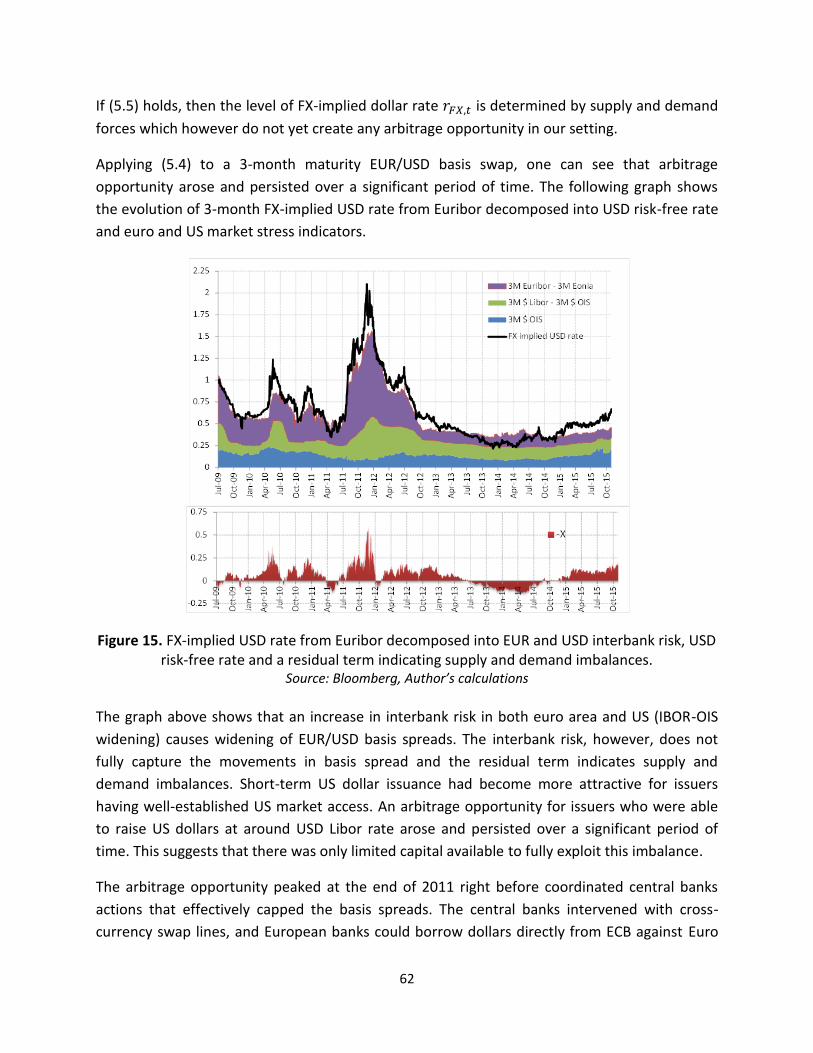
62
If (5.5) holds, then the level of FX-implied dollar rate is determined by supply and demand
forces which however do not yet create any arbitrage opportunity in our setting.
Applying (5.4) to a 3-month maturity EUR/USD basis swap, one can see that arbitrage
opportunity arose and persisted over a significant period of time. The following graph shows
the evolution of 3-month FX-implied USD rate from Euribor decomposed into USD risk-free rate
and euro and US market stress indicators.
Figure 15. FX-implied USD rate from Euribor decomposed into EUR and USD interbank risk, USD risk-free rate and a residual term indicating supply and demand imbalances.
Source: Bloomberg, Author’s calculations
The graph above shows that an increase in interbank risk in both euro area and US (IBOR-OIS
widening) causes widening of EUR/USD basis spreads. The interbank risk, however, does not
fully capture the movements in basis spread and the residual term indicates supply and
demand imbalances. Short-term US dollar issuance had become more attractive for issuers
having well-established US market access. An arbitrage opportunity for issuers who were able
to raise US dollars at around USD Libor rate arose and persisted over a significant period of
time. This suggests that there was only limited capital available to fully exploit this imbalance.
The arbitrage opportunity peaked at the end of 2011 right before coordinated central banks
actions that effectively capped the basis spreads. The central banks intervened with cross-
currency swap lines, and European banks could borrow dollars directly from ECB against Euro
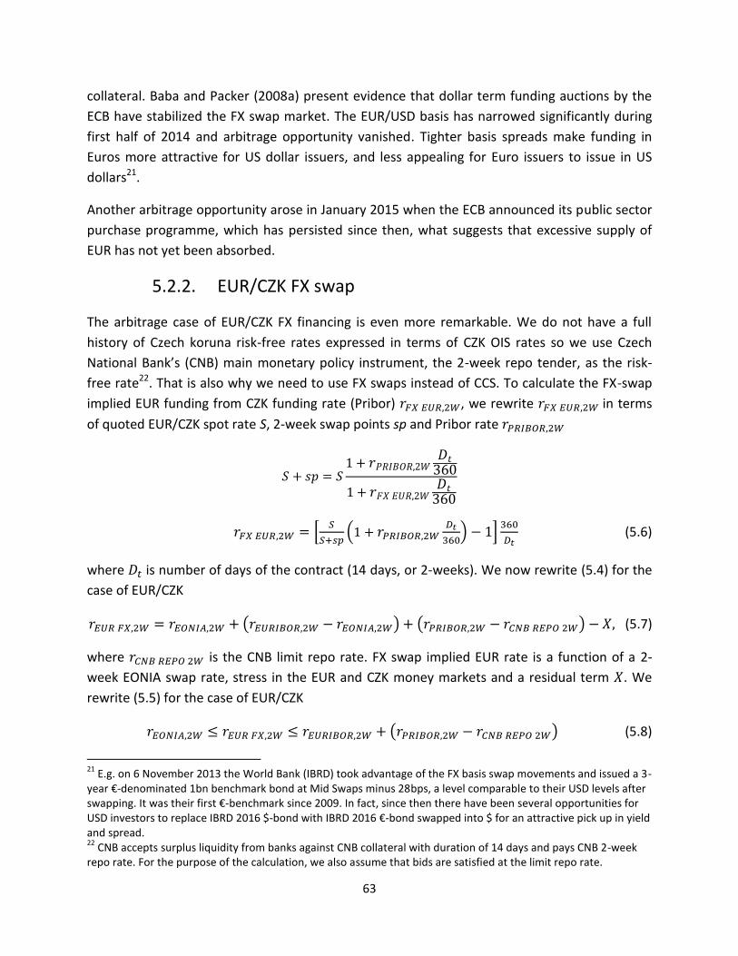
63
collateral. Baba and Packer (2008a) present evidence that dollar term funding auctions by the
ECB have stabilized the FX swap market. The EUR/USD basis has narrowed significantly during
first half of 2014 and arbitrage opportunity vanished. Tighter basis spreads make funding in
Euros more attractive for US dollar issuers, and less appealing for Euro issuers to issue in US
dollars21.
Another arbitrage opportunity arose in January 2015 when the ECB announced its public sector
purchase programme, which has persisted since then, what suggests that excessive supply of
EUR has not yet been absorbed.
5.2.2. EUR/CZK FX swap
The arbitrage case of EUR/CZK FX financing is even more remarkable. We do not have a full
history of Czech koruna risk-free rates expressed in terms of CZK OIS rates so we use Czech
National Bank’s (CNB) main monetary policy instrument, the 2-week repo tender, as the risk-
free rate22. That is also why we need to use FX swaps instead of CCS. To calculate the FX-swap
implied EUR funding from CZK funding rate (Pribor) , we rewrite in terms
of quoted EUR/CZK spot rate S, 2-week swap points sp and Pribor rate
[
(
) ]
(5.6)
where is number of days of the contract (14 days, or 2-weeks). We now rewrite (5.4) for the
case of EUR/CZK
( ) ( ) (5.7)
where is the CNB limit repo rate. FX swap implied EUR rate is a function of a 2-
week EONIA swap rate, stress in the EUR and CZK money markets and a residual term . We
rewrite (5.5) for the case of EUR/CZK
( ) (5.8)
21
E.g. on 6 November 2013 the World Bank (IBRD) took advantage of the FX basis swap movements and issued a 3-year €-denominated 1bn benchmark bond at Mid Swaps minus 28bps, a level comparable to their USD levels after swapping. It was their first €-benchmark since 2009. In fact, since then there have been several opportunities for USD investors to replace IBRD 2016 $-bond with IBRD 2016 €-bond swapped into $ for an attractive pick up in yield and spread. 22
CNB accepts surplus liquidity from banks against CNB collateral with duration of 14 days and pays CNB 2-week repo rate. For the purpose of the calculation, we also assume that bids are satisfied at the limit repo rate.
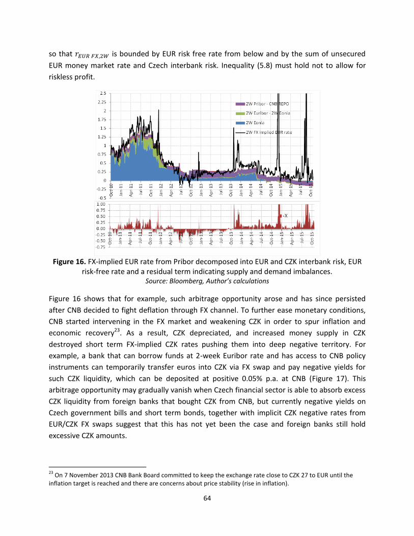
64
so that is bounded by EUR risk free rate from below and by the sum of unsecured
EUR money market rate and Czech interbank risk. Inequality (5.8) must hold not to allow for
riskless profit.
Figure 16. FX-implied EUR rate from Pribor decomposed into EUR and CZK interbank risk, EUR
risk-free rate and a residual term indicating supply and demand imbalances. Source: Bloomberg, Author’s calculations
Figure 16 shows that for example, such arbitrage opportunity arose and has since persisted
after CNB decided to fight deflation through FX channel. To further ease monetary conditions,
CNB started intervening in the FX market and weakening CZK in order to spur inflation and
economic recovery23. As a result, CZK depreciated, and increased money supply in CZK
destroyed short term FX-implied CZK rates pushing them into deep negative territory. For
example, a bank that can borrow funds at 2-week Euribor rate and has access to CNB policy
instruments can temporarily transfer euros into CZK via FX swap and pay negative yields for
such CZK liquidity, which can be deposited at positive 0.05% p.a. at CNB (Figure 17). This
arbitrage opportunity may gradually vanish when Czech financial sector is able to absorb excess
CZK liquidity from foreign banks that bought CZK from CNB, but currently negative yields on
Czech government bills and short term bonds, together with implicit CZK negative rates from
EUR/CZK FX swaps suggest that this has not yet been the case and foreign banks still hold
excessive CZK amounts.
23
On 7 November 2013 CNB Bank Board committed to keep the exchange rate close to CZK 27 to EUR until the inflation target is reached and there are concerns about price stability (rise in inflation).
65
Figure 17. 2-week FX-implied CZK rate from Euribor, 2-week Pribor rate and CNB repo rate.
Source: Bloomberg
Similar analysis can be easily replicated choosing different maturity (e.g. 3-months) and
different CZK risk-free rate (e.g. 3-month government T-bill). However, in that case, one could
rather focus on specific instrument and maturity due to historical availability of data. In
practice, one has to account for bid-offer spreads and as we have seen IBOR rates are different
to real borrowing rates of individual banks, however, there is no loss of generality in equations
(5.6)-(5.8) and they can be easily applied to other cases and tenors.
To conclude, this chapter discussed factors that influence cross-currency basis swap spreads, in
particular, credit and liquidity risks and supply and demand pressures. We have discussed that
basis spreads in the short-end of the curve are more influenced by IBOR fixing and
credit/liquidity premium while the long-end is more a function of supply and demand. We built
regression models for changes in 3-month and 5-year EUR/USD basis swap spread that
explained 50% and 30% of the variance of weekly spread changes. The model confirmed, for
example, that increased credit risk in European banks widens the EUR/USD basis spread. But
interbank risk only does not fully capture the level of basis spreads. The residual term may be
partially assigned to supply and demand imbalances that may arise and persist over a longer
period of time. In the case of EUR/CZK, we have shown that recent FX-intervention distorted
Czech money market that has not yet been able to absorb excessive CZK money supply.
66
6. Valuation of Zero-coupon Inflation Swaps
The market for inflation linked products has grown significantly in recent years. Government
issuers have been the main driver behind the growth of inflation-linked (I/L) bond markets. I/L
bonds offer investor protection of purchasing power as their coupons and principal payments
are linked to changes in price indices. Inflation derivatives have been developed together with
I/L bonds and are used to manage inflation risk.
In this chapter we describe main elements of zero-coupon inflation linked swaps including their
use, their mechanics, and their pricing. The aim of this chapter is similar; to present a consistent
valuation approach to zero-coupon inflation swaps that properly reflects the risk of its cash-
flows however we provide a general overview on functioning of inflation markets as well. We
first provide a brief review of relevant studies on inflation market. Then we offer an insight into
the inflation market, its main participants, inflation measurement, and breakeven inflation
rates. We also discuss the real yield of inflation-linked bond (“linkers”) versus the nominal yield
of the traditional bond. Then we touch on mechanics of zero-coupon inflation swap and present
a consistent approach to its valuation. This approach is further illustrated using OIS discounting
for the case of zero-coupon inflation swap collateralized with cash.
From a number of studies that analyse inflation markets we refer to the ones that focus on
market liquidity of inflation swaps, price discovery of breakeven inflation, and relationship
between nominal yields, real yields, or inflation expectations.
Fleming and Sporn (2013) study trading activity and pricing transparency of zero-coupon
inflation swap trades in the US. They find that despite low trading volumes and number of
trades and their OTC nature, the market is reasonably transparent and liquid, in particular, the
traded prices of the sample were close to end-of-day quoted prices and that customer buy and
sell prices essentially matched bid-ask spreads quoted by the dealers.
Schulz and Stapf (2011) analyse price discovery for breakeven inflation rate using high
frequency data in the US and the euro area and concluded that during crisis price formation
was concentrated mostly in government bonds (due to their liquidity and low credit risk). In
general, for maturities up to 5 years, price discovery comes from both swap and bond market,
for longer maturities bond markets dominate.
Haubrich et al. (2012) introduce a model to analyse term structure of nominal, real, and
inflation rates from inflation swaps, government bonds, and government inflation linked bonds
67
(TIPS) in the US and found that TIPS were underpriced in their early years and then during the
period of recent financial crisis.
Bauer (2014) shows that changes in inflation expectations alone or when caused by macro data
surprises explain a sizable share of changes in nominal rates.
Regarding pricing of inflation linked derivatives, Mercurio (2005) derives analytical formulas for
inflation indexed swaps and caps using FX analogy and looking at real rates as nominal rates in
foreign economy and at CPI as an exchange rate between nominal and real rates.
On the other hand, there are not many recent papers focusing on valuation of inflation
derivatives that take into account the risk of the derivative, which affects the choice of discount
rates. In Section 2, we present such valuation approach for zero-coupon inflation swap and
discuss the proper choice for discounting curves based on the risk of the trade and the way this
risk is mitigated. We then illustrate this on the example of using OIS discounting for zero-
coupon inflation swap collateralized with cash.
6.1. Inflation Market
The inflation bond market started in the UK with the first inflation-linked (I/L) Gilt in 1981.
However, the global market started to develop after the US Treasury began issuing TIPS
(Treasury Inflation Protected Securities) in 1997. France issued the first bond linked to French
inflation in 1998. In 2001, France started issuing government bonds linked to European inflation
(Euro HICP), and took advantage of a liquid market with wider investor base. Italy, Greece, and
Germany soon followed and many other sovereigns have since been able to develop inflation-
linked securities in their local markets. Most of the issuance has been however concentrated in
the US, UK and France.
Main issuers of I/L securities are governments and government agencies. Governments have
partly natural needs to issue I/L bonds since tax revenues are linked to inflation. Issuing I/L
bonds is also convenient for governments as it allows to increase the duration of their debt
portfolio.
The growth and turnover of the I/L market has increased supported by overall lower levels of
inflation and inflation targeting as the primary monetary policy objective, and availability of
statistical inflation data. In the emerging markets, growth expectations also increased the
demand for inflation-linked bonds.
68
Inflation derivatives have been developed together with I/L bonds. In general, market
participants use inflation derivatives or I/L bonds to manage their assets and liabilities for
inflation exposure. Inflation products are thus used to transfer inflation risk of assets or
liabilities. Investors also buy I/L bonds to diversify their investments and issuers issue I/L bonds
to diversify their funding sources (and expand their investor base), or to exploit relative value
opportunities.
As previously mentioned, governments are the main I/L issuers and inflation payers. From
private sector, inflation sellers include companies with revenues linked to infrastructure
projects. For example, real estate investors may hedge inflation risk of rental revenues where
rents are indexed to inflation. On the other side, receiving inflation protects investors’ real
return. Pension funds and insurance companies use inflation derivatives or I/L bonds to hedge
those pensions that are linked to inflation. Banks are buyers of inflation-linked government
bonds in general when they asset swap it against LIBOR rates that measure their short term
funding costs. Further, banks may want to receive inflation to hedge their I/L retail products.
Asset managers buy inflation for those funds that are inflation-benchmarked.
6.1.1. Measuring Inflation
Consumer Price Index (CPI) is used as a standard measure of inflation. It is defined and
calculated by statistical agencies, and it measures the cost of a basket of consumer goods and
services in nominal prices. It is often calculated once a month and published around two weeks
later.
The inflation rate between time and T is measured as the change in the CPI index
where is the price of the basket at time T, and is the price of the basket at time
. Annual inflation rate is considered as the most common reference for inflation. It is
measured by the change in the CPI over 12 months
69
Euro HICP Index
Different inflation indices in different countries may give distorted picture about inflation rates
among countries. To measure inflation consistently, same methodology or index definition
should be applied, such as Harmonized Index of Consumer Prices (HICP), which makes it
possible to compare rates of inflation across European countries. Eurostat calculates the Euro-
area inflation rate as a weighted average of national indices (excluding tobacco) of all countries
in the Eurozone and publishes Euro HICP flash estimate usually on the last working day of the
reference month and revised data approximately 18 days later (see Eurostat (2015)). Euro HICP
Index is used as the reference index for European I/L bonds and the European Central Bank
uses HICPs as the reference measure of inflation in the Euro-area countries.
6.1.2. Inflation-Linked Bond
The purpose of a bond linked to inflation index is to preserve the value of money and the
purchasing power for investor. It guarantees an investor a real return as both the notional of
the bond and coupons rise with inflation. In year T, the notional and the coupon equal to
, where is the original bond notional.
, where is the real coupon.
The real coupon is usually set lower than a coupon of a conventional bond if positive inflation is
expected. In this case, the inflation-linked bond pays lower coupons during bond’s life but the
redemption value at maturity is higher (adjusted for positive inflation). Therefore, the duration
of I/L bond is also longer. However, the duration of a linker represents the relationship of a
price change to change in real yield, while the duration of the traditional bond takes the
nominal yield into account. Therefore, the duration of a linker cannot be directly compared to
the duration of the traditional bond.
The yield of a linker is quoted on a real basis; it is calculated from real coupons and notional
without adjusting for inflation expectations. To make the real yields of a linker comparable with
nominal yield of a traditional bond, inflation expectations must be added to the real yield.
In case of a zero-coupon inflation-linked bond, which has a single payment at maturity T, the
nominal present value of such bonds includes inflation expectation and is different from
nominal present value of standard zero-coupon bond
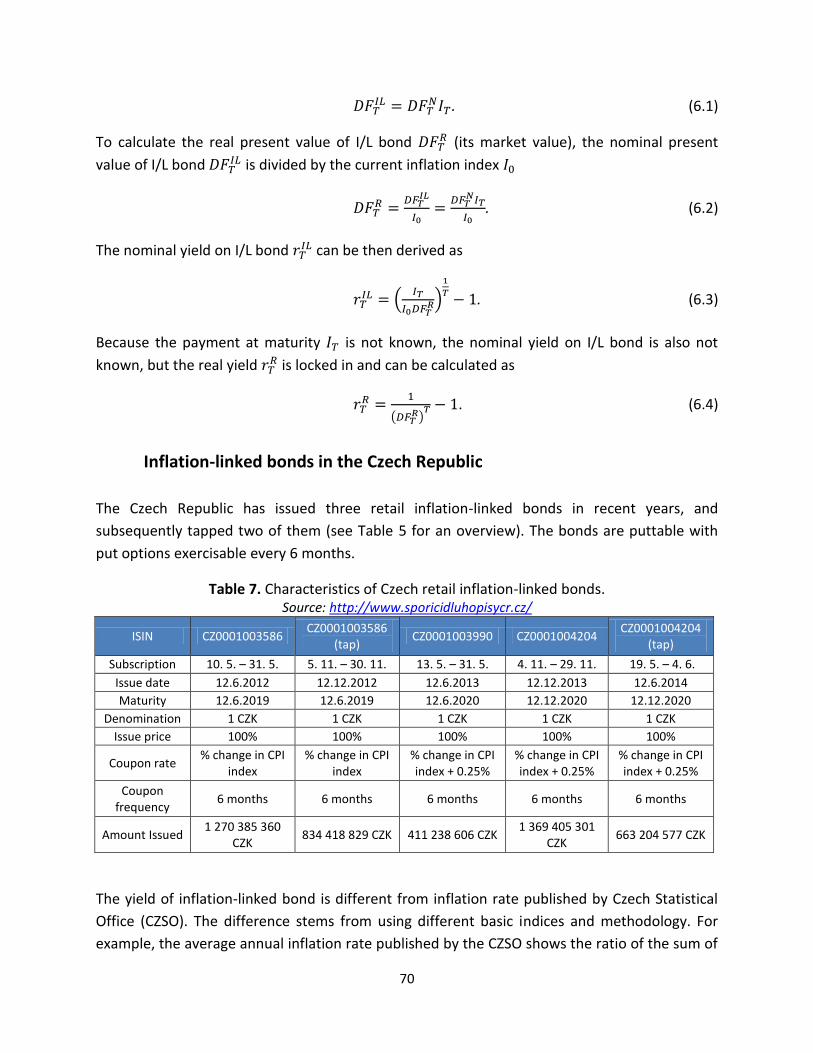
70
. (6.1)
To calculate the real present value of I/L bond (its market value), the nominal present
value of I/L bond is divided by the current inflation index
. (6.2)
The nominal yield on I/L bond can be then derived as
(
)
. (6.3)
Because the payment at maturity is not known, the nominal yield on I/L bond is also not
known, but the real yield is locked in and can be calculated as
( )
. (6.4)
Inflation-linked bonds in the Czech Republic
The Czech Republic has issued three retail inflation-linked bonds in recent years, and
subsequently tapped two of them (see Table 5 for an overview). The bonds are puttable with
put options exercisable every 6 months.
Table 7. Characteristics of Czech retail inflation-linked bonds. Source: http://www.sporicidluhopisycr.cz/
ISIN CZ0001003586 CZ0001003586
(tap) CZ0001003990 CZ0001004204
CZ0001004204 (tap)
Subscription period
10. 5. – 31. 5. 2012
5. 11. – 30. 11. 2012
13. 5. – 31. 5. 2013
4. 11. – 29. 11. 2013
19. 5. – 4. 6. 2014 Issue date 12.6.2012 12.12.2012 12.6.2013 12.12.2013 12.6.2014
Maturity 12.6.2019 12.6.2019 12.6.2020 12.12.2020 12.12.2020
Denomination 1 CZK 1 CZK 1 CZK 1 CZK 1 CZK
Issue price 100% 100% 100% 100% 100%
Coupon rate % change in CPI
index % change in CPI
index % change in CPI index + 0.25%
% change in CPI index + 0.25%
% change in CPI index + 0.25%
Coupon frequency
6 months 6 months 6 months 6 months 6 months
Amount Issued 1 270 385 360
CZK 834 418 829 CZK 411 238 606 CZK
1 369 405 301 CZK
663 204 577 CZK
The yield of inflation-linked bond is different from inflation rate published by Czech Statistical
Office (CZSO). The difference stems from using different basic indices and methodology. For
example, the average annual inflation rate published by the CZSO shows the ratio of the sum of
71
the last 12 months CPI values over the sum of the previous 12 months (12 month moving
average). Year-on-year (yoy) inflation rate is the yearly percentage change in CPI levels
calculated as a ratio of last month’s CPI level to the CPI level of the corresponding month in the
previous year while month-on-month (mom) inflation rate compares the change in last month’s
CPI level to the preceding month, see CZSO (2015).
Both measures are however different from the yield of inflation-linked bond. The bond pays a
six month coupon, however, the coupon rate is not calculated as the average 6-month inflation
rate, but rather as the percentage change in CPI level of the current month and the CPI level six
months back. The current month is lagged by two months from the month of the coupon
payment date. The coupon is further floored at zero to protect investor from deflation. Because
the coupon is not paid but reinvested, the coupon rate is higher or equal than the yoy inflation
rate (higher in case of deflation) and the buyer is thus protected from inflation.
6.1.3. Breakeven inflation rate
The breakeven inflation rate is used to compare yields of inflation-linked and traditional bonds;
it is the average annual inflation rate that needs to be realized to make the yields of the
traditional bond and the inflation-linked bond equal. It is calculated by making the present
value of cash flows of the linker discounted with the yield of the traditional bond equal to the
price of the linker. If the breakeven inflation rate is lower than expected inflation rate, then
investor would buy the inflation-linked bond.
To assess breakeven inflation rate, it is also possible to use a simpler Fisher equation that shows
the relationship between nominal yield and real yield
( ) (
) ( )
(
)
( ) , (6.5)
or its first approximation
.
The breakeven inflation b rate can be thus approximated as the difference between the
nominal yield of the traditional bond and the real yield of inflation-linked bond
. If we
ignore credit and liquidity risk premium of the inflation-linked bond, and the compounding
effect linked to inflation-linked bonds, then the breakeven inflation is the market expected
inflation over I/L bond’s life.
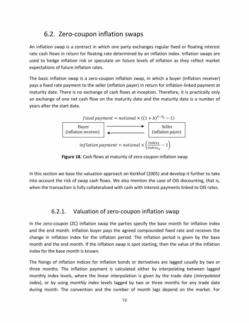
72
6.2. Zero-coupon inflation swaps
An inflation swap is a contract in which one party exchanges regular fixed or floating interest
rate cash flows in return for floating rate determined by an inflation index. Inflation swaps are
used to hedge inflation risk or speculate on future levels of inflation as they reflect market
expectations of future inflation rates.
The basic inflation swap is a zero-coupon inflation swap, in which a buyer (inflation receiver)
pays a fixed rate payment to the seller (inflation payer) in return for inflation-linked payment at
maturity date. There is no exchange of cash flows at inception. Therefore, it is practically only
an exchange of one net cash flow on the maturity date and the maturity date is a number of
years after the start date.
Figure 18. Cash flows at maturity of zero-coupon inflation swap
In this section we base the valuation approach on Kerkhof (2005) and develop it further to take
into account the risk of swap cash flows. We also mention the case of OIS discounting, that is,
when the transaction is fully collateralized with cash with interest payments linked to OIS rates.
6.2.1. Valuation of zero-coupon inflation swap
In the zero-coupon (ZC) inflation swap the parties specify the base month for inflation index
and the end month. Inflation buyer pays the agreed compounded fixed rate and receives the
change in inflation index for the inflation period. The inflation period is given by the base
month and the end month. If the inflation swap is spot starting, then the value of the inflation
index for the base month is known.
The fixings of inflation indices for inflation bonds or derivatives are lagged usually by two or
three months. The inflation payment is calculated either by interpolating between lagged
monthly index levels, where the linear interpolation is given by the trade date (interpolated
index), or by using monthly index levels lagged by two or three months for any trade date
during month. The convention and the number of month lags depend on the market. For
Buyer
(inflation receiver)
Seller
(inflation payer)
(( ) )
(
)
73
example, if the inflation index is the European HICP index with base month being three months
before the trade date, then the value of such index for the base month is published around two
months before the trade date, and is therefore known at the trade date. At maturity, value of
the index for the end month would be known as well). If the index value for the base month is
not known, then it is forward starting inflation swap.
For spot starting ZC inflation swap, the index for the base month is known while
the index for the end month is the only unknown. The breakeven inflation rate b is
the quoted fixed rate in the market.
As for any interest rate swap, at inception, the present value of the fixed leg must equal the
present value of the inflation leg
( ) ( )
The present value of the fixed leg is the discounted compounded fixed rate
( ) (( ) ). (6.6)
The present value of the inflation leg is the value of the change in inflation index for the period
. From (6.2) we have
; therefore
( ) (
)
, (6.7)
where is the nominal discount factor. The present value of both legs thus depends on
discount factors . When calculating
, proper discounting method needs to be chosen
to take into account the risk of the cash flows. The traditional approach used swap rates (with
floating rates linked to LIBOR) to construct the discount curve, but this approach is not
arbitrage free given the presence of credit and liquidity risks. The value of the transaction
depends on the risk of the transaction and the way this risk is mitigated during the life of the
trade. The traditional approach has been further developed by the market to take into account
the risk of default of the counterparty, the risk of one’s own default, or the interest paid on the
collateral as discussed in previous chapters.
To illustrate how discounting affects the valuation of zero-coupon inflation swap, we consider
the case of cash collateralized swap (we assume that the swap is fully collateralized with cash
which pays the interest rate equal to overnight index average rate and that the OIS market
exists for all maturities). Then is bootstrapped from the overnight indexed swap (OIS)
rates as in (3.11)
∑
, (6.8)
74
where is the OIS swap rate for period and is the year fraction between t-1 and t. As
discussed in previous chapters, OIS discounting has recently become a market standard for
valuation of cash collateralized derivatives.
The only unknown in (6.7) thus remains the real discount factor . Because PVs of both swap
legs are equal, can be easily derived as
( ) (6.9)
6.2.2. Construction of zero coupon inflation swap curve
To value existing swap we need an inflation curve, i.e. the breakeven reference rates not only
for years, but for all months in between years. An inflation curve is constructed from market
prices of zero-coupon inflation swaps combined with seasonality adjustments. Quotes of annual
zero-coupon inflation swaps provide market projections of CPI increase over the term of the
swap (projected future CPI fixings). From projected CPI fixings, one can interpolate between
two values to calculate annual trend in inflation. A linear, cubic or other interpolation method
can be used. Because of seasonal behaviour of CPI indices it is not possible to assume that CPI
indices grow constantly; therefore the interpolation has to be finally adjusted for seasonality.
Projected CPI index for the index reference date T years after starting reference date
( ) is calculated as
( ) (6.10)
where is the quoted zero-coupon swap fixed rate with maturity T years (T years breakeven
rate) and is CPI index value for the start date. Choosing linear interpolation between
and we obtain the annual inflation rate trend (growth rate in
breakeven rate) as
(
) (6.11)
A common approach is to use continuously compounded forward inflation rate. The annual
trend in fact determines yearly forward inflation rates unadjusted for seasonality. Projected CPI
for date T years and m months after the start date and before seasonal adjustment can be then
calculated as
(
)
(6.12)
75
Finally, we need to incorporate monthly seasonality to get seasonally adjusted projected CPIs
values by adding a seasonal component to annual trend
(
)
∑ (6.13)
where is monthly seasonal component for i-th month after start month24. The sum of
seasonal adjustment components should equal to zero so they do not affect quoted swap rates.
Further, it is often assumed that seasonality is a set of 12 monthly seasonal components that
remain constant over time.
Seasonality of inflation
Seasonality and volatility of inflation can largely affect the inflation trend and often depends on
commodity prices (food and energy prices) or changes in fiscal policy (i.e. tax changes).
Seasonality in prices of inflation-linked bonds and swaps is in general not accounted for when
looking at breakeven rates (inflation products are linked to price indices that are unadjusted for
seasonality). Seasonal adjustment is therefore necessary to uncover the trend in inflation rates
outside standard yearly maturity dates. Seasonality can be measured either by statistical
methods (for example by using autoregressive moving average models, typically X-12 ARIMA25)
or can be derived from market prices of inflation swaps with different expiry dates.
Building Euro HICPx curve
As an example, we build an inflation curve for the euro-area for maturities up to 30 years as of
trade date April 27, 2015. Euro zero coupon inflation swap rates are exchanged against change
in Eurozone HICP excluding tobacco unrevised index subject to a 3-month lag (payoff at
maturity of such swap is displayed in Figure 18). Unrevised numbers are the ones initially
released by Eurostat, see Eurostat (2015). Published HICP indices are not seasonally adjusted.
For illustration purposes, we extract monthly seasonal adjustment from the ECB calculations of
seasonally adjusted HICPs ex tobacco26 for the last 12 months (April 2014 – March 2015) using
(6.13) (for ECB seasonal adjustment methodology we refer to ECB (2000)). We can see that in
January and February prices are lower than inflation trend, while from March to June prices
appear higher (Table 7). For simplicity, we assume that this monthly seasonality remains
constant over time.
24
If the seasonal component is annual then it needs to be divided by 12. 25
X-12 ARIMA and newer X-13 ARIMA-SEATS is software for seasonal adjustment produced by US Census Bureau: https://www.census.gov/srd/www/x13as/ 26
The ECB produces seasonally adjusted HICP ex tobacco: http://sdw.ecb.europa.eu/browseSelection.do?ADJUSTMENT=S&node=2120778&DATASET=0&SERIES_KEY=122.ICP.M.U2.S.X02200.3.INX
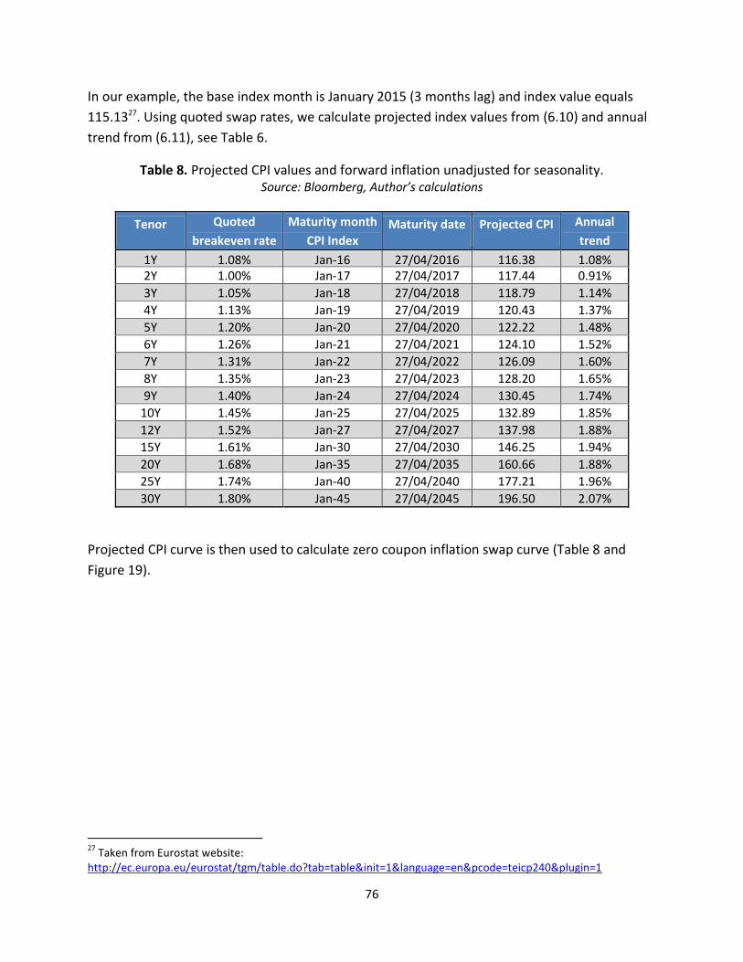
76
In our example, the base index month is January 2015 (3 months lag) and index value equals
115.1327. Using quoted swap rates, we calculate projected index values from (6.10) and annual
trend from (6.11), see Table 6.
Table 8. Projected CPI values and forward inflation unadjusted for seasonality. Source: Bloomberg, Author’s calculations
Tenor Quoted
breakeven rate
Maturity month
CPI Index Maturity date Projected CPI Annual
trend
1Y 1.08% Jan-16 27/04/2016 116.38 1.08% 2Y 1.00% Jan-17 27/04/2017 117.44 0.91%
3Y 1.05% Jan-18 27/04/2018 118.79 1.14%
4Y 1.13% Jan-19 27/04/2019 120.43 1.37%
5Y 1.20% Jan-20 27/04/2020 122.22 1.48%
6Y 1.26% Jan-21 27/04/2021 124.10 1.52%
7Y 1.31% Jan-22 27/04/2022 126.09 1.60%
8Y 1.35% Jan-23 27/04/2023 128.20 1.65%
9Y 1.40% Jan-24 27/04/2024 130.45 1.74%
10Y 1.45% Jan-25 27/04/2025 132.89 1.85%
12Y 1.52% Jan-27 27/04/2027 137.98 1.88%
15Y 1.61% Jan-30 27/04/2030 146.25 1.94%
20Y 1.68% Jan-35 27/04/2035 160.66 1.88%
25Y 1.74% Jan-40 27/04/2040 177.21 1.96%
30Y 1.80% Jan-45 27/04/2045 196.50 2.07%
Projected CPI curve is then used to calculate zero coupon inflation swap curve (Table 8 and
Figure 19).
27
Taken from Eurostat website: http://ec.europa.eu/eurostat/tgm/table.do?tab=table&init=1&language=en&pcode=teicp240&plugin=1
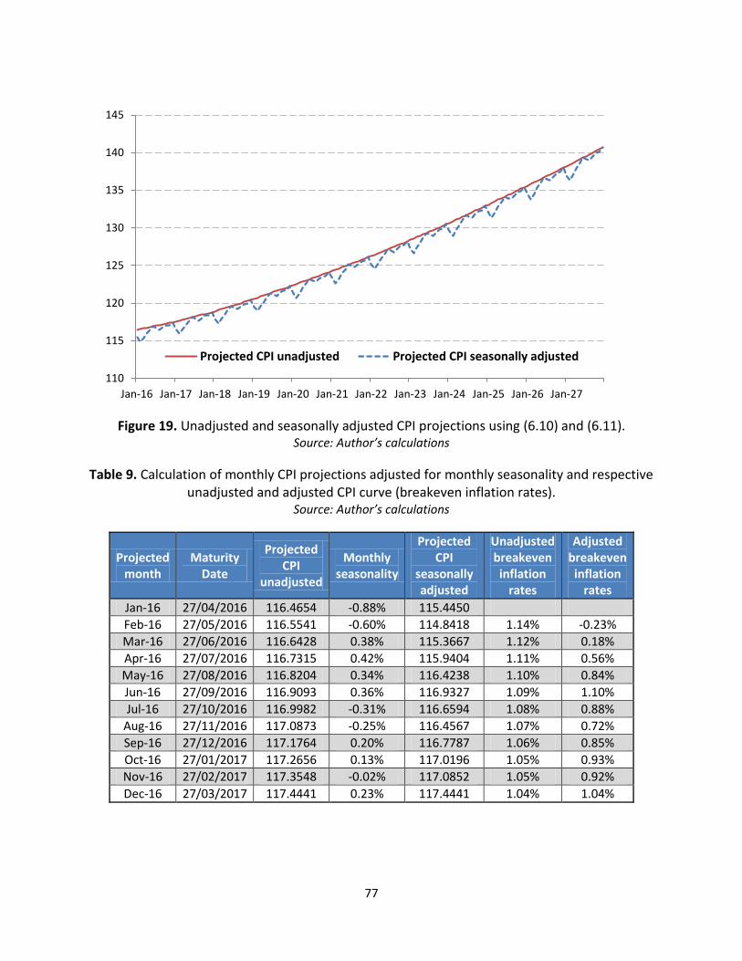
77
Figure 19. Unadjusted and seasonally adjusted CPI projections using (6.10) and (6.11). Source: Author’s calculations
Table 9. Calculation of monthly CPI projections adjusted for monthly seasonality and respective unadjusted and adjusted CPI curve (breakeven inflation rates).
Source: Author’s calculations
Projected month
Maturity Date
Projected CPI
unadjusted
Monthly seasonality
Projected CPI
seasonally adjusted
Unadjusted breakeven inflation
rates
Adjusted breakeven inflation
rates
Jan-16 27/04/2016 116.4654 -0.88% 115.4450
Feb-16 27/05/2016 116.5541 -0.60% 114.8418 1.14% -0.23%
Mar-16 27/06/2016 116.6428 0.38% 115.3667 1.12% 0.18%
Apr-16 27/07/2016 116.7315 0.42% 115.9404 1.11% 0.56%
May-16 27/08/2016 116.8204 0.34% 116.4238 1.10% 0.84%
Jun-16 27/09/2016 116.9093 0.36% 116.9327 1.09% 1.10%
Jul-16 27/10/2016 116.9982 -0.31% 116.6594 1.08% 0.88%
Aug-16 27/11/2016 117.0873 -0.25% 116.4567 1.07% 0.72%
Sep-16 27/12/2016 117.1764 0.20% 116.7787 1.06% 0.85%
Oct-16 27/01/2017 117.2656 0.13% 117.0196 1.05% 0.93%
Nov-16 27/02/2017 117.3548 -0.02% 117.0852 1.05% 0.92%
Dec-16 27/03/2017 117.4441 0.23% 117.4441 1.04% 1.04%
110
115
120
125
130
135
140
145
Jan-16 Jan-17 Jan-18 Jan-19 Jan-20 Jan-21 Jan-22 Jan-23 Jan-24 Jan-25 Jan-26 Jan-27
Projected CPI unadjusted Projected CPI seasonally adjusted
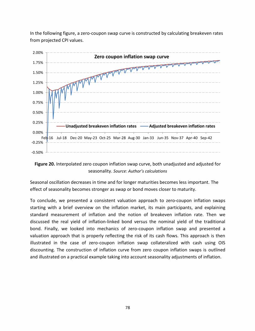
78
In the following figure, a zero-coupon swap curve is constructed by calculating breakeven rates
from projected CPI values.
Figure 20. Interpolated zero coupon inflation swap curve, both unadjusted and adjusted for
seasonality. Source: Author’s calculations
Seasonal oscillation decreases in time and for longer maturities becomes less important. The
effect of seasonality becomes stronger as swap or bond moves closer to maturity.
To conclude, we presented a consistent valuation approach to zero-coupon inflation swaps
starting with a brief overview on the inflation market, its main participants, and explaining
standard measurement of inflation and the notion of breakeven inflation rate. Then we
discussed the real yield of inflation-linked bond versus the nominal yield of the traditional
bond. Finally, we looked into mechanics of zero-coupon inflation swap and presented a
valuation approach that is properly reflecting the risk of its cash flows. This approach is then
illustrated in the case of zero-coupon inflation swap collateralized with cash using OIS
discounting. The construction of inflation curve from zero coupon inflation swaps is outlined
and illustrated on a practical example taking into account seasonality adjustments of inflation.
-0.50%
-0.25%
0.00%
0.25%
0.50%
0.75%
1.00%
1.25%
1.50%
1.75%
2.00%
Feb-16 Jul-18 Dec-20 May-23 Oct-25 Mar-28 Aug-30 Jan-33 Jun-35 Nov-37 Apr-40 Sep-42
Zero coupon inflation swap curve
Unadjusted breakeven inflation rates Adjusted breakeven inflation rates
79
Conclusion
Interbank rates are not risk-free and neither are IBOR swap rates. The market has moved from
discounting on IBOR swap rates to discounting on OIS rates and reflecting all economic costs of
derivatives on top of OIS rates. OIS rates are generally considered as a good proxy for risk-free
rates and their use is further justified by the fact that the interest rate paid on collateral is
linked to OIS rate. Basis spreads in basis swaps or cross-currency basis swaps are here to stay;
they impact the valuation and the discount factors and must be therefore part of the valuation
equation. One curve can no longer be used to estimate forward rates and to discount future
cash flows. In fact, changing the discount curve means changing the market value of a
derivative. These are some of the general outcomes of the thesis. Others are more specific.
We discussed recently introduced valuation adjustments to derivatives that are needed to
reflect both risk and costs of the transaction. Specifically, we showed how credit valuation
adjustment (CVA), debit valuation adjustment (DVA), funding valuation adjustment (FVA),
capital valuation adjustment (KVA), and initial margin valuation adjustment (MVA) step into the
risk-neutral valuation of derivatives.
Then we focused on derivatives’ discounting in detail. We derived discount factors and forward
rates that are consistent with market prices and showed how basis swap spreads impact the
valuation. We discussed in detail valuation of interest rate swaps, basis swaps and cross-
currency swaps and showed why multiple curves need to be used to estimate forward rates and
to discount future cash flows. In the last section we derived the approximation for discount
curves implied from cross-currency market quotes and the discount curve of the base currency.
We also decomposed basis spread into individual elements. We saw that CCS basis spread can
be decomposed into basis spread that reflects credit and liquidity risk between the two
currencies and an OIS basis spread reflecting demand and supply of one currency vs. another
one. We used this decomposition to analyse basis spread, in particular, for the Czech
derivatives’ market in chapter 4.
We moved on to apply several of the findings on Czech derivatives market. We proposed an
estimation of CZK OIS curve when not all OIS quotes are available. Interestingly, when we first
investigated this topic, CZK OIS quotes have been only available up to one year and have only
recently started to be quoted for maturities up to ten years. We assume there became a
structural need for banks to pay and receive CZK OIS rates linked to CZK cash collateral earning
CZEONIA rate. We also analysed EUR/CZK cross-currency basis swap spreads by decomposing
them into individual components to find out that although the risk premium in CZK rates is
higher than in EUR, the increased supply of CZK and higher demand for EUR via FX swap market
80
is pushing synthetic CZK rates into negative territory and it is the main factor that contributes to
significantly negative EUR/CZK basis swap spreads. In the very long end (above 12 years) the
main contribution to negative basis spread becomes the liquidity and credit risk premium of
CZK rates. We also showed such breakdown can be used to approximate implied discount rates
of the second leg of the cross-currency swap and may help optimize collateral posting for the
counterparty that is out of the money.
We continued to analyse cross-currency basis spreads, this time, from a different angle. We
discussed what is driving the credit and liquidity risk and supply and demand pressure of one
currency versus another one. We built regression models for changes in 3-month and 5-year
EUR/USD basis swap spread that explained 50% and 30% of the variance of weekly spread
changes. The model confirmed, for example, that increased credit risk in European banks
widens the EUR/USD basis spread. We then tested arbitrage-free boundaries for cross-currency
funding and investing and identified several periods of arbitrage opportunities in cases of
EUR/USD and EUR/CZK markets where for market participants able to raise unsecured funding
in one currency and swapping it into another currency.
Finally, we focused inflation derivatives. We provided an overview of inflation markets and
discussed inflation measurement, real yields, nominal yields, and the construction of inflation
curve from zero coupon inflation swaps taking into account inflation seasonality. We also
presented consistent valuation approach to zero-coupon inflation swaps reflecting the risk of its
future cash-flows.
Understanding risk premiums in derivatives rates and pricing is helpful for decision making
when acting in the market. The perception of risk and risk premium has changed over time.
Although OIS rates have been generally accepted risk-free rate proxies and have replaced IBOR
rates for derivatives’ discounting (and they also reflect the interest rate paid on collateral), the
new discounting poses a number of challenges. For example, we saw that the choice of
collateral impacts market price, be it bond or cash, in one currency or another. OIS discounting
is complicated because CSA annexes may be very different from one to another and often allow
counterparties to post a number of different assets as collateral. They further have different
threshold, margins, or minimum transfer amounts. This optionality impacts the pricing as well
and banks generally opt to discount by the cheapest to deliver collateral. But this needs to be
monitored because market factors change and so can the cheapest to deliver asset. More
standardized CSA would certainly help28 and regulators seem to be setting up rules to make
28
In fact, ISDA published Standard CSA in June 2013 aimed at standardizing market practice in collateral management by removing optionality and promotes OIS (http://www2.isda.org/news/isda-publishes-2013-standard-credit-support-annex-scsa). Due to new regulatory changes (for example, Basel rules on margining as mentioned in Chapter 2), ISDA is now working on amendments to the Standard CSA.
81
central clearing of derivatives attractive also for those derivatives for which clearing will not be
mandatory.
There also seems to be ambiguity in using and pricing different valuation adjustments. Some of
them, e.g. MVA also raise computational challenges as their calculations may need a
considerable amount of time. Although we have focused on valuation only, introducing
valuation adjustment into practice is not only pricing it. It creates additional challenges for
other departments such as risk management, reporting, or accounting. Discounting of
derivatives has changed from a simple and straightforward task to sometimes impractically
complex even for seemingly simple linear derivatives. Valuation of derivatives will certainly
keep both academia and market community busy for the years to come.
82
References
Ametrano, F., Bianchetti M., (2009). Bootstrapping the Illiquidity: Multiple Yield Curves
Construction For Market Coherent Forward Rates Estimation. “Modeling Interest Rates: Latest
Advances for Derivatives Pricing", Risk Books, 2009. ISBN: 1906348138
Ando M., (2012). Recent Developments in U.S. Dollar Funding Costs through FX Swaps. Bank of
Japan Review 2012-J-3.
Baba, N., Packer F., (2008a), Interpreting deviations from covered interest parity during the
financial market turmoil of 2007–2008, BIS working paper, no 267.
Baba, N., Packer F., Nagano, T., (2008b). The spillover of money market turbulence to FX swap
and cross-currency swap markets. BIS quarterly review: international banking and financial
market developments, March 2008.
Baran J., Witzany J., (2014). Konstrukce výnosových křivek v pokrizovém období. Politická ekonomie. 2014, Vol. 62, No. 1, pp. 67–99. Basel (2011). Basel III: A global regulatory framework for more resilient banks and banking systems - revised version June 2011. Available at: http://www.bis.org/publ/bcbs189.htm Basel/IOSCO (2015). Margin requirements for non-centrally cleared derivatives – revised version March 2015. Available at: http://www.bis.org/bcbs/publ/d317.pdf Bauer, M.D. (2014). Inflation Expectations and the News. International Journal of Central
Banking, Forthcoming. http://ssrn.com/abstract=2417046
Bianchetti, M. (2008). Two Curves, One Price: Pricing & Hedging Interest Rate Derivatives
Decoupling Forwarding and Discounting Yield Curves. Working paper. 2008.
http://ssrn.com/abstract=1334356
Bianchetti, M.; Carlicchi, M. (2012). Interest Rates After The Credit Crunch: Multiple-Curve
Vanilla Derivatives and SABR. Working paper. 2012. http://ssrn.com/abstract=1783070
Boenkost, W.; Schmidt, W.M. (2005). Cross Currency Swap Valuation, Working Paper no.2, HfB
– Business School of Finance and Management, 2005.
Burgard, Ch., Kjaer, M., (2013) Funding Costs, Funding Strategies. Risk, 82-87, Dec 2013.
Available at http://ssrn.com/abstract=2027195
83
Caceres C., et al. (2010). Sovereign Spreads: Global Risk Aversion, Contagion or Fundamentals?,
IMF Working Paper WP/10/120, Monetary and Capital Markets Department IMF, May 2010.
Carver, L. (2013). Introducing the XVA desk – a treasurer’s nightmare. Risk Magazine, August,
2013.http://www.risk.net/risk-magazine/feature/2291080/introducing-the-xva-desk-a-
treasurers-nightmare
Chang, Y.; Schlogl, E. (2012). Carry Trade and Liquidity. Risk Evidence from forward and Cross-
Currency Swap Markets. Working Paper. 2012. http://ssrn.com/abstract=2137444
Chibane, M.; Sheldon, G.; Selvaraj, J. (2009). Building Curves on a Good Basis. Working paper.
2009. http://ssrn.com/abstract=1394267
Chibane, M.; Huang, Y.; Selvaraj, J. (2012). Discounting Consistently with Collateral Posting,
Working Paper. 2012.
Collin-Dufresne, P.; Solnik, B. (2001). On the Term Structure of Default Premia in the Swap and
Libor Market. The Journal of Finance. 2001, Vol. 56(3), pp 1095-1115.
Cortes F. (2006). Understanding the term structure of swap spreads, Bank of England Quarterly Bulletin: Spring 2006 CZSO (2015): Consumer Price Indices (User´s methodological manual). Czech Statistical Office,
https://www.czso.cz/documents/10180/26822363/manual_isc_2015en.pdf/64cc2d38-7d3b-
41cb-99eb-5637fd29c77e?version=1.0, [accessed 6 April 2015]
Černý, J., Witzany, J. (2013). Interest Rate Swap Credit Valuation Adjustment. IES Working
Paper: 16/2014. Available at SSRN: http://ssrn.com/abstract=2302519
Černý, J., Witzany, J. (2015). A Copula Approach to CVA Modeling. Working paper. Available at
SSRN: http://ssrn.com/abstract=2685413
Douglas, R., Pugachevsky, D. (2012). Comparing Alternate Methods for Calculating CVA Capital
Charges under Basel III. Quantifi. Available at Quantifi: http://www.quantifisolutions.
com/quantifi-releases-whitepaper-on-calculating-cvacapital-charges-under-basel-lll-co-
authored-by-jon-gregory.aspx.
ECB (2000): Seasonal Adjustment of Monetary Aggregates and HICP for the Euro Area.
European Central Bank, https://www.ecb.europa.eu/pub/pdf/other/sama0008en.pdf
Eurostat (2015): Inflation in the euro area, http://ec.europa.eu/eurostat/statistics-explained/index.php/Inflation_in_the_euro_area, [accessed 14 February 2015]
84
Fujii, M.; Shimada, Y.; Takahashi, A. (2010a). A Note on Construction of Multiple Swap Curves
with and without Collateral. CARF Working Paper Series No. CARF-F-154. 2010.
http://ssrn.com/abstract=1440633.
Fleming M.J., Sporn J.R. (2013). Trading Activity and Price Transparency in the Inflation Swap
Market, FRBNY Economic Policy Review, May 2013.
http://www.newyorkfed.org/research/epr/2013/0513flem.pdf
Green, A., Kenyon, Ch., Dennis, Ch. (2014). KVA: Capital Valuation Adjustment, Risk, December
2014. Available at SSRN: http://ssrn.com/abstract=2400324
Green, A., Kenyon, Ch. (2015). MVA: Initial Margin Valuation Adjustment by Replication and
Regression. arXiv preprint 2015. Available at: http://arxiv.org/abs/1405.0508
Gregory, J. (2015). The xVA Challenge: Counterparty Credit Risk, Funding, Collateral, and Capital,
3rd Edition, September 2015, The Wiley Finance Series, 496 pages, ISBN: 978-1-119-10941-9
Haubrich J., Pennacchi G., Ritchken, P. (2012). Inflation Expectations, Real Rates, and Risk
Premia: Evidence from Inflation Swaps, Rev. Financ. Stud. 2012, vol. 25, issue 5, pp 1588-1629
Henrard, M. (2009). The Irony in the Derivatives Discounting Part II: The Crisis. Working Paper.
2009.
Heppke-Falk K., Hüfner F., (2004). Expected budget deficits and interest rate swap spreads –
Evidence for France, Germany and Italy, Discussion Paper Series 1: Studies of the Economic
Research Centre No 40/2004, Deutsche Bundesbank
Huang Y., Neftci S., Jersey I., (2002). What Drives Swap Spreads, Credit or Liquidity? ICMA
Centre Discussion Papers in Finance, No. 2003-05, Henley Business School, Reading University.
Hull, J.; White, A. (2012a). CVA, DVA, FVA and the Black-Scholes-Merton Arguments. Working
Paper. University of Toronto. 2012.
Hull, J.; White, A. (2012b). LIBOR vs. OIS: The Derivatives Discounting Dilemma. Working Paper.
University of Toronto. 2012.
Hull, J.; White, A. (2012c). The FVA Debate. Risk, 25th anniversary edition, July 2012, 83-85
Hull, J.; White, A. (2014). Valuing Derivatives: Funding Value Adjustments and Fair Value.
Financial Analysts Journal, Vol 70, No. 3 (2014): 46-56.
ISDA. (2015). ISDA Margin Survey 2015. International Swaps and Derivatives Association.
http://www2.isda.org/functional-areas/research/surveys/margin-surveys/
85
Ivashina, V. et al. (2012). Dollar Funding and the Lending Behavior of Global Banks. Research
paper no. 2012-74. Finance and Economics Discussion Series (FEDS), Divisions of Research &
Statistics and Monetary Affairs Federal Reserve Board, Washington, D.C.. 2012.
Johannes, M.; Sundaresan, S. (2003). Pricing Collateralized Swaps. Columbia Business School
Working Pape]. 2003.
Johannes, M.; Sundaresan, S. (2007). The Impact of Collateralization on Swap Rates, Journal of
Finance, 2007, Vol. 62(1), pp 383-410.
Kerkhof J. (2005): Inflation Derivatives Explained: Markets, Products, and Pricing, Fixed Income
Quantitative Research, Lehman Brothers, July 2005, pp 1-80.
Kijima, M.; Tanaka, K.; Wong, T. (2009). A multi-quality model of interest rates. Quantitative
Finance, 2009, pp. 133–145.
Málek, J.; Radová, J.; Štěrba, F. (2007). Konstrukce výnosové křivky pomocí vládních dluhopisů v
České republice. Politická ekonomie, 2007, pp. 1-17.
Mercurio F. (2005). Pricing inflation-indexed derivatives, Quantitative Finance, 2005, vol. 5,
Issue 3, pp 289-302.
Mercurio, F. (2010). Interest Rates and the Credit Crunch: New Formulas and Market Models,
Bloomberg Portfolio Research Paper No. 2010-01-FRONTIERS.
Morini, M. (2009). Solving the Puzzle in the Interest Rate Market. Working Paper.
Pallavicini, A., Perini, D., Brigo, D. (2011). Funding Valuation Adjustment: A Consistent
Framework Including CVA, DVA, Collateral, Netting Rules and Re-Hypothecation. Available at
SSRN: http://ssrn.com/abstract=1969114
Piterbarg, V. (2010). Funding beyond discounting. Risk Magazine, 2010. pp. 97-102.
Pulman, C. (2003). Short End of the Curve. Working paper. Lehman Brothers Research.
Pykhtin, M., Rosen, D. (2010). Pricing Counterparty Risk at the Trade Level and CVA Allocations,
2010. FEDS Working Paper No. 10. Available at SSRN: http://ssrn.com/abstract=1782063
Ruiz, I. (2015). A Complete XVA Valuation Framework: Why the “Law of One Price” is dead,
January 2015. Working paper. iRuiz Consulting. Available at http://iruizconsulting.com/wp-
content/uploads/2015/04/iRuiz_XVA.pdf
86
Sherif, N., Chambers, M. (2015). The rise of KVA. Risk magazine, September 2015. Available at:
http://www.risk.net/risk-magazine/feature/2424571/the-rise-of-kva-how-10-banks-are-pricing-
the-capital-crunch
Schulz A.; Stapf J. (2011): Price discovery on traded inflation expectations: does the financial
crisis matter?, Proceedings of the IFC Conference on "Initiatives to address data gaps revealed
by the financial crisis", BIS Basel, 2011, vol. 34, pp 202-231.
http://www.bis.org/ifc/events/5ifcconf/schulz.pdf
Tuckman, B.; Porfirio, P. (2003). Interest Rate Parity, Money Market Basis Swaps and Cross-
Currency Basis Swaps. Working paper. Lehman Brothers Fixed Income Liquid Markets Research.
Wu, Z. (2011). OIS versus Cross Currency Basis Implied Discount Curves. [Working paper].
Bloomberg IDOC #2064753.
Wu, Z. (2012). Approximate Multi-Currency CSA Curves. [Working paper]. Bloomberg IDOC
#2066988.
Zhu, S. H. and Pykhtin, M., A Guide to Modeling Counterparty Credit Risk. GARP Risk Review,
July/August 2007. Available at SSRN: http://ssrn.com/abstract=1032522
87
List of figures Figure 1: Historical development of 3M USD Libor, 3M USD T-Bills and their difference (TED
spread, LHS), and 3M USD Libor, 3M USD OIS swap rates and their difference (Libor-OIS
spread, RHS) since 2005. 8
Figure 2. 5-year spreads in 3M/6M Euribor and 3M/6M Pribor basis swaps. 29
Figure 3. Five year EUR/USD and EUR/CZK cross-currency basis swap spread (3M USD LIBOR vs.
Euribor + spread, 3M Euribor vs. 3M Pribor + spread) since 2005. 31
Table 1, Figure 4. Comparison of market quotes of EUR/USD OIS basis swap spreads and their
approximations as at 7 November, 2015. 38
Figure 5. Decomposition of cross-currency EUR/USD IBOR swap. 39
Figure 6. Time structure of basis swap spreads Fed Funds vs. 3M USD Libor and Eonia vs. 3M
Euribor as at 7 November, 2015. 42
Figure 7. Comparing synthetic CZK OIS curve from FX swaps up to 3 years with quoted OIS
market rates on 7 November, 2015. 44
Table 2, Figure 8. Implied swap rates and on 7 November 2015. 45
Figure 9. Term structure of CCS spreads of 3M Euribor against 3M USD Libor flat (dotted line)
and 3M Pribor against 3M Euribor flat (solid line) as at 5 November 2015. 48
Figure 10. 3M Euribor-Eonia spread in basis points (left hand side, inverted) and EUR/USD 2-
year CCS spread since 2009. 52
Figure 11. Ratio of Fed to ECB balance sheet (LHS) and EUR/USD 2-year basis swap spread since
2009. 53
Figure 12. Asset swap spread term structure of EIB bonds in GBP, USD and EUR, i.e. term
structure of spreads vs. 6M Euribor in September 2013 . Source: Bloomberg, Author’s
calculations 55
Figure 13. Evolution of 5-year EUR/USD basis spread (LHS) and a spread between 5-year
European and US financials CDS (Credit Default Swaps). 56
Figure 14. Residuals (left axis), fitted, and actual data (right axis) of 3-month basis spread (LHS)
and 5-year basis spread (RHS) 58
Figure 15. FX-implied USD rate from Euribor decomposed into EUR and USD interbank risk, USD
risk-free rate and a residual term indicating supply and demand imbalances. 62
Figure 16. FX-implied EUR rate from Pribor decomposed into EUR and CZK interbank risk, EUR
risk-free rate and a residual term indicating supply and demand imbalances. 64
Figure 17. 2-week FX-implied CZK rate from Euribor, 2-week Pribor rate and CNB repo rate. 65
Figure 18. Cash flows at maturity of zero-coupon inflation swap 72
Figure 19. Unadjusted and seasonally adjusted CPI projections using (6.10) and (6.11). 77
88
Figure 20. Interpolated zero coupon inflation swap curve, both unadjusted and adjusted for
seasonality. Source: Author’s calculations 78
List of tables
Table 1, Figure 4. Comparison of market quotes of EUR/USD OIS basis swap spreads and their
approximations as at 7 November, 2015. 38
Table 2, Figure 8. Implied swap rates and on 7 November 2015. 45
Table 3. Calculated basis swap spreads , and quoted
on 7 November 2015. 45
Table 4. Yield curves used to discount future cash flows of collateralized derivatives. The choice
of the curve depends on the type of derivative and the currency of collateral. 46
Table 5: Least square multiple regression output and summary statistics 58
Table 6: autocorrelation and partial autocorrelation of the residuals for 3-month (LHS) and 5-
year (RHS) EUR/USD basis spread regression model 59
Table 7. Characteristics of Czech retail inflation-linked bonds. 70
Table 8. Projected CPI values and forward inflation unadjusted for seasonality. 76
Table 9. Calculation of monthly CPI projections adjusted for monthly seasonality and respective
unadjusted and adjusted CPI curve (breakeven inflation rates). 77
89
List of notations
Chapter 1 FRA Forward rate agreement IBOR Interbank offered rate IRS Interest rate swap OIS Overnight Indexed Swap
Chapter 2 CVA Credit valuation adjustment DVA Debit valuation adjustment FVA Funding valuation adjustment KVA Capital valuation adjustment MVA Initial margin valuation adjustment R Recovery rate L Discounted loss in case of counterparty’s default τ Time of counterparty’s default Counterparty exposure at time of default at time τ Discount factor (present value of one unit payment that will be received at time τ)
( | ) Expected discounted exposure conditional on counterparty’s default at time t Risk neutral probability of counterparty’s default between time 0 and t
T Final maturity date of the transaction Expected exposure at time .
Market value of derivative i at time t. Value of collateral received at time
ctpty Notation of parameters linked to counterparty’s default own Notation for one’s own default. Funding spread on top of one’s own credit spread
Chapter 3 Discount factor (present value of one unit payment that will be received at time t) Discount factor calculated from the OIS swap rates OIS Discount factor for the j-th currency in cross-currency basis swap, j=1,2
Discount factor for the j-th currency in cross-currency basis swap, j=1,2
90
Implied forward reference rates of the floating leg of the swap at times t-1 to t Implied forward OIS rate of the floating leg of the OIS swap for period t-1 to t Implied forward rate for i-th leg of either basis swap or cross currency basis swap, i=1, 2 Year fraction for period between t-1 and t for i-th leg (i=1,2) Actual number of days between t-1 and t B Number of days in a year according to the day count convention for the respective currency (e.g. for EUR, USD or CZK B=360) Quoted IBOR swap rate Overnight (ON) money market cash rate Tommorow next money market cash rate (overnight rate starting tomorrow) Quoted OIS swap rate for maturity n ONIA OverNight Index Average (EONIA for EUR, Federal funds effective rate for USD and CZEONIA (Czech OverNight Index Average) for CZK). ISDA International Swaps and Derivatives Association CSA Credit support annex CCP Central counterparty EMIR European Market Infrastructure Regulation Basis spread for maturity m in basis swap Basis spread for maturity m in cross-currency basis swap Basis spread representing credit and liquidity risk between two currencies IBOR-based cross-currency basis spread OIS cross-currency basis spread
Chapter 4 Discount factor from CZK OIS rates Swap rate implied from EUR/CZK basis swap spreads S FX spot rate sp Swap points Basis spread of EUR/CZK OIS cross-currency swap (EONIA vs CZEONIA + spread) Basis spread that shows credit and liquidity risk between CZK and EUR rates
Basis spread of EUR/CZK cross currency basis swap
Chapter 5 Regression coefficients, i=1,...,5 Weekly change in cross-currency basis spread FX swap implied USD funding rate from EUR funding rate (Euribor)
FX-swap implied EUR funding from CZK funding rate (Pribor) Indicator of an arbitrage opportunity
91
Chapter 6 Price of the consumer basket at time T Price of the basket at time .
CPI Consumer price index HICP Harmonized Index of Consumer Prices I/L Inflation-linked Inflation-linked bond notional in year
Inflation-linked bond real coupon in year
Discount factor to calculate nominal present value of inflation-linked bond
Discount factor to calculate nominal present value of standard bond
Discount factor to calculate real present value of inflation-linked bond
Nominal yield of inflation linked bond Real yield of inflation linked bond Quoted zero-coupon swap fixed rate with maturity T years Projected CPI for date T years and m months after the start date Monthly seasonal component for i-th month after start month


![__gloabl__ proc(float *arr,float *brr){ float v; __shared__ float shared[L]; shared[threadIdx.x] = brr[threadIdx.x]; __syncthreads(); if(threadIdx.x!=0){](https://img.pdfslide.us/doc/110x75/56649eeb5503460f94bfc7bd/gloabl-procfloat-arrfloat-brr-float-v-shared-float-sharedl.jpg)