UniversitatAutònomade Barcelona

Multitask Learning Techniques forAutomatic Face Classification

A dissertation submitted by Agata Lapedrizai Garcia at Universitat Autonoma de Barcelonato fulfil the degree of Doctor en Informatica.

Bellaterra, April 2009

Director: Dr. Jordi Vitria i MarcaDept. Matematica Aplicada i Analisi, Universitat de Barcelona.Computer Vision Center, Universitat Autonoma de Barcelona.

Co-director: Dr. David Masip i RodoEstudis d’Informatica, Multimedia i Telecomunicacions,Universitat Oberta de Catalunya.Computer Vision Center, Universitat Autonoma de Barcelona.

Centre de Visióper Computador

This document was typeset by the author using LATEX2ε.

The research described in this book was carried out at the Computer Vision Center,Universitat Autonoma de Barcelona.

Copyright c© 2009 by Agata Lapedriza i Garcia. All rights reserved. No part ofthis publication may be reproduced or transmitted in any form or by any means,electronic or mechanical, including photocopy, recording, or any information storageand retrieval system, without permission in writing from the author.

ISBN 978-84-936529-6-8

Printed by Ediciones Graficas Rey, S.L.

Als meus pares i al Jordi

Agraıments

Aquesta tesi ha estat dirigida pel Dr. Jordi Vitria i el Dr. David Masip. Es evidentque sense ells aquest treball no s’hauria pogut realitzar. En primer lloc vull agrairal Jordi el temps i la dedicacio que ha invertit en mi durant aquests anys. He apresmoltes coses d’ell, es una persona amb molts coneixements, molta intuıcio i molta visiode futur. Voldria donar-li les gracies especialment per la seva disponibilitat sempreque l’he necessitat, i perque penso que el seu paper com a director ha estat basic perpoder tirar endavant aquesta tesi. Tambe li vull agrair al David tot el suport quem’ha donat, les hores que m’ha dedicat i la seva paciencia. Gracies per escoltar-me icomprendre’m sempre, per compartir amb mi les teves idees, pels teus consells i perser tan bon amic.

Vaig comencar a fer el doctorat gracies a l’oferta d’una placa de Professora As-sociada al Departament de Ciencies de la Computacio de la Universitat Autonomade Barcelona, amb la contribucio del Centre de Visio per Computador (CVC). Voliaagrair a aquestes dues institucions el fet d’haver-me obert aquesta porta. D’altrabanda, la darrera part de la tesi ha estat realitzada des de la Universitat Oberta deCatalunya (UOC), on actualment estic treballant com a professora. Vull agrair tambea la UOC, en particular als Estudis d’Informatica, Multimedia i Telecomunicacions,l’oportunitat de combinar la tasca de docencia amb l’acabament de la tesi.

Vull fer un agraıment a tres persones amb les quals he tingut la sort de treballaren algun moment a nivell de recerca. Les seves aportacions han estat claus per aque es poguessin dur a terme alguns dels treballs que es presenten en aquesta tesi.Gracies Santi, treballar amb tu va ser molt divertit i sense la teva contribucio potserel JFSCL no existiria. Gracies al Manuel Jesus, amb qui vam fer alguns experimentsde classificacio de cares amb caracterıstiques externes durant la seva estada al CVC, iamb qui he coincidit a diferents congressos i cursos (siempre es emocionante pensar enque paıs nos vamos a encontrar la proxima vez!). Gracies tambe al Matthias, qui vadescobrir abans que ningu que, per fer reconeixement automatic, la resolucio optimaper representar les cares es 37× 37 pixels.

En el CVC he passat molts bons moments i he conegut gent genial a qui maioblidare. Us vull donar les gracies a tots per haver fet d’aquesta etapa un perıodetan especial. Gracies Enric, per ser un bon amic, per les multiples hores de converses(de vegades profundes i d’altres surrealistes) i per estar sempre disposat a escoltar,i a dir una paraula amable. Gracies Agnes per ser una amiga genial i una confidentfantastica, i pel teu magnıfic sentit de l’humor. Gracies Anton per ser oficialment lapersona mes divertida del CVC a part d’un amic excepcional, i per tenir la virtut

i

ii AGRAIMENTS

d’encomanar bon rotllo sense poder-ho evitar. Gracies Jaume (i respectives orelles)perque crec que actualment et podrıem atorgar el tıtol del mes divertit del CVC.Gracies pels teus numerets desinteressats amb les gerres d’aigua de magisteri, i perles teves bromes faltones, que suposo que en el fons m’agraden. Gracies al Xevi, alSergio i al Ricky per les seves classes clandestines de conduir, i per tantes altres cosesque hem compartit. Gracies tambe a la Carme, una magnıfica companya de cubicle,en Francesc, l’Aura, la Debora, la Laura, l’Alıcia, en Robert, la Raquel, en Miquel,l’Anna, l’Ana Maria, la Maria, la Marta, la Pilar, la Montse, l’Helena, en Joan, laMireia, l’Ignasi, en Poal, en Fernando, en Jose, ...

D’altra banda, vull fer un agraıment a totes les persones que he conegut aquestsdarrers mesos a la UOC. Gracies a tots per mantenir aquest bon ambient que hi ha alsestudis, gracies per les bones estones, les converses de l’esmorzar i del dinar, esperoque en compartim moltes mes. Un agraıment especial per l’Angels, l’Elena Planas ila Ma.Antonia.

Tambe vull donar les gracies a aquells amics i amigues que, fora del meu entornlaboral, m’han ajudat a recordar que en el mon hi ha moltes altres coses a fer apart de classificar cares. Gracies als amics de l’institut, especialment al Quim, undels meus nens preferits al qual m’uneixen un munt de coses. I tambe al Marc,la Laia, la Marta, en Niko, l’Oriol, en Josep... tots sou per a mi persones moltimportants. Gracies a totes les Clementines i els Arturs, la Monica, l’Olga, la Irene,en Josep i especialment a l’Elena, la meva filologa preferida i una de les meves millorsamigues. Aquests darrers mesos de reunions, sopars, xerrades i debats han estat moltinteressants, divertits i enriquidors. Gracies als de Matematiques, en particular alXavi Taixes, i tambe al Jordi Taixes, la Sandra, en Xavi Llort, en Roger i l’Arnau,amb qui espero seguir compartint sopars de ”remember when”, musica contemporaniai Mac-freakisme, entre altres temes. Gracies tambe a la gent d’Elaia (actualmentMegara Voluntariat), especialment als joves i a l’Anna, qui em va animar a venir ales excursions que tant m’han aportat a nivell personal.

Vull agrair a la meva famılia el suport constant que m’ha donat sempre en tot elque he fet. Gracies als meus tiets, als meus cosins i als meus avis. Gracies tambe alsgermanets, Marc i Esther, i al Josep i la Rosa. Un agraıment molt especial pels meuspares, Jordi i Pilar, de qui evidentment he apres moltıssimes coses. Probablementmai podre arribar a agrair-vos tant com mereixeu tot el que heu fet per mi. Graciesper la vostra generositat i per estar sempre a punt quan us necessito, us estimo molt.

Finalment, m’agradaria agrair al Jordi tantes coses que no se per on comencar.Crec sincerament que ets la millor persona que he conegut a la vida. Gracies peraguantar-me en els moments difıcils, per transmetre’m constantment il·lusio i energia,per recolzar-me sempre en tot el que faig i per fer-me tan felic.

Abstract

Automatic face classification is currently a popular research area in Computer Vi-sion. The goal of this topic is to get the ability of assigning a label to a face image,according a predefined criterion, using a stored database of faces. It involves severalsubproblems, such as subject recognition, gender classification or subject verification.

The interest for developing automatic face classification systems has grown rapidlyin the past years. The reason is that they can be applied in several situations, forexample in security devices or in user-friendly interfaces. However, current methodsare still nowadays far from the human ability to classify faces.

The main difficulty of the automatic face classification is caused by the high intra-class variability. This intra-class variability is due to the changes of the imagingconditions produced by the presence of highlights, partial occlusions or facial expres-sions, which are very common in images acquired in non-controlled environments.The solution of the high intra-class variability handicap seems to rely on getting alarge amount of training data, to represent as much variability as possible of eachclass. However to obtain labeled data is usually a difficult issue. For this reason, it isessential the research on methods that just need a small sized training set to robustlylearn a face classification task.

In this context, we propose to use Multitask Learning techniques for automaticface classification as a possible solution to the lack of training samples or the highvariability among elements of the same class. Multitask Learning is an emergentsubtopic of Machine Learning, focused on simultaneously learning multiple relatedtasks in order to achieve an improvement in the overall performance, when comparedto independent training strategies. For appropriate applications, Multitask Learningalgorithms need less training samples per task to achieve the same classification resultsas independent learning strategies. On the other hand, a Multitask Learning systemtrained with a sufficient number of related tasks should be able to find good solutionsto a novel related task.

This thesis explores, proposes and tests some Multitask Learning methods spe-cially developed for face classification problems, with the aim of overcoming the effectsof the small sample sized problem.

First of all, after a literature overview on Multitask Learning, we develop a methodfor learning a classifier that jointly selects, during the training process, the mostappropriate subset of features to classify the faces. We extend this method to performa Multitask Learning feature selection and perform some experiments.

In a second stage, we describe and test two Multitask Learning methods for face

iii

iv ABSTRACT

classification. These methods are developed under a Bayesian framework and useregularization constraints to encourage the different tasks to share information.

In face classification applications, the development of Online Learning techniquesis an important research issue. The goal of these techniques is to update learnedclassifiers using new training data, instead of retraining the whole system. This isvery important in face classification because the retraining of the whole system can becomputationally demanding, while the updating can be faster performed. The needof these kind of methods is illustrated with the following problems: (a) update theclassifier to verify a person, making it to evolve across the time, removing informationof old samples and adding new recent images, (b) given a system for recognizing Kdifferent persons, adapt the classifier to include a new subject in the system, or removean existing one.

The Online Learning methods are closely related with a particular scenario ofMultitask Learning, called the Sequential Multitask Learning. In this context, a thirdblock of contributions in this thesis is the proposal two Multitask Learning techniquesfor Online Learning in face classification domain.

The last contribution in the Multitask Learning context is a new task relatednessdefinition and the development of two Multitask Learning techniques dealing withthis new framework.

Finally, we conclude the thesis and propose some future research lines related withthe proposed methodologies.

Additionally, we present two more contributions dealing with the small samplesized problem in face classification that do not belong to the Multitask Learningtopic. The first one is the proposal of a method for extracting external face features,located at hear, chin or ears, for classification purposes. Traditionally, automatic faceclassification techniques are focused on features difficult to imitate, such as eyes, noseor mouth (internal features), given that the main application of these methods wasrelated to security. However, nowadays it is more usual to find electronic deviceswith small embedded cameras in our everyday life, running applications not relatedto security. In these new areas, the use of the external face features as an additionalinformation source can improve the current systems, specially when there are just fewtraining samples to learn the classification task.

The second contribution out of the Multitask Learning context is an empiricalstudy to determine the most suitable face image resolution to perform subject recog-nition task. It is usual to use the grey intensity of each pixel as the initial featurevector for face classification purposes. In this case, given a classification problem,the face image resolution is a key issue in order start from an appropriate initial facerepresentation: very low resolutions can lose a lot of crucial details that are necessaryfor the correct classification of the face, while very high resolutions make the dataprocessing computationally unfeasible and include redundant features that can con-fuse the classifier. In our last study, we evaluate three measures to determine the faceimage resolution with higher discriminant information to perform subject recognition.

Resum

La classificacio automatica de cares es actualment una de les arees de recerca mespopulars de la Visio per Computador. El seu objectiu es el seguent: donat un criteri declassificacio, es vol adquirir l’habilitat d’assignar automaticament a qualsevol imatgefacial la seva corresponent categoria, amb l’ajuda d’una base de dades de cares. Aquestcamp de recerca inclou diversos subproblemes, com ara el reconeixement de persones,la classificacio en genere o be la verificacio de subjectes.

Durant els darrers anys l’interes a desenvolupar sistemes automatics de classifi-cacio facial ha crescut rapidament. La rao d’aquest fet es que aquests metodes tenenmoltes aplicacions practiques, com ara en dispositius de seguretat o en interfıcies deprogramari de facil usabilitat. Malauradament, els sistemes actuals de reconeixementfacial encara estan molt lluny de l’habilitat que tenim les persones per fer aquest tipusde tasques.

La principal dificultat en els problemes de classificacio automatica de cares vedonada per la forta variabilitat entre els elements que pertanyen a una mateixa classe.La causa d’aquesta variabilitat son els canvis en les condicions d’adquisicio de lesimatges, produıts pels reflexos, les oclusions parcials o les diferents expressions facials.Aquest tipus de canvis son especialment frequents quan les imatges s’adquireixen enentorns no controlats. Una possible solucio a aquest inconvenient seria intentar obteniruna gran quantitat de dades d’aprenentatge, per tal de tenir la maxima representaciopossible de la variabilitat d’imatges pertanyents a la mateixa classe. El problema,pero, es que l’obtencio d’un volum raonable de dades etiquetades acostuma a serdifıcil, o inclus impossible, en alguns casos. Per aquest motiu es essencial desenvoluparmetodes de reconeixement facial que necessitin poques imatges d’entrenament peraprendre una tasca de forma robusta.

En aquest context, nosaltres proposem utilitzar tecniques d’Aprenentatge Multi-tasca per al reconeixement facial, com una possible solucio a la manca d’exemplesd’entrenament i a la forta variabilitat entre els elements de la mateixa classe. L’Apre-nentatge Multitasca es un camp de recerca emergent de l’Aprenentatge Artificial, elqual es focalitza a aprendre varies tasques relacionades a la vegada amb la finalitatd’assolir una millora en el rendiment global. En general, els algorismes d’AprenentatgeMultitasca necessiten menys exemples d’entrenament per tasca per poder assolirels mateixos resultats de classificacio que les estrategies classiques d’aprenentatge.D’altra banda, un sistema Multitasca entrenat amb un nombre suficient de tasquesrelacionades hauria de poder solucionar facilment una nova tasca que tambe estiguirelacionada amb les altres.

v

vi RESUM

Aquesta tesi explora, proposa i testeja alguns metodes d’Aprenentatge Multitascaespecialment desenvolupats per a problemes de classificacio facial, amb la finalitatde fer front al problema de l’aprenentatge amb pocs exemples. En primer lloc, des-pres d’una revisio de la literatura sobre l’Aprenentatge Multitasca, desenvolupem unmetode per aprendre un classificador que, durant el proces d’entrenament, seleccionales caracterıstiques mes adequades per resoldre el problema que es planteja. Tambeestenem aquest metode per poder fer una seleccio de caracterıstiques Multitasca ipresentem els resultats d’alguns experiments.

En segon lloc es proposen i es testegen dos metodes de classificacio en l’ambitde l’Aprenentatge Multitasca. Aquests metodes estan desenvolupats sota un plante-jament Bayesia i utilitzen restriccions de regulacio per promoure que les diferentstasques comparteixin informacio.

En les aplicacions de reconeixement facial, el desenvolupament de tecniques d’Apre-nentatge Continu constitueix una area de recerca molt important. L’objectiu d’aques-tes tecniques es actualitzar amb noves dades aquells classificadors que han estat apre-sos previament, enlloc de reaprendre’ls de nou. Aquest enfoc es especialment impor-tant en els problemes de classificacio de cares perque el reentrenament complet delsistema pot resultar computacionalment molt costos, mentre que la seva actualitzacioes pot fer d’una forma molt mes rapida. La necessitat d’aquest tipus de metodes potil·lustrar-se amb els seguents problemes: (a) actualitzar el classificador que verificauna persona, fent-lo evolucionar al llarg del temps, eliminant la informacio de lesdades antigues i incorporant nous exemples, (b) donat un sistema per reconeixer Kpersones, adaptar el classificador per incloure un nou subjecte al sistema o be pereliminar-ne un d’ells.

Els metodes d’Aprenentatge Continu estan molt relacionats amb un dels escenarisde l’Aprenentatge Multitasca, anomenat Aprenentatge Multitasca Sequencial. Enaquest context, el tercer bloc de contribucions d’aquesta tesi es la proposta de duestecniques d’Aprenentatge Multitasca per fer Aprenentatge Continu en el domini dela classificacio de cares.

La darrera contribucio relacionada amb l’ambit de l’Aprenentatge Multitasca esla definicio d’un nou concepte de relacio entre tasques i el desenvolupament de duestecniques d’Aprenentatge Multitasca per aquest nou marc relacional.

Finalment, es presenten unes conclusions i algunes lınies de treball futur rela-cionades amb les tecniques proposades.

De forma addicional, aquesta tesi conte dues contribucions mes en el context delreconeixement facial amb pocs exemples d’entrenament, les quals no pertanyen al’ambit de l’Aprenentatge Multitasca. La primera contribucio es tracta d’un metodeper extreure caracterıstiques externes d’imatges de cares, com ara el cabell, la barbetao les orelles. La finalitat es poder usar aquesta informacio en processos de classifi-cacio de cares. Tradicionalment, les tecniques de reconeixement facial s’han centraten caracterıstiques difıcils d’imitar, essencialment en els ulls, el nas o la boca (carac-terıstiques internes). El motiu d’aquest fet es que les principals aplicacions d’aquestssistemes pertanyien a l’ambit de la seguretat. Actualment, pero, cada vegada es meshabitual trobar, a la nostra vida quotidiana, dispositius electronics amb cameres fentfuncions que no estan relacionades amb la seguretat. En aquestes noves arees, l’usde les caracterıstiques externes com a font addicional d’informacio pot contribuir a

vii

millorar els metodes actuals, especialment quan nomes es disposa de pocs exemplesper entrenar.

La segona contribucio fora del context de l’Aprenentatge Multitasca es un estudiempıric per determinar quina es la resolucio mes adequada per representar cares si esvol fer reconeixement automatic de persones. En el reconeixement facial es bastanthabitual usar el valor d’intensitat de gris de cada pixel com a conjunt inicial de ca-racterıstiques. En aquest cas, donat un problema de classificacio, la resolucio de laimatge es un aspecte clau a tenir en compte: resolucions molt baixes poden produiruna perdua important de detalls que son necessaris per classificar acuradament, men-tre que resolucions molt altes poden impossibilitar el processament de les dades permotius de cost computacional, a part d’incloure molta informacio redundant que potconfondre el classificador. En el darrer estudi que es presenta en aquesta tesi hemavaluat tres mesures de discriminabilitat per determinar quina es la resolucio optimaper la tasca de reconeixement facial de persones.

viii RESUM

Contents

Agraıments i

Abstract iii

Resum v

1 Introduction 31.1 Motivation of the thesis . . . . . . . . . . . . . . . . . . . . . . . . . . 31.2 Traditional Machine Learning techniques for Automatic Face Classifi-

cation . . . . . . . . . . . . . . . . . . . . . . . . . . . . . . . . . . . . 71.2.1 Dimensionality Reduction . . . . . . . . . . . . . . . . . . . . . 81.2.2 Classification . . . . . . . . . . . . . . . . . . . . . . . . . . . . 121.2.3 Online Learning . . . . . . . . . . . . . . . . . . . . . . . . . . 171.2.4 Conclusions . . . . . . . . . . . . . . . . . . . . . . . . . . . . . 19

1.3 Contributions and Overview of the Thesis . . . . . . . . . . . . . . . . 20

2 A Survey on Multitask Learning 232.1 Introduction . . . . . . . . . . . . . . . . . . . . . . . . . . . . . . . . . 23

2.1.1 Multitask Learning Scenarios . . . . . . . . . . . . . . . . . . . 262.1.2 Related Work . . . . . . . . . . . . . . . . . . . . . . . . . . . . 28

2.2 A Categorization of Multitask Learning Techniques . . . . . . . . . . . 332.2.1 Instance Sharing . . . . . . . . . . . . . . . . . . . . . . . . . . 342.2.2 Feature Representation . . . . . . . . . . . . . . . . . . . . . . 342.2.3 Parametrical Approach . . . . . . . . . . . . . . . . . . . . . . 362.2.4 General Loss Function . . . . . . . . . . . . . . . . . . . . . . . 402.2.5 Relational Knowledge . . . . . . . . . . . . . . . . . . . . . . . 41

2.3 Theory on Multitask Learning and Task Relatedness definitions . . . . 422.3.1 Limitations of Multitask Learning . . . . . . . . . . . . . . . . 43

2.4 Summary and Conclusions . . . . . . . . . . . . . . . . . . . . . . . . . 44

3 The JFSCL and its application for Multitask Feature Selection 453.1 Preliminaries . . . . . . . . . . . . . . . . . . . . . . . . . . . . . . . . 46

3.1.1 Vector Machines . . . . . . . . . . . . . . . . . . . . . . . . . . 463.1.2 The Lasso Problem and the BLasso Algorithm . . . . . . . . . 48

3.2 The Laplacean Relevance Vector Machine (L-RVM) . . . . . . . . . . . 51

ix

x CONTENTS

3.2.1 Experiments and Discussion . . . . . . . . . . . . . . . . . . . . 523.3 The JFSCL method . . . . . . . . . . . . . . . . . . . . . . . . . . . . 53

3.3.1 Experiments and Discussion . . . . . . . . . . . . . . . . . . . . 543.4 Performing Multitask Feature Selection with the JFSCL method . . . 61

3.4.1 Experiments and Discussion . . . . . . . . . . . . . . . . . . . . 613.5 Conclusions . . . . . . . . . . . . . . . . . . . . . . . . . . . . . . . . . 65

4 Multitask Learning Techniques for Classification 674.1 The Quadratic Classifier . . . . . . . . . . . . . . . . . . . . . . . . . . 67

4.1.1 A Multitask Extension . . . . . . . . . . . . . . . . . . . . . . . 694.1.2 Experiments and Discussion . . . . . . . . . . . . . . . . . . . . 704.1.3 Discussion . . . . . . . . . . . . . . . . . . . . . . . . . . . . . . 73

4.2 The Logistic Regression Model . . . . . . . . . . . . . . . . . . . . . . 744.2.1 A Multitask Extension . . . . . . . . . . . . . . . . . . . . . . . 754.2.2 Experiments and Discussion . . . . . . . . . . . . . . . . . . . . 77

4.3 Conclusions . . . . . . . . . . . . . . . . . . . . . . . . . . . . . . . . . 79

5 Online Multitask Learning 815.1 Reference Methods . . . . . . . . . . . . . . . . . . . . . . . . . . . . . 82

5.1.1 Incremental Principal Component Analysis . . . . . . . . . . . 825.1.2 Incremental Linear Discriminant Analysis . . . . . . . . . . . . 84

5.2 The Online Boosting Algorithm . . . . . . . . . . . . . . . . . . . . . . 865.2.1 The JointBoost Algorithm . . . . . . . . . . . . . . . . . . . . . 875.2.2 Online extension of the JointBoost Algorithm . . . . . . . . . . 915.2.3 Experiments and Discussion . . . . . . . . . . . . . . . . . . . . 93

5.3 The Online Multitask Quadratic Classifier . . . . . . . . . . . . . . . . 985.3.1 Incremental and Decremental Sample Learning . . . . . . . . . 995.3.2 Incremental and Decremental Class Learning . . . . . . . . . . 1005.3.3 Experiments and Discussion . . . . . . . . . . . . . . . . . . . . 101

5.4 Conclusions . . . . . . . . . . . . . . . . . . . . . . . . . . . . . . . . . 103

6 Independent Tasks: a New Relatedness Concept 1056.1 Mutual Information . . . . . . . . . . . . . . . . . . . . . . . . . . . . 106

6.1.1 Shannon’s definition . . . . . . . . . . . . . . . . . . . . . . . . 1066.1.2 Other Mutual Information definitions . . . . . . . . . . . . . . 1086.1.3 Mutual Information and the Bayes Error . . . . . . . . . . . . 109

6.2 The Independent Tasks Problem . . . . . . . . . . . . . . . . . . . . . 1106.3 Feature Ranking for Independent Tasks . . . . . . . . . . . . . . . . . 111

6.3.1 Experiments and Discussion . . . . . . . . . . . . . . . . . . . . 1156.4 Linear Feature Extraction for Independent Tasks . . . . . . . . . . . . 116

6.4.1 Linear Feature Extraction Algorithm . . . . . . . . . . . . . . . 1186.4.2 Experiments and Discussion . . . . . . . . . . . . . . . . . . . . 124

6.5 Conclusions . . . . . . . . . . . . . . . . . . . . . . . . . . . . . . . . . 127

7 Final Conclusions 1297.1 Future Work . . . . . . . . . . . . . . . . . . . . . . . . . . . . . . . . 132

CONTENTS xi

A External Face Feature Extraction 135A.1 External Features Extraction . . . . . . . . . . . . . . . . . . . . . . . 136

A.1.1 Preliminaries . . . . . . . . . . . . . . . . . . . . . . . . . . . . 137A.1.2 Building Blocks Set Construction . . . . . . . . . . . . . . . . . 140A.1.3 Representation of Unseen Images . . . . . . . . . . . . . . . . . 141

A.2 Experiments and Discussion . . . . . . . . . . . . . . . . . . . . . . . . 143A.2.1 Gender Recognition . . . . . . . . . . . . . . . . . . . . . . . . 145A.2.2 Subject Verification . . . . . . . . . . . . . . . . . . . . . . . . 148A.2.3 Subject Recognition . . . . . . . . . . . . . . . . . . . . . . . . 149

A.3 Conclusions and Future Work . . . . . . . . . . . . . . . . . . . . . . . 150

B Optimal Face Image Resolution for Subject Recognition 153B.1 Evaluation of Recognition Performance . . . . . . . . . . . . . . . . . . 153B.2 Experiments . . . . . . . . . . . . . . . . . . . . . . . . . . . . . . . . . 154B.3 Discussion and Conclusions . . . . . . . . . . . . . . . . . . . . . . . . 155

C Databases 157C.1 ARFace Database . . . . . . . . . . . . . . . . . . . . . . . . . . . . . . 157C.2 FRGC Database . . . . . . . . . . . . . . . . . . . . . . . . . . . . . . 158C.3 UCI Machine Learning Repository . . . . . . . . . . . . . . . . . . . . 159

D Notation and Terminology 161

E Publications 165

Bibliography 169

xii CONTENTS

List of Tables

2.1 Different categories for MTL techniques, according to what is sharedamong the different tasks . . . . . . . . . . . . . . . . . . . . . . . . . 33

3.1 Boosted Lasso Algorithm (BLasso) [250] . . . . . . . . . . . . . . . . . 50

3.2 Comparison of classification performance between RVM and L-RVM.For each used database we show the number of training samples N ,the number of testing samples Ntest, the number of features d, themean error rates, and the 95% confidence intervals for the RVM andL-RVM algorithms. The results are computed performing 100 runswith different splits of train and test sets. . . . . . . . . . . . . . . . . 52

3.3 Mean error rate using the synthetic Gaussian data sets, varying thedistance between the Gaussian centroids to get different overlappinglevels between the classes. The error rate is shown as a function ofboth data dimensionality and inter-class centroid distance. . . . . . . . 57

3.4 Mean error rates obtained in the classification of the 40-dimensionalsynthetic data with different values for the design parameters of themethod. Parameter ε corresponds to the step parameter in the BLassoalgorithm, and the κ is the parameter of Equation 3.10 . . . . . . . . 58

3.5 Obtained results (mean error rate and 95% confidence interval) usingthe JFSCL, and mean number of rejected features (in percentage). . . 59

3.6 PIMA Diabetes Database experiments. Obtained results (mean errorand 95% confidence interval) using the state-of-the-art feature selectionmethods FSF, BSF, FR and FS, per number of selected features (from1 to 7). Notice that the proposed JFSCL method selected in this case51.66% of the features (between 4 and 5 components) and obtained anerror of 24.23± 0.34. . . . . . . . . . . . . . . . . . . . . . . . . . . . . 59

3.7 Breast Cancer Database experiments. Obtained results (mean errorand 95% confidence interval) using the state-of-the-art feature selectionmethods FSF, BSF, FR and FS, per number of selected features (from1 to 8) . Notice that the proposed JFSCL method selected in this case58.75% of the features (between 5 and 6 components) and obtained anerror of 26.52± 0.92. . . . . . . . . . . . . . . . . . . . . . . . . . . . . 60

xiii

xiv LIST OF TABLES

3.8 Heart Database experiments. Obtained results (mean error and 95%confidence interval) using the state-of-the-art feature selection methodsFSF, BSF, FR and FS, per number of selected features (from 1 to 12).Notice that the proposed JFSCL method selected in this case 68.85%of the features (between 8 and 9 components) and obtained an error of16.28± 0.65. . . . . . . . . . . . . . . . . . . . . . . . . . . . . . . . . 60

3.9 Mean accuracy and confidence intervals of gender classification exper-iments using the ARFace Database. The training set is composed of10% of the people (around 8-9 subjects), including one image per per-son randomly selected among the 4 possible image types. The testingset is composed of images belonging to the complementary 90% of thepeople (around 80 subjects), all 4 image types. The following secondtask is considered in parallel in the case of MTL-JFSCL: separate 2women (not included in the training and testing set of the Gendertask), using all their 4 image types (8 images per person). . . . . . . . 62

3.10 Mean accuracy and confidence intervals of gender classification exper-iments using the ARFace Database. The training set is composed of10% of the people (around 8-9 subjects), including one image of type1 per person. The testing set is composed of images belonging to thecomplementary 90% of the people (around 80 subjects), all 4 imagetypes. The following second task is considered in parallel in the caseof MTL-JFSCL: separate 2 women (not included in the training andtesting set of the Gender task), using all their 4 image types (8 imagesper person). . . . . . . . . . . . . . . . . . . . . . . . . . . . . . . . . . 65

4.1 Subject recognition using the all the subjects of ARFace database andFRGC Database having at least 26 images (113 subjects) . . . . . . . 72

4.2 Subject verification experiments using 10 different persons. The Meanaccuracy and confidence intervals obtained by the MTL extension ofthe Logistic Regression model. . . . . . . . . . . . . . . . . . . . . . . 78

4.3 Classification experiments performed with some multi-class databasesfrom the UCI Machine Learning Repository. The training test is com-posed by 90% of the available data and the rest of samples are used fortesting. Obtained accuracies and mean intervals of a 10-fold cross vali-dation test, using the Logistic Regression Model with classical L−2 reg-ularization (STL Logistic) and the hierarchical MTL extension (MTLLogistic). . . . . . . . . . . . . . . . . . . . . . . . . . . . . . . . . . . 78

4.4 Classification experiments performed with some multi-class databasesfrom the UCI Machine Learning Repository. The training test is com-posed by 10% of the available data and the rest of samples are used fortesting. Obtained accuracies and mean intervals of a 10-fold cross vali-dation test, using the Logistic Regression Model with classical L−2 reg-ularization (STL Logistic) and the hierarchical MTL extension (MTLLogistic). . . . . . . . . . . . . . . . . . . . . . . . . . . . . . . . . . . 79

5.1 Gentle AdaBoost Algorithm [81] . . . . . . . . . . . . . . . . . . . . . 89

LIST OF TABLES xv

5.2 JointBoost Algorithm [223] . . . . . . . . . . . . . . . . . . . . . . . . 925.3 Online Boosting Algorithm . . . . . . . . . . . . . . . . . . . . . . . . 945.4 Subject Recognition Experiments with the Online Boosting algorithm,

the ILDA and the IPCA. Mean accuracy of the recognition experimentswith the FRGC and the ARFace databases. Only 25 classes are usedfor training, a total of 135 extra classes have been added in the FRGCcase, and 65 in the AR Face. . . . . . . . . . . . . . . . . . . . . . . . 95

6.1 Mean accuracy (in percentage) and confidence intervals of the 100 sub-ject recognition experiments at 100, 200, 300, 400 dimensionalities re-spectively. The criterion of feature extraction are CR1, CR2, CR3 andCR4 specified above. . . . . . . . . . . . . . . . . . . . . . . . . . . . . 116

6.2 Subject recognition using the ARFace database (51 subjects), using 2neutral frontal images per subject in the training set and testing withimages having expressions, high local changes in the illumination andpartial occlusions. . . . . . . . . . . . . . . . . . . . . . . . . . . . . . 126

6.3 Subject recognition using the FRGC database (166 subjects), whereimages are acquired in uncontrolled environments. . . . . . . . . . . . 127

A.1 Projected gradient descent algorithm for Non-Negative Matrix Factor-ization with sparseness constraints [105]. . . . . . . . . . . . . . . . . . 139

A.2 Algorithm for solving the following problem: given a vector x find theclosest (in the Euclidean sense) non-negative vector with a given L1

norm and a given L2 norm [105]. . . . . . . . . . . . . . . . . . . . . . 140A.3 Building Blocks learning algorithm. . . . . . . . . . . . . . . . . . . . . 142A.4 Gender classification experiments with external face feature using the

FRGC database. The classifiers are Maximum Entropy (ME), Sup-port Vector Machines (SVM), Nearest Neighbor (NN), Linear classifier(Linear) and Quadratic classifier (Quadratic). The 95% confidence in-tervals for each method are also provided. . . . . . . . . . . . . . . . . 145

A.5 Gender classification experiment with ARFace Database. Results achievedusing only internal features, only external features, and both internaland external features. . . . . . . . . . . . . . . . . . . . . . . . . . . . 146

A.6 Gender classification experiment for the different ARFace database im-age types. Accuracies achieved using internal features (Int), externalfeatures (Ext) and both internal and external features (All) using NNand ME classifiers. The confidence intervals are shown under each result.147

A.7 Configuration of the Gallery and the Probe sets in the face verificationexperiments. For each set, the second column indicates the number ofsubjects and if they are or not of our environment (client or impostor). 148

A.8 Subject recognition experiment with the FRGC database. . . . . . . . 150

C.1 Databases from the UCI Machine Learning Repository used in this thesis.160

xvi LIST OF TABLES

List of Figures

1.1 Different face captures of the same person (images obtained from theofficial website of Madonna, www.madonna.com). . . . . . . . . . . . . 4

1.2 General framework of a face classification scheme . . . . . . . . . . . . 5

2.1 A Transfer Learning scheme . . . . . . . . . . . . . . . . . . . . . . . . 24

2.2 A Multitask Learning scheme . . . . . . . . . . . . . . . . . . . . . . . 25

2.3 Illustration of the benefit of using a sharing representation approachfor solving 4 classification tasks. In (a) different classifiers are used pereach task. In (b) a shared representation is considered. . . . . . . . . . 27

2.4 MTL Neural Network architecture with a shared layer . . . . . . . . . 28

2.5 Sequential MTL learning of different tasks: the algorithm learns thedifferent tasks successively. At each stage a task is added to the system,and the method uses the new training samples and the backgroundknowledge of the known tasks to learn the new one. At the same time,the knowledge contributed by the new task improves the knowledge onthe previously learned tasks, updating their models or predictors. . . . 29

2.6 Sequential MTL scheme for online learning: the algorithm receivesthe training samples successively. When a new sample arrives to thesystem, the predictor of its task, T1 in this example, is updated. Thisproduces a growth in knowledge on task T1, and the method uses it toupdate the predictors of the other tasks. . . . . . . . . . . . . . . . . . 30

2.7 A MTL scheme with a private subnetwork. Common subnetwork learnsthe regularities of the domain and private subnetworks learn specificregularities of each task, using additionally the desired values of theother task as extra input [84]. . . . . . . . . . . . . . . . . . . . . . . . 35

2.8 Evolution of the Root Mean Squared Error (RMSE) per number oftraining samples. Results of the Gen-Test (top) and Trans-test (bot-tom), using the single-task baseline method and its extension to theMTL topic that uses a the Meta-level Prior [138]. . . . . . . . . . . . . 38

xvii

xviii LIST OF FIGURES

2.9 Comparison of the efficiency of class-specific and shared features torepresent the different object classes. (a) Mean number of featuresneeded to reach a 95% of detection accuracy for all the objects. Theresults are averaged across 20 training sets and different combinationsof objects and error bars correspond to 80% intervals. (b) Mean numberof features allocated for each object class [223]. . . . . . . . . . . . . . 41

3.1 Example of a linear separable problem. The central line is the optimalhyperplane obtained by SVM. . . . . . . . . . . . . . . . . . . . . . . . 47

3.2 Some examples of Laplace distributions, with mean µ and variance b. . 49

3.3 Sigmoid function . . . . . . . . . . . . . . . . . . . . . . . . . . . . . . 51

3.4 Scatter of samples from the synthetic Gaussian data set. Symbol (+)represents points from class 1 and symbol (.) represents points fromclass 2. . . . . . . . . . . . . . . . . . . . . . . . . . . . . . . . . . . . . 55

3.5 Comparison of classification performance between RMV, L-RVM andJFSCL using the synthetic Gaussian data set. The X axis representsthe data dimension, note that the only important dimensions are thetwo first ones, and the rest dimensions are Gaussian noise. The Y axisrepresent the obtained mean error rate over 20 runs. . . . . . . . . . . 56

3.6 Image types of the ARFace database used in the experiments of Section3.4.1. . . . . . . . . . . . . . . . . . . . . . . . . . . . . . . . . . . . . . 62

3.7 Protocol of the first experiment for testing the MTL-JFSCL . . . . . . 63

3.8 Protocol of the second experiment for testing the MTL-JFSCL . . . . 64

4.1 Transformation function to compute the distance between covariancematrices. . . . . . . . . . . . . . . . . . . . . . . . . . . . . . . . . . . . 70

4.2 Subject Recognition for 10, 20, 30, 40, 50 classes. . . . . . . . . . . . . 71

4.3 Subject recognition according to the number of images per subject inthe training set. . . . . . . . . . . . . . . . . . . . . . . . . . . . . . . . 72

4.4 ROC curve for the MTL classifiers learning simultaneously 5, 10, 50and 80 face verification tasks. . . . . . . . . . . . . . . . . . . . . . . 73

5.1 Graphical representation of the Online Boosting algorithm. First 50boosting steps for a 10 class problem (a representative face of the train-ing set is shown for each class). We plot white squares for denotingthe samples that belong to the positive cluster, and black squares forthe ones belonging to the negative one. The last row shows the clus-terization learned by the Online Boosting algorithms for a new unseenclass. . . . . . . . . . . . . . . . . . . . . . . . . . . . . . . . . . . . . . 95

5.2 Subject Recognition Experiments with the Online Boosting algorithm,the ILDA and the IPCA. Accuracy as a function of the number of classes. 96

5.3 Mean accuracy of different initial training sets (with 5, 10, 15, 20 and25 classes) as a function of the initial number of classes, using theOnline Boosting algorithm. . . . . . . . . . . . . . . . . . . . . . . . . 97

5.4 Incremental Class Learning Experiments using the Online Learningextension of the MTL Quadratic Classifier . . . . . . . . . . . . . . . . 102

LIST OF FIGURES xix

5.5 Decremental Class Learning Experiments using the two Online Learn-ing extensions of the MTL Quadratic Classifier . . . . . . . . . . . . . 103

6.1 Entropy of a Binomial distribution according to the parameter p . . . 107

6.2 Example of independent tasks: (T1) separate triangles and circles (T2)separate the points depending on the brightness. . . . . . . . . . . . . 111

6.3 Example of biased training set, in an independent tasks problem. . . . 112

6.4 Illustration of the suitable data representation to perform two tasksthat are independent. If the data representation is suitable to performtask T1 (subject recognition) it may be not suitable to perform taskT2 (appearance classification), and the opposite. . . . . . . . . . . . . 113

6.5 Mutual information of the first 50 principal components according tothe subject classification (T1) and image type classification (T2) re-spectively . . . . . . . . . . . . . . . . . . . . . . . . . . . . . . . . . . 117

6.6 Mean accuracy in the performed subject recognition experiments ateach dimensionality, considering the criterions for feature extractionspecified above. . . . . . . . . . . . . . . . . . . . . . . . . . . . . . . . 118

6.7 Training framework considered in the Linear Feature Extraction for In-dependent Tasks. Notice that the training set is biased in the followingsense: there are no dark triangles and circles. In Figure 6.2 the entiredata distribution of triangles and circles is shown. . . . . . . . . . . . 119

6.8 An example of linear data transformation presents a good discrim-inability capacity with a biased training set for the target task T1.Notice that the discriminability capacity of this transformation to per-form task T2 is a quite poor. . . . . . . . . . . . . . . . . . . . . . . . 120

6.9 An example of linear data transformation that offers high discriminabil-ity capacity to perform the task T2, corresponding to the classificationaccording to the brightness. . . . . . . . . . . . . . . . . . . . . . . . . 121

6.10 Optimal linear transformation of the data to perform task T1, with theability of generalizing in the presence of dark triangles and circles. No-tice that this transformation do have discriminant capacity to performtask T2. . . . . . . . . . . . . . . . . . . . . . . . . . . . . . . . . . . . 122

6.11 Algorithm pseudocode . . . . . . . . . . . . . . . . . . . . . . . . . . . 125

A.1 Example of Internal Features (first image), External Features (secondimage) and full face. . . . . . . . . . . . . . . . . . . . . . . . . . . . . 135

A.2 Internal face features in both portraits are exactly the same, but veryfew human observers are aware of this after an attentive inspection ofthe images if they are not warned of this fact. This example illustratesthe importance of the external features in face recognition problems. . 136

A.3 Here are illustrated the stability of the internal features and the highvariability of the external features of human faces. . . . . . . . . . . . 137

A.4 External features of a human face. The three face zones that containrelevant external face features are demarcated. . . . . . . . . . . . . . 138

A.5 Scheme of the Building Blocks set construction process. . . . . . . . . 141

A.6 Some of the building blocks used in the experiments. . . . . . . . . . . 141

xx LIST OF FIGURES

A.7 Reconstruction of the external information using the linear combina-tion of fragments in the Building Blocks, which is computed with theNMF algorithm. . . . . . . . . . . . . . . . . . . . . . . . . . . . . . . 144

A.8 Samples from the FRGC database with partially occluded externalfeatures, that have not been considered in our experiments. . . . . . . 144

A.9 Some examples of misclassified faces in the Gender Recognition exper-iments using the FRGC database. . . . . . . . . . . . . . . . . . . . . . 146

A.10 Subject verification experiments using the FRGC database. . . . . . . 149A.11 Subject verification experiments using the ARFace database. . . . . . 150A.12 Subject recognition experiment with FRGC: mean accuracy as a func-

tion of the extracted features. The obtained result using directly theNN classifier in the original space is also indicated. . . . . . . . . . . . 151

B.1 Example of Blackman-Harris window (first figure), representation ofinternal face features subimage (second figure) and optimal size repre-sentation of the face (around 37× 37 pixels). . . . . . . . . . . . . . . 155

B.2 MI, FLD and NDA measures at each face dimensionality. . . . . . . . 156

C.1 One sample from each of the image types in AR Face Database. Theimage types are the following: (1) neutral expression, (2) smile, (3)anger, (4) scream, (5) left light on, (6) right light on, (7) all side lightson, (8) wearing sun glasses, (9) wearing sun glasses and left light on,(10) wearing sun glasses and right light on, (11) wearing scarf, (12)wearing scarf and left light on, (13) wearing scarf and right light on. . 158

C.2 Examples of images from the FRGC database acquired in controlledscenes. . . . . . . . . . . . . . . . . . . . . . . . . . . . . . . . . . . . . 158

C.3 Examples of images from the FRGC database acquired in uncontrolledscenes. . . . . . . . . . . . . . . . . . . . . . . . . . . . . . . . . . . . . 159

Contents

1

2 CONTENTS

Chapter 1

Introduction

Humans are able to classify faces easily and robustly. Our capability to recognize par-ticular individuals, estimate people’s age or determine their gender after observing aface is quite remarkable, even in presence of partial occlusions or appearance changes.Because of this human ability, a special interest in methods that automatically achievethese capacities has emerged in computer vision. In this context, if such processescould be electronically performed, applications with small embedded cameras relatedto security or human-computer interaction might be enhanced.

In the recent years, face classification research has grown rapidly. We can finda large number of papers published in journals and conferences dedicated to thisarea, where many approaches to the face classification problem have been proposed.However, automatic systems are still far from the human capability.

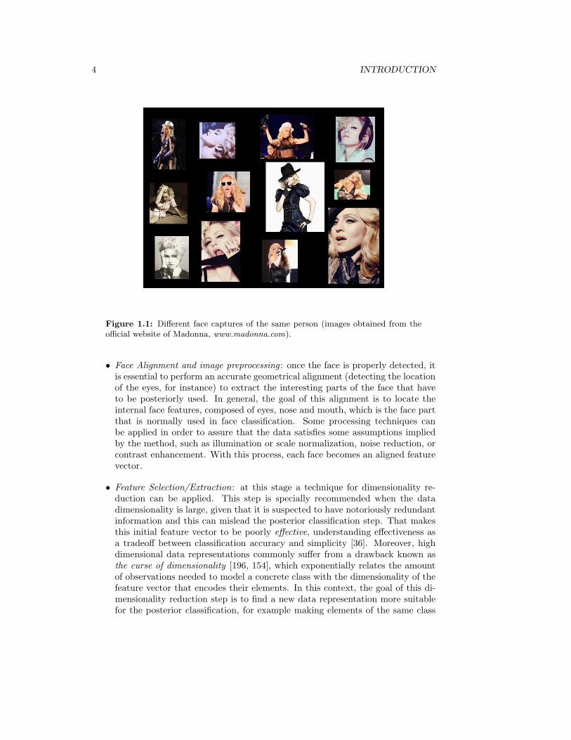
The main difficulty of automatic face classification is due to the changes of theimaging conditions. Observe, for example, the different face captures of the singerMadonna shown in Figure 1.1. We can appreciate several variations in pose, illumi-nation, accessories, color or occlusions, making her recognition in some situations ahard task. In general, the goal of automatic systems is to deal with real environments,where faces suffer from such appearance changes. Moreover, the contribution of otherhandicaps such as facial expressions or age effects make automatic face classificationto be still nowadays an open problem.

1.1 Motivation of the thesis

In general, an automatic system for face classification is divided into the followingstages, which are graphically shown in the scheme of Figure 1.2:

• Face Detection: given an image, the first step is to detect the exact location ofthe face. This stage is performed by a binary classifier that determines whethera concrete image is a face or not. Then, this classifier is run with all the possiblesubpatches of the original image to detect in which part of the image is locatedthe face. This classifier is usually learned from a large database composed oflabeled samples of faces and non-faces.

3

4 INTRODUCTION

Figure 1.1: Different face captures of the same person (images obtained from theofficial website of Madonna, www.madonna.com).

• Face Alignment and image preprocessing : once the face is properly detected, itis essential to perform an accurate geometrical alignment (detecting the locationof the eyes, for instance) to extract the interesting parts of the face that haveto be posteriorly used. In general, the goal of this alignment is to locate theinternal face features, composed of eyes, nose and mouth, which is the face partthat is normally used in face classification. Some processing techniques canbe applied in order to assure that the data satisfies some assumptions impliedby the method, such as illumination or scale normalization, noise reduction, orcontrast enhancement. With this process, each face becomes an aligned featurevector.

• Feature Selection/Extraction: at this stage a technique for dimensionality re-duction can be applied. This step is specially recommended when the datadimensionality is large, given that it is suspected to have notoriously redundantinformation and this can mislead the posterior classification step. That makesthis initial feature vector to be poorly effective, understanding effectiveness asa tradeoff between classification accuracy and simplicity [36]. Moreover, highdimensional data representations commonly suffer from a drawback known asthe curse of dimensionality [196, 154], which exponentially relates the amountof observations needed to model a concrete class with the dimensionality of thefeature vector that encodes their elements. In this context, the goal of this di-mensionality reduction step is to find a new data representation more suitablefor the posterior classification, for example making elements of the same class

1.1. Motivation of the thesis 5

Figure 1.2: General framework of a face classification scheme

6 INTRODUCTION

to be close and elements of different classes to be far. There are two optionsto aim this goal: to transform the original features space by mapping it into amore reduced one (Feature Extraction) or to select the most relevant featuresof the original space (Feature Selection). These techniques of dimensionality re-duction use a set of examples to learn the new data representation, and they areclassified in supervised and unsupervised methods. In the first case the methodsdo use the data labels according to the classification task during the learningprocess, while in the second case the class memberships of the data samples arenot taken into account.

• Classification: finally, the new feature space has to be partitioned, defining asmany disjunct zones as possible classes. This will allow the automatic catego-rization of new inputs. For this goal a classifier is required, which will be learnedfrom a database of labeled samples, called the training set. This training set iscomposed of some data examples with their corresponding class membershipsaccording to the task that has to be learned.

• Online Learning : online learning topic studies the capacity to evolve and updateprevious knowledge given new data inputs. That is, once a dimensionalityreduction transformation or a classifier is learned using an initial training set,the idea of online learning algorithms is to readjust the transformation or theclassifier when new labeled data appears, without retraining the whole system.

In this thesis we focus our attention in the last part of the presented generalframework, which is emphasized in the scheme of Figure 1.2. This part of the processinvolves dimensionality reduction, classifiers learning and online learning method-ologies, and these techniques belong to the Machine Learning field, which play anessential role in any automatic face classification system.

Machine Learning is a subfield of Artificial Intelligence. It is focused on auto-matically extracting information from data by using computational and statisticalmethods. There are many applications for machine learning [53, 206, 160, 234], beingvisual face classification a remarkable example. In the next section we offer a briefoverview of the Machine Learning techniques that have been applied to face classifica-tion. These techniques show promising results in the case of large sized training sets,given that the methods can model more easily the different classes of the classificationtask. However, these methods are still vulnerable when just a few amount of trainingdata is available or the intra-class variation is high, and both factors are very frequentin real life situations. In these cases, the algorithms yield non-robust classifiers withpoor capability of generalization.

Contrary, this dependency on the abundance of training data is not so evidentin human learning processes. Psychological studies show that humans are able tolearn from a very small number of examples, and even from a single datum [5, 243].This fact suggest that humans use something more than just training data to learn atask. Apparently, the key of this generalization ability is that people use their priorknowledge to learn new things, exploiting an enormous amount of training data fromother experiences that are related with the target one [167, 168], or finding patternsand analogies from other domains to reuse them in new situations [169]. For example,

1.2. Traditional Machine Learning techniques for Automatic Face Classification 7

when learning to drive a car, there is a lot of background knowledge that influence thisprocess, like years of experience with bicycles, motorbikes, traffic patterns or logicalreasoning [218].

This idea of knowledge sharing among different tasks is clearly relevant in the faceclassification domain. For instance, certain features, like the shape of eyes or nose,are more important than others to determine the gender of a face image. In parallel,these invariant features are also relevant to perform the task of subject recognition.Then, we can assume that the tasks of gender classification and subject recognitionare related in some sense, and we can use this extra information to learn any of them.More formally, the psychological studies performed by De Gelder et al. [85] showa relation between face detection and subject identification processes in the humanbrain. Apparently, face identification system is part of the object recognition systembut derives its specificity in part from interaction with the face-specific detectionsystem.

In computer science, there are different research approaches for such sharingknowledge techniques, being the Multitask Learning framework one of the most de-veloped area [183]. The term Multitask Learning (MTL) was introduced by Caruana[44] in 1997 and currently constitutes an emergent subtopic of Machine Learning. Itis focused on learning simultaneously different related tasks by sharing some infor-mation during the training process. The goal is to achieve an improvement in theoverall performance when compared to independent training strategies. The differ-ence between MTL and traditional single-task learning techniques is deeply discussedin Chapter 2.

Some empirical results support the use of MTL methods in the automatic faceclassification domain. For instance, Lando et al. described a computational modelfor face recognition, which generalizes from single views of faces. The system tookadvantage of prior experience with other faces, seen under a wider range of viewingconditions [131]. Another example is the face recognizer of Beymer et al. [23], whichuses a set face views at different poses to represent a prior knowledge on facial ro-tation, in order to find a pose-invariant face representation. In both cases we canappreciate an improvement on the overall performance when using these knowledgetransfer approaches. However, the current state-of-the-art techniques for automaticface classification learn separately the different tasks and do not make use of the MTLprinciples.

The main motivation of this thesis is the research on MTL techniques for automaticface classification, mainly focussed on overcoming the small sample sized problem inthis domain.

1.2 Traditional Machine Learning techniques for Au-tomatic Face Classification

In this section we give a brief overview of the most common dimensionality reduction,classification and online learning techniques that are applied to face classificationproblems.

Before starting let us introduce some terminology and notation that will be used

8 INTRODUCTION

in this thesis. To learn a classification task T, such as subject verification or subjectrecognition, we need a training set, which is composed of a set of samples X ={x1, . . . ,xN} with their corresponding class memberships c = {c1, . . . , cN} accordingto the task. The training samples belong to the input space X, which is a subset ofR

D that includes, in our case, all the possible vectors that represent a face image.On the other hand, the class labels ci are elements of the output space of the targettask, L = {1, . . . ,K}. For example, if we consider the task of subject recognition, theoutput space will be L = {1, 2, ...,K}, where the label 1 represents the first subjectwe want to recognize and the label K represents the last one. More details about thenotation used in this thesis can be found in Appendix D.

1.2.1 Dimensionality Reduction

Formally, a dimensionality reduction method learns from training data a transforma-tion Ψ of the original space,

Ψ : X ⊆ RD → Y := Ψ(X) ⊆ R

d (1.1)

with d < D. These techniques can be divided in Feature Selection and FeatureExtraction methods. In the first case, the algorithm finds a subset of relevant com-ponents from the initial data representation, while in the second case the algorithmproperly transforms the initial feature set into a new lower dimensional one.

Different methods of feature selection and extraction can be found in the liter-ature. They can be can be categorized into unsupervised or supervised algorithms.Unsupervised methods do not use the data labels to learn the new feature space, whilesupervised techniques make use of the data samples class membership to learn thenew data representation.

On the other hand, feature extraction algorithms can be divided in linear andnon-linear methods, meaning that the feature transformation is a linear or a non-linear function respectively. In this context, we can see the output of the featureselection methods as a particular linear feature extraction techniques, because thedata transformation is done by a (d×D)-dimensional matrix having zeros in all theentries except a 1 per row. Some specific benefits of performing a feature selectionstep is that they may facilitate data understanding, reducing the measurement, thestorage requirements, as well as the computational cost of the posterior classifierlearning [96].

Following we give a brief description of the most common dimensionality reductiontechniques in the automatic face classification domain.

Principal Component Analysis (PCA)

One of the most successful unsupervised feature extraction techniques is PrincipalComponent Analysis (PCA), which was introduced by Pearson in [119]. Briefly, themethod seeks a linear transformation of the data keeping as much information aspossible under the Euclidean reconstruction criterion. The PCA method is moredeeply described in Chapter 5 Section 1.

1.2. Traditional Machine Learning techniques for Automatic Face Classification 9

One of the first applications of PCA in face classification problems was performedby Kirby [126] and later, Turk and Pentland [225] introduced the notion of eigenfacesfor classification, using PCA for building a base set and representing the faces aslinear combination of these elements. More recently, Moon and Phillips published anempirical study on the performance and computational aspects of the different PCAbased face recognition algorithms [166].

Non-negative Matrix Factorization (NMF)

Another relevant unsupervised linear feature extraction approach is Non-negative Ma-trix Factorization (NMF) [137]. Given a positive training samples set, this algorithmseeks for a decomposition of these data into 2 positive factors. Then, one of thefactors can be seen as base elements while the other represents a weights set. Thus,the original data is approximated by a linear combination of the base elements. Moredetails about NMF can be found in Appendix A Section 1.

This method is specially suitable in computer vision field, given that in severalcases the input elements are described with positive measurements, such as pixelintensity, and that makes plausible the use of NMF to represent the data. Its appli-cation is supported by biological principles [144, 182] and it has been shown to bespecially robust against partial occlusions and illumination changes.

We can find several applications of NMF in face classification problems. Chenet al. [237] used the algorithm in a face detection application, while Wang et al.[231] proposed a framework of face recognition using an NMF constraint to get bothintuitive features and good recognition results. A weighted version of the algorithmwas introduced by Guillamet et al. [63, 92], to focus the decomposition computationin some specific samples. More recently, a new topology preserving NMF method forface recognition was proposed by Zhang et al. [248], which is based on minimizing aconstrained gradient distance in the high-dimensional space.

Independent Component Analysis (ICA)

Independent Component Analysis (ICA) is an unsupervised linear feature extractionmethod that finds new features by maximizing the statistical independence of theestimated components [106]. The main assumption of this approach is that data isobtained by mixing independent sources, what makes this technique specially appro-priated for redundancy reduction. In this context, the computation of the trans-formation matrix can be solved using a Maximum Likelihood approach, maximizingthe non-gaussianity of the independent components [106] or minimizing their mutualinformation [51].

This technique has been successfully applied in the face classification problems.For example, Bartlett et al. [14] provided two architectures of ICA for face recognitiontask. The first one finds spatially local basis images for the faces while the secondproduces a factorial code for face representation. Both approaches show promisingresults in recognizing faces across days and changes in expression. On the other hand,we can find in the literature several comparisons between PCA and ICA. The workof Draper et al. [68] compared these two techniques in the context of a baselineface recognition system, and showed how the relative performance of PCA and ICA

10 INTRODUCTION

depends on the task statement, the ICA architecture and the ICA algorithm. Theyconcluded that the FastICA algorithm [107] configured according to second ICA ar-chitecture yields the highest performance for identifying faces, while the InfoMax [19]algorithm configured according to the same architecture of ICA is better for recogniz-ing facial actions. On the other hand, the studies Liu and Wechsler [142] suggest thatfor enhanced performance ICA should be carried out in a compressed and whitenedPCA space, where the vectors corresponding to small eigenvalues are discarded.

Linear Discriminant Analysis (LDA)

Linear Discriminant Analysis (LDA)[78, 82] is probably the most known approachfor supervised feature extraction and it is currently considered an state-of-the-artapproach for face classification problems. It is a linear method and is based on scattermatrices for finding a linear transformation of the data by maximizing the inter-classdispersion while the intra-class dispersion is minimized. In Chapter 5 Section 1 wegive more details about LDA.

This method has been successfully applied in many face classification problems.For example, Etemad and Chellappa [73] applied the LDA to study the discrimina-tion power of various human facial features, while Belhumeur et al. [18] proposed aprojection method for automatic face classification based on LDA, which seems toseparate accurately different subjects even when the faces are acquired under severelighting variations and different facial expressions. On the other hand, Martinez andKak [153] performed a set of experiments in order to compare PCA and LDA, andshowed that PCA can outperform LDA when the training data set is small. Finally,Zhao et al. [251] presented a new method for face recognition that combines PCAand LDA, in order to improve the generalization capability of LDA when only fewsamples per class are available.

The main drawbacks of LDA is the Gaussian assumption on the class distributionsand a limitation on the dimensionality of the new feature space conditioned by thenumber classes. In order to overcome this handicaps, Fukunaga and Mantoch [83]proposed the Nonparametric Discriminant Analysis method (NDA). The main ideaof this approach is the use of a nonparametric between-class scatter matrix to measurethe inter-class dispersion of the data. Thus, this matrix is generally non singular, andthis eliminates any limitation on the dimensionality of the new feature space as wellas the Gaussian assumption on the class distributions. An application of NDA to theface classification domain can be found in the work of Bressan and Vitria [37].

Kernel Methods

Most of the feature extraction techniques that have been successfully applied in faceclassification problems are linear. However, the face manifold in a vectorial spaceneed not be linear. For this reason, it can be useful to extend these techniques to benon-linear, in order to improve their performance. A proper way of generalizing thesemethods is using the kernel trick [6], which is a system to extend linear methods thatjust depend on dot products between vectors to non-linear versions. This techniqueis based on the Mercer theorem, which states that any continuous, symmetric andpositive semi-definite function

1.2. Traditional Machine Learning techniques for Automatic Face Classification 11

K : RD × R

D → R (1.2)

can be expressed as a dot product in a high-dimensional space. That is, thereexists a transformation

Υ : RD → R

D, (1.3)

with D >> D, such that

K(x,y) = Υ(x) ·Υ(y) ∈ R (1.4)

for every x,y ∈ RD. Then, substituting all the dot products of the original linear

method by the evaluation of the function K, the linear algorithm is equivalent itselfoperating in the transformed high-dimensional space, producing non-linear behaviorsin the original space.

We can find in the literature kernel extensions of PCA, ICA and LDA. For in-stance, Yang et al. [158] investigate the Kernel PCA and their empirical results insubject recognition experiments showed that kernel PCA outperforms the classicalPCA method. Moreover, Yang [241] explored the use of Kernel PCA and KernelLDA for learning low dimensional representations for face recognition and his ex-perimental results showed that kernel methods provide better representations andachieve lower error rates for face recognition than other classical methods. On theother hand, Bach and Jordan [11] presented a kernelized ICA method, which use con-trast functions based on canonical correlations in a reproducing kernel Hilbert space.They proofed that these contrast functions were related to mutual information andother measures of statistical dependence, while a set of simulations showed that theiralgorithms outperform many of the current known algorithms. Furthermore, we canfind a kernel generalization of the NMF algorithm in the work of Zhang et al. [58].Other proposals of kernel methods for automatic face classification can be found in[240, 252, 146].

On the other hand, we can find in the literature some extensions of this method,such as the Kernel PCA [158], which produces a nonlinear map replacing the innerproducts of vectors in the input space by a kernel evaluation.

Feature Selection

One of the simplest mechanisms of feature selection is Feature Ranking and it usuallyshows good empirical results. It is a supervised technique and the idea is to evaluateeach feature separately following some criterion J and pick up the features with high-est mark. There are different criteria, for example correlation or mutual informationbetween the variables and the data labels.

On the other hand, instead of evaluating the features separately as in featureranking, there are methods focused on finding the best feature subgroup of size damong the D dimensions, evaluating at a time all the selected components. In thiscase the goal is to find the features subset that assumes the higher value of an indi-cator J . The most straightforward approach would be the Exhaustive Search, thatis, to evaluate all the possible subsets of d features and select the one with largest

12 INTRODUCTION

J . However, this is not computationally feasible for even moderately high D or d.To overcome this drawback, the Sequential Floating Search [193] is one of the mostsuccessful proposals. This is an heuristic approach that sequentially finds a featuresubset which is as effective as possible according to some determined criterion J ,based for instance in correlation and mutual information or entropy measurements.The idea is to monotonically add in the set a feature that makes no decreasing in theclass separability criterion.

Finally, there are other methods for feature subset selection, which are based onthe use of a posterior classifier performance as criterion J to evaluate the quality of thesubgroup. In this context there are two possible approaches: Wrappers [96, 127] andEmbedded [96, 34] methods. In the first case the algorithm utilizes the classificationas a black box to score subsets of variable according to their predictive power, while inthe second case the method performs the variable selection in the process of classifiertraining, obtaining a features subgroup that is specific to the considered classificationmethod. A common option for this second case is the use of an L1 regularization[171].

The application of feature selection techniques in automatic face classification isless common than feature extraction, but we can find some examples in the literature.For example, Ekenel and Sankur [71] addressed the feature selection problem for facerecognition in the independent component subspace, making experiments with largeface databases in order to compare four feature selection schemes. They observedthat the discriminatory features seem to be concentrated around spatial details of thenose, the eyes and the facial contour. On the other hand, Liu et al. [143] proposeda novel hybrid illumination invariant feature selection scheme for face recognition,which is a combination of geometrical feature extraction and linear subspace projec-tion, while Gokberk et al. [90] designed a pose-invariant face recognizer that performsfeature selection on a set of Gabor wavelets that encode the local feature informa-tion. Furthermore, Bart and Ullman [13] presented an image normalization technique,which remove from the PCA those basis component having high mutual informationof noise artifacts, in order to obtain a new face representation less sensitive to thespecific conditions of the image acquisition.

1.2.2 Classification

The goal of this stage is to learn a classifier, that is, a function

f : Y ⊆ Rd → L = {1, . . . ,K} (1.5)

which assigns to any element in y ∈ Y its estimated label according to the classi-fication task. Thus, the classification of an element x ∈ X will be done by f(Ψ(x)),being Ψ the feature transformation learned in the past stage. In this section, to sim-plify the notation, we will refer to any sample x ∈ X by its extracted feature vectory = Ψ(x).

It is difficult to make a proper taxonomy of classifier learning algorithms giventhat they can be divided according to different criteria. For example, methods canbe divided into linear and non-linear, as in the case of Feature Extraction. Thedistinction between these two types depend on the boundaries defined by the classifier

1.2. Traditional Machine Learning techniques for Automatic Face Classification 13

in the feature space. Then, linear methods are those that separate the regions of thefeature space by linear manifolds while non-linear methods are the ones that produceother decision boundary types. On the other hand, methods can be categorized inprobabilistic or non-probabilistic, depending on their main approach. However, somenon-probabilistic methods are based on finding decision boundaries, using a geometricapproach, while they can be also interpreted from a probabilistic perspective. Thismakes the distinction between probabilistic and non-probabilistic methods to be fuzzyin some cases.

Following we give a brief overview of the most common classification learningalgorithms that are used in automatic face classification problems.

Bayesian Framework

In Bayesian frameworks the class labels of the elements are supposed to be events of arandom variable C, taking values in the output space L = {1, . . . ,K}. The approachassumes that the samples y are measurements of the output elements L = {1, . . . ,K}that help to make a more accurate decision about them. Thus, these outputs aredistributed in Y ⊆ Rd according to a conditional probability density function P (y|c),c ∈ L such that

∫

Y

p(y|c)dy = 1, for all c = 1, . . . ,K (1.6)

Then, the posterior probability of a label can be computed once the sample is seenusing the Bayes formula

P (c|y) =P (c)P (y|c)

P (y)=

P (c)P (y|c)∑K

l=1 P (l)P (y|l)(1.7)

and the posterior classification is made using a Maximum A Posteriory rule (MAP)

f(y) = arg maxc=1,...,K

P (c|y) (1.8)

This classifier is the one that minimizes the probability of error (see Chapter 6Section 1 for more details about this measure, called the Bayes Error) under thisframework.

In this context, if the conditional probability density function P (y|c) is known orassumed, we say the method is parametric, while it is considered non-parametric ifthis conditional probability density function is not known.

The most simple Bayesian classifier is Naıve Bayes method [67]. It assumes statis-tical independence among the features, approximating the conditional density func-tion P (y|c) by the product of the unidimensional densities on each feature

P (y|c) =

D∏

j=1

P (yj |c) (1.9)

for all j = 1, . . . , D.

14 INTRODUCTION

Other relevant Bayesian approaches are the Linear Classifier and the QuadraticClassifier [148]. Their name comes after the name of discriminant functions they use.In both cases it is assumed that elements of the same class are Gaussian distributed.In the first case, however, the assumption is stronger, given that it is supposed that allthe classes have the same covariance matrix, while in the second case the covariancematrices are supposed to be class-specific. More details about the Quadratic Classifiercan be found in Chapter 4 Section 1.

We can find in the literature different applications of Bayesian frameworks toautomatic face classification. For example, Phung et al. [188] used a Naıve Bayesmodel as a took to analyze the effects on classification performance of different imagepreprocessing, while Sebe and Lew [210] presented a Cauchy Naıve Bayes methodto recognize facial expression and emotions. On the other hand, Pronk et al. [192]used the statistical properties of the method in order to calculate confidence inter-vals, enabling more refined classification strategies than the usual operators. Moregenerally, Liu and Wechsler [48] introduced a Bayesian framework for face recognitionwhich unifies popular feature extraction methods, such as PCA and LDA, to generatetwo novel probabilistic reasoning models with enhanced performance, while Moghad-dam et al. [164] proposed a new technique for direct visual matching of images, forthe purposes of face recognition and image retrieval, using a probabilistic measure ofsimilarity, that is based on a Bayesian analysis of image differences.

Nearest Neighbor Classifier (NN)

One of the most simple classifiers is the k-Nearest Neighbor [54]. Given a new inputsample represented by y, the method finds the k closest elements (according to aconcrete distance) belonging to the training set,{yi1 , . . . ,yik

}, and assigns to the newinput the most frequent label among ci1 , . . . , cik

. This is a non-parametric approachwith a Bayesian interpretation. Concretely the class-conditional density is modelledby

P (y|c) =nc

NcV(1.10)

where V is a measure of volume occupied by the k neighbors of y, nj is thenumber of the neighbors {yi1 , . . . ,yik

} belonging to c-th class, and Nc is the numberof elements in the training set belonging to c-th class. The variants of the k-NearestNeighbor method are yielded by the distance type it uses as well as the number k ofneighbors that are taken into account.

Although the simplicity of the approach, it has been shown to be efficient inmany situations and it is still frequently used nowadays. The main handicap of thisalgorithm is an opposite tradeoff between robustness and computational time. Theprobability of classification error of the method tends to 0 when the number of trainingsamples tends to ∞, while the computational cost increases considerably when theamount of training samples is even moderately.

This classification framework is very common in visual face recognition, speciallyin multi-class problems, due to its practical and theoretical properties. In thesecases, a previous feature extraction step is usually performed, specially suitable for aposterior Nearest Neighbor classification. Actually this is the case of LDA and NDA,

1.2. Traditional Machine Learning techniques for Automatic Face Classification 15

that transform the feature space in order to make samples of the same class to be closeand samples of different classes to be far. In this context, Bressan and Vitria [37], forinstance, sought a linear data transformation adapted to improve NN performanceand they observed that the obtained solution was quite close to NDA. On the otherhand, Masip and Vitria [156] introduced a new embedding technique to find thelinear projection that maximizes the performance of the posterior NN classification,while Nobumasa and Takeshi [174] discussed a Nearest Neighbor approach to realizea robust face recognition not sensitive to the lighting conditions. Furthermore, Yangand Zhang [242] introduced a Regression Nearest Neighbor framework for general faceclassification tasks.

Support Vector Machines (SVM)

One of the most successful approaches for binary classification are the Support VectorMachines (SVM) [49, 42, 213]. They operate by finding a hypersurface in the featurespace that attempt to separate training samples of different classes. In addition, thishypersurface is demanded to achieve a maximum separation or margin between thetwo classes, in order to get a better generalization capability. By this we mean thatthe method picks the hyperplane so that the distance from the hyperplane to thenearest data point is maximized. The roots of SVM are located in the StatisticalLearning Theory developed by Vladimir Vapnik et al. [228]. The first proposal ofSVM we can find in the literature are the Linear Support Vector Machines and laterappeared their non-linear version [43], which uses the kernel trick to define non-linearboundaries between the different classes. On the other hand, there are some extensionsof SVM to the multi-class case, which are generally based on Error Correcting OutputCodes (ECOC) [65, 55].

We can find many applications of SVM in automatic face classification. For in-stance, Guo et al. [95] used SVM with a binary tree recognition strategy to approachthe face recognition problem. On the other hand, Heisele et al. [100] presented acomponent-based method and two global methods based on SVM for face recogni-tion, and evaluate them with respect to robustness against pose changes. Anotherexample of SVM application is the work of Jonsson et al. [118], that studied the SVMin the context of face verification and recognition. Their results supports the hypoth-esis that the SVM are able to extract the relevant discriminatory information fromthe training data. Moreover, we can find different applications of SVM to automaticgender recognition [165].

Ensemble Methods: Bagging and Boosting

Another important strategy for classifier learning is the combination of weak classi-fiers. The term weak classifiers defines low complexity methods that are unstable operform just poorly, with an accuracy probability strictly higher than 1/K in K-classproblems. There are different reasons that motivate the use of classifiers combination[148]. For example, different classifiers trained on the same data may differ in globalperformance, because each of them uses to be robust in concrete regions while performbadly in other zones. The idea is to build a classifier taking just the best of each one.On the other hand, feature vectors can be constructed joining different data sources,

16 INTRODUCTION

and in these cases it may be appropriated to use a combination of different classifiers,each one specialized in a concrete data source.

Multiple binary methods have been proposed for combining weak classifiers, beingthe most popular Bagging and Boosting. The idea of Bagging is to generate randombootstrap replicates from the training samples and construct a classifier on each sub-set. Then, these classifiers are combined using a voting rule [35]. On the other hand,the general idea of Boosting is to construct iteratively a prediction rule incremen-tally adding a weak classifier per iteration [148]. The weak classifier joined to theensemble at each iteration is trained using a data selectively sampled from the train-ing elements. This sampling distribution starts from uniform and is updated at eachround, depending on the difficulty of classifying each example. There are differentboosting methods, being AdaBoost [81] and its variants the most known. AdaBoostwas originally proposed for binary problems, although we can find some multi-classextensions. In short, there are two approaches to extend the binary Adaboost clas-sifier to the multi-class case. The first is to adapt the optimized loss function to themulticlass case [115], and the second to combine different binary classifiers using anECOC strategy [208, 223]. A deeper description of binary Adaboost and its extensionto the multiple class case can be found in Chapter 5 Section 2.

One of the most known applications of Boosting in visual face classification prob-lems is the face detector of Viola and Jones [230]. They described in their work aface detection framework that is capable of processing images extremely rapidly whileachieving high detection rates. One of their contributions is a simple and efficient clas-sifier which is built using the AdaBoost learning algorithm to select a small number ofcritical visual features from a very large set of potential features. On the other hand,Lu et al. [147] proposed a novel ensemble-based approach to boost performance oftraditional LDA based methods used in face recognition. The ensemble approach wasbased on boosting, and attempts to build a strong learner by increasing the diversitybetween the classifiers created by the learner. More application examples of thesetechniques to face classification problems are the pairwise classification framework forface recognition proposed by Guo et al. [94] or the multi-class extension of AdaBoostfor subject recognition proposed by Guo and Zhang [93], which is based on a majorityvoting strategy.

Neural Networks

Neural networks constitute a non-parametric and non-probabilistic family of meth-ods for multi-class classification, that try to simulate some properties of the humanbrain. Neural networks can be viewed as massively parallel computing systems con-sisting of an extremely large number of simple processors, called neurons, with manyinterconnections [110]. They can model complex behaviors using flexible procedures,having the ability of learning non-linear relations between the input features and thecorresponding output with sequential training procedures. Moreover, they are able toadapt themselves to the data and can yield to suitable methods for non-linear featureextraction.

In the literature we can find a wide variety of papers about neural networks antheir applications. There are many families of neural networks, being the feed-forward

1.2. Traditional Machine Learning techniques for Automatic Face Classification 17

network [77] one of the most common in classification tasks. This group includesthe multilayer perceptron [99] and the Radial-Basis Function (RBF) [87]. Recently,Hinton and Salakhutdinov [103] proposed a dimensionality reduction tool based on amultilayer neural network with a small central layer to reconstruct high-dimensionalinput vectors. They showed that a gradient descent algorithm can be used for fine-tuning the weights of the network and described an effective way of initializing theseweights.

Neural networks have been applied in automatic face classification in differentways. For example, Lawrence et al. [135] presented a hybrid neural network solutionfor face recognition. The system combines different neural networks with local im-age sampling and provides invariance to minor changes in the image sample, partialinvariance to translation, rotation, scale, and deformation. Bryliuk and Starovoitov[40] used a multilayer perceptron Neural Network for automatic access control basedon face image verification. They studied the robustness of neural network classifierswith respect to the False Acceptance and False Rejection errors and showed that thesearchitectures may be used in real-time applications. On the other hand Smach et al.[75] implemented a classifier based on a multilayer perceptron neural networks forface detection, while Nakano et al. [170] used a neural network for age and genderclassification, using as input features the information of all wrinkles in the face andthe neck.

1.2.3 Online Learning

As previously stated, the online learning paradigm studies the capacity to evolveand update previous knowledge, given new data inputs. In the machine learningcommunity, the terms online learning, incremental learning and life long learning areusually used as synonymous, referring always to the need of rapidly adapting in timeto past mastered tasks.

The online learning topic can be applied to the face classification field at differentlevels. Let us illustrate them considering a subject classification task T with Kdifferent classes (subjects). Suppose that we have initially learned T using a trainingset {X, c}. Different problems arise in this context from the evolving environment. Onthe one hand people change their aspect, so more instances of each subject should beperiodically incorporated to the training set, while old samples should be removed.On the other hand new people can join the data set so the model must take intoaccount the addition of new classes at any time. Additionally, data privacy issuespose the need of eliminating all the information from a specific subject when he/sheasks to be eliminated from the system, being the class removing from the systemanother learning case in this situation.

In this thesis we will distinguish between the following 4 Online Learning sub-problems derived from this formulation:

1. Incremental Sample Learning : which considers the addition to the system of asample belonging to an existing class.

2. Decremental Sample Learning : which considers the removing of a sample be-longing to an existing class, supposing that the class does not disappear (that

18 INTRODUCTION

is, there remains in the training set at least another sample of the same class).

3. Incremental Class Learning : which considers the addition to the system of newsamples belonging to a new unseen class.

4. Decremental Class Learning : which considers the subtraction of an existingclass from the system.

In our taxonomy, algorithms for points 1 and 2 will be also referred as classupdating strategies.

Online Learning literature is mostly devoted to the class updating learning. Onejustification of this fact could be the following: in some problems, like gender classi-fication for instance, the number of classes is fixed and it has not sense to performIncremental Class Learning or the Decremental Class Learning. However, there are alot of real problems where these approaches could be applied.

Following we give a brief overview of the most common Online Learning meth-ods, which are extensions of dimensionality reduction or classifier learning algorithmsdescribed above.

Incremental PCA (IPCA)

The Incremental Principal Component Analyis was proposed by Hall et al. [97] andlater extended by Artac et al. [10]. It is a constructive method for incrementallyadding observations to an eigenspace model. Hall et al. included in their work anIPCA application for automatic face classification problems, where the observationswere images which lied in a linear space formed by lexicographically ordered pixels.Their experiments showed the method to be useful for face classification because itcomputed the smaller eigenspace model representing the observations. It is deeplydescribed in Chapter 5 Section 1 of this thesis.

Incremental LDA (ILDA)

The Incremental LDA is an extension of the classic LDA algorithm in order to incor-porate to the system new samples from the current known classes and also samplesfrom new unseen classes. It was proposed by Pang et al. [184], who presented bothsequential and a chunk versions of the algorithm. Their experimental results showedthat the proposed ILDA could effectively evolve a discriminant eigenspace over a fastand large data stream, and extract features with superior discriminability in classi-fication, when compared with other methods. A deeper description of ILDA can befound in Chapter 5 Section 1 of this thesis.

Recently, Zhao and Yuen [249] developed a new ILDA algorithm called GSVD-ILDA in order to handle the inverse of the within-class scatter matrix, which is oneof the main difficulties of ILDA method. They performed a set of face recognitionexperiments and their results showed that the proposed GSVD-ILDA gives the sameperformance as other ILDA algorithms with much smaller computational complexity.More results of ILDA applied to face classification problems can be found in [56].

1.2. Traditional Machine Learning techniques for Automatic Face Classification 19

Other techniques

We can find in the literature other proposals of Online Learning methods that havenot been applied to face classification problems. For example, several online versionsof the SVM classifiers for incremental sample problems have been developed. Diehland Cauwenberghs [64] proposed a general algorithm to online adapt the SVM modelto changes in regularization and kernel parameters and, after that, many variations ofthese incremental SVM algorithms have been developed in the recent literature, eachpromoting different optimization criteria or efficiency [123, 66, 132, 163]. On the otherhand, there are some interesting approaches to decremental sample strategies. Amongthem we can highlight the work of Cauwenberghs and Poggio [45], that proposes thefirst sample decremental version of the SVM algorithm. In their paper, they suggestedan incremental algorithm for SVM with decremental sample updating capabilities.Nevertheless the binary nature of the SVM makes unfeasible its direct extension tothe incremental class case. Similarly posterior works of Tveit et al. [226] developed adecremental SVM with a more efficient computational performance.

On the other hand, some classifier ensembles have been extended to the incremen-tal sample case. For example, Oza et al. [180, 179, 173] proposed online versions forthe Adaboost and Bagging ensemble learning while Javed et. al. [111] proposed anonline modification of the co-training algorithm.

Finally, there are some extensions of neural networks to the online learning case.For example, Polikar et al.[190] presented the learn++, a multi layer perceptron ap-proach to incremental sample learning, with a training step analogous to the Adaboostalgorithm [80].

1.2.4 Conclusions

In this section we have seen a brief overview of the developed techniques for dimen-sionality reduction (feature extraction and feature selection), classification and onlinelearning, applied to face classification problems. Moreover, our literature review showshow they have been successfully used in many face classification cases. However, aspreviously stated, automatic face classification is still nowadays an unsolved problem.

In this overview, as well as in the past section, we have mentioned the main draw-back of automatic face classification. For example, the high intra class variability,illustrated in Figure 1.1, or the curse of dimensionality phenomenon, caused by thehigh-dimensionality of the input elements and the lack of training samples. Appar-ently, it seems that the solution relies on getting a large amount of training data,to have represented as much variability as possible of each class, and to reduce thedifference between the data dimensionality and the available training samples. Inthis case, furthermore, the statistical methods would yield, theoretically, more sta-ble classification schemes with higher capability of generalization. Unfortunately, toobtain labeled data is in general not easy, specially in cases of face classification. Insecurity applications, for instance, the goal can be the detection of suspicious subjectsfrom which just few instances are available, maybe with low resolution or acquireda long time ago. On the other hand, to process a large amount of data might becomputationally unfeasible. For these reasons, it is essential the research on methodsthat just need a small sized training set to robustly learn a task, and, in this context,

20 INTRODUCTION

the use of MTL methodologies is an interesting approach to deal with the presentedframework.

1.3 Contributions and Overview of the Thesis

In this thesis we explore, propose and test some MTL techniques specially developedfor automatic face classification problems.

Chapter 2 gives a literature review on MTL, briefly describing the most relevantalgorithms developed during the recent years.

In Chapter 3 we present a new embedded system for joint feature selection andclassifier learning, called the JFSCL method, and propose its extension to the MTLparadigm. Chapter 4 is focussed on MTL techniques for classification and proposesMTL extensions of two classification methods: the Quadratic Classifier and the Lo-gistic Regression Model. After that, Chapter 5 presents two MTL methodologies forOnline Learning. The first is called the Online Boosting algorithm, and it is basedon the JointBoost method [223]. The second one is an Online Learning extension ofthe MTL Quadratic Classifier presented in Chapter 4. In Chapter 6 we present a newMTL framework, called the Independent Tasks Problem. In this chapter we formallydefine a new task relatedness concept and present a feature selection and a featureextraction methodologies dealing with this framework. Finally, Chapter 7 concludesthe thesis and proposes some future research lines.

As previously stated, this thesis is essentially focussed on the development of MTLalgorithms specially suitable for face classification problems in the case of small sizedtraining samples. However, we have briefly approached two other points that can alsoimprove the current face classification systems, that are not in the MTL context:

• The use of external face features as an additional information source: althoughthe most part of algorithms that can be found in the literature for classifyingfaces are focused on internal features, we consider the external information lo-cated at hair and ears as a reliable source of information. These features haveoften been discarded due to the difficulty of their extraction and alignment, andthe lack of robustness in security related applications. Nevertheless, there area lot of applications where these considerations are not valid, and the properprocessing of external features can be an important additional source of infor-mation for classifications tasks. In Appendix A we propose and test a systemto encode external face features.

• The optimal face image resolution to represent the data in classification prob-lems: as stated before, an appropriate data representation is very important inautomatic classification methods. A face image can be presented at differentresolutions and it is not trivial to know which one is the most appropriated to bethe initial face representation for the classification system. Very low resolutionscan lose lot of indispensable information, while very high resolutions make thedata processing computationally unfeasible and include redundant features thatcan confuse the classifier. In Appendix B we present an empirical study thatevaluates the quality of different face resolutions to perform automatic subject

1.3. Contributions and Overview of the Thesis 21

classification.

In Appendix C we describe all the publicly available databases used in our ex-periments. A summary of the notation and terminology used in this thesis can befound in Appendix D. Finally, Appendix E lists the publications related with the workpresented in this thesis.

22 INTRODUCTION

Chapter 2

A Survey on Multitask Learning

This chapter provides an overview of the literature on Multitask Learning. Thissurvey attempts to summarize the different methods, results and open problems fromthis Machine Learning field, and proposes a categorization of the different techniquesthat have been developed during the past recent years.

The organization of the chapter is the following. First we describe the MultitaskLearning topic and present some problem scenarios where this research area is applied.Then, we briefly discuss about other Machine Learning topics that are related to thisfield and show some examples of conceptual overlaps between them. In Section 2.2we propose a categorization of Multitask Learning methods, based on what is sharedamong the different tasks, and give an overview of the different techniques that canbe found in the literature. Section 2.3 presents some theoretical work on MultitaskLearning, which is mainly related on formal task relatedness definitions and theoreticalbounds that prove the relevance of the Multitask Learning paradigm. Finally, Section2.4 summarizes and concludes the chapter.

2.1 Introduction

Traditional Machine Learning techniques for automatic classification are focused ontraining a separate learner for each problem. Formally, given a classification task, thesystem receives as input a set of samples, and the goal is to learn a predictor able toautomatically perform the classification task.

As stated in Chapter 1, we can find a lot of methods that have proven to be success-ful in such single-task problems. However, most of the algorithms are still vulnerablewhen just a few amount of training data are available or the intra-class variation ishigh. In order to overcome these drawbacks, the idea of knowledge transferring amongdifferent tasks seems to be an interesting research area. The concept of knowledge inthis context can be understood as the expertise, information or familiarity acquiredby a machine, gained by experience of a fact or situation. For instance, suitableorganizations of the data to perform a classification task, predictors, or models areexamples of knowledge that can acquire a machine.

This idea of knowledge sharing across tasks is inspired in the human learning

23

24 A SURVEY ON MULTITASK LEARNING

Figure 2.1: A Transfer Learning scheme

system, which is able to learn from a very small set of samples. Apparently, thiscapacity is due to the fact that humans use previous knowledge and experiences tolearn a new task. For example, the ability of recognizing bicycles can help to recognizemotorbikes, while knowing to play an electronic organ can help to play a piano. Inthe Machine Learning field, the topic that studies these kind of procedures is knownas Transfer Learning [183], and it is focused on how to transfer knowledge acrossdomains, tasks, and distributions that are similar but not the same.

In general, the different tasks that are involved in a Transfer Learning scheme donot play the same role. Usually, the methods transfer knowledge from one or moresource tasks to a target task, as illustrated in Figure 2.1. We can find a large varietyof Transfer Learning approaches, depending on the relationships between the differenttasks, as well as on the available training data and whether they are labeled or not.

A particular case of this framework is when all the involved tasks are in the samelevel, that is, all of them are source and target tasks at a time. In this case, themethods that attempt to learn all the tasks in parallel by sharing knowledge amongthem are called Multitask Learning methodologies (MTL), and constitute a subfieldof the Transfer Learning topic. This general idea of MTL is illustrated in Figure 2.2.

2.1. Introduction 25

Figure 2.2: A Multitask Learning scheme

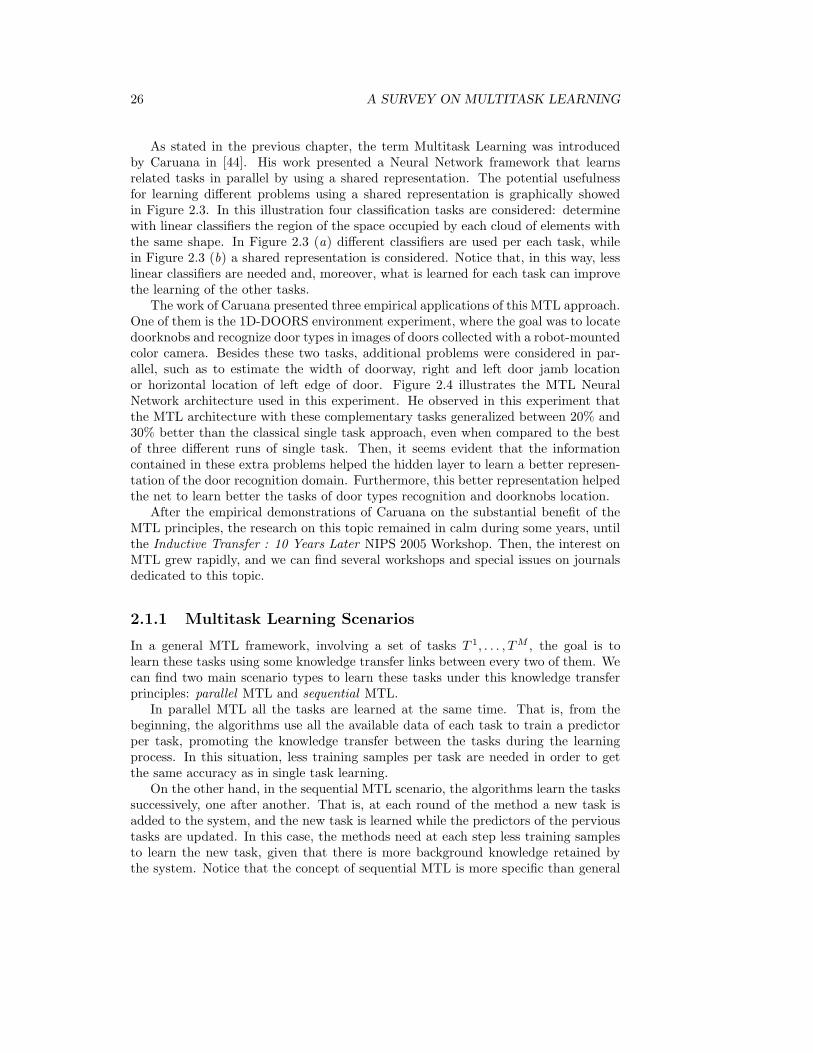
26 A SURVEY ON MULTITASK LEARNING

As stated in the previous chapter, the term Multitask Learning was introducedby Caruana in [44]. His work presented a Neural Network framework that learnsrelated tasks in parallel by using a shared representation. The potential usefulnessfor learning different problems using a shared representation is graphically showedin Figure 2.3. In this illustration four classification tasks are considered: determinewith linear classifiers the region of the space occupied by each cloud of elements withthe same shape. In Figure 2.3 (a) different classifiers are used per each task, whilein Figure 2.3 (b) a shared representation is considered. Notice that, in this way, lesslinear classifiers are needed and, moreover, what is learned for each task can improvethe learning of the other tasks.

The work of Caruana presented three empirical applications of this MTL approach.One of them is the 1D-DOORS environment experiment, where the goal was to locatedoorknobs and recognize door types in images of doors collected with a robot-mountedcolor camera. Besides these two tasks, additional problems were considered in par-allel, such as to estimate the width of doorway, right and left door jamb locationor horizontal location of left edge of door. Figure 2.4 illustrates the MTL NeuralNetwork architecture used in this experiment. He observed in this experiment thatthe MTL architecture with these complementary tasks generalized between 20% and30% better than the classical single task approach, even when compared to the bestof three different runs of single task. Then, it seems evident that the informationcontained in these extra problems helped the hidden layer to learn a better represen-tation of the door recognition domain. Furthermore, this better representation helpedthe net to learn better the tasks of door types recognition and doorknobs location.

After the empirical demonstrations of Caruana on the substantial benefit of theMTL principles, the research on this topic remained in calm during some years, untilthe Inductive Transfer : 10 Years Later NIPS 2005 Workshop. Then, the interest onMTL grew rapidly, and we can find several workshops and special issues on journalsdedicated to this topic.

2.1.1 Multitask Learning Scenarios

In a general MTL framework, involving a set of tasks T 1, . . . , TM , the goal is tolearn these tasks using some knowledge transfer links between every two of them. Wecan find two main scenario types to learn these tasks under this knowledge transferprinciples: parallel MTL and sequential MTL.

In parallel MTL all the tasks are learned at the same time. That is, from thebeginning, the algorithms use all the available data of each task to train a predictorper task, promoting the knowledge transfer between the tasks during the learningprocess. In this situation, less training samples per task are needed in order to getthe same accuracy as in single task learning.

On the other hand, in the sequential MTL scenario, the algorithms learn the taskssuccessively, one after another. That is, at each round of the method a new task isadded to the system, and the new task is learned while the predictors of the pervioustasks are updated. In this case, the methods need at each step less training samplesto learn the new task, given that there is more background knowledge retained bythe system. Notice that the concept of sequential MTL is more specific than general

2.1. Introduction 27

(a)

(b)

Figure 2.3: Illustration of the benefit of using a sharing representation approachfor solving 4 classification tasks. In (a) different classifiers are used per each task. In(b) a shared representation is considered.

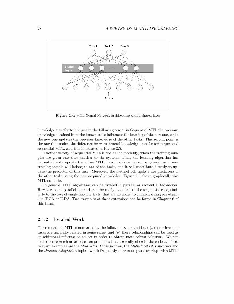
28 A SURVEY ON MULTITASK LEARNING

Figure 2.4: MTL Neural Network architecture with a shared layer

knowledge transfer techniques in the following sense: in Sequential MTL the previousknowledge obtained from the known tasks influences the learning of the new one, whilethe new one updates the previous knowledge of the other tasks. This second point isthe one that makes the difference between general knowledge transfer techniques andsequential MTL, and it is illustrated in Figure 2.5.

Another variety of sequential MTL is the online modality, when the training sam-ples are given one after another to the system. Thus, the learning algorithm hasto continuously update the entire MTL classification scheme. In general, each newtraining sample will belong to one of the tasks, and it will contribute directly to up-date the predictor of this task. Moreover, the method will update the predictors ofthe other tasks using the new acquired knowledge. Figure 2.6 shows graphically thisMTL scenario.

In general, MTL algorithms can be divided in parallel or sequential techniques.However, some parallel methods can be easily extended to the sequential case, simi-larly to the case of single task methods, that are extended to online learning paradigm,like IPCA or ILDA. Two examples of these extensions can be found in Chapter 6 ofthis thesis.

2.1.2 Related Work

The research on MTL is motivated by the following two main ideas: (a) some learningtasks are naturally related in some sense, and (b) these relationships can be used asan additional information source in order to obtain more robust solutions. We canfind other research areas based on principles that are really close to these ideas. Threerelevant examples are the Multi-class Classification, the Multi-label Classification andthe Domain Adaptation topics, which frequently show conceptual overlaps with MTL.

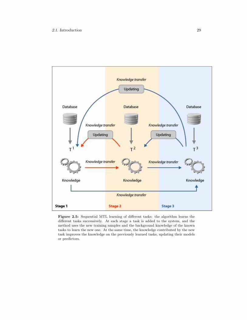
2.1. Introduction 29

Figure 2.5: Sequential MTL learning of different tasks: the algorithm learns thedifferent tasks successively. At each stage a task is added to the system, and themethod uses the new training samples and the background knowledge of the knowntasks to learn the new one. At the same time, the knowledge contributed by the newtask improves the knowledge on the previously learned tasks, updating their modelsor predictors.

30 A SURVEY ON MULTITASK LEARNING

Figure 2.6: Sequential MTL scheme for online learning: the algorithm receives thetraining samples successively. When a new sample arrives to the system, the predictorof its task, T1 in this example, is updated. This produces a growth in knowledge ontask T1, and the method uses it to update the predictors of the other tasks.

2.1. Introduction 31

Multi-class Classification

Most of the state-of-the-art techniques for automatic classification are suitable justfor binary problems. Some relevant examples are the SVM or the AdaBoost methods,that are described in the previous chapter. However, in real world applications wecan find a lot of multi-class classification problems, that can not be directly solvedwith binary techniques.

In order to deal with automatic K-multi-class classification tasks, K > 2, thereare different options, such as extending binary classifiers to address the multi-classcase or designing other multi-class algorithms. However, alternative solutions basedon the combination of binary subproblems usually perform better than these options.In this context, the Error Correcting Output Codes (ECOCs) [65] is a powerful toolfor approaching multi-class problems. The main idea of the ECOCs strategy is tocodify each class as a fixed size binary string, and solve one different binary problemfor each bit of the string. Then, given a new input, these binary classifiers return astring associated to this sample. Finally, this new element is classified in the classwith that has the more similar string, according to a determined distance.

A particular and simple case of ECOC is the one-versus-all approach [202]. Theidea is to consider, for each class k ∈ {1, . . . ,K}, the binary problem of separatingelements belonging to the k-th class from elements belonging to the other classes.In this case, if all the classifiers are successfully learned, the multi-class label of anyinput element can be correctly predicted.

With the one-versus-all approach, the methods for solving K-multi-class problemscan be closely related to MTL. Notice that, if the classes are disjoint, there is anatural relationship among the K classification tasks: if the k-th predictor classifiesan element in the k-th class, all the other r-th predictors, r 6= k, should not classifysuch element in the r-th class. Moreover, when these K classifiers are trained inparallel imposing some information sharing during the process, the system is actuallya MTL framework. In the literature overview of the next section we will see someexamples of such approaches for multi-class problems, as well as in the rest of thisthesis.

Multi-label Classification

Traditional classification problems are concerned with learning from a database ofexamples that are associated with a single label from a set of possible disjoint labelsL = {1, . . . ,K}. In multi-label classification, the examples are associated with a sub-set of labels in L. That is, the possible classes are not disjoint. The firsts applicationsof Multi-label classification were mainly motivated by the tasks of text categorizationand medical diagnosis. Currently, however, the research on Multi-label classificationis increasing rapidly, and it is applied to domains such as semantic scene classificationor music categorization.

A natural way to deal with Multi-label problems is to construct a binary clas-sifier for each label, yielding to a set of independent binary classification problems.Then, as in the case of multi-class classification, if these predictors are trained sharingsome information during the process, the learning method can be considered a MTLtechnique.

32 A SURVEY ON MULTITASK LEARNING

In the literature, we can find some methods that show this overlapping with MTL.For example, Ji et al. [113] considered a general framework for extracting sharedstructures in multi-label classification. They stated that the semantics transmittedby different labels are usually correlated, and, based on this fact, they proposedto exploit this correlation information assuming that a common subspace could beshared among the different binary tasks. Under this assumption, Shuiwang et al.[114]developed an efficient algorithm for Multi-label problems. Their experiments oneleven multi-topic web page categorization tasks demonstrated the effectiveness ofthe proposed formulation in comparison with several representative algorithms. Onthe other hand, Kang et al. [120] presented a novel framework for multi-label learn-ing termed Correlated Label Propagation that explicitly models interactions betweenlabels in an efficient manner. They proposed an algorithm for label co-propagationbased on properties of submodular functions that efficiently finds an optimal solutionto the multi-label classification. Their experiments on two real-world computer visiontasks involving several hundreds of labels demonstrate that the approach leads to sig-nificant gains in precision and recall against standard techniques. More examples ofmethods that exploit this label correlation within the context of multi-label learningare the work of Griffiths and Ghahramani [91], that introduces a Bayesian model toassign labels through underlying latent representations, or the proposal of Yu et al.[244], that uses a regression model to find appropriate linear combination weightsamong the different categories.

Domain Adaptation

The concept of sequential MTL is closely related with the Domain Adaptation topic[108, 116], which studies the problem that arises when the data distribution in thetest domain is different from the one in the training domain, or evolves in time. Theneed for domain adaptation research is prevalent in many real-world classificationproblems. For instance, spam filters can be trained on some public collection of spamemails, but we may want to adapt the generic solution to achieve a better performancewhen applied to the inbox of an individual person.

Strictly speaking, domain adaptation is a different problem than multi-task learn-ing because there is only a single task, although there are different domains. However,the formulation of the two problems can be very similar [116], making some domainadaptation methods recently presented to be also MTL algorithms. In this context,Bickel and Scheffer [26] proposed to use a Dirichlet process to the problem of spam fil-tering adaptation that can be seen as a MTL technique. On the other hand, Daume III[59] proposed a simple method for domain adaptation based on feature duplications,which is equivalent to promote information sharing among the model parameters ofthe different domains. Finally, Ben-David et al. [20] presented an analysis of datarepresentations for Domain Adaptation problems, and proposed a new model thatuses jointly the train and test domains to seek the new feature space.

2.2. A Categorization of Multitask Learning Techniques 33

Table 2.1: Different categories for MTL techniques, according to what is sharedamong the different tasks

Instance SharingShares training data among the different tasks us-ing a re-weighting strategy

Feature RepresentationPerforms a MTL dimensionality reduction step.Usually the methods find a new common featurespace suitable for all the tasks

Parametrical ApproachTransfers knowledge across the different tasks us-ing the assumption that the tasks share some pa-rameters or model priors

General Loss FunctionMinimizes a general loss function that involves allthe tasks, making them sharing some information

Relational KnowledgeTransfers information across the tasks in the con-text of their input data relationships

2.2 A Categorization of Multitask Learning Tech-niques

In this section we propose a categorization of MTL methods, which is partially basedon the taxonomy of Transfer Learning algorithms proposed by Pan and Yang [183].Our categorization is focused on grouping methods according to how the knowledgeis shared among the tasks.

The first context is the Instance Sharing approach. Its main assumption is thattraining data can be shared among the tasks with a re-weighting strategy. Thus, anytask can use training data from the other tasks to be learned. A second context isFeature Representation, which tries to find new feature spaces for all the tasks underthe MTL principles. Actually, a usual procedure of this approach is to find a commonfeature space for all the tasks. A third category is the Parametrical Approach, whichassumes that all the tasks share some parameters or model priors, and uses this idea totransfer knowledge across the different problems. Another MTL context is the use ofa General Loss Function. In this approach the methods seek to minimize a global costfunction that involve the empirical error of each task while promotes the knowledgetransfer between them. Finally, the last context is the Relational Knowledge approach.In this case the information to share across the tasks is the relationship among thedata of the different input spaces. These five contexts are summarized in Table 2.2.

Following we give a literature review of the MTL methods. We have groupedthem according to the taxonomy above described, although there are algorithms thatmight belong to more than one category. For example, some methods that seek a newfeature representation for different related tasks use a parameter based approach inorder to obtain this new feature space. Such a method would belong to both FeatureRepresentation and Parametrical approaches and could be difficult to classify. How-ever, the algorithms usually have a main approach, which allows their categorizationin the most suitable group.

34 A SURVEY ON MULTITASK LEARNING

2.2.1 Instance Sharing

As previously stated, the Instance Sharing approach is based on the idea that trainingsamples of one task can be reused among the different tasks.

In this context, Dai et al. [57] presented a novel framework called TrAdaBoost,which is an extension of the AdaBoost algorithm [81] to the sequential MTL para-digm, specially designed for Domain Adaptation problems. At each round the methodre-weights the old data to reduce their influence, encouraging the new samples to con-tribute more in the learning process. The authors showed theoretically and empiricallythat the TrAdaBoost can learn an accurate model using only a tiny amount of newtraining samples and a large amount of old data, even when the quantity of newsamples is not sufficient to train a model alone.

More recently, Bickel et al. [25] proposed a technique based on a distributionmatching strategy for HIV drug therapy design. The goal was the outcome predictionof a therapy for a patient who carries an HIV virus with a set of observed geneticproperties. The motivation of using a MTL approach is based on the fact that distinctdrug combinations can have similar effects when they intersect in jointly containeddrugs, or when they include drugs that use similar mechanisms to affect the virus.Therefore, it is desirable to exploit data from related problems in order to predict theoutcome of a given drug combination, and thereby achieve generalization over bothvirus mutations and combinations of drugs. In this context, the proposal of Bickelet al. was a new MTL model that can handle arbitrarily different data distributionsfor different tasks without making assumptions about the data generation processor the relation between tasks. In short, the method matches the distribution thatgoverns the pool of examples of all tasks to each of the single task distributions byan appropriate instance weighting.

On the other hand, Ozawa and Roussinov [181] presented a new algorithm foronline multitask pattern recognition problems. They considered a dynamic MTLenvironment where labeled training samples are given sequentially to the system,with no information about the task category. The algorithm detects automaticallythe task where the new input holds and utilizes the previous knowledge to improvethe global classification accuracy. This online automated task recognition allows thesystem to collect and learn on its own. The transfer of knowledge between the differenttasks is based on sequentially activating and deactivating transferring memory itemsassociated with the training samples on the pool of data.

2.2.2 Feature Representation

In general, the goal of the Feature Representation approach is to find a lower dimen-sional feature space for the input data to be shared across all the tasks. Then, afterthis common dimensionality reduction, each task learns separately its predictor.

We can find in the literature a wide variety of MTL methods based on this context.A relevant subgroup of methods under the Feature Representation approach are theMTL neural networks architectures. The first example of this framework was the workof Caruana [44] previously described. Later, following this line, Ghosn and Bengio[88] performed several experiments with backpropagation networks to predict futurereturns of stocks, in order to take financial decisions. They compared the strategy

2.2. A Categorization of Multitask Learning Techniques 35

Figure 2.7: A MTL scheme with a private subnetwork. Common subnetwork learnsthe regularities of the domain and private subnetworks learn specific regularities ofeach task, using additionally the desired values of the other task as extra input [84].

of building a separate network for each stock, and the strategy of sharing the samenetwork for all the stocks. Their experiments performed with Canadian stocks showedthat sharing some parameters across stocks can improve single task strategies. Morerecently, Liao and Carin [140] extended the Radial Basis Function (RBF) networksto the scenario in which multiple correlated tasks are learned simultaneously, andpresented the corresponding learning algorithms. On the other hand, Garcıa-Laencinaet al. [84] proposed a new MTL neural network architecture that uses a privatesubnetwork per task. Thus, the private subnetworks learns specific regularities ofeach task, and then a common subnetwork learns the regularities of the domain, asshown in Figure 2.7. Their results provided from artificial and real data sets showedhow the use of this private subnetworks in MTL produces a better generalizationcapability and a faster learning. Finally, Jin and Sun tested an MTL Neural Networkin face recognition problems [117]. More examples of such approach can be found in[128, 212, 50, 201].

On the other hand, there are MTL methods under the context of Feature Repre-sentation that are not related with neural networks. For example, Florian and Ngai[79] presented a MTL extension of the transformation-based learning paradigm pro-posed by Brill [38] and applied it to natural language processing. Problems relatedto natural language processing are usually composed of multiple subtasks which needto be resolved simultaneously, and they can take benefit from being learned in a jointframework. Their results showed that the simultaneous learning of multiple tasksdoes achieve an improvement on each task. Later, Jebara [112] constructed a featureselection and kernel selection strategy for multiple SVMs trained on different relateddata sets. He generates a novel extension of SVMs using a maximum entropy discrim-ination, which allows the different datasets to mutually reinforce a common choice ofrelevant features for their specific classifiers. Tur [224] presented a MTL method fornatural language intent classification, that trains the tasks in parallel using a shared

36 A SURVEY ON MULTITASK LEARNING

representation. The approach allows the automatic re-use of labeled data from var-ious applications that have similar distributions. His empirical results showed thatit is possible to improve significantly the performance of a spoken language under-standing system when there is not much training data available. Finally, Xiong etal. [236] studied the problem of joint feature selection when learning multiple relatedclassification or regression tasks. Their probabilistic framework imposes an automaticrelevance determination prior on the hypothesis classes, associated with each of thetasks and a regularization constraint on the variance of the hypothesis parameters.Thus, similar feature patterns among the different tasks are enforced, allowing toidentify those features that are relevant to all the tasks. Their experimental resultsshowed that the approach outperformed some traditional methods where individualtasks were learned independently.

2.2.3 Parametrical Approach

The MTL Parametrical approach includes those methods that promote the tasks toshare some parameters of their models or some priors. Currently, the Parametricalapproach is the most developed MTL category.

Most of the MTL methods that we found in the literature under the parametricalapproach can be grouped into the following three categories: Regularization Con-straints, Kernel Methods and Bayesian Framework. The first category includes thosemethods that focus the principles of MTL in a penalty on the parameter space. Onthe other hand, the main idea of the methods belonging to the second category is toextend single-task Kernel methods to the MTL paradigm. Finally, the MTL BayesianFramework can be seen as an extension of the single-task Bayesian approach to theMTL topic.

These categories are frequently overlapped. For example, kernel methods usuallyfocused on regularization constraints in order to encourage the different tasks toshare knowledge, while some of these regularization constraints are based on Bayesianframeworks. Nevertheless, as in the case of the general taxonomy, the algorithmsusually show a main line that allows its categorization.

On the other hand, there are other MTL methods under the Parametrical ap-proach that do not hold under any of these three classes. For instance, the workof Abernethy et al. [2], that considers the problem of prediction with expert adviceseeking a few experts that perform well on all the tasks at a time. They presentedan algorithm based on mixing priors to solve the problem, as well as an efficientrandomized extension that reduces the computational requirements of the algorithm.Also in the context of prediction with expert advice, Agarwal et al. [4] proposed aMTL framework that encourages the knowledge transfer across tasks by enforcing themethod to select a lesser number of best experts than the number of tasks. Theyshowed that this idea is equivalent to learning under structural matrix constraints,and propose a regularization approach to promote these restrictions. They also pro-vided a theoretical analysis of a concrete regularizer in order to show the benefits ofthis setup.

Other examples of algorithms under the general parametrical approach are meth-ods focused on learning informative meta-level priors for finding common feature

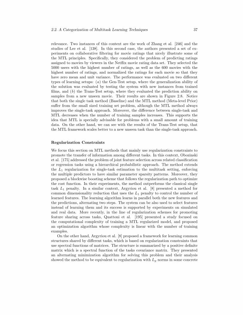
2.2. A Categorization of Multitask Learning Techniques 37

relevance. Two instances of this context are the work of Zhang et al. [246] and thestudies of Lee et al. [138]. In this second case, the authors presented a set of ex-periments on collaborative filtering for movie ratings that nicely illustrate some ofthe MTL principles. Specifically, they considered the problem of predicting ratingsassigned to movies by viewers in the Netflix movie rating data set. They selected the5000 users with the highest number of ratings, as well as the 600 movies with thehighest number of ratings, and normalized the ratings for each movie so that theyhave zero mean and unit variance. The performance was evaluated on two differenttypes of learning setups: (a) the Gen-Test setup, where the generalization ability ofthe solution was evaluated by testing the system with new instances from trainedfilms, and (b) the Trans-Test setup, where they evaluated the prediction ability onsamples from a new unseen movie. Their results are shown in Figure 2.8. Noticethat both the single task method (Baseline) and the MTL method (Meta-level Prior)suffer from the small sized training set problem, although the MTL method alwaysimproves the single-task approach. Moreover, the difference between single-task andMTL decreases when the number of training samples increases. This supports theidea that MTL is specially advisable for problems with a small amount of trainingdata. On the other hand, we can see with the results of the Trans-Test setup, thatthe MTL framework scales better to a new unseen task than the single-task approach.

Regularization Constraints

We focus this section on MTL methods that mainly use regularization constraints topromote the transfer of information among different tasks. In this context, Obozinskiet al. [175] addressed the problem of joint feature selection across related classificationor regression tasks using a hierarchical probabilistic approach. The method extendsthe L1 regularization for single-task estimation to the multitask setting, enforcingthe multiple predictors to have similar parameter sparsity patterns. Moreover, theyproposed a blockwise boosting scheme that follows the regularization path to optimizethe cost function. In their experiments, the method outperforms the classical singletask L1 penalty. In a similar context, Argyriou et al. [8] presented a method forcommon dimensionality reduction that uses the L1 penalty to control the number oflearned features. The learning algorithm learns in parallel both the new features andthe predictions, alternating two steps. The system can be also used to select featuresinstead of learning them and its success is supported by experiments on simulatedand real data. More recently, in the line of regularization schemes for promotingfeature sharing across tasks, Quattoni et al. [195] presented a study focused onthe computational complexity of training a MTL regularized model, and proposedan optimization algorithm whose complexity is linear with the number of trainingexamples.

On the other hand, Argyriou et al. [8] proposed a framework for learning commonstructures shared by different tasks, which is based on regularization constraints thatuse spectral functions of matrices. The structure is summarized by a positive definitematrix which is a spectral function of the tasks covariance matrix. They presentedan alternating minimization algorithm for solving this problem and their analysisshowed the method to be equivalent to regularization with Lp norms in some concrete

38 A SURVEY ON MULTITASK LEARNING

Figure 2.8: Evolution of the Root Mean Squared Error (RMSE) per number oftraining samples. Results of the Gen-Test (top) and Trans-test (bottom), using thesingle-task baseline method and its extension to the MTL topic that uses a the Meta-level Prior [138].

2.2. A Categorization of Multitask Learning Techniques 39

examples. Experiments on two real data sets indicated that the algorithm scaleswell with the number of tasks and improves some current state-of-the-art statisticalclassification performance.

Kernel Methods

The research on Kernel Methods for MTL learning has been quite active during lastyears. Micchelli and Pontil [159] provided a method for MTL classification reproduc-ing kernel Hilbert spaces of vector-valued functions, in order to capture the relation-ships between the predictors of the different tasks. These interactions are reflectedby the use of a linear matrix-valued kernel and the approach allows the extension ofsingle-task classifiers, like SVMs, to the MTL paradigm. In a similar line, Evgeniouand Pontil [74] proposed the use of a novel kernel function to model relationshipsbetween tasks, using a task-coupling parameter as a regularization function.

Later, Evgeniou et al. [217] studied the problem of learning multiple relatedtasks simultaneously by using kernel methods with a novel form of regularization con-straints. Moreover, they proved that their MTL approach is equivalent to a single-taskone for an appropriate choice of the kernel function. Their experimental results showedthat the use of their framework improved significantly standard single-task techniqueswhen there are many related tasks but few data per task. Girolami and Rogers [89]presented a Bayesian hierarchical model which enables kernel learning and presentedeffective variational Bayes estimators for regression and classification, demonstratingthe utility of the proposed method with different empirical experiments.

More recently, Ruckert and Kramer [205] considered the problem of finding asuitable bias for a new data set, given a set of known data sets in the context ofsequential MTL. Their method aimed to find a suitable kernel function for a newtask while generating kernels that generalize well on the known data sets, using aminimization function under a meta-learning problem that compares the data sets.Their proposal was tested on small molecule and text data, and their kernel-basedapproach showed an improvement, in almost all the cases, over the best single-tasklearning methodology based in kernels.

Bayesian Framework

We can find in the literature several MTL algorithms belonging to the Bayesian frame-work. For example, Baxter [16] proposed a model for learning multiple tasks usingan objective prior distribution approach, and provided some bounds on the amountof information required to learn a task, when it is simultaneously learned with otherrelated tasks. Heskes [102] presented a new Bayesian model for empirical MTL withhidden weights that are shared among the tasks. The learning method was imple-mented in a single feed-forward network using an hyper-parametrical approach. In hisstudies, Heskes presented practical simulations on newspapers and magazine sales toillustrate the benefits of the MTL principles. Raina et al. [197] proposed an algorithmfor automatically constructing a multivariate Gaussian prior over the parameters of alogistic regression model, that encodes useful domain knowledge by capturing under-lying dependencies between the parameters. Their work was focused on binary textclassification and their experimental results showed a test error reduction over other

40 A SURVEY ON MULTITASK LEARNING

commonly used priors. More recently, Raykar et al. [199] presented a Bayesian MTLalgorithm that automatically identifies the relevant feature subset for classificationpurposes. The algorithm exploits information from different data sets while learningmultiple related classifiers, and it is specially suitable for Multiple Instance Learningproblems [151]. Finally, Zhang et al. [247] proposed a MTL probabilistic frameworkbased on a set of latent variable models. They showed that the framework is a gen-eralization of standard learning methods for single-task prediction problems that caneffectively model the shared structure among different prediction tasks.

Some researchers have developed MTL methods in the context of Gaussian Processes[28]. Lawrence and Platt [134] presented the MT-IVM method, an extension of theInformative Vector Machine (IVM) [133] to the MTL paradigm. The algorithm learnsthe parameters of Gaussian Processes of different tasks sharing the same prior. Theexperimental results showed the method to be more effective than the traditional IVMin a speaker dependent phoneme recognition task. Later, Schwaighofer et al. [209]proposed a novel method for learning with Gaussian process regression using hier-archies, while Bonilla et al. [30] presented a model that learns a shared covariancefunction on input-dependent features and a free-form covariance matrix over tasks, formodelling inter-task dependencies. Finally, Chai et al. [47] proposed a MTL methodbased on Gaussian Process priors to be applied in dynamics problem for a roboticmanipulator.

More MTL methods under the Bayesian framework can be found in [233, 62, 245,31, 244, 172, 215, 7, 24].

2.2.4 General Loss Function

In the General Loss Function approach, the methods seek to minimize a loss functionthat involves the empirical error of all the tasks. This framework is closely related tothe Parametrical approach, specially to the subcategory of Regularization Constraints.This is because methods of the Regularization Constraints subcategory can be usuallystated as the minimization of a loss function that involve all the tasks, and includean additional term, the regularizer, that enforces the tasks to share information.However, we can find in the literature MTL methods focused on minimizing a generalcost function that do not use regularization. In general they belong to the MTLapproach of multi-class classifiers, which has been described in Section 2.2.1.

One of the most known examples of the General Loss Function approach is theJointBoost algorithm, proposed by Torralba et al. [223]. This method is a multi-classextension of the binary GentleBoost [81] that uses the MTL principles. It trains mul-tiple binary classifiers at a time in order to minimize the empirical error on each class,while finds features that are shared among them. With this methodology the featuresselected by the algorithm are more generic and this yields to a better generalizationin classification problems. One of the experiments performed in this work illustratesthat the MTL paradigm can yield to less complex models. The experiment consistedon training in parallel a set of detectors for 29 different object categories. In Figure2.9 (a) a we can see the number of features needed to achieve a 95% of detection ratein all the categories, for both class-specific and shared features approaches. Noticethat in the case of separate detectors the number of features grows linearly, while in

2.2. A Categorization of Multitask Learning Techniques 41

Figure 2.9: Comparison of the efficiency of class-specific and shared features torepresent the different object classes. (a) Mean number of features needed to reacha 95% of detection accuracy for all the objects. The results are averaged across 20training sets and different combinations of objects and error bars correspond to 80%intervals. (b) Mean number of features allocated for each object class [223].

the MTL framework it grows as a logarithm of the number of objects. However, aswe see in Figure 2.9 (b) in the shared case the features become less informative fora single class, and, therefore more features per class are needed to achieve the sameperformance compared to using class-specific features. The JointBoost algorithm isdeeply described in Chapter 5 Section 2 of this thesis.

On the other hand, Dekel et al. [61] presented a sequential MTL method forlearning online multiple tasks in parallel. Concretely, the algorithm receives an in-stance and makes a prediction for each one of the tasks. To evaluate these multiplepredictions the authors constructed a common loss function that involves all the in-dividual losses. Moreover, they proposed a collection of online algorithms which canuse this global loss approach and proved worst-case relative loss bounds for all of theiralgorithms.

2.2.5 Relational Knowledge

The Relational Knowledge category is the less developed in the context of MTL.Methods of this approach seek to share information about the relationship betweenthe input data of the different tasks. In general, these algorithms are used to deal

42 A SURVEY ON MULTITASK LEARNING

with relational domains, that is, environments where the samples of the input spacesexhibit a relation based structure.

Under the principles of MTL, this Relational Knowledge category can be espe-cially important when using statistical relational learning. For example, in a domaindescribing an academic institution, the entities may be people, publications, andcourses, while the relations may be advised-by, taught-by, written-by. It seems evi-dent that several aspects of learning from relational data contribute to the complexityof the problem. For this reason it is desirable to extrapolate the knowledge of suchrelationships to other relationship domains, like industry for instance. In this case,the role of a professor in an academic domain is at the same level as the role of themanager in industry, while the relationship between a professor with his/her studentsis similar to the relationship between a manager with his/her workers [183].

Currently, up to our knowledge, there is no work holding on MTL RelationalKnowledge. However, we can find some works under this approach in the more generalKnowledge Transfer area [161, 162, 60].

2.3 Theory on Multitask Learning and Task Relat-edness definitions

As we have seen in the previous section, the general approach of MTL has been provento be quite successful in many practical applications. However, there are not manyworks on theoretical justifications for this success.

One of the most significant works on MTL theoretical treatment was done byBaxter in [15]. His work is based on the idea that any learner must to be biasedin some way to achieve a good generalization capacity. Then, assuming that anylearner is embedded within an environment of related problems, Baxter proposedto consider all the problems together in order to automatically learn this bias. Inthis context, he developed an extension of the VC-dimension notion of Vapnik [228]to the MTL case, as well as the basic generalization bounds of Statistical LearningTheory [228]. The goal of Baxter’s approach for the problem of bias learning was tochoose an optimal hypothesis space from a family of hypothesis spaces. Then, afterdefining an extended VC-dimension for a family of hypothesis spaces, he used it toderive generalization bounds on the average error of M tasks. With this approach,the general error decreases at best 1/M times. Moreover, the upper bound on thenumber of examples required to train each task never increases with the number oftasks, and at best decreases as 1/M times.

On the other hand, Ben-David and Schuller [22] derived from this extended VC-dimension new bounds that hold for each task, instead of holding just on the averageerror among the involved tasks. Actually, the authors provided a formal frameworkfor task relatedness and, in this framework, they stated general conditions, underwhich the derived bounds guarantee smaller sample size per task than the knownbounds for the single task learning approach. Further information in this context canbe found in [21], a more recent work of the same authors.

More theoretical studies on MTL were performed by Maurer [157], who presenteddata-dependent bounds for linear MTL preprocessing. These bounds are constructed

2.3. Theory on Multitask Learning and Task Relatedness definitions 43

using the margins of the task-specific classifiers, the Hilbert-Schmidt norm of theselected preprocessor and the Hilbert-Schmidt norm of the covariance operator forthe total mixture of all task distributions, or, alternatively, the Frobenius norm ofthe total Gramian matrix for the data-dependent version. Later, Mahmud and Ray[150] formalized a task relatedness measure using conditional Kolmogorov complexity.They analyzed how to share the right amount of information in sequential transferlearning under a Bayesian setting. Finally, Cavallanti et al. [46] stated the taskrelatedness concept in different ways, and derive theoretic bounds that guarantee theperformance advantage provided by the interaction.

2.3.1 Limitations of Multitask Learning

An important question in the MTL research is to know when the knowledge sharingis appropriate and when it can have negative consequences. The use of a MTLmethodology involving tasks that are too dissimilar may confuse the system, yieldingto predictors that perform worst that the ones obtained with single-task algorithms.

Currently there is no much research on how to avoid such negative transfer ofknowledge, although it is a key issue for the success of MTL approaches. In thiscontext, Rosentein et al. [204] presented an study on how detecting and avoidingthis kind of negative transfer between tasks. They described a transfer-aware versionof the Naıve Bayes classifier and empirically showed that the benefits of knowledgetransfer depend on the similarity of the involved tasks. However, there is a trade-off between the task relatedness identification and the potential benefits of a MTLmethod: the probability of correctly detecting relatedness among tasks increases witha large amount of training examples, while the need of knowledge transfer becomesdiminished.

On the other hand, some researchers have proposed MTL algorithms that auto-matically cluster the different tasks according to their amount of relatedness. Afterthat, they promote the knowledge transfer just among those tasks that are related.An example of this procedure is the work of Bakker and Heskes [12]. They pre-sented a Bayesian approach in which some of the model parameters are shared amongtasks, while others are loosely connected through a joint prior distribution that canbe learned from the data. Moreover, using single Gaussian or mixtures of Gaussianpriors, the method does an unsupervised task clustering while learning the predic-tors. This can be further generalized to a mixture of experts architecture with thegates depending on task characteristics. More recently, Argyriou et al. [9] consideredthe situation where the tasks can be automatically divided into groups, according totheir level of relationship. In their work, they presented an algorithm that computeda common feature representation, specific for each group of tasks. The learning al-gorithm uses a gradient descent strategy to find the feature maps that describe theshared subspaces, and its efficiency is theoretically justified by a generalization boundon the transfer error. The authors presented a set of experiments, which show theadvantage of the approach over single-task learning and a previous transfer learningmethod.

In a similar context, some researchers have developed methods that use DirichletProcess Priors in order to identify groups of related tasks. For example, Xue et al.

44 A SURVEY ON MULTITASK LEARNING

[239] considered the problem of learning MTL Logistic Regression models, involvingtasks whose data set were not drawn from the same statistical distribution. Theyproposed a statistical model based on Dirichlet process for learning the multiple pre-dictors, and presented a variational Bayesian algorithm to learn the different tasks inparallel under this framework, as well as a Markov Chain Monte Carlo formulationfor sequential MTL. Their experimental results on two real life MTL problems showedthat the proposed algorithms can automatically identify relationships between tasksand improve the performance of simpler approaches, such as single-task methodolo-gies. Other examples of using Dirichlet process to cluster the tasks according to theirsimilarity were proposed by Xue et al. in [238] and, more recently, by Qi et al. [194].

2.4 Summary and Conclusions

The traditional approach of Machine Learning aims for learning a separate predictor ormodel for each problem. Several techniques have been proposed under this framework,but they usually suffer from drawbacks as the lack of training samples or the highintra-class variability. Unfortunately, these conditions are very frequent in real worldapplications.

Inspired by the human learning system, that uses more information than justtraining data to learn a new task, an emergent topic known as MTL has appearedrecently in the Machine Learning research. The goal of MTL methods is to learndifferent tasks sharing some knowledge during the training process, in order to obtainmore robust solutions with higher generalization ability.

In this chapter we have reviewed some of the works on MTL that have been pre-sented in the past recent years, which empirically show the success of MTL algorithmsin many applications. Moreover, we proposed a categorization of MTL techniques,according to what is transferred across the tasks. The different categories are the fol-lowing: Instance Sharing, Feature Representation, Parametrical Approach, GeneralLoss Function and Relational Knowledge.

Most of the current MTL methods assume that the tasks are related, promot-ing always the interaction among the different problems. However, the use of MTLtechniques may be inappropriate when the tasks are too dissimilar. Moreover, someempirical results performed in a Bayesian framework have shown that the benefits ofknowledge transfer depend on the similarity of the involved tasks.

Currently there is no much research on when sharing knowledge is appropriate. Wefound just a few methods that automatically perform a task clustering according totheir similarity, encouraging just the related tasks to share information. Nevertheless,to avoid a negative knowledge transfer seems to be a key issue in MTL topic.

Chapter 3

The JFSCL and its application forMultitask Feature Selection

The estimation of sparse models or predictors is currently playing an important rolein the Machine Learning community. Formally, a solution produced by an algorithmis sparse when only a small number of the coefficients that describe the model orthe predictor are non-zero. The sparsity is a very useful property given that sparsemethods allow a faster evaluation of the models and have demonstrated a highergeneralization performance [228].

Several methods for classification and regression have been recently developed inthe context of the sparsity [139, 214, 176, 72, 232], but just a few of the proposalsdeal also with MTL, as we have seen in the previous chapter. However, to exploreMTL techniques under a sparse framework seems an interesting research line and thiswas the initial idea of the work presented in this chapter.

One of the most successful sparse systems developed during the past years isthe Relevance Vector Machines (RVM) of Tipping [220]. This method is an sparseBayesian approach of the SVM that uses dramatically fewer basis functions than acomparable SVM. Moreover, it presents a number of additional advantages, such asthe benefits of probabilistic predictions, the automatic estimation of tuning parame-ters, and the facility to use arbitrary basis functions instead of Kernels.

As stated in the first chapter, it is recommended to use some dimensionality re-duction technique when the input data lies in high-dimensional spaces, in order toreduce redundant information or noise that can mislead the classifier. In this context,one of the options is to use a feature selection strategy. Some methods for featureselection are based on the idea of sparsity, specially the embedded methods that finda feature subset while learning a classifier. For example, Costen et al. [52] presenteda method for performing feature selection with SVM imposing a sparsity constrainton the parameters. Thus, using a L1 norm restriction, the method can take a subsetof features that are more robust for the SVM than the original ones.

In order to mix these ideas of sparsity applied to the SVM classifier, we havedeveloped the Joint Feature Selection and Classifier Learning (JFSCL) method. TheJFSCL algorithm is an embedded system for selecting features while learning a sparse

45

46THE JFSCL AND ITS APPLICATION FOR MULTITASK FEATURE SELECTION

predictor similar to the RVM. The algorithm is based on the minimization of a costfunction, composed of two terms. The first term is associated with the negated log-likelihood of a probabilistic model based on a Bayesian approach of the SVM. Thesecond term is a regularization constraint, that imposes a prior on the parameters ofthe model to get sparsity on the selected SVM basis, and a restriction that allowsto activate or deactivate the features. This regularization constraint consist of a L1

norm restriction on a set of parameters.In the next section we describe JFSCL preliminary techniques and Section 3.3 is

focused on the JFSCL method and its empirical application.One of the advantages of the JFSCL is that its formulation is very flexible. This

flexibility makes the algorithm to be easily extensible to the MTL paradigm, per-forming a common feature selection for different tasks. Section 3.4 details this MTLextension of the JFSCL, and shows some experiments of its application to the genderrecognition problem, in the face classification domain.

Finally, Section 3.5 concludes the chapter.

3.1 Preliminaries

In this section we describe some work related with the JFSCL. First, we brieflyreview the classical formulation of the SVM, its main drawbacks, and the RVM as apossible solution of the SVM handicaps. Second, we describe the Lasso problem, anapproach for sparsity promoting based on L1 regularization. Moreover, we describesome methods to solve Lasso problems, making a special emphasis to the BLassoalgorithm, which is the learning strategy used in the JFSCL. Finally, we presentthe Laplacean RVM (L-RVM), a new RVM approach that is the base of the JFSCLmethod.

3.1.1 Vector Machines

As previously stated, Support Vector Machine (SVM) [228] is one of the most success-ful binary classifiers developed in the pattern recognition field. Briefly, consideringa binary classification task T, with possible classes L = {0, 1} and training samples{X, c}, a linear SVM predicts the expected labels as

f(x) = 1(0,∞)

( N∑

i=1

wi(xxi) + w0

)(3.1)

where 1(0,∞) is the indicator function of the (0,∞) interval, and w = (w0, ..., wN )is a weights vector that should be learned to minimize the empirical classificationerror.

The SVM operates by finding a hyperplane in the input space, that attempts toseparate the examples from the different classes. Moreover, this hyperplane is foundsubject to the margin maximization restriction: it has to be as far as possible fromits closest sample of both classes. This property of maximum margin is stronglyrelated to the generalization ability of the learned predictor. The optimal hyperplane

3.1. Preliminaries 47

Figure 3.1: Example of a linear separable problem. The central line is the optimalhyperplane obtained by SVM.

is defined by a set of the training samples, called support vectors. In Figure 3.1 weshow a toy classification example with SVM.

Using the kernel trick described in Chapter 1, the SVM can be extended to non-linear solutions, replacing the dot product on the prediction function by the evaluationof a kernel function G [6]. This formulation yields to the following expression forpredicting the labels of a new instance x ∈ R

D,

f(x) = 1(0,∞)

( N∑

i=1

wiG(x,xi) + w0

)(3.2)

what produces a frontier in the input space, which is a general hypersurface insteadof an hyperplane. Further details on the SVM can be found in [49, 42, 213].

Although the SVM have shown to be successful in a lot of binary problems, itsuffers from some limitations, such as:

• Predictions are binary, and no probabilistic value can be derived from the clas-sification of a sample.

• Usually, the number of selected support vectors is small, but no specific prior isimposed on the solution to control the desired sparsity level.

48THE JFSCL AND ITS APPLICATION FOR MULTITASK FEATURE SELECTION

• In general, the classes are not linearly separable. In these cases a parameter isneeded to fix the optimal operation point that us used to compute the error ofthe margin. This process can only be solved by cross validating the training set,being the tuning process computationally costly.

• There is a variety of kernel functions G to use, but they must satisfy the Mercer’scondition.

To overcome these drawbacks, Tipping [220] proposed the RVM classifier, wherea Bayesian approach for learning the parameters w is followed. Briefly, he suggestedthe use of a set of hyperparameters associated to the generation of the weights w,obtaining a sparse distribution on w. The experimental results show a generalizationcapability close to the SVM, using an impressively few number of support vectors.

3.1.2 The Lasso Problem and the BLasso Algorithm

As we have stated in Chapter 1, traditional approaches to learning methods seek tooptimize a function associated to the empirical error rate. Several statistical proce-dures use likelihood or negated likelihood estimators to learn the parameters of themodel. However, given that the training data is usually a finite set, learning algo-rithms could lead to an arbitrary complex model as a consequence of the trainingerror minimization, obtaining in that way a classifier that presents high variance onunseen data and poor classification results on the testing data. To avoid this factsome regularization constraints on the parameter set can be jointly imposed duringthe training step. Thus, the learning method optimizes a loss function subject tosome model complexity restriction.

Lasso is a regularization approach for parameter estimation originally proposedby Effron et al. [69] that shrinks a learned model through an L1 penalty on theparameters set. Formally, in a statistical classification framework with parameters w,the Lasso loss can be expressed as

J(w) = L(w) + λR(w) (3.3)

where L(w) is a negated empirical error function (such as the negated log-likelihoodof the model), R(w) is the imposed L1 restriction on the parameters, R(w) = ‖w‖1 ∈R, and λ is a positive real value. Actually, the sum term λR(w) is the negated log-likelihood obtained when we impose a centered Laplace distribution on the compo-nents of w, with variance inversely proportionally to λ (see Figure 3.2). Consequently,this constraint imposes sparsity on the w components, and the parameter λ is con-trolling the regularization level on the estimate. Observe that parameter λ is a crucialselection to get a good solution. Notice that setting λ = 0 reverses the Lasso problemto minimizing the unregularized loss while a very large value will completely shrinkthe parameters to 0, leading to an empty model.

Based on the seminal paper of Effron [69], different computational algorithms havebeen developed to solve this regularization path. Osborne et al. [178, 177] developedthe homotopy method for the squared loss function case, and later Efron et al. [70]proposed the Least Angle Regression method, a new model selection algorithm thatcan be extended to implement the Lasso estimates.

3.1. Preliminaries 49

Figure 3.2: Some examples of Laplace distributions, with mean µ and variance b.

Lasso has been successfully applied to multiple disciplines. In the bioinformaticsfield Vert et al. [229] adapted the Lasso sparse modelling to the problem of siRNAefficacy prediction. Tibshirani et al. [219] applied their fussed Lasso algorithm toprotein mass spectroscopy and gene expression data, while Ghosh and Chinnaiyan [86]adapted the Lasso algorithm to the selection and classification of genomic biomarkers.

Recently, Zhao and Yu developed a numerical method that approximates the Lassopath in general situations [250]. The method is called the Boosted Lasso (BLasso)algorithm and has the computational advantages of Boosting converging to the Lassosolution with global L1 regularization. Furthermore, the algorithm can automaticallytune the parameter λ.

The BLasso consists of a forward step similar to the statistical interpretation ofBoosting [81], where an additive logistic regression model is sought using a maximumlikelihood approach as a criterion. Moreover, there is a backward step that makesthe algorithm able to correct mistakes made in early stages. This step uses the sameminimization rule as the forward step to define each fitting stage with an additionalrestriction that enforces the model complexity to decrease. The algorithm is specifiedin Table 3.1. The constant ε, which represents the step size, controls the finenessof the grid BLasso runs on. On the other hand, the tolerance ξ controls how big adescend needs to be made for a backward step to be taken. This parameter should bemuch smaller than ε to have a good approximation and can be even set to 0 when thebase learners set is finite. In this case, there is a theorem stated and proved in [250]that guarantees the convergence of the algorithm to the Lasso path when ε tends to0 and the empirical loss J(w) is strictly convex and continuously differentiable in w.

BLasso can be easily extended to deal with convex penalties other than the L1 re-striction. This extended version, known as the Generalized Boosted Lasso algorithm,

50THE JFSCL AND ITS APPLICATION FOR MULTITASK FEATURE SELECTION

Table 3.1: Boosted Lasso Algorithm (BLasso) [250]

Notation

va, a ∈ A = {1, ..., d} is a vector with having all 0s except a 1 in the position a.Inputs:

• ε > 0: small step size

• ξ ≥ 0: small tolerance parameter.

Initialization

• (a, s) = arg mina∈A,s=±ε

∑n

i=1L(Zi; sva)

• w0 = sva

• λ0 = 1ε(∑n

i=1L(Zi; 0)−

∑n

i=1L(Zi; w

0))

• I0 = {a}

• r = 0

Iterative Step

• Compute (a) = arg mina∈(Ir)

∑n

i=1L(Zi; w

r + sava) where sa = −sign(wra)

• If G(Br + sa1j, λr)−G(wr, λr) < −ξ then

– wr+1 = wr + sa1j

and λr+1 = λr.

• Otherwise

– (a, s) = arg mina∈A,s=±ε

∑n

i=1L(Zi; wr + sva)

– wr+1 = wr + sva

– λr+1 = min{λr, 1ε(∑n

i=1L(Zi; w

r)−∑n

i=1L(Zi; w

r+1))

– Ir+1 = Ir ∪ {a}

End: Stop when λr ≤ 0.

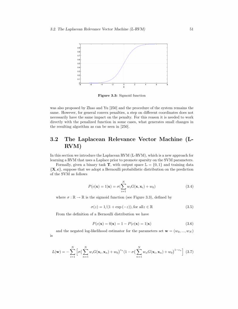
3.2. The Laplacean Relevance Vector Machine (L-RVM) 51

−8 −6 −4 −2 0 2 4 6 80

0.1

0.2

0.3

0.4

0.5

0.6

0.7

0.8

0.9

1

x

Figure 3.3: Sigmoid function

was also proposed by Zhao and Yu [250] and the procedure of the system remains thesame. However, for general convex penalties, a step on different coordinates does notnecessarily have the same impact on the penalty. For this reason it is needed to workdirectly with the penalized function in some cases, what generates small changes inthe resulting algorithm as can be seen in [250].

3.2 The Laplacean Relevance Vector Machine (L-RVM)

In this section we introduce the Laplacean RVM (L-RVM), which is a new approach forlearning a RVM that uses a Laplace prior to promote sparsity on the SVM parameters.

Formally, given a binary task T, with output space L = {0, 1} and training data{X, c}, suppose that we adopt a Bernoulli probabilistic distribution on the predictionof the SVM as follows

P (c(x) = 1|x) = σ(

N∑

i=1

wiG(x,xi) + w0) (3.4)

where σ : R→ R is the sigmoid function (see Figure 3.3), defined by

σ(z) = 1/(1 + exp (−z)), for allz ∈ R (3.5)

From the definition of a Bernoulli distribution we have

P (c(x) = 0|x) = 1− P (c(x) = 1|x) (3.6)

and the negated log-likelihood estimator for the parameters set w = (w0, ..., wN )is

L(w) = −N∑

i=1

[σ( N∑

n=1

wiG(xi,xn) + w0

)cn(1− σ

( N∑

n=1

wnG(xi,xn) + w0

)1−cn

](3.7)

52THE JFSCL AND ITS APPLICATION FOR MULTITASK FEATURE SELECTION

Table 3.2: Comparison of classification performance between RVM and L-RVM.For each used database we show the number of training samples N , the number oftesting samples Ntest, the number of features d, the mean error rates, and the 95%confidence intervals for the RVM and L-RVM algorithms. The results are computedperforming 100 runs with different splits of train and test sets.

Data Set N Ntest d RVM L-RVMPIMA Diabetes 468 300 8 24.10 ± 1.06 23.98± 0.58Breast Cancer 200 77 9 26.04 ± 4.74 26.30 ± 0.80

Heart 170 100 13 16.34 ± 3.53 16.30 ± 0.68

To promote sparsity on the selected vectors we can penalize the loss function L(w)through a constraint such as R(w) = ‖w‖1, getting the following loss function

J(w) = L(w) + λR(w) (3.8)

where λ a positive real value that controls the importance of the regularizationterm R(w).

Given that this optimization corresponds to a Lasso problem, we propose to min-imize this function using the BLasso algorithm. This new formulation of the RVMwill be called the L-RVM.

3.2.1 Experiments and Discussion

In this section we present some experiments to empirically compare the L-RVM withthe classical RVM.

We have used in these tests a Gaussian kernel function G(z1, z2) in the predictionmodel (see equation 3.2),

G(z1, z2) = exp(−γ‖z1 − z2‖22), for all z1, z2 ∈ R

D, (3.9)

where γ is an appropriate positive real value that has been determined by crossvalidation.

We have performed experiments with three binary public databases from the UCIMachine Learning Repository: the PIMA Diabetes, the Breast Cancer, and the Heartdisease data. To train and test the methods we have used public data sets fromhttp://ida.first.fraunhofer.de/projects/bench/benchmarks.htm, and the obtained re-sults are specified in Table 3.2.

We can see that, in these tests, the proposed RVM and L-RVM have performedequivalently in terms of classification, being the average error rates overlapped interms of statistical significance. Notice, however, that the confidence intervals of theL-RVM are smaller than the RVM ones, what suggests that the proposed L-RVMapproach is more stable. In these experiments, the inputs of the method were ε = 1and ξ = 10−5 and have been also determined by cross validation.

3.3. The JFSCL method 53

3.3 The JFSCL method

As stated in the first chapter of this thesis, the classification accuracy of a classifier canbe improved by performing an appropriate feature selection and determining which isthe most suitable subset of variables to be considered during the classification process[96]. In this section we propose an extension of the L-RVM to jointly perform featureselection while the parameters of the classifier are learned. We call this system theJoint Feature Selection and Classifier Learning (JFSCL) algorithm.

For this goal, we add a new parameters vector that will control the activation ofthe relevant features. More concretely, we add a new sum term in the regularizationpart of the global loss function (3.8) obtaining a new cost function that can also beoptimized using the described BLasso algorithm.

To control the activation of the features we consider a function σDκ : R

D → RD

defined as follows

σDκ (z ) = (σκ(z1), ..., σκ(zD)) , for all z ∈ R

D (3.10)

where κ is any positive real value and σκ : R→ R is the sigmoid function,

σκ(z) =1

1 + exp (−κz), for all z ∈ R (3.11)

Let be v = (v1, ..., vD) a new parameters vector and x ∈ RD an input data. Then

consider the following expression

σDκ (v)� x := (σκ(v1)x1, ..., σκ(vD)xD) (3.12)

where � denotes the Hadamark product. Observe, from the definition of thesigmoid function (equation 3.10), that the components of σD

κ (v) take, in general,values very close to 0 or very close to 1, supposing that κ is large enough. Thus,equation (3.12) can express an activation or a deactivation of the kth feature by itscorresponding parameter vk.

After these definitions and observations we can consider a new global loss functionfor the RVM that is constrained by an extended parameter set {w,v}:

J(w,v) = L(w,v) + λ1‖w‖1 + λ2‖σDκ (v)‖1 (3.13)

where

L(w,v) = −N∑

i=1

[σ( N∑

n=1

wiG(σDκ (v)� xi, σ

Dκ (v)� xn) + w0

)cn · (3.14)

·(1− σ( N∑

n=1

wnG(σDκ (v)� xi, σ

Dκ (v)� xn) + w0

)1−cn

](3.15)

This new loss function represents a preference for solutions that use a small setof components from a small set of samples. In this case, a reasonable choice is to

54THE JFSCL AND ITS APPLICATION FOR MULTITASK FEATURE SELECTION

impose the same value for both regularization terms, λ := λ1 = λ2. Thus, we obtainthe following expression of the loss:

J(w,v) = L(w,v) + λ(‖w‖1 + ‖σD

κ (v)‖1)

(3.16)

that can be minimized using the extended version of BLasso, the above mentionedGeneralized BLasso.

3.3.1 Experiments and Discussion

In this section we evaluate different aspects of the JFSCL. For this aim we usedsynthetic data and three binary public databases from the UCI Machine LearningRepository: the PIMA Dabetes, the Breast Cancer and the Heart disease.

First of all we evaluated the performance of the proposed L-RVM and comparedit with the classical RVM approach. After that, we tested the proposed JFSCL usingsynthetic data and performed some experiments to evaluate the sensitivity of themethod to the design parameters. Finally we tested the performance of the JFSCLwith real data and compared this proposed method with other feature selection filters.

As in the experiments of L-RVM and RVM comparison, we have used a Gaussiankernel function in the prediction model, and the parameter γ has been also determinedby cross validation.

JFSCL for synthetic data

In this section we present two synthetic experiments that test the feature selectionperformance of the JFSCL. This first synthetic experiment was designed as follows:D-dimensional data from two Gaussian distributions were generated with means:

µ1 = [1√2,

1√2, 0, . . . , 0] (3.17)

µ2 = [− 1√2,− 1√

2, 0, . . . , 0] (3.18)

and standard deviation 1 for all the components (notice that the distance betweenthe d-dimensional Gaussian distribution centroids is 2). According to the optimallinear classifier, the theoretical Bayes error can be computed exactly for these twosets, and it is 15.19.

In the experiment, 200 samples (100 from each class) have been used for trainingthe classical RVM, the proposed L-RVM, and the proposed JFSCL. The testing setwas composed by 1000 samples (500 from each class). An example of the scatter ofthe first two features and two noise features is shown in Figure 3.4.

Figure 3.5, shows the mean error rate of 20 random generations of the same ex-periment, as a function of the space dimensionality. As can be observed, the influenceof adding spurious features on the RVM and L-RVM confused the classifier, while theJFSCL kept a quite constant error rate that is close to the Bayes error. Moreover,the method focused itself on the first two features, the ones with class separabilityinformation.

3.3. The JFSCL method 55

−4 −3 −2 −1 0 1 2 3 4−4

−3

−2

−1

0

1

2

3

4

(a) Scatter of the two first features from the Gaussian set

−4 −3 −2 −1 0 1 2 3 4−4

−3

−2

−1

0

1

2

3

4

(b) Scatter of two noise features from the Gaussian set

Figure 3.4: Scatter of samples from the synthetic Gaussian data set. Symbol (+)represents points from class 1 and symbol (.) represents points from class 2.

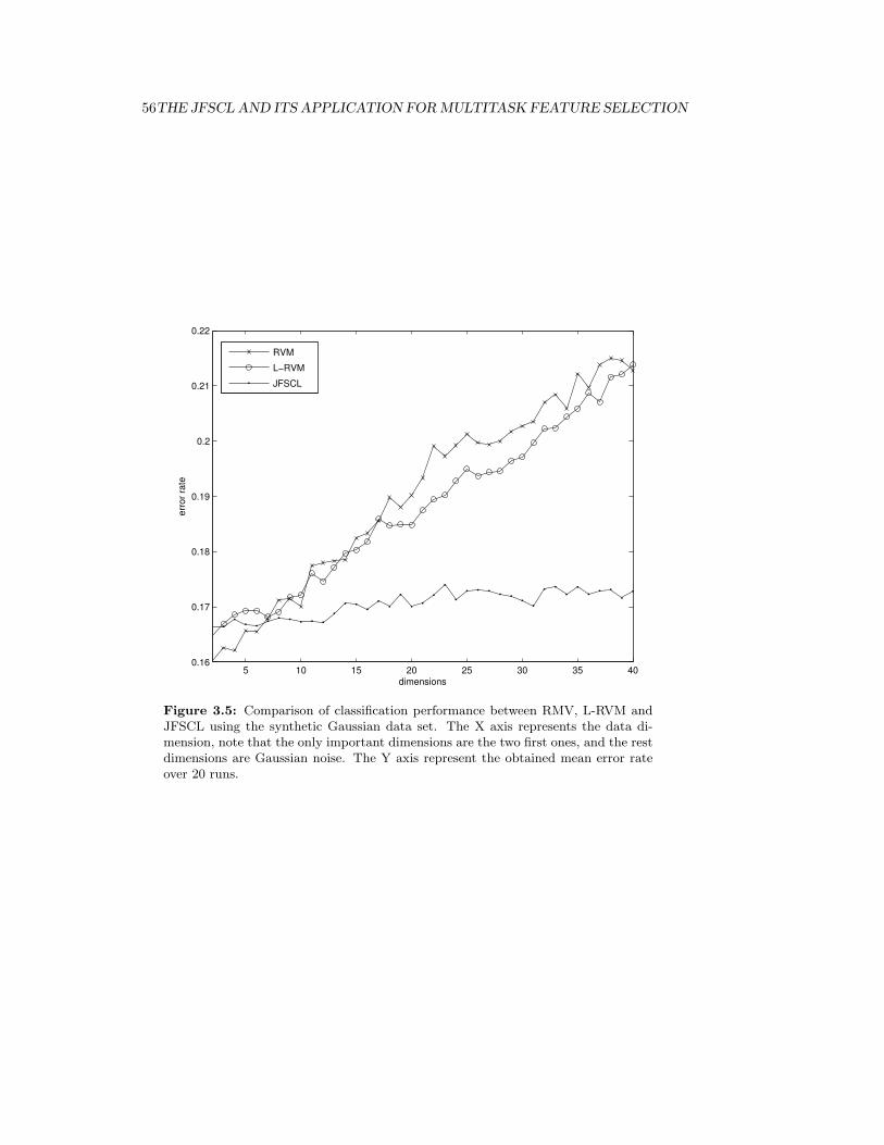
56THE JFSCL AND ITS APPLICATION FOR MULTITASK FEATURE SELECTION

5 10 15 20 25 30 35 400.16

0.17

0.18

0.19

0.2

0.21

0.22

dimensions

erro

r rat

e

RVM

L−RVM

JFSCL

Figure 3.5: Comparison of classification performance between RMV, L-RVM andJFSCL using the synthetic Gaussian data set. The X axis represents the data di-mension, note that the only important dimensions are the two first ones, and the restdimensions are Gaussian noise. The Y axis represent the obtained mean error rateover 20 runs.

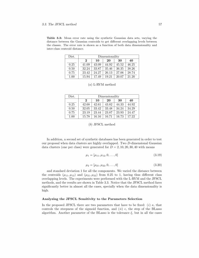
3.3. The JFSCL method 57

Table 3.3: Mean error rate using the synthetic Gaussian data sets, varying thedistance between the Gaussian centroids to get different overlapping levels betweenthe classes. The error rate is shown as a function of both data dimensionality andinter-class centroid distance.

Dist. Dimensionality

0.250.500.751.00

2 10 20 30 4041.09 43.09 44.92 45.52 46.2532.24 33.87 35.46 36.35 38.2623.42 24.27 26.13 27.06 28.7415.94 17.49 19.21 20.07 21.20

(a) L-RVM method

Dist. Dimensionality

0.250.500.751.00

2 10 20 30 4042.68 42.61 43.82 44.33 44.9232.05 33.42 33.48 34.24 34.2923.19 23.44 23.87 23.93 24.4715.78 16.16 16.71 16.73 17.22

(b) JFSCL method

In addition, a second set of synthetic databases has been generated in order to testour proposal when data clusters are highly overlapped. Two D-dimensional Gaussiandata clusters (one per class) were generated for D = 2, 10, 20, 30, 40 with means

µ1 = [µ11, µ12, 0, . . . , 0] (3.19)

µ2 = [µ21, µ22, 0, . . . , 0] (3.20)

and standard deviation 1 for all the components. We varied the distance betweenthe centroids (µ11, µ12) and (µ21, µ22) from 0.25 to 1, having thus different classoverlapping levels. The experiments were performed with the L-RVM and the JFSCLmethods, and the results are shown in Table 3.3. Notice that the JFSCL method faressignificantly better in almost all the cases, specially when the data dimensionality ishigh.

Analyzing the JFSCL Sensitivity to the Parameters Selection

In the proposed JFSCL there are two parameters that have to be fixed: (i) κ, thatcontrols the steepness of the sigmoid function, and (ii) ε, the step of the BLassoalgorithm. Another parameter of the BLasso is the tolerance ξ, but in all the cases

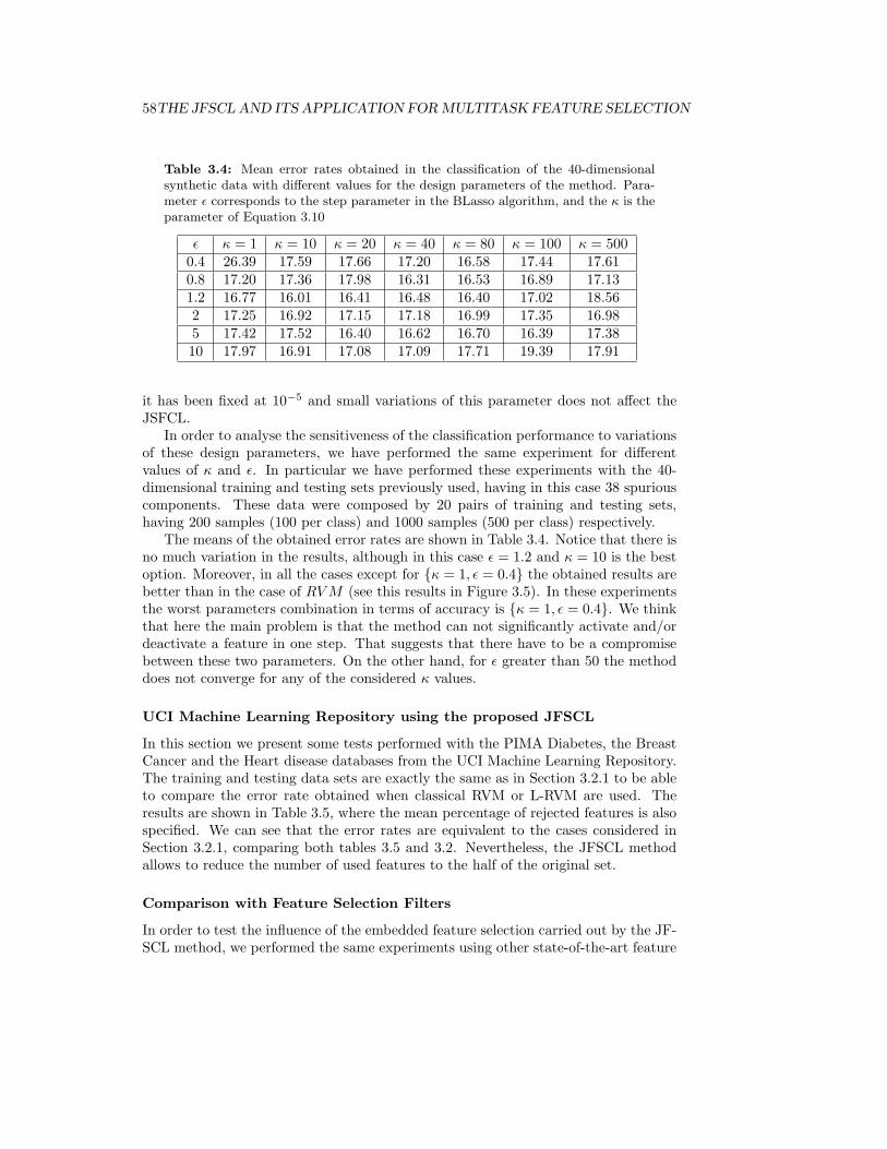
58THE JFSCL AND ITS APPLICATION FOR MULTITASK FEATURE SELECTION

Table 3.4: Mean error rates obtained in the classification of the 40-dimensionalsynthetic data with different values for the design parameters of the method. Para-meter ε corresponds to the step parameter in the BLasso algorithm, and the κ is theparameter of Equation 3.10

ε κ = 1 κ = 10 κ = 20 κ = 40 κ = 80 κ = 100 κ = 5000.4 26.39 17.59 17.66 17.20 16.58 17.44 17.610.8 17.20 17.36 17.98 16.31 16.53 16.89 17.131.2 16.77 16.01 16.41 16.48 16.40 17.02 18.562 17.25 16.92 17.15 17.18 16.99 17.35 16.985 17.42 17.52 16.40 16.62 16.70 16.39 17.3810 17.97 16.91 17.08 17.09 17.71 19.39 17.91

it has been fixed at 10−5 and small variations of this parameter does not affect theJSFCL.

In order to analyse the sensitiveness of the classification performance to variationsof these design parameters, we have performed the same experiment for differentvalues of κ and ε. In particular we have performed these experiments with the 40-dimensional training and testing sets previously used, having in this case 38 spuriouscomponents. These data were composed by 20 pairs of training and testing sets,having 200 samples (100 per class) and 1000 samples (500 per class) respectively.

The means of the obtained error rates are shown in Table 3.4. Notice that there isno much variation in the results, although in this case ε = 1.2 and κ = 10 is the bestoption. Moreover, in all the cases except for {κ = 1, ε = 0.4} the obtained results arebetter than in the case of RV M (see this results in Figure 3.5). In these experimentsthe worst parameters combination in terms of accuracy is {κ = 1, ε = 0.4}. We thinkthat here the main problem is that the method can not significantly activate and/ordeactivate a feature in one step. That suggests that there have to be a compromisebetween these two parameters. On the other hand, for ε greater than 50 the methoddoes not converge for any of the considered κ values.

UCI Machine Learning Repository using the proposed JFSCL

In this section we present some tests performed with the PIMA Diabetes, the BreastCancer and the Heart disease databases from the UCI Machine Learning Repository.The training and testing data sets are exactly the same as in Section 3.2.1 to be ableto compare the error rate obtained when classical RVM or L-RVM are used. Theresults are shown in Table 3.5, where the mean percentage of rejected features is alsospecified. We can see that the error rates are equivalent to the cases considered inSection 3.2.1, comparing both tables 3.5 and 3.2. Nevertheless, the JFSCL methodallows to reduce the number of used features to the half of the original set.

Comparison with Feature Selection Filters

In order to test the influence of the embedded feature selection carried out by the JF-SCL method, we performed the same experiments using other state-of-the-art feature

3.3. The JFSCL method 59

Table 3.5: Obtained results (mean error rate and 95% confidence interval) usingthe JFSCL, and mean number of rejected features (in percentage).

DataSet JFSCL Error rate Rejected FeaturesPIMA Diabetes 24.23 ± 0.34 48.33%Breast Cancer 26.52 ± 0.92 41.25%

Heart 16.28 ± 0.65 31.15%

Table 3.6: PIMA Diabetes Database experiments. Obtained results (mean errorand 95% confidence interval) using the state-of-the-art feature selection methodsFSF, BSF, FR and FS, per number of selected features (from 1 to 7). Notice thatthe proposed JFSCL method selected in this case 51.66% of the features (between 4and 5 components) and obtained an error of 24.23 ± 0.34.

FSF BSF FR FS1 33.11± 0.57 30.66± 0.78 33.11± 0.57 26.46± 0.242 25.19± 0.49 25.38± 0.45 28.59± 0.71 26.43± 0.273 24.46± 0.43 24.98± 0.51 23.90± 0.52 25.86± 0.284 24.48± 0.37 24.66± 0.37 23.37± 0.32 24.91± 0.235 24.51± 0.38 24.56± 0.43 23.74± 0.32 24.60± 0.246 24.15± 0.35 24.31± 0.36 23.95± 0.33 24.78± 0.227 24.40± 0.39 24.26± 0.36 24.20± 0.32 24.66± 0.21

selection techniques. In all the cases we ran the feature selection algorithm select-ing from one up to the maximum number of features (all the possibilities) and thenperformed the classification with the L-RVM classifier.

We have applied the following feature selection filters: (a) Forward Feature Se-lection (FFS) [191],(b) Backward Feature Selection (BFS) [1], (c) Feature Ranking(FR) using 1-Nearest Neighbor leave-one-out [96], and (d) Floating Search (FS) [193].

The results obtained in these tests are shown in tables 3.6, 3.7, 3.8. Notice that inthe Heart database experiments, the JFSCL performs always better than the othermethods. However, with the other databases there are methods that perform as wellas the proposed JFSCL. For instance, with the PIMA Diabetes database the bestaccuracy is obtained with Feature Ranking using 5 features, being the error 23.74%.Nevertheless, although this result is slightly better that the 24.23% obtained withthe JFSCL, the difference is not statistically significant, given that the confidenceintervals are overlapped. On the other hand, notice that the tested state-of-the-artfeature selection methods are not able to automatically fix the number of neededfeatures, while the proposed JFSCL can automatically select both the features andthe number of features. Moreover, these results suggest that the number of featuresselected by the JFSCL is the most appropriated. For instance, in the case of PIMADiabetes Database the best accuracy is obtained using 5 features and the JFSCLselects in this case between 4 and 5 features. A similar behavior can be observed inthe results obtained with the other databases.

60THE JFSCL AND ITS APPLICATION FOR MULTITASK FEATURE SELECTION

Table 3.7: Breast Cancer Database experiments. Obtained results (mean error and95% confidence interval) using the state-of-the-art feature selection methods FSF,BSF, FR and FS, per number of selected features (from 1 to 8) . Notice that theproposed JFSCL method selected in this case 58.75% of the features (between 5 and6 components) and obtained an error of 26.52 ± 0.92.

FSF BSF FR FS1 28.80± 0.90 28.82± 0.89 28.80± 0.90 28.81± 0.902 28.90± 0.90 29.07± 0.89 28.80± 0.90 25.16± 0.963 29.16± 0.87 29.56± 0.89 28.80± 0.90 24.83± 0.824 29.31± 0.91 28.38± 0.97 28.32± 0.90 25.48± 0.825 27.17± 1.00 27.31± 0.94 26.58± 0.92 26.04± 0.826 26.40± 0.95 26.78± 0.90 25.21± 0.9 26.30± 0.977 26.13± 0.83 26.23± 0.86 25.21± 0.89 26.62± 0.828 25.86± 0.89 25.54± 0.94 25.61± 0.84 26.62± 0.87

Table 3.8: Heart Database experiments. Obtained results (mean error and 95%confidence interval) using the state-of-the-art feature selection methods FSF, BSF,FR and FS, per number of selected features (from 1 to 12). Notice that the pro-posed JFSCL method selected in this case 68.85% of the features (between 8 and 9components) and obtained an error of 16.28 ± 0.65.

FSF BSF FR FS1 42.84± 1.11 38.90± 1.65 42.84± 1.11 23.47± 0.702 30.39± 1.10 29.35± 1.08 37.30± 1.22 24.32± 0.793 26.44± 0.94 24.35± 0.80 33.35± 0.97 19.75± 0.794 24.08± 0.76 21.07± 0.86 31.08± 0.96 18.08± 0.785 2.22± 0.85 20.10± 0.79 28.16± 0.92 17.65± 0.756 20.64± 0.73 19.80± 0.75 24.40± 0.83 17.52± 0.797 19.83± 0.73 19.25± 0.70 23.31± 0.85 16.90± 0.698 19.78± 0.66 18.76± 0.73 24.31± 0.78 16.94± 0.699 19.11± 0.71 18.69± 0.75 23.54± 0.81 16.98± 0.7510 18.72± 0.69 18.08± 0.73 21.97± 1.00 16.76± 0.7511 18.52± 0.74 18.19± 0.75 19.27± 0.88 16.96± 0.6712 17.90± 0.74 17.76± 0.68 18.79± 0.80 17.11± 0.68

3.4. Performing Multitask Feature Selection with the JFSCL method 61

3.4 Performing Multitask Feature Selection with theJFSCL method

In this section we show how the JFSCL can be extended to the MTL paradigm. Themain idea is to learn a specific classifier per task but performing a common featureselection.

Formally, let be T1, . . . ,TM a set of binary tasks, with respective training data{X1, c1}, . . . , {XM , cM}, where each {Xt, ct} is composed of N training samples withtheir corresponding class labels according to the t-th task, t = 1, . . . ,M . Let bew1, . . . ,wM a set N -dimensional vectors of parameters, one per task, and v a D-dimensional vector of parameters. The MTL extension of JFSCL (MTL-JFSCL)aims to minimize the following global loss function

L(w1, . . . ,wM ,v) =M∑

t=1

Lt(wT ,v) + λ[ M∑

t=1

‖wt‖1 + ‖v‖1]

(3.21)

where each Lt(wT ,v) corresponds to the negated log-likelihood for the t-th task,as in equation 3.15, and v controls the activation and deactivation of the features(common for all the tasks), as detailed in equation 3.12.

Under this formulation, the global loss function to be minimized, L(w1, . . . ,wM ,v),is composed of two parts. The first one is the negated log-likelihoods of the M tasks,∑M

t=1 Lt(wT , v), which expres the empirical loss of the predictors, and the second is a

regularization term,[ ∑M

t=1 ‖wt‖1 +‖v‖1], which enforces the sparsity on the vectors

wt as well as the common feature selection. This function can be also optimized usingthe Blasso algorithm, as in the case of JFSCL.

3.4.1 Experiments and Discussion

We have tested the MTL-JFSCL performing two gender classification experimentswith the ARFace database. We have considered just the image types 1,5,6 and 7,corresponding to neutral frontal image, left light on, right light on, and both lightson. This image types are shown in Figure 3.6. We have performed 20 rounds of eachexperiment, randomly selecting the training and the testing sets according to the cor-responding protocol. In these experiments we used as data just the subwindow of theinternal part of the face, at 33× 34 pixels. Moreover we reduced the data dimension-ality using PCA, getting a new sample representation in a 100-dimensionality featurespace.

To avoid the parameter fitting of the Gaussian Kernel we used in these experimentsa quadratic kernel,

G(z1, z2) = (z1z2)2 =

100∑

j=1

[z1jz2j

]2, for all z1, z2 ∈ R

100, (3.22)

In the first experiment the training set was composed of 10% of the people (around8-9 persons), including one image per person randomly selected among the 4 possible

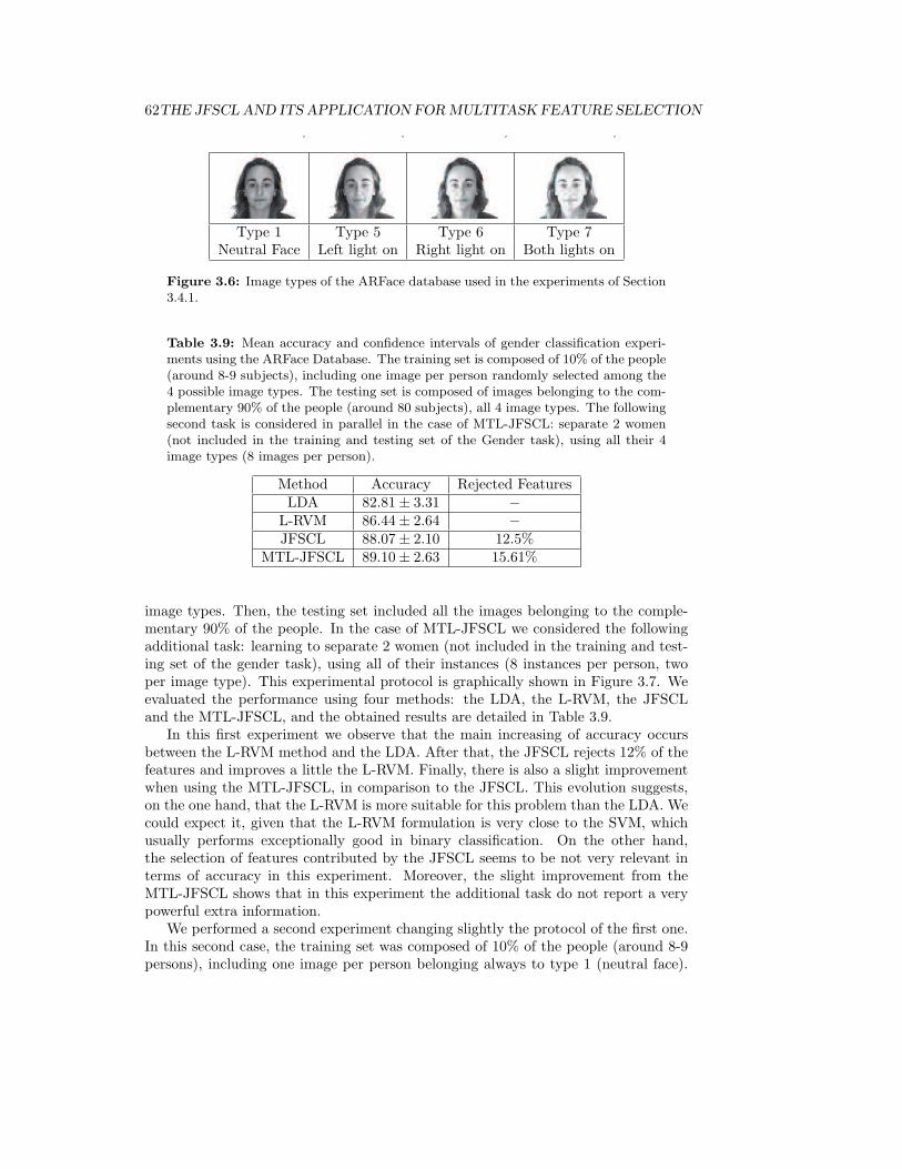
62THE JFSCL AND ITS APPLICATION FOR MULTITASK FEATURE SELECTION

Type 1 Type 5 Type 6 Type 7Neutral Face Left light on Right light on Both lights on

Figure 3.6: Image types of the ARFace database used in the experiments of Section3.4.1.

Table 3.9: Mean accuracy and confidence intervals of gender classification experi-ments using the ARFace Database. The training set is composed of 10% of the people(around 8-9 subjects), including one image per person randomly selected among the4 possible image types. The testing set is composed of images belonging to the com-plementary 90% of the people (around 80 subjects), all 4 image types. The followingsecond task is considered in parallel in the case of MTL-JFSCL: separate 2 women(not included in the training and testing set of the Gender task), using all their 4image types (8 images per person).

Method Accuracy Rejected FeaturesLDA 82.81± 3.31 −

L-RVM 86.44± 2.64 −JFSCL 88.07± 2.10 12.5%

MTL-JFSCL 89.10± 2.63 15.61%

image types. Then, the testing set included all the images belonging to the comple-mentary 90% of the people. In the case of MTL-JFSCL we considered the followingadditional task: learning to separate 2 women (not included in the training and test-ing set of the gender task), using all of their instances (8 instances per person, twoper image type). This experimental protocol is graphically shown in Figure 3.7. Weevaluated the performance using four methods: the LDA, the L-RVM, the JFSCLand the MTL-JFSCL, and the obtained results are detailed in Table 3.9.

In this first experiment we observe that the main increasing of accuracy occursbetween the L-RVM method and the LDA. After that, the JFSCL rejects 12% of thefeatures and improves a little the L-RVM. Finally, there is also a slight improvementwhen using the MTL-JFSCL, in comparison to the JFSCL. This evolution suggests,on the one hand, that the L-RVM is more suitable for this problem than the LDA. Wecould expect it, given that the L-RVM formulation is very close to the SVM, whichusually performs exceptionally good in binary classification. On the other hand,the selection of features contributed by the JFSCL seems to be not very relevant interms of accuracy in this experiment. Moreover, the slight improvement from theMTL-JFSCL shows that in this experiment the additional task do not report a verypowerful extra information.

We performed a second experiment changing slightly the protocol of the first one.In this second case, the training set was composed of 10% of the people (around 8-9persons), including one image per person belonging always to type 1 (neutral face).

3.4. Performing Multitask Feature Selection with the JFSCL method 63

Figure 3.7: Protocol of the first experiment for testing the MTL-JFSCL

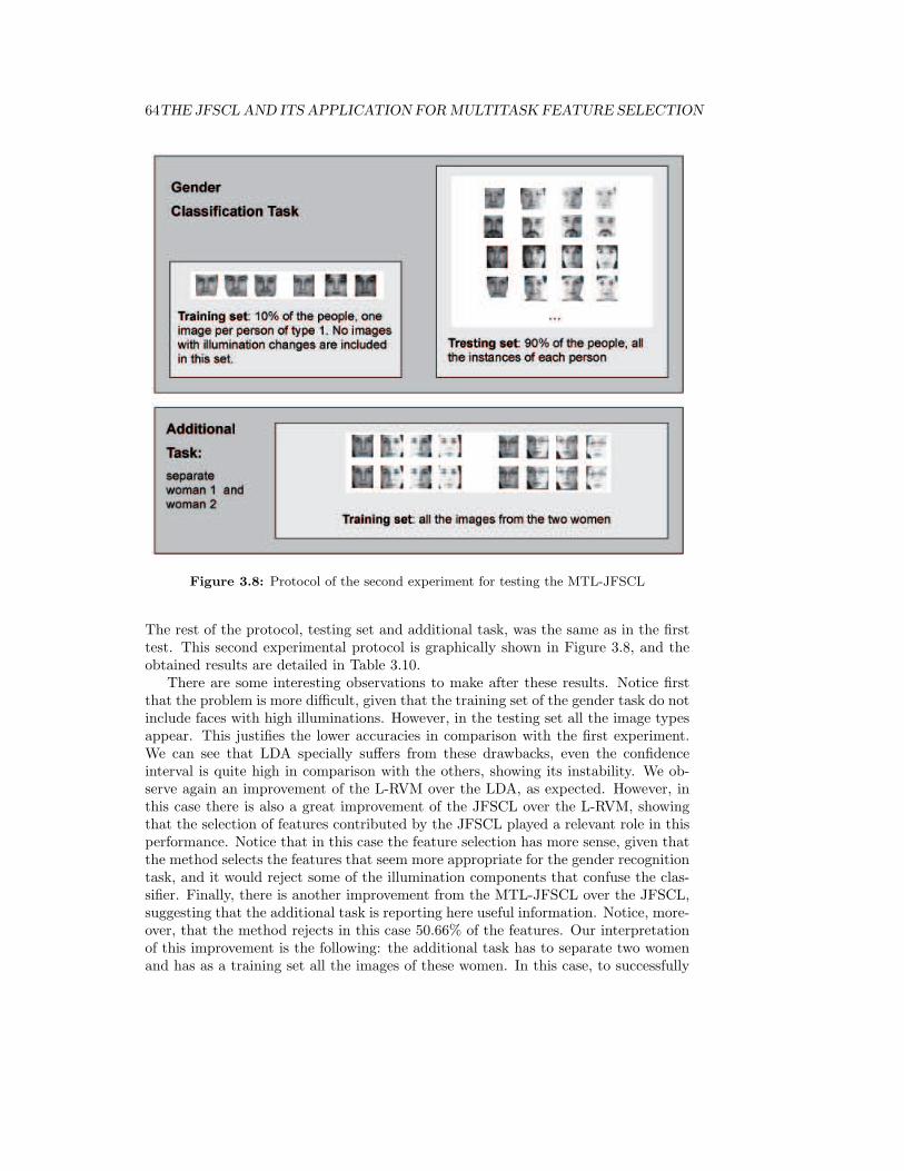
64THE JFSCL AND ITS APPLICATION FOR MULTITASK FEATURE SELECTION

Figure 3.8: Protocol of the second experiment for testing the MTL-JFSCL

The rest of the protocol, testing set and additional task, was the same as in the firsttest. This second experimental protocol is graphically shown in Figure 3.8, and theobtained results are detailed in Table 3.10.

There are some interesting observations to make after these results. Notice firstthat the problem is more difficult, given that the training set of the gender task do notinclude faces with high illuminations. However, in the testing set all the image typesappear. This justifies the lower accuracies in comparison with the first experiment.We can see that LDA specially suffers from these drawbacks, even the confidenceinterval is quite high in comparison with the others, showing its instability. We ob-serve again an improvement of the L-RVM over the LDA, as expected. However, inthis case there is also a great improvement of the JFSCL over the L-RVM, showingthat the selection of features contributed by the JFSCL played a relevant role in thisperformance. Notice that in this case the feature selection has more sense, given thatthe method selects the features that seem more appropriate for the gender recognitiontask, and it would reject some of the illumination components that confuse the clas-sifier. Finally, there is another improvement from the MTL-JFSCL over the JFSCL,suggesting that the additional task is reporting here useful information. Notice, more-over, that the method rejects in this case 50.66% of the features. Our interpretationof this improvement is the following: the additional task has to separate two womenand has as a training set all the images of these women. In this case, to successfully

3.5. Conclusions 65

Table 3.10: Mean accuracy and confidence intervals of gender classification experi-ments using the ARFace Database. The training set is composed of 10% of the people(around 8-9 subjects), including one image of type 1 per person. The testing set iscomposed of images belonging to the complementary 90% of the people (around 80subjects), all 4 image types. The following second task is considered in parallel inthe case of MTL-JFSCL: separate 2 women (not included in the training and testingset of the Gender task), using all their 4 image types (8 images per person).

Method Accuracy Rejected FeaturesLDA 69.97± 5.59 −

L-RVM 75.81± 2.76 −JFSCL 83.75± 3.24 10.16%

MTL-JFSCL 87.63± 3.13 50.66%

perform this task, the method rejects all the features containing information from thelight variations. If the method would not do this, the two images of the same typefrom the different women would be confused. Then, given that the feature selectionis common to both tasks, the gender task does not use these rejected features, whichsupposedly contain information from the illumination. Thus, the obtained predictor isless sensitive to the illumination variations, and has a better generalization capacity.

3.5 Conclusions

In this chapter we presented the JFSCL method, an embedded algorithm for featureselection and classifier learning. The algorithm is easily scalable to the MTL para-digm in order to perform a common feature selection for different tasks, while theirrespective predictors are learned.

The JFSCL method was developed after the idea of exploring sparse MTL meth-ods. It is based on a Bayesian formulation of the RVM, a sparse approach of the SVM.This new formulation of the RVM is called the L-RVM and uses the Lasso problemfor learning the classifier. More concretely, the predictor is learned by minimizing anempirical loss with L1 penalty using the BLasso algorithm. Then, the L-RVM can beextended to the JFSCL, adding a new vector of parameters that controls the activa-tion and deactivation of the features. And, finally, the JFSCL can be easily scaled toperform a common feature selection for different tasks, yielding to the MTL-JFSCL.

We have performed several experiments to test both L-RVM and JFSCL. First,we have seen that the proposed L-RVM can perform as well as the classical RVMapproach. The main advantages of the L-RVM is that we do not have to computeany derivative of the model and, moreover, the approach can be easily extended, forinstance, imposing other constraints on the parameters set.

On the other hand, we have tested the JFSCL using both synthetic data andreal data. In the case of the synthetic data, where the problem is specially designedaccording to the assumptions of the method, we can see that the JFSCL performsconsiderably better than the L-RVM or the classical RVM. However, this differenceis not evident in the case of real data. In this second case the JFSCL can perform as

66THE JFSCL AND ITS APPLICATION FOR MULTITASK FEATURE SELECTION

well as the L-RVM while it uses less features (just the selected ones).Finally we have tested the MTL-JFSCL with two gender classification experi-

ments. We have empirically seen that the contribution of the MTL principles of thismethod depend on the considered tasks, as expected. In the first experiment with theMTL-JFSCL we could appreciate just a slight improvement over the JFSCL. However,in the second experiment the improvement was higher. This is because in this secondexperiment the additional task contributes with more useful information, given thatthe training set of the gender classification task was less representative than in thefirst experiment. The additional task inhibited the main task from the effects of thefeatures related to illumination changes, even when the training set of the main taskdid not include images with highlights.

After our experiments with the JFSCL and the MTL-JFSCL in the face classifi-cation domains, we think that feature selection is not a very suitable dimensionalityreduction strategy for automatic face classification problems. It is better to performa feature extraction, transforming the initial feature set into a new lower-dimensionalone, instead of just selecting relevant features. From a theoretic point of view, theJFSCL is easily scalable to perform a joint linear feature extraction and classifierlearning. However, in the case of linear feature extraction, we need as a parametersset the matrix of the transformation instead of a vector to control the activation anddeactivation of the features. Then, the new loss function could not be optimized withthe BLasso algorithm because of the computational complexity of the problem. Noticethat, in order to to perform an embedded linear feature extraction, the method has tolearn a (d ×D)-dimensional matrix, where d would be the new data dimensionality,instead of a D-dimensional vector.

One important issue of the proposed JFSCL is the following: it can be seen asa meta-method to jointly learn a classifier and, at the same time, select the mostappropriate features to consider. This methodology could be applied to other lossfunctions and classifiers. On the other hand, given the classifier embedded nature ofthe JFSCL, density estimations on the data sets are avoided.

Chapter 4

Multitask Learning Techniques forClassification

In this chapter we present MTL extensions of two well known Bayesian classifiers: theLogistic Regression and the Quadratic Classifier. In both cases the MTL approach isbased on a regularization constraint on the parameters of the models, that promotesthe knowledge transfer among the different tasks. The proposed MTL systems aretested in the domain of face classification, performing different verification tasks inparallel. Moreover we also performed some tests with some databases of the UCIMachine Learning Repository.

The proposed MTL extension of the Quadratic Classifier is able to automaticallydetermine the degree of relatedness among the tasks. Thus, the method can controlthe quantity of information shared across the problems, depending on their similar-ity. However, the MTL extension of the Logistic Regression model does not havethis property. As we will see in the experiments, this difference between the twoproposed approaches will illustrate the importance of studying the relatedness amongthe involved tasks.

The organization of the chapter is the following: there are two main sections,one for the Quadratic Classifier and the other one for the Logistic Regression Model.These two sections are structured in a similar way. First we briefly review the batchmethod, second we describe the proposed MTL extension, and then we show theperformed experiments. Finally, the last section concludes the chapter.

4.1 The Quadratic Classifier

The quadratic classifier is named after the type of discriminant function it uses [148].It separates measurements of two different classes by a quadratic surface. Moreover,this methodology is frequently applied in K-multi-class classification problems, learn-ing K classifiers with a one-versus-all strategy [202]. In this case, the K discriminantfunctions are learned by a transformation from the posterior probabilities, using aMaximum A Posteriori (MAP) approach.

Formally, let be X = {x1, . . . ,xN} the set of training samples, each one belonging

67

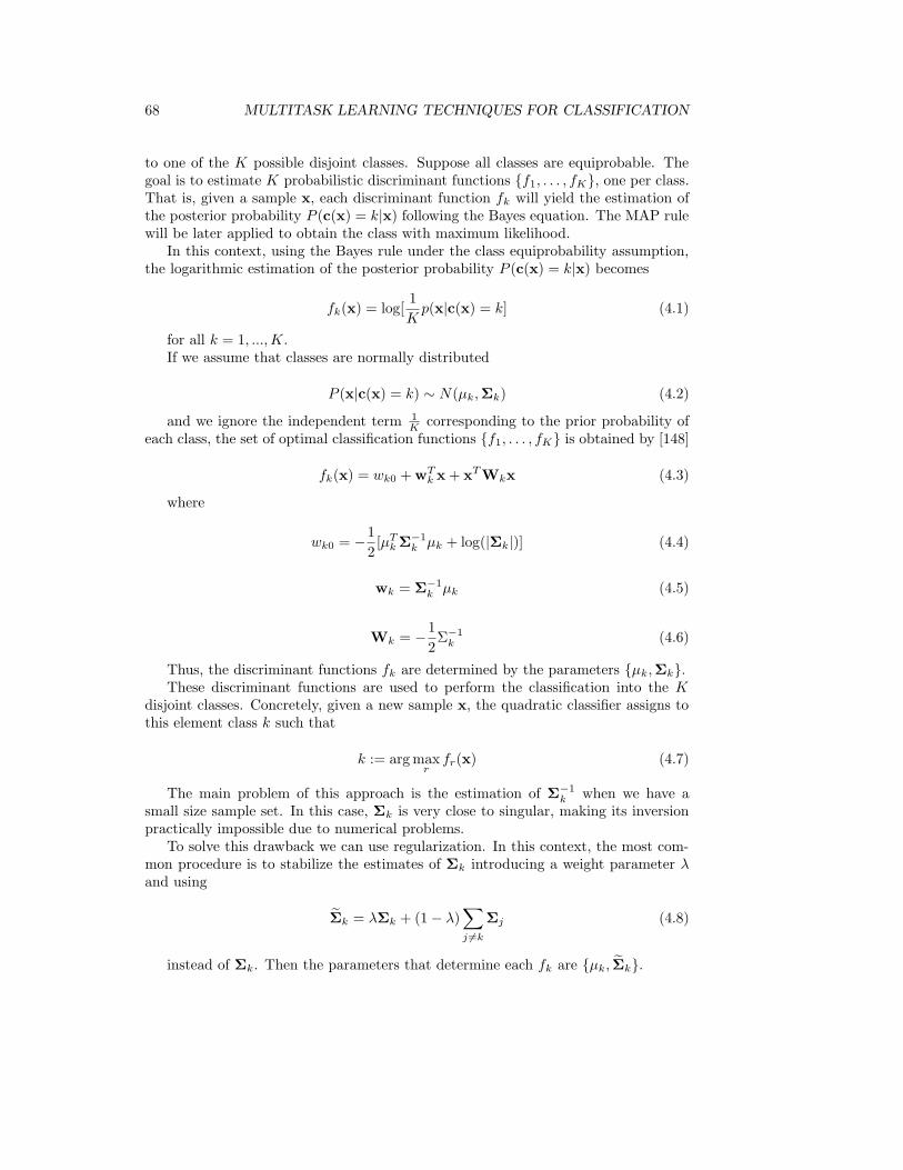
68 MULTITASK LEARNING TECHNIQUES FOR CLASSIFICATION

to one of the K possible disjoint classes. Suppose all classes are equiprobable. Thegoal is to estimate K probabilistic discriminant functions {f1, . . . , fK}, one per class.That is, given a sample x, each discriminant function fk will yield the estimation ofthe posterior probability P (c(x) = k|x) following the Bayes equation. The MAP rulewill be later applied to obtain the class with maximum likelihood.

In this context, using the Bayes rule under the class equiprobability assumption,the logarithmic estimation of the posterior probability P (c(x) = k|x) becomes

fk(x) = log[1

Kp(x|c(x) = k] (4.1)

for all k = 1, ...,K.If we assume that classes are normally distributed

P (x|c(x) = k) ∼ N(µk,Σk) (4.2)

and we ignore the independent term 1K

corresponding to the prior probability ofeach class, the set of optimal classification functions {f1, . . . , fK} is obtained by [148]

fk(x) = wk0 + wTk x + xT Wkx (4.3)

where

wk0 = −1

2[µT

k Σ−1k µk + log(|Σk|)] (4.4)

wk = Σ−1k µk (4.5)

Wk = −1

2Σ−1

k (4.6)

Thus, the discriminant functions fk are determined by the parameters {µk,Σk}.These discriminant functions are used to perform the classification into the K

disjoint classes. Concretely, given a new sample x, the quadratic classifier assigns tothis element class k such that

k := arg maxr

fr(x) (4.7)

The main problem of this approach is the estimation of Σ−1k when we have a

small size sample set. In this case, Σk is very close to singular, making its inversionpractically impossible due to numerical problems.

To solve this drawback we can use regularization. In this context, the most com-mon procedure is to stabilize the estimates of Σk introducing a weight parameter λand using

Σk = λΣk + (1− λ)∑

j 6=k

Σj (4.8)

instead of Σk. Then the parameters that determine each fk are {µk, Σk}.

4.1. The Quadratic Classifier 69

We state that the learning of each fk is a task, and thus we can see the K classclassification problem as the problem of simultaneously learning K different tasks.Notice, then, that the described regularization approach promotes different tasks toshare information in a parametrical context, given that every discriminant function fk

is estimated using information from the other tasks. For this reason we consider thisregularization framework as a MTL approach for estimating f1, ..., fK , i.e. a simplesolution that considers all tasks equally related. However, this regularization may benot appropriated when the covariances of different tasks differ too much, yielding tofunctions that can be very biased from the reality.

4.1.1 A Multitask Extension

In order to deal with small sized training set problems, and to avoid the mentioneddrawback of the classical regularization, we propose to approximate each Σk by aweighted average of the covariance matrices corresponding to the other r-th tasksthat are related with the k-th task, r 6= k. We will assume that tasks relatednesscan be measured and quantified by a distance metric in the parameter space of thediscriminant functions. Concretely, we conjecture that related tasks can be solved bysimilar classifiers, therefore the parameters governing these classification tasks can beused to measure the degree of relatedness between tasks.

Formally, let be Tk and Tr two different tasks. We suppose that Tk and Tr arerelated if their covariance matrices Σk and Σr are similar. Thus, each Σk can beestimated by

Σk =K∑

r=1

λkrΣr (4.9)

where λkr are weights computed according to the following considerations:

1. First, the weight λkk ∈ [0, 1] is selected

2. Then, the other weights λkr, r 6= k have to be proportional to the similaritybetween Σk and Σr, and have to verify

∑r 6=k λkr = (1− λkk).

Thus, we control first the contribution of Σk to the weighted mean Σk by λkk

(that can be empirically fixed by cross validation), and then the importance of theother Σr, r 6= k, will depend on the task relatedness between Tk and Tr.

To compute these parameters λkr, r 6= k, (point 2), we need first to estimate thesimilarity between two tasks, meaning here the similarity between their covariancematrices. For this purpose we use a covariance matrices distance proposed by Brum-mer and Strydom [39], which is related to the Gaussian log-likelihood measure [27].More specifically, we compute the distance between two covariance matrices Σk andΣr by

d(Σk,Σr) =‖ Φ(log(Σk))− Φ(log(Σr)) ‖2 (4.10)

where ‖ ‖ is the Euclidean distance and Φ is the transformation from Rn×n to

vectors in Rn+(n−1)+(n−2)...+1 illustrated in Figure 4.1.

70 MULTITASK LEARNING TECHNIQUES FOR CLASSIFICATION

Figure 4.1: Transformation function to compute the distance between covariancematrices.

Now, let us denote by

dkr := d(Σk,Σr) (4.11)

the corresponding distances according to the above definition, and

Dk =

K∑

r=1

d−1kr (4.12)

We propose to compute the weights λkr in equation 5.55, r 6= k, as

λkr :=1− λkk

dkrDk

(4.13)

Notice that we are assuming that dkr 6= 0 for all r 6= k, what means that Σk 6= Σr.Consequently we have that Dk 6= 0 for all r = 1, ...,K. Then, λkr are well defined.

4.1.2 Experiments and Discussion

We performed different tests in order to show the improvement obtained with theproposed Bayesian MTL estimation. We used in the experiments the publicly availableARFace database [152] and the subset of FRGC [187] database composed of the imagesacquired in controlled environments. We include from FRGC just those subjectshaving at least 26 images. We joined these two databases in order to obtain a dataset with more subjects and more variability among the images, and we always usedthese composed set in all the experiments.

We have aligned all the images according to the eyes and we used just the internalfeatures in a resolution of 36×33 pixels. Moreover, in all the experiments we reduced

4.1. The Quadratic Classifier 71

10 20 30 40 500.5

0.55

0.6

0.65

0.7

0.75

0.8

0.85

0.9

0.95

1

Number of classes

Rec

ogni

tion

perfo

rman

ce

Subject Recognition

Single TaskClassic RegularizationMultitask

Figure 4.2: Subject Recognition for 10, 20, 30, 40, 50 classes.

the data dimensionality with Principal Component Analysis, learning with the train-ing set the projection that keeps a number of features corresponding to 80% of thedata variance.

We performed 100 rounds of all the experiments here presented. Subjects andimages for the training and testing sets have been always randomly selected at eachround. Moreover, the parameter λ of the proposed MTL approaches has been fixedto 0.4 in all the cases by cross-validation.

The first experiment is subject recognition, considering 10, 20, 30, 40 and 50different subjects. In this case we used 11 images per class to train the models, whilethe rest of the images (at least 15) were used in the testing step. We computed theaccuracies obtained by the single task approach, the classical regularization and theproposed MTL approach, and they are shown in Figure 4.2.

The second experiment is subject recognition fixing the number of classes (50).We have computed the mean accuracies obtained depending on the number of imagesper subject included in the training set. The mean results obtained by the single taskapproach, the classical regularization and the proposed MTL approach are shown inFigure 4.3. Notice that in the single task case we can not compute the models whenwe have 5 samples per subject or less, because of numerical problems in the inversionof the covariances.

The third experiment is subject recognition with all the subjects in ARFace andFRGC having 26 images or more (113 different persons). We used 11 images persubject to build the training sets. We show in Table 4.1 the mean accuracies obtainedby the single task approach, the classical regularization and the proposed MTL ap-proach. Moreover, we include as a performance reference the accuracies obtained byPCA and FLD with the Nearest Neighbor Classifier.

Finally, in order to show the relevance of the MTL approach, we plot in Figure4.4 ROC curves for subject verification experiments with the proposed Bayesian MTL

72 MULTITASK LEARNING TECHNIQUES FOR CLASSIFICATION

2 4 6 8 10 12 14 16 18 200.1

0.2

0.3

0.4

0.5

0.6

0.7

0.8

Number of training samples per class

Rec

ogni

tion

accu

racy

Subject Recognition, 50 subjects

Single Task approachClassical RegularizationMultitask approach

Figure 4.3: Subject recognition according to the number of images per subject inthe training set.

Table 4.1: Subject recognition using the all the subjects of ARFace database and FRGCDatabase having at least 26 images (113 subjects)

Method Accuracy

PCA + NN 44.65%± 0.12%FLD + NN 53.85%± 1.54%Single Task 28.71%± 1.63%

Classical Regularization 53.77%± 0.18%MTL Bayesian 56.25%± 0.20%

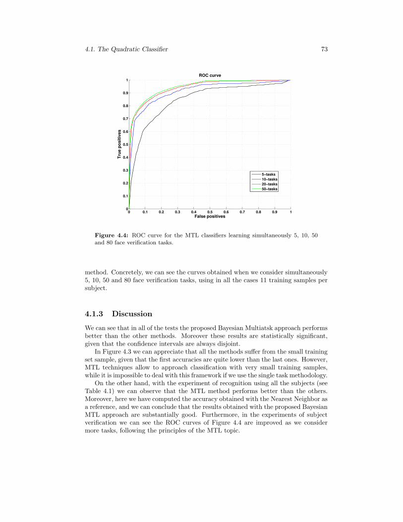
4.1. The Quadratic Classifier 73

0 0.1 0.2 0.3 0.4 0.5 0.6 0.7 0.8 0.9 10

0.1

0.2

0.3

0.4

0.5

0.6

0.7

0.8

0.9

1

False positives

True

pos

itive

s

ROC curve

5−tasks10−tasks20−tasks50−tasks

Figure 4.4: ROC curve for the MTL classifiers learning simultaneously 5, 10, 50and 80 face verification tasks.

method. Concretely, we can see the curves obtained when we consider simultaneously5, 10, 50 and 80 face verification tasks, using in all the cases 11 training samples persubject.

4.1.3 Discussion

We can see that in all of the tests the proposed Bayesian Multiatsk approach performsbetter than the other methods. Moreover these results are statistically significant,given that the confidence intervals are always disjoint.

In Figure 4.3 we can appreciate that all the methods suffer from the small trainingset sample, given that the first accuracies are quite lower than the last ones. However,MTL techniques allow to approach classification with very small training samples,while it is impossible to deal with this framework if we use the single task methodology.

On the other hand, with the experiment of recognition using all the subjects (seeTable 4.1) we can observe that the MTL method performs better than the others.Moreover, here we have computed the accuracy obtained with the Nearest Neighbor asa reference, and we can conclude that the results obtained with the proposed BayesianMTL approach are substantially good. Furthermore, in the experiments of subjectverification we can see the ROC curves of Figure 4.4 are improved as we considermore tasks, following the principles of the MTL topic.

74 MULTITASK LEARNING TECHNIQUES FOR CLASSIFICATION

4.2 The Logistic Regression Model

Logistic Regression model is mainly used in binary classification problems, althoughit can be extended to the multi-class case. In short, it is used for predicting theposterior class probability modelling the occurrence of an event by fitting data to alogistic curve.

Formally, let be T a binary classification task with output space L = {0, 1}. Givenan element x ∈ X ⊆ R

D belonging to the input space of T, the Logistic Regressionmodels its posterior class probabilities by

P (c(x) = 1|x) =1

1 + exp(−wx)(4.14)

and

P (c(x) = 0|x) = 1− P (c(x) = 1|x) (4.15)

where w = (w1, . . . , wD) are the parameters of the model.The estimation of w is usually performed with the Maximum Likelihood estimator,

using a set of training samples X = {x1, . . . ,xN} with their corresponding class labelsc = {c1, . . . , cN}. Concretely, the strategy is to minimize the negated logarithmicLikelihood obtained by

L(ω) = − log[ N∏

i=1

P (c(xi) = ci|xi,w)]

= −[ N∑

i=1

log(P (c(xi) = ci|xi,w)

)](4.16)

It is usual to add in this criterion a regularization term to avoid overfitting. Inthis context, the most usual priors that are imposed to the parameters set are theGaussian, obtained with the minimization of the following restriction

R2(w) =1

σ2‖w‖2 , (4.17)

and the Laplacian, obtained with the minimization of

R1(ω) =1

σ2‖ω‖1 (4.18)

In both cases σ is a real positive corresponding to the variance of the prior distri-bution. These regularization functions promote smoothness among the componentsof w in the first case (equation 4.17), and sparsity among the components of w inthe second case (equation 4.18). Moreover, other priors that are more general can beconsidered, such as Lp norms of Lebesgue spaces, (p ∈ N, p > 0),

Rp(ω) =1

σ2‖ω‖p =

1

σ2p

√√√√N∑

i=1

ωpi (4.19)

With the enforcement of any regularization term Rp, the initial likelihood approachbecomes a MAP method, which seeks the w that minimizes the criterion

4.2. The Logistic Regression Model 75

J(w) = L(w) + Rp(w) (4.20)

Then, once the model is estimated, a new input x ∈ X is classified in class k suchthat

k := arg maxr=0,1

P (C(x) = r|x) (4.21)

We denote the learned probability model by f , which is determined by the para-meters vector w.

4.2.1 A Multitask Extension

Suppose we have M binary tasks T1, ...,TM with their corresponding training samplesX1, . . . ,XM and class labels c1, ..., cM . Consider for each task a logistic regressionmodel, that is, for each Tt we learn a model ft, that will give the probability of class1 according to the t-th task for any input element x ∈ X

m,

ft(x) = P (c(x) = 1|x,Tt) =1

1 + exp(−wtx)(4.22)

where wt = (wt1, ..., w

tD) is the parameters vector of the t-th task. Let be W the

parameters matrix, considering all the tasks,

W =

w11 . . . wM

1...

......

w1D . . . wM

D

To learn the parameters of the model we can apply as before the MAP method,summing all the negated log-likelihood estimators (one per each t-th task, denoted byJ t) as well as the corresponding regularization terms (one per task, denoted by Rt

p).Thus, we have a general negated log-Likelihood that involve all the tasks

L(w) =

T∑

t=1

(Lt) = −T∑

t=1

[ N∑

i=1

log(P

(ct(xt

i) = cti|xt

i,W))]

(4.23)

and a general regularization term

Rp(W) =

T∑

t=1

Rtp = σ

T∑

t=1

‖wt‖p =1

σ2‖W‖p (4.24)

Then, the elements of the matrix W are obtained by the minimization of thefollowing general loss function

J(W) = L(W) + Rp(W) (4.25)

Notice that for an even p, for instance p = 2, this optimization problem can besolved with a gradient descent algorithm [227], given that J(W) is differentiable.Actually, the Gaussian prior is the most common regularization criterion.

76 MULTITASK LEARNING TECHNIQUES FOR CLASSIFICATION

Notice that in this presented framework there is no transit of information betweenthe models of the different tasks, given that this strategy is equivalent to imposing anindependent regularization constraint at each column of matrix W. However, assumethat these tasks are related and suppose that we want to promote information sharingamong them during the training process. For this purpose, we can impose priordistributions on each row of W in a hierarchical way [149]. Concretely, consideringthe mean vector w = (w1, ..., wD) where

wj =

∑Mt=1 wt

j

M(4.26)

we can impose first a Gaussian centered prior to the mean vector w and after thatwe can enforce each j-th row of W to follow a Gaussian distribution with wj mean.In short, this can be formulated by the minimization of the loss function

J(W) = L(W) +1

σ21

‖w‖2 +1

σ22

T∑

t=1

‖wt − w‖2 (4.27)

where L(W) is again the sum of the negated log-likelihood estimators (see equation4.23) and σ2

k are the corresponding variances of the imposed priors, k = 0, 1. Let usto denote by S(W) the new regularization expression,

S(W) =1

σ21

‖w‖2 +1

σ22

T∑

t=1

‖wt − w‖2 (4.28)

Notice that the new global criterion J(W) of equation 4.27 is differentiable. There-fore, we can minimize it using a gradient descent strategy. In this thesis we have usedthe BFGS gradient descent method [227]. The principal idea of the method is toconstruct an approximate Hessian matrix of J(W), by analyzing successive gradientvectors. This approximation of the function derivatives allows the application of aquasi-Newton fitting method in order to move towards the minimum in the parameterspace.

Thus, we need to compute the partial derivatives

∂J(W)

∂wtr

=∂L(W)

∂wtr

+∂S(W)

∂wtr

(4.29)

Observe that S(W) can be rewritten as follows

S(W) =D∑

j=1

[w2

j

σ21

+1

σ22

t∑

t=1

(wtj − wj)

2] (4.30)

and this is the only part of J(W) that depends on w. Thus, given that we wantto minimize this function, we can get an expression for wj depending on W by

wj = arg minv

(v2

σ21

+1

σ22

T∑

t=1

(ωtj − v)2) (4.31)

4.2. The Logistic Regression Model 77

that yields

wj(W) =σ2

1

∑Tt=1 ωt

j

σ22 + Tσ2

1

(4.32)

and consequently

∂wj(W)

∂ωtr

=

{σ21

σ22+Tσ2

1

if r = j

0 if r 6= j

Finally, we can compute the derivatives of J(W) by

∂J(W)

∂wtj

=2wj

σ21

∂wj

∂ωtj

+2

σ22

T∑

t=1

[(wt

j−wj)∂wj

∂ωtj

]=

2wjσ21

σ21(σ2

2 + Tσ21)

+2

σ22

T∑

t=1

[ (ωtj − wj)σ

21

σ22 + Tσ2

1

]

4.2.2 Experiments and Discussion

First, we tested the presented model using the ARFace Database, performing differentsubject verification experiments.

We considered from 2 to 10 verification problems. Given that the MTL paradigmis specially suitable for the small sized training set, we used just 2 positive samplesand 4 negative samples per task to train the system. More concretely, we repeated10 rounds of the following experimental protocol:

• Select 10 persons at random, and label them by 1,2,. . . ,10, respectively

• Pick at random 2 instances from the subject 1, and 4 images from the restto construct the training set. Learn the subject 1 and test with 18 images ofsubject 1 and 36 images from the rest of the subjects, all randomly selectedamong the instances not considered in the training stage. Include this result inthe performances set corresponding to the case where just one person is includedto the system.

• Construct training sets as before for subjects 1 and 2. Train the discriminantfunctions and test each verification with 18 images of the subject that repre-sents and 36 images from the rest of the subjects, all randomly selected amongthe instances not considered in the training stage. Include this result in theperformances set corresponding to the case where two persons are included tothe system.

• Follow this procedure until the 10 persons are jointly considered by the algo-rithm.

The parameters of the method that we have used in the MTL case are σ1 = 2 andσ2 = 6. In the single task case we used σ = 2.

Table 4.2 includes the mean accuracies obtained in each case as well as the corre-sponding confidence intervals.

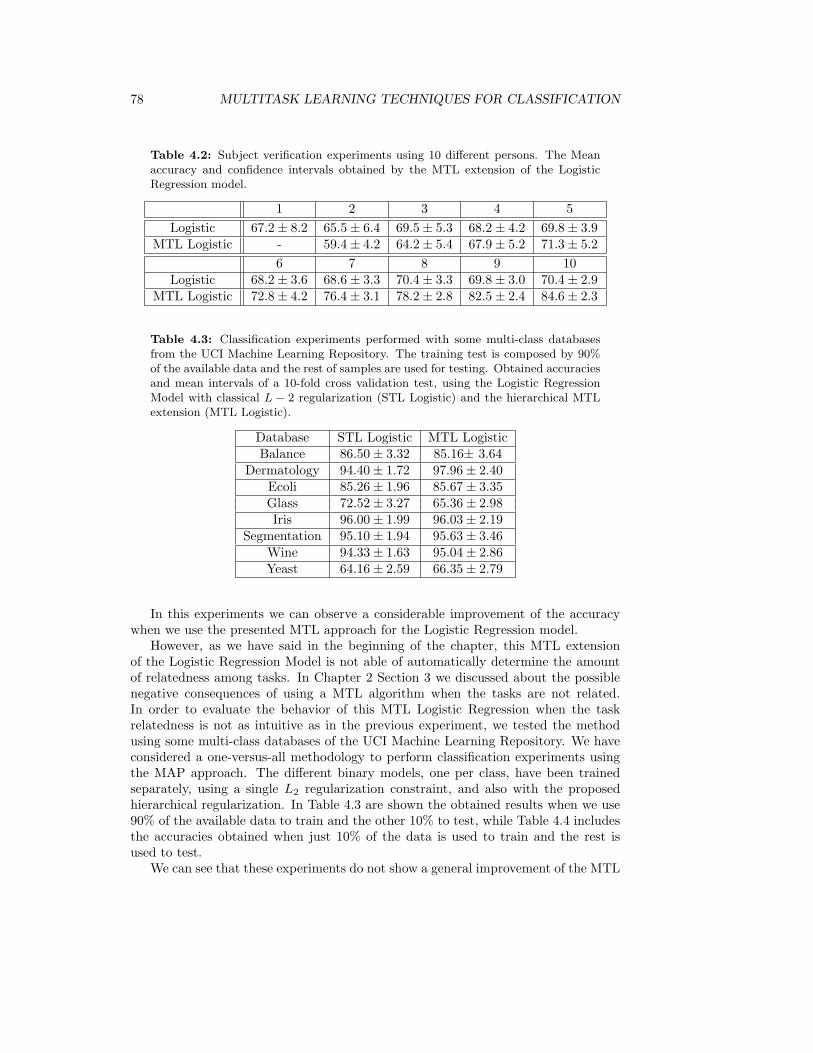
78 MULTITASK LEARNING TECHNIQUES FOR CLASSIFICATION

Table 4.2: Subject verification experiments using 10 different persons. The Meanaccuracy and confidence intervals obtained by the MTL extension of the LogisticRegression model.

1 2 3 4 5

Logistic 67.2± 8.2 65.5± 6.4 69.5± 5.3 68.2± 4.2 69.8± 3.9MTL Logistic - 59.4± 4.2 64.2± 5.4 67.9± 5.2 71.3± 5.2

6 7 8 9 10Logistic 68.2± 3.6 68.6± 3.3 70.4± 3.3 69.8± 3.0 70.4± 2.9

MTL Logistic 72.8± 4.2 76.4± 3.1 78.2± 2.8 82.5± 2.4 84.6± 2.3

Table 4.3: Classification experiments performed with some multi-class databasesfrom the UCI Machine Learning Repository. The training test is composed by 90%of the available data and the rest of samples are used for testing. Obtained accuraciesand mean intervals of a 10-fold cross validation test, using the Logistic RegressionModel with classical L − 2 regularization (STL Logistic) and the hierarchical MTLextension (MTL Logistic).

Database STL Logistic MTL LogisticBalance 86.50± 3.32 85.16± 3.64

Dermatology 94.40± 1.72 97.96± 2.40Ecoli 85.26± 1.96 85.67± 3.35Glass 72.52± 3.27 65.36± 2.98Iris 96.00± 1.99 96.03± 2.19

Segmentation 95.10± 1.94 95.63± 3.46Wine 94.33± 1.63 95.04± 2.86Yeast 64.16± 2.59 66.35± 2.79

In this experiments we can observe a considerable improvement of the accuracywhen we use the presented MTL approach for the Logistic Regression model.

However, as we have said in the beginning of the chapter, this MTL extensionof the Logistic Regression Model is not able of automatically determine the amountof relatedness among tasks. In Chapter 2 Section 3 we discussed about the possiblenegative consequences of using a MTL algorithm when the tasks are not related.In order to evaluate the behavior of this MTL Logistic Regression when the taskrelatedness is not as intuitive as in the previous experiment, we tested the methodusing some multi-class databases of the UCI Machine Learning Repository. We haveconsidered a one-versus-all methodology to perform classification experiments usingthe MAP approach. The different binary models, one per class, have been trainedseparately, using a single L2 regularization constraint, and also with the proposedhierarchical regularization. In Table 4.3 are shown the obtained results when we use90% of the available data to train and the other 10% to test, while Table 4.4 includesthe accuracies obtained when just 10% of the data is used to train and the rest isused to test.

We can see that these experiments do not show a general improvement of the MTL

4.3. Conclusions 79

Table 4.4: Classification experiments performed with some multi-class databasesfrom the UCI Machine Learning Repository. The training test is composed by 10%of the available data and the rest of samples are used for testing. Obtained accuraciesand mean intervals of a 10-fold cross validation test, using the Logistic RegressionModel with classical L − 2 regularization (STL Logistic) and the hierarchical MTLextension (MTL Logistic).

Database STL Logistic MTL LogisticBalance 66.30± 4.54 70.27± 2.37

Dermatology 91.85± 2.35 95.18± 1.04Ecoli 67.33± 4.33 67.89± 2.28Glass 42.78± 3.30 40.50± 4.05Iris 90.98± 2.09 93.03± 1.03

Segmentation 88.52± 2.08 89.76± 0.40Wine 77.50± 3.36 79.62± 1.32Yeast 48.93± 3.44 48.53± 2.46

approach over the single task one. In some cases the MTL approach performs worstthan the single task one in terms of accuracy. Moreover, there are cases where theconfidence intervals of the MTL Logistic Regression are larger than the ones obtainedwith the single task procedure, showing in these cases a higher instability of the MTLmethod.

4.3 Conclusions

In this chapter we have proposed MTL extensions of the Quadratic Classifier andthe Logistic Regression model. Both cases are parallel MTL frameworks where theknowledge sharing among the tasks is promoted by a parametrical approach.

In the case of the Quadratic Classifier we defined a new quantifiable task re-latedness measure based on evaluating an specific distance on the parameter space.Thus, the method is able to automatically determine the similarity degree betweenthe tasks and promotes the sharing of knowledge proportionally to this similarity.The technique outperforms the traditional regularized approach, showing interestingaccuracies even when the number of training samples is considerably reduced.

On the other hand, the information sharing in the MTL Logistic Regression modelis promoted by a hierarchical regularization constraint. In this case the algorithm isnot able of automatically determine whether two tasks are related or not. The exper-imental results have empirically demonstrated the possible negative consequences ofapplying a MTL strategy for learning tasks that are not similar enough.

80 MULTITASK LEARNING TECHNIQUES FOR CLASSIFICATION

Chapter 5

Online Multitask Learning

In Chapter 1 we introduced the Online Learning paradigm as a subfield of the MachineLearning topic. As stated, the research on Online Learning algorithms studies thecapacity of evolving and updating previous knowledge given new data inputs.

Most of the Online Learning methods for classification are focused on the problemof updating the predictors when new data from existing classes arrive to the system.However, the research of methods for online adding classes has not been very active,although the need of adding new classes is a frequent scenario in real problems. Forexample, an application for recognizing K people may need to include a new subject,or a system for automatically detecting a determined set of objects may need toinclude a new one. In these situations, the retraining of the whole system can be verycomputationally demanding. For this reason, the development of Online Learningalgorithms for adding classes is an interesting issue of research.

Currently, up to our knowledge, the state-of-the-art algorithms for adding newclasses to a classification system are the Online Learning extensions of PCA andLDA, called Incremental PCA and Incremental LDA respectively. These methods aredescribed in the next section.

On the other hand, in the context of knowledge updating, there are problems inthe face classification domain that do not deal with addition of samples belonging toexisting classes. For example, consider the problem of recognizing K subjects. Asexpected, people change their aspect along the time. In this case, the informationabout the old samples should be removed and the system updated. Otherwise, thepredictor will remain biased. Moreover, data privacy issues pose the need of elimi-nating all the information from a specific subject when he/she asks to be eliminatedfrom the system, being the class removing from the system another learning case.

Summarizing all the presented situations, we consider that the Online Learningparadigm involves 4 different generic problems: (a) Incremental Sample Learning,when given a previously trained classifier, we update its parameters to model newunseen samples from known classes; (b) Decremental Sample Learning when we adjustclassifier parameters to forget specific samples from known classes; (c) IncrementalClass Learning, when the classifier is modified in order to take into account samplesbelonging to a new class not previously learned; and (d) Decremental Class Learning

81

82 ONLINE MULTITASK LEARNING

when the classifier must be adjusted to remove the complete set of samples from aknown class. Notice the difference between online sample learning (both incrementaland decremental), which normally involves a small change in the classifier parameters,and online class learning (both incremental and decremental), which usually involvesmore important structural changes in the classifier.

As stated in Chapter 2 there is a connection between the Online Learning topicand the MTL paradigm. Concretely, in the sequential MTL scenario. From our pointof view, MTL methods that learn the tasks successively or MTL algorithms thatreceive the training samples one after another can be seen as MTL Online Learningmethodologies. This chapter is focused on these type of systems, making a specialattention on Incremental Class Learning and Decremental Class Learning problems.

Sections 5.2 and 5.3 propose two methods for Online Learning under the MTLprinciples. The first method is an online extension of the JointBoost algorithm[223] for incrementally adding classes. The second one is an online extension of theMTL Quadratic Classifier described in the previous chapter. In this second case, themethodology is able to incrementally adding new samples of existing classes and alsonew classes. Moreover we extend the MTL Quadratic Classifier to the DecrementalLearning, for both cases of removing just some samples from a class or even the wholeclass. Furthermore, we propose a new idea of the Decremental Class Learning. Thisnew idea is based on keeping information from the removed classes that can help tocorrectly classify the rest of the categories. Finally, Section 5.4 concludes the chapter.

5.1 Reference Methods

Classic Online Learning techniques applied to classification are focused on performingfeature extraction. In these cases the classification is carried out by standard pat-tern recognition methods on the reduced space, for instance the Mahalanobis mean-distance [97] or the Nearest Neighbor. In these cases, first a feature transformation islearned with an initial training set and then the online learning techniques allow theupdating of the learned transformation when new learning instances are given to thesystem.

As stated in the Chapter 1, the most common feature extraction techniques forautomatic face classification are PCA and FLD. For both cases we can find in theliterature Online Learning extensions of these algorithms. These extensions are calledIncremental PCA (IPCA) and the Incremental LDA (ILDA) respectively, and theyare described in this section. The idea of these methods is the following: we supposethat a projection matrix W has been learned with initial data X = {x1, . . . ,xN}using the corresponding classical method (PCA or LDA). Then a new sample xN+1

is added to the training set and the goal is to update W, obtaining a new projectionmatrix W close or equal to the projection matrix that would be learned by the classicalmethod with initial data {x1, . . . ,xN ,xN+1}, but avoiding the whole retraining.

5.1.1 Incremental Principal Component Analysis

In this section we describe the IPCA algorithm, reviewing first the PCA method.More details about the IPCA and its experimental robustness can be found in [10].

5.1. Reference Methods 83

PCA method

Principal Component Analysis (PCA) [126] is a non-supervised feature extractiontechnique. It is frequently applied in classification problems given its simplicity andoptimality under the criterion of L2 reconstruction error. Briefly, the PCA findsan orthogonal set of projection vectors computed as the first eigenvectors of the datacovariance matrix, which are sorted in order to preserve the maximum possible amountof data variance.

Formally, let be X ⊆ RD a data matrix and µ ∈ R

D the corresponding meanvector. The covariance matrix of X can be estimated by

Σ ' E[(X− µ)(X− µ)T] =

σ11 . . . σD1

......

...σD1 . . . σDD

where (X − µ) denotes the centered data (obtained by subtracting µ from eachelement in X). Each entry σij (i 6= j) is an estimation of the covariances betweenthe random variables Xi and Xj , corresponding to the events of randomly picking upan i-th and a j-th component of an input element respectively. Notice, then, that σii

approximates the variance of the random variable Xi.By definition, the estimations of covariance matrices are always symmetric. Thus

we can compute the spectral decomposition of Σ, obtaining its eigenvalues {λ1, ..., λD}and their corresponding eigenvectors {v1, ...,vD}. By sorting the eigenvectors in theorder of descending eigenvalues (largest first), we obtain an orthogonal basis of theinput space with the first eigenvector having the direction of largest variance of thedata.

The most common use of PCA is to reduce the data dimensionality. For thisaim, we can proceed as follows: let be W the matrix composed by the d first sortedeigenvectors as rows (d ≤ D). Given any element x of the input space, we canrepresent it by

y = W(x− µ) (5.1)

and this is the representation of x in a d-dimensional space that minimizes themean-square error in the reconstruction process. With this, we can reduce the dimen-sion of the data preserving as much as possible the original information.

IPCA method

Let be X = {x1, ...,xN} a data set and W the (d×D)-matrix learned by PCA fromX, with mean µ, as above described. Suppose now that a new training sample xN+1

arrives to the system. To update the projection matrix W we will add a new vectorand apply a rotational transformation. The first step is to compute the residual vector

uN+1 = (WT (WxN+1) + µ)− xN+1 ∈ Rd (5.2)

Then we normalize u as follows

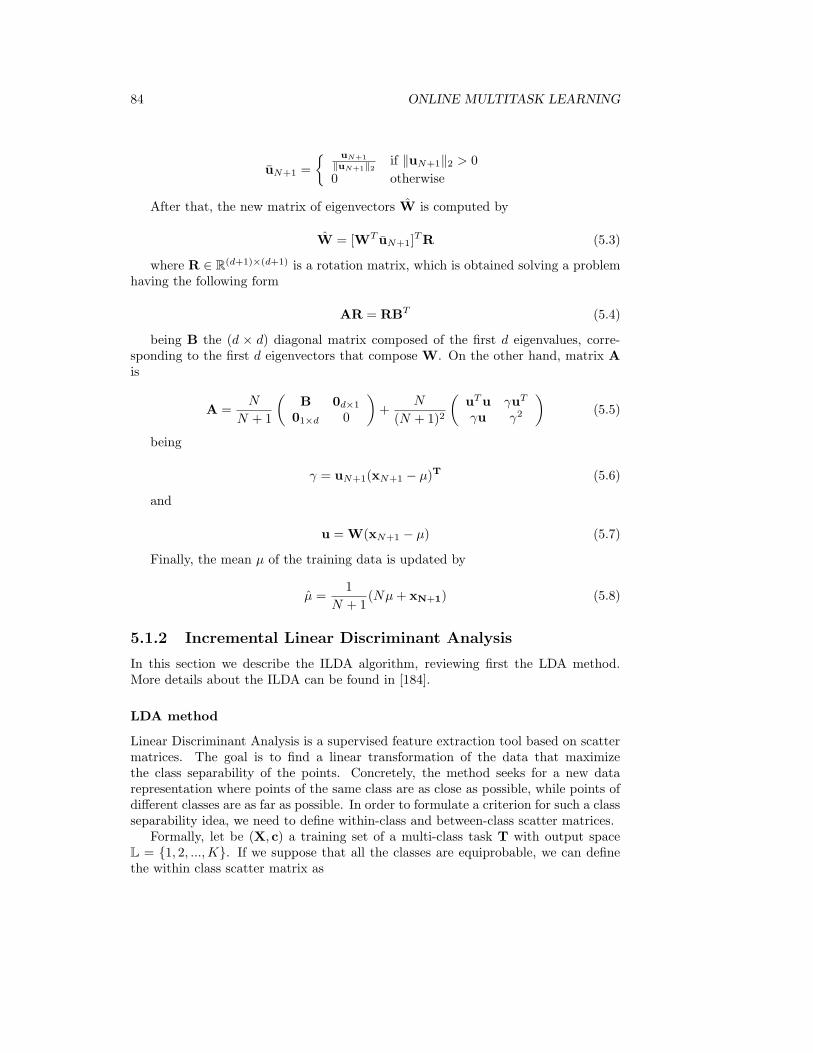
84 ONLINE MULTITASK LEARNING

uN+1 =

{ uN+1

‖uN+1‖2if ‖uN+1‖2 > 0

0 otherwise

After that, the new matrix of eigenvectors W is computed by

W = [WT uN+1]T R (5.3)

where R ∈ R(d+1)×(d+1) is a rotation matrix, which is obtained solving a problem

having the following form

AR = RBT (5.4)

being B the (d × d) diagonal matrix composed of the first d eigenvalues, corre-sponding to the first d eigenvectors that compose W. On the other hand, matrix Ais

A =N

N + 1

(B 0d×1

01×d 0

)+

N

(N + 1)2

(uT u γuT

γu γ2

)(5.5)

being

γ = uN+1(xN+1 − µ)T (5.6)

and

u = W(xN+1 − µ) (5.7)

Finally, the mean µ of the training data is updated by

µ =1

N + 1(Nµ + xN+1) (5.8)

5.1.2 Incremental Linear Discriminant Analysis

In this section we describe the ILDA algorithm, reviewing first the LDA method.More details about the ILDA can be found in [184].

LDA method

Linear Discriminant Analysis is a supervised feature extraction tool based on scattermatrices. The goal is to find a linear transformation of the data that maximizethe class separability of the points. Concretely, the method seeks for a new datarepresentation where points of the same class are as close as possible, while points ofdifferent classes are as far as possible. In order to formulate a criterion for such a classseparability idea, we need to define within-class and between-class scatter matrices.

Formally, let be (X, c) a training set of a multi-class task T with output spaceL = {1, 2, ...,K}. If we suppose that all the classes are equiprobable, we can definethe within class scatter matrix as

5.1. Reference Methods 85

SW =1

K

K∑

k=1

Sk (5.9)

where Sk is the k-th class-conditional covariance matrix estimated from the data,

Sk =

N∑

i=1

1k(ci)(xi − µk)(xi − µk)T (5.10)

where

1k(ci) =

{1 if ci = k0 otherwise

for all i = 1, . . . , N .On the other hand, we can define the between class scatter matrix by

SB =1

K

K∑

k=1

(µk − µ)(µk − µ)T (5.11)

where µ is the global mean vector of the training samples X. With these defini-tions, Linear Discriminant Analysis seeks for a linear transformation W that projectsthe data into a lower dimensional space following the class separability idea abovedescribed. To aim this goal we need to summarize these scatters in a numeric crite-rion that should be high when the between class scatter is large and the within classvariation is small. Several ways for computing this indicator have been defined in theliterature [82], being the most used

J(V) = tr[(VS−1

W VT )(VSBVT )]

(5.12)

Fortunately, the maximization of J(V) has an analytical solution [83]. Concretely,the matrix

W = arg maxV

J(V) (5.13)

has as rows the first d eigenvectors corresponding to the highest d eigenvalues ofS−1

W SB .

ILDA method

Similarly to the case of PCA, we can find in the literature an online extension ofLDA, known as the Incremental LDA algorithm (ILDA) [184]. This method updatesthe matrix W when a new training sample xN+1 is added to the system. Notice thatLDA is a supervised technique, meaning that the class labels of the data are takeninto account to learn the feature extraction matrix. For this reason, when a newsample arrives to the system, we have to consider separately the following two cases:

1. The new sample xN+1 belongs to an existing class, that is, cN+1 = k ∈ {1, ...,K}2. The new sample xN+1 belong to a new class K + 1

86 ONLINE MULTITASK LEARNING

1. The new sample belongs to an existing class

Let us begin with the first case. Suppose that we have a new training sample xN+1

belonging to class k ∈ {1, ...,K}. We have to update SW and SB . First we need toupdate the global mean and the k-th class mean by

µ =Nµ + xN+1

N + 1(5.14)

µk =Nkµk + xN+1

Nk + 1(5.15)

where Nk is the number of elements in X belonging to class k. Then, we updateSW and SB by

SW = SW − Sk + Sk (5.16)

SB = SB − (µk − µ)(µk − µ)T + (µk − µ)(µk − µ)T (5.17)

where

Sk = Sk + (xN+1 − µk)(xN+1 − µk)T (5.18)

2. The new sample belongs to a new class

Suppose now that the new training sample xN+1 belongs to a new class, K + 1. Wehave to update the global mean as before,

µ =Nµ + xN+1

N + 1(5.19)

and the between-class scatter matrix has to be recomputed

SB =1

K + 1

K+1∑

k=1

(µk − µ)(µk − µ)T (5.20)

where µK+1 = xN+1.On the other hand, the within-class scatter matrix SW does not change.

5.2 The Online Boosting Algorithm

As stated in Chapter 1, the the Boosting family of classifiers has been shown tobe efficient and robust in many situations [80]. We can find in the literature someextensions of these methods to the Online Learning paradigm [180, 179, 173], butthese proposals just allow the inclusion of new samples to update the classifier, butnot the addition of classes. Actually these methods just deal with binary problemsand they are not related at all with the MTL paradigm.

5.2. The Online Boosting Algorithm 87

One of the most robust approaches that have been proposed in the literature toextend Boosting to the multiple class case is the JointBoost algorithm [223]. Prob-ably, the reason that makes this method to have more success than others is thatit uses the principles of the MTL topic. In short, the JointBoost approaches the Kmulti-class problem using a one-versus-all strategy and makes use of features that areshared among the different classes. That makes the algorithm to choose more generalfeatures, instead of using class-specific ones, what increases its generalization ability.Moreover, for a given performance level, the method needs less training data thansingle-task approaches.

In this section we propose a MTL online extension of the JointBoost algorithmand perform different subject recognition experiments to test the method. The wholelearning procedure is divided in two steps: first a model is learned with the JointBoostusing an initial set of classes, and second we propose an online Boosting algorithm toupdate the learned classifier for adding new classes to the system.

5.2.1 The JointBoost Algorithm

To properly describe the JointBoost algorithm proposed by Torralba et al. in [223],let us start with a brief review of Boosting for binary classification.

Boosting for Binary Classification

Suppose that we have a binary classification task T and denote by L = {−1,+1} theoutput space of T. The goal of Boosting is to sequentially fit an additive model ofthe form

f(x) =

R∑

r=1

hr(x) (5.21)

where x is an element of the input space, R the number of boosting rounds, and

f(x) = logP (c(x) = 1|x)

P (c(x) = −1|x)(5.22)

Then,

exp[f(x)

]=

P (c(x) = 1|x)

P (c(x) = −1|x)(5.23)

and

P (c(x) = 1|x) = exp[f(x)

]P (c(x) = −1|x) = exp

[f(x)

](1−P (c(x) = 1|x)

)(5.24)

Isolating P (c(x) = 1|x), we have that

P (c(x) = 1|x) =exp

[f(x)

]

1 + exp[f(x)

] (5.25)

The boosting strategy minimizes the cost function

88 ONLINE MULTITASK LEARNING

J(x) = E{

exp[−c(x)f(x)]}

(5.26)

where E represents the empirical average over the training data (expectation).This loss function can be interpreted as an approximation to the likelihood of thetraining data under a Logistic Regression model [81] or as an upper bound on theclassification error [207].

There are different ways to optimize J(x), which yield the different Boosting al-gorithms [81]. One of the most effective and robust versions is the Gentle AdaBoostprocedure, that minimizes the loss function using adaptive Newton steps, correspond-ing to minimizing a weighted squared error at each step. Formally, at each boostinground r, we have

f(x) =

r−1∑

s=1

hs(x) (5.27)

and have to learn hr that minimize

J(x) = E{

exp[− c(x)

(f(x) + hr(x)

)]}(5.28)

Given that

∂J(f(x) + h(x)

)

∂h(x)

∣∣∣h(x)=0

= −E[exp(−c(x)f(x)

)c(x)|x

](5.29)

and

∂2J(f(x) + h(x)

)

∂h(x)2

∣∣∣h(x)=0

= E[exp(−c(x)f(x)

)|x

](5.30)

the Newton update is

f(x)← f(x) +E

[exp(−c(x)f(x)

)c(x)|x

]

E[exp(−c(x)f(x)

)|x

] (5.31)

This expectation is estimated with the training data (X, c). Hence, the update isobtained by the following weighted average

hr(x) = Ew(c(x)|x) =

N∑

i=1

wi

[P (ci = 1|xi)− P (ci = −1|xi)

](5.32)

where each wi is

wi = exp[− cif(xi)

](5.33)

This procedure yields to the Gentle AdaBoost algorithm which is detailed in Table5.1.

Regarding to the weak learners hr(x), it is common to use simple functions of theform

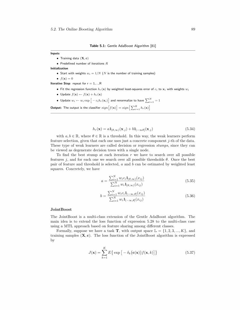
5.2. The Online Boosting Algorithm 89

Table 5.1: Gentle AdaBoost Algorithm [81]

Inputs

• Training data (X, c)

• Predefined number of iterations R

Initialization

• Start with weights wi = 1/N (N is the number of training samples)

• f(x) = 0

Iterative Step: repeat for r = 1,...,R

• Fit the regression function hr(x) by weighted least-squares error of ci to xi with weights wi

• Update f(x)← f(x) + hr(x)

• Update wi ← wi exp[− cihr(xi)

]and renormalize to have

∑N

i=1= 1

Output: The output is the classifier sign[f(x)

]= sign

[∑R

r=1hr(x)

]

hr(x) = a1(θ,∞)(x.j) + b1(−∞θ](x.j) (5.34)

with a, b ∈ R, where θ ∈ R is a threshold. In this way, the weak learners performfeature selection, given that each one uses just a concrete component j-th of the data.These type of weak learners are called decision or regression stumps, since they canbe viewed as degenerate decision trees with a single node.

To find the best stump at each iteration r we have to search over all possiblefeatures j, and for each one we search over all possible thresholds θ. Once the bestpair of feature and threshold is selected, a and b can be estimated by weighted leastsquares. Concretely, we have

a =

∑Ni=1 wici1(θ,∞)(xij)∑Ni=1 wi1(θ,∞)(xij)

(5.35)

b =

∑Ni=1 wici1(−∞,θ](xij)∑Ni=1 wi1(−∞,θ](xij)

(5.36)

JointBoost

The JointBoost is a multi-class extension of the Gentle AdaBoost algorithm. Themain idea is to extend the loss function of expression 5.28 to the multi-class caseusing a MTL approach based on feature sharing among different classes.

Formally, suppose we have a task T, with output space L = {1, 2, 3, ...,K}, andtraining samples (X, c). The loss function of the JointBoost algorithm is expressedby

J(x) =K∑

k=1

E{

exp[− δk

(c(x)

)f(x, k)

]}(5.37)

90 ONLINE MULTITASK LEARNING

where

δk

(c(x)

)=

{1 if c(x) = k−1 otherwise

and the additive model to be learned

f(x, k) =

R∑

r=1

hr(x, k) (5.38)

which satisfies

f(x, k) = logP (δk

(c(x) = 1|x

)

P (δk

(c(x) = −1|x

) (5.39)

The basic idea of the training procedure is that at each round r, the algorithm willchoose a subset of classes that will share a feature to reduce their classification error.Concretely, at each boosting step, the multi-class classification problem is transformedto a binary problem by grouping the classes in two clusters, a positive one (denotedby Pos), and a negative one (denoted by Neg), and a decision stump hr(x) is trainedon this binary problem.

Regarding to the grouping in positive and negative clusters, Torralba et al. [223]proposed two possibilities to construct them: (a) considering all the possible group-ings (exhaustive search), which has complexity O(2K), or (b) using a greedy search(forward selection), with complexity O(K2). Their experiments showed that on ar-tificial data this second approach is a very good approximation to the exhaustivesearch.

The procedure of the greedy search heuristically selects a class grouping with lowclassification error and defines a binary problem for each boosting step. Concretely,the process is the following:

1. Train K different weak learners by considering each class as the only candidatemember of the positive cluster (the remaining classes are included in the negativecluster). Each weak learner is built by considering a feature and the optimaldecision stump classifier which can be defined for the binary problem on thatfeature

2. Select, from the K problems the one which shows minimum weighted classifica-tion error and add the associated class to the initial Positive cluster

3. For the remaining classes, and until no improvement on the classification errorcan be found, iterate the following steps:

• Train a set of different classifiers by considering the previous Positive clus-ter but adding one class candidate from the Negative cluster.

• Add the class candidate to the Positive cluster only if the joint selectionimproves the previous classification error

5.2. The Online Boosting Algorithm 91

As we can see in equation 5.38, the shared stumps of the JointBoost algorithmdepend on both the sample and the class membership. Moreover, as in the regularGentle AdaBoost algorithm, the samples are weighted. However, the difference hereis that JointBoost has a weight per training sample and per class. That is, given aclass k and a training sample xi, we have a weight wik.

Regarding to the weak learners, the form of a shared stump in this case is

fr(x, k) =

a if x.j > θ and k ∈ Posb if x.j ≤ θ and k ∈ Posκ(k) if k /∈ Pos

As before, to fit these values we proceed as follows: at each iteration, once thefeature j, the threshold θ and the class grouping are fixed, we have to compute theparameters of the weak learner solving a weighted least squares problem at eachiteration. This strategy yields to the following solutions

a(j, θ) =

∑k∈Pos

∑Ni=1 wikδk(ci)1(θ,∞)(xij)∑

k∈Pos

∑Ni=1 wik1(θ,∞)(xij)

(5.40)

b(j, θ) =

∑k∈Pos

∑Ni=1 wikδk(ci)1(−∞,θ)(xij)∑

k∈Pos

∑Ni=1 wik1(−∞,θ)(xij)

(5.41)

κ(k) =

∑Ni=1 wikδk(ci)∑N

i=1 wik

(5.42)

The whole JointBoost algorithm is detailed in Table 5.2.

5.2.2 Online extension of the JointBoost Algorithm

As a result of the JointBoost algorithm performing R boosting rounds, we obtainthe following classification rule: a new input element x is classified in class k ∈ L ={1, . . . ,K} such that

k := arg maxc=1,...,K

f(x, c) = arg maxc=1,...,K

R∑

r=1

hr(x, k) (5.47)

Moreover, the algorithm learns the corresponding class clusterings {Posr; r =1, ..., R}. Thus, once the JointBoost algorithm is trained, it can be used only for thelearned K-class problem. Then, when a new class K + 1 is added to the system, thewhole model must be retrained. Notice that, in a K-class problem, the JointBoostalgorithm has to try a lot of possible ways of grouping the classes at each iteration.Moreover, for each grouping it has to find the best feature, trying each time allthe D possibilities. Actually, the exhaustive search for K = 100 and D = 500is computationally unfeasible in a reasonable amount of time using a Pentium IVcomputer.

The idea of the proposed Online Boosting algorithm is to take benefit of the classgrouping performed in the sharing features step, in order to online incorporate new

92 ONLINE MULTITASK LEARNING

Table 5.2: JointBoost Algorithm [223]

Inputs

• Training data (X, c)

• Predefined number of iterations R

Initialization

• Start with weights: wik = 1

• Set f(x, k) = 0 for all k = 1, ..., K

Iterative Step: repeat for r = 1, ..., R

• For all the considered ways of grouping the classes in Positive and Negative clusters, Poss (s =1, ..., 2K − 1 if we consider the exhaustive search)

– Learn the shared regression stumps

hsr(x, k) =

{a if x.j > θ and k ∈ Posb if x.j ≤ θ and k ∈ Posκ(k) if k /∈ Pos

– Compute the weighted error for the class grouping as:

ErrsPos =

K∑

k=1

n∑

i=1

wik

(δPoss

(ci)− hsr(xi, ci)

)2. (5.43)

• Find the binary grouping of classes s with minimum ErrsPos

s = arg mins

ErrsPos (5.44)

and set hr := hsr and Posr = Poss

• Update the data weights:

wik ← wik exp{− δk(ci)hr(xi, ci)

}(5.45)

• Update the class estimates:f(x, k)← f(x, k) + hr(x, k) (5.46)

Output:The output is the predictor f(x, k) =∑R

r=1hr(x, k) and corresponding class clusterings Posr,

r = 1, ..., R

5.2. The Online Boosting Algorithm 93

classes to the system. Thus we can avoid the mentioned computationally expensivepart of the learning stage. More concretely, when we want to add a new class K + 1to the model, the Online Boosting is iterated R times. At each iteration r we have toperform 2 steps:

1. Update Posr. That is, for each iteration there is a class grouping of classes1, ...,K in a positive and a negative clusters, obtained by the JointBoost. Thisfirst step consists on assigning the new class K + 1 to the most suitable clusterunder an error minimization criterion, using the feature and the parameters pre-viously learned. Moreover, the weak learner is adjusted using the new trainingsamples.

2. According to the cluster assignation done in the previous step, the weights ofthe examples are updated, as well as the model f(x, k).

Notice that the computational complexity of the algorithm to add a new class isO(R), while to retrain the whole system for K +1 classes using the exhaustive searchwould be O(R × (K + 1)2). On the other hand, the method allows the inclusion ofmany new classes, given that the same process can be iteratively repeated adding anew class each time. Furthermore, notice that the cost of adding a new class K + 1do not depend on the number of classes K.

More details and the pseudo code of the Online Boosting algorithm can be foundin Table 5.3. Particularly, the iterative process is described in points (1)-(7). Thefirst step, consisting on the cluster updating, is composed by stages (1)-(5), while thesecond stage of the iterative process, where the weights are adjusted and the classifieris updated, is performed in stages (6)-(7).

On the other hand, an example of the Online Boosting application to face recog-nition is shown in Figure 5.1. First, we show the class groupings of an initial 10 classproblem along 50 boosting steps, using the JointBoost. At each round, elements inthe positive cluster are denoted with a white square, while elements in the negativecluster are denoted with black squares. Then, in the last row, we show the clusterassignation of a new class, obtained with the Online Boosting at each iteration.

5.2.3 Experiments and Discussion

The experiments have been performed using the FRGC and the AR Face databases.The faces have been rotated and scaled according to the inter-eye distance. Then,the samples were cropped obtaining a 37×33 thumbnail, preserving only the internalregion of the faces. Thus, the final sample from each image becomes a 1221 featurevector.

We repeated all the experiments 10 times, according to the following protocol:

• We randomly take 25 classes (subjects) from each database to set up the onlinelearning algorithms

• Then, we progressively add one class at each step up to the maximum numberof classes, updating the online model parameters at each class addition.

94 ONLINE MULTITASK LEARNING

Table 5.3: Online Boosting Algorithm

Inputs

• Training data (X, c) of the learned K-class problem

• Classifier f(x, k) =∑R

r=1hr(x, k) and corresponding class clusterings Posr, r = 1, ..., R of the

learned K-class problem

• Training samples of the new class K + 1, {xN+1, ...,xN+NK+1}

Initialization

• Initialize the set of weights: wik = 1,

• Set f(x, k) = 0

Iterative Step: repeat for r = 1, ..., R

1. Assign the new class K +1 to the Positive cluster, according to the optimal class grouping selectedon the step r in the previous model, Posr, obtaining the clustering Posp

r

2. Classify the training data {X,xN + 1, ...,xN+NK+1} using the decision stumps generated at the

r-th step of the previous JointBoost algorithm but adjusting the parameter κ(K + 1) using thenew samples.

hpr(x, k) =

{a if x.j > θ and k ∈ Posb if x.j ≤ θ and k ∈ Posκ(k) if k /∈ Pos

3. Compute the weighted error for the class grouping as:

Errp =

K+1∑

k=1

N+NK+1∑

i=1

wik(δPosp(ci)−Hp

r (xi, ci))2. (5.48)

4. Assign the new samples to the Negative cluster, according to the optimal class grouping selectedon the step r in the previous model f(x, k), obtaining the clustering Posn

r , and compute the errorErrn as in 2 and 5.48.

5. Assign the new class to the clustering with minimum error s = arg minp,r(Errp, Errn) and set

hr := hsr, ˆPosr = Poss

r

6. Update the data weights:

wik ← wik exp{− δk(ci)h

′r(xi, c)

}(5.49)

7. Update the estimation for each class: f(x, k)← f(x, k) + hr(x, k)

Output: Classifier f(x, k) =∑R

r=1hr(x, k) and corresponding class clusterings ˆPosr, r = 1, ..., R

5.2. The Online Boosting Algorithm 95

Figure 5.1: Graphical representation of the Online Boosting algorithm. First 50boosting steps for a 10 class problem (a representative face of the training set isshown for each class). We plot white squares for denoting the samples that belongto the positive cluster, and black squares for the ones belonging to the negative one.The last row shows the clusterization learned by the Online Boosting algorithms fora new unseen class.

Table 5.4: Subject Recognition Experiments with the Online Boosting algorithm,the ILDA and the IPCA. Mean accuracy of the recognition experiments with theFRGC and the ARFace databases. Only 25 classes are used for training, a total of135 extra classes have been added in the FRGC case, and 65 in the AR Face.

FRGC (160 subjects) Accuracy ± Interval

IPCA 0.833±0.181ILDA 0.859±0.013

Online Boosting 0.921±0.010

ARFACE (80 subjects) Accuracy ± Interval

IPCA 0.605±0.022ILDA 0.679±0.015

Online Boosting 0.752±0.011

For all the classes we used 50% of the samples for training and the rest for testing.The experiments have been performed with 3 methods: IPCA, ILDA and the

proposed Online Boosting.We evaluated in all the stages the mean accuracy across the 10 iterations as well

as the 95% confidence intervals near the mean value. In Figure 5.2 we show theaccuracies as a function of the number of classes and specify in Table 5.4 the finalresults, when all the classes have been included to the model.

One of the free parameters of the proposed algorithm is the number of initialclasses to train the model. In order to analyze the influence of this initial class set onthe global accuracy we performed the same experiment as above, but using initial setsof 5, 10, 15, 20 and 25 classes. Figure 5.3 shows the mean accuracies as a function ofthe number of classes in the FRGC and ARFace data sets.

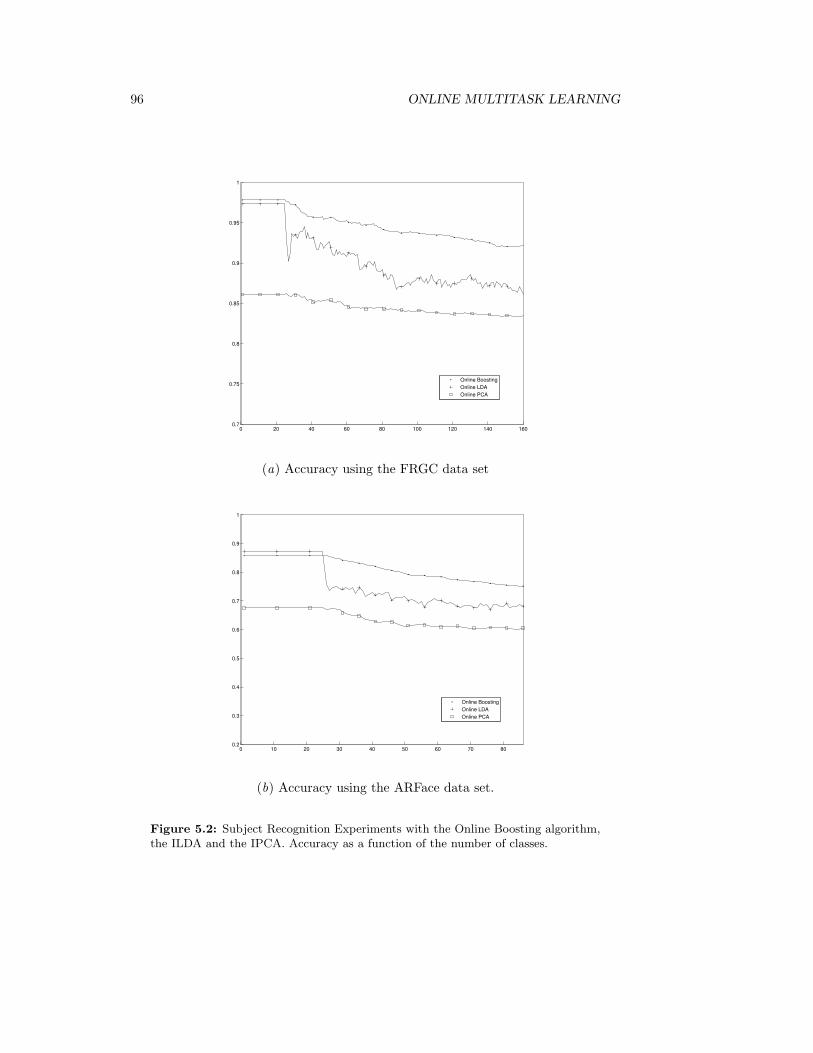
96 ONLINE MULTITASK LEARNING

0 20 40 60 80 100 120 140 1600.7

0.75

0.8

0.85

0.9

0.95

1

Online BoostingOnline LDAOnline PCA

(a) Accuracy using the FRGC data set

0 10 20 30 40 50 60 70 800.2

0.3

0.4

0.5

0.6

0.7

0.8

0.9

1

Online BoostingOnline LDAOnline PCA

(b) Accuracy using the ARFace data set.

Figure 5.2: Subject Recognition Experiments with the Online Boosting algorithm,the ILDA and the IPCA. Accuracy as a function of the number of classes.

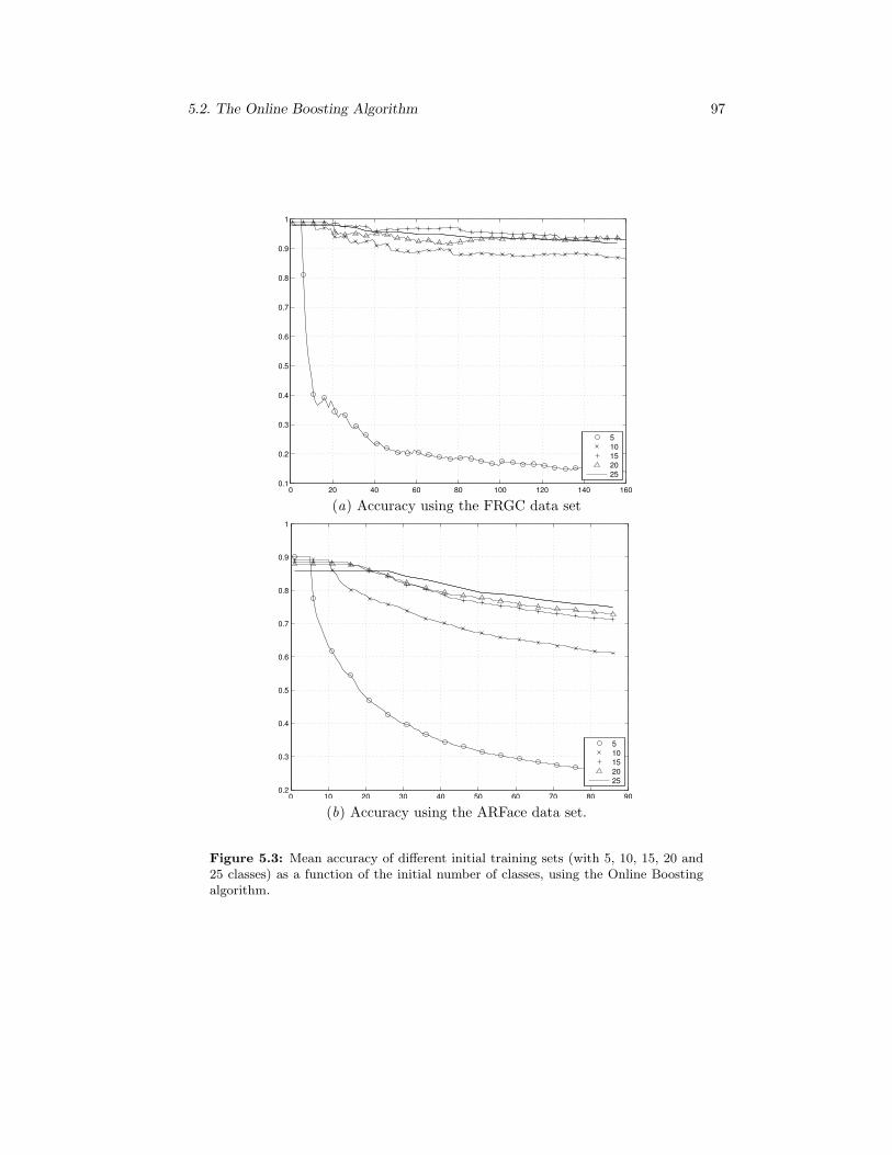
5.2. The Online Boosting Algorithm 97

0 20 40 60 80 100 120 140 1600.1

0.2

0.3

0.4

0.5

0.6

0.7

0.8

0.9

1

510152025

(a) Accuracy using the FRGC data set

0 10 20 30 40 50 60 70 80 900.2

0.3

0.4

0.5

0.6

0.7

0.8

0.9

1

510152025

(b) Accuracy using the ARFace data set.

Figure 5.3: Mean accuracy of different initial training sets (with 5, 10, 15, 20 and25 classes) as a function of the initial number of classes, using the Online Boostingalgorithm.

98 ONLINE MULTITASK LEARNING

Discussion

In Figure 5.2 we can see that in all the cases the accuracy decreases when new classesare added to the system, as expected. This happens due to the fact that larger classproblems are more difficult to classify. Moreover, there is usually an implicit errorin the model when it is updated with the arrival of a new sample, given that thewhole model has not been retrained. On the other hand, we want to emphasize thatJointBoost shows an accuracy close to 98% in the initial 25 classes problem of theFRGC database, while the application of the feature extraction methods with theNN classifier obtain an initial 92%. This fact suggests that for a normalized set of faceimages acquired under controlled conditions, the use of JointBoost is a good optionfor multi-class face classification problems.

In the presented experiments, the best performance is generally done by the pro-posed Online Boosting algorithm, while the second best performing method in bothdata sets is the Online LDA. Notice, however, that its accuracy abruptly decreaseswhen the models are updated the first time. The reason is that in high dimensionaldata the proper estimation of the class distributions (scatters) become unprecise.Finally, the performance of the IPCA algorithm is clearly inferior, given that classmemberships are not taken into account in the feature extraction process.

Regarding to the initial class set selection, we observe in Figure 5.3 that the algo-rithm fares better with large initial class sets, given that the sharing process involvedin the JointBoost algorithm can use richer information for the face recognition task.In the small initial class sets, the drop in the accuracy is noticeable. Nevertheless,as the amount of initial classes increases, the improvement on the accuracy is lessimportant, being not statistically significant considering an initial set composed of 20classes, approximately. The experiment suggests that an initial 25 class set could beenough to initialize the JointBoost model.

5.3 The Online Multitask Quadratic Classifier

In this section we present the online learning extension of the Multitask QuadraticClassifier presented in the first section of Chapter 4. The proposed framework candeal with the four online learning problems detailed at the beginning of this chapter.That is, we present classifier updating equations for

• Addition and subtraction of samples belonging to existing classes (IncrementalSample Learning and Decremental Sample Learning).

• Addition of new classes (Incremental Class Learning).

• Elimination of existing classes (Decremental Class Learning).

An important contribution of this proposal is a new Decremental Class Learningapproach. Concretely, instead of focusing only on eliminating classes reversing themodel, we propose to preserve the information of the eliminated class that is usefulfor modelling the other classes. This idea is deeply described in Section 5.3.2.

Following we detail the proposed online methodologies for the Multitask QuadraticClassifier and test these approaches.

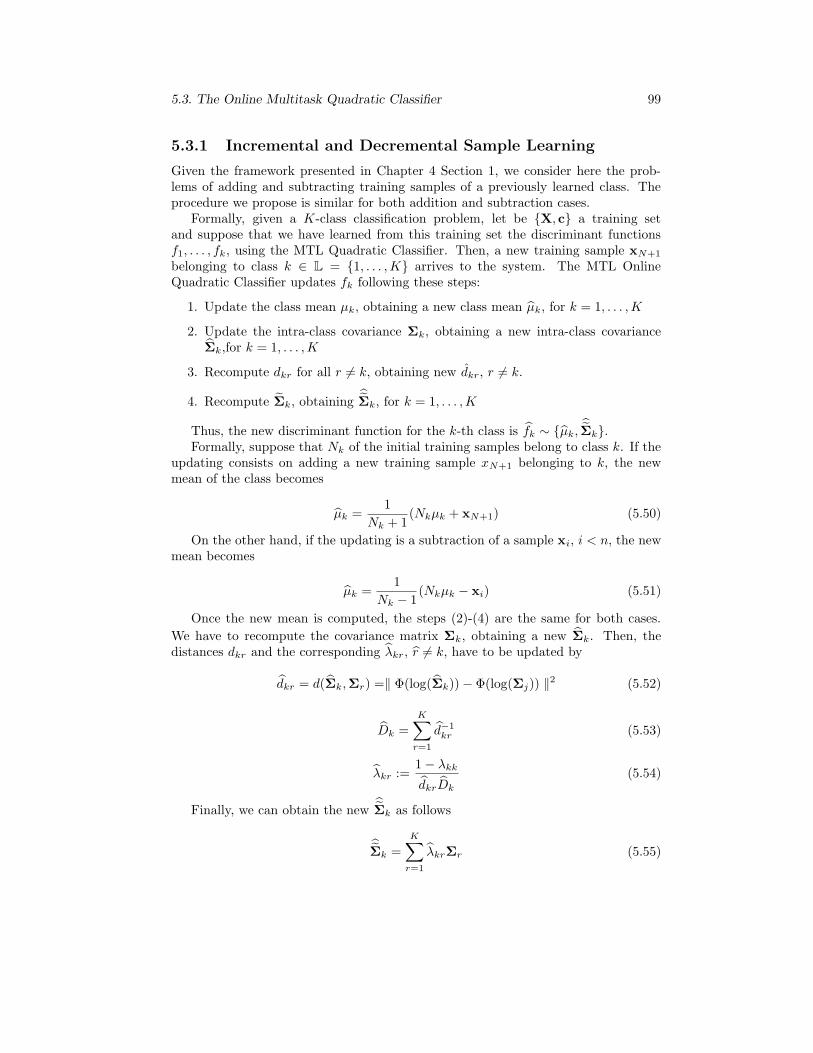
5.3. The Online Multitask Quadratic Classifier 99

5.3.1 Incremental and Decremental Sample Learning

Given the framework presented in Chapter 4 Section 1, we consider here the prob-lems of adding and subtracting training samples of a previously learned class. Theprocedure we propose is similar for both addition and subtraction cases.

Formally, given a K-class classification problem, let be {X, c} a training setand suppose that we have learned from this training set the discriminant functionsf1, . . . , fk, using the MTL Quadratic Classifier. Then, a new training sample xN+1

belonging to class k ∈ L = {1, . . . ,K} arrives to the system. The MTL OnlineQuadratic Classifier updates fk following these steps:

1. Update the class mean µk, obtaining a new class mean µk, for k = 1, . . . ,K

2. Update the intra-class covariance Σk, obtaining a new intra-class covarianceΣk,for k = 1, . . . ,K

3. Recompute dkr for all r 6= k, obtaining new dkr, r 6= k.

4. Recompute Σk, obtainingΣk, for k = 1, . . . ,K

Thus, the new discriminant function for the k-th class is fk ∼ {µk,Σk}.

Formally, suppose that Nk of the initial training samples belong to class k. If theupdating consists on adding a new training sample xN+1 belonging to k, the newmean of the class becomes

µk =1

Nk + 1(Nkµk + xN+1) (5.50)

On the other hand, if the updating is a subtraction of a sample xi, i < n, the newmean becomes

µk =1

Nk − 1(Nkµk − xi) (5.51)

Once the new mean is computed, the steps (2)-(4) are the same for both cases.

We have to recompute the covariance matrix Σk, obtaining a new Σk. Then, thedistances dkr and the corresponding λkr, r 6= k, have to be updated by

dkr = d(Σk,Σr) =‖ Φ(log(Σk))− Φ(log(Σj)) ‖2 (5.52)

Dk =

K∑

r=1

d−1kr (5.53)

λkr :=1− λkk

dkrDk

(5.54)

Finally, we can obtain the newΣk as follows

Σk =

K∑

r=1

λkrΣr (5.55)

100 ONLINE MULTITASK LEARNING

5.3.2 Incremental and Decremental Class Learning

In this section we consider both the addition of a new class to the system and thesubtraction of an existing class.

Incremental Class Learning

Let us suppose that we have previously learned K different classes (K ≥ 1) froma training set {X, c}. We have obtained the corresponding discriminant functionsf1, . . . , fK , and we need to add a new class K + 1 to the system.

Let be xN+1, . . . ,xN+NK+1a set of samples belonging to the new class K +1. The

online adaptation of the system can be done by following this procedure:

1. Learn fK+1 from the whole training samples set {X,xN+1, . . . ,xN+NK+1} with

their corresponding class labels

2. Update f1, ..., fK , obtaining the new models f1, ..., fK that take into accountthe samples of the new class K + 1

To learn fK+1 we have to compute ΣK+1 and drK+1 for all r = 1, ...,K,

drK+1 = d(Σr,ΣK+1) (5.56)

Now, the equations that update the models f1, . . . , fK are, for all r = 1, ...,K,

Dr = Dr + d−1rK+1 (5.57)

Σr =

Dr

Dr

Σr + αrK+1ΣK+1 (5.58)

being,

αrK+1 =1

DK+1djK+1(5.59)

where DK+1 =∑K+1

k=1 d−1rk

Decremental Class Learning

Suppose again we have learned K tasks (K ≥ 2), getting the corresponding f1, ..., fK ,and suppose we need to suppress the K-th class from the system. We propose heretwo approaches: the Decremental Class Unlearning and the Retaining DecrementalLearning methods.

1. Decremental Class Unlearning

In this first option the idea is to subtract from the system all the informationrelated to K-th class. For notation simplicity suppose we want to remove classK. In this case, we have to follow these steps:

(a) Eliminate fK

5.3. The Online Multitask Quadratic Classifier 101

(b) update f1, ..., fK−1, obtaining new models f1, ..., fK−1, forgetting the con-tribution of K-th class to all the models fr, r 6= K

In this case, the equations that update the models f1, ..., fK−1 are, for all r =1, ...,K − 1,

Dr = Dr − d−1rK (5.60)

Σr =

Dr

Dr

[Σr − αrK+1ΣK+1] (5.61)

an thus we obtain the exact models we would have if we did not ever seensamples of K-th class.

2. Retaining Decremental Learning

As stated in Chapter 1 of this thesis, several computational algorithms do afirst step to build a model of the environment and then they evolve to adapttheir knowledge to specific problems. In this context, in decremental learning itseems reasonable to preserve the contribution of a concrete class to this generalknowledge, even when this class have to be removed from the system. Forthis reason we propose the following strategy for the Retaining DecrementalLearning: eliminate fK but preserving the useful information of class K inf1, ..., fK+1. That means, in our case, to perform just the first step of thedecremental unlearning.

5.3.3 Experiments and Discussion

The experiments are designed to show the accuracy evolution when new persons areadded to the system (Incremental Class Learning) or existing persons are subtracted(Decremental Class Learning). The Online Sample Learning proposals are exact com-putations, for this reason we do not test explicitly these algorithms. The evolution ofthe MTL Quadratic Classifier’s accuracies with the inclusion or subtraction of samplesis tested in Chapter 4, Section 4.1.2.

We used here the ARFace database and the subset of the FRGC database com-posed of the images acquired in controlled environments, including those subjectshaving at least 26 images. We joined these two databases in order to obtain a dataset with more subjects and more variability among the images. We have aligned allthe images according to the eyes and we have used in our experiments just the internalpart of the face, in a resolution of 36 × 33 pixels. Moreover, in all the experimentswe reduced the data dimensionality with the PCA, learning the transformation withthe training set and keeping a number of features corresponding to 80% of the datavariance.

We performed 100 rounds of all the experiments here presented. In all the cases thesubjects and the images for the training and testing sets have been randomly selectedat each round. Moreover, the parameter λ of the proposed multitask approaches havebeen fixed to 0.4 in all the cases by cross-validation.

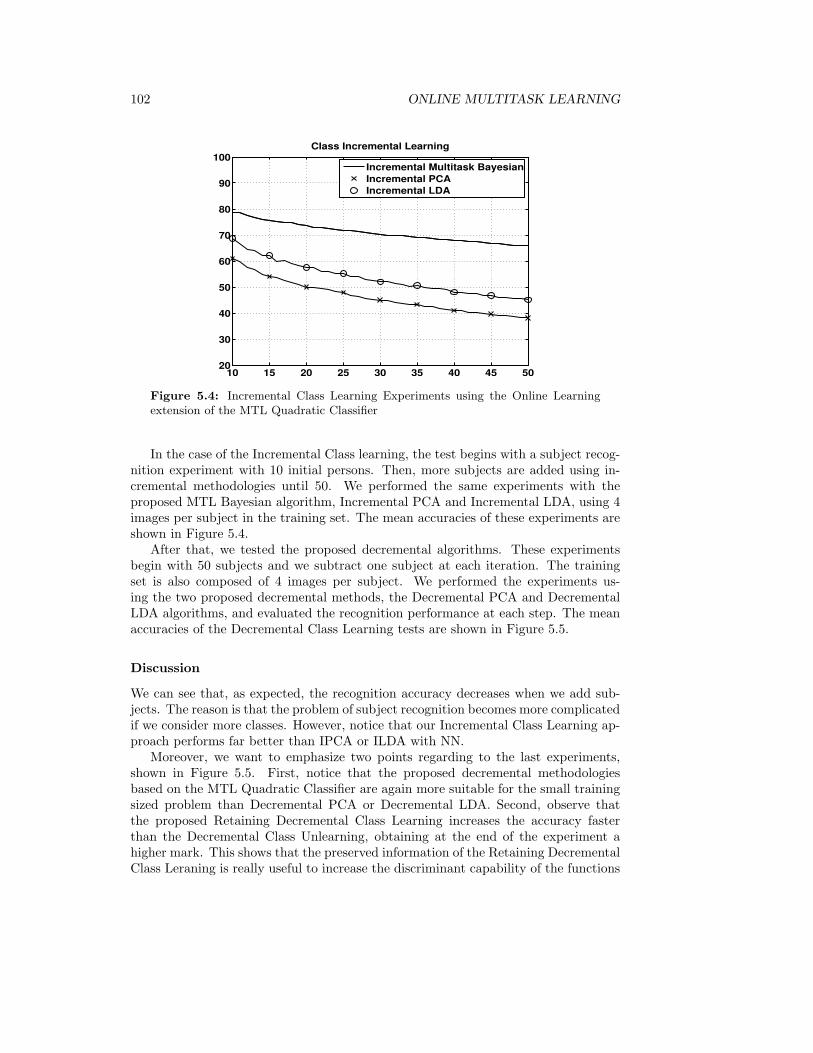
102 ONLINE MULTITASK LEARNING

10 15 20 25 30 35 40 45 5020

30

40

50

60

70

80

90

100Class Incremental Learning

Incremental Multitask BayesianIncremental PCAIncremental LDA

Figure 5.4: Incremental Class Learning Experiments using the Online Learningextension of the MTL Quadratic Classifier

In the case of the Incremental Class learning, the test begins with a subject recog-nition experiment with 10 initial persons. Then, more subjects are added using in-cremental methodologies until 50. We performed the same experiments with theproposed MTL Bayesian algorithm, Incremental PCA and Incremental LDA, using 4images per subject in the training set. The mean accuracies of these experiments areshown in Figure 5.4.

After that, we tested the proposed decremental algorithms. These experimentsbegin with 50 subjects and we subtract one subject at each iteration. The trainingset is also composed of 4 images per subject. We performed the experiments us-ing the two proposed decremental methods, the Decremental PCA and DecrementalLDA algorithms, and evaluated the recognition performance at each step. The meanaccuracies of the Decremental Class Learning tests are shown in Figure 5.5.

Discussion

We can see that, as expected, the recognition accuracy decreases when we add sub-jects. The reason is that the problem of subject recognition becomes more complicatedif we consider more classes. However, notice that our Incremental Class Learning ap-proach performs far better than IPCA or ILDA with NN.

Moreover, we want to emphasize two points regarding to the last experiments,shown in Figure 5.5. First, notice that the proposed decremental methodologiesbased on the MTL Quadratic Classifier are again more suitable for the small trainingsized problem than Decremental PCA or Decremental LDA. Second, observe thatthe proposed Retaining Decremental Class Learning increases the accuracy fasterthan the Decremental Class Unlearning, obtaining at the end of the experiment ahigher mark. This shows that the preserved information of the Retaining DecrementalClass Leraning is really useful to increase the discriminant capability of the functions

5.4. Conclusions 103

10152025303540455020

30

40

50

60

70

80

90

100Class Decremental Learning

Decremental Multitask BayesianDecremental PCADecremental LDARetaining Multitask Bayesian

Figure 5.5: Decremental Class Learning Experiments using the two Online Learningextensions of the MTL Quadratic Classifier

f1, . . . , fK−1, when the K-th class is removed.

5.4 Conclusions

In this chapter we proposed two online learning extensions of MTL classifiers.We presented first an online extension of the JointBoost algorithm in order to

solve real world face recognition problems. The main contribution of this work withrespect to the state-of-the-art is the possibility of incrementally adding new classes toa previously trained problem, which is specially useful in face recognition applications.It has been shown experimentally that the use of JointBoost achieves high accura-cies in face classification. Nevertheless, the computational cost makes the methodunfeasible when the problem has too many classes, due to the BFS clustering step(O(K2)). More concretely, training the JointBoost algorithm using an initial set of 25classes takes 8 hours on a Pentium IV computer (using the Matlab software), whilelearning the same algorithm using 80 classes can take weeks. However, to extend theprevious 25 class problem to the new 80 class problem using our approach takes justa few minutes. Moreover, the 160 final class problem is nowadays non computable ina reasonable amount of time.

In both JointBoost and Online Boosting methods, the multi-class problem is seenas a set of multiple binary classification tasks (one versus all) that are trained sharingthe feature space. The method uses an initial set to build a model using the JointBoostalgorithm and then the system is readjusted when new classes are added to the initialset. In that way the proposed Online Boosting for face recognition is able to consider afinal amount of subjects that will be computationally unfeasible with the JointBoost.

We have experimentally validated our proposal using two different face databases:the FRGC database acquired in a controlled environment, and the AR Face database

104 ONLINE MULTITASK LEARNING

which contains important artifacts due to strong changes in the illumination andpartial occlusions. When the original sets are extended to large class problems, theresults show that the classification accuracy decreases less drastically than using theclassic NN rule used in state-of-the-art Online Learning methods.

The initial number of classes necessary to build the JointBoost model dependsexclusively on the final application, being limited by the availability of samples intraining time and the computational resources. In the experiments performed, weshow that an initial 25 class set yields us a good trade off between training time andfinal accuracies.

On the other hand, we have presented a second MTL method for Online Learning,which is an extension of the MTL Quadratic Classifier presented in Chapter 4. Theproposed framework is suitable for the four online learning problems: IncrementalSample Learning, Decremental Sample, Incremental Class Learning and DecrementalClass Learning. Given that the two first cases are exact computations, we tested justthe Incremental Class Learning and the Decremental Class Learning methods. Wehave seen that our methodologies fare better than IPCA or ILDA with NN, whichare the most common methods that allow the inclusion or subtraction of classes.

Furthermore, we have proposed a new approach for the Decremental Class Learn-ing problem, based on keeping in the system useful information of a concrete classwhen it has to be removed. In this case, the performed experiments showed a higheraccuracy of this new approach over the classical decremental strategy.

Chapter 6

Independent Tasks: a NewRelatedness Concept

The research presented in this chapter was inspired by the following idea: given twosubjects, suppose that we are able to recognize person 1 under different conditions,such as wearing glasses or sunglasses, and/or a scarf. Suppose, however, that we arenot able to recognize subject 2 under these appearance variations. The question is:can we extrapolate somehow the background knowledge acquired with person 1, tobe able to recognize person 2 under these variations? Intuitively, the variations of thefaces of two different subjects under the same appearance changes have to be similarin some aspects.

In this example, we found a relationship between the tasks of subject identifica-tion and face appearance classification: if the variation of any face follows a concretepattern when the appearance conditions vary, we can learn from this pattern to benot sensitive to the appearance changes. Then, if we learn this insensitivity to theface appearance changes of the same subject, we can improve the subject recognizingability. More concretely, if the face representation is suitable to perform the sub-ject recognition task (elements of the same class together and elements of differentclasses separated), then the face representation is not suitable to perform appearanceclassification task.

In this chapter we define a new task relatedness concept, dealing with the ideaabove presented. The framework is called the Independent Tasks Problem. More-over we propose, test and discuss two dimensionality reduction techniques speciallydeveloped for problems involving tasks with this kind of relationship.

We give a formal definition of the independent tasks concept in Section 6.2, whichis based on the mutual information measure. The proposed dimensionality reductiontechniques to deal with the independent tasks problem are based also in this statistic.Next section introduces the mutual information and some of its properties.

The rest of the chapter is structured as follows: Section 6.3 presents an initialstudy proposing a feature selection criterion that is specially suitable for the inde-pendent tasks problem, and Section 6.4 proposes a feature extraction method to findappropriate data representations to deal with this framework. Finally we conclude

105

106 INDEPENDENT TASKS: A NEW RELATEDNESS CONCEPT

the work in Section 6.5.

6.1 Mutual Information

The mutual information between two random variables is a quantity that measurestheir dependence [235, 141, 185]. It may be thought of as the reduction in uncertaintyabout one random variable given the knowledge of the other. Then, high mutualinformation indicates a large reduction in uncertainty while low mutual informationindicates a small reduction. Moreover, zero mutual information between two randomvariables means the variables are independent.

There are different definitions of mutual information. Following we introducethe Shannon’s mutual information and analyze some of its properties, as well as itsrelationship with the Shannon’s entropy measure. Then, we briefly review alternativemutual information definitions that can be found in the literature.

An interesting point of mutual information is its relevance in estimating the errorthat can be made by a classifier. Actually, the mutual information between the datarepresentation and their labels may be understood as an indicator of classificationperformance. In the end of this section we include a discussion of the relationshipbetween mutual information and the Bayes error.

6.1.1 Shannon’s definition

Let us focus our attention on the definition of mutual information between a contin-uous random variable X and a discrete random variable C. In this case the mutualinformation between X and C is

I(X , C) :=

∫

x

∑

c

p(x, c) log2

(p(x, c)

p(x)p(c)

)dxdc (6.1)

where p(x, c) is the joint probability density function of X and C, while p(x) andp(c) are the probability density functions of X and C respectively.

Shannon’s Entropy and its relationship with Mutual Information

One interpretation of the mutual information is related with the entropy concept.The Shannon’s entropy of a discrete random variable C, H(C), is defined as

H(C) = −∑

c

p(c) log2(p(c))dc (6.2)

In the case of continuous random variables the computation of the entropy is thesame but substituting the sum for an integral.

The entropy of a random variable may be interpreted as an uncertainty measure.For example, suppose that we have a binary random variable Z, that may be modelledwith a Binomial distribution of probability p. That is, we have two possible eventswith probabilities p and 1 − p per event. In this case, the entropy of the randomvariable is

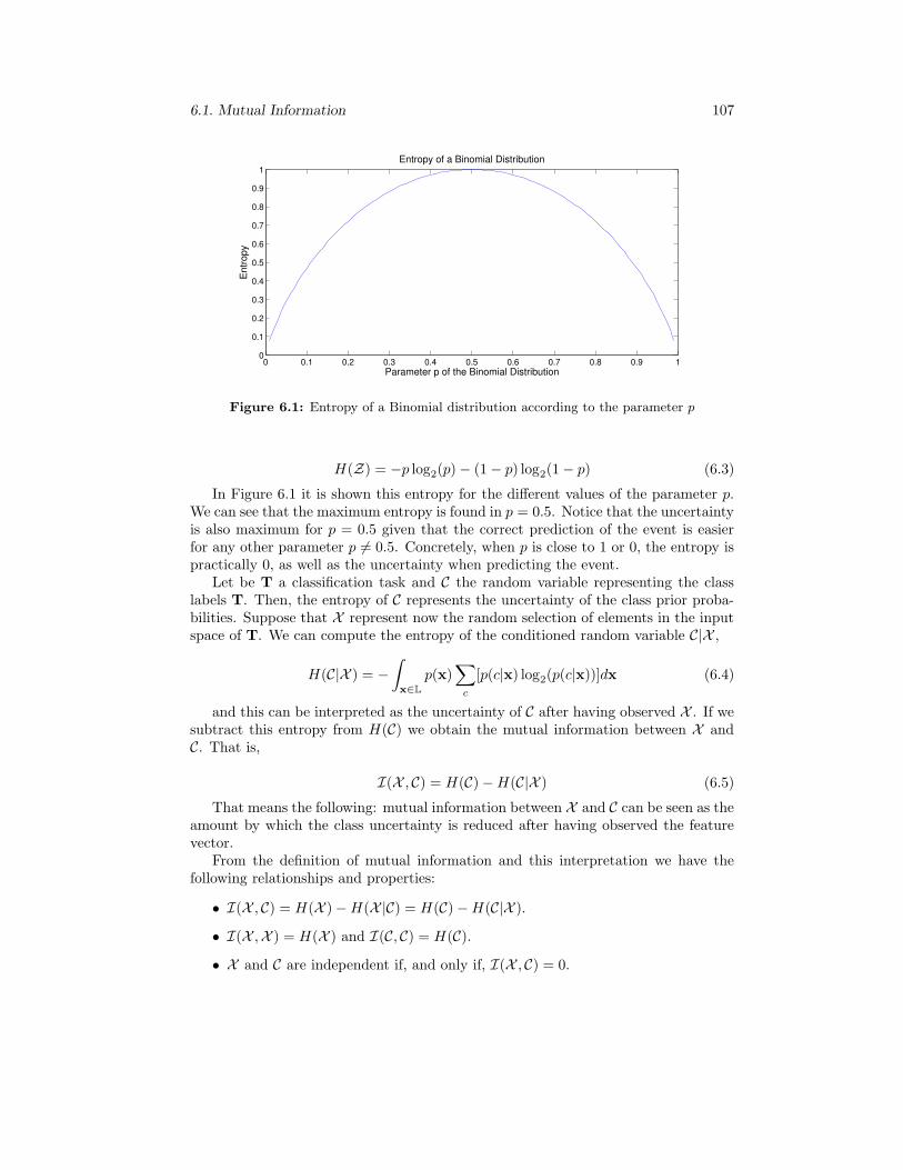
6.1. Mutual Information 107

0 0.1 0.2 0.3 0.4 0.5 0.6 0.7 0.8 0.9 10

0.1

0.2

0.3

0.4

0.5

0.6

0.7

0.8

0.9

1

Parameter p of the Binomial Distribution

Ent

ropy

Entropy of a Binomial Distribution

Figure 6.1: Entropy of a Binomial distribution according to the parameter p

H(Z) = −p log2(p)− (1− p) log2(1− p) (6.3)

In Figure 6.1 it is shown this entropy for the different values of the parameter p.We can see that the maximum entropy is found in p = 0.5. Notice that the uncertaintyis also maximum for p = 0.5 given that the correct prediction of the event is easierfor any other parameter p 6= 0.5. Concretely, when p is close to 1 or 0, the entropy ispractically 0, as well as the uncertainty when predicting the event.

Let be T a classification task and C the random variable representing the classlabels T. Then, the entropy of C represents the uncertainty of the class prior proba-bilities. Suppose that X represent now the random selection of elements in the inputspace of T. We can compute the entropy of the conditioned random variable C|X ,

H(C|X ) = −∫

x∈L

p(x)∑

c

[p(c|x) log2(p(c|x))]dx (6.4)

and this can be interpreted as the uncertainty of C after having observed X . If wesubtract this entropy from H(C) we obtain the mutual information between X andC. That is,

I(X , C) = H(C)−H(C|X ) (6.5)

That means the following: mutual information between X and C can be seen as theamount by which the class uncertainty is reduced after having observed the featurevector.

From the definition of mutual information and this interpretation we have thefollowing relationships and properties:

• I(X , C) = H(X )−H(X|C) = H(C)−H(C|X ).

• I(X ,X ) = H(X ) and I(C, C) = H(C).• X and C are independent if, and only if, I(X , C) = 0.

108 INDEPENDENT TASKS: A NEW RELATEDNESS CONCEPT

The definition of Shannon’s entropy is based on a set of postulates or axioms[141, 3, 129]. Different measures of uncertainty can be defined, depending on differentconditions or even based just on a subset of these axioms.

The Kullback-Leibler divergence and its relationship with Mutual Infor-mation

Another interpretation of the mutual information is related as the Kullback-Leiblerdivergence measure. This functional quantifies the difference between two probabilitydistributions. In general, for two probability density functions g1 and g2, the Kullback-Leibler divergence is defined as

K(g1, g2) =

∫

x

g1(x) log2

g1(x)

g2(x)dx (6.6)

We stated before that the mutual information measures dependence between ran-dom variables. On the other hand, we know that two random variables X and Care independent when their joint density can be factored as the product of marginaldensities, that is

p(x, c) = p(x)p(c) (6.7)

Then, if we want to quantify the dependence between X and C, we can computethe Kullback-Leibler divergence between p(x, c) and p(x)p(c). This computation isexactly the same definition of I(X ,Y) as before.

6.1.2 Other Mutual Information definitions

In the past fifty years researchers have been interested in generalizations of informa-tion measures. In this context, the work of Renyi [200] is a fundamental contributionto this theory. He pointed out that in many classes of problems other informationquantities may serve as well, or even better, as measures of information. Actually,Kapur [121] argues that less restrictive definitions are enough when the aim is not tocompute an accurate value of the entropy. In fact, in several applications the goal isto find a distribution that optimizes this entropy given some constraints, instead ofthe computation of this measure for a concrete distribution.

The proposal of Renyi is a generalized entropy, which includes Shannon’s entropyas a particular case, leading to alternative information definitions. Concretely, givena discrete random variable C and a continuous random variable X , the Renyi entropyis defined by

HRa(C) =

1

1− alog2

∑

c

p(c)a (6.8)

HRa(X ) =

1

1− alog2

∫

x

p(x)adx (6.9)

where a > 0, a 6= 1. Notice that lima→1 HRais the Shannon’s mutual information.

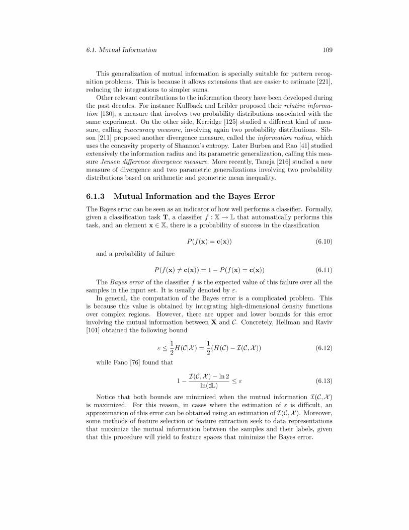
6.1. Mutual Information 109

This generalization of mutual information is specially suitable for pattern recog-nition problems. This is because it allows extensions that are easier to estimate [221],reducing the integrations to simpler sums.

Other relevant contributions to the information theory have been developed duringthe past decades. For instance Kullback and Leibler proposed their relative informa-tion [130], a measure that involves two probability distributions associated with thesame experiment. On the other side, Kerridge [125] studied a different kind of mea-sure, calling inaccuracy measure, involving again two probability distributions. Sib-son [211] proposed another divergence measure, called the information radius, whichuses the concavity property of Shannon’s entropy. Later Burbea and Rao [41] studiedextensively the information radius and its parametric generalization, calling this mea-sure Jensen difference divergence measure. More recently, Taneja [216] studied a newmeasure of divergence and two parametric generalizations involving two probabilitydistributions based on arithmetic and geometric mean inequality.

6.1.3 Mutual Information and the Bayes Error

The Bayes error can be seen as an indicator of how well performs a classifier. Formally,given a classification task T, a classifier f : X → L that automatically performs thistask, and an element x ∈ X, there is a probability of success in the classification

P (f(x) = c(x)) (6.10)

and a probability of failure

P (f(x) 6= c(x)) = 1− P (f(x) = c(x)) (6.11)

The Bayes error of the classifier f is the expected value of this failure over all thesamples in the input set. It is usually denoted by ε.

In general, the computation of the Bayes error is a complicated problem. Thisis because this value is obtained by integrating high-dimensional density functionsover complex regions. However, there are upper and lower bounds for this errorinvolving the mutual information between X and C. Concretely, Hellman and Raviv[101] obtained the following bound

ε ≤ 1

2H(C|X ) =

1

2(H(C)− I(C,X )) (6.12)

while Fano [76] found that

1− I(C,X )− ln 2

ln(]L)≤ ε (6.13)

Notice that both bounds are minimized when the mutual information I(C,X )is maximized. For this reason, in cases where the estimation of ε is difficult, anapproximation of this error can be obtained using an estimation of I(C,X ). Moreover,some methods of feature selection or feature extraction seek to data representationsthat maximize the mutual information between the samples and their labels, giventhat this procedure will yield to feature spaces that minimize the Bayes error.

110 INDEPENDENT TASKS: A NEW RELATEDNESS CONCEPT

6.2 The Independent Tasks Problem

Let be T1 and T2 two tasks and suppose that the input spaces T1 and T2 are thesame, X

1 = X2 = X. Let be (X , C1), (X , C2) the random variables representing

arbitrary samples selection with its corresponding class labels, for tasks T1 and T2

respectively.Definition: the tasks T1 and T2 are independent if C1 and C2 are independent

random variables. That is, given x ∈ X,

P ((c1(x) = k1) ∩ (c2(x) = k2)) = P (c1(x) = k1)(c2(x) = k2) (6.14)

for all possible classes k1 ∈ L1 of T1 and k2 ∈ L

2 of T2.Independent tasks examples can be found in real problems of computer vision. For

instance, a set of manuscript symbols can be categorized according to which symbolappears in the image or according to the person who drew it. In that case, thesetwo tasks are independent if we assume that the probability of writing a concretesymbol is the same for all of the authors. On the other hand, considering a set of faceimages having some kind of expression (smile, anger, scream or neutral) we can dividethe set according to the subject that is in the image or according to the expression.Then, supposing that the expression does not depend on the subject, we have alsotwo independent classification tasks.

In Figure 6.2 an example of independent tasks is graphically shown. The tasksare: (T1) separate triangles and circles (T2) separate the elements depending on thebrightness. These tasks are independent given that, for example, if we take randomlyone element and we just know that it is a circle, we do not know anything about itsbrightness (the probability of being dark is exactly the same of being bright).

In several real situations, a task should be learned from a reduced set of trainingsamples, where the variability according to an independent task may be not repre-sented. For instance, in face classification field, we can consider the target task ofsubject recognition. In most of these cases, we will have just a few number of trainingsamples per class. Moreover, in real situations, these images are captured in controlledenvironments, appearing no local changes in the illumination and no representationsof the subject with partial occlusions. However, the goal is to recognize people in anyuncontrolled condition.

This drawback can be also illustrated graphically with the example of Figure 6.2.Suppose that the target task is T1, the classification depending on the shape, butsuppose that our training set is biased in the sense that it just include bright pieces.In this case, if we learn a linear classifier, a reasonable solution may be the oneillustrated in Figure 6.3 (a). Then, when we test this solution the classification willmiss in several dark triangles, that will be classified as circles, as shown in Figure 6.3(b).

In this chapter we explore solutions for the independent tasks problem. Concretely,the framework we consider is the following: we have a target task T1 and anothertask T2 that is independent respect to T1. These tasks are sharing the input space,X := X

1 = X2, and we have training sets (X1, c1),(X2, c2). In fact we have two

possible representations of the training data in this framework:

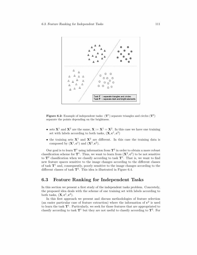
6.3. Feature Ranking for Independent Tasks 111

Figure 6.2: Example of independent tasks: (T1) separate triangles and circles (T2)separate the points depending on the brightness.

• sets X1 and X2 are the same, X := X1 = X2. In this case we have one trainingset with labels according to both tasks, (X, c1, c2)

• the training sets X1 and X2 are different. In this case the training data iscomposed by (X1, c1) and (X2, c2).

Our goal is to learn T1 using information from T2 in order to obtain a more robustclassification scheme for T1. Thus, we want to learn from (X2, c2) to be not sensitiveto T2 classification when we classify according to task T1. That is, we want to findnew feature spaces sensitive to the image changes according to the different classesof task T1 and, consequently, poorly sensitive to the image changes according to thedifferent classes of task T2. This idea is illustrated in Figure 6.4.

6.3 Feature Ranking for Independent Tasks

In this section we present a first study of the independent tasks problem. Concretely,the proposed idea deals with the scheme of one training set with labels according toboth tasks, (X, c1, c2).

In this first approach we present and discuss methodologies of feature selection(an easier particular case of feature extraction) where the information of c2 is usedto learn the task T1. Particularly, we seek for those features that are appropriated toclassify according to task T1 but they are not useful to classify according to T2. For

112 INDEPENDENT TASKS: A NEW RELATEDNESS CONCEPT

(a)

(b)

Figure 6.3: Example of biased training set, in an independent tasks problem.

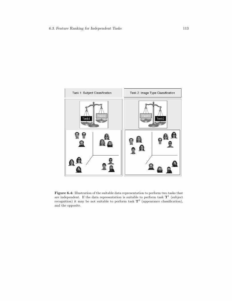
6.3. Feature Ranking for Independent Tasks 113

Figure 6.4: Illustration of the suitable data representation to perform two tasks thatare independent. If the data representation is suitable to perform task T1 (subjectrecognition) it may be not suitable to perform task T2 (appearance classification),and the opposite.

114 INDEPENDENT TASKS: A NEW RELATEDNESS CONCEPT

this aim we use the mutual information to propose a ranking criteria for selecting thefeatures.

First, we find an orthogonal basis to represent the data according to their vari-ance, using the strategy followed by Principal Component Analysis. Then, we per-form feature selections according to different criteria and compare them. This idea ismotivated by the work of Bart and Ullman [13], which propose an illumination nor-malization rejecting the PCA components with high mutual information according tothe illumination conditions.

A common procedure for feature selection using the mutual information is featureranking [96]. The idea is to sort the features in a decreasing order of their mutualinformation with the target values and select the first d.

Let us focus in the problem of independent tasks stated in Section 6.2. Formally,we have two tasks that are independent, T1 and T2. We want to select optimalfeatures to perform T1. Here we suppose the training data is presented as follows

• training samples X = {x1, ...,xN}• class labels according to the target task T1 for all the training samples, c1 ={c1

1, ..., c1N}

• class labels according to task T2 for all the training samples, c2 = {c21, ..., c

2N}

In that case we can compute for each j-th feature its mutual information accordingto c1 and c2, respectively denoted by I1

j = I(Xj , c1) and I2

j = I(Xj , c2). The idea is

to explore ranking criteria for feature selection using both indicators at a time.Notice the following considerations: from the nature of our problem we need

features able to model T1 but poorly sensitive to the different classes of T2. Thissuggest that appropriate features should have high mutual information according toC1 and low mutual information according to C2. Thus, from these observations wepropose the following two approaches for selecting the PCA components

• reject the components having high I2j and select after this rejection the d com-

ponents corresponding to the highest eigenvectors module

• find a feature selection criterion combining both indicators and select the firstd. The idea here is to use j-th features having high I1

j and low I2j . In cases

that these values are close enough we can use the substraction criteria I1j −I2

j .However, we are not able define a general combined criterion valid for all datatypes and tasks. This is because the mutual information is not upper boundedand that this concept is not a distance between variables. For this reason theexploration of combined criterion should be designed according to the concretedata and tasks.

Mutual Information estimation

The main drawback of the mutual information definition is that the densities areall unknown and are hard to estimate from the data, particulary when they arecontinuous. For this reason different approaches for mutual information estimationhave been proposed in the literature [222, 17].

6.3. Feature Ranking for Independent Tasks 115

We follow in this case a simplified estimation approach, discretizing the variables inbins. Concretely, to estimate Ij = I(Xj , C), we discretize Xj in s bins, {B1, ..., Bs},and compute the frequency of each bin. Therefore, if we have K possible classes,{1, ..., k, ...,K}, the computation is done by

Ij =

s∑

b=1

K∑

k=1

p(Bb, k)log

(p(Bb, k)

p(Bb)p(k)

)(6.15)

where the densities are estimated as:

p(k) =#{ci = k}i=1,..,N

N(6.16)

p(Bb) =#{xij ;xij ∈ Bb}i=1,..,N

N(6.17)

p(Bb, k) =#{xij ∈ Bb; ci = k}i=1,..,N

N(6.18)

6.3.1 Experiments and Discussion

The goal of this section is to illustrate and compare the proposed ideas in a realproblem. With this aim, we performed subject recognition experiments using thepublicly available ARFace database [152]. We used here just the internal part of theface, aligning the images according to the eyes and resizing them to be 36×33 pixels.

This database is specially appropriated to illustrate our idea given that there aretwo tasks represented: subject classification (target task, T1) and image type classi-fication (T2). We have discussed in Section 6.2 that these two tasks are independent.

We have performed 100 subject verification experiments following this protocol:for each subject, 13 images are randomly selected to perform the feature extractionstep and the rest of the images are used to test.

Three different criteria of feature extraction are considered:

• Criterion 1 (CR1 ): PCA and selection of the features corresponding to the higheigenvalues module.

• Criterion 2 (CR2 ): PCA and selection of the features having more mutualinformation according to C1.

• Criterion 3 (CR3 ): PCA and rejection of the features having more mutualinformation according to C2.

• Criterion 4 (CR4 ): PCA and selection of features having higher score accordingto the substraction criteria I1

j − I2j .

The classification is performed in all the cases with the Nearest Neighbor.To apply the fourth feature extraction system we need to ensure that the mutual

information from the features according to the subject criteria or the image typecriteria have the same order. In Figure 6.5 are plotted these values for the first 50

116 INDEPENDENT TASKS: A NEW RELATEDNESS CONCEPT

principal components of the original data. Notice that they are of the same order.Moreover, features having a special high value according to one partition have lowvalue according to the other one, what is consistent with our hypothesis. Thus, thistwo observations support the use of the criterion I1

j − I2j for feature selection.

In Figure 6.6 are plotted the mean accuracy obtained in the performed experimentsat each dimensionality. On the other hand, Table 6.1 shows the accuracies and theconfidence intervals for some dimensionalities.

Table 6.1: Mean accuracy (in percentage) and confidence intervals of the 100 subjectrecognition experiments at 100, 200, 300, 400 dimensionalities respectively. The criterionof feature extraction are CR1, CR2, CR3 and CR4 specified above.

100 200 300 400CR1 38.45± 2.13 38.80± 2.31 38.78± 2.26 38.77± 2.30CR2 57.50± 3.65 43.07± 3.24 40.83± 3.69 39.84± 3.68CR3 55.73± 3.38 54.31± 3.35 52.85± 3.17 52.14± 3.26CR4 63.54± 3.06 64.11± 2.89 64.24± 3.05 64.21± 3.12

Discussion

The most successful approach in our experiments is the feature selection accordingto the proposed combined criterion, while the worst option is PCA. Notice, however,that PCA is the only case where the feature selection is non-supervised. For thisreason we can not achieve results as high as when we use the other approaches. Inthe proposed problem we are preserving from the beginning features that are speciallysuitable to perform T2 and rejecting some of them that are useful for T1.

We can see that the selection of variables that have high mutual informationaccording to T1 is specially appropriated for the initial components. However, if weuse just this criterion, from the 70-th variable we are adding features that are not assuitable as the first ones. For this reason the accuracy begins to decrease. On theother hand, the accuracy evolution is more stable when we reject the features withhigh mutual information according to T2.

Although the combined system is not enough general to be applied systemati-cally, the results show that the use of independent problems can actually improvethe performance of a task. For this reason we explore in the next sections a moresophisticated approach to the independent tasks problem.

6.4 Linear Feature Extraction for Independent Tasks

In this section we propose a method for linear feature extraction designed for theindependent tasks problem. To learn the feature transformation we use again themutual information measure between data and class labels of both tasks. The idea isto extract features that keep the information useful to perform the target task, butnot preserving the information of the independent task.

6.4. Linear Feature Extraction for Independent Tasks 117

Figure 6.5: Mutual information of the first 50 principal components according tothe subject classification (T1) and image type classification (T2) respectively

118 INDEPENDENT TASKS: A NEW RELATEDNESS CONCEPT

0 50 100 150 200 250 300 350 4000

0.1

0.2

0.3

0.4

0.5

0.6

0.7

dimensionality

mea

n ac

cura

cy

Subject recognition experiments

CR1CR2CR3CR4

Figure 6.6: Mean accuracy in the performed subject recognition experiments ateach dimensionality, considering the criterions for feature extraction specified above.

The approach here proposed deals with the scheme where the training sets X1 andX2 are different. In this case the training data is composed by (X1, c1) and (X2, c2).In Figure 6.7 we show graphically this framework.

6.4.1 Linear Feature Extraction Algorithm

The idea is to find a linear projection W : RD → R

d, d < D, such that

• the transformed data Y = WX1 keep as much mutual information as possibleaccording to the target task T1

• the mutual information between the new data representation and the class labelsaccording to T2 is as low as possible

Let us to illustrate the sense of this approach in the framework of Figure 6.7. Wecan see in Figure 6.8 a linear feature transformation of the training data that showsdiscriminability capacity to separate bright circles and bright triangles. However, thistransformation mixes just a bit the bright and dark figures, meaning that the new fea-ture space has some information about task T2. On the other hand, Figure 6.9 showsa linear transformation that is suitable to perform classification according to task T2

(brightness). That means that the new data has lot of information about this task.However, the new representation do not show at all discriminant ability to performtask T1. Finally, Figure 6.10, shows the optimal linear transformation to generalize

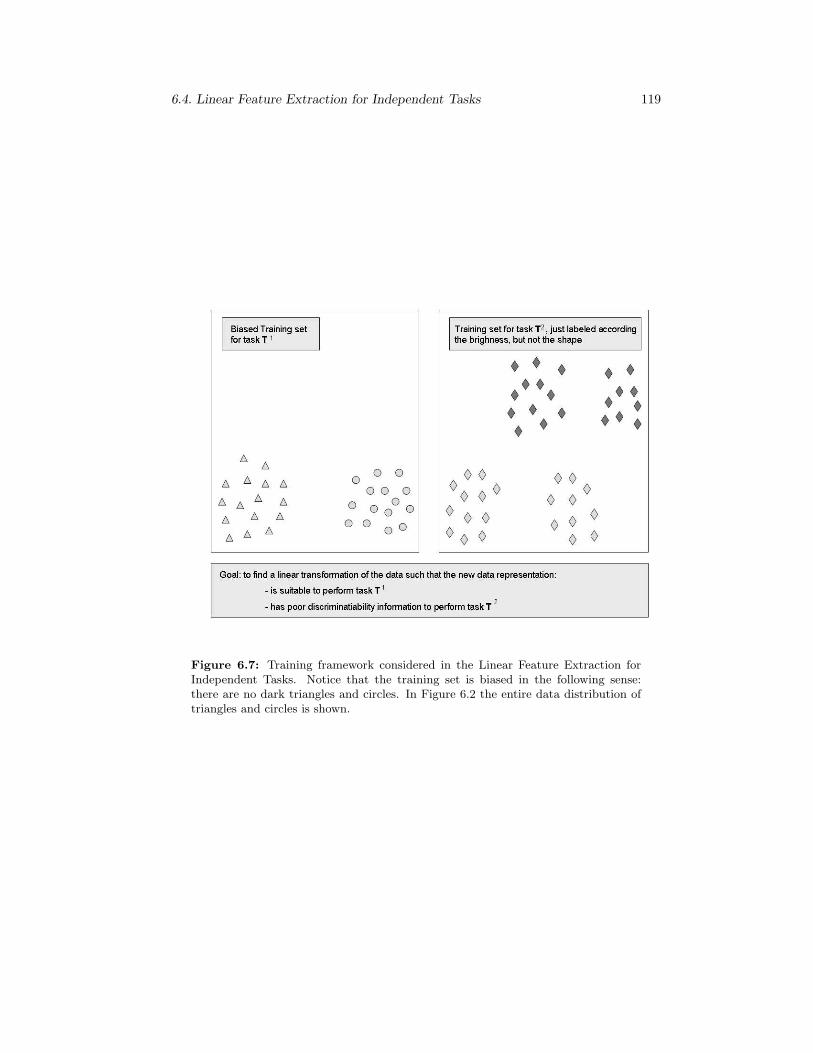
6.4. Linear Feature Extraction for Independent Tasks 119

Figure 6.7: Training framework considered in the Linear Feature Extraction forIndependent Tasks. Notice that the training set is biased in the following sense:there are no dark triangles and circles. In Figure 6.2 the entire data distribution oftriangles and circles is shown.

120 INDEPENDENT TASKS: A NEW RELATEDNESS CONCEPT

Figure 6.8: An example of linear data transformation presents a good discrim-inability capacity with a biased training set for the target task T1. Notice that thediscriminability capacity of this transformation to perform task T2 is a quite poor.

performing task T1. Notice that in this case the bright and dark points become ab-solutely mixed in the new feature space, meaning that this data representation hasno information about task T2.

Formally, we seek the linear projection

W = arg maxV

Jλ(V) (6.19)

Jλ(V) := I(VX1, c1)− λI(VX2, c2) (6.20)

where λ is a positive weight. This parameter controls the amount of T2 contri-bution to learn a new feature space for T1. Notice that if we set this parameter to 0then the method just takes into account the training data of task T1.

Given that Shannon’s mutual information between data and labels is difficultto estimate, we use in this thesis the Quadratic Mutual Information proposed byTorkkola [222]. The main idea is to use Renyi quadratic entropy instead of Shannon’sdefinition of entropy. In that case, the Renyi quadratic entropy can be estimated as asum of local interactions if the density functions of the variables are estimated usingParzen window method [186]. Following we describe the procedure of this mutualinformation computation for a generic framework.

Consider a set of training data X = {x1, ...,xN} ⊆ X ⊆ RD, and a transformation

of the data Y = {y1, ...,yN} = VX ⊆ Y ⊆ Rd. Suppose that the goal is to compute

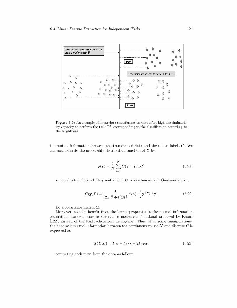
6.4. Linear Feature Extraction for Independent Tasks 121

Figure 6.9: An example of linear data transformation that offers high discriminabil-ity capacity to perform the task T2, corresponding to the classification according tothe brightness.

the mutual information between the transformed data and their class labels C. Wecan approximate the probability distribution function of Y by

p(y) =1

N

N∑

i=1

G(y − yi, σI) (6.21)

where I is the d× d identity matrix and G is a d-dimensional Gaussian kernel,

G(y,Σ) =1

(2π)d2 det(Σ)

12

exp(−1

2yT Σ−1y) (6.22)

for a covariance matrix Σ.Moreover, to take benefit from the kernel properties in the mutual information

estimation, Torkkola uses as divergence measure a functional proposed by Kapur[122], instead of the Kullbach-Leibler divergence. Thus, after some manipulations,the quadratic mutual information between the continuous valued Y and discrete C isexpressed as

I(Y, C) = IIN + IALL − 2IBTW (6.23)

computing each term from the data as follows

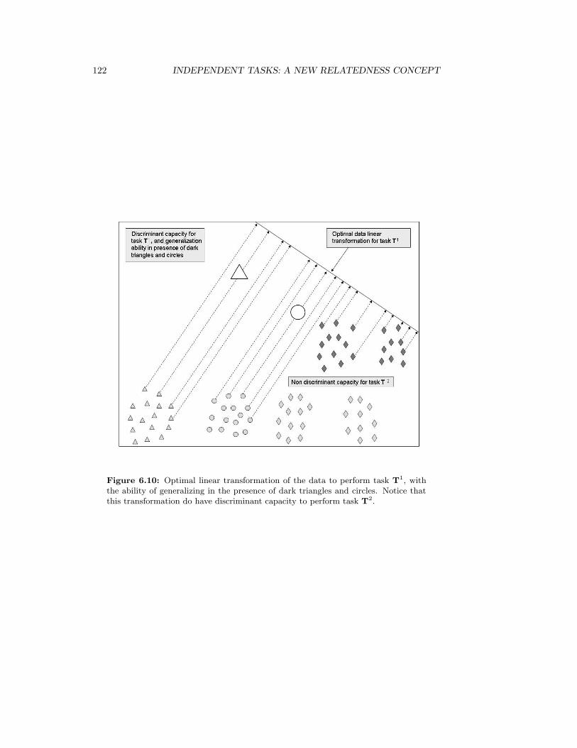
122 INDEPENDENT TASKS: A NEW RELATEDNESS CONCEPT

Figure 6.10: Optimal linear transformation of the data to perform task T1, withthe ability of generalizing in the presence of dark triangles and circles. Notice thatthis transformation do have discriminant capacity to perform task T2.

6.4. Linear Feature Extraction for Independent Tasks 123

IIN =1

N2

∑

k

Nk∑

j=1

Nk∑

i=1

G(ykj − yki, 2σ2I) (6.24)

IALL =1

N2(∑

k=1

(Nk

N)2)

N∑

j=1

N∑

i=1

G(yj − yi, 2σ2I) (6.25)

IBTW =1

N2

∑

k=1

Nk

N

Nk∑

j=1

N∑

i=1

G(ykj − yi, 2σ2I) (6.26)

where I denotes here the N×N identity matrix. In these expressions a transformedsample is denoted by one index yi if its class is irrelevant, and it is denoted by twoindexes ykj when its class is relevant. In this second case k represents the class indexand j represents the within-class index, being Nk the number of training samples inclass k.

On the other hand, given that

∂

∂yi

G(yi − yj) = G(yi − yj , 2σ2I)

(yj − yi)

2σ2(6.27)

the corresponding derivatives ∂VIN

∂yki, ∂VALL

∂ykiand ∂VBT W

∂ykiare, respectively,

∑Nk

j=1 G(ykj − yki, 2σ2I)(ykj − yki)

N2σ2(6.28)

(∑NT

r=1(Nr

N)2)

∑Nj=1 G(yj − yki, 2σ

2I)(yj − yi)

N2σ2(6.29)

∑NT

r=1Nr+Nk

2N

∑Nr

j=1 G(yrj − yki, 2σ2I)(yrj − yki)

N2σ2(6.30)

In this way we obtain expressions for the mutual information and the correspond-ing derivatives expressed in function of y1, ...yN .

With this approach we can compute the derivatives of the proposed loss function(equation 6.20) and use them for optimizing this function. Concretely, the previouscalculations allows to express Jλ depending on y1, ...yN . Thus, we have

∂Jλ

∂W=

N∑

i=1

∂Jλ

∂yi

∂yi

∂W=

N∑

i=1

∂Jλ

∂yi

xTi (6.31)

and we can use gradient ascent techniques for optimizing the criterion Jλ. Con-cretely, to maximize this function we used a two-sample stochastic gradient ascent,given that a classical gradient ascent procedure is not computationally feasible forlarge sets of high dimensional data. It is specially appropriated the use of two-samplesubsets to approximate Jλ and their derivatives because of the expressions simplifi-cation.

Concretely, the updating of this gradient ascent is performed by

124 INDEPENDENT TASKS: A NEW RELATEDNESS CONCEPT

Wt+1 = Wt + ξ∂Jλ

∂W(6.32)

where ∂Jλ/∂W is approximated at each iteration using a predetermined number Qof sample pairs. Thus, given arbitrary x1,x2 ∈ {X1,X2} and y1 = Wx1, y2 = Wx2,

∂Jλ

∂W=

∂Jλ

∂y1

∂y1

∂W+

∂Jλ

∂y2

∂y2

∂W=

∂Jλ

∂y1xT

1 +∂Jλ

∂y2xT

2 (6.33)

and

∂Jλ

∂yi

=∂I(X, C1)

∂yi

− λI(X, C2)

∂yi

(6.34)

where X denotes the set {x1,x2}. From equations 6.26, we have

I(Xt, Ct) =1

4(G(0, 2σ2I)−G(y1 − y2, 2σ

2I)) (6.35)

if ct(x1) 6= ct(x2) and I(X, Ct) = 0 otherwise (for t = 1, 2), and

∂I(X, Ct)

∂y1= −∂I(X, Ct)

∂y2= − 1

8σ2G(y1 − y2, 2σ

2I)(y2 − y1) (6.36)

if ct(y1) 6= ct(y2), and ∂I(X,Ct)∂y1

= ∂I(X,Ct)∂y2

= 0 otherwise, t = 1, 2.

For more details of these derivations see [221].The stochastic gradient ascent to optimize Jλ is detailed in Table 6.11.Notice that essential points in this procedure are: (a) to decide whether two

elements x1,x2 ∈ {X1,X2} are in the same class according to partitions T2 or not,and (b) the use of the labels c2 in the algorithm. Both points should be consideredand appropriately approached depending on the tasks and the data sets.

6.4.2 Experiments and Discussion

We used in our experiments the publicly available ARFace database [152] and thesubset of FRGC [187] database composed by the images acquired in non-controlledenvironments.

We have aligned all the images according to the eyes and have used in our exper-iments just the internal part of the face, in a resolution of 36× 33 pixels.

In all the experiments we consider subject recognition as a target task T1, andimage type classification as an independent task T2. The independence assumptionbetween these two tasks has been discussed in Section 6.2.

To perform the experiments the available data for the target task T1 is alwayssplit in two subsets: (X1, c1) and (X1

test, C1test). Then, we learn the linear feature

extraction matrix W using (X1, c1) and all the available data of task T2, (X2, c2).The classification of X1

test is performed with the Nearest Neighbor Classifier (NN) inthe new feature space.

In all the tests we show the obtained classification accuracies using the follow-ing features: (a) original feature space (NN), (b) feature extraction using PCA

6.4. Linear Feature Extraction for Independent Tasks 125

• Initialize W0 (randomly, by PCA or by LDA, using (X1, c1))

• Set Y1 = W0X1 and Y2 = W0X

2

• σ = σ(Y1) (for example, maximum distance between samples / 2)

• while σ < σf (for example, mean distance between samples)

– repeat

∗ draw R sample pairs {X1, .., XR} from {Y1,Y2} at random

∗ approximate Jλ as the mean of all Jλ(Xr), r = 1, .., R, Jλ

∗ approximate the gradient ∂(Jλ)/∂Wt as the mean of ∂(Jλ(Xr)/∂Wt,∂(Jλ)/∂Wt

∗ update Wt+1 = Wt + ξ∂(Jλ)/∂Wt

∗ project the data in the new space, Y1 = Wt+1X1 and Y2 = Wt+1X

2

– until Jλ does not decrease

• end while

Figure 6.11: Algorithm pseudocode

(PCA+NN) (c) feature extraction using FLD (FLD +NN), (d) the maximizationof I(WX 1, C1) (J0 + NN), and (v) the proposed Jλ, for λ > 0, (Jλ + NN). More-over, in the latest case we specify the parameter λ that has been selected by crossvalidation.

Subject Recognition with the ARFace database

Here we test the proposed method making a subject recognition experiment using theARFace database. In this experiment we will use a reduced training set composed oftwo neutral faces per person corresponding to type 1 ARFace database images. Thetarget task will be their recognition under the other imaging conditions (ARFace types2 to 13). The complementary task will be based on the classification of the differentimaging artifacts (corresponding to ARFace types 1 to 13) for a non overlapping setof subjects.

The total number of subjects have been split in 5 subsets of 17 persons. Weperform the experiments according to the following protocol: for all the possiblesubsets combinations,

• 2 of these subsets compose X2 (34 subjects).

• the 3 remaining subsets (51 subjects), are divided in X1, which include justimages of type 1 (two neutral images), and X1

test composed of the rest of theimages (image types from 2 to 13 of these 51 subjects, a set of 24).

In this case, elements in X1 are labelled according to both T1 and T2. On the

126 INDEPENDENT TASKS: A NEW RELATEDNESS CONCEPT

Table 6.2: Subject recognition using the ARFace database (51 subjects), using 2 neutralfrontal images per subject in the training set and testing with images having expressions,high local changes in the illumination and partial occlusions.

Method Accuracy

NN 32.43%± 3.84%PCA + NN 31.45%± 3.58%FLD + NN 31.94%± 3.31%J0 + NN 40.66%± 3.62%J1 + NN 51.94%± 2.62%

other hand, given that the target task is to recognize the 51 subjects that com-pose X1, we decided to label all the elements x ∈ X2 by c2(x) = 52. Then, whenI(W(X1,X2), C1) is estimated, we take into account just the pairs of elements in X1

belonging to a different class, or the pairs composed of one element in X1 and theother in X2. This is a way of ignoring the discriminant information related to thesubjects in X2, that actually we do not need to model. However, notice that all thesamples in {X1,X2} are used to estimate I(W(X1,X2), C2).

Table 6.2 includes the mean accuracies and the confidence intervals obtained inthis experiment.

Subject Recognition with the FRGC database using the ARFace as a Com-plementary Set

In this experiment, we consider the images from the 166 subjects of the FRGC data-base having more than 4 samples acquired in non controlled environments. The targettask T1 is their recognition in the same kind of scenarios. The independent task T2

is the classification of image types from 1 to 7 of the ARFace database. In this casethe training sets of T1 and T2 belong to different databases. We expect that thisindependent task can make the new feature space not sensitive to systematic changesof image conditions.

We performed 10 experiments rounds according to the following protocol:

• X1 is composed by 50% the images per subject randomly selected and the restof images are included in the test set, X1

test.

• X2 is composed by all the images in the ARFace database belonging to imagetypes from 1 to 7.

Here, elements in X1 are labelled just according to T1. Given that these images arenot labelled according to T2, we have supposed that none of them can be univocallyidentified with any concrete image types (from 1 to 7) of T2 . For this reason welabel them as c2(x) = 8 for all x ∈ X1. Moreover, following the same strategy as inthe experiment presented above, we label elements x ∈ X2 by c1(x) = 167.

The obtained results and the confidence intervals are shown in Table 6.3.

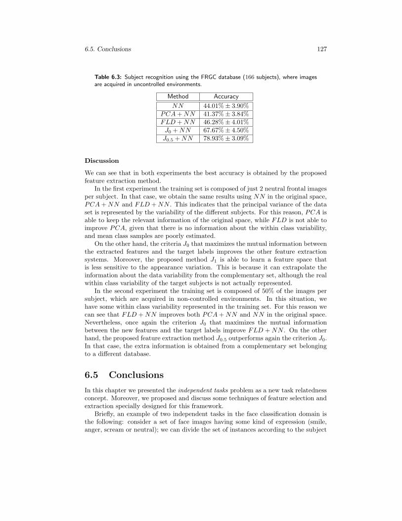
6.5. Conclusions 127

Table 6.3: Subject recognition using the FRGC database (166 subjects), where imagesare acquired in uncontrolled environments.

Method Accuracy

NN 44.01%± 3.90%PCA + NN 41.37%± 3.84%FLD + NN 46.28%± 4.01%J0 + NN 67.67%± 4.50%J0.5 + NN 78.93%± 3.09%

Discussion

We can see that in both experiments the best accuracy is obtained by the proposedfeature extraction method.

In the first experiment the training set is composed of just 2 neutral frontal imagesper subject. In that case, we obtain the same results using NN in the original space,PCA + NN and FLD + NN . This indicates that the principal variance of the dataset is represented by the variability of the different subjects. For this reason, PCA isable to keep the relevant information of the original space, while FLD is not able toimprove PCA, given that there is no information about the within class variability,and mean class samples are poorly estimated.

On the other hand, the criteria J0 that maximizes the mutual information betweenthe extracted features and the target labels improves the other feature extractionsystems. Moreover, the proposed method J1 is able to learn a feature space thatis less sensitive to the appearance variation. This is because it can extrapolate theinformation about the data variability from the complementary set, although the realwithin class variability of the target subjects is not actually represented.

In the second experiment the training set is composed of 50% of the images persubject, which are acquired in non-controlled environments. In this situation, wehave some within class variability represented in the training set. For this reason wecan see that FLD + NN improves both PCA + NN and NN in the original space.Nevertheless, once again the criterion J0 that maximizes the mutual informationbetween the new features and the target labels improve FLD + NN . On the otherhand, the proposed feature extraction method J0.5 outperforms again the criterion J0.In that case, the extra information is obtained from a complementary set belongingto a different database.

6.5 Conclusions

In this chapter we presented the independent tasks problem as a new task relatednessconcept. Moreover, we proposed and discuss some techniques of feature selection andextraction specially designed for this framework.

Briefly, an example of two independent tasks in the face classification domain isthe following: consider a set of face images having some kind of expression (smile,anger, scream or neutral); we can divide the set of instances according to the subject

128 INDEPENDENT TASKS: A NEW RELATEDNESS CONCEPT

that appears in the image (task T1) or according to the facial expression (task T2).Supposing that the expression does not depend on the subject, we say that tasksT1 and T2 are independent. Intuitively, we can improve the learning of task T2 ifwe learn to be not sensitivity to the classification according to T2: if the faces arewell represented to perform T1 (elements of the same class together and elements ofdifferent classes separated), then the faces are not well represented to perform taskT2.

In the first study we presented a new criterion based on mutual information forfeature selection. This criterion uses both labels of the tasks T1 and T2 to selectthe features. We performed some experiments to compare our proposal with othercriteria and the promising results suggested that the approach is appropriated for thepresented problem.

For this reason, in a second stage of our work, we developed a more sophisticatedsystem to deal with feature extraction in the independent tasks problem. The algo-rithm is based again in mutual information, using both T1 and T2 tasks and seeksfor a linear transformation of the data that keeps the information according to T1,rejecting the information of T2. The method has been applied to the face recognitionfield, in order to: (a) mitigate the effects of the small sample size problem, beingthe method able to extract from the complementary tasks useful subspace informa-tion for the main classification problem, and (b) inhibit the feature extraction taskfrom known environmental artifacts that can be incorporated as prior knowledge.The results of our experiments suggest again that the proposed method seems to beappropriated for the independent tasks problem.

Notice that the proposed techniques do not strictly belong to the MTL field, giventhat the methods just learn the target task, using the other one as a source task. Then,the methods should be considered as general Knowledge Transfer algorithms.

Chapter 7

Final Conclusions

This thesis is basically focused on exploring, developing and testing MTL techniquesfor automatic face classification, in order to overcome one of the main inconveniencesof this problem: the small sized training set.

The goal of the MTL topic is the simultaneous learning of multiple related tasks,with the aim of achieving an improvement in the overall performance, when comparedto independent training strategies. For appropriate applications, MTL algorithmsneed less training samples per task to achieve the same classification results as in-dependent learning strategies. Moreover, a MTL classifier trained with a sufficientnumber of related tasks should be able to find good solutions to a novel related task.

A literature survey on MTL is included in Chapter 2 of this thesis, where we pro-posed a categorization of MTL techniques and described multiple MTL applications.We can find in this review a wide variety of experiments, where the MTL strategieshave shown an improvement over the single task methodologies.

The works reviewed in Chapter 2 suggest that the MTL paradigm can contributeto overcome the small sized training set problem of the face classification domain. Inthis thesis we have proposed different MTL methods for Feature Selection, FeatureExtraction, Classification and Online Learning, specially developed for face classifi-cation problems.

On the other hand, there are other strategies that can help to mitigate the effects ofthe small sample sized inconvenient, out of the MTL context. For example, automaticface classification could be improved with the use of the external face features as anextra information source. On the other hand, an appropriate choice of the face imageresolution can be a determining factor to obtain an efficient classification system. InAppendix A and Appendix B we present some studies related to these two solutionsfor improving the current face classification approaches.

The contributions of this thesis in the MTL context are structured in 4 blocks:

• The JFSCL method and its extension to the MTL paradigm

The first contribution is the development of the JFSCL method, an embeddedsystem for selecting features and learning a classifier. The algorithm is easilyscalable to the MTL paradigm in order to perform a common feature selection

129

130 FINAL CONCLUSIONS

for different tasks, while their respective predictors are learned. During thetraining process of the JFSCL, the predictor is learned by minimizing an em-pirical loss with L1 penalty using the BLasso algorithm, and the activation anddeactivation of the features are controlled by an additional vector of parameters.

In our tests, the MTL extension of the JFSCL showed an improvement on theaccuracy compared with the single-task approach. However, we think that fea-ture selection is not a very suitable dimensionality reduction step for automaticface classification problems. Instead, we suggest the use of a feature transfor-mation strategy.

• MTL Classifiers

In a second stage of the thesis we proposed a MTL extension of two single-task Bayesian classifiers: the Quadratic Classifier and the Logistic RegressionModel. These MTL extensions are based on a regularization constraint on theparameters’ set, which promotes the knowledge transfer among the differenttasks.

The most interesting difference between these two MTL extensions is that theamount of information sharing in the MTL Quadratic Classifier depends on theamount of similarity between the tasks. More concretely, in the MTL QuadraticClassifier case we defined a new quantifiable task relatedness measure based onevaluating an specific distance on the parameters’ space. Then, given two tasks,the similarity between the parameters of their predictors will depend on thesimilarity between them as a classification tasks.

Our experimental results have empirically demonstrated the possible negativeconsequences of applying a MTL strategy for learning tasks that are not similarenough. In the case of the MTL Logistic Regression Model, we found exampleswhere the MTL contribution improves the single-task approach and exampleswhere the MTL contribution is negative, producing lower performance than thesingle task method. However, in the case of the MTL Quadratic Classifier, whenthe amount of knowledge transfer is controlled by the amount of task similarity,we have not appreciated negative consequences when using the MTL approach.

• MTL methods for Online Learning

This block is focused on the following problem: given an application for recog-nizing K people we may need to include a new subject (Incremental ClassLearning); remove one of the existing subjects (Decremental Class Learning);or update the information about the current subjects, including new samples(Incremental Sample Learning), or removing obsolete instances (DecrementalSample Learning). In these situations, the retraining of the whole system canbe computationally demanding. For this reason, the development of OnlineLearning algorithms dealing with any of the four presented actions is an in-teresting issue of research. Moreover, in cases where the small sample sizedproblem is usual, the use of MTL Online Learning techniques can improve thecurrent systems.

131

We have proposed in this thesis two MTL Online Learning methods: The OnlineBoosting algorithm and the Online Learning extension of the MTL QuadraticClassifier. The first proposal is specially suitable for the Incremental ClassLearning problem, while the second can deal with the four situations abovedescribed.

In the case of the Online MTL Quadratic Classifier, we have also proposed anew approach for the Decremental Class Learning problem. This approach isbased on keeping in the system useful information of a concrete class when ithas to be removed, and it is called the Retaining Decremental Class Learning.The performed experiments showed a higher accuracy of this new approach overthe classical decremental strategy.

In general, our experimental results in the face classification domain showed ahigher classification accuracy of the proposed methods, in comparison with theclassic NN rule used in state-of-the-art Online Learning methods.

• The Independent Tasks Problem

We presented a framework called the Independent Tasks Problem in order todefine a new task relatedness concept. An example of two independent tasksin the face classification domain are subject recognition and facial expressionclassification, if we consider that the expression do not depend on the subject.

We have proposed a Feature Selection and a Feature Extraction algorithms, spe-cially suitable for the Independent Tasks framework. Both the algorithms andthe definition of the Independent Tasks concept are based on the Mutual Infor-mation Statistic. These methods showed in our experiments an improvementover the single-task strategies.

On the other hand, this thesis contents two more contributions related to the smallsample sized problem in automatic face classification, which are out of the context ofthe MTL paradigm. These contributions can be found in Appendix A and AppendixB, respectively. The general ideas of these works are the following:

• The Use of the External Face Features for Automatic Face Classification

The goal of this study was to show the relevance of the external face features forautomatic face classification purposes. We developed an algorithm to extractinformation of these parts of the face, which is based in a Top-Down segmen-tation method. The proposed method encodes the external face features as analigned feature vector, and then this codified information can be used as inputto any standard pattern recognition classifier.

We tested this feature extraction methodology in different face classificationproblems: gender recognition, subject verification and subject recognition. Theobtained results showed that the external features encoded with the proposedsystem contribute useful information for classification purposes. On the otherhand, we performed some experiments combining the information provided bythe external and the internal features. Our results showed that both kinds

132 FINAL CONCLUSIONS

of information are complementary, and external features provide and extra in-formation source that can improve the classification performance, specially inpresence of partial occlusions or high local changes in the illumination.

• Optimal Face Image Resolution for Subject Recognition

The data representation of the input elements is a key issue in any classificationsystem. In the face domain, it is usual to start from the pixel values as aninitial feature representation, and then apply a dimensionality reduction tech-nique, before training a classifier. In this context, to determine an appropriateresolution of the face image for the input elements is an important aspect toconsider. Very low resolutions can lose a lot of crucial details that are necessaryfor the correct classification of the face, while very high resolutions make thedata processing computationally unfeasible and include redundant features thatcan confuse the classifier.

In this thesis we presented an empirical study to compare the quality of the dif-ferent face image resolutions, in order to perform subject recognition task in themachine. The quality of the different resolutions has been evaluated with threediscriminative measures, which achieve a maximum when the image resolutionis around 37 × 37 pixels. We conclude from the results that the face repre-sentation in this resolution is appropriate to perform the subject classificationtask.

7.1 Future Work

After the experiments presented in this thesis, we have some suggestions of futurework related with the different blocks of contributions:

• The JFSCL method and its extension to the MTL paradigm

As previously stated, we think that feature selection is not an appropriate di-mensionality reduction technique for automatic face classification. For this rea-son, we suggest to extend the JFSCL to perform joint linear feature extractionand classifier learning. Unfortunately, the current system do not allow to ex-tract features instead of selecting them because its computational complexity.For this aim, another optimization algorithm should be developed, although thegeneral formulation would remain very similar.

On the other hand, the JFSCL can be seen as a meta-method to jointly learn aclassifier and, at the same time, select the most appropriate features to consider.This methodology could be applied to other loss functions and classifiers.

• MTL Classifiers

More MTL extensions of other single-task algorithms for classification can bedeveloped, using a parametric approach or any other of the sharing frameworksdescribed in Chapter 2. We think, however, that it is essential to develop these

7.1. Future Work 133

extensions following the idea of the MTL Quadratic Classifier, that includes asystem to control the negative knowledge transfer among the tasks. On theother hand, a further study on the MTL Logistic Regression model could beperformed, to formally determine the task relatedness it assumes. Thus, thenegative knowledge transfer could be avoided.

Finally, notice that these MTL classifiers are developed for multi-class classifi-cation using the one-versus-all approach. Other MTL classification schemes formulti-class problems could be developed, using a more general ECOC approach,instead the one-versus-all strategy. We think that it can be an interesting re-search line.

• MTL methods for Online Learning

In the case of the Boosted Online Learning, the method uses an initial set tobuild a model using the JointBoost algorithm, and then the system is readjustedwhen new classes are added to the initial set. We think that a deeper analysisabout the importance of the initial set of classes can be performed. A diversechoice of the initial classes should allow a more general base for extending theclassifier. Moreover, the use of an extra validation set could improve slightlythe accuracies.

On the other hand, a deeper study on the Decremental Learning topic is re-quired. This approach can be applied to many real situations, but it has beenpoorly explored and the literature on this area is very slender. Moreover, theRetaining Decremental Class Learning idea seems a useful MTL approach thatcould be used with other Online Learning algorithms.

Finally, the Incremental Class Learning could be also an interesting researchline, specially when dealing with the MTL principles. Currently there are notmany approaches dealing with this framework, although it can be applied tomany real problems.

• The Independent Tasks Problem

We plan as a future work the development of an alternative feature extractionmethods for the Independent Tasks framework. For example, the addition ofsparsity priors could benefit the isolation of features focused only on the mainclassification task. On the other hand, the optimal initialization of the matrixW and possible non linear extensions of the method are also subjects of furtherdevelopment.

Moreover, the framework can be applied to many real world problems, suchas handwritten letter recognition, speech, audio or automatic text classifica-tion. For this reason we plan also to test the proposed ideas in other patternrecognition fields.

• The Use of the External Face Features for Automatic Face Classification

Some aspects of the system for external face features extraction presented in thisthesis can be improved. For example, in the Building Blocks learning stage, the

134 FINAL CONCLUSIONS

method could take benefit from using some kind of illumination normalizationon the fragments generation. In particular, we propose the use of techniques ofridges and valleys detection to filter the images as a previous step of the featureextraction. Moreover, the addition of a diversity measure can be considered, inorder to model a larger rank of hairstyles.

Although our experiments have been performed with images acquired in con-trolled scenes, the goal is to be able of extracting external features from facesacquired in uncontrolled conditions. In this case, where the background wouldbe irregular, the matching criterion should be revised. Maybe the use of shapeor texture descriptors can improve the correspondence between hair types. Fur-thermore, a more robust matching criterion would allow to incorporate the chinzone to this feature extraction system.

Finally, another line of future work is to define a more robust combination ruleof the internal and external information. In this context, the use of classifierensembles can be an appropriate choice.

• Optimal Face Image Resolution for Subject Recognition

The appropriateness of the face image resolution at 37 × 37 pixels for subjectclassification purposes could be ratified with further empirical studies, usingmore databases or other discriminative measures. On the other hand, similarstudies can be performed for other face classification problems, such as genderor age classification.

The MTL techniques presented in this thesis are specially designed for face clas-sification problems. However, they could be used in other classification domains, andit would be interesting to test them with other data types.

Finally, we want to state the difficulty on finding appropriate databases to testMTL algorithms. We think that an important future work in the MTL area is to createdata sets specially designed to perform MTL experiments, in order to define generaltesting protocols. That would allow experimental comparisons among different MTLmethods.

Appendix A

External Face Feature Extraction

Most of the automatic face classification methods found in the literature focus theiralgorithms in features difficult to imitate, such as eyes, nose and mouth, which areknown as Internal Features. One of the reasons of this fact is that face classificationapplications were normally related to security and in this area the stability of theinformation source is essential. Nevertheless, as technology evolves, it is easier to findmore electronic devices with small embedded cameras in our everyday life, runningapplications not directly related to security. In these new areas, it is not necessary toreject information of the External Features located at hear, chin or ears. In this way,more sources of information are taken into account and these new characteristics canhelp to improve the existing algorithms. In Figure A.1 the internal and external facefeatures are illustrated.

Figure A.1: Example of Internal Features (first image), External Features (secondimage) and full face.

To know the role that different facial features play in our judgments of identity isnot easy. However, there are different psychological tests performed to understand thecontribution of the different face zones in visual face recognition purposes [189, 109].For instance, some studies performed by Sinha et. al [109] have shown externalfeatures to be more relevant than internal ones in low resolution images, while the twofeature sets reverse in importance as resolution increases. On the one hand, internalfeatures seem to be more useful than external ones for recognition of familiar faces,while the contribution of the external features is more relevant for unfamiliar faces

135

136 EXTERNAL FACE FEATURE EXTRACTION

Figure A.2: Internal face features in both portraits are exactly the same, but veryfew human observers are aware of this after an attentive inspection of the imagesif they are not warned of this fact. This example illustrates the importance of theexternal features in face recognition problems.

recognition. Of course the higher accuracy in Sinha et. al studies is obtained whenboth sources of information are considered, and it has been shown that the relativespatial configuration is an important issue for a visual successful classification. Thisrelevance of the external features in face recognition is illustrated with a visual illusionin Figure A.2.

The main problem to deal with external features in automatic face classificationis the high variability of this face area and their lack of a natural alignment. Thisdrawbacks are graphically shown in Figure A.3. For this reason, most of the currentfeature extraction systems can not be directly applied to deal with this problematicand new approaches have to be developed.

In this thesis we present a system to encode external features, which is basedon a Top-Down reconstruction algorithm. The proposed methodology encodes thisinformation in an aligned feature vector. After that, standard feature extraction orclassification methods can be used to empirically test the feature extraction algorithm.In this context, we performed some experiments to show the contribution of externalface features in automatic face classification

A.1 External Features Extraction

In this section we detail the proposed method to extract information from the externalfeatures of a face image. Figure A.4 illustrates the external zone of a face and empha-sizes the three face zones that will be considered separately during the entire feature

A.1. External Features Extraction 137

Figure A.3: Here are illustrated the stability of the internal features and the highvariability of the external features of human faces.

extraction process: Left Face, Central Head and Right Face respectively. These zonescan be automatically detected if the location of the eyes is known.

Our method is inspired in a Top-Down segmentation algorithm developed byBorenstein et all. [33, 32] and has been adapted for our purpose. It is divided intwo parts:

1. First we learn a model from face images, called the Building Blocks set. Thismodel is composed of representative image fragments belonging to the externalface zone.

2. Then, any unseen image is represented using these Building Blocks: the frag-ments of the learned model are used as puzzle pieces and the unseen image isreconstructed with them, using those pieces that are more similar to the originalimage.

During these processes, we use some known techniques that should be mentioned.They are briefly described below and then the different steps of our method aredetailed.

A.1.1 Preliminaries

Our algorithm needs frequently to decide whether a fragment is present or not inan image, as well as determine which is the most suitable place in the image tolay a given patch. On the other hand, we will need to measure in some occasionsthe similarity between two images. For this purpose, an image matching criterion isrequired. We have used in this thesis the Normalized Cross-Correlation technique,which is a template matching system motivated by the squared Euclidean distance.

138 EXTERNAL FACE FEATURE EXTRACTION

Figure A.4: External features of a human face. The three face zones that containrelevant external face features are demarcated.

To compute the Normalized Cross-Correlation between a fragment F and an imageI we proceed as follows: for any image patch IP of I having the same size as F, thevalue of the Normalized Cross-Correlation is calculated by

NCC(IP ,F) =1D

∑i,j(IP (i, j)− IP )(F(i, j)− F)

σIPσF

(A.1)

where D is the number of pixels in F, IP and F are the means of IP and F re-spectively, while σIP

and σF are their standard deviations. The maximum value ofthese results for all the possible image patches IP having the same size as F is theNormalized Cross-Correlation between the piece F and the image I, and the part ofthe image that gives this maximum value indicates the most suitable position for Fin I.

On the other hand, as previously stated, once the model of Building Blocks is con-structed, we approximate the external features of any new image using the learnedfragments. For this purpose, we use a particular case of Non-Negative Matrix Factor-ization (NMF) [136]. This method finds a factorization of any non-negative matrixin two non-negative factors by minimizing the mean squared error.

Formally, given a non-negative (D ×N)-dimensional matrix X, the method findsnon-negative (D×R)-dimensional matrix B and (R×D)-dimensional matrix W suchthat

X ' BW (A.2)

meaning that the product BW approximates X with minimum mean squarederror.

Let us consider that X is a data set with positive D-dimensional data vectors ascolumns, X = (x1, ...,xN ). The product BW is an approximation of X done as apositive linear combination of the B columns. Therefore, the column vectors of B

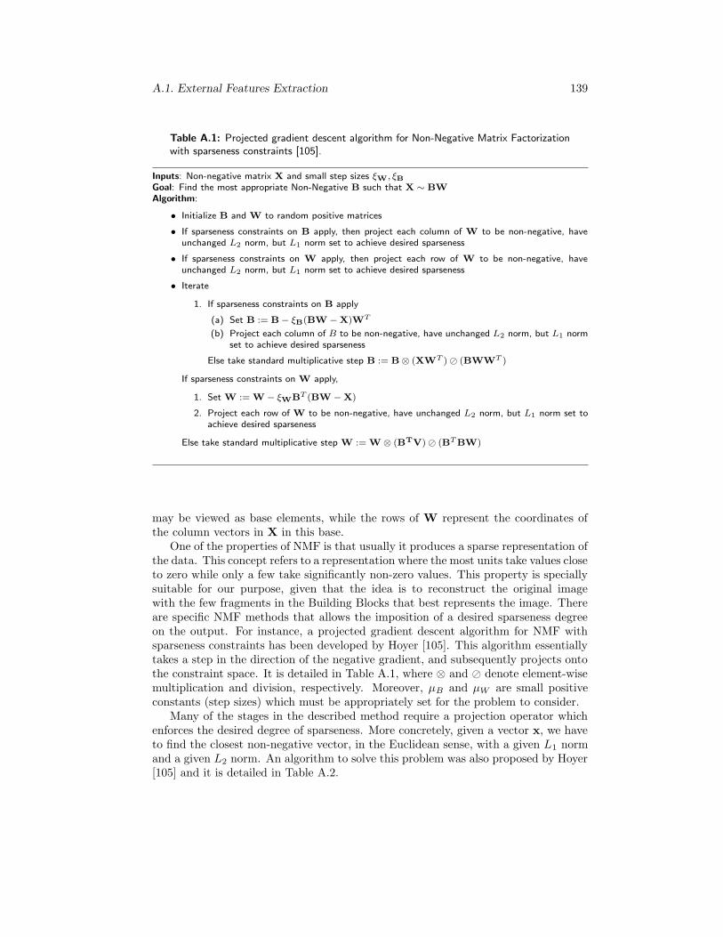
A.1. External Features Extraction 139

Table A.1: Projected gradient descent algorithm for Non-Negative Matrix Factorizationwith sparseness constraints [105].

Inputs: Non-negative matrix X and small step sizes ξW, ξBGoal: Find the most appropriate Non-Negative B such that X ∼ BW

Algorithm:

• Initialize B and W to random positive matrices

• If sparseness constraints on B apply, then project each column of W to be non-negative, haveunchanged L2 norm, but L1 norm set to achieve desired sparseness

• If sparseness constraints on W apply, then project each row of W to be non-negative, haveunchanged L2 norm, but L1 norm set to achieve desired sparseness

• Iterate

1. If sparseness constraints on B apply

(a) Set B := B− ξB(BW −X)WT

(b) Project each column of B to be non-negative, have unchanged L2 norm, but L1 normset to achieve desired sparseness

Else take standard multiplicative step B := B⊗ (XWT )� (BWWT )

If sparseness constraints on W apply,

1. Set W := W − ξWBT (BW −X)

2. Project each row of W to be non-negative, have unchanged L2 norm, but L1 norm set toachieve desired sparseness

Else take standard multiplicative step W := W ⊗ (BTV)� (BT BW)

may be viewed as base elements, while the rows of W represent the coordinates ofthe column vectors in X in this base.

One of the properties of NMF is that usually it produces a sparse representation ofthe data. This concept refers to a representation where the most units take values closeto zero while only a few take significantly non-zero values. This property is speciallysuitable for our purpose, given that the idea is to reconstruct the original imagewith the few fragments in the Building Blocks that best represents the image. Thereare specific NMF methods that allows the imposition of a desired sparseness degreeon the output. For instance, a projected gradient descent algorithm for NMF withsparseness constraints has been developed by Hoyer [105]. This algorithm essentiallytakes a step in the direction of the negative gradient, and subsequently projects ontothe constraint space. It is detailed in Table A.1, where ⊗ and � denote element-wisemultiplication and division, respectively. Moreover, µB and µW are small positiveconstants (step sizes) which must be appropriately set for the problem to consider.

Many of the stages in the described method require a projection operator whichenforces the desired degree of sparseness. More concretely, given a vector x, we haveto find the closest non-negative vector, in the Euclidean sense, with a given L1 normand a given L2 norm. An algorithm to solve this problem was also proposed by Hoyer[105] and it is detailed in Table A.2.

140 EXTERNAL FACE FEATURE EXTRACTION

Table A.2: Algorithm for solving the following problem: given a vector x find the closest(in the Euclidean sense) non-negative vector with a given L1 norm and a given L2 norm[105].

• Set si := xi + (L1 −∑

xi)/dim(x), ∀i

• Set S := ∅

• Iterate

1. Set

– if i ∈ Z qi := 0

– else, qi := L1/(dim(x)− size(S))

2. Set s := q + α(x − q), where α ≥ 0 is selected such that the resulting s satisfies the L2

norm constraint. This requires a quadratic equation resolution

3. If all components of s are non-negative, return s, end

4. Set S := S⋃{i; si < 0}

5. Set si := 0, ∀i ∈ S

6. Calculate a = (∑

xi − L1)/(dim(x)− size(S))

7. Set si := si − a, ∀i ∈ S

A.1.2 Building Blocks Set Construction

In this step, the algorithm learns a model composed by a representative set of imagefragments corresponding to the external zones of the face. This fragments set is calledthe Building Blocks and is constructed by selecting fragments from the Left Face,Central Head and Right Face zones that appear in face images with more frequency(see Figure A.4). This is the most computationally expensive stage of the method,but it is performed only once, off line, and using a generic face training set.

To learn the Building Blocks we need two mutually exclusive sets. The first one,Face, is a collection of aligned face images with visible external characteristics toanalyze. The other one, Face, is composed by non-face images acquired in naturalenvironments. Then we follow these steps:

• For each one of the Left Face, Central Head and Right Face zones from setFace, generate all subimages at sizes ranging from s1 × s1 pixels to sr × sr

pixels, r ∈ N. Each of these fragments will be a candidate fragment Fi.

• For each Fi, we compute the Normalized Cross-Correlation with each one of theimages in the training set, denoting by NFacei the correlation between Fi andeach image from Face, and NFacei the correlation between Fi and Face.

• For each Fi a value θi is computed. This value takes into account a predefinednumber of false positives that can be tolerated, α. The value θi is selected tofulfill the following restriction: P (NFacei > θi) ≤ α.

• The model is built by storing the R fragments from each zone (Left Face, Central

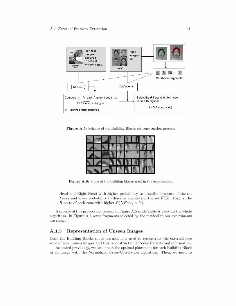
A.1. External Features Extraction 141

Figure A.5: Scheme of the Building Blocks set construction process.

Figure A.6: Some of the building blocks used in the experiments.

Head and Right Face) with higher probability to describe elements of the setFaces and lower probability to describe elements of the set Face. That is, theR parts of each zone with higher P (NFacei > θi).

A scheme of this process can be seen in Figure A.5 while Table A.3 details the wholealgorithm. In Figure A.6 some fragments selected by the method in our experimentsare shown.

A.1.3 Representation of Unseen Images

Once the Building Blocks set is learned, it is used to reconstruct the external facezone of new unseen images and this reconstruction encodes the external information.

As stated previously, we can detect the optimal placement for each Building Blockin an image with the Normalized Cross-Correlation algorithm. Then, we need to

142 EXTERNAL FACE FEATURE EXTRACTION

Table A.3: Building Blocks learning algorithm.

Inputs:

• The face images set Face

• The set Face of non face images

• The possible sizes of the fragments to analyze s1, . . . , sr,

• The maximum number of fragments R that will be considered as Building Blocks from each ofthe three zones

• The predefined threshold of false positives α.

Algorithm:

1. For each of the three zones (Left, Central and Right)

(a) For each fragment size si

• Extract all the possible subimages of size si from the set Face using a sliding windowprocedure.

• Add each subimage to the candidate fragments set.

• Calculate and store the normalized correlation between each candidate fragment Fi

and each image from Face and Face.

(b) Compute the threshold θi for each fragment Fi that allows at most an α false positive ratiofrom the training set, P (NFacei > θi) ≤ α.

(c) Compute the probability (frequency) of each fragment to describe elements from class Faceusing the threshold θi, P (NFacei > θi).

(d) Select the R fragments with highest value P (NFacei > θi) and include these fragments inthe Building Blocks set.

A.2. Experiments and Discussion 143

quantify the relative contribution of each Building Block for reconstructing the image.Notice that Normalized Cross-Correlation assigns a place for every Building Block ina face zone, but this does not mean that all Building Blocks are representative of thatface. Therefore we need a system for simultaneously selecting relevant Building Blocksand for computing their contribution in a way that minimizes the reconstruction errorof the external face features. We have selected an specific algorithm for this aim, theNon-negative Matrix Factorization (NMF) explained in the previous section.

The main steps of the process used to encode an unseen image I using the BuildingBlocks set is the following:

1. For each element Fi of the Building Blocks, we construct a black image Bi

having the same size as I. Then a copy of Fi is located on Bi in the placesuggested by NCC(I,Fi) (see equation A.1).

The set of Bi images constitute the base that will be used to reconstruct theimage I

2. Then, given these base elements {Bi}i=1:3R for I, we compute a weight vector wwith the NMF method, imposing an appropriate sparseness constraint. Thus,the external face part of the new image I is reconstructed by

I '∑

i=1:3R

wiBi (A.3)

and the vector w = (w1, . . . , w3R) represents the encoded external features ofthe face.

The complete process of the external face features reconstruction for a test imageis shown in Figure A.7, which includes two examples of reconstructions obtained inour experiments are included.

A.2 Experiments and Discussion

To test this external feature extraction system we have performed different classifica-tion experiments. Here we present some results showing that the proposed methodallows to obtain significant information from the external zones of the face. In someof the presented experiments we performed classification using internal features asa reference, to compare their contribution with the information obtained from theexternal features.

We have used in these tests the ARFace Database and the subset of face in FRGCDatabase composed of images acquired under controlled conditions. In the secondcase, we suppressed some samples having the external features partially occluded.Some of them are shown in Figure A.8.

We used as internal features the pixel values in a 34 × 34 resolution. Then, theinternal features of a face are represented by a 1156-dimensional vector.

Regarding to the external features, they are encoded with the proposed system,constructing the Building Blocks set as follows:

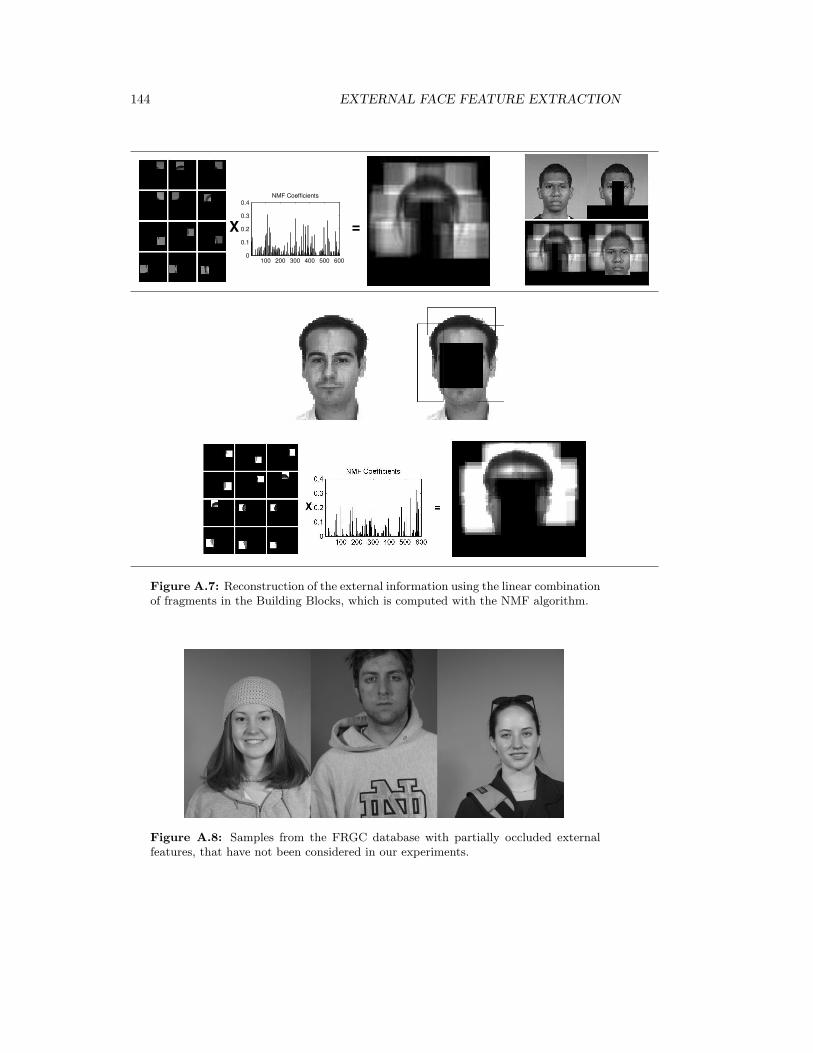
144 EXTERNAL FACE FEATURE EXTRACTION

100 200 300 400 500 6000

0.1

0.2

0.3

0.4NMF Coefficients

X =

Figure A.7: Reconstruction of the external information using the linear combinationof fragments in the Building Blocks, which is computed with the NMF algorithm.

Figure A.8: Samples from the FRGC database with partially occluded externalfeatures, that have not been considered in our experiments.

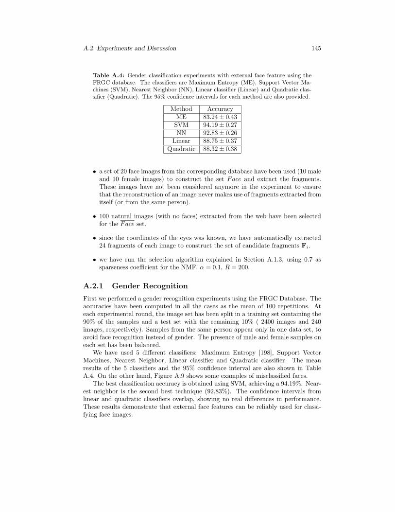
A.2. Experiments and Discussion 145

Table A.4: Gender classification experiments with external face feature using theFRGC database. The classifiers are Maximum Entropy (ME), Support Vector Ma-chines (SVM), Nearest Neighbor (NN), Linear classifier (Linear) and Quadratic clas-sifier (Quadratic). The 95% confidence intervals for each method are also provided.

Method AccuracyME 83.24± 0.43SVM 94.19± 0.27NN 92.83± 0.26

Linear 88.75± 0.37Quadratic 88.32± 0.38

• a set of 20 face images from the corresponding database have been used (10 maleand 10 female images) to construct the set Face and extract the fragments.These images have not been considered anymore in the experiment to ensurethat the reconstruction of an image never makes use of fragments extracted fromitself (or from the same person).

• 100 natural images (with no faces) extracted from the web have been selectedfor the Face set.

• since the coordinates of the eyes was known, we have automatically extracted24 fragments of each image to construct the set of candidate fragments Fi.

• we have run the selection algorithm explained in Section A.1.3, using 0.7 assparseness coefficient for the NMF, α = 0.1, R = 200.

A.2.1 Gender Recognition

First we performed a gender recognition experiments using the FRGC Database. Theaccuracies have been computed in all the cases as the mean of 100 repetitions. Ateach experimental round, the image set has been split in a training set containing the90% of the samples and a test set with the remaining 10% ( 2400 images and 240images, respectively). Samples from the same person appear only in one data set, toavoid face recognition instead of gender. The presence of male and female samples oneach set has been balanced.

We have used 5 different classifiers: Maximum Entropy [198], Support VectorMachines, Nearest Neighbor, Linear classifier and Quadratic classifier. The meanresults of the 5 classifiers and the 95% confidence interval are also shown in TableA.4. On the other hand, Figure A.9 shows some examples of misclassified faces.

The best classification accuracy is obtained using SVM, achieving a 94.19%. Near-est neighbor is the second best technique (92.83%). The confidence intervals fromlinear and quadratic classifiers overlap, showing no real differences in performance.These results demonstrate that external face features can be reliably used for classi-fying face images.

146 EXTERNAL FACE FEATURE EXTRACTION

Figure A.9: Some examples of misclassified faces in the Gender Recognition exper-iments using the FRGC database.

Table A.5: Gender classification experiment with ARFace Database. Resultsachieved using only internal features, only external features, and both internal andexternal features.

NN MEInternal Features 81.5± 0.3 80.4± 0.63External Features 64.4± 0.4 82.8± 0.57

Combination 87.8± 0.4 84.8± 1.0

We have also performed gender classification experiments with the ARFace Data-base. In this case we used only internal information, only external information andfinally both internal and external information together. The aim is to know if theaccuracies obtained with internal features improve with the addition of the externalinformation. In these experiments we used two classifiers: the Nearest Neighbor (NN)classifier using Euclidean distance and the Maximum Entropy (ME).

In Table A.5 are included the accuracies obtained with both classifiers. Theseresults show that the classification rates obtained using only external features aresignificant and that the accuracy increases if we consider both features.

On the other hand, we have performed the same experiment testing each ARFacedatabase type separately. The results are shown in Table A.6. In the first columnthe image type is indicated. We show the accuracies of each case and the confidenceintervals. The best accuracy is marked with an ’*’, and the methods whose confidenceintervals overlap with the best results are shown in boldface.

As we can observe, in almost all the cases the best accuracies are obtained usingcombining internal and external features. Notice that the extra information of theexternal features is specially important on the data sets with occlusions. See thatonly in 3 data sets the internal features are slightly better than using the combinedfeature set, which are characterized by strong lateral illumination.

A.2. Experiments and Discussion 147

Table A.6: Gender classification experiment for the different ARFace database im-age types. Accuracies achieved using internal features (Int), external features (Ext)and both internal and external features (All) using NN and ME classifiers. Theconfidence intervals are shown under each result.

ME Int Ext All NN Int Ext All

83.7 82.7 88.5∗ 82.8 64.5 85.3AR01 ±0.6 ±1.4 ±1.2 ±1.9 ±2.4 ±1.9

84.4 81.8 86.7∗ 81.6 66.2 85.4AR02 ±0.6 ±1.2 ±2.2 ±2.1 ±2.6 ±2.0

85.6 87.2 91.0∗ 80.4 65.5 83.7AR03 ±0.5 ±1.3 ±2.4 ±1.9 ±2.5 ±2.4

82.8 79.6 85.4 82.1 62.9 85.5∗AR04 ±0.6 ±1.2 ±2.8 ±2.2 ±2.8 ±2.3

84.3 83.6 86.8 85.1 66.4 87.5∗AR05 ±0.7 ±1.2 ±1.2 ±1.9 ±2.6 ±1.9

92.3∗ 1.1 87.3 89.6 65.6 90.9AR06 ±0.5 ±1.1 ±2.2 ±1.6 ±2.3 ±1.9

91.5∗ 78.3 85.3 89.0 64.1 91.0AR07 ±0.5 ±1.1 ±2.0 ±1.8 ±2.3 ±1.8

87.5 85.3 89.9∗ 86.1 68.9 87.9AR08 ±0.4 ±1.6 ±2.1 ±1.6 ±2.6 ±1.7

88.3 83.8 90.9∗ 87.6 65.8 89.7AR09 ±0.5 ±1.6 ±1.5 ±1.6 ±2.4 ±1.6

89.8∗ 79.8 88.7 88.1 68.0 89.2AR10 ±0.4 ±1.6 ±1.5 ±1.8 ±2.6 ±1.7

57.3 69.1 72.1∗ 67.5 57.1 71.4AR11 ±0.9 ±1.4 ±3.0 ±2.7 ±2.3 ±2.3

59.3 68.5 69.7 69.9 58.1 74.9∗AR12 ±1.1 ±1.8 ±1.9 ±2.4 ±2.3 ±2.2

72.5 71.1 72.0 70.6 63.1 73.4∗AR13 ±1.0 ±1.4 ±2.2 ±2.4 ±2.3 ±2.4

148 EXTERNAL FACE FEATURE EXTRACTION

Table A.7: Configuration of the Gallery and the Probe sets in the face verificationexperiments. For each set, the second column indicates the number of subjects andif they are or not of our environment (client or impostor).

FRGC Experimentset subjects ] images per person total images

Training (G) client: 100 3 300Testing (P ) client: 100 2 200

impostor : 50 5 250ARFace Experiment

set subjects ] images per person total imagesTraining (G) client: 70 3 210Testing (P ) client: 70 2 140

impostor : 35 5 175

A.2.2 Subject Verification

We performed different subject verification experiments using internal and externalfeatures separately. We used again images from the FRGC Database and the ARFaceDatabase, as in the case of Gender Recognition.

Here we used the LBDP method [155] to reduce the data dimensionality, workingafter that with 300 components in both internal features and external features cases.The classification is performed by the Nearest Neighbor algorithm.

The experiments are based on the Sep96 FERET testing protocol [203]. In thisprotocol, two sets are distinguished: a target set (T), composed by the known facialimages, and the query set (Q), including the unknown facial images to be identified.Two subsets should be selected from each of these sets: a gallery G ⊂ T and a probeset P ⊂ Q. After this selection, the performance of the system is characterized by twostatistics. The first is the probability of accepting a correct identity. This is referredto as the verification probability, denoted by PV (also referred to as the hit rate inthe signal detection literature). The second is the probability of incorrectly verifyinga claim. This is called the false-alarm rate and is denoted by PF .

The details of the sets used in this experiments are specified in Table A.7. Theyhave been chosen following the scheme of the Lausanne Protocol configuration-1 [120].There are two kind of subjects: clients (known by the system) and impostors (un-known by the system). The number of subjects in each set is limited by the numberof different subjects in the database as well as the quantity of images per person.

In the first experiment we considered images acquired under controlled conditions,which are far from a real spontaneous capture. The obtained results are shown inFigure A.10, where a graphic with the probability of verification versus the falseacceptance probability is shown. Given that the internal face zone is clear enough inall the images and all the faces have a neutral expression, the results obtained usingthe internal features are better than the ones obtained with the external features. Inthis case, when the conditions are quite optimal, the instability of the hair is higher

A.2. Experiments and Discussion 149

0 0.1 0.2 0.3 0.4 0.5 0.6 0.7 0.8 0.9 10

0.1

0.2

0.3

0.4

0.5

0.6

0.7

0.8

0.9

1

False acceptance probability (PF)

Pro

babi

lity

of v

erifi

catio

n (P

V)

Subject verification experiment with the FRGC database

−−−−− External Features___ Internal Features

Figure A.10: Subject verification experiments using the FRGC database.

that the instability that can affects the internal features. Notice, however, that theinformation contributed by the external features is also significant for verificationpurposes, since the probability of acceptance is always higher than the false acceptanceprobability.

The second experiment was performed with the ARFace database. We have seenbefore that this database is composed by 13 subsets of images, including variety ofexpressions, high local changes in the illumination and even partial occlusions. Forthis reason, this set of images is more close to a real life situation than the set ofFRGC images. The results obtained in this second experiment are included in FigureA.11. In this second case we observe that the external features are more relevant thanthe internal features. The reason is that in this experiment, where the images are notas regular as in the first performance, the stability of the external features is higherthan the stability of the internal features, which sometimes are partially occludedor have highlights that cause an important loss of information. Notice, nevertheless,that some of these artifacts affect also the external features.

A.2.3 Subject Recognition

Different subject recognition experiments with external features have been performedusing the FRGC database. In all the cases, the training set was composed of 10images from each subject selected at random, while the remaining images composedthe test set.

We reduced the data dimensionality with the LBDP method, as before. Theclassification is performed with Nearest Neighbor in both the original space and theLBDP reduced space. The results are shown in Table A.8. The last row indicates the

150 EXTERNAL FACE FEATURE EXTRACTION

0 0.1 0.2 0.3 0.4 0.5 0.6 0.7 0.8 0.9 10

0.1

0.2

0.3

0.4

0.5

0.6

0.7

0.8

0.9

1

False acceptance probability (PF)

Pro

babi

lity

of v

erifi

catio

n (P

V)

Subject verification experiment using the ARFace database

−−−−− External features___ Internal features

Figure A.11: Subject verification experiments using the ARFace database.

Table A.8: Subject recognition experiment with the FRGC database.

1 NClass 2 NClass 3 NClass 4 NClass 5 NClass

NN 43.3 53.3 66.0 69.3 74.7

LBDP + NN 56.0 66.7 71.6 73.8 76.6Dim 315 302 220 180 387

dimensionality where the rates of second row are obtained. On the other hand, weplot in Figure A.12 the evolution of the accuracies obtained using LBDP with NearestNeighbor as a function of the number of extracted features.

The results here obtained show that the external features contribute relevant in-formation for the subject recognition purpose.

A.3 Conclusions and Future Work

In this appendix we show the importance of the external features in face classificationproblems, and propose a methodology to automatically extract them. The presentedscheme follows a Top-Down segmentation approach to deal with the diversity inherentto the external regions of facial images. Our method encodes the external face featuresas an aligned feature vector and then this codified information can be used as inputto any standard pattern recognition classifier.

The proposed technique is validated using two publicly available face databasesin different face classification problems: gender recognition, subject verification andsubject recognition. The obtained results show that the external features encoded

A.3. Conclusions and Future Work 151

0 50 100 150 200 250 300 350 4000

0.1

0.2

0.3

0.4

0.5

0.6

0.7

0.8

Dimensionality

Acc

urac

y

1st nearest class2nd nearest class3rd nearest class4th nearest class5th nearest classNearest neighbor on the original space

Figure A.12: Subject recognition experiment with FRGC: mean accuracy as afunction of the extracted features. The obtained result using directly the NN classifierin the original space is also indicated.

with our methodology contribute useful information for classification purposes. Onthe other hand, we performed some experiments combining the information providedby the external and the internal features. The tests show that both kinds of infor-mation are complementary, and external features provide and extra information cuethat can improve the classification results in presence of occlusions and local changesin the illumination.

The system presented in this thesis can be improved at different levels. Firstthe learning of the Building Blocks model could take benefit from using some kindof normalization on the fragments generation. In particular, we propose the use oftechniques of ridges and valleys detection to filter the images as a previous step ofthe feature extraction. Second, we plan to improve the selection of the fragmentsthat compose the Building Blocs by adding a diversity measure that could model alarger rank of hairstyles. On the other hand, the matching criterion should be revisedif we want to extract external information from images captured in non-controlledenvironments with cluttered backgrounds. Finally, another line of future work is todefine a more robust combination rule of the internal and external information. Inthis context, the use of classifier ensembles seems to be an appropriate choice.

152 EXTERNAL FACE FEATURE EXTRACTION

Appendix B

Optimal Face Image Resolution forSubject Recognition

In the first section of Chapter 1 we showed the general framework of an automaticface classification system. As previously stated, after the face alignment and imagepreprocessing step we obtain a feature vector that encodes the visual face informa-tion. This feature vector is usually composed by some measurements, such as thepixel values in grey intensity. In this case, given a classification problem, the faceimage resolution is a key issue in order start from an appropriate initial face represen-tation: very low resolutions can lose a lot of crucial details that are necessary for thecorrect classification of the face, while very high resolutions make the data process-ing computationally unfeasible and include redundant features that can confuse theclassifier.

In this appendix we perform an empirical study to compare the quality of thedifferent face image resolutions in order to perform subject recognition task in themachine. In the next section we describe the evaluation strategy of the differentresolutions. Then we show our results and, finally, last section concludes this study.

B.1 Evaluation of Recognition Performance

The best criterion to evaluate the effectiveness of a features set to perform a con-crete classification task is the Bayes error (see Chapter 6 Section 1), given that it isindependent of any specific classifier. As previously stated, the Bayes error is a the-oretical definition that can not be computed if the probability densities of the dataare unknown. However, upper bounds of this value can be estimated from a set ofsamples and these measures can be used to compare different feature sets in orderto determine which is the most competitive to perform a concrete classification task.In this study we evaluate three of the discriminabilitiy measures obtained from twodifferent upper bounds of the Bayes error:

1. Mutual Information between the samples and their corresponding class: as de-tailed in Chapter 6 Section 1, bounds of Hellman and Raviv [101], as well as

153

154 OPTIMAL FACE IMAGE RESOLUTION FOR SUBJECT RECOGNITION

Fano inequality [76], demonstrate that Bayes error is minimized when the men-tioned Mutual Information is maximized. In this context, an image resolutioncan be considered better than another for subject recognition purposes if thefirst one shows a higher mutual information according the subject labels.

2. LDA measure: it is based on the Battacharyya upper bound of the Bayes error[82], which is computed with data scatter matrices. Formally, let be SW thewithin class scatter matrix

SW =1

K

K∑

k=1

(µk − µ)(µk − µ0)T (B.1)

where µk is the class-conditional sample mean and µ is the global sample mean;and SB the between class scatter matrix computed by

SB =1

K

K∑

k=1

Σk (B.2)

where Σk is the class-conditional covariance matrix for k-th class, estimatedfrom the data; the LDA measure can be expressed by

J = trace(SW SB) (B.3)

3. NDA measure: it also based on the Battacharyya upper bound of the Bayeserror and it is computed as the LDA measure, but substituting the previous SB

by

SB =1

n

∑

x∈X

∆xB (B.4)

where ∆xB is the local between-class matrix for x ∈ X, that is computed as

follows: suppose that the class label of x is k, and denote by ¯class(x) the subsetof the r nearest neighbors of x among the data points in X belonging to L\{k}.In this case, ∆x

B can be calculated as

∆xB =

1

K − 1

∑

z∈L\{k}

(z− x)(z− x)T (B.5)

B.2 Experiments

Here we present the experiments performed in order to compare the quality of differentface image resolutions to perform automatic subject recognition.

In this test we have used the images of the FRGC database acquired under con-trolled conditions. We selected those subjects having more than 20 images to obtain

B.3. Discussion and Conclusions 155

Figure B.1: Example of Blackman-Harris window (first figure), representation ofinternal face features subimage (second figure) and optimal size representation of theface (around 37 × 37 pixels).

more accurate estimators of the discriminability measures. This set is composed by1736 pictures from 55 different subjects. Original images have been aligned accordingthe eyes and down-sampled to 256 × 256 pixels. Moreover, to suppress the externalfeatures (hair, chin, jaw-line) we use a centered 4-term Blackman-Harris window [98](see first picture of Figure B.1).

To assess the resolution-dependence of the automatic face recognition we adoptedthe following procedure: using a bilinear interpolation scheme each image was resizedto continuously smaller sizes, starting with an initial size of 64× 64 pixels (see FigureB.1). At each resolution we evaluated the three discriminability measures described.In Figure B.2 we show the obtained results.

B.3 Discussion and Conclusions

Here we presented an experiment to evaluate the the quality of the different faceimage resolution to perform automatic subject recognition. We evaluate three classdiscriminability measures in several resolutions to seek for a representation with min-imum Bayes error. All three measures gave similar results and revealed an unimodaldistribution with a maximum at a resolution near 37×37 pixels. As a consequence, itis reasonable that artificial face recognition systems focus on these face image size toachieve an optimal recognition performance, given that they are the most effective interms of class discriminability. Because these critical spatial frequencies correspondto quite small image patches, a further advantage emerges through an economic useof resources for both processing and storing faces.

Curiously, there is an interesting link between these results and psychologicalstudies on how humans process face identity. It seems that human brain prefers toperform this task using a face representation that is very similar to this highlightedresolution. For more details about the psychological results see [124, 104, 145].

156 OPTIMAL FACE IMAGE RESOLUTION FOR SUBJECT RECOGNITION

0 10 20 30 40 50 60 700

0.1

0.2

0.3

0.4

0.5

0.6

0.7

0.8

0.9

1

Face width (number of pixels)

Nor

mal

ized

MI m

easu

re

MI Measure

0 10 20 30 40 50 60 700

0.2

0.4

0.6

0.8

1

Face width (number of pixels)

Nor

mal

ized

FLD

mea

sure

FLD Measure

0 10 20 30 40 50 60 700

0.2

0.4

0.6

0.8

1

Face width (number of pixels)

Nor

mal

ized

ND

A m

easu

re

NDA Measure

Figure B.2: MI, FLD and NDA measures at each face dimensionality.

Appendix C

Databases

In this thesis we have used different databases in order to test the proposed method-ologies. Following we give a brief description of each database. Notice that most ofthese sets are face databases, given that the proposed algorithms are in general de-signed for face classification. However, in some validations we have used more generalmachine learning databases.

C.1 ARFace Database

ARFace Database [152] was created by Aleix Martinez and Robert Benavente with theComputer Vision Center (CVC) at Universitat Autonoma de Barcelona. It containsover 4000 color images corresponding to 126 people’s faces (56 women and 70 men).The images of the data set consist of frontal view faces with different facial expressions,illumination conditions, and occlusions (sun glasses and scarf). The pictures weretaken at the CVC under strictly controlled conditions and no restrictions on wear(clothes, glasses), make-up or hair style were imposed to participants.

There are, in general, 26 images per person (some of the subjects just have 13samples). These pictures were acquired in two different sessions (13 pictures persession and person), separated by two weeks time, and the same picture types weretaken in both sessions.

The image types considered in this database are the following: neutral frontal im-age, 3 facial expressions (smiling, anger and scream), 3 different extra light conditions(left light on, right light on, and both lights on), 3 images with the subject wearingsunglasses (simple sunglasses, sunglasses with extra left light illumination, and sun-glasses with extra right light illumination) and 3 images wearing scarf (simple scarf,scarf with extra left light illumination, and scarf with extra right light illumination).Figure C.1 shows an example of each image type.

This database is specially suitable to benchmark algorithms claimed to be robustto occlusions and local changes in the illumination. Moreover, notice that each imageis labelled according to at least 3 criteria: subject, gender, and acquisition conditions(image type). This property is specially useful to test some of the methods proposedin this thesis.

157

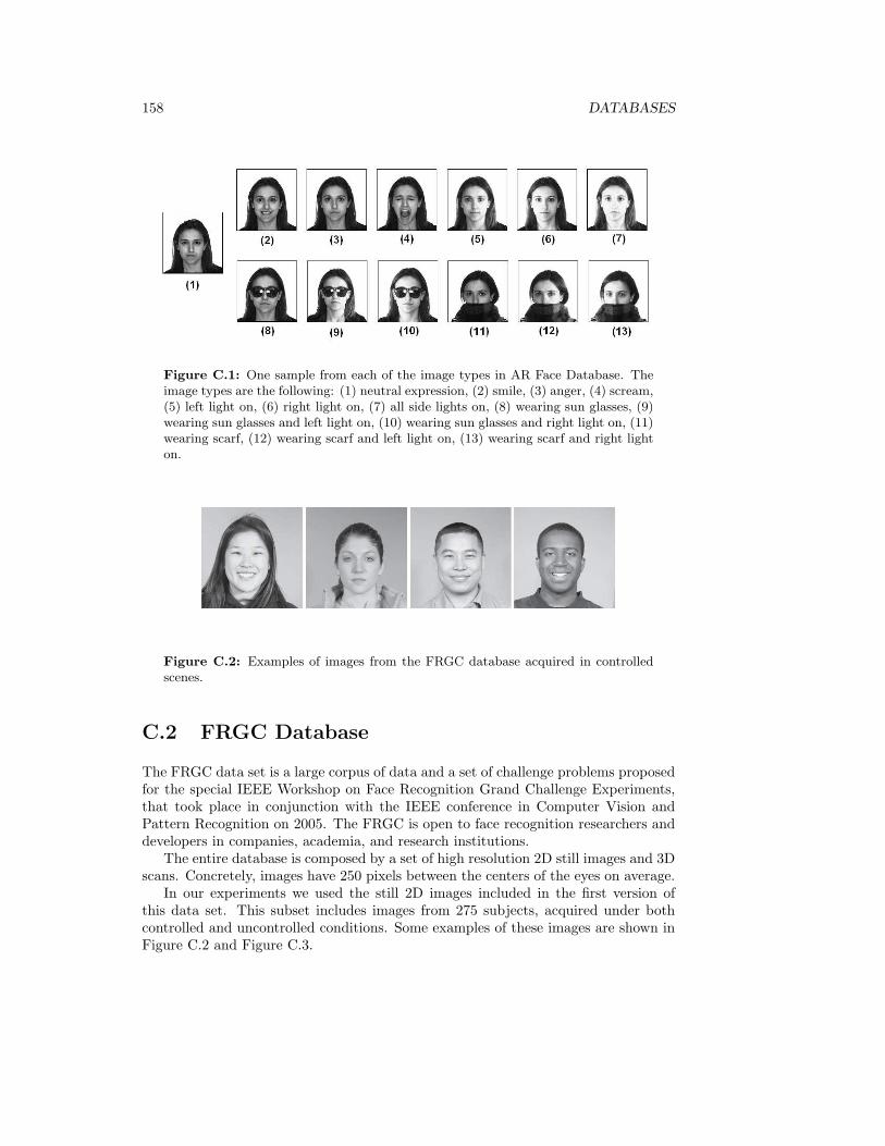
158 DATABASES

Figure C.1: One sample from each of the image types in AR Face Database. Theimage types are the following: (1) neutral expression, (2) smile, (3) anger, (4) scream,(5) left light on, (6) right light on, (7) all side lights on, (8) wearing sun glasses, (9)wearing sun glasses and left light on, (10) wearing sun glasses and right light on, (11)wearing scarf, (12) wearing scarf and left light on, (13) wearing scarf and right lighton.

Figure C.2: Examples of images from the FRGC database acquired in controlledscenes.

C.2 FRGC Database

The FRGC data set is a large corpus of data and a set of challenge problems proposedfor the special IEEE Workshop on Face Recognition Grand Challenge Experiments,that took place in conjunction with the IEEE conference in Computer Vision andPattern Recognition on 2005. The FRGC is open to face recognition researchers anddevelopers in companies, academia, and research institutions.

The entire database is composed by a set of high resolution 2D still images and 3Dscans. Concretely, images have 250 pixels between the centers of the eyes on average.

In our experiments we used the still 2D images included in the first version ofthis data set. This subset includes images from 275 subjects, acquired under bothcontrolled and uncontrolled conditions. Some examples of these images are shown inFigure C.2 and Figure C.3.

C.3. UCI Machine Learning Repository 159

Figure C.3: Examples of images from the FRGC database acquired in uncontrolledscenes.

C.3 UCI Machine Learning Repository

The UCI Machine Learning Repository [29] is a collection of databases, domain the-ories, and data generators that are used by the machine learning community for theempirical analysis of their algorithms. This collection was created by David Aha andgraduate students at the University of California, Irvine (USA), on 1987. The currentversion of the repository is composed of 176 data sets.

The sets of the UCI Machine Learning Repository that have been used in thisthesis as well as their properties are summarized in Table C.1.

160 DATABASES

Table C.1: Databases from the UCI Machine Learning Repository used in thisthesis.

Data Set ] Classes ] Samples ] FeaturesBalance 3 625 4

Breast Cancer 2 699 10Dermatology 6 366 34

Ecoli 8 336 8Glass 7 214 10Heart 2 270 13Iris 3 150 4

PIMA Diabetes 2 768 8Segmentation 7 2310 19

Wine 3 178 13Yeast 10 1484 8

Appendix D

Notation and Terminology

• A classification task is denoted by a capital bold T. If we consider more thanone task we index them by T1, . . . ,Tt, . . . ,TM

• Given a task, the input space is the set composed of all the possible elementsthat can be considered by the task, and is denoted by X. On the other hand,the output space is composed of all the possible labels that can be assigned toan element in the input space, and is denoted by L.

• A task T will be provided with a training set, composed by N training sam-ples X = {x1, ...,xi, ...,xN} ⊆ X with their corresponding class labels, c ={c1, ..., ci, ..., cN} ⊆ L.

In some chapters of the thesis we use the term data matrix for a generic dataset X.

• If we consider more than one task, T1, . . . ,TM , the training set of the t-thtask is denoted by Xt = {xt

1, ...,xti, ...,x

tN} and ct = {ct

1, ..., cti, ..., c

tn}. The

input and output spaces are denoted by Xt and L

t respectively. For notationsimplicity we suppose that all the training sets are composed of N pairs (xt

i, cti),

for all t = 1, . . . ,M .

• The classes of a label space L are denoted by {1, 2, ..., k, ...,K}. The cardinalityof L, K, may be also denoted by ]L. Exceptionally, in binary problems, wherethe number of possible classes is 2, the classes can be denoted by {0, 1} or{−1, 1}, in order to simplify the notation.

• Given an arbitrary element x belonging to a input space X, its correspondinglabel according to a task T is denoted by c(x). If we consider more than onetask, T1, . . . ,TM , the class label of an element x according the t-th tasks isdenoted by ct(x).

• A particular MTL framework is related to the one-versus-all approach of a K-class classification problem. In this case, the learning of each predictor (one perclass) is seen as a task. However, instead of denoting separately the training

161

162 NOTATION AND TERMINOLOGY

sets per each task, we suppose that there is just one common training set for allthe classes, X, with the corresponding class labels c, where each ci ∈ c satisfiesci ∈ {1, . . . ,K}. Moreover, we denote by Nk the number of training elementsin X belonging to the k-th class, for all k ∈ {1, . . . ,K}.

• We will suppose that elements in the training set are always D-dimensionalcolumn vectors. Even when we consider more than one task we will supposethat the dimensionality of the input space is D for all the tasks, to simplify thenotation.

• Given a vector v we denote by dim(v) its dimensionality.

• We denote by X and C the random variables corresponding to the events ofrandomly picking up samples and labels of a concrete task. Notice that X ={X1, ...,XD} is a random vector composed of D real random variables, one perdata dimension. In general, we use this typeface to denote random variables.

• A feature extraction function from an input space to a lower dimensional spacewill be denoted by Greek letters, Ψ or Φ. When the transformations are linearfunctions, the matrix corresponding to the transformation will be denoted bybold capitals W or V.

• Eventually, when there is no possibility of confusion, a bold capital W candenote a matrix of weights.

• Given a training set X and a linear feature extraction function Ψ with associatedmatrix W, we denote the projected data by Y := Ψ(X) = WX. More generally,the input space X is transformed to Y := WX. In this case Y ⊆ R

d, d ≤ D.

Moreover, given an arbitrary x ∈ X ⊆ RD belonging to an input space, we

denote its transformation by y = Wx ∈ Y ⊆ Rd.

• The mutual information between two random variables X and Y is denoted byI(X ,Y).

• Given a training set {X, c} of a task T, we denote by I(X, C) the estimation ofthe theoretical I(X , c) computed with the elements in the training set.

• A classifier of a task T is a function f : X → L that predicts an output labelfor every element in the input set. Discrimination functions, classifiers andprobabilistic models are denoted in this thesis by f , g or h.

• Given a vector v or a matrix W, we denote by vT and WT their respectivetransposed.

• The indicator function is denoted by 1. In particular, given [a, b] ⊆ R an intervaland x ∈ R,

1[a,b](x) =

{1 if x ∈ [a, b]0 otherwise

163

• Given a vector x ∈ RD, we indicate by xj its j-th component. Thus, the j-

th component of a concrete element xi belonging to a data set X is denotedby xij . Moreover, given a data set X = {x1, . . . ,xN}, we denote by x.j theN -dimensional vector composed of the j-th components of each element in thedata set.

• We denote by 0D×d the (D×d)-dimensional matrix having all the entries equalto 0.

• In Online Learning approaches, where the goal is to update a learned classifieror model f , the sought model will be denoted by f .

• We denote by ∅ the empty set.

164 NOTATION AND TERMINOLOGY

Appendix E

Publications

Journals

• David Masip, Agata Lapedriza, and Jordi Vitria. Boosted Online Learning forFace Recognition. IEEE Transactions on Systems Man and Cybernetics part B.Vol 39, Issue 2, 530-538. April 2009. ISI: 1.353 (33/93).

• Matthias S. Keil, Agata Lapedriza, David Masip, and Jordi Vitria. Preferredspatial frequencies for human face processing are associated with optimal classdiscrimination in the machine. PLoS ONE, Public Library of Science. PLoSONE 3(7): e2590 doi:10.1371/journal.pone.0002590.

• Agata Lapedriza, Santi Seguı, David Masip, and Jordi Vitria. A Sparse BayesianApproach for Joint Feature Selection and Classifier Learning. Pattern Analysisand Applications. Vol 11, Issue 3-4 299-308. ISI: 0.515 (71/93)

• Agata Lapedriza, David Masip, and Jordi Vitria. On the Use of External Fea-tures for Face Verification. Journal of Multimedia (JMM). Acedemy Publisher.Vol 1, n. 4 July 2006.

Book Chapters

• David Masip, Agata Lapedriza, and Jordi Vitria. Measuring external Face ap-pearance for Face Classification. Invited Chapter in the Face Recognition Book.ARS Ed. ISBN 978-3-902613-03-5.

Lecture Notes in Computer Science

• Agata Lapedriza, David Masip, and Jordi Vitria. A Hierarchical Approach forMulti-task Logistic Regression. In Proc. 3rd Iberian Conference on PatternRecognition and Image Analysis. J. Martı et al. (Eds.). Lecture Notes in

165

166 PUBLICATIONS

Computer Science 4478. Pattern Recognition and Image Analysis, June 2007,pp. 258-265. Springer-Verlag Berlin Heidelberg. ISBN 978-3-540-72848-1.

• Agata Lapedriza, David Masip, and Jordi Vitria. The Contribution of ExternalFeatures to Face Recognition. In Proc. 2nd Iberian Conference on PatternRecognition and Image Analysis. J.S. Marques et al. (Eds.). Lecture Notes inComputer Science 3523. Pattern Recognition and Image Analysis, June 2005,pp. 537-544. Springer-Verlag Berlin Heidelberg. ISBN 0302-9743. ISI: 0.402(62/71).

Conferences

• Agata Lapedriza, David Masip and Jordi Vitria. On the use of independenttasks for face recognition. IEEE Conference on Computer Vision and PatternRecognition, 2008. CVPR 2008. 23-28 June 2008 Page(s):1 - 6. Anchorage,Alaska

• David Masip, Agata Lapedriza, and Jordi Vitria. Multitask Learning: An appli-cation to Incremental Face Recognition. International Conference on ComputerVision Theory and Applications - VISAPP 2008.

• Agata Lapedriza, David Masip, and Jordi Vitria. Subject Recognition Using aNew Approach for Feature Extraction. International Conference on ComputerVision Theory and Applications - VISAPP 2008.

• Agata Lapedriza, David Masip, and Jordi Vitria. Shared Regularization Tech-niques for Logistic Regression Model. 2nd CVC Internal Workshop, ComputerVision: Progress of Research and Development, J. Llados (ed.).

• Agata Lapedriza, Manuel Jesus Jimenez-Marın, and Jordi Vitria. Gender Recog-nition in Non-Controlled Environments. In proceedings of the InternationalConference on Pattrern Recognition (ICPR 2007). Hong Kong, China.

• David Masip, Agata Lapedriza, and Jordi Vitria. Multitask learning applied toface recognition. 1st Spanish Workshop on Biometrics. SWB2007. June 2007,Girona.

• David Masip, Agata Lapedriza, and Jordi Vitria. Face Verification SharingKnowledge from Different Subjects. In Proceedings of International Conferenceon Computer Vision Theory and Applications - VISAPP 2007, Barcelona, Spain,2007.

• Agata Lapedriza, David Masip, and Jordi Vitria. Face Verification using Exter-nal Features. 7th IEEE International Conference on Automatic Face and Ges-ture Recognition, 2006. FGR 2006. 10-12 Abril 2006. IEEE Eds. pp(s):132-137.ISBN 0-7695-2503-2. Southampton, UK.

• Agata Lapedriza, David Masip, and Jordi Vitria. Experimental Study of theUsefulness of External Features for Face Classification. Catalan Conference on

167

Artificial Intelligence , 2005. In Artificial Intelligence Research and Develop-ment, IOS Press, Amsterdam, 2005, pp. 99-106. ISBN 0922-6/1-58603-560-6.L’Alguer, Italy.

• Agata Lapedriza, David Masip, and Jordi Vitria. Are External Face FeaturesUseful for Automatic Face Classification?. Accepted for oral presentation inthe IEEE Workshop on Face Recognition Grand Challenge Experiments, inconjunction with Computer Vision and Pattern Recognition (CVPR 2005) SanDiego, California USA.

• Agata Lapedriza, and Jordi Vitria. Open N-Grams and Discriminant Featuresin Text World: an empirical study. Catalan Conference on Artificial Intelligence, 2004. In Recent Advances in Artificial Intelligence Research and Development,IOS Press, IOS Press, Amsterdam. ISBN 1-58603-466-9. Barcelona, Spain.

Technical Reports

• Agata Lapedriza. Face Classification using External Face Features. CVC Tech-nical Report ]83. Computer Vision Center, Barcelona (Spain)

168 PUBLICATIONS

Bibliography

[1] S. Abe, “Modified backward feature selection by cross validation,” in EuropeanSymposium on Artificial Neural Networks Bruges, 2005.

[2] J. D. Abernethy, P. Bartlett, and A. Rakhlin, “Multitask learning with ex-pert advice,” EECS Department, University of California, Berkeley, Tech. Rep.UCB/EECS-2007-20, Jan 2007.

[3] J. Aczel and Z. Daroczy, “On measures of information and their characteriza-tions,” New York, 1975.

[4] A. Agarwal, A. Rakhlin, and P. Bartlett, “Matrix regularization techniques foronline multitask learning,” EECS Department, University of California, Berke-ley, Tech. Rep. UCB/EECS-2008-138, Oct 2008.

[5] W. K. Ahn and W. F. Brewer, “Psychological studies of explanation-basedlearning,” Investigating Explanation-Based Learning, 1993.

[6] A. Aizerman, E. M. Braverman, and L. I. Rozoner, “Theoretical foundationsof the potential function method in pattern recognition learning,” Automationand Remote Control, vol. 25, pp. 821–837, 1964.

[7] Q. An, C. Wang, I. Shterev, E. Wang, L. Carin, and D. B. Dunson, “Hierarchi-cal kernel stick-breaking process for multi-task image analysis,” in ICML ’08:Proceedings of the 25th international conference on Machine learning. NewYork, NY, USA: ACM, 2008, pp. 17–24.

[8] A. Argyriou, T. Evgeniou, and M. Pontil, “Multi-task feature learning,” inAdvances in Neural Information Processing Systems 19. MIT Press, 2007, p.2007.

[9] A. Argyriou, A. Maurer, and M. Pontil, “An algorithm for transfer learningin a heterogeneous environment,” in ECML PKDD ’08: Proceedings of the2008 European Conference on Machine Learning and Knowledge Discovery inDatabases - Part I. Berlin, Heidelberg: Springer-Verlag, 2008, pp. 71–85.

[10] M. Artac, M. Jogan, and A. Leonardis, “Incremental pca or on-line visual learn-ing and recognition,” in ICPR (3), 2002, pp. 781–784.

169

170 BIBLIOGRAPHY

[11] F. Bach and M. Jordan, “Kernel independent component analysis,” Journal ofMachine Learning Research, vol. 3, pp. 1–48, 2002.

[12] B. Bakker and T. Heskes, “Task clustering and gating for bayesian multitasklearning,” J. Mach. Learn. Res., vol. 4, pp. 83–99, 2003.

[13] E. Bart and S. Ullman, “Image normalization by mutual information,” in BritishMachine Vision Conference, 2004.

[14] M. Bartlett, J. Movellan, and T. Sejnowski, “Face recognition by independentcomponent analysis,” IEEE Transactions on Neural Networks, vol. 13, pp. 1450–1464, 2002.

[15] Baxter, “A model of inductive bias learning,” Journal of Machine LearningResearch, vol. 12, pp. 149–198, 2000.

[16] J. Baxter, “A bayesian/information theoretic model of learning to learn viamultiple task sampling,” Machine Learning, vol. 28, no. 1, pp. 7–39, July 1997.

[17] R. Bekkerman, R. El-Yaniv, N. Tishby, and Y. Winter, “Distributional wordclusters vs. words for text categorization,” J. Mach. Learn. Res., vol. 3, pp.1183–1208, 2003.

[18] P. N. Belhumeur, J. P. Hespanha, and D. J. Kriegman, “Eigenfaces vs. fisher-faces: Recognition using class specific linear projection,” IEEE Trans. PatternAnalysis and Machine Intelligence, vol. 19, no. 7, pp. 711–720, Jul 1997.

[19] A. J. Bell and T. J. Sejnowski, “An information-maximization approach toblind separation and blind deconvolution,” Neural Computation, vol. 7, no. 6,pp. 1129–1159, 1995.

[20] S. Ben-David, J. Blitzer, K. Crammer, and F. Pereira, “Analysis of representa-tions for domain adaptation,” in NIPS, 2007.

[21] S. Ben-David and R. S. Borbely, “A notion of task relatedness yielding provablemultiple-task learning guarantees,” Mach. Learn., vol. 73, no. 3, pp. 273–287,2008.

[22] S. Ben-david and R. Schuller, “Exploiting task relatedness for multiple tasklearning,” in Proceedings of Computational Learning Theory (COLT, 2003.

[23] D. Beymer and T. Poggio, “Face recognition from one example view,” iccv,vol. 00, p. 500, 1995.

[24] J. Bi, T. Xiong, S. Yu, M. Dundar, and R. B. Rao, “An improved multi-tasklearning approach with applications in medical diagnosis,” in ECML PKDD’08: Proceedings of the 2008 European Conference on Machine Learning andKnowledge Discovery in Databases - Part I. Berlin, Heidelberg: Springer-Verlag, 2008, pp. 117–132.

BIBLIOGRAPHY 171

[25] S. Bickel, J. Bogojeska, T. Lengauer, and T. Sheffer, “Multi-task learning forhiv therapy screening,” in Proceedings, Twenty-Fifth International Conferenceon Machine Learning, A. McCallum and S. Roweis, Eds. Helsinki, Finland:Omnipress, 2008, pp. 56–63.

[26] S. Bickel and T. Scheffer, “Dirichlet-enhanced spam filtering based on biasedsamples,” in Advances in Neural Information Processing Systems 19. MITPress, 2007, pp. 161–168.

[27] F. Bimbof, I. Magrin-Chagnolleau, and L. Mathim, Second-order statistical mea-sures for text-independent speaker idenhpcation, 1995, vol. 17.

[28] C. M. Bishop, Pattern Recognition and Machine Learning (Information Scienceand Statistics). Springer, August 2006.

[29] C. Blake and C. Merz, “UCI repository of machine learning databases,” 1998.[Online]. Available: http://www.ics.uci.edu/$\sim$mlearn/MLRepository.html

[30] E. Bonilla, K. M. Chai, and C. Williams, “Multi-task gaussian process pre-diction,” in Advances in Neural Information Processing Systems 20, J. Platt,D. Koller, Y. Singer, and S. Roweis, Eds. Cambridge, MA: MIT Press, 2008,pp. 153–160.

[31] E. V. Bonilla, F. V. Agakov, and C. K. I. Williams, “Kernel multi-task learningusing task-specific features,” in In Proceedings of the Eleventh InternationalConference on Artificial Intelligence and Statistics, March 2007, pp. 19–22.

[32] E. Borenstein and Ullman, “Learning to segment,” in ECCV (3), 2004, pp.315–328.

[33] E. Borenstein and S. Ullman, “Class-specific, top-down segmentation,” inECCV ’02: Proceedings of the 7th European Conference on Computer Vision-Part II. Springer-Verlag, 2002, pp. 109–124.

[34] Breiman, “Arcing classifiers,” The Annals of Statistics, vol. 26, no. 3, pp. 801–849, 1998.

[35] L. Breiman, “Bagging predictors,” Machine Learning, vol. 24, no. 2, pp. 123–140, 1996.

[36] M. Bressan, “Statistical independence for classification for high dimensionaldata,” Ph.D. dissertation, Computer Vision Center, Universitat Autonoma deBarcelona, March 2003.

[37] M. Bressan and J. Vitria, “Nonparametric discriminant analysis and nearestneighbor classification,” Pattern Recognition Letters, vol. 24, no. 15, pp. 2743–2749, nov 2003.

[38] E. Brill, “Transformation-based error-driven learning and natural languageprocessing: A case study in part-of-speech tagging,” Computational Linguis-tics, vol. 21, pp. 543–565, 1995.

172 BIBLIOGRAPHY

[39] J. N. L. Brummer and L. R. Strydom, “An euclidean distance measure betweencovariance matrices of speech cepstra for text-independent speaker recognition,”in IEEE Symposium on Communications and Signal Processing. IEEE Com-puter Society, 1997, pp. 167–172.

[40] D. Bryliuk and V. Starovoitov, “Human face recognition using radial basis func-tion neural network,” in 2nd International Conference on Artificial Intelligence,2002, pp. 428–436.

[41] J. Burbea and C. R. Rao, “Entropy differential metric, distance and divergencemeasures in probability spaces: A unified approach,” J. Multi. Analysis, vol. 12,pp. 575–596, 1982.

[42] C. J. C. Burges, “A tutorial on support vector machines for pattern recognition,”Data Min. Knowl. Discov., vol. 2, no. 2, pp. 121–167, 1998.

[43] C. Campbell, “Kernel methods: a survey of current techniques,” Neurocomput-ing, vol. 48, pp. 63–84, 2002.

[44] R. Caruana, “Multitask learning.” Machine Learning, vol. 28, no. 1, pp. 41–75,1997.

[45] G. Cauwenberghs and T. Poggio, “Incremental and decremental support vectormachine learning,” in NIPS, 2000, pp. 409–415.

[46] G. Cavallanti, N. Cesa-Bianchi, and C. Gentile, “Linear algorithms for onlinemultitask classification,” in COLT, 2008, pp. 251–262.

[47] K. M. A. Chai, C. K. I.Williams, S. Klanke, and S. Vijayakumar, “Multi-taskgaussian process learning of robot inverse dynamics,” in Advances in Neural In-formation Processing Systems 20, J. Platt, D. Koller, Y. Singer, and S. Roweis,Eds. Cambridge, MA: MIT Press, 2008.

[48] L. Chengjun and H. Wechsler, “A unified bayesian framework for face recog-nition,” in Proceedings of the International Conference on Image Processing,vol. 1, 1998, pp. 151 – 155.

[49] P.-H. C. Chih-Jen, “A tutorial on v-support vector machines, national taiwanuniversity TR.” [Online]. Available: citeseer.ist.psu.edu/605359.html

[50] R. Collobert and J. Weston, “A unified architecture for natural languageprocessing: deep neural networks with multitask learning,” in ICML, 2008,pp. 160–167.

[51] P. Comon, “Independent component analysis, a new concept?” Signal Process.,vol. 36, no. 3, pp. 287–314, 1994.

[52] N. Costen, M. Brown, and S. Akamatsu, “Sparse models for gender classifica-tion,” in FGR, 2004, pp. 201–206.

[53] R. Courant and D. Hilbert, Introduction to Machine Learning (Adaptive Com-putation and Machine Learning). New York: MIT Press, 2004.

BIBLIOGRAPHY 173

[54] T. M. Cover and P. E. Hart, “Nearest neighbor pattern classification,” IEEE,Transactions on Information Theory, IT-13, vol. 1, pp. 21–27, 1967.

[55] K. Crammer and Y. Singer, “On the algorithmic implementation of multiclasskernel-based vector machines,” J. Mach. Learn. Res., vol. 2, pp. 265–292, 2002.

[56] I. Dagher and R. Nachar, “Face recognition using ipca-ica algorithm,” IEEETransactions on Pattern Analysis and Machine Intelligence, vol. 28, no. 6, pp.996–1000, 2006.

[57] W. Dai, Q. Yang, G. R. Xue, and Y. Yu, “Boosting for transfer learning,” inICML ’07: Proceedings of the 24th international conference on Machine learn-ing. New York, NY, USA: ACM, 2007, pp. 193–200.

[58] Z.-H. Z. Daoqiang Zhang and, , and S. Chen, “Non-negative matrix factorizationon kernels,” in PRICAI 2006: Trends in Artificial Intelligence, 2006, pp. 404–412.

[59] H. Daume, III, “Frustratingly easy domain adaptation,” in Proceedings of the45th Annual Meeting of the Association of Computational Linguistics. Prague,Czech Republic: Association for Computational Linguistics, June 2007, pp.256–263.

[60] J. Davis and P. Domingos, “Deep transfer via second-order markov logic,” inIn Proceedings of the AAAI-2008 Workshop on Transfer Learning for ComplexTasks, Chicago, Illinois, USA, July 2008.

[61] O. Dekel, Y. Singer, and P. Long, “Online multitask learning,” in COLT, 2006.

[62] A. Deshpande, B. Milch, L. S. Zettlemoyer, and L. P. Kaelbling, “Learningprobabilistic relational dynamics for multiple tasks.” in Probabilistic, Logicaland Relational Learning - A Further Synthesis, ser. Dagstuhl Seminar Proceed-ings, L. D. Raedt, T. G. Dietterich, L. Getoor, K. Kersting, and S. Muggleton,Eds., vol. 07161. Internationales Begegnungs- und Forschungszentrum fuerInformatik (IBFI), Schloss Dagstuhl, Germany, 2007.

[63] M. D.Guillamet and J.Vitria, “Weighted non-negative matrix factorization forlocal representations,” in CVPR, Kauai, Hawaii, 2001, pp. 942–947.

[64] C. P. Diehl and G. Cauwenberghs, “Svm incremental learning, adaptation andoptimization,” in In Proceedings of the 2003 International Joint Conference onNeural Networks, 2003, pp. 2685–2690.

[65] T. G. Dietterich and G. Bakiri, “Solving multiclass learning problems via error-correcting output codes,” Journal of Artificial Intelligence Research, vol. 2, pp.263–286, 1995.

[66] C. Domeniconi and D. Gunopulos, “Incremental support vector machine con-struction,” in ICDM ’01: Proceedings of the 2001 IEEE International Confer-ence on Data Mining. Washington, DC, USA: IEEE Computer Society, 2001,pp. 589–592.

174 BIBLIOGRAPHY

[67] P. Domingos and G. Provan, “On the optimality of the simple bayesian classifierunder zero-one loss,” in Machine Learning, 1997, pp. 103–130.

[68] B. A. Draper, K. Baek, M. S. Bartlett, and J. R. Beveridge, “Recognizing faceswith pca and ica,” Comput. Vis. Image Underst., vol. 91, no. 1-2, pp. 115–137,2003.

[69] B. Effron, T. Hastie, I. Johnstone, and R. Tibshinrani, “Regression shrinkageand selection via the lasso,” J. Royal. Statist. Soc B., vol. 58(1), pp. 267–288,1996.

[70] B. Efron, T. Hastie, I. Johnstone, and R. Tibshirani, “Least angle regression,”Annals of Statistics, vol. 32, p. 407, 2004.

[71] H. Ekenel and B. Sankur, “Feature selection in the independent componentsubspace for face recognition,” Pattern Recognition Letters, vol. 25, pp. 1377–1388, 2004.

[72] M. Elad and M. Aharon, “Image denoising via sparse and redundant represen-tations over learned dictionaries,” IEEE Trans. on Image Processing, vol. 15,no. 12, pp. 3736–3745, 2006.

[73] K. Etemad and R. Chellappa, “Discriminant analysis for recognition of humanface images,” Journal of the Optical Society of America A, vol. 14, no. 8, pp.1724–1733, 1997.

[74] T. Evgeniou and M. Pontil, “Regularized multi–task learning,” in KDD ’04:Proceedings of the tenth ACM SIGKDD international conference on Knowledgediscovery and data mining. New York, NY, USA: ACM, 2004, pp. 109–117.

[75] J. M. F. Smach, M. Atri and M. Abid, “Design of a neural networks classifierfor face detection,” 2005.

[76] R. M. Fano, Transmission of Information: A Statistical theory of Communica-tions, Wiley, New York, 1961.

[77] T. L. Fine, Feedforward Neural Network Methodology. Springer, 1999.

[78] R. Fisher, “The use of multiple measurements in taxonomic problems,” Ann.Eugenics, vol. 7, pp. 179–188, 1936.

[79] R. Florian and G. Ngai, “Multidimensional transformation-based learning,” inConLL ’01: Proceedings of the 2001 workshop on Computational Natural Lan-guage Learning. Morristown, NJ, USA: Association for Computational Lin-guistics, 2001, pp. 1–8.

[80] Y. Freund and R. E. Schapire, “Experiments with a new boosting algorithm,”in International Conference on Machine Learning, 1996, pp. 148–156.

[81] J. Friedman, T.Hastie, and R.Tibshirani, “Additive logistic regression: a sta-tistical view of boosting,” Annals of statistics, vol. 28, pp. 337–374, 2000.

BIBLIOGRAPHY 175

[82] K. Fukunaga, Introduction to Statistical Pattern Recognition, 2nd ed. Boston,MA: Academic Press, 1990.

[83] K. Fukunaga and J. Mantock, “Nonparametric discriminant analysis,” IEEETransactions on Pattern Analysis and Machine Intelligence, vol. 5, no. 6, pp.671–678, nov 1983.

[84] P. J. Garcıa-Laencina, A. R. Figueiras-Vidal, J. Serrano-Garcıa, and J.-L.Sancho-Gomez, “Exploiting multitask learning schemes using private subnet-works,” in IWANN, 2005, pp. 233–240.

[85] D. Gelder and B. Rouw, “Beyond localisation: A dynamical dual route accountof face recognition,” Acta Psychologica, vol. 107, pp. 183–207, 2001.

[86] D. Ghosh and A. Chinnaiyan, “Classification and selection of biomarkers ingenomic data using lasso,” Journal Of Biomed Biotechnology, vol. 2005, no. 2,pp. 147–54, 2005.

[87] J. Ghosh and A. Nag, An Overview of Radial Basis Function Networks.Physica-Verlag, 2000.

[88] J. Ghosn and Y. Bengio, “Multi-task learning for stock selection,” in NeuralInformation Processing Systems 9, 1997.

[89] M. Girolami and S. Rogers, “Hierarchic bayesian models for kernel learning,”in ICML ’05: Proceedings of the 22nd international conference on Machinelearning. New York, NY, USA: ACM, 2005, pp. 241–248.

[90] B. Gokberk, L. Akarun, and E. Alpaydyn, “Feature selection for pose invari-ant face recognition,” in 16th International Conference on Pattern Recognition,vol. 4, 2002, pp. 403–406.

[91] T. Griffiths and Z. Ghahramani, “Infinite latent feature models and the indianbuffet process,” 2005.

[92] D. Guillamet, J. Vitria;, and B. Schiele, “Introducing a weighted non-negativematrix factorization for image classification,” Pattern Recogn. Lett., vol. 24,no. 14, pp. 2447–2454, 2003.

[93] G.-D. Guo and H. Zhang, “Boosting for fast face recognition,” in Second Inter-national Workshop on Recognition, Analysis and Tracking of Faces and Gesturesin Real-time Systems, 2001, pp. 96–100.

[94] G.-D. Guo, H.-J. Zhang, and S. Li, “Pairwise face recognition,” in Proceedingsof the IEEE International Conference on Computer Vision, vol. 2, 2001, pp.282–287.

[95] G. Guo, S. Li, and K. Chan, “Face recognition by support vector machines,” inProceedings of the Automatic Face and Gesture Recognition, 2000, pp. 196–201.

[96] I. Guyon and A. Elisseeff, “An introduction to variable and feature selection,”J. Mach. Learn. Res., vol. 3, pp. 1157–1182, 2003.

176 BIBLIOGRAPHY

[97] P. M. Hall, A. D. Marshall, and R. R. Martin, “Incremental eigenanalysis forclassification.” in BMVC, 1998.

[98] F. Harris, “On the use of windows for hamrmonic analysis with the discretefourier transform,” in Proceedings of the IEEE, vol. 66, no. 1, 1978, pp. 51–84.

[99] S. Haykin, Neural Networks: A Comprehensive Foundation. Prentice Hall,1998.

[100] B. Heisele, P. Ho, and T. Poggio, “Face recognition with support vector ma-chines: global versus component-based approach,” in Proceedings of the Inter-national Conference on Computer Vision, vol. 2, 2001, pp. 688–694.

[101] M. E. Hellman and J. Raviv, “Probability of error, equivocation and the chernoffbound,” IEEE Transactions on Information Theory, vol. 16, pp. 368–372, 1970.

[102] T. Heskes, “Empirical bayes for learning to learn,” in ICML ’00: Proceedings ofthe Seventeenth International Conference on Machine Learning. San Francisco,CA, USA: Morgan Kaufmann Publishers Inc., 2000, pp. 367–374.

[103] G. E. Hinton and R. R. Salakhutdinov, “Reducing the dimensionality of datawith neural networks,” Science, vol. 313, no. 5786, pp. 504–507, July 2006.

[104] C. Howe and D. Purves, “Range image statistics can explain the anomalousperception of length,” Proceedings of the National Academy of Sciences USA,vol. 99, 2002.

[105] P. O. Hoyer, “Non-negative matrix factorization with sparseness constraints,”J. Mach. Learn. Res., vol. 5, pp. 1457–1469, 2004.

[106] A. Hyvarinen and E. Oja, “Independent component analysis,” Helsinki Univer-sity of Technology, Tech. Rep., April 1999.

[107] A. Hyvarinen, “The fixed-point algorithm and maximum likelihood estimationfor independent component analysis,” Neural Process. Lett., vol. 10, no. 1, pp.1–5, 1999.

[108] H. D. III and D. Marcu, “Domain adaptation for statistical classifiers,” Journalof Artficial Intelligence Research, vol. 26, pp. 101–126, 2006.

[109] Izzat N. Jarudi and P. Sinha, “Relative contributions of internal and externalfeatures to face recognition,” Massachusetts Institute of technology, Tech. Rep.,2003.

[110] A. K. Jain, R. P. W. Duin, and J. Mao, “Statistical pattern recognition: Areview,” IEEE Transactions on Pattern Analysis and Machine Intelligence,vol. 22, no. 1, pp. 4–37, 2000.

[111] O. Javed, S. Ali, and M. Shah, “Online detection and classification of movingobjects using progressively improving detectors,” in CVPR (1), 2005, pp. 696–701.

BIBLIOGRAPHY 177

[112] T. Jebara, “Multi-task feature and kernel selection for svms,” in ICML ’04:Proceedings of the twenty-first international conference on Machine learning.New York, NY, USA: ACM Press, 2004, p. 55.

[113] S. Ji, L. Tang, S. Yu, and J. Ye, “Extracting shared subspace for multi-labelclassification,” in KDD ’08: Proceeding of the 14th ACM SIGKDD internationalconference on Knowledge discovery and data mining. New York, NY, USA:ACM, 2008, pp. 381–389.

[114] ——, “Extracting shared subspace for multi-label classification,” in KDD ’08:Proceeding of the 14th ACM SIGKDD international conference on Knowledgediscovery and data mining. New York, NY, USA: ACM, 2008, pp. 381–389.

[115] H. Z. Ji Zhu, Saharon Rosset and T. Hastie, “Multi-class adaboost,” StandfordUniversity, Tech. Rep., January 2006.

[116] J. Jiang, “A literature survey on domain adaptation of statistical classifiers,”2007.

[117] F. Jin and S. Sun, “A multitask learning approach to face recognition based onneural networks,” in IDEAL ’08: Proceedings of the 9th International Confer-ence on Intelligent Data Engineering and Automated Learning. Berlin, Heidel-berg: Springer-Verlag, 2008, pp. 24–31.

[118] K. Jonsson, J. V. Kittler, Y. P. Li, and J. Matas, “Learning support vectorsfor face verification and recognition,” in International Conference on AutomaticFace and Gesture Recognition, 2000, pp. 208–213.

[119] P. K., “On lines and planes of closest fit to systems of points in space.” Philo-sophical Magazine, vol. 2, p. 559:572, 1901.

[120] F. Kang, R. Jin, and R. Sukthankar, “Correlated label propagation with ap-plication to multi-label learning,” in CVPR ’06: Proceedings of the 2006 IEEEComputer Society Conference on Computer Vision and Pattern Recognition.New York City, NY, USA: IEEE Computer Society, 2006, pp. 1719–1726.

[121] J. N. Kapur, Measures of Information and their applications, Wiley, New Delhi,India, 1994.

[122] J. Kapur and H. K. Kesavan, Entropy optimization principles with applications.San Diego, London: Academic Press, 1992.

[123] S. Katagiri and S. Abe, “Incremental training of support vector machines usinghyperspheres,” Pattern Recogn. Lett., vol. 27, no. 13, pp. 1495–1507, 2006.

[124] M. S. Keil, A. Lapedriza, D. Masip, and J. Vitria, “Preferred spatial frequenciesfor human face processing are associated with optimal class discrimination inthe machine,” PLoS ONE, vol. 3, no. 7, p. e2590, jul. 2008.

[125] D. Kerridge, “Inaccuaracy and inference,” Statistical Society. Series B (Method-ological), vol. 23, no. 1, pp. 184–194, 1961.

178 BIBLIOGRAPHY

[126] M. Kirby and L. Sirovich, “Application of the Karhunen-Loeve procedure forthe characterization of human faces,” IEEE Transactions on Pattern Analysisand Machine Intelligence, vol. 12, no. 1, pp. 103–108, Jan 1990.

[127] R. Kohavi and G. John, “Wrappers for feature selection,” Artificial Intelligence,pp. 273–324, 1997.

[128] K. Kovac, “Multitask learning for bayesian neural networks,” Ph.D. disserta-tion, Graduate Department of Computer Science, University of Toronto, 2005.

[129] S. Kullback, “Information theory and statistics,” New York, 1959.

[130] S. Kullback and R. Leibler, “On information and sufficiency,” Annals of Math-ematical Statistcs, vol. 22, pp. 79–86, 1951.

[131] M. Lando and S. Edelman, “Generalizing froma single viewin face recognition,”TechnicalReport CS-TR 95-02, 1993.

[132] P. Laskov, , C. Gehl, S. Kruger, and K.-R. Muller, “Incremental support vectorlearning: Analysis, implementation and applications,” J. Mach. Learn. Res.,vol. 7, pp. 1909–1936, 2006.

[133] N. Lawrence, M. Seeger, and R. Herbrich, “Fast sparse gaussian process meth-ods: The informative vector machine,” in Advances in Neural InformationProcessing Systems 15. MIT Press, 2003, pp. 609–616.

[134] N. D. Lawrence and J. C. Platt, “Learning to learn with the informative vectormachine,” in ICML ’04: Proceedings of the twenty-first international conferenceon Machine learning. New York, NY, USA: ACM, 2004, p. 65.

[135] S. Lawrence, C. L. Giles, A. C. Tsoi, and A. D. Back, “Face recognition: aconvolutional neural-network approach,” Neural Networks, IEEE Transactionson, vol. 8, no. 1, pp. 98–113, 1997.

[136] D. Lee and S. Seung, “Algorithms for non-negative matrix factorization,” inNIPS, 2000, pp. 556–562.

[137] D. Lee and H. S. Seung, “Learning the parts of objects with nonnegative matrixfactorization,” Nature, vol. 401, pp. 788–791, July 1999.

[138] S.-I. Lee, V. Chatalbashev, D. Vickrey, and D. Koller, “Learning a meta-levelprior for feature relevance from multiple related tasks,” in ICML ’07: Proceed-ings of the 24th international conference on Machine learning. New York, NY,USA: ACM, 2007, pp. 489–496.

[139] Y. Li, A. Cichocki, and S. Amari, “Analysis of sparse representation and blindsource separation,” Neural computation, vol. 16, no. 6, pp. 1193–1234, 2004.

[140] X. Liao and L. Carin, “Radial basis function network for multi-task learning,” inAdvances in Neural Information Processing Systems 18, Y. Weiss, B. Scholkopf,and J. Platt, Eds. Cambridge, MA: MIT Press, 2006, pp. 795–802.

BIBLIOGRAPHY 179

[141] J. Lin, “Divergence measures based on the Shannon entropy,” IEEE Transac-tions on Information theory, vol. 37, no. 1, pp. 145–151, 1991.

[142] C. Liu and H. Wechsler, “Comparative assessment of independent componentanalysis (ica) for face recognition,” in Second International Conference onAudio- and Video-based Biometric Person Authentication, Washington D.C.,USA, 1999, pp. 211–216.

[143] Y. Liu, H. Yao, W. Gao, and D. Zhao, “Feature selection for pose invariant facerecognition,” in Advances in multimedia information processing: 6th PacificRim Conference on Multimedia, 2005, pp. 13–16.

[144] N. Logothetis and D. Sheinberg, “Visual object recognition,” Anual Review ofNeuroscience, vol. 19, pp. 577–621, 1996.

[145] F. Long, Z. Yang, and D. Purves, “Spectral statistics in natural scenes pre-dict hue, saturation, and brightness,” Proceedings of the National Academy ofSciences USA, vol. 103, 2006.

[146] J. Lu, K. Plataniotis, and A. Venetsanopoulos, “Face recognition using ker-nel direct discriminant analysis algorithms,” IEEE Trans. on Neural Networks,vol. 14, no. 1, pp. 117–126, 2003.

[147] J. Lu, K. Plataniotis, A. Venetsanopoulos, and S. Li, “Ensemble-based discrimi-nant learning with boosting for face recognition,” IEEE Transactions on NeuralNetworks, vol. 17, no. 1, pp. 166–178, 2006.

[148] Ludmila I. Kuncheva, Combining Pattern Classifiers: Methods and Algorithms.New Jersey: Wiley, July 2004.

[149] D. Madigan, A. Genkin, D. Lewis, and D. Fradkin, “Bayesian multinomiallogistic regression for author identification,” Bayesian Inference and MaximumEntropy Methods in Science and Engineering, vol. 803, pp. 509–516, 2005.

[150] M. M. Mahmud and S. R. Ray, “Transfer learning using kolmogorov complex-ity: Basic theory and empirical evaluations.” in NIPS, J. C. Platt, D. Koller,Y. Singer, and S. T. Roweis, Eds. MIT Press, 2007.

[151] O. Maron and T. A. L. p Erez, “A framework for multiple-instance learning,”in Advances in Neural Information Processing Systems. MIT Press, 1998, pp.570–576.

[152] A. Martinez and R. Benavente, “The AR Face database,” Computer VisionCenter, Tech. Rep. 24, june 1998.

[153] A. M. Martinez and A. C. Kak, “Pca versus lda,” IEEE Transactions on PatternAnalysis and Machine Intelligence, vol. 23, no. 2, pp. 228–233, 2001.

[154] D. Masip, “Face classification using discriminative features and classifier com-bination,” Ph.D. dissertation, Computer Vision Center, Universitat Autonomade Barcelona, September 2005.

180 BIBLIOGRAPHY

[155] D. Masip and J. Vitria, “Boosted linear projections for discriminant analy-sis,” Frontiers in Artificial Intelligence and Applications. IOS Press, J.Vitria,P.Radeva and I.Aguilo Eds., pp. 45–52, 2004.

[156] D. Masip and J. Vitria, “Boosted discriminant projections for nearest neighborclassification,” Pattern Recognition, vol. 39, no. 2, pp. 164–170, 2006.

[157] A. Maurer and N. Cristianini, “Bounds for linear multi-task learning,” Journalof Machine Learning Research, vol. 7, p. 2006, 2006.

[158] D. K. M.H. Yang, N. Ahuja, “Face recognition using kernel eigenfaces,” in InProceedings of Int. Conf. on Image Processing, vol. 1, 2000, pp. 37–40.

[159] C. A. Micchelli and M. Pontil, “Kernels for multi–task learning,” in NIPS, 2004.

[160] R. S. Michalski, J. G. Carbonell, and T. M. Mitchell, Pattern Recognition inIndustry. Elsevier, 2005.

[161] L. Mihalkova, T. N. Huynh, and R. J. Mooney, “Mapping and revising markovlogic networks for transfer learning,” in In Proceedings of the AAAI-07 Work-shop on Transfer Learning For Complex Tasks, 2007, pp. 608–614.

[162] L. Mihalkova and R. J. Mooney, “Transfer learning by mapping with minimaltarget data,” in In Proceedings of the AAAI-07 Workshop on Transfer LearningFor Complex Tasks, 2008.

[163] P. Mitra, C. A. Murthy, and S. K. Pal, “Data condensation in large databasesby incremental learning with support vector machines,” in ICPR, 2000, pp.2708–2711.

[164] B. Moghaddam, T. Jebara, and A. Pentland, “Bayesian face recognition,” Pat-tern Recognition, vol. 33, no. 11, pp. 1771–1782, 2000.

[165] B. Moghaddam and Yang, “Learning gender with support faces,” IEEE Trans.Pattern Anal. Mach. Intell., vol. 24, no. 5, pp. 707–711, jan 2002.

[166] H. Moon and P. Phillips, “Computational and performance aspects of pca-basedface recognition algorithms,” Perception, vol. 30, pp. 303–321, 2001.

[167] G. Murphy and D. Medin, “The role of theories in conceptual coherence,” Psy-chological Review, vol. 92, pp. 289–316, 1985.

[168] G. V. Nakamura, “Knowledge-based classification of ill-defined categories,”Memory and Cognition, vol. 13, pp. 377–384, 1985.

[169] G. Nakamura, “The mechanisms of analogical learning,” Similarity and Ana-logical Reasoning, pp. 199–241, 1989.

[170] M. Nakano, F. Yasukata, and M. Fukumi, “Age and gender classification fromface images using neural networks,” in 2nd International Conference on Artifi-cial Intelligence, 2004.

BIBLIOGRAPHY 181

[171] A. Y. Ng, “Feature selection, L1 vs. L2 regularization, and rotational invari-ance,” in ACM International Conference Proceeding Series, 2004.

[172] K. Ni, L. Carin, and D. Dunson, “Multi-task learning for sequential data viaihmms and the nested dirichlet process,” in ICML ’07: Proceedings of the 24thinternational conference on Machine learning. New York, NY, USA: ACM,2007, pp. 689–696.

[173] Nikunj C. Oza, “Online bagging and boosting,” in International Conferenceon Systems, Man, and Cybernetics, Special Session on Ensemble Methods forExtreme Environments. New Jersey: Institute for Electrical and ElectronicsEngineers, October 2005, pp. 2340–2345.

[174] Y. Nobumasa and S. Takeshi, “Nearest neighbor face recognition with compen-sating lighting conditions,” IEIC Technical Report, 2000.

[175] G. Obozinski, B. Taskar, and M. Jordan, “Multi-task feature selection,” Depart-ment of Statistics, University of California, Berkeley, Tech. Rep., June 2006.

[176] B. Olshausen, P. Sallee, and M. Lewicki, “Learning sparse image codes usinga wavelet pyramid architecture,” Advances in neural information processingsystems, pp. 887–893, 2001.

[177] M. Osborne, B. Presnell, and B. Turlach, “On the lasso and its dual,” Journalof Computational and Graphical Statistics, vol. 9, no. 2, pp. 319–337, 2000.

[178] M. Osborne, B. Presnell, and B. A. Turlach, “A new approach to variableselection in least squares problems,” Journal of Numerical Analysis, vol. 20,no. 3, pp. 389–403, 2000.

[179] N. C. Oza, “Online ensemble learning,” Ph.D. dissertation, The University ofCalifornia, Berkeley, CA, Sep 2001.

[180] N. C. Oza and S. Russell, “Online bagging and boosting,” in Eighth Inter-national Workshop on Artificial Intelligence and Statistics, T. Jaakkola andT. Richardson, Eds. Key West, Florida. USA: Morgan Kaufmann, January2001, pp. 105–112.

[181] S. Ozawa and A. Roy, “Incremental learning for multitask pattern recognitionproblems,” Machine Learning and Applications, Fourth International Confer-ence on, vol. 0, pp. 747–751, 2008.

[182] E. Palmer, “Hierarchical structure in perceptual representaion,” Cognitive Psy-chology, vol. 9, pp. 441–447, 1977.

[183] S. J. Pan and Q. Yang, “A survey on transfer learning,” Department of Com-puter Science and Engineering, Hong Kong University of Science and Technol-ogy, Hong Kong, China, Tech. Rep. HKUST-CS08-08, November 2008.

[184] S. Pang, S. Ozawa, and N. Kasabov, “Incremental linear discriminant analysisfor classification of data streams,” IEEE Transactions on Systems, Man, andCybernetics-Part B, vol. 35, no. 5, pp. 905–914, October 2005.

182 BIBLIOGRAPHY

[185] A. Papoulis, S. Pillai, P. A, and P. SU, Probability, random variables, andstochastic processes. McGraw-Hill New York, 1965.

[186] E. Parzen, “On the estimation of a probability density function and mode,”Annals of Mathematical Statistics, vol. 33, pp. 1065–1076, 1962.

[187] P. J. Phillips, P. J. Flynn, T. Scruggs, K. Bowyer, J. Chang, K. Hoffman, J. Mar-ques, J. Min, and W. Worek, “The 2005 ieee workshop on face recognition grandchallenge experiments,” in CVPR ’05: Proceedings of the 2005 IEEE ComputerSociety Conference on Computer Vision and Pattern Recognition (CVPR’05) -Workshops. Washington, DC, USA: IEEE Computer Society, 2005, p. 45.

[188] S. L. Phung, A. Bonzerdormi, D. Chai, and A. Watson, “Naıve bayesi face/non-face classifier: a studi of preprocessing and feature extraction techniques,” inInternational Conference on Image Processing, 2004.

[189] K. S. Pilz, H. H. Bulthoff, and I. M. Thornton, “Internal and external facialfeatures differentially bias person recognition - an approach using animationtechniques,” in 9th Tuebingen Perception Conferenc, 2006.

[190] R. Polikar, L. Udpa, S. S. Udpa, and V. Honavar, “Learn++: An incrementallearning algorithm for supervised neural networks,” IEEE Trans. on Systems,Man and Cybernetics. Part C, vol. 31, pp. 497–508, 2001.

[191] E. Pranckeviciene, T. Ho, and R. L. Somorjai, “Class separability in spacesreduced by feature selection,” in ICPR (3). IEEE Computer Society, 2006, pp.254–257.

[192] V. Pronk, S. Gutta, and W. Verhaegh, “Incorporating confidence in a naıvebayesian classifier,” in User Modeling 2005. Springer Berlin, 2006, pp. 317–326.

[193] P. Pudil, J. Novovicova, and J. Kittler, “Floating search methods in feature-selection,” Pattern Recognition Letters, vol. 15, no. 11, pp. 1119–1125, Novem-ber 1994.

[194] Y. Qi, D. Liu, D. Dunson, and L. Carin, “Multi-task compressive sensing withdirichlet process priors,” in ICML ’08: Proceedings of the 25th internationalconference on Machine learning. New York, NY, USA: ACM, 2008, pp. 768–775.

[195] A. Quattoni, X. Carreras, M. Collins, and T. Darrell, “A projected subgradientmethod for scalable multi-task learning,” Massachusetts Institute of Technology,Tech. Rep., 2008.

[196] R. Bellman, Adaptive Control Process: A Guided Tour. New Jersey: PrincetonUniversity Press, 1961.

[197] R. Raina, A. Y. Ng, and D. Koller, “Constructing informative priors using trans-fer learning,” in ICML ’06: Proceedings of the 23rd international conference onMachine learning. New York, NY, USA: ACM, 2006, pp. 713–720.

BIBLIOGRAPHY 183

[198] A. Ratnaparkhi, “A simple introduction to maximum entropy models for naturallanguage processing,” Tech. Rep., 1997.

[199] V. C. Raykar, B. Krishnapuram, J. Bi, M. Dundar, and R. B. Rao, “Bayesianmultiple instance learning: automatic feature selection and inductive trans-fer,” in ICML ’08: Proceedings of the 25th international conference on Machinelearning. New York, NY, USA: ACM, 2008, pp. 808–815.

[200] A. Renyi, “On measures of entropy and information,” 4th Berkeley Symposiumon Mathematics, Statsistics and Probability, vol. 1, pp. 547–461, 1961.

[201] K. Richmond, “A multitask learning perspective on acoustic-articulatory inver-sion,” 2007.

[202] R. Rifkin and A. Klautau, “In defense of one-vs-all classification,” J. Mach.Learn. Res., vol. 5, pp. 101–141, 2004.

[203] S. A. Rizvi, P. J. Phillips, and H. Moon, “The feret verification testing protocolfor face recognition algorithms,” in FG ’98: Proceedings of the 3rd. InternationalConference on Face & Gesture Recognition. Washington, DC, USA: IEEEComputer Society, 1998, p. 48.

[204] M. T. Rosenstein, Z. Marx, and L. P. Kaelbling, “To transfer or not to transfer,”in In a NIPS-05 Workshop on Inductive Transfer: 10 Years Later, December2005.

[205] U. Ruckert and S. Kramer, “Kernel-based inductive transfer,” in ECML PKDD’08: Proceedings of the European conference on Machine Learning and Knowl-edge Discovery in Databases - Part II. Berlin, Heidelberg: Springer-Verlag,2008, pp. 220–233.

[206] S. M. Ryszard, J. G. Carbonell, and T. M. Mitchell, Machine Learning: AnArtificial Intelligence Approach. New York: Springer-Verlag, 1983.

[207] R. Schapire, “A brief introduction to boosting,” in IJCAI, 1999, pp. 1401–1406.

[208] R. E. Schapire, “Using output codes to boost multiclass learning problems,” inProc. 14th International Conference on Machine Learning. Morgan Kaufmann,1997, pp. 313–321.

[209] A. Schwaighofer, V. Tresp, and K. Yu, “Learning gaussian process kernels viahierarchical bayes,” in Advances in Neural Information Processing Systems 17,L. K. Saul, Y. Weiss, and L. Bottou, Eds. Cambridge, MA: MIT Press, 2005,pp. 1209–1216.

[210] N. Sebe, M. S. Lew, I. Cohen, A. Garg, and T. S. Huang, “Emotion recog-nition using a cauchy naıve bayes classifier,” in ICPR ’02: Proceedings of the16 th International Conference on Pattern Recognition (ICPR’02) Volume 1.Washington, DC, USA: IEEE Computer Society, 2002, p. 10017.

184 BIBLIOGRAPHY

[211] R. Sibson, “Information radius,” Journal Probability Theory and Related Fields(Mathematics and Statistics collection, vol. 14, no. 2, pp. 149–160, June 1969.

[212] D. L. Silver and R. E. Mercer, “The parallel transfer of task knowledge us-ing dynamic learning rates based on a measure of relatedness,” in ConnectionScience Special Issue: Transfer in Inductive Systems, 1996, pp. 277–294.

[213] A. Smola and B. Scholkopf, “A tutorial on support vector regression. Neuro-COLT2 Technical Report NC2-TR-1998-030, 1998,” 1998.

[214] J. Starck, M. Elad, and D. Donoho, “Image decomposition via the combinationof sparse representations and a variational approach,” IEEE transactions onimage processing, vol. 14, no. 10, pp. 1570–1582, 2005.

[215] C. Sutton and A. Mccallum, “Composition of conditional random fields fortransfer learning,” in HLT ’05: Proceedings of the conference on Human Lan-guage Technology and Empirical Methods in Natural Language Processing. Mor-ristown, NJ, USA: Association for Computational Linguistics, 2005, pp. 748–754.

[216] I. J. Taneja, L. P. Llorente, D. M. Gonzalez, and M. L. Menendez, “On gen-eralized information and divergence measures and their applications: A briefreview,” Quaderns d’Estadistica, Sistemes, Informatica i Investigacio Opera-tiva, vol. 13, pp. 47–73, 1989.

[217] T.Evgeniou, C.Micchelli, and M.Pontil, “Learning multiple tasks with kernelmethods,” Journal of Machine Learning Research, vol. 6, pp. 615–637, 2005.

[218] S. Thrun, “Is learning the n-th thing any easier than learning the first,” inAdvances in Neural Information Processing Systems. The MIT Press, 1996,pp. 640–646.

[219] R. Tibshirani, M. Saunders, S. Rosset, J. Zhu, and K. Knight, “Sparsity andsmoothness via the fused lasso,” Journal Of The Royal Statistical Society SeriesB, vol. 67, no. 1, pp. 91–108, 2005.

[220] M. E. Tipping, “Sparse bayesian learning and the relevance vector machine,”Journal of Machine Learning Research, vol. 1, pp. 211–244, 2001.

[221] Torkkola, “On feature extraction by mutual information maximization,” inIEEE International Conference on Acoustics Speech and Signal Processing,vol. 1. IEEE; 1999, 2002.

[222] K. Torkkola, “Feature extraction by non parametric mutual information maxi-mization,” J. Mach. Learn. Res., vol. 3, pp. 1415–1438, 2003.

[223] A. Torralba, K. P. Murphy, and W. T. Freeman, “Sharing visual featuresfor multiclass and multiview object detection,” IEEE Transactions on PatternAnalysis and Machine Intelligence, vol. 29, no. 5, pp. 854–869, 2007.

BIBLIOGRAPHY 185

[224] G. Tur, “Multitask learning for spoken language understanding,” in Proceedingsof the IEEE International Conference on Acoustics, Speech and Signal Process-ing, May 2006.

[225] M. Turk and A. Pentland, “Eigenfaces for recognition,” Journal of CognitiveNeuroscience, vol. 3, no. 1, pp. 71–86, Mar 1991.

[226] A. Tveit, M. L. Hetland, and H. Engum, “Incremental and decremental proximalsupport vector classification using decay coefficients,” in DaWaK, ser. LectureNotes in Computer Science, vol. 2737. Springer, 2003, pp. 422–423.

[227] G. Vanderplaats, Numerical optimization techniques for engineering design:with applications. McGraw-Hill New York, 1984.

[228] V. N. Vapnik, The nature of statistical learning theory. New York, NY, USA:Springer-Verlag New York, Inc., 1995.

[229] J.-P. Vert, N. Foveau, C. Lajaunie, and Y. Vandenbrouck, “An accurate andinterpretable model for sirna efficacy prediction,” BMC Bioinformatics, vol. 7,pp. 520–537, 2006.

[230] P. Viola and M. Jones, “Robust real-time object detection,” International Jour-nal of Computer Vision, pp. 137 – 154, 2002.

[231] Y. Wang, Y. Jia, C. Hu, and M. Turk, “Non-negative matrix factorizationframework for face recognition,” International Journal of Pattern Recognitionand Artificial Intelligence, vol. 19, no. 4, pp. 495–511, 2005.

[232] O. Williams, A. Blake, and R. Cipolla, “Sparse bayesian learning for efficientvisual tracking,” IEEE Transactions on Pattern Analysis and Machine Intelli-gence, vol. 27, no. 8, pp. 1292–1304, 2005.

[233] A. Wilson, A. Fern, S. Ray, and P. Tadepalli, “Multi-task reinforcement learn-ing: a hierarchical bayesian approach,” in ICML ’07: Proceedings of the 24thinternational conference on Machine learning. New York, NY, USA: ACM,2007, pp. 1015–1022.

[234] I. H. Witten and E. Frank, Data Mining: Practical Machine Learning Tools andTechniques. Elsevier: Springer-Verlag, 2005.

[235] I. Witten and E. Frank, “Data mining: practical machine learning tools andtechniques with Java implementations,” ACM SIGMOD Record, vol. 31, no. 1,pp. 76–77, 2002.

[236] T. Xiong, J. Bi, B. Rao, and V. Cherkassky, “Probabilistic joint feature selectionfor multi-task learning,” in SDM, 2007.

[237] S. L. X.R. Chen, L. Gu and H. Zhang, “Learning local features for face detec-tion,” in In Proceedings of IEEE International Conference on Computer Visionand Pattern Recognition, Hawaii, December 2001, pp. 19–26.

186 BIBLIOGRAPHY

[238] Y. Xue, D. Dunson, and L. Carin, “The matrix stick-breaking process for flex-ible multi-task learning,” in ICML ’07: Proceedings of the 24th internationalconference on Machine learning. New York, NY, USA: ACM, 2007, pp. 1063–1070.

[239] Y. Xue, X. Liao, L. Carin, and B. Krishnapuram, “Multi-task learning for clas-sification with dirichlet process priors,” Journal of Machine Learning Research,vol. 8, p. 2007, 2007.

[240] M.-H. Yang, “Face recognition using kernel methods,” in Advances in NeuralInformation Processing Systems, vol. 14, 2002.

[241] M. H. Yang, “Kernel eigenfaces vs. kernel fisherfaces: Face recognition usingkernel methods,” in FGR ’02: Proceedings of the Fifth IEEE International Con-ference on Automatic Face and Gesture Recognition. Washington, DC, USA:IEEE Computer Society, 2002, p. 215.

[242] S. Yang and C. Zhang, “Regression nearest neighbor in face recognition,” inICPR ’06: Proceedings of the 18th International Conference on Pattern Recog-nition. Washington, DC, USA: IEEE Computer Society, 2006, pp. 515–518.

[243] Y.Moses, S.Ullman, and S. Edelman, “Generalization across changes in illumi-nation and viewing position in upright and inverted faces,” Technical ReportCS-TR 93-14, 1993.

[244] K. Yu, S. Yu, and V. Tresp, “Multi-label informed latent semantic indexing,” inSIGIR ’05: Proceedings of the 28th annual international ACM SIGIR conferenceon Research and development in information retrieval. New York, NY, USA:ACM, 2005, pp. 258–265.

[245] S. Yu, V. Tresp, and K. Yu, “Robust multi-task learning with t-processes,” inICML ’07: Proceedings of the 24th international conference on Machine learn-ing. New York, NY, USA: ACM, 2007, pp. 1103–1110.

[246] J. Zhang, “Sparsity models for multi-task learning,” School of Computer Sci-ence, Carnegie Mellon Univesity, Pittsburg, USA, 2005.

[247] J. Zhang, Z. Ghahramani, and Y. Yang, “Flexible latent variable models formulti-task learning,” Mach. Learn., vol. 73, no. 3, pp. 221–242, 2008.

[248] T. Zhang, B. Fang, G. He, J. Wen, and Y. Tang, “Face recognition using topol-ogy preserving nonnegative matrix factorization,” in International Conferenceon Computational Intelligence and Security, 2007, pp. 405–409.

[249] H. Zhao and P. C. Yuen, “Incremental linear discriminant analysis for facerecognition,” Systems, Man, and Cybernetics, Part B, IEEE Transactions on,vol. 38, no. 1, pp. 210–221, 2008.

[250] P. Zhao and B. Yu, “Stagewise lasso,” Journal of Machine Learning Research,vol. 8, pp. 2701–2726, 2007.

BIBLIOGRAPHY 187

[251] W. Zhao, A. Krishnaswamy, R. Chellappa, D. Swets, and J. Weng, “Discrimi-nant analysis of principal components for face recognition,” Face Recognition:From Theory to Applications, pp. 73–85, 1998.

[252] S. Zhou, R. Chellappa, and B. Moghaddam, “Intra-personal kernel space forface recognition,” in Proc. of the 6th International Conference on AutomaticFace and Gesture Recognition, Seoul, Korea, 2004, pp. 235–240.