Embed Size (px)
Citation preview
Università degli Studi di Messina
Dottorato di Ricerca in Geofisica per l’Ambiente ed il Territorio XXII° ciclo
ANALISI NEL DOMINIO SPAZIALE E TEMPORALE DI DATI GRAVIMETRICI
TIME AND SPACE DOMAIN ANALYSIS
OF GRAVIMETRIC DATA
Tesi per il conseguimento del titolo di
DOTTORE DI RICERCA
presentata da
STEFANO PANEPINTO
(Settore disciplinare GEO 11)
Coordinator
Prof. A. Teramo
Tutor
Prof. D. Luzio
Time and space domain analysis of gravimetric data S. Panepinto
2
INDEX ABSTRACT
p. 6
SECTION 1
CHAPTER 1
p. 9
1.1 INTRODUCTION 9
1.2 DISCRETE GRAVITY MEASUREMENTS NETWORK AT MT. ETNA 10
1.3 CONTINUOUSLY RUNNING GRAVITY STATIONS 12
1.4 SETUP OF CONTINUOUSLY RUNNING STATIONS
14
CHAPTER 2
p. 17
2.1 INTRODUCTION 17
2.2 TIDAL THEORY 18
2.3 DEFINITION OF THE TIDAL ACCELERATIONS 19
2.4 TIDAL POTENTIAL 21
2.5 TIDAL POTENTIAL CATALOGUES 24
2.6 COMPUTATION OF TIDAL ACCELERATIONS USING A TIDAL POTENTIAL
CATALOGUE 26
2.7 TIDAL ANALYSIS PROCEDURE 28
2.8 CALIBRATION OF THE LCR GRAVIMETERS AND SENSITIVITY
VARIATIONS 29
2.9 MODELING THE TIDAL PARAMETERS 31
2.10 STANDARDIZING THE CALIBRATION FACTORS INSIDE THE ETNA
STATIONS 36
2.11 TIDAL GRAVITY OBSERVATIONS AT STROMBOLI 38
2.12 CONCLUSIONS
39
CHAPTER 3
p. 41
3.1 INTRODUCTION 41
3.2 EFFECTS OF EXTERNAL INFLUENCING PARAMETERS ON GRAVITY
METERS
41
3.3 DISCRETE WAVELET TRASFORM AND MULTI -RESOLUTION ANALYSIS 42
3.4 CHOICE OF THE WAVELET BASIS 45
3.5 DATA PROCESSING, COMPARATIVE TECHNIQUE AND RESULTS 46
3.6 CONCLUSIONS 52
Time and space domain analysis of gravimetric data S. Panepinto
3
CHAPTER 4
p. 54
4.1 INTRODUCTION 54
4.2 GEOLOGICAL SETTING 54
4.3 THE 2002 NE-RIFT ERUPTION 58
4.4 DATA PRESENTATION AND DISCUSSION 59
4.5 CONCLUSIVE REMARKS 62
SECTION 2
CHAPTER 5
p. 65
5.1 INTRODUCTION 65
5.2 BRIEF DESCRIPTION OF THE BOUNDARY CONDITIONS 65
5.3 SITES OF MEASUREMENT AND DATA 67
5.4 THE METHOD OF ANALYSIS 69
5.5 STACK SYNTHETIC TESTS RESULTS 73
5.6 RESULTS 75
5.7 DISCUSSION AND CONCLUSIONS 77
SECTION 3
CHAPTER 6
p. 82
6.1 INTRODUCTION 82
6.2 INVESTIGATED AREA AND DATA SETS 82
6.3 THE SEQUENTIAL INVERSION PROCEDURE 84
6.4 RESULTS AND CONCLUSION 89
REFERENCES
p.
96

Time and space domain analysis of gravimetric data S. Panepinto
4
To my beloved Vanda and Lucia…
Time and space domain analysis of gravimetric data S. Panepinto
5
ACKNOWLEDGEMENTS
This research project was supported by the interuniversity consortium Palermo-Messina-Lecce in
the frame of the doctoral school of Geophysics for Environment and Territory.
I would like to thank Professor D. Luzio for supervising this project and for providing constant
support.
I thank the INGV group (Catania section) in the persons of: G. Budetta, D. Carbone, C. Del Negro,
F. Greco, for permission to use their gravity data, for cheerful assistance in the field and for many
valuable discussions and explanations.
I am most grateful to Professor B. Ducarme (International Centre for Earth Tide, R.O.B.), M. van
Ruymbeke (Royal Observatory of Belgium), K. Snopek (Helmholtz Centre Potsdam, Geodesy and
Remote Sensing) for many valuable discussions and explanations.
I am most grateful to L. Zambito (University of Toronto) for English improvement and corrections.
Time and space domain analysis of gravimetric data S. Panepinto
6
ABSTRACT
The goal of this PhD thesis is to provide an overview on the very different aspects of modern
gravimetric research. In particular, this geophysical method is applied here on the one hand as
volcano monitoring tool essentially by continuous gravity observations while, on the other hand, for
the construction of density-velocity 3D regional models by an integrated inversion procedure of
gravimetric and seismic data.
The first section concentrates on continuous gravity observation performed at different sites of both
Etna and Stromboli volcanoes. The gravity studies allow investigation of mass displacements
(magma) and density variations (deep structures) under volcano edifices. Results are presented from
high precision gravity measurements fully corrected using tidal and drift optimization programs and
having a standard error of few µgal. Tidal analyses results of the treated data sets are also shown
and discussed in the first section. Moreover, the simultaneous recording of external parameters
(atmospheric pressure, temperature and humidity) is essential as their effects must be removed from
the gravity records. The analyses carried out with different processing techniques on several data
sets led us to point out the temperature as the responsible parameter for the annual drift present in
the records of spring gravimeters. During the end of 2002 one of the gravimetric signals acquired on
Mt. Etna showed, in its final residuals reaching a 5 µgal precision, a strong decrease of about 400
µgal in few hours. Correlation between this gravity decrease, on the one hand, and the other
geophysical and geochemical signals – in particular the seismic and ground deformation data – as
well as the observed summit activities, on the other hand, enable us to qualify the recorded gravity
variation as a precursor of the 2002 eruption period. By comparison with simultaneous ground
deformation data it is shown that the observed gravity changes are not in general caused by
elevation changes but are due to the direct gravitational effect of subsurface movements of matter.
Residual gravity changes are interpretable entirely in terms of mass changes in crater conduits and
in near-surface dykes lying along know fissure system. Furthermore, the summit activity is
consistent with a source at greater depth. Gravity measurements may thus not only contribute to a
better understanding of some important features of geodynamics in volcanoes but may also be used
directly for the monitoring and the prediction of the eruptions.
Section two addresses the unresolved question of the possible interference between tidal forces and
volcanism. After the discussion of gravimetric tide results and the determination of tidal parameters,
this section is completely devoted to “tidal modulation” of thermometric data acquired at sites very
close to the summit active craters of Mt Etna. The intuition that these types of data may contain
some geophysical signals related to the tidal stress-strain action, as an evidence of the tidal
Time and space domain analysis of gravimetric data S. Panepinto
7
influence on volcanic processes, comes from the following boundary consideration: since the
volcanic areas are characterised by high heat fluxes due to the presence of magma bodies near the
surface, taking into account that convection is the major heat transfer mechanism, the tidal strain
field within the volcanic edifice could affect this convective process. Some time variations of the
efficiency of the convective process should produce corresponding temperature changes observable
at shallow depth. The aim of the study is thus to investigate about the presence of a periodic
variation due to the main lunar tidal component (M2, tidal period of 12.421 hours). This component
is chosen in order to rule out the solar radiation effects. The data set at hand was thus processed
with a stacking technique coupled with a wavelet analysis for a preliminary denoising. Through the
proposed procedure an anomalous amplitude of the spectral component with a period equal to that
of the M2 tidal wave was found. This evidence opens a scientific speculative argument about the
interaction between tidal forces and volcanic processes highlighting the possibility, under some
particular conditions, of dynamic triggering.
The last section deals with a seismo-gravity integrated inversion procedure for the construction of
reliable 3D models of the Sicilian area and its surrounding basins. The proposed procedure allows
inverting seismic and gravimetric data with a sequential technique to avoid the problematic
optimization of assigning relative weights to the different types of data. The proposed procedure
underlined the necessity of the different data integration although the seismic problem seemed to be
a priori well constrained. Furthermore, it allowed highlighting some velocity and density features
that could play a crucial rule for the reconstruction of the geodynamic evolution of the study area.

Time and space domain analysis of gravimetric data S. Panepinto
8
SECTION 1
Time and space domain analysis of gravimetric data S. Panepinto
9
CHAPTER 1
1.1 Introduction
This section deals with micro-gravity observations as a volcanic monitoring tool. Micro-gravity
studies have been shown to provide valuable information on the processes occurring within active
volcanoes both during eruptive and quiescent periods (Jachens and Eaton, 1980; Sanderson, 1982;
Eggers, 1983; Rymer and Brown, 1987; Rymer et al., 1993a, b, 1995; Budetta and Carbone, 1998;
Budetta et al., 1999). Gravity changes with time may reflect variations in the subsurface magmatic
system. The magma movements within the volcano edifice lead to deformations of the normal time-
space trend of the local gravity field. The magnitude of the perturbation depends on several factors
i.e. the magma amount injected in the main conduit or the secondary fracture systems, the type of
deformation of the volcanic edifice and the degree of magma vesiculation. The amplitude of the
produced temporal variations depends on the volume and the depth of the bodies in which a change
of density occurs and reflects the magnitude of the perturbing process. The characteristic periods of
the gravity field changes, depend on the rate of evolution of the considered volcanic event.
When comparing traditional gravimetric prospecting and gravimetric monitoring, one observes that
the former pertains to the construction of three-dimensional models of density, i.e. a space
coordinate function only, while the latter pertains to the construction of four-dimensional density
models ),,,( tzyxρ . The construction of four-dimensional models is necessary since the gravity
changes, associated with the dynamics of a volcanic system, can vary meaningfully both in space
and time. In the space domain, the wavelengths are comprised between hundreds of meters and tens
of kilometres, in the time domain the periods span from a few minutes to decades, while in
amplitude the effects can vary from few µGal to hundreds of µGal.
The choice of the monitoring strategy is thus of fundamental importance in order to obtain a
sufficient and reliable characterization of the density model. Indeed, one of the main drawbacks of
repeated discrete network monitoring is the lack of information on the rate at which the volcanic
processes occur. The problem is that only changes in the subsurface mass distribution between
successive surveys (generally ranging between about one month and one year) can be assessed. The
rate of change between successive measurement times is unknown and therefore there remains
ambiguity as to the nature of the causative processes.
Hence, based on the signal characteristics, a dense sampling of the gravitational field both in space
and time would be opportune; it should be carried out with a spatial sampling of the order of tens of
meters and a rate of temporal sampling of about one minute. A reasonable compromise, for volcano
monitoring purposes, consists in the superimposition of two modalities of acquisition: the first is
space rich but poor temporarily and is commonly defined as discrete network acquisition; viceversa
Time and space domain analysis of gravimetric data S. Panepinto
10
the second one is rich temporarily but poor regarding the spatial information and is commonly
defined as continuous acquisition.
With respect to the evolution of the volcanic systems:
- The discrete microgravity monitoring provides only instantaneous pictures about the mass
distribution and it does not allow to analyze phenomena with periods smaller than twice the
temporal sampling rate.
- The continuous gravity monitoring provides an accurate reconstruction about the temporal
evolution of the volcanic effects but it does not give constraints about the localization and
geometric characterization of perturbing sources.
It is therefore necessary to join the two modalities of acquisition in order to correctly assessing
geophysical parameters.
Continuous microgravity studies at active volcanoes have been scarcely made in the past because of
the logistical difficulties of running them in places where the conditions are far from the clean, ideal
environment and so it is quite difficult to attain the required precision in the data (Budetta et al.,
2004).
Most of the available studies deal with continuous measurements acquired at sites remote from the
summit craters to obtain precise tidal gravity factors of the area where the volcano lies (Davis,
1981; d'Oreyeet al., 1994, Goodkind, 1986; Levine et al., 1986; Merriam, 1995; Baker et al., 1996),
to determine anomalous tidal responses in active areas (Yanshin et al., 1983), to correlate tidal
gravity anomalies with other geophysical parameters (Melchior and De Becker, 1983; Robinson,
1991; Melchior, 1995) and to implement correction algorithms for the main meteorological
perturbations related to the instrument behaviour (Warburton and Goodkind, 1977, El Wahabi et al.,
1997, Carbone et al., 2003, Panepinto et al., 2006).
In the section, as general information about “state of the art” gravity monitoring at Mt. Etna, the
discrete gravity network is also described. Therefore, this section concentrates on continuous
gravity recordings, tide analyses, processing techniques for signals denoising and finally on
anomalous volcano related signals.
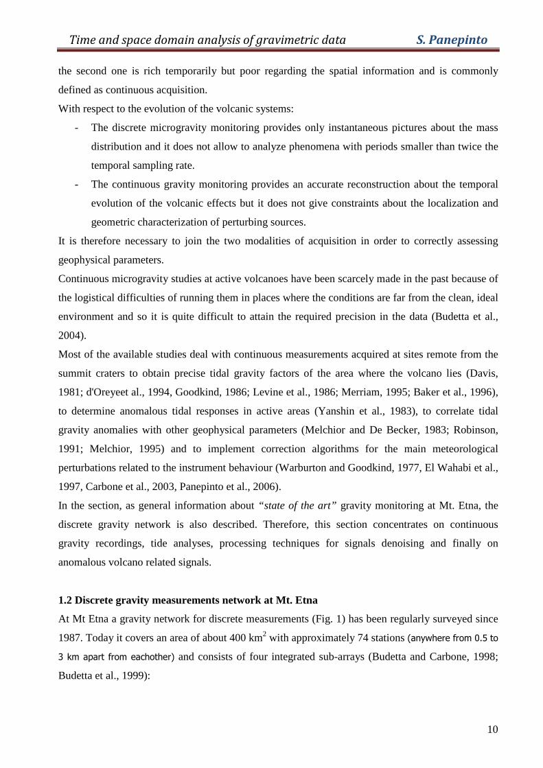
1.2 Discrete gravity measurements network at Mt. Etna
At Mt Etna a gravity network for discrete measurements (Fig. 1) has been regularly surveyed since
1987. Today it covers an area of about 400 km2 with approximately 74 stations (anywhere from 0.5 to
3 km apart from eachother) and consists of four integrated sub-arrays (Budetta and Carbone, 1998;
Budetta et al., 1999):
Time and space domain analysis of gravimetric data S. Panepinto
11
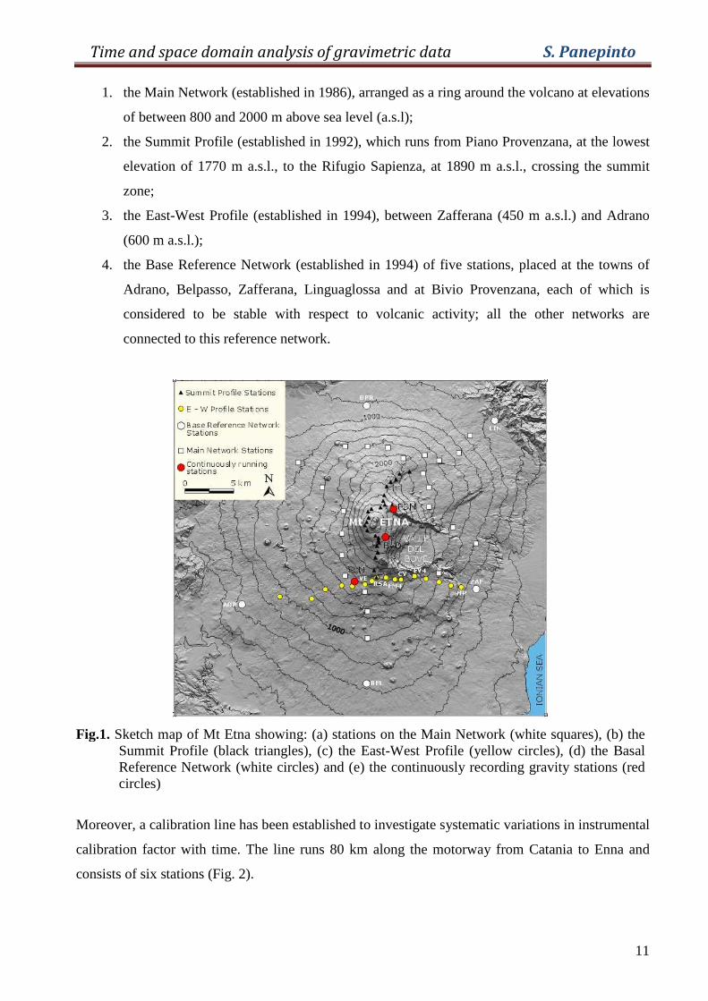
1. the Main Network (established in 1986), arranged as a ring around the volcano at elevations
of between 800 and 2000 m above sea level (a.s.l);
2. the Summit Profile (established in 1992), which runs from Piano Provenzana, at the lowest
elevation of 1770 m a.s.l., to the Rifugio Sapienza, at 1890 m a.s.l., crossing the summit
zone;
3. the East-West Profile (established in 1994), between Zafferana (450 m a.s.l.) and Adrano
(600 m a.s.l.);
4. the Base Reference Network (established in 1994) of five stations, placed at the towns of
Adrano, Belpasso, Zafferana, Linguaglossa and at Bivio Provenzana, each of which is
considered to be stable with respect to volcanic activity; all the other networks are
connected to this reference network.
Fig.1. Sketch map of Mt Etna showing: (a) stations on the Main Network (white squares), (b) the Summit Profile (black triangles), (c) the East-West Profile (yellow circles), (d) the Basal Reference Network (white circles) and (e) the continuously recording gravity stations (red circles)
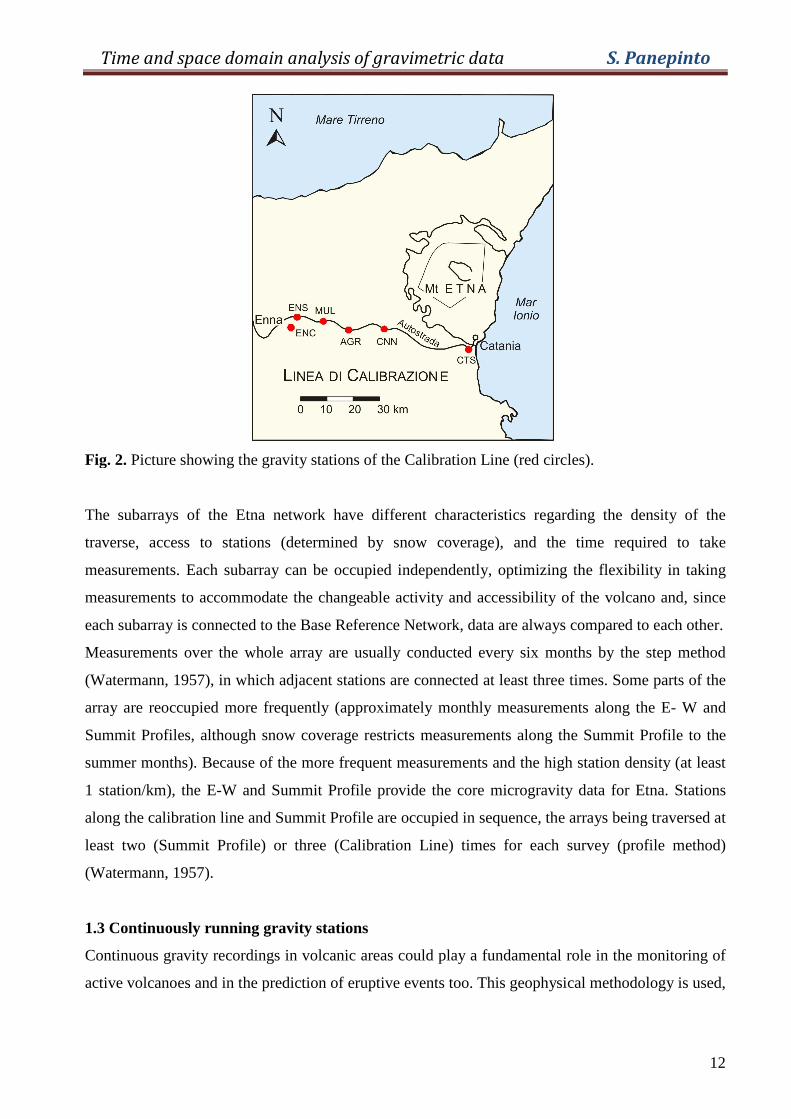
Moreover, a calibration line has been established to investigate systematic variations in instrumental
calibration factor with time. The line runs 80 km along the motorway from Catania to Enna and
consists of six stations (Fig. 2).
Time and space domain analysis of gravimetric data S. Panepinto
12
Fig. 2. Picture showing the gravity stations of the Calibration Line (red circles).
The subarrays of the Etna network have different characteristics regarding the density of the
traverse, access to stations (determined by snow coverage), and the time required to take
measurements. Each subarray can be occupied independently, optimizing the flexibility in taking
measurements to accommodate the changeable activity and accessibility of the volcano and, since
each subarray is connected to the Base Reference Network, data are always compared to each other.
Measurements over the whole array are usually conducted every six months by the step method
(Watermann, 1957), in which adjacent stations are connected at least three times. Some parts of the
array are reoccupied more frequently (approximately monthly measurements along the E- W and
Summit Profiles, although snow coverage restricts measurements along the Summit Profile to the
summer months). Because of the more frequent measurements and the high station density (at least
1 station/km), the E-W and Summit Profile provide the core microgravity data for Etna. Stations
along the calibration line and Summit Profile are occupied in sequence, the arrays being traversed at
least two (Summit Profile) or three (Calibration Line) times for each survey (profile method)
(Watermann, 1957).
1.3 Continuously running gravity stations
Continuous gravity recordings in volcanic areas could play a fundamental role in the monitoring of
active volcanoes and in the prediction of eruptive events too. This geophysical methodology is used,
Time and space domain analysis of gravimetric data S. Panepinto
13
on active volcanoes, in order to detect mass changes linked to magma transfer processes and, thus,
to recognize forerunners to paroxysmal volcanic events.
After a period of testing, the Etna discrete gravity network previously described, has been integrated
with three continuous running stations (Fig. 1). Furthermore, a permanent gravity station was also
installed at Stromboli Island to monitor the activity of this volcano. Thus, all the data referred to
here come from continuously running gravity stations placed at both of the Mt. Etna and Stromboli
volcanoes.
The continuous gravity observations at hand were performed over an interval of about fifteen years.
The sequences analyzed are not uninterrupted and were recorded using both LaCoste and Romberg
(LCR) and Scintrex spring gravimeters, located (Fig. 1): (i) about 10 km south of the active craters
at Serra la Nave Astrophysical Observatory (SLN; 1740 m a.s.l.); (ii) 2 km north-east of the summit
NE crater at the Pizzi Deneri Volcanological Observatory (PDN; 2820 m a.s.l.) and (iii) about 1 km
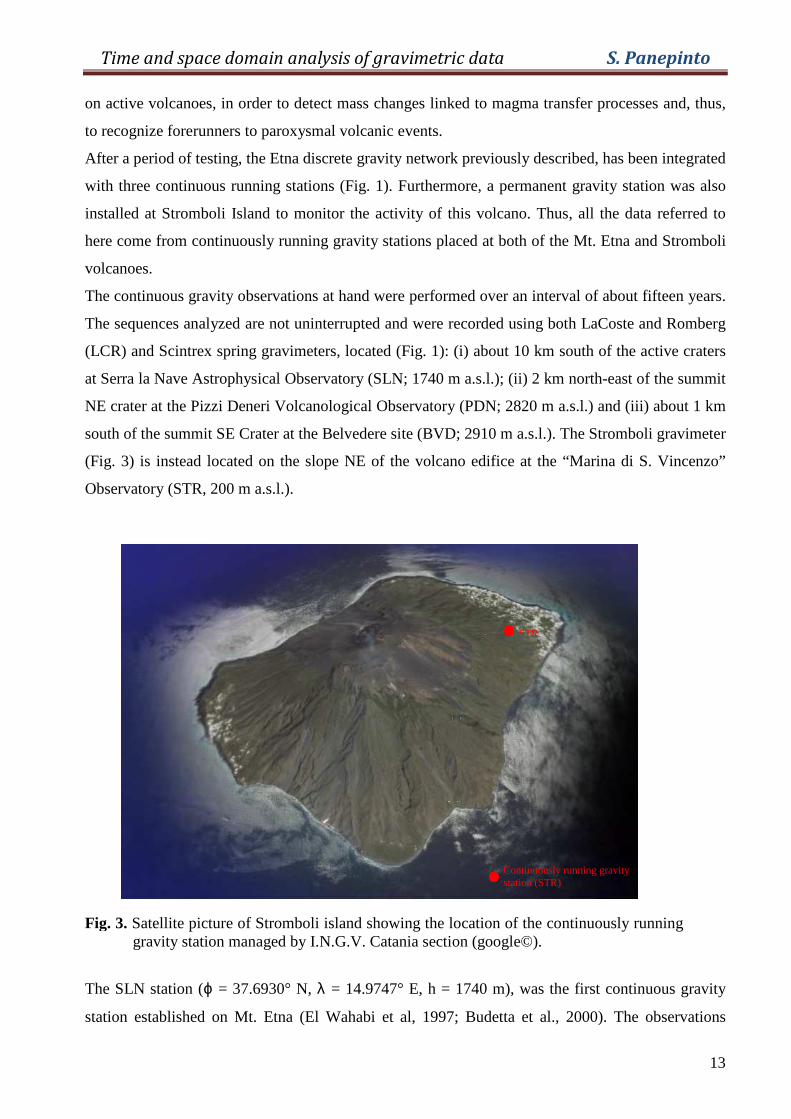
south of the summit SE Crater at the Belvedere site (BVD; 2910 m a.s.l.). The Stromboli gravimeter
(Fig. 3) is instead located on the slope NE of the volcano edifice at the “Marina di S. Vincenzo”
Observatory (STR, 200 m a.s.l.).
Fig. 3. Satellite picture of Stromboli island showing the location of the continuously running gravity station managed by I.N.G.V. Catania section (google©).
The SLN station (ϕ = 37.6930° N, λ = 14.9747° E, h = 1740 m), was the first continuous gravity
station established on Mt. Etna (El Wahabi et al, 1997; Budetta et al., 2000). The observations
Continuously running gravity station (STR)
STR
Time and space domain analysis of gravimetric data S. Panepinto
14
acquired in this station have been performed both with a LCR G-8 (managed by the Royal
Observatory of Belgium), between 1992 and 1995, and recently with a Scintrex CG-3M (managed
by the Istituto Nazionale di Geofisica e Vulcanologia – Catania).
The PDN station (ϕ = 37.7643° N, λ = 15.0154° E, h = 2820 m), is one of the two stations which
are very close to the active craters. Observations in this station were performed with the gravimeters
LCR D-185 and LCR PET-1081. The BVD station (ϕ = 37.7408° N, λ = 15.0091° E, h = 2910 m)
is equipped with a LCR D-185. Finally, the STR station (ϕ = 38.80° N, λ = 15.2270° E, h = 200 m)
is the only one located at Stromboli and the gravity meter for the recordings is the LCR D-157.
1.4 Setup of continuously running stations
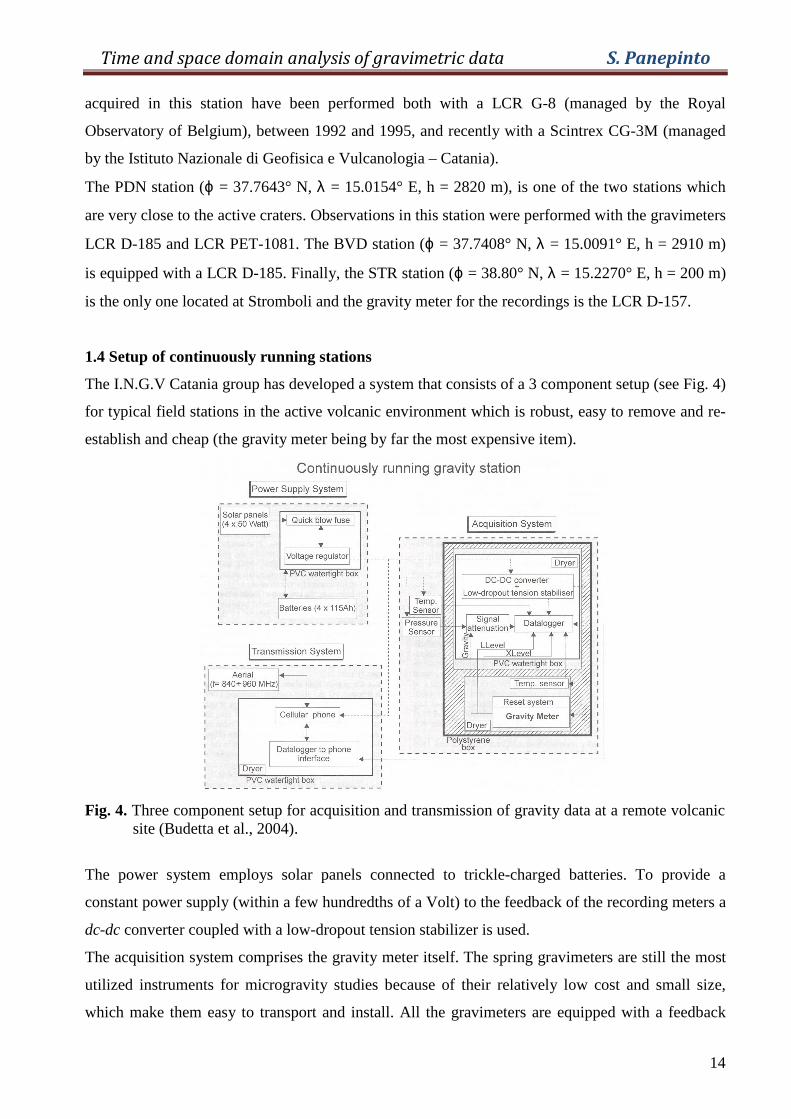
The I.N.G.V Catania group has developed a system that consists of a 3 component setup (see Fig. 4)
for typical field stations in the active volcanic environment which is robust, easy to remove and re-
establish and cheap (the gravity meter being by far the most expensive item).
Fig. 4. Three component setup for acquisition and transmission of gravity data at a remote volcanic site (Budetta et al., 2004).
The power system employs solar panels connected to trickle-charged batteries. To provide a
constant power supply (within a few hundredths of a Volt) to the feedback of the recording meters a
dc-dc converter coupled with a low-dropout tension stabilizer is used.
The acquisition system comprises the gravity meter itself. The spring gravimeters are still the most
utilized instruments for microgravity studies because of their relatively low cost and small size,
which make them easy to transport and install. All the gravimeters are equipped with a feedback
Time and space domain analysis of gravimetric data S. Panepinto
15
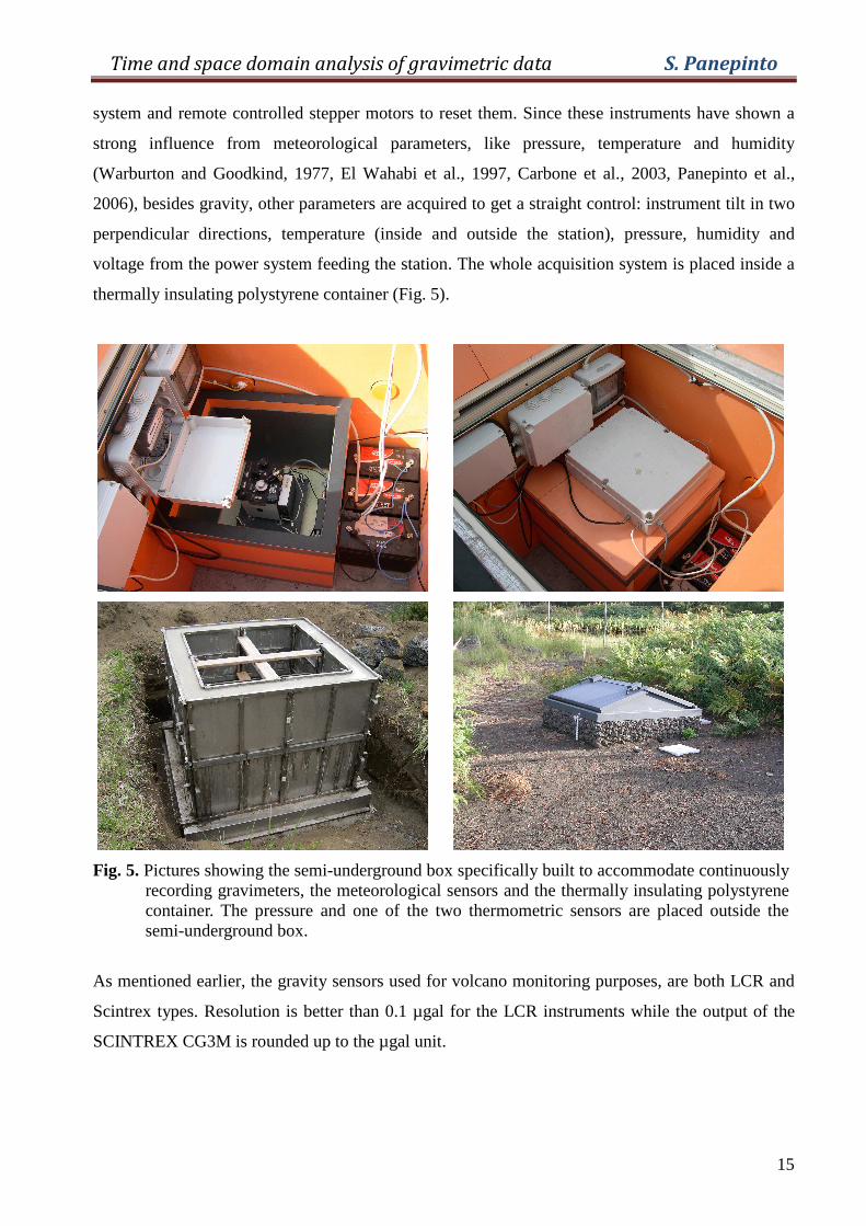
system and remote controlled stepper motors to reset them. Since these instruments have shown a
strong influence from meteorological parameters, like pressure, temperature and humidity
(Warburton and Goodkind, 1977, El Wahabi et al., 1997, Carbone et al., 2003, Panepinto et al.,
2006), besides gravity, other parameters are acquired to get a straight control: instrument tilt in two
perpendicular directions, temperature (inside and outside the station), pressure, humidity and
voltage from the power system feeding the station. The whole acquisition system is placed inside a
thermally insulating polystyrene container (Fig. 5).
Fig. 5. Pictures showing the semi-underground box specifically built to accommodate continuously recording gravimeters, the meteorological sensors and the thermally insulating polystyrene container. The pressure and one of the two thermometric sensors are placed outside the semi-underground box.
As mentioned earlier, the gravity sensors used for volcano monitoring purposes, are both LCR and
Scintrex types. Resolution is better than 0.1 µgal for the LCR instruments while the output of the
SCINTREX CG3M is rounded up to the µgal unit.

Time and space domain analysis of gravimetric data S. Panepinto
16
All the data are recorded at a 1datum/min sampling rate (each datum is the average calculated over
60 measurements) through a CR10X Campbell Scientific data-logger (A/D bits: 13).1 Data, after
being temporally stored in the solid-state memory of the data logger, are dumped to the INGV
Catania section automatically every 24 hours by the transmission system which employs a cellular
phone.
Furthermore, two of the three stations (SLN and BVD) are housed in semi-underground boxes
specifically built to accommodate continuously recording gravimeters (Fig. 5).
1 See the website www.campbellsci.com/cr10x for more details
Time and space domain analysis of gravimetric data S. Panepinto
17
CHAPTER 2
2.1 Introduction
Continuous gravity observations performed in the last few years, both at Mt. Etna and Stromboli,
have prompted the need to improve the tidal analysis in order to acquire the best corrected data for
the detection of volcano related signals. On Mt. Etna, the sites are very close to each other and the
expected tidal factors differences are negligible. It is thus useful to unify the tidal analysis results of
the different data sets in a unique tidal model. This tidal model, which can be independently
confirmed by a modeling of the tidal parameters based on the elastic response of the Earth to tidal
forces and the computation of the ocean tides effects on gravity, is very useful for the precise tidal
gravity prediction required by absolute or relative discrete gravity measurements.
Although spring gravimeters are severely affected by meteorological effects (Warburton and
Goodkind, 1977; El Wahabi et al., 1997, 2001; Carbone et al., 2003; Panepinto et al., 2006) and
suffer from strong instrumental drift compared to superconducting ones (see chapter 3), these
instruments are still suitable for continuous gravity recording and tidal analysis.
The main focus of continuous gravity observations on an active volcano is the detection of gravity
changes associated with volcanic events with a wide range of evolution rates (periods ranging from
minutes to months). However, for periods longer than 10 hours, the tidal gravity variations will
mask other geophysical phenomena. It is thus very important to efficiently remove the tidal signal,
possibly on line. A precise tidal prediction model is thus required. Such a model is also necessary
for relative field gravity measurements on volcanoes and the precision requirements are much more
demanding if absolute measurements are considered. A first priority of tidal gravity observations on
volcanoes is thus to build up an experimental model that can be compared with a modeling of the
tidal parameters based on the elastic response of the Earth to tidal forces and the computation of the
ocean tides effects on gravity (§ 2.9).
Two main instrumental problems have to be addressed in order to obtain coherent results using
spring gravimeters and especially LaCoste & Romberg instruments: the adjustment of the scale
factor (§ 2.10) and the changes of sensitivity (§ 2.8). The maker provides a calibration constant but,
when recording the very tiny (less than 0.3 mgal) tidal changes, one should generally apply a scale
factor or normalization constant. This quantity can be determined either by recording side by side
with well calibrated instruments (Wenzel et al., 1991; Ducarme and Somerhausen, 1997) or by
checking the scale factor on specially designed short baselines e.g. the Hannover vertical base line
(Kangieser and Torge, 1981; Timmen and Wenzel, 1994).
Time and space domain analysis of gravimetric data S. Panepinto
18
On the other hand, spring gravimeters often show sensitivity variations in the order of a few percent
(van Ruymbeke, 1998), due for example to ground tilting or temperature effects on the electronics.
It is thus necessary to continuously monitor the instrumental sensitivity in order to maintain
accurate information concerning real gravity changes.
The change in gravimeter sensitivity over time is also an important issue to be checked since it
affects not only the results of tidal analysis but also the accuracy of the observed gravity changes.
Conversely, if a good tidal model is available, the sensitivity variations can be accurately
reconstructed so as to retune observed tidal records with the synthetic tide, since the tidal
parameters are assumed to be constant at a given location.
2.2 Tidal theory
For a full account of the standard background to earth tide theory the reader is referred to Melchior
(1966, 1978), Torge (1989) and Wilhelm et al. (1997). Here is given an outline of the important
steps.
For all bodies in the Universe moving in a stationary orbit (which is in first approximation a Kepler
ellipse), the gravitational accelerations produced by other bodies (planets and satellites) are
completely compensated in their centres of mass by centrifugal accelerations due to the orbital
motion of the body. Because of the spatial extension of the body (e.g. the Earth), the gravitational
accelerations due to other celestial bodies (e.g. Moon, Sun) are slightly position dependent, whereas
the centrifugal accelerations are constant within the body and on the surface of the body. The
difference between the gravitational accelerations and the centrifugal accelerations are small tidal
accelerations; on the Earth, the tidal accelerations are less than ±1µm/s2 = 10-7 of the Earth’s
gravity, g.
The computation of functionals of the tidal potential (e.g. tidal accelerations, tidal tilt, tidal strain) at
a specific station and epoch can be carried out using one of the following two methods:
- Using ephemerides (coordinates) of the celestial bodies (Moon, Sun and planets),
functionals of the tidal potential can be computed for a rigid oceanless Earth model with
very high precision. This method is used to compute tidal potential catalogues and so-called
benchmark series to check tidal potential catalogues (e.g. Wenzel, 1996a). But its practical
application is restricted to less precise demands because it is impossible to compute
accurately tidal effects for an elastic Earth covered with oceans using the ephemeris method.
- The tidal potential can be expanded in solid spherical harmonics; the spectral analysis of the
tidal potential’s spherical harmonic expansion yields a tidal potential catalogue (a table of
amplitudes, phases and frequencies for some tidal waves). There are currently available
Time and space domain analysis of gravimetric data S. Panepinto
19
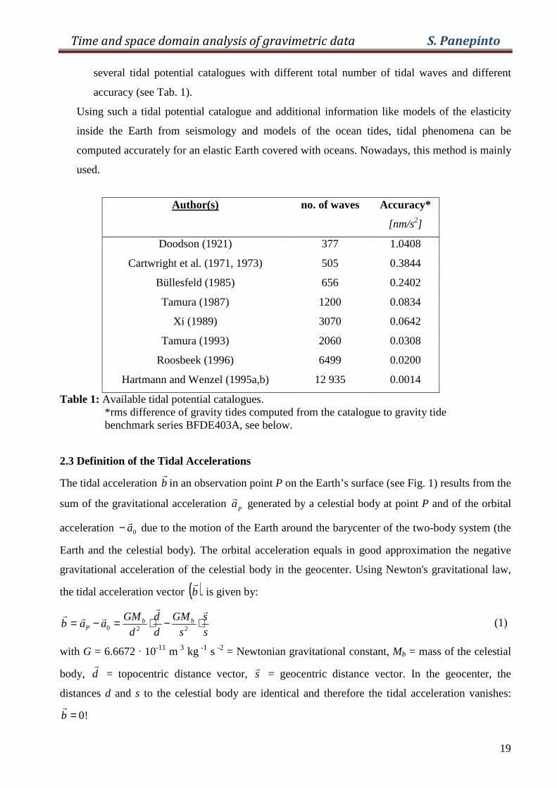
several tidal potential catalogues with different total number of tidal waves and different
accuracy (see Tab. 1).
Using such a tidal potential catalogue and additional information like models of the elasticity
inside the Earth from seismology and models of the ocean tides, tidal phenomena can be
computed accurately for an elastic Earth covered with oceans. Nowadays, this method is mainly
used.
Author(s) no. of waves Accuracy*
[nm/s2]
Doodson (1921) 377 1.0408
Cartwright et al. (1971, 1973) 505 0.3844
Büllesfeld (1985) 656 0.2402
Tamura (1987) 1200 0.0834
Xi (1989) 3070 0.0642
Tamura (1993) 2060 0.0308
Roosbeek (1996) 6499 0.0200
Hartmann and Wenzel (1995a,b) 12 935 0.0014
Table 1: Available tidal potential catalogues. *rms difference of gravity tides computed from the catalogue to gravity tide benchmark series BFDE403A, see below.
2.3 Definition of the Tidal Accelerations
The tidal acceleration br
in an observation point P on the Earth’s surface (see Fig. 1) results from the
sum of the gravitational acceleration par
generated by a celestial body at point P and of the orbital
acceleration 0ar− due to the motion of the Earth around the barycenter of the two-body system (the
Earth and the celestial body). The orbital acceleration equals in good approximation the negative
gravitational acceleration of the celestial body in the geocenter. Using Newton's gravitational law,
the tidal acceleration vector ( )br
is given by:
s
s
s
GM
d
d
d
GMaab bb
P
rrrrr
⋅−⋅=−=220 (1)
with G = 6.6672 · 10-11 m 3 kg -1 s -2 = Newtonian gravitational constant, Mb = mass of the celestial
body, dr
= topocentric distance vector, sr
= geocentric distance vector. In the geocenter, the
distances d and s to the celestial body are identical and therefore the tidal acceleration vanishes:
!0=br
Time and space domain analysis of gravimetric data S. Panepinto
20
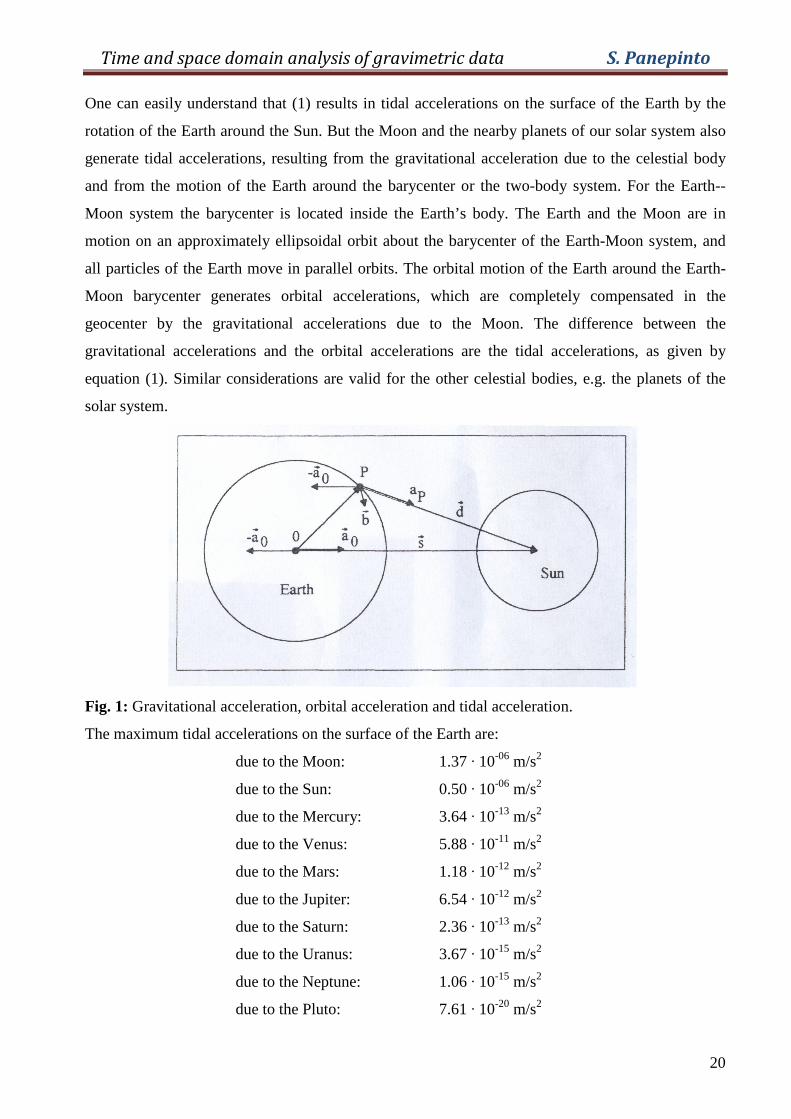
One can easily understand that (1) results in tidal accelerations on the surface of the Earth by the
rotation of the Earth around the Sun. But the Moon and the nearby planets of our solar system also
generate tidal accelerations, resulting from the gravitational acceleration due to the celestial body
and from the motion of the Earth around the barycenter or the two-body system. For the Earth--
Moon system the barycenter is located inside the Earth’s body. The Earth and the Moon are in
motion on an approximately ellipsoidal orbit about the barycenter of the Earth-Moon system, and
all particles of the Earth move in parallel orbits. The orbital motion of the Earth around the Earth-
Moon barycenter generates orbital accelerations, which are completely compensated in the
geocenter by the gravitational accelerations due to the Moon. The difference between the
gravitational accelerations and the orbital accelerations are the tidal accelerations, as given by
equation (1). Similar considerations are valid for the other celestial bodies, e.g. the planets of the
solar system.
Fig. 1: Gravitational acceleration, orbital acceleration and tidal acceleration.
The maximum tidal accelerations on the surface of the Earth are:
due to the Moon:
due to the Sun:
due to the Mercury:
due to the Venus:
due to the Mars:
due to the Jupiter:
due to the Saturn:
due to the Uranus:
due to the Neptune:
due to the Pluto:
1.37 · 10-06 m/s2
0.50 · 10-06 m/s2
3.64 · 10-13 m/s2
5.88 · 10-11 m/s2
1.18 · 10-12 m/s2
6.54 · 10-12 m/s2
2.36 · 10-13 m/s2
3.67 · 10-15 m/s2
1.06 · 10-15 m/s2
7.61 · 10-20 m/s2
Time and space domain analysis of gravimetric data S. Panepinto
21
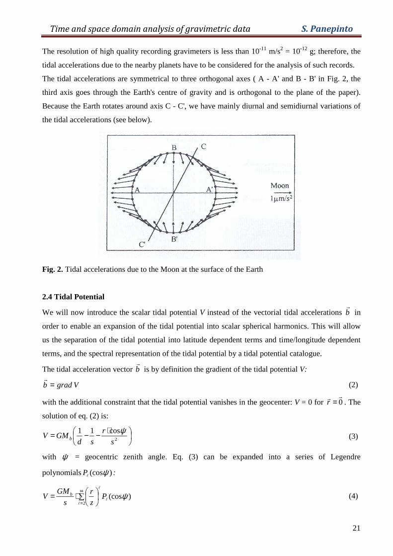
The resolution of high quality recording gravimeters is less than 10-11 m/s2 = 10-12 g; therefore, the
tidal accelerations due to the nearby planets have to be considered for the analysis of such records.
The tidal accelerations are symmetrical to three orthogonal axes ( A - A' and B - B' in Fig. 2, the
third axis goes through the Earth's centre of gravity and is orthogonal to the plane of the paper).
Because the Earth rotates around axis C - C', we have mainly diurnal and semidiurnal variations of
the tidal accelerations (see below).
Fig. 2. Tidal accelerations due to the Moon at the surface of the Earth
2.4 Tidal Potential
We will now introduce the scalar tidal potential V instead of the vectorial tidal accelerations br
in
order to enable an expansion of the tidal potential into scalar spherical harmonics. This will allow
us the separation of the tidal potential into latitude dependent terms and time/longitude dependent
terms, and the spectral representation of the tidal potential by a tidal potential catalogue.
The tidal acceleration vector br
is by definition the gradient of the tidal potential V:
Vgradb =r
(2)
with the additional constraint that the tidal potential vanishes in the geocenter: V = 0 for 0rr =r . The
solution of eq. (2) is:
⋅−−=2
cos11
s
r
sdGMV b
ψ (3)
with ψ = geocentric zenith angle. Eq. (3) can be expanded into a series of Legendre
polynomials )(cosψl
P :
∑
⋅=∞
=2)(cos
ll
l
ψPz
r
s
GMV b (4)
Time and space domain analysis of gravimetric data S. Panepinto
22
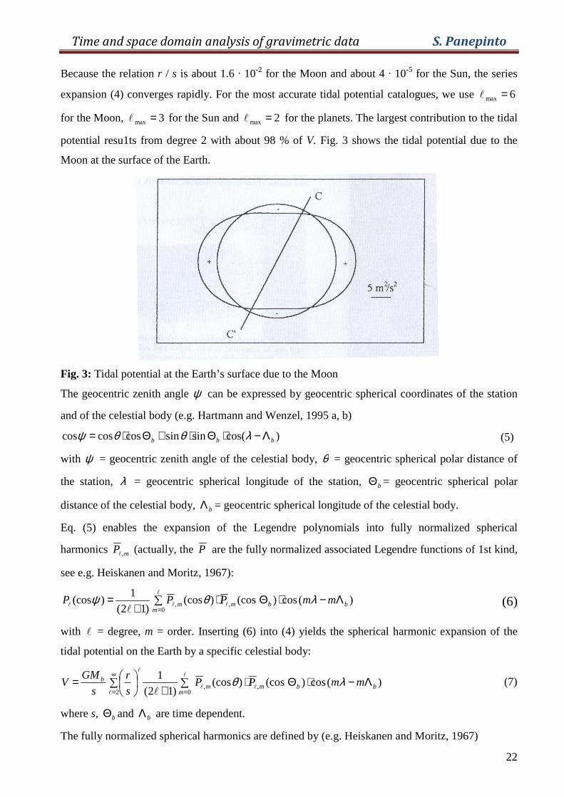
Because the relation r / s is about 1.6 · 10-2 for the Moon and about 4 · 10-5 for the Sun, the series
expansion (4) converges rapidly. For the most accurate tidal potential catalogues, we use 6max =l
for the Moon, 3max =l for the Sun and 2max =l for the planets. The largest contribution to the tidal
potential resu1ts from degree 2 with about 98 % of V. Fig. 3 shows the tidal potential due to the
Moon at the surface of the Earth.
Fig. 3: Tidal potential at the Earth’s surface due to the Moon
The geocentric zenith angle ψ can be expressed by geocentric spherical coordinates of the station
and of the celestial body (e.g. Hartmann and Wenzel, 1995 a, b)
)cos(sinsincoscoscos bbb Λ−⋅Θ⋅+Θ⋅= λθθψ (5)
with ψ = geocentric zenith angle of the celestial body, θ = geocentric spherical polar distance of
the station, λ = geocentric spherical longitude of the station, bΘ = geocentric spherical polar
distance of the celestial body, bΛ = geocentric spherical longitude of the celestial body.
Eq. (5) enables the expansion of the Legendre polynomials into fully normalized spherical
harmonics mP ,l (actually, the P are the fully normalized associated Legendre functions of 1st kind,
see e.g. Heiskanen and Moritz, 1967):
∑ Λ−⋅Θ⋅+
==
l
llll 0
,, )(cos)(cos)(cos)12(
1)(cos
mbbmm mmPPP λθψ (6)
with l = degree, m = order. Inserting (6) into (4) yields the spherical harmonic expansion of the
tidal potential on the Earth by a specific celestial body:
∑ Λ−⋅Θ⋅∑+
=∞
= =2,,
0)(cos)(cos)(cos
)12(
1l
ll
ll
lbbmm
m
b mmPPs
r
s
GMV λθ (7)
where s, bΘ and bΛ are time dependent.
The fully normalized spherical harmonics are defined by (e.g. Heiskanen and Moritz, 1967)
Time and space domain analysis of gravimetric data S. Panepinto
23
( ) )2()!(
)!()12(1
!2
1)1()1()( 0,
222, mm
mmm
m ml
mlx
dx
d
dx
dxxP δ−
+−+
−−−= l
l
l
l
l
ll (8)
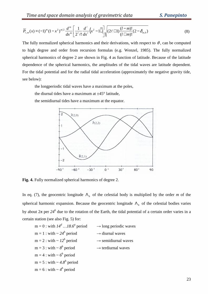
The fully normalized spherical harmonics and their derivations, with respect to θ , can be computed
to high degree and order from recursion formulas (e.g. Wenzel, 1985). The fully normalized
spherical harmonics of degree 2 are shown in Fig. 4 as function of latitude. Because of the latitude
dependence of the spherical harmonics, the amplitudes of the tidal waves are latitude dependent.
For the tidal potential and for the radial tidal acceleration (approximately the negative gravity tide,
see below):
the longperiodic tidal waves have a maximum at the poles,
the diurnal tides have a maximum at ±45° latitude,
the semidiurnal tides have a maximum at the equator.
Fig. 4. Fully normalized spherical harmonics of degree 2.
In eq. (7), the geocentric longitude bΛ of the celestial body is multiplied by the order m of the
spherical harmonic expansion. Because the geocentric longitude bΛ of the celestial bodies varies
by about 2π per 24h due to the rotation of the Earth, the tidal potential of a certain order varies in a
certain station (see also Fig. 5) for:
m = 0 : with 14d …18.6a period → long periodic waves
m = 1 : with ~ 24h period → diurnal waves
m = 2 : with ~ 12h period → semidiurnal waves
m = 3 : with ~ 8h period → terdiurnal waves
m = 4 : with ~ 6h period
m = 5 : with ~ 4.8h period
m = 6 : with ~ 4h period
Time and space domain analysis of gravimetric data S. Panepinto
24
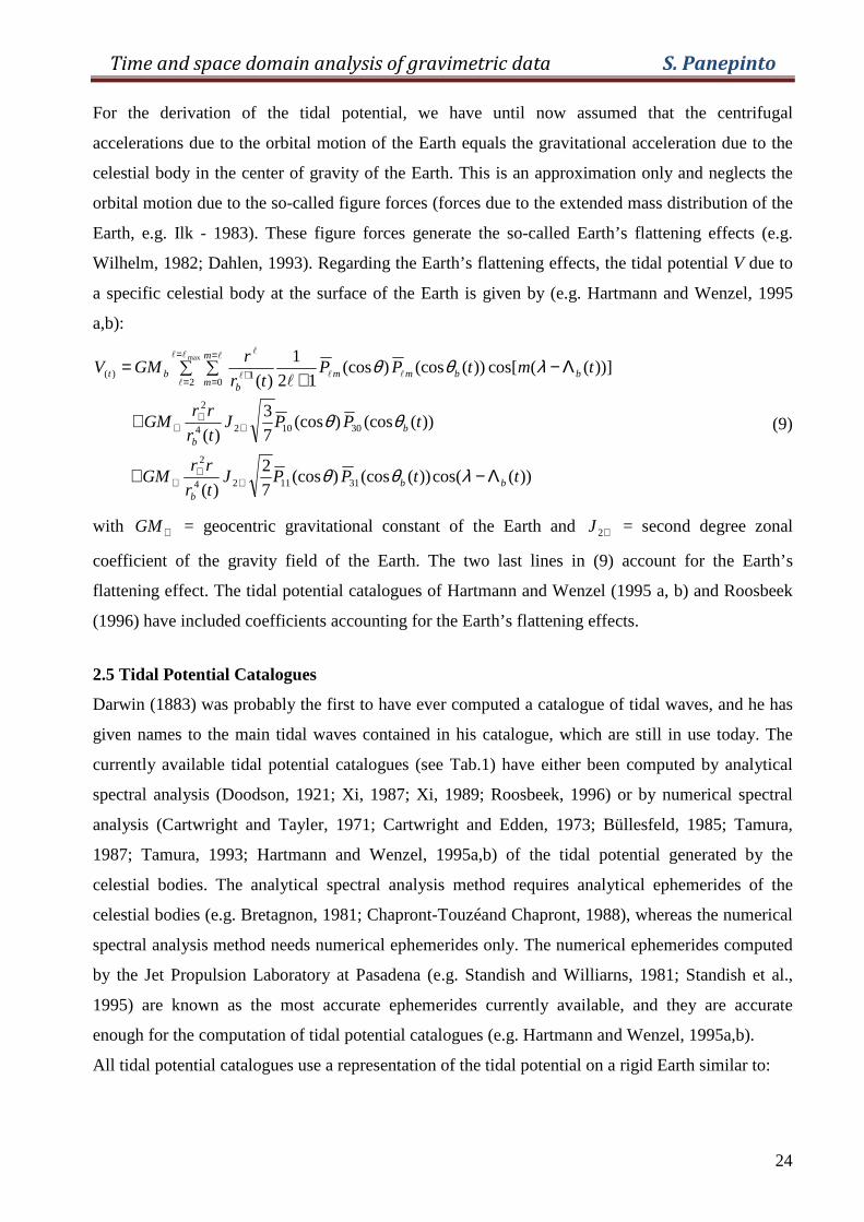
For the derivation of the tidal potential, we have until now assumed that the centrifugal
accelerations due to the orbital motion of the Earth equals the gravitational acceleration due to the
celestial body in the center of gravity of the Earth. This is an approximation only and neglects the
orbital motion due to the so-called figure forces (forces due to the extended mass distribution of the
Earth, e.g. Ilk - 1983). These figure forces generate the so-called Earth’s flattening effects (e.g.
Wilhelm, 1982; Dahlen, 1993). Regarding the Earth’s flattening effects, the tidal potential V due to
a specific celestial body at the surface of the Earth is given by (e.g. Hartmann and Wenzel, 1995
a,b):
))(cos())((cos)(cos7
2
)(
))((cos)(cos7
3
)(
))]((cos[))((cos)(cos12
1
)(
311124
2
301024
2
2 01)(
max
ttPPJtr
rrGM
tPPJtr
rrGM
tmtPPtr
rGMV
bbb
bb
m
mbbmm
bbt
Λ−+
+
∑ ∑ Λ−+
=
⊕⊕
⊕
⊕⊕
⊕
=
=
=
=+
λθθ
θθ
λθθll
l
l
lll
l
l
(9)
with ⊕GM = geocentric gravitational constant of the Earth and ⊕2J = second degree zonal
coefficient of the gravity field of the Earth. The two last lines in (9) account for the Earth’s
flattening effect. The tidal potential catalogues of Hartmann and Wenzel (1995 a, b) and Roosbeek
(1996) have included coefficients accounting for the Earth’s flattening effects.
2.5 Tidal Potential Catalogues
Darwin (1883) was probably the first to have ever computed a catalogue of tidal waves, and he has
given names to the main tidal waves contained in his catalogue, which are still in use today. The
currently available tidal potential catalogues (see Tab.1) have either been computed by analytical
spectral analysis (Doodson, 1921; Xi, 1987; Xi, 1989; Roosbeek, 1996) or by numerical spectral
analysis (Cartwright and Tayler, 1971; Cartwright and Edden, 1973; Büllesfeld, 1985; Tamura,
1987; Tamura, 1993; Hartmann and Wenzel, 1995a,b) of the tidal potential generated by the
celestial bodies. The analytical spectral analysis method requires analytical ephemerides of the
celestial bodies (e.g. Bretagnon, 1981; Chapront-Touzéand Chapront, 1988), whereas the numerical
spectral analysis method needs numerical ephemerides only. The numerical ephemerides computed
by the Jet Propulsion Laboratory at Pasadena (e.g. Standish and Williarns, 1981; Standish et al.,
1995) are known as the most accurate ephemerides currently available, and they are accurate
enough for the computation of tidal potential catalogues (e.g. Hartmann and Wenzel, 1995a,b).
All tidal potential catalogues use a representation of the tidal potential on a rigid Earth similar to:
Time and space domain analysis of gravimetric data S. Panepinto
25
[ ]∑ ∑ +⋅∑ ⋅Γ
==
=
=
=
max
1 0)( ))(sin()())(cos()()(cos)(
ll
l
lll
l
l
ii
mii
mi
m
mmt tatStatCP
a
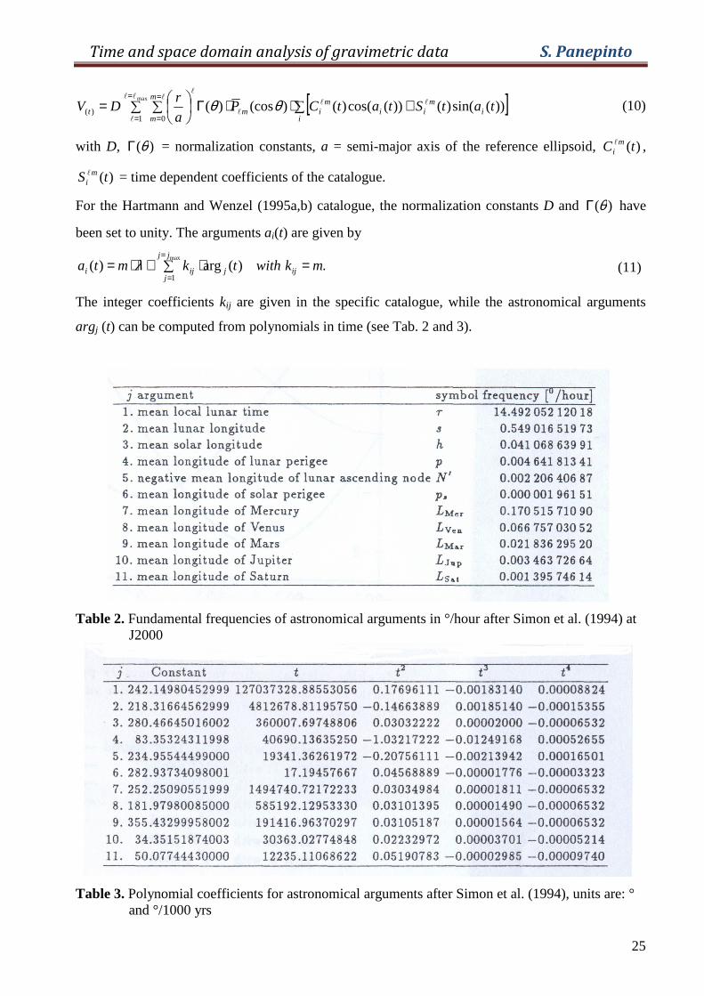
rDV θθ (10)
with D, )(θΓ = normalization constants, a = semi-major axis of the reference ellipsoid, )(tC mil ,
)(tS mil = time dependent coefficients of the catalogue.
For the Hartmann and Wenzel (1995a,b) catalogue, the normalization constants D and )(θΓ have
been set to unity. The arguments ai(t) are given by
.)(arg)(max
1mkwithtkmta ij
jj
jjiji =∑ ⋅+⋅=
=
=λ (11)
The integer coefficients kij are given in the specific catalogue, while the astronomical arguments
argj (t) can be computed from polynomials in time (see Tab. 2 and 3).
Table 2. Fundamental frequencies of astronomical arguments in °/hour after Simon et al. (1994) at J2000
Table 3. Polynomial coefficients for astronomical arguments after Simon et al. (1994), units are: ° and °/1000 yrs
Time and space domain analysis of gravimetric data S. Panepinto
26
The time dependent coefficients )(tC mil , )(tS m
il are given by:
mi
mi
mi C1C0C lll ⋅+= tt)( (12)
mi
mi
mi S1S0S lll ⋅+= tt)( (13)
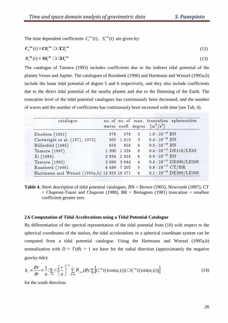
The catalogue of Tamura (1993) includes coefficients due to the indirect tidal potential of the
planets Venus and Jupiter. The catalogues of Roosbeek (1996) and Hartmann and Wenzel (1995a,b)
include the lunar tidal potential of degree 5 and 6 respectively, and they also include coefficients
due to the direct tidal potential of the nearby planets and due to the flattening of the Earth. The
truncation level of the tidal potential catalogues has continuously been decreased, and the number
of waves and the number of coefficients has continuously been increased with time (see Tab. 4).
Table 4. Short description of tidal potential catalogues. BN = Brown (1905), Newcomb (1897), CT = Chapront-Touzé and Chapront (1988), BR = Bretagnon (1981) truncation = smallest coefficient greater zero
2.6 Computation of Tidal Accelerations using a Tidal Potential Catalogue
By differentiation of the spectral representation of the tidal potential from (10) with respect to the
spherical coordinates of the station, the tidal accelerations in a spherical coordinate system can be
computed from a tidal potential catalogue. Using the Hartmann and Wenzel (1995a,b)
normalization with D = )(θΓ = 1 we have for the radial direction (approximately the negative
gravity tide):
[ ]∑ +⋅∑∑
⋅⋅=∂∂=
==
−
ii
mii
mi
mmr tatStatCP
a
r
ar
Vb ))(sin()())(cos()()(
10
,1
1ll
l
ll
l
l θ (14)
for the south direction:
Time and space domain analysis of gravimetric data S. Panepinto
27
[ ]∑ +⋅∑∂
∂∑
⋅=∂⋅
∂===
−
ii
mii
mi
m
m tatStatCP
a
r
ar
vb ))(sin()())(cos()(
10
,
1
1ll
ll
l
l
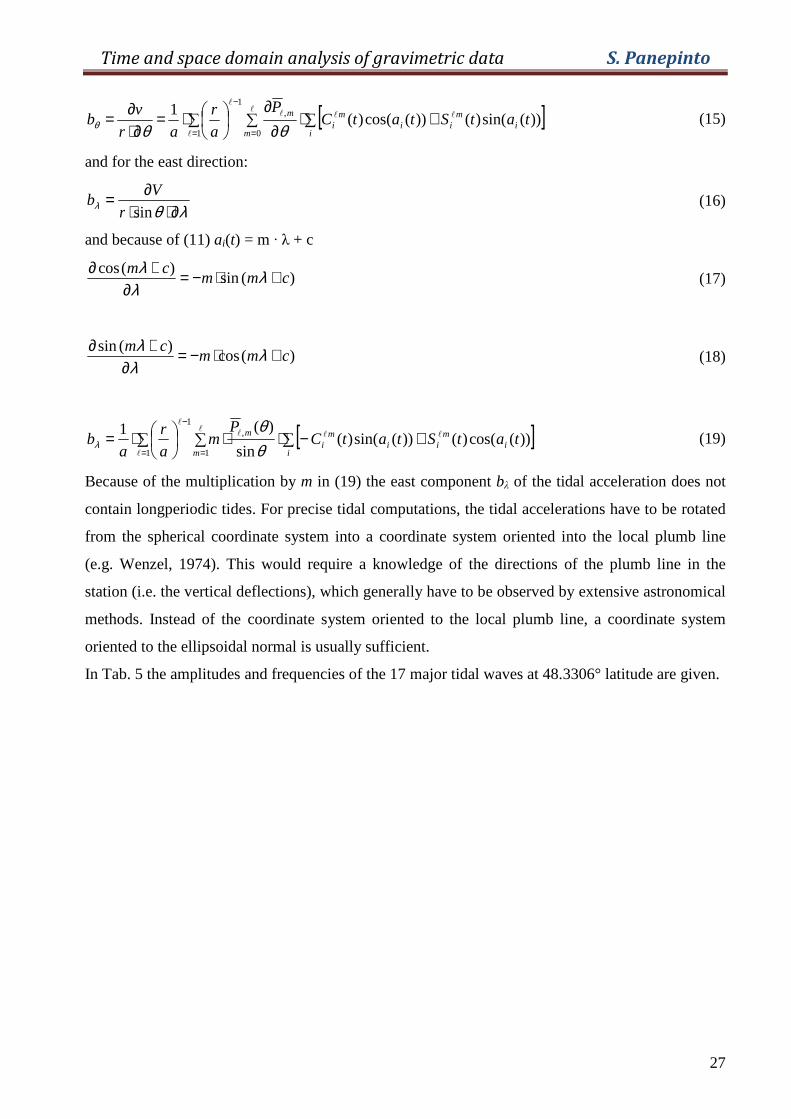
θθθ (15)
and for the east direction:
λθλ ∂⋅⋅∂=
sinr
Vb (16)
and because of (11) ai(t) = m · λ + c
)(sin)(cos
cmmcm +⋅−=
∂+∂ λ
λλ
(17)
)(cos)(sin
cmmcm +⋅−=
∂+∂ λ
λλ
(18)
[ ]∑ +−⋅∑ ⋅∑
⋅===
−
ii
mii
mi
m
m tatStatCP
ma
r
ab ))(cos()())(sin()(
sin
)(11
,
1
1ll
ll
l
l
θθ
λ (19)
Because of the multiplication by m in (19) the east component bλ of the tidal acceleration does not
contain longperiodic tides. For precise tidal computations, the tidal accelerations have to be rotated
from the spherical coordinate system into a coordinate system oriented into the local plumb line
(e.g. Wenzel, 1974). This would require a knowledge of the directions of the plumb line in the
station (i.e. the vertical deflections), which generally have to be observed by extensive astronomical
methods. Instead of the coordinate system oriented to the local plumb line, a coordinate system
oriented to the ellipsoidal normal is usually sufficient.
In Tab. 5 the amplitudes and frequencies of the 17 major tidal waves at 48.3306° latitude are given.
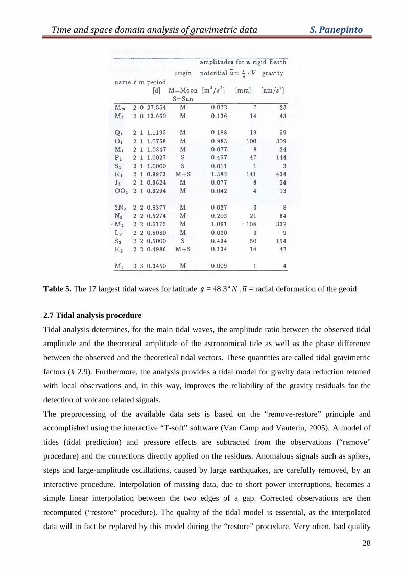
Time and space domain analysis of gravimetric data S. Panepinto
28
Table 5. The 17 largest tidal waves for latitude N°= 3.48φ .u = radial deformation of the geoid
2.7 Tidal analysis procedure
Tidal analysis determines, for the main tidal waves, the amplitude ratio between the observed tidal
amplitude and the theoretical amplitude of the astronomical tide as well as the phase difference
between the observed and the theoretical tidal vectors. These quantities are called tidal gravimetric
factors (§ 2.9). Furthermore, the analysis provides a tidal model for gravity data reduction retuned
with local observations and, in this way, improves the reliability of the gravity residuals for the
detection of volcano related signals.
The preprocessing of the available data sets is based on the “remove-restore” principle and
accomplished using the interactive “T-soft” software (Van Camp and Vauterin, 2005). A model of
tides (tidal prediction) and pressure effects are subtracted from the observations (“remove”
procedure) and the corrections directly applied on the residues. Anomalous signals such as spikes,
steps and large-amplitude oscillations, caused by large earthquakes, are carefully removed, by an
interactive procedure. Interpolation of missing data, due to short power interruptions, becomes a
simple linear interpolation between the two edges of a gap. Corrected observations are then
recomputed (“restore” procedure). The quality of the tidal model is essential, as the interpolated
data will in fact be replaced by this model during the “restore” procedure. Very often, bad quality
Time and space domain analysis of gravimetric data S. Panepinto
29
data are kept to avoid the creation of gaps. For the same reason, gaps of various extensions are
interpolated, which introduces a non-Gaussian non-stationary noise (Ducarme et al., 2004). Indeed,
gaps can introduce systematic errors by leakage, but inappropriate interpolations can be misleading
too. Thus, the data are inevitably subjected to various perturbations, including interruptions of the
recordings. Completely automated procedures such as the PRETERNA program (Wenzel, 1994)
can be dangerous. This is why the “T-soft” software has been developed with a high degree of
interactivity.
Data are then decimated to 1-hour sampling for a classical tidal analysis using the ETERNA3.4
software (Wenzel, 1998). Tidal analysis was performed on the data sets acquired both at Etna and
Stromboli. The series have different time spans and were performed with different gravity sensors.
As underlined before, the calibration of different gravimeters is not always coherent. On Etna we
have thus scaled all the instruments directly on the best data set, the records of LCR G-8 in Serra la
Nave. The scale factor of this instrument had been previously determined in the reference station of
Brussels (Melchior, 1994). This normalization will be discussed in § 2.10. On Stromboli it was
difficult to get a reliable model to scale the gravimeter (§ 2.11).
2.8 Calibration of the LCR gravimeters and sensitivity variations
The change in time of the calibration is an important issue to be checked since it affects not only the
quality of the data available but also the accuracy of the tidal analysis results and of the observed
gravity changes. The goal of any tidal measurements is to determine the response of the Earth to the
tidal force F(t) through an instrument, using a modeling system. In the output O(t) we cannot
separate which response in the physical system is due to the Earth and which is due to the
instrument itself. Doing a calibration means determining independently the transfer function of the
instrument in amplitude as well as in phase. In the Tidal bands the phase behavior of the LCR
gravimeter equipped with a feedback electronics can be assimilated to a constant time lag, close to
30s. The maker performs an initial absolute calibration, providing a dial calibration constant K that
expresses the force applied to the beam of the gravimeter by a unit rotation of the dial and is usually
expressed in µgal/(dial division). On the other hand, we have to transform the output of the
datalogger into equivalent acceleration applied to the beam, i.e. determine the scale calibration C in
[physical units] per [recording units]. The usual way of calibrating a LCR instrument is to turn the
micrometric screw of n divisions in order to apply a force with a known magnitude nK. If the
amplitude of the response of the instrument is l, the calibration factor of the instrument C is
C = nK/l = K/d. (20)
Time and space domain analysis of gravimetric data S. Panepinto
30
C is expressed in [physical units (µgal)] per [recording units] and d = l/n is the reaction of the
instrument per one division of the micrometer. Let us call this procedure “physical calibration”. The
original observations should be multiplied by C prior to tidal analysis.
The instrumental sensitivity s, inverse of the calibration, is then given by
s =1/C= d/K, (21)
expressed in [recording units] per [physical units]. Unfortunately, the calibration of a LCR
gravimeter equipped with an electronic feedback shows fluctuations of a few per cent (van
Ruymbeke, 1998). As the “physical calibration” of an instrument is generally a long and tedious
procedure and, what is worse, is perturbing the tidal records, there are only a few calibrations
available during the recording period and the sensitivity behavior between two calibrations is
unknown. The best we can do is to compute an instantaneous calibration value by linear
interpolation between two successive calibrations. Fortunately, we can accurately follow the
changes of sensitivity using the tidal records themselves as we suppose that the tidal parameters are
perfectly stable. If we have a good model for the tidal amplitude factors and phase differences, we
can generate a tidal prediction in physical units and fit the observations on the prediction with a
given window size e.g. 48 hours (Ducarme, 1970). The regression coefficient s’, expressed in
[recording units] per [physical units], can be called “apparent sensitivity”. If the tidal model and the
calibration C are correct and if the sensitivity is perfectly stable we should have always s’= s.
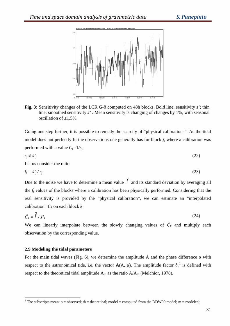
An option has been implemented in “T-soft” under "moving window regression", providing a
sequence of apparent sensitivity values s’j for every block j (Fig. 5). Auxiliary channels, such as
pressure can be incorporated in a multi-linear regression. We can thus follow the sensitivity
variations from block to block. Due to noise and perturbations, it is in general necessary to smooth
the individual values s’ j to get a sequence ŝ’ j with a continuous behavior. As an example, we show
in Figure 5 the sensitivity changes of the LCR G-8 during the whole acquisition period. The
apparent sensitivity increased by 1% in three and a half years. By the proposed procedure we may
obtain a general overview on the behavior of the gravimeter. Furthermore, it seems a good tool to
detect strong instrumental perturbation during any ongoing volcanic activity and avoid confusion
between purely instrumental effects and geophysical ones.
Time and space domain analysis of gravimetric data S. Panepinto
31
01-01-92 01-07-92 01-01-93 01-07-93 01-01-94 01-07-94 01-01-95
0.99
1.00
1.01
1.02
1.03
ETNA:LCR 8: d' apparent sensitivity (nms**-2/Hz) ETN A:LCR 8:sensitivity smoothed (nms**-2/Hz)
Fig. 3: Sensitivity changes of the LCR G-8 computed on 48h blocks. Bold line: sensitivity s’; thin
line: smoothed sensitivity ŝ’ . Mean sensitivity is changing of changes by 1%, with seasonal oscillation of ±1.5%.
Going one step further, it is possible to remedy the scarcity of “physical calibrations”. As the tidal
model does not perfectly fit the observations one generally has for block j, where a calibration was
performed with a value Cj=1/sj,
sj ≠ ŝ’ j (22)
Let us consider the ratio
fj = ŝ’ j / sj (23)
Due to the noise we have to determine a mean value f and its standard deviation by averaging all
the fj values of the blocks where a calibration has been physically performed. Considering that the
real sensitivity is provided by the “physical calibration”, we can estimate an “interpolated
calibration” Čk on each block k
Čk =f / ŝ’ k (24)
We can linearly interpolate between the slowly changing values of Čk and multiply each
observation by the corresponding value.
2.9 Modeling the tidal parameters
For the main tidal waves (Fig. 6), we determine the amplitude A and the phase difference α with
respect to the astronomical tide, i.e. the vector A(A, α). The amplitude factor δo1 is defined with
respect to the theoretical tidal amplitude Ath as the ratio A/Ath (Melchior, 1978).
1 The subscripts mean: o = observed; th = theoretical; model = computed from the DDW99 model; m = modeled;
Time and space domain analysis of gravimetric data S. Panepinto
32
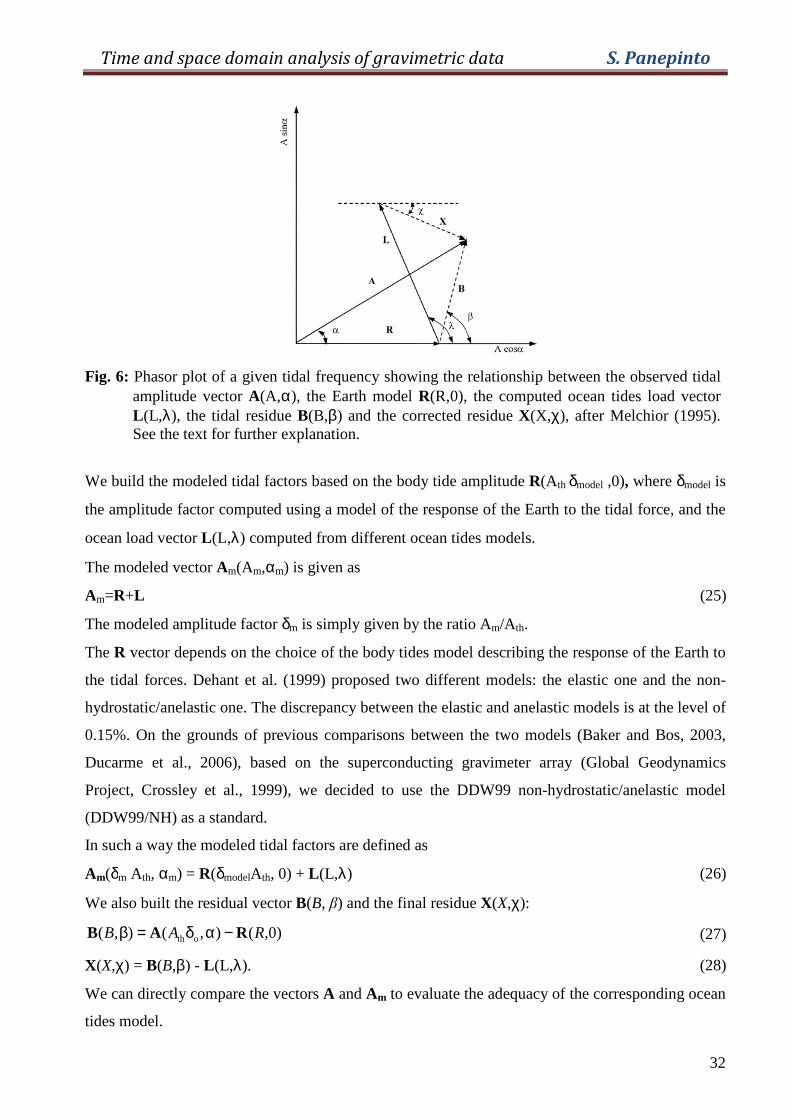
Fig. 6: Phasor plot of a given tidal frequency showing the relationship between the observed tidal amplitude vector A(A,α), the Earth model R(R,0), the computed ocean tides load vector L (L,λ), the tidal residue B(B,β) and the corrected residue X(X,χ), after Melchior (1995). See the text for further explanation.
We build the modeled tidal factors based on the body tide amplitude R(A th δmodel ,0), where δmodel is
the amplitude factor computed using a model of the response of the Earth to the tidal force, and the
ocean load vector L (L,λ) computed from different ocean tides models.
The modeled vector Am(Am,αm) is given as
Am=R+L (25)
The modeled amplitude factor δm is simply given by the ratio Am/Ath.
The R vector depends on the choice of the body tides model describing the response of the Earth to
the tidal forces. Dehant et al. (1999) proposed two different models: the elastic one and the non-
hydrostatic/anelastic one. The discrepancy between the elastic and anelastic models is at the level of
0.15%. On the grounds of previous comparisons between the two models (Baker and Bos, 2003,
Ducarme et al., 2006), based on the superconducting gravimeter array (Global Geodynamics
Project, Crossley et al., 1999), we decided to use the DDW99 non-hydrostatic/anelastic model
(DDW99/NH) as a standard.
In such a way the modeled tidal factors are defined as
Am(δm Ath, αm) = R(δmodelAth, 0) + L (L,λ) (26)
We also built the residual vector B(B, β) and the final residue X(X,χ):
)0,(),(),( oth RAB RAB −αδ=β (27)
X(X,χ) = B(B,β) - L (L,λ). (28)
We can directly compare the vectors A and Am to evaluate the adequacy of the corresponding ocean
tides model.
Time and space domain analysis of gravimetric data S. Panepinto
33
As early as 1979, Schwiderski constructed ocean tide models (SCW80; Schwiderski, 1980) using
the hydrodynamic interpolation method and introducing tide gauge data on coast lines and islands.
For the first time, he provided a relatively complete and basic ocean tidal model for loading
correction in geodesy and geophysics. Since 1994, a series of new ocean tidal models has been
developed based mainly on the Topex/Poseidon (T/P) satellite altimeter data. The first generation of
models we consider here are: CSR3 (Eanes and Bettadpur, 1996), FES95 (Le Provost et al., 1994)
and ORI96 (Matsumoto et al., 1995). These models were extensively tested in Shum et al. (1997).
Most of the more recent ones used subsequently represent updates of the previous ones: CSR4,
NAO99 (Matsumoto et al., 2000), GOT00 (Ray, 1999), FES02 and TPX06. An important difference
between models is the grid size which has been progressively refined from (1°x1°) for SCW80, to
(0.5°x0.5°) for CSR3, CSR4, FES95, GOT00, NAO99, ORI96 and finally (0.25°x0.25°) for FES02
and TPX06. As a result the approximation of the real shape of the coast was steadily improved. A
second improvement concerns the global water mass balance during one tidal cycle. It is never
perfectly achieved but has also been continuously improved.
The tidal loading vector L was evaluated by performing a convolution integral between the ocean
tide models and the load Green's function computed by Farrell (1972). The Green’s functions are
tabulated according to the angular distance between the station and the load. The water mass is
condensed at the centre of each cell and the Green’s function is interpolated according to the
angular distance. This computation is rather delicate for coastal stations and models computed on a
coarse grid, as the station can be located very close to the centre of the cell. The numerical effect
can be largely overestimated. To avoid this problem our tidal loading computation checks the
position of the station with respect to the centre of the grid. If the station is located inside the cell,
this cell is eliminated from the integration and the result is considered not reliable (Melchior et al.,
1980). For the first generation of models, the effect of the imperfect mass conservation is corrected
on the basis of the code developed by Moens (Melchior et al., 1980). Following Zahran’s (2000)
suggestion, we also computed mean tidal loadings for different combinations of models.
In Table 6, we present the tidal factors modeled using the DDW99/NH model (Dehant et al., 1999)
and nine different ocean tides models for the SLN station. In this comparison we restrict ourselves
to the three main tidal waves: two main diurnal tidal components (O1 lunar declinational wave,
period 25h 49m; K1 luni-solar declinational wave, period 23h 56m) and the main semidiurnal
component (M2 Lunar principal wave, period 12h 25m).
We can consider two groups of models, the older models until 1996 (SCW80, ORI96, CSR3,
FES95) on the one hand, and the new generation of models (FES02, CSR4, GOTOO, NA099 and
TPX06) on the other. Mean modeled tidal amplitude factors and phase differences are presented in
Time and space domain analysis of gravimetric data S. Panepinto
34
Table 6 for the older models (mean 1-4), for the models of second generation (mean 5-9) and for all
the models (global). The standard deviations on the mean of the 9 models are close to 0.1% for the
amplitude factors and 0.07° on the phase difference. The precision on the mean should be 3 times
better.
The observations made with LCR G-8 have the highest internal precision (Table 8) and the scale
factor of this instrument has been previously adjusted in Brussels (Melchior, 1994). This instrument
is thus a good reference to appreciate the validity of the modeled factors. The observed amplitude
factors δo are in agreement with the mean modeled ones δm within the associated errors. The
calibration is thus confirmed. The ratio δM2/δO1, which is independent from the calibration, fits
perfectly the mean of the 5 recent models (Table 6).
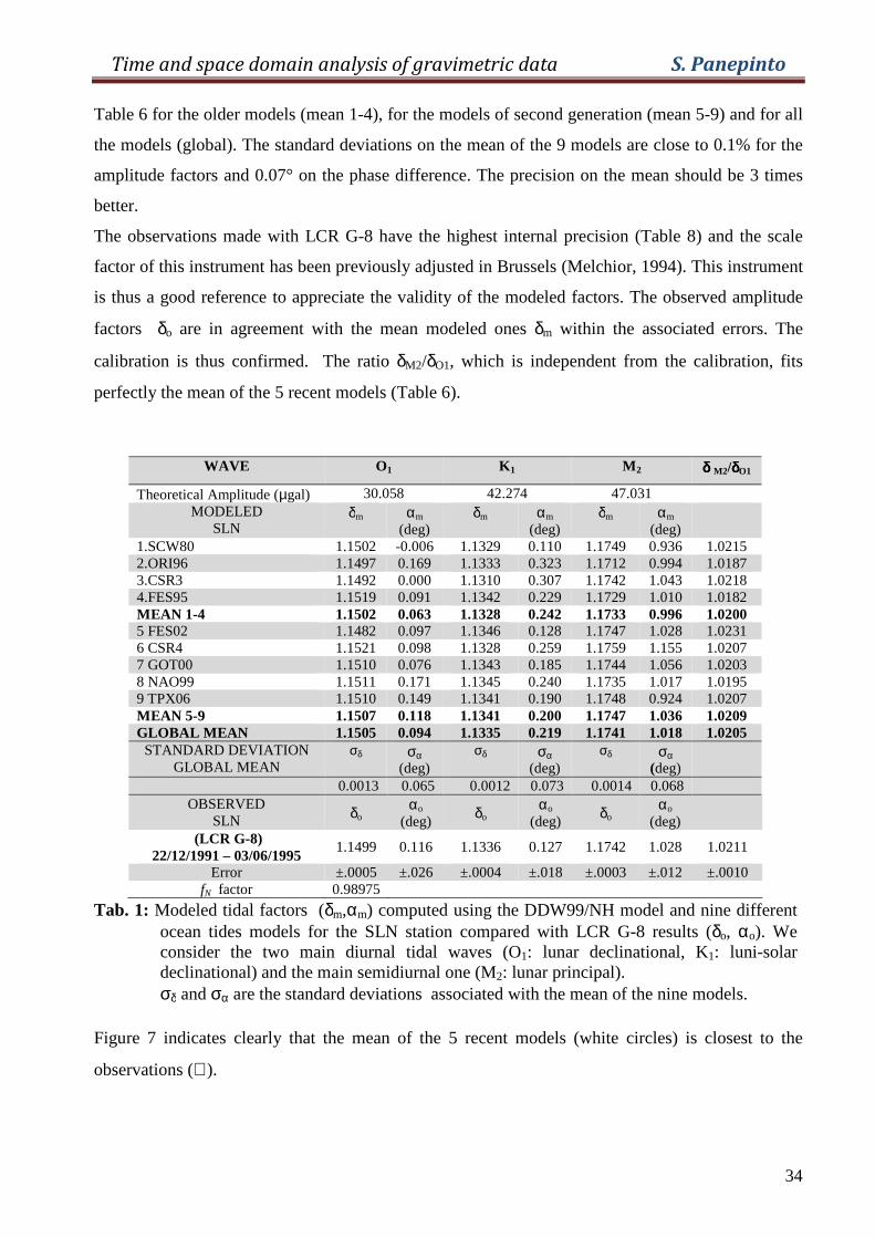
WAVE O1 K 1 M 2 δδδδ M2/δδδδO1
Theoretical Amplitude (µgal) 30.058 42.274 47.031 MODELED
SLN δm αm
(deg) δm αm
(deg) δm αm
(deg)
1.SCW80 1.1502 -0.006 1.1329 0.110 1.1749 0.936 1.0215 2.ORI96 1.1497 0.169 1.1333 0.323 1.1712 0.994 1.0187 3.CSR3 1.1492 0.000 1.1310 0.307 1.1742 1.043 1.0218 4.FES95 1.1519 0.091 1.1342 0.229 1.1729 1.010 1.0182 MEAN 1-4 1.1502 0.063 1.1328 0.242 1.1733 0.996 1.0200 5 FES02 1.1482 0.097 1.1346 0.128 1.1747 1.028 1.0231 6 CSR4 1.1521 0.098 1.1328 0.259 1.1759 1.155 1.0207 7 GOT00 1.1510 0.076 1.1343 0.185 1.1744 1.056 1.0203 8 NAO99 1.1511 0.171 1.1345 0.240 1.1735 1.017 1.0195 9 TPX06 1.1510 0.149 1.1341 0.190 1.1748 0.924 1.0207 MEAN 5-9 1.1507 0.118 1.1341 0.200 1.1747 1.036 1.0209 GLOBAL MEAN 1.1505 0.094 1.1335 0.219 1.1741 1.018 1.0205 STANDARD DEVIATION
GLOBAL MEAN σδ σα
(deg) σδ σα
(deg) σδ σα
(deg)
0.0013 0.065 0.0012 0.073 0.0014 0.068 OBSERVED
SLN δo αo
(deg) δo
αo
(deg) δo
αo
(deg)
(LCR G-8) 22/12/1991 – 03/06/1995
1.1499 0.116 1.1336 0.127 1.1742 1.028 1.0211
Error ±.0005 ±.026 ±.0004 ±.018 ±.0003 ±.012 ±.0010 fN factor 0.98975
Tab. 1: Modeled tidal factors (δm,αm) computed using the DDW99/NH model and nine different ocean tides models for the SLN station compared with LCR G-8 results (δo, αo). We consider the two main diurnal tidal waves (O1: lunar declinational, K1: luni-solar declinational) and the main semidiurnal one (M2: lunar principal). σδ and σα are the standard deviations associated with the mean of the nine models.
Figure 7 indicates clearly that the mean of the 5 recent models (white circles) is closest to the
observations (⊕).
Time and space domain analysis of gravimetric data S. Panepinto
35
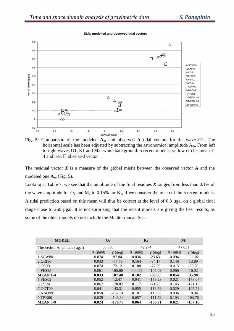
Fig. 5: Comparison of the modeled Am and observed A tidal vectors for the wave O1. The horizontal scale has been adjusted by subtracting the astronomical amplitude Ath. From left to right waves O1, K1 and M2. white background: 5 recent models, yellow circles mean 1-4 and 5-9, ⊕ observed vector
The residual vector X is a measure of the global misfit between the observed vector A and the
modeled one Am (Fig. 5).
Looking at Table 7, we see that the amplitude of the final residues X ranges from less than 0.1% of
the wave amplitude for O1 and M2 to 0.15% for K1, if we consider the mean of the 5 recent models.
A tidal prediction based on this mean will thus be correct at the level of 0.3 µgal on a global tidal
range close to 260 µgal. It is not surprising that the recent models are giving the best results, as
some of the older models do not include the Mediterranean Sea.
MODEL O1 K 1 M 2
Theoretical Amplitude (µgal) 30.058 42.274 47.031 X (µgal) χ (deg) X (µgal) χ (deg) X (µgal) χ (deg) 1.SCW80 0.074 97.84 0.036 23.63 0.094 111.02 2.ORI96 0.033 -77.75 0.164 -84.17 0.146 13.89 3.CSR3 0.074 72.12 0.188 -72.90 0.015 -80.20 4.FES95 0.061 165.66 0.0.088 -105.09 0.066 16.02 MEAN 1-4 0.033 107.48 0.102 -69.95 0.054 35.98 5 FES02 0.052 12.47 0.041 -178.23 0.021 -178.07 6 CSR4 0.067 170.82 0.117 -71.25 0.145 -121.15 7 GOT00 0.041 143.31 0.055 -118.59 0.029 -107.52 8 NAO99 0.050 -137.61 0.101 -110.53 0.036 18.94 9 TPX06 0.039 -148.80 0.057 -111.72 0.103 104.76 MEAN 5-9 0.024 -176.48 0.064 -105.71 0.021 -157.16
SLN: modelled and observed tidal vectors
-0.1
0
0.1
0.2
0.3
0.4
0.5
0.6
0.7
0.8
0.9
in Phase (µgal)
out o
f pha
se (
µgal
)
SCW80 ORI96 CSR3 FES95 FES02 CSR4 GOT00 NAO99 TPX06 MEAN 1-4 MEAN 5-9 observed
4.2 4.4 4.6 4.8 5 5.2 5.4 5.6 5.8
Time and space domain analysis of gravimetric data S. Panepinto
36
Tab. 7: Final residues X at SLN, computed using the DDW99/NH model and nine different ocean
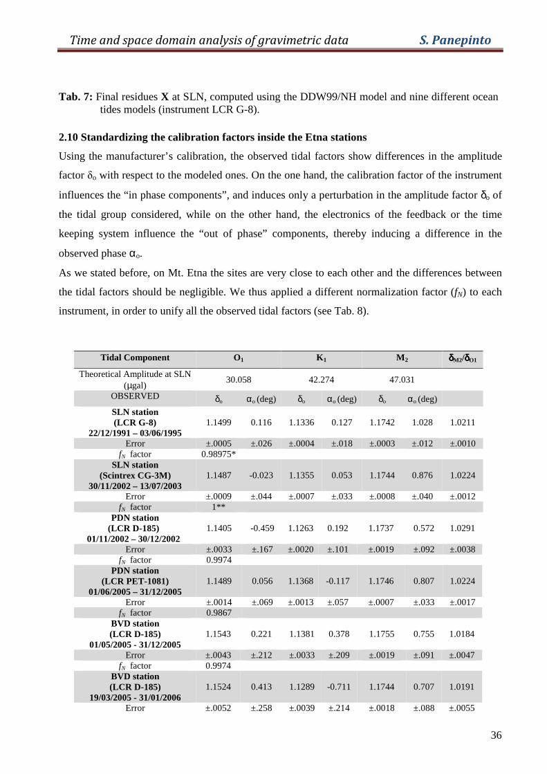
tides models (instrument LCR G-8). 2.10 Standardizing the calibration factors inside the Etna stations
Using the manufacturer’s calibration, the observed tidal factors show differences in the amplitude
factor δo with respect to the modeled ones. On the one hand, the calibration factor of the instrument
influences the “in phase components”, and induces only a perturbation in the amplitude factor δo of
the tidal group considered, while on the other hand, the electronics of the feedback or the time
keeping system influence the “out of phase” components, thereby inducing a difference in the
observed phase αo.
As we stated before, on Mt. Etna the sites are very close to each other and the differences between
the tidal factors should be negligible. We thus applied a different normalization factor (fN) to each
instrument, in order to unify all the observed tidal factors (see Tab. 8).
Tidal Component O1 K 1 M 2 δδδδM2/δδδδO1
Theoretical Amplitude at SLN (µgal)
30.058 42.274 47.031
OBSERVED δo αo (deg) δo αo (deg) δo αo (deg)
SLN station (LCR G-8)
22/12/1991 – 03/06/1995 1.1499 0.116 1.1336 0.127 1.1742 1.028 1.0211
Error ±.0005 ±.026 ±.0004 ±.018 ±.0003 ±.012 ±.0010 fN factor 0.98975*
SLN station (Scintrex CG-3M)
30/11/2002 – 13/07/2003 1.1487 -0.023 1.1355 0.053 1.1744 0.876 1.0224
Error ±.0009 ±.044 ±.0007 ±.033 ±.0008 ±.040 ±.0012 fN factor 1**
PDN station (LCR D-185)
01/11/2002 – 30/12/2002 1.1405 -0.459 1.1263 0.192 1.1737 0.572 1.0291
Error ±.0033 ±.167 ±.0020 ±.101 ±.0019 ±.092 ±.0038 fN factor 0.9974
PDN station (LCR PET-1081)
01/06/2005 – 31/12/2005 1.1489 0.056 1.1368 -0.117 1.1746 0.807 1.0224
Error ±.0014 ±.069 ±.0013 ±.057 ±.0007 ±.033 ±.0017 fN factor 0.9867
BVD station (LCR D-185)
01/05/2005 - 31/12/2005 1.1543 0.221 1.1381 0.378 1.1755 0.755 1.0184
Error ±.0043 ±.212 ±.0033 ±.209 ±.0019 ±.091 ±.0047 fN factor 0.9974
BVD station (LCR D-185)
19/03/2005 - 31/01/2006 1.1524 0.413 1.1289 -0.711 1.1744 0.707 1.0191
Error ±.0052 ±.258 ±.0039 ±.214 ±.0018 ±.088 ±.0055
Time and space domain analysis of gravimetric data S. Panepinto
37
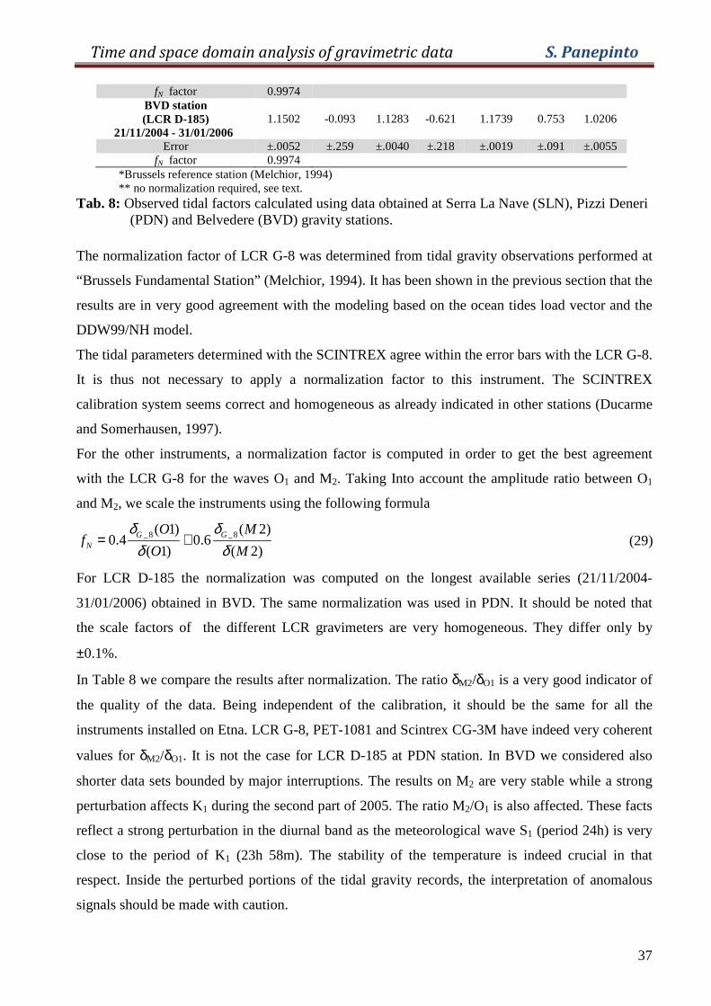
fN factor 0.9974 BVD station (LCR D-185)
21/11/2004 - 31/01/2006 1.1502 -0.093 1.1283 -0.621 1.1739 0.753 1.0206
Error ±.0052 ±.259 ±.0040 ±.218 ±.0019 ±.091 ±.0055 fN factor 0.9974
*Brussels reference station (Melchior, 1994) ** no normalization required, see text.
Tab. 8: Observed tidal factors calculated using data obtained at Serra La Nave (SLN), Pizzi Deneri (PDN) and Belvedere (BVD) gravity stations.
The normalization factor of LCR G-8 was determined from tidal gravity observations performed at
“Brussels Fundamental Station” (Melchior, 1994). It has been shown in the previous section that the
results are in very good agreement with the modeling based on the ocean tides load vector and the
DDW99/NH model.
The tidal parameters determined with the SCINTREX agree within the error bars with the LCR G-8.
It is thus not necessary to apply a normalization factor to this instrument. The SCINTREX
calibration system seems correct and homogeneous as already indicated in other stations (Ducarme
and Somerhausen, 1997).
For the other instruments, a normalization factor is computed in order to get the best agreement
with the LCR G-8 for the waves O1 and M2. Taking Into account the amplitude ratio between O1
and M2, we scale the instruments using the following formula
_8 _8( 1) ( 2)0.4 0.6
( 1) ( 2)G G
N
O Mf
O M
δ δδ δ
= +
(29)
For LCR D-185 the normalization was computed on the longest available series (21/11/2004-
31/01/2006) obtained in BVD. The same normalization was used in PDN. It should be noted that
the scale factors of the different LCR gravimeters are very homogeneous. They differ only by
±0.1%.
In Table 8 we compare the results after normalization. The ratio δM2/δO1 is a very good indicator of
the quality of the data. Being independent of the calibration, it should be the same for all the
instruments installed on Etna. LCR G-8, PET-1081 and Scintrex CG-3M have indeed very coherent
values for δM2/δO1. It is not the case for LCR D-185 at PDN station. In BVD we considered also
shorter data sets bounded by major interruptions. The results on M2 are very stable while a strong
perturbation affects K1 during the second part of 2005. The ratio M2/O1 is also affected. These facts
reflect a strong perturbation in the diurnal band as the meteorological wave S1 (period 24h) is very
close to the period of K1 (23h 58m). The stability of the temperature is indeed crucial in that
respect. Inside the perturbed portions of the tidal gravity records, the interpretation of anomalous
signals should be made with caution.
Time and space domain analysis of gravimetric data S. Panepinto
38
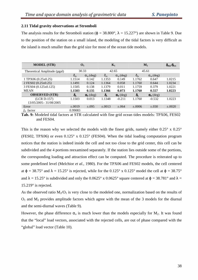
2.11 Tidal gravity observations at Stromboli
The analysis results for the Stromboli station (ϕ = 38.800°, λ = 15.227°) are shown in Table 9. Due
to the position of the station on a small island, the modeling of the tidal factors is very difficult as
the island is much smaller than the grid size for most of the ocean tide models.
MODEL (STR) O1 K 1 M 2 δδδδM2/δδδδO1
Theoretical Amplitude (µgal) 30.33 42.65 45.61 δm αm (deg) δm αm (deg) δm αm (deg)
1 TPX06 (0.25x0.25) 1.1514 0.142 1.1353 0.149 1.1762 0.647 1.0215 2 FES02 (0.25x0.25) 1.1491 0.124 1.1364 0.058 1.1760 0.644 1.0234 3 FES04 (0.125x0.125) 1.1505 0.138 1.1379 0.011 1.1759 0.379 1.0221 MEAN 1.1503 0.135 1.1366 0.073 1.1760 0.557 1.0223
OBSERVED (STR) δδδδo αααα0 (deg) δδδδo αααα0 (deg) δδδδo αααα0 (deg) (LCR D-157)
13/05/2005– 31/08/2005 1.1503 0.013 1.1348 -0.211 1.1760 -0.532 1.0223
Error ±.0019 ±.095 ±.0013 ±.064 ±.0006 ±.030 ±.0020 fN factor 0.99083
Tab. 9: Modeled tidal factors at STR calculated with fine grid ocean tides models: TPX06, FES02 and FES04.
This is the reason why we selected the models with the finest grids, namely either 0.25° x 0.25°
(FES02, TPX06) or even 0.125° x 0.125° (FES04). When the tidal loading computation program
notices that the station is indeed inside the cell and not too close to the grid center, this cell can be
subdivided and the 4 portions reexamined separately. If the station lies outside some of the portions,
the corresponding loading and attraction effect can be computed. The procedure is reiterated up to
some predefined level (Melchior et al., 1980). For the TPX06 and FES02 models, the cell centered
at ϕ = 38.75° and λ = 15.25° is rejected, while for the 0.125° x 0.125° model the cell at ϕ = 38.75°
and λ = 15.25° is subdivided and only the 0.0625° x 0.0625° square centered at ϕ = 38.781° and λ =
15.219° is rejected.
As the observed ratio M2/O1 is very close to the modeled one, normalization based on the results of
O1 and M2 provides amplitude factors which agree with the mean of the 3 models for the diurnal
and the semi-diurnal waves (Table 9).
However, the phase difference αo is much lower than the models especially for M2. It was found
that the “local” load vectors, associated with the rejected cells, are out of phase compared with the
“global” load vector (Table 10).
Time and space domain analysis of gravimetric data S. Panepinto
39
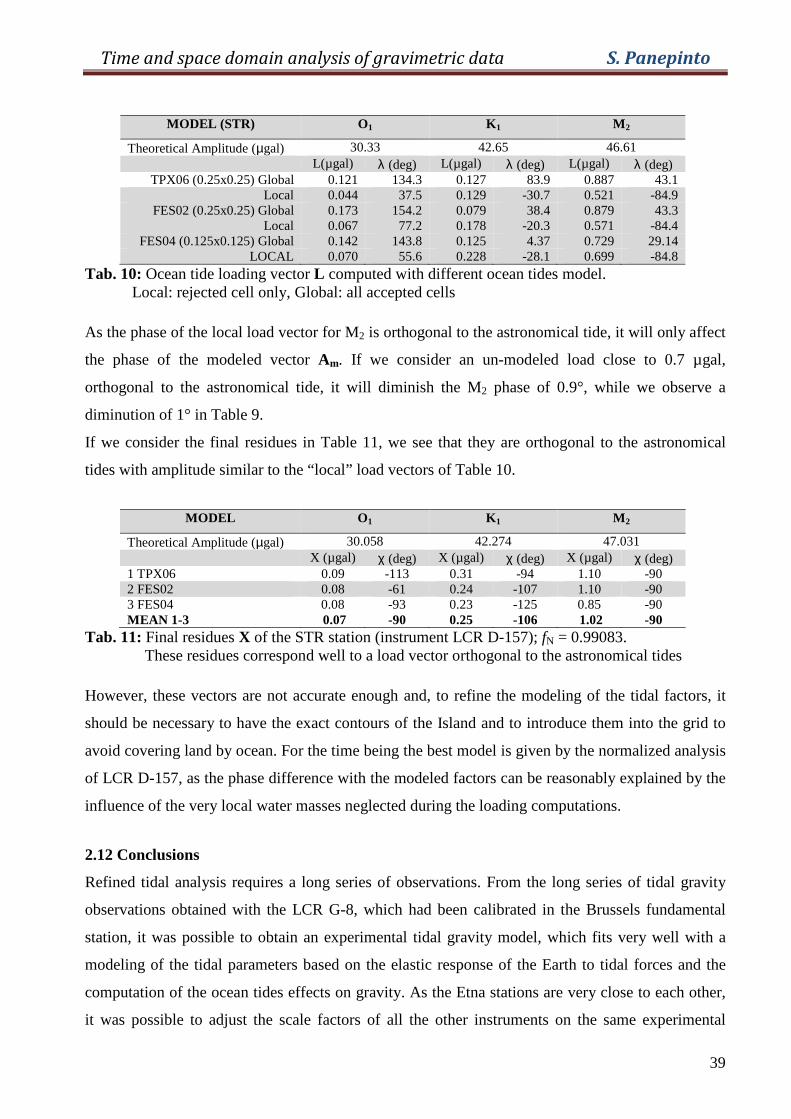
MODEL (STR) O1 K 1 M 2
Theoretical Amplitude (µgal) 30.33 42.65 46.61 L(µgal) λ (deg) L(µgal) λ (deg) L(µgal) λ (deg)
TPX06 (0.25x0.25) Global 0.121 134.3 0.127 83.9 0.887 43.1 Local 0.044 37.5 0.129 -30.7 0.521 -84.9
FES02 (0.25x0.25) Global 0.173 154.2 0.079 38.4 0.879 43.3 Local 0.067 77.2 0.178 -20.3 0.571 -84.4
FES04 (0.125x0.125) Global 0.142 143.8 0.125 4.37 0.729 29.14 LOCAL 0.070 55.6 0.228 -28.1 0.699 -84.8
Tab. 10: Ocean tide loading vector L computed with different ocean tides model. Local: rejected cell only, Global: all accepted cells As the phase of the local load vector for M2 is orthogonal to the astronomical tide, it will only affect
the phase of the modeled vector Am. If we consider an un-modeled load close to 0.7 µgal,
orthogonal to the astronomical tide, it will diminish the M2 phase of 0.9°, while we observe a
diminution of 1° in Table 9.
If we consider the final residues in Table 11, we see that they are orthogonal to the astronomical
tides with amplitude similar to the “local” load vectors of Table 10.
MODEL O1 K 1 M 2
Theoretical Amplitude (µgal) 30.058 42.274 47.031 X (µgal) χ (deg) X (µgal) χ (deg) X (µgal) χ (deg) 1 TPX06 0.09 -113 0.31 -94 1.10 -90 2 FES02 0.08 -61 0.24 -107 1.10 -90 3 FES04 0.08 -93 0.23 -125 0.85 -90 MEAN 1-3 0.07 -90 0.25 -106 1.02 -90
Tab. 11: Final residues X of the STR station (instrument LCR D-157); fN = 0.99083. These residues correspond well to a load vector orthogonal to the astronomical tides
However, these vectors are not accurate enough and, to refine the modeling of the tidal factors, it
should be necessary to have the exact contours of the Island and to introduce them into the grid to
avoid covering land by ocean. For the time being the best model is given by the normalized analysis
of LCR D-157, as the phase difference with the modeled factors can be reasonably explained by the
influence of the very local water masses neglected during the loading computations.
2.12 Conclusions
Refined tidal analysis requires a long series of observations. From the long series of tidal gravity
observations obtained with the LCR G-8, which had been calibrated in the Brussels fundamental
station, it was possible to obtain an experimental tidal gravity model, which fits very well with a
modeling of the tidal parameters based on the elastic response of the Earth to tidal forces and the
computation of the ocean tides effects on gravity. As the Etna stations are very close to each other,
it was possible to adjust the scale factors of all the other instruments on the same experimental
Time and space domain analysis of gravimetric data S. Panepinto
40
model. The calibration of the LaCoste & Romberg gravimeters used in this study is now fairly
homogeneous and accurate. The Scintrex CG-3M did not require any normalization.
Since the ratio δM2/δO1 does not depend on the calibration factor of the instrument, we compare the
ratios obtained by the observations with the modeled ones. As a result, the values δM2/δO1 of the
LCR G-8, Scintrex CG-3M and LCR PET-1081 are very close to the model value 1.021. Some
portions of the records with LCR D-185 are perturbed. It is probably difficult to detect any
geophysical signal in the LCR D-185 series.
The observations performed on Stromboli Island highlighted the difficulty of getting a correct
model from tidal loading computation, as the grid of the best ocean tides models is still too coarse
to accurately follow the repartition of the ocean and land masses. Fortunately, the influence of the
water masses closest to the station is affecting essentially the phase of the observations so that a
normalization of the gravimeter was still possible.
We also presented a methodology to follow the sensitivity variations of the spring gravimeters when
a good tidal model is available. It is an important issue as these sensitivity variations affect not only
the quality of the available data but also the accuracy of the tidal analysis results and of the
observed gravity changes. It also seems a good tool to detect strong instrumental perturbations
during any ongoing volcanic activity and avoid confusion between purely instrumental effects and
geophysical ones.
The series of normalized gravity residues routinely obtained on Etna and Stromboli could be used to
better detect the possible signals due to volcanic activity. Finally, the improved tidal gravity model
will be useful for gravity surveys and absolute measurements.
Time and space domain analysis of gravimetric data S. Panepinto
41
CHAPTER 3
3.1 Introduction
Spring gravimeters are still the most used instruments for microgravity studies because of their
relatively low cost and small size, which make them easy to transport and install. Continuous
gravity measurements are now increasingly performed at sites very close to active craters, where
there is the greatest opportunity to detect significant gravity changes due to volcanic activity.
Unfortunately, spring gravity meters show a strong influence of meteorological parameters (i.e.
pressure, temperature and humidity), especially in the adverse environmental conditions usually
encountered at such places. As the gravity changes due to the volcanic activity could be very small
compared to other geophysical or instrumental effects, there is thus a need to get, through
mathematical tools, reliable gravity residuals susceptible to reflect the volcanic effects. In the
following I present and discuss my work about the comparison between the traditional filtering
methodology and wavelet transform. The overall results show that the performance of the wavelet-
based filter seems better than the Fourier one. Moreover, the possibility of getting a multi-resolution
analysis to study local features of the signal in the time domain makes the proposed methodology a
valuable tool for gravity data processing.
3.2 Effects of external influencing parameters on gravity meters
Studies on the effect of external influencing parameters on the behavior of gravity sensors for the
monitoring of volcanic activity have revealed that temperature, pressure and humidity play a very
critical role [El Wahabi et al., 1997; Warburton and Goodkind, 1997]. Several authors have
demonstrated that meteorological parameters, especially atmospheric temperature, do affect
continuously running spring gravimeters. In particular, in El Wahabi et al. (1997) it has been proven
that, over a yearly period, temperature changes can cause up to a 1 mGal instrumental effect. An
admittance up to 0.2 mGal/°C, over changes with a period longer than 1 month, has been evidenced
in Carbone et al (2003). An important issue with the gravity data sequences is the need of separating
the useful signal (i.e. the volcano-related one) from unwanted components (signal due to tides,
instrumental and meteorological effects). Obviously, frequency-domain filters cannot be applied to
remove the effect of these perturbations since the spectrum of each component of various origins
has wide intervals of superposition.
The aim of the present work is to get a preliminary test concerning the application of the wavelet
decomposition to the continuous gravity data. The wavelet transform is thus applied to a short
sequence (7 months registration) acquired at Mt Etna site (see Figure 1). The continuously running
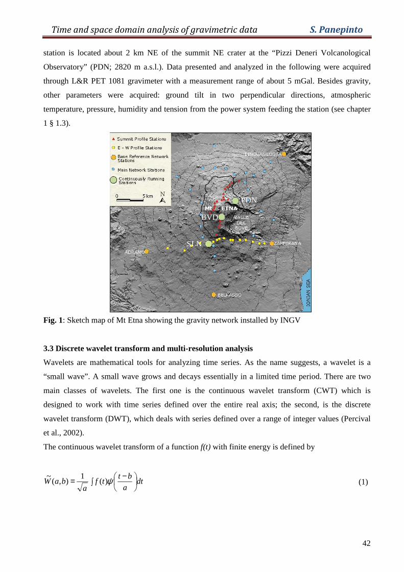
Time and space domain analysis of gravimetric data S. Panepinto
42
station is located about 2 km NE of the summit NE crater at the “Pizzi Deneri Volcanological
Observatory” (PDN; 2820 m a.s.l.). Data presented and analyzed in the following were acquired
through L&R PET 1081 gravimeter with a measurement range of about 5 mGal. Besides gravity,
other parameters were acquired: ground tilt in two perpendicular directions, atmospheric
temperature, pressure, humidity and tension from the power system feeding the station (see chapter
1 § 1.3).
Fig. 1: Sketch map of Mt Etna showing the gravity network installed by INGV
3.3 Discrete wavelet transform and multi-resolution analysis
Wavelets are mathematical tools for analyzing time series. As the name suggests, a wavelet is a
“small wave”. A small wave grows and decays essentially in a limited time period. There are two
main classes of wavelets. The first one is the continuous wavelet transform (CWT) which is
designed to work with time series defined over the entire real axis; the second, is the discrete
wavelet transform (DWT), which deals with series defined over a range of integer values (Percival
et al., 2002).
The continuous wavelet transform of a function f(t) with finite energy is defined by
∫
−= dta
bttf
abaW ψ)(
1),(
~ (1)
PDN
PDN
BVD
SLN
Time and space domain analysis of gravimetric data S. Panepinto
43
where Rb∈ and +∈ Ra , with R+ being the set of positive real numbers. Every wavelet is obtained
by a translation and dilation of a “mother wavelet” )(2 RL∈ψ , where L2(R) denotes the Hilbert
space of square-integrable functions. The function ψ has unit energy and zero mean although
higher order moments may also be zero; it is chosen with a compact support to obtain localization
in space.
For practical applications the scale parameter a and location parameter b need to be discretized.
With the choice a = 2l and b = ka with Zkl ∈, (Z is the set of integers), the discrete family of
orthonormal wavelets,
( ),22
1
2
2
2
1)(, kt
ktt l
ll
l
lkl −=
−= −ψψψ (2)
is obtained by dilating or contracting and translating the function .)()( 0,0 tt ψψ ≡
In this case, the discrete wavelet transform (DWT) is
∫=∞
∞−dtttfw klkl )()(~
,, ψ (3)
and the inverse wavelet transform is
∑ ∑=+∞
−∞=
+∞
−∞=l kklkl twtf )(~)( ,, ψ (4)
in the L2-sense.
The framework of multi-resolution analysis, developed by Mallat (1992) and Meyer (1993), allows
a signal to be approximated at certain scales or resolutions (Foufoula-Georgiou and Kumar, 1994).
At a fixed level l of resolution 2-l samples per unit length, the approximation of the signal is given
by its orthogonal projection, ∑=∞
−∞=kklkll tffS )(, ,, φφ 1, onto the vector space Vl included in L2(R).
The vector space Vl represents the space of all possible approximated signals at resolution 2-l, and
the orthonormal basis kl ,φ derives from a function φ defined as the scale function or “father
wavelet”. The details of the signal at any scale 2l characterize the difference between the process
carried out at two different scales 2l and 2l – 1, or equivalently at two different resolutions. If kl ,ψ is
the orthonormal basis in the vector space Ol (orthogonal complement of Vl in Vl-1), the details are
given by the orthogonal projection, ∑=∞
−∞=kklkll tffD )(, ,, ψψ , of the original signal on to the vector
space Ol, so Ol is orthogonal to Vl, i.e.
1 klf ,,φ is the inner product: ∫=∞
∞−dtttff klkl )()(, ,, φφ
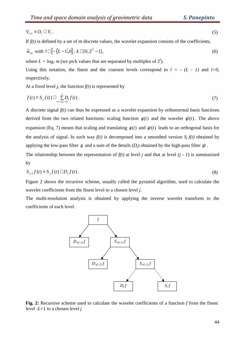
Time and space domain analysis of gravimetric data S. Panepinto
44
.1 lll VOV ⊕=− (5)
If f(t) is defined by a set of m discrete values, the wavelet expansion consists of the coefficients,
klw ,~ with ( )[ ]0,1−−∈ Ll ; ]12,0[ −∈ lk , (6)
where L = log2 m (we pick values that are separated by multiples of 2l).
Using this notation, the finest and the coarsest levels correspond to l = - (L - 1) and l=0 ,
respectively.
At a fixed level j, the function f(t) is represented by
∑+=−−=
j
Lllj tfDtfStf
)1()()()( . (7)
A discrete signal f(t) can thus be expressed as a wavelet expansion by orthonormal basis functions
derived from the two related functions: scaling function )(tφ and the wavelet )(tψ . The above
expansion (Eq. 7) means that scaling and translating )(tφ and )(tψ leads to an orthogonal basis for
the analysis of signal. In such way f(t) is decomposed into a smoothed version Sj f(t) obtained by
applying the low-pass filter φ and a sum of the details (Dj) obtained by the high-pass filter ψ .
The relationship between the representation of f(t) at level j and that at level (j - 1) is summarized
by
)()()(1 tfDtfStfS jjj +=− . (8)
Figure 2 shows the recursive scheme, usually called the pyramid algorithm, used to calculate the
wavelet coefficients from the finest level to a chosen level j.
The multi-resolution analysis is obtained by applying the inverse wavelet transform to the
coefficients of each level.
Fig. 2: Recursive scheme used to calculate the wavelet coefficients of a function f from the finest level -L+1 to a chosen level j
D-(L-1) f S-(L-1) f
D-(L-2) f
S-(L-2) f
Dj f
Sj f
f
Time and space domain analysis of gravimetric data S. Panepinto
45
The advantage of analysing a signal with wavelets is that it enables local features of the signal to be
studied with a detail matching their characteristic scale. In the temporal domain, such a property
allows transient signals to be represented effectively (Carrozzo M.T. et al., 2002). Thus it can be
said that the DWT enables a multi-resolution analysis of a signal to be made.
3.4 Choice of the wavelet basis
Different wavelet bases are obtained by varying the support width of the wavelet. Changes in the
wavelet support in general affect the final frequency characteristics of the wavelet transform.
Usually the amplitudes of the coefficients change and, consequently, the scale where the signal and
noise separate also changes.
The choice of a wavelet bases could represent an open problem for filtering. Since it was impossible
to test the filter effectiveness with statistical significance for all the wavelets available in the
Matlab® software package, some criteria were used to make a preliminary selection of a set of
wavelet bases.
Deighan and Watts (1997) and Grubb and Walden (1997) considered the compactness of the
wavelet functions in the time and frequency domains as a useful parameter for choosing the best
wavelet basis to solve a specific problem.
A criterion to evaluate the suitability of a wavelet of a specific shape to represent the signal is to
determine how concise and localized its wavelet representation is.
The “maximum compactness” or “minimum entropy” criterion, which Coifman and Wickerhauser
(1993) and Fedi and Quarta (1998) applied for data compression and data analysis, respectively,
was used here in an attempt to optimize the choice of the wavelet basis.
In particular, this criterion was applied to one of the sequences available for this study (the most
uninterrupted one), which spanned from June to December 2005 and was acquired at one of the
Etna’s continuous gravity stations (PDN). To find the most appropriated support for our case the
transform is repeated using different bases and Shannon's entropy of the analysed gravity sequence
was then calculated. As underlined by the test carried out over 39 wavelet bases, it seems that the
range of relative variability of the values calculated is more restricted only for a narrow number of
wavelet bases and leads to the selection of a set of six wavelets: Symmlet 8, Bior 6.8, Daubechies 5-
7-9, Rbio 2.8. The averages of the entropy values are shown in Table 1 for each tested basis of this
small group.
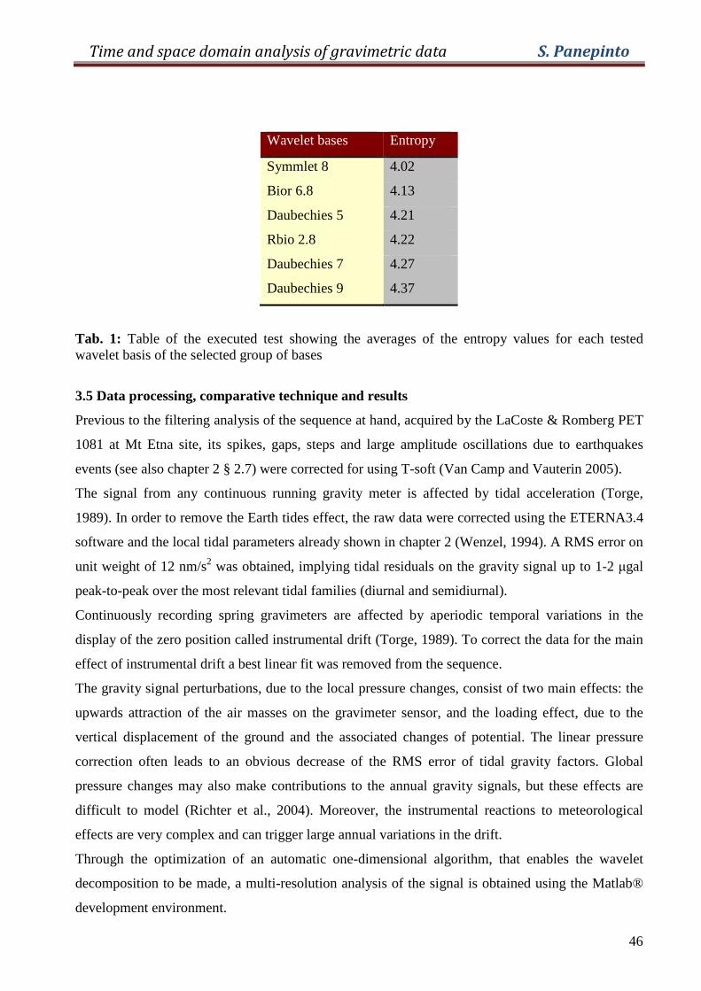
Time and space domain analysis of gravimetric data S. Panepinto
46
Wavelet bases Entropy
Symmlet 8 4.02
Bior 6.8 4.13
Daubechies 5 4.21
Rbio 2.8 4.22
Daubechies 7 4.27
Daubechies 9 4.37
Tab. 1: Table of the executed test showing the averages of the entropy values for each tested wavelet basis of the selected group of bases
3.5 Data processing, comparative technique and results
Previous to the filtering analysis of the sequence at hand, acquired by the LaCoste & Romberg PET
1081 at Mt Etna site, its spikes, gaps, steps and large amplitude oscillations due to earthquakes
events (see also chapter 2 § 2.7) were corrected for using T-soft (Van Camp and Vauterin 2005).
The signal from any continuous running gravity meter is affected by tidal acceleration (Torge,
1989). In order to remove the Earth tides effect, the raw data were corrected using the ETERNA3.4
software and the local tidal parameters already shown in chapter 2 (Wenzel, 1994). A RMS error on
unit weight of 12 nm/s2 was obtained, implying tidal residuals on the gravity signal up to 1-2 µgal
peak-to-peak over the most relevant tidal families (diurnal and semidiurnal).
Continuously recording spring gravimeters are affected by aperiodic temporal variations in the
display of the zero position called instrumental drift (Torge, 1989). To correct the data for the main
effect of instrumental drift a best linear fit was removed from the sequence.
The gravity signal perturbations, due to the local pressure changes, consist of two main effects: the
upwards attraction of the air masses on the gravimeter sensor, and the loading effect, due to the
vertical displacement of the ground and the associated changes of potential. The linear pressure
correction often leads to an obvious decrease of the RMS error of tidal gravity factors. Global
pressure changes may also make contributions to the annual gravity signals, but these effects are
difficult to model (Richter et al., 2004). Moreover, the instrumental reactions to meteorological
effects are very complex and can trigger large annual variations in the drift.
Through the optimization of an automatic one-dimensional algorithm, that enables the wavelet
decomposition to be made, a multi-resolution analysis of the signal is obtained using the Matlab®
development environment.
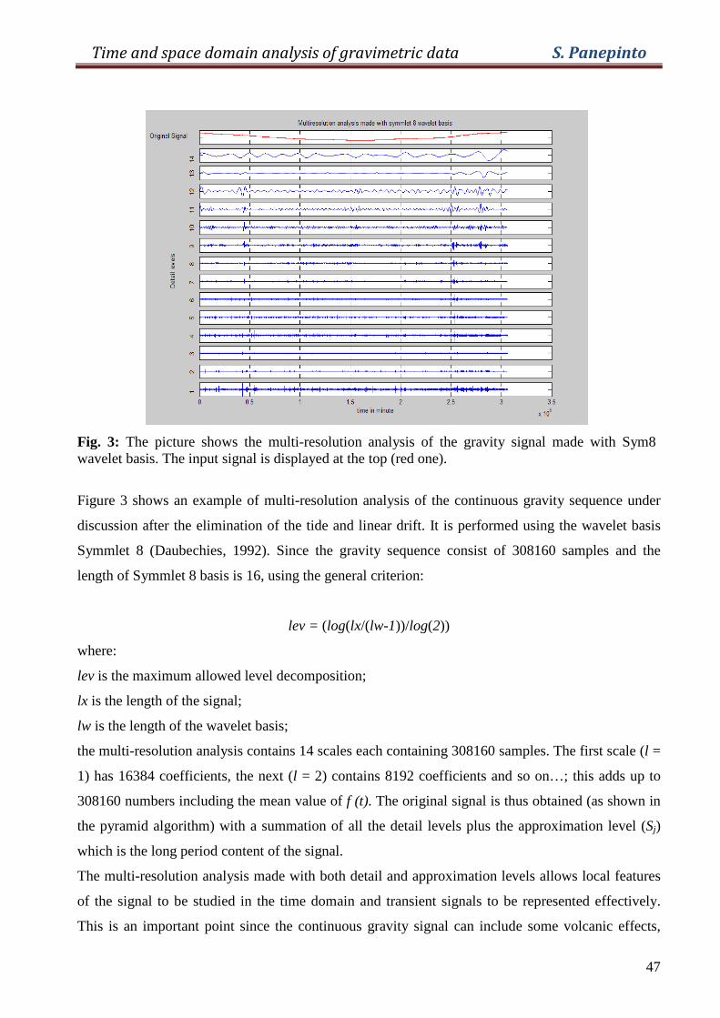
Time and space domain analysis of gravimetric data S. Panepinto
47
Fig. 3: The picture shows the multi-resolution analysis of the gravity signal made with Sym8 wavelet basis. The input signal is displayed at the top (red one).
Figure 3 shows an example of multi-resolution analysis of the continuous gravity sequence under
discussion after the elimination of the tide and linear drift. It is performed using the wavelet basis
Symmlet 8 (Daubechies, 1992). Since the gravity sequence consist of 308160 samples and the
length of Symmlet 8 basis is 16, using the general criterion:
lev = (log(lx/(lw-1))/log(2))
where:
lev is the maximum allowed level decomposition;
lx is the length of the signal;
lw is the length of the wavelet basis;
the multi-resolution analysis contains 14 scales each containing 308160 samples. The first scale (l =
1) has 16384 coefficients, the next (l = 2) contains 8192 coefficients and so on…; this adds up to
308160 numbers including the mean value of f (t). The original signal is thus obtained (as shown in
the pyramid algorithm) with a summation of all the detail levels plus the approximation level (Sj)
which is the long period content of the signal.
The multi-resolution analysis made with both detail and approximation levels allows local features
of the signal to be studied in the time domain and transient signals to be represented effectively.
This is an important point since the continuous gravity signal can include some volcanic effects,
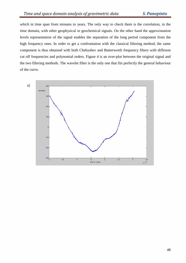
Time and space domain analysis of gravimetric data S. Panepinto
48
which in time span from minutes to years. The only way to check them is the correlation, in the
time domain, with other geophysical or geochemical signals. On the other hand the approximation
levels representation of the signal enables the separation of the long period component from the
high frequency ones. In order to get a confrontation with the classical filtering method, the same
component is thus obtained with both Chebyshev and Butterworth frequency filters with different
cut off frequencies and polynomial orders. Figure 4 is an over-plot between the original signal and
the two filtering methods. The wavelet filter is the only one that fits perfectly the general behaviour
of the curve.
a)
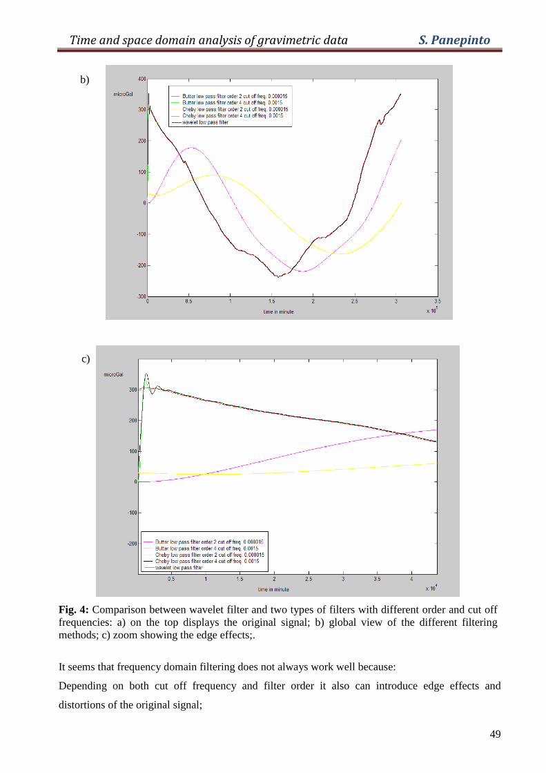
Time and space domain analysis of gravimetric data S. Panepinto
49
Fig. 4: Comparison between wavelet filter and two types of filters with different order and cut off frequencies: a) on the top displays the original signal; b) global view of the different filtering methods; c) zoom showing the edge effects;.
It seems that frequency domain filtering does not always work well because:
Depending on both cut off frequency and filter order it also can introduce edge effects and
distortions of the original signal;
b)
c)
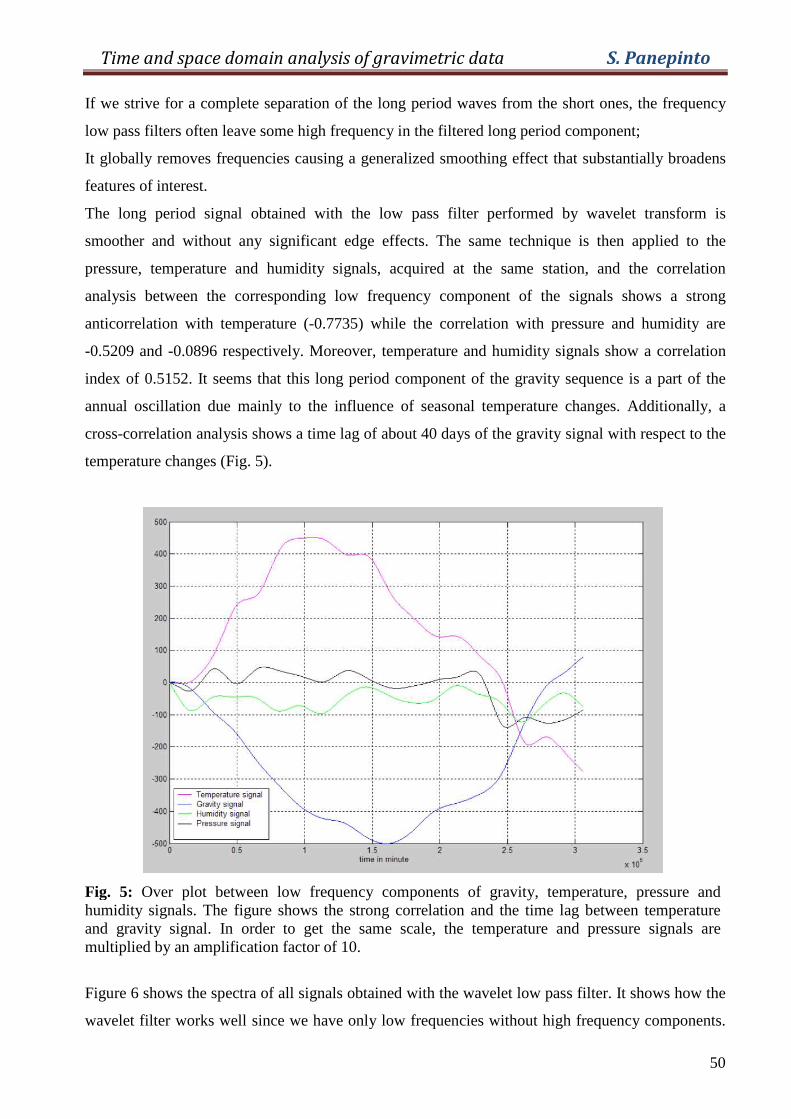
Time and space domain analysis of gravimetric data S. Panepinto
50
If we strive for a complete separation of the long period waves from the short ones, the frequency
low pass filters often leave some high frequency in the filtered long period component;
It globally removes frequencies causing a generalized smoothing effect that substantially broadens
features of interest.
The long period signal obtained with the low pass filter performed by wavelet transform is
smoother and without any significant edge effects. The same technique is then applied to the
pressure, temperature and humidity signals, acquired at the same station, and the correlation
analysis between the corresponding low frequency component of the signals shows a strong
anticorrelation with temperature (-0.7735) while the correlation with pressure and humidity are
-0.5209 and -0.0896 respectively. Moreover, temperature and humidity signals show a correlation
index of 0.5152. It seems that this long period component of the gravity sequence is a part of the
annual oscillation due mainly to the influence of seasonal temperature changes. Additionally, a
cross-correlation analysis shows a time lag of about 40 days of the gravity signal with respect to the
temperature changes (Fig. 5).
Fig. 5: Over plot between low frequency components of gravity, temperature, pressure and humidity signals. The figure shows the strong correlation and the time lag between temperature and gravity signal. In order to get the same scale, the temperature and pressure signals are multiplied by an amplification factor of 10.
Figure 6 shows the spectra of all signals obtained with the wavelet low pass filter. It shows how the
wavelet filter works well since we have only low frequencies without high frequency components.
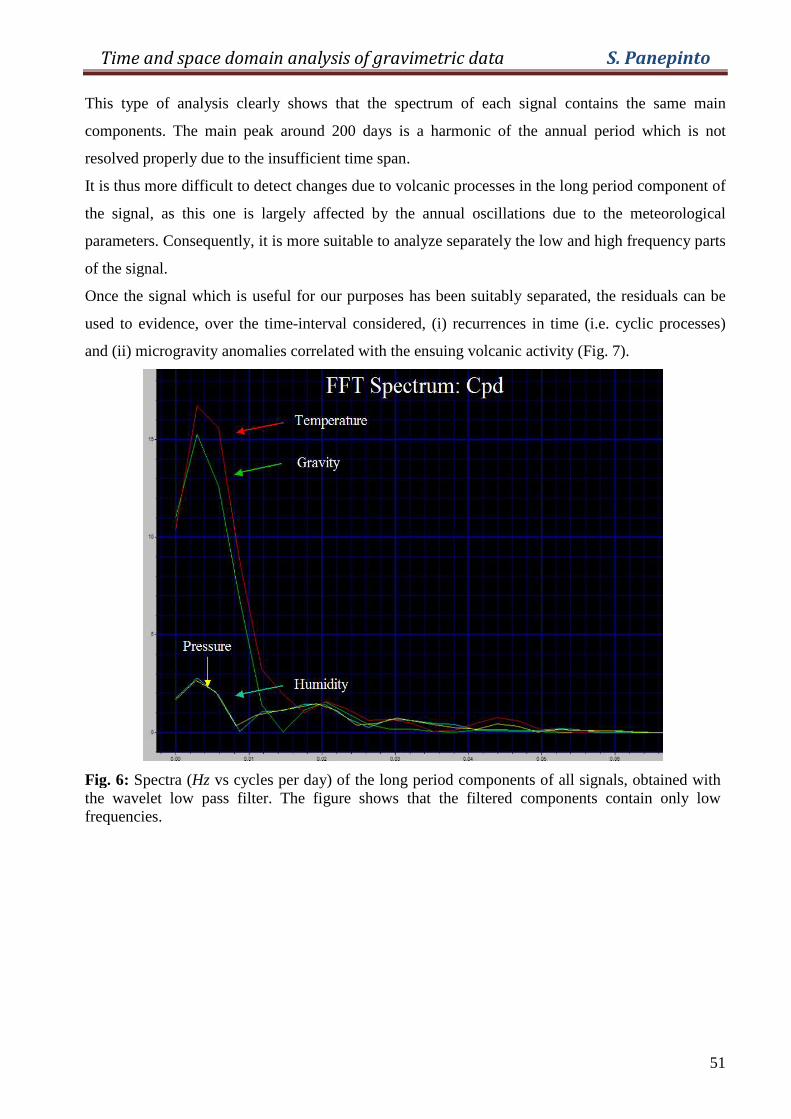
Time and space domain analysis of gravimetric data S. Panepinto
51
This type of analysis clearly shows that the spectrum of each signal contains the same main
components. The main peak around 200 days is a harmonic of the annual period which is not
resolved properly due to the insufficient time span.
It is thus more difficult to detect changes due to volcanic processes in the long period component of
the signal, as this one is largely affected by the annual oscillations due to the meteorological
parameters. Consequently, it is more suitable to analyze separately the low and high frequency parts
of the signal.
Once the signal which is useful for our purposes has been suitably separated, the residuals can be
used to evidence, over the time-interval considered, (i) recurrences in time (i.e. cyclic processes)
and (ii) microgravity anomalies correlated with the ensuing volcanic activity (Fig. 7).
Fig. 6: Spectra (Hz vs cycles per day) of the long period components of all signals, obtained with the wavelet low pass filter. The figure shows that the filtered components contain only low frequencies.
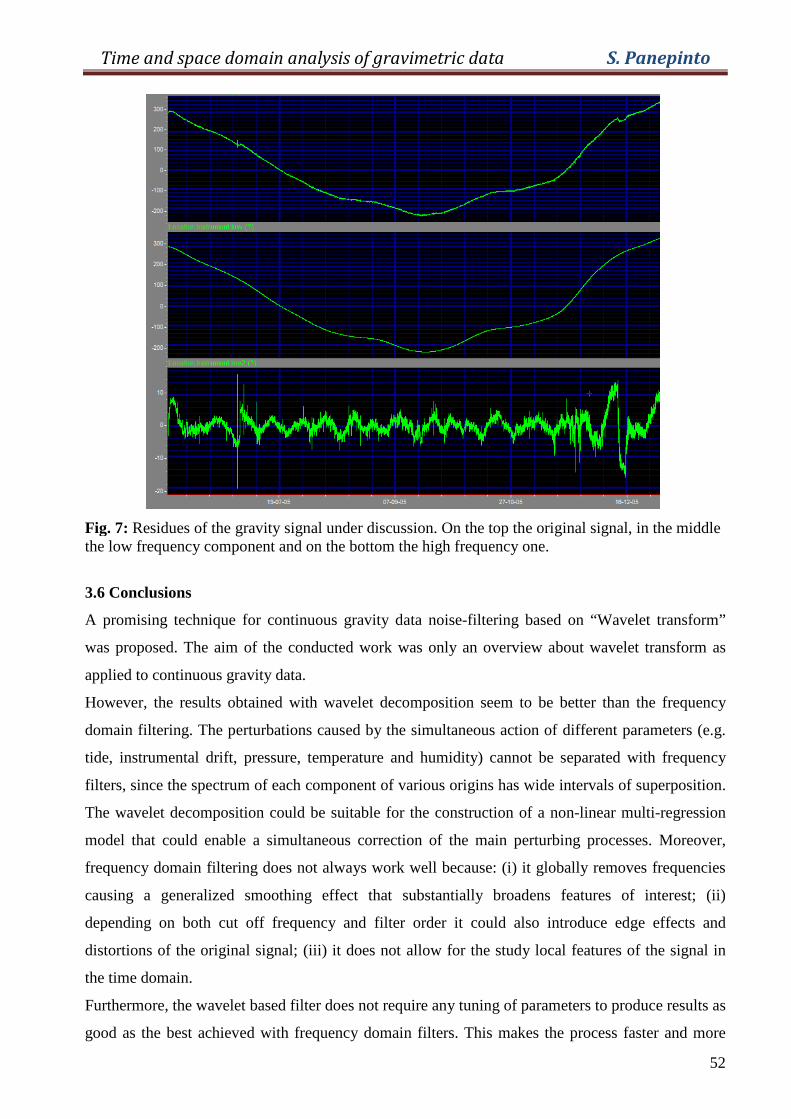
Time and space domain analysis of gravimetric data S. Panepinto
52
Fig. 7: Residues of the gravity signal under discussion. On the top the original signal, in the middle the low frequency component and on the bottom the high frequency one.
3.6 Conclusions
A promising technique for continuous gravity data noise-filtering based on “Wavelet transform”
was proposed. The aim of the conducted work was only an overview about wavelet transform as
applied to continuous gravity data.
However, the results obtained with wavelet decomposition seem to be better than the frequency
domain filtering. The perturbations caused by the simultaneous action of different parameters (e.g.
tide, instrumental drift, pressure, temperature and humidity) cannot be separated with frequency
filters, since the spectrum of each component of various origins has wide intervals of superposition.
The wavelet decomposition could be suitable for the construction of a non-linear multi-regression
model that could enable a simultaneous correction of the main perturbing processes. Moreover,
frequency domain filtering does not always work well because: (i) it globally removes frequencies
causing a generalized smoothing effect that substantially broadens features of interest; (ii)
depending on both cut off frequency and filter order it could also introduce edge effects and
distortions of the original signal; (iii) it does not allow for the study local features of the signal in
the time domain.
Furthermore, the wavelet based filter does not require any tuning of parameters to produce results as
good as the best achieved with frequency domain filters. This makes the process faster and more

Time and space domain analysis of gravimetric data S. Panepinto
53
convenient. Finally, the wavelet transform has others advantages over the Fourier transform: multi-
resolution decomposition and time-space localization, two important characteristics for denoising
problems.
Time and space domain analysis of gravimetric data S. Panepinto
54
CHAPTER 4
4.1 Introduction
After the discussion, in previous chapters, about tidal gravity reduction and signals processing, the
chapter 4 deals with an example of detection of gravity signals strictly related to volcanic activity.
In the following I present and discuss a short-period (a few hours) gravity anomaly that was
observed at the PDN station (see Fig.1 chapter 1 and Fig.2 of the current chapter) during the night
between 26 and 27 October 2002, a few hours before the onset of the 2002-03 eruption. This event
occurred from two distinct fissure systems (Calvari et al., 2003) that opened at about 2750 m on the
southern flank of the volcano, and at elevations between 2470 and 1900 m on the northeastern
flank, along Etna’s Northeast Rift (Kieffer, 1975; thereafter NE-Rift). In particular, the eruption
from the southern flank lasted 93 days and was characterized by intense explosive activity, while
the eruption from the northeastern flank lasted 9 days and emitted a more degassed magma (Calvari
et al., 2003).
Mount Etna is characterized by a fractured edifice so that the seismic activity and the ground
deformation are often minimal with respect to the ensuing volcanic process. In this case, the
microgravity changes represent a valuable volcano monitoring tool to detect the mass changes in
relation with the movement of fresh magma to shallower levels.
Before the short gravity sequence is discussed, paragraph 4.2 will give a brief description of the
geological setting and of the 2002 NE-Rift Eruption (§ 4.3), to better understand the final
consideration and interpretation.
4.2 Geological setting
Mt. Etna is one of the most studied volcanoes of the world. It is situated on the eastern part of
Sicily, and is highly active, with almost perennial degassing from the summit craters and recurrent
summit and flank eruptions. Etna is a very complex edifice, a result of its eventful history, whose
morphology is that of an asymmetric shield volcano topped by a stratocone and whose eastern flank
hosts the Valle del Bove depression. It grew in proximity to the collision boundary of the African
and Eurasian continental plates (Fig. 1), from repeated eruptions of alkali basalts-hawaiites over the
last 200 ka (Chester et al., 1985). It is Europe's highest (3310 m as of early 2002) and most active
volcano, lies in a structurally highly complex, and not yet fully understood, setting which is
reflected in the abundance and variety of models proposed for the volcano and its tectonic
environment (G. Vai and P. Martini, 2001).
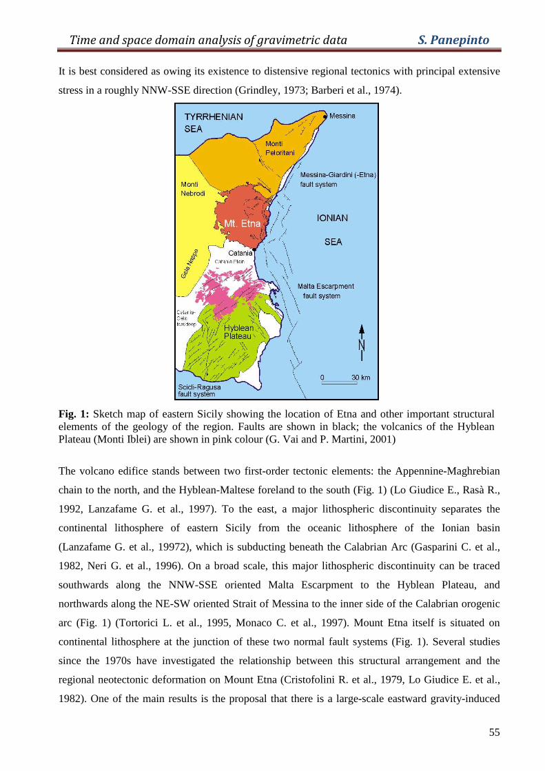
Time and space domain analysis of gravimetric data S. Panepinto
55
It is best considered as owing its existence to distensive regional tectonics with principal extensive
stress in a roughly NNW-SSE direction (Grindley, 1973; Barberi et al., 1974).
Fig. 1: Sketch map of eastern Sicily showing the location of Etna and other important structural elements of the geology of the region. Faults are shown in black; the volcanics of the Hyblean Plateau (Monti Iblei) are shown in pink colour (G. Vai and P. Martini, 2001)
The volcano edifice stands between two first-order tectonic elements: the Appennine-Maghrebian
chain to the north, and the Hyblean-Maltese foreland to the south (Fig. 1) (Lo Giudice E., Rasà R.,
1992, Lanzafame G. et al., 1997). To the east, a major lithospheric discontinuity separates the
continental lithosphere of eastern Sicily from the oceanic lithosphere of the Ionian basin
(Lanzafame G. et al., 19972), which is subducting beneath the Calabrian Arc (Gasparini C. et al.,
1982, Neri G. et al., 1996). On a broad scale, this major lithospheric discontinuity can be traced
southwards along the NNW-SSE oriented Malta Escarpment to the Hyblean Plateau, and
northwards along the NE-SW oriented Strait of Messina to the inner side of the Calabrian orogenic
arc (Fig. 1) (Tortorici L. et al., 1995, Monaco C. et al., 1997). Mount Etna itself is situated on
continental lithosphere at the junction of these two normal fault systems (Fig. 1). Several studies
since the 1970s have investigated the relationship between this structural arrangement and the
regional neotectonic deformation on Mount Etna (Cristofolini R. et al., 1979, Lo Giudice E. et al.,
1982). One of the main results is the proposal that there is a large-scale eastward gravity-induced
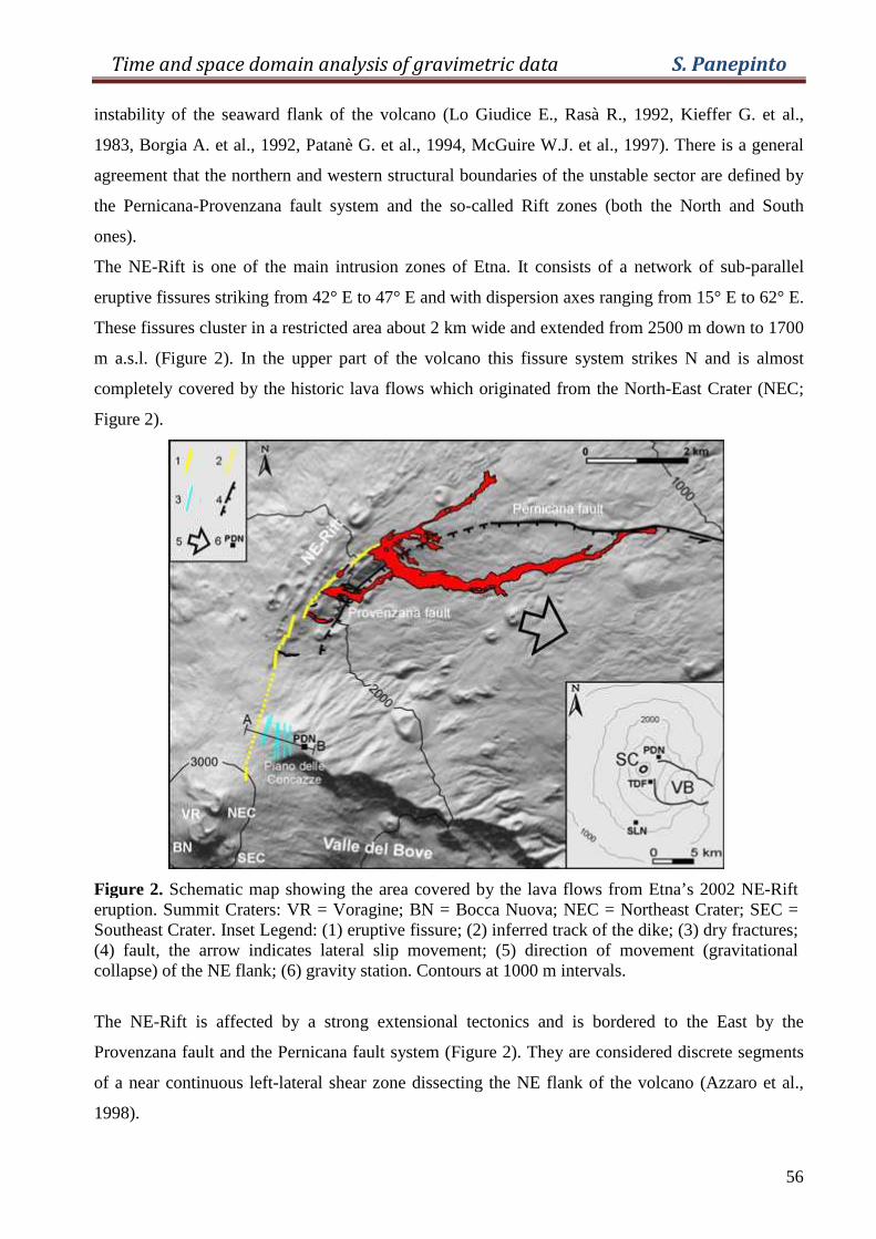
Time and space domain analysis of gravimetric data S. Panepinto
56
instability of the seaward flank of the volcano (Lo Giudice E., Rasà R., 1992, Kieffer G. et al.,
1983, Borgia A. et al., 1992, Patanè G. et al., 1994, McGuire W.J. et al., 1997). There is a general
agreement that the northern and western structural boundaries of the unstable sector are defined by
the Pernicana-Provenzana fault system and the so-called Rift zones (both the North and South
ones).
The NE-Rift is one of the main intrusion zones of Etna. It consists of a network of sub-parallel
eruptive fissures striking from 42° E to 47° E and with dispersion axes ranging from 15° E to 62° E.
These fissures cluster in a restricted area about 2 km wide and extended from 2500 m down to 1700
m a.s.l. (Figure 2). In the upper part of the volcano this fissure system strikes N and is almost
completely covered by the historic lava flows which originated from the North-East Crater (NEC;
Figure 2).
Figure 2. Schematic map showing the area covered by the lava flows from Etna’s 2002 NE-Rift eruption. Summit Craters: VR = Voragine; BN = Bocca Nuova; NEC = Northeast Crater; SEC = Southeast Crater. Inset Legend: (1) eruptive fissure; (2) inferred track of the dike; (3) dry fractures; (4) fault, the arrow indicates lateral slip movement; (5) direction of movement (gravitational collapse) of the NE flank; (6) gravity station. Contours at 1000 m intervals.
The NE-Rift is affected by a strong extensional tectonics and is bordered to the East by the
Provenzana fault and the Pernicana fault system (Figure 2). They are considered discrete segments
of a near continuous left-lateral shear zone dissecting the NE flank of the volcano (Azzaro et al.,
1998).
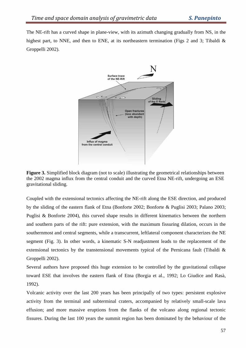
Time and space domain analysis of gravimetric data S. Panepinto
57
The NE-rift has a curved shape in plane-view, with its azimuth changing gradually from NS, in the
highest part, to NNE, and then to ENE, at its northeastern termination (Figs 2 and 3; Tibaldi &
Groppelli 2002).
Figure 3. Simplified block diagram (not to scale) illustrating the geometrical relationships between the 2002 magma influx from the central conduit and the curved Etna NE-rift, undergoing an ESE gravitational sliding.
Coupled with the extensional tectonics affecting the NE-rift along the ESE direction, and produced
by the sliding of the eastern flank of Etna (Bonforte 2002; Bonforte & Puglisi 2003; Palano 2003;
Puglisi & Bonforte 2004), this curved shape results in different kinematics between the northern
and southern parts of the rift: pure extension, with the maximum fissuring dilation, occurs in the
southernmost and central segments, while a transcurrent, leftlateral component characterizes the NE
segment (Fig. 3). In other words, a kinematic S-N readjustment leads to the replacement of the
extensional tectonics by the transtensional movements typical of the Pernicana fault (Tibaldi &
Groppelli 2002).
Several authors have proposed this huge extension to be controlled by the gravitational collapse
toward ESE that involves the eastern flank of Etna (Borgia et al., 1992; Lo Giudice and Rasà,
1992).
Volcanic activity over the last 200 years has been principally of two types: persistent explosive
activity from the terminal and subterminal craters, accompanied by relatively small-scale lava
effusion; and more massive eruptions from the flanks of the volcano along regional tectonic
fissures. During the last 100 years the summit region has been dominated by the behaviour of the
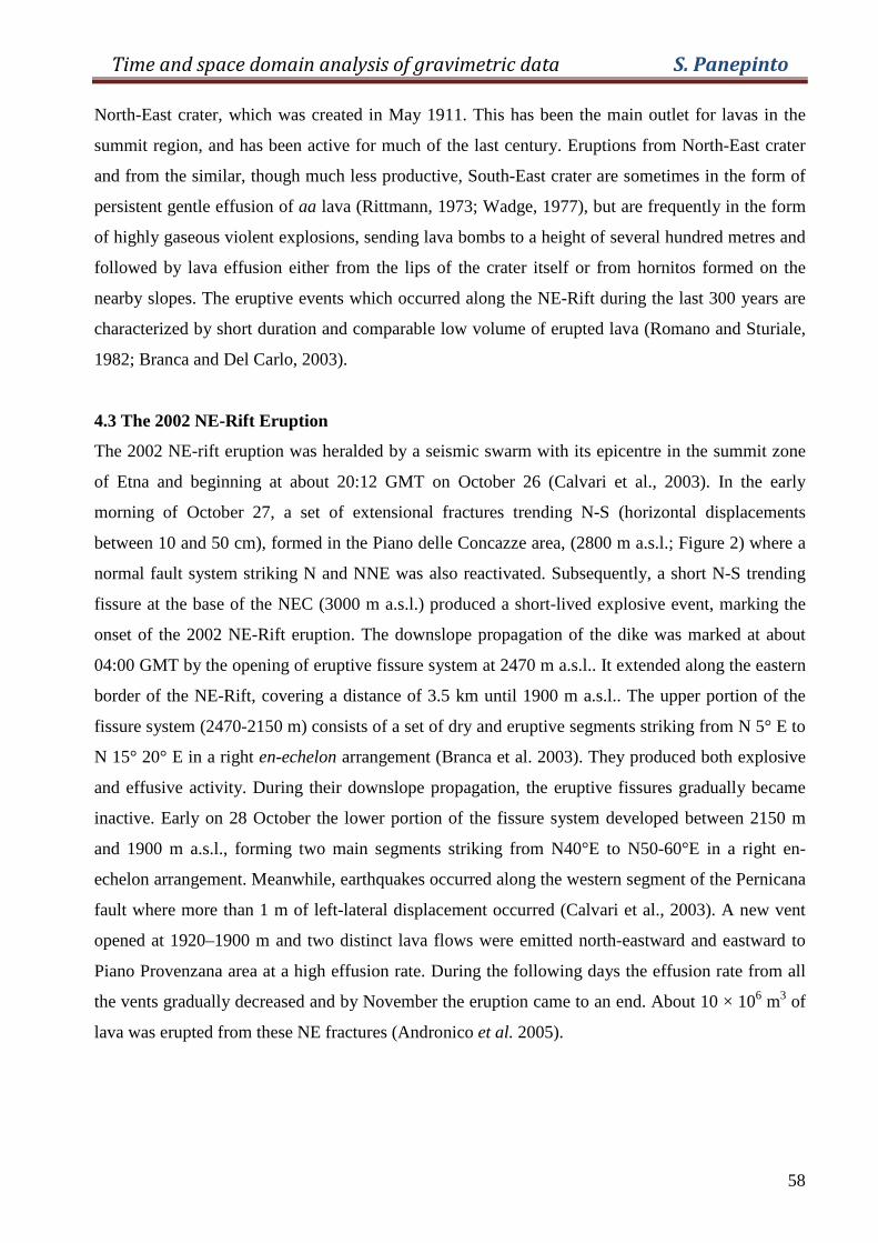
Time and space domain analysis of gravimetric data S. Panepinto
58
North-East crater, which was created in May 1911. This has been the main outlet for lavas in the
summit region, and has been active for much of the last century. Eruptions from North-East crater
and from the similar, though much less productive, South-East crater are sometimes in the form of
persistent gentle effusion of aa lava (Rittmann, 1973; Wadge, 1977), but are frequently in the form
of highly gaseous violent explosions, sending lava bombs to a height of several hundred metres and
followed by lava effusion either from the lips of the crater itself or from hornitos formed on the
nearby slopes. The eruptive events which occurred along the NE-Rift during the last 300 years are
characterized by short duration and comparable low volume of erupted lava (Romano and Sturiale,
1982; Branca and Del Carlo, 2003).
4.3 The 2002 NE-Rift Eruption
The 2002 NE-rift eruption was heralded by a seismic swarm with its epicentre in the summit zone
of Etna and beginning at about 20:12 GMT on October 26 (Calvari et al., 2003). In the early
morning of October 27, a set of extensional fractures trending N-S (horizontal displacements
between 10 and 50 cm), formed in the Piano delle Concazze area, (2800 m a.s.l.; Figure 2) where a
normal fault system striking N and NNE was also reactivated. Subsequently, a short N-S trending
fissure at the base of the NEC (3000 m a.s.l.) produced a short-lived explosive event, marking the
onset of the 2002 NE-Rift eruption. The downslope propagation of the dike was marked at about
04:00 GMT by the opening of eruptive fissure system at 2470 m a.s.l.. It extended along the eastern
border of the NE-Rift, covering a distance of 3.5 km until 1900 m a.s.l.. The upper portion of the
fissure system (2470-2150 m) consists of a set of dry and eruptive segments striking from N 5° E to
N 15° 20° E in a right en-echelon arrangement (Branca et al. 2003). They produced both explosive
and effusive activity. During their downslope propagation, the eruptive fissures gradually became
inactive. Early on 28 October the lower portion of the fissure system developed between 2150 m
and 1900 m a.s.l., forming two main segments striking from N40°E to N50-60°E in a right en-
echelon arrangement. Meanwhile, earthquakes occurred along the western segment of the Pernicana
fault where more than 1 m of left-lateral displacement occurred (Calvari et al., 2003). A new vent
opened at 1920–1900 m and two distinct lava flows were emitted north-eastward and eastward to
Piano Provenzana area at a high effusion rate. During the following days the effusion rate from all
the vents gradually decreased and by November the eruption came to an end. About 10 × 106 m3 of
lava was erupted from these NE fractures (Andronico et al. 2005).
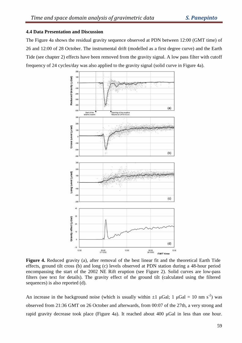
Time and space domain analysis of gravimetric data S. Panepinto
59
4.4 Data Presentation and Discussion
The Figure 4a shows the residual gravity sequence observed at PDN between 12:00 (GMT time) of
26 and 12:00 of 28 October. The instrumental drift (modelled as a first degree curve) and the Earth
Tide (see chapter 2) effects have been removed from the gravity signal. A low pass filter with cutoff
frequency of 24 cycles/day was also applied to the gravity signal (solid curve in Figure 4a).
Figure 4. Reduced gravity (a), after removal of the best linear fit and the theoretical Earth Tide effects, ground tilt cross (b) and long (c) levels observed at PDN station during a 48-hour period encompassing the start of the 2002 NE Rift eruption (see Figure 2). Solid curves are low-pass filters (see text for details). The gravity effect of the ground tilt (calculated using the filtered sequences) is also reported (d).
An increase in the background noise (which is usually within ±1 µGal; 1 µGal = 10 nm s-2) was
observed from 21:36 GMT on 26 October and afterwards, from 00:07 of the 27th, a very strong and
rapid gravity decrease took place (Figure 4a). It reached about 400 µGal in less than one hour.
Time and space domain analysis of gravimetric data S. Panepinto
60
Subsequently, the mean value of the gravity signal started rising again at a high rate (roughly 100
µgal/hour).
In general, instrumental effects linked to atmospheric parameters are expected to be very small over
periods of the order of a few hours (Andò and Carbone, 2001). Furthermore, in the case of the
gravity sequence presented above, contemporaneous temperature, pressure and relative humidity
changes were surely too weak (within 0.1°C, 2% RH and 4 mbar respectively) to produce any
significant effect. Ground tilt changes accompanying the above gravity sequence are presented in
Figures 4b and 4c. They are measured along two perpendicular directions, parallel to (long level)
and 90 degrees from (cross level) the direction of the meter’s beam, using the electronic levels fitted
to the instrument (resolution = 2.5 µrad; LaCoste and Romberg, 1997). The amplitude of the gravity
effect of the tilt changes is within 30 µgal (Figure 4d). Obviously, tilt changes that move the meter
away from the horizontal position (where it measures the full force of gravity) produce a negative
effect. The continuous GPS station, situated at PDN, recorded a positive height change (∆h) of
about 20 cm between 26 and 27 October (Mattia and Aloisi, 2003). If the nominal ∆g/∆h value of -
2.33 µgal/cm (Rymer, 1994) is assumed, this change implies a gravity decrease of about 50 µgal.
Unfortunately, deformation data at PDN are acquired on a daily basis and thus an accurate reduction
of the gravity sequence under discussion (1 datum/min) is not possible. However, if it is feasible
that a part of the 400 µgal gravity decrease observed during the onset of the 2002 NE-Rift eruption
is due to the combined effect of ground tilt and height changes, it cannot be ruled out that most of
the same anomaly is linked to subsurface mass redistributions. In particular, the negative part of the
observed gravity anomaly could have been caused by the opening of a dry fracture system in the
area of Piano delle Concazze (within 1 km of the station), during the early stage of the paroxysmal
event (Fig. 5). By assuming the new forming fractures to be dry, we rule out the magma
overpressure as a cause of their opening and thus we suggest they are rather the effect of external
forces. Accordingly, the right en-echelon arrangement of the new fracture system, observed in the
field, reflects the eastward gravitational sliding of the mega-block delimited by the Provenzana-
Pernicana fault system (Fig. 3). Magma from the central conduit would have entered the new
fracture system ‘‘passively’’, using it as a path to the eruptive vents downslope, and thus giving rise
to the observed gravity increase which roughly compensated the previous decrease (Fig. 5). It is
noteworthy that the eruptive dynamic (short duration and effusion rate decreasing rapidly with
time), which follows that of many historical eruptions from the NE-Rift (Romano and Sturiale,
1982), is in keeping with the inferred intrusive mechanism.
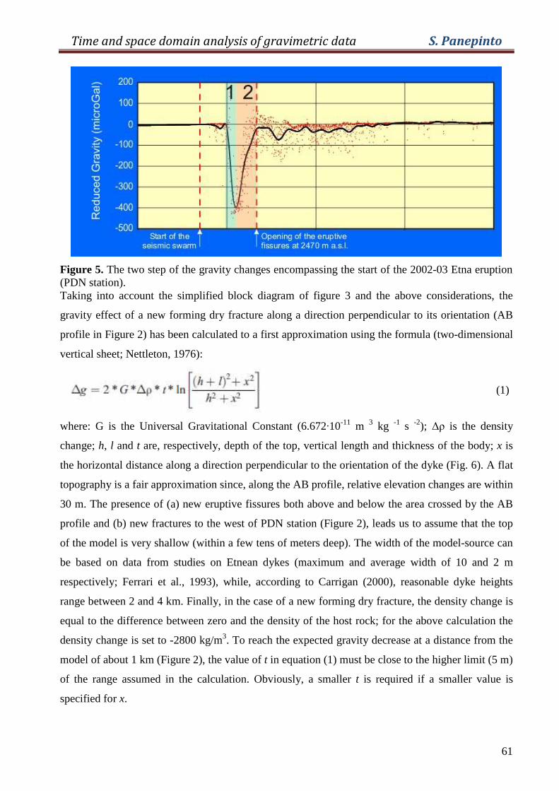
Time and space domain analysis of gravimetric data S. Panepinto
61
Figure 5. The two step of the gravity changes encompassing the start of the 2002-03 Etna eruption (PDN station). Taking into account the simplified block diagram of figure 3 and the above considerations, the
gravity effect of a new forming dry fracture along a direction perpendicular to its orientation (AB
profile in Figure 2) has been calculated to a first approximation using the formula (two-dimensional
vertical sheet; Nettleton, 1976):
(1)
where: G is the Universal Gravitational Constant (6.672·10-11 m 3 kg -1 s -2); ∆ρ is the density
change; h, l and t are, respectively, depth of the top, vertical length and thickness of the body; x is
the horizontal distance along a direction perpendicular to the orientation of the dyke (Fig. 6). A flat
topography is a fair approximation since, along the AB profile, relative elevation changes are within
30 m. The presence of (a) new eruptive fissures both above and below the area crossed by the AB
profile and (b) new fractures to the west of PDN station (Figure 2), leads us to assume that the top
of the model is very shallow (within a few tens of meters deep). The width of the model-source can
be based on data from studies on Etnean dykes (maximum and average width of 10 and 2 m
respectively; Ferrari et al., 1993), while, according to Carrigan (2000), reasonable dyke heights
range between 2 and 4 km. Finally, in the case of a new forming dry fracture, the density change is
equal to the difference between zero and the density of the host rock; for the above calculation the
density change is set to -2800 kg/m3. To reach the expected gravity decrease at a distance from the
model of about 1 km (Figure 2), the value of t in equation (1) must be close to the higher limit (5 m)
of the range assumed in the calculation. Obviously, a smaller t is required if a smaller value is
specified for x.
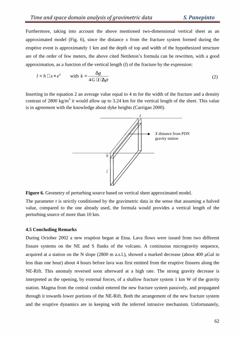
Time and space domain analysis of gravimetric data S. Panepinto
62
Furthermore, taking into account the above mentioned two-dimensional vertical sheet as an
approximated model (Fig. 6), since the distance x from the fracture system formed during the
eruptive event is approximately 1 km and the depth of top and width of the hypothesized structure
are of the order of few meters, the above cited Nettleton’s formula can be rewritten, with a good
approximation, as a function of the vertical length (l) of the fracture by the expression:
kexhl ×+= with ρ∆⋅⋅
∆=tG
gk
4 (2)
Inserting in the equation 2 an average value equal to 4 m for the width of the fracture and a density contrast of 2800 kg/m3 it would allow up to 3.24 km for the vertical length of the sheet. This value is in agreement with the knowledge about dyke heights (Carrigan 2000).
Figure 6. Geometry of perturbing source based on vertical sheet approximated model.
The parameter t is strictly conditioned by the gravimetric data in the sense that assuming a halved value, compared to the one already used, the formula would provides a vertical length of the perturbing source of more than 10 km.
4.5 Concluding Remarks
During October 2002 a new eruption began at Etna. Lava flows were issued from two different
fissure systems on the NE and S flanks of the volcano. A continuous microgravity sequence,
acquired at a station on the N slope (2800 m a.s.l.), showed a marked decrease (about 400 µGal in
less than one hour) about 4 hours before lava was first emitted from the eruptive fissures along the
NE-Rift. This anomaly reversed soon afterward at a high rate. The strong gravity decrease is
interpreted as the opening, by external forces, of a shallow fracture system 1 km W of the gravity
station. Magma from the central conduit entered the new fracture system passively, and propagated
through it towards lower portions of the NE-Rift. Both the arrangement of the new fracture system
and the eruptive dynamics are in keeping with the inferred intrusive mechanism. Unfortunately,
X distance from PDN gravity station
Time and space domain analysis of gravimetric data S. Panepinto
63
PDN is the only continuous gravity station of the Etna array which was working during the onset of
the above event, because of this it is difficult to asses any geometrical consideration about the
source.
The present study represents a further step towards the definition of the real potential for continuous
gravity studies to make an effective volcano-monitoring tool. The gravity data under discussion not
only allow the timing of the intrusive event to be described in greater detail but also, in conjunction
with other volcanological evidences, permit some constraints to be set on the characteristics of the
inferred injection.
The gravity sequence we present and discuss above is the first real-time evidence of an intrusive
mechanism that has only been indirectly inferred after previous similar events through a posteriori
geological and structural data. The strong gravity decrease, marking the start of the 2002 NE-Rift
paroxysmal event and interpreted as the effect of the opening of new voids, indicates that the
magma did not actively trigger the opening of the eruptive fissures but intruded after the
development of the fracture system, which was instead driven by the large-scale collapse of Etna’s
northeastern flank.

Time and space domain analysis of gravimetric data S. Panepinto
64
SECTION 2
Time and space domain analysis of gravimetric data S. Panepinto
65
CHAPTER 5
5.1 Introduction
Section II, as stated in the introduction, concentrates on the analysis of thermometric signals
acquired at Mt. Etna for the detection of weak tidal modulations of heat flux.
Volcanic areas are characterised by high heat fluxes due to the presence of magma bodies near the
surface. In these areas convection is the major heat transfer mechanism. The tidal strain field within
the volcanic edifice could affect this convective process. Time variations of the efficiency of the
convective process should produce corresponding temperature changes observable at shallow depth.
The aim of the proposed study was to relate some of the observed temperature changes to the main
tidal periods and investigate the presence of a periodic variation due to the main lunar tidal
component (M2, 12.421 hours period; see chapter 2 for further explanation). This component was
chosen in order to avoid solar radiation effects. Four thermometric signals recorded on Etna volcano
at sites very close to the main active craters have been analysed. The data sets at hand were
processed with a stacking technique coupled with a wavelet transform analysis for preliminary
denoising. Through this procedure an anomalous amplitude of the spectral component with a period
equal to that of the M2 tidal wave was found in one of the investigated thermometric records.
5.2 Brief description of the boundary conditions
Surface temperature, gas flows and temperature gradient distributions have been used to
characterise shallow magmatic bodies while time changes of the surface heat flow have been linked
to the thermal state variations (Lardy M. Tabbagh A., 1999). In the following we want to relate
some of the thermometric time changes with tidal periods (by introducing the tidal stress-strain
oscillating action concept) in order to evaluate a feasible interaction between the tidal stress-strain
and any of the flow processes occurring within the volcano edifice of Mt. Etna.
A volcanic system is subjected to stress fields due to its interaction with the interior and the exterior
of the Earth. The total stress field is a superposition of different time dependent terms, some of
which are periodic with well known periods. The periodic components are linked mainly to the
earth-tides which are well defined and entirely predictable (Melchior, 1978). These oscillating
stresses are created in the Earth’s crust by the gravitational forces exerted mainly by the Sun and the
Moon (see chapter 2).
Tides have long been implicated in the controlling of volcanic processes but evidence showing this
has been sparse. Nevertheless, the idea that tides could have an influence on volcanic processes has
been puzzling geophysicists for a great number of volcanoes e.g. Pavlof volcano in Alaska (S. R.
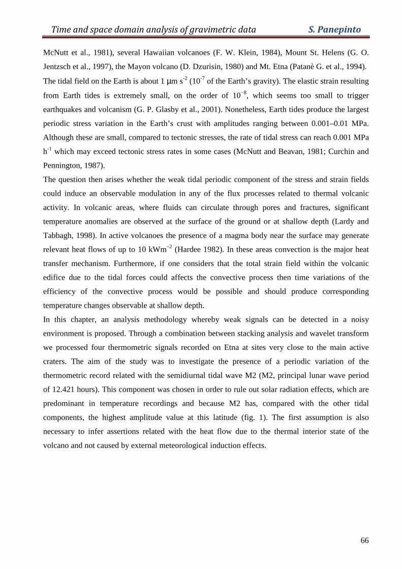
Time and space domain analysis of gravimetric data S. Panepinto
66
McNutt et al., 1981), several Hawaiian volcanoes (F. W. Klein, 1984), Mount St. Helens (G. O.
Jentzsch et al., 1997), the Mayon volcano (D. Dzurisin, 1980) and Mt. Etna (Patanè G. et al., 1994).
The tidal field on the Earth is about 1 µm s-2 (10-7 of the Earth’s gravity). The elastic strain resulting
from Earth tides is extremely small, on the order of 10−8, which seems too small to trigger
earthquakes and volcanism (G. P. Glasby et al., 2001). Nonetheless, Earth tides produce the largest
periodic stress variation in the Earth’s crust with amplitudes ranging between 0.001–0.01 MPa.
Although these are small, compared to tectonic stresses, the rate of tidal stress can reach 0.001 MPa
h-1 which may exceed tectonic stress rates in some cases (McNutt and Beavan, 1981; Curchin and
Pennington, 1987).
The question then arises whether the weak tidal periodic component of the stress and strain fields
could induce an observable modulation in any of the flux processes related to thermal volcanic
activity. In volcanic areas, where fluids can circulate through pores and fractures, significant
temperature anomalies are observed at the surface of the ground or at shallow depth (Lardy and
Tabbagh, 1998). In active volcanoes the presence of a magma body near the surface may generate
relevant heat flows of up to 10 kWm–2 (Hardee 1982). In these areas convection is the major heat
transfer mechanism. Furthermore, if one considers that the total strain field within the volcanic
edifice due to the tidal forces could affects the convective process then time variations of the
efficiency of the convective process would be possible and should produce corresponding
temperature changes observable at shallow depth.
In this chapter, an analysis methodology whereby weak signals can be detected in a noisy
environment is proposed. Through a combination between stacking analysis and wavelet transform
we processed four thermometric signals recorded on Etna at sites very close to the main active
craters. The aim of the study was to investigate the presence of a periodic variation of the
thermometric record related with the semidiurnal tidal wave M2 (M2, principal lunar wave period
of 12.421 hours). This component was chosen in order to rule out solar radiation effects, which are
predominant in temperature recordings and because M2 has, compared with the other tidal
components, the highest amplitude value at this latitude (fig. 1). The first assumption is also
necessary to infer assertions related with the heat flow due to the thermal interior state of the
volcano and not caused by external meteorological induction effects.
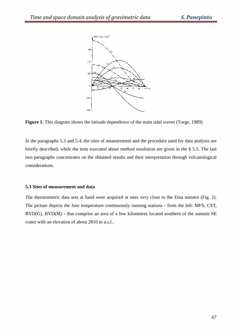
Time and space domain analysis of gravimetric data S. Panepinto
67
Figure 1. This diagram shows the latitude dependence of the main tidal waves (Torge, 1989)
In the paragraphs 5.3 and 5.4, the sites of measurement and the procedure used for data analysis are
briefly described, while the tests executed about method resolution are given in the § 5.5. The last
two paragraphs concentrates on the obtained results and their interpretation through volcanological
considerations.
5.3 Sites of measurement and data
The thermometric data sets at hand were acquired at sites very close to the Etna summit (Fig. 2).
The picture depicts the four temperature continuously running stations - from the left: MFS, CST,
BVD(G), BVD(M) - that comprise an area of a few kilometres located southern of the summit SE
crater with an elevation of about 2810 m a.s.l..
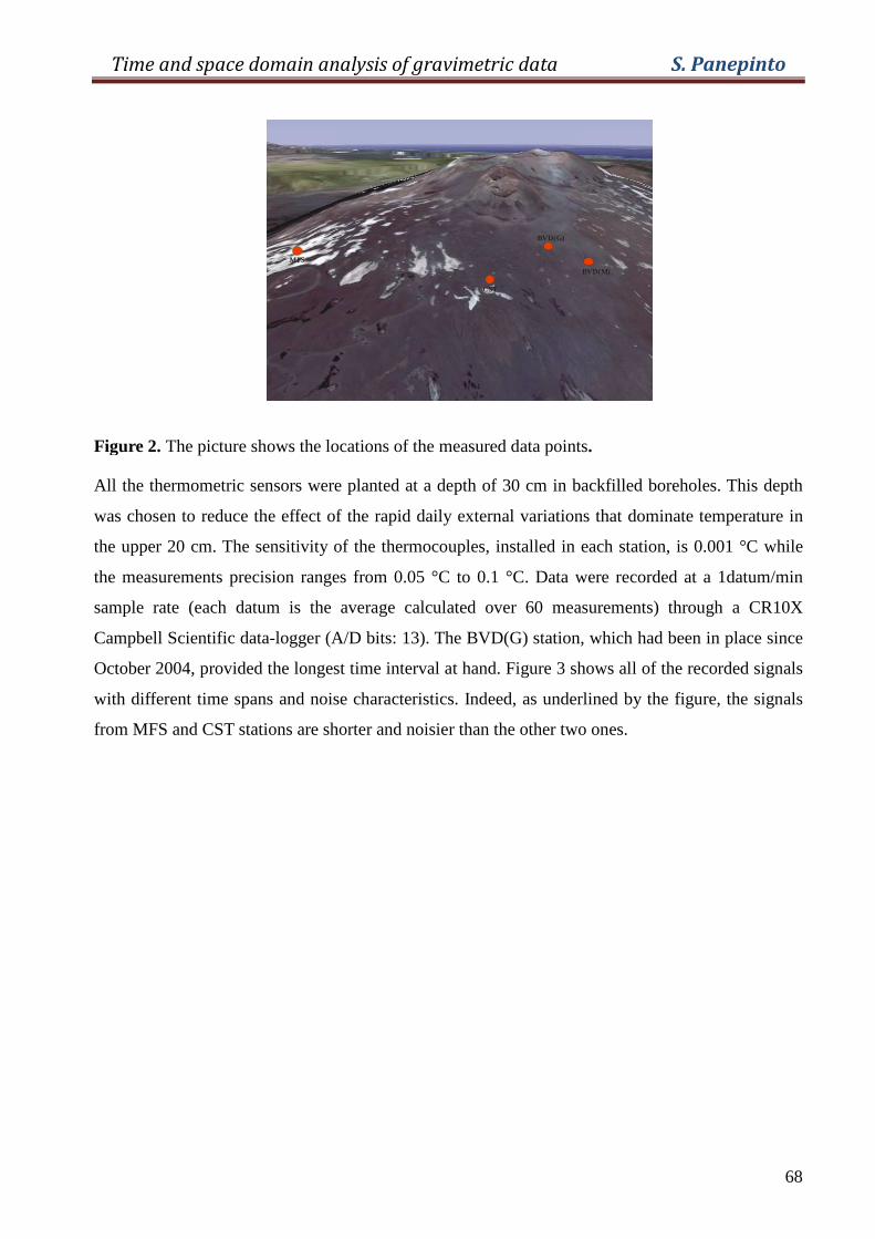
Time and space domain analysis of gravimetric data S. Panepinto
68
Figure 2. The picture shows the locations of the measured data points.
All the thermometric sensors were planted at a depth of 30 cm in backfilled boreholes. This depth
was chosen to reduce the effect of the rapid daily external variations that dominate temperature in
the upper 20 cm. The sensitivity of the thermocouples, installed in each station, is 0.001 °C while
the measurements precision ranges from 0.05 °C to 0.1 °C. Data were recorded at a 1datum/min
sample rate (each datum is the average calculated over 60 measurements) through a CR10X
Campbell Scientific data-logger (A/D bits: 13). The BVD(G) station, which had been in place since
October 2004, provided the longest time interval at hand. Figure 3 shows all of the recorded signals
with different time spans and noise characteristics. Indeed, as underlined by the figure, the signals
from MFS and CST stations are shorter and noisier than the other two ones.
MFS
CST
BVD(G)
BVD(M)
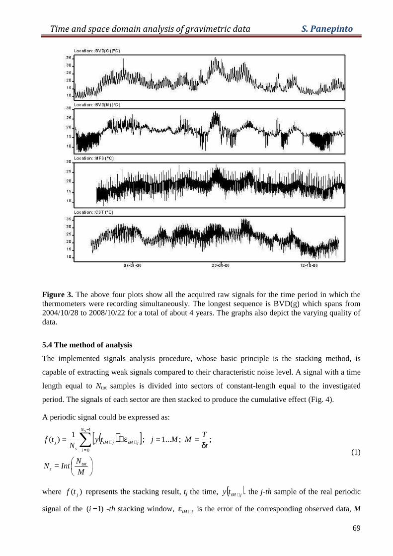
Time and space domain analysis of gravimetric data S. Panepinto
69
Figure 3. The above four plots show all the acquired raw signals for the time period in which the thermometers were recording simultaneously. The longest sequence is BVD(g) which spans from 2004/10/28 to 2008/10/22 for a total of about 4 years. The graphs also depict the varying quality of data.
5.4 The method of analysis
The implemented signals analysis procedure, whose basic principle is the stacking method, is
capable of extracting weak signals compared to their characteristic noise level. A signal with a time
length equal to Ntot samples is divided into sectors of constant-length equal to the investigated
period. The signals of each sector are then stacked to produce the cumulative effect (Fig. 4).
A periodic signal could be expressed as:
( )[ ]
=
δ==ε+= ∑
−
=
++
M
NIntN
t
TMMjty
Ntf
tots
sN
i
jiMjiMs
j ;;...1;1
)(1
0 (1)
where )( jtf represents the stacking result, tj the time, ( )jiMty + the j-th sample of the real periodic
signal of the )1( −i -th stacking window, jiM +ε is the error of the corresponding observed data, M
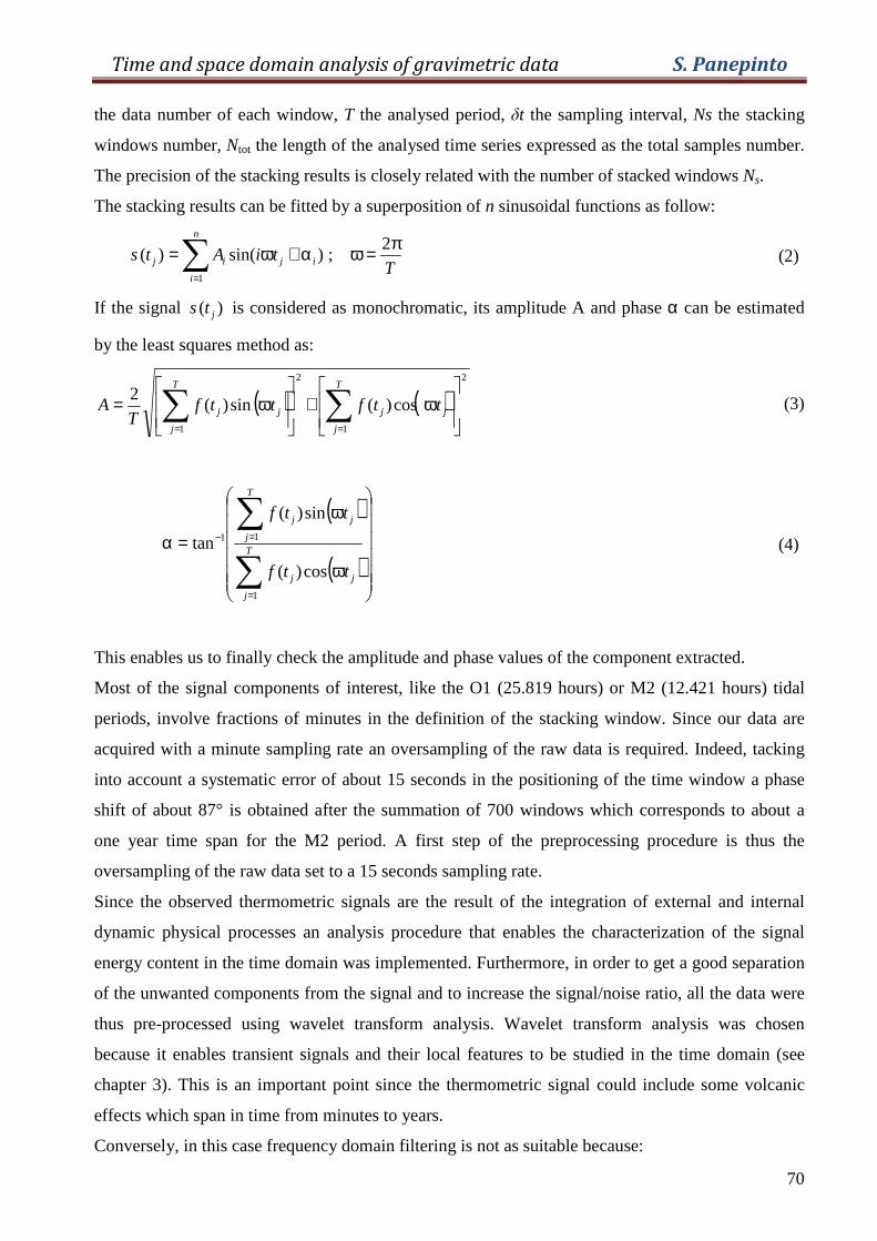
Time and space domain analysis of gravimetric data S. Panepinto
70
the data number of each window, T the analysed period, δt the sampling interval, Ns the stacking
windows number, Ntot the length of the analysed time series expressed as the total samples number.
The precision of the stacking results is closely related with the number of stacked windows Ns.
The stacking results can be fitted by a superposition of n sinusoidal functions as follow:
∑=
π=ωα+ω=n
i
ijij TtiAts
1
2;)sin()( (2)
If the signal )( jts is considered as monochromatic, its amplitude A and phase α can be estimated
by the least squares method as:
( ) ( )2
1
2
1
cos)(sin)(2
ω+
ω= ∑∑
==
T
j
jj
T
j
jj ttfttfT
A (3)
( )
( )
ω
ω
=α
∑
∑
=
=−T
j
jj
T
j
jj
ttf
ttf
1
11
cos)(
sin)(
tan (4)
This enables us to finally check the amplitude and phase values of the component extracted.
Most of the signal components of interest, like the O1 (25.819 hours) or M2 (12.421 hours) tidal
periods, involve fractions of minutes in the definition of the stacking window. Since our data are
acquired with a minute sampling rate an oversampling of the raw data is required. Indeed, tacking
into account a systematic error of about 15 seconds in the positioning of the time window a phase
shift of about 87° is obtained after the summation of 700 windows which corresponds to about a
one year time span for the M2 period. A first step of the preprocessing procedure is thus the
oversampling of the raw data set to a 15 seconds sampling rate.
Since the observed thermometric signals are the result of the integration of external and internal
dynamic physical processes an analysis procedure that enables the characterization of the signal
energy content in the time domain was implemented. Furthermore, in order to get a good separation
of the unwanted components from the signal and to increase the signal/noise ratio, all the data were
thus pre-processed using wavelet transform analysis. Wavelet transform analysis was chosen
because it enables transient signals and their local features to be studied in the time domain (see
chapter 3). This is an important point since the thermometric signal could include some volcanic
effects which span in time from minutes to years.
Conversely, in this case frequency domain filtering is not as suitable because:
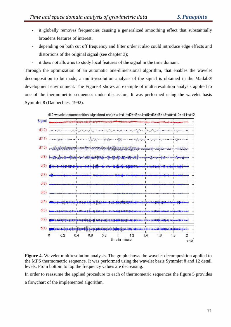
Time and space domain analysis of gravimetric data S. Panepinto
71
- it globally removes frequencies causing a generalized smoothing effect that substantially
broadens features of interest;
- depending on both cut off frequency and filter order it also could introduce edge effects and
distortions of the original signal (see chapter 3);
- it does not allow us to study local features of the signal in the time domain.
Through the optimization of an automatic one-dimensional algorithm, that enables the wavelet
decomposition to be made, a multi-resolution analysis of the signal is obtained in the Matlab®
development environment. The Figure 4 shows an example of multi-resolution analysis applied to
one of the thermometric sequences under discussion. It was performed using the wavelet basis
Symmlet 8 (Daubechies, 1992).
Figure 4. Wavelet multiresolution analysis. The graph shows the wavelet decomposition applied to the MFS thermometric sequence. It was performed using the wavelet basis Symmlet 8 and 12 detail levels. From bottom to top the frequency values are decreasing.
In order to reassume the applied procedure to each of thermometric sequences the figure 5 provides
a flowchart of the implemented algorithm.
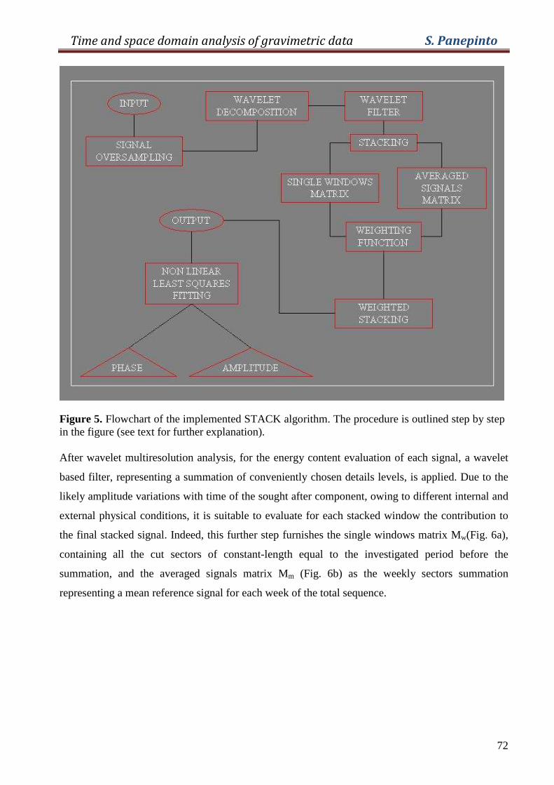
Time and space domain analysis of gravimetric data S. Panepinto
72
Figure 5. Flowchart of the implemented STACK algorithm. The procedure is outlined step by step in the figure (see text for further explanation). After wavelet multiresolution analysis, for the energy content evaluation of each signal, a wavelet
based filter, representing a summation of conveniently chosen details levels, is applied. Due to the
likely amplitude variations with time of the sought after component, owing to different internal and
external physical conditions, it is suitable to evaluate for each stacked window the contribution to
the final stacked signal. Indeed, this further step furnishes the single windows matrix Mw(Fig. 6a),
containing all the cut sectors of constant-length equal to the investigated period before the
summation, and the averaged signals matrix Mm (Fig. 6b) as the weekly sectors summation
representing a mean reference signal for each week of the total sequence.
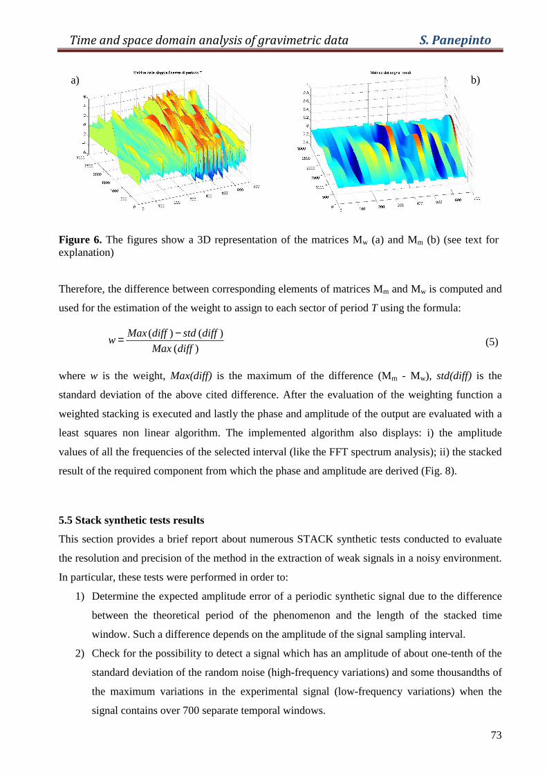
Time and space domain analysis of gravimetric data S. Panepinto
73
Figure 6. The figures show a 3D representation of the matrices Mw (a) and Mm (b) (see text for explanation)
Therefore, the difference between corresponding elements of matrices Mm and Mw is computed and
used for the estimation of the weight to assign to each sector of period T using the formula:
)(
)()(
diffMax
diffstddiffMaxw
−= (5)
where w is the weight, Max(diff) is the maximum of the difference (Mm - Mw), std(diff) is the
standard deviation of the above cited difference. After the evaluation of the weighting function a
weighted stacking is executed and lastly the phase and amplitude of the output are evaluated with a
least squares non linear algorithm. The implemented algorithm also displays: i) the amplitude
values of all the frequencies of the selected interval (like the FFT spectrum analysis); ii) the stacked
result of the required component from which the phase and amplitude are derived (Fig. 8).
5.5 Stack synthetic tests results
This section provides a brief report about numerous STACK synthetic tests conducted to evaluate
the resolution and precision of the method in the extraction of weak signals in a noisy environment.
In particular, these tests were performed in order to:
1) Determine the expected amplitude error of a periodic synthetic signal due to the difference
between the theoretical period of the phenomenon and the length of the stacked time
window. Such a difference depends on the amplitude of the signal sampling interval.
2) Check for the possibility to detect a signal which has an amplitude of about one-tenth of the
standard deviation of the random noise (high-frequency variations) and some thousandths of
the maximum variations in the experimental signal (low-frequency variations) when the
signal contains over 700 separate temporal windows.
a) b)
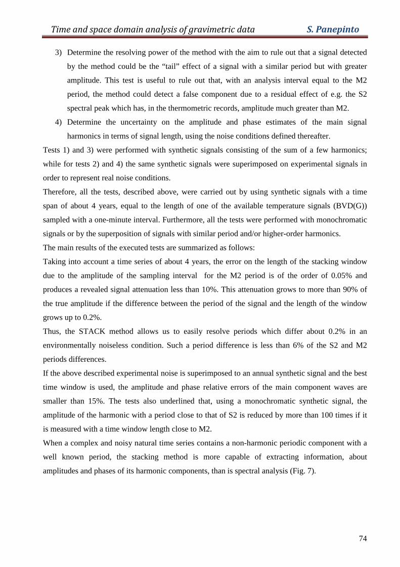
Time and space domain analysis of gravimetric data S. Panepinto
74
3) Determine the resolving power of the method with the aim to rule out that a signal detected
by the method could be the “tail” effect of a signal with a similar period but with greater
amplitude. This test is useful to rule out that, with an analysis interval equal to the M2
period, the method could detect a false component due to a residual effect of e.g. the S2
spectral peak which has, in the thermometric records, amplitude much greater than M2.
4) Determine the uncertainty on the amplitude and phase estimates of the main signal
harmonics in terms of signal length, using the noise conditions defined thereafter.
Tests 1) and 3) were performed with synthetic signals consisting of the sum of a few harmonics;
while for tests 2) and 4) the same synthetic signals were superimposed on experimental signals in
order to represent real noise conditions.
Therefore, all the tests, described above, were carried out by using synthetic signals with a time
span of about 4 years, equal to the length of one of the available temperature signals (BVD(G))
sampled with a one-minute interval. Furthermore, all the tests were performed with monochromatic
signals or by the superposition of signals with similar period and/or higher-order harmonics.
The main results of the executed tests are summarized as follows:
Taking into account a time series of about 4 years, the error on the length of the stacking window
due to the amplitude of the sampling interval for the M2 period is of the order of 0.05% and
produces a revealed signal attenuation less than 10%. This attenuation grows to more than 90% of
the true amplitude if the difference between the period of the signal and the length of the window
grows up to 0.2%.
Thus, the STACK method allows us to easily resolve periods which differ about 0.2% in an
environmentally noiseless condition. Such a period difference is less than 6% of the S2 and M2
periods differences.
If the above described experimental noise is superimposed to an annual synthetic signal and the best
time window is used, the amplitude and phase relative errors of the main component waves are
smaller than 15%. The tests also underlined that, using a monochromatic synthetic signal, the
amplitude of the harmonic with a period close to that of S2 is reduced by more than 100 times if it
is measured with a time window length close to M2.
When a complex and noisy natural time series contains a non-harmonic periodic component with a
well known period, the stacking method is more capable of extracting information, about
amplitudes and phases of its harmonic components, than is spectral analysis (Fig. 7).
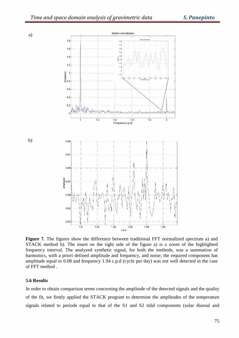
Time and space domain analysis of gravimetric data S. Panepinto
75
Figure 7. The figures show the difference between traditional FFT normalized spectrum a) and STACK method b). The insert on the right side of the figure a) is a zoom of the highlighted frequency interval. The analyzed synthetic signal, for both the methods, was a summation of harmonics, with a priori defined amplitude and frequency, and noise; the required component has amplitude equal to 0.08 and frequency 1.94 c.p.d (cycle per day) was not well detected in the case of FFT method .
5.6 Results
In order to obtain comparison terms concerning the amplitude of the detected signals and the quality
of the fit, we firstly applied the STACK program to determine the amplitudes of the temperature
signals related to periods equal to that of the S1 and S2 tidal components (solar diurnal and
b)
a)
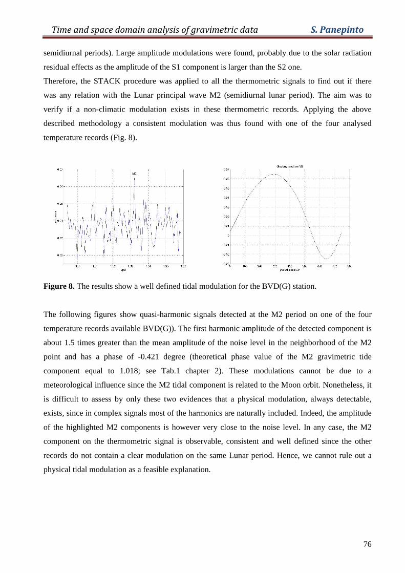
Time and space domain analysis of gravimetric data S. Panepinto
76
semidiurnal periods). Large amplitude modulations were found, probably due to the solar radiation
residual effects as the amplitude of the S1 component is larger than the S2 one.
Therefore, the STACK procedure was applied to all the thermometric signals to find out if there
was any relation with the Lunar principal wave M2 (semidiurnal lunar period). The aim was to
verify if a non-climatic modulation exists in these thermometric records. Applying the above
described methodology a consistent modulation was thus found with one of the four analysed
temperature records (Fig. 8).
Figure 8. The results show a well defined tidal modulation for the BVD(G) station.
The following figures show quasi-harmonic signals detected at the M2 period on one of the four
temperature records available BVD(G)). The first harmonic amplitude of the detected component is
about 1.5 times greater than the mean amplitude of the noise level in the neighborhood of the M2
point and has a phase of -0.421 degree (theoretical phase value of the M2 gravimetric tide
component equal to 1.018; see Tab.1 chapter 2). These modulations cannot be due to a
meteorological influence since the M2 tidal component is related to the Moon orbit. Nonetheless, it
is difficult to assess by only these two evidences that a physical modulation, always detectable,
exists, since in complex signals most of the harmonics are naturally included. Indeed, the amplitude
of the highlighted M2 components is however very close to the noise level. In any case, the M2
component on the thermometric signal is observable, consistent and well defined since the other
records do not contain a clear modulation on the same Lunar period. Hence, we cannot rule out a
physical tidal modulation as a feasible explanation.
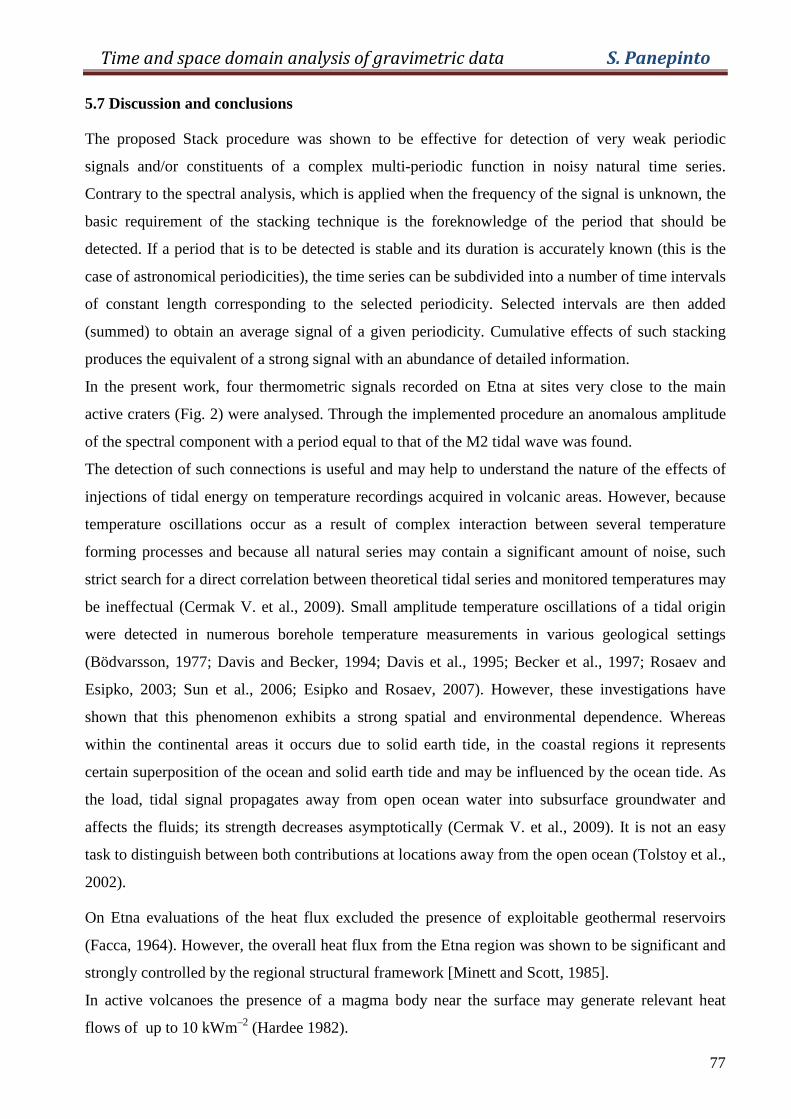
Time and space domain analysis of gravimetric data S. Panepinto
77
5.7 Discussion and conclusions
The proposed Stack procedure was shown to be effective for detection of very weak periodic
signals and/or constituents of a complex multi-periodic function in noisy natural time series.
Contrary to the spectral analysis, which is applied when the frequency of the signal is unknown, the
basic requirement of the stacking technique is the foreknowledge of the period that should be
detected. If a period that is to be detected is stable and its duration is accurately known (this is the
case of astronomical periodicities), the time series can be subdivided into a number of time intervals
of constant length corresponding to the selected periodicity. Selected intervals are then added
(summed) to obtain an average signal of a given periodicity. Cumulative effects of such stacking
produces the equivalent of a strong signal with an abundance of detailed information.
In the present work, four thermometric signals recorded on Etna at sites very close to the main
active craters (Fig. 2) were analysed. Through the implemented procedure an anomalous amplitude
of the spectral component with a period equal to that of the M2 tidal wave was found.
The detection of such connections is useful and may help to understand the nature of the effects of
injections of tidal energy on temperature recordings acquired in volcanic areas. However, because
temperature oscillations occur as a result of complex interaction between several temperature
forming processes and because all natural series may contain a significant amount of noise, such
strict search for a direct correlation between theoretical tidal series and monitored temperatures may
be ineffectual (Cermak V. et al., 2009). Small amplitude temperature oscillations of a tidal origin
were detected in numerous borehole temperature measurements in various geological settings
(Bödvarsson, 1977; Davis and Becker, 1994; Davis et al., 1995; Becker et al., 1997; Rosaev and
Esipko, 2003; Sun et al., 2006; Esipko and Rosaev, 2007). However, these investigations have
shown that this phenomenon exhibits a strong spatial and environmental dependence. Whereas
within the continental areas it occurs due to solid earth tide, in the coastal regions it represents
certain superposition of the ocean and solid earth tide and may be influenced by the ocean tide. As
the load, tidal signal propagates away from open ocean water into subsurface groundwater and
affects the fluids; its strength decreases asymptotically (Cermak V. et al., 2009). It is not an easy
task to distinguish between both contributions at locations away from the open ocean (Tolstoy et al.,
2002).
On Etna evaluations of the heat flux excluded the presence of exploitable geothermal reservoirs
(Facca, 1964). However, the overall heat flux from the Etna region was shown to be significant and
strongly controlled by the regional structural framework [Minett and Scott, 1985].
In active volcanoes the presence of a magma body near the surface may generate relevant heat
flows of up to 10 kWm–2 (Hardee 1982).
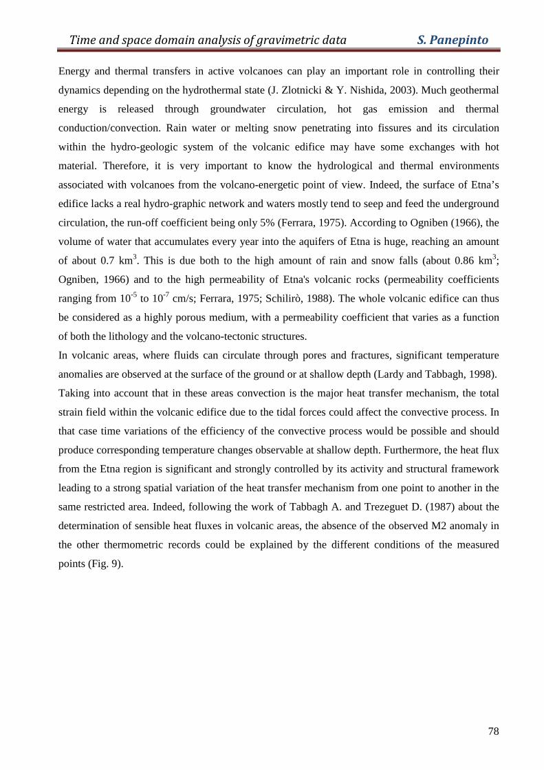
Time and space domain analysis of gravimetric data S. Panepinto
78
Energy and thermal transfers in active volcanoes can play an important role in controlling their
dynamics depending on the hydrothermal state (J. Zlotnicki & Y. Nishida, 2003). Much geothermal
energy is released through groundwater circulation, hot gas emission and thermal
conduction/convection. Rain water or melting snow penetrating into fissures and its circulation
within the hydro-geologic system of the volcanic edifice may have some exchanges with hot
material. Therefore, it is very important to know the hydrological and thermal environments
associated with volcanoes from the volcano-energetic point of view. Indeed, the surface of Etna’s
edifice lacks a real hydro-graphic network and waters mostly tend to seep and feed the underground
circulation, the run-off coefficient being only 5% (Ferrara, 1975). According to Ogniben (1966), the
volume of water that accumulates every year into the aquifers of Etna is huge, reaching an amount
of about 0.7 km3. This is due both to the high amount of rain and snow falls (about 0.86 km3;
Ogniben, 1966) and to the high permeability of Etna's volcanic rocks (permeability coefficients
ranging from 10-5 to 10-7 cm/s; Ferrara, 1975; Schilirò, 1988). The whole volcanic edifice can thus
be considered as a highly porous medium, with a permeability coefficient that varies as a function
of both the lithology and the volcano-tectonic structures.
In volcanic areas, where fluids can circulate through pores and fractures, significant temperature
anomalies are observed at the surface of the ground or at shallow depth (Lardy and Tabbagh, 1998).
Taking into account that in these areas convection is the major heat transfer mechanism, the total
strain field within the volcanic edifice due to the tidal forces could affect the convective process. In
that case time variations of the efficiency of the convective process would be possible and should
produce corresponding temperature changes observable at shallow depth. Furthermore, the heat flux
from the Etna region is significant and strongly controlled by its activity and structural framework
leading to a strong spatial variation of the heat transfer mechanism from one point to another in the
same restricted area. Indeed, following the work of Tabbagh A. and Trezeguet D. (1987) about the
determination of sensible heat fluxes in volcanic areas, the absence of the observed M2 anomaly in
the other thermometric records could be explained by the different conditions of the measured
points (Fig. 9).
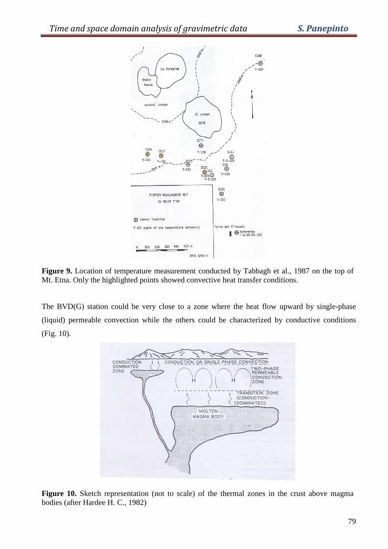
Time and space domain analysis of gravimetric data S. Panepinto
79
Figure 9. Location of temperature measurement conducted by Tabbagh et al., 1987 on the top of Mt. Etna. Only the highlighted points showed convective heat transfer conditions.
The BVD(G) station could be very close to a zone where the heat flow upward by single-phase
(liquid) permeable convection while the others could be characterized by conductive conditions
(Fig. 10).
Figure 10. Sketch representation (not to scale) of the thermal zones in the crust above magma bodies (after Hardee H. C., 1982)
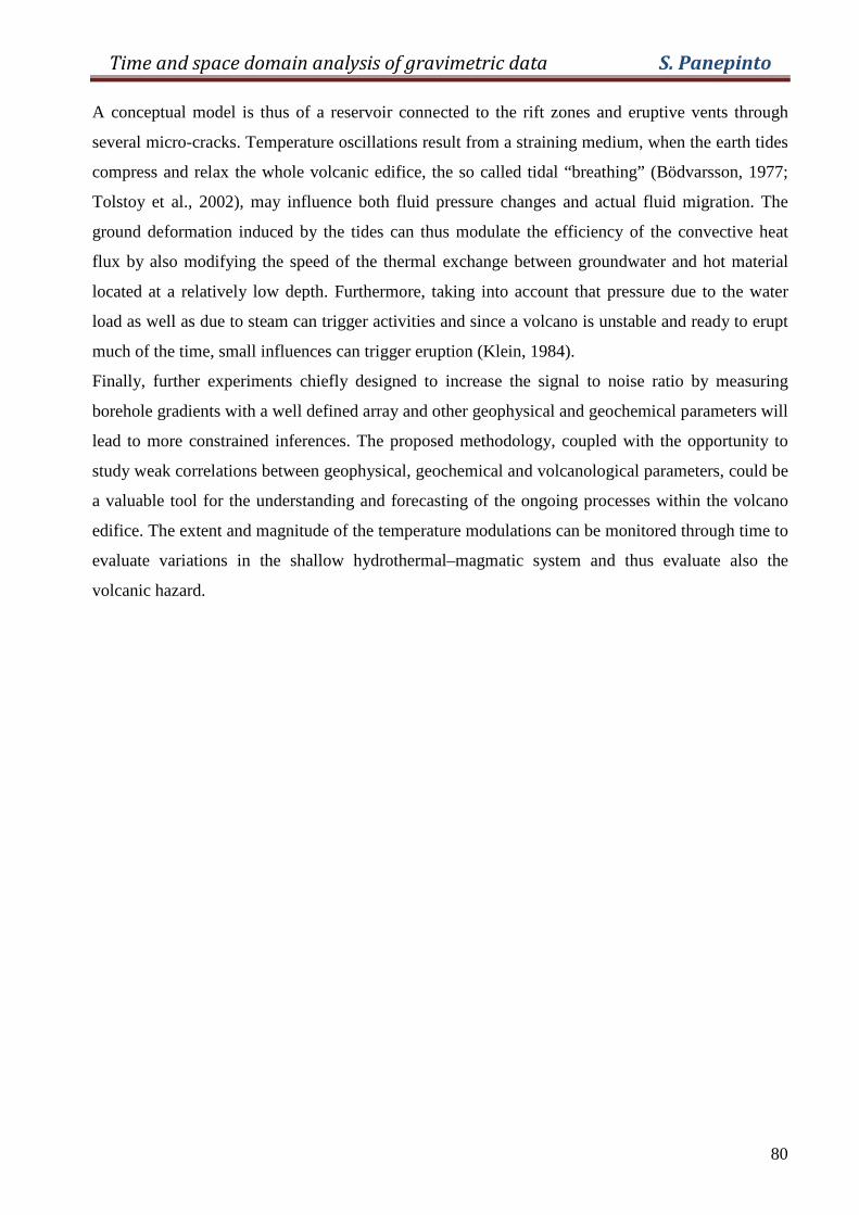
Time and space domain analysis of gravimetric data S. Panepinto
80
A conceptual model is thus of a reservoir connected to the rift zones and eruptive vents through
several micro-cracks. Temperature oscillations result from a straining medium, when the earth tides
compress and relax the whole volcanic edifice, the so called tidal “breathing” (Bödvarsson, 1977;
Tolstoy et al., 2002), may influence both fluid pressure changes and actual fluid migration. The
ground deformation induced by the tides can thus modulate the efficiency of the convective heat
flux by also modifying the speed of the thermal exchange between groundwater and hot material
located at a relatively low depth. Furthermore, taking into account that pressure due to the water
load as well as due to steam can trigger activities and since a volcano is unstable and ready to erupt
much of the time, small influences can trigger eruption (Klein, 1984).
Finally, further experiments chiefly designed to increase the signal to noise ratio by measuring
borehole gradients with a well defined array and other geophysical and geochemical parameters will
lead to more constrained inferences. The proposed methodology, coupled with the opportunity to
study weak correlations between geophysical, geochemical and volcanological parameters, could be
a valuable tool for the understanding and forecasting of the ongoing processes within the volcano
edifice. The extent and magnitude of the temperature modulations can be monitored through time to
evaluate variations in the shallow hydrothermal–magmatic system and thus evaluate also the
volcanic hazard.

Time and space domain analysis of gravimetric data S. Panepinto
81
SECTION 3
Time and space domain analysis of gravimetric data S. Panepinto
82
CHAPTER 6
6.1 Introduction
This short chapter describes a study of Southern Tyrrhenian and Sicilian regions by a sequential
inversion technique to integrate seismic and Bouguer anomaly data.
In the following, a procedure is proposed for the construction of 3D velocity-density models and
earthquake relocation by sequential inversion of P and S wave travel-times and Bouguer anomaly
distribution. This procedure was applied to a large data set concerning the Sicilian area and portions
of the surrounding basins. Its application to the Sicilian area underlined the necessity of the
integration of experimental data of these two different typologies, to well constrain lithospheric
models and to define new assessment criteria of the results obtained by the inversions of each data
type.
In the paragraph 6.2 the investigated area and data sets are presented with a short description of the
seismicity characteristics and seismic inversion procedure to derive tomographic images.
Subsequently, the implemented iterative procedure used to integrate the different data types is
shown while, in the last paragraph, some preliminary results are presented.
6.2 Investigated area and data sets
The seismicity of the southern Tyrrhenian and Sicilian area can be subdivided into 3 subsets (fig. 1).
Figure 1. The 3 subsets that characterize the seismicity of the southern Tyrrhenian and Sicilian area.
1
3
2
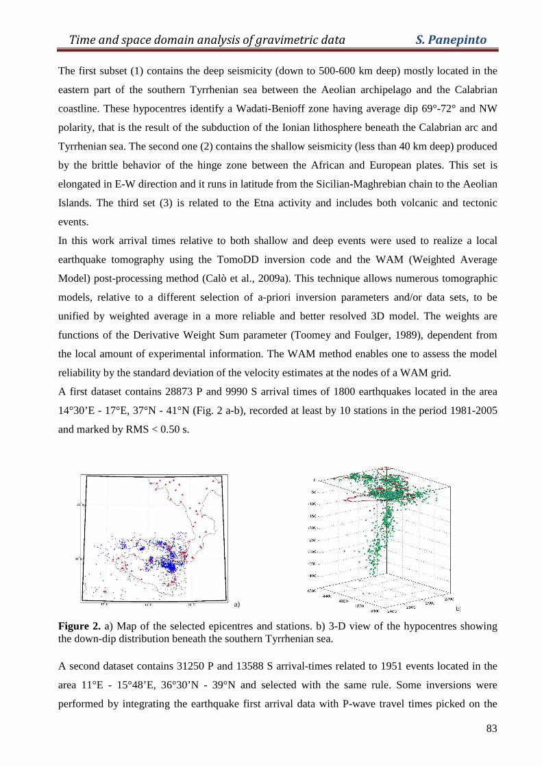
Time and space domain analysis of gravimetric data S. Panepinto
83
The first subset (1) contains the deep seismicity (down to 500-600 km deep) mostly located in the
eastern part of the southern Tyrrhenian sea between the Aeolian archipelago and the Calabrian
coastline. These hypocentres identify a Wadati-Benioff zone having average dip 69°-72° and NW
polarity, that is the result of the subduction of the Ionian lithosphere beneath the Calabrian arc and
Tyrrhenian sea. The second one (2) contains the shallow seismicity (less than 40 km deep) produced
by the brittle behavior of the hinge zone between the African and European plates. This set is
elongated in E-W direction and it runs in latitude from the Sicilian-Maghrebian chain to the Aeolian
Islands. The third set (3) is related to the Etna activity and includes both volcanic and tectonic
events.
In this work arrival times relative to both shallow and deep events were used to realize a local
earthquake tomography using the TomoDD inversion code and the WAM (Weighted Average
Model) post-processing method (Calò et al., 2009a). This technique allows numerous tomographic
models, relative to a different selection of a-priori inversion parameters and/or data sets, to be
unified by weighted average in a more reliable and better resolved 3D model. The weights are
functions of the Derivative Weight Sum parameter (Toomey and Foulger, 1989), dependent from
the local amount of experimental information. The WAM method enables one to assess the model
reliability by the standard deviation of the velocity estimates at the nodes of a WAM grid.
A first dataset contains 28873 P and 9990 S arrival times of 1800 earthquakes located in the area
14°30’E - 17°E, 37°N - 41°N (Fig. 2 a-b), recorded at least by 10 stations in the period 1981-2005
and marked by RMS < 0.50 s.
a)
Figure 2. a) Map of the selected epicentres and stations. b) 3-D view of the hypocentres showing the down-dip distribution beneath the southern Tyrrhenian sea. A second dataset contains 31250 P and 13588 S arrival-times related to 1951 events located in the
area 11°E - 15°48’E, 36°30’N - 39°N and selected with the same rule. Some inversions were
performed by integrating the earthquake first arrival data with P-wave travel times picked on the
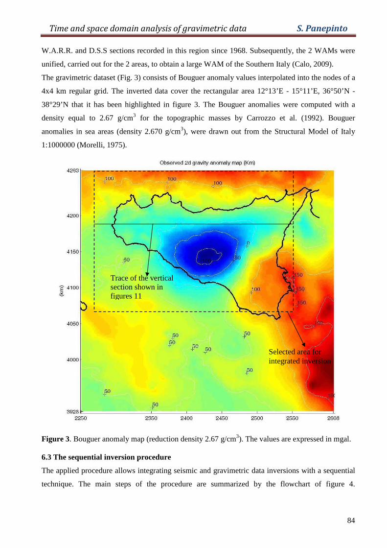
Time and space domain analysis of gravimetric data S. Panepinto
84
W.A.R.R. and D.S.S sections recorded in this region since 1968. Subsequently, the 2 WAMs were
unified, carried out for the 2 areas, to obtain a large WAM of the Southern Italy (Calo, 2009).
The gravimetric dataset (Fig. 3) consists of Bouguer anomaly values interpolated into the nodes of a
4x4 km regular grid. The inverted data cover the rectangular area 12°13’E - 15°11’E, 36°50’N -
38°29’N that it has been highlighted in figure 3. The Bouguer anomalies were computed with a
density equal to 2.67 g/cm3 for the topographic masses by Carrozzo et al. (1992). Bouguer
anomalies in sea areas (density 2.670 g/cm3), were drawn out from the Structural Model of Italy
1:1000000 (Morelli, 1975).
Figure 3. Bouguer anomaly map (reduction density 2.67 g/cm3). The values are expressed in mgal. 6.3 The sequential inversion procedure
The applied procedure allows integrating seismic and gravimetric data inversions with a sequential
technique. The main steps of the procedure are summarized by the flowchart of figure 4.
Selected area for integrated inversion
Trace of the vertical section shown in figures 11
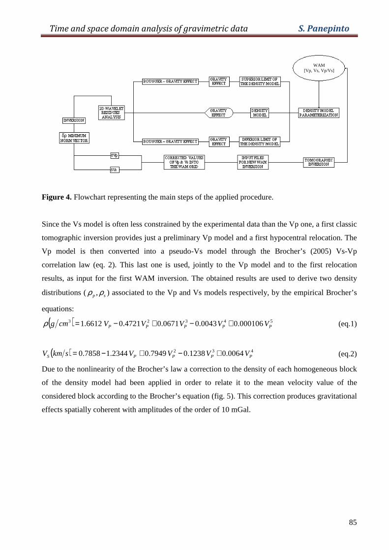
Time and space domain analysis of gravimetric data S. Panepinto
85
Figure 4. Flowchart representing the main steps of the applied procedure.
Since the Vs model is often less constrained by the experimental data than the Vp one, a first classic
tomographic inversion provides just a preliminary Vp model and a first hypocentral relocation. The
Vp model is then converted into a pseudo-Vs model through the Brocher’s (2005) Vs-Vp
correlation law (eq. 2). This last one is used, jointly to the Vp model and to the first relocation
results, as input for the first WAM inversion. The obtained results are used to derive two density
distributions ( sp ρρ , ) associated to the Vp and Vs models respectively, by the empirical Brocher’s
equations:
( ) 54323 000106.00043.00671.04721.06612.1 PPPPP VVVVVcmg +−+−=ρ (eq.1)
( ) 432 0064.01238.07949.02344.17858.0 PPPPS VVVVskmV +−+−= (eq.2)
Due to the nonlinearity of the Brocher’s law a correction to the density of each homogeneous block
of the density model had been applied in order to relate it to the mean velocity value of the
considered block according to the Brocher’s equation (fig. 5). This correction produces gravitational
effects spatially coherent with amplitudes of the order of 10 mGal.
WAM [Vp, Vs, Vp/Vs]
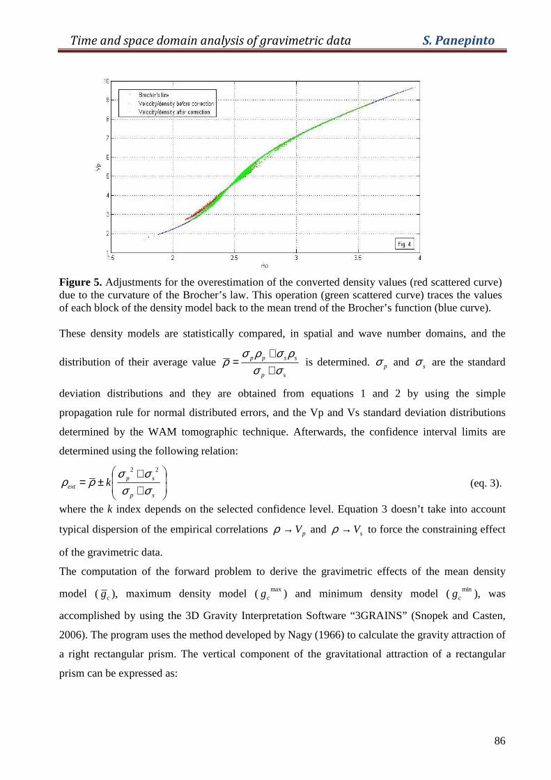
Time and space domain analysis of gravimetric data S. Panepinto
86
Figure 5. Adjustments for the overestimation of the converted density values (red scattered curve) due to the curvature of the Brocher’s law. This operation (green scattered curve) traces the values of each block of the density model back to the mean trend of the Brocher’s function (blue curve). These density models are statistically compared, in spatial and wave number domains, and the
distribution of their average value sp
sspp
σσρσρσ
ρ++
= is determined. pσ and sσ are the standard
deviation distributions and they are obtained from equations 1 and 2 by using the simple
propagation rule for normal distributed errors, and the Vp and Vs standard deviation distributions
determined by the WAM tomographic technique. Afterwards, the confidence interval limits are
determined using the following relation:
++
±=sp
spext k
σσσσ
ρρ22
(eq. 3).
where the k index depends on the selected confidence level. Equation 3 doesn’t take into account
typical dispersion of the empirical correlations pV→ρ and sV→ρ to force the constraining effect
of the gravimetric data.
The computation of the forward problem to derive the gravimetric effects of the mean density
model ( cg ), maximum density model ( maxcg ) and minimum density model (min
cg ), was
accomplished by using the 3D Gravity Interpretation Software “3GRAINS” (Snopek and Casten,
2006). The program uses the method developed by Nagy (1966) to calculate the gravity attraction of
a right rectangular prism. The vertical component of the gravitational attraction of a rectangular
prism can be expressed as:
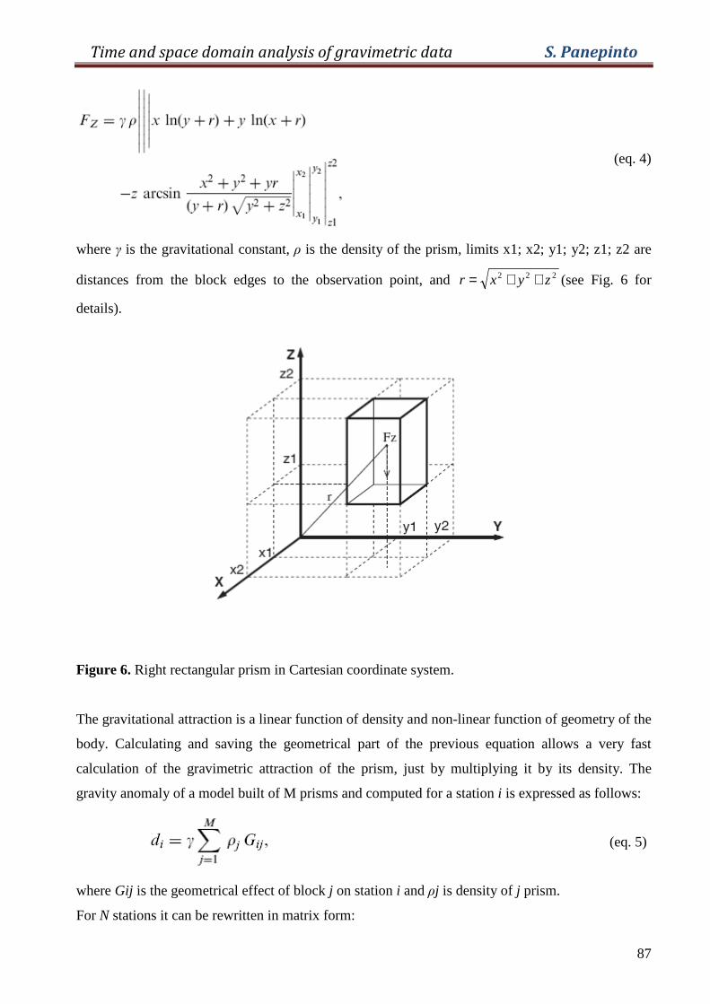
Time and space domain analysis of gravimetric data S. Panepinto
87
(eq. 4)
where γ is the gravitational constant, ρ is the density of the prism, limits x1; x2; y1; y2; z1; z2 are
distances from the block edges to the observation point, and 222 zyxr ++= (see Fig. 6 for
details).
Figure 6. Right rectangular prism in Cartesian coordinate system.
The gravitational attraction is a linear function of density and non-linear function of geometry of the
body. Calculating and saving the geometrical part of the previous equation allows a very fast
calculation of the gravimetric attraction of the prism, just by multiplying it by its density. The
gravity anomaly of a model built of M prisms and computed for a station i is expressed as follows:
(eq. 5)
where Gij is the geometrical effect of block j on station i and ρj is density of j prism.
For N stations it can be rewritten in matrix form:
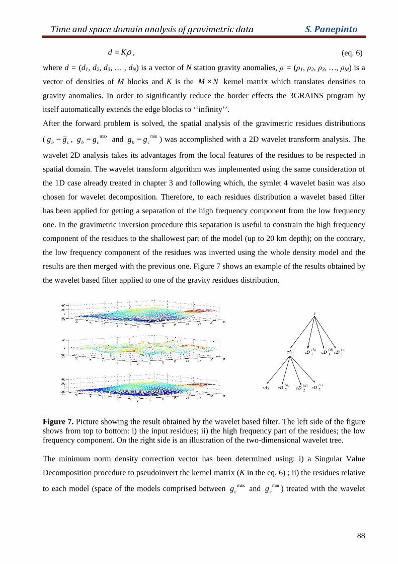
Time and space domain analysis of gravimetric data S. Panepinto
88
ρKd = , (eq. 6)
where d = (d1, d2, d3, … , dN) is a vector of N station gravity anomalies, ρ = (ρ1, ρ2, ρ3, …, ρM) is a
vector of densities of M blocks and K is the NM × kernel matrix which translates densities to
gravity anomalies. In order to significantly reduce the border effects the 3GRAINS program by
itself automatically extends the edge blocks to ‘‘infinity’’.
After the forward problem is solved, the spatial analysis of the gravimetric residues distributions
( cb gg − , maxcb gg − and min
cb gg − ) was accomplished with a 2D wavelet transform analysis. The
wavelet 2D analysis takes its advantages from the local features of the residues to be respected in
spatial domain. The wavelet transform algorithm was implemented using the same consideration of
the 1D case already treated in chapter 3 and following which, the symlet 4 wavelet basin was also
chosen for wavelet decomposition. Therefore, to each residues distribution a wavelet based filter
has been applied for getting a separation of the high frequency component from the low frequency
one. In the gravimetric inversion procedure this separation is useful to constrain the high frequency
component of the residues to the shallowest part of the model (up to 20 km depth); on the contrary,
the low frequency component of the residues was inverted using the whole density model and the
results are then merged with the previous one. Figure 7 shows an example of the results obtained by
the wavelet based filter applied to one of the gravity residues distribution.
Figure 7. Picture showing the result obtained by the wavelet based filter. The left side of the figure shows from top to bottom: i) the input residues; ii) the high frequency part of the residues; the low frequency component. On the right side is an illustration of the two-dimensional wavelet tree. The minimum norm density correction vector has been determined using: i) a Singular Value
Decomposition procedure to pseudoinvert the kernel matrix (K in the eq. 6) ; ii) the residues relative
to each model (space of the models comprised between maxcg and min
cg ) treated with the wavelet
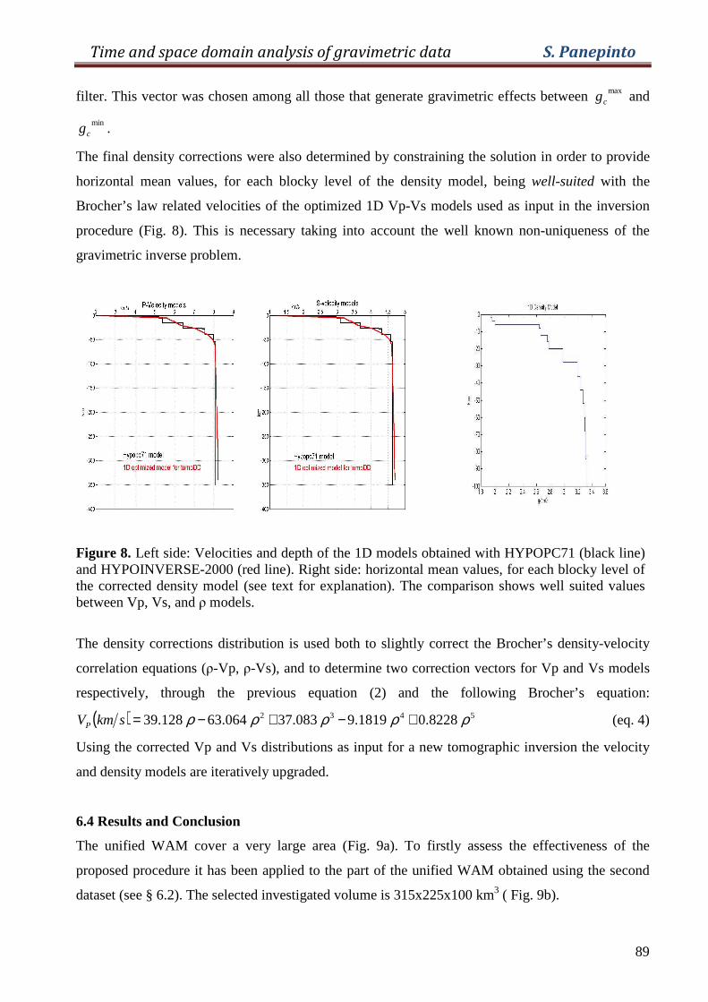
Time and space domain analysis of gravimetric data S. Panepinto
89
filter. This vector was chosen among all those that generate gravimetric effects between maxcg and
mincg .
The final density corrections were also determined by constraining the solution in order to provide
horizontal mean values, for each blocky level of the density model, being well-suited with the
Brocher’s law related velocities of the optimized 1D Vp-Vs models used as input in the inversion
procedure (Fig. 8). This is necessary taking into account the well known non-uniqueness of the
gravimetric inverse problem.
Figure 8. Left side: Velocities and depth of the 1D models obtained with HYPOPC71 (black line) and HYPOINVERSE-2000 (red line). Right side: horizontal mean values, for each blocky level of the corrected density model (see text for explanation). The comparison shows well suited values between Vp, Vs, and ρ models.
The density corrections distribution is used both to slightly correct the Brocher’s density-velocity
correlation equations (ρ-Vp, ρ-Vs), and to determine two correction vectors for Vp and Vs models
respectively, through the previous equation (2) and the following Brocher’s equation:
( ) 5432 8228.01819.9083.37064.63128.39 ρρρρρ +−+−=skmVP (eq. 4)
Using the corrected Vp and Vs distributions as input for a new tomographic inversion the velocity
and density models are iteratively upgraded.
6.4 Results and Conclusion
The unified WAM cover a very large area (Fig. 9a). To firstly assess the effectiveness of the
proposed procedure it has been applied to the part of the unified WAM obtained using the second
dataset (see § 6.2). The selected investigated volume is 315x225x100 km3 ( Fig. 9b).
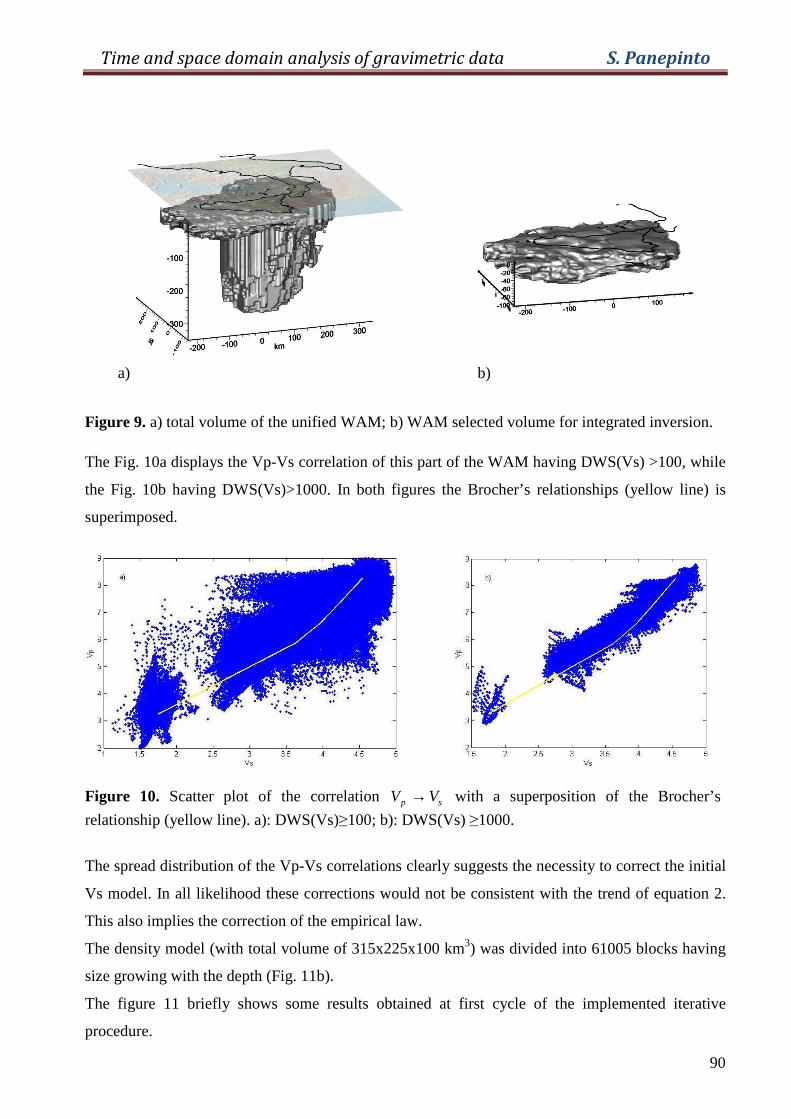
Time and space domain analysis of gravimetric data S. Panepinto
90
Figure 9. a) total volume of the unified WAM; b) WAM selected volume for integrated inversion. The Fig. 10a displays the Vp-Vs correlation of this part of the WAM having DWS(Vs) >100, while
the Fig. 10b having DWS(Vs)>1000. In both figures the Brocher’s relationships (yellow line) is
superimposed.
Figure 10. Scatter plot of the correlation sp VV → with a superposition of the Brocher’s
relationship (yellow line). a): DWS(Vs)≥100; b): DWS(Vs) ≥1000.
The spread distribution of the Vp-Vs correlations clearly suggests the necessity to correct the initial
Vs model. In all likelihood these corrections would not be consistent with the trend of equation 2.
This also implies the correction of the empirical law.
The density model (with total volume of 315x225x100 km3) was divided into 61005 blocks having
size growing with the depth (Fig. 11b).
The figure 11 briefly shows some results obtained at first cycle of the implemented iterative
procedure.
a) b)
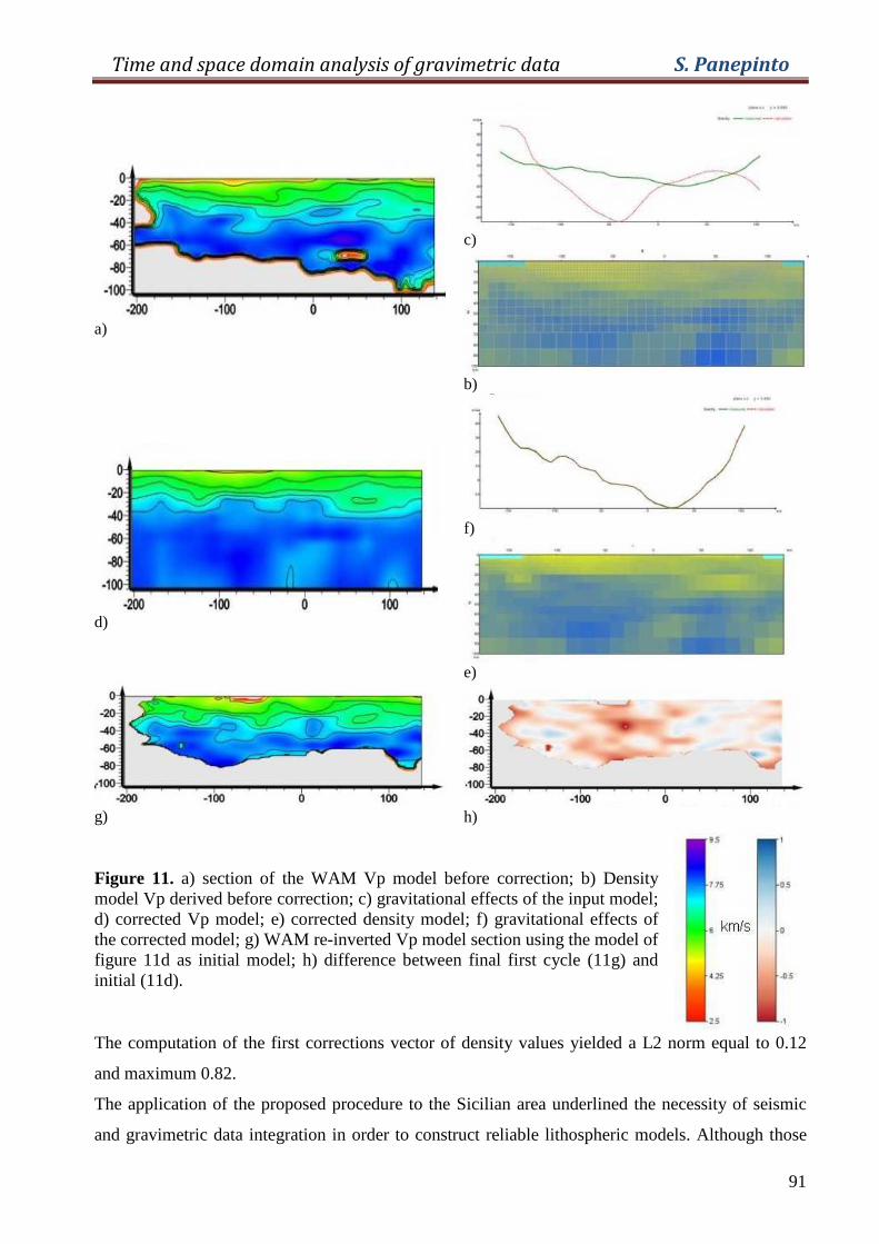
Time and space domain analysis of gravimetric data S. Panepinto
91
a)
c)
b)
d)
f)
e)
g)
h)
Figure 11. a) section of the WAM Vp model before correction; b) Density model Vp derived before correction; c) gravitational effects of the input model; d) corrected Vp model; e) corrected density model; f) gravitational effects of the corrected model; g) WAM re-inverted Vp model section using the model of figure 11d as initial model; h) difference between final first cycle (11g) and initial (11d).
The computation of the first corrections vector of density values yielded a L2 norm equal to 0.12
and maximum 0.82.
The application of the proposed procedure to the Sicilian area underlined the necessity of seismic
and gravimetric data integration in order to construct reliable lithospheric models. Although those
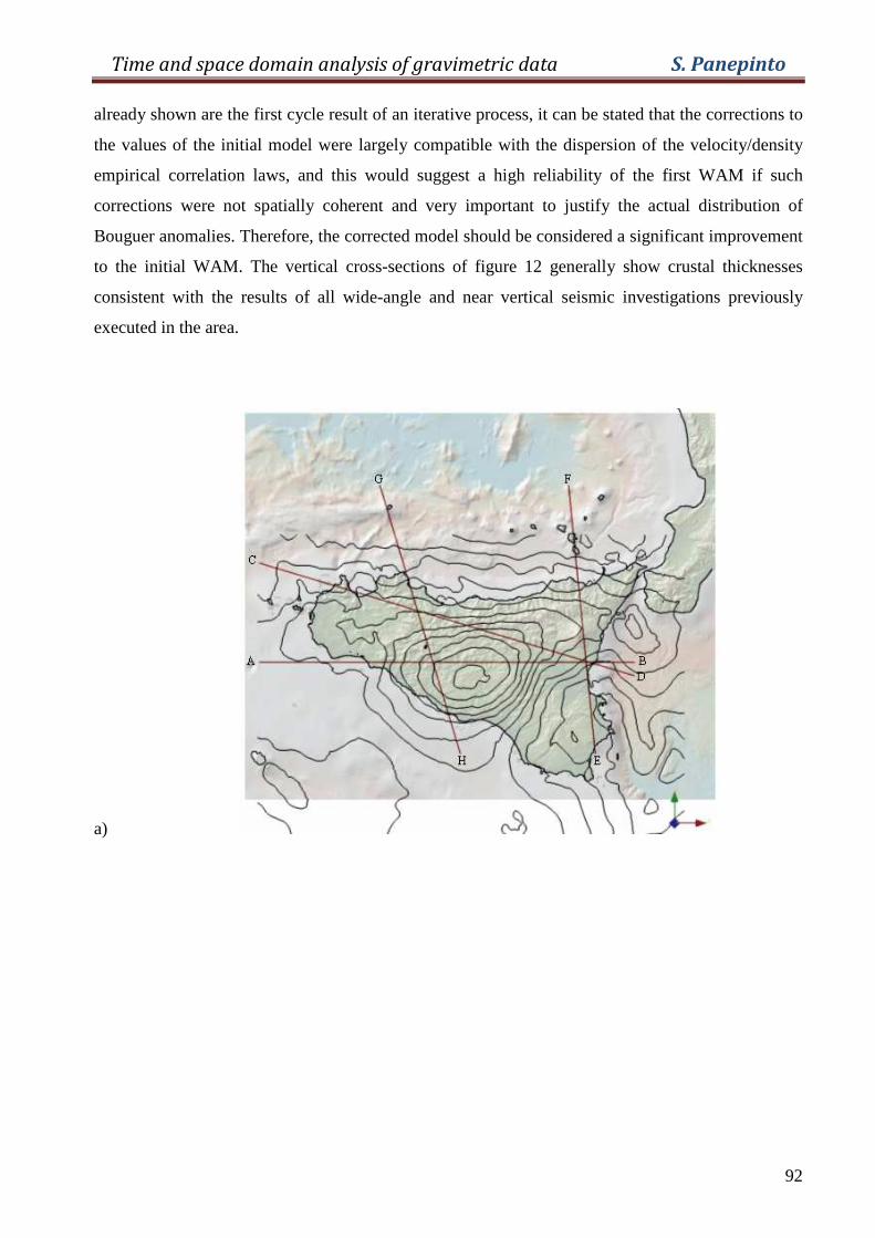
Time and space domain analysis of gravimetric data S. Panepinto
92
already shown are the first cycle result of an iterative process, it can be stated that the corrections to
the values of the initial model were largely compatible with the dispersion of the velocity/density
empirical correlation laws, and this would suggest a high reliability of the first WAM if such
corrections were not spatially coherent and very important to justify the actual distribution of
Bouguer anomalies. Therefore, the corrected model should be considered a significant improvement
to the initial WAM. The vertical cross-sections of figure 12 generally show crustal thicknesses
consistent with the results of all wide-angle and near vertical seismic investigations previously
executed in the area.
a)
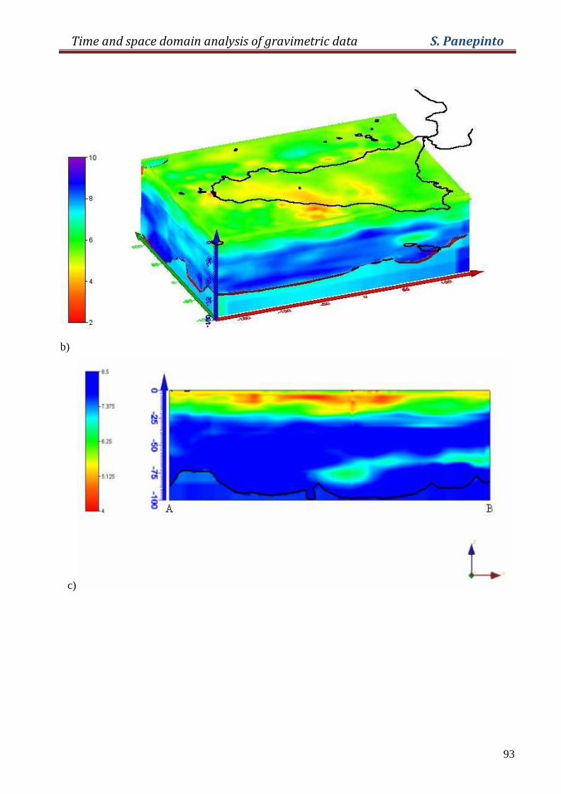
Time and space domain analysis of gravimetric data S. Panepinto
93
b)
c)
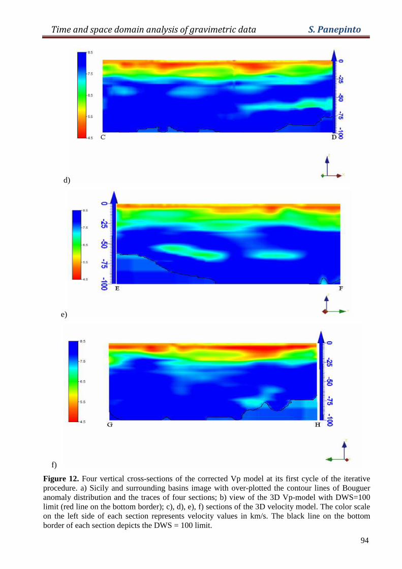
Time and space domain analysis of gravimetric data S. Panepinto
94
d)
e)
f)
Figure 12. Four vertical cross-sections of the corrected Vp model at its first cycle of the iterative procedure. a) Sicily and surrounding basins image with over-plotted the contour lines of Bouguer anomaly distribution and the traces of four sections; b) view of the 3D Vp-model with DWS=100 limit (red line on the bottom border); c), d), e), f) sections of the 3D velocity model. The color scale on the left side of each section represents velocity values in km/s. The black line on the bottom border of each section depicts the DWS = 100 limit.
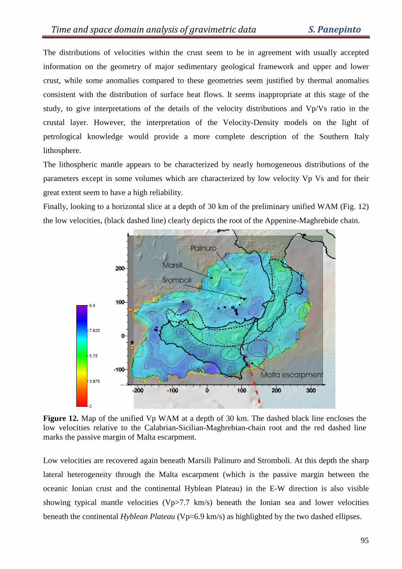
Time and space domain analysis of gravimetric data S. Panepinto
95
The distributions of velocities within the crust seem to be in agreement with usually accepted
information on the geometry of major sedimentary geological framework and upper and lower
crust, while some anomalies compared to these geometries seem justified by thermal anomalies
consistent with the distribution of surface heat flows. It seems inappropriate at this stage of the
study, to give interpretations of the details of the velocity distributions and Vp/Vs ratio in the
crustal layer. However, the interpretation of the Velocity-Density models on the light of
petrological knowledge would provide a more complete description of the Southern Italy
lithosphere.
The lithospheric mantle appears to be characterized by nearly homogeneous distributions of the
parameters except in some volumes which are characterized by low velocity Vp Vs and for their
great extent seem to have a high reliability.
Finally, looking to a horizontal slice at a depth of 30 km of the preliminary unified WAM (Fig. 12)
the low velocities, (black dashed line) clearly depicts the root of the Appenine-Maghrebide chain.
Figure 12. Map of the unified Vp WAM at a depth of 30 km. The dashed black line encloses the low velocities relative to the Calabrian-Sicilian-Maghrebian-chain root and the red dashed line marks the passive margin of Malta escarpment.
Low velocities are recovered again beneath Marsili Palinuro and Stromboli. At this depth the sharp
lateral heterogeneity through the Malta escarpment (which is the passive margin between the
oceanic Ionian crust and the continental Hyblean Plateau) in the E-W direction is also visible
showing typical mantle velocities (Vp>7.7 km/s) beneath the Ionian sea and lower velocities
beneath the continental Hyblean Plateau (Vp≈6.9 km/s) as highlighted by the two dashed ellipses.
Time and space domain analysis of gravimetric data S. Panepinto
96
REFERENCES
Andò, B., and D. Carbone, A Methodology for Reducing the Signal from a Continuously Recording
Gravity Meter for the Effect of Meteorological Parameters, IEEE Transactions on
Instrumentation and Measurement, 50(5), 1248–1254, 2001.
Azzaro, R., S. Branca, S. Giammanco, S. Gurrieri, R. Rasa`, and M. Valenza, New evidence for the
form and extent of the Pernicana Fault System (Mt. Etna) from structural and soil-gas
surveying, J. Vulcanol. Geotherm. Res., 84, 143– 152, 1998.
Azzaro, R., Seismicity and active tectonics along the pernicana fault, Mt. Etna (Italy), Acta
Vulcanol., 9, 7 –14, 1997.
Baker T.F., Bos M.S. (2003) Validating Earth and ocean models using tidal gravity measurements.
Geophys. J. Int., 152, 468-485.
Bartels J, 1938: Random Fluctuations, Persistence and Quasi-persistence in Geophysical and
Cosmical periodicities. Terr. Magn. Atmos. Electricity, 40, 1,60
Becker, K., Fisher, A.T., Davis, E.E., 1997. The CORK experiment in hole 949CC: long-term
observations of pressure and temperature in the Barbados accretionary prism. In: Shipley, T.H.,
Ogawa, Y., Blum, P., Bahr, J.M. (Eds.), Proceedings of the Ocean Drilling Program, Scientific
Results, vol. 156, pp. 247–252.
Behncke B, 2001: Volcanism in the Southern Apennines and Sicily. In: Vai GB and Martini IP (eds)
Anatomy of an orogen: the Apennines and adjacent Mediterranean basins. Kluwer Academic
Publishers, Dordrecht-Boston-London: 105-120 (Etna: pp. 111-113).
Bödvarsson, G., 1977. Interpretation of borehole tides and other elastomechanicaloscillatory
phenomena in geothermal systems. Proceed. 3rd Workshop on Geothermal Reservoir
Engineering, December, 1977. Stanford Univ., Stanford, California (USA), pp. 203–208.
Bonaccorso, A., M. Aloisi, and M. Mattia, Dike emplacement forerunning the Etna July 2001
eruption modelled through continuous tilt and GPS data, Geophys. Res. Lett., 29(13), 2002.
Borgia A., L. Ferrari, G. Pasquarè, Importance of gravitational spreading in the tectonic and
volcanic evolution of Mount Etna, Nature 357 (1992) 231-235.
Borgia, A., L. Ferrari, and G. Pasquare`, Importance of gravitational spreading in the tectonic and
volcanic evolution of Mount Etna, Nature, 357,231– 235, 1992.
Branca, S., and P. Del Carlo, Eruptions of Mt. Etna during the past 3,200 Years: A revised
compilation integrating the historical and stratigraphic records, in Etna Volcano Laboratory,
Geophys. Monogr. Ser., edited by S. Calvari, A. Bonaccorso, M. Coltelli, C. Del Negro, and S.
Falsaperla, AGU, in press, 2003.
Time and space domain analysis of gravimetric data S. Panepinto
97
Bretagnon, P. 1982. Théorie du mouvement de l'ensemble des planètes, solution VSOP82. Astron.
Astrophys. 144: 278 - 288.
Brocher M. T. (2005). Empirical Relations between Elastic Wavespeeds and Density in the Earth’s
Crust. Bulletin of the Seismological Society of America, Vol. 95, No. 6, pp. 2081–2092.
Brown, W.E. 1905. Theory of the motion of the Moon. Mem. Royal Astron. Soc. 57: 136-141.
Budetta G., Carbone D., Greco F. and Hazel R., 2004. Microgravità Studies at Mount Etna (Italy).
American Geophysical Union-Geophysical Monograph Series 143: 221-240.
Budetta G., Carbone D., Greco, F., 2004: Technological improvements in gravity monitoring of
active volcanoes. Quaderni di Geofisica, 35, 103-109.
Budetta, G., and D. Carbone, Temporal variations in gravity at Mt. Etna (Italy) associated with the
1989 and 1991 eruptions, Bull. Volcanol., 59, 311 –326, 1998.
Budetta, G., D. Carbone, and F. Greco, Subsurface mass redistribution at Mount Etna (Italy) during
the 1995– 96 explosive activity detected by microgravity studies, Geophys. J. Int., 138, 77– 88,
1999.
Budetta, G., D. Carbone, F. Greco (2000): Gravity measurements. In “Data Related to Eruptive
Activity, Unrest Phenomena and Other Observations on the Italian Active Volcanoes – 1996”
(L. Villari, Editor). Acta Vulcanologica, 12 (1-2), 86-90.
Büllesfeld, F.-J. 1985. Ein Beitrag zur harmonischen Darstellung des gezeitenerzeu genden
Potentials. Deutsche Geod. Komm. C 314: l - 103.
Caló M., Dorbath C., Luzio D., Rotolo S. G., D'anna G. (2009). Local Earthquake Tomography in
the Southern Tyrrhenian Region of Italy: Geophysical and Petrological Inferences on the
Subducting Lithosphere. Frontiers in Earth Sciences - Subduction Zone Geodynamics - Springer
Berlin Heidelberg, pp. 85-99.
Calò M., Dorbath C., Luzio D., Rotolo S.G., D’Anna G., (2008).Calo’, M. Tomography of
subduction zones using regional earthquakes: methodological developments and application to
the Ionian slab, (2009), [PhD. Thesis], EOST, University of. Strasbourg, p. 1-134. Calvari, S., et
al., The first period of the 2002 Etna eruption (27 October– 5 November): Preliminary results,
Quaderni di Geofisica, in press, 2003.
Camacho, A. G., Fernández J., Charco, M., Tiampo, K. F., Jentzsch, G. (2007): Interpretation of
1992-1994 gravity changes around Mayon volcano, Philippines, using point sources. Pure
appl. Geophys., 733-749, DOI 10.1007/s00024-007-0185-8
Carbone D., Budetta G. and Greco F., 2003a. Possible mechanisms of magma redistribution under
Mt. Etna during 1994-1999 period detected through microgravity measurements. Geophys. J.
Int., 153: 187-200
Time and space domain analysis of gravimetric data S. Panepinto
98
Carbone D., Budetta G., Greco F. and Rymer H., 2003b. Combined discrete and continuous gravity
observations at Mt. Etna. J. Volcanol. Geotherm. Res., 123:123-135
Carbone D., Budetta G., Greco F. and Rymer H., 2003b: Combined discrete and continuous gravity
observations at Mt. Etna. J. Volcanol. Geotherm. Res., 123:123-135
Carbone, D., G. Budetta, and F. Greco, Possible mechanisms of magma redistribution under Mt.
Etna during the 1994 – 1999 period detected through microgravity measurements, Geophys. J.
Int., 153, 187 – 200, 2003a.
Carbone, D., G. Budetta, F. Greco and H. Rymer (2003). Combined discrete and continuous gravity
observations at Mt. Etna. Journal Volcanol. Geotherm. Res., 123, 123-135.
Carbone, D., G. Budetta, F. Greco, and H. Rymer, Combined discrete and continuous gravity
observations at Mount Etna, J. Volcanol. Geotherm. Res., 123, 123– 135, 2003b.
Carbone, D., Greco F. (2007): Review of microgravity observations at Mt. Etna: a powerful tool to
monitor and study active volcanoes. Pure appl. Geophys., 769-790, DOI 10.1007/s00024-007
- 0194-7
Carrigan, C. R., Plumbing systems, in Encyclopedia of Volcanoes, Academic, 219–235, 2000.
Carrozzo M.T., R. de Franco, L. De Luca, D. Luzio, R. Primiceri, T. Quarta and M. Vitale. Wavelet
correlation filter for wide-angle seismic data. Geophysical Prospecting, 2002, 50, 547-564
Cartwright, D.E. and C.A. Edden. 1973. Corrected Tables of Tidal Harmonics. Geophys. J. R. astr.
Soc. 33: 253 - 264.
Cartwright, D.E. and R.J. Tayler. 1971. New Computations of the Tide Generating Potential.
Geophys. J. R. astr. Soc. 23: 45 - 74.
Cermak V., Bodri L. , Safanda J., 2009. Tidal modulation of temperature oscillations monitored in
borehole Yaxcopoil-1 (Yucatán, Mexico). Earth and Planetary Science Letters 282 (2009) 131–
139.
Chapront-Touzé, M. and J. Chapront. 1988. ELP-2000-85: A semi-analytical lunar ephemeris
adequate for historical times. Astron. Astrophy.. 190: 342 - 352.
Chester, D. K., A. M. Duncan, J. E. Guest, C. R. J. Kilburn, 1985: Mount Etna: the anatomy of a
volcano, 404 pp., Chapman and Hall, London.
Coifman R.R. and Wickerhauser M.V. 1993. Wavelets and adapted waveform analysis. A toolkit
for signal processing and numerical analysis. Proceedings of Symposia in Applied
Mathematics 47, 119-145.
Continisio R, Ferrucci F, Gaudiosi G, Lo Bascio D and Ventura G., 1997: Malta escarpment and
Mt. Etna: early stages of an asymmetric rifting process? Evidences from geophysical and
geological data. Acta Vulcanologica 9: 45-53.
Time and space domain analysis of gravimetric data S. Panepinto
99
Cristofolini R., F. Lentini, G. Patanè, R. Rasà, Integrazione di dati geologici, geofisici e petrologici
per la stesura di un profilo crostale in corrispondenza dell'Etna, Boll. Soc. Geol. It. 98 (1979)
239-247.
Crossley, D., Hinderer, J., Casula G., Francis O., Hsu, H.T., Imanishi, Y., Jentzsch G., Kääriäinen
J., Merriam, J., Meurers B., Neumeyer J., Richter B., Shibuya K., Sato T., Van Dam T.
(1999) Network of superconducting gravimeters benefits a number of disciplines. EOS, 80,
11, 121/125-126.
Curchin, J.M. and W.D. Pennington. 1987. Tidal triggering of intermediate and deep focus
earthquakes. J.geophys. Res. 92: 13957-13967.
Dahlen, F.A. 1993. Effect of the Earth's ellipticity on the lunar potential. Geophys. J. Int. 113: 250 -
251.
Darwin, G.H. 1883. Report of a committee for the harmonic analysis of tidal observations. Brit. Ass.
Rep.: 48 - 118.
Daubechies I. 1992. Ten Lectures on Wavelets. Society for Industrial and Applied Mathematics.
Davis, E.E., Becker, K., 1994. Formation temperatures and pressures in a sedimented rift
hydrothermal system: 10 months of CORK observations, Holes 857D and 858G.Proceedings of
the Ocean Drilling Program, Scientific Results, vol. 139, pp. 649–666.
Davis, E.E., Becker, K.,Wang, K., Carson, B., 1995. Long term observations of pressure and
temperature in hole 892B, Cascadia accretionary prism. Proceed. of the Ocean Drilling
Program, Scientific Results, vol. 146, pp. 299–311.
Dehant, V., P. Defraigne, and J. Wahr (1999): Tides for a convective Earth. Journal Geophys. Res.,
104, B1, 1035-1058.
Deighan A.J. and Watts D.R. 1997. Ground roll suppression using the wavelet ttansform.
Geophysics 62, 1896-1903.
Di Geronimo I, Ghisetti F, Lentini F and Vezzani L., 1978: Lineamenti neotettonici della Sicilia
orientale. Memorie della Società Geologica Italiana 19: 543-549.
Doglioni C, Innocenti F and Mariotti G., 2001: Why Mt Etna? Terra Nova 13: 25-31.
Doodson, A.T. 1921. The harmonic development of the tide generating potential. Proc. Royal Soc.
London A 100: 306 - 328. Reprint in Int. Hydrogr. Rev. 31.
Ducarme B., Sun H. P., Xu J. Q., 2006. Determination of the free core nutation period from tidal
gravity observations of the GGP superconducting gravimeter network. Journal of Geodesy,
81, 179-187, DOI: 10.1007/s00190-006-0098-9.
Ducarme, B. (1970) Sensitivity smoothing before the analysis of tidal data. Bull. Inf. Marées
Terrestres, 81, 4962-4981.
Time and space domain analysis of gravimetric data S. Panepinto
100
Ducarme, B., A.P. Venedikov, J. Arnoso and R. Vieira (2004). Determination of the long period
tidal waves in the GGP superconducting gravity data. Journal of Geodynamics, 38, 307-324.
Ducarme, B., Somerhausen, A. (1997). Tidal gravity recording at Brussels with a SCINTREX CG3-
M gravimeter. Bull. Inf. Marées Terrestres, 126, 9611-9634
Eanes, R. and S. Bettadpur (1996): The CSR3.0 global ocean tide model: Diurnal and Semi-diurnal
ocean tides from TOPEX/POSEIDON altimetry, CRS-TM-96-05, Univ. of Texas, Centre for
Space Research, Austin, Texas.
El Wahabi A., Ducarme B., Van Ruymbeke M., d’Oreyè N. and Somerhausen A., 1997. Continuous
gravity observations at Mt. Etna (Sicily) and Correlations between temperature and
gravimetric records. Cahiers du Centre Européen de Géodynamique et de Séismologie, 14:
105-119.
El Wahabi A., Ducarme B., Van Ruymbeke M., d’Oreyè N. and Somerhausen A., 1997: Continuous
gravity observations at Mt. Etna (Sicily) and Correlations between temperature and gravimetric
records. Cahiers du Centre Européen de Géodynamique et de Séismologie, 14: 105-119.
El Wahabi, A., B. Ducarme, M. van Ruymbeke, N. d’Oreyè and A. Somerhausen (1997):
Continuous gravity observations at Mt. Etna (Sicily) and Correlations between temperature
and gravimetric records. Cahiers du Centre Européen de Géodynamique et de Séismologie,
14, 105-119.
El Wahabi, A., Ducarme, B., van Ruymbeke, M. (2001): Humidity and temperature effects on
LaCoste & Romberg gravimeters. Proc. 14th Int. Symp. On Earth Tides, J. Geodetic Soc. of
Japan47, 1, 10-15.
Emter D., Zürn W., Schick R., Lombardo G., 1986: Search for Tidal Effects on Volcanic Activities
at Mt. Etna and Stromboli. Proc. Tenth Int. Symp. on Earth Tides, Madrid, September 23-27,
1985. R. Vieira ed., Consejo Superior Investigaciones Cientificas, Madrid, 765-774
Esipko, O.A., Rosaev, A.E., 2007. The temperature monitoring in Vorotilovo deep well and global
climate warming. Geophys. Res. Abstr. 9, 00533.
Facca, G., 1964: Studi geotermici sull’Etna. Rivista Mineraria Siciliana, 85-87, 66-75.
Farrell, W.E. (1972): Deformation of the Earth by surface load. Rev. Geophys., 10, 761-779.
Fedi M. and Quatta T. 1998. Wavelet analysis for the regional residual and local separation of the
potential field anomalies. Geophysical Prospecting 46, 507-525.
Ferrara V., 1975: Idrogeologia del versante orientale dell'Etna, in: Proc. of the 3rd Intern. Conf. on
Groundwaters, 91-144.
Ferrara, V., 1990: Carta della vulnerabilità all'inquinamento dell'acquifero vulcanico dell'Etna,
C.N.R. Valutazione della Vulnerabilità degli Acquiferi, S.E.L.C.A. Firenze.
Time and space domain analysis of gravimetric data S. Panepinto
101
Ferrari, L., V. H. Gardun˜o, and M. Neri, I dicchi della Valle del Bove, Etna: Un metodo per
stimare le dilatazioni di un apparato vulcanico, Mem. Soc. Geol. It., 47, 495– 508, 1993.
Foufoula-Georgiou E. and Kumar P. 1994. Wavelets in Geophysics. Academic Press, Inc.
Gasparini C., G. Iannaccone, P. Scandone, R. Scarpa, Seismotectonics of the Calabrian Arc,
Tectonophysiscs 84 (1982) 267-286.
Gillot PY, Kieffer G and Romano R., 1994: The evolution of Mount Etna in the light of potassium-
argon dating. Acta Vulcanologica 5: 81-87.
Glasby G. P., Kasahara J. (2001). Influence of tidal effects on periodicity of earthquake activity in
diverse geological settings with particular emphasis on submarine hydrotermal systems. Earth
Science Reviews 52 (2001) 261- 297
Greco F, Budetta G, Carbone D, Panepinto S, Luzio D. (2007). The Application of a Denoising
Method Aimed at Reducing Continuous Gravity Data. COMMUNICATIONS TO SIMAI
CONGRESS, vol. 2; 1-10, ISSN: 1827-9015, doi: 10.1685/CSC06091.
Grubb H.]. and Walden A.T. 1997. Characterizing seismic time series using the discrete wavelet
transform. Geophysical Prospecting 45, 183-205.
Gvirtzman Z and Nur A., 1999: The formation of Mount Etna as the consequence of slab rollback.
Nature 401: 782-785.
Hardee H.C. (1982). Permeable convection above magma bodies. Tectonophysics, 84 (1982) 179-
195
Hartmann, T. and H.-G. Wenzel. 1994a. Catalogue of the earth tide generating potential due to the
planets. Bull. Inf. Marées. Terrestres. 119: 8847 - 8880.
Hartmann, T. and H.-G. Wenzel. 1994b. The harmonic development of the earth tide generating
potential due to the direct effects of the planets. Geophys. Res. Lett. 21: 1991 - 1993.
Hartmann, T. and H.-G. Wenzel. 1995a. The HW95 ti dal potential catalogue. Geophys. Res. Lett.
22: 3553 - 3556.
Hartmann, T. and H.-G. Wenzel. 1995b. Catalogue HW95 of the tide generating potential. Bull. Inf.
Marées Terrestres. 123: 9278 - 9301.
Heiskanen, W.A. and H. Moritz. 1967. Physical geodesy. W.H. Freeman and Co., San Francisco.
Ilk, K.H. 1983. Ein Beitrag zur Dynamik ausgedehnter Körper – Gravitationswechselwirkung.
Deutsche Geod. Komm., C 288.
Kangieser, E., Torge, W. (1981). Calibration of LaCoste-Romberg gravity meters, Model G and D.
Bull. Inf. Bur. Grav. Int., 49,50-63.
Time and space domain analysis of gravimetric data S. Panepinto
102
Kieffer G., L'évolution structurale de l'Etna (Sicile) et les modalités du contrôle tectonique et
volcano-tectonique de son activité, faits et hypothèses après l'éruption de 1978^ 1979, Rev.
Geol. Dyn. Geogr. Phys. 24 (1983) 129-152.
Kieffer, G., Sur l’existence d’une ‘‘Rift zone’’ a` L’Etna, C. R. Acad. Sci. Paris D, 280, 236– 266,
1975.
Kilburn, R. J., and R. Lopes, The growth of Aa lava flow fields on Mount Etna, Sicily, J. Geophys.
Res., 93, 14,759– 14,772, 1988.
Klein, F. W., Eruption Forecasting at Kilauea Volcano, Hawaii, J. Geophys. Res., 89, 30593073,
1984.
LaCoste and Romberg, Instruction Manual, Model G and D Gravity Meter, Austin, Texas, 1997.
Lanzafame G, Neri M, Coltelli M, Lodato L and Rust D., 1997: North-south compression in the Mt.
Etna region (Sicily): spatial and temporal distribution. Acta Vulcanologica 9: 121-133.
Lanzafame G., M. Neri, M. Coltelli, L. Lodato, D. Rust, North-South compression in the Mt. Etna
region (Sicily): spatial and temporal distribution, Acta Vulcanol. 9 (1997) 121-133
Lardy M. & Tabbagh A. (1999) Measuring and interpreting heat fluxes from shallow volcanic
bodies using vertical temperature profiles: a preliminary test. Bulletin of Volcanology, 60: 441-
447
Le Provost, C., M.L. Genco, F. Lyard, P. Vincent and P. Canceil (1994): Spectroscopy of the ocean
tides from a finite element hydrodynamic model. Journal of Geoph. Res., 99 (C12), 24777-
24797.
Lo Giudice E., G. Patanè, R. Rasà, R. Romano, The structural framework of Mt. Etna, Mem. Soc.
Geol. It. 23 (1982) 125-158.
Lo Giudice E., Rasà R., Very shallow earthquakes and brittle deformation in active volcanic areas:
the Etnean region as example, Tectonophysics 202 (1992) 257-268.
Lo Giudice, E., and R. Rasa`, Very shallow earthquakes and brittle deformation in active volcanic
areas: The Etnean region as an example, Tectonophysics, 202, 257– 268, 1992.
Mallat S. 1992. Multiresolution approximation and wavelets. Transactions of the American
Mathematical Society 315, 69-88.
Mallat S. 1999. A Wavelet Tour of Signal Processing. Academic Press, Inc.
Matsumoto K, Ooe M, Sato T et al. (1995) Ocean tides model obtained from TOPEX/POSEIDON
altimeter data. J. Geophys. Res., 100, 25319-25330.
Matsumoto, K., T. Takanezawa and M. Ooe (2000): Ocean tide models developed by assimilating
TOPEX/POSEIDON altimeter data into hydrodynamical model: a global model and a regional
model around Japan. Journal.Oceanography, 56, 567-581
Time and space domain analysis of gravimetric data S. Panepinto
103
McGuire W.J., I.S. Stewart, S.J. Saunders, Intra-volcanic rifting at Mount Etna in the context of
regional tectonics, Acta Vulcanol. 9 (1997) 147-156.
McGuire WJ, Stewart IS and Saunders SJ., 1997: Intra-volcanic rifting at Mount Etna in the context
of regional tectonics. Acta Vulcanologica 9: 147-156.
McNutt, S.R., and Beavan, R.J., Volcanic earthquakes at Pavlof Volcano correlated with the solid
earth tide, Nature, v. 294, no. 5842, pp. 515-618, 1981.
Melchior, P (1994): A new data bank for tidal gravity measurements (DB92). Physics Earth Planet.
Interiors, 82, 125-155.
Melchior, P. (1978): The tides of the planet Earth. Pergamon Press, 609.
Melchior, P., M. Moens and B. Ducarme (1980): Computations of tidal gravity loading and
attraction effects. Bull. Inf. Marées Terrestres, 4, 5, 95-133.
Merriam, J.B. 1993. A comparison of recent tidal catalogues. Bull. Inf. Marée. Terrestres 115: 8515
- 8535.
Meyer Y. 1993. Wavelets Algorithms mid Applications. Society for Industrial and Applied
Mathematics.
Minett, S. T., and S. C. Scott, 1985: Theoretical considerations of heat flux on Mount Etna, Sicily,
J. Volcanol. Geotherm. Res., 25, 53-67.
Monaco C, Tapponnier P, Tortorici L and Gillot PY (1997): Late Quaternary slip rates on the
Acireale-Piedimonte normal faults and tectonic origin of Mt. Etna (Sicily). Earth and Planetary
Science Letters 147: 125-139.
Nagy, D., 1966. The gravitational attraction of a righ rectangular prism. Geophysics 31, 362–371.
Neri G., D. Caccamo, O. Cocina, A. Montalto, Geodynamic implications of earthquake data in the
southern Tyrrenian sea, Tectonophysics 258 (1996) 233-249.
Nettleton, L. L., Gravity and magnetics in oil prospecting, McGraw-Hill, 1976.
Newcomb, S. 1897. A new determination of precessional constant with the resulting precessional
motions. Astron. Papers Am. Ephemeris VIII, Part l, Washington.
Ogniben, L., 1966: Lineamenti idrogeologici dell'Etna, Rivista Mineraria Siciliana, 100-102, 1-24.
Panepinto, S., F. Greco, D. Luzio and B. Ducarme (2006): An overview on wavelet multi-resolution
decomposition compared with traditional frequency domain filtering for continuous gravity
data denoising. Bull. Inf. Marées Terrestres, 141, 11213-11223.
Panepinto S, Calò M, Dorbath C, D’alessandro A, D’anna G, Luzio D. (2009). Sequential
Technique For Joint Inversion Of Gravimetric And Seismic Data Applied To The Sicilian Area.
GNGTS, vol. 28°, pp. 184-187.
Time and space domain analysis of gravimetric data S. Panepinto
104
Panepinto S, Greco F, Ducarme B, Luzio D. (2008). Tidal Gravity Observations at Mt. Etna and
Stromboli: results concerning the modeled and observed tidal factors. Annals of Geophysics,
vol. 51, n. 1.
Patanè G., A. Montalto, S. Imposa, S. Menza, The role of regional tectonics, magma pressure, and
gravitational spreading in earthquakes of the eastern sector of Mount Etna volcano (Italy), J.
Volcanol. Geotherm. Res. 61 (1994) 253-266.
Patanè G., Frasca A., Agodi A. and S. Imposa (1994): Earth tides and etnean volcanic eruptions: an
attempt of correlation between the two phenomena during the 1983, 1985 and 1986 eruptions.
Physics of the Earth and Planetary Interior, 87, 123-135.
Percival D. B. and Walden A. T. 2002. Wavelet methods for time series analysis. Cambridge
University Press
Ray, R.D. (1999): A global ocean tide model from TOPEX/POSEIDON altimetry: GOT99. NASA
Tech. Mem. 209478, Goddard Space Flight Centre, Greenbelt, MD, USA
Romano, R., and C. Sturiale, The historical eruptions of Mt. Etna (Volcanological data), Mem. Soc.
Geol. It., 23, 75–97, 1982.
Roosbeek, F. 1996. RATGP95: A harmonic development of the tide generating potential using an
analytical method. Geophys. J. Int. 126: 197 - 204.
Rosaev, A.E., Esipko, O.A., 2003. Lithospheric tidal effects from observations in deep wells.
Celestial Mechanics and Dynamical Astronomy 87, 203–207.
Rymer, H., Microgravity changes as a precursor to volcanic activity, J. Volcanol. Geotherm. Res.,
87, 141– 149, 1994.
Schilirò, F., 1988: Proposta metodologica per una zonazione geologico-tecnica del centro abitato
di Maletto, Geologia Tecnica, 3/88, 32-53.
Schwiderski, E.W. (1980): Ocean Tides I, Global ocean tidal equations. Marine Geodesy, 3, 161-
217.
Shum, C.K., P.L. Woodworth, O.B. Andersen, G. Egbert, O. Francis, C. King, S. Klosko, C. Le
Provost, X. Li, J.M. Molines, M. Parke, R. Ray, M. Schlax, D. Stammer, C. Temey, P.
Vincent and C. Wunsch (1997): Accuracy assessment of recent ocean tide models. Journal of
Geophysical Research, 102 (C11), 25, 173-25, 194.
Simon, J.L., P. Bretagnon, J. Chapront, M. Chapront-Touzé, G. Francou and J. Laskar. 1994.
Numerical expression for precession formulae and mean elements for the Moon and the
planets. Astron. Astrophys. 282: 663 - 683.
Snopek, K., Casten, U. (2006) 3GRAINS: 3D Gravity Interpretation Software and its application to
density modeling of the Hellenic Subduction Zone, Computers & Geosciences, 32, 592-
Time and space domain analysis of gravimetric data S. Panepinto
105
603.Standish, E.M. and J.G. Williams. 1981. Planetary and lunar ephemerides DE200 / LE200
(magnetic tape).
Standish, E.M., X.X. Newhall, J.G. Williams and W.F. Folkner. 1995. JPL planetary and lunra
ephemerides DE403/LE403. Jet Propulsion Laboratory, Inter Office Memorandum 314.10-
127, Pasadena.
Sun, H., Koch, M., Markoe, A., 2006. Tidally induced changes of fluid pressure, geothermal
temperature and rock seismicity. Proceed.of the 7th Int.Conf. on HydroScience and
Engineering, Philadelphia, USA, Sept.10–13, 2006 (ICHE 2006). ISBN: 0977447405, pp. 1–18.
Tabbagh A., Trezeguet D., (1987). Determination of sensible heat flux in volcanic areas from
ground temperature measurements along vertical profiles: the case study of Mount Etna (Sicily,
Italy). Journal of Geophysical Research, Vol., 92, NO. B5, 3635-3644
Tamura, Y. 1987. A harmonic development of the tide-generating potential. Bull. Inf. Marées
Terrestres 99: 6813 - 6855.
Tamura, Y. 1993. Additional terms to the tidal harmonic tables. Proc. 12th Int. Symp. Earth Tides
pp. 345 - 350. H.-T. Hsu (ed.). Science Press, Beijing.
Tanguy J-C, Condomines M and Kieffer G (1997): Evolution of the Mount Etna magma:
Constraints on the present feeding system and eruptive mechanism. Journal of Volcanology and
Geothermal Research 75: 221-250.
Timmen, L., Wenzel H.-G. (1994). Improved gravimetric Earth tide parameters for station
Hannover. Bull. Inf. Marées Terrestres, 119, 8834-8846.
Tolstoy, M., Vermon, F.L., Orcutt, J.A., Wyatt, F.K., 2002. Breathing of the seafloor: tidal
correlations of seismicity at Axial volcano. Geology 30, 503–506.
Tortorici L., C. Monaco, C. Tansi, O. Cocina, Recent and active tectonics in the Calabrian arc
(Southern Italy), Tectonophysics 243 (1995) 37-55.
Vai G.B. & Martini P. (2001): Anatomy of orogen. Kluwer Academic Publishers
Van Camp, M. and P. Vauterin (2005): Tsoft: graphical and interactive software for the analysis of
time series and Earth tides. Computer & Geosciences, 31, 631-640.
van Ruymbeke M., Beauducel Fr., Somerhausen A. , 2001: The Environmental Data Acquisition
System (EDAS) developed at the Royal Observatory of Belgium. Journal of the Geodetic Society
of Japan, 47, 1,41-46
van Ruymbeke M., R. Howard, E. Pütz, Fr. Beauducel, A. Somerhausen and J-P. Barriot, 2003: An
Introduction to the use of HICUM for signal Analysis.
Time and space domain analysis of gravimetric data S. Panepinto
106
van Ruymbeke, M. (1998): Internal precision of the calibration for the LaCoste & Romberg
gravimeters equipped with a feedback system. Proc. of the XIIIth Int. Symp.on Earth Tides,
Brussels, July 22-25, 1997, 59-68.
Warburton R. J. and Goodkind J. M., 1997. The influence of barometric-pressure variations on
gravity. Geophys. J. R. Astron. Soc., 48: 281-292.
Warburton R. J. and Goodkind J. M., 1997: The influence of barometric-pressure variations on
gravity. Geophys. J. R. Astron. Soc., 48: 281-292.
Warburton, R. J. and J. M. Goodkind (1977): The influence of barometric-pressure variations on
gravity. Geophys. J. R. Astron. Soc., 48, 281-292.
Wenzel, H. G., Earth tide data processing package ETERNA 3.30: the nanoGal software, In:
Ducarme B and Paquet P ed., Proc. 13th Int. Sympos. Earth Tides, Brussels, 487–494, 1998.
Wenzel, H. G., The nanogal software: Earth tide data processing package ETERNA 3.30, Bull. Inf.
Marees Terrestres, 124, 9425–9439, 1996.
Wenzel, H. G., Zürn, W., Baker, T. F., (1991). In situ calibration of LaCoste-Romberg Earth Tide
Gravity meter ET19 at BFO Schiltach. Bull. Inf. Marées Terrestres, 109, 7849-7883.
Wenzel, H.G. (1994): Earth tide analysis package ETERNA 3.0. Bulletin d’Informations des
Marées Terrestres, 118, 8719-8721.
Wenzel, H.-G. 1974. The conection of the tidal force development to the ellipsoidal normal. Bull.
Inf. Marées Terrestres 68: 3748 - 3790.
Wenzel, H.-G. 1976. Zur Genauigkeit von gravimetrischen Erdgezeitenbeobachtungen. Wiss.
Arbeiten d. Lehrstühle Geodäsie, Photogrammetrie u. Kartographie Techn. Univ. Hannover
67: 1 - 177.
Wenzel, H.-G. 1985. Hochauflösende Kugelfunktionsmodelle für das Gravitationspotential der
Erde. Wiss. Arbeiten Fachr. Vermessungswesen Univ. Hannover 137: 1 - 154. Hannover.
Wenzel, H.-G. 1996a. Accuracy assessment for tidal potential catalogues. Bull. Inf. Marées
Terrestres 124: 9394 - 9416.
Wilhelm, H. 1982. Earth's flattening effects on the tidal forcing field. J. Geophysics, 1983: 131 -
135.
Wilhelm, H. and W. Zürn. 1984. Tides of the Earth. In: Landolt-Börnstein, Neue Serie V/2a 2.5.2:
259 - 279. H. Soffel, K. Fuchs (eds.), Springer, Berlin.
Xi, Q. 1993. On the comparison of the new developments of the tidal generating potential. Bull. Inf.
Marées Terrestres 115: 8439 - 8445.
Xi, Q. 1987. A new complete development of the tide-generating potential for the epoch J2000.
Bull. Inf. Marées Terrestres 99: 6766 - 6812.
Time and space domain analysis of gravimetric data S. Panepinto
107
Xi, Q. 1989. The precision of the development of the tidal generating and some explanatory notes.
Bull. Inf. Marées Terrestres 105: 7396 - 7404.
Zahran, K.H. (2000): Accuracy assessment of Ocean Tide loading computations for precise
geodetic observations. PhD thesis, Universität Hannover.
Zlotnicki J., Nishida Y., 2003: Review on Morphological Insights of Self-Potential Anomalies on
Volcanoes. Surveys in Geophysics, Volume 24, Number 4, 200307, pp. 291-338(48).
Zürn W., Rydelek P.A., 1994: Revisiting the phasor-walkout method for detailed investigation of
Harmonic Signals in Time Series. Surveys in Geophysics, 15, 409-431