Universal edge transport in interacting Hall systems

Giovanni Antinucci1, Vieri Mastropietro2, and Marcello Porta∗1

1University of Zurich, Institute for Mathematics, Winterthurerstrasse 190, 8057 Zurich,Switzerland

2University of Milano, Department of Mathematics “F. Enriquez”, Via C. Saldini 50,20133 Milano, Italy

May 18, 2018

Abstract

We study the edge transport properties of 2d interacting Hall systems, displaying single-mode chiral edge currents. For this class of many-body lattice models, including for instancethe interacting Haldane model, we prove the quantization of the edge charge conductanceand the bulk-edge correspondence. Instead, the edge Drude weight and the edge susceptibil-ity are interaction-dependent; nevertheless, they satisfy exact universal scaling relations, inagreement with the chiral Luttinger liquid theory. Moreover, charge and spin excitations dif-fer in their velocities, giving rise to the spin-charge separation phenomenon. The analysis isbased on exact renormalization group methods, and on a combination of lattice and emergentWard identities. The invariance of the emergent chiral anomaly under the renormalizationgroup flow plays a crucial role in the proof.

1 Introduction

It is a recent discovery that insulating systems, in the single-particle approximation, admit atopological classification. Hamiltonians labeled by different topological invariants cannot becontinuously connected without destroying their insulating features or breaking their basic sym-metry properties. The very first examples of topological insulators are the integer quantumHall systems: there, the topological invariant is the bulk Hall conductivity, which can onlytake integer values [43, 53]. The simplest example of Hall system is the Haldane model [32], agraphene-like system describing fermions on the honeycomb lattice exposed to a suitable zero-flux magnetic field.

While insulating in the bulk, Hall insulators support edge currents, [34]; see [14] for a com-prehensive theoretical and experimental review. Bulk and edge transport properties are relatedby a remarkable duality, the bulk-edge correspondence, stating the equality of edge conductanceand bulk conductivity. This duality is by now well understood from a mathematical viewpointfor singe-particle models, and has been extended to various classes of topological insulators[39, 51, 16, 30, 31, 49].

∗New address: University of Tubingen, Department of Mathematics, Auf der Morgenstelle 10, 72076 Tubingen,Germany.

1

arX

iv:1

708.

0851

7v4

[m

ath-

ph]

17

May

201

8

Much less is known in the presence of many-body interactions, where the single particledescription breaks down. If the strength of the interaction is much smaller than the gap of thesingle-particle Hamiltonian, one expects the bulk transport properties to be unaffected. This isin agreement with formal field-theoretic arguments [15, 44], suggesting the universality of thebulk Hall conductivity. The situation becomes much less clear for the gapless edge excitations.Their behavior could be strongly affected by many-body interactions, no matter how small.In the case of single-mode edge currents, the chiral Luttinger model has been proposed as aneffective field theory for the edge states of Hall systems [54, 21]. This effective continuum theorydescribes chiral 1 ` 1 dimensional massless relativistic fermions with short range interactions.Such approximate description suggests, in the weak coupling regime, the universality of edgeconductance and the non-universality of other transport coefficients, like the susceptibility κ andthe Drude weight D. Remarkably, the nonuniversal transport coefficients of the chiral Luttingermodel are connected by exact scaling relations, stating for instance that D “ κv2

c , where vc isthe dressed charge velocity of the chiral fermions.

The chiral Luttinger model can be solved using an exact mapping into free bosons, both inthe spinless and spinful case. This effective theory, however, neglects important effects comingfrom the nonlinearity of the energy bands, from Umklapp scattering and from the bulk degrees offreedom, which a priori might affect the transport coefficients. Nevertheless, in analogy with thetheory of Luttinger liquids [33], whose predictions have been rigorously established in severalnon-solvable models [10, 11, 5, 8, 9, 6, 7, 24, 25], one is naturally led to conjecture that thescaling relations between transport coefficients found in the chiral Luttinger model hold true fora wide universality class, which includes quantum Hall edge states, at least if the interactionstrength is not too large. Large interactions are expected to drastically modify the transportproperties, see [36, 50, 40] for reviews. The bosonic description of the chiral Luttinger model isthe basis of a phenomenological theory for the fractional quantum Hall effect [54, 19], in whichthe edge modes are described by free chiral bosons parametrized by a rational number ν relatedto the Hall conductivity, see also [41, 14, 20, 21].

Coming now to rigorous results, the geometrical approach of [53, 3] has been generalizedto many-body lattice Hamiltonians in [37] (see [4] for a streamlined proof), where the exactquantization of the bulk Hall conductivity is proven under the assumption that the interactingspectrum is gapped. This assumption has been recently proven in [38], for Hamiltonians obtainedas perturbations of free Fermi gases. On a more field-theoretic side, the approach of [15] canbe implemented in a rigorous way [27], using constructive Quantum Field Theory methods toprove convergence of perturbation theory and lattice Ward identities to prove universality of theHall conductivity in the interaction strength. The proof of [27] works provided the interactionstrength is smaller than the gap in the single-particle spectrum. More recently, the strategy of[27] has been improved in [28, 29], to prove quantization of the Hall conductivity arbitrarily closeto criticality, for models displaying conical intersections in the spectrum at the critical point, likethe Haldane-Hubbard model. The same methods can be used to prove the universality of thelongitudinal conductivity for interacting graphene-like models, [26], whose spectrum is gapless.Thus, the main advantage of the field-theoretic methods of [26, 28, 29] is that they allow to proveuniversality of transport coefficients without assuming the presence of a gap in the spectrum.

Concerning the edge transport properties of interacting topogical insulators, no rigorousresults are available in the literature. Aim of this paper is to investigate the edge modes of aclass of interacting Hall systems defined on a cylinder, supporting single-mode edge currents.That is, each edge of the cylinder supports one edge state, modulo the spin degeneracy. A famous

2

example of such class of systems is the interacting Haldane model, in the nontrivial topologicalphases [35]. We prove the exact quantization of the edge conductance, for weak interactions: allinteraction corrections cancel out. Combined with [27] and with the noninteracting bulk-edgecorrespondence [39, 51, 16], this result provides the first proof of the bulk-edge correspondencefor an interacting many-body quantum system. Moreover, we also consider the edge Drudeweight and the edge susceptibility, both for charge and spin degrees of freedom; we find explicitexpressions for these quantities, which turn out to be nonuniversal in the coupling strength.Nevertheless, the Drude weight D and the susceptibility κ satisfy the universal scaling relationD “ κv2

c , as in the Luttinger model. Finally, we compute the two-point function, and we showthat it exhibits spin-charge separation.

Notice that our analysis does not extend in a straightforward way to the case of multi-edgecurrents. The reason being the scattering between different edge modes. In the renormalizationgroup terminology, the edge states scattering is a marginal process; our method allows to controlthe scattering between edge states with the same velocity, thanks to the comparison with thechiral Luttinger model (see below), but does not allow to control the scattering of edge stateswith different velocities. We leave the generalization to multi-edge channels Hall systems as avery interesting open problem, on which we plan to come back in the future.

The paper is organized as follows. In Section 2 we introduce the class of interacting latticemodels we will consider, and we define bulk and edge transport coefficients, in the linear responseregime. In Section 3 we recall some known facts about noninteracting Hall systems. Then, inSection 4 we present our main result, Theorem 4.1. In the rest of the paper, we discuss the proofof Theorem 4.1. In Section 5 we introduce a functional integral representation for fermioniclattice models, and in particular in Section 5.2 we derive a rigorous relationship between themodel of interest and an interacting one-dimensional quantum field theory. This result actuallyapplies to models with a general number of edge states. Starting from Section 6, we restrictthe attention to single-channel Hall systems. In Section 6 we introduce the chiral Luttingermodel, rigorously constructed by renormalization group methods in [18, 7], which plays the roleof reference model in our proof, and in Proposition 6.1 we state the precise connection betweenthe correlation function of the reference model and those of the lattice model. This allows touse the reference model, whose correlations can be computed explicitly, to describe the largescale properties of the edge excitations. In Section 7 we derive exact Ward identities for boththe lattice and the reference model, following from Up1q gauge symmetry. In Section 8 we proveour main result, Theorem 4.1, using the connection with the reference model, Proposition 6.1,and the Ward identities of Section 7. Finally, in Section 9 we introduce an exact RG scheme,that allows to prove Proposition 6.1 in Section 9.5. This is done by tuning the bare parametersof the reference model in order to match the asymptotic behavior of the lattice correlations,up to multiplicative and additive finite renormalization. All these finite renormalizations turnout to be completely determined by the lattice and emergent Ward identities. The advantageof the reference model with respect to the lattice one is the presence of extra, chiral, Wardidentities. These relations are anomalous, and their anomaly satisfies a nonrenormalizationproperty, analogous to the Adler-Bardeen theorem [1], see [45] for a rigorous analysis in one-dimensional system. As a result, the anomaly is linear in the bare coupling, with an explicitprefactor. This, together with the computations of the finite renormalizations relating latticeand reference model, are the crucial facts behind the explicit expressions for edge transportcoefficients of Theorem 4.1 and the validity of universal scaling relations. Finally, in AppendixA we collect some technical results needed for the RG analysis, and in Appendix B we prove a

3

rigorous version of the Wick rotation for the edge transport coefficients.

2 Setting

In this section we will introduce the class of interacting lattice models we will be interested in.In Section 2.1, we will start by defining the models in first quantization. In Section 2.2, we willswitch to a grand-canonical Fock space description, and in Section 2.3 we will define bulk andedge transport coefficients.

2.1 Many-body fermionic lattice models

Given L P N, we consider a system of N interacting fermions on a finite square lattice of side L:

ΛL :“ t~x P Z2 | ~x “ n1~e1 ` n2~e2 , 0 ď ni ď L , i “ 1, 2u (2.1)

where ~e1 “ p1, 0q and ~e2 “ p0, 1q. For the moment, we leave the boundary conditions unspeci-fied. At first, suppose that N “ 1. The single particle wave function is denoted by ψ ” ψp~x, rq,with ~x P ΛL and r “ 1, . . . ,M an internal degree of freedom. The spin of the particle, σ “ÒÓ,is an example of possible internal degree of freedom. The wave function satisfies the usual nor-malization condition ψ22 “

ř

~x,r |ψp~x, rq|2 “ 1. The dynamics of the particle is generated by a

Schrodinger operator H : hL Ñ hL, with hL “ CL2b CM the single particle Hilbert space.

Suppose now that N ą 1. The state of the system is described by a normalized, antisym-metric wave function ψN ” ψN p~x1, r1; . . . ; ~xN , rN q, an element of h^NL with ^ the antisymmetrictensor product. The dynamics of the N -particle system is generated by the many-body Hamil-tonian HN : h^NL Ñ h^NL :

HN :“Nÿ

i“1

Hpiq ` λNÿ

iăj

wpijq (2.2)

where Hpiq :“ 1bpi´1qbH b 1

bpN´iq with H the single particle Hamiltonian and 1 the identityon hL; wpijq :“ wpxpiq, xpjqq is the pair interaction among the particles i, j, with xpiq :“ 1

bpi´1qb

xb 1bpN´iq where x is the position operator, and with wp~x, ~yq an M ˆM matrix; λ P R is the

coupling constant. In the following, we will assume that both the single particle Hamiltonianand the interaction potential are finite range. More precisely, we shall consider Hamiltoniansallowing hoppings between nearest and next-to-nearest neighbours: Hrr1p~x, ~yq “ wrr1p~x, ~yq “ 0whenever ~x ´ ~y ą

?2, with ¨ the Euclidean distance on the lattice. This is not a loss of

generality: one can always enlarge the number of internal degrees of freedom M in such a waythat this holds true.

We assume periodic boundary conditions and translation invariance in the ~e1 direction. Thatis, the kernels of the single particle Schrodinger operator and of the interaction potential havethe form:

Hrr1p~x, ~yq ” Hrr1px1 ´ y1;x2, y2q , wrr1p~x, ~yq ” wrr1px1 ´ y1;x2, y2q , (2.3)

and Hrr1p~x, ~yq ” Hrr1p~x`nL~e1, ~y`mL~e1q, wrr1p~x, ~yq ” wrr1p~x`nL~e1, ~y`mL~e1q for all n,m P Z.Let S1 the circle of length 2π, and let S1

L “ S1X 2πL Z its discretization of mesh 2πL. Let k1 P S

1L.

4

We define the Fourier transforms:

Hrr1pk1;x2, y2q :“Lÿ

z1“0

eik1z1Hrr1pz1;x2, y2q , wrr1pk1;x2, y2q :“Lÿ

z1“0

eik1z1wrr1pz1;x2, y2q .

(2.4)For fixed k1, the operator Hpk1q defines an effective one-dimensional Schrodinger operator. Itacts as, for all ϕ P CL b CM :

pHpk1qϕqx2 “ Apk1qϕx2`1 `Apk1q˚ϕx2´1 ` V pk1qϕx2 , (2.5)

where Apk1q and V pk1q are M ˆM matrices, with V pk1q “ V pk1q˚, and detApk1q ‰ 0. We

shall impose Dirichlet boundary conditions at x2 “ 0, L by setting Hrr1pk1;x2, y2q “ 0 when-ever x2, y2 R r1, L ´ 1s. Concerning the many-body Hamiltonian (2.2), the Dirichlet boundarycondition enters by setting wrr1p~x, ~yq “ 0 whenever x2, y2 R r1, L ´ 1s. That is, this choice ofboundary conditions reduces ΛL to a cylinder.

In the following, we will also be interested in the case of periodic boundary conditions in both~e1 and ~e2 directions. In this case, ΛL will be equivalent to a torus. We shall denote by H(per)

the corresponding one-particle Schrodinger operator, H(per)rr1 p~x, ~yq “ H

(per)rr1 p~x` ~nL, ~y ` ~mLq for

all ~n, ~m P Z2. We shall assume that H(per) is translation invariant, H(per)rr1 p~x, ~yq ” H

(per)rr1 p~x´ ~yq.

As before, we can introduce the effective one-dimensional Schodinger operator H(per)pk1q. Beingthe system translation invariant in the ~e2 direction as well, we can define the Bloch Hamiltonianas, for ~k “ pk1, k2q P T2

L ” S1L ˆ S

1L:

Hpperqp~kq :“ÿ

~zPΛL

ei~z¨~kH(per)p~zq , Hpperqp~kq : CM Ñ CM . (2.6)

We will denote by w(per) the interaction potential in the presence of periodic boundary conditions,

w(per)rr1 p~x, ~yq ” w

(per)rr1 p~x`~nL, ~y` ~mLq, w

(per)rr1 p~x, ~yq ” w

(per)rr1 p~x´~yq, and by H

(per)N the corresponding

many-body Hamiltonian.For finite L, the spectra of Hpk1q, H

(per)pk1q are discrete. The eigenfunctions of H(per)pk1q

are extended, and have the form p1?Lqe´ik2x2uαp~kq, with uαp~kq the Bloch functions of H(per)p~kq,

with α “ 1, 2, . . . ,M the band label. The spectrum of Hpk1q might be qualitatively differentfrom the one of Hpperqpk1q: edge states might appear. These are solutions of the Schrodingerequation decaying in the bulk of the system as e´c|x2| or as e´c|x2´L|. The edge modes areessential for the edge transport properties of topological insulators, which will be the focus ofthe present paper.

Example: the Haldane model. The Haldane model [32] is a paradigmatic example of topologicalinsulator. Here, M “ 2: neglecting the spin for simplicity, the two internal degrees of freedomcorrespond to the two triangular sublattices forming the honeycomb lattice. Let ϕA~x , ϕ

B~x P C

be the values of the wave function corresponding to the two lattice sites enclosed by the oval inFig. 1. We define ϕT~x “ pϕ

A~x , ϕ

B~x q. Let px1, x2q be the coordinates on the A-triangular lattice

in the basis ~a1, ~a2, see Figure 1. The Haldane model describes fermions on the honeycomblattice, hopping between nearest and next-to-nearest neighbours, in the presence of a zero-flux magnetic field and of a staggered chemical potential. Consider the model in the presence ofperiodic boundary conditions. The corresponding effective one-dimensional Schrodinger operator

5

BA

(x1, x2)

~a2

~a1

(x1, x2 − 1)

(x1 − 1, x2)

Figure 1: The honeycomb lattice of the Haldane model. The empty dots belong to the A-sublattice, while the black dots belong to the B-sublattice. The ovals encircle the two sites ofthe fundamental cell, which are labeled by the coordinates px1, x2q, corresponding to the basis~a1, ~a2 of the A triangular lattice.

H(per)pk1q has the form (2.5), with:

A(per)pk1q “

ˆ

´t2eiφe´ik1 ´ t2e

´iφ 0´t1 ´t2e

´iφe´ik1 ´ t2eiφ

˙

V pperqpk1q “

ˆ

W ´ t2eiφeik1 ´ t2e

´iφe´ik1 ´t1e´ik1 ´ t1

´t1eik1 ´ t1 ´W ´ t2e

´iφeik1 ´ t2eiφe´ik1

˙

. (2.7)

The energy bands and the eigenfunctions of Hpperqpk1q can be computed explicitly. It turns outthat its spectrum is gapped, for a generic choice of the parameters. The eigenvalues of H(per)pk1q

are labeled by k2 P S1L and by the band label α “ ˘. They are:

e˘p~kq “ ´2t2 cosφrcospk1 ´ k2q ` cos k2 ` cos k1s ˘

b

mp~kq2 ` t21|Ωp~kq|2 , (2.8)

where Ωp~kq “ t1p1` e´ik1 ` e´ik2q and mp~kq “W ´ 2t2 sinφrsinpk1´ k2q ` sin k2´ sin k1s. The

corresponding eigenfunctions are:

φ˘x2p~kq “

e´ik2x2?L

u˘p~kq , u˘p~kq “eiγ˘p

~kq

N˘p~kq

˜

t1Ω˚p~kq

˘pmp~kq2 ` t21|Ωp~kq|2q12 `mp~kq

¸

, (2.9)

where N˘p~kq ensures the normalization u˘2 “ 1, and γ˘p~kq is a phase. In the L Ñ 8

limit, it is well known that it might be impossible to choose γ`p~kq, γ´p~kq as single-valued,continuous functions on the Brillouin zone T2 “ S1 ˆ S1, [53, 3]. This is the manifestation ofa nontrivial topology of the Bloch bundle EαB “ tp~k, vαp~kqq P T2 ˆ C2 | vαp~kq P RanPαp~kqu, with

Pαp~kq “ |uαp~kqyxuαp~kq| the projector over the α-th energy band. This fact is deeply related with

6

the presence of a nonzero Hall conductivity, [32]. Concerning the model on the cylinder, theeigenfunctions and the eigenvalues do not have simple expressions as on the torus. Nevertheless,choosing the parameters of the model in the topologically nontrivial phases, corresponding toa nonzero Hall conductivity, one can show that the Schrodinger equation admits two solutions,edge modes, decaying in the bulk respectively as e´cx2 , e´cpL´x2q [35].

2.2 Second quantization

In order to study the system for λ ‰ 0, it is convenient to switch to a Fock space description.Given hL “ CL2

b CM , the fermionic Fock space is defined as FL :“À

Ně0 h^NL . Notice that,

for L ă 8, dimFL ă 8 (by Pauli principle). It is convenient to introduce fermionic creationand annihilation operators, a`~x,r resp. a´~x,r, as the operators that allow to move between different

sectors of the fermionic Fock space. For any ϕ “ pϕp0q, ϕp1q, . . . , ϕpnq, . . . , q P FL, we define:

pa`~y,rϕqpnqp~x1, r1, . . . , ~xn, rnq

:“1?n

nÿ

j“1

p´1qjδ~y,~xjδr,rjϕpn´1qp~x1, r1, . . . , ~xj´1, rj´1, ~xj`1, rj`1, . . . , ~xn, rnq ,

pa´~y,rϕqpnqp~x1, r1, . . . , ~xn, rnq :“ p

?n` 1qϕpn`1qp~y, r, ~x1, r1, . . . , ~xn, rnq , (2.10)

with δ¨,¨ the Kronecker delta. It follows that a` “ pa´q˚. We will encode the boundary conditionsin the fermionic operators by setting a˘~x,r “ 0 whenever x2 “ 0, L, and a˘~x,r ” a˘x1`nL,x2,r forall n P Z. Starting from these definitions, one can easily check the canonical anticommutationrelations:

ta`~x,r , a´~y,r1u “ δ~x,~yδr,r1 , ta`~x,r , a

`y,r1u “ ta

´~x,r , a

´~y,r1u “ 0 . (2.11)

We let the partial Fourier transforms of the fermionic creation/annihilation be:

a˘k1,x2 “Lÿ

x1“0

e¯ik1x1 a˘~x @k1 P S1L ðñ a˘~x “

1

L

ÿ

k1PS1L

e˘ik1x1 a˘k1,x2 @x1 P Z . (2.12)

Let HN be the Hamiltonian acting on the N -particle sector of the Fock space, F pNqL ” h^NL ,

defined in Eq. (2.2). The second quantized Hamiltonian is defined as HL :“ÀML2

Ně0rHN ´ µN s.In terms of the fermionic creation and annihilation operators,

HL “ÿ

~x,~y

ÿ

r,r1

a`~x,rHrr1p~x, ~yqa´~y,r1 ` λ

ÿ

~x,~y

ÿ

r,r1

”

ρ~x,r ´1

2

ı

wrr1p~x, ~yq”

ρ~y,r1 ´1

2

ı

´ µNL , (2.13)

where ρ~x,r “ a`~x,ra´~x,r and NL “

ř

~x,r ρ~x,r. The factors ´12 have been introduced in order tosimplify the Grassmann representation of the model, see Section 5; these factors simply amountto a redefinition of the parameter µ. The Gibbs state associated with HL is:

x¨yβ,L “TrFL ¨ e

´βHL

Zβ,L, Zβ,L “ TrFLe

´βHL . (2.14)

The parameter µ plays the role of chemical potential, and it is chosen so to fix the averagedensity of the system. We shall also use the notation x¨y8 :“ limβÑ8 limLÑ8x¨yβ,L.

7

We define the imaginary-time (or Euclidean) evolution of the fermionic operators as:

a˘x,r :“ ex0HLa˘~x,re´x0HL , x “ px0, ~xq with x0 P r0, βq . (2.15)

In the following, we shall also denote by a˘x,r the antiperiodic extension of (2.15) to all x0 P R.

Let MFβ “

2πβ pZ`

12q be the set of fermionic Matsubara frequencies. The time Fourier transform

of a˘x is defined as, for k0 P MFβ , a˘k0,~x “

şβ0 dx0 e

¯ik0x0 a˘x . Also, let MBβ “

2πβ Z be the set of

bosonic Matsubara frequencies, and let O be an even observable on the Fock space, i.e. a linearcombination of monomials of even degree in the fermionic creation/annihilation operators. We

define its time Fourier transform as, for p0 PMBβ , Op0 “

şβ0 dx0 e

ip0x0Ox0 .Given any set of fermionic operators aεixi,ri , i “ 1, . . . , n, we define the fermionic time-ordered

product as:Taε1x1,r1a

ε2x2,r2 ¨ ¨ ¨ a

εnxn,rn “ sgnpπqa

επp1qxπp1q,rπp1q ¨ ¨ ¨ a

επpnqxπpnq,rπpnq , (2.16)

where the permutation π is such that x0,πp1q ě x0,πp2q ě ¨ ¨ ¨ ě x0,πpnq; in case some times areequal the ambiguity is solved by normal ordering. The n-point Schwinger function is defined as:

Sβ,Ln px1, ε1, r1; . . . ; xn, εn, rnq :“ xTaε1x1,r1aε2x2,r2 ¨ ¨ ¨ a

εnxn,rnyβ,L . (2.17)

Information on the ground state of the system can be obtained by studying the zero temperature,infinite volume limit of the Schwinger functions,

Snpx1, ε1, r1; . . . ; xn, εn, rnq :“ limβÑ8

limLÑ8

Sβ,Ln px1, ε1, r1; . . . ; xn, εn, rnq . (2.18)

In the absence of interactions, the Gibbs state is quasi-free, and all the Schwinger functionscan be computed starting from the two-point function via the fermionic Wick rule. The noninter-

acting two-point function Sβ,L,p0q2 can be computed explicitly as follows. Let x “ px0, x1q and k “

pk0, k1q. Suppose that x0´y0 ‰ nβ. Then, setting Sβ,L,p0q2 px, r; y, r1q ” S

β,L,p0q2 px,´, r; y,`, r1q:

Sβ,L,p0q2 px, r; y, r1q “

1

βL

ÿ

kPMFβˆS

1L

e´ik¨px´yq

´ik0 ` Hpk1q ´ µpx2, r; y2, r

1q

”1

βL

ÿ

kPMFβˆS

1L

e´ik¨px´yqMLÿ

q“1

ϕqx2pk1; rqϕqy2pk1; r1q

´ik0 ` eqpk1q ´ µ, (2.19)

where ϕqpk1q, eqpk1q are the eigenfunctions and the eigenvalues of Hpk1q. If instead x0´y0 “ nβ,

then Sβ,L,p0q2 ppy0 ` nβ, ~xq,´, r; y,`, r1q “ p´1qn limx0´y0Ñ0´ S

β,L,p0q2 px,´, r; y,`, r1q. We will

also consider the analogous quantities in the presence of periodic boundary conditions. In thiscase, the Hamiltonian H is replaced by Hpperq, and the fermionic operators are compatiblewith the periodic boundary conditions: a˘~x,r “ a˘~x`~nL,r for all ~n P Z2. We will denote by

x¨ypperqβ,L the corresponding Gibbs state. The two-point function can be obtained from Eq. (2.19)

replacing ϕqx2pk1; rq with p1?Lqe´ik2x2uαp~k; rq, with uαp~kq, α “ 1, . . . ,M , the Bloch functions

of Hpperqp~kq:

Sβ,L,p0q2,per px, r; y, r1q “

1

βL2

ÿ

kPMFβˆT

2L

Mÿ

α“1

e´ik¨px´yq

´ik0 ` eαp~kq ´ µuαp~k; rquαp~k; r1q . (2.20)

8

As an example, consider the Haldane model. The periodic two-point function can be computedexplicitly starting from Eq. (2.20) and the explicit expressions of the energy bands and theBloch functions, given respectively in Eqs. (2.8), (2.9). One gets:

Sβ,L,p0q2,per px, r; y, r1q “

1

βL2

ÿ

kPMFβˆT

2L

e´ik¨px´yq

¨

ˆ

´ik0 `mpkq ´ α1pkq ´ µ ´t1Ω˚pkq´t1Ωpkq ´ik0 ´mpkq ´ α1pkq ´ µ

˙´1

rr1(2.21)

where α1p~kq “ 2t2 cosφrcospk1 ´ k2q ` cos k2 ` cos k1s.

2.3 Linear response theory

The Schwinger functions can be used to investigate the transport properties of the system inthe framework of linear response theory. To this end, we define the current operator as follows.The time-derivative of the density operator ρx “

ř

r ρx,r satisfies the continuity equation:

iBx0ρx ` div~x~jx “ 0 , (2.22)

where div~x is the lattice divergence, div~xfx “ d1f1,x ` d2f2,x “ f1,x ´ f1,x´e1 ` f2,x ´ f2,x´e2 ,with e1 “ p0, ~e1q, e2 “ p0, ~e2q, and the current density operator ~jx is given by:

~jx “ ex0H~j~xe´x0H , ~j~x :“ ~e1j1,~x ` ~e2j2,~x (2.23)

j1,~x :“ j~x,~x`~e1 `1

2pj~x,~x`~e1´~e2 ` j~x,~x`~e1`~e2q `

1

2pj~x´~e2,~x`~e1 ` j~x`~e2,~x`~e1q

j2,~x :“ j~x,~x`~e2 `1

2pj~x,~x´~e1`~e2 ` j~x,~x`~e1`~e2q `

1

2pj~x´~e1,~x`~e2 ` j~x`~e1,~x`~e2q

with the bond current:

j~x,~y :“ÿ

r,r1

pia`~x,rHrr1p~x, ~yqa´~y,r1 ´ ia

`~y,rHrr1p~y, ~xqa

´~x,r1q . (2.24)

For convenience, we collect the density and the current density operators in single three-dimensional Euclidean current jµ,x, with µ “ 0, 1, 2, by setting j0,x :“ ρx. With these notations,the continuity equation (2.22) reads: dµjµ,x “ 0, with d0 ” iB0.

Let us first discuss the bulk transport properties. The response of the system to bulk pertur-bations is expected to be insensitive to boundary effects. Kubo formula provides an expressionfor the bulk conductivity matrix; it is given by, choosing for convenience periodic boundaryconditions:

σij :“ limηÑ0`

i

η

”

ż 0

´8

dt etη xxxrjiptq , jjsyyypperq8 ´xxxrXi , jjsyyy

pperq8

ı

, i, j “ 1, 2 , (2.25)

where ~jptq “ eiHt~je´iHt is the real-time evolution of the total current ~j “ř

~xPΛL~j~x , ~X is the

second quantization of the position operator, xxx ¨ yyypperq8 :“ limβÑ8 limLÑ8 L

´2x¨ypperqβ,L , and, with

a slight abuse of notations, the factor i in front of the integral is?´1. The quantity σii is called

the longitudinal conductivity, while σ12 “ ´σ21 is called the transverse, of Hall, conductivity.

9

For general insulating systems σii “ 0, while σ12 might be different from zero. If so, we shallsay that the system is a Hall insulator. Eq. (2.25) describes the linear response of the systemat the time t “ 0 after introducing an external perturbation ´eηt ~E ¨ ~X, for t ď 0 (see [22] for aformal derivation).

Let us now discuss the edge transport properties. These are very relevant for the physics oftopological insulators. Here one is interested in the response of physical observables, such as thecharge or the current, supported in the proximity of one edge, after exposing the system to aperturbation localized around the same edge. Let us suppose that the system is equipped withcylindric boundary conditions, as described in Section 2.1. We will focus on the transport ofcharge or of spin in the vicinity of the x2 “ 0 edge. Given an operator O~x on FL, compatible withthe cylindric boundary conditions, let us introduce the notation Oďap1 :“

řLx1“0

řax2“0 e

ip1x1O1,~x,

for p1 P2πL Z. Then, we define, for a ą a1 and a “ pa, a1q:

Gapη, p1q :“ ´i

ż 0

´8

dt etη xxxrρďap1 ptq , jďa1

1,´p1syyy8 (2.26)

where now xxx ¨ yyy8 :“ limβ,LÑ8 L´1x¨yβ,L (notice the change of normalization with respect to Eq.

(2.25)). The edge charge conductance is defined as:

G :“ lima1Ñ8

limaÑ8

limp1Ñ0

limηÑ0`

Gapη, p1q . (2.27)

The above quantity measures the response at t “ 0 of the current along the ~e1 direction,supported in a strip of width a1, after introducing at t “ ´8 a perturbation of the formeηtδµρďap1 , for L " a " a1 " 1. The motivation for this range of parameters is as follows: we areinterested in the effect of macroscopic perturbations, on observables that capture the presenceof edge states on just one boundary of the system, corresponding to x2 “ 0. The decay of theedge modes takes place on a microscopic scale, which explains the choice a " a1. As we shallsee, the dependence of Ga on a, a1 is exponentially small for a, a1 large, which allows to take thea1, aÑ8 limit.

The order of the p1, η Ñ 0 limit in Eq. (2.27) corresponds to a static situation, in which theedge current is driven by the space modulation of a local chemical potential. Also, notice thatthe limit β Ñ 8 is performed before η Ñ 0`: for this reason, Ga defines a zero temperaturetransport coefficient. Positive temperature transport could be studied by taking the limit η Ñ 0`

for β ă 8; this choice of limits poses additional difficulties, [52], which will not be addressed inthis paper.

One can also study the variation of the density as a result of the application of an electricfield in a strip of width a from the edge x2 “ 0:

rGapη, p1q :“ i

ż 0

´8

dt etη xxxrjďa1,p1ptq , ρďa

1

´p1syyy8 , rG :“ lima1Ñ8

limaÑ8

limηÑ0`

limp1Ñ0

rGapη, p1q . (2.28)

In this case, the order of the limits η, p1 Ñ 0 is reversed with respect to Eq. (2.27). This order oflimits corresponds to the situation in which the variation of the density is driven by a dynamicalperturbation. Similarly, we define:

κapη, p1q :“ ´i

ż 0

´8

dt etη xxxrρďap1 ptq , ρďa1

´p1syyy8 , (2.29)

Dapη, p1q :“ i”

ż 0

´8

dt etη xxxrjďa1,p1ptq , jďa

1

1,´p1syyy8 ´xxxrX

ďa1 , jďa

1

1 syyy8

ı

.

10

Notice that, due to the presence of the periodic boundary condition in the ~e1 direction, theposition operator X1 is not well defined; however, the commutator in Eq. (2.29) is a welldefined object. More precisely, the commutator in Eq. (2.29) has to be understood as theperiodization on ΛL of the analogous quantity on Z ˆ r0, Ls. This gives rise to a well definedoperator, provided a ą a1. To see this, we compute (using Eq. (7.2)):

rXďa1 , jďa1

1 s “ÿ

y1

ÿ

y2ďa1

ÿ

x1

ÿ

x2ďa

x1rρ~x, j1,~ys

“ÿ

y1,y2ďa1

”

´ i1py2 ď aqτ~y,~y`~e1 `i

2

`

y11py2 ď aq ´ py1 ` 1q1py2 ď a` 1q˘

τ~y,~y`~e1´~e2

`i

2

`

y11py2 ď aq ´ py1 ` 1q1py2 ď a´ 1q˘

τ~y,~y`~e1`~e2

`i

2

`

y11py2 ď a` 1q ´ py1 ` 1q1py2 ď aq˘

τ~y´~e2,~y`~e1

`i

2

`

y11py2 ď a´ 1q ´ py1 ` 1q1py2 ď aq˘

τ~y`~e2,~y`~e1

ı

, (2.30)

with τ~x,~y the kinetic energy associated to the hopping between ~x and ~y:

τ~x,~y “ÿ

r,r1

pa`~x,rHrr1p~x, ~yqa´~y,r1 ` a

`~y,rHrr1p~y, ~xqa

´~x,r1q . (2.31)

In Eq. (2.30), the y1 factors cancel out for a ą a1. One gets the well defined expressionxxxrXďa1 , jďa

1

1 syyy8 “ ´iř

y2ďa1∆1,y2 , with:

∆1,y2 “ limβ,LÑ8

∆β,L1,y2

, ∆β,L1,y2

“ xτ~y,~y`~e1 `1

2

ÿ

~z:~y´~z“?

2

τ~y,~zyβ,L . (2.32)

Notice that ∆β,L1,y2

does not depend on y1 by translation invariance in the ~e1 direction. The edgecharge susceptivity and the Drude weight are defined as:

κ :“ lima1Ñ8

limaÑ8

limp1Ñ0

limηÑ0`

κapη, p1q , D :“ lima1Ñ8

limaÑ8

limηÑ0`

limp1Ñ0

Dapη, p1q . (2.33)

In the same way, one can also define edge spin transport coefficients. Suppose that H commuteswith the spin operator, namely that H “ HÒ ‘ HÓ, where Hσ acts on the spin sector labeledby σ “Ò, Ó. In the following, it will also be convenient to label the internal degrees of freedomas r “ pr, σq, with σ “ÒÓ the spin degree of freedom, and r “ 1, . . . ,M2 the internal degreeof freedom of Hσ (notice that, by spin symmetry, M is even). More precisely, we shall identifythe internal degree of freedom r “ 1, . . . ,M2 with p1, Òq, . . . , pM2, Òq, and the edge statesr “M2` 1, . . . ,M with p1, Óq, . . . , pM2, Óq. Let ρx,σ “

ř

r ρx,pr,σq. We define the spin densityoperator as ρsx :“ ρx,Ò ´ ρx,Ó. The continuity equation for the spin density is:

iBx0ρsx ` div~x~j

sx “ 0 , (2.34)

where ~js~x :“ ~j~x,Ò ´ ~j~x,Ó and ~j~x,σ is the current density associated to the Hamiltonian Hσ. We

define the edge spin transport coefficients Gas , rG

as , D

as , κ

as , and their limits Gs, rGs, Ds, κs, by

simply replacing in Eqs. (2.26)–(2.33) the charge density ρ~x and the density of charge current

11

~j~x by the spin density ρs~x and the density of spin current ~js~x. For later convenience, we shallcollect all edge transport coefficients in a matrix:

G01 ” G , G10 ” rG , G00 ” κ G11 ” D , (2.35)

Gs01 ” Gs , Gs10 ”rGs , Gs00 ” κs Gs11 ” Ds .

Also, we shall set Gcµν ” Gµν , and we will collect both charge and spin transport coefficients in

G7µν , 7 “ c, s.

Remark 2.1. In general, one could also be interested in mixed transport coefficients, describingfor instance the response of the spin current after introducing a voltage drop at the edges of thesystem. This is precisely the relevant setting for spin Hall systems, such as the Kane-Mele model[42]. We refer the reader to [47], where the interacting, spin-conserving Kane-Mele model hasrecently been studied, via an extension of the methods introduced in this paper. Here we shallfocus on a class of models for which all these transport coefficients are zero by spin symmetry.

3 Noninteracting Hall systems

Here we recall some known facts about noninteracting Hall insulators. Let us consider theHamiltonian H(per) for a system on the torus. Suppose that H(per) is gapped, and let us placethe Fermi level µ in the gap: µ R σpHpperqpk1qq for all k1 P S

1L. Thanks to the gap condition, in

the absence of interactions all correlation functions decay exponentially:

ˇ

ˇSβ,L,p0q2,per px, r; y, r1q

ˇ

ˇ ď Ce´cx´yβ,L (3.1)

for some C, c ą 0 independent of β, L, and where ¨β,L is the distance on the torus of sides β, L:aβ,L :“ minnPZ3

a

|a0 ´ n0β|2 ` |a1 ´ n1L|2 ` |a2 ´ n2L|2. The constant c is proportional tothe distance of µ to the spectrum of Hpperq.

Consider the noninteracting conductivity matrix σp0qij ” σij |λ“0, as given by Eq. (2.25). Let

P p~kq “ř

α: eαp~kqăµ|uαp~kqyxuαp~kq| be the Fermi projector associated with Hpperqp~kq. Then, [3]:

σp0qij “ i

ż

T2

d2~k

p2πq2TrP p~kqrBiP p~kq , BjP p~kqs . (3.2)

This shows immediately that σp0qii “ 0. Moreover, it turns out that σ

p0q12 P 1

2πZ, [53, 3]. The

quantization of the transverse, or Hall, conductivity σp0q12 has a deep topological interpretation:

σp0q12 is the Chern number of the Bloch bundle.

Now, consider the Hamiltonian H for the system on the cylinder. The spectrum of Hpk1q

might differ from the one of Hpperqpk1q by the appearance of isolated eigenvalues in the gap ofHpperqpk1q. As a function of k1, they describe discrete eigenvalue branches k1 ÞÑ εpk1q. For a fixedk1, the eigenvalue branch corresponds to a solution of the Schrodinger equation Hpk1qξpk1q “

εpk1qξpk1q, with ξpk1q22 “

ř

x2,r|ξx2pk1; rq|2 “ 1, satisfying the Dirichlet boundary condition,

ξ0pk1; rq “ ξLpk1; rq “ 0. We will be interested in the eigenvalue branches that cross the Fermilevel µ. The corresponding solutions of the Schrodinger equation are called the edge states ofH. The value of k1 for which the eigenvalue branch crosses the Fermi level is called the Fermi

12

point kF of the edge state. More precisely, kF is defined as the element k1 P S1L that minimizes

|εpk1q ´ µ| (which tends to zero as LÑ8).In order to deal with the presence of multiple edge states, we introduce an edge state label

e “ 1, . . . , nedge, that counts the number of eigenvalue branches intersecting the Fermi level.The value keF is the Fermi point of the edge state labeled by e. We shall consider the class ofHamiltonians specified by the following assumption.

Assumption 1. There exists δ, δ, L0 ą 0, with δ ě δ and δ, δ independent of L, such that,for L ě L0, the following is true. The Hamiltonian H has the form H “ HÒ ‘ HÓ, with Hσ

the Hamiltonian acting on the σ P tÒ, Óu spin sector, and HÒ “ HÓ. The number of edgestates nedge is L-independent. For every e “ 1, . . . , nedge, the set tk1 P S

1L | |εepk1q ´ µ| ď δu

supports two and only two edge states of H, spin degenerate. Moreover, let Bk1 be the discretederivative, Bk1fpk1q “ pL2πqpfpk1 `

2πL q ´ fpk1qq. The edge states of H satisfy, for all n P N,

e “ 1, . . . , nedge and k1 P S1L such that |εepk1q ´ µ| ă δ:

|Bnk1εepk1q| ď Cn , (3.3)

either |Bnk1ξex2pk1; rq| ď Cne

´cx2 or |Bnk1ξex2pk1; rq| ď Cne

´cpL´x2q ,

with Cn, C independent of L. Moreover, ve :“ Bk1εepkeF q ‰ 0 for all e “ 1, . . . , nedge.

Remark 3.1. • The bounds (3.3) are generically true for the class of Hamiltonians intro-duced in Section 2.1. The proof is straightforward, and will be omitted.

• In the following, it will be convenient to label the edge states by e “ pe, σq, with σ “ÒÓthe spin degree of freedom, and e “ 1, . . . , nedge2 the edge state label for Hσ (noticethat, by spin symmetry, nedge is even). More precisely, we shall identify the edge statese “ 1, . . . , nedge2 with p1, Òq, . . . , pnedge2, Òq, and the edge states e “ nedge2` 1, . . . , nedgewith p1, Óq, . . . , pnedge2, Óq.

In this setting, the two-point function, Eq. (2.19), can be written as:

Sβ,L,p0q2 px, r; y, r1q “

nedgeÿ

e“1

e´ikeF px1´y1q

ξex2pkeF ; rqξey2pk

eF ; r1q

´ipx0 ´ y0q ` vepx1 ´ y1q`Rpx, r; y, r1q , (3.4)

where ve “ B1εepkeF q is the velocity of the edge state, and |Rpx, r; y, r1q| ď Cx´y´1´θ

β,L e´c|x2´y2|

for some θ ą 0. Due to the presence of the edge states, the Hamiltonian is gapless at theFermi level, and the correlations decay algebraically. From the transport viewpoint, the systemsupports metallic currents on its boundaries. The edge transport properties of the system canbe described by the transport coefficients introduced in Section 2.3. For λ “ 0, they can beexplicitly computed.

Proposition 3.2. (Noninteracting edge transport coefficient.) Let H be a Hamiltoniansatisfying Assumption 1. Then, the following is true.

i) Noninteracting edge transport coefficients. Let ωe “ sgnpveq, p “ pη, p1q, a ą a1. The

13

noninteracting edge charge and spin transport coefficients are given by, for 7 “ c, s:

κa,p0q7

ppq “ÿ

e

1

π|ve|

vep1

´iη ` vep1`R

a,p0qκ,7 ppq ,

Ga,p0q7

ppq “ ´ÿ

e

ωeπ

vep1

´iη ` vep1`R

a,p0qG,7 ppq ,

rGa,p0q7

ppq “ ´ÿ

e

ωeπ

´iη

´iη ` vep1`R

a,p0qrG,7ppq ,

Da,p0q7

ppq “ÿ

e

|ve|

π

´iη

´iη ` vep1`R

a,p0qD,7 ppq , (3.5)

where the asterisk restricts the sums to the edge states satisfying the first bound in thesecond line of Eq. (3.3), and the error terms are bounded as |Ra,p0qppq| ď Cna

1p|p|θ ` |a1´a|´nq ` Cna

1´n for some θ ą 0 and all n P N. In particular:

κp0q7“

ÿ

e

1

2π|ve|, D

p0q7“

ÿ

e

|ve|

2π, G

p0q7“ rG

p0q7“ ´

ÿ

e

ωe2π

. (3.6)

ii) Noninteracting bulk-edge correspondence. The following relation holds:

Gp0q “ σp0q21 . (3.7)

The proof of item iq of Proposition 3.2 will be a corollary of the proof of item iq of ourmain result, Theorem 4.1. The proof of item iiq is well known [51, 16]. Finally, notice that,for the class of models specified by Assumption 1, all mixed transport coefficients (for instance,involving the spin current - charge density correlation function) are zero; this follows from thefact that they are odd under the symmetry transformation σ Ñ ´σ.

4 Edge transport in interacting Hall systems

In this section we consider interacting systems, λ ‰ 0, and we present our main result, Theorem4.1. We restrict the attention to the class of models specified by the following assumption,stronger than Assumption 1.

Assumption 2. Let H be a Hamiltonian satisfying Assumption 1. We have nedge “ 4: the edgestates e “ p1, σq are localized on the x2 “ 0 edge, while the edge states e “ p2, σq are localizedon the x2 “ L edge,

|Bnk1ξp1,σqx2 pk1; rq| ď Cne

´cx2 , |Bnk1ξp2,σqx2 pk1; rq| ď Cne

´cpL´x2q , @n P N . (4.1)

Morever, the many-body interaction is spin independent: vrr1p~x, ~yq ” vrr1p~x, ~yq, if r “ pr, σq,r1 “ pr1, σ1q, real valued and symmetric: vrr1p~x, ~yq “ vr1rp~y, ~xq.

A well known example of model satisfying these assumptions is the spinful Haldane model inthe topologically nontrivial phase [35], see Section 2.1. We shall say that these models supportsingle-channel edge currents. We are now ready to state our main result.

14

Theorem 4.1. (Main result.) Let H be a Hamiltonian satisfying Assumption 2. Then, thereexists λ ą 0 such that the Schwinger functions are analytic in λ, for |λ| ă λ. Moreover, thefollowing is true.

i) Interacting edge transport coefficients. Let ω “ sgnpvp1,σqq, p “ pη, p1q, a ą a1. The edgecharge and spin transport coefficients are given by, for 7 “ c, s:

κa7ppq “

1

πv7

ωv7p1

´iη ` ωv7p1`R

aκ,7ppq , G

a7ppq “ ´

ω

π

ωv7p1

´iη ` ωv7p1`R

aG,7ppq ,

rGa7ppq “ ´

ω

π

´iη

´iη ` ωv7p1`R

arG,7ppq , D

a7ppq “

v7π

´iη

´iη ` ωv7p1`R

aD,7ppq (4.2)

where: vc ” vcpλq “ |vp1,σq| ` Opλq is the renormalized charge velocity and vs ” vspλq “vcpλq ´ pAπqλ`Opλ

2q is the renormalized spin velocity, with

A “ÿ

x2,y2r,r1

wrr1p0;x2, y2qξp1,σqx2 pkF ; rqξp1,σqx2 pkF ; rqξ

p1,σqy2 pkF ; r1qξp1,σqy2 pkF ; r1q , (4.3)

and kF ” kF pλq “ kp1,σqF `Opλq; the error terms are bounded as |Rappq| ď Cnap|p|

θ`pa1´aq´nq ` Cna

1´n, for some θ ą 0 and for all n P N. In particular:

κ7 “1

πv7, D7 “

v7π, G7 “ rG7 “ ´

ω

π. (4.4)

ii) Spin-charge separation. The 2-point Schwinger function is given by, for x ‰ y:

S2px, r; y, r1q “

1

Z

e´ikF px1´y1qξp1,σqx2 pkF ; rqξ

p1,σqy2 pkF ; r1q

a

pvspx0 ´ y0q ` iωpx1 ´ y1qqpvcpx0 ´ y0q ` iωpx1 ´ y1qq

`Rpx, r; y, r1q , (4.5)

where |Rpx, r; y, r1q| ď Cnx ´ y´1´θ|x2 ´ y2|´n for all n P N and some θ ą 0, C ą 0,

and Z ” Zpλq “ 1`Opλq.

iii) Bulk-edge correspondence. The following relation holds true:

G “ σ21 . (4.6)

The proof of item iq, iiq will be discussed below, starting from Section 5. In particular, theproof of item iiq follows from the analogous result of [18], for the chiral Luttinger model. Therelativistic chiral Luttinger model of [18] will play the role of reference model for our analysis, andit will be discussed in Section 6. The comparison with this effective relativistic model will allowto control the renormalization group flow of the edge states scattering, which is marginal in therenormalization group sense. The proof of item iiiq immediately follows from the combinationof item iq together with the bulk-edge correspondence for noninteracting systems, Eq. (3.7),and the universality of the Hall conductivity [27].

A similar result can be proven for spinless fermions, after multiplying all (charge) transportcoefficients by 12. In this case, the proof turns out to be much simpler. In fact, one of the

15

main technical challenges we have to face is to control the renormalization group flow of theedge states scattering, which is marginal in the RG sense; the infrared behavior of the theory isgoverned by a nontrivial RG fixed point. In the spinless case, instead, the quartic interactionturns out to be irrelevant in the RG terminology, thanks to Pauli exclusion principle: localquartic interactions are zero.

Our result proves the quantization of the edge conductance and provides the first proof of thebulk-edge correspondence for an interacting system. This is particularly remarkable, in view ofthe fact that the interaction changes the value of the other transport coefficients, and producesa drastic modification of the 2-point Schwinger function. In particular, the interaction gives riseto two different velocities for charge and spin excitations, vs “ vc ´ Aλ`Opλ

2q, thus resolvingthe degeneracy between charge and spin transport coefficients found in the noninteracting case.Despite all these renormalizations, the following exact relations, analogous to the Luttingerliquid relations of [33], hold true:

D “ κv2c , Ds “ κsv

2s . (4.7)

Finally, note also that Eqs. (4.2) are the correlation functions of the space-time derivatives of amassless Gaussian free field, thus justifying the chiral Luttinger liquid theory of quantum Halledge states of [54].

5 Functional integral representation

In this section we will introduce a Grassmannian functional integral representation for the latticemodel, which will allow to rewrite all Euclidean correlation functions as the derivatives of a suit-able generating functional. This generating functional will then be studied via cluster expansiontechniques and renormalization group. The connection with the real-time transport coefficientswill be provided by Proposition 5.1, via a rigorous version of the Wick rotation. Finally, inSection 5.2 we will discuss how to integrate the bulk degrees of freedom. The outcome of theintegration will be the generating functional of a suitable one-dimensional Grassmann field.

We will set up the strategy by considering the general class of models specified by Assumption1. Later, we will restrict the attention to the single-channel case, Assumption 2.

5.1 Euclidean quantum field theory

Let χpsq be a smooth, even, compactly supported function, such that χpsq “ 0 for |s| ą 2 andχpsq “ 1 for |s| ă 1. Let N P N, and MF˚

β “ tk0 P MFβ | χp2

´Nk0q ą 0u. Let D˚β,L “ MF˚β ˆ S1

L.

We consider the finite Grassmann algebra generated by the the Grassmann variables tΨ˘k,qu with

k P D˚β,L, q “ 1, . . . ,ML. The Grassmann Gaussian integrationş

PN pdΨq is a linear functional

acting on the Grassmann algebra as follows. Its action on a given monomialśnj“1 Ψ

εjkj ,qj

is zero

unless |tj : εj “ `u| “ |tj : εj “ ´u|, in which case:ż

PN pdΨqΨ´k1,q1Ψ`p1,q11¨ ¨ ¨ Ψ´kn,qn

Ψ`pn,q1n“ detrCpkj , qj ; pk, q

1kqsj,k“1,...,n, (5.1)

where Cpk, q; p, q1q “ βLδk,pδq,q1 gβ,L,N pk, qq and

gβ,L,N pk, qq :“χN pk0q

´ik0 ` eqpk1q ´ µ, χN pk0q ” χ0p2

´Nk0q , (5.2)

16

with teqpk1quMLq“1 the eigenvalues of Hpk1q. Eq. (5.2) is the definition of the Green’s function, or

free propagator of the noninteracting lattice model. We define the configuration space Grassmannfields as:

Ψ`x,r :“1

βL

ÿ

kPD˚β,L

MLÿ

q“1

eik¨x ϕqx2pk1; rqΨ`k,q , Ψ´x,r :“1

βL

ÿ

kPD˚β,L

MLÿ

q“1

e´ik¨x ϕqx2pk1; rqΨ´k,q ,

(5.3)where ϕqpk1q, q “ 1, . . . ,ML, are the normalized eigenfunctions of Hpk1q. We have:

ż

PN pdΨqΨ´x,rΨ`y,r1 “ gβ,L,N px, r; y, r

1q, (5.4)

where

gβ,L,N px, r; y, r1q “

1

βL

ÿ

kPD˚β,L

MLÿ

q“1

e´ik¨px´yqϕqx2pk1; rqϕqy2pk1; r1qgβ,L,N pk, qq. (5.5)

As N Ñ 8 and for x0 ‰ y0, the propagator converges pointwise to the two-point Schwingerfunction of the noninteracting lattice model, Eq. (2.19).

If needed,ş

PN pdΨq can be written explicitly in terms of the usual Berezin integralş

dΨ,which is the linear functional on the Grassmann algebra acting non trivially on a monomial onlyif the monomial is of maximal degree, in which case

ż

dΨź

kPD˚β,L

MLź

q“1

Ψ´k,qΨ`k,q “ 1.

The explicit expression ofş

PN pdΨq in terms ofş

dΨ is

ż

PN pdΨq`

¨˘

“1

Nβ,L,N

ż

dΨ exp!

´1

βL

ÿ

kPD˚β,L

MLÿ

q“1

Ψ`k,q“

gβ,L,N pk, qq‰´1

Ψ´k,q

)

`

¨˘

,

with Nβ,L,N “ź

kPD˚β,L

MLź

q“1

rβLsgβ,L,N pk, qq . (5.6)

The Grassmann counterpart of the many-body interaction is:

Vβ,LpΨq :“ λ

ż β

0dx0

ÿ

~x,~yPΛL

Mÿ

r,r1“1

nx,rwrr1p~x, ~yqnpx0,~yq,r1 , (5.7)

where nx,r “ Ψ`x,rΨ´x,r is the Grassmann counterpart of the density operator. We define nx,σ :“

ř

r nx,pr,σq and ncx :“ř

σ nx,σ, nsx :“ř

σ σnx,σ as the Grassmann counterparts of the chargeand spin densities, respectively (performing the identification σ “Ò” `, σ “Ó” ´). We alsointroduce the Grassmann counterpart of the charge and spin currents as ~Jcx :“

ř

σ~Jx,σ, ~Jsx :“

ř

σ σ~Jx,σ, with, recalling that ei “ p0, ~eiq, i “ 1, 2:

J1,x,σ :“ Jx,x`e1,σ `1

2pJx,x`e1´e2,σ ` Jx,x`e1`e2,σq `

1

2pJx´e2,x`e1,σ ` Jx`e2,x`e1,σq

J2,x,σ :“ Jx,x`e2,σ `1

2pJx,x´e1`e2,σ ` Jx,x`e1`e2,σq `

1

2pJx´e1,x`e2,σ ` Jx`e1,x`e2,σq ,

17

with the Grassmann bond current:

Jx,y :“ÿ

r,r1

iΨ`x,rHrr1p~x, ~yqΨ´y,r1 ´ iΨ

`y,rHrr1p~y, ~xqΨ

´x,r1 . (5.8)

For convenience, we set Jc0,x ” ncx, Js0,x ” nsx, and we collect Grassmann densities and Grassmann

current densities in J 7µ,x, µ “ 0, 1, 2. We then define the source terms as:

BpΨ;φq :“

ż β

0dx0

ÿ

~xPΛL

Mÿ

r“1

φ`x,rΨ´x,r `Ψ`x,rφ

´x,r , ΓpΨ;Aq :“

ż β

0dx0

ÿ

~xPΛL

ÿ

µ“0,1,2

ÿ

7“c,s

A7µ,xJ7µ,x ,

(5.9)where φ˘x , A

7µ,x are, respectively, Grassmann and a complex valued external fields. The gener-

ating functional of the correlation functions Wβ,LpA, φq is:

Wβ,LpA, φq :“ limNÑ8

Wβ,L,N pA, φq :“ limNÑ8

log

ż

PN pdΨqe´Vβ,LpΨq`ΓpΨ;Aq`BpΨ;φq , (5.10)

provided the limit exists. Thanks to Eq. (5.6), we can also rewrite the functional integral in theright-hand side as:

ż

PN pdΨqe´Vβ,LpΨq`ΓpΨ;Aq`BpΨ;φq “1

Nβ,L,N

ż

dΨ e´Sβ,LpΨq`ΓpΨ;Aq`BpΨ;φq (5.11)

where

Sβ,LpΨq :“1

βL

ÿ

kPD˚β,L

ÿ

x2,y2

Ψ`k,x2,r“

p´ik0 ´ µqδr,r1δx2,y2 ` Hrr1pk1;x2, y2q‰

Ψ´k,y2,r1 ` Vβ,LpΨq .

(5.12)It is a well-known fact in quantum statistical mechanics that the Schwinger functions of theGibbs state defined in Section 2.2 can be obtained as functional derivatives of the generatingfunctional. Setting jcµ ” jµ, we have:

xTaε1x1,r1 ; ¨ ¨ ¨ ; aεnxn,rn ; j71µ1,y1; ¨ ¨ ¨ ; j7mµm,ymyβ,L “

Bn`mWβ,LpA, φq

Bφε1x1,r1 ¨ ¨ ¨ Bφεnxn,rnBA

71µ1,y1 ¨ ¨ ¨ BA

7mµm,ym

ˇ

ˇ

ˇA“0φ“0

.

(5.13)We refer the reader to, e.g., Section 5.1 of [27] for a proof of this statement. The usefulnessof this result is that the Grassmann representation of the model can be investigated usingcluster expansion techniques and rigorous renormalization group. Moreover, one can recover thereal-time transport coefficients starting from the Euclidean correlation functions thanks to thefollowing proposition.

Proposition 5.1. (Wick rotation.) Under the same assumption of Theorem 4.1, the followingis true. Let η ‰ 0, p1 ‰ 0. Let ηβ P

2πβ Z such that it minimizes |ηβ ´ η|. The charge transport

coefficients can be rewritten as, for µ, ν “ 0, 1 (recall Eq. (2.35)):

Gaµνpη, p1q “ÿ

y2ďa1

”

ÿ

x2ďa

limβ,LÑ8

xxxTjµ,p,x2 ; jν,´p,y2yyyβ,L `∆µ,y2δµν

ı

p´1qδµ,1 , (5.14)

where ∆0,y2 “ 0, ∆1,y2 is given by Eq. (2.32), xxx¨yyyβ,L “ pβLq´1x¨yβ,L and p “ pηβ, p1q. Similarly,

the spin transport coefficients are obtained from Eq. (5.14) replacing jµ,x with jsµ,x, for µ “ 0, 1.

Proposition 5.1 is proven in Appendix B. The proof is a slight modification of the Wickrotation of [27], inspired by Theorem 5.4.12 of [12]. Proposition 5.1 will be the starting for theevaluation of the edge transport coefficients.

18

5.2 Reduction to a one-dimensional theory

In this section we start discussing the evaluation of the generating functional of the correlationfunctions. In particular, we shall describe the integration of the bulk degrees of freedom, thatallows to rewrite the generating functional in terms of a suitable 1` 1-dimensional Grassmannfield, associated with the edge modes. This is the content of the next proposition.

Proposition 5.2. (Reduction to a one-dimensional theory.) Let µe, e “ 1, . . . , nedge, bea sequence of real numbers such that |µe ´ µ| ď C|λ|. Let, for x “ px0, x1q, k “ pk0, k1q:

g(1d)e,N px´ yq :“

1

βL

ÿ

kPD˚β,L

e´ik¨px´yqχN pk0qχepk1q

´ik0 ` εepk1q ´ µ(5.15)

where χepk1q ” χpp2δq|εepk1q ´ µe|q with δ as in Assumption 1. Then, there exists λ ą 0 suchthat for |λ| ă λ:

Wβ,LpA, φq “W(bulk)β,L pA, φq ` lim

NÑ8log

ż

PN pdψqeV (1d)pψ;A,φq , (5.16)

where ψ ” ψ˘x,e is a 1` 1-dimensional Grassmann field and PN pdψq is a Gaussian Grassmannintegration, with propagator:

ż

PN pdψqψ´x,eψ

`y,e1 “ δe,e1 g

p1dqe,N px´ yq . (5.17)

The effective one dimensional action is:

V (1d)pψ;A, φq “ÿ

Γ

ż

β,LDXDYDZψΓpXqφΓpYqAΓpZqW

(1d)Γ pX,Y,Zq (5.18)

where: Γ “ tΓψ,Γφ,ΓAu, with Γψ “ tpe1, ε1q, . . . , pen, εnqu, Γφ “ tpr1, κ1q, . . . , prs, κsqu, ΓA “tpµ1, 71q, . . . , pµm, 7mqu, collects all field indices;

ř

Γ sums over all field configurations, for any

n ě 1, m, s ě 0;ş

β,L dx ”şβ0 dx0

ř

~xPΛL; DX “

śni“1 dxi, DY “

śsj“1 dyj, DZ “

śmk“1 dzk;

ψΓpXq “śni“1 ψ

εixi,ei

, φΓpYq “śsj“1 φ

κjyj ,rj , with εi, κj “ ˘, and AΓpZq “

śmk“1A

7kzk,µk ; the

kernels W(1d)Γ pX,Y,Zq ”W

(1d)Γ ptxiu, tyju, tzkuq are analytic in |λ| ă λ, are translation invari-

ant in the e0 “ p1, 0, 0q and e1 “ p0, ~e1q directions and satisfy the bounds, for some constantC ą 0 depending only tnij , miju:

ż

β,LDQD rQ2

ź

iăj

qi´ q

jnijβ,L

ź

lăk

|ql,2 ´ qk,2|mlk |W

p1dqΓ pQ, rQ2q| ď βLC , @nij , mij P N (5.19)

where ¨β,L is the distance on the 2-torus of sides β, L, and Q “ tx1, . . . , xn, y1, . . . , y

s, z1, . . . , zmu,

rQ2 “ ty1,2, . . . , ys,2, z1,2, . . . , zm,2u. The formula (5.18) has to be understood with the conven-

tions ψH “ AH “ φH “ 1, WH “ 0. Finally, the generating functional W(bulk)β,L pA, φq is given

by an expression of the form (5.18), with n “ 0; its kernels satisfy a bound like (5.19) with βLreplaced by βL2.

Remark 5.3. The choice of replacing µ with µe at the argument of the cutoff functions ismotivated by the renormalization of the chemical potential, that will be introduced later.

19

Proof. We rewrite the propagator as:

gβ,L,N px, r; y, r1q “ g

(edge)β,L,N px, r; y, r

1q ` g(bulk)β,L,N px, r; y, r

1q (5.20)

where, for δ as in Assumption 1,

g(edge)β,L,N px, r; y, r

1q :“1

βL

ÿ

kPD˚β,L

nedgeÿ

e“1

e´ik¨px´yqξex2pk1; rqξey2pk1; r1qχN pk0qχepk1q

´ik0 ` εepk1q ´ µ, (5.21)

with ξepk1q the edge state with dispersion relation εepk1q and with Fermi point keF (recallthe discussion after Eq. (3.2)). Since |µe ´ µ| ď C|λ|, for |λ| small enough the support ofχepk1q ” χpp2δq|εepk1q ´ µe|q is contained in the support of χpp1δq|εepk1q ´ µ|q. Notice that,by Assumption 1, for fixed k1 the sum over e involves one edge state, whose spin is determinedby the internal degrees of freedom r, r1. Instead, the bulk propagator is given by:

g(bulk)β,L,N px, r; y, r

1q “1

βL

ÿ

kPD˚β,L

nedgeÿ

e“1

e´ik¨px´yq´ χN pk0qχepk1q

´ik0 ` Hpk1q ´ µP eKpk1q

¯

px2, r; y2, r1q

`1

βL

ÿ

kPD˚β,L

e´ik¨px´yq´ χN pk0qχěpk1q

´ik0 ` Hpk1q ´ µ

¯

px2, r; y2, r1q , (5.22)

with P eKpk1q “ 1´ P epk1q, Pepk1q “ |ξ

epk1qyxξepk1q|, and χěpk1q “ 1´

ř

e χpe,σqpk1q. Thus, byconstruction, the bulk propagator is massive, and satisfies the bound, see Appendix A.1:

|g(bulk)β,L,N px, r; y, r

1q| ďCnδ

´2

1` pδx´ yβ,Lqne´cδ|x2´y2| , @n P N , (5.23)

for some constants c, Cn independent of β, L,N, δ. We now use the addition principle ofGrassmann Gaussian variables to write the Grassmann field as sum of two independent fields,

Ψ˘x “ Ψpedgeq˘x ` Ψ

pbulkq˘x , having propagators g(edge), g(bulk), respectively. The integration of

the “massive” field Ψpbulkq can be performed in a standard way, following for example Section5.2 of [27] with some minor changes discussed in Appendix A.1. The result is:

Wβ,L,N pA, φq “Wpbulkqβ,L,N pA, φq ` log

ż

PN pdΨ(edge)qeV(edge)pΨ(edge);A,φq (5.24)

with:

V (edge)pΨ;A, φq “ÿ

Γ1

ż

β,LDXDYDZ ΨΓ1pXqφΓ1pYqAΓ1pZqW

pedgeqΓ1 pX,Y,Zq (5.25)

where Γ1 “ tΓ1ψ,Γ1φ,Γ

1Au, with Γ1ψ “ tpr1, ε1q, . . . , prn, εnqu, Γ1φ “ tpr

11, κ1q, . . . , pr

1s, κsqu, Γ1A “

tpµ1, 71q, . . . , pµm, 7mqu, and n ě 1. The kernels WpedgeqΓ1 pX,Y,Zq are explicit and analytic in

|λ| ă λ, for some λ ą 0 independent of β, L. They satisfy the bound:

ż

β,LDXDYDZ

ź

iăj

qi´ q

jnijβ,L|qi,2 ´ qj,2|

mij |WpedgeqΓ1 pQq| ď βLC , @nij ,mij P N (5.26)

20

with Q “ tX,Y,Zu, and for some C only dependent on tnij ,miju. The presence of the βLfactor follows from translation invariance in the e0, e1 directions1. The bulk effective action

Wpbulkqβ,L,N pA, φq is given by an expression like (5.25), with n “ 0; the kernels satisfy the bounds

(5.26), with βL replaced by βL2. Now we use that, as proven in Appendix A.2:ż

PN pdΨ(edge)qeV(edge)pΨ(edge);A,φq “

ż

P 1N pdψqeV (edge)pψ˚ξ;A,φq , (5.27)

where P 1N pdψq is a Grassmann Gaussian integration for some new 1 ` 1-dimensional GaussianGrassmann fields ψ˘x,e with covariance (5.17), and

pψ´ ˚ ξqx,r :“ÿ

e

ÿ

h

ψ´px0,hq,e

ξex2px1 ´ h; rq , pψ` ˚ ξqx,r :“ÿ

e

ÿ

h

ψ`px0,hq,e

ξex2px1 ´ h; rq ,

(5.28)where we introduced:

ξex2px1; rq :“1

L

ÿ

k1PS1L

e´ik1x1 ξex2pk1; rqχpp1δq|εepk1q ´ µe|q . (5.29)

By the exponential decay of ξex2 , Eq. (3.3), and by the compact support of χ we easily get that,using the regularity in k1 of both ξe and χ:

|ξex2px1; rq| ď Cne´cx2

1` pδ|x1|Lqn

or |ξex2px1; rq| ď Cne´cpL´x2q

1` pδ|x1|Lqn, @n P N , (5.30)

with | ¨ |L the distance on the circle of length L. Finally, defining V (1d)pψ;A, φq :“ V (edge)pψ ˚ξ;A, φq we get an expression of the form (5.18), with kernels:

W(1d)Γ pX,Y,Zq “

ÿ

txk,2, hk, r1ku

”

nź

k“1

ξekxk,2phk; r1kq

ı

WpedgeqΓ1 pX`H,Y,Zq (5.31)

with Γφ “ Γ1φ, ΓA “ Γ1A and Γψ “ tpe1, ε1q, . . . , pen, εnqu; ξek “ ξek if εk “ ´ or ξek “ ξek if

εk “ `; X ` H is a shorthand notation for txi,0, xi,1 ` hi, xi,2uni“1. As a consequence of the

translation invariance of WpedgeqΓ1 , the kernels W

(1d)Γ are also translation invariant in the e0 and

e1 directions. To prove the bound (5.19) we proceed as follows. We write (omitting the β, Llabels in the distances):

”

ź

iăj

qi´ q

jnij

ı”

ź

lăk

|ql,2 ´ qk,2|ml,k

ı

|W(1d)Γ pQ, rQ2q| ď

ÿ

thku

”

ź

iăj

qi´ q

jnij

qi´ q

j` hij

nij

1

1` |hi|m

ı

ÿ

txk,2utr1ku

”

nź

k“1

|ξekxk,2phk; r1kq||hk|

Kı

“

ź

iăj

qi´ q

j` hij

nij‰“

ź

kăl

|qk,2 ´ ql,2|mkl

‰

|WpedgeqΓ1 pQ`Hq|

with Q`H1 “ pX`H1,Y,Zq, hij “ p0, hi ´ hjq, for K ” Kpmq and m suitably large. Usingthat q

i´ q

jnij ď Cpq

i´ q

j` hij

nij ` hijnij q, the first product of the right-hand side can

1Notice that we are not integrating in the xi,2 variables: this, together with the fast decay in x2´y2 of (5.23),is the reason why the right-hand side of (5.26) is bounded proportionally to βL and not βL2.

21

be bounded proportionally toś

iăj hijnijp1` |hi|

mq, which is summable in thku for m largeenough. Finally, using the bounds (5.30) together with the bound on the edge kernels (5.26),Eq. (5.19) follows.

As mentioned in Remark 5.3, the parameters µe appearing in Proposition 5.2 play the roleof renormalized chemical potentials. We rewrite the Gaussian integration as:

ż

P 1N pdψqeV p1dqpψ;A,φq “

ż

rPN pdψqeV (1d)pψ;A,φq`

ř

e νepψ`e ,ψ

´e q , (5.32)

where pψ`e , ψ´e q “

şβ0 dx0

ř

x1ψ`x,eψ

´x,e, and the new Grassmann Gaussian integration rPN pdψq

has covariance:ż

rPN pdψqψ´k,eψ

`q,e1 “ βLδe,e1δk,q

χN pk0qχepk1q

´ik0 ` εepk1q ´ µ` νepkq(5.33)

with νepkq “ νeχN pk0qχepk1q. The parameters νe ” νep0, keF q will be chosen later on; for the

moment, we shall only suppose that |νe| ď Cλ, and we shall set µe :“ µ ´ νe. From nowon, we shall denote by keF ” keF pλq the interacting Fermi momentum, that is the solution ofεepk

eF q “ µ´ νe ” µe.We are now ready to integrate the field ψ. Being the covariance massless, we cannot integrate

the field in a single step. Instead, we will proceed in a multiscale fashion, by decomposing thefield over single scale fields, living on well defined energy scales. We start by writing ψ “

ψ(u.v.) ` ψpi.r.q, where the ψ(u.v.) has propagator given by, setting k “ keF ` k1:

ż

Pr1,Nspdψpu.v.qqψ

(u.v.)´k,e ψ

(u.v.)`q,e1 “ βLδk,qδe,e1 g

(u.v.)e pkq (5.34)

g(u.v.)e pkq “

rχN pk0qχepk1q ´ χ0,epk1qs

´ik0 ` εepk1q ´ µ` νepk1q,

where χ0,epk1q :“ χ

`

p1δ1eqb

k20 ` v

2ek121

˘

and δ1e ą 0 small enough such that the support of

χ0,epk1q is contained in the support of χN pk0qχepk1q, and

ż

Pi.r.pdψpi.r.qqψ

(i.r.)´k,e ψ

(i.r.)`q,e1 “ βLδk,qδe,e1 g

(i.r.)e pkq , g(i.r.)

e pkq “χ0,epk

1q

´ik0 ` εepk1q ´ µe. (5.35)

Here we used that, by possibly taking a smaller δ1e, νepkq “ νep0, keF q ” νe for k1 in the support

of χ0,epk1q. Now, the propagator g

(u.v.)e satisfies the bound

|g(u.v.)e px´ yq| ď

Cnδ´1

1` pδx´ yβ,Lqn, @n P N , (5.36)

which can be used to integrate the ψ(u.v.) in a single step, proceeding as for Ψpbulkq. Theintegration of the ψpu.v.) field can be performed uniformly in the ultraviolet cutoff N ; we referto, e.g., Section 5.3 of [27] for the details. The result is:

Wβ,LpA, φq “Wpbulkqβ,L pA, φq `Wpu.v.q

β,L pA, φq ` log

ż

Pi.r.pdψ(i.r.)qeV

(i.r.)pψ(i.r.);A,φq (5.37)

where V (i.r.)pψ(i.r.);A, φq,Wpu.v.qβ,L pA, φq have the form (5.18), with kernels W

(i.r.)Γ satisfying the

bounds (5.19).

22

6 The reference model

The result of the previous section is that the generating functional of the correlations can beexpressed in terms of the generating functional of a suitable one-dimensional quantum field

theory, with propagator given by gpi.r.qe , Eq. (5.35), and effective action V (i.r.)pψ(i.r.);A, φq, in-

volving arbitrarily high powers of the fields monomials. Being V (i.r.)pψ(i.r.);A, φq a very involvedobject, computing directly the correlation functions of this effective one-dimensional theory is,in general, an impossible task.

In this section we shall introduce a reference model for the effective one-dimensional theoryobtained in Section 5.2, which captures the asymptotic behavior of the correlations of the classof models specified by Assumption 2, and for which the current-current correlation functions andthe two-point Schwinger function can be computed explicitly. This model is the chiral Luttingermodel, investigated in [18, 7] via rigorous RG methods. Proposition 6.1 will then allow to writethe correlation functions of the full lattice model in terms of those of the reference model, aftera suitable fine tuning of its bare parameters. The proof of Proposition 6.1 will be postponed toSection 9.5.

6.1 Chiral relativistic fermions

Let Λβ,L,M ĂβMZ ˆ L

MZ be the lattice made of the points x “ pn0βM , n1

LMq, ni “ 0, 1, . . . ,M.

With each lattice site x P Λβ,L,M we associate a Grassmann field ψ˘x,ω,σ, with ω “ ˘ and

σ “ÒÓ. Let χN`

kq :“ χp2´Nb

k20 ` v

(ref)2k21

˘

, v(ref) P R. We introduce the Grassmann Gaussian

measure P(ref)ďN pdψq as:

P(ref)ďN pdψq :“ N´1

β,L,N,M

“

ź

ω“˘

ź

σ“ÒÓ

ź

xPΛβ,L,M

dψ`x,ω,σdψ`x,ω,σ

‰

e´pψ`,gpďNq´1ψ´q

pψ`, gpďNq´1ψ´q :“ÿ

ω,σ

ż

β,L,M

dk

p2πq2ψ`k,ω,σ g

pďNqω pkq´1ψ´k,ω,σ , (6.1)

where: Nβ,L,N,M is a suitable normalization factor;ş

β,L,Mdkp2πq2

is a short-hand notation for1βL

ř

kPD˚β,L,M, with D˚β,L,M :“ tk “ p2π

β pn0 `12q,

2πL pn1 `

12qq | ni “ 1, . . . ,M , χN pkq ą 0u; the

Fourier transform of the field is ψ˘k,ω,σ “ pβLM2qř

xPΛβ,L,Me¯ik¨xψ˘x,ω,σ for k P D˚β,L,M and zero

otherwise; and, finally, the propagator is:

gpďNqω pkq :“1

Z(ref)

χN pkq

´ik0 ` ωv(ref)k1. (6.2)

We define the many-body interaction of the reference model as:

V pa

Z(ref)ψq :“ λ(ref)Z(ref)2 ÿ

σ,σ1

ÿ

ω

ż

β,L,Mdxdy wpx´ yqnx,σ,ωny,σ1,ω , (6.3)

where:ş

β,L,M dx is a shorthand notation for pβLM2qř

xPΛβ,L,M, wpx´ yq is the restriction to

Λβ,L,M of a smooth, short-ranged, rotation invariant interaction potential on R2, and nx,σ,ω “ψ`x,σ,ωψ

´x,σ,ω. The real parameters λ(ref), Z(ref) ą 0, v(ref) ą 0, so far unknown, will be chosen

23

later on. For later convenience, we will assume that wp0q “ 1. The generating functional of theSchwinger functions of the reference model is

Wprefqβ,L,N,Mpψ;A, φq :“ log

ż

PprefqďN pdψqe

´V p?Z(ref)ψq`Γp

?Z(ref)ψ;Aq`Bpψ;φq (6.4)

where, for np,ω,σ :“ş

β,L,Mdkp2πq2

ψ`k`p,ω,σψ´k,ω,σ, ncp,ω “ np,ω,Ò ` np,ω,Ó, n

sp,ω “ np,ω,Ò ´ np,ω,Ó:

Γpψ;Aq :“ÿ

ω,7

ÿ

µ“0,1

Lÿ

x2“0

ż

β,L,M

dp

p2πq2A7p,x2,µ,ωn

7p,ωZ

prefq7,µ px2q (6.5)

Bpψ;φq :“ÿ

r“pr,σqω

Lÿ

x2“0

ż

β,L,M

dk

p2πq2“

ψ`k,ω,σQprefq´r px2qφ

´k,x2,r,ω

` φ`k,x2,r,ωQ(ref)`r px2qψ

´k,ω,σ

‰

withş

β,L,M

dp

p2πq2a short-hand notation for 1

βL

ř

kPrDβ,L,Mwhere rDβ,L,M :“ tp “ p2π

β n0,2πL n1q |

ni “ 1, . . . ,Mu. As for the other parameters, the functions Z(ref)7,µ px2q, Q

(ref)˘r px2q will be chosen

later on. We define the correlation functions of the reference model as derivatives with respect

to the external fields of Wprefqβ,L,N pψ;A, φq :“ limMÑ8Wprefq

β,L,N,Mpψ;A, φq. For instance:

Qprefq´r1 py2qQ

prefq`r px2qxxxψ

´k,ω,σψ

`k,ω1,σ1yyy

(ref)β,L,N :“

B2Wprefqβ,L,N pψ;A, φq

Bφ`k,x2,r,ωBφ´k,y2,r1,ω1

ˇ

ˇ

ˇ

A“φ“0

Zprefq7,µ pz2qQ

prefq`r1 py2qQ

prefq´r2 px2qxxxn

7p,ω ; ψ´k`p,ω1,σ1ψ

`k,ω2,σ2yyy

(ref)β,L,N

:“B3Wprefq

β,L,N pψ;A, φq

BA7p,z2,µ,ωBφ`k`p,x2,r1,ω1

Bφ´k,y2,r2,ω2

ˇ

ˇ

ˇ

A“φ“0

Zprefq7,µ pz2qZ

prefq71,ν pw2qxxxn

7p,ω ;n7

1

´p,ω1yyy(ref)β,L,N :“

B2Wprefqβ,L,N pψ;A, φq

BA7p,z2,µ,ωBA71

´p,w2,ν,ω1

ˇ

ˇ

ˇ

A“φ“0. (6.6)

Also, we shall set xxx ¨ ¨ ¨ yyyβ,L :“ limNÑ8 xxx ¨ ¨ ¨ yyyβ,L,N . The generating functional of the correlationfunctions can be constructed using rigorous renormalization group methods, [18]. As discussedin the next proposition, the reference model can be used to capture the asymptotic behaviourof the correlation funciton of interacting Hall insulators exhibiting single-channel edge models,

by properly tuning the bare parameters λ(ref), Z(ref), v(ref), Z(ref)7,µ pz2q, Q

prefq˘px2q.Recall that e “ p1, σq are the edge states localized around x2 “ 0, Eq. (4.1). In the

following, we shall set ω :“ sgnpvp1,σqq, and vω :“ vp1,σq. Similarly, we shall set kωF ” kp1,σqF and

ξωx2,r ” ξp1,σqx2 pk

p1,σqF ; rq.

Proposition 6.1. (Relation with the lattice model.) Let λ be the bare coupling constantof the lattice model. There exists λ ą 0 independent of β, L such that for |λ| ă λ there existschoices of the bare parameters of the reference model satisfying, for all n P N:

λprefq “ Aλ`Opλ2q , vprefq “ |vω| `Opλq , Zprefq “ 1`Opλq , |Zprefq7,µ px2q| ď

Cn1` xn2

,

|Qprefq`r px2q| ďCn

1` xn2, Qprefq`r 2 “ 1`Opλq , Qprefq´r pk, x2q “ Q

prefq`r pk, x2q , (6.7)

24

with A given by Eq. (4.3), such that the following is true. For k1 “ κ, p ! κ, k1 ` p ď κand κ small enough,

xxxTa´k1`kωF ,x2,r

a`k1`kωF ,y2,r

1yyyβ,L (6.8)

“ xxxψ´k1,ω,σ

ψ`k1,ω,σ1

yyyprefqβ,L

”

Qprefq`r px2qQprefq´r1 py2q `R

β,Lω,r,r1pk

1;x2, y2q

ı

xxxTj7µ,p,z2 ; a´k1`p`kωF ,x2,r

a`k1`kωF ,y2,r

1yyyβ,L

“ xxxn7p,ω ; ψ´k1`p,ω,σ

ψ`k1,ω,σ1

yyy(ref)β,L

”

Zprefq7,µ pz2qQ

prefq`r px2qQ

prefq´r1 py2q `R

β,Lµ,ω,r,r1pk

1, p;x2, y2, z2q

ı

xxxTj7µ,p,x2 ; j71

ν,´p,y2yyyβ,L “ Zprefq7,µ px2qZ

prefq71,ν py2qxxxn

7p,ω ; n7

1

´p,ωyyyprefqβ,L `R

β,Lµ,ν,7pp;x2, y2q

where µ, ν “ 0, 1; the error terms are bounded as, for all n P N, and for some θ, Cn, C ą 0independent of β, L:

|R8ω,r,r1pk1;x2, y2q| ď

Cnκθ

1` |x2 ´ y2|n, |R8µ,ω,r,r1pk

1, p;x2, y2, z2q| ďCnκ

θ

1` dpx2, y2, z2qn

|R8µ,ν,7pp;x2, y2q| ďCn

1` |x2 ´ y2|n,

ÿ

y2

|R8µ,ν,7pp;x2, y2q ´R8µ,ν,7p0;x2, y2q| ď C|p|θ(6.9)

with dpx2, y2, x2q “ mint|x2 ´ y2| ` |y2 ´ z2| , |x2 ´ z2| ` |z2 ´ y2|u.

The faster than any power decays could be improved to exponential decay, but it will not beneeded here. This proposition is the main technical ingredient of the paper, and will be provedin Section 9.5. Before discussing this, let us show how to use Proposition 6.1 to prove Theorem

4.1. To do this, we will need to compute explicitly the coefficients Z(ref)7,µ pz2q, together with the

correlation functions of the reference model. Both problems will be solved using Ward identities.

7 Ward identities

Ward identities are nonperturbative relations among correlation functions, implied by conserva-tion laws. In Section 7.1 we will derive Ward identities for the correlation functions of the latticemodel, implied by the conservation of current. In Section 7.2 we shall derive Ward identitiesfor the reference model, as a consequence of Up1q gauge symmetry. As we shall see, in this lastcase the presence of the momentum regularization gives rise to anomalies.

7.1 Ward identities for the lattice model

Let us consider the continuity equation, Eq. (2.22). Writing Tρxjν,y “ θpx0´y0qρxjν,y`θpy0´

x0qjν,yρx, it implies:

iBx0xTρx ; jν,yyβ,L “ ´divxxTjx ; jν,yyβ,L ` ixrρx , jν,ysyβ,Lδpx0 ´ y0q , (7.1)

where the last term follows from the derivative of the θ functions, and δpx0 ´ y0q is the Diracdelta. The commutator in the right-hand side can be computed explicitly (using the notation

25

~e3 ” ~e1):

xrρ~x , ji,~ysyβ,L “ ipδ~x,~y ´ δ~x,~y`~eiqτ~y,~y`~ei `i

2pδ~x,~y ´ δ~x,~y`~ei´~ei`1

qτ~y,~y`~ei´~ei`1

`i

2pδ~x,~y ´ δ~x,~y`~ei`~ei`1

qτ~y,~y`~ei`~ei`1`i

2pδ~x,~y´~ei`1

´ δ~x,~y`~eiqτ~y´~ei`1,~y`~ei

`i

2pδ~x,~y`~ei`1

´ δ~x,~y`~eiqτ~y`~ei`1,~y`~ei , i “ 1, 2 ,

xrρ~x , j0,~ysyβ,L “ 0 , (7.2)

with δ~x,~y the Kronecker delta and τ~x,~y given by Eq. (2.31). Therefore, after summing over x2

one gets, recalling the Dirichlet boundary conditionsřLx2“0 d2j2,x “ ´j2,px,0q ` j2,px,Lq “ 0:

dx0

Lÿ

x2“0

xTρx ; j0,yyβ,L ` dx1

Lÿ

x2“0

xTj1,x ; j0,yyβ,L “ 0 (7.3)

dx0

Lÿ

x2“0

xTρx ; j1,yyβ,L ` dx1

Lÿ

x2“0

xTj1,x ; j1,yyβ,L “ ´δpx0 ´ y0qpδx1,y1 ´ δx1,y1`1q∆β,L1,y2

,

where ∆β,L1,y2

has been defined in Eq. (2.32). For short, setting ∆β,L0,y2

” 0, we have:

ÿ

µ“0,1

dxµ

Lÿ

x2“0

xTjµ,x ; jν,yyβ,L “ ´δpx0 ´ y0qpδx1,y1 ´ δx1,y1`1q∆β,Lν,y2 , ν “ 0, 1 . (7.4)

The ∆β,Lν,y2 term is called the Schwinger term. Eq. (7.4) is the Ward identity for the current-

current correlation functions. One can also derive a Ward identity relating the vertex functionof the lattice model to the two point correlation functions. Setting δx,y ” δ~x,~yδpx0 ´ y0q:

ÿ

µ“0,1,2

dzµxTjµ,z ; a´y,r1a`x,ryβ,L “ i

“

xTa´y,r1a`x,ryβ,Lδx,z ´ xTa

´y,r1a

`x,ryβ,Lδy,z

‰

. (7.5)

Taking the Fourier transform, Eqs. (7.4), (7.5) imply, for p0 P2πβ Z and p1 P

2πL Z, introducing

η0ppq :“ i, η1ppq :“ p1´ eip1qp´ip1q:

ÿ

µ“0,1

ηµppqpµ

Lÿ

x2“0

xxxTjµ,pp,x2q ; jν,p´p,y2qyyyβ,L “ ´ηνppqpν∆β,Lν,y2 , ν “ 0, 1 ,

´ÿ

µ“0,1

ηµppqpµ

Lÿ

z2“0

xxxTjµ,p,z2 ; a´k`p,y2,r1 a`k,x2,r

yyyβ,L

“ xxxTa´k,y2,r1 a`k,x2,r

yyyβ,L ´xxxTa´k`p,y2,r1

a`k`p,x2,ryyyβ,L (7.6)

with xxx¨yyyβ,L “ pβLq´1Tr ¨e´βpH´µN qZβ,L. One can derive similar identities for the spin densities

and spin currents:

ÿ

µ“0,1

ηµppqpµ

Lÿ

x2“0

xxxTjsµ,pp,x2q ; jsν,p´p,y2qyyyβ,L “ ´ηνppqpν∆β,Lν,y2 , ν “ 0, 1 ,

´ÿ

µ“0,1

ηµppqpµ

Lÿ

z2“0

xxxTjsµ,p,z2 ; a´k`p,y2,r1 a`k,x2,r

yyyβ,L

“ σrxxxTa´k,y2,r1 a`k,x2,r

yyyβ,L ´xxxTa´k`p,y2,r1

a`k`p,x2,ryyyβ,Ls , (7.7)

26

where r “ pσ, rq. All these lattice Ward identities will allow to compute the renormalizedcoefficients that connect the lattice correlations to those of the reference model, recall Proposition6.1.

7.2 Ward identities for the reference model

Ward identities can be derived for the reference model as well. They follow from the fact thatthe Up1q transformation ψ˘x,ω,σ Ñ eiαx,σ,ωψ˘x,ω,σ has Jacobian equal to one. Thus, we have:

ż

PprefqďN pdψqe

´V p?Z(ref)ψq`Γp

?Z(ref)ψ;Aq`Bpψ;φq

“

ż

PprefqďN pdψqe

´V p?Z(ref)ψq`Γp

?Z(ref)ψ;Aq`Bpψ;eiαφq`rΓpψ;αq (7.8)

where Bpψ; eiαφq is given by Eq. (6.5) with φ¯x,x2,r,ω Ñ e˘iαx,σ,ωφ¯x,x2,r,ω, and

rΓpψ;αq :“ peiαψ`, gpďNq´1e´iαψ´q ´ pψ`, gpďNq´1ψ´q . (7.9)

The identity (7.8) can be used to obtain relations among the correlation functions of the referencemodel. Let αx,ω,σ be a periodic function on Λβ,L,M. Differentiating both sides of Eq. (7.8) with

respect to αp,ω,σ1 , φ`k`p,x2,r,ω

, φ´k,y2,r1,ω1 one gets the following identity, Eq. (91) of [18]:

DωppqZ(ref)xxxnp,ω,σ1 ; ψ

´k`p,ω,σψ

`k,ω,σyyy

prefqβ,L,N “ δσσ1rxxxψ

´k,ω,σψ

`k,ω,σyyy

prefqβ,L,N ´xxxψ

´k`p,ω,σψ

`k`p,ω,σyyy

(ref)β,L,N s

`∆(ref)β,L,N ;ω,σ,σ1pk, pq , (7.10)

where:

∆prefqβ,L,N ;ω,σ,σ1pk, pq :“

ż

β,L

dq

p2πq2Z(ref)CN ;ωpq ` p, qqxxxψ

`p`q,ω,σ1ψ

´p,ω,σ1 ; ψ

´k`p,ω,σψ

`k,ω,σyyy

prefqβ,L,N

CN ;ωpq ` p, qq :“ Dωpq ` pqr1´ χN pq ` pq´1s ´Dωpqqr1´ χN pqq

´1s (7.11)

with Dωpkq “ ´ik0 ` ωvprefqk1. Similarly, differentiating with respect to αp,ω,σ, A´p,ω,σ1 onefinds:

DωppqZ(ref)2

xxxnp,ω,σ ; n´p,ω,σ1yyyprefqβ,L,N “

r∆prefqβ,L,N ;ω,σ,σ1ppq , (7.12)

where:

r∆prefqβ,L,N ;ω,σ,σ1ppq :“

ż

β,L

dq

p2πq2Z(ref)2

CN ;ωpq ` p, qqxxxψ`p`q,ω,σψ

´p,ω,σ ; n´p,ω,σ1yyy

prefqβ,L,N (7.13)

It turns out that the correction terms ∆prefqβ,L,N , r∆

prefqβ,L,N do not vanish in the limit N Ñ8. Instead,

they produce anomalies in the Ward identities.

Proposition 7.1. (Anomalous Ward identities for the reference model.) Let xxx ¨yyy(ref)8 :“

limβ,LÑ8 xxx ¨yyy(ref)β,L . There exists λ ą 0 such that for |λ(ref)| ă λ the following identities hold true:

xxxnp,ω,σ1 ; ψ´k`p,ω,σψ

`k,ω,σyyy

prefq8 “

aωppq ` σσ1aωppq

2Z(ref)

“

xxxψ´k,ω,σψ`k,ω,σyyy

prefq8 ´xxxψ´k`p,ω,σψ

`k`p,ω,σyyy

prefq8

‰

Dωppqxxxnp,ω,σ ; n´p,ω,σ1yyy(ref)8 “ ´

δσσ1

4πvprefqZprefq2D´ωppq

`1

4πvprefqD´ωppqωppqλ

(ref)ÿ

σ

xxxnp,ω,σ ; n´p,ω,σ1yyy(ref)8 (7.14)

27

where aωppq :“ 1Dωppq´τwppqD´ωppq

and aωppq :“ 1Dωppq

, with τ “ λprefq

2πvprefq.

The first Ward identity is the content of Theorem 3 of [18]. The proof of the second identitycan be reconstructed from the proof of Theorem 3 of [18], see also Section 3 of [7]. We will omitthe details. Notice that, with respect to [18], our coupling constant is ´λ instead of λ.

These Ward identities are called anomalous due to the presence of a nontrivial prefactor inthe right-hand side of the first of (7.14), and a nonzero right-hand side in the last of (7.14); τis called the chiral anomaly. It satisfies a nonrenormalization property, as in the Adler-Bardeentheorem [1], see [45] for a rigorous analysis for one-dimensional system.

Finally, the last equation in (7.14) can be used to derive the following exact identities forthe correlation functions of ncp,ω and nsp,ω, which will be used in the next section:

rDωppqxxxncp,ω ; nc´p,ωyyy

(ref)8 “ ´

1

2πvprefqZprefq2

D´ωppq

1´ τwppq

Dωppqxxxnsp,ω ; ns´p,ωyyy

(ref)8 “ ´

D´ωppq

2πvprefqZprefq2, (7.15)

with rDωppq :“ ´ip0 ` ωvprefq

´

1`τwppq1´τwppq

¯

p1.

8 Proof of Theorem 4.1

We have now all the ingredients to prove Theorem 4.1. In Section 8.1 we will compute theedge transport coefficients, item iq of Theorem 4.1. In Section 8.2 we will prove the spin-charge separation, item iiq of Theorem 4.1. As discussed after Theorem 4.1, the bulk-edgecorrespondence, item iiiq, follows from the analogous result for noninteracting systems, Eq.(3.7), together with the universality of G and of σ21. The universality of the Hall conductivityhas been proven in [27].

8.1 The edge transport coefficients

Let us start by discussing the charge transport coefficients. By Proposition 5.1 we can rewritethe edge transport coefficients in terms of Euclidean correlation functions. Let L ą a ą a1 ą 0.We have, setting p0 ” η:

Gaµνppq “a1ÿ

y2“0

”

aÿ

x2“0

xxxTjµ,p,x2 ; jν,´p,y2yyy8 `∆µ,y2δµν

ı

p´1qδµ,1 , µ, ν “ 0, 1 , (8.1)

where xxxT ¨ yyy8 “ limβ,LÑ8pβLq´1xT¨yβ,L. The existence of the limits can be proven as in

Lemma 2.6 of [6]. We will first use Proposition 6.1 to express Eq. (8.1) in terms of the correlationfunctions of the reference model, that can be computed explicitly thanks Proposition 7.1, see Eqs.(7.15), up to some renormalized coefficients. We will then exploit the lattice Ward identities,Section 7.1, and the anomalous Ward identity, Proposition 7.1, to fix the values of the coefficients.By Proposition 6.1, we have:

xxxTjµ,p,x2 ; jν,´p,y2yyy8 “ Zprefqc,µ px2qZ

prefqc,ν py2qxxxn

cp,ω ; nc´p,ωyyy

prefq8 `R8µν,cpp;x2, y2q , (8.2)

28

for some exponentially decaying functions Zprefqµ,c px2q, so far unknown, and an error term satisfying

the bounds (6.9). Plugging Eq. (8.2) into Eq. (8.1) we have:

Gaµνppq “a1ÿ

y2“0

”

Zprefqc,ν py2q

aÿ

x2“0

Zprefqc,µ px2qxxxn

cp,ω ; nc´p,ωyyy

prefq8 `Aaµνpy2q

ı

p´1qδµ,1 ` rRaµν,cppq , (8.3)

where:

Aaµνpy2q “ ∆µ,y2δµν `aÿ

x2“0

R8µν,cp0;x2, y2q (8.4)

| rRaµν,cppq| ď

aÿ

x2“0

a1ÿ

y2“0

|R8µν,cpp;x2, y2q ´R8µν,cp0;x2, y2q| .

Thanks to the third of Eq. (6.9),

|Aaµνpy2q ´A8µνpy2q| ď

ÿ

x2ąa

|R8µν,cp0;x2, y2q| ď Cnp1` |y2 ´ a|nq (8.5)

for all n P N. Therefore,ř

y2ďa1|Aaµνpy2q ´A

8µνpy2q| ď Cna

1|a´ a1|n Ñ 0 as aÑ8. Moreover,

the last of Eq. (6.9) implies that | rRaµν,cppq| ď Ca1|p|θ. The next step is to combine the lattice

Ward identity together with the anomalous Ward identity to compute explicitly A8µνpx2q. In theLÑ8 limit, the Ward identity reads:

ÿ

µ“0,1

ηµppqpµ

”

8ÿ

x2“0

xxxTjµ,pp,x2q ; jν,p´p,y2qyyy8 ` δµν∆µ,y2

ı

“ 0 . (8.6)

Let Zprefqc,µ :“

ř8x2“0 Z

prefqc,µ px2q; the sum exists thanks to the bound |Z

prefqc,µ py2q| ď Cnp1 ` |y2|

nq

for all n P N, recall Proposition 6.1. Rewriting the current-current correlation in Eq. (8.6) interms of the reference model we get:

ÿ

µ“0,1

ηµppqpµ

´

Zprefqc,µ Zprefq

c,ν py2qxxxncp,ω ; nc´p,ωyyy

prefq8 `A8µνpy2q

`

8ÿ

x2“0

rR8µν,cpp;x2, y2q ´R8µν,cp0;x2, y2qs

¯

“ 0 . (8.7)

The density-density correlation functions of the reference model have been explicitly computedin Eq. (7.15). We will use this computation together with the identity Eq. (8.7) to determineA8µνpy2q. Let us define:

vs :“ vprefq , vc :“ vprefq´1` τ

1´ τ

¯

. (8.8)

As it will be clear from the discussion below, these quantities play the role of spin velocity vsand the charge velocity vc for the edge excitations. By the first of Eq. (7.15), recalling thatwp0q “ 1 and that |wppq ´ wp0q| ď C|p|, we have:

xxxncp,ω ; nc´p,ωyyyprefq8 “ ´

1

2πvsZprefq2

1

1´ τ

´ip0 ´ ωvsp1

´ip0 ` ωvcp1`Rω,cppq , (8.9)

29

with |Rω,cppq| ď C|p|θ for some θ ą 0. Plugging Eq. (8.9) into Eq. (8.7) we get, for some new

error term | pRµν,cppq| ď C|p|θ:

ÿ

µ“0,1

ηµppqpµ

´

´Zprefqc,µ Z

prefqc,ν py2q

2πvsZprefq2

1

1´ τ

´ip0 ´ ωvsp1

´ip0 ` ωvcp1`A8µν,ωpy2q ` pRµν,cppq

¯

“ 0 . (8.10)

The crucial remark now is that the error term pRµν,cppq is continuous in p, and vanishes forpÑ 0. Let us set p0 “ 0 in Eq. (8.10). We get:

η1ppqp1

´Zprefqc,1 Z

prefqc,ν py2q

2πvsZprefq2

1

1´ τ

vsvc`A81νpy2q ` pR1ν,cp0, p1q

¯

“ 0 ; (8.11)

therefore, dividing by p1 and taking the limit p1 Ñ 0:

A81νpy2q “ ´Zprefqc,1 Z

prefqc,ν py2q

2πvcZprefq2

1

1´ τ, ν “ 0, 1 . (8.12)

In order to compute A80νpy2q, we repeat the strategy interchanging the roles of p0 and p1. Weget:

A80νpy2q “Zprefqc,0 Z

prefqc,ν py2q

2πvsZprefq2

1

1´ τ, ν “ 0, 1 . (8.13)

Therefore, plugging Eqs. (8.9), (8.12), (8.13) into Eq. (8.3), we obtain, after also writingř

y2ďa1Zprefqc,ν py2q

ř

x2ďaZprefqc,µ px2q “ Z

(ref)c,ν Z

(ref)c,µ `Opa´nq `Opa1´nq:

Ga1νppq “

Z(ref)c,1 Z

(ref)c,ν

πvcZ(ref)2

1

p1´ τq2´ip0

´ip0 ` ωvcp1`R

a1ν,cppq

Ga0νppq “

Z(ref)c,0 Z

(ref)c,ν

πvcZ(ref)2

1

p1´ τq2ωp1vc

´ip0 ` ωvcp1`R

a0ν,cppq (8.14)

for some new error term Raµν,cppq, |R

aµν,cppq| ď Cna

1p|p|θ` |a1´ a|´nq`Cna1´n. To conclude, we

are left with computing the parameters Z(ref)c,µ , Z(ref). This will be done by comparing the vertex

Ward identities for the lattice and reference model. Recall the lattice vertex Ward identity, Eq.(7.6):

´ÿ

µ“0,1

ηµppqpµ

8ÿ

z2“0

xxxTjµ,p,z2 ; a´k`p,y2,r1 a`k,x2,r

yyy8 “ xxxTa´k,y2,r1

a`k,x2,ryyy8 ´ xTa´k`p,y2,r1

a`k`p,x2,ryyy8 .

(8.15)We can use Proposition 6.1 to rewrite the correlations appearing in both sides of Eq. (8.15) interms of those of the reference model. We have, for k1 “ κ, k1 ` p ď κ and κ small enough,recalling that r “ pσ, rq:

´ÿ

µ“0,1

ηµppqpµxxxncp,ω ; ψ´

k1`p,ω,σ1ψ`k1,ω,σ

yyyprefq8

`

Zprefqc,µ Qprefq´

r px2qQprefq`r1 py2q `Opκ

θq

¯

(8.16)

“ δσσ1´

xxxψ´k1,ω,σ

ψ`k1,ω,σ

yyy(ref)8 ´xxxψ´

k1`p,ω,σψ`k1`p,ω,σ

yyyprefq8

¯´

Qprefq´r px2qQ

prefq`r1 py2q `Opκ

θq

¯

.

30

Multiplying left-hand side and right-hand side of Eq. (8.16) by Qprefq´r px2qQ

prefq`r1 py2q, summing

over x2, r, y2, r1, and using that Qprefq˘2 “ 1`Opλq ą 0, Qprefq˘1 ď C we get:

´ÿ

µ“0,1

ηµppqpµxxxncp,ω ; ψ´

k1`p,ω,σψ`k1,ω,σ

yyyprefq8

`

Zprefqc,µ `Opκθq

˘

“

´

xxxψ´k1,ω,σ

ψ`k1,ω,σ

yyy(ref)8 ´xxxψ´

k1`p,ω,σψ`k1`p,ω,σ

yyyprefq8

¯´

1`Opκθq¯

, (8.17)

At the same time, recall the anomalous Ward identity for the vertex function of the referencemodel, Eq. (7.14); summing it over σ1 we get:

ZprefqrDωppqxxxn

cp,ω ; ψ´k`p,ω,σψ

`k,ω,σyyy

prefq8 “

1

1´ wppqτ

“

xxxψ´k,ω,σψ`k,ω,σyyy

prefq8 ´xxxψ´k`p,ω,σψ

`k`p,ω,σyyy

prefq8

‰

(8.18)

where we recall that rDωppq “ ´ip0`ωvs

´

1`τwppq1´τwppq

¯

p1. Therefore, comparing Eqs. (8.17), (8.18),

we easily find, for κÑ 0:

Zprefqc,0 “ Zprefqp1´ τq , Z

prefqc,1 “ ´Zprefqωvcp1´ τq ” ´Z

prefqωvsp1` τq . (8.19)

Plugging these relations into Eq. (8.14), we finally get:

Ga00ppq “

1

πvc

ωvcp1

´ip0 ` ωvcp1`R

a00,cppq , G

a01ppq “ ´

ω

π

ωvcp1

´ip0 ` ωvcp1`R

a01,cppq ,

Ga10ppq “ ´

ω

π

´ip0

´ip0 ` ωvcp1`R

a10,cppq , G

a11ppq “

vcπ

´ip0

´ip0 ` ωvcp1`R

a11,cppq . (8.20)

This proves the desired claim, Eqs. (4.2), for the charge transport coefficients. Let us nowconsider the spin transport coefficients. After Wick rotation:

Ga,sµν ppq “a1ÿ

y2“0

”

aÿ

x2“0

xxxTjsµ,p,x2 ; jsν,´p,y2yyy8 `∆µ,y2δµν

ı

p´1qδµ,1 . (8.21)

The strategy to compute Ga,sµν ppq will be identical to the one followed for G

aµνppq. We write:

Ga,sµν ppq “a1ÿ

y2“0

”

Zprefqs,ν py2q

aÿ

x2“0

Zprefqs,µ px2qxxxn

sp,ω ; ns´p,ωyyy

prefq8 ` rAaµνpy2q

ı

p´1qδµ,1 ` rRaµν,sppq , (8.22)

where, by the second of Eq. (7.15):

xxxnsp,ω ;ns´p,ωyyy(ref)8 “ ´

1

2πvsZprefq2

´ip0 ´ ωvsp1

´ip0 ` ωvsp1. (8.23)

Then, proceeding as in Eqs. (8.10)–(8.13), this time using the first Ward identity in Eq. (7.7),we get:

A81νpy2q “ ´Zprefqs,1 Z

prefqs,ν py2q

2πvsZprefq2, A80νpy2q “

Zprefqs,0 Z

prefqs,ν py2q

2πvsZprefq2. (8.24)

31

To compute the Zprefqs,µ coefficients, we proceed as in Eqs. (8.15)–(8.19). The first of Eq. (7.14)

implies:

Dωppqxxxnsp,ω ; ψ´k`p,ω,σψ

`k,ω,σyyy

prefq8 “ σ

“

xxxψ´k,ω,σψ`k,ω,σyyy

prefq8 ´xxxψ´k`p,ω,σψ

`k`p,ω,σyyy

prefq8

‰

. (8.25)

Then, recalling the vertex Ward identity in Eq. (7.7), we get:

Zprefqs,0 “ Zprefq , Z

prefqs,1 “ ´Zprefqωvs . (8.26)

Plugging these last expressions in Eq. (8.22) we finally find:

Ga,s00 ppq “

1

πvs

ωvsp1

´ip0 ` ωvsp1`R

a00,sppq , G

a,s01 ppq “ ´

ω

π

ωvsp1

´ip0 ` ωvsp1`R

a01,sppq ,

Ga,s10 ppq “ ´

ω

π

´ip0

´ip0 ` ωvsp1`R

a10,sppq , G

a,s11 ppq “

vsπ

´ip0

´ip0 ` ωvsp1`R

a11,sppq (8.27)

with |Raµν,sppq| ď Cna

1p|p|θ`|a1´a|´nq`Cna1´n. This proves the claim about the spin transport

coefficients, and concludes the proof of item iq of Theorem 4.1.

To conclude, the same strategy can of course be repeated to evaluate the edge transportcoefficients in the (much simpler) case λ “ 0. This time, we can assume the presence of anarbitrary number of edge states, as specified by Assumption 1. The only difference is that thecurrent-current correlations have now the form, for 7 “ c, s:

xxxTj7µ,p,x2 ; j7ν,´p,y2yyyp0q8 “

ÿ

e

Zprefq7,µ,epx2qZ

prefq7,ν,e py2qxxxn

7p,ω ; n7´p,ωyyy

prefq,p0q8,e `R8µν,7pp;x2, y2q , (8.28)

where the asterisk restricts the sum to the edge states localized around x2 “ 0, and xxx ¨ yyyprefq,p0q8,e

is a noninteracting reference model with velocity v(ref) “ |ve|. By repeating the same argumentdescribed above, item iq of Proposition 3.2 follows.

8.2 Spin-charge separation

The proof of spin-charge separation immediately follows from Proposition 6.1, together with thespin-charge separation for the reference model. One has, [18, 7]:

xψ´x,ω,σψ`y,ω,σ1y

prefq8 “

δσσ1

Z

p1`Rω,σpx, yqqa

pvspx0 ´ y0q ` iωpx1 ´ y1qqpvcpx0 ´ y0q ` iωpx1 ´ y1qq, (8.29)

where Z “ 1 ` Opλq, |Rω,σpx, yq| ď Cx ´ y´θ for some θ ą 0, and vs, vc given by Eq. (8.8).The analogous claim for the lattice model, Eq. (4.5), follows after plugging Eq. (8.29) into thefirst of Eq. (6.8). This concludes the proof of item iiq of Theorem 4.1.

9 Renormalization group analysis

In the remaining part of the paper, we will discuss the renormalization group analysis leadingto the proof of Proposition 6.1. The method can be used to construct all correlation function ofboth lattice and reference model.

32

Our goal will be to set up a convergent expansion for the generating functional of the cor-relation functions, Wβ,LpA,ψq, uniformly β and L. The starting point is the outcome of theintegration of the bulk and ultraviolet degrees of freedom, Eq. (5.37). The trouble in eval-uating the Grassmann integral in Eq. (5.37) is that, due to the absence of a mass gap, theGrassmann field ψpi.r.q cannot be integrated in a single step. In fact, its propagator decays as

|g(i.r.)e px ´ yq| ď Cx ´ y´1, a bound which gives rise to apparent infrared divergences in the

fermionic cluster expansion. To solve this problem, we will perform a multiscale analysis, bydecomposing the field into a sum of single scale fields. The single scale fields will be integratedin a progressive way, starting from the high energy scales until the lowest energy scales. Thecovariance and the effective action at a given scale will be defined inductively, via the com-bination of suitable localization and renormalization operations. This will ultimately allow toexploit cancellations in the naive expansion in a systematic way, and to prove analyticity of thecorrelation functions for |λ| ă λ for some λ independent of β, L.

9.1 Quasi-particles

Let ψpď0q˘x,e “ e¯ik

eF x1ψ

(i.r.)˘x,e . The field ψ

pď0qe is called the quasi-particle field. Let k1 “ k ´ keF .

Recalling the short-hand notationş

β,L dk1 ” 1

βL

ř

k1PD˚β,L, the propagator of this new field is:

ż

P0pdψpď0qqψpď0q´

x,e ψpď0q`y,e1 “ δee1

ż

β,L

dk1

p2πq2e´ik

1¨px´yq χ0,epk1q

´ik0 ` εepkF ` k11q ´ µe

” δee1gpď0qe px´ yq , (9.1)

that is gpď0qe px´ yq “ e´ik

eF px´yqg

pi.r.qe px´ yq. After rewriting the effective action in terms of the

quasi-particle fields, we get:

Wβ,LpA, φq “Wp0qβ,LpA, φq ` log

ż

P0pdψpď0qqeV

p0qpψpď0q;A,φq (9.2)

where Wp0qβ,LpA, φq “W

pbulkqβ,L pA, φq `Wpu.v.q

β,L pA, φq and

V p0qpψ;A, φq “ÿ

Γ

ż

β,LDXDYDZψΓpXqφΓpYqAΓpZqW

(0)Γ pX,Y,Zq (9.3)

with

Wp0qΓ pX,Y,Zq “

”

nź

k“1

eiεikekF xk,1

ı

W(1d)Γ pX,Y,Zq . (9.4)

Note that, by translation invariance,

xWp0qΓ pK 1, pQ1, y2q, pP , z2qq “ δ

´

ÿ

i

p´1qεiki `ÿ

j

p´1qκjqj`ÿ

s

ps

¯

xWp0qΓ pK 1, pQ1, y2q, pP , z2qq

where δp¨q is the Kronecker delta function. In the following, we shall only write the independent

momenta at the argument of the Fourier transforms of the kernels. For instance: xWp0qΓ pk11, k

12q ”

δpk1 ´ k2qxWp0qΓ pk11q. The support of the fermionic field ψ

pď0qe coincides with the support of the

propagator gpď0qe . In the following, we shall choose the parameter δ1e appearing in the definition of

33

the cutoff function χ0,epk1q, Eq. (5.34), small enough so that the only nonvanishing contributions

to the effective action (9.3) are those verifyingř

ip´1qεikeiF “ 0.For later convenience, we rewrite the effective action as:

V p0qpψ;A, φq “ ´V p0qpψq ` Γp1qpψ;A, φq `Bp1qpψ;φq ` Vp0qR pψ;A, φq , (9.5)

where: V p0qpψq “ ´V p0qpψ; 0, 0q; ncp,e “ np,pe,Òq ` np,pe,Óq, nsp,e “ np,pe,Òq ´ np,pe,Óq;

Γp1qpψ;A, φq “ÿ

e,7

ÿ

µ

ÿ

z2

ż

β,L

dp

p2πq2A7µ,p,z2 n

7p,eZ1,7,µ,epz2q

Bp1qpψ;φq “ÿ

r,e

ÿ

x2

ż

β,L

dk1

p2πq2

”

φ`k1`keF ,x2,r

Q`1,r,epk11, x2qψ

´k1,e ` ψ

`

k1,eQ´1,r,epk

1, x2qφ´

k1`keF ,x2,r

ı

.

Eq. (5.31), together with the fast decay of the edge kernels, easily implies the estimates:

|Z1,7,µ,epz2q| ďCn

1` |z2|ne

, |Q˘1,e,rpk1, x2q| ď

Cn1` |x2|

ne

, (9.6)

with | ¨ |e “ | ¨ |, | ¨ ´L|, depending on whether the edge state labeled by e satisfies the firstor the second bound in Eq. (3.3). In particular, Q˘1,r,epk

1, x2q “ ξex2pk1; rq ` ζex2pk1; rq, with

ζepk1qp “ Opλq for all p ě 1. In the absence of interactions, λ “ 0, these functions can becomputed explicitly. For simplicity, let us suppose that only nearest neighbour hoppings arepresent: Hp~x, ~yq “ 0 for ~x´ ~y ą 1. Recalling that Hrr1p~x, ~yq ” Hrr1px1 ´ y1;x2, y2q:

Qp0q`1,r,e pk

1, x2q “ ξex2pk11 ` k

eF ; rq , Q

p0q´1,r,e “ Q

p0q`1,r,e , Z

p0q1,7,0,epz2q “

ÿ

r

|ξez2pkeF ; rq|2 , (9.7)

Zp0q1,7,1,epz2q “

ÿ

r,r1

ξez2pkeF ; rq

`

ie´ikeFHrr1p´1; z2, z2q ´ ie

ikeFHrr1p1; z2, z2q˘

ξez2pkeF ; r1q .

The coefficient Zp0q1,7,2,epz2q can be computed in a similar way. Notice that, as L Ñ 8, we get

ř8z2“0 Z

p0q1,7,1,epz2q “ ´ve. In fact:

8ÿ

z2“0

Zp0q1,7,1,epz2q “

8ÿ

z2“0

ÿ

r,r1

ξez2pkeF ; rq

`

ie´ikeFHσ

rr1p´1; z2, z2q ´ ieikeFHσ

rr1p1; z2, z2q˘

ξez2pkeF ; r1q

” ´

8ÿ

z2“0

ÿ

r,r1

ξez2pkeF ; rqBk1H

σrr1pk

eF ; z2, z2qξ

ez2pk

eF ; r1q

“ ´Bk1xξepk1q, H

σpk1qξepk1qy|k1“keF

” ´ve , (9.8)

where in the last step we used that, since Hσrr1p~x, ~yq “ 0 whenever ~x´~y ą 1, Bk1H

σpk1;x2, y2q “ř

z1‰0 eik1z1iz1H

σpz1;x2, y2q “ δx2,y2ř

z1‰0 eik1z1iz1H

σpz1;x2, x2q. Finally, the effective poten-

tial V p0qpψq has the form:

V p0qpψq “

ż

β,Ldx

”

ÿ

e

ψ`x,eψ´x,en0,e `

ÿ

e

ψ`x,e1ψ´x,e2ψ

`x,e3ψ

`x,e4u0,e

ı

` remainder (9.9)

34

where n0,e “ νe `Opλq and

u0,e “ λδ`

4ÿ

i“1

p´1qi`1keiF˘

ÿ

x2,y2r,r1

wrr1p0;x2, y2qξe1x2pk

e1F ; rqξe2x2pk

e2F ; rqξe3y2pk

e3F ; r1qξe4y2pk

e4F ; r1q `Opλ2q ,

(9.10)while the remainder term is irrelevant in the RG sense, as discussed in the next sections.

9.2 Multiscale analysis

In order to compute the functional integral in the right-hand side of Eq. (9.2), we will proceedin an inductive way. Let h P Z´, 0 ě h ě hβ :“ minetlog2pπδ

1eβqu. Suppose that the generating

functional can be written as:

Wβ,LpA, φq “Wphqβ,LpA, φq ` log

ż

PhpdψpďhqqeV

phqp?Zhψ

pďhq;A,φq , (9.11)

where:

i) the notation?Zhψ

pďhq means that every field ψpďhq˘x,e appearing in the effective action

V phq is multiplied by a factora

Zh,e.

ii) The effective interaction and the generating functional on scale h have the form:

V phqpψ;A, φq “ÿ

Γ

ż

β,LDXDYDZψΓpXqφΓpYqAΓpZqW

phqΓ pX,Y,Zq

Wphqβ,LpA, φq “

ÿ

Γ: Γψ“H

ż

β,LDYDZφΓpYqAΓpZqW

phqΓ pY,Zq (9.12)

for some kernels analytic in λ ă |λ|. The effective interaction can be further rewritten as:

V phqpψ;A, φq “ ´V phqpψq ` Γph`1qpψ;Aq `Bph`1qpψ;φq ` VphqR pψ;A, φq , (9.13)

where: V phqpψq “ ´V phqpψ; 0, 0q,

Γph`1qpψ;Aq “ÿ

e,µ,7

ÿ

z2

ż

β,L

dp

p2πq2A7µ,p,z2 n

7p,eZh`1,7,µ,epz2q

Bph`1qpa

Zhψ;φq “ÿ

r,e

ÿ

x2

ż

β,L

dk1

p2πq2

”

φ`k1`keF ,x2,r

Q`h`1,r,epk11, x2qψ

´k1,e ` ψ

`

k1,eQ´h`1,r,epk

1, x2qφ´

k1`keF ,x2,r

ı

where Q˘h`1, Zh`1,7,µ,e are analytic functions of λ, to be defined inductively and for a

suitable VphqR , to be defined inductively as well.

iii) The Grassmann Gaussian measure Phpdψpďhqq has covariance given by:

ż

Phpdψqψpďhq´x,e ψ

pďhq`y,e1 “ δee1

ż

β,L

dk1

p2πq2e´ik

1¨px´yqgpďhqe pk1q

gpďhqe pk1q “1

Zh,e

χh,epk1q

´ik0 ` vh,ek11

p1` rh,epk11qq , (9.14)

35

where χh,epk11q ” χ

`

p2´hδ1eqb

k20 ` v

2h,ek

121

˘

, and gpďhqe pk1q is the renormalized propagator

on scale h; the quantities rh,e, Zh,e, vh,e are analytic functions of λ for |λ| ă λ such that:

|rh,epk11q| ď C|k11|

θ with θ ą 0, |vh,e ´ ve| ď C|λ| ,ˇ

ˇ

ˇ

Zh,eZh´1,e

ˇ

ˇ

ˇď ec|λ| . (9.15)

The parameter vh,e is the effective Fermi velocity while Zh,e is the wave function renormalization.The inductive assumption is trivially true for h “ 0, see Section 9.1. We claim that it is truefor h replaced by h´ 1. To prove this, we proceed as follows.

9.2.1 Localization and renormalization: A “ 0, φ “ 0

In this section we will discuss the localization and renormalization procedure, that will allow usto integrate the single scale field. We will start by discussing the case A “ 0, φ “ 0. In order toinductively prove Eq. (9.11), we split V phqpψq as LV phqpψq `RV phqpψq, where R “ 1 ´ L andL, the localization operator, is a linear operator on monomials of the Grassmann fields, definedin the following way. Let:

V phqn pψq “ÿ

Γ: ΓA“Γφ“H, |Γψ |“n

ż

β,LDX ψΓpXqW

phqΓ pXq . (9.16)

Then, we define:

LV phq2 pψq “ÿ

e

ż

β,Ldx1dx2 ψ

`x1,e1

Wphq2,0,0;e1,e2

px1, x2qpψ´x1,e2

` px2 ´ x1q ¨ Bψ´x1,e2

q ,

LV phq4 pψq “ÿ

e

ż

β,Ldx1dx2dx3dx4 ψ

`x1,e1

ψ´x1,e2ψ`x1,e3

ψ´x1,e4Wphq4,0,0;epx1, x2, x3, x4q ,

LV phqn pψq “ 0 , @n ą 4 , (9.17)

where B1 is the symmetrized discrete derivative, defined as B1fpx0, x1q “ p12qpfpx0, x1 ` 1q ´fpx0, x1 ´ 1qq. That is, the renormalization operator R “ 1 ´ L acts on a given Grassmannmonomial as:

Rψ`x1,e1ψ´x2,e2

“ ψ`x1,e1ψ´x2,e2

´ ψ`x1,e1pψ´x1,e2

` px2 ´ x1q ¨ Bψ´x1,e2

q

Rψ`x1,e1ψ´x2,e2

ψ`x3,e3ψ´x4,e4

“ ψ`x1,e1ψ´x2,e2

ψ`x3,e3ψ´x4,e4

´ ψ`x1,e1ψ´x1,e2

ψ`x1,e3ψ´x1,e4

(9.18)

Will abbreviate “n, 0, 0” at the subscript of the kernels by just “n”. In the β, LÑ8 limit, onecan think the operator L as acting directly on the Fourier transforms as follows:

LxW phq2;e pk

1q “ xWphq2;e1,e2

p0q ` k1 ¨ Bk1xWphq2;e1,e2

p0q

LxW phq4;e pk

11, k

12, k

13q “ xW

phq4;e p0, 0, 0q

LxW phqn;e pk

11, . . . , k

1n´1q “ 0 @n ą 4. (9.19)

Notice that, by momentum conservation, the kernels are automatically zero unlessř

ip´1qεikeiF “0. It is convenient to define:

xWphq2;e,ep0q “ 2hnh,e , Bk0

xWphq2;e,ep0q “ ´iz0,h,e

Bk11xWphq2;e,ep0q “ z1,h,e , xW

phq4;e p0, 0, 0q “ uh,e . (9.20)

36

We assume inductively that:

nh,e P R, zi,h,e P R, uh,e P R , |nh,e| ď C|λ|, |zi,h,e| ď C|λ|, |ue| ď C|λ| . (9.21)

The fact that the coefficients are real is a straightforward consequence of the fact Sβ,LpΨq,defined in Eq. (5.12), is invariant under the following transformation, which has Jacobian equalto 1:

Ψ`k,x2,r Ñ ´Ψ´k,x2,r , Ψ´k,x2,r Ñ Ψ`k,x2,r , cÑ c , k0 Ñ ´k0 , (9.22)

where c denotes a generic constant appearing in Sβ,LpΨq. This symmetry property can be readily

checked using that Hrr1pk1;x2, y2q “ Hr1rpk1; y2, x2q (selfadjointness). Instead, the bounds in Eq.(9.21) are harder to prove; they will be proven in Section 9.4, for the case of models exhibiting

single-channel edge modes, recall Assumption 2. We now reabsorb part of LV phq2 p?Zhψq in a

redefinition of the Gaussian integration. We have:

Phpdψpďhqqe´V

phqp?Zhψ

pďhqq “ eβLth rPhpdψpďhqqe´

rV phqp?Zhψ

pďhqq (9.23)

where: rPhpdψpďhqq is a Gaussian integration with covariance:

ż

rPhpdψpďhqqψpďhq´x,e ψ

pďhq`y,e1 “ δee1

ż

β,L

dk1

p2πq2e´ik

1¨px´yqgpďhqe pk1q

gpďhqe pk1q “1

rZh´1,epk1q

χh,epk1q

´ik0 ` rvh´1,epk1qk11

p1` rh´1,epk1qq , (9.24)

with |rh´1,epk1q| ď C|k11|

θ for θ ą 0, and new renormalized parameters

rZh´1,epk1q “ rZh,epk

1q ` Zh,ez0,h,eχh,epk1q

rZh´1,epk1qrvh´1,epk

1q “ rZh,epk1qrvh,epk

1q ` Zh,ez1,h,eχh,epk1q ; (9.25)

the new effective action is:

rV phqpψq “ LV phq4 pψq `ÿ

e

2hnh,e

ż

β,Ldxψ`x,eψ

´x,e `RV phqpψq ; (9.26)

the constant th takes into account the change of normalization. Defining Zh´1,e “ rZh´1,ep0q, werescale the fermionic fields,

rV phqpa

Zhψq “: pV phqpa

Zh´1ψq ; (9.27)

therefore, the local part of the new effective action becomes:

LpV phqpψq

“

ż

β,Ldx

”

ÿ

e

ψ`x,eψ´x,e2

h Zh,eZh´1,e

nh,e

`ÿ

e

ψ`x,e1ψ´x,e2ψ

`x,e3ψ

`x,e4

a

Zh,e1Zh,e2Zh,e3Zh,e4a

Zh´1,e1Zh´1,e2Zh´1,e3Zh´1,e4

uh,e

ı

”

ż

β,Ldx

”

ÿ

e

ψ`x,eψ´x,e2

hνh,e `ÿ

e

ψ`x,e1ψ´x,e2ψ

`x,e3ψ

`x,e4λh,e

ı

, (9.28)

37

where we defined:

νh,e :“Zh,eZh´1,e

nh,e , λh,e :“

a

Zh,e1Zh,e2Zh,e3Zh,e4a

Zh´1,e1Zh´1,e2Zh´1,e3Zh´1,e4

uh,e . (9.29)

This concludes the discussion of the localization operation in the absence of external fields.

9.2.2 Localization and renormalization: A ‰ 0, φ ‰ 0

Let us now suppose that A ‰ 0, φ ‰ 0. Let:

V phqn,r,mpψ;A, φq “ÿ

Γ: |Γψ |“n, |Γφ|“r, |ΓA|“m

ż

β,LDXDYDZψΓpXqφΓpYqAΓpZqW

phqΓ pX,Y,Zq

(9.30)In addition to Eq. (9.17), we define:

LV phqR;2,0,1pψ;A, φq “ÿ

e,µ,7

ż

β,Ldx1dx2dzψ

`z,eψ

´z,eA

7z,µW

phq2,0,1;e,e,µ,7px1, x2, zq ,

LV phqR;1,1,0pψ;A, φq “ÿ

e,r

ż

β,Ldydx

“

φ`y,rWphq`1,1,0;r,epx,yqψ

´x,e ` ψ

`x,eW

phq´1,1,0;r,epx,yqφ

´y,r

‰

,

LV phqR;n,r,mpψ;A, φq “ 0 otherwise. (9.31)

By spin symmetry Wphq2,0,1;pe,Òq,pe,Òqµ,c “ W

phq2,0,1;pe,Óq,pe,Óqµ,c, W

phq2,0,1;pe,Òq,pe,Òqµ,s “ ´W

phq2,0,1;pe,Óq,pe,Óqµ,s.

Hence:ÿ

e,µ

ψ`z,eψ´z,eA

cz,µW

phq2,0,1;e,e,µ,cpx1, x2, zq “

ÿ

e,µ

ncz,eAcz,µW

phq2,0,1;pe,Òq,pe,Òq,µ,cpx1, x2, zq

ÿ

e,µ

ψ`z,eψ´z,eA

sz,µW

phq2,0,1;e,e,µ,spx1, x2, zq “

ÿ

e,µ

nsz,eAcz,µW

phq2,0,1;pe,Òq,pe,Òq,µ,spx1, x2, zq . (9.32)

Proceeding as in Eqs. (9.23)–(9.26), we have:

ż

PhpdψpďhqqeV

phqp?Zhψ

pďhq;A,φq “ eβLthż

rPhpdψpďhqqe

rV phqp?Zhψ

pďhq;A,φq (9.33)

where: rPh has been defined in Eq. (9.23), and the effective potential rV phq is:

rV phqpψ;A, φq “ ´rV phqpψq ` rΓph`1qpψ;Aq ` rBph`1qpψ;φq `RV phqR pψ;A, φq

rΓph`1qpψ;Aq “ Γph`1qpψ;Aq ` LV phqR;2,0,1pψ;A, φq

rBph`1qpψ;φq “ Bph`1qpψ;φq ` LV phqR;1,1,0pψ;A, φq , (9.34)

with rV phq given by Eq. (9.26). We finally rescale the fermionic field:

rV phqpa

Zhψ;A, φq “: pV phqpa

Zh´1ψ;A, φq

” ´pV phqpa

Zh´1ψq ` Γphqpa

Zh´1ψ;Aq

`Bphqpa

Zh´1ψ;φq `RpVphqR p

a

Zh´1ψ;A, φq (9.35)

38

where:

Γphqpψ;A, φq “ÿ

µ,e,7

ÿ

z2

ż

β,L

dp

p2πq2A7µ,p,z2 n

7p,eZh,7,µ,epz2q (9.36)

Bphqpa

Zh´1ψ;φq “ÿ

r,e

ÿ

x2

ż

β,L

dk1

p2πq2

”

φ`k1`keF ,x2,r

Q`h,r,epk11, x2qψ

´k1,e ` ψ

`

k1,eQ´h,r,epk

1, x2qφ´

k1`keF ,x2,r

ı

and we introduced:

Q`h,r,epk1, y2q “ Q`h`1,r,epk

1, y2q `xWphq`1,1,0;r,epk

1, y2q

Q´h,r,epk1, y2q “ Q´h`1,e,rpk

1, y2q `xWphq´1,1,0;r,epk

1, y2q

Zh´1Zh,7,µ,epz2q “ ZhZh`1,7,µ,epz2q ` ZhxWphq2,0,1;pe,Òq,pe,Òq,µ,7p0, 0, z2q . (9.37)

9.2.3 Single-scale integration

We are now ready to perform the single scale integration. We write the Grassmann field ψpďhq

as a sum of two independent Grassmann fields, ψpďhq “ ψpďh´1q ` ψphq, where the single-scalefield ψphq has covariance given by:

ż

rPhpdψphqqψphq´x,e ψ

phq`y,e1 “ δee1

ż

β,L

dk1

p2πq2e´ik

1¨px´yqgphqe pk1q

gphqe pk1q “1

rZh´1,epk1q

fh,epk1q

´ik0 ` rvh´1,epk1qk11

p1` rh´1,epk1qq (9.38)

where fh,epk1q “ χh,epk

1q ´ χh´1,epk1q with χh´1,epk

1q “ χ`

p2´h`1δ1eqb

k20 ` v

2h´1,ek

121

˘

and

vh´1,e “ rvh´1,ep0q. Instead, the field ψpďh´1q has covariance:

ż

Ph´1pdψpďh´1qqψpďh´1q´

x,e ψpďh´1q`y,e1 “ δee1

ż

β,L

dk1

p2πq2e´ik

1¨px´yqgpďh´1qe pk1q

gpďh´1qe pk1q “

1

Zh´1,e

χh´1,epk1q

´ik0 ` vh´1,ek11

p1` rh´1,epk11qq . (9.39)

In deriving Eq. (9.39), we used that Zh´1,epk1q “ Zh´1,ep0q, vh´1,epk

1q “ vh´1,ep0q for k1 in thesupport of χh´1,epk

1q. We then write:

ż

rPhpdψpďhqqe

rV phqp?Zhψ

pďhq;A,φq “

ż

Ph´1pdψpďh´1qq

ż

rPhpdψphqqe

pV phqp?Zh´1pψ

pďh´1q`ψphqq;A,φq

(9.40)and we define the new effective potential on scale h´ 1 as:

eWph´1qpA,φq`V ph´1qp

?Zh´1ψ

pďh´1q;A,φq“ eW

phqpA,φq´βLth

ż

rPhpdψqepV phqp

?Zh´1pψ

pďh´1q`ψphqq;A,φq .

(9.41)The integration of the scale h is done by expanding the exponential, and taking the Gaussianexpectation of all monomials; it will be discussed in Section 9.3. As we shall see, under the

39

inductive assumptions (9.15), (9.21), we will be able to recover the expression (9.11) with hreplaced by h´ 1. This allows to iterate the process until the last scale2 h “ hβ. As discussedbelow, the inductive assumption (9.21) will be verified for the class of models exhibiting single-channel edge modes.

Finally, following for instance Section 3.4 of [23], it is possible to prove that the kernels Q˘hsatisfy the recursion relation:

Q`h,r,epk1, y2q “ Q`h`1,r,epk

1, y2q ´xWphq2,0,0;e,epk

1q

1ÿ

k“h`1

gpkqe pk1qQ`k,r,epk1, y2q

Q´h,r,epk1, y2q “ Q`h,r,epk

1, y2q (9.42)

with Q˘h,r,epk1;x2q given by Eq. (9.7). Notice that, in the support of g

phqe pk1q, the interation of

Eq. (9.42) implies:

Q`h,r,epk1, y2q “ Q`1,r,epk

1, y2qr1´xWphq2,0,0;e,epk

1qgph`1qe pk1qs . (9.43)

As we shall see, Eq. (9.43) together with the inductive assumptions (9.15), (9.21) and thebounds discussed in Section 9.3 will allow to prove that Q`h,r,epk

1, y2q “ Q`1,r,epk1, y2qp1`Opλqq.

9.3 Tree expansion

The scale h is integrated expanding the exponential in Eq. (9.41), and taking the Gaussianexpectation. We have:

Wph´1qpA, φq ` V ph´1qpa

Zh´1ψpďh´1q;A, φq “WphqpA, φq ´ βLth `

ÿ

ně0

1

n!ETh ppV phq ; ¨ ¨ ¨ ; pV phq

loooooooomoooooooon

n times

q

(9.44)where ETh denotes the truncated expectation (or cumulant) with respect to the Grassmann Gaus-

sian measure rPhpdψq. Eq. (9.44) can be iterated over all scales h, h ` 1, . . ., until h “ 0. Theresult can be expressed as a sum of Gallavotti-Nicolo (GN) trees. To begin, let us discuss thecase A “ 0, φ “ 0.

9.3.1 Tree expansion for the free energy

In this section we will derive a convergent expansion for the kernels WphqΓ , with ΓA “ Γφ “ H,

for all scales h. We will discuss later the modifications needed in order to take into account theexternal fields. To describe the expansion, we need to introduce some definitions.

i) An unlabeled tree is a connected graph with no loops connecting a point r, the root, withan ordered set of n ě 1 points, the endpoints of the tree, so that r is not a branchingpoint. The number n will be called the order of the unlabeled tree, and its branchingpoints will be called the non-trivial vertices. The unlabeled trees are partially orderedfrom the root to the endpoints in a natural way. Two unlabeled trees are identified ifthey can be superposed by a continuous deformation, which is compatible with the partial

2The fact that the iteration stops at the scale h “ hβ is a consequence of the fact that k0 P2πβpZ` 1

2q, hence

|k0| ěπβ

. That is, the temperature provides a natural infrared cutoff.

40

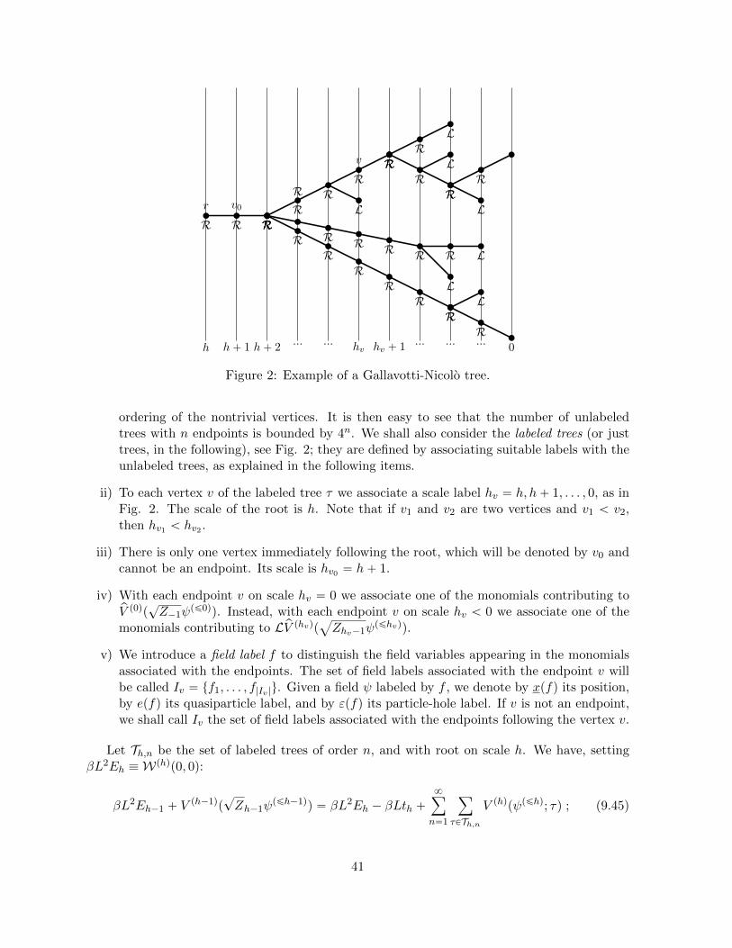
R RR RRR

RR

RR

L

RR

RR

RRR

L

RR

RL

RR

RRR

L

L

L

R L

h h` 1 h` 2... ... hv hv ` 1 ... ... ...

0

v

r v0

R

R R R R

Figure 2: Example of a Gallavotti-Nicolo tree.

ordering of the nontrivial vertices. It is then easy to see that the number of unlabeledtrees with n endpoints is bounded by 4n. We shall also consider the labeled trees (or justtrees, in the following), see Fig. 2; they are defined by associating suitable labels with theunlabeled trees, as explained in the following items.

ii) To each vertex v of the labeled tree τ we associate a scale label hv “ h, h` 1, . . . , 0, as inFig. 2. The scale of the root is h. Note that if v1 and v2 are two vertices and v1 ă v2,then hv1 ă hv2 .

iii) There is only one vertex immediately following the root, which will be denoted by v0 andcannot be an endpoint. Its scale is hv0 “ h` 1.

iv) With each endpoint v on scale hv “ 0 we associate one of the monomials contributing topV p0qp

?Z´1ψ

pď0qq. Instead, with each endpoint v on scale hv ă 0 we associate one of themonomials contributing to LpV phvqp

a

Zhv´1ψpďhvqq.

v) We introduce a field label f to distinguish the field variables appearing in the monomialsassociated with the endpoints. The set of field labels associated with the endpoint v willbe called Iv “ tf1, . . . , f|Iv |u. Given a field ψ labeled by f , we denote by xpfq its position,by epfq its quasiparticle label, and by εpfq its particle-hole label. If v is not an endpoint,we shall call Iv the set of field labels associated with the endpoints following the vertex v.

Let Th,n be the set of labeled trees of order n, and with root on scale h. We have, settingβL2Eh ”Wphqp0, 0q:

βL2Eh´1 ` Vph´1qp

?Zh´1ψ

pďh´1qq “ βL2Eh ´ βLth `8ÿ

n“1

ÿ

τPTh,n

V phqpψpďhq; τq ; (9.45)

41

if τ1, . . . , τs are the subtrees of τ with root v0, V phqpψpďhq; τq is defined inductively as follows:

V phqpψpďhq; τq “p´1qs`1

s!ETh`1

`

Vph`1q

pψpďhq; τ1q ; ¨ ¨ ¨ ;Vph`1q

pψpďh`1q; τsq˘

, (9.46)

where: Vph`1q

pψpďhq; τiq “ RpV p?Zhψ

pďh`1qq if τi contains more than one endpoint, or if it

contains one endpoint but it is not a trivial subtree; Vph`1q

pψpďhq; τiq “ LpV ph`1qp?Zhψ

pďh`1qq

if τi is trivial and h` 1 ă 0; or finally Vph`1q

pψpďhq; τiq “ pV p0qp?Z´1ψ

pď0qq if the subtree τi istrivial and h ` 1 “ 0. Using this inductive definition, the right-hand side of Eq. (9.45) can befurther expanded, and in order to describe the resulting expansion we proceed as follows. Weassociate with any vertex v of the tree a subset Pv of Iv, the external fields of v. These subsetsof fields must satisfy the following constraints. First of all, if v is not an endpoint and v1, . . . , vsvare the sv ě 1 vertices immediately following it, then Pv Ď

Ť

i Pvi ; if v is an endpoint, Pv “ Iv.If v is not an endpoint, we shall denote by Qvi “ Pv X Pvi ; this implies that Pv “

Ť

iQvi . Theunion Iv of the subsets PvizQvi is, by definition, the set of internal fields of v, and is nonempty ifsv ą 1. Given τ P Th,n, there are many possible choices of the subsets Pv, v P τ , compatible withall the constraints. We shall denote by Pτ the family of all these choices and P the elements ofPτ .

The final expansion is obtained iterating Eq. (9.46). In order to better explain the outcomeof the iteration, let us suppose for the moment that R “ 1: we will take into account the Roperator in a second moment. Given v P τ , let τv be the subtree of τ with first nontrivial vertexcorresponding to v. We have:

V phqpψpďhq; τvq “ÿ

PPPτv

V phqpP; τvq , V phqpP; τvq “

ż

β,LDXv

rψpďhqpPvqKph`1qτv ,P

pXvq ,

(9.47)where Xv “

Ť

fPPvxpfq and:

rψpďhqpPvq “ź

fPPv

b

Zh,epfqψpďhqεpfqxpfq,epfq . (9.48)

The function Kph`1qτ,P pXv0q is defined inductively by the following equation, valid for any v P τ

which is not an endpoint:

Kphvqτ,P pXvq (9.49)

“1

sv!

”

ź

fPPv

a

Zhv ,epfqa

Zhv´1,epfq

ı

svź

i“1

rKphv`1qvi pXviqsEThv

`

rψphvqpPv1zQv1q ; ¨ ¨ ¨ ; rψphvqpPvsv zQvsv q˘

where rψphvqpPvizQviq has a definition similar to Eq. (9.48). In Eq. (9.49), if vi is an endpoint

on scale hv “ 0, Kphv`1qvi pXviq is equal to one of the kernels of the monomials contributing

to pV p0qp?Z´1ψ

pď0qq; if vi is an endpoint on scale hv ă 0, Kphv`1qvi pXviq is equal to one of

the kernels of the monomials contributing to LpV phvqpa

Zhv´1ψpďhvqq; instead, if vi is not an

endpoint, Kphv`1qvi “ K

phv`1qτi,Pi

, where Pi “ tPw, w P τiu. If v ą v0 then Pv ą 0.

Eqs. (9.45)–(9.49) are the final form of our expansion. We further decompose V phqpτ,Pqby using a convenient representation of the truncated expectation appearing in the right-hand

42

side of Eq. (9.49). Let us set s ” sv, Pi ” PvizQvi ; moreover, we order in an arbitrary waythe sets P˘i “ tf P Pi | εpfq “ ˘u, we call f˘ij their elements and we define X´i “

Ť

fPP´ixpfq,

X`i “Ť

fPP`ixpfq, x´ij “ xpf´ij q, x

`ij “ xpf`ij q. Note that

řsi“1 |P

´i | “

řsi“1 |P

`i | ” n, otherwise

the truncated expectation vanishes. A pair ` “ pf´ij , f`ij q ” pf

´` , f

`` q will be called a line joining

the fields with labels f´ij , f`ij and quasi-particle indices e´` “ epf´` q, e`` “ epf`ij q, connecting the

points x´` “ x´ij , x`` “ x`ij , called the endpoints of `. We then use the Brydges-Battle-Federbush

formula [13] for truncated expectations, saying that, up to a sign, if s ą 1:

ETh p rψphqpP1q ; ¨ ¨ ¨ ; rψphqpPsqq “ÿ

T

ź

`PT

δe´` e``Zh,e`g

phqe`px´` ´ x

`` q

ż

dµT ptqdetGh,T ptq , (9.50)

where T is a set of lines forming an anchored tree graph between the clusters of points Xi “

tX´i YX`i u, that is T is a set of lines which becomes a tree graph if one identifies all the points

in the same cluster. Moreover, t “ ttii1 P r0, 1s, 1 ď i, i1 ď su, dµT ptq is a probability measurewith support on a set of t such that tii1 “ ui ¨ ui1 for some family of vectors ui P Rs of unitnorm. Finally, Gh,T ptq is a pn´ s` 1q ˆ pn´ s` 1q matrix, whose elements are given by:

Gh,Tij,i1j1ptq “ tii1δe´` e``Zh,e`g

phqe`px´ij ´ x

`i1j1q , (9.51)

with pf´ij , f`i1j1q not belonging to T . In the following, we shall use Eq. (9.50) even for s “ 1,

when T is empty, by interpreting the r.h.s. as 1 if |P1| “ 0, otherwise as equal to detGh “ETh p rψphqpP1qq. Using Eq. (9.50) for each vertex of τ different from its endpoints, we get:

V phqpP; τq “ÿ

TPT

ż

β,LDXv0

rψpďhqpPv0qWphqτ,P,T pXv0q , (9.52)

where T is a special family of graphs on the set of points Xv0 , obtained by putting togetheran anchored graph Tv for each nontrivial vertex v. Note that any graph T P T becomes a treegraph on Xv0 , if one identifies all the points in the sets Xv, with v an endpoint of the tree.Given τ P Th,n and the labels P, T , calling v˚1 , . . . , v

˚n the endpoints of τ and setting hi ” hv˚i

,

the explicit representation of Wphqτ,P,T pXv0q in Eq. (9.52) is:

Wphqτ,P,T pXv0q “

”

nź

i“1

Kphiq

v˚ipXv˚i

q

ı

(9.53)

¨ź

vnot e.p.

ź

fPPv

´

a

Zhv ,epfqa

Zhv´1,epfq

¯ 1

sv!

ż

dPTvptvq detGhv ,Tvptvq”

ź

`PTv

δe`` e´`Zhv ,e`g

phvqe`px´` ´ x

`` q

ı

.

Now, recall the inductive assumptions (9.15), (9.21):

ˇ

ˇ

ˇ

Zk,eZk´1,e

ˇ

ˇ

ˇď ec|λ| , |vk´1,e ´ ve| ď C|λ| , |λk,e| ď C|λ| , |νk,e| ď C|λ| .

These estimates can be used to prove, following [10], Section 3.14:

detGhv ,Tvptvq8 ď Cřsvi“1

|Pvi |

2´|Pv |2´psv´1q2hvp

řsvi“1

|Pvi |

2´|Pv |2´psv´1qq

|Zk,eBn1x0 B

n2x1 g

pkqe px´ yq| ď

Cn`n1`n22kp1`n1`n2q

1` p2kx´ yβ,Lqn`n1`n2, @n P N . (9.54)

43

The first bound follows from the Gram-Hadamard inequality for determinants (using that thesingle-scale propagator admits a Gram representation, Eq. (3.97) of [10]), while the secondfollows from the smoothness and support properties of the single-scale propagator in momentumspace. The bounds (9.54) can be used to prove:

1

βL

ż

β,LDX |W

phqτ,P,T pXv0q| ď

ÿ

ně1

Cn2hp2´|Pv0 |

2q (9.55)

¨

”

ź

v not e.p.

ec|λ||Pv |1

sv!2´phv´hv1 qp

|Pv |2´2q

ı”

nź

i“1

2hv1 p|Iv |2´2q

ı”

nź

i“1

Cpi |λ|pi2´1ı

,

where v1 is the vertex immediately preceding v on the tree τ , and hence hv ´ hv1 ą 0 (in fact,hv ´ hv1 “ 1). This bound however does not imply summability in the scale labels for all P,due to the fact that Pv can be smaller than 4. The contributions to the effective action on scalehv with |Pv| “ 2 are called relevant; if |Pv| “ 4 they are marginal, while if |Pv| ą 4 they areirrelevant.

To prove an estimate which is uniform in h, we reintroduce the R operator. The analogousexpansion is, see Section 3 of [10]:

V phqpP; τq “ÿ

TPT

ÿ

α

ż

DXv0rrψpďhqpPv0qsαW

phqτ,P,T,αpXv0q , (9.56)

where:r rψpďhqpPvqsα “

ź

fPPv

b

Zh,epfqDqαpfqα ψpďhqεpfqxpfq,epfq , (9.57)

with qαpfq P t0, 1, 2u and D the discrete derivative, Dαψεx,e “ ψεx,e ´ ψεxpαq,e, D2αψ

εx,e “ ψεx,e ´

ψεxpαq,e ´ px ´ xpαqq ¨ Bψεx,e for a suitable localization point xpαq; the index α is a multi-indexthat keeps track of the various terms arising after the action of R on a Grassmann monomial,

see e.g. Eq. (9.18). The kernels Wphqτ,P,T,α admit a representation similar to (9.53), see Eq. (3.81)

of [10]. Proceeding as in Section 3.14 of [10], we have:

1

βL

ż

β,LDX |W

phqτ,P,T,αpXv0q| ď

ÿ

ně1

Cn2hp2´|Pv0 |

2q (9.58)

¨

”

ź

v not e.p.

ec|λ||Pv |1

sv!2´phv´hv1 qp

|Pv |2´2`zvq

ı”

nź

i“1

2hv1 p|Iv |2´2q

ı”

nź

i“1

Cpi |λ|pi2´1ı

,

where the dimensional gain zv is due to the presence of the R operator, and it is:

zv “

$

&

%

2 if |Pv| “ 21 if |Pv| “ 40 otherwise.

(9.59)

The number Dv “ |Pv|2 ´ 2 ` zv is called the scaling dimension of the vertex v. We are now

ready to bound the kernel WphqΓ,αpXq “

ř

τPTh,nř˚

PPPτř

TPTWphqτ,P,T,αpXq, where, for any l ě 1,

Γ “ tpe1, ε1q, . . . , pel, εlqu, and the asterisk denotes the constrains |Pv0 | “ |Γ| ” 2l, epfiq “ ei,

44

εpfiq “ εi. Using that the number of unlabeled trees or order n is bounded by 4n, that thenumber of addends in

ř

TPT is bounded by Cnś

v not e.p. sv!, and definition (9.59), we have:

1

βL

ż

β,LDX |W

phq2l,α;epXq| ď 2hp2´lq

ÿ

uě1

Cu|λ|u . (9.60)

In a similar way, one can prove that:

1

βL

ż

β,LDX

ź

ij

xi ´ xjmij |W

phq2l,α;epXq| ď 2hp2´l´

ř

ij mijqÿ

uě1

Cu|λ|u . (9.61)

This is the final result of this section. Analyticity in λ can be proven inductively, assuming thatthe running coupling constants are analytic on all scales ě h, which is true on scale 0. The bound(9.61), combined with Eq. (9.43), also allows to prove thatQ`h,r,epk

1, y2q “ Q`1,r,epk1, y2qp1`Opλqq.

Remark 9.1. (The short memory property.) Thanks to the presence of the zv factors inEq. (9.58), each branch between two nontrivial vertices v ą v1 comes with a factor 2´Dvphv´hv1 q,where Dv ě D “ 1 ´ Opλq. This implies that long trees are exponentially suppressed: if onerestricts the sum

ř

τPTh,n to the trees having at least one vertex on scale k ą h, then the final

bound is improved by a factor 2θph´kq, for θ P p0, Dq. This property is usually referred to as theshort memory property of the GN trees.

Remark 9.2. (The continuity property.) Consider a tree τ P Th,n with value Valpτq ”

Wphqτ,P,T pXv0q. Suppose that |Valpτq| ď BDpτq, where BDpτq is the dimensional bound of the

tree, obtained as in (9.58), with Dv ě D. Consider a propagator gphvqe arising from the

truncated expectation associated with the vertex v P τ . Suppose that gphvqe pk1q is replaced by

gphvqe pk1q ` δg

phvqe pk1q, with |δg

phvqe pk1q| ď C2´hv2θhv for some 12 ą θ ą 0, and admitting a

Gram representation. Let Valpτq ` δValpτq be the new value of tree. The contribution δValpτqcan be bounded as follows. Let C be the path on τ that connects v to the root. Then, writing2θhv “ 2θh

ś

vPC 2´θ and using that Dv ě 1´Opλq, we have:

|δValpτq| ď 2θhBD´θpτq . (9.62)

Analogously, suppose that Zhv ,eZhv,e´1 is replaced by Zhv ,eZhv´1,e ` δz0,hv ,e, with |δz0,hv ,e| ď

C2θhv , or that λhv ,e is replaced by λhv ,e ` δλhv ,e, with |λhv ,e| ď C2θhv . Then, the value of thecorresponding tree is Valpτq ` δValpτq, with δValpτq satisfying the bound (9.62). We shall referto this property as the continuity property of the GN trees.

9.3.2 Tree expansion for the Schwinger functions

Let us briefly discuss the changes needed in order to adapt the previous expansion to theSchwinger functions. For each n ě 0 and m ě 1, we introduce a family T mh,n of rooted la-beled trees, defined in a way similar to Th,n, but now allowing for the presence of m special

vertices, corresponding to the source terms. We will set Pv “ Pψv ` PAv ` P φv , where PAv , P φvcollect the external fields of type A, φ associated with the vertex v. We then have:

Wβ,LpA, φq “ÿ

ně0

ÿ

mě1

ÿ

hěhβ

ÿ

τPT mh,n

ÿ

PPPτ

ÿ

TPT

WphqpP, T ; τq , (9.63)

45

where the contribution WphqpP, T ; τq can be further rewritten as:

WphqpP, T ; τq “

ż

β,LDYv0DZv0 ApP

Av0qφpP

φv0qW

phqτ,P,T pYv0 ,Zv0q , (9.64)

where Wphqτ,P,T pYv0 ,Zv0q admits a tree representation, which can be obtained proceeding as in

the case φ “ A “ 0, with the following differences. If v is a normal endpoint the function Kphvqv

is defined as before, while if v is a special endpoint it is defined as follows. For a special endpoint

of type φ˘r,y2 , then Kphvqv pxq “

ş

β,L dyqQ˘hv ,r,evpx´y, x2qg

phvqev pyq, with qQpx, x2q the inverse Fourier

transform of Qpk1, x2q; while for a special endpoint of type A7µ, Kphvqv pzq “ Zhv ,7,µ,evpz2q. The

various contributions to Eq. (9.63) can be bounded as in (9.58). The main difference is that the

scaling dimension of a given vertex (non endpoint) is now Dv “ |Pψv |2` |P

φv |2` |PAv | ´ 2` zv,

with dimensional gain given by:

zv “

$

’

’

’

&

’

’

’

%

2 if |Pψv | “ 2, |P φv | “ 0, |PAv | “ 0

1 if |Pψv | “ 4, |P φv | “ 0, |PAv | “ 0

1 if |Pψv | “ 2, |P φv | “ 0, |PAv | “ 10 otherwise.

(9.65)

We shall use this expansion to get bounds on the current-current correlation functions. Pro-ceeding in a way analogous to, say, Section 2.2.7, of [26], Eqs. (2.79)–(2.84), one finds:

ˇ

ˇxTjµ,x ; jν,yyβ,Lˇ

ˇ ďC

1` x´ y2β,L

Cn1` |x2 ´ y2|

n, @n P N , (9.66)

for some C,Cn ą 0 independent of β, L. The |x2´ y2|-dependence of the bound comes from thedecay of the bulk propagators, see Eq. (5.23), and from |Q˘h,r,epk

1, x2q| ď Cnp1 ` |x2|ne q with

| ¨ |e “ | ¨ |, | ¨ ´L|, depending on which boundary the edge state is localized, see Eq. (9.43).Concerning the x´yβ,L-dependence, the bound (9.66) is not enough to prove the bounded-

ness of xTjµ,p,x2 ; jν,´p,y2yβ,L uniformly in p. These correlation functions are the crucial objectsentering the Euclidean formulation of the edge transport coefficents, see Eq. (5.14). In order tocompute the edge transport coefficients, Eq. (5.14), we will need to exploit cancellations in theexpansion.

9.4 The flow of the running coupling constants

In order to conclude the discussion of the integration of the single scale, we are left with verifyingour inductive assumptions (9.54). To do this, we shall expoit the recursion relations induced by

46

the multiscale integration, which read as follows:

Zh´1,e

Zh,e“ 1` z0,h,e “: 1` βzh,e

vh´1,e “Zh,eZh´1,e

pvh,e ` z1,h,eq “: vh ` βvh,e

2hνh,e “Zh,eZh`1,e

xWphq2,0,0;e,ep0q “: 2h`1νh`1,e ` 2h`1βνh`1,e

λh,e “

a

Zh,e1Zh,e2Zh,e3Zh,e4a

Zh´1,e1Zh´1,e2Zh´1,e3Zh´1,e4

xWphq4,0,0;ep0, 0, 0q “: λh`1,e ` β

λh`1,e

Zh,7,µ,epz2q “Zh,eZh´1,e

xWphq2,0,1;µ,e,e,7p0, 0, z2q “: Zh`1,7,µ,epz2q ` β

7

h`1,µ,epz2q . (9.67)

The function βh,e ” βhptZk,e, vk,e, νk,e, λk,eu0k“h`1q “ pβ

zh,e, β

vh,e, β

νe , β

λh,e, β

7

h,eq is called the betafunction, and its properties determine the flow of the running coupling constants. The runningcoupling constant νh,e is relevant, while all the others are marginal. From a mathematical pointof view, the main difficulty is to prove that the flow of the effective coupling constant λh,e isbounded. This is a highly nontrivial property, that needs not to be true in general.

The general solution of this problem is beyond the scope of this paper. Instead, we willrestrict the attention to the class of models satisfying Assumpion 2, that is exhibiting single-channel edge currents. We will distinguish two kinds of effective coupling constants, namely:

λh,e “! λh,e for e “ ppe, Òq, pe, Óq, pe, Óq, pe, Òqq

rλh,e if ei ‰ ej for some i, j.(9.68)

We denote by βλh,e the beta function of λh,e, and by rβλh,e the beta function of rλh,e. Notice that

for h “ 0, |λ0,e| ď C|λ| and |rλ0,e| ď C|λ|e´cL. This last bound can be proven from Eq. (9.10),using the exponential decay of the edge modes and of the bulk propagator. The flow of therunning coupling constants can be controlled thanks to the following proposition.

Proposition 9.3. (Bounds for the beta function.) Suppose that |νk,e| ď C2θk|λ|, for allk ą h. Then, under the same assumption of Theorem 4.1, the following is true. Let 2θhβ ěCe´cL. The beta function satisfies the following bounds:

|βzk,e| ď C|λ|22θk , |βvk,e| ď C|λ|2θk , |β7k`1,µ,epz2q| ď C|Z1,7,µ,epz2q||λ|22θpk`1q

|βλk`1,e| ď C|λ|22θpk`1q , |rβλk`1,e| ď C|λ|2e´2cL , (9.69)

for all k ě h, and for some C, c ą 0 independent of h.

This proposition together with the recursive equations (9.67) immediately allows to provethat:

|Zh,e ´ Z0,e| ď C|λ|2 , |vh,e ´ v0,e| ď C|λ| , |Zh,7,µ,epz2q| ď C|Z1,7,µ,epz2q|

|λh,e ´ λ0,e| ď C|λ|2 , |rλh,e| ď C|λ||h|e´2cL ď C|λ|e´cL . (9.70)

which concludes the check of the inductive assumption for all running coupling constants exceptνk,e, that will be discussed in Proposition 9.4. Also, Proposition 9.3 gives a bound on the speed

47

of convergence of the flow of the running coupling constants:

|λhβ ,e ´ λh,e| ď C|λ|22θh , |Zhβ ,7,µ,epz2q ´ Zh,7,µ,epz2q| ď C|λ|22θhZ1,7,µ,epz2q

|vhβ,e ´ vh,e| ď C|λ|2θh ,ˇ

ˇ

ˇ

Zh´1,e

Zh,e´ 1

ˇ

ˇ

ˇď C|λ|22θh . (9.71)

Proof. We proceed by induction. Suppose that the bounds (9.69) are true for k ą h. Considerthe beta function of the effective coupling constant λh. We rewrite it as:

βλh`1,e “ βλ,pď´1qh`1,e ` δβλh`1,e (9.72)

where βλ,pď´1qh`1,e is given by a sum of trees with endpoints at most on scale ´1. By the short-

memory property of the Gallavotti-Nicolo trees, Remark 9.1, we get |δβλh`1,e| ď C|λ|22θph`1q.Then, we further rewrite:

βλ,pď´1qh`1,e “ β

λ,prelqh`1,e ` δβ

λ,pď´1qh`1,e , (9.73)

where βλ,prelqh`1,e is obtained from β

λ,pď´1qh`1,e by setting, for all k ą h:

rk,epk1q “ 0 , νk,e “ 0 ,

Zk,eZk´1,e

“ 1 , vk,e “ vh,e , λk,e “ λh,e , rλk,e “ 0 . (9.74)

Now, using the inductive assumption on the beta functions of the running coupling constantswe have:

|λk,e ´ λh`1,e| ď C|λ|22θk , |rλk,e| ď C|λ|e´cL , |νk,e| ď C2θk|λ| , (9.75)

|vk,e ´ vh`1,e| ď C|λ|2θk ,ˇ

ˇ

ˇ

Zk,eZk´1,e

´ 1ˇ

ˇ

ˇď C|λ|22θk , |rk,epk1q| ď C2θk .

Correspondingly, we write gpkqe pk1q “ g

pkqe,relpk

1q ` δgpkqe pk1q where g

pkqe,relpk

1q is the chiral relativistic

propagator specified by (9.74) and δgpkqe pk1q is a correction term:

gpkqe,relpk

1q “fk,epk

1q

´ik0 ` vh,ek11

, |δgphqe pk1q| ď C2θh2´hk , (9.76)

with fk,epk1q “ χ

`

p2´kδ1eqb

k20 ` v

2h,ek

11

2˘´ χ

`

p2´k`1δ1eqb

k20 ` v

2h,ek

11

2˘. Also, we assume that

all sums over momenta in βλprelqh`1,e are replaced by integrals; the error introduced by this replace-

ment is of order L´1`β´1 ď C2θh, see Lemma 2.6 of [6]. Therefore, using the continuity of the

GN trees, Remark 9.2, we have |δβλpď´1qh`1,e | ď C|λ|22θph`1q. Finally, we are left with β

λprelqh`1,e. By

construction, this contribution is given by a sum of trees involving the relativistic approxima-tion of the propagator, Eq. (9.76). Let ω “ sgnpveq, that is vh,e “ ω|vh,e|. Since the velocity isthe same in all propagators, we can perform a change of variables in the integrals, and replace

vh,e “ ω everywhere. We denote by gpkqω,rel the propagator (9.76) with vh,e “ ω. Let Rα be the

rotation matrix:

Rα “

ˆ

cosα sinα´ sinα cosα

˙

. (9.77)

48

We have:gpkqω,relpRαkq “ e´iωαg

pkqω,relpkq . (9.78)

By the analyticity of βλ,prelqh`1,e in λh`1,e, we write: β

λ,prelqh`1,e “

ř

pě2 βλ,prelqh`1,e,pλ

ph`1,e. The Taylor

coefficient βλ,prelqh`1,e,p is given by the sum of Feynman graphs obtained from the contraction of 4p´4

fields, which means 2p´2 propagators. Let us consider the p-dependent rotation Rp ” R π2p

. By

Eq. (9.78), we get:

βλ,prelqh`1,e,p “ e

´iω π2pp2p´2q

βλ,prelqh`1,e,p ” e

´iωπp1´ 1pqβλ,prelqh`1,e,p (9.79)

which is zero, for all p ě 2. This concludes the inductive step for the proof of the bound on

βλh`1,e. Then, consider βvh,e, βzh,e. Proceeding as before one gets βαh,e “ β

α,prelqh,e `δβαh,e for α “ v, z,

with |δβvh,e| ď C|λ|2θh, δβzh,e ď C|λ|22θh. Let us now study the relativistic contribution. Wedefine the directional derivative:

Bω :“1

2

´

iB

Bk0` ω

B

Bk11

¯

. (9.80)

Clearly, Bk0 “ p´iqpB` ` B´q and Bk11 “ B` ´ B´. We have:

Bω gpkqω,relpRαk

1q “ e´2iωαBω gpkqω,relpk

1q , B´ω gpkqω,relpk

1q “ 0 . (9.81)

The Taylor coefficients βα,prelqh,e,p are given by Feynman graphs containing 2p´ 1 propagators, one

of them being differentiated by B` ˘B´. We rewrite: βα,prelqh,e,p “ β

α,prelq,ωh,e,p ` β

α,prelq,´ωh,e,p , depending

on whether the coefficient contains Bω gpkqω pk1q or B´ω g

pkqω pk1q. Using Eqs. (9.78), (9.81) we get:

βα,prelq,ωh,e,p “ e´iωπβ

α,prelq,ωh,e,p “ 0 @p ě 1

βα,prelq,´ωh,e,p “ 0 @p ě 1 . (9.82)

Therefore, this implies βα,prelqh,e “ 0, and concludes the inductive step for the proof of the bound

on βαh`1,e. Consider now β7h`1,µ,e, 7 “ c, s. Repeating the previous argument, we get β7h`1,µ,e “

β7,prelqh`1,µ,e`δβ

7

h`1,e, with |δβ7h`1,µ,epz2q| ď C|λ|2|Z1,7,e,µpz2q|2θph`1q. We now notice that the Taylor

coefficient β7,prelqh`1,µ,e,p is given by sums of Feynman graphs obtained contracting 4p fields, hence

2p propagators. We have:

β7,prelqh`1,µ,e,p “ e´iωπβ

7,prelqh`1,µ,e,p “ 0 @p ě 1 . (9.83)

This implies β7,prelqh`1,µ,e “ 0, and concludes the inductive step for the proof of the bound on β7h`1,µ,e.

Finally, the proof of the last of Eq. (9.69) follows from the observation that linear contribution

in λe,k to rβλ,(rel)h`1,e is vanishing: its p-th Taylor coefficients rβ

λ,prelqh`1,e,p is given by a sum of diagrams

all containing propagators with the same chirality, which allows to repeat the previous argument

and conclude that rβλ,prelqh`1,e,p “ 0 for all p. Thus, rβ

λ,prelqh`1,e is at least quadratic in rλk,e, k ą h; the

bound in Eq. (9.69) follows from |k|e´2cL ď e´cL for L large enough. This concludes the proof.

49

To conclude the section, let us show how to control the flow of the parameters νk,e.

Proposition 9.4. (The flow of the chemical potential.) Suppose that the bounds (9.70)hold true for all scales k ą h. Then, under the same assumptions of Theorem 4.1, there existνe, |νe| ď C 1|λ|, such that:

|νk,e| ď C2θk|λ| , for all k ě h, (9.84)

for some constants C, θ ą 0 independent of h.

Proof. To begin, we notice that |βνk`1,e| ď C|λ|2θk, for θ ą 0. This follows from the fact

that βνprelqk`1,e,p contains 2p ´ 1 propagators; therefore, proceeding as in the proof of Proposition

9.3 βνprelqk`1,e,p “ e

´iωπp1´ 12pqβνprelqk`1,e,p “ 0 for all p ě 1. Then, we set: βνk`1,e ” 2θk rβνk`1,e, with

|rβνk`1,e| ď C|λ|. We rewrite flow equation for νk,e as:

νk,e “ 2νk`1,e ` 22θk rβνk`1,e ” 2´kνe `0ÿ

j“k

2j´k`12θj rβνj`1,e . (9.85)

Choosing νe “ ´ř0j“h 2j`12θj rβνj`1,e, we get:

νk,e “ ´kÿ

j“h

2j´k`12θj rβνj`1,e . (9.86)

Eq. (9.86) can be understood as a fixed point equation for the sequence tνk,e, . . . , ν0,eu. It isnot difficult to show that Eq. (9.86) defines a contraction in the space of sequences:

Mh :“ tpνk,eq0k“h | |νk,e| ď C2θk|λ|u . (9.87)

See, for instance, Section 4.1 of [10]. Then, the proof follows from a standard application ofBanach contraction mapping principle.

9.5 Proof of Proposition 6.1

In this section we shall use the expansion discussed in the previous sections to prove Proposition6.1, which is the main technical ingredient in the proof of Theorem 4.1. The proof will be basedon a comparison of the expansions for the lattice and reference models. In fact, the referencemodel can be constructed using RG methods similar to those introduced in the previous sections;we refer the reader to [18, 7] for details. Let us give a brief overview of the outcome of the RGanalysis. The integration of the single scale fields is performed in an iterative way, this timestarting from momenta on scale |k| „ 2N , with N ą 0, down to the infrared scales. As aresult, one has to control the flow of suitable running coupling constants, associated with therelevant and marginal terms appearing in the effective action of the reference model on any scalehβ ď h ď N . This has been done in [18]. The running coupling constants on scale N are the

bare couplings, λ(ref), Z(ref), v(ref), Z(ref)7,µ , Q

prefq˘r . On scale h ă N , the analog of the running

coupling constants λh,e, Zh,e, vh,e, Zh,7,µ,e, Q˘h,r,e of the lattice model are denoted by λ

(ref)h,ω , Z

(ref)h,ω ,

v(ref)h,ω , Z

(ref)h,7,µ,ω, Q

prefq˘h,r,ω , for ω “ ˘. By symmetry, there is no ν

(ref)h,ω appearing in the iteration.

50

All these running coupling constants are marginal. Their flow in the ultraviolet regime,1 ď h ď N , has been controlled in Theorem 2 of r18s. In the infrared regime, the flow of therunning coupling constants can be controlled using the same argument of the proof of Proposition9.3, to show the vanishing of the relativistic part of the beta function of the lattice model. Wesummarize these results in the following proposition.

Proposition 9.5. (The running coupling constants of the reference model.) Thereexists λ ą 0 such that for |λ(ref)| ă λ the following is true. The running coupling constants ofthe reference model on scale 0 satisfy the bounds:

|λ(ref) ´ λ(ref)0,ω | ď C|λ(ref)|2 , |Z(ref) ´ Z

(ref)0,ω | ď C|λ(ref)|2 ,

|Z(ref)7,µ pz2q ´ Z

(ref)0,7,µ,ωpz2q| ď C|λ(ref)|2|Z

(ref)7,µ | , |ωv(ref) ´ v

(ref)0,ω | ď C|λ(ref)|

|Q(ref)˘r px2q ´Q

(ref)˘0,r,ω px2q| ď C|λ(ref)||Q(ref)˘

r px2q| .

(9.88)

Also, for all h ď 0:

λ(ref)h,ω “ λ

(ref)0,ω , Z

(ref)h,ω “ Z

(ref)0,ω , v

(ref)h,ω “ v

(ref)0,ω ,

Z(ref)h,7,µ,ω “ Z

(ref)0,7,µ,ω , Q

(ref)˘h,r,ω px2q “ Q

(ref)˘0,r,ω px2q . (9.89)

Moreover, the running coupling constants are analytic in λ(ref) and are smooth functions of theirbare counterparts, with first derivatives bounded away from zero uniformly λ(ref).

The proof of Eq. (9.88) is given by Theorem 2 of [18], while the proof of Eq. (9.89) isa repetition of the argument used to prove the vanishing of the relativistic part of the betafunction for the lattice model. Finally, the statement about differentiability of the runningcoupling constants is a byproduct of the proof of Theorem 2 of [18].

To conclude the introduction to this section, let us briefly anticipate how the reference modelwill be used to describe the lattice model. Let e “ p1, σq be the edge states localized aroundthe x2 “ 0 edge. By the implicit function theorem, we will choose the bare parameters ofthe reference model in such a way that the running coupling constants of the reference modelparametrized by ω “ sgnpveq match the running coupling constants of the lattice model on thesmallest possible scale h “ hβ. For this choice of bare parameters, we will be able to prove thatthe asymptotic behavior of the correlations of the lattice model is captured by the correlationsof the reference model.

Proof of Proposition 6.1. The proof is based on the tree expansion of Section 9.3. Let us startby proving the first of (6.8). The starting point is to separate the trees with endpoints on scale

ď ´1 from the trees having at least one endpoint on scale ě 0. Let us denote by T 2pď´1qh,n the

former set of trees. Setting ω :“ sgnpvp1,σqq and kωF :“ kp1,σqF , we have:

xxxTa´k1`kωF ,x2,r

a`k1`kωF ,y2,r

1yyyβ,L “ÿ

ně0

ÿ

hβďhď´1

ÿ

τPT 2pď´1qh,n

ÿ

PPPτ

ÿ

TPT

xWphqτ,P,T pk

1;x2, y2q ` Ep1q2,0 pk1;x2, y2q

(9.90)

where the asterisk on the P sum recalls that Pv0 “ P φv0 “ tf1, f2u, εpf1q “ ´εpf2q “ ´,kpf1q “ kpf2q “ k1 ` keF , rpf1q “ r, rpf2q “ r1, x2pf1q “ x2, x2pf2q “ y2. The asterisk on

51

the τ sum also recalls that only trees decorated with e “ p1, σq labels appear in the sum; thecontributions coming from the edge state p2, σq are collected in the error term. The dimensionalbound for the two-point function that can be proven via the tree expansion of Section 9.3.2 isOp2´hk1 |x2 ´ y2|

´nq, with hk1 “ tlog2 |k1|u. Therefore, by the short memory property of the GN

trees (see Remark 9.1), using also |λh,e| ď C|λ|e´cL ď C|λ|2θh, it is not difficult to see that

|Ep1q2,0 pk1;x2, y2q| ď Cn2θhk12´hk1 p1 ` |x2 ´ y2|

nq for some θ ą 0. Let us now focus on the firstterm in the right-hand side of Eq. (9.90). The goal is to rewrite it as the contribution comingfrom a suitable reference model, plus subleading terms in k1. We consider a reference modelwith bare parameters chosen so that:

λ(ref)hβ ,ω

“ λhβ ,e , Z(ref)hβ ,ω

“ Zhβ ,e , v(ref)hβ ,ω

“ vhβ ,e , Q(ref)˘hβ ,r,ω

px2q “ Q˘hβ ,r,epkeF , x2q .

(9.91)This can be done by the implicit function theorem, thanks to the fact that all running couplingconstants are nonconstant, differentiable functions of their bare counterparts, recall Proposition9.5. Notice that, by Eq. (9.89), the flow of the beta function of the reference model is trivial onscales h ď 0. Then, by Eqs. (9.71) and by Proposition 9.5 we get:

|λ(ref)k,ω ´ λk,e| ď C|λ|22θk ,

ˇ

ˇ

ˇ

Zk´1,e

Zk,e´ 1

ˇ

ˇ

ˇď C|λ|22θk , (9.92)

|v(ref)k,ω ´ vk,e| ď C|λ|2θk , |Q

(ref)˘k,r,ω px2q ´Q

˘k,r,epk

eF , x2q| ď C|λ|2θkQ˘1,r,epk

eF , x2q .

Correspondingly, we write gpkqe pk1q “ g

pkqe,refpk

1q ` δgpkqe pk1q, where g

pkqe,refpk

1q is the single-scalepropagator of the reference model, given by Eq. (9.76) with vk,e replaced by vhβ ,e, and where

|δgpkqe pk1q| ď C2θk2´k. Therefore,

xxxTa´k1`keF ,x2,r

a`k1`keF ,y2,r

1yyyβ,L

“ÿ

ně0

ÿ

hβďhď1

ÿ

τPT 2pď´1qh,n

ÿ

PPPτ

ÿ

TPT

xWphqprefqτ,P,T pk1;x2, y2q `

ÿ

α“1,2

Epαq2,0 pk1;x2, y2q , (9.93)

where xWphqprefqτ,P,T pk1;x2, y2q is the value of the tree of a reference model specified by the previous

discussion, and Ep2q2,0 pk1;x2, y2q is a new error term, collecting all the errors introduced with the

replacement of the running coupling constants and the propagators with those of the reference

model. By the continuity of GN trees, Remark 9.2, |Ep2q2,0 pk1;x2, y2q| ď Cn2θhk12´hk1 p1 ` |x2 ´

y2|nq. Therefore, we write:

ÿ

ně0

ÿ

hβďhď´1

ÿ

τPT 2pď´1qh,n

ÿ

PPPτ

ÿ

TPT

xWphqprefqτ,P,T pk1;x2, y2q

“ Q(ref)`r px2qQ

prefq´r1 py2qxxxψ

´

k1,ω,σψ`k1,ω,σ1

yyy(ref)β,L ` Ep3q2,0 pk

1;x2, y2q (9.94)

where Ep3q2,0 pk1;x2, y2q is the error term collecting all trees of the reference model with at least

one endpoint on scale ě 0. Thus, by the short-memory of the GN trees of the reference model

and the decay of Q˘ functions, |Ep3q2,0 pk1;x2, y2q| ď Cn2θhk12´hk1 p1 ` |x2 ´ y2|

nq. All in all, by

52

Eqs. (9.93), (9.94), using that xxxψ´k1,ω,σ

ψ`k1,ω,σ1

yyy(ref)β,L » 2´hk1 :

xxxTa´k1`kωF ,x2,r

a`k1`kωF ,y2,r

1yyyβ,L “ xxxψ´

k1,ω,σψ`k1,ω,σ1

yyy(ref)β,L rQ

(ref)`r px2qQ

prefq´r1 py2q `Op2

θhk1 |x2 ´ y2|´nqs

(9.95)This proves the first of Eq. (6.8). Consider now the second of Eq. (6.8). Proceeding as in Eqs.(9.90)–(9.93) we get, for µ “ 0, 1, k1 “ κ, k1 ` p ď κ, p ! κ and κ small enough:

xxxTj7µ,p,z2 ; a´k1`kωF ,x2,r

a`k1`p`kωF ,y2,r

1yyyβ,L (9.96)

“ÿ

ně0

ÿ

hβďhď´1

ÿ

τPT 2pď´1qh,n

˚ÿ

PPPτ

ÿ

TPT

xWphqprefqτ,P,T pk1, p;x2, y2, z2q `

ÿ

α“1,2

Epαq2,1 pk1, p;x2, y2, z2q

where the double asterisk recalls the constraint Pv0 “ PAv0 Y P φv0 , with P φv0 as after (9.90), andPAv0 “ tf3u with µpf3q “ µ, ppf3q “ p, x2pf3q “ z2. The first term in the right-hand side of Eq.(9.96) corresponds to a reference model specified by the conditions (9.91), plus the presence of

a source term coupled to the A field, with a suitable z2-dependent bare parameter Zprefq7,µ pz2q,

chosen so that Zprefqhβ ,7,µ,ω

pz2q “ Zhβ ,7,µ,epz2q, which can be done by the implicit function theorem;

also, by Eq. (9.71) and by Proposition 9.5 we get, for µ “ 0, 1, |Zk,7,µ,epz2q ´ Z(ref)k,7,µ,ωpz2q| ď

C|λ|2θk|Z1,7,µ,ωpz2q|. The error term Ep1q2,1 takes into account the trees containing at least one

rλhv ,e endpoint, and the trees with at least one endpoint on scale ě 0, while the error term Ep2q2,1

contains the contributions arising from the replacement of the running coupling constants and ofthe propagators with those of the reference model. Notice that in the dimensional bound for thetree expansion of this Schwinger function all vertices v have negative scaling dimension exceptfor those corresponding to monomials Aφ`ψ´, Aψ`φ´, which have zero scaling dimension. Theconstraint on the external momenta forces the number of vertices of this type to be of order1, therefore no logarithmic divergence arises in the sum over the scale labels. Proceeding as inEqs. (9.90)–(9.94), we have:

ÿ

ně0

ÿ

hβďhď1

ÿ

τPT 2pď´1qh,n

˚ÿ

PPPτ

ÿ

TPT

xWphqprelqτ,P,T pk1, p;x2, y2, z2q (9.97)

“ Z(ref)7,µ pz2qQ

prefq`r,ω px2qQ

prefq´r1,ω py2qxxxnp,ω ; ψ´

k1,ωψ`k1,ωyyy

(ref)β,L ` Ep3q2,1 pk

1, p;x2, y2, z2q .

where Ep3q takes into account the trees of the reference model with at least one endpoint onscale ě 0. The fast decay of Zhβ ,7,µ,epz2q, together with the bound in Eq. (9.71) and Proposition

9.5, implies that |Zprefq7,µ pz2q| ď Cnp1 ` |z2|

ne q. By the short-memory and the continuity of the

GN trees, the error terms are bounded as: |Epαq2,1 pk, p;x2, y2, z2q| ď Cnκ´2`θp1` dpx2, y2, z2q

nq.

Using also that xxxnp,ω ; ψ´k1,ω

ψ`k1,ωyyy

(ref)β,L » 2´2hk1 , we get:

xxxTj7µ,p,z2 ; a´k1`kωF ,x2,r

a`k1`p`kωF ,y2,r

1yyyβ,L (9.98)

“ xxxnp,ω ; ψ´k1,ω

ψ`k1,ωyyy

(ref)β,L

”

Z(ref)7,µ pz2qQ

prefq`r,ω px2qQ

prefq´r1,ω py2q `Opκ

θdpx2, y2, z2q´nq

ı

.

53

This proves the second of (6.8). To conclude, let us prove the last one of Eq. (6.8). Proceedingas for the previous two Schwinger functions one gets, for µ, ν “ 0, 1:

xxxTj7µ,p,x2 ; j71

ν,´p,y2yyyβ,L “ Zprefq7,µ px2qZ

prefq71,ν py2qxxxn

7p,ω ; n7

1

´p,ωyyyprefqβ,L `

ÿ

α“1,2,3

Epαq0,2 pp;x2, y2q , (9.99)

where the error terms have the same meaning as in the previous discussions. We claim that, forsome θ ą 0:

|Epαq0,2 pp;x2, y2q| ďCn

1` |x2 ´ y2|n, |Epαq0,2 pp;x2, y2q´Epαq0,2 p0;x2, y2q| ď

Cn|p|θ

1` |x2 ´ y2|n, @n P N .

(9.100)These bounds imply the estimates for the error term in the last one of Eq. (6.8). To prove them,

we proceed as follows. Consider the error terms in coordinate space, qEpαq0,2 px,yq. Forgettingabout the dimensional gains coming from the short-memory and the continuity properties of

the GN trees, one gets, proceeding as in Section 2.2.7, of [26], Eqs. (2.79)–(2.84), |qEpαq0,2 px,yq| ď

Cnx´ y´2β,L|x2 ´ y2|

´n. This bound is not even enough to prove uniform boundedness in p of

the Fourier transform. Instead, exploiting the dimensional gain „ 2θh for the trees with root on

scale h contributing to qEpαq0,2 px,yq, implied by the short-memory and the continuity of the GN

trees, one gets the improved bound: |qEpαq0,2 px,yq| ď Cnx´y´2´θβ,L |x2´y2|

´n. This bound can be

used to prove the Lipshitz continuity in p of |x2 ´ y2|nEpαq0,2 pp;x2, y2q with exponent 0 ă θ ă θ.

This proves the bounds (9.100). Finally, the existence of the β, L Ñ 8 limit of the correlationfunction can be proven as in Lemma 2.6 of [6]. This concludes the proof of Proposition 6.1.

Acknowledgements. The work of G. A. and M. P. has been carried out thanks to the supportof the NCCR SwissMap. Furthermore, the work of G. A. and of M. P. has been supported by theSwiss National Science Foundation via the grant “Mathematical Aspects of Many-Body Quan-tum Systems”. V. M. has received funding from the European Research Council (ERC) underthe European Union’s Horizon 2020 research and innovation programme (ERC CoG UniCoSM,grant agreement n.724939). V. M. also acknowledges support from the Gruppo Nazionale perla Fisica Matematica (GNFM).

A Details on the integration of the massive modes

A.1 Bounds on the propagators

In this Appendix we shall discuss some details of the proof of Proposition 5.2. We will prove twokey technical results, that allow to prove Proposition 5.2 by repeating the analysis of Section5.2 of [27]. We start with the proof of Eq. (5.23).

Proposition A.1. (Decay of the bulk propagator.) For any n P N there exists Cn ą 0,independent of β, L,N, δ and c ą 0, independent of β, L,N, δ, n such that:

|gpbulkqβ,L,N px, r; y, r

1q| ďCnδ

´2

1` pδx´ yβ,Lqne´cδ|x2´y2| @x,y . (A.1)

54

Proof. Recall Eq. (5.22),

g(bulk)β,L,N pk;x2, r; y2, r

1q “

nedgeÿ

e“1

´ χN pk0qχepk1q

´ik0 ` Hpk1q ´ µP eKpk1q

¯

px2, r; y2, r1q

`

´ χN pk0qχěpk1q

´ik0 ` Hpk1q ´ µ

¯

px2, r; y2, r1q . (A.2)

We claim that for all k P Dβ,L:

ˇ

ˇBnk g(bulk)β,L,N pk;x2, r; y2, r

1qˇ

ˇ ďCn

pk20 ` δ

2qn`12

e´cδ|x2´y2| , (A.3)

with Bk the discrete gradient: Bk0fpk0, k1q “ pβ2πqpfpk0`2πβ, k1q´fpk0, k1qq and Bk1fpk0, k1q “

pL2πqpfpk0, k1 ` 2πLq ´ fpk0, k1qq. If so, the bound (A.1) can be easily proven via integra-

tion by parts. Let dLpx1q “Lπ sin

´

πx1L

¯

, dβpx0q “βπ sin

´

πx0β

¯

. Notice that C´1x2β,L ď

dLpx1q2`dβpx0q

2 ď Cx2β,L, for some C ą 0. Let n0, n1 P N, and suppose that n “ n0`n1 ą 0.We have:

ˇ

ˇdLpx1 ´ y1qn1dβpx0 ´ y0q

n0gpbulkqβ,L,N px, r; y, r

1qˇ

ˇ

“

ˇ

ˇ

ˇ

1

βL

ÿ

kPMFβˆS

1L

e´ik¨px´yqBn1k1Bn0k0g

(bulk)β,L,N pk;x2, r; y2, r

1q

ˇ

ˇ

ˇď Cnδ

´n´2e´c|x2´y2| . (A.4)

The final estimate easily follows from the bound (A.3). Suppose now that n1 “ n0 “ 0. In

this case, the bound (A.3) is not enough to bound |gpbulkqβ,L,N px, r; y, r

1q|. Instead, a uniform boundeasily follows from the fact that, for large k0, the resolvent is approximately odd in k0. In fact,ř

k0χN pk0qp´ik0` Hpk1q´µq

´1 “ř

k0χN pk0qp´ik0` Hpk1q´µq

´1pHpk1q´µqpik0` Hpk1q´

µq´1, which is finite. The validity of the bound (A.4) for all n0, n1 P N immediately implies Eq.(A.1).

Therefore, the proof is reduced to checking (A.3). To begin, let n “ 0. Consider the secondterm in the right-hand side of Eq. (A.2). Due to the presence of the cutoff function, the resolventis gapped. Exponential decay follows from a standard Combes-Thomas estimate, see for instanceProposition 10.5 of [2]:

ˇ

ˇ

ˇ

´ χN pk0qχěpk1q

´ik0 ` Hpk1q ´ µ

¯

px2, r; y2, r1q

ˇ

ˇ

ˇď

Ca

k20 ` δ

2e´cδ|x2´y2| . (A.5)

Let us now consider the first term in Eq. (A.2). We write:

´ χN pk0qχepk1q

´ik0 ` Hpk1q ´ µP eKpk1q

¯

px2, r; y2, r1q ”

´ χN pk0qχepk1q

´ik0 ` HeKpk1q ´ µ

P eKpk1q

¯

px2, r; y2, r1q (A.6)

with HeKpk1q :“ P eKpk1qHpk1qP

eKpk1q. By construction, He

Kpk1q is gapped in the support of

χepk1q. Also, the kernel HeKpk1;x2, y2q decays exponentially in |x2´ y2|, as a consequence of the

exponential decay of P eKpk1;x2, y2q and of the short range of Hpk1;x2, y2q. Therefore, we canagain apply the Combes-Thomas bound to get:

ˇ

ˇ

ˇ

´ χN pk0qχepk1q

´ik0 ` HeKpk1q ´ µ

P eKpk1q

¯

px2, r; y2, r1q

ˇ

ˇ

ˇď

Ca

k20 ` δ

2e´cδ|x2´y2| , (A.7)

55

This concludes the proof of (A.3) for n “ 0. Let us now prove it for n ą 0. Let us take nderivatives of Eq. (A.2). Consider the contribution coming from differentiation of the secondterm in (A.2). We get a sum of terms of the form:

Am “ Bm1k1pχN pk0qχěpk1qq

1

´ik0 ` Hpk1q ´ µBm2k1Hpk1q

1

´ik0 ` Hpk1q ´ µ¨ ¨ ¨ B

mnk1Hpk1q (A.8)

withř

imi “ n. The resolvents are gapped in the support of χěpk1q, hence we can ap-ply again the Combes-Thomas bound. Moreover, by the assumption on the Hamiltonian,Bmk1Hpk1;x2, y2q is compactly supported in x2 ´ y2. Thus, one easily gets |Ampx2, r; y2, r

1q| ď

Cnpk20 ` δ2q´

n`12 e´cδ|x2´y2|. The terms obtained differentiating the second contribution in the

right-hand side of Eq. (A.2) can be bounded in a similar way, we omit the details. This concludesthe proof.

Remark A.2. The asymptotic oddness of the resolvent could be used to improve the bound (A.1)by replacing δ´2 with δ´1. We will not need such improvement.

The next proposition proves that the bulk propagator admits a Gram representation. Thisallows to apply the Brydges-Battle-Federbush formula, as in Section 5.2 of [27], to prove theconvergence of the integration of the bulk degrees of freedom, Eqs. (5.24)–(5.26). The proof ofProposition A.3 is by direct inspection, and will be omitted.

Proposition A.3. (Gram representation.) Let gpbulkqβ,L,N “

ř

e gpbulkq1,e ` g

pbulkq2 , with:

gpbulkq1,e px, r; y, r1q :“

ż

β,L

dk

p2πq2e´ik¨px´yq

´ χN pk0qχepk1q

´ik0 ` Hpk1q ´ µP eKpk1q

¯

px2, r; y2, r1q

gpbulkq2 px, r; y, r1q :“

ż

β,L

dk

p2πq2e´ik¨px´yq

´ χN pk0qχěpk1q

´ik0 ` Hpk1q ´ µ

¯

px2, r; y2, r1q . (A.9)

Then,

gpbulkq1,e px, r; y, r1q “ xAe1,x,r , B

e1,y,r1y ”

ÿ

r2

ż

β,LdzAe1,x,rpz, r

2qBe1,y,r1pz, r

2q ,

gpbulkq2 px, r; y, r1q “ xA2,x,r , B2,y,r1y ”

ÿ

r2

ż

β,LdzA2,x,rpz, r2qB2,y,r1pz, r

2q , (A.10)

where:

Ae1,x,rpz, r2q :“

ż

β,L

dk

p2πq2eik¨px´zq

´χN pk0q12χepk1q

12

k20 ` pHpk1q ´ µq2

P eKpk1q

¯

pz2, r2;x2, rq (A.11)

Be1,y,r1pz, r

2q :“

ż

β,L

dk

p2πq2eik¨py´zq

´

χN pk0q12χepk1q

12pik0 ` Hpk1q ´ µq¯

pz2, r2; y2, rq

A2,x,rpz, r2q :“

ż

β,L

dk

p2πq2eik¨px´zq

´χN pk0q12χěpk1q

12

k20 ` pHpk1q ´ µq2

¯

pz2, r2;x2, rq

B2,y,r1pz, r2q :“

ż

β,L

dk

p2πq2eik¨py´zq

´

χN pk0q12χěpk1q

12pik0 ` Hpk1q ´ µq¯

pz2, r2; y2, rq .

56

A.2 Proof of Eq. (5.27)

The next proposition is the key technical result behind Eq. (5.27). Eq. (5.27) follows by Taylorexpanding the exponential in the integral, and applying Proposition A.4 to each term in thesum.

Proposition A.4. (One-dimensional representation of the edge field.) Let ξex2px1; rq,pψ` ˚ ξqx,r, pψ

´ ˚ ξqx,r as in Eqs. (5.28), (5.29). Let ETΨ, ETψ be the truncated expectations with

respect to the Gaussian Grassmann fields Ψpedgeq, ψ. Then:

ETΨpΨ(edge)pP1q ; Ψ(edge)pP2q ; ¨ ¨ ¨ ; Ψ(edge)pPqqq “ ETψ ppψ ˚ ξqpP1q ; pψ ˚ ξqpP2q ; ¨ ¨ ¨ ; pψ ˚ ξqpPqqq ,(A.12)

where Pi “ tfju|Pi|j“1 is a set of field labels, and we used the notations ΨpPiq “

ś

fPPiΨεpfqxpfq,rpfq,

pψ ˚ ξqpPiq “ś|Pi|fPPi

pψεpfq ˚ ξqxpfq,rpfq.

Proof. The proof is based on a separate evaluation of the left-hand side and of the right-handside of Eq. (A.12), via the Brydges-Battle-Federbush formula (9.50). Let us start with theleft-hand side. We have:

ETΨpΨ(edge)pP1q ; Ψ(edge)pP2q ; ¨ ¨ ¨ ; Ψ(edge)pPqqq “ÿ

TPT

αTź

`PT

gpedgeq`

ż

dPT ptq detGpedgeqT ptq

(A.13)

where rGpedgeqT ptqsf,f 1 “ tipfq,ipf 1qg

pedgeqpxpfq, rpfq; ypf 1q, r1pf 1qq. By the Leibniz formula we get:

detGpedgeqT ptq “

ÿ

πPSd

sgnpπqrGpedgeqT ptqs1,πp1qrG

pedgeqT ptqs2,πp2q ¨ ¨ ¨ rG

pedgeqT ptqsd,πpdq , (A.14)

where d “ n ´ q ` 1 is the dimension of the matrix, with 2n “řqi“1 |Pi|, and Sd is the set of

permutations of t1, . . . , du. It is useful to rewrite the propagator g(edge) as:

gpedgeqpx, r; y, r1q “ÿ

e

ż

β,L

dk

p2πq2e´ik¨px´yqξex2pk1; rqξey2pk1; rq

χN pk0qχepk1q

´ik0 ` εepk1q ´ µ

”ÿ

e,e1

ÿ

w1,z1

ξex2pw1; rqξe1y2pz1; r1qδe,e1gp1dqe px´ y ´ w1 ` z1q , (A.15)

with gp1dqe given by Eq. (5.15). By using Eq. (A.15), we can write the determinant as:

detGpedgeqT ptq “

ÿ

e,e1z1,w1

dź

j“1

ξejx2,j pw1,j ; rjqξ

e1jy2,j pz1,j ; r1jq

ÿ

πPSd

sgnpπqdź

f 1“1

rG(1d)T pt; e, e1, w, zqsf 1,πpf 1q

(A.16)

where rG(1d)T pt; e, e1, w, zqsf,f 1 :“ tipfq,ipf 1qδepfq,e1pf 1qg

p1dqepfqpxf ´ y

f 1´ w1,f ` z1,f 1q. Similarly, we

have:

ź

`PT

gpedgeq` “

ÿ

e,e1,z1,w1

“

ź

`PT

ξep`qx2p`q

pw1p`q; rp`qqξe1p`qy2p`q

pz1p`q; r1p`qq‰

ź

`PT

g(1d)` pe, e1, w, zq , (A.17)

57

where, if ` “ pf, f 1q, g(1d)` pe, e1, w, zq :“ δepfq,e1pf 1qg

(1d)epfqpxpfq ´ ypf 1q ´ w1pfq ` z1pf

1qq. Eqs.

(A.16), (A.17) imply:

ETΨpΨ(edge)pP1q ; Ψ(edge)pP2q ; ¨ ¨ ¨ ; Ψ(edge)pPqqq “ÿ

TPT

αTÿ

e,e1z1,w1

“

nź

i“1

ξeix2,ipw1,i; riqξe1iy2,ipz1,i; r1iq

‰

¨ź

`PT

g(1d)` pe, e1, w, zq

ż

dPT ptq detG(1d)T pt; e, e1, w, zq . (A.18)

Now, it is not difficult to see that, by the multilinearity of the truncated expectation, (A.18) isexactly what one gets after applying the Brydges-Battle-Federbush formula to the right-handside of Eq. (A.12). This concludes the proof.

B Wick rotation

Here we prove the Wick rotation, Proposition 5.1. The proof is based on the combination ofthe ideas of [27], with the ideas of the proof of Theorem 5.4.12 of [12]. The starting point is thefollowing lemma.

Lemma B.1. Let A, B be two operators on FL, such that3:

1

LxAp´itqA˚yβ,L ď C ,

1

LxB˚p´itqByβ,L ď C , @t P r0, βs

ż β

0dt

1

LxAp´itqA˚yβ,L ď C ,

ż β

0dt

1

LxB˚p´itqByβ,L ď C , (B.1)

for some constant C ą 0 independent of β, L. Let T ą 0, η ą 0. Then,ż 0

´Tdt eηt

1

LxrAptq, Bsyβ,L “ i

ż β

0dt e´iηβt

1

LxAp´itqByβ,L ` Eβ,LpT, ηq , (B.2)

where ηβ P2πβ Z is such that |η ´ ηβ| “ minη1P 2π

βZ|η ´ η

1|, and where the error term satisfies the

boundˇ

ˇEβ,LpT, ηqˇ

ˇ ď Cp1pη2βq ` e´ηT q.

Proof. We start by writing:ż 0

´Tdt eηtxrAptq, Bsyβ,L “

ż 0

´Tdt“

eηtxAptqByβ,L ´ eηtxBAptqyβ,L

“

ż 0

´Tdt“

eηtxAptqByβ,L ´ eηtxApt´ iβqByβ,L

‰

, (B.3)

where in the last line we used that, by cyclicity of the trace Tre´βHBAptq “ TrAptqe´βHB “

Tre´βHApt´ iβqB. Let ηβ be the closest element of 2πβ Z to η: |η´ ηβ| “ minη1P 2π

βZ |η´ η

1|. We

rewrite (B.3) as, using that eiηββ “ 1:ż 0

´Tdt eηt

1

LxrAptq, Bsyβ,L “

ż 0

´Tdt“

eηβt1

LxAptqByβ,L´e

ηβpt´iβq1

LxApt´ iβqByβ,L

‰

`Ep1qβ,LpT, ηq ,(B.4)

3Notice that xAp´itqA˚yβ,L ě 0, xB˚p´itqByβ,L ě 0. In fact, by cyclicity of the trace, xAp´itqA˚yβ,L “xAp´it2qAp´it2q˚yβ,L ě 0, xB˚p´itqByβ,L “ xB

˚p´it2qBp´it2qyβ,L ě 0.

58

where the error term can be estimated as, by Cauchy-Schwarz inequality and thanks to theassumption (B.1), for some C ą 0:

ˇ

ˇEp1qβ,LpT, ηqˇ

ˇ ď1

L

ż 0

´Tdtˇ

ˇeηt ´ eηβtˇ

ˇ

“

xAA˚y12β,LxB

˚By12β,L ` xAp´iβqA

˚y12β,LxB

˚p´iβqBy12β,L

‰

ďC

η2β. (B.5)

Now, we notice that the function eηβzxApzqByβ,L is entire in z P C. Therefore, by Cauchytheorem we conclude that the integral of eηβzxApzqByβ,L along the boundary of the complexrectangle p0, 0q Ñ p0,´iβq Ñ p´T,´iβq Ñ p´T, 0q is equal to zero. The two term in Eq. (B.4)correspond respectively to the paths p´T, 0q Ñ p0, 0q and p0,´iβq Ñ p´T,´iβq. Thus we canwrite:

ż 0

´Tdt“

eηβt1

LxAptqByβ,L´e

ηβpt´iβq1

LxApt´iβqByβ,L

‰

“ i

ż β

0dt e´iηβt

1

LxAp´itqByβ,L`E

p2qβ,LpT, ηq

(B.6)where the error term collects the contribution of the path p´T,´iβq Ñ p´T, 0q,

Ep2qβ,LpT, ηq “ i

ż β

0dt eηβp´T´itq

1

LxAp´T ´ itqByβ,L

ˇ

ˇEp2qβ,LpT, ηqˇ

ˇ ď e´ηT1

L

ż β

0dt xAp´itqA˚y

12β,LxB

˚p´itqBy12β,L (B.7)

ď e´ηT´

ż β

0dt

1

LxAp´itqA˚yβ,L

¯12´ż β

0dt

1

LxB˚p´itqByβ,L

¯12ď Ce´ηT .

The first bound follows from Cauchy-Schwarz inequality for x¨yβ,L, the second bound follows fromCauchy-Schwarz inequality for the time integration, while last follows from the assumptions Eq.(B.1). All in all we have:

ż 0

´Tdt eηt

1

LxrAptq, Bsyβ,L “ i

ż β

0e´iηβt

1

LxAp´itqByβ,L `

2ÿ

i“1

Epiqβ,LpT, ηq (B.8)

where, by Eqs. (B.5), (B.7),ˇ

ˇ

ř2i“1 E

piqβ,LpT, ηq

ˇ

ˇ ď Cp1pη2βq ` e´ηT q. This concludes the proof.

We are now ready to prove Proposition 5.1.

Proof of Proposition 5.1. Let us start by studying the charge transport coefficients. ConsiderGa01ppq. The proof for the other coefficients will be exactly the same, with the exception ofG

a11ppq,

that will be discussed below. Let us first check the assumptions of Lemma B.1. Let p1 ‰ 0. Weset A :“ ρďap1 ´ xρ

ďap1 yβ,L, B :“ jďa

1

1,´p1´ xjďa

1

1,´p1yβ,L (a shift by a constant does not change the

commutators). The first assumption in Eq. (B.1) can be checked using the bound in Eq. (9.66),

1

LxAp´itqA˚yβ,L ”

1

Lxρďap1 p´itq ; ρďa´p1yβ,L ď

1

L

ÿ

x2,y2ďa

Lÿ

x1,y1“0

1

1` t2 ` |x1 ´ y1|2L

Cn1` |x2 ´ y2|

n

“ Ca (B.9)

59

A similar bound holds true for B. This proves the validity of the first two assumptions in Eq.(B.1). Consider now the second assumptions in Eq. (B.1). We notice that, for µ “ 0, 1:

ż β

0dt

1

Lxjďaµ,p1p´itq ; jďaµ,´p1yβ,L ”

1

βLxT jďaµ,p0,p1q ; jďaµ,p0,´p1qyβ,L , (B.10)

where jďaµ,p0,p1q “şβ0 dx0

řLx1“0

řax2“0 e

ip¨xjµ,x. By the existence of the β, L Ñ 8 limit of the

Euclidean correlations, Lemma 2.6 of [6], we know that

1

βLxT jďaµ,p0,p1q ; jďaµ,p0,´p1qyβ,L “ xxxT jďaµ,p0,p1q ; jďaµ,p0,´p1qyyy8 `Opaβ

´θq for some θ ą 0; (B.11)

thus, thanks to Proposition 6.1, this allows to prove that | 1βLxT jďaµ,p0,p1q ; jďaµ,p0,´p1qyβ,L| ď Ca. A

similar bound holds for B. This concludes the check of the last two assumptions in Eq. (B.1).Hence, we can apply Lemma B.1 to analytically continue the real times transport coefficient toimaginary times, for finite β, L. The existence of the β, L Ñ 8 limit can be proven as in [27],item iiq of Proposition 6.1 (see also Proposition 5.2 of [46]); it follows from the existence of theinfinite volume dynamics, that can be proven via Lieb-Robinson bounds, and from the existenceof the zero temperature, infinite volume Gibbs state, that can be proven with the RG methodsdiscussed in this paper. Taking also the T Ñ8 limit, Eq. (5.14) follows. The proof for the spintransport coefficients G

a,sµν ppq is exactly the same. This concludes the proof of Proposition 5.1.

References

[1] S. L. Adler and W. A. Bardeen. Absence of Higher-Order Corrections in the AnomalousAxial-Vector Divergence Equation. Phys. Rev. 182, 1517 (1969).

[2] M. Aizenman and S. Warzel. Random Operators. Disorder Effects on Quantum Spectraand Dynamics. Graduate Studies in Mathematics 168, Americal Mathematical Society(2015).

[3] J. E. Avron, R. Seiler and B. Simon. Homotopy and Quantization in Condensed MatterPhysics. Phys. Rev. Lett. 51, 51 (1983).

[4] S. Bachmann, A. Bols, W. De Roeck and M. Fraas. Quantization of conductance ingapped interacting systems. Ann. Henri Poincare 19, 695–708 (2018)

[5] G. Benfatto, P. Falco and V. Mastropietro. Extended Scaling Relations for PlanarLattice Models. Comm. Math. Phys. 292, 569–605 (2009)

[6] G. Benfatto, P. Falco and V. Mastropietro. Universality of One-Dimensional FermiSystems, I. Response Functions and Critical Exponents. Comm. Math. Phys. 330,153–215 (2014)

[7] G. Benfatto, P. Falco and V. Mastropietro. Universality of One-Dimensional FermiSystems, II. The Luttinger Liquid Structure. Comm. Math. Phys. 330, 217–282 (2014).

[8] G. Benfatto and V. Mastropietro. Drude Weight in Non Solvable Quantum Spin Chains.J. Stat. Phys. 143, 251–260 (2011).

60

[9] G. Benfatto and V. Mastropietro. Universality Relations in Non-solvable QuantumSpin Chains. J. Stat. Phys. 138, 1084–1108 (2011).

[10] G. Benfatto and V. Mastropietro. Renormalization group, hidden symmetries and ap-proximate Ward identities in the XY Z model. Rev. Math. Phys. 13, 1323–1435 (2001).

[11] G. Benfatto and V. Mastropietro. Ward Identities and Chiral Anomaly in the LuttingerLiquid. Comm. Math. Phys. 258, 609–655 (2005).

[12] O. Bratteli and D. W. Robinson. Operator Algebras and Quantum Statistical Mechan-ics 2. Equilibrium States. Models in Quantum Statistical Mechanics. Second edition,Springer (1997).

[13] D. C. Brydges. A short course on cluster expansions. In Phenomenes critiques, systemesaleatoires, theories de jauge, (Les Houches, 1984), 129-183. North-Holland, Amsterdam(1986).

[14] A. M. Chang. Chiral Luttinger liquids at the fractional quantum Hall edge. Rev. Mod.Phys. 75, 1449–1505 (2003).

[15] S. Coleman and B. Hill. No more corrections to the topological mass term in QED3.Phys. Lett. B. 159, 184 (1985).

[16] P. Elbau and G. M. Graf. Equality of bulk and edge Hall conductance revisited. Comm.Math. Phys. 229, 415–432 (2002).

[17] A. Elgart, G. M. Graf and J. H. Schenker. Equality of the Bulk and Edge Hall Con-ductances in a Mobility Gap. Comm. Math. Phys. 259, 185–221 (2005).

[18] P. Falco and V. Mastropietro. Renormalization Group and Asymptotic Spin-ChargeSeparation for Chiral Luttinger Liquids. J. Stat. Phys. 131, 79–116 (2008).

[19] J. Frohlich and T. Kerler. Universality in quantum Hall systems. Nucl. Phys. B. 354,369–417 (1991).

[20] J. Frohlich and U. M. Studer. Gauge invariance and current algebra in nonrelativisticmany-body theory. Rev. Mod. Phys. 65, 733 (1993).

[21] J. Frohlich, U.M. Studer and E. Thiran. Quantum Theory of Large Systems of Non-Relativistic Matter. cond-mat/9508062.

[22] A. Giuliani. Order, disorder and phase transitions in quantum many body systems.arXiv:1711.06991

[23] A. Giuliani and V. Mastropietro. The Two-Dimensional Hubbard Model on the Hon-eycomb Lattice. Comm. Math. Phys. 293, 301–346 (2010).

[24] A. Giuliani, V. Mastropietro and F. Toninelli. Height fluctuations in interacting dimers.Ann. Inst. H. Poincare Probab. Statist. 53, 98–168 (2017).

[25] A. Giuliani, V. Mastropietro and F. Toninelli. Haldane relation for interacting dimers.J. Stat. Mech.: Theor. Exp. 2017, (2017)

61

[26] A. Giuliani, V. Mastropietro and M. Porta. Universality of Conductivity in InteractingGraphene. Comm. Math. Phys. 311 317–355 (2012).

[27] A. Giuliani, V. Mastropietro and M. Porta. Universality of the Hall conductivity ininteracting electron systems. Comm. Math. Phys. 349, 1107–1161 (2017).

[28] A. Giuliani, I. Jauslin, V. Mastropietro and M. Porta. Topological phase transitionsand universality in the Haldane-Hubbard model. Phys. Rev. B 94, 205139 (2016).

[29] A. Giuliani, V. Mastropietro and M. Porta. Quantization of the interacting Hall con-ductivity in the critical regime. arXiv:1803.11213

[30] G. M. Graf and M. Porta. Bulk-Edge Correspondence for Two-Dimensional TopologicalInsulators. Comm. Math. Phys. 324, 851–895 (2013).

[31] G. M. Graf and C. Tauber. Bulk-Edge correspondence for two-dimensional Floquettopological insulators. Ann. Henri Poincare 19, 709–741 (2018).

[32] F. D. M. Haldane. Model for a Quantum Hall Effect without Landau Levels:Condensed-Matter Realization of the “Parity Anomaly”. Phys. Rev. Lett 61, 2015(1988).

[33] F. D. M. Haldane. “Luttinger liquid theory” of one-dimensional quantum fluids. J.Phys. C: Solid State Phys. 14, 2585 (1981).

[34] B. I. Halperin. Quantized Hall conductance, current-carrying edge states, and the ex-istence of extended states in a two-dimensional disordered potential. Phys. Rev. Lett.25, 2185 (1982).

[35] N. Hao et al.. Topological edge states and quantum Hall effect in the Haldane model.Phys. Rev. B 78, 075438 (2008).

[36] M. Z. Hasan and C. L. Kane. Colloquium: Topological insulators. Rev. Mod. Phys. 82,3045 (2010).

[37] M. B. Hastings and S. Michalakis. Quantization of Hall Conductance for InteractingElectrons on a Torus. Comm. Math. Phys. 334, 433-471 (2015).

[38] M. B. Hastings. The Stability of Free Fermi Hamiltonians. arXiv:1706.02270

[39] Y. Hatsugai. Chern number and edge states in the integer quantum Hall effect. Phys.Rev. Lett. 71, 3697 (1993).

[40] M. Hohenadler and F. F. Assaad. Correlation effects in two-dimensional topologicalinsulators. J. Phys.: Condens. Matter 25, 143201 (2013).

[41] C. L. Kane and M. P. A. Fisher. Edge-State Transport. In Perspectives in QuantumHall Effects: Novel Quantum Liquids in Low-Dimensional Semiconductor Structures.Editors: S. Das Sarma, A. Pinczuk. Wiley (2007).

[42] C. L. Kane and E. J. Mele. Z2 topological order and the quantum spin Hall effect.Phys. Rev. Lett. 95, 146802 (2005).

62

[43] R. B. Laughlin. Quantized Hall conductivity in two dimensions. Phys. Rev. B 23,5632(R) (1981)

[44] K. Ishikawa and T. Matsuyama. Magnetic Field Induced Multi-Component QED3 andQuantum Hall Effect. Z. Phys. C 33, 41–45 (1986).

[45] V. Mastropietro. Non perturbative Adler-Bardeen theorem. J. Math. Phys. 48, 022302(2007).

[46] V. Mastropietro and M. Porta. Canonical Drude Weight for Non-integrable QuantumSpin Chains. J. Stat. Phys. (2018). https://doi.org/10.1007/s10955-018-1994-0

[47] V. Mastropietro and M. Porta. Spin Hall insulators beyond the helical Luttinger model.Phys. Rev. B 96, 245135 (2017).

[48] D. C. Mattis and E. H. Lieb. Exact Solution of a Many-Fermion System and Its Asso-ciated Boson Field. J. Math. Phys. 6, 304–312 (1965).

[49] E. Prodan and H. Schulz-Baldes. Bulk and Boundary Invariants for Complex Topo-logical Insulators. From K-Theory to Physics. Mathematical Physics Studies, Springer(2016).

[50] X.-L. Qi and S.-C. Zhang. Topological insulators and superconductors. Rev. Mod. Phys.83, 1057 (2011).

[51] H. Schulz-Baldes, J. Kellendonk and T. Richter. Simultaneous quantization of edgeand bulk Hall conductivity. J. Phys. A: Math. Gen. 33 L27 (2000).

[52] J. Sirker, R. G. Pereira and I. Affleck. Conservation laws, integrability, and transportin one-dimensional quantum systems. Phys. Rev. B 83, 035115 (2011).

[53] D. J. Thouless, M. Kohmoto, M. P. Nightingale and M. den Nijs. Quantized HallConductance in a Two-Dimensional Periodic Potential. Phys. Rev. Lett. 49, 405 (1982).

[54] X. G. Wen. Chiral Luttinger liquid and the edge excitations in the fractional quantumHall states. Phys. Rev. B 41, 12838–12844 (1990).

63