UNIT-UNIT1 Vector Analysisassets.vmou.ac.in/MPH02.pdf · Vector Analysis Structure of the Unit 1.0 Objectives 1.1 Introduction 1.2 Scalar Product 1.3 Vector Product (Cross Product)

1

UNIT- 1

Vector Analysis

Structure of the Unit

1.0 Objectives

1.1 Introduction

1.2 Scalar Product

1.3 Vector Product (Cross Product)

1.4 Scalar Triple Product .A B C

1.5 Vector Triple Product

CBA

1.6 Gradient

1.7 Self Learning Exercise-I

1.8 Divergence

1.9 Curl

1.10 Self Learning Exercise-II

1.11 Summary

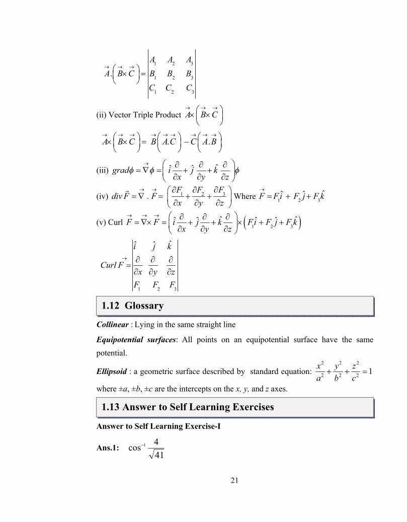
1.12 Glossary

1.13 Answer to Self Learning Exercises

1.14 Exercise

1.15 Answers to Exercise

1.0 Objective Vector analysis is a mathematical shorthand. The vector form helps to provide a clearer understanding of the physical laws. This makes the calculus of the vector functions the natural instrument for the physicist and engineers in solid mechanics, electromagnetism, and so on. To meet objectives ,we emphasize the physical interpretation of vector functions.

UNIT-1 Vector Analysis

1.0 Objectives

2

1.1 Introduction

Vector algebra is introduced early in the text. The unit deals with vector functions and extends the differential calculus to these vector functions. We finally discuss physical meaning of three important concepts namely ,the gradient, divergence and curl. 1.2 Scalar Product

Scalar Product (dot product) of two vectors A

and B

is defined as

. cosA B AB

where 0

Here is the angle between

A and

B . Note that

BA. is a scalar quantity.

General Properties of Scalar Product:-

(i)

ABBA .. (Commutative Law)

(ii)

CABACBA ..).(

(iii) ˆ ˆˆ ˆ ˆ ˆ. . . 1i i j j k k

ˆ ˆˆ ˆ ˆ ˆ. . . 0i j j k k i

(iv) If 1 2 3ˆˆ Â Ai A j A k

and 1 2 3ˆˆ ˆB B i B j B k

, then

332211. BABABABA

23

22

21

2. AAAAAA

(v)

BABA.

(vi)

BA. is independent of co-ordinate system.

Typical Applications of Scalar Product:-

(i) If 0

A , 0

B and 0.

BA , then

Aand

B will be perpendicular.

1.2 Scalar Product

1.1 Introduction

3

(ii) Component of vector

A along

n direction is .A n

, where

n is unit

vector.

(iii) Angle between

A and

B can be found out by . ˆ ˆcos .A B A BAB

Example1.1 Find the angle between side AC and side AB of a triangle ABC.

Coordinates of the vertices A,B,C are (1 2 3 ,1, 2) , (1,1,2) , (1,3,2) respectively.

Sol.

AB =Position vector of

B − Position Vector of

A

ˆ ˆˆ ˆ ˆ ˆ ˆ2 1 2 3 2 2 3AB i j k i j k i

2 3AB

AC P.V. of

C - P.V. of

A

ˆ ˆˆ ˆ ˆ ˆ3 2 1 2 3 2AC i j k i j k

ˆ ˆ2 3 2i j

2 22 3 2 4AC

By dot product

ˆ ˆ ˆ2 3 . 2 3 2. 3cos

22 3 .4

i i jAB AC

AB AC

030


Vector product of two vectors

Aand

B is defined as ˆsinA B AB n

where

0 and

n is a unit vector in direction of

BA . Direction of unit victor

n

is perpendicular to the plane formed by

A and

B and it is given by right handed system.


4

General Properties of Vector Product:-

(i) If A

and B

are parallel or antiparallel i.e. collinear , then A B

=0

0

AA

ˆ ˆ 0i i , ˆ ˆ 0j j , ˆ ˆ 0k k

(ii) A B B A

(Anti commutative law)

(iii)

CABACBA

(iv) ˆˆ ˆ ,i j k ˆˆ ˆ,j k i ˆ ˆ ,k i j

ˆˆ ˆ ,j i k ˆ ˆ ˆ,k j i ˆˆ ˆ,i k j

(v) If 1 2 3ˆˆ Â Ai A j A k

and 1 2 3ˆˆ ˆB B i B j B k

,Vector product of two

vectors

Aand

B as a determinant is represented as given below

1 2 3

1 2 3

ˆˆ î j kA B A A A

B B B

2 3 3 2 1 3 3 1 1 2 2 1ˆˆ Â B i A B A B j A B A B k A B A B

Typical Applications of Vector Product:-

(i) Area of the parallelogram with sides

A and

B is

BA

Figure 1.1

Area=Ah=AB sin

=

BA

5

(ii) Area of the Triangle with sides

A and

B is

BA21

Figure 1.2

Area =

BAABAh21sin

21

21

(iii) Unit vector that is perpendicular to the plane formed by

Aand

B is given by

ˆ A BnA B

Example1.2 A solid sphere is rotating with an angular velocity 30 r.p.m. about a fixed axis MN. Position vectors of the points M and N of the sphere are

ˆˆ ˆ2 3i j k m and ˆˆ ˆ4 5 6i j k m respectively. There is an insect at a point

ˆˆ ˆ2 2 5i j k m on the surface of the sphere. Calculate the speed of the insect.

Sol. Angular Velocity =30 rev. per minute 60230

secrad

secrad

Figure 1.3

6

Angular velocity

is an axial vector. Let it be along

MN .

ˆ ˆˆ ˆ ˆ ˆ4 5 6 2 3

ˆˆ ˆ3 3 3

MN N M i j k i j k

i j k

ˆˆ ˆ.3

MN i j kMN

Position vector of the point P with respect to point M is

MPr

ˆ ˆ ˆˆ ˆ ˆ ˆ ˆ ˆ2 2 5 2 3 4 2r i j k i j k i j k

Linear velocity of P is

rv

ˆˆ ˆ

1 1 13 1 4 2

i j k

ˆˆ ˆ2 ( 4) 2 1 4 13

i j k

ˆˆ ˆ6 5

3i j k

sec36225136

3mv

1.4 Scalar Triple Product . A B C

1 2 31 2 3

1 2 3 1 2

1 2 31 2 3

ˆˆ ˆwhere

ˆˆ ˆ.

ˆˆ ˆ

A A i A j A kA A AA B C B B B B B i B j B k

C C C C C i C j C k

2 2 2

ˆ ˆˆ ˆ ˆ ˆ3 3 333 3 3

MN i j k i j k

MN

1.4 Scalar Triple Product . A B C

7

Note that

CBA. is scalar quantity. We can write scalar triple product

CBA. as ABC we read ABC as box product.

General Properties of Scalar Triple Product:-

(i)

BACACBCBA ... i.e. CABBCAABC

(ii) ˆ ˆ ˆ ˆˆ ˆ ˆ ˆ ˆ ˆ ˆ ˆ1 & 1i j k j k i k i j i k j

(iii) Magnitude of the scalar triple product

CBA. of three vectors is equal to

the volume of a parallelepiped having sides

A ,

B and

C

(iv) 0..0.

CAAeiCAA

0..0.

AACeiAAC

(v) If scalar triple product vanishes i.e. 0.

CBA then

A ,

B and

C are

coplanar. In that case volume of parallelepiped formed by them is zero

Note:

CBA. is meaningless. Similarly

CBA .. is also meaningless.

Geometrical Interpretation of Scalar Triple Product: -

Figure 1.4

COCBOBAOA ,,

nCBCB sin

8

= (Area of Parallelogram OBEC)

n

=

nS

Here hheightADAnA

cos.1..

Thus

nSACBA ..

= ShnAS

.

= Volume of parallelepiped

1.5 Vector Triple Product A B C

. .A B C B A C C A B

Note that

CBA is a vector quantity

General Properties:-

(i) 0A B C B C A C A B

(ii) We have in general

CBACBA

1.6 Gradient

Vector differentiable operator

is defined as ˆˆ î j kx y z

is called ‘del’

Gradient: if zyx ,, is a differentiable scalar field then gradient of is defined

by ˆˆ ˆgrad i j kx y z

ˆˆ î j k

x y z

1.5 Vector Triple Product A B C

1.6 Gradient

9

Note that

is a vector field .


(i) 2121

(ii)

CC where C is constant

(iii) If =constant then 0

Geometrical Interpretation of gradient:-

“The magnitude of this

is equal to maximum value of rate of change of with

distance.”

Figure 1.5

Consider a surface S1 that has constant potential . At distance MN, there is another surface S2 which has constant potential d . Here MN is the shortest distance between the two surface 1S and 2S . If we move from 1S to 2S , then change in dis .Rate of change of with distance is highest along the normal MN. So grad at point M is directed along MN.

“

points in the direction of maximum rate of increase of the function with space”

“For any point on the constant surface, direction of vector

at that point will be normal to the constant surface.”

Directional Derivate:

The component of grad in the direction of vector

b is equal to ,.

b it is called

10

directional derivate of in direction of vector

b

Example1.3 Scalar Potential is given by zyx and an ellipsoid is

given by 394

222 zyx

Find

(i)

at point (1,2,3)

(ii) Unit vector, that is normal to ellipsoid surface at the point (1,2,3)

(iii) Directional derivative of in the direction of the outward normal of the given ellipsoid at the point (1,2,3)

Sol. (i) ˆˆ î j k x y zx y z

ˆˆ î x y z j x y z k x y z

x y z

î j k

which is constant vector and independent of the position of point

(ii) For ellipsoid surface 94

,,22

2 zyxzyx = constant, then

will be

perpendicular to the surface zyx ,, =constant 2 2

2ˆ ˆ4 9y zi j k x

x y z

2 2 2 2 2 22 2 2ˆˆ ˆ

4 9 4 9 4 9y z y z y zi x j x k x

x y z

2 ˆˆ ˆ22 9y zxi j k

At the point 3,2,1

2 ˆˆ ˆ23

i j k

37

11

Unit vector 6 3 2 ˆˆ ˆ7 7 7

n i j k

Another unit vector normal to the surface is 6 3 2 ˆˆ ˆ7 7 7

i j k

Its direction is opposite to that above.

(iii) Required directional derivate

n.

6 3 2ˆ ˆˆ ˆ ˆ ˆ.

7 7 7i j k i j k

711

7236

Example1.4 Electric potential due to positive point charge Q is given by r

kQV

.Find grad V

Sol. ˆˆ ˆ kQV i j kx y z r

1 1 1ˆˆ ˆV kQ i j kx r y r z r

2 2 2

ˆˆ î r j r k rV kQr x r y r z

2ˆ ˆkQ r r rV i j k

r x y z

Here ˆˆ ˆr xi yj zk

2222 zyxr Partial differentiation with respect to x gives

rx

xrx

xrr

0022

Similarlyrz

zr

ry

yr

,

12

Thus 2ˆˆ ˆkQ x y zV i j k

r r r r

rrkQ

3

rrkQV 3 where

rrr

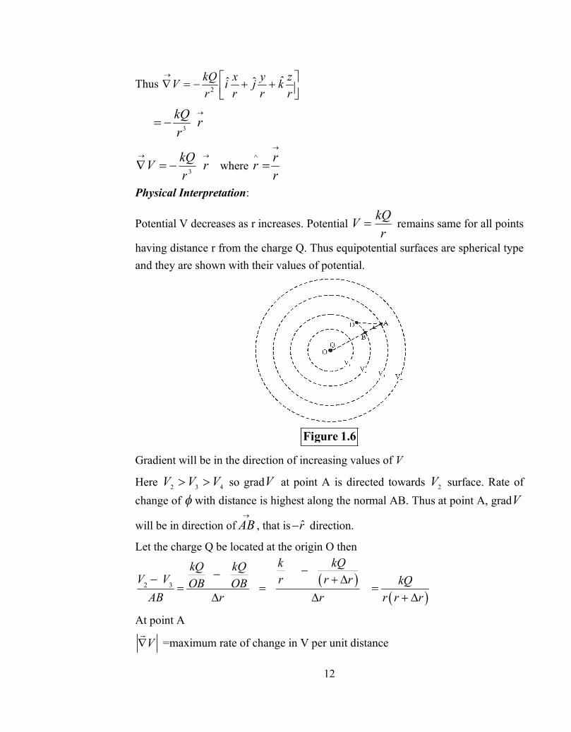
Physical Interpretation:

Potential V decreases as r increases. Potential r

kQV remains same for all points

having distance r from the charge Q. Thus equipotential surfaces are spherical type and they are shown with their values of potential.

Figure 1.6

Gradient will be in the direction of increasing values of V

Here 432 VVV so gradV at point A is directed towards 2V surface. Rate of change of with distance is highest along the normal AB. Thus at point A, gradV

will be in direction of

AB , that is r direction.

Let the charge Q be located at the origin O then

2 3

k kQkQ kQV V r r r kQOB OB

AB r r r r r

At point A

V

=maximum rate of change in V per unit distance

13

AB

VVLimr

32

0 2r

kQ


Very Short Answer Type Questions

Q.1 Find the angle made by vector ˆˆ ˆ4 4 3A i j k

with x axis.

Q.2 “If

CBA ,, are not null vectors and

CABA .. then

B need not be equal to

C ” give an example in favour of above statement.

Short Answer Type Questions

Q.3 If 1ˆˆ ˆ

2aa i j k

, 2ˆˆ ˆ

2aa i j k

and 3ˆˆ ˆ

2aa i j k

represent the

primitive translation vectors (sides of primitive cell) of the BCC lattice then find the volume of the primitive cell. Here a is the side of conventional cell.

Q.4 Find 2r

1.8 Divergence

If

F is differentiable vector field then divergence of

F is

F. which is defined as

1 2 3ˆ ˆˆ ˆ ˆ ˆ. .F i j k F i F j F k

x y z

31 2.FF F

Fx y z

where 1 2 3ˆˆ ˆF Fi F j F k

General Properties of Divergence:-

(i)

ACAC ..

where C is constant

(ii)

BABA ...


1.8 Divergence

14

(iii)

AAA ...

(iv)

.. AA

Note that

zA

yA

xAA 321. is an operator

(v) If

A=constant, then 0.

A

(vi) 2

2

2

2

2

22.

zyx

where2 2 2

22 2 2x y z

is Laplacian operator

Physical Interpretation of Divergence:

0

.S

V

F d Sdiv F Lim

V

Here volume element V is bounded by the infinitesimal surface S in the

neighbourhood of a point P.

S

SdF . is the net out flow flux of

F through

infinitesimal surface S.

Thus “divergence of vector field

F at the point P is equal to net outward flux per unit volume as the volume shrinks to zero in the neighbourhood of the point P.”

If div

F is positive, it means net flux is coming out through infinitesimal volume element at the point P and that point acts as a source.

Figure 1.7

15

In the given figure 1.7, the point P acts as source.

Negative value of div

F means net flux is going into infinitesimal volume element at the point P and that point acts as a sink.

Figure 1.8

If 0.

F then

F is called Solenoidal vector.

Magnetic field

B is a solenoid vector 0.

B means there is neither source nor

sink for field

B . Magnetic field lines always make closed loop. Due to that fact net out flow flux any infinitesimal volume is zero.

Example1.5 Electric field inside a uniformly charged solid sphere is03

rE .

Find div

E .

Sol.

rrE .

33.

00

0

ˆ ˆˆ ˆ ˆ ˆ.3

i j k xi yj zkx y z

z

zy

yx

x03

3

3 0

0

.

E which is Gauss’s in electrostatics

16

1.9 Curl

If

F (x,y,z) is a differentiable vector field, then curl of

F is defined as

Curl 1 2 3ˆ ˆˆ ˆ ˆ ˆF F i j k Fi F j F k

x y z

3 32 1 2 1ˆˆ ˆF FF F F FCurl F i j k

y z y z y z

1 2 3

ˆˆ î j k

Curl Fx y z

F F F


(i) Curl

BA =curl

A+curl

B

(ii) Curl rad 0G

i.e. 0

(iii) If c

is constant vector, then curl

0c

(iv)

AAA

(v) Div Curl 0A

i.e.

. 0A

(vi)

AAA 2.

(vii) If curl 0

F then field

F is called irrotional field and line integral

rdFB

A.

is independent of the path joining any two points A and B. In above case,

circulation .F d r

zero for any closed path in that region.

(viii) If curl 0

F , then three components of

F are interrelated as

1.9 Curl

17

zF

yF

23 ,

xF

zF

31 ,

yF

xF

12

(ix) If curl 0

F it follows

F i.e. vector field

F can be expressed as gradient of scalar field .

(x) If div 0

F it follows

AF

0Adivcurl

Example1.6 A field

F is given by 2 ˆF x j

Calculate curl

F . Sol.

2

ˆˆ ˆ

0 0

i j k

Curl Fx y z

x

2ˆ ˆ0 0 0i x j

y z x z

2ˆ 0k xx y

= ˆˆ ˆ0 0 2i j xk

Curl ˆ2F xk

Physical Interpretation:

Value of F increases with x and

F is directed along positive y direction.It is obvious from figure1.9, higher value of F is represented by larger arrow. Now we

calculate the line integral

rdF . along closed loop ABCDA in anticlockwise

direction.

Figure 1.9

18

rdFrdFrdFrdFrdFDACDBCAB

.....

00

180cos90cos0cos90cos 00 drFdrFdrFdrFDACDBCAB

= DAFBCF DABC 00

yDABC

xAB

yFFrdF DABC.

2 2 2x x x y F x

22 22x x x x x y

yxxx 2

xxyx

rdF

2.

xxABCDArea

rdF

2.

When 0,0 yx , Area ABCD become infinitesimally small and

component of Fcurl

along z direction is given by xABCDArea

rdF2

.

We know that area vector is perpendicular to plane of area. Here, we have

calculated in

rdF . in xy plane and for anti-clockwise rotation, outward unit

vector is

k which is perpendicular to xy plane.

Thus Fcurl

has component x2 along k direction. Similarly we can show that

Fcurl

do not have components along

i and

j directions.

Example1.7 If electrostatic field 3rraE

,then find curl

E where a is constant

19

Sol. 3 3 3 3

ˆˆ ˆ ˆˆ ˆxi yj zk ax ay azE a i j kr r r r

3 3 3

ˆˆ î j k

Fx y z

ax ay azr r r

3 3

ˆ az ayiy r z r

3 3

az axjx r z r

3 3

ˆ ay axkx r z r

4 4ˆ 3 3r rE i az r ay ry z

4 4ˆ 3 3r rj az r ax r

x z

4 4ˆ 3 3r rk ay r ax r

x y

We know that 2222 zyxr partial differential . .w r to x gives

xr

xrx

xrr

22

Similarlyrz

zr

ry

yr

, putting these values,

E becomes

4 4ˆ 3 3y zE i az r ay r

r r

4 4ˆ 3 3x zj az r ax r

r r

4 4ˆ 3 3x yk ay r ax r

r r

ˆˆ ˆ0 0 0 0i j k

Note: Here

rrfrra

rraE 23 where 2r

arf is function of radial

distance. rrfE ˆ0

Similarly we can prove that any vector field which can be written as rrf ˆ ,curl of that field will be zero. That type of field is known as central field. So curl of

20

central field is always zero and it is conservative in nature. Electrostatic field and gravitational field are central fields.

Example1.8 A vector field is given by ˆˆ ˆF f x i f y j f z k

, then

prove that curl 0

F ,where xf is function of x only, yf is function of y

only, zf function of z only.

Sol.

ˆˆ î j k

Curl Fx y z

f x f y f z

ˆˆ î f z f y j f z f x k f y f xy z x z x y

= ˆˆ ˆ0 0 0 0 0 0 0i j k



Q.1 If 2 3 1/2 ˆˆ ˆ1 3F x i y j z k

then find curl F

Q.2 For particular path

0. rdF .Does it imply 0

F


Q.3 A vector field is ˆF i r

. Is this field solenoidal?

Q.4 Continuity equation is given by 0.

tJ

,where ˆ ˆJ axi byj

then

find where a and b are constants.

1.11 Summary

(i) Scalar Triple Product .( )A B C


1.11 Summary

21

1 2 3

1 2 3

1 2 3

.A A A

A B C B B BC C C

(ii) Vector Triple Product A B C

. .A B C B A C C A B

(iii) ˆˆ ˆgrad i j kx y z

(iv) 31 2.FF F

div F Fx y z

Where 1 2 3

ˆˆ ˆF Fi F j F k

(v) Curl 1 2 3ˆ ˆˆ ˆ ˆ ˆF F i j k Fi F j F k

x y z

1 2 3

ˆˆ î j k

Curl Fx y z

F F F

1.12 Glossary

Collinear : Lying in the same straight line

Equipotential surfaces: All points on an equipotential surface have the same potential.

Ellipsoid : a geometric surface described by standard equation:

2 2 2

2 2 2 1x y za b c

where ±a, ±b, ±c are the intercepts on the x, y, and z axes.


Answer to Self Learning Exercise-I

Ans.1: 414cos 1

1.12 Glossary


22

Ans.2: Let ˆ ˆˆ ˆ ˆ ˆ ˆ, ,A i j k B i j C j k

Ans.3: 2

.3

321

aaaa

Ans.4:

r2

Answer to Self Learning Exercise-II

Ans.1:

0FCrul since ˆˆ ˆCrul F f x i f y j f z k

Ans.2: No, if

0. rdF for all paths then 0

F

Ans.3: Yes, because 0.

F

Ans.4: tba )(0 where 0 is constant

1.14 Exercise Section A : Very Short Answer Type Questions

Q.1 Diamond unit cell consists a basis in which one atom at origin ‘O’ and

another atom at point P

4,

4,

4aaa

. Find the angle made by

OP with

zyx ,, axes.

Q.2 2

32r

rarrF

,Is this field

F irrotational?

Q.3 If jyixA ˆˆ 22

,then find

ADiv

SectionB : Short Answer Type Questions

Q.4 A particle is displaced from position 1ˆˆ ˆ2 3 4r i j k

to 2ˆˆ ˆ4 2r i j k

under a constant force ˆˆ ˆF i j k

.All units are in S.I. Calculate the work

done by the force on the particle for given displacement.

Q.5 Reciprocal lattice vector of a unit cell are 2 2 2 ˆˆ ˆ, ,i j ka b c . Find the

volume of the cell formed by these reciprocal lattice vectors.

1.14 Exercise

23

Q.6 A solenoidal vector field is given by ˆˆ ˆF xi byj czk

. Find the relation between c and b.

Q.7 Position vector of a moving particle is given by 2ˆ ˆr ti t j

. Find the areal

velocity of the particle about origin at time t=2 sec. All units are in SI and

areal velocity is

vrdt

Ad21

Section C : Long Answer Type Questions

Q.8 A particle of mass m is moving with velocity

rwv , where

w is constant

vector. Angular momentum of the particle is

rwrmL then

find curl

L .

Q.9 Find curl of the following vector fields-

(i) 1ˆF y i

(ii) 2ˆF x j

(iii) 3 1 2ˆ ˆF F F yi x j

Q.10 A wire of radius ‘R’ carries current along positive z direction. Magnetic field

inside the wire is

rJB2

0 where

kJJ is uniform current density.

Calculate the curl

B inside the wire.

Q.11 If

rv then find

v. and

v where

k


Ans.1:

31cos 1 with each axis

Ans.2: Yes ,because

rrfF

Ans.3: yx 22

Ans.4: 2 1. 2W F r r Joule


24

Ans.5: abc

3)2(

Ans.6: 0.

F gives 1 cb

Ans.7: ˆHint , 2d r d Av kdt dt

Ans.8:

vm3

Ans.9: (i) 1ˆcurl F k

(ii) 2ˆcurl F k

(iii) 021

FFcurl

Note that all these three fields

1F ,

2F and

3F are not in the form of

ˆˆf x i f y j f z k

, 01

Fcurl , 02

Fcurl , 03

Fcurl .Thus field

which is not in the form of ˆˆ ˆf x i f y j f z k its curl may be zero or

may not be zero.

Ans.10:

JuBCurl 0

Ans.11: 2 2

ˆˆ. 0 , xi ykv v

x y

References and Suggested Readings

1. Murray R.Spiegal ,Vector Calculus ,Schaum’s Outline Series,McGraw-Hill Book Company(2003)

2. George B. Arfken &Hans J. Weber ,Mathematical Methods for Physicists ,Sixth Edition, Academic Press-Harcourt(India)Private Ltd. (2002)

3. E.Kreyszig ,Advanced Engineering Mathematics ,8th Edition, John Wiley &Sons(Asia)P.Ltd.(2001)

4. P.N.Chatterji, Vector Calculus, Rajhans Prakashan Mandir (1999)


25

NIT- 2

Coordinate Systems

Structure of the Unit 2.0 Objectives

2.1 Introduction

2.2 Cartesian coordinate system

2.2.1 Differential Elements in Cartesian Coordinates

2.3 Cylindrical coordinate system

2.3.1 Differential Elements in Cylindrical Coordinates

2.4 Spherical coordinate system

2.4.1 Differential Elements in Spherical Coordinates

2.5 Illustrative Examples

2.6 Self Learning Exercises-I

2.7 Transformation between coordinate system

2.7.1 Transformation between Cartesian and Cylindrical coordinates system

2.7.2 Transformation between Cartesian and Spherical coordinates system


2.9 Curvilinear coordinate system

2.10 Differential vector operations

2.11 Self Learning Exercises-II

2.12 Summary

2.13 Glossary

2.14 Answers to self learning exercises

2.15 Exercises 2.16 Answers to exercise


UNIT- 2 Coordinate Systems

26

The chapter provides a simple formalism for expressing certain basic ideas about the coordinates system. The aim of this chapter is to enable the reader to understand the relationship and formalisms between different coordinates system. Topics have covered the algebra and differential calculus of various operations. Transformation between coordinates system is also well explained. Added feature on curvilinear coordinates system are extremely useful in the study of this chapter.

Coordinate system is a basic idea which is used to define the position of an object in given space. The position of an object is identified by coordinates of its concerned coordinate system. These coordinates are based on measurements of position (displacements, directions, projections, angle etc.) from a given location. There are mainly three types of coordinate systems.

We are quite familiar with Cartesian coordinate system. For systems exhibiting cylindrical or spherical symmetry, it is easy to use the cylindrical and spherical coordinate systems respectively.

The idea of Cartesian coordinate system was invented by (and is named after) French philosopher, physicist, physiologist, and mathematician René Descartes in the 17th century. A Cartesian or Rectangular coordinate system usually consists of three mutually intersecting perpendicular co – ordinate axes are set – up which are labeled as X, Y and Z axes. The point where three axis (X,Y,Z) cross or intersect is called the origin (0,0,0).

2.0 Objectives

2.1 Introduction

2.2 Cartesian or Rectangular Coordinate System

Cartesian Coordinate System

Coordinate Systems

Cylindrical Coordinate System

Spherical Coordinate System

27

In rectangular coordinates system a point P is identified by coordinates xi, yi, and zi (three dimensions) where these values are all measured from the origin (see figure.1).

Fig.1: Location of point P in Cartesian

In a three dimensional space a point P can be identified as the intersection of three surfaces as shown in fig. When the surfaces intersect perpendicularly we have an orthogonal coordinate system. The point P ( xi, yi, zi) is located at the intersection of three constant surfaces i.e.,

Ranges of Variables

x = const. (Planer Surface) )z(

y = const. (Planer Surface) )z(

z = const. (Planer Surface) )z(

Unit vectorsx

a , y

a and z

a are perpendicular to the planer surfaces.

Fig.2: Location of point P in Cartesian coordinate constant surfaces

O

P (xi, yi, zi)

(0,0,0) Y

X

Z

z = constant

Y

X

Z

P

x = constant

y = constant

28

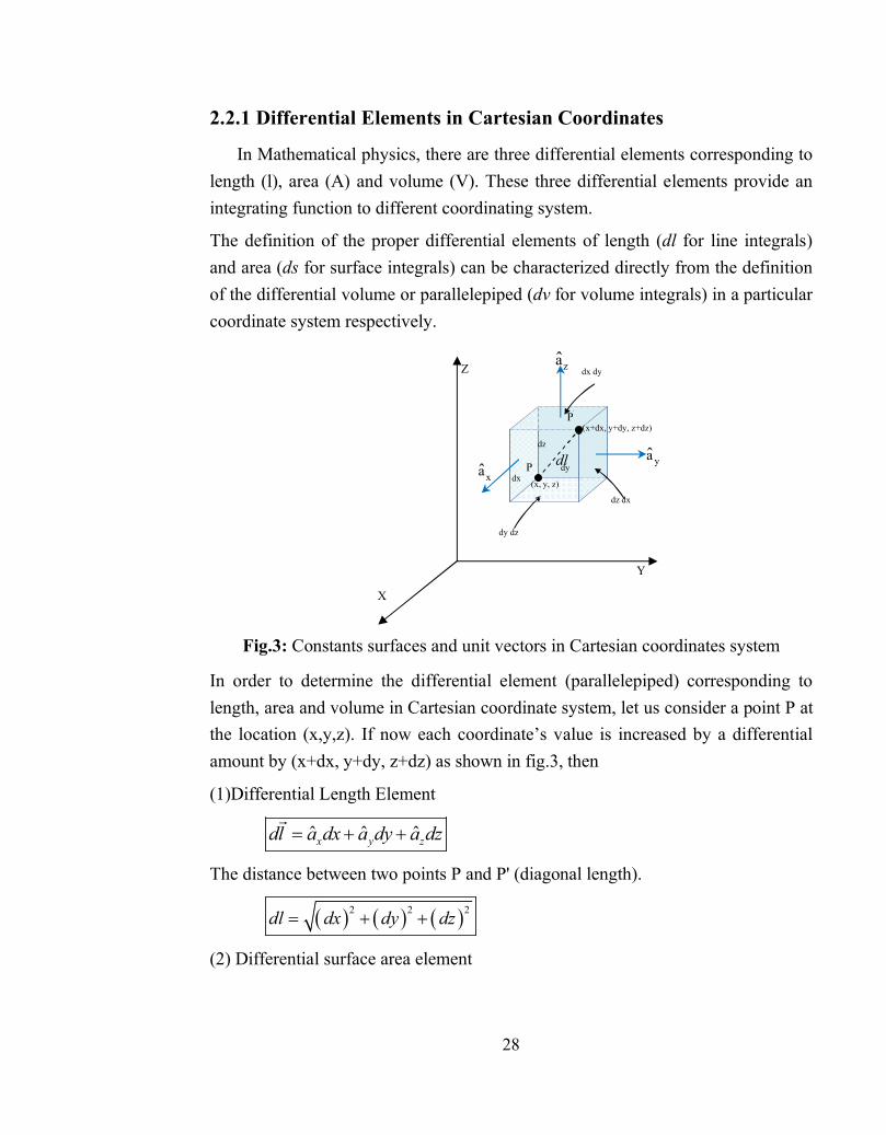
2.2.1 Differential Elements in Cartesian Coordinates

In Mathematical physics, there are three differential elements corresponding to length (l), area (A) and volume (V). These three differential elements provide an integrating function to different coordinating system.

The definition of the proper differential elements of length (dl for line integrals) and area (ds for surface integrals) can be characterized directly from the definition of the differential volume or parallelepiped (dv for volume integrals) in a particular coordinate system respectively.

Fig.3: Constants surfaces and unit vectors in Cartesian coordinates system

In order to determine the differential element (parallelepiped) corresponding to length, area and volume in Cartesian coordinate system, let us consider a point P at the location (x,y,z). If now each coordinate’s value is increased by a differential amount by (x+dx, y+dy, z+dz) as shown in fig.3, then

(1)Differential Length Element

ˆ ˆ ˆx y zdl a dx a dy a dz

The distance between two points P and P' (diagonal length).

2 2 2dl dx dy dz

(2) Differential surface area element

dldz

dy dx

dx dy

dz dx

dy dz

Y

X

Z

P'

P

(x+dx, y+dy, z+dz)

(x, y, z)

ya

za

xa

29

ˆˆ

ˆ

x x

y y

z z

ds dy dz ads dx dz ads dx dy a

or

dydxds

dzdxds

dzdyds

z

y

x

(3) Differential volume element dv dxdydz

In cylindrical coordinates system a point P is specified by three coordinates

(ρ,φ , z), where ρ represents a radial distance, φ an angular displacement (Azimuth Angle) and z an axial displacement (see figure.4).

In circular cylindrical coordinate system a point P can also be identified as intersection of three mutually perpendicular surfaces as follows:

Fig.4: Constants surfaces and unit vectors in cylindrical coordinates system

Ranges of Variables

ρ = const. (A circular cylinder); )(0 ρ

φ = const. (A Plane); π)2φ(0

z = const. (Another plane). )z(

2.3 Cylindrical Coordinate System

Y

ρ = constant

P

φ = constant

z = constant

Z

X

ρaaza

30

Unit vectors in cylindrical coordinates system are characterized as follow:

ρ ρˆ a const. (Perpendicular to the circular cylindrical Surface)

ˆ a const.(Perpendicular to the planer Surface)

ˆ za z const.(Perpendicular to the planer Surface)

2.3.1 Differential Elements in Cylindrical Coordinate System The differential element corresponding to length, area and volume in

cylindrical coordinate system can be found as shown in fig below;

Fig.5: Differential element in cylindrical coordinates system


dzadr adaldzˆφˆρˆρ


zz

r

add sd

adzdsd

adzd sd

ˆφρρˆρ

ˆφρ

φφ

ρ

or

φρρρφρ

φ

dd ds

dzdds

dzd ds

z

r

(3) Differential volume element

dzdd dv φρρ

Y

X

Z

dZ

ρ dφ

dρ A

P B

C

D

E

F

G

O

Oʹ

ρ

Z

φ dφ

31

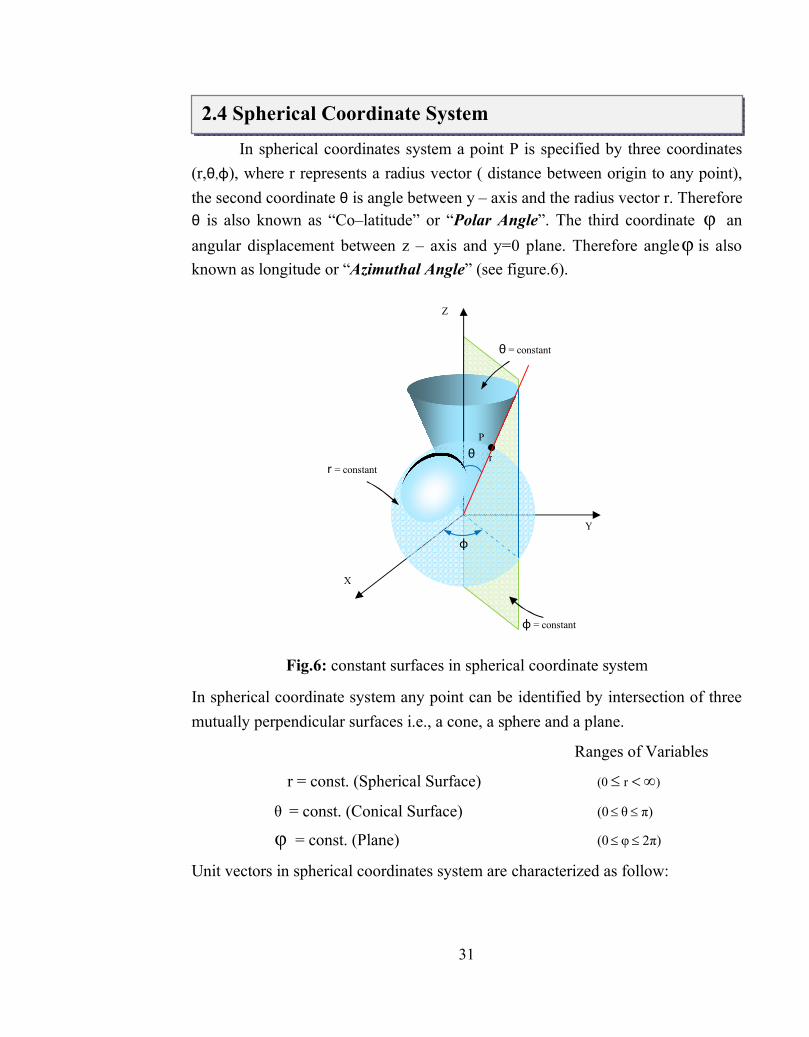
In spherical coordinates system a point P is specified by three coordinates (r,θ,φ), where r represents a radius vector ( distance between origin to any point), the second coordinate θ is angle between y – axis and the radius vector r. Therefore θ is also known as “Co–latitude” or “Polar Angle”. The third coordinate φ an angular displacement between z – axis and y=0 plane. Therefore angleφ is also known as longitude or “Azimuthal Angle” (see figure.6).

Fig.6: constant surfaces in spherical coordinate system

In spherical coordinate system any point can be identified by intersection of three mutually perpendicular surfaces i.e., a cone, a sphere and a plane.

Ranges of Variables

r = const. (Spherical Surface) )r(0

θ = const. (Conical Surface) π)θ(0

φ = const. (Plane) π)2φ(0

Unit vectors in spherical coordinates system are characterized as follow:

2.4 Spherical Coordinate System

Y

r = constant

φ = constant

θ = constant

Z

X

P

r

φ

θ

32

θ

φ

θ

ˆˆ

φˆ

ra r const. (Perpendicular to the spherical cylindrical Surface)

a const.(Perpendicular to the conical Surface)

a const.(Perpendicular to the planer Surface)

2.4.1 Differential Elements in Spherical Coordinate System

The differential elements corresponding to length, area and volume in cylindrical coordinate system can be found as shown in fig.5;

Fig.7: Differential Elements in spherical coordinate system


ˆ ˆ ˆ sinrdl a dr a r d a r d


φφ

θθ

ˆˆφˆφ

θ

θ

θθ

addrr sd

addrsinrsd

ad d sin rsdr

2

r

or

θ

θ

θθ

φ

θ φφ

ddrr ds

ddrsinrds

d d sin rds 2

r

(3) Differential volume element

2 sindv r dr d d Example 1 Given two points P1and P2 are located with the position vectors r1 and r2 respectively. What is the distance between them in the following coordinate systems?

Y

Z

X

φ dφ

dθ θ

dr

φθdsinr

θdr

Y

Z

X

φ

θ

ra

a

θa

33

(a) Cartesian coordinate system

(b) Cylindrical coordinate system

(c) Spherical coordinate system

Sol. (a) In Cartesian coordinate system

2

12

2

12

2

12 )z(z)y(y)x(x d

(b) In Cylindrical coordinate system

212

22

21

)z(zcos( d 2 )φφρρρρ 1221

(c) In Spherical coordinate system

θ θ θ θ φ φ 2 21 2 1 2 1 2 1 2 1 2 2 2d r r 2r r cos cos 2r r sin sin cos( )

Example 2 Determine the volume of a sphere of radius ‘2a’ from the differential volume element.

Sol. By eqn. φθθ dddr sin rdv 2

π π

θ φθ θ φ

r 2a 22

r 0 0 0Volume dv r sin dr d d

3

a32cos

3

r dd sindrrV

32

32ar

0r

2

00

2 πφφ π

0

π

0

2

0

π

φ

π

θθθθ

a

Example 3 Determine the surface area of a sphere of radius ‘a’ from the differential volume element.

Sol. Consider an infinitesimal area element on the surface of a sphere of radius a (see fig)

The area of this element has magnitude

φ)φ θθθθ)( ddsin rd sinr d(rdA 2

φ

π

φ

π

πθθ d d sinadA AreaSurface

2

0

2

222 a4cosaA πφ π

0

π

πθ


34


Q.1 What are coordinates of origin in Cartesian coordinate system?

Q.2 What is the range of azimuthal angle in cylindrical coordinate system?

Q.3 Who invented the idea of Cartesian coordinate system?


Q.4 Write the differential volume element for the Cartesian coordinate system?

Q.5 Write the differential volume element for the cylindrical coordinate system?

Q.6 Write the differential volume element for the spherical coordinate system?

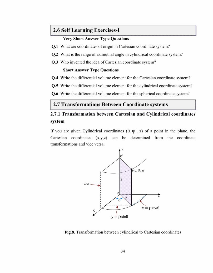
2.7.1 Transformation between Cartesian and Cylindrical coordinates system

If you are given Cylindrical coordinates (ρ,φ , z) of a point in the plane, the Cartesian coordinates (x,y,z) can be determined from the coordinate transformations and vice versa.

Fig.8. Transformation between cylindrical to Cartesian coordinates

2.7 Transformations Between Coordinate systems


θρsiny

θρcosx

P(ρ,φ , z)

O

Oʹ

φ Y

X

Z

ρ

Z Z=z

35

Cartesian to Cylindrical Cylindrical to Cartesian cossin

xyz z

zz

x

ytan

yx

1-

22

φ

ρ

The unit vectors also are related by the coordinate transformations

(a) Rectangular to Cylindrical unit vectors Transformation

zzyx

A,A,AA,A,A φρ

The transformation of unit vectors from rectangular to cylindrical coordinates requires the components of the rectangular coordinate vector ‘A’ in the direction of the cylindrical coordinate unit vectors (using the dot product). The required dot products are

0a.aa.aAa.aA

a.aAa.aAa.aAa.aAaAaAa.AA

zyyxx

zzyyxxzzyyxxCartesian

ρρρ

ρρρρρρ

ˆˆˆˆˆˆˆˆˆˆˆˆˆˆˆˆˆ

0a.aa.aAa.aA


zyyxx

zzyyxxzzyyxxCartesian

φφφ

φφφφφφ

ˆˆˆˆˆˆˆˆˆˆˆˆˆˆˆˆˆ

1ˆˆˆˆˆˆˆˆˆˆˆˆˆˆˆˆˆ

zzzyzxz

zzzzyyzxxzzzyyxxzCartesianz

a.a 0;a.aa.aA


where the za unit vector is identical in both orthogonal coordinate systems. The four remaining unit vector dot products can be determined with the help of geometry relationships between two coordinate systems.

Fig.9: Transformations of cylindrical unit vectors in terms of Cartesian unit vectors

yx

yx

acosasina

asinacosa

ˆφˆφˆˆφˆφˆ

φ

ρ

φ x

φ φ 90° - φ

90° - φ

y

z xa

φa

ρa

ya

ρ

36

ρ φ φ φˆ ˆ ˆ ˆ ˆ y y x ya .a a .(cos a sin a ) sin

φ φ φ φˆ ˆ ˆ ˆ ˆ x x x ya .a a .( sin a cos a ) sin

φ φ φ φˆ ˆ ˆ ˆ ˆ y y x ya .a a .( sin a cos a ) cos

Substituting these values in above eqn.,we have

φ

φφφ

ρρρ

ˆ

φφˆˆˆˆ

φφˆˆˆˆ

aA

sinAcosAa.aAa.aAA

sin AcosAa.aAa.aAA

z

xyyyxx

yxyyxx

The resulting cylindrical coordinate vector is

zzxyyx

zzrlCylindrica

aAasinAcosAasin AcosA

aAaAaAA

ˆˆφ)φ(ˆφ)φ(ˆˆˆ

φρ

φφρ

Also, in matrix form

z

y

x

z A

A

A

100

0cossin

0sincos

A

A

A

φφφφ

φ

ρ

Similarly, the transformation from cylindrical to rectangular coordinates can be found as the inverse of the rectangular to cylindrical transformation.

zzz

y

x

A

A

A

100

0cossin

0sincos

A

A

A

100

0cossin

0sincos

A

A

A

φ

ρ

φ

ρ

1

φφφφ

φφφφ

The cylindrical coordinate variables in the transformation matrix must be expressed in terms of rectangular coordinates.

2222 yx

yysinand

yx

xxcos

ρφ

ρφ

The resulting transformation is

ρ φ φ φˆ ˆ ˆ ˆ ˆ x x x ya .a a .(cos a sin a ) cos

37

z

2222

2222

z

y

x

A

A

A

100

0yx

x

yx

y

0yx

y

yx

x

A

A

A

φ

ρ

The cylindrical to rectangular transformation can be written as

ρ ρ ρ ρˆ ˆ ˆ ˆ ˆ ˆ ˆ ˆ ˆ ˆ

Cartesian x x y y z z x x y y z zA A a A a A a .a A a .a A a .a A a .a

ρ φ ρ φφ φ φ φˆ ˆ ˆ x y z z(A cos A sin ) a (A sin A cos ) a A a

ρ φ ρ φˆ ˆ ˆ

x y z z2 2 2 2 2 2 2 2

x y y xA A a A A a A a

x y x y x y x y

2.7.2 Transformation between Cartesian and Spherical coordinates system

Fig.10: Transformation between Spherical to Cartesian coordinates

Cartesian to Spherical Spherical to Cartesian

θ φx r sin cos

θ φy r sin sin

θz r cos

2z 2 2r x y

θ

φ

-1

2 2 2

-1

zco s

x y z

ytan

x

Y

Z

X

φ

θ

P(r,θ,φ )

O

r

φθ sinsinry

φθcossinrx

θcosrz

38

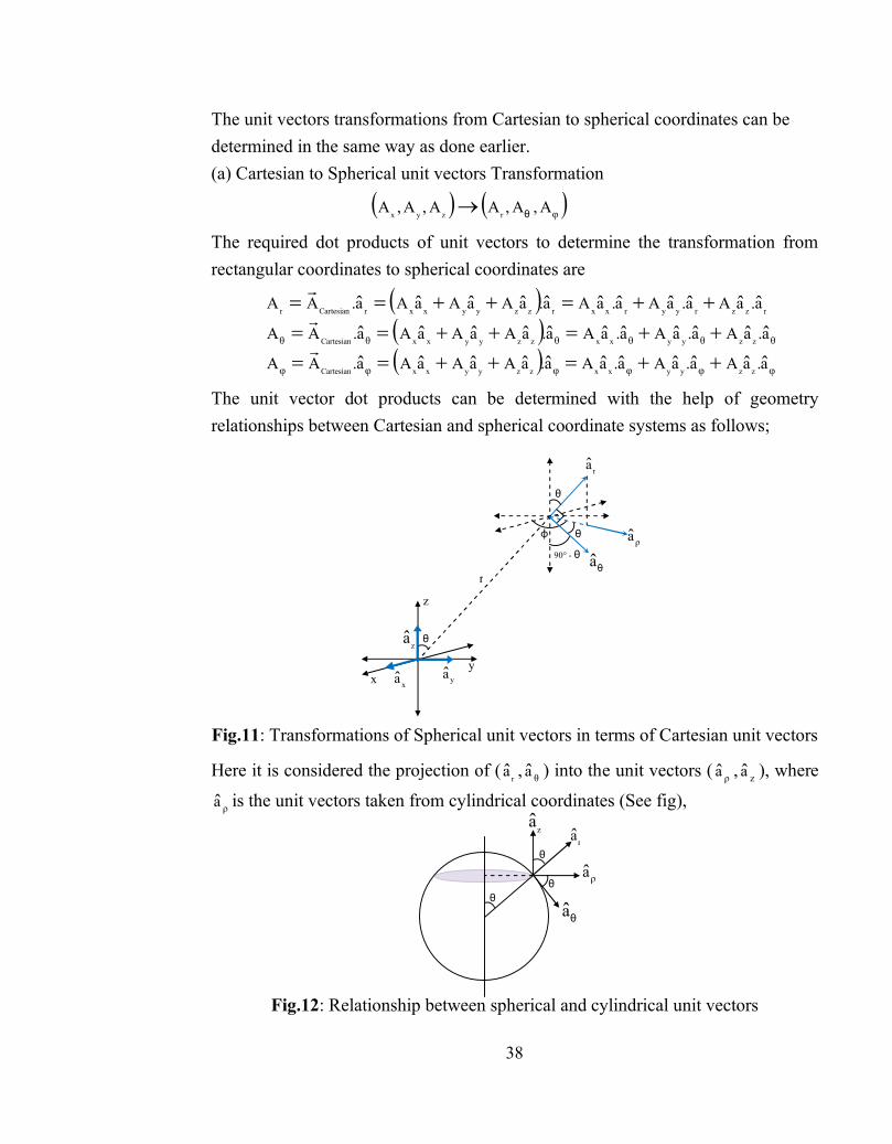
The unit vectors transformations from Cartesian to spherical coordinates can be determined in the same way as done earlier. (a) Cartesian to Spherical unit vectors Transformation

φA,A,AA,A,A θrzyx

The required dot products of unit vectors to determine the transformation from rectangular coordinates to spherical coordinates are

rzzryyrxxrzzyyxxrCartesianr a.aAa.aAa.aAa.aAaAaAa.AA ˆˆˆˆˆˆˆˆˆˆˆ

θθθθθθ ˆˆˆˆˆˆˆˆˆˆˆ a.aAa.aAa.aAa.aAaAaAa.AA zzyyxxzzyyxxCartesian

φφφφφφ ˆˆˆˆˆˆˆˆˆˆˆ a.aAa.aAa.aAa.aAaAaAa.AA zzyyxxzzyyxxCartesian

The unit vector dot products can be determined with the help of geometry relationships between Cartesian and spherical coordinate systems as follows;

Fig.11: Transformations of Spherical unit vectors in terms of Cartesian unit vectors

Here it is considered the projection of (r

a , θa ) into the unit vectors ( ρa , za ), where

ρa is the unit vectors taken from cylindrical coordinates (See fig),

Fig.12: Relationship between spherical and cylindrical unit vectors

θ

ρa

raza

θaθ

θ

θ

x

φ

90° - θ

y

z

xa

ρa

ra

ya

za

r

θ

θa

θ

39

The vector decomposition of ρa in to the Cartesian unit vectors (x

a , ya );

Therefore,

The dot products relationships are then

and the rectangular to spherical unit vector transformation may be written as

z

y

x

A

A

A

0cossin

sinsincoscoscos

cossinsincossin

A

A

A

φφφφφφ

θ θ θ

θ θ θ

φ

θ

r

Example 4 Deduce the Spherical to Cartesian unit vectors transformation.

Sol. The unit vector transformation from Spherical to Cartesian coordinates system can be found as the inverse of the rectangular to cylindrical transformation.

φ

θ

r

φ

θ

r

1

θθ

θ θ

θ θ

θ θ θ

θ θ θ

φφφφφφ

φφφφφφ

A

A

A

0sincos

cossincossinsin

sinsincoscossin

A

A

A

0cossin

sinsincoscoscos

cossinsincossin

A

A

A

z

y

x

We can write the spherical coordinate variables in terms of the Cartesian coordinate variables.


0

θ θ θ

θ θ θ

φφφ

θθθ

rrr

ˆˆ φφˆˆ φˆˆˆˆ φˆˆ φˆˆˆˆ φˆˆ φˆˆ

a.asincosa.asina.a

sina.asincosa.acoscosa.a

cosa.asinsina.acossina.a

zyx

zyx

zyx

yx acosasin.a ˆφˆφˆφ

zyx

zyxz

asinasincosacoscos

asinasinacoscosacosacos.a

ˆˆφˆφˆ)ˆφˆφ(ˆ-(ˆˆ

θθθ

θθθ)θ 90ρθ

zyx

zyxzr

acosasinsinacossin

acosasinacossinacosasin.a

ˆˆφˆφˆ)ˆφˆφ(ˆˆˆ

θθθ

θθθθ ρ

yx asinacosa ˆφˆφˆρ

40

2222

2222

22

yx

xxcosand

yx

yysin

yx

zzcosand

yx

yxsin

ρφ

ρφ

ρrρ

22θθ

zz

The resulting transformation is

φ

θ

r

22

22

22

A

A

A

0yx

yx

yx

z

yx

x

yxyx

yz

yx

yyx

y

yxyx

xz

yx

x

A

A

A

22

22

22

22222222

22222222

z

y

x

zz

zz

zz

Example 5 Find the location of the point (1,1,1) in cylindrical and spherical coordinate systems.

Sol. (a) In Cylindrical Coordinate System.

units2(1)(1)yx r 2222

45

1

1tan

x

ytan 1-1- φφ and

z =1

(b)In Spherical Coordinate System.

451

1tan

x

ytan

47543

1cos

zyx

zcos

units3(1)(1)(1)zyx r

1-1-

1-

222

1-

222222

φφ

θ

Curvilinear coordinate system is simply a general way to represent all coordinate systems (Cartesian, Cylindrical and spherical etc) which may be orthogonal and nonorthogonal. Cartesian, cylindrical and Spherical coordinate systems are only special cases of generalized curvilinear coordinates system.

2.9 Orthogonal Curvilinear Coordinates

41

Let us proceed to develop a general formula in generalized curvilinear coordinate system from which the all specific coordinate system can be easily obtained by simply putting suitable parameters.

Let us consider the eqn. of surface as

u (x,y,z)i=ic ( constant) … (1)

This eqn (1) represents the surface in space. It is well known that intersection of two surfaces is line i.e., the system of two surfaces u1 = c1 and u2 = c2 represent a line where the two surfaces intersect. Intersection of three surfaces is a point in space i.e., the system of three surfaces u1 = c1, u2 = c2 and u3 = c3 represent a point where the three surfaces intersect.

Therefore, in generalized coordinate system, three family of surfaces, described by u1=c1 (constant), u2=c2 (constant), u3=c3 (constant) which intersect at point P. Consider these three such surfaces

332211

czy,x,uandczy,x,u;czy,x,u … (2)

The value of u1,u2,u3 for the three surfaces intersecting at P are called curvilinear co-ordinates or curvilinear surfaces. For example the u1 coordinate curves are defined as the intersection of the coordinate surfaces u2 =constant and u3 =constant.

If these three coordinate surfaces intersect mutually perpendicular at every point P, then the curvilinear coordinates (u1,u2,u3) are said to be orthogonal curvilinear coordinates.

Fig.13: A General Curvilinear Coordinates system

A point P can be described by curvilinear coordinate (u1,u2,u3) same as Cartesian coordinate system.

3...zy,x,uuzy,x,uuzy,x,uu

33

22

11

P

1a

2a

3a

curve1u

11cu

curve2u

curve3u

33cu

22cu

42

Also, we can associate a unit vector ia normal to the surface ui (x,y,z)i=ic ( constant) and in the direction on increasing ui. In generalized curvilinear coordinates system, the variables u1, u2, and u3 are not measures of length directly and hence each variable should be multiplied by a general function of u1, u2, and u3, in order to determine sides of the parallelepiped as shown in fig. Therefore, we define three new quantity h1, h2, and h3 (function of u1, u2, and u3) are known as scale factors. The scale factor hi gives the magnitude of elemental length ds when we make infinitesimal change in coordinate ui from ui to ui+dui i.e., scale factor relating elemental length of the sides of parallelepiped s to coordinate increments.

Hence the elemental length of the sides of differential volume (parallelepiped) can be found as.

i i 1 2 3 i

i i i

ds h u ,u ,u du ... 4

ds h du

The infinitesimal volume element is therefore

5...dududuhhhduhduhduhdsdsdsdV 321321332211321

The scale factors and variables for three coordinate systems (Cartesian, Cylindrical and Spherical) are tabulated as

Table.1: variables, scale factors and unit vectors for three coordinate systems

S.No. Curvilinear Cartesian Cylindrical Spherical

1 Variables

u

u

u

3

2

1

z

y

x

z

r

φ φθr

2 FactorsScale

h

h

h

3

2

1

1

1

1

1

r

1

θsinr

r

1

3 VectorUnit

e

e

e

3

2

1

ˆˆˆ

z

y

x

a

a

a

ˆˆˆ

z

r

a

a

a

ˆˆˆ

φ

φ

θ

ˆˆˆ

a

a

ar

43

From above results, differential volume element for three coordinate systems (Cartesian, Cylindrical and Spherical) can be tabulated as follow:

Table.2. Differential volume element for different coordinate systems

Coordinate System Volume Element

Curvilinear 321321 dududuhhh

Cartesian dzdydx

Cylindrical dzdφdrr

Spherical dφdθdrθsinr 2

(1) Gradient. In curvilinear co-ordinates system grad f is

ˆ ˆ ˆ

1 2 3

1 1 2 2 3 3

1 f 1 f 1 fgrad f f a a a

h u h u h u

The ‘gradf’ in Cartesian coordinates, we have h1=1,h2=1,h3=1,u1=x,u2=y,u3=z; so we have

ˆ ˆ ˆ

x y z

f f fgrad f (cartesian) a a a

x y z Similarly, in cylindrical coordinates and spherical coordinates the gradf can be written as follows;

zr

az

fa

f

r

1a

r

fcal)(cylinderi fgrad ˆˆˆ φ

θ φˆ ˆ ˆθ φ

r

1 2

f 1 f 1 fgrad f (spherical) a a a

u r u r sin d

(2) Divergence. In orthogonal curvilinear co-ordinates system divA is

1 2 3 2 1 3 3 1 2

1 2 3 1 2 3

1divA A h h A h h A h h

h h h u u u

x y zdivA(cartesian) A A A

x y z

2.10 Differential Vector Operators

44

φφ

r z

1divA(cylindrical) A r A A r

r r z

θ φθ θθ θ φ

2r2

1divA(cylindrical) A r sin A r sin A r

r sin r

(3) Curl. In orthogonal curvilinear co-ordinates system curlA is

ˆ ˆ ˆ

1 1 2 2 3 3

1 2 3 1 2 3

1 1 2 2 3 3

h a h a h a

1curlA

h h h u u u

A h A h A h

(4) Laplacian. In orthogonal curvilinear co-ordinates system f2 is

2 2 3 3 1 1 2

1 2 3 1 1 1 2 2 1 3 3 3

h h h h1 f f h h ff

h h h u h u u h u u h u

Curl and Laplacian in Cartesian, cylindrical and spherical coordinate system can be obtained by substitution of suitable parameters.

Very Short Type Questions

Q.1 What is the shape of constant surface corresponding polar angle in spherical coordinate system?

Q.2 What is the shape of constant surface corresponding X-axis in Cartesian coordinate system?

Q.3 What is the shape of constant surface corresponding to coordinate ρ in cylindrical coordinate system?


Q.4 Calculate the distance between two points P1(1,1,2) and P2(1,2,4) in the In Cartesian coordinate system.

Q.5 Calculate the distance between two points P1(1,π/2,2) and P2(2, 3π/2,4) in the In cylindrical coordinate system.


45

Q.6 Calculate the distance between two points P1(2, π/2, π/4) and P2(4, 3π/2,

π/2) in the In spherical coordinate system.

● Coordinate system is used to define the position of an object in given space.

● There are mainly three types of coordinate systems.

● In Cartesian, cylindrical and spherical coordinates system a point P is identified by intersection of three mutually perpendicular surfaces as follows:

Coordinate Systems

Cartesian Cylindrical Spherical

x = const. (Plane) ρ = const. (circle) r = const. (Sphere)

y = const. (Plane) φ = const. (Plane) θ = const. (Cone)

z = const. (Plane) z = const. (Plane) φ = const. (Plane)

● The distance between two points in a coordinate system can be expressed as

Coordinate systems

Cartesian 2

12

2

12

2

12 )z(z)y(y)x(x d

Cylindrical 212

22

21

)z(zcos( d 2 )φφρρρρ 1221

Spherical )cos(sinsinr2rcoscosr2rrr d 22212121212

22

1 φφθθθθ

●The transformation relationship between Cartesian and Cylindrical coordinates

system can be expressed as

Cartesian to Cylindrical Cylindrical to Cartesian

zz

sin y

cos x

φρφρ

zz

x

ytan

yx

1-

22

φ

ρ

2.12 Summary

46

●The transformation relationship between Cartesian and Spherical coordinates system can be expressed as

Cartesian to Spherical Spherical to Cartesian

θ

θ

θ

φφ

cosr z

sinsinr y

cossinrx

x

ytan

zyx

zcos

yx r

1-

222

1-

22

φ

θ

2z

●Generalized curvilinear coordinate system is simply a general way to represents all coordinate systems (Cartesian, Cylindrical and spherical etc) which may be orthogonal and nonorthogonal.

●The scale factors, variables and unit vectors for three coordinate systems (Cartesian, Cylindrical and Spherical) can be tabulated as table.1.

●Differential volume element for different coordinate systems can be expressed as

Coordinate System Volume Element

Curvilinear 321321 dududuhhh

Cartesian dzdydx

Cylindrical dzdφdrr

Spherical dφdθdrθsinr 2

● Gradient for different coordinate systems can be expressed as

Coordinate System Gradient

Orthogonal Curvilinear 3

33

2

22

1

11

au

f

h

1a

u

f

h

1a

u

f

h

1ffgrad ˆˆˆ

Cartesian zyxa

z

fa

y

fa

x

f fgrad ˆˆˆ

Cylindrical zra

z

fa

f

r

1a

r

f fgrad ˆˆˆ φ

Spherical φθ ˆφθ

ˆˆ ad

f

sinr

1a

u

f

r

1a

u

ffgrad

2

r

1

47

● Divergence for different coordinate systems can be expressed as

Coordinate System

Divergence

Orthogonal Curvilinear

213

3

312

2

321

1321

hhAu

hhAu

hhAuhhh

1divA

Cartesian

zyx

Az

Ay

Ax

divA

Cylindrical

rAz

ArArr

1divA

zr φφ

Spherical

rAsinr AsinrArsinr

1divA 2

r2 φθ φθ

θθ

θ

●In orthogonal curvilinear co-ordinates system curlA can be written as

332211

321

332211

321

hAhAhAuuu

ahahah

hhh

1curlA

ˆˆˆ

●In orthogonal curvilinear co-ordinates system Laplacian vector f2 can be written as

33

21

312

13

211

32

1321

2

u

f

h

hh

uu

f

h

hh

uu

f

h

hh

uhhh

1f

Orthogonal coordinate system: When the surfaces intersect perpendicularly we have an orthogonal coordinate system.

Curvilinear co-ordinates: The value of u1,u2,u3 for the three surfaces intersecting at P are called curvilinear co-ordinates or curvilinear surfaces

Answers to Self Learning Exercise -I

2.13 Glossary

2.14 Answers to Self Learning Exercises

48

Ans.1 : (0,0,0) Ans.2 : π)2φ(0

Ans.3 : René Descartes Ans.4 : dzdydxdv Ans.5 : dzdd dv φρρ Ans.6 : φθθ dddr sin rdv 2

Answers to Self Learning Exercise -II Ans.1 : Conical Ans.2 : Plane

Ans.3 : A circular cylinder Ans.4 : 5 units

Ans.5 : 13 units Ans.6 : 25 22 units

Section-A (Very Short Answer Type Questions)

Q.1 In orthogonal curvilinear coordinate system three axes are ………. to each other.

Q.2 Write the formula to determine the base vector for coordinates system?

Q.3 In which coordinate system uses two angles and one distance?

Q.4 In which coordinate system uses two distances and one angle?

Q.5 In which coordinate system uses only distance?

Section-B (Short Answer Type Questions)

Q.6 Compute the vector directed from (1,1,1) to (2,2,2) in Cartesian coordinates system.

Q.7 Determine the value of A

at point (1,-1,1). If kzjzx- ixy A 2

Q.8 Find the location of the point (1,2,3) in cylindrical coordinates system.

Q.9 Write the formula of the base vectors for a coordinate system.

Q.10 Find the location of the point (1,2,3) in spherical coordinates system.

Section C (Long Answer Type Questions)

Q.11 Determine the base vectors for the cylindrical coordinate system.

Q.12 Determine the base vectors for the spherical coordinate system.

Q.13 Derive the expressions for the distance between two points in the cylindrical and spherical coordinate systems.

2.15 Exercises

49

Q.14 Evaluate the transformation relationship between cylindrical to spherical coordinate system.

Q.15 Transform the vector kzjzx- ixy A 2

from Cartesian coordinates to cylindrical and spherical coordinate systems.

Ans.1 : Mutually Perpendicular

Ans.2 : Plane

Ans.3: Spherical

Ans.4 : Cylindrical

Ans.5 : Cartesian Ans.6 :

zyx aaa A ˆˆˆ

Ans.7 : -1

Ans.8 : r = 5 units, 3463 φ , z =3

Ans.9 : 1,2,3iu

Rb

i

i

Ans.10 : r = 14 units, 990.θ , 3463 φ

1. K.D. Prasad, ‘Electromagnetic Fields and Waves’, 1st edition, Satya Prakashan, New Delhi (1999).

2. Satya Prakash, ‘Electromagnectic Theory and Electrodynamics’, Eleventh edition, Kedar Nath Ram Nath & Co. Meerut (2000).

3. B.S. Rajput, Mathematical Physics, 1st edition,Pragati Prakashan, Meerut (INDIA).

4. George Arfken, ‘Mathematical Methods for Physicists’, 2nd edition, Academic press,1970.



50

UNIT -3

Gauss’s theorem, Stokes’s theorem


3.0 Objectives

3.1 Introduction

3.2 Line Integrals

3.3 Properties of the Line Integral

3.4 Application of the Line Integral

3.5 Surface Integral

3.6 Surface Integral for Flux

3.7 Volume Integral

3.8 Self Learning Exercise

3.9 Gauss Divergence Theorem

3.10 Applications of Gauss’s divergence theorem

3.11 Stoke’s Theorem

3.12 Summary

3.13 Glossary

3.14 Answers to Self Learning Exercise

3.15 Exercise


References ad Suggested Readings

3.0 Objective

After gone through this unit learner will able to solve any physical problem in which vector integration is used. Learner can apply Gauss divergence theorem & convert surface integral into volume integral.

UNIT-3

Gauss’s theorem, Stokes’s theorem

3.0 Objectives

51

3.1 Introduction

In this unit integral calculus part of vector calculus is discussed. Vector line integral, vector surface integral & volume integral are explained. Using of Gauss divergence theorem & Stoke theorem with various examples are explained.

3.2 Line Integrals

Suppose a continuous vector function z,y,xF defined at each point of the curve C

kthjtgitftr , bta .

We partition the curve into a finite number of sub arcs. The typical sub arc has length ks in each sub arc we choose we point kkk z,y,x and from the sum

n

kkkkkn sz,y,xFS

1 (1)

The sum in (1) approaches a limit as n increases, and the length ks approach zero. We call this limit the integral of F over the Curve C from a to b .

n

kkkkk

nCsz,y,xFlimz,y,xf

1 (2)

Let rF be a continuous vector function, then component of rF along the tangent at P is

dsdr.rF (

dsdr is unit tangent vector at P)

Z

Y

X

O

t=b

S zyxP ,,

C

b

a

3.1 Introduction

3.2 Line Integrals

52

and

C dsdr.rF or

Cdr.rf

is called the tangent line integral of rF along the curve C.

Let kFjFiFrF 321

kzjyixr

1 2 3ˆ ˆˆ ˆ ˆ ˆ. .

C C

F dr Fi F j F k dxi dyj dzk

1 2 3 1 2 3C C

dx dy dzF dx F dy F dz F F F dtdt dt dt

C

dtdtdr.rF

3.3 Properties of the Line Integral Let F and G be two continuous vector point function and k is any constant, then

1. . .C C

k F dr k F dr

2. . . .C C C

F G d r F d r G d r

3. 1

. .C C

F dr F dr

Where direction of 1C is opposite to curve C.

4. 1 2

. . .C C C

F dr F dr F dr

5. If the line integral depends only on the end points of the curve, not on the path joining them then vector field is called conservative vector field.

Let F ; F is conservative field and is its scalar potential.

. . ( )b b

aaC

F dr F dr

ba kdzjdyidx.k

zj

yi

x

3.3 Properties of the Line Integral

53

ba dz

zdy

ydx

x

ba

bad ab

Thus, if the curve is closed, then the line integral of conservative vector field

rF is zero i.e. C

dr.F 0 .

3.4 Application of the Line Integral (a) Circulation: If F represent the velocity of a fluid and C is a closed curve, then the integral

Cdr.F is called circulation of F around the curve C i.e.

Circulation C

dr.F

(b) Work done by a Force : If F represents the force acting on a particle moving along an arc AB , then the work done by the force F during the displacement from A to B is

Work done BA dr.F

If F is a conservative vector field and is scalar potential of F , then

Work done BA dr.F

BA dr.

AB

If curve is closed, then work done 0 dr.F .

Example 1 Find the total work done in moving a particle in a force field given by

kxjyixyF 1053 along the curve 12 tx , 22ty , 3tz from 1t to 2t

Sol. Total work done CC

kdzjdyidx.kxjzixydr.F 1053

Since 12 tx , 22ty and 3tz

kdzjdyidxdr

kdttjtdtitdt 2342

3.4 Application of the Line Integral

54

Now work done 2

122322 3421105213 kdttjtdtitdt.ktjtitt

2

122423 13020112 dtttttt

2

12343 30121012 dttttt

21

2

1

3456303

330

412

510

612 t.t.t.t. units.

Example 2 If jxyiyxF 422 2 . Evaluate C

dr.F around a triangle ABC

in the xy-plane with A(0, 0), B(2, 0), C(2, 1) in counter clockwise direction. What is its value in clockwise direction.

Sol. The curve C is union of three curves 1C , 2C and 3C

321 CCCC

dr.Fdr.Fdr.Fdr.F

321 III (say)

Along 1C : Straight line AB, y=0, z=0 and x varies from 0 to 2.

dxidrxir

1

.432.1CC

dxijxyiyxdrFI

2

0

2 221

xdxdxyxC

420

2 x

Y

XA (0 , 0) B (2 ,0 )

C(2 , 1 )

1C

2C3C

55

Along 2C : The straight line BC, x=2, z=0 and y varies from 0 to 1.

jdydryjir 2

Thus, 22

432CC

jdy.jxydr.FI

1

083 dyy

1

0

2 823

yy

2138

23

Along 3C : The straight line CA, z = 0, 2y = x and x varies from 2 to 0

dxjijdxdxidrkjxxir

220

2

Thus,

CCdxji.jxyiyxdr.FI

2432 2

3

3

43212 2

Cdxxyyx

0

2

2

24

43

42 dxxxxx

0

2

23

83

12

xx 613

812

128

The required integral in counter clockwise direction is

314

613

2134321

IIIdr.F

C

The value of the integral in clockwise direction.

CC

drFdrF ..1

3

14

3.5 Surface Integral Let R is the shadow region of a surface S defined by the equation Cz,y,xf and g is a continuous function defined at the points of S , then the

integral of g over S is the integral

3.5 Surface Integral

56

RS

dA.f

fz,y,xgdSz,y,xg … (3)

Where P is a unit vector normal to R and 0 P.f . The integral itself is called a surface integral.

3.6 Surface Integral for Flux Suppose that F is a continuous vector field defined over a two-sided surface S and n is the unit normal field on the surface. The integral of n.F over S is called the flux across S in the positive direction

Flux S

dSn.F

R

dAP.g

ggg.F

R

dAP.g

g.F … (4)

Example 3 : Find the flux of the vector field

kyxjzyxizxA 532 through the upper side of the triangle ABC with vertices at the points A(1, 0, 0), B(0, 1, 0) and C(0, 0, 1).

Sol. Equation of the plane containing the give triangle ABC is

1 zyxz,y,xf

Unit normal n to ABC is

ˆ1 1 1

f i j knf

kji 3

1

Y

X

A(1,0,0)

B(0,1,0)

C(0,0,1)

Z

O

n

3.6 Surface Integral for Flux

57

Flux of ˆ ˆ. .ˆ.S S

dAA A nds A nn k

AOB

dxdy.kji.kyxjzyxix

313

532

1

0

1

0532 dxdyyxzyxzx

x

1

0

1

0147 dxdyyxyx

x

dxyyxx

1

0

1

0

2

2518

dxxxx

1

0

2125118

35

232

611

232

3211

1

0

23

xxx

Example 4 : Evaluate

Sdsn.A over the entire surface S of the region bounded by

the cylinder 922 zx , x=0, y=0, z=0 and y=8 where xkiyxziA 26 .

Sol. Here the entire surface S consist of 5 surfaces, namely. 1S : lateral surface of the cylinder ABCD, 2S : AOED, 3S : OBCE, 4S : OAB, 5S : CDE.

58

Thus, 1 2 3 4 5

ˆ ˆ. .S S S S S

S

A ndS A ndS

521 SSS

dSn.A...dSn.AdSn.A

54321 IIIII (say)

1S : ABCD : The curved surface 1S is 922 zxf . The unit outward normal to

1S is

344

2222

zkxi

zx

zkxiffn

3

26 zjxi.kzkjyxzin.A

xzxzxz356

31

and 3zk.n

8

0

3

0 335

1 y xS zdxdyxzdSn.A

8

0

3

05 xdxdy 180

2895

2S : AOED : The surface 2S is xy-plane i.e. z=0. Unit outward normal to the surface is kn

k.kdxdyk.xkjyxzidSn.A

S26

2

8

0

3

y oxdxdyx

36829

280

3

0

2

y.x

3S : OBCE : Surface 3S is yz-plane i.e. x=0. Unit outward normal to 3S is in .

3

0

8

026

3 z yS i.idydzi.xkjyxzidSn.A

59

3

0

8

06 dydzz 216

26 8

0

3

0

2

yz

4S : OAB : The section OAB is in xz-plane i.e. y=0. The unit outward normal to

4S is jn .

3

0

9

0

2

4

26x

S j.jdxdzj.xkjyxzidSn.A

3

0

9

0

2

2x

dxdzx

3

0

90

22 dxzx x

3

0

292 dxxx

23

9232x 1827

32

5S : CDE : The section 5S is parallel to xz-plane, y=8. The outward normal to 5S is jn .

3

0

9

0

2

5

26x

S j.jdxdzj.xkjyxzidSn.A

3

0

9

0

2

82x

dxdzx

3

0

90

282 dxzx x

3

0

2942 dxxx

60

1

0

12232

32949

24

22392

xsin.xx..x

118

Thus, the required surface integral is

1818181821636180 S

dSn.A

3.7 Volume Integral Let V be a region in space enclosed by a closed surface S. Let be a scalar point function and F be a vector point function, then the triple integral

V

dV and V

FdV

and called volume integrals.

Example 5 : Evaluate V

fdV where yxf 2 , V is the closed region bounded

by the cylinder 24 xz and the planes 0x , 0y , 2y and 0z .

Sol.

2

0

2

0

4

0

2

2y x

x

zVdzdxdyyxfdV

2

0

2

0

40

22

y x

x dxdyyzxz

Y

X

A(2,0,0)

B (0,0,4)

Z

O

0z

2y

3.7 Volume Integral

61

2

0

2

0

22 442y x

dxdyxyxx

2

0 388816

ydyyy

3

803

321623

1682

0

2

yy

Example 6 : Evaluate the value of V

dVFdiv

, where kzjixF 224

and V

is the region bounded by 422 yx ; 0z and 3z .

Sol. First we take

kzjyix.z

ky

jx

iF.Fdiv 2224

Now

Rz

VdzdydxzydVFdiv 3

0244

R

dydxzyzz30

244

R

dydxy 9112

(Taking parametric equation of the curve 422 yx i.e., cosrx , sinry drdrdydx )

R

drdrsinr 1221

2

02

0 1221r drdrsinr

dsinrr2

0

20

32

4221

dsin

20 3242

203242 cos

62

84323284 0


Q.1 Work done by a particle in a force field F

on moving particle from point A to point B is given by..

Q.2 Write the unit normal vector to surface 2222 azyx at point

0

21

21 ,, .

Section – B (Short Answer type Question)

Q.3 Find the circulation of jyx

xiyx

yF 2222

round the circle

122 yx in xy plane.

Q.4 Evaluate S

dSn.F

where kyzjxiyxF 2222

& S is surface of plane

622 zyx in first octant.

Section – C (Long Answer type Question)

Q.5 Evaluate V

dVFdiV

where kyzjxzizyF 222222

& V is volume

bounded by sphere 1222 zyx above xy -plane.

Q.6 Evaluate S

dsFCurl

where kzxjyzixyF 2

& S is open surface of

rectangle parallel piped formed by planes 0x , 1x , 0y , 2y & 3z above xy -plane.


The Gauss divergence theorem transforms double (surface) integral into volume Integral with the help of divergence of a vector point function. Gauss’s divergence theorem is also known as Ostogradsky’s theorem.

Statement : If F

be a continuously differential vector point function and S is a closed, smooth and orientable surface enclosing a region V , then



63

ˆ. div . . .S S V

F ndS F dV F dV

or ˆ. divS V

F ndxdy F dxdydz

,

where n is the unit outward drawn normal vector on the surface S .


The divergence theorem finds applications in evaluating the integrals of dot and cross products of vector fields and scalar fields.

(A) Product of a scalar function z,y,xg and a vector field z,y,xF

The surface integral, with respect to a surface S , of the scalar product Fg

is evaluated by using the following result:

VS

dVF.gg.Fdsn.Fg

(B) Cross product of two vector fields GF

:

The surface integral, with respect to a surface S , of the cross product GF

is evaluated by using the following result :

VS

dVG.FF.GdS.GF

(C) Product of scalar function z,y,xf and a non zero constant vector

Following result exists for the evaluation of surface integral of product of a scalar function, f , and a non zero constant vector.

VS

dVffdS

(D) Cross product of a vector field F

and a non-zero constant vector

Application of divergence theorem to the cross product of a vector field F

and a non-zero constant vector, gives following result:

VS

dVFFSd


64

Example 7 : Evaluate the surface integral S

dsn.F

, where

kjizyxF 222, S is the tetrahedron 0x , 0y , 0z , 2 zyx

and n is the unit outward drawn normal to the closed surface S .

Sol. It is convenient to use Gauss’s theorem for the evaluation of the integral.

By Gauss’s theorem

VS

dV.Fdivdsn.F

Here kjizyxF 222

222 zyxx

Fdiv

zyx 222

VS

dVzyxdsn.F 2

2

0

2

0

2

02

x yxdzdydxzyx

2

0

2

0

2

0

2

22

x yx

dydxzzyx

2

0

2

0

222122

xdydxyxyxyx

2

0

2

0

2

222

x

Sdydxyxdsn.F

A(2,0,0)

(0,2,0)

C(0 ,0,2)

O

n

z

x

yB

65

2

0

2

0

3

622 dxyxy

x

2

0

3

668222 dxxx 4

24382

2

0

42

xxx

Example 8 : Verify divergence theorem for kxyzjzxyiyzxF 222

taken over the rectangular parallelepiped ax 0 , by 0 , cz 0 .

Sol.

For verification of divergence theorem, we shall evaluate the volume and surface integrals separately and show that they are equal

Now, div zyxxyzz

zxyy

yzxx

F

2222

c b a

VdzdydxzyxdVFdiv

0 0 02

c ba

dydzzxyxx0 0

0

2

22

cb

c b dzazyayyadydzzayaa0

0

22

0 0

2

222

22

c

c zabzabzbadzabzabba

0

222

0

22

2222

222

cbaabcabccabbca 222 … (1)

To evaluate the surface integrals, divide the closed surface S of the rectangular parallelepiped into 6 parts.

66

1S : the face BCOA , 2S : the face CAOB , 3S : the face BPCA , 4S : the face BPCA , 5S : the face ABOC , 6S : the face CPAB

Also

1 2 3

4 5 6

ˆ ˆ ˆ ˆ. . . .

ˆ ˆ ˆ. . .S S S S

S S S

F ndS F ndS F ndS F ndS

F ndS F ndS F ndS

On 01 zS , we have kn , kxyjyixF 22

So that xyk.kxyjyixn.F 22

bbb aS

baydyadyxyxydxdydSn.F0

22

0

22

0 0 422

On czS 2 , we have kn , kxycjcyyicyxF 222

So that xyck.kxycjcyyicyxn.F 2222

bb aS

baabcdyyaacdydxxycdSn.F0

222

22

0 02

422

On 03 xS , we have in , kzjyiyzF 22

So that yzi.kzjyiyzn.F 22

cc b

ScbzdzbdzdyyzdSn.F

0

222

0 0 423

On axS 4 , we have in , kayzjazyiyzaF 222

So that yzai.kayzjazyiyzan.F 2222

cc bS

cbbcadzzbbadydzyzadSn.F0

222

22

0 02

424

On 05 yS , we have jn , kzjzxixF 22

So that zxj.kzjzxixn.F 22

aa c

ScadxxcdxdzzxdSn.F

0

222

0 0 425

On byS 6 , we have jn , kbxzjzxbibzxF 222

67

So that zxbj.kbxzjzxbibzxn.F 2222

a c

SdxdzzxbdSn.F

0 02

6

c cacabdxxccb0

222

22

42

444444

222

22222

22222

22 cacabcacbbcacbbaabcbadSn.FS

… (2)

The equality of (1) and (2) verifies divergence theorem.

Example 9 : Verify divergence theorem for kzjyixF 2224

taken over the

region bounded by the cylinder 422 yx , 0z , 3z .

Sol. Since div zyzz

yy

xx

F 24424 22

VV

dzdydxzydVFdiv 244

22

4

4

30

2

2244x

xdxdydzzy

22

4

4

30

22

244x

xdxdyzyz

22

4

4

22

4

4

2

2

2

22191212 x

x

x

xdxdydxdyy

[since y12 is an old function aa dyy 012 ]

68

20

222

2 484442 dxxdxx

1sin2842

sin24

2484 1

2

0

12

xxx

842

284

… (1)

To evaluate the surface integral divide the closed surface S of the cylinder into 3 parts.

1S : the circular base in the plane 0z

2S : the circular top in the plane 3z

3S : the curved surface of the cylinder, given by the equation 422 yx

Also 321 SSSS

dSn.FdSn.FdSn.FdSn.F

On 01 zS , we have kn , jyixF 224

So that 024 2 k.jyixn.F

01

S dSn.F

On 32 zS , we have kn , kjyixF 924 2

So that 9924 2 k.kjyixn.F

222

99SSS

dydxdydxdSn.F

9 area of surface 3629 22 .S

On 3S , 422 yx

A vector normal to the surface 3S is given by jyixyx 22422

n a unit vector normal to surface 3S

4422

44

2222

jyix

yx

jyix , [since 422 yx ]

2

jyix

69

n.F

3222 22

24 yxjyix.kzjyix

Also, on 3S , i.e., 422 yx , cosx 2 , siny and dzddS 2 .

To cover the whole surface 3S , z varies from 0 to 3 and varies from 0 to 2 .

20

30

32 22223

ddzsincosdSn.FS

20

32 316 dsincos

20

32 4848 dsincos

20

20

3220

2 022

14 dsin,dcosdcossince

8448360 S dSn.F

The equality of (1) and (2) verifies divergence theorem.

3.11 Stoke’s Theorem The Stoke’s theorem transforms line integral into surface integral with the help of curl of a vector point function. Stoke’s theorem is the vector form of Green’s theorem or generalized Green’s theorem.

Statement : If S is the open surface bounded by a closed curve C and

kfjfifF 321

is any continuously differentiable vector function, then

ˆ ˆ. . .C S

F d r Curl F nds F nds

,

Where n is the unit outward normal drawn to the surfaces.

Example 10 : Evaluate S

dsn.A

over the surface of intersection of cylinders

222 ayx , 222 azx , which is included in the first octant given that

kzxjyxiyzA 2232

.

Sol. By Stoke’s theorem

CS

rd.Adsn.A

3.11 Stoke’s Theorem

70

Here C is the curve consisting of four arcs namely 1C : AB , 2C : BP , 3C : PD ,

4C : DA . Thus, we evaluate RHS of (1), along these four arcs one by one.

Along 1C : 0z , yayx 222 varies from 0 to a .

11

2232CC

dzzxdyyxyzdxrd.A

1

23C

dyyx

adyyya

0

22 23

a

yyysinayay

0

212

22 223

222

aaard.AC

22

32

22

1

(2)

Along 2C : 0x , ay ; 0dx ; 0dy and z varies from 0 to a

22

2

0

2

022

azzdzzdzrd.Aaa

CC

… (3)

Along 3C : 0x , az ; 0dx ; 0dz and y varies from a to 0

a

CCdyydyyrd.A

02323

33

aayy

a

22

322

3 202

… (4)

71

Along 4C : 0y , 222 azx , z varies from a to 0

0

220

2

4 aaCdzzzadzzxrd.A

23

223

1 230232 aazzza

a

… (5)

Thus, the desired integral is sum of (2), (3), (4), (5)

i.e. 23

222

32

22

34

232222 aaaaaaaadsn.AS

aaaa 83123

24

232 Ans.

Example 11 : Verify Stoke’s theorem for kzxzxyjiyxF 32 235 over

the surface of the hemisphere 16222 zyx above the xy -plane.

Sol. Here S is the surface 16222 zyx and C is the boundary of the

hemispherical surface and is given by C : 1622 yx .

tcosx 4 , tsiny 4 , 0z , 20 t

ktjsinticosr 044

dttjcostisindr 44

and tjcos.tsinitsintcosF 484416 2

Stoke’s theorem is

72

k.n

dAn.Fdr.FR

C

Where R is the region in xy -plane bounded by curve C

L.H.S. of Stoke’s theorem

C

dr.F

2

0

222 192161664 dttcostsintsintsintcostsin

2

0

2 162

116128 dttsintcostsintcos

2

0

316248

3128

tcostsinttcos

16 … (1)

Now

22 234 zxzxyyxzyx

kji

F

130200 ykzji

kyzj 132

4444

222222

zkyjxi

zyx

zkyjxin

zyyz 13241

143

4

yzyz

R.H.S. of Stokes theorem k.n

dxdyn.FR

4

14 z

dxdy.yz

R

4

4

16

16

2

2

1x

x

dydxy

73

4

4

16

162

2

2dxyy

x

x

4

4

2162 dxx

4

4

1242

16162

2

xsinxx

2216

16 L.H.S. Hence verified.

Example 12 If kzyxjyxzixzyF 222222222 Evaluate

S

dsn.F taken over the surface 0222 azaxyxS , 0z

Sol. The given surface 0222 azaxyxS is bounded by the curve C :

0222 axyx , 0z .

or 222 ayax , 0z

or tcosaax , tsinay , 0z

tjsinaitcosar 1

dttjcosatjsinadr

and

ktcosajtsinatcosaitcosatsinaF 1211 222223222

By Stokes theorem

dr.Fnds.FS

2

0

222222 11 dttcosatsintcosatsinatcostsina

2

0

223 1212 dttcostcostsintcostsina

2

0

22

0

3 22

12

22 dttcostsintcostcosdttsintsina

74

2

0

22

0

3 22

12

22 dttcostsintcostcosdttsintsina

2

0

3333

2

0

23

22

224

22

tsinatsintatsinatcostcosa

32 a

Example 13 : Use Stoke’s theorem to evaluate C rd.F where

jxcosiyxsinF

and C is the boundary of the triangle whose vertices are 00, , 02 , and 12 , .

Sol. Evaluating C rd.F by using Stoke’s theorem means expressing the line

integral in terms of its equivalent surface integral and then evaluating the surface integral.

By Stoke’s theorem SC

Sd.Fcrulrd.F

, where S is any open two-

sided surface bounded by C .

To simplify the work, we shall choose S as the plane surface R in the XY -plane bounded by C .

SC

dydxk.Fcurelr.F [ for the XOY -plane , kn and dydxdS ]

For this problem,

Curl

kxsin

xcosyxsinzyx

kji

F 1

00

The given line integral

75

R

dydxxsin1

1

0

1

0

22

22

1

yy

xcosxdydxxsin

1

0 222dyycosy

242

242

1

0

2

ysinyy

3.12 Summary In this unit line integral in vector calculus is discussed. After that volume

& surface integral are discussed. Conversion of line integral into surface integral & surface integral into volume integral is explained. Use of Gauss divergence theorem & Stokes theorem is discussed by using various examples.

3.13 Glossary

Vector : A physical quantity having both magnitude & directions.

Line Integral : An integral calculated along a curve.

Surface Integral : An integral calculated on the surface of any curve.

3.14 Answer to Self Learning Exercise

Ans.1 : BA rd.F

Ans.2 : ji2

12

1

Ans.3 : 2 Ans.4 : 37

Ans.5 : 12 Ans.6 : 1

3.15 Exercise

Section – A (Very Short Answer Type Question)

Q.1 State Gauss divergence theorem.

Q.2 State Stoke’s theorem.

3.12 Summary

3.13 Glossary


3.15 Exercise

76

Q.3 Write value of S

Sd.F

in line integral.

Q.4 Write value of line integral of jxixF 22

along x -axis from 1x to 2x .

Q.5 If C is closed curve then write value of C rd.F where F

is conservative

field.

Section – B (Short Answer type Question)

Q.6 Find the work done in the force field kxjxieF zy 22 in moving the

particle from 000 ,, to 122 ,, .

Q.7 Evaluate C

dyxyxydx 2 where C is boundary of square in xy -plane with

vertices 01, , 01, , 10, , 10 , using Stoke’s theorem.

Q.8 Evaluate C rd.F where jxiyF

& C is boundary of ellipse

12

2

2

2

by

ax , 0z .

Q.9 Evaluate S dSn.F

where kzjyixF 2224

& S is region bounded by

422 yx & plane 0z to 3z .

Q.10 Evaluate S dSn.F

where 3rrF

& S is surface 2222 azyx .

Section – C (Long Answer type Question)

Q.11 Verify Gauss divergence theorem for kyzjyixzF 24

over the surface of cube bounded by 0n , 0y , 0z , 1x , 1y , 1z .

Q.12 Verify Gauss divergence theorem for kxjxyizxF 4232 2

over the region bounded by co-ordinate planes & 422 zyx .

Q.13 Verify Gauss divergence theorem for kzjyixF 222

over the surface

of ellipsoid 12

2

2

2

2

2

cz

by

ax .

Q.14 Verify Stoke’s theorem for vector point function jyxixF 2 round the

square in plane 0z whose sides are along straight lines 0 yx & ayx .

77

Q.15 Verify Stoke’s theorem for kxyjxzxiyF 2

over the surface of

sphere 2222 azyx above xy -plane.


Ans.3 : C rd.F Ans.4 : 3

Ans.5 : 0 Ans.6 : 42e

Ans.7 : 34 Ans.8 : 0

Ans.9 : 84 Ans.10 : 4


1. J.N.Sharma & A.R. Vasishtha ,Vector Calculus ,Krishna Prakashan , Meerut ,1996

2. Murray R.Spiegal ,Vector Calculus ,Schaum’s Outline Series,McGraw-Hill Book Company(2003)

3. E.Kreyszig ,Advanced Engineering Mathematics ,8th Edition, John Wiley &Sons(Asia)P.Ltd.(2001)



78

Structure of the unit

4.0 Objectives

4.1 Introduction

4.2 N-dimensional space

4.3 Contravariant and covariant vectors

4.4 Self learning exercise-I

4.5 Algebraic operations with tensors

4.6 Contraction

4.7 Direct product

4.8 Quotient rule

4.9 Symmetric and anti-symmetric tensor

4.10 Pseudo-tensor

4.11 Self learning exercise-II

4.12 Summary

4.13 Glossary

4.14 Answers of self learning exercises

4.15 Exercise


References and Suggested Readings.

4.0 Objective In this unit we are going to discuss about tensors and its properties.

After going through this unit you will be able to learn

N-dimensional space

Contravariant and covariant vectors

UNIT- 4

Tensor Analysis

4.0 Objectives

79

Algebraic operations with tensors

Contraction ,Direct product, Quotient rule

Symmetric and anti-symmetric tensor, Pseudo-tensor

4.1 Introduction The fundamental postulate of Physics is that the laws of nature are covariant. The meaning of covariant is that they have the same form in all reference frames. Tensor formulation is a mathematical tool in which all the physical laws can be formulated in a covariant way.

The tensor formulation was originally given by G. Ricci and it became popular when Albert Einstein used it as a natural tool for the description of his general theory of relativity. It has became an important mathematical tool in almost every branch of theoretical physics such as Mechanics, Electrodynamics, Elasticity, Fluid mechanics etc. Tensor analysis is the generalization of vector calculus.

4.2 N-dimensional space In three dimensional space (Cartesian system), the coordinates of a point are given by (x, y, z) where x, y, z are numbers. For the generalization of concept of space, from three dimensions to N-dimensions this representation is not suitable.

An ordered set of N real variables 푥 ,푥 , … . .푥 can be associated with a point in space and will be called the coordinates of the point. All the points corresponding to all of the coordinates are said to form an N-dimensional space, denoted by푉 .

Transformation of Coordinates:-

The process of obtaining one set of numbers from the other is known as coordinate transformation. Consider two different N-dimensional spaces. Let us

consider two sets of variables (푥 ,푥 , … . 푥 ) and (푥 ,푥 , … .푥′ ). A

transformation from (푥 ,푥 , … . 푥 ) to the new set of variables

(푥 ,푥 , … . 푥′ ) through the equations

푥 = 푓 (푥 , 푥 , … . 푥 ) (1)

4.1 Introduction

4.2 N-dimensional space

80

gives a transformation of coordinates. Here 푓 is assumed to be single valued real function of the coordinates and possess continuous partial derivatives. This ensures the existence of inverse transformation and is given as

푥 = 푔 (푥 ,푥 , … . 푥 ) (2)

The suffixes or indices i, j in 퐴 are called superscript and subscript respectively.

Concepts of Scalar, Vector and Tensor: - Scalar: A physical quantity that can be completely described by a real number. Example:- Temperature, mass, density, potential etc. The expression of its component is independent of the choice of the coordinate system.

Vector: A physical quantity that has both direction and length. Example:- Displacement, velocity, force, heat flow etc. The expression of its component is dependent of the choice of the coordinate system.

Tensor: A tensor defines an operation that transforms a vector to another vector. A tensor contains the information about the directions and the magnitudes in those directions.

4.3 Contravariant and Covariant Vectors

Contravariant vectors:-

A set of N functions 퐴 (푖 = 1 …푁) of the N coordinates 푥 (푖 = 1 …푁) are said to be components of a contravariant vector if they transform according to the equation

ii j

j

xA Ax

(3)

on change of the coordinates 푥 to 푥 .

Covariant vectors:-

A set of N functions 퐴 (푖 = 1 …푁) of the N coordinates 푥 (푖 = 1 …푁) are said to be components of a covariant vector if they transform according to the equation

j

ii j

xA Ax (4)

4.3 Contravariant and Covariant Vectors

81

on change of the coordinates 푥 to 푥 .

Only in Cartesian coordinate

휕푥휕푥

=휕푥휕푥

… (5)

So that there is no difference between covariant and contravariant transformations in Cartesian coordinates. In other coordinate systems, eqn. (5) in general doesn’t apply and there is difference between covariant and contravariant transformations in other coordinate systems. This is important in the curved Riemannian space of general relativity.

Definitions of tensors of rank 2:-

The rank goes as the number of partial derivatives in the definition:

0 for scalar, 1 for vector, 2 for a second rank tensor and so on.

A covariant tensor 퐴 of rank two is transformed as

k l

i jij klkl

x xA Ax x (6)

A contravariant tensor 퐴 of rank two is transformed as

i jij kl

k lkl

x xA Ax x

(7)

A mixed tensor is contravariant in some indices and covariant in the others. A

mixed tensor 퐴 of rank two is transformed as

i li k

k jj lkl

x xA Ax x

(8)

The components of a vector transform according to eqns. (6), (7), (8) yield entities that are independent of the choice of reference frame. That’s why tensor analysis is important in physics.

Example 4.1 A covariant tensor has components 푥푦 , 2푦 − 푧 ,푥푧 in rectangular co-ordinates. Find its covariant components in spherical co-ordinates.

Sol. Let 퐴 denote the covariant component in rectangular co-ordinates

82

푥 = 푥, 푥 = 푦, 푥 = 푧. Then 퐴 = 푥푦 = 푥 푥

퐴 = 2푦 − 푧 = 2푥 − (푥 )

퐴 = 푥푧 = 푥 푥

Let 퐴 denote the covariant component in spherical co-ordinates 푥 = 푟, 푥 = 휃,푥 = 휑.

Then 퐴′ = 퐴 (1)

In spherical coordinates

푥 = 푟 sin 휃 cos휑

표푟 푥 = 푥 sin 푥 cos푥

푦 = 푟 sin휃 sin휑

표푟 푥 = 푥 sin 푥 sin 푥

푧 = 푟 cos 휃

표푟 푥 = 푥 cos푥

Therefore equation (1) yields the covariant component.

퐴′ = 휕푥휕푥

퐴 +휕푥휕푥

퐴 +휕푥휕푥

퐴

= (sin 푥 cos푥 )(푥 푥 ) + (sin 푥 sin 푥 )(2푥 − (푥 ) )+ cos푥 (푥 푥 )

= (sin 휃 cos휑)(푟 sin 휃 sin휑 cos휑)+ (sin휃 sin휑)(2푟 sin 휃 sin휑 − 푟 cos 휃)+ (cos휃)(푟 sin 휃 cos휃 cos휑)

퐴 = 휕푥휕푥

퐴 +휕푥휕푥

퐴 +휕푥휕푥

퐴

= (푟 cos휃 cos휑)(푟 sin 휃 sin휑 cos휑) + (푟 cos 휃 sin휑) (2푟 sin 휃 sin휑− 푟 cos 휃) + (−푟 sin 휃)(푟 sin 휃 cos 휃 cos휑)

퐴 = 휕푥휕푥

퐴 +휕푥휕푥

퐴 +휕푥휕푥

퐴

= (−푟 sin 휃 sin휑)(푟 sin 휃 sin휑 cos휑)+ (푟 sin 휃 cos휑) (2푟 sin 휃 sin휑 − 푟 cos 휃) + 0.

83


Q.1 What is the rank of tensor 퐴 ?

Q.2 Write the transformation of covariant tensor 퐵 ?

Q.3 Write one example of a mixed tensor of rank 3.

4.5 Algebraic Operations with Tensors

Kronecker Delta: -

The Kronecker delta is defined as

If i j1

I i j0 f

ij

ij

So by definition of Kronecker delta we can write

훿 = 훿 = 훿 = ⋯ = 훿 = 1

훿 = 훿 = ⋯ = 0

The coordinates 푥 ,푥 , … ,푥 are independent so Kronecker delta can also be written as

ii

j j

xx

Similarly we can write

휕푥′휕푥

= 훿

Addition and Subtraction of Tensors:-

The sum of two or more tensors of the same rank and type (i.e. same number of contra-variant and same numbers of covariant indices) is also a tensor of the same rank and type. Thus the sum of two tensors

퐶 = 퐴 + 퐵

is also a tensor.


4.5 Algebraic Operations with Tensors

84

We can also subtract two tensors provided they are of the same rank and type. The difference of two tensors of same rank and type is another tensor of the same rank and type.

퐶 = 퐴 − 퐵

Theorem: - The sum or difference of two tensors of the same rank and type is again a tensor of the same rank and type.

Proof: - Let 퐴 and 퐵 are two tensors in coordinate system 푥 and having the

following transformation relations in the coordinate system 푥

퐴 = 퐴휕푥휕푥

휕푥휕푥

(1)

퐵 = 퐵휕푥휕푥

휕푥휕푥

(2)

From (1) and (2) we get

(퐴 ± 퐵 ) = (퐴 ±퐵 )휕푥휕푥

휕푥휕푥

Which shows that (퐴 ± 퐵) follows the same law of transformation as in 퐴 and 퐵. Hence (퐴 ± 퐵) is also a tensor of the same rank and type.

4.6 Contraction

If in a tensor we put one contra-variant and one covariant indices equal (i.e. same) then the summation over equal indices is to be taken according to the summation convention. The process is called contraction of a tensor.

Consider a tensor 퐴 of rank five. If we put푗 = 푖, we get 퐴 and is a tensor

of rank 3 obtained by contracting 퐴 .

Theorem :- If in a mixed tensor, contra variant of rank p and covariant of rank q, we equate a covariant and contra variant index and sum with regard to that index then the resulting set of 푁 sums is mixed tensor, contra variant of rank (p-1) and covariant of rank (q-1).

Proof: Consider a mixed tensor 퐴 of rank five, contra variant of rank two and covariant of rank three.

4.6 Contraction

85


휕푥휕푥

휕푥휕푥

휕푥휕푥

휕푥휕푥

Let 푗 = 푛, we get


휕푥휕푥

휕푥휕푥

휕푥휕푥

휕푥휕푥

= 퐴휕푥휕푥

휕푥휕푥

휕푥휕푥

휕푥휕푥

휕푥휕푥

= 퐴휕푥휕푥

휕푥휕푥

휕푥휕푥

휕푥휕푥

= 퐴휕푥휕푥

휕푥휕푥

휕푥휕푥

훿

= 퐴휕푥휕푥

휕푥휕푥

휕푥휕푥

= 퐴휕푥휕푥

휕푥휕푥

휕푥휕푥

In this last expression we have put 퐴 = 퐴 . This is the law of transformation of a tensor of rank three.

Thus 퐴 = 퐴 is a tensor of rank 3 contra variant of rank 2-1 i.e. 1 and covariant of rank 3-1 i.e. 2.

4.7 Direct Product

Let 퐴 is a covariant vector (first rank tensor) and 퐵 is a contra-variant vector

(first rank tensor) then component of 퐴 and 퐵 may be multiplied component by

component to give the general term 퐴 퐵 .

k j

j li li k

x xA B A Bx x

k j

li l k

x x A Bx x

Contracting, we get

퐴 퐵 = 퐴 퐵

4.7 Direct Product

86

The operation of adjoining two vectors 퐴 and 퐵 is known as the direct product of tensors. The product of two vectors is a tensor of rank two. In general, the direct product of two tensors is a tensor whose rank is the sum of the ranks of the given tensors.

퐴 퐵 = 퐶

Where 퐶 is a tensor of fourth rank. The direct product is a technique for creating new higher-rank tensors.

The word “tensor product” refers to a way of constructing a big vector space out of two (or more) smaller vector spaces. If a vector V is n-dimensional and a vector is m-dimensional then the product of these two vector spaces is nm-dimensional.

In Quantum mechanics, for each dynamical degree of freedom we associate a Hilbert space. For example, a free particle in has three dynamical degrees of

freedom 푝 , 푝 , 푝 in three dimensional system. Note that we can specify only

푝 or x, but not both and hence each dimension gives only one degree of freedom but in classical mechanics you have two

Example 4.2 Prove that 퐴 퐵 is invariant if 퐴 is covariant tensor and 퐵 is contravariant tensor.

Sol. By the law of transformation of tensors we have

k

ii k

xA Ax

ii l

l

xB Bx

Then we can get k i

i li li k

x xA B A Bx x

l k

k lA B

( )k l

k lA B

i k ii k iA B A B A B

Hence 퐴 퐵 is an invariant.

87

Theorem: - The product of two tensors is a tensor of whose rank (or order) is the sum of the ranks of the two tensors.

Proof: Consider two tensors 퐴 and 퐵 . Let the product of these two tensors be a

tensor 퐶 , that is

퐶 = 퐴 퐵 (1)

Now we have to show that 퐶 is a tensor of rank 5. We know that


휕푥휕푥

휕푥휕푥

(2)


휕푥휕푥

(3 )

Multiplying equation (2) and (3), we get

퐴 퐵 = 퐴 퐵휕푥휕푥

휕푥휕푥

휕푥휕푥

휕푥휕푥

휕푥휕푥

Using (1)

= 퐶휕푥휕푥

휕푥휕푥

휕푥휕푥

휕푥휕푥

휕푥휕푥

We may write above equation as

퐶 = 퐶휕푥휕푥

휕푥휕푥

휕푥휕푥

휕푥휕푥

휕푥휕푥

(4)

Relation (4) is the law of transformation of a mixed tensor of rank five. Hence

퐶 is a mixed tensor of rank 5.

Hence the theorem is proved.

Example 4.3 If A and B are compononents of a contravariant and covariant tensor of rank one, the prove that

C A B are the components of a mixed tensor of rank two.

Sol. Using tensor transformation

xA Ax

88

xB Bx

Thus x xC A B A Bx x

x x A Bx x

x xC Cx x

Hence above equation is transformation equation for a mixed tensor of rank two.

4.8 Quotient rule By this law we can test whether a given quantity is a tensor or not. Suppose we are given a quantity X and we don’t know whether X is a tensor or not. To test X, we take product of X with an arbitrary tensor, if this product is tensor then X is also a tensor. This is called Quotient law. The Quotient law is a simple indirect test which can be used to ascertain whether a set of quantities form the components of a tensor.

Theorem: - If the product of a set of quantities 퐴 with an arbitrary tensor 퐵

yield a non-zero tensor 퐶 then the quantities 퐴 are the components of a tensor.

Proof: We consider an arbitrary co-ordinate transformation 푥 → 푥 , from this

transformation 퐴 → 퐴 ,퐵 → 퐵 ,퐶 → 퐶 .

Consider the product

퐶 = 퐴 퐵 (1)

In transformed coordinates 푥 , equation (1) becomes

퐶 = 퐴 퐵 (2)

But we have

퐶 = 퐶휕푥휕푥

휕푥휕푥

(3)


휕푥휕푥

휕푥휕푥

(4)

4.8 Quotient rule

89

Substituting equation (3) and (4) into (2), we get

퐶휕푥휕푥

휕푥휕푥

= 퐴 퐵휕푥휕푥

휕푥휕푥

휕푥휕푥

퐴 퐵휕푥휕푥

휕푥휕푥


휕푥휕푥

휕푥휕푥

By changing dummy indices 푞 → 푙; 푖 → 푚 and 푗 → 푛, we get

퐴 퐵휕푥휕푥

휕푥휕푥


휕푥휕푥

휕푥휕푥

휕푥휕푥

퐴휕푥휕푥

휕푥휕푥

− 퐴휕푥휕푥

퐵 = 0 (5)

We know that

휕푥휕푥

휕푥휕푥

퐵 = 휕푥휕푥

퐵 = 퐵 (6)

Multiplying equation (5) by and substituting equation (6), one gets

퐴휕푥휕푥

휕푥휕푥

− 퐴휕푥휕푥

퐵 = 0 (7)

Since equation is valid for arbitrary 퐵 , therefore the quantity under bracket is zero i.e.

퐴휕푥휕푥

휕푥휕푥

= 퐴휕푥휕푥

Multiplying both sides by

, one gets

퐴휕푥휕푥

휕푥휕푥

= 퐴휕푥휕푥

휕푥휕푥

휕푥휕푥

L.H.S. is non zero for 푖 = 푠 and 푗 = 푡 and hence


휕푥휕푥

휕푥휕푥

(8)

From equation (8), we see that 퐴 is a tensor of third rank and contra-variant in all indices. This completes the proof of Quotient law.

90

4.9 Symmetric and Anti-Symmetric Tensor

Based on permutation of the indices a tensor can be of two types:-

1. Symmetric tensor

2. Anti-symmetric tensor

A tensor is said to be symmetric in two indices of the same type i.e. both covariant or both contravariant, if the value of any component is not changed by permuting them. If for a tensor 퐴

ij jiA A

Then it is called symmetric tensor.

A tensor is said to be anti-symmetric in two indices of the same type i.e. both covariant or both contravariant, if the value of any component changes its sign by permuting them. If for a tensor 퐴

ij jiA A

Then it is called anti-symmetric tensor. A general tensor can be split up into a symmetric and an anti-symmetric part:

1 12 2ij ij ji ij jiA A A A A

Where the first part in the right hand side is symmetric part and second part is anti-symmetric part.

Theorem:- A symmetric tensor of rank two has at most 푁(푁 + 1) different

components in 푁 - dimensional vector space.

Proof: Let 퐴 be a tensor of rank two. The number of its all components in N-

dimensional vector space is 푁 . All the components of 퐴 are

퐴 퐴 퐴 퐴 … 퐴



... ... ... .... .... ....


4.9 Symmetric and Anti-Symmetric Tensor

91

Number of independent components is 푁 (퐴 퐴 퐴 퐴 … 퐴 ). Hence the number of components corresponding to distinct subscripts are 푁 − 푁. But the components are symmetric i.e. 퐴 = 퐴 etc.

Number of different components of this form is (푁 − 푁). Thus total number of different (i.e. independent) components

= (푁 − 푁) + 푁 = 푁(푁 + 1).

Theorem: A skew-symmetric (anti-symmetric) tensor of rank two has 푁(푁 −1) different components in 푁 - dimensional vector space.

Proof: Let 퐴 be a tensor of rank two. The number of its all components in N-

dimensional vector space is푁 . All the components of 퐴 are




... ... ... .... .... ....


Number of independent components 푁 (퐴 퐴 퐴 퐴 … 퐴 ) will be zero. Hence the number of components corresponding to distinct subscripts are 푁 − 푁. But the components are symmetric i.e. 퐴 = −퐴 etc.

Number of different components of this form is (푁 − 푁). Thus total number of different (i.e. independent) components

= (푁 − 푁) + 0= 푁(푁 − 1). Example 4.4 Show that any tensor of rank two can be expressed as a sum of a symmetric and an antisymmetric tensor, both of rank two.

Sol. A tensor of A of rank two can be expressed as

1 1

2 2A A A A A

B C

92

Where 12

B A A and 12

C A A

By addition and subtraction laws of tensors, it is evident that B and C are tensors of rank two.

By interchanging the indices in B and C ,we have

12

B A A

12

A A B

Hence B is symmetric tensor of rank two.

Similarly

12

C A A

12

A A C

Hence C is Anti-symmetric tensor of rank two.

Thus any tensor of rank two can be expressed as a sum of a symmetric and an antisymmetric tensor, both of rank two.

Example 4.5 If A is arbitrary contravariant vector and C A A

is an invariant

then prove that C C is a covariant tensor of second order.

Sol. Here A is an arbitrary contravariant vector and C A A

is invariant, so

C A A C A A (1)

By tensor transformation

x xC A A C A Ax x

x xC A A C A Ax x

By interchanging the dummy indices and ,we have

93

x xC A A C A Ax x

(2)

By interchanging the dummy indices and ,we have

x xC A A C A Ax x

(3)

By adding (2)&(3)

x xC C A A C C A Ax x

(4)

By eq.(1)

C A A C A A C A A

And

C A A C A A C A A

By adding

C C A A C C A A (5)

By using eq.(5),we can write eq.(4) as

x xC C A A C C A Ax x

0x xC C C C A Ax x

Here A and A are arbitrary, so

0x xC C C Cx x

On multiplication of x xx x

wit above equation ,we have

0x x x x x xC C C Cx x x x x x

x xC C C Cx x

94

x xC C C Cx x

That is transformation law for covariant tensor of second rank.

Hence C C is a covariant tensor of second order.

4.10 Pseudo Tensors

Levi-civita tensor: -

The Levi-civita tensor 휖 is defined as follows:-

If any two of the indices are equal.

If is an even permutation of 1, 2, 3.

If is an odd permutation of 1, 2, 3.

0

1

1

ijk

ijk

ijk

For example

휖 = 휖 = 휖 = 1

휖 = 휖 = 휖 = −1

휖 = 휖 = 휖 = ⋯ = 0

A change in orientation i.e. from a left-handed to a right handed system as in reflection produces a change in sign. Such tensors which changes sign under a change of orientation are called Pseudo tensor.

From every anti-symmetric tensor 퐴 of the second rank a pseudo tensor of the same rank can be obtained by multiplying the former with a pseudo-tensor of rank 4,

푖. 푒. 퐴∗ = ∑ 휖 퐴,

Properties of Pseudo tensors:-

1. The sum or difference of two Pseudo tensors f the same rank is a Pseudo tensor.

2. The product of a tensor with a Pseudo tensor is a Pseudo tensor. 3. The product of two Pseudo tensors is a tensor.

4. The partial derivative of a Pseudo tensor w. r. t. 푥 is a Pseudo tensor. 5. A contracted Pseudo tensor is a Pseudo tensor.

4.10 Pseudo Tensors

95

The relation between pseudo tensor 휖 and Kronecker delta tensor 훿 is given as

ijm klm ik jl il jk

Example 4.6 Prove that

휖 휖 = 2훿 .

Sol. We know 휖 휖 = 훿 훿 − 훿 훿

Taking 푘 = 푙 we get

휖 휖 = 훿 훿 − 훿 훿

Now 훿 = 훿 + 훿 + 훿 = 1 + 1 + 1 = 3

훿 훿 = 훿

So we get 휖 휖 = 3훿 − 훿

= 2훿


Q.1 What is the value of Levi-civita tensor 휖 ?

Q.2 What is the sum of two tensors of the same rank and type?

Q.3 What is the value of Kronecker delta 훿 ?

4.12 Summary

This unit is started with the introduction about the tensor analysis. In this we have defined N-dimensional space and the transformation of coordinates. In tensor algebra sum, contraction, direct product etc. are defined with the examples and theorems. We also studied the quotient rule and definition and properties of pseudo tensor.

4.13 Glossary Contravariant: For a vector (such as a direction vector or velocity vector) to be basis-independent, the components of the vector must contra-vary with a


4.13 Glossary

4.12 Summary

96

change of basis to compensate. The components of vectors (as opposed to those of dual vectors) are said to be contravariant

N-dimensional space: (mathematics) A vector space having n vectors as its basis

Permutation: the notion of permutation relates to the act of rearranging, or permuting, all the members of a set into some sequence or order (unlike combinations, which are selections of some members of the set where order is disregarded)

Covariant: The meaning of covariant is that they have the same form in all reference frames.


Answers of self learning exercise-I

Ans.1: 3

Ans.2: 퐵 = ∑ 퐵

Ans.3 : 퐶 is a mixed tensor of rank 3.

Answers of self learning exercise-II Ans.1: Zero.

Ans.2: Tensor of same rank and type.

Ans.3: 1

4.15 Exercise Section A (Very short answer type questions)

Q.1 Write the number of components of a rank two tensor in 3-dimensional space.

Q.2 Write the total number of independent components of a rank two anti-symmetric tensor in 3-dimensional space.

Q.3 What is rank of the tensor 퐵 ?

Section B (Short answer type questions)

Q.4 What is the difference between covariant and contravariant tensor?

Q.5 What do you mean by a mixed tensor and give one example of mixed tensor?

4.15 Exercise


97

Q.6 Define the product of two tensors with example.

Section C (Long answer type questions)

Q.7 Prove that the contracted tensor 퐵 is a scalar.

Q.8 Show that the sum and difference of two tensors 퐵 and 퐵 are also tensors.

Q.9 퐴 is a contravariant tensor and 퐵 is a covariant tensor. Show that 퐴 퐵 is

a tensor of rank three, but 퐴 퐵 is a tensor of rank one.


Ans.1: The number of components of a rank two tensor in 3-dimensinal space is 9.

Ans.2: 3

Ans.3: 2

References and Suggested Readings 1. Mathematical Physics with Classical Mechanics by Satya Prakash, ,Fourth

edition,2003 ,Sultan chand &Sons

2. Mathematical Methods for Physics by George B. Arfken, Hans J. Weber,2007, Academic Press.

3. Advance Engineering Mathematics , Erwin Kreyszing, Wiley student edition,2008

4. Mathematical Physics by H.K. Das

5. Applied mathematics for engineers and physicists by Pipes and Harvell, Mc Graw hill.

6. Mathematical Physics by B.S. Rajput 1st edition,Pragati Prakashan, Meerut



98

UNIT- 5

Matrices Structure of the Unit

5.0 Objectives

5.1 Introduction

5.2 Matrix and its Transpose

5.3 Orthogonal Matrix

5.4 Illustrative Example

5.5 Symmetric & Anti symmetric Matrix

5.6 Conjugate of Matrix and Transpose conjugate of Matrix

5.7 Hermitian and Anti Hermitian Matrix

5.8 Unitary Matrix



5.11 Eigenvalues and Eigenvectors

5.12 Diagonalization of a Matrix


5.14 Summary

5.15 Glossary


5.17 Exercise



5.0 Objective In this unit we will learn the basic concepts related to Orthogonal ,Hermitian ,Unitary ,Eigenvectors etc. This unit is concerned with the most important matrices

UNIT-5 Matrices

5.0 Objectives

99

of physics and engineering. These matrices are frequently used in classical Mechanics and Quantum Mechanics.

5.1 Introduction The theory and applications of the matrices have connection with the solution of linear system of equations in engineering problems. There is a great importance of the study of the properties of matrices. A matrix ia a rectangular array of numbers. In this chapter emphasis is given on Hermitian and Unitary Matrices. We finally discuss the important concepts related to eigenvectors.


Matrix:

A matrix of order m n is a rectangular array of numbers having m rows and n columns. We can write it in the form

11 12 1

21 22 2

1 2

...

...... ... ... ...

...

n

n

m m mn

a a aa a a

A

a a a

Each number ija in this matrix is called an element of the matrix A. Here subscripts i and j represent respectively the row and column of the matrix in which the element exists.

Transpose of Matrix : By interchanging of rows and corresponding columns of matrix A, we

obtain TA ( i.e. transpose of matrix) If matrix ij m n

A a

then Tji n m

A a

Transpose of matrix is denoted by , , TAA A For example

2 3 56 7 9

Ai

2 63 75 9

T

iA

5.1 Introduction


100

Important properties of Transpose of a Matrix

(i) ( )T TA A

(ii) ( )T TkA kA where k is any scalar (iii) ( )T T TA B A B

(iv) ( )T T TAB B A


We consider a real square matrix A. The matrix A is called orthogonal if

T TAA I A A (5.1)

Where I is unit matrix (Identity Matrix)

We can write the condition 1TA A for A to be an orthogonal matrix.

We can prove this condition in following way

TAA I or 1 1( )TA AA A I

or 1 1TA A A A

or 1TIA A

or 1TA A (5.2)

Any one of these relations (5.1) & (5.2) is both the necessary and the sufficient condition for matrix A to be orthogonal.

Here 0A ,so A is nonsingular matrix and 1A exists. Important property of orthogonal matrix is determinant of an orthogonal matrix can only have values +1 or -1.

Proof : TAA I

TAA I

1TA A

1A A TA A

2 1A 1A


101


Example 5.1 If A and B are orthogonal matrices then prove that both AB & BA are also orthogonal matrices.

Sol. Since A and B are orthogonal matrices, so

T TAA A A I and T TBB B B I

Let Z AB

( )( )T TZZ AB AB

( )T TAB B A A(BB )T TA

( ) TA I A ( ) TAI A

TAA

TZZ I Hence Z i.e. AB is orthogonal matrix

Similarly BA is also orthogonal matrix.

Example 5.2 Show that matrixcos sin

sin cosA

is an orthogonal matrix

Sol. cos sin cos sin

sin cos sin cos

TTAA

cos sin cos sinsin cos sin cos

2 2

2 2

cos sin ( cos sin sin cos )

( sin cos cos sin ) (sin cos )

1 00 1

I

Hence proved

5.5 Symmetric &Anti symmetric Matrix

Symmetric matrix :

We consider real matrix A


5.5 Symmetric & Antisymmetric Matrix

102

A square matrix A is called symmetric if TA A

i.e. matrix elements i j j ia a for all values of i and j, where ijA a

For example

2 7 97 3 149 14 4

is Symmetric Matrix

Antisymmetric or Skew symmetric Matrix :

We consider real matrix A

A square matrix A is called anti symmetric if TA A

i.e. matrix elements i j j ia a for all values of i and j, where i jA a .

If we put i = j then ii iia a or 2 0iia or 0iia . i.e. all diagonal elements of the anti symmetric matrix are zero. Trace (sum of diagonal elements of a square matrix) of anti symmetric matrix is zero.

For example

00

0

is an antisymmetric matrix


Conjugate of Matrix:

Conjugate of matrix A is obtained by taking the complex conjugate ( )i i of

each element of the matrix A conjugate of matrix A is denoted by *A or A

If [ ]i jA a then * *[ ]i jA a

For example

If 2 4 5

3i i

Ai

Then * 2 4 53

i iA

i


103

Important properties of conjugate of a matrix:

(i)

**A A

(ii) * * *A B A B

(iii)

* * *kA k A where k is a complex number

(iv)

* * *AB A B

Transpose of Conjugate (or Conjugate transpose) of a Matrix A :

Transpose conjugate of matrix A is denoted by † orA A †A (read as A dagger)

*† * T TA A A

i.e. conjugate transpose of a matrix is the same as the transpose of its conjugate

If 2 34 5

iA

i i

* 2 3

4 5i

Ai i

* 2 4

3 5T i

A Ai i

Important properties of the transpose conjugate of a matrix

(i)

A A

(ii) A B A B

(iii) *kA k A Where k is complex number

(iv)

AB B A

5.7 Hermitian and Anti Hermitian Matrix

Hermitian Matrix:

A square matrix i jA a is Hermitian if A A

5.7 Hermitian & Anti Hermitian Matrix

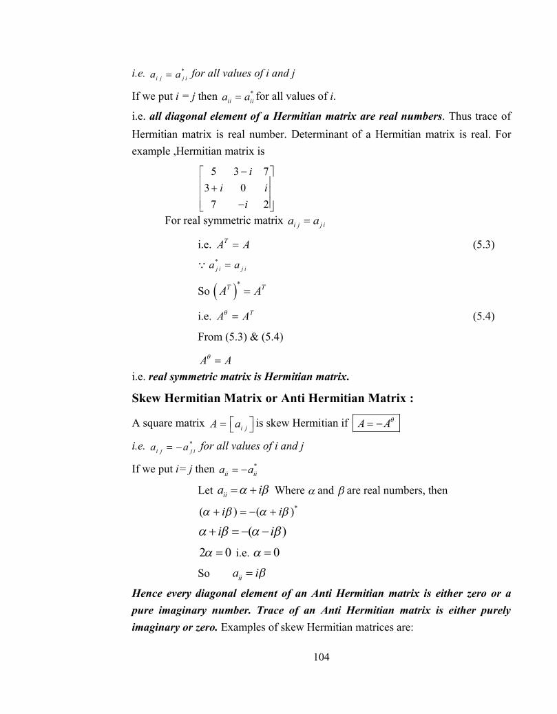
104

i.e. *i j j ia a for all values of i and j

If we put i = j then *ii iia a for all values of i.

i.e. all diagonal element of a Hermitian matrix are real numbers. Thus trace of Hermitian matrix is real number. Determinant of a Hermitian matrix is real. For example ,Hermitian matrix is

5 3 73 0

7 2

ii i

i

For real symmetric matrix i j j ia a

i.e. TA A (5.3)

*j i j ia a

So *T TA A

i.e. TA A (5.4)

From (5.3) & (5.4)

A A i.e. real symmetric matrix is Hermitian matrix.

Skew Hermitian Matrix or Anti Hermitian Matrix :

A square matrix i jA a is skew Hermitian if A A


If we put i= j then *ii iia a

Let iia i Where and are real numbers, then

*( ) ( )i i

( )i i

2 0 i.e. 0

So iia i

Hence every diagonal element of an Anti Hermitian matrix is either zero or a pure imaginary number. Trace of an Anti Hermitian matrix is either purely imaginary or zero. Examples of skew Hermitian matrices are:

105

4 3 00 4 0 3

, , 3 0 74 0 3

0 7

ii

ii i

i i

etc.

We can prove that real anti symmetric matrix is skew Hermitian matrix. Determinant of skew Hermitian matrix is either zero or purely imaginary number.

Example 5.3 If Y is Hermitian matrix then prove that †X YX is also Hermitian matrix for every matrix X.

Sol. Since Y is Hermitian matrix

†Y Y Let †Z X YX

†† †Z X YX

† † † †(X )X Y † † † †( )ABC C B A

† † XX Y ††A A

†X YX Y is Hermitian

†Z Z

So †X YX is Hermitian

5.8 Unitary Matrix

A square finite matrix U is unitary if UU I

i.e. U U I UU

Important properties of Unitary matrices:

(i) Determinant of a unitary matrix is of unit modulus. Hence unitary matrix is not singular matrix.

Proof :

Here UU I UU I

1U U

5.8 Unitary Matrix

106

* 1U U

* **

T

T

U U

U U U U

This shows that modulus of the determinant of a unitary matrix is unity. (ii) If U is Unitary matrix then

1U U (alternate condition of Unitary matrix)

Proof. We have UU I

1 1( )U UU U I

1 1U U U U

1IU U

1U U

(iii) Real Unitary matrices are orthogonal matrices. Proof :

* T TU U U * for real matricesA A

UU I

TUU I

Hence U is also orthogonal matrix.

(iv) The products of two unitary matrices are also unitary matrix.

Proof : Let A and B are Unitary matrices then

AA I and BB I

Let Z AB

Here ( )( )ZZ AB AB

( )( )AB B A ( )A B B A

( )A I A ( )AI A

AA

ZZ I Thus Z i.e. AB is unitary matrix

5.9 Illustrative Examples 5.9 Illustrative Examples

107

Example 5.4 Prove that Pauli matrix

00i

i

is Unitary matrix

Sol. *0 0

0 0

T Ti ii i

00i

i

We can write

0 00 0i i

i i

2

2

0 0 00 0 0

ii

1 00 1

Example 5.5 If A is a Hermitian matrix then prove that matrix iAe is unitary matrix.

Sol. Let iAZ e

iA iA iA iAZZ e e e e

iA iAe e for Hermitian matrixA A

ZZ I

Hence Z i.e. iAe is unitary matrix



Q.1 Show that inverse of a unitary matrix is also unitary.


Q.2 If A is Hermitian matrix, then prove that iA is anti Hermitian matrix .

Q.3 If X and Y are Hermitian matrices, then prove that


108

(i) X Y Y X is also Hermitian matrix

(ii) X Y Y X is anti Hermitian matrix

(iii) i( X Y Y X ) is Hermitian matrix

Q.4 If matrix 1

1i

A ai

is Unitary ,then find the value of a.


Let ijA a be an n n square matrix and X is a column vector. We consider the

vector equation (linear translation) AX X (i)

where is a scalar.

Here zero vector 0X is a solution for any value of . But solution 0X is of no importance in practical situations.

Value of for which equation AX X has a solution 0X (i.e. a nontrivial solution) is called an eigen value of matrix A.

Eigenvalue is also known as characteristic value, latent root, proper values. Word ‘Eigen’ is German and that means ‘proper’ or ‘characteristic’.

Corresponding to each eigenvalue , solution 0X is called eigenvector (characteristic vector) of matrix A belonging to that eigenvalue.

Here equation AX X

AX IX {Where I is unit matrix}

0AX IX ( ) 0A I X

For nontrivial solution

det.( ) 0A I

This equation in is known as characteristic equation and det.( )A I is known as characteristic determinant we can write

AX X


109

1 111 12 1

21 22 2 2 2

1 2

...

...... ... ... ... ... ...

...

n

n

n n nn n n

x xa a aa a a x x

a a a x x

For nontrivial solution

11 12 1

21 22 2

1 2

...

...det( ) 0

... ... ... ......

n

n

n n nn

a a aa a a

A I

a a a

which shows a polynomial equation of degree n in

Operator interpretation of Matrices :

Matrix A can be thought as an operator which operates on column vector X and produces another column vector Y i.e. A X Y

In general X and Y have the different directions. Here X is not an eigenvector. For particular case in which Y has the same direction of X i.e. Y is constant multiple of X or Y X where is number.

In that case AX X and X is known as eigen vector corresponds to eigen value

Illustrative Examples

Example 5.6 For given matrix 3 41 2

A

Find the eigenvalues and eigenvectors for matrix A.

Sol. We consider equation AX X i.e.

1 1

2 2

3 41 2

x xx x

(5.5)

1 2 13 4x x x

1 2 22x x x

We can write above equations as

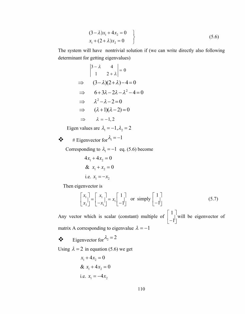
110

1 2

1 2

(3 ) 4 0(2 ) 0

x xx x

(5.6)

The system will have nontrivial solution if (we can write directly also following determinant for getting eigenvalues)

3 40

1 2

(3 )(2 ) 4 0

26 3 2 4 0

2 2 0

( 1)( 2) 0

1, 2

Eigen values are 1 21, 2

# Eigenvector for 1 1

Corresponding to 1 1 eq. (5.6) become

1 24 4 0x x

1 2& 0x x

i.e. 1 2x x

Then eigenvector is

1 11

12

11

x xx

xx

or simply

11

(5.7)

Any vector which is scalar (constant) multiple of 11

will be eigenvector of

matrix A corresponding to eigenvalue 1

Eigenvector for 2 2

Using 2 in equation (5.6) we get

1 24 0x x

1 2& 4 0x x

i.e. 1 24x x

111

Then eigenvector is

1 22

2 2

4 41

x xx

x x

or simply 4

1

Any vector which is scalar (constant) multiple of 4

1


matrix A corresponding to eigenvalue 2

Note : We can understand this constant multiple of 4

1

in following way

From (5.5),we have

1 1

2 2

3 41 2

x xx x

From (5.7) 2 2

3 4 4 41 2 1 1

x x

3 4 4 41 2 1 1Eigen

valueEigenvector EigenvectorMatrix

Example 5.7 Find the eigenvalues and normalized eigenvector of the following matrix A

1 1 11 2 21 3 1

A

Sol. We consider equation AX X

1 1

2 2

3 3

1 1 11 2 21 3 1

x xx xx x

(5.8)

1 2 3 1

1 2 3 2

1 2 3 3

2 23

x x x xx x x x

x x x x

112

1 2 3

1 2 3

1 2 3

(1 ) 0(2 ) 2 03 (1 ) 0

x x xx x xx x x

(5.9)

The system will have nontrivial solution if

(1 ) 1 11 (2 ) 2 01 3 (1 )

(1 ) 2 (1 ) 6 1 (1 ) 2 1 3 (2 ) 0

(1 )(2 )(1 ) 6(1 ) (1 ) 2 2 (1 ) 0

(1 ) (2 )(1 ) 6 0 2(1 ) 3 4 0

(1 )( 1)( 4) 0

Eigenvalues are 1,1,4 For Eigenvectors :

Putting 1 1 in equation (5.9) we get

1 2 32 0x x x (5.10)

1 2 33 2 0x x x (5.11)

1 2 33 2 0x x x

From equation(5.10)

3 2 2 32 2 3 0x x x x

3 2x x (5.12)

From (5.10)&(5.12)

1 3x x

Thus eigenvector corresponds to eigenvalue 1 1 is

31

2 3 3

3 3

111

xxx x xx x

or simply

111

113

Normalized eigenvectors i.e. unit eigenvectors have length 1 i.e. sum of the squares of their components is 1.

Such eigenvectors can be found out by dividing each vector by the square root of the sum of the squares of the components.

Thus normalized eigenvector corresponding to 1 1 is

131

1 11 or3 31

13

{Note : For normalized form of

abc

, we divide each element by 2 2 2a b c }

We put 2 1 in equation(5.9) for getting eigenvector

2 3

1 2 3

02 0

x xx x x

1 23 0x x

i.e. 1 23x x & 3 2x x

Thus eigen vector corresponding to eigen value 2 1 is

1 2

2 2 2

3 2

3 311

x xx x xx x

or simply

311

The normalized eigenvector is

311

1111

11

We put 3 4 in equation(5.9) for getting eigenvector

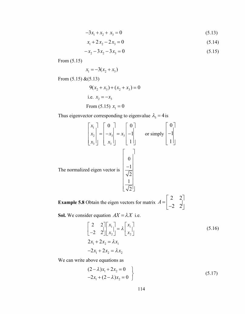
114

1 2 33 0x x x (5.13)

1 2 32 2 0x x x (5.14)

2 2 33 3 0x x x (5.15)

From (5.15)

1 2 33( )x x x

From (5.15) &(5.13)

2 3 2 39( ) ( ) 0x x x x

i.e. 2 3x x

From (5.15) 1 0x

Thus eigenvector corresponding to eigenvalue 3 4 is

1

2 3 3

3 3

0 01

1

xx x xx x

or simply

01

1

The normalized eigen vector is

012

12

Example 5.8 Obtain the eigen vectors for matrix 2 22 2

A

Sol. We consider equation AX X i.e.

1 1

2 2

2 22 2

x xx x

(5.16)

1 2 12 2x x x

1 2 22 2x x x

We can write above equations as

1 2

1 2

(2 ) 2 02 (2 ) 0

x xx x

(5.17)

115

The system will have nontrivial solution if

So

2 20

2 2

2(2 ) 4 0 2(2 ) 4 2 2(2 ) 4i

(2 ) 2i

2 2 , 2 2i i

Eigen values are 1 22 2 , 2 2i i

Eigenvector for 1 2 2i

Corresponding to 1 2 2i eq.(5.17) become

1 2 2 12 2 0i x x x i x

21 2 2 1& 2 2 0 1x ix x ix i

i.e. 2 1x ix

Then eigenvector is

1 11

12

1x xx

ix ix

or simply

1i

(5.18)

Any vector which is scalar (constant) multiple of 1i


matrix A corresponding to eigenvalue 1 2 2i

Eigenvector for 2 2 2i

Using 2 2 2i in equation(5.17) we get

1 2 2 12 2 0i x x x i x

2

1 2 2 1& 2 2 0 1x ix x ix i

i.e. 2 1x ix

Then eigenvector is

116

1 11

2 1

1x xx

x ix i

or simply 1i

Important properties of Eigenvalues :

(i) The product of eigenvalues of a matrix A is equal to the determinant of the

matrix 1 2 3det . . ...... nA

Where 1 2 3, , ,..... n are eigenvalues of a matrix. Set of eigen values{

1 2 3, , ,..... n } is called spectrum of matrix A. (ii) The sum of eigenvalues of a matrix is equal to the trace of the matrix i.e.

1 2 ..... nTrace A

(iii) Eigenvalues of any matrix Aand its transpose TA are same. (iv) If eigenvalues of A are 1 2 3, , ,..... n then

Eigenvalues of pA are 1 2 3,p ,p ,.....p np , where p is non zero scalar.

Eigenvalues of mA are 1 2, , .......m m mn

Eigenvalues of 1A are 1 2

1 1 1, ,....n

(v) The eigenvalues of a diagonal matrix are the elements in the diagonal. (vi) The eigenvalues of a Hermitian matrix (or real symmetric matrix) are real. (vii) The eigenvalues of a skew Hermitian matrix (or real skew symmetric matrix)

are either zero or pure imaginary numbers. (viii) The eigenvalues of a unitary (or real orthogonal matrix) are of unit

modulus. (ix) Every square matrix satisfies its own characteristic equation. This is known as

Cayley-Hamilton theorem. Suppose characteristic polynomial of matrix A is given by

20 1 2 ....... 0n

na a a a Where 0 1 2, , ,....... na a a a are constants and is eigenvalue, then

20 1 2 ....... 0n

na I a A a A a A (Cayley-Hamilton Theorem)

(x) Any two eigenvectors corresponding to two distinct eigenvalues of Hermitian (or real symmetric) matrix are orthogonal.

(xi) Any two eigenvectors corresponding to two distinct eiganvalues of Anti Hermitian (or real asymmetric) matrix are orthogonal.

117

(xii) An n n matrix B is called similar to A if there is a non singular n n matrix P

such that 1B P AP Similar matrices have the same eigenvalues. If an eigenvector of matrix A is

X then 1Y P X will be an eigenvector of B corresponding to the same eigenvalue.

5.12 Diagonalization of a Matrix In many physical situations it is desirable to reduce the matrix to a diagonal form (non diagonal elements all equal to zero) .Moment of inertia I of a rigid body is direct example of this diagonalization process. Theorem : If a non singular square matrix A of order n n has n linearly

independent eigenvectors, then a matrix X can be found such that 1D X AX is

a diagonal with the eigenvalues of A as the matrix entries on the main diagonal. Here X is the matrix with these eigenvectors as column vectors.

For example , if distinct eigenvalues of 1 1

2 2

a bA

a b

are 1 2,

and corresponding eigenvectors

11

1

xX

y

and 22

2

xX

y

We can write 1 2

1 2

x xX

y y

Then 11

2

00

D X AX

Now we can say that A has been reduced to diagonal form. We can prove this in following way Characteristic equation is given by 0A I i.e. for eigenvalue 1

1 1 1 1 1 1 1 1 1 1 1

2 1 2 1 1 2 1 2 1 1 1

(a ) 0a ( ) 0

x b y a x b y xx b y a x b y y

(5.19)

Similarly for eigenvalue 2

1 2 1 2 2 2

2 2 2 2 2 2

aa

x b y xx b y y

(5.20)

5.12 Diagonalization of a Matrix

118

Now 1 1 1 2

2 2 1 2

aa

b x xAX

b y y

1 1 1 1 1 2 1 2

2 1 2 1 2 2 2 2

a aa a

x b y x b yx b y x b y

1 1 2 2

1 1 2 2

x xy y

1 2 1

1 2 2

00

x xAX

y y

A X X D where 1

2

00

D

1 1( ) ( )X AX X XD

1X AX ID 1X X I

1X AX D

Illustrative Examples

Example 5.9 If matrix 4

6A

has eigenvalues 4,6.Then find the values of

and

Sol. Trace= 4 6 10

Det A= . 24 4.6

. 0

If 0, then 10 or

If 0, then 10

Example 5.10 A matrix of order2 2 is given by

a bA

c d

For this matrix prove that 2 . . 0TraceA Det A ,where is the eigen value of the matrix A.

Sol. Characteristic equation is given by

( ) 0Det A I

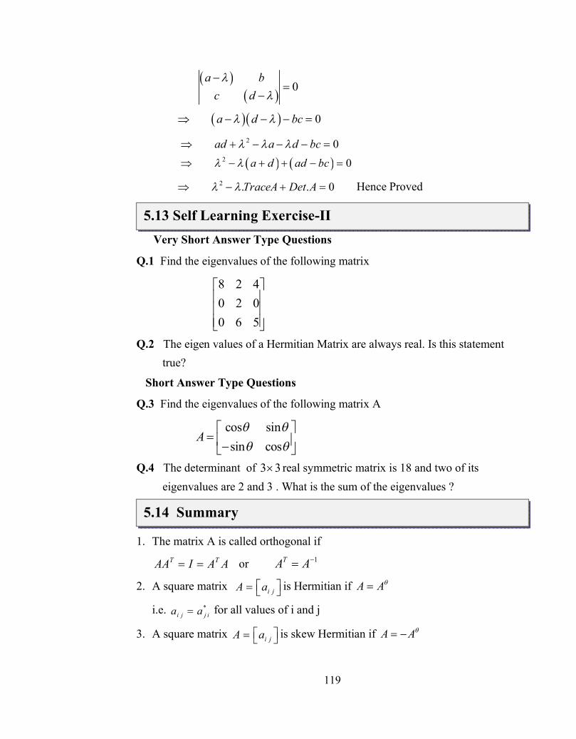
119

0a b

c d

0a d bc

2 0ad a d bc

2 0a d ad bc

2 . . 0TraceA Det A Hence Proved



Q.1 Find the eigenvalues of the following matrix

8 2 40 2 00 6 5

Q.2 The eigen values of a Hermitian Matrix are always real. Is this statement true?


Q.3 Find the eigenvalues of the following matrix A

cos sinsin cos

A

Q.4 The determinant of 3 3 real symmetric matrix is 18 and two of its eigenvalues are 2 and 3 . What is the sum of the eigenvalues ?

5.14 Summary

1. The matrix A is called orthogonal if

T TAA I A A or 1TA A

2. A square matrix i jA a is Hermitian if A A


3. A square matrix i jA a is skew Hermitian if A A


5.14 Summary

120


4. A square finite matrix U is unitary if UU I

i.e. U U I UU

5. Value of for which equation AX X has a solution 0X (i.e. a nontrivial solution) is called an eigen value of matrix A.

det.( ) 0A I

5.15 Glossary Trace: The sum of the elements in the principal diagonal of a square matrix.

Skew: not symmetrical

Conjugate: having the same real parts and equal magnitudes but opposite signs of imaginary parts.

5.16 Answers to Self Learning Exercises Answers to Self Learning Exercise-I

Ans.1: For Unitary matrix 1U U

Here 1 1U U U U

U U I

Ans.2: Hint- Show that † ( )iA iA

Ans.4: 12

Answers to Self Learning Exercise-II Ans.1: 2,5,8

Note: eigen values of triangular matrix are diagonal elements in that matrix.

Ans.2: Yes

Ans.3: 1 cos sin ii e , 2 (cos sin ) e ii

Ans.4: Product of Eigen values=determinant of the Matrix

1 2 3. . 18

5.15 Glossary


121

3 32.3. 18 3 Sum of the eigenvalues

1 2 3 2 3 3 8 5.17 Exercise

Section A: Very Short Answer Type Questions

Q.1 “If the eigenvalues of the anti symmetric matrix A is zero and its determinant is also zero, then each eigenvalue of the matrix A must be zero.”Is this statement true?

Q.2 “If one of the eigen value of matrix A is zero, then matrix A must be singular.”Is this statement true?

Q.3 “A matrix can have real eigen values without being Hermitian”.Is this statement true?

Section B : Short Answer Type Questions

Q.4 Show that matrix 1 111 13

ii

is Unitary matrix.

Q.5 Show that cos sinsin cos

ii

is Unitary matrix

Q.6 Prove that for any square matrix A

(i) A A

is a Hermitian matrix

(ii) A A

is skew Hermitian matrix

(iii) AA is a Hermitian matrix

Q.7 Find the eigenvalues of the given matrix

1 0 00 1 10 1 1

A

Q.8 A matrix is given by

0 1 00 0 22 0 0

A

5.17 Exercise

122

Its eigenvalues are 1 2 3, ,

Find (i) 1 2 3 (ii) 1 2 3. . Section C : Long Answer Type Questions

Q.8 Prove that any complex square matrix can always be expressed as the sum of a Hermitian matrix and a skew Hermitian matrix.


Ans.1 : No

Ans.2 : Statement is true.

Hint: 1 2. ..... 0n

1 2. . .....

. 0nDet A

Det A

Thus A is singular Matrix.

Ans.3 : Yes, See example 5.6

Ans.7 : 0,1,2

Ans.8 : (i) Trace= Sum of eigenvalues= 1 2 3 0 0 0 0

(ii) Det.A= 1 2 3. .

0(0 2) 1(0 2) 0(0 0) 4 References and Suggested Readings

1. Satya Prakash ,Mathematical Physics with Classical Mechanics ,Fourth Edition, Sultan Chand&Sons(2002)

2. George B. Arfken &Hans J. Weber ,Mathematical Methods for Physicists , Sixth Edition, Academic Press-Harcourt(India)Private Ltd. (2002)

3. Murray R. Spiegal ,Advanced Mathematics for Engineers &Scientists , Schaum’s Outline Series, McGraw-Hill Book Company(2003)

4. E.Kreyszig ,Advanced Engineering Mathematics ,8th Edition, John Wiley & Sons(Asia)P.Ltd.(2001)

5. H.K.Dass, Mathematical Physics,Fourth-Edition,S.Chand &Company Ltd.

( 2004)



123


6.0 Objectives 6.1 Introduction

6.2 Functions of a complex variable

6.3 Complex Algebra 6.4 Cauchy-Riemann Conditions


6.6 Self learning exercise-I 6.7 Branch Points and Branch Lines


6.9 Cauchy’s Integral Theorem

6.10 Multiply Connected Regions 6.11 Self learning exercise-II

6.12 Summary

6.13 Glossary


6.15 Exercise



6.0 Objective Complex numbers are widely used in modern mathematics and its applications. It turns out that it is convenient to obtain many relationships between real quantities by using complex numbers and functions in intermediate calculations. This chapter

UNIT- 6 Complex Algebra: Cauchy –Riemann

Conditions, Cauchy’s Integral Theorem

6.0 Objectives

124

is intended to introduce many of the useful results of complex function theory. We shall derive the conditions that a complex function theory. We shall derive the conditions that a complex function ( )W z has to satisfy so as to have a unique derivative at the point z. Such a function is said to be analytic at the point z.

6.1 Introduction In this chapter we develop some of the most powerful and widely useful tools in all of mathematical analysis. These include Cauchy-Riemann conditions and Cauchy’s integral theorem. We introduce some elementary function of Z and find their real and imaginary parts. We also discuss their analyticity. We define branch points and branch lines etc.

6.2 Functions of a complex variable “The imaginary numbers are a wonderful flight of God’s spirit; they are

almost an amphibian between being and not being.”

Gotterfied Wilhelm Von Leibniz (1702)

Why complex variables are so important? It will be evident several areas of applications :

1. For many pairs of functions 푢 and 푣, both 푢 and 푣 satisfy Laplace’s equation :

∇ =휕 (푥, 푦)

휕푥+휕 (푥, 푦)

휕푦= 0

Either 푢 or 푣 may be used to describe a two dimensional electrostatic potential. The other function that gives a family of curves orthogonal to those of

the first function, may then be used to describe the electric field 퐸 .

In similar case of hydrodynamics : 푢 → velocity potential, 푣 →stream function

푢 and 푣 : create a co-ordinate system.

2. Second order differential equation – power series

If 푓(푧) at 푧 is given, the behavior of 푓(푧) elsewhere is knowable (analytic continuation).

3. The change of parameter 푘 from real to imaginary, 푘 → 푖푘 transforms the Helmholtz equation into diffusion equation.

6.1 Introduction

6.2 Functions of a Complex Variable

125

4. Integrals in the Complex plane have a wide variety of useful applications :

(a) Evaluating definite integrals (b) Inverting power series (c) Forming infinite products (d) Stability of oscillating systems

6.3 Complex Algebra

A complex number is nothing more than an ordered pair of two ordinary(real) numbers (푎, 푏)

We can write this pair as 푎 + 푖푏.

Similarly, a complex variable is an ordered pair of two real variables, ( , )z x y x iy All our complex variable analysis can be developed in terms of

ordered pairs of numbers (푎, 푏), variables (푥, 푦) and functions

[푢(푥, 푦),푣(푥,푦)].The 푖 is not necessary but it is convenient.

Argand Diagram

Complex PlaneFigure6.1

Complex variable [cos sin ]z r i

iz re

6.3 Complex Algebra

126

r z

푟 is called modules of 푧

휃 is called argument or plane of 푧 .

Triangle Inequalities :

1 2 1 2 1 2z z z z z z

Using Polar form we can show

1 2 1 2. .z z z z

Also 1 2 1 2arg . arg argz z z z

Complex function 푤(푧) may be resolved into real and complex parts as 푤(푧) = 푢 (푥, 푦) + 푖 푣 (푥,푦)

The relationship between the independent variable 푧 and dependent

variable 푤 is best pictured as a mapping operations :

Thefunction w(z)=u(x,y)+iv(x,y) maps pointsin the xy-plane into pointsin the uv plane

Figure6.2

Complex Conjugation :

127

Complex Conjugation of an expression is change from 푖 to −푖. Complex Conjugate Points :

z x iy * –z x iy

* 2 2 2( )zz x y r

*( )zz z

Complex conjugate pointsFigure6.3

Functions of a Complex Variable :

All the elementary functions of real variables may be extended into the complex

plane – replacing the real variable 푥 by complex variable 푧 . This is an example of analytic continuation.

De Moivre’s Formula :

ie cos i sin

cos sin cos sin nn i n i

ln 푧 = ln 푟 푒

= ln 푟 + 푖 휃 푇ℎ푖푠 푖푠 푛표푡 푐표푚푝푙푒푡푒

128

We can add 2푛휋 in 휃 with no change in 푧

ln 푧 = ln 푟 푒 ( ) = ln 푟 + 푖 (휃 + 2푛휋)

∴ ln 푧 is a multivalued function having an infinite number of values for a single pair of real values 푟 and 휃.

To avoid ambiguity, we usually agree to set 푛 = 0 and limit the phase to an

interval of length 2휋 such as (−휋,휋). The line in the 푧-plane that is not crossed the negative real axis in this case , is labeled a cut line. The value of 푙푛 푧 with 푛 = 0 is called principal value of 푙푛 푧.

Analytic Functions : If 푓(푧) is differentiable at 푧 = 푧 and in some

small region around 푧 , we say that 푓(푧) is analytic at 푧 = 푧 .

If 푓(푧) is analytic everywhere in the (finite) complex plane, we call it an entire

function. If zf does not exist at 푧 = 푧 , then 푧 is labeled a singular point.

6.4 Cauchy-Riemann Conditions

We know proceed to differentiate complex functions of a Complex variables.

The derivative of 푓(푧), like that of a real function, is defined as :

lim →

푓(푧 + 훿푧)푧 + 훿푧 − 푧

= lim →

훿푓(푧)훿푧

=푑푓푑푧

표푟 푓 (푧)

Provided that the limit is independent of the particular approach to the point 푧.

For real variables we require that the right hand limit (푥 → 푥 from above) and

the left hand limit (푥 → 푥 from below) be equal for the derivative ( ) to exist

at 푥 = 푥 .

Now with 푧(표푟 푧 ) some point in a plane, our requirement that the limit be independent of path.

6.4 Cauchy-Riemann Conditions

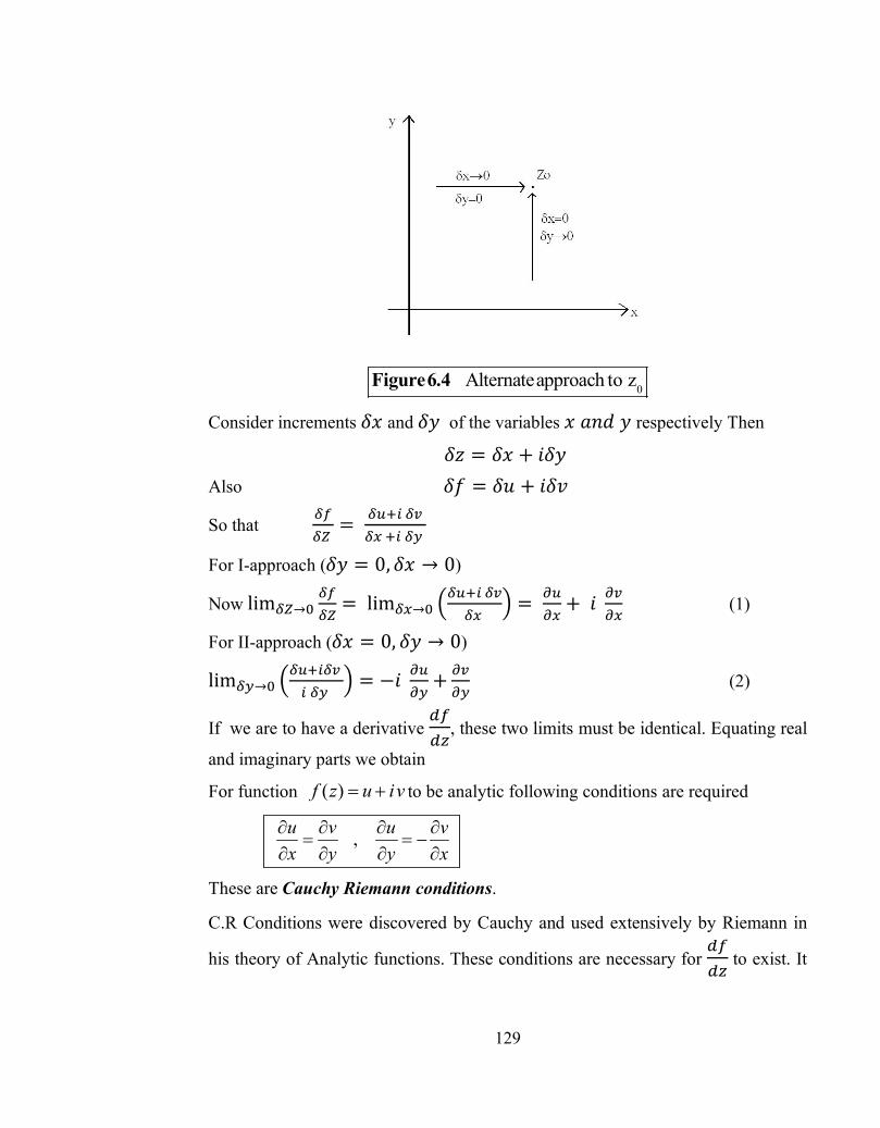
129

0Alternateapproach to zFigure6.4

Consider increments 훿푥 and 훿푦 of the variables 푥 푎푛푑 푦 respectively Then

훿푧 = 훿푥 + 푖훿푦 Also 훿푓 = 훿푢 + 푖훿푣

So that =

For I-approach (훿푦 = 0,훿푥 → 0)

Now lim → = lim →

= + 푖 (1)

For II-approach (훿푥 = 0, 훿푦 → 0)

lim →

= −푖 + (2)

If we are to have a derivative , these two limits must be identical. Equating real

and imaginary parts we obtain

For function ( )f z u iv to be analytic following conditions are required

,u v u vx y y x

These are Cauchy Riemann conditions.

C.R Conditions were discovered by Cauchy and used extensively by Riemann in

his theory of Analytic functions. These conditions are necessary for to exist. It

130

is worth noting that the C.R. condition guarantees that the curves 푢 = 푐 will be orthogonal to the curves 푣 = 푐 .


Example 6.1 If 푓(푧) 표푟 푤(푧) = 푧 ,then find out real and imaginary part of 푓(푧) Sol. 푓(푧) = (푥 + 푖푦)

= (푥 − 푦 ) + 푖 2푥푦 푅푒푎푙 푝푎푟푡 표푓 푓(푧) = 푢(푥, 푦) = 푥 − 푦

퐼푚푎푔푖푛푎푟푦 푝푎푟푡 표푓 푤(푧) = 푣 (푥,푦) = 2푥푦

Example 6.2 푓(푧) = 푥 − 푖 푦 ,State whether this function analytic or not analytic.

Sol. 푢 = 푥, 푣 = −푦

휕푢휕푥

= 1,휕푢휕푦

= 0 ; 휕푣휕푥

= 0,휕푣휕푦

= −1

CR equations are not satisfied.

Nowhere analytic.푓(푧)is continuous everywhere but nowhere differentiable.

Example 6.3 푓(푧) = 푧 푧 = 푥 + 푦

Is this function analytic?

Sol. 푢 = 푥 + 푦 , 푣 = 0

휕푢휕푥

= 2푥 ,휕푢휕푦

= 2푦 ; 휕푣휕푥

= 0 ,휕푣휕푦

= 0

are continuous everywhere, However the Cauchy Riemann equation is 2푥 = 0, 2푦 = 0 are satisfied only at the origin. Hence 푧 = 0 is the only point at which 푓′(푧) exists and therefore 푓(푧) = 푧푧 nowhere analytic.

The Elementary functions of z :

The exponential function 푒 is of fundamental importance, not only for its own sake but also as a basis for defining all the other transcendental functions. In


131

its definition we seek to preserve as many of the familiar properties of the real

exponential function 푒 as possible. Specifically we desire that

a. 푒 shall be single valued and analytic

b. = 푒

c. 푒 shall reduce to 푒 when 퐼푚(푧) = 0

If we let

푒 = 푢 + 푖 푣 (a)

The derivative of an analytic function can be written in the form :

푓 (푧) = 휕푢휕푥

+ 푖 휕푣휕푥

Now, to satisfy the condition b, we must have :

휕푢휕푥

+ 푖 휕푣휕푥

= 푢 + 푖푣

∴ = 푢 (b)

= 푣 (c)

Eq. (b) will be satisfied if 푢 = 푒 (푦)

Also form (c)

휕푣휕푥

= 푣

표푟 −휕푢휕푦

= 푣

표푟 = − (by CR Condition)

표푟 휕 푢휕푦

= − 휕푢휕푥

= −푢 푓푟표푚 (푏)

Substituting 푢 = 푒 (푦) in eq. = −푢

푒 "(푦) = −푒 (푦)

표푟 " (푦) = − (푦)

132

This is a simple linear differential equation whose solution can be written down at once :

(푦) = 퐴 cos 푦 + 퐵 sin 푦

∴ 푢 = 푒 (푦)

= 푒 [퐴 cos 푦 + 퐵 sin 푦]

and 푣 = − = −푒 [−퐴 sin푦 + 퐵 cos 푦]

∴ 푒 = 푢 + 푖푣 = 푒 [(퐴 cos푦 + 퐵 sin 푦) + 푖 (퐴 sin푦 − 퐵 cos푦)]

Finally, if this is to reduce to 푒 when 푦 = 0 as required, we must give

푒 [퐴 − 푖 퐵], which will be true if and only if 퐴 = 1,퐵 = 0.

Thus we have been led inevitably to the conclusion that if there is a function of 푧

satisfying the conditions(a),(b),(c) then it must be :

푒 = 푒 = 푒 [cos 푦 + 푖 sin푦] (d)

That this expression does indeed meet our requirements can be checked

immediately ; hence we adopt its as the definition of 푒 .

mod 푒 = |푒 | = 푒

and arg 푒 = 푦

From eq.(d)

If 푥 = 0, 푦 = 휃 we have

cos휃 + 푖 sin 휃 = 푒

and thus 푟 [cos휃 + 푖 sin 휃] = 푟푒

cos sinie i

cos sinie i

cos , sin

2 2

i i i ie e e ei

On the basis of these equations, we extend the definition of sine and

cosine into the complex domain by the formulas:

133

cos 푧 = 푒 + 푒

2

sin 푧 = 푒 − 푒

2푖

From these definitions it is easy to establish the validity of such familiar formulas as :

푐표푠 푧 + 푠푖푛 푧 = 1

cos (푧 ± 푧 ) = cos 푧 cos 푧 ± sin 푧 sin 푧

sin (푧 ± 푧 ) = sin 푧 cos 푧 ± cos 푧 sin 푧

푑푑푡

cos 푧 = − sin 푧

푑푑푡

sin 푧 = cos 푧

cos 푧 = 푒 ( ) + 푒 ( )

2=

푒 푒 + 푒 푒2

= cos푥 푒 + 푒

2− 푖 sin 푥.

푒 − 푒2

≡ cos 푥 cos ℎ푦 − 푖 sin 푥 sinh 푦

The logarithm of 푧, we define implicitly as the function 푤 = 푙푛푧 which satisfies the equation:

푒 = 푧 (1)

Let 푤 = 푢 + 푖 푣, 푧 = 푟 푒

∴ 푒 = 푟푒

푒 푒 = 푟푒

푒 = 푟 ∴ 푢 = ln 푟

푒 = 푒 ∴ 푣 = 휃

푤 = ln 푟 + 푖휃

푤 = ln|푧| + 푖 arg 푧(2)

If we let 휃 be the principal argument of 푧, i.e. the particular argument of 푧

which lies in the interval then –휋 < 휃 ≤ 휋, 푡ℎ푒푛 (2) can be written as

푙푛 푧 = ln|푧| + 푖 (휃 + 2푛휋), 푛 = 0, ±1, ±2, … … …

134

Which shows that the logarithmic function is infinitely many valued.

For any particular value of n a unique branch of the function is determined and the logarithm becomes effectively single valued.

If 푛 = 0, the resulting branch of the logarithmic function is called the principal value.

For every 푛, the corresponding branch of ln 푧 is obviously discontinuous at

푧 = 0. Moreover, for each 푛 the corresponding branch is also discontinuous at every point of the negative real axis.

To verify this, we note that if 푛 = 푛 , the corresponding branch of ln 푧 is

= ln|푧| + 푖 arg 푧,푤ℎ푒푟푒 (2푛 − 1)휋 < arg 푧 ≤ (2푛 + 1)휋

Hence if 푃 is an arbitrary point on the negative real axis, the limit of 푎푟푔 푧 as 푧 approaches 푃 through the second quadrant is (2푛 + 1)휋. While the limit of

푎푟푔 푧 as 푧 approaches P through the third quadrant is (2푛 − 1)휋.

Since these two values are different, it follows that on any particular branch, 푙푛 푧

does not approach a limit as 푧 approaches and arbitrary point on the negative real axis and therefore is discontinuous at every such point.

At all points except the points on the nonpositive real axis each branch of ln 푧 is continuous and analytic. In fact from the definition.

ln ln argz z i z

푙푛 푧 =12

ln(푥 + 푦 ) + 푖 푡푎푛푦푥

=u+iv It is easy to verify that the Cauchy-Reimann equations are satisfied everywhere at the origin. Moreover from the preceding discussions, it is clear that

푢 =12

ln(푥 + 푦 ) , 푣 = 푡푎푛푦푥

are continuous except on the nonpositive real axis.

Hence, by Cauchy Reimann theorem it follows that everywhere except on the nonpositive real axis :

135

The familiar laws for the logarithms of real quantities all hold for the logarithms of complex quantities in the following sense. If a suitable choice is made among the

infinite number of possible values of ln(푧 푧 ), ln , ln 푧 ,then

ln 푧 푧 = ln 푧 + 푙푛 푧

ln푧푧

= ln 푧 − 푙푛 푧

ln 푧 = 푚 ln 푧

For example, to show that ln 푧 푧 = ln 푧 + 푙푛 푧

Let 푧 = 푟 푒 , 푧 = 푟 푒 . Then

ln 푧 + 푙푛 푧 =[ln 푟 + 푖 (휃 + 2푛 휋)] + [ln 푟 + 푖 (휃 + 2푛 휋)]

=[ln 푟 + ln 푟 ] + 푖[(휃 + 휃 ) + 2 (푛 + 푛 )휋]

= ln 푟 푟 + 푖 [(휃 + 휃 ) + 2푛 휋]

= ln|푧 푧 | + 푖 arg 푧 푧 = 푙푛푧 푧

Since 휃 + 휃 + 2 (푛 + 푛 )휋 is one of the arguments of 푧 푧

However, the familiar laws of logarithms are not necessarily true if we restrict ourselves to a particular branch of ln 푧.

Since ln 푧 = ln|푧| + 푖 arg 푧

ln[푖(−1 + 푖)] = ln(−1 − 푖) = ln√2 − 푖3휋4

푤ℎ푒푟푒 ln 푖 + ln(−1 + 푖) = 푖휋2

+ ln√2 + 푖3휋4

= ln√2 + 푖5휋4

Clearly, the principal value of 푙푛 [푖(−1 + 푖)] differs from the sum of the principal values of 푙푛 푖 and 푙푛 (−1 + 푖) by 2휋 푖. For principal values, the proper generalization of the familiar laws of logarithms are contained in the following theorem whose proof we shall leave as an exercise.

Note :

136

(1) ln 푧 푧 = ln 푧 + ln 푧 − 2푖 휋 ; 휋 < arg + arg 푧 ≤ 2휋

ln 푧 + ln 푧 ; −휋 < arg 푧 + arg 푧 ≤ 휋푙푛푧 + ln 푧 + 2 푖 휋 ; 2휋 < arg 푧 + arg 푧 ≤ −휋

ln푧푧

= ln 푧 − ln 푧 − 2푖 휋 ; 휋 < arg 푧 − arg 푧 ≤ 2휋ln 푧 − ln 푧 ; −휋 < arg 푧 − arg 푧 ≤ 휋

푙푛푧 − ln 푧 + 2 푖 휋 ; −2휋 < arg 푧 − arg 푧 ≤ −휋

ln 푧 = 푚 ln 푧 − 2 푘 푖 휋

m an integer

Where 푘 is the unique integer such that

푎푟푔푧 − ≤ 푘 ≤ arg 푧 +

(2) General powers of 푧 are defined by the formula.

푧 = exp(훼 ln 푧)

Since 푙푛 푧 is infinitely many valued, so too in 푧 , in general specifically.

푧 = exp (훼 ln 푧) = exp{훼 [ln|푧| + 푖 (휃 + 2푛휋)]}

= exp (훼 ln|푧|)푒 . 푒

The last factor in the product clearly involves infinitely many different values

unless 훼 is a rational number, say , in which case, as we saw in our discussion of

De Movier’s theorem, there are only 푞 distinct values.

Example 6.4 What is the principal value of (1 + 푖)

Sol. 푧 = exp(훼 ln 푧) = 푒

∴ (1 + 푖) = exp[(2 − 푖) ln(1 + 푖)]

= exp (2 − 푖) ln √2 + 푖 휋4

+ 2푛휋

ln 푧 = ln|푧| + 푖 (휃 + 2푛휋) The principal value of this, obtained by taking 푛 = 0, is

= exp (2 − 푖) ln √2 + 푖휋4

= exp 2 ln √2 +휋4

+ 푖 − ln √2 + 휋2

137

= exp ln 2 +휋4

+ cos휋2− ln √2 + 푖 sin

휋2− ln √2

= 푒 . (sin 0.3466 + 푖 cos 0.3466)

= 1.490 + 4.126 푖

The inverse trigonometric and hyperbolic function

These functions we define implicitly.

For instance 푤 = 푐표푠 푧

We define as the value or values of 푤 which satisfies the equation.:

푧 = cos푤 = 푒 + 푒

2

From this, by obvious steps, we obtain successively

푒 − 2푧푒 + 1 = 0

푒 = 푧 ± 푧 − 1

and finally, by taking logarithms and solving for 푤.

푤 = 푐표푠 푧 = −푖 ln(푧 ± 푧 − 1)

Since the logarithm is infinitely many valued, so too is 푐표푠 푧.

Similarly, we can obtain the formulas

푠푖푛 푧 = −푖 ln(푖푧 ± 1 − 푧 )

푡푎푛 푧 = 푖2

ln푖 + 푧푖 − 푧

푐표푠ℎ 푧 = ln(푧 ± 푧 − 1)

푠푖푛ℎ 푧 = ln(푧 ± 푧 − 1)

푡푎푛ℎ 푧 =12

ln1 + 푧1 − 푧

From, these after their principal values have been suitably defined by choosing the plus sign preceding the square root and the principal value of the logarithm in each case, the usual differentiation formulas can be obtained without difficulty.

Polynomial functions :

138

These functions are defined by

푤 = 푎 푧 + 푎 푧 + 푎 푧 + 푎 = 푃(푧) (1)

Where 푎 ≠ 0,푎 ,푎 , … … … … ,푎 are complex constants and 푛 is a positive integer called the degree of the polynomial.

푤 = 푎 푧 + 푏 푖푠 푐푎푙푙푒푑 푎 푙푖푛푒푎푟 푡푟푎푛푠푓표푟푚…(2)

Rational Algebraic Functions : are defined by

푤 = 푃(푧)푄(푧) (3) 푃(푧),푄(푧)푎푟푒 푝표푙푦푛표푚푖푎푙푠

(Sometimes (3) is called a rational transform)

Special case 푤 =

,푤ℎ푒푟푒 푎푑 − 푏푐 ≠ 0 푖푠 표푓푡푒푛 푐푎푙푙푒푑 푎 푏푖푙푖푛푒푎푟 표푟 푓푟푎푐푡푖표푛푎푙 푙푖푛푒푎푟 푡푟푎푛푠푓표푟푚

. 푤 = 푒 = 푒 = 푒 [cos푦 + 푖 sin 푦]

If 푎 real and positive : 푎 = 푒

Logarithmic Functions : If 푧 = 푒 , 푡ℎ푒푛 푤푒 푤푟푖푡푒

푤 = ln 푧

= ln푟 + 푖 (휃 + 2푘휋) , 푘 = 0, ±1, ±2, … … . . Principal value of 푙푛 푧 (or principal branch) of 푙푛 푧 = 푙푛 푟 + 푖휃, 푤ℎ푒푟푒 0 ≤ 휃 ≤2휋

However, any other interval of length 2휋 can be used. e.g

. –휋 < 휃 ≤ 휋 푒푡푐.

If 푧 = 푎 ∴ 푤 = 푙표푔 푧,푤ℎ푒푟푒 푎 > 0 푎푛푑 푎 ≠ 0, 1.


Section A : Very Short Answer Type Questions

Q.1 Write down the Cauchy Riemann condition in polar form for a function to be analytic?

Q.2 푓(푧) = 푧 = (푥 − 푦 ) + 2 푖 푥푦

Is this function analytic?

Section B: Short Answer Type Questions


139

Q.3 Obtain the general value of the log(1+i )+log(1−i)

Q.4 Prove 푧 푧 푧 = 푧 푧 푧

6.7 Branch Points and Branch Lines

Suppose we are given the function 푧

We allow 푧 to make a complete circuit around the origin starting from point A

(Counter clockwise) 푤 = 푧

푧 = 푟 푒

∴ 푤 = 푟 푒

at point A, 푤 = 푟 푒

Figure6.5

After a complete circuit back to A, 휃 = 휃 + 2휋

푤 = √푟 푒( )

= −√푟 푒

Thus we have not achieved the same value of 푤 with which we started.

However, by making a second complete circuit back to 퐴, i.e. 휃 = 휃 + 4휋,

푤 = √푟 푒 ( )= √푟 푒

and we do obtain the same value of 푤 with which we started. We can describe the above by stating that if 0 ≤ 휃 < 2휋 we are on one branch of the multiple valued

function 푧 , while if 2휋 ≤ 휃 < 4휋 we are on the other branch of the function.

6.7 Branch Points and Branch Lines

140

Each branch of the function is single valued .In order to keep the function single valued, we setup an artificial barrier such as 푂퐵, where 퐵 is at ∞ (although any other line from 푂 can be used) which we agree not to cross. This barrier (drawn heavy in the figure) is called a branch line or branch cut, and point 푂 is called branch point.

It should be noted that a circuit around any point other than 푧 = 0 does not lead to different values, thus 푧 = 0 is the only finite branch point.


Example 6.5 Evaluate ∫ [(2푦 + 푥 ) 푑푥 + (3푥 − 푦)푑푦] ( , )( , ) along

the parabola 푥 = 2푡, 푦 = 푡 + 3.

Sol. Integral

= [2(푡 + 3) + 4푡 ]2푑푡 + [3(2푡)− (푡 + 3)]2푑푡

= 4푡3 + 3푡 + 8

푡3 + 12

푡2 − 2

푡3 − 6푡

= 413 + 3 +

83 − 0 + 12 ×

12 − 2 ×

13 − 6

= 4 ×103 +

83 + 6 −

23 − 6

=403 +

83 −

23 =

463

Example6.6 Evaluate ∫ 푧 푑푧 푓푟표푚 푧 = 0 푡표 푧 = 4 + 2 푖 along the curve C

given by 푧 = 푡 + 푖푡 Sol. If 푧 = 0, 푡hen 푡 = 0

푧 = 4 + 2 푖, then 푡 = 2

∫ 푧 푑푧 = ∫ (푡 − 푖푡)(2푡푑푡 + 푖푑푡)

= [2푡 푑푡 − 푖푡 푑푡 + 푡푑푡] = 10 −8푖3

Theorem : Prove that if 푓(푧) is integrable along a curve 퐶 having finite length

퐿 and if there exists a positive number 푀 such that |푓(푧)| ≤ 푀 on 퐶 then


141

C

f z dz ML

Proof : ∫ 푓(푧)푑푧 = lim → ∑ 푓(휉 ) ∆ 푧

Now |∑ 푓(휉 )∆푧 | ≤ ∑ |푓(휉 )||∆푧 |

≤ 푀 |∆푧 |

≤ 푀퐿

Example 6.7 Prove Green’s Theorem in the Plane i.e. prove

∮ (푃 푑푥 + 푄 푑푦) = ∬ − 푑푥 푑푦

Sol. ∵ ∬ 푑푥 푑푦 = ∫ ∫ 푑푦( )( ) 푑푥

= ∫ [푃(푥, 푦)] ( )( )푑푥 = ∫ [푃(푥, 푦 ) − 푃(푥, 푦 )]푑푥

= −∫ 푃(푥,푦 )푑푥 − ∫ 푃(푥,푦 )푑푥

= −∮푃 푑푥 (1)

푠푖푚푖푙푎푟푙푦 휕푄휕푥 푑푥 푑푦 = 푄 푑푦 (2)

∴ 퐴푑푑푖푛푔 (1) 푎푛푑 (2):

푃푑푥 + 푄푑푦 = 휕푄휕푥 −

휕푃휕푦 푑푥 푑푦

Figure6.6

142


Integration pathFigure6.7

The integral of a complex variable over a contour in the complex plane may be defined in close analogy to the (Riemann) integral of a real function integrated along the real x-axis.

We divide the contour 푧 푧 into n intervals by picking 푛 − 1 intermediate points

푧 , 푧 , … … .., on the contour. Consider the sum

푆 = 푓 휉 푧 − 푧

Where 휉 is a point on the curve between 푧 and 푧 . Now let 푛 → ∞ with

푧 − 푧 → 0 for all 푗. If the lim → ,푆 exists and is independent of the

details of choosing the points 푧 and 휉 then

lim→

푓 휉 푧 − 푧 = 푓(푧)푑푧

If a function 푓(푧) is analytic (therefore single valued) and its partial derivatives are continuous throughout some simply connected region 푅 (A simply connected region or domain is one in which every closed contour in that region


143

encloses only the points contained in it), the line integral of 푓(푧) around C is zero

: ∫ 푓(푧)푑푧 = ∮ 푓(푧)푑푧 = 0

푓(푧)푑푧 = (푢 + 푖 푣)(푑푥 + 푖 푑푦)

= (푢 푑푥 − 푣 푑푦) + 푖 (푣 푑푥 + 푢 푑푦)

A closed contour C within a simplyconnected region RFigure6.8

Stokes’s Theorem Proof : These two line integrals may be converted to

surface integrals by Stokes’s Theorem, then a procedure that is justified if the partial derivatives are continuous within C.

Using 푣 = 푣 횤 + 푣 횥 ⟹ ∮ 푣 . 푑푙 = ∮ ∇ × 푣 . 푑푎

푣 푑푥 + 푣 푑푦 = 휕푣휕푥 −

휕푣휕푦 푑푥 푑푦

푓(푧)푑푧 = (푢 푑푥 − 푣 푑푦) + 푖 (푣 푑푥 + 푢 푑푦)

=−휕푣휕푥 −

휕푢휕푦 푑푥 푑푦 + 푖

휕푢휕푥 −

휕푣휕푦 푑푥 푑푦 = 0

(Using CR condition )

Cauchy-Goursat Proof :

In the Stoke’s theorem proof Cauchy’s integral theorem, the proof is marred from a theoretical point of view by the need for continuity of the first partial derivatives. Actually, as shown by Goursat, this condition is not essential. An outline of the Goursat proof is as follows :

144

We subdivide the region inside the contour C into a network of small squares as indicated in figure. Then

CauchyGoursat contoursFigure6.9

푓(푧)푑푧 = 푓(푧)푑푧

For ∮ 푓(푧)푑푧 ,We construct the function :

훿 푧 , 푧 =( ) − ( ) ,푧 is an interior point of the 푗 subregion

Approximation to the derivative at 푧 = 푧

훿 푧 , 푧 ~ 푧 − 푧 , approaching to zero as the network was made finer we may take

훿 (푧 , 푧 ) < 휀

Where 휀 is an arbitrary chosen small positive quantity.

Solving for 푓(푧) and integrating around 푐 , we obtain

푓(푧)푑푧 = 푧 − 푧 훿 푧, 푧 푑푧

145

The consequence of the Cauchy integral theorem is that for analytic functions, the line integral is a function only of its end points, independent of the path of integration :

푓(푧)푑푧 = 퐹(푧 ) − 퐹(푧 ) = − 푓(푧)푑푧

again exactly like the case of a conservative force.

6.10 Multiply Connected Regions

The original statement of Cauchy Integral Theorem demanded simply connected region.

This restriction may easily be relaxed by the creation of a barrier ,a cut line.

Consider the multiply connected region of figure (a), in which 푓(푧) is not defined for the interior

R

Cauchy’s integral theorem is not valid for the contour 퐶, as shown but we can

construct a contour C for which

Cthe theorem holds.

We cut from the interior forbidden region to the forbidden region exterior to 푅 and then run a new contour , as shown (b)

A closed contour Cin a

multiplyconnected regionFigure6.10

R

C

6.10 Multiply Connected Regions

146

Conversion of a multiplyconnected regioninto a simply connected region

Figure6.11

The new contourC through ABDEFGA never crosses the cut lines that literally converts 푅 into a simply connected region.

∵∫ 푓(푧)푑푧 = − ∫ 푓(푧)푑푧,

푓(푧) having been continuous across the cut line segments 퐷퐸 as 퐺퐴. Arbitrarily close together

Then ∮ 푓(푧)푑푧 = ∫ 푓(푧)푑푧 + ∫ 푓(푧)푑푧 = 0

Applying again equation 1

2

2

1

)()()( )( 12

z

z

z

z

dzzfzFzFdzzf

With 퐴퐵퐷 → 퐶 푎푛푑 퐸퐹퐺 → −퐶 ,푤푒 표푏푡푎푖푛

∮ 푓(푧)푑푧 = ∮ 푓(푧)푑푧

In which 퐶 and 퐶 are noth travesed in the same (Counter clockwise) direction.

It should be emphasized that the cut line here is a matter of mathematical convenience, to permit the application of Cauchy’s integral theorem. Since 푓(푧) is analytic in the annular region, it is necessarily single valued and continuous across any such cut line. When we consider branch points our functions will not be single valued and a cutline will be required to make them single valued.

147



Q.1 Evaluate∫ (푧 + 1) 푑푧


Q.2 Show that for any analytic function f=u+iv ,the following relation must hold |∆푢| = |∆푣|

Q.3 What do you mean by Branch points?

6.12 Summary This chapter summarizes some of the important theorem regarding analytic functions. These are Cauchy-Riemann conditions and Cauchy integral theorem. These are basic to further advance in the theory of functions of complex variables.

6.13 Glossary

Mar : to spoil something, making it less good or less enjoyable

Annular : Ring-shaped



Ans.1: = , = − Ans.2: 퐴푛푎푙푦푡푖푐

Ans.3: log2+4nπi


Ans.1:

6.15 Exercise


Q.1 What do you mean by Analytic function?

Q.2 Evaluate∫ 푧 푐표푠푧 푑푧



6.12 Summary

6.13 Glossary


6.15 Exercise

148

Q.3 Derive the necessary and sufficient condition for a function to be analytic.


Q.4 Which of the following are analytic functions of complex variable z=x+iy

(i) |푧| (ii) Re.z (iii) sinz (iv) logz

Q.5 State and prove Cauchy’s integral theorem.


Ans.2: − sinπ2

Ans.4 : (i) Not analytic (ii) Not analytic (iii) analytic (iv) Not analytic


1. George B. Arfken, Hans J. Weber ,Mathematical Methods for Physics, 5e, Academic Press2001. 2. Satya Prakash ,Mathematical Physics with Classical Mechanics, , Sultan Chand & Sons.1999

3. Erwin Kreyszing, Advance Engineering Mathematics, , Wiley student edition2000



149

UNIT -7

Cauchy’s integral formula, Laurent expansion, analytic continuation Mapping


7.1 Introduction

7.2 Cauchy’s Integral Formula

7.3 Laurent Expansion

7.4 Analytic Continuation


7.6 Laurent Series



7.9 Summary 7.10 Glossary 7.11 Answer to Self Learning Exercises 7.12 Exercise 7.13 Answer to Exercises References and Suggested Readings

7.0 Objective

This chapter introduces most fundamental formulae in the theory of the functions of complex variables. These include Cauchy’s integral formula, Laurent expansion and the Concept of analytic continuation.

7.1 Introduction

UNIT -7 Cauchy’s Integral Formula, Laurent

expansion, Analytic Continuation Mapping

7.0 Objectives

7.1 Introduction

150

In this chapter we deduce a remarkable result concerning analytic function ( )f zthat is analytic on a closed contour C and within the interior region bounded by C. We shall deduce that the value of an analytic function ( )f z is given at an interior point once the values on the boundary C are specified. This result is Cauchy’s integral formula. This result guarantees not only the first derivative of ( )f z but derivatives of all orders as well. This formula opens up the way for the derivative of Taylor’s series.

7.2 Cauchy’s Integral Formula We consider a function 푓(푧) that is analytic on a closed contour 퐶 and within the interior region bounded by 퐶. We seek to prove that :

0

0

2 ( )C

f z dzi f z

z z

∮ (7.1)

In which 푧 is some point in the interior region bounded by 퐶. Note : carefully that since 푧 is on the contour 퐶 while 푧 is in the interior, 푧 − 푧 ≠ 0 and the integral (7.1) is well defined.

Exclusion of singular pointFigure7 .1

Although 푓(푧) is assumed analytic, the integral ( ) is not analytic at 푧 = 푧 .

Cauchy’s integral theorem applies :

푓(푧)푧 − 푧 푑푧 −

푓(푧)푑푧푧 − 푧 = 0

7.2 Cauchy’s Integral Formula

151

Where 퐶 = original contour

퐶 = Circle surrounding the point 푧 transvered in a counter clockwise direction.

Let 푧 = 푧 + 푟 푒 Here 푟 is small and will eventually be made to approach zero.

∴ 푓(푧)푑푧푧 − 푧 =

푓 푧 + 푟푒푟푒 푟 푖 푒 푑휃

Taking the limit as 푟 → 0, we obtain

푓(푧)푑푧푧 − 푧 = 푖 푓 (푧 ) 푑휃 = 2 휋 푖 푓 (푧 )

Since 푓(푧) is analytic and therefore continuous at 푧 = 푧 .

If 푧 is exterior to 퐶, in this case the entire integrand is analytic and either 퐶, Cauchy’s integral theorem applies and the integral vanishes.

0 0

0 0

;12 ( ) 0 ;C

f z z interiorf z dzi z z z exterior

∮ (7.2)

Derivatives :

Cauchy’s integral formula may be used to obtain an expression for the derivative of 푓(푧). From (7.1) with 푓(푧) analytic 푓(푧 − 훿푧 ) − 푓(푧 )

훿푧

=1

2휋 푖 훿푧푓(푧)

푧 − 푧 − 훿푧 푑푧 −푓(푧)푧 − 푧 푑푧

Then, by definition of derivative :

푓 (푧 ) = lim→

12휋푖훿푧

훿푧 푓(푧)(푧 − 푧 )(푧 − 푧 − 훿푧 ) 푑푧

20

1 ( )( )2 ( )

f z dzi z

f zz

∮

This technique for constructing derivatives may be repeated :

푓( )(푧 ) =2

2휋푖 푓(푧)푑푧

(푧 − 푧 )

152

10

0

!2 ( )

nn

f z dznf zi z z

∮ (7.3)

That is ,the requirement that 푓(푧) be analytic not only guarantees a first derivative but derivatives of all orders as well.

For example

Figure7 .2

퐼 = ∮ , Where 푐 is a simple closed curve.

The function 푤(푧) = is analytic for any value of 푧 except for 푧 = 0. If

therefore, the simple closed curve 퐶 enclosed the origin, let us draw an arc 퐶 of small radius 푟 with center at the origin as shown.

Since is analytic in the region between 퐶 and 퐶 we have

∮ = ∮ , Now on circle

푧 = 푟 푒 ,푑푧 = 푟 푖 푒 푑휃

1

0 does not encloseorigin2 enclosesoriginC C

If Cdz dzi If Cz z


The Cauchy integral formula opens up the way for another derivation of Taylor’s series, but this time for functions of a complex variables.

Suppose we are trying to expand 푓(푧) about 푧 = 푧 and we have 푧 = 푧 as the nearest point on the argand diagram for which 푓(푧) is not analytic.


153

We construct a circle 퐶 centred at 푧 = 푧 with radius

|푧 − 푧 | < |푧 − 푧 |

Since 푧 was assumed to be the nearest point at which 푓(푧) was not analytic 푓(푧) is necessarily analytic on and within 퐶.

Figure7 .3

From the Cauchy integral formula.

푓(푧) = 1

2휋푖 푓(푧 )푑푧′(푧 − 푧)

= ∮ ( ) ( )

= ∮( ) ( )

Here 푧 is a point on the contour 퐶 and 푧 is any point interior or to C.

It is not rigorously legal to expand the denominator of the integrand by the Binomial theorem, for we have not yet proved the complex variables. Instead we note the identity.

= 1 + 푡 + 푡 + 푡 + ⋯ = ∑ 푡 (7.4)

154

Which may easily be verified by multiplying both sides by 1 − 푡. The infinite series is convergent for |푡| < 1.

Now for point 푧 interior to 퐶,. |푧 − 푧 | < |푧 − 푧 |, ∴Using (7.4) we get from (7.1)

푓(푧) =1

2휋푖 (푧 − 푧 )

(푧 − 푧 ) 푓(푧 )푑푧′

Interchanging the order integration and summation

푓(푧) =1

2휋푖 (푧 − 푧 )

푓(푧 )푑푧′(푧 − 푧 )

= ∑ (푧 − 푧 ) . ( )!

2휋푖

∵ ∮( )

( ) = ( )!

0

00

( ).

!

nn

n

f zf z z z

n

Which is our desired Taylor expansion.

Note that it is based only on the assumption that 푓(푧) is analytic for

0 0z z z z . Just as for real variable power series, this expansion is unique for

a given 푧 .

From the Taylor expansion for 푓(푧) a binomial theorem may be derived.

Schwarz Reflection Principle :

From the binomial expansion of 푔(푧) = (푧 − 푥 ) for integral 푛 it is easy to see that the complex conjugate of the function is the function of the complex conjugate:

푔∗(푧) = (푧 − 푥 ) ∗ = (푧∗ − 푥 ) = 푔(푧∗)

This leads us to the Schwartz reflection principle.

If a function 푓(푧) is (i)analytic over some region including the real axis and (ii)real when 푧 is real, then 푓∗(푧) = 푓 (푧∗)

155

Schwartz ReflectionFigure7 .4

7.4 Analytic Continuation In the foregoing discussion we assumed that 푓(푧) has an isolated non analytic or singular point 푧 = 푧 . For a specific example of this behavior consider

푓(푧) =

which becomes infinite at 푧 = −1. Therefore 푓(푧) is non-analytic at 푧 =−1 표푟 푧 = −1 is our singular point.

Using Taylor Expansion formula:

푓(푧) = (푧 − 푧 ) 푓( )(푧 )

푛! , 푖푡 푓표푙푙표푤푠 푡ℎ푎푡

= 1 − 푧 + 푧 − 푧 + ⋯∑ (−1) 푧 (7.5)

퐶표푛푣푒푟푔푒푛푡 푓표푟 |푧| < 1

If we label this circle of convergence 퐶 eq.(7.5) holds for 푓(푧) in the interior of 퐶 , which we label region 푆 .

The situation is that 푓(푧) expanded about the origin holds only in 푆 (and on

7.4 Analytic Continuation

156

퐶 excluding 푧 = −1), but we know from the form of 푓(푧) that it is well defined and analytic everywhere in the complex plane outside 푆 .

Analytic ContinuationFigure7 .5

Analytic continuation is a process of extending the region in which a function such as the series (7.5) is defined :

For instance, suppose we expand 푓(푧) about the point 푧 = 푖. we have

푓(푧) = 1

1 + 푧 =1

1 + 푖 + (푧 − 푖)

= ( )

= 1 +

푓(푧) = 1

1 + 푖 1 −푧 − 푖1 + 푖 +

푧 − 푖1 + 푖 … … … … .

Convergent for |푧 − 푖| < |1 + 푖| = √2

Our circle of convergence is 퐶 and the region bounded by 퐶 is labeld 푆 . Now 푓(푧) is defined for 푆 and extends out further in the complex plane.

157

This extension is an analytic continuation, and when we have only isolated singular points to contend with, the function can be extended indefinities.

Permanence of Algebraic form :

All elementary functions 푒 , sin 푧 and so on can be extended into the complex plane. For instance, they can be defined by power series expansions such as

푒 = 1 +!+

!+ ⋯… . = ∑

! for the exponential.

Such definitions agree with the real variable definitions along the real x-axis and literally constitute an analytic continuation of the corresponding real function into the complex plane. This result is often called permanence of the algebraic form.



Q.1 Write down the Cauchy’s Integral formula.


Q.2 What do you mean by Analytic Continuation

Q.3 Show that ∮ 푧 푑푧 = 훿 ,

(with the contour encircling the origin once counter clockwise)

Q.4 Evaluate ∫ 푑푧,where C is the circle |푧 + 1| = 1

7.6 Laurent Series

We frequently encounter functions that are analytic in an annular region, say of inner radius 푟 and outer radius 푅.

Drawing an imaginary contour line to convert our region into a simply connected region, we apply Cauchy’s integral formula, and for two circles 퐶 and 퐶 , centered at 푧 = 푧 and with radii 푟 or 푟 respectively, where 푟 < 푟 < 푟 <푅, we have

푓(푧) = 1

2휋푖푓(푧 )푑푧′푧 − 푧 −

12휋푖

푓(푧 )푑푧′(푧 − 푧)


7.6 Laurent Series

158

Figure7 .6

We write 푧 − 푧 ⟹ (푧 − 푧 ) − (푧 − 푧 )

Note that for 퐶 ; |푧′ − 푧 | > |푧 − 푧 |

While for 퐶 ; |푧′ − 푧 | < |푧 − 푧 |

We find :

푓(푧) = 1

2휋푖(푧 − 푧 )

푓(푧 )푑푧′(푧′ − 푧 )

+1

2휋푖 (푧 − 푧 ) (푧 − 푧 ) 푓(푧 )푑푧′

The minus sign has been absorbed by the binomial expansion.

Labeling the first series 푆 and the second 푆 .

푆 =1

2휋푖(푧 − 푧 )

푓(푧 )푑푧′(푧 − 푧 )

Which is the regular Taylor expansion, convergent for |푧 − 푧 | < |푧′ − 푧 | = 푟

That is, for all 푧 interior to the larger circle 퐶 .

For the second series, we have

푆 =1

2휋푖(푧 − 푧 ) (푧′ − 푧 ) 푓 (푧 ) 푑푧′

159

Convergent for |푧 − 푧 | > |푧′ − 푧 | = 푟 , that is, for all 푧 exterior to the smaller circle 퐶 . Remember 퐶 now goes counter clockwise.

The two series may be combined into one series (a Laurent series) by

0

0

1 ( )where 2 ( )

n

n nn

n f z dzaz

z zz

f zi

a

Note :- Frequently our interest in a function will be restricted to its behavior at the points of some specified part of the z-plane. However before we can undertake discussions of this sort, we must define and explain some of the simpler properties of the sets of points we intend to consider.

Neighborhood of a point 푧 , we mean any set consisting of all the points which satisfy an inequality of the form : |푧 − 푧 | < 휖 , 휖 > 0

Geometrically speaking a neighborhood of 푧 thus consists of all the points within but not on a circle having 푧 as center.

Important Points :-

A point 푧 belonging to a set 푆 is said to be an interior point of 푆 if there exists at least one neighborhood of 푧 whose points all belong to 푆.

A set each of whose points is an interior point is said to be open.

A point 푧 not belonging to a set 푆 is said to be exterior to 푆 or an exterior point of 푆 if there exists at least one neighbor hood of 푧 none of whose points belongs to 푆.

Intermediate between points interior to 푆 and point exterior to 푆 are the boundary points of 푆.

A point 푧 is said to be a boundary point of a set 푆 if every neighborhood of 푧 contains both points belonging to 푆 and points not belonging to 푆.

A point 푧 is said to be a limit point of a set if every neighborhood of the point contains at least one point of the set distinct from 푧 .

A set which contains all its boundary points is said to be closed.

Clearly, a set can be defined to contain some but a not all its boundary points; hence it is clear that set may be neither open nor closed.

160

If a set 푆 has the property that every pair of its points can be joined by a polygonal line whose points all belong to the set, it is said to be connected.

An open connected set is said to be a domain.

A set consisting of a domain together with none, some, or all its boundary points is called a region.

A connected set 푆 with the property that every simple closed curve which can be drawn in its interior contains only points of 푆 is said to be simply connected.

If it is possible to draw in 푆 at least one simple closed curve whose interior contains one or more points not belonging to 푆, then 푆 is said to be multiply connected.

If there exists a circle with a center at the origin enclosing all the points of a set 푆, that is, if these exists a number 푑 such that

|푧| < 푑 푓표푟 푎푙푙 푧 푖푛 푆 ,then 푆 is said to be bounded.

A set which is not bounded is said to be unbounded.

The set consisting of points between two concentric circles is said to be an annular region or annulus.

Figure7 .7 (a),(b)

푆 : |푧 − 푧 | < 푟

푆 ∶ 푟 ≤ |푧 − 푧 | < 푟

푆 : 푟 ≤ |푧 − 푧 |

푆 consists of all points interior to circle |푧 − 푧 | = 푟 . It is bounded and simply connected. Since the points on the boundary circle |푧 − 푧 | = 푟 are not included in the definition of 푆 ,the set is open and is therefore a domain.

161

The set 푆 consists of all the points in the annulus between the circles |푧 − 푧 | = 푟 and |푧 − 푧 | = 푟 plus the point on the inner boundary of the annulus but not those on the outer boundary.Since 푆 thus contains some but not all of its boundary points ,it is neither open nor closed and is therefore neither a domain nor a closed region.

Clearly, there are closed curves in 푆 , namely, any curve encircling the inner boundary, which encloses points not belonging to 푆 , namely, the point of 푆 .Hence 푆 is multiply connected. Obviously 푆 is bounded.

The set 푆 consists of all points on and outside the circle |푧 − 푧 | = 푟 . It is therefore unbounded, closed and multiply connected.

Example 7.1 . If 푓(푧) = ( ) , 푠ℎ표푤 푡ℎ푎푡

lim → lim → 푓(푧) = 1 푎푛푑 lim → [lim → 푓(푧)] = 1

But that lim → 푓(푧) does not exist.

Sol. Clearly lim → lim →( ) = lim → [1] = 1

And lim → lim →( ) = lim → [1] = 1

On the other hand, for lim → 푓(푧) to exist ,it is necessary that 푓(푧) approach the same value along all paths leading to the origin, and this is not the case, for along the path 푦 = 푚푥, we have

lim→푓(푧) = lim

→

(푥 + 푦)푥 + 푦 = lim

→

푥 (1 + 푚)푥 [1 + 푚 ]

The limiting value have clearly depends on 푚, i.e.푓(푧) approaches different values along different radial lines and hence no limit exists.

Because simply connection regions are in many respects easier to work with then multiply connected regions, it is often desirable to be able to reduce the later to the former through the introduction of auxiliary boundary arcs, or cross cuts, joining boundary curves that were originally disconnected. The modified region is therefore simply connected, as desired.

Mapping : 푤 = 푓(푧) = 푢 (푥, 푦) + 푖 푣 (푥,푦)

Then for a point in the Z-plane (specific values for 푥 and 푦) there may correspond

162

specific values for 푢(푥, 푦) and 푣(푥, 푦) ,which then yield a point in the w-plane.

Our purpose is to see how lines and areas map from the z-plane to the w-plane for a number of simple functions.

A. Translation : 푤 = 푧 + 푧 = 푥 + 푖 푦 + 푥 + 푖 푦

= (푥 + 푥 ) + 푖 (푦 + 푦 )

= 푢 + 푖 푣

푢 = (푥 + 푥 )

푣 = (푦 + 푦 )

TranslationFigure7 .8

Rotation :

푤 = 푧푧 Here it is convenient to return to the polar representation, using

푤 = 휌푒 , 푧 = 푟 푒 , 푧 = 푟 푒

∴ 휌푒 = 푟 푟 푒 ( )

RotationFigure7 .9

163

The modules 푟 has been modified, either expanded or contracted by the factor 푟 .

Second, the argument 휃 has been increased by the additive constant 휃 .This represents the rotation of complex variable through an angle 휃 .

Special case of 푧 = 푖, we have a pure rotation through radians.

Inversion :

푤 =

휌 푒 = = 푒

∴ 휌 = , = −휃 … … … … . . (퐴)

The first part of (A) shows that inversion clearly. The interior of the unit circle is mapped onto the exterior and vice-versa.

InversionFigure7 .10

To see how lines in the z-plane transform into the w-plane. We simply return to the Cartesian form :

푤 =1

푧

푢 + 푖푣 =1

푥 + 푖 푦 =푥 − 푖 푦푥 + 푦

푢 + 푖푣 =푥

푥 + 푦 − 푖푦

푥 + 푦

푢 =푥

푥2+푦2 , 푣 = −푦

푥2+푦2

164

= − (1)

∴ 푢 = −푦푢푣

푦 푢푣 + 푦

표푟 푦2 푢2

푣2+1

푦= −

1

푣

푦 = −푣

푢2+푣2 (2)

푥 =푢

푢 + 푣 푠푖푛푐푒 푢푣 = −

푥푦

A circle centered at the origin in the z-plane has the form :

푥 + 푦 = 푟

푢 + 푣

(푢 + 푣 ) = 푟

푢 + 푣 =1푟 = 휌

which describes a circle in the w-plane also centered at the origin.

Using (2),the horizontal line 푦 = 푐 transforms into

−푣푢 + 푣 = 푐

Or 푢 + 푣 + =( )

which describes a circle in the w-plane of radius and centred at 푢 = 0, 푣 =

− 푐 .

Instead of transformations involving one to one correspondence of point involving one to one correspondence of points in the z-plane to the points in the w-plane. Now to illustrate the variety of transformations that are possible and the problems that can arise, we introduce first a two to one correspondence and then a many to one correspondence.

Consider first the transformation :

푤 = 푧

휌 = 푟 Non linear , = 2휃 phase angle of the argument is doubled

165

First quadrant of 푧; 0 ≤ 휃 < ⟹ upper half plane of 푤; 0 ≤ < 휋.

Upper half plane of 푧; 0 ≤ 휃 < 휋 ⟹ whole plane of 푤; 0 ≤ < 2휋.

The lower half plane of 푧 maps into the already covered entire plane of 푤, thus covering the w-plane a second time. This is our two to one correspondence, two distinct points in the z-plane, 푧 and 푧 푒 = −푧 , corresponding to single point 푤 = 푧 (two to one transform)

In Cartesian representation :

w=z2

⟹ 푢 + 푖 푣 = (푥 + 푖 푦)

= 푥 − 푦 + 2 푖 푥 푦

∴ 푢 = 푥 − 푦

& 푣 = 2푥푦

Hence the lines 푢 = 푐 , 푣 = 푐 in the w-plane correspond to 푥 − 푦 = 푐 , 2푥푦 = 푐 , rectangular (and orthogonal) hyperbolas in the z-plane.

Mapping Hyperbolic coordinatesFigure7 .12

To every point on the hyperbola 푥 − 푦 = 푐 in the right half plane 푥 > 0, one point on the line 푢 = 푐 corresponds and viceversa.


Example7.2 Find the Laurent series about the indicated singularity for the


166

following function. Name the singularity in this case and give the region of

convergence ( ) ; 푧 = 1

Sol. 푧 − 1 = 푣

Then . 푧 = 1 + 푣 and 푒

(푧 − 1) =푒(푣) =

푒(푣) 푒

=푒

(푣) 1 + 2푣 +(2푣)

2! +(2푣)

3! +(2푣)

4! + ⋯ .

=푒

(푧 − 1) +2푒

(푧 − 1) +2푒푧 − 1 +

4푒3 +

2푒3

(푧 − 1) + ⋯

푧 = 1 is a pole of the order 3 or triple pole.



Q.1 Write the Laurent series expansion formula.


Q.2 Show that ∮ (푧 − 푧 ) 푑푧 = 2휋푖 푛 = −10 푛 ≠ −1

Where the contour 퐶 encircles the point 푧 = 푧 in a positive (counter clockwise) sense. The exponent 푛 is an integer.

Q.3 (a) Prove that the sequence is uniformly convergent to zero for all z

such that|푧| ≥ 2 (b) Can the region of uniform convergence in part (a) be extended ? Explain.

7.9 Summary

In this chapter we have summarized the derivation of Cauchy’s integral formula and its application to the Taylor’s expansion. We have studied Schwarz reflection principle and the concept of analytic continuation.

7.10 Glossary Contour : An outline representing or bounding the shape or form of something:


7.9 Summary

7.10 Glossary

167

Mapping :An operation that associates each element of a given set (the domain) with one or more elements of a second set (the range).



Ans.1: We consider a function 푓(푧) that is analytic on a closed contour 퐶 and within the interior region bounded by 퐶.

푓(푧)푑푧푧 − 푧 = 2휋푖푓(푧 )

In which 푧 is some point in the interior region bounded by 퐶.

Ans.4 : 0


Ans.1: 푓(푧) = ∑ 푎 (푧 − 푧 )

Where 푎 = ∮( )

( )

Ans.3: (b) If δ is any positive number, the largest value of | | in |푧| ≥ δ

occurs for |푧| = δ and is given by .As in part (a),it follows that the

sequence converges uniformly to zero for all z such that |푧| ≥ δ,i.e. in any region which excludes all points in a neighborhood of z=0. Since δ can be chosen arbitrarily close to zero,it follows that the region of (a) can be extended considerably. 7.12 Exercise


Q.1 Evaluate ∮ where 퐶 is the circle |푧| = 2

Q.2 Expand 푓(푧) =( )

in a Laurent series valid for

(a)|푧| < 3 (b) |푧| > 3

Long Answer Type Question


7.12 Exercise

168

Q.3 Find the region of the convergence of the series ∑ ( )( )

Q.4 If 퐹 (푧) = ∑ is an analytic continuation of 퐹 (푧) =∑ (푧) , showing graphically the regions of convergence of the series.

7.13 Answers To Exercise

Ans.2: (a) − − 푧 − 푧 − 푧 −⋯

(b) z−1+3 z−2 +9z−3 +27z−4+……

Ans.3: Hint: The given series converges absolutely for |푧 + 2| ≤ 4.Geometrically this is the set of all points inside and on the circle of radius 4 with center at z=−2, called the circle of convergence .The radius of convergence is equal to 4 .




7.13 Answers To Exercise


169

UNIT 8

Calculus of residues Structures of the Unit

8.0 Objectives

8.1 Introduction

8.2 Calculus of Residues

8.3 Calculus of Residues : (Residue Theorem)


8.5 Evaluation of Definite Integrals


8.7 Self Learning Exercise- I


8.9 Evaluation of Certain integrals between the limits and .

8.10 Jordan’s Lemma

8.11Self Learning Exercise II

8.12 Summary

8.13 Glossary


8.15 Exercise

8.16 Answer to Exercises


8.0 Objective

In this chapter we define the singular point 0z of the function ( )f z if ( )f z is not

analytic at 0z z but is analytic at neighboring points. We deduce Cauchy’s residue theorem and use it to evaluate definite integrals.

8.1 Introduction

UNIT-8 Calculus of Residues

8.0 Objectives

8.1 Introduction

170

Definite integrals appear repeatedly in problems of mathematical physics as well as in pure mathematics. Three general techniques are useful in evaluating definite integrals viz. contour integration, conversion to gamma or beta functions, and numerical integration.

The method of contour integration is perhaps the most versatile of these methods, since it is applicable to a wide variety of integrals. In this chapter we introduce the different methods of evaluation of definite integrals.


Singularities : The Laurent expansion represents a generalization of the Taylor

series in the presence of singularities. We define the point 푧 as an isolated singular point of the function 푓(푧) if 푓(푧) is not analytic at 푧 = 푧 but is analytic at neighboring points. A function that is analytic throughout the entire finite complex plane except for isolated poles is called “meromorphic”.

Poles : In the Laurent expansion of 푓(푧) about 푧 ∶

푓(푧) = 푎 (푧 − 푧 ) (1)

If 푎 = 0 for 푛 < −푚 < 0 and 푎 ≠ 0 , we say that 푧 is a pole of order 푚. For

instance, if 푚 = 1, i.e. if ( )

is the first nonvanishing term in the Laurent

series, we have a pole of order one, often called a simple pole.

If on the other hand, the summation continues to 푛 = −∞, the 푧 is a pole of infinite order and is called an essential singularity of 푓(푧).

The essential singularities have many pathological features. For instance, we can show that in any small neighborhood of an essential singularity of 푓(푧) the function 푓(푧) comes arbitrarily close to any (and therefore every) preselected complex quantity 푤 (Due to Picard theorem) Literally the entire w-plane is mapped into the neighborhood of the point 푧 . One point of fundamental difference between the a pole of finite order and an essential singularity is that a pole of order 푚 can be removed by multiplying 푓(푧) by (푧 − 푧 ) . This obvious can not be done for an essential singularity.


171

The behavior of 푓(푧) as 푧 → ∞ is defined in terms of the behavior of 푓 as 푡 → 0. Consider the function :

sin 푧 = (−1) 푧

(2푛 + 1)!

As 푧 → ∞ , we replace the 푧 by to obtain

푠푖푛 1푡 =

(−1)(2푛 + 1)! 푡

Clearly, from the definition, 푠푖푛 푧 has an essential singularity at infinity.

푠푖푛 푧 = 푠푖푛 푖푦 , = 푖 푠푖푛 ℎ푦 푤ℎ푒푛 푥 = 0 , which approaches infinite exponentially as 푦 → ∞.

Branch Points :

There is another sort of singularity that will be important in the latter sections.

Consider 푓(푧) = 푧 , here a is not an integer.

As 푧 moves around the unit circle from 푒 to 푒 .

푓(푧) = 푒 ≠ 푒 . for nonintegral 푎.

We have a branch point at the origin another at infinity. The points 푒 and 푒 in the z-plane coincide but these coincident points lead to different values of 푓(푧); that is 푓(푧) is a multivalued function.

The problem is resolved by constructing a cut line joining both branch points so that 푓(푧) will be uniquely specified for a given point in the z-plane.

Note carefully that a function with a branch point and a required cut line will not be continuous across the cut line. In general, there will be a phase difference on opposite sides of this cut line. Hence line integrals on opposite sides of this branch point cut line will not generally cancel each other. Numerous examples of this are given below :

The contour line used to convert a multiply connected region into a simply connected region is completely different. Our function is continuous across the contour line, and no phase difference exists.

172

We can take following example

Consider the function : 푓(푧) = (푧 − 1) = (푧 + 1) (푧 − 1)

The first factor on the right hand side, (푧 + 1) has a branch point at 푧 = −1.

The second factor has a branch point at 푧 = +1.

To check on the possibility of taking the line segment joining 푧 = +1 and 푧 = −1 as a cut line, let us follow the phases of these two factors.

as we move along the contour shown in Fig.

Figure 8.1

For convenience in following the changes of phase 푙푒푡 푧 + 1 = 푟 푒 and 푙푒푡 푧 − 1 = 휌 푒

∴phase of 푓(푧) is .

We start at point 1 where both 푧 + 1and 푧 − 1 have a phase of zero. Moving from point 1 to point 2,, the phase of 푧 − 1 = 휌 푒 increases by.

휋 (푧 − 1becomes negative).The phase then stays constant until the circle is completed, moving from 6 to 7. 휃 , the phase of 푧 + 1 = 푟 푒 shows a similar behavior, increasing by 2휋 as we move from 3 to 5.

The phase of the function 푓(푧) = (푧 + 1) (푧 − 1) = 푟 휌 푒( )

is .

This is tabulated below:

Phase angle :

173

Points 휃 휃 + 2

1 0 0 0

2 0 휋 휋2

3 0 휋 휋2

4 휋 휋 휋

5 2휋 휋 3휋2

6 2휋 휋 3휋2

7 2휋 2휋 2휋

Two features emerge :

1. The phase at points 5 and 6 is not the same as the phase at point 2 and 3. This behavior can be expected at a branch point cut line.

2. The phase at point 7 exceeds that at point 1 by 2휋 and the function

푓( 푧) = ( 푧2 − 1)1

2 is therefore single valued for the contour shown, encircling the both branch points.

If we take the x-axis −1 ≤ 푥 ≤ 1 as a cut line, 푓( 푧) is uniquely specified.

Alternatively the positive x-axis for 푥 > 1 and the negative x-axis for 푥 < −1 may be taken as cut lines. The branch points cannot be encircled and the function remains single valued.

Generalizing from this example we have that the phase of a function.

푓 (푧 ) = 푓 1(푧 ).푓 2(푧 ).푓 3(푧 ) ….

is the algebraic sum of the phase of its individual factors.

1 2 3arg ( ) arg ( ) arg ( ) arg ( ) ...f z f z f z f z

Where 1arg ( ) tan ii

i

vf zu

For the case of a factor of the form : 0( ) ( )if z z z ,the phase corresponds to the

phase angle of a two dimensional vector from0z to z ,the phase increasing by 2

174

as the point +푧 is encircled. Conversely the traversal of any closed loop not encircling

0z does not change the phase of 푧 − 푧 .

Note : Liouville’s theorem : A function that is finite everywhere (bounded) and analytic must be a constant.


If the Laurent expansion of a function 0( ) ( )nn

nf z a z z

is integrated term

by term using a closed contour that encircles one isolated singular point 0z once in a counterclockwise sense, we obtain

1

1

10

0( )( )

1

znn

n nz

z za z z dz an

0 for all 1n (i)

However, if 1n

1

1 0 1 1( ) 2i

iire da z z dz a ia

re

(ii)

From (i)&(ii)

1

1 ( )2

f z dz ai

The constant 1a , the coefficient of 10( )z z in the Laurent expansion, is called

the residue of f(z) at 0z z .

ExcludingisolatedSingularityFigure 8.2


175

A set of isolated singularities can be handled very nicely by deforming our contour as shown in figure8.2. Cauchy’s integral theorem leads

The circular integral around any singular point is given by

0 1 2

( ) ( ) ( ) ( ) ... 0C C C C

f z dz f z dz f z dz f z dz

1( ) 2i

i

zC

f z dz ia (Clockwise assuming a Laurent expansion about the

singular point iz z .

0 1 21 1 1( ) 2 .....z z z

C

f z dz i a a a

( ) 2 Sumof theenclosed residues

C

f z dz i

This is the residue theorem.

The problem of evaluating one or more contour integrals is replaced by the algebraic problem of computing residues at the enclosed singular points.

For example if we take

1

2 21 [1 (z 1)]

( 1) ( 1)z z z

For

0 1 1z

2 3

2 2

1 1 1 ( 1) ( 1) ( 1) ...( 1) ( 1)

z z zz z z

2

1 1 1 ( 1) ....( 1) ( 1)

zz z

This function has a pole of order 2 at 1z and its principal part there is

2

1 1( 1) ( 1)z z

In fact if the Laurent expansion of f(z) in the neighborhood of an isolated singular point z = a contains only a finite number of negative powers of (z – a), then z = a is

called a pole of f(z).If ( ) mz a is the highest negative power in the expansion,

176

the pole is said to be of order m and the sum of all terms containing negative powers namely

2

2 1.......( ) ( ) ( )m

a m a az a z a z a

is called powers of part of f(z) at z = a

The Laurent expansion of f(z) in the neighborhood of an isolated singular point z = a contains infinitely many negative powers of z−a ,then z = a is called essential singulars of f(z).

On the other hand 1ze is represented for all values of z except z = 0 by the series

1

2 2

1 1 11 .....2 3

zez z z

It has an essential singularity at the origin.


Example 8.1 What is the integral of 3 4f(z)

( 1)( 2)z

z z z

Around the circle 32

z ?

Sol. Let ( )1 2

A B Cf zz z z

3 4 ( 1)( 2) ( )( 2) ( )( 1)( 1)( 2) ( 1)( 2)

z A z z B z z C Z zz z z z z z

2 2 23 2 ( 2 ) ( )( 1)( 2)

A z z B z z C z zz z z

By comparing powers of z

3 2 3, 2 4, 0A B C A A B C

Solving this we get 2 , 1, 1A B C

2 1 1( )1 2 1 2

A B Cf zz z z z z z


177

In this case, although there are three singular points of function namely, the three first order poles at z = 0, z = 1 and z = 2. Ones z = 0 and z = 1 lie within the path of integration.

Hence the core of the problem is to find the residues of f(z) at these two points

We write

2 1 1( )1 2

f zz z z

1 12 (1 ) (2 )z z

z

22 12 (1 ...) 2 (1 ...)

2 2z zz z

z

222 1(1 ...) ( ...)

2 4 8z zz z

z

22 3 5 9 ....

2 4 8z z

z

Thus the residue of f(z) at z = 0, that is the coefficient of the term 1z

in the last

expansion is 2. Also in the neighborhood of z =1, we have

2 1 1( )1 2

f zz z z

1 11( ) 2 1 ( 1) 1 ( 1)

1f z z z

z

2 212[1 (z 1) (z 1) ...] [1 (z 1) (z 1) ....]

1z

21 3 ( 1) 3( 1) .....

1z z

z

Hence the residue of f(z) at z = 1 is −1.

Therefore according to the residue theorem

3 4 2 [2 ( 1)] 2( 1)( 2)c

z dz i iz z z

178

Since the determination of residues by the use of series expansions in the manner just illustrated is often tedious and sometimes very difficult, it is desirable to have a simpler alternative procedure. Such a process is provided by the following considerations. Suppose first that f(z) has a simple or first order, pole at z = 1. It follows that we can write :

1

0 1( ) ( ) .....af z a a z az a

If we multiply this identity by (z– a) , we get

2

1 0 1(z ) ( ) ( ) ( ) .....a f z a a z a a z a

Now let z a , we obtain for the residue

1, a lim( ) ( )

z aFor firstorder pole residueis z a f z

If f(z) has a second order pole at z = a, then

22 10 1 22f(z) ( ) ( ) ....

( ) ( )a a a a z a a z a

z a z a

To obtain the residue 1a we must multiply this identity by 2( )z a , getting

2 2 3 4

2 1 0 1 2( ) ( ) ( ) ( ) ( ) ( ) ....z a f z a a z a a z a a z a a z a

and then differentiate w.r.t. z before we let z a . The result this time is

2

1, a lim ( )z a

dFor Second order pole residueis z a f zdz

The same procedure can be extended to poles by higher order.

1

1 11, a lim ( )

1 !

mm

mz a

dFor poleof order m residueis z a f zm dz


2

0

cos ,sinf d

The calculus of residues is useful in evaluating a wide variety of definite integrals in both physical and purely mathematical problems. We consider, first, integrals of the form :


179

2

0

cos ,sinI f d

Where f is finite for all values of .

We also require f to be a rational function of sin and cos so that it will be single valued. Let

,i iz e dz ie d

i

idz idzde z

1 1

sin ,cos2 2

z z z zi

1 1

,2 2

z z z z dzI i fi z

With path of integration the unit circle. By the residue theorem

( )2I i i residues within the unit circle.

Note that we evaluate the residues of ( )f zz


Example 8.2 2

0 1 cosdI

1

Sol. Let iz e dz id z

idzdz

1 .

2

i i

idzIe ez

1 2

211 . 2 .2

Unitcircle

idz idzz z zz z

z


180

22

2 ( 1)dzi

z z

2

221

i dzzz

2

22 1

i dzIz z

The denominator has the roots

2 2 1 0z z

22 4 4

2z

2

1 1 1

2

11 1 1z

2

21 1 1z

As 1 , 2z is within the unit circle and 1z is outside.

For first order pole at z = z2,residue is

2

22 1

i dzIz z

2 ( )iI f z dz

2 2iI i Sumof enclosed residues

2 1

1( )( )( )

f zz z z z

181

21 2Forfirstorderpole,residueis a lim( ) ( )

z zz z f z

21 2

2 1

1a lim ( )( )( )z z

z zz z z z

1 2

2 1

1a( ) 2 1z z

2 2iI i Sumof enclosed residues

2

2 22 1

iI i

2

2 , 11

Example 8.3 Evaluate

2

20

cos21 2 cos

dp p

1 1p

Sol. We note first that by adding and subtracting 2p, the denominator of the integrand can be written in either of two equivalent forms.

2 2 21 2 cos 1 2 2 2 cos (1 ) 2 (1 cos )p p p p p p p p

2 21 p 2 2 2 cos (1 ) 2 (1 cos )p p p p p

From the first of these it is clear that if 0 1p the denominator is different from zero for all values of and from the second it is clear that if

1 0p , the denominator is also different from zero for all values of . Hence if 1 1p the integrand is finite on the closed interval 0 2 .

2 2 2 2

cos22 2

i ie e z z

and thus the given integral becomes

2 2

12

1. .(z z )2 1 2

2C

z z dzIizp p

4

2 2 21. .

2z z dz

z z pz p p z iz

182

4

2(1 )dz

2 ( ) ( )z

iz z p pz z p

4

2(1 )dz

2 ( )(1 p )z

iz z p z

of the three poles z = 0 ,z = p ,z = 1/p of the integrand, only the first order pole at

z = p and the second order pole at z = 0 lie within the unit circle C .

For the residue at the pole z = p, we have

lim → (푧 − 푝)푓(푧) ≡ lim → (푧 − 푝) 4

2(1 )

2 ( )(1 p )z

iz z p z

4

2 21

2 (1 p )p

ip

For the residue at the second order pole z = 0 we have

lim → 푧 ( )

= lim→

12푖

(푧 − 푝푧 − 푝 + 푝 푧)4푧 − (1 + 푧 )(1− 2푧푝 + 푝 )(푧 − 푝푧 − 푝 + 푝 푧)

2

2

1 12

pi p

2 ( )I i Sumof enclosedresidues

4 2

2 2 2

1 122 (1 ) 2

p pI iip p ip

2

221

pp

Example 8.4 Find the residues of the function

2 2( )zew z

z a

at its poles

Sol. ( )( )( )

zew zz ia z ia

Has two simple poles, one at z ia and another at z ia

183

To evaluate the residue at z ia we write

210 1 0 2 0

0

( ) ( ) ( ) .....aw z a a z z a z zz z

1a lim → (푧 − 푧 )푤(푧)

= lim → (푧 − 푖푎)푤(푧)

= lim→

( )( ) ( ) 2

z iae ez iaz ia z ia ia

Similarly the Residue at z = -ia is 2

iaeia

Residues at Simple Poles of ( )( )( )

F zw zG z

:

Frequently it is required to evaluate residues of a function w(z) that has the form

( )( )( )

F zw zG z

where G(z) has simple zeros and hence w(z) has simple poles. If 0z z is a simple pole of w(z), then we have

0. ( )z zRes w z lim → [(푧 − 푧 ) 푤(푧)]

= lim → (푧 − 푧 ) ( )( )

Since 푧 = 푧 is a simple pole of w(z), we must have 0( ) 0G z , so that

expression (A) becomes 00 . To evaluate we use 'L Hospital’s rule and obtain

0

. ( )z zRes w z lim→

01. ( ) ( ) '( )'( )

F z z z F zG z

00

0

( )Residueof ( ) at( )

F zw z z z isG z

For example, we can find the residue of 2 2( )izew z

z a

at the simple pole z=ia

In following way

184

( )( )( )( ) ( )

ize F zw zz ia z ia G z

.

0

0

( ). ( )'( ) 2 .1 2

i ia a

z ia

F z e eRes w zG z ia ia

Example 8.5 Find the residue of 3( )( )

zzew zz a

at the third order pole z = a.

Sol. Using the formula

0

1

1 011 ( ) ( )

( 1)!

mm

m z z

da z z w zm dz

2

32 3

1 (z a) .2! ( )

z

z a

d zedz z a

1 . 1.2!

z zd z e edz

1 1. .2!

z z z

z ae z e e

1 .2

a a ae a e e

2[2 a] . 12 2 2

aa ae a ae e



Q.1 Write Residue theorem.


Q.2 Determine the poles and residue of the following function

2

2 1( )2

zf zz z


Example 8.6 If a > b > 0, prove that



185

2 2

2 22

0

sin 2( cos )

dI a a ba b b

Sol. Let ie z 1

sin2 2

i ie e z zi i

iie d dz

1 dzdi z

2

2

1 11

(2 ) 1

2

dzzz i zI

i zza b

2

2

2 2

1 121

(2 ) 2 ( 1)2

dzzz i z

i az b zz

22

2 2

1 121

(2 ) 22

dzzz i zI

i az bz bz

4 2

2 21 2 1. .2

[2az bz b] 4z zi dz

z

2 2

2 2

( 1)22 [z z 1]

i z dzabz

b

2 2

2 2

( 1)22 [z z 1]

i z dzab z

b

(i)

For poles 2 2 2 1 0az z zb

2 2

2( 1)

2 ( )( )i z dzb z z p z q

For poles 2 2 2 1 0az z zb

186

2

22 4 4

0 &2

a ab bz z

2

2 1a ab b

2 2a a bp

b

2 2a a bq

b

0a b it is seen that p is the only simple pole of the integrand inside the unit circle and the origin is a pole of order 2.

We must now compute the residues of {by (i)}

2 2

2( 1)( )

( )( )zS z

z z p z q

at the poles z = p and z = 0.

The residue at z = p.

2 2

2z p

( 1)liRe . m( )

( )z p

s S z zz z q

2

2 2

2

1( 1)

( ) ( )

ppp

p p q p q

2( )( )p q p qp q

11

pq

qp

2 22 a bb

The residue at the double pole z = 0.

2

0z 0Re . ( ) ( )

z

ds S z z S zdz

2 2 2

20

.(z 1)lim( )(z q)z

d zdz z z p

187

2 2 2

2 20

( )( )2( 1).2 ( 1) [2 (p )]lim(z p) ( )z

z p z q z z z z qz q

2 2 2

2( ) 2

1

ap q abp q b

2 22 222i a a bI ib b b

2 2

2

2 a a bb

8.9 Evaluation of Certain integrals between the limits and .

We shall now consider the evaluation of integrals of the type :

( )Q x dx I

Where Q(z) is a function that satisfies the following restrictions :

(1) It is analytic in the upper half plane except at a finite number of poles. (2) It has no poles on the real axis.

(3) ( ) 0zQ z Uniformly as z for 0 arg z x

(4) When x is real, ( ) 0xQ z as x in such a way that 0

( )Q x dx

and

0

( )Q x dx both converge

then ( ) 2Q x dx i R

Where R denotes the sum of the residues of ( )a z at its pole in the upper half plane.

Proof.

8.9 Evaluation of Certain Integrals between the Limits and .

188

Figure 8.3

Then by Cauchy’s residue theorem we have

( ) (z) 2R

R C

Q x dx Q dz i R

Now by condition (3), if R is large enough, we have

( )zQ z

for all points on C and so

0 0 0

(z) ( ) ( )c

Q dz Q z izd Q z zd d

Hence R the integral around C tends to zero and if IV is satisfied we have

( ) 2Q x dx i R

Example 8.7 Evaluate 21dxI

x

Sol. According to theorem 2 21

dxI i residuesx

(upper half plane)

Rewriting the integrand as

2

1 11 ( )( )z z i z i

We see that there are simple poles (order 1) at z = i, and z = -i

A simple pole at 0z z indicates (and in indicated by) a Laurent Expansion of the form

189

10 0

10

(z) (z z )nn

n

af a az z

The residue 1a is easily isolated as

1 00

( ) ( )a z z f zz z

Residue at z = i is

11 1( ).

( )( ) 2a z i

z iz i z i i

Similarly residue at z = -i is 12i

2

12 21 2

dx i R ix i

Here we have used 112

ai for the residue of the one included pole at z = i.


4 4 30 2 2

dxx a a

Sol. Consider 4 4

1( )Q zz a

For poles 4 4 0z a This function has simple poles at 3 5 7

4 4 4 4, , ,i i i i

ae ae ae ae

Only the first two of these poles are in the upper half plane.

The function Q(z) clearly satisfies the conditions of the theorem.

Therefore 3

4 44 4 2 (Res.at and )

i idx i ae aex a

0

0

0

( )( )( ) Re . ( )( ) '( )z z

F zF zw z s w zG z G z

0Re . ( )z zs Q z lim →

190

4

34

31Re . ( )

4i

i

z aes Q z e

a

and 34

94

31Re . ( )

4i

i

z aes Q z e

a

3 94 4

4 4 3 3

1 124 4

i idx i e ex a a a

3

3 3 9 9cos sin cos sin2 4 4 4 4

i i ia

32a

Since the function Q(x) is an even function of x, we have

4 4 4 4

0

2dx dxx a x a

4 4 3

0 2 2dx

x a a

8.10 JORDAN’S LEMMA

( ) iaxI f x e dx

with a real and positive.

This is a Fourier Transform.

We assume the two conditions.

a. F(z) is analytic in the upper half plane except for a finite number of poles. b. lim| |→∞ 푓(푧) = 0 0 ≤ arg 푧 ≤ 휋

A very useful and important theorem will now be proved. It is usually known as Jordan’s Lemma.

Let Q(z) be a function of the complex variable z that satisfies the following conditions.

1. Analytic in the upper half plane except at a finite number of poles.

2. ( ) 0Q z Uniformly as z for 0 arg z 3. m is a positive number

8.10 Jordan’s Lemma

191

Then lim →∞ ( ) 0imz

c

e Q z dz

This result is known as Jordan’s Lemma

Where C is a semicircle with its center at the origin and radius R.

Proof. For all points on C we have

Re ( sin )iz R cos i

Reidz i d

Now ( sin )imz imR cos ie e sinmRe

By condition 2, if R is sufficiently large, we have for all points on C

( )Q z

sin

0 0

( ) ( ) Re Reimz imz i mR

c

Q z e dz Q z e d d

2

sin

0

2 e mRR d

It can be proved that sin

decreases steadily from 1 to 2

as increases from 0

to 2

Hence

sin 2

when 20

Therefore

2 2

0

( ) 2Rm

imz

c

Q z e dz R e d

1 mRem

m

From which its follows

192

lim →∞ ( ) 0imz

c

e Q z dz

Note : Following type of integrals may be evaluate

( )( )( )

N zQ zD z

Where N(z) and D(z) are polynomial and D(z) has no real zeros.

Then if (i) the degree of D(z) exceeds that of N(z) by at least 1 and (ii) m > 0 we have,

( ) 2imza x e dx i R

Where R is sum of the residues of ( ) imza z e at its poles in the upper half plane.

To prove this integrate ( )eimzQ Z around the closed contour of figure

Figure 8.4

We then have

Q(x) ( )R

imx imz

R C

e dx Q z e dz

2 Res.inside the contouri

Since ( )eimzQ Z satisfies the conditions of Jordan’s Lemma, we have on letting R , we get the result

Q(x) 2imze dx i R

( ( ) 0imz

C

Q z e dz for infinite arc)

Taking the real and imaginary parts

193

we can evaluate integrals of the type

( )cosQ x mxdx

and ( )sinQ x mxdx

Example 8.9 Show 2 20

cos2

axdx ex a a

where a > 0

Sol. We consider the function 2 2

izez a

, and since it satisfies the above conditions,

we have 2 2 2ixe dx i R

x a

The only pole of the integrand the upper half plane is at ia, the residue there is2

aeia

2 2 2

2

ix a ae dx e eix a ia a

Taking the real part of ixe ,we have

2 2 2 2

0

cos cos2axdx e xdx

x a a x a

2 20

cos2

axdx ex a a

8.11 Self Learning Exercise II


Q.1 Find the poles for the following function 2

sin zz


Q.2 Prove that 3

cosh

C

zdz iz

if C is the square with vertices at ±2,±2i

8.12 Summary

We have discussed Cauchy’s residue theorem and its application in evaluating

8.11 Self Learning Exercise - II

8.12 Summary

194

definite integrals. We have given several illustrative examples to clarify its use in evaluating the integrals.

8.13 Glossary

Lemma : A subsidiary or intermediate theorem in an argument or proof

Singular : Relating to or of the nature of singularity.



Ans.2:1,2;1/3,5/3z


Ans.1: z=0,

8.15 Exercise


Q.1 Write the statement of Jordan’s-Lemma Theorem

Q.2 Find cos

1C

z dzz

where C is the circle 3z


Q.3 Evaluate2

0

sin35 3cos

d


Q.4 Find the residues of

(a) 2

2 2

2( )( 1) ( 4)

z zf z andz z

(b) 2( ) csczf z e z

At all its poles in the finite plane.

8.13 Glossary


8.15 Exercise

195

Q.5 Find 60 1

dxx


Ans. 2 : 2 i

Ans. 3: 0

Ans. 4(a) Residue at 1z is 1425

,Residue at 2z i is 725

i,

Residue at 2z i is 725

i

(b) 22( ) csc

sin

zz ef z e z

z has double poles at

0, , 2 ,.... . . 0, 1, 2,...z i e z m wherem

Ans. 5 : 23






196

UNIT-9

Partial Differential Equations

Structure of the unit

9.0 Objectives

9.1 Introduction

9.2 Order of a partial differential equation

9.3 Degree of a partial differential equation

9.4 Linear and non-linear partial differential equations

9.5 Illustrative examples

9.6 Self Learning exercise I

9.7 Partial differential equation-Notations

9.8 Classification of first order partial differential equations

9.9 Linear partial differential equation of order one


9.11 Non- Linear partial differential equations of order one

9.12 Method of Separation of variables


9.14 Self learning Exercise-II

9.15 Summary

9.16 Glossary

9.17 Answers to self-learning exercises

9.18 Exercise



9.0 Objective

UNIT-9 Partial Differential Equations

9.0 Objectives

197

The simplified analysis of physical systems with various assumptions leads to ordinary differential equations, but when more realistic approach is adopted the partial differential equations arise. The formulation of problems in most of the areas of physics leads to partial differential equations. Thus to know about partial differential equations and methods of solving them is of great significance for a physicist. The objective of this unit is to define partial differential equations and to describe the methods for solving them.

9.1 Introduction

The problems in physics involve changing entities which are known as variables. The variables may change with respect to other variables; therefore the rate of change of one variable with respect to another variable is called as derivative.

For example in a problem, velocity

v (one variable) is changing with respect to

time t (another variable), then dt

vd

is the derivative.

When an equation is written which shows relation between variables and their derivatives, this equation is known as differential equation.

When a differential equation involves derivatives with respect to a single independent variable only, it is known as ordinary differential equation.

And when a differential equation involves partial derivatives with respect to more than one independent variable, it is known as partial differential equation.

For example dxexxdy )( 22 and 22

2td x dx e

dt dt

are ordinary differential

equations.

Whereas xyp

xp 3

(Partial derivatives with respect to x, y) and

02

2

2

2

2

2

zv

yv

xv (Partial derivatives with respect to x, y, z) are partial

differential equations.

Thus partial differential equations involve dependence on two or more independent variables. Partial differential equations arise in connection with

9.1 Introduction

198

various physical problems in different areas of physics such as heat transfer, electricity, fluid mechanics, electromagnetic theory, quantum mechanics etc.

9.2 Order of a Partial Differential Equation

The order of a partial different equation is the order of the highest derivative involved in that equation.

02

2

2

2

yu

xu

The order of the above equation is 2

Whereas for 02

zu

xu the order is one.

9.3 Degree of a Partial Differential Equation

The degree of Partial differential equations is the degree of the highest derivative in that equation, after removing radicals and fractions from the concerned derivatives in that equation.

12

xz

yz

xz

Multiplying xz

on both the sides

xz

yz

xz

2

2

Thus this equation is of second degree because the order of the highest

derivative xz is one and the highest degree is 2.

9.4 Linear and Non-Linear Partial Differential Equations

A partial differential equation is known as linear if following conditions are satisfied.

(i) Every dependent variable and each derivative in the equation is present in the first degree only.

(ii) There should not be products of dependent variables and/or derivatives.

9.2 Order of a Partial Differential Equation

9.3 Degree of a Partial Differential Equation

9.4 Linear and Non-Linear Partial Differential Equations

199

A partial differential equation for which the above conditions are not satisfied is called as non-linear partial differential equation.

e.g. 22

3

yz

xz

xzz the above equation is non-linear as derivative

xz ,

yz occur in second degree and also there is product of z and xz .

Note: The above definitions for order, degree and linearity are true for both ordinary and partial differential equations.


Example 1 Find the order and degree of the following partial differential equations

(i) 032 2

yp

xpx

(ii) xyyz

xz

22

(iii)

yz

xz

xzx 22

2

2

22

(iv)1

2 2

2 1u ux y

Sol.

(i) Order is one and degree is also one as the derivative ,p px y

occur with one

degree.

(ii) Order is one and degree is two.

(iii) Order is two

2

2

xz and degree is one.

(iv) On squaring the equation 1

2 2

2 1u ux y

to remove radical we get-

22

2 1u ux y

Thus for this equation order is two and degree is also two.


200

Example 2 Check the following partial differential equations for linearity.

(i) 3 0u ux y

(ii) xypyp

xp

3

(iii) yyz

xzz

(iv) xyyz

xz

22

Sol. Eq. (i) and (ii) are linear but (iii) and (iv) are non-linear as e.q (iii) consist of

product of z and xz e.q. (iv) is of second degree.


Very Short Answer type Questions

Q.1 Check the order of equation 2 2 2

2 3 2xy x x

Q.2 Check the degree of equation 23 2

2 2u uy x

Q.3 Is equation linear? 1

2

1u ux y

Short Answer type Questions

Q.4 Why equation 5z zzx y

is non-linear?

Q.5 Name the dependent and independent variable in equation xvx

yv

xv

22

2

2

2

Q.6 How many independent variables are present in ordinary differential equation?

9.7 Notations

Let us consider the one of two independent variables x and y and let us assume the


9.7 Notations

201

dependent variable as z, then usually following notations are used in the study of partial differential equations.

Independent variables x, y

Dependent variables z 2 2

2, , ,z z z zp q r sx y x x y

and 2

2

yzt

If there are n-independent variable such as 1 2, ............. nx x x and the dependent variable is z then following notations are generally used:

Independent variable 1 2 3, , ............. nx x x x

Dependent variable z

11 x

zp

, 2

2 xzp

, 3

3 xzp

……………………n

n xzp

Another way of expressing partial differential equations is by making use of suffixes, such as

2 2

2, , ,x y xy xxu u u uu u u ux y x y x

and 2

2yyuu

y

9.8 Classification of First Order Differential Equation

(i) Linear equation :– The equation is linear if it is of the form , , , ,P x y P Q x y q R x y z S x y

For e.q. 322 xyzxyxyqypx

(ii) Semi-Linear equation:- An equation which is of the form

, , , ,P x y p Q x y q R x y z is semi-linear

For e.q. 3222 zyxxyqypx

(iii) Quasi-Linear Equation: – An equation which is of the form

, , , , , ,P x y z p Q x y z q R x y z is quasi-linear

zxyzqxyyzpx 22

(iv) Non-Liner equation: – An equation apart from above three types is non- linear

For e.q. 122 qp

9.8 Classification of First Order Differential Equation

202

9.9 Linear Partial Differential Equation of Order One

A quasi-linear Partial differential equation of order one of the form

zyxRqzyxQpzyxP ,,,,,, is known as Lagrange’s equation

Equation of form dx dy dzP Q R are known as Lagrange’s auxiliary or

subsidiary equations.

Theorem (without proof): If u(x,y,z) =a and v(x,y,z) =b are two

independent solutions of the system of differential equations Rdz

Qdy

Pdx

then

0),( vu ) is a solution of Lagrange’s equation Pp Qq R

Lagrange’s method of solving Pp Qq R

(i) Convert the linear Partial differential equation of order one to standard from Pp Qq R (1)

(ii) Write the Lagrange’s auxiliary equations Rdz

Qdy

Pdx

(2)

(iii) Let u(x,y,z)=a and v(x,y,z)=b be the two independent solution of (2) obtained by solving (2).

(iv) The general solution of (1) is then , 0,u v u v or v u where is arbitrary function.


Example 3 Solve 2p+5q=1

Sol. Given 2p+5q=1 (1)

Here P=2, Q=5, R=1 thus Lagrange’s auxiliary equations as

152dzdydx

(2)

Taking first two fractions of 52dydx

or 5dx-2dy=0 (3)

Integrating (3)

we have 5x-2y=c1, where c1 is an arbitrary constant. (4)

9.9 Linear Partial Differential Equation of Order One


203

Taking last two fractions of (2)

15dxdy

or dy-5dz=0 (5)

Integrating (5) y-5z=c2 (6)

Where c2 is an arbitrary constant From (4) and (6) the required general solution is 05,25 zyyx , being an arbitrary function.

Example 4 Solve 22

yxzqpxzy

Sol. the Lagrange’s subsidiary equations for the given equations are

22 ydz

xzdy

xzy

dx (1)

Taking first two fractions and rearranging

zdyyzdxx 22 Or dyydxx 22 (2)

Multiplying (2) by 3 both the sides

dxydxx 22 33 or dxydxx 22 33 (3)

Integrating (3) 133 cyx where c1 is an arbitrary constant (4)

How taking first and last fractions 22 ydz

xzy

dx

Rearrange zdzxdx (5)

Multiplying (5) by 2 both the sides zdzxdx 22 or 022 zdzxdx (6)

Integrating (6) 222 czx , 2c is one arbitrary constant (7)

From (4) and (7) the general solution is 0, 2233 zxyx where is an arbitrary function.

Example 5 Solve 42 xqypxxyzz

Sol. Rearranging the given equation

422 xqxyzyzpxyzxz (1)

The Lagrange’s auxiliary equations for (1) are given by

422 xdz

xyzyzdy

xyzxzdx

(2)

204

Taking first two fractions and rearranging

0y

dyx

dx (3)

Integrating (3) we have

log x + logy=logc1, or xy=c1 (4)

Using (4) and taking first and last fractions of (2) we have

41

2 xdz

czxydx

or 0133 dzzczdxx (5)

Integrating (5)

2

21

44

244czczx

or 22

144 42 czczx (6)

From (4) and (6) the required solution is 02, 21

44 zczxxy where is an arbitrary function.

Example 6 Solve bxayqazcxpcybz

Sol. Writing the Lagrange’s auxiliary equations for the given equations

bxaydz

azcxdy

cybzdx

(1)

Taking x,y,z as multipliers of each fraction respectively and adding

0)()()(zdzydyxdx

bxayzazcxycybzxzdzydyxdx

0 zdzydyxdx Or 0222 zdzydyxdx

Integrating 1222 czyx , 1c is as arbitrary constant (2)

Now taking a,b,c as multipliers of each fraction respectively and adding

0)()()(cdzbdyadx

bxaycazcxbcybzacdzbdyadx

0 cdzbdyadx (3)

Integrating (3) 2cczbyax , 2c is an arbitrary constant (4)

From (2) and (4) the required solution is 0,222 czbyaxzyx where an arbitrary constant.

205

9.11 Non-Linear Partial Differential Equations of Order One

Let a relation 0,,,, bazyx be derived from partial differential equations 0,,,, rpzyxf

Have zyx ,, are variables such that z is dependent on x and y and xzp

and yzq

. a and b are two arbitrary constants.

Complete Integral or complete solution

The solution 0,,,, bazyx consisting of as many arbitrary constants as the number of independent variables is called the complete integral of equation 0,,,, rpzyxf

Particular Integral

If we give particular values to the constants a and b then the solution becomes particular integral

Singular Integral or Singular Solution

The relation formed by eliminating a and b between 0,,,, bazyx , 0dad ,

0dbd is called the singular integral

(i) Charpit’s Method

(General method of solving partial differential equations of order one but of any degree)

Let the partial differential equations be 0,,,, rpzyxf (1)

since z depends on x and y, thus

qdypdxdyyzdx

xzdz

(2)

The Charpit’s auxiliary equations are given by

0x z y z p q p q

dp dq dz dx dy dff pf f qf pf qf f f

(3)

9.11 Non-Linear Partial Differential Equations of Order One

206

Whereqff

pff

zff

yff

xff qpzyx

,,,, ,

Select two proper fractions such that a simple relation involving at least one of p and q is found

0, qpf (4)

The relation (4) is solved along with the given equation to determine p and q. putting these values of p and q in (2) and integrating will give the complete integral of the given equation.

Example 7 Find complete integral of 22 qpqypxz

Sol. The given equation 0,,,, 22 qpqypxzqpzyxf (1)

The Charpit’s auxiliary equation are written as

qf

dy

pf

dx

qfq

pfp

dz

zfq

yf

dq

zfp

xf

dp

(2)

Thus qy

dypx

dxqyqpxp

dzdqdp22)2()2(00

(3)

From first fraction apdp 0 (4)

From second fraction bqdq 0 (5)

Putting ap and bq in (1) the complete integral is 22 babyaxz , where a and b are arbitrary constant.

Example 8 Find complete integral of 2222 xyqyp

Sol. The given equation is 0,,,, 2222 xyqypqpzyxf (1)

Writing the Charpit’s auxiliary equations

qpqpzyzx fdy

fdx

qfpfdz

qffdq

pffdp

Thus 222 22222 ydy

pdx

qypdz

yqydq

xdp

(2)

Taking first and fourth fraction and rearranging

0 xdxpdp

Integrating 22 xp = constant

207

Let constant be 2a thus 222 axp (3)

Solving (1) and (3) and obtaining values of p and q

2122 xap And

12

2

yaq (4)

Using (4) in qdypdxdz

dyyadxxadz

12

22

122

Integrating byy

aaxaxaxz

21

222 sin

22

tcons

axaxaxdxxa tansin

221

22222

Thus 2 21

2 2 12 sin2 2 2x a x az a x y b

a

is required complete integral where a,b are arbitrary constants

(ii) Standard Methods

Charpit’s method is a general method, however many equations can be reduced to four standard forms and their complete integral can be found by inspection or short methods.

Standard Form I: Equations involving p and q only 0),( qpf (1)

The complete integral is given by cbyaxz (2)

Where a and b are related by 0, baf , aFb (3)

The equation of standard form I do not have singular solution.

Example 9 Find the complete integral of pqqp

Sol. The solution is cbyaxz according to standard form I provided abba

,

1

aab

cya

aaxz

)1(

is the complete integral

Standard Form II Clairaut equation

208

A first order partial differential equations is said to be Clairaut equation if it can be written as

),( qpfqypxz

The complete integral is of ),( bafbyaxz

Example 10 Find complete integral of 222 1 qpzqypx

Sol. Rewriting the given equation 221 qpzqypx

Or 221 qpqyaxz (1)

The complete integral is given by 221 babyaxz (2)

Standard Form III – Equation of the form 0),,( zqpf . To solve equation of the

form 0),,( zqpf take ayxu where is an arbitrary constant. Put dudzp and

dudzaq in the equation and solve the resulting ordinary differential equation.

Example 11 Find Complete Integral of zpq 4

Sol. The given equation zpq 4 (1)

is of standard form III i.e 0),,( zqpf . So therefore taking, ayxu , where a is

an arbitrary constant and putting dudzp and

dudzaq in (1)

zdudza

dudz 4

zdudza 4

2

Or az

dudz 2

Or dudzza 2

Or duz

dza

212

Integrating buaz

Or 2buaz

209

Or 2bayxaz is the complete integral.

Standard Form IV Equation of the form qyfpxf ,, 11

Such equation are solved by using apxf ,1 and aqyf ,2

Solving p and q and putting their values in qdypdxdz

Integrating (2) we obtain the complete integral.

Example 12 Find complete integral of yqxp 223

Sol. This equation is of standard form IV thus equating each side to arbitrary constant a, we have

axp 23 And ayq 2 23xap And 2

1yaq

Using these values in qdypdxdz

dyyadxxadz 2123

Integrating (3)

byaxaxz 233

32 is the complete integral

Note: Charpit’s method is a general method for solving equation with two independent variables. It is used mainly when the given equation is not of any standard forms I-IV.

9.12 Method of Separation of Variables The partial differential equation involves the dependence on two or more independent variables which may be space or time coordinators. By use of method of separation of variable the given equation is separated into differential equations where each differential equation contains only a single variable. For this the given function which depends on coordinates zyx ,, is written as xyz where x is function of x only, Y is fraction of y only and Z is function of z only.


Example 13 Solve 052

yy

xx


9.12 Method of Separation of Variables

210

Sol. The given equation is 052

yy

xx (1)

Where depends on x and y . Now writing ),( yx as product of functions X( x ) and Y( y )

Where X is function of x only and y is function of Y only.

yYxXyx , (2)

Putting (2) in (1)

0)(5)(2

yxyy

xxyx

052

yYX

xYY

Dividing (3) by XY

052

yY

Yy

xX

Xx

yY

Yy

xX

Xx

52 (4)

In this equation L.H.S. is function of only and R.H.S. is function of Y only. Equating each side to some constant (say m)

mxX

Xx

2

myY

Yy

5

Integrating 1loglog2

log cxmX ee

12 logloglog cxX

m

ee

21

mxcX (7)

Similarly solving (6) we have

52

mycY

Therefore solution of given differential equation is

5221

mmyxccxy

211

Or 52mm

ycx

Where 21ccc

Example 14 Solve 02

2

2

2

yx

Sol. The given equation is 02

2

2

2

yx (1)

Since is a function of variable x and y therefore we can write

)()(, yYxXyx (2)

Using (2) in (1)

0)()(2

2

2

2

yXY

xXY or 02

2

2

2

yYX

xXY (3)

Dividing (3) by XY

2

2

2

2 11yY

YxX

X

(4)

Each side of equation (4) is function of one variable only and therefore we can equate each side to some constant (say k2)

01 22

22

2

2

Xk

xXk

xX

X

01 22

22

2

2

ykyYk

yY

Y

The solution of equation (5) is given as kxeAX 1 + kxeB

1 (7)

[Ordinary differential equation of order two solutions]

Similarly solving equation (6) gives

kyBkyAY sincos 22

Therefore the solution is given by

)sincos(),(, 221 kyBkyAeBeAXYyx kxkx

Example 15 Solve 02

2

2

2

2

2

zu

yu

xu

212

Sol. This equation is most commonly used and very important differential equation in physics such as in study of gravitational potential, electrostatic potential, magnetic potential, thermal equilibrium, hydro-dynamics etc.

The equation 02

2

2

2

2

22

zu

yu

xuu (1)

is known as Laplace’s equation

Here u is a function of x,y,z. by method of separation of variables

)(xXu )(yY )(zZ (2)

Where X,Y and Z is function of x,y,z only respectively.

Using (2) in (1)

2

2

2

2

2

2

zZXY

yYZX

xXYZ

(3)

Dividing (3) by XYZ and rearranging

2

2

2

2

2

2 111zZ

ZyY

YxX

X

(4)

L.H.S. is function of x only whereas R.H.S. is function of y and z.

Equating each side to some constant say 21m we have

212

21 mxX

X

and 2

12

2

2

2 11 mzZ

ZyY

Y

or 0212

2

Xm

xX (5)

Solution of (5) is xmeCX ,1 Where C1is an arbitrary constant

Now taking other part

22

2

2

2

111 mzZ

ZyY

Y

( 6)

Here L.H.S. depends on y only and R.H.S. is function of z only therefore, we can equate each side to some constant m22.

222

21 myY

Y

or 02

22

2

Ym

yY (7)

And 212

21 mzZ

Z

or )(1 22

212

2

mmzZ

Z

213

0232

2

ZmzZ (8)

And 023

22

21 mmm (9)

Solution of (7) and (8) is

2Cy yem2 (10)

And zmeCZ 33 (11)

This general solution of Laplace’s equation is zmymxm eeeCCCXYZU 321

321

321 CCC zmymxme 321 (12)

Where m1, m2 m3 are related by (9) and c1, c2 ,c3 are arbitrary constants.


Very Short Answer type Questions

Q.1 The standard form of equation Pp + Qq = R is known as

Q.2 Equation of form Pp + Qq =R is linear or non-linear?

Q.3 What is equation of form ),( qpfqypxz known as?


Q.4 What is the complete integral of equation in standard form I 0),( qpf ?

Q.5 What is the complete integral of equation in standard form II ),( qpfqypxz ?

Q.6 Charpit’s method is used for solution of which equations?

9.15 Summary The unit presents an introduction of partial differential equations. The

order, degree, linearity and non-linearity of partial differential equations have been discussed. Method of solutions for linear and non-linear partial differential equations of order one have been described and explained through illustrative examples. The method of separation of variables has been described which is very important in solution of many problems in physics. Many second degree partial differential equations occur in physics such as Laplace equation, wave equation,


9.15 Summary

214

heat conduction equation, Schrodinger equation etc., which may be solved through method of separation of variables.

9.16 Glossary

Arbitrary: Mathematics (Of a constant or other quantity) of unspecified value.

Quasi: Being partly or almost

9.17 Answers to Self-Learning Exercises

Answers to Self-Learning Exercise-I

Ans.1 : Three

Ans.2 : Two

Ans.3 : No

Ans.4 : Because dependent variable z is multiplied with yz

Ans.5 : Dependent variable v, independent variables x, y.

Ans.6 : Single independent variable

Answers to Self-Learning Exercise-II

Ans.1 : Lagrange’s equation

Ans.2 : Linear

Ans.3 : Clairaut equation

Ans.4 : 0),(, bafcbyaxz

Ans.5 : ),( bafbyaxz

Ans.6 : Equation of order one but of any degree

9.18 Exercise

Section A (Very Short Answer type Questions)

Q.1 Is equation zqypx 222 linear or non-linear?

Q.2 What are equations Rdz

Qdy

Pdx

known as?

9.18 Exercise


9.16 Glossary

215

Q.3 What is the order and degree of equation 122 qp where xzp

and

yzq

Q.4 What is the order and degree of equation 12

2

2

2

yu

xu

Section B (Short Answer type Questions)

Q.5 Define partial differential equation

Q.6 What is the difference between ordinary and partial differential equations?

Q.7 What is the significance of partial differential equations in physics?

Q.8 Give four examples of second order partial differential equations which commonly occur in physics

Q.9 Define complete integral and particular integral.

Q.10 What do you understand by singular solution of a partial differential equation?

Section C (Long Answer type Questions)

Q.11 Find complete integral of pqxyz 2 using Charpit’s method.

Q.12 Solve xyzxqyzp

Q.13 Solve Helmholtz equation 022 u k

Or 022

2

2

2

2

2

uk

zu

yu

xu by method of separation of variable

Q.14 Find complete and singular integral of pqqypxz 2

Q.15 Solve 0 pqqypy


Ans.1 : Linear

Ans.2 : Lagrange’s auxiliary equation

Ans.3 : Order one, degree two

Ans.4 : Order two, degree one


216

Ans.11 : byxz aa 1

Ans.12 : 0, 2222 zxyx

Ans.13 : 1 1

2 2 2 2

3 3 3 3

, cos sin ,cos sin

ik x ik xu XYZX Ae Be Y A k x B k xZ A k x B k x

Ans.14: Clairaut equation solution complete integral abbyaxz 2 Singular integral 1 zyzx

Ans.15 : Standard Form IV

2221

22 bayxa

az

Where a, b are arbitrary Constants.

References and Suggested Readings 1. Mathematical Methods for physics and engineering, K.F. Riley, M.P. Hobson,

S.J.Bence, Cambridge.

2. Advance Engineering Mathematics, Erwin Kreyszing, Wiley student edition.

3. Essential Mathematical methods for Physicists, Weber and Arfken, Elsevier.

4. Ordinary and partial differential equations, M.D. Raisinghania, S.Chand.

5. Mathematical Physicals, B.D. Gupta, Vikas Publishing.

6. Mathematical Physics, Satya Prakash, Sultan Chand and sons.

7. Applied mathematics for engineers and physicists, Pipes and Harvell, Mc Graw hill.


217

UNIT-10

Series Solutions- Frobenius Method, Recurrence relation

Structure of the Unit 10.0 Objectives 10.1 Introduction

10.2 Solution of second order differential equations with constant coefficients

10.3 Self learning exercise I

10.4 Power series solution; Frobenius' Method

10.5 Linear Independence of Solutions

10.6 Recurrence relation

10.7 Self learning exercise II

10.8 Summary

10.9 Glossary


10.11 Exercise


10.0 Objective In this unit we briefly discuss series solution of second order differential

equations. We will solve the differential equation by power series method and Frobenius method.

10.1 Introduction

Differential equations may be divided into two large classes

(i) linear equations and,

(ii) nonlinear equations

UNIT-10 Series Solutions- Frobenius Method,

Recurrence relation

10.0 Objectives

10.1 Introduction

218

Nonlinear equations of second and higher orders are rather difficult to solve while linear equations are much simpler in many respects. The linear differential equations play an important role in theoretical physics for example, in connection with mechanical vibrations, electric circuits, networks etc.

A linear differential equations of order n is having the form

a x d ydx

a x d ydx

a x dydx

a x y f xn

n

n

n n n0 1

1

1 1( ) ( ) .... ( ) ( ) ( )

where 0 1 2, , ,.... na a a a and f(x) are given functions of independent variable x and

0a ≠ 0. This equation is linear in y and its derivative.

If n = 2, we have the linear differential equation of second order; this is written in the form

d ydx

P x dydx

Q x y F x2

2 ( ) ( ) ( )

The characteristic feature of this equation is that it is linear in y and its derivatives while P(x), Q(x) and F(x), may be any given functions of independent variable x. The function on the right F(x) represents a source (Ex. electrostatic charge) or a driving force (Ex. driven oscillator).

Any equation of second order which cannot be written in above form is said to, be non-linear equations.

For example

d ydx

y e xx2

2 4 sinand

x d ydx

x dydx

x y22

22 1 0 ( )

are linear equations, while

d yd x

y d yd x

an d d yd x

y2

2

2

20 0

are nonlinear equations.

219

Linear differential equations of second order play an important role in many differential problems of theoretical physics. It may be noted that some of these equations are very simple because their solutions are elementary functions; while others are more complicated and their solutions are important higher functions as Bessel, Legendre and hypergeometric functions.

If the function F(x) on the right hand of the equation is zero, it is said to be homogeneous and if F(x) is not zero, it is said to be non homogeneous.

The linear homogeneous differential equations with constant coefficient can be solved by algebraic methods and their solutions are elementary functions. On the other hand, in case of linear homogeneous differential equations with variable coefficient, the situation is more complicated and their solutions may be important higher non elementary functions. Bessels, Legendre's and hypergeometric equations are of this type. Since these and other such equations and their solutions play an important role in theoretical physics, we shall now consider a method for solving such equations. The solutions will appear in the form of power series and the method is, therefore, known as power series or series integration method.

20 0 1 0 2 0

0( ) ( ) ( ) ...m

mm

c x x c c x x c x x

where c0, c1, c2 ….. are constants, called the coefficients of the series, x is a variable and x0 is a constant called the centre.

The expression

0 1 0 0( ) ( ) ..... ( ) nn nS x c c x x c x x

is called the nth partial sum of the series. Clearly, if we omit the terms of Sn, the remaining expression

1 21 0 2 0( ) ( ) ( ) ...n n

n n nR x c x x c x x

This is known as remainder, after the term cn(x).

It may happen that for x=x0, the sequence of partial sums S1(x), S2(x), …. Sn(x) …. converges, say

0 0( ) ( )nnLim S x S x

220

Then we may say that the series is convergent at x =x0, the number S(x0) is called the sum of x0 and we write

0 00

( ) ( )mm

mS x c x x

If this series is divergent at x=x0, then the series is said to be divergent at x=x0.

10.2 Solution of Second Order Differential Equations with Constant Coefficients Consider the differential equation

d ydx

a dydx

a y f x2

2 1 2 ( )

Let us introduce the symbol of operation

D ddx

i e D ddx

and D ddx

rr

r . . 22

2

Then above equation may be expressed in the form : 2

1 2( ) ( )D a D a y f x

( ) ( )L D y f x

If f(x) = 0, then equation reduces to ( ) 0L D y

This is called the reduced equation and its solution is called the complementary function denoted by yC. Then we may specify

( ) 0CL D y

The general solution of equation of equation consists of them sum of two parts:

The complementary function yC and

The particular integral yP; which may be seen as follows :

The particular integral yP satisfies equation, i.e.

( ) ( )PL D y f x

Adding above equations; we get

10.2 Solution of Second Order Differential Equations with Constant Coefficients

221

( )( ) ( )P CL D y y f x

( )( ) ( )P CL D y y f x

If we substitute y = yC + yP

We obtain

L(D)y = f(x)

This proves the proposition that the general solution of a linear differential equation with constant coefficients is the sum of a particular integral yP and the complementary function yC.

If and are the roots of auxiliary equation. 2

1 2( ) 0D a D a y

then we may write equation in the form

(D−)(D−)y = f(x)

Substituting (D−)y = u

then (D−)u = f(x)

dudx

u f x ( )

This is a first order linear equation and solution of this equation with p(x) = - and y(x) = u(x)

u A e e e f x dxx x x z1 ( )

e A xx [ ( )]1 Where

( ) ( )x e f x dxxx

z0

If we substitute this value of u in equation; we get

(D − )y = ex [(A1 + (x)]

222

(D− )y = f(x)

where f(x) = ex [(A1 + (x)]

Equation is again first order linear differential equation; hence its solution is

y A e e e F x dxx x x z2 ( )

Substituting value of f(x); we get.

y A e e e e A x dxx x x x z2 1 [ ( )]

zA e e e A x dxx x x

2 1 ( ) [ ( )]

z zA e e A e dx e e x dxx x x x x

2 1 ( ) ( ) ( )

zA e A e e e e x dxx

xx x x

21

. ( )( ) ( )

On changing the meaning of constant A1; solution may be written as

y A e A e e e x dxx x x x z1 2

( ) ( )

In this solution the first two terms represent the complementary function while remaining last term represents the particular integral.

10.3 Self Learning Exercise I


Q.1 Write down the uses of linear differential equation in theoretical physics.

Q.2 Solve y’-2xy=0


Q.3 Define linear differential equation.

Q.4 Define nonlinear differential equation.

10.4 Power Series Solution; Frobenius' Method

The standard form of linear homogeneous differential equation of second order


10.4 Power Series Solution; Frobenius' Method

223

d ydx

P x dydx

Q x y2

2 0 ( ) ( ) (1)

We shall confine our discussion to a solution of (1) in the neighborhood of x=0. When coefficients of series P(x) and Q(x) at point x = a i.e. P(a) and Q(a) are finite, the point x= a is called an ordinary point of (1). When (x-a)P (x) and

(x-a)2 Q(x) remain finite at x=a, then the point x=a is called a regular point of (1). Otherwise x=a is called a singular point of (1). The following method is applicable when x=0 is ordinary or regular point of (1).

y(x) = xk = (c0 + c1x + c2x2 + …. cmxm + …..)

x c x c x ckm

m

mm

k m

m0 00,

(2)

where the exponent k and all the coefficients cm are undermined. By differentiating (term by term) twice is succession, we obtain

dydx

k m c xm

mk m

( )

0

1

x kc k c x k m c xkm

m10 11[ ( ) .... ( ) .....] (3)

d ydx

k m k m c xmk m

m

2

22

0

1

( )( )

= xk-2 [k(k-1)c0+[k+1)kc1x+…+(k+m)(k+m-1)xm+…..] (4)

when x=0 is a regular point, then xP(x) and x2 Q(x) are finite at x=0; so we can write

xP x p x( ) ( ) (5)

and x Q x q x2 ( ) ( ) (6)

Substituting P(x) and Q(x) from (5) and (6), (1) takes the form

d xdx

p xx

dydx

q xx

y2

2 2 0 ( ) ( )

224

or x d x

dxxp x dy

dxq x y2

2

2 0 ( ) ( ) (1')

p(x) and q(x) may be expanded as a power series as

p(x) = p0 + p1x + p3x2 + pmxm + …..

q(x) = q0 + q1x + q3x2 + qmxm + …. (7)

Inserting values from (2), (3), (4) and (7) in equation (1'), we obtain

xk[k(k-1) c0 + (k+1)kc1x+ …..+(k+m)(k+m-1)cmxm+…..]

+(p0+p1x+p2x2+…+pmxm+..) xk(kc0+(k+1) c1x +…+(k+m)cmxm + ….]

+(q0+q1x+q2x2+…+qmxm+….) xk(c0+c1x+c2x

2+…+cmxm+….]= 0 (8)

This is a power series and will be equal to zero if the coefficients of various powers of x are separately zero. Hence equating the coefficients of xk, xk+1,…., xk+m,… equal to zero, we obtain a system of equation involving the unknown coefficients cm viz.

[k(k - 1) + p0k + q0] = 0 (9a)

[(k+1)k + p0(k+1) + q0]c1 + (p1k + q1)c0 = 0 (9b)

[(k+2)(k+1)+p0(k+2)+q0]c2+[p1(k+1)+q1]c1+…+(p2k+q2)c0 = 0 (9c)

In general

[(k+m)(k+m-1)+p0(k+m)+q0]cm+[p1(k+m-1)+q1]cm-1+…+(pmk+qm)c0 = 0 (9d)

Since c0 ≠ 0, equation (9a) implies

k(k-1) + p0k + q0 = 0 i.e. k2 + (p0 -1)k q0 = 0 (10)

This is an important quadratic equation and is called the indicial equation of (1) or

(1'). Let its roots be and . Equation (9d) gives two sets of coefficients cm which

are determined by and respectively. Thus two independent solutions of (1) can be derived.

Let us consider the following three possible cases :

Case (i) The roots of the indicial equation are distinct and do not differ by an

integer i.e. , - is not a positive integer.

225

If we substitute k = into the system of equations (9) and determine the coefficients c1, c2, … successively, then we obtain a solution.

y1(x) = x(c0 + c1x + c2x2 + … + cmxm + ….)

If we substitute k = into that system of equations and determine the coefficients cm successively then we get another independent solution.

y2(x) = x(c0* + c1* + c2* + … + cm*xm + ….)

Case (ii). The indicial equation has double root : i.e. =.

The indicial equation (10) may be written as

k2 + (p0 -1)k + + q0 = 0

Its roots are given by 2

0 0 0( 1) ( 1) 42

p p q

Obviously, the indicial equation has double root k== is the only if (p0-1)2 - 4q0 = 0 and then

k p

12

0

Then we may determine the first solution y1(x) as usual

y x x c c x c x c xmm

1 0 1 22( ) ( .... ....)

(11) To find another solution we apply the method of variation of parameters i.e. we replace the constant c in the solution cy1 by a function u(x) to be determined such that.

y2(x) = u(x)y1(x) (12)

is a solution of equation (1).

Differentiating Eq. (12) twice successively, we get.

dydx

dudx

y u dydx

21

1 dydx

dudx

y u dydx

21

1 (13)

226

d ydx

d udx

y dudx

dydx

u d ydx

22

2

2 11

21

22 . (14)

Substituting values of y and its derivative from (12), (13) and (14) in (1) we get

x d udx

y dudx

dydx

u d ydx

xp dudx

y u dydx

quy22

2 11

21

2 11

12 0 FHG

IKJ F

HGIKJ .

(15)

As y1 is a solution of (1'), therefore the sum of the terms involving u must be zero i.e.

u x d ydx

xp dydx

qy22

12

11 0

LNM

OQP

Consequently equation (15) reduces to

x y d udx

x dydx

dudx

xpy dudx

21

2

22 1

12 0

Dividing throughout by x2y1 and inserting the power series for p(x), we obtain

d udx

dy dxy

px

p p x dudx

2

21

1

01 22 0

LNM

OQP

( / .... (16)

Now from equation (11) if follows that

( / ( ) ....[ ...]

dy dxy

x c c xx c c x

1

1

10 1

0 1

1

LNM

OQP

1 10 1

0 1xc c x

c c x ( ) ....

[ ... x

......

In the last expression and in the following the dots denote the terms which are constant and involve positive powers of x.

Hence eqn. (16) can be written as

d udx

px

dudx

2

202 0

L

NMOQP

..... (17)

From equation (11)

227

d u dxdu dx x

2 2 1//

.....

Integrating we get

log log ...du xdx

dudx x

e1 ...b g

Expanding the exponential function in powers of x and integrating again, the expression for u will be of the form.

u = logx+k1x + k2x2 + ….

Substituting this in (12), we get the second solution

y2(x) = (logx+k1x+k2x2 + …..)y1(x)

Using (11) this may be written in the form.

y x y x x xm

m

m2 1

0

( ) log

(18)

Case (iii) The roots of the indicial equation differ by an integer i.e., ,

- is a positive integer.

If the roots of the indicial equation (10) differ by an integer, say =-l, where l is a positive integer. Then we may determine the first solution y1(x)

corresponding to root as

y1(x) = x (c0 + c1x+c2x2+….)

To determine the second solution y2(x) we proceed as in case (ii). The first steps are literally the same and yield equation (17). From elementary algebra we known that in indicial equation (10) the coefficient.

(p0 - l) = -(+)

Here =-l; therefore (p0 - l) = l -2

From 17,

228

d udx

lx

dudx

2

2

1 0

LNM

OQP .. ...

d u dx

du dxl

x

2 2 1//

....

LNM

OQP

Integrating we find

log ( ) log ....dudx

l x 1

( 1) (...)ldu x edx

where dots denote some series involving non-negative powers of x.

Expanding the exponential function in powers, of x, we obtain a series of the form

dudx x

kx

kx

k k xl ll

l l

11

11 2.... ...

Integrating again we get

ulx

kl x

k x k xl l

1

111

1 1 1b g .. .. log ...

Substituting this in second solution y2(x) = u(x)y1(x), we obtain

y x

lxk

l xk x k x y xl l l2 1

11 1 1

11

( )( )

... log ... ( )

LNM

OQP

Using (19) and remembering that -l =, we get the second solution y2(x) in the form

y x k y x x x xm

m

m2 1 1

0

( ) ( ) log

(20)

Conclusively if the indicial equation (10) has roots that differ by an integer, then there are two independent solutions, one corresponding to the larger root () is given by (19) while the other corresponding to the smaller root () is given by (20).

It may be noted that for a double root of indicial equation (10) the second solution always contains a logarithmic term ; but in the case (iii) where roots differ by an integer, the coefficient ki may be zero and consequently the logarithmic term may be missing.

229

10.5 Linear Independence of Solutions Let yi be set of functions. These functions are linearly dependent if there exists a relation of the form

i ii

y 0

in which not all of the coefficient (i) are zero. On the other hand, if the only

solution is i = 0 for all values of i, then the set of functions yi are said to be linearly independent.

Let us assume that the functions yi are differentiable as needed. Then differentiating above equation repeatedly, we generate a set of equations

i ii

y ' 0 ,

i ii

y '' 0,…,

i ii

y ' '' 0

where we have used yi' ( ), yi

'' ( ) and so on i.e., the order of derivative is

indicated by the number of dashes.

Thus we get a set of homogeneous linear equations in which i are the unknown

quantities. This system of equations has a solution i ≠ 0 if and only if the

determinant of the coefficients of the i's vanishes. This means.

y y yy y y

y y y

n

n

n nn

n

1 2

1 2

11

21 1

... ...

... ...... ... ... ... ...... ... ... ... ...

... ...

' ' '

( ) ( ) ( )

This determinant is called the Wronskian.

If the Wronskian is not equal to zero, then above equation has no solution

other than i = 0. The set of functions yi is therefore linearly independent.

10.5 Linear Independence of Solutions

230

If the Wronskian is zero over the entire range of variable, the functions yi are linearly dependent over this range.

In particular in the case of second order linear homogeneous equations, the two solutions y1 (x) and y2 (x) are linearly independent if the Wronskian of y1 and y2 i.e.,

y yy y

1 2

1 2

0' '

10.6 Recurrence Relation

Example 1 Find the power series solution of linear oscillator equation.

d ydx

y or y y2

22 20 0 ' '

in powers of x.

Sol. The given differential equation is

d ydx

y2

22 0

(1)

The point x = 0 is a regular point; therefore power series Frobenius' method is applicable. Let the solution be

y x x x a x ak km

m

m

( ) ,

00

0

a xmk m

m 0 Differentiating equation twice we get

dydx

a k m xmk m

m

( ) 1

0 d ydx

a k m k m xmk m

m

2

22

01

( )( )

Substituting these values of y, in equation (1), we get.

10.6 Recurrence Relation

231

2 2

0 0( )( 1) 0k m k m

m mm m

a k m k m x a x

(2)

From the condition of uniqueness of power series, the coefficients of each power of x must vanish individually.

The lowest power of above equation is xk-2 for m = 0 in the first summation: The requirement that the coefficients of xk-2 vanish, yields,

0 ( 1) 0a k k

As 0 0a being the coefficient of lowest non-vanishing terms of the series; hence.

( 1) 0k k

This is called the indicial equation and gives k = 0 or k = 1. Now equating the coefficients of xk+ r in equation (2) to zero (m = r + 2) in first summation and in m = r in the second summation (since both summations are independent), we get.

22 ( 2)( 1) 0r ra k r k r a

ak r k r

ar r 2

2

2 1

( )( (3)

This is a two term recurrence relation. If ar is given, then ar+2, ar+4 ... etc. are calculated throw above equation.

It is obvious that if we start with ao, equation leads to the even coefficients a2, a4 ... etc. and ignores a1, a3. a5 etc. Since a, is arbitrary, it may be set equal to zero and then by above equation

3 5 7... 0a a a

i.e.., all the odd power coefficient vanish.

Case (i) When k = 0; the recurrence relation (3) becomes.

ar r

ar r 2

2

2 1

( )( ) This leads to

232

a a a2

2

0

2

01 2 2

. ! 2 4

4 4 03.4 4!a a a

2 6

6 4 05 .6 6 !a a a

and so on

... ... ... ...

The general term is

an

ann

n

2

2

012

( )( ) !

Substituting these even coefficient in series solution [keeping in mind k = 0], we get the solution.

y x ax x x

a x( )! !

. . . cos LNMM

OQPP 0

2 4 6

012 4 6!

b g b g b g (4)

Case (ii) When k = 1, the recurrence relation (3) gives 2

2 ( 3)( 2 )r ra ar r

Substituting r = 0, 2, 4 successively, we obtain 2 2

2 0 03 .2 3!a a a

2 4

4 0 05 .4 5 !a a a

2 6

6 0 07.6 7 !a a a

and so on. The General term is

an

ann

n

2

2

012 1

b g ( )!

Substituting these values [keeping in mind k = 1] we get.

233

y x a x x x x( ) ( )!

( )!

( )!

... LNM

OQP0

2 4 6

13 5 7

(5)

Thus the Frobenius' method gives two solution (4) and (5) of the linear oscillator equation.

Example 2 Solve the differential equation

ddx

E x2

22 0 c h

such that = 0 as |x|

Sol. The given differential equation is

ddx

E x2

22 0 c h

(1)

This equation often occurs in quantum mechanics.

Substituting

( ) /x x e x b g 2 2 (2)

ddx

e dex

x ex x

2 22 2/ /. .

And

2 2 2 22 2

/ 2 / 2 /2 2 /22 2 2x x x xd d de xe e x e

dx dx dx

Substituting these values in equation (1), we get.

22

/2 2 22 2 ( 1) ( ) 0x d de x x E x

dx dx

Dividing throughout by e x 2 2/; we get

3 5 70 0( ) ( ) ( )( ) ... sin

3! 5! 7!a x x x ax x

234

ddx

x ddx

E2

2 2 1 0 b g

Let its series solution in descending powers of x be

a xrk r

r 0 (3)

then

ddx

a k r xrk r

r

( ) 1

0 and

dd x

a k r k r xrk r

r

2

22

0

1

( ) b g

substituting these values; we get

a k r k r x x a k r x E a xrk r

rr

k rr

k r

rr

( ) ( )

1 2 1 02

0

1

0b g b g

or

2

0 0( )( 1) ( 1) 2( ) 0k r k r

r rr r

a k r k r x a E k r x

(4)

This equation is an identity; therefore coefficients of various powers of x must vanish.

Let us first equate the coefficients of xk, the highest power of x to zero (by putting r=0 in second term, we get

0( 1 2 ) 0E k a

As a0 ≠ 0; being the coefficient of the first term of the series; therefore, we must

have E k or k E

1 2 0 12 (5)

Now equating to zero the coefficients of xk-1 to zero [by putting r=1 in second term of (4)]; we get

235

1[ 1 2( 1)] 0E k a

As [ 1 2( 1)] 0E k ; therefore we must have

1 0a (6)

Now equating to zero the coefficient of xk-r-2, the general term in equation (4), we

get

2

2

( )( 1) [ 1 2( 2)] 0( )( 1)

[ 1 2( 2)]

r r

rr

a k r k r E k r aa k r k raE k r

1 1 12 2

11 2 22

rE Ea r r

EE r

(7)

Substituting r = 0, 2, 4, 6 … successively in equation (7); we get

a

E E

aE E E E

a2 2 2 0

12

32

2 21 3 5 7

8 2 4

FHG

IKJ

FHG

IKJ

. . .b gb gb gb g

a

E E

a6 4

92

112

2 6

FHG

IKJ

FHG

IKJ

.

E E E E E E

a1 3 5 7 9 11

8 2 4 63 0b gb gb gb gb gb g

. , , and so on

Also since a1 = 0, we have from (7) 3 5 7 ... 0a a a

Substituting this values in (3); we get

x a xE E

xE Eb g b gb gb g b g L

NM

01 2 5 21 3

8 2/ / /

.

236

OQP

E E E Ex E

1 3 5 78 2 4

9 22

b gb gb gb g b g. .

/ ..... (9)

of in equation (2), the series solution of given differential equation (1) becomes

LNM

a e xE E

xx E E0

2 1 2 5 22 1 38 2

/ ( ) / /

.b gb g b g

OQP

E E E Ex E1 3 5 7

8 2 429 2b gb gb gb g b g

. ./


Very Short Answer Type Questions:

Q.1 Define Wronskian.

Short Answer Type Questions:

Q.2 Find a series solution around x0=0 for the following differential equation.

y’-xy=0

Q.3 Find a series solution around x0=2 for the following differential equation.

y’-xy=0

10.8 Summary

The unit starts with the introduction of nonlinear and linear differential equations and then solved second order differential equations with constant coefficients. We solved the differential equation by power series method and Frobenius method and understand them with many examples.

10.9 Glossary Differential equation:

An equation that expresses a relationship between functions and their derivatives.

Recurrence relation:

In mathematics, a recurrence relation is an equation that recursively defines a sequence, once one or more initial terms are given: each further term of the


10.9 Glossary

10.8 Summary

237

sequence is defined as a function of the preceding terms. The Fibonacci numbers are the archetype of a linear, homogeneous recurrence relation with constant coefficients. The logistic map is another common example. Dependent equations:

A system of equations that has an infinite number of solutions

Independent equations:

A system of equations is said to be independent if the system has exactly one solution.



Ans.1 : Mechanical vibrations, electric circuits, networks etc

Ans.2 : 20 1 2 ...y a a x a x

Ans.3 : A linear differential equations of order n is having the form

a x d ydx

a x d ydx

a x dydx

a x y f xn

n

n

n n n0 1

1

1 1( ) ( ) .... ( ) ( ) ( )

where 0 1 2, , ,.... na a a a and f(x) are given functions of independent variable

x and 0a ≠ 0. This equation is linear in y and its derivative.

Ans.4 : Any equation of second order which cannot be written in above form is said to, be non-linear equations. For example

d ydx

y e xx2

2 4 sin,

x d ydx

x dydx

x y22

22 1 0 ( )

are linear equations, while

d ydx

y dydx

and d ydx

y2

2

2

20 0

are nonlinear equations.


238

Answer to Self Learning Exercise-II 3

01

3 1

11

Ans.2: ( ) 12.3.5.6...(3 1).3

2.3.5.6...3 .(3 1)

k

k

k

k

xy x ak k

xa xk k

2 30

3 41

1Ans.3: ( ) 1 ( 2) ( 2) ...6

1 1 ( 2) ( 2) ( 2) ...3 12

y x a x x

a x x x

10.11 Exercise

Q.1 Use Frobenius method to obtain the general solution of the equation.

2 2 9'' ' ( ) 04

x y xy x y

Q.2 Use the method of Frobenius to solve the homogeneous differentia equation. 2'' 2 ' ( 2 ) 0y xy x y


1. Mathematical Physics with Classical Mechanics by Satya Prakash, 2014.

2. Mathematical Physics by H.K. Das, 1997.

3. Special Functions and their applications by N.N. Lebedev, R. Silverman, 1973

10.11 Exercise


239

UNIT-11 Bessel Functions of the First Kind,

Generating Function, Orthogonality


11.0 Objectives

11.1 Introduction

11.2 Solution of Bessel equation


11.4 Recurrence Formulae

11.5 Generating Function

11.6 Orthonormality of Bessel's Functions


11.8 Summary

11.9 Glossary

11.10 Answer to self learning exercise

11.11 Exercise


11.0 Objective

In this unit we briefly discuss Bessel equation and their solution. After reading this unit students can solve a special kind of differential equation.

11.1 Introduction

The differential equation

22 2 2

2 ( ) 0d y d yx x x n yd x d x

UNIT-11 Bessel Functions of the First Kind,

Generating Function, Orthogonality

11.0 Objectives

11.1 Introduction

240

is called the Bessel's differential equation and particular solutions of this equation are called Bessel's functions of order n.

We find the Bessel's equation while solving Laplace equation in polar coordinates by the method of separation of variables. This equation has a number of applications in engineering and science.

Bessel's functions are involved in

1. Theory of plane wave

2. Cylindrical and spherical waves

3. Potential theory

4. Elasticity

5. Fluid motion

6. Propagation of waves

7. Planetary motion

8. Oscillatory motion

Bessel's functions are also known as Cylindrical and Spherical function.

11.2 Solution of Bessel Equation

Bessel differential equation 2

2 2 22 ( ) 0d y d yx x x n y

d x d x

This equation can also be put in the form

2 2

2 2

1 1 0d y d y n yd x x d x x

(1)

The solutions of this equation are called Bessel's functions of order n.

Let the series solution of equation (1) in ascending powers of x may be written as

y x a a x a x a x a xk r k r

r

0 1 22

20

. . . . . . . . . .c h (2)

d yd x

a k r xrk r

r

( ) 1

0 (3)

11.2 Solution of Bessel Equation

241

and

d yd x

a k r k r xrk r

r

2

22

0

1

( ) ( ) (4)

Substituting these value in (1), we get

a k r k r xx

a k r x nx

a xrk r

rr

k r

rr

k r

r

( )( ) ( ) FHG

IKJ

1 1 1 02

0

12

20 0 On

simplification, we get

2 2

0 0

[ ( ) ( 1) ( ) ] 0k r k rr r

r r

a k r k r k r n x a x

2 2

0 0[( )( 1 1) ] 0k r k r

r rr r

a k r k r n x a x

2 2 2

0 0

[( ) ] 0k r k rr r

r r

a k r n x a x

(5)

This equation is an identity, therefore the coefficients of various powers of x must be equal to zero.

Equating to zero the coefficients of lowest of x i.e. xk-2 in eq (5); we get 2 2

0 ( ) 0a k n

But 0a 0, therefore. k2 - n2 = 0 or k = + n (6)

Now equating to zero the coefficient of xk-1 in (5), we get 2 2

1 [ ( 1 ) ] 0a k n

But (k+1)2 - n2 0 since k = + n; hence we have 1a = 0.

Again, equating to zero coefficient of general term i.e. xk-r in (5); we get 2 2

2 [ ( 2 ) ] 0r ra k r n a

2 [ ( 2 ) ( 2 )] 0r ra k r n k r n a

2 [( 2 )( 2 )]

rr

aak r n k r n

(7)

Since 1a = 0, therefore, eq (7) gives all odd a coefficient to be zero.

Now for k = +n; there are two cases :

242

Case (i) when k = n; we have

a a

n r rr 2

2

2 2 2b gb g (8)

Substituting r = 0, 2, 4 … etc. we get

a an

an n

a20 0

2 02 2 2 2 2 11

2 1 1

( ). . . ( ) . !( ) 0

4 02 2

1 1.(2 4 )4 2 2!( 2) 2 ( 1)

aa an n n

204

1( 1)2 2 !( 1)( 2 )

an n

Similarly,

a an n n6

062 3 1 2 3

!b gb gb g

Substituting k = n and the values of 1 2 3, , , .... na a a a etc. in equation (2); we get

y a x xn

xn n

n

LNMM0

2

22

4

41 12 1 1

12 2 1 2

( )! !b g b g b gc h

OQP

. . . .! . . . . . . . . .

12 1 2

2

2b g b gb g b gr

r

rx

r n n n r (9)

If we substitute

ann01

2 1

b g , then the solution of Bessel's equation represented by eq (9) is called Bessel's function of first kind and is symbolized by

J x xn

xn

xn nn

n

nb g b g b g b g b g b g

LNM2 11 1

2 1 11

2 2 1 2

2

22

4

4 ! !( )

OQP

. . . .! . . . . . . . . .

12 1 2

2

2b g b gb g b gr

r

rx

r n n n r

xn

xn n n r

n

nr

r

rr2 1

12 1 2

2

20 b g b g

! ( )( ) . . . . ( )

243

22

0( ) ( 1)

!( 1) ! 2

n rrr

nr

x xJ xr n r

(10)

Case (ii) When k = -n; then the series solution is obtained by substituting -n for n in equation (10) i.e.

J xr n r

xn

r

r

n r

FHG

IKJb g b g b g1 1

1 20

2

! (11) If n=0,

22 2 4 6

0 2 2 2 2 2 20

( ) ( 1) 1 . ..! ) ! 2 2 2 .4 2 .4 .6

rrr

r

x x x x xJ xr r

If n=1 3 5

1 2 2 2( ) ...2 2 .4 2 .4 .6x x xJ x

We draw the graph of these functions. These functions are oscillatory with period and decreasing amplitude.

Case I. If n is not an integer or zero, then the complete solution of Bessel's equation is

n ny A J x B J x (12)

244

where A and B are two arbitrary constants.

Case II. If n=0, then y1=y2 and complete solution of Bessel's equation of order zero.

Case III. If n is positive integer, then y2 is not solution of Bessel's equation and y1 fails to give a solution for negative value of n. of order zero.

Example 1 Show that Bessel function Jn(x) is an even function when n is even and odd when n is odd.

Sol. We know 22

0( ) ( 1)

! ( 1) ! 2

n rrr

nr

x xJ xr n r

Replacing x by –x 22

0

( ) ( 1)!( 1) ! 2

n rrr

nr

x xJ xr n r

Case I If n is even then n+2r is even

22

0( ) ( 1) ( )

!( 1)! 2

n rrr

n nr

x xJ x J xr n r

Hence Jn(x) is even function

Case II

If n is odd then n+2r is odd 22

0( ) ( 1 ) ( )

! ( 1) ! 2

n rrr

n nr

x xJ x J xr n r

Hence Jn(x) is odd function

Example 2 Show that

( ) ( ) s in/i J x

xx1 2

2 F

HGIKJ

( ) ( ) c o s/ii J x

xx F

HGIKJ1 2

2

( ) / /iii J x J x

x1 22

1 22 2b g b g

245

Sol. We know that

J xr n r

xn

r

r

n r

b g b gb g

FHG

IKJ

1

1 20

2

! 2 4

21 ... .. . .(1)2 1 2 .2 ( 1) 2 .4 .2 ( 1) ( 2 )

n

n

x x xn n n n

(i) Substituting n = 1/2 in equation (1) we get

J x x x x x x x xx1 2

1 2

1 2 32

2 4 1 2

1 2 12

12

3 5

21

2 3 2 3 4 5 2 2 3 2 3 4 5/

/

/

/

/. . . .... .

. . . .....b g b g b g

LNM

OQP

LNM

OQP

F

HGIKJ LNM

OQP F

HGIKJ

23 5

23 5

xx x x

xx

! !. . . s in

(2)

(ii) Substituting n =1/2 in equation (1), we get 1 / 2 2 4

1 / 2 1 / 2( ) 1 . . .2 (1 / 2 ) 2 2 .3 .4

x x xJ x

1/2 2 4

1/21 ...

2! 4!2x x x

F

HGIKJ

2 x

xc o s (3)

(iii) Squaring and adding Eq. (2) and (3); we get

2 21 / 2 1 / 2

2( ( ) ) ( ( ) )J x J xx

Example 3 Show that

(1) 3 / 22 s in( ) c o sxJ x xx x

(2) 3 / 22 c o s( ) s in xJ x x

x x

Sol. We know that

J xr n r

xn

r

r

n r

b g b gb g

FHG

IKJ

1

1 20

2

!

246

2 4

21 . . . . . . . (1 )2 1 2 .2 ( 1) 2 .4 .2 ( 1 ) ( 2 )

n

nx x xn n n n

(1) Substituting n = 3/2 in (1), we get

J x x x x x3 2

3 2

3 2 52

2 4 6

21

2 5 2 4 5 7 2 4 6 7 9/

/

/ . . . . . . . .. . .b g b g

LNM

OQP

3 / 2 4 6 82

23 / 2

1. . . .3 1 2 .5 2 .4 .5 .7 2 .4 .6 .5 .7 .92 .2 2

x x x xxx

4 6 82

1/ 21/ 2

1 1 1. . ...3 2.5 2.4.5 .7 2.4.6 .5.7.92

x x xxx

FHG

IKJ LNM

OQP

23 2 3 5 2 3 4 5 7 2 3 4 6 7 9

2 4 6 8

xx x x x

. . . . . . . . . . .. . .

FHG

IKJ LNM

OQP

2 23

45

67

89

2 4 6 8

xx x x x! ! ! !

. . .

FHG

IKJ

LNM

OQP

2 3 13

5 15

7 17

9 19

2 4 6 8

xx x x xb g b g b g b g

! ! ! !. . .

F

HGIKJ F

HGIKJ F

HGIKJ F

HGIKJ

LNM

OQP

2 12

13

14

15

16!

17

18!

19

2 4 6 8

xx x x x

! ! ! ! ! !...

FHG

IKJ

FHG

IKJ

FHG

IKJ

LNM

OQP

22 4 6 ! 3 5 7

2 4 6 2 4 6

xx x x x x x

! !. . .

!. . .

{Adding and subtracting 1}

J xx

x x xx

x x x x3 2

2 4 6 3 5 72 12 4 6!

13 5 7/ ! !

. ..! ! !

. . .b g FHG

IKJ

FHG

IKJ

FHG

IKJ

FHG

IKJ FHG

IKJ F

HGIKJ FHG

IKJ

2 1 2 x

xx

xx

xx

xc o s s in s in c o s… (2)

(2) We have from (1)

J x xn

xn

xn nn

n

nb g b g b g b gb g

LNM

OQP2 1

12 2 1 2 4 2 1 2

2 4

2 . . .

247

Multiplying the nominator and denominator by (n+1)

J xx n

nxn

xn nn

n

nb g b gb g b g b gb g

LNM

OQP

12 1

12 2 1 2 4 2 1 2

2 4

2 . . . Substituting n = -3/2

J xx x x

x xx x

LNM

OQP F

HGIKJ

LNM

OQP3 2

3 2 12

3 2 12

2 4 2 4

21

2 2 4 112 1 1

2 2 4/

/

/ . . .... .

....b g b g

b g

FHG

IKJ F

HGIKJ F

HGIKJ

RSTUVW

LNM

OQP

2 1 1 1 12

16

12 4

2 4

x xx x . . .

FHG

IKJ

FHG

IKJ

FHG

IKJ

LNM

OQP

2 1 12 2 4

16

2 42

4

x xx x

xx x. . . . . . .

FHG

IKJ

FHG

IKJ

FHG

IKJ

LNM

OQP

2 1 12 2 4

13

2 42

3

x xx x

xx x

! !. . .

!. . .

FHG

IKJ LNM

OQP

2 1 x x

x xco s sin


Q.1 Write down Bessel equation of order n.

Q.2 Bessel's functions are also known as ………

Q.3 Write down applications of Bessel equation.

Q.4 Draw J0(x)

Q.5 Draw J1(x)

Q.6 Draw J2(x)

11.4 Recurrence Formula For Bessel Function

These formulae are very useful in solving the questions.

(1) n n n 1x.J x nJ x J x

Proof. We know that Bessel's function of first kind is

J x

r n rx

n

r

r

n r

b g b gb g

FHG

IKJ

11 20

2

!


11.4 Recurrence Formula For Bessel Function

248

Differentiating above equation with respect to x, we get.

J xr n r

n r xn

r n r

r

'

! ( ).b g b g b g

FHG

IKJ

1

12

212

2 1

0 Multiplying both sides by x:

x J x n rr n r

x xn

rn r

r

'

! ( ).b g b g

FHG

IKJ

1 21 2 2

2 1

0

FHG

IKJ

FHG

IKJ

nr n r

x rr n r

x xr n r r

r

n r

r

.! ( ) ! ( )

.1

1 21 2

1 2 2

2

0

2 1

0

b g b g

FHG

IKJ

n J x xr n r

xn

r n r

rb g b g

b g b g.!

11 1 2

2 1

0

FHG

IKJ

n J x xr n r

xn

r n r

rb g b g

b g b g.!

11 1 2

2 1

1 Now substituting r-1 =s

xJ n J x xs n s

xn n

r n s

s

' .!

FHG

IKJ

b g b gb g

12 2

2 1

0

n J x xs n s

xn

r n s

sb g b g

b gm r

FHG

IKJ

11 1 2

1 2

0 !

( )

Hence xJ x nJ x xJ xn n n' b g b g b g 1

(2) 1( ) ( ) ( )n n nx J x n J x x J x (2)

Proof. We have 22

0( ) ( 1)

!( 1) ! 2

n rrr

nr

x xJ xr n r

Differentiating above equation with respect of x, we get

J xr n r

n r xn

r

r

n r

'

!.b g b g

b g b g

FHG

IKJ

1

12

2120

2 1

Multiplying both sides by x; we get.

249

x J xn r

r n rx

n

r

r

n r

'

!b g b g b g

b g

FHG

IKJ

1 2

1 20

2

FHG

IKJ

1 2 21 20

2b g b gb g

r

r

n rn r n

r n rx

!

FHG

IKJ

FHG

IKJ

1 21 2

11 20

2

0

2b g b gb g

b gb g

r

r

n r r

r

n rn r

r n rx n

r n rx

! !

FHG

IKJ

120

2 1b gb g

r

r

n r

nr n rx x n J x

!( )

1 2

0

1( 1) ( )! ( 1 ( 1) ) ! 2

n rr

nr

xx n J xr n r

x J x n J xn n1 b g b g Hence

'1( ) ( ) ( )n n nx J x n J x x J x

(3) 2 1 1x J x n J x J xn n n' b g b g (3)

Proof. Recurrence relation 1 and 2 are

xJn'(x) = nJn(x) - xJn+1 (x)

'1( ) ( ) ( )n n nx J x n J x x J x

Adding above equations, we get

2xJ'n(x) = x[Jn-1(x) - Jn+1] (x)]

Hence 2J'n(x) = Jn-1(x) - Jn+1(x)

(4) 2nJn(x) = x[Jn-1(x) + Jn+1(x)]

Proof. Recurrence relations 1 and 2 are

xJn'(x) = nJn(x) - xJn+1(x) (1)

xJn'(x) = -nJn(x) + xJn - 1(x) (2)

Subtracting (2) from (1); we get

0 = 2nJn(x) - xJn+1(x) - xJn-1(x) (3) 2nJn = x[Jn+1(x) + Jn-1(x)] (4)

250

(5) (5) Proof :

ddx

x J x nx J x x J x x nJ x xJ xnn

nn

nn

nn x

b g b g b g b g1 1' '( )

Using recurrence relation

x J x n J x x J xn n n' b g b g b g 1

We have

11 1[ ( )] [ ( ) ( ) ( )] ( )n n n

n n n n nd x J x x nJ x nJ x xJ x x J xdx

i.e.d

d xx J x x J xn

nn

n

b g b g1

(6) 1[ ( ) ] ( )n nn n

d x J x x J xd x (6)

Proof:

dd x

x J x n x J x x J x x n J x Jnn

nn

nn

nn n[ ( ) ] [ ]' ' 1 1b g b g

x nJ x nJ x xJ xnn n n

11[ b g b g b gm r

= xn-1[xJn-1(x)] (using recurrence relation 2)

dd x

x J x x J xnn

nn[ ]b g b g 1

11.5 Generating Function For Jn(X)

Theorem: When n is a positive integer, Jn(x) is the coefficient of zn in the

expansion of ex z

zF

HGIKJ

1

2in ascending and descending powers of z and also J-n(x)

or (-1)nJn'(x) is the coefficient of z-n in the above expression i.e.

e z J x

x zz

nn

FHG

IKJ

1

2 b g (1)

dd x

x J x x J xnn

nn

b g b g1

11.5 Generating Function For Jn(x)

251

Proof : We know that :

e xz x z

nxzx z

n/

!. . . . .

!. . .2

2

12

12 2

12

FHG

IKJ F

HGIKJ

(2) 2

/ 2 1 11 .. .. ( 1) ...2 2 ! 2 ! 2

nx z nx x xe

z z n z

(3)

Hence

e e ex z

zx z x z

FHG

IKJ

1

2 2 2/ . /

FHG

IKJ F

HGIKJ

LNMM1

212 2

12

2xz xzz n

xz n

!.. .

!

FHG

IKJ

FHG

IKJ

OQPP

11 2

12 2

1 2

nxz

nxzn n

b g b g! !. . .

F

HGIKJ

FHG

IKJ

LNMM1

212 2

12

2xz

xz n

xx

n n

!. . .

!b g

FHG

IKJ

FHG

IKJ

OQPP

11 2

12 2

1 1 2b gb g

b gb g

n n n n

nxz n

xz! !

. . .

(4)

Coefficient of zn in the above product is:

12

11 2

12 2 2

2 4

nx

nx

nxn n n

! ! ! !...F

HGIKJ

FHG

IKJ

FHG

IKJ

b gb g

b g

FHG

IKJ

FHG

IKJ

FHG

IKJ

12

11 1 2

12 2 2

0 2 2 4b g b gb g

b gn

xn

xn

xn n n

! ! ! ! ( ) !

FHG

IKJ

....! !

....1

2

2b gb g

r n r

r n rx

FHG

IKJ

FHG

IKJ

1 12

11 2

2

0

2

0b g b g

b gb g b gr

n r

r

n

rnr n r

x rr n r

x J x! ! ! (5)

Similarly, coefficient of z-n in the product (4) is

FHG

IKJ

FHG

IKJ

FHG

IKJ

12

11 2

12 2 2

1 2 2 4b g b g b gb g

n n n n n n

nx

nx

nx

! ( )! !...

252

FHG

IKJ

FHG

IKJ

FHG

IKJ

LNMM

OQPP

1 12

11 2

12 2 2

2 2 4

b g b gb g

b gb g

nn n n

nx

nx

nx

! ! ! !. . .

FHG

IKJ

1 1 120

2

b g b g b gn r

r

n r

r n rx

! !

FHG

IKJ

11

1 21

0

2

b g b g b g b g b gnr

r

n rn

n nr n rx J x J x

! ( ) (6)

Since 1 nn nJ x J x

Combining (5) and (6), we may write

Hence

e z J xx z

zn

nn

FHG

IKJ

1

2 b g

Cor.I We have

e z J x

x zz

nn

n

FHG

IKJ

1

2 b g

= J0(x) + zJ1(x) + z-1J-1(x) + z2J2(x) + z-2J-2(x) + … + znJn(x) + z-nJ-n(x) + ….

Using the property J-n(x) = (-1)nJn(x); we get

e J x zz

J x zz

J xx z

zF

HGIKJ

FHG

IKJ F

HGIKJ

1

20 1

22 2

1 1b g . ..

LNM

OQP z

zJ xn n

nn1 1b g b g.

(8)

Cor. II. The coefficient of z0 in the expression (4) is

1

2 2 4

2

2

4

2 2 x x

... ....

(9)

Therefore from equation (7), we get

J x x x0

2

2

4

2 212 2 4

( ) (10)

253


If and are the roots of the equation Jn() = 0 then :

The condition of orthogonality of Bessel's function over the interval (0,1) with

weight function x is:

J x J x xdx forn n b g b g

0

10z

(1)

with the condition of normalization is

x J x dx J xn n[ ]b g b g

0

1 2 21

12z

(2) Both the above equation represent the condition of orthonormality and may be written in the form of a single equation as

J x J x xdx Jn n n b g b g b g

0

1 21

12z

(3) where is Kronecker delta symbol.

Proof. We know that Jn(x) is the solution of Bessel's equation

d ydx x

dydx

nx

y2

2

2

21 1 0

FHG

IKJ

(4) Let us consider two Bessel's function of first kind of order n

u = Jn(x) and = Jn(x) (5)

Substituting x for x and u for y in equation (4)

d ud x x

dud x

nx

u2

2

2

21 1 0

b g b g b g FHG

IKJ

1 1 1 02

2

2 2

2

2 2 d udx x

dudx

nx

u FHG

IKJ

x d u

dxx du

dxx n u2

2

22 2 2 0 c h

(6)

Similarly, substitute x for x and v for y in Bessel's equation (4)


254

22 2 2 2

2 ( ) 0d dx x x ndx dx (7)

Multiplying equation (6) by and (7) by and subtracting, we get

2 22 2

2 2 ( ) 0d u d du dx u u xudx dx dx dx

2 2( ) 0d du dx u xudx dx dx

2 2( ) ( ) ( ) ( ) ( ) ( ) ( ) 0n n n n n nd d dx J x J x J x J x xJ x J xdx dx dx

(8)

Integrating above equation with respect to x between the limits 0 and 1, we get 1

0

1 2 2

0

( ) ( ) ( ) ( )

( ) ( ) ( ) 0

n n n n

n n

d d dx J x J x J x J xdx dx dx

xJ x J x

(9)

Case (i) If and are different roots of Jn () = 0 when Jn()=0, Jn()=0 and also Jn (0) are all finite; the first term in equation (9) vanishes for both the limits. Hence equation (9) give

2 2 0 zc h b g b gxJ x J x dxn n as ; we have the condition of orthogonality

xJ x J x dxn n b g b g z 0

0

1

(10) Case (ii) If = then equation (9) gives

1

0( ) ( )n nx J x J x

1

2 20

1lim ( ) ( ) ( ) ( )

0 ( )0

n n n nd dx J x J x J x J xdx dx

(11)

255

To evaluate this we let Jn () = 0; but let approach as a limit. Then we can use L Hospital's rule to evaluate the right hand side of (11). With Jn()=0 R.H.S. of (11) is

LimxJ x d

dxJ xn n

LNM

OQP

b g b g0

1

2 2 (12)

Recurrence relation (5) for Jn(x) is d

d xx J x x J xn

nn

n

b g b g1

or

x ddx

J x n x J x x J xnn

nn

nn

b g b g b g1

1

Or

x d

dxJ x nJ x xJ xn n nb g b g b g 1

(13) Replacing x by (x), we get

x dd x

J x nJ x xJ xn n nb g b g b g b g 1

Or

x ddx

J x n J x xJ xn n n b g b g b g 1 (14)

R.H.S. of (11)

= Lim

J x nJ x xJ xn n n

b g b g b gm r1 0

1

2 2

LimJ x J xn n

b g 1 0

1

2 2

( )

[using Jn=(0) = 0 for n = 1, 2, 3 …]

LimJ J

Lim

JJn n

nn

[ ]

( )

b g b g b g b g1

2 2

1

2 (15)

Substituting for x in recurrence relation equation (13); we get

256

J nJ Jn n nb g b g b g 1

i.e.

J

nJ Jnn n

b g b g b g 1

1[ ]

Substituting this in (15); we get R.H.S. of (11)

Lim nJ J Jn n n

2

11 1b g b g b g

2 2 1 1nJ J Jn n nb g b g b g

12

21J n b g

using this relation, equation (11) becomes

xJ x dx Jn n2 1

2 12

0

1

b g b g z

This required normalization condition for Bessel's functions.

Combining (10) and (16) we may express orthonormality condition of Bessel's functions as

xJ x J x dx Jn n n b g b g b g z 12 1

2

0

1


Q.1 Write down the condition of orthogonality of Bessel's function

Q.2 Prove Recurrence formulae.

x.J'n (x) = nJn(x) - Jn+1 (x)

'1( ) ( ) ( )n n nxJ x nJ x xJ x

11.8 Summary

The unit starts with the introduction of Bessel’s equation and its solution. The solution of Bessel’s equation explains many differential equations. In this


11.8 Summary

257

chapter we also understand the properties of Bessel’s equation like Recurrence Formulae, Generating Function and Orthonormality of it.

11.9 Glossary Differential equation: An equation that expressesa relationship between functions and their derivatives. Recurrence relation: In mathematics, a recurrence relation is an equation that recursively defines a sequence, once one or more initial terms are given: each further term of the sequence is defined as a function of the preceding terms. The Fibonacci numbers are the archetype of a linear, homogeneous recurrence relation with constant coefficients. The logistic map is another common example. Spherical coordinates: (Also called polar coordinates in space, geographical coordinates.) A system of curvilinear coordinates in which the position of a point in space is designated by

its distance r from the origin or pole along the radius vector, the angle φ between the radius vector and a vertically directed polar axis called the cone angle or colatitude, and the angle θ between the plane of φ and a fixed meridian plane through the polar axis, called the polar angle or longitude. Dependent equations: A system of equations that has an infinite number of solutions Independent equations: A system of equations is said to be independent if the system has exactly one solution. 11.10 Answer Self Learning Exercises

Answer Self Learning Exercise-I

Ans.1 : The differential equation 2

2 2 22 ( ) 0d y d yx x x n y

d x d x

is called the Bessel's differential equation

Ans.2 : Cylindrical and Spherical function.

Ans.3 : Bessel's functions are involved in Theory of plane wave, Cylindrical and spherical waves, Potential theory

11.9 Glossary

11.10 Answer Self Learning Exercises

258

Elasticity, Fluid motion, Propagation of waves, Planetary motion Oscillatory motion

Ans.4 : If n=0, 22 2 4 6

0 2 2 2 2 2 20

( ) ( 1) 1 .. .! ) ! 2 2 2 .4 2 .4 .6

rrr

r

x x x x xJ xr r

Ans.5 : If n=1 3 5

1 2 2 2( ) . . .2 2 .4 2 .4 .6x x xJ x

Ans.6 : refer section 11.2

Answer Self Learning Exercise-II Ans.1 : The condition of orthogonality of Bessel's function over the interval (0,1)

with weight function x is:

J x J x xdx forn n b g b g0

10z

11.11 Exercise

Q.1 Show that 1 3 5/ 2 ( ) 3 ( ) 5 ( )....x J x J x J x

Q.2 Show that 2 2 22 4 6sin / 2 2 ( ) 4 ( ) 6 ( )....x x J x J x J x

Q.3 Show that 2 2 21 3 5cos / 2 1 ( ) 3 ( ) 5 ( )....x x J x J x J x




3. Special Functions and their applications by N.N.Lebedev, R. Silverman, 1973.

11.11 Exercise


259

UNIT-12

Bessel Functions of the Second kind Structure of the Unit

12.0 Objectives

12.1 Introduction

12.2 Bessel functions of the Second kind

12.3 Limiting values of Jn(x) and Yn(x)


12.5 Differential Equation Reducible to Bessel’s Equation

12.6 Recurrence relations

12.7 Wronskian formulas

12.8 Spherical Bessel’s Functions


12.10 Summary

12.11 Glossary

12.12 Answer to self Learning Exercise

12.13 Exercise


12.0 Objective In this unit we briefly discuss Bessel functions of the Second kind,

recurrence relations, Wronskian formulas. After reading this unit students can solve a special kind of differential equation. 12.1 Introduction

When n is not an integer, J-n(x) is distinct from Jn(x), hence the most general solution of Bessel's equation is

( )n ny A J x B J x

UNIT-12 Bessel Functions of the Second kind

12.0 Objectives

12.1 Introduction

260

where A and B are two arbitrary constants.

However, when n is integer and since n appears in the differential equation only as n2, there is no loss of generality in taking n to be positive integer. Then J-n(x) is not distinct from Jn(x), In this case the denominator of the first n terms of series of J-

n(x) for values of r=0,1,2,…,(n-1) will have gamma function of negative numbers. As the gamma function of negative numbers is always infinite, so

1(−푛 + 푟 + 1) = 0

thereby indicating that the first n terms of the series for J-n(x) vanish. Therefore, we shall have the terms left for r=n and onwards, i.e.

J xr n r

xn

r

r

n r

FHG

IKJb g b g b g1 1

1 20

2

! Substituting s = r n, i.e. r = n+s, we get

2

0

1( ) ( 1)! ( 1) 2

n sn s

ns

xJ xn s s

As n+s!=(n+s+1) and (s+1)=s!, we have 2

0

1( ) ( 1) ( 1)( 1) ! 2

n sn s

ns

xJ xn s s

i.e. ( ) ( 1) ( )nn nJ x J x

Thus, in this case we no longer have two linearly independent solutions of Bessel’s equation and an independent second solution must be found.

We have seen that when 푛 is an integer, then 퐽 (푥) are not independent since they are related as 퐽 (푥) = (−1) 퐽 (푥). Therefore, it is necessary to find a second solution of Bessel’s equation. Let us first consider the simplest case of 푛 = 0; for which the two solutions 퐽 (푥) and 퐽 (푥) are identical.


The Bessel’s equation of order zero (푛 = 0) is


261

푑 푦푑푥 +

1푥푑푦푑푥 + 푦 = 0

The solution of this equation is 퐽(푥). As this is a second order equation, it must have two solutions. By power-series solution method: the second solution of this equation must be of the form

푦(푥) = 퐽 (푥) log푥 + 휆 푥

So that 푑푦푑푥 = 퐽 (푥) log푥 +

1푥 퐽

(푥) + 푚휆 푥

and 푑 푦푑푥 = 퐽 (푥) log푥 +

2푥 퐽

(푥) + 푚(푚 − 1)

휆 푥

Substituting these values in Bessel’s equation of order zero; we get

퐽 (푥) log푥 +2푥 퐽

(푥)−1푥 퐽 (푥) + 푚(푚− 1)

휆 푥

+퐽

푥 푙표푔 푥 +1푥 퐽 (푥) +

1푥 푚

휆 푥 + 퐽 (푥) log 푥 + 휆 푥

= 0

Or

푙표푔푥 푑 퐽 (푥)푑푥 +

1푥

푑퐽 (푥)푑푥 + 퐽 (푥) +

2푥 퐽

(푥)

+ 푚(푚 − 1)

휆 푥 +1푥 푚휆 푥 + 휆 푥 = 0

The first term in bracket is zero, since 퐽 (푥) is the solution of Bessel’s equation of order zero; therefore, we have

2푥 퐽

(푥) + 푚(푚 − 1)

휆 푥 +1푥 푚휆 푥 + 휆 푥 = 0

Or 2 퐽 (푥) + ∑ 푚(푚 − 1) 휆 푥 + ∑ 푚휆 푥 + ∑ 휆 푥 = 0

or 2 ∑ ( ) ( !)

+ ∑ {푚(푚 − 1) + 푚} 휆 푥 + ∑ 휆 푥 = 0

or

262

2(−1) 2푚 푥

2 (푚 !) +

푚 휆 푥 +

휆 푥 = 0

or (−1) 푥

2 푚 ! (푚− 1)! +

푚 휆 푥 +

휆 푥 = 0

Above Equation is an identity, therefore the coefficients of various powers of x must separately vanish.

Equating coefficients of 푥 to zero i.e. 휆 =0

Equating the coefficients of 푥 to zero, we get (2푝 + 1) 휆 + 휆 = 0

∴ 휆 = −1

(2푝 + 1) 휆

Since 휆 = 0; therefore if we substitute 푝 = 1,2,3,…etc., we get

휆 = 휆 = 휆 =. … . . = 0

Again equating to zero the coefficients of 푥 , we get

(−1) 2 (푝 + 1)!푝 ! + (2푝 + 2) 휆 + 휆 = 0

Substituting

푝 = 0, −( !)

+ 2 휆 = 0

∴ 휆 =1 4 =

12 (1 !) 1

Substituting 푝 = 1, ! . !

+ 4 휆 + 휆 = 0

∴ 16휆 = −1

2 2 ! .1! − 휆 = −1

2 2 ! .1 ! −14

∴ 휆 = −1

2 (2 !) (1 −12

)

…………………

Ingeneral 퐴 = ( )( !)

1 + + + ⋯+ = ( )( !)

( 푤ℎ푒푟푒 ℎ = 1 +12 +

13 + ⋯+

1푚)

263

Hence ,the Bessel’s function of second kind of zero order are given as

푌 (푥) = 퐽 (푥) log푥 + (−1) ℎ2 (푚 !) 푥

!

Where

ℎ = 1 + + + ⋯+

Therefore the complete solution of Bessel’s equation of zero order is

푦 = 퐴퐽 (푥) + 퐵푌 (푥)

In the case of Bessel’s equation of nth order, the complete solution of Bessel’s equation is

푦 = 퐴퐽 (푥) + 퐵푌 (푥)

where

푌 (푥) =2휋 푙표푔

푥2 + 훾

−1휋

(−1) (푥2)푚 ! (푛 + 푚)! 푘 + 푘

−1휋 (

푥2)

(푛 −푚 − 1)!푚!

where 훾 is Euler’s constant defined by

훾 = lim→

1 +12 +

13 + ⋯+

1푛 − log푛 = 0.57772157

and for 푚 = 0 instead of ( 푘 + 푘 ) 푤푒 푤푟푖푡푒 푘

The form of 푌 is not the usual standard form. The usual standard form of Bessel function of second kind 푌 (x), also denoted by 푁 (x), is obtained by taking the particular linear combination of 퐽 (x) and 퐽 (x) as

cos ( )( )

sinn n

n n

n J x J xY x N x

n

264

This is also known as Neumann’s function. For non-integral n, Yn(x) clearly satisfies Bessel’s equation because it is a linear combination of known solution Jn(x) and J-n(x). However for integral n, we have

퐽 (x) =(-1)n 퐽 (x)

So that above equationbecomes indeterminate. Evaluating Yn(x) by L’Hospital rule for indeterminate forms, we obtain

푌 (푥) = d

dn [cos푛휋 퐽 (푥)− 퐽{ }(푥)d

dn sin푛휋

=− sin 푛휋 퐽 (푥) + 푐표푠푛휋 푑퐽푑푛 −

푑퐽{ }(푥)푑푛

cos푛휋

=1휋푑퐽 ( )

푑푛 −(−1) 푑퐽 (푥)

푑푛

A series expansion using (푥 ) = 푥 푙표푔푥 gives result Yn(x). The logarithmic dependence of Yn(x) verifies the dependence of Jn(x) and Yn(x). It is seen fro Yn(x) diverges at least logarithmically. Any boundary condition that requires the solution to be finite at the origin, automatically excludes Yn(x). Conversely, in the absence of such a requirement Yn(x) must be considered. Thus we conclude that the most general solution of Bessel’s equation for any value of m may be written as

Y=A Jn(x)+BYn(x)

12.3 Limiting Values of Jn(x) and Yn(x)

A precise analysis shows

lim→

퐽 (푥) =cos( 푥 − 휋

4 −푛휋2 )

√πx/2

lim→

푌 (푥) =sin( 푥 − 휋

4 −푛휋2 )

√πx/2

That is, for large values of argument x, the Bessel functions behave like trigonometric functions of decreasing amplitude.

12.3 Limiting Values of Jn(x) and Yn(x)

265

Also lim → 퐽 (푥) =!

and lim → 푌 (푥) =

Since for small values of x, Yn(x) is of the order 1/xn of n0 and of the order logx if n=0.

Example 1 Derive Bessel equation from Legendre differential equation.

Sol. The Legendre differential equation is the second-order ordinary differential equation

2

22 1 2 1 0d y dyx x l l y

dx dx

which can be rewritten

푑푑푥

푑푦푑푥

(1− 푥 ) + 푙(푙 + 1)푦 = 0

The above form is a special case of the so-called "associated Legendre differential equation" corresponding to the case m=0. The Legendre differential equation has regular singular points at -1, 1 and .

If the variable x is replaced by cos, then the Legendre differential equation becomes

푑 푦푑휃 +

푐표푠휃푠푖푛휃

푑푦푑휃 + 푙(푙 + 1)푦 = 0

derived below for the associated m0 case.

Since the Legendre differential equation is a second-order ordinary differential equation, it has two linearly independent solutions. A solution Pl(x) which is regular at finite points is called a Legendre function of the

first kind, while a solution Ql(x) which is singular at 1 is called a Legendre function of the second kind. If l is an integer, the function of the first kind reduces to a polynomial known as the Legendre polynomial.

Differentiating m times by Leibnitz theorem

266

(1 − 푥 ) + 퐶 (−2푥) + 퐶 (−2) −

2푥 + 퐶 (2) + 푛(푛 + 1) = 0

i.e.

(1 − 푥 )푑 푦푑푥 + (−2푚푥)

푑 푦푑푥 −

2푚(푚− 1)2!

푑 푦푑푥 − 2푥

푑 푦푑푥 − 2푚

푑 푦푑푥

+ 푛(푛 + 1)푑 푦푑푥 = 0

Or (1 − 푥 ) − 2(푚 + 1)푥 + [(푛 + 1)−푚(푚 + 1) = 0

Substituting 푓 =

We get

(1− 푥 )푑 푓푑푥 − 2(푚 + 1)푥

푑푦푑푥 + [푛(푛 + 1) −푚(푚 + 1)푓 = 0

Now using 푔 = 푓(1− 푥 )

i.e. f= 푔(1− 푥 ) 푑푓푑푥 = (1− 푥 )

푑푔푑푥 + 푚푥(1 − 푥 ) 푔

푑 푓푑푥 = (1− 푥 )

푑 푔푑푥 + 2푚푥(1 − 푥 ) 푑푔

푑푥+ 푚{1 + (푚 + 1)푥 }(1− 푥 ) .푔

Now

(1 − 푥 )[(1− 푥 )푑 푔푑푥 + 2푚푥(1− 푥 ) 푑푔

푑푥+ 푚{1 + (푚 + 1)푥 }(1− 푥 ) .푔]

−2(푚 + 1)푥 (1 − 푥 )푑푔푑푥 + 푚푥(1− 푥 ) 푔

+ [푛(푛 + 1) −푚(푚 + 1)]푔(1 − 푥 ) = 0

(1− 푥 )푑 푔푑푥 + {2푚푥 − 2(푚 + 1)푥}

푑푔푑푥

+ 푛(푛 + 1)−푚(푚 + 1)−2푚(푚 + 1)푥

1 − 푥 +푚{1 + (푚 + 1)푥 }

1 − 푥 푔

= 0

Or

267

(1− 푥 )푑 푔푑푥 + {2푥}

푑푔푑푥 + 푛(푛 + 1) +

푚1 − 푥 푔 = 0

Now to change independent variable x, we put

푧 = 푛 1 − 푥

Or 1 − 푥 =

푑푧푑푥 = −

푛푥√1 − 푥

푑푔푑푥 =

푑푔푑푧

푑푧푑푥 = −

푛푥√1− 푥

푑푔푑푧

푑 푔푑푥 =

푑푑푥

푑푔푑푥 =

푑푑푥 −

푛푥√1− 푥

푑푔푑푧

푑푔푑푥 =

푑푔푑푧

푑푧푑푥 = −

푛푥√1− 푥

푑푔푑푧

1 3 1 2

2 2 22 2 22

11 1 2 12

dg dg d g dgn x x x x x xdz dz dz dx

3 1 2

2 2 2 22 22 2

1 1 11

dg d g nxn x x x x xdz dz x

= −푛 (1 − 푥 )푑푔푑푧 +

푑 푔푑푧 −

푛푥1− 푥

= −푛 푥

1 − 푥 푑 푔푑푧 − 푛(1 − 푥 )

푑푔푑푧

Now

32 2 2

2 2 22 2 2

1 1 21 1n x d g dg nx dgx n x x

x dz dz dzx

2

21 01

mn n gx

When 푛 → ∞, above equation becomes

푑 푔푑푧 +

1푧푑푔푑푧 + 1−

푚푧 푔 = 0

푧푑 푔푑푧 + 푧

푑푔푑푧 + (푧 − 푚 )푔 = 0

268

This is required Bessel’s equation.

12.4 Self Learning Exercise I Q.1 Define Bessel equation. Q.2 Define Legendre differential equation.

Q.3 Write down singular points of Legendre differential equation

Q.4 The behavior of Bessel function (a) For large value of x (b) For small value of x

Q.5 Plot Bessel function of the second kind. 12.5 Differential Equation Reducible to Bessel’s Equation

In various branches of Physics there occur differential equations which can be reduced to Bessel’s equation. Some of such equations are listed below with substitutions to reduce these equations in the form of Bessel’s equation for convenience of solution in terms of Bessel’s function. 1. 푥 푦" + 푥푦′+ (휆 푥 − 푛 )푦 = 0 (휆푥 = 푧) 2. 푥 푦" + 푥푦′+ 4(푥 − 푛 )푦 = 0 (푥 = 푧) 3. 4푥 푦" + 4푥푦′+ (푥 − 푛 )푦 = 0 (√푥 = 푧) 4. 푥푦"− 푦′ + 푥푦 = 0 (푦 = 푥푢)

5. 푦" + 푥푦 = 0 [푦 = 푢√푥, 푥 = 푧]

6. 푥푦" + (1 + 2푘)푦′ + 푥푦 = 0 (푦 = )

7. 푥 푦" + (1− 2)푥푦′+ 푛 (푥 + 1 − 푛 = 0 (푦 = 푥 푢, 푥 = 푧)

Example 2 Starting from the relation

푒 = 퐽 (푛)푡

Hence deduce that

퐽 (푥 + 푦) = 퐽 (푥)퐽 (푦)

Sol. The generating function for Jn(x) is


12.5 Differential Equation Reducible to Bessel’s Equation

269

푒 = 푛 = 퐽 (푥)푡

∴ 푒( ) = 퐽 (푥 + 푦)푡

i.e.

푒 푒 = 퐽 (푥 + 푦)푡

i.e.

퐽 (푥)푡 퐽 (푦)푡 = 퐽 (푥 + 푦)푡

퐽 (푥) 퐽 (푦)푡 = 퐽 (푥 + 푦)푡

Equating coefficients of 푡 on both sides i.e. 푘 + 푠 = 푛

(or 푠 = 푛 − 푘)

we get

퐽 (푥 + 푦) = 퐽 (푥)퐽 (푦)

This is the required result

Example 3 Starting from the generating function for 퐽 (푥), find the Jacobi series and hence show that

(i) cos푥 = 푗 − 2퐽 + 2퐽 − ⋯…

and

(ii) sin 푥 = 2퐽 − 2퐽 + 2퐽 − ⋯

Sol. We know that

exp. 푥 푧 − /2 = 퐽 + 푧 − 퐽 + 푧 + + 푧 + + ⋯

Substituting 푧 = 푒 , we get

푒푥푝푥 푒 − 푒

2 = 퐽 + 푒 − 푒 퐽 + 푒 − 푒 퐽 + 푒 − 푒 퐽

+ ⋯

270

or

exp. {푥푖 sin휃} = 퐽 + (2푖 sin 휃)퐽 + (2 cos 2휃)퐽 + 2푖 sin 3휃 퐽 + ⋯

or

cos(푥 sin 휃) + 푖 sin(푥 sin 휃) = (퐽 + 2 cos 2휃 퐽 + 2 cos 4휃 퐽 + … ) +푖(2 sin휃퐽 + 2 sin 3휃 퐽 + ⋯)

Equating real and imaginary parts, we get

cos(푥 sin 휃) = 퐽 + 2 cos 2휃 퐽 + 2 cos 4휃 퐽 + ⋯

sin(푥 sin 휃) = 2 sin휃 퐽 + 2 sin 3휃 퐽 + 2 sin 5휃 퐽 +

Above equations are known as Jacobi series

Substituting 휃 = in equations (1) and (2) ; we get

cos 푥 = 퐽 − 2퐽 + 2퐽 + ⋯

sin 푥 = 2퐽 − 2퐽 + 2퐽 − ⋯

12.6 Recurrence Relations

These formulae are very useful in solving the questions.

(5) 1 12 n n nY x Y x Y x

Proof. Recurrence relation 1 and 2 are

xYn'(x) = nYn(x) - xYn+1 (x)

'1( ) ( ) ( )n n nxY x nY x xY x

Adding above equations, we get

2xY'n(x) = x[Yn-1(x) - Yn+1 (x)]

Hence 2Y'n(x) = Yn-1(x) - Yn+1(x)

(6) 2nYn(x) = x[Yn-1(x) + Yn+1(x)] Proof. Recurrence relations are

xYn'(x) = nYn(x) - xYn+1(x) … (1)

xYn'(x) = -nYn(x) + xYn - 1(x) … (2)

Subtracting (2) from (1); we get

0 = 2nYn(x) - xYn+1(x) - xYn-1(x) …(3) 2nYn = x[Yn+1(x) + Yn-1(x)] … (4)


271

12.7 Wronskian Formulas

If y1(x) and y2(x) are solutions of a self-adjoint ODE of the form

p(x)y”+ q(x)y’ + r(x)y = 0,

for which q(x) = p’(x), we can use Abel's Theorem to obtain the Wronskian

푊(푦 , 푦 )(푥) = 푦 (푥)푦 (푥)– 푦 (푥)푦 (푥) = 퐶푒 ∫( )

( ) =퐶

푝(푥)

where C is a constant.

By writing the Bessel equation in the form 푥푦′′ + 푦′ + (푥 − /푥)푦 = 0;

so that it is self-adjoint, we obtain, for non-integer ,

퐽(푥)퐽 (푥)− 퐽 (푥)퐽 (푥) =퐴

푥

where A is a constant that depends only on , not x.

This constant can be determined by considering any convenient value of x, such as x = 0. Examining the leading terms of the series representations of the Bessel functions, which yield approximations for small x

퐽(푥)1

( + 1)푥2

퐽′(푥)

2( + 1)푥2

퐽 (푥)1

(1 − )푥2

퐽′ (푥)−

2(1 − )푥2

We obtain

푊 퐽, 퐽 (푥) = − 2

푥 (1 + )(1− ) = −2푠푖푛푥

We conclude that

퐴 = −2푠푖푛푥

12.7 Wronskian Formulas

272

When is an integer, we obtain A = 0, and therefore the Wronskian is zero. This is expected, since Jn and J-n are linearly dependent when n is an integer.


In some physical problems (e.g., Helmholtz equation is spherical polar coordinates when separated, the radial equation) the following equation is encountered

푟 + 2푟 + [푘 푟 − 푛(푛 + 1)]푅 = 0 ...(1)

This equation is not Bessel’s equation; but if we substitute

푅(푘푟) = ( )( ) / …(2)

Then equation (1) reduces to Bessel’s equation of order 푛 + 푖. 푒.

222 2 2

21 02

d Z dZr r k r n Zdr dr

…(3a)

Or

+ + 푘 − 푍 = 0 …(3b)

The solution of this equation is 푍(푘푟). The solution of equation (1), i.e.

푅(푘푟) = / ( )( ) / …(4)

is called Spherical Bessel function and because of importance of spherical coordinates this combination often occurs. The spherical Bessel functions are defined in terms of Bessel functions of different kinds as follows:

푗 (푥) = 퐽 (5a)

푦 (푥) = 푌 (푥) = (−1) 퐽 ( ) (5b)

The spherical Bessel functions 푗 (푥) of first kind may be expressed in series form by using series expansion of 퐽 (푥), 푖. 푒.

i.e.


273

퐽 (푥) =(−1)

푟 ! Γ(푛 + 푟 + 1)푥2

Replacing 푛 by 푛 +

퐽 (푥) = ∑ ( ) ! ( )

…(6)

Using Legendre duplication formula

Γ(푧 + 1)Γ 푧 + =2 휋 (2푧 + 2) …(7)

Γ 푛 + 푟 +32 =

2 √휋Γ(2n + 2r + 2)Γ(n + r + 1)

=2 √휋(2n + 2r + 1)!

(n + r)!

Substituting this value in equation (6), we get

퐽 (푥) = ∑ ( ) ( )!√ ( )! !

…(8)

Substituting this value in (5a); we get

퐽 (푥) =휋

2푥(−1) 2 (n + r)!√휋 (2푛+ 2푟 + 1)! 푟!

푥2

= 2 푥 ∑ ( ) ( )! ! ( )

푥 …(9)

Which is series expansion for 퐽 (푥)

Now 푌 = (−1) 퐽 ( / )(푥) and from definition of 퐽 (푥) (substituting

–푛 − for n); we find that

퐽 ( / ) = ∑ ( ) !( )!

( / ) (10)

This yields

푦 (푥) = (−1)2푛√휋푥

(−1)

푟! (푟 − 푛 − 12)!

푥2

Using again Legendre duplication formula, we get

푦 (푥) = ( ) ∑ ( ) ( )! !( )!

푥 (11)

274

However, for positive integral values of n, it is awkward to use equation (11) because of the factorials in both numerator and denominator.

These spherical Bessel’s functions are closely related to trigonometric functions as may be seen by considering the special case for n=0. Then we have from (9);

푗 (푥) = ∑ ( ) ! !( )!

푥 = ∑ (−1)

( )!= ..(12)

And from(11)

푦 (푥) = ( )∑ ( ) ( )!

푥 = − …(13)

12.9 Self Learning Exercise II Q.1 Prove that

퐽 (푥 + 푦) = 퐽 (푥)퐽 (푦)

Q.2 Using 퐽 (푥), find the Jacobi series.

Q.3 Define the Spherical Bessel function of first kind of order 푛.

Q.4 Define Spherical Bessel function of second kind.

where 푛 is non-integer.

Q.5 Prove Recurrence formulae. x.Y’n (x) = nYn(x) - Yn+1 (x)

'1( ) ( ) ( )n n nx Y x n Y x x Y x

12.10 Summary

The unit starts with the introduction of Bessel functions of the Second kind and its solution. The solution of Bessel’s equation explains many differential equations. In this chapter we also understand the properties of Bessel’s equation like Recurrence Formulae, Wronskian formulas, Spherical Bessel’s Functions.

12.11 Glossary Differential equation




12.10 Summary

12.11 Glossary

275

In mathematics, a recurrence relation is an equation that recursively defines a sequence, once one or more initial terms are given: each further term of the sequence is defined as a function of the preceding terms.

Legendre polynomials:

Legendre polynomials Pn(푥) are polynomial of degree n defined as:

2

1 )( 12 !

n n

n n n

dP x xn dx


Answers to Self Learning Exercise-I Ans.1 : The ordinary differential equation of the form

22 2 2

2 ( ) 0d y dyx x x n ydx dx

Is called Bessel equation of order n, n being a nonnegative real number. Ans.2 : The Legendre differential equation is the second-order ordinary

differential equation

푑 푦푑푥

(1− 푥 )− 2푥푑푦푑푥 + 푙(푙 + 1)푦 = 0

which can be rewritten 푑푑푥

푑푦푑푥

(1− 푥 ) + 푙(푙 + 1)푦 = 0

The above form is a special case of the so-called "associated Legendre differential equation" corresponding to the case m=0.

Ans.3 : The Legendre differential equation has regular singular points at -1, 1 and

.

Ans.4 : lim → 퐽 (푥) =( )

√ /

lim→

푌 (푥) =sin( 푥 − 휋

4 −푛휋2 )

√πx/2

a. for large values of argument x, the Bessel functions behave like trigonometric functions of decreasing amplitude.


276

Also lim → 퐽 (푥) =!

And lim → 푌 (푥) =

b. for small values of x, Yn(x) is of the order 1/xn of n0 and of the order logx if n=0.

Ans.5 :

Answers to Self Learning Exercise-II Ans.1 : See example

Ans.2 : See Example

Ans.3 : 푗 (푥) = ∑ ( ) ! !( )!

푥 = ∑ (−1)

( )!=

Ans.4 : 푦 (푥) = ( )∑ ( ) ( )!

푥 = −

Ans.5 : See section Recurrence formula

12.13 Exercise

Q.1 Use the definition of Neumann function Y(x) to show that Y(0) is

unbounded for any real (0). Q.2 Use the series representation of Yn(x) to derive the principal asymptotic form

for large order, where x is fixed and n for Neumann function of integer order n.

12.13 Exercise

277

푌 (푥)~− (2/휋푛) (푒푥/2푛)

Q.3 Use the series representation of Y0(x) to Find the asymptotic expression for

Y0(x) when x 0. References and Suggested Readings



3. Special Functions and their applications by N.N. Lebedev, R. Silverman, 1973.


278

UNIT-13

Hankel functions, Modified Bessel functions


13.0 Objectives

13.1 Introduction

13.2 Bessel’s Functions of third kind : Hankel Functions

13.3 Bessel’s Integral



13.6 Modified Bessel’s Functions


13.8 Summary

139 Glossary

13.10 Answer to self learning exercise

13.11 Exercise


13.0 Objective In this unit we briefly discuss Hankel functions, modified Bessel functions.

After reading this unit students can understand third kind of Bessel function.

13.1 Introduction

The standard form of Bessel function of first kind 퐽 (x), 22

0( ) ( 1)

!( 1)! 2

n rrr

nr

x xJ xr n r

UNIT-13 Hankel functions, Modified Bessel

functions

13.0 Objectives

13.1 Introduction

279

Bessel function of second kind 푌 (x), also denoted by 푁 (x), is obtained by taking the particular linear combination of 퐽 (x) and 퐽 (x) as

cos ( )

( )sin

n nn n

n J x J xY x N x

n

This is also known as Neumann’s function.

13.2 Bessel’s Functions of Third kind : Hankel Functions In some physical problems there arise complex combinations of Bessel’s

functions of the first and second kinds so frequently that it has been found convenient to define the new functions known as Bessel’s functions of third kind

or Hankel functions. The Hankel functions 퐻( )(푥) and 퐻( )(푥) are defined as

(1)

n n nH x J x iY x ( 1)

( 2 )

n n nH x J x iY x (2)

Series expansion of Hankel functions may be obtained by combining definitions of 퐽 (푥) and 푌 (푥). Since Hankel functions are linear combinations, with constant coefficients, of 퐽 (푥) and 푌 (푥) ; they satisfy the same recurrence relations.

For large x, i.e. , fixed x>>n

퐻( )(푥) = (2/휋푥) 푒

퐻( )(푥) = (2/휋푥) 푒


Example 1 Show that

(i) 퐽 (푥) = ∫ cos(푛휃 − 푥 sin 휃)푑휃

(ii) 퐽 (푥) = ∫ cos(푥 cos휃)푑휃

and hence deduce that

퐽 (푥) = 1 −푥2 +

푥2 . 4 −

푥2 4 6 + ⋯

(−1) 푥(2 푟!)

Sol. From Jacobi series we have


13.2 Bessel’s Functions of Third kind : Hankel Functions

280

cos(푥 sin 휃) = 퐽 + 2퐽 cos 2휃 + ⋯+ 2퐽 cos 2푚휃 + ⋯ (1)

sin(푥 sin휃) = 2 sin휃 퐽 + 2 sin 3휃 퐽 + 2 sin 5휃 퐽 + … + 2퐽 sin(2푚 +1)휃 + ⋯ (2)

(i) Multiplying both sides of (1) by cos(2m휃 )and integrating between the limits 0 to 휇

cos(푥 sin 휃) cos 2푚휃 = 퐽 cos 2푚휃푑휃 + 2퐽 cos 2휃 cos 2푚휃푑휃 + ⋯

+2퐽 cos 2푚휃푑휃 + ⋯

= 0 + 0 + ⋯퐽 (1 + cos 4m ) d + ⋯

= 퐽 .휋

표푟 ∫ cos( 푥 sin 휃) cos 2푚휃푑휃 = 휋. 퐽 (3)

Again, multiplying (1) by 푐표푠(2푚 + 1) 휃 and integrating between limits 0 and 휋; we get

∫ cos(푥 sin 휃) cos(2푚 + 1)휃 푑휃 = 0 (4)

Now multiplying (2) by sin (2m+1) 휃 and integrating between the limits 0 and ; we get

sin (푥 sin 휃) sin (2푚 + 1)휃 푑휃

= 0 + 0 … + 2퐽 sin (2푚 + 1)휃 푑휃 + 0 + ⋯

or

sin(푥 sin휃) sin(2푚 + 1)휃 푑휃 = 퐽 {1 − cos(2푚 + 1)휃} 푑휃

= 휋퐽 (5)

Again multiplying (2) by sin 2푚휃 and integrating between the limits 0 and ; we get

∫ sin(푥 sin 휃) sin 2푚휃 푑휃 = 0 (6)

Now adding (3) and (6); we get

∫ cos(2푚휃 − 푥 sin휃) 푑휃 = 휋퐽 (7)

adding (4) and (5); we get

281

∫ cos{(2푚 + 1)휃 − 푥 sin 휃}푑휃 = 휋퐽 (8)

Equation (7) holds for even integers (2m) and (8) holds for odd integers (2m+1); therefore combining (7) and (8); we have for all integral values of n

cos(푛휃 − 푥 sin 휃)푑휃 = 휋퐽

i.e. 퐽 = ∫ cos(푛휃 − 푥 sin 휃)푑휃 (9)

(ii) Substituting 휃 = + ∅ in equation (1); we get

cos(푥 cos∅) = 퐽 − 2퐽 cos 2∅ + 2퐽 cos 4∅ −⋯

∴ cos(푥 cos∅)푑∅ = 퐽 푑∅ − 2퐽 cos 2∅ 푑∅ + ⋯

= 퐽 . − 0 + 0 …

∴ 퐽 = ∫ cos(푥 cos∅)푑∅ (10)

Deduction: Equation (10) may be expressed as

퐽 (푥) =1휋 1 −

푥 cos ∅2 ! +

푥 cos ∅4 ! −

푥 cos 휃6 ! + ⋯ 푑∅

Using the definite integral

cos ∅푑∅ =1.3.5. . (2푟 − 1)

2.4.6 … 2푟 .휋;

We get

퐽 (푥) =1휋 휋

푥2 ! .

휋2 +

푥4 ! .

1.32.4휋 −

푥6 ! .

1.3.52.4.6휋 + ⋯

= 1 −푥2 +

푥2 .4 −

푥2 . 4 . 6 + ⋯

= 1 − +( ) !

−( !)

+ ⋯ = ∑ ( )[ !]

(11)

Example 2 Prove that

푒 퐽 (푏푥)푑푥 = −1

(푎 + 푏 );푎, 푏 ≥ 0

Sol. From Jacobi series we have

cos(푥 sin 휃) = 퐽 + 2퐽 cos 2휃 + ⋯+ 2퐽 ⋯ (1)

Integrating above equation with respect to 휃 between limits 0 to 휋 , we get

282

cos(푥 푠푖푛휃) 푑휃 = 퐽 푑휃 + 2퐽 cos 2휃 푑휃 + ⋯+ 2퐽 cos 2푚휃 푑휃 + ⋯

` = 퐽 .휋 + 0 + 0 + ⋯+ 0 + ⋯

∴ 퐽 (푥) = 1휋 cos(푥 sin 휃) 푑휃

퐼 = 푒

퐽 (푏푥)푑푥 = 푒 1

휋 푐표푠 (푏푥 푠푖푛 휃)푑휃 푑푥

= 1휋 푒 cos(푏푥 푠푖푛휃) 푑푥

푑휃

=1휋 푒 . 푒

2 푑푥

푑휃

=1

2휋 푒 ( ) + 푒 (

푑푥 푑휃

=1

2휋푒 ( )

−(푎 + 푖푏 sin 휃 + 푒 ( )

−(푎 − 푖푏 sin휃

푑휃

=1

2휋1

푎 + 푖푏 sin휃 +1

푎 − 푖푏 sin 휃 푑휃

=1

2휋2푎

푎 + 푏 푠푖푛 휃 푑휃

=2푎2휋 2

1푎 + 푏 푠푖푛 휃 푑휃

/

=2푎휋

푐표푠푒푐 휃푎 푐표푠푒푐 휃 + 푏 푑휃

/

=2푎휋

푐표푠푒푐 휃 푑휃(푎 + 푏 ) + 푎 푐표푡 휃

/

=2푎휋

1

푎 (푎2 + 푏 )푐표푡 1

푎 cot 휃(푎2 + 푏2)

0

/

푓표푟 푎, 푏 ≥ 0

=2

휋 (푎2 + 푏2)[푐표푡 10 − 푐표푡 1 ]

=2

휋 (푎 + 푏 )휋/2

=1

(푎2 + 푏2)

283

Example 3

If n > -1, show that

푥 퐽 (푥)푑푥 = 1

2 푛 ! − 푥 퐽 (푥)0

Sol. We have

푑푑푥

[푥 퐽 (푥)] = 푥 퐽 (푥)

Integrating this between limits 0 and x, we get

푥 퐽 (푥)푑푥 = −[푥 퐽 (푥)]

= 푥 퐽 (푥) + lim→푥 퐽 ( )

But Lim→

푥 퐽 (푥) = Lim→

( ) 푓표푟푚

lim→

푑푑푥 퐽 ( )

푛 ! =1푛 ! . 2

푛 !2푛(푛 + 1)

=푛 !

2 (푛 !) =1

2 푛 !

∴ Equation (2) gives

푥 퐽 (푥)푑푥 = −푥 퐽 (푥) +1

2 푛 !


Q.1 Show that

푥 퐽 (푥)푑푥 = 푥 퐽 (푥)

Q.2 Prove that

퐽 (푥) = (−2) 푥푑

푑(푥 ) 퐽 (푥)

Q.3 Prove that

퐽 (푥) =1

√휋 푛 + 12

푥2 푐표푠 (푥 푠푖푛∅) 푐표푠 ∅ 푑∅

Q.4 Write down the standard form of Bessel function of first and second kind.


284

Q.5 Define Hankel function.


The spherical Bessel functions are defined in terms of Bessel functions of different kinds as follows:

푗 (푥) = 퐽휋

2푥

푦 (푥) =2

2휋 푌 (푥) = (−1)휋

2푥 퐽 ( )

1(1)12

( )2n n n

nh x H x j x iy x

x

2(2)12

( )2n n n

nh x H x j x iy x

x

Spherical Bessel’s functions are closely related to trigonometric functions as may be seen by considering the special case for n=0.

푗 (푥) =(−1) r !

푟! (2푟 + 1)!푥 =1푥

(−1)푥

(2푟 + 1)! =sin 푥푥

And

푦 (푥) =(−1)푥

(−1) (2푟 )! 푥 = −

cos푥푥

Spherical Hankel functions

ℎ ( )(푥) =1푥 (sin 푥 + 푖 cos푥) =

1푥 푒

ℎ ( )(푥) =1푥 (sin 푥 + 푖 cos푥) =

1푥 푒

Recurrence Relations

The recurrence relations for spherical Bessel functions may be obtained from known recurrence relations for 푗 (푥). The recurrence relation for 푗 (푥) is

푗 푗 =2푛푥 푗 (푥)

Replacing 푛 by 푛 + ; we get


285

퐽 ( / ) + 퐽 ( / ) =(2푛 + 1)

푥 퐽 ( / )(푥)

Multiplying both sides by

; we get

휋2푥

퐽 ( / ) +휋

2푥

퐽 ( / ) =(2푛 + 1)

푥휋

2푥 . 퐽 ( / )(푥)

and therefore the recurrence relation for spherical function takes the form

퐽 (푥) + 퐽 (푥) =(2푛 + 1)

푥 퐽 (푥)

Similarly, in recurrence relation III for 퐽 (푥) and multiplying with ; we get

푛푗 (푥)− (푛 + 1)푗 (푥) = (2푛 + 1)푗 (푥)

Similarly, from recurrence relation; we get 푑푑푥

[푥 푗 (푥)] = 푥 푗 (푥)

푑푑푥

[푥 푗 (푥)] = −푥 푗 (푥)

Similar recurrence relations hold for 푦 (푥), ℎ ( )(푥) and ℎ ( )(푥)

Substituting n=0 in above equation; we get 푑푑푥

[푗 (푥)] = −푗 (푥)

∴ 푗 (푥) = − [푗 (푥)]

= − = −

Substituting n=1; we get 푑푑푥

푗 (푥)푥 = −푗 (푥)

∴ 푗 (푥) = −푑푑푥

sin 푥푥 −

cos푥푥

= − sin 푥 − cos 푥

Similarly, if we use recurrence relation for 푦 (푥): we get

푦 (푥) = −cos푥푥 −

sin 푥푥

286

푦 (푥) =3푥 −

1푥 cos 푥 −

3푥 sin 푥

By mathematical induction, we have in general

푗 (푥) = (−1) 푥1푥푑푑푥

sin 푥푥

푗 (푥) = −(−1) 푥1푥푑푑푥

cos푥푥

Obviously, the spherical Bessel’s functions 푗 (푥) and 푦 (푥) may always be expressed as 푠푖푛 푥 and 푐표푠 푥 with coefficients that are polynomials involving negative powers of 푥. For spherical Hankel functions

ℎ ( )(푥) = 푖(−1) 푥1푥 .

푑푑푥

푒푥

ℎ ( )(푥) = 푖(−1) 푥1푥 .

푑푑푥

푒푥

13.6 Modified Bessel’s Functions a) First Kind: In(x) in the solution to the modified Bessel’s equation is referred to as a modified Bessel function of the first kind.

b) Second Kind Kn(x) in the solution to the modified Bessel’s equation is referred to as a modified Bessel function of the second kind or sometimes the Weber function or the Neumann function.

In physical problems the equation

푑 푦푑푥 +

1푥푑푦푑푥 + −1 −

푛푥 푦 = 0

…(1) Occurs frequently. This is not quite Bessel’s equation; but it may be put in the form of Bessel’s equation by the substitution of 푥 = −푖푡, so that 푑푥 = 푖 푑푡, 푖. 푒.,

푑푡푑푥 =

1푖 = 푖

∴ 푑푦푑푥 =

푑푦푑푡 .

푑푡푑푥 = 푖

푑푦푑푡

and 푑 푦푑푥

=푑푑푥

푑푦푑푥 =

푑푑푡

푑푦푑푥

푑푡푑푥 =

푑푑푡 푖

푑푦푑푡 . 푖 =

푑 푦푑푡

13.6 Modified Bessel’s Functions

287

Substituting these values (1); we get

−푑 푦푑푡 +

1(−푖푡) 푖

푑푦푑푡 −1 −

푛(−푖푡) 푦 = 0

or 푑 푦푑푡 +

1푡푑푦푑푡 + 1−

푛푡 푦 = 0

(2) This is Bessel’s equation whose solution is

푦(푡) = 퐽 (푡)퐽 (푖푥) 푠푖푛푐푒 푡 = − 푥 = 푖푥 (3) The equation (1) which has been reduced to Bessel equation (2) is called modified Bessel equation.

We have

퐽 (푡) = (−1)1

푟! (푛 + 푟)!푡2

∴ 퐽 (푖푥) = (−1)1

푟! (푛 + 푟)!푖푥2

= (−1)1

푟! (푛 + 푟)! (푖)푥2

= 푖 (−1) (푖 )푟! (푛 + 푟)!

푥푟

= 푖 (−1)

푟! (푛 + 푟)!푥2

(Since 푖 = −1)

∴ 푖 퐽 (푖푥) =1

푟! (푛 + 푟)!푥2

(Since (−1) = 1)

The function 푖 퐽 (푖푥) is denoted by 퐼 (푥) , i.e.,

퐼 (푥) = 푖 퐽 (푖푥) = ∑!( )!

(4)

Choosing the normalization so that 퐼 (푥) is defined by equation (4); then 퐼 (푥) is a real function and being the solution of modified Bessel equation (1) is called the

288

modified Bessel function of first kind of order 푛. Often 퐼 (푥) is written in the form

2 2in i

n nI x e J xe

(5)

Another fundamental solution to equation (1) is known as modified Bessel function of second kind and is defined as

/ 2 ( )

sinn n nK x I x I xn

(6)

where 푛 is non-integer.

The general solution of equation (1) is then

( )n ny AI x BK x (7)

Where n is non- integer. 퐴 and 퐵 are arbitrary constants.

In contrast to the Bessel function 퐽 (푥) and 푌 (푥), the functions 퐼 (푥) and 퐾 (푥)

are not of oscillating type; but they behave like exponential functions.

For large value of 푥, we have

퐼 (푥) =푒

√2휋푥 푎푛푑 퐾 (푥) =

휋2푥

And for small values of 푥; we have

퐼 (푥) ≈ 1 and 퐾 (푥) ≃ − log


Q.1 Define the modified Bessel function of first kind of order 푛. Q.2 Define modified Bessel function of second kind

퐾 (푥) =휋/2

sin 푛휋[퐼 (푥)− 퐼 (푥)]

where 푛 is non-integer. Q.3 Plot 퐽 , 퐽 , 퐽 , 0 < x < 20.

Q.4 Define Spherical Hankel functions

Q.5 Write down recurrence relation for 푦 (푥), 퐽 (푥),ℎ (푥)


289

13.8 Summary The unit starts with the introduction of Bessel functions of the third kind

and its solution. The solution of Bessel’s equation explains many differential equations. In this chapter we also understand the Bessel’s Integral, Spherical Bessel’s Functions and Modified Bessel’s Functions.

13.9 Glossary

Differential equation:



In mathematics, a recurrence relation is an equation that recursively defines a sequence, once one or more initial terms are given: each further term of the sequence is defined as a function of the preceding terms. The Fibonacci numbers are the archetype of a linear, homogeneous recurrence relation with constant coefficients. The logistic map is another common example. Legendre polynomials:

Pn(푥) are polynomial of degree n defined as:

2 1 )( 1

2 !

n n

n n ndP x x

n dx


Answer to Self Learning Exercise-I Ans. 1: From recurrence relation, we have

푑푑푥

[푥 퐽 (푥)] = 푥 퐽 (푛)

integrating this equation with respect of x between limits 0 and x, we get

[푥 퐽 (푥)] = 푥 퐽 (푥)푑푥

Or

푥 퐽 (푥)− 0 = 푥 퐽 (푥)푑푥

Hence we get

푥 퐽 (푥)푑푥 = 푥 퐽 (푥)

13.9 Glossary


13.8 Summary

290

Ans. 2: Bessel’s equation of zeroth order is

푑 푦푑푥 +

1푥푑푦푑푥 + 푦 = 0

The solution of this equation is 퐽 (푥). Changing the independent variable from x to t by the relation 푥 = 푡;

∴푑푡푑푥 = 2푥

So that

푑푦푑푥 =

푑푦푑푡 .

푑푡푑푥 = 2푥

푑푦푑푡 = 2 푡

푑푦푑푡

And

푑 푦푑푥 =

푑 푑푡

푑푦푑푥 =

푑푑푥 2 푡

푑푦푑푡

=푑푑푡 2 푡

푑푦푑푥

푑푡푑푥

= 2√푡푑 푦푑푡 +

1√푡푑푦푑푡 . 2√푡

= 4푡푑푦푑푡 + 2

푑푦푑푡

Substituting these values in equation (1); we get

4푡푑 푦푑푡 + 2

푑푦푑푡 +

1√푡

2√푡푑푦푑푡 + 푦 = 0

4푡푑 푦푑푡 + 4

푑푦푑푡 + 푦 = 0

Differentiating above equation 푛 times w.r. to 푡 by Leibnitz’s theorem, we get

4 푡푑푑푡 + 푐 . 1.

푑 푦푑푡 + 4

푑 푦푑푡 +

푑 푡푑푡 = 0

Or

4푡푑 푦푑푡 4(푛 + 1)

푑 푦푑푡 +

푑 푦푑푡 = 0

Substituting ∅ = = , equation becomes

4푡푑 ∅푑푡 + 4(푛 + 1)

푑∅푑푡 + ∅ = 0

291

…|(a)

As 퐽 (푥) is the solution of Bessel’s equation of 푛 order

+ + 1 − 푦 = 0

Substituting 푦 = 푥 푧;so that 푑푦푑푥 = 푥

푑푧푑푥 + 푛 푥 푧

푑 푦푑푥 = 푥

푑 푧푑푥 + 2푛 푥

푑푧푑푥 + 푛(푛 − 1)푥 푧 = 0

we get

푥푑 푧푑푥 − 2푛 푥 푧 +

1푥 푥

푑푧푑푥 + 푛 푥 푧 + 1−

푛푥 푥 푧 = 0

Or

푥푑 푧푑푥 + (2푛 + 1)푥

푑푧푑푥 푥 푧 = 0

Or 푑 푧푑푥 +

(2푛 + 1)푥

푑푧푑푥 + 푧 = 0

Substituting 푥 = 푡, equation, becomes

4푡푑 푧푑푡 + 4(푛 + 1)

푑푧푑푡 + 푧 = 0

…(b) Comparing equations (a) and (b); we get

푧 = ∅ =푑 퐽 (푥)푑푡 =

푑 퐽 (푥)푑(푥 )

But y= 푥 푧

Hence 퐽 (푥) = 퐶푥 ( )( )

Where C is a constant to be determines. As

퐽 (푥) = (−1) 푥(2 푟 !)

∴ 푑 퐽 (푥)푑(푥 ) =

푑푑(푥 )

(−1) 푥(2 푟 !)

=푑

푑(푥 )(−1) (푥 )[2 (푛 + 푟) !]

292

[Since all those terms in which index of x is less than 2n will vanish on differentiation n times with respect to 푥 ]

= (−1) (푛 + 푟 − 1) … … (푟 + 1)(푥 )

2 (푛 + 푟 !)

= (−1)( ) (푛 + 푟) !푟 !

푥2 {(푛 + 푟) !}

=(−1) 푥

2 (푛 + 푟) ! 푟 !

∴ 퐽 (푥) = 퐶푥(−1) 푥

2 (푛 + 푟) ! ! = 퐶(−1)

2(−1) . 1

푟 ! (푛 + 푟) !푥2

= 퐶(−1)

2 퐽 (푥)

퐶 =2

(−1) = (−2)

Hence

퐽 (푥) = (−2) 푥푑 퐽 (푥)푑(푥 )

Ans. 3: From trigonometric expansion of cosine, we now that

cos(푥 sin∅) = 1 − 푥 푠푖푛 ∅

2 ! +푥 푠푖푛 ∅

4 ! + ⋯+ (−1)푥 푠푖푛 ∅

(2푟 !)

(−1)푥

(2푟) ! 푠푖푛 ∅

Hence

푐표푠(푥 sin∅) 푐표푠 ∅ 푑∅

= (−1)푥

(2푟 !) 푠푖푛 ∅ 푐표푠 ∅푑∅

= (−1)푥

(2푟 !) . 2 푠푖푛 2푟/

∅ 푐표푠 ∅ 푑∅

= 2. (−1)푥

(2푟 !) .2푟 + 1

22푛 + 푖

22 2푛 + 2푟 + 2

2

= (−1)푥

(2푟 !)

2푛 + 12 2푟 − 1

2 . 2푟 − 32 … 3

2 . 12

12

2⌈(푛 + 푟 + 1)

293

= (−1)푥

(2푟)! 푛 + 1

2⌈(푛 + 푟 + 1) .

12

2푟 ! 12

2푟. (2푟 − 2)(2푟 − 4) … 4.2

= (−1)푥2

푛 + 12

⌈(푛 + 푟 + 1) √휋푟 !

∴1

휋 푛 + 12

푥2

푐표푠(푥 푠푖푛 ∅)푐표푠 ∅ 푑∅

=1

푧 푛 + 12

푥2

(−1)푥2

푛 + 12

(푛 + 푟 + 1)

√휋푟 !

(−1)

푟 ! ⌈(푛 + 푟 + 1)푥2 = 퐽 (푥)

∴ 퐽 (푥) =1

√휋 푛 + 12

푥2 푐표푠(푥 푠푖푛 ∅) cos ∅푑∅

Ans. 4: The standard form of Bessel function of first kind 퐽 (x),

22

0( ) ( 1)

!( 1)! 2

n rrr

nr

x xJ xr n r

Bessel function of second kind 푌 (x) is obtained by taking the particular linear combination of 퐽 (x) and 퐽 (x) as

cos ( )

( )sin

n nn n

n J x J xY x N x

n

Ans. 5: The Hankel functions 퐻( )(푥) and 퐻( )(푥) are defined as

퐻( )(푥) = 퐽 (푥) + 푖 푌 (푥)

퐻( )(푥) = 퐽 (푥)− 푖 푌 (푥)

Answer to Self Learning Exercise-II Ans.1: The modified Bessel function of first kind of order 푛.

퐼 (푥) = 푒 퐽 (푥푒 / ) Ans. 2: Modified Bessel function of second kind

퐾 (푥) =휋/2

sin푛휋[퐼 (푥) − 퐼 (푥)]

294

where 푛 is non-integer. Ans. 3 :

Ans. 4: ℎ ( )(푥) = (sin 푥 + 푖 cos푥) = 푒

ℎ ( )(푥) =1푥 (sin 푥 + 푖 cos 푥) =

1푥 푒

Ans. 5 : 푦 (푥) = − −

푦 (푥) =3푥 −

1푥 cos 푥 −

3푥 sin 푥

푗 (푥) = (−1) 푥1푥푑푑푥

sin 푥푥

푗 (푥) = −(−1) 푥

ℎ ( )(푥) = 푖(−1) 푥1푥 .

푑푑푥

푒푥

ℎ ( )(푥) = 푖(−1) 푥1푥 .

푑푑푥

푒푥

295

13.11 Exercise

Q.1 Plot modified Bessel functions.

Q.2 Prove orthogonality of spherical Bessel’s function.

Q.3 Use the formulas for derivatives and recurrence relations to show that: 퐽 (푥) = −퐽 (푥)

퐽 (푥) =12 [퐽 (푥)− 퐽 (푥)]

푥 퐽 (푥)푑푥 = 푥 퐽 (푥) + 퐶

푥 퐽 (푥)푑푥 = −푥 퐽 (푥) + 퐶

퐽 (푥)푑푥 = 퐽 (푥)푑푥 − 2퐽 (푥) + 퐶

there C denotes an arbitrary constant.

Q.4 To evaluate

1. ∫ 퐽 (푥)푑푥

2. ∫ 퐽 (푥)푑푥

3. ∫ 푥 퐽 (푥)푑푥

4. ∫ 퐽 (푥)푑푥




3. Special Functions and their applications by N.N. Lebedev, R. Silverman, 1973.

13.11 Exercise


296

UNIT -14

Legendre Polynomials Structure of the Unit

14.0 Introduction

14.1 Objectives

14.2 Legendre Differential Equation:

14.3 Solution of Legendre Equation:

14.4 Generating Function:

14.5 Rodrigue’s Formula



14.8 Recurrence Relations for Legendre Polynomial


14.10 Orthogonal Property for Legendre Polynomial

14.11 Summary

14.12 Glossary


14.14 Exercise

14.15 Answer to Exercise


After reading this unit, Student can understand Legendre polynomial & its properties. Student can able to use Legendre polynomial & its properties in different physical problems.

14.1 Introduction It is not always possible to obtain the closed form of solution to a differential

UNIT-14

Legendre Polynomials

14.1 Introduction

14.0 Objectives

297

equation in whish dependent variables are functions of . Therefore it requires obtaining the solutions of such series in terms of infinite series. In this chapter we will solve some differential equations in terms of typical infinite series, which can be put in terms of some function of special characters. These functions are called as special function. These are also called as power series solutions.

14.2 Legendre Differential Equation The differential equation, frequently occurring in the magneto hydrodynamic problems, of the type

is known as Legendre’s equation. It’s solution is called as Legendre polynomial & denoted by .

14.3 Solution of Legendre Equation

The differential equation of the form

or (1)

is called Legendre’s differential equation where is any real number. This equation can be solved in series of ascending or descending powers of , but the solution of (1) in descending power of is more important, so we apply the Frobenius method in descending power of . Assume that the solution of (1) is

, (2)

Now using (2) in (1), we get

x

011 2

ynn

dxdyx

dxd

( )nP x

011 2

ynn

dxdyx

dxd

0121 2

22 ynn

dxdyx

dxydx

nx

xx

0r

rmr xAy 00 A

0

22 11r

rmr xrmrmAx

0121 2

22 ynn

dxdyx

dxydx

14.2 Legendre Differential Equation

14.3 Solution of Legendre Equation

298

(3)

Equating to zero the coefficient of highest power of (i.e. ), we get the indicial equation is

,

, (4)

This shows that the roots are distinct. The difference of the roots is and is assumed to be a non-integer; hence two independent solutions can be obtained corresponding to the roots.

Equating to zero the coefficient of the general term, i.e. , we obtain the recurrence relation is

(5)

Here, is to be evaluated. It can be done by equating to zero the next lower power of , i.e. , which gives

00

1 012r

rmr

r

rmr xAnnxrmAx

00

2 11r

rmr

r

rmr xrmrmAxrmrmA

01200

r

rmr

r

rmr xAnnxrmA

0

21r

rmr xrmrmA

01210

r

rmr xnnrmrmrmA

0110

2

0

2

r

rmr

r

rmr xnnrmrmAxrmrmA

010

22

0

2

r

rmr

r

rmr xnrmnrmAxrmrmA

01100

2

r

rmr

r

rmr xnrmnrmAxrmrmA

x mx

010 nmnmA 00 A

nm 1 n

12 n

rmx

01122 nrmnrmArmrmA rr

2112

rr Anrmnrm

rmrmA

1A

x 1mx

011 nmnmA

299

[ neither nor by virtue of (4)]

From (5), it follows that

and

and so on.

Now substituting the above values in (2), we get

(6)

When , we get one solution of (1) as

Now, if we take , then the above solution is denoted by ,

i.e.

. .(7)

is called the Legendre’s function of first kind. When is a positive integer, the series in (7) terminator and therefore is also called Legendre polynomial of degree . We can also write

Where (8)

01 A 01 nm 0 nm

0753 ....AAA

,A

nmnmmmA 02 12

1

24 34

32 Anmnm

mmA

03142

321 Anmnmnmnm

mmmm

20 12

11 xnmnm

mmxAy m

...x

nmnmnmnmmmmm 4

3142321

nm

...xnn.nnnnx

nnnxAy n 42

0 321242321

12211

!n

n.......A 125310

xPn

2122

112531 nnn x

nnnx

nn.......xP

!

.....x

nn..nnnn n 4

321242321

xPx n xPx

n

rnN

rn

r

x xrnrn

rnr

xP 2

0 22221

!!

!

!

odd is if

even is if

n,nnn

N21

2

300

Further, when the other solution of (1) is

Now if we take , then the above solution is denoted by ,

i.e.

(9)

is called Legendre’s function of second kind. is an infinite (or non terminating) series as is positive integer.

Hence, the complete solution of (1) given by

Where and are arbitrary constants.

On putting , 1, 2, … in (7), we get

,

,

,

,

, etc.


To show that is the coefficient of in the expansion of in ascending powers of , i.e.

1 nm

210 322

211 xn

nnxAy n

...xnn..

nnnn 4523242

4321

124310

n.......!nA xQn

31322

2112531

nnn x

nnnx

n.......!nxQ

...xnn..

nnnn n 5523242

4321

xQn xQn

n

xQCxPCy nn 21

1C 2C

0n

0 1P x

1P x x

2

23 1

2xP x

3

35 3

2x xP x

4 24

1 35 30 38

P x x x

xPnnt 21221

txt

t


301

Proof. Since

Therefore, we write

The coefficient of in the term is

Also, the coefficient of in the term is

1

2 2

01 2 n

nn

xt t t P x

.....z!

..z

!

.zz 3221

325

23

21

223

21

2111

.....txt!

..txt

!

.txtttx 332221 2

325

23

21

22

23

21

221121

...txt....txt

.

.txt 3322 26425312

42312

211

nn txt

n.......n............

22264232531 1 nn txt

n.......n.......

22642

32531

nt nn txt

n.......n.......

2

264212531

nxn.......

n....... 22642

12531

nx.!n

n....... 12531

nt 11 2

2264232531

nn txt

n.......n.......

2

11 2

2264232531

nn xCn.......n.......

22222642

132531

nn xn.......

nn.......

2221222642

121232531

nn xnnn.......

nnnn.......

222122

121232531

nn

n xn!n

nnnn.......

2122

11232531

nxn

nn.!n

nn.......

302

Again, the coefficient of in the term is

Proceeding in similar manner, we see that the coefficient of in the expansion of

is

Thus, it can be observed that , , ….., etc. are the coefficients of , , ….., etc. respectively.

Hence, we have

or

The function is called the generating function of the Legendre polynomials .


To prove that

Proof: Let

which on differentiation gives

or

Now differentiating the above equation with respect to , times by using

nt 22 2

4264252531

nn txtn.......n.......

432124232112531

nxnn.nnnn.

!nn.......

nt

21221

txt

.....xnn.nnnnx

nnnx

!nnm....... nnn 42

321242321

122112531

xPn

xP1 xP2 xPn t2t nt

.....xPt.....xPtxtPtxt nn

2

21

212 121

0

21221n

nn xPttxt

21221

txt xPn

21( ) 1!2

n n

n n ndP x x

n dx

nxy 12

x.xndxdy n

2112

nxydxdyx 212

x 1n


303

Leibnitz theorem, we get

Leibnitz theorem for the derivative of product of two functions of states that

Where stands for

or

or

Here, on substituting , we get

(1)

Which is Legendre’s equation and its solution is

or

(2)

Now on taking , we have

(3)

Since

Differentiating times by using Leibnitz theorem, we obtain

n

n

n

n

n

n

dxydnn

dxydxn

dxydx 1121 1

1

2

22

112 1

1.

dxydn

dxydxn n

n

n

n

thn x

DvDCvuDuvD nnnn 11

vDu.....vDuDC nnn 222

nD

n

n

dxd

0121 1

1

2

22

n

n

n

n

n

n

dxydnn

dxydx

dxydx

0121 1

1

2

22

n

n

n

n

n

n

dxydnn

dxydx

dxydx

n

n

dxydz

0121 2

22 znn

dxdzx

dxzdx

xPcz n

xPcdx

ydnn

n

1x

1

xn

n

dxydc 11 nP

nnnxxxy 1112

n

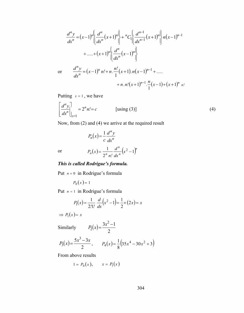
304

or

Putting , we have

[using (3)] (4)

Now, from (2) and (4) we arrive at the required result

or

This is called Rodrigue’s formula.

Put in Rodrigue’s formula

Put in Rodrigue’s formula

Similarly

,

From above results

,

11

1

1 1111

nnn

nnn

n

nn

n

nxnx

dxdCx

dxdx

dxyd

nn

nn x

dxdx..... 11

.....xn.x!n.n!nxdx

yd nnn

n 111

11

nn xxn.x!n.n 111

1 1 !n

1x

c!ndx

yd n

xn

n

21

n

n

n dxyd

cxP 1

nn

n

nn xdxd

!nxP 1

21 2

0n

10 xP

1n

xxxdxd

!!xP 2

211

121 2

1

xxP 1

2

13 2

2

xxP

2

35 3

3xxxP

3303581 24

4 xxxP

xP01 xPx 1

305

(Putting )

In similar way

,


Example 1 Express in terms of Legendre Polynomials.

Sol. As found above , ,

and as

so

Substituting these values in ,

Example 2 Express , in terms of Legendre Polynomial.

Sol. Using , , and


Section – A (Very Short Answer type Questions)

Q.1 Write Legendre Differential equation.

2

121322

13 2222

2

2

PxxxPxxP

22 022 PPx

xP01

532 133 PPx

0244 7208

351 PPPx

253 244 xxxxxf

01 P 1Px 3

2 022 PPx

532 113 PPx

3303581 24

4 xxP

0244 7208

351 PPPx

xf

xPxPxPxPxf 0234 105224

212

56

358

25 23 xxxxf

10 P 1Px 3

2 022

PPP

532 133 PPx

010213 223532

51 PPPPPPxf

xPxPxP 023 31

310

52



306

Q.2 Write generating function for .

Section – B (Short Answer type Questions)

Q.3 Express in term of Legendre polynomial.

Q.4 Prove that

Section – C (Long Answer type Questions)

Q.5 Solve Legendre equation

Q.6 Prove that is generating function for Legendre Polynomial.


(I ) or Proof : By generating formula of the Legendre’s function,

(1)

Differentiating both sides of (1) w.r.t. ,

(2)

Multiplying (2) throughout by ,

or [by (1)]

or (3)

Comparing the coefficient of on both the sides, we get,

[Note]

By transporting the required formula is

(4)

xPn

435 23 xxxxf

0

2322 12211n

nn txPntxtx

0121 2

22 ynn

dxdyx

dxydx

21221

txt

11112 nnn nPPnxPn 11 121 nnn PnPxnPn

0

21221

nn

nPzzxz

z

0

1232 2221

21

nn

n Pnzzxzxz

221 zxz

0

12212 2121

nn

n Pnzzxzzxzzx

0

12

021

nn

n

nn

n PnzzxzPzzx

0

1

0 nn

n

nn

n PzPzx

0

1

00

1 2n

nn

nn

n

nn

n PnzPnzxPnz

nz

111 121 nnnnn Pn_PxnPnPxP

11112 nnn PnPnPxn


307

Another form :

Replacing by in (4), we get the following useful form

(5)

(II)

Proof : By generating formula of the Legendre’s function

(1)

Differentiating (1) w.r.t. and simplifying

(2)

Again differentiating (1) w.r.t. , and simplifying,

where dash denote the differentiation w.r.t.

Multiplying both sides by ,

(3)

Now by (2) and (3),

or,

Comparing the coefficients of on both sides, the required results in obtained.

(III) Proof : By recurrence relation LR I,

(1)

Differentiating (1) w.r.t.

(2)

Again by recurrence relation II,

n 1n

21 112 nnn PnPxnPn

1 nnn PPxPn

0

21221

nn

n xPzzxz

x

0

123221

nn

n xPnzzxzzx

x

0

23221

nn

nPzzxzz

' x

zx

0

23221

nn

nPzzxzxzzxz

00

1

nn

n

nn

n PzzxPnzz

0

1

00 n

nn

n

nn

n

nn zPzPxnzP

nz

1112 nnn PPPn

11112 nnn PnPnPxn

x

1111212 nnnn PnPnPnPxn

308

(3)

Using (3) in (2), we have

or,

or,

Deduction. Directly by integration,

,

is the constant of integration.

(IV)

Proof : By recurrence relation LR II and LR III,

(1)

and (2)

(V)

Proof : Multiplying recurrence formula LR II throughout by ,

(1)

Replacing by in recurrence formula IV,

(2)

(VI)

Proof : The recurrence formula LR I is

(1)

or,

or, (2)

again by recurrence formula LR V,

(3)

The required result is obtained by (2) and (3).

1 nnn PPnPx

111 11212 nnnnn PnPnPnPnPn

11 11112 nnn PnPnPnn

1112 nnn PPPn

11121

nnn PPn

dxPc

c

nnn PxPPn 11

1 nnn PPxnP

1112 nnn PPPn

12 nnn PxPPn 11

nnn xPPnPx 121

x

12

nnn PxPxxnP

n 1n

11 nnn PxPnP

nnn PxxPPn 2

1 112

12 11 nnn PxPnPx

11112 nnn PnPnPxn

1111 nnn PnPnPxnn

nnnn xPPnPPxn 111

nnn xPPnPx 121

309

(VII) Beltrami’s results

Proof : By recurrence formula LR V,

(1)

and by LR VI, (2)

Multiplying (1) by and (2) by and adding, we get

or,

or, 14.9 Illustrative Examples


(i)

(ii)

(iii)

Sol. (i) We know that

Putting , we get

Equating the coefficients of , we get

(ii) Again if we put , we have

112 1112 nnn PPnnPxn

nPnPx nn 121

12 11 nn PnnPx

1n n

nn PxnPxn 22 111

11 11 nn PnnPnn



11 nP

nnP 11

xPxP nn

n 1

0

21221n

nn xPttxt

1x

0

1212 1121n

nnPtttt

0

2 11n

nnn Pt...t...tt

001

nn

n

n

n Ptt

nt 11 nP

1x

0

1212 1121n

nnPtttt


310

Now equating the coefficients of , we get

(iii) We have

(1)

Since

(2)

Equating the coefficients of , we get

Example 4 Show that

(i)

(ii)

(iii)

Sol. (i)We know that

Differentiating both sides with respect to , we get

0

32 111n

nnnn Pt...t...ttt

0011

nn

n

n

nn Ptt

nt

nnP 11

0

21221n

nn xPttxt

212212 2121

ttxtxt

0nn

n xPt

01

nn

nn xPt

212212 2121

ttxtxt

0nn

n xPt

nt

( ) ( 1) ( )nn nP x P x

xPnxPnxPxn nnn 11112

121221

11

nnndxxPxPx nn

321212

121

111

2

nnn

nndxxPxPx nn

0

21221n

nn xPttxt

t

311

or

or

or

Now equating the coefficients of from both the sides, we get

or (2)

(ii) Replacing by in the above equation (2), we have

Multiplying the above equation by on both the sides and integrating with respect to between the limits – 1 to 1, we get

(other integral becomes zero by virtue of orthogonality property of the Legendre’s function)

(iii) Again replacing by and in the equation (2), we have

(3)

(4)

Multiplying the above equations (3) and (4) and integrating with respect to between the limits to , we have

(using orthogonality of Legendre’s function)

0

1232 222121

n

nn nt.xPtxtxt

0

12212 2121n

nn

x txPntxttxttx

0

1

0

221n

nn

n

xnn txPntxttxPtx

21110 21 txt.....txPtxP...xPtxPtx n

nn

n

.....txPntxnPtxPn...txPxP nn

nn

nn 1

12121 112

nt

xPnxnxPxPnxPxxP nnnnn 111 121

xnPxPnxPn nnn 11112

n 1n

xPnxnPxPn nnn 21 112

xPn

x

11 2

11

211 1 112 dxxPxPndxxPndxxPxPxn nnnnn

122

n

n

121221

1 1 nn

dxxPxxP nn

n 1n 1n

xPnxnPxxPn nnn 21 112

xPnxPnxxPn nnn 1232 21

x1 1

11

211 11

2 13212 dxxPnndxxPxPxnn nnn

312


(i)

(ii)

Sol. (i)We have

Putting , we get

Comparing the coefficients of on both the sides, we get

[ all the power of on R.H.S. are even]

(ii)

where , when is even and when is odd.

Putting , the last term will be and the last term in when .

12

21

n

.nn

321212

1211 11

2

nnn

nndxxPxPx nn

222

221

26421253110

!m!m

n....m......P m

mmm

0012 mP

0

21221n

nn txttxP

0x

0

21210n

nn ttP ...t

r.......r............t

.

.t rr

2422642

1253114231

211

mt 2

m...

m......P mm 2642

12531102

t

m......m...

m.....m.....m

264226422642125311

m.....!m

mm........m

m

264222126543211

gm........!m

!mm

m

2322212221

222

2122

21!m

!m!m!m

!mm

m

mmm

N

rn

rnr

n r!n!r!n!rx!r!nxP

0

2

22221

2nN n

21

nN n

12 mn mN 0012 mP

0x

313

Example 6 If , then show that

Sol. Integrating by part taking as first function

But

As so it is .


Sol. The generating formula of the Legendre’s function

(1)

Differentiating both sides of (1) w.r.t. , we get

Multiplying throughout by ,

(2)

or

or Hence Proved.

nm

1

1

2 01 dxPPxI mnmn

nPx 21

1

1

2

0

11

2 211 dxPPxPxxPPxI mnnmnmn

nnn PnnPxPx 121 2

1

11 dxPPnn mn

mn 0

0232

212

21

1

n

nn zxPn

zxz

z

0

21221

nn

nPzzxz

z

0

1232 2221

21

nn

n Pnzzxzxz

z2

0

232 2212

nn

nPnzzxzzxz

002322

122

21

2

21

121n

nn

nn

n PnzPzzxz

zxz

zxz

0232

212

21

221

nn

nPznzxz

zxzzxz

0232

212

21

1

nn

nPznzxz

z

314


Sol. LHS

[By generating function] (1)

Using (2) in (1), we get

LHS

RHS Hence Proved.


Sol. Case I. When

Integrating by parts taking as the second function in the given integral, we obtain

012

1

21

1

n

nnn zPP

zzxzz

z

z

zxzzxzz

121211 2122

12

z

xPzxPzz n

nn

nn

n 11

00

...Pz.....PzPzzPPPz nn

nn

n

1

13

32

210

0

...Pz...PzzPPz nn 13

2211 10 P

011

nn

nPzz

001

111

nn

nn

nz

PPzzz

001

nn

n

nn

n PzPz

01

n

nnn zPP

nm

nnn

Nn,m;nm,dxPPx nm

1212

011

12

nm

nP

11

211

211

2 111 dxPxdxdPPPxdxPPx mnnm

IIn

Im

11

2 210 dxPPxPx nmm

315

[by Legendre’s eq.]

[By orthogonality]

Therefore

Example 10 Prove that all the roots of are distinct,

Sol. Suppose all the roots of are not different, then at least two roots must be equal.

Let the equal root be , then by the theory of equations,

and (1)

Since is the solution of Legendre’s equation, therefore

(2)

Differentiate (2) times w.r.t. with Leibnitz theorem, and simplifying, we obtain

(3)

Now putting and in (3) and using (1), we get

(4)

Again putting and in (3) and using (1) and (4), we have

(5)

similar replacing in (3) and simplifying as above, we obtain

(6)

But

11 10 dxPP.mm nm

0121 2 mmm PmmPxPx

111 dxPPmm nm

mnwhen,m

mn,mm

1220

1

mnwhen,

mmm

mnwhen,dxPPx nm

1212

011

12

0xPn

0xPn

0nP 0 nP

nP

0121 2 nnn PnnPxPx

r x

xPDCxxPDx nrr

nr 1

122 121

0122 12 xPDnnCC. nrrr

0r x

0001 2 ''Pn 0 nP

1r x

0001 2 '''Pn 0'''Pn

2332 nn,.....,r

nnnn P..............PP 40

.......x.n

nnx!n

n........xP nnn

2122

11231

316

(7)


Sol. By Rodrigues formula, the given integral

,

[Integrating by parts]

,

,

[Again integrating by parts]

[ times, when ] (1)

[because ]

Part II. When , then by (1).

012311231

n.......!n.

!nn.........xPD n

n

0 nn PD

nm,

n!n

Zn,nm,dxxPx nn

m

122

0211

1

11

211

12

1 dxxdx!n

xdxxPx nnm

nm

11

2 12

1 dxxDx!n.

nII

nmIn dxdD

11

2111

1

21 112

1 dxxDmxxDx!n.

nnmnnmn

11

211 12

1 dxxDx!nm. n

IInm

In

11

222 12

11 dxxDx!n

mm. nnmn

11

20 121 dxxDx

!n!m. nmn

n

m

2m nm

1

1

21 121

nmnn

mxD

!n!m.

0 1 mn

nm

317

[integrand is even function]

[on taking ]

[By Gamma Formula]

Hence Proved.

Example 12 Prove that :

Sol. Case I. when

We know that

Therefore,

Case II. when : By Rodrigues formula

,

Integrating both sides w.r.t. between the limits and ,

11

211

221

11

211

21 dxxdxxdxxPx

nn

nnn

n

nn

11

2122 dxx

nn

2

012

121 dcos nn sinx

2322

211

21

1 n

n.n

.....n.n!n.n

21

23

212

2122

1

nn 1

..........nn.!n n

n 1312122

2

1

...........nnnn

.........nn!n12342212212

242222

!n

......n.n!n12

12221222

!n

!n!n!n!n

nn

122

222

21

Nn,n,

dxxPn 0021

1

0n

10 xP

2111

11

11 0

xdx.dxxP

Nn

12

1 2 xD!n

xP nnn dxdD

x 1 1

318

(1)

Now

Using Leibnitz theorem in RHS.

(2)

and exist in each terms of (2), therefore for or 1, the RHS of .

Therefore

Hence by (1), .


The Legendre polynomial satisfy the following orthogonal property

Proof : Case I

Let the Legendre polynomials and satisfy the differential equations

(1)

(2)

11

211

12

1 dxx.D!n

dxxPnn

nn

1

1

21 12

1

nnn xD

!n

nnnnn xxDxD 111 121

...xDx.nnxDx nnnnnn 11111 211

nnn xDx 11 1

...x!!n.xnnx

!!nx nn 21 1

2111

11

11 x!nx n

1x 1x 1x

02

011

1

21

nn xD

011 dxxPn

xPn

nm,n

nm,dxxnPxPm

12201

1

1

1

2( ) ( )2 1m n mnP x P x dxn

nm

xPm xPn

0121 2 mmm PmmPxPx

0121 2 nnn PnnPxPx


319

Multiplying (1) by and (2) by and subtracting we obtain

Combining the first two terms, we obtain

Integrating from to we obtain

Case II

This part can be proved using Rodrigue’s formula or using generating function. Using the generating function we have

(1)

Sparing both sides and then integrating w.r.t. from to we obtain

(2)

Now

xPn xPm

01121 2 nmmnnmmnnm PPnnmmPPPPxPPPPx

0111 2 nmmnnm PPnnmmPPPPxdxd

mnnmnm PPPPxdxdPPnmnm 211

1 1

01111

12

1

1

mnnmnm PPPPxdxxPxPnmm

01

1

dxxPxP nm

nm

0

21221n

nn t.xPtxt

x 1 1

1

1

1

1

2221

dxtxPtxt

dx nn

1

1

211 2 2

211n21

ttxt

txtdx

22 2211n211n21 ttttt

22 11n11n21 ttt

ttt

11n11n1

ttt

11n11n1

320

(3)

Also

[using the 1st part]

(4)

From (2) using (3) and (4) we obtain

Equating the coefficients of from both sides we obtain


Sol. We have

[Other terms vanish due to orthogonality]

...ttt...ttt

t 32321 3232

...

nt...tt n

125312

242

1

1

1

1

2dxtxPtxPdxtxP n

nn

nn

n

dxtxP n

nn

2

0

1

1

2

dxxPtn

nn

0

1

1

22

dxxPt...nt...tt

nn

nn

0

1

1

22242

125312

nt 2

12

21

1

2

n

dxxPn

12

2

21

1

12

n

hdxhxh

xP nn

dxhxPxPdx

hxh

xP

m

mmn

n

1

1

1

1

1221

1

1dxhxP.xP n

nn

12

21

1

2

n

hdxxPhn

nn

321

Example 14 Show that and hence prove that

Sol. We know that

[Recurrence relations] (1)

and (2)

multiplying (1) by and (2) by and then on adding we get

or

or

or

Multiplying both sides by and integrating w.r.t. from to , we have

14.11 Summary In this unit Legendre polynomial & its properties are discussed. Solution of Legendre differential equation is explained. Generating function & Rodrigue formula for obtaining Legendre polynomial are discussed. Recurrence relations & orthogonal property of Legendre polynomial are explained.


3212

1211

11

2

nn

nndxPPx nn

nnn xPPnPx 121

12 11 nnn PxPnPx

1n n

1122 11111 nnnn PnnPnnPxnPxn



112

1211

nnn PP

nnnPx

1nP x 1 1

1

1111

1

11

21211 dxPPP

nnndxPPx nnnnn

1

111

1

1

2112

1 dxPPdxPnnn

nnn

0112

2121

nnnn

1

1

0m nP P dx if m n

14.11 Summary

322

14.12 Glossary

Polynomial : An expression in integer power of variable.

Differential equation : An equation involving independent variable, dependent variable & its derivatives.

Generating function : A function when expanded gives values in coefficients of powers of variables.

Recurrence relation : A relation by which we can find next value by using

previous value.

Orthogonality :Is a property in which curves intersect each other at right angle.


Ans.1:

Ans.2:

Ans.3:

14.14 Exercise

Section A (Very Short Answer type Questions)

Q.1 State Rodrigue’s formula for Legendre polynomial.

Q.2 Write the value of

Q.3 Write the formula for Legendre polynomial

Q.4 Write Legendre differential equation.

Q.5 State orthogonal property for Legendre polynomial.

Section B (Short Answer type Questions)

Q.6 Using Rodrigue’s formula. Evaluate

Expend the polynomial in a series of Legendre polynomial (Q. 7-8)

Q.7

Q.8

0121 2

22 ynn

dxdyx

dxydx

21221

txt

xPxPxPxP 0123 13182631

xP2

xP5

253 234 xxxx

21 xx

14.12 Glossary


14.14 Exercise

323

Q.9 Prove that

Q.10 Prove that

Section C (Long Answer type Questions)

Q.11 State & Prove Rodrigue’s formula.

Q.12 Prove that

(i)

(ii)

Q.13 Prove that

(i)

(ii)

Q.14 State & prove Orthogonal property for Legendre polynomial.

Q.15 Prove that

(i)

(ii)


Ans.1 :

Ans.2 :

Ans.3 :

0232

212

21

1

n

nn txPn

txt

t

3214

122

1

111

2

nxnndxPPx nn

11 121 nnn PxPxnPn

1112 nnn PPPn


1 nnn PPxPn

nm

nnn

Nn,m,nm,dxPPx nm

1212

01

1

1

2

3212

1211

11

2

nn

nndxPPx nn

nn

n

nn xdxd

!nxP 1

21 2

2

13 2

2

xxP

rnN

rn

r

n x!rn!rn!r

!rnxP 2

0 22221

oddisifn

evenisifn

N

21

2


324

Ans.4 :

Ans.5 :

Ans.6 :

Ans.7 :

Ans.8 :


1. Mathematical Physics with Classical Mechanics, Satya Prakash, Sultan Chand & Sons.

2. Advance Engineering Mathematics, Erwin Kreyszing, Wiley student edition


0121 2

22 ynn

dxdyx

dxydx

nm,n

nm,dxxPxP mn

12201

1

15706381 35 xx

xPxPxPxPxP 01234 105224

534

212

56

358

xPxPxP 210 32

32


325

UNIT -15

Hermite functions, Hermite Polynomials Structure of the Unit 15.0 Objectives

15.1 Introduction

15.2 Rodrigues’ formula for Hermite polynomial 퐻 (푥)


15.4 Generating function for the 퐻 (푥)


15.6 Orthogonality relation for Hermite polynomials

15.7 Recurrence relation for the Harmonic oscillator energy Eigenfunctions


15.9 Self learning exercise

15.10 Summary

15.11 Glossary


15.13 Exercise



15.0 Objective In this unit we are going to discuss about another type of polynomial i.e.

Hermite polynomials and its properties.

After going through this unit you will be able to learn

Hermite differential equation

Rodrigues’ formula for Hermite polynomial 퐻 (푥)and Recurrence Relations

UNIT -15

Hermite functions, Hermite Polynomials

15.0 Objectives

326

Generating function for the 퐻 (푥)

Orthogonality relation for Hermite polynomials

The Harmonic oscillator energy Eigenfunctions

15.1 Introduction In the treatment of the harmonic oscillator in quantum mechanics,

Hermite’s differential equation arises and which is defined as

2 2 0y xy ny (1)

Where 푦 = , 푦 = . n is a real number. For n is a non-negative integer, i.e. n = 0,1,2,3,..., the classical set of solutions of Hermite’s differential equation are often referred to as Hermite Polynomials 퐻 (푥). These polynomials are useful in solving physical problems using algebraic and analytic methods. Hermite polynomials are defined by

2 2

( ) ( 1)n

n x xnn

dH x e edx

(2)

Let 푦 = ∑ 푎 푥 (3)

푦 = ∑(푚 + 푟)푎 푥 (4) 푦 = ∑(푚 + 푟)(푚 + 푟 − 1)푎 푥 (5)

Putting equation (2)-(4) in (1) we get ∑(푚 + 푟)(푚 + 푟 − 1)푎 푥 − 2∑(푚 + 푟)푎 푥 +2푛∑ 푎 푥 = 0

∑(푚 + 푟)(푚 + 푟 − 1)푎 푥 + ∑(2푛 − 2푚 − 2푟)푎 푥 = 0

Comparing coefficient of 푥 , m(m-2)푎 = 0

Since 푎 ≠ 0, m = 0 or 1

Comparing coefficient of 푥 , m(m+1)푎 = 0 or 푎 = 0

Finally, comparing coefficient of 푥 ,

(m+r+2)(m+r+1) 푎 +2(n-m-r) 푎 = 0

∴ 푎 = − ( )( )( )

푎

15.1 Introduction

327

Case I: m=0.

∴ 푎 = ( )

( )( )푎

∴ 푎 =− !푎 ;

푎 = ( )

. !푎 = ( )

!푎 ;

푎 = ( ) ( )

. .푎

= −2 푛(푛 − 2)(푛 − 4)

6!푎

Now, 푦 = ∑푎 푥 = 푎 + 푎 푥 + 푎 푥 + 푎 푥 + ⋯

∴ 푦 = 푎 [1 − !푥 + ( )

!푥 − ( )( )

!푥 + ⋯ ]

Case II : m =1.

푎 = ( )

( )( )푎

∴ 푎 = ( )푎 = − ( )푎 ;

푎 = ( )

.( )푎 = ( )( )

!푎

∴ 푦 = 푎 푥[1 − ( )!

푥 + ( )( )!

푥 + ⋯ ]

Hence we can write the solution for m = 0 and m =1 in more general form

푦 = 푎 [1 − !푥 + ( )

!푥 − ( )( )

!푥 + ⋯+

( ) ( )( )…( )!

푥 + ⋯ ] (6)

푦 = 푎 푥[1 − ( )!

푥 + ( )( )!

푥 + ⋯+

( ) ( )( )…( )( )!

푥 + ⋯ ] (7)

and the general solution of Hermite equation is the superposition of (6) and (7) .

15.2 Rodrigues’ formula for Hermite polynomial Hn(x) The Hermite polynomials are given by the formula

15.2 Rodrigues’ formula for Hermite Polynomial Hn(x)

328

2 2

( ) ( 1)n

n x xnn

dH x e edx

If we put 푛 = 0,1,2, … in

0 ( ) 1H x

1( ) 2H x x

2

2( ) 4 2H x x

2

3( ) 8 12H x x x

4 2

4 16 48 12H x x x

5 3

5 32 160 120H x x x x

Proof : Let 푝 = 푒 , then

퐷p + 2푥p = 0, Where 퐷 =

Differentiating (n+1) times by the Leibnitz’ rule, we get

퐷 p + 2푥퐷 푝 + 2(푛 + 1)퐷 p = 0

Writing 푦 = (−1) 퐷 푝

퐷 y + 2푥퐷푦 + 2(푛 + 1)푦 = 0 (8)

Substitute 푢 = 푒 y then

퐷푢 = 푒 (2푥푦 + 퐷푦)And

D u = e (D y + 4xDy + 4x y + 2y)

Hence by equation (8), we get

퐷 u − 2푥퐷푢 + 2푛푢 = 0 Which indicates that

푢 = (−1) 푒 퐷 푒

is a polynomial solution of Hermite equation.

15.3 Recurrence Relations 15.3 Recurrence Relations

329

Hermite polynomials satisfy the following relations :-

1. 퐻 (푥) = 2푥퐻 (푥) −퐻 (푥)

Proof: We know the Rodrigues’ formula

퐻 (푥) = (−1) 푒 푑푑푥

푒

Differentiating this with respect to , we get

퐻 (푥) = (−1) 2푥 푒 푒 + (−1) 푒 푒 (9)

Which gives us

퐻 (푥) = 2푥퐻 (푥) −퐻 (푥) (10)

2. 퐻 (푥) = 2퐻 (푥) + 2푥퐻 (푥) − 퐻 (푥)

Proof: Again differentiating equation (9) with respect to 푥 , we get

퐻 (푥) = 2(−1) 푒 푑푑푥

푒 + (−1) 4푥 푒 푑푑푥

푒

+ (−1) 2푥 푒 푑푑푥

푒 + (−1) 2푥 푒 푑푑푥

푒

+ (−1) 푒 푑푑푥

푒

From this, we get

퐻 (푥) = 2퐻 (푥) + 2푥퐻 (푥) − 퐻 (푥) (11)

3. 퐻 (푥) = 2(푛 + 1)퐻 (푥) Proof: We know that Hermite function 퐻 (푥) satisfies the Hermite’s equation

퐻 (푥) − 2푥퐻 (푥) + 2푛)퐻 (푥) = 0 (12)

Putting the value of 퐻 (푥) from equation (11) to equation (12), we get

2퐻 (푥) + 2푥퐻 (푥) − 퐻 (푥) − 2푥퐻 (푥) + 2푛퐻 (푥) = 0

Which gives us the result

퐻 (푥) = 2(푛 + 1)퐻 (푥) (13)

330

4. 퐻 (푥) = 2푥퐻 (푥) − 2(푛 + 1)퐻 (푥)

Proof: Replacing n by n+1 in equation (10) we get

퐻 (푥) = 2푥퐻 (푥) −퐻 (푥)

Putting the value of 퐻 (푥) from equation (13), we get

2(푛 + 1)퐻 (푥) = 2푥퐻 (푥) − 퐻 (푥)

Then we get the following result

퐻 (푥) = 2푥퐻 (푥) − 2(푛 + 1)퐻 (푥)

From this relation, we can get the higher polynomials.

15.4 Generating function for the Hn(x) The generating function for the Hermite polynomial is given by

2 2 22 { ( }

0

),!

nnxt t x t x

n

nt H xg x t e e

n

Differentiating 푔(푥, 푡) = 푒 ( ) with respect to t

휕푔휕푡

= (2푥 − 2푡)푔

| = 2푥 = 퐻 (푥) = −푒 푒

Where 퐻 (푥) is defined by the Rodrigues’ formula.

Now to establish the general term

(−1) 푒 푒 = (−1) 푒 푒

= (−1) 푒 − 2푥푒 푒

= − 퐻 (푥) + 2푥퐻 (푥)

Using recurrence relation, we get

(−1) 푒푑푑푥

푒 = −푑푑푥

퐻 (푥) + 2푥퐻 (푥)

= 퐻 (푥)

In general, 푛 differential of function 푔(푥, 푡) at t = 0

15.4 Generating function for the Hn(x)

331

퐻 (푥) = ( )

= (−1) 푒 푒

So the function 푔(푥, 푡) is known as the generating function of Hermite polynomials. Using the generating function, we can also prove the recurrence reation:

퐻 (푥) = 2푛퐻 (푥)

Proof: We know that

푒 = 푡 퐻 (푥)

푛!

Differentiating above equation with respect to 푥, we get

2푡 푒 = 푡 퐻 ′(푥)

푛!

or 2푡 ∑ ( )!

= ∑ ( )!

Now equating the coefficient of 푡 , it follows that

퐻 (푥) = 2푛퐻 (푥)

And 퐻 (푥) = 2푛퐻′ (푥)


Example 15.1 Calculate the first three Hermite polynomials by using the generating function.

Sol. We know that generating function for Hermite polynomial is given by

푔(푥, 푡) = 푒 = 푡 퐻 (푥)

푛!

Expanding the left-hand side of the above equation and combining equal power of t yields

1 + 2푥푡 + (2푥 − 1)푡 + higher degree

Comparing the coefficients of powers of t in both sides, we get


332

퐻 (푥) = 1, 퐻 (푥) = 2푥,

퐻 (푥) = 4푥 − 2

These are the first three Hermite polynomials calculated by using the generating function.

Example15.2 Calculate the third Hermite polynomial by using the recurrence relation.

Sol. We know that recurrence relation

퐻 (푥) = 2푥퐻 (푥) − 2푛퐻 (푥)

Setting n=1 , we get

퐻 (푥) = 2푥퐻 (푥) − 2퐻 (푥)

But we know that

퐻 (푥) = 1, 퐻 (푥) = 2푥

Putting the values of 퐻 (푥) and 퐻 (푥), we get

퐻 (푥) = 2푥. 2푥 − 2

= 4푥 − 2

The same result for the third Hermite polynomial can also be obtained by using the generating function.

15.6 Orthogonality relation for Hermite polynomials We know that Hermite function satisfies the Hermite differential equation

퐻 (푥) − 2푥퐻 (푥) + 2푛퐻 (푥) = 0

This equation can be written as

푒 (푒 퐻 (푥))+ 2푛퐻 (푥) = 0 (14)

Changing the index n by m, we can write

푒 (푒 퐻 (푥))+ 2푚퐻 (푥) = 0 (15)

Multiplying equation (15) by 퐻 (푥) and equation (14) by 퐻 (푥), we get the following equations

15.6 Orthogonality Relation for Hermite Polynomials

333

퐻 (푥)푒 (푒 퐻 (푥))+ 2푚퐻 (푥)퐻 (푥) = 0 (16)

And

퐻 (푥)푒 (푒 퐻 (푥))+ 2푛퐻 (푥)퐻 (푥) = 0 (17)

Subtracting equation (16) and (17), we get

2(푚 − 푛)푒 퐻 (푥)퐻 (푥) = 퐻 (푥)푒 푒 퐻 (푥) −

퐻 (푥)푒 푒 퐻 (푥)

Integrating the above equation from −∞ to ∞, we get

2(푚 − 푛) 푒 퐻 (푥)퐻 (푥)푑푥

= ∫ 푒 퐻 (푥)퐻 (푥) − 퐻 (푥)퐻 (푥) 푑푥 = 0

Which gives

2( ) ( ) ( ) 0xm ne H x H x dx for m n

This is known as the orthogonality relation of Hermite polynomials.

Let us define

퐼 , = ∫ 푒 퐻 (푥)퐻 (푥)푑푥

Then

퐼 , = ∫ 푒 퐻 (푥)퐻 (푥)푑푥

We know the recurrence relation

퐻 (푥) = 2푥퐻 (푥) − 2푛퐻 (푥)

⇒ ∫ 푒 퐻 (푥)(2푥퐻 (푥) − 2푛퐻 (푥) )푑푥 = 0

⇒ ∫ 2푥푒 퐻 (푥)퐻 (푥)푑푥 = 2푛퐼 , (푥)

Putting the value of Hermite polynomial 퐻 (푥) = (−1) 푒 푒 ,

we get

−∫ 2푥푒 푒 푒 푑푥 = 2푛퐼 , (푥)

334

⇒ −∫푒 푒 푒 푑푥 − ∫ 푒 푒 푒

= 2푛퐼 , (푥)

Which gives us

퐼 , (푥) = 2 푛! 퐼 ,

Where

퐼 , = 푒 푑푥 = √휋

Then 퐼 , (푥) = 2 푛!√휋

So the orthonormality relation can be written as

2

2 !x nm n mne H x H x dx n

15.7 Recurrence relation for the Harmonic oscillator energy Eigenfunctions

The harmonic oscillator energy eigenfunctions 휓 (푥) satisfy the recurrence relation

훼푥휓 (푥) = 휓 (푥) + 휓 (푥) …. (18)

Where 훼 =ℏ

.

We can prove this in following manner

The energy eigenfunction for harmonic oscillator is defined as

2 2 /2( ) x

n n nx N H x e

푛 = 0,1,2, …. The recurrence relation for the Hermite polynomial is

퐻 (푥) = 2푥퐻 (푥) − 2푛퐻 (푥)

Then

15.7 Recurrence relation for the Harmonic Oscillator Energy Eigenfunctions

335

훼푥휓 (푥) = 훼푥푁 퐻 (훼푥)푒 /

= 푁 퐻 (훼푥) + 푛퐻 (훼푥) 푒 /

=푁

2푁푁 퐻 (훼푥)푒 / +

푛푁푁

푁 퐻 (훼푥)푒 /

Which gives us

훼푥휓 (푥) =푛 + 1

2휓 (푥) +

푛2휓 (푥)


Example 15.3 Using the recurrence relation calculate 휓 (푥).

Sol. The recurrence relation for the energy eigenfunction for harmonic oscillator is

휓 (푥) = 훼푥휓 (푥) − 휓 (푥)

Setting n = 2, we get

휓 (푥) = [훼푥휓 (푥) − 휓 (푥)]

= 훼푥 훼푥휓 (푥) − 휓 (푥) − 휓 (푥)

= (훼 푥 − 1)휓 (푥) −√휓 (푥)

By knowing the wave functions 휓 (푥) and 휓 (푥) we can the value of 휓 .

Example15.4 Prove that

2 2 1

(2 )!(0) ( 1) ; (0) 0!

nn n

nH Hn

Sol. Using the Generating function ,we have

24 2

0

( )!

tx tn

n

H xt e

n

(1)

Replacing x by 0 in equation(1),We have


336

22

4

0 0

(0) ( )! !

ntn

n n

H tt en n

Or 4 2

0 0

(0) ( 1)! !

nnn

n n

Ht t

n n

(2)

Equating coefficients of 2nt on both sides of (2) ,we have

2 (0) ( 1)2

nnHn n

Or 2

( 1) 2(0)n

n

nHn

The right hand side of equation (2) does not contain odd powers of t .Then equating coefficients of 2 1nt on the both side of equation (2) gives

2 1(0)0

2 1nHn

So 2 1(0) 0nH

Example 15.5 Express 4 3 2( ) 2 2 3H x x x x x in terms of Hermite’s polynomials.

Sol. We know that

0 ( ) 1H x

1( ) 2H x x

2

2 ( ) 4 2H x x

3

3( ) 8 12H x x x

And 4 24 ( ) 16 48 12H x x x

From these,we have

4 2

4

1 3( ) 316 4

x H x x (1)

3

3

1 3( )8 2

xx H x (2)

2

2

1 1( )4 2

x H x (3)

337

1

1 ( )2

x H x (4)

01 ( )H x (5)

2 24

1 3( ) ( ) 3 2 316 4

H x H x x x x by(1)

3 2

4

1 15( ) 2 516 4

H x x x x

By using(2)

24 3

1 1 3 15( ) ( ) 2 ( ) 516 8 2 4

H x H x H x x x x

2

4 3

1 1 15( ) ( ) 5 216 4 4

H x H x x x

By using(3)

4 3 2

1 1 1 1 15( ) ( ) ( ) 5 ( ) 216 4 4 2 4

H x H x H x H x x

4 3 2

1 1 5 5( ) ( ) ( ) 216 4 4 4

H x H x H x x

By using(4)

4 3 2 1 0

1 1 5 5( ) ( ) ( ) ( ) ( ) ( )16 4 4 4

H x H x H x H x H x H x

The above equation represents the expression of ( )H x in terms of Hermite’s polynomials.

Example 15.6 Express 2( ) 5 2H x x x in terms of Hermite’s polynomials.

Sol. We know that

0 ( ) 1H x , 1( ) 2H x x and 22 ( ) 4 2H x x

From these we have

2

2

1 1( )4 2

x H x

1

1 ( )2

x H x then

338

2( ) 5 2H x x x

2 1

1 1 1( ) 5 ( ) 2. ( )4 2 2

H x H x H x

2 1

5 5( ) ( )4 2

H x H x

2 1

5 5( ) ( )4 2

H x H x


2 22 1( ) 2

2x n

nx e H x dx n n

Sol. From the recurrence relation ,we know that

1 1( ) 2 ( ) 2 ( )n n nH x xH x nH x

Or 1 1

1( ) ( ) ( )2n n nxH x nH x H x (1)

Or 21 1( ) ( ) ( )

2n n n

xx H x nxH x H x (2)

Replacing n by 1n and 1n successively in eq(1).

We get

1 2

1( ) 1 ( ) ( )2n n nxH x n H x H x (3)

and

1 2

1( ) 1 ( ) ( )2n n nxH x n H x H x (4)

Using(3) and (4),(2) becomes

22

2

1( ) 1 ( ) ( )2

1 11 ( ) ( )2 2

n n n

n n

x H x n n H x H x

n H x H x

2 2

1 11 ( ) ( ) ( )4 2n n nn n H x H x n H x

(5)

Multiplying both sides of (5) by 2

( )xne H x and then integrating with respect to x

from to ,we get

339

2 2

2 2

222

2

2

( ) ( 1) ( ) ( )

1 1( ) ( ) ( )4 2

x xn n n

x xn n n

x e H x dx n n e H x H x dx

e H x H x dx n e H x dx

10 0 22

nn n

2

( ) ( ) 2x nn m mne H x H x dx n

2 22 1( ) 2

2x n

nx e H x dx n n

Example 15.8 Show that

1 11

0

( ) ( ) ( ) ( ) ( ) ( )2 2 ( )

nk k n n n n

k nk

H x H y H y H x H x H yk n y x

Sol. From the recurrence relation

1 1( ) 2 ( ) 2 ( )n n nH x xH x nH x

Or 1 1

1( ) ( ) ( )2n n nxH x nH x H x (1)

Replacing x by y in equation(1),we get

1 1

1( ) ( ) ( )2n n nyH y nH y H y (2)

Multiplying equation (2) by ( )nH x and equation (1) by ( )nH y then subtracting, we get

1 1

1 1

1( ) ( ) ( ) ( ) ( ) ( )22 ( ) ( ) ( ) ( )

n n n n n n

n n n n

y x H x H y H y H x H x H y

H x H y H y H x

(3)

Putting 0,1,2,...( 1),n n n in eq(3),we have

0 0 1 0 1 0

1( ) ( ) ( ) ( ) ( ) ( ) ( ) 02

y x H x H y H y H x H x H y (4)

340

1 1 2 1 2 1

0 1 0 1

1( ) ( ) ( ) ( ) ( ) ( ) ( )2

( ) ( ) ( ) ( )


H x H y H y H x

(5)

2 2 3 2 3 2

1 2 1 2

1( ) ( ) ( ) ( ) ( ) ( ) ( )22 ( ) ( ) ( ) ( )


H x H y H y H x

(6)

1 1 1 1

1 1 2 1

1( ) ( ) ( ) ( ) ( ) ( ) ( )2

2 ( ) ( ) ( ) ( )

n n n n n n

n n n n


H x H y H y H x

(7)

1 1

1 1

1( ) ( ) ( ) ( ) ( ) ( ) ( )22 ( ) ( ) ( ) ( )

n n n n n n

n n n n


H x H y H y H x

(8)

Multiplying (4),(5),(6),(7),(8) by 2 3 1

1 1 1 1 11, , , ,......, ,2.1 2 2. 2 . 3 2 1. 2 .n nn n

Respectively and adding ,we get

1 11

0

( ) ( ) ( ) ( ) ( ) ( )( )

2 2

nk k n n n n

k nk

H x H y H y H x H x H yy x

k n

Or 1 11

0

( ) ( ) ( ) ( ) ( ) ( )2 2 ( )

nk k n n n n

k nk

H x H y H y H x H x H yk n y x

Example 15.9 Prove that ( ) ( 1) ( )nn nH x H x

Sol. We have 22

0

( 1) !(2 )( )( 2 )! !

ns n s

ns

n xH xn s s

22

0

( 1) !( 2 )( )( 2 )! !

ns n s

ns

n xH xn s s

2 22

0

( 1) ( 1) !(2 )( 2 )! !

ns n s n s

s

n xn s s

22

0

( 1) !(2 )( 1)( 2 )! !

ns n s

n

s

n xn s s

341

( 1) ( )nnH x

Thus ( ) ( 1) ( )nn nH x H x

Example 15.10 Prove that for m n ,

2 !( ) ( )( )!

m m

m n n m

d nH x H xn mdx

Sol.

2 !( ) ( )( )!

m m

m n n m

d nH x H xn mdx

After differentiation m times partially with respect to x, we have

2

2

2

0

2

( )!

2

n m mz zx

m mnn

m z zx

z d dH x en dx dx

z e

0

( )(2 )

!m nn

n

H xz z

n

0

( )(2)

!m m nn

n

H xz

n

Putting m+n=s or n=s-m on right side we get

( )

( ) 2! !

n mm ss m

m nn s s m

H xz d H x zn dx s m

Comparing the powers of zn on either side, we get

( )1 ( ) 2

! !

mm n m

m n

H xd H xn dx n m

!( ) 2 ( )

!

mm

m n n m

d nH x H xdx n m

Hence Proved


Q.1 Write one example from quantum mechanics where Hermite polynomials appear.


342

Q. 2 Write the value of Hermite polynomial 퐻 (푥).

Q. 3 Write the value of Hermite polynomial 퐻 (0).

Q. 4 Write the value of Hermite polynomial 퐻 (푥).

Q.5 By using Rodrigues’ formula for Hermite polynomials prove the

following Recurrence relation

퐻푛′′(푥) = 2퐻푛(푥) + 2푥퐻푛

′ (푥) − 퐻푛+1′ (푥)


following Recurrence relation

(i) 퐻 (푥) = 2(푛 + 1)퐻 (푥)

(ii)퐻 (푥) = 2푥퐻 (푥) − 2(푛 + 1)퐻 (푥)

15.10 Summary

We started this topic with the introduction of Hermite differential equation which appears in the treatment of Harmonic oscillator in quantum mechanics. We defined the recurrence relations for the Hermite polynomials by which we can get the higher degree polynomial. We also defined the generating function for the Hermite polynomial which can generate the Hermite polynomial of any degree. We ended up with application of recurrence relation for the harmonic oscillator energy eigenfunctions.

15.11 Glossary

Eigen : Proper; characteristic

Polynomial: An expression of more than two algebraic terms, especially the sum of several terms that contain different powers of the same variable(s).

Recurrence: the fact of happening again

Generate: to cause something to exist

Hermite: Charles Hermite (December 24, 1822 – January 14, 1901) was a French mathematician who did research on number theory, invariant theory, orthogonal polynomials, elliptic functions, and algebra.Hermite

15.10 Summary

15.11 Glossary

343

polynomials, Hermite interpolation, Hermite normal form, Hermitian operators are named in his honor

15.12 Answers of Self Learning Exercise

Ans. 1: In the treatment of Harmonic oscillator

Ans. 2: 4푥 − 2

Ans. 3: 1( ) 2H x x

1(0) 2.0 0H

Ans. 4: 4 24 16 48 12H x x x

15.13 Exercise

Section A-Very Short Answer Type Questions

Q.1 Write down the Rodrigues’ formula for Hermite polynomial 퐻 (푥)

Q.2 What do you mean by the generating function of Hermite polynomials.

Section B-Short Answer type Questions

Q.3 Using the recurrence relation calculate the Hermite polynomial 퐻 (푥).

Q.4 Show that for the energy eigenfunction of harmonic oscillator

휓 (푥) =25훼푥휓 (푥) − √2휓 (푥)

Q.5 Using the recurrence relation calculate 퐻’ (푥).


following Recurrence relations

퐻 (푥) = 2푥퐻 (푥) −퐻 (푥)

Section C-Long Answer type Questions

Q.7 Show that the uncertainty relation

1. ( )2

x p n

holds for the harmonic oscillator energy eigenstates.

15.12 Answers of Self Learning Exercise

15.13 Exercise

344


Ans. 1: 2 2

( ) ( 1)n

n x xnn

dH x e edx

Ans. 2: The generating function for the Hermite polynomial is given by

2 2 22 { ( }

0

),!

nnxt t x t x

n

nt H xg x t e e

n


1. Mathematical Physics with Classical Mechanics by Satya Prakash, ,Fourth edition,2003 ,Sultan chand &Sons

2. Mathematical Methods for Physics by George B. Arfken, Hans J. Weber,2007

Academic Press.

3. Advance Engineering Mathematics , Erwin Kreyszing, Wiley student edition,2008

4. Mathematical Physics by B.S. Rajput 1st edition,Pragati Prakashan, Meerut



345

UNIT 16

Fourier Series Structure of theUnit

16.0 Objectives

16.1 Introduction

16.2 Definition of Fourier Series

16.3 Evaluation of coefficients of Fourier Series

16.4 Even and Odd Functions

16.5 Dirichlet’s conditions

16.6 Self-Learning Exercise I

16.7 Applications of Fourier Series


16.9 Complex form of Fourier Series

16.10 Fourier Series in interval ( 0,T)

16.11 Internal Change for Fourier expansion from (- , ) to (-l, l)

16.12 Fourier Half Range Series

16.13 Some important notes


16.15 Self-Learning Exercise II

16.16 Summary

16.17 Glossary


16.19 Exercise



UNIT- 16 Fourier Series

346

16.0 Objective

The objective of this unit is to introduce the concept of Fourier series and their applications in various problems of Physics. As Fourier series is a powerful tool for analysis of periodic functions, the unit aims at describing the methods for expressing piecewise continuous periodic functions through Fourier series expansion.

16.1 Introduction In practice we encounter many signals which are periodic in nature. For

example

-During communications and transmitting signals, periodic signals are used in modulator.

-Problems involving vibrations or oscillations- water waves, electromagnetic waves and fields, sound waves, alternating electrical current, voltage etc.

-Periodic signals are used in power supplies.

-Periodicity in crystal structure and x-ray crystallography.

The simple periodic signal with definite frequency is expressed mathematically by the sine or cosine function. This definite (single) frequency is known as fundamental frequency. But many times the signal is not pure i.e. it contains a number of frequencies (harmonics) which are integer time the fundamental frequency along with the fundamental frequency. Such a signal is complicated periodic function.

This complicated function may be mathematically expressed as an infinite series of terms including fundamental frequency and harmonics and the series is known as Fourier series.

16.2 Definition Of Fourier Series A Fourier series may be defined as an expansion of any complex periodic function f(x) in a series of series or cosines such as

01 1

cos sinn n

n nn n

f x a a nx b nx

(1)

16.0 Objectives

16.2 Definition of Fourier Series

16.1 Introduction

347

The above equation is valid if the function f(x) satisfies the following two conditions known as Dirichlet conditions :

(i) The function has only a finite number of extreme values i.e. maxima and minima.

(ii) The function has finite discontinuities in finite number in one oscillation.

These conditions are sufficient but not necessary because some functions which do not satisfy these conditions may be expressed by Fourier series.

The function 푓(푥) is defined in interval (−휋,휋) and has period 2휋 as 푠푖푛 푥 and 푐표푠 푥 have period of 2휋 and also 푠푖푛 푛 푥 and cos 푛 푥

∵ sin푛 (푥 + 2휋) = sin푛 푥

cos푛 (푥 + 2휋) = cos푛 푥

16.3 Evaluation of Coefficients of Fourier Series

In equation (1) 푎 ,푎 푎푛푑 푏 are called the coefficients of the Fourier series.

Value of coefficient a0 :

Let us integrate equation (1) on both the sides between the limits –휋 푎푛푑 휋.

∫ 푓(푥)푑푥 = 푎 ∫ 푑푥 + ∫ ∑ 푎 cos 푛 푥 + ∫ ∑ 푏 sin푛 푥 (2)

It reduces to

푓(푥)푑푥 = 푎 푑푥 + 0 + 0

{퐴푠 푎푙푙 표푡ℎ푒푟 푖푛푡푒푔푟푎푙푒푠 푣푎푛푖푠ℎ}

Or ∫ 푓(푥)푑푥 = 푎 2휋

0

12

a f x dx

(3)

Value of coefficient an :

Multiply equation (i) by 푐표푠 푚 푥 on both the sides and integrating between the

limits –휋 푎푛푑 휋.

16.3 Evaluation of Coefficients of Fourier Series

348

푓(푥)cos푚 푥 푑푥 = 푎 cos푚 푥 푑푥

+ ∑ 푎 ∫ cos푚 푥 cos 푛 푥 푑푥 + ∑ 푏 ∫ cos푚 푥 sin 푛 푥 푑푥 (4)

By orthogonal property of sine and cosine function we have

sin cos 0mx nxdx

(5)

푓표푟 푚, 푛 ≠ 0 sin sin cos cos mnmx nxdx mx nxdx

(6)

01

mn

mn

for m nfor m n

Using (5) and (6) in (4) we have

푓(푥) cos푚 푥 푑푥 = 0 + 푎 휋 훿 + 0

∫ 푓(푥) cos푚 푥 푑푥 = 푎 휋 [푓표푟 푚 = 푛]

푎 = ∫ 푓(푥) cos푚 푥 푑푥

Replacing m by n, we have

1 cosna f x nx dx

(7)

Value of coefficient 풃풏:

Multiply (1) on both the sides by 푠푖푛 푚 푥 and integrate between the limits –휋 푎푛푑 휋.

푓(푥) sin푚 푥 푑푥 = 푎 sin푚 푥 푑푥

+ 푎 sin푚 푥 cos 푛 푥 푑푥 + 푏 sin푚 푥 sin 푛 푥 푑푥

= 0 + 0 + 푏 휋 훿 [푈푠푖푛푔 5 푎푛푑 6]

349

= 푏 휋

∴ 푏 = 1휋

푓(푥) sin푚 푥 푑푥

Replacing m by n

1 sinnb f x nxdx

(8)

Thus the values of the coefficients are given by eq (3), (7) and (8).


We can write any function 푓(푥) as

푓(푥) = ( ) ( ) + ( ) ( ) (1)

표푟 푓(푥) = 푓 (푥) + 푓 (푥) (2)

푤ℎ푒푟푒 푓 (푥) = ( ) ( ) (3)

푎푛푑 푓 (푥) = ( ) ( ) (4)

From (3) we can see that

푓 (−푥) = 푓(−푥) + 푓(푥)

2= 푓 (푥)

표푟 푓 (−푥) = 푓 (푥) (5)

Thus the functions which satisfy equation (5) are known as even function for

which the functions remain same on replacing 푥 푏푦 – 푥.

For example 푐표푠 (−푥) = 푐표푠 푥

Thus 푐표푠 푥 is an even function

From (4) we can see that

푓 (푥) = 푓(−푥) + 푓(푥)

2= −

푓(푥) − 푓(−푥)2

표푟 푓 (−푥) = − 푓 (푥) (6)

Thus the functions which satisfy equation (6) are known as odd functions.

For example 푠푖푛 (−푥) = −푠푖푛 푥


350

Thus 푠푖푛 푥 is an odd function.

From (2) we can see that we can always split each function into some of even and odd functions but if 푓(푥) is a periodic function, then 푓 (푥) and 푓 (푥) should also be periodic functions.

If functions 푓(푥) is an even function then 푓(−푥) = 푓(푥)

∴ 푓 (푥) = ( ) ( ) = 0 (7)

Therefore 푓(푥) = 푓 (푥) (8)

Thus even functions when represented by Fourier series will not contain odd function terms i.e. sinnx series.

The Fourier series for an even function is

푓(푥) = 푓 (푥) = 푎 + 푎 cos푛 푥 (9)

Similarly if 푓(푥) is an odd function then 푓(−푥) = −푓(푥)

Therefore 푓 (푥) = 0 (10)

Thus Fourier series for an odd function will contain series of sinnx.

The Fourier series for an odd function is

푓(푥) = 푓 (푥) = 푏 sin 푛 푥 (11)

The graph of an even function is symmetrical about 푥 = 0.

The area of the curve of even function form −휋 to 휋 is twice the area under the curve from 0 to 휋 i.e.

푓(푥)푑푥 = 2 푓(푥)푑푥

Therefore for even function

푎 =1

2휋 푓(푥)푑푥 =1휋 푓(푥)푑푥

푎 =1휋

푓(푥) cos푛 푥 푑푥 =2휋

푓(푥) cos푛 푥 푑푥

푎푛푑 푏 = 0

351

The graph of an odd function is asymmetrical with respect to 푥 = 0. The area under the curve from −휋 to 휋 for an odd function is zero.

∴ ∫ 푓(푥)푑푥 = 0

∴ 푎 = 0, 푎 = 0

푎푛푑 푏 =2휋

푓(푥) sin 푛 푥 푑푥

Thus Fourier series of a periodic function may be written as

푓(푥) = 푎 + (푎 cos푛 푥 + 푏 sin 푛 푥)

Periodic function = constant + even periodic function 푓 + odd periodic function 푓 .

This function is periodic in phase angle 푥 as.

푓 (푥 + 2휋) = 푎 + {푎 cos푛(푥 + 2휋) + 푏 sin 푛(푥 + 2휋)}

= 푎 + {푎 cos푛 푥 + 푏 sin 푛 푥 }

If 푥 = 푡 and T is time period then Fourier series is written as

푓 (푡) = 푎 + 푎 cos 푛 2휋푇푡 + 푏 sin푛

2휋푇푡

= 푎 + {푎 cos푛 휔 푡 + 푏 sin 푛 휔 푡}

16.5 Dirichlet’s conditions

The Dirichlet’s Theorem states that if a function 푓(푥) is well defined and bounded

in the interval –휋 < 푥 < 휋 and has only a finite number of maxima and minima, has finite number of points of discontinuities and satisfies periodicity condition

푓(푥 + 2휋) = 푓(푥)

then the function may be expanded in Fourier series.

16.5 Dirichlet’s Conditions

352

Thus Fourier series expansion is valid for following conditions.

(i) Function should be well defined, single valued in interval (−휋,휋) (ii) Function should be continuous or may have only finite number of points of

infinite discontinuities and only a finite number of maxima and minima. (iii) The function is integrable in the interval (−휋,휋) and series is integrable

term by term and series is uniformly convergent in the interval.



Q.1 What are the conditions imposed on function for expansion by Fourier series known as?

Q.2 If Fourier series of a function contain only sine terms then what is the function known as?


Q.3 What is an even function?

Q.4 Function f(x) = x sin x is even or odd in range , ?

16.7 Applications of Fourier Series Fourier series decomposes any periodic function or signal into the sum of

sine and cosine functions (or complex exponentials). Fourier series was originally developed to solve the heat equation but it has been applied to a wide variety of mathematical and physical problems. Fourier series has its applications in heat transfer, electrical engineering, vibration analysis, acoustics, optics, signal processing, image processing, mechanical engineering, quantum mechanics etc. Since Fourier series is a sum of multiple sines and cosines it is easily differentiated and integrated which often simplifies the analysis of functions. In particular the fields of electronics, quantum mechanics and electrodynamics all make use of Fourier series. Other very useful methods for fields of Digital Signal processing and spectral Analysis are fast Fourier transform and discrete Fourier transform which are based on Fourier series. Thus Fourier series finds applications in Harmonic analysis, spectrum analyzer, Lock-in-amplifier, in solutions of partial differential equations, radio and communication etc.


16.7 Applications of Fourier Series

353


Example 1 Express output voltage in a Half wave Rectifier by Fourier series.

Sol. The output signal of a half-wave rectifier with real value is known.

Mathematically it is expressed as

V = 0 : −휋 ≤ 푡 ≤ 0

V = 푉 sin휔푡 : 0 ≤ 푡 ≤ 휋

Taking 푓(푥) = v 푎푛푑 푥 = 푡 푓(푥) = 0 − 휋 ≤ 푥 ≤ 0

푓(푥) = 푉 sin 푥 0 ≤ 푥 ≤ 휋

This function cannot be expressed as even or odd therefore Fourier series for this function is

푓(푥) = 푎 + (푎 cos 푛 푥 + 푏 sin 푛 푥)

푎 =1

2휋 푓(푥)푑푥

=1

2휋 푓(푥)푑푥 + 푓(푥)푑푥

=1

2휋 0 푑푥 + 푉 sin 푥 푑푥

=1

2휋 [0 + 푉 (– cos 푥) ]

∴ 푎 = 푉휋

푎 = 1휋

푓 (푥) cos푛 푥 푑푥

= 1휋

푓 (푥) cos 푛 푥 푑푥 + 푓 (푥) cos푛 푥 푑푥

= 1휋

0. cos푛 푥 푑푥 + 푉 sin 푥 cos 푛 푥 푑푥


354

= 푉휋

12

{sin(1 + 푛)푥 + sin(1 − 푛)푥} 푑푥

= 푉2휋

– cos(1 + 푛)푥

(1 + 푛) 휋0 +

− cos(1 − 푛)푥1 − 푛

휋0

= 푉2휋

1 − cos(1 + 푛)휋

(1 + 푛) +

1 − cos(1 − 푛)휋(1 − 푛)

The second term on R.H.S. is indeterminate at n=1, 3, 5 and on evaluation it comes out to be zero.

푎 = 0 푛 = 1, 3, 5 … ….

푎 =2푉

휋(1 − 푛 ) 푛 = 2, 4, 6 … ….

푏 =1


=1휋

{ 푓(푥) sin 푛 푥 푑푥 + 푓(푥) sin푛 푥 푑푥}

=푉2휋

{cos(푛 − 1)푥 − cos(푛 + 1)푥} 푑푥

Solving we have

푏 =푉2휋

× 휋 = 푉2

푏 = 0 푓표푟 표푡ℎ푒푟 푣푎푙푢푒푠

Thus Fourier series is

푓(푥) =푉휋

+ 2푉

휋(1 − 푛 )cos푛 푥 + 푏 sin 푥

푓(푥) =푉휋

+푉2

sin 푡 − 2푉휋

cos 2 푡

3+

cos 4 푡15

+ … … . .

Example 2 Express saw tooth wave by Fourier series. The function for saw

tooth wave is 푓(푥) = 푥 in interval –휋 < 푥 ≤ 휋. Sol. The function for saw tooth wave is represented as

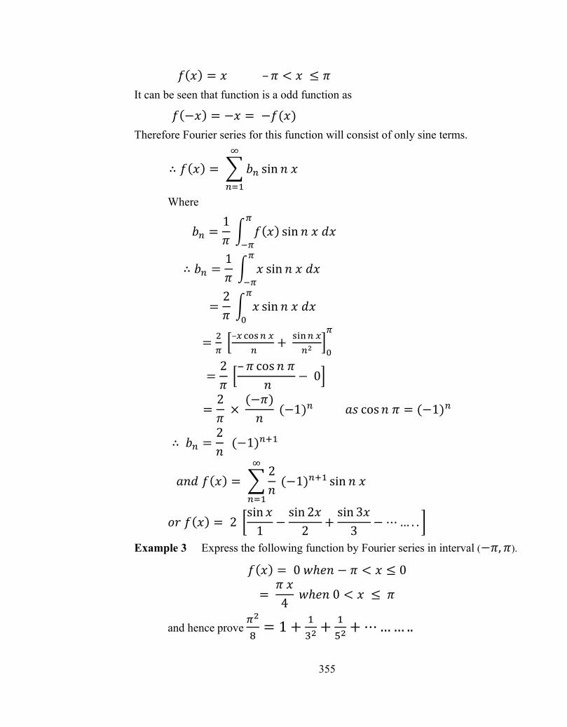
355

푓(푥) = 푥 –휋 < 푥 ≤ 휋 It can be seen that function is a odd function as

푓(−푥) = −푥 = −푓(푥)

Therefore Fourier series for this function will consist of only sine terms.

∴ 푓(푥) = 푏 sin 푛 푥

Where

푏 =1휋


∴ 푏 =1휋

푥 sin 푛 푥 푑푥

=2휋

푥 sin 푛 푥 푑푥

= –

+

=2휋

–휋 cos 푛 휋

푛− 0

=2휋

× (−휋)푛

(−1) 푎푠 cos푛 휋 = (−1)

∴ 푏 =2푛

(−1)

푎푛푑 푓(푥) = 2푛

(−1) sin 푛 푥

표푟 푓(푥) = 2 sin 푥

1−

sin 2푥2

+sin 3푥

3−⋯… . .

Example 3 Express the following function by Fourier series in interval (−휋,휋).

푓(푥) = 0 푤ℎ푒푛 − 휋 < 푥 ≤ 0

= 휋 푥4

푤ℎ푒푛 0 < 푥 ≤ 휋

and hence prove = 1 + + + ⋯… … ..

356

Sol. Let

푓(푥) = 푎 + 푎 cos푛 푥 + 푏 sin 푛 푥 (1)

푎 =1

2휋 푓(푥)푑푥 =

12휋

푓(푥)푑푥 +1

2휋 푓(푥)푑푥

=1

2휋 0 +

휋푥4푑푥 =

12휋

.휋4

푥2

=휋16

(2)

푎 =1휋

푓(푥) cos푛 푥 푑푥

=1휋

푓(푥) cos푛 푥 푑푥 + 푓(푥) cos 푛 푥 푑푥

=1휋

0 +휋푥4

cos 푛 푥 푑푥 =14

푥 cos 푛 푥 푑푥

=14푥 sin 푛 푥

푛+

cos 푛 푥푛

=14

cos푛 휋푛

−1푛

=1

4푛[cos푛 휋 − 1] =

(−1) − 14푛

(3)

∵ cos ( 1)nn

푏 =1휋

푓(푥) sin푛 푥 푑푥

=1휋

푓(푥) sin 푥 푑푥 + 푓(푥) sin푛 푥 푑푥

= 0 + ∫ sin 푛 푥 푑푥

Integrating

푏 = − (−1) 휋

4 푛 (4)

Using (2), (3) and (4) in (1)

푓(푥) = + ∑ ( ) cos푛 푥 − ( ) sin 푛 푥 (5)

357

= + − cos 푥 + sin 푥 −.

sin 2 푥 −.

cos 3 푥 +.

sin 3푥 (6)

Putting 푥 = 휋 푖푛 (6)

푓(푥) =휋16

+12

1 +1

3+

15

+ ⋯ . .

퐵푢푡 푓(휋) =12

[푓 (−휋 + 0) + 푓(휋 − 0)] =12

0 + 휋푥4

=휋8

∴휋8

= 휋16

+12

1 +1

3+

15

+ ⋯ . .

휋8

= 1 +1

3+

15

+ ⋯ ℎ푒푛푐푒 푝푟표푣푒푑


Fourier series can be expressed in complex form by using

1cos2

inx inxnx e e

and

1sin2

inx inxnx e e

In

푓(푥) = 푎 + 푎 cos푛 푥 + 푏 sin 푛 푥

∴ 푓(푥) = 푎 + 푎푒 + 푒

2+ 푏

푒 − 푒2푖

푓(푥) = 푎 +푎 − 푖푏

2푒 +

(푎 + 푖푏 )2

푒 (1)

As we know

푎 =1휋

푓(푥) cos 푛푥 푑푥 푎푛푑 푏

= ∫ 푔(푥) sin 푛푥 푑푥 (2)


358

∴ 푎 ± 푖푏 =1휋

푓(푥) (cos푛푥 ± 푖 sin 푛푥)푑푥 (3)

Keeping –푛 instead of 푛

푎 + 푖푏 − =1휋

푓(푥) (cos 푛푥 − 푖 sin푛푥)푑푥

∴ 푎 + 푖푏 = 푎 − 푖푏 … … (4)

Keeping in last term of RHS of (1) –푛 instead of 푛

푓(푥) = 푎 +(푎 − 푖푏 )

2푒 +

(푎 + 푖푏 )2

푒

Using (4)

푓(푥) = 푎 +(푎 − 푖푏 )

2 푒 + (푎 − 푖푏 )

2 푒

Let

퐶 =푎 − 푖푏

2 , 퐶 = 푎

푓(푥) = 퐶 + 퐶 푒 + 퐶 푒

= 퐶 푒 + 퐶 푒

inx

nf x C e

… . (5)

Here

퐶 =푎 − 푖푏

2=

12휋

푓(푥)(cos 푛푥 − 푖 sin 푛푥)푑푥

12

inxnC f x e dx

… … (6)

Equation (5) is required complex form of Fourier series.

359

16.10 Fourier Series in interval (0, T)

The Fourier series of a periodic piecewise continuous wave function 푓(푡) with time period T is given by

01 1

cos sinn nn n

f t a a n t b n t

(1)

Constant 푎 : To evaluate constant 푎 we integrate (1) with respect to 푡 between the limits 0 to T and obtain

0

0

1 T

a f t dtT

(2)

Constant 푎 : To evaluate na multiply (1) by 푐표푠 푛 푡 and integrate between limits 0 to T

푓(푡) cos푛 푡 푑푡 = 푎 푐표푠 푛 푡 푑푡 + 0

Solving

0

2 cosT

na f t n t dtT

(3)

푏 : To evaluate 푏 multiply (1) by 푠푖푛 푛 푡 and integrate between the limits 0 to T.

푓(푡) sin푛 푡 푑푡 = 푏 푠푖푛 푛 푡 푑푡 + 0

= 푇

0

2 sinT

nb f t n t dtT

(4)

The complex form of Fourier series can also be written for function 푓(푡) in interval (0, T)

As

16.10 Fourier Series in interval (0, T)

360

2in t

in t Tn n

n n

f T C e or C e

(5)

Where 퐶 is given by

2

0 0

1 1T T in tin t T

nC f t e dt f t e dtT T

(6)

∵ = 2휋푇

16.11 Internal Change for Fourier expansion from (–휋,휋) to (-l, l)

Let the periodic function has period 2l. Let us consider.

푧 = 휋푥푙

표푟 푥 = 푙푧휋

Then Fourier series is written as

01 1

cos sinn nn n

lzf x f a a nz b nz

0

1 1

cos sinn nn n

n x n xf x a a bl l

(1)

This is the Fourier series and the coefficients are given by

푎 =1

2휋 푓

푙푧휋

푑푧 = 1

2휋 푓(푥)푑

휋푥푙

0

12

l

l

a f x dxl

1 cosl

nl

n xa f x dxl l

1 sinl

nl

n xb f x dxl l

16.11 Internal Change for Fourier expansion from (–휋,휋) to (-l, l)

361


Interval (0, 휋)

Within the range (0, 휋) or (0, 푙) both series and cosines form mathematically complete sets. This means we can expand any function within this range in terms of either sines or cosines depending on nature of 푓(푥).

Fourier Cosine Series :

The cosine representation of a function 푓(푥) is

01

cosnn

f x a a nx

Where

00

1a f x dx

and 0

2 cosna f x nx dx

Fourier Sine Series :

It is given by

1

sinnn

f x b nx

Where 0

2 sinnb f x nxdx

Interval (0, l)

Fourier cosine series in interval (0, l) is written as

푓(푥) = 푎 + 푎 cos푛휋푥푙

where

푎 = ∫ 푓(푥)푑푥


362

and

푎 =2푙

푓(푥) cos푛휋푥푙푑푥

Fourier sine series is written as

푓(푥) = 푏 sin푛휋푥푙

where

푏 =2푙

푓(푥) sin푛휋푥푙

푑푥

16.13 Some Important Points

1. Every periodic function may be decomposed into a sum of one or more cosine and or sine terms of selected frequency dependent on the original function.

2. If 푓(푥) is piecewise continuous the definite integrals exist and fourier coefficient can be evaluated but if 푓(푥) is not piecewise continuous then we cannot find Fourier coefficient with surity as some of the integrals may be improper which are divergent.

3. The function 푓(푥) and its Fourier series are only equal to each other if and whenever 푓(푥) is continuous.

4. The constant term (a0) in a Fourier series represents the average value of the function 푓(푥) over its entire domain.


Example 4 Find a Fourier series for 푓(푥) = 푥 ,−2 < 푥 < 2

푓( 푥 + 4) = 푓(푥 )

Sol. Here T = 2 l = 4 hence l = 2

As the function f(x) is an odd function it would contain sine terms.

푏 =1

2 푥 sin

푛휋푥2

푑푥 2

2

16.13 Some Important Points


363

=12

−2푥푛휋

푐표푠푛휋푥

2−

2푛휋

푐표푠푛휋푥

2푑푥

=−4푛휋

푐표푠푛휋

If n = even 푏 = , if n is odd 푏 =

∴ 푏 = (−1) 4

푛휋

Thus

푓(푥) =4휋

(−1)푛

푠푖푛푛휋푥

2

Example 5 Write the Fourier series for a square wave.

defined by 푓(푡) = 푉 ; 0 < 푡 <

= −푉 ; 푇2

< 푡 < 푇

Sol. The Fourier series is given by

푓(푡) = 푎 + ∑ 푎 푐표푠 푛휔푡 + ∑ 푏 sin푛휔푡 (1)

The function is an odd function hence contain sine terms only in Fourier expansion.

푏 =2푇

푓(푡) sin(푛휔푡)푑푡

=2푇

푉 sin 푛휔푡 푑푡 + (−푉 ) sin푛휔푡 푑푡/

/

=2푉푇

− cos푛휔푡푛휔

/+

cos푛휔푡푛휔 /

=2푉푛휔푇

− cos푛2휋푡푇

/

+ cos 푛2휋푡푇 /

=2푉푛휔푇

[− cos푛휋 + 1 + cos 2푛휋 − cos푛휋]

364

=2푉푛휔푇

[2 − 2 cos푛휋] [∵ 푐표푠 2푛휋 = 1]

=2푉 × 2푛 × 2휋

[1 − 푐표푠푛휋] [∵ 휔푇 = 2휋 ]

=2푉푛휋

(1 − cos 푛휋)

When n is even , cos 푛휋 = +1 therefore 푏 = 0 When n is odd, cos nπ = −1 therefore 푏 =

Therefore the Fourier series for square wave is.

푓(푡) = 푏 sin푛휔푡 푤ℎ푒푛 푛 = 1,3,5 … .

=4푉

휋 sinωt +

1

3sin 3 휔푡 +

1

5sin 5휔푡 + ⋯… … .

16.15 Self-Learning Exercise II Very Short Answer Type Questions

Q.1 If function is odd the Fourier half range series will consist of which terms?

Q.2 If function is even which Fourier coefficient is zero?


Q.3 What is a periodic function?

Q.4 The formulae for evaluating ao, an and bn are known as?

Q.5 What is the significance of coefficient 푎 ?

Q.6 When is the function and its Fourier series representation equal to each other?

16.16 Summary This unit presents the introduction to Fourier series and its applications.

Fourier series is a powerful fool for representing any periodic functions as a sum of sines and cosines. The full range Fourier series has been defined and evaluation of Fourier coefficients has been specified. Even and odd functions are defined and Fourier series for them has been described. Half range Fourier series, Change of interval and complex form of Fourier series has been explained. Fourier series

16.15 Self-Learning Exercise II

16.16 Summary

365

finds its applications in solution of differential equations, signal analysis, data analysis, communications etc.

16.17 Glossary

Periodic: occurring at intervals

Digital : (of signals or data) expressed as series of the digits 0 and 1,


Answers to Self Learning Exercise-I Ans.1: Dirichlet’s conditions

Ans.2: Odd Function

Ans.3: 푓(−푥) = 푓(푥) for an even function

Ans.4: even function

Answers to Self Learning Exercise-II Ans.1: sine terms

Ans.2: 푏

Ans.3: A function is periodic with period 푇 > 0 if for all x , 푓(푥 + 푇) = 푓(푥) and T is the least of such values.

Ans.4: Euler-Fourier Formulae

Ans.5: It represents average value of function over entire domain.

Ans.6: Whenever function is continuous.

16.19 Exercise

Section A: Very Short Answer Type Questions

Q.1 Function 푥 when expanded by Fourier series will contain which terms in

interval (−휋,휋)

Q.2 Function 푥 sin 푥 is even or odd in interval (−휋,휋)?

Q.3 Fourier series is used to represent which kind of functions?


161 16.17 Glossary


16.19 Exercise

366

Q.4 Define Fourier series and Fourier coefficient for interval (−휋,휋).

Q.5 State the Dirichlets conditions for Fourier series expansion.

Q.6 Define even and odd functions.

Q.7 What do you understand by Fourier Half Range series?

Q.8 Write the complex form of Fourier series.

Section C: Long Answer Type Questions

Q.9 A function 푔(푥) is defined by

푔 (푥 ) =

푥퐿

푖푓 표 ≤ 푥 < 퐿/2

1 −푥퐿푖푓 퐿/2 ≤ 푥 < 퐿

By expanding 푔(푥 ) as a fourier sine series show that

푔 (푥 ) = 4(−1)푛 휋

sin푛휋푥퐿

Q.10 A function 푓(푥) is defined by

푓 (푥 ) = 1 0 ≤ 푥 < 퐿/2 0 퐿/2 ≤ 푥 < 퐿

Expand 푓 (푥 ) as a fourier cosine series and show that 푎 = 0 if n is even and if n is odd

푎 =2푛휋

(−1)( )

Write the cosine series in 0 ≤ 푥 < 퐿 and deduce 휋4

= 1 −1

3+

1

5−

1

7

Q.11 Find Fourier series expansion of 푓(푥) = 푒 in the interval (−휋,휋).

Q.12 Represent function 푓(푥) = 푥 in the interval (0, 2휋)by Fourier series and show that

푥 =4휋

3+

4푛

cos 푛푥 −4휋푛

sin 푛푥

367

Q.13 Expand the function 푓(푥) = 푥 as Fourier series in (−휋,휋 ) and hence

deduce that + + + + ⋯… … … =

Q.14 Express function 푓(푥) = |푥| in interval (-L, L) by Fourier series expansion and show

푓(푥) =퐿2−

4퐿휋

푐표푠 휋푥퐿1

+푐표푠 3휋푥

퐿3

+ … … . .

6.20 Answers to Exercise Ans.1 : Cosine

Ans.2 : Even

Ans.3 : Piecewise continuous periodic

Ans.7: 푒 = − cos 푥 − cos 2푥 + ⋯ . + sin 푥 −

sin 2푥 + ⋯ . .

References and Suggested Readings 1. Mathematical physics, Eugene Butkov, Addison Wesley publishing, London.

2. Mathematical Methods for physics and engineering, J.F. Riley, M.P. Hobson, S. J. Bence, Cambridge.

3. Mathematical methods for physicists, G.B. Arfken , H.J. Weber, Elsevier.

4. Mathematical physics, Satya prakash, Sultan chand and sons.

5. Mathematical Physics, B D Gupta, Vikas Publishing house.

6. Mathematics for physics M.M. Woolfson, M.S. Woolfson, Oxford University press.



368

UNIT- 17

Integral Transforms Structure of the Unit

17.0 Objectives

17.1 Introduction

17.2 Integral Transforms

17.3 The Laplace Transform


17.5 Sufficient conductions for existences of Laplace transforms

17.6 Some properties of Laplace transform

17.7 Self Learning exercise-I

17.8 Fourier transform

17.9 Fourier sine transform

17.10 Fourier cosine transform

17.11 Complex Fourier transform

17.12 Some theorems and properties of Fourier transform


17.14 Hankel transform

17.15 Some points related to Hankel transform

17.16 Some relations for Bessel functions of first kind


17.18 Inversion theorem

17.19 Self Learning exercise-II

17.20 Summary

17.21 Glossary


UNIT- 17 Integral Transforms

369

17.23 Exercise



17.0 Objective The aim of the chapter is to introduce the readers to the concept and

importance of integral transforms. Various transform such as Laplace, Fourier and Hankel transforms have been discussed. These transforms have wide applicability in Physics and other areas of science. In the chapter Laplace, Fourier and Hankel transforms are defined and their properties are presented. Methods for finding these transforms have been shown through examples to familiarize readers with fundamental concepts.

17.1 Introduction Integral transforms constitute a very powerful tool for the solution of

various problems in science and especially physics. Laplace transforms provide a very convenient method of solution of Linear constant-coefficient differential equations. Likewise Fourier transforms are widely applied to areas such as optics, astronomy, quantum mechanics, crystallography, electrical, electronics and biomedical engineering etc. Laplace, Fourier and Hankel transforms have applications in various boundary value problems. Hankel transform may be considered as the Fourier transform of a Bessel function expansion.

17.2 Integral Transforms A general linear integral transformation of a function is expressed by following equation:

( ) ( ) ( ) (s, )b

a

g s Tf t f t k t dt (1)

The function g(s) is called the integral transform of f(t) though kernel (s, )k t . The kernel (s, )k t is a prescribed function of parameter s and variable t.

There are different integral transforms depending on the type of kernel (s, )k t used and the range of integration. For example

17.0 Objectives

17.1 Introduction

17.2 Integral Transforms

370

( ) ( ) istg s f t e dt

(Fourier Transform)

0

( ) ( ) stg s f t e dt

(Laplace Transform)

0

( ) ( ) J ( )ng s f t st dt

(Hankel Transform)

1

0

( ) ( ) t sg s f t dt

(Mellin Transform)

All integral transforms have the following linearity properties.

( ) ( ) ( )I f g I f I g

퐼(푐푓) = 푐퐼(푓) for constant c.

17.3 The Laplace Transform The Laplace transform of a function f(t) is given by:

0

F(s) ( ) ( ) stL f t f t e dt

where the symbol L indicates the Laplace transform of the function. The Laplace

transform is said to exist when and only when the integral 0

( ) stf t e dt

converges

for some value of s. Here s is a parameter which may be real or complex.

17.4 Illustrative Examples Example 1 Find the Laplace transform of following

(i) ( ) 1f t (ii) ( )f t t

Sol. (i) ( ) 1f t

00

F(s) 1st

st eL e dts

1s

11Ls

(ii) ( )f t t

17.3 The Laplace Transform


371

0

F(s) .stL t e tdt

00

st ste et dts s

0

10 ste dts

2

0

1 1stes s s

21L ts

Example 2 Find the Laplace transform of

(i) c (constant) (ii) nt , 0n (iii) t (iv) kt

Sol. (i) ( ) ( tan )f t c cons t

0 0

F(s)st

st e cL c e cdt cs s

cL cs

(ii) ( ) nf t t

0

F(s) n st nL t e t dt

1

00

. . tst

n st ne nt e dts s

(Integration by parts)

1 22

00

( 1)0 . .tst

n st nn e n nt e dts s s

(again Integrating by parts)

The first two term vanish and repeating integration by parts

33

0

( 1)( 2) . tst nn n n e dts

Like this repeating integration by parts

372

0

0

( 1)( 2)...........3.2.1 .tstn

n n n e dts

1

1 !.n n

n ns s s

Alternative

1 1

0 0

F(s) nn st n stL t e t dt e t dt

1 1

1 !n n

n ns s

1

0

sx nnne x dx

s

1!n

nnL t

s

(iii) 1

2( )f t t t 3 11 22

0 0

F(s) st stt e dt t e dt

3 32 2

32

2s s

(iv) ( )f t kt

0 0

F(s) st ste ktdt k e tdt

2

ks

Example 3 Find the transform of

(i) kte (ii) kte (iii) sin kt

(iv) cos kt (v) sinh kt (vi) cosh kt

Sol. (i) kte (t) ektf

( )

0 0

F(s) kt kt tk st sL e e dt e te d

( )

( ) t

0 0( )

s k ts k ee dt

s k

1

s k

373

1kt

keL

s

(ii) kte ( ) ktf t e

( )

0 0

F(s) kt kt st s k tL e e e dt e dt

1

s k

1ktL es k

(iii) sin kt ( ) sinf t kt

0 0

F(s) sin sin2

ikt iktst st e eL kt e ktdt e dt

i

( ) ( )

0

12

s ik t s ik te e dti

2 21 1 12

ki s ik s ik s k

2 2sin kL kts k

(iv) cos kt

0 0

F(s) cos cos2

ikt iktst st e eL kt e ktdt e dt

( ) ( )

0

12

s ik t s ik te e dti

1 1 12i s ik s ik 2 2

ss k

2 2cos sL kts k

(v) sinh kt

0

F(s) sinh sinhstL kt e ktdt

374

( ) ( )

0 0

12 2

kt ktst s k t s k te ee dt e e dt

2 21 1 12

ks k s k s k

(vi) cosh kt

0

s( ) co h2

kt ktst e ekt dts eF L

( ) ( )

0

12

s k t s k te e dt

2 21 1 12

ss k s k s k

Example 4 Find Laplace transform of

(i) 2sin t (ii) sinkte t

Sol. (i) 2sin t

2 1sin (1 co( ) s 2 )2

t LF ts L

21 1 1(1) (cos 2 )2 2 4

sL L ts s

(ii) sinkte wt

0 0

e sin t sin 2

( )i t i t

kt kt st kt ste ee t e dt e e dL ti

F s

(s k i ) t ( )

0

12

s k i te e dti

2 21 1 12 ( )i s k i s k i s k

17.5 Sufficient Conductions for Existence of Laplace Transforms 17.5 Sufficient Conductions for Existence of Laplace

Transforms

375

(i) The function f(t) should be piecewise or sectionally continuous in every finite interval.

(ii) The function should be of exponential order.

A function f(t) is said to be the function of exponential order m as t ,if for a given positive integer m there exists real constant M > 0 such that

( ) ( )mt mte f t M or f t Me for every 0t

17.6 Some Properties of Laplace Transform (1) Linearity – For every pair of constants 1k and 2k the Laplace transform of

the linear combination of any number of function satisfies.

1 1 2 2 1 1 2 2( ) ( ) ( ) ( )L k f t k f t k L f t k L f t

The proof is simple and left as an exercise for readers.

(2) Change of scale – If F(s) is the Laplace transform of f(t), the Laplace

transform of f(kt) is 1 SFk k

Proof. 0

( ) ( )stLf kt e f kt dt

Putting kt = u

0

1 1(u)su

k se f du Fk k k

1( ) sL f kt Fk k

(3) Shifting or translation properties –

(i) First translation or shifting property – If F(s) is Laplace transform of f(t)

then Laplace transform of ( )kte f t will be (s k)F .

Proof. 0

( ) ( ) (t)stL f t F s e f dt

( )

0 0

( ) (t) (t)kt st kt s k tL e f t e e f dt e f dt

17.6 Some Properties of Laplace Transform

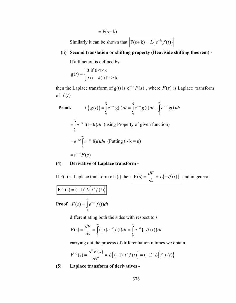
376

F(s k)

Similarly it can be shown that F(s k) ( )ktL e f t

(ii) Second translation or shifting property (Heaviside shifting theorem) -

If a function is defined by

0 if 0<t<k

( )( ) if t > k

g tf t k

then the Laplace transform of g(t) is e ( )ks F s , where ( )F s is Laplace transform of ( )f t .

Proof. 0 0

( ) g(t) (t) g(t)k

st st st

k

L g t e dt e g dt e dt

f(t k)st

k

e dt

(using Property of given function)

0

f(u)sk sue e du

(Putting t - k = u)

( )ske F s

(4) Derivative of Laplace transform -

If F(s) is Laplace transform of f(t) then F'(s) ( )dF L tf tds

and in general

( )F (s) ( 1) ( )n n nL t f t

Proof. 0

( ) (t)stF s e f dt

differentiating both the sides with respect to s

0 0

F'(s) ( ) (t) { ( )}st stdF t e f dt e tf t dtds

carrying out the process of differentiation n times we obtain.

( ) ( )F (s) ( 1) ( ) ( 1) ( )n

n n n n nn

d F s L t f t L t f tds

(5) Laplace transform of derivatives -

377

Let f(t) be a continuous differentiable function with a sectionally continuous

derivative f´(t). If f(t) and ( )df tdt

are Laplace transformable, then the Laplace

transform of derivative ( )df tdt

is given by

( ) ( ) (0) ( ) (0)df tL sL f t f sF s fdt

Where f(0) is the value of f(t) at t = 0 and

F(s) ( )L f t

Proof. 0

( ) ( )stdf t df tL e dtdt dt

By integration by Parts

0

0

( ) ( ) ( )st stdf tL f t e s e f t dtdt

(0) { ( )} ( ) (0)f sL f t sF s f ( ) ( ) (0)df tL sF s f

dt

This theorem is useful in solving differential equations with constant coefficients and it is applicable for n th derivatives.

General formula for the Laplace transform of the n th derivative ( )nf t is

1 2 2 1{f (t)} s ( ) (0) s '(0)............sf (0) f (0)n n n n n nL F s s f f

(6) Laplace transform of Integral -

F(s) {f(t)}L then 0

( )( )t F sL f t dt

s

Proof. Let 0

( ) ( )t

g t f t dt

then 0

'( ) ( ) ( )tdg t f t dt f t

dt

By Laplace transform of derivative we have

378

'(t) {g(t)} g(0)L g sL .

s (t) 0L g

1 f(t) (t)L L gs

Hence

0

( )( )t F sL f t dt

s

* (i) If F(s) ( )L f t then ( ) ( 1) ( )n

n nn

dL t f t F sds

(ii) If F(s) ( )L f t then ( ) ( )

s

f tL F s dst

provided the integral exists

(7) Laplace transform of periodic functions -

If f(t) is a periodic function with the period T i.e. ( ) ( )f t T f t

Then 0

( ){f(t)}

1

Tst

sT

e f t dtL

e

Proof. 0

{f(t)} ( )stL e f t dt

=( 1)2

0

( ) ( ) ......... ( ) .....n TT T

st st st

T nT

e f t dt e f t dt e f t dt

( 1)

0( )

n Tst

n nT

e f t dt

Putting t = u + nT i.e. dt = du

( )

0 0

{f(t)} ( )T

s u nT

ne uL f u nT d

0 0

( )T

sTn su

ne e f u nT du

379

0 0

( )T

nsT su

ne e f u du

2

0

1 .... (u)duT

sT sT sue e e f

0

1 (u)du(1 )

Tsu

sT e fe

0

1 (t)dt1

Tst

sT e fe

[replacing u by t]

Example 5 Find Laplace transform of sinh mt sin mt

Sol. f(t) sinhmt sin .2 2

mt mt imt imte e e emti

(1 ) (1 ) (1 ) (1 )14

mt i mt i mt i mt ie e e ei

Putting (1 )m i r and (1 ) qm i

1{sinhmt sinmt}4

rt rt qt qtL L e e e ei

14

rt rt qt qtL e L e L e L ei

As 1rtL es r

and 1rtL es r

1 1 1 1 14i s r s r s q s q

2 2

2 2 2 2 2 2 2 21 2 2 (r q )4 2( )( )

s s isi s r s q s r s q

Putting 2 2 2 2 2 2 22 , 2 , ( ) 4r im q im i r q m

2 2 2 2 4 4(s r )(s q ) s 4m

2 2

4 4 4 4

4 2(sinhmt sinmt)2(s 4m ) 4

m s m SLs m

Example 6 Find Laplace transform of a square wave

380

( ) 02Tf t V for t

02Tfor t T

and ( ) (t)f t T f

Sol. For periodic functions 0

1( ) ( )1

Tst

sTLf t e f t dte

2

0

1 Vdt 01

T

stsT e

e

2

01

Tst

sT

V ee s

21

(1 )

sT

sT

V e

s e

Example 7 Find Laplace transform of 2( ) 6sin 2 2 cos4tf t t e t

Sol. 2( ) ( ) 6sin2 2 {e cos4t}tF s L f t L t L

Using linearity property

2

2{sin 2 t}4s

∟

22

2{ cos 4 t}( 2) 16

t ses

∟

2 2

2 2( ) 6 24 ( 2) 16

sF ss s

2 2

12 2 44 ( 2) 16

ss s

Example 8 Find Laplace transform of 2 2tt e

Sol. We know {t f(t)} ( 1) ( )n

n nn

dL F sds

2

2 2 22

1{t e } ( 1)2

t dLds s

3

2!( 2)s

381


Q.1 What is Laplace transform of sin 3t ?

Q.2 Find the Laplace transform of 3 2tt e .

Q.3 Find Laplace transform of sin t

t.

Q.4 What is Laplace transform of 37t ?

Q.5 What is Laplace transform of 2 coste t ?

17.8 Fourier Transform A general Fourier Transform is defined by

( ) ( ) istF s f t e dt

which is based on kernel iste and its real and imaginary parts. Fourier Integral transform can be defined from Fourier integral.

1( ) ( )2

i t i xf t e d f x e dx

This is Fourier integral

It can be rewritten as

1 1( ) ( )2 2

i t i xf t e d f x e dx

1 ( )2

i te F d

Here 1( ) ( )2

i xF f x e dx

Or 1( ) {f(t)} ( )2

istF s f t e dt

F

is the Fourier integral transform.

The inverse Fourier transform is expressed as


17.8 Fourier Transform

382

1 1{F(s)} ( ) ( )2

istf t e F s ds

F

If we define

1( ) ( )2

istF s f t e dt

…(1)

then 1( ) ( )2

istf t F s e ds

…(2)

Eq.(1)&(2)constitute Fourier Integral Theorem.

Here F(s) is known as the Fourier transform of the f(t) i.e. ( ) {f(t)}F s F

Here f(t) is known as the inverse Fourier transform of the F(s) i.e.1( ) { ( )}f t F sF

Alternative

There is no way why the factors ist iste or e can not be interchanged i.e. we could

have defined 1( ) ( )2

istF s f t e dt

…(3)

then

1( ) ( )2

istf t e F s ds

…(4)

However, we will follow the eq.(1) &(2) in this chapter

Alternative

If we define ( ) ( ) istF s f t e dt

then

1( ) ( )2

istf t e F s ds

17.9 Fourier Sine Transforms The Fourier transform can be written as

1( ) ( ){cos(st) i sin(st)}dt2

F s f t

17.9 Fourier Sine Transforms

383

If f(t) is an odd function of t i.e.

( ) ( )f t f t

2F(s) iF ( ) ( )sin s s i f t st dt

0

2F ( ) ( )sins s f t st dt

or 0

2F ( ) ( )sins f t tdt

Here F ( )s is infinite Fourier sine transform of odd function f(t).

The inverse Fourier sine transform

0

2( ) ( )sinsf t F td

If the function f(t) is non-vanishing only in the interval 0 t .

0

2F ( ) ( )sins f t tdt

0

2F (n) ( )sinns f t tdt

In interval (0, l) finite Fourier sine transform is

0

2F ( ) ( )sinsn xn f x dx

l l

17.10 Fourier Cosine Transform If f(t) is an even function then the infinite Fourier cosine transform is written as

0

2F (s) ( )cos(st)dtc f t

0

2( ) ( )coscf t F t d

17.10 Fourier Cosine Transform

384

The finite Fourier cosine transform is written as

0

2F (n) (x)cosl

cn xf dx

l l

By putting xt

l

in 0

2F ( ) ( )cos tdtc n f t n

17.11 Complex Fourier Transform For x the complex Fourier transform of a function f(x) is expressed as

F( ) ( ) inxn f x e dx

Here inxe is kernel of the transform

The inverse is 1( ) ( )2

inxf x F n e dx

17.12 Some Theorems and Properties of Fourier Transform

(1) Linearity – If 1 1 2 2( ) ( ) ( ) ......f t a f t a f t

then Fourier transform of f(t) is

1 1 2 2F(s) (s) (s) .....a F a F

Where 1(s)F , 2(s)F , ……. are Fourier transforms of 1( )f t , 2( )f t , ……..

(2) Change of scale or similarity theorem :

If F(s) is Fourier transform of f(t) then Fourier transform of f(at) is 1 sFa a

(3) Shifting – If F(s) is Fourier transform of f(t) then the Fourier transform of

( )f t a is e ( )isa F s

(4) Conjugate Theorem – If F(s) is Fourier transform of f(t) then the Fourier

transform of complex conjugate of f(t) is F*( s) .

(5) Modulation Theorem – Fourier transform of f(t)cos at is

17.11 Complex Fourier Transform

17.12 Some Theorems and Properties of Fourier Transform

385

1 F( ) ( )2

s a F s a Where F(s) in Fourier transform of f(t).

(6) Convolution Theorem or Faltung Theorem

If f(x) and g(x) are two functions for x then convolution *f g is defined as

* ( ) ( )f g f n g x n dn

and the Fourier transform of the convolution is the product of their Fourier transforms.

(7) Parseval’s Theorem – If F(s) is Fourier transform of f(t) then

2 2( ) ( )f t dt F s ds

(8) Fourier transform of the square modulus of a function is 12

times the

self convolution of its Fourier transform.

If 2( ) ( ) * ( ) ( )g t f t f t f t

Then 1{g(t)} ( ') *( ' ) '2

F s F s s ds

F

Where F(s) is Fourier transform of f(t)

(9) Derivative of Fourier transform

( ) ( ) {t f(t)}n

n nn

d F s ids

F

or ( ) ( ) ( )2

n nn ist

nd F s i t f t e dt

ds

(1)

is the thn derivative of Fourier transform of f(t).

The inverse Fourier transform of (1) is

1 ( ) ( ) ( )n

nn

d F s it f tds

F (2)

386

(10) Fourier transform of derivative

F ( ) ( ) ( )nn s is F s

Here F(s) is Fourier transform of f(t) and F ( )n s is Fourier transform of thn derivative of function f(t).

(11) Fourier sine and cosine transforms of derivatives

The Fourier sine and cosine transforms of a function f(t) are

0

2F ( ) ( )sin tdts f t

(1)

0

2F ( ) ( )cos tdtc f t

(2)

Here function f(t) is well behaved such that it and its derivatives approach zero as t

Fourier sine transform of first derivative dfdt

is

10

2F ( ) sin tdtsdfdt

00

2 2( )sin . ( )cos tdtf t t f t

The first term is zero as ( ) 0f t for t .

1F ( ) F ( )s c (3)

The Fourier cosine transform of first derivative of f(t) is

10

2F ( ) cos tdtcdfdt

00

2 2( )cos . ( )sin tdtf t t f t

2 2(0) ( ) ( ) (0)s sf F F f

(4)

Now Fourier transform of second derivative of f(t) is

387

2

2 200 0

2 2 2F ( ) sin tdt sin cos tdtsd f df dftdt dt dt

The first term becomes zero as t .

22 1

2F ( ) ( ) (0) ( )s c sF f F

(5)

Like this the Fourier cosine transform of second derivative of f(t) is

2

2 200 0

2 2 2F ( ) cos tdt cos sin tdtcd f df dftdt dt dt

21

2 2'(0) ( ) '(0) ( )s cf F f F

(12) Fourier transforms of two and three variable functions

If f(x, y) is a function of two variables then Fourier transform of f(x, y is

( )1F(u,v) ( , )2

i ux vyf x y e dxdy

(1)

Fourier inverse transform in

(u )1(x, y) (u,v)2

i x vyf F e dudv

(2)

If f(x, y, z) is a function of three variables then Fourier transform of

f(x, y, z) is

(ux vy wz)3

2

1F(u,v,w) ( , , )(2 )

if x y z e dxdydz

(3)

Fourier inverse transform is

(ux vy wz)3

2

1(x, y,z) (u,v, w)(2 )

if F e dudvdw

(4)


Example 9 Find the Fourier transform of 2 te

Sol. 21( )2

t istF s e e dt


388

2 212

t ist t iste e e e dt

0(2 ) (2 )

0

1(2 ) (2 )2

t is t ise eis is

1 1 1(2 ) (2 )2 is is

2 2 2

1 2 242

is iss

2 2 2

1 4(4 )2 s

Example 10 Find the Fourier transform of the Gaussian distribution function 2

( ) xf x Ne where and N are constants

Sol. 1( ) ( )2

i xF f x e dx

21

2x i xNe e dx

2( )

2x i xN e dx

2 22

2 2

2

i i ix xN e e dx

22

24

2

ixN e e dx

2

24

2mN e e dm

(Putting 2ix m

)

2

4

2N e

2me dm

=2

4

2N e

Example 11 Find the Fourier sine transformation of e-x

389

Sol. 0

( ) sinxsF e xdx

2 20

( ) ( sin cos )1 1

x

seF x x

Example 12 Find Fourier complex transform of

21 , 1

( )0, 1

x xf x

x

Sol. 1

2

1

( ) 1 i xf x e dx

1

2

1

2(1 x )i x

i xe xe dxi i

1 1

211

2 20i x

i xxe e dxi i i

1

2 21

2 2 i xi i ee e

i

2 3

2 2i i i ie e e ei

2 3 3

4 4 4cos sin ( cos sin )

17.14 Hankel Transform

If J ( )n px be the Bessel function of the first kind of order n, then the Hankel transform of a function f(x) is the interval 0 x is expressed as

0

( ) ( ). J ( )nF p f x x px dx

Here xJ ( )n px is the kernel of the transform.

17.15 Some Points Related to Hankel Transform

(i) Inversion formula

17.14 Hankel Transform

17.15 Some Points Related to Hankel Transform

390

If F(p) be the Hankel transform of the function f(x) for x i.e.

{f(x)} f(p) ( ).xJ ( )nH f x px dx

then

0

( ) (p).pJ ( )nf x f px dp

is the inversion relation.

(ii) Parseval Theorem

If F(p) and G(p) are Hankel transforms of f(x) and g(x) respectively then

0 0

(x)g(x)dx (p) (p)dpxf pF G

(iii) Linearity Theorem

1 2 1 2{c f(x) c g(x)} H{f(x)} c {g(x)}H c H

(iv) Hankel transform of the derivatives of function

The first derivative of Hankel transform of order n of the function f(x) is given by

'1 1

1 1( ) ( ) (p)2 2n n n

n nF p p F p Fn n

Similarly the second derivative is

4 2

''2 22

1 3 1( ) ( ) 2 (p) ( )4 1 1 1n n n np n n nF p F p F F p

n n n

Here 1 1 2 2(p),F ( ), ( ), ( ) ( )n n n n nF p F p F p and F p are Hankel transforms of function f(x) of order n-1, n+1, n-2 and n+2, respectively.

(v) Finite Hankel Transforms

If f(r)is a function which satisfies Dirichlet’s conditions in the interval (0, a) then its finite Hankel transform is expressed as

i0

F(p ) (r)J ( . )a

n irf p r dr

where ip is a positive root of the transcendental equation J ( .a) 0n ip .

391

17.16 Some Relations for Bessel functions of First kind

While finding Hankel transform the following relations for Bessel’s function are frequently used.

Recurrence relation

'1 1n n n n nxJ nJ xJ xJ nJ (1)

'1 12 n n nJ J J (2)

1 12 n n nnJ x J J (3)

1( )n nn n

d x J x Jdx

(4)

1( )n nn n

d x J x Jdx (5)

1 00

(x)dx ( ) ( ), 0u

un n nn n nx J x J x u J u n (6)

0 10

( ) ( )a arJ pr dr J ap

p (7)

2

2 20 1 03 2

0

4 2( ) ( ) ( )a a ar a r J pr dr J pa J pa

p p (8)

1

22 2

00

( )axe J px dx a p

(9)

1 2 20

1 1( )axe J px dxp p a p

(10)

3

22 20

0

( ) ( )axxe J px dx a a p

(11)

3

22 21

0

( ) ( )axxe J px dx p a p

(12)

1

22 2

10

( )( )ax dx a p ae J pxx p

(13)

17.16 Some Relations for Bessel functions of First kind

392

2

2

2

4

2( 1) 1 2 ( 1) 2 2 .4 ( 1( ) 1

)( 22 )

n

n nx x xJ xҐ n n n n

(14)


Example 13 Find Hankel transform of axe

x

with kernel 0( )xJ px

Sol. Were ( )axef x

x

hence

00

H{f(x)} . ( )axe xJ px dx

x

00

( )axe J px dx

Using (9) of previous section 12 2 2H{f(x)} (a p )

Example 14 Find Hankel transform of following function

1, , 0

( )0, , 0

o x a nf x

x a n

Taking 0( )xJ px as the kernel

Sol. 00

H{f(x)} f(x). ( )xJ px dx

0 00

1. ( ) 0. ( )a

a

xJ px dx xJ px dx

00

( )a

xJ px dx

Using relation (7) of previous section

1H{f(x)} ( ) .( )aF p J app

Example 15 Find 1 2H [p e ]ap for n = 1.

Sol. Using inversion formula


393

1 2 21

0

H [p e ] p e . J (px)dpap ap p

10

dpe J (px)ap

p

Using (13) of previous section

12 2 2

1 2H [p e ]ap a x ax

Example 16 Find Hankel transform of dfdx

when ( )axef x

x

for n = 1.

Sol. 10

( )df dfH x J px dxdx dx

0( )pF p

Using (iv) of previous section

00

( ) ( )dxp xf x J px

00

e ( )dxaxp J px

Using (9) of previous section

12 2 2(a p )

df pHdx

17.18 Inversion Theorem The inversion theorem states that if F(s) is Laplace transform of f(t) where f(t) is of exponential order and has a continuous derivative than

1( ) ( ) , 02

ist

i

f t e F s ds ti

Proof. Let ( )t be a function of t with ( )t dt

being absolutely convergent, then

the Fourier’s integral is written as

0

1( ) (u)cosx(t u)t dx du

(1)

17.18 Inversion Theorem

394

The equation (1) can also be expressed in parts in terms of cosx(t u) and sinx(t u) as cosine is an even function and sine is an odd function of x. Therefore

1( ) (u)cosx(t u)2

t dx du

(2)

and 10 (u)sinx(t u)2

dx du

(3)

Expanding

0 1 (u) cos cos sin sin2

dx xt xu xt xu du

(4)

and 10 (u) sin cos cos sin2

dx xt xu xt xu du

(5)

Multiply (5) by i and add to (4) we obtain

1( ) (u) cos cos sin sin sin cos cos sin2

t dx xt xu xt xu i xt xu xt xu du

1 (u) (cos sin )(cosxu sin2

dx xt i xt i xu du

1 (u)e2

ixt ixudx e du

=1

2휋푒 푑푥 ψ(u)e du

Let ( ) ( )tt e f t for t > 0 and ( ) 0t for t < 0 then for t > 0.

1( ) f(u)e ,2

t ixt u ixue f t e dx e du t

( )1 f(u)2

ixt ix ue dx e du

Thus 1( ) ( ix)2

t ixte f t e dxF

(6)

[Here ( ix)F is Fourier transform]

395

Using ix s and ds dxi in (6) we have

( )1( ) (s)ds2

it s t

i

e f t e Fi

(s)ds2

itst

i

e e Fi

Therefore 1( ) (s)ds2

ist

i

f t e Fi

Hence proved

17.19 Self Learning Exercise -II Section A (Very Short Answer type Questions)

Q.1 What is the kernel of Fourier transform?

Q.2 What is the kernel of Hankel transform?

Q.3 For which functions Fourier cosine transform is used?

Section B (Short answer type Questions)

Q.4 State Convolution Theorem.

Q.5 State Parseval’s theorem for Fourier transform.

Q.6 State Parseval theorem for Hankel transform.

17.20 Summary The unit described the three types of integral transforms i.e. Laplace

transform, Fourier transform and Hankel Transform. Some important properties and theorems related to these transforms have been outlined. Methods of estimation of these transforms have been shown through examples.

17.21 Glossary Periodic: occurring at intervals

Convergent:(Of a series) approaching a definite limit as more of its terms are added.



Ans.1 : Ans.2 : !

( )

17.19 Self Learning Exercise -II

17.20 Summary

17.21 Glossary


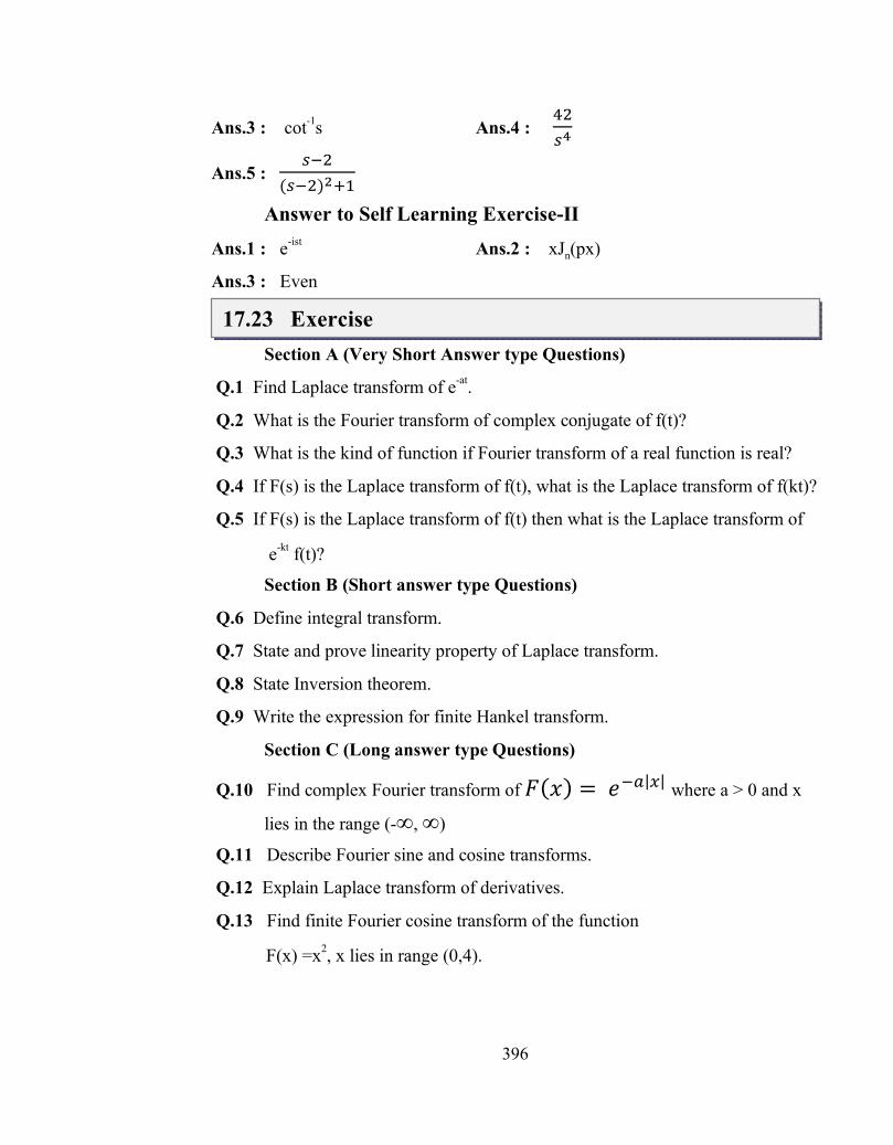
396

Ans.3 : cot-1s Ans.4 :

Ans.5 : ( )

Answer to Self Learning Exercise-II Ans.1 : e-ist Ans.2 : xJn(px)

Ans.3 : Even

17.23 Exercise Section A (Very Short Answer type Questions)

Q.1 Find Laplace transform of e-at.

Q.2 What is the Fourier transform of complex conjugate of f(t)?

Q.3 What is the kind of function if Fourier transform of a real function is real?

Q.4 If F(s) is the Laplace transform of f(t), what is the Laplace transform of f(kt)?

Q.5 If F(s) is the Laplace transform of f(t) then what is the Laplace transform of

e-kt f(t)?

Section B (Short answer type Questions)

Q.6 Define integral transform.

Q.7 State and prove linearity property of Laplace transform.

Q.8 State Inversion theorem.

Q.9 Write the expression for finite Hankel transform.

Section C (Long answer type Questions)

Q.10 Find complex Fourier transform of 퐹(푥) = 푒 | | where a > 0 and x

lies in the range (-∞, ∞)

Q.11 Describe Fourier sine and cosine transforms.

Q.12 Explain Laplace transform of derivatives.

Q.13 Find finite Fourier cosine transform of the function

F(x) =x2, x lies in range (0,4).

17.23 Exercise

397


Ans.1 : Ans.2 : F*(-s)

Ans.3 : Even Ans.4 : 퐹( )

Ans.10 : √ Ans.13 : 푐표푠푛휋

References and Suggested Readings 1. Mathematical Methods for physics and engineering, J.F. Riley, M.P. Hobson,

S. J. Bence, Cambridge.

2. Mathematical methods for physicists, G.B. Arfken , H.J. Weber, Elsevier.

3. Mathematical physics, Satya prakash, Sultan chand and sons.

4. Mathematics for physics M.M. Woolfson, M.S. Woolfson, Oxford University press.

5. Mathematical Physics, B. D. Gupta, Vikas Publishing House.

6. Mathematical Physics, B. S. Rajput, Pragati Prakashan.



398

UNIT – 18

Non-homogeneous Equation, Green’s Function, The Gamma Function

Structure of the Unit 18.0 Objectives 18.1 Introduction

18.2 Non-homogeneous equation

18.3 Definition-Green’s function

18.4 Construction of Green’s function



18.7 Dirac-delta function

18.8 Solution by Poisson’s Equation by Green’s function method

18.9 Symmetry of Green’s Function

18.10 The Gamma Function



18.13 Summary

18.14 Glossary


18.16 Exercise



18.0 Objective A mathematician George Green (1793-1841) was from England, has given contributions significantly to electricity and magnetism, fluid mechanics and

UNIT – 18 Non-homogeneous Equation, Green’s

Function, The Gamma Function

18.0 Objectives

399

partial differential equations. The importance of potential functions was recognized first by Green, that was published in 1828 as an essay on electricity and magnetism. In this paper, the functions, called Green’s functions as a means of solving boundary value problem and the integral transformation theorems of which Green’s theorem in the plane is a particular case, was introduced.

The famous mathematician L. Euler (1729) introduced gamma function as a natural extension of the factorial operation n! from positive integers n to real and even complex values of the argument. The gamma functions are useful in mathematics, the exact sciences and engineering. The incomplete gamma function (special case of gamma function) is used in solid state physics and statistics.

18.1 Introduction

Many physical problems involve second order differential equations. Some of these applications contain homogeneous equation but the more general case is the non-homogeneous equation. Laplace’s equation 2 0 is an example of homogeneous equation and Poisson’s equation 2 is an example of non-homogeneous equation. The general solution for non-homogeneous equation contain a solution hy of its homogeneous equation.

Consider the differential equation of non-homogeneous equation

2

2

d y dyp x q x y x r xdx dx

Its general solution h py x y x y x

The Green’s function method is a powerful method for solving non-homogeneous differential equations.

18.2 Non-homogenous Equation

Consider the second order linear differential equation of the form:

2

2 d y dyP x Q x R x y x G xdx dx

(1)

where P, Q, R and G are continuous functions. This equation is called non-homogeneous equation, if 0G x . Equation (1) is said to be homogeneous if 0G x .

18.1 Introduction

18.2 Non-homogenous Equation

400

Again, consider the non-homogeneous Boundary Value Problem (BVP)

2

2 d y dyP x Q x R x y x G xdx dx

a x b (2)

with boundary conditions

1 2 1' a y a a y a c

1 2 2b y b b y b c (3)

where P, Q, R and G are continuous functions and , ,i i ia b c , i = 1, 2 are real constants. Also 1a and 2a are not both zero simultaneously. Similarly 1b and

2b are not both zero simultaneously.

The BVP is said to be homogeneous if G = 0 and 1 2 0c c .

18.3 Definition: Green’s function Our goal of this chapter is to construct Green’s function and using this, we

solve a non-homogeneous BVP.

Consider the non-homogeneous BVP

0 L y f x , a x b ……(1)

where L is differential operator defined as L y py qy , where

0 ,p p and q are real valued continuous functions on ,a b . The problem has following boundary conditions:

1 2 0a y a a y a (2)

1 2 0b y b b y b (3)

where 1 2 1 2, , ,a a b b are constants. Also, at least one of 1 2,a a and atleast one of 1 2,b b are non-zero.

Definition:- A function ,G x s defined on , ,a b a b is said to be Green’s function for 0L y , if for a given s,

1

2

, ,,

, ,

G x s if x sG x s

G x s if x s

where 1G and 2G be such that

(1) 1G satisfies the boundary condition (2) at x a and 1 0L G for x s .

18.3 Definition: Green’s function

401

(2) 2G satisfies the boundary condition (3) at x b and 2 0L G for x s .

(3) The function ,G x s is continuous at x s .

(4) The function Gx

has a jump discontinuity at x s , and

2 1 1

x s

G Gx x p s

18.4 Construction of Green’s Function

Let 1y x and 2y x are linearly independent solutions of 0L y on ,a b .

Let 1 1 1G c y x and 2 2 2G c y x , where 1c and 2c are constants.

Again, let,

1 1

2 2

,,

,

c y x if x sG x s

c y x iff x s

(4)

We choose 1c and 2c such that

2 2 1 1 0c y s c y s (4a)

2 2 1 11c y s c y s

p s (4b)

In starting, we have assumed that 1y and 2y are linearly independent solutions of 0L y . Therefore,

1 0L y and 2 0L y

1 1 0py qy (5)

and 2 2 0py qy (6)

Multiplying (5) by 2y and multiplying (6) by 1,y we have

2 1 1 2 0y py qy y …….(7) and 1 2 1 2 0y py qy y (8)

Using (7) and (8), we get

1 2 2 1 0y py y py

1 2 1 2 0d p y y y ydx

18.4 Construction of Green’s Function

402

1 2 1 2p x y x y x y x y x c , ,x a b (9)

where c is non-zero constant due to the Wronskian term

1 2 1 2w x y x y x y x y x , which must be non-zero as 1y and

2y are linearly independent solutions of 0L y .

Putting x s in equation (9), we get

11 2 2cy s y s y s y s

p s , 0c (10)

Using equation (4b) and (10), we get

12

( ) ,y scc

21

( )y scc

Using these values of 1c and 2c in equation (4), we get,

1 2

1 2

,,

,

y x y sif x s

cG x sy s y x

if x sc

1 2

1 2

,,

,

y x y sif x s

p x w xG x s

y s y xif x s

p x w x

(11)

which is Green’s function.

Theorem 1:- Consider the non-homogeneous BVP:

0,L y f x a x b

with 1 2 0a y a a y a

1 2 0 b y b b y b (12)

where 1 2 1, ,a a b and 2b fulfill the conditions defined above in equation (1), (2) and (3).

Then, y x is a solution of equation (12) if and only if

,b

ay x G x s f s ds

where ,G x s is a Green’s function defined in equation (11).

403


Example-1: Solve 2

2

d y f xdx

, 0 1x with Boundary conditions,

0 1 0y y .

Sol. Compare this with 0 L y f x

0 py q y f x

0py p y qy f x

We get, 1, 0, 0, 1 p x q x a b .

Let 1y x be a function which satisfy 2

2 0d ydx

with 0 0y . Then

2

11 1 22 0

d y y x c x cdx

Using 0 0y , we get 2 0c . Then,

1 1y x c x

Let 2y x be a function which satisfy 2

2 0d ydx

with 1 0y . Then,

2

22 0d y

dx 2 3 4y x c x c

Using 4 31 0, y c c . Then,

2 3 1y x c x

Now, the Wronskian 1 2 1 2w x y x y x y x y x

1 3 1 3 1c x c c c x

1 3c c

The Green’s function is defined by

,G x s

1 2

1 2

,

,

y x y sif x s

p x w x

y s y xif x s

p x w x


404

=

1 3

1 3

1 3

1 3

1,

11

,1

c xc sif x s

c cc s c x

if x sc c

= 1 ,

1 ,

x s if x s

s x if x s

Hence, the solution of given problem is given by

1

0,y x G x s f x ds

1

0,y x G x s f s ds

Example-2 Solve 2

22

d y k y f xdx

, 0 x L with 0 0 , 0y y L .

Sol. Let 1y x be a function which satisfy 2

22 0d y k y

dx with 0 0y . Then,

2

2112 0

d y k y xdx

, 1 0 0y

1 1 2cos siny x c kx c kx

using 1 0 0,y we get 1 0c , so

1 2 siny x c kx

Let 2y x be the solution of 2

22 0d y k y

dx with 0y L . Then,

2

2222 0

d y k ydx

with 2 0y L

2 3 4cos siny x c kx c kx

Using 2 0y L we get 3 4sincos

kLc ckL

So, 2 4 4sin cos sincos

kLy x c kx c kxkL

= 4 cos sin sin coscos

c kx kL kx kL

kL

42

sincos

c k x Ly x

kL

405

Now, the Wronskian, 1 2 1 2w x y x y x y x y x

4 42 2

cos sinsin cos .

cosc k x L k c k x L

c kx c k kxcos kL kL

= 2 4 sincosc c k k x x L

kL

= 2 4sincos

kLc c kkL

So, the Green’s function ,G x s =

1 2

1 2

,

,

y x y sif x s

p x w x

y s y xif x s

p x w x

=

2 4

2 4

2 4

2 4

sin sin,sin1. cos

cossin sin

,sin1. coscos

c kx c k s Lif x skLc c k kL

kLc ks c k x L

if x skLc c k kLkL

=

sin sin,

sinsin sin

,sin

kx s L kif x s

k kLks x L k

if x sk kL

The solution of the given problem is

0

,L

y x G x s f s ds

18.6 Self Learning Exercise - I

Very Short Answer Type Questions:

Q.1 Identify the BVP 0y y with 0 1 1y y whether it is homogeneous or non-homogenous.

Q.2 For what value of c, the BVP 0y y y with 0 2y y c , is homogeneous.

Q.3 Define Green’s function.

18.6 Self Learning Exercise - I

406

Short Answer Type Questions:

Q.4 Solve 2

2

d y f xdx

with 0 0, 0y y L using Green’s function method.

Q.5 Find the Green’s function for BVP 2

2

d y f xdx

, 0 1x with 0y ,

' 1y .

Q.6 Find the Green’s function for BVP y f x with 0 0y , 1 1 0y y

18.7 Dirac-delta Function

The one-dimensional Dirac-delta function is defined by the following property as

0 0x at x

0f f x x dx

(1)

where f x is any well behaved function and the integration includes the origin.

If 1f x , then

0 1. 1f x dx

1x dx

[Special case of equation(1)]

The value x at 0x is so large that its integral is equal to unity.

The function x is not analytic but it can be obtained as a limiting case of either analytic continuous or piesewise continuous functions. Some of the possible representations are given by

x = 2 /1lim x a

ae

a

x = 2 21lim .

a

aa x

and x = sin 1lim lim2

a ixt

aa a

ax e dtx

And graphical representations f(x) versus x are given by

18.7 Dirac-delta Function

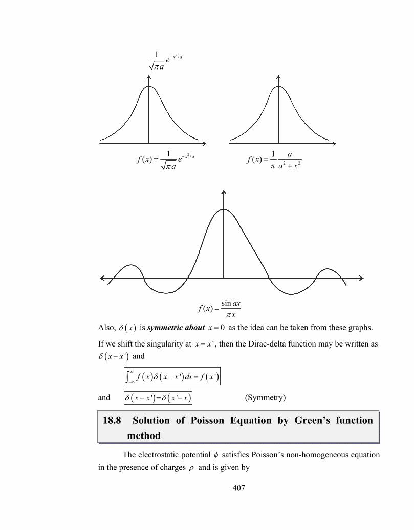
407

2 /1 x aea

2 /1( ) x af x e

a

2 2

1( ) af xa x

sin( ) axf xx

Also, x is symmetric about 0x as the idea can be taken from these graphs.

If we shift the singularity at 'x x , then the Dirac-delta function may be written as 'x x and

' 'f x x x dx f x

and ' 'x x x x (Symmetry)

18.8 Solution of Poisson Equation by Green’s function method

The electrostatic potential satisfies Poisson’s non-homogeneous equation in the presence of charges and is given by

18.8 Solution of Poisson Equation by Green’s function method

408

2

0

(SI system) (1)

and Laplace’s homogeneous equation

2 0 (2)

where there is no electric charge (i.e. 0 ).

If the charges are point charges iq , then

0

14

i

i i

qr

(3)

Using Coulomb’s law for the force between two point charges 1q and 2q , a superposition of single point charge solution is given by

1 22

04q q

r

rF (4)

By replacement of the discrete point charges with a smeared-out distributed charge, charge density , equation (3) gives.

0

104

r dr

r

(5)

For the potential at 1r r away from the origin and the charge at 2r r , we have,

2

0

14

d 2

11 2

r

rr r

(6)

Now, we need a Green’s function G to satisfy Poisson’s equation with a point source at the point 2r , is given by

2G 1 2 r r (7)

Clearly, G is the potential at 1r corresponding to a unit source 0 at 2r . Therefore, using Green’s theorem

2 22 . G G d G G d (8)

Taking the volume so large that the surface integral vanishes, leaving

2 22 2 G d G d (9)

or by substituting in equation (1) and (7), we get

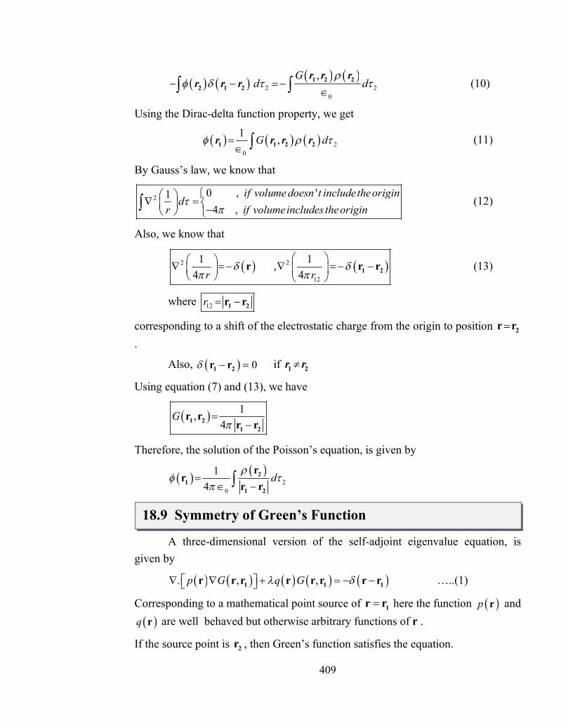
409

2 2

0

,Gd d

1 2 22 1 2

r r rr r r (10)

Using the Dirac-delta function property, we get

20

1 ,G d 1 1 2 2 r r r r (11)

By Gauss’s law, we know that

2 0 , '14 ,

if volume doesn t includetheorigind

if volumeincludes theoriginr

(12)

Also, we know that

2 2

12

1 1,4 4r r

1 2r r r

(13)

where 12r 1 2r r

corresponding to a shift of the electrostatic charge from the origin to position 2r r.

Also, 0 1 2r r if 1 2r r

Using equation (7) and (13), we have

1,4

G 1 2

1 2

r rr r

Therefore, the solution of the Poisson’s equation, is given by

2

0

14

d 2

11 2

rr

r r


A three-dimensional version of the self-adjoint eigenvalue equation, is given by

. , , p G q G1 1 1r r r r r r r r …..(1)

Corresponding to a mathematical point source of 1r r here the function p r and q r are well behaved but otherwise arbitrary functions of r .

If the source point is 2r , then Green’s function satisfies the equation.


410

, ,p G q G 2 2 2r r r r r r r r (2)

Multiplying equation (2) by G(r, r1) and (1) by G(r, r2) and then subtracting, we get,

2, . , , . ,

, ,

G p G G p G

G G

1 1 2

2 1 1 2

r r r r r r r r r r

r r r r r r r r

Integrating over whole volume, we get

, . , , . ,

, ,

V

V

G p G G p G d

G G d

2 1 1 2

1 2 2 1

r r r r r r r r r r

r r r r r r r r

where d is the small element of the volume. Using property of Dirac-delta function on RHS and Green’s theorem to change volume integral into surface integral on LHS, we get.

1 1, , , , .

,

S

G p G G p G d

G G

2 2

2, 1 1 2

r r r r r r r r r r s

r r r r

Under the requirement that Green’s function ,G 1r r and ,G 2r r have the same values over the surface S and their normal derivatives have the same values over the surface S or that the Green’s functions vanish over the surface S the surface integral vanishes and , ,G G1 2 2 1r r r r showing the symmetry of Green’s function.

18.10 The Gamma Function The Gamma function is useful in some physical problems such as the

normalization of Coulomb wave functions and the computation of probabilities in statistical mechanics. It is also useful in developing other functions that have direct physical applications.

There are the following types of definitions of the Gamma function:

(1) In form of Infinite Limit (Euler):

The first definition, named after Euler, is

1.2.3.........lim1 2 ............

z

n

nz nz z z z n

, 0, 1, 2, 3,....z

18.10 The Gamma Function

411

where z may be real or complex.

Replacing z with 1z , we get

11.2.3.........1 lim1 2 3 .......... 1

z

n

nz nz z z z n

1.2.3........1 lim1 1 2 ............

z

n

nz nz nz n z z z z n

1z z z

which is the basic functional relation for the gamma function and also a difference equation. The Gamma function is one of a general class of functions that do not satisfy any differential equation with rational coefficients as well as the gamma function doesn’t satisfy either the hypergeometric differential equation or the confluent hypergeometric equation.

In particular,

1.2.3.......1 lim 1

1.2.3.......... . 1n

n nn n

1 1

2 1 1 11 1

3 2 1 2 2 2.1 2

4 3 1 3 3 3.2.1 6

1 .........3.2.1 1 !n n n

(2) In form of Definite Integral (Euler):

The following definite integral represents the gamma function, also called the Euler integral, is given by

1

0

t zz e t dt , Re 0z (1)

This form is found in some physical problems and some other forms which found in physical problems, are

2 2 1

02 t zz e t dt

, Re 0z (2)

412

1

1

0

11z

z n dtt

, Re 0z (3)

Put 12

z in equation (1), the integral is called Gauss Error Integral and we have

12

Equivalence of these two definitions:

For showing this, consider the function of two variables

1

0, 1

nn ztF z n t dt

n

, Re 0z (4)

where n being a positive integer as lim 1n

t

n

t en

(5)

Taking n in equation (4), we get

1

0lim , , t z

nF z n F z e t dt z

(6)

Again, put tun

in equation (4), we get

1 1

0, 1 nz zF z n n u u du (7)

Integrating by part , we get

1

1 1

00

,1 1

zn n z

z

F z n u nu u u dun z z

(8)

Repeating this with the integrated part vanishing at both end points each time, we get

1 1

0

1 .......1,

1 ............ 1z z nn n

F z n n u duz z z n

1.2.3...1 2 ...

zn nz z z z n

(9)

Which is the form of infinite limit (Euler) for the gamma function. Therefore,

lim , ,n

F z n F z z

413

(3) In form of Infinite Product (Weierstrass):

The another definition of the gamma function, which is called a Weierstrass form, is given by

1

1 1zz n

n

zze enz

(10)

where is the usual Euler-Mascheroni constant and 0.577216 …………

This infinite product can be used to develop the reflection identity. This can be found by

1

1

1.2.3.......lim lim 11 ........

nz z

n nm

n zz n nz z z n m

(11)

Inverting equation (11) and using 1nn zzn e

We get

1

1

1 lim 1n

n n z

n m

zz emz

(12)

Multiplying and dividing by

1

1 1 1exp 1 ...2 3

n zm

mz e

n

(13)

We obtain

1

1 1 1 1lim exp 1 ... lim 12 3

n zm

n n m

zz ln n z en mz

(14)

The infinite series in the exponent converges and defines , the Euler-Mascheroni constant. Hence, equation (10) follows.

In probability theory, the gamma distribution is given by

11 , 0

0 , 0

xx e x

f x xx

(15)

The constant 1

is choosen so that the total probability will be unity.

Factorial Notation :

414

According to Jeffreys and others, the -1 of z-1 exponent in our second definition is a continual nuisance. The equation (4) can be re-written as

0

!t ze t dt z , Re 1z (16)

for factorial notation !z . We may still encounter Gauss’s notation zfor the factorial function

!z z (17)

The notation is due to Legendre. The factorial function of Equation (16), is related to the gamma function

1 ! 1 !z z z z (18)

If z n , a positive integer, we have seen that ! ! 1.2.3...z n n

It should be noted that the factorial function defined by equation (16) and (18) are no longer limited to positive integral values of the argument. The difference equation, then becomes,

!1 ! zzz

This shows that 0! 1 and !n for n, a negative integer.

Some Important results of Gamma functions:

(1) 1

0

n axn

nx e dxa

(2) 2

0

1 12 2sin cos

222

m n

m n

dm n

(3) Legendre’s Duplication formula:

2 1

1 22 2 mm m m

, m Z

(4) 1 cossin

n n ec nn

415


Example 3: Evaluate

(i) 5

0

xx e dx

(ii) 6 2

0

xx e dx

(iii) 3

0

xx e dx

Sol. (i) 5 6 1

0 06 5! 120x xx e dx x e dx

(ii) Put 2x y , then

6

6 2

0 0 2 2x yy dyx e dx e

7 1

0

1 1 6! 457128 128 128 8

yy e dy

(iii) Put , 3x y then

3 13

2 30 0 3x y dyx e dx y e

y

1 2

0

13

yy e dy

1 12

0

13

yy e dy

1 13 2 3

Example 4 Prove that 60 1 3 3x dxx

Sol. Put 13 3tan tanx x , then LHS becomes

1

32 2 2320

tan 1. tan sec1 tan 3

I d

(say)

2 1

30

1 tan3

d

2 1 1

3 30

1 sin cos3

d


416

1 1 3 2 33 2 1

16 sin

3

1 2.6 3 3 3

Example 5 Prove that 2

0

1cos2 2

x dx

Sol. Put 12 2x y x y , then

1 1 12 2

0 0

1 1cos . cos2 2

I y y dy y y dy

12

11 1 1 1 12 cos .2 2 2 2 2 221

18.12 Self Learning Exercise – II

(Very Short Answer Type Questions):-

Q.1 Define the Gamma function in terms of the definite integral form.

Q.2 Define the Gamma function in terms of the infinite limit form.

Q.3 What is relation between factorial and the Gamma function.

(Short Answer Type Questions)

Q.4 Prove that 2

13

13 .2

1 36

Q.5 Evaluate 1 4

01 x dx

Q.6 Prove that 2

0tan sec

2 2m mx dx

18.13 Summary

The unit starts with construction of the Green’s function and then using it in solving non-homogeneous boundary value problem. The example of non-homogeneous BVP can be Poisson’s Equation with boundary condition which we

18.12 Self Learning Exercise – II

18.13 Summary

417

solved by Green’s function technique. Many practical problems involves non-homogeneous BVP, which can be solved by Green’s function technique.

Further, we define the gamma function in various forms, and then some results based on it. Many physical problems involve the gamma function form that can be solved

18.14 Glossary

Homogeneous – all of the same or similar kind or nature

Differential – the result of mathematical differentiation

Equivalence – a state of being essentially equal or equivalent.

Symmetry – an attribute of a shape or balance among the parts of something.

Gamma – the 3rd letter of the Greek alphabet


Answers to Self Learning Exercise – I Ans.1 : Non-homogeneous

Ans.2 : 0c

Ans.4 : 0

,L

y x f s G x s ds , where

,,

,

x L sif x s

LG x ss L x

if x sL

Ans.5 : , 0

,, 1

x x sG x s

s s x

Ans.6 :

1 2 , 02,1 2 , 12

s x x sG x s

x s s x

Answers to Self Learning Exercise – II

Ans.1 : 1

0

t zz e t dt , Re 0z

Ans.2 :

1.2.3.....lim1 2 .....

z

n

nz nz z z z n

, 0z , -1, -2, -3….

18.14 Glossary


418

Ans.3 : 1 !z z , 0z , -1, -2, -3, …

Ans.5 : 1

436 4

18.16 Exercise

Section – A (Very Short Answer Type Questions)

Q.1 Define the Green’s function.

Q.2 Write the solution of the non-homogeneous BVP in terms of the Green’s function.

Q.3 Define the non-homogeneous equation (differential equation).

Q.4 What is the relation between Beta and the Gamma function.

Q.5 Evaluate 72

Section – B (Short Answer Type Questions)

Q.6 Evaluate (i) 1 32

01x x dx (ii)

1

0

1 x dxx

Q.7 Evaluate 12 4 2 2

04x x dx

Q.8 Prove

2

2

14 40 4

14

cos sin 4

da b ab

Q.9 Prove the symmetry property of the Green’s function.

Q.10 Prove the theorem-1.

Section – C (Long Answer Type Questions)

Q.11 Construct the Green’s function for the non-homogeneous BVP.

Q.12 Find the solution of the Poisson’s equation using Green’s function.

Q.13 Define the various definitions of the Gamma function and prove the equivalency of the definite integral form and infinite limit form.

Q.14 Prove that

18.16 Exercise

419

1

2

12

21 2 3 1.........

n

nn n n n n

, n Z , 1n


Ans.1 : See Section 18.3

Ans.2 : See the theorem-1

Ans.3 : See section 18.2

Ans.4 : , m nB m nm n

Ans.5 : 7 5 5 5 5 3 5 3 3 5 3 1 5 3 1 1 51 1 . . 1 . . .2 2 2 2 2 2 2 2 2 2 2 2 3 2 2 2 4

Ans.6 : (i) 160

(ii) 2

Ans.7 : 2


1. Mathematical Methods for Physics, 5e, George B. Arfken, Hans J. Weber,

Academic Press.

2. Mathematical Physics with Classical Mechanics, Satya Prakash, Sultan

Chand & Sons.



420

UNIT-19

Introduction to Computers, DOS. Windows, Structure of the Unit

19.0 Objectives

19.1 Introduction

19.2 Development of Computers

19.3 Classification of Computers

19.4 Computer Structure

19.5 Self learning Exercise-I

19.6 Operating System

19.7 Disk Operating System

19.8 Windows

19.9 Word Processing Package

19.10 Graphics Package

19.11 Spreadsheet Package

19.12 Data base Management System


19.14 Summery

19.15 Glossary


19.17 Exercise



19.0 Objective The aim of the Unit is to introduce the readers to the fundamentals of computer system, operating systems such as DOS and windows and familiarize them to the word processing, graphics, spreadsheet and database packages. The

19.0 Objectives

UNIT-19 Introduction to Computers

421

present era is of information technology where computers are being used in every sphere, therefore basic understanding of computer has become a necessity for everyone. This unit intends to provide a fundamental knowledge of computers to the readers.

19.1 Introduction Computers were originally developed for performing faster calculations and therefore the name ‘computer’ was given, which implies a machine that computes or calculates. But today the computers have evolved and are now widely used for various purposes apart from calculating. Today a computer is mainly a data processor which operates on data and is used to store, process and retrieve data for wide variety of applications. Computers have become fundamental in exchange of information and therefore they have penetrated everywhere i.e. banks, railways, recruitments, public sector organizations, scientific institutes, educational institutes homes etc. The popularity of computers can be attributed to the fact that they have evolved as a highly powerful and useful tool with high degree of accuracy, speed and versatility.

19.2 Development of Computers The development of computers has been divided into five generations. Charles Babbage is considered to be the father of computer and Dr. J.V. Neumann influenced the development of modern computer by introducing stored programs in computers.

i) First Generation (1942-1955)- These were made of vacuum tubes, used electromagnetic relay memory and punched cards secondary storage. The instructions were in machine and assembly languages. These were bulky, costly and required constant maintenance. Examples – ENIAC, EDVAC, EDSAC, UNIVACI, IBM 701

ii) Second Generation (955-1964)- These consisted of transistors, magnetic

core memory, magnetic tapes and disks secondary storage. Batch operating system and high level programming languages were used with these. Use of transistors made these computers more reliable, smaller and less expensive, but still the commercial production was difficult.

19.1 Introduction

19.2 Development of Computers

422

Examples- Honey well 400, IBM 7030, CDC 1604, UNIVAC LARC

iii) Third Generation (1964-1975)- These computers used Integrated circuits (ICs) with SSI and MSI technology. Larger magnetic core memory and larger capacity magnetic disks and tapes were used with these. During this period high level programming languages were standardized and time sharing operating system were used. Use of ICs made these computers faster, smaller, cheaper and easier to produce commercially.

Examples- IBM 360/370, PDP-8, PDP-11, CDC -6600

iv) Fourth Generation (1975-1989)- This period experienced development of

microprocessors with ICs involving Very Large Scale Integration (VLSI) technology. Microprocessor contains all circuits for arithmetic, logical and control functions on a single chip, this lead to development of personal computers. Further developments took place in high-speed computer networks (LAN, WAN), operating systems such as MS-DOS, MS-Windows, Tropical User Interface, Programming languages, PC-based applications and network based applications. Semiconductor memories took place of magnetic core memories.

Examples- IBM PC, Apple II, TRS-80, VAX9000, CRAY etc.

v) Fifth Generation (1989-Present)- Ultra Large Scale Integration (ULSI)

technology in fifth generation computer led to the increase in speed and reduction in size of microprocessors. Thus very powerful and compact computers were produced commercially at reduced costs. Optical disks became popular, there has been revolution in information through Word Wide Web (WWW).Various application areas as virtual library, electronic commerce, distance learning, vertical classrooms, multimedia etc. evolved.

Example- IBM notebook, Pentium PCs, PARAM 10000, Sun, workstations etc.

19.3 Classification of Computers Computers are classified on the basis of

(1) Purpose (2) Technology used (3) Size and storage capacity

(1).Purpose-

(i) General purpose computers- computers which are used commonly

19.3 Classification of Computers

423

in offices, institutes etc for commercial, educational, general application are known as general purpose computers.

(ii) Special purpose computer- These are the computer which are designed to perform some specific function such as scientific, weather forecasting, space applications, medical use, research application etc.

(2) Technology (i) Analog Computer- These computers are designed for measuring physical

quantities like temperature, pressure, current, voltage etc. These store data of physical quantities and perform computations on these. These computers are mainly used for scientific and engineering applications.

(ii) Digital Computers- These represent and store data in discrete quantities or numbers. These are binary digits (0 and 1) for data processing. Almost all computers used presently are digital computers for general purpose.

(iii) Hybrid Computers- These employ the technology of both analog and digital computers. These have analog to digital converters and digital to analog convertors. These are mainly used in robotics and computer aided manufacturing.

(3) Size and Storage Capacity- (i) Micro Computers- These are the smallest computers designed for one person use. These have microprocessor, storage and input-output elements.

(ii) Mini computers- These are designed to handle multiple users simultaneously. They provide more storage capacity and communication link between users.

(iii) Mainframe computers- These are large computers with many powerful peripheral devices.

(iv) Super Computers- These have very high speed and are very large. These are mainly used for high end scientific applications.


The internal architecture of computers is usually different for different models but the basic organization is same for all computers. The basic hardware components of a computer system are


424

(1) Central Processing Unit (CPU)

(2) Memory

(3) Input/Output devices

(1) Central Processing Unit-

It is the brain of the computer. All the major calculations, computations, execution of instructions are being carried out in central processing unit. The central processing unit consists of control unit and Arithmetic-Logic Unit (ALU). It performs mainly three functions

- Interfacing with main memory through bus

- Controlling each operation through control unit

- Performing arithmetic and logical operations through ALU

The processor cosmists of several special purpose registers. These registers are high speed memory units which are used to hold information temporarily during transfer of information between various parts of the computer. A register which can store 8-bits is referred to as an 8-bit register, which is the length of the register. Presently most of the CPU today usually have 32 bit or 64-bit registers. The larger the word size (i.e. number of bits) the speed of the computer increases proportionally.

The commonly used registers with processor of computers are-

(i) Memory Address Register- It holds the address of the active memory location.

(ii) Memory Buffer Register- It is used to hold information while it is transferred to and from memory.

(iii) Accumulator Register- It holds the data to be operated in ALU, intermediate results of processing and the results from ALU before transfer to main memory through memory buffer register. Thus it accumulates data and results.

(iv) Program control Register- It holds the address of the instruction which is to be executed next in the sequence.

(v) Instruction Register- The instruction which is to be executed currently is stored in it. When instruction gets stored its address part and operation part are separated and sent to memory address register and control unit respectively.

425

(vi) Input/Output Register- The transfer of data and information from input devices and to output devices in done through this registers.

Along with registers a control unit has decoder which decoder thee instructions and interprets. Thus the control of the execution of an instruction is done by control unit with help of registers and decoder. It does not perform any actual processing of data but controls and coordinates the various components of a computer system. It takes instructions from a program in main memory, interprets them, sends signals to the appropriate unit for execution of the task and communicates with input/output devices.

The Arithmetic and Logic Unit (ALU) of the processor is responsible for the actual execution of the set of instructions during data processing. Arithmetic operations such as addition, subtraction, multiplication, division etc or logical operations such as lesser than, greater than, equal to etc. are performed in ALU. Thus whenever control unit comes across an instruction related to arithmetic or logical operation it sends the instructions to ALU. The ALU consists of many registers and circuits which help it perform the required operation and processing of data.

The speed of the execution of an instruction is linked directly to the built-in clock of the computer. This clock speed is expressed in MHz or GHz (Megahertz or Gigahertz). The higher the clock frequency, the faster is the processor.

The Processors are mainly classified as-

1. CISC Processors- Processors with large instruction set with variable length instruction are known as complex Instruction set computer processor.

2. RISC Processor- To develop less complex and less expensive computers, the instructions were reduced and therefore reduced instruction set computer architecture was developed.

3. EPIC Processor- It breaks the sequential nature of processing for operation to be performed in parallel. For this computer extracts information in parallel and describes it to processor, thus uses Explicitly Parallel Instruction Computing.

4. Multicore processors- These processors have multiple core instead of a single core. Such processors can handle more work in parallel and are more energy-efficient but requires multi threaded soft ware.

(2) Memory-

426

The memory unit of a computer stores the data, information and instruction before and after processing. The memory unit of a computer consists of three parts.

(i) Main memory or primary or internal memory

(ii) Secondary memory (secondary storage device)

(iii) Cache memory.

(i) Main memory- It is internal or built in memory of the computer. It stores instruction and data temporarily for execution. It consists of collection of integrated circuits for storage of data and information for CPU so that the processing speed is increased as it fetches and retrieves data very quickly as compared to secondary storage devices.

The memory capacity of a computer system is usually referred to in kilobytes (KB) where 1 KB = 1024 bytes, megabytes (MB) which is 1, 048,567 bytes (~106) or gigabytes (GB) which is 1,073,741,824 bytes (~109).

The main memory is of following types:

a) Read only Memory (ROM)- It is a non-volatile memory chip in which data is stored permanently and can only be read. The instructions are not lost or erased when computer is switched off. Computer manufacturers store important micro programs in ROM which cannot be modified by users.

Manufacturer –Programmed ROM- It is a chip in which data is burnt by the manufacturer of an electronic equipment and is supplied by manufacturers. For example printer manufacturer may store printer without software in ROM chip of each printer.

User-Programmed ROM- It is commonly known as Programmable Read-Only memory (PROM) as users can record the program or information in it. But once the information is recorded it cannot be changed.

Erasable Programmable Read Only Memory- Here it is possible to erase the information stored in it and it can be reprogrammed for storage of new information. The information on EPROM may be erased through use of ultra violet light or by using high voltage electric pulses, and therefore these are known as ultraviolet EPROM (UVEPROM) or Electrically EPROM (EEPROM), respectively. EEPROM are also known as flash memory.

427

b) Random Access Memory (RAM)- it is the component of memory which is temporary in nature and is erased when the computer is switched off. It is a read/write type of memory and can be read and written by the user. It is of two types static RAM and Dynamic RAM. Static RAM stores data as long as power is supplied to the chip whereas Dynamic RAM retains data only for a limited time (almost 10ns) after which data is lost.

c) Complementary metal oxide semiconductor memory- It is used to store the system configuration data, time and some other important data. During booting when computer is switched on the Basic Input Output System (BIOS) matches and checks the information on CMOS memory with peripheral devices.

2) Secondary Memory- The primary memory is important for maintaining the speed of processing data but it is volatile in nature and has limited capacity. The cost is also higher as compared to secondary storage elements. Thus when more data is to be stored, secondary or auxiliary memory is used. Secondary storage has low operating speeds and lower cost. These are used for storage of large amount of data permanently and can be transferred to primary storage for processing requirements. The secondary storage devices are classified as

a) Sequential Access Device and (b) Direct Access Devices

a) Sequential Access Devices – These devices employ the accessing of information in sequential or serial manner i.e. the information is retrieved in the same sequence in which it is stored. Example- magnetic tape.

b) Direct Access Devices- Through these the information can be accessed directly or randomly. Example- Magnetic disks, Optical disks and memory storage devices.

Magnetic disks are floppy disks and hard disks (zip disk, Disk pack and Winchester Disk) Optical Disks are available as CD-ROM, WORM (CD-R), CD-RW and DVD. Memory Storage devices are available as Flash drives (Pen drives) and memory cards.

3) Cache Memory- Though primary memory helps in reducing the memory- processor speed mismatch but still the CPU is almost 10 times faster than the main memory. Thus to improve the overall performance of the processor it becomes essential to minimize the memory-processor speed mismatch. For this a small memory which is extremely fast is placed between the CPU and primary memory.

428

This high speed memory is known as cache memory and is used to store data temporarily during processing. This aids in improving the processing speed.

(3) Input/Output devices-

These are the devices with which computer communicates with the users. These are also known as peripheral devices.

An input device accepts data from the outside environment and transfers it to computer’s primary storage in a form understandable by computer.

An output device accepts data from the computer converts it to a form understandable by users and supplies it to users.

The main types of input devices are

1) Keyboard devices- These use set of keys mounted on a keyboard connected to a computer system for transfer of data.

2) Paint and Draw devices- These are mainly used to create graphic elements such as lines, curves, shapes etc. on computer screen. These allow freehand movement and faster response. Example- mouse, trackball, joystick, electronic pen, touch screen etc.

3) Data Scanning devices- These allow direct entry of data from source document to computer system. Example- Image scanner, Optical character recognition, optical mark reader, Bar code reader, magnetic ink character recognition etc.

4) Digitizer – These are used to digitize pictures, drawings etc for storage in computers. These are used in computer Aided Design (CAD) and Geographical Information System (GIS).

5) Electronic Card Reader- It is used to read the data encoded with the help of computer and transfers data to computer for processing Example- ATM Card

6) Speech Recognition devices- Through these data is transferred to the computer through speaking.

7)Vision-input system- A computer with vision input device consists of a digital camera which transfers data in form of image to computer in digital form.

The main types of output devices are-

429

1) Monitors- Monitors are just like TV screens and display the output of the computer. Monitors are mainly two types CRT (Cathode Ray Tube) monitor and LCD (Liquid Crystal Display) monitors.

2) Printers- Through printers the output can be obtained on paper in form of hard copy. There are varieties of printers such as dot-matrix, inkjet, laser etc.

3) Plotters – For high precision graphic output in hard copy, plotters are used by architects, engineers etc.

4) Screen image projector - The output from computer can be projected on a large screen through the help of projector , such system is used during presentation lectures etc. so that a large number of people can view the information simultaneously.

5) Voice response system – These system enable the computer to communicate with the users through audio output.

19.5 Self Learning Exercise -I


Q.1 What is called as brain of computer?

Q.2 What is gigabyte?

Q.3 What is the memory between CPU and primary memory knows as?


Q.4 Define Ram.

Q.5 What is function of control unit?

Q.6 What does EPROM means?


It is a set of programs or system software which manages the resources of computer, facilitates its operation and provides an interface to the users to operate the computer system.

The major functions of an operating system is to manage processes, file, memory, input/output devices, secondary storage, provides security of data, allocates data and resources, facilitates communication and detects errors or faults

19.5 Self Learning Exercise -I


430

Some popular operating systems are MS- DOS, WINDOWS, UNIX, LINUX etc.

19.7 Disk Operating System (DOS)

Microsoft disk operating system (MS–DOS) is a single user operating system; it is a 16 bit operating system. It does not support multiuser or multitasking. It was most popular operating system for personal computers in 1980’s. It provides way to store information, process data and coordinate computer components. It instructs computer to read data stored on disk. DOS translates the command issued by the user in the format that is understandable by the computer and instructs the computer to function accordingly. It translates the result and converts the error message in the format for the user to understand. DOS can be loaded into the PC from hard disk; loading DOS is known as booting up the pc.

When the computer is switched on, the program in read only memory (ROM) known as basic input output system (BIOS) reads programs and data i.e. operating system and loads it into memory (RAM) This process is known as bootstrapping the operating system. Once loaded takes charge of the computer, handles user interaction and executes application programs. DOS booting involves reading following files namely IO.SYS. MSDOS.SYS and COMMAND.com

The main functions of DOS are to manage disk files and allocate system resources according to the requirement. It provides vital features to control hardware device such as keyboard, screen, disk devices, printers, modems and programs.

Information or data is stored on a disk in form of a file. When storing a file, a unique name is given to the file. Different files are identified by their extensions such as EXE, COM, BAT are executable files, extensions TXT, DOC, BAK, BAS represent text file. A directory is a named section of the storage of the disk which is used for storing files. The directory serves the purpose of sharing the files in an organized manner.

Any instruction given to the computer to perform a specific task is called a command. DOS has several commands which are mainly classified as two types 1) internal 2) External.

Internal commands are built-in commands stored in command interpreter

19.7 Disk Operating System (DOS)

431

file example DATE, TIME, DIR, CLS etc.

External commands are separate files that are kept in disk until required. For example FORMAT, CHKDSK, MOVE, PRINT etc.

19.8 Windows

Microsoft windows operating system was developed by Microsoft to overcome the drawbacks of the MS DOS. The main features of Microsoft Windows are

- It is a graphical user interface and therefore it is easy to use and learn for beginners

- It is a single user multitasking operating system. More than one program can be run at a time different program can be viewed on different windows of the monitor screen.

- All the program of Microsoft windows follow a standard way of working hence it is easier to use different programs of MS Windows.

- It is faster, reliable and more compatible than DOS. - With Windows the user need not learn or type any command. He can click

on with the help of mouse and perform operations.

Microsoft Windows successfully addressed the limitation of MS DOS and presented user friendly interface. Windows are rightly named as it allows user to work on several windows simultaneously Microsoft released the first version of Windows in 1985. Windows 3.0 was released by Microsoft in 1990. It was a 32 bit operating system with advanced graphics. It included program manager, file manager and print manager, further developments in windows led to better feature for performance, power, reliability, security, enhanced multimedia capabilities, easy installation etc. Various versions have been released- Window 95, Windows 98, Windows 2000, Windows XP , Windows Professional and Windows Vista.

Microsoft Windows NT is a multi user timesharing operating system. It can be used for powerful workstation networks and database servers. It included support for multiprocessor architecture. It was developed for users and had a rich application programming interface which made it easy to run high end engineering and scientific applications.

19.8 Windows

432


A word processing package enables to create, edit, view, format, store and print documents through a computer system. The package makes use of hardware and software for creating a document. The package allows entering text, editing text, formatting text, inserting mathematical symbols and equations, inserting picture and graphics, changing page setup, saving, retrieving, deleting document, checking spelling and grammar.

The word processing software is one of the most significant application package of Windows. Drafts, letters, reports, write ups articles etc. can be created with the help of work processing software. Earlier Word Star was popularly used but presently the most commonly used work processing package is Microsoft Word. It is a component of Microsoft office system. The main features of MS Word are

- It is easy to learn and use for general users.

- It’s feature such as page setup, symbols, font, spell check, table, bullets etc. allow users to create document with accuracy.

- The text file generated by MS Word is. Doc or .docx.

- This file can be used with other applications and such files can be easily attached with emails for transfer of information.


A graphics package allows a user to create edit, format view, store, retrieve and print graphs drawings pictures etc. Some commonly supported features in modern graphic packages are drawing designs, printing drawing and pictures, creating graphics and chats, importing and exporting images and graphics objects etc. Examples of these packages are Coral Draw, Auto CAD etc.

The feature of drawing design enable users to draw objects of various shapes such as lines, circles ellipses, rectangular, arcs etc. Various features are provided for moving, selecting, rotating, cropping, resizing etc. Options are provided for filling the objects with colours and also to insert textures and effects in the objects as per requirements.



433

In vector graphics a design is composed of pattern of lines, point circle or other geometric shapes with x, y coordinates. In raster graphics an image consists of pattern of dots called pixels. This image is mapped of screen based on binary bits so it is called bit mapped image. The resolution of image or picture improves with more numbers of pixels. Vector graphics usually occupy less space than raster graphics, but raster graphics provide more flexibility and creativity to the images and drawings.

Usually print software comes with a clip art library of stored images which can be used to drag and drop objects in creating pictures or images. The graphics software also provides an option for importing pictures and editing them as per requirement. The feature of screen capture allows users to take a snapshot of screen and convert it into image. The screen is captured as a bitmapped image and stored in computer it can be inserted into any document when required.

19.11 Spread Sheet Package

Spread Sheet is a computer application that allows creation of computerized ledger. Just like a paper worksheet or manual ledger, spreadsheet consists of multiple cells forming grid having rows and columns each forming grid having rows and columns. Each spreadsheet cell may contain text, number or formula.

VisiCalc is considered as the original electronic spreadsheet. Lotus 1-2-3 was the most popular spreadsheet in use when DOS was used as operating system commonly. Presently Excel is the most popular choice. Microsoft Excel dominates the commercial spreadsheet market.

Spread sheet package has made the preparation of worksheets for financial purpose, research purpose, keeping stocks, tracking records and analysis etc. a lot easier as compared to manual efforts. Further the speeds and accuracy also increase with computerized worksheets. Today spreadsheet package is commonly used in business accountancy, investments, personal records, institutional records, educational organizations etc.

A spread sheet consists of rows and columns. Rows are designated by numbers and columns are identified by alphabets. The intersection of a row and column is known as cell. Data in form of number, letter or formula is stored in cell.

19.11 Spread Sheet Package

434

Cell is identified by its address for example D 6, which shows that column is D and row is 6.

Spreadsheet package provides a set of commands such as move, delete, format, save, copy, insert etc. Charts can be created in the spread sheet through the use of the numerical data stored in the spreadsheet. Different types of charts such as line bar, pie, venn diagram, hologram etc can be created and edited. Formulae can also be inserted in the spreadsheet and calculations can be performed in the worksheet in a much easier way and less time consuming manner.

There are various database functions available in spreadsheet Microsoft Excel. These assist in extracting information from database. The database functions are DAVERAGE, DCOUNT, DGET, DMIN, DPRODUCT, DSTDEV, DSUM, DVAR etc.

19.12 Database Management System (DBMS)

Database is a software program which enables the users to organize a large volume of data. It is used to store, delete, update and retrieve data. Some of the database management systems available in the market are Sybase, Microsoft SQL server, Oracle RDBMS, MySQL etc.

The database management system offer advantage of storage of large volume of data in a systematic manner. The unique data field is assigned a primary key which helps in identification of data and reduces data redundancy. There systems are not language dependent and the tables can be edited conveniently. The database can be used by number of users simultaneously. The database management system also offers data security, data consistency and ease of retrieval.

The common examples of commercial application of database management system are inventory, personnel record, grading, banks etc.

Users interact with database systems through query languages. The query languages perform two main tasks – one is defining of the data structure and other is data manipulation in a speedily manner.

The main components of a DBMS are

- the memory manager - the query processor

19.12 Database Management System (DBMS)

435

- the transaction manager.

The query processor converts a user query into instructions a DBMS can process. The memory manager obtains data from the database that satisfies the queries compiled by the query processor. Finally the transaction manager ensures that the execution of transaction satisfies the ACID (atomicity, consistency, isolation and durability) properties.



Q.1 What is the extension of MS Word file?

Q.2 What is the intersection of a row and column in a spreadsheet known as?

Q.3 What is the pattern of dots in an image known as?


Q.4 Which software is used for preparing reports and letters?

Q.5 What is GUI?

Q.6 What is DBMS?

19.14 Summary

The unit described in brief the development, classification and structure of computers. The functions of various component like central processing unit, memory and input-output derives has been outlined. Operating system has been defined. MS-DOS and MS-Windows features have been described. Various software packages such as word processing, graphics, spreadsheet and database management system has been introduced.

19.15 Glossary

Computer – A machine that allows user to store and process information in a fast accurate manner.

Data – Representation of information in a formalized manner suitable for communication, interpretation and processing.


19.14 Summary

19.15 Glossary

436

Hardware – The physical equipment required to create, use, manipulate and store electronic data.

Software – The set of instructions that enables operating a computer, processing of data and carrying out specific tasks.

Peripheral Device – Any piece of equipment in a computer system which is not actually inside the computer.

IC – Integrated circuit

Process – A systematic series of action of computer carried out to manipulate data.

Programming Language – A set of rules, vocabulary and syntax used to instruct the computer to perform certain tasks.

Computer Program – A set of instructions that are used by a computer to carry out a process.

System Software – It includes operating system and all the utilities that enable a computer to function.

Application Software – Programs that users use to carry out certain tasks.

Binary number system – It uses 0 and 1 to represent values.

Bit or Binary Digit – A digit in the binary number system. It is the smallest unit of information.

Byte – A combination of bits that represent one character. It is composed of 8 bits.

Bus – The channel that allows the different parts of computer to communicate with each other.

Back up – To copy a computer file or collection of files to a second medium.

Virus – A program that is planted in one computer and then transferred with intention of corrupting or wiping out information in recipient computer.

Local Area Network (LAN) – A computer network located in a small area such as building or campus.

Wide Area Network (WAN) – A computer network that covers a large area.

Intranet – An internal computer network that belongs to an organization and is accessible to its members only.

437

Internet – A collection of computer networks that are linked together to exchange data and information.

World Wide Web – Network system which allows users to browse through information round the world available on computers.


Answers to Self Learning Exercise-I

Ans.1: CPU

Ans.2: 1,073, 741, 824 bytes

Ans.3: Cache memory

Answers to Self Learning Exercise-II Ans.1: doc or .docx

Ans.2: cell

Ans.3: Pixel

Ans.4: MS-Word

Ans.5: Graphical User Interface

Ans.6: DataBase Management System

19.17 Exercise

Section A:Very Short Answer Type Questions

Q.1 How many bits form a byte?

Q.2 What are computers used to measure physical quantities known as?

Q.3 The results of arithmetic and logical operation are stored in which register?

Q.4 Which output device is preferred for high precision hard copy output?

Q.5 Users interact with database system through which language?

Section B: Short answer type Questions

Q.6 What is primary memory?

Q.7 What does CISC and RISC stand for?

Q.8 What are input devices? Give examples.


19.17 Exercise

438

Q.9 What are the advantages of MS-Windows over MS-DOS?

Q.10 Where are spreadsheets packages commonly used?

Section C: Long Answer type Questions

Q.11 Describe the components of Central Processing Unit.

Q.12 Differentiate between primary and secondary memory of computer.

Q.13 What is an operating system and what is its function? Describe features of MS-Windows?

Q.14 What is Graphics software and where is it used? List some features of graphics package?

Q.15 Describe the features and uses of word-processing packages.


Ans.1: 8

Ans.2: Analog

Ans.3: Accumulator

Ans.4: Plotter

Ans.5: Query Language


1. Fundamentals of Computers, V. Rajaraman, Prentice Hall of India.

2. Introduction to Computer Science, ITL Education Solutions Ltd., Pearson Education.

3. Computer Fundamentals, Architecture & Organization, B. Ram, New Age International Publishers.

4. Handbook of Computer Science, Swarup K. Das, Wisdom Press.

5. Computer Fundamentals, Pradeep K. Sinha, Priti Sinha, BPB Publications.

6. http://www.irmt.org



439


20.1 Introduction

20.2 Finite Differences

20.3 Newton – Gregory Forward Interpolation Polynomial

20.4 Newton-Gregory backward difference interpolation formula

20.5 Stirling’s Formula

20.6 Illustrative Example’s


20.8 Principle of Least Square

20.9 Fitting a straight line

20.10 Fitting of a Parabola

20.11 Fitting of General Polynomial



20.14 Summary

20.15 Glossary


20.17 Exercise



20.0 Objective

After gone through this unit learner will aware of various numerical methods of

UNIT-20 Finite difference,Least square curve fitting

20.0 Objectives

440

interpolation. He will be able to fit a desire curve from given set of data of an

observation. He can approximate a value within an interval.

20.1 Introduction

In this unit finite differences & several interpolation formulas discussed. In the topic curve fitting, using principle of least square fitting of various curves is explained. Fitting of lines, parabolas & general polynomial from given data is explained.

20.2 Finite Differences Forward finite differences

First finite forward differences f x is defined as

f x f x h f x

2nd finite difference f x is defined as

2 f x f x h f x

{ 2 { }f x h f x h fx h f x

2 2 9f x h f x h f x

So in general the nth finite difference n f x is defined as

1 1 1n n n nf x f x f x h f x

Writing the finite differences in the form of a table, a model finite difference table is as given below :

In this table the difference 0y is written in space between 0y and 1y in the next column.

The same difference table acts as the forward differenced table when read form above to below and as the backward difference table when read form below successively in upwards direction.

For given 5 observations 0 0 1 1 4 4, , , ............ ,x y x y x y

the5th difference 50y will be = 0

20.1 Introduction

20.2 Finite Differences

441

Difference Table

x y f x f x 2 f x 3 f x 4 f x 5 f x

0x

1x

2x

3x

4x

0y

1y

2y

3y

4y

0 1 0

1

y y yy

1 2 1

2

y y yy

2 3 2

3

y y yy

3 4 2

4

y y yy

2

02

1

yy

2

12

2

yy

3

22

4

yy

3

03

2

yy

3

13

4

yy

4

04

4

yy

5

05

4

00

yy

Reading Backward Differences from the table.

The difference 1f a nh f a n h f a nh is called back

difference

So 1n nf a nh y y for 1, 2,.....n The back differences

are 1 0 2 1, 1, ..... n ny y y y y y

are denoted by 1, 2,......, ny y y

respectively, and are called first second etc. backward differences where ,is the backward difference operator. Similarly we can define higher order differences i.e.

1n n ny y y

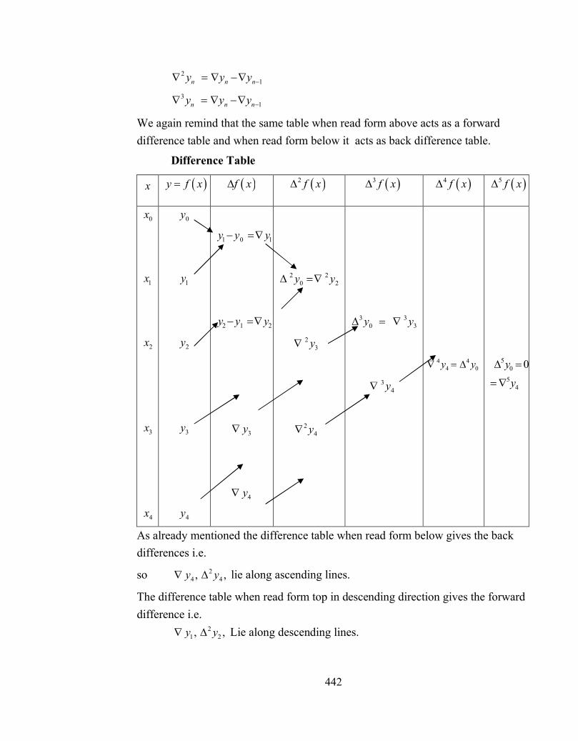
442

21n n ny y y

31n n ny y y

We again remind that the same table when read form above acts as a forward difference table and when read form below it acts as back difference table.

Difference Table

x y f x f x 2 f x 3 f x 4 f x 5 f x

0x

1x

2x

3x

4x

0y

1y

2y

3y

4y

1 0 1y y y

2 1 2y y y

3y

4y

2 2

0 2y y

2

3y

2

4y

3 3

0 3y y

3

4y

4 4

4 0y y

5

05

4

0yy

As already mentioned the difference table when read form below gives the back differences i.e.

so 24 4, ,y y lie along ascending lines.

The difference table when read form top in descending direction gives the forward difference i.e. 2

1 2, ,y y Lie along descending lines.

443


Given a set of 1n data

0 0 1 0 1 2 0 2, , ( , ) 2 , ..... ,n nx y x x h y x x h y x nh y

Let a polynomial ,nP x f x where

0 1 0 2 0 1 0 1 1...... .....n nf x a a x x a x x x x a x x x x x x

..(1)

Be fitted to these data

Putting 0x x in 1 , we get

0 0 0 0f x a

Next Putting 1 0 ,x x x h we get

0 0 1 0 1f x h a a f x a

So 01 0 0

f xa f x h f x

h

Similarly, we get 20

2 2 .......2f x

ah

and 0

n

n n

f xa

h n

Also putting 0x x hu so that 0x x hu

1 0 01 ......., n nnx x h u x x h f x

Putting these values in (1), we get

20 0 0 0

1...

1 2

nnu uu uf x f x f x f x f x

n

This is known as the Newton – Gregory’s forward difference interpolation formula.


Let n nP x f x hu be a nth degree polynomial expressed as

0 1 2 1 1 1..... .....n n n n n nf x a a x x a x x x x a x x x x x x

To be fitted to the set of 1n data.



444

0, 0 1 1 2 0 2 0, , , 2 , ...... ,n nx y x h y x x h y x x nh y

Putting nx x in (1)

0nf x a

Putting 1nx x in (1)

1 1 0 1n n nf x f x a x x

So 11

1

n n n

n n

f x f x f xa

x x h

1

nf xh

or

1ny

h

Similarly on putting 2nx x in (1) we get

2

2 2 2 na f xh

or 2

2 ....2ny

h

Proceeding in their way 1 nn nna y

h n

Putting ,nx x hu we get

21 1.... ....

1 2n

n n n n n

u u u nuf x f x hu f x f x f x f xn

20.5 Stirling’s formula

In order to interpolate the value of y corresponding some x lying near the centre of the interval 0 0, ,x x nh is assumed as origin at some central value which may

be 0 2nx h or 0

12

nx h or 0

12

nx h which ever is integral. Relative to this

origin denoted by 0 the values prior to it are denoted by 1, 2, 3...... and those after it as + 1, + 2………..

The difference table is then designated as follows :

0x

relative to original at

0 3x h

y y 2 y 3 y 4 y 5 y

20.5 Stirling’s formula

445

0x

0x h

0 2x h

0 3x h

0 4x h

0 4x h

0 6x h

3

2

1

0

1

2

3

3y

2y

1y

0y

1y

2y

3y

3y

2y

1y

0y

1y

2

3y

2

2y

2

1y

2

0y

3

3y

3

2y

3

1y

4

3y

4

2y

5

4y

Origin is at 0 3 .x h

Let 0 3x x h hu

Then the Stirling’s central difference formula which is average of Gauss’s forward and back difference formula is given below is expressed as.

20 1 2

0 11 2 2uy yu uy y y

2 2 23 3

41 22

1 1.....

3 2 4u u u uy y y

Gauss’s forward difference formula is

446

1

2 30

1 10 0 1 1 .....

1 2 3u u u u uuf x hu f f f f

and back difference formula is

2 30

1 1 10 1 1 2 ....

1 2 3u u u u uuf x hu f f f f

The upper arrow in wavy form corresponds to Gauss’s back difference formula and lower arrow in wavy form to Gauss’s forward different formula.

The arrows marked in the above table, starting from 0y will help in writing the above formula. The upward arrows diverge to 2

1y and so on. The term in the

stirling’s formula with coefficient 1u etc. will be

Multiplied by their averages. So the 2nd term is 0 1

1 2y yu

At second difference. both the arrows converge to 21y so the corresponding

term is 21

1 12 2

u u u uy

2

212

u y

And so on in this way.


Example 1 Find the cubic polynomial which take the following values

x : 0 1 2 3

f x : 0 1 2 3

Hence or otherwise find 4f

Sol . we know that

21 2

u uf a hu f a C f a C f a

Substituting 0, 1,a h and u x

2 31 1 20 0 0 0

2 3x x x x x

f x f x f f f


447

x f x f x 2 f x 3 f x

0 i 1

1 0 2 1 6

2 1 8 ,9 4 27 6y

3 10 4 19y

4 10y

4 4y

or 2 3 21 3 2f x x x x x x x (putting values)

3 22 1f x x x The polynomial is cubic, therefore 4 427 6 33y y

(Third difference should be constant and equal to 6)

Example 2 In an examination the number of candidates who obtained marks between certain limits were as follows :

Marks : 0-19 20-39 40-59 60-79 80-99

No of candidates 41 62 65 50 17

Sol. : from given data the cumulative frequency table is given below :

Marks : x 19 39 59 79 99

No of candidates 41 103 168 218 235

Difference table

x y y 2 y 3 y 4 y

19 41 62 39 103 3 65 18 59 168 15 0 50 18 79 218 33 17 99 235

448

Here we have 19, 20, 70a h a uh

19 20 70 2.55u u

Now by Newton’s forward interpolation formula.

2 31 1 ( 2)2! 3!

u u u u uf a uh f a u f a f a f a

Or 2.55 1.55 2.55 1.55 0.5570 41 2.55 62 3 182 6

f

41 158.10 5.39 6.52

198 .51 199 .approx

Example3. The population of a town in the decennial census were as under. Estimate the population for the year 1925.

years x : 1891 1901 1911 1921 1931 Population y : 46 66 81 93 101

(in thousands)

Sol. From the given data, the difference table is as given below :

Year Population x y y 2 y 3 y 4 y

1891 46 20 1901 66 5 15 2 1911 81 3 3 12 1 1921 93 4 8 1931 101

Here h = 10, a = 1891, a + nh = 1931, (a + nh) + uh =1925 (given) or

1931 + × 10 = 1925 1925 1931 0.610

u

Now using Newton’s backward interpolation formula.

449

21......

11 2!u u

y a nh hu f a nh f a nh f a nh

0.6 0.4 0.6 0.4 1.41925 101 0.6 8 4 1

2! 3!y

101 4.8 0.48 0.056 96 96.6352 .approx Ans.

Example 4. Use Stirling’s formula to find 28,y and 30,y given

20y = 49225, 25y = 48316 30y = 47236

35y = 45926, 40y = 44306

Sol .: Difference table is

x 305

x u f f 2 f 3 f 4 f

20

25

30

35

40

2

1

0

1

2

49225

48316

47236

45926

44306

909

1080

1310

1620

171

230

310

69

80

11

30 5x u

2

20 10 1

2 2f f uf x f u f

2 3 22 4

4 1 1 2 1 26 2 24

u f f uu f

For 28 3028, 0.45

x u

21310 1080 0.4 0.4 0.16 1 80 528 47236 0.4 230

2 2 6 2a

f

47236 478 18.4 3.9 0.1176 47692 Approx

450

2 3 3 320 1

04 4 4 1 21

2 2 6 2uy y y yy u u y

2 2 3

0 1 21 3 1 1 212 6 2

yydy dy du u y yu ydx du dx x

1 1310 108030 30 54 so 4 = 0 = 2392

xh

Example 5 Use Stirling’s formula to find 32u from following table.

20 14.035U , 25 13.674U , 30 13.257U

35 12.734U , 40 12.089,U 45 11.309U

Sol : Forward difference table for the given data is.

x 305

x f x f 2 f 3 f 4 f

20

25

30

35

40

45

2

1

0

1

2

3

14.035

13.674

13.257

12.724

12.089

11.309

.361

0.417

0.523

0.645

0.780

0.056

0.106

0.122

0.125

0.050

0.016

0.013

0.034

0.013

0.021

For 0x=32, 32 =x + hu = 30 +54,so u= 0.4

By stirling formula

2

21 00 11 ! 2 2

f fu uf x f f

2 2 23 3

41 22

1 16 2 24

u u u uf f f

451

= 0.417 0.523 0.1613.257 0.4 0.1062 2

2 0.16 1 0.5 0.0160.46 2

13.257 0.188 0.00848 13.061

Example 6 Use Gauss forward formula to find 3.75y from the following table

x 2.5 3.0 3.5 4.0 4.5 5.0

y 24.145 22.043 20.225 18.644 17.262 16.047

Sol : Taking 3.5 as origin 5 .h the value of u corresponding to 3.75 is

3.75 3.5 0.5.5

u

Difference Table

x u uy uy 2uy 3

uy 4uy 5

uy

2.5 2 24.145 2.102 3.0 1 22.043 .248 1.818 .047 3.5 …..0 20.225………………… .237……………………. .009…… 1.581 .038 .003 4.0 1 18.644 .199 .006 1.382 .032 4.5 2 17.262 .167 1.215 5.0 3 16.047

Gauss forward formula is : -

2 60 0 1 1

1 1 12! 6u

u u u u uy y u y y y

42

1 1 224

u u u uy

52

2 1 2.......

120u u u

y

.(1)

Replacing .5u and desired values form the difference table in the formula (1), we get

452

1/2

5 5 1.5 .5 .520.225 5 1.581 .237 .003

2 120y

.1.5 .5 .5 1.5 2.5 1.5 .5 .5 1.5.009 .003

24 120

20.225 0.7905 0.029625 0.002375 0.00210938 0.0000352

or , 3.75 19.40y

Example 7.interpolate by means of Gauss’s Backward formula the population for the year 1976, form the following table :

Year : 1931 1941 1951 1961 1971 1981

Population (in lacs) : 12 15 20 27 39 52

Sol :. According to the question 10h and taking 1961as origin,

For the year 1976, 976 1961 1.510

u

Difference table

x u uy uy 2uy 3

uy 4uy 5

uy

1931 3 12 3 1941 2 15 2 5 0 1951 1 20 2 3 7 3 10 1961 0 27 5 7 12 4 1971 1 39 1 13 1981 2 52

Gauss backward formulas is : 1 2 1 3 2 4 2 5

0 1 1 2 1 3 2 4 2 5 3 .......u u u u uuy y C y C y C y C y C y

1.52.5 1.5 2.5 1.5 .52.7 1.5 7 5 3

2 6y

3.5 2.5 1.5 .53.5 2.5 1.5 .5 7 1024 120

453

= 27 10.5 9.375 0.9375 1.9140625 0.2734375

= 46.171875 lacs (apporx).


Q.1 The following table gives the sales of a firm for the last five years. Estimate the sale for the year 1951

Years 1946 1948 1950 1952 1954

Sales (in thousands) 40 43 48 52 57

Q.2 The ordinates of the normal curve are given by the following table

x : 0.0 0.2 0.4 0.6 0.8

y : 0.3989 0.3910 0.3683 0.3332 0.2897

Find : (a) y (0.25) (b) y (0.62)

Q.3 From the following tale find the number of students who obtained marks between 40 and 45:

Marks obtained No. of students

30-40 31

40-50 42

50-60 51

60-70 35

70-80 31

Q.4 Given the following date:

:x 010 020 030 040 050 060 070 080

:y 0.9848 0.9397 0.8660 0.5660 0.6428 0.500 0.342 0.1737

Evaluate : 025a y 032b y 073c y

Q.5 A second degree polynomial passes through 0.1 , 1.3 , 2.7 and 3.13 . find the polynomial

Q.6 Find 1.5f from the following table:

:x 1 2 3 4 5 6 7 8

:y 1 8 27 64 125 216 343 512


454

Q.7 Use Stirling’s formula to comput 12.2u from the following data :

:x 10 11 12 13 14

510 xu 23967 28060 31788 35209 38368

Q.8 Given :

00 05 010 015 020 025 030 tan 0.0000 0.0875 0.1763 0.2679 0.3640 0.4663 0.5774

Q.9 Use Stirling formula to find 35y from the following data :

20 30 40 50512, 439, 346, 243.y y y y

Q.10 Interpolate by means of Gauss’s Backward formula the population for the year 1936, from the following table :

Year 1901 1911 1921 1931 1941 1951

Population (in thousands) 12 15 20 27 39 52

20.8 Principle of Least Square Principle of least square is the most systematic procedures to fit a unique curve through given data. It states “Curve of best fit for a given data is that for which sum of square of deviation is minimum”.

Suppose we have to fit the curve y f x for given set of data ,i ix y (I = 1, 2 …..n) At ix x the experimental value of the ordinate is 푦 & the corresponding value on fitting curve is .f x

If 푒 be the error of Approximation at ix x then we have

i i ie y f x

ie may be (–ve) or (+ve) so by giving equal weightage to each residuals consider

2

1

ni ii

S y f x

Now according to principal of least square curve of best fit is that for which S is minimum.


Let , / 1, 2,...........,i ix y i m be a set of observations. We have to fit a straight

line y a bx (2)

20.8 Principle of Least Square


455

and corresponding observed value is .iy Let ie be the error at ,ix x then

,i i ie y Y i = 1, 2, ………., m

Or ,i i ie y a bx i = 1, 2, ………., m

The sum of squares S (say) of this error is given by

2

1

ni ii

S y a bx

(3)

Least squares principle requires that S be minimum. Form(3), it is clear that S depends on a and b, that is, S is a function of a and b. Thus, we have to find the value of a and b so that S become minimum. By the theory of maxima-minima,the necessary conditions for S to be minimum are

0 ,S Sa b

Form (3), we have

12 0n

i iiy a bx

and 12 0n

i i iix y a bx

On simplification of these two equations, we have

1 1

n ni ii i

y na b x

1

n

ia ma

Or i iy na b x (4)

and 21 1

n n ni i i ii i i

x y a x b x

(5)

Equation (4) & (5) are said to be normal equations. We can determine values of a & b by solving these equations.


Let 2y a bx cx be a parabola to be fitted for the data ( , )i ix y

(i =1,2,3….n) the error at ix x is

2i i i i i i ie y f x e y a bx cx

Let 2 21 1

n ni i i ii i

S e y a bx cx

Now by principal of least square for best fit S is minimum i.e.


456

0, 0 & 0S S Sa b c

212 0n

i i iiy a bx cx

212 0n

i i i iiy a bx cx x

2 212 0n

i i i iiy a bx cx x

On solving 2

1 1 1

n n ni i ii i i

y an b x c x

31 1 1

n n ni i i ii i i

x y a x b x

2 2 3 41 1 1 1

n n n ni i i i ii i i i

x y a x b x c x

Note : (1) For fitting parabola 2y a bx

Normal equations are

21 1

n ni ii i

y an b x

& 2 2 41 1 1

n n ni i i ii i i

x y a x b x

(2) For fitting parabola 2y ax bx

Normal equations are

2 31 1 1

n n ni i i ii i i

x y a x b x

& 2 3 41 1 1

n n ni i i ii i i

x y a x b x


We can fit a general polynomial of degree n by using principal of least square let

polynomial be

21 2 ...... n

o nY a a x a x a x

Which is to be filled to given data ,i ix y , i=1,2,3,…….n then

1

ni ii

S y Y

Where i iY Y x 2

0 1 2 ...... ni i n ia a x a a x


457

so 220 1 2 .....n n

i i i n iiS y a a x a x a s

For S to be minimum, we must have

0 1

0, 0,......, 0,n

s s sa a a

That is, 20 1 2 21

0

2 ...... 0n ni i i n ii

s y a a x a a x a xa

,

20 11

1

2 ..... 0,n ni i i n ii

s x y a a x a xa

2 21 21

2

2 .. 0,n ni i o i i n ii

S x y a a x a x a xa

…. …. ….

21 21

2 .. 0,n n ni i o i i n ii

n

S x y a a x a x a xa

Simplifying above (n+1) equations, we get following normal equations, 2

1 2 .... ni o i i n iy a n a x a x a x

2 3 11 2 ... ,n

i i o i i i n ix y a x a x a x a x 2 2 3 4 2

1 2 ... ,ni i o i i i n ix y a x a x a x a x

……………………………………………………………………………..

2

2 2 1 2 21 1 ... ,n n n n

i i o i i i i n ix y a x a x a x a x a x

These (n+1) equations can be solved for (n+1) unknowns 1 2, , ...... ,o na a a a


Example 8: Using the method of least-squares find a straight line that fits the

following data:

x 71 68 73 69 67 65 66 67 y 69 72 70 70 68 67 68 64

Also find the value of y at x = 68.5.

Solution : Let the required straight line be

y a bx …(i)


458

The normal equations are

i iy na b x …(ii)

and 2i i i ix y a x b x …(iii)

Now, to get the values of , ,i i i iy x b x y and 2 ,ix , we construct following table:

I ix iy i ix y

2ix

1 2 3 4 5 6 7 8

71 68 73 69 67 65 66 67

69 72 70 70 68 67 68 64

4899 4896 5110 4830 4556 4355 4488 4288

5041 4624 5329 4761 4489 4225 4356 4489

Sum 546 548 37422 37314 Hence, 546, 548i ix y

237422, 37314i i ix y x

and total number of given data m =8,

substituting these values in (ii) and (iii), we get

548 = 8a + 546b

37422 = 546a + 37314 b

Solving these two equations for a and b, we get

39.545484a and 0.424242b

Thus, the required straight line is

39.545484 0.424242y x

Now at x = 68.5, value of y is given by

39.545484 0.424242 683.5y

68.606061 Example 9 : Fit a straight line to the given data

459

x 1 2 3 4 5 6 y 2.6 2.7 2.9 3.025 3.2 3.367

Also find value of y at x = 5.5.

Solution : Let the required straight lne be

y a bx

then, the normal equation are

i iy na b x

and 2i i i ix y a x b x

Now, from the given data, we have following table :

I ix iy i ix y

2ix

1 2 3 4 5 6

1 2 3 4 5 6

2.6 2.7 2.9 3.025 3.2 3.367

2.6 5.4 8.7 12.1 16 20.202

1 4 9 16 25 36

Sum 21 17.792 65.002 91 Hence, 21, 17.792i ix y

265.002, 91i i ix y x

and m = 6

then, the normal equations become

17.792 6 21a b and 65.002 21 91a b

Solving these equations, we get

2.419333, 0.156a b

Hence, required straight line is given by the equation

2.419333 0.156y x

Now at 5.5,x , value of y is given by

2.419333 0.156 5.5y

460

3.277333 Example 10 : Fit a curve of the form 2y ax bx to the given data:

x 1 1.5 2 2.5 3 3.5 4 y 1.1 1.95 3.2 5 8.1 11.9 16.4

Solution : Equation of the required curve is

2y ax bx which can be written as

y a bxx ….(i)

Let y Yx , then the above equation becomes

Y a bx ….(ii)

Normal equation for this curve are given by

i iY na b x

and 2i i i ix Y a x b x

Using given data, we construct following table:

I x y yYx

xY

2x

1 2 3 4 5 6 7

1 1.5 2 2.5 3 3.5 4

1.1 1.95 3.2 5 8.1 11.9 16.4

1.1 1.3 1.6 2.0 2.7 3.4 4.1

1.1 1.95 3.2 5 8.12 11.9 16.4

1 2.25 4 6.25 9 12.25 16

Sum 17.5 - 16.2 47.65 50.75 From the table we have

17.5, 16.2,i ix y

247.65, 50.75i i ix y x

and m = 7

substituting these values in normal equations, we get

461

16.2 7 17.5a b

and 47.65 1.5 50.75 ,a b

Solving these equations, we get

80.239827, 1.021429a b

Thus, from (ii) we have,Now at ,yYx

we have

20.239287 1.021429y x x which is the required equation.

Example 11 : Fit a second degree polynomial to given data:

x -4 -3 -2 -1 0 1 2 3 4

y -5 -1 0 1 3 4 4 3 2

Solution : Let the required equation of the curve be

2y a bx cx

Normal equation for this curve are

2i i iy na b x c x

2 3i i i i ix y a x b x c x

2 2 3 4i i i i ix y a x b x c x

From the given data we construct following table :

i ix iy i ix y

2ix

2ix y

3ix

4ix

1 2 3 4 5 6 7 8 9

-4 -3 -2 -1 0 1 2 3 4

-5 -1 0 1 3 4 4 3 2

20 3 0 -1 0 4 8 9 8

16 9 4 1 0 1 4 9 16

-80 -9 0 1 0 4 16 27 32

-64 -27 -8 -1 0 1 8 27 64

256 81 16 1 0 1 16 81 256

Sum 0 11 51 60 -9 0 708

462

Thus, 0, 11, 51i i i ix x x y

32 260, 9, 0,i i i ix x y x

4 708 9ix and n

Substituting above values in normal equations, we get

11 9 .0 60a b c or 11 9 60a c

51 .0 .60 .0a b c or 51 60 ,b

9 .60 .0 .708a b c or 9 60 708a c

Solving above equations for a, b and c, we get

3.004329, 0.85, 0.267316A b c

So, the required equation is given by

23.004329 0.85 0.26731Y x x

Example 12 : Population of a city in different years are given in the following table :

x 1970 1980 1990 2000 2010

y (in thousands) 1450 1600 1850 2150 2500

Fit a parabola to the given data, using least squares principle. Also estimate the population of the city in 2005.

Solution : Since the magnitude of given data is large and values of x are given at equal intervals, therefore we reduce it by shift of origin and scale. Let 0 1990x be origin of x-values and 0 1850y be origin of y-values.

Then, let 1990 185010 50

x yX and Y .…(i)

Let required curve be 2y a bx cx ,

after change of orogin and scale, it will be

2Y a bX cX ….(ii)

Now, we construct following table:

463

x X y Y XY

2X

2X Y

3X

4X

1970 1980 1990 2000 2010

-2 -1 0 1 2

1450 1600 1850 2150 2500

-8 -5 0 6 13

16 5 0 6 26

4 1 0 1 4

-32 -5 0 6 52

-8 -1 0 1 8

16 1 0 1 16

Sum 0 - 6 53 10 21 0 34 Normal equations, in new variables, will be

2i i iY na b X c X

2 3i i i i iX Y a X b X c X

2 2 3 4i i i i iX Y a X b X c X

From the table, we have

0, 6, 53i i i iX Y X Y

2 2 310, 21, 0i i i iX X Y X

4 34 5,iX and n

Substituting above values in normal equations, we have

6 5 .0 .10a b c

or 6 5 10a c

53 .0 .10 .0a b c

or 53 10 ,b

and 21 .10 .0 .34a b c

or 21 10 34a c

Solving above equations for a, b and c, we get

0.08714, 5.3, 0.642857a b c

Now from (ii), we have

20.08714, 5.3 0.642857Y x x …..(iii)

From (i), we have

464

21850 1990 19900.085714 5.3 0.642857

50 10 10y x x

On simplification, we have

1222008.286 1252.7854 0.3214285Y x x

Which is the required equation of parabola. Now, in the year 2005, population of the city will be given by

21222008.286 1252.78543 2005 0.3214285 2005Y

2324.10456 2324 thousands, approximately


Q.1 Derive normal equations for fitting parabola 2y a bx .

Q.2 Derive normal equations for fitting parabola 2y ax bx .

20.14 Summary In this unit operators for interpolation with equal interval are discussed,

various methods for interpolation with equal interval viz Newton forward, Newton Backward & Stirling central difference formulas are discussed. In other part of unit principle of least square for fitting of curves is discussed, fitting of straight line, parabola, fitting of polynomial are discussed.

20.15 Glossary

Interpolation :To approximate a value between given values.

Forward difference: Difference of next value & that value.

Backward difference: Difference of that value & previous value.

Curve Fitting :Fitting a curve from given set of data.

Least square :For which sum of square of values is minimum.


Answers to Self Learning Exercise-II Ans.1: Normal equations are


20.14 Summary

20.15 Glossary


465

21 1

n ni ii i

y an b x

2 2 41 1 1

n n ni i i ii i i

x y a x b x

Ans.2: Normal equations are

2 31 1 1

n n ni i i ii i i

x y a x b x

2 3 41 1 1

n n ni i i ii i i

x y a x b x

20.17 Exercise

Q.1 Fit a curve of the form 2y ax bx to the given data : x 1 2 3 4 5 6 y 2..6 5.4 8.7 12.1 16 20.2

Q.2 Fit a straight line to the following data : x 1 2 3 4 5 8 y 2.4 3 3.6 4 5 6

Q.3 Compute the constants and such that the curve xy fits the given data:

x 1 2 3 4 5 6 y 151 100 61 50 20 8

Q.4 Fit a curve of the form by ax to the given below : x 2 4 7 10 20 40 60 80 y 43 25 18 13 8 5 3 2

Q.5 Fit the curve rp V k to the data given in the table :

P 0.5 1 1.5 2 2.5 3 V 1.62 1 0.75 0.62 0.52 0.46

Q.6 Fit the curve bxy ae to the following data :

x 2 4 6 8 10 y 4.077 11.084 30.128 81.897 222.62

Also estimate y at 7x

20.17 Exercise

466

Q.7 Fit a second degree polynomiasl to the following data, taking x as independent variable:

x 1 1.5 2 2.5 3 3.5 4 y 1.1 1.3 1.6 2.0 2.7 3.4 3.1

Q.8 Fit a second degree parabola to the given data: x 1929 1930 1931 1932 1934 1935 1936 1937 y 352 356 357 358 360 361 360 359

Q.9 Obtain a least-squares quadratic approximation to the function y x x on 0,1 with respect to the weight function 1w x

Q.10 The temperature 휃and length l of a heated rod are given below. Establish a relation between and l of the form l a b using least-squares principle.

0 C 20 30 40 50 60 70

l (mm) 800.3 800.4 800.6 800.7 800.9 800.10

20.18 Answers to Exercise Ans.1: 32.41973 0.15589y x

Ans.2: 1.76 0.506 , 3.747 3.5y x y at x

Ans.3: 309 , 5754a

Ans.4: 4.36 , 0.7975a b

Ans.5: 1.4224, 0.9970r k

Ans.6: 1.499, 0.5 49.6401a b c

Ans.7: 21.0368 0.1932 0.2429y x x

Ans.8: 21010135 1044.67 0.27y x x

Ans.9: 21 6 48 20 )35

y x x

Ans.10: a = 800, b = 0.0146


467


1. S.R.K. Iyenger. R.K. Jain, ‘Numerical Methods’, New Age International Publishers (INDIA).

2. C.F. Gerald, P.O. Wheatley, Applied Numerical Analysis, Addison-Wesley, 1998.

3. Kuldeep Singh Gehlot, ‘Mathematical Methods for Numerical Analysis and Optimization ’, 1st edition, College Book House, (Pvt) Ltd, Jaipur (2007).


468

UNIT -21

Numerical Solution of Nonlinear Equations


21.0 Objectives

21.1 Introduction

21.2 Rate of convergence

21.3 Newton-Raphson Method

21.4 Rate of convergence of Newton Raphson method


21.6 Secant Method

21.7 Rate of convergence of Secant method


21.9 System of linear equations

21.10 Matrix inversion method


21.12 Gauss Elimination method


21.14 Self learning exercise

21.15 Answers to self learning exercise

21.16 Summary

21.17 Glossary

21.18 Exercise



UNIT -21

Numerical Solution of Nonlinear Equations

469

21.0 Objective

In this chapter, we find numerical solution of non-linear equation of the form 0f x . For this, we discuss two methods named Newton Raphson method and Secant method. We also discuss the convergence of these two methods which depends on the choosen root that how closed the root is choosen to the original root. Instead of this, we discuss the system of linear equations of the form AX B and their solution. For this, we learn two methods named Gauss Elimination method and matrix inversion method.

21.1 Introduction The non-linear equations arise in various problems such as projectile motion, pipeline flow, pipe-pump system and many physical problems.

Any polynomial with degree one, is called linear equation. The equation, which is not linear, is called non-linear equation. For example, x-1 =0 is linear and

2 1 0x x is non-linear.

21.2 Rate of Convergence We consider that the initial approximation to the root is sufficiently close to the desired root, then the rate of convergence can be defined as following.

Definition: An iterative method is said to be of order p or has the rate of convergence p, if p is the largest positive real number for which there exists a finite constant 퐶 ≠ 0 such that

1| | | |pk kC

where∈ = 푥 − 휉 is the error in thekth iterate.

The constant C is called the asymptotic error constant and usually depends on derivatives of 푓(푥) at 푥 = 휉.

21.3 Newton Raphson Method For roots with different multiplicity, Newton Raphson Method is given by different formulae.

(i) For Simple roots:

For simple root, the nth iteration root of the equation 푓(푥) = 0 is given by

21.0 Objectives

21.1 Introduction

21.2 Rate of Convergence

21.3 Newton Raphson Method

470

1( )( )

nn n

n

f xx xf x

푛 = 0, 1, 2,3, ….

(ii) For multiple roots: (a). When multiplicity is given:

In this method, we use the following formula

1( )( )

nn n

n

f xx x mf x

where m is multiplicity of root.

(b). When multiplicity is not given:

Let 푥 = 푎 be root of 푓(푥) = 0 of multiplicity m.So, the function f (x)can be written as

푓(푥) = (푥 − 푎) 푔(푥)

푓 (푥) = 푚(푥 − 푎) 푔(푥) + (푥 − 푎) 푔 (푥)

= (푥 − 푎) [푚푔(푥) + (푥 − 푎)푔 (푥)]

∴ 푓(푥)푓 (푥) = (푥 − 푎)ℎ(푥)

Let (푥) = ( )( )

NR Method is given by

푥 = 푥 −(푥 ) (푥 )

= 푥 − ( )/ ( )( ) ( ) ( ) ( )

( )

1 2

( )( ) ( )

n nn n

n n n

f x f xx x

f x f x f x

푛 = 0,1,2,3, … ….

(iii) Newton Raphson Method for pth root:

How to find the nth root of a real number N ? For this consider it be x. Then

푥 = 푁 /

표푟 푥 = 푁

표푟 푥 − 푁 = 0

퐿푒푡 푓(푥) = 푥 − 푁

471

푁푒푤푡표푛 푅푎푝ℎ푠표푛 푀푒푡ℎ표푑 푖푠given by

푥 = 푥 −푓(푥 )푓 (푥 )

표푟 푥 = 푥 −푥 − 푁푝푥

표푟 푥 =푝푥 − 푥 + 푁

푝푥

1 1

1 pn

n pn

p x Nx

px

(a) 퐹표푟 푠푞푢푎푟푒 푟표표푡 푖. 푒. √푁 = 푁 / : In this case p = 2 and 2

1 2n

nn

x Nxx

(b) 퐹표푟 푐푢푏푖푐 푟표표푡 푖. 푒. 푁 : In this case p = 3 and 2

1 2

23n

nn

x Nxx

(c)For inverse of a number i.e. ∶ 퐼푛 푡ℎ푖푠 푐푎푠푒 푝 = −1and

푥 =−2 1

푥 + 푁

−1푥

= 푥 (2−푁푥 )

21.4 Rate of Convergence of Newton Raphson method

The NR Method for solution of 푓(푥) = 0 is

푥 = 푥 −푓(푥 )푓 (푥 ) (1)

Let ξ be a simple root of given equation then 푓(휉) = 0 and ∈ = 푥 − 휉= Error in nth iteration.

Equation (1) becomes

ξ+∈ = 휉 +∈ − ( ∈ )( ∈ )

21.4 Rate of Convergence of Newton Raphson method

472

표푟 ∈ =∈ −푓(휉) +∈ 푓 (휉) + ∈

2 푓 (휉) + ⋯

푓 (휉) +∈ 푓 (휉) + ∈2 푓 (휉) + ⋯

=∈ −∈ ∈ ( )

( ) ⋯

∈ ( )( )

∈ ( )( ) ⋯

12 2

1 12 2

nn nn n n

f f for

f f f

=∈ −∈ +∈푓 (휉)푓 (휉) −

∈2푓 (휉)푓 (휉) + 0(∈ )

=12푓 (휉)푓 (휉) ∈ + 0(∈ )

∈ = 퐶 ∈

where퐶 = ( )( )

and neglecting ∈ and higher terms.

Hence Newton Raphson Method has second order convergence or quadratic convergence.


Example 1: Solve 푥 − 푥 − 10 = 0 by NewtonRaphson method.

Sol. Let 푓(푥) = 푥 − 푥 − 10

푓 (푥) = 4푥 − 1

Now 푓(0) = −10

푓(1) = −10

푓(2) = 4

Therefore, 푎root of 푓(푥) = 0 lie between 1 and 2 as f (1) f (2)< 0 .

Let 푥 = 2

푓(푥 ) = 4

∴ 푓 (푥 ) = 31

By Newton Raphson method

푥 = 푥 − ( )( )

= 1.87097 (for푛 = 1)


473

푥 = 푥 −푓(푥 )푓 (푥 )

= 1.85578

푥 = 푥 − ( )( )

=1.85558

푛 = 3

푥 = 푥 −푓(푥 )푓 (푥 )

= 1.85558

Hence a root of given equation is 1.85558 correct upto 5 decimals.

Example 2: Solve x푙표푔 푥 = 1.2 by Newton Raphson method.

Sol. Let 푓(푥) = 푥푙표푔 푥 − 1.2 = 0

푓 (푥) = 푙표푔 푥 + 푥. . 푙표푔 푒

= 푙표푔 푥 + 0.43429

푓(1) = −1.2

푓(2) = −0.59794

푓(3) = 0.23136

푥 = 3

푥 = 푥 −푓(푥 )푓 (푥 )

= 푥 − ( . ).

= . ..

For 푛 = 1,2,3 …

푥 = 2.74615

푥 = 2.74065

푥 = 2.74065

Example 3: Find double root of equation 푥 − 푥 − 푥 + 1 = 0 by Newton-Raphson Method. starting with0.8. (multiplicity is given as 2)

Sol. Let 푓(푥) = 푥 − 푥 − 푥 + 1

푓 (푥) = 3푥 − 2푥 − 1

Here 푥 = 0.8

474

Newton Raphson method for a root with multiplicity 2 is

푥 = 푥 − 2푓(푥 )푓 (푥 ) , 푛 = 0,1,2, ….

= 푥 −2(푥 − 푥 − 푥 + 1)

3푥 − 2푥 − 1

=푥 + 푥 − 2

3푥 − 2푥 − 1

For n = 0,1,2

푥 =푥 + 푥 − 2

3푥 − 2푥 − 1= 1.011765

푥 = 1.00003

푥 = 1

Hence 1 is root of 푓(푥) = 0 with multiplicity 2.

Example 4: Find the multiple root of

27푥 + 27푥 + 36푥 + 28푥 + 9푥 + 1 = 0

by Newton Raphson method. (multiplicity is not unknown)

Sol. Let 푓(푥) = 27푥 + 27푥 + 36푥 + 28푥 + 9푥 + 1

∴ 푓 (푥) = 135푥 + 108푥 + 108푥 + 56푥 + 9

푓 (푥) = 540푥 + 324푥 + 216푥 + 56

Here multiplicity of root is not given. Therefore multiple root of 푓(푥) = 0 can be considered as simple root of (푥) = 0,푤ℎ푒푟푒

(푥) =푓(푥)푓 (푥)

(0) =19 = 0.11111

(−1) = −0.18182

Multiple root of 푓(푥) = 0 lies between 0 and -1. Take 푥 = 0.

Newton Raphson Method for multiple root is given by

푥 = 푥 −푓(푥 )푓 (푥 )

{푓 (푥 )} − 푓(푥 )푓 (푥 )

For n = 0,1,2

푥 = −0.36

푓(푥 ) = −0.000578

475

푓 (푥 ) = 0.065434

푓 (푥 ) = −4.963840

∴ 푥 = −0.333224

푓(푥 ) = −0.333115

푓 (푥 ) = 0.000001

푓 (푥 ) = 0.019677

푥 = −0.333173

Example 5 Find 20 / .

Sol. Here N = 20 and√16 = 4, √25 = 5

Take 푥 = 4.5

Newton Raphson method for square root is

푥 =푥 + 푁

3푥 , 푛 = 0,1,2,3 ….

푥 =푥 + 20

2푥

For n = 0,1,2,3

푥 =푥 + 20

2푥 = (4.5) + 20

2(4.5) =(4.5) + 20

9

= 4.47222

푥 =푥 + 20

2푥 = (4.47222) + 20

2(4.47222) = 4.472136

푛 = 2

푥 =푥 + 20

2푥 = 4.472136

∴ √20 = 4.472136

Example 6: 퐹푖푛푑 18 / .

Sol.

Here 푁 = 18

(8) / = 2, (27) / = 3

푇푎푘푒 푥 = 2.5

Newton Raphson Method for cubic root is

푥 =

476

For n = 0, 1, 2

푥 = = 2.626667

푥 = 2.620755

푥 = 2.620741

21.6 Secant Method

The Newton Raphson method requires the evaluation of derivatives of the function and this is not always possible, particularly in the case of functions arising in practical problems. In the secant method, the derivative at x, is approximated by the formula

푓 (푥 ) =푓(푥 )− 푓(푥 )

푥 − 푥

which can be written as

푓 =푓 − 푓푥 − 푥

where 푓 = 푓(푥 ). Hence, the NewtonRaphson formula becomes

푥 = 푥 −(푥 − 푥 )푓푓 − 푓 =

푥 푓 − 푥 푓푓 − 푓

1 11

1

i i i ii

i i

x f x fxf f

It should be noted that this formula requires two initial approximations to the root.

21.7 Rate of Convergence of Secant Method

We assume that ξ is a simple root of 푓(푥) = 0. Substituting푥 = 휉 +∈ 푖푛 (1) 푤푒 표푏푡푎푖푛

∈ =∈ −(∈ −∈ )푓(휉 +∈ )

푓(휉 +∈ ) − 푓(휉 +∈ ) (2)

Expanding 푓(휉 +∈ )and 푓(휉 +∈ ) in Taylor’s series about the point ξ and noting that 푓(휉) = 0.

∈ =∈ −(∈ −∈ ) ∈ 푓 (휉) + 1

2 ∈ 푓 (휉) + ⋯…

(∈ −∈ )푓 (휉) + 12 (∈ −∈ )푓 (휉) + ⋯ . .

21.6 Secant Method

21.7 Rate of Convergence of Secant Method

477

=∈ − ∈ +12 ∈

푓 (휉)푓 (휉) + ⋯ 1 +

12 (∈ +∈ )

푓 (휉)푓 (휉) + ⋯

∈ =12푓 (휉)푓 (휉) ∈ ∈ + 푂(∈ ∈ +∈ ∈ )

∈ = 퐶 ∈ ∈ (3)

where퐶 = ( )( )

and higher powers of ∈ are neglected.

The relation of the form (3) is called the error equation. Keeping in view the definition of the rate of convergence, we seek a relation of the from.

∈ = 퐴 ∈ (4)

where A and p are to be determined.

From (4) we have

∈ = 퐴 ∈ 표푟 ∈ = 퐴 / ∈ /

Substituting the values of ∈ and ∈ in (3), we get

∈ = 퐶퐴 ( ) ∈ / (5)

Equating the powers of ∈ on both sides, we get

푝 = 1 +1푝

which gives 푝 = (1 ± √5)

Neglecting the minus sign, we find the rate of convergence for the secant method is 푝 = 1.618.

From (5), we have 퐴 = 퐶 /( )


Example 7: Solve the equation 4 sin 푥 + 푥 = 0. Find the root of equation by Secant method.

Sol. Let 푓(푥) = 4 sin 푥 + 푥 = 0

푓(−1) = −2.36588, 푓(−2) = 0.362810 푓(−1)푓(1) < 0

So, a root lies between -1 & -2 and let

푥 = −1 , 푥 = −2


478

Now

푥 =(−1)(0.362810)− (−2)(−2.36588)

0.362810 + 2.36588

=−5.094572.728690 = −1.867039

푓(푥 ) = −0.339926

Now 푥 = −2 푥 = 1.867039

푓(푥 ) = 0.362817 , 푓(푥 ) = 0.334926

푥 =1.357232−0.702726 = −1.93138

푓(푥 ) = −0.01269

Now

푥 =푥 푓(푥 ) − 푥 푓(푥 )푓(푥 ) − 푓(푥 )

=−0.6330020.327326 = −1.93384

푓(푥 ) = 0.00045

Now

푥 =푥 푓(푥 ) − 푥 푓(푥 )푓(푥 )− 푓(푥 )

=−0.0254520.013162 = −1.93375

푓(푥 ) = −0.00002

Now

푥 =푥 푓(푥 ) − 푥 푓(푥 )푓(푥 ) − 푓(푥 )

=0.001135−0.000587 = −1.93375

Thus, the approximate value to the root is -1.93375 correct up to five decimals.

Example 8: Determine p, q and r so that the order of iteration method.

푥 = 푝푥 +푎푞푥 +

푟푎푥

becomes as high as possible for root of ξ= 푎 / .

Sol. Here 휉 = 푎 / => 휉 = 푎

479

That is, we have found cube root of a, using∈ = 푥 − 휉

We have 휉 + ∈ = 푝(휉 + ∈ ) +( ∈ )

+( ∈ )

= 푝(휉 +∈ ) + 푎푞 (휉 +∈ ) + 푟푎 (휉 + ∈ )

= 푝(휉 +∈ ) + 푎푞휉 1 +

∈휉 +

푟푎휉 5 1 +

∈휉

= 푝(휉 +∈ ) + 푎푞휉 1 −

2 ∈휉 +

3 ∈휉 −

4 ∈휉 + ⋯ . .

+ 푟푞휉 1 −

5 ∈휉 +

15 ∈휉 −

35 ∈휉 + ⋯ . .

∈ + 휉 = 푝(휉 +∈ ) + 푞 휉 1 −2 ∈휉 +

3 ∈휉 −

4 ∈휉 + ⋯ . .

+ 푟 휉 1 −5 ∈휉 +

15 ∈휉 −

35 ∈휉 + ⋯ . .

∈ = 휉 [−1 + 푝 + 푞 + 푟] +∈ (푝 − 2푞 − 5푟) + ∈휉

(3푞 + 15푟)

+∈휉

(−4푞 − 35푟)

If we take

−1 + 푝 + 푞 + 푟 = 0 (1)

푝 − 2푞 − 5푟 = 0 (2)

3푞 + 15 푟 = 0 (3)

By (1) 푝 = +1 − 푞 − 푟

By(2) 1 − 푞 – 푟 − 2푞 − 5푟 = 0

=> −3푞 − 6푟 = −1 => 3푞 + 6푟 = 1

=> 3푞 + 6푟 = 1

3푞 + 15푟 = 0

−9푟 = 1

푟 = −19

−3푞 = −1 + 푟

−3푞 = => 푞 = +

480

∴ 푝 = 1 −59 +

19 => 푝 =

9 − 5 + 19 =

59

We have 푝 = 푞 = , 푟 =

Eq.(1) becomes ∈ = ∈ + ⋯

∈ =5

3휉 ∈

= 퐶 ∈

Hence given method has order 3.

21.9 System of Linear Equations

Consider the system of n linear equations in n unknowns :

푎 푥 + 푎 푥 + ⋯+ 푎 푥 = 푏

푎 푥 + 푎 푥 + ⋯+ 푎 푥 = 푏

… … … … …

… … … … …

푎 푥 + 푎 푥 + ⋯+ 푎 푥 = 푏 (1)

The matrix form of the system (1) is

퐴푋 = 퐵 (2)

where

퐴 =

⎣⎢⎢⎢⎡푎 푎 … … 푎푎 푎 … … 푎… … … … …… … … … …푎 푎 … … 푎 ⎦

⎥⎥⎥⎤ , 푋 =

⎣⎢⎢⎢⎡푥푥……푥 ⎦⎥⎥⎥⎤

푎푛푑 퐵 =

⎣⎢⎢⎢⎡푏푏……푏 ⎦⎥⎥⎥⎤

21.10 Matrix Inversion Method

Suppose A is non-singular, that is det퐴 ≠ 0.Then 퐴 exists. Therefore, pre-multiplying (2) by 퐴 ,푤푒 푔푒푡

퐴 퐴푋 = 퐴 퐵

푋 = 퐴 퐵

Using this formula , all unknowns can be determined.


21.9 System of Linear Equations

21.10 Matrix Inversion Method


481

Example 9 Solve the system of linear equations

푥 + 푦 + 2푧 = 1

푥 + 2푦 + 3푧 = 1

2푥 + 3푦 + 푧 = 2

Sol. We have

|퐴| =1 1 21 2 32 3 1

= −4 ≠ 0

Also

퐴 =14

7 − 5 1−5 3 11 1 − 1

Hence

푋 =푥푦푧

= 퐴 퐵 =14

7 − 5 1−5 3 11 1 − 1

112

=14

400

=100

Therefore, 푥 = 1,푦 = 0, 푧 = 0


3푥 + 6푥 + 푥 = 1

푥 + 2푥 − 푥 = 2

3푥 + 3푥 + 2푥 = 3

Sol. The coefficient matrix is given by

퐴 =3 6 11 2 − 13 3 2

푇ℎ푢푠 푋 = 퐴 푏

=>푥푥푥

= −1

12

7 − 9 − 8−5 3 4−3 9 0

123

푥푥푥

= −1

12

−351315

푥 =3512 ,푥 = −

1312 , 푥 = −

1512

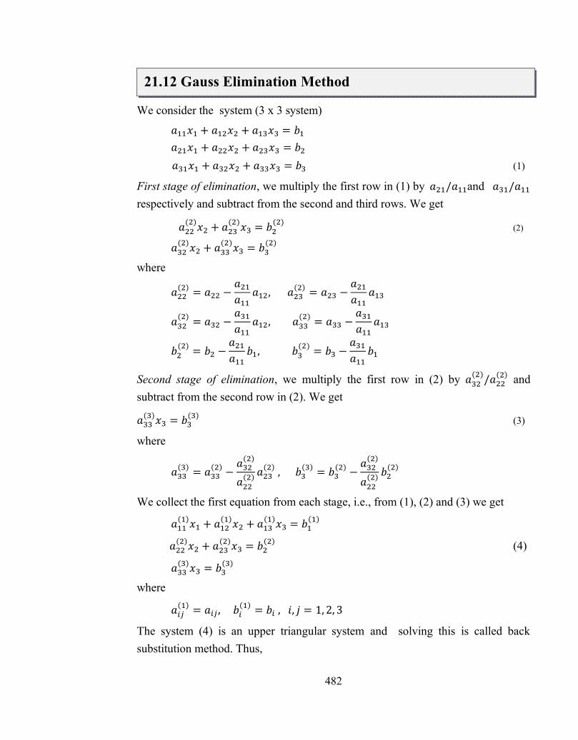
482

21.12 Gauss Elimination Method

We consider the system (3 x 3 system)

푎 푥 + 푎 푥 + 푎 푥 = 푏

푎 푥 + 푎 푥 + 푎 푥 = 푏

푎 푥 + 푎 푥 + 푎 푥 = 푏 (1)

First stage of elimination, we multiply the first row in (1) by 푎 /푎 and 푎 /푎 respectively and subtract from the second and third rows. We get

푎( )푥 + 푎( )푥 = 푏( ) (2)

푎( )푥 + 푎( )푥 = 푏( )

where

푎( ) = 푎 −푎푎 푎 , 푎( ) = 푎 −

푎푎 푎

푎( ) = 푎 −푎푎 푎 , 푎( ) = 푎 −

푎푎 푎

푏( ) = 푏 −푎푎 푏 , 푏( ) = 푏 −

푎푎 푏

Second stage of elimination, we multiply the first row in (2) by 푎( )/푎( ) and subtract from the second row in (2). We get

푎( )푥 = 푏( ) (3)

where

푎( ) = 푎( ) −푎( )

푎( ) 푎( ) , 푏( ) = 푏( ) −

푎( )

푎( ) 푏( )

We collect the first equation from each stage, i.e., from (1), (2) and (3) we get

푎( )푥 + 푎( )푥 + 푎( )푥 = 푏( )

푎( )푥 + 푎( )푥 = 푏( ) (4)

푎( )푥 = 푏( )

where

푎( ) = 푎 , 푏( ) = 푏 , 푖, 푗 = 1, 2, 3

The system (4) is an upper triangular system and solving this is called back substitution method. Thus,

21.12 Gauss Elimination Method

483

[퐴|푏] −− −− − −−→ [푈|푐 ] (5)

where [A|b] is the augmented matrix. The elements 푎( ), 푎( )and 푎( ) which have been assumed to be non-zero are known as pivot elements. The elimination procedure described above to determine the variables(unknowns) is called the Gauss elimination method. We may also make the pivot as 1 before elimination, at each step. At the end of the elimination procedure, we produce 1 at each of the positions of the diagonal elements.

We now solve the system (1) in n unknowns by performing the Gauss elimination on the augmented matrix [A|b].

The elimination is performed in (n — 1) steps, k = 1, 2, ... , n — 1. In the

elimination process, if any one of the pivot elements 푎( ), 푎( ), … … , 푎( )vanishes or becomes very small compared to other elements in that column, then we attempt to rearrange the remaining rows so as to obtain a non-vanishing pivot or to avoid the multiplication by a large number. This strategy is called pivoting. The pivoting is of the following two types.

Partial Pivoting

In the first stage of elimination, the first column is searched for the largest element in magnitude and brought as the first pivot by interchanging the first equation with the equation having the largest element in magnitude. In the second elimination stage, the second column is searched for the largest element in magnitude among the n-1 elements leaving the first element, and this element is brought as the second pivot by an interchange of the second equation with the equation having the largest element in magnitude. This procedure is continued until we arrive at the equations (5).

Complete Pivoting

We search the matrix A for the largest element in magnitude and bring it as the first pivot. This requires not only an interchange of equations but also an interchange of the position of the variables.




484

푥 + 10푥 + 푥 = 12

10푥 + 푥 + 푥 = 12

푥 + 푥 + 10푥 = 12

Sol. Rearranging the system of linear equations

10푥 + 푥 + 푥 = 12 (1)

푥 + 10푥 + 푥 = 12 (2)

푥 + 푥 + 10푥 = 12 (3)

[퐴 | 푏] =10 1 11 10 11 1 10

121212

푅 → 푅 −1

10푅 , 푅 → 푅 −1

10푅

=10 1 10 99/10 9/100 9/10 99/10

12108/10108/10

푅 →1099 푅

=

⎣⎢⎢⎢⎡10 1 1

0 1 1

11

0 9

109910

121211

10811 ⎦

⎥⎥⎥⎤

푅 → 푅 −9

10 푅

=

⎣⎢⎢⎢⎡10 1 1

0 1 1

11

0 0 10811

121211

10811 ⎦

⎥⎥⎥⎤

by back substitution, we get

푥 =1,푥 = 1,푥 = 1

Example 12 Solve the equations

10푥 − 푥 + 2푥 = 4

푥 + 10푥 − 푥 = 3

2푥 + 3푥 + 20푥 = 7

using the Gauss elimination method.

485

Sol. As seen, the system doesn’t need pivoting. We get, after the first elimination stage

10푥 − 푥 + 2푥 = 4

10110 푥 −

1210푥 =

2610

3210 푥 +

19610 푥 =

6210

second elimination stage

10푥 − 푥 + 2푥 = 4

10110 푥 −

1210푥 =

2610

201801010 푥 =

54301010

Using back substitution, we get

푥 = 0.269, 푥 = 0.289 푎푛푑 푥 = 0.375

Example 13 Find the solution of thesystem of equations

푥 + 푥 + 푥 = 6

3푥 + 3푥 + 4푥 = 20

2푥 + 푥 + 3푥 = 13

Sol. In the first step we eliminate 푥 from the last two equations and obtain

푥 + 푥 + 푥 = 6

푥 = 2

−푥 + 푥 = 1

Here, the pivot in the second equation is zero and so we cannot proceed as usual. We interchange the equations 2 and 3 before the second step. We obtain the upper triangular system

푥 + 푥 + 푥 = 6

−푥 + 푥 = 1

푥 = 2

which has the solution

푥 = 3, 푥 = 1 푎푛푑 푥 = 2

Example 14: Solve the system of linear equations

푥 + 2푥 + 3푥 = 14

486

2푥 + 5푥 + 2푥 = 18

3푥 + 푥 + 5푥 = 20

Sol. Given system can be written as

3푥 + 푥 + 5푥 = 20 (1)

2푥 + 5푥 + 2푥 = 18 (2)

푥 + 2푥 + 3푥 = 14 (3)

[퐴 |푏] =3 1 5 | 202 5 2 | 181 2 3 | 14

푅 → 푅 −23푅 , 푅 → 푅 −

13푅

=

3 1 5 | 2013 4 140 |3 3 35 4 220 |3 3 3

푅 → 푅 −5

13푅

=

3 1 5 | 2013 4 140 |3 3 3

24 720 0 |3 3

By back substitution, we get 푥 = 3, 푥 = 2 , 푥 = 1


Very Short Answer type Questions Q.1 Define the rate of convergence for any iterative method.

Q.2 Write the order of convergence for Newton Raphson method.

Q.3 Write the order of convergence for Secant method.

Short Answer type questions Q.4 Solve the non-linear equation 4 10 0x x by Newton Raphson method.


487

Q.5 Solve the following system of linear equation

1 2 34 4x x x

1 2 34 2 4x x x

1 2 33 2 4 6x x x

by Gauss Elimination method with partial pivoting.

Q.6 Find the positive root of the equation 2 5 2 0x x , correct to 4 decimal places, using Newton-Raphson method with 0 0.5x


Ans.2 : Quadratic convergence i.e. order 2

Ans.3 : 1.618

Ans.4 : 1.856

Ans.5 : 1 2 31 1, , 12 2

x x x

Ans.6 : 0.4384

21.16 Summary

In this chapter, we discussed about the numerical solution of non-linear equation by Newton-Raphson method and Secant method. Then, we discussed about the solution of the system of linear equation by Matrix Inversion method and Gauss Elimination method.

21.17 Glossary

Elimination: The removal of a variable from an equation, typically by substituting another which is shown by another equation to be equivalent: Convergent: (Of a series) approaching a definite limit as more of its terms are added.

21.18 Exercise

Very Short Answer Type Questions Q.1 Write the formula of Newton Raphson method for determining the square root


21.16 Summary

21.17 Glossary

21.18 Exercise

488

of 15.

Q.2 Write the Newton-Raphson formula for determining the cubic root of the number N.

Q.3 Write the Newton Raphson formula for determining the multiple root with multiplicity m for non-linear equation.


Q.4 Find the positive root of the equation 2 1 0x x correct to 3 decimal places, using Newton Raphson method with 0 0x .

Q.5 Find the cubic root of 15 by Newton Raphson method.

Q.6 Find the numerical solution of the system of linear equations 4 16x y z , 3 2 18x y z and 4 2 20x y z correct to 3 decimal places, using Gauss Elimination method without partial pivoting.

Long Answer Type Questions Q.7 Derive the rate of convergence for (i) Newton Raphson Method (ii) Secant method Q.8 Solve the system

2 10x y z

3 2 3 18x y z

4 9 16x y z

by (i) Gauss Elimination method and (ii) Matrix inversion method

Q.9 Solve the system

2 2 12x y z

3 2 2 8x y z

5 10 8 10x y z

by (i) Gauss Elimination Method (ii) Matrix Inversion Method


Ans.1 :

2

115

2n

nn

xxx

Ans.2 :

3

1 2

23n

nn

x Nxx


489

Ans.3 : 1

nn n

n

mf xx x

f x

Ans.4 : 0.618

Ans.5 : 2.4662 Ans.6 : 0.64, 5.44, 5.2x y z

Ans.8 : 7, 9, 5x y z Ans.9 : 12.75, 14.375, 8.75x y z References and Suggested Readings


2. C.F. Gerald, P.O. Wheatley, Applied Numerical Analysis, Addison-Wesley, 1998.


490


22.0 Objectives

22.1 Introduction

22.2 Approximations of derivatives

22.2.1 First order approximation

Forward difference approximation

Backward difference approximation

Central difference approximation 22.2.2 Error Analysis



22.5 Numerical Differentiation

22.5.1 Method based on Interpolation formula


22.7 Method based on Operator


22.9 Summary 22.10 Glossary


22.12 Exercise


Numerical differentiation and integration methods are frequently used in

22.0 Objectives

UNIT- 22 Numerical Differentiation

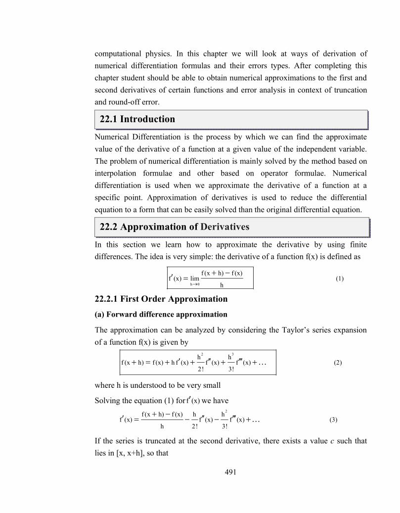
491

computational physics. In this chapter we will look at ways of derivation of numerical differentiation formulas and their errors types. After completing this chapter student should be able to obtain numerical approximations to the first and second derivatives of certain functions and error analysis in context of truncation and round-off error.

Numerical Differentiation is the process by which we can find the approximate value of the derivative of a function at a given value of the independent variable. The problem of numerical differentiation is mainly solved by the method based on interpolation formulae and other based on operator formulae. Numerical differentiation is used when we approximate the derivative of a function at a specific point. Approximation of derivatives is used to reduce the differential equation to a form that can be easily solved than the original differential equation.

In this section we learn how to approximate the derivative by using finite differences. The idea is very simple: the derivative of a function f(x) is defined as

h 0

f (x h) f (x)f (x) lim (1)

h

22.2.1 First Order Approximation (a) Forward difference approximation

The approximation can be analyzed by considering the Taylor’s series expansion of a function f(x) is given by

2 3h h

f (x h) f (x) h f (x) f (x) f (x) (2)2! 3!

where h is understood to be very small

Solving the equation (1) for (x)f we have

2f (x h) f (x) h h

f (x) f (x) f (x) (3)h 2! 3!

If the series is truncated at the second derivative, there exists a value c such that lies in [x, x+h], so that

22.2 Approximation of Derivatives

22.1 Introduction

492

(4)(c)f

!2

h

h

(x)fh)(xf(x)f

where the reminder term shows the approximation error for derivative

forwardΟ

hE(f, h) f (c) (h) (5)

2!

is the truncation error or first order accurate. We see that this approximation is first-order accurate because the first term is dominating in the expression O(h) for small h. So, the forward difference approximation of the first derivative (x)f is

f (x h) f (x)

f (x) (7)h

And a true error for the forward difference formula is

0xx

0h

(x)fh)(xf(x)f)x(xT

central

(b) Backward difference approximation

In similar way, one can write the Taylor series expansion of a function f(x) about x to determine f(x−h) by replacing h by –h.

2 3h hf (x h) f(x) h f (x) f (x) f (x) (8)

2! 3!

Solving the equation (8) for (x)f we have

(9)(x)f!4

h(x)f

!3

h(x)f

!2

h

h

h)(xf(x)f(x)f 4

33

2

If the series is truncated at the second derivative, there exists a value c such that lies in [x-h, x], so that

(10)(c)f

!2

h

h

h)(xf(x)f(x)f

where the reminder term shows the approximation error for derivative

backwardΟ

hE(f, h) f (c) (h) (11)

2!

493

is the truncation error or first order accurate. We see that this approximation is first-order accurate because the dominate term in the truncation error is Oback(h) for small h. So, the backward difference approximation of the first derivative (x)f is

f (x) f (x h)

f (x) (13)h

And a True error for the backward difference formula is

0xx

0h

h)(xf(x)f(x)f)x(xT

central

(c) Central difference approximation

We can derive a more accurate estimate of the derivative by using the forward and backward Taylor series expansion about x.

(14)(x)f

!4

h(x)f

!3

h(x)f

!2

h(x)fhf(x)h)(xf 4

43

32

(15)(x)f

!4

h(x)f

!3

h(x)f

!2

h(x)fhf(x)h)(xf 4

43

32

Subtracting the eqn (15) from (14), we see that the terms involving even powers of h cancel out, leaving terms are

(x)f

!5

h(x)f

!3

h(x)fh2h)(xfh)(xf 5

53

3

or, solving for (x)f we have

(x)f

!5

h(x)f

!3

h(x)fh2h)(xfh)(xf 5

53

3

(x)f

!5

h(x)f

!3

h

2h

h)(xfh)(xf(x)f 5

43

2

If the series is truncated at the second derivative, there exists a value c such that lies in [x-h, x+h], so that

(c)f

!3

h

2h

h)(xfh)(xf(x)f 3

2

Where the reminder term shows the approximation error for derivative

494

centerΟ

23 2h

E(f, h) f (c) (h ) (16)3!

is truncation error or first order accurate. We see that the center difference approximation is second-order accurate because the dominate term in its truncation error is Ocenter(h

2) for small h. The center difference approximation is more accurate than the forward difference due to its smaller truncation error. So, the central difference approximation of the first derivative (x)f is

(17)

2h

h)(xfh)(xf(x)f

And a true error for the forward difference formula is

(18)

2h

h)(xfh)(xf(x)f)x(xT

0xx

0

central

Note: Error reduced if forward and backward difference approximations are combined.

22.2.2 Error Analysis

By same proceeding we can obtain the higher order approximation of derivatives with finite difference. Let us next discuss about the round-off error. Such errors arise due to limitation of the finite word in computers. Suppose h)(xf

0 and

h)(xf0 are approximated by the numerical values

1y and

1y and

1e and

1e are the

associated round – off error then

h)E(f,2h

yy)(xf 11

0

where

h)(f,Eh)(f,Eh)E(f,truncround

(18)6

(c)fh

2h

ee 3211

Hence the total error in numerical differentiation formula is truncation (approximation) plus round-off. If

εε 11e,e and

(x)fMaxM 3

b][a,x

495

then ε

2M hE(f, h) (19)

2h 6

Concept of Total Error (optimal choice of h)

The optimal choice of h represents a compromise between the conflicting requirements of minimizing the round-off error, the first term which requires a large value of h, and minimizing the approximation error, the second term, which requires a small value of ‘h’. To reduce the truncation error, we need to reduce h.

But as h is reduced, the round-off error grows. The value of h that minimizes the error term in above eqn.

ε

1 33

h (20)M

Now consider an example to understand the concept of total error

Example 1 Let sinxf(x)

(a) Use formula (18) with step sizes h= 0.0001, 0.001, 0.01and 0.1 and calculate

approximations for fʹ(0.5).

(b) Calculate the optimal value of ‘h’.

Sol. (a) fʹ(x) = cosx then

true value of cos(0.5) = 0.8775825 (7 decimal place)

from the approximation formula (18)

2h

h)(0.5fh)(0.5f(0.5)f

Gives us different values of approximation for the different h (as shown in table)

Step Size Approximation

fʹ(0.5)

Error = True−Approx

0.1 0.8761205 1.4620619×10−3

0.01 0.8775700 1.2561920×10−5

0.001 0.8775906 −8.0380800×10−6

0.0001 4.8279724 − 3.9503898

496

(b) We can use the bound

1cos(x)(x)fM 3

and the values of f are given to seven decimal places, we will assume that the

round-off error is bounded by ε = 0.5 × 10−7(machine epsilon). The optimal value of h can be easily calculated:

Num 0.00531331

100.53

M

3h

317

31

ε

the step size 0.001is closer to the optimal value 0.0053133 and it gives the best

approximation to fʹ(0.5) among the four choices.

Example 2 Let cosxsinx(x)f .

Calculate approximations for (0)f by all three difference formula with h=0.1, 0.01 and 0.001 and compute also

(a) Compute an upper bound for each approximation error.

(b) Compute the true error.

Sol. Let be given cosxsinx(x)f , then

sinxcosx(x)f ; 1(0)f

forward difference approximation

h

1(h)cos(h)sin

h

(0)f(h)f(0)fforward

backward difference approximation

h

(h)cos(h)sin1

h

(h)cos(h)sin1

h

h)(f(0)f(0)fbackward

central difference approximation

h

(h)sin

2h

(h)cos(h)sin(h)cos(h)sin

2h

h)(f(h)f(0)fcentral

Also,

( ) sin cosf x x x

22. 3 Illustrative Examples

497

(0) 1f and ( ) cos sinf x x x (0) 1f

An approximation error is

2

h1)(

!2

h(0)f

!2

h(c)f

!2

hR forward

Similarly, one can obtain

2

h1)(

!2

h(0)f

!2

h(c)f

!2

hR backward

and

6

h1)(

!3

h(0)f

!3

h(c)f

!3

hR

2222

central

Table for forward difference

h

Approximations

h

1(h)cos(h)sin

True Error

h

1(h)cos(h)sin1

Approx. Error

2

h

0.1 0.0174380 0.9825619 0.05

0.01 0.0174517 0.9825482 0.005

0.001 0.0174531 0.9825469 0.0005

Table for backward difference

h

Approximations

h

(h)cos(h)sin1

True Error

0xxh

(h)cos(h)sin11

Approx. Error

2

h

0.1 0.0174685 0.9825315 0.05

0.01 0.0174548 0.9825452 0.005

0.001 0.0174534 0.9825465 0.0005

498

Table for central difference

h Approximations

h

(h)sin

True Error

0xxh

(h)sin1

Approx. Error

6

h2

0.1 0.0174532 0.9825467 1.67×10−3

0.01 0.0174532 0.9825467 1.67×10−5

0.001 0.0174532 0.9825467 1.67×10−7

Example 3 Derive the expression for the Second-Order Approximation of first Derivative on forward difference.

Sol. The Taylor series expansion of the function f(x) can be written as

(1)(x)f

!3

h(x)f

!2

h(x)fh(x)fh)(xf 3

32

solving this equation for (x)f we have

(2)(x)f

!3

h(x)f

!2

h

h

(x)fh)(xf(x)f 3

2

If we truncate the Taylor series (Eq. 1) at the third term (at the second derivative), the result will be as follows:

Now the forward difference approximation of the second derivative is given by

(3)

h

(x)fh)(xf(x)f

But h

h)(xf2h)(xfh)(xf

and

h

(x)fh)(xf(x)f

Putting these equations in eqn.3 will give the following results

2h

(x)fh)(x2f2h)(xf(x)f

Substituting this eqn in (2) we get

(x)f!3

h

h

(x)fh)(x2f2h)(xf

!2

h

h

(x)fh)(xf(x)f 3

2

2

499

(x)f!3

h

2h

(x)fh)(x2f2h)(xf(x)fh)(x2f(x)f 3

22

(x)f!3

h

2h

(x)3fh)(x4f2h)(xf(x)f 3

2

h)E(f,2h

(x)3fh)(x4f2h)(xf(x)f

Where the reminder term shows the approximation error for derivative

(x)f!4

h(x)f

!3

hh)E(f, 4

33

2

and

forwardΟ 2

2 h(h ) f (x)

3!

is truncation error or second order accurate. Finally, one can write the second-order approximation of first derivative (x)f is

2h

(x)3fh)(x4f2h)(xf(x)f


Q.1 What is first order accurate in forward difference approximation?

Q.2 What is first order accurate in backward difference approximation?

Q.3 What is first order accurate in central difference approximation?


Q.4 Why the center difference approximation is more accurate than the forward difference?

Q.5 Use the backward difference formula to approximate the first derivative of the function f(x)= sinx at πx0 using h=0.1.

Q.6 Use the backward difference formula to approximate the first derivative of the

function f(x)= cosx at πx0 using h=0.01.


500

In numerical differentiation It is essential required the proper selection of interpolation formulae to solve the numerical differentiation problems.

Selection of formula (a)If the values of the argument are equally spaced, the formula is represented by Newton’s Gregory formula to determine the numerical differentiation as desired.

(b)If we want to find the derivative of function at a point near beginning of end of a set of tabular value, then we use Newton’s Gregory forward (backward) formula as desired.

(c)If the values of argument are not equally spaced, we shall use Newton’s divided formula or Lagrange’s formula to represent the function.

22.5.1 Method based on Interpolation formula In this method, the formula is represented by an interpolation formula and then differentiating many times as required. For exp. let us consider Newton’s Gregory formula,

Δ Δ Δ 2 3u (u 1) u (u 1) (u 2)

f(u) f(0) u f (0) f (0) f (0) (1)2! 3!

Where 0x x

u (2)h

df (u) df (u) du 1 df (u)

(3)dx du dx h du

Now differentiating eqn (1) w.r.t u and applying (3), we get

(4)(0)f!3

26u3u(0)f

!2

1)(2u(0)f

h

1

du

(u)df

h

1

dx

(u)df 32

2

ΔΔΔ

Once again differentiating above eqn (1) w.r.t ‘u’, we get

Similarly, one can determine the higher order derivative as desired.

Special Case: Numerical differentiation at the particular value 0

xx

2Δ Δ

23

2 2

d f (u) d df (u) d df (u) du 1 d df (u) 1f (0) (u 1) f (0) (5)

dx dx dx du dx dx h du dx h

22.5 Numerical Differentiation

501

Putting 0

xx and 0u in eqn (4) and (5)

(6)(0)f!3

2(0)f

!2

1(0)f

h

1

dx

(u)df 32

ΔΔΔ0xx

and

(7)(0)f(0)fh

1

dx

(u)fd3

22

2

ΔΔ2

0xx

Note: The same process can be used to other interpolation formulae such as Lagrange’s, Sterling’s and Bessel’s etc.

Example 4 Determine the first (dy/dx) and second derivative (d2y/dx2) of function tabulated below at the point x=0.35.

x 0.25 0.50 0.75 1.00 1.25 1.50

f(x) − 0.4219 − 0.1250 − 0.0156 0.0000 0.0156 0.1250

Sol. By inspection of the question, the value of argument is equally spaced and required derivative are at a point near the beginning of the table. In this case, we shall use Newton’s Gregory forward interpolation formula. The finite difference table is as under:

x (x)f (x)fΔ (x)f2Δ (x)f3Δ (x)f4Δ (x)f5Δ 0.25 − 0.4219

0.2969

0.50 − 0.1250 − 0.1875

0.1094 0.0937

0.75 − 0.0156 − 0.0938 0.0001

0.0156 0.0938 − 0.0001

1.00 0.0000 0.0000 0.0000

0.0156 0.0938

1.25 0.0156 0.0938

0.1094

1.50 0.1250

Newton’s Gregory forward interpolation formula is


502

Δ Δ Δ

Δ Δ

2 3 22 3

4 3 2 5 4 3 24 5

(u u) (u 3u 2u)f (x) f (a uh) f(a) u f (a) f (a) f (a)

2! 3!

(u 6u 11u 6u) (u 10u 35u 50u 256u) f (a) f (a)

4! 5!

where,

x au

h

Differentiating with respect to x, we have

df (x) df (x) du df (x) d x a 1 df (x)

dx du dx du dx h h du

(a)f120

256)100u105u40u(5u(a)f

24

6)22u18u(4u

(a)f6

2)6u(3u(a)f

2

1)(2u(a)f

h

1

du

(x)df

h

1(x)f

dx

d

5234

423

32

2

ΔΔ

ΔΔΔ

The second derivative of f(x)

2

2

d f (x) d df (x) du 1 d df (x)

dx du dx dx h du dx

(a)f120

256)100u105u40u(5u(a)f

24

6)22u18u(4u

(a)f6

2)6u(3u(a)f

2

1)(2u(a)f

du

d

h

1

dx

(x)fd

5234

423

32

2

22

2

ΔΔ

ΔΔΔ

(a)f24

20)42u24u(4u

(a)f12

11)18u(6u(a)f1)(u(a)f

h

1

dx

(x)fd

523

42

32

22

2

Δ

ΔΔΔ

Here a=0.25, and h=0.25. At x=0.35, 0.40.25

0.250.35

h

axu

Therefore, the first derivative

0.0001)((1.9197)(0.0001)(0.0073)

(0.0937)(0.0133)0.1875)0.1)((0.29690.25

1(0.35)f

(0.0002)(0.0000)(0.0012)(0.0188)0.29690.25

1(0.35)f

503

1.26680.25

0.3167(0.0002)(0.3169)

0.25

1(0.35)f

In similar way, the second derivative

0.0001)(0.2827)(

(0.0001)(0.3967)(0.0937)0.6)(0.1875)((0.25)

1(0.35)f

2

3.89920.0625

0.2437(0.0000)(0.0000)(0.0562)0.1875

0.0625

1(0.35)f

Example 5 Determine the first (dy/dx) and second derivative (d2y/dx2) of function tabulated below at the point x=1.1.

x 0.2 0.4 0.6 0.8 1.0 1.2

f(x) 0.968 0.904 0.856 0.872 1.000 1.288

Sol. The value of argument is equally spaced and required derivative are at a point near the end of the table. So we shell use of the central difference formula. In this case, we shall use Newton’s backward formula.

The finite difference table is as under:

x (x)f (x)fΔ (x)f2Δ (x)f3Δ

0.2 0.968

− 0.064

0.4 0.904 0.016

− 0.048 0.048

0.6 0.856 0.064

0.016 0.048

0.8 0.872 0.112

0.128 0.048

1.0 1.000 0.160

0.288

1.2 1.288

504

Newton’s backward formula is

Δ Δ Δ

2 3 22 3

n n n n n

(u u) (u 3u 2u)f (x) f (x uh) f(x ) u f (x ) f (x ) f (x )

2! 3!

where, nx x

uh

Differentiating with respect to x, we have

du

(x)df

h

1

h

xx

dx

d

du

(x)df

dx

du

du

(x)df

dx

(x)df n

)(xf

6

2)6u(3u)(xf

2

1)(2u)(xf

h

1

du

(x)df

h

1(x)f

dx

dn

32

n2

n ΔΔΔ

The second derivative of f(x)

dx

(x)df

du

d

h

1

dx

du

dx

(x)df

du

d

dx

(x)fd2

2

)(xf1)(u)(xfh

1

dx

(x)fdn

3

n

2

22

2

ΔΔ

Here xn= 1.2, and h= 0.2. At x=1.1, 0.50.2

1.21.1

h

xxu n

Therefore, the first derivative

1.430.002]5[0.288(0.048)]0.042)(160)(0.000)(0.[(0.288)0.2

1(1.1)f

In similar way, the second derivative

4.625(0.184)(0.048)]0.5)(0.160)[((0.2)

1(1.1)f

2

Example 6 Determine the first (dy/dx) and second derivative (d2y/dx2) of function tabulated below at x=2.

x 1 1.5 2 2.5 3 3.5

f(x) 0 0.25 1 2.25 4 6.25

Sol. By inspection of the question the value of argument is equally spaced and required derivative are at a point near the middle of the table. So we shell use of

505

the central difference formula. In this case, we have used Gauss’s forward interpolation formula.

Here new variant h

xxu m

for x=2, u=0.

The finite difference table is as under: u x (x)f (x)fΔ (x)f2Δ (x)f3Δ

− 2 1 0

0.25

− 1 1.5 0.25 0.5

0.75 0

0 2 1 0.5

1.25 0

1 2.5 2.25 0.5

1.75 0

2 3 4 0.5

2.25

3 3.5 6.25

Gauss’s interpolation formula with new variant ‘u’ is;

2)(f!4

2u)u2u(u

1)(f!3

u)(u1)(f

!2

u)(u(0)fuf(0)uh)(xff(x)

234

33

22

m

4Δ

ΔΔΔ

first derivative of

du

(x)df

h

1

h

xx

dx

d

du

(x)df

dx

du

du

(x)df

dx

(x)df m

Now differentiating (1) w.r.t u and using u=0 and h=0.5, we get 2 3 2

2 3 4df(u) 1 (2 1) (3 1) (4 6 2 2)f(0) f ( 1) f ( 1) f ( 2) ...du 2 6 24

u u u u uh

506

2(0.5)2

1)(1.25

0.5

1

du

(u)df

2x

0

Similarly,

dx

(x)df

du

d

h

1

dx

du

dx

(x)df

du

d

dx

(x)fd2

2

2)(f24

2)12u(12u1)(f u1)(f

h

1 232

2

4ΔΔΔ

Therefore,

2(0.5)0.5

1

du

(u)fd2

2x

2

2

Example 7 Determine the first (dy/dx) and second derivative (d2y/dx2) of function tabulated below at the point x=11.

x 2 4 9 13 16 21

f(x) 13 81 811 2367 4353 9703

Sol. The value of argument is unequally spaced. In this case, we shall use Newton’s divided difference formula.

The divided difference table is as under:

x (x)f (x)fΔ (x)f2Δ (x)f3Δ

2 13

34

4 81 16

146 1

9 811 27

389 1

13 2367 39

662 1

16 4353 51

1070

21 9703

507

Newton’s divided difference formula is

(a)fc)b)(xa)(x(x(a)fb)a)(x(x(a)fa)(xf(a)(x)f 32 ΔΔΔ

(a)fabc}bc)xac(abc)xb(a{x

(a)fab}b)x(a{x(a)fa)(xf(a)(x)f323

22

ΔΔΔ

Differentiating w.r.t x

(a)fbc)}ac(abc)xb2(a{3x(a)fb)}(a{2x(a)f(x)f 322 ΔΔΔ The second derivative of f(x)

(a)fc)}b2(a{6x(a)f2(x)f 32 ΔΔ

Putting x=11, a=2,b=4,c=9 and the values of differences from the table, we get

3859525634(95)(1)(16)(16)34(11)f

and

68(1)(36)2(16)(x)f

Approximate expression for the central difference derivative

(a) First difference derivative

As we know that (1)yyy

1/2n1/2nn δ

and (2)y[yy 1/2n1/2nn ]21μ

Therefore, (3)yyy1/2n1/2nn

][μδμ

Now ]21]

21μ n1n1/21/2n1/21/2n1/2n y[yy[yy

And ]21]

21μ 1nn1/21/2n1/21/2n1/2n y[yy[yy

Substituting these values in eqn. (3), we get

(4)y[y

y[yy[yyyy

n1n

1nnn1n1/2n1/2nn

]21

]21]

21][μδμ

1

22.7 Method based on Operator

508

][]21

nhD

1nnhDhD yeyye[e

ny[sinhD]

or ....δμ 3

DhhDsinhD

33

hDδμ (neglecting higher order terms)

Now, (approx)y[yhD n1n ]21

1

or 11 ]2 n n n 1 n

dDy (y ) [y y (5)

dx h

This is called as first derivative formula for central difference derivative.

(b) Second difference derivative

Now 1/2n1/2nnn

yyyy δδδδ2

1/2n1/2nyy δδ

1/21/2n1/21/2n1/21/2n1/21/2n

yyyy

1/21/2n1/21/2n1/2n1/21/2n1/21/2n1/2n

yyyandyyy δδ

n1n1n1nnn1nn

yyyyyyyy 2δ2

nnhDhD y1coshD2yee 2

n

22n

22 y...Dhy1...Dh2

112

approxyDhyn

22n2δ (neglecting higher order terms)

Therefore n1n1nn

22n

yyyyDhy 2δ2

or 1 2 2

2n n n 1 n 1 n2 2

dD y (y ) y y y (6)

dx h

This is called as second derivative formula for central difference derivative.

(c) Third difference derivative

Once again nn

22n

33 yhDyDhhDyDh 2δ

509

n1n1n

yyy 2δμ hDδμ

1n1n11n11n11n11n yyyyyy 21

21

1n1nn yyy

21δμ

1n1n2nnn2n yyyyyy 21

21

2n1n1n2n yyyy 2221

1 2 2

33

n n n 2 n 1 n 1 n 23 3

dD y (y ) y y y y (7)

dx 2h

This is called as third derivative formula for central difference derivative.

Symbolic derivation of derivatives of a function

Let the function y=f(x) and x=x0+hu

where h= difference of interval

Therefore y=f(x0+hu) =Eu y0 (8)

where y0=y(x0)

Now, differentiating (8) w.r.t x at x0

000 xxxxxx

dx

du)y(E

du

d)y(E

dx

d

dx

dy0

u0

u

0u0u

0u

0u )y(ElogE

h

1)y(E

du

d

h

1

00 y1logh

1ylogE

h

1

from logarithmic expansion

0

432

xx

y...432h

1

dx

dy

0

ΔΔΔΔ

...y

4

1y

3

1y

2

1y

h

10

40

30

20 ΔΔΔΔ

510

similarly,

022

2

y1logh

1

dx

yd 2Δ0

xx

by logarithmic expansion and taking square root we get

...y6

5y

12

11yy

h

1

dx

yd0

50

40

30

2

2xx

2

2

0

ΔΔΔΔ

In general form

0

n

nn

n

y1logh

1

dx

yd Δ0

xx Example 8 Prove that

...y

4

1y

3

1y

2

1y

h

1y 432 ΔΔΔΔ

and

...y

12

11yy

h

1y 432

2ΔΔΔ

Sol. As we know that hDeE

hDe1 Δ

or )(1logh

1D Δ

therefore )y(1logh

1Dy Δ

y...

432h

1 432

ΔΔΔΔ

...y

4

1y

3

1y

2

1y

h

1y 432 ΔΔΔΔ

Similarly we know that

1e hD

)(1logh

1D

511

Now y)(1logh

1yDy

2

2

y...

12

11

2

1

h

12

32

2

ΔΔΔ

2

32

2...y

12

11y

2

1y

h

1

ΔΔΔ


Q.1 Which formula is used to determine the numerical differentiation while the values of the argument are equally spaced?

Q.2 Which formula is used to determine the numerical differentiation at a point near beginning of end of a set of tabular value?

Q.3 Which formula is used to determine the numerical differentiation while the values of the argument are not equally spaced?

Short Type Answer Type Questions

Q.4 Find the first (dy/dx) derivative of the function y = sinx tabulated below at the point x=0.95.

x 0.7 0.8 0.9 1 1.1

y 0.644218 0.717356 0.783327 0.841471 0.891207

Q.5 Find the first (dy/dx) derivative of the function y = cosx tabulated below at the point x=0.75.

x 0.7 0.8 0.9 1 1.1

y 0.764842 0.696707 0.621610 0.540302 0.453596

Q.6 Prove that

3hx3hx2hx2hxh-xhxx yy

3h

1yy

2h

1yy

h

1hy

dx

d


512

● Numerical Differentiation is the process by which we can find the approximate value of the derivative of a function at a given value of the independent variable.

●First order approximation and associated truncation error

(a) Forward difference approximation

h

(x)fh)(xf(x)f

(c)f

!2

hh)E(f,

(b) Backward difference approximation

h

h)(xf(x)f(x)f

(c)f!2

hh)E(f,

(c) Central difference approximation

2h

h)(xfh)(xf(x)f

(c)f

!3

hh)E(f, 3

2

● the total error in numerical differentiation formula is given by sum of the truncation (approximation) and round-off error.

● In numerical differentiation

(a) If the values of the argument are equally spaced, the formula is represented by Newton’s Gregory formula to determine the numerical differentiation as desired. (b) If we want to find the derivative of function at a point near beginning of end of a set of tabular value, then we use Newton’s Gregory forward (backward) formula as desired.

22.9 Summary

513

(c) If the values of argument are not equally spaced, we shall use Newton’s divided formula or Lagrange’s formula to represent the function.

Truncate: Shorten (something) by cutting off the top or the end

Interpolate: Insert (an intermediate value or term)into a series by estimating or calculating it from surrounding known values


Ans.1: (c)f!2

h

Ans.2: (c)f!2

h

Ans.3:

(c)f!3

h 32

Section-A: (Very Short Answer Type Questions)

Q.1 Define round-off error.

Q.2 Define the approximation of a function.

Q.3 What is truncation error order for the first derivative of forward difference formula?

Q.4 What is truncation error order for the first derivative of central difference formula?

Q.5 What is truncation error order for the first derivative of backward difference formula?

Section-B :(Short Answer Type Questions)

Q.6 Let cosxsinx(x)f .

Calculate approximations for by all three difference formula with =0.1, (0)f

22.12 Exercises

22.10 Glossary


514

0.01 and 0.001 and compute also

(a) Compute an upper bound for each approximation error.

(b) Compute the true error.

Q.7 How many terms are required in calculation of the

approximate 0.5 (1.648721...) correct to four decimal places after rounding?

Q.8 Let cosxf(x)

(a) Use formula (18) with step sizes h= 0.0001, 0.001, 0.01and 0.1 and

calculate approximations for fʹ(0.5).

(b) Calculate the optimal value of ‘h’.

Q.9 Use the central difference formula to approximate the derivative of the function f(x) = cosx at πx0 using h=0.01.

Q.10 Use the Second-Order approximation of first derivative on forward difference formula to approximate the derivative of the function f(x) = sinx at

πx0 using h=0.1.

Section C: (Long Answer Type Questions)

Q.11 Consider xe(x)f and evaluate (1)f using h=0.01 for the forward, backward and central approximation. Which is the best approximation?

Q.12 Determine the first (dy/dx) and second derivative (d2y/dx2) of function tabulated below at the point x=10.

x 2 4 9 13 16 21

f(x) 13 81 811 2367 4353 9703

Q.13 Find the first (dy/dx) derivative of the function y = cosx tabulated below at the point x=0.87.

x 0.7 0.8 0.9 1 1.1

y 0.764842 0.696707 0.621610 0.540302 0.453596

Q.14 Determine the first (dy/dx) derivative of the function tabulated below at the points x=0.1.0.6 and 1.1 by using backward difference, forward difference and central difference approximation. Give comments.

515

x 0.2 0.4 0.6 0.8 1.0 1.2

f(x) 0.968 0.904 0.856 0.872 1.000 1.288

Q.15 Assuming Bessel’s interpolation formula, prove that

...y

24

1yy

dx

d23x

321xx ΔΔ


1. Thomas Finny, ‘Calculus and Analytic Geometry’, 9st edition, Pearson Education, Asia (2001).

2. John.H. Mathews, ‘Numerical Methods Using MATLAB’, Third edition, Prentice Hall, Upper Saddle River, NJ 07458 (1999).

3. Kuldeep Singh Gehlot, ‘Mathematical Methods for Numerical Analysis and Optimization ’, 1st edition, College Book House, (Pvt) Ltd, Jaipur (2007).


516


23.0 Objectives

23.1 Introduction

23.1.1 Definition of numerical integration

23.1.2 Newton-Cotes Integration Formulas

23.2. The Trapezoidal Rule

23.2.1 Derivation of the Trapezoidal Rule using Newton-Gregory Formula

23.3Illustrative Examples

23.4. The Simpson’s1/3 Rule


23.6. The Simpson’s 3/8 Rule

23.7. The Weddle’s Rule

23.8. Runge-Kutta Methods

23.8.1. Runge-Kutta 1st order Method(Euler’s Method)

23.8.2. Runge -Kutta 2nd order Method

Heun’s method the midpoint method

Ralston’s method.

23.8.3. Runge -Kutta 3rd order Method 23.9. Self Learning Exercises-II

23.10. Summary

23.11. Glossary

23.12. Answers to self learning exercise

23.13. Exercise


UNIT-23 Numerical integration

517

This chapter explores study methods for approximating the integral of a function over a given interval and for determining the error associated with the rules. We know that every function cannot be easily solved analytically. This type of integral can be easily solved by numerical methods.

Numerical integration has always been useful in many areas of science and economics to evaluate distribution functions and other quantities.

Numerical integration is the study of how the numerical value of an integral can be found. This method in general is known as numerical quadrature, which refers to finding a square whose area is the same as the area under a curve. It is one of the important topics of numerical analysis. Our main interest is to find out the process of approximating a definite integral from values of the integrand.

The basic quadrature methods can be categorized in two main classes:

1. The methods that are based on data points which are equally spaced: these are Newton cotes formulas, the midpoint rule, the trapezoid rule and Simpson rule.

2. The methods that are based on data points which are not equally spaced: these are Gaussian quadrature formulas.

23.1.1 Definition of numerical integration By definition, the integral of some function f(x) between the limits a and b

may be thought of as the area A between the curve at the x-axis and is written mathematically as (shown in Figure)

b

a

A f (x) dx (1)

23.1 Introduction

23.0 Objectives

f(x)

a b

x

A

518

In general, a numerical integration is the basic idea of the approximation of a definite integration by a “weighted” sum of function values at discrete points within the interval limit. thus

(2)E)(xdx(x)f ti

b

a

n

1iifw

where wi is the weighted factor which depends on the schemes used in the integration, f (xi) is the function value evaluated at the given point xi (node) and Et is the truncation error.

23.1.2 Newton-Cotes Integration Formulas

According to this idea a complicated function or a tabulated data can be replaced by an approximating (interpolating) function.

(2)dx(x)Pdx(x)fI

b

a

n

b

a

where Pn(x) is an nth order interpolating polynomial.

In general, for the given nodes }x,x,x{ n10 we can use the interpolation polynomial formula to obtain integration.

(3)dx(x)Edx(x)Pdx(x)f

b

a

n

b

a

n

b

a TermErrorTheionApproximatThe

1st order Polynomial

AA

2nd order Polynomial

f(x)

a b

x

f(x)

a b

x

Actual Curve

Approximate

Curve

Actual Curve Approximate

Curve

1n

)a(ba...

2

)a(baa)(ba(x)dxP

dxxa...xaa(x)dxP

1n1n

n

22

10

b

a n

b

a

nn10

b

a n

519

This integral is can be determined numerically by dividing the domain [a; b] into n equally spaced. Different choices for m’s lead to different formulas as follow (see table below):

Trapezoid method (First order polynomials are used)

b

a 10

b

adxxaadx(x)f

Simpson’s 1/3 rule (Second order polynomials are used)

b

a

2210

b

adxxaxaadx(x)f

m Polynomial Formula Error

1 Linear Trapezoid O(h2)

2 Quadratic Simpson’s 1/3 O(h4)

3 Cubic Simpson’s 3/8 O(h4)

Fig. A Sketch for calculating area under the curve f(x).

The area under the curve F(x)y is the sum of a triangle and a rectangular. This area A can be easily calculated as

(1)heightAverageWidth

2

(a)f(b)fh

2

a)(b(a)f(b)fa)(b(a)fI

23.2. The Trapezoidal Rule

(x)f

a bx

(a)f

(b)f

520

where, we have used h=b-a. For the exact result of numerical integration the f(x) should be a linear function. This is known as Trapezoidal Rule. If f(x) is quadratic or higher order curve then we should find a better way of calculating the numerical integration. For more precession, we can divide whole area in small segments of trapezoidal. For example, we consider an area which is divided into five trapezoids

Now we find the sums of the area of these five trapezoids from a to b. therefore,

2

)(xf)(xf

2

)(xf)(xf

2

)(xf)(xf

n

abA 542110

where,

b ah

n ( n=5 for five trapezoids)

)}(xf)(xf)}(xf)(xf)}(xf)(x{f2n

abA 542110

{{

Finely, we get

)(xf)(x2f)(x2f)(x2f)(x2f)(xf2n

abA 543210

In general,

0 1 2 n 1 n

b aA f (x ) 2f (x ) 2f (x ) 2f (x ) f (x )

2n

A

k n-1

0 n nk 1

hf (x ) 2 f (x ) f (x )

2

n

b

a

lim f (x) dx

f(x)

a bx

0x

1x 5

x2

x 3x 4

x

hhhhh

521

As the bigger n you use, the more accuracy in area will be.

Example 1 Let be f(x) = sinx. Calculate the approximate area A by using the Trapezoidal Rule as shown in figure below.

Sol. we find the numerical integral

0

dxsinA

4)n(since44

0

n

abh

ππ

then, using the trapezoidal rule

)(f

4

32f

22f

42f(0)f

2(4)A πππππ

1.89602

2212

2

220

8

π

23.2.1 Derivation of the Trapezoidal Rule using Newton-Gregory Formula

Suppose f(x) takes the values y0, y1, y2, ...,yn for x0, x1, x2, ...,xn.The interval (a,b) is divided into n equal parts of width h, so that

a = x0, x1 = x0+h, x2 = x0 +2h, ..., xn = x0+nh=b

Then

(1)hduydxydxyIn

0

x

x

x

x

b

a0

0

0

nh

nh

where duhdxh

xxu 0

By Newton-Gregory Formula of f(x)

f(x)

0 πx

1

2

π4

π4

3π

522

nn2 Ry

!n

)n(u1)(uuy

!2

1)(uuyuyy

0000 Δ1ΔΔ

where, )(y!1n

)n(u1)(uuhR 1n1n ξ

1n

and0

n yΔ is the nth forward difference.

Now, using Newton cotes integration formula, we get

b

a

n0n

02

00dxRy

!n

)n(u1)(uuy

!2

1)(uuyuyI Δ1ΔΔ

change integration limits from x to u, then

nu

0u

bx

ax

duhdxdu,hdx

n

0

n0n

02

00hduRy

!n

)n(u1)(uuy

!2

1)(uuyuyI Δ1ΔΔ

(ξ)

1Δ Δ Δ

n2 n

0 0 0 0

0

nn 2 n 1

0

u (u 1) u (u 1) (u n )I h y u y y y du

2! n!

u (u 1) (u n 1)h y du [a, b] (2)

n 1!

Above equation is called as Newton quadrature formula, which is also known as quadrature formula.

For n = 1, we have only one interval (x0, x1) such that a = x0 and b = x1 and then the above integration formula gives trapezoidal rule.

Now setting n=1(Polynomial of the first degree in x or a straight line), we get

termmainderReorder1

)(ξ

st

Δ

1

0

3

1

0

00duy

!2

1)(uuhduyuyhI

1

0

1

0

)(ξΔ

2

u

3

u

2

yh

2

uyyhI

233

2

00

where 010

yyy Δ

523

(3)]x,[xy12

h

2

yyhdxydxyI

10

310

x

x

x

x

1

0

0

0

tEErrorTruncationRuleTrapezoid

h

)(ξ

where ξ is somewhere between x0 and x1 .Trapezoidal rule is first order accurate. It can integrate linear polynomials exactly. Similarly, for subsequent intervals,

2

yyhdxydxyI 21

x

x

x

x

2

1

0

0

h2

h

2

yyhdxydxyI

2

yyhdxydxyI

n1n

x

x

x

x

32

x

x

x

x

n

1-n

0

0

3

2

0

0

nh

h)1n(

h3

h2

By adding all above equations, we obtain

h 22

n

0

x

0 1 2 n-1 n

x

I y dx y y y y y

This is known as Trapezoidal rule.

Example 2 show the estimated integral (area) region and error area region according to trapezoidal rule in given figure below.

Sol.

23.3Illustrative Examples

f(x)

a b

x

524

More accurate estimate of an integral can be found if a high-order polynomial is used to connect the points. In Simpson’s rule it is approximated the value of a definite integral by using quadratic (second order) polynomials. In Simpson's method the straight line is replaced by parabolas.

Let’s first derive a formula for the area under a parabola of equation cbxaxy 2 (2nd order Polynomial) passing through the three points )yh,(

0 ,

)y(0,0

and )y(h,2

. Then, the definition of integration, the value of integration can be found the area between the limits –h to +h.

h

h

2 dxc)bx(axA

2ch

3

2ahcx

2

bx

3

ax 323

h

h

6c)(2ah3

h2

23.4. The Simpson’s1/3 Rule

(x)fy

h 0

x

)y(0,1

hx

2y

1y

0y

)yh,(0

)y(h,2 2nd order Polynomial

cbx 2ax(x)fy

f(x)

a b

x

Integral estimate

Error

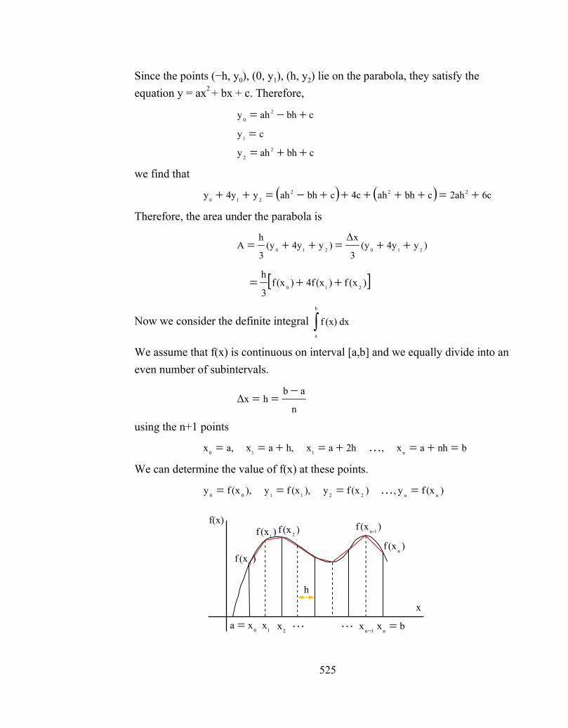
525

Since the points (−h, y0), (0, y1), (h, y2) lie on the parabola, they satisfy the equation y = ax2 + bx + c. Therefore,

cbhahy

cy

cbhahy

22

1

20

we find that

6c2ahcbhah4ccbhahy4yy 222210

Therefore, the area under the parabola is

)y4y(y

3

x)y4y(y

3

hA 210210

Δ

)(xf)(x4f)(xf

3

h210

Now we consider the definite integral b

a

dx(x)f

We assume that f(x) is continuous on interval [a,b] and we equally divide into an even number of subintervals.

n

abhx

Δ

using the n+1 points

bnhax,2haxh,axa,xn110

We can determine the value of f(x) at these points.

)(xfy,)(xfy),(xfy),(xfynn221100

f(x)

x

0xa bx

n1

x2

x1n

x

h

)(xf2)(xf

1

)(xf0

)(xf1-n

)(xfn

526

One can determine the integral by adding the areas under the parabolic arcs through these successive points.

)n(xf)1-n(x4f)(x2f)(x4f)(x2f)(x4f)(xf3

h43210

432210 )n(xf)1-n(x4f)2-n(xf)(xf)(x4f)(xf)(xf)(x4f)(xf3

hb

adx(x)f

By simplifying, we obtain

)(xf)(xf2)(xf4)(xf3

hn

2-n

2,4,6ij

1-n

1,3,5ii0

Example 3 Derive the Simpson’s 1/3 Rule using Newton-Gregory Formula.

Sol. By using eqn.2 of previous section

n

0

1n2n

n

0

0n

02

00

duy!1n

1)n(u1)(uuh

duy!n

)n(u1)(uuy

!2

1)(uuyuyhI

)(ξ

Δ1ΔΔ

For n = 2, we have two subintervals [x0, x1] and [x1, x2] of equal width h such that a= x0 and b = x2 and then the above integration formula becomes. Setting n=2(Polynomial of the second degree in x or a parabola), we get

2

Re2

(ξ)Δ Δ

ξ ξnd

h

mainder termorder

0 2

0 0

x x 2 22 3

0 0 0

x x 0 0

0 2 0 2

u (u 1) u (u 1)(u 2)I y dx y dx h y u y y du h y du

2! 3!

x x or [x , x ]

Therefore integral term,

2

0

02

00

x

x

duy!2

1)(uuyuyhdxyI

2

0

ΔΔ

2

0

)y2y(y

2

u

3

u

2

1)y(y

2

uuyhdxyI 012

23

01

2

0

x

x

2

0

)y2y(y y and)y(yy0120

2010

ΔΔ

)y4y(y3

hI 210

527

This result is a part of the Simpson’s rule. Similarly, for the next intervals,

)y4y(y3

hdxydxyI 432

x

x

x

x

4

2

0

0

h4

h2

6

4

h

h

0 6

0 4

x x

4 5 6

x x

hI y dx y dx (y 4y y )

3

( 2)

nh

n h

0 n

0 n -2

x x

n-2 n-1 n

x x

hI y dx y dx (y 4y y )

3

By adding all above equations, we obtain

n

0

x

0 1 3 n-1 2 4 n-2 n

x

hI y dx y 4 y y y 2 y y y y

3

This is known as Simpson’s 1/3 rule.


Q.1 Define the Trapezoidal Rule.

Q.2 What is highest order of polynomial integrand for which Simpson’s 1/3 rule of integration is exact.

Q.3 What is the order of error in Trapezoidal Rule.


Q.4 Integrate the function xe(x)f from a=0 to b=2 using the Trapezoidal rule.

Q.5 Integrate the function 2xx(x)f from a=0 to b=10 using the Trapezoidal rule in steps of h=1.

Q.6 Integrate the function 2x)(1(x)f from a=1 to b=5 using the Simpson’s 1/3 rule with h=0.5.

Simpson’s 3/8 rule can be obtained by using fourth-order polynomials to fit four points. Integration over the four points (three

34

2210

xaxaxaa(x)fy

23.6. The Simpson’s 3/8 Rule


528

intervals) simplifies to:

(1)dx(x)Pdx(x)fIb

a

n

b

a

0 1 2 3

3hI f (x ) 3f (x ) 3f (x ) f (x )

8

Weddle’s rule can be obtained by using5

64

53

42

210xaxaxaxaxaa(x)fy sixth-order polynomials to fit sixth

points. Integration over the six points (five intervals) simplifies to:

Where n = 6,

Example 4 Compute the value of the definite integral 2

0

3 dxx by

(a) Trapezoidal rule

(b) Simpson’s 1/3 Rule

(c) Simpson’s 3/8 Rule

with using 10 intervals, after computing the true value of the integral, compare the errors in the all four cases.

23.7. The Weddle’s Rule

b ah6

b

0 1 2 3 4 5 6a

3hI f(x)dx f 5f f 6f f 5f f10

Approximate Curve

Actual Curve

f(x)

0xa 4xb

x1x

2x

x

529

Sol. In this case divide the range of integration into ten equal parts by taking h=0.2 and then the values of the function are calculated for each point of sub-division which is as under:

x yx= x3

x0 0.0 0.0000

x0+h 0.2 0.0080

x0+2h 0.4 0.0640

x0+3h 0.6 0.2160

x0+4h 0.8 0.5120

x0+5h 1.0 1.0000

x0+6h 1.2 1.7280

x0+7h 1.4 2.7440

x0+8h 1.6 4.0960

x0+9h 1.8 5.8320

x0+10h 2.0 8.0000

(a) we have given

n=10, h=0.2, and yx=x3

By trapezoidal rule,

)(xf)(xf2)(xf

2

hdxy n

1-nk

1kn0

x

x x

0

0

nh

Substituting the values of h, y0, y1,…..,yn in the above formula , we obtain

4.040

82(16.2)0.185.832.....0.008202

0.2dxx

2

0

3

(b) By Simpson’s 1/3 Rule

)(xf)(xf2)(xf4)(xf

3

hdxy n

2-n

2,4,6ij

1-n

1,3,5ii0

x

x x

0

0

nh

530

4.000

84.0961.7280.5120.0642

5.8322.74410.21600.008403

0.2dxx

2

0

3

(c) By Simpson’s 3/8 Rule

n63310

2

0

3 yyy2yy3y8

3hdxx

3.971

85.8321.7280.2162

5.8322.74410.21600.008308

3(0.2)dxx

2

0

3

Now the value of the integral is

4

4

xdxxI

2

0

42

0

3

Therefore the errors are

By Trapezoidal rule = - 0.040

By Simpson’s 1/3 Rule = 0.000

By Simpson’s 3/8 Rule = 0.029

In numerical analysis, the Runge – Kutta methods are a series of numerical methods for the approximation solutions of differential equations involving initial value problems. In order to understand the fundamental concepts, let us start with the equation

(1)h)h,y,(xyyiii1i

φ

where h),y,(xii

φ is called an increment function which represents the slope from i to i+1. The increment function can be written in general form as

(2)kakakann2211

φ

intervalfirst theof begining at the Slope )y,(xfkii1

h)kq y, hp(xfk111i1i2

23.8. Runge-Kutta Methods

531

h)kqhkq y, hp(xfk

h)kqhkq y, hp(xfk

1-n1-n1,-n11,1-niiin

222121i2i3

Here ai, pi, qij constants are chosen to match Taylor’s series expansion. By Taylor expansion

23.8.1. Runge-Kutta 1st order Method

We can get the first order version of equation (2) by using n=1

h)k(ayy11i1i

where )y,(xfk

ii1 , therefore

(3))hy,(xfayyii1i1i

We can use this equation only when we know the constant a1. To determine the constant a1, we use that the first-order Taylor series for yi+1 in terms of yi and

)y,(xfiii

.

(4))hy,(xfyyiii1i

Now, comparing the same term in equations (3) and (4), we get

a1=1

thus the equation (3) becomes

i 1 i i iy y f (x , y )h The result of this equation is same as that of Euler’s method.

23.8.2. Runge -Kutta 2nd order Method

Similarly, we can get the second order version of equation (2) by using n=2

(5)h)kak(ayy2211i1i

where

(6))y,(xfkii1

and

(7)h)kq y, hp(xfk111i1i2

therefore

532

Now, we use a Taylor series to expand eqn. (7). The Taylor series for a two – variable function can be defined as

y

fs

x

fry)(x,fs)rr,(xf

Using this equation to expand eqn. (7) gives

(8))(hy

fhkq

x

fhp)y,(xfh)kq y, hp(xfk 2

1111ii111i1i2 Ο

Putting eqn. (6) and (8) in (5), we get

(9))(hy

f)y,(xfhqa

x

fhpa)y,(xf ha)y,(xf hayy 3

ii2

1122

12ii2ii1i1i Ο

To determine the constant a1 a2, p1 and q11, we use that the second -order Taylor series for yi+1 in terms of yi and )y,(xf

iiisame as above.

)(hh2!

)y,(xf)hy,(xfyy 32ii

iii1i Ο

where )y,(xfii

can be determined by chain-rule differentiation

f

y

f

x

fy

y

f

x

f

dx

dy

y

y)f(x,

x

y)(x,f)y,(xf ii

Thus

(10))(h2!

h)y,(xf

y

f

x

f)hy,(xfyy 3

2

iiiii1i Ο

Comparing eqn. (9) and (10), we obtain

(11)constants4contains3equtions

2

1qa

2

1pa

1aa

112

12

21

533

Here, we have three simultaneous equations with four constants, therefore, we must assume a value of one of the unknown constant to determine for the other three.

Method.1. If we assume a2=1/2, then eqn. 11. can be solved for a2=1/2 and p1=

q11= 1. By putting of these parameters in equation (5), second order Runga – Kutta method becomes:

i 1 i 1 2

1y y (k k )h (12)

2

where (12a))y,(xfkii1

(12b)h)k y, h(xfk1ii2

This is Heun’s method with single corrector.

Method.2. If we assume a2=1, then eqn. 11. can be solved for a1= 0 and p1= q11=

1/2. By putting of these parameters in equation (5), second order Runga – Kutta method becomes:

i 1 i 2y y k h (13)


(13b)hk y, hxfk 1ii2 2

1

2

1

This is the midpoint method.

Method.3. If we chose a2=2/3, then eqn. 11. can be easily solved for a2= 1/3 and p1= q11= 3/4. By putting of these parameters in equation (5), second order Runga – Kutta method becomes:

i 1 i 1 2

1 2y y k k h (14)

3 3



3

4

3

This is Ralston’s method.

534

23.8.3. Runge -Kutta 3rd order Method For n=3, a third order derivation similar to first and second order can be obtained with six equation and eight unknown constants, therefore

i 1 i 1 2 3

1y y (k 4k k )h (15)

6

where

(15a))y,(xfkii1


1

2

1

(15c)h2khk y, hxfk 21ii3 2

1

Example 5 Use second order Runge – Kutta method.2 (midpoint method). to solve

the ordinary differential equation yxdx

dy , with initial condition y(0) = 2 in

steps of 0.1.

Sol. Here x0= 0, y0= 2, h=0.1and f(x,y)=x+y giving us

220)y,(xfk001

2.150.120.050

hkyhxhk y, hxfk 1001002 2

1

2

1

2

1

2

1

therefore

2.215)(2.15)(0.12hkyy201

Very short Answer type Questions

Q.1 Write the Simpson’s 1/3 and 3/8 rules.

Q.2 Define the Weddle’s rule.

Q.3 What is the order of error in Weddle’s rule?


Q.4 Integrate the function 2x(x)f from a=0 to b=5 using the Simpson’s 3/8 rule.

23.9. Self Learning Exercises-II

535

Q.5 Integrate the function 2x)(1(x)f from a=0 to b=10 using the Weddle’s rule in steps of h=1.

Q.6 Solve the following problem numerically from x = 0 to 2:

2) y(0yx

dx

dy

Use the third-order R-K method with a step size of 0.5.

Trapezoidal Rule: The trapezoidal rule is based on a first-order approximation

(i.e., correspond to the first order polynomial) of the area of a function between

two points:

)](xf)(x[f

2

xxdx(x)fI 21

22

x

x

2

1

Simpson’s 1/3 Rule: This method is the second-order polynomial approximation of the function. For equally spaced points, the integral of the function between points x0 and x2 is

Δ

2

0

x

0 1 2

x

xI f (x) dx f (x ) 4f (x ) f (x )

3

Simpson’s 3/8 Rule: This method is based on a fourth-order polynomial approximation of the function.

)(xf)(x3f)(x3f)(xf

8

x3I 3210

Δ

Weddle’s Rule: This rule is the sixth-order 5

64

53

42

210xaxaxaxaxaa(x)fy polynomial approximation of the

function.

Runge -Kutta Methods: Runge -Kutta Methods are a series of numerical methods for the approximation solutions of differential equations involving initial value problems.

Runge-Kutta 1st order Method (Euler’s Method): The first order method corresponds to n=1

23.10. Summary

536

h)k(ayy11i1i

Runge -Kutta 2nd order Method

Similarly, we can get the second order method corresponds to n=2

h)kak(ayy2211i1i

Trapezoid: A quadrilateral with one pair of sides parallel

Interpolate: Insert (an intermediate value or term)into a series

by estimating or calculating it from surrounding known values.


Ans.1: h 22

n

0

x

0 1 2 n-1 n

x

I y dx y y y y y

This is known as Trapezoidal rule.

b ah

n

Answers to Self Learning Exercise -II Ans.1: By adding all above equations, we obtain

n

0

x

0 1 3 n-1 2 4 n-2 n

x

hI y dx y 4 y y y 2 y y y y

3

This is known as Simpson’s 1/3 rule.

Section-A (Very Short Answer Type Questions)

Q.1 State the composite Trapezoidal rule.

Q.2 State the composite Simpson’s 1/3 and 3/8 rules.

Q.3 What is the order of error in Simpson’s rule?

Q.4 What is the order of error in Weddle’s rule?

Q.5 State the Runge- Kutta method.

23.11. Glossary

23.12. Answers to Self Learning Exercises

23.13. Exercise

537

Section-B (Short Answer Type Questions)

Q.6 Use Trapezoidal rule to evaluate 2

2-dx y from the values of x and y tabulated as

under:

x –2 –1.5 –1.0 –0.5 0.0 0.5 1.0 1.5 2.0

y 4 2.25 1 0.25 0 0.25 1 2.25 4

Q.7 Use Simpson’s rule to evaluate 5

0

x dx e from the values of x and y tabulated as

under:

x 0 0.5 1.0 1.5 2.0 2.5 3.0 3.5 4.0

ex 1 1.65 2.72 4.48 7.39 12.18 20.09 33.12 54.60

and compare with the exact value.

Q.8 Find the value of the following integral by using Weddle’s rule:

5

0 2dx

x1

1

Q.9 Find the value of the following integral by using Trapezoidal rule:

/2

0dx sin

Q.10 Find the value of the following integral by using Simpson’s rule:

/2

0dx cos

Section C (Long Answer Type Questions)

Q.11 Approximate the following integral using composite Trapezoidal rule with the values of n=8

2

2-dx

x1

1

Q.12 Approximate the following integral using composite Simpson’s rule with the values of n=6

2

2

x dx xe

Q.13 Find the value of the following integral 6

0 e dx xlog by

(a) Trapezoidal rule

538

(b) Simpson’s 1/3 rule

(c) Simpson’s 3/8 rule

(d) Weddle’s rule

and compare errors in the four cases.

Q.14 Use the Runge - Kutta 3rd order method to solve the equation xydx

dy with

initial condition y (0) = 2 from x=0.5 to x=1, when h=0.5.

Q.15 Using the Ralston’s (Runge – Kutta 2nd order) method to solve the equation

22 yxdx

dy , y (1) = 2 at x=0.4 with h=0.2.


2. John.H. Mathews, ‘Numerical Methods Using MATLAB’, Third edition, Prentice Hall, Upper Saddle River, NJ 07458 (1999).

3. George Arfken, ‘Mathematical Methods for Physicists’, 2nd edition, Academic press, 1970.


Documents

UNIT-UNIT1 Vector Analysisassets.vmou.ac.in/MPH02.pdf · Vector Analysis Structure of the Unit 1.0 Objectives 1.1 Introduction 1.2 Scalar Product 1.3 Vector Product (Cross Product)