Vector Algebra and Calculus

1. Revision of vector algebra, scalar product, vector product

2. Triple products, multiple products, applications to geometry

3. Differentiation of vector functions, applications to mechanics

4. Scalar and vector fields. Line, surface and volume integrals, curvilinear co-ordinates

5. Vector operators — grad, div and curl

6. Vector Identities, curvilinear co-ordinate systems

7. Gauss’ and Stokes’ Theorems and extensions

8. Engineering Applications

3. Differentiating Vector Functions of a Single Variable

• Your experience of differentiation and integration has extended as far as scalar functions of single and multiplevariables

d

dxf (x) and

∂

∂xf (x, y , t)

• No surprise that we often wish to differentiate vector functions.

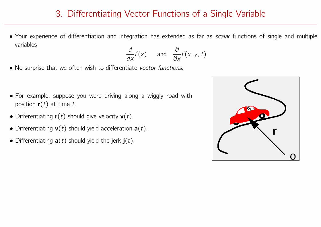
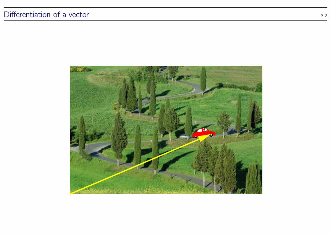
• For example, suppose you were driving along a wiggly road withposition r(t) at time t.

• Differentiating r(t) should give velocity v(t).• Differentiating v(t) should yield acceleration a(t).• Differentiating a(t) should yield the jerk j(t).

r

o

Differentiation of a vector 3.2

Differentiation of a vector 3.3

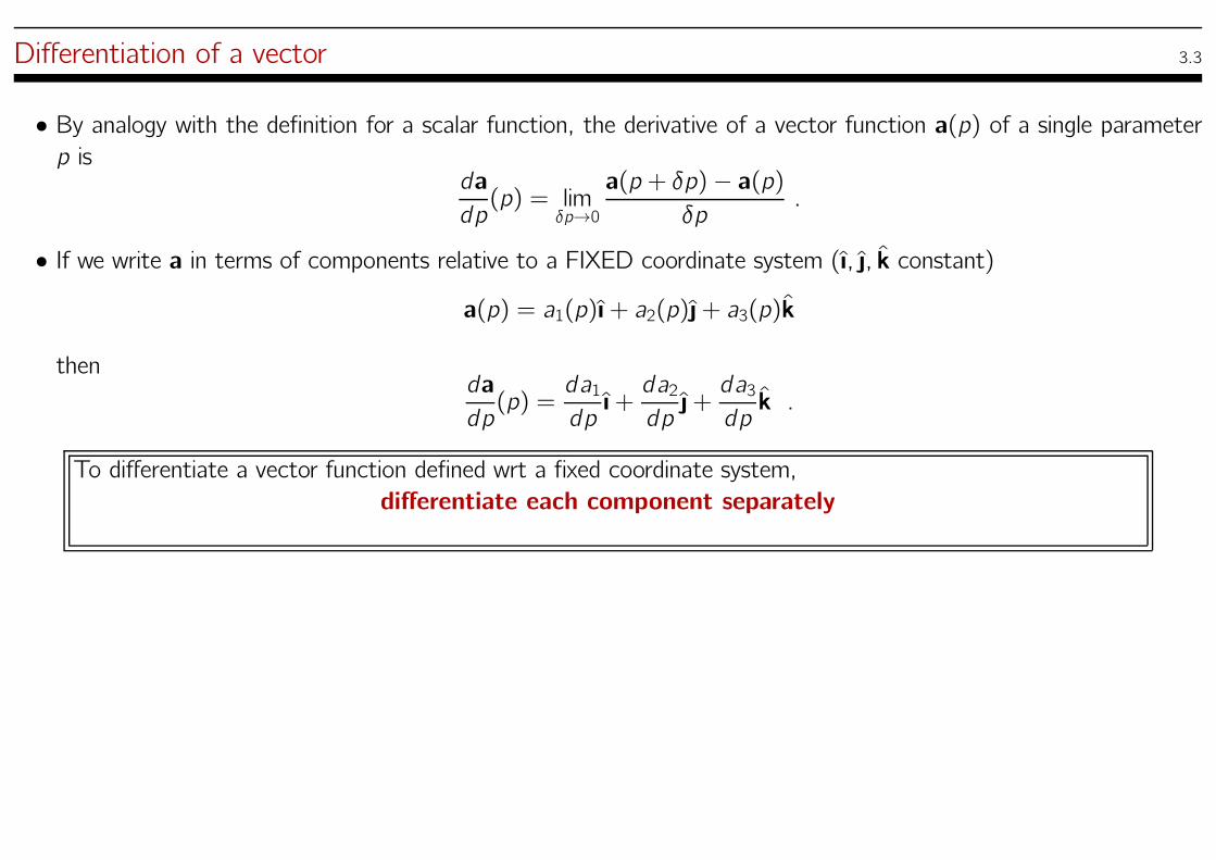
• By analogy with the definition for a scalar function, the derivative of a vector function a(p) of a single parameterp is

da

dp(p) = lim

δp→0

a(p + δp)− a(p)δp

.

• If we write a in terms of components relative to a FIXED coordinate system (ı, , k constant)

a(p) = a1(p)ı+ a2(p)+ a3(p)k

thenda

dp(p) =

da1dpı+da2dp+da3dpk .

To differentiate a vector function defined wrt a fixed coordinate system,

differentiate each component separately

All the familiar stuff works ... 3.4

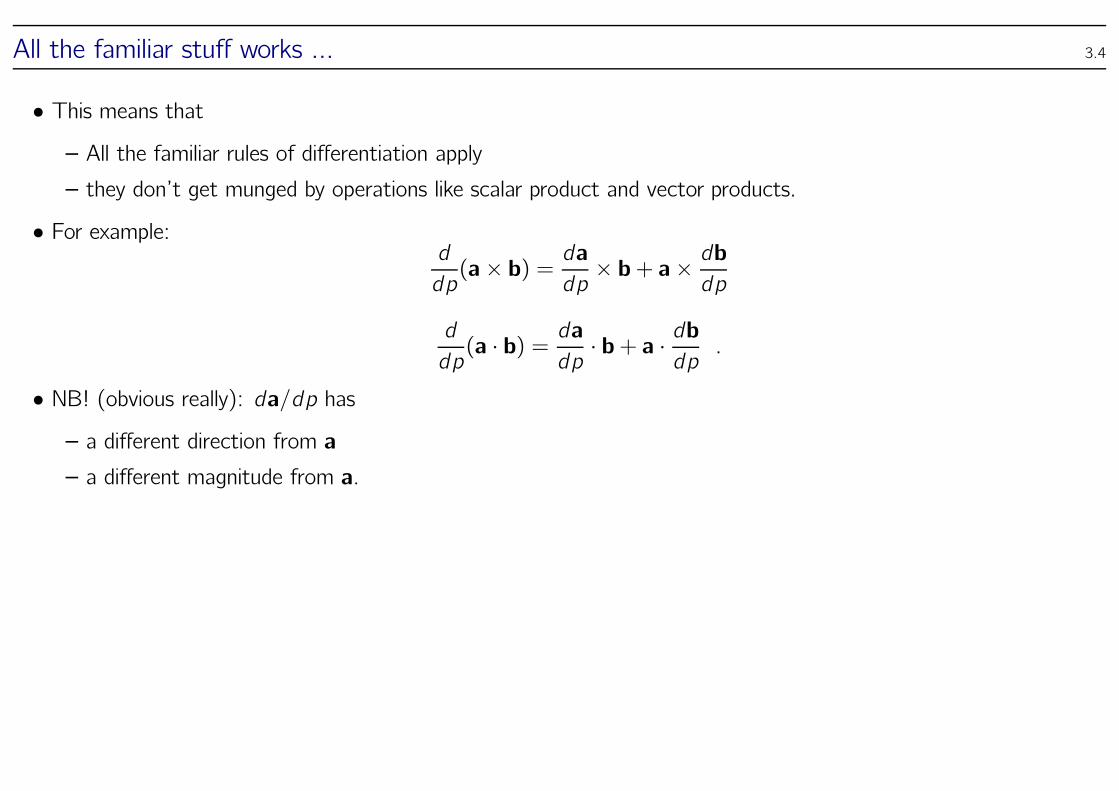
• This means that– All the familiar rules of differentiation apply

– they don’t get munged by operations like scalar product and vector products.

• For example:d

dp(a× b) = da

dp× b+ a× db

dp

d

dp(a · b) = da

dp· b+ a · db

dp.

• NB! (obvious really): da/dp has– a different direction from a

– a different magnitude from a.

Position, velocity and acceleration 3.5

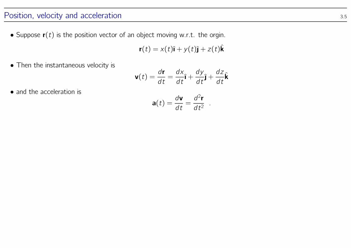
• Suppose r(t) is the position vector of an object moving w.r.t. the orgin.

r(t) = x(t )ı+ y(t ) + z(t)k

• Then the instantaneous velocity isv(t) =

dr

dt=dx

dtı+dy

dt+dz

dtk

• and the acceleration isa(t) =

dv

dt=d2r

dt2.

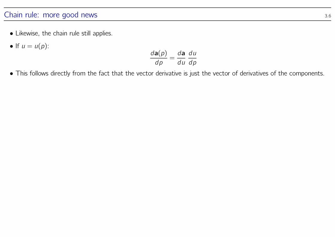
Chain rule: more good news 3.6

• Likewise, the chain rule still applies.• If u = u(p):

da(p)

dp=da

du

du

dp

• This follows directly from the fact that the vector derivative is just the vector of derivatives of the components.

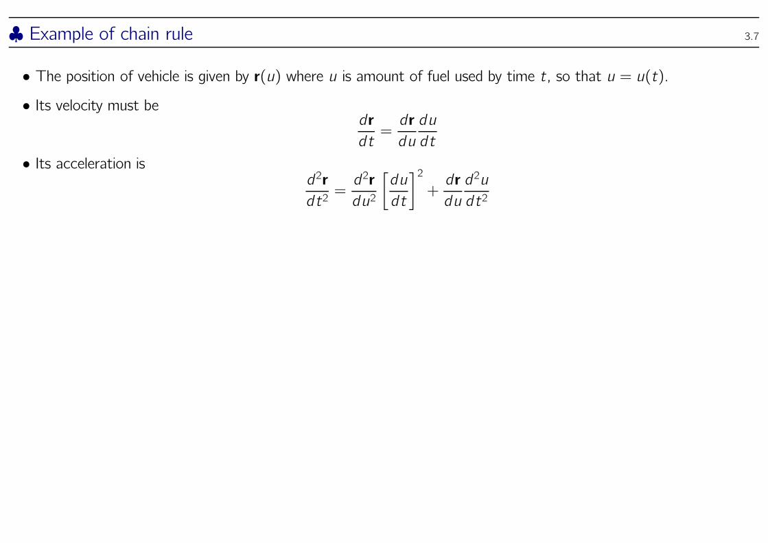
♣ Example of chain rule 3.7

• The position of vehicle is given by r(u) where u is amount of fuel used by time t, so that u = u(t).• Its velocity must be

dr

dt=dr

du

du

dt

• Its acceleration isd2r

dt2=d2r

du2

[

du

dt

]2

+dr

du

d2u

dt2

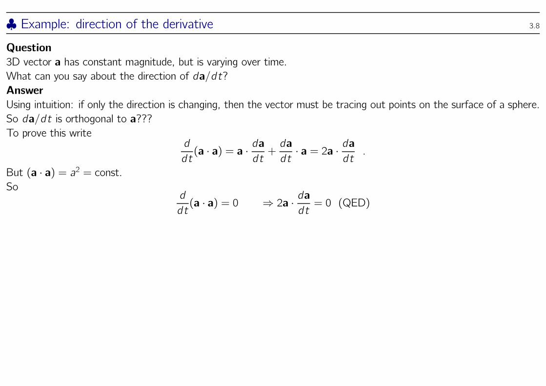
♣ Example: direction of the derivative 3.8

Question

3D vector a has constant magnitude, but is varying over time.

What can you say about the direction of da/dt?

Answer

Using intuition: if only the direction is changing, then the vector must be tracing out points on the surface of a sphere.

So da/dt is orthogonal to a???

To prove this writed

dt(a · a) = a · da

dt+da

dt· a = 2a · da

dt.

But (a · a) = a2 = const.So

d

dt(a · a) = 0 ⇒ 2a · da

dt= 0 (QED)

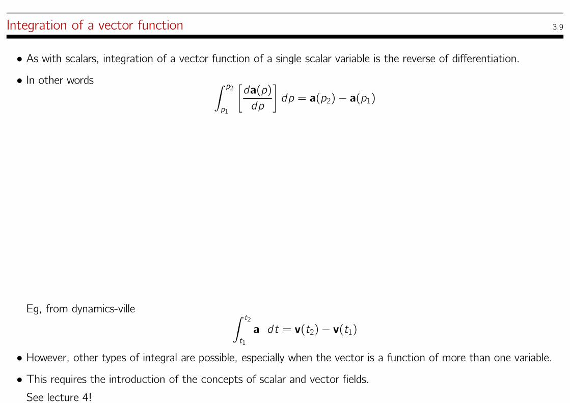
Integration of a vector function 3.9

• As with scalars, integration of a vector function of a single scalar variable is the reverse of differentiation.• In other words

∫ p2

p1

[

da(p)

dp

]

dp = a(p2)− a(p1)

Eg, from dynamics-ville∫ t2

t1

a dt = v(t2)− v(t1)

• However, other types of integral are possible, especially when the vector is a function of more than one variable.• This requires the introduction of the concepts of scalar and vector fields.See lecture 4!

Geometrical interpretation of derivatives 3.10

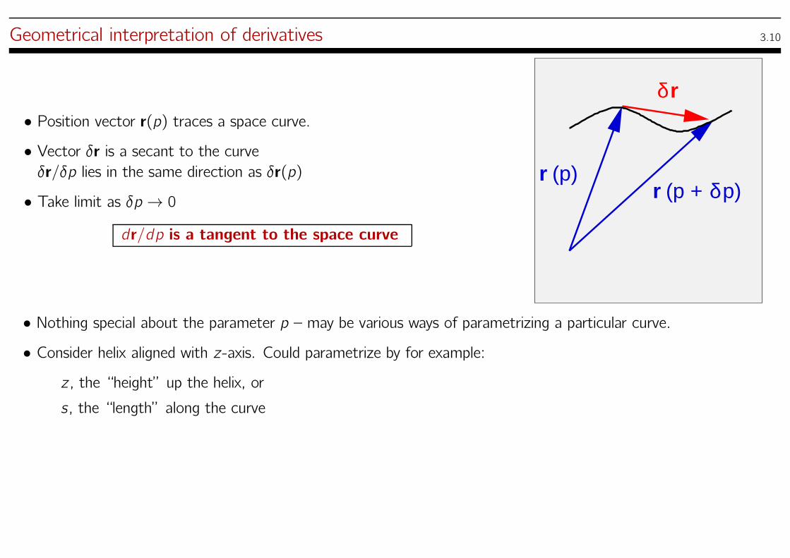
• Position vector r(p) traces a space curve.• Vector δr is a secant to the curveδr/δp lies in the same direction as δr(p)

• Take limit as δp → 0

dr/dp is a tangent to the space curve

δr

r(p)r

p)δ(p +

• Nothing special about the parameter p – may be various ways of parametrizing a particular curve.• Consider helix aligned with z -axis. Could parametrize by for example:

z , the “height” up the helix, or

s , the “length” along the curve

Geometrical interpretation of derivatives /ctd 3.11

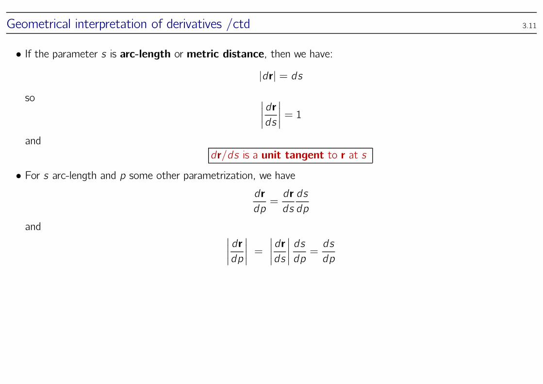
• If the parameter s is arc-length or metric distance, then we have:

|dr| = ds

so∣

∣

∣

∣

dr

ds

∣

∣

∣

∣

= 1

and

dr/ds is a unit tangent to r at s

• For s arc-length and p some other parametrization, we havedr

dp=dr

ds

ds

dp

and∣

∣

∣

∣

dr

dp

∣

∣

∣

∣

=

∣

∣

∣

∣

dr

ds

∣

∣

∣

∣

ds

dp=ds

dp

Geometrical interpretation of derivatives /ctd 3.12

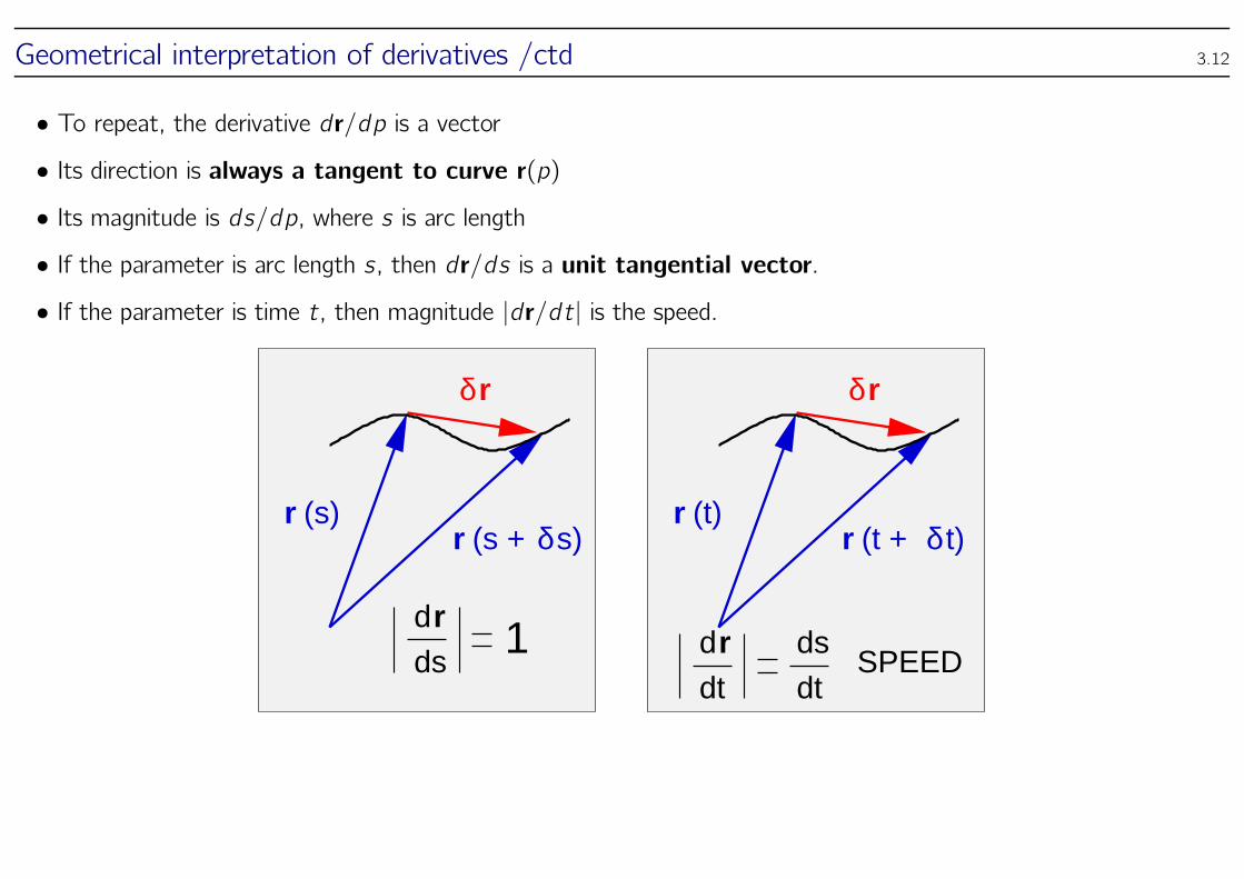
• To repeat, the derivative dr/dp is a vector• Its direction is always a tangent to curve r(p)• Its magnitude is ds/dp, where s is arc length• If the parameter is arc length s , then dr/ds is a unit tangential vector.• If the parameter is time t, then magnitude |dr/dt| is the speed.

ds1

r

rδ

r δ

dr

(s +r (s)

rδ

r δs)(t)

(t + t)

rd

dt

ds

dt SPEED

♣ Example 3.13

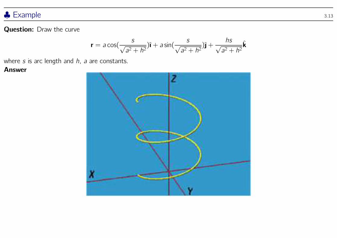
Question: Draw the curve

r = a cos(s√a2 + h2

)ı+ a sin(s√a2 + h2

)+hs√a2 + h2

k

where s is arc length and h, a are constants.

Answer

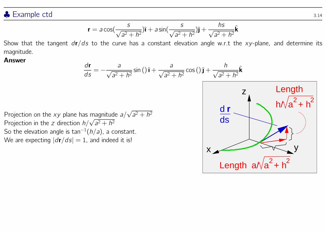
♣ Example ctd 3.14

r = a cos(s√a2 + h2

)ı+ a sin(s√a2 + h2

)+hs√a2 + h2

k

Show that the tangent dr/ds to the curve has a constant elevation angle w.r.t the xy -plane, and determine its

magnitude.

Answerdr

ds= − a√

a2 + h2sin () ı+

a√a2 + h2

cos () +h√a2 + h2

k

Projection on the xy plane has magnitude a/√a2 + h2

Projection in the z direction h/√a2 + h2

So the elevation angle is tan−1(h/a), a constant.We are expecting |dr/ds| = 1, and indeed it is!

22a/ a + h

dds

r2

h/ a + h 2

x y

z

Length

Length

Why can’t we say any old parameter is arc length? 3.15

• Arc length s parameter is special because ds = |dr|,• Or, in integral form, whatever the parameter p,

Accumulated arc length =

∫ p1

p0

∣

∣

∣

∣

dr

dp

∣

∣

∣

∣

dp .

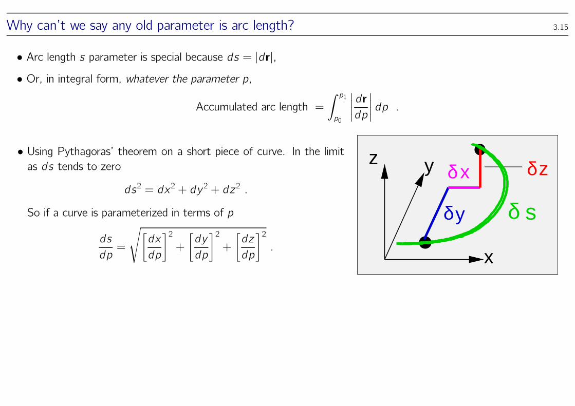
• Using Pythagoras’ theorem on a short piece of curve. In the limitas ds tends to zero

ds2 = dx2 + dy 2 + dz2 .

So if a curve is parameterized in terms of p

ds

dp=

√

[

dx

dp

]2

+

[

dy

dp

]2

+

[

dz

dp

]2

.

z y

x

δy

δzδx

δ s

Arc length is special /ctd 3.16

• Suppose we had parameterized our helix as

r = a cos pı + a sin p + hpk

• p is not arc length because∣

∣

∣

∣

dr

dp

∣

∣

∣

∣

=

√

[

dx

dp

]2

+

[

dy

dp

]2

+

[

dz

dp

]2

=

√

a2 sin2 p + a2 cos2 p + h2

=√

a2 + h2

6= 1

• So if we want to parameterize in terms of arclength, replace p with s/√a2 + h2.

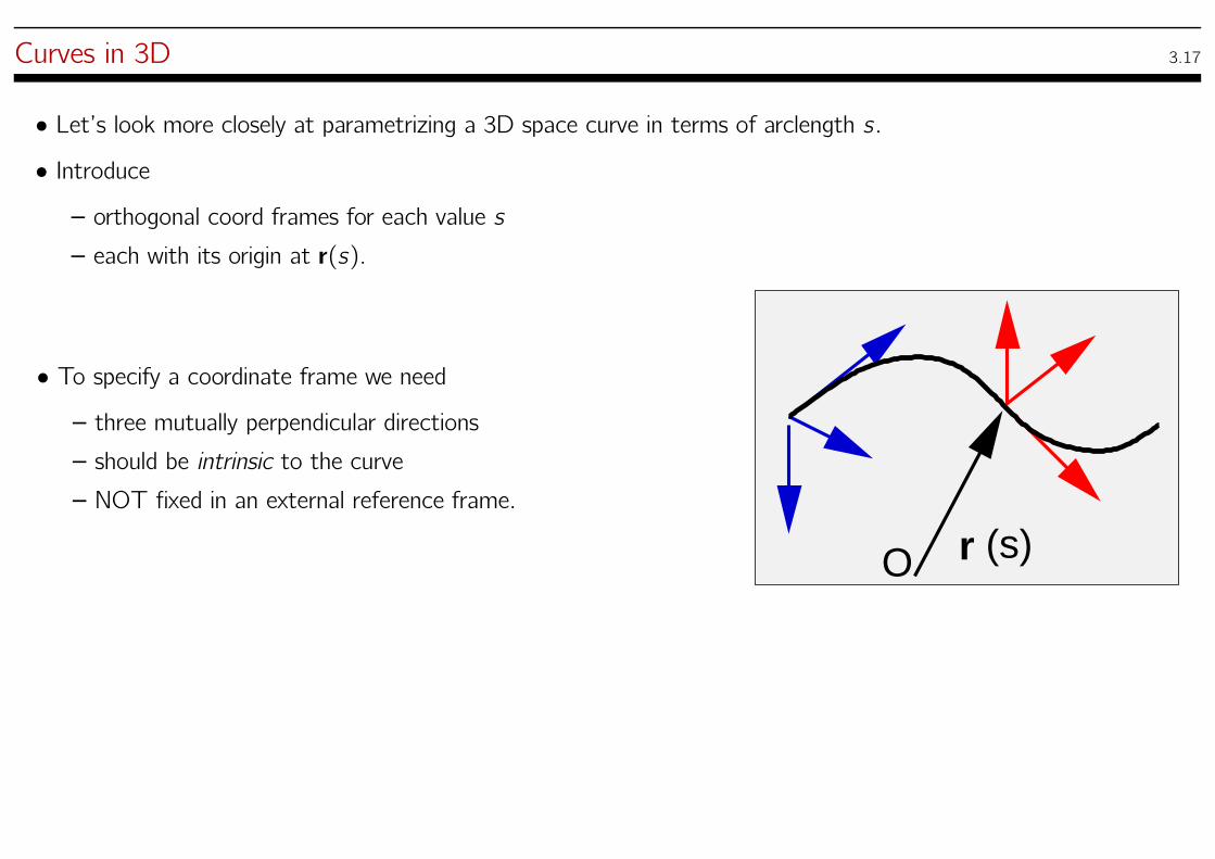
Curves in 3D 3.17

• Let’s look more closely at parametrizing a 3D space curve in terms of arclength s .• Introduce– orthogonal coord frames for each value s

– each with its origin at r(s).

• To specify a coordinate frame we need– three mutually perpendicular directions

– should be intrinsic to the curve

– NOT fixed in an external reference frame.

r (s)O

Curves in 3D 3.18

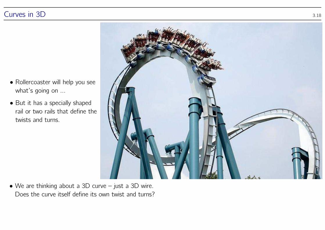
• Rollercoaster will help you seewhat’s going on ...

• But it has a specially shapedrail or two rails that define the

twists and turns.

• We are thinking about a 3D curve – just a 3D wire.Does the curve itself define its own twist and turns?

The Frenet-Serret Local Coordinates 3.19

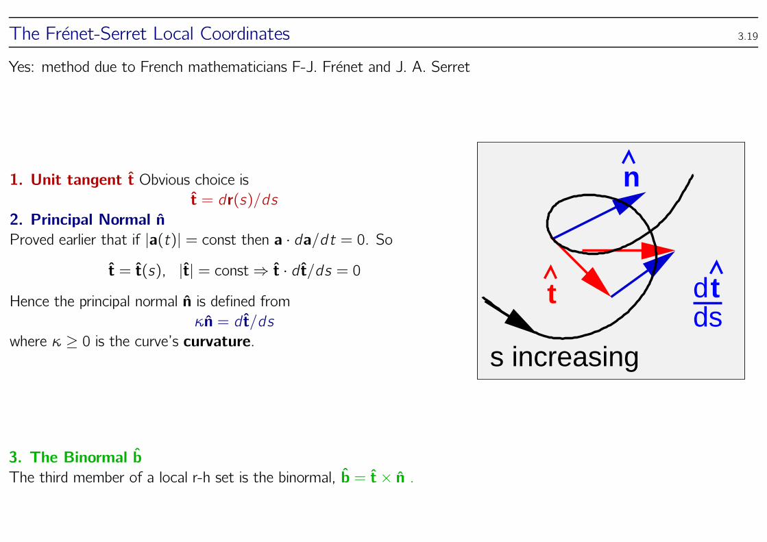
Yes: method due to French mathematicians F-J. Frenet and J. A. Serret

1. Unit tangent t Obvious choice is

t = dr(s)/ds

2. Principal Normal n

Proved earlier that if |a(t)| = const then a · da/dt = 0. So

t = t(s), |t| = const⇒ t · d t/ds = 0

Hence the principal normal n is defined from

κn = d t/ds

where κ ≥ 0 is the curve’s curvature.

n

t dds

t

s increasing

3. The Binormal b

The third member of a local r-h set is the binormal, b = t× n .

Deriving the Frenet-Serret relationships 3.20

Tangent t, Normal n : d t/ds = κn, Binormal b = t× n• Since b · t = 0, if we differentiate wrt s ...

d b

ds· t+ b · d t

ds=d b

ds· t+ b · κn = 0

from whichd b

ds· t = 0.

• This means that d b/ds is along the direction of n:

d b

ds= −τ(s)n(s)

where τ is the space curve’s torsion.

Deriving the Frenet-Serret relationships 3.21

Tangent t, Normal n, Binormal b = t× nd t/ds = κn, d b/ds = −τ(s)n(s)

• Differentiating n · t = 0:

(d n/ds) · t+ n · (d t/ds) = 0(d n/ds) · t+ n · κn = 0

(d n/ds) · t = −κ

• Now do the same to n · b = 0:

(d n/ds) · b+ n · (d b/ds) = 0(d n/ds) · b+ n · (−τ)n = 0

(d n/ds) · b = +τ

• HENCEd n

ds= −κ(s )t(s) + τ(s)b(s).

Summary of the Frenet-Serret relationships 3.22

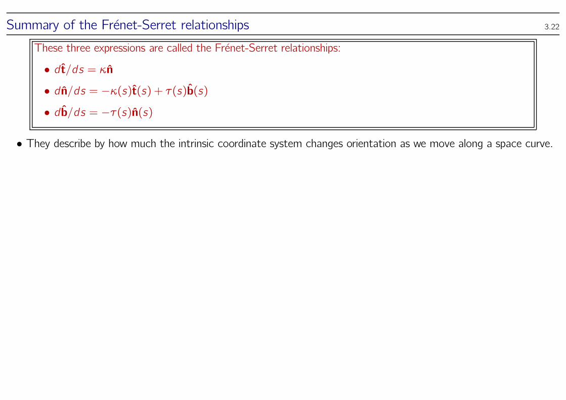
These three expressions are called the Frenet-Serret relationships:

• d t/ds = κn• d n/ds = −κ(s )t(s) + τ(s)b(s)• d b/ds = −τ(s)n(s)

• They describe by how much the intrinsic coordinate system changes orientation as we move along a space curve.

♣ Example 3.23

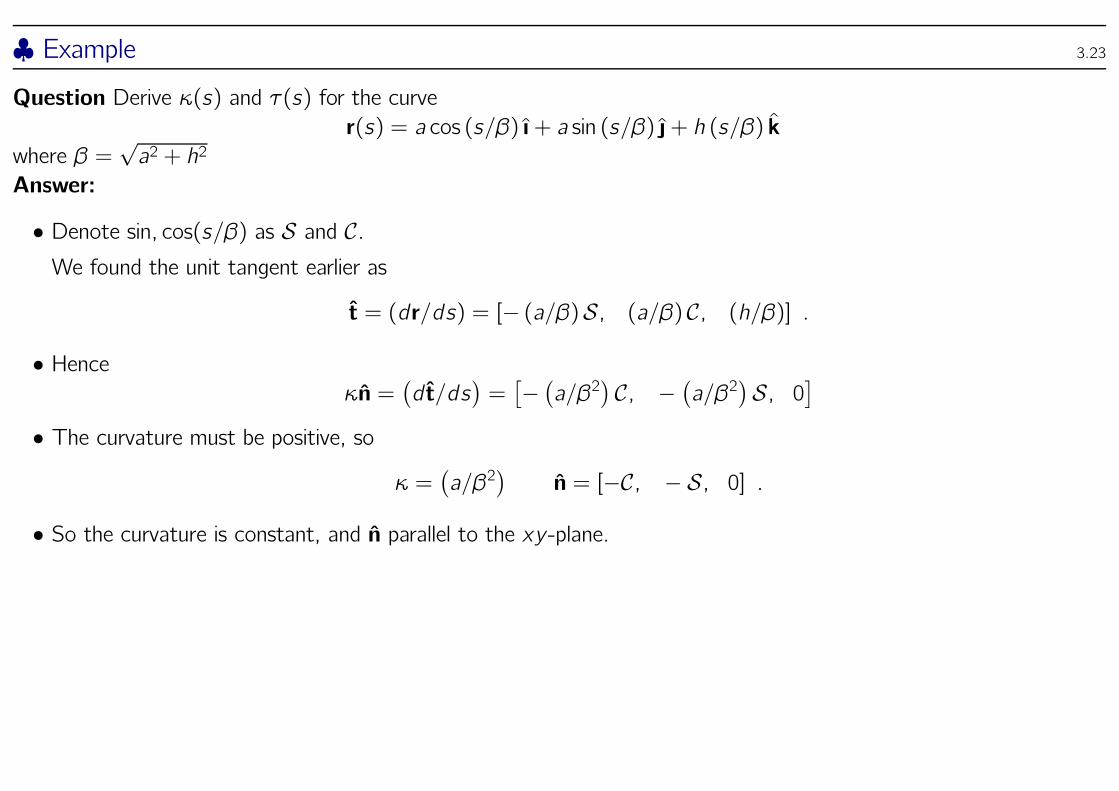
Question Derive κ(s) and τ(s) for the curve

r(s) = a cos (s/β) ı+ a sin (s/β) + h (s/β) k

where β =√a2 + h2

Answer:

• Denote sin, cos(s/β) as S and C.We found the unit tangent earlier as

t = (dr/ds) = [− (a/β)S, (a/β) C, (h/β)] .

• Henceκn =

(

d t/ds)

=[

−(

a/β2)

C, −(

a/β2)

S, 0]

• The curvature must be positive, so

κ =(

a/β2)

n = [−C, − S, 0] .

• So the curvature is constant, and n parallel to the xy -plane.

♣ Example /continued 3.24

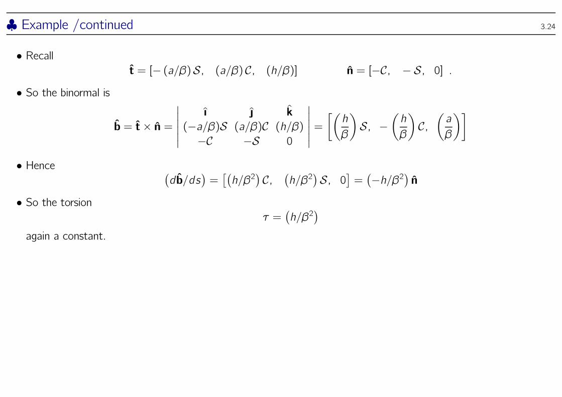
• Recallt = [− (a/β)S, (a/β) C, (h/β)] n = [−C, − S, 0] .

• So the binormal is

b = t× n =

∣

∣

∣

∣

∣

∣

ı k

(−a/β)S (a/β)C (h/β)−C −S 0

∣

∣

∣

∣

∣

∣

=

[(

h

β

)

S, −(

h

β

)

C,(

a

β

)]

• Hence(

d b/ds)

=[(

h/β2)

C,(

h/β2)

S, 0]

=(

−h/β2)

n

• So the torsionτ =

(

h/β2)

again a constant.

Derivative (eg velocity) components in plane polars 3.25

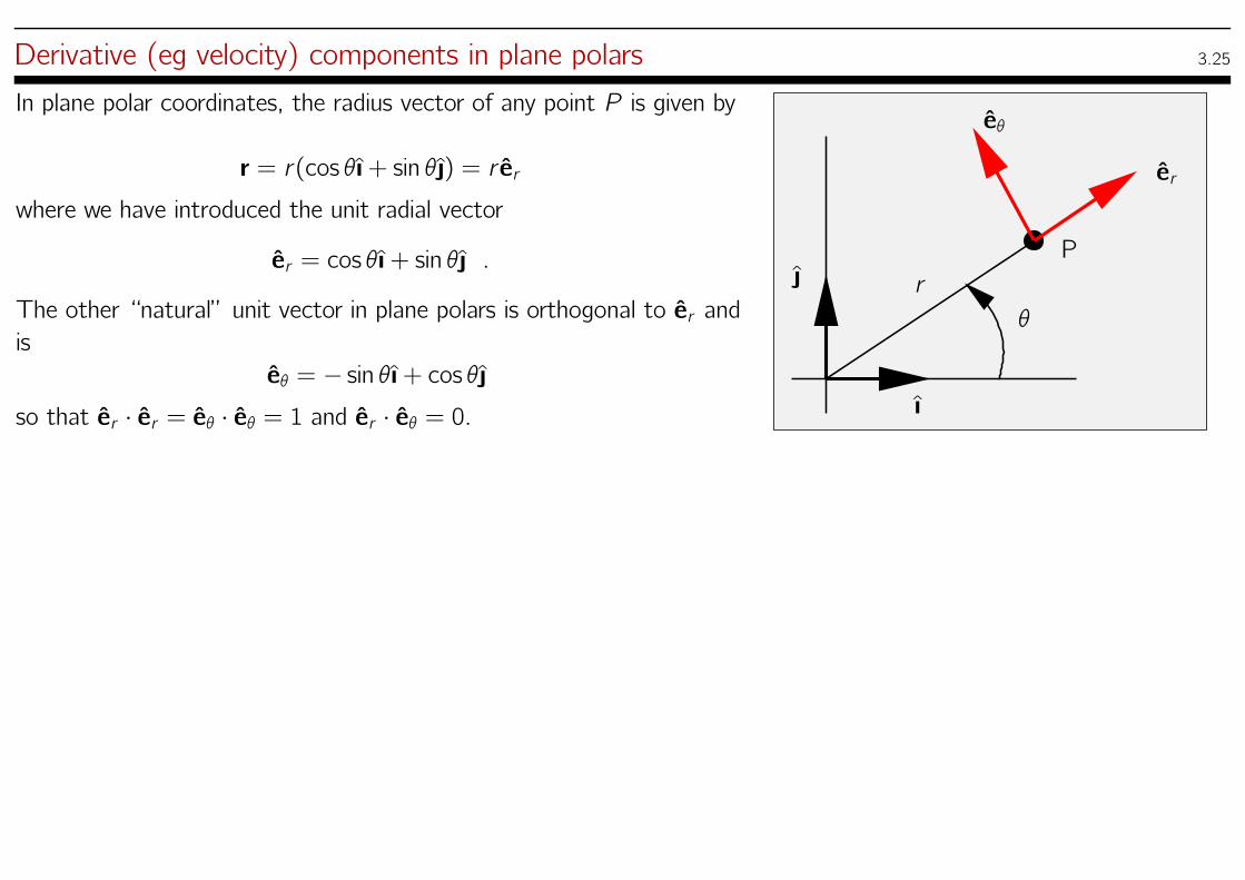
In plane polar coordinates, the radius vector of any point P is given by

r = r(cos θı+ sin θ) = r er

where we have introduced the unit radial vector

er = cos θı+ sin θ .

The other “natural” unit vector in plane polars is orthogonal to er and

is

eθ = − sin θı+ cos θso that er · er = eθ · eθ = 1 and er · eθ = 0.

er

eθ

ı

θ

r

P

Aside: notation 3.26

• Some texts will use the notationr, θθθ

to denote unit vectors in the radial and tangential directions

• I prefer the more general notationer , eθ

(as used in, eg, Riley).

• You should be familiar and comfortable with either

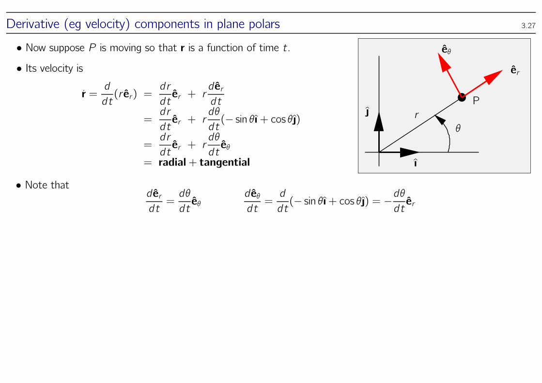
Derivative (eg velocity) components in plane polars 3.27

• Now suppose P is moving so that r is a function of time t.• Its velocity is

r =d

dt(r er) =

dr

dter + r

d erdt

=dr

dter + r

dθ

dt(− sin θı+ cos θ)

=dr

dter + r

dθ

dteθ

= radial+ tangential

er

eθ

ı

θ

r

P

• Note thatd erdt=dθ

dteθ

d eθdt=d

dt(− sin θı+ cos θ) = −dθ

dter

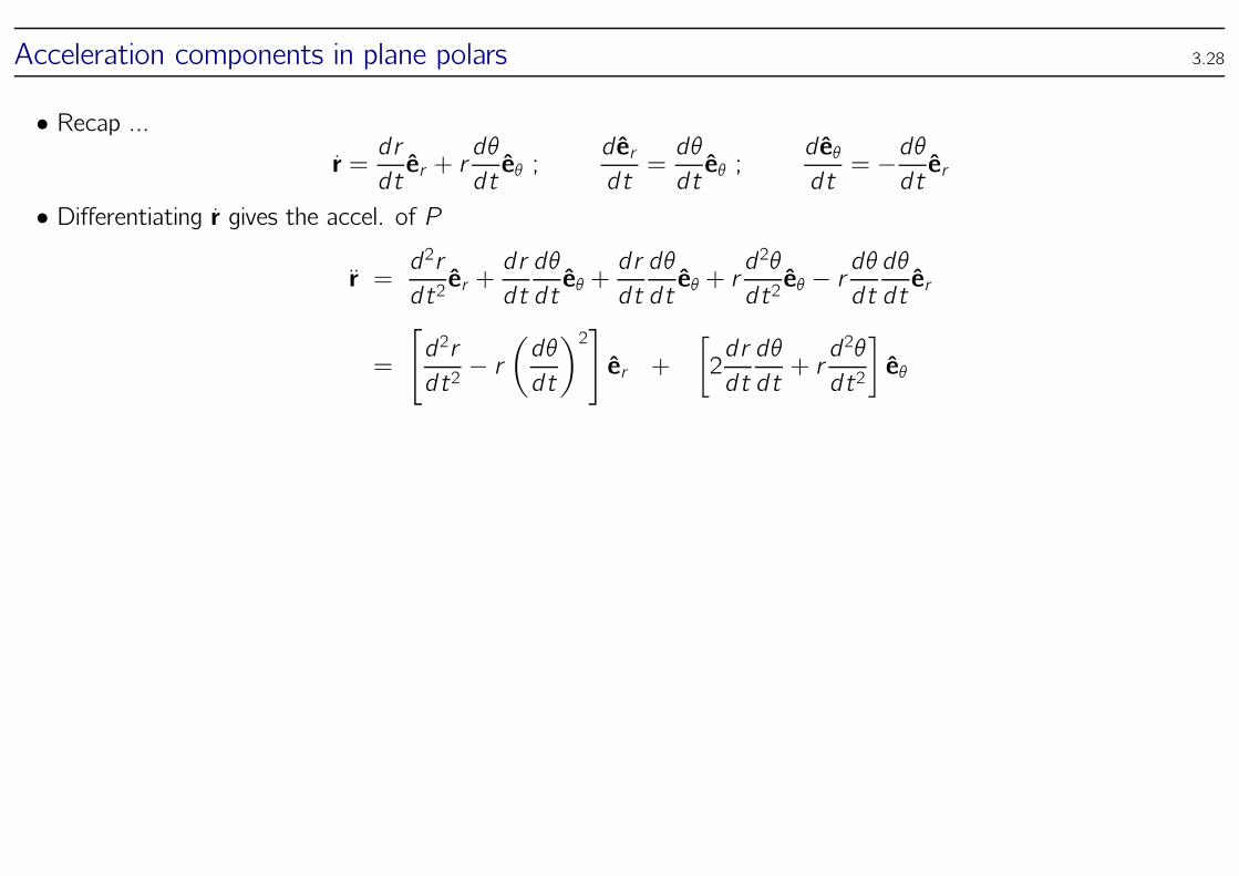
Acceleration components in plane polars 3.28

• Recap ...r =dr

dter + r

dθ

dteθ ;

d erdt=dθ

dteθ ;

d eθdt= −dθdter

• Differentiating r gives the accel. of P

r =d2r

dt2er +

dr

dt

dθ

dteθ +

dr

dt

dθ

dteθ + r

d2θ

dt2eθ − r

dθ

dt

dθ

dter

=

[

d2r

dt2− r

(

dθ

dt

)2]

er +

[

2dr

dt

dθ

dt+ rd2θ

dt2

]

eθ

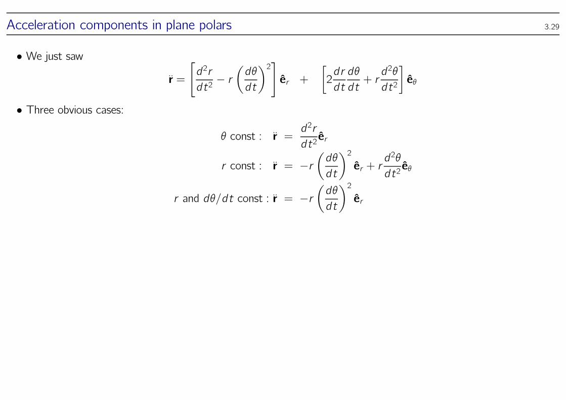
Acceleration components in plane polars 3.29

• We just saw

r =

[

d2r

dt2− r

(

dθ

dt

)2]

er +

[

2dr

dt

dθ

dt+ rd2θ

dt2

]

eθ

• Three obvious cases:

θ const : r =d2r

dt2er

r const : r = −r(

dθ

dt

)2

er + rd2θ

dt2eθ

r and dθ/dt const : r = −r(

dθ

dt

)2

er

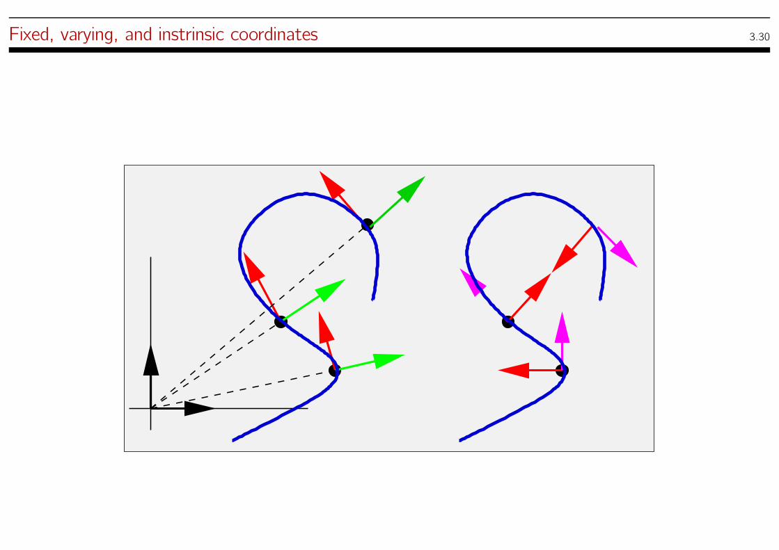
Fixed, varying, and instrinsic coordinates 3.30

Rotating systems 3.31

• Body rotates with constant ω about axis passingthrough the body origin.

Assume the body origin is fixed.

We observe from a fixed coord system Oxyz .

ω

ρ

• If ρ is a vector of constant mag and constant direction in the rotating system, then in the fixed system it must bea function of t.

r(t) = R(t)ρ ⇒ dr

dt= Rρ = RR⊤r

* dr/dt will have fixed magnitude;

* dr/dt will always be perpendicular to the axis of rotation;

* dr/dt will vary in direction within those constraints;

* r(t) will move in a plane in the fixed system.

Rotating systems 3.32

Consider the term RR⊤

• Note that RR⊤ = I, hence

RR⊤ + RR⊤ = 0

RR⊤ = −RR⊤

• Thus RR⊤ is anti-symmetric:

RR⊤ =

0 −z y

z 0 −x−y x 0

• Application of a matrix of this form to an arbitrary vector has precisely the same effect as the cross productoperator, ω×, where ω = [xyz ]⊤.• Thus

r = ω × r

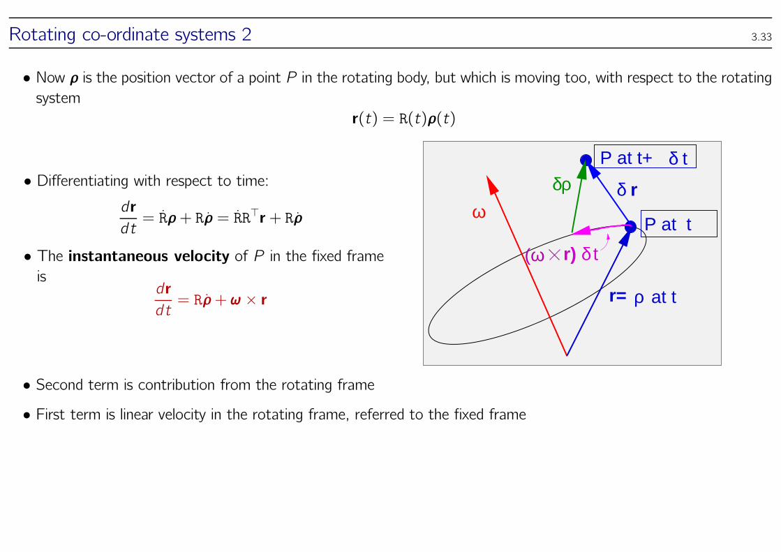
Rotating co-ordinate systems 2 3.33

• Now ρ is the position vector of a point P in the rotating body, but which is moving too, with respect to the rotatingsystem

r(t) = R(t)ρ(t)

• Differentiating with respect to time:dr

dt= Rρ+ Rρ = RR⊤r + Rρ

• The instantaneous velocity of P in the fixed frameis

dr

dt= Rρ+ ω × r

δρ δ

P at t+

r= at tρ

r

P at t

δ t

ω

(ω r) δ t

• Second term is contribution from the rotating frame• First term is linear velocity in the rotating frame, referred to the fixed frame

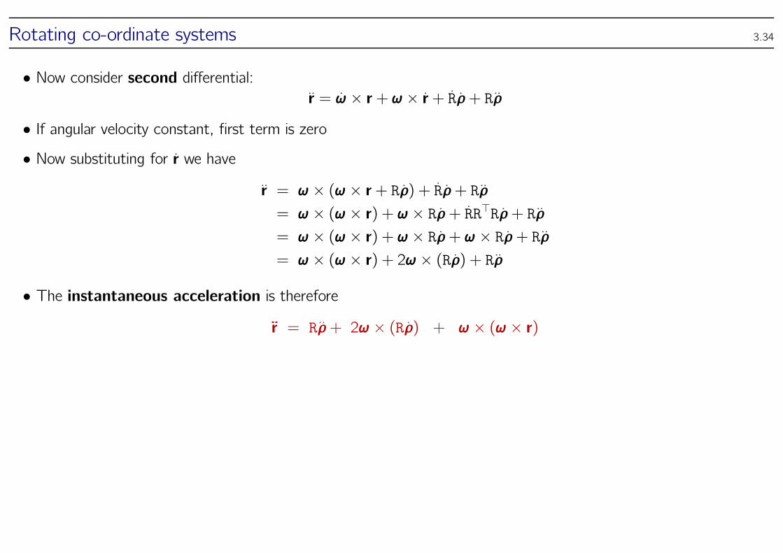
Rotating co-ordinate systems 3.34

• Now consider second differential:r = ω × r + ω × r + Rρ+ Rρ

• If angular velocity constant, first term is zero• Now substituting for r we have

r = ω × (ω × r + Rρ) + Rρ+ Rρ= ω × (ω × r) + ω × Rρ+ RR⊤Rρ+ Rρ= ω × (ω × r) + ω × Rρ+ ω × Rρ+ Rρ= ω × (ω × r) + 2ω × (Rρ) + Rρ

• The instantaneous acceleration is therefore

r = Rρ+ 2ω × (Rρ) + ω × (ω × r)

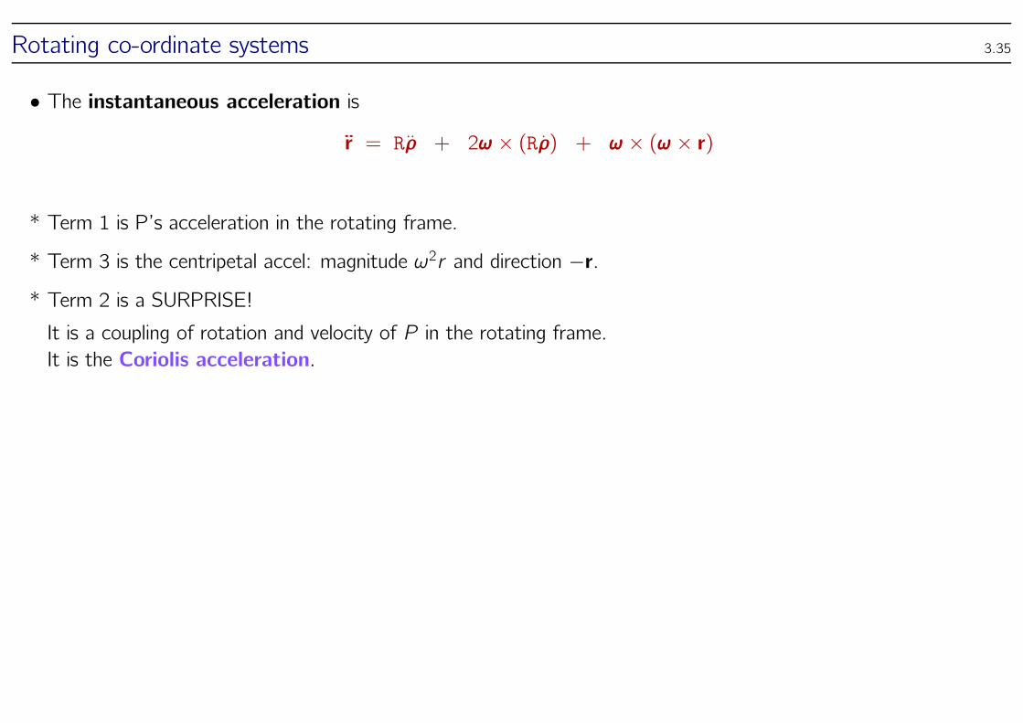
Rotating co-ordinate systems 3.35

• The instantaneous acceleration is

r = Rρ + 2ω × (Rρ) + ω × (ω × r)

* Term 1 is P’s acceleration in the rotating frame.

* Term 3 is the centripetal accel: magnitude ω2r and direction −r.* Term 2 is a SURPRISE!

It is a coupling of rotation and velocity of P in the rotating frame.

It is the Coriolis acceleration.

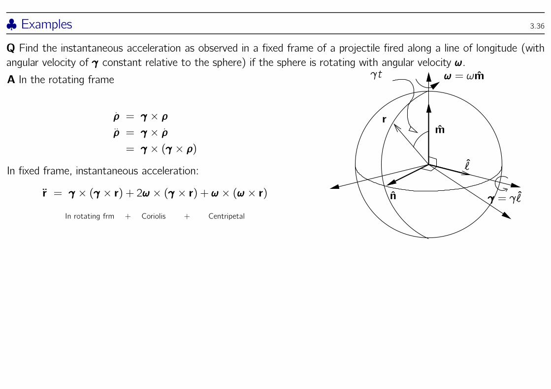
♣ Examples 3.36

Q Find the instantaneous acceleration as observed in a fixed frame of a projectile fired along a line of longitude (with

angular velocity of γ constant relative to the sphere) if the sphere is rotating with angular velocity ω.

A In the rotating frame

ρ = γ × ρρ = γ × ρ= γ × (γ × ρ)

In fixed frame, instantaneous acceleration:

r = γ × (γ × r) + 2ω × (γ × r) + ω × (ω × r)

In rotating frm + Coriolis + Centripetal

r

γt ω = ωm

m

n

ℓ

γ = γℓ

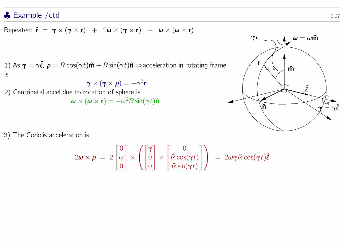
♣ Example /ctd 3.37

Repeated: r = γ × (γ × r) + 2ω × (γ × r) + ω × (ω × r)

1) As γ = γℓ, ρ = R cos(γt)m+R sin(γt)n ⇒acceleration in rotating frameis

γ × (γ × ρ) = −γ2r2) Centripetal accel due to rotation of sphere is

ω × (ω × r) = −ω2R sin(γt)n

r

γt ω = ωm

m

n

ℓ

γ = γℓ

3) The Coriolis acceleration is

2ω × ρ = 2

0

ω

0

×

γ

0

0

×

0

R cos(γt)

R sin(γt)

= 2ωγR cos(γt)ℓ

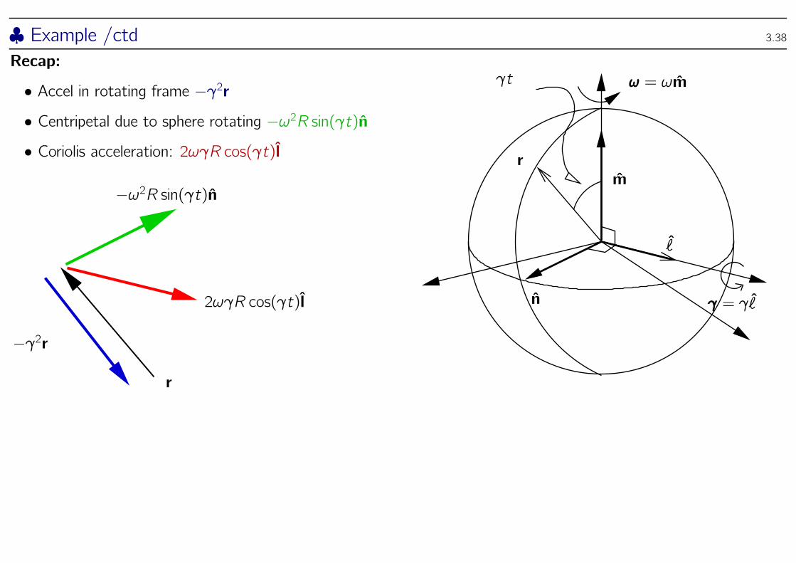
♣ Example /ctd 3.38

Recap:

• Accel in rotating frame −γ2r• Centripetal due to sphere rotating −ω2R sin(γt)n• Coriolis acceleration: 2ωγR cos(γt )l

2ωγR cos(γt )l

−ω2R sin(γt)n

−γ2r

r

r

γt ω = ωm

m

n

ℓ

γ = γℓ

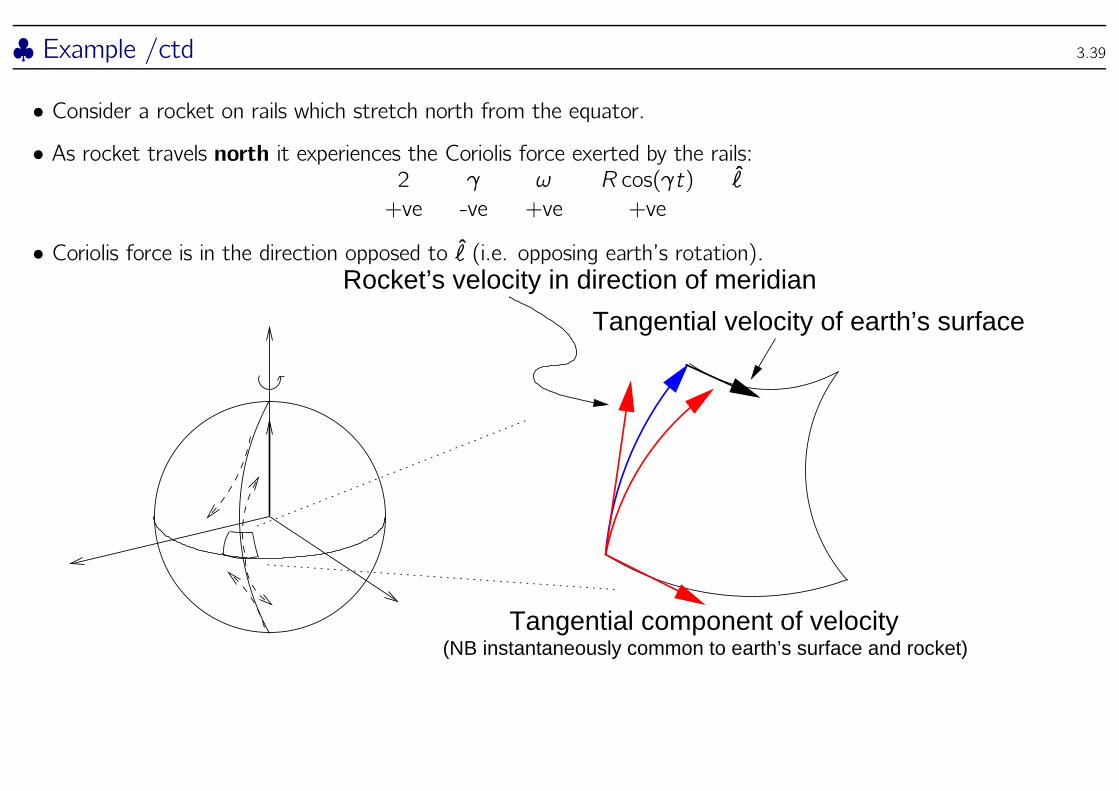
♣ Example /ctd 3.39

• Consider a rocket on rails which stretch north from the equator.• As rocket travels north it experiences the Coriolis force exerted by the rails:

2 γ ω R cos(γt) ℓ

+ve -ve +ve +ve

• Coriolis force is in the direction opposed to ℓ (i.e. opposing earth’s rotation).

(NB instantaneously common to earth’s surface and rocket)Tangential component of velocity

Rocket’s velocity in direction of meridian

Tangential velocity of earth’s surface

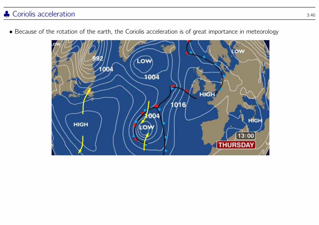
♣ Coriolis acceleration 3.40

• Because of the rotation of the earth, the Coriolis acceleration is of great importance in meteorology

♣ Coriolis acceleration 3.41

Summary 3.42

• We started by differentiating vectors wrt to a fixed coordinate system.• Then looked at the properties of the derivative of a position vector r with respect to a general parameter p and thespecial parameters of arc-length s , and time t

• considered derivatives with respect to other coordinate systems, in particular those of the position vector in polarcoordinates with respect to time.

• derived Frenet-Serret relationships — a method of describing a 3D space curve by describing the change in a intrinsiccoordinate system as it moves along the curve.

• discussed rotating coordinate systems; we saw that there is coupled term in the acceleration, called the Coriolisacceleration.