Embed Size (px)
Citation preview

Underwater Optical Wireless Communications
Dr Mark Leeson
School of Engineering
University of Warwick
Acknowledgements:

Contents Introduction
Current Underwater Technology: Acoustic & RF
Technology Comparisons
The Underwater Channel
Channel Modelling
Scattering & its Modelling
Impact of Link Orientation
Maximum Link Distance
Practical Link Distance Prediction
A Fuller Treatment
Field of View (FOV) Simulation
Conclusions
Future Directions
2

Where is the University of Warwick?
3

Connected Systems Research Group
Within Connected Systems, the Communication Systems Lab (https://www2.warwick.ac.uk/fac/sci/eng/research/grouplist/connectedsystems) is home to research in Photonic Systems, Optical Technology, Wireless Communications, Machine Learning and Nanoscale Communications. The fundamental advances in the laboratory will produce impact in areas such as next generation mobile data networks, vehicular communications and future healthcare monitoring systems.
4
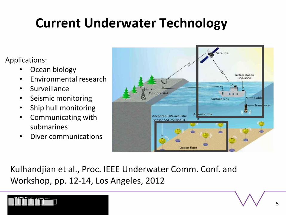
Current Underwater Technology
Applications: • Ocean biology • Environmental research • Surveillance • Seismic monitoring • Ship hull monitoring • Communicating with
submarines • Diver communications
Kulhandjian et al., Proc. IEEE Underwater Comm. Conf. and Workshop, pp. 12-14, Los Angeles, 2012
5

Acoustics: Current Technology
Typical application, adapted from Heidemann et al., IEEE WCNC Conference, pp. 228-235,2006.
6
Typical modem (Evo Logics)

Path Loss –absorption
7
signal loss from conversion of acoustic energy to heat, denoted by a(f) Thorp’s empirical approximation:
Path Loss -Spreading Loss
8
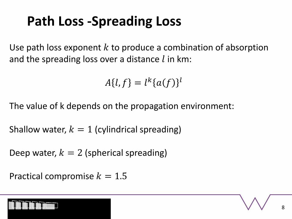
Use path loss exponent 𝑘 to produce a combination of absorption and the spreading loss over a distance 𝑙 in km:
𝐴 𝑙, 𝑓 = 𝑙𝑘 𝑎 𝑓 𝑙 The value of k depends on the propagation environment: Shallow water, 𝑘 = 1 (cylindrical spreading) Deep water, 𝑘 = 2 (spherical spreading) Practical compromise 𝑘 = 1.5

Noise
From turbulence, shipping, wind and heat
9
Operating region

Attenuation Noise (AN) Factor
10
Consider a narrow band of frequencies ∆𝑓 about some centre
frequency 𝑓𝑐
𝑆𝑁𝑅 = 𝑆 𝑓 𝐴 𝑙, 𝑓 𝑁 𝑓 ∆𝑓
The quantity 𝐴 𝑙, 𝑓 𝑁 𝑓 is known as the attenuation noise (AN)
factor 0.5
km
3 km
BW increasingly
limited

RF is also established
Typical application from Edwards, New buoys enable submerged subs to communicate https://phys.org/news/2010-07-buoys-enable-submerged-subs.html
11

RF Attenuation in Sea Water
12
(Lanzagorta, Underwater Communications, Morgan & Claypool, 2013)

RF Implementations vs. Acoustic
13
(Adapted from Lloret et al., Sensors, 2012)
Technology Frequency Modulation Distance Data Rate
RF 100 kHz BPSK 6 m 1 kbps
RF 10 kHz BPSK 16 m 1 kbps
RF 1 kHz BPSK 2 m 1 kbps
Acoustic 800 kHz BPSK 1 m 80 kbps
Acoustic 24 kHz QPSK 2500 m 30 kbps
Acoustic 70 kHz ASK 70 m 200 bps
RF 2.4 GHz QPSK 0.17 m 2 Mbps
RF 2.4 GHz CCK 0.16 m 11 Mbps

Future Technology
14
Goals
• Higher bandwidth
• Communication through the air/water interface
• Secure/covert
Optical wireless is a possible solution:
transmission of a modulated light beam through an
open environment to obtain broadband communication

UOWC Performance Results
15
Types of lasers operating in blue-green spectrum
Distance Power Source Data Rate
20 - 30 m 500 mW Blue LED Few kbps
200 m 5 W LED 1.2 Mbps
30 m (pool) 3 m (ocean)
5 W Laser 1.2 Mbps 0.6 Mbps
2 m 10 mW Laser 1 Gbps
30 - 50 m 1 W Laser 1 Gbps
31 m (deep sea) 18 m (clean ocean) 11 m (coastal)
100 mW LED 1 Gbps
64 m (clear ocean) 8 m (turbid harbour)
3 W Laser 5 Gbps 1 Gbps
7 m (coastal) 12 mW Laser 2.3 Gbps
5.4 m 15 mW Laser 4.8 Gbps
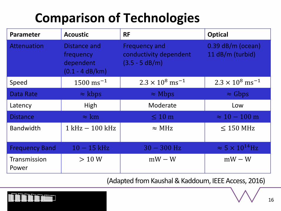
Comparison of Technologies
16
Parameter Acoustic RF Optical
Attenuation Distance and frequency dependent (0.1 - 4 dB/km)
Frequency and conductivity dependent (3.5 - 5 dB/m)
0.39 dB/m (ocean) 11 dB/m (turbid)
Speed 1500 ms−1 2.3 × 10⁸ ms−1 2.3 × 10⁸ ms−1
Data Rate ≈ kbps ≈ Mbps ≈ Gbps
Latency High Moderate Low
Distance ≈ km ≤ 10 m ≈ 10 − 100 m
Bandwidth 1 kHz − 100 kHz ≈ MHz ≤ 150 MHz
Frequency Band 10 − 15 kHz 30 − 300 Hz ≈ 5 × 10¹⁴Hz
Transmission Power
> 10 W mW − W mW − W
(Adapted from Kaushal & Kaddoum, IEEE Access, 2016)

Underwater Technology Comparison Acoustic: long range (km); low bandwidth (kHz); low
efficiency (~100 bits J-1 – 10000 J bit-1)*
Radio frequency: short range (<10m); low bandwidth (kHz); energy efficient (~6kbits J-1 – 166 J bit-1)+
Optical wireless: short-mid range (up to 100s of m); high bandwidth (GHz); very energy efficient (30k bits J-1 – 33 J bit-1)*
* e.g. Farr et al., OCEANS 2010 IEEE, Sydney, 24-27 May 2010; +e.g. O’Rourke et al., WUWNet, Los Angeles, California, 2012.
17

Underwater Optical Wireless Links
18
LOS point-to-point LOS diffuse
Retroreflector diffuse Non-LOS diffuse
LOS boundary
Configurations

Underwater Scenarios
Atlantic Ocean Thames, UK
Laser likely
Longer range
Tracking
LED likely
Shorter range
Multipath
19

The Underwater Channel
20
Photosynthetic life
Light too faint to support
photosynthesis
No light passes
Coastal Oceanic
Ocean Zones

Jerlov Water Types
21
Water types divided into two categories:
oceanic (blue water) with 3 subdivisions
Type I: extremely pure ocean water
Type II: tropical-subtropical water
Type III: mid-latitude water
coastal (littoral zone) subdivided into nine types
Type 1 – least turbid
…
Type 9 – most turbid

22
Transmittance of Water Types
Jerlov, 1976

Channel Variation
23
Image: Google Earth (accessed 03/03/13)
1
2
3

Absorption Variation
24

Transmission Window Electromagnetic attenuation in water
25
Adapted from http://www1.lsbu.ac.uk/water/water_vibrational_spectrum.html

Light Sources: Lasers
26
Type Wavelength Advantages Disadvantages
Argon-ion 455-529 nm High output - Low efficiency; needs high input power; needs cooling
Nd:YAG 532 nm (green) 473 nm (blue)
Very high output power; long life time; compact
Variable efficiency; costly; can be hard to modulate
Ti: Sapphire 455 nm Ultra fast output; tunable
Costly; sensitive to vibrations
Metal vapour 441.6 nm, 570 nm and 578 nm High power; long life time
Requires cooling
Dye 450 nm - 530 nm Very high power ; tunable; high data rate
Costly; requires cooling arrangements
Semiconductor 405 nm & 450 - 470 nm (InGaN) 375 nm to 473 nm (GaN)
Highly efficient; compact
Costly; easily damaged due to over current
(Adapted from Kaushal & Kaddoum, IEEE Access, 2016)

Light Sources: LEDs
27
Manufacturer Wavelength (nm) Luminous Flux (Im)
Lamina Atlas NT-42C1-0484 460 - 470 63
AOP LED Corp PU-5WAS 455 - 475 54
Kingbright AAD1-
9090QB11ZC/3 460 35.7
Ligitek LGLB-313E 460 - 475 30.6
Toshiba TL12B01(T30) 460 6
Lumex SML-LX1610USBC 470 5
(Adapted from Kaushal & Kaddoum, IEEE Access, 2016)

Channel Modelling
Beer’s Law: At a depth 𝑧 and a wavelength , the optical
path loss as a function of distance 𝐿 may be approximated
by: 𝑒−𝑐 𝜆,𝑧 𝐿 The attenuation coefficient is made up of: 𝑐 𝜆, 𝑧 = 𝑎 𝜆, 𝑧 + 𝑏 𝜆
Attenuation = absorption + scattering
Typical Ballpark Values
Water type 𝑎 𝑚−1 𝑏 𝑚−1
Clean water 0.114 0.037
Turbid water 0.226 1.824
28

Optically Significant Components of Aquatic Media
29

Channel Variation
30

Channel Variation
31

Attenuation from Components
32
Pure water Phytoplankton CDOM*
*colour dissolved organic material -dead & decaying organic matter

Scattering
33
Process causing changes in the direction of electromagnetic energy in an optical beam due to localised nonuniformities - from different particles within the medium - medium state variations resulting in varying refractive index

Scattering
34
Pure seawater and particulate scattering spectra, where
small particles are defined as having a diameter < 1 µm.
(data from Haltrin, 1999)

Modelling Scattering
35
Define volume
scattering function
(VSF), 𝛽 𝜃, 𝜆 to
describe angular
distribution of scattered
light to the incident
irradiance per unit
volume. For unpolarised incident light and isotropic water,
the scattering becomes angular dependent and
VSF for an angle θ into a solid angle ∆Ω is:
𝛽 𝜃, 𝜆 = lim∆𝑟→0
lim∆Ω→0
∆𝐵 𝜃, 𝜆
∆𝑟∆Ω
Inherent optical property geometry (Mobley, 1994)

Modelling Scattering
36
Alternatively, use the angle between the direction vector
of the incoming light 𝐧 and the direction vector of the
scattered light 𝒏′ and relate it to scattering phase
function 𝛽 𝒓, 𝜃 (that describes the angular distribution of
the scattered photons) by β 𝐫, 𝐧, 𝐧′ = 𝑏𝛽 𝒓, 𝜃 , where θ
is defined as the scattering angle between 𝒏 and 𝒏′, i.e.
𝒏. 𝒏′ = cos 𝜃.
Form of 𝛽 𝒓, 𝜃 is a subject of ongoing work, the
historical versions such as Henyey-Greenstein (HG) are
old and not up to the job.

3D Simulation Model
37
𝑥 (a. u. )
𝑦 (a.
u.)
Cross-section through output

3D Model: Scattering Effect
38
metres
relative power

Impact of Link Orientation
39
T
T
T non-refracted
path
T
refracted path
refractive index attenuation coefficient

Link Orientation: Why it Matters
40
T
T R T
T
R
R R
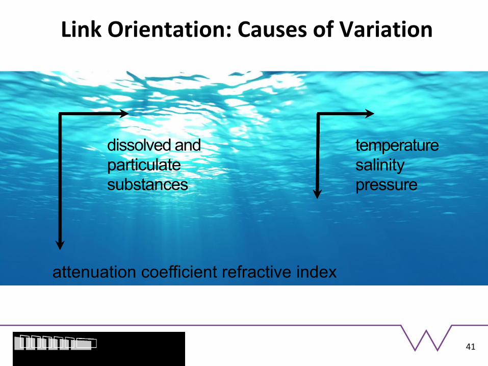
Link Orientation: Causes of Variation
41
attenuation coefficient refractive index
dissolved and particulate substances
temperature salinity pressure

Attenuation Variation
Simulation of 200m links from a fixed starting position with average attenuation for each angle recorded
42
attenuation coefficient (m-1)

Attenuation Variation
Attenuation with depth is
found using bio-optical
models of phytoplankton
with depth and relations
between constituent
concentrations
43
0
50
100
150
200
250
De
pth
in
me
tre
s
attenuation coefficient (m-1)
Johnson, Green and Leeson, App. Opt. 52(33), 2013
0 0.1 0.2

Attenuation Variation
Johnson, Green and Leeson, App. Opt. 52(33), 2013
Specific case for illustration purposes Type “S3”
44

Absorption with Depth
45

Maximum Link Distance
46
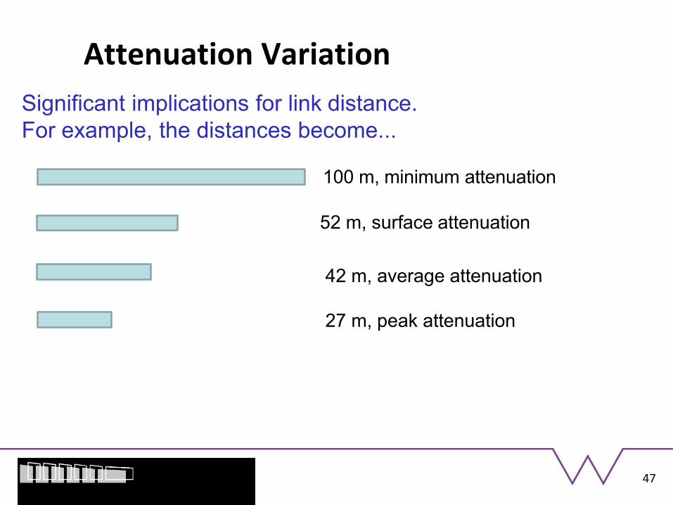
Attenuation Variation
47
100 m, minimum attenuation
52 m, surface attenuation
Significant implications for link distance.
For example, the distances become...
42 m, average attenuation
27 m, peak attenuation

Practical Attenuation Variation
Measured data are shown by the circles with a MATLAB fit (solid line)
“The murky depths!”
48

Practical Link Distance Prediction
49

Optimal Transmission Wavelengths
Increasing surface turbidity
0 m
530 nm
250 m
500 m
490 nm
430 nm
50

Refractive Index Variation
Changes grouped by scale
Small scale, scattering
Medium scale, turbulence
Large scale, global gradients
Causes
Salinity, pressure, temperature,
density
51

Refractive Index Variation
52
Refractive index gradients
found using data
available for research
using an algorithm which
calculates refractive
indices, based on the
values of temperature,
wavelength, salinity and
pressure
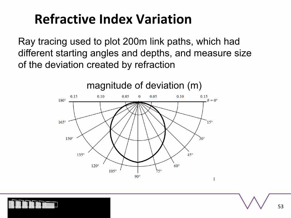
Refractive Index Variation
53
Ray tracing used to plot 200m link paths, which had
different starting angles and depths, and measure size
of the deviation created by refraction
magnitude of deviation (m)

Refractive Index Variation
54
Significance of the findings significant depends on
beam angle, transmitter FOV, the magnitude of
deviation (m) and the amount of scattering in the
link

A Fuller Treatment
55
We have to employ the Radiative Transfer Equation (RTE)
No analytical solutions for useful scenarios
Approximate analytical solutions possible for transmitter field
of view (FOV) less than 10° but loses the temporal
information as scattered and non-scattered photons are
considered to travel the same distance in the same time.
Numerical solutions – Monte Carlo
1
𝜈 𝜕
𝜕t+ 𝐧 . 𝛁𝐫 I t, 𝐫, 𝐧 = β 𝐫, 𝐧, 𝐧′ I t, 𝐫, 𝐧′ d𝐧′
4π
− cI t, 𝐫, 𝐧 + E t, 𝐫, 𝐧

FOV Simulation: Diffuse LOS Link
56
Jasman, Green and Leeson, Microwave and Optical
Technology Letters, 59(4) 837-840, 2017.

FOV Simulation: Power Distribution
57

FOV Simulation: Frequency Response
58
Clear water Turbid water

FOV Simulation: Frequency Response
59
On the same scale – much reduced in turbid water

Practical Work
60
Transmission of data using IRDA protocol 8
Mbps

Some Practical Results
61
Multiple hop arrangement
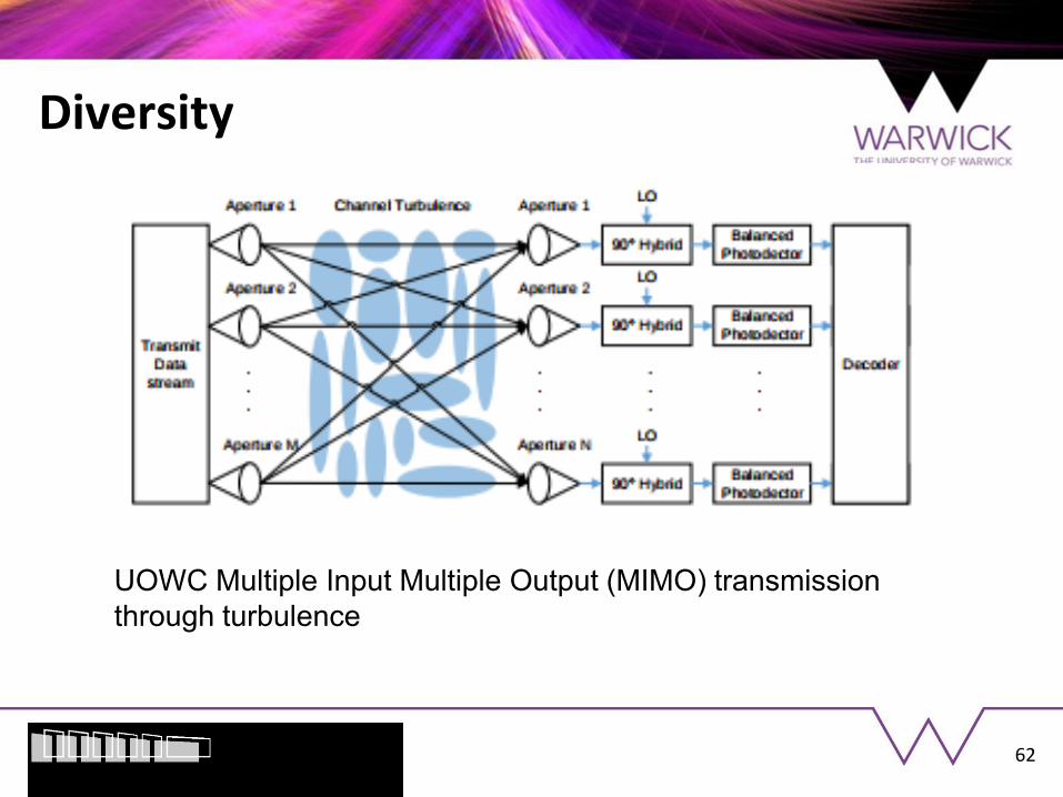
Diversity
62
UOWC Multiple Input Multiple Output (MIMO) transmission
through turbulence

Diversity: Outage Performance
Gamma-Gamma turbulence
63

Hybrid System
64
Han et al., China Communications, 11(5), 49–59, 2014

Hybrid Systems
Work needed on implementing protocols and functions
in FPGAs or similar
65

Latest Comparison
66
Muth, Laser Focus World, 53(5), 2017

Conclusions The incumbent technologies have major limitations
Optical wireless shows promise underwater
Visible light is essential
Understanding of water properties needed
Link orientation is important
High bit rates are possible in
– clearer water or
– over short distances
There are many subtleties in absorption and refraction
67

Future Directions Improved channel modelling
Coding and error correction
Modulation methods
Improved practical arrangement
Receiver enhancements
– Optical preamplifiers
– More on Coherent transmission
68

Questions
Thank you for your attention.
69