Understanding Developmental Crime Trajectories at Places: Social Disorganization and

The author(s) shown below used Federal funds provided by the U.S. Department of Justice and prepared the following final report: Document Title: Understanding Developmental Crime

Trajectories at Places: Social Disorganization and Opportunity Perspectives at Micro Units of Geography

Author: David Weisburd, Elizabeth R. Groff, Sue-Ming

Yang Document No.: 236057

Date Received: September 2011 Award Number: 2005-IJ-CX-0006 This report has not been published by the U.S. Department of Justice. To provide better customer service, NCJRS has made this Federally-funded grant final report available electronically in addition to traditional paper copies.

Opinions or points of view expressed are those

of the author(s) and do not necessarily reflect the official position or policies of the U.S.

Department of Justice.

Understanding Developmental Crime

Trajectories at Places: Social

Disorganization and Opportunity

Perspectives at Micro Units of Geography

Final Report to the National Institute of Justice

Award Number: 2005-IJ-CX-0006

David Weisburd George Mason University

Hebrew University

Elizabeth R. Groff Temple University

And

Sue-Ming Yang Georgia State University

November 2009

This document is a research report submitted to the U.S. Department of Justice. This report has not been published by the Department. Opinions or points of view expressed are those of the author(s) and do not necessarily reflect the official position or policies of the U.S. Department of Justice.

ii

Acknowledgements

There are many people that we need to thank who have helped us in the development of this

research and in the preparation of the manuscript. We are especially indebted to Chief Gil

Kerlikowske of Seattle (now the Director of the Office of National Drug Control Policy) who

supported our research from the outset, and facilitated our collection of official crime data as

well as other data sources in Seattle. Many other people from the Seattle PD assisted us, but we

owe a special debt to Lt. Ron Rasmussen who played a particularly important role as our main

contact regarding data drawn from the police department.

A number of research assistants helped us in identifying, collecting and preparing data for this

project. Kristen Miggans, then a graduate student at the University of Maryland, was

particularly important in getting data collection off the ground and collected quite a bit of it.

Rachel Philofsky, Chien-min Lin, Nancy Morris, Breanne Cave, Julie Willis, Amy J. Steen, and

Janet Hagelgens also provided important assistance. We are grateful to all of these younger

scholars for their commitment and interest in our work. Cody Telep of George Mason

University deserves special mention because of his efforts in the rewrites, development of tables

and figures, and editing of the report. Cody added tremendously to the quality of this work.

We thank Dan Nagin for his assistance with our trajectory models and Ned Levine for his

comments on spatial point pattern statistics.

Finally we want to thank Kimberly Schmidt of the University of Maryland for her help and

support in managing the NIJ grant that supported our research. We also want to thank our grant

monitor, Carrie Mulford, for keeping us on track and reminding us of the importance of getting

our work done.


iii

Abstract

Individuals and communities have traditionally been the focus of criminological research,

but recently criminologists have begun to explore the importance of “micro” places (e.g.

addresses, street segments, and clusters of street segments) in understanding and controlling

crime. Recent research provides strong evidence that crime is strongly clustered at hot spots and

that there are important developmental trends of crime at place, but little is known about the

geographic distribution of these patterns or the specific correlates of crime at this micro level of

geography.

We report here on a large empirical study that sought to address these gaps in our

knowledge of the “criminology of place.” Linking 16 years of official crime data on street

segments (a street block between two intersections) in Seattle, Washington to a series of data sets

examining social and physical characteristics of micro places over time, we examine not only the

geography of developmental patterns of crime at place but also the specific factors that are

related to different trajectories of crime. We use two key criminological perspectives, social

disorganization theories and opportunity theories, to inform our identification of risk factors in

our study and then contrast the impacts of these perspectives in the context of multivariate

statistical models.

Our first major research question concerns whether social disorganization and

opportunity measures vary across micro units of geography, and whether they are clustered, like

crime, into “hot spots.” Study variables reflecting social disorganization include property value,

housing assistance, race, voting behavior, unsupervised teens, physical disorder, and

urbanization. Measures representing opportunity theories include the location of public


iv

facilities, street lighting, public transportation, street networks, land use, and business sales. We

find strong clustering of such traits into social disorganization and opportunity “hot spots,” as

well as significant spatial heterogeneity.

We use group-based trajectory modeling to identify eight broad developmental patterns

across street segments in Seattle. Our findings in this regard follow an earlier NIJ study that

identified distinct developmental trends (e.g. high increasing and high decreasing patterns) while

noting the overall stability of crime trends for the majority of street segments in Seattle. We go

beyond the prior study by carefully examining the geography of the developmental crime

patterns observed. We find evidence of strong heterogeneity of trajectory patterns at street

segments with, for example, the presence of chronic trajectory street segments throughout the

city. There is also strong street to street variability in crime patterns, though there is some

clustering of trajectory patterns in specific areas. Our findings suggest that area trends influence

micro level trends (suggesting the relevance of community level theories of crime). Nonetheless,

they also show that the bulk of variability at the micro place level is not explained by trends at

larger geographic levels.

In identifying risk factors related to developmental trajectories, we find confirmation of

both social disorganization and opportunity theories. Overall, street segments evidencing higher

social disorganization are also found to have higher levels of crime. For many social

disorganization measures increasing trends of social disorganization over time were associated

with increasing trajectory patterns of crime. Similarly, in the case of opportunity measures

related to motivated offenders, suitable crime targets, and their accessibility, we find that greater

opportunities for crime are found at street segments in higher rate trajectory patterns. Finally, we

use multinomial logistic regression to simultaneously examine opportunity and social


v

disorganization factors and their influence on trajectory patterns. The most important finding

here is that both perspectives have considerable salience in understanding crime at place, and

together they allow us to develop a very strong level of prediction of crime.

Our work suggests it is time to consider an approach to the crime problem that begins not

with the people who commit crime but with the micro places where crimes are committed. This

is not the geographic units of communities or police beats that have generally been the focus of

crime prevention, but it is a unit of analysis that is key to understanding crime and its

development.


vi

Table of Contents

Acknowledgments..........................................................................................................................ii

Abstract.........................................................................................................................................iii

List of Figures.............................................................................................................................viii

List of Tables.................................................................................................................................xi

Executive Summary.......................................................................................................................1

Chapter 1: Introduction.............................................................................................................17

Crime and Place.............................................................................................................................22

Theoretical Foundations for Understanding Crime at Place..........................................................38

What Follows.................................................................................................................................42

Chapter 2: Context, Unit of Analysis, and Data......................................................................46

Why Seattle?..................................................................................................................................48

Unit of Analysis.............................................................................................................................52

Crime Data.....................................................................................................................................56

Characteristics of Street Segments: Opportunity Perspectives......................................................58

Characteristics of Street Segments: Social Disorganization.........................................................67

Conclusions....................................................................................................................................74

Chapter 3: Social Disorganization and Social Capital at Micro Places.................................75

Structural and Mediating Variables of Social Disorganization.....................................................76

Structural Variables.......................................................................................................................78

Intermediating Variables..............................................................................................................113

Conclusions..................................................................................................................................129

Chapter 4: Variation in Opportunity Factors for Crime across the Urban Landscape...131

Classifying Opportunity Measures.............................................................................................132

Description of Spatio-Temporal Variation in Opportunity Factors............................................138

Motivated Offenders...................................................................................................................140

Suitable Targets...........................................................................................................................146

Accessibility/Urban Form............................................................................................................168

Guardianship................................................................................................................................180

Discussion of Opportunity Variables...........................................................................................193

Chapter 5: The Distribution of Crime at Street Segments...................................................195

Is Crime Concentrated at Street Segments?.................................................................................196

Developmental Patterns of Crime at Place..................................................................................200

Conclusions..................................................................................................................................216


vii

Chapter 6: Geography of the Trajectories.............................................................................218

Analytic Strategy.........................................................................................................................219

Findings.......................................................................................................................................225

Conclusions..................................................................................................................................254

Chapter 7: Linking Characteristics of Places with Crime....................................................256

Social Disorganization and Crime Trajectories at Street Segments............................................258

Opportunity Theories and Crime and Trajectories of Crime at Street Segments........................272

Conclusions..................................................................................................................................287

Chapter 8: Explaining Crime at Place....................................................................................290

An Overall Model for Explaining Developmental Trajectories of Crime at Place.....................292

Comparing Increasing and Decreasing Crime Trajectories.........................................................310

Conclusions. ................................................................................................................................314

Chapter 9: Conclusions............................................................................................................316

Key Findings................................................................................................................................317

Policy Implications......................................................................................................................327

Limitations...................................................................................................................................331

Conclusions..................................................................................................................................333

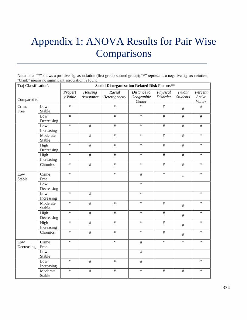
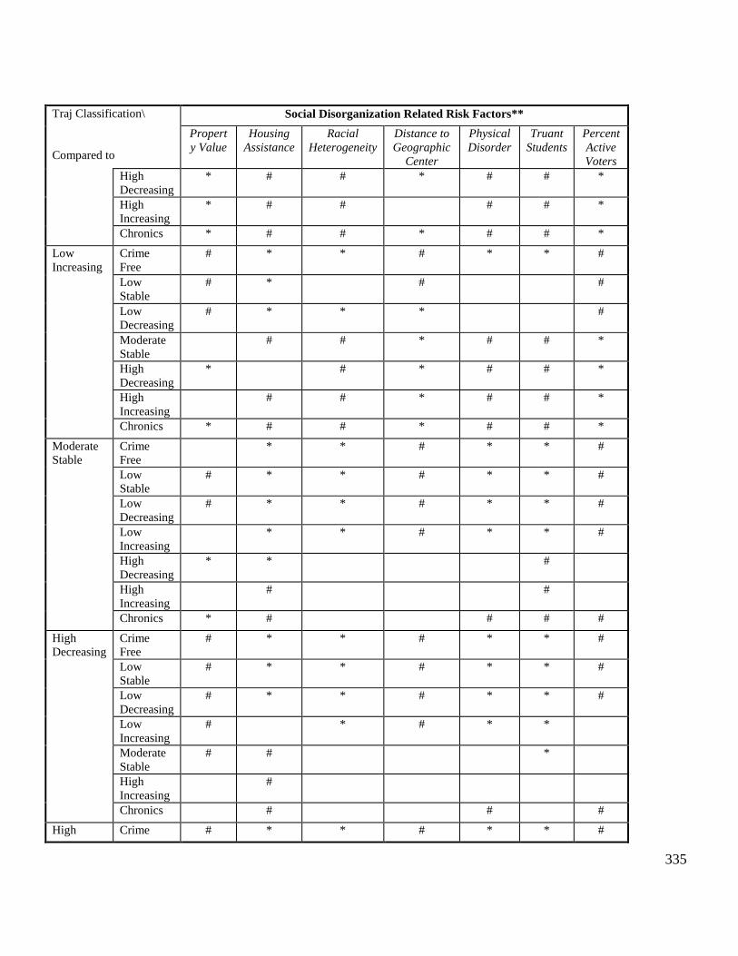
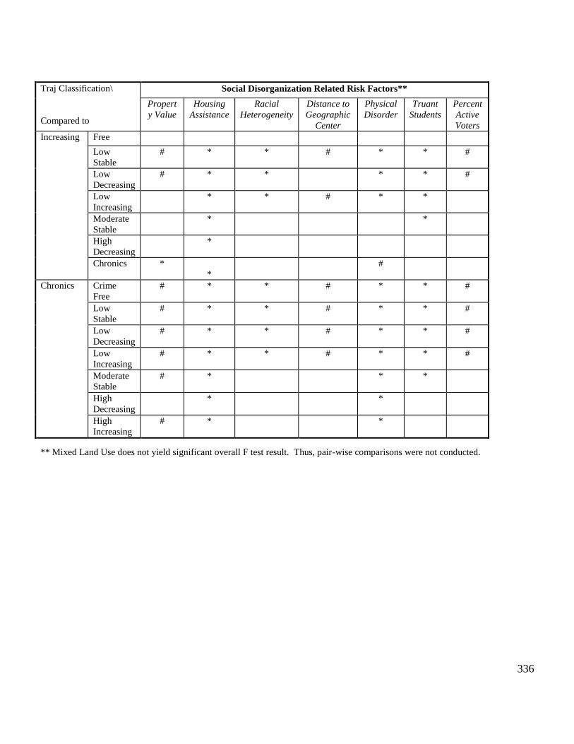
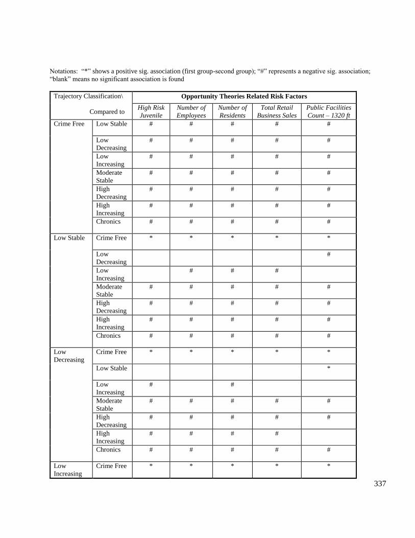
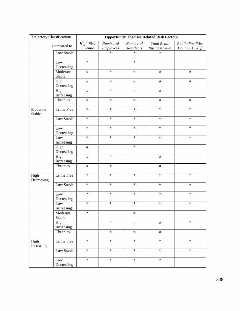
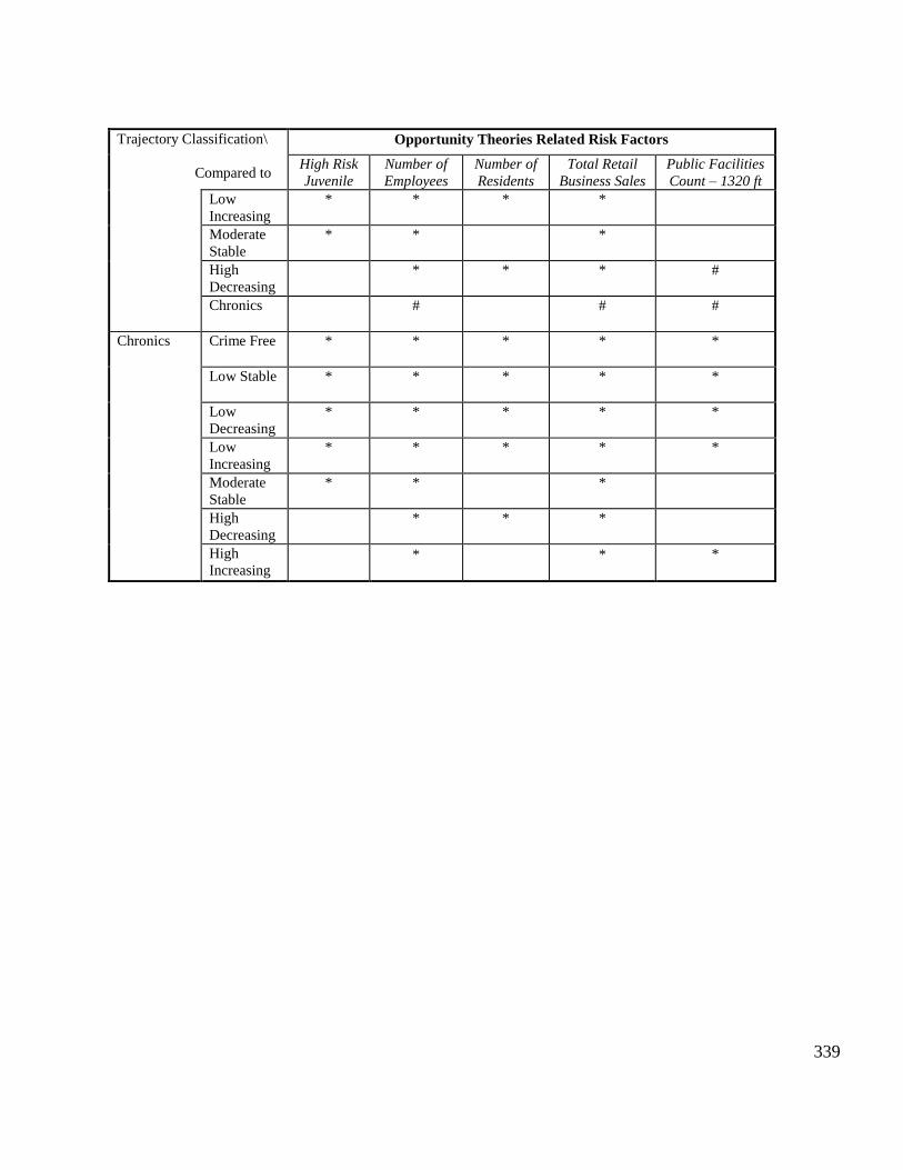
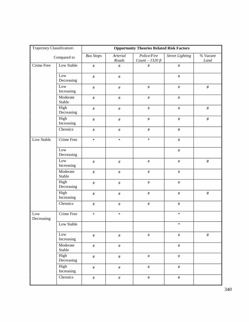
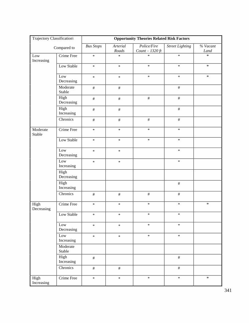
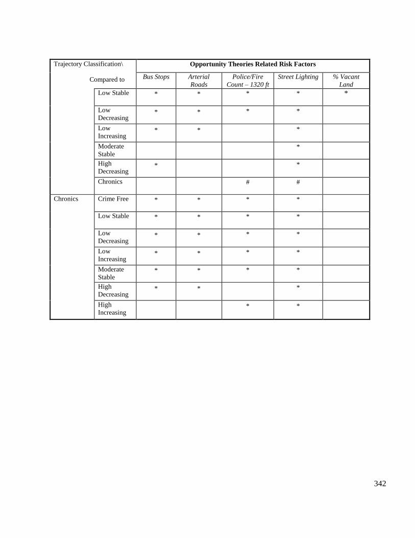
Appendix 1: ANOVA Results for Pair Wise Comparisons....................................................334

References...................................................................................................................................343


viii

List of Figures

Figure 2.1: Map of Seattle.................................................................................................... 50

Figure 3.1: Concentration Graph of Property Value Index.................................................. 81

Figure 3.2: Frequency Distributions of Property Value Index............................................. 82

Figure 3.3: Quantile Maps of Property Value Index........................................................... 83

Figure 3.4: Maps of Concentration of Property Values........................................................ 84

Figure 3.5: LISA Maps of Property Values (1991 vs. 2004................................................. 86

Figure 3.6: Concentration Graph of Housing Assistance.................................................... 89

Figure 3.7: Frequency Distributions of Housing Assistance................................................ 90

Figure 3.8: Geographic Locations of Housing Assistance....................................................91

Figure 3.9: Concentration Maps of Housing Assistance..................................................... 92

Figure 3.10: LISA Maps of Housing Assistance 1998-2004............................................... 93

Figure 3.11: Concentration Graph of Mixed Land Use........................................................ 95

Figure 3.12: Geographic Distributions of Streets with Mixed Land Use............................ 96

Figure 3.13: LISA Maps of Mixed Land Use of 1991 and 2004......................................... 97

Figure 3.14: The Trend of Racial Heterogeneity from 1992/1993 to 2003/2004

(school year) ..........................................................................................................................102

Figure 3.15: Frequency Distributions of Racial Heterogeneity Index, Racial

Heterogeneity Coefficient .12 (Student Data)........................................................................103

Figure 3.16: Geographic Distribution of Racial Heterogeneity (Student Data)................... 104

Figure 3.17: LISA Maps of Racial Heterogeneity (Student Data)...................................... 105

Figure 3.18: Distance to the Center of Seattle...................................................................... 106

Figure 3.19: Trend of Physical Disorder from 1993-2004................................................... 107

Figure 3.20: Concentration Graph of Physical Disorder Incidents....................................... 109

Figure 3.21: Frequency Distributions of Physical Disorder Over Time............................... 110

Figure 3.22: Geographic Distribution of Physical Disorder Incidents (1993 vs. 2004)...... 111

Figure 3.23: 50 Percent Concentration Maps of Physical Disorder Incidents..................... 112

Figure 3.24: LISA Maps of Physical Disorder Count (1993 vs. 2004)................................113

Figure 3.25: Number and Percentage of Truant Students on Streets.................................... 116

Figure 3.26: Concentration Graph of Truant Students......................................................... 117

Figure 3.27: Frequency Distributions of Truant Students.................................................... 118

Figure 3.28: Geographic Distributions of Truant Juveniles................................................ 119

Figure 3.29: Geographic Distributions of 50 Percent Concentration of Truant Juveniles...120

Figure 3.30: LISA Maps of Truant Juveniles.........................................................................121

Figure 3.31: The Trends of Active Voters from 1999 to 2004.............................................125

Figure 3.32: Frequency Distributions of Active Voters.......................................................126

Figure 3.33: Geographic Distributions of Active Voters..................................................... 127

Exhibit 3.34: Geographic Distributions of 50 Percent Concentration of Active Voter.......128

Figure 3.35: LISA Maps of Active Voters Data.................................................................. 129


ix

Figure 4.1: Concentration of High Risk Juveniles across Street Segments......................... 142

Figure 4.2: Distribution of Street Segments that Account for 50 Percent of High Risk

Juveniles................................................................................................................................. 143

Figure 4.3: Distribution of the Residences of High Risk Juveniles across Street

Segments................................................................................................................................ 144

Figure 4.4: LISA Results for High Risk Juveniles................................................................145

Figure 4.5: Concentration of Employment across Street Segments.....................................147

Figure 4.6: Distribution of Street Segments that Account for 50 percent of Employment..148

Figure 4.7: Distribution of Employment across Street Segments........................................ 149

Figure 4.8: LISA Results for Employment.......................................................................... 150

Figure 4.9: Concentration of Residential Population across Street Segments..................... 152

Figure 4.10: Distribution of Street Segments that Account for 50 Percent of Residential

Population.............................................................................................................................. 153

Figure 4.11: Distribution of Residential Population across Street Segments...................... 154

Figure 4.12: LISA Results for Residential Population........................................................ 155

Figure 4.13: Concentration of Total Retail Sales across Street Segments........................... 156

Figure 4.14: Distribution of Street Segments that Account for 50 Percent of Total Retail

Business Sales........................................................................................................................ 157

Figure 4.15: Distribution of Total Retail Business Sales..................................................... 158

Figure 4.16: LISA Results for Total Retail Business Sales................................................. 160

Figure 4.17: Ripley’s K for Distribution of Public Facilities across Street Segments........ 163

Figure 4.18: Distribution of Public Facilities across Street Segments................................. 164

Figure 4.19: Distribution of Public Facilities across Street Segments 1989-1991.............. 165

Figure 4.20: Distribution of Public Facilities across Street Segments 2002-2004.............. 166

Figure 4.21: Average Number of Public Facilities across Street Segments........................ 167

Figure 4.22: Linear Ripley’s K for Arterial Streets............................................................. 171

Figure 4.23: Distribution of Street Types............................................................................. 173

Figure 4.24: Concentration of Bus Stops across Street Segments....................................... 175

Figure 4.25: Distribution of Street Segments that Account for 50 Percent of Bus Stops..... 177

Figure 4.26: Distribution of Bus Stops across Street Segments.......................................... 178

Figure 4.27: LISA Results for Bus Stops............................................................................ 179

Figure 4.28: Concentration of Vacant Land Parcels across Street Segments....................... 182

Figure 4.29: Distribution of Street Segments that Account for 50 Percent of Vacant Land

Parcels.................................................................................................................................... 183

Figure 4.30: Distribution of Vacant Land Parcels at Street Segments................................. 184

Figure 4.31: LISA Results for Vacant Land Parcels across Street Segments.......................185

Figure 4.32: Linear Ripley’s K for Police and Fire Stations............................................... 186

Figure 4.33: Distribution of Street Segments that Account for 50 Percent of Street

Lighting... .............................................................................................................................. 187

Figure 4.34: Concentration of Street Lighting across Street Segments................................ 189

Figure 4.35: Distribution of Street Segments that Account for 50 Percent of Street

Lighting.................................................................................................................................. 190

Figure 4.36: Distribution of Street Lighting........................................................................ 191

Figure 4.37: LISA Results for Street Lighting.................................................................... 192

Figure 5.1: Seattle Street Segment Crime Trends.................................................................197

Figure 5.2: Crime Incident Concentration............................................................................ 198


x

Figure 5.3: Crime Concentration Stability Over Time......................................................... 199

Figure 5.4: 22 Trajectories of Crime Incidents..................................................................... 205

Figure 5.5: Crime Free Trajectory Pattern........................................................................... 206

Figure 5.6: Low Stable Trajectory Pattern............................................................................207

Figure 5.7: Moderate Stable Trajectory Group..................................................................... 209

Figure 5.8: Chronic Trajectory Group.................................................................................. 209

Figure 5.9: Low Rate Decreasing Trajectory Pattern........................................................... 211

Figure 5.10: High Rate Decreasing Trajectory Pattern......................................................... 212

Figure 5.11: Low Rate Increasing Trajectory Pattern........................................................... 213

Figure 5.12: High Rate Increasing Trajectory Pattern......................................................... 214

Figure 5.13: Crime Drop Analysis........................................................................................ 215

Figure 6.1: Spatial Distribution of Temporal Trajectories (Northern Seattle).................... 227

Figure 6.2: Spatial Distribution of Temporal Trajectories (Central Seattle)....................... 229

Figure 6.3: Spatial Distribution of Temporal Trajectory Patterns (Southern Seattle)......... 231

Figure 6.4: Ripley’s K of All Trajectory Patterns............................................................... 235

Figure 6.5: LISA for Crime Free, Low Stable, and Low Decreasing Trajectory Group

Patterns................................................................................................................................... 238

Figure 6.6: Center City LISA for Crime Free Street Segments........................................... 239

Figure 6.7: Street Segments by Trajectory Pattern with LISA for Crime Free Segments

Segments................................................................................................................................ 241

Figure 6.8: LISA for Low Increasing, Moderate Stable, and High Decreasing Trajectory

Patterns................................................................................................................................... 243

Figure 6.9: High Increasing and Chronic LISA for Trajectory Patterns............................. 244

Figure 6.10: Graphical Representation of Pair Wise Comparisons for Low Rate Crime Street

Segments................................................................................................................................ 250

Figure 6.11: Graphical Representation of Pair Wise Comparisons for High Rate Crime Street

Segments................................................................................................................................ 251


xi

List of Tables

Table A: Opportunity Theory Characteristics Used in Analysis.......................................... 7

Table B: Social Disorganization Characteristics Used in Analysis...................................... 7

Table 2.1: Roots of Characteristics Used in the Model (Opportunity Perspectives)........... 59

Table 2.2: Sources and Extents of Opportunity Theory Variables...................................... 66

Table 2.3: Roots of Characteristics Used in the Model (Social Disorganization)............... 68

Table 2.4: Social Disorganization Variables Spatial and Temporal Extent......................... 73

Table 3.1: Theoretical Concepts Represented by the Data (Social Disorganization)........... 78

Table 3.2: Descriptive Statistics of Variable Representing Mixed Land Use (N = 19,635).94

Table 3.3: Descriptive Statistics of Racial Distribution of Seattle’s Public School Students

from 1993 to 2004..................................................................................................................100

Table 3.4: Descriptives of Physical Disorder........................................................................108

Table 3.5: Descriptive Statistics for Only Those Study Streets with Any Voter................. 123

Table 3.6: Descriptive of Active Voter and Percentage of Active Voter from 1999 to

2004....................................................................................................................................... 124

Table 4.1: Theoretical Concepts Represented by the Data (Opportunity Theories)............. 135

Table 4.2: Number of Public Facilities over Time............................................................... 162

Table 5.1: Odds of Correct Classification by Trajectory...................................................... 204

Table 6.1: Cross K Results................................................................................................... 252

Table 7.1: Risk Analysis for Property Value Index (Measure of SES).................................259

Table 7.2: Risk Analysis for Housing Assistance (Combining Public Housing and

Section 8 Vouchers).............................................................................................................. 261

Table 7.3: Risk Analysis for Mixed Land Use......................................................................263

Table 7.4: Risk Analysis for Racial Heterogeneity (Based on Public School Student

Data)....................................................................................................................................... 265

Table 7.5: Risk Analysis for Urbanization/Distance to Center of the City (miles).............. 266

Table 7.6: Risk Analysis for Total Number of Physical Disorder Incidents........................ 267

Table 7.7 Risk Analysis for Truant Students/Unsupervised Teens....................................... 269

Table 7.8: Risk Analysis for Percentage of Active Voters (Collective Efficacy)................. 271

Table 7.9: Risk Analysis for High Risk Juveniles................................................................ 274

Table 7.10: Risk Analysis for Employment.......................................................................... 276

Table 7.11: Risk Analysis for Total Residents..................................................................... 277

Table 7.12: Risk Analysis for Total Retail Sales (in thousands of dollars).......................... 279

Table 7.13: Risk Analysis for Number of Public Facilities Within 1,320 Feet of a Street

Segment..................................................................................................................................280

Table 7.14: Risk Analysis for Number of Bus Stops............................................................ 282

Table 7.15: Risk Analysis for Arterial Roads....................................................................... 283

Table 7.16: Risk Analysis for Number of Police/Fire Stations Within 1,320 Feet of Street

Segment..................................................................................................................................284

Table 7.17: Risk Analysis for Street Lighting (in Watts)..................................................... 285

Table 7.18: Risk Analysis for Percentage of Vacant Land................................................... 286

Table 8.1: Description of included variables and mean and standard deviation for both starting

values and change variables (when applicable)..................................................................... 294


xii

Table 8.2: Likelihood Ratio Tests for the Multinomial Logistic Regression........................299

Table 8.3: Odds Ratios from the Multinomial Logistic Regression of Impact of Social

Disorganization and Opportunity Variables (Including Change Variables) on Trajectory

Group Pattern Membership (Crime Free Pattern is the Reference Group)............................ 301

Table 8.4: Comparison of Low Increasing Trajectory Pattern vs. Low Decreasing

Pattern.................................................................................................................................... 311

Table 8.5: Comparison of High Increasing Trajectory Pattern vs. High Decreasing

Pattern.................................................................................................................................... 312


1

Executive Summary:

Understanding Developmental Crime Trajectories at Places: Social

Disorganization and Opportunity Perspectives at Micro Units of

Geography

Grant #2005-IJ-CX-0006

“Neighbors next door are more important than relatives far away”

Chinese Folk Saying

Traditionally, research and theory in criminology have focused on two main units of

analysis: individuals and communities (Nettler, 1978; Sherman, 1995). Crime prevention

research and policy have also been focused primarily on offenders or the communities in which

they live (Akers, 1973; Gottfredson & Hirschi, 1990). While the individual and the community

have long been a focus of crime research and theory, and of prevention programs, only recently

have criminologists begun to explore other potential units of analysis that may contribute to our

understanding and control of crime.

An important catalyst for this work came from theoretical perspectives that emphasized

the context of crime and the opportunities that are presented to potential offenders. In a ground

breaking article on routine activities and crime, for example, Cohen and Felson (1979) suggest

that a fuller understanding of crime must include a recognition that the availability of suitable

crime targets and the presence or absence of capable guardians influence crime events. Around

the same time, the Brantinghams published their influential book Environmental Criminology,

which emphasized the role of place characteristics in shaping the type and frequency of human

interaction (Brantingham & Brantingham, 1981 [1991]). Researchers at the British Home Office


2

in a series of studies examining “situational crime prevention” also challenged the traditional

focus on offenders and communities (Clarke, 1983). These studies showed that the crime

situation and the opportunities it creates play significant roles in the development of crime events

(Clarke, 1983).

One implication of these emerging perspectives is that crime places are an important

focus of inquiry. While concern with the relationship between crime and place is not new and

indeed goes back to the founding generations of modern criminology (Guerry, 1833; Quetelet,

1842 [1969]), the “micro” approach to places suggested by recent theories has just begun to be

examined by criminologists.1 Places in this “micro” context are specific locations within the

larger social environments of communities and neighborhoods (Eck & Weisburd, 1995). They

are sometimes defined as buildings or addresses (e.g. see Green, 1996; Sherman et al., 1989);

sometimes as block faces, „hundred blocks‟, or street segments (e.g. see Taylor, 1997; Weisburd

et al., 2004); and sometimes as clusters of addresses, block faces or street segments (e.g. see

Block et al., 1995; Sherman & Weisburd, 1995; Weisburd & Green, 1995).

Recent studies point to the potential theoretical and practical benefits of focusing research

on crime places. A number of studies, for example, suggest that there is a very significant

clustering of crime at places, irrespective of the specific unit of analysis that is defined

(Brantingham & Brantingham, 1999; Crow & Bull, 1975; Pierce et al., 1986; Roncek, 2000;

Sherman et al., 1989; Weisburd et al., 1992; Weisburd & Green, 1994; Weisburd et al., 2004).

The extent of the concentration of crime at place is dramatic. In one of the pioneering studies in

this area, Lawrence Sherman and colleagues (1989) found that only three percent of the

addresses in Minneapolis produced 50 percent of all calls to the police. Fifteen years later in a

1 For a notable example of an early approach which did place emphasis on the “micro” idea of place as discussed

here, see Shaw et al. (1929).


3

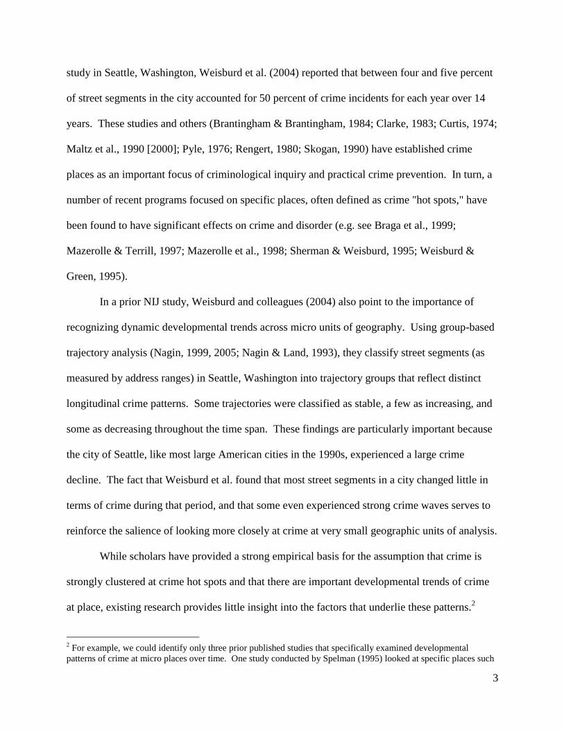
study in Seattle, Washington, Weisburd et al. (2004) reported that between four and five percent

of street segments in the city accounted for 50 percent of crime incidents for each year over 14

years. These studies and others (Brantingham & Brantingham, 1984; Clarke, 1983; Curtis, 1974;

Maltz et al., 1990 [2000]; Pyle, 1976; Rengert, 1980; Skogan, 1990) have established crime

places as an important focus of criminological inquiry and practical crime prevention. In turn, a

number of recent programs focused on specific places, often defined as crime "hot spots," have

been found to have significant effects on crime and disorder (e.g. see Braga et al., 1999;

Mazerolle & Terrill, 1997; Mazerolle et al., 1998; Sherman & Weisburd, 1995; Weisburd &

Green, 1995).

In a prior NIJ study, Weisburd and colleagues (2004) also point to the importance of

recognizing dynamic developmental trends across micro units of geography. Using group-based

trajectory analysis (Nagin, 1999, 2005; Nagin & Land, 1993), they classify street segments (as

measured by address ranges) in Seattle, Washington into trajectory groups that reflect distinct

longitudinal crime patterns. Some trajectories were classified as stable, a few as increasing, and

some as decreasing throughout the time span. These findings are particularly important because

the city of Seattle, like most large American cities in the 1990s, experienced a large crime

decline. The fact that Weisburd et al. found that most street segments in a city changed little in

terms of crime during that period, and that some even experienced strong crime waves serves to

reinforce the salience of looking more closely at crime at very small geographic units of analysis.

While scholars have provided a strong empirical basis for the assumption that crime is

strongly clustered at crime hot spots and that there are important developmental trends of crime

at place, existing research provides little insight into the factors that underlie these patterns.2

2 For example, we could identify only three prior published studies that specifically examined developmental

patterns of crime at micro places over time. One study conducted by Spelman (1995) looked at specific places such


4

What characteristics of places are associated with crime hot spots, and how do the characteristics

of hot spots differ from places that are relatively crime free? Do high and low crime places

differ in substantive ways that can be empirically identified? What accounts for the differing

developmental crime trends that have been identified at micro units of place over time? What

leads some micro places to experience a large decline in crime trends over time, while others in

the same city experience crime waves and still others vary little in crime trends during the same

period? Perhaps just as critical in increasing our understanding of micro units of geography and

crime and place is exploring whether crime trends observed at such geographic units are simply

reflections of higher order neighborhood or community effects, or if focus on these higher order

geographic areas has led us to miss important insights about the causes of crime at the micro

geographic level.

For the last century criminologists have focused on describing the nature and causes of

individual offending. In this report we turn our attention to a different problem that has only

recently drawn criminological attention, but has the potential to improve our predictions of crime

and also our ability to develop practical crime prevention. Our focus is on how crime distributes

across very small units of geography. A Chinese proverb suggests that “neighbors next door are

more important than relatives far away.” We argue that the action of crime research and practice

should be focused much more on micro crime places.

Site and Methods

Seattle makes a good choice for a longitudinal study of places for several reasons. First,

as a large city it has enough geography, population and crime to undertake a micro level study.

as high schools, public housing projects, subway stations and parks in Boston, using three years of official crime

information. Taylor (1999) examined crime and fear of crime at 90 street blocks in Baltimore, Maryland using a

panel design with data collected in 1981 and 1994 (see also Taylor, 2001). These studies are limited only to a small

number of locations and to a few specific points in time. The final study by Weisburd et al. (2004) examined all the

street „hundred blocks‟ in Seattle. This research extends that earlier work.


5

The distinguishing feature of Seattle was the length of the time for which they had crime data

available. Moreover, Seattle was led at the time of our study by an innovative Chief of Police,

Gil Kerlikowske, now the Director of the Office of National Drug Control Policy, who offered to

facilitate the collection of data both from the police department and other government sources in

Seattle.

The study period we used is 1989 – 2004. In 1990 the population of the city had begun to

rebound for the first time in decades, reaching 516,259. This upward trend continued over the

next decade and by the 2000 census there were 563,374 people living in Seattle (U.S. Census

Bureau, 1990, 2000).

The geographic unit of analysis for this study is the street segment (sometimes referred to

as a street block or face block). We define the street segment as both sides of the street between

two intersections. Only residential and arterial streets were included in our study. We excluded

limited access highways because of their lack of interactive human activity.3 This left us with

24,023 units of analysis (i.e., street segments) in Seattle. We chose the street segment for a

variety of theoretical and practical reasons. Theoretically, scholars have long recognized the

relevance of street blocks in organizing life in the city (Appleyard, 1981; Brower, 1980; Jacobs,

1961; Taylor et al., 1984; Unger & Wandersman, 1983). Taylor (1997, 1998) made the case for

why street segments (his terminology was street blocks) function as behavior settings. We also

thought that crime data was unlikely to be accurately coded at the address level, and thus the

street segment in our view represented a micro level of geography that was likely to include

accurate crime information.

3 The street centerline file we obtained from Seattle GIS included many different line types (e.g. trails, railroad and

transit lines to name a few). Our study included only residential streets, arterial streets and walkways/stairs

connecting streets.


6

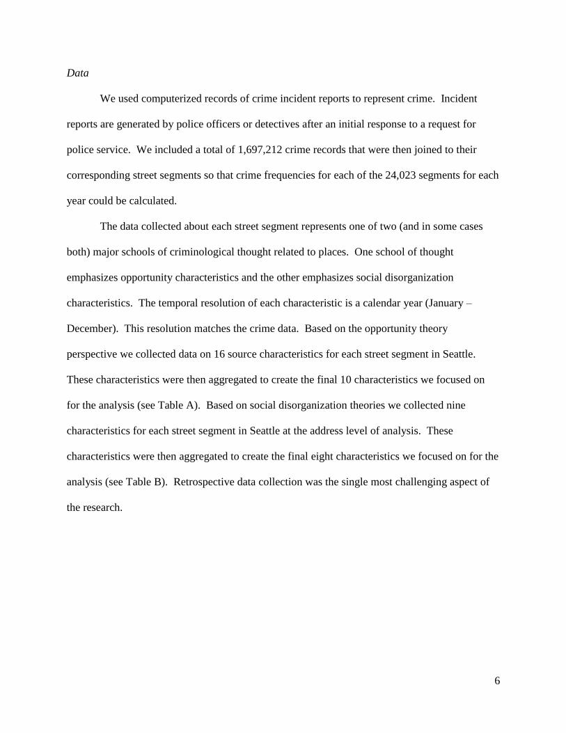
Data

We used computerized records of crime incident reports to represent crime. Incident

reports are generated by police officers or detectives after an initial response to a request for

police service. We included a total of 1,697,212 crime records that were then joined to their

corresponding street segments so that crime frequencies for each of the 24,023 segments for each

year could be calculated.

The data collected about each street segment represents one of two (and in some cases

both) major schools of criminological thought related to places. One school of thought

emphasizes opportunity characteristics and the other emphasizes social disorganization

characteristics. The temporal resolution of each characteristic is a calendar year (January –

December). This resolution matches the crime data. Based on the opportunity theory

perspective we collected data on 16 source characteristics for each street segment in Seattle.

These characteristics were then aggregated to create the final 10 characteristics we focused on

for the analysis (see Table A). Based on social disorganization theories we collected nine

characteristics for each street segment in Seattle at the address level of analysis. These

characteristics were then aggregated to create the final eight characteristics we focused on for the

analysis (see Table B). Retrospective data collection was the single most challenging aspect of

the research.


7

Table A: Opportunity Theory Characteristics Used in Analysis

Characteristic Composition

Motivated Offenders

High risk juveniles

Truant or low academic achieving

juvenile residents

Suitable Targets

Employment

Residents

Retail business-related Crime

generators/Crime attractors

Public facilities as Crime


Number of employees

Total juveniles + total registered voters

Total sales for retail businesses

Number of public facilities within 1,320

feet

o Community centers

o Hospitals

o Libraries

o Parks

o Schools

Accessibility/Urban Form

Type of street

Bus stops

1= arterial, 0 = residential

Total number of bus stops

Guardianship

Vacant Land

Police station/Fire station

Street lighting

Percentage of vacant land

Number of Police or fire stations within

1,320 feet

Watts per foot of lighting

Table B: Social Disorganization Characteristics Used in Analysis

Structural Dimensions (Variables within dimension)

SES

o Property Values

(Weighted ranking of single- and multi-family housing)

Public Housing / Assistance

Mixed Land Use

Racial Heterogeneity

o Race of Public School Students


8

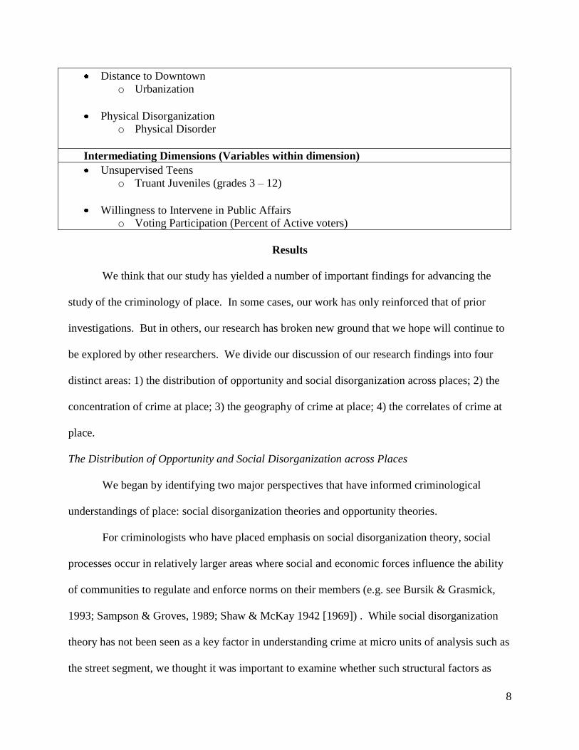
Distance to Downtown

o Urbanization

Physical Disorganization

o Physical Disorder

Intermediating Dimensions (Variables within dimension)

Unsupervised Teens

o Truant Juveniles (grades 3 – 12)

Willingness to Intervene in Public Affairs

o Voting Participation (Percent of Active voters)

Results

We think that our study has yielded a number of important findings for advancing the

study of the criminology of place. In some cases, our work has only reinforced that of prior

investigations. But in others, our research has broken new ground that we hope will continue to

be explored by other researchers. We divide our discussion of our research findings into four

distinct areas: 1) the distribution of opportunity and social disorganization across places; 2) the

concentration of crime at place; 3) the geography of crime at place; 4) the correlates of crime at

place.

The Distribution of Opportunity and Social Disorganization across Places

We began by identifying two major perspectives that have informed criminological

understandings of place: social disorganization theories and opportunity theories.

For criminologists who have placed emphasis on social disorganization theory, social

processes occur in relatively larger areas where social and economic forces influence the ability

of communities to regulate and enforce norms on their members (e.g. see Bursik & Grasmick,

1993; Sampson & Groves, 1989; Shaw & McKay 1942 [1969]) . While social disorganization

theory has not been seen as a key factor in understanding crime at micro units of analysis such as

the street segment, we thought it was important to examine whether such structural factors as


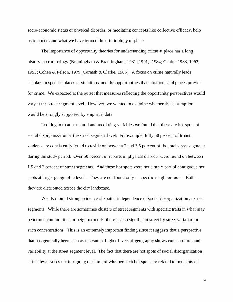
9

socio-economic status or physical disorder, or mediating concepts like collective efficacy, help

us to understand what we have termed the criminology of place.

The importance of opportunity theories for understanding crime at place has a long

history in criminology (Brantingham & Brantingham, 1981 [1991], 1984; Clarke, 1983, 1992,

1995; Cohen & Felson, 1979; Cornish & Clarke, 1986). A focus on crime naturally leads

scholars to specific places or situations, and the opportunities that situations and places provide

for crime. We expected at the outset that measures reflecting the opportunity perspectives would

vary at the street segment level. However, we wanted to examine whether this assumption

would be strongly supported by empirical data.

Looking both at structural and mediating variables we found that there are hot spots of

social disorganization at the street segment level. For example, fully 50 percent of truant

students are consistently found to reside on between 2 and 3.5 percent of the total street segments

during the study period. Over 50 percent of reports of physical disorder were found on between

1.5 and 3 percent of street segments. And these hot spots were not simply part of contiguous hot

spots at larger geographic levels. They are not found only in specific neighborhoods. Rather

they are distributed across the city landscape.

We also found strong evidence of spatial independence of social disorganization at street

segments. While there are sometimes clusters of street segments with specific traits in what may

be termed communities or neighborhoods, there is also significant street by street variation in

such concentrations. This is an extremely important finding since it suggests that a perspective

that has generally been seen as relevant at higher levels of geography shows concentration and

variability at the street segment level. The fact that there are hot spots of social disorganization

at this level raises the intriguing question of whether such hot spots are related to hot spots of


10

crime (see later). But irrespective of that relationship our work is the first establish that social

disorganization variables are concentrated at micro places and that they are spread across the city

landscape.

Opportunity measures are as we expected also concentrated, and also evidence variability

across places. The overwhelming finding is one of concentration at specific places. For

example, 50 percent of high risk juveniles (a proxy in our work for “motivated offenders”) are

consistently found on between three and four percent of the total number of Seattle street

segments. In turn, half of all the employees (a proxy for “suitable targets”) in the city were

located on less than one percent of Seattle street segments. There are hot spots of motivated

offenders, suitable targets and capable guardians. This was not suprising given prior theorizing,

but our data are among the first to illustrate this fact.

Finally, as with social disorganization measures we find that opportunity characteristics

of places evidence much spatial heterogeneity. In statistical terms there is a significant degree of

negative spatial autocorrelation evident in the variables we examine. In this sense while there

are hot spots of opportunities, such hot spots are not clustered only in specific neighborhoods.

Our results suggest that characteristics reflecting opportunity theories are indeed associated with

specific street segments, and are not simply reflecting larger area trends.

The Concentration of Crime at Place

Using 16 years of data and adding refinement to the definition of street segments our

analyses follow closely those of prior studies of crime at place. Our study confirms prior

research showing that crime is tightly clustered in specific places in urban areas, and that most

places evidence little or no crime (Sherman et al., 1989; Weisburd et al., 2004). Fifty percent of

the crime each year in Seattle was found at just five to six percent of the street segments in the


11

city. We think this pattern is consistent enough to suggest a “law of concentration” of crime.

Following prior study (see Weisburd et al., 2004) we were also able to show that there is a high

degree of stability of crime at micro places over time. While there is overall stability in the

trajectory patterns we observe in our study, there is also evidence of strong increasing and

decreasing patterns of crime. One pattern of developmental trends we observe for example,

suggest strong crime waves during a 16 year period of general crime declines in the city. More

generally, our data suggest that crime trends at specific segments are central to understanding

overall changes in crime in a city.

The Geography of Crime at Place

Our analyses of the geography of developmental patterns of crime at street segments

provided important insights into our understanding of the processes that generate crime trends at

street segments. Perhaps the key objection to our work would be that we have unnecessarily

rarified our geographic analysis and that our choice of a micro place unit for studying crime has

simply masked higher order geographic processes.

We do not find evidence suggesting that the processes explaining crime patterns at street

segments come primarily from higher geographic influences such as communities. There are

indications of the influence of higher order trends in our data. One example is the fact that

higher crime street segments are not distributed at random, and are more likely to be closer to

each other than would be predicted simply by chance. But these indications of macro geographic

influences are much outweighed in our data by evidence of the importance of looking at crime at

the micro level that we have defined as street segments in our study. There is strong street to

street variability in crime patterns in our data, and such variability emphasizes the importance of

studying crime at place at a micro unit of analysis. Evidence of spatial independence at the street


12

segment level further reinforces this. Much of the action of crime comes from the street

segment, as we have defined it. We think our findings suggest that it is time to move the

geographic cone of criminological interests to the criminology of place.

The Correlates of Crime at Place

Having established that an important part of the crime equation is generated at a very

micro level of geography, it was natural to turn to the factors that would explain crime at place.

Earlier we noted that characteristics of social disorganization and opportunity were concentrated

at places and that they evidenced strong geographic heterogeneity. Can we explain selection to

different developmental crime patterns with variables representing these key theoretical

dimensions of place?

Our research has provided an unambiguous answer to this question. Looking at risk

factors for crime, we found a large number of both opportunity measures and social

disorganization measures to significantly distinguish trajectory membership. Of the six

structural indicators of social disorganization that we examined, five are directly related to crime

levels of trajectories. In the case of mediating factors of social disorganization two key measures

were related to the level of crime in trajectory patterns. Our ten measures of motivated

offenders, suitable targets and accessibility are all linked strongly to initial crime levels of

trajectory patterns. The relationship of these factors to developmental trends, while not as

uniform, follows the patterns overall that would be expected.

Our risk analysis suggested the importance of both opportunity and social disorganization

theories as correlates of crime at place. But we also looked at these factors in the context of an

overall model explaining developmental patterns of crime at street segments. We used a direct

method for comparing the influence of the two theoretical perspectives on crime patterns at


13

places. It suggested that both perspectives are providing a strong explanation for developmental

patterns of crime at place. The opportunity perspective provided an explained variance value of

(“pseudo” R2) of .66 versus .51 for the social disorganization measures. This suggests that a

model exclusively concerned with opportunities for crime (as we measure them) is likely to

provide a higher level of prediction of trajectory patterns. However, we think what is most

significant here overall is that in the multivariate context, both perspectives maintain strong and

significant influences on crime at place. Both social disorganization theory and opportunity

theories need to be considered in understanding why crime varies across places.

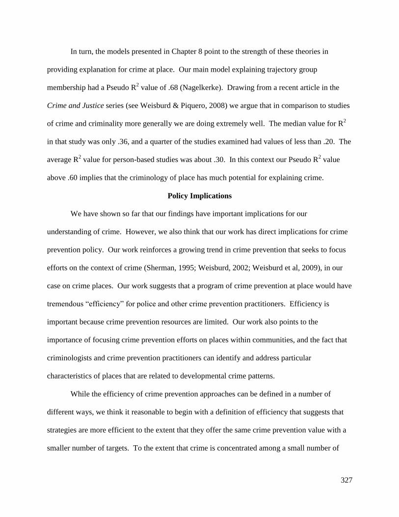
In turn, the models presented point to the strength of these theories in providing

explanation for crime at place. Our main model explaining trajectory group membership had a

Pseudo R2 value of .68 (Nagelkerke). Drawing from a recent article in the Crime and Justice

series (see Weisburd & Piquero, 2008) we argued that in comparison to studies of crime and

criminality more generally prediction is very high in our model. The median value for R2

in that

study was only .36, and a quarter of the studies examined had values of less than .20. The

average R2 value for person based studies was about .30. In this context our Pseudo R

2 value

above .60 implies that the criminology of place has much potential for explaining crime.

Policy Implications

We have shown so far that our findings have important implications for our

understanding of crime. However, we also think that our work has direct implications for crime

prevention policy. Our work reinforces a growing trend in crime prevention that seeks to focus

efforts on the context of crime (Sherman, 1995; Weisburd, 2002; Weisburd et al., 2009), in our

case on crime places.


14

While the efficiency of crime prevention approaches can be defined in a number of

different ways, we think it reasonable to begin with a definition of efficiency that suggests that

strategies are more efficient to the extent that they offer the same crime prevention value with a

smaller number of targets. We find that five to six percent of street segments each year include

half of all crime incidents. One percent of the street segments in the chronic trajectory group are

responsible for more than a fifth of all crime incidents in the city. This means that crime

prevention practitioners can focus their resources on relatively few crime hot spots and deal with

a large proportion of the crime problem. Importantly, as well, places are not “moving targets.”

Place-based crime prevention provides a target that “stays in the same place.” This is not an

insignificant issue when considering the investment of crime prevention resources.

Evidence of the stability of crime patterns at places in our work, also suggests the

efficiency of place based approaches. We show not only that about the same number of street

segments were responsible for 50 percent of the crime each year, but that the street segments that

tended to evidence very low or very high activity at the beginning of the period of study in 1989

were similarly ranked at the end of the period in 2004. Accordingly, a strategy that is focused on

chronic hot spots is not likely to be focusing on places that will naturally become cool a year

later. The stability of crime at place across time makes crime places a particularly salient focus

for investment of crime prevention resources.

Our work also reinforces the importance of focusing in on “places” rather than larger

geographic units such as communities or police precincts. Our data suggest that crime

prevention at larger geographic units is likely to suffer an “ecological fallacy” in which crime

prevention resources are spread thinly across large numbers of street segments, when the

problems that need to be addressed are concentrated only on some of the street segments in that


15

area. Criminologists and crime prevention practitioners need to recognize that definitions of

neighborhoods as “bad” or problematic, is likely to miss the fact that many places in such areas

have no or little crime. In turn, crime prevention resources should be focused on the hot spots of

crime within “good” and “bad” neighborhoods.

Our data also illustrate that criminologists and crime prevention practitioners can identify

key characteristics of places that are correlated with crime. At a policy level, our research

reinforces the importance of initiatives like “hot spots policing” that address specific streets

within relatively small areas (Braga, 2001; Sherman & Weisburd, 1995; Weisburd & Green,

1995). If police become better at recognizing the “good streets” in the bad areas, they can take a

more holistic approach to addressing crime problems.

Limitations

While we think our work has contributed a good deal to our knowledge of the

criminology of place, we note in our report some specific limitations of our data. Perhaps most

significant is the fact that by necessity we were limited to retrospective data collection. Having

noted that we were able to provide a more in depth view of crime at place than any prior study

we know of, we think it important to recognize that retrospective data collection is by its nature

limited. Many of our measures are proxies for variables we would have liked to collect but were

unable to identify.

A second key limitation of our study relates to our use of observational data in

understanding developmental crime patterns. While we examine the correlates of developmental

crime patterns at places, we cannot make unambiguous statements about the causal patterns

underlying our data. For example, reports of physical disorder are very strongly correlated with

presence in more serious or chronic trajectory patterns. But our data do not allow us to establish


16

that physical disorder leads to more serious crime problems. Even though we find that changes

in physical disorder and changes in crime are related, it may be that a third cause unmeasured in

our analysis is in fact the ultimate cause of the relationships observed. This limitation is not

unique to our study, but one that affects all observational studies (Shadish et al., 2002).

Nonetheless, it is important to keep this limitation in mind when considering the implications of

our work.

Conclusions

For most of the last century criminologists and crime prevention practitioners have tried

to understand why people become involved in crime and what programs can be developed to

discourage criminality. Our work suggests that it is time to consider another approach to the

crime problem that begins not with the people who commit crime but the places where crimes

are committed. Our work shows that street segments in the city of Seattle represent a key unit

for understanding the crime problem. This is not the geographic units of communities or police

beats that have generally been the focus of criminologists or police in crime prevention, but it is

a unit of analysis that is key to understanding crime and its development.


17

Chapter 1: Introduction

“Neighbors next door are more important than relatives far away”

Chinese Folk Saying

Traditionally, research and theory in criminology have focused on two main units of

analysis: individuals and communities (Nettler, 1978; Sherman, 1995). In the case of

individuals, criminologists have sought to understand why certain people as opposed to others

become criminals (e.g. see Akers, 1973; Gottfredson & Hirschi, 1990; Hirschi, 1969; Raine,

1993), or to explain why certain offenders become involved in criminal activity at different

stages of the life course or cease involvement at other stages (e.g. see Laub & Sampson, 2003;

Moffitt, 1993; Sampson & Laub, 1993). In the case of communities, criminologists have often

tried to explain why certain types of crime or different levels of criminality are found in some

communities as contrasted with others (e.g. see Agnew, 1999; Bursik & Grasmick, 1993;

Sampson & Groves, 1989; Sampson & Wilson, 1995; Shaw et al., 1929), or how community-

level variables, such as relative deprivation, low socioeconomic status, or lack of economic

opportunity may affect individual criminality (e.g. see Agnew, 1992; Cloward & Ohlin, 1960;

Merton, 1968; Wolfgang & Ferracuti, 1967). In most cases, research on communities has

focused on the “macro” level, often studying states (Loftin & Hill, 1974), cities (Baumer et al.,

1998), and neighborhoods (Bursik & Grasmick, 1993; Sampson, 1985).

Crime prevention research and policy have also been focused primarily on offenders or

the communities in which they live. Scholars and practitioners have looked to define strategies

that would deter individuals from involvement in crime (see Nagin, 1998), or that would

rehabilitate offenders (e.g. see Andrews et al., 1990; Sherman et al., 1997, 2002). In recent


18

years, crime prevention efforts have often focused on the incapacitation of high rate or dangerous

criminals so that they are not free to victimize people in the community (e.g. see Blumstein et al.,

1986). Community-based crime prevention has also played a major role in the development of

crime prevention programs. Whether looking to strengthen community bonds (Sampson et al.,

1997; Sherman et al., 1997; Skogan, 1990; Tierney et al., 1995), or to enlist the community in

crime prevention efforts (Skogan, 1996), the community has traditionally been viewed as an

important context for crime prevention research and policy development.

While the individual and the community have long been a focus of crime research and

theory, and of prevention programs, only recently have criminologists begun to explore other

potential units of analysis that may contribute to our understanding and control of crime. An

important catalyst for this work came from theoretical perspectives that emphasized the context

of crime and the opportunities that are presented to potential offenders. In a ground breaking

article on routine activities and crime, for example, Cohen and Felson (1979) suggest that a fuller

understanding of crime must include a recognition that the availability of suitable crime targets

and the presence or absence of capable guardians influence crime events. Around the same time,

the Brantinghams published their influential book Environmental Criminology, which

emphasized the role of place characteristics in shaping the type and frequency of human

interaction (Brantingham & Brantingham, 1981 [1991]). Researchers at the British Home Office

in a series of studies examining “situational crime prevention” also challenged the traditional

focus on offenders and communities (Clarke, 1983). These studies showed that the crime

situation and the opportunities it creates play significant roles in the development of crime events

(Clarke, 1983).

One implication of these emerging perspectives is that crime places are an important


19

focus of inquiry. While concern with the relationship between crime and place is not new and

indeed goes back to the founding generations of modern criminology (Guerry, 1833; Quetelet,

1842 [1969]), the “micro” approach to places suggested by recent theories has just begun to be

examined by criminologists.1 Places in this “micro” context are specific locations within the

larger social environments of communities and neighborhoods (Eck & Weisburd, 1995). They

are sometimes defined as buildings or addresses (e.g. see Green, 1996; Sherman et al., 1989);

sometimes as block faces, „hundred blocks‟, or street segments (e.g. see Taylor, 1997; Weisburd

et al., 2004); and sometimes as clusters of addresses, block faces or street segments (e.g. see

Block et al., 1995; Sherman & Weisburd, 1995; Weisburd & Green, 1995). Research in this area

began with attempts to identify the relationship between specific aspects of urban design

(Jeffery, 1971) or urban architecture and crime (Newman, 1972) but broadened to take into

account a much larger set of characteristics of physical space and criminal opportunity (e.g.

Brantingham & Brantingham, 1975; Brantingham & Brantingham, 1981 [1991]; Duffala, 1976;

Hunter, 1988; LeBeau, 1987; Mayhew et al., 1976; Rengert, 1980, 1981).

Recent studies point to the potential theoretical and practical benefits of focusing research

on crime places. A number of studies, for example, suggest that there is a very significant

clustering of crime at places, irrespective of the specific unit of analysis that is defined

(Brantingham & Brantingham, 1999; Crow & Bull, 1975; Pierce et al., 1986; Roncek, 2000;

Sherman et al., 1989; Weisburd et al., 1992; Weisburd & Green, 1994; Weisburd et al., 2004).

The extent of the concentration of crime at place is dramatic. In one of the pioneering studies in

this area, Lawrence Sherman and colleagues (1989) found that only three percent of the

addresses in Minneapolis produced 50 percent of all calls to the police. Fifteen years later in a

1 For a notable example of an early approach that did place emphasis on the “micro” idea of place as discussed here,

see Shaw et al. (1929).


20

study in Seattle, Washington, Weisburd et al. (2004) reported that between four and five percent

of street segments in the city accounted for 50 percent of crime incidents for each year over 14

years. These studies and others (Brantingham & Brantingham, 1984; Clarke, 1983; Curtis, 1974;

Maltz et al., 1990 [2000]; Pyle, 1976; Rengert, 1980; Skogan, 1990) have established crime

places as an important focus of criminological inquiry and practical crime prevention. In turn, a

number of recent programs focused on specific places, often defined as crime "hot spots," have

been found to have significant effects on crime and disorder (e.g. see Braga et al., 1999;

Mazerolle & Terrill, 1997; Mazerolle et al., 1998; Sherman & Weisburd, 1995; Weisburd &

Green, 1995).

Weisburd and colleagues (2004) also point to the importance of recognizing dynamic

developmental trends across micro units of geography. Using group-based trajectory analysis

(Nagin, 1999, 2005; Nagin & Land, 1993), they classify street segments (as measured by address

ranges) in Seattle, Washington into trajectory groups that reflect distinct longitudinal crime

patterns. Some trajectories were classified as stable, a few as increasing, and some as decreasing

throughout the time span. These findings are particularly important because the city of Seattle,

like most large American cities in the 1990s, experienced a large crime decline. The fact that

Weisburd et al. found that most street segments in a city changed little in terms of crime during

that period, and that some even experienced strong crime waves serves to reinforce the salience

of looking more closely at crime at very small geographic units of analysis.

While scholars have provided a strong empirical basis for the assumption that crime is

strongly clustered at crime hot spots and that there are important developmental trends of crime

at place, existing research provides little insight into the factors that underlie these patterns.2

2 For example, we could identify only three prior published studies that specifically examined developmental

patterns of crime at micro places over time. One study conducted by Spelman (1995) looked at specific places such


21

What characteristics of places are associated with crime hot spots, and how do the characteristics

of hot spots differ from places that are relatively crime free? Do high and low crime places

differ in substantive ways that can be empirically identified? What accounts for the widely

differing developmental crime trends that have been identified at micro units of place over time?

What leads some micro places to experience a large decline in crime trends over time, while

others in the same city experience crime waves and still others vary little in crime trends during

the same period? Perhaps just as critical in increasing our understanding of micro units of

geography and crime and place is exploring whether crime trends observed at such geographic

units are simply reflections of higher order neighborhood or community effects, or if focus on

these higher order geographic areas has led us to miss important insights about the causes of

crime at the micro geographic level.

Do these factors suggest specific policy proscriptions or specific crime prevention

approaches on the part of the police or communities? Or do they indicate that the causes of

crime declines at specific places are the result of broader societal trends that are unlikely to be

the subject of manipulation by the police or the public? Are there “early warnings” that identify

street segments in trajectories that experienced crime waves over time, and can these indicators

be used to identify places “at risk” before crime waves begin? What factors can be seen as “risk

factors” in the development of crime at micro levels of geography and which can be seen as

“protective factors”?

In the following chapters we report on a large empirical study that sought to answer these

critical questions about the “criminology of place” (Sherman et al., 1989). Linking 16 years of

as high schools, public housing projects, subway stations and parks in Boston, using three years of official crime

information. Taylor (1999) examined crime and fear of crime at 90 street blocks in Baltimore, Maryland using a

panel design with data collected in 1981 and 1994 (see also Taylor, 2001). These studies are limited only to a small

number of locations and to a few specific points in time. The final study by Weisburd et al. (2004) examined all the

street „hundred blocks‟ in Seattle. This research extends that earlier work.


22

official crime data on street segments (a street block between two intersections, see Chapter 2) in

Seattle to a series of data sets examining the social and physical characteristics of micro places

over time we were able to extend present knowledge and explore areas that have not been the

subject of systematic research to date. In this introductory chapter we wanted to provide a

context for our approach to the criminology of place and our identification of data relevant for

understanding and explaining crime concentrations and developmental patterns of crime.

Accordingly, we turn next to a historical review of the study of place and crime, focusing in

particular on the developing trend of scholars to see the “action of crime” as being in lower and

lower units of geography. We then turn to the key theoretical perspectives that have been used to

understand the criminology of places, in particular contrasting what we term “social

disorganization theories” with “opportunity theories.” Finally, in concluding we provide an

overall road map to the chapters that follow.

For the last century criminologists have focused on describing the nature and causes of

individual offending. In this report we turn our attention to a different problem that has only

recently drawn criminological attention, but has the potential to improve our predictions of crime

and also our ability to develop practical crime prevention. Our focus is on how crime distributes

across very small units of geography. A Chinese proverb suggests that “neighbors next door are

more important than relatives far away.” The chapters that follow will argue that the action of

crime research and practice should be focused much more on micro crime places.

Crime and Place3

Examining the history of the study of crime and place, one is struck by the continuation

of themes from the earliest studies to the present day. Poverty, urbanization, and population

3 This section of our chapter draws heavily from a paper by Weisburd, Bruinsma, and Bernasco (2009). We are

especially indebted to Gerben Bruinsma for his insights and comments on the historical development of crime and

place.


23

heterogeneity, which were to become key elements of social disorganization theories of crime,

and continue to have salience in recent criminological work (e.g. see Cancino et al., 2009; Hipp,

2007a; Hipp et al., 2009; Schreck et al., 2009; Sampson et al., 2002) were key variables in the

very earliest crime and place studies. Importantly, however, there has been a consistent trend

over the last two centuries of moving the lens of criminological interest to smaller and smaller

units of geography.

The study of crime at places began with the publication of statistics on the French

population summarized in very large areas, or departments, by the French Home Office in the

1820s. The publication of the Comptes Générales de l’administration de la justice criminelle en

France inspired many statisticians and other scholars to explore crime data in more detail. In

1829 the first geographical map of crime was published. Partly based on the Comptes Générales

de l’administration de la justice criminelle en France, Michel-André Guerry and the Venetian

cartographer Adriano Balbi published on one large sheet, three maps on the distribution of crime

in France in the years 1825-1827. It was a novelty in the new field of criminology that they

made use of a cartographic method of presenting statistical material. Their work was to

emphasize an enduring interest of criminologists with urbanization and crime. They found that

in urban areas, especially in the capital of Paris, the highest numbers of property and personal

crimes could be observed. Later, when Guerry became head of the Crime Statistics Unit of the

France ministry of Justice, he continued his work on mapping crime. In 1833 his influential

Essai sur la statistique morale de la France was published (Guerry, 1833). Inspired by the

Reform Movement4 of the 19

th century, Guerry examined whether poverty and density of

population might lead to higher crime rates. He observed an empirical complexity. The rich

north departements were confronted with higher property crime rates than the poor departements

4 In France and England the Reform Movement focused its policy on public health and education for the poor.


24

in the south of France. He concluded that the level of poverty was not the direct cause of crime.

Similarly, his data suggested that population density was not a cause of crime.

The French scholar Michel-André Guerry is often bracketed together with the Belgium

statistician and astronomer Adolphe Quetelet who discovered the normal distribution in statistics

with which deviations can be observed and calculated (Landau & Lazarsfeld, 1968). Quetelet

(1831 [1984]) also used large areal units such as provinces and countries as units of analyses. He

explained the higher rates of property crimes of the richer provinces by the unequal distribution

of wealth: a great number of people possess nothing compared to the relatively few rich citizens

(Quetelet, 1831 [1984], p. 38). Presaging the focus of late 20th

century criminologists on

opportunity and crime (e.g. see Cohen and Felson, 1979; Felson & Clarke, 1998), Quetelet

concluded that poverty was not in itself the cause of crime, but rather that crime develops when

the poor and disadvantaged “are surrounded by subjects of temptation and find themselves

irritated by the continual view of luxury and of an inequality of fortune” (1831[1984], p. 38).

These French and Belgian scholars were the first who scientifically analyzed crime at

place. They focused on the administrative and political borders of their time in their

geographical crime analyses and began to raise key issues related to poverty, urbanization,

population heterogeneity and even crime opportunities in understanding crime problems, though

they did not always come to singular conclusions. Nations, regions, counties, provinces,

departments and quartiers were the units of analyses, and they were used as a unit for systematic

comparisons of crime figures. They were fully dependent on official crime data and other data

arranged within these larger geographic units that the government supplied. While the early

French and Belgian researchers concerned with crime and place also examined some variability

of crime within cities, their overall focus was generally on larger administrative units.


25

Pioneers in England in the 19th

Century

France and Belgium were not the only countries where geographical studies on crime

were carried out in the 19th

century. Members of The Statistical Society of London also regularly

published on crime topics in their statistical journal. John Glyde (1856) was the first to question

the validity of the research findings when large areas were chosen as units of analysis in

geographic criminology. In his paper Localities of crime in Suffolk he showed very clearly that

larger units of analysis hide underlying variations in crime. When smaller units than districts or

departements were taken into account, significant differences in crime rates across smaller areas

appeared. As Morris (1957, p. 58) notes: “Of the regional studies, a major criticism is that the

county was the smallest territorial unit considered, but Glyde, by breaking Suffolk down into its

seventeen Poor Law Unions was able to demonstrate that the „County Aggregate‟ masked

considerable differences between the smaller geographical units of which it was composed.”

In studies of crime and place in England in the 19th

century, the work of Henry Mayhew

(1851 [1950]) is particularly important. He is well-known in criminology (and cited therefore)

for his descriptive studies of the underworld of London in the middle Victorian Age. However,

Mayhew also tried to uncover patterns in the distribution of crime in the city of London

combining ethnographic methods with statistical data.5 He interviewed prostitutes, criminals and

other citizens about alcoholism, poverty, housing conditions and economic uncertainty. He was

the first scholar who focused on small areas like squares, streets and buildings as a unit of

analysis in criminological research, predating modern interests in micro crime places (see later)

by over a century.

5 In a sense Mayhew practiced already the methodology that Robert Park (1925 [1967]) advocated 70 years later in

the 1920s in Chicago.


26

Chicago and the Dynamics of Cities: Neighborhoods and Square Miles as Units of Analyses

After the turn of the century, the locus of geographic research on crime moved to the

United States, and especially to the city of Chicago. At the University of Chicago, a group of

sociologists6

took the initiative to undertake new research on urban problems, which centered in

part, on crime (Beirne & Messerschmidt, 1991; Bulmer, 1984; Faris, 1967; Harvey, 1987). They

also moved the action of crime and place research from broad comparisons across large

geographic areas to more careful comparisons within cities. Interestingly, the Chicago School

scholars were either not aware of or ignored until 1933 the work of 19th

century crime and place

researchers in Europe (Elmer, 1933). At this point a group of American sociologists, among

them, Robert Park, William Thomas, Louis Wirth, Ernest Burgess, Clifford Shaw and Henry

McKay took a leadership role in the development of the criminology of place, in contrast to the

statisticians, criminal lawyers or psychiatrists who dominated criminology more generally in

Europe (Vold et al., 2002).

William Thomas contributed to the criminology of place by introducing the important

concept of social disorganization, referring to “a decrease of the influence of existing social

rules of behavior upon individual members of the group” (Thomas, 1966, p. 3). Though the

Chicago sociologists studied many of the same variables as earlier European scholars, and

especially those that focused on poverty and related social problems, they concentrated on

neighborhoods or communities rather than much larger administrative areas. Robert Park (1864-

1944), who was recruited by Thomas, was the initiator of urban social research on crime places,

shifting the unit of analyses from countries and large areas to cities and their neighborhoods

(Park, 1925 [1967]). The city in his opinion was more than:

6 As Burgess and Bogue (1964a, p.1) demonstrated, other disciplines and governmental agencies also studied urban

life in Chicago extensively (also see Bulmer, 1984; Faris, 1967).


27

“…a congeries of individual men and of social conveniences – streets, buildings, electric

lights, tramways, and telephones, etc; something more, also, than a mere constellation of

institutions and administrative devices – courts, hospitals, schools, police and, civil

functionaries of various sorts. The city is, rather, a state of mind, a body of costumes and

traditions, and of the organized attitudes and sentiments that inhere in these costumes and

are transmitted with this tradition. The city is not, in other words, merely a physical

mechanism and an artificial construction. It is involved in the vital process of the people

who compose it; it is a product of nature, and particularly of human nature” (Park

1925[1967], p. 1).

Park argued that urban life must be studied in this context in terms of “its physical organization,

its occupations, and its culture” and especially the changes therein (Park, 1925 [1967], p. 3).

Neighborhoods in his view were the elementary form of cohesion in urban life.

His younger colleague, Ernest Burgess, drawing from an inventory of price changes in

housing values in Chicago areas, developed a concentric zone model of the distribution of social

problems and crime for cities (especially for Chicago) (Burgess, 1925 [1967]).7 Burgess

suggested that Chicago included five concentric8 zones, each containing various neighborhoods,

four of them situated around „The Loop‟ (the business center of the city): “the typical processes

of the expansion of the city can best be illustrated, perhaps, by a series of concentric circles,

which may be numbered to designate both the successive zones of urban extension and the types

of areas differentiated in the process of expansion” (Burgess, 1925 [1967], p. 50). Burgess‟ unit

of analyses was a series of neighborhoods within cities that share similar characteristics. He

assumed that depending on the distances to the center and the special features of these zones, the

levels of crime would vary.

Clifford Shaw was one of the first Chicago sociologists to carry out extensive empirical

research on the geographical distribution of crime on the basis of Burgess‟ zone model (Shaw et

7 The real estate agent had discovered zones in the city of Chicago when he made up an inventory of price changes

of houses and real estate. He contacted Burgess regarding his findings, which led to the now famous geographic

model of crime and social problems in the urban context. 8 In reality only half circles because Chicago is situated at the border of Lake Michigan.


28

al., 1929). This study can be seen as a landmark in the history of crime and place studies

because of its detailed data collection, advanced methods and innovative statistical tools. Based

on the concentric zone model of Burgess, he studied the distribution of truancy of young people,

juvenile delinquents and adult offenders in Chicago. Assisted by young researchers like Henry

McKay, Frederick Zorbaugh and Leonard Cottrell, he took natural areas as units of analyses

(Abbott, 1997) but in more detail than ever before in these kinds of studies.9 Shaw introduced

new units of analyses. First, he introduced spot maps by plotting the home address of thousands

of offenders on a map of Chicago. Second, he combined the offender address data with census

data to created delinquency rate maps of square mile areas. And finally, he constructed radial

maps and zone maps, which displayed delinquency rates at regular distances from the city center

(Snodgras, 1976).

In the same year Shaw‟s research assistant Harvey Zorbaugh published his PhD in which

he compared a slum neighborhood (The Lower North Side) with a wealthy area (Gold Coast) in

Chicago, both situated in close proximity (Zorbaugh, 1929). In this more qualitative study,

Zorbaugh presented only a few maps, all of them less detailed in information than Shaw‟s study.

However, his research demonstrated clearly that two areas in close physical proximity were not

necessarily similar and thus physical and social distances do not always coincide. Zorbaugh‟s

work made it clear that administrative and political areas and social spaces are not identical.

Depending on the size of the area, a variety of social communities with different identities can

9 It is interesting to note that a similar approach was taken by Cyrill Burt (1883-1971) who studied the location of

the home addresses of delinquent boys and girls in the years 1922 and 1923 in London. Following the Chicago

School findings, he noted that the highest concentrations in crime were found in three neighborhoods situated

closely to the city centre: Holborn, Finsbury, and Shoreditch (Burt, 1924[1944]). According to Burt, these oldest

but not poorest neighborhoods of London were of strategic importance for offenders, because they were situated

closely to attractive crime targets in the inner city and - if necessary – they could function as a place to hide from the

police.


29

exist. Importantly, he concluded that the smaller the unit of analysis, the greater the chance of a

homogeneous community.

In 1942, Clifford Shaw and Henry McKay published their magnum opus, Juvenile

Delinquency and Urban Areas, in which they not only presented their geographical and

etiological analyses of crime rates in the city of Chicago, but also those of other cities:

Philadelphia, Boston, Cincinnati, Cleveland, and Richmond. In all of the studied cities, they

found similar patterns in the geographical distribution of crime. The rapid changes in the city of

Chicago over a long period of time enabled them also to study the effects of the dynamics of the

city on crime and other phenomena. One of their findings was that: “The data on trends also

demonstrate with equal sharpness the rapid rise in rates of delinquents in certain areas when a

population with a different history and different institutions and values takes over areas in a very

short period of time” (Shaw & McKay, 1942 [1969], p. 382). This work established the idea of

population heterogeneity as a key factor in the study of crime and place and criminology more

generally.

The Chicago studies inspired criminologists to carry out empirical crime and place

research in other cities (e.g. see Burgess & Bogue, 1964a, 1964b).10

At the same time, as the

decades passed, empirical and methodological critics of the Chicago approach began to emerge

(Lander, 1954). First, it was argued that Shaw and colleagues (1929) and Shaw & McKay (1942

[1969]) could not distinguish between the dwelling place of the offender and the location where

he or she committed a crime, neglecting the variability in the mobility of offenders (see also

Boggs, 1965). Secondly, by relying on official crime figures, their research was seen as biased

10

Interesting to mention here is the relatively unknown policy report of Edwin Sutherland (1883-1950) on the

geographical distribution of juvenile delinquency of the city of Bloomington, Indiana (Sutherland, 1937). Inspired

by the work of Shaw and McKay and using the zone model of Burgess, he revealed like in Chicago, certain

delinquent neighborhoods with high numbers of adult and juvenile offenders.


30

because offenders of the lower class had (and still have) a greater chance to be processed in the

criminal justice system (e.g. see Beirne & Messerschmidt, 1991; Chilton, 1964; Gordon, 1967).

Thirdly, delinquency rates after 1945 in Chicago did not conform to the distribution patterns of

Shaw and McKay‟s early assumptions (Bursik, 1984, 1986). European studies also showed

contradicting results. Morris (1957) examined the offender rates of the county of Croydon, but

could not confirm the zone model of Burgess. Twenty years later, Morris‟ findings were

replicated in the city of Sheffield (Baldwin & Bottoms, 1976).

Another criticism that is key to our focus on micro units of analysis is that brought by

Robinson (1950) who discussed the use of ecological correlations in geographical studies like

that of Shaw and McKay (1942 [1969]). According to Robinson (1950, p. 351) the object of an

ecological correlation is a group of persons, not a person: “…the individual correlation depends

on the internal frequencies of the within-areas individual correlations, while the ecological

correlation depends upon the marginal frequencies of the within-areas individual correlations”

(Robinson, 1950, p. 354). He concluded that ecological correlations cannot validly be used as

substitutes for individual correlations. Such an ecological fallacy leads to meaningless

conclusions. Looking back, these empirical and methodological criticisms diminished the

attention of criminologists in studies of crime and place for almost 20 years.

Reemerging interest in communities

In the 1980s, Albert J. Reiss Jr. was to encourage a group of younger criminologists to

return to the interests of the Chicago School where he had received his Ph.D. in 1949. Reiss

(1986) saw the criminological tradition as including two major theoretical positions, one that

focused on individuals and a second that focused on crimes. Communities and crime was a main

focus of the latter tradition and he sought to rekindle criminological interest in understanding


31

variability of crime within and across communities. Editing an early volume in the Crime and

Justice series, Reiss and Michael Tonry (1986) sought to bring Communities and Crime to the

forefront of criminological interests.

Reiss did not see the new interest as simply mimicking the insights of the Chicago School

criminologists. Rather, he sought to raise a new set of questions about crime at community that

had been ignored in earlier decades: “Recent work on communities and crime has turned to the

observation that Shaw and McKay neglected: not only do communities change their structures

over time but so often do their crime rates, a recognition that communities as well as individuals

have crime careers” (Reiss, 1986, p. 19). This volume and other work developed in this period

drew upon the identification of neighborhoods and communities to expand insights about the

development of crime (Brantingham & Brantingham, 1981 [1991]; Bursik, 1986; Bursik &

Webb, 1982; Clarke, 1983; Hunter, 1988; Kobrin & Scherman, 1981; LeBeau, 1987; Rengert,

1980, 1981; Roncek & Bell, 1981; Sampson, 1985; Sampson & Groves, 1989; Scherman &

Kobrin, 1986; Skogan, 1986).

Smith (1986), for example, identified neighborhood variation in the behavior of the

police, suggesting the importance of place in understanding not only the etiology of crime, but

also the etiology of criminal justice. Skogan brought new insights not only to our understanding

of the interaction of community characteristics and policing (Skogan, 1987), but also more

generally to the developmental processes that led to the emergence of crime and disorder in

urban communities (Skogan, 1990). More recently, scholars led by Robert Sampson have used a

focus on the community to draw new insights into developmental crime patterns, arguing that

social cohesion within communities and shared expectations of community members combine to


32

affect both crime and social disorder (Sampson & Raudenbush, 1999; Sampson et al., 1997).

These insights are examined in our work as they relate to micro units of crime and place.

Consistent with Reiss‟ call for investigation of the criminal careers of communities,

Bursik (1986; see also Bursik & Webb, 1982) revisited crime in Chicago neighborhoods over

time and challenged earlier views of the stability of crime within neighborhoods and

communities, arguing that stability in crime patterns was a result of long term stability in the

social characteristics of places, and that instability in such patterns would also lead to instability

in crime rates. Similarly, Schuerman and Kobrin (1986) identified stability and variability in

criminal careers of communities, focusing on the residences of juvenile delinquents as had Shaw

and McKay (1942 [1969]). Using the number of residential addresses of officially known

delinquents by census tracts in Los Angeles as an indicator of aggregate crime, they found three

general patterns that led to high crime rates in 1970. The first pattern they termed “emerging”,

and referred to those clusters that were relatively crime free in 1950 but had moderate to high

crime in 1960 and 1970, respectively. The second pattern, “transitional”, refers to those clusters

that had moderately high crime in 1950, a higher level 1960 and an even higher level in 1970.

The last pattern is referred to as “enduring” and refers to those clusters that had persistently high

crime rates at all points in time. The vast majority of census tracts within the clusters were

designated as having enduring crime rates over the time span, with fewer census tracts in the

transitional and emerging categories.

Interestingly, though the approach of the Chicago School called for the identification of

units of geography that would not be drawn from administrative data collection, but from the

social units that defined neighborhoods or communities, this new generation of scholars

concerned with communities and crime have generally used officially defined units for drawing


33

their data and conclusions. In this case, the US Census definitions, most often census tracts or

the smaller census block groups, have become the main source for defining the units of

geography that are the focus of research in the US, despite the fact that the goals of the census in

creating physically contiguous geographic units are often inconsistent with the goals of

community and crime researchers (see Rengert & Lockwood, 2009). Often such studies will

simply assume that census units such as census tracts reflect actual community boundaries (Hipp,

2007b), though some scholars in this area combine census units with the idea of creating

boundaries of communities that are more consistent with the theoretical interests of researchers

(e.g. see Sampson et al., 1997). Importantly, this new focus on communities and crime often led

to the study of much smaller geographic units of analysis than had drawn the interests of the

early Chicago School scholars.

The Emphasis on Micro Units of Geography in the “Criminology of Place”

While a reemergence of interest in communities and crime had been one important source

for renewed study of crime and place in recent decades, the 1980s produced a more radical

reformulation of the unit of geography that should form the basis of crime place studies,

continuing to push the unit of geographic analysis to a more micro level. Traditional

criminological interest in place has focused on higher level geographic units such as regions,

cities, communities or neighborhoods. One reason for this focus on macro levels of geography is

simply that data were often not available at geographic levels lower than the standard

administrative or census divisions. But even when data were on hand, statistical and analytic

tools were not readily available for linking crime easily to micro units of geography.

Certainly, the difficulty of mapping crimes to specific places and of analyzing geographic

data was a factor that prevented the study of crime at micro units of geography, but another


34

barrier was the lack of consistent theoretical interest in micro places as contrasted with research

on individual criminality, or crime across macro geographic units (Weisburd & McEwen, 1997;

Weisburd et al., 2004). Such theoretical interest was not to emerge until the late 1970s and

1980s, about the time that computerized crime mapping and more sophisticated geographic

statistical tools were to emerge (Weisburd & McEwen, 1997). A new group of theorists

challenged traditional criminological interests and began to focus more on the “processes

operating at the moment of the crime‟s occurrence” (Birkbeck & LaFree, 1993, p. 114). One

influential critique that was to have strong influence on the development of interest in micro

units of geography was brought by Lawrence Cohen and Marcus Felson (1979). They argued

that the emphasis placed on individual motivation in criminological theory failed to recognize

the importance of other elements of the crime equation. Specifically, that crime rates could be

affected by changing the nature of targets or of guardianship, irrespective of the nature of

criminal motivations. The “routine activities” perspective they presented established the spatial

and temporal context of criminal events as an important focus of study.

Canadian criminologists Patricia Brantingham and Paul Brantingham (1993a) made the

connection between routine activities and place even more directly in their development of

“crime pattern theory.” Crime pattern theory focuses directly upon places by examining how the

transportation networks and land use patterns influence human activity which in turn shapes the

locations and timing of offender-victim convergences. They identified the important role that

facilities play as crime attractors and crime generators, places that attract people because of their

reputation for criminal opportunity and places that simply attract large numbers of people,

respectively (Brantingham & Brantingham, 1995). In addition, they focus on human activity and

how it influences both where targets cluster and how targets come to the attention of offenders.


35

These factors, in turn, influence the distribution of crime events over time and across places.

Like Cohen and Felson, Brantingham and Brantingham see routine human social and economic

activities as a critical feature of the crime equation, but in this case the place is made an explicit

rather than implicit part of this equation, providing a “backcloth” which influences human

behavior.

Building on work by urban planners, other researchers focused on environmental design

issues (Appleyard, 1981; Jacobs, 1961). Design-centered strategies such as “defensible space”

(Jeffery, 1971) and “Crime Prevention through Environmental Design” (Newman, 1972, 1975)

identified changes in the physical environment to improve surveillance, control access, and

encourage territoriality by both residents and users. By changing the physical environment, one

could „set the stage‟ to discourage criminal activity.

Drawing upon similar themes, British scholars led by Ronald Clarke began to explore the

theoretical and practical possibilities of “situational crime prevention” in the 1980s (Clarke,

1983, 1992, 1995; Cornish & Clarke, 1986). Their focus was on criminal contexts and the

possibilities for reducing the opportunities for crime in very specific situations. Their approach

turned traditional crime prevention theory on its head. At the center of their crime equation was

opportunity, and they sought to change opportunity rather than reform offenders. In situational

crime prevention, more often than not, “opportunity makes the thief” (Felson & Clarke, 1998).

This was in sharp contrast to the traditional view that the thief simply took advantage of a very

large number of potential opportunities. Importantly, in a series of case studies situational crime

prevention advocates showed that reducing criminal opportunities in very specific contexts can

lead to crime reduction and prevention (Clarke, 1992, 1995).

These perspectives led researchers to consider a much more micro unit of place than had


36

been the focus of earlier studies concerned with how crime varies across places. We have seen

this is part of a more general evolution since the 19th

century, as criminologists developed

interest in smaller and smaller units of geography. Places in this “micro” context are specific

locations within the larger social environments of communities and neighborhoods (Eck &

Weisburd, 1995). They are, as we noted earlier, sometimes defined as buildings or addresses

(e.g. see Green, 1996; Sherman et al., 1989); sometimes as block faces, „hundred blocks‟, or

street segments (e.g. see Taylor, 1997; Weisburd et al., 2004); and sometimes as clusters of

addresses, block faces or street segments (e.g. see Block et al., 1995; Sherman & Weisburd,

1995; Weisburd & Green, 1995). In 1989, Sherman and colleagues coined the term the

“criminology of place,” to describe this new approach that drew its theoretical grounding from

routine activities and situational crime prevention to emphasize the importance of micro crime

places in the etiology of crime.

Empirical studies have strongly confirmed the importance of micro crime places as a

focus of criminological inquiry. In a ground breaking paper in 1989, Sherman et al. examined

the concentration of emergency crime calls to the police across addresses in the city of

Minneapolis. They found that less than four percent of the street addresses in Minneapolis

produced more than half of all crime calls. Their proposal that crime was concentrated in hot

spots in urban areas has now been confirmed in a series of studies conducted in different cities

using different definitions of hot spot areas (see Brantingham & Brantingham, 1999; Eck et al.,

2000; Roncek, 2000; Spelman, 1995; Weisburd & Green, 1994; Weisburd & Mazerolle, 2000;

Weisburd et al., 1992; Weisburd et al., 2004; Weisburd et al., in press). For example, Weisburd

and Mazerolle (2000) found that approximately 20 percent of all disorder crimes and 14 percent

of crimes against persons were concentrated in just 56 drug crime hot spots in Jersey City, New


37

Jersey, an area that comprised only 4.4 percent of street segments and intersections in the city.

Similarly, Eck et al. (2000) found that the most active 10 percent of places (in terms of crime) in

the Bronx and Baltimore accounted for approximately 32 percent of a combination of robberies,

assaults, burglaries, grand larcenies and auto thefts.

Weisburd et al. (2004) extended this work on crime concentrations by examining

developmental trends in crime at micro places over time. Examining crime at street segments in

Seattle over a 14 year period, Weisburd, Bushway, Lum and Yang (2004) found not only that

there was a very high concentration of crime at places in a specific time period, but that the

concentration of crime at micro units of geography is relatively stable over time. Importantly,

Weisburd et al. (2004) also found that there were distinct developmental trends at street

segments, which suggested significant variability in the nature of crime trends over time at micro

levels of geography. Using group-based trajectory analysis (Nagin, 1999, 2005; Nagin & Land,

1993) they identified 18 separate developmental trajectories. Despite the fact that Seattle, as

other major American cities at the time (Blumstein & Wallman, 2000), had experienced a 24

percent crime drop during the study period, the bulk of these trajectories and the vast majority of

the street segments in the city experienced little change in the 14 years examined. The crime

“drop” in Seattle was driven by only 14 percent of the street segments in the study. And despite

the overall crime decline, some two percent of street segments in the city evidenced stark

increases in crime: while crime in the city overall declined 24 percent, in these increasing

trajectory segments it increased fully 42 percent.

The finding that street segments in a city evidence different developmental trends

reinforces the importance of looking more carefully at the dynamic processes that lead to

variation in crime at very small units of geography. It is not possible to simply speak about


38

community or citywide trends in crime, and to try to explain them, if indeed within such areas

there are strongly different trends. What is needed in this case is an explanation for crime trends

at such micro crime places. What is it about specific micro places that lead them to be free of

crime? What leads other street segments to be chronic crime hot spots? To date, criminologists

concerned with micro crime places or crime hot spots have generally not been able to empirically

examine the risk factors or causal mechanisms that underlie developmental trends of crime at

place. This is the main focus of our report and its main contribution to our understanding of

crime.

Theoretical Foundations for Understanding Crime at Place

As we noted above, crime and place scholars have looked primarily to opportunity

theories, specifically routine activity theory (see Cohen & Felson, 1979) as an explanation for

why crime trends vary at places and as a basis for constructing practical crime prevention

approaches (Eck, 1995; Sherman et al., 1989; Weisburd et al., 2004). Cohen and Felson (1979)

and later Felson (1994) suggested that crime trends over time could be explained by

understanding structural changes in the routine activities, movements and interactions of

individuals. Routine activities are relevant to the explanation of crime because these activities, if

influenced, could affect the convergence of three necessary elements for crimes to occur: a

motivated offender, a suitable target, and the absence of a capable guardian. If any of these three

elements could be blocked or transformed by changing routines, then so too could crime rates be

affected. Cross-sectional studies examining the factors that predict crime at micro places

generally confirm this relationship (see Roncek & Bell, 1981; Roncek & Maier, 1991; Smith et

al., 2000).


39

A theory of routine activities at crime hot spots (see Sherman et al., 1989) might explain

the variability in developmental trends represented by increasing and decreasing crime

trajectories at micro places (see Schmid, 1960a, 1960b; Shaw & McKay, 1942 [1969]). It may

be that declining trajectories are places where aspects of routine activities that prevent crime

have been encouraged, perhaps because the police have focused more attention on them or

citizens have increased elements of guardianship. Increasing crime trajectories could represent

places where crime opportunities have increased, perhaps as a result of the introduction of new

targets through urban renewal, or motivated offenders through the introduction of easy

transportation access. In this regard environmental criminologists have focused on the ways in

which changes in the “urban form” of places can influence opportunities and routine activities

(Brantingham & Brantingham, 1981 [1991], 1984). A variety of studies have been conducted

that link physical characteristics of street blocks to crime levels (Duffala, 1976; Painter, 1993;

Roman, 2002; Roncek & Bell, 1981; Roncek & Maier, 1991; Roncek et al., 1981).

One recent study has provided initial empirical data suggesting the salience of the routine

activities perspective for understanding developmental trends at street segments. Weisburd et al.

(in press) examined “juvenile arrest incidents” in Seattle Washington between 1989 and 2002 by

identifying every crime incident in which a juvenile was arrested. Their work replicated earlier

findings regarding crime incidents more generally by identifying distinct developmental trends

as well as strong concentration of crime at a small number of crime hot spots. Importantly, they

were also able to show that juvenile crime was heavily concentrated at juvenile activity spaces

such as malls, schools and restaurants.

While opportunity theories have been a central feature of recent interest in crime hot

spots, we think that it is important in our study to also consider a group of other theories that


40

have been critical in the explanation of crime at larger units of geography. As we described

above, theories of social disorganization have played a critical role in understanding

communities and crime, and indeed the key variables of this perspective have been an enduring

part of crime and place inquiry from the early 19th

century. A key question is whether such

theories have relevance for understanding crime at micro units of geography such as street

segments.

A straightforward application of social disorganization and other community-based

theories of crime would assume that there are strong neighborhood or community wide trends

that are influencing more micro geographic units such as street segments. Indeed, the idea of

social disorganization was, as noted earlier, linked by the Chicago School to the dynamic

processes that occur in communities, and in this sense we would expect the primary influence of

social disorganization to be a common one in larger areas in which street segments or other

micro geographic crime place units are found. This would suggest, for example, the

concentration of crime hot spots in specific neighborhoods as larger neighborhood trends of

poverty, social heterogeneity and low collective efficacy (see Morenoff et al., 2001; Sampson et

al., 1997; Sampson & Groves, 1989) influence the people who live on street segments in those

areas.

But as we illustrate later in this report, there is very strong street by street heterogeneity

in crime at the street segments we study (see Chapter 6). Indeed, hot spots of crime are found

near cool spots, and there are hot spots throughout the city landscape and not simply in specific

high crime neighborhoods. While our work does suggest that larger area effects are important,

an issue we discuss in detail later in this volume, there is much variability among street segments

in the city that cannot be explained by larger area trends suggested by social disorganization


41

theory. The question is whether the theory of social disorganization also has relevance to these

more micro units of analysis.

We began our work with the assumption that the underlying constructs of social

disorganization may also operate at micro units of geography. For example, people who live in

cities are well aware of the fact that a movement from one block to the next can reflect major

structural changes in terms of housing, shopping, and even the types of people who live and hang

out on a block. We set out to see whether there was variability in characteristics reflecting social

disorganization at the street segment level. As we detail in Chapter 3 there is indeed significant

street by street variability in such factors, a fact that reinforces our approach of examining

whether social disorganization as a theoretical perspective has salience not simply at the

community level but also at crime places such as street segments.

In this context we might expect for example, relying on studies of communities, that there

would be a stability of crime patterns where there is an underlying social and demographic

stability at places (Bursik & Webb, 1982). And declining crime rates could be explained by

stabilization over time as micro places establish themselves after periods of rapid social and

economic change (Bursik & Webb, 1982). Increasing crime rates at micro places, accordingly,

may be explained by sudden instability and change in the social and economic characteristics of

places.

Absent detailed empirical data at the micro place unit of analysis, scholars have only

been able to speculate on the specific factors that predict developmental trends of crime at micro

places over time. Nonetheless, both for crime prevention practice and policy it is crucial to

identify the specific factors that lead to increasing, decreasing and stable crime trends at micro

places. If opportunity and routine activities variables are important factors, for example, in


42

understanding why specific micro places evidence crime drops or crime waves over time, then it

would encourage continued focus on immediate and proximate causes of crime that can be

influenced by the police and the community. However, if social disorganization variables

explain the crime patterns we observe, formal social controls, such as hot spots policing, may

have less potential for affecting the trajectories of crime at places. If the primary causal

mechanism underlying crime trajectories can be found in factors such as racial heterogeneity and

economic deprivation, all linked to the social disorganization perspective, then perhaps a much

wider set of social interventions would be required to change the form of trajectories at crime hot

spots. Then again, this finding could also provide support for micro level efforts to improve the

socio-economic status and collective efficacy block by block. Of course, it may be that a

combination of routine activities and social disorganization variables influence crime patterns at

micro places (see Smith et al., 2000), and thus a complex combination of interventions might be

required to have a meaningful and long-term impact on crime at place.

What Follows

In the next chapter we introduce our empirical study of crime at place. We begin by

describing our original collection of crime data in Seattle, which had archived crime incidents

since 1989 linked to specific geographic coordinates. We detail our strategy for defining these

data, and for linking them to street segments (street blocks between intersections). We then

describe how we defined and then collected detailed information linked to the street segment

level reflecting perspectives focusing primarily on opportunity factors (Brantingham &

Brantingham, 1981 [1991]; Cohen & Felson, 1979); and those concerned primarily with social

structure (e.g. Bursik & Grasmick, 1993; Shaw et al., 1929). The Seattle project is the first

major study to allow for a comprehensive examination of the factors that predict variability in

crime at micro place.


43

Much is known about the distribution of social disorganization and social capital at

macro levels across the urban landscape (Bursik & Grasmick, 1993; Sampson, 1985; Sampson &

Groves, 1989; Sampson & Morenoff, 2004; Sampson et al., 1997; Sampson et al., 2002; Shaw &

McKay, 1942 [1969]; Shaw et al., 1929). However, in Chapter 3 we provide the first

examination of which we are aware of this distribution at a micro place level such as the street

segment. Earlier geographic studies have by necessity been focused on much larger units, such

as census tracts, for which social data are available. Our study collected data reflecting many

elements of social disorganization and social capital at the street segment level including (but not

limited to) property value, race, voting behavior, unsupervised teens, physical disorder, and

urbanization. Such data allow us to examine the distribution of social disorganization and social

capital at a micro place geographic level. Importantly, a key question here is whether there are

hot spots of social disorganization at street segments, as there are hot spots of crime. In later

chapters we will examine these relationships directly.

In Chapter 4 we examine the distribution of routine activities and crime opportunities at

street segments. How do routine activities in a city differ across place and time? Are places in

which routine activities encourage crime likely to be spread across the city, or are such places

clustered in certain areas? Are there hot spots of opportunities for crime as there are hot spots of

crime? What of other environmental and situational opportunities for crime? Are they similarly

structured? This chapter allows us to answer a number of critical questions that have been asked

about the distribution of routine activities and crime opportunities across the urban landscape.

For example, early criminologists argued that crime opportunities were not a useful focus of

study because they were so numerous in the urban environment (Sutherland, 1947). Are criminal

opportunities so widely spread as to make focus of crime prevention at places useless? More


44

generally, this chapter will allow for the first systematic examination of the distribution of

routine activities and crime opportunities at micro crime places across time. Data described in

this chapter include (but are not limited to) the location of public facilities, street lighting, public

transportation, street networks, land use and business size.

In Chapter 5 we turn to the key question of the concentration of crime at place. Our work

here replicates that conducted in prior studies (see Weisburd et al., 2004; Weisburd et al., in

press), and lays the groundwork for linking social disorganization and opportunity factors to

crime trends. It begins by illustrating the general crime decline that was found in Seattle

between 1989 and the first years of this century. It shows that crime at street segments in Seattle

is highly concentrated. The chapter then uses statistical tools (primarily group-based trajectory

analysis) to group street segments into developmental patterns (such as increasing, stable and

decreasing) over time.

Chapter 6 examines the geographical distribution of these trajectory patterns and then

asks to what extent there is clustering of specific crime patterns in specific areas. This chapter

deals with the crucial “geography” of developmental patterns of crime. Most importantly, do our

data suggest that a large part of the variability of crime is located at the micro place level (i.e.

street segment in our study)? Or is there evidence of strong area trends in our data? Our

findings show that area trends do influence micro level trends (suggesting the relevance of

traditional community level theories of crime). Nonetheless, they also show that the bulk of

variability at the micro place level is not explained by trends at larger geographic levels. These

findings reinforce the importance of studying the causes of crime at micro places.

In Chapter 7 we explore the basic relationships between social disorganization and

opportunity variables identified in Chapters 3 and 4 and the developmental patterns of crime


45

described in Chapter 5. What factors seem to be related to increasing or decreasing

developmental trends? Are hot spots of high social disorganization or high crime opportunity

street segments linked to hot spots of crime? What are risk factors in terms of increasing rates of

crime, and protective factors in terms of crime declines? We then develop an overall model of

factors that influence developmental trends of crime at place in Chapter 8. This model allows us

to compare and contrast the importance of social disorganization and opportunity theories for

understanding crime at place. Which theories have the most explanatory power in understanding

overall trends, or in explaining specific developmental processes?

Finally, in Chapter 9 we summarize our findings, and describe their implications for

theory and practice in crime and justice. Criminology has been focused on people or places at

macro levels of geography. Our work demonstrates the importance of the development of a

“criminology of place,” to complement traditional criminological perspectives. We also examine

how our findings change what is presently known about crime and place. Moreover, we ask

whether existing theories are sufficient to explain developmental trends of crime at micro places.

Finally, we focus on the implications of our work for policy and practice. What are the policy

proscriptions suggested by our study? How can they be implemented?


46

Chapter 2: Context, Unit of Analysis, and

Data

Longitudinal studies of individuals have been a key part of the development of

knowledge about criminality. In the 1930s and 1940s Sheldon and Eleanor Glueck followed

youths released from a Massachusetts Reformatory for five, 10 and then 15 years (Glueck &

Glueck, 1950, 1968), drawing important insights about the idea of criminal careers. Recently

John Laub and Robert Sampson were able to track these offenders much later in life, again

developing important criminological insights, especially about the relevance of transitions in

later years for the development of criminality and for desistence from criminal involvement

(Laub & Sampson, 2003; Sampson & Laub, 1993). The first study to look at factors affecting

offending in a cohort (as opposed to a sample of delinquents or offenders) was likely conducted

by Nils Christie (1960) in Norway.1 But it was Marvin Wolfgang‘s groundbreaking examination

of a birth Cohort in Philadelphia first published in 1972 that was to lead to increasing interest in

how criminality develops over time. Wolfgang‘s finding that a relatively small part of criminal

population produced a very large proportion of crime was to strongly influence thinking and

about policy crime. Importantly, a series of large cohort studies have been developed in recent

years in both the US (e.g. see Browning et al., 1999; Elliott et al., 1985; Loeber et al., 2001) and

Europe (e.g. see Blokland et al., 2005; Farrington, 1995; Tiihonen et al., 1997; Wikström, 2006).

While the developmental processes underlying individual offending have become a key

area of interest in criminology, little attention has been given to the question of the distribution

of crime at micro places over time. We could identify only four published studies that

1 This observation is made by Wolfgang (1991), who notes that Christie‘s dissertation has never been translated

from Norwegian and published in English.


47

specifically examined this issue longitudinally. One study conducted by Spelman (1995) looks

at specific places such as high schools, public housing projects, subway stations and parks in

Boston, using 3 years of official crime information. Dividing his data set into 28-day periods,

Spelman used a pooled time series cross-sectional design to examine the sources of variability

over time and across the types of sites examined. His findings again replicate the more general

assumption of a concentration of crime at specific hot spots, with the ―worst 10 percent of

locations and times accounting for about 50 percent of all calls for service‖ (Spelman, 1995, p.

129). But he also finds evidence of a very high degree of stability of crime over time at the

places he examines. Taylor (1999) also reports evidence of a high degree of stability of crime at

place over time, examining crime and fear of crime at 90 street blocks in Baltimore, Maryland

using a panel design with data collected in 1981 and 1994 (see also Robinson et al., 2003;

Taylor, 2001). Finally, Weisburd et al. (2004) and Weisburd et al. (in press) examine crime

trends generally and specifically juvenile crime trends longitudinally in Seattle, Washington, the

site of the present study as described earlier.

We thought that existing knowledge on the concentration of crime at place, and the initial

research reported by Weisburd et al. (2004) regarding developmental patterns of crime in Seattle

over a 14 year period, justified a much larger and systematic review of the development of crime

at place that would link characteristics of places to trajectories of crime at place. We recognized

at the outset that this project would be a difficult one to develop, and in trying to gain knowledge

about places over time we were often striking out ―in the dark‖ in trying to collect data in new

ways and from sources that had not been the subject of criminological inquiry earlier. In this

chapter we describe our approach to the collection of data about places in our site, Seattle,

Washington. We begin with a description of Seattle, and the reasons for choosing it as a site for


48

this first large scale longitudinal study of crime at place. We then turn to the definition of our

unit of analysis—the street segment—and how we worked to have the theoretical idea of the

street segment fit with the empirical realities of the geography of Seattle. Finally we detail the

data sources that we used in our study. A retrospective study like ours is by necessity dependent

on data that is archived by government or private sources. We think it important at the outset to

detail those sources and the data we drew from them.

Why Seattle?

Seattle makes a good choice for a longitudinal study of places for several reasons. First,

as a large city it has enough geography, population and crime to undertake a micro level study.

Having enough crime has never been a trivial issue but it becomes even more critical as we

progress down the geographic cone of resolution to the street segment. Simply put, in a small

city or one that had very low levels of crime it would have been difficult to identify significant

variation in crime trends at such a low level of geography.

However there are many cities that have robust crime trends, large enough geographies

for systematic study, and larger populations. These were key issues but not the most important

in finally identifying Seattle as a study site. The distinguishing feature of Seattle was the length

of the time for which they had crime data available. Weisburd, Lum and Yang (2004) originally

identified Seattle‘s unusually long crime data record. In preparation for their study, they

undertook a nationwide study examining the availability of historical records of large police

departments. Seattle emerged as the best candidate ( see Weisburd, Lum, & Yang, 2004 for

more details). Moreover, Seattle was led at the time of their study and our own by an innovative

Chief of Police, R. Gil Kerlikowske, now the Director of the Office of National Drug Control


49

Policy, who offered to facilitate the collection of data both from the police department and other

government sources in Seattle.

We undertook two major challenges in studying Seattle. The first was the decision to

focus on micro level places, and more specifically, street segments as defined in the behavioral

settings research (more on this below in the Units of Analysis section). This required that we

collect our data at the address-level so that they could be aggregated to the street block. It also

required substantial editing to the Seattle street centerline file to ensure our definition of a street

block was reflected in the line segments used for analysis.

The second decision was to collect longitudinal data about places to match the time

period for which we had crime data. Retrospective data collection of longitudinal information

proved to be more challenging than we would have ever dreamed possible. If cross-sectional,

the study could have been completed with substantially less time and effort. However, cross-

sectional data would not have allowed us to explore our core hypotheses.

Seattle, Washington

Seattle lies on the west coast of the United States. It is bounded on the west by the Puget

Sound and on the east by Lake Washington (see Figure 2.1). This unusual geography has

significant ramifications for human activity patterns. The western border of the city is permeable

only to water traffic (via a ferry system). Automobile and bus traffic can enter Seattle from the

east using one of two bridges. It is only on the two shortest borders (on the north and the south)

that typical levels of porosity in boundaries are found. This attribute of Seattle cuts down on

concerns about spatial edge effects. Seattle is long and thin, giving it a noticeable north-south

orientation.


50

Figure 2.1: Map of Seattle

Source: City of Seattle (http://www.seattle.gov/html/citizen/maps_seattle.htm)


http://www.seattle.gov/html/citizen/maps_seattle.htm

51

Once inside Seattle, there are additional natural barriers in the form of waterways. The

southern section of the city is split northwest to southeast by the Duwamish Waterway (three

roads cross it). The northern section of the city is split from the central by a waterway consisting

of Salmon Bay, Lake Union, Portage Bay, and Union Bay). There are six roads that cross the

northern waterway. These natural barriers are extremely important in understanding human

activity patterns. Altogether Seattle is 91.57 square miles in area. About 3.07 square miles is

water and the rest is land (Seattle City Government, 2009).

The study period we are using is 1989 – 2004. It may be helpful in understanding our

results if we first examine Seattle‘s profile at the beginning of our study (1990) and in 2000. In

1990, population in the city had begun to rebound for the first time in decades, reaching 516,259.

This upward trend continued over the next decade and by the 2000 census there were 563,374

people living in Seattle (U.S. Census Bureau, 1990, 2000).

In addition to an increasing population, the city of Seattle had another unusual

characteristic, its racial profile. In 1990, 75.3% of the residents of Seattle (388,858) were white,

10.1% (51,948) were African American, 11.8% (60,819) were Asian or Pacific Islander, and less

than 3% were other races (U.S. Census Bureau, 1990). This unusual race distribution persisted

in 2000 when 70.1% (394,889) were white, 8.4% (47,541) were African American, 13.1%

(73,910) were Asian or Pacific Islander, and once again other races made up less than 3% of the

population (U.S. Census Bureau, 2000). According to the U.S. Census Bureau (2000), Seattle

has the 10th

largest Asian population in the country.

In the time period immediately preceding and during our study, Seattle endured three

major economic boom and bust cycles followed by growth periods. These occurred in the early


52

1980s, early 1990s, and between 2001 and 2004 (HistoryLink.org Online Encyclopedia of

Washington State History, 2009). During the early 1990s, Boeing went through yet another

round of downsizing. Fortunately, by the end of the decade Boeing seemed to have recovered.

Microsoft Corporation continued to grow in size and influence during the 1990s. In 2001,

recession hit Seattle harder than it had in at least the previous 30 years (King County Budget

Office, 2004). Contractions at Boeing led to massive layoffs. These problems were

compounded by the attacks of 9/11/2001 and the dot com bust in 2002. Despite an overall

negative economic climate, Seattle continued to add population and in 2004 had an estimated

population of 572,600 (Office of Financial Management, 2008).

Unit of Analysis

The development of opportunity-related theories of crime set the stage for an increasing

interest in micro level places. Scholars clearly identified the potential role of human activity and

the urban backcloth but lacked the data and computing power to test their theories. More

powerful computers and desktop geographic information systems enabling the data collection,

analysis and display of the large quantities of information needed for micro level analysis served

as the catalyst to enable empirical studies at the micro level (Kurtz et al., 1998; Perkins et al.

1993; Taylor et al., 1995; Weisburd et al., 2004). While we think the street segment offers many

advantages, the general topic of appropriate spatial units of analysis is receiving increasing

attention (see Weisburd et al., 2009).

The geographic unit of analysis for this study is the street segment (sometimes referred to

as a street block or face block). We define the street segment as both sides of the street between


53

two intersections.2 We chose the street segment for a variety of theoretical and operational

reasons.

Theoretically, scholars have long recognized the relevance of street blocks in organizing

life in the city (Appleyard, 1981; Brower, 1980; Jacobs, 1961; Taylor et al., 1984; Unger &

Wandersman, 1983). Ecological psychology in particular has attempted to understand how

places function (Barker, 1968; Wicker, 1987). From his observations of places, Barker

developed ‗behavior settings theory.‘ Both Barker and Wicker define ―behavior settings as

small-scale social systems whose components include people and inanimate objects. Within the

temporal and spatial boundaries of the system, the various components interact in an orderly,

established fashion to carry out the setting‘s essential functions‖ (Wicker, 1987, p. 614).

Taylor (1997, 1998) made the case for why street segments (his terminology was street

blocks) function as behavior settings. First, people who frequent a street segment get to know

one another and become familiar with each other‘s routines. This awareness of the standing

patterns of behavior of neighbors provides a basis from which action can be taken. For example,

activity at the corner store is normal during business hours but abnormal after closing. Second,

residents develop certain roles they play in the life of the street segment (e.g. the busybody, the

organizer, and so on). Consistency of roles increases the stability of a place. On many streets

there is at least one neighbor who will accept packages for other residents when they are not at

home. Third, norms about acceptable behavior develop and are generally shared. Shared norms

develop from interactions with other residents and observations of behaviors that take place on

the block without being challenged. Fourth, blocks have standing patterns of behavior that are

temporally specific. The mail carrier delivers at a certain time of day, the corner resident is

2 The original study operationalized street blocks as hundred blocks (Weisburd, Bushway et al., 2004). In this work,

we use the street centerline file in GIS as our base and include all the addresses between two intersections.


54

always home by 5pm, another neighbor always mows their lawn on Saturday. The specific type

of frequently occurring patterns of behavior varies by temporal unit of analysis (e.g. daily,

weekly and seasonally). Fifth, a street block has boundaries that contain its setting. It is

bounded by the cross streets on each end. Interaction is focused inward toward the street. Sixth,

street segments, like behavior settings, are dynamic. Residents move out and new ones move in.

Land uses shift as residences become stores at street level and remain residential on the upper

floors. These types of changes to the social and physical environment of the street segment can

alter the standing patterns of behavior.

However, the street segments do not exist in a vacuum. The rhythms of the street are

influenced by non-residents who are just passing through and ones who work on the block as

well as by the conditions of the surrounding neighborhood in which the street block is situated

(Taylor, 1997, 1998). In addition, the combination of residential and nonresidential land uses on

a street segment (and the blocks immediately adjacent to a block) as well as the transportation

network directly influence the amount and type of activity on a street segment.

Taylor‘s (1997, 1998) extension of behavior settings theory to street segments offers an

eloquent illustration of how street segments function as a key units for informal social control at

a micro-ecological level of analysis. In this way, the street segment provides a unit of analysis

that ‗fits‘ with both ecological theories and opportunity theories and is capable of illustrating

both bottom up and top down processes producing crime events.

Beyond the theoretical reasons for using street segments to understanding how places

work, other advantages have been found. First, unlike neighborhood boundaries, street segments

are easily recognized by residents and have well-defined boundaries (Taylor, 1988). Second, the

small size of street segments minimizes spatial heterogeneity and makes for easier interpretation


55

of significant effects (Rice & Smith, 2002; Smith et al., 2000). Third, processes of informal

social control and territoriality (Taylor et al., 1984) are more effective in smaller settings such as

street segments. Fourth, significant variations in collective participation in block level

organizations have been found across street segments (Perkins et al., 1990).

Operationally, the choice of street segments over smaller units such as addresses (see

Sherman et al., 1989) also minimizes the error likely to develop from miscoding of addresses in

official data (see Klinger & Bridges, 1997; Weisburd & Green, 1994). We recognize however,

that crime events may be linked across street segments. For example, a drug market may operate

across a series of blocks (Weisburd & Green, 1995; Worden et al., 1994), and a large housing

project and problems associated with it may transverse street segments in multiple directions (see

Skogan & Annan, 1994). Nonetheless, we thought the street segment offers a useful

compromise because it allows a unit large enough to avoid unnecessary crime coding errors, but

small enough to avoid aggregation that might hide specific trends.

In earlier studies using the street segment as a unit of analysis, ‗hundred blocks‘ were

used as a proxy for street segments (e.g. see Groff et al., 2009; Weisburd et al., 2004; Weisburd

et al., in press.; Groff et al., forth.). The hundred block offered a convenient computational

method of identifying street segments since in cities like Seattle, street block numbers between

one and one hundred for example, indicated a full street between two intersections. However,

our own examination of the street grid in Seattle suggested that hundred block ranges were not

always confined to a single street segment between two intersections but sometimes spanned

street segments.

The errors that would develop in descriptive studies of crime concentrations from this

distinction were not serious ones. However, in a study like ours that sought to link


56

characteristics of street segments to their developmental crime patterns, we thought it was

important to develop a more precise definition of the street segment that was linked directly to

the geography of streets in Seattle. Accordingly we identified street segments in our study using

the Seattle street centerline.3 This was a very time consuming task, but one that brought two

benefits. The first was to provide a geographic base to which we could integrate characteristics

of the built and social environment. This approach made it much easier for us to link physical

and social characteristics of the street segments to developmental crime patterns. Second, it

enabled us to more faithfully represent the construct of a ‗behavior setting‘ as both sides of a

street between two intersections. Using a geographically-based file ensured the unit of analysis

matched the definition of a behavior setting (i.e., both sides of a street between two

intersections).

Only residential and arterial streets were included in our study. We excluded limited

access highways because of their lack of interactive human activity.4 This left us with 24,023

units of analysis (i.e., street segments) in Seattle. Arterial streets made up 26.6 percent (n

=6,395) of all units of analysis.

Crime Data

We used computerized records of crime incident reports to represent crime. Incident

reports are generated by police officers or detectives after an initial response to a request for

police service. In this sense, they represent only those events which were both reported to the

police and deemed to be worthy of a crime report by the responding officer. In this way, incident

3 We used the topology editor in ArcGIS 9.2 to identify streets which crossed other streets but did not have a node at

the intersection. We also removed nodes where on and off ramps artificially split a street segment prior to an

intersection. 4 The street centerline file we obtained from Seattle GIS included many different line types (e.g., trails, railroad and

transit lines to name a few). Our study included only residential streets, arterial streets and walkways/stairs

connecting streets.


57

reports provide a measure of ‗true‘ crime, at least the crime that is reported to the police.

Specifically, we include all crime events for which a report was taken except those which occur

at an intersection.

There are two main reasons for excluding crime at intersections, one technical and one

substantive. Technically, intersections result from the intersection of two or more street

segments. Thus, they are ‗part of‘ each street segment. While it is possible to randomly assign

the events at intersections to the street segments involved, this strategy has its drawbacks. For

example, it could artificially inflate the crime rate for low crime street segments participating in a

high crime intersection, especially in a situation where the crime is ‗flowing' from other

participating segments to the intersection but is mostly unrelated to the low crime segment.

However, it is also the case that incident reports at intersections differed dramatically from those

at street segments. For example, traffic-related incidents accounted for only 3.77 percent of

reports at street segments, but for 45.3 percent of reports at intersections. After excluding

intersections, records that lacked a specific address, and records that could not be geocoded, we

were left with 1,885,881 incident reports over the 16 years of data we collected (1989-2004).

We exclude these and three other types of records: 1) those whose location was given as a

police precinct or police headquarters; 2) those written for crimes that occurred outside city

limits; and 3) those which occur on the University of Washington campus.5 The use of a police

precinct‘s address as a location of a crime is common, according to the Seattle police

department, when no other address can be ascertained by the reporting officer. Because we

introduced a new unit of analysis in this study (as contrasted with Weisburd et al., 2004), we had

5 Data on crime from the University of Washington campus were not geocoded and provided to the Seattle Police

Department after 2001. .


58

to re-geocode6 all the crime events over the study period to the new units of analysis. We were

left with 1,697,212 crime records that were then joined to their corresponding street segments so

that crime frequencies for each of the 24,023 segments for each year could be calculated.

Characteristics of Street Segments: Opportunity Perspectives

The data collected about each street segment represents one of two (and in some cases

both) major schools of criminological thought related to places. One school of thought

emphasizes opportunity characteristics and the other emphasizes social disorganization

characteristics. The theoretical rationale for including these characteristics is discussed in

Chapters 3 and 4 of the report. The purpose of this section is to provide a description of the data

used in the study. The temporal resolution of each characteristic is a calendar year (January –

December). This resolution matches the crime data. We begin by describing the collection of

data of characteristics of street segments associated with ―opportunity‖ theories. We then turn to

characteristics reflecting theories of social disorganization.

Based on opportunity theory perspective we collected data on 16 characteristics for each

street segment in Seattle (Table 2.1). These characteristics were then aggregated to create the

final 10 characteristics we focused on for the analysis (Table 2.2). The 16 source characteristics

are discussed next. Overall, the geocoding rate for data sets was very good. It varied from a low

of 87% for the business data to a high of 100% for some of the public facilities. Vacant land is

6 All geocoding was done in ArcGIS 9.1 using a geocoding locator service with an alias file of common place names

to improve our hit rate. The geocoding locater used the following parameters: spelling sensitivity = 80, minimum

candidate score = 30, minimum match score = 85, side offset = 0, end offset 3 percent, and Match if candidates tie =

no. Manual geocoding was done on unmatched records in ArcGIS 9.1 and then in ArcView 3.x using the

‗MatchAddressToPoint‘ tool (which allowed the operator to click on the map to indicate where an address was

located) to improve the overall match rate. Research has suggested hit rates above 85% are reliable (Ratcliffe,

2004). Our final geocoding percentage for crime incidents was 97.3 percent.


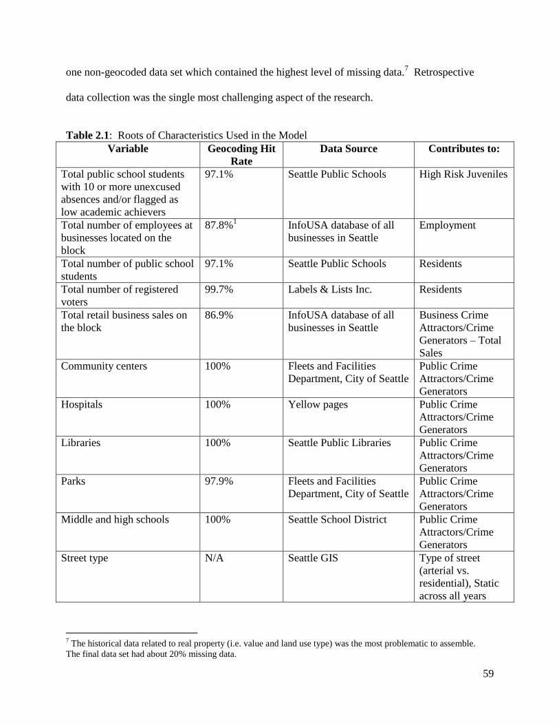
59

one non-geocoded data set which contained the highest level of missing data.7 Retrospective

data collection was the single most challenging aspect of the research.

Table 2.1: Roots of Characteristics Used in the Model

Variable Geocoding Hit

Rate

Data Source Contributes to:

Total public school students

with 10 or more unexcused

absences and/or flagged as

low academic achievers

97.1% Seattle Public Schools High Risk Juveniles

Total number of employees at

businesses located on the

block

87.8%1 InfoUSA database of all

businesses in Seattle

Employment

Total number of public school

students

97.1% Seattle Public Schools Residents

Total number of registered

voters

99.7% Labels & Lists Inc. Residents

Total retail business sales on

the block

86.9% InfoUSA database of all


Business Crime

Attractors/Crime

Generators – Total

Sales

Community centers 100% Fleets and Facilities

Department, City of Seattle

Public Crime

Attractors/Crime

Generators

Hospitals 100% Yellow pages Public Crime

Attractors/Crime

Generators

Libraries 100% Seattle Public Libraries Public Crime

Attractors/Crime

Generators

Parks 97.9% Fleets and Facilities


Public Crime

Attractors/Crime

Generators

Middle and high schools 100% Seattle School District Public Crime

Attractors/Crime

Generators

Street type N/A Seattle GIS Type of street

(arterial vs.

residential), Static

across all years

7 The historical data related to real property (i.e. value and land use type) was the most problematic to assemble.

The final data set had about 20% missing data.


60

Variable Geocoding Hit

Rate



within 2,640 feet of a street

block

Came as

shapefile

Department of Transportation

(Metro Transit Division) Bus Stops


parcels

N/A2 Developed from Historic

Assessor‘s Data (Seattle

Planning Department) and

parcel boundaries (King

County GIS).

Vacant Land

Total number of police

stations within 1,320 feet of a

street block

100% Fleets and Facilities

Department of the city of

Seattle - location source,

variable calculated by

researchers

Fire and Police

Stations

Total number of fire stations

within 1,320 feet of a street

block

100% Fleets and Facilities


- location source, variable

calculated by researchers

Fire and Police

Stations

Total amount of watts per

street segment

Came as shape

file

Seattle Public Utilities Street Lighting

1Since this data set was pulled by zip code there are quite a few records that are outside the city of Seattle but still

have Seattle addresses. In addition, some address fields are blank and others have PO Boxes and not street

addresses. 2 Getting the historical information joined to the shape file of parcels required several steps and resulted in an

average of 81% of the parcels having land use information. Note: The geocoding rate listed represents an average across all years.

Public School Students

Data about public school students was obtained from Seattle Public Schools. It includes

all public school students from grades 3 – 12. The total number of public school students ranges

from a low of 35,857 in 1992 to a high of 37,433 in 2004. The number of juveniles has been

relatively stable over the study period with 37,029 registered in 2004. Three analysis variables

are developed for use in the study: 1) total number of public school students who reside on each

street segment, 2) the total number of students who were considered truant (10 or more absences


61

in a school year) and 3) the total number of students who were considered to be low academic

achievers.8

The number of students classified as low academic achieving (LAA) is typically three

times that of truant students in any given year (mean of 14,366 versus 4,634). The year with the

lowest number of LAA students was 2004 (25.11%) and the year with the highest number was

1997 when there were 13,563 (38.2%) LAA students identified. That was also the year with the

highest proportion of students classified as LAA. The lowest number of truant students in any

given year was 3,581 (9.85%) which occurred in 2004. The highest number occurred in 1994

when there were 6,489 (18.4%) truant students. That was also the year with the highest

proportion of students classified as truant.

For our final analysis we created a variable defined as ‗high risk juveniles‘ which

represented the total number of students who were considered either truant (i.e. they had 10 or

more unexcused absences) or were categorized as low academic achievers. The number of high

risk juveniles fluctuated from 14,524 in 1992 to a high of 15,908 in 1997 before falling to its

lowest level in 2004 (n=11,230).

Businesses

After trying unsuccessfully to obtain business license data, we finally purchased data

from InfoUSA. While they had data available from 1998 to 2004, the data were expensive so we

purchased every other year (i.e., 1998, 2000, 2002, and 2004). The vendor could only pull data

by zip code which meant we obtained quite a few records from outside of Seattle which still had

8 Data describing the number of public schools students were provided at the hundred-block and geocoded by the

researchers to the street segment. The data were for academic years. We refer to each academic year by its earlier

calendar year (e.g., data for 1989-1990 are used to represent 1989).


62

Seattle addresses.9 We believe the relatively low geocoding rate of 87.8% reflects the influence

of businesses located outside Seattle and thus unmatchable. Unfortunately, it was impossible to

distinguish between those records that were unmatched because they were outside of Seattle and

those that were genuinely unmatched but inside Seattle. Thus the inability to identify records

outside of Seattle artificially lowered our match rate; the true rate was in all likelihood much

higher. The total number of businesses per year ranged from a low of 32,517 in 1998 to 37,916

in 2000 before dropping again to 34,547 in 2004. The average number of businesses per year

was 35,573. We aggregated the geocoded records to street segments and calculated the total

number of employees.

Because of the important relationship between retail establishments and crime levels we

isolated all businesses that were primarily retail focused and used total retail sales as the

measurement of the intensity of retail on a street.10

Roughly 10 percent of all businesses were

retail businesses. The number of retail businesses declined over the time period. The highest

number was 3,333 in 2000 followed by 3,331 in 2002. The earliest and latest years were both

lower with 3,251 in 1998 and 3,160 in 2004. We then aggregated the total amount of sales for

each retail business to the street segment on which it was located.

Registered Voters

Our figures related to voting behavior also were purchased from a vendor, Labels & Lists

Inc (Table 2.1). These data were originally collected by the Elections Department for King

9 The following zip codes were used to define Seattle: 98101, 98102, 98103, 98104, 98105, 98106, 98107, 98108,

98109, 98112, 98115, 98116, 98117, 98118, 98119, 98121, 98122, 98125, 98126, 98133, 98134, 98136, 98144,

98146, 98168, 98177, 98178, 98195, and 98199. 10

The following North American Industrial Classification (NAIC) codes were used to identify retail businesses: 441

-Motor Vehicle and Parts Dealers; 442 -Furniture and Home Furnishings Stores; 443 -Electronics and Appliance

Stores; 444 -Building Material and Garden Equipment and Supplies Dealers; 44612 -Cosmetics, Beauty Supplies,

and Perfume Stores; 44613 -Optical Goods Stores; 44619 -Other Health and Personal Care Stores; 448 -Clothing

and Clothing Accessories Stores (Retail); 451 -Sporting Goods; Hobby, Book, and Music Stores (Retail); 452 -

General Merchandise Stores (Retail); 453 -Miscellaneous Store Retailers (Retail).


63

County but they do not keep historical records. Thus, we turned to Labels & Lists Inc., which

kept historical records back to 1999. From these records we developed a variable that contains

the total number of registered voters for each year. This information was used later to help

estimate adult residential population.

Public Facilities

The data on the locations of facilities were primarily obtained from the city departments

that run them (Table 2.1). Seattle Fleets and Facilities Department was helpful with the police

facilities, fire facilities, parks and community centers. Obtaining the current locations was very

straightforward. As mentioned earlier, the challenge came when we tried to establish which

facilities had opened, closed (even temporarily), or changed location during our study period.

The number of each type of public facilities was relatively small and very stable. There were 26

community centers from 1989 to 2003. Two were added in 2004 for a total of 28 community

centers at the end of the study period. There were 13 hospitals in Seattle over the entire study

period. There were 17 libraries in 1989 and 21 in 2004. Middle and high schools had some

minor fluctuations over the years (e.g. closing for remodeling) but in general they showed an

increase from 28 facilities in 1989 to 30 in 2004. Except for hospitals, public facilities were

distributed across Seattle.

To represent the crime generating effect of public and quasi-public facilities on nearby

street segments we calculated a spatial variable using a geographic information system (GIS).

This variable represents the number of public and quasi-public facilities (i.e., community centers,

hospitals, libraries, parks, and middle and high schools) within a 1,320 foot distance (i.e. a

quarter mile) of each street segment. Distance was measured along the street network using

ArcGIS Network Analyst extension. Using street network distance was especially important in a


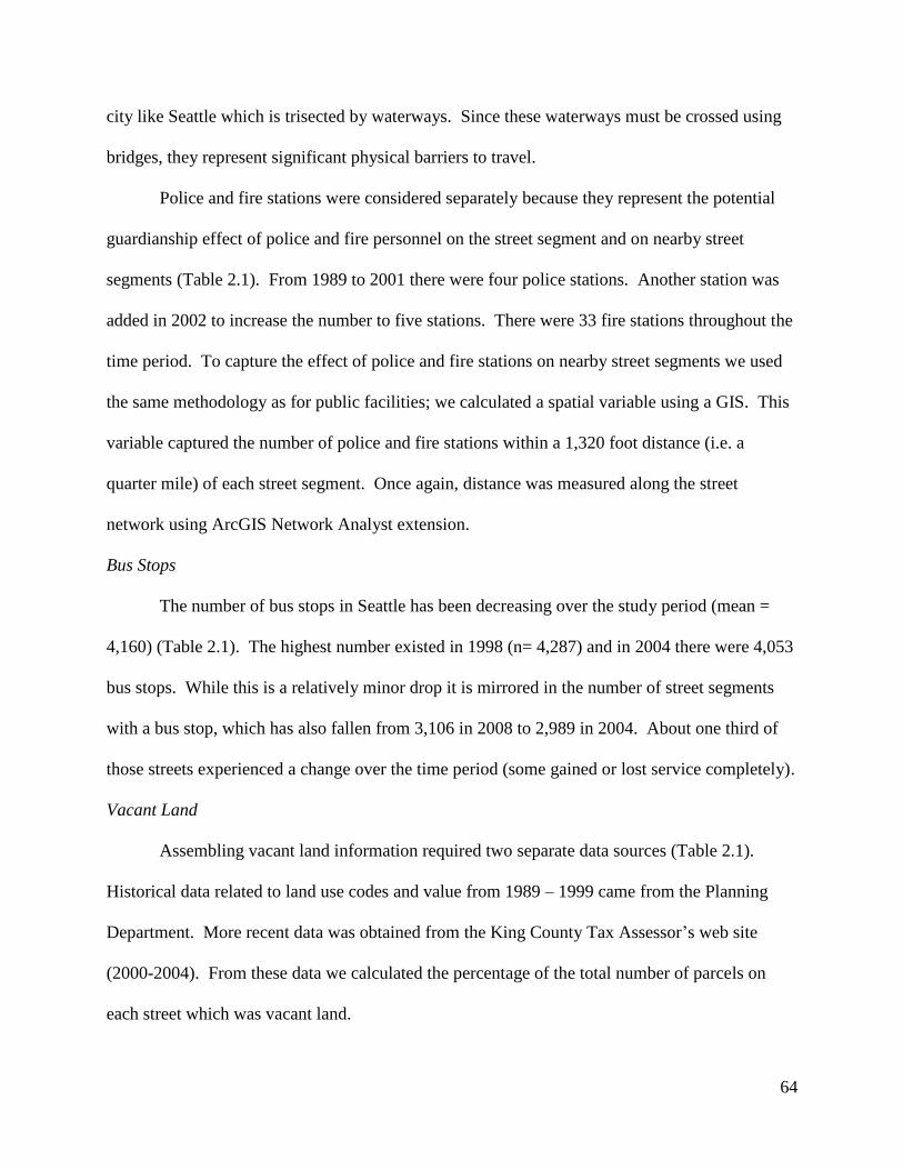
64

city like Seattle which is trisected by waterways. Since these waterways must be crossed using

bridges, they represent significant physical barriers to travel.

Police and fire stations were considered separately because they represent the potential

guardianship effect of police and fire personnel on the street segment and on nearby street

segments (Table 2.1). From 1989 to 2001 there were four police stations. Another station was

added in 2002 to increase the number to five stations. There were 33 fire stations throughout the

time period. To capture the effect of police and fire stations on nearby street segments we used

the same methodology as for public facilities; we calculated a spatial variable using a GIS. This

variable captured the number of police and fire stations within a 1,320 foot distance (i.e. a

quarter mile) of each street segment. Once again, distance was measured along the street

network using ArcGIS Network Analyst extension.

Bus Stops

The number of bus stops in Seattle has been decreasing over the study period (mean =

4,160) (Table 2.1). The highest number existed in 1998 (n= 4,287) and in 2004 there were 4,053

bus stops. While this is a relatively minor drop it is mirrored in the number of street segments

with a bus stop, which has also fallen from 3,106 in 2008 to 2,989 in 2004. About one third of

those streets experienced a change over the time period (some gained or lost service completely).

Vacant Land

Assembling vacant land information required two separate data sources (Table 2.1).

Historical data related to land use codes and value from 1989 – 1999 came from the Planning

Department. More recent data was obtained from the King County Tax Assessor‘s web site

(2000-2004). From these data we calculated the percentage of the total number of parcels on

each street which was vacant land.


65

Street Lighting

Information on street lighting was supplied by the Seattle Public Utilities Department and

was used to create a total number of watts per street value for 1997 - 2004 (Table 2.1).11

The

number of street poles and their associated lights increased steadily over the time period (from

68,725 in 1997 to 83,709 in 2004). This overall increase is in contrast to variability at the

individual street segment level where there was change in both directions. The street lighting

wattage decreased on 540 streets (413 were residential and 127 were arterial). Almost all these

streets are concentrated in one suspiciously rectangular area in the northeast part of the city. The

Utility department had no explanation for this ‗dark‘ area. Wattage increased on 5,420 streets

(4,059 were residential and 1,361 were arterial). Street segments with decreasing lighting were

spread throughout the city except for west Seattle in which there was no increasing streets.

Street Type

We obtained street type information as part of the street centerline file (Table 2.1).12

Seattle GIS provided their 2006 street centerline file which we used to develop the units of

analysis and to obtain information on street type. We consider two types of streets in the study:

arterial and residential (which includes walkways/stairs). Arterial streets are higher traffic streets

which have higher speed limits.13

They collect traffic flowing from residential streets and

provide for movement within areas of the city while still enabling access to abutting land uses.

11

When representing lighting related to a street, we only included light poles that were within 90 feet of the street

centerline for residential roads and within 300 feet for arterial roads. The two different thresholds were used

because of the difference in the average width of an arterial street and a residential street. After establishing the street poles whose light might reach the edge of the street, we then found the total wattage the street lights associated

with each pole and aggregated the total watts by street segment. 12

We used the 2006 centerline file because the Seattle Planning Department and Seattle GIS department verified

there had been no significant changes in the street configuration nor had there been any annexations during the study

period. 13

Information on street classifications was retrieved from the King County Department of Transportation web site at

http://www.kingcounty.gov/transportation/kcdot/Roads/TransportationPlanning/ArterialClassificationSystem.aspx.

Briefly, arterial streets are those that carry larger volumes of traffic. Residential streets run through neighborhoods

and are designed to carry lower volumes of local travel at slower speeds. Walkways are non-vehicular paths or

stairways that typically connect two residential streets.


http://www.kingcounty.gov/transportation/kcdot/Roads/TransportationPlanning/ArterialClassificationSystem.aspx

66

Residential streets also provide access to land uses but they have lower speed limits and are

designed to carry less traffic.

Final Characteristics for Analysis

These characteristics were then used to create the final characteristics for analyses

reported in the chapters that follow (Table 2.2). Each of the final 10 characteristics represents

one of four constructs: motivated offenders, suitable targets, guardianship or accessibility/urban

form. All the final data sets have a geographic extent that includes the entire city of Seattle.

However, their temporal extent varies. We were able to get only the crime data and the public

facilities data over the entire study period. The temporal period of the other characteristics range

from four years of coverage to 13 years of coverage.

Table 2.2: Sources and Extents of Opportunity Theory Variables

Variable Definition Source Temporal

Extent

Years

High Risk

Juveniles

Total number of

public school students

with 10 or more

unexcused absences

and/or flagged as low

academic achievers

Seattle Public Schools 13 years 1992 -

2004

Employment Total number of

employees at

businesses located on

the block

InfoUSA database of all


7 years 1998,

2000,

2002,

2004

Residents Composite variable

combining the total

number of public

school students and

the total number of

registered votes

Seattle Public Schools

(public school students),

Labels & Lists Inc.

(voter registration)

6 years 1999 -

2004

Business Crime

Attractors/Crime

Generators

Total retail business

sales on the block

InfoUSA database of all


7 years 1998,

2000,

2002,

2004


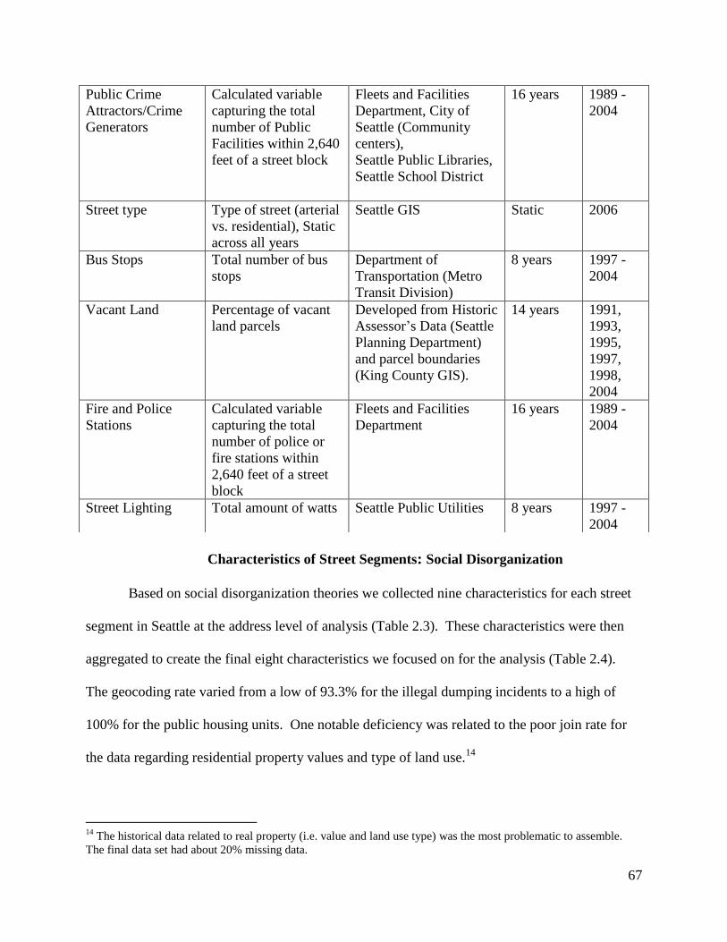
67

Characteristics of Street Segments: Social Disorganization

Based on social disorganization theories we collected nine characteristics for each street

segment in Seattle at the address level of analysis (Table 2.3). These characteristics were then

aggregated to create the final eight characteristics we focused on for the analysis (Table 2.4).

The geocoding rate varied from a low of 93.3% for the illegal dumping incidents to a high of

100% for the public housing units. One notable deficiency was related to the poor join rate for

the data regarding residential property values and type of land use.14

14

The historical data related to real property (i.e. value and land use type) was the most problematic to assemble.

The final data set had about 20% missing data.

Public Crime

Attractors/Crime

Generators

Calculated variable

capturing the total

number of Public

Facilities within 2,640

feet of a street block

Fleets and Facilities

Department, City of

Seattle (Community

centers),

Seattle Public Libraries,

Seattle School District

16 years 1989 -

2004

Street type Type of street (arterial

vs. residential), Static

across all years

Seattle GIS Static 2006

Bus Stops Total number of bus

stops

Department of

Transportation (Metro

Transit Division)

8 years 1997 -

2004

Vacant Land Percentage of vacant

land parcels

Developed from Historic


Planning Department)

and parcel boundaries

(King County GIS).

14 years 1991,

1993,

1995,

1997,

1998,

2004

Fire and Police

Stations

Calculated variable

capturing the total

number of police or

fire stations within

2,640 feet of a street

block

Fleets and Facilities

Department

16 years 1989 -

2004

Street Lighting Total amount of watts Seattle Public Utilities 8 years 1997 -

2004


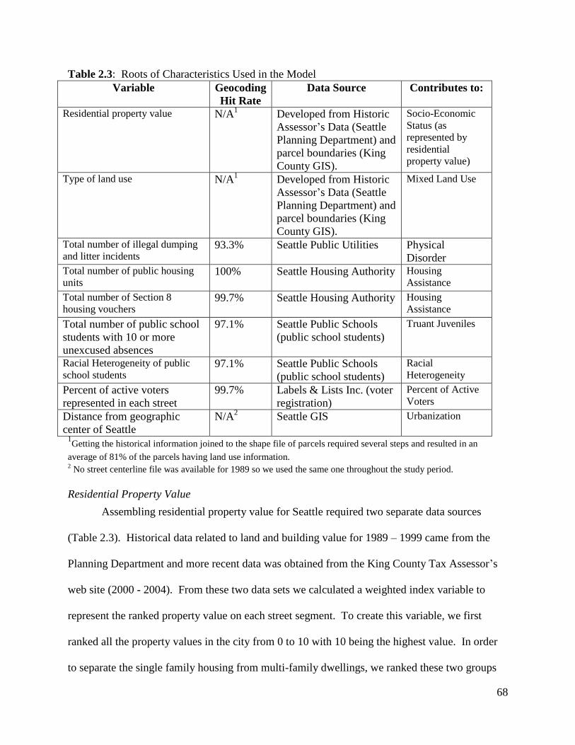
68

Table 2.3: Roots of Characteristics Used in the Model

Variable Geocoding

Hit Rate


Residential property value N/A1 Developed from Historic




County GIS).

Socio-Economic

Status (as

represented by

residential

property value)

Type of land use N/A1 Developed from Historic




County GIS).

Mixed Land Use

Total number of illegal dumping

and litter incidents 93.3% Seattle Public Utilities Physical

Disorder Total number of public housing

units 100% Seattle Housing Authority

Housing

Assistance

Total number of Section 8

housing vouchers 99.7% Seattle Housing Authority

Housing

Assistance

Total number of public school

students with 10 or more

unexcused absences

97.1% Seattle Public Schools

(public school students)

Truant Juveniles

Racial Heterogeneity of public

school students 97.1% Seattle Public Schools

(public school students)

Racial

Heterogeneity

Percent of active voters

represented in each street

99.7% Labels & Lists Inc. (voter

registration)

Percent of Active

Voters

Distance from geographic

center of Seattle

N/A2 Seattle GIS Urbanization

1Getting the historical information joined to the shape file of parcels required several steps and resulted in an

average of 81% of the parcels having land use information. 2 No street centerline file was available for 1989 so we used the same one throughout the study period.

Residential Property Value

Assembling residential property value for Seattle required two separate data sources

(Table 2.3). Historical data related to land and building value for 1989 – 1999 came from the

Planning Department and more recent data was obtained from the King County Tax Assessor‘s

web site (2000 - 2004). From these two data sets we calculated a weighted index variable to

represent the ranked property value on each street segment. To create this variable, we first

ranked all the property values in the city from 0 to 10 with 10 being the highest value. In order

to separate the single family housing from multi-family dwellings, we ranked these two groups


69

separately. Then we combined the ranks of single-family housing (SF) and multi-family housing

(MF) into a final value that represents the property value of a street. We also weight the ranks by

percentage of housing type in the given street so the composite score also reflects the proportion

of the type of property. This variable contributed to SES (Table 2.4).

Land Use Type

Similarly, assembling land use information required two separate data sources (Table

2.3). Historical data related to land use codes from 1989 – 1999 came from the Planning

Department. No historical data related to land use was available from the King County Tax

Assessor‘s web site; 2004 data were available however and those were used. From these two

data sources we calculated the percentage of the total of each type of land use on each street

segment. Finally, we created a dichotomous variable representing those streets with percent

residential land use between 25% and 75 % which also have nonresidential land uses present

(e.g. commercial, institutional, industrial etc. but not solely water or vacant land). Streets

meeting this criterion were coded as mixed land use. This variable contributed to Mixed Land

Use (Table 2.4).

Physical Disorder

Data documenting physical disorder incidents was collected from the Seattle Public

Utilities department (Tables 2.3 and 2.4). The incidents in this database were generated from

problems noticed by both inspectors (self-initiated), reports from other agencies, and from

citizens calling the hot line or emailing the agency to report illegal dumping problems. The

physical disorder measure includes: illegal dumping, litter, graffiti, weeds, vacant buildings,

inoperable cars on the street, junk storage, exterior abatement, substandard housing and minor

property damage. The type of dumping and litter items recorded in the database consists of


70

things like tires, appliances, yard waste, mattresses, and freezers, to list just a few. This database

covers the time period from 1992-2004. But the information was not consistently gathered for

1992. Therefore, this study only uses information from 1993 to 2004. There were 42,331

incidents in the original database and 93.3% of them were successfully geocoded.

Public Housing

The total locations of public housing communities and the total number of units in each

community were collected from the Seattle Housing Authority (Table 2.3). Several of the large

communities reported one total number of units for the entire complex (High Point, New Holly

and Rainier Vista). For these, we divided the total number of units by the number of street

segments which participated in the development and allocated the resulting number of units to

each street in the development. There were 5,857 public housing units from 1989 – 1997. In

1997, the number dropped to 5,299 units and stayed there until 2002 when it dropped again to

4,218. Two subsequent changes occurred in the last two years of the study period: first a

reduction to 3,838 units in 2003 and then a slight increase to 3,896 units in 2004. This variable

contributed to the composite variable of Housing Assistance (Table 2.4).

Section 8

We obtained information on the allocation of Section 8 vouchers in Seattle from the

Seattle Housing Authority (Table 2.3). Section 8 housing vouchers can be used to rent any

apartment for which the management will accept the vouchers. Vouchers allow individuals to

rent market rate apartments for reduced cost with the voucher bridging the gap between what the

individual can pay and market rate rent. The number of vouchers has increased from 1,674 to

2,250 between 1998 and 2004, a 34.4% increase. The minimum number of vouchers on a given

street was 0 across all years while the maximum ranged from a low of 125 in 2003 to high of 152


71

in 1999. This variable contributed to the composite variable of Housing Assistance (Table 2.4).

The presence of public housing units and Section 8 voucher holders show where the

disadvantaged populations are located.

Truant Juveniles

Data about truant juveniles was obtained from Seattle Public Schools as part of the public

school‘s student database (Tables 2.3 and 2.4). Truant juveniles were defined as the total

number of students with 10 or more unexcused absences in a school year (see earlier section on

public school data for more information). The lowest number of truant students in any given

year was 3,581 (9.85%) in 2004. The highest number occurred in 1994 when there were 6,489

(18.4%) truant students. That was also the year with the highest proportion of students classified

as truant.


Racial heterogeneity measurement was estimated using information that was part of the

Seattle Public School‘s student database (Tables 2.3 and 2.4). The data contain racial

identification of all students enrolled in Seattle‘s public schools from 1992 to 2004. Four racial

groups were identified in this study including white, black, Asian, and Hispanic. The

probabilities of each racial group encountering another out-group member were then computed

and averaged to form an overall racial heterogeneity index. The detailed computation process of

the variable is described in Chapter 3.

Percent of Active Voters

The variable Percent Active Voters was drawn from the voting database (Tables 2.3 and

2.4). The data include not only the registered voters‘ voting behaviors (whether they voted or

not in the given year) for the current year but also their past voting frequency dating back to


72

1990. To differentiate active voters from the rest, we compared each registered voter‘s short-

term average voting behavior to the population‘s short-term voting average in the most recent

two years. In any given year, if a person had an average short-term voting behavior greater than

the mean of Seattle‘s registered voters, then we assigned this person an active voter status. On

each street, the number of active voters is divided by the number of total registered voters to get

the percent of active voter. This value is used as a proxy of residents‘ willingness to participate

in public affairs.

Distance from City Center

The distance from city center was calculated from each street segment to the geographic

center of Seattle (Tables 2.3 and 2.4).15

This measure represents the degree of urbanization of

each street. The geographic center of Seattle was located at 331 Minor Ave N.16

Distance was

measured along the street network using the ArcGIS Network Analyst extension. Using street

network distance was especially important in a city like Seattle which is trisected by waterways.

Since these waterways must be crossed using bridges, they represent significant physical barriers

to travel.

Final Characteristics for Analysis

These characteristics were then used to create the final characteristics for analyses

reported in later chapters (Table 2.4). Each of the final eight characteristics represents one of

two theoretical dimensions. The structural dimension includes socioeconomic status, mixed land

use, urbanization, housing assistance, physical disorder, and racial heterogeneity. The

15

We also considered using the cultural center of Seattle but we could find no documentation regarding a cultural

center. The librarians at the Seattle Public Library identified the Westlake Center (4th Ave. and Pine St) which

opened in 1988 as the cultural center (personal conversation, 2008). Since the two addresses are only 3,650 feet (a

little less than three-quarters of a mile) apart as the crow flies, we went with the geographic center which was a

known fact. 16

The geographic center of Seattle is located at N 47° 37.271 W 122° 19.986 which translates to 331 Minor Ave N

(see http://www.waymarking.com/waymarks/WM29A8).


73

intermediating dimension of the effects of structural factors on crime includes unsupervised teens

and willingness to intervene in public affairs.

The spatial and temporal extent of each characteristic as well as its definition is included

in Table 2.4. All the final data sets have a geographic extent that includes the entire city of

Seattle. However, their temporal extent varies. We were not able to obtain any of these

characteristics for the entire study period. The temporal coverage of other characteristics ranged

from a low of four years of coverage for concentrated disadvantage to a high of 13 years for

physical disorder. For the sake of brevity, only the one composite variable that is new to the

discussion is described below.

Housing Assistance

The variable called Housing Assistance consists of the total number of public housing

units plus the total number of Section 8 vouchers in use on a street segment. We created this

variable to capture the total number of housing units on each street segment receiving some type

of housing assistance (Table 2.4).

Table 2.4: Social Disorganization Variables Spatial and Temporal Extent

Variable Definition Temporal

Extent

Years

Socio-Economic

Status (as

represented by

residential

property value)

To create this variable, we first ranked

all the property in the city from 1 to 10

with 10 being the highest value. In order

to separate the single family (SF)

housing from multi-family (MF)

dwellings, we ranked these two groups

separately. Then we combined the ranks

of SF and MF into a final value that

represents the property value of a street.

We also weigh the ranks by percentage

of housing type in the given street so the

composite score of SES also reflects the

proportion of the type of property.

Covers 6

years over a

14 year

period.

1991, 1993, 1995,

1997, 1998, 2004


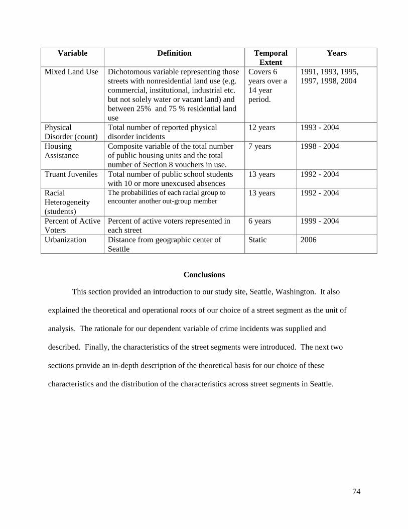
74

Variable Definition Temporal

Extent

Years

Mixed Land Use

Dichotomous variable representing those

streets with nonresidential land use (e.g.

commercial, institutional, industrial etc.

but not solely water or vacant land) and

between 25% and 75 % residential land

use

Covers 6

years over a

14 year

period.

1991, 1993, 1995,

1997, 1998, 2004

Physical

Disorder (count)

Total number of reported physical

disorder incidents

12 years 1993 - 2004

Housing

Assistance

Composite variable of the total number

of public housing units and the total

number of Section 8 vouchers in use.

7 years 1998 - 2004

Truant Juveniles Total number of public school students

with 10 or more unexcused absences

13 years 1992 - 2004

Racial

Heterogeneity

(students)

The probabilities of each racial group to

encounter another out-group member 13 years 1992 - 2004

Percent of Active

Voters

Percent of active voters represented in

each street

6 years 1999 - 2004

Urbanization Distance from geographic center of

Seattle

Static 2006

Conclusions

This section provided an introduction to our study site, Seattle, Washington. It also

explained the theoretical and operational roots of our choice of a street segment as the unit of

analysis. The rationale for our dependent variable of crime incidents was supplied and

described. Finally, the characteristics of the street segments were introduced. The next two

sections provide an in-depth description of the theoretical basis for our choice of these

characteristics and the distribution of the characteristics across street segments in Seattle.


75

Chapter 3: Social Disorganization and

Social Capital at Micro Places

As described in Chapter 1, social disorganization theory has played a central role in

place-based understandings of crime in criminology. But the impact of social disorganization on

crime has been described at much higher units of analysis than our interests in the study of crime

and place in Seattle. Social disorganization theorists have focused their concerns on

―communities‖ and ―neighborhoods‖ not on street segments or even small groups of street

segments. Even Shaw and McKay (1942 [1969]), who began their investigation of juvenile

delinquency with the addresses of the youths they studied, focused their theoretical interests on

the general patterns of delinquency in large areas of the city. Are indicators of social

disorganization at the street segment level relevant to understanding variability in crime at place,

or rather is the influence of such factors relevant only at the higher levels of geography that

social disorganization theorists have ordinarily studied? To answer this question, we must first

ask whether there is variability in the distribution of characteristics of social disorganization at

the street segment level.

In this chapter we explore the distribution of characteristics of social disorganization

across street segment in Seattle. Prior studies have, for example, noted that a very large

proportion of crime in the city is found at a very small number of places that have been identified

as crime hot spots (Pierce et al., 1986; Sherman et al., 1989; Weisburd & Green, 1994; Weisburd

et al., 2004; Weisburd et al., in press). Is the same true for the concentration of evidence of

social disorganization at street segments? Are there, for example, hot spots of social or physical

disorder? If there are, of course, this then raises the question of whether hot spots of social


76

disorganization and hot spots of crime occur in the same places (a question we will review in

later chapters). Similarly, do we find evidence of variability across geography in the

concentration of characteristics of social disorganization? Social disorganization theorists have

ordinarily seen characteristics reflecting this perspective as occurring at a neighborhood level.

This would suggest that there is relatively little variability in such traits within neighborhoods.

But if such traits vary greatly within neighborhoods and across street segments then it would

seem reasonable to begin to examine how variability in social disorganization at the street

segment level affects developmental patterns of crime at that level.

As far as we are aware, ours is the first study to examine the salience of social

disorganization theory at a micro place unit of analysis. In this context, we present in this

chapter the first systematic review of how characteristics of social disorganization concentrate

and distribute across street segments in an urban context. We find overall that social

disorganization at the street segment level evidences strong concentrations across the city and

that such concentrations are not necessarily limited to specific larger geographic contexts such as

neighborhoods. There are hot spots of social disorganization at a micro place unit of analysis,

and these hot spots evidence a significant degree of spatial dispersion. Our findings provide a

strong basis for asking whether the distribution of social disorganization at the street segment

level is related to developmental patterns of crime at street segments later in our report.

Structural and Mediating Variables of Social Disorganization

Indicators of social disorganization have generally been divided into two main domains:

the structural characteristics of places and the intermediating mechanisms that govern these

places (e.g. see Bursik & Grasmick, 1993; Lowenkamp et al., 2003; Osgood & Chambers, 2000;

Sampson & Groves, 1989; Sampson et al., 1997). We identify information that represents


77

critical structural characteristics of places including socio-economic status (SES), physical

disorder, racial heterogeneity, mixture of land use, urbanization, and concentration of

disadvantage. All of these factors have been used widely in past literature to represent the level

of social organization of places. Since mediating factors are variables that represent the ability

of places to regulate activities that occur within them, we include variables such as the presence

of unsupervised teens and voting participation. These variables demonstrate levels of social

control, social capital, and the capacities of collective efficacy. Variables are categorized under

several major themes of social disorganization theory in Table 3.1.1

1 Chapters 3 and 4 examine the distribution of characteristics across all 24,178 street segments (i.e., including the

University of Washington campus).


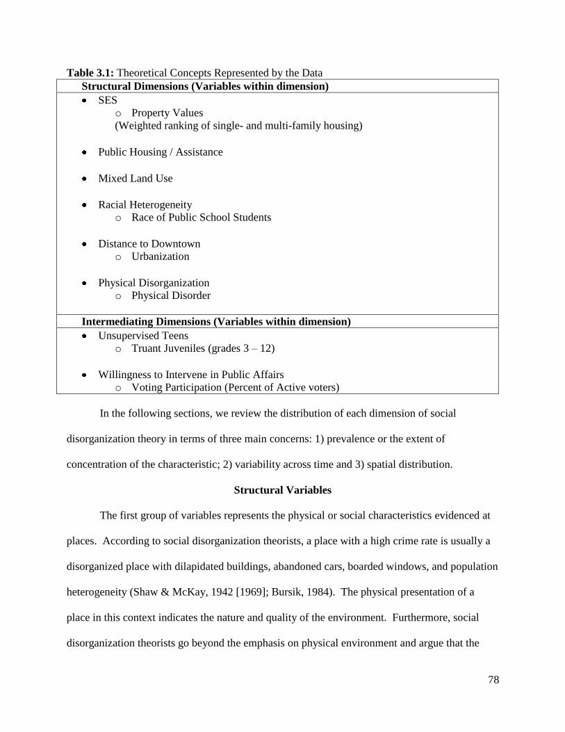
78

Table 3.1: Theoretical Concepts Represented by the Data

Structural Dimensions (Variables within dimension)

SES

o Property Values

(Weighted ranking of single- and multi-family housing)

Public Housing / Assistance

Mixed Land Use


o Race of Public School Students

Distance to Downtown

o Urbanization

Physical Disorganization

o Physical Disorder

Intermediating Dimensions (Variables within dimension)

Unsupervised Teens

o Truant Juveniles (grades 3 – 12)

Willingness to Intervene in Public Affairs

o Voting Participation (Percent of Active voters)

In the following sections, we review the distribution of each dimension of social

disorganization theory in terms of three main concerns: 1) prevalence or the extent of

concentration of the characteristic; 2) variability across time and 3) spatial distribution.

Structural Variables

The first group of variables represents the physical or social characteristics evidenced at

places. According to social disorganization theorists, a place with a high crime rate is usually a

disorganized place with dilapidated buildings, abandoned cars, boarded windows, and population

heterogeneity (Shaw & McKay, 1942 [1969]; Bursik, 1984). The physical presentation of a

place in this context indicates the nature and quality of the environment. Furthermore, social

disorganization theorists go beyond the emphasis on physical environment and argue that the


79

lack of homogeny in a place further reduces the likelihood that people will be willing to work

with each other to improve the conditions. In the following section, we review the theoretical

foundation of each of the variables we collected and then present the distributions of these

variables across places and over time.

Socio-Economic Status: Property Values

In the original version of social disorganization theory, Shaw and McKay (1942 [1969])

contend that the concentration of industry and businesses in the downtown area makes it an

undesirable place to live. People who cannot afford to move out of town ended up in the

transitional zone—the area between the industrial center and the residential area. Thus, the

transitional area tends to contain low socio-economic status residents, high crime rates, and other

social illnesses. In social disorganization theory, the socio-economic status (SES) of residents is

an important indicator of crime ridden areas. Even in recent social disorganization theory, SES

is still used widely to represent resources and capabilities of residents to invest in the community

where they live (e.g. see Bellair, 1997; Bursik & Grasmick, 1993; Sampson & Groves, 1989;

Veysey & Messner, 1999). In this study, we measure SES using the average property values

(combined land and building value data) of each street, using it as a proxy to represent the

average socio-economic status of residents on each street in Seattle.2

As mentioned in Chapter 2, about 80 percent of the streets have detailed records about

housing values and land use. The majority of the areas in Seattle are used for residential

purposes. Among all the streets with valid information, 19,425 street segments have at least one

residential building (88 percent). For example, in 1989 out of the 17,152 streets with any

2 Specifically, we use the combined land and building value data because local experts felt it was the most reliable

field in their historical data set.


80

residential building, 16,052 streets had single family houses while only 3,482 streets had multi-

family residential buildings.

One complication of using the raw property value data for the residential areas is that it

includes both single family housing and multi-family dwellings. If we simply compare property

values without addressing the differences between single family houses and multi-dwelling

buildings, the results will be misleading. Single family houses tend to be worth less than high

rise buildings simply because of the size of the land or physical construction; however, people

who live in single family houses are more likely to own their homes. To take into account the

impact of both single family dwellings and multi-family dwellings, we rank single family

housing and multi-family housing separately and then create a composite to represent the SES of

the street. To achieve this, we separately rank averaged property values for single family

housing and multi-family housing, assigning each street a rank between 0 and 10 based on the

average values of properties. For example, streets with the highest 9 percent of single family

building values received a rank of 10 while streets with the lowest values received a rank of 0.

The same procedure was repeated for multi-family housing. Finally, the ranks of each street on

the single family property value and multi-family property value were then weighted by the

percentages of the type of housing of a given street and then combined to create a property value

index to represent the SES of a street.

Based on the social disorganization tradition, we want to first understand whether high

SES (or low) street segments, like other factors we review, are concentrated in limited areas or

spread randomly throughout the city. By default, the property values are only present in the

streets with residential dwellings. Thus, the following analyses will focus only on the 19,425

streets (88 percent) with valid information on residential building values in Seattle. In the


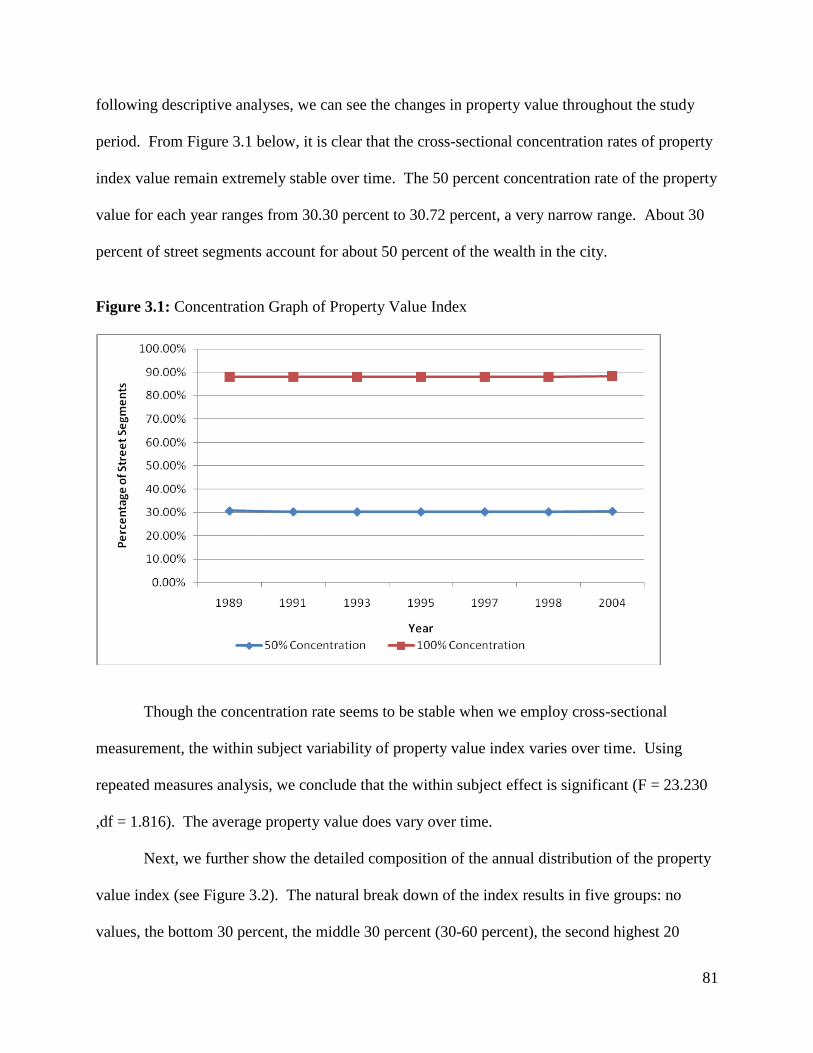
81

following descriptive analyses, we can see the changes in property value throughout the study

period. From Figure 3.1 below, it is clear that the cross-sectional concentration rates of property

index value remain extremely stable over time. The 50 percent concentration rate of the property

value for each year ranges from 30.30 percent to 30.72 percent, a very narrow range. About 30

percent of street segments account for about 50 percent of the wealth in the city.

Figure 3.1: Concentration Graph of Property Value Index

Though the concentration rate seems to be stable when we employ cross-sectional

measurement, the within subject variability of property value index varies over time. Using

repeated measures analysis, we conclude that the within subject effect is significant (F = 23.230

,df = 1.816). The average property value does vary over time.

Next, we further show the detailed composition of the annual distribution of the property

value index (see Figure 3.2). The natural break down of the index results in five groups: no

values, the bottom 30 percent, the middle 30 percent (30-60 percent), the second highest 20


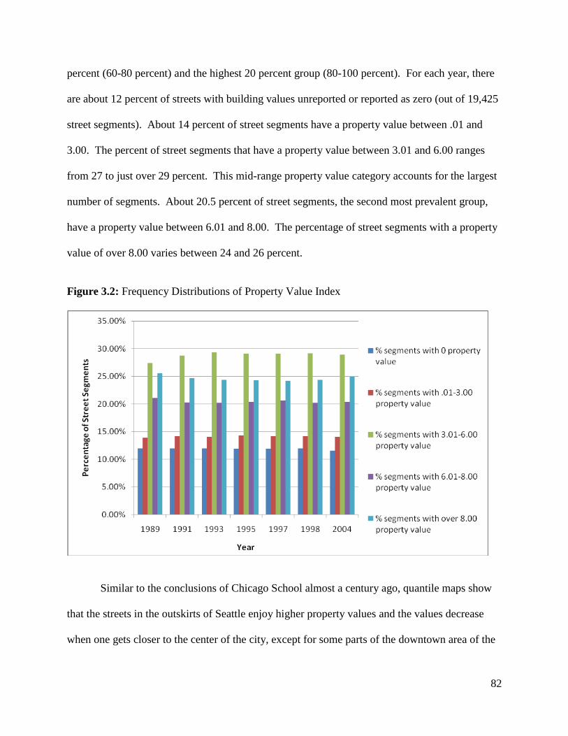
82

percent (60-80 percent) and the highest 20 percent group (80-100 percent). For each year, there

are about 12 percent of streets with building values unreported or reported as zero (out of 19,425

street segments). About 14 percent of street segments have a property value between .01 and

3.00. The percent of street segments that have a property value between 3.01 and 6.00 ranges

from 27 to just over 29 percent. This mid-range property value category accounts for the largest

number of segments. About 20.5 percent of street segments, the second most prevalent group,

have a property value between 6.01 and 8.00. The percentage of street segments with a property

value of over 8.00 varies between 24 and 26 percent.

Figure 3.2: Frequency Distributions of Property Value Index

Similar to the conclusions of Chicago School almost a century ago, quantile maps show

that the streets in the outskirts of Seattle enjoy higher property values and the values decrease

when one gets closer to the center of the city, except for some parts of the downtown area of the


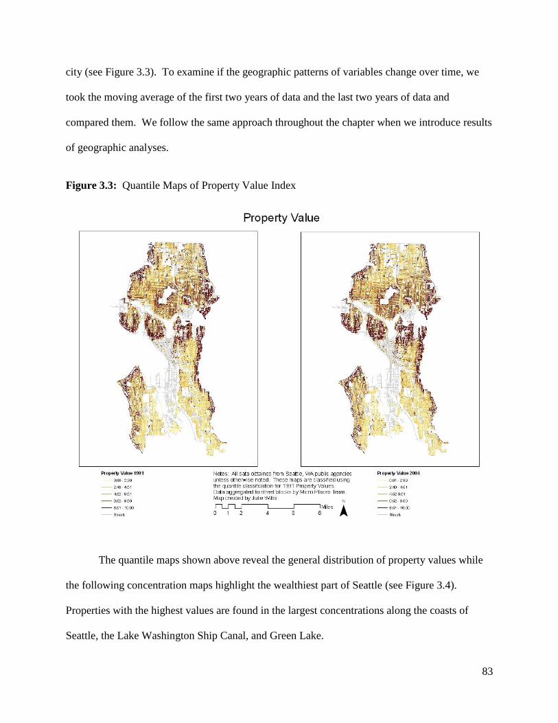
83

city (see Figure 3.3). To examine if the geographic patterns of variables change over time, we

took the moving average of the first two years of data and the last two years of data and

compared them. We follow the same approach throughout the chapter when we introduce results

of geographic analyses.

Figure 3.3: Quantile Maps of Property Value Index

The quantile maps shown above reveal the general distribution of property values while

the following concentration maps highlight the wealthiest part of Seattle (see Figure 3.4).

Properties with the highest values are found in the largest concentrations along the coasts of

Seattle, the Lake Washington Ship Canal, and Green Lake.


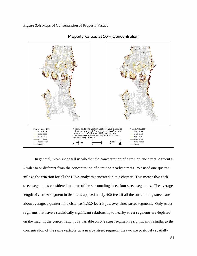
84

Figure 3.4: Maps of Concentration of Property Values

In general, LISA maps tell us whether the concentration of a trait on one street segment is

similar to or different from the concentration of a trait on nearby streets. We used one-quarter

mile as the criterion for all the LISA analyses generated in this chapter. This means that each

street segment is considered in terms of the surrounding three-four street segments. The average

length of a street segment in Seattle is approximately 400 feet; if all the surrounding streets are

about average, a quarter mile distance (1,320 feet) is just over three street segments. Only street

segments that have a statistically significant relationship to nearby street segments are depicted

on the map. If the concentration of a variable on one street segment is significantly similar to the

concentration of the same variable on a nearby street segment, the two are positively spatially


85

auto-correlated. Positive spatial autocorrelation can describe either a situation in which street

segments with high concentrations of a trait are near other street segments with high

concentrations or a situation in which street segments with low concentrations of the variable are

near other street segments with low concentrations. If the concentration of a trait on one street

segment is significantly different from the concentration on another nearby street segment, the

two street segments are negatively spatially auto-correlated. Negative spatial autocorrelation can

describe either a situation where street segments with high concentrations of a trait are near street

segments with low concentrations of the same trait or one in which street segments with low

concentrations of a variable are near street segments with high concentrations of the same

variable.

In the case of property value, the LISA maps reveal large areas of generally positive

spatial autocorrelation that is statistically significant (see Figure 3.5). The LISA analysis

confirms the concentration of high value street segments along the coasts and in the northern part

of the central section and the northern sections of the city. Generally, we can see the red dots

(representing high value properties surrounded by other high value properties) are clustering in

the north and along the coast. Interestingly, there are often street segments dominated by low

value properties sprinkled among them. The blue dots (representing low value properties near

other lower value properties) are concentrated in the south. Similarly, there are also street

segments dominated by high value properties sprinkled among them but with far less frequency.


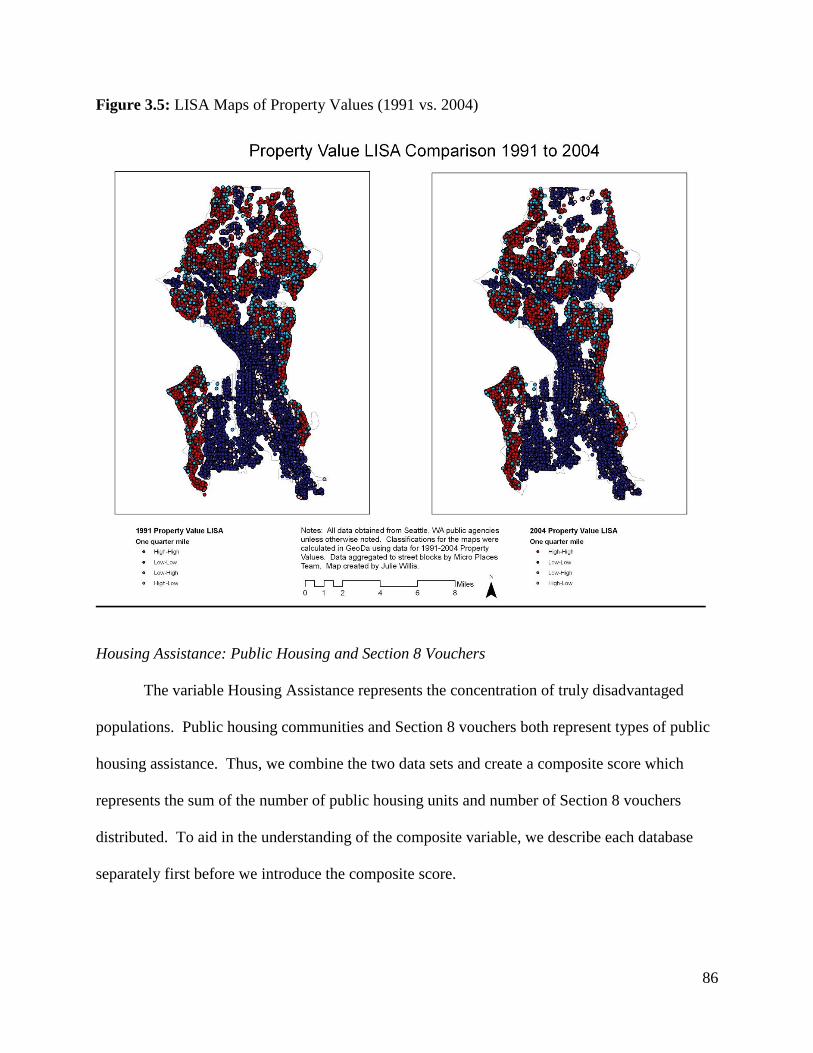
86

Figure 3.5: LISA Maps of Property Values (1991 vs. 2004)

Housing Assistance: Public Housing and Section 8 Vouchers

The variable Housing Assistance represents the concentration of truly disadvantaged

populations. Public housing communities and Section 8 vouchers both represent types of public

housing assistance. Thus, we combine the two data sets and create a composite score which

represents the sum of the number of public housing units and number of Section 8 vouchers

distributed. To aid in the understanding of the composite variable, we describe each database

separately first before we introduce the composite score.


87

Public Housing

Identifying the locations of public housing is a very straightforward way to show the

geographic distribution of the population who are at the bottom of the wealth spectrum. Instead

of using census information to identify the areas where residents’ salaries fall below the poverty

line, the information on public housing tells us where truly disadvantaged people live. In Seattle,

there are different types of housing projects consisting of high rise units (approximately 75-300

units per building) and four garden communities (community style: approximately 525 units).

High rise buildings were built in the 1970s; garden communities were built in the 1940s, and

some have been renovated and redeveloped over time. The structures and locations of public

housing in Seattle have been fairly stable, especially within our study period. However, when

change did occur, the magnitude was very large. For example, the total number of units

decreased from 5,856 in 1989 to 3,896 in 2004, which represents a decrease of 33.4 percent.

Additionally, less than 1 percent of streets in Seattle have public housing units on them (around

200 streets). 3

Based on social disorganization theory, we would predict that the locations of public

housing overlap with crime hot spots, an issue we examine in Chapter 7. Due to the lack of

resources and investment devoted to these areas by residents, collective efficacy and systemic

social control perspectives (Bursik & Grasmick, 1993; Sampson et al., 1997; Sampson &

Wilson, 1995) both predict these areas to be extremely disadvantaged and thus, plagued with

crime problems.

3 Some of the communities report individual addresses while others report only one aggregate figure even when the

development stretches across several streets. If we try to analyze the individual unit reporters then the housing data

will be intrinsically clustered. Using a typical spatial statistic would not produce meaningful results. Another issue

is the problem of a large development that reports on one total number of units even though the development

stretches across several street segments. We decided that for each large development in the study period, we would

allocate a number of units to each street by dividing the total number of units by the number of streets in each

development. This is the reason why there are fractional numbers on the legends of the maps.


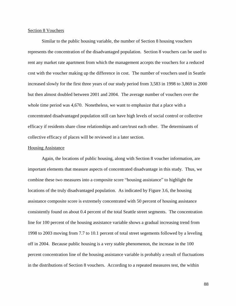
88

Section 8 Vouchers

Similar to the public housing variable, the number of Section 8 housing vouchers

represents the concentration of the disadvantaged population. Section 8 vouchers can be used to

rent any market rate apartment from which the management accepts the vouchers for a reduced

cost with the voucher making up the difference in cost. The number of vouchers used in Seattle

increased slowly for the first three years of our study period from 3,583 in 1998 to 3,869 in 2000

but then almost doubled between 2001 and 2004. The average number of vouchers over the

whole time period was 4,670. Nonetheless, we want to emphasize that a place with a

concentrated disadvantaged population still can have high levels of social control or collective

efficacy if residents share close relationships and care/trust each other. The determinants of

collective efficacy of places will be reviewed in a later section.

Housing Assistance

Again, the locations of public housing, along with Section 8 voucher information, are

important elements that measure aspects of concentrated disadvantage in this study. Thus, we

combine these two measures into a composite score ―housing assistance‖ to highlight the

locations of the truly disadvantaged population. As indicated by Figure 3.6, the housing

assistance composite score is extremely concentrated with 50 percent of housing assistance

consistently found on about 0.4 percent of the total Seattle street segments. The concentration

line for 100 percent of the housing assistance variable shows a gradual increasing trend from

1998 to 2003 moving from 7.7 to 10.1 percent of total street segements followed by a leveling

off in 2004. Because public housing is a very stable phenomenon, the increase in the 100

percent concentration line of the housing assistance variable is probably a result of fluctuations

in the distributions of Section 8 vouchers. According to a repeated measures test, the within


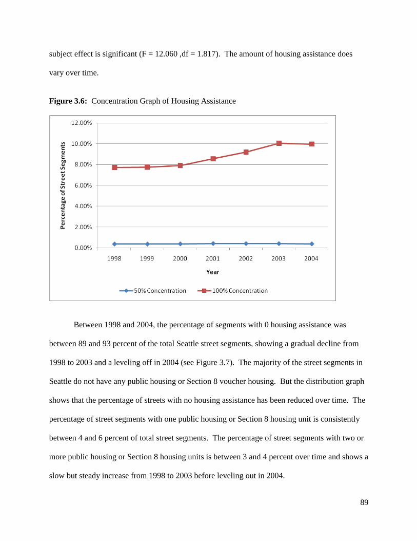
89

subject effect is significant (F = 12.060 ,df = 1.817). The amount of housing assistance does

vary over time.

Figure 3.6: Concentration Graph of Housing Assistance

Between 1998 and 2004, the percentage of segments with 0 housing assistance was

between 89 and 93 percent of the total Seattle street segments, showing a gradual decline from

1998 to 2003 and a leveling off in 2004 (see Figure 3.7). The majority of the street segments in

Seattle do not have any public housing or Section 8 voucher housing. But the distribution graph

shows that the percentage of streets with no housing assistance has been reduced over time. The

percentage of street segments with one public housing or Section 8 housing unit is consistently

between 4 and 6 percent of total street segments. The percentage of street segments with two or

more public housing or Section 8 housing units is between 3 and 4 percent over time and shows a

slow but steady increase from 1998 to 2003 before leveling out in 2004.


90

Figure 3.7: Frequency Distributions of Housing Assistance

The quantile maps of housing assistance per street segment indicate areas of

concentration in the north sector, the central sector and in north-south swaths in the south sector

(see Figure 3.8). Compared to the locations of public housing above, it seems like the housing

assistance program extends beyond the areas where public housing units are present.


91

Figure 3.8: Geographic Locations of Housing Assistance

But if we only focus on the streets with the top 50 percent concentration of housing

assistance, then the maps below now show a more spatially concentrated pattern (see Figure 3.9).

In sum, the maps provide evidence of the dispersion of high housing assistance street segments

across the city of Seattle; housing assistance is not clustered in just a few neighborhoods of the

city.


92

Figure 3.9: Concentration Maps of Housing Assistance

The LISA maps more clearly identify the areas where streets with high numbers of public

assistance units are interspersed with streets that have little or no housing assistance on them (see

Figure 3.10). The maps also clearly identify the sections of the city with little or no housing

assistance units at all (the dark blue areas). The spatial pattern of housing assistance is very

stable over time, as the stability in the number of public housing units and Section 8 vouchers

would predict.


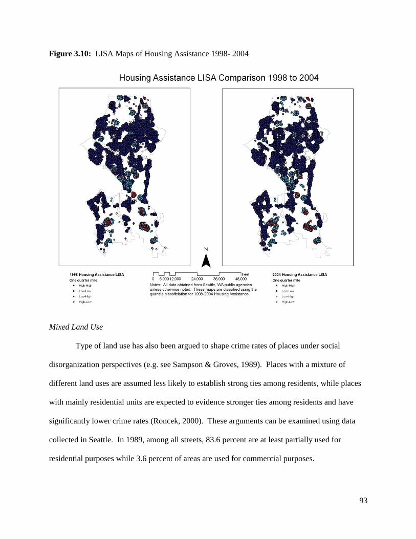
93

Figure 3.10: LISA Maps of Housing Assistance 1998- 2004

Mixed Land Use

Type of land use has also been argued to shape crime rates of places under social

disorganization perspectives (e.g. see Sampson & Groves, 1989). Places with a mixture of

different land uses are assumed less likely to establish strong ties among residents, while places

with mainly residential units are expected to evidence stronger ties among residents and have

significantly lower crime rates (Roncek, 2000). These arguments can be examined using data

collected in Seattle. In 1989, among all streets, 83.6 percent are at least partially used for

residential purposes while 3.6 percent of areas are used for commercial purposes.


94

A key issue in assessing mixed land use is the lack of consensus on what level of mixture

of land use is required to reach a tipping point that creates a high risk of increasing crime. Thus,

there is no clear guideline to differentiate between homogeneous land use and what is considered

mixed land use from the prior literature. The common practice is to define any place with less

than 100 percent of total area used for residential purposes as including mixed land use (e.g. see

Sampson & Groves, 1989; Wilcox et al., 2004). We used a more conservative measure of mixed

land use with a threshold of 25 percent and 75 percent. The percent of residential land use had to

be between 25 to 75 percent to be defined as mixed land use in our study

Table 3.2 describes mixed land use over time. Like the property value variable, the data

between 1999 and 2003 are missing and thus are not included in the analysis. Over time, only

about five percent of the total streets are classified as including mixed land use

Table 3.2: Descriptive Statistics of Variable Representing Mixed Land Use (N = 19,635)

1991 1993 1995 1997 1998 2004

Mean .055 .055 .056 .056 .057 .058

Std. Dev. .2288 .2287 .2295 .2308 .2310 .2330

Min. 0 0 0 0 0 0

Max 1 1 1 1 1 1

Mixed land use is an extremely concentrated phenomenon. As shown in Figure 3.11, less

than three percent of street segments account for over 50 percent of segments with mixed land

use. All the segments meeting the definition of mixed land use are found on around five to six

percent of streets in Seattle. The percentages of mixed land use have been increasing in a steady

fashion, but with a very minimal degree of increase (a 0.22 percent increase over 14 years).


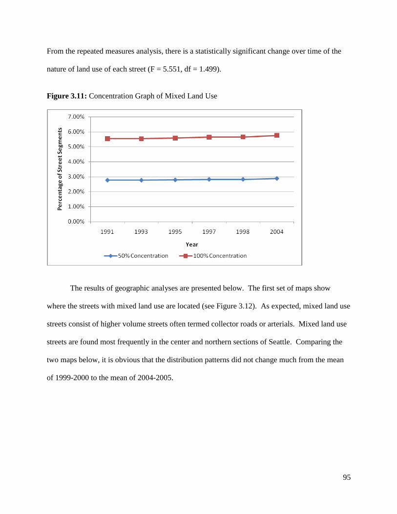
95

From the repeated measures analysis, there is a statistically significant change over time of the

nature of land use of each street (F = 5.551, df = 1.499).

Figure 3.11: Concentration Graph of Mixed Land Use

The results of geographic analyses are presented below. The first set of maps show

where the streets with mixed land use are located (see Figure 3.12). As expected, mixed land use

streets consist of higher volume streets often termed collector roads or arterials. Mixed land use

streets are found most frequently in the center and northern sections of Seattle. Comparing the

two maps below, it is obvious that the distribution patterns did not change much from the mean

of 1999-2000 to the mean of 2004-2005.


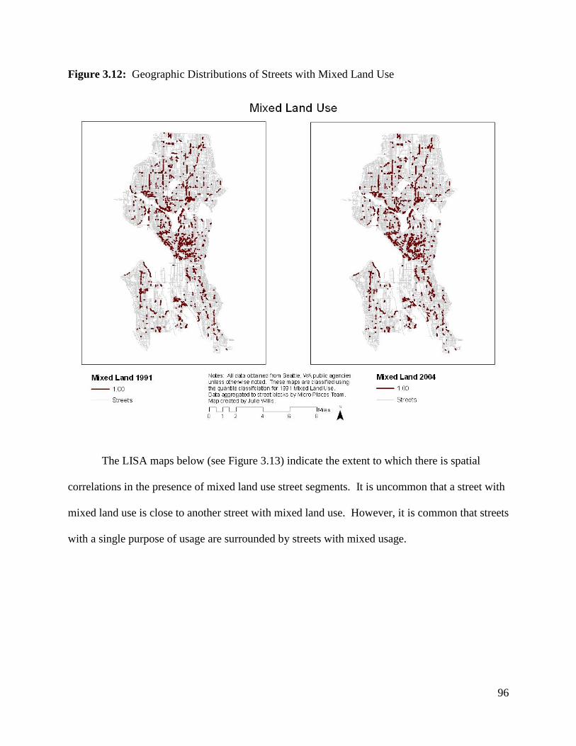
96

Figure 3.12: Geographic Distributions of Streets with Mixed Land Use

The LISA maps below (see Figure 3.13) indicate the extent to which there is spatial

correlations in the presence of mixed land use street segments. It is uncommon that a street with

mixed land use is close to another street with mixed land use. However, it is common that streets

with a single purpose of usage are surrounded by streets with mixed usage.


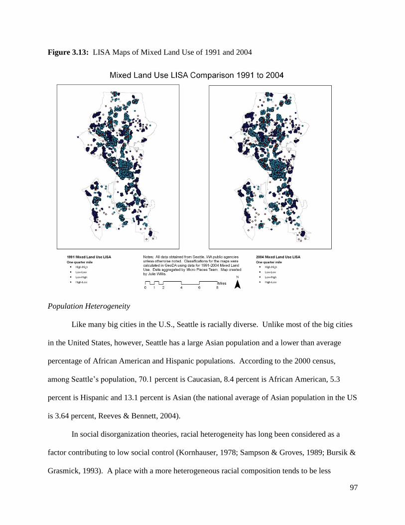
97

Figure 3.13: LISA Maps of Mixed Land Use of 1991 and 2004

Population Heterogeneity

Like many big cities in the U.S., Seattle is racially diverse. Unlike most of the big cities

in the United States, however, Seattle has a large Asian population and a lower than average

percentage of African American and Hispanic populations. According to the 2000 census,

among Seattle’s population, 70.1 percent is Caucasian, 8.4 percent is African American, 5.3

percent is Hispanic and 13.1 percent is Asian (the national average of Asian population in the US

is 3.64 percent, Reeves & Bennett, 2004).

In social disorganization theories, racial heterogeneity has long been considered as a

factor contributing to low social control (Kornhauser, 1978; Sampson & Groves, 1989; Bursik &

Grasmick, 1993). A place with a more heterogeneous racial composition tends to be less


98

cohesive and have a lower level of social control as the racial difference can sometimes become

a barrier for people to communicate and identify with each other. Thus, residents are less likely

to develop a strong tie and as a result, the population turnover rate is high. This can also be a

result of a natural selection process, as places with more racial heterogeneity tend to have more

rental properties or affordable housing. Consequently, crime tends to occur at places that are

more heterogeneous, even if racial make-up itself might not lead to a high crime rate (Shaw &

McKay, 1942 [1969]).

In prior studies, the percentage of blacks (or minority residents) has traditionally been

used as an indicator of racial heterogeneity (see Blau & Blau, 1982; Messner, 1983). Williams

(1984) pointed out that the relationship between the percentage of blacks and homicide rates is

actually an inverted-U shape, not linear. The reason behind the phenomenon is simple: when a

place has a high percentage of minority residents, it is actually more homogeneous than

heterogeneous as minorities become the dominant group at that place. After passing the tipping

point, the high percentage of minority residents actually leads to a more stable social control

system and a lower crime rate. To support this argument, Williams reanalyzed data from

Messner (1983) and Blau and Blau (1982) with the new specification and the performance of

models improved substantially (variance explained increased 14 percent).

However, using the pure percentage of blacks can be a flawed approach. With the

changes of population composition in the United States, using a percentage of blacks to represent

population heterogeneity has become more and more problematic. As of the year 2000,

Hispanics have surpassed blacks and have become the largest minority group in America.

Additionally, Seattle has a disproportionate Asian population compared to the nationwide

average. Thus, we follow an approach used by Smith et al. (2000) and Smith and Jarjoura (1988)


99

and define racial heterogeneity using a probability-based approach. They multiply the

percentage of whites by the percentage of non-whites to indicate the probability that two

randomly selected individuals from an area will be members of different racial groups. To take

into account the multi-racial feature of Seattle, we use the same formula mentioned above but

further modify the approach to incorporate the racial dynamics in Seattle. Four racial groups

were identified in this study including white, black, Asian, and Hispanic. The probabilities of

each racial group to encounter another out-group member were then computed and averaged to

form an overall racial heterogeneity index. The racial heterogeneity index was created based on

the following equation

HETEROGENITYj= {(%WHITEj * %NONWHITEj)+ (%BLACKj * %NONBLACKj)+

(%ASIANj * %NONASIANj)+ (%HISPANICj * %NONHISPANICj)}/4

* j denotes year of information.

The overall index represents the level of heterogeneity of each street segment. To

capture the complexity of racial heterogeneity in Seattle, a racial heterogeneity index was created

by the method detailed above. Each street is assigned a score where the lowest possible score is

0, indicating no racial heterogeneity in the street, and the highest possible score is .1875 which

represents a scenario of an extremely heterogeneous environment. After examining the data

carefully, a cut-off point of .12 was chosen to distinguish streets that we consider are

heterogeneous from streets that are more homogeneous.

Because census data are not available at the street segment level, we draw information on

racial composition from data provided by the public schools in Seattle. We recognize at the

outset that these data do not provide an accurate accounting of the overall racial composition of

Seattle residents. For example, Seattle is estimated to be about 70 percent white in 2000 by the

census bureau. In our data, about 40 percent of the students are defined as white in the same


100

year. Nonetheless, we think that the student data provide the best method available for

identifying racial heterogeneity at the street segment level. In this case, our interest is not in

identifying an accurate portrait of the overall weighting of race in the city but rather the extent to

which there is heterogeneity of race at the street segment level.

Based on the information of public school students, the overall racial compositions

remain very stable over time (see Table 3.3). In Seattle’s public schools, white students account

for about 41 percent of the student population, 22-24 percent of students are Asians, 23 percent

are blacks, around 7-11 percent of students are Hispanics, and around 3 percent of students are

American Indians. It is worth noting that the Hispanic student population has shown a steady

increase over the 12 years examined, starting from only 7 percent and then reaching 11 percent

by the end of the series. Additionally, Asians and blacks are over-represented in the student

population while whites are underrepresented compared to the general population in Seattle (see

U.S. Census, 2000).

Table 3.3: Descriptive Statistics of Racial Distribution of Seattle’s Public School Students from

1993 to 2004

Year White Asian Black Hispanic American

Indian Total

1993

Sum 14,368 8,438 8,039 2,496 1,183 34,524

Mean 0.594 0.349 0.332 0.103 0.049

Std. Dev. 1.596 1.804 1.485 0.542 0.326

1994

Sum 14,599 8,604 8,110 2,604 1,208 35,125

Mean 0.604 0.356 0.335 0.108 0.050

Std. Dev. 1.655 1.789 1.154 0.570 0.330

1995

Sum 14,724 8,629 8,010 2,701 1,178 35,242

Mean 0.609 0.357 0.331 0.112 0.049

Std. Dev. 1.630 1.750 1.526 0.595 0.315


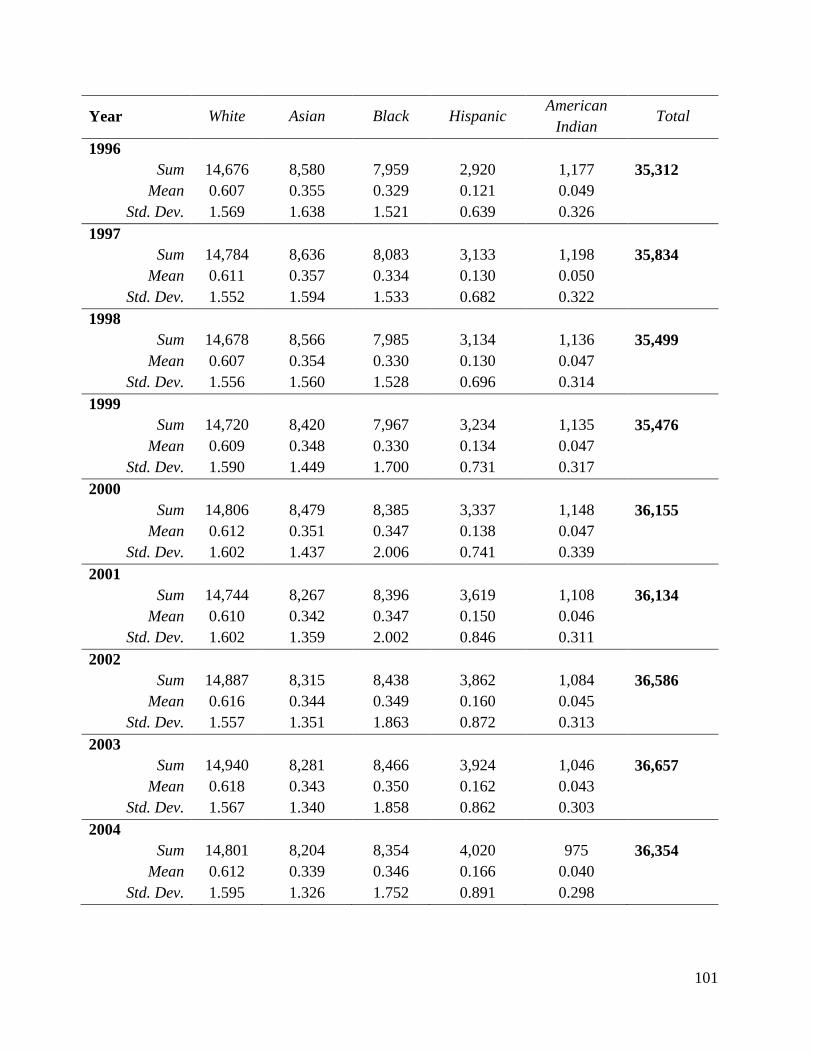
101

Year White Asian Black Hispanic American

Indian Total

1996

Sum 14,676 8,580 7,959 2,920 1,177 35,312

Mean 0.607 0.355 0.329 0.121 0.049

Std. Dev. 1.569 1.638 1.521 0.639 0.326

1997

Sum 14,784 8,636 8,083 3,133 1,198 35,834

Mean 0.611 0.357 0.334 0.130 0.050

Std. Dev. 1.552 1.594 1.533 0.682 0.322

1998

Sum 14,678 8,566 7,985 3,134 1,136 35,499

Mean 0.607 0.354 0.330 0.130 0.047

Std. Dev. 1.556 1.560 1.528 0.696 0.314

1999

Sum 14,720 8,420 7,967 3,234 1,135 35,476

Mean 0.609 0.348 0.330 0.134 0.047

Std. Dev. 1.590 1.449 1.700 0.731 0.317

2000

Sum 14,806 8,479 8,385 3,337 1,148 36,155

Mean 0.612 0.351 0.347 0.138 0.047

Std. Dev. 1.602 1.437 2.006 0.741 0.339

2001

Sum 14,744 8,267 8,396 3,619 1,108 36,134

Mean 0.610 0.342 0.347 0.150 0.046

Std. Dev. 1.602 1.359 2.002 0.846 0.311

2002

Sum 14,887 8,315 8,438 3,862 1,084 36,586

Mean 0.616 0.344 0.349 0.160 0.045

Std. Dev. 1.557 1.351 1.863 0.872 0.313

2003

Sum 14,940 8,281 8,466 3,924 1,046 36,657

Mean 0.618 0.343 0.350 0.162 0.043

Std. Dev. 1.567 1.340 1.858 0.862 0.303

2004

Sum 14,801 8,204 8,354 4,020 975 36,354

Mean 0.612 0.339 0.346 0.166 0.040

Std. Dev. 1.595 1.326 1.752 0.891 0.298


102

As mentioned earlier, we computed the racial heterogeneity index for all street segments

in Seattle where any public school students live. We did not create a 50 percent and 100 percent

concentration graph for this variable because it simply makes no sense to compute the

concentration of a coefficient. Thus, the following graph merely shows the trend line of racial

heterogeneity from student records (see Figure 3.14). In sum, the percentage of racially

heterogeneous street segments (with a heterogeneity index greater than 0.12) was fairly stable at

between 6 percent and 7.5 percent of Seattle street segments from the 1992-1993 to the 2003-

2004 school year. Based on the results of repeated measures analysis, the within subject effect is

significant (F = 42.757, df = 6.679) and thus, the average racial heterogeneity value does vary

over time.

Figure 3.14: The Trend of Racial Heterogeneity from 1992/1993 to 2003/2004 (school year)

Racial Heterogeneity (Students)

5.80%

6.00%

6.20%

6.40%

6.60%

6.80%

7.00%

7.20%

7.40%

92

-93

93

-94

94

-95

95

-96

96

-97

97

-98

98

-99

99

-00

00

-01

01

-02

02

-03

03

-04

% of Segments With Heterogeneity Index > .12

The frequency distributions of the racial heterogeneity index show an extremely stable

long term pattern. Between the 1993 and the 2004 school year, the percentage of segments with


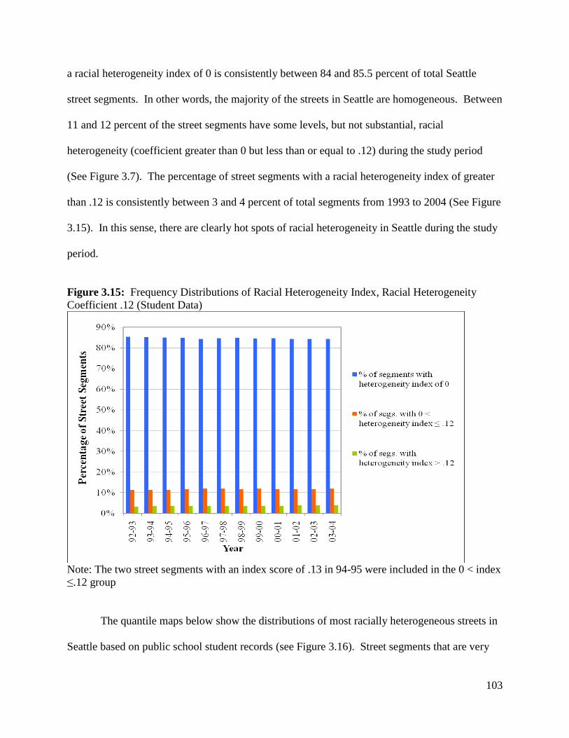
103

a racial heterogeneity index of 0 is consistently between 84 and 85.5 percent of total Seattle

street segments. In other words, the majority of the streets in Seattle are homogeneous. Between

11 and 12 percent of the street segments have some levels, but not substantial, racial

heterogeneity (coefficient greater than 0 but less than or equal to .12) during the study period

(See Figure 3.7). The percentage of street segments with a racial heterogeneity index of greater

than .12 is consistently between 3 and 4 percent of total segments from 1993 to 2004 (See Figure

3.15). In this sense, there are clearly hot spots of racial heterogeneity in Seattle during the study

period.

Figure 3.15: Frequency Distributions of Racial Heterogeneity Index, Racial Heterogeneity

Coefficient .12 (Student Data)

Note: The two street segments with an index score of .13 in 94-95 were included in the 0 < index

≤.12 group

The quantile maps below show the distributions of most racially heterogeneous streets in

Seattle based on public school student records (see Figure 3.16). Street segments that are very


104

heterogeneous are found throughout the city of Seattle with the exception of downtown and the

industrial area in the southern section. The highest densities are in the southeastern and

southwestern sections. The northern section also has quite a few street segments that are

heterogeneous. However, there are very few dots that appeared in the northern section. As far as

temporal change, the northern and southwestern sections seem to have increased in heterogeneity

over the study period.

Figure 3.16: Geographic Distribution of Racial Heterogeneity (Student Data)

The patterns described based on the quantile map are even easier to see in the LISA maps

(see Figure 3.17). There are large swaths of positive (low-low) spatial autocorrelation. There

are also large swaths of negative spatial autocorrelation (highly heterogeneous street segments


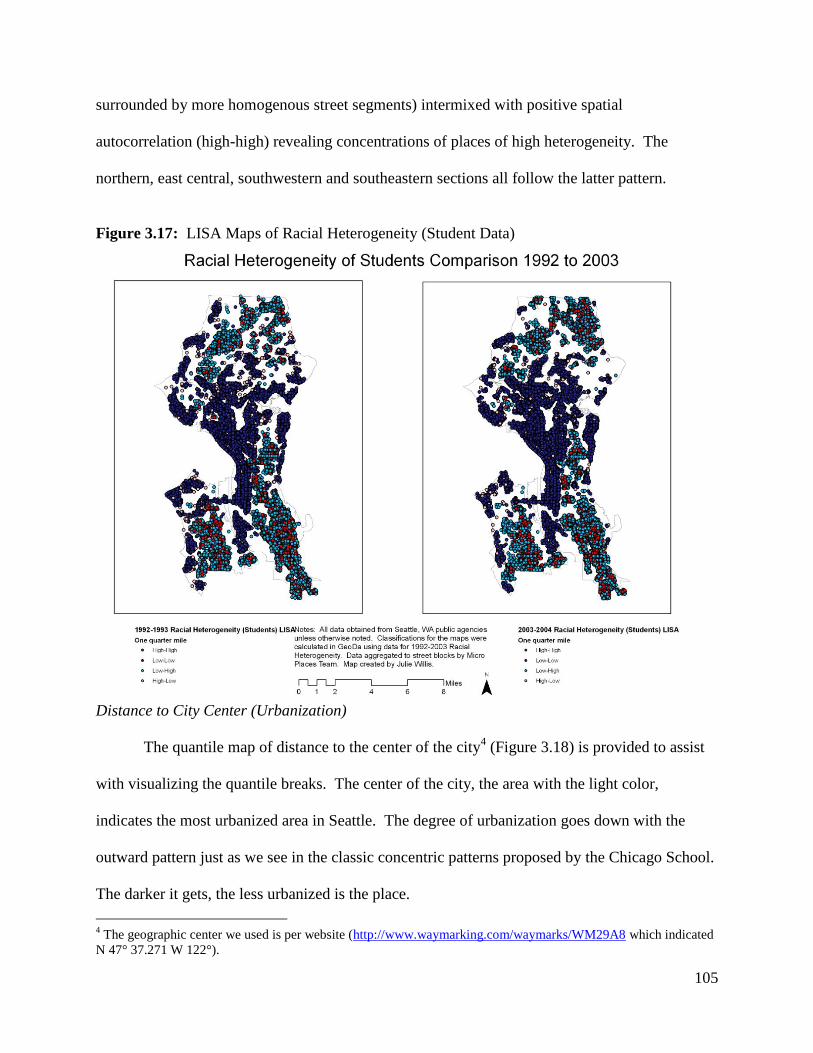
105

surrounded by more homogenous street segments) intermixed with positive spatial

autocorrelation (high-high) revealing concentrations of places of high heterogeneity. The

northern, east central, southwestern and southeastern sections all follow the latter pattern.

Figure 3.17: LISA Maps of Racial Heterogeneity (Student Data)

Distance to City Center (Urbanization)

The quantile map of distance to the center of the city4 (Figure 3.18) is provided to assist

with visualizing the quantile breaks. The center of the city, the area with the light color,

indicates the most urbanized area in Seattle. The degree of urbanization goes down with the

outward pattern just as we see in the classic concentric patterns proposed by the Chicago School.

The darker it gets, the less urbanized is the place.

4 The geographic center we used is per website (http://www.waymarking.com/waymarks/WM29A8 which indicated

N 47° 37.271 W 122°).


http://www.waymarking.com/waymarks/WM29A8

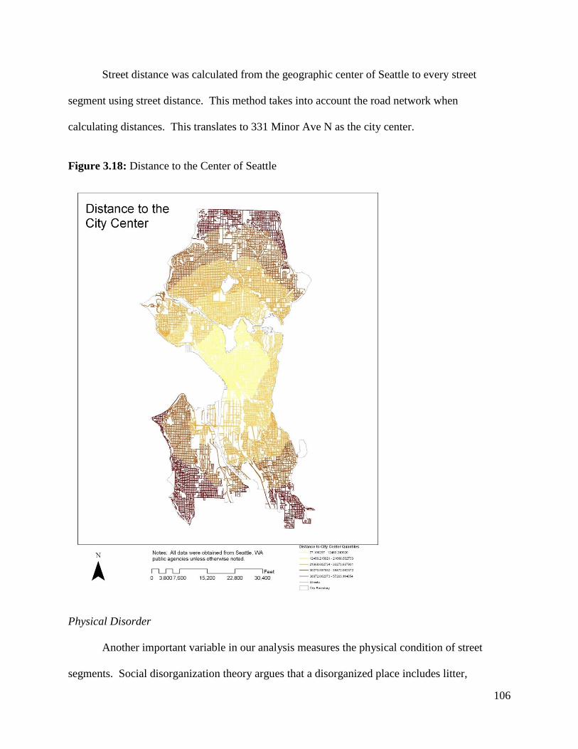
106

Street distance was calculated from the geographic center of Seattle to every street

segment using street distance. This method takes into account the road network when

calculating distances. This translates to 331 Minor Ave N as the city center.

Figure 3.18: Distance to the Center of Seattle

Physical Disorder

Another important variable in our analysis measures the physical condition of street

segments. Social disorganization theory argues that a disorganized place includes litter,


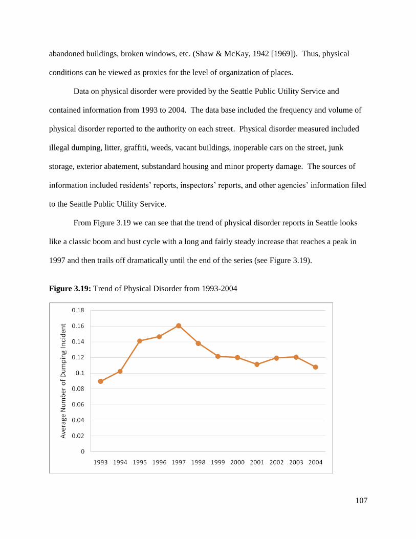
107

abandoned buildings, broken windows, etc. (Shaw & McKay, 1942 [1969]). Thus, physical

conditions can be viewed as proxies for the level of organization of places.

Data on physical disorder were provided by the Seattle Public Utility Service and

contained information from 1993 to 2004. The data base included the frequency and volume of

physical disorder reported to the authority on each street. Physical disorder measured included

illegal dumping, litter, graffiti, weeds, vacant buildings, inoperable cars on the street, junk

storage, exterior abatement, substandard housing and minor property damage. The sources of

information included residents’ reports, inspectors’ reports, and other agencies’ information filed

to the Seattle Public Utility Service.

From Figure 3.19 we can see that the trend of physical disorder reports in Seattle looks

like a classic boom and bust cycle with a long and fairly steady increase that reaches a peak in

1997 and then trails off dramatically until the end of the series (see Figure 3.19).

Figure 3.19: Trend of Physical Disorder from 1993-2004


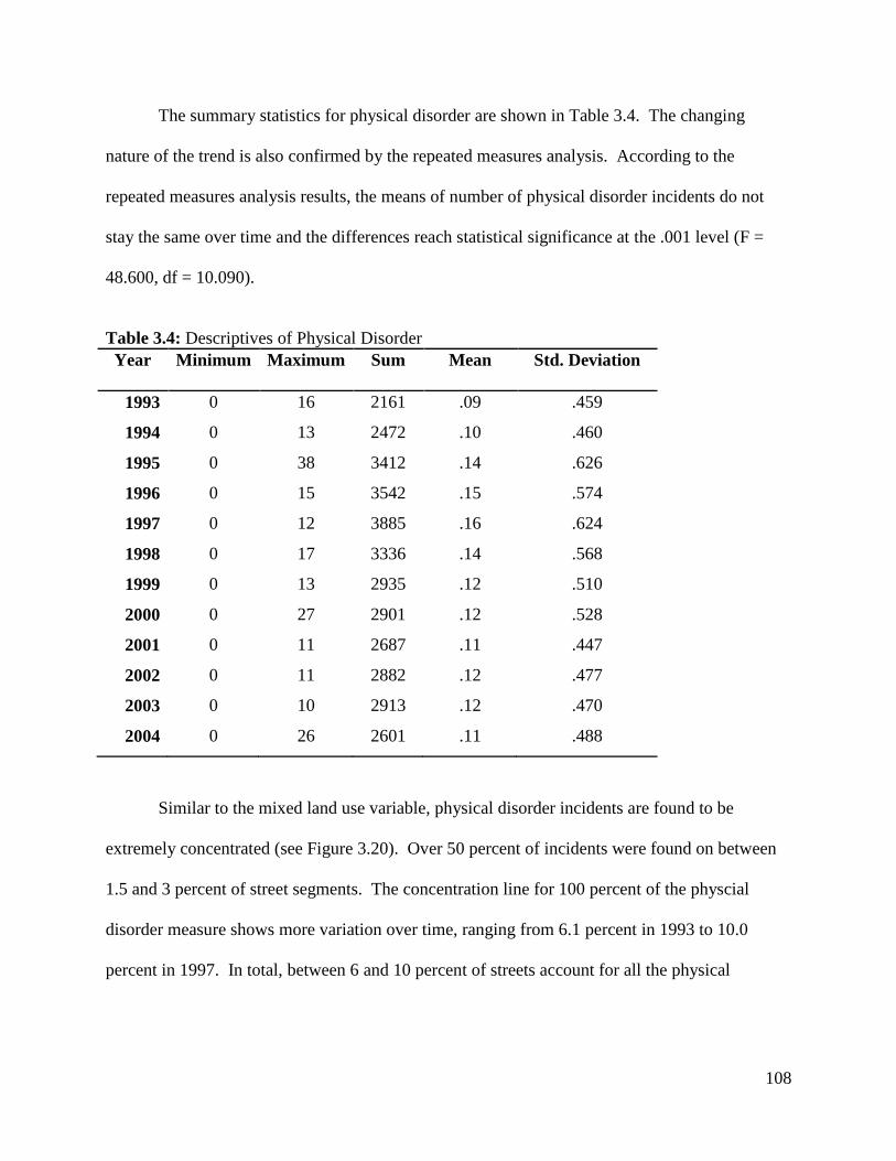
108

The summary statistics for physical disorder are shown in Table 3.4. The changing

nature of the trend is also confirmed by the repeated measures analysis. According to the

repeated measures analysis results, the means of number of physical disorder incidents do not

stay the same over time and the differences reach statistical significance at the .001 level (F =

48.600, df = 10.090).

Table 3.4: Descriptives of Physical Disorder

Year Minimum Maximum Sum Mean Std. Deviation

1993 0 16 2161 .09 .459

1994 0 13 2472 .10 .460

1995 0 38 3412 .14 .626

1996 0 15 3542 .15 .574

1997 0 12 3885 .16 .624

1998 0 17 3336 .14 .568

1999 0 13 2935 .12 .510

2000 0 27 2901 .12 .528

2001 0 11 2687 .11 .447

2002 0 11 2882 .12 .477

2003 0 10 2913 .12 .470

2004 0 26 2601 .11 .488

Similar to the mixed land use variable, physical disorder incidents are found to be

extremely concentrated (see Figure 3.20). Over 50 percent of incidents were found on between

1.5 and 3 percent of street segments. The concentration line for 100 percent of the physcial

disorder measure shows more variation over time, ranging from 6.1 percent in 1993 to 10.0

percent in 1997. In total, between 6 and 10 percent of streets account for all the physical


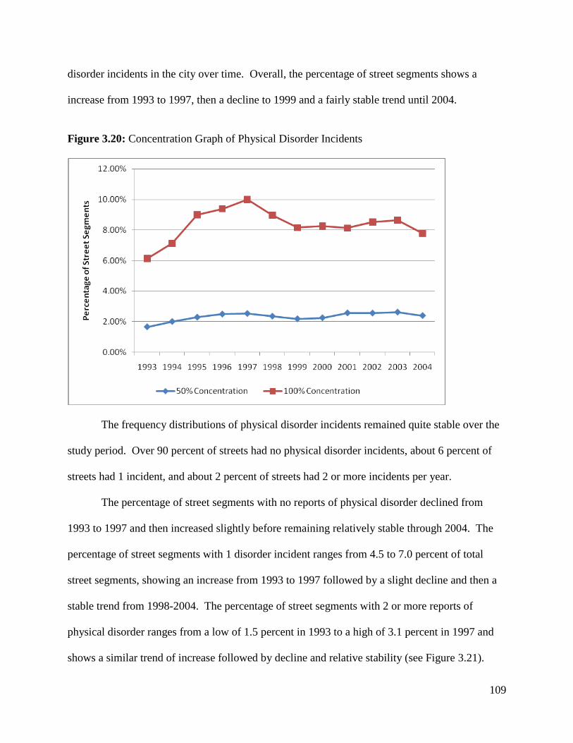
109

disorder incidents in the city over time. Overall, the percentage of street segments shows a

increase from 1993 to 1997, then a decline to 1999 and a fairly stable trend until 2004.

Figure 3.20: Concentration Graph of Physical Disorder Incidents

The frequency distributions of physical disorder incidents remained quite stable over the

study period. Over 90 percent of streets had no physical disorder incidents, about 6 percent of

streets had 1 incident, and about 2 percent of streets had 2 or more incidents per year.

The percentage of street segments with no reports of physical disorder declined from

1993 to 1997 and then increased slightly before remaining relatively stable through 2004. The

percentage of street segments with 1 disorder incident ranges from 4.5 to 7.0 percent of total

street segments, showing an increase from 1993 to 1997 followed by a slight decline and then a

stable trend from 1998-2004. The percentage of street segments with 2 or more reports of

physical disorder ranges from a low of 1.5 percent in 1993 to a high of 3.1 percent in 1997 and

shows a similar trend of increase followed by decline and relative stability (see Figure 3.21).


110

Figure 3.21: Frequency Distributions of Physical Disorder Over Time

According to Figure 3.12 physical disorder is widespread in Seattle (see Figure 3.22).

However, the quantile map indicates there are areas with higher numbers of reports of disorder.

These areas include the center and southeastern sections. A new area of concentration appears in

the south central part of the northern section in the years of 2004-2005.


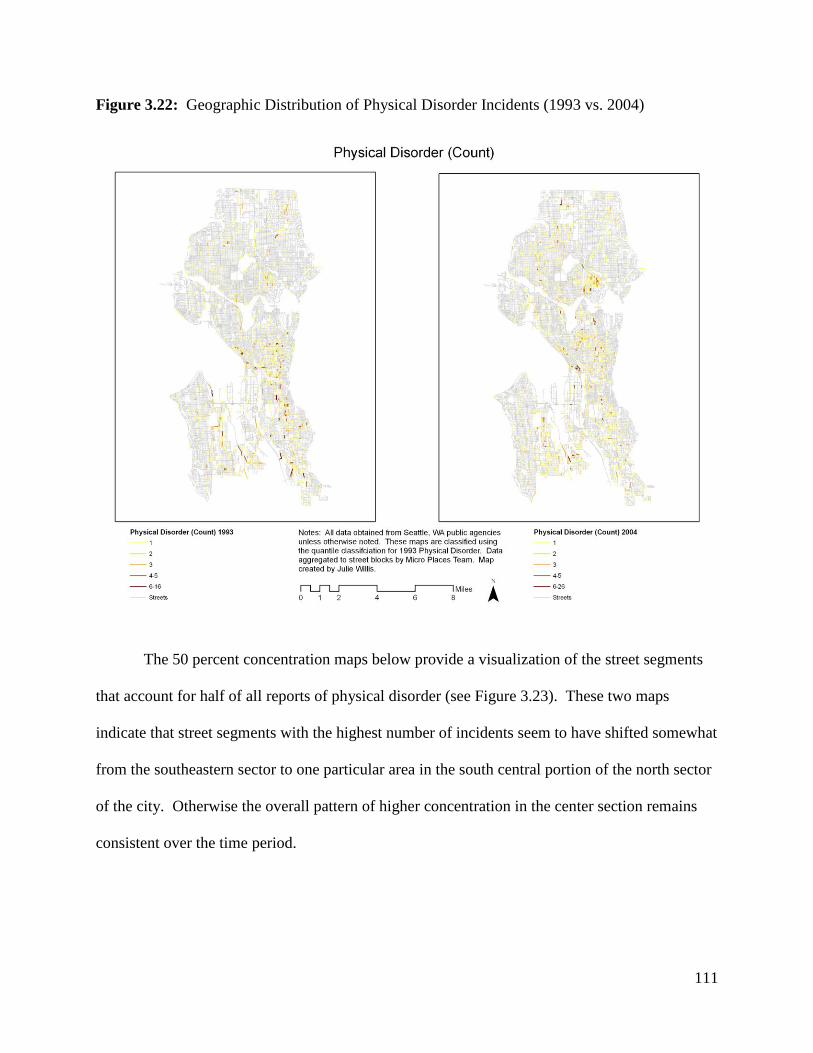
111

Figure 3.22: Geographic Distribution of Physical Disorder Incidents (1993 vs. 2004)

The 50 percent concentration maps below provide a visualization of the street segments

that account for half of all reports of physical disorder (see Figure 3.23). These two maps

indicate that street segments with the highest number of incidents seem to have shifted somewhat

from the southeastern sector to one particular area in the south central portion of the north sector

of the city. Otherwise the overall pattern of higher concentration in the center section remains

consistent over the time period.


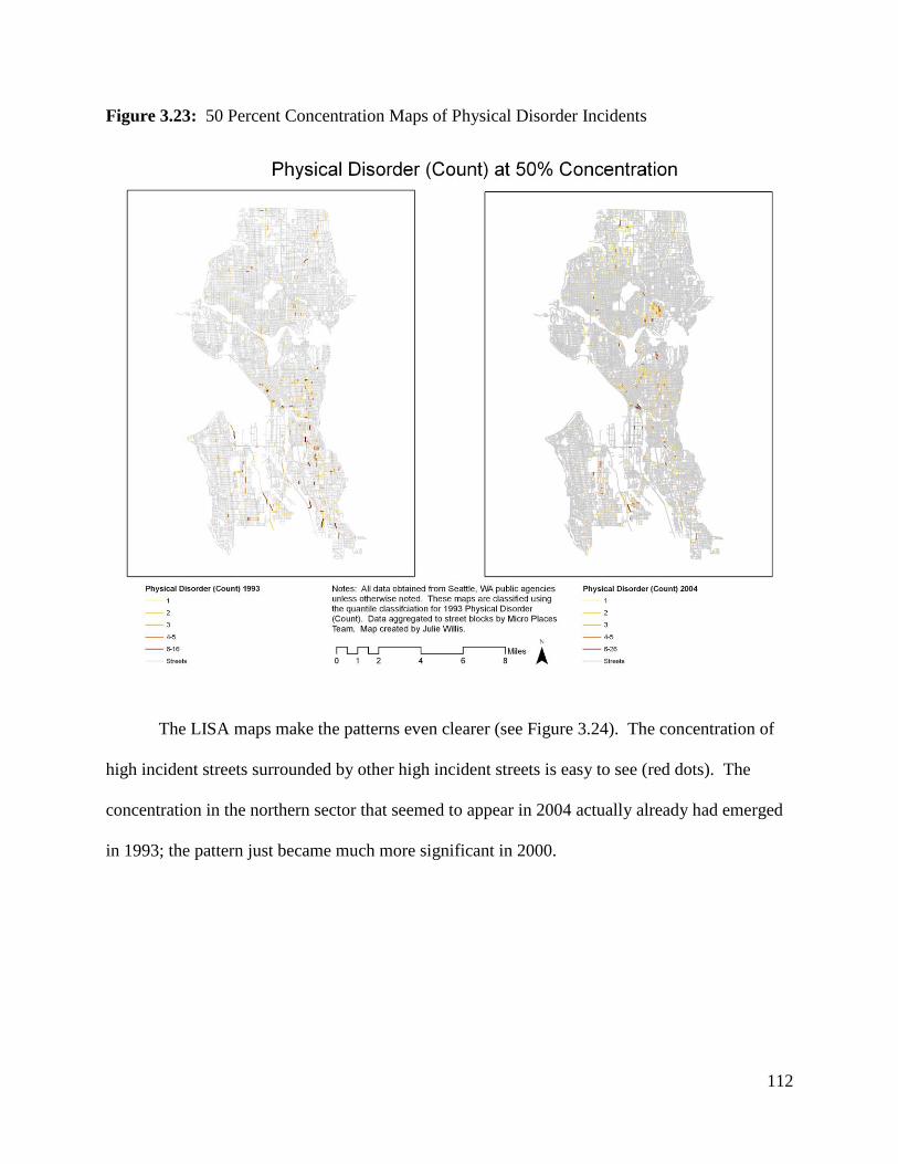
112

Figure 3.23: 50 Percent Concentration Maps of Physical Disorder Incidents

The LISA maps make the patterns even clearer (see Figure 3.24). The concentration of

high incident streets surrounded by other high incident streets is easy to see (red dots). The

concentration in the northern sector that seemed to appear in 2004 actually already had emerged

in 1993; the pattern just became much more significant in 2000.


113

Figure 3.24: LISA Maps of Physical Disorder Count (1993 vs. 2004)

Intermediating Variables

After the 1970s, the popularity of social disorganization theory declined, and the classic

theory was criticized as being tautological because crime can be viewed both as a proxy of social

disorganization and a result of the social disorganization of places (see Bursik, 1988). Research

findings indicate that the relationship between the structural variables and crime is not linear, but

conditioned by the level of social control at place (Hayslett-McCall, 2008). To address this

problem, recent conceptualizations of social disorganization theory generally incorporate social

control or similar concepts as the mediating mechanism linking the structural characteristics and


114

outcome variables like crime (see Bursik, 1988; Sampson & Groves, 1989; Sampson & Wilson,

1995). The mediating mechanism generally represents the level of systemic networks, kinship,

and social control necessary for a place to effectively exercise strong social controls. The

common factors identified in prior studies to operationalize the concepts include participation in

local organizations (Taylor et al., 1984; Sampson & Groves, 1989), willingness (or perception of

responsibility) to intervene in public affairs (Taylor et al., 1984; Sampson et al., 1997), local

friendship networks (Sampson & Groves, 1989), mutual trust (Sampson et al., 1997), and

unsupervised teens (Sampson & Groves, 1989). These variables are believed to condition the

effects of structural disadvantage on local crime problems. By incorporating the mediating

factors, social disorganization theorists argue that social disorganization is now ―clearly

separable not only from the processes that may lead to it….but also from the degree of criminal

behavior that may be a result‖ (Bursik, 1988; cited in Sampson & Wilson, 1995, p. 46).

In this study, we include the number of unsupervised teens, and percent of active voters

to represent local social control as well as collective efficacy on each street segment.

Unsupervised Teens

This concept was first conceptualized by Sampson and Groves (1989, p. 778), who argue

that ―communities that are unable to control street-corner teenage groups will experience higher

rates of delinquency than those in which peer groups are held in check through collective social

control.‖ It is not because these street-corner teenagers are all ―criminals‖ but the appearance of

unsupervised teens in the street corner is evidence of the lack of social control in a community.

Accordingly, a community with fewer kids wandering on a street during school time is better at

controlling its residents than a community with many truant students unattended—assuming they

have equal student populations. In this study, we use the number of truant students on each


115

street to represent the concept of unsupervised teens. When identifying truant students, we use

the public school student data described in the earlier section. To determine truancy, we

followed the definition used by Seattle’s Department of Education, which considers a student

who has more than 10 unexcused absences in a school year to be truant.

Figure 3.25 shows two trends regarding student truancy—number of truant students and

percentage of truant students relative to all students on a street. The average number of truant

students living on a specific street segment has been declining during the 13 year period, except

for the 1994-1995 school year. According to the results of repeated measures tests, there has

been a significant change in the total number of truant students on streets over time. Similarly,

the percentages of truant students per street follow the same pattern as the number of truants per

street.


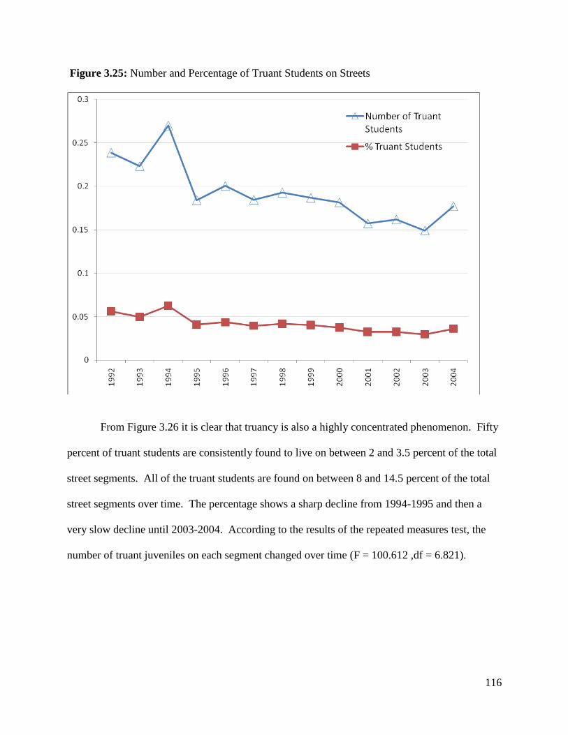
116

Figure 3.25: Number and Percentage of Truant Students on Streets

From Figure 3.26 it is clear that truancy is also a highly concentrated phenomenon. Fifty

percent of truant students are consistently found to live on between 2 and 3.5 percent of the total

street segments. All of the truant students are found on between 8 and 14.5 percent of the total

street segments over time. The percentage shows a sharp decline from 1994-1995 and then a

very slow decline until 2003-2004. According to the results of the repeated measures test, the

number of truant juveniles on each segment changed over time (F = 100.612 ,df = 6.821).


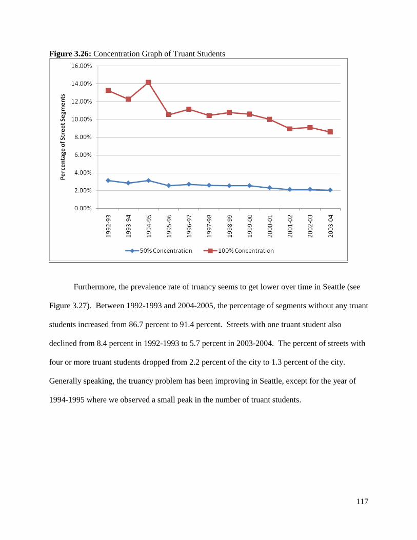
117

Figure 3.26: Concentration Graph of Truant Students

Furthermore, the prevalence rate of truancy seems to get lower over time in Seattle (see

Figure 3.27). Between 1992-1993 and 2004-2005, the percentage of segments without any truant

students increased from 86.7 percent to 91.4 percent. Streets with one truant student also

declined from 8.4 percent in 1992-1993 to 5.7 percent in 2003-2004. The percent of streets with

four or more truant students dropped from 2.2 percent of the city to 1.3 percent of the city.

Generally speaking, the truancy problem has been improving in Seattle, except for the year of

1994-1995 where we observed a small peak in the number of truant students.


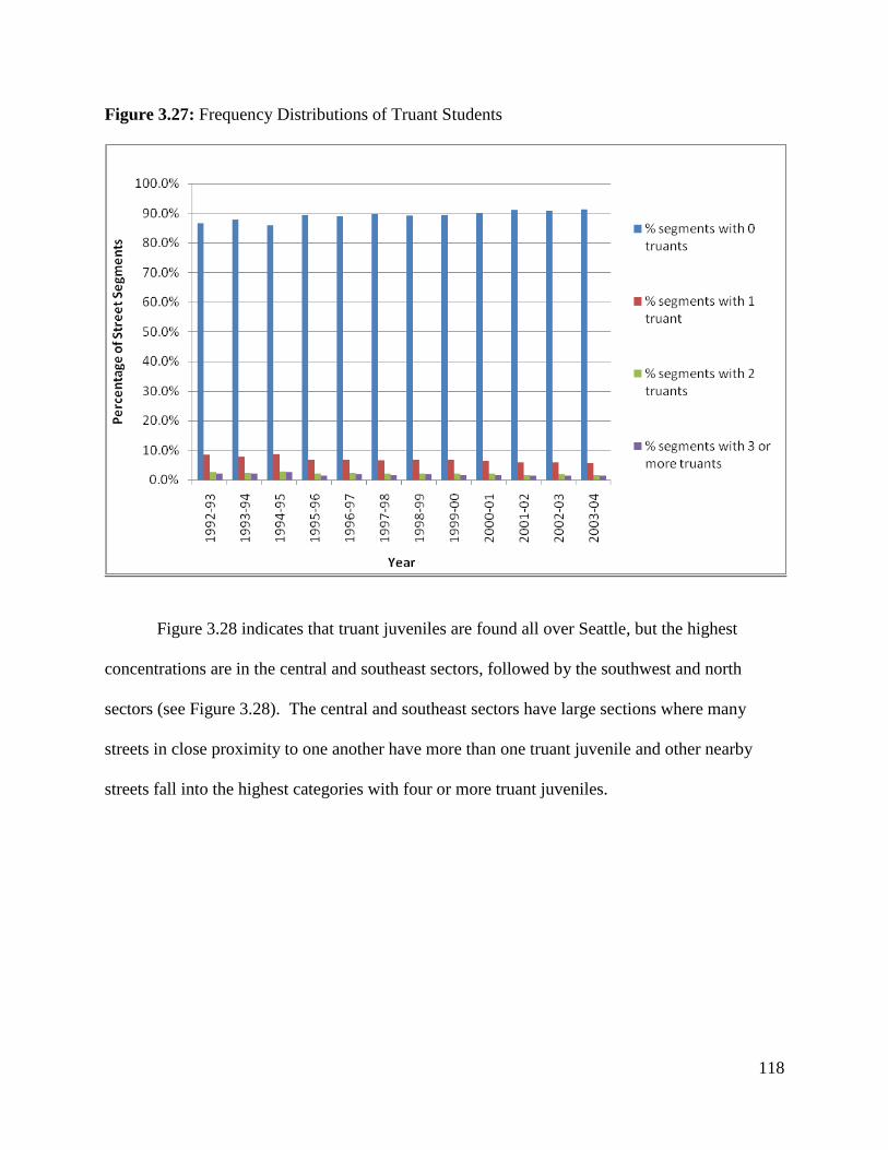
118

Figure 3.27: Frequency Distributions of Truant Students

Figure 3.28 indicates that truant juveniles are found all over Seattle, but the highest

concentrations are in the central and southeast sectors, followed by the southwest and north

sectors (see Figure 3.28). The central and southeast sectors have large sections where many

streets in close proximity to one another have more than one truant juvenile and other nearby

streets fall into the highest categories with four or more truant juveniles.


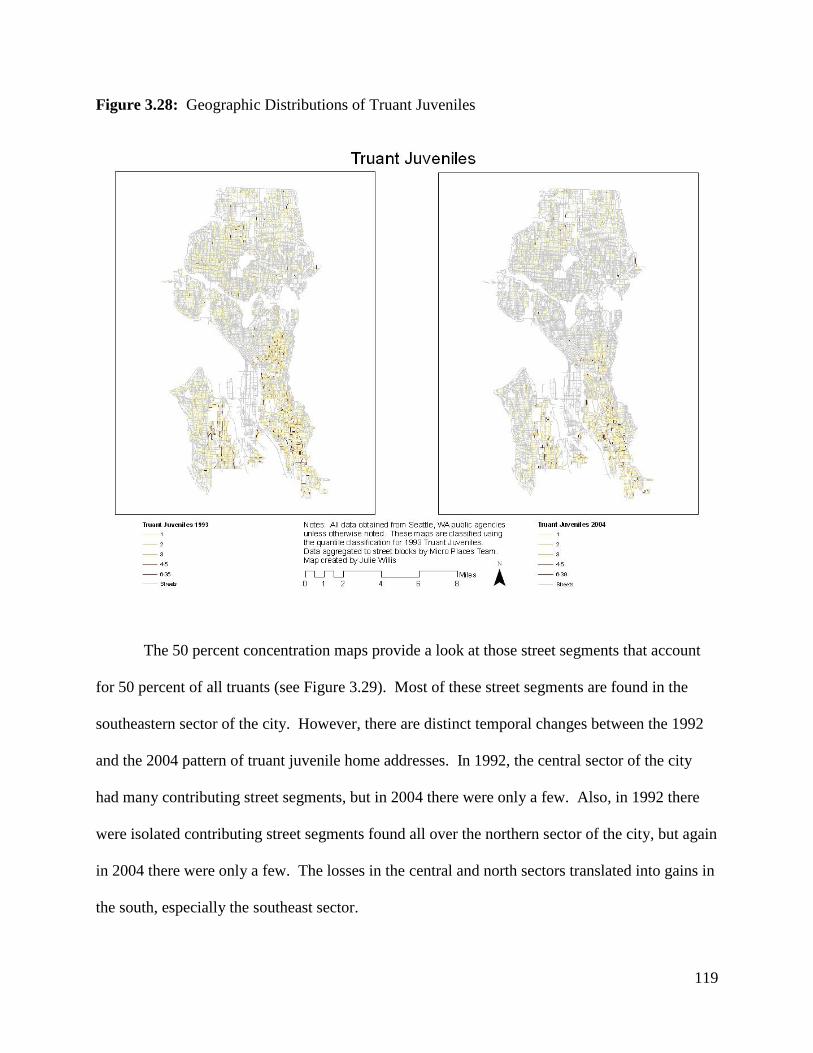
119

Figure 3.28: Geographic Distributions of Truant Juveniles

The 50 percent concentration maps provide a look at those street segments that account

for 50 percent of all truants (see Figure 3.29). Most of these street segments are found in the

southeastern sector of the city. However, there are distinct temporal changes between the 1992

and the 2004 pattern of truant juvenile home addresses. In 1992, the central sector of the city

had many contributing street segments, but in 2004 there were only a few. Also, in 1992 there

were isolated contributing street segments found all over the northern sector of the city, but again

in 2004 there were only a few. The losses in the central and north sectors translated into gains in

the south, especially the southeast sector.


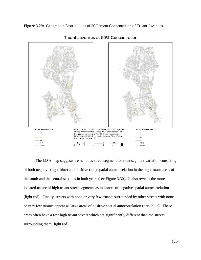
120

Figure 3.29: Geographic Distributions of 50 Percent Concentration of Truant Juveniles

The LISA map suggests tremendous street segment to street segment variation consisting

of both negative (light blue) and positive (red) spatial autocorrelation in the high truant areas of

the south and the central sections in both years (see Figure 3.30). It also reveals the more

isolated nature of high truant street segments as instances of negative spatial autocorrelation

(light red). Finally, streets with none or very few truants surrounded by other streets with none

or very few truants appear as large areas of positive spatial autocorrelation (dark blue). These

areas often have a few high truant streets which are significantly different than the streets

surrounding them (light red).


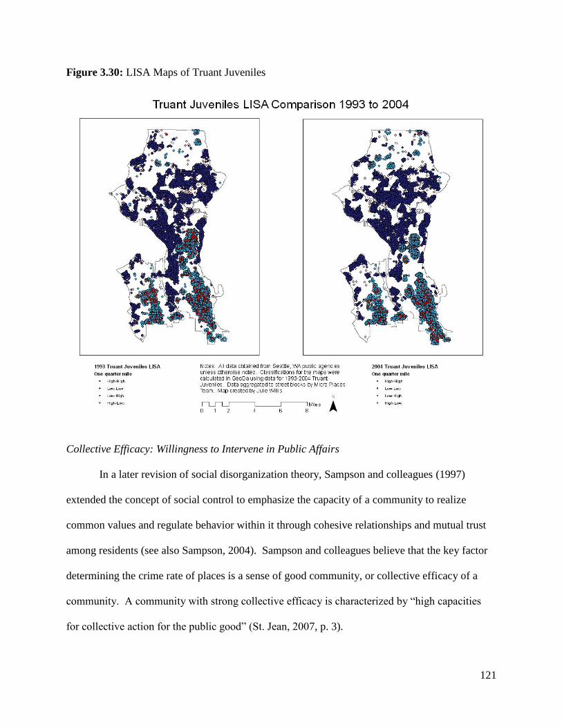
121

Figure 3.30: LISA Maps of Truant Juveniles

Collective Efficacy: Willingness to Intervene in Public Affairs

In a later revision of social disorganization theory, Sampson and colleagues (1997)

extended the concept of social control to emphasize the capacity of a community to realize

common values and regulate behavior within it through cohesive relationships and mutual trust

among residents (see also Sampson, 2004). Sampson and colleagues believe that the key factor

determining the crime rate of places is a sense of good community, or collective efficacy of a

community. A community with strong collective efficacy is characterized by ―high capacities

for collective action for the public good‖ (St. Jean, 2007, p. 3).


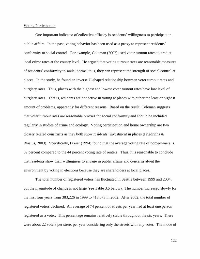
122

Voting Participation

One important indicator of collective efficacy is residents’ willingness to participate in

public affairs. In the past, voting behavior has been used as a proxy to represent residents’

conformity to social control. For example, Coleman (2002) used voter turnout rates to predict

local crime rates at the county level. He argued that voting turnout rates are reasonable measures

of residents’ conformity to social norms; thus, they can represent the strength of social control at

places. In the study, he found an inverse U-shaped relationship between voter turnout rates and

burglary rates. Thus, places with the highest and lowest voter turnout rates have low level of

burglary rates. That is, residents are not active in voting at places with either the least or highest

amount of problems, apparently for different reasons. Based on the result, Coleman suggests

that voter turnout rates are reasonable proxies for social conformity and should be included

regularly in studies of crime and ecology. Voting participation and home ownership are two

closely related constructs as they both show residents’ investment in places (Friedrichs &

Blasius, 2003). Specifically, Dreier (1994) found that the average voting rate of homeowners is

69 percent compared to the 44 percent voting rate of renters. Thus, it is reasonable to conclude

that residents show their willingness to engage in public affairs and concerns about the

environment by voting in elections because they are shareholders at local places.

The total number of registered voters has fluctuated in Seattle between 1999 and 2004,

but the magnitude of change is not large (see Table 3.5 below). The number increased slowly for

the first four years from 383,226 in 1999 to 418,673 in 2002. After 2002, the total number of

registered voters declined. An average of 74 percent of streets per year had at least one person

registered as a voter. This percentage remains relatively stable throughout the six years. There

were about 22 voters per street per year considering only the streets with any voter. The mode of


123

voter distribution is two per street for all the years in the study. The majority of streets (about 75

percent) have less than 30 voters. There are few streets with extremely high numbers of voters

(i.e. 409-803) and this is probably a result of having high rise buildings on the given streets.

There are a little fewer than five percent of the streets with only one voter.

Table 3.5: Descriptive Statistics for Only Those Study Streets with Any Voter

1999 2000 2001 2002 2003 2004

Mean 21.40 22.32 23.12 23.18 21.84 19.46

Std. Dev. 27.20 28.97 30.43 30.48 27.73 22.58

Min. 1 1 1 1 1 1

Max 513 680 782 803 605 409

Sum 383,226 401,486 416,589 418,673 392,982 345,671

We define active voters as people who voted more frequently than the average voter in

Seattle. We use a moving average of the two previous years’ voting behavior to identify active

voting behavior. In Table 3.6, we summarize the characteristics of both the number of active

voters and the percentage of total voters that are active. From 1999 to 2004, the average number

of active voters increased slightly and then declined afterwards until the end of the series. On

average, there are around seven active voters per street and a little less than 40 percent of the

voters on each street are active voters. The range of the variable distribution is wide; some

streets have more than 300 active voters while other streets have none.


124

Table 3.6: Descriptive of Active Voter and Percentage of Active Voter from 1999 to 2004

Year Number of Active Voters Percentage of Active Voter Total Voters

1999 383,226

Mean 7.49 37.30%

Std. Dev. 11.53 0.32

Min-Max 0-330 0-100

2000 401,486

Mean 8.87 42.29%

Std. Dev. 13.39 0.33

Min-Max 0-353 0-100

2001 416,589

Mean 7.89 37.08%

Std. Dev. 12.03 0.31

Min-Max 0-336 0-100

2002 418,673

Mean 7.92 36.95%

Std. Dev. 12.08 0.31

Min-Max 0-348 0-100

2003 392,982

Mean 6.95 34.00%

Std. Dev. 10.77 0.30

Min-Max 0-338 0-100

2004 345,671

Mean 6.11 32.19%

Std. Dev. 9.68 0.29

Min-Max 0-340 0-100

When we identify the concentration patterns of active voters, we find that 50 percent of

the total active voters consistently lived on between 12 and 13 percent of Seattle’s street

segments (see Figure 3.31). The percentage of street segments where 100 percent of voters

resided ranged from 68 to 70 percent. In 2003 and 2004, there is a slight decline, but there is no

substantial change over time. The finding that active voters are found to reside in the majority of

Seattle’s residential streets provides us with confidence that the number of active voters can be a

reasonable representation of the strength of collective efficacy on each street. Using a repeated


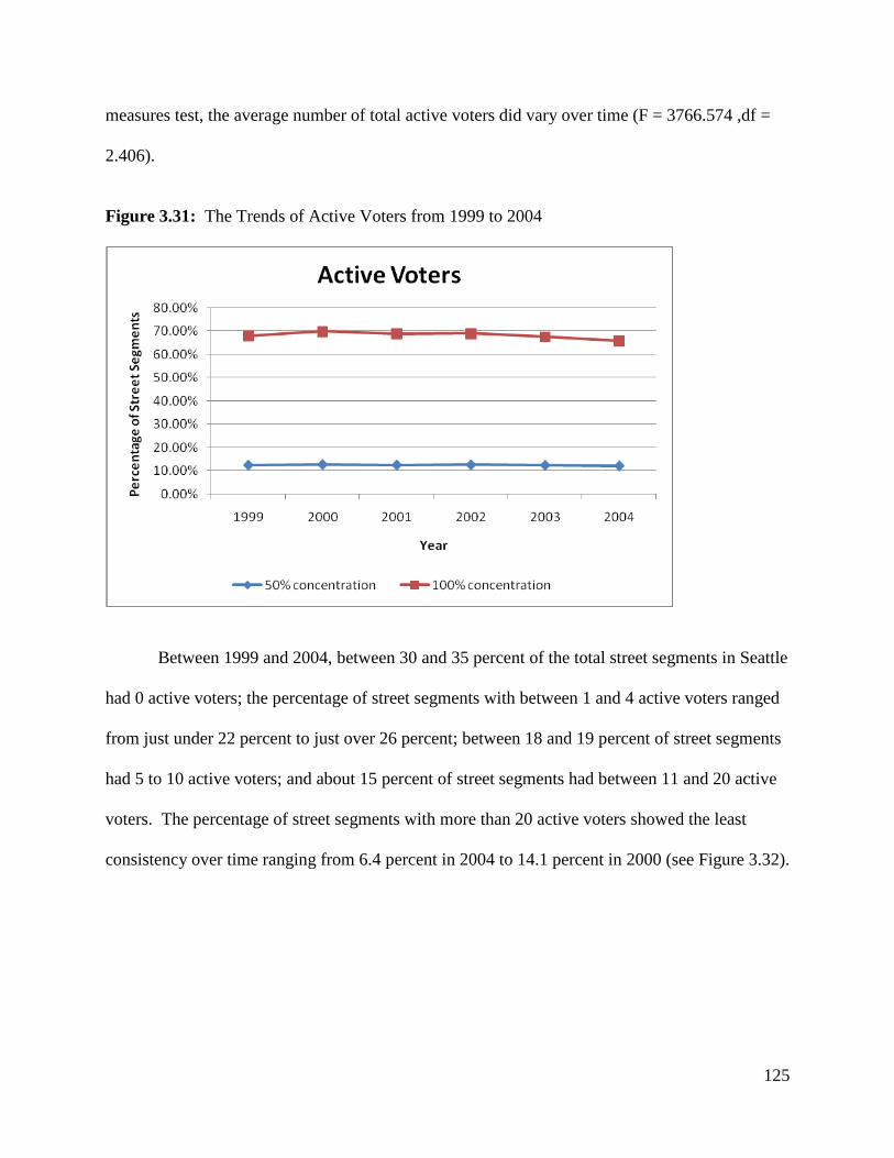
125

measures test, the average number of total active voters did vary over time (F = 3766.574 ,df =

2.406).

Figure 3.31: The Trends of Active Voters from 1999 to 2004

Between 1999 and 2004, between 30 and 35 percent of the total street segments in Seattle

had 0 active voters; the percentage of street segments with between 1 and 4 active voters ranged

from just under 22 percent to just over 26 percent; between 18 and 19 percent of street segments

had 5 to 10 active voters; and about 15 percent of street segments had between 11 and 20 active

voters. The percentage of street segments with more than 20 active voters showed the least

consistency over time ranging from 6.4 percent in 2004 to 14.1 percent in 2000 (see Figure 3.32).


126

Figure 3.32: Frequency Distributions of Active Voters

The quantile maps below indicate that the largest numbers of active voters are found in

the north sector (see Figure 3.33). There are also concentrations of street segments with high

numbers of active voters in the coastal part of the southwest sector and in the central sector on

the edge of the downtown core. The distribution of active voters is widespread and generally

reflects the population distribution (see Figure 4.11 in Chapter 4).


127

Figure 3.33: Geographic Distributions of Active Voters

The 50 percent concentration maps reinforce the earlier pattern but make it more visible.

This map clearly shows the concentration of active voters in the north sector with other notable

concentrations in the central and southwest sectors of the city (see Figure 3.34).


128

Exhibit 3.34: Geographic Distributions of 50 Percent Concentration of Active Voters

The LISA maps provide additional detail within the high concentration sectors (see

Figure 3.35). In the north sector, street segments with high numbers of active voters are often in

proximity to other street segments with high numbers of active voters. However, they are also

significantly associated with street segments having lower numbers of active voters. Thus, even

within areas of generally high voting activity there are street segments with low voting activity.

The southeast sector, which has generally the lowest number of active voters, shows up as more

uniform (dark blue) but also has a few isolated street segments with high numbers of active

voters (light red).


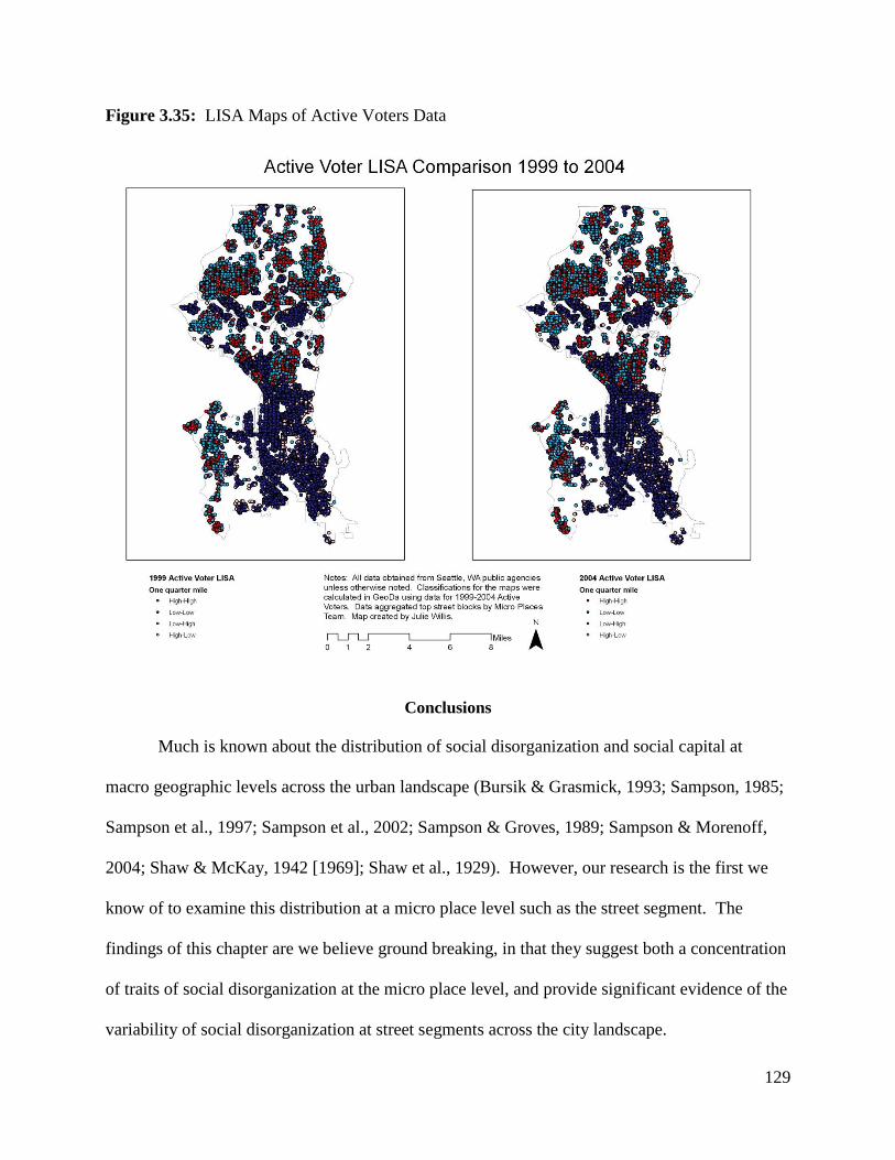
129

Figure 3.35: LISA Maps of Active Voters Data

Conclusions

Much is known about the distribution of social disorganization and social capital at

macro geographic levels across the urban landscape (Bursik & Grasmick, 1993; Sampson, 1985;

Sampson et al., 1997; Sampson et al., 2002; Sampson & Groves, 1989; Sampson & Morenoff,

2004; Shaw & McKay, 1942 [1969]; Shaw et al., 1929). However, our research is the first we

know of to examine this distribution at a micro place level such as the street segment. The

findings of this chapter are we believe ground breaking, in that they suggest both a concentration

of traits of social disorganization at the micro place level, and provide significant evidence of the

variability of social disorganization at street segments across the city landscape.


130

Looking both at structural and mediating variables we find that there are hot spots of

social disorganization at the street segment level. Moreover, such hot spots are not found only in

specific neighborhoods. Rather they are often distributed across the city landscape. In turn, we

found strong evidence of spatial independence of social disorganization at street segments.

While there are sometimes clusters of street segments with specific traits in what may be termed

communities or neighborhoods, there is also significant street by street variation in such

concentrations.

Together these findings raise intriguing questions about the relationship between social

disorganization and crime at the street segment level. Are hot spots of social disorganization

located in the same places as hot spots of crime? Does street level variability in social

disorganization relate to developmental trends of crime at place? Moreover, we found evidence

of temporal trends in the levels of social disorganization over time. Do those trends predict

developmental trends in crime at street segments over time?

In Chapters 6 and 7 we will explore these relationships between social disorganization

and crime at street segments. But our findings so far provide a strong basis for testing social

disorganization theories at micro places. Those who have studied criminology of place have

generally ignored social disorganization theories in favor of the opportunity and rational choice

perspectives we review in the next chapter. Our data so far suggest that social disorganization

may have more salience for understanding the criminology place than scholars have so far

recognized.


131

Chapter 4: Variation in Opportunity Factors

for Crime across the Urban Landscape

Most study of the criminology of place has relied upon opportunity theories (e.g. see

Cohen & Felson, 1979) as an explanation for why crime trends vary at places and as a basis for

constructing practical crime prevention approaches (see Eck, 1995; Sherman et al., 1989). The

main assumptions of this perspective are that specific characteristics of places such as the nature

of guardianship, the presence of motivated offenders, and the availability of suitable targets will

strongly influence the likelihood of criminal events (see also Felson, 1994). Studies examining

the factors that predict crime at micro places generally confirm this relationship (see Roncek &

Bell, 1981; Roncek & Maier, 1991; Smith et al., 2000). Opportunity theories, in turn, place

emphasis on the context of crime at place, identifying specific characteristics of urban

environments that facilitate or discourage criminal activity (Brantingham & Brantingham, 1984;

1981 [1991]; Cohen & Felson, 1979).

Given the sustained interest in opportunity theories by scholars who have studied micro

crime places, we would expect to observe significant variability in the characteristics of places at

the street segment level. Interestingly, there have been very few descriptions of the variation in

opportunity factors for crime at place, as contrasted with studies of the distribution of crime at

place. To what extent do crime opportunities concentrate at hot spots? And do they show strong

street to street variability? Is there strong variation in the developmental patterns of

opportunities over time? These questions are key to understanding the role of opportunities in

crime causation at places, but they have been given little empirical attention to date.


132

We draw from two of the most comprehensive opportunity theories (Perkins et al., 1993,

p. 30), crime pattern theory (Brantingham & Brantingham, 1984) and routine activity theory

(Cohen & Felson, 1979), to construct the set of street-level characteristics associated with crime.

This chapter describes the spatio-temporal distribution of crime-related place characteristics

across individual street segments in Seattle, Washington. We divide the characteristics into four

main categories: 1) motivated offenders; 2) suitable targets; 3) guardianship; and 4)

accessibility/urban form. Characteristics in each category are discussed individually and then as

a group.

Classifying Opportunity Measures

We are interested in the variation of characteristics across space as it relates to the uneven

distribution of people and in particular, of potential offenders and targets. The distribution of

people across places is driven by the uneven distribution of opportunities for housing,

employment, and recreation as well as access to the transportation network among places. But

people are not stationary; they move about the city in the course of the day, and those

movements tend to have a routine structure to them. Previous research has identified the

combination of the places an individual visits frequently and the routes taken among those places

as his or her activity space (Brantingham & Brantingham, 1981 [1991]; Horton & Reynolds,

1971). Activity spaces are dynamic; they grow and change over time in response to changes in

the physical environment and the lives of individuals.

Some places are anchors in the activity spaces of individuals (i.e., they are visited

frequently) (Golledge, 1978; Golledge & Stimson, 1997; Rengert, 1989). Anchor places act as

‘jumping off’ points. Individuals tend to know more about the area surrounding an anchor point

than they would around a route between two places. Anchor points also promote the acquisition


133

of knowledge about places near them and new routes to and from other nodes in an activity

place. For example, every person’s activity space typically has a home anchor point and a work

place or school anchor point. We tend to know more about the areas surrounding these places.

Some people have additional anchor points such as a significant other’s apartment, or a relative’s

house through which they begin to learn about the areas surrounding those anchor points.

Individuals also have nodes that they visit regularly but not as consistently or for as a long a

duration as they would an anchor point. In sum, activity spaces are both a reflection of and the

underpinning for, the uneven distribution of people across places (Brantingham & Brantingham,

1981 [1991]; Hägerstrand, 1970; Horton & Reynolds, 1971). Since motivated offenders and

suitable targets are simply subsets of the total population, if we can quantify who it likely to

frequent a place, we can quantify the potential number of motivated offenders and suitable

targets.

The grouping of opportunity related characteristics into four categories allow us to

describe both the concentration of people at a place and the potential roles those people might

take on while there (i.e., motivated offender or suitable target). Since the calculus of crime has

factors that take into account the situational characteristics, especially as they relate to

guardianship, we include characteristics to quantify the amount of guardianship at a place.

Finally, the number of people at a place is a function both of the attractiveness of a place and

also its accessibility. Thus, we include measures of urban form and accessibility. These

measures control for why a particular route among two places might be chosen over an

alternative route.

Traditionally, facilities have played an important role in understanding crime. A typical

approach has been to examine the effect of facilities on nearby places. At the start of this


134

undertaking, we scoured the literature for types of facilities that had been identified as crime

attractors or crime generators. We also included facilities that were related to the provision of

public safety services (e.g., police and fire stations).

Using this list, we began collecting information about the number and location of these

types of facilities for each year of our study period. As described below, what we found is that

most types of facilities are fairly stable over time. When the number of facilities increases it is

typically an accretive process rather than a churn process. Thus while new library locations are

added, the original ones remained where they were built. Facilities with these spatio-temporal

properties include: community centers, fire stations, hospitals, libraries, parks, police stations,

and schools. These facilities have low numbers to begin with and do not change rapidly. Other

types of facilities are distributed more widely across places and tend to be less stable, especially

locally. For example, while the number of fast food restaurants across the entire city may remain

fairly stable or increase, the opening and closing of 20 percent of those locations each year has a

far greater proportional impact on the streets that are near locations that close or open.

Place characteristics which are grouped under the accessibility/urban form category

describe how easy it is to get to a place and how likely someone is to use or be aware of places

because they are along an arterial route or have opportunities for public transportation. These

characteristics of a place describe how likely it is to be a part of the routine activity spaces of

both potential targets and potential offenders.

Table 4.1 classifies each opportunity-related characteristic by the theoretical construct it

describes. Sometimes a characteristic consists of only one type of data but other times a

characteristic is composed of several data items.


135

Table 4.1: Theoretical Concepts Represented by the Data

Characteristic Composition

Motivated Offenders

High risk juveniles

Truant or low academic achieving

juvenile residents

Suitable Targets

Employment

Residents

Retail business-related Crime


Public facilities as Crime


Number of employees

Total juveniles + total registered voters

Total sales for retail businesses

Number of public facilities within 1,320

feet

o Community centers

o Hospitals

o Libraries

o Parks

o Schools


Type of street

Bus stops

1= arterial, 0 = residential


Guardianship

Vacant Land

Police station/Fire station

Street lighting


Number of Police or fire stations within

1,320 feet

Watts per foot of lighting

The first major group of place characteristics has to do with the number of motivated

offenders who might live at a place. To measure the number of likely offenders who live on a

street segment we use a subset of the juvenile population that we term high risk juveniles. Since

these juveniles are more likely than other age groups to be involved in crime (Cohen & Felson,


136

1979), we use the total number of juveniles in grades three through twelve who live at a place

and who have low academic achievement and/or are classified as truants.1

The second major group of characteristics captures the likely number of suitable targets

at a place. We recognize that the total number of people at a place consists of both motivated

offenders and/or suitable targets.2 However, since we have no specific way to separate them, we

include all measures that capture the total number of people at a place under suitable targets.

These characteristics include those that describe the resident population and those that describe

visitors. We represent the total resident population by combining two proxy measures, total

number of residents who attend public school and total number of residents who are registered to

vote. Characteristics that capture how easy it is to get to a place are in the next grouping (i.e.,

accessibility/urban form).

The size of the non-resident population is determined to a large extent by the

attractiveness of a place. The greater the attractiveness, the greater the likelihood that people

(both offenders and targets) will know about the place and visit it. The more offenders and

targets at a place, the greater the likelihood that a target will be at the same place and time as a

motivated offender. Nonresidents fall into two main categories, visitors and employees. Visitors

are those that are attracted to a place to use the facilities and businesses. The following types of

facilities tend to attract a large number of visitors to a place and thus are considered crime

generators: community centers, hospitals, libraries, parks, retail and service businesses, and

schools (Brantingham & Brantingham, 1995). We use the presence of such facilities to represent

the visitor population.

1 Students with ten or more unexcused absences in a school year are classified as truants (See

http://www.seattleschools.org/area/truancy/index.htm). 2 The same population that we are characterizing as suitable targets could also be considered potential guardians

under routine activity theory (Cohen & Felson, 1979). We do not differentiate between the two.


http://www.seattleschools.org/area/truancy/index.htm

137

Employment provides a different measure of the number of non-residents likely to be at a

place routinely. These non-residents have the place as an anchor in their activity spaces. To

capture this type of non-resident we are use total employment across all types of business

sectors. Our measure captures the total number of non-resident employees who would routinely

come to a place.3 Together, public facilities and employment are used to capture the relative

number of nonresidents at places.

Two final characteristics are captured under the third category of accessibility/urban

form. These characteristics describe how easy it is to get to a place and how likely someone is

to use or be aware of places because they are located along an arterial street or are easily

accessible by public transportation. They also describe how likely a specific place is to be a part

of the routine activity spaces of both potential targets and potential offenders. The variables used

in this category are type of street (i.e., residential versus arterial) and the number of bus stops.

The fourth major group of place characteristics describes the level of guardianship at a

place. Guardianship is important to several opportunity theories including crime pattern theory

(Clarke & Cornish, 1985); routine activity theory (Eck, 1995) and rational choice theory (Felson,

2001, 2002). Guardianship can be provided by formal (i.e., people who are connected to a place

or a person) and informal guardians. More recent research has identified two types of formal

guardians by their specific role in a given situation; the roles are place managers (Wilson &

Kelling, 1982) and intimate handlers (Sampson & Raudenbush, 2001).

Characteristics such as percentage vacant land, presence of fire and/or police stations, and

the amount of street lighting describe both informal and formal guardianship at a place. The

presence of police and fire stations serves to increase the level of formal guardianship on the

3 Technically our measure does not account for people who live and work on the same street segment. However, we

feel any inflation of our estimates of people on the street due to ‘double counting’ of this population is minor.


138

street and on surrounding streets that are used for ingress and egress from the facilities. Simply

having a fire or police station on the street segment increases the trips by formal guardians to and

from the place. Those types of facilities can also serve as focal points for increased community

activism.

We include a measure of vacant land since vacant lots are sometimes an indicator of

decline (although they can indicate the beginning of a process of revitalization), often becoming

receptacles for trash and debris. This increases the perception of place users that a place is not

safe, and provides a place to commit crime. Street lighting’s relationship to crime and

guardianship is complicated; in general, lighting makes people feel safer and thus they may act

as if they are safer by going out of them homes more often. Such behavior increases the number

of ‘eyes on the street’ (Jacobs, 1961) and in doing so increases the amount of informal

surveillance and potential guardians.4

Description of Spatio-Temporal Variation in Opportunity Factors

In Chapter 3 we relied on the LISA statistic to characterize the distribution of social

disorganization constructs across Seattle. But in this chapter the measures examined often

involved the distribution of facilities. In those cases we examined the degree of clustering in the

distribution of facilities across space. Modifications are made where necessary because of low

numbers of observations. Our analysis of the opportunity factors begins with a description of the

characteristic and its distribution across street segments in Seattle. The first step is to aggregate

each characteristic to the street segment (our unit of analysis) along which it occurs. This

involves producing a value representing the number or frequency of the variable that existed on

the street for each year in the study period (only the years for which we were able to collect data

are represented).

4 For a comprehensive review of the literature on street lighting see Farrington & Welsh (2002).


139

Once we have an aggregate amount of a characteristic for each year, as in Chapter 3 we

describe the characteristic across street segments in terms of three main aspects: 1) prevalence;

2) variability across time and 3) spatial distribution. Prevalence captures the number of

observations affected by the characteristic of interest. To describe prevalence, we compute a

percentage of street segments with the characteristic.

Variability across time is not an issue in characteristics with a low rate of prevalence.

Consequently, variability across time is only calculated for characteristics which are found on at

least one percent of the units of analysis. With this analysis we are answering two questions: 1)

How does prevalence vary across time? and 2) Are the streets with the characteristic the same

across time, or do they vary? If a characteristic is stable over time we take the average and

provide a spatial distribution of the average. If the characteristic varies over time we use the first

year and last years for which we have data to capture the change over time.

If the distribution of the locations across space was the subject of the exploration, as with

facilities, then Ripley’s K was used.5 The Ripley’s K statistic allows us to conduct a distance

analysis to answer the question of whether the places with a certain type of facility are clustered

in space. We are also able to say whether the characteristic itself was more clustered than could

be expected based on a random distribution or on the distribution of streets across Seattle. If the

goal was to determine whether the frequency of a characteristic found on one street segment is

similar, different, or unrelated to the amount of the same characteristic on nearby street

segments, spatial autocorrelation measures were used. We calculated both global (Moran’s I and

Geary’s C) and local measures (Anselin’s LISA) of spatial autocorrelation to examine whether

the amounts of a characteristic are spatially dependent.

5 Facilities typically are very rare events (i.e. they are found on less than one percent of all segments). In these

cases a spatial autocorrelation would be inappropriate. Instead, we use Ripley’s K to provide a quantitative measure

of the spatial pattern. For all analyses, Ripley’s K was used with 100 simulations.


140

We think it important at the outset, to note that neither Moran’s I nor Geary’s C found

significant global spatial autocorrelation for any of the characteristics explained. This finding, as

those reported in the previous chapter, suggests that there is tremendous street segment-by-street

segment variation in characteristics. Additional evidence for heterogeneity as the explanation for

the lack of global spatial autocorrelation was provided by the LISA analysis which indicated

significant amounts of both negative and positive spatial autocorrelation.6

Similar geographic analyses were performed on all data layers with the exception of

facilities where the numbers of observations which had a facility present were so small as to

make the results of a typical geographic analysis for spatial autocorrelation meaningless (e.g.

libraries, police stations etc.). In those cases, a subset of the full geographic analysis was

applied.

Motivated Offenders

Motivated offenders are a necessary element for a crime to occur (Cohen & Felson,

1979). While we did not have any information to quantify the total number of motivated

offenders across places, we did have a measure of high risk juveniles. Since the contributing role

of juveniles in crime at places is widely recognized, we include a separate variable that describes

the population of juveniles who are likely to exhibit delinquent behavior on a particular street

segment.

Resident High Risk Juvenile Population

Some students are more likely to commit crimes than other students. One indicator is

truancy and another is low academic achievement. If a student is either a truant or designated as

6 The results of the LISA analysis are subject to the distances between street segment midpoints. While the average

length of a street is 400 feet, there is considerable variation. The LISA statistic uses a simple spatial weights file

that is based on distance. Since the midpoints are used in the calculation, street segments that are connected end-to-

end may be farther away than those located on either side of the target street segment. Only when the distance

between midpoints is shorter than one-quarter mile will the statistic identify them as neighbors.


141

a low academic achiever or both, they are included in our measure of total high risk juveniles

who live on the street segment. At the beginning of the study period there were 5,366 students

classified as high risk juveniles, out of a total student population of 34,525 in 1992-1993. The

number of high risk juveniles has declined steadily between the school year of 1992-1993

(N=5,366) and 2004-2005 (N=4,383). The proportion has dropped from about 16 to 12 percent.

This occurs over a time period when the number of public school students per year is fairly

stable, ranging from 34,525 in 1992-1993 to 36,153 in 2004-2005.

This aggregate stability masks significant changes on the individual street segments over

time. According to the repeated measures analysis, the within subject effect is significant (F =

62.177, df = 3.783). The average number of high risk juveniles per street segment does vary

over time.

Juveniles tend to be concentrated on particular segments rather than spread evenly across

them (see Figure 4.1). In Seattle, 50 percent of high risk juveniles are consistently found on

between three and four percent of the total number of Seattle street segments. These may be

seen as hot spots for high risk juveniles.


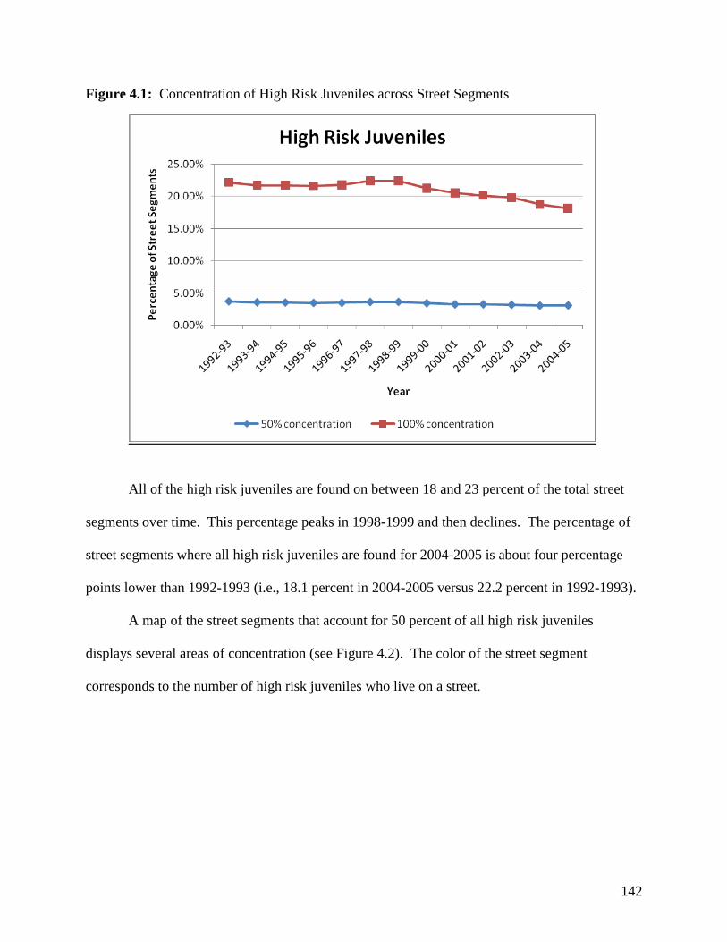
142

Figure 4.1: Concentration of High Risk Juveniles across Street Segments

All of the high risk juveniles are found on between 18 and 23 percent of the total street

segments over time. This percentage peaks in 1998-1999 and then declines. The percentage of

street segments where all high risk juveniles are found for 2004-2005 is about four percentage

points lower than 1992-1993 (i.e., 18.1 percent in 2004-2005 versus 22.2 percent in 1992-1993).

A map of the street segments that account for 50 percent of all high risk juveniles

displays several areas of concentration (see Figure 4.2). The color of the street segment

corresponds to the number of high risk juveniles who live on a street.


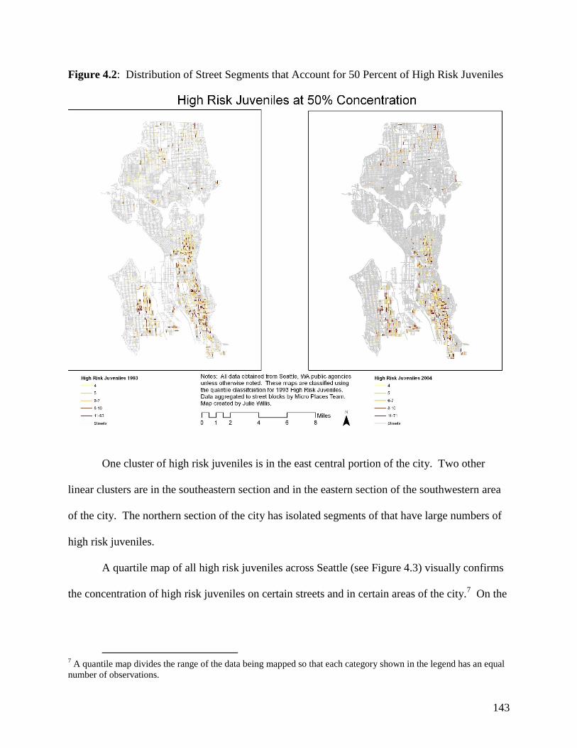
143

Figure 4.2: Distribution of Street Segments that Account for 50 Percent of High Risk Juveniles

One cluster of high risk juveniles is in the east central portion of the city. Two other

linear clusters are in the southeastern section and in the eastern section of the southwestern area

of the city. The northern section of the city has isolated segments of that have large numbers of

high risk juveniles.

A quartile map of all high risk juveniles across Seattle (see Figure 4.3) visually confirms

the concentration of high risk juveniles on certain streets and in certain areas of the city.7 On the

7 A quantile map divides the range of the data being mapped so that each category shown in the legend has an equal

number of observations.


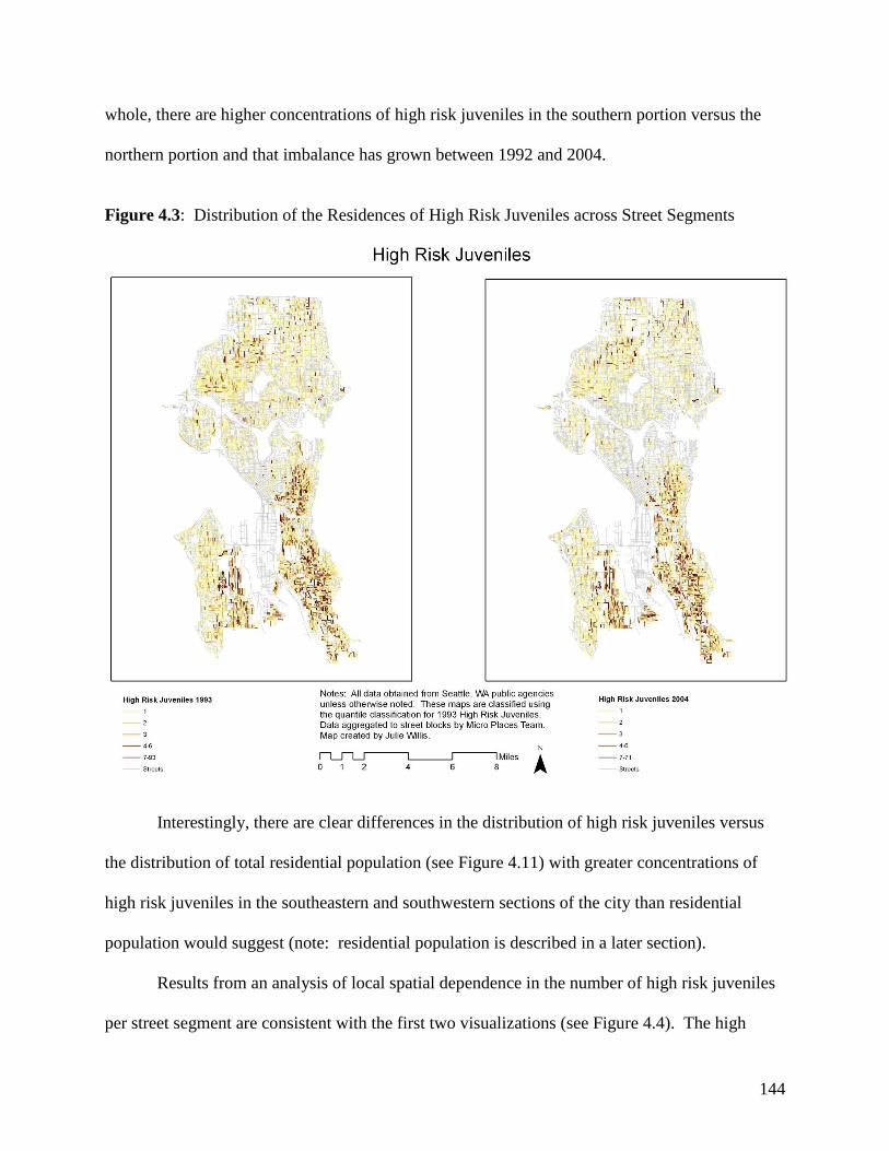
144

whole, there are higher concentrations of high risk juveniles in the southern portion versus the

northern portion and that imbalance has grown between 1992 and 2004.

Figure 4.3: Distribution of the Residences of High Risk Juveniles across Street Segments

Interestingly, there are clear differences in the distribution of high risk juveniles versus

the distribution of total residential population (see Figure 4.11) with greater concentrations of

high risk juveniles in the southeastern and southwestern sections of the city than residential

population would suggest (note: residential population is described in a later section).

Results from an analysis of local spatial dependence in the number of high risk juveniles

per street segment are consistent with the first two visualizations (see Figure 4.4). The high


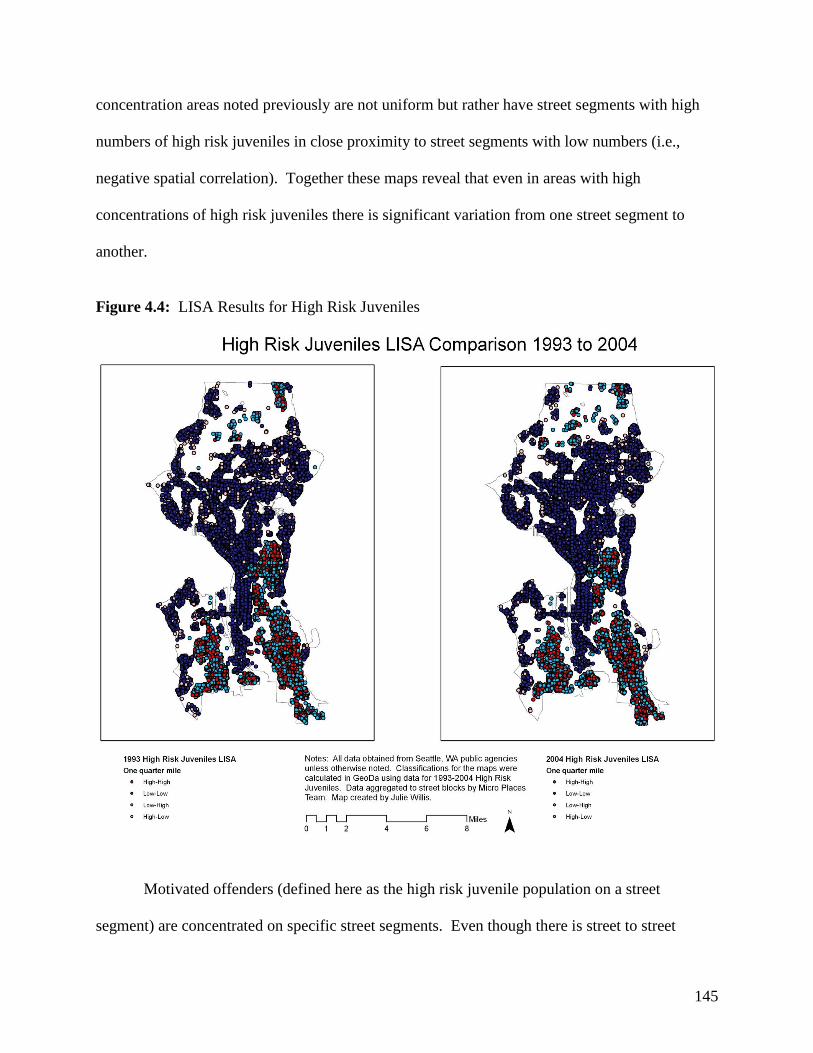
145

concentration areas noted previously are not uniform but rather have street segments with high

numbers of high risk juveniles in close proximity to street segments with low numbers (i.e.,

negative spatial correlation). Together these maps reveal that even in areas with high

concentrations of high risk juveniles there is significant variation from one street segment to

another.

Figure 4.4: LISA Results for High Risk Juveniles

Motivated offenders (defined here as the high risk juvenile population on a street

segment) are concentrated on specific street segments. Even though there is street to street


146

variation in the number of high risk juveniles, street segments with high numbers of motivated

offenders tend to be in the vicinity of other street segments with high numbers of motivated

offenders. This finding is consistent across study years even while the number of motivated

offenders per street segment displays significant change over the same years. Thus, even when

high risk juveniles are changing residences they seem to consistently be found on street segments

in the vicinity of other high risk juveniles.

Suitable Targets

These measures capture both residents and non-residents who frequent a street segment.

While residents live on the street segment, non-residents are typically present for reasons related

to employment or some type of facility located on the street segment, but they could also be on

their way somewhere else and the street segment is just a component of their overall route

between two totally unrelated places. Alternatively, they could be visiting a friend or relative.

While we do not have data to capture all these dimensions, we can provide proxy measures of

employment, residential population, crime generators, and crime attractors.

Employment

Under opportunity theory, the number of people attracted to a place has a large bearing

on the place’s crime potential. While home is one major anchor point in an individual’s activity

space, for employed persons, work is another. Thus, quantifying the number of people who

work at a place provides an important foundational element for understanding crime. In Seattle,

we were able to obtain data about the entire spectrum of businesses. One attribute of the

business data is the number of employees who work at each business. From this data set we

were able to construct the number of people who travel to a place for work.


147

Employment is highly concentrated in Seattle (see Figure 4.5). Between 1998 and 2004,

half of all the employees in the city were located on about 0.8 percent of Seattle street segments.

All employment was concentrated on between 25 and 28.5 percent of total street segments over

the study period. There is more variation in the concentraton of total employment over time than

the 50 percent employment figure. The total number of street segments with employees

increased from 1998 to 2002 and then showed a slight decline in 2004. These figures point to

the concentration of most employment on relatively few street segments that are fairly stable

over time. It is the smaller employers and home-based businesses that contribute to the larger

number of streets at 100 percent.

Figure 4.5: Concentration of Employment across Street Segments

Although the overall number of employees varied only a couple of percentage points per

year, according to the repeated measures analysis, the within subject effect is significant at p <


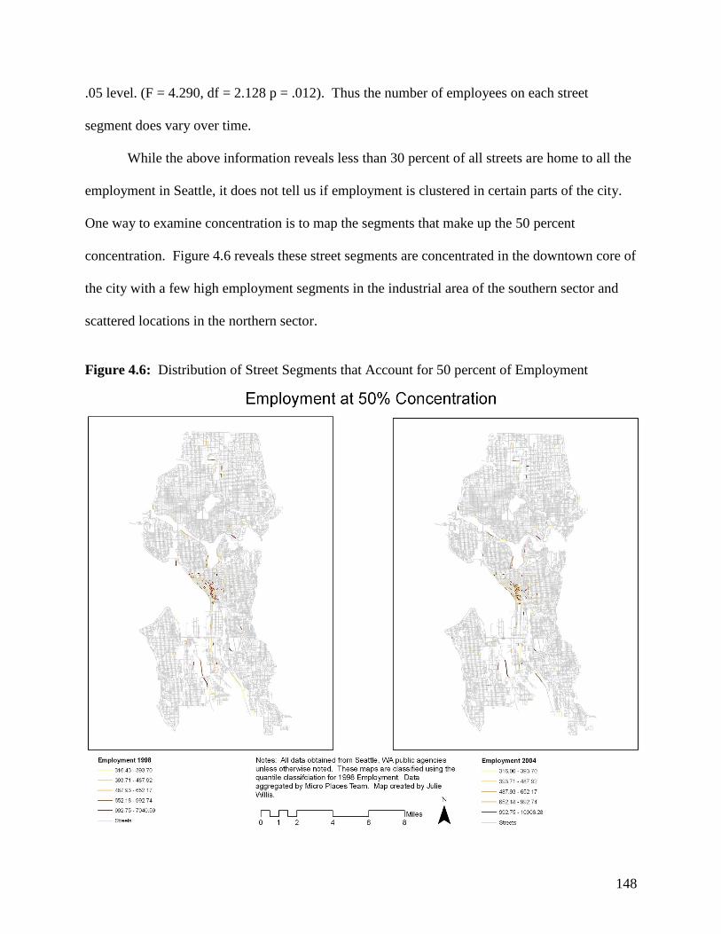
148

.05 level. (F = 4.290, df = 2.128 p = .012). Thus the number of employees on each street

segment does vary over time.

While the above information reveals less than 30 percent of all streets are home to all the

employment in Seattle, it does not tell us if employment is clustered in certain parts of the city.

One way to examine concentration is to map the segments that make up the 50 percent

concentration. Figure 4.6 reveals these street segments are concentrated in the downtown core of

the city with a few high employment segments in the industrial area of the southern sector and

scattered locations in the northern sector.

Figure 4.6: Distribution of Street Segments that Account for 50 percent of Employment


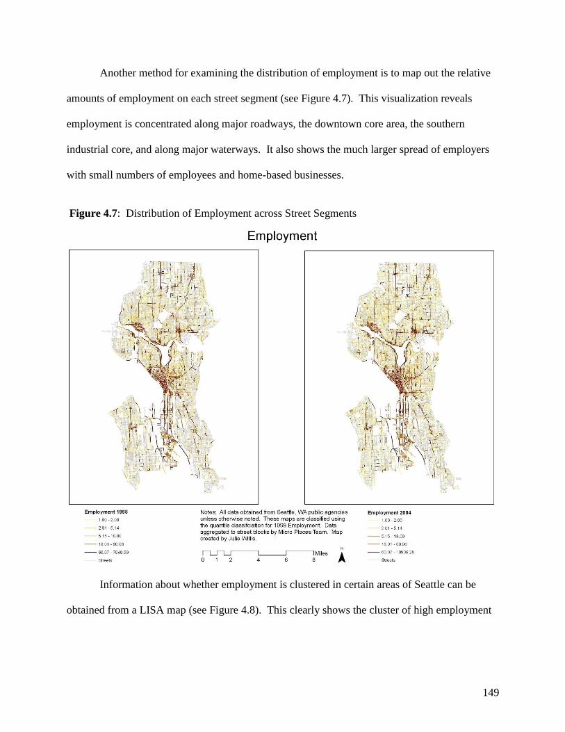
149

Another method for examining the distribution of employment is to map out the relative

amounts of employment on each street segment (see Figure 4.7). This visualization reveals

employment is concentrated along major roadways, the downtown core area, the southern

industrial core, and along major waterways. It also shows the much larger spread of employers

with small numbers of employees and home-based businesses.

Figure 4.7: Distribution of Employment across Street Segments

Information about whether employment is clustered in certain areas of Seattle can be

obtained from a LISA map (see Figure 4.8). This clearly shows the cluster of high employment


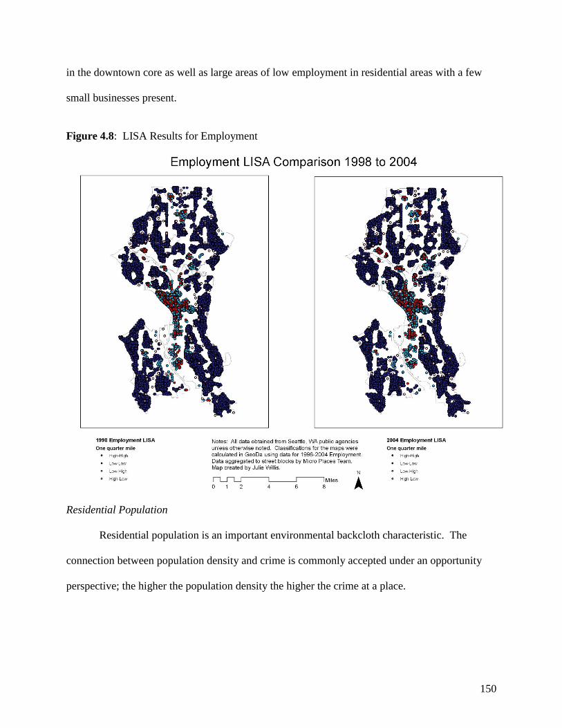
150

in the downtown core as well as large areas of low employment in residential areas with a few

small businesses present.

Figure 4.8: LISA Results for Employment

Residential Population

Residential population is an important environmental backcloth characteristic. The

connection between population density and crime is commonly accepted under an opportunity

perspective; the higher the population density the higher the crime at a place.


151

The natural starting point for estimating residential population is census data. However,

our focus on the micro level made using census data impossible.8 So we chose to use

characteristics of micro level places that would provide information about the resident population

in the absence of a 100 percent head count. The only two sources of information we were able to

obtain about residential population at the street segment level described the number of registered

voters and the number of public school students. Both measures are individually biased but in

different directions. The population of public school students tends to emphasize areas with

children under the age of 18, lower income areas, and minority areas. The population of

registered voters is biased toward higher income, white areas which are also the areas more

likely to send their kids to private school. Places with high populations of public school are not

the same as place with high populations of registered voters. By adding together the total

number of public school students and the total number of registered voters we can create an

approximation of the total number of people who are living on a particular street segment. This

measure counts both adults and juveniles; however, it excludes those who under the age of five

and those who attend private schools. In addition, it excludes those who are ex-felons (until they

have completed their sentence and paid all fines, fees, and court costs) and those who have not

registered to vote regardless of their reason. For example, non-US citizens would be

undercounted by this measure as would those populations who tend not to register to vote.

Our proxy measure produced a population estimate of 437,612 in 2001 which decreased

to 381,815 by 2004. As expected, these figures are less than the total population of Seattle in

both time periods. The census reports a population of 563,374 in 2000 (U.S. Census Bureau,

2000) and 536,946 in 2005 (U.S. Census Bureau, 2005). Our proxy measure revealed the

8 The smallest unit of analysis used by the census is the census block. The census block aggregates one side of the

street for four different street segments into a census block. The US Census Bureau was unable to accommodate our

request to use original census data.


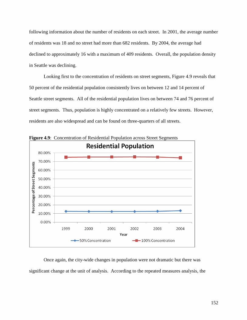
152

following information about the number of residents on each street. In 2001, the average number

of residents was 18 and no street had more than 682 residents. By 2004, the average had

declined to approximately 16 with a maximum of 409 residents. Overall, the population density

in Seattle was declining.

Looking first to the concentration of residents on street segments, Figure 4.9 reveals that

50 percent of the residential population consistently lives on between 12 and 14 percent of

Seattle street segments. All of the residential population lives on between 74 and 76 percent of

street segments. Thus, population is highly concentrated on a relatively few streets. However,

residents are also widespread and can be found on three-quarters of all streets.

Figure 4.9: Concentration of Residential Population across Street Segments

Once again, the city-wide changes in population were not dramatic but there was

significant change at the unit of analysis. According to the repeated measures analysis, the


153

within subject effect is significant (F = 1180.196 ,df = 1.923). The average number of total

residents per street segment does vary over time.

The densest residential areas are found in the central and northern parts of the city (see

Figure 4.10). There are also isolated areas of high concentration in the southern part of the city

but they are fewer, and the distance between them is greater. Half of all residents in the city live

on the colored streets on the map.

Figure 4.10: Distribution of Street Segments that Account for 50 Percent of Residential

Population

Figure 4.11 shows the geographic distribution of all residents and reveals how

widespread residential population is in the city. While most of the city is covered by residential


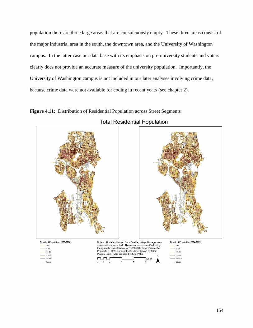
154

population there are three large areas that are conspicuously empty. These three areas consist of

the major industrial area in the south, the downtown area, and the University of Washington

campus. In the latter case our data base with its emphasis on pre-university students and voters

clearly does not provide an accurate measure of the university population. Importantly, the

University of Washington campus is not included in our later analyses involving crime data,

because crime data were not available for coding in recent years (see chapter 2).

Figure 4.11: Distribution of Residential Population across Street Segments


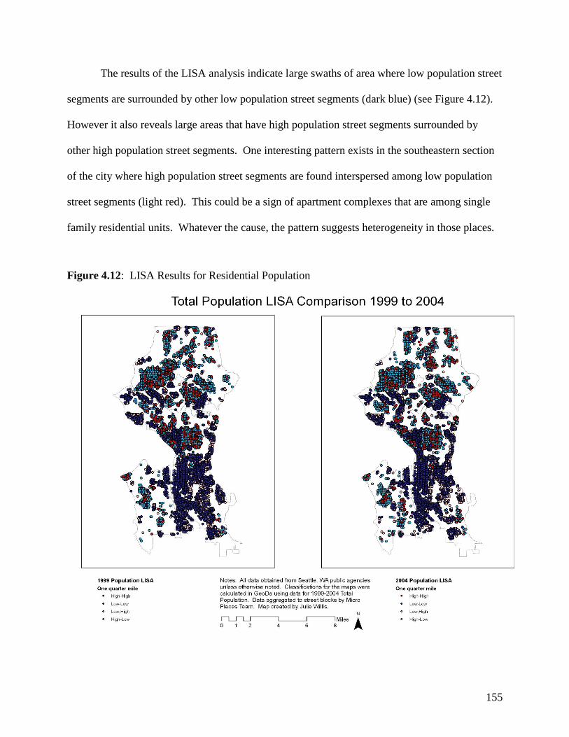
155

The results of the LISA analysis indicate large swaths of area where low population street

segments are surrounded by other low population street segments (dark blue) (see Figure 4.12).

However it also reveals large areas that have high population street segments surrounded by

other high population street segments. One interesting pattern exists in the southeastern section

of the city where high population street segments are found interspersed among low population

street segments (light red). This could be a sign of apartment complexes that are among single

family residential units. Whatever the cause, the pattern suggests heterogeneity in those places.

Figure 4.12: LISA Results for Residential Population


156

Business-related Crime Generators and Attractors

Businesses located at a place play a key role in attracting suitable targets. For this

characteristic we add up the total sales for all the retail businesses on the street segment. We

purchased data from InfoUSA for four different years: 1998, 2000, 2002, and 2004. 1998 was

the earliest year with available data and cost precluded purchasing every year. Between 1998

and 2004, 50 percent of all retail sales in Seattle were consistently found on about 0.2 percent of

the total street segments in Seattle (see Figure 4.13). Clearly, retail sales are concentrated in

retail sales hot spots. For 100 percent of total retail sales, the trend line again shows a fairly

consistent trend at about 6.0 percent of all street segments. These figures also show that

approximately 94 percent of streets have no retail business sales in any given year.

Figure 4.13: Concentration of Total Retail Sales across Street Segments


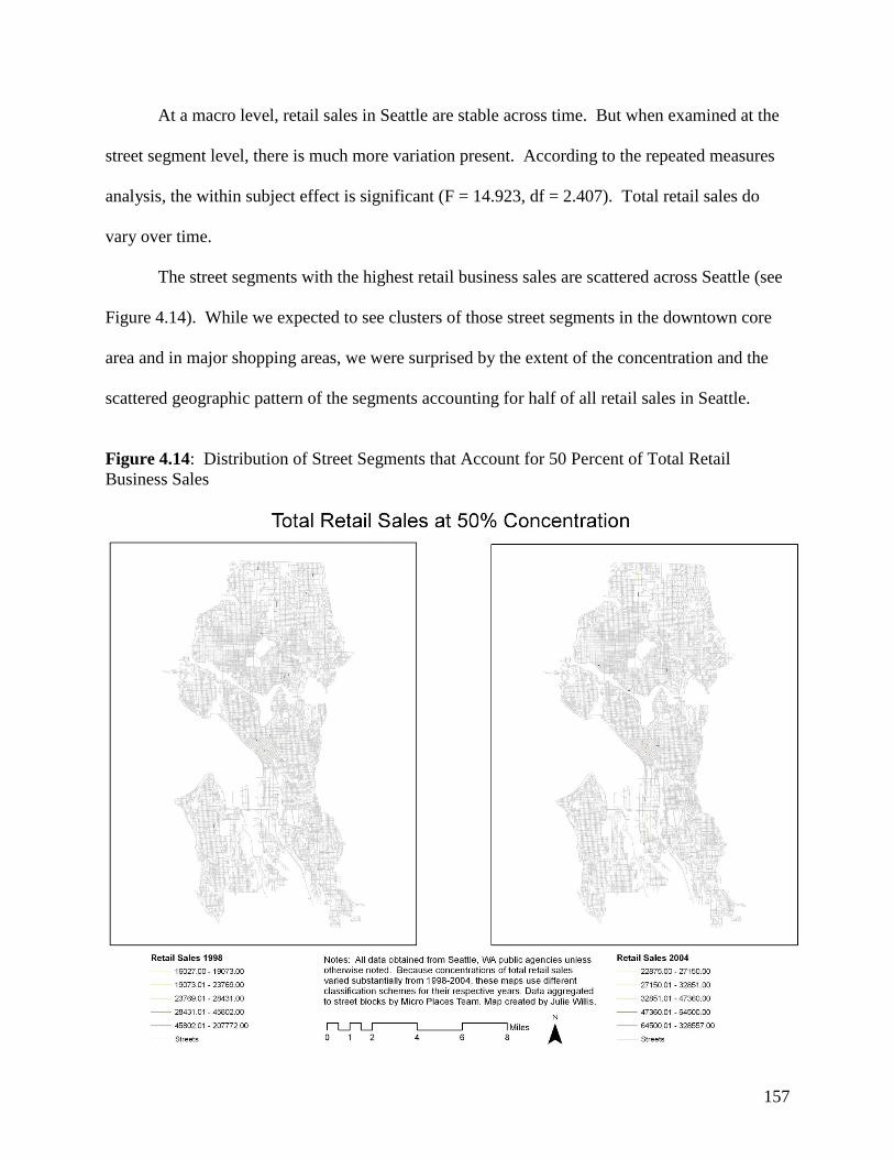
157

At a macro level, retail sales in Seattle are stable across time. But when examined at the

street segment level, there is much more variation present. According to the repeated measures

analysis, the within subject effect is significant (F = 14.923, df = 2.407). Total retail sales do

vary over time.

The street segments with the highest retail business sales are scattered across Seattle (see

Figure 4.14). While we expected to see clusters of those street segments in the downtown core

area and in major shopping areas, we were surprised by the extent of the concentration and the

scattered geographic pattern of the segments accounting for half of all retail sales in Seattle.

Figure 4.14: Distribution of Street Segments that Account for 50 Percent of Total Retail

Business Sales


158

The quantile map which shows the total retail sales on each of the street segments

indicates the expected geographic distribution of businesses sales (see Figure 4.15). Retail sales

are clustered along major arteries and in business districts such as the downtown area and the

industrial area south of downtown.

Figure 4.15: Distribution of Total Retail Business Sales

The LISA for retail businesses sales confirms this pattern (see Figure 4.16). The

downtown core has many street segments with high retail sales near other street segments with

high retail sales. However, there are also streets with low retail sales street segments

interspersed within those high sales street segments. The large dark blue areas are


159

predominantly residential with low numbers of low volume establishments. Finally, there are

individual street segments (found in all parts of the city) where a street has significantly higher

retail sales than the streets around it. These clusters represent commercial areas in the midst of

residential ones.


160

Figure 4.16: LISA Results for Total Retail Business Sales

Public Facility-Related Crime Generators and Attractors

Public facilities also play a key role in attracting suitable targets. For this characteristic

we summarized all the government facilities that are on a street segment.9 Public and quasi-

public facilities on the street segment include: 1) community centers; 2) hospitals; 3) libraries; 4)

parks and 5) middle and high schools. Because of the low number of facilities present in Seattle,

we operationalized the construct as the average number of public facilities within one quarter of

a mile of a place. In the following paragraphs, we first describe the distribution of facilities

9 Parks and schools present an analytical challenge in that they often are bounded by more than one street segment.

This issue is not addressed in the study. Parks and schools are allocated to the street segment on which their street

address is located. We recognize this as a deficiency but given the relatively small numbers of parks and schools

believe the effect on the results will be minimal.


161

across our units of analysis. The distribution of the ‘total number of public facilities within one

quarter of a mile of a place’ is described next.

The number of public facilities in Seattle ranged from 379 in 1989 to 419 in 2004. The

number decreased for the first two years of the study period and then began a steady increase

between 1993 and 2002 (see Table 4.2). In 2003, there was a slight decrease before rebounding.

These changes were due to both temporary closings for renovations, permenant closings, and

relocations, as well as new facilities being added. Given the small number of facilities, no

concentration graphs or maps are provided. Community centers (n=26) and hospitals (n=13)

were stable. The overall number of public facilities in Seattle increased over the time period

largely due to more parks being created (an increase of 44 parks). Schools added two locations

and libraries added four.


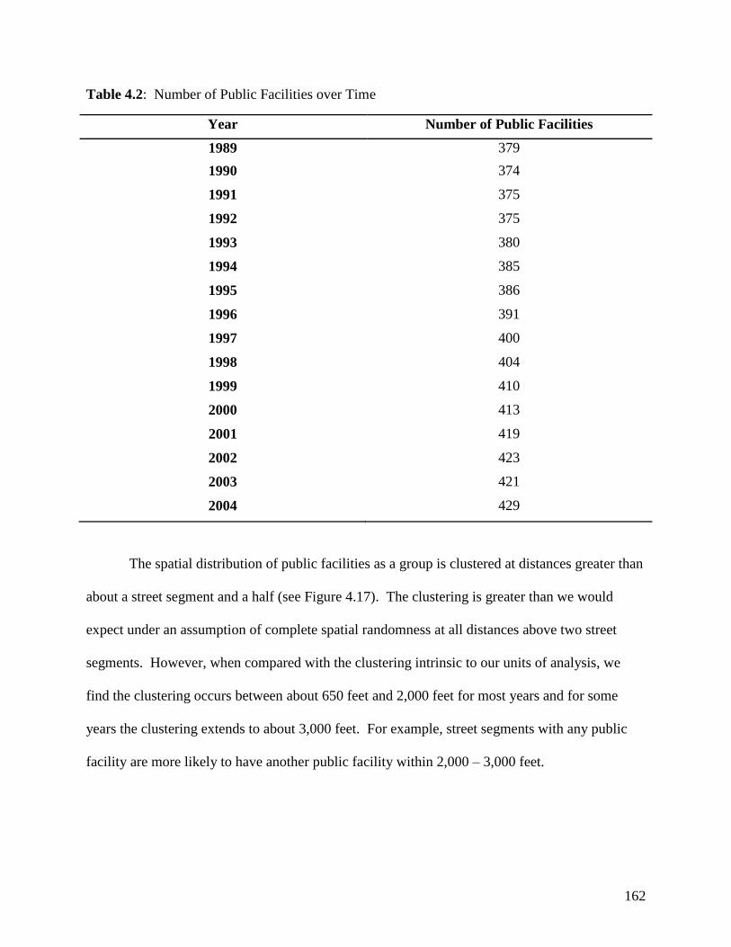
162

Table 4.2: Number of Public Facilities over Time

Year Number of Public Facilities

1989 379

1990 374

1991 375

1992 375

1993 380

1994 385

1995 386

1996 391

1997 400

1998 404

1999 410

2000 413

2001 419

2002 423

2003 421

2004 429

The spatial distribution of public facilities as a group is clustered at distances greater than

about a street segment and a half (see Figure 4.17). The clustering is greater than we would

expect under an assumption of complete spatial randomness at all distances above two street

segments. However, when compared with the clustering intrinsic to our units of analysis, we

find the clustering occurs between about 650 feet and 2,000 feet for most years and for some

years the clustering extends to about 3,000 feet. For example, street segments with any public

facility are more likely to have another public facility within 2,000 – 3,000 feet.


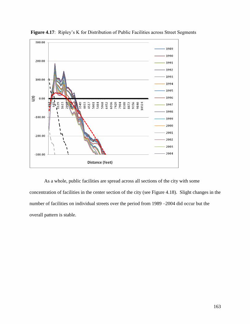
163

Figure 4.17: Ripley’s K for Distribution of Public Facilities across Street Segments

As a whole, public facilities are spread across all sections of the city with some

concentration of facilities in the center section of the city (see Figure 4.18). Slight changes in the

number of facilities on individual streets over the period from 1989 –2004 did occur but the

overall pattern is stable.


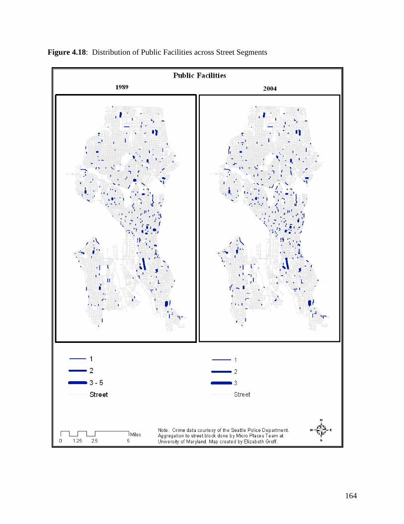
164

Figure 4.18: Distribution of Public Facilities across Street Segments


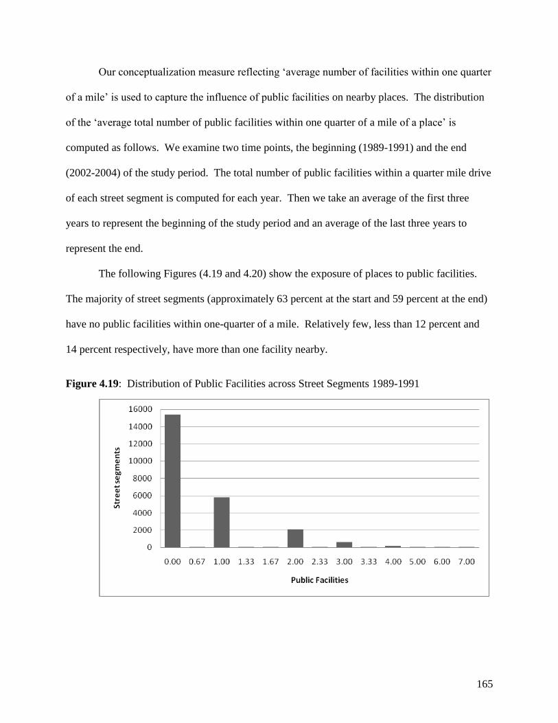
165

Our conceptualization measure reflecting ‘average number of facilities within one quarter

of a mile’ is used to capture the influence of public facilities on nearby places. The distribution

of the ‘average total number of public facilities within one quarter of a mile of a place’ is

computed as follows. We examine two time points, the beginning (1989-1991) and the end

(2002-2004) of the study period. The total number of public facilities within a quarter mile drive

of each street segment is computed for each year. Then we take an average of the first three

years to represent the beginning of the study period and an average of the last three years to

represent the end.

The following Figures (4.19 and 4.20) show the exposure of places to public facilities.

The majority of street segments (approximately 63 percent at the start and 59 percent at the end)

have no public facilities within one-quarter of a mile. Relatively few, less than 12 percent and

14 percent respectively, have more than one facility nearby.

Figure 4.19: Distribution of Public Facilities across Street Segments 1989-1991


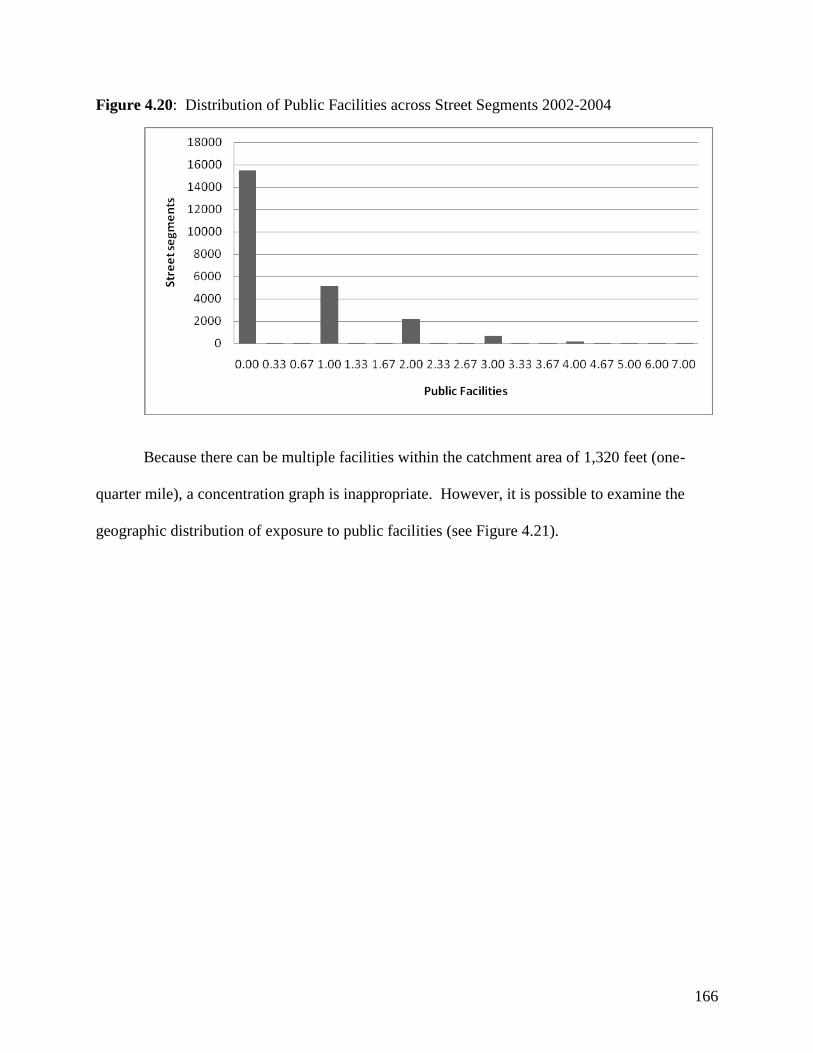
166

Figure 4.20: Distribution of Public Facilities across Street Segments 2002-2004

Because there can be multiple facilities within the catchment area of 1,320 feet (one-

quarter mile), a concentration graph is inappropriate. However, it is possible to examine the

geographic distribution of exposure to public facilities (see Figure 4.21).


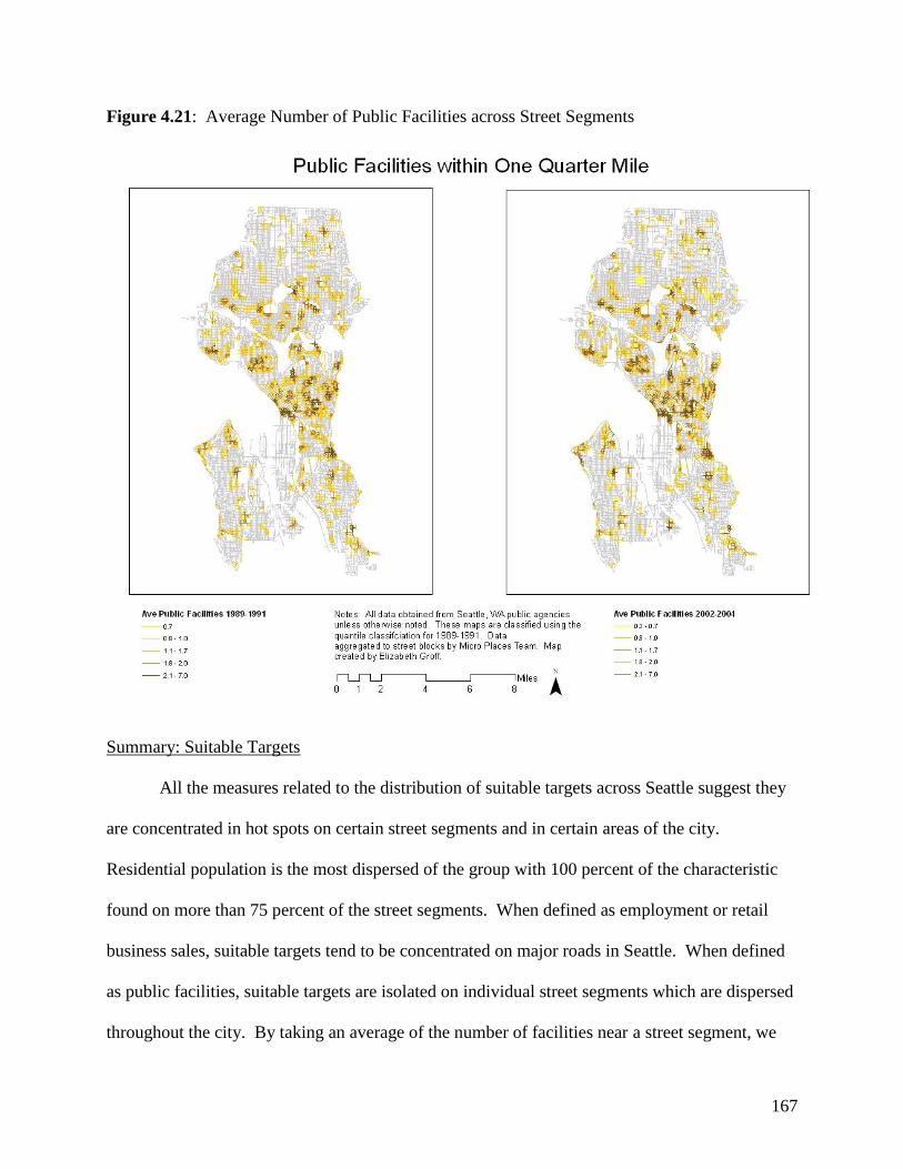
167

Figure 4.21: Average Number of Public Facilities across Street Segments

Summary: Suitable Targets

All the measures related to the distribution of suitable targets across Seattle suggest they

are concentrated in hot spots on certain street segments and in certain areas of the city.

Residential population is the most dispersed of the group with 100 percent of the characteristic

found on more than 75 percent of the street segments. When defined as employment or retail

business sales, suitable targets tend to be concentrated on major roads in Seattle. When defined

as public facilities, suitable targets are isolated on individual street segments which are dispersed

throughout the city. By taking an average of the number of facilities near a street segment, we


168

can get a clearer picture of the potential sphere of influence of those facilities. Still, their

influence is concentrated on particular street segments near those relatively infrequent facility

locations.


The place characteristics in this section provide a method for describing the accessibility

of a place. Opportunity theories recognize that places with more people who frequent them or

with which more people are familiar are more likely to experience crime. The relationship

between numbers of people and crime is not necessarily a linear one, but rather more of a

precondition that makes a particular set of outcomes more likely. Just as an accident can occur

on a deserted road but is more likely on a crowded urban street, crime can occur in places with

few people but is far more likely in places with many people. One related aspect of accessibility

is that it increases the number of people who know about a place. Studies at the street segment

level of analysis have established the relationship between traffic flow and accessibility (number

of ‘turning’ opportunities) and property crime (Brantingham & Brantingham, 1993a, 1993b).

Type of Street

We begin with an intrinsic characteristic of the road network, type of street. We consider

only two categories, arterial roads and non-arterial roads. Arterial streets are those that carry

larger volumes of traffic. The non-arterial roads consist of residential streets and walkways.10

Residential streets run through neighborhoods and are designed to carry only neighborhood

traffic. Walkways are non-vehicular paths or stairways that typically connect two residential

streets.

Arterial streets are of particular interest to this study because of their role in increasing

accessibility and serving as change points across the urban landscape. High crime

10

Limited access highways are excluded from the study since they do not fit our definition of a place.


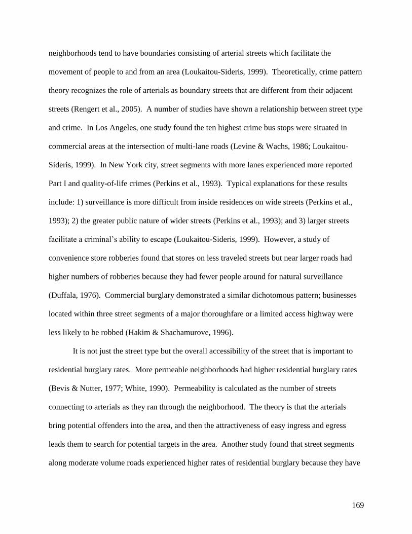
169

neighborhoods tend to have boundaries consisting of arterial streets which facilitate the

movement of people to and from an area (Loukaitou-Sideris, 1999). Theoretically, crime pattern

theory recognizes the role of arterials as boundary streets that are different from their adjacent

streets (Rengert et al., 2005). A number of studies have shown a relationship between street type

and crime. In Los Angeles, one study found the ten highest crime bus stops were situated in

commercial areas at the intersection of multi-lane roads (Levine & Wachs, 1986; Loukaitou-

Sideris, 1999). In New York city, street segments with more lanes experienced more reported

Part I and quality-of-life crimes (Perkins et al., 1993). Typical explanations for these results

include: 1) surveillance is more difficult from inside residences on wide streets (Perkins et al.,

1993); 2) the greater public nature of wider streets (Perkins et al., 1993); and 3) larger streets

facilitate a criminal’s ability to escape (Loukaitou-Sideris, 1999). However, a study of

convenience store robberies found that stores on less traveled streets but near larger roads had

higher numbers of robberies because they had fewer people around for natural surveillance

(Duffala, 1976). Commercial burglary demonstrated a similar dichotomous pattern; businesses

located within three street segments of a major thoroughfare or a limited access highway were

less likely to be robbed (Hakim & Shachamurove, 1996).

It is not just the street type but the overall accessibility of the street that is important to

residential burglary rates. More permeable neighborhoods had higher residential burglary rates

(Bevis & Nutter, 1977; White, 1990). Permeability is calculated as the number of streets

connecting to arterials as they ran through the neighborhood. The theory is that the arterials

bring potential offenders into the area, and then the attractiveness of easy ingress and egress

leads them to search for potential targets in the area. Another study found that street segments

along moderate volume roads experienced higher rates of residential burglary because they have


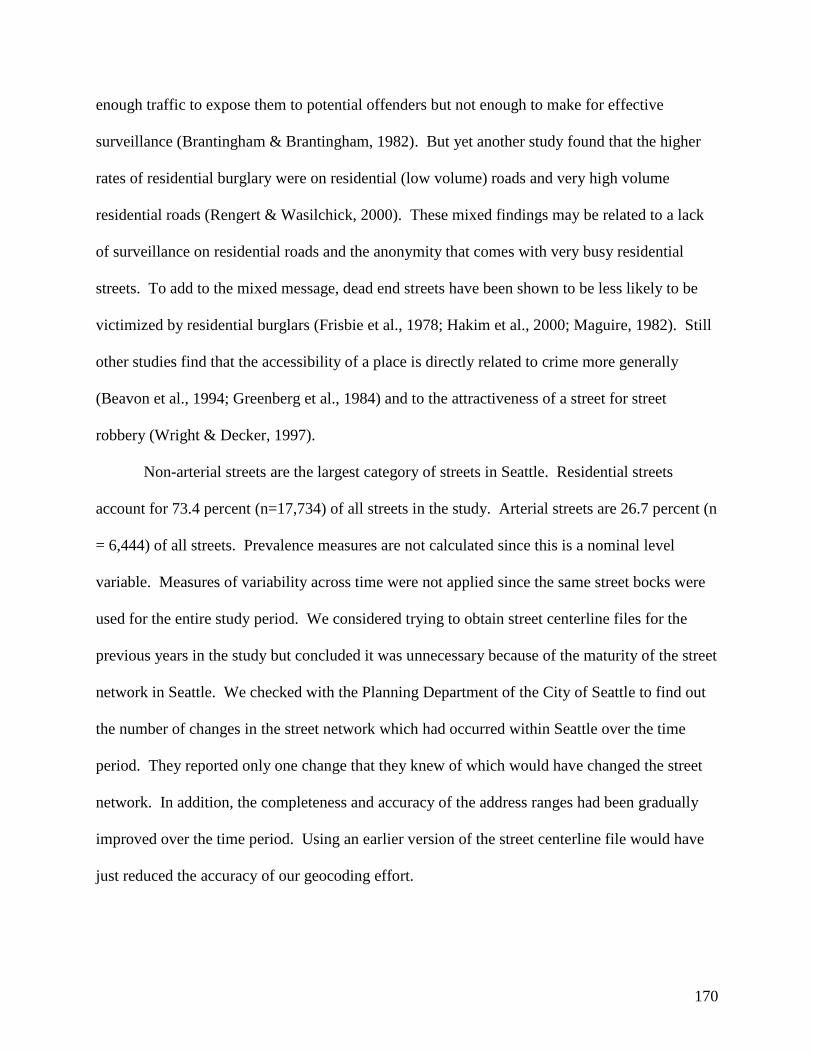
170

enough traffic to expose them to potential offenders but not enough to make for effective

surveillance (Brantingham & Brantingham, 1982). But yet another study found that the higher

rates of residential burglary were on residential (low volume) roads and very high volume

residential roads (Rengert & Wasilchick, 2000). These mixed findings may be related to a lack

of surveillance on residential roads and the anonymity that comes with very busy residential

streets. To add to the mixed message, dead end streets have been shown to be less likely to be

victimized by residential burglars (Frisbie et al., 1978; Hakim et al., 2000; Maguire, 1982). Still

other studies find that the accessibility of a place is directly related to crime more generally

(Beavon et al., 1994; Greenberg et al., 1984) and to the attractiveness of a street for street

robbery (Wright & Decker, 1997).

Non-arterial streets are the largest category of streets in Seattle. Residential streets

account for 73.4 percent (n=17,734) of all streets in the study. Arterial streets are 26.7 percent (n

= 6,444) of all streets. Prevalence measures are not calculated since this is a nominal level

variable. Measures of variability across time were not applied since the same street bocks were

used for the entire study period. We considered trying to obtain street centerline files for the

previous years in the study but concluded it was unnecessary because of the maturity of the street

network in Seattle. We checked with the Planning Department of the City of Seattle to find out

the number of changes in the street network which had occurred within Seattle over the time

period. They reported only one change that they knew of which would have changed the street

network. In addition, the completeness and accuracy of the address ranges had been gradually

improved over the time period. Using an earlier version of the street centerline file would have

just reduced the accuracy of our geocoding effort.


171

The spatial distribution of streets by type is as would be expected. The arterial streets

tend to be near other arterial streets (near in this case is a linear concept since streets are

connected at their ends) (see Figure 4.22).

Figure 4.22: Linear Ripley’s K for Arterial Streets

Since Seattle is a mature city, it is not surprising that the residential road network covers

the majority of the land surface that is not covered by water (see Figure 4.23). Water is a major

factor in shaping transportation in Seattle because it acts as a barrier. The ‘blank’ areas of the

city depicted on Figure 4.23 are major water bodies. Seattle is bordered by Puget Sound on the

west and Lake Washington to the east. In addition, the city is cut into sections by major

waterways. In the southern portion, the Duwamish Waterway is the gateway to a large industrial

area of the city. There is only one bridge across the waterway and that is near the mouth of the

waterway. The Duwamish Waterway splits the southern section of Seattle into southwestern and


172

southeastern sections. The Lake Washington Ship Canal splits the northern section of the city

from the central section. There are three arterial bridges that cross this waterway.


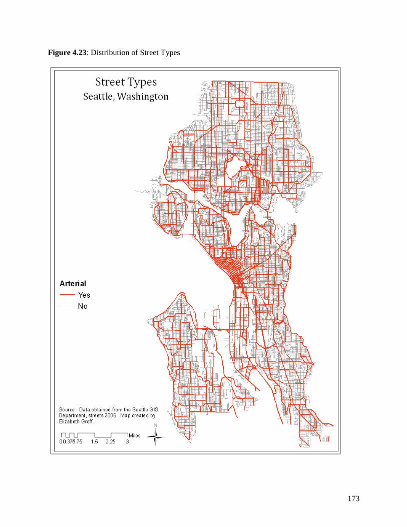
173

Figure 4.23: Distribution of Street Types


174

Bus Stops

The only place characteristic related to accessibility which changed over the study period

is the number of bus stops. Bus stops are used as a measure of public transportation

accessibility. Previous studies have examined crime near bus stops (Roman, 2005) while others

have used the presence of bus stops as part of a composite measure of ‘busy places’

(Brantingham & Brantingham, 1981 [1991]; Horton & Reynolds, 1971). Yet another study

focused on school bus stops and crime, finding that census blocks with higher numbers of school

bus stops are associated with higher crime (Golledge & Stimson, 1997; Rengert, 1988). These

studies have indicated that bus stops on a street segment contribute to ‘setting the stage’ for

criminal events.

The King County Metro agency serves Seattle as well as the rest of King County. We

focus just on bus service within the city of Seattle. The average number of bus stops across

streets in Seattle is 4,160 per year. The average number of streets with at least one bus stop is

3,026. About one third of those streets experienced a change in the number of bus stops over the

time period (some gained or lost service completely). The average density of bus stops was just

over three per mile, one every third of a mile.

While the number of bus stops has decreased slightly over the study period the number of

streets served by buses has remained essentially stable (see Figure 4.24). In addition, the

concentration of bus stops on streets is extremely high. Between 1997 and 2004, 50 percent of

the total bus stops were consistently found on about 4 percent of Seattle street segments. All of

the bus stops were located on between 12 and 13 percent of the total street segments, indicating a

fairly stable global trend over time.


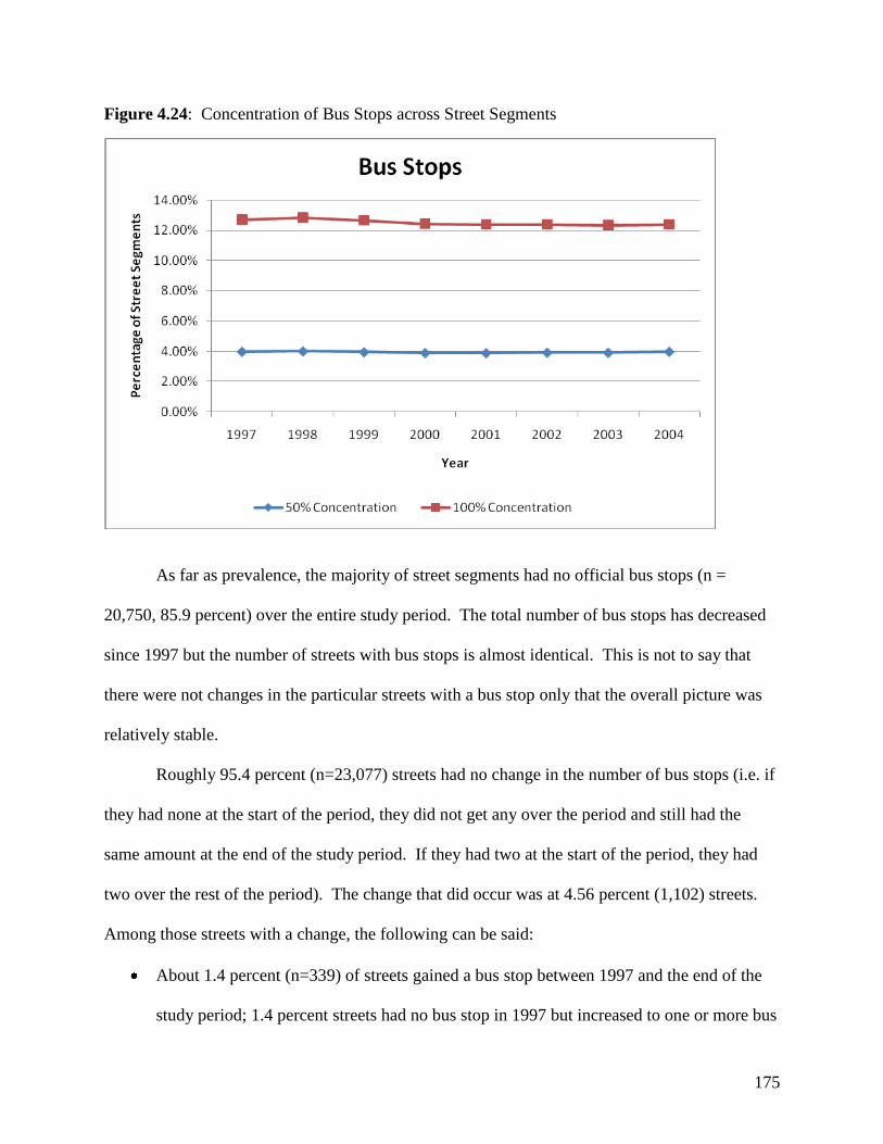
175

Figure 4.24: Concentration of Bus Stops across Street Segments

As far as prevalence, the majority of street segments had no official bus stops (n =

20,750, 85.9 percent) over the entire study period. The total number of bus stops has decreased

since 1997 but the number of streets with bus stops is almost identical. This is not to say that

there were not changes in the particular streets with a bus stop only that the overall picture was

relatively stable.

Roughly 95.4 percent (n=23,077) streets had no change in the number of bus stops (i.e. if

they had none at the start of the period, they did not get any over the period and still had the

same amount at the end of the study period. If they had two at the start of the period, they had

two over the rest of the period). The change that did occur was at 4.56 percent (1,102) streets.

Among those streets with a change, the following can be said:

About 1.4 percent (n=339) of streets gained a bus stop between 1997 and the end of the

study period; 1.4 percent streets had no bus stop in 1997 but increased to one or more bus


176

stops at some point in the study period (they went from absence to presence at some point

during study period – includes all years)

A few streets, just over 1.63 percent (n= 394) of streets, had a net increase in bus stops

over the period.

About 2.39 percent (n=578) of streets had a net decrease in bus stops over the period.

Even though the above description paints a stable picture across time, according to the

repeated measures analysis, the within subject effect is significant (F = 25.892, df = 2.906)

(meaning that the time effect is significant). The number of bus stops on each unit of analysis

does vary over time.

The spatial distribution of bus stops follows the major arteries with fewer stops in

neighborhoods. The geographic distribution of the street segments that account for 50 percent of

all bus stops is clustered along major arteries (see Figure 4.25).


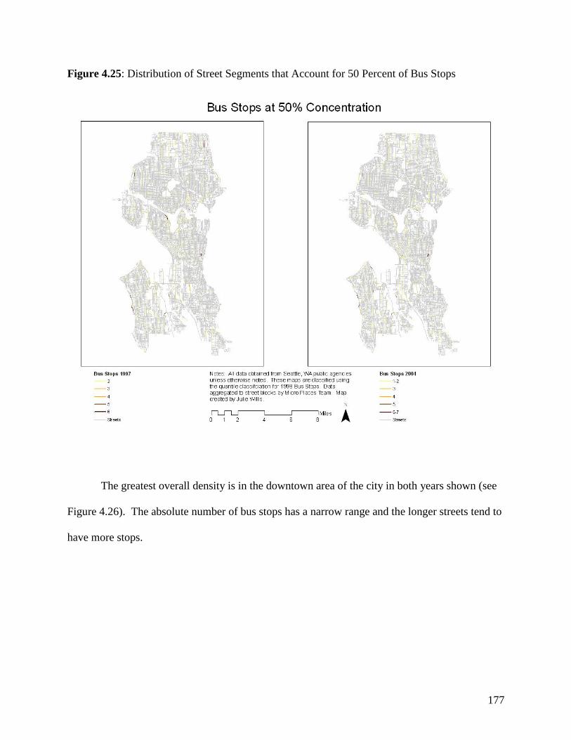
177

Figure 4.25: Distribution of Street Segments that Account for 50 Percent of Bus Stops

The greatest overall density is in the downtown area of the city in both years shown (see

Figure 4.26). The absolute number of bus stops has a narrow range and the longer streets tend to

have more stops.


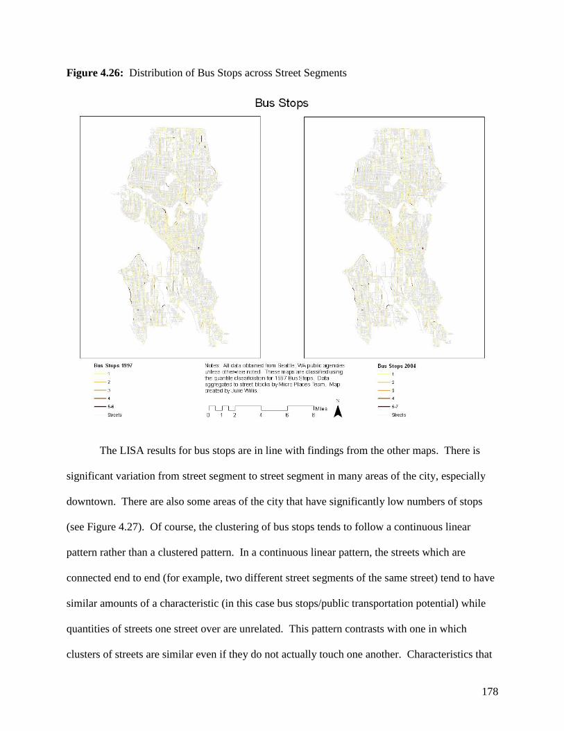
178

Figure 4.26: Distribution of Bus Stops across Street Segments

The LISA results for bus stops are in line with findings from the other maps. There is

significant variation from street segment to street segment in many areas of the city, especially

downtown. There are also some areas of the city that have significantly low numbers of stops

(see Figure 4.27). Of course, the clustering of bus stops tends to follow a continuous linear

pattern rather than a clustered pattern. In a continuous linear pattern, the streets which are

connected end to end (for example, two different street segments of the same street) tend to have

similar amounts of a characteristic (in this case bus stops/public transportation potential) while

quantities of streets one street over are unrelated. This pattern contrasts with one in which

clusters of streets are similar even if they do not actually touch one another. Characteristics that


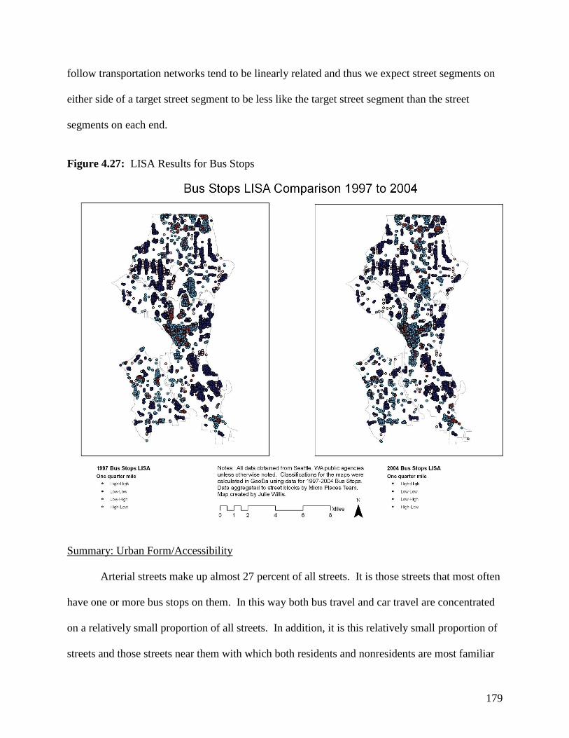
179

follow transportation networks tend to be linearly related and thus we expect street segments on

either side of a target street segment to be less like the target street segment than the street

segments on each end.

Figure 4.27: LISA Results for Bus Stops

Summary: Urban Form/Accessibility

Arterial streets make up almost 27 percent of all streets. It is those streets that most often

have one or more bus stops on them. In this way both bus travel and car travel are concentrated

on a relatively small proportion of all streets. In addition, it is this relatively small proportion of

streets and those streets near them with which both residents and nonresidents are most familiar


180

Guardianship

The following section addresses the concept of guardianship at a particular place.

Perception of the guardianship at a place is very important in offender decision making. In

places with high levels of informal social control both guardianship and perceived guardianship

are high. Factors related to guardianship are the visibility of targets and guardians and numbers

of capable guardians present. Capable guardians are represented by the total number of police

stations and fire station within one-quarter of a mile of a place. Percent vacant land use

represents the presence of a consistent hole in the fabric of informal social control on a street

segment (Rice & Smith, 2002). Vacant land is not typically a destination for legal activities and

it has no place managers at all; thus, it decreases the potential for informal social control. Two

facility-related characteristics linked to guardianship are also included in this section; police

stations and fire stations. By definition these facilities attract capable guardians in the form of

police officers and firefighters. This benefit does not stop at the facility but extends to the streets

which are used to arrive at and leave those stations. Finally, the amount of street lighting

captures the visibility at a place during evening hours. It has also been hypothesized to represent

the investment of a city in a place (Groff & LaVigne, 2001).

Percent Vacant Land Use

This characteristic is pulled from the parcel data for Seattle which has a land use code

that identifies parcels that are vacant. The category includes developable land that is currently

vacant (land uses such as cemeteries, parks, easements etc. are not included in this measure).

Previous research shows that at the street segment level, vacant/parking lots were

significantly related to increased auto theft (Taylor et al., 1995). When vacant lots were included

as part of an index of nonresidential properties, streets with more vacant land experienced more


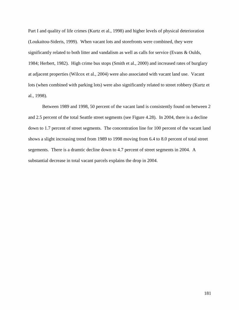
181

Part I and quality of life crimes (Kurtz et al., 1998) and higher levels of physical deterioration

(Loukaitou-Sideris, 1999). When vacant lots and storefronts were combined, they were

significantly related to both litter and vandalism as well as calls for service (Evans & Oulds,

1984; Herbert, 1982). High crime bus stops (Smith et al., 2000) and increased rates of burglary

at adjacent properties (Wilcox et al., 2004) were also associated with vacant land use. Vacant

lots (when combined with parking lots) were also significantly related to street robbery (Kurtz et

al., 1998).

Between 1989 and 1998, 50 percent of the vacant land is consistently found on between 2

and 2.5 percent of the total Seattle street segments (see Figure 4.28). In 2004, there is a decline

down to 1.7 percent of street segments. The concentration line for 100 percent of the vacant land

shows a slight increasing trend from 1989 to 1998 moving from 6.4 to 8.0 percent of total street

segements. There is a dramtic decline down to 4.7 percent of street segments in 2004. A

substantial decrease in total vacant parcels explains the drop in 2004.


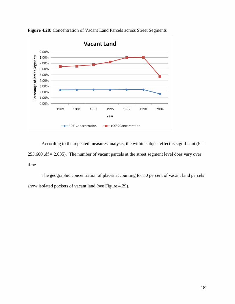
182

Figure 4.28: Concentration of Vacant Land Parcels across Street Segments

According to the repeated measures analysis, the within subject effect is significant (F =

253.600 ,df = 2.035). The number of vacant parcels at the street segment level does vary over

time.

The geographic concentration of places accounting for 50 percent of vacant land parcels

show isolated pockets of vacant land (see Figure 4.29).


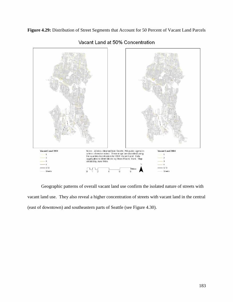
183

Figure 4.29: Distribution of Street Segments that Account for 50 Percent of Vacant Land Parcels

Geographic patterns of overall vacant land use confirm the isolated nature of streets with

vacant land use. They also reveal a higher concentration of streets with vacant land in the central

(east of downtown) and southeastern parts of Seattle (see Figure 4.30).


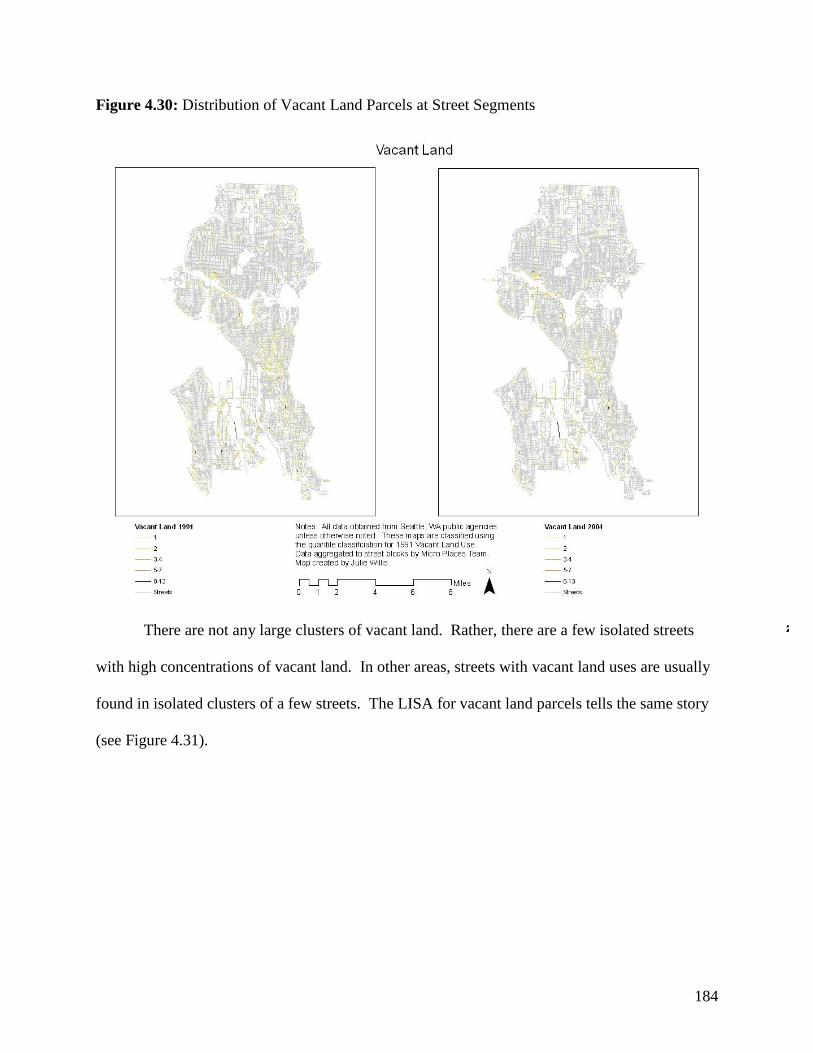
184

Figure 4.30: Distribution of Vacant Land Parcels at Street Segments

There are not any large clusters of vacant land. Rather, there are a few isolated streets

with high concentrations of vacant land. In other areas, streets with vacant land uses are usually

found in isolated clusters of a few streets. The LISA for vacant land parcels tells the same story

(see Figure 4.31).

1

991 2

004


185

Figure 4.31: LISA Results for Vacant Land Parcels across Street Segments

Police and Fire Stations

Together there were a total of 39 streets that had an emergency station on them during the

study period from 1989-2004. The number of emergency stations was very stable. For most of

the time period there were 37 stations (1989-2002). When one police station moved from one

location to another there were 36 active stations in 1999 and then 37 again in 2000. In 2003 a

new police station opened in southwest Seattle which brought the number up to 38 stations.

Like the fire stations alone, the joint distribution of police and fire stations is random in

all years up to about 4,100 feet (1999, 2000-2002 and 2003-2004) (see Figure 4.32). From 1989-

1998, the distribution is random up to just over a mile. Afterwards, both dispersed until about


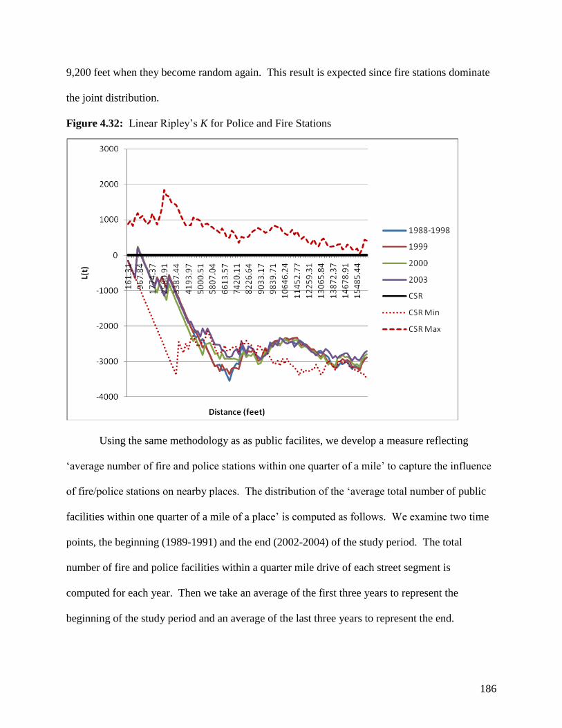
186

9,200 feet when they become random again. This result is expected since fire stations dominate

the joint distribution.

Figure 4.32: Linear Ripley’s K for Police and Fire Stations

Using the same methodology as as public facilites, we develop a measure reflecting

‘average number of fire and police stations within one quarter of a mile’ to capture the influence

of fire/police stations on nearby places. The distribution of the ‘average total number of public

facilities within one quarter of a mile of a place’ is computed as follows. We examine two time

points, the beginning (1989-1991) and the end (2002-2004) of the study period. The total

number of fire and police facilities within a quarter mile drive of each street segment is

computed for each year. Then we take an average of the first three years to represent the

beginning of the study period and an average of the last three years to represent the end.


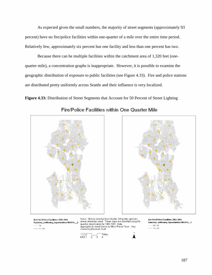
187

As expected given the small numbers, the majority of street segments (approximately 93

percent) have no fire/police facilities within one-quarter of a mile over the entire time period.

Relatively few, approximately six percent has one facility and less than one percent has two.

Because there can be multiple facilities within the catchment area of 1,320 feet (one-

quarter mile), a concentration graphs is inappropriate. However, it is possible to examine the

geographic distribution of exposure to public facilities (see Figure 4.33). Fire and police stations

are distributed pretty uniformly across Seattle and their influence is very localized.

Figure 4.33: Distribution of Street Segments that Account for 50 Percent of Street Lighting


188

Street Lighting

Street lighting is measured using total number of watts. This information is calculated

using a multistep process. First, we locate all the light poles along the streets included in the

study. Information from the Seattle Public Utility is then used to identify the number and

illumination of each light on a pole. Second, the total amount of light being provided by each

pole is summed. Third, all the poles on each street are summarized to arrive at the total light (in

watts) on a street segment. This multi-step procedure enables us to examine the amount of street

lighting on each street.

As mentioned above, the amount of street lighting has been shown to be related to crime

levels. One study found eight of the ten highest crime bus stops lacked adequate street lighting

and were within 300 feet of liquor outlets/bars (Loukaitou-Sideris, 1999). Another demonstrated

gas drive-offs could be reduced by as much as 65 percent with increased lighting at convenience

stores (LaVigne, 1994). British studies find that increased street lighting decreases crime

(Painter & Farrington, 1997, 1999). An early review of the literature concluded that targeted

increases in street lighting were more effective than general ones and that improved lighting

decreases fear of crime (Pease, 1999). A more recent meta-analysis of street lighting and crime

found a reduction in crime when lighting is increased (Farrington & Welsh, 2002).

Looking at the city as a whole, between 1997 and 2004, 50 percent of the total street

lighting was consistently found on between 11.5 and 13 percent of Seattle street segments (see

Figure 4.34). All of the street lighting was located on between 84 and 87 percent of the total

street segments. Both trend lines are fairly stable over time. This follows the pattern of extreme

concentration at relatively few places but widespread presence across most places. Between 13

and 16 percent of streets have no lighting in any given year.


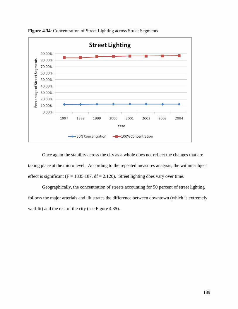
189

Figure 4.34: Concentration of Street Lighting across Street Segments

Once again the stability across the city as a whole does not reflect the changes that are

taking place at the micro level. According to the repeated measures analysis, the within subject

effect is significant (F = 1835.187, df = 2.120). Street lighting does vary over time.

Geographically, the concentration of streets accounting for 50 percent of street lighting

follows the major arterials and illustrates the difference between downtown (which is extremely

well-lit) and the rest of the city (see Figure 4.35).


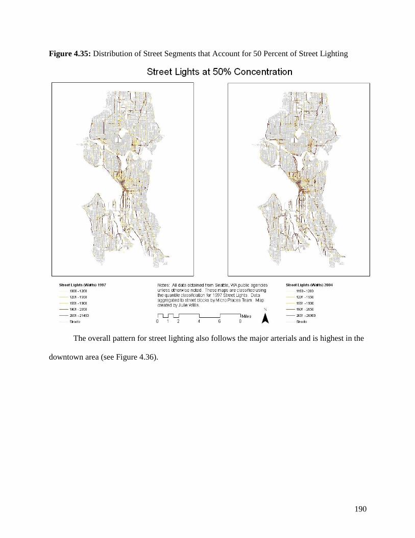
190

Figure 4.35: Distribution of Street Segments that Account for 50 Percent of Street Lighting

The overall pattern for street lighting also follows the major arterials and is highest in the

downtown area (see Figure 4.36).


191

Figure 4.36: Distribution of Street Lighting

At the local level, streets with high levels of street lighting are interspersed with streets

that have lower levels of street lighting (see Figure 4.37). Once again, and not surprisingly, the

pattern appears to be linear.


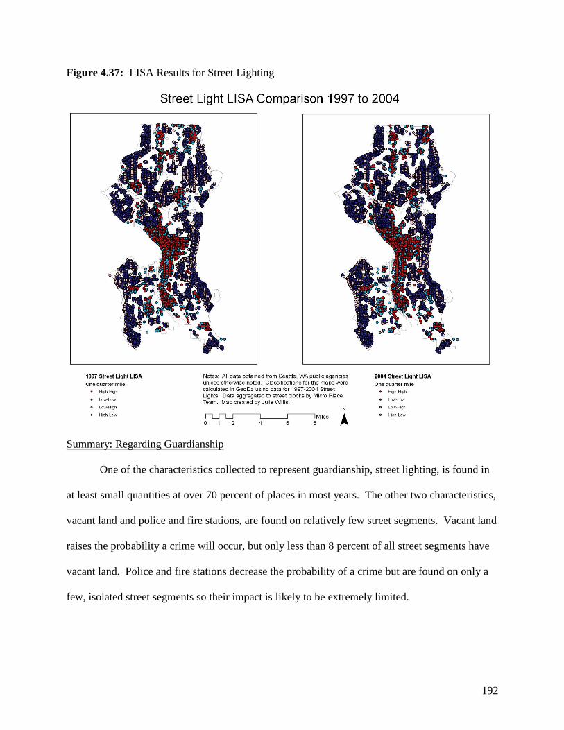
192

Figure 4.37: LISA Results for Street Lighting

Summary: Regarding Guardianship

One of the characteristics collected to represent guardianship, street lighting, is found in

at least small quantities at over 70 percent of places in most years. The other two characteristics,

vacant land and police and fire stations, are found on relatively few street segments. Vacant land

raises the probability a crime will occur, but only less than 8 percent of all street segments have

vacant land. Police and fire stations decrease the probability of a crime but are found on only a

few, isolated street segments so their impact is likely to be extremely limited.


193

Discussion of Opportunity Variables

This chapter focused on the opportunity-related concepts of motivated offenders, suitable

targets, accessibility/urban form and guardianship. We explored the spatio-temporal distribution

of variables representing each of those theoretical concepts across places. This section

summarizes the results of that exploration.

The overwhelming finding is one of concentration at specific places. Motivated

offenders (operationalized as high risk juveniles) are concentrated on individual segments and in

specific areas of the city. With the exception of residential population, which tends to be

widespread, suitable target variables are also very concentrated, most often on major roads. The

characteristic of accessibility is also concentrated in a particular set of places involving major

roads. Finally, guardianship is a mixed bag. Street segments with vacant land and emergency

stations are dispersed and isolated representing distributed concentration. In contrast, street

lighting is found in at least small quantities at over 70 percent of places.

Another finding is one of temporal stability. The relative distribution of opportunity-

related characteristics across places is stable. Although there is significant change from year to

year on specific street segments, the overall pattern of relationships among those street segments

changes little over the study period. Another way of saying this is that change tends to be local

rather than global.

Finally, there is a significant amount of negative spatial autocorrelation evident for all

variables. In other words, the amount of a variable on one street segment is significantly

different from the amount on street segments within a quarter mile (in Seattle that is about three

street segments). This result reveals a great deal of street segment to street segment variation in

a characteristic that is occurring at the sub-neighborhood level of analysis. There are also large


194

areas of the city where street segments have similar amounts of a characteristic. However, even

these relatively homogenous areas have street segments on the opposite end of the spectrum

interspersed (e.g., high amounts in areas where most street segments have low amounts of the

characteristic or vice versa).

In sum, the opportunity characteristics of street segments exhibit spatial and temporal

characteristics that are very similar to the spatial and temporal characteristics of crime. This

finding lends greater credence to their inclusion in the risk analysis and multivariate analyses that

are discussed in the following chapters.


195

Chapter 5: The Distribution of Crime at

Street Segments

In the previous chapters we focused on the distribution of variables that have been

identified by criminologists as important in understanding the development of crime across space

and time. Though prior studies have generally not been able to examine these characteristics at

the very micro level that is the focus of our research, we have seen that even at the street block

level there is important variability in these characteristics. Many are concentrated at a relatively

small number of street segments that are in some sense ―hot spots‖ for such characteristics.

Often, there is strong street to street variability in the prevalence or frequency of such factors.

And we have also documented important variability across time.

The question we ask in this chapter is whether there is also concentration of crime in hot

spots, and whether there is stability or variability in crime at street segments across time. As we

noted in our introductory chapter, there is strong evidence from prior studies that crime is

concentrated at small units of geography. Our initial question in this chapter is whether we

identify such concentrations when we examine crime using the street block unit of analysis we

describe in Chapter 2. We then examine whether the concentration of crime at place is

consistent year to year in an urban setting.

A related question that has generally not been examined in earlier studies (for exceptions

see Weisburd et al., 2004; Weisburd et al., in press), primarily because of the restricted periods

that have been examined, is whether specific places evidence consistent or variable trends over

time. For example, many studies have noted that crime is concentrated at a small number of

places and that this provides important opportunities for focusing crime prevention resources

more efficiently (Sherman et al. 1989; Weisburd et al., 2004; Weisburd et al., in press). But are


196

such crime concentrations stable at particular places, or are there developmental trends of crime

at street segments, as there are among individuals (Farrington, 2003; LeBlanc & Loeber, 1998;

Moffitt, 1993; Wolfgang et al., 1972; Weisburd et al., 2004)? To examine this question, we use

an approach that has become common in the examination of patterns of human development. It

is now well established that different types of people evidence different trajectories or

development trends across the life course (Elder, 1998; Laub et al., 1998; Loeber & Hay, 1997;

Nagin & Land, 1993; Nagin et al., 1995). Some are chronic offenders, while some have

intermittent experiences with criminality. Importantly, even many chronic offenders appear to

―age out of crime.‖ Is this also true of the developmental patterns of crime at places over time?

Do chronic crime places naturally experience reduced levels of offending across time? Or is

there greater stability in the developmental patterns of places?

Is Crime Concentrated at Street Segments?

Our first question is simply whether our data confirm prior studies that suggest that crime

is very strongly concentrated at crime hot spots. Certainly, our data suggest that there are many

places that are free of crime. About 2,218 street segments out of 24,023 we examined over a 16

year period had no incident reports at all. The mean number of incidents per segment per year

that had any crime was approximately 4.42 (sd = 14.14). It is also important to note that crime

trends in Seattle overall followed the national pattern (see Blumstein & Wallman, 2000),

experiencing a decline in incident reports at least since 1992 (see Figure 5.1). Between 1989 and

2004, Seattle street segments saw a 23.4 percent decline (from 121,869 in 1989 to 93,324 in

2004) in the number of incidents recorded. We return to this finding in more detail at the end of

the chapter, when we examine developmental trends of street segments.


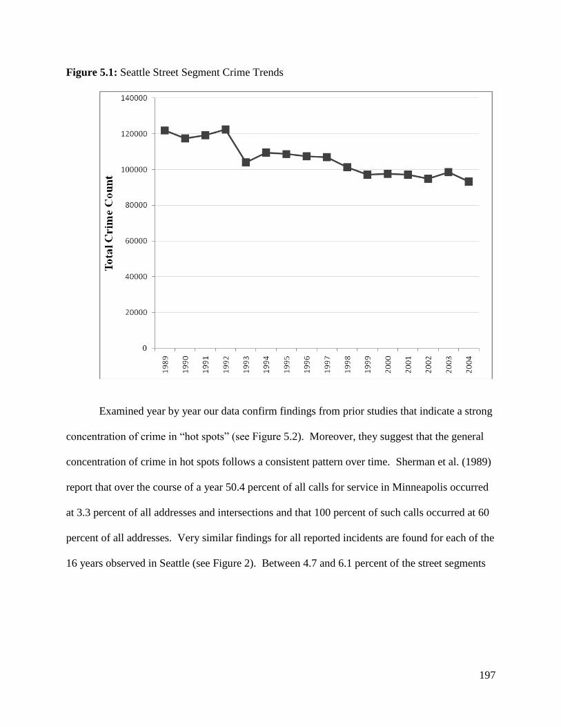
197

Figure 5.1: Seattle Street Segment Crime Trends

Examined year by year our data confirm findings from prior studies that indicate a strong

concentration of crime in ―hot spots‖ (see Figure 5.2). Moreover, they suggest that the general

concentration of crime in hot spots follows a consistent pattern over time. Sherman et al. (1989)

report that over the course of a year 50.4 percent of all calls for service in Minneapolis occurred

at 3.3 percent of all addresses and intersections and that 100 percent of such calls occurred at 60

percent of all addresses. Very similar findings for all reported incidents are found for each of the

16 years observed in Seattle (see Figure 2). Between 4.7 and 6.1 percent of the street segments


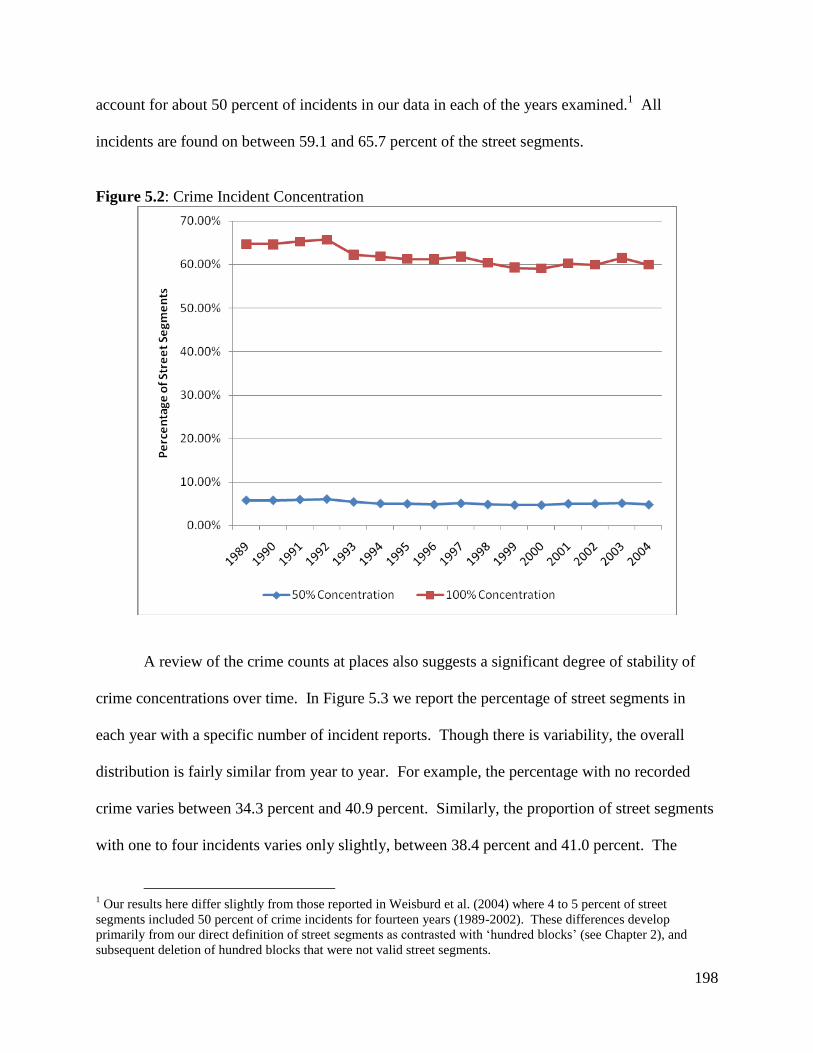
198

account for about 50 percent of incidents in our data in each of the years examined.1 All

incidents are found on between 59.1 and 65.7 percent of the street segments.

Figure 5.2: Crime Incident Concentration

A review of the crime counts at places also suggests a significant degree of stability of

crime concentrations over time. In Figure 5.3 we report the percentage of street segments in

each year with a specific number of incident reports. Though there is variability, the overall

distribution is fairly similar from year to year. For example, the percentage with no recorded

crime varies between 34.3 percent and 40.9 percent. Similarly, the proportion of street segments

with one to four incidents varies only slightly, between 38.4 percent and 41.0 percent. The

1 Our results here differ slightly from those reported in Weisburd et al. (2004) where 4 to 5 percent of street

segments included 50 percent of crime incidents for fourteen years (1989-2002). These differences develop

primarily from our direct definition of street segments as contrasted with ‗hundred blocks‘ (see Chapter 2), and

subsequent deletion of hundred blocks that were not valid street segments.


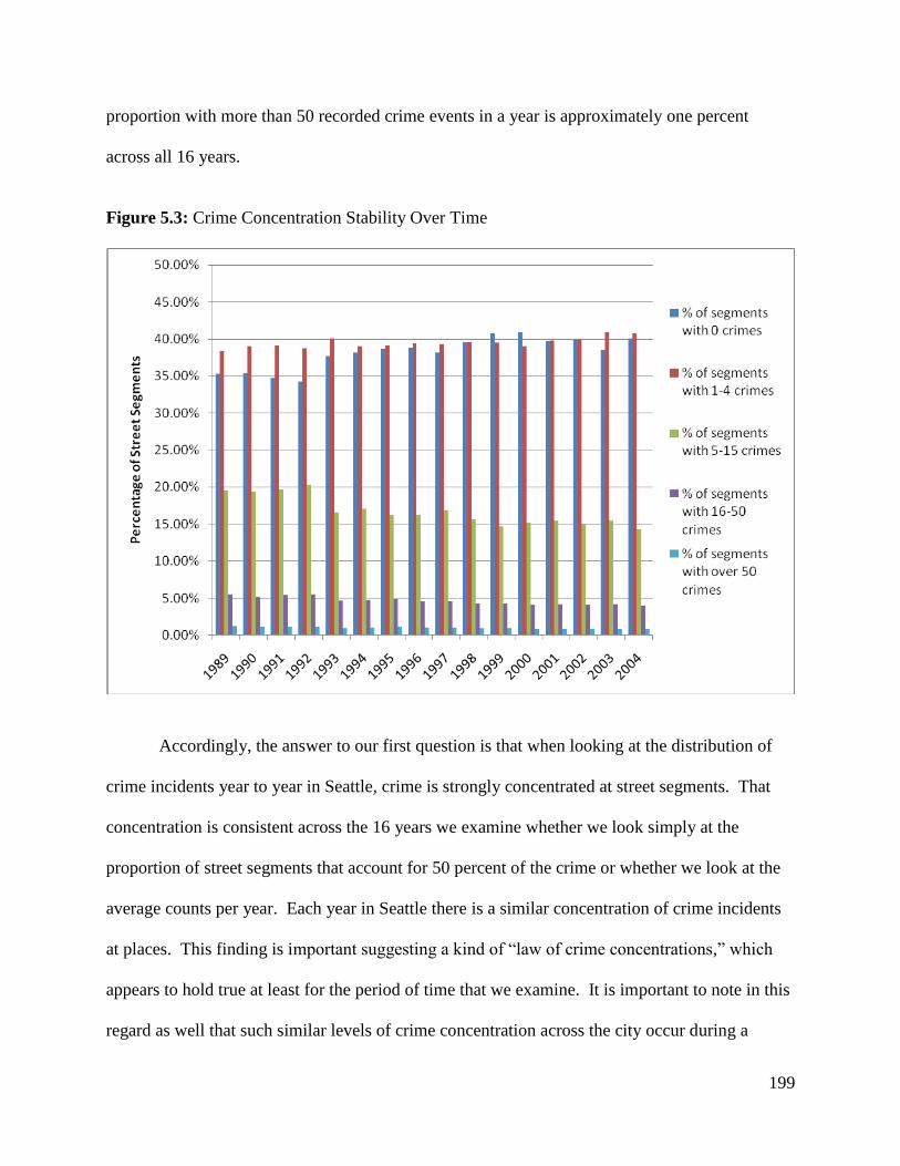
199

proportion with more than 50 recorded crime events in a year is approximately one percent

across all 16 years.

Figure 5.3: Crime Concentration Stability Over Time

Accordingly, the answer to our first question is that when looking at the distribution of

crime incidents year to year in Seattle, crime is strongly concentrated at street segments. That

concentration is consistent across the 16 years we examine whether we look simply at the

proportion of street segments that account for 50 percent of the crime or whether we look at the

average counts per year. Each year in Seattle there is a similar concentration of crime incidents

at places. This finding is important suggesting a kind of ―law of crime concentrations,‖ which

appears to hold true at least for the period of time that we examine. It is important to note in this

regard as well that such similar levels of crime concentration across the city occur during a


200

period of a substantial crime decline. While the overall number of crimes declines, the relative

concentration at crime hot spots remains similar.

Developmental Patterns of Crime at Place

Though the proportions of street segments with specific thresholds of crime activity

remain fairly consistent year to year, it may be that the specific segments within each of these

thresholds change. Accordingly, it is important to identify not only the general patterns over

time but also how each of the 24,023 street segments‘ crime frequencies changed. This

descriptive exercise on the aggregate data leads to two key questions. First, is the stability

evidenced in our simple descriptive analysis of the proportion of places with a specific threshold

of crime in a specific year replicated if we examine the developmental patterns of offending of

places over time? Second, are there different patterns of crime over time for different groups of

street segments?

Trajectory Analysis

We are unaware of any available technique in use in the criminology of place that would

allow us to answer these questions, but such a technique—group-based trajectory analysis—has

been used in developmental social science more broadly (Nagin, 1999, 2005; Nagin & Land,

1993). This technique and related complementary growth curve techniques, such as hierarchical

linear modeling (Bryk & Raudenbush, 1987, 1992; Goldstein, 1995) and latent curve analysis

(McArdle & Epstein, 1987; Meredith & Tisak, 1990; Muthén, 1989; Willett & Sayer, 1994) are

designed to allow developmental researchers in the social sciences to measure and explain

differences across population members as they follow their developmental path.2 The need for

such techniques arose in the 1980s as psychologists, sociologists and criminologists all began to

2 For an overview of these methods, see Raudenbush (2001), Muthén (2001), or Nagin (1999, 2005).


201

turn to the study of developmental processes rather than to static events or states (see Bushway et

al., 2001; Hagan & Palloni, 1988; Laub et al., 1998; Loeber & LeBlanc, 1990; Moffitt, 1993).

The group-based trajectory model, first described by Nagin and Land (1993) and further

elaborated by Nagin (1999, 2005), is specifically designed to identify clusters of individuals with

similar developmental trajectories, and it has been utilized extensively to study patterns of

change in offending and aggression as people age (see Nagin, 1999; Nagin & Tremblay, 1999).

As such, we believe it is particularly well suited to our goal of exploring the patterns of change

in the Seattle data.

Formally, the model specifies that the population is approximated by a finite number of

groups of individuals who follow distinctive developmental trajectories. Each such group is

allowed to have its own offending trajectory (a map of offending rates throughout the time

period) described by a distinct set of parameters that are permitted to vary freely across groups.

This type of model has three key outputs: the parameters describing the trajectory for each group,

the estimated proportion of the population belonging to each group, and the posterior probability

of belonging to a given group for each individual in the sample. The posterior probability, which

is the probability of group membership after the model is estimated, can be used to assign

individuals to a group based on their highest probability.3

This approach is less efficient than linear growth models but allows the estimation of

qualitatively different patterns of behavior over time. There is broad agreement that delinquency

and crime are cases where this group-based trajectory approach might be justified, in large part

3 The group-based trajectory is often identified with typological theories of offending such as Moffitt (1993) because

of its use of groups (see Nagin et al., 1995). But it is important to keep in mind that group assignments are made

with error. In all likelihood, the groups only approximate a continuous distribution. The lack of homogeneity in the

groups is the explicit trade off for the relaxation of the parametric assumptions about the random effects in the linear

models (Bushway et al., 2003). For a different perspective on this issue, see Eggleston et al. (2004). Furthermore,

Bushway et al. (2009) found that both group-based trajectory analysis and growth curve modeling identify very

similar average developmental patterns of criminality.


202

because not everyone participates in crime, and people appear to start and stop at very different

ages (Muthén, 2001; Nagin, 1999, 2005; Raudenbush, 2001). Given that we have no strong

expectation about the basic pattern of change, the group-based trajectory approach appears to be

a good choice for identifying major patterns of change in our data set.4

There are two software packages available that can estimate group-based trajectories:

Mplus, a proprietary software package, and Proc Traj, a special procedure for use in SAS, made

available at no cost by the National Consortium on Violence Research (for a detailed discussion

of Proc Traj, see Jones et al., 2001).5 In using Proc Traj, we had three choices when estimating

trajectories of count data: parametric form (Poisson vs. normal vs. logit), functional form of the

trajectory over time (linear vs. quadratic vs. cubic), and number of groups.

The Poisson distribution is a standard distribution used to estimate the frequency

distribution of offending that we would expect given a certain unobserved offending rate

(Lehoczky, 1986; Maltz, 1996; Osgood, 2000).6 We found that the quadratic was uniformly a

better fit than the linear model, and that the cubic model did not improve the fit over the

quadratic in the case of a small number of groups. In choosing the number of groups we relied

upon the Bayesian Information Criteria (BIC) because conventional likelihood ratio tests are not

appropriate for defining whether the addition of a group improves the explanatory power of the

model (D‘Unger et al., 1998). BIC = log(L) – 0.5*log(n)*(k); where ―L‖ is the value of the

4 Those interested in a more detailed description of the group-based trajectory approach should see Nagin (1999) or

Nagin (2005). 5 The procedure, with documentation, is available at www.ncovr.heinz.cmu.edu.

6 Proc Traj also provides the option of estimating a zero inflated Poisson (ZIP) model. The ZIP model builds on a

Poisson by accommodating more non-offenders in any given period than predicted by the standard Poisson

distribution. The zero-inflation parameter can be allowed to vary over time, but cannot be estimated separately for

each group. It is sometimes called an intermittency parameter, since it allows places to have ―temporary‖ spells of

no offenses without recording a change in their overall rate of offending. In this context, the ZIP model‘s

differentiation between short-term and long-term change is problematic. The Poisson model, on the other hand,

tracks movement in the rate of offending in one parameter, allowing all relatively long-term changes to be reflected

in one place. We believe this trait of the Poisson model makes it the better model for modeling trends, especially

over relatively short panels, even though the ZIP model provides a better fit according to the BIC criteria used for

model selection. For a similar argument see Bushway et al. (2003).


http://www.ncovr.heinz.cmu.edu/

203

model‘s maximized likelihood estimates, ―n‖ is the sample size, and ―k‖ is the number of

parameters estimated in a given model. Because more sophisticated models almost always

improve the fit of a given analysis, the BIC encourages a parsimonious solution by penalizing

models that increase the number of trajectories unless they substantially improve fit. In addition

to the BIC, trajectory analysis requires that researchers also consider theoretical guidance,

posterior probabilities of trajectory assignments, odds of correct classification, estimated group

probabilities, and whether meaningful groups are revealed (for a more detailed discussion, see

Nagin, 2005).

These models are highly complex, and researchers run the risk of arriving at a local

maximum, or peak in the likelihood function, which represents a sub-optimal solution. The

stability of the answer when providing multiple sets of starting values should be considered in

any model choice (McLachlan & Peel, 2000). In the final analysis, the utility of the groups is

determined by their ability to identify distinct trajectories, the number of units in each group, and

their relative homogeneity (Nagin, 2005).

We began our modeling exercise by fitting the data to three trajectories. We then fit the

data to four trajectories and compared this fit with the three-group solution. When the four-

group model proved better than the three-group, we then estimated the five-group model and

compared it to the four-group solution. We continued adding groups, each time finding an

improved BIC, until we arrived at 24 groups. Models for 23 and 24 groups were not stable and

could not be replicated consistently. After reviewing the Bayesian Information Criteria and the

patterns observed in each solution, it was determined that a 22 group model was the most

optimal model for the crime data. We therefore chose the 22 group model.


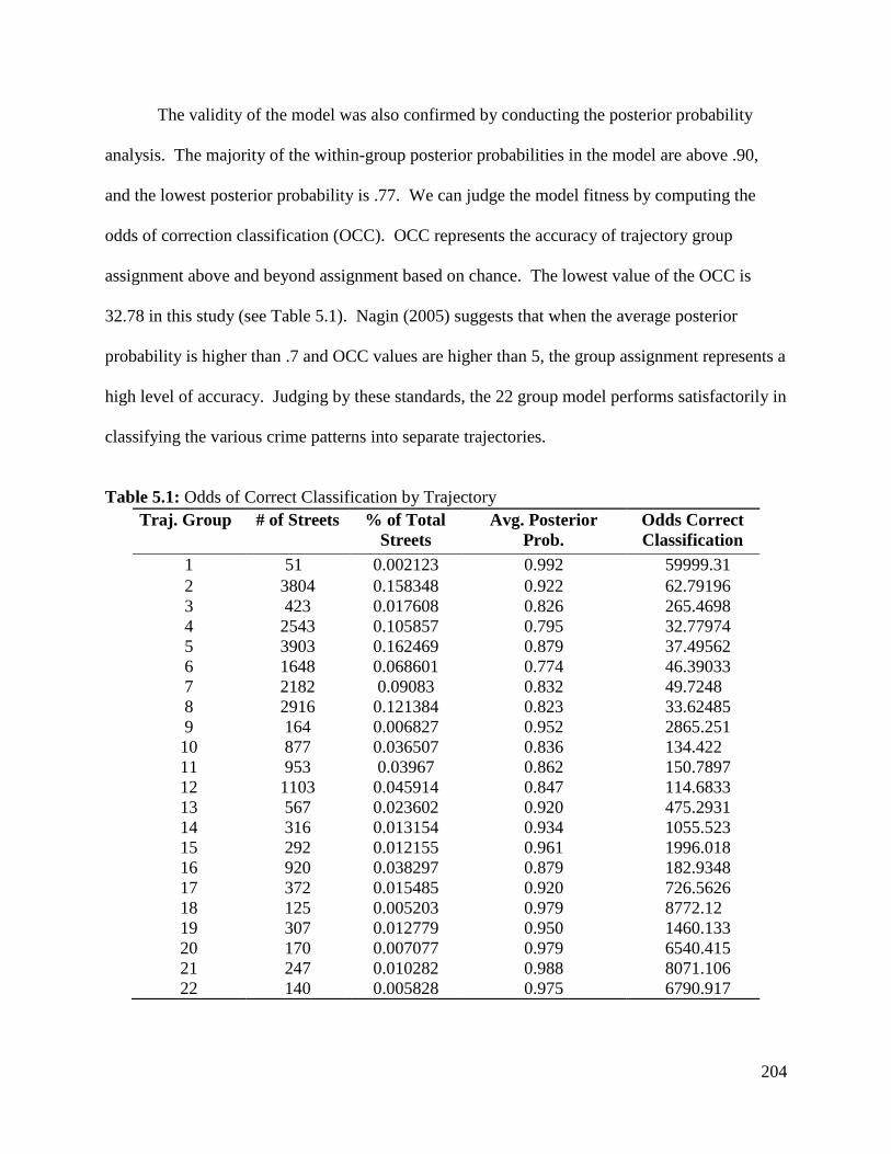
204

The validity of the model was also confirmed by conducting the posterior probability

analysis. The majority of the within-group posterior probabilities in the model are above .90,

and the lowest posterior probability is .77. We can judge the model fitness by computing the

odds of correction classification (OCC). OCC represents the accuracy of trajectory group

assignment above and beyond assignment based on chance. The lowest value of the OCC is

32.78 in this study (see Table 5.1). Nagin (2005) suggests that when the average posterior

probability is higher than .7 and OCC values are higher than 5, the group assignment represents a

high level of accuracy. Judging by these standards, the 22 group model performs satisfactorily in

classifying the various crime patterns into separate trajectories.

Table 5.1: Odds of Correct Classification by Trajectory

Traj. Group # of Streets % of Total

Streets

Avg. Posterior

Prob.

Odds Correct

Classification

1 51 0.002123 0.992 59999.31

2 3804 0.158348 0.922 62.79196

3 423 0.017608 0.826 265.4698

4 2543 0.105857 0.795 32.77974

5 3903 0.162469 0.879 37.49562

6 1648 0.068601 0.774 46.39033

7 2182 0.09083 0.832 49.7248

8 2916 0.121384 0.823 33.62485

9 164 0.006827 0.952 2865.251

10 877 0.036507 0.836 134.422

11 953 0.03967 0.862 150.7897

12 1103 0.045914 0.847 114.6833

13 567 0.023602 0.920 475.2931

14 316 0.013154 0.934 1055.523

15 292 0.012155 0.961 1996.018

16 920 0.038297 0.879 182.9348

17 372 0.015485 0.920 726.5626

18 125 0.005203 0.979 8772.12

19 307 0.012779 0.950 1460.133

20 170 0.007077 0.979 6540.415

21 247 0.010282 0.988 8071.106

22 140 0.005828 0.975 6790.917


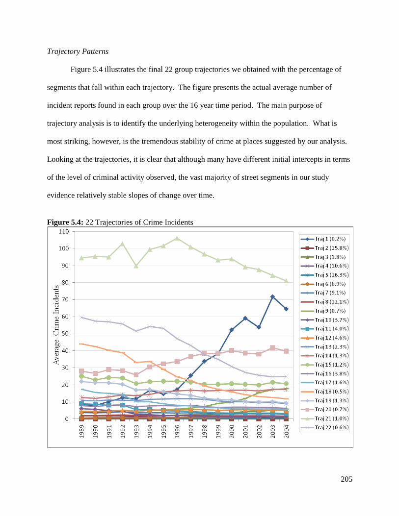
205

Trajectory Patterns

Figure 5.4 illustrates the final 22 group trajectories we obtained with the percentage of

segments that fall within each trajectory. The figure presents the actual average number of

incident reports found in each group over the 16 year time period. The main purpose of

trajectory analysis is to identify the underlying heterogeneity within the population. What is

most striking, however, is the tremendous stability of crime at places suggested by our analysis.

Looking at the trajectories, it is clear that although many have different initial intercepts in terms

of the level of criminal activity observed, the vast majority of street segments in our study

evidence relatively stable slopes of change over time.

Figure 5.4: 22 Trajectories of Crime Incidents


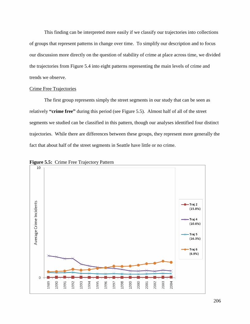
206

This finding can be interpreted more easily if we classify our trajectories into collections

of groups that represent patterns in change over time. To simplify our description and to focus

our discussion more directly on the question of stability of crime at place across time, we divided

the trajectories from Figure 5.4 into eight patterns representing the main levels of crime and

trends we observe.

Crime Free Trajectories

The first group represents simply the street segments in our study that can be seen as

relatively “crime free” during this period (see Figure 5.5). Almost half of all of the street

segments we studied can be classified in this pattern, though our analyses identified four distinct

trajectories. While there are differences between these groups, they represent more generally the

fact that about half of the street segments in Seattle have little or no crime.

Figure 5.5: Crime Free Trajectory Pattern


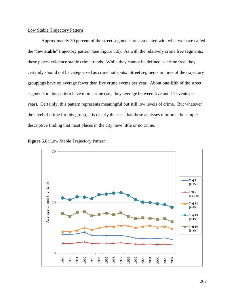
207

Low Stable Trajectory Pattern

Approximately 30 percent of the street segments are associated with what we have called

the ―low stable‖ trajectory pattern (see Figure 5.6). As with the relatively crime free segments,

these places evidence stable crime trends. While they cannot be defined as crime free, they

certainly should not be categorized as crime hot spots. Street segments in three of the trajectory

groupings have on average fewer than five crime events per year. About one-fifth of the street

segments in this pattern have more crime (i.e., they average between five and 11 events per

year). Certainly, this pattern represents meaningful but still low levels of crime. But whatever

the level of crime for this group, it is clearly the case that these analyses reinforce the simple

descriptive finding that most places in the city have little or no crime.

Figure 5.6: Low Stable Trajectory Pattern


208

Moderate Stable and Chronic Trajectory Patterns

Two other trajectory patterns represent places with much more serious crime problems,

though they also evidence strong stability in trends over time. What we term the ―moderate

stable‖ trajectory pattern includes about 1.2 percent of the street segments (see Figure 5.7).

These street segments average around 20 crime incidents throughout the study period. What we

term the ―chronic‖ group can be defined as the most serious crime hot spots in the city (see

Figure 5.8). The average number of crimes per segment is consistently more than 80 crime

incidents per year. Though only one percent of the street segments are found in this group, it is

important to note that this means that there are 247 street segments in the city with this very high

level of crime activity throughout the study period. These 247 street segments account for fully

21.96 percent of the crime incidents in Seattle between 1989 and 2004. While there is evidence

of a crime decline in the chronic street segments, the decline is modest (about 14%). Moreover,

despite a modest decline over time, these street segments remain by far the highest rate hot spots

throughout the study of period.

Of course, an especially important substantive and policy concern here is whether such

crime hot spots are concentrated in specific places in the city comprising bad areas or bad

neighborhoods. We examine this concern directly in the next chapter, though we think it

important to note here that we will illustrate surprising diffusion of crime trajectories of similar

types throughout the city.


209

Figure 5.7: Moderate Stable Trajectory Group

Figure 5.8: Chronic Trajectory Group


210

Increasing and Decreasing Trends in Crime Trajectories

The trajectory patterns we have described so far all represent relatively stable crime

trends. This, as we noted earlier, is a very important finding of our research. More than 80

percent of the street segments in Seattle can be seen as part of stable trajectory groups. Despite

the crime decline we noted earlier for Seattle more generally, for these street segments, little

changed in terms of crime in the 16 year study period. During the ―crime drop‖ in Seattle most

places remained basically the same in terms of crime levels. While this does not mean that

people living in these places did not benefit from the crime decline in their experiences

throughout the city, it does suggest that even major changes in crime in a city are concentrated at

specific places. It is in this sense misleading to speak of a crime drop across the city. Our

findings below further reinforce this approach to understanding crime trends.

The four remaining trajectory patterns include only about one in five street segments in

the city. But nonetheless, they represent interesting trends that help us not only to understand the

overall crime decline in Seattle, but also to recognize that crime trends at very micro levels of

geography are more complex than overall city trends would suggest. Two of the trajectory

patterns evidence decreasing crime trends during this period. The ―low rate decreasing‖ pattern

includes three trajectories (see Figure 5.9) that account for almost 10 percent of the street

segments in the city. The three trends are very similar, though the groups differ substantially on

the levels of crime they have in 1989. Street segments in trajectory group 17 began with an

average of almost 18 crime incidents. Street segments in trajectory group 10 began with only

about 8 crime incidents per street segment. Importantly, by the end of the study period each of

these groups had declined to less than half of the crime averages evidenced at the outset.


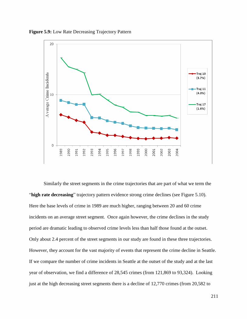
211

Figure 5.9: Low Rate Decreasing Trajectory Pattern

Similarly the street segments in the crime trajectories that are part of what we term the

―high rate decreasing‖ trajectory pattern evidence strong crime declines (see Figure 5.10).

Here the base levels of crime in 1989 are much higher, ranging between 20 and 60 crime

incidents on an average street segment. Once again however, the crime declines in the study

period are dramatic leading to observed crime levels less than half those found at the outset.

Only about 2.4 percent of the street segments in our study are found in these three trajectories.

However, they account for the vast majority of events that represent the crime decline in Seattle.

If we compare the number of crime incidents in Seattle at the outset of the study and at the last

year of observation, we find a difference of 28,545 crimes (from 121,869 to 93,324). Looking

just at the high decreasing street segments there is a decline of 12,770 crimes (from 20,582 to


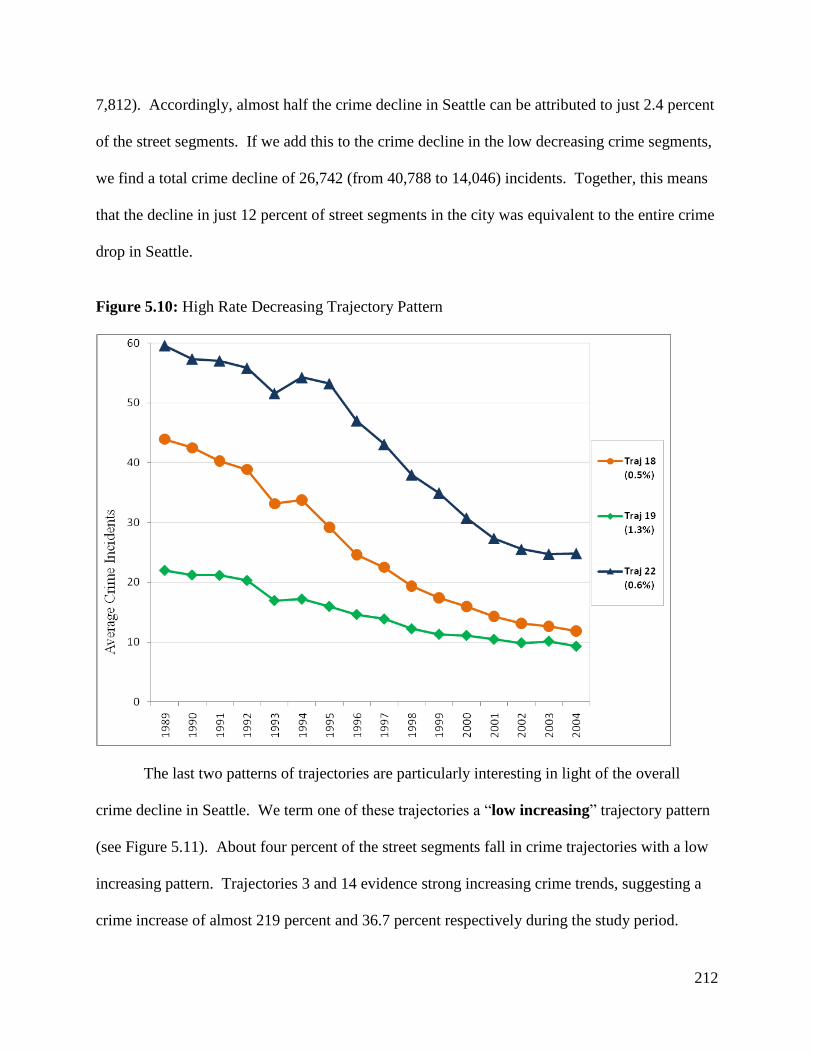
212

7,812). Accordingly, almost half the crime decline in Seattle can be attributed to just 2.4 percent

of the street segments. If we add this to the crime decline in the low decreasing crime segments,

we find a total crime decline of 26,742 (from 40,788 to 14,046) incidents. Together, this means

that the decline in just 12 percent of street segments in the city was equivalent to the entire crime

drop in Seattle.

Figure 5.10: High Rate Decreasing Trajectory Pattern

The last two patterns of trajectories are particularly interesting in light of the overall

crime decline in Seattle. We term one of these trajectories a ―low increasing‖ trajectory pattern

(see Figure 5.11). About four percent of the street segments fall in crime trajectories with a low

increasing pattern. Trajectories 3 and 14 evidence strong increasing crime trends, suggesting a

crime increase of almost 219 percent and 36.7 percent respectively during the study period.


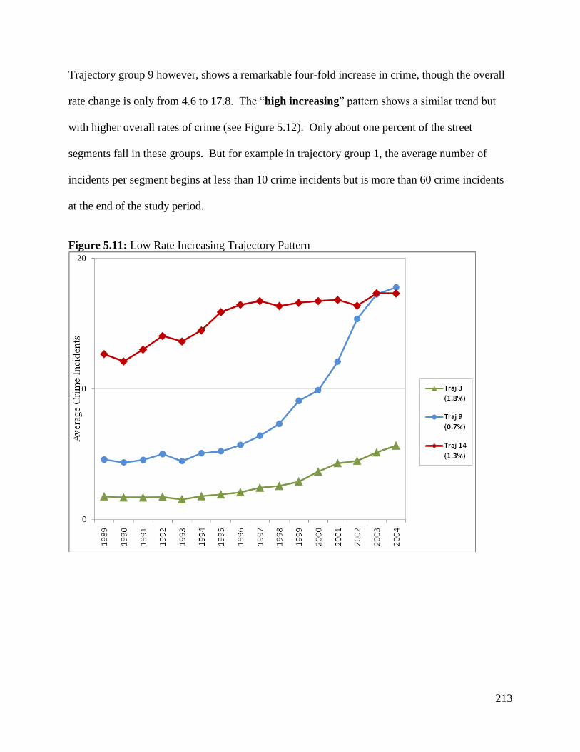
213

Trajectory group 9 however, shows a remarkable four-fold increase in crime, though the overall

rate change is only from 4.6 to 17.8. The ―high increasing‖ pattern shows a similar trend but

with higher overall rates of crime (see Figure 5.12). Only about one percent of the street

segments fall in these groups. But for example in trajectory group 1, the average number of

incidents per segment begins at less than 10 crime incidents but is more than 60 crime incidents

at the end of the study period.

Figure 5.11: Low Rate Increasing Trajectory Pattern


214

Figure 5.12: High Rate Increasing Trajectory Pattern

Street segments in these two groups evidence an increase in crime of almost 93.4%

during the study period (from 5,192 to 10,041). This means that during the period of the crime

drop in Seattle, 221 street segments experienced a crime wave. If we link these findings to those

regarding decreasing and stable street segments, we come to a very different understanding of

crime trends than what has commonly been assumed. It is in this context misleading to simply

speak of an overall crime decline in Seattle. If we bring our analysis down to the level of street

segments we are brought to understand that places in a city are likely to evidence very different

developmental trends. This is illustrated by Figure 5.13 which lists the contribution of each

trajectory pattern to the overall crime trends that we observe.


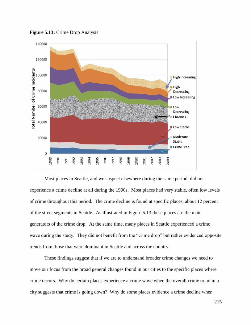
215

Figure 5.13: Crime Drop Analysis

Most places in Seattle, and we suspect elsewhere during the same period, did not

experience a crime decline at all during the 1990s. Most places had very stable, often low levels

of crime throughout this period. The crime decline is found at specific places, about 12 percent

of the street segments in Seattle. As illustrated in Figure 5.13 these places are the main

generators of the crime drop. At the same time, many places in Seattle experienced a crime

wave during the study. They did not benefit from the ―crime drop‖ but rather evidenced opposite

trends from those that were dominant in Seattle and across the country.

These findings suggest that if we are to understand broader crime changes we need to

move our focus from the broad general changes found in our cities to the specific places where

crime occurs. Why do certain places experience a crime wave when the overall crime trend in a

city suggests that crime is going down? Why do some places evidence a crime decline when


216

most places show little change in crime over time? These questions bring us down to a much

lower level of geography than is traditional in the study of crime. But we think our data suggest

that such an approach is warranted.

Conclusions

Our analyses confirm prior research showing that crime is tightly clustered in specific

places in urban areas, and that most places evidence little or no crime. But we also are able to

show that there is a high degree of stability of crime at micro places over time. This stability is

evident in the vast majority of street segments in our study of 16 years of official data. Our data

however, also suggest that crime trends at specific segments are central to understanding overall

changes in crime. The crime drop in Seattle was confined to very specific groups of street

segments with decreasing crime trajectories over time. If the trends in Seattle are common to

other cities, the crime drop should be seen not as a general phenomenon common to places

across a city but rather as focused at specific places. Such places in our study are also street

segments where crime rates are relatively high.

It is interesting to note in this regard that the variability we observe across street

segments in Seattle reflects broader trends in crime and violence across American cities. While

the national trends illustrate an overall decrease in crime during the 1990s, there was a good deal

of variability across cities (Blumstein, 2000; Travis & Waul, 2002). When looking at specific

crimes there has also been acknowledgement of important differences across populations. For

example, Cook and Laub (1998, 2002) observe that the youth violence epidemic was

concentrated among minority males who resided in poor neighborhoods, used guns, and engaged

in high risk behaviors such as gang participation (see also Braga, 2003). We are not surprised by

this variability, and see it more generally as reinforcing the importance of digging more deeply


217

into the phenomenon of overall crime trends. But whatever the trends across cities, or across

specific populations, our data suggest the importance of focusing on crime at very small units of

geography. We have argued that the street segment provides an important focus of

criminological analysis. Our data at this juncture emphasize that at the street segment level of

analysis there are very different developmental trends.

These analyses raise important questions which are the focus of the rest of this report.

The first concern was raised earlier in the chapter. We find that crime is concentrated at street

segments, and that relatively few street segments are responsible for most of the crime in Seattle.

But so far, we have not discussed the geography of the street segments. Are the very high rate

hot spots all in one area, or are they spread throughout the city? More generally, do street

segments near each other evidence very similar patterns of crime? These questions (addressed in

Chapter 6) are critical ones for our work because they raise important concerns about the unit of

analysis we use in our study.

Our analyses have also raised important questions about developmental trends of crime at

street segments. Why do some street segments evidence much more crime than others? Is it the

case that they have specific characteristics? As we noted earlier, a major concern of our research

was to see how well social disorganization and opportunity theories explain crime at place. In

this regard our trajectory analysis has shown us that there are distinct developmental trends at

crime places. Do the variables we have identified in prior chapters help us to understand such

trends? For example, do characteristics of social disorganization or crime opportunities (or

changes in such characteristics over time) explain membership in different trajectory patterns?

This is the focus of our analyses in Chapters 7 and 8.


218

Chapter 6: Geography of the Trajectories

Our data show clearly that there are different developmental trends at street segments,

and that a relatively small number of places, which can be termed hot spots of crime, produce a

substantial proportion of crime in a city. In turn, we have also illustrated that radically different

patterns of trajectories operate during the same time period in Seattle. It is misleading to speak

of an overall crime drop in the city, when a small but meaningful proportion of the city‟s street

segments experience crime waves. These findings suggest the importance of examining crime at

very small geographic units. But our analyses so far do not answer key questions regarding the

geography of trajectory patterns in the city.

For example, it may be that a relatively few hot spots are responsible for large

proportions of the crime in Seattle. But are these hot spots concentrated in specific areas? Put

differently, it may be that our examination of the crime at the street segment level has masked

the very consequential clustering of crime in communities or larger geographic areas. For

example, are high crime street segments concentrated in high crime neighborhoods, or do bad

places arise even in stable neighborhoods? Are such hot spots concentrated in large groupings in

some neighborhoods or do temporal trajectories of crime vary street segment by street segment?

If there are spatio-temporal patterns in the concentration of crime across micro places, can their

identification inform our understanding of the processes driving them?

Additionally, we are faced with a broad concern regarding what the study of crime at

micro places adds beyond the influences that come from larger social trends in communities or

other large geographic units. Does the variability of crime at the street segment level add

significant new variation beyond that indicated by study of larger geographic areas? There is a

long history of study in criminology of communities and their importance for understanding


219

crime trends (e.g. see Boggs, 1965; Bursik & Grasmick, 1993; Bursik & Webb, 1982; Byrne &

Sampson, 1986; Chilton, 1964; Kornhouser, 1978; Reiss & Tonry, 1986; Schuerman & Kobrin,

1986; Skogan, 1986; Stark, 1987). Does the study of variation across street segments suggest

that the action of crime should be brought lower down the cone of geography?

To answer these questions we apply geographic analysis to the distribution of street

segments with similar temporal patterns (i.e., street segments with the same trajectory pattern

assignment). Using the trajectory pattern assignment as the dependent variable, we investigate

whether street segments next to one another have the same temporal pattern (i.e., they tend to be

found in homogenous clusters). We also explore the spatial distribution of the street segments in

each trajectory pattern. Do they tend to be in one part of the city, or are they spread throughout

the city? Is there significant variability in crime trends at this low level of geography, and does it

suggest that explanations for crime need to be focused on micro crime places?

Analytic Strategy

The incorporation of spatial methods into criminological research has increased rapidly

since the 1990s (Messner & Anselin, 2004). Researchers have taken seriously the error

introduced by failing to account for spatial effects when analyzing inherently spatial data and

have responded by incorporating a range of spatial data analysis techniques.1 This research

continues that trend by using spatial statistics to describe geographic patterns of crime

trajectories across street segments.

The geographic analysis undertaken here requires multiple spatial and statistical

packages. Unfortunately no one package includes all the necessary functions combined with a

1 The volume of research explicitly examining spatial dependence or spatial error in their models is far too large to

detail here. The following studies are provided as examples: Baller et al., (2001); Chakravorty & Pelfrey (2000);

Cohen & Tita (1999); Cork (1999); Jefferis (2004); Morenoff & Sampson (1997); Roman (2002).


220

powerful cartographic display engine. Consequently data analysis and display were done using a

variety of software packages including SPlus©

Spatial Stats module, SPlancs©

, CrimeStat©

,

GeoDa©

and ArcGIS©

9.2.

Recall the group membership designation identified which street segments experienced

similar trends in crime incidents over the entire study period.2 We grouped those distinct

trajectory groups into eight general patterns that described the levels and trends in crime rates

over time: 1) crime free, 2) low stable, 3) low decreasing, 4) low increasing, 5) moderate stable,

6) high decreasing, 7) high increasing, and 8) chronic. Since group membership is a limited

categorical variable, we are constrained in the techniques we can use to examine the distribution

of street segments on the variable of interest.

When approaching the subject of space-time patterns, previous studies have used a

sequential approach by conducting a spatial analysis on the output of the temporal statistical

techniques (Griffiths & Chavez, 2004; Groff et al., 2009; Kubrin & Herting, 2003; Weisburd et

al., 2004). We also take that approach here. We use a variety of spatial statistics to describe the

spatial distributions of street segments within each trajectory pattern. The analysis of spatial

patterns is divided into sections that address the following research questions: 1) What is the

spatial pattern of street segments within the same trajectory pattern (i.e., clustered, dispersed, or

random)?; 2) Are trajectories of street segments related to the trajectories of nearby street

segments (i.e., is there spatial autocorrelation present and if so, what type?)?; and 3) Are street

segments of certain trajectory patterns found near one another, or are they spatially independent

(e.g., do high-increasing street segments and low-increasing street segments tend to be found

close to one another?)? To answer these questions, a series of point pattern statistical techniques

2 The groups used in the study are not the original trajectories identified by the TRAJ PROC. We grouped those

original trajectories by the overall trend and level into the eight trajectory group patterns discussed previously in

Chapter 5.


221

are used to analyze the spatial patterns of street segments. Each street segment is represented by

a dot (i.e., a point) on the map. The exercise of quantifying the patterns in the data is conducted

to further our understanding of the “underlying process that generated the points” (Fotheringham

et al., p. 131).

A series of formal tests of the spatial distribution of crime events is employed to

characterize the spatial patterning. The techniques applied to the data are termed local statistics;

that is, statistics which are designed to examine the second order effects (i.e., local relationships)

related to spatial dependence (Bailey & Gatrell, 1995; Fotheringham et al., 2000). Specifically,

the second order or local variation in the data is examined using the Ripley‟s K-function, a cross-

K function and local indicators of spatial association (LISA). Together the three provide a more

nuanced picture of local variation than would be possible with any one alone.

Ripley’s K

Ripley‟s K describes the proximity of street segments in the same trajectory pattern to

one another. For each street segment, it counts the number of street segments of the same

trajectory pattern that fall within a specified distance band and then repeats for each distance

band in use. In this way it characterizes spatial dependence among locations of street segments

with the same trajectory pattern at a wide range of scales. If street segments having the same

temporal trajectory pattern are clustered, then the processes underlying that trajectory pattern are

also clustered. If the results show a dispersed pattern, then the street segments are spread out,

and there is pattern to that spread. Thus the processes underlying a dispersed pattern are also

„spaced out.‟ A finding of randomness would indicate the pattern of the street segments in the

temporal trajectory pattern and the processes underlying them are both random.


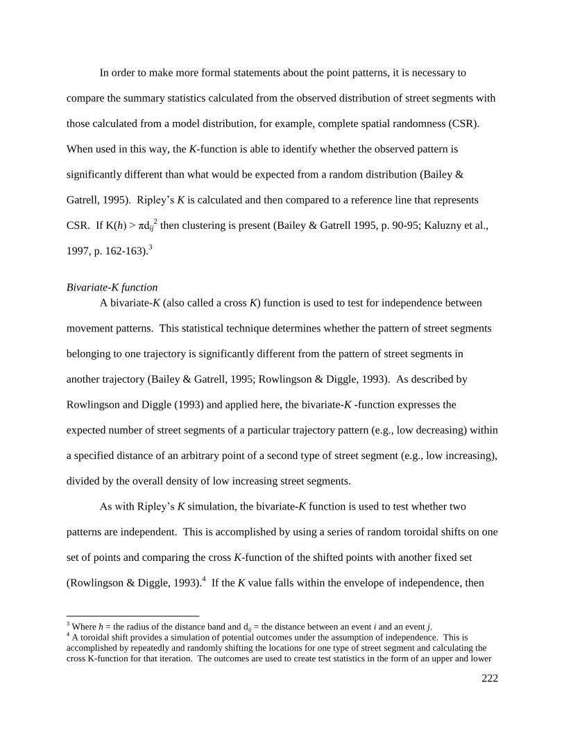
222

In order to make more formal statements about the point patterns, it is necessary to

compare the summary statistics calculated from the observed distribution of street segments with

those calculated from a model distribution, for example, complete spatial randomness (CSR).

When used in this way, the K-function is able to identify whether the observed pattern is

significantly different than what would be expected from a random distribution (Bailey &

Gatrell, 1995). Ripley‟s K is calculated and then compared to a reference line that represents

CSR. If K(h) > πdij2 then clustering is present (Bailey & Gatrell 1995, p. 90-95; Kaluzny et al.,

1997, p. 162-163).3

Bivariate-K function

A bivariate-K (also called a cross K) function is used to test for independence between

movement patterns. This statistical technique determines whether the pattern of street segments

belonging to one trajectory is significantly different from the pattern of street segments in

another trajectory (Bailey & Gatrell, 1995; Rowlingson & Diggle, 1993). As described by

Rowlingson and Diggle (1993) and applied here, the bivariate-K -function expresses the

expected number of street segments of a particular trajectory pattern (e.g., low decreasing) within

a specified distance of an arbitrary point of a second type of street segment (e.g., low increasing),

divided by the overall density of low increasing street segments.

As with Ripley‟s K simulation, the bivariate-K function is used to test whether two

patterns are independent. This is accomplished by using a series of random toroidal shifts on one

set of points and comparing the cross K-function of the shifted points with another fixed set

(Rowlingson & Diggle, 1993).4 If the K value falls within the envelope of independence, then

3 Where h = the radius of the distance band and dij = the distance between an event i and an event j.

4 A toroidal shift provides a simulation of potential outcomes under the assumption of independence. This is

accomplished by repeatedly and randomly shifting the locations for one type of street segment and calculating the

cross K-function for that iteration. The outcomes are used to create test statistics in the form of an upper and lower


223

the two patterns are independent of one another; there is no evidence of spatial interaction (i.e.,

attraction or dispersion). If the K value falls above the envelope, significant attraction exists at

that distance.5 If the K value line is below the envelope, significant dispersion is present between

the two patterns. The x-axis (s) represents the distance in feet, and the y-axis the cross K value.

In the case of our observations, a finding of attraction in the configuration of two

trajectory patterns can be interpreted as a situation in which the pattern of street segments of one

trajectory group is similar to the pattern of street segments of the comparison trajectory group.

Since the patterns „hang‟ together it can be assumed that the same underlying process or

processes are driving both patterns. A finding of independence in the comparison can be

interpreted as showing no relationship between the locations of street segments in the two

patterns. Thus, it is more likely that different processes are driving the observed patterns. The

scale at which processes operate provides evidence regarding the appropriate unit of analysis for

understanding them.

LISA

Finally, the LISA statistic is calculated in order to measure the degree of spatial

autocorrelation in the pattern (i.e., how likely a street segment of one group is to be near a street

segment of the same or any another group). This statistic identifies four types of spatial

autocorrelation; two characterize positive spatial autocorrelation and two negative spatial

autocorrelation. In positive spatial autocorrelation, observations with high values are near other

observations with high values or low values are near other observations with low values.

Negative correlation describes situations in which high values are near low values or vice versa.

envelope. One thousand iterations were used for each simulation except the generation of the test statistic for the

crime free trajectory pattern. Because of the large number of members we used one hundred iterations. 5 Since street segments are stationary, attraction in this context refers to a tendency for street segments of one

trajectory pattern to be found in closer proximity to street segments of another trajectory pattern than would be

expected under independence (i.e., their patterns are similar).


224

The limited nature of the dependent variable, in this case trajectory patterns, provides a

challenge to measuring spatial autocorrelation. Typically, measures of spatial autocorrelation

such as Moran's I and LISA measure the pattern in the deviation of an observation from the mean

for the distribution. This requires a ratio level variable such as the number or rate of total crimes.

For example, if number of crimes was the dependent variable, Moran‟s I would characterize the

existence and strength of the relationship between the number of crimes on one street segment

and the number on nearby street segments. However, the focus of this research is on the

distribution of street segments by type of trajectory, which involves a limited dependent variable

and makes the use of spatial autocorrelation techniques inappropriate without recoding.

Following recent research, this study dummy coded the dependent variable to allow a series of

comparisons; each trajectory pattern, in turn, was compared to all others (Griffiths & Chavez,

2004).

In this context, a finding of positive correlation among the trajectory pattern being tested

is significantly more likely to be found near other members of the pattern being tested; there is

clustering of members within the tested trajectory pattern. A finding of negative spatial

autocorrelation indicates the existence of street segment to street segment variation. In these

areas, street segments of the target trajectory pattern are significantly more likely to be found

near street segments of other trajectory patterns or street segments of any other trajectory pattern

are significantly more likely to be found near street segments that are members of the tested

trajectory pattern.

In sum, this mix of techniques provides information about the patterns in the temporal

variation of crime at street segments. Together they tell us the type of patterns (i.e., clustered,

random, dispersed) and the scale. From these patterns we can infer the pattern and the scale of


225

the underlying processes. Findings of street segment to street segment variation in the temporal

patterns of crime would provide support for the operation of micro/street segment level

processes. Any finding of small scale clustering or attraction provides support for the argument

that there are micro level processes at work. On the other hand, findings of positive spatial

autocorrelation across larger areas would tend to support the view of macro level processes that

are working across large swaths of street segments.

Findings

We begin our examination of the geography of temporal trajectories with a series of three

maps, which enable the inspection of variation in trajectory pattern membership across street

segments. Next, local relationships among the locations of street segments within the same

temporal trajectory pattern are investigated more quantitatively through the application of a

Ripley‟s K. Then, we examine the spatial dependence in one group compared to all other groups

using a LISA. Finally, we use a series of bivariate-K statistics to examine commonalities in pair-

wise comparisons in the spatial distributions of two trajectory patterns (e.g., low increasing street

segments and high increasing street segments).

Each map depicts the eight trajectory patterns across the northern (see Figure 6.1), middle

(see Figure 6.2) and southern (see Figure 6.3) portions of Seattle. These maps offer an excellent

visualization of the distribution of groups. The thinnest and lightest lines are the crime free

pattern members. As crime increases so does the darkness and thickness of the lines. Street

segments that are members of the chronic high group are the darkest and thickest of all.

At first glance the impression is one of clusters of streets of the same shade and thickness

broken up by linear patterns of differently shaded and thickness streets. However, upon closer

inspection, the variety in the pattern is discernible. While there are clusters of the crime free and


226

low stable groups (not surprising given their overwhelming numbers, 12,033 and 7,696 street

segments respectively), they are broken up by streets from different trajectory patterns. There

are also several arterial roads belonging to the high crime group patterns that are easily

discernable.

In the northern part of the city (see Figure 6.1), there is an area that is adjacent to the

University of Washington campus and on both sides of Broadway that has tremendous street

segment by street segment variation in high rate temporal trajectory patterns. The area is only

approximately 50 street segments in size but within that area all the high rate trajectory patterns

are represented and are neatly surrounded by crime free and low stable trajectory pattern street

segments.


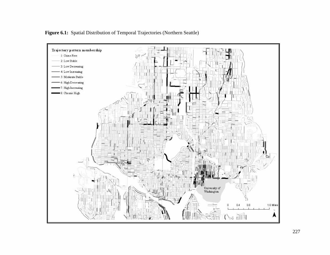
227

Figure 6.1: Spatial Distribution of Temporal Trajectories (Northern Seattle)


228

Turning to the middle of the city (see Figure 6.2), which includes the downtown area and

some of the most densely populated areas in the city we see a definite increase in the street

segment to street segment variation of the temporal trajectories.6 The downtown core is the first

area we see that has several adjacent chronic street segments. The middle section of Seattle also

seems to have a greater frequency of high rate street segments in general than the other two

sections of the city.

6 Readers should note slight scale changes among Figures 6.1, 6.2 and 6.3. These were necessary to provide

maximum enlargement of the three sections of Seattle.


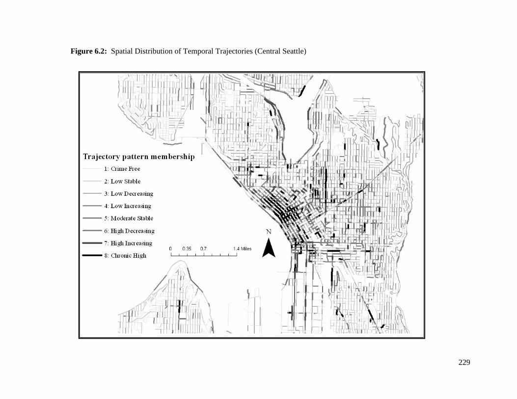
229

Figure 6.2: Spatial Distribution of Temporal Trajectories (Central Seattle)


230

Finally, turning to Figure 6.3, which covers the southwestern and southeastern sections of

the city, yet another pattern emerges. Once again we see clusters of low crime and crime free

street segments interspersed with the other trajectory types. There seem to be more linear

patterns of high rate street segments that often follow major arteries.

While these maps do not provide statistical substantiation for the significance of the

spatial associations revealed, they do offer a strong indication of heterogeneity as well as

homogeneity in crime patterns at the street segment level. Together these visualizations provide

striking evidence of street segment to street segment variation in crime rates that is often linear in

form. The next section examines whether street segments of the same temporal trajectory pattern

are clustered in space and if so, at what distances.


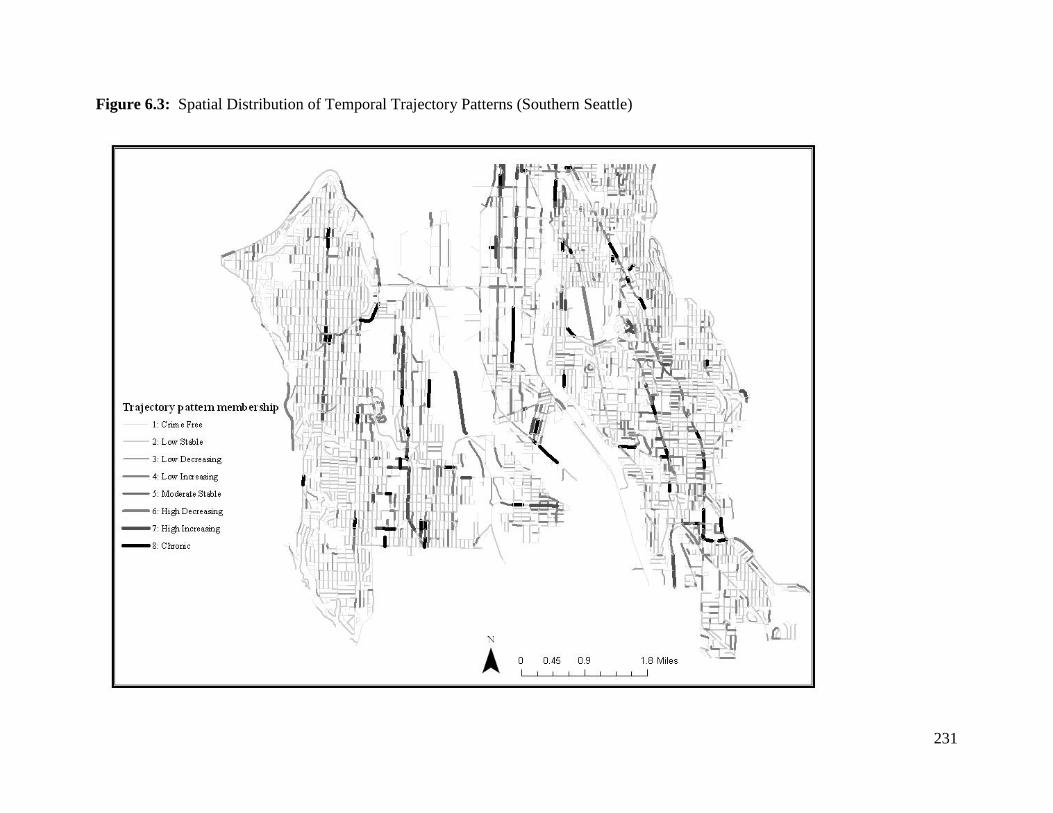
231

Figure 6.3: Spatial Distribution of Temporal Trajectory Patterns (Southern Seattle)


232

Clustering of Street Segments or Spatial Randomness?

Ripley‟s K provides information on whether street segments of the same trajectory are

clustered in space. In addition, the statistic reveals whether the observed clustering is greater or

less than would be expected under an assumption of complete spatial randomness (CSR).

Ripley‟s K also quantifies the spatial extent of dependence within the set of places in a given

trajectory. The L value from Ripley‟s K in CrimeStat is reported here. This is a rescaled

Ripley‟s K where CSR is represented by a horizontal zero line. In order to provide a measure of

significance, one hundred Monte Carlo simulations were used to develop an envelope of the

minimum and maximum values under CSR. The odds of getting a result outside the envelope

were one in one-hundred (or .01). The presence of the L-value line (dark blue line) above and

outside the simulation envelopes (CSR MIN and CSR MAX) indicates that the members of the

trajectory pattern are closer together than would be expected under CSR (i.e., the distances

between street segments of the same trajectory pattern are shorter than would be expected under

CSR).

Figure 6.4 shows the L(t) line for each of the trajectory patterns; the higher the line, the

greater the amount of clustering among the places that are members of the trajectory group

pattern. We compare the clustering in trajectory patterns to both CSR and to the intrinsic

clustering in the pattern of the streets themselves.7 All trajectory patterns are more clustered than

would be expected under a CSR assumption and the street network as a whole at short distances

(less than about a half mile if you include the crime free pattern and less than about one and a

quarter miles if you only consider street segments with crime). The degree of clustering varies

7 To calculate the clustering in the street network, we took the midpoint of each street and created a point pattern.

We then ran Ripley‟s K on the point pattern representing the streets. Since the density of the street network varies

across a city, using the intrinsic clustering of the street network as a comparison is helpful when interpreting the

clustering among members of each trajectory group pattern.


233

by the rate of crime. Trajectory patterns consisting of high rate temporal trends were the most

clustered at all distances. The four high crime patterns also have the highest degree of clustering

at all distances. In other words, if the crime rate on a street segment is high, it tends to be near

(but not necessarily adjacent to) other street segments that are also exhibiting a similar high

crime temporal pattern. Only three trajectory patterns, crime free, low stable, and low

increasing, have truncated clustering (i.e., they do not exhibit clustering at all distances up to

three miles).

More specifically, chronic street segments have the greatest clustering at just under a mile

from one another. The high increasing pattern exhibits a slower rise in clustering as distances

increase and peak at about 5,500 to 6,500 feet before dropping off steeply. The high decreasing

pattern does not hit its peak clustering until about 8,500 feet and remains stable until about

12,500 feet. The moderate stable pattern is the least clustered. It peaks at about 6,000 feet and

then stays at that level until it begins declining at just over 9,000 feet.

At the other end of the spectrum, among low rate trajectory patterns, it is the low

increasing street segments which are the most clustered until about 3,500 feet, when the low

decreasing pattern becomes more clustered and remains more clustered than CSR until just under

two miles. The crime free and low stable street segments are the least clustered and are barely

more clustered than the street segments themselves, although they are more clustered than would

be expected under CSR. The crime free street segments remain more clustered than random until

approximately 3,000 feet (i.e., about a 1,000 feet more than the street segments line). The low

stable street segments remain more clustered than CSR until about 6,700 feet.

In sum, all of the trajectory patterns are more clustered than would be expected under an

assumption of complete spatial randomness up to at least one-half of a mile. High rate trajectory


234

patterns, as well as the low decreasing trajectory pattern, are more clustered than would be

expected under an assumption of CSR up to at least two miles. Low increasing pattern street

segments are more clustered up to about one and three-quarter miles. Clustering at a distance of

over one and three-quarter miles means that within neighborhood-size areas, if you have one

street segment of a certain trajectory you are significantly more likely to find another street

segment of the same trajectory group than would be predicted by chance or by the intrinsic level

of clustering in the street network.


235

Figure 6.4: Ripley‟s K of All Trajectory Patterns


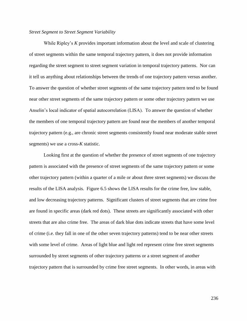
236

Street Segment to Street Segment Variability

While Ripley‟s K provides important information about the level and scale of clustering

of street segments within the same temporal trajectory pattern, it does not provide information

regarding the street segment to street segment variation in temporal trajectory patterns. Nor can

it tell us anything about relationships between the trends of one trajectory pattern versus another.

To answer the question of whether street segments of the same trajectory pattern tend to be found

near other street segments of the same trajectory pattern or some other trajectory pattern we use

Anselin‟s local indicator of spatial autocorrelation (LISA). To answer the question of whether

the members of one temporal trajectory pattern are found near the members of another temporal

trajectory pattern (e.g., are chronic street segments consistently found near moderate stable street

segments) we use a cross-K statistic.

Looking first at the question of whether the presence of street segments of one trajectory

pattern is associated with the presence of street segments of the same trajectory pattern or some

other trajectory pattern (within a quarter of a mile or about three street segments) we discuss the

results of the LISA analysis. Figure 6.5 shows the LISA results for the crime free, low stable,

and low decreasing trajectory patterns. Significant clusters of street segments that are crime free

are found in specific areas (dark red dots). These streets are significantly associated with other

streets that are also crime free. The areas of dark blue dots indicate streets that have some level

of crime (i.e. they fall in one of the other seven trajectory patterns) tend to be near other streets

with some level of crime. Areas of light blue and light red represent crime free street segments

surrounded by street segments of other trajectory patterns or a street segment of another

trajectory pattern that is surrounded by crime free street segments. In other words, in areas with


237

light red or light blue dots, there is significant street segment to street segment variation when

crime free street segments are compared to all other trajectory patterns.

Low stable street segments have a different pattern from the crime free street segments.

They are concentrated in the central part of the northern section of the city. In this area there is

once again a tremendous amount of negative spatial autocorrelation with low stable street

segments surrounded by street segments of other trajectory patterns. There are also pockets of

low stable street segments throughout the city.

The low decreasing street segments tend to be in the east central portion of the city. Once

again we see light blue mixed with dark red indicating that low decreasing street segments are

near other low decreasing street segments in the same areas where street segments of other

trajectory patterns are significantly associated with low decreasing street segments. This clearly

demonstrates street segment to street segment variation in the trajectories of individual places.


238

Figure 6.5: LISA for Crime Free, Low Stable, and Low Decreasing Trajectory Group Patterns

Returning to our discussion of the crime free pattern, we more closely examine the center

portion of the city, which is almost uniformly dark blue except for some light red dots (see

Figure 6.6). These dots represent streets that are surrounded by streets of some other trajectory

pattern. The light red dots are where crime free streets are near streets that are not crime free.

Thus, there seem to be pockets of „safe‟ streets even in the center city. This clearly shows how

crime free street segments can be surrounded by street segments of other trajectory patterns.

From this map it is apparent that there are no instances in the downtown area where a crime free

street segment is surrounded by other crime free street segments (dark red). However, outside of

downtown there are many more cases in which a crime free street segment is significantly

correlated with other crime free street segments (dark red). In other cases, crime free street


239

segments are surrounded by street segments that are part of high crime trajectory patterns (light

red).

Figure 6.6: Center City LISA for Crime Free Street Segments


240

The limitation of the maps discussed so far is that we do not immediately know which

group patterns are surrounding crime free street segments. To answer this question we would

need a different map where we overlay the LISA results on the streets with each street

symbolized by its trajectory pattern (see Figure 6.7 below for an example).

In order to answer the question of what trajectory patterns are near the crime free

trajectory streets, it is necessary to zoom in even farther. Although Figure 6.7 is a bit cluttered,

by picking out a particular street the reader is able to ascertain the specific trajectory group

pattern of the street segments near it. To aid in this process, direct your attention to the center of

the yellow circle to find several crime free street segments. Notice that within this small circle

every one of the trajectory patterns is represented. Thus, there are low increasing and low

decreasing street segments next to crime free street segments, and high decreasing street

segments next to high increasing street segments. The street segment by street segment variation

is clearly visible.


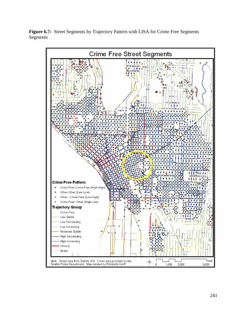
241

Figure 6.7: Street Segments by Trajectory Pattern with LISA for Crime Free Segments

Segments


242

The lesser numbers of street segments in trajectories representing low increasing,

moderate stable and low decreasing patterns produce arrangements of more isolated clusters (see

Figure 6.8). There are significant clusters of low increasing street segments as well as significant

negative spatial autocorrelation where low increasing street segments are intermixed with other

street segments in downtown and in all sections of the city. A similar situation occurs with

moderate stable street segments, which are significantly positively auto correlated with other

street segments in the central section of the city and near the University of Washington campus.

High decreasing street segments are even more clustered but with only one large cluster in

downtown and then some smaller clusters near the University of Washington, in the southeast

section of the city, and near Salmon Bay.


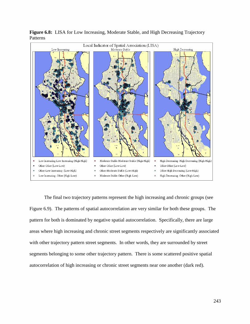
243

Figure 6.8: LISA for Low Increasing, Moderate Stable, and High Decreasing Trajectory

Patterns

The final two trajectory patterns represent the high increasing and chronic groups (see

Figure 6.9). The patterns of spatial autocorrelation are very similar for both these groups. The

pattern for both is dominated by negative spatial autocorrelation. Specifically, there are large

areas where high increasing and chronic street segments respectively are significantly associated

with other trajectory pattern street segments. In other words, they are surrounded by street

segments belonging to some other trajectory pattern. There is some scattered positive spatial

autocorrelation of high increasing or chronic street segments near one another (dark red).


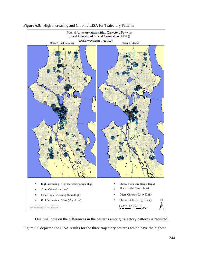
244

Figure 6.9: High Increasing and Chronic LISA for Trajectory Patterns

One final note on the differences in the patterns among trajectory patterns is required.

Figure 6.5 depicted the LISA results for the three trajectory patterns which have the highest

Other – Other (Low – Low)


245

numbers of street segments in them: crime free (n = 12,033), low stable (n = 7,696), and low

decreasing (n = 2,212). Because of the high numbers, there were more instances of the target

temporal trajectory pattern street segments and fewer street segments of other trajectory patterns.

Thus, Figure 6.5 shows more variety in positive and negative spatial correlation findings than

Figures 6.8 or 6.9, where there were far fewer target street segments to compare. Overall, these

findings indicate that street segments of one trajectory pattern tend to be positively associated

with street segments of the same trajectory pattern in particular areas of the city. In other areas

of the city, street segments of a trajectory pattern are likely to be found near street segments of

other trajectory patterns (i.e., they are negatively correlated). Interestingly, the downtown area is

one in which all trajectory pattern display positive spatial autocorrelation. Together these

findings indicate that there is tremendous street segment by street segment variation in the

downtown area for all types of temporal trajectory patterns.

Do Trajectory Patterns Share Underlying Spatial Processes?

We now turn to the question of whether there are specific temporal trajectory patterns

that are also physically proximal. The application of a cross-K analysis allows us to

systematically compare the distances between each street segment in one trajectory pattern with

each member of another trajectory pattern. For example, we can directly compare moderate

stable street segments with high increasing street segments. A finding that two patterns exhibit

attraction to one another provides evidence that the temporal pattern observed and classified via

the trajectory group membership is driven by a shared spatial process. For example, if we

assume that there are similar processes driving an increase in crime wherever it occurs, we would

expect trajectory patterns that have a temporal trend of predominantly increasing crime rates to

have a similar spatial distribution. Thus, a finding that street segments of similar trajectory


246

patterns are dependent at larger distances would support a macro level explanation, while a

finding of dependence at short distances or independence would support the argument for a

micro level examination of crime.

We conducted a series of pair wise comparisons to evaluate the spatial distribution of

each trajectory pattern as compared to those of every other trajectory pattern (i.e., pattern 1 to

pattern 2, pattern 1 to pattern 3 etc.). To create the envelopes, one thousand simulations were

run of each pair wise comparison. Thus there is a one in one thousand possibility the results

were obtained by chance. The null hypothesis of the cross-K test is independence between the

two spatial distribution patterns (i.e., the spatial pattern of one trajectory group pattern is

unrelated to the pattern of the other pattern being compared). When the entire length of the K(i,j)

line falls within the significance simulation envelope, the pattern of street segments in the two

temporal trajectory patterns being compared is independent at all distances. For distances at

which the K(i,j) line is above the simulation envelope, the two patterns display attraction. In

other words, they are dependent upon one another, and the form of the dependence is attraction

(rather than repulsion which would be the finding if the K(i,j) line was below the simulation

envelope). When the K(i,j) line falls on the upper bound of the simulation envelope the

interpretation is one of weak attraction in the two patterns.8

Each trajectory pattern was individually compared to every other trajectory pattern (see

Figures 6.10 and 6.11, Table 6.1 beginning on p. 33). In total, this yields 28 sets of comparisons.

In all but eight of the comparisons, the patterns of street segments of one trajectory pattern were

more likely to be found near the comparison trajectory pattern street segments (the Khat(I,j) line

is above the envelope) at some distances. However, in most of the cases the attraction was only

8 These analyses produced 28 graphs for each of the distances examined for a total of 56 graphs. Space constraints

do not allow the inclusion of the graphs in this chapter; however, they are available from the authors.


247

weakly significant and occurred only at distances of less than two miles.9 Trajectory patterns

whose pattern was independent (i.e., the differences in pattern were not significant) were as

follows:

Crime free as compared to high decreasing, high increasing, moderate stable, and

chronic.

Low decreasing as compared to moderate stable, high decreasing, high increasing,

and chronic.

But what do these results mean for our understanding of the processes underlying crime

at place? Basically, a finding of independence in the patterns of temporal crime change across

street segments signifies the two patterns are generated by different processes. In other words,

different collections of factors are acting on each group. The finding is atheoretical in that we

are not testing whether a specific characteristic or set of characteristics is responsible for the

difference, only that there is a difference and it is worth looking into (i.e., significant).

Specifically, these findings signify that crime free street segments are most likely generated by a

process different from the one that generates any of the high rate street segments. Low

decreasing street segments are similarly generated by a process different from all of the high rate

street segments.

Only one of the pair wise comparisons exhibited strong attraction, low increasing with

moderate stable. The dominant association was one of weakly significant attraction at short

distances. The following section discusses the results from the low-rate trajectory patterns (see

9 In order to better see the detail in the graphs, the cross-K analysis was done two separate times. The first run

examined the distribution of the trajectory pairs at distances up to 10 miles (using 1,320 foot bins). Because the

Khat(i,j) statistic line fell on the upper bound of the independence envelope in many of the comparisons, the analysis

was rerun at a distance of two miles (10,560 feet, 1,320 foot bins). This allowed us to more closely inspect the

relationship of the cross K statistic to the upper bound of the confidence envelope.


248

Figure 6.10) first and then turns to the high-rate trajectory patterns (see Figure 6.11). Street

segments with a crime free pattern tended to be associated with other low rate street segments.

With one exception, low stable pattern streets were weakly attracted to all other patterns of street

segments at distances of almost a mile. Several pairs of trajectory patterns exhibited weak

attraction for the full two miles: crime free street segments with low stable street segments, low

stable with moderate stable, and low increasing with high increasing. Since low decreasing, low

stable, and crime free street segments all exhibit at least a weak attraction to one another, we can

make the case that they may share an underlying process that generates low crime rates. Further,

the shared process operates at the street segment level as well as across several street segments at

a time. Low increasing street segments were also more likely to be found near other low-rate

street segments but for shorter distances (significant only up to 2,900 feet for all comparisons

with one exception, low decreasing). Interestingly, the locations of low increasing and low

decreasing street segments were mostly independent of one another. Even for places with low

levels of crime, different factors were driving the changes in crime trends at spatially separate

locations.

The emerging picture regarding low crime rate street segments is that they tend to be

found in the same areas, except for low increasing and low decreasing street segments, which are

mostly independent of one another. Interestingly, low stable street segments tends be attracted to

most other trajectory pattern types. Perhaps this is an indication that many of the characteristics

of low stable places are also found at higher rate segments with the exception of whatever is

driving the crime trend at the other streets. It also could indicate low stable streets act as buffers

between streets with „better‟ and „worse‟ crime rates. One factor which may be influencing this

finding is the large number of crime free and low stable street segments in Seattle. Together


249

these two groups account for almost 82 percent of all the street segments in Seattle and thus

reflect the dominant processes at work, so in that way it is not surprising that they tend to be

found in large numbers across many areas.

We now turn to the groups that were high in crime (see Figure 6.11). The trend of

chronic street segments was weakly associated with all other high rate patterns at distances of

less than one-half-mile. Chronic street segments were also weakly associated with low

increasing street segments up to about three quarters of a mile. High increasing and high

decreasing street segments were weakly attracted to every other pattern except crime free and

low decreasing. High decreasing street segments did not display a distinct pattern, as was

discovered with the low decreasing street segments. Rather, the patterns of high decreasing and

moderate stable street segments were very similar to that of high increasing street segments (with

slight differences in the distances at which attraction was significant). For the high-rate temporal

trajectory patterns, the underlying processes are likely to be shared at micro level distances.

However, the finding of weak attraction at micro distances for low stable street segments with

moderate stable, high increasing, and high decreasing street segments suggests a shared set of

common characteristics that manifest themselves differently at the micro level. In other words,

while there may be consistency in some of the foundational elements of the situational backcloth,

at the same time there is place to place variation that is driving the changes in temporal crime

patterns. These spatial patterns also support our earlier finding of street segment to street

segment variation in the temporal trajectory pattern of nearby street segments.


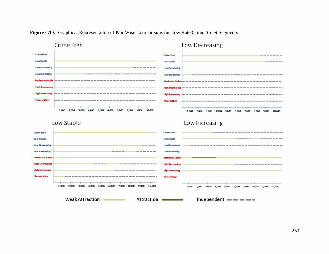
250

Figure 6.10: Graphical Representation of Pair Wise Comparisons for Low Rate Crime Street Segments


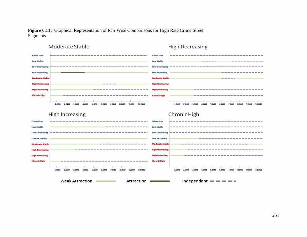
251

Figure 6.11: Graphical Representation of Pair Wise Comparisons for High Rate Crime Street

Segments


252

Table 6.1: Cross K Results

2–Low

Stable

3–Low

Decreasing

4–Low

Increasing

5–Moderate

Stable

6–High

Decreasing

7–High

Increasing

8–Chronic

1–Crime

Free

Weak

attraction at

all distances

Weak

attraction to

8,400 feet,

then

Independent

Weak

attraction to

3,500 feet, then

Independent

Independent

at all

distances

Independent at all

distances

Independent

at all

distances

Independent at all

distances

2–Low

Stable

Weak

attraction to

about 9,000

feet, then

Independent

Weak

attraction to

about 6,000

feet, then

Independent until 7,500

feet, then

Weak

attraction until 8,500

feet, then

Independent

Weak

attraction at

all distances

Weak

attraction to

about 4,500

feet, then

Independent

until 5,500

feet, then

Weak

attraction until 7,000

feet, then

Independent

Weak

attraction at

distances up

to about

6,500 feet,

then

Independent

Weak

attraction to

1,500 feet,

then

Independent

3–Low

Decreasing

Weak

attraction to

1,500 feet, then

Independent

Independent at all

distances

Independent at all

distances

Independent at all

distances

Independent at all

distances

4–Low

Increasing

Weak

attraction to

about 1,500

feet, then

Attraction

until 4,000

feet, then

Weak

attraction

Weak

attraction to

about 6,000

feet, then

Independent

Weak

attraction at

all distances

Weak

attraction to

about 4,000

feet, then

Independent

to 6,000 feet,

then Weak

attraction


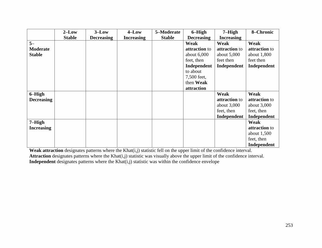
253

2–Low

Stable

3–Low

Decreasing

4–Low

Increasing

5–Moderate

Stable

6–High

Decreasing

7–High

Increasing

8–Chronic

5–

Moderate

Stable

Weak

attraction to

about 6,000

feet, then

Independent to about

7,500 feet,

then Weak

attraction

Weak

attraction to

about 5,000

feet then

Independent

Weak

attraction to

about 1,800

feet then

Independent

6–High

Decreasing

Weak

attraction to

about 3,000

feet, then

Independent

Weak

attraction to

about 3,000

feet, then

Independent

7–High

Increasing

Weak

attraction to

about 1,500

feet, then

Independent

Weak attraction designates patterns where the Khat(i,j) statistic fell on the upper limit of the confidence interval.

Attraction designates patterns where the Khat(i,j) statistic was visually above the upper limit of the confidence interval.

Independent designates patterns where the Khat(i,j) statistic was within the confidence envelope


254

Conclusions

Our analyses of the geography of developmental patterns of crime at street segments,

provides important answers to the questions that we raised at the outset of this chapter. We do

not find evidence suggesting that the processes explaining crime patterns at street segments come

primarily from higher geographic influences such as communities. While there are indications of

the influence of higher order trends in our data, there is also clear and convincing evidence of the

importance of micro level trends in understanding variability in trajectory patterns at street

segments. There is strong street to street variability in crime patterns in our data, and such

variability emphasizes the importance of studying crime at place at a micro unit of analysis.

On a broader level our findings suggest that there are both micro and macro influences

that condition the developmental patterns of crime at place. The fact that there is clustering of

street segments at specific distances indicates the importance of larger order trends, such as those

that would be predicted by variability in economic and social characteristics at the community

level. But we think that the evidence of heterogeneity of street segments in specific areas, for

example the inner city, and the presence of crime hot spots throughout the city landscape, point

to the critical importance of understanding how characteristics of places at the street segment

level influence crime. Evidence of spatial independence at the street segment level further

reinforces this view, especially given the well known law of geography that places closer to each

other are likely to be more alike (Tobler, 1970).

These findings lay the ground for the following chapters. Now that we have established

that micro level processes are at work in developing patterns of crime at street segments, it is

reasonable to turn to the question of what specific factors influence crime at place. In this


255

context, we now turn to how measures reflecting social disorganization and opportunity theories

correlate with patterns of crime at place.


256

Chapter 7: Linking Characteristics of

Places with Crime

In previous chapters we have established the importance of the street segment in

identifying variability of both characteristics of places and crime. Incorporating variables

representing social disorganization and collective efficacy, as well as those representing routine

activities and crime opportunities we found that there was tremendous variation of place

characteristics from place to place. In the two previous chapters we established that crime varies

across street segments and that there are specific developmental patterns of crime at street

segments over time. Importantly, our analyses also have shown that there is a “micro” level

component to crime that is not simply explained by larger area changes. Our work suggests that

the action of crime is at a much lower level of geography than traditional study of crime and

place in criminology.

In this chapter we want to see whether there is a link between place characteristics and

crime patterns at street segments. Is variability in such structural characteristics of places as

property values, mixed land use, physical disorder, or racial heterogeneity related to the overall

levels of crime at street segments or their developmental patterns? Is there a relationship

between unsupervised teens or collective efficacy and crime patterns at the street segment level?

While these elements of what are often termed social disorganization theories have been linked

to crime patterns in larger geographic areas like census tracts and neighborhoods (e.g. see

Bellair, 1997; Bursik & Grasmick, 1993; Sampson & Groves, 1989; Sampson et al., 1997), our

study is the first we know of us to systematically examine whether they have salience for

understanding variability of crime at small micro level units of geography. This question is

particularly important because social disorganization theories have been linked closely to the


257

concept of communities and neighborhoods (Bursik & Grasmick, 1993; Sampson & Groves,

1989). It has generally been assumed that the key to such theories is found in the dynamics of

larger geographic areas than the street segments we study.

While what we have termed routine activities and opportunity theories are often seen as

being linked to the specific places where crime occurs, our study is also the first we know of to

systematically examine the relationship between key features of routine activities and

opportunity theories and developmental patterns of crime at micro places. Are such factors as

the presence of high risk juveniles living on a street segment (“motivated offenders”) or the

presence of large numbers of people working there (“suitable targets”) related to levels of crime

or developmental patterns of crime at street segments? Is the accessibility of places as

represented by bus stops related to crime at street segments? Finally, is the level of guardianship

as measured by the location of police or fire stations, street lighting, or the percentage of vacant

land linked to crime at street segments?

In this chapter we want to focus on whether variability of characteristics of places

representing broad theories about crime and crime events is related to variability in crime levels

and developmental crime patterns at street segments. Our concern is not with causality but what

scholars sometimes define as “risk factors” (Green et al., 2008; Nagin, 1999; Nagin & Tremblay,

2001). We simply want to identify at this point, for example, whether high rates of social

disorganization or greater crime opportunities are related to high rates of crime at street segments

and whether changes over time in factors reflecting social disorganization and opportunities for

crime can be linked with developmental patterns of crime over time. We leave for the next

chapter the task of identifying whether such links are causal, and the broader questions of which


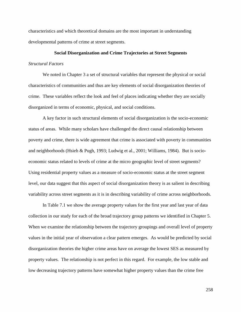
258

characteristics and which theoretical domains are the most important in understanding

developmental patterns of crime at street segments.

Social Disorganization and Crime Trajectories at Street Segments

Structural Factors

We noted in Chapter 3 a set of structural variables that represent the physical or social

characteristics of communities and thus are key elements of social disorganization theories of

crime. These variables reflect the look and feel of places indicating whether they are socially

disorganized in terms of economic, physical, and social conditions.

A key factor in such structural elements of social disorganization is the socio-economic

status of areas. While many scholars have challenged the direct causal relationship between

poverty and crime, there is wide agreement that crime is associated with poverty in communities

and neighborhoods (Hsieh & Pugh, 1993; Ludwig et al., 2001; Williams, 1984). But is socio-

economic status related to levels of crime at the micro geographic level of street segments?

Using residential property values as a measure of socio-economic status at the street segment

level, our data suggest that this aspect of social disorganization theory is as salient in describing

variability across street segments as it is in describing variability of crime across neighborhoods.

In Table 7.1 we show the average property values for the first year and last year of data

collection in our study for each of the broad trajectory group patterns we identified in Chapter 5.

When we examine the relationship between the trajectory groupings and overall level of property

values in the initial year of observation a clear pattern emerges. As would be predicted by social

disorganization theories the higher crime areas have on average the lowest SES as measured by

property values. The relationship is not perfect in this regard. For example, the low stable and

low decreasing trajectory patterns have somewhat higher property values than the crime free


259

pattern. For a city like Seattle, this phenomenon is possibly due to the fact that housing prices

are higher in more developed areas than in less populated areas, even though the latter have

fewer crime problems. This possibility is also consistent with the results that crime free

segments showed only non-significant housing values inflation over our study period among all

segments. Thus, there are relatively large and statistically significant differences between the

trajectory group patterns reflecting higher property value scores and the trajectory groups that

have overall higher crime rates (see Appendix 1 for pair wise comparisons between the trajectory

patterns for all variables).1

Table 7.1: Risk Analysis for Property Value Index (Measure of SES)

Classification

of Trajectories

SES Initial

Value

(1991)

SES Ending

Value (2004)

Individual

Block Change

Over Time

Sig. of Paired

Sample t test for

Individual Blocks

Group

Mean

Change

Crime Free

(n=12,033)

4.1995 4.1961 -.0035 .740 -0.08%

Low Stable

(n=7,696)

5.0722 5.1396 .0674 .000*** 1.33%

Low Decreasing

(n=2,212)

5.0829 5.3407 .2578 .000*** 5.07%

Low Increasing

(n=903)

3.7955 3.9350 .1395 .005** 3.68%

Moderate Stable

(n=292)

3.6388 3.7315 .0927 .031* 2.55%

High

Decreasing

(n=574)

2.5625 2.7726 .2101 .000*** 8.20%

High Increasing

(n=221)

3.0769 3.2881 .2112 .024* 6.86%

1 We use Tukey‟s PostHoc tests for generating these estimates, which takes into account the bias for running a large

number of tests simultaneously on a single construct. Results are available from the authors upon request.


260

Chronics

(n=247)

1.7545 1.9321 .1776 .023* 10.12%

*** p< .01, ** p<.01, * p<.05

When we look at change over time the relationship between property value and crime

trajectory patterns becomes less clear. Two sets of comparisons in our data are especially salient

for examining such changes over time: trajectories associated with what we have defined as the

low stable, low decreasing, and low increasing patterns; and those associated with the moderate

stable, high decreasing, and high increasing patterns. Following social disorganization theories

we would expect that increasing crime rates would be associated with declines in SES reflecting

more general increases in social disorganization, in this case at street segments. In turn,

increases in property values would be expected to be associated with decreasing crime rates.

The data do not strongly reflect such patterns. Looking at the low trajectory patterns we

do find that the largest increases in property values are in the low decreasing group, but the

magnitude of change is not large for any of the groups. Again, for the high rate trajectory pattern

the largest increase is found in the chronic trajectory, which is a little over 10 percent. It is

important to note that the relationships between property values and other social variables may

be confounding our view of change. As we noted above, in this chapter we wanted to examine

the simple relationship between such characteristics and crime trajectories. In the next chapter

we will examine property value and other variables in the context of a multivariate statistical

analysis that will allow us to control for such confounding.

Public housing and Section 8 vouchers are also indicators of SES, as described in Chapter

3. Specifically, this measure captures the population that relies on public assistance and, thus is

at the bottom of the SES spectrum. We term the combination of these two variables housing

assistance. In Table 7.2 we report the proportion of street segments with public housing or with


261

people who use Section 8 vouchers for each of the trajectory patterns. It is important to note that

in this table as well as for other variables we report “moving averages” for three years of data as

we were concerned that there might be strong year to year variability (Baller et al., 2001).

The findings here are again strongly consistent in terms of the levels of crime found in

the trajectories. The crime free segments in this regard have significantly lower levels of

housing assistance than any of the other patterns (see Appendix 1). The chronic trajectory street

segments have 70 times the level of housing assistance as that found in the crime free trajectory

segments. The high activity segments vary greatly in the level of housing assistance but overall,

with the exception of the high decreasing group, have much higher levels than that found in the

low crime trajectories. In this case, trends over time also appear consistent with the social

disorganization perspective. In the low increasing and high increasing trajectory patterns there

are strong and significant increases in housing assistance. In the low decreasing pattern there is a

negative trend over time, and while the high decreasing pattern shows increasing public

assistance, it is half that of the increasing group.

Table 7.2: Risk Analysis for Housing Assistance (Combining Public Housing and Section 8

Vouchers)

Classification

of Trajectories

Housing

Assistance

Initial Value

(1998-2000)

Housing

Assistance

Ending Value

(2002-2004)

Individual

Block

Change

Over Time

Sig. of Paired

Sample t test for

Individual

Blocks

Group

Mean

Change

Crime Free

(n=12,033)

0.1110 0.0634 -.0476 .000*** -42.88

Low Stable

(n=7,696)

0.2387 0.2833 .0446 .000*** 18.68%

Low

Decreasing

(n=2,212)

0.2751 0.2358 -.0393 .044* -14.29%


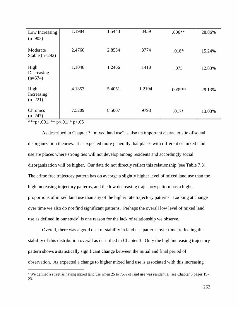
262

Low Increasing

(n=903)

1.1984 1.5443 .3459 .006** 28.86%

Moderate

Stable (n=292)

2.4760 2.8534 .3774 .018* 15.24%

High

Decreasing

(n=574)

1.1048 1.2466 .1418 .075 12.83%

High

Increasing

(n=221)

4.1857 5.4051 1.2194 .000*** 29.13%

Chronics

(n=247)

7.5209 8.5007 .9798 .017* 13.03%

***p<.001, ** p<.01, * p<.05

As described in Chapter 3 “mixed land use” is also an important characteristic of social

disorganization theories. It is expected more generally that places with different or mixed land

use are places where strong ties will not develop among residents and accordingly social

disorganization will be higher. Our data do not directly reflect this relationship (see Table 7.3).

The crime free trajectory pattern has on average a slightly higher level of mixed land use than the

high increasing trajectory patterns, and the low decreasing trajectory pattern has a higher

proportions of mixed land use than any of the higher rate trajectory patterns. Looking at change

over time we also do not find significant patterns. Perhaps the overall low level of mixed land

use as defined in our study2 is one reason for the lack of relationship we observe.

Overall, there was a good deal of stability in land use patterns over time, reflecting the

stability of this distribution overall as described in Chapter 3. Only the high increasing trajectory

pattern shows a statistically significant change between the initial and final period of

observation. As expected a change to higher mixed land use is associated with this increasing

2 We defined a street as having mixed land use when 25 to 75% of land use was residential; see Chapter 3 pages 19-

23.


263

trajectory. Increases are also found in the low decreasing and high decreasing trajectory patterns,

though these are not statistically significant, and of smaller magnitude.

Table 7.3: Risk Analysis for Mixed Land Use

Classification

of Trajectories

Mixed Land

Use Initial

Value (1991)

Mixed Land

Use Ending

Value (2004)

Individual

Block

Change

Over Time

Sig. of Paired

Sample t Test for

Individual Blocks

Group

Mean

Change

Crime Free

(n=12,033)

0.0416 0.0432 .0017 .059 3.85%

Low Stable

(n=7,696)

0.0464 0.0477 .0013 .281 2.80%

Low Decreasing

(n=2,212)

0.0570 0.0592 .0023 .398 3.86%

Low Increasing

(n=903)

0.0454 0.0476 .0022 .564 4.85%

Moderate Stable

(n=292)

0.0479 0.0445 -.0034 .706 -7.10%

High

Decreasing

(n=574)

0.0523 0.0540 .0017 .739 3.25%

High Increasing

(n=221)

0.0407 0.0588 .0181 .045* 44.47%

Chronics

(n=247)

0.0445 0.0526 .0081 .158 18.20%

*** p<.01, ** p<.01, * p<.05

Just as mixed land use is expected to impact upon the ability of communities to prevent

social disorganization, population heterogeneity is seen to impact upon social cohesion and thus

social control among community residents (Bursik & Grasmick, 1993; Kornhauser, 1978;

Sampson & Groves, 1989). Ethnic and racial diversity has been assumed to make it more


264

difficult for community members to communicate and collaborate. In this context, we would

expect that higher crime trajectories would also have higher levels of population heterogeneity.

In this case, the overall patterns in our data are consistent with social disorganization

theories. The lowest level of population heterogeneity is found in the crime free trajectory

pattern (see Table 7.4). And the difference between the crime free street segments and each

other pattern is large and statistically significant (see Appendix 1). The largest differences are

found in the high crime trajectory groupings, which have more than 10 times the level of

population heterogeneity as that of the crime free trajectory pattern. While the chronic group has

a slightly lower level of population heterogeneity than the high crime trajectory patterns the

differences are not statistically significant (see Appendix 1). In contrast, the low crime trajectory

patterns have lower levels than the high and chronic patterns.

When we examine change over time, these observations are reinforced. For the high

trajectory groupings we find that the high increasing pattern shows a strong (23 percent) and

statistically significant increase in racial heterogeneity between the first and last years of

observation. In contrast the high decreasing pattern shows a statistically significant decline in

racial heterogeneity. The moderate stable group shows a slight increase, but not statistically

significant at the five percent threshold. For the low rate groupings the pattern is the same. The

increasing pattern shows a strong (29 percent) and statistically significant increase in racial

heterogeneity in the second period compared to the first. The low decreasing pattern shows little

change, and the low stable pattern shows a small absolute increase which is statistically

significant because of the large number of segments (7,696) found in this trajectory pattern.

While overall there is a 26 percent increase in racial heterogeneity in the crime free pattern, it is


265

important to note that the absolute change for individual blocks is very small (.0009) in good part

because the weighted average from the initial period was very low in this group.

Table 7.4: Risk Analysis for Racial Heterogeneity (Based on Public School Student Data)

Classification

of Trajectories

Heterogeneity

(Student)

Initial Value

(1992-1995)

Heterogeneity

(Student)

Ending Value

(2002-2004)

Individual

Block

Change

Over Time

Sig. of Paired

Sample t test

for Individual

Blocks

Group

Mean

Change

Crime Free

(n=12,033)

0.0034 0.0043 .0009 .000** 26.47%

Low Stable

(n=7,696)

0.0296 0.0315 .0018 .018* 6.08%

Low

Decreasing

(n=2,212)

0.0264 0.0253 -.0011 .386 -4.17%

Low Increasing

(n=903)

0.0300 0.0387 .0087 .000** 29.00%

Moderate

Stable

(n=292)

0.0399 0.0430 .0032 .087 8.02%

High

Decreasing

(n=574)

0.0379 0.0342 -.0039 .249 -10.29%

High

Increasing

(n=221)

0.0396 0.0486 .0090 .002**

22.73%

Chronics

(n=247)

0.0331 0.0312 -.0019 .099 -5.74%

*** p<.001, ** p<.01, * p<.05

Social disorganization theorists have also seen distance to the city‟s geographic center

(i.e., urbanization) as an important factor in understanding crime (see Table 7.5). More

urbanized areas in a city are assumed to have a tendency towards greater social disorganization,


266

and such urbanization is reflected at least in part by the closeness of an area to the city center.

Overall our data support this idea of the relationship between closeness to the city center and

crime. The highest crime trajectories are on average closest to the city‟s geographic center.

Indeed the high activity trajectories are on average about 3.5 miles from the geographic center of

the city while the low crime trajectories are about a mile farther out. The crime free trajectory

pattern segments are on average most distant from the city center (i.e., approximately 5 miles).

According to librarians at the Seattle Public Library, the cultural center of Seattle is considered

to be the Westlake Center at the corner of 4th

and Pine in downtown Seattle. Since the two

locations are only .73 miles apart as the crow flies, we simply used the geographic center for the

rest of the analyses. It is important to note that the designation of geographic center does not

change over time. Thus, the t tests and change scores were not computed.

Table 7.5: Risk Analysis for Urbanization/Distance to Center of the City (miles)

Classification of

Trajectories

Distance to

Geographic Center

Distance to

Cultural Center

Crime Free (n=12,033)

5.11 5.17

Low Stable (n=7,696)

4.88 4.95

Low Decreasing (n=2,212)

4.06 4.09

Low Increasing (n=903)

4.60 4.58

Moderate Stable (n=292)

3.54 3.56

High Decreasing (n=574)

3.41 3.31

High Increasing (n=221)

3.76 3.68

Chronics (n=247) 3.57 3.39

The variables we have examined so far reflect social disorganization indirectly. In

contrast, physical disorder is a direct and visceral indication of the social order of the street


267

segments we examine. Looking at physical disorder incidents we find a direct and strong

relationship with the trajectory patterns (see Table 7.6).

Consistent with social disorganization theory, we find that the number of physical

disorder incidents increases as the levels of crime in trajectory patterns increase in the initial

period of observations. This relationship is significant and strong across the trajectory groupings

(see Appendix 1). By far the lowest number of physical disorder incidents is found in the crime

free group. In the low rate trajectory groupings there is an increase in incidents of about four

times, and in the high rate trajectory patterns this increase is more than tenfold as compared with

the crime free trajectory pattern. For the chronic group the increase is much higher.

Looking at change over time, the relationships are also strong. For the high increasing

and moderate stable trajectory patterns the number of physical disorder incidents increases,

though the change is statistically significant only for the stable grouping. In contrast, in the high

decreasing group there is a statistically significant decline in the number of physical disorder

incidents in the final observation period. The same pattern emerges looking at the low rate

trajectory patterns. In the low increasing group there is about a 40 percent increase in the

number of physical disorder incidents, and the change is highly significant. There is a

statistically significant though smaller decline in the low decreasing group. The low stable group

shows almost no change during the period.

Table 7.6: Risk Analysis for Total Number of Physical Disorder Incidents

Classification

of Trajectories

Physical

Disorder

Initial Value

(93-95)

Physical

Disorder

Ending Value

(02-04)

Individual

Block

Change

Over Time

Sig. of Paired

Sample t test

for Individual

Blocks

Group

Mean

Change

Crime Free

(n=12,033)

0.0373 0.0425 .0052 .012* 13.94%


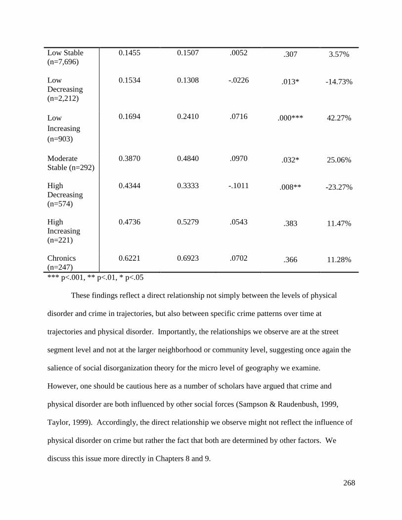
268

Low Stable

(n=7,696)

0.1455 0.1507 .0052 .307 3.57%

Low

Decreasing

(n=2,212)

0.1534 0.1308 -.0226 .013* -14.73%

Low

Increasing

(n=903)

0.1694 0.2410 .0716 .000*** 42.27%

Moderate

Stable (n=292)

0.3870 0.4840 .0970 .032* 25.06%

High

Decreasing

(n=574)

0.4344 0.3333 -.1011 .008** -23.27%

High

Increasing

(n=221)

0.4736 0.5279 .0543 .383 11.47%

Chronics

(n=247)

0.6221 0.6923 .0702 .366 11.28%

*** p<.001, ** p<.01, * p<.05

These findings reflect a direct relationship not simply between the levels of physical

disorder and crime in trajectories, but also between specific crime patterns over time at

trajectories and physical disorder. Importantly, the relationships we observe are at the street

segment level and not at the larger neighborhood or community level, suggesting once again the

salience of social disorganization theory for the micro level of geography we examine.

However, one should be cautious here as a number of scholars have argued that crime and

physical disorder are both influenced by other social forces (Sampson & Raudenbush, 1999,

Taylor, 1999). Accordingly, the direct relationship we observe might not reflect the influence of

physical disorder on crime but rather the fact that both are determined by other factors. We

discuss this issue more directly in Chapters 8 and 9.


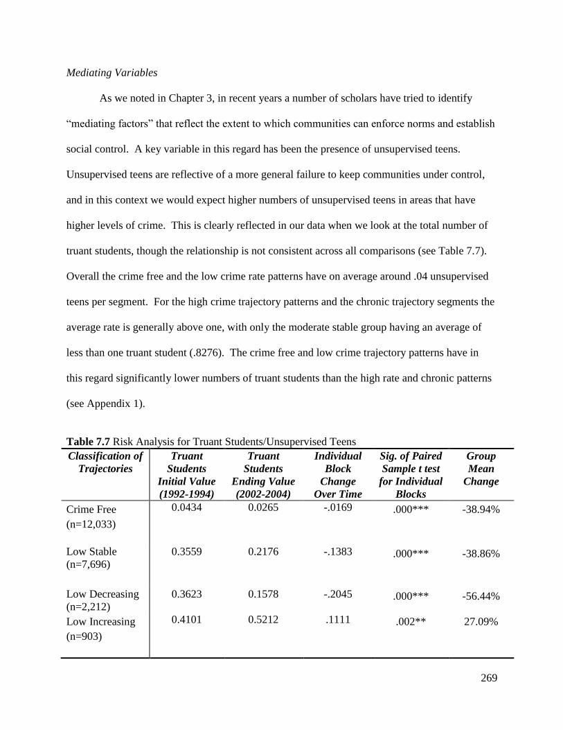
269

Mediating Variables

As we noted in Chapter 3, in recent years a number of scholars have tried to identify

“mediating factors” that reflect the extent to which communities can enforce norms and establish

social control. A key variable in this regard has been the presence of unsupervised teens.

Unsupervised teens are reflective of a more general failure to keep communities under control,

and in this context we would expect higher numbers of unsupervised teens in areas that have

higher levels of crime. This is clearly reflected in our data when we look at the total number of

truant students, though the relationship is not consistent across all comparisons (see Table 7.7).

Overall the crime free and the low crime rate patterns have on average around .04 unsupervised

teens per segment. For the high crime trajectory patterns and the chronic trajectory segments the

average rate is generally above one, with only the moderate stable group having an average of

less than one truant student (.8276). The crime free and low crime trajectory patterns have in

this regard significantly lower numbers of truant students than the high rate and chronic patterns

(see Appendix 1).

Table 7.7 Risk Analysis for Truant Students/Unsupervised Teens

Classification of

Trajectories

Truant

Students

Initial Value

(1992-1994)

Truant

Students

Ending Value

(2002-2004)

Individual

Block

Change

Over Time

Sig. of Paired

Sample t test

for Individual

Blocks

Group

Mean

Change

Crime Free

(n=12,033)

0.0434 0.0265 -.0169 .000*** -38.94%

Low Stable

(n=7,696)

0.3559 0.2176 -.1383 .000*** -38.86%

Low Decreasing

(n=2,212)

0.3623 0.1578 -.2045 .000*** -56.44%

Low Increasing

(n=903)

0.4101 0.5212 .1111 .002** 27.09%


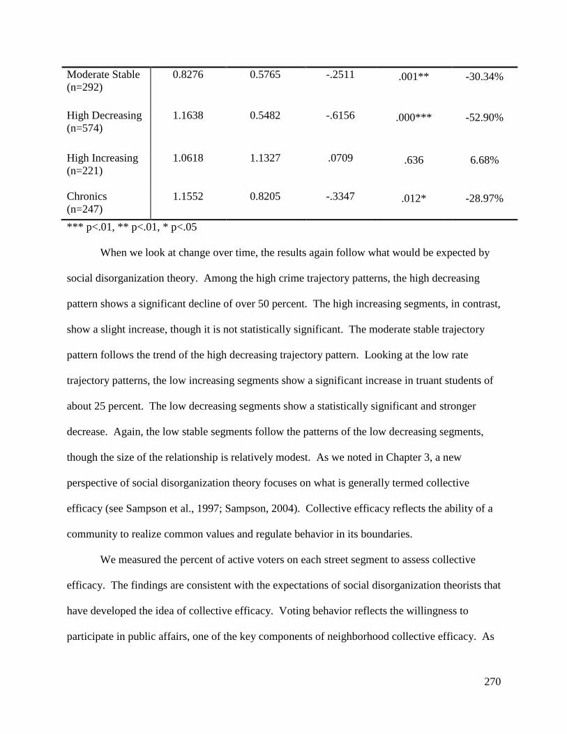
270

Moderate Stable

(n=292)

0.8276 0.5765 -.2511 .001** -30.34%

High Decreasing

(n=574)

1.1638 0.5482 -.6156 .000*** -52.90%

High Increasing

(n=221)

1.0618 1.1327 .0709 .636 6.68%

Chronics

(n=247)

1.1552 0.8205 -.3347 .012* -28.97%

*** p<.01, ** p<.01, * p<.05

When we look at change over time, the results again follow what would be expected by

social disorganization theory. Among the high crime trajectory patterns, the high decreasing

pattern shows a significant decline of over 50 percent. The high increasing segments, in contrast,

show a slight increase, though it is not statistically significant. The moderate stable trajectory

pattern follows the trend of the high decreasing trajectory pattern. Looking at the low rate

trajectory patterns, the low increasing segments show a significant increase in truant students of

about 25 percent. The low decreasing segments show a statistically significant and stronger

decrease. Again, the low stable segments follow the patterns of the low decreasing segments,

though the size of the relationship is relatively modest. As we noted in Chapter 3, a new

perspective of social disorganization theory focuses on what is generally termed collective

efficacy (see Sampson et al., 1997; Sampson, 2004). Collective efficacy reflects the ability of a

community to realize common values and regulate behavior in its boundaries.

We measured the percent of active voters on each street segment to assess collective

efficacy. The findings are consistent with the expectations of social disorganization theorists that

have developed the idea of collective efficacy. Voting behavior reflects the willingness to

participate in public affairs, one of the key components of neighborhood collective efficacy. As


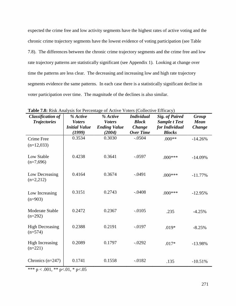
271

expected the crime free and low activity segments have the highest rates of active voting and the

chronic crime trajectory segments have the lowest evidence of voting participation (see Table

7.8). The differences between the chronic crime trajectory segments and the crime free and low

rate trajectory patterns are statistically significant (see Appendix 1). Looking at change over

time the patterns are less clear. The decreasing and increasing low and high rate trajectory

segments evidence the same patterns. In each case there is a statistically significant decline in

voter participation over time. The magnitude of the declines is also similar.

Table 7.8: Risk Analysis for Percentage of Active Voters (Collective Efficacy)

Classification of

Trajectories

% Active

Voters

Initial Value

(1999)

% Active

Voters

Ending Value

(2004)

Individual

Block

Change

Over Time

Sig. of Paired

Sample t Test

for Individual

Blocks

Group

Mean

Change

Crime Free

(n=12,033)

0.3534 0.3030 -.0504 .000** -14.26%

Low Stable

(n=7,696)

0.4238 0.3641 -.0597 .000*** -14.09%

Low Decreasing

(n=2,212)

0.4164 0.3674 -.0491 .000*** -11.77%

Low Increasing

(n=903)

0.3151 0.2743 -.0408 .000*** -12.95%

Moderate Stable

(n=292)

0.2472 0.2367 -.0105 .235 -4.25%

High Decreasing

(n=574)

0.2388 0.2191 -.0197 .019* -8.25%

High Increasing

(n=221)

0.2089 0.1797 -.0292 .017* -13.98%

Chronics (n=247) 0.1741 0.1558 -.0182 .135 -10.51%

*** p < .001, ** p<.01, * p<.05


272

Summary

What is clear is that the structural variables that have been linked to crime in

communities are also very salient for understanding crime at micro geographic levels. Of the six

structural indicators of social disorganization that we examined, five are directly related to crime

levels of trajectories. In two of the cases (population heterogeneity and physical disorganization)

we also found strong and significant relationships to the shape of trajectory patterns. In the case

of mediating factors of social disorganization both truant teens and voting behavior were

strongly related to the level of crime in trajectory patterns. The number of truant teens was also

strongly related to the overall changes we found in the trajectory pattern. Our data bring the first

systematic evidence of the relevance of social disorganization theory for longitudinal patterns in

micro-level geographic data.

Opportunity Theories and Crime and Trajectories of Crime at Street Segments

In Chapter 4 we examined the distribution of variables that reflect opportunity theories

about crime. Key to these theories is the idea of routine activities (Cohen & Felson, 1979; Eck,

1995; Felson, 2001) and its salience for understanding crime in specific situations. Routine

activities theory argues that crime occurs when three factors are present: 1) the absence of

capable guardianship; 2) the presence of motivated offenders; 3) and the presence of suitable

targets. Below we examine the relationship between each of these dimensions and crime

trajectory patterns, again focusing on the levels of crime in trajectory patterns and change over

time. We also examine accessibility and urban form, as opportunity theorists have also

emphasized the urban backcloth of crime events (see Brantingham & Brantingham, 1993a,

1993b).


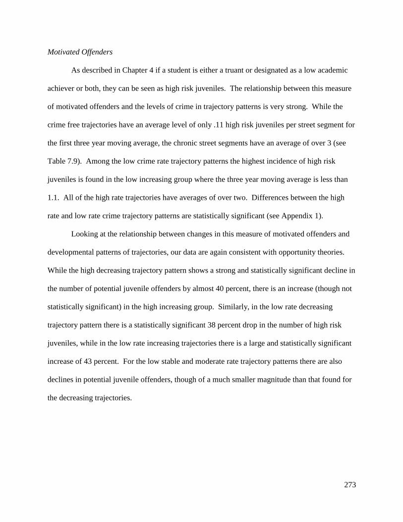
273

Motivated Offenders

As described in Chapter 4 if a student is either a truant or designated as a low academic

achiever or both, they can be seen as high risk juveniles. The relationship between this measure

of motivated offenders and the levels of crime in trajectory patterns is very strong. While the

crime free trajectories have an average level of only .11 high risk juveniles per street segment for

the first three year moving average, the chronic street segments have an average of over 3 (see

Table 7.9). Among the low crime rate trajectory patterns the highest incidence of high risk

juveniles is found in the low increasing group where the three year moving average is less than

1.1. All of the high rate trajectories have averages of over two. Differences between the high

rate and low rate crime trajectory patterns are statistically significant (see Appendix 1).

Looking at the relationship between changes in this measure of motivated offenders and

developmental patterns of trajectories, our data are again consistent with opportunity theories.

While the high decreasing trajectory pattern shows a strong and statistically significant decline in

the number of potential juvenile offenders by almost 40 percent, there is an increase (though not

statistically significant) in the high increasing group. Similarly, in the low rate decreasing

trajectory pattern there is a statistically significant 38 percent drop in the number of high risk

juveniles, while in the low rate increasing trajectories there is a large and statistically significant

increase of 43 percent. For the low stable and moderate rate trajectory patterns there are also

declines in potential juvenile offenders, though of a much smaller magnitude than that found for

the decreasing trajectories.


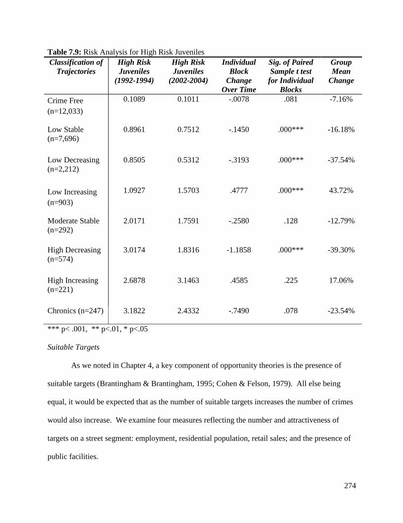
274

Table 7.9: Risk Analysis for High Risk Juveniles

Classification of

Trajectories

High Risk

Juveniles

(1992-1994)

High Risk

Juveniles

(2002-2004)

Individual

Block

Change

Over Time

Sig. of Paired

Sample t test

for Individual

Blocks

Group

Mean

Change

Crime Free

(n=12,033)

0.1089 0.1011 -.0078 .081 -7.16%

Low Stable

(n=7,696)

0.8961 0.7512 -.1450 .000*** -16.18%

Low Decreasing

(n=2,212)

0.8505 0.5312 -.3193 .000*** -37.54%

Low Increasing

(n=903)

1.0927 1.5703 .4777 .000*** 43.72%

Moderate Stable

(n=292)

2.0171 1.7591 -.2580 .128 -12.79%

High Decreasing

(n=574)

3.0174 1.8316 -1.1858 .000*** -39.30%

High Increasing

(n=221)

2.6878 3.1463 .4585 .225 17.06%

Chronics (n=247) 3.1822 2.4332 -.7490 .078 -23.54%

*** p< .001, ** p<.01, * p<.05

Suitable Targets

As we noted in Chapter 4, a key component of opportunity theories is the presence of

suitable targets (Brantingham & Brantingham, 1995; Cohen & Felson, 1979). All else being

equal, it would be expected that as the number of suitable targets increases the number of crimes

would also increase. We examine four measures reflecting the number and attractiveness of

targets on a street segment: employment, residential population, retail sales; and the presence of

public facilities.


275

When we look at the number of people who work on a street block in the initial

observation period and the levels of crime of the trajectory patterns, our analyses once again

confirm the basic propositions of opportunity theories (see Table 7.10). There are very large

differences between the higher crime rate and the lower rate trajectory patterns in the initial

observation year and these differences are statistically significant (see Appendix 1). For

example, all of the low rate trajectory patterns have fewer than 30 employees on average on a

block, while the high rate patterns have averages between 95 and almost 400. At the other end of

the spectrum, the crime free trajectory segments have an average of only one employee, while

the chronic trajectory segments have an average of 377. Looking at the change over time in

employment and the trajectory patterns the relationship is less clear, but appears to follow

opportunity theory in the sample. The low increasing trajectory pattern shows on average a

modest increase in employment between the first observation years and the last years, while the

low decreasing segments show a small decrease. The results here are not statistically significant

at the traditional five percent threshold (though for the low decreasing pattern the p value is less

than .10).

Table 7.10: Risk Analysis for Employment

Classification of

Trajectories

Employment

(1998)

Employment

(2004)

Individual

Block

Change

Over Time

Sig. of Paired

Sample t test

for Individual

Blocks

Group

Mean

Change

Crime Free

(n=12,033)

1.0435 1.1617 .1182 .138 11.33%

Low Stable

(n=7,696)

9.7915 9.8835 .0920 .857 0.94%

Low Decreasing

(n=2,212)

15.9928 14.2862 -1.7065 .082 -10.67%


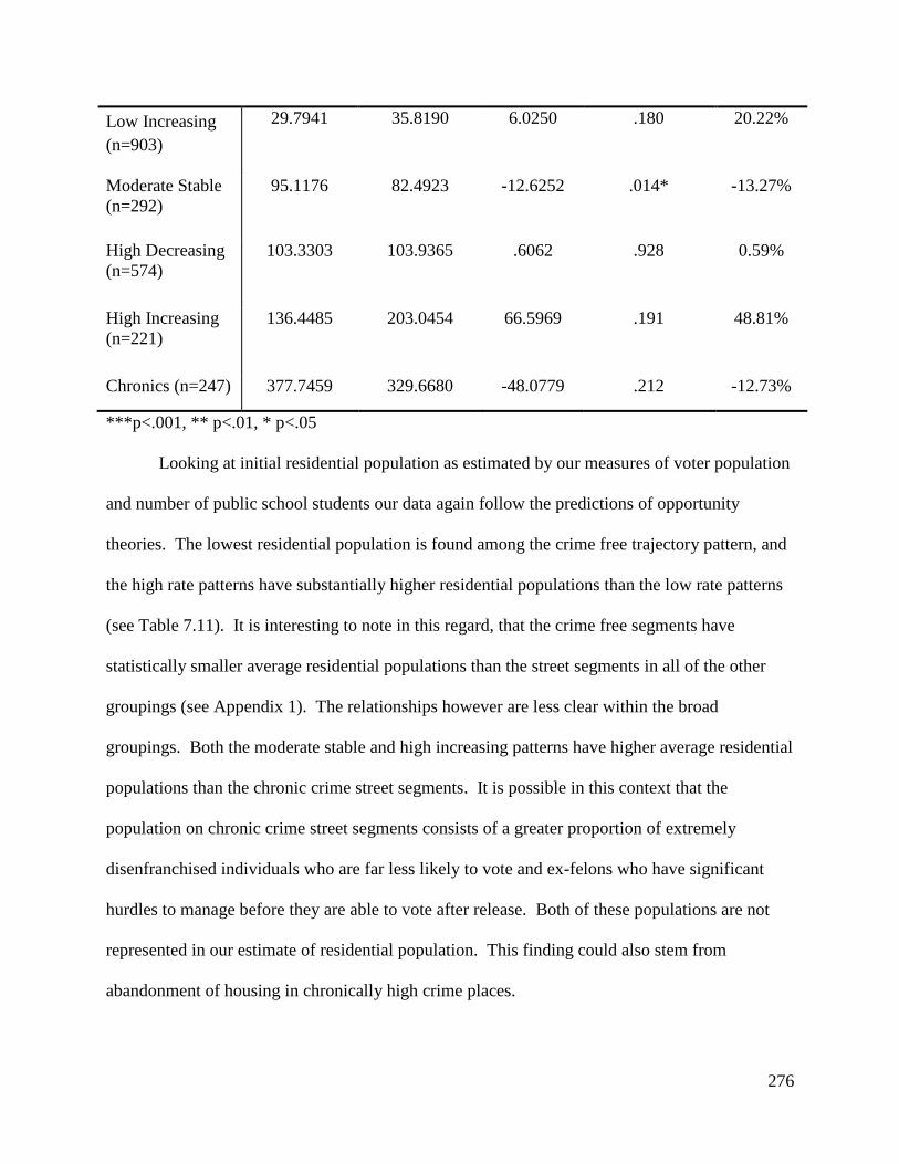
276

Low Increasing

(n=903)

29.7941 35.8190 6.0250 .180 20.22%

Moderate Stable

(n=292)

95.1176 82.4923 -12.6252 .014* -13.27%

High Decreasing

(n=574)

103.3303 103.9365 .6062 .928 0.59%

High Increasing

(n=221)

136.4485 203.0454 66.5969 .191 48.81%

Chronics (n=247) 377.7459 329.6680 -48.0779 .212 -12.73%

***p<.001, ** p<.01, * p<.05

Looking at initial residential population as estimated by our measures of voter population

and number of public school students our data again follow the predictions of opportunity

theories. The lowest residential population is found among the crime free trajectory pattern, and

the high rate patterns have substantially higher residential populations than the low rate patterns

(see Table 7.11). It is interesting to note in this regard, that the crime free segments have

statistically smaller average residential populations than the street segments in all of the other

groupings (see Appendix 1). The relationships however are less clear within the broad

groupings. Both the moderate stable and high increasing patterns have higher average residential

populations than the chronic crime street segments. It is possible in this context that the

population on chronic crime street segments consists of a greater proportion of extremely

disenfranchised individuals who are far less likely to vote and ex-felons who have significant

hurdles to manage before they are able to vote after release. Both of these populations are not

represented in our estimate of residential population. This finding could also stem from

abandonment of housing in chronically high crime places.


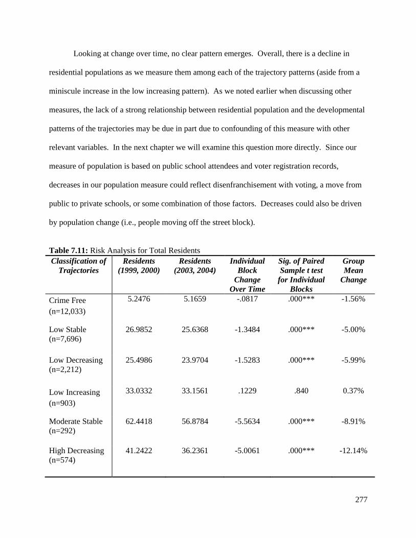
277

Looking at change over time, no clear pattern emerges. Overall, there is a decline in

residential populations as we measure them among each of the trajectory patterns (aside from a

miniscule increase in the low increasing pattern). As we noted earlier when discussing other

measures, the lack of a strong relationship between residential population and the developmental

patterns of the trajectories may be due in part due to confounding of this measure with other

relevant variables. In the next chapter we will examine this question more directly. Since our

measure of population is based on public school attendees and voter registration records,

decreases in our population measure could reflect disenfranchisement with voting, a move from

public to private schools, or some combination of those factors. Decreases could also be driven

by population change (i.e., people moving off the street block).

Table 7.11: Risk Analysis for Total Residents

Classification of

Trajectories

Residents

(1999, 2000)

Residents

(2003, 2004)

Individual

Block

Change

Over Time

Sig. of Paired

Sample t test

for Individual

Blocks

Group

Mean

Change

Crime Free

(n=12,033)

5.2476 5.1659 -.0817 .000*** -1.56%

Low Stable

(n=7,696)

26.9852 25.6368 -1.3484 .000*** -5.00%

Low Decreasing

(n=2,212)

25.4986 23.9704 -1.5283 .000*** -5.99%

Low Increasing

(n=903)

33.0332 33.1561 .1229 .840 0.37%

Moderate Stable

(n=292)

62.4418 56.8784 -5.5634 .000*** -8.91%

High Decreasing

(n=574)

41.2422 36.2361 -5.0061 .000*** -12.14%


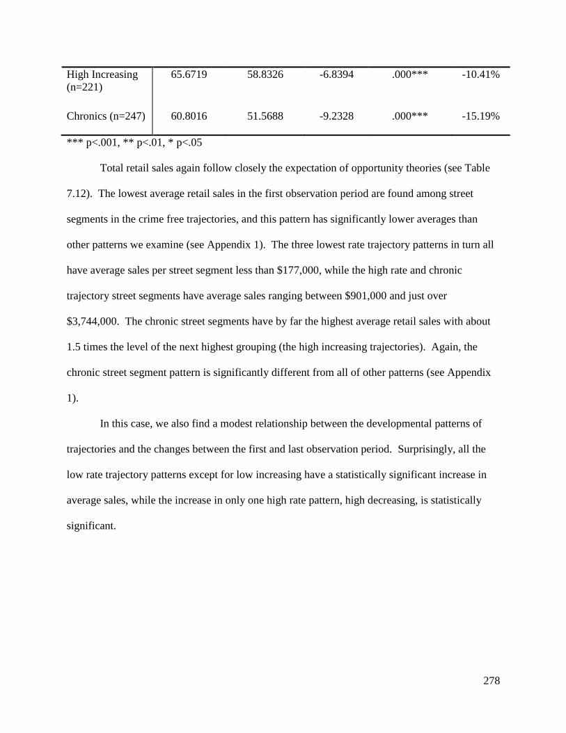
278

High Increasing

(n=221)

65.6719 58.8326 -6.8394 .000*** -10.41%

Chronics (n=247) 60.8016 51.5688 -9.2328 .000*** -15.19%

*** p<.001, ** p<.01, * p<.05

Total retail sales again follow closely the expectation of opportunity theories (see Table

7.12). The lowest average retail sales in the first observation period are found among street

segments in the crime free trajectories, and this pattern has significantly lower averages than

other patterns we examine (see Appendix 1). The three lowest rate trajectory patterns in turn all

have average sales per street segment less than $177,000, while the high rate and chronic

trajectory street segments have average sales ranging between $901,000 and just over

$3,744,000. The chronic street segments have by far the highest average retail sales with about

1.5 times the level of the next highest grouping (the high increasing trajectories). Again, the

chronic street segment pattern is significantly different from all of other patterns (see Appendix

1).

In this case, we also find a modest relationship between the developmental patterns of

trajectories and the changes between the first and last observation period. Surprisingly, all the

low rate trajectory patterns except for low increasing have a statistically significant increase in

average sales, while the increase in only one high rate pattern, high decreasing, is statistically

significant.


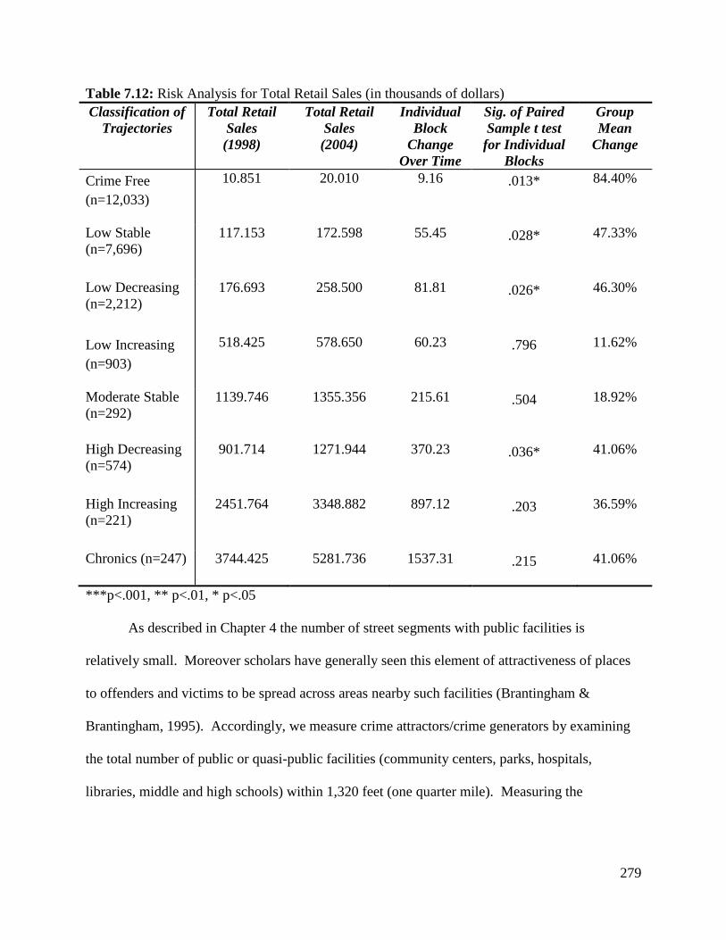
279

Table 7.12: Risk Analysis for Total Retail Sales (in thousands of dollars)

Classification of

Trajectories

Total Retail

Sales

(1998)

Total Retail

Sales

(2004)

Individual

Block

Change

Over Time

Sig. of Paired

Sample t test

for Individual

Blocks

Group

Mean

Change

Crime Free

(n=12,033)

10.851 20.010 9.16 .013* 84.40%

Low Stable

(n=7,696)

117.153 172.598 55.45 .028* 47.33%

Low Decreasing

(n=2,212)

176.693 258.500 81.81 .026* 46.30%

Low Increasing

(n=903)

518.425 578.650 60.23 .796 11.62%

Moderate Stable

(n=292)

1139.746 1355.356 215.61 .504 18.92%

High Decreasing

(n=574)

901.714 1271.944 370.23 .036* 41.06%

High Increasing

(n=221)

2451.764 3348.882 897.12 .203 36.59%

Chronics (n=247) 3744.425 5281.736 1537.31 .215 41.06%

***p<.001, ** p<.01, * p<.05

As described in Chapter 4 the number of street segments with public facilities is

relatively small. Moreover scholars have generally seen this element of attractiveness of places

to offenders and victims to be spread across areas nearby such facilities (Brantingham &

Brantingham, 1995). Accordingly, we measure crime attractors/crime generators by examining

the total number of public or quasi-public facilities (community centers, parks, hospitals,

libraries, middle and high schools) within 1,320 feet (one quarter mile). Measuring the


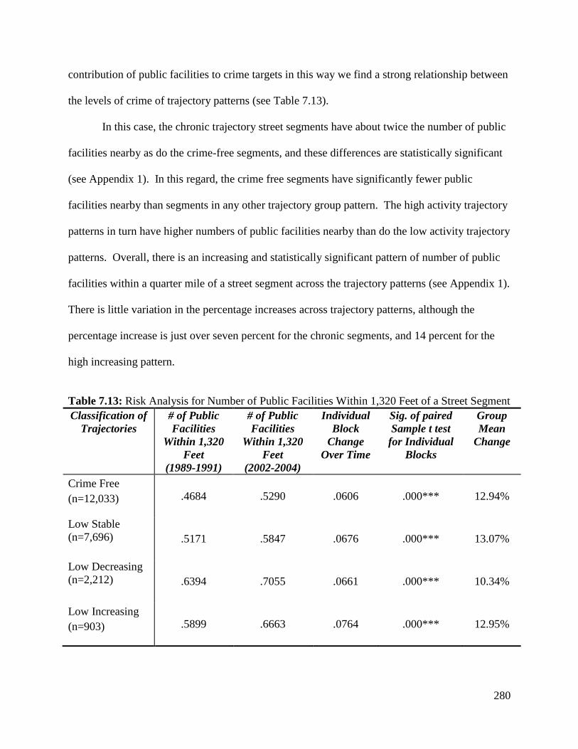
280

contribution of public facilities to crime targets in this way we find a strong relationship between

the levels of crime of trajectory patterns (see Table 7.13).

In this case, the chronic trajectory street segments have about twice the number of public

facilities nearby as do the crime-free segments, and these differences are statistically significant

(see Appendix 1). In this regard, the crime free segments have significantly fewer public

facilities nearby than segments in any other trajectory group pattern. The high activity trajectory

patterns in turn have higher numbers of public facilities nearby than do the low activity trajectory

patterns. Overall, there is an increasing and statistically significant pattern of number of public

facilities within a quarter mile of a street segment across the trajectory patterns (see Appendix 1).

There is little variation in the percentage increases across trajectory patterns, although the

percentage increase is just over seven percent for the chronic segments, and 14 percent for the

high increasing pattern.

Table 7.13: Risk Analysis for Number of Public Facilities Within 1,320 Feet of a Street Segment

Classification of

Trajectories

# of Public

Facilities

Within 1,320

Feet

(1989-1991)

# of Public

Facilities

Within 1,320

Feet

(2002-2004)

Individual

Block

Change

Over Time

Sig. of paired

Sample t test

for Individual

Blocks

Group

Mean

Change

Crime Free

(n=12,033) .4684 .5290 .0606 .000*** 12.94%

Low Stable

(n=7,696) .5171 .5847 .0676 .000*** 13.07%

Low Decreasing

(n=2,212) .6394 .7055 .0661 .000*** 10.34%

Low Increasing

(n=903) .5899 .6663 .0764 .000*** 12.95%


281

Moderate Stable

(n=292) .8733 .9635 .0902 .000*** 10.33%

High Decreasing

(n=574)

1.0331 1.1220 .0889 .000*** 8.61%

High Increasing

(n=221) .7195 .8220 .1026 .014** 14.26%

Chronics (n=247) 1.0634 1.1390 .0756 .091 7.11%

*** p<.001, ** p<.01, * p<.05

Accessibility

As described in Chapter 4, accessibility of an area is generally seen to increase

opportunities for crime (Brantingham & Brantingham, 1991; Roman, 2005). Our primary

measures of accessibility are the number of bus stops on a street and whether a street is an

arterial road. Opportunity theories predict that bus stops and arterial roads will bring both

potential victims and motivated offenders to the same urban space, and thus creates a

convergence of victims and offenders that facilitates crime (Cohen & Felson, 1979).

Our data confirm this idea at least in terms of the levels of crime found in the trajectory

patterns (see Table 7.14). The crime free street segments have by far the lowest average number

of bus stops in the initial observation period, and the chronic segments have the highest. The

crime free segments in turn have significantly fewer bus stops per street segment than any of the

other trajectory patterns (see Appendix 1). The differences between the low rate trajectory

patterns and the high rate patterns are consistent. On average the high rate patterns have twice

the number of bus stops as the low rate patterns. When we look at change over time, the single

pattern observed is an overall decrease in the number of bus stops across the trajectory

groupings.


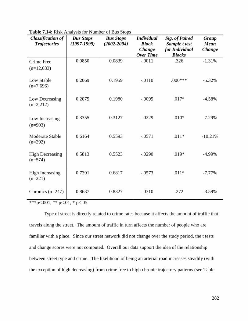
282

Table 7.14: Risk Analysis for Number of Bus Stops

Classification of

Trajectories

Bus Stops

(1997-1999)

Bus Stops

(2002-2004)

Individual

Block

Change

Over Time

Sig. of Paired

Sample t test

for Individual

Blocks

Group

Mean

Change

Crime Free

(n=12,033)

0.0850 0.0839 -.0011 .326 -1.31%

Low Stable

(n=7,696)

0.2069 0.1959 -.0110 .000*** -5.32%

Low Decreasing

(n=2,212)

0.2075 0.1980 -.0095 .017* -4.58%

Low Increasing

(n=903)

0.3355 0.3127 -.0229 .010* -7.29%

Moderate Stable

(n=292)

0.6164 0.5593 -.0571 .011* -10.21%

High Decreasing

(n=574)

0.5813 0.5523 -.0290 .019* -4.99%

High Increasing

(n=221)

0.7391 0.6817 -.0573 .011* -7.77%

Chronics (n=247) 0.8637 0.8327 -.0310 .272 -3.59%

***p<.001, ** p<.01, * p<.05

Type of street is directly related to crime rates because it affects the amount of traffic that

travels along the street. The amount of traffic in turn affects the number of people who are

familiar with a place. Since our street network did not change over the study period, the t tests

and change scores were not computed. Overall our data support the idea of the relationship

between street type and crime. The likelihood of being an arterial road increases steadily (with

the exception of high decreasing) from crime free to high chronic trajectory patterns (see Table


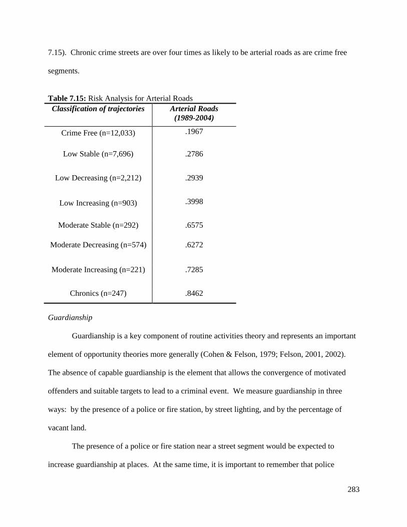
283

7.15). Chronic crime streets are over four times as likely to be arterial roads as are crime free

segments.

Table 7.15: Risk Analysis for Arterial Roads

Classification of trajectories Arterial Roads

(1989-2004)

Crime Free (n=12,033) .1967

Low Stable (n=7,696) .2786

Low Decreasing (n=2,212) .2939

Low Increasing (n=903) .3998

Moderate Stable (n=292) .6575

Moderate Decreasing (n=574) .6272

Moderate Increasing (n=221) .7285

Chronics (n=247) .8462

Guardianship

Guardianship is a key component of routine activities theory and represents an important

element of opportunity theories more generally (Cohen & Felson, 1979; Felson, 2001, 2002).

The absence of capable guardianship is the element that allows the convergence of motivated

offenders and suitable targets to lead to a criminal event. We measure guardianship in three

ways: by the presence of a police or fire station, by street lighting, and by the percentage of

vacant land.

The presence of a police or fire station near a street segment would be expected to

increase guardianship at places. At the same time, it is important to remember that police


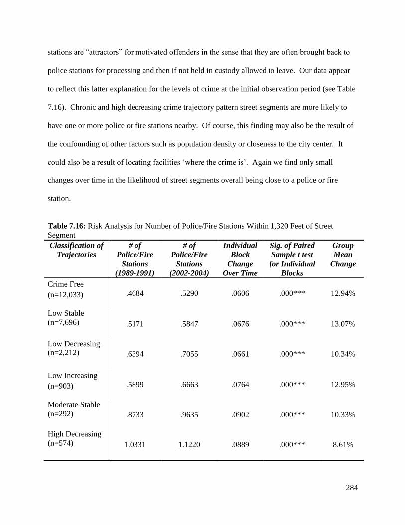
284

stations are “attractors” for motivated offenders in the sense that they are often brought back to

police stations for processing and then if not held in custody allowed to leave. Our data appear

to reflect this latter explanation for the levels of crime at the initial observation period (see Table

7.16). Chronic and high decreasing crime trajectory pattern street segments are more likely to

have one or more police or fire stations nearby. Of course, this finding may also be the result of

the confounding of other factors such as population density or closeness to the city center. It

could also be a result of locating facilities „where the crime is‟. Again we find only small

changes over time in the likelihood of street segments overall being close to a police or fire

station.

Table 7.16: Risk Analysis for Number of Police/Fire Stations Within 1,320 Feet of Street

Segment Classification of

Trajectories

# of

Police/Fire

Stations

(1989-1991)

# of

Police/Fire

Stations

(2002-2004)

Individual

Block

Change

Over Time

Sig. of Paired

Sample t test

for Individual

Blocks

Group

Mean

Change

Crime Free

(n=12,033) .4684 .5290 .0606 .000*** 12.94%

Low Stable

(n=7,696) .5171 .5847 .0676 .000*** 13.07%

Low Decreasing

(n=2,212) .6394 .7055 .0661 .000*** 10.34%

Low Increasing

(n=903) .5899 .6663 .0764 .000*** 12.95%

Moderate Stable

(n=292) .8733 .9635 .0902 .000*** 10.33%

High Decreasing

(n=574)

1.0331 1.1220 .0889 .000*** 8.61%


285

High Increasing

(n=221) .7195 .8220 .1026 .014** 14.26%

Chronics (n=247) 1.0634 1.1390 .0756 .091* 7.11%

***p<.001, ** p<.01, * p<.05

Following the pattern of other variables reflecting guardianship, street lighting as

measured by number of watts on a street has the opposite relationship with crime levels of

trajectory patterns than would be predicted (see Table 7.17). Higher crime rate patterns have

much higher wattage on street segments in the initial observation period. In turn, overall there is

a similar increase in wattage for all of the trajectory patterns across the study period. We think

that these results again are likely to be strongly confounded, which suggests the importance of

looking at the influence of the risk factors we have identified in the context of a multivariate

analytic framework.

Table 7.17: Risk Analysis for Street Lighting (in Watts)

Classification of

Trajectories

Lighting

Initial Value

(1997-1999)

Lighting

Ending Value

(2002-2004)

Individual

Block

Change

Over Time

Sig. of Paired

Sample t test

for Individual

Blocks

Group

Mean

Change

Crime Free

(n=12,033)

212.8447 230.9359 18.0912 .000*** 8.50%

Low Stable

(n=7,696)

448.3398 494.1797 45.8398 .000*** 10.22%

Low Decreasing

(n=2,212)

514.9224 568.8314 53.9090 .000*** 10.47%

Low Increasing

(n=903)

684.7767 771.3843 86.6076 .000*** 12.65%

Moderate Stable

(n=292)

1127.0890 1227.9110 100.8219 .000*** 8.95%


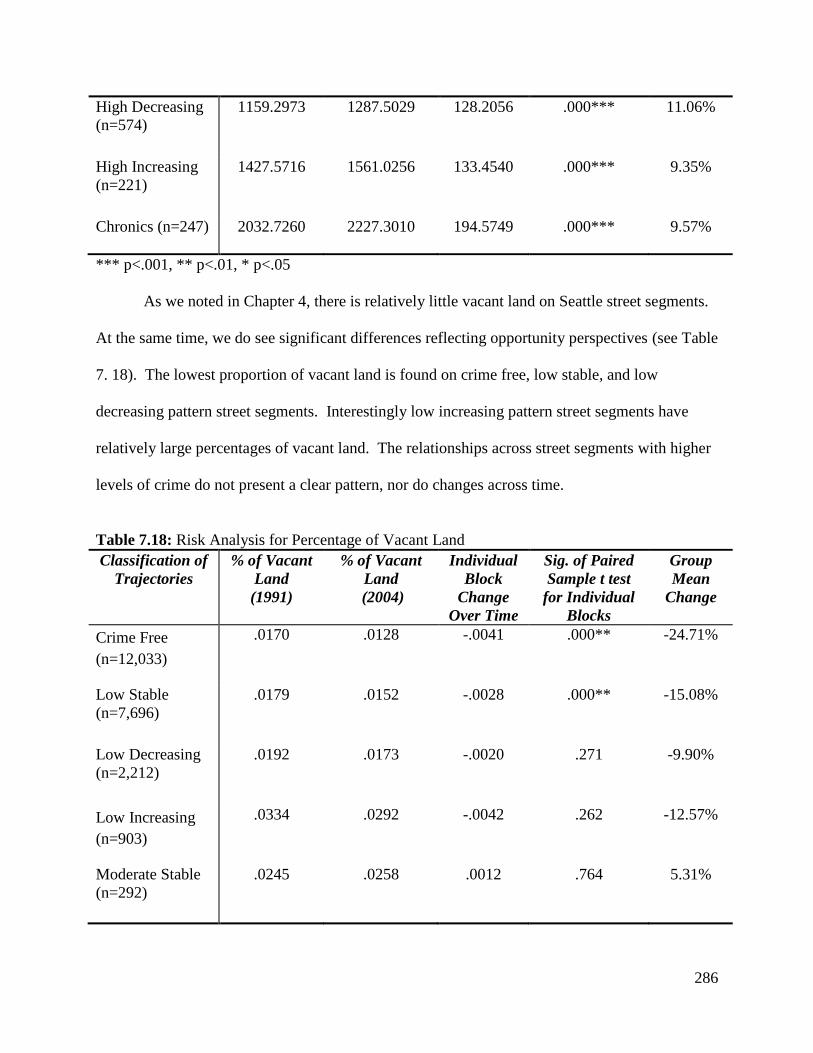
286

High Decreasing

(n=574)

1159.2973 1287.5029 128.2056 .000*** 11.06%

High Increasing

(n=221)

1427.5716 1561.0256 133.4540 .000*** 9.35%

Chronics (n=247) 2032.7260 2227.3010 194.5749 .000*** 9.57%

*** p<.001, ** p<.01, * p<.05

As we noted in Chapter 4, there is relatively little vacant land on Seattle street segments.

At the same time, we do see significant differences reflecting opportunity perspectives (see Table

7. 18). The lowest proportion of vacant land is found on crime free, low stable, and low

decreasing pattern street segments. Interestingly low increasing pattern street segments have

relatively large percentages of vacant land. The relationships across street segments with higher

levels of crime do not present a clear pattern, nor do changes across time.

Table 7.18: Risk Analysis for Percentage of Vacant Land

Classification of

Trajectories

% of Vacant

Land

(1991)

% of Vacant

Land

(2004)

Individual

Block

Change

Over Time

Sig. of Paired

Sample t test

for Individual

Blocks

Group

Mean

Change

Crime Free

(n=12,033)

.0170 .0128 -.0041 .000** -24.71%

Low Stable

(n=7,696)

.0179 .0152 -.0028 .000** -15.08%

Low Decreasing

(n=2,212)

.0192 .0173 -.0020 .271 -9.90%

Low Increasing

(n=903)

.0334 .0292 -.0042 .262 -12.57%

Moderate Stable

(n=292)

.0245 .0258 .0012 .764 5.31%


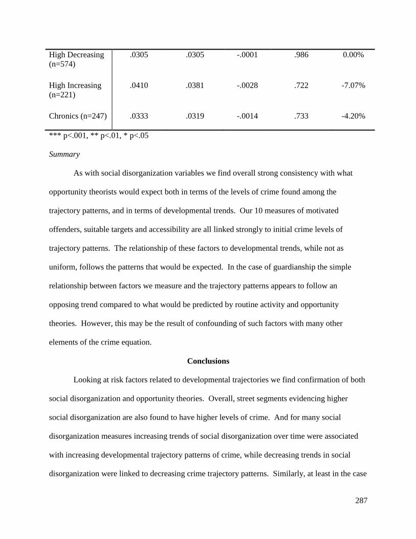
287

High Decreasing

(n=574)

.0305 .0305 -.0001 .986 0.00%

High Increasing

(n=221)

.0410 .0381 -.0028 .722 -7.07%

Chronics (n=247) .0333 .0319 -.0014 .733 -4.20%

*** p<.001, ** p<.01, * p<.05

Summary

As with social disorganization variables we find overall strong consistency with what

opportunity theorists would expect both in terms of the levels of crime found among the

trajectory patterns, and in terms of developmental trends. Our 10 measures of motivated

offenders, suitable targets and accessibility are all linked strongly to initial crime levels of

trajectory patterns. The relationship of these factors to developmental trends, while not as

uniform, follows the patterns that would be expected. In the case of guardianship the simple

relationship between factors we measure and the trajectory patterns appears to follow an

opposing trend compared to what would be predicted by routine activity and opportunity

theories. However, this may be the result of confounding of such factors with many other

elements of the crime equation.

Conclusions

Looking at risk factors related to developmental trajectories we find confirmation of both

social disorganization and opportunity theories. Overall, street segments evidencing higher

social disorganization are also found to have higher levels of crime. And for many social

disorganization measures increasing trends of social disorganization over time were associated

with increasing developmental trajectory patterns of crime, while decreasing trends in social

disorganization were linked to decreasing crime trajectory patterns. Similarly, at least in the case


288

of opportunity measures related to the presence of motivated offenders, the suitability of crime

targets and their accessibility, we found that greater opportunities for crime were found at street

segments in higher rate crime trajectories. In turn, it was often the case that increasing levels of

crime opportunities over time was related to increasing rate crime trajectories, while decreasing

opportunities was related to street segments being found in decreasing crime trajectories.

These data show more generally that the concentrations of characteristics of places that

we identified in Chapters 3 and 4 are strongly related to the concentrations of crime in hot spots

that we identified in Chapter 5. It is not simply that some street segments have greater

concentrations of social disorganization or crime opportunities; it is that such places are also

likely to show concentrations of crime. Hot spots of social disorganization and crime

opportunities are in this sense risk factors for hot spots of crime.

We are not surprised by the strong relationships observed for routine activities measures

in part because such theories have long emphasized the importance of the immediate situation to

crime (see Clark 1980, 1983). But we think the identification of strong relationships between

social disorganization measures and trajectory patterns is a particularly important finding. This

is the first study we know of to examine the salience of social disorganization theory at such a

micro geographic level. The fact that social disorganization variables are related to variability of

crime at street segments suggests, as we argued in Chapter 2, that the street segment forms an

important locus for interaction and identification of people in the city that applies more generally

to the social patterns of these micro places.

At this juncture, we think it interesting that variables reflecting both social

disorganization and opportunity theories are found to be risk factors in understanding trajectories

of crime at place. While these theories are often seen as competing explanations for crime, our


289

analyses so far suggest that they may both contribute to the development of crime at place. But

before we begin to interpret these relationships it is important to examine the salience of both

theoretical perspectives using multivariate models that allow us to control out for the

confounding we have discussed in this chapter, and also to identify which factors (controlling for

others) have the most important relationships to the developmental patterns we have observed in

our data.


290

Chapter 8: Explaining Crime at Place

In the previous chapters our interest was primarily in description. We sought to identify

how crime and other social and contextual characteristics varied across places and to examine

whether the idea of hot spots could be applied not only to crime but also to social disorganization

and opportunity variables that we identified as possible causal factors in understanding the

criminology of place. Our data confirm prior studies that crime is concentrated at small

geographic units of analysis, and that there are distinct developmental trends of crime at place

across time. Our analyses in Chapter 6 confirmed not only that there are developmental trends,

but that there is significant street to street variability in such trends suggesting the inherent

importance of understanding causal processes at the level of street segments. In Chapters 3 and

4 we established not only that crime is clustered at place, but also that there is clustering of social

disorganization and opportunity measures at street segments. There are, simply stated, hot spots

of crime opportunities and hot spots of social disorganization at the very micro geographic level

of street segments.

In Chapter 7 we provided an initial portrait of how the variability of social

disorganization and opportunity factors and that of crime at place are related. Our description

provided what is often called a “risk analysis” of factors related to crime at place. We identified

clearly that crime at place is strongly related to the two main theoretical perspectives we have

identified. Hot spots of social disorganization and crime opportunities do overlap with hot spots

of crime. But in this chapter, we want to go beyond this simple description of the relationship

between these perspectives and crime to develop an overall model of explanation for crime at

place. When we draw these variables into a single overall model that describes membership in


291

the trajectory patterns we have identified, do we provide a powerful explanation of the

distribution of crime at street segments? In a context in which these perspectives and the

individual measures they represent are used to understand trajectory membership, do we

continue to find that both perspectives provide important information about crime at place?

While our work so far has established the relevance of both social disorganization and

crime opportunities at places in identifying the developmental patterns of crime at place, we have

not taken into account the fact that the variables we examine are themselves strongly related and

accordingly, simple descriptive patterns may be misleading.1 Our analyses so far have shown

that specific measures reflecting social disorganization and crime opportunities vary directly

with crime trajectories. But we have not yet examined which variables continue to maintain

strong and independent effects when they are examined in the context of a larger model that

distinguishes factors that predict trajectory pattern membership.

This is our goal in the present chapter, in which we provide a broad quantitative

assessment of the factors that explain developmental crime patterns at places. We focus on two

separate types of analyses. In the first and main analysis, we ask whether specific measures are

relevant for understanding trajectory patterns generally. In this case we use a type of statistical

analysis called “multinomial logistic regression” (Begg & Gray, 1984; Long, 1997). Using

logistic regression approaches, we also examine separately trajectory pattern membership for two

specific comparisons: high decreasing versus high increasing trajectories; and low increasing

1 This problem is often stated in terms of “confounding” of effects of independent variables (Greenland et al., 1999;

Meinert, 1986; Robins, 1989; Weisburd & Britt, 2007). When two variables are strongly related a bivariate analysis

will not allow the researcher to distinguish between the independent effect of the variable of interest from the effect

observed, which includes that effect as well as a spurious component due to the correlation with the third variable.

For example, in measuring the effect of a specific treatment for drug abuse, the researcher must account for the

effect of “creaming” of subjects (Larzelere et al., 2004; Miller et al., 2004; Rhodes et al., 2001). A simple bivariate

analysis showing that “treated” individuals did better than untreated offenders would likely overestimate the

influence of treatment since it does not take into account the possible explanation that “volunteers” who chose

treatment may be predisposed to doing better. A model that examined treatment while controlling for

“predispositions” for improvement in outcomes would take this confounding into account.


292

versus low decreasing trajectories. We think that these comparisons provide a particularly

important context for assessing the impact of social disorganization and opportunity variables in

understanding developmental patterns of crime at street segments.

An Overall Model for Explaining Developmental Trajectories of Crime at Place

Our dependent variable in these analyses is trajectory classification, which includes the

eight trajectory patterns defined in Chapter 5: crime free, low stable, low decreasing, low

increasing, moderate stable, high decreasing, high increasing and chronic trajectories. Our

statistical problem is that we want to develop a model that would simultaneously allow us to

assess the placement of street segments in each of these patterns. Traditional statistical

approaches to categorical or nominal level dependent variables have generally constrained the

dependent variable to two choices (Agresti, 1996; Long, 1997; Reynolds, 1977). Accordingly,

we might have conducted a separate statistical analysis for each of the possible comparisons in

our study (e.g. crime free versus low stable, crime free versus low decreasing, etc.). But our

main question is whether the variables examined impact upon trajectory pattern membership, not

whether they predict membership in one specific pattern as compared with another. Moreover, if

we take this approach then each of our comparisons would be based on different samples, and

those samples would have varied a good deal because our trajectory patterns range in size from

about 200 to 12,000 street segments. The statistical problem here is that the varying sample sizes

would then result in incorrect tests of statistical significance levels.2 Multinomial logistic

regression provides a straightforward solution to these problems because it allows a simultaneous

examination of the different possible comparisons (Agresti, 1996; Begg & Gray, 1984; Long,

1997; Peng & Nichols, 2003; Weisburd & Britt, 2007). It provides both an overall assessment of

2 This is because the standard errors of the estimates would be over or underestimated depending on the specific

samples used (see Weisburd & Britt, 2007)


293

the statistical importance of the measures examined in predicting trajectory pattern, as well as a

specific set of coefficients for understanding the varying effects of those factors across different

sets of comparisons.

In defining our model we included all of the independent variables examined in Chapter

7. Table 8.1 provides a basic description of those variables including a definition of how they

are measured in the multinomial regression analysis. We also include two new sets of variables

that we thought critical for developing an understanding of developmental trajectory patterns.

The first are simply time varying measures that take characteristics that we have measured over

time. For example in the case of unsupervised juveniles (drawn from the social disorganization

perspective) we created a variable that represents the change in the number of truant juveniles

between the first three years of measurement (1992-1994) and the last three years (2002-2004).

This is often called a difference of moving averages (Baller et al., 2000). Change measures are

included in the model for all variables which we have sufficient data to compute a valid measure

of change over time (see Table 8.1). We also created a spatial lag term which reflects the

average number of crimes on street segments within one quarter of a mile of the segment

examined. A spatial lag term (Anselin, 1988; Anselin et al., 2000) is a variable that averages the

neighboring values of a location (the value of each neighboring location is multiplied by the

spatial weight and then the products are summed). Spatial lag terms allow us to take into

account in our model that some of the relationships observed may be affected by the crime levels

on nearby street segments (Rosenfeld et al., 2007). Our spatial lag term captures the change in

crime rates for the neighboring streets (i.e., within one quarter of a mile) between the first and

last three years of observation. Finally, we include a measure of the exact length of the street

segments. This allows us to control for the variation in density that might occur when 100


294

residents are distributed along a 100 foot street segment versus when 100 residents live on a

5,000 foot street segment.

Table 8.1: Description of included variables and mean and standard deviation for both starting

values and change variables (when applicable)

Variable Name Description Beginning

Mean (S.D.)

Change

Mean (S.D.)

Social Disorganization

Property Value Residential property values

(combination of weighed ranking of single

family housing and multi-family housing of a

given street)

4.491

(3.608)

N/A

Mixed Land

Use

Mixed Land Use

(dichotomous variable, representing whether the

place has mixture of between 25 percent and75

percent of residential and other types of land

use)

.04

(.207)

N/A

Physical

Disorder

The total number of physical disorder incidents

(Sum of the incidents on each street)

.112

(.379)

.005

(.410)

Housing

Assistance

Combination of public housing and Section 8

voucher distribution

(Sum the number of unit of public housing and

the number of Section 8 vouchers given out on a

street)

.375

(4.615)

N/A

Truant Juveniles Total number of truant juveniles .244

(.834)

-.088

(.691)

Racial

Heterogeneity

Racial heterogeneity of public school students

(The probabilities of each racial group to

encounter another out-group member were

computed and averaged to form an overall racial

heterogeneity index)

.017

(.038)

.001

(.036)

% Active voters Percent of active voters out of all the registered

voters

.375

(.317)

N/A

Urbanization Distance of a street to the center of city (The 255.712 N/A


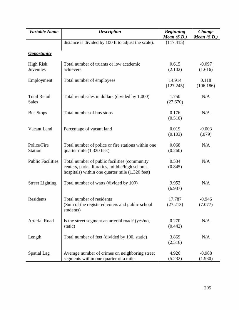
295

Variable Name Description Beginning

Mean (S.D.)

Change

Mean (S.D.)

distance is divided by 100 ft to adjust the scale).

(117.415)

Opportunity

High Risk

Juveniles

Total number of truants or low academic

achievers

0.615

(2.102)

-0.097

(1.616)

Employment Total number of employees 14.914

(127.245)

0.118

(106.186)

Total Retail

Sales

Total retail sales in dollars (divided by 1,000)

1.750

(27.670)

N/A

Bus Stops Total number of bus stops

0.176

(0.510)

N/A

Vacant Land Percentage of vacant land

0.019

(0.103)

-0.003

(.079)

Police/Fire

Station

Total number of police or fire stations within one

quarter mile (1,320 feet)

0.068

(0.260)

N/A

Public Facilities Total number of public facilities (community

centers, parks, libraries, middle/high schools,

hospitals) within one quarter mile (1,320 feet)

0.534

(0.845)

N/A

Street Lighting Total number of watts (divided by 100)

3.952

(6.937)

N/A

Residents Total number of residents

(Sum of the registered voters and public school

students)

17.787

(27.213)

-0.946

(7.077)

Arterial Road Is the street segment an arterial road? (yes/no,

static)

0.270

(0.442)

N/A

Length Total number of feet (divided by 100, static)

3.869

(2.516)

N/A

Spatial Lag Average number of crimes on neighboring street

segments within one quarter of a mile.

4.926

(5.232)

-0.988

(1.930)


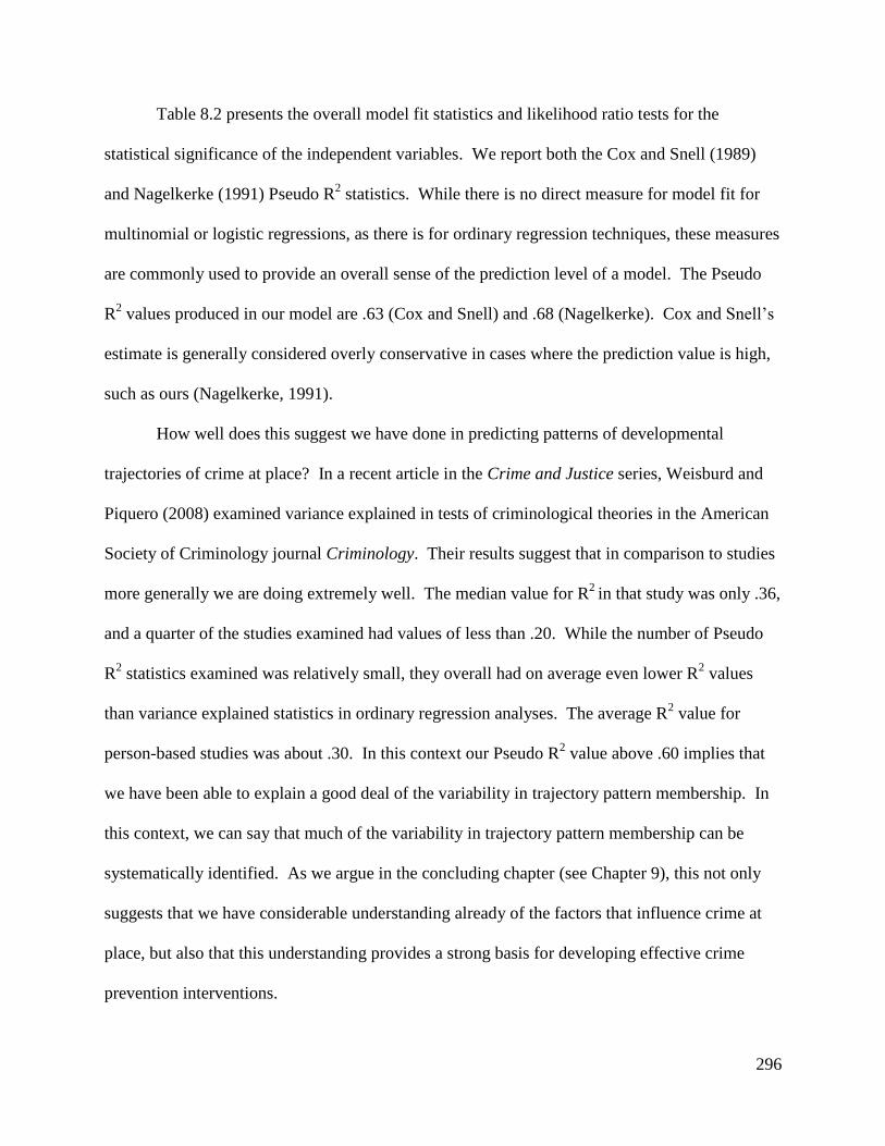
296

Table 8.2 presents the overall model fit statistics and likelihood ratio tests for the

statistical significance of the independent variables. We report both the Cox and Snell (1989)

and Nagelkerke (1991) Pseudo R2 statistics. While there is no direct measure for model fit for

multinomial or logistic regressions, as there is for ordinary regression techniques, these measures

are commonly used to provide an overall sense of the prediction level of a model. The Pseudo

R2 values produced in our model are .63 (Cox and Snell) and .68 (Nagelkerke). Cox and Snell’s

estimate is generally considered overly conservative in cases where the prediction value is high,

such as ours (Nagelkerke, 1991).

How well does this suggest we have done in predicting patterns of developmental

trajectories of crime at place? In a recent article in the Crime and Justice series, Weisburd and

Piquero (2008) examined variance explained in tests of criminological theories in the American

Society of Criminology journal Criminology. Their results suggest that in comparison to studies

more generally we are doing extremely well. The median value for R2

in that study was only .36,

and a quarter of the studies examined had values of less than .20. While the number of Pseudo

R2 statistics examined was relatively small, they overall had on average even lower R

2 values

than variance explained statistics in ordinary regression analyses. The average R2 value for

person-based studies was about .30. In this context our Pseudo R2 value above .60 implies that

we have been able to explain a good deal of the variability in trajectory pattern membership. In

this context, we can say that much of the variability in trajectory pattern membership can be

systematically identified. As we argue in the concluding chapter (see Chapter 9), this not only

suggests that we have considerable understanding already of the factors that influence crime at

place, but also that this understanding provides a strong basis for developing effective crime

prevention interventions.


297

It is interesting in this regard to compare the overall degree of explanation of the two

theoretical perspectives that we have used to understand crime at place in this report.

Accordingly, we ran separate regressions which included only the social disorganization and

only the opportunity measures. While these results should be viewed with some caution because

they do not account for the possibility that variance of one perspective is being spuriously

accounted for by related variables of another perspective, they suggest again that both

perspectives are providing a strong explanation for developmental patterns of crime at place.

Both perspectives provide Nagelkerke R2 values of above .50. While the opportunity perspective

provides a larger value (.66 versus .51) we do not think that the differences allow us to draw

strong conclusions.

Table 8.2 also suggests that the individual variables examined continue to maintain

significant relationships with trajectory pattern membership in this multivariate context. An

overall test of significance for each measure on the general allocation of street segments into

trajectory patterns is provided by the Likelihood Ratio Test (see Weisburd & Britt, 2007). The

first observation to be drawn from this table is that the individual measures overall have a

strongly statistically significant impact on membership in trajectory groups. Irrespective of

which trajectory, they help us to distinguish the choice of being in one of the eight trajectory

patterns.

Nearly all of the measures examined are statistically significant at the .001 level,

suggesting that the observed effects are not due simply to chance. In this regard it is important to

note that the very large overall sample size of our study means that even relatively smaller

variable effects observed in our analyses can be distinguished from random noise in the

distributions examined (Weisburd & Britt, 2007). At the same time there are specific variables


298

that appear to have little or no impact on the selection into a specific developmental trajectory

pattern. Following our bivariate results, mixed land use is not a significant factor in

understanding trajectory pattern membership. We suggested in Chapter 7 that this might be the

case because of our conservative definition of mixed land. While racial heterogeneity, a

component of the social disorganization perspective, had strong and significant bivariate

relationships with trajectory group pattern, when we examine this variable in a model which

controls both for other social disorganization measures and measures of criminal opportunities it

is not statistically significant.3 Total retail business sales and whether a street segment is located

close to a fire or police station, elements of the opportunity perspective, also do not have

statistically significant impacts in our model.

But the important story here is the statistical significance of most of the variables

examined, even in this multivariate context in which many factors are controlled for

simultaneously. This suggests again that social disorganization and opportunity factors are both

very important in understanding why crime develops in specific street segments. Importantly,

the effects observed remain despite our taking into account spatial lag terms for crime levels

which would indicate and distinguish larger area effects. While the spatial lag terms have very

high levels of statistical significance, they do not minimize the effects of social disorganization

and opportunity measures at the street segment level.

3 One possible explanation for the loss of statistical significance would be multicollinearity or model instability. We

ran several sensitivity analyses to explore the potential confounding effects. For example, residential population and

racial heterogeneity are highly correlated and the inclusion of residential population shared the variability originally

explained by racial heterogeneity. This makes sense as both variables were constructed (partially) using data

collected from public school students. The shared data source explains the possible multicollinearity problem;

however, the findings also show the confounding nature of certain variables across both theoretical perspectives.


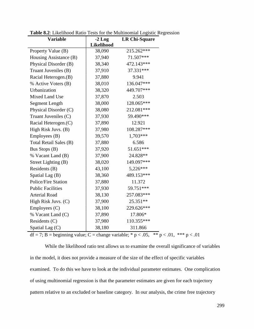
299

Table 8.2: Likelihood Ratio Tests for the Multinomial Logistic Regression

Variable -2 Log

Likelihood

LR Chi-Square

Property Value (B) 38,090 215.262***

Housing Assistance (B) 37,940 71.507***

Physical Disorder (B) 38,340 472.143***

Truant Juveniles (B) 37,910 37.331***

Racial Heterogen.(B) 37,880 9.941

% Active Voters (B) 38,010 136.047***

Urbanization 38,320 449.707***

Mixed Land Use 37,870 2.503

Segment Length 38,000 128.065***

Physical Disorder (C) 38,080 212.081***

Truant Juveniles (C) 37,930 59.490***

Racial Heterogen.(C) 37,890 12.921

High Risk Juvs. (B) 37,980 108.287***

Employees (B) 39,570 1,703***

Total Retail Sales (B) 37,880 6.586

Bus Stops (B) 37,920 51.651***

% Vacant Land (B) 37,900 24.828**

Street Lighting (B) 38,020 149.097***

Residents (B) 43,100 5,226***

Spatial Lag (B) 38,360 489.153***

Police/Fire Station 37,880 11.372

Public Facilities 37,930 59.751***

Arterial Road 38,130 257.083***

High Risk Juvs. (C) 37,900 25.351**

Employees (C) 38,100 229.626***

% Vacant Land (C) 37,890 17.806*

Residents (C) 37,980 110.355***

Spatial Lag (C) 38,180 311.866

df = 7; B = beginning value; C = change variable; * p < .05, ** p < .01, *** p < .01

While the likelihood ratio test allows us to examine the overall significance of variables

in the model, it does not provide a measure of the size of the effect of specific variables

examined. To do this we have to look at the individual parameter estimates. One complication

of using multinomial regression is that the parameter estimates are given for each trajectory

pattern relative to an excluded or baseline category. In our analysis, the crime free trajectory


300

pattern is the reference group or excluded category both because it includes the largest number of

cases, and thus provides statistical stability to the overall model, and because it provides a logical

comparison group in understanding the analysis. In this context we are comparing all of the

trajectory groups with some criminal activity to a pattern that is distinguished by being almost

crime free during the observation period. Table 8.3 lists the odds ratios for each of the seven

other trajectory patterns relative to the excluded category. Following the results of our

likelihood ratio tests we do not interpret parameter estimates for non-significant variables.4

4 Following our approach of first identifying whether the overall effect of a variable is significant in determining

trajectory pattern membership, we assume that the individual comparisons cannot be reliably interpreted when the

likelihood test is non-significant.


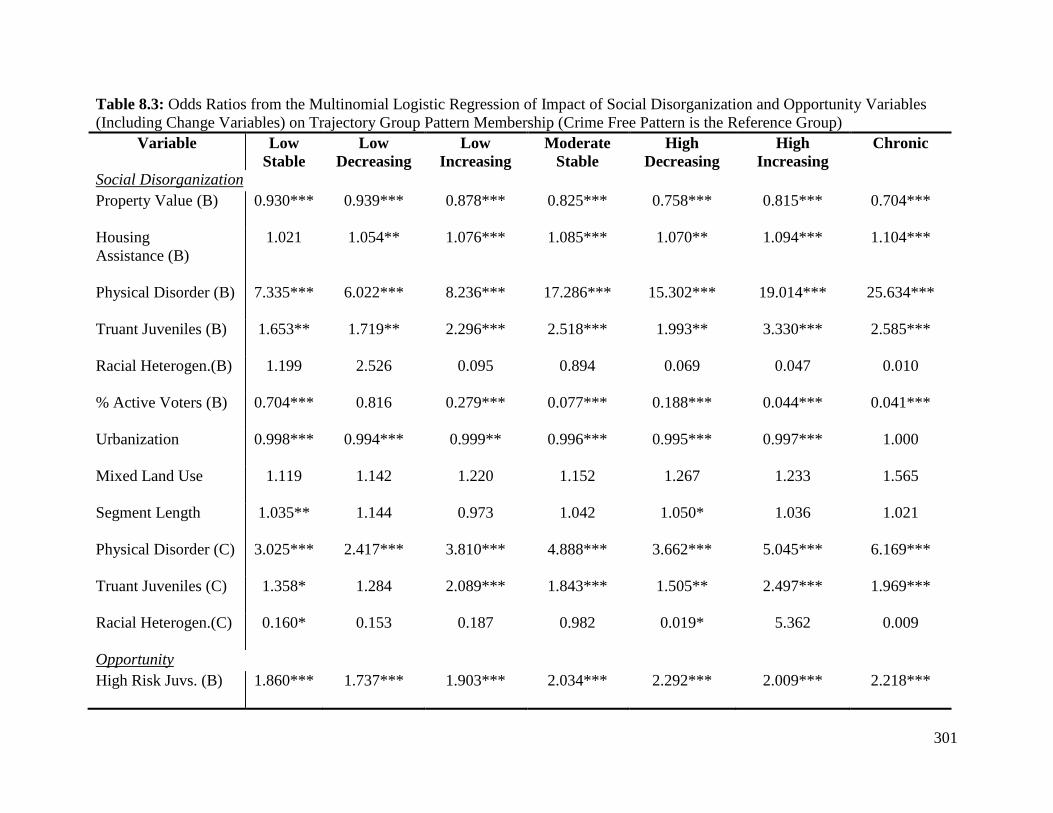
301

Table 8.3: Odds Ratios from the Multinomial Logistic Regression of Impact of Social Disorganization and Opportunity Variables

(Including Change Variables) on Trajectory Group Pattern Membership (Crime Free Pattern is the Reference Group)

Variable Low

Stable

Low

Decreasing

Low

Increasing

Moderate

Stable

High

Decreasing

High

Increasing

Chronic


Property Value (B)

0.930*** 0.939*** 0.878*** 0.825*** 0.758*** 0.815*** 0.704***

Housing

Assistance (B)

1.021 1.054** 1.076*** 1.085*** 1.070** 1.094*** 1.104***

Physical Disorder (B)

7.335*** 6.022*** 8.236*** 17.286*** 15.302*** 19.014*** 25.634***

Truant Juveniles (B)

1.653** 1.719** 2.296*** 2.518*** 1.993** 3.330*** 2.585***

Racial Heterogen.(B)

1.199 2.526 0.095 0.894 0.069 0.047 0.010

% Active Voters (B)

0.704*** 0.816 0.279*** 0.077*** 0.188*** 0.044*** 0.041***

Urbanization

0.998*** 0.994*** 0.999** 0.996*** 0.995*** 0.997*** 1.000

Mixed Land Use

1.119 1.142 1.220 1.152 1.267 1.233 1.565

Segment Length

1.035** 1.144 0.973 1.042 1.050* 1.036 1.021

Physical Disorder (C)

3.025*** 2.417*** 3.810*** 4.888*** 3.662*** 5.045*** 6.169***

Truant Juveniles (C)

1.358* 1.284 2.089*** 1.843*** 1.505** 2.497*** 1.969***

Racial Heterogen.(C)

0.160* 0.153 0.187 0.982 0.019* 5.362 0.009

Opportunity

High Risk Juvs. (B)

1.860*** 1.737*** 1.903*** 2.034*** 2.292*** 2.009*** 2.218***


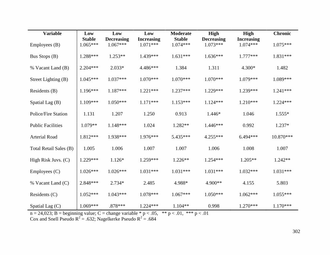
302

Variable Low

Stable

Low

Decreasing

Low

Increasing

Moderate

Stable

High

Decreasing

High

Increasing

Chronic

Employees (B)

1.065*** 1.067*** 1.071*** 1.074*** 1.073*** 1.074*** 1.075***

Bus Stops (B)

1.288*** 1.253** 1.439*** 1.631*** 1.636*** 1.777*** 1.831***

% Vacant Land (B)

2.204*** 2.033* 4.486*** 1.384 1.311 4.300* 1.482

Street Lighting (B)

1.045*** 1.037*** 1.070*** 1.070*** 1.070*** 1.079*** 1.089***

Residents (B)

1.196*** 1.187*** 1.221*** 1.237*** 1.229*** 1.239*** 1.241***

Spatial Lag (B)

1.109*** 1.050*** 1.171*** 1.153*** 1.124*** 1.210*** 1.224***

Police/Fire Station

1.131 1.207 1.250 0.913 1.446* 1.046 1.555*

Public Facilities

1.079** 1.148*** 1.024 1.282** 1.446*** 0.992 1.237*

Arterial Road

1.812*** 1.938*** 1.976*** 5.435*** 4.255*** 6.494*** 10.870***

Total Retail Sales (B)

1.005 1.006 1.007 1.007 1.006 1.008 1.007

High Risk Juvs. (C)

1.229*** 1.126* 1.259*** 1.226** 1.254*** 1.205** 1.242**

Employees (C)

1.026*** 1.026*** 1.031*** 1.031*** 1.031*** 1.032*** 1.031***

% Vacant Land (C)

2.848*** 2.734* 2.485 4.988* 4.900** 4.155 5.803

Residents (C)

1.052*** 1.043*** 1.078*** 1.067*** 1.050*** 1.062*** 1.055***

Spatial Lag (C) 1.069*** .878*** 1.224*** 1.104** 0.998 1.270*** 1.170***

n = 24,023; B = beginning value; C = change variable * p < .05, ** p < .01, *** p < .01

Cox and Snell Pseudo R2 = .632; Nagelkerke Pseudo R

2 = .684


303

Social Disorganization Variables

We identified a series of structural variables reflecting social disorganization in

earlier chapters. A key measure of this dimension is SES. We have two measures of

SES, residential property values and housing assistance. Residential property value

varies in influence across the seven comparisons with crime free trajectories, though the

direction of change is consistent. For a unit increase in rank in residential property value

(in a scale ranging from 0 to 10) there is between a 6 and 30 percent decrease in the

likelihood of being in one of the seven examined trajectory patterns as opposed to the

crime free trajectory pattern. The largest effect is found in the chronic trajectory group

and the smallest effect in the low stable pattern. The results here show a strong and

consistent relationship for SES with higher level crime trajectories showing the largest

differences, and accordingly reinforce the idea that SES is an important part of

understanding crime at place, even after we control for opportunity factors that relate to

SES such as employment, land use and number of residents on the street segment.

Housing assistance also reflects SES at the street segment. Our measure here

combined units of public housing and the number of Section 8 vouchers. While most

street segments had very low values for this measure, a few street segments (i.e. those in

public housing communities) had very high values (see Chapter 4). Again, the direction

of change is similar across the comparisons, and the magnitudes follow what social

disorganization theory would predict. A unit increase in public assistance for the two

lowest crime trajectory patterns leads to an increase of between 2 and 5 percent in the

odds of trajectory membership in that pattern as opposed to the crime free pattern. For

the chronic trajectory pattern the increase is 10 percent.


304

Another key structural variable reflecting social disorganization is mixed land

use. We have already noted that mixed land use does not significantly impact trajectory

membership, though its impacts are consistent and in the expected direction for the

comparisons with crime free segments. Racial heterogeneity also was not found to be

statistically significant in this multivariate model though it was highly significant in our

risk analysis. Indeed, in this case the effects vary in direction and do not follow the

pattern that would be expected by social disorganization theory. It seems reasonable to

conclude from this that elements of social disorganization reflecting variability in land

use or population are not important predictors of developmental trajectories of crime at

place once other variables reflecting social disorganization and criminal opportunities are

taken into account.

Another structural component of social disorganization theories--distance from

the city center--does have a strong and significant impact upon trajectory pattern

membership. A relatively short one hundred foot increase in distance from the city center

leads to a less than one percent decrease in the likelihood of being in the low, moderate or

high trajectory groups. But if we examine, for example, the impact of a half mile

distance, we can get a sense for the effect of this factor. Here, being 2,500 feet from the

city center decreases the likelihood of being in the high decreasing patterns as opposed to

the crime free group pattern by fully 11.8 percent. The effects here, however, are not

fully consistent. There is no significant effect of distance to the city center in

distinguishing the chronic trajectory group from the no crime pattern. This suggests that

while overall the crime free pattern segments are more distant from the city center than

other trajectory patterns, it is not a distinguishing characteristic for chronic trajectory


305

street segments. This reinforces our observation earlier in the report that hot spots of

crime are spread throughout the city. Moreover, while the low and high crime trajectory

patterns are significantly different from the crime free trajectory pattern, there is not a

clear pattern among the low and high crime trajectory groupings.

Physical disorder is the most direct indicator of social disorganization, and its

relationship to developmental trajectories of crime at street segments is very strong. The

smallest coefficients are found for the low crime trajectory patterns and the largest for the

higher crime trajectory patterns. But it is important to note the magnitude of effects.

Even for the low stable trajectory pattern, each additional report of physical disorder

leads to a sevenfold increase in the odds of being in the low stable as opposed to the

crime free trajectory pattern. In our sample a street segment is 25 times more likely to be

in the chronic trajectory group as opposed to the crime free pattern, if it has an additional

physical disorder incident. Change in physical disorder is also strongly related to

trajectory group pattern membership with increases in incidents associated with higher

likelihoods of being in the higher crime rate trajectory patterns.

Mediating variables that reflect the ability of communities, or in this case street

segments, to regulate behavior are also important in the social organization framework.

A key variable in this context is truant juveniles. An additional truant juvenile on a street

segment significantly increases the likelihood of being in any of the crime trajectory

patterns as compared with the crime free trajectory pattern. Increased truancy has the

largest impact in the high increasing trajectory pattern and the chronic trajectory group

where an additional truant juvenile resident increases the likelihood of group membership

by 2 ½ to more than 3 times. The change variable also influences the likelihood of group


306

membership, and suggests a strong relationship between increasing truancy and

increasing crime, though we will examine this finding more directly in the next sections.

We used percent of active voters as an indicator of collective efficacy at the street

segment level. Overall, the measure follows what would be expected from social

disorganization theory with the largest impacts being found in the chronic trajectory

group and high increasing trajectory pattern. At the same time, this measure is not

significant in making comparisons between the low decreasing and crime free patterns.

The size of the effect is overall very meaningful. In the case where there are no active

voters as contrasted with a situation where all eligible residents are active voters, the

probability of being in the chronic trajectory group compared with the no crime trajectory

pattern decreases almost 96 percent.

Opportunity and Routine Activities

Accessibility of an area is generally seen to increase opportunities for crime

(Levine & Wachs, 1986; Rengert et al., 2005). We have two main measures of

accessibility: the number of bus stops on a street and whether the street is an arterial road.

Our data strongly suggest that bus stops are associated with more crime. Even in the low

decreasing trajectory group (which shows the smallest effect) more bus stops increase the

likelihood of being in that trajectory pattern as contrasted with the crime free trajectory

pattern. For each bus stop there is an increase of about 25 percent in the odds of

membership in the low stable trajectory pattern. The increase in the odds for a bus stop

in the chronic group is more than 80 percent. The other groups fall somewhere between,

overall following the theory that bus stops create greater accessibility and increase the

likelihood of crime.


307

Additionally, being on an arterial road increases crime risks. Arterial streets are

more than 10 times more likely to be in the chronic group as contrasted with the crime

free trajectory pattern. Arterial roads are about twice as likely to be in the low rate

trajectory patterns as in the crime free trajectory pattern. Overall this indicates that crime

is higher on arterial roads and the impact is much more significant in higher crime

trajectories.

A key component of opportunity theories of crime is the concept of motivated

offenders (Cohen, 1981; Cohen & Felson, 1979). In our analysis we used the total

number of truants and low academic achievers on a block to reflect “high risk” juveniles,

or potential motivated offenders. The distribution of this measure, though highly

correlated with the truant students measure used to reflect the social disorganization

perspective, captures in our view a more general measure of “motivated offenders.” The

variable has strong impacts on trajectory pattern membership and follows overall

expected patterns. For the moderate, high and chronic trajectory patterns, each additional

high risk juvenile doubles the odds of being in those groups as contrasted with the no

crime trajectory pattern. Change in high risk juveniles over time also distinguishes

between the crime trajectories and the crime free street segments. However, there do not

appear to be strong differences in effects across the crime trajectory patterns.

A second component of routine activities is the number of suitable targets. In this

regard, the larger the number of employees the less likely a segment is to be in the crime

free trajectory pattern. The effects are largest in the high crime patterns, where an

additional employee on a block increases the likelihood of being in high or chronic

trajectory patterns as contrasted with the crime free trajectory pattern by about 7 ½


308

percent. It should be noted that the number of employees on street segments varies

between none and over 7,000. The change variable also distinguishes the crime free

trajectory pattern from others.

Looking at residential population our findings are reinforced. The effects here are

very large, with fewer residents being associated with an increased likelihood of

membership in the crime free trajectory pattern. An additional resident on a block

increases the odds of being in the chronic group as opposed to the crime free pattern by

almost 25 percent. Clearly residential population is a critical factor in explaining crime at

street segments. Even in the low stable trajectory pattern, an additional resident increases

the odds by almost 20 percent. Again the change variable follows a similar pattern,

though in this case comparisons between the increasing and decreasing trajectory patterns

are particularly interesting. While the increase of one resident over time leads to a four

percent greater likelihood of being in the low decreasing trajectory pattern as contrasted

with the crime free trajectory pattern, it leads to almost an eight percent increase in the

low increasing trajectory pattern. Less dramatically but in the same direction, the value is

five percent in the high decreasing pattern versus six percent in the high increasing

trajectory pattern.

As noted earlier, retail business sales as a measure of suitable targets does not

have a statistically significant impact in our model, though it follows the expected pattern

in our data with higher sales associated with membership in the crime trajectory patterns

as opposed to the crime free trajectory pattern. The presence of public facilities within a

quarter mile of a street segment decreases the probability of being in the crime free

trajectory pattern. The largest impact is found in the chronic trajectory group, where


309

having a public facility such as a community center, park, library, middle and high

school, or hospital, within a quarter mile increases the likelihood of being in that group

by about 25 percent. In our data, it is difficult to identify whether such facilities

influence the number of suitable targets or motivated offenders, and indeed this measure

may represent both constructs. Interestingly, this measure was not significant for both

the low increasing and high increasing trajectory pattern comparisons.

As we noted in Chapter 7, the presence of a police station or fire station within a

quarter of a mile does not significantly increase guardianship and decrease crime in our

data. Importantly, the multivariate analysis suggests that the finding of increasing crime

with the presence of fire and police stations in Chapter 7 is spurious. However, street

lighting continues to have a strong and positive effect on developmental trajectories.

Here we find that an increase in wattage on a street increases the likelihood of

membership in all of the trajectory patterns as contrasted with the crime free trajectory

pattern. The largest effects are found in the high increasing trajectory pattern and chronic

trajectory group where an increase of one hundred watts of light increases the likelihood

of being in those groups by eight to nine percent. Again, we are faced with the finding

that more street lighting appears to increase the likelihood of membership in higher crime

trajectories. And this finding holds true when controlling for the full range of variables

we have included in our model. Of course, we cannot distinguish whether lighting was

increased in response to a prior crime problem. It may also be that the long-held

assumption that street lighting reduces crime is spurious or that the relationship of

lighting to crime is too complex to be accurately parsed using total crime over both

daytime and nighttime hours.


310

Vacant land also suggests a lack of guardianship. While the proportion of vacant

land in Seattle street segments is relatively low, the proportion of vacant land does have

an important impact on developmental crime trajectories. However, the largest

influences are found in the low crime trajectory patterns and not in the higher crime

trajectory patterns. This suggests a non-linear relationship in which street segments with

higher proportions of vacant land are more likely to have crime, but they are not as likely

to be in the highest rate crime trajectory patterns. Perhaps this reflects a balance between

guardianship and crime opportunities. At some level, when most of the land is vacant

there may be less guardianship, but there also may be fewer opportunities for crime. It is

interesting however, that when we turn to the change variable, we do find that increases

in vacant land are associated more strongly with membership in the highest crime rate

trajectory patterns.

Comparing Increasing and Decreasing Crime Trajectories

As we noted in Chapter 7, the low decreasing and increasing, and high decreasing

and increasing trajectory patterns provide particularly interesting comparisons which

allow us to more directly examine change variables. In the multinomial logistic

regression we compared all trajectory patterns to the crime free pattern and provided an

overall assessment of the importance of social disorganization and opportunity variables

in explaining developmental trajectories of crime at place. We want to turn here to the

specific question of which factors distinguish increasing from decreasing trajectory

patterns. Accordingly, we present two simple logistic regression analyses which compare

low increasing/decreasing trajectory patterns, and high increasing/decreasing trajectory

patterns. As illustrated in Tables 8.4 and 8.5 these models appear to fit less strongly to


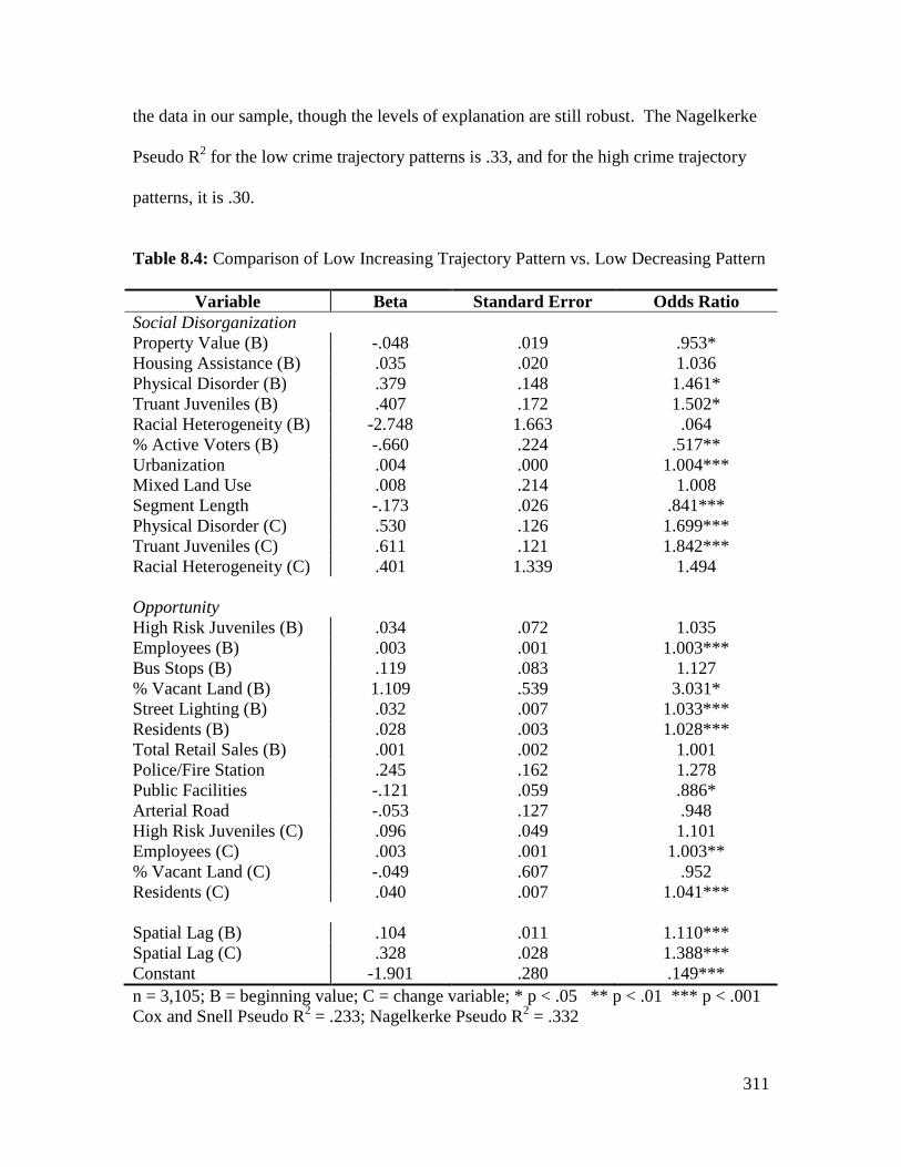
311

the data in our sample, though the levels of explanation are still robust. The Nagelkerke

Pseudo R2 for the low crime trajectory patterns is .33, and for the high crime trajectory

patterns, it is .30.

Table 8.4: Comparison of Low Increasing Trajectory Pattern vs. Low Decreasing Pattern

Variable Beta Standard Error Odds Ratio


Property Value (B) -.048 .019 .953*

Housing Assistance (B) .035 .020 1.036

Physical Disorder (B) .379 .148 1.461*

Truant Juveniles (B) .407 .172 1.502*

Racial Heterogeneity (B) -2.748 1.663 .064

% Active Voters (B) -.660 .224 .517**

Urbanization .004 .000 1.004***

Mixed Land Use .008 .214 1.008

Segment Length -.173 .026 .841***

Physical Disorder (C) .530 .126 1.699***

Truant Juveniles (C) .611 .121 1.842***

Racial Heterogeneity (C) .401 1.339 1.494

Opportunity

High Risk Juveniles (B) .034 .072 1.035

Employees (B) .003 .001 1.003***

Bus Stops (B) .119 .083 1.127

% Vacant Land (B) 1.109 .539 3.031*

Street Lighting (B) .032 .007 1.033***

Residents (B) .028 .003 1.028***

Total Retail Sales (B) .001 .002 1.001

Police/Fire Station .245 .162 1.278

Public Facilities -.121 .059 .886*

Arterial Road -.053 .127 .948

High Risk Juveniles (C) .096 .049 1.101

Employees (C) .003 .001 1.003**

% Vacant Land (C) -.049 .607 .952

Residents (C) .040 .007 1.041***

Spatial Lag (B) .104 .011 1.110***

Spatial Lag (C) .328 .028 1.388***

Constant -1.901 .280 .149***

n = 3,105; B = beginning value; C = change variable; * p < .05 ** p < .01 *** p < .001


2 = .332


312

Table 8.5: Comparison of High Increasing Trajectory Pattern vs. High Decreasing

Pattern

Variable Beta Standard Error Odds Ratio


Property Value (B) .052 .037 1.053

Housing Assistance (B) .030 .012 1.030*

Physical Disorder (B) .410 .161 1.506*

Truant Juveniles (B) .442 .169 1.556**

Racial Heterogeneity (B) -.468 2.810 .626

% Active Voters (B) -1.165 .488 .312*

Urbanization .001 .001 1.001

Mixed Land Use .138 .445 1.148

Segment Length -.006 .031 .994

Physical Disorder (C) .465 .157 1.592**

Truant Juveniles (C) .461 .142 1.586**

Racial Heterogeneity (C) 6.182 4.986 484.007*

Opportunity

High Risk Juveniles (B) -.099 .056 .906

Employees (B) .000 .000 1.000

Bus Stops (B) .037 .114 1.037

% Vacant Land (B) 1.158 .928 3.183

Street Lighting (B) .003 .008 1.003

Residents (B) .007 .007 1.007**

Total Retail Sales (B) .003 .002 1.003

Police/Fire Station -.383 .257 .682

Public Facilities -.373 .099 .689***

Arterial Road -.426 .255 .653

High Risk Juveniles (C) -.048 .049 .953

Employees (C) .001 .000 1.001*

% Vacant Land (C) .477 .899 1.611

Residents (C) .008 .007 1.008

Spatial Lag (B) .078 .016 1.081***

Spatial Lag (C) .230 .036 1.258***

Constant -2.068 .545 .126***

n = 793; B = beginning value; C = change variable; * p < .05 ** p < .01 *** p < .001


2 = .301

We can see that the variable effects in these comparisons closely follow our

findings in the multinomial model, though the number of statistically significant variables

is fewer. This importantly is due in part to the much smaller sample that these


313

comparisons are drawn from. Of the SES measures of social disorganization, property

value continues to have a significant impact in the low rate comparisons, while housing

assistance has a significant effect in the high rate comparisons. In both cases the effects

are in the expected direction, with higher property values in the low comparison

associated with the decreasing trajectory pattern and higher housing assistance associated

with the increasing trajectory pattern in the high rate comparison. In both models, each

additional truant juvenile raises the likelihood of being in the increasing as opposed to

decreasing trajectory pattern by 50 percent.

Distance from the city center has a strong impact in predicting the low rate

trajectory pattern membership. However, in this analysis we find that longer distances

from the city center are significantly associated with being in the increasing trajectory

pattern. The measure is not significantly related to trajectory pattern membership in the

high rate comparison. These findings reinforce our earlier interpretation, noting that for

the highest rate crime places, being located close to the city center is not an important

factor as has often been assumed.

Increases in reports of physical disorder lead to significantly higher likelihoods of

membership in the increasing trajectory patterns, though the effect size here is

considerably smaller than in the earlier analysis (the odds ratios here are both

approximately 1.5 compared to odds ratios ranging from 6.0 to greater than 25.0 in Table

8.3). A similar effect size is found for change in physical disorder between the first and

last periods of observation. Again, collective efficacy as indicated by active voters has a

strong and significant impact on trajectory membership. That is, streets with a higher


http://www.wjh.harvard.edu/soc/faculty/sampson/%20articles/1995_TheoryOfRace_Wilson.pdf

http://www.cityofseattle.net/CityArchives/Facts/info.htm

Documents

Understanding Developmental Crime Trajectories at Places: Social Disorganization and