Embed Size (px)
Citation preview

University of South CarolinaScholar Commons
Theses and Dissertations
8-9-2014
ULTRASONICS TRANSDUCTION INMETALLIC AND COMPOSITESTRUCTURES FOR STRUCTURAL HEALTHMONITORING USING EXTENSIONAL ANDSHEAR HORIZONTAL PIEZOELECTRICWAFER ACTIVE SENSORSAyman Kamal AbdelrahmanUniversity of South Carolina - Columbia
Follow this and additional works at: http://scholarcommons.sc.edu/etd
This Open Access Dissertation is brought to you for free and open access by Scholar Commons. It has been accepted for inclusion in Theses andDissertations by an authorized administrator of Scholar Commons. For more information, please contact [email protected].
Recommended CitationAbdelrahman, A. K.(2014). ULTRASONICS TRANSDUCTION IN METALLIC AND COMPOSITE STRUCTURES FORSTRUCTURAL HEALTH MONITORING USING EXTENSIONAL AND SHEAR HORIZONTAL PIEZOELECTRIC WAFERACTIVE SENSORS. (Doctoral dissertation). Retrieved from http://scholarcommons.sc.edu/etd/2787
ULTRASONICS TRANSDUCTION IN METALLIC AND COMPOSITE STRUCTURES
FOR STRUCTURAL HEALTH MONITORING USING EXTENSIONAL AND SHEAR
HORIZONTAL PIEZOELECTRIC WAFER ACTIVE SENSORS
by
Ayman Kamal Abdelrahman
Bachelor of Science
Ain Shams University, 2008
Master of Engineering
University of South Carolina, 2014
Submitted in Partial Fulfillment of the Requirements
For the Degree of Doctor of Philosophy in
Mechanical Engineering
College of Engineering & Computing
University of South Carolina
2014
Accepted by:
Victor Giurgiutiu, Major Professor
Yuh Chao, Committee Member
Lingyu Yu, Committee Member
Bin Lin, Committee Member
Matthieu Gresil, Committee Member
Paul Ziehl, Committee Member
Lacy Ford, Vice Provost and Dean of Graduate Studies

ii
© Copyright by Ayman Kamal Abdelrahman, 2014
All Rights Reserved

iii
DEDICATION
I would like to dedicate this work to my family and thank my father, Mohammed Kamal,
my mother, Bahira Mohammed, and my sister, Eman Kamal, for their support, praying,
and their valuable advice both in my life and my research. I would like to dedicate this
dissertation to my wife, Nour Habib, for her love and support and to our families.

iv
ACKNOWLEDGEMENTS
I would like to thank my advisor Dr. Victor Giurgiutiu for his great support, giving me
the opportunity to join the Laboratory of Active Materials and Smart Structures
(LAMSS), and his support of advising me throughout my course work and research. I
would like also to thank Dr. Yuh Chao, Dr. Paul Ziehl, Dr. Lingyu Yu, Dr. Bin Lin, and
Dr. Matthieu Gresil for being part of my Dissertation Committee. I would like to thank
Dr. Lingyu Yu for working in her lab and using laser vibrometer equipment, Zhenhua
Tian for his help with the experiments, Dr Bin Lin for his great tips in MATLAB and
writing nice papers, Dr. Jingjing Bao for all his programming advice, and Dr Mohammed
Elkholy for his help producing efficient MATLAB programs.
I would like to thank all my smart colleagues working in LAMSS for their
friendship and support. Last but not least thanks to Dr. Mike Lowe from Imperial College
of London, Dr. Ivan Bartoli from Drexel University, and Dr. Alessandro Marzani from
The University of Bologna for their help in providing some dispersion curves simulations
using computer packages they developed. Thanks to Dr. Stanislav Rokhlin, Dr. Evgeny
Glushkov, and Dr Natalia Glushkova for their invaluable comments. I would like to thank
Ashley Valovcin, Nour Habib and Dr. Victor Giurgiutiu for proof reading my dissertation.
Funding supports from Dr Giurgiutiu’s research assistantship, the National
Science Foundation # CMS-0925466; Office of Naval Research # N00014-11-1-0271, Dr.
Ignacio Perez, Program manager; Air Force Office of Scientific Research #FA9550-11-1-
0133, Dr. David Stargel, Program Manager are thankfully acknowledged.
v
ABSTRACT
Structural health monitoring (SHM) is crucial for monitoring structures performance,
detecting the initiation of flaws and damages, and predicting structural life span. The
dissertation emphasizes on developing analytical and numerical models for ultrasonics
transduction between piezoelectric wafer active sensors (PWAS), and metallic and
composite structures.
The first objective of this research is studying the power and energy transduction
between PWAS and structure for the aim of optimizing guided waves mode tuning and
PWAS electromechanical (E/M) impedance for power-efficient SHM systems. Analytical
models for power and energy were developed based on exact Lamb wave solution with
application on multimodal Lamb wave situations that exist at high excitation frequencies
and/or relatively thick structures. Experimental validation was conducted using Scanning
Laser Doppler Vibrometer. The second objective of this work focuses on shear horizontal
(SH) PWAS which are poled in the thickness-shear direction (d35 mode). Analytical and
finite element predictive models of the E/M impedance of the free and bonded SH-PWAS
were developed. Next, the wave propagation method has been considered for isotropic
materials. Finally, the power and energy of SH waves were analytically modeled and a
MATLAB graphical user interface (GUI) was developed for determining the phase and
group velocities, modeshapes, and the energy of SH waves.
vi
The third objective focuses on guided wave propagation in composites. The
transfer matrix method (TMM) has been used to calculate dispersion curves of guided
waves in composites. TMM suffers numerical instability at high frequency-thickness
values, especially in multilayered composites. A method of using stiffness matrix method
was investigated to overcome instability. A procedure of using combined stiffness
transfer matrix method (STMM) was presented and coded in MATLAB. This was
followed by a comparative study between commonly used methods for the calculation of
ultrasonic guided waves in composites, e.g. global matrix method (GMM), semi–
analytical finite element (SAFE).
The last part of this dissertation addresses three SHM applications: (1) using the
SH-PWAS for case studies on composites, (2) testing of SHM industrial system for
damage detection in an aluminum aerospace-like structure panel, and (3) measuring
dispersion wave propagation speeds in a variable stiffness CFRP plate.

vii
TABLE OF CONTENTS
DEDICATION ............................................................................................................................................. iii
ACKNOWLEDGEMENTS ......................................................................................................................... iv
ABSTRACT ................................................................................................................................................... v
LIST OF TABLES ......................................................................................................................................... x
LIST OF FIGURES ...................................................................................................................................... xi
CHAPTER 1: BACKGROUND AND RESEARCH OBJECTIVES .................................................... 1
1.1. BACKGROUND ................................................................................................................................ 1
1.2. MOTIVATION ................................................................................................................................ 18
1.3. RESEARCH GOAL, SCOPE, AND OBJECTIVES ................................................................................. 21
PART I THEORETICAL DEVELOPMENTS & VALIDATION EXPERIMENTS ....................... 28
CHAPTER 2: POWER AND ENERGY ................................................................................................ 29
2.1. LITERATURE REVIEW ................................................................................................................... 34
2.2. ANALYTICAL DEVELOPMENT ....................................................................................................... 38
2.3. SIMULATION RESULTS .................................................................................................................. 63
2.4. EXPANDING TO MULTIMODE LAMB WAVE................................................................................... 69
2.5. EXPERIMENTAL AND FEM STUDY ................................................................................................ 76
2.6. SUMMARY AND CONCLUSIONS ..................................................................................................... 84
CHAPTER 3: SHEAR HORIZONTAL COUPLED PWAS ............................................................... 87
3.1. LITERATURE REVIEW ................................................................................................................... 90
3.2. THEORETICAL MODELS OF SH-PWAS IMPEDANCE SPECTROSCOPY ............................................ 96
3.3. FINITE ELEMENT MODELING OF SH-PWAS IMPEDANCE RESPONSE .......................................... 121

viii
3.4. EXPERIMENTAL SETUP ............................................................................................................... 125
3.5. RESULTS AND DISCUSSIONS OF IMPEDANCE SPECTROSCOPY ...................................................... 126
3.6. GUIDED WAVE EXCITATION BY SH-PWAS ............................................................................... 132
3.7. POWER AND ENERGY TRANSDUCTION WITH SH-PWAS ............................................................ 148
3.8. SH-MATLAB GRAPHICAL USER INTERFACE ............................................................................ 155
3.9. SUMMARY AND CONCLUSIONS ................................................................................................... 157
CHAPTER 4: GUIDED WAVES PROPAGATION IN COMPOSITES ......................................... 160
4.1. LITERATURE REVIEW ................................................................................................................. 163
4.2. DETAILS OF TMM AND STIFFNESS MATRIX DERIVATIONS ......................................................... 177
4.3. STIFFNESS MATRIX METHOD (SMM) AND STABLE FORMULATION ........................................... 198
4.4. FRAMEWORK OF STMM AND SEPARATING MODES BY MODE TRACING .................................... 207
4.5. STMM MATLAB GRAPHICAL USER INTERFACE ...................................................................... 212
4.6. COMPARATIVE STUDY BETWEEN SEVERAL METHODS FOR CALCULATING ULTRASONIC GUIDED
WAVES IN COMPOSITES.............................................................................................................. 213
4.7. EXPERIMENTAL VS. PREDICTIVE FINITE ELEMENT CASE STUDY ................................................ 225
4.8. SUMMARY AND CONCLUSIONS ................................................................................................... 232
PART II APPLICATIONS ....................................................................................................................... 236
CHAPTER 5: SHEAR HORIZONTAL PWAS FOR COMPOSITES SHM ................................... 237
5.1. MATERIALS ................................................................................................................................ 237
5.2. ELECTROMECHANICAL IMPEDANCE SPECTROSCOPY AND ADMITTANCE .................................... 240
5.3. GUIDED SH WAVE PROPAGATION IN COMPOSITES ..................................................................... 245
5.4. SUMMARY AND CONCLUSIONS .................................................................................................. 261
CHAPTER 6: GUIDED WAVE DAMAGE DETECTION IN AN AEROSPACE PANEL ........... 263
6.1. MATERIALS ................................................................................................................................ 263
6.2. EXPERIMENTAL SET UP FOR MD7 ANALOG SENSOR-ASSEMBLE SYSTEM .................................. 264
6.3. OPERATION OF MD7 SYSTEM ..................................................................................................... 267
6.4. ANALYZING EXPERIMENTAL MEASUREMENTS BY METIS DESIGN SHM SOFTWARE .............. 268

ix
6.5. PROPOSED WORK ........................................................................................................................ 272
6.6. SUMMARY AND CONCLUSIONS ................................................................................................... 273
CHAPTER 7: SHM OF VARIABLE STIFFNESS CFRP PLATE ................................................... 274
7.1. MATERIALS ................................................................................................................................ 274
7.2. WAVE PROPAGATION EXPERIMENTS .......................................................................................... 276
7.3. SHORT TIME FOURIER TRANSFORM ............................................................................................ 278
7.4. SUMMARY AND CONCLUSIONS ................................................................................................... 280
CHAPTER 8: CONCLUSIONS AND FUTURE WORK .................................................................. 281
8.1. RESEARCH CONCLUSIONS .......................................................................................................... 283
8.2. MAJOR CONTRIBUTIONS ............................................................................................................. 288
8.3. RECOMMENDATION FOR FUTURE WORK .................................................................................... 290
REFERENCES .......................................................................................................................................... 291
x
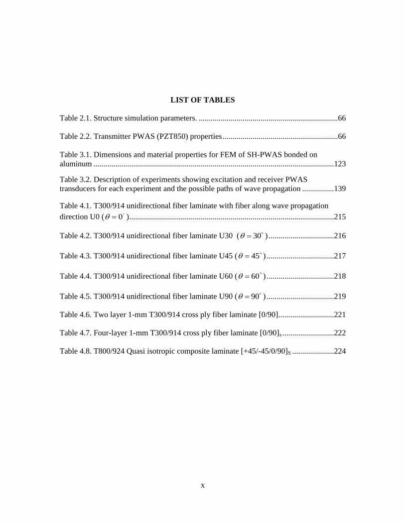
LIST OF TABLES
Table 2.1. Structure simulation parameters. ......................................................................66
Table 2.2. Transmitter PWAS (PZT850) properties ..........................................................66
Table 3.1. Dimensions and material properties for FEM of SH-PWAS bonded on
aluminum .........................................................................................................................123
Table 3.2. Description of experiments showing excitation and receiver PWAS
transducers for each experiment and the possible paths of wave propagation ................139
Table 4.1. T300/914 unidirectional fiber laminate with fiber along wave propagation
direction U0 ( 0 ) .......................................................................................................215
Table 4.2. T300/914 unidirectional fiber laminate U30 ( 30 ) .................................216
Table 4.3. T300/914 unidirectional fiber laminate U45 ( 45 ) ..................................217
Table 4.4. T300/914 unidirectional fiber laminate U60 ( 60 ) ..................................218
Table 4.5. T300/914 unidirectional fiber laminate U90 ( 90 ) ..................................219
Table 4.6. Two layer 1-mm T300/914 cross ply fiber laminate [0/90] ............................221
Table 4.7. Four-layer 1-mm T300/914 cross ply fiber laminate [0/90]s ..........................222
Table 4.8. T800/924 Quasi isotropic composite laminate [+45/-45/0/90]S .....................224
xi
LIST OF FIGURES
Figure 1.1. (a) Excitation signal, (b) Sensing after traveling through the plate:
dispersion Lamb wave signals S0: symmetric Lamb wave, A0:
antisymmetric Lamb wave. .............................................................................3
Figure 1.2. Dispersion curves for an aluminum plate, (a) phase velocities, (b)
group velocities ...............................................................................................3
Figure 1.3. Mode shapes of Lamb waves at different excitation frequencies
(Pavlakovic and Lowe, 2003) .........................................................................4
Figure 1.4. (a) Conventional ultrasonic transducers, (b) Rectangular and circular
PWAS, (c) SH-PWAS ....................................................................................5
Figure 1.5. Schematic of the PWAS shows the coupling of the in-plane shear
stress (Giurgiutiu, 2008) .................................................................................6
Figure 1.6. Different PWAS poling directions ...................................................................6
Figure 1.7. The various ways in which PWAS are used for structural sensing
includes (a) propagating Lamb waves, (b) standing Lamb waves and
(c) phased arrays. The propagating waves methods include: pitch-
catch; pulse-echo; thickness mode; and passive detection of impacts
and acoustic emission (Giurgiutiu, 2008). ......................................................9
Figure 1.8. Lamb wave experimental tuning curves for 1-mm aluminum plate
using 7 mm x 7 mm x 0.2 mm PWAS ..........................................................10
Figure 1.9. Electromechanical admittance of a free 7 mm x 7 mm x 0.2 mm
PWAS ...........................................................................................................11
Figure 1.10. Low frequency E/M impedance of bonded 7 mm x 7 mm x 0.2 mm
PWAS on 1-mm thick aluminum beam ........................................................12
Figure 1.11. Differences in the deformation of isotropic, orthotropic and
anisotropic materials subjected to uniaxial tension and pure shear
stresses, (Jones, 1999) ...................................................................................16
Figure 1.12. Axial and flexural approximation of S0 and A0 Lamb wave modes
for aluminum plate ........................................................................................18

xii
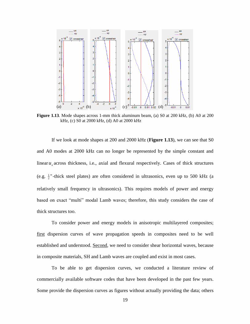
Figure 1.13. Mode shapes across 1-mm thick aluminum beam, (a) S0 at 200 kHz,
(b) A0 at 200 kHz, (c) S0 at 2000 kHz, (d) A0 at 2000 kHz ........................19
Figure 2.1. PWAS transmitter under constant voltage excitation (a) power rating,
(b) wave power (Lin and Giurgiutiu, 2012) ..................................................36
Figure 2.2. Energy supplied to the waveguide versus the patch size (Glushkov et
al., 2006) .......................................................................................................37
Figure 2.3. Symmetric and antisymmetric particle motion across the plate
thickness. .......................................................................................................40
Figure 2.4. Reciprocity relation, (Santoni, 2010) .............................................................41
Figure 2.5. Pin force model for structurally- bonded PWAS, reproduced from
Giurgiutiu (2008); (a) PWAS pin forces at the ends on the upper
surface; (b) shear stresses developed. ...........................................................47
Figure 2.6. Normal mode expansion for particle velocity fields (a) aluminum S0,
(b) aluminum A0, (c) steel S0, and (d) steel A0 mode. ................................51
Figure 2.7. PWAS constrained by an overall structural stiffness kstr. ...............................54
Figure 2.8. PWAS transmitter power flow (Lin et al., 2012) ...........................................55
Figure 2.9. Representation of the stresses and velocities at an arbitrary section of
the structure. ..................................................................................................58
Figure 2.10. Dispersion curves (a) aluminum 1 mm, (b) steel 12.7 mm (1/2 in). ............65
Figure 2.11. Simulation results for 1-mm aluminum plate, (a) electrical active
power, (b) reactive power, (c) Lamb wave power, (d) Lamb wave
kinetic and potential energy. .........................................................................67
Figure 2.12. Comparison between axial and flexural wave powers and S0/A0
Lamb wave powers. ......................................................................................68
Figure 2.13. Parametric study for Active power for 1-mm aluminum simulation. ...........70
Figure 2.14. Parametric study for total Lamb wave energy for 1-mm aluminum
simulation. .....................................................................................................70
Figure 2.15. ADAMS step function. .................................................................................71
Figure 2.16. Normal mode expansion for particle velocity fields for 12.7 mm steel
plate with 3 symmetric modes and 3 antisymmetric modes
(smoothed). (Kamal,et al., 2013) ..................................................................72
xiii
Figure 2.17. Summation of normal mode expanded velocities in x and y directions
with applied modal participation factors (a) symmetric, (b)
antisymmetric modes. ...................................................................................73
Figure 2.18. Simulation results for 12.7-mm steel plate, (a) electrical active power,
(b) reactive power. ........................................................................................74
Figure 2.19. (a) Lamb wave power, (b) Lamb wave power separated as symmetric
modes and antisymmetric modes. .................................................................74
Figure 2.20. Power partitioning between modes of Lamb wave propagation in ½"-
thick steel beam.............................................................................................75
Figure 2.21. Scanning laser vibrometer PSV-400-M2, source: Polytec.com ...................76
Figure 2.22. Experimental setup of function generator, laser vibrometer, and
oscilloscope for measuring Lamb wave tuning. ...........................................77
Figure 2.23. Sample of received signals by PWAS and laser measurements at 120
kHz ................................................................................................................78
Figure 2.24. Experimental received signals by the receiver PWAS at 160 mm
distance .........................................................................................................79
Figure 2.25. Analytical tuning curves, vx is the inplane particle velocity, vy: the
out of plane. ..................................................................................................79
Figure 2.26. Comparison between analytical prediction and laser measurements of
vy of A0 ........................................................................................................79
Figure 2.27. Experimental setup for E/M impedance test, (a) HP4194A impedance
analyzer, (b) test specimen with bonded PWAS. ..........................................81
Figure 2.28. FEM mesh and mode shapes at resonances of bonded PWAS.....................81
Figure 2.29. E/M admittance of a bonded PWAS on 1-mm aluminum structure: (a)
analytical prediction, (b) experimental and FEM results ..............................82
Figure 2.30. Dispersion of received wave packets............................................................83
Figure 2.31. (a) Wave power predicted analytically, (b) received signals power
experimentally...............................................................................................83
Figure 2.32. (a) A0 wave K.E predicted analytically. (b) A0 wave K.E. of point #2
on structure surface based on the laser vibrometer measurements. ..............84
Figure 3.1. Different modes of piezoelectric actuation (Heeg, 1993) ...............................91
xiv
Figure 3.2. (a) Adaptive sandwich beam and (b) surface mounted actuation beam
(Sun and Zhang, 1995) ..................................................................................92
Figure 3.3. (a) Proposed torsional actuator by Glazounov and Zhang (1998), (b)
proposed actuator-flap system (Centolanza et al., 2002) ..............................93
Figure 3.4. PZT actuator model for generation of Lamb mode S0 (Su, et al., 2007) .......93
Figure 3.5. (a) Various magnetostrictive transducers used to generate SH waves
(Lee et al., 2009),(b) MsS magnetostrictive sensor system, (c) MsS
for pipe inspection (www.swri.org) ..............................................................95
Figure 3.6. (a) Schematic for SH-PWAS, shaded areas are the electrodes
(Giurgiutiu, 2008), (b) transducer schematic from manufacturer,
source: APC piezoceramic Int Ltd ................................................................96
Figure 3.7. Free SH-PWAS free body diagram ................................................................98
Figure 3.8. Constrained SH-PWAS model .....................................................................107
Figure 3.9. (a) Constrained SH-PWAS model for axial-flexural response, (b)
Interaction between SH-PWAS with the structure, axial and flexural
load transfer ................................................................................................108
Figure 3.10 (a) Constrained SH-PWAS model for shear horizontal response, (b)
Interaction between SH-PWAS and structure, SH response solution .........115
Figure 3.11. Modeshapes of vibrations for free SH-PWAS using finite element
analysis, (a) mode shape at 200 kHz, (b) modeshape at resonance
frequency 900 kHz ......................................................................................122
Figure 3.12. FEM for bonded SH-PWAS on 1-mm thick aluminum beams (a) 2-D
model, (b) 3-D model ..................................................................................123
Figure 3.13. FEM for bonded SH-PWAS on 3-mm thick steel beams: SH-PWAS
orientation-1: (a) 2-D model, (b) 3-D model. (c) SH-PWAS
orientation-2, 3-D model .............................................................................124
Figure 3.14. Experimental setup for SH-PWAS bonded on 1-mm aluminum beams
(a) orientation-1, (b) orientation-2, (the black arrow indicates poling
direction) .....................................................................................................125
Figure 3.15. Experimental setup for SH-PWAS bonded on 3-mm steel beams (a)
orientation-1, (b) orientation-2, (the black arrow indicates poling
direction) .....................................................................................................126
xv
Figure 3.16. Results comparison for the free SH-PWAS (APC 850): (a) impedance,
constant E analytical model, (b) impedance, constant D analytical
model, (c) admittance..................................................................................127
Figure 3.17. Comparison between experimental results, analytical predictions and
finite element simulations for E/M impedance of SH-PWAS bonded
on 3-mm thick steel beam (orientation-1) ...................................................128
Figure 3.18 Modeshapes of vibrations of 3-mm thick steel beams with bonded SH-
PWAS in orientation-1 (axial-flexural orientation), at excitation
frequency: (a) 48 kHz, (b) 137 kHz, (c)145 kHz ........................................129
Figure 3.19. Modeshapes of vibrations of 3-mm thick steel beam with bonded SH-
PWAS in orientation-2 (SH orientation) at excitation frequency: (a)
30 kHz, (b) 60 kHz, (c)90 kHz, (d)123 kHz, (e)146 kHz ...........................129
Figure 3.20. Comparison between experimental results, analytical predictions and
finite element simulations for E/M impedance of SH-PWAS bonded
on 3-mm thick steel beam (orientation-2) ...................................................130
Figure 3.21 Comparison between experimental results and finite element
simulations for E/M impedance of SH-PWAS bonded on 1-mm thick
aluminum beam (orientation-1) ..................................................................131
Figure 3.22 Comparison between experimental results and finite element
simulations for E/M impedance of SH-PWAS bonded on 1-mm thick
aluminum beam (orientation-2) ..................................................................132
Figure 3.23. Shear horizontal wave speeds for aluminum (a) phase velocities, (b)
group velocities ...........................................................................................134
Figure 3.24 Pitch catch experiment to excite SH waves and catch it with another
SH-PWAS ...................................................................................................136
Figure 3.25. Waveforms associated with pitch catch SH waves experiment on 3.4-
mm thick aluminum ....................................................................................136
Figure 3.26. Experimental vs. analytical wave group velocity curves (SH-PWAS
experiment on 3.4-mm thick aluminum plate) ............................................137
Figure 3.27. Numbering and directions of pitch catch experiments on aluminum
plate, (a) directivity experiment, (b) separated experiments for
combination of SH-PWAS-regular PWAS pitch catch configurations. .....139
Figure 3.28. Dispersion group velocity curves for received wave signals (SH-
PWAS experiment on aluminum) ...............................................................142
xvi
Figure 3.29 Amplitudes of different waves at different angles of pitch-catch
experiments, associated with directivity experiment ..................................143
Figure 3.30. FEM simulations for waves excited at 60 kHz by (a) SH-PWAS, (b)
inplane PWAS. Variable plotted in (a) is z displacement, variable
plotted in (b) is y displacement ...................................................................145
Figure 3.31. FEM simulation for the case of 90 degree orientation difference
between two SH-PWAS ..............................................................................146
Figure 3.32. Guided SH waves power for three SH modes: two symmetric modes:
SH0, SH2, and one antisymmetric mode: SH1, (a) individual wave
power for SH0, SH2, (b) SH1 wave power, (c) total symmetric waves
power, (d) total antisymmetric waves power. .............................................152
Figure 3.33. Guided SH waves energy (kinetic and potential energies) in [J] ...............153
Figure 3.34. SH GUI, developed in LAMSS (www.me.sc.edu/Research/lamss/) ..........155
Figure 3.35. Example of plotting phase velocities of antisymmetric modes only ..........156
Figure 3.36. Group velocities for both symmetric and antisymmetric modes ................156
Figure 3.37. normalized and non-normalized mode shapes ............................................157
Figure 4.1. Composite layers notation and coordinates ..................................................166
Figure 4.2. Instability of TMM at high frequency-thickness products, (a),(b) 1-mm
aluminum layer, (c),(d) 1-mm unidirectional CFRP lamina with 45
fibers ...........................................................................................................171
Figure 4.3. GMM formulation (Pavlakovic and Lowe, 2003). .......................................173
Figure 4.4. Generic point O and its 18 neighboring points in the lattice (Delsanto
et al., 1997) .................................................................................................176
Figure 4.5. Flow chart of total SM recursive algorithm..................................................195
Figure 4.6. Notation of subscripts for displacements and stresses at top and bottom
of each layer. ...............................................................................................196
Figure 4.7. Stable STMM for aluminum layer: (a) unstable TMM results in
wavenumber-frequency domain; (b) unstable TMM results in
frequency-speed domain; (c) stable SMM results in ξh-freq domain;
(d) stable SMM results in freq-c domain; (e) stable robust STMM in
ξh-freq domain; (f) stable robust STMM in freq-c domain. The
frames indicate the regions of numerical instability. ..................................202
Figure 4.8. The technique for separating modes based on mode shapes ........................208
xvii
Figure 4.9. The TMM wavenumber-frequency dispersion plots for a unidirectional
CFRP layer: (a) the raw data or roots; (b) separation of modes based
on cubic extrapolation .................................................................................209
Figure 4.10. SMM solution over the whole domain for a unidirectional CFRP
layer.............................................................................................................209
Figure 4.11. Dispersion plots of a unidirectional CFRP layer: (a) instability of
TMM and mode tracking between TMM solution, then SMM solution;
(b) complete solution using STMM; (c) complete phase velocity
solution using STMM; (d) complete group velocity solution using
STMM. Lamb wave solution, - - - Shear horizontal wave
solution ........................................................................................................210
Figure 4.12. Dispersion plots of a unidirectional CFRP layer with 45º fibers: (a)
instability of TMM and mode tracking between TMM solution, then
SMM solution; (b) complete solution using STMM; (c) phase
velocity using only the stable region of the TMM solution (d)
complete phase velocity solution using STMM; (e) group velocity
using only the stable regionof the TMM solution; (f) complete group
velocity solution using STMM. Lamb wave solution, - - - Shear
horizontal wave solution .............................................................................211
Figure 4.13. Dispersion plots of cross ply fiber composite laminate [0/90]: (a) root
finding; (b) complete wavenumber-frequency solution using STMM.
Lamb wave solution, - - - Shear horizontal wave solution ........................212
Figure 4.14. LAMSS STMM graphical user interface for dispersion curves
analysis in composites.................................................................................213
Figure 4.15. Modeshapes for unidirectional CFRP layer with 0º fibers: (a) SH1
mode, (b) S0 mode. .....................................................................................213
Figure 4.16.LISA vs. GMM for 1.5-mm thick unidirectional IM7 Cycom 977-3
composite (Nadella and Cesnik, 2012) .......................................................220
Figure 4.17. Equivalent Matrix method for [0/90] T300/914 CFRP laminate ...............223
Figure 4.18. Experimental setup for guided wave propagation between in-plane
PWAS and SH-PWAS in 1-mm thick GFRP plate .....................................226
Figure 4.19. Group velocities in 1-mm woven GFRP plate, (a) DISPERSE, (b)
LAMSS STMM ..........................................................................................227
Figure 4.20. Experimental group velocities of guided waves in 1-mm thick woven
GFRP plate, analytical predictions ___, experimental □□□ .......................227
xviii
Figure 4.21. FEM for guided wave propagation between PWAS1 and SH-PWAS7
on GFRP......................................................................................................229
Figure 4.22. 2-D simulation results for wave propagation in1-mm thick woven
GFRP plate at, (a) particle displacement inplane Y direction, (b)
inplane X direction, (c) out of plane Z direction, (d) out of plane
strain tensor .................................................................................................230
Figure 4.23. FEM vs. experimental results for guided wave propagation in 1-mm
thick woven GFRP ......................................................................................230
Figure 4.24. Tuning experimental data for wave propagation in GFRP composite,
□□□ A0 mode, ooo S0 mode; Δ Δ Δ SH0 mode (Santoni, 2010). .............232
Figure 5.1. FEM mesh of the SH-PWAS bonded to GFRP plate ...................................241
Figure 5.2. E/M response of SH-PWAS bonded on woven GFRP: (a) impedance,
(b) admittance .............................................................................................242
Figure 5.3. COMSOL simulation of 400 kHz response of the SH-PWAS bonded
to GFRP plate ..............................................................................................243
Figure 5.4. COMSOL simulation of GFRP plate resonance modes under excitation
of SH-PWAS: (a) at 20 kHz, (b) at 50 kHz. ...............................................243
Figure 5.5. E/M response of SH-PWAS bonded on [0/45/45/0]s CFRP: (a)
impedance, (b) admittance. .........................................................................244
Figure 5.6. Group velocities of ultrasonic guided waves in 1-mm woven GFRP
plate, (a) DISPERSE, (b) STMM. ..............................................................246
Figure 5.7. Group velocity dispersion curves for (a) 1-mm woven GFRP, (b) 2-
mm [0/45/45/0]s CFRP ................................................................................246
Figure 5.8. Schematic of transducers positions for SH-PWAS experiments on
woven GFRP plate ......................................................................................248
Figure 5.9. Experiments numbering and directions of pitch catch experiments
between various SH-PWAS and PWAS on GFRP .....................................248
Figure 5.10. Dispersion group velocity curves for received wave signals (SH-
PWAS experiment on GFRP): (a) SH7SH8, (b) SH8PWAS2, (c)
SH7PWAS1 ............................................................................................249
Figure 5.11. Schematic of transducers positions for SH-PWAS experiments on 8-
ply CFRP plate ............................................................................................250
xix
Figure 5.12. Experiments numbering and directions of pitch catch experiments
between various SH-PWAS and PWAS on CFRP .....................................250
Figure 5.13. Group velocity curves for CFRP experiments: (a) SHSH, (b)
modified SHSH, (c) SH9PWAS1, (d) SH10PWAS2......................251
Figure 5.14. FEM schematic for guided wave propagation between SH-PWAS7
and SH-PWAS8 ..........................................................................................253
Figure 5.15. 2-D simulation results for wave propagation in 1-mm thick woven
GFRP plate, inplane particle displacement in the Y direction: (a) at 50
s ,(b) at 70 s . Out of plane particle displacement in the Z direction:
(c) at 50 s ,(d) at 70 s ..............................................................................254
Figure 5.16. FEM vs. experimental results for guided wave propagation in 1-mm
thick woven GFRP (SH-PWAS to SH-PWAS). .........................................255
Figure 5.17. 2-D simulation results for wave propagation in1-mm thick woven
GFRP plate at, (a) particle displacement inplane Y direction, (b)
inplane X direction, (c) out of plane Z direction, (d) out of plane
strain tensor .................................................................................................256
Figure 5.18. FEM vs. experimental results for guided wave propagation in 1-mm
thick woven GFRP ......................................................................................258
Figure 5.19. FEM geometry for guided wave propagation between SH-PWAS9
and SH-PWAS10 on CFRP plate ................................................................259
Figure 5.20. 2-D simulation results for wave propagation in 2-mm thick CFRP
plate, particle displacement inplane Y direction: (a) at 45 s ,(b) at 70
s .(c) Out of plane Z particle displacement at 70 s ................................260
Figure 5.21. FEM vs. experimental results for guided wave propagation in 2-mm
thick CFRP ..................................................................................................261
Figure 6.1. Image of the 2024-T3 Al plate under test .....................................................264
Figure 6.2. Blue print of the experimental panel developed at Sandia National Lab. ....264
Figure 6.3. (a) MD7 VectorLocator™, (b) MD7 IntelliConnector™. Source: Metis
Design .........................................................................................................265
Figure 6.4. MD7 Data Accumulator hub, HubTouch™, source: Metis Design
manual .........................................................................................................265
Figure 6.5. Sensors node VectorLocator™ after bonding. Connectors are used to
connect different sensors node together or to the data accumulator
hub...............................................................................................................266

xx
Figure 6.6. Complete setup of the MD7 SHM system ....................................................267
Figure 6.7. Profile of a measurement, to be uploaded to the memory card before
test ...............................................................................................................268
Figure 6.8. CAD Model on COMSOL for possible separate FEM later. .......................268
Figure 6.9. Exported mesh files and move.txt file for relative position, rotation and
unit conversion ............................................................................................269
Figure 6.10. Module launcher for Metis Design software package ................................270
Figure 6.11. Layout of the sensor nodes .........................................................................271
Figure 6.12. Required files in the working directory of the software. ............................271
Figure 6.13. Damage detection and visualization module, after importing our test
structure.......................................................................................................272
Figure 6.14. Preliminary result based on a baseline measurement and a
measurement after inducing the clay on the plate at 80 kHz ......................273
Figure 7.1. Fabricated CFRP panel with variable fiber orientation (Tatting and
Gurdal, 2003) ..............................................................................................275
Figure 7.2. The part provided for performing wave propagation tests on ......................275
Figure 7.3. The VS CFRP plate with PWAS transducers installed and clay around
boundaries ...................................................................................................276
Figure 7.4. Experimental results of dispersion wave propagation group velocities
for CFRP VS plate ......................................................................................277
Figure 7.5. Time domain signal at excitation signal of 66 kHz along U0 direction .......278
Figure 7.6. Short time Fourier transform of the time signal at 66 kHz along U0 ...........278
Figure 7.7. Black and White version of Figure 7.6 for printing purposes .....................279
Figure 7.8. STFT of all the received signals from 12 kHz to 300 kHz ...........................279
Figure 7.9. Black and white version of Figure 7.8 for printing purposes. .....................280

1
CHAPTER 1: BACKGROUND AND RESEARCH OBJECTIVES
Structural health monitoring (SHM) is a fast-growing field that is extending into many
industries. SHM uses a set of sensing elements permanently attached to or embedded in
the structure in order to effectively monitor its structural integrity, detect, and quantify
damage that develops during the entirety of its life. Effective SHM will not only increase
the safety of structures, it will also limit the amount of manual error prone inspections
that currently dominate the field. Over the past several decades, much work has been
done in developing SHM methods.
1.1. BACKGROUND
Wave Propagation Theory 1.1.1.
Lamb waves are elastic waves, propagating in solid plates, whose particle motion
lies in the plane that contains the direction of wave propagation and the direction
perpendicular to the plate. In 1917, Sir Horace Lamb published his classic analysis and
description of acoustic waves of this type; these waves were therefore called Lamb waves.
An infinite medium supports two wave modes traveling at unique velocities, pressure and
shear waves, whereas plates support two infinite sets of Lamb waves modes whose
properties depend on various parameters such as plate elastic properties, thickness, and
frequency, etc.
2
A comprehensive mathematical description of the problem of Lamb waves
propagation in solids can be found in various textbooks, such as: Viktorov (1967); Graff
(1991); Rose (1999); Giurgiutiu (2008). Lamb waves can exist in two basic types:
symmetric and antisymmetric, and for each of these types, various modes appear as
solutions of the Rayleigh-Lamb equations.
The speeds at which Rayleigh-Lamb waves propagate are referred to as dispersion
wave speeds. The term “dispersion” in wave propagation context means that the wave
packet stretches out as it travels through the medium; dispersion happens because the
frequency components of the wave travel at different wave speeds. Lamb waves are
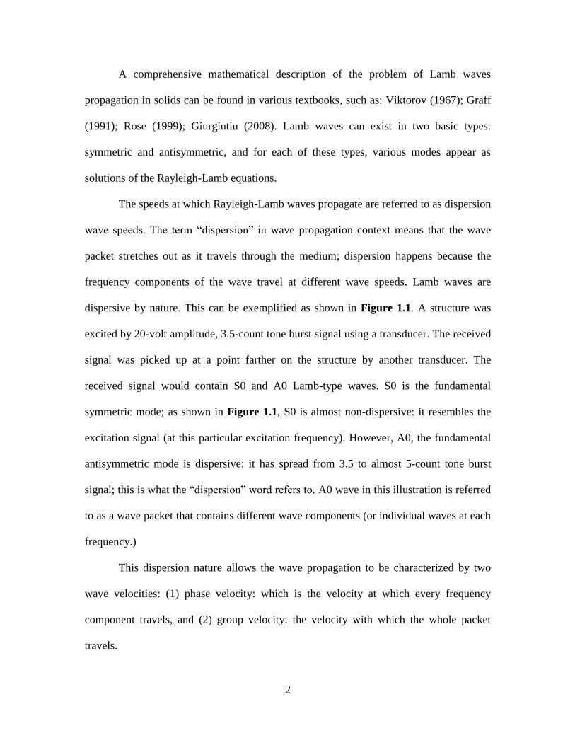
dispersive by nature. This can be exemplified as shown in Figure 1.1. A structure was
excited by 20-volt amplitude, 3.5-count tone burst signal using a transducer. The received
signal was picked up at a point farther on the structure by another transducer. The
received signal would contain S0 and A0 Lamb-type waves. S0 is the fundamental
symmetric mode; as shown in Figure 1.1, S0 is almost non-dispersive: it resembles the
excitation signal (at this particular excitation frequency). However, A0, the fundamental
antisymmetric mode is dispersive: it has spread from 3.5 to almost 5-count tone burst
signal; this is what the “dispersion” word refers to. A0 wave in this illustration is referred
to as a wave packet that contains different wave components (or individual waves at each
frequency.)
This dispersion nature allows the wave propagation to be characterized by two
wave velocities: (1) phase velocity: which is the velocity at which every frequency
component travels, and (2) group velocity: the velocity with which the whole packet
travels.
3
Figure 1.1. (a) Excitation signal, (b) Sensing after traveling through the plate: dispersion Lamb
wave signals S0: symmetric Lamb wave, A0: antisymmetric Lamb wave.
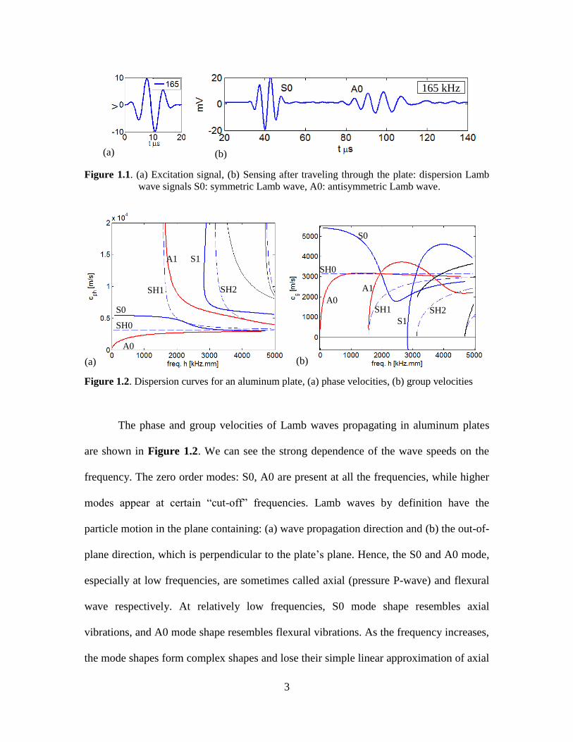
Figure 1.2. Dispersion curves for an aluminum plate, (a) phase velocities, (b) group velocities
The phase and group velocities of Lamb waves propagating in aluminum plates
are shown in Figure 1.2. We can see the strong dependence of the wave speeds on the
frequency. The zero order modes: S0, A0 are present at all the frequencies, while higher
modes appear at certain “cut-off” frequencies. Lamb waves by definition have the
particle motion in the plane containing: (a) wave propagation direction and (b) the out-of-
plane direction, which is perpendicular to the plate’s plane. Hence, the S0 and A0 mode,
especially at low frequencies, are sometimes called axial (pressure P-wave) and flexural
wave respectively. At relatively low frequencies, S0 mode shape resembles axial
vibrations, and A0 mode shape resembles flexural vibrations. As the frequency increases,
the mode shapes form complex shapes and lose their simple linear approximation of axial
165 kHz
(b) (a)
A0
SH0
S0
SH1
A1 S1
SH2
(a)
SH2 A0
SH0
S0
SH1
A1
S1
(b)
4
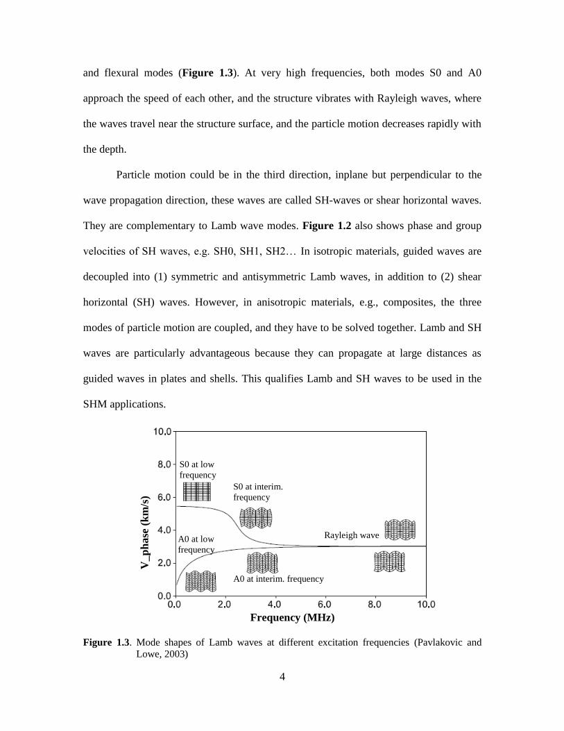
and flexural modes (Figure 1.3). At very high frequencies, both modes S0 and A0
approach the speed of each other, and the structure vibrates with Rayleigh waves, where
the waves travel near the structure surface, and the particle motion decreases rapidly with
the depth.
Particle motion could be in the third direction, inplane but perpendicular to the
wave propagation direction, these waves are called SH-waves or shear horizontal waves.
They are complementary to Lamb wave modes. Figure 1.2 also shows phase and group
velocities of SH waves, e.g. SH0, SH1, SH2… In isotropic materials, guided waves are
decoupled into (1) symmetric and antisymmetric Lamb waves, in addition to (2) shear
horizontal (SH) waves. However, in anisotropic materials, e.g., composites, the three
modes of particle motion are coupled, and they have to be solved together. Lamb and SH
waves are particularly advantageous because they can propagate at large distances as
guided waves in plates and shells. This qualifies Lamb and SH waves to be used in the
SHM applications.
Figure 1.3. Mode shapes of Lamb waves at different excitation frequencies (Pavlakovic and
Lowe, 2003)
S0 at low
frequency S0 at interim.
frequency
Rayleigh wave A0 at low
frequency
A0 at interim. frequency
V_p
hase
(k
m/s
)
Frequency (MHz)
5
Piezoelectric Wafer Active Sensor (PWAS) 1.1.2.
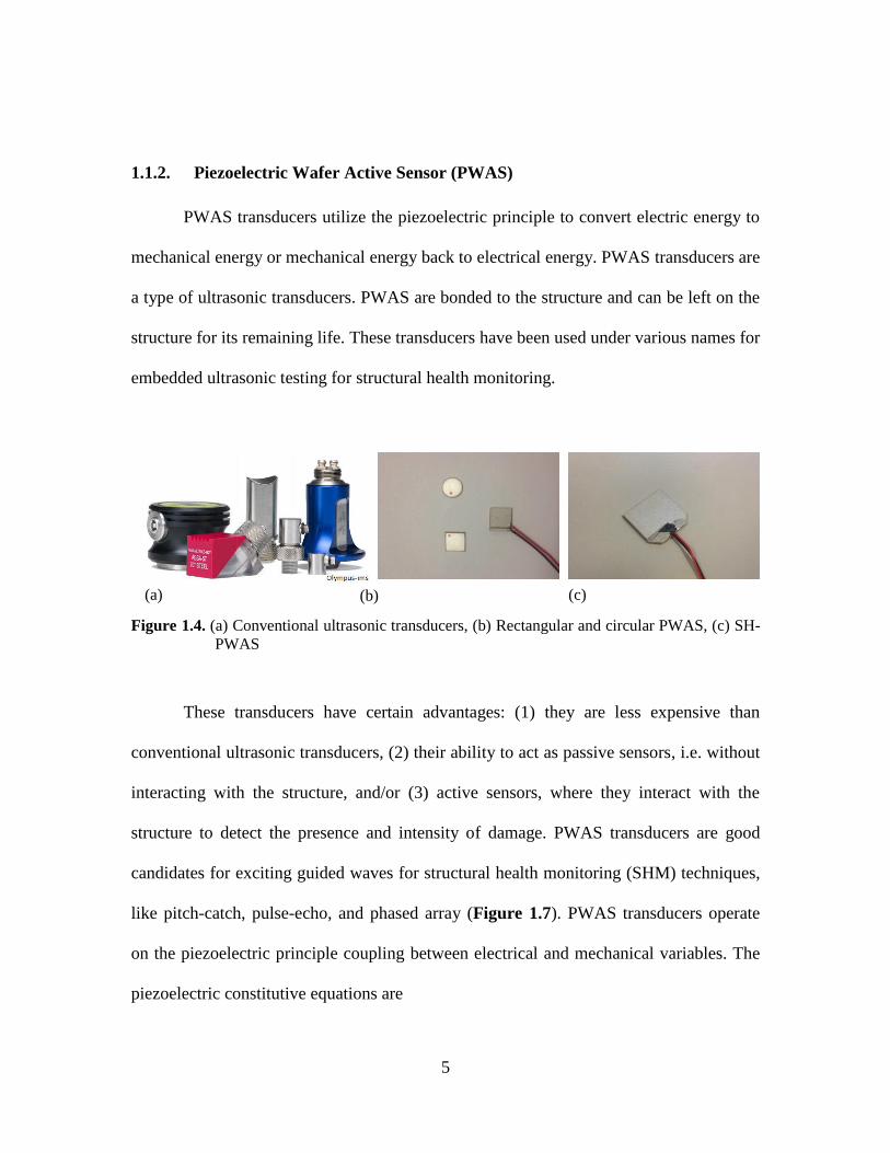
PWAS transducers utilize the piezoelectric principle to convert electric energy to
mechanical energy or mechanical energy back to electrical energy. PWAS transducers are
a type of ultrasonic transducers. PWAS are bonded to the structure and can be left on the
structure for its remaining life. These transducers have been used under various names for
embedded ultrasonic testing for structural health monitoring.
Figure 1.4. (a) Conventional ultrasonic transducers, (b) Rectangular and circular PWAS, (c) SH-
PWAS
These transducers have certain advantages: (1) they are less expensive than
conventional ultrasonic transducers, (2) their ability to act as passive sensors, i.e. without
interacting with the structure, and/or (3) active sensors, where they interact with the
structure to detect the presence and intensity of damage. PWAS transducers are good
candidates for exciting guided waves for structural health monitoring (SHM) techniques,
like pitch-catch, pulse-echo, and phased array (Figure 1.7). PWAS transducers operate
on the piezoelectric principle coupling between electrical and mechanical variables. The
piezoelectric constitutive equations are
(a) (b) (c)
6
E
ij ijkl kl kij kS s T d E (1.1)
T
j jkl kl jk kD d T E (1.2)
Equations (1.1) and (1.2) define how the mechanical strain ijS , stress klT , the electrical
field kE , and electric displacement jD , relate, where
E
ijkls is the mechanical compliance
of the material at zero electrical field ( 0)E , T
jk is the dielectric constant at zero stress
( 0)T , and jkld is the induced strain coefficient (mechanical strain per unit electric
field). In order to create in-plane strain from a transverse electric field or vice versa, the
31d property is utilized by the PWAS.
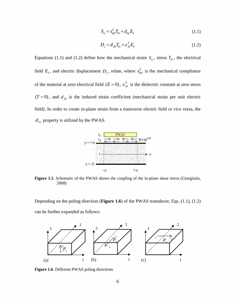
Figure 1.5. Schematic of the PWAS shows the coupling of the in-plane shear stress (Giurgiutiu,
2008)
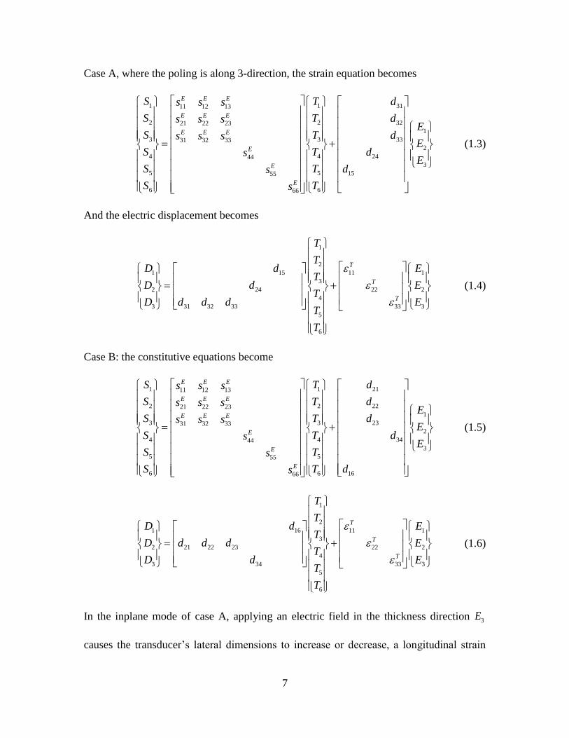
Depending on the poling direction (Figure 1.6) of the PWAS transducer, Eqs. (1.1), (1.2)
can be further expanded as follows:
Figure 1.6. Different PWAS poling directions
(a)
Ps
+ -
1
2 3
(b)
Ps
+
1
2 3
-
(c)
Ps +
1
2 3
-
7
Case A, where the poling is along 3-direction, the strain equation becomes
1 1 3111 12 13
2 2 3221 22 23
1
3 3 3331 32 33
2
4 4 2444
3
5 5 1555
6 666
E E E
E E E
E E E
E
E
E
S T ds s s
S T ds s sE
S T ds s sE
S T dsE
S T ds
S Ts
(1.3)
And the electric displacement becomes
1
2
1 15 11 1
3
2 24 22 2
4
3 31 32 33 33 3
5
6
T
T
T
T
TD d E
TD d E
TD d d d E
T
T
(1.4)
Case B: the constitutive equations become
1 1 2111 12 13
2 2 2221 22 23
1
3 3 2331 32 33
2
4 4 3444
3
5 555
6 6 1666
E E E
E E E
E E E
E
E
E
S T ds s s
S T ds s sE
S T ds s sE
S T dsE
S Ts
S T ds
(1.5)
1
2
1 16 11 1
3
2 21 22 23 22 2
4
3 34 33 3
5
6
T
T
T
T
TD d E
TD d d d E
TD d E
T
T
(1.6)
In the inplane mode of case A, applying an electric field in the thickness direction 3E
causes the transducer’s lateral dimensions to increase or decrease, a longitudinal strain
8
will occur 1 31 3d E , where 13d is the piezoelectric coupling coefficient measured in
[m/V]. Thickness mode is a mode that occurs simultaneously with extension mode, but
dominates at higher frequencies in MHz, in which strain in the thickness direction will
occur 3 33 3d E , where 33d is the piezoelectric coupling coefficient in thickness
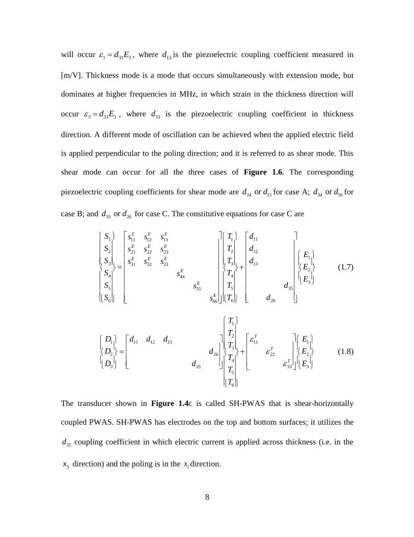
direction. A different mode of oscillation can be achieved when the applied electric field
is applied perpendicular to the poling direction; and it is referred to as shear mode. This
shear mode can occur for all the three cases of Figure 1.6. The corresponding
piezoelectric coupling coefficients for shear mode are 24 15 or d d for case A; 34 16 or d d for
case B; and 35 26 or d d for case C. The constitutive equations for case C are
1 1 1111 12 13
2 2 1221 22 23
1
3 3 1331 32 33
2
4 444
3
5 5 3555
6 6 2666
E E E
E E E
E E E
E
E
E
S T ds s s
S T ds s sE
S T ds s sE
S TsE
S T ds
S T ds
(1.7)
1
2
1 11 12 13 11 1
3
2 26 22 2
4
3 35 33 3
5
6
T
T
T
T
TD d d d E
TD d E
TD d E
T
T
(1.8)
The transducer shown in Figure 1.4c is called SH-PWAS that is shear-horizontally
coupled PWAS. SH-PWAS has electrodes on the top and bottom surfaces; it utilizes the
35d coupling coefficient in which electric current is applied across thickness (i.e. in the
3x direction) and the poling is in the 1x direction.
9
1.1.2.1. PWAS for guided wave propagation and wave tuning
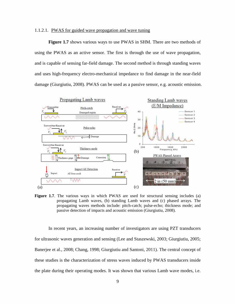
Figure 1.7 shows various ways to use PWAS in SHM. There are two methods of
using the PWAS as an active sensor. The first is through the use of wave propagation,
and is capable of sensing far-field damage. The second method is through standing waves
and uses high-frequency electro-mechanical impedance to find damage in the near-field
damage (Giurgiutiu, 2008). PWAS can be used as a passive sensor, e.g. acoustic emission.
Figure 1.7. The various ways in which PWAS are used for structural sensing includes (a)
propagating Lamb waves, (b) standing Lamb waves and (c) phased arrays. The
propagating waves methods include: pitch-catch; pulse-echo; thickness mode; and
passive detection of impacts and acoustic emission (Giurgiutiu, 2008).
In recent years, an increasing number of investigators are using PZT transducers
for ultrasonic waves generation and sensing (Lee and Staszewski, 2003; Giurgiutiu, 2005;
Banerjee et al., 2008; Chang, 1998; Giurgiutiu and Santoni, 2011). The central concept of
these studies is the characterization of stress waves induced by PWAS transducers inside
the plate during their operating modes. It was shown that various Lamb wave modes, i.e.
(a)
(b)
(c)
10
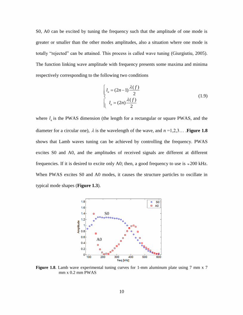
S0, A0 can be excited by tuning the frequency such that the amplitude of one mode is
greater or smaller than the other modes amplitudes, also a situation where one mode is
totally “rejected” can be attained. This process is called wave tuning (Giurgiutiu, 2005).
The function linking wave amplitude with frequency presents some maxima and minima
respectively corresponding to the following two conditions
( )(2 1)
2
( )(2 )
2
a
a
fl n
fl n
(1.9)
where al is the PWAS dimension (the length for a rectangular or square PWAS, and the
diameter for a circular one), is the wavelength of the wave, and n =1,2,3… .Figure 1.8
shows that Lamb waves tuning can be achieved by controlling the frequency. PWAS
excites S0 and A0, and the amplitudes of received signals are different at different
frequencies. If it is desired to excite only A0; then, a good frequency to use is 200 kHz.
When PWAS excites S0 and A0 modes, it causes the structure particles to oscillate in
typical mode shapes (Figure 1.3).
Figure 1.8. Lamb wave experimental tuning curves for 1-mm aluminum plate using 7 mm x 7
mm x 0.2 mm PWAS
S0
A0
11
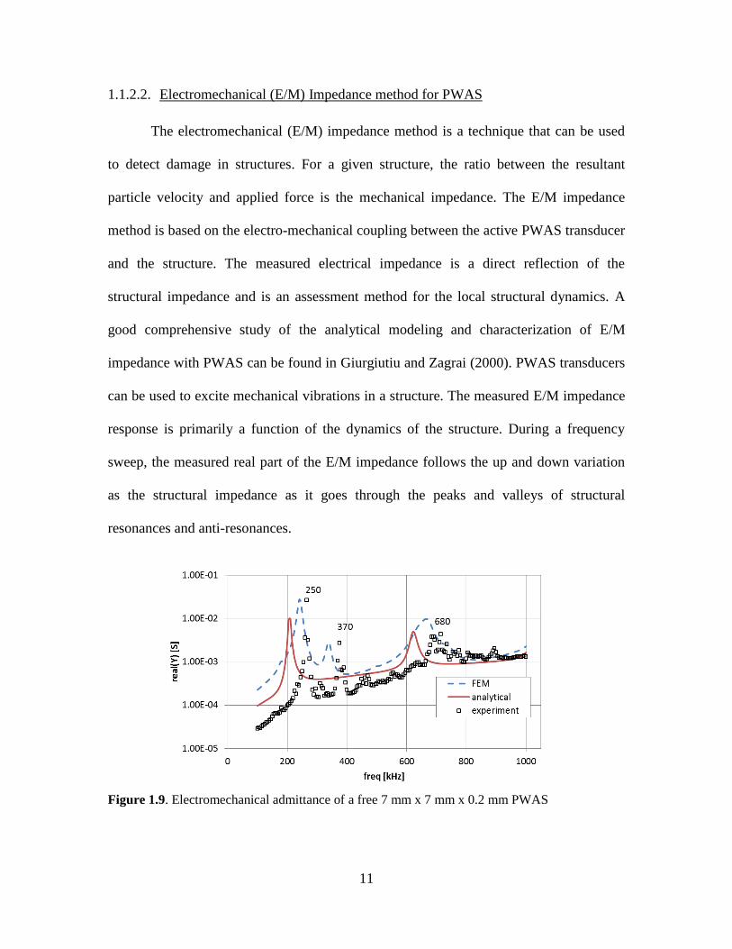
1.1.2.2. Electromechanical (E/M) Impedance method for PWAS
The electromechanical (E/M) impedance method is a technique that can be used
to detect damage in structures. For a given structure, the ratio between the resultant
particle velocity and applied force is the mechanical impedance. The E/M impedance
method is based on the electro-mechanical coupling between the active PWAS transducer
and the structure. The measured electrical impedance is a direct reflection of the
structural impedance and is an assessment method for the local structural dynamics. A
good comprehensive study of the analytical modeling and characterization of E/M
impedance with PWAS can be found in Giurgiutiu and Zagrai (2000). PWAS transducers
can be used to excite mechanical vibrations in a structure. The measured E/M impedance
response is primarily a function of the dynamics of the structure. During a frequency
sweep, the measured real part of the E/M impedance follows the up and down variation
as the structural impedance as it goes through the peaks and valleys of structural
resonances and anti-resonances.
Figure 1.9. Electromechanical admittance of a free 7 mm x 7 mm x 0.2 mm PWAS
12
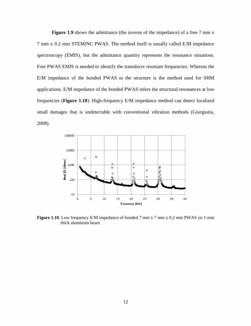
Figure 1.9 shows the admittance (the inverse of the impedance) of a free 7 mm x
7 mm x 0.2 mm STEMiNC PWAS. The method itself is usually called E/M impedance
spectroscopy (EMIS), but the admittance quantity represents the resonance situations.
Free PWAS EMIS is needed to identify the transducer resonant frequencies. Whereas the
E/M impedance of the bonded PWAS to the structure is the method used for SHM
applications. E/M impedance of the bonded PWAS infers the structural resonances at low
frequencies (Figure 1.10). High-frequency E/M impedance method can detect localized
small damages that is undetectable with conventional vibration methods (Giurgiutiu,
2008).
Figure 1.10. Low frequency E/M impedance of bonded 7 mm x 7 mm x 0.2 mm PWAS on 1-mm
thick aluminum beam
13
Composite Materials 1.1.3.
The term “composite” can be used to describe any material that is comprised of a
homogeneous matrix reinforced by material with higher strength and stiffness properties.
When designing a structure for an application, material selection is an essential process.
The properties of materials are analyzed, often with a metric to assist in the process, and a
material is selected based on trade-offs between its desirable and undesirable properties.
Because simple mechanical properties like stiffness and strength are not the only traits
that need to be taken into account, the process of material selection can be complicated.
For aerospace, automotive, and naval applications, materials with a high strength
to weight ratio offer desirable performance. Composite materials offer such properties
along with other desirable properties, thus placing composite material use at the leading
edge of material selection for many types of structures. A composite material can have a
strength-to-weight ratio in certain directions around 5 times that of aluminum or steel.
This is especially useful in the aerospace industry, where weight is at a premium. Another
unique and beneficial trait of composite materials is the ability to customize their
properties in different directions, creating an anisotropic material; however, composite
material can be very costly compared to metals and hard to predict in terms of behavior
due to their complex structure.
One of the most important definitions that will be used frequently when we treat
the composite materials is the anisotropy and the level of anisotropy, so it will be covered
here briefly.
The isotropic material is the one that has the same material properties in every
direction at a point in the body (Jones, 1999). Anisotropic material is the opposite and
14
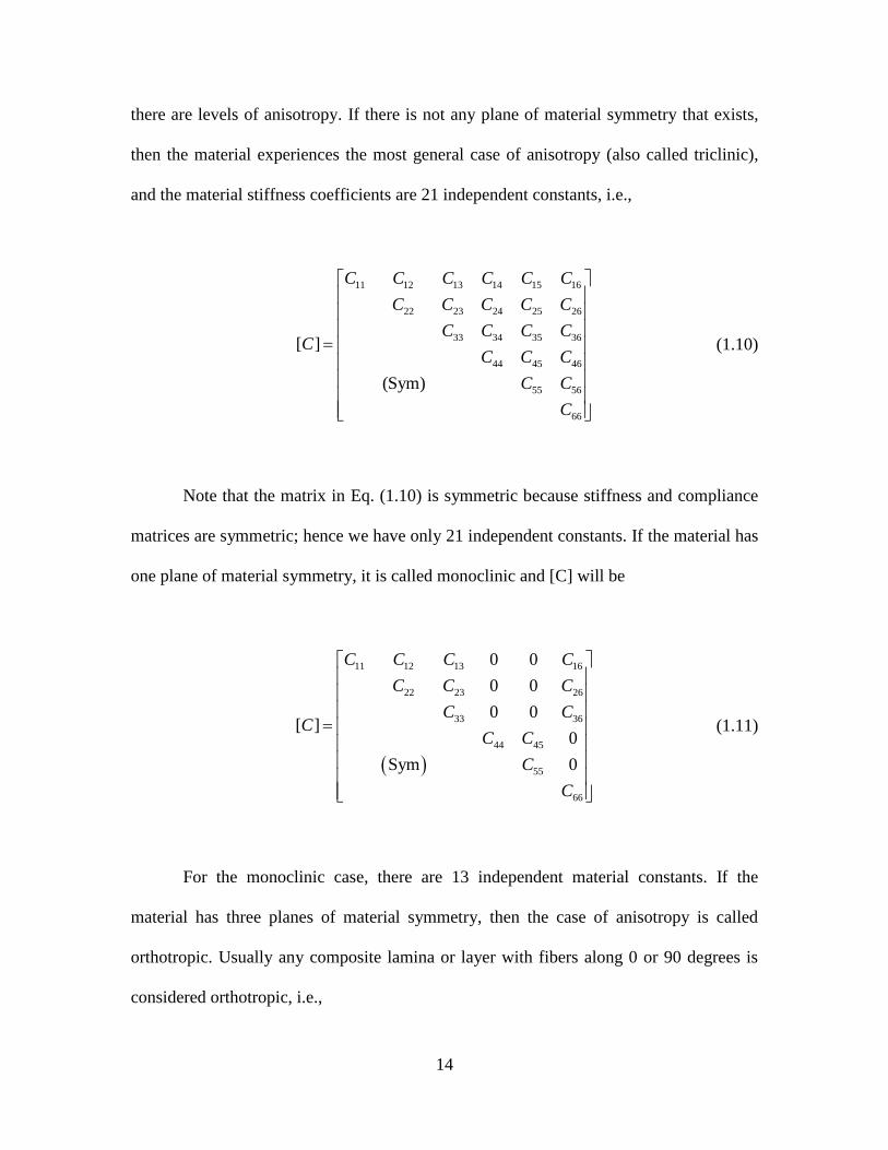
there are levels of anisotropy. If there is not any plane of material symmetry that exists,
then the material experiences the most general case of anisotropy (also called triclinic),
and the material stiffness coefficients are 21 independent constants, i.e.,
11 12 13 14 15 16
22 23 24 25 26
33 34 35 36
44 45 46
55 56
66
[ ]
(Sym)
C C C C C C
C C C C C
C C C CC
C C C
C C
C
(1.10)
Note that the matrix in Eq. (1.10) is symmetric because stiffness and compliance
matrices are symmetric; hence we have only 21 independent constants. If the material has
one plane of material symmetry, it is called monoclinic and [C] will be
11 12 13 16
22 23 26
33 36
44 45
55
66
0 0
0 0
0 0[ ]
0
Sym 0
C C C C
C C C
C CC
C C
C
C
(1.11)
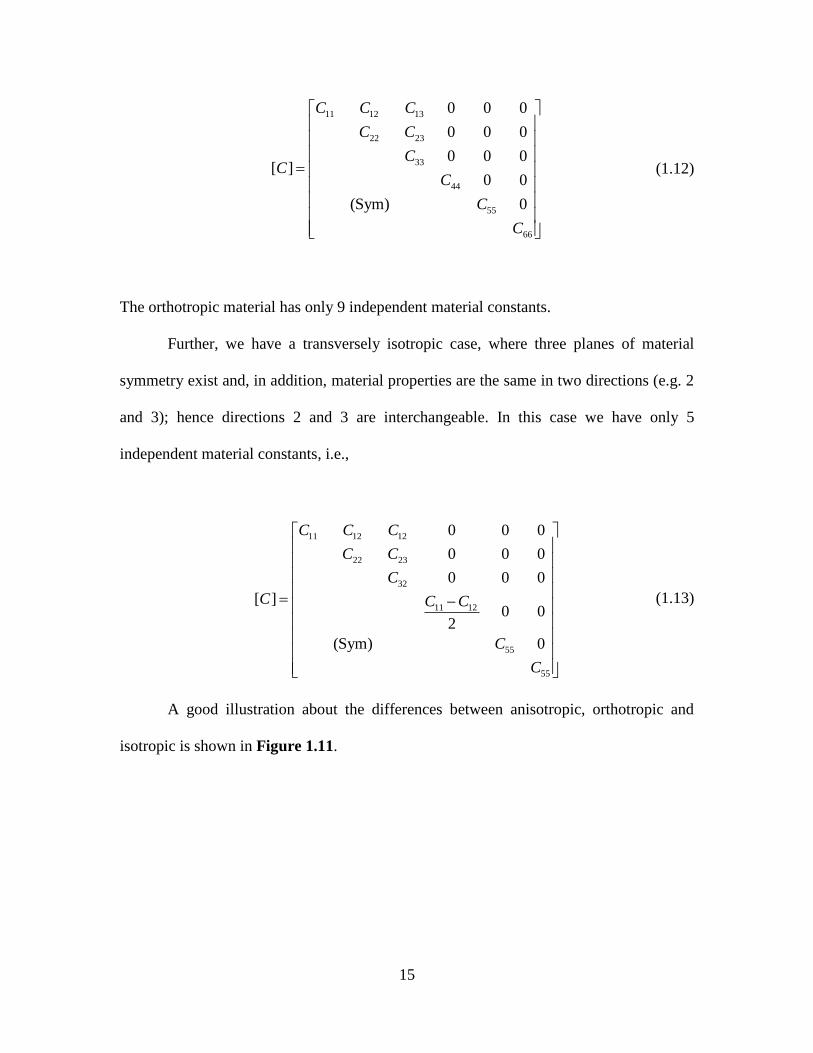
For the monoclinic case, there are 13 independent material constants. If the
material has three planes of material symmetry, then the case of anisotropy is called
orthotropic. Usually any composite lamina or layer with fibers along 0 or 90 degrees is
considered orthotropic, i.e.,
15
11 12 13
22 23
33
44
55
66
0 0 0
0 0 0
0 0 0[ ]
0 0
(Sym) 0
C C C
C C
CC
C
C
C
(1.12)
The orthotropic material has only 9 independent material constants.
Further, we have a transversely isotropic case, where three planes of material
symmetry exist and, in addition, material properties are the same in two directions (e.g. 2
and 3); hence directions 2 and 3 are interchangeable. In this case we have only 5
independent material constants, i.e.,
11 12 12
22 23
32
11 12
55
55
0 0 0
0 0 0
0 0 0
[ ]0 0
2
(Sym) 0
C C C
C C
C
C C C
C
C
(1.13)
A good illustration about the differences between anisotropic, orthotropic and
isotropic is shown in Figure 1.11.

16
Figure 1.11. Differences in the deformation of isotropic, orthotropic and anisotropic materials
subjected to uniaxial tension and pure shear stresses, (Jones, 1999)
Finally, in the isotropic case, we have three planes of material symmetry and the
material properties are the same in all the three directions; this is typically for metallic
structures. In this case, we have
11 12 12
11 12
11
44
44
44
44 11 12
0 0 0
0 0 0
0 0 0
0 0
(Sym) 0
( ) / 2
C C C
C C
CC
C
C
C
C C C
(1.14)
We have 2 independent material constants, because the three shear moduli are all
the same and are related to the Young’s Modulus and Poisson ratio by / (2(1 ))G E .
17
Guided Waves in Polymer Composite Materials 1.1.4.
The benefits of using composites come at the cost of a more complicated
mechanical response to the applied loads, static or dynamic. The anisotropic nature of the
composite material introduces many interesting wave phenomena that are not observed in
isotropic bodies; for example, the directional dependence of wave speeds. An
understanding of the nature of waves in anisotropic materials is required if we want to
use these materials effectively in structural design, or if we want to inspect them using
ultrasonic methods, which is one of the goals of our present work.
The type of waves we investigate within the scope of this study are guided elastic
waves in free-anisotropic plates, i.e. plates with traction-free surfaces, where the waves
are confined within plate surfaces.
State of the art textbooks that treat ultrasonic wave propagation in anisotropic
composites are several, they include: Auld (1990); Nayfeh (1995); Rose (1999); and
Rokhlin et al. (2011). Some useful tips for obtaining dispersion wave propagation curves
can be found in Lowe (1995); Glushkov et al. (2011); Su et al. (2006). There are different
methods to calculate dispersion curves in multilayered composite materials (a) transfer
matrix method (TMM); (b) global matrix method (GMM); (c) semi-analytical finite
element method (SAFE); (d) local interaction simulation approach (LISA); and (e)
equivalent matrix method (EMM). Mathematical formulations of these techniques are
presented, along with highlighting key features. GMM was studied comprehensively by
Lowe (1995), and there is a commercial software that has been developed based on
GMM, which is called DISPERSE (Pavlakovic and Lowe, 2003).
18
1.2. MOTIVATION
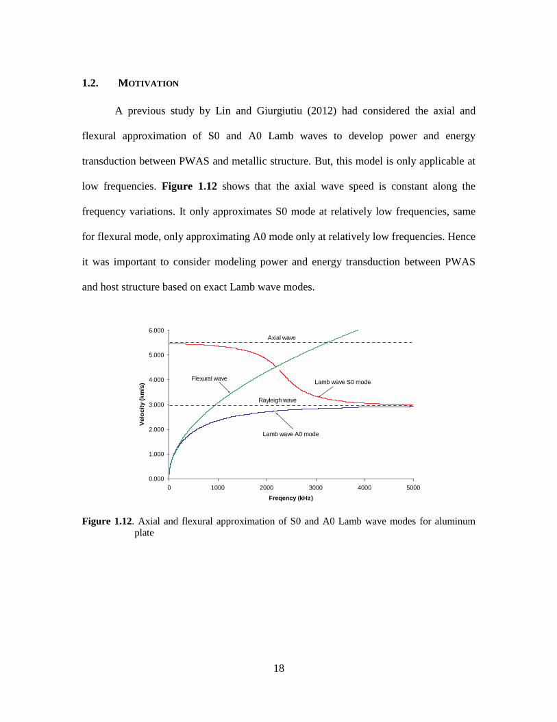
A previous study by Lin and Giurgiutiu (2012) had considered the axial and
flexural approximation of S0 and A0 Lamb waves to develop power and energy
transduction between PWAS and metallic structure. But, this model is only applicable at
low frequencies. Figure 1.12 shows that the axial wave speed is constant along the
frequency variations. It only approximates S0 mode at relatively low frequencies, same
for flexural mode, only approximating A0 mode only at relatively low frequencies. Hence
it was important to consider modeling power and energy transduction between PWAS
and host structure based on exact Lamb wave modes.
0.000
1.000
2.000
3.000
4.000
5.000
6.000
0 1000 2000 3000 4000 5000
Freqency (kHz)
Ve
loc
ity
(k
m/s
)
Axial wave
Flexural wave
Lamb wave A0 mode
Lamb wave S0 mode
Rayleigh wave
Figure 1.12. Axial and flexural approximation of S0 and A0 Lamb wave modes for aluminum
plate
19
Figure 1.13. Mode shapes across 1-mm thick aluminum beam, (a) S0 at 200 kHz, (b) A0 at 200
kHz, (c) S0 at 2000 kHz, (d) A0 at 2000 kHz
If we look at mode shapes at 200 and 2000 kHz (Figure 1.13), we can see that S0
and A0 modes at 2000 kHz can no longer be represented by the simple constant and
linear xu across thickness, i.e., axial and flexural respectively. Cases of thick structures
(e.g. 12"-thick steel plates) are often considered in ultrasonics, even up to 500 kHz (a
relatively small frequency in ultrasonics). This requires models of power and energy
based on exact “multi” modal Lamb waves; therefore, this study considers the case of
thick structures too.
To consider power and energy models in anisotropic multilayered composites;
first dispersion curves of wave propagation speeds in composites need to be well
established and understood. Second, we need to consider shear horizontal waves, because
in composite materials, SH and Lamb waves are coupled and exist in most cases.
To be able to get dispersion curves, we conducted a literature review of
commercially available software codes that have been developed in the past few years.
Some provide the dispersion curves as figures without actually providing the data; others
(a) (b) (c) (d)
20
frequently miss one of the modes we wanted to predict their speed (namely SH0). Hence,
for more flexibility and to integrate dispersion wave speeds in composites with power
and energy models, we considered developing a predictive tool based on transfer matrix
method (TMM). TMM was described in details in Nayfeh (1995). A software, “LAMSS
Guided Waves in Composites” based on TMM has been developed in our group (Santoni,
2010). Two key issues need to be highlighted, (1) Nayfeh approach leads to a singular
situation if the material is isotropic or quasi-isotropic, and (2) TMM suffers instability at
higher frequencies, or as layers of the composite laminate increase. Our study tries to
eliminate these issues by combining Nayfeh approach (TMM) with the stiffness matrix
method (SMM) by Rokhlin et al. (2011). A combined stiffness transfer matrix method
(STMM) is proposed to obtain correct and stable results over the entire domain of interest.
STMM procedure is coded in a MATLAB graphical user interface that also allows
displaying modeshapes at any selected root of interest.
To experimentally validate our SH waves prediction in metallic and composite
materials, we needed to understand, to model, and to characterize SH-PWAS. It is shown
in Chapter-3 that SH waves are good candidates for SHM, e.g., capturing delaminatons in
composites; and inferring the shear stiffness of bonding layers, which is a vital role for
adhesive bonded layers. For these reasons, it was very promising and worthwhile to work
on predictive models of SH-PWAS behavior, including free SH-PWAS predictive models
for admittance and impedance, in addition to the bonded SH-PWAS case, which
contributes to the advancement of knowledge beyond the state of the art.
21
1.3. RESEARCH GOAL, SCOPE, AND OBJECTIVES
The goals of this research are (1) to understand, model, and predict the power and
energy transduction mechanism between piezoelectric wafer active sensor (PWAS) and
the host structure and (2) to characterize and model shear horizontal-coupled
piezoelectric wafer active sensor and to study the impedance spectroscopy and wave
propagation methods associated with this transducer.
In terms of materials, the scope of this study is to develop analytical and finite
element predictive models for (1) isotropic metallic structures and (2) anisotropic
polymer composites. In terms of type and number of guided waves excited in the
structure, the study covers: (1) single symmetric and antisymmetric Lamb wave modes,
which typically exist in thin structures; (2) multimodal Lamb waves that typically exist in
thick structures and at high excitation frequencies; and (3) coupled shear horizontal and
Lamb waves in anisotropic composite laminates.
The objectives of this research are defined as follows:
1. To develop analytical equations for power and energy transduction between the
PWAS and hosted structure based on exact Lamb wave modes and normal mode
expansion (NME) method and to identify model assumptions, limitations, and the
range of applicability.
2. To characterize SH-PWAS, including the impedance, wave propagation, and
power and energy of SH waves.
3. To develop analytically the electromechanical impedance and admittance of the
constrained SH-PWAS (which is bonded to a host structure) based on normal
22
mode expansion method and elasticity solution of the structural displacement
response.
4. To develop a graphical user interface by MATLAB for SH-waves analysis in the
common isotropic materials. This will complement existing developed software in
our group for Lamb waves, e.g. WAVESCOPE and MODESHAPE.
5. To solve dispersion wave propagation speeds in multilayered composites based on
the transfer matrix method (TMM) and to develop stable and robust predictive
tool for predicting dispersion curves and modeshapes in composite materials.
6. To demonstrate experiments of SH waves propagation in composites and, in
general, the coupled guided waves in composites. In addition, to demonstrate
FEM predictions of wave propagation and impedance spectroscopy methods in
composites.
7. To perform application studies on complex aerospace-like structures and
composite plates and to identify challenges of SHM of complex metallic and
composite structures.
Dissertation Layout and Research Topics 1.3.1.
To accomplish the objectives set forth in the preceding section, the dissertation is
organized in six chapters divided into two parts.
In part I, we address theoretical developments and validation experiments.
Chapter-2 presents power and energy studies, and these cover the following topics:
23
Topic-1 Exact Lamb waves’ power and energy, based on the normal mode expansion
theory (NME) and harmonic waves.
Topic-2 Multimodal Lamb waves case in thick structures.
Topic -3 Power partitioning based on constant voltage.
Topic -4 Experiments using laser vibrometer for measuring actual amplitudes and
validating analytical tuning curves based on (a) signal amplitude values and
(b) signal energy content.
Topic -5 Experiments and FEM of impedance spectroscopy.
Chapter-3 presents the SH-PWAS, as a candidate for SHM compared to other
state-of-the-art transducers. Characterization of the SH-PWAS includes the analytical
development of the free transducer (in 35d mode). We developed the E/M impedance and
admittance of the free transducer based on the constant electric field assumption and
based on the constant electric displacement assumption. Analytical models were
compared with experiments and FEM results. Furthermore, we extended the analytical
development to find closed-form expressions for the E/M impedance and admittance of
the constrained (bonded) SH-PWAS. We studied the power and energy of multimodal
SH-waves based on NME, and we developed a MATLAB graphical user interface (GUI)
for calculating SH waves dispersion phase and group velocities, mode shapes, and wave
energies. The research topics of this chapter are summarized as:
Topic -1 Analytical modeling of the E/M impedance and admittance of the free SH-
PWAS, as well as experimental and FEM validations.
24
Topic -2 Analytical modeling of the E/M impedance and admittance for the bonded
SH-PWAS, based on NME and structural elasticity solution.
Topic -3 Performed experiments of the bonded SH-PWAS on structures at low
frequencies to capture structural resonances.
Topic -4 Performed wave propagation experiments between different combinations of
PWAS and SH-PWAS to study the generation and reception of SH waves by
SH-PWAS and to study the effect of SH-PWAS poling.
Topic -5 Development of the power and energy models of SH waves analytically.
Topic -6 Building a GUI on MATLAB for SH waves’ analysis.
Chapter-4 presents guided wave propagation in composites. We developed
analytically the equations of TMM, based on Nayfeh (1995) and the equations of SMM,
based on Rokhlin, et al. (2011). Then, we integrated TMM and SMM as a combined
stable stiffness transfer matrix method (STMM). We presented in detail the procedure
needed to code this method in a way to avoid numerical instability and to be applicable
on an isotropic plate; a multi-layered isotropic plate; a unidirectional fiber composite
lamina with fibers along 0 or 90 degrees w.r.t. wave propagation direction; a
unidirectional fiber composite lamina with arbitrary fiber angles; multilayered
unidirectional composite with fibers along 0 direction; and cross-ply composites. For
each of the preceding cases, we obtained phase velocities, group velocities, and
wavenumber-frequency domain solutions. Afterwards, a comparable study was
established between the STMM results and results from commercially available software,

25
e.g. DISPERSE based on GMM, and GUIGUW based on SAFE. This is followed by
experimental and FEM studies. The research topics of this chapter are:
Topic -1a Understanding TMM and SMM, identifying instability and singularity issues
Topic -1b Obtaining stable results based on the stable combined stiffness transfer
matrix method (STMM): (a) f (b)phc (c)
gc .
Topic -2 Analyzing a multilayered isotropic case (a) f (b)phc (c)
gc .
Topic -3 Analyzing a unidirectional composite case with fibers angle along 0 or 90
degree directions w.r.t wave propagation direction: (a) f (b)phc (c)
gc .
Topic -4 Analyzing a unidirectional composite case with arbitrary fibers angle, e.g.
30, 45, 60: (a) f (b)phc (c)
gc .
Topic -5 Developing cross ply solutions based on equivalent matrix method:
(a) f (b)phc (c)
gc .
Topic -6 Developing multilayered unidirectional and cross ply solutions based on
STMM: (a) f (b)phc (c)
gc .
Topic -7 Comparative study between different methods, GMM, STMM, and SAFE for
(a) unidirectional, (b) cross ply, and (c) quasi- isotropic laminates.
Topic -8 Experimental validation.
Topic-9 Performing FEM on a cross-ply situation and showing the directional
dependence of wave propagation on composites.
26
Part II addresses some SHM applications and related issues
In Chapter 5, we performed a case study of using SH-PWAS on composites, we
exemplified the case studies by a 1-mm thick woven GFRP and a 2-mm thick
[0/45/45/0]s CFRP plate with woven prepreg layers. We studied impedance spectroscopy
and wave propagation methods on both materials. Then, we built predictive finite element
models and addressed the challenges and limitations. The research topics of this chapter
are:
Topic-1 Experimental and FEM studies of E/M impedance and admittance for the
SH-PWAS bonded on GFRP and CFRP plates.
Topic -2 Combination of pitch catch experiments between PWAS and SH-PWAS on
both GFRP and CFRP plates.
Topic -3 Finite element models for 2-D wave propagation for the following cases
(a) The SH-PWAS is the transmitter transducer (both GFRP, CFRP).
(b) The regular PWAS is the transmitter in GFRP case.
In Chapter 6, we studied a commercial SHM system for damage detection in
aerospace-like structure. The research topics of this chapter are:
Topic -1 Sensors installation and the equipment setup (contribution: this task was
done by Dr. Bin Lin, research PostDoc, USC.)
Topic -2 Performing experiments on pristine complex structure.
Topic -3 Inducing different damage cases and testing the system for damage
detection.

27
Topic -4 Modeling includes (1) building CAD files for such plates, (2) meshing by
ANSYS, meshing was done by Dr. Bin Lin, and (3) input of the mesh to the
software.
In Chapter 7, we studied wave propagation in a variable stiffness CFRP plate that
was designed as a buckling resistance plate. We performed pitch catch experiments
between PWAS transducers at different angles and at different locations of the plate. We
addressed the possible data analysis procedures to measure dispersion group velocities.
The research topics of this chapter are:
Topic -1 Design of experiment for installation locations of PWAS transducers.
Topic -2 Performing pitch catch experiments.
Topic -3 Analyzing the results using time of flight (TOF) method by using (1)
Hilbert envelop method and (2) short time Fourier transform (STFT).

28
PART I THEORETICAL DEVELOPMENTS & VALIDATION
EXPERIMENTS
29
CHAPTER 2: POWER AND ENERGY
This chapter presents an analytical model for the power and energy transfer between the
excited piezoelectric wafer active sensors (PWAS) and a host structure. This model is
based on exact multi-modal Lamb waves, normal mode expansion technique, and the
orthogonality of Lamb waves. Modal participation factors were presented to show the
contribution of every mode to the total energy transfer. The model assumptions included:
(a) waves are of straight-crested multimodal harmonic type; (b) evanescent (non-
propagating) waves were ignored; and (c) ideal bonding (pin-force) connection between
the PWAS and structure. The admittance of the constrained PWAS (bonded PWAS to the
structure) was reviewed. Electrical active power; mechanical converted power; and Lamb
waves kinetic and potential energies were derived in closed form formulae. Numerical
simulations were performed for both the symmetric and antisymmetric excitation of thin
aluminum structures. The simulation results were compared with the axial and flexural
approximation for the case of low frequency Lamb waves. In addition, a thick steel
structure example was considered to illustrate the case of multimodal guided waves. A
parametric study for different excitation frequencies and different transducer sizes was
performed to show the best match of the PWAS size and the excitation frequency to
achieve maximum energy transfer into the excited structure. Finally, experimental study
was performed to validate Lamb wave tuning (using a scanning laser vibrometer) and to
validate the PWAS E/M impedance (using an impedance analyzer). This chapter is based
on the 2014 Article: J. Int. Mat. Syst. Struct 25, 4 Sage: doi:10.1177/1045389X13498310

30
NOMENCLATURE
An = amplitude of nth antisymmetric mode
A0, A1, A2 = antisymmetric Lamb-wave modes
a = half-length of the piezoelectric-wafer transducer, m
an(x) = modal-participation factor
Bn = amplitude of nth symmetric mode
b = width, m
C = mode contribution factor
C0 = capacitance, F
c = wave speed, m/s
cp = pressure (longitudinal) wave speed m/s
cs = shear(transverse) wave speed m/s
d = plate half thickness, m
d31 = piezoelectric coupling coefficient in 31, m/V
E = Young’s modulus, GPa
ee = time-averaged total Lamb wave energy
F = force vector
F0(ω) = pin-force at PWAS ends
f = frequency, Hz
gn = coefficient to simplify modal participation factor
h = plate thickness = 2d, m
I = electric current, Ampere
i = 1

31
Im = imaginary part of a complex quantity
ke = kinetic energy
ek = time-averaged kinetic energy
kPWAS = PWAS stiffness, N/m
kstr = dynamic stiffness, N/m
k31 = electromechanical cross-coupling coefficient
l,la = PWAS length = 2a
Pmn = power factor. Measure of average power flow
p = power, W
p = time-averaged power
R = eigen coefficients
r(ω) = dynamic stiffness ratio
Re = real part of a complex quantity
Sij = mechanical strains
S0, S1, S2 = symmetric Lamb-wave modes
11
Es = mechanical compliance under constant electric field, m2/N
T = period time, s
Tij = stress in tensor notation
Tn = stress tensor for nth guided-wave mode, Pa
t = time, s
ta = PWAS thickness, m
tx(x) = traction in x direction
U = displacement amplitudes, m. Also orthogonal modes

32
u = displacement, m
uISA = induced strain actuation PWAS displacement
V = voltage
v = velocity
v = velocity vector
ve = potential energy
ev = time-averaged potential energy
W = parameter to simplify normalized modes formula, unit: m-2
x,y,z = global coordinates, m
x1,x2,x3 = material polarization directions
Y = admittance (simens)
Y = absolute of admittance
YI = imaginary part of admittance
YR = real part of admittance
α, β = wave numbers, m-1
δ = kronecker delta
T
jk = dielectric permittivity measured at zero mechanical stress, T = 0
λ = Lame constant, Pa
μ = Material shear modulus,quivalent to the engineering constant G),
Pa
ν = poisson ratio
ξ = wave numbers, m-1
ρ = material density kg/m3

33
τ, τa = shear stress at PWAS tip x = a
= Lamb-wave longitudinal potential function
( ) = dynamic
= Lamb-wave shear potential function
Ω = domain
ω = angular frequency, rad/s
Subscripts
A = antisymmetric modes
i, j = indices = 1,2,3
m, n = different normal modes
n = nth guided wave mode
S = symmetric modes
x, y, z = global coordinates, m
1 = solution due to source excitation
2 = solution due to homogeneous solution (free mode shapes)
Superscripts
A = antisymmetric modes
m, n = different normal modes
S = symmetric modes
1 = solution due to source excitation
2 = solution due to homogeneous solution (free mode shapes)

34
a = conjugate of a
a = amplitude of a
2.1. LITERATURE REVIEW
Ultrasonic Lamb waves are used to find damage and flaws in plates, pipes, rails,
thin-wall structures, multi-layered structures, and composite materials. The advantage of
Lamb waves over other common ultrasonic techniques is that they travel large distances
along the structure. Lamb waves can be ‘tuned’ to excite certain modes; some modes are
more sensitive to certain types of defects.
Chinthalapudi and Hassan (2005) showed that energy loss of guided waves may
be due to multiple reasons, such as existing flaws in the structure. Impedance mismatch is
considered as an “energy-stealing” agent that results from flaws like delamination, splits,
and cavities. In practice, the sensitivity to most simple defects, such as notches and
cracks, is adequate and of similar magnitude due to the fairly uniform distribution of
energy through the thickness of the plate. The sensitivity considerations become much
more important in anisotropic materials. Wilcox, et al. (2001) showed an example of
delamination detection in composites where certain modes were found to be blind to
delamination at certain depths. Other studies (Alleyne and Cawley, 1992; Koh et al.,
2002) gave more insights on how different defects interact with Lamb waves, and how
the severity of impact damages can be predicted from the transmitted power. Generally,
the failure theories based on energy methods are more robust in predicting failure. Hence,
it is very important to model Lamb wave power and energy transduction between PWAS
and host structures. Other applications that have attracted more interest recently are
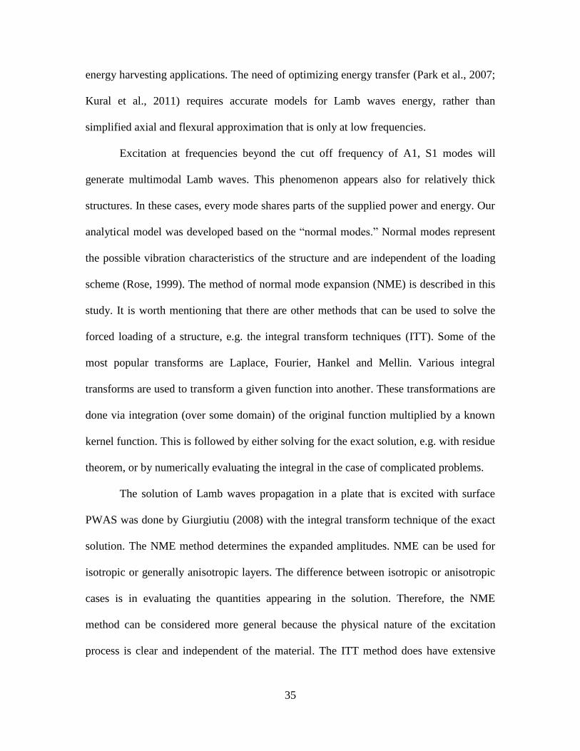
35
energy harvesting applications. The need of optimizing energy transfer (Park et al., 2007;
Kural et al., 2011) requires accurate models for Lamb waves energy, rather than
simplified axial and flexural approximation that is only at low frequencies.
Excitation at frequencies beyond the cut off frequency of A1, S1 modes will
generate multimodal Lamb waves. This phenomenon appears also for relatively thick
structures. In these cases, every mode shares parts of the supplied power and energy. Our
analytical model was developed based on the “normal modes.” Normal modes represent
the possible vibration characteristics of the structure and are independent of the loading
scheme (Rose, 1999). The method of normal mode expansion (NME) is described in this
study. It is worth mentioning that there are other methods that can be used to solve the
forced loading of a structure, e.g. the integral transform techniques (ITT). Some of the
most popular transforms are Laplace, Fourier, Hankel and Mellin. Various integral
transforms are used to transform a given function into another. These transformations are
done via integration (over some domain) of the original function multiplied by a known
kernel function. This is followed by either solving for the exact solution, e.g. with residue
theorem, or by numerically evaluating the integral in the case of complicated problems.
The solution of Lamb waves propagation in a plate that is excited with surface
PWAS was done by Giurgiutiu (2008) with the integral transform technique of the exact
solution. The NME method determines the expanded amplitudes. NME can be used for
isotropic or generally anisotropic layers. The difference between isotropic or anisotropic
cases is in evaluating the quantities appearing in the solution. Therefore, the NME
method can be considered more general because the physical nature of the excitation
process is clear and independent of the material. The ITT method does have extensive
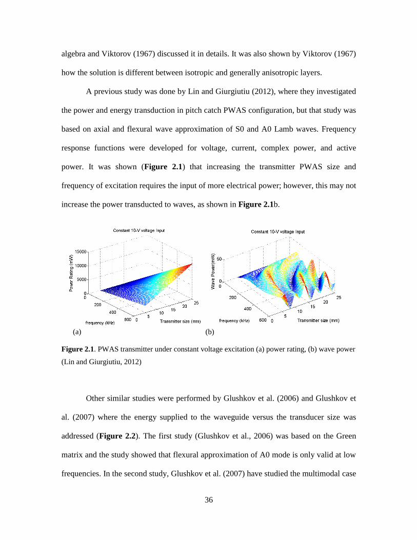
36
algebra and Viktorov (1967) discussed it in details. It was also shown by Viktorov (1967)
how the solution is different between isotropic and generally anisotropic layers.
A previous study was done by Lin and Giurgiutiu (2012), where they investigated
the power and energy transduction in pitch catch PWAS configuration, but that study was
based on axial and flexural wave approximation of S0 and A0 Lamb waves. Frequency
response functions were developed for voltage, current, complex power, and active
power. It was shown (Figure 2.1) that increasing the transmitter PWAS size and
frequency of excitation requires the input of more electrical power; however, this may not
increase the power transducted to waves, as shown in Figure 2.1b.
Figure 2.1. PWAS transmitter under constant voltage excitation (a) power rating, (b) wave power
(Lin and Giurgiutiu, 2012)
Other similar studies were performed by Glushkov et al. (2006) and Glushkov et
al. (2007) where the energy supplied to the waveguide versus the transducer size was
addressed (Figure 2.2). The first study (Glushkov et al., 2006) was based on the Green
matrix and the study showed that flexural approximation of A0 mode is only valid at low
frequencies. In the second study, Glushkov et al. (2007) have studied the multimodal case
(a) (b)
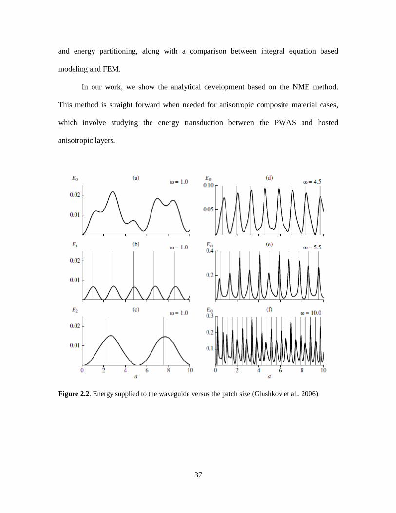
37
and energy partitioning, along with a comparison between integral equation based
modeling and FEM.
In our work, we show the analytical development based on the NME method.
This method is straight forward when needed for anisotropic composite material cases,
which involve studying the energy transduction between the PWAS and hosted
anisotropic layers.
Figure 2.2. Energy supplied to the waveguide versus the patch size (Glushkov et al., 2006)

38
2.2. ANALYTICAL DEVELOPMENT
Lamb Waves Normal Mode Expansion 2.2.1.
The normal mode expansion method is used to (a) directly find the amplitudes of
a given mode in terms of loading parameters and (b) evaluate the contribution factor of
every mode to the total wave power and energy. Normal modes of the guided waves in
the structure serve as the eigenfunctions. The method assumes that the desired solution
can be written in the form of a series of known functions, each with unknown amplitudes.
Then, those amplitudes are to be determined either numerically or by finding a general
expression that is valid for all modes.
Normal modes (eigenfunctions) of the analyzed structure are assumed ‘complete,’
meaning that any function can be represented exactly in terms of a finite or infinite
number of functions in the set of ‘normal modes.’ The second condition for the NME
method is the orthogonality of the base functions (Rose, 1999). The NME of the
displacement can be written as a summation of mode functions:
1
( , , ) ( , ) i t
j j
j
u x y t C U x y e
(2.1)
where jC is the contribution factor for each mode and
jU is mode shape. This solution is
assumed for the particular case of time harmonic with angular frequency .
Lamb waves (guided plate waves) are fully analyzed in a number of textbooks:
Graff (1991); Rose (1999); Giurgiutiu (2008). Here, we reproduce the essentials for
power and energy models. The wave equations are:
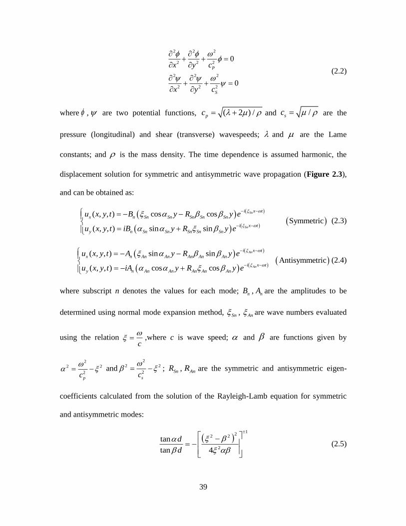
39
2 2 2
2 2 2
2 2 2
2 2 2
0
0
P
S
x y c
x y c
(2.2)
where , are two potential functions, ( 2 ) /pc and /sc
are the
pressure (longitudinal) and shear (transverse) wavespeeds; and are the Lame
constants; and is the mass density. The time dependence is assumed harmonic, the
displacement solution for symmetric and antisymmetric wave propagation (Figure 2.3),
and can be obtained as:
( , , ) cos cos Symmetric
( , , ) sin sin
Sn
Sn
i x t
x n Sn Sn Sn Sn Sn
i x t
y n Sn Sn Sn Sn Sn
u x y t B y R y e
u x y t iB y R y e
(2.3)
( , , ) sin sin Antisymmetric
( , , ) cos cos
An
An
i x t
x n An An An An An
i x t
y n An An An An An
u x y t A y R y e
u x y t iA y R y e
(2.4)
where subscript n denotes the values for each mode; nB , nA are the amplitudes to be
determined using normal mode expansion method, Sn , An are wave numbers evaluated
using the relation c
,where c is wave speed; and are functions given by
22 2
2
pc
and
22 2
2
sc
; SnR , AnR are the symmetric and antisymmetric eigen-
coefficients calculated from the solution of the Rayleigh-Lamb equation for symmetric
and antisymmetric modes:
12
2 2
2
tan
tan 4
d
d
(2.5)
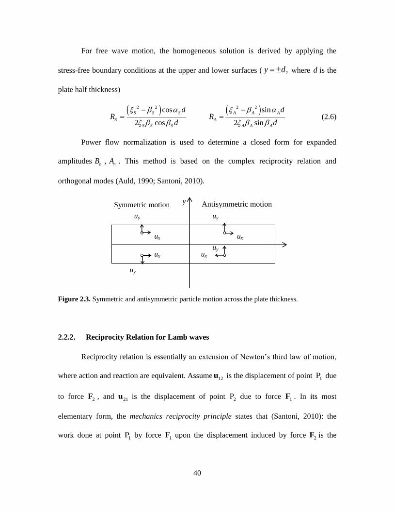
40
For free wave motion, the homogeneous solution is derived by applying the
stress-free boundary conditions at the upper and lower surfaces ( ,y d where d is the
plate half thickness)
2 2 2 2cos sin
2 cos 2 sin
S S S A A A
S A
S S S A A A
d dR R
d d
(2.6)
Power flow normalization is used to determine a closed form for expanded
amplitudes nB , nA . This method is based on the complex reciprocity relation and
orthogonal modes (Auld, 1990; Santoni, 2010).
Figure 2.3. Symmetric and antisymmetric particle motion across the plate thickness.
Reciprocity Relation for Lamb waves 2.2.2.
Reciprocity relation is essentially an extension of Newton’s third law of motion,
where action and reaction are equivalent. Assume 12u is the displacement of point 1P due
to force 2F , and 21u is the displacement of point 2P due to force 1F . In its most
elementary form, the mechanics reciprocity principle states that (Santoni, 2010): the
work done at point 1P by force 1F upon the displacement induced by force 2F is the
uy
ux
uy
ux
uy
ux
uy
ux
Symmetric motion Anti-symmetric motion Antisymmetric motion y

41
same as the work done at point 2P by force 2F upon the displacement induced by force
1F , i.e., 1 12 2 21 F u F u
For Lamb waves, we have real reciprocity and complex reciprocity; we focus on
complex reciprocity following Auld (1990).
Considering a generic body , and two sources 1F and 2F applied at points 1P
and 2P (Figure 2.4); the two force sources produce two wave fields with velocity and
stress 1 1,v T and 2 2,v T . Using equation of motion and applying the two different sources
(1) and (2) and adding the two field equations together, we can prove the complex
reciprocity form that relates the velocity responses, tractions and applied sources for
harmonic excitation, i.e.,
2 1 1 2 2 1 1 2 v T v T v F v F (2.7)
For Lamb waves, a similar relation has been derived in Santoni (2010), with the
assumption of time harmonic solution. One important assumption considered throughout
the analysis is that Lamb waves fields are z-invariant. Hence, the only surviving stresses
are normal stresses, xxT ,yyT and shear stress
xyT ; velocity fields are xv ,yv ; superscript
1,2
indicate fields due to sources 1,2.
Figure 2.4. Reciprocity relation, (Santoni, 2010)
1
2
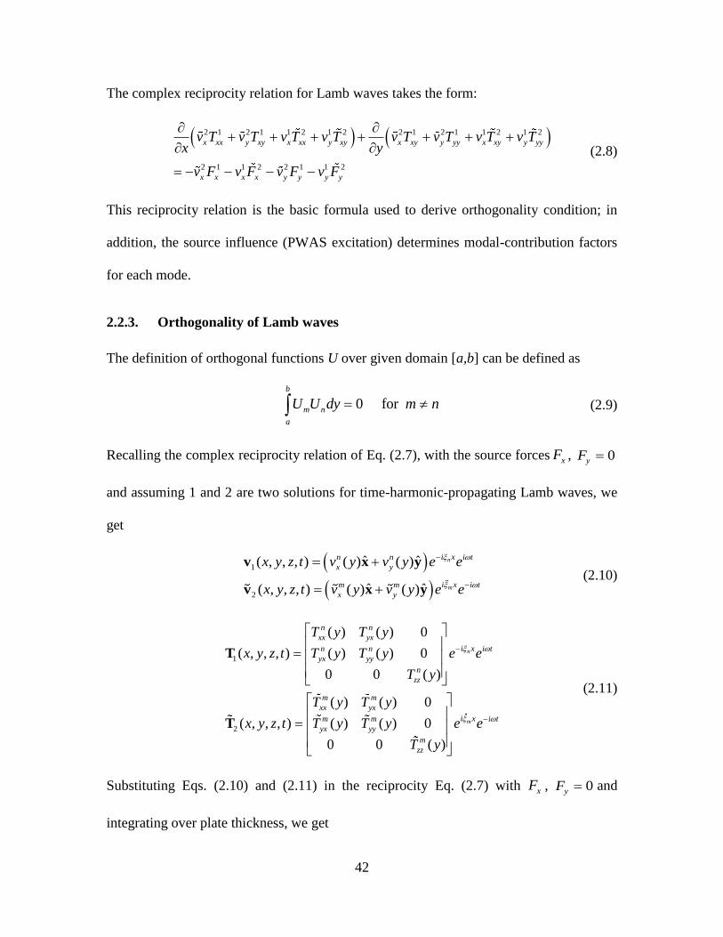
42
The complex reciprocity relation for Lamb waves takes the form:
2 1 2 1 1 2 1 2 2 1 2 1 1 2 1 2
2 1 1 2 2 1 1 2
x xx y xy x xx y xy x xy y yy x xy y yy
x x x x y y y y
v T v T v T v T v T v T v T v Tx y
v F v F v F v F
(2.8)
This reciprocity relation is the basic formula used to derive orthogonality condition; in
addition, the source influence (PWAS excitation) determines modal-contribution factors
for each mode.
Orthogonality of Lamb waves 2.2.3.
The definition of orthogonal functions U over given domain [a,b] can be defined as
0 for
b
m n
a
U U dy m n (2.9)
Recalling the complex reciprocity relation of Eq. (2.7), with the source forces xF , 0yF
and assuming 1 and 2 are two solutions for time-harmonic-propagating Lamb waves, we
get
1
2
ˆ ˆ( , , , ) ( ) ( )
ˆ ˆ( , , , ) ( ) ( )
n
m
i xn n i t
x y
i xm m i t
x y
x y z t v y v y e e
x y z t v y v y e e
v x y
v x y (2.10)
1
2
( ) ( ) 0
( , , , ) ( ) ( ) 0
0 0 ( )
( ) ( ) 0
( , , , ) ( ) ( ) 0
0 0 ( )
n
m
n n
xx yx
i xn n i t
yx yy
n
zz
m m
xx yx
i xm m i t
yx yy
m
zz
T y T y
x y z t T y T y e e
T y
T y T y
x y z t T y T y e e
T y
T
T
(2.11)
Substituting Eqs. (2.10) and (2.11) in the reciprocity Eq. (2.7) with xF , 0yF and
integrating over plate thickness, we get
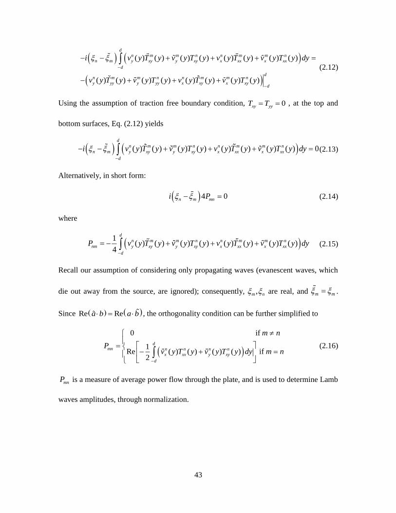
43
( ) ( ) ( ) ( ) ( ) ( ) ( ) ( )
( ) ( ) ( ) ( ) ( ) ( ) ( ) ( )
d
n m m n n m m n
n m y xy y xy x xx x xx
d
dn m m n n m m n
y yy y yy x xy x xyd
i v y T y v y T y v y T y v y T y dy
v y T y v y T y v y T y v y T y
(2.12)
Using the assumption of traction free boundary condition,
0xy yyT T , at the top and
bottom surfaces, Eq. (2.12) yields
( ) ( ) ( ) ( ) ( ) ( ) ( ) ( ) 0
d
n m m n n m m n
n m y xy y xy x xx x xx
d
i v y T y v y T y v y T y v y T y dy
(2.13)
Alternatively, in short form:
4 0n m mni P (2.14)
where
1
( ) ( ) ( ) ( ) ( ) ( ) ( ) ( )4
d
n m m n n m m n
nm y xy y xy x xx x xx
d
P v y T y v y T y v y T y v y T y dy
(2.15)
Recall our assumption of considering only propagating waves (evanescent waves, which
die out away from the source, are ignored); consequently, ,m n are real, and m m .
Since Re Rea b a b , the orthogonality condition can be further simplified to
0 if
1Re ( ) ( ) ( ) ( ) if
2
dmn n n n n
x xx y xy
d
m n
Pv y T y v y T y dy m n
(2.16)
mnP is a measure of average power flow through the plate, and is used to determine Lamb
waves amplitudes, through normalization.
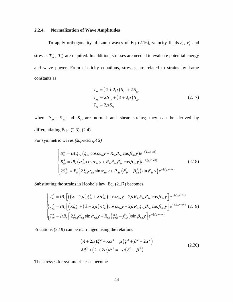
44
Normalization of Wave Amplitudes 2.2.4.
To apply orthogonality of Lamb waves of Eq. (2.16), velocity fields n
xv , n
yv and
stresses n
xxT , n
xyT are required. In addition, stresses are needed to evaluate potential energy
and wave power. From elasticity equations, stresses are related to strains by Lame
constants as
2
2
2
xx xx yy
yy xx yy
xy xy
T S S
T S S
T S
(2.17)
where xxS ,yyS and
xyS are normal and shear strains; they can be derived by
differentiating Eqs. (2.3), (2.4)
For symmetric waves (superscript S)
2
2 2
cos cos
cos cos
2 2 sin sin
Sn
Sn
Sn
i x tS
xx n Sn Sn Sn Sn Sn Sn
i x tS
yy n Sn Sn Sn Sn Sn Sn
i x tS
xy n Sn Sn Sn Sn Sn Sn Sn
S iB y R y e
S iB y R y e
S B y R y e
(2.18)
Substituting the strains in Hooke’s law, Eq. (2.17) becomes
2 2
2 2
2 2
2 cos 2 cos
2 cos 2 cos
2 sin sin
Sn
Sn
Sn
i x tS
xx n Sn Sn Sn Sn Sn Sn Sn
i x tS
yy n Sn Sn Sn Sn Sn Sn Sn
i x tS
xy n Sn Sn Sn Sn Sn Sn Sn
T iB y R y e
T iB y R y e
T B y R y e
(2.19)
Equations (2.19) can be rearranged using the relations
2 2 2 2 2
2 2 2 2
2 2
2
(2.20)
The stresses for symmetric case become
45
2 2 2
2 2
2 2
2 cos 2 cos
cos 2 cos
2 sin sin
Sn
Sn
Sn
i x tS
xx n Sn Sn Sn Sn Sn Sn Sn Sn
i x tS
yy n Sn Sn Sn Sn Sn Sn Sn
i x tS
xy n Sn Sn Sn Sn Sn Sn Sn
T i B y R y e
T i B y R y e
T B y R y e
(2.21)
Similarly for antisymmetric waves, (superscript A) for the sake of completeness
2
2
2 2
sin sin
sin sin
2 2 cos cos
An
An
An
i x tA
xx n An An An An An An
i x tA
yy n An An An An An An
i x tA
xy n An An An An An An An
S iA y R y e
S iA y R y e
S A y R y e
(2.22)
The stresses for antisymmetric case are
2 2 2
2 2
2 2
2 sin 2 sin
sin 2 sin
2 cos cos
An
An
An
i x tA
xx n An An An An An An An An
i x tA
yy n An An An An An An An
i x tA
xy n An An An An An An An
T i A y R y e
T i A y R y e
T A y R y e
(2.23)
Velocity fields are evaluated by taking time derivative of displacements in Eqs. (2.3) and
(2.4)
cos cos
sin sin
S
S
Si x tS x
x S S S S S
S
y i x tS
y S S S S S
uv i B y R y e
t
uv B y R y e
t
(2.24)
sin sin
cos cos
A
A
Ai x tA x
x A A A A A
A
y i x tA
y A A A A A
uv i A y R y e
t
uv A y R y e
t
(2.25)
Substituting Eqs. (2.21),(2.23),(2.24) and (2.25) in Eq. (2.16) and performing the
integration yields
2 2
(Symmetric) (Antisymmetric)2 2
n n
nn S nn A
B AP W P W
(2.26)
46
where
2 2 2 2 2 2
2 2 2
2 2
sin cos1 3
sin cos4
4 sin cos 2 3 cos sin
S S
S S S S S S S S
S
S S
S S S S S
S
S S S S S S S S S S
d dd R R
d dW
R d d R d d
(2.27)
2 2 2 2 2 2
2 2 2
2 2
sin cos1 3
sin cos4
4 cos sin 2 3 sin cos
A A
A A A A A A A A
A
A A
A A A A A
A
A A A A A A A A A A
d dd R R
d dW
R d d R d d
(2.28)
The symmetric mode coefficient nB and the antisymmetric mode coefficient nA can be
resolved as
2 2
(symmetric) (antisymmetric)nn nn
n n
Sn An
P PB A
W W (2.29)
For normal modes, we may assume 1nnP ; hence,
2 2
(symmetric) (antisymmetric)n n
Sn An
B AW W
(2.30)
Modal Contribution Factors and PWAS Excitation 2.2.5.
Basic assumptions used in this study are: (1) straight crested Lamb waves, i.e., z-
invariant, and (2) ideal bonding (pin-force) connection between PWAS and structure
(Figure 2.5). After consideration of the orthogonality of Lamb wave modes and after the
normalization of modes amplitudes with respect to the power, modal-participation factor
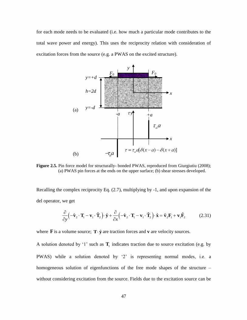
47
for each mode needs to be evaluated (i.e. how much a particular mode contributes to the
total wave power and energy). This uses the reciprocity relation with consideration of
excitation forces from the source (e.g. a PWAS on the excited structure).
Figure 2.5. Pin force model for structurally- bonded PWAS, reproduced from Giurgiutiu (2008);
(a) PWAS pin forces at the ends on the upper surface; (b) shear stresses developed.
Recalling the complex reciprocity Eq. (2.7), multiplying by -1, and upon expansion of the
del operator, we get
2 1 1 2 2 1 1 2 2 1 1 2ˆ ˆ
y x
v T v T y v T v T x v F v F (2.31)
where F is a volume source; ˆT y are traction forces and v are velocity sources.
A solution denoted by ‘1’ such as 1T indicates traction due to source excitation (e.g. by
PWAS) while a solution denoted by ‘2’ is representing normal modes, i.e. a
homogeneous solution of eigenfunctions of the free mode shapes of the structure –
without considering excitation from the source. Fields due to the excitation source can be
F0 F0
y
x
y=+d
y=-d
h=2d
y
x
-a +a
(a)
(b)
48
represented as normal modes summation over all possible modes (Rose, 1999; Santoni,
2010), i.e.
1 1
1 1
( , ) ( ) ( )
( , ) ( ) ( )
m m
m
m m
m
x y a x y
x y a x y
v v v
T T T (2.32)
where ( )ma x are the modal-participation factors that must be determined.
Homogeneous solution ‘2’ can be represented as
2
2
( , ) ( )
( , ) ( )
n
n
i x
n
i x
n
x y y e
x y y e
v v
T T (2.33)
Integrate Eq. (2.31) with respect to the plate thickness y from ( y d to y d ) to get
2 1 1 2 2 1 1 2 2 1ˆ ˆ
d dd
dd d
dy dyx
v T v T y v T v T x v F (2.34)
Substitution of Eqs. (2.32) and (2.33) ,and rearrangement yields
1 1
1
ˆ( ) ( )
ˆ( ) ( ) ( ) ( ) ( ) ( )
n
n n
di x
n nd
d d
i x i x
m n m m n n
m d d
y y e
e a x y y y y dy e y dyx
v T v T y
v T v T x v F
(2.35)
Recall the orthogonality relation in its general form
1
ˆ( ) ( ) ( ) ( )4
d
mn m n n m
d
P y y y y dy
v T v T x (2.36)
In the absence of a volume force source term 1F , Eq. (2.35) yields
1 1ˆ 4 ( ) 0n n
di x i x
n n m mnd
m
e e a x Px
v T v T y (2.37)
49
Since the modes are orthogonal, the summation in (2.37) has only one nonzero term
corresponding to the propagating mode n ( n real) for which 0nnP . Hence, Eq. (2.37)
becomes
1 1ˆ4 ( )
d
nn n n n nd
P i a xx
v T v T y (2.38)
This is a general ordinary differential equation, which needs to be solved to get the modal
participation factor ( )na x .
nT is the traction force; it must satisfy the traction free boundary condition for Lamb
waves, 0n
xy dT
and 0n
yy dT
. 1T is the excitation shear. We have ( )xy xd
T t x at the
upper surface, and 0xy dT
on the lower surface, since PWAS excitation is only on the
upper surface (Figure 2.5).
For Lamb waves, Eq. (2.38) takes the form
1 1
1 1
( ) ( ) ( ) ( )4 ( )
( ) ( ) ( ) ( )
dn n
y yy y yy
nn n n n n
x xy x xy d
v y T y v y T yP i a x
x v y T y v y T y
(2.39)
Applying traction free conditions and PWAS excitation, then solving the ODE, yields
( )
( ) ( ) for 4
n n
an
i x i xx
n x
nn a
v da x e t x dx e x a
P
(2.40)
It should be noted that this formula is only for the forward wave solution and outside the
excitation region, i.e. for x a .
50
The total particle velocity using NME can be written as
( , ) ( ) ( )n n
n
x y a x yv v (2.41)
where ( )n yv is the velocity modeshape of the thn mode, i.e.,
( )( )
( )
n
x
n n
y
v yy
v y
v . ( )n yv
can be derived using the combination of the symmetric particle velocity in Eq. (2.24)
with the symmetric normalization coefficient of Eq. (2.30) and the antisymmetric particle
velocity Eq. (2.25) and antisymmetric normalization coefficient of Eq. (2.30).
We exemplify the NME method for velocity fields with two examples: (a) 1-mm
thick aluminum plate, up to 2000 kHz where only S0, A0 modes exist; (b) 2.6-mm thick
steel plate, with excitation up to 500 kHz. Figure 2.6 shows the particle velocity at the
plate’s surface in the x-axis and y-axis for the two plates. Note that the values of NME
velocities are not multiplied yet by PWAS excitation. The displayed results are only for
the first symmetric S0 and antisymmetric A0 modes; the multi-modes demonstration will
be shown in a later section.
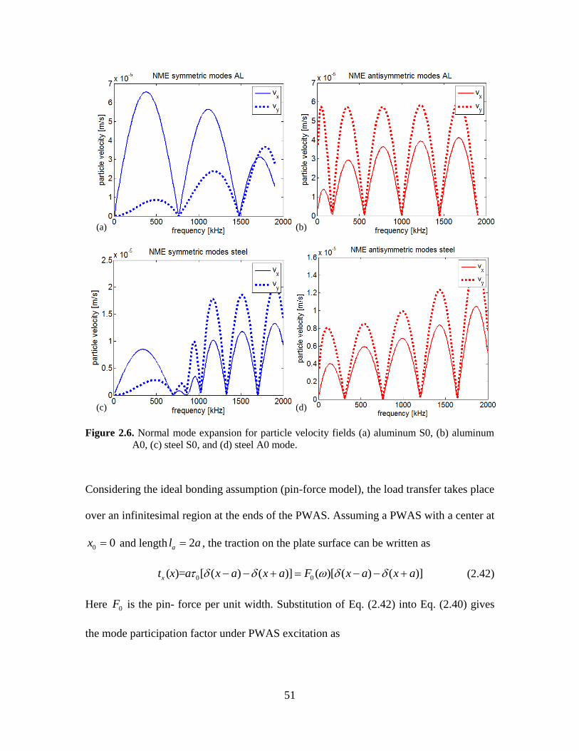
51
Figure 2.6. Normal mode expansion for particle velocity fields (a) aluminum S0, (b) aluminum
A0, (c) steel S0, and (d) steel A0 mode.
Considering the ideal bonding assumption (pin-force model), the load transfer takes place
over an infinitesimal region at the ends of the PWAS. Assuming a PWAS with a center at
0 0x and length 2al a , the traction on the plate surface can be written as
0 0( )= [ ( ) ( )] ( )[ ( ) ( )]xt x a x a x a F x a x a (2.42)
Here 0F is the pin- force per unit width. Substitution of Eq. (2.42) into Eq. (2.40) gives
the mode participation factor under PWAS excitation as
(d) (c)
(a) (b)
52
0 0 0( ) ( )[ ] ( )4
n n n n
n
x i a i a i x i xPWAS
n n
nn
v da x F e e e g F e
P
(2.43)
where ng is the coefficient
[ ]4
n n
n
x i a i a
n
nn
v dg e e
P
The Lamb wave NME of the particle displacement under PWAS excitation is
0
1( , ) ( ) ( )ni x
n n
n
u x y g F e yi
v (2.44)
The displacement in x-direction at the PWAS end ( , x a y d ) is
0
1( , ) ( )[ ] ( )
4n n n
n
x i a i a i an
x x
n nn
v du a d v d e e F e
i P
(2.45)
PWAS – Structure Interaction 2.2.6.
Consider a PWAS of length 2l a , width b and thickness at ; the relation between
the PWAS pin-force applied to the structure and the particle displacement is through the
structural dynamic stiffness. The structures as well as the PWAS stiffness are now
analyzed. When the PWAS transmitter is excited by an oscillatory voltage, its volume
expands in phase with the voltage in accordance with the piezoelectric effect, (Figure
2.7). Expansion of the PWAS mounted on the surface of the structure induces a surface
reaction from the structure in the form of a force at the PWAS end. The PWAS end
displacement is constrained by the plate and is equal to the plate displacement at x a .
The reaction force along the PWAS edge, .0F b , depends on the PWAS displacement,
PWASu , and on the frequency-dependent dynamic stiffness, strk , presented by the
structure to the PWAS.
0 ,str xF b k u a d (2.46)
53
The two stiffness elements on the right and the left of PWAS are selected to be
2 strk ; hence the overall structure stiffness is strk (Figure 2.7). Under harmonic excitation,
the dynamic stiffness strk is obtained by dividing the force by the displacement given
by Eq. (2.44), i.e.
1
0( )
ˆ ( , )ni a
str n n
nx
F bk i b g e d
u a d
v (2.47)
Define the static stiffness PWASk of a free PWAS as
11
a
PWAS E
t bk
s a (2.48)
The dynamic stiffness ratio is defined as the ratio between strk and PWASk , i.e.,
str
PWAS
kr
k
(2.49)
The relation between pin-force force per unit width and the static stiffness of the PWAS
is
0
1( , )
2PWAS x ISAF b k u a d u
(2.50)
where ISAu is the “induced strain actuation” displacement (Giurgiutiu, 2008), defined as,
31ˆ /ISA au ld V t and the quantity 1
2( , )x ISAu a d u represents the total x-direction
displacement at the right tip of the PWAS (because of symmetry, only the forward
propagating wave needs to be considered.)
Substitute ( , )xu a d from Eq. (2.45) into Eq. (2.50) and solve for 0F using strk from Eq.
(2.47) to get
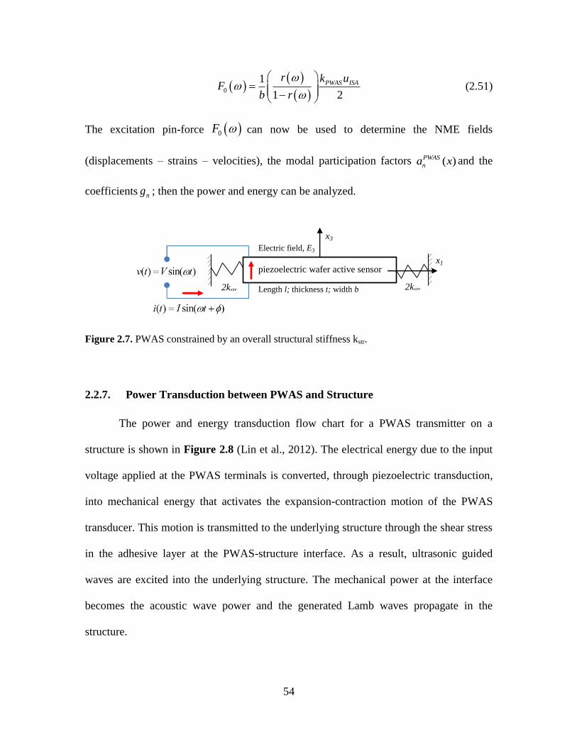
54
0
1
1 2
PWAS ISAr k u
Fb r
(2.51)
The excitation pin-force 0F can now be used to determine the NME fields
(displacements – strains – velocities), the modal participation factors ( )PWAS
na x and the
coefficients ng ; then the power and energy can be analyzed.
Figure 2.7. PWAS constrained by an overall structural stiffness kstr.
Power Transduction between PWAS and Structure 2.2.7.
The power and energy transduction flow chart for a PWAS transmitter on a
structure is shown in Figure 2.8 (Lin et al., 2012). The electrical energy due to the input
voltage applied at the PWAS terminals is converted, through piezoelectric transduction,
into mechanical energy that activates the expansion-contraction motion of the PWAS
transducer. This motion is transmitted to the underlying structure through the shear stress
in the adhesive layer at the PWAS-structure interface. As a result, ultrasonic guided
waves are excited into the underlying structure. The mechanical power at the interface
becomes the acoustic wave power and the generated Lamb waves propagate in the
structure.
piezoelectric wafer active sensor
Electric field, E3
x3
2kstr Length l; thickness t; width b 2kstr
x1
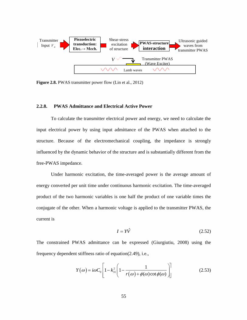
55
Figure 2.8. PWAS transmitter power flow (Lin et al., 2012)
PWAS Admittance and Electrical Active Power 2.2.8.
To calculate the transmitter electrical power and energy, we need to calculate the
input electrical power by using input admittance of the PWAS when attached to the
structure. Because of the electromechanical coupling, the impedance is strongly
influenced by the dynamic behavior of the structure and is substantially different from the
free-PWAS impedance.
Under harmonic excitation, the time-averaged power is the average amount of
energy converted per unit time under continuous harmonic excitation. The time-averaged
product of the two harmonic variables is one half the product of one variable times the
conjugate of the other. When a harmonic voltage is applied to the transmitter PWAS, the
current is
ˆI YV (2.52)
The constrained PWAS admittance can be expressed (Giurgiutiu, 2008) using the
frequency dependent stiffness ratio of equation(2.49), i.e.,
2
0 31
11 1
( )cot ( )Y i C k
r
(2.53)
Piezoelectric
transduction:
Elec.→ Mech.
PWAS-structure
interaction
Shear-stress
excitation
of structure
Transmitter
Input
Transmitter PWAS
(Wave Exciter)
V
B2
Lamb waves
Ultrasonic guided
waves from
transmitter PWAS
56
where ( ) ( )a . A simplified form of Eq. (2.53) can be obtained under the quasi-
static assumption in which the PWAS dynamics are assumed to happen at much higher
frequencies than the Lamb-wave propagation ( ( ) 0 , ( )cot ( ) 1 ), i.e.,
2
0 3111
rY i C k
r
(2.54)
This simplified model of admittance was used in Lin and Giurgiutiu (2012); it
was used for axial and flexural wave propagation at low frequency excitation. Here we
use a new definition of r in Eq. (2.49) and strk in Eq. (2.47) based on NME for
multi-modal Lamb waves propagation.
The power rating, time-averaged active power, and reactive power are
2 2 2 2 21 1 1ˆ ˆ ˆ 2 2 2
rating active reactive active R reactive IP Y V P P P Y V P Y V (2.55)
where RY is the real part of admittance and IY is the imaginary part of admittance.
The active power is the power that is converted to the mechanical power at the interface.
The reactive power is the imaginary part of the complex power that is not consumed and
is recirculated to the power supply. The power rating is the power requirement of the
power supply without distortion. In induced-strain transmitter applications, the reactive
power is the dominant factor, since the transmitter impedance is dominated by its
capacitive behavior (Lin et al., 2012). Managing high reactive power requirements is one
of the challenges of using piezoelectric induced-strain actuators.
57
Mechanical Power 2.2.9.
Due to the electro-mechanical transduction in the PWAS, the electrical active
power is converted into the mechanical power; through shear effects in the adhesive layer
between the PWAS and the structure. The mechanical power transfers into the structure
and excites the guided wave. Santoni (2010) studied shear lag solution for the case of
multiple Lamb wave modes. This solution can be simplified by considering that the shear
stress transfer is concentrated over some infinitesimal distances at the ends of the PWAS
actuator (Figure 2.5). The concept of ideal bonding (also known as the pin-force model)
assumed that all the load transfer takes place over an infinitesimal region at the PWAS
ends; the generated mechanical power is the multplication of this load times the structure
particle velocity at the PWAS tip. The time-averaged power is defined as
0
1 T
p p t dtT
(2.56)
The time-averaged product of two harmonic variables is one half the product of one
variable times the conjugate of the other. The time-averaged mechanical power at
PWAS-structure interface is
0 0 0
1ˆ
2p F v (2.57)
Mechanical power excites both forward and backward propagating waves initiating from
the two end tips at x a and x a . Due to symmetry, we only need to consider the
forward wave, which will contain only half of the mechanical power converted from the
electrical active power.
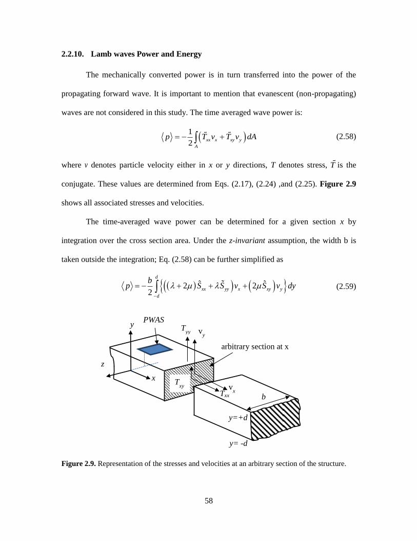
58
Lamb waves Power and Energy 2.2.10.
The mechanically converted power is in turn transferred into the power of the
propagating forward wave. It is important to mention that evanescent (non-propagating)
waves are not considered in this study. The time averaged wave power is:
1
2xx x xy y
A
p T v T v dA (2.58)
where v denotes particle velocity either in x or y directions, T denotes stress, T is the
conjugate. These values are determined from Eqs. (2.17), (2.24) ,and (2.25). Figure 2.9
shows all associated stresses and velocities.
The time-averaged wave power can be determined for a given section x by
integration over the cross section area. Under the z-invariant assumption, the width b is
taken outside the integration; Eq. (2.58) can be further simplified as
2 22
d
xx yy x xy y
d
bp S S v S v dy
(2.59)
Figure 2.9. Representation of the stresses and velocities at an arbitrary section of the structure.
x
y PWAS
arbitrary section at x
Txx
z
Tyy
Txy
b
y=+d
y= -d
vx
vy
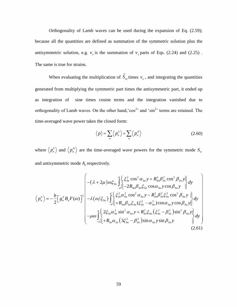
59
Orthogonality of Lamb waves can be used during the expansion of Eq. (2.59);
because all the quantities are defined as summation of the symmetric solution plus the
antisymmetric solution, e.g. xv is the summation of xv parts of Eqs. (2.24) and (2.25) .
The same is true for strains.
When evaluating the multiplication of xxS times xv , and integrating the quantities
generated from multiplying the symmetric part times the antisymmetric part, it ended up
as integration of sine times cosine terms and the integration vanished due to
orthogonality of Lamb waves. On the other hand,‘cos2’ and ‘sin
2’ terms are retained. The
time-averaged wave power takes the closed form:
S A
n n
n n
p p p (2.60)
where S
np and A
np are the time-averaged wave powers for the symmetric mode nS
and antisymmetric mode nA respectively.
2 2 2 2 2
2 2 2 2 2 2 22
2 2
cos cos2
2 cos cos
cos cos( )
2 ( )cos cos
2
d
Sn Sn Sn Sn Sn
Sn
d Sn Sn Sn Sn Sn
dSn Sn Sn Sn Sn Sn SnS S
n n n Sn
d Sn Sn Sn Sn Sn Sn Sn
S
y R ydy
R y y
y R ybp g B F dy
R y y
2 2 2 2 2 2
2 2
sin sin
3 sin sin
dn Sn Sn Sn Sn Sn Sn Sn
d Sn Sn Sn Sn Sn Sn
y R ydy
R y y
(2.61)
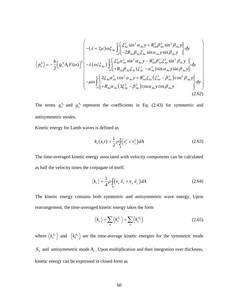
60
2 2 2 2 2
2 2 2 2 2 2 22
2 2
sin sin2
2 sin sin
sin sin( )
2 ( )sin sin
2
d
An An An An An
An
d An An An An An
dAn An An An An An SnA A
n n n An
d An An An An An An An
A
y R ydy
R y y
y R ybp g A F dy
R y y
2 2 2 2 2 2
2 2
cos os
3 cos cos
dn An An An An An An An
d An An An An An An
y R c ydy
R y y
(2.62)
The terms nS
ng and nA
ng represent the coefficients in Eq. (2.43) for symmetric and
antisymmetric modes.
Kinetic energy for Lamb waves is defined as
2 21( , )
2e x y
A
k x t v v dA (2.63)
The time-averaged kinetic energy associated with velocity components can be calculated
as half the velocity times the conjugate of itself.
1
. .4
e x x y y
A
k v v v v dA (2.64)
The kinetic energy contains both symmetric and antisymmetric wave energy. Upon
rearrangement, the time-averaged kinetic energy takes the form
n nS A
e e e
n n
k k k (2.65)
where nS
ek and nA
ek are the time-average kinetic energies for the symmetric mode
nS and antisymmetric mode nA . Upon multiplication and then integration over thickness,
kinetic energy can be expressed in closed form as
61
2 2 2 2 2 2
2
2 2 2 2 2 2
cos cos 2 cos cos
( )4
sin sin 2 sin sin
n n
d
Sn Sn Sn Sn Sn Sn Sn Sn Sn Sn
dS S
e n n d
Sn Sn Sn Sn Sn Sn Sn Sn Sn Sn
d
y R y R y y dyb
k g B F
y R y R y y dy
(2.66)
2 2 2 2 2 2
2
2 2 2 2 2 2
sin sin 2 sin sin
( )4
cos os 2 cos cos
n n
d
An An An An An An An An An An
dA A
e n n d
An An An An An An An An An An
d
y R y R y y dyb
k g A F
y R c y R y y dy
(2.67)
Equations (2.66), (2.67) can be further simplified as
2 2 22( ) cos cos sin sin
4n n
d
S S
e n n Sn Sn Sn Sn Sn Sn Sn Sn Sn Sn
d
bk g B F y R y y R y dy
(2.68)
2 2 22( ) sin sin cos cos
4n n
d
A A
e n n An An An An An An An An An An
d
bk g A F y R y y R y dy
(2.69)
Potential energy of the wave can be evaluated by the double inner (double dot) product
between stress and strain
1
( , ) : 2
e
A
v x t dA T S (2.70)
1
( , ) : 2
xx xy xz xx xy xz
e yx yy yz yx yy yz
A
zx zy zz zx zy zz
T T T S S S
v x t T T T S S S dA
T T T S S S
(2.71)
zzT and zzS are ignored due to the z-invariant assumption. Also yx xyT T , zx xzT T ,
zy yzT T due to symmetry of both stress and strain tensors; Eq. (2.71) yields
62
1
( , ) 2 2 22
e xx xx yy yy xy xy xz xz yz yz
A
v x t T S T S T S T S T S dA (2.72)
The stresses and strains associated with Lamb waves are xxT ,xyT ,
yyT and xxS ,xyS ,
yyS ; then
Lamb wave potential energy reduces to
1
( , ) 22
e xx xx yy yy xy xy
A
v x t T S T S T S dA (2.73)
The time-averaged potential energy is
1
2 2 2 2 24
e xx xx yy xx yy yy xy xy
A
v S S S S S S S S dA (2.74)
Similar to the kinetic energy, the time-averaged potential energy is the summation of the
potential energy of all modes, i.e.
n nS A
e e e
n n
v v v (2.75)
where nS
ev and nA
ev are the time-averaged potential energy for symmetric mode nS
and antisymmetric mode nA respectively, i.e.,
22
2 2 2 2 2 2 2
2 22
0
22
2 cos cos
cos cos2
( )cos cos( )
42 cos cos
2
n n
d
Sn Sn Sn Sn Sn Sn
d
dSn Sn Sn Sn Sn Sn Sn
dS S Sn Sn Sn Sn Sn Sn Sn
e n nd
Sn Sn Sn Sn Sn Sn
d
Sn
y R y dy
y R ydy
R y ybv g B F
y R y dy
2
2 2sin sin
d
Sn Sn Sn Sn Sn Sn
d
y R y dy
(2.76)
63
22
2 2 2 2 2 2 2
2 22
0
22
2 sin sin
sin sin2
( )sin sin( )
42 sin sin
2
n n
d
An An An An An An
d
dAn An An An An An An
dA A An An An An An An An
e n nd
An An An An An An
d
An
y R y dy
y R ydy
R y ybv g A F
y R y dy
2
2 2cos cos
d
An An An An An An
d
y R y dy
(2.77)
The total energy for Lamb waves per unit length is the summation of the kinetic and
potential energy. The total time-averaged Lamb wave energy at the plate cross section
corresponding to the PWAS end is
e e ee k v (2.78)
2.3. SIMULATION RESULTS
This section gives results of the simulation of power and energy transduction
between the PWAS and structure using the exact Lamb waves model. Comparison was
performed between the exact Lamb waves model results were presented here, and the
simplified axial and flexural waves model results of Lin and Giurgiutiu (2012). This was
followed by a parametric study to show how wave power and energy were changed with
different PWAS-sizes and excitation frequencies. The last part of this section shows the
applicability of our model for the case of multi-modal Lamb waves, which happens either
at higher frequency or in thicker structures. We examplify with the simulation of two
plates: (a) 1-mm aluminum up to 2000 kHz, and (b) 12.7-mm ( 12 in) steel up to 500 kHz
64
frequency. Figure 2.10a,b shows dispersion curves for the two plates. Figure 2.10a also
shows how the simplified axial and flexural waves compare with S0 and A0 Lamb waves
at low frequencies.
For the 1-mm aluminum plate, harmonic excitation of 10-volts was applied on a
7- mm PWAS with a frequency sweep from 1-2000 kHz such that only S0 and A0 Lamb
waves exist. However, the 12.7-mm steel plate (Figure 2.10b) was excited up to 500 kHz,
such that three symmetric modes (S0, S1, S2) and three antisymmetric modes (A0, A1,
A2) exist. Complete simulation parameters are given in Table 2.1 and Table 2.2.
Thin Plate Structure (One Symmetric and one Antisymmetric mode) 2.3.1.
The simulation results for the 1-mm aluminum structure are given in Figure 2.11.
As expected, the reactive electrical power required for PWAS excitation was orders of
magnitude larger than the active electrical power. Hence, the power rating of the PWAS
transmitter was dominated by the reactive power, i.e., by the capacitive behavior of the
PWAS. We noted that the transmitter reactive power was directly proportional to the
transmitter admittance (Y i C ), whereas the transmitter active power was the power
converted into the ultrasonic acoustic waves generated into the structure from the
transmitter. A remarkable variation of active power with frequency is shown in Figure
2.11a: we noticed that the active power (i.e., the power converted into the ultrasonic
waves) was not monotonic with frequency, but manifested peaks and valleys. As a result,
the ratio between the reactive and active powers was not constant, but presented the
peaks and valleys. The increase and decrease of active power with frequency corresponds
to the PWAS tuning in and out of various ultrasonic waves traveling into the structure.
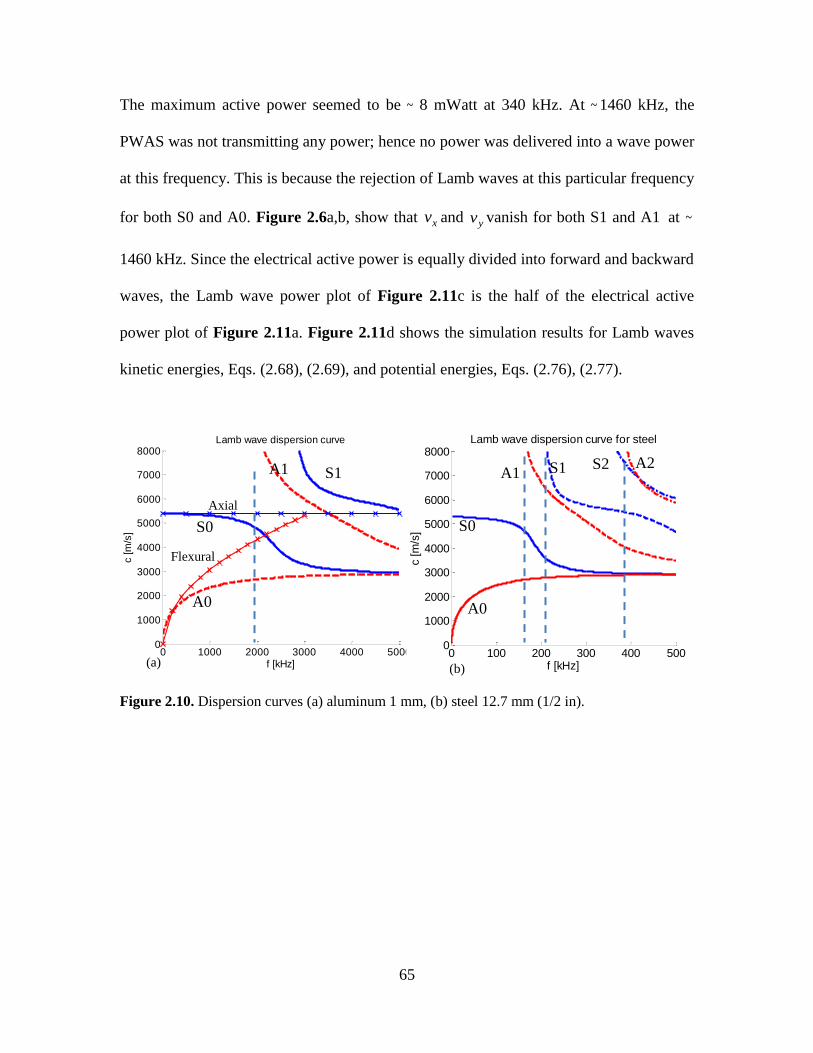
65
The maximum active power seemed to be ~ 8 mWatt at 340 kHz. At ~ 1460 kHz, the
PWAS was not transmitting any power; hence no power was delivered into a wave power
at this frequency. This is because the rejection of Lamb waves at this particular frequency
for both S0 and A0. Figure 2.6a,b, show that xv and yv vanish for both S1 and A1 at ~
1460 kHz. Since the electrical active power is equally divided into forward and backward
waves, the Lamb wave power plot of Figure 2.11c is the half of the electrical active
power plot of Figure 2.11a. Figure 2.11d shows the simulation results for Lamb waves
kinetic energies, Eqs. (2.68), (2.69), and potential energies, Eqs. (2.76), (2.77).
Figure 2.10. Dispersion curves (a) aluminum 1 mm, (b) steel 12.7 mm (1/2 in).
0 1000 2000 3000 4000 50000
1000
2000
3000
4000
5000
6000
7000
8000Lamb wave dispersion curve
f [kHz]
c [m
/s]
(a) 0 100 200 300 400 500
0
1000
2000
3000
4000
5000
6000
7000
8000Lamb wave dispersion curve for steel
f [kHz]
c [m
/s]
(b)
S0
A0
A1 S1
Flexural
Axial
A0
S0
A1 S1
A2 S2
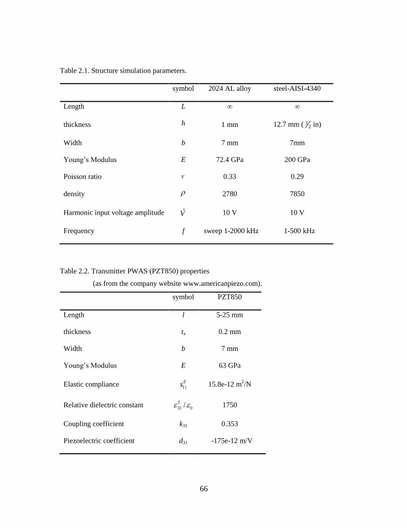
66
Table 2.1. Structure simulation parameters.
symbol 2024 AL alloy steel-AISI-4340
Length L ∞ ∞
thickness h 1 mm 12.7 mm ( 12 in)
Width b 7 mm 7mm
Young’s Modulus E 72.4 GPa 200 GPa
Poisson ratio 0.33 0.29
density 2780 7850
Harmonic input voltage amplitude V 10 V 10 V
Frequency f sweep 1-2000 kHz 1-500 kHz
Table 2.2. Transmitter PWAS (PZT850) properties
(as from the company website www.americanpiezo.com).
symbol PZT850
Length l 5-25 mm
thickness ta 0.2 mm
Width b 7 mm
Young’s Modulus E 63 GPa
Elastic compliance 11
Es 15.8e-12 m2/N
Relative dielectric constant 33 0/T 1750
Coupling coefficient k31 0.353
Piezoelectric coefficient d31 -175e-12 m/V
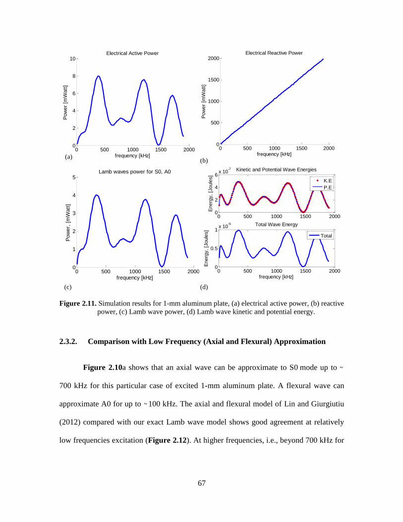
67
Figure 2.11. Simulation results for 1-mm aluminum plate, (a) electrical active power, (b) reactive
power, (c) Lamb wave power, (d) Lamb wave kinetic and potential energy.
Comparison with Low Frequency (Axial and Flexural) Approximation 2.3.2.
Figure 2.10a shows that an axial wave can be approximate to S0 mode up to ~
700 kHz for this particular case of excited 1-mm aluminum plate. A flexural wave can
approximate A0 for up to ~ 100 kHz. The axial and flexural model of Lin and Giurgiutiu
(2012) compared with our exact Lamb wave model shows good agreement at relatively
low frequencies excitation (Figure 2.12). At higher frequencies, i.e., beyond 700 kHz for
(c)
(b)
(d)
0 500 1000 1500 20000
2
4
6
8
10
frequency [kHz]
Pow
er
[mW
att
]
Electrical Active Power
(a) 0 500 1000 1500 2000
0
500
1000
1500
2000
frequency [kHz]
Pow
er
[mW
att
]
Electrical Reactive Power
0 500 1000 1500 20000
1
2
3
4
5
frequency [kHz]
Pow
er,
[m
Watt
]
Lamb waves power for S0, A0
0 500 1000 1500 20000
2
4
6x 10
-7
Energ
y,
[Joule
s]
Kinetic and Potential Wave Energies
K.E
P.E
0 500 1000 1500 20000
0.5
1x 10
-6
frequency [kHz]
Energ
y,
[Joule
s]
Total Wave Energy
Total
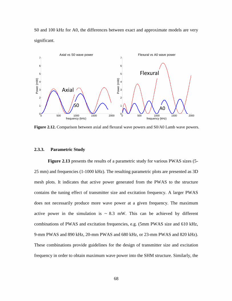
68
S0 and 100 kHz for A0, the differences between exact and approximate models are very
significant.
Figure 2.12. Comparison between axial and flexural wave powers and S0/A0 Lamb wave powers.
Parametric Study 2.3.3.
Figure 2.13 presents the results of a parametric study for various PWAS sizes (5-
25 mm) and frequencies (1-1000 kHz). The resulting parametric plots are presented as 3D
mesh plots. It indicates that active power generated from the PWAS to the structure
contains the tuning effect of transmitter size and excitation frequency. A larger PWAS
does not necessarily produce more wave power at a given frequency. The maximum
active power in the simulation is ~ 8.3 mW. This can be achieved by different
combinations of PWAS and excitation frequencies, e.g. (5mm PWAS size and 610 kHz,
9-mm PWAS and 890 kHz, 20-mm PWAS and 680 kHz, or 23-mm PWAS and 820 kHz).
These combinations provide guidelines for the design of transmitter size and excitation
frequency in order to obtain maximum wave power into the SHM structure. Similarly, the
0 500 1000 1500 20000
1
2
3
4
5
6
7Axial vs S0 wave power
frequency (kHz)
Pow
er
(mW
)
0 500 1000 1500 20000
1
2
3
4
5
6
7Flexural vs A0 wave power
frequency (kHz)P
ow
er
(mW
)
Flexural
A0 S0
Axial

69
total Lamb wave energy shows the same tuning trend in relation to the PWAS size and
excitation frequency as shown in Figure 2.14.
2.4. EXPANDING TO MULTIMODE LAMB WAVE
Thick Plate Structure (multi-mode Lamb waves) 2.4.1.
A multi-modal Lamb waves simulation was performed on a 12.7-mm thick steel
plate for up to 500 kHz excitation frequency and 10V harmonic voltage applied to PWAS.
All structural simulation parameters are listed in Table 2.1 and PWAS parameters are
listed in Table 2.2.
The objective is to evaluate electrical active power, reactive power and show how
the active power part is converted to Lamb wave power in the presence of multi-modal
Lamb waves. Dispersion curves plots in Figure 2.10b show that the S1 mode starts ~
215 kHz, S2 starts at ~ 370 kHz, while A1 starts at ~ 170 kHz, and A2 starts at 390 kHz.
Due to the sudden appearance of Lamb wave modes at cut-off frequencies, the normal
mode expansion solution encounters sudden jumps. This is due to the appearance of new
components caused by the new modes. For that reason, a smoothing function is applied as
described in the next section.
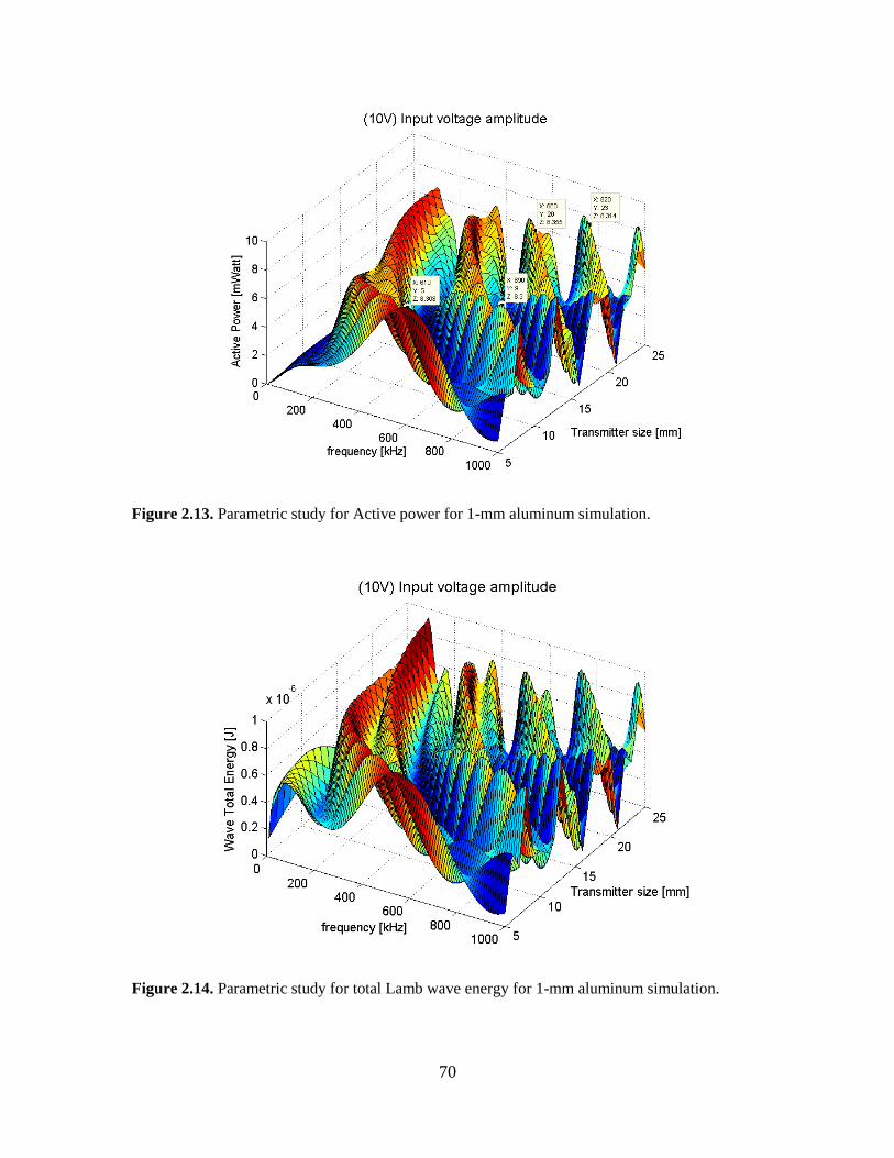
70
Figure 2.13. Parametric study for Active power for 1-mm aluminum simulation.
Figure 2.14. Parametric study for total Lamb wave energy for 1-mm aluminum simulation.

71
Smoothing function
The smoothing function is a smoothed step function, (Sohoni, 1995) as shown in
Figure 2.15. The mathematical formula is
1 1
1 1 2 2 1 2
2 2
( ) ( , , , , )
h x X
f x f x X h X h X x X
h x X
(2.79)
1 1 1( ) [ / ]*( ) [ / 2 ]*sin{(2 / )*( )}f x h h x x X h x x X (2.80)
This is implemented in our NME solution by setting X1 to the cut-off frequency of
the selected mode and h1 to zero; hence the mode is forced to start from zero, and
consequently its contribution to the NME summation is smoothed. 1h ; x is arbitrary;
we selected 150x kHz, for symmetric modes, and 120x kHz for antisymmetric
modes.
Figure 2.15. ADAMS step function.
X1 X2
h1
h2
Independent variable
Function value
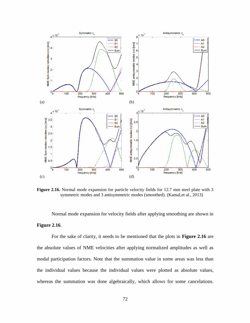
72
Figure 2.16. Normal mode expansion for particle velocity fields for 12.7 mm steel plate with 3
symmetric modes and 3 antisymmetric modes (smoothed). (Kamal,et al., 2013)
Normal mode expansion for velocity fields after applying smoothing are shown in
Figure 2.16.
For the sake of clarity, it needs to be mentioned that the plots in Figure 2.16 are
the absolute values of NME velocities after applying normalized amplitudes as well as
modal participation factors. Note that the summation value in some areas was less than
the individual values because the individual values were plotted as absolute values,
whereas the summation was done algebraically, which allows for some cancelations.
(c)
(b) (a)
(d)
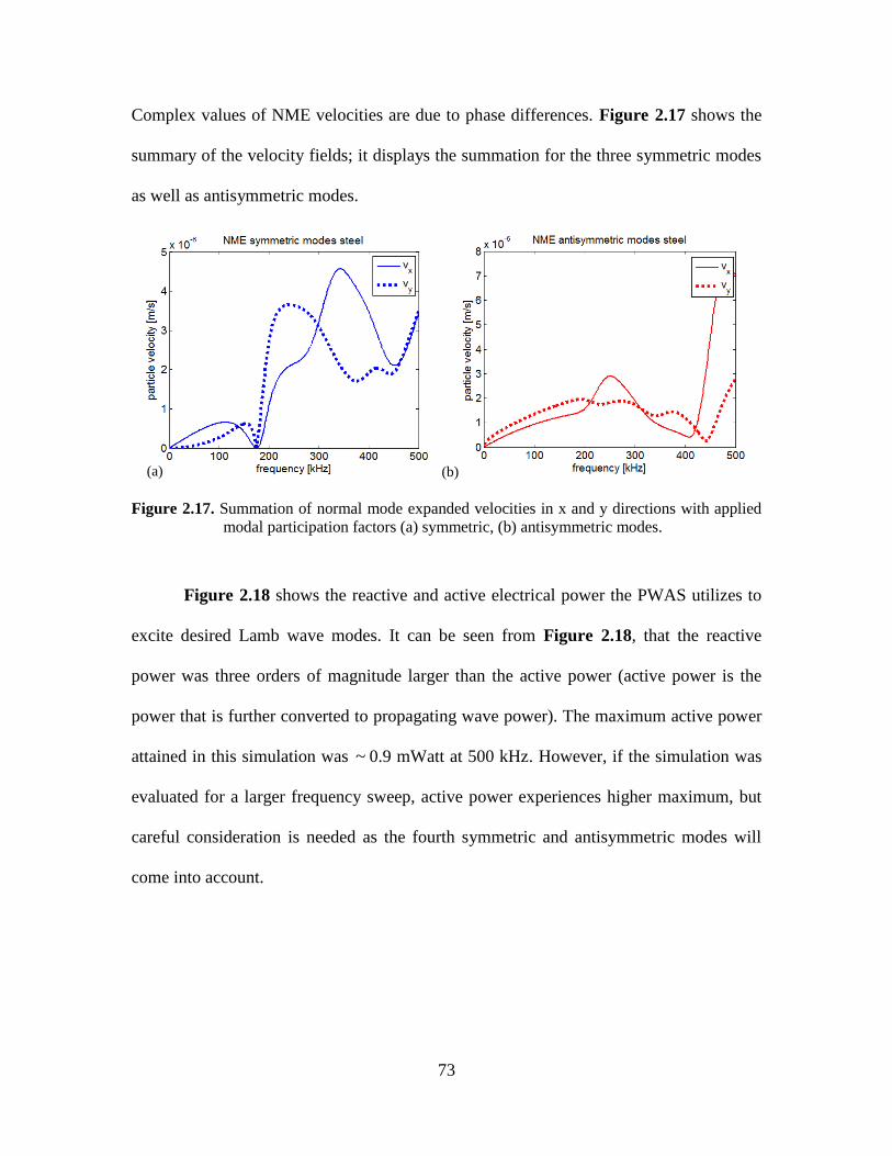
73
Complex values of NME velocities are due to phase differences. Figure 2.17 shows the
summary of the velocity fields; it displays the summation for the three symmetric modes
as well as antisymmetric modes.
Figure 2.17. Summation of normal mode expanded velocities in x and y directions with applied
modal participation factors (a) symmetric, (b) antisymmetric modes.
Figure 2.18 shows the reactive and active electrical power the PWAS utilizes to
excite desired Lamb wave modes. It can be seen from Figure 2.18, that the reactive
power was three orders of magnitude larger than the active power (active power is the
power that is further converted to propagating wave power). The maximum active power
attained in this simulation was ~ 0.9 mWatt at 500 kHz. However, if the simulation was
evaluated for a larger frequency sweep, active power experiences higher maximum, but
careful consideration is needed as the fourth symmetric and antisymmetric modes will
come into account.
(a) (b)
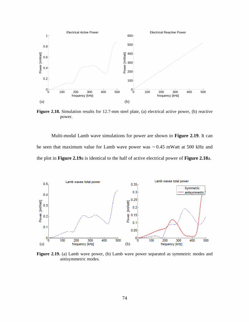
74
Figure 2.18. Simulation results for 12.7-mm steel plate, (a) electrical active power, (b) reactive
power.
Multi-modal Lamb wave simulations for power are shown in Figure 2.19. It can
be seen that maximum value for Lamb wave power was ~ 0.45 mWatt at 500 kHz and
the plot in Figure 2.19a is identical to the half of active electrical power of Figure 2.18a.
Figure 2.19. (a) Lamb wave power, (b) Lamb wave power separated as symmetric modes and
antisymmetric modes.
0 100 200 300 400 5000
0.2
0.4
0.6
0.8
1
frequency [kHz]
Pow
er
[mW
att
]
Electrical Active Power
(b) (a)
0 100 200 300 400 5000
100
200
300
400
500
600
frequency [kHz]
Pow
er
[mW
att
]
Electrical Reactive Power
(b) (a)
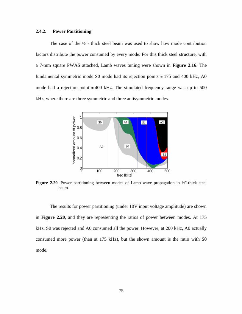
75
Power Partitioning 2.4.2.
The case of the ½"- thick steel beam was used to show how mode contribution
factors distribute the power consumed by every mode. For this thick steel structure, with
a 7-mm square PWAS attached, Lamb waves tuning were shown in Figure 2.16. The
fundamental symmetric mode S0 mode had its rejection points 175 and 400 kHz, A0
mode had a rejection point 400 kHz. The simulated frequency range was up to 500
kHz, where there are three symmetric and three antisymmetric modes.
Figure 2.20. Power partitioning between modes of Lamb wave propagation in ½"-thick steel
beam.
The results for power partitioning (under 10V input voltage amplitude) are shown
in Figure 2.20, and they are representing the ratios of power between modes. At 175
kHz, S0 was rejected and A0 consumed all the power. However, at 200 kHz, A0 actually
consumed more power (than at 175 kHz), but the shown amount is the ratio with S0
mode.
0 100 200 300 400 5000
0.2
0.4
0.6
0.8
1
freq [kHz]
norm
alized a
mount of pow
er
S0
A1
A0
S1
S2
A2
S0
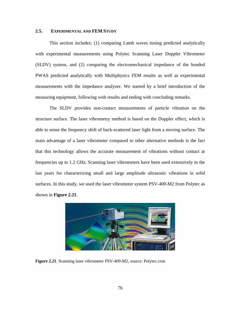
76
2.5. EXPERIMENTAL AND FEM STUDY
This section includes: (1) comparing Lamb waves tuning predicted analytically
with experimental measurements using Polytec Scanning Laser Doppler Vibrometer
(SLDV) system, and (2) comparing the electromechanical impedance of the bonded
PWAS predicted analytically with Multiphysics FEM results as well as experimental
measurements with the impedance analyzer. We started by a brief introduction of the
measuring equipment, following with results and ending with concluding remarks.
The SLDV provides non-contact measurements of particle vibration on the
structure surface. The laser vibrometry method is based on the Doppler effect, which is
able to sense the frequency shift of back-scattered laser light from a moving surface. The
main advantage of a laser vibrometer compared to other alternative methods is the fact
that this technology allows the accurate measurement of vibrations without contact at
frequencies up to 1.2 GHz. Scanning laser vibrometers have been used extensively in the
last years for characterizing small and large amplitude ultrasonic vibrations in solid
surfaces. In this study, we used the laser vibrometer system PSV-400-M2 from Polytec as
shown in Figure 2.21.
Figure 2.21. Scanning laser vibrometer PSV-400-M2, source: Polytec.com
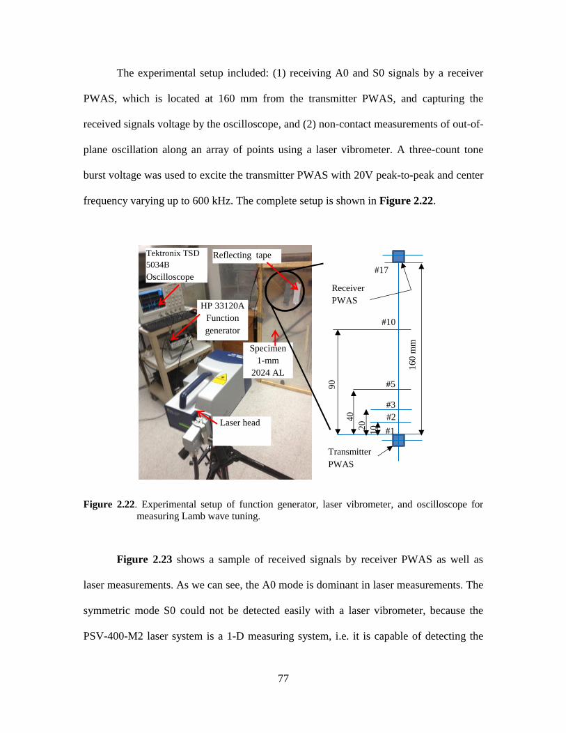
77
The experimental setup included: (1) receiving A0 and S0 signals by a receiver
PWAS, which is located at 160 mm from the transmitter PWAS, and capturing the
received signals voltage by the oscilloscope, and (2) non-contact measurements of out-of-
plane oscillation along an array of points using a laser vibrometer. A three-count tone
burst voltage was used to excite the transmitter PWAS with 20V peak-to-peak and center
frequency varying up to 600 kHz. The complete setup is shown in Figure 2.22.
Figure 2.22. Experimental setup of function generator, laser vibrometer, and oscilloscope for
measuring Lamb wave tuning.
Figure 2.23 shows a sample of received signals by receiver PWAS as well as
laser measurements. As we can see, the A0 mode is dominant in laser measurements. The
symmetric mode S0 could not be detected easily with a laser vibrometer, because the
PSV-400-M2 laser system is a 1-D measuring system, i.e. it is capable of detecting the
#17
#10
#5
#2 1
60
mm
10
40
#1
90
Transmitter
PWAS
#3
20
Laser head
HP 33120A Function
generator
Tektronix TSD
5034B
Oscilloscope
Specimen 1-mm
2024 AL
Receiver
PWAS
Reflecting tape
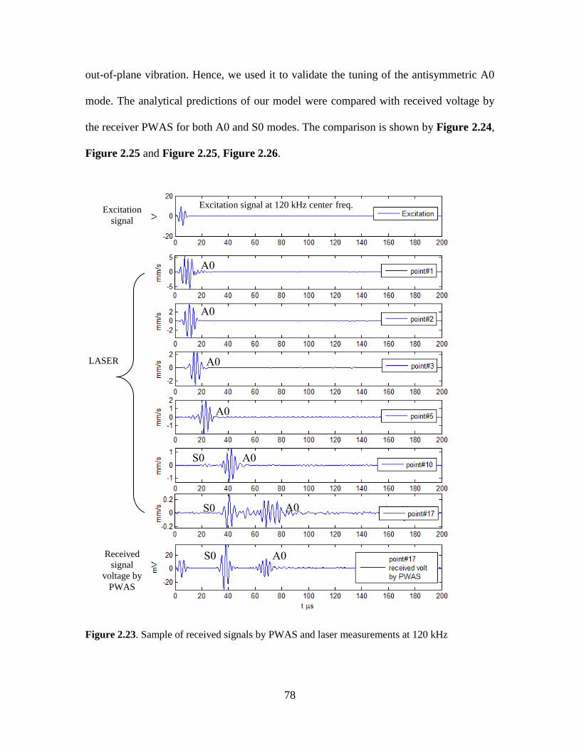
78
out-of-plane vibration. Hence, we used it to validate the tuning of the antisymmetric A0
mode. The analytical predictions of our model were compared with received voltage by
the receiver PWAS for both A0 and S0 modes. The comparison is shown by Figure 2.24,
Figure 2.25 and Figure 2.25, Figure 2.26.
Figure 2.23. Sample of received signals by PWAS and laser measurements at 120 kHz
LASER
Excitation signal at 120 kHz center freq.
A0
A0
A0
A0
A0
A0
A0 S0
S0
S0
Received
signal
voltage by
PWAS
Excitation
signal
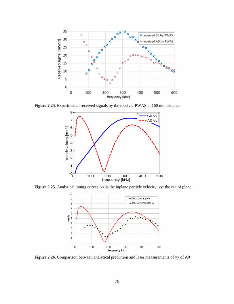
79
Figure 2.24. Experimental received signals by the receiver PWAS at 160 mm distance
Figure 2.25. Analytical tuning curves, vx is the inplane particle velocity, vy: the out of plane.
Figure 2.26. Comparison between analytical prediction and laser measurements of vy of A0
0 100 200 300 400 5000
1
2
3
4
5
6
7
8
frequency [kHz]
part
icle
vel
ocity
[mm
/s]
S0 vx
A0 vy
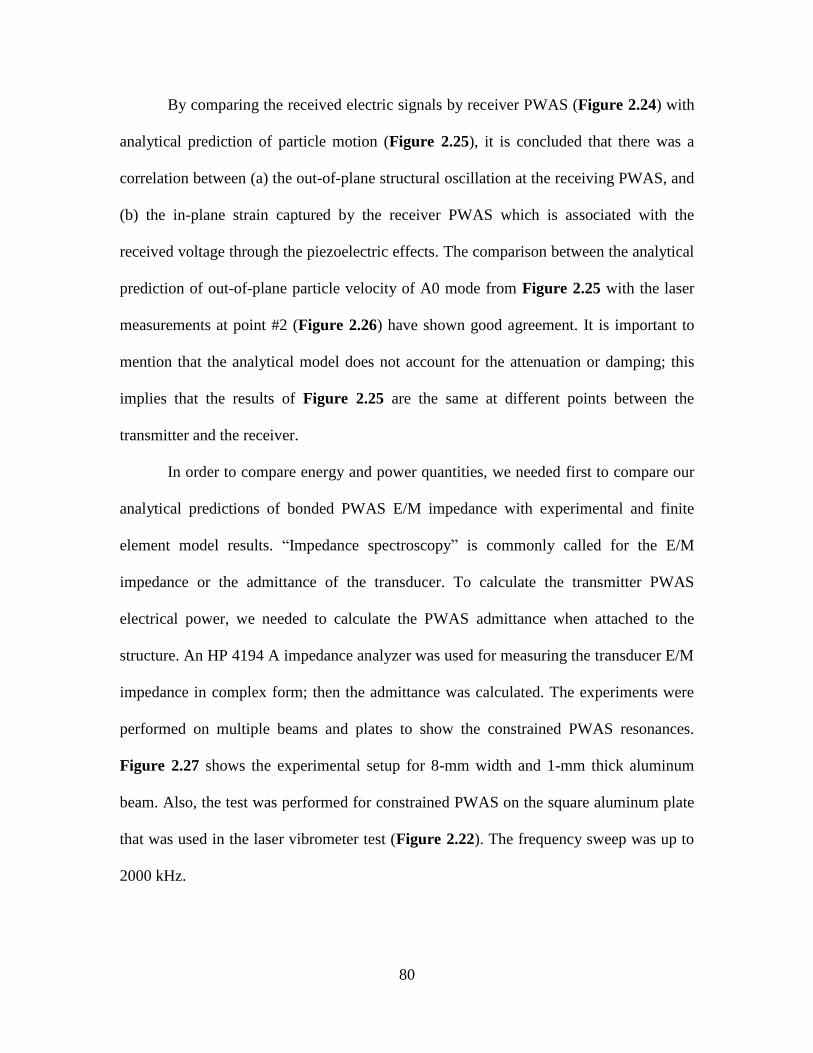
80
By comparing the received electric signals by receiver PWAS (Figure 2.24) with
analytical prediction of particle motion (Figure 2.25), it is concluded that there was a
correlation between (a) the out-of-plane structural oscillation at the receiving PWAS, and
(b) the in-plane strain captured by the receiver PWAS which is associated with the
received voltage through the piezoelectric effects. The comparison between the analytical
prediction of out-of-plane particle velocity of A0 mode from Figure 2.25 with the laser
measurements at point #2 (Figure 2.26) have shown good agreement. It is important to
mention that the analytical model does not account for the attenuation or damping; this
implies that the results of Figure 2.25 are the same at different points between the
transmitter and the receiver.
In order to compare energy and power quantities, we needed first to compare our
analytical predictions of bonded PWAS E/M impedance with experimental and finite
element model results. “Impedance spectroscopy” is commonly called for the E/M
impedance or the admittance of the transducer. To calculate the transmitter PWAS
electrical power, we needed to calculate the PWAS admittance when attached to the
structure. An HP 4194 A impedance analyzer was used for measuring the transducer E/M
impedance in complex form; then the admittance was calculated. The experiments were
performed on multiple beams and plates to show the constrained PWAS resonances.
Figure 2.27 shows the experimental setup for 8-mm width and 1-mm thick aluminum
beam. Also, the test was performed for constrained PWAS on the square aluminum plate
that was used in the laser vibrometer test (Figure 2.22). The frequency sweep was up to
2000 kHz.
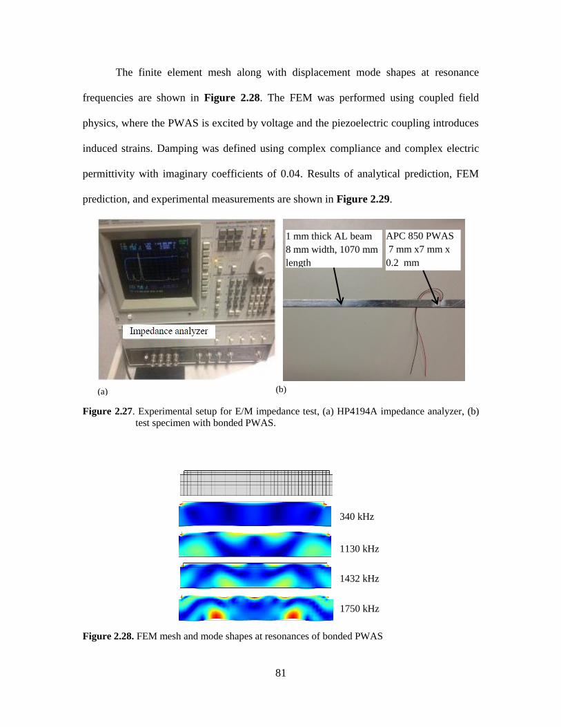
81
The finite element mesh along with displacement mode shapes at resonance
frequencies are shown in Figure 2.28. The FEM was performed using coupled field
physics, where the PWAS is excited by voltage and the piezoelectric coupling introduces
induced strains. Damping was defined using complex compliance and complex electric
permittivity with imaginary coefficients of 0.04. Results of analytical prediction, FEM
prediction, and experimental measurements are shown in Figure 2.29.
Figure 2.27. Experimental setup for E/M impedance test, (a) HP4194A impedance analyzer, (b)
test specimen with bonded PWAS.
Figure 2.28. FEM mesh and mode shapes at resonances of bonded PWAS
1 mm thick AL beam
8 mm width, 1070 mm
length
APC 850 PWAS
7 mm x7 mm x
0.2 mm
(a) (b)
340 kHz
1130 kHz
1432 kHz
1750 kHz
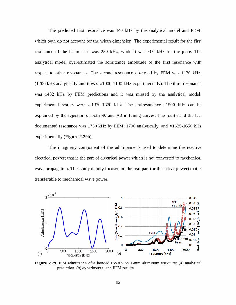
82
The predicted first resonance was 340 kHz by the analytical model and FEM;
which both do not account for the width dimension. The experimental result for the first
resonance of the beam case was 250 kHz, while it was 400 kHz for the plate. The
analytical model overestimated the admittance amplitude of the first resonance with
respect to other resonances. The second resonance observed by FEM was 1130 kHz,
(1200 kHz analytically and it was 1000-1100 kHz experimentally). The third resonance
was 1432 kHz by FEM predictions and it was missed by the analytical model;
experimental results were 1330-1370 kHz. The antiresonance 1500 kHz can be
explained by the rejection of both S0 and A0 in tuning curves. The fourth and the last
documented resonance was 1750 kHz by FEM, 1700 analytically, and 1625-1650 kHz
experimentally (Figure 2.29b).
The imaginary component of the admittance is used to determine the reactive
electrical power; that is the part of electrical power which is not converted to mechanical
wave propagation. This study mainly focused on the real part (or the active power) that is
transferable to mechanical wave power.
Figure 2.29. E/M admittance of a bonded PWAS on 1-mm aluminum structure: (a) analytical
prediction, (b) experimental and FEM results
0 500 1000 1500 20000
1
2x 10
-4
frequency [kHz]
Adm
itta
nce [1/
]
(a) (b)
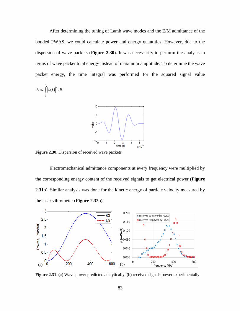
83
After determining the tuning of Lamb wave modes and the E/M admittance of the
bonded PWAS, we could calculate power and energy quantities. However, due to the
dispersion of wave packets (Figure 2.30). It was necessarily to perform the analysis in
terms of wave packet total energy instead of maximum amplitude. To determine the wave
packet energy, the time integral was performed for the squared signal value
1
0
2
( )
t
t
E s t dt
Figure 2.30. Dispersion of received wave packets
Electromechanical admittance components at every frequency were multiplied by
the corresponding energy content of the received signals to get electrical power (Figure
2.31b). Similar analysis was done for the kinetic energy of particle velocity measured by
the laser vibrometer (Figure 2.32b).
Figure 2.31. (a) Wave power predicted analytically, (b) received signals power experimentally
(a) (b)
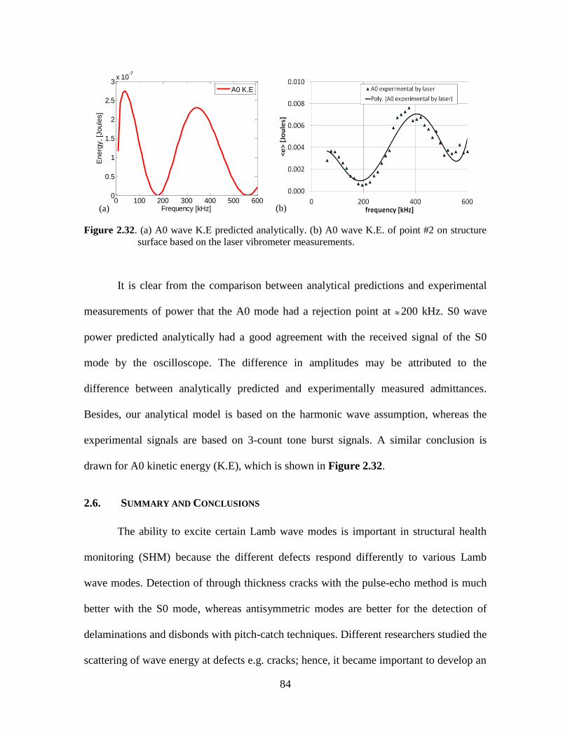
84
Figure 2.32. (a) A0 wave K.E predicted analytically. (b) A0 wave K.E. of point #2 on structure
surface based on the laser vibrometer measurements.
It is clear from the comparison between analytical predictions and experimental
measurements of power that the A0 mode had a rejection point at 200 kHz. S0 wave
power predicted analytically had a good agreement with the received signal of the S0
mode by the oscilloscope. The difference in amplitudes may be attributed to the
difference between analytically predicted and experimentally measured admittances.
Besides, our analytical model is based on the harmonic wave assumption, whereas the
experimental signals are based on 3-count tone burst signals. A similar conclusion is
drawn for A0 kinetic energy (K.E), which is shown in Figure 2.32.
2.6. SUMMARY AND CONCLUSIONS
The ability to excite certain Lamb wave modes is important in structural health
monitoring (SHM) because the different defects respond differently to various Lamb
wave modes. Detection of through thickness cracks with the pulse-echo method is much
better with the S0 mode, whereas antisymmetric modes are better for the detection of
delaminations and disbonds with pitch-catch techniques. Different researchers studied the
scattering of wave energy at defects e.g. cracks; hence, it became important to develop an
0 100 200 300 400 500 6000
0.5
1
1.5
2
2.5
3x 10
-7
Energ
y, [J
oule
s]
Frequency [kHz]
A0 K.E
(b) (a)
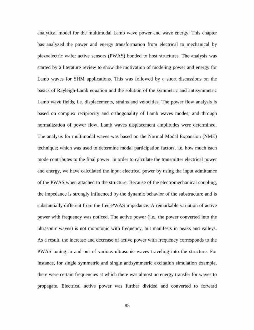
85
analytical model for the multimodal Lamb wave power and wave energy. This chapter
has analyzed the power and energy transformation from electrical to mechanical by
piezoelectric wafer active sensors (PWAS) bonded to host structures. The analysis was
started by a literature review to show the motivation of modeling power and energy for
Lamb waves for SHM applications. This was followed by a short discussions on the
basics of Rayleigh-Lamb equation and the solution of the symmetric and antisymmetric
Lamb wave fields, i.e. displacements, strains and velocities. The power flow analysis is
based on complex reciprocity and orthogonality of Lamb waves modes; and through
normalization of power flow, Lamb waves displacement amplitudes were determined.
The analysis for multimodal waves was based on the Normal Modal Expansion (NME)
technique; which was used to determine modal participation factors, i.e. how much each
mode contributes to the final power. In order to calculate the transmitter electrical power
and energy, we have calculated the input electrical power by using the input admittance
of the PWAS when attached to the structure. Because of the electromechanical coupling,
the impedance is strongly influenced by the dynamic behavior of the substructure and is
substantially different from the free-PWAS impedance. A remarkable variation of active
power with frequency was noticed. The active power (i.e., the power converted into the
ultrasonic waves) is not monotonic with frequency, but manifests in peaks and valleys.
As a result, the increase and decrease of active power with frequency corresponds to the
PWAS tuning in and out of various ultrasonic waves traveling into the structure. For
instance, for single symmetric and single antisymmetric excitation simulation example,
there were certain frequencies at which there was almost no energy transfer for waves to
propagate. Electrical active power was further divided and converted to forward
86
propagating wave power and backward wave propagating power; our simulations were
performed for only the forward wave and showed that the wave power was half of
electrical active power.
The developed model for Lamb waves case was compared with the axial and
flexural waves, that approximate Lamb waves at relatively low frequencies and the two
simulations showed good agreement. This was followed by a parametric study to
optimize the transducer size with excitation frequency to guarantee maximum energy
transfer between the source and the examined structure. In this study, it was shown that
the maximum wave power can be achieved with different combinations of PWAS-size
and excitation frequencies. Multi-modal waves simulations were presented, multi-modal
waves typically exist in practical applications for most on-site thick structures at which
not only S0 and A0 modes exist when excited by the PWAS. An experimental study was
performed using the scanning laser vibrometer to compare the out-of-plane structural
oscillation at the receiver PWAS with analytical predictions, as well as the received
voltage through the piezoelectric effects. The results have shown good agreement.
Afterwards, admittance of bonded PWAS was evaluated experimentally and was
compared with FEM and analytical predictions. Finally, the received signals by the
oscilloscope and the laser-detected out-of-plane particle velocities were used to determine
the wave electric power and kinetic energy respectively.
87
CHAPTER 3: SHEAR HORIZONTAL COUPLED PWAS
This chapter discusses a shear horizontal coupled piezoelectric wafer active sensor (SH-
PWAS). The chapter starts with a review of the state-of-the-art for the applications of SH
transducers and their importance in non-destructive evaluation (NDE) and structural
health monitoring (SHM). This is followed by the basic piezoelectric sensing and
actuation equations with the electro- mechanical coupling coefficient 35d . The electro-
mechanical (E/M) impedance of the SH-PWAS was studied analytically under a constant
electric field assumption as well as under a constant electric displacement assumption.
We also extended the analytical development to constrained SH-PWAS bonded to
structures in the form of beams. The model is based on the normal mode expansion
(NME) technique. The interaction between the SH-PWAS and the structure was studied.
The structure frequency response functions were presented. We developed a closed-form
equation of structure dynamic stiffness by coupling the mechanical response solution of
the SH-PWAS to the structure elasticity solution. The analytical model was compared
with experimental results and finite element analysis.
The chapter is later devoted to the discussion of shear horizontal (SH) guided-
waves that can be excited with the SH-PWAS. Analytical prediction of SH wave speeds
was performed. A wave propagation experimental study was conducted between different
combinations of SH-PWAS and regular inplane PWAS transducers.
.
88
Experimental results were compared with analytical predictions for aluminum
plates, and showed good agreement. 2-D wave propagation effects were studied by
Multiphysics FEM. In part II of the dissertation: Applications, we apply the study on
GFRP and CFRP composite structures.
The amplitudes of shear horizontal wave modes were normalized with respect to
the wave power; the normal mode expansion (NME) method was used to account for
superposition of multimodal SH waves. Modal participation factors were presented to
show the contribution of every mode. Model assumptions included: (a) straight crested
guided wave propagation; (b) ignoring evanescent waves; and (c) ideal bonding between
the PWAS and structure with shear load transfer concentrated at PWAS tips. The power
and energy transfer between the PWAS and structure were analyzed in order to optimize
the sensor size and excitation frequency; for maximum wave energy production for a
given source.
Finally, we presented simulations of our developed wave power and energy
analytical models along with a MATLAB graphical user interface (GUI) for the analysis
of SH-waves including dispersion phase and group velocities, mode shapes, and wave
energy.
NOMENCLATURE
kD = electric displacement vector [C/m2]
kjd = piezoelectric strain constants [m/V] or [C/N]
35d = piezoelectric strain constant for shear mode [m/V] or [C/N]
iE or kE = electric field [V/m]

89
35e = piezoelectric stress constant for shear mode [N/Vm]
ijg = piezoelectric voltage constants [m2/C] or [Vm/N] or [(V/m)/Pa]
35g = piezoelectric voltage constant for shear mode [m2/C] or [Vm/N] or
[(V/m)/Pa]
jS = strain tensor
D
ijs = mechanical compliance tensor at zero electric displacement, D=0
[m2/N]
55
Ds = mechanical shear compliance at zero electric displacement, D=0
[m2/N]
iT or jT = stress tensor [N/m
2]
= wave number [1/m]
T
ik = dielectric permittivity matrix at zero mechanical stress, T=0 [F/m]
33
S = dielectric permittivity in 33 direction measured at zero mechanical
strain, S=0
33
T = dielectric permittivity in 33 direction measured at zero mechanical
stress, T=0
K = electromechanical coupling factor
= shear modulus [Pa]
= angular frequency [rad/s]
90
Introducing some relations
3535
33
T
dg
2
35
33 33 55
1 1T S D
g
s 35
35
55
E
de
s
33 33 35 35
T S d e
21S D
T E
sK
s
35 35
33 55
S D
e g
s
2 22 35 35 55
55 33 33
D
E T S
d e sK
s
3.1. LITERATURE REVIEW
A Conventional piezoelectric wafer active sensor (PWAS) is a thin rectangular or
circular wafer that is poled in the thickness direction with electrodes on the top and
bottom surfaces; those types of PWAS are either used in the inplane or thickness mode.
In the inplane mode, applying an electric field in the thickness direction 3E causes the
transducer’s lateral dimensions to increase or decrease, a longitudinal strain will occur
1 13 3d E , where 13d is the piezoelectric coupling coefficient measured in [m/V].
Thickness mode is a mode that occurs simultaneously with extension mode, but
dominates at higher frequencies in MHz, in which strain in the thickness direction will
occur 3 33 3d E , where 33d is the piezoelectric coupling coefficient in thickness
direction. A different mode of oscillation can be achieved when the applied electric field
is applied perpendicular to the poling direction; and it is referred to as shear mode.
(Figure 3.1). The common piezoelectric coupling coefficient known for this mode is
defined as 15d , however, this coupling coefficient is only when the electric current is
applied in 1E direction and the poling is across thickness direction. The shear coupled
PWAS presented in this study is associated with the 35d coupling coefficient in which
electric current is applied across thickness (i.e. in 3x direction) and the poling is in 1x
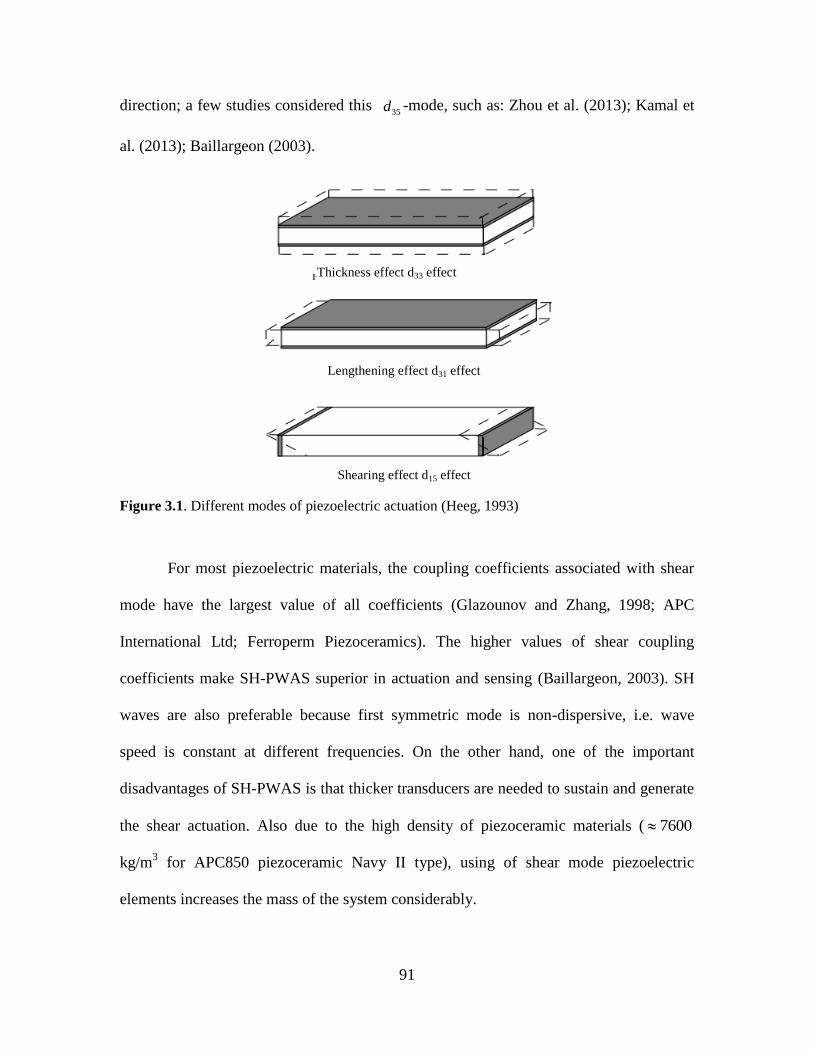
91
direction; a few studies considered this 35d -mode, such as: Zhou et al. (2013); Kamal et
al. (2013); Baillargeon (2003).
Figure 3.1. Different modes of piezoelectric actuation (Heeg, 1993)
For most piezoelectric materials, the coupling coefficients associated with shear
mode have the largest value of all coefficients (Glazounov and Zhang, 1998; APC
International Ltd; Ferroperm Piezoceramics). The higher values of shear coupling
coefficients make SH-PWAS superior in actuation and sensing (Baillargeon, 2003). SH
waves are also preferable because first symmetric mode is non-dispersive, i.e. wave
speed is constant at different frequencies. On the other hand, one of the important
disadvantages of SH-PWAS is that thicker transducers are needed to sustain and generate
the shear actuation. Also due to the high density of piezoceramic materials ( 7600
kg/m3 for APC850 piezoceramic Navy II type), using of shear mode piezoelectric
elements increases the mass of the system considerably.
Thickness effect d33 effect
Lengthening effect d31 effect
Shearing effect d15 effect
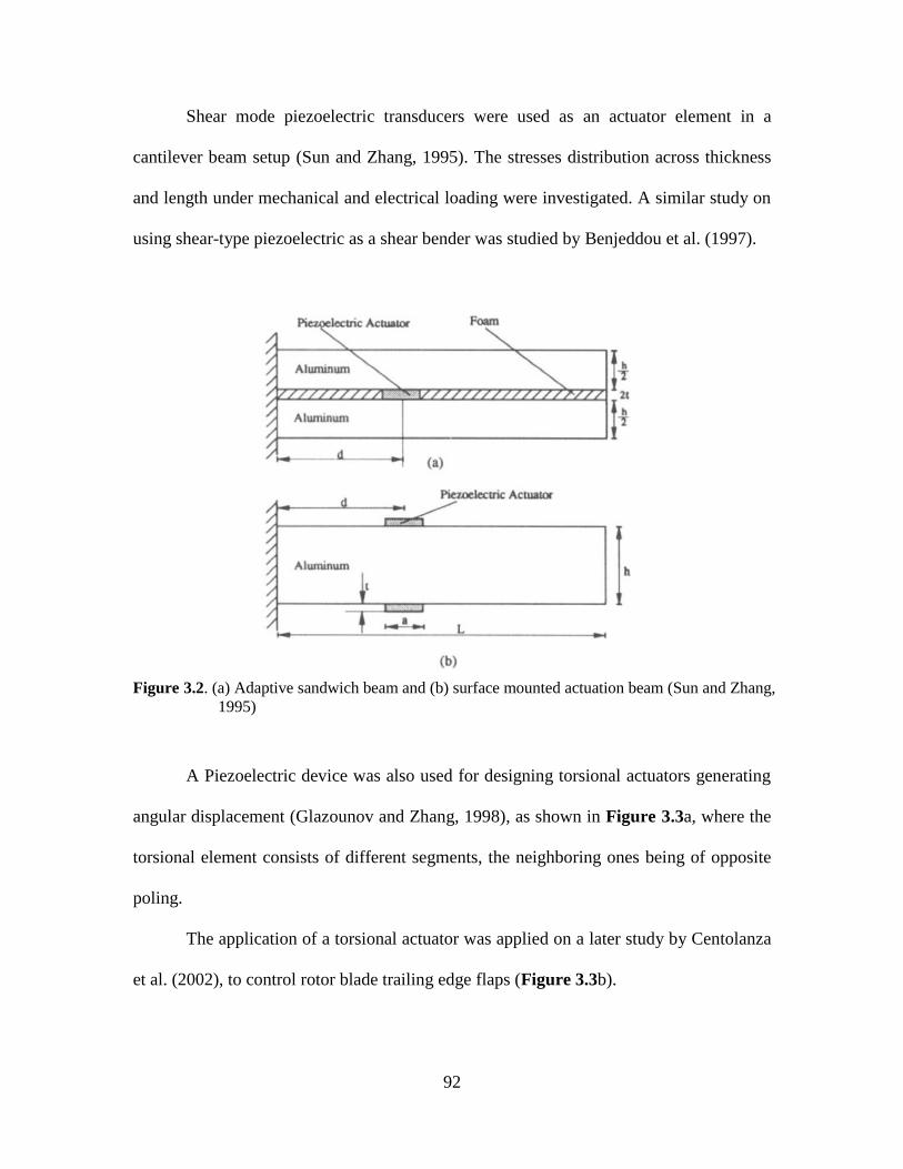
92
Shear mode piezoelectric transducers were used as an actuator element in a
cantilever beam setup (Sun and Zhang, 1995). The stresses distribution across thickness
and length under mechanical and electrical loading were investigated. A similar study on
using shear-type piezoelectric as a shear bender was studied by Benjeddou et al. (1997).
Figure 3.2. (a) Adaptive sandwich beam and (b) surface mounted actuation beam (Sun and Zhang,
1995)
A Piezoelectric device was also used for designing torsional actuators generating
angular displacement (Glazounov and Zhang, 1998), as shown in Figure 3.3a, where the
torsional element consists of different segments, the neighboring ones being of opposite
poling.
The application of a torsional actuator was applied on a later study by Centolanza
et al. (2002), to control rotor blade trailing edge flaps (Figure 3.3b).
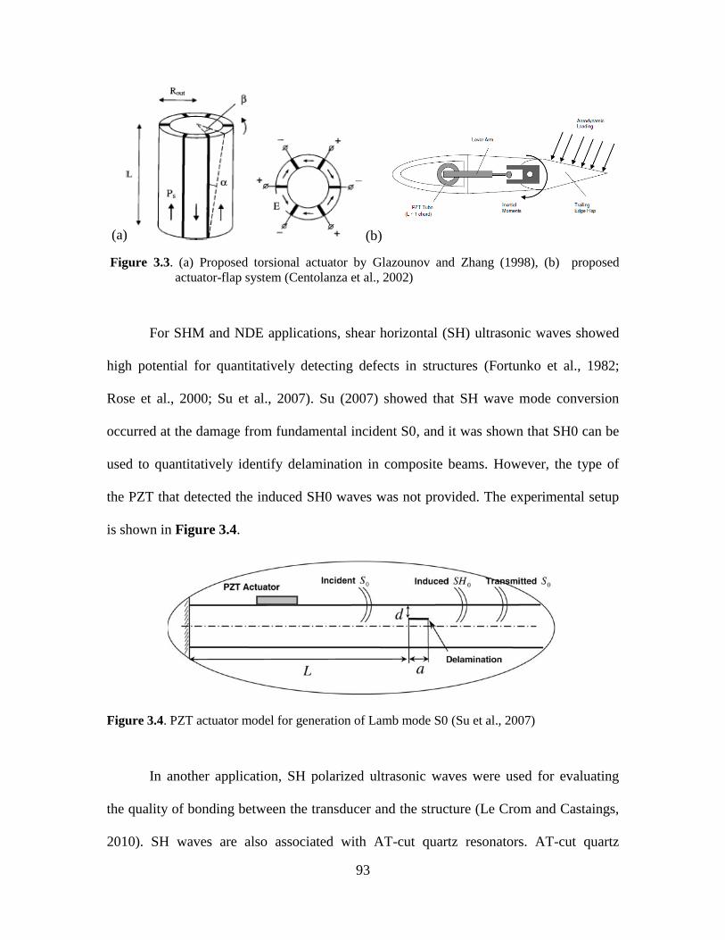
93
Figure 3.3. (a) Proposed torsional actuator by Glazounov and Zhang (1998), (b) proposed
actuator-flap system (Centolanza et al., 2002)
For SHM and NDE applications, shear horizontal (SH) ultrasonic waves showed
high potential for quantitatively detecting defects in structures (Fortunko et al., 1982;
Rose et al., 2000; Su et al., 2007). Su (2007) showed that SH wave mode conversion
occurred at the damage from fundamental incident S0, and it was shown that SH0 can be
used to quantitatively identify delamination in composite beams. However, the type of
the PZT that detected the induced SH0 waves was not provided. The experimental setup
is shown in Figure 3.4.
Figure 3.4. PZT actuator model for generation of Lamb mode S0 (Su et al., 2007)
In another application, SH polarized ultrasonic waves were used for evaluating
the quality of bonding between the transducer and the structure (Le Crom and Castaings,
2010). SH waves are also associated with AT-cut quartz resonators. AT-cut quartz
(b) (a)
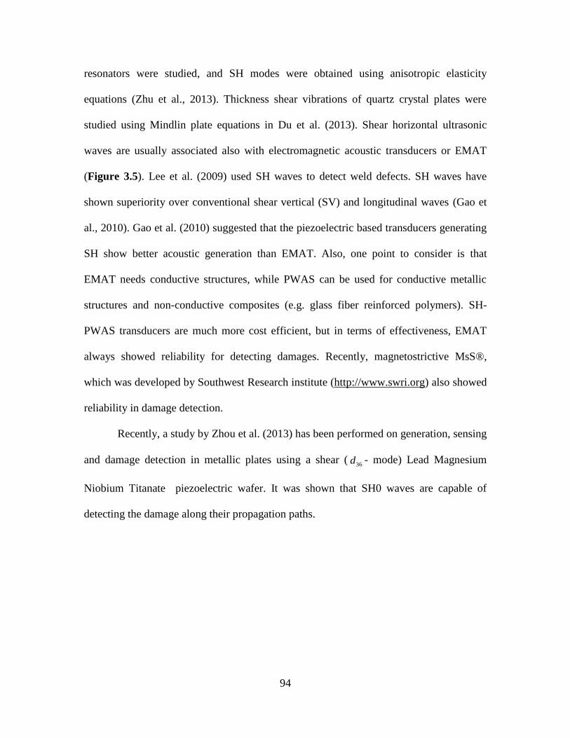
94
resonators were studied, and SH modes were obtained using anisotropic elasticity
equations (Zhu et al., 2013). Thickness shear vibrations of quartz crystal plates were
studied using Mindlin plate equations in Du et al. (2013). Shear horizontal ultrasonic
waves are usually associated also with electromagnetic acoustic transducers or EMAT
(Figure 3.5). Lee et al. (2009) used SH waves to detect weld defects. SH waves have
shown superiority over conventional shear vertical (SV) and longitudinal waves (Gao et
al., 2010). Gao et al. (2010) suggested that the piezoelectric based transducers generating
SH show better acoustic generation than EMAT. Also, one point to consider is that
EMAT needs conductive structures, while PWAS can be used for conductive metallic
structures and non-conductive composites (e.g. glass fiber reinforced polymers). SH-
PWAS transducers are much more cost efficient, but in terms of effectiveness, EMAT
always showed reliability for detecting damages. Recently, magnetostrictive MsS®,
which was developed by Southwest Research institute (http://www.swri.org) also showed
reliability in damage detection.
Recently, a study by Zhou et al. (2013) has been performed on generation, sensing
and damage detection in metallic plates using a shear (36d - mode) Lead Magnesium
Niobium Titanate piezoelectric wafer. It was shown that SH0 waves are capable of
detecting the damage along their propagation paths.
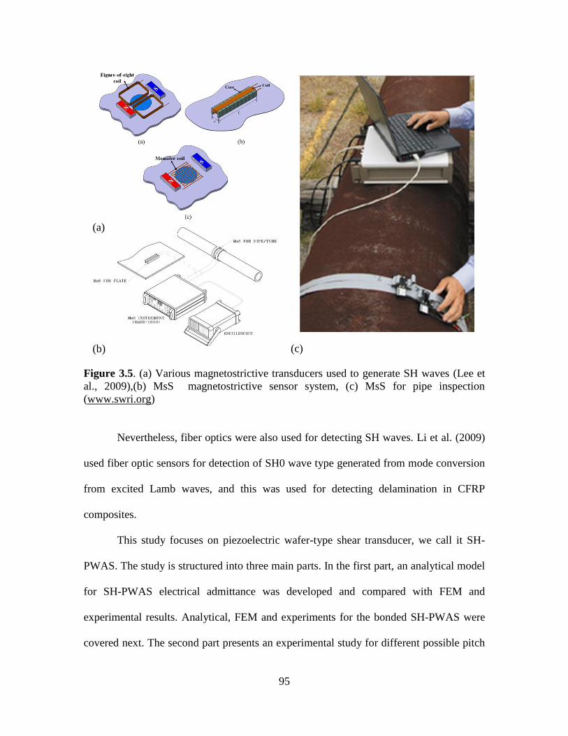
95
Figure 3.5. (a) Various magnetostrictive transducers used to generate SH waves (Lee et
al., 2009),(b) MsS magnetostrictive sensor system, (c) MsS for pipe inspection
(www.swri.org)
Nevertheless, fiber optics were also used for detecting SH waves. Li et al. (2009)
used fiber optic sensors for detection of SH0 wave type generated from mode conversion
from excited Lamb waves, and this was used for detecting delamination in CFRP
composites.
This study focuses on piezoelectric wafer-type shear transducer, we call it SH-
PWAS. The study is structured into three main parts. In the first part, an analytical model
for SH-PWAS electrical admittance was developed and compared with FEM and
experimental results. Analytical, FEM and experiments for the bonded SH-PWAS were
covered next. The second part presents an experimental study for different possible pitch
(b)
(a)
(c)
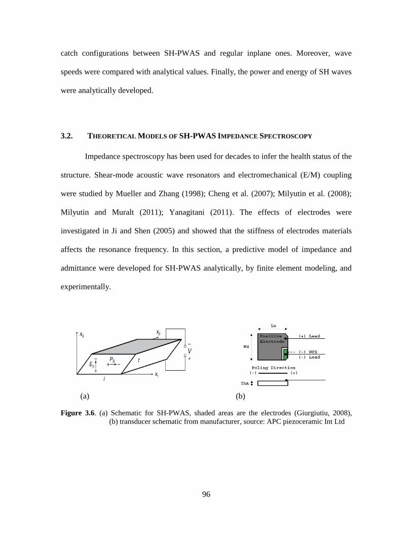
96
catch configurations between SH-PWAS and regular inplane ones. Moreover, wave
speeds were compared with analytical values. Finally, the power and energy of SH waves
were analytically developed.
3.2. THEORETICAL MODELS OF SH-PWAS IMPEDANCE SPECTROSCOPY
Impedance spectroscopy has been used for decades to infer the health status of the
structure. Shear-mode acoustic wave resonators and electromechanical (E/M) coupling
were studied by Mueller and Zhang (1998); Cheng et al. (2007); Milyutin et al. (2008);
Milyutin and Muralt (2011); Yanagitani (2011). The effects of electrodes were
investigated in Ji and Shen (2005) and showed that the stiffness of electrodes materials
affects the resonance frequency. In this section, a predictive model of impedance and
admittance were developed for SH-PWAS analytically, by finite element modeling, and
experimentally.
Figure 3.6. (a) Schematic for SH-PWAS, shaded areas are the electrodes (Giurgiutiu, 2008),
(b) transducer schematic from manufacturer, source: APC piezoceramic Int Ltd
(a)
(b)

97
SH-PWAS Sensing and Actuation Constitutive Relations 3.2.1.
Most literature mentioned earlier deal with the shear dielectric coupling
coefficient 15d , however, this is only applicable if the electric field ( 1E ) is applied in the
in-plane direction and the piezoelectric poling is in thickness direction. In our model and
FEM simulations we use 35d . The SH-PWAS transducer we used (APC International
Ltd) has its electrodes on the top and bottom; hence electric field is applied along 3x
direction and the poling is applied along 1x direction (Refer to Figure 3.6a). Recall the
constitutive equations of piezoelectricity in contracted Voigt notations,
1 1 1111 12 13
2 2 1221 22 23
1
3 3 1331 32 33
2
4 444
3
5 5 3555
6 6 2666
E E E
E E E
E E E
E
E
E
S T ds s s
S T ds s sE
S T ds s sE
S TsE
S T ds
S T ds
(3.1)
1
2
1 11 12 13 11 1
3
2 26 22 2
4
3 35 33 3
5
6
T
T
T
T
TD d d d E
TD d E
TD d E
T
T
(3.2)
where jS are the strain components,
E
ijs is the compliance matrix under constant electric
field condition, iT are the stress components, kjd are the piezoelectric coupling
coefficients, kE represents the electric field vector, kD is the electric displacement vector,
and T
ik are the electric permittivity constants of the PWAS material. Equation (3.1) is
considered the piezoelectric converse effect, where the applied electric field will result in
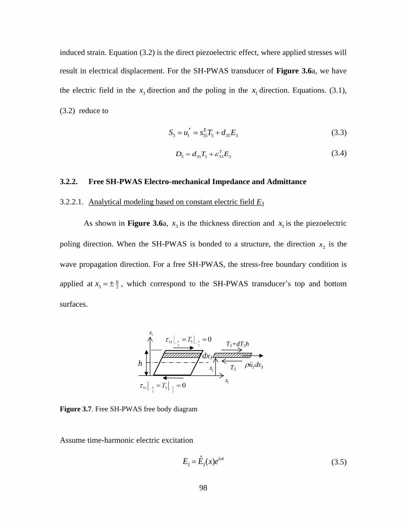
98
induced strain. Equation (3.2) is the direct piezoelectric effect, where applied stresses will
result in electrical displacement. For the SH-PWAS transducer of Figure 3.6a, we have
the electric field in the 3x direction and the poling in the 1x direction. Equations. (3.1),
(3.2) reduce to
5 1 55 5 35 3
ES u s T d E (3.3)
3 35 5 33 3
TD d T E (3.4)
Free SH-PWAS Electro-mechanical Impedance and Admittance 3.2.2.
3.2.2.1. Analytical modeling based on constant electric field E3
As shown in Figure 3.6a, 3x is the thickness direction and 1x is the piezoelectric
poling direction. When the SH-PWAS is bonded to a structure, the direction 2x is the
wave propagation direction. For a free SH-PWAS, the stress-free boundary condition is
applied at 3 2hx , which correspond to the SH-PWAS transducer’s top and bottom
surfaces.
Figure 3.7. Free SH-PWAS free body diagram
Assume time-harmonic electric excitation
3 3ˆ ( ) i tE E x e (3.5)
h
dx3
T5+dT5h
T5
99
where is the circular frequency in rad/sec.
Considering the Newton law of motion applied to the element in Figure 3.7, we have
5T 5 5dT T 1 3u dx (3.6)
upon simplification, Eq. (3.6) becomes,
5 1T u (3.7)
where is piezoelectric material type density, 1u is the second derivative of 1u
displacement with respect to time. Differentiating Eq. (3.3) with respect to 3x and
assuming constant electric field 3E across thickness yields
5 55 5
ES s T (3.8)
where
3x
and 5T is the shear stress in 13 direction. Recall strain displacement
relation for shear deformation, i.e.,
315
3 1
uuS
x x
1u (3.9)
where 551 Es is the shear modulus for piezoelectric material. Substitution of Eq. (3.9)
into Eq. (3.8) yields
5 1T u (3.10)
Differentiation of the Eq. (3.10) with respect to 3x and substitution into Eq. (3.7) yields,
1 1u u (3.11)
Assuming time harmonic solution 1 1
i tu u e reduces Eq. (3.11) to
2
1 1ˆ ˆ 0u u (3.12)
100
Then, the space solution of the differential Eq. (3.11) is
1 1 3 2 3ˆ sin cosu C x C x (3.13)
Define speed of SH-wave in the piezoelectric material as c , and the corresponding wave
number as
2 1
, , c cc
(3.14)
Mechanical response:
Imposing stress free boundary condition 5
2
0hT in Eq. (3.3) yields
5 35 3
2
ˆhS d E
(3.15)
Using the strain – displacement relation Eq. (3.9) and the derivative of Eq. (3.13) into Eq.
(3.15) yields
1 11 1 2 35 32 2
2
1 11 1 2 35 32 2
2
ˆˆ cos sin
ˆˆ cos sin
h
h
u C h C h d E
u C h C h d E
(3.16)
Solving the two equations in (3.16) yields
35 3
1 212
ˆ , 0
cos
d EC C
h (3.17)
Substitution of Eq. (3.17) into Eq. (3.13) yields the space domain solution
35 3 3
1 3 12
ˆ sinˆ ( )
cos
d E xu x
h
(3.18)
Differentiation of Eq. (3.18) yields the strain
315 35 3 1
3 2
ˆ cosˆ ˆ cos
xuS d E
x h
(3.19)
101
Define induced strain actuation (ISA) which is the PWAS strain in the absence of
mechanical loading, i.e.,
5 35 3ˆ ˆ( )ISAS d E (3.20)
Corresponding induced displacement is defined as
5 35 3ˆ ˆ( )ISA ISAu S h d E h (3.21)
Equation (3.18) and Eq. (3.19) can be rearranged in the form
31 3 1 1
2 2
sin1ˆ ( )
2 cos
ISAu xu x
h h
(3.22)
35 3 5 1
2
cosˆ ˆ( ) ( ) cos
ISA
xS x S
h
(3.23)
Electrical response
Eliminating the stress 5T between Eqs. (3.3), (3.4), and using Eq. (3.9) yields
353 1 35 3 33 3
55
ˆ ˆT
E
dD u d E E
s
(3.24)
Upon rearrangement, Eq. (3.24) becomes
2 1
3 33 3 35
35 3
ˆ 1 1ˆ
T uD E K
d E
(3.25)
where the electromechanical coupling factor 35K is defined as
22 3535
55 33
E T
dK
s (3.26)
Integrating the electrical displacement in Eq. (3.25) over the electrodes area yields the
electric charge
2
2
3 3 3 1 2 3 3 1 2
0
( ) ( ) ( )
l
l
b
A
Q x D x dx dx D x dx dx
(3.27)
102
Equation (3.27) indicates that electric charge varies across the thickness. We define
equivalent average charge across thickness as
2
2
3 3
1ˆ ( )
h
h
eqQ Q x dxh
(3.28)
Substituting 3D from Eq. (3.25) into Eq. (3.28) and performing the integration yields
2
21 3
2 233 335 35
35 3
ˆ ( )ˆˆ 1
ˆ
h
h
eq
u xE blQ K h K
h d E
(3.29)
Defining PWAS capacitance as
33
T blC
h (3.30)
Substituting 1 3ˆ ( )u x from Eq. (3.22); the electric field is related to voltage by
3
ˆˆ VE
h ; and
recalling ISAu from Eq. (3.21); then Eq. (3.29) can be simplified to
1
2 235 1
2
tanˆ ˆ 1 1eq
hQ CV K
h
(3.31)
The electric current I is defined as the time derivative of electric charge, i.e. I Q i Q ,
hence ˆI i Q and Eq. (3.31) simplifies to
1
2 235 1
2
ˆ tan1 1
ˆ
hIY i C K
hV
(3.32)
And the free SH-PWAS electrical impedance is
11
2 235 1
2
ˆ tan11 1
ˆ
hVZ K
i C hI
(3.33)
103
Result in Eq. (3.32) is slightly different from that of Milyutin et al. (2008), where the
stress-charge piezoelectric equations were used and the model was for 15d - mode, where
the transducer electrodes were on the sides not on the top and bottom surfaces like in our
case.
3.2.2.2. Analytical modeling based on constant electric displacement D3
The constant electric field assumption is usually more appropriate in piezoelectric
stacks with internal electrodes, where flow of charge exists (i.e. closed circuit) and the
corresponding electric displacement forms a half wave distribution at the resonator
(Sherrit et al., 2013). However, in most other cases of single resonators, such as thickness
shear mode, no current flows through the resonator, which makes the constant electric
displacement assumption (i.e. zero current or open circuit) more realistic. Bar
piezoelectric ceramic transformers were studied under constant electric displacement
condition (Erhart et al., 2013), where impedance was modeled for the longitudinal mode
( 31d ). In this section, we derive analytically the E/M impedance and admittance based on
constant electric displacement D3. The predicted models are compared with experimental
measurements to investigate which assumption best fits our SH-PWAS transducer.
For the electric field restricted in 3x direction, the 5T stress shown in Figure 3.6a,
takes the following form in Voigt notations,
355 5 3
55 55
1 ˆD D
gT S D
s s (3.34)
The electric field in the case of constant electric displacement is derived starting from Eq.
(3.4)
104
3 35 5 33 3
TD d T E (3.35)
Rearranging Eq.(3.35), and eliminating stress 5T using Eq.(3.34) yields
35 353 5 3 35 5 3 3
33 33 55 55 33
1 1 1ˆ ˆ ˆT T D D T
d gE T D g S D D
s s
(3.36)
Upon rearrangement, Eq.(3.36) becomes
353 5 3
55 33
1 ˆD S
gE S D
s
(3.37)
where
2
35
55 33 33
1 1D T S
g
s
(3.38)
Mechanical Response
Substitute the stress free boundary condition (3
52
0hx
T
) into Eq.(3.34) to get
5 35 3
2
ˆhS g D
(3.39)
Using 15 1
3
uS u
x
and replacing 1 1 by u u that represents the amplitude value with
ignoring time harmonic exponential
1 11 1 2 35 32 2
2
1 11 1 2 35 32 2
2
ˆˆ cos sin
ˆˆ cos sin
h
h
u C h C h g D
u C h C h g D
(3.40)
Solving the two equations in (3.40) yields
35 3
1 212
ˆ , 0
cos
g DC C
h (3.41)
Substitution of Eq. (3.41) into Eq. (3.13) yields the space domain solution

105
35 3 31 3 1
2
ˆ sinˆ ( )
cos
g D xu x
h
(3.42)
Differentiation of Eq. (3.42) yields the strain as
315 35 3 1
3 2
ˆ cosˆ ˆ cos
xuS g D
x h
(3.43)
Electrical response
Using Eq.(3.37) and substituting strain ( 5S ) from Eq.(3.43) yields,
2
35 3 33 31
55 332
23 323 35 33 3
351 133 55 332 2
ˆ cos 1 ˆcos
ˆ ˆcos cos 1 1
cos cos
D S
S
S D S
g D xE D
s h
x xD g DK
s h h
(3.44)
where the electromechanical coupling factor 35K is defined as
22 2
2 35 55 35 33 55 35 3335
33 55 33 55
D S D S
S D S D
e s g s gK
s s
(3.45)
Integrating the electrical displacement over electrodes area, results in the electric charge
2
2
3 1 2 3 1 2 3
0
ˆ ˆ ˆ ˆ
l
l
b
A
Q D dx dx D dx dx blD
(3.46)
As before, the electric current I is calculated from the time derivative of electric charge
3ˆ ˆˆ ˆI Q i Q i blD (3.47)
Electric voltage is related to electric field by
2
2
3 3ˆ ˆ
h
h
V E dx
(3.48)
Substitution of Eq. (3.44) into Eq. (3.48) yields
106
2
2
2
2
32335 31
33 2
132 23 3 235 351 1
33 332 2
ˆ cosˆ 1cos
sinˆ ˆ 2sin1 1
cos cos
h
h
h
h
S
S S
xDV K dx
h
x hD Dh K h K
h h h h
(3.49)
As before, defining PWAS capacitance as
33
S blC
h (3.50)
The impedance is defined as ˆ
ˆ
VZ
I and using Eqs. (3.47), (3.49); the electromechanical
impedance is
2 2
35 351 1 1 133 2 2 2 2
ˆ 1 1 11 1
ˆ cot cotS
V hZ K K
i bl h h i C h hI
(3.51)
Defining 12
h , the electromechanical impedance can further be written as
2
35
1 11
cotZ K
i C
(3.52)
And the electromechanical admittance is
1
2
35
ˆ 11
ˆ cot
IY i C K
V
(3.53)
Bonded SH-PWAS Analytical Model 3.2.3.
SH-PWAS bonded on a plate structure is shown in Figure 3.8. When the SH-
PWAS is bonded to the structure, the direction 2x (global x-direction) is the SH wave
propagation direction. Depending on which plane is considered for analysis, the SH-
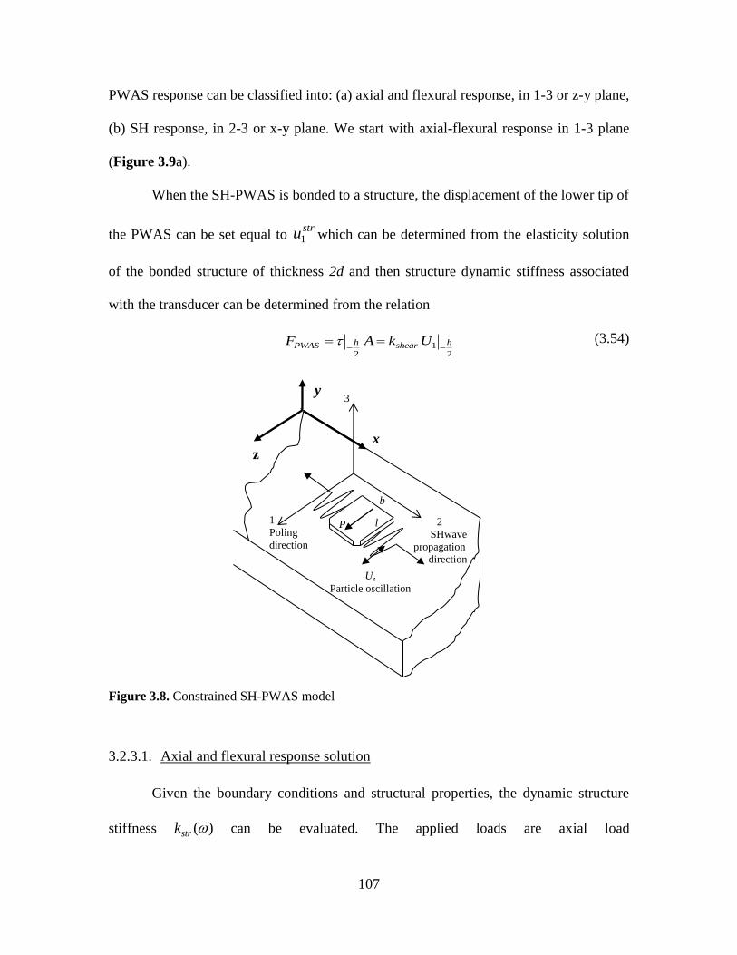
107
PWAS response can be classified into: (a) axial and flexural response, in 1-3 or z-y plane,
(b) SH response, in 2-3 or x-y plane. We start with axial-flexural response in 1-3 plane
(Figure 3.9a).
When the SH-PWAS is bonded to a structure, the displacement of the lower tip of
the PWAS can be set equal to 1stru which can be determined from the elasticity solution
of the bonded structure of thickness 2d and then structure dynamic stiffness associated
with the transducer can be determined from the relation
1
2 2
h hPWAS shearF A k U
(3.54)
Figure 3.8. Constrained SH-PWAS model
3.2.3.1. Axial and flexural response solution
Given the boundary conditions and structural properties, the dynamic structure
stiffness ( )strk can be evaluated. The applied loads are axial load
2
SHwave
propagation
direction
3
1
Poling direction
P
b
l
y
x z
Uz
Particle oscillation
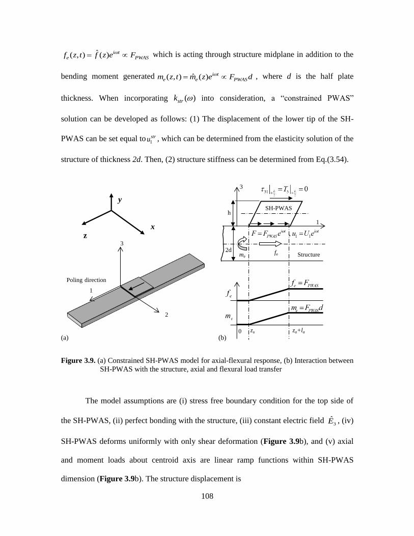
108
ˆ( , ) ( ) i te PWASf z t f z e F which is acting through structure midplane in addition to the
bending moment generated ˆ( , ) ( ) i te e PWASm z t m z e F d , where d is the half plate
thickness. When incorporating ( )strk into consideration, a “constrained PWAS”
solution can be developed as follows: (1) The displacement of the lower tip of the SH-
PWAS can be set equal to1stru , which can be determined from the elasticity solution of the
structure of thickness 2d. Then, (2) structure stiffness can be determined from Eq.(3.54).
Figure 3.9. (a) Constrained SH-PWAS model for axial-flexural response, (b) Interaction between
SH-PWAS with the structure, axial and flexural load transfer
The model assumptions are (i) stress free boundary condition for the top side of
the SH-PWAS, (ii) perfect bonding with the structure, (iii) constant electric field 3E , (iv)
SH-PWAS deforms uniformly with only shear deformation (Figure 3.9b), and (v) axial
and moment loads about centroid axis are linear ramp functions within SH-PWAS
dimension (Figure 3.9b). The structure displacement is
1
3
h
SH-PWAS
Structure 2d fe me
za za+la 0
(a) (b)
3
Poling direction
1
2
y
x z
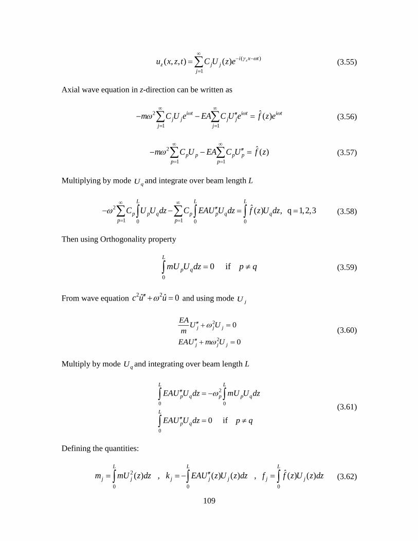
109
( )
1
( , , ) ( ) xi x tz j j
j
u x z t C U z e
(3.55)
Axial wave equation in z-direction can be written as
2
1 1
ˆ ( )i t i t i tj j j j
j j
m C U e EA C U e f z e
(3.56)
2
1 1
ˆ ( )p p p p
p p
m C U EA C U f z
(3.57)
Multiplying by mode qU and integrate over beam length L
2
1 10 0 0
ˆ( ) , q 1,2,3
L L L
p p q p p q q
p p
C U U dz C EAU U dz f z U dz
(3.58)
Then using Orthogonality property
0
0 if
L
p qmU U dz p q (3.59)
From wave equation 2 2ˆ ˆ 0c u u and using mode
jU
2
2
0
0
j j j
j j j
EAU U
m
EAU m U
(3.60)
Multiply by mode qU and integrating over beam length L
2
0 0
0
0 if
L L
p q p p q
L
p q
EAU U dz mU U dz
EAU U dz p q
(3.61)
Defining the quantities:
2
0 0 0
ˆ( ) , ( ) ( ) , ( ) ( )
L L L
j j j j j j jm mU z dz k EAU z U z dz f f z U z dz (3.62)
110
Substitute Eq.(3.62) in Eq.(3.58) using p=q=j
2( )j j j jC m k f (3.63)
2 2 2( ) where
j j
j j j
j j
f kC
m m (3.64)
But due to orthonormality, that is orthogonality in addition to normalization to get
constant jC in sinj j jU C l substituting in orthogonality relation for p=q
2
0
( ) 1
L
j jm mU z dz (3.65)
Then normalization factor is 2
jCml
and Eq.(3.64) is written as
2 2( ) j j jC f (3.66)
Define modal participation factors: 2 2( )
j
j
f
then normal mode expansion (NME)
solution can be evaluated by substituting in Eq.(3.55)
( )
2 21
( , , ) ( ) ( )
xj i x t
z j
j j
fu x z t U z e
(3.67)
where normalization factor is included in ( )jU z such that 2
( ) sinj jU z lml
For more realistic modeling, damping to be introduced as and Eq.(3.67) is written as
( )
2 21
( , , ) ( ) ( 2 )
xj i x t
z j
j j j
fu x z t U z e
i
(3.68)
For SH-PWAS bonded on structure exerting certain force pattern, NME can be further
simplified. As loads exerted by SH-PWAS can be separated to axial normal force ef and
111
bending moment em , where both are defined as linearly increasing functions from zero at
one PWAS end to maxima at the other end,
max max
, e PWAS e PWASf F m F d (3.69)
Space wise, the axial force and bending moment can be represented by Heaviside
function, ( )aH z z , and linear function of z as shown in Figure 3.9b, hence
( , ) ( ) ( ) ( ( )) ( ( )) i te PWAS a a a a a af z t F z z H z z z z l H z z l e (3.70)
( , ) ( ) ( ) ( ( )) ( ( )) i te PWAS a a a a a am z t F d z z H z z z z l H z z l e (3.71)
Axial part
The forced vibration governing equation for axial responses
( , ) ( , ) ( , )eAu z t EAu z t f z t (3.72)
Substituting axial force space distributed Heaviside function into equation of motion
( , ) ( , ) ( ) ( ( )) i tPWASa a a
FAu z t EAu z t H z z H z z l e
l
(3.73)
where l in the denominator was added to balance equation dimensions to force per unit
length. Applying Eq.(3.55), and following the same procedure of free response yields,
2 2( ) nn n
n
fC
m (3.74)
2 2
( )
nn
n n
fC
m
(3.75)
where 0
ˆ ( ) ( )
L
n nf f z U z dz and can be calculated by multiplying by ( )nU z and
integrating over beam length
112
0
( ) ( ( )) ( )
LPWAS
n a a a n
Ff H z z H z z l U z dz
l (3.76)
( ) ( )
a a a
L LPWAS
n n n
z z l
Ff U z dz U z dz
l
(3.77)
The factor Cn can be evaluated as
2 2
1 ( ) ( )
( )a a a
L LPWAS
n n n
n z z l
FC U z dz U z dz
Al
(3.78)
And finally the axial displacement can be written as:
( )
2 21
( )
( , , ) ( ) ( 2 )
a a
a x
z l
n
z i x tPWASz n
n n n
U z dzF
u x z t U z eAl i
(3.79)
Flexural part
Equation of motion is
( , ) ( , ) ( , )eAw z t EIw z t m z t (3.80)
Using Eq.(3.71) in Eq.(3.80), considering that the second derivative of linear z function
will yield a Dirac function
( , ) ( , ) ( ) ( ( )) i tPWASa a a
F dAw z t EIw z t z z z z l e
l
(3.81)
Applying modal expansion model:
( )
1
( , , ) ( ) xi x tn n
n
w x z t C W z e
(3.82)
With similar procedure like Eqs. (3.74) - (3.77) ,we get the Cn as
2 2
0
1 [ ( ) ( ( ))] ( )
( )
LPWAS
n a a a n
n
F dC z z z z l W z dz
Al
(3.83)
113
Using the property of Dirac function when multiplied by a function and then integrated.
This integration equals to the evaluation of the function at the shifted value of Dirac
function; Eq.(3.83) reduces to
2 2
1 ( ) ( )
( )
PWASn n a n a a
n
F dC W z W z l
Al
(3.84)
Then the final normal mode expanded displacement can be evaluated
( )
2 21
( ) ( )( , , ) ( )
( 2 )
xn a n a a i x tPWAS
n
n n n
W z W z lF dw x z t W z e
Al i
(3.85)
Noting that w displacement is the flexural displacement that is in y-direction in our global
co-ordinates. The total axial displacement consists of the part from the axial solution as
well as the effect of the slope of the flexural solution.
pu u w d (3.86)
Ignoring the x and t terms in Eqs. (3.79) and (3.85) , and considering the effective
displacement along SH-PWAS length as
1 1effective
0
1( )
Lstr str
a
u u z dzl
(3.87)
2
2 212
2
2
2 21
( )
ˆ ( 2 )
( ) ( )
( 2 )
a a
a
a a a
w w w
z l
n
z
PWASPWAS n a n n
n a a n a
n w n n
U z dz
Fu i
Al
W z l W zd
i
(3.88)
And then we can define dynamic stiffness of the structure ( )strk as
114
12
2 2 21
2
2
2 21
( )
( ) ( 2 )ˆ
( ) ( )
( 2 )
a a
a
a a a
w w w
z l
n
z
PWASstr str str str n a n n
PWAS
n a a n a
n w n n
U z dz
Fk A l i
u
W z l W zd
i
(3.89)
For actual evaluating the dynamic stiffness of the structure, vibration modes need to be
determined, and the modes depend on boundary condition, for instance for free-free
structural beam bonded with the SH-PWAS, we have (Giurgiutiu and Zagrai, 2000)
( ) cos( )a an n nU z A z ,
2anA
ml ,
a
an
n
l
,
a a
str
n n c ,str
str
str
Ec
,na = 1,2, (3.90)
The speed of the SH-wave in the piezoelectric material c is different from the axial wave
speed in the structure, hence the latter is denoted by strc
For flexural modal solution,
( ) cosh cos sinh sinw w W w w w wn n n n n n nW z A z z z z
(3.91)
2
w wn n flexa , str
flex
str str
EIa
A , 2
01/
w
l
nw nA W z dz (3.92)
where the numerical values for wn ,
wnl can be found from Giurgiutiu (2008), pg. 89.
3.2.3.2. Shear horizontal response solution
Shear horizontal response can be determined with a similar procedure to the one
of the axial-flexural response, but taking into consideration the plane of the analysis
containing SH wave propagation direction, i.e. plane 2-3 in Figure 3.10a.
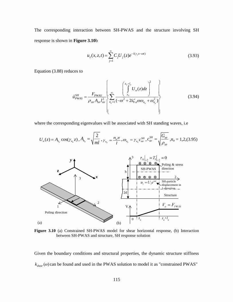
115
The corresponding interaction between SH-PWAS and the structure involving SH
response is shown in Figure 3.10b
( )
1
( , , ) ( ) xi x tz j j
j
u x z t C U z e
(3.93)
Equation (3.88) reduces to
2
2 2 21
( )
ˆ( 2 )
a a
a
a a a
z l
n
zSH PWASPWAS
nstr str str a n n
U z dzF
uA l i
(3.94)
where the corresponding eigenvalues will be associated with SH standing waves, i.e
( ) cos( )a an n nU z A z ,
2anA
ml ,
a
an
n
l
,
a a
SH
n n strc ,SH strstr
str
Gc
,na = 1,2,(3.95)
Figure 3.10 (a) Constrained SH-PWAS model for shear horizontal response, (b) Interaction
between SH-PWAS and structure, SH response solution
Given the boundary conditions and structural properties, the dynamic structure stiffness
( )sheark can be found and used in the PWAS solution to model it as "constrained PWAS"
2
3
h
SH-PWAS
Structure 2d
za z
a+l
a 0
V
Poling & stress
direction
SH-particle
displacement in 1-direction
(b)
3
1
Poling direction
2
y
x
z
(a)

116
3.2.3.3. SH-PWAS tip displacement solution and connection to elasticity solution
Recall SH-PWAS equation of motion
2 2
1 1
2 2
3
u u
x t
(3.96)
1 3 1 3( , ) ( ) i tu x t U x e (3.97)
221
12
3
i t i tUe U e
x
(3.98)
Define the shear wave speed inside the SH-PWAS
2 /c (3.99)
we get
22 21
12
3
0U
c Ux
(3.100)
2
1 120U U
c
(3.101)
Define the shear wave number
/ c (3.102)
we get
1 1 3 2 3sin cosU C x C x (3.103)
11 3 2 3
3
cos sinU
C x C xx
(3.104)
2
2 211 3 2 3 12
3
sin cosU
C x C x Ux
(3.105)
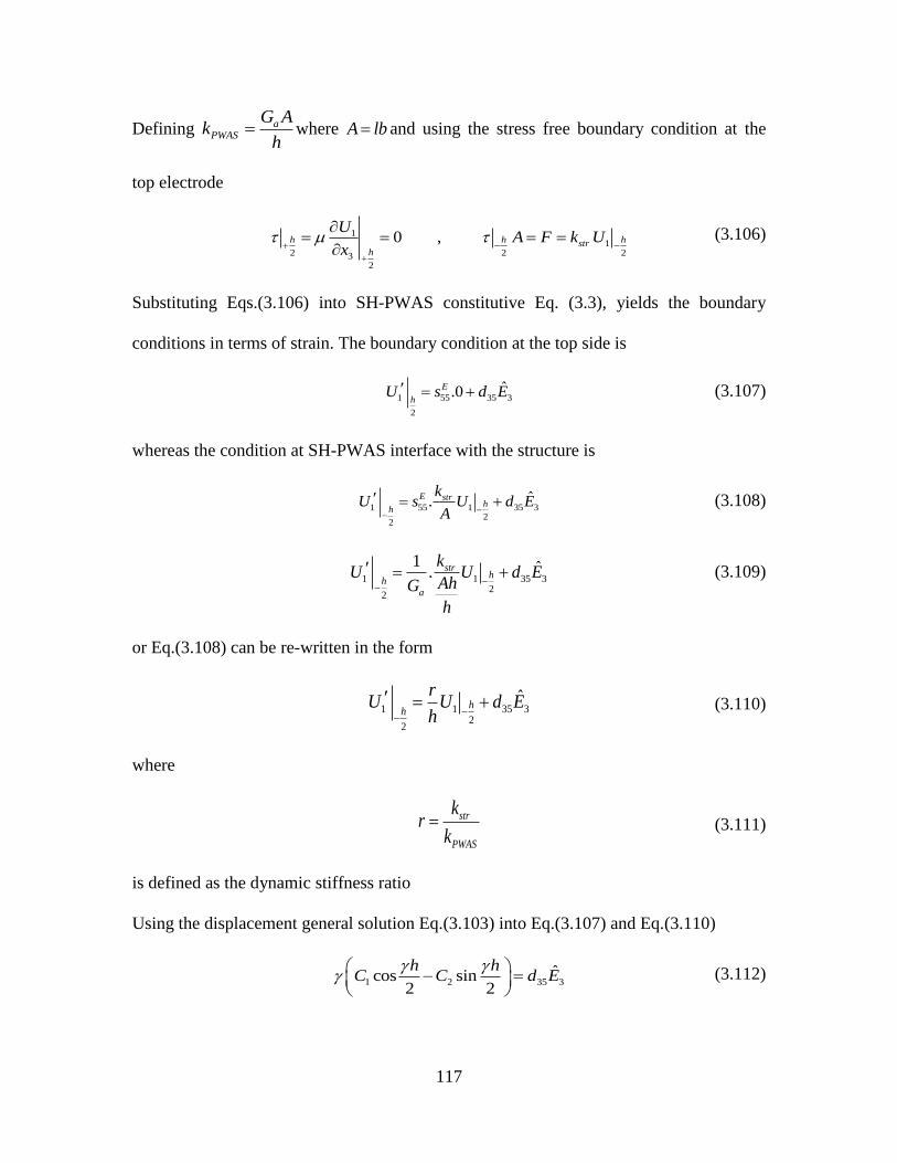
117
Defining aPWAS
G Ak
h where A lb and using the stress free boundary condition at the
top electrode
11
2 2 232
0 , h h hstrh
UA F k U
x
(3.106)
Substituting Eqs.(3.106) into SH-PWAS constitutive Eq. (3.3), yields the boundary
conditions in terms of strain. The boundary condition at the top side is
1 55 35 3
2
ˆ.0E
hU s d E (3.107)
whereas the condition at SH-PWAS interface with the structure is
1 55 1 35 3
22
ˆ.E strh
h
kU s U d E
A
(3.108)
1 1 35 3
22
1 ˆ. strh
ha
kU U d E
AhG
h
(3.109)
or Eq.(3.108) can be re-written in the form
1 1 35 32
2
ˆh
h
rU U d E
h
(3.110)
where
str
PWAS
kr
k (3.111)
is defined as the dynamic stiffness ratio
Using the displacement general solution Eq.(3.103) into Eq.(3.107) and Eq.(3.110)
1 2 35 3
ˆcos sin2 2
h hC C d E
(3.112)
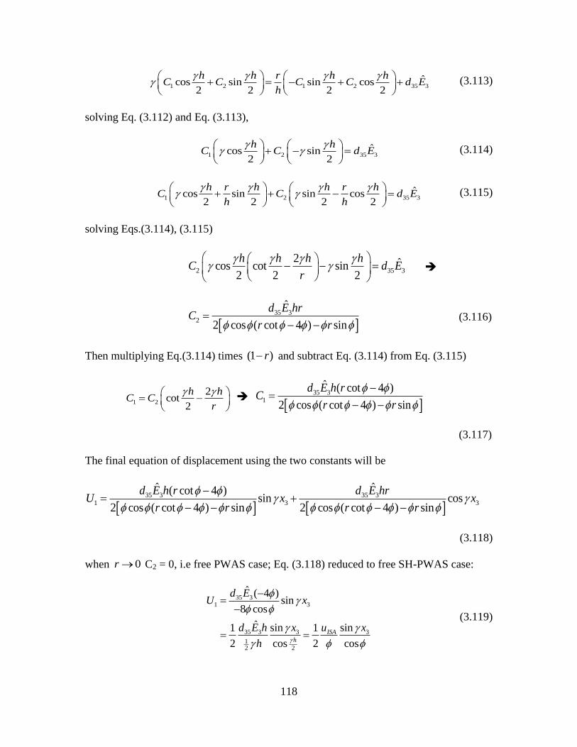
118
1 2 1 2 35 3
ˆcos sin sin cos2 2 2 2
h h r h hC C C C d E
h
(3.113)
solving Eq. (3.112) and Eq. (3.113),
1 2 35 3
ˆcos sin2 2
h hC C d E
(3.114)
1 2 35 3
ˆcos sin sin cos2 2 2 2
h r h h r hC C d E
h h
(3.115)
solving Eqs.(3.114), (3.115)
2 35 3
2 ˆcos cot sin2 2 2
h h h hC d E
r
35 3
2
ˆ
2 cos ( cot 4 ) sin
d E hrC
r r
(3.116)
Then multiplying Eq.(3.114) times (1 )r and subtract Eq. (3.114) from Eq. (3.115)
1 2
2cot
2
h hC C
r
35 3
1
ˆ ( cot 4 )
2 cos ( cot 4 ) sin
d E h rC
r r
(3.117)
The final equation of displacement using the two constants will be
35 3 35 3
1 3 3
ˆ ˆ( cot 4 )sin cos
2 cos ( cot 4 ) sin 2 cos ( cot 4 ) sin
d E h r d E hrU x x
r r r r
(3.118)
when 0r C2 = 0, i.e free PWAS case; Eq. (3.118) reduced to free SH-PWAS case:
35 31 3
35 3 3 3
12 2
ˆ ( 4 )sin
8 cos
ˆ sin sin1 1
2 cos 2 cos
ISA
h
d EU x
d E h x u x
h
(3.119)
119
Checking Eq.(3.119) for bottom surface ,i.e. 0r and 3 / 2x h ;
35 3
35 3
ˆ cos ( cot 4 )sin
2 cos ( cot 4 ) sin
ˆ2(1 cos 2 )
2 cos 2 4 sin 2
a
d E h r rU
r r
d E h
r
(3.120)
For calculating the bonded SH-PWAS impedance and admittance, we substitute Ua from
Eq.(3.120) with the same procedure in the electrical displacement Eq. (3.24)
353 5 35 3 33 3
55
ˆ ˆ(2 )E
dD S d E E
s
(3.121)
2
35 353 1 3 33 3
55 55
ˆ ˆE E
d dD u E E
s s (3.122)
2 1
3 33 3 35
35 3
ˆ 1 1ˆ
uD E K
d E
(3.123)
Where we define the electromechanical coupling factor 35K as
2
3535
55 33
E
dK
s (3.124)
Integrating the electrical displacement over electrodes area, results in the electric charge
2
2
3 3 1 2 3 1 2
0
( )
l
l
b
A
Q x D dx dx D dx dx
(3.125)
Substituting 3D from Eq.(3.123)
2 1
3 33 3 35
35 3
ˆ( ) 1 1ˆ
uQ x E bl K
d E
(3.126)
Then, equivalent charge across thickness can be determined by integrating over thickness
120
2
2
3 3
1ˆ ( )
h
h
eqQ Q x dxh
(3.127)
Substituting Eq.(3.126) into Eq.(3.127) and integrating over the thickness, yields
2
21 3
2 233 335 35
35 3
ˆ ( )ˆˆ 1
ˆ
h
h
eq
u xE blQ K h K
h d E
(3.128)
Substituting 1 3ˆ ( )u x from Eq.(3.118) , and defining SH-PWAS capacitance 33
T blC
h , the
electric field is related to voltage by 3
ˆˆ VE
h and recalling ISAu from Eq.(3.21) ; then
Eq.(3.128) can be simplified to
2
35
( cot 4 )sinˆ ˆ 1 1cos ( cot 4 ) sin
eq
rQ CV K
r r
(3.129)
The electric current I is defined as the time derivative of electric charge, i.e. I Q i Q ,
hence Eq.(3.129) simplifies to
2
35
( cot 4 )sin1 1
cos ( cot 4 ) sin
I rY i C K
V r r
(3.130)
And the constrained SH-PWAS electrical impedance is
1
2
35
1 ( cot 4 )sin1 1
cos ( cot 4 ) sin
V rZ K
I i C r r
(3.131)
121
3.3. FINITE ELEMENT MODELING OF SH-PWAS IMPEDANCE RESPONSE
Free SH-PWAS Models 3.3.1.
A multiphysics finite element model (FEM) was constructed for free SH-PWAS
to compute the shear deformation modeshapes. The transducer is modeled with
COMSOL multiphysics using coupled-physics finite element. The maximum element
size is selected as 0.5 mm. The coordinate system is defined such that the poling of SH-
PWAS is defined along the x1 direction. Harmonic voltage is applied to the top electrode
and the mechanical response is recorded. The free SH-PWAS dimensions are 15 mm x
15mm x 1 mm. The SH-PWAS material is APC850, detailed properties can be found on
the APC website ( APC International Ltd.). From the provided information, the
transducer capacitance 33( / )SC bl h is found as 3.48±20% nF. A frequency sweep from
10 kHz to 2000 kHz is performed with the frequency domain solver of the FEM software.
The deformation modeshapes are captures and the electromechanical (E/M) impedance is
calculated. Figure 3.11 shows the modeshapes of vibration at (a) 200 kHz to show the
shear deformation of the transducer, (b) first resonance frequency of the transducer at 900
kHz, where nonlinear effects start to appear at SH-PWAS ends.
Constrained SH-PWAS Models 3.3.2.
Finite element models were constructed for bonded SH-PWAS on 1-mm thick
aluminum beams as well as 3-mm thick steel beams. In both cases, three models are
constructed: (i) a 2-D model for the case where poling of the SH-PWAS is along beam
length, (ii) a 3-D model for the same case of having poling direction parallel to beam
length (Figure 3.9a), and (iii) a 3-D model for the case of transducer poling
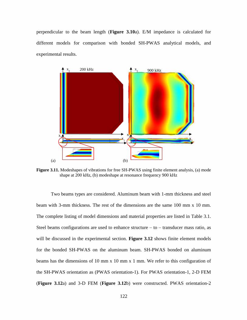
122
perpendicular to the beam length (Figure 3.10a). E/M impedance is calculated for
different models for comparison with bonded SH-PWAS analytical models, and
experimental results.
Figure 3.11. Modeshapes of vibrations for free SH-PWAS using finite element analysis, (a) mode
shape at 200 kHz, (b) modeshape at resonance frequency 900 kHz
Two beams types are considered. Aluminum beam with 1-mm thickness and steel
beam with 3-mm thickness. The rest of the dimensions are the same 100 mm x 10 mm.
The complete listing of model dimensions and material properties are listed in Table 3.1.
Steel beams configurations are used to enhance structure – to – transducer mass ratio, as
will be discussed in the experimental section. Figure 3.12 shows finite element models
for the bonded SH-PWAS on the aluminum beam. SH-PWAS bonded on aluminum
beams has the dimensions of 10 mm x 10 mm x 1 mm. We refer to this configuration of
the SH-PWAS orientation as (PWAS orientation-1). For PWAS orientation-1, 2-D FEM
(Figure 3.12a) and 3-D FEM (Figure 3.12b) were constructed. PWAS orientation-2
900 kHz 200 kHz
x1
x3
x2
x1
x2
x3
(a) (b)
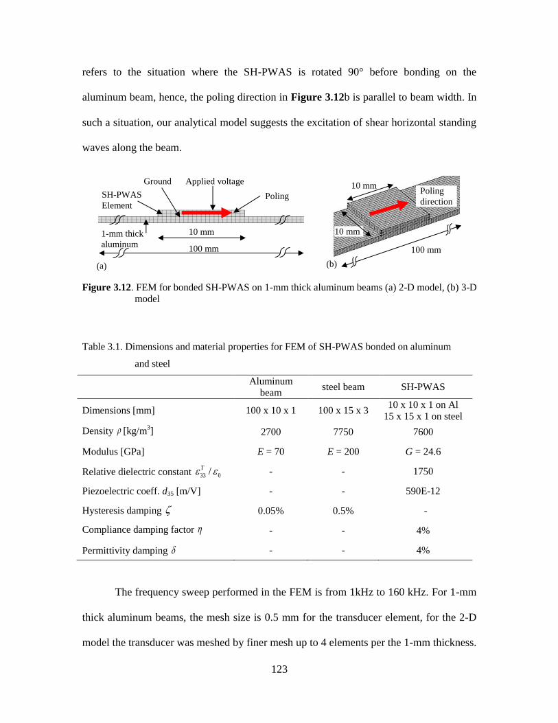
123
refers to the situation where the SH-PWAS is rotated 90° before bonding on the
aluminum beam, hence, the poling direction in Figure 3.12b is parallel to beam width. In
such a situation, our analytical model suggests the excitation of shear horizontal standing
waves along the beam.
Figure 3.12. FEM for bonded SH-PWAS on 1-mm thick aluminum beams (a) 2-D model, (b) 3-D
model
Table 3.1. Dimensions and material properties for FEM of SH-PWAS bonded on aluminum
and steel
Aluminum
beam steel beam SH-PWAS
Dimensions [mm] 100 x 10 x 1 100 x 15 x 3 10 x 10 x 1 on Al
15 x 15 x 1 on steel
Density [kg/m3] 2700 7750 7600
Modulus [GPa] E = 70 E = 200 G = 24.6
Relative dielectric constant 33 0/T - - 1750
Piezoelectric coeff. d35 [m/V] - - 590E-12
Hysteresis damping 0.05% 0.5% -
Compliance damping factor - - 4%
Permittivity damping - - 4%
The frequency sweep performed in the FEM is from 1kHz to 160 kHz. For 1-mm
thick aluminum beams, the mesh size is 0.5 mm for the transducer element, for the 2-D
model the transducer was meshed by finer mesh up to 4 elements per the 1-mm thickness.
Applied voltage Ground
SH-PWAS
Element Poling
10 mm
100 mm
(a)
1-mm thick
aluminum
10 mm
100 mm
10 mm
Poling
direction
(b)
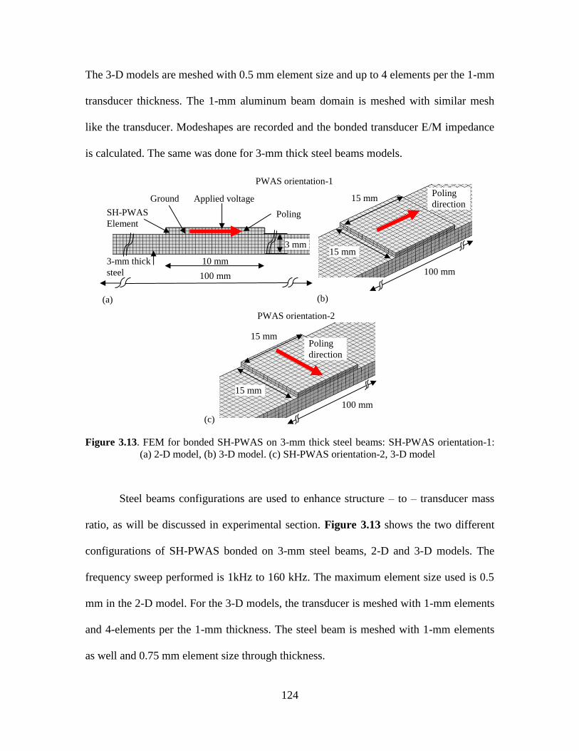
124
The 3-D models are meshed with 0.5 mm element size and up to 4 elements per the 1-mm
transducer thickness. The 1-mm aluminum beam domain is meshed with similar mesh
like the transducer. Modeshapes are recorded and the bonded transducer E/M impedance
is calculated. The same was done for 3-mm thick steel beams models.
Figure 3.13. FEM for bonded SH-PWAS on 3-mm thick steel beams: SH-PWAS orientation-1:
(a) 2-D model, (b) 3-D model. (c) SH-PWAS orientation-2, 3-D model
Steel beams configurations are used to enhance structure – to – transducer mass
ratio, as will be discussed in experimental section. Figure 3.13 shows the two different
configurations of SH-PWAS bonded on 3-mm steel beams, 2-D and 3-D models. The
frequency sweep performed is 1kHz to 160 kHz. The maximum element size used is 0.5
mm in the 2-D model. For the 3-D models, the transducer is meshed with 1-mm elements
and 4-elements per the 1-mm thickness. The steel beam is meshed with 1-mm elements
as well and 0.75 mm element size through thickness.
Applied voltage Ground
SH-PWAS
Element Poling
10 mm
100 mm
(a)
3-mm thick
steel
15 mm
100 mm
15 mm
Poling
direction
(b)
PWAS orientation-1
PWAS orientation-2
3 mm
Poling
direction
15 mm
15 mm
100 mm
(c)
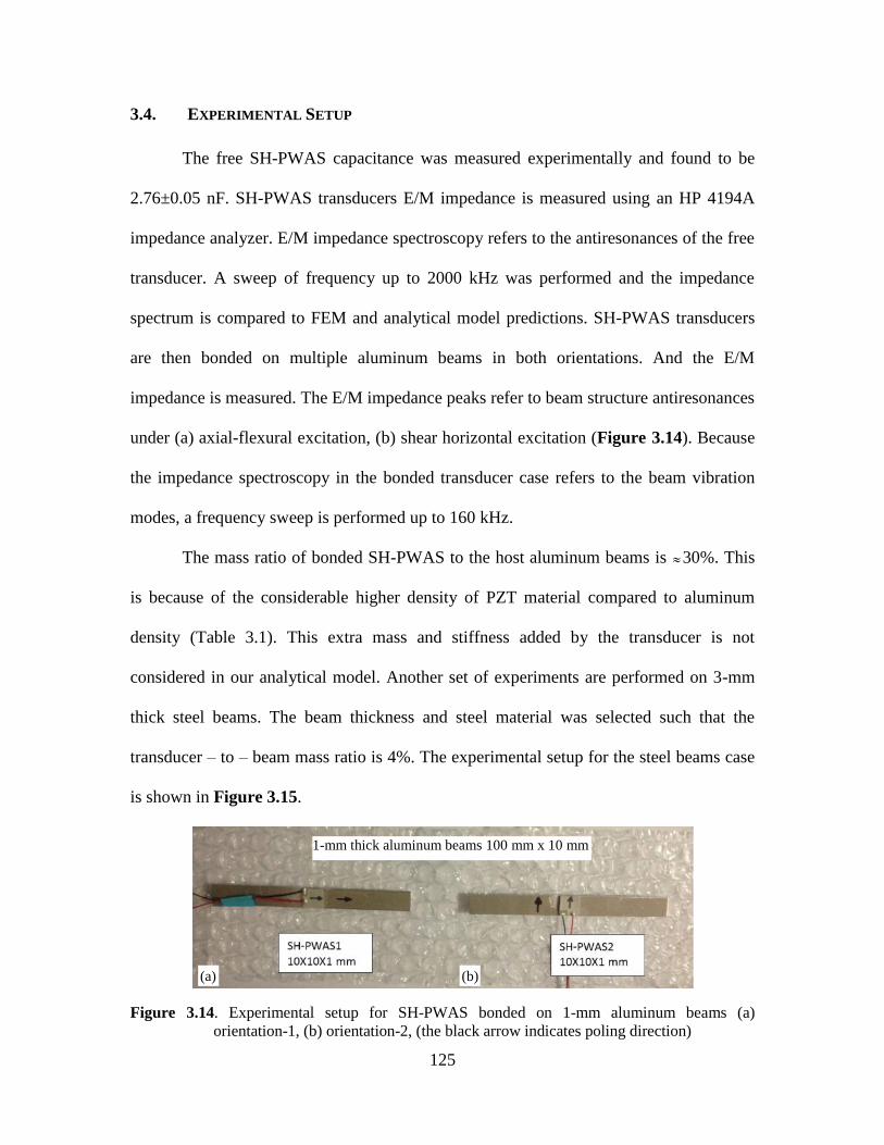
125
3.4. EXPERIMENTAL SETUP
The free SH-PWAS capacitance was measured experimentally and found to be
2.76±0.05 nF. SH-PWAS transducers E/M impedance is measured using an HP 4194A
impedance analyzer. E/M impedance spectroscopy refers to the antiresonances of the free
transducer. A sweep of frequency up to 2000 kHz was performed and the impedance
spectrum is compared to FEM and analytical model predictions. SH-PWAS transducers
are then bonded on multiple aluminum beams in both orientations. And the E/M
impedance is measured. The E/M impedance peaks refer to beam structure antiresonances
under (a) axial-flexural excitation, (b) shear horizontal excitation (Figure 3.14). Because
the impedance spectroscopy in the bonded transducer case refers to the beam vibration
modes, a frequency sweep is performed up to 160 kHz.
The mass ratio of bonded SH-PWAS to the host aluminum beams is 30%. This
is because of the considerable higher density of PZT material compared to aluminum
density (Table 3.1). This extra mass and stiffness added by the transducer is not
considered in our analytical model. Another set of experiments are performed on 3-mm
thick steel beams. The beam thickness and steel material was selected such that the
transducer – to – beam mass ratio is 4%. The experimental setup for the steel beams case
is shown in Figure 3.15.
Figure 3.14. Experimental setup for SH-PWAS bonded on 1-mm aluminum beams (a)
orientation-1, (b) orientation-2, (the black arrow indicates poling direction)
(a) (b)
1-mm thick aluminum beams 100 mm x 10 mm
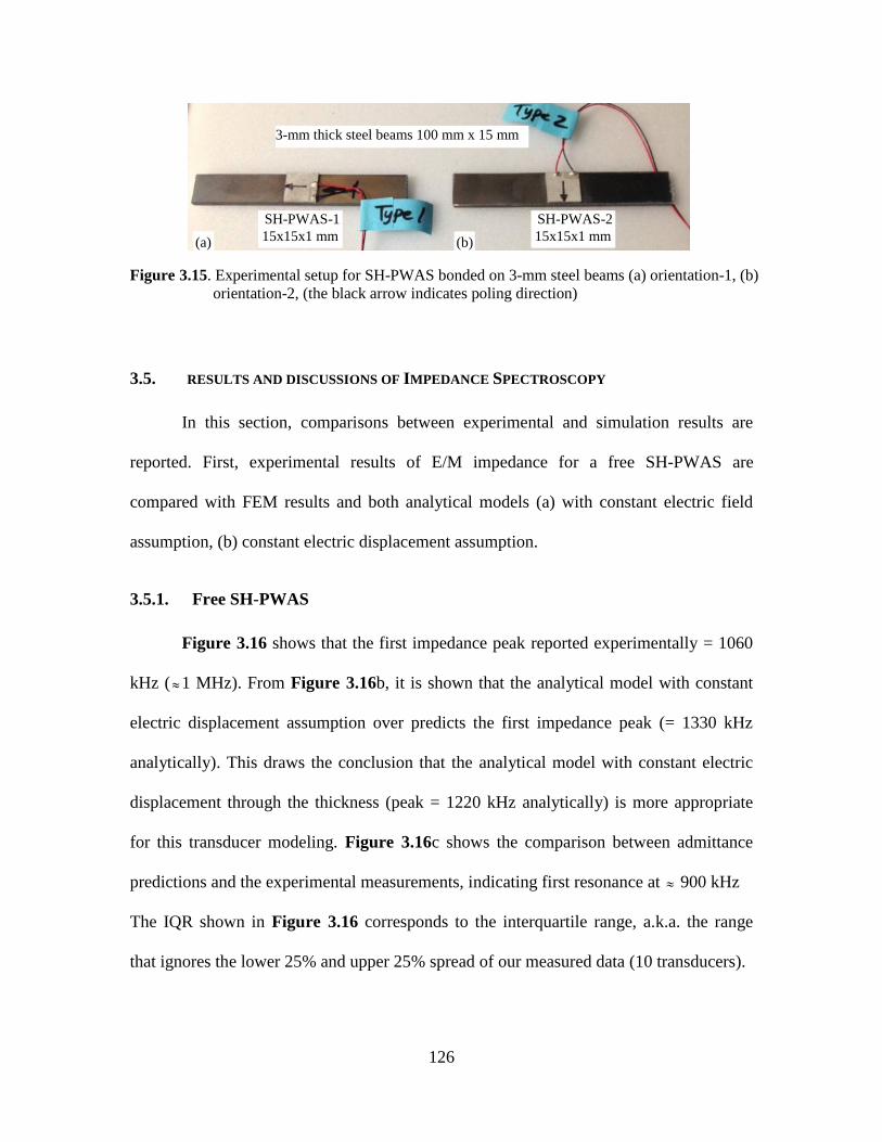
126
Figure 3.15. Experimental setup for SH-PWAS bonded on 3-mm steel beams (a) orientation-1, (b)
orientation-2, (the black arrow indicates poling direction)
3.5. RESULTS AND DISCUSSIONS OF IMPEDANCE SPECTROSCOPY
In this section, comparisons between experimental and simulation results are
reported. First, experimental results of E/M impedance for a free SH-PWAS are
compared with FEM results and both analytical models (a) with constant electric field
assumption, (b) constant electric displacement assumption.
Free SH-PWAS 3.5.1.
Figure 3.16 shows that the first impedance peak reported experimentally = 1060
kHz (1 MHz). From Figure 3.16b, it is shown that the analytical model with constant
electric displacement assumption over predicts the first impedance peak (= 1330 kHz
analytically). This draws the conclusion that the analytical model with constant electric
displacement through the thickness (peak = 1220 kHz analytically) is more appropriate
for this transducer modeling. Figure 3.16c shows the comparison between admittance
predictions and the experimental measurements, indicating first resonance at 900 kHz
The IQR shown in Figure 3.16 corresponds to the interquartile range, a.k.a. the range
that ignores the lower 25% and upper 25% spread of our measured data (10 transducers).
3-mm thick steel beams 100 mm x 15 mm
SH-PWAS-1
15x15x1 mm
SH-PWAS-2
15x15x1 mm (a) (b)
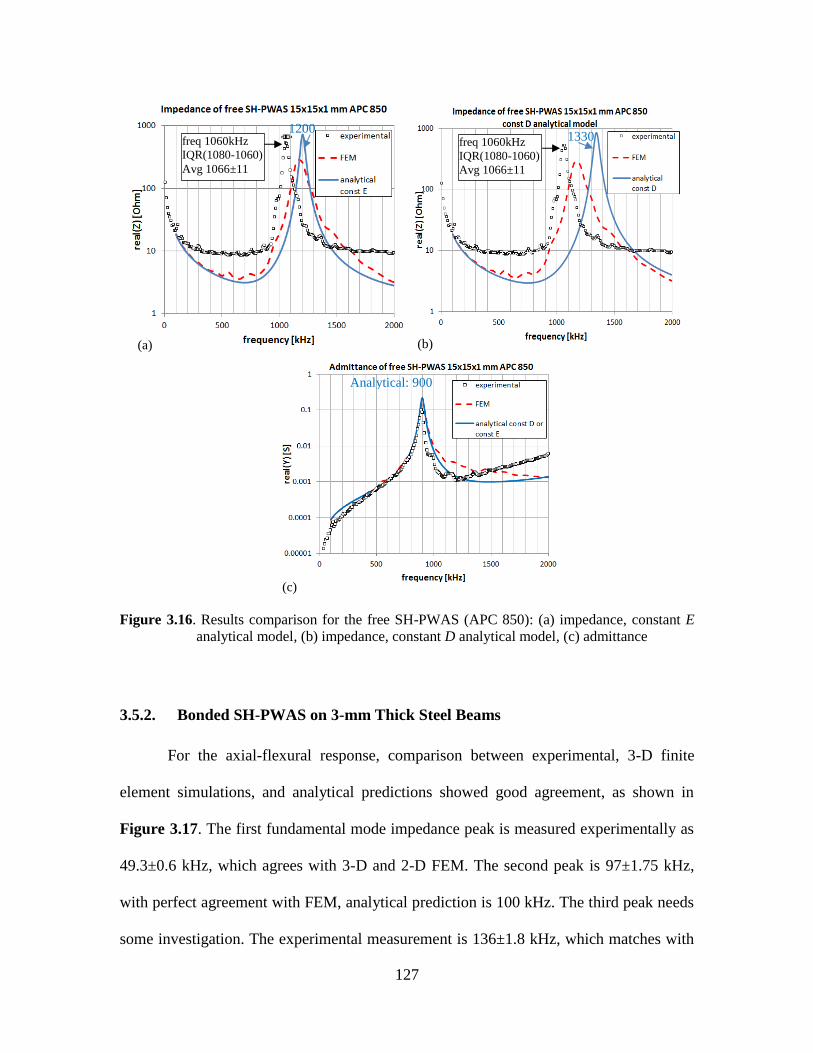
127
Figure 3.16. Results comparison for the free SH-PWAS (APC 850): (a) impedance, constant E
analytical model, (b) impedance, constant D analytical model, (c) admittance
Bonded SH-PWAS on 3-mm Thick Steel Beams 3.5.2.
For the axial-flexural response, comparison between experimental, 3-D finite
element simulations, and analytical predictions showed good agreement, as shown in
Figure 3.17. The first fundamental mode impedance peak is measured experimentally as
49.3±0.6 kHz, which agrees with 3-D and 2-D FEM. The second peak is 97±1.75 kHz,
with perfect agreement with FEM, analytical prediction is 100 kHz. The third peak needs
some investigation. The experimental measurement is 136±1.8 kHz, which matches with
freq 1060kHz
IQR(1080-1060)
Avg 1066±11
(a) (b)
1200 1330 freq 1060kHz
IQR(1080-1060)
Avg 1066±11
(c)
Analytical: 900
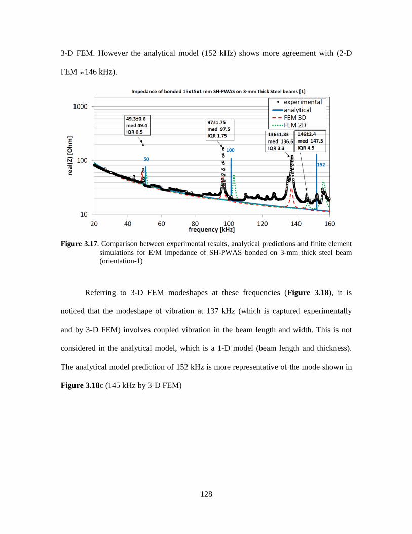
128
3-D FEM. However the analytical model (152 kHz) shows more agreement with (2-D
FEM 146 kHz).
Figure 3.17. Comparison between experimental results, analytical predictions and finite element
simulations for E/M impedance of SH-PWAS bonded on 3-mm thick steel beam
(orientation-1)
Referring to 3-D FEM modeshapes at these frequencies (Figure 3.18), it is
noticed that the modeshape of vibration at 137 kHz (which is captured experimentally
and by 3-D FEM) involves coupled vibration in the beam length and width. This is not
considered in the analytical model, which is a 1-D model (beam length and thickness).
The analytical model prediction of 152 kHz is more representative of the mode shown in
Figure 3.18c (145 kHz by 3-D FEM)
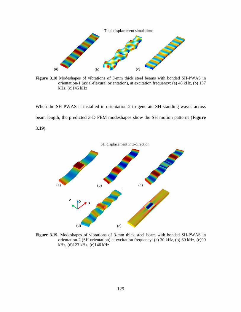
129
Figure 3.18 Modeshapes of vibrations of 3-mm thick steel beams with bonded SH-PWAS in
orientation-1 (axial-flexural orientation), at excitation frequency: (a) 48 kHz, (b) 137
kHz, (c)145 kHz
When the SH-PWAS is installed in orientation-2 to generate SH standing waves across
beam length, the predicted 3-D FEM modeshapes show the SH motion patterns (Figure
3.19).
Figure 3.19. Modeshapes of vibrations of 3-mm thick steel beam with bonded SH-PWAS in
orientation-2 (SH orientation) at excitation frequency: (a) 30 kHz, (b) 60 kHz, (c)90
kHz, (d)123 kHz, (e)146 kHz
(a) (b) (c)
Total displacement simulations
(a) (b) (c)
(d) (e)
z x y
SH displacement in z-direction

130
Figure 3.20. Comparison between experimental results, analytical predictions and finite element
simulations for E/M impedance of SH-PWAS bonded on 3-mm thick steel beam
(orientation-2)
Comparison between experimental results, analytical predictions, and finite
element simulations (Figure 3.20) shows good agreement for SH-PWAS orientation-2
that generates SH deformation in the structure. It is noticed that the impedance peaks are
multiples of 30 kHz. The third peak of 95 kHz shows the best match between
experiments and simulations. Also, the experimental measurement at 145 kHz shows
agreement with 3-D FEM, however this peak is not captured by the analytical prediction.
Referring to modeshapes (Figure 3.19), it is noticed that the 5th
mode of vibration is a
local mode and it drives the beam into some torsional vibration. The 4th
mode starts not to
be a uniform SH deformation; it may contain coupled modes of vibration.
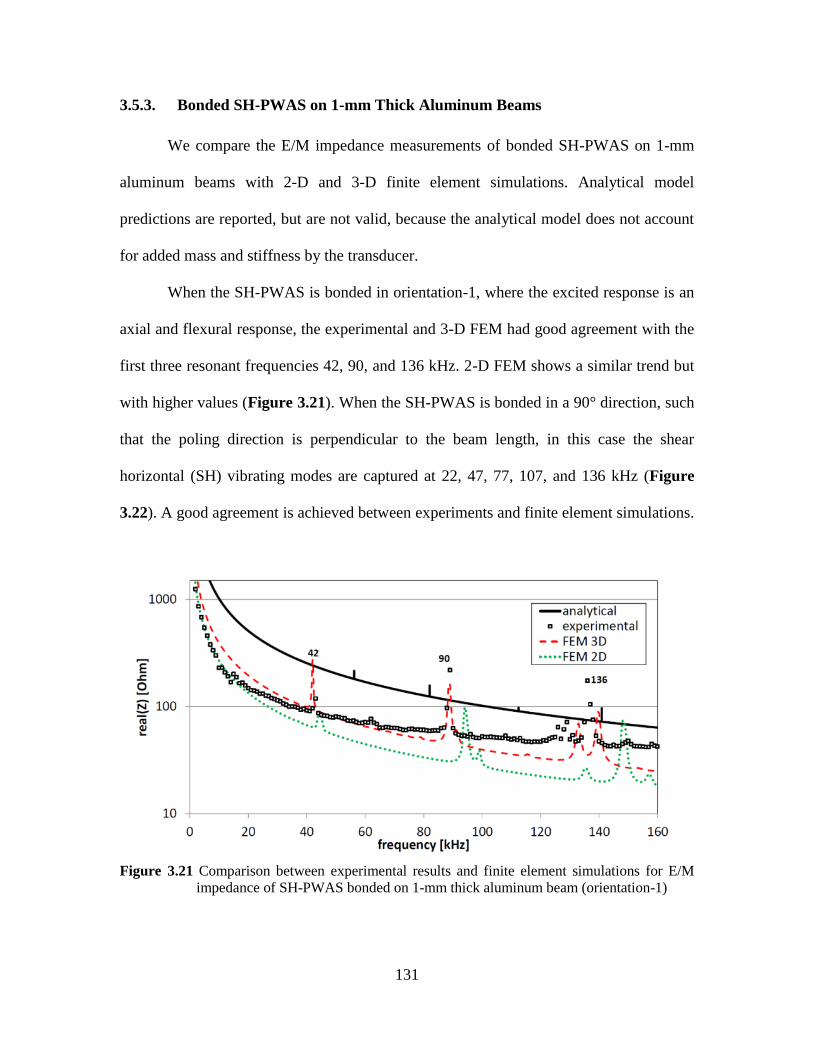
131
Bonded SH-PWAS on 1-mm Thick Aluminum Beams 3.5.3.
We compare the E/M impedance measurements of bonded SH-PWAS on 1-mm
aluminum beams with 2-D and 3-D finite element simulations. Analytical model
predictions are reported, but are not valid, because the analytical model does not account
for added mass and stiffness by the transducer.
When the SH-PWAS is bonded in orientation-1, where the excited response is an
axial and flexural response, the experimental and 3-D FEM had good agreement with the
first three resonant frequencies 42, 90, and 136 kHz. 2-D FEM shows a similar trend but
with higher values (Figure 3.21). When the SH-PWAS is bonded in a 90° direction, such
that the poling direction is perpendicular to the beam length, in this case the shear
horizontal (SH) vibrating modes are captured at 22, 47, 77, 107, and 136 kHz (Figure
3.22). A good agreement is achieved between experiments and finite element simulations.
Figure 3.21 Comparison between experimental results and finite element simulations for E/M
impedance of SH-PWAS bonded on 1-mm thick aluminum beam (orientation-1)
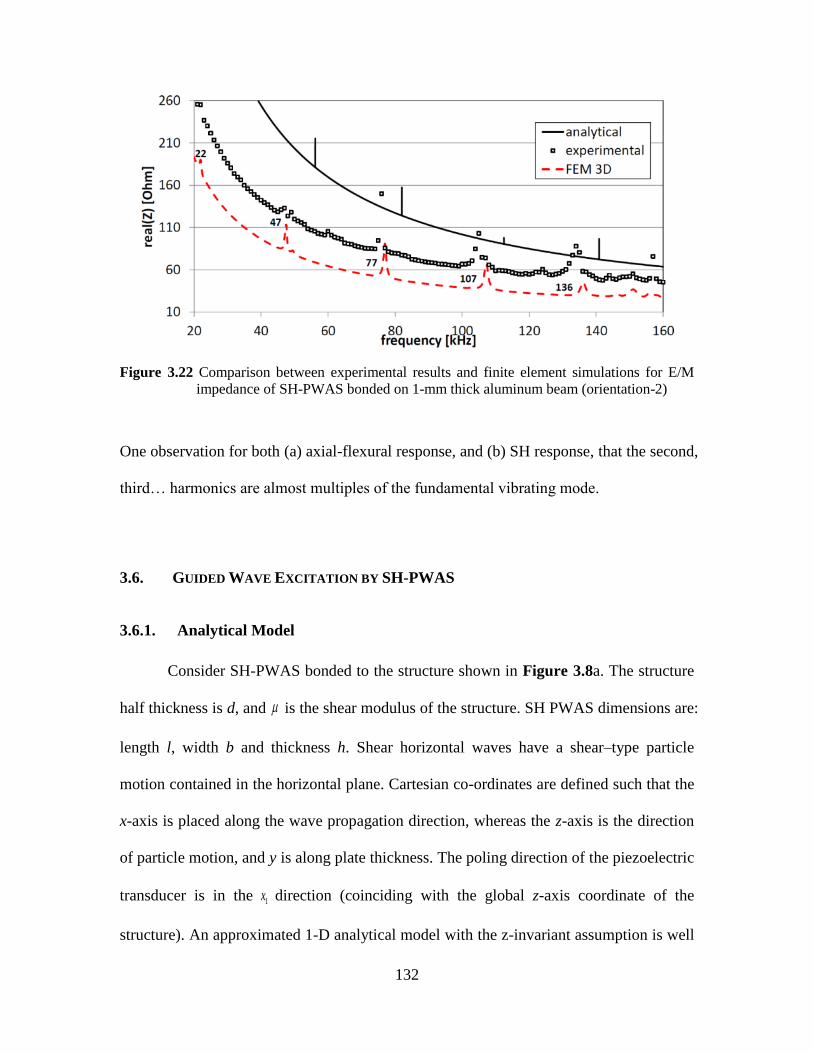
132
Figure 3.22 Comparison between experimental results and finite element simulations for E/M
impedance of SH-PWAS bonded on 1-mm thick aluminum beam (orientation-2)
One observation for both (a) axial-flexural response, and (b) SH response, that the second,
third… harmonics are almost multiples of the fundamental vibrating mode.
3.6. GUIDED WAVE EXCITATION BY SH-PWAS
Analytical Model 3.6.1.
Consider SH-PWAS bonded to the structure shown in Figure 3.8a. The structure
half thickness is d, and is the shear modulus of the structure. SH PWAS dimensions are:
length l, width b and thickness h. Shear horizontal waves have a shear–type particle
motion contained in the horizontal plane. Cartesian co-ordinates are defined such that the
x-axis is placed along the wave propagation direction, whereas the z-axis is the direction
of particle motion, and y is along plate thickness. The poling direction of the piezoelectric
transducer is in the 1x direction (coinciding with the global z-axis coordinate of the
structure). An approximated 1-D analytical model with the z-invariant assumption is well
133
developed in many previous studies, such as: Auld (1990); Graff (1991); Rose (1999).
The analytical model only predicts SH wave motion of particle oscillation along z
direction and propagating in x direction. We use the analytical model to predict
dispersion wave speeds of SH waves. The displacement is assumed to be harmonic
( , , ) ( )i x t
z zu x y t U y e
(3.132)
where is the wave number in x direction. Guided SH waves in plates (similar to guided
Lamb waves) are multimodal in nature; as the frequency of excitation increases, new
modes are excited in the plate. The frequencies at which new modes appear are called
cut-off frequencies. The cut-off frequency can be determined by solving the characteristic
equation sin( )cos( ) 0S Ad d for d values, and substitute in
1
( )2
scut off
cf d
d
(3.133)
where is defined from 2 2 2 2
sc , and sc is the shear wave speed. We define cut-
off frequency in units of Hz, or normalized frequency. The nth
symmetric mode
displacement is
( , , ) cos( )Sni xn S i t
z n nu x y t B y e e
(3.134)
The nth
antisymmetric mode displacement is
( , , ) sin( )Ani xn A i t
z n nu x y t A y e e
(3.135)
The total displacement is
( , , ) sin( ) cos( )A Sn ni x i xA S i t
z n n n nu x y t A y e B y e e
(3.136)
The amplitudes nA , nB are normalized with respect to power flow and found to be
(Santoni, 2010)
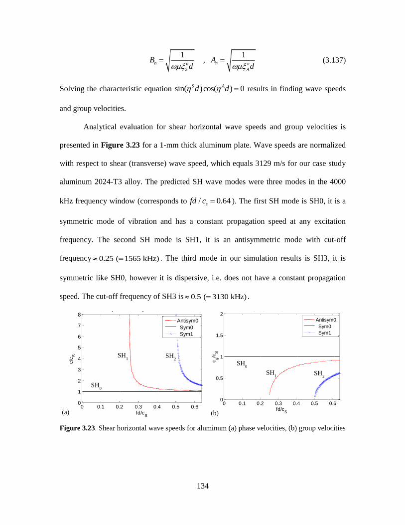
134
1 1
, n nn n
S A
B Ad d
(3.137)
Solving the characteristic equation sin( )cos( ) 0S Ad d results in finding wave speeds
and group velocities.
Analytical evaluation for shear horizontal wave speeds and group velocities is
presented in Figure 3.23 for a 1-mm thick aluminum plate. Wave speeds are normalized
with respect to shear (transverse) wave speed, which equals 3129 m/s for our case study
aluminum 2024-T3 alloy. The predicted SH wave modes were three modes in the 4000
kHz frequency window (corresponds to / 0.64sfd c ). The first SH mode is SH0, it is a
symmetric mode of vibration and has a constant propagation speed at any excitation
frequency. The second SH mode is SH1, it is an antisymmetric mode with cut-off
frequency 0.25 ( 1565 kHz) . The third mode in our simulation results is SH3, it is
symmetric like SH0, however it is dispersive, i.e. does not have a constant propagation
speed. The cut-off frequency of SH3 is 0.5 ( 3130 kHz) .
Figure 3.23. Shear horizontal wave speeds for aluminum (a) phase velocities, (b) group velocities
0 0.1 0.2 0.3 0.4 0.5 0.60
1
2
3
4
5
6
7
8
fd/cS
c/c
S
SH waves phase velocity of Aluminum-2024-T3
Antisym0
Sym0
Sym1
0 0.1 0.2 0.3 0.4 0.5 0.60
0.5
1
1.5
2
fd/cS
cg/c
S
SH waves group velocity of Aluminum-2024-T3
Antisym0
Sym0
Sym1
SH0
SH1 SH
2
SH0
SH1 SH
2
(a) (b)
135
Experimental Studies 3.6.2.
3.6.2.1. Proof of concept
Three sets of experiments are performed; the first set of experiments was a proof
of concept that was performed on 3.4-mm thick aluminum 7075 T6 alloy plate (Figure
3.24). The SH-PWAS was 15 mm x 15 mm x 1 mm and its material was APC850. SH-
PWAS poling direction was along z-direction (Figure 3.24c). The distance between the
two SH-PWAS was 150 mm, the excitation was 3-count tone burst signal with 10 V
amplitude. The excitation frequencies used were 30, 45, 60, 75, and 90 kHz as shown in
the waveforms (Figure 3.25). It was noticed that the received signals in Figure 3.25 were
non-dispersive, (i.e. they have shown the same shape as excitation signal, 3 count tone
burst), especially at frequencies 60, 75 and 90 kHz. This implies that the wave packet
speed does not change with frequency and this is the intrinsic property of SH0 (the first
shear horizontal guided wave in isotropic materials). In addition, it was observed that no
waves propagate along (path 2) in Figure 3.24c. The actuation mechanism of SH-PWAS,
that is shown from free transducer mode shapes (Figure 3.11) implies that the SH-PWAS
resonates in z-direction and the generated waves propagate along x-direction. The
comparison between analytical and experimental results is shown in Figure 3.26.
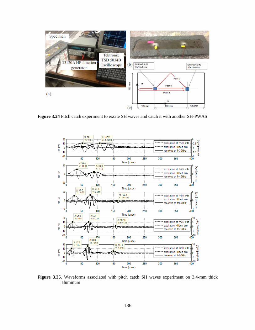
136
Figure 3.24 Pitch catch experiment to excite SH waves and catch it with another SH-PWAS
Figure 3.25. Waveforms associated with pitch catch SH waves experiment on 3.4-mm thick
aluminum
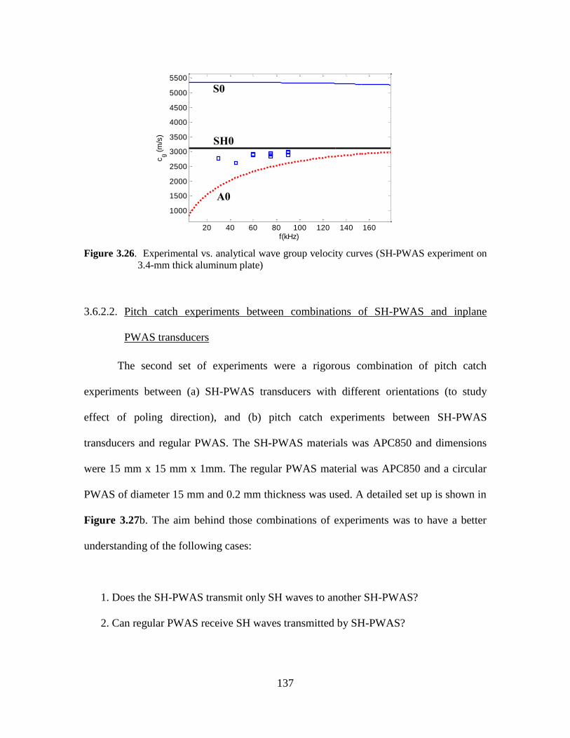
137
Figure 3.26. Experimental vs. analytical wave group velocity curves (SH-PWAS experiment on
3.4-mm thick aluminum plate)
3.6.2.2. Pitch catch experiments between combinations of SH-PWAS and inplane
PWAS transducers
The second set of experiments were a rigorous combination of pitch catch
experiments between (a) SH-PWAS transducers with different orientations (to study
effect of poling direction), and (b) pitch catch experiments between SH-PWAS
transducers and regular PWAS. The SH-PWAS materials was APC850 and dimensions
were 15 mm x 15 mm x 1mm. The regular PWAS material was APC850 and a circular
PWAS of diameter 15 mm and 0.2 mm thickness was used. A detailed set up is shown in
Figure 3.27b. The aim behind those combinations of experiments was to have a better
understanding of the following cases:
1. Does the SH-PWAS transmit only SH waves to another SH-PWAS?
2. Can regular PWAS receive SH waves transmitted by SH-PWAS?
20 40 60 80 100 120 140 160
1000
1500
2000
2500
3000
3500
4000
4500
5000
5500
f(kHz)
cg (
m/s
)
S0
A0
SH0
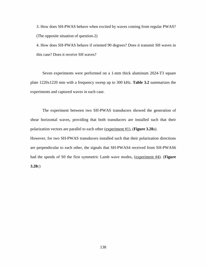
138
3. How does SH-PWAS behave when excited by waves coming from regular PWAS?
(The opposite situation of question-2)
4. How does SH-PWAS behave if oriented 90 degrees? Does it transmit SH waves in
this case? Does it receive SH waves?
Seven experiments were performed on a 1-mm thick aluminum 2024-T3 square
plate 1220x1220 mm with a frequency sweep up to 300 kHz. Table 3.2 summarizes the
experiments and captured waves in each case.
The experiment between two SH-PWAS transducers showed the generation of
shear horizontal waves, providing that both transducers are installed such that their
polarization vectors are parallel to each other (experiment #1), (Figure 3.28a).
However, for two SH-PWAS transducers installed such that their polarization directions
are perpendicular to each other, the signals that SH-PWAS4 received from SH-PWAS6
had the speeds of S0 the first symmetric Lamb wave modes, (experiment #4). (Figure
3.28c)
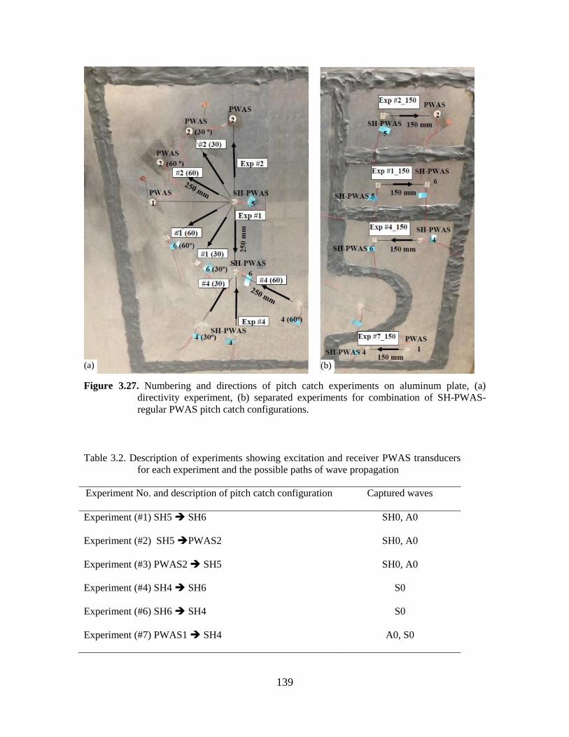
139
Figure 3.27. Numbering and directions of pitch catch experiments on aluminum plate, (a)
directivity experiment, (b) separated experiments for combination of SH-PWAS-
regular PWAS pitch catch configurations.
Table 3.2. Description of experiments showing excitation and receiver PWAS transducers
for each experiment and the possible paths of wave propagation
Experiment No. and description of pitch catch configuration Captured waves
Experiment (#1) SH5 SH6 SH0, A0
Experiment (#2) SH5 PWAS2 SH0, A0
Experiment (#3) PWAS2 SH5 SH0, A0
Experiment (#4) SH4 SH6 S0
Experiment (#6) SH6 SH4 S0
Experiment (#7) PWAS1 SH4 A0, S0
(a) (b)
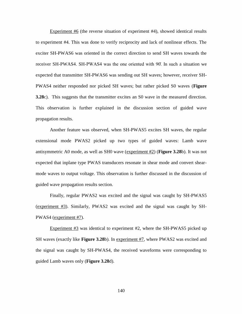
140
Experiment #6 (the reverse situation of experiment #4), showed identical results
to experiment #4. This was done to verify reciprocity and lack of nonlinear effects. The
exciter SH-PWAS6 was oriented in the correct direction to send SH waves towards the
receiver SH-PWAS . SH-PWAS was the one oriented with 0 . In such a situation we
expected that transmitter SH-PWAS6 was sending out SH waves; however, receiver SH-
PWAS4 neither responded nor picked SH waves; but rather picked S0 waves (Figure
3.28c). This suggests that the transmitter excites an S0 wave in the measured direction.
This observation is further explained in the discussion section of guided wave
propagation results.
Another feature was observed, when SH-PWAS5 excites SH waves, the regular
extensional mode PWAS2 picked up two types of guided waves: Lamb wave
antisymmetric A0 mode, as well as SH0 wave (experiment #2) (Figure 3.28b). It was not
expected that inplane type PWAS transducers resonate in shear mode and convert shear-
mode waves to output voltage. This observation is further discussed in the discussion of
guided wave propagation results section.
Finally, regular PWAS2 was excited and the signal was caught by SH-PWAS5
(experiment #3). Similarly, PWAS2 was excited and the signal was caught by SH-
PWAS4 (experiment #7).
Experiment #3 was identical to experiment #2, where the SH-PWAS5 picked up
SH waves (exactly like Figure 3.28b). In experiment #7, where PWAS2 was excited and
the signal was caught by SH-PWAS4, the received waveforms were corresponding to
guided Lamb waves only (Figure 3.28d).
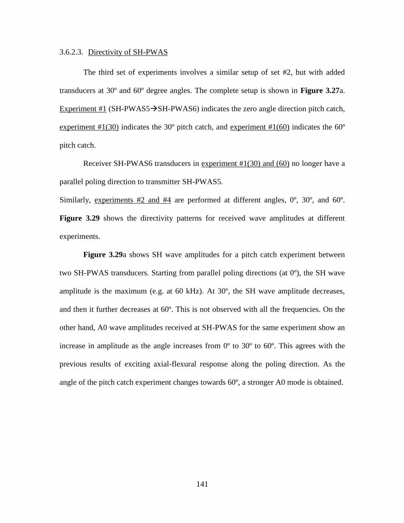
141
3.6.2.3. Directivity of SH-PWAS
The third set of experiments involves a similar setup of set #2, but with added
transducers at 30º and 60º degree angles. The complete setup is shown in Figure 3.27a.
Experiment #1 (SH-PWAS5SH-PWAS6) indicates the zero angle direction pitch catch,
experiment #1(30) indicates the 30º pitch catch, and experiment #1(60) indicates the 60º
pitch catch.
Receiver SH-PWAS6 transducers in experiment #1(30) and (60) no longer have a
parallel poling direction to transmitter SH-PWAS5.
Similarly, experiments #2 and #4 are performed at different angles, 0º, 30º, and 60º.
Figure 3.29 shows the directivity patterns for received wave amplitudes at different
experiments.
Figure 3.29a shows SH wave amplitudes for a pitch catch experiment between
two SH-PWAS transducers. Starting from parallel poling directions (at 0º), the SH wave
amplitude is the maximum (e.g. at 60 kHz). At 30º, the SH wave amplitude decreases,
and then it further decreases at 60º. This is not observed with all the frequencies. On the
other hand, A0 wave amplitudes received at SH-PWAS for the same experiment show an
increase in amplitude as the angle increases from 0º to 30º to 60º. This agrees with the
previous results of exciting axial-flexural response along the poling direction. As the
angle of the pitch catch experiment changes towards 60º, a stronger A0 mode is obtained.
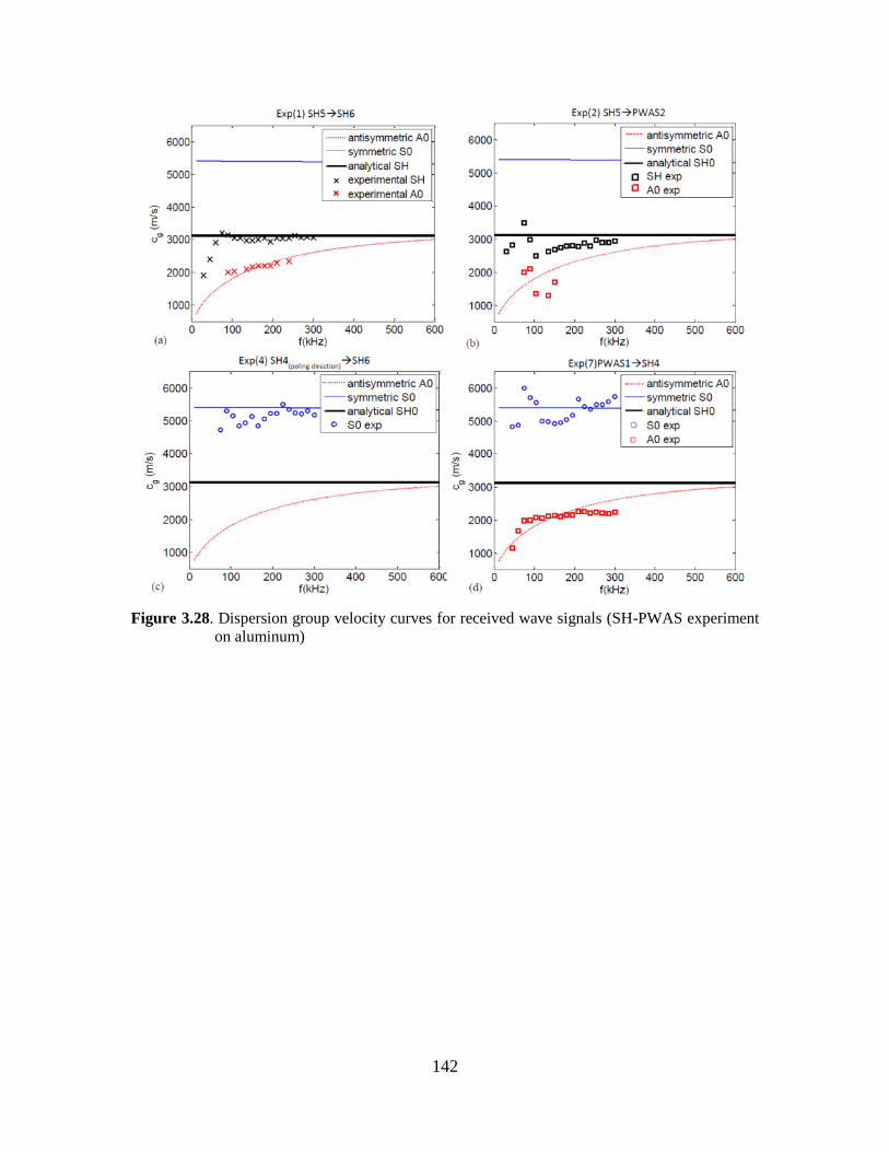
142
Figure 3.28. Dispersion group velocity curves for received wave signals (SH-PWAS experiment
on aluminum)
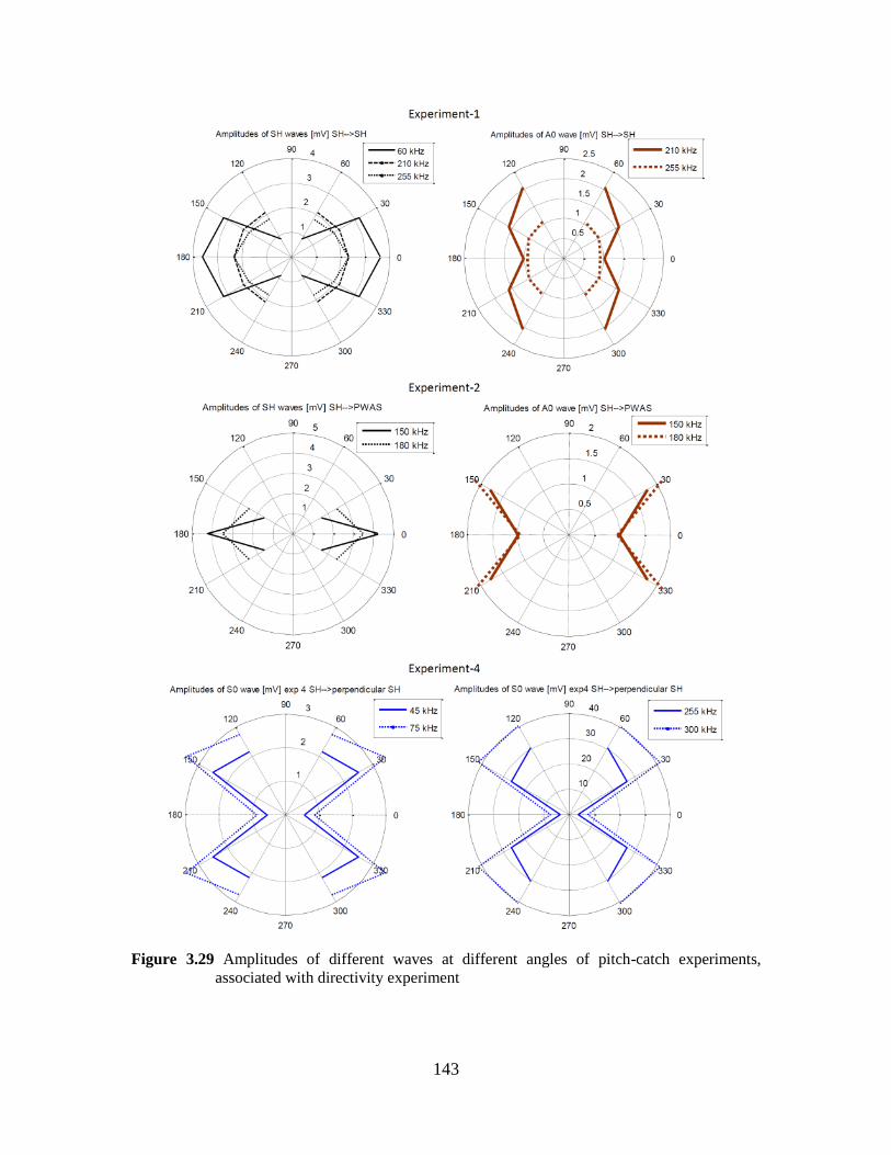
143
Figure 3.29 Amplitudes of different waves at different angles of pitch-catch experiments,
associated with directivity experiment
144
Experiment #2 (SH-PWAS5 regular PWAS2) showed similar patterns to
experiment #1. However, the received signals at 60º were noisy. Figure 3.29c shows
amplitudes of SH waves received by PWAS2 and generated by SH-PWAS5, for
experiment #2, 2(30), and 2(60). Figure 3.29d shows amplitudes of received A0 waves.
Experiments #3 are the opposites of experiments #2. Those are not performed in this
study.
Experiment #4 (SH-PWAS4 SH-PWAS6) involves the pitch catch experiments
between two SH-PWAS transducers having poling directions perpendicular to each other
(for 0º case). Figure 3.29e,f are for the same received S0 wave amplitudes, but at
different frequencies. They are plotted on two polar plots, because of considerable change
in amplitude values in [mV] between 45,75 kHz and 255,300 kHz. It is observed that the
S0 amplitudes are much less at lower frequencies. Also, it is observed that the
perpendicular poling directions – experiment #4(0) – cause the least S0 wave amplitudes.
S0 wave amplitudes are much higher at 30º and 60º angles between poling directions of
the two transducers.
Finite Element Simulations 3.6.3.
The models in section 2.3 predict SH-PWAS effects at 0º and 90º separately. Also,
it is hard to combine (axial-flexural) and (shear horizontal) separate responses of Figure
3.9b into 2-D analytical model. Hence 2-D multiphysics FEM simulations are constructed
to better understand the possible excited waves by SH-PWAS, and to verify directivity
experiments. Shear horizontal SH0, symmetric S0 and antisymmetric A0 Lamb waves
were picked by FEM simulations.
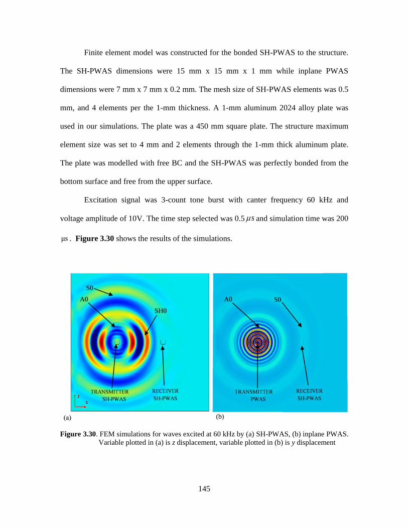
145
Finite element model was constructed for the bonded SH-PWAS to the structure.
The SH-PWAS dimensions were 15 mm x 15 mm x 1 mm while inplane PWAS
dimensions were 7 mm x 7 mm x 0.2 mm. The mesh size of SH-PWAS elements was 0.5
mm, and 4 elements per the 1-mm thickness. A 1-mm aluminum 2024 alloy plate was
used in our simulations. The plate was a 450 mm square plate. The structure maximum
element size was set to 4 mm and 2 elements through the 1-mm thick aluminum plate.
The plate was modelled with free BC and the SH-PWAS was perfectly bonded from the
bottom surface and free from the upper surface.
Excitation signal was 3-count tone burst with canter frequency 60 kHz and
voltage amplitude of 10V. The time step selected was 0.5 s and simulation time was 200
μs . Figure 3.30 shows the results of the simulations.
Figure 3.30. FEM simulations for waves excited at 60 kHz by (a) SH-PWAS, (b) inplane PWAS.
Variable plotted in (a) is z displacement, variable plotted in (b) is y displacement
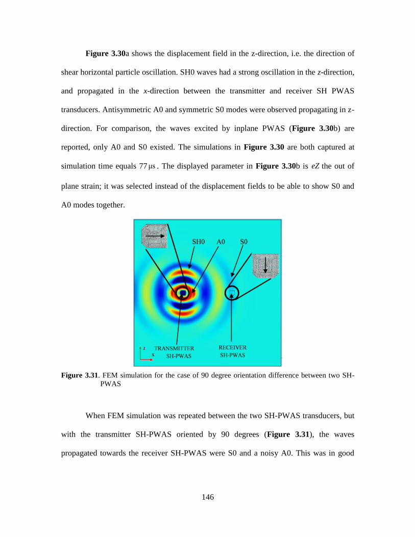
146
Figure 3.30a shows the displacement field in the z-direction, i.e. the direction of
shear horizontal particle oscillation. SH0 waves had a strong oscillation in the z-direction,
and propagated in the x-direction between the transmitter and receiver SH PWAS
transducers. Antisymmetric A0 and symmetric S0 modes were observed propagating in z-
direction. For comparison, the waves excited by inplane PWAS (Figure 3.30b) are
reported, only A0 and S0 existed. The simulations in Figure 3.30 are both captured at
simulation time equals 77μs . The displayed parameter in Figure 3.30b is eZ the out of
plane strain; it was selected instead of the displacement fields to be able to show S0 and
A0 modes together.
Figure 3.31. FEM simulation for the case of 90 degree orientation difference between two SH-
PWAS
When FEM simulation was repeated between the two SH-PWAS transducers, but
with the transmitter SH-PWAS oriented by 90 degrees (Figure 3.31), the waves
propagated towards the receiver SH-PWAS were S0 and a noisy A0. This was in good
147
agreement with the observed results from experiment #4 (Figure 3.27b and Figure
3.28c).
Figure 3.31 shows the displacement fields in x-direction at 40μs . Particle motion
in the x-direction was selected; because for such configuration, SH waves had a particle
oscillation in the x-direction and propagated in the z-direction. Besides, S0 Lamb wave
was propagating in the x-direction – with dominant particle motion in the x-direction.
Discussion of Guided Wave Propagation Results 3.6.4.
The FEM simulations of SH wave propagation between two SH-PWAS
transducers (Figure 3.30a) validate the transducer actuation mechanism of exciting SH
waves in the direction perpendicular to the poling direction. SH wave amplitude
decreases as the direction of measured response changes from 0º towards 90º. This agrees
with Figure 3.29a at excitation frequency 60 kHz. Recalling experiment #6 in the pitch
catch experiments, i.e. the opposite of experiment #4 (Figure 3.27b). The receiving of the
S0 waves seem to contradict with the results of Figure 3.28a, where SH0 and A0 were
only captured along the direction perpendicular to the poling direction of transmitter SH-
PWAS. Referring to Figure 3.30a, a very weak S0 mode appears along 45 degrees from
the x-direction (almost vanishes along the x-direction). Hence, one can conclude that the
SH-PWAS actually excites S0 waves in the same direction of exciting SH waves, and this
is due to 2-D effects and the fact that structure particle vibrations at one side of the
transducer definitely affect vibrating particles at the other sides. The considerably
reduced S0 wave amplitudes are proven from Figure 3.29e,f along the 0º direction.
148
The feature observed in experiment #2 in section 3.6.2.2 was that the regular
inplane PWAS was able to pick up SH waves. This means that it resonates in its
extensional-contraction mechanism when shear wave front hits the transducer. Two
dimensional effects can be the reason; that is, SH waves excited by SH-PWAS (with
structure particles vibrations in the z-direction) arrive at regular PWAS with the z-
direction vibrations, and due to 2-D effects, z-direction oscillations are actually
considered extension-contraction oscillations (if viewed from another diameter of the
receiver PWAS). In addition to the 2-D effects, SH waves can be mode converted at the
receiver PWAS; because the transducer itself is considered an inhomogeneity in the wave
field. A similar observation in Su et al. (2007) suggested that S0 wave mode converts to
SH0. SH0 can be mode converted (at the time of flight of receiving SH0) to a mode that a
regular PWAS interacts with.
3.7. POWER AND ENERGY TRANSDUCTION WITH SH-PWAS
The study of power and energy transduction between the PWAS and structure has
been presented in chapter-2 where we studied exact guided Lamb waves power and
energy. Energy transfers from electrical to mechanical in the transducer, then the
mechanical energy causes the wave to propagate. This study presents an analytical model
for SH waves power and energy based on the normal mode expansion (NME) technique.
The solution assumes straight crested harmonic waves and no evanescent (i.e. non
propagating) waves exist. Mode amplitudes are normalized with respect to power flow;
and the actual amplitudes can be determined from Eq. (3.137).
Considering that only SH waves are propagating; the surviving strains are
149
, z zyz xz
u uS S
y x
(3.138)
Strains and stresses can be evaluated given the total displacement, Eq. (3.136); however,
as we will show in the next page the symmetric and the antisymmetric displacements can
be in separate solutions; because the orthogonality condition cancels the terms involving
multiplications between cosine and sine terms from symmetric and antisymmetric modes.
Hence, we can proceed with separate analysis. This can be useful to separate wave energy
and power and quantify the partition of symmetric modes as well as the antisymmetric
ones. Following the method presented in Santoni (2010) , modal participation factors are
found to be
/2
2
/2
2 2
/2
2
( )( ) for
4
( )( ) ( ) for
4
0 for
n n
n n
bni x i xz b
z
nn b
xni x i xz b b
n z
nn b
b
v de e t x dx x
P
v da x e e t x dx x
P
x
(3.139)
Noting that this is valid for forward propagating mode only, b is the width of SH-PWAS
and it is the transducer dimension along x direction in our study, d is half the plate
thickness, nnP is power flow factor (.)n
zv is the conjugate of velocity field in z direction
for the mode n, zt is the PWAS traction or shear stress. We denote ( )na x by a + sign to
show that it is for the forward propagating mode. Modal participation factor is an extra
term to be multiplied by the wave amplitudes. It is a function of the distance x and also
accounts for the transducer dimension b. We define S
na the modal participation factor for
150
the nth
symmetric mode, similarly A
na for the nth
antisymmetric mode. Eqs.(3.136),
(3.139) yield the strains and stresses as
cos sin
sin cos
cos sin
sin cos
A Sn n
A Sn n
A Sn n
An
i x i xA A S S i t
yz n n n n n n
i x i xA A S S i t
xz n n n n n n
i x i xA A S S i t
yz n n n n n n
i xA A S S
xz n n n n n n
S A ye B ye e
S i A ye B ye e
T A ye B ye e
T i A ye B y
Sni x i te e
(3.140)
The total strain response (due to symmetric and antisymmetric waves) and the conjugate
values of the strain are
( ) ( )
( ) ( )
( ) ( )
sin cos
sin cos
cos sin
cos
A Sn n
A Sn n
A Sn n
i x t i x tA A A S S S
xz n n n n n n n n
i x t i x tA A A S S S
xz n n n n n n n n
i x t i x tA A A S S S
yz n n n n n n n n
A A
yz n n n n
S a i A y e a i B y e
S a i A y e a i B y e
S a A y e a B y e
S a A
( ) ( )sin
A Sn ni x t i x tA S S S
n n n ny e a B y e
(3.141)
It needs to be mentioned that strain quantities in Eq. (3.141) are summation for one single
symmetric mode and one single antisymmetric mode, taking into account the modal
participation factors.
From the total displacement equation, Eq. (3.136), we obtain the velocity and the
conjugate velocity as
( ) ( )
( ) ( )
sin cos
sin cos
A Sn n
A Sn n
i x t i x tA A S S
z n n n n n n
i x t i x tA A S S
z n n n n n n
v a i A y e a i B y e
v a i A y e a i B y e
(3.142)
The time averaged power is
1
.2 2
d
xz z xz z
A d
bp T v dA S v dy
(3.143)
151
Substituting Eqs. (3.141), (3.142) in Eq. (3.143) and simplifying yields the time averaged
power as,
22 2
2 2
.2
sin 2[ ] ( )[ ] ( ) cos
2
2 2
[ ] ( ) sin
d
xz z
d
SdS S nS S Sn n n
n n n nSn
d
d
A A A
n n n n
d
bp S v dy
da Ba B y dy
b b
a A y dy
2 sin 2[ ] ( )
2
AA A nn n n
An
d
da A d
(3.144)
First: terms with multiplied sine and cosine functions from the symmetric mode and the
antisymmetric mode are cancelled; for the characteristic equations of the symmetric and
the antisymmetric modes, either sine or cosine terms will be zero at a time. Hence, there
is no dependency between symmetric and antisymmetric modes. Second: terms with
sin(2 )nd appearing with the analysis of single type of waves are also crossed out
because sin(2 ) 2sin( )cos( )n n nd d d and for our characteristic equations for symmetric
and antisymmetric, either sine or cosine terms will be zero at a time. The final result for
wave power takes the from
2 2[ ] [ ]
2
S S A A
n n n n n n
n n
p bd a B a A
(3.145)
The time-averaged power varies at different x values, as the x dependency comes from
the modal participation factors. All the following numerical illustrations are shown at the
top surface of the structure (y=d) and at the edge of the transducer, where (x=b/2).
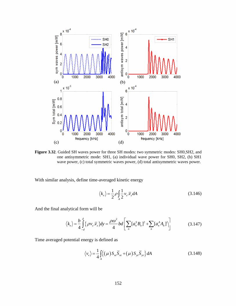
152
Figure 3.32. Guided SH waves power for three SH modes: two symmetric modes: SH0,SH2, and
one antisymmetric mode: SH1, (a) individual wave power for SH0, SH2, (b) SH1
wave power, (c) total symmetric waves power, (d) total antisymmetric waves power.
With similar analysis, define time-averaged kinetic energy
1 1
.2 2
e z z
A
k v v dA (3.146)
And the final analytical form will be
2
2 2. [ ] [ ]4 4
d
S A
e z z n n n n
n nd
bk v v dy bd a B a A
(3.147)
Time averaged potential energy is defined as
1
4e xz xz yz yz
A
v S S S S dA (3.148)
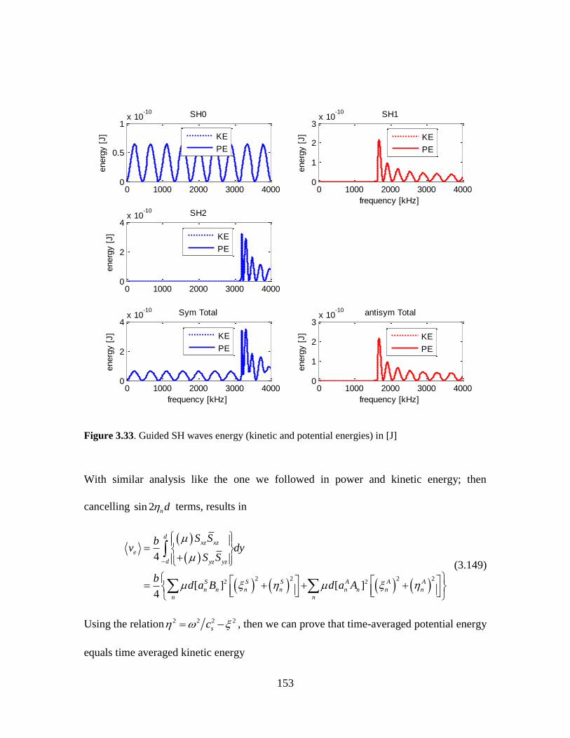
153
Figure 3.33. Guided SH waves energy (kinetic and potential energies) in [J]
With similar analysis like the one we followed in power and kinetic energy; then
cancelling sin 2 nd terms, results in
2 2 2 2
2 2
4
[ ] [ ]4
dxz xz
e
d yz yz
S S S A A A
n n n n n n n n
n n
S Sbv dy
S S
bd a B d a A
(3.149)
Using the relation 2 2 2 2
sc , then we can prove that time-averaged potential energy
equals time averaged kinetic energy
0 1000 2000 3000 40000
0.5
1x 10
-10
energ
y [
J]
SH0
KE
PE
0 1000 2000 3000 40000
2
4x 10
-10
energ
y [
J]
SH2
KE
PE
0 1000 2000 3000 40000
2
4x 10
-10
frequency [kHz]
energ
y [
J]
Sym Total
KE
PE
0 1000 2000 3000 40000
1
2
3x 10
-10
frequency [kHz]
energ
y [
J]
SH1
KE
PE
0 1000 2000 3000 40000
1
2
3x 10
-10
frequency [kHz]
energ
y [
J]
antisym Total
KE
PE
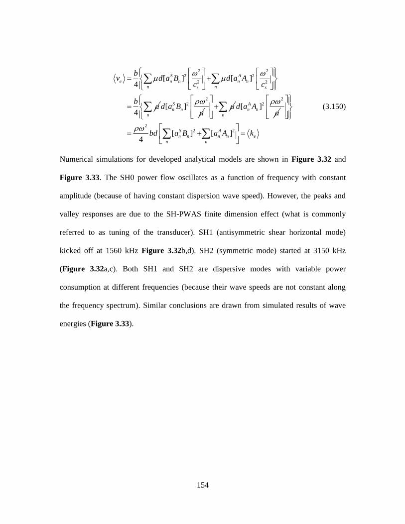
154
2 22 2
2 2[ ] [ ]
4
4
S A
e n n n n
n ns s
bv d a B d a A
c c
b
22[ ]S
n nd a B
n
2
2[ ]A
n nd a A
22 2[ ] [ ]
4
n
S A
n n n n e
n n
bd a B a A k
(3.150)
Numerical simulations for developed analytical models are shown in Figure 3.32 and
Figure 3.33. The SH0 power flow oscillates as a function of frequency with constant
amplitude (because of having constant dispersion wave speed). However, the peaks and
valley responses are due to the SH-PWAS finite dimension effect (what is commonly
referred to as tuning of the transducer). SH1 (antisymmetric shear horizontal mode)
kicked off at 1560 kHz Figure 3.32b,d). SH2 (symmetric mode) started at 3150 kHz
(Figure 3.32a,c). Both SH1 and SH2 are dispersive modes with variable power
consumption at different frequencies (because their wave speeds are not constant along
the frequency spectrum). Similar conclusions are drawn from simulated results of wave
energies (Figure 3.33).
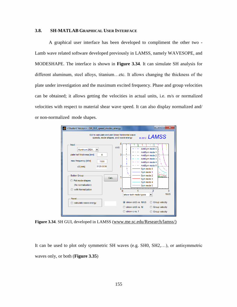
155
3.8. SH-MATLAB GRAPHICAL USER INTERFACE
A graphical user interface has been developed to compliment the other two -
Lamb wave related software developed previously in LAMSS, namely WAVESOPE, and
MODESHAPE. The interface is shown in Figure 3.34. It can simulate SH analysis for
different aluminum, steel alloys, titanium…etc. It allows changing the thickness of the
plate under investigation and the maximum excited frequency. Phase and group velocities
can be obtained; it allows getting the velocities in actual units, i.e. m/s or normalized
velocities with respect to material shear wave speed. It can also display normalized and/
or non-normalized mode shapes.
Figure 3.34. SH GUI, developed in LAMSS (www.me.sc.edu/Research/lamss/)
It can be used to plot only symmetric SH waves (e.g. SH0, SH2,…), or antisymmetric
waves only, or both (Figure 3.35)
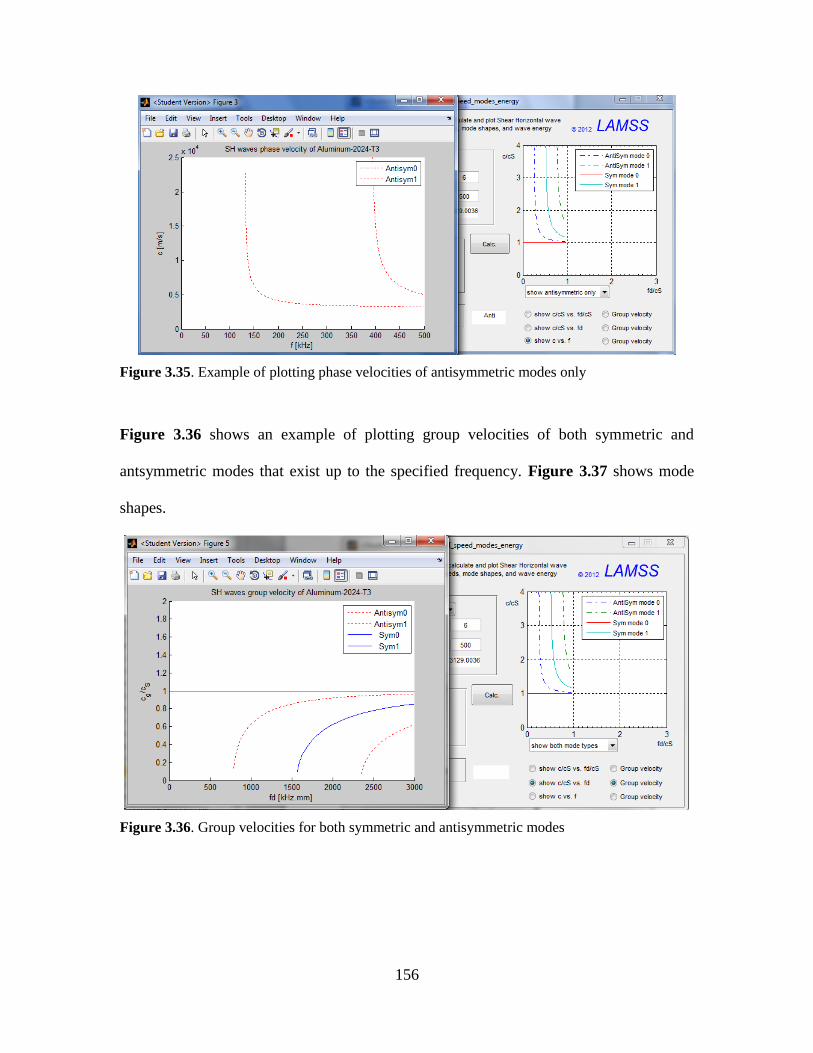
156
Figure 3.35. Example of plotting phase velocities of antisymmetric modes only
Figure 3.36 shows an example of plotting group velocities of both symmetric and
antsymmetric modes that exist up to the specified frequency. Figure 3.37 shows mode
shapes.
Figure 3.36. Group velocities for both symmetric and antisymmetric modes

157
Figure 3.37. normalized and non-normalized mode shapes
3.9. SUMMARY AND CONCLUSIONS
The chapter presented predictive analytical models for electromechanical
impedance of shear horizontal (SH) coupled piezoelectric wafer active sensor (PWAS)
transducers. Investigation of E/M impedance of free SH-PWAS indicated that the
analytical model with the constant electric field assumption is more representative of the
experimental case and FEM. The first resonance frequency of the free transducer is 900
kHz. Experiments and FEM of bonded PWAS on structures showed the local resonance
effects of the PWAS at frequencies greater than 100 kHz. Discrepancies exist in the
analytical model of SH-PWAS bonded on a structure such that the mass ratio of the
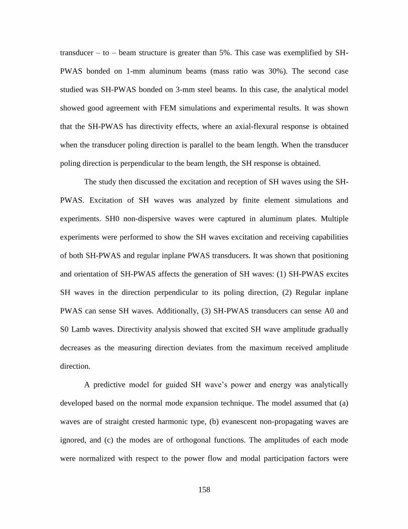
158
transducer – to – beam structure is greater than 5%. This case was exemplified by SH-
PWAS bonded on 1-mm aluminum beams (mass ratio was 30%). The second case
studied was SH-PWAS bonded on 3-mm steel beams. In this case, the analytical model
showed good agreement with FEM simulations and experimental results. It was shown
that the SH-PWAS has directivity effects, where an axial-flexural response is obtained
when the transducer poling direction is parallel to the beam length. When the transducer
poling direction is perpendicular to the beam length, the SH response is obtained.
The study then discussed the excitation and reception of SH waves using the SH-
PWAS. Excitation of SH waves was analyzed by finite element simulations and
experiments. SH0 non-dispersive waves were captured in aluminum plates. Multiple
experiments were performed to show the SH waves excitation and receiving capabilities
of both SH-PWAS and regular inplane PWAS transducers. It was shown that positioning
and orientation of SH-PWAS affects the generation of SH waves: (1) SH-PWAS excites
SH waves in the direction perpendicular to its poling direction, (2) Regular inplane
PWAS can sense SH waves. Additionally, (3) SH-PWAS transducers can sense A0 and
S0 Lamb waves. Directivity analysis showed that excited SH wave amplitude gradually
decreases as the measuring direction deviates from the maximum received amplitude
direction.
A predictive model for guided SH wave’s power and energy was analytically
developed based on the normal mode expansion technique. The model assumed that (a)
waves are of straight crested harmonic type, (b) evanescent non-propagating waves are
ignored, and (c) the modes are of orthogonal functions. The amplitudes of each mode
were normalized with respect to the power flow and modal participation factors were

159
determined. Modal participation factors are functions of transducer dimension. The wave
power, kinetic energy, and potential energy were modelled and numerical results were
presented. As expected, the kinetic energy equals the potential energy in total and for
separate modes as well, due to the fact that modes are orthogonal. SH0 mode wave power
and wave energy oscillate with frequency, but have constant amplitude due to the
constant wave propagation speed of SH0 in isotropic materials. SH1 and SH2 modes are
dispersive shear horizontal modes.
Investigation of SH waves excitation in composite materials, predictive finite
element models for SH-PWAS electromechanical impedance for the bonded transducer
on composites are covered in a following chapter.
160
CHAPTER 4: GUIDED WAVES PROPAGATION IN COMPOSITES
The first objective of this chapter is to review the different predictive models for
evaluating dispersion curves of ultrasonic guided waves in composites. The second
objective is to develop a stable robust code for predicting dispersion curves in composites,
apply it to case studies, and compare the results with commercial software.
In order to fully extend power and energy models of Chapter 2 to anisotropic
multilayered composite materials, dispersion wave propagation speeds needs to be
determined; that is the focus of this chapter.
The algorithms which we review for the wave propagation analysis in layered
composite plates are: (a) transfer matrix method (TMM), (b) global matrix method
(GMM), (c) semi-analytical finite element method (SAFE), (d) local interaction
simulation approach (LISA), and (e) equivalent matrix method (EMM). Description of
each technique was covered. Then, the advantages and distinct features of those
techniques were presented. Case studies for unidirectional, cross ply, and general quasi
isotropic laminates were presented. Finally, experimental and finite element simulation
studies were performed on glass fiber reinforced polymer composites (GFRP).
Simulations and applications on carbon fiber reinforced polymer composites (CFRP) are
presented later in Chapters 5 and 7.

161
NOMENCLATURE
Ak = transfer matrix for kth layer in the TM method
Auσ = component of the TM relates displacements with stresses
A0 = fundamental antisymmetric Lamb wave mode
Bi = amplitudes of partial aves in GM method
cij = stiffness matrix components in layer local coordinates, i, j =
1,2,…,6 Pa
c = stiffness in tensor notation
c = stiffness matrix in global coordinates
[ ]D = the matrix relates amplitudes of partial waves to displacement and
stress fields
diq = values relate amplitudes of partial waves to stress fields for the qth
eigenvalue, i = 1,2,3
f = frequency, Hz
f j = element force vector
i = square root of (-1)
Kj = layer stiffness matrix and element stiffness matrix in FEM
k = layer index in a composite layup
L = element size in FEM
Mj = element mass matrix in FEM
N = number of nodes per wavelength in FEM
N(x1, x2) = FEM interpolation functions
p = force vector in FEM

162
Q = eigenvector or mode shapes in FEM
S0 = fundamental symmetric Lamb wave mode
SH0 = fundamental shear horizontal guided wave mode
S = strains tensor
T = transformation matrix between local and global coordinates
Tt = transpose of transformation matrix
Ti = stress components, i = 1, 2…6, Pa
t = time, s
t = traction vector
U1, U2, U3 = displacement amplitudes, m
U1q = displacement amplitudes of the partial waves for the qth
eigenvalue
U j(x3) = nodal displacement vector of element j
u = displacements vector
u± = displacements at the top (-) and bottom (+) of a layer
Vq, Wq = ratios of amplitudes of partial waves
v = velocity
w = displacement in LISA, m
ẅ = displacement second derivative with respect to time, i.e.
acceleration,
x1, x2, x3 = global coordinates, m
α = ratio between the wave numbers in the x3 and x1 directions
αM = mass proportional damping coefficient, rad/s
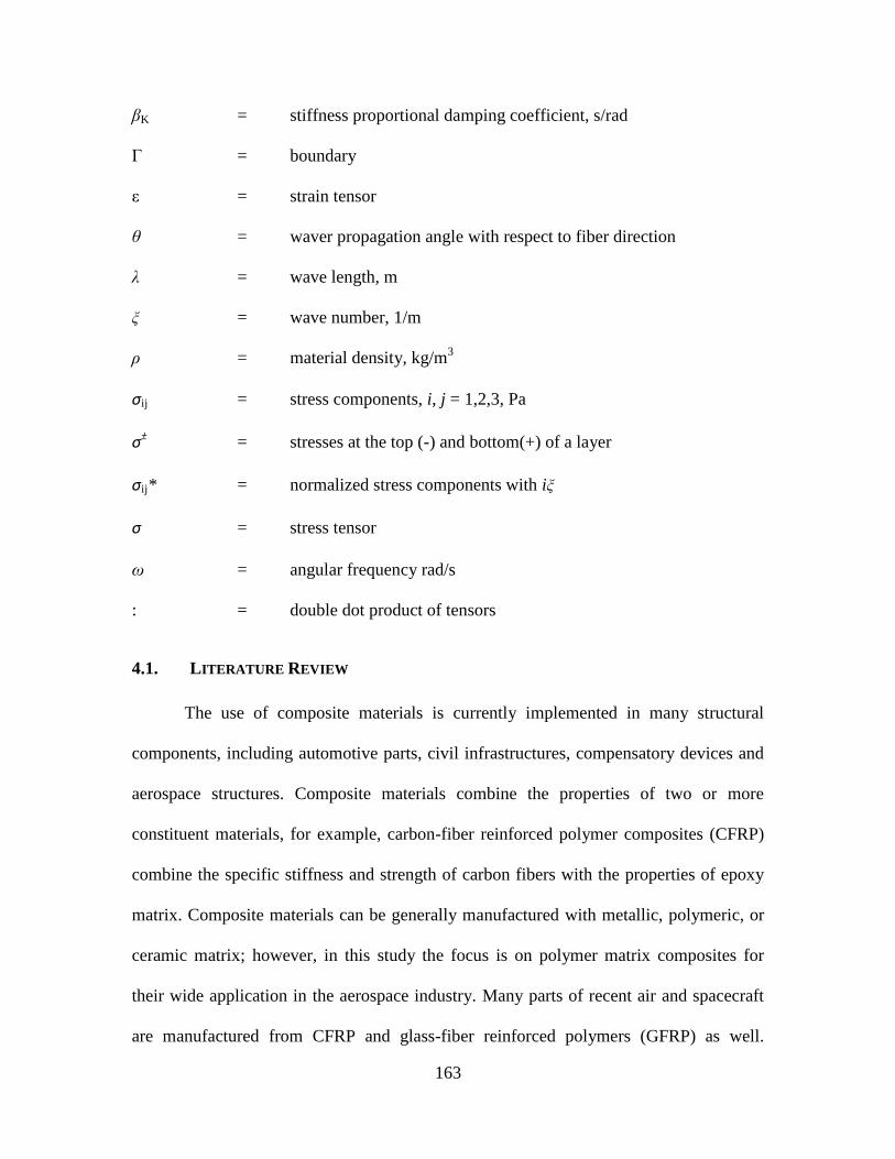
163
βK = stiffness proportional damping coefficient, s/rad
Γ = boundary
ε = strain tensor
θ = waver propagation angle with respect to fiber direction
λ = wave length, m
ξ = wave number, 1/m
ρ = material density, kg/m3
σij = stress components, i, j = 1,2,3, Pa
σ± = stresses at the top (-) and bottom(+) of a layer
σij* = normalized stress components with iξ
σ = stress tensor
ω = angular frequency rad/s
: = double dot product of tensors
4.1. LITERATURE REVIEW
The use of composite materials is currently implemented in many structural
components, including automotive parts, civil infrastructures, compensatory devices and
aerospace structures. Composite materials combine the properties of two or more
constituent materials, for example, carbon-fiber reinforced polymer composites (CFRP)
combine the specific stiffness and strength of carbon fibers with the properties of epoxy
matrix. Composite materials can be generally manufactured with metallic, polymeric, or
ceramic matrix; however, in this study the focus is on polymer matrix composites for
their wide application in the aerospace industry. Many parts of recent air and spacecraft
are manufactured from CFRP and glass-fiber reinforced polymers (GFRP) as well.
164
Because of the challenge of constructing high strength structural parts with constrained
light weights; polymer composites are more favorable than metallic alloys. Also, polymer
composites can be manufactured into complex shaped components and their properties
can be tailored by changing the stacking sequence of layup, i.e. layers or individual
lamina. Detection of damages and flaws as well as structural integrity of polymer
composites is receiving as much attention as the advantages and applications of these
materials. Ultrasonic Lamb waves, or guided plate waves, have long been acknowledged
for damage detection in composites (Rose, 1999; Su et al., 2006; Giurgiutiu and Santoni,
2011). For any study of guided wave propagation in structures, wave propagation speeds
are essential for further analysis, e.g. impact source localization, reflection, transmission
and mode conversion at damages. In many cases, robust predictive models of wave
speeds are needed before conducting experimental studies. Therefore; in this study, our
goal is comparing different methods of calculating ultrasonic guided wave speeds in
composite materials.
Lamb wave theory is well documented in many references, such as: Rose (1999);
Graff (1991); Viktorov (1967); Giurgiutiu (2008). For isotropic materials, the wave
equation can be expressed by two potential functions, and the pressure and shear wave
velocities. The shear horizontal (SH) wave propagation in this case is decoupled from
symmetric and antisymmetric Lamb waves propagation. Lamb waves are symmetric and
antisymmetric and they are dispersive by nature, i.e. (are having different speeds at
different frequencies). The characteristic equation (Rayleigh-Lamb equation) is obtained
by solving wave equation and applying stress free boundary conditions at upper and
lower surfaces of the plate.
165
In the case of fiber reinforced polymer (FRP) composites, where the material is
generally anisotropic, the three types of guided waves (P, SV, and SH) are coupled and it
is not possible to find closed form solution of the dispersion curves. Several textbooks
have documented guided wave propagation in composites: Nayfeh (1995); Rose (1999);
Rokhlin et al. (2011). There are different methods to calculate dispersion curves in
multilayered composite materials (a) transfer matrix method (TMM); (b) global matrix
method (GMM); (c) semi-analytical finite element method (SAFE); (d) local interaction
simulation approach (LISA); and (e) equivalent matrix method (EMM). Mathematical
formulations of those techniques are presented, along with highlighting key features.
Transfer Matrix Method (TMM) 4.1.1.
Transfer matrix method (Thomson, 1950; Haskell, 1953) is a technique for wave
propagation analysis in layered media; its advantage is that it condenses the multi-layered
system into few equations (four in the case of decoupled SH waves or six in the case of
coupled SH waves) relating the boundary conditions at the first and the last interface. It
eliminates all other intermediate interfaces; this saves a lot of computational time and
complexity. Hence, TMM is favorable. One drawback TMM suffers is the numerical
instability of the solution at large frequency-thickness product values (Lowe, 1995). We
followed the formulation in Nayfeh (1995) and Santoni (2010). Considering the
composite plate layer is in 1x , 2x plane with wave propagation along 1x direction
(Figure 4.1). The angle of fibers with respect to direction of wave propagation is .
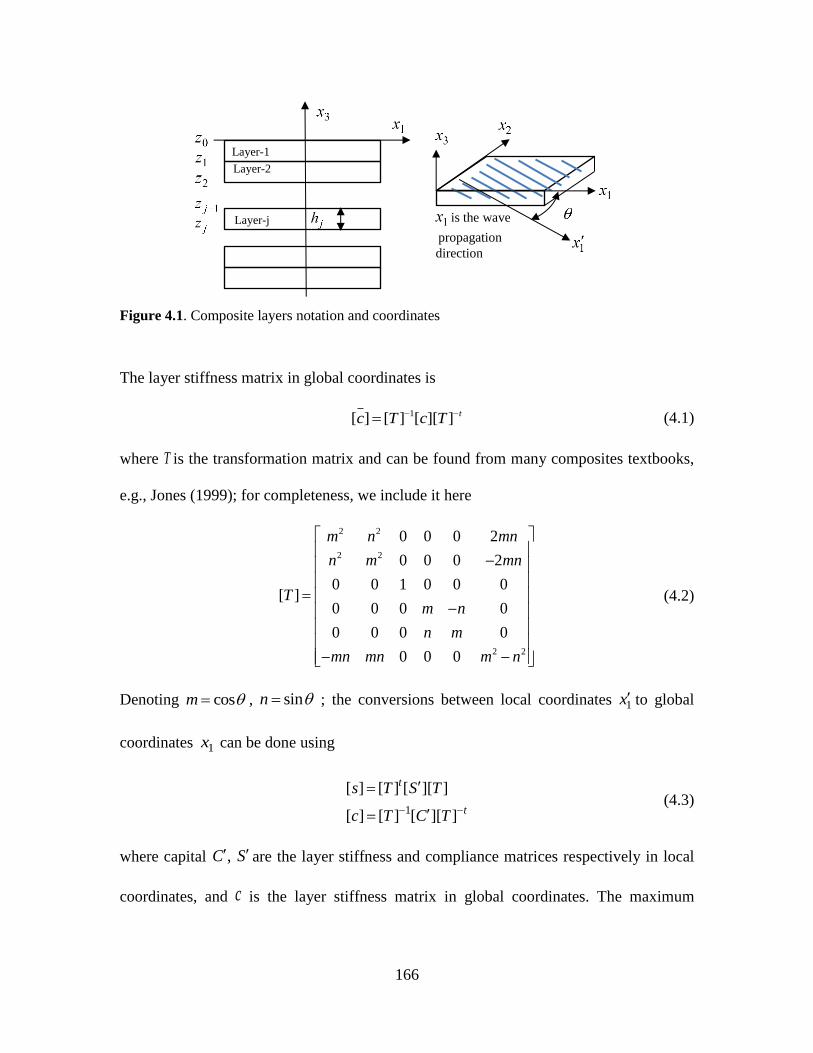
166
Figure 4.1. Composite layers notation and coordinates
The layer stiffness matrix in global coordinates is
1[ ] [ ] [ ][ ] tc T c T (4.1)
where T is the transformation matrix and can be found from many composites textbooks,
e.g., Jones (1999); for completeness, we include it here
2 2
2 2
2 2
0 0 0 2
0 0 0 2
0 0 1 0 0 0[ ]
0 0 0 0
0 0 0 0
0 0 0
m n mn
n m mn
Tm n
n m
mn mn m n
(4.2)
Denoting cosm , sinn ; the conversions between local coordinates 1x to global
coordinates 1x can be done using
1
[ ] [ ] [ ][ ]
[ ] [ ] [ ][ ]
t
t
s T S T
c T C T
(4.3)
where capital , C S are the layer stiffness and compliance matrices respectively in local
coordinates, and c is the layer stiffness matrix in global coordinates. The maximum
is the wave
propagation
direction
x
Layer-1 Layer-2
Layer-j
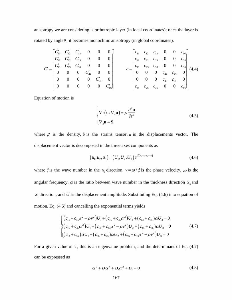
167
anisotropy we are considering is orthotropic layer (in local coordinates); once the layer is
rotated by angle , it becomes monoclinic anisotropy (in global coordinates).
11 12 13 11 12 13 16
12 22 23 12 22 23 26
13 23 33 13 23 33 36
44 44 45
55 45 55
66 16 26 36 66
0 0 0 0 0
0 0 0 0 0
0 0 0 0 0
0 0 0 0 0 0 0 0 0
0 0 0 0 0 0 0 0 0
0 0 0 0 0 0 0
C C C c c c c
C C C c c c c
C C C c c c cC c
C c c
C c c
C c c c c
(4.4)
Equation of motion is
2
2: s
s
t
uc u
u S
(4.5)
where is the density, S is the strains tensor, u is the displacements vector. The
displacement vector is decomposed in the three axes components as
1 3
1 2 3 1 2 3, , , ,i x x vt
u u u U U U e
(4.6)
where is the wave number in the 1x direction, /v is the phase velocity, is the
angular frequency, is the ratio between wave number in the thickness direction 3x and
1x direction, and iU is the displacement amplitude. Substituting Eq. (4.6) into equation of
motion, Eq. (4.5) and cancelling the exponential terms yields
2 2 2
11 55 1 16 45 2 13 55 3
2 2 2
16 45 1 66 44 2 45 36 3
2 2
13 55 1 36 45 2 55 33 3
0
0
0
c c v U c c U c c U
c c U c c v U c c U
c c U c c U c c v U
(4.7)
For a given value of v , this is an eigenvalue problem, and the determinant of Eq. (4.7)
can be expressed as
6 4 2
1 2 3 0B B B (4.8)
168
where iB values are found in Nayfeh (1995) with slight corrections as
2 2 2
1 11 33 44 13 44 13 36 45 13 44 55 13 45 16 33 45 33 55 66 36 55
2 2
33 44 33 55 44 55 45
2 2 2
2 11 33 66 11 36 11 36 45 11 44 55 11 45 13 66 13 16 36 13 16 45 13
[ 2 2 2 2
( ) ] /
[ 2 2 2 2
B c c c c c c c c c c c c c c c c c c c c c
c c c c c c c v
B c c c c c c c c c c c c c c c c c c c c c c
55 66
2
16 33 16 36 55
2 2 2 2
11 33 11 44 13 13 55 16 45 33 66 36 36 45 44 55 45 55 66
2 4
33 44 55
2 2 2 2 4 3 6
3 11 55 66 16 55 11 55 11 66 16 55 66 11 55 66
2
( 2 2 2 )
( ) ] /
[ ( ) ( )
c c
c c c c c
c c c c c c c c c c c c c c c c c c c v
c c c v
B c c c c c c c c c c c c v c c c v v
2
33 44 55 33 45
] /
c c c c c
(4.9)
By solving Eq. (4.8) symbolically, it can be shown that the eigenvalues i are found in
pairs, i.e.
2 1 4 3 6 5 , , (4.10)
Each pair of eigenvalues represents a pair of similar partial waves propagating in
opposite 3x directions, one downward, and the other upward. Using any two equations in
Eq. (4.7), we find the displacements ratios (i.e. eigenvectors). However, careful selection
of the two equations is important. If this algorithm is used for isotropic metallic layer or a
composite layer that is almost isotropic, the displacements ratio 3 1/q q qW U U suffers a
singularity situation. Therefore, the ratios documented in Nayfeh (1995) and Santoni
(2010) were exchanged by (Rokhlin et al., 2011)
2 2 2
11 55 45 36 16 45 13 552
2 2 21 13 55 66 44 16 45 45 36
22 2 2 2 2
11 55 66 44 16 453
2 2 21 16 45 45 36 13 55 66 44
q q q qq
q
q q q q q
q q qq
q
q q q q q
c c v c c c c c cUV
U c c c c v c c c c
c c v c c v c cUW
U c c c c c c c c v
(4.11)
169
where q= 1,…6 represents the partial wave number. By doing this, a more general robust
algorithm is attained. The displacements in Eq. (4.6) can be written as
1 3
6
1 2 3 1
1
, , 1, , qi x x vt
q q q
q
u u u V W U e
(4.12)
The stresses are
1 3
11 13 161
12 23 262
13 33 363
144 45
4
45 555
6 16 36 66
q
q q q
q q q
q q q i x x vt
qq q q qq
q q q q
q q q
c c W c VT
c c W c VT
c c W c VTi U e
c V c WT
c V c WT
T c c W c V
(4.13)
The stresses that are of interest are 33 13 23, , . Stress free boundary condition is applied
on them; we define
1 3
6* * * * * *
33 13 23 3 5 4 1 2 3 1
1
, , , , , , qi x x vt
q q q q
q
T T T d d d U e
(4.14)
where * i , and
1 2 3, ,q q qd d d are terms extracted from Eq. (4.13)
1 13 33 36
2 45 55
3 44 45
q q q q
q q q q q
q q q q q
d c c W c V
d c V c W
d c V c W
(4.15)
Combining the displacement and stress relations yields the state vector in a layer
1 3
1 3
3 3
1 11
1 1 3 3 5 52 12
1 1 3 3 5 53 13
*11 11 13 13 15 1533 14
*21 21 23 23 25 2513
*31 31 31 31 35 3523
1 1 1 1 1 1
{ }
{ }
i x
i x
i x
u U e
V V V V V Vu U e
W W W W W Wu u U e
d d d d d d U e
d d d d d d
d d d d d d
1
3 3
5 3
5 3
15
16
i x vt
i x
i x
i x
e
U e
U e
(4.16)
170
The idea of the TMM is relating the layer properties and the boundary conditions at the
top and bottom surfaces with those of the other layers. This is done by applying
continuity of displacements and equilibrium of stresses. The layer transfer matrix kA
relates the displacements and stresses of the top of the layer to those of the bottom of the
layer
uu u
u
u uA A
A A
(4.17)
Call kA the 4 x 4 hyper matrix of Eq. (4.17), X the 6 x 6 matrix of Eq. (4.16), U the
vector of 1iU elements, and H the diagonal matrix of elements 3ii xe
; hence,
1
k k k kA X H X (4.18)
The total TM is calculated by multiplying the transfer matrix of individual layers
consecutively. And to satisfy stress free boundary condition for the whole laminate;
and in Eq. (4.17) are set to zero, hence the characteristic equation to find dispersion
phase velocities versus wavenumbers is
0uA (4.19)
Usually Eq. (4.19) is solved numerically to find dispersion phase velocities versus
wavenumbers or frequencies.
Instability of Transfer Matrix Method 4.1.2.
Rokhlin et al. (2011) showed that, due to refraction within one or more layers of
the laminate, some of the plane waves can be internally reflected, meaning that their
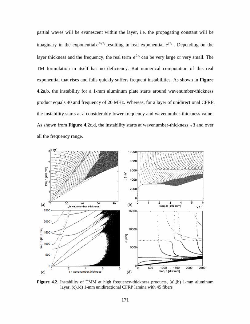
171
partial waves will be evanescent within the layer, i.e. the propagating constant will be
imaginary in the exponential 3i xe
resulting in real exponential 3x
e
. Depending on the
layer thickness and the frequency, the real term 3xe
can be very large or very small. The
TM formulation in itself has no deficiency. But numerical computation of this real
exponential that rises and falls quickly suffers frequent instabilities. As shown in Figure
4.2a,b, the instability for a 1-mm aluminum plate starts around wavenumber-thickness
product equals 40 and frequency of 20 MHz. Whereas, for a layer of unidirectional CFRP,
the instability starts at a considerably lower frequency and wavenumber-thickness value.
As shown from Figure 4.2c,d, the instability starts at wavenumber-thickness 3 and over
all the frequency range.
Figure 4.2. Instability of TMM at high frequency-thickness products, (a),(b) 1-mm aluminum
layer, (c),(d) 1-mm unidirectional CFRP lamina with 45 fibers
(c)
(b) (a)
(d)
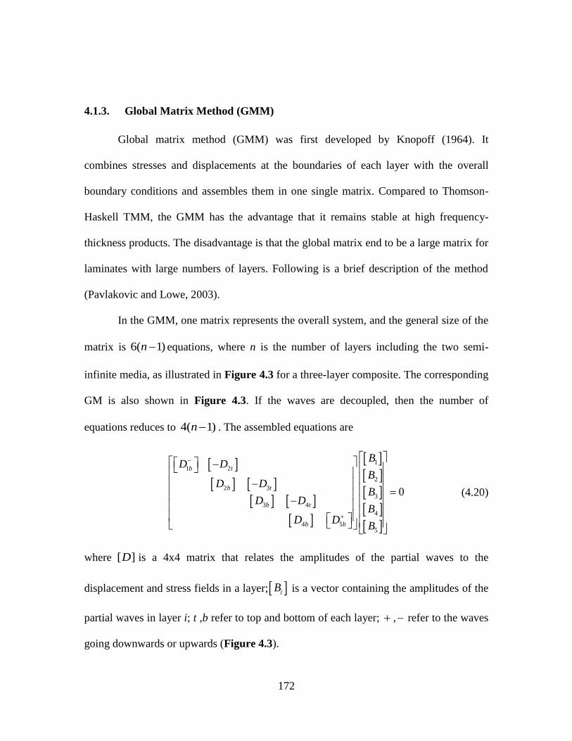
172
Global Matrix Method (GMM) 4.1.3.
Global matrix method (GMM) was first developed by Knopoff (1964). It
combines stresses and displacements at the boundaries of each layer with the overall
boundary conditions and assembles them in one single matrix. Compared to Thomson-
Haskell TMM, the GMM has the advantage that it remains stable at high frequency-
thickness products. The disadvantage is that the global matrix end to be a large matrix for
laminates with large numbers of layers. Following is a brief description of the method
(Pavlakovic and Lowe, 2003).
In the GMM, one matrix represents the overall system, and the general size of the
matrix is 6( 1)n equations, where n is the number of layers including the two semi-
infinite media, as illustrated in Figure 4.3 for a three-layer composite. The corresponding
GM is also shown in Figure 4.3. If the waves are decoupled, then the number of
equations reduces to 4( 1)n . The assembled equations are
11 2
2
2 3
3
3 4
4
4 55
0
b t
b t
b t
b b
BD D
BD D
BD D
BD D
B
(4.20)
where [ ]D is a 4x4 matrix that relates the amplitudes of the partial waves to the
displacement and stress fields in a layer; iB is a vector containing the amplitudes of the
partial waves in layer i; t ,b refer to top and bottom of each layer; , refer to the waves
going downwards or upwards (Figure 4.3).
173
Figure 4.3. GMM formulation (Pavlakovic and Lowe, 2003).
Semi Analytical Finite Element Method (SAFE) 4.1.4.
SAFE is becoming popular for analyzing guided wave propagation in composites
(Bartoli et al., 2006). SAFE is basically a finite element method discretizing the structure
cross section allowing different cross sections to be analyzed. In the same time it solves
analytically in the direction of wave propagation. This makes it more efficient in terms of
computational time and memory than a complete FEM (Gavric, 1995; Sorohan et al.,
2011). The advantage of discretizing the cross section is that it allows the modeling of
any arbitrary cross sections, e.g. track rails (Hayashi et al., 2003; Bartoli et al., 2006).
The material is defined in FEM by stiffness matrix; this makes SAFE method very
straight forward for application of anisotropic materials. SAFE solutions are obtained in a
174
stable manner through an algebraic eigenvalue problem, and thus do not require the root-
searching algorithms used in the TMM and GMM approaches. A brief description of the
SAFE method is presented following Hayashi et al. (2003). The virtual work principle
states,
( T T T
V V
d dV dV
u t u u) ε σ (4.21)
where T is the transpose; is the density; (.)d
and (.)V
dV are the surface and the
volume integrations of the element, respectively. T d
u t denotes the work done by the
external traction t . The two terms on the right hand side of Eq. (4.21) are the kinetic
energy and the potential energy. The wave solution along the wave propagation direction
is represented by exponential orthogonal functions 3exp( )ii x . The next step is similar to
FEM discretization, where we define the displacement vector at an arbitrary point
1 2 3( , ) ( )exp( )jx x x i t u N U (4.22)
where ( , )x yN is the interpolation function, and ( )j zU is the nodal displacement vector of
the element j. Strains are determined from the displacements and the derivatives of the
interpolation functions with respect to 1 2,x x . Similar formulation is used for the traction
vector t in terms of the nodal external traction vector. The stress vector is σ = cε in
which material stiffness matrix c is incorporated. Substituting displacements, tractions,
strains, and stresses in Eq. (4.21) yields
2 2
1 2 3
j j j j j j ji f K K K U M U (4.23)
where jf is the element force vector; j
iK , i = 1,2,3, and jM are the integrals determined
by numerical integration techniques and they are functions of geometry; is the wave
175
number; is the angular frequency. jU is the element nodal displacement vector. Results
at common nodes are overlapped and the total system’s governing equations are
determined. It is easy to introduce damping by considering complex form of the K
matrices. The final governing equation (Hayashi et al., 2003; Bartoli et al., 2006),
22
11
2
31 2
000 , , ,
0 -i
A B Q p
K M UK MA B Q p
fK UK M K
(4.24)
When the force vector p equals to zero, the eigenvalues m of the system can be
determined and the phase velocity is given by /m mc . Consequently; nodal solutions
and the mode shapes can be determined.
Local Interaction Simulation Approach (LISA) 4.1.5.
LISA discretizes the system into a lattice like in the finite difference method and
its formulation is based on elastodynamic equations. The advantage of LISA appears
when discontinuities or changes needed to be applied to the material properties; those
changes are treated by modifying the properties of the lattice at the corresponding
locations. LISA was studied by Delsanto et al. (1997) for 3-D case, starting from the
elastodynamic wave equation
,( ) ( , , , 1,3)l klmn m n kS w w k l m n (4.25)
where S is the stiffness tensor, is the material density, w is the displacement. Time is
discretized; the propagation medium is discretized into a lattice with special steps
(Ruzzene et al., 2005). Finite difference (FD) formulation is used in recursive equations

176
to represent the second order space derivatives of the neighboring points of a generic
point O in the lattice.
The finite difference formalism is used with the elastodynamic equation of motion
to generate three iterative equations which allow computation of displacements pu at time
1t as a linear combination of displacement components at time t and 1t . A well-
organized formulation was reported in Nadella and Cesnik (2012) with experimental
validations of LISA for both isotropic and anisotropic media. Another study (Ruzzene et
al., 2005) compared LISA approach with experimental results using laser vibrometer
measurements on elastic plates.
Figure 4.4. Generic point O and its 18 neighboring points in the lattice (Delsanto et al., 1997)
Equivalent Matrix Method (EMM) 4.1.6.
Equivalent matrix method (EMM) is a quick and robust approach to analyze cross
ply laminates. It uses the fact that the transformation matrix between 0 and 90 degrees is
straight forward and can be done manually. EMM can be applied for generally orientated
layers as well. This method was used in Monnier (2006). The code developed in this
study was only for cross ply laminates. The procedure is as follows
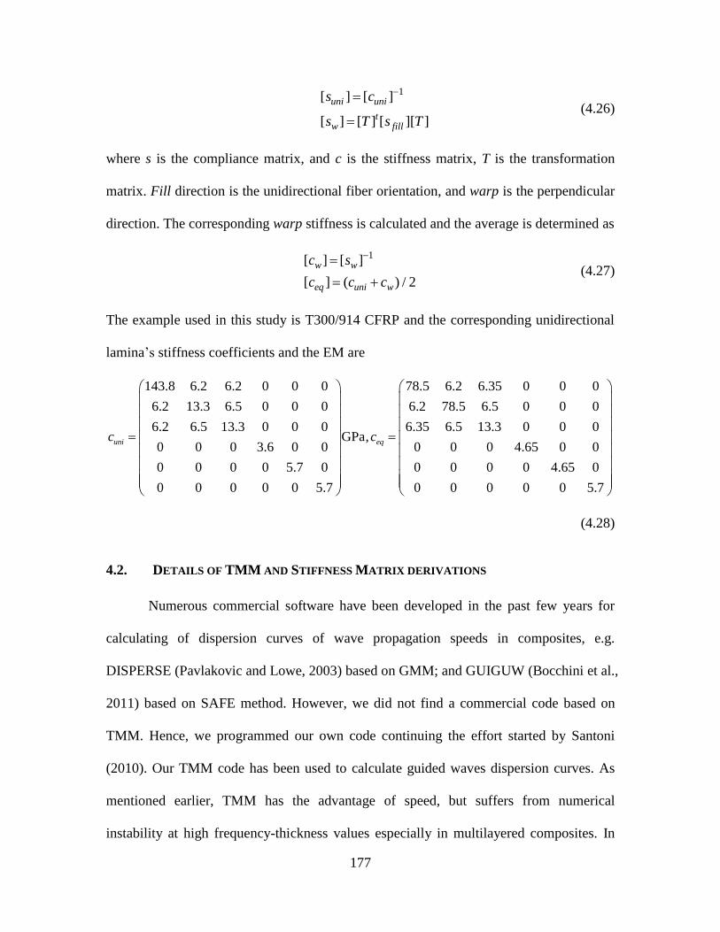
177
1[ ] [ ]
[ ] [ ] [ ][ ]
uni uni
tw fill
s c
s T s T
(4.26)
where s is the compliance matrix, and c is the stiffness matrix, T is the transformation
matrix. Fill direction is the unidirectional fiber orientation, and warp is the perpendicular
direction. The corresponding warp stiffness is calculated and the average is determined as
1[ ] [ ]
[ ] ( ) / 2
w w
eq uni w
c s
c c c
(4.27)
The example used in this study is T300/914 CFRP and the corresponding unidirectional
lamina’s stiffness coefficients and the EM are
143.8 6.2 6.2 0 0 0 78.5 6.2 6.35 0 0 0
6.2 13.3 6.5 0 0 0 6.2 78.5 6.5 0 0 0
6.2 6.5 13.3 0 0 0 6.35 6.5 13.3 0 0 0GPa,
0 0 0 3.6 0 0 0 0 0 4.65 0 0
0 0 0 0 5.7 0 0 0 0 0 4.65 0
0 0 0 0 0 5.7 0 0 0 0 0 5.7
uni eqc c
(4.28)
4.2. DETAILS OF TMM AND STIFFNESS MATRIX DERIVATIONS
Numerous commercial software have been developed in the past few years for
calculating of dispersion curves of wave propagation speeds in composites, e.g.
DISPERSE (Pavlakovic and Lowe, 2003) based on GMM; and GUIGUW (Bocchini et al.,
2011) based on SAFE method. However, we did not find a commercial code based on
TMM. Hence, we programmed our own code continuing the effort started by Santoni
(2010). Our TMM code has been used to calculate guided waves dispersion curves. As
mentioned earlier, TMM has the advantage of speed, but suffers from numerical
instability at high frequency-thickness values especially in multilayered composites. In
178
this section, we present the framework that has been followed by many researchers, e.g.,
Schmidt and Jensen (1985); Wang and Rokhlin (2001); Glushkov et al. (2011) to
overcome this instability problem using the stiffness matrix method (SMM). Detailed
formulation of the approach is presented for the following cases: isotropic; orthotropic
unidirectional fibers along wave propagation direction or perpendicular to it; and
generally anisotropic layers. In the next section, we integrate SMM and TMM into an
integrated approach called the stiffness transfer matrix method (STMM) and we study the
following cases: isotropic layer, anisotropic layer, and anisotropic multilayer composite.
Transfer Matrix Method Details 4.2.1.
In this part we added extra steps for the analytical development that was covered
in Nayfeh (1995) and Santoni (2010), we highlighted some typos that were identified in
the original text and which are relevant for coding these equations in a computer program
to obtain the dispersion curves. This is followed by detailed derivation of the roots of Eq.
(4.8) for two cases: (a) an isotropic layer, and (b) orthotropic composite layer with fibers
along 0 or 90 directions. In both cases, guided waves are decoupled into (1) symmetric
and antisymmetric Lamb waves, (2) shear horizontal (SH) waves.
Starting from the equation of motion, Eq. (4.5)
2
2: s
s
t
uc u
u S
(4.29)
we expand the double dot product between stiffness tensor c and the gradient operator ,
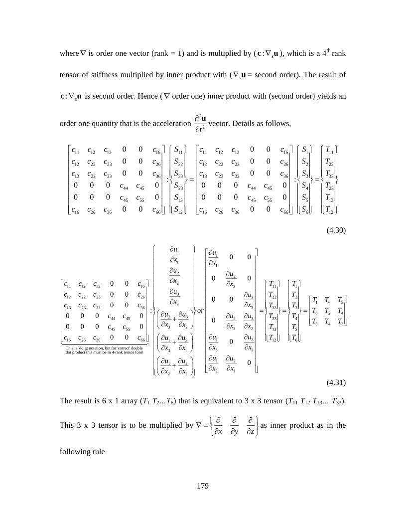
179
where is order one vector (rank = 1) and is multiplied by ( : sc u ), which is a 4th
rank
tensor of stiffness multiplied by inner product with ( s u = second order). The result of
: sc u is second order. Hence ( order one) inner product with (second order) yields an
order one quantity that is the acceleration 2
2t
uvector. Details as follows,
11 12 13 16 11 12 13 1611
12 22 23 26 12 22 23 2622
13 23 33 36 13 23 33 3633
44 45 44 4523
45 55 45 5513
16 26 36 66 12
0 0 0 0
0 0 0 0
0 0 0 0:
0 0 0 0 0 0 0 0
0 0 0 0 0 0 0 0
0 0
c c c c c c c cS
c c c c c c c cS
c c c c c c c cS
c c c cS
c c c cS
c c c c S
1 11
2 22
3 33
4 23
5 13
16 26 36 66 6 12
:
0 0
S T
S T
S T
S T
S T
c c c c S T
(4.30)
11 12 13 16
12 22 23 26
13 23 33 36
44 45
45 55
16 26 36 66
This is Voigt notation, but for 'correct' double dot product this must be in 4-rank tensor form
0 0
0 0
0 0
0 0 0 0
0 0 0 0
0 0
c c c c
c c c c
c c c c
c c
c c
c c c c
11
11
22
22
33
33
32 32
3 2 3 2
3131
3 13 1
1 21 2
2 12 1
0 0
0 0
0 0
:
0
0
0
uu
xx
uu
xx
uu
xx
oruu uu
x x x x
uuuu
x xx x
u uu ux xx x
111
222
1 6 5
333
6 2 4
423
5 4 3
513
612
TT
TTT T T
TTT T T
TTT T T
TT
TT
(4.31)
The result is 6 x 1 array (T1 T2…T6) that is equivalent to 3 x 3 tensor (T11 T12 T13… T33).
This 3 x 3 tensor is to be multiplied by x y z
as inner product as in the
following rule
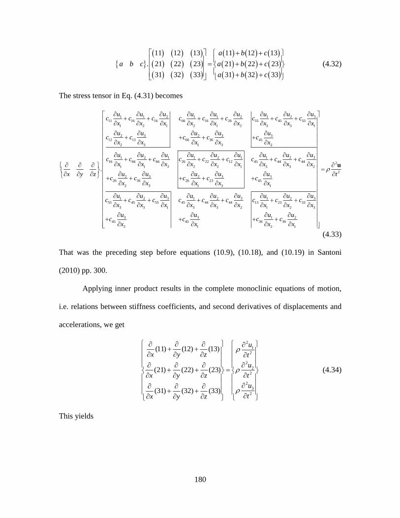
180
11 12 13 11 12 13
. 21 22 23 21 22 23
31 32 33 31 32 33
a b c
a b c a b c
a b c
(4.32)
The stress tensor in Eq. (4.31) becomes
31 1 2 1 1 2 1 211 16 16 66 16 26 55 45 55
1 2 1 2 1 2 3 3 1
3 32 2 312 13 66 36 45
2 3 1 3 2
1 2 116 66 66
1 1 2
3226 36
2
.
uu u u u u u u uc c c c c c c c c
x x x x x x x x x
u uu u uc c c c c
x x x x x
u u uc c c
x x x
uux y zc c
x x
31 2 1 1 226 22 12 45 44 44
2 2 1 3 3 2
32 326 23 45
3 1 3 1
3 3 31 2 1 2 1 255 45 55 45 44 44 13 23 33
3 3 1 3 3 2 1 2 3
3 33645 45
2 1
uu u u u uc c c c c c
x x x x x x
uu uc c c
x x x
u u uu u u u u uc c c c c c c c c
x x x x x x x x x
u ucc c
x x
2
2
1 236
2 1
t
u uc
x x
u
(4.33)
That was the preceding step before equations (10.9), (10.18), and (10.19) in Santoni
(2010) pp. 300.
Applying inner product results in the complete monoclinic equations of motion,
i.e. relations between stiffness coefficients, and second derivatives of displacements and
accelerations, we get
2
1
2
2
2
2
2
3
2
(11) (12) (13)
(21) (22) (23)
(31) (32) (33)
u
x y z t
u
x y z t
u
tx y z
(4.34)
This yields
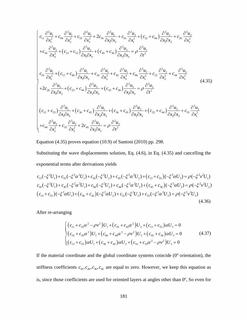
181
2 2 2 2 2 2 2
1 1 1 1 2 2 211 66 55 16 16 12 66 262 2 2 2 2
1 2 3 1 2 1 1 2 2
2 22 2
3 32 145 13 55 45 362 2
3 1 3 2 3
2 2 2 2
1 1 1 116 12 66 26 452 2
1 1 2 2
2u u u u u u u
c c c c c c c cx x x x x x x x x
u uu uc c c c c
x x x x x t
u u u uc c c c c
x x x x x
2 2 2
2 2 266 22 442 2 2 2
3 1 2 3
2 22 2
3 32 226 23 44 45 36 2
1 2 2 3 1 3
22 2 2 2
31 1 2 213 55 36 45 36 45 23 44 55 2
1 3 2 3 1 3 2 3 1
2 2
344 332
2
2
u u uc c c
x x x
u uu uc c c c c
x x x x x x t
uu u u uc c c c c c c c c
x x x x x x x x x
u uc c
x
2 2
3 3 3452 2
3 1 2
2u u
cx x x t
(4.35)
Equation (4.35) proves equation (10.9) of Santoni (2010) pp. 298.
Substituting the wave displacements solution, Eq. (4.6), in Eq. (4.35) and cancelling the
exponential terms after derivations yields
2 2 2 2 2 2 2 2 2
11 1 55 1 16 2 45 2 13 55 3 1
2 2 2 2 2 2 2 2 2
16 1 45 1 66 2 44 2 45 36 3 2
2 2 2 2 2
13 55 1 36 45 2 55 3 33
( ) ( ) ( ) ( ) ( ) ( )
( ) ( ) ( ) ( ) ( ) ( )
( ) ( ) ( ) (
c U c U c U c U c c U v U
c U c U c U c U c c U v U
c c U c c U c U c
2 2
3 3) ( )U v U
(4.36)
After re-arranging
2 2 2
11 55 1 16 45 2 13 55 3
2 2 2
16 45 1 66 44 2 45 36 3
2 2
13 55 1 36 45 2 55 33 3
0
0
0
c c v U c c U c c U
c c U c c v U c c U
c c U c c U c c v U
(4.37)
If the material coordinate and the global coordinate systems coincide (0º orientation), the
stiffness coefficients 16 26 36 45, , ,c c c c are equal to zero. However, we keep this equation as
is, since those coefficients are used for oriented layers at angles other than 0º, So even for
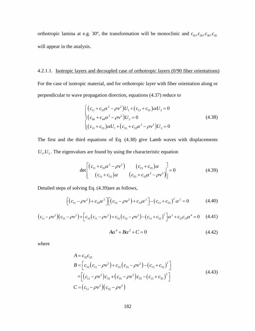
182
orthotropic lamina at e.g. 30º, the transformation will be monoclinic and 16 26 36 45, , ,c c c c
will appear in the analysis.
4.2.1.1. Isotropic layers and decoupled case of orthotropic layers (0/90 fiber orientations)
For the case of isotropic material, and for orthotropic layer with fiber orientation along or
perpendicular to wave propagation direction, equations (4.37) reduce to
2 2
11 55 1 13 55 3
2 2
66 44 2
2 2
13 55 1 55 33 3
0
0
0
c c v U c c U
c c v U
c c U c c v U
(4.38)
The first and the third equations of Eq. (4.38) give Lamb waves with displacements
1 3,U U . The eigenvalues are found by using the characteristic equation
2 2
11 55 13 55
2 2
13 55 55 33
det 0c c v c c
c c c c v
(4.39)
Detailed steps of solving Eq. (4.39)are as follows,
22 2 2 2 2
11 55 55 33 13 55 0c v c c v c c c
(4.40)
22 2 2 2 2 4
11 55 33 11 55 55 13 55 55 33 0c v c v c c v c c v c c c c
(4.41)
4 2 0A B C (4.42)
where
55 33
22 2
33 11 55 55 13 55
22 2
11 33 55 55 13 55
2 2
11 55
=
A c c
B c c v c c v c c
c v c c v c c c
C c v c v
(4.43)
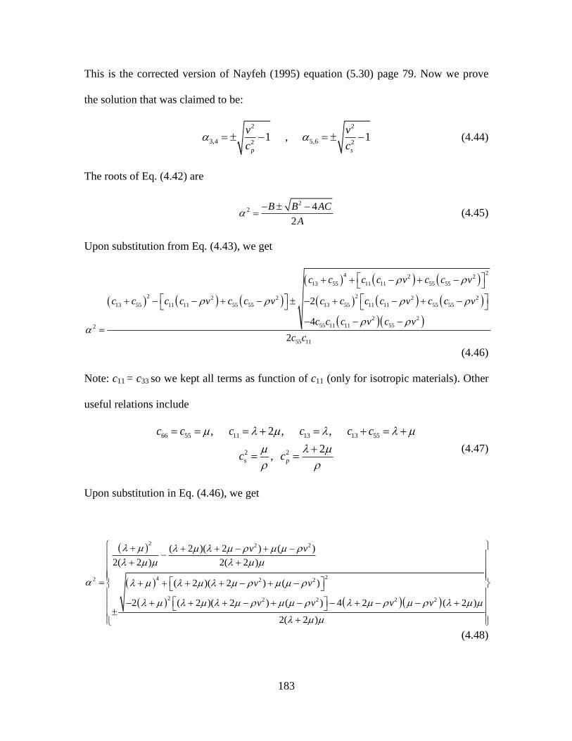
183
This is the corrected version of Nayfeh (1995) equation (5.30) page 79. Now we prove
the solution that was claimed to be:
2 2
3,4 5,62 21 , 1
p s
v v
c c (4.44)
The roots of Eq. (4.42) are
2
2 4
2
B B AC
A
(4.45)
Upon substitution from Eq. (4.43), we get
24 2 2
13 55 11 11 55 55
2 22 2 2 2
13 55 11 11 55 55 13 55 11 11 55 55
2 2
55 11 11 552
55 11
2
4
2
c c c c v c c v
c c c c v c c v c c c c v c c v
c c c v c v
c c
(4.46)
Note: c11 = c33 so we kept all terms as function of c11 (only for isotropic materials). Other
useful relations include
66 55 11 13 13 55
2 2
, 2 , ,
2, s p
c c c c c c
c c
(4.47)
Upon substitution in Eq. (4.46), we get
2 2 2
242 2 2
2 2 2 2 2
( 2 )( 2 ) ( )
2( 2 ) 2( 2 )
( 2 )( 2 ) ( )
2 ( 2 )( 2 ) ( ) 4 2 ( 2 )
2( 2 )
v v
v v
v v v v
(4.48)
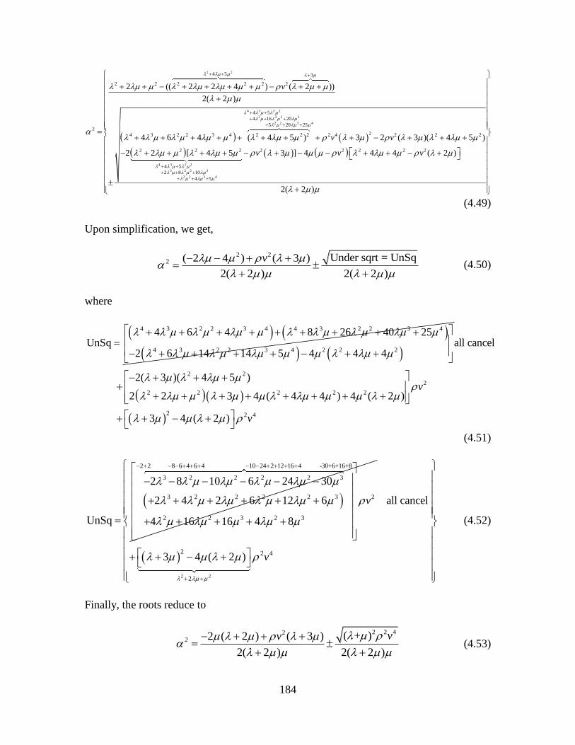
184
2 2
4 3 2 2
3 2 2 3
2 2 3 4
4 5 3
2 2 2 2 2 2
4 5
4 16 20
5 20 252
4 3 2 2 3 4 2 2 2
2 (( 2 2 4 ) ( 2 ))
2( 2 )
4 6 4 ( 4 5 )
v
4 3 2 2
3 2 2 3
2 2 3 4
22 4 2 2 2
2 2 2 2 2 2 2 2 2
4 5
2 8 10
4 5
3 2 ( 3 )( 4 5 )
2 2 [ 4 5 3 ] 4 4 4 ( 2 )
2( 2 )
v v
v v v
(4.49)
Upon simplification, we get,
2 2
2 Under sqrt = UnSq( 2 4 ) ( 3 )
2( 2 ) 2( 2 )
v
(4.50)
where
4 3 2 2 3 4 4 3 2 2 3 4
4 3 2 2 3 4 2 2 2
4 6 4 8 26 40 25UnSq
2 6 14 14 5 4 4 4
2 2
2
2 2 2 2 2
2 2 4
all cancel
2( 3 )( 4 5 )
2 2 3 4 ( 4 4 ) 4 ( 2 )
3 4 ( 2 )
v
v
(4.51)
2 2 8 6 4 6 4 10 24 2 12 16 4 -30+6+16+8
3 2 2 2 2 3
3 2 2 2 2 3
2 2 3 2 3
2 8 10 6 24 30
2 4 2 6 12 6
UnSq 4 16 16 4 8
2v
2 2
2 2 4
2
all cancel
3 4 ( 2 ) v
(4.52)
Finally, the roots reduce to
2 2 422 ( + )2 ( 2 ) ( 3 )
2( 2 ) 2( 2 )
vv
(4.53)
185
2 22
first
2
3,4
2 2 2
11
2
11 11
2 ( 2 ) ( 3 ) ( + )
2( 2 )
2 [ ( 2 )]
2 ( 2 )
1 1p
v v
v
v c v v
c c c
(4.54)
and
2 22
second
2 2
5,6
2 2 2
55
2
55 55
2 ( 2 ) ( 3 ) ( + )
2( 2 )
2( 2 )[ ]
2 ( 2 )
1 1s
v v
v v
v c v v
c c c
(4.55)
Also we had proved earlier in Eq. (4.10) that the eigenvalues i exist in pairs. So for
Lamb-type waves we have 4 roots, i.e., 4 values for i . The mode shapes associated with
Lamb waves can be determined from the first and third equations of Eq. (4.38), i.e.,
3 2
1 1
(for Lamb waves), (forSH:not defined in this case)q q
q q
q q
U UW V
U U (4.56)
q = 1,2,3, …6, but as discussed before, the roots exist in pairs, hence for Lamb wave
solution, we have subscripts q=3 and 5. The subscript q=1 is for SH solution, which is not
considered here. Expanding Wq for the cases of q = 3, and q = 5 yields
2 211 11 3
2 2 2233 11 55 11
3 3
13 13 55 3 11
2 2 2 2
11 55 3 11 11 3 11 55 3
13 55 3 13 55 3
11 553
13 55
=
2
v c c
U c c v v cW
U c c c
v c c c c c c
c c c c
c c
c c
3 3
(4.57)
186
and
2 2 2235 11 55
5 5
15 13 55 5
2 2 2 2
11 55 5 5 11 5
13 55 5 13 55 3
11
13 55 5 5 5
2 1 1
( )
U c c v vW
U c c
v c c c
c c c c
c
c c
(4.58)
Recall the values 1 2 3, ,q q qd d d extracted from Eq. (4.13), i.e.
1 13 33 36
2 45 55
3 44 45
q q q q
q q q q q
q q q q q
d c c W c V
d c V c W
d c V c W
(4.59)
Recall that 36 0c , 45 0c ; hence, the quantities in Eq. (4.59) associated with Lamb-type
waves are
3
2313 13 3 33 3
2
11
11
( 2 )d c c W
v c
c
( 2 )
2
22 2
5
( 2 )
2 1 1
v
vv
(4.60)
15 13 5 33 5 5
5
23 55 3 3 3
2
525 55 5 5
5
1( ) ( 2 ) 2
2
1
d c c W
d c W
d c W
(4.61)
Recalling Eq. (4.16), and cancelling SH-related terms yields
187
1
2
u
u
3
*
33
*
13
*
23
u
1 3
11
1 1 3 3 5 5
1 1 3 3 5 5
11 11 13 13 15 15
21 21 23 23 25 25
31 31 33 33 35 35
1 1 1 1 1 1 i xU e
V V V V V V
W W W W W W
d d d d d d
d d d d d d
d d d d d d
1 3
12
i xU e
3 3
1
3 3
5 3
5 3
13
14
15
16
i xi x vt
i x
i x
i x
U ee
U e
U e
U e
(4.62)
Upon simplification, the displacements and the stresses for Lamb-type wave solution are
given by
3 3
3 3
1
5 3
5 3
1 13
3 3 3 5 5 14
*
33 13 13 15 15 15
*
13 23 23 25 25 16
1 1 1 1 i x
i xi x vt
i x
i x
u U e
u W W W W U ee
d d d d U e
d d d d U e
(4.63)
We define our layer thickness as h, and take 3 0x at the top “j-1”, 3x h at the bottom
“j”. To follow Rokhlin et al. (2011), we call the displacements and stress vector in the left
hand side of Eq. (4.63) Pk , and we call the 4x4 matrix X. The right hand side vector can
be decomposed into a diagonal matrix Hk multiplied by the amplitudes vector Uk
3 3
3 3
1
5 3
5 3
1 13
3 3 3 5 5 14
*
33 13 13 15 15 15
*
13 23 23 25 25 16
1 1 1 1 0 0 0
0 0 0
0 0 0
0 0 0
i x
i xi x vt
i x
i x
u Ue
u W W W W Uee
d d d d Ue
d d d d Ue
(4.64)
Equation (4.64) is written with H functions as
1 1 3 13
3 3 3 5 5 2 3 14
*
33 13 13 15 15 3 3 15
*
13 23 23 25 25 4 3 16
1 1 1 1 ( ) 0 0 0
0 ( ) 0 0
0 0 ( ) 0
0 0 0 ( )
u H x U
u W W W W H x U
d d d d H x U
d d d d H x U
(4.65)
i.e. in compact notations and ignoring 1i x vt
e
,
3 3( ) ( ) P x X H x U (4.66)
188
At the top surface “j-1”, where 3 0x , the H diagonal matrix becomes unit matrix,
(0) IH , and Eq. (4.65) becomes
1131
13 3 5 5 143
113 13 15 15 1533
123 23 25 25 1613
1 1 1 1j
j
j
j
Uu
W W W W Uu
d d d d U
d d d d U
(4.67)
At the bottom surface “j”, where 3x h , we substitute in 3 3i xe
by 3x h , and we
call the quantities H1,..H4
1 2 3 4 131
3 1 3 2 5 3 5 4 143
13 1 13 2 15 3 15 4 1533
23 1 23 2 25 3 25 4 1613
j
j
j
j
H H H H Uu
W H W H W H W H Uu
d H d H d H d H U
d H d H d H d H U
(4.68)
Equations (4.67), (4.68) can be written as
( ) 1 1 1
( )
, ITop j j j
k k k k k k
Bottom j j
k k k
P X H U X U H
P X H U
(4.69)
Pk for the top and the bottom of a layer can be combined together as
( ) ( ) 1Bot j Top j
k k kP A P (4.70)
where the transfer matrix (TM) is defined as
1 or k k k k k k k kA X H X A X H x (4.71)
where 1 k kx X . The TM can be multiplied by each other for multilayers
1 1n nA A A A (4.72)
MATLAB consumes considerable time and computation for calculating inverse of
matrices. We found that providing MATLAB with the matrix’s inverse as elements will
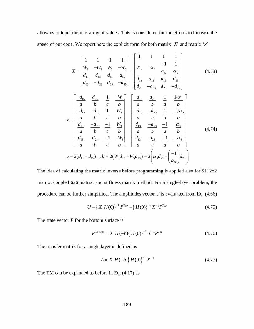
189
allow us to input them as array of values. This is considered for the efforts to increase the
speed of our code. We report here the explicit form for both matrix ‘X’ and matrix ‘x’
3 33 3 5 5
5 5
13 13 15 15
13 13 15 15
23 23 25 25
23 23 25 25
1 1 1 11 1 1 1
1 1W W W W
Xd d d d
d d d dd d d d
d d d d
(4.73)
15 25 5 15 25 5
15 25 5 15 25 5
13 23 3 13 23 3
13 23 3 13 23 3
13 15 3 25 5 23
11 1
11 1
1 1
1 1
2( ) , 2
d d W d d
a b a b a b a b
d d W d d
a b a b a b a bx
d d W d d
a b a b a b a b
d d W d d
a b a b a b a b
a d d b W d W d
3 25 23
5
12 d d
(4.74)
The idea of calculating the matrix inverse before programming is applied also for SH 2x2
matrix; coupled 6x6 matrix; and stiffness matrix method. For a single-layer problem, the
procedure can be further simplified. The amplitudes vector U is evaluated from Eq. (4.66)
1 1 1 (0) (0)Top TopU X H P H X P (4.75)
The state vector P for the bottom surface is
1 1 ( ) (0)Bottom TopP X H h H X P (4.76)
The transfer matrix for a single layer is defined as
1 1 ( ) (0)A X H h H X (4.77)
The TM can be expanded as before in Eq. (4.17) as
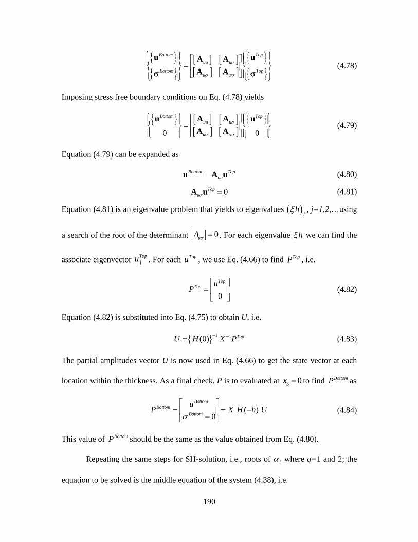
190
Bottom Top
uu u
Bottom Topu
u uA A
A A (4.78)
Imposing stress free boundary conditions on Eq. (4.78) yields
0 0
Bottom Top
uu u
u
u uA A
A A (4.79)
Equation (4.79) can be expanded as
Bottom Top
uuu A u (4.80)
0Top
u A u (4.81)
Equation (4.81) is an eigenvalue problem that yields to eigenvalues j
h , j=1,2,…using
a search of the root of the determinant 0uA . For each eigenvalue h we can find the
associate eigenvector Top
ju . For each Topu , we use Eq. (4.66) to find TopP , i.e.
0
Top
Top uP
(4.82)
Equation (4.82) is substituted into Eq. (4.75) to obtain U, i.e.
1 1(0) TopU H X P (4.83)
The partial amplitudes vector U is now used in Eq. (4.66) to get the state vector at each
location within the thickness. As a final check, P is to evaluated at 3 0x to find BottomP as
( ) 0
Bottom
Bottom
Bottom
uP X H h U
(4.84)
This value of BottomP should be the same as the value obtained from Eq. (4.80).
Repeating the same steps for SH-solution, i.e., roots of i where q=1 and 2; the
equation to be solved is the middle equation of the system (4.38), i.e.
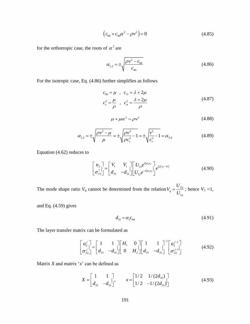
191
2 2
66 44 0c c v (4.85)
for the orthotropic case, the roots of 2 are
2
661,2
44
v c
c
(4.86)
For the isotropic case, Eq. (4.86) further simplifies as follows
66 11
2 2
, 2
2 , s p
c c
c c
(4.87)
2 2v (4.88)
2 2 2
1,2 5,62 21 1
s s
v v v
c c
(4.89)
Equation (4.62) reduces to
1 3
1
1 3
2 1 1 11
*
23 31 31 12
i xi x vt
i x
u V V U ee
d d U e
(4.90)
The mode shape ratio Vq cannot be determined from the relation2
1
q
q
q
UV
U ; hence V1 =1,
and Eq. (4.59) gives
31 1 44d c (4.91)
The layer transfer matrix can be formulated as
1 112 2
131 31 31 31223 23
1 1 1 10
0
j j
j j
Hu u
d d d dH
(4.92)
Matrix X and matrix ‘x’ can be defined as
31
31 31 31
1 1 1/ 2 1/ (2 ),
1/ 2 1/ (2 )
dX x
d d d
(4.93)
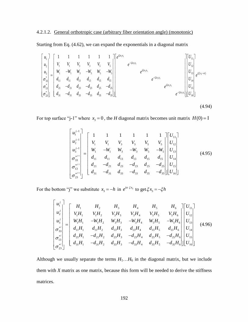
192
4.2.1.2. General orthotropic case (arbitrary fiber orientation angle) (monotonic)
Starting from Eq. (4.62), we can expand the exponentials in a diagonal matrix
1 3
1 3
3 3
3 3
5 3
5 3
1
1 1 3 3 5 52
1 1 3 3 5 53
*11 11 13 13 15 1533
*21 21 23 23 25 2513
*31 31 33 33 35 3523
1 1 1 1 1 1 i x
i x
i x
i x
i x
i x
u e
V V V V V Vu e
W W W W W Wu e
d d d d d d e
d d d d d d e
d d d d d d e
1
11
12
13
14
15
16
i x vt
U
U
Ue
U
U
U
(4.94)
For top surface “j-1” where 3 0x , the H diagonal matrix becomes unit matrix (0) IH
1
1
1
1
111
1
2 1 1 3 3 5 5 12
1
3 1 1 3 3 5 5 13
*11 11 13 13 15 15 1433
* 21 21 23 23 25 25 1513
31 31 33 33 35 35 16*
23
1 1 1 1 1 1
j
j
j
j
j
j
uU
u V V V V V V U
u W W W W W W U
d d d d d d U
d d d d d d U
d d d d d d U
(4.95)
For the bottom “j” we substitute 3x h in 3i xe
to get 3x h
11 2 3 4 5 6
2 1 1 1 2 3 3 3 4 5 5 5 6
3 1 1 1 2 3 3 3 4 5 5 5 6
*11 1 11 2 13 3 13 4 15 5 15 633
* 21 1 21 2 23 3 23 4 25 5 25 613
31 1 31 2 33 3 33 4 35 5*
23
j
j
j
j
j
j
uH H H H H H
u V H V H V H V H V H V H
u W H W H W H W H W H W H
d H d H d H d H d H d H
d H d H d H d H d H d H
d H d H d H d H d H
11
12
13
14
15
35 6 16
U
U
U
U
U
d H U
(4.96)
Although we usually separate the terms H1…H6 in the diagonal matrix, but we include
them with X matrix as one matrix, because this form will be needed to derive the stiffness
matrices.
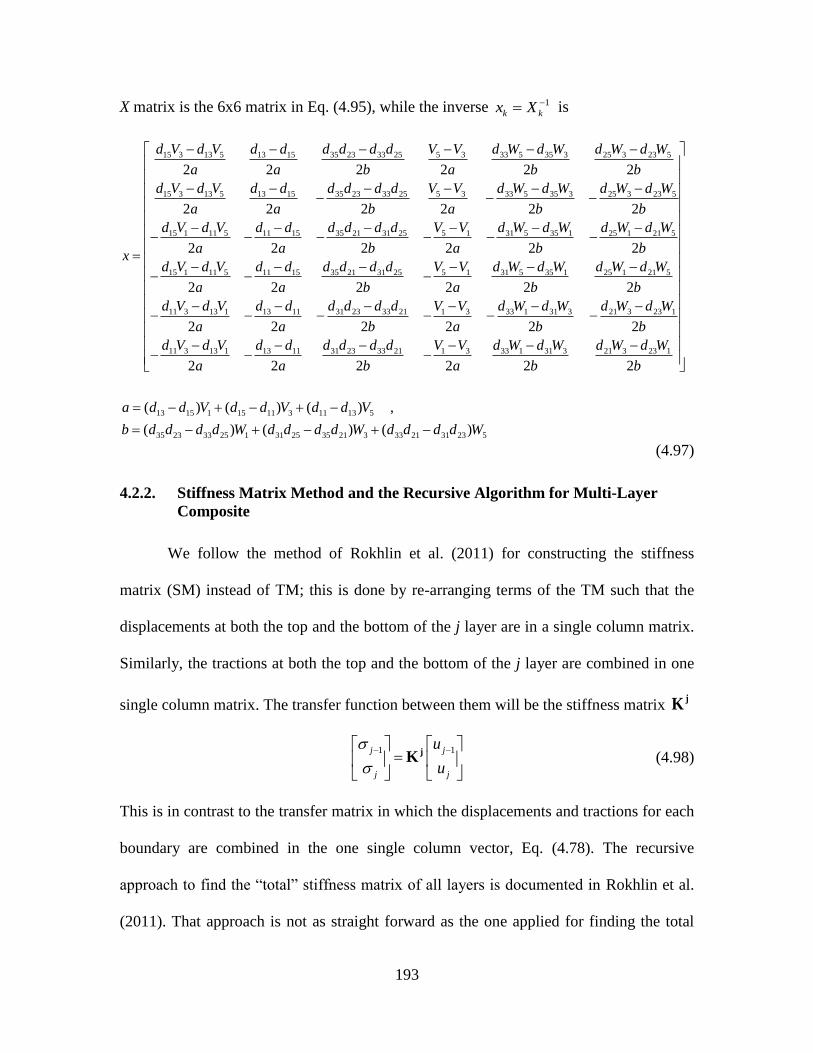
193
X matrix is the 6x6 matrix in Eq. (4.95), while the inverse 1 k kx X is
15 3 13 5 13 15 35 23 33 25 5 3 33 5 35 3 25 3 23 5
15 3 13 5 13 15 35 23 33 25 5 3 33 5 35 3 25 3 23 5
15 1 11 5 11 15 35 21 31 25 5 1 31 5
2 2 2 2 2 2
2 2 2 2 2 2
2 2 2 2
d V d V d d d d d d V V d W d W d W d W
a a b a b b
d V d V d d d d d d V V d W d W d W d W
a a b a b b
d V d V d d d d d d V V d W
a a b ax
35 1 25 1 21 5
15 1 11 5 11 15 35 21 31 25 5 1 31 5 35 1 25 1 21 5
11 3 13 1 13 11 31 23 33 21 1 3 33 1 31 3 21 3 23 1
11 3 13 1 13 11 31 23
2 2
2 2 2 2 2 2
2 2 2 2 2 2
2 2
d W d W d W
b b
d V d V d d d d d d V V d W d W d W d W
a a b a b b
d V d V d d d d d d V V d W d W d W d W
a a b a b b
d V d V d d d d
a a
33 21 1 3 33 1 31 3 21 3 23 1
13 15 1 15 11 3 11 13 5
35 23 33 25 1 31 25 35 21 3 33 21 31 23 5
2 2 2 2
( ) ( ) ( ) ,
( ) ( ) ( )
d d V V d W d W d W d W
b a b b
a d d V d d V d d V
b d d d d W d d d d W d d d d W
(4.97)
Stiffness Matrix Method and the Recursive Algorithm for Multi-Layer 4.2.2.
Composite
We follow the method of Rokhlin et al. (2011) for constructing the stiffness
matrix (SM) instead of TM; this is done by re-arranging terms of the TM such that the
displacements at both the top and the bottom of the j layer are in a single column matrix.
Similarly, the tractions at both the top and the bottom of the j layer are combined in one
single column matrix. The transfer function between them will be the stiffness matrix jK
1 1j j
j j
u
u
jK (4.98)
This is in contrast to the transfer matrix in which the displacements and tractions for each
boundary are combined in the one single column vector, Eq. (4.78). The recursive
approach to find the “total” stiffness matrix of all layers is documented in Rokhlin et al.
(2011). That approach is not as straight forward as the one applied for finding the total
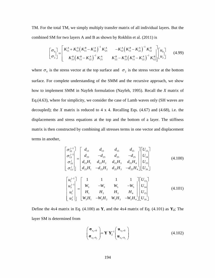
194
TM. For the total TM, we simply multiply transfer matrix of all individual layers. But the
combined SM for two layers A and B as shown by Rokhlin et al. (2011) is
1 1
11 12 11 22 21 12 11 22 120 0
1 12 2
21 11 22 21 22 21 11 22 12
A A B A A A B A B
B B A A B B B A B
K K K K K K K K K u
uK K K K K K K K K
(4.99)
where 0 is the stress vector at the top surface and 2 is the stress vector at the bottom
surface. For complete understanding of the SMM and the recursive approach, we show
how to implement SMM in Nayfeh formulation (Nayfeh, 1995). Recall the X matrix of
Eq.(4.63), where for simplicity, we consider the case of Lamb waves only (SH waves are
decoupled); the X matrix is reduced to 4 x 4. Recalling Eqs. (4.67) and (4.68), i.e. the
displacements and stress equations at the top and the bottom of a layer. The stiffness
matrix is then constructed by combining all stresses terms in one vector and displacement
terms in another,
113 13 15 15 1333
123 23 25 25 1413
13 1 13 2 15 3 15 4 1533
23 1 23 2 25 3 25 4 1613
j
j
j
j
d d d d U
d d d d U
d H d H d H d H U
d H d H d H d H U
(4.100)
1131
13 3 5 5 143
1 2 3 4 151
3 1 3 2 5 3 5 4 163
1 1 1 1j
j
j
j
Uu
W W W W Uu
H H H H Uu
W H W H W H W H Uu
(4.101)
Define the 4x4 matrix in Eq. (4.100) as Y, and the 4x4 matrix of Eq. (4.101) as Y2; The
layer SM is determined from
3 3
3 3
0 01
2 j j
x x
x h x h
σ uY Y
σ u (4.102)
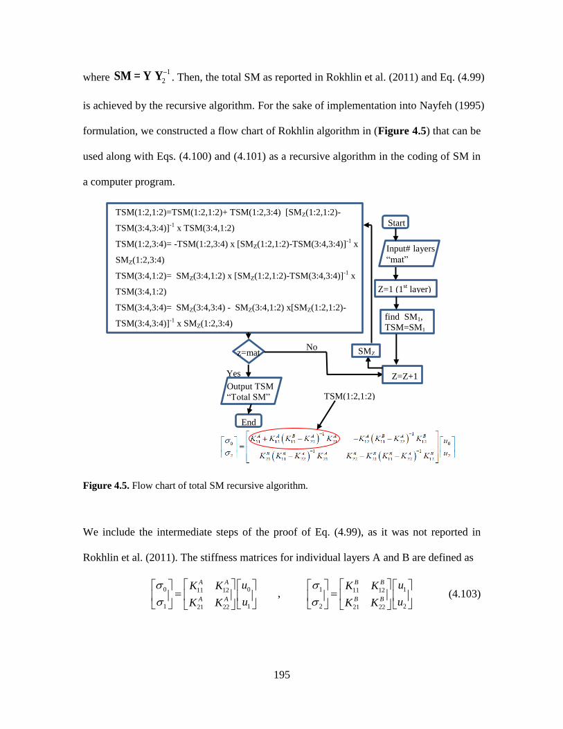
195
where 1
2 SM = Y Y . Then, the total SM as reported in Rokhlin et al. (2011) and Eq. (4.99)
is achieved by the recursive algorithm. For the sake of implementation into Nayfeh (1995)
formulation, we constructed a flow chart of Rokhlin algorithm in (Figure 4.5) that can be
used along with Eqs. (4.100) and (4.101) as a recursive algorithm in the coding of SM in
a computer program.
Figure 4.5. Flow chart of total SM recursive algorithm.
We include the intermediate steps of the proof of Eq. (4.99), as it was not reported in
Rokhlin et al. (2011). The stiffness matrices for individual layers A and B are defined as
0 0 1 111 12 11 12
1 1 2 221 22 21 22
, A A B B
A A B B
u uK K K K
u uK K K K
(4.103)
find SM1,
TSM=SM1
Start
Input# layers
“mat”
Z=1 (1st layer)
Z=Z+1
z=mat
Yes
No SMZ
TSM(1:2,1:2)=TSM(1:2,1:2)+ TSM(1:2,3:4) [SMZ(1:2,1:2)-
TSM(3:4,3:4)]-1
x TSM(3:4,1:2)
TSM(1:2,3:4)= -TSM(1:2,3:4) x [SMZ(1:2,1:2)-TSM(3:4,3:4)]-1
x
SMZ(1:2,3:4)
TSM(3:4,1:2)= SMZ(3:4,1:2) x [SMZ(1:2,1:2)-TSM(3:4,3:4)]-1
x
TSM(3:4,1:2)
TSM(3:4,3:4)= SMZ(3:4,3:4) - SMZ(3:4,1:2) x[SMZ(1:2,1:2)-
TSM(3:4,3:4)]-1
x SMZ(1:2,3:4)
TSM(1:2,1:2)
End
Output TSM
“Total SM”
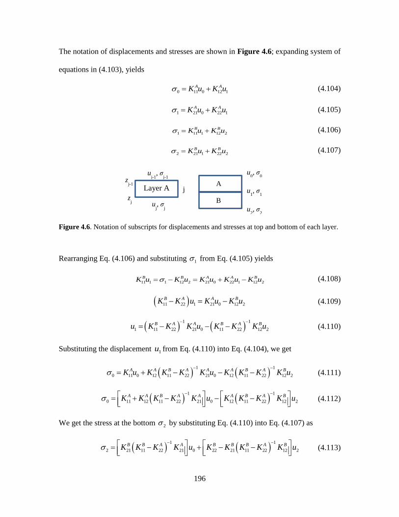
196
The notation of displacements and stresses are shown in Figure 4.6; expanding system of
equations in (4.103), yields
0 11 0 12 1
A AK u K u (4.104)
1 21 0 22 1
A AK u K u (4.105)
1 11 1 12 2
B BK u K u (4.106)
2 21 1 22 2
B BK u K u (4.107)
Figure 4.6. Notation of subscripts for displacements and stresses at top and bottom of each layer.
Rearranging Eq. (4.106) and substituting 1 from Eq. (4.105) yields
11 1 1 12 2 21 0 22 1 12 2
B B A A BK u K u K u K u K u (4.108)
11 22 1 21 0 12 2
B A A BK K u K u K u (4.109)
1 1
1 11 22 21 0 11 22 12 2
B A A B A Bu K K K u K K K u
(4.110)
Substituting the displacement 1u from Eq. (4.110) into Eq. (4.104), we get
1 1
0 11 0 12 11 22 21 0 12 11 22 12 2
A A B A A A B A BK u K K K K u K K K K u
(4.111)
1 1
0 11 12 11 22 21 0 12 11 22 12 2
A A B A A A B A BK K K K K u K K K K u
(4.112)
We get the stress at the bottom 2 by substituting Eq. (4.110) into Eq. (4.107) as
1 1
2 21 11 22 21 0 22 21 11 22 12 2
B B A A B B B A BK K K K u K K K K K u
(4.113)
zj-1
Layer A
zj
j
uj, σ
j
uj-1
, σj-1
u0, σ
0
u1, σ
1
u2, σ
2
A
B
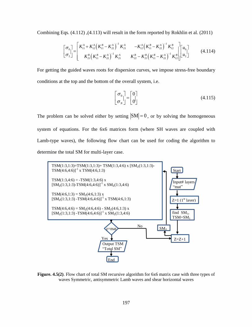
197
Combining Eqs. (4.112) ,(4.113) will result in the form reported by Rokhlin et al. (2011)
1 1
11 12 11 22 21 12 11 22 120 0
1 12 2
21 11 22 21 22 21 11 22 12
A A B A A A B A B
B B A A B B B A B
K K K K K K K K K u
uK K K K K K K K K
(4.114)
For getting the guided waves roots for dispersion curves, we impose stress-free boundary
conditions at the top and the bottom of the overall system, i.e.
0 0
0N
(4.115)
The problem can be solved either by setting SM 0 , or by solving the homogeneous
system of equations. For the 6x6 matrices form (where SH waves are coupled with
Lamb-type waves), the following flow chart can be used for coding the algorithm to
determine the total SM for multi-layer case.
Figure. 4.5(2). Flow chart of total SM recursive algorithm for 6x6 matrix case with three types of
waves Symmetric, antisymmetric Lamb waves and shear horizontal waves
find SM1,
TSM=SM1
Start
Input# layers
“mat”
Z=1 (1st layer)
Z=Z+1
z=mat
Yes
No SMZ
TSM(1:3,1:3)=TSM(1:3,1:3)+ TSM(1:3,4:6) x [SMZ(1:3,1:3)-
TSM(4:6,4:6)]-1
x TSM(4:6,1:3)
TSM(1:3,4:6) = -TSM(1:3,4:6) x
[SMZ(1:3,1:3)-TSM(4:6,4:6)]-1
x SMZ(1:3,4:6)
TSM(4:6,1:3) = SMZ(4:6,1:3) x
[SMZ(1:3,1:3) -TSM(4:6,4:6)]-1
x TSM(4:6,1:3)
TSM(4:6,4:6) = SMZ(4:6,4:6) - SMZ(4:6,1:3) x
[SMZ(1:3,1:3) -TSM(4:6,4:6)]-1
x SMZ(1:3,4:6)
End
Output TSM
“Total SM”
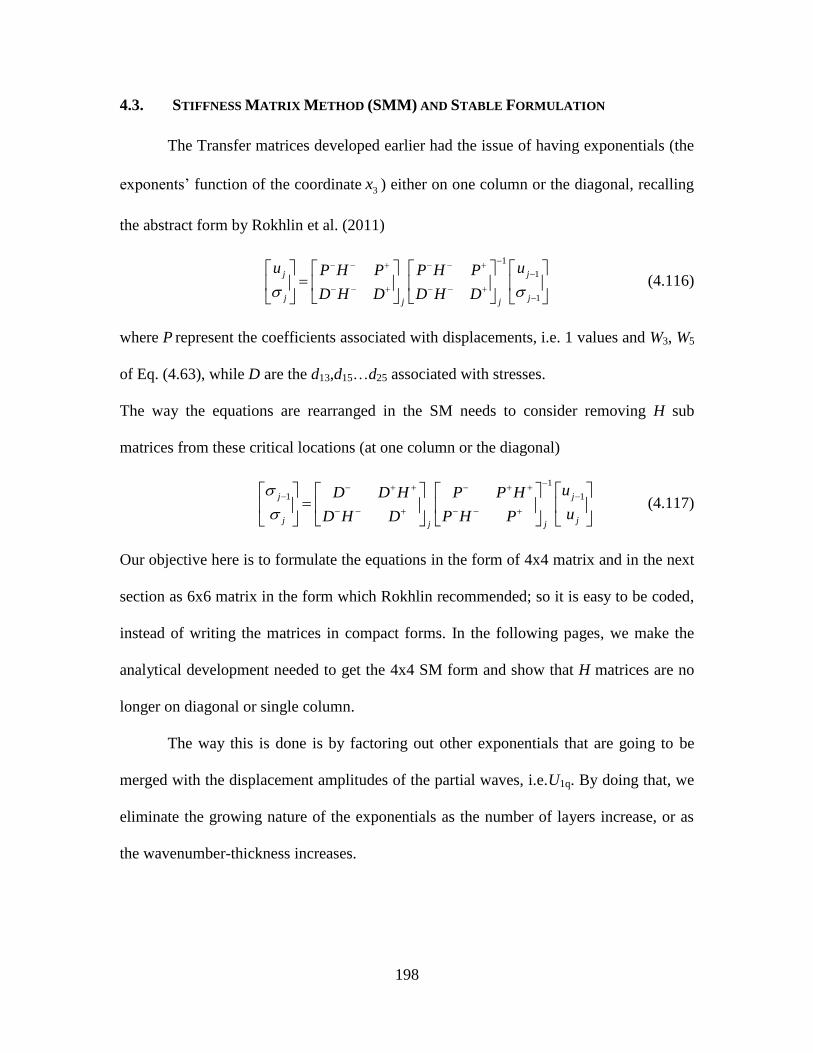
198
4.3. STIFFNESS MATRIX METHOD (SMM) AND STABLE FORMULATION
The Transfer matrices developed earlier had the issue of having exponentials (the
exponents’ function of the coordinate 3x ) either on one column or the diagonal, recalling
the abstract form by Rokhlin et al. (2011)
1
1
1
j j
j jj j
u uP H P P H P
D H D D H D
(4.116)
where P represent the coefficients associated with displacements, i.e. 1 values and W3, W5
of Eq. (4.63), while D are the d13,d15…d25 associated with stresses.
The way the equations are rearranged in the SM needs to consider removing H sub
matrices from these critical locations (at one column or the diagonal)
1
1 1j j
j jj j
uD D H P P H
uD H D P H P
(4.117)
Our objective here is to formulate the equations in the form of 4x4 matrix and in the next
section as 6x6 matrix in the form which Rokhlin recommended; so it is easy to be coded,
instead of writing the matrices in compact forms. In the following pages, we make the
analytical development needed to get the 4x4 SM form and show that H matrices are no
longer on diagonal or single column.
The way this is done is by factoring out other exponentials that are going to be
merged with the displacement amplitudes of the partial waves, i.e.U1q. By doing that, we
eliminate the growing nature of the exponentials as the number of layers increase, or as
the wavenumber-thickness increases.
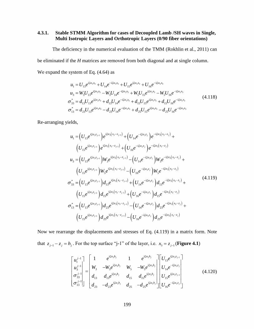
199
Stable STMM Algorithm for cases of Decoupled Lamb /SH waves in Single, 4.3.1.
Multi Isotropic Layers and Orthotropic Layers (0/90 fiber orientations)
The deficiency in the numerical evaluation of the TMM (Rokhlin et al., 2011) can
be eliminated if the H matrices are removed from both diagonal and at single column.
We expand the system of Eq. (4.64) as
3 3 3 3 5 3 5 3
3 3 3 3 5 3 5 3
3 3 3 3 5 3 5 3
3 3 3 3
1 13 14 15 16
3 3 13 3 14 5 15 5 16
*
33 13 13 13 14 15 15 15 16
*
13 23 13 23 14
i x i x i x i x
i x i x i x i x
i x i x i x i x
i x i x
u U e U e U e U e
u W U e W U e W U e W U e
d U e d U e d U e d U e
d U e d U e
5 3 5 3
25 15 25 16
i x i xd U e d U e
(4.118)
Re-arranging yields,
3 3 1 3 33 1 3
5 3 1 5 35 1 5
3 3 1 3 33 1 3
5 3 1 55 1 5
1 13 14
15 16
3 13 3 14 3
15 5 16 5
j jj j
j jj j
j jj j
jj j
i x z i x zi z i z
i x z i x zi z i z
i x z i x zi z i z
i x z i xi z i z
u U e e U e e
U e e U e e
u U e W e U e W e
U e W e U e W e
3
3 3 1 3 33 1 3
5 3 1 5 35 1 5
3 3 1 3 33 1 3
5 35 1
*
33 13 13 14 13
15 15 16 15
*
13 13 23 14 23
15 25
j
j jj j
j jj j
j jj j
jj
z
i x z i x zi z i z
i x z i x zi z i z
i x z i x zi z i z
i x zi z
U e d e U e d e
U e d e U e d e
U e d e U e d e
U e d e
1 5 35
16 25
jji x zi z
U e d e
(4.119)
Now we rearrange the displacements and stresses of Eq. (4.119) in a matrix form. Note
that 1j j jz z h . For the top surface “j-1” of the layer, i.e.
3 1jx z (Figure 4.1)
3 5 3 1
3 5 3
3 5 5 1
3 5 5
113
1
13 3 5 5 143
1
33 13 13 15 15 151
1323 23 25 25 16
1 1j j j
j j j
j j j
j j j
i h i h i zj
i h i h i zj
j i h i h i z
ji h i h i z
e e U eu
W W e W W e U eu
d d e d d e U e
d d e d d e U e
(4.120)
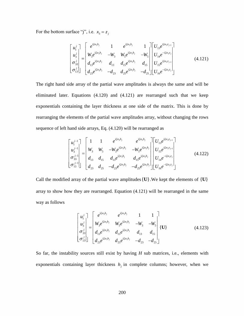
200
For the bottom surface “j”, i.e. 3 jx z
3 5 3 1
3 5 3
3 5 5 1
3 5 5
131
3 3 5 5 143
33 13 13 15 15 15
1323 23 25 25 16
1 1j j j
j j j
j j j
j j j
i h i h i zj
i h i h i zj
j i h i h i z
ji h i h i z
e e U eu
W e W W e W U eu
d e d d e d U e
d e d d e d U e
(4.121)
The right hand side array of the partial wave amplitudes is always the same and will be
eliminated later. Equations (4.120) and (4.121) are rearranged such that we keep
exponentials containing the layer thickness at one side of the matrix. This is done by
rearranging the elements of the partial wave amplitudes array, without changing the rows
sequence of left hand side arrays, Eq. (4.120) will be rearranged as
3 5 3 1
3 5 5 1
3 5 3
3 5 5
113
1
13 5 3 5 153
1
33 13 15 13 15 141
1323 25 23 25 16
1 1 j j j
j j j
j j j
j j j
i h i h i zj
i h i h i zj
j i h i h i z
ji h i h i z
e e U eu
W W W e W e U eu
d d d e d e U e
d d d e d e U e
(4.122)
Call the modified array of the partial wave amplitudes{ }U .We kept the elements of { }U
array to show how they are rearranged. Equation (4.121) will be rearranged in the same
way as follows
3 5
3 5
3 5
3 5
1
3 5 3 53
33 13 15 13 15
1323 25 23 25
1 1
{ }
j j
j j
j j
j j
i h i hj
i h i hj
j i h i h
ji h i h
e eu
W e W e W Wu
d e d e d d
d e d e d d
U (4.123)
So far, the instability sources still exist by having H sub matrices, i.e., elements with
exponentials containing layer thickness jh in complete columns; however, when we
201
formulate the SM by collecting all the stresses in one array and all the displacements in
another array, we get
3 5
3 5
3 5
3 5
3 5
3 5
113 15 13 15
33
123 25 23 2513
33 13 15 13 15
1323 25 23 25
3 5 3 5
.
1 1
j j
j j
j j
j j
j j
j j
i h i hj
i h i hj
j i h i h
ji h i h
i h i h
i h i h
i
d d d e d e
d d d e d e
d e d e d d
d e d e d d
e e
W W W e W e
e
3 5
3 5
1
1
1
1
3
1
33 5 3 5
1 1j j
j j
j
j
jh i h
ji h i h
u
u
ue
uW e W e W W
(4.124)
The product of the two 4x4 matrices is the SM, and to compare the system with Rokhlin
et al. (2011) formulation, we condense the system as
1
1 1j j
j jj j
uD D H P P H
uD H D P H P
(4.125)
The key point is that H matrices are no longer in the main diagonal nor in a single column.
This prevents getting singularity cases when diagonally-placed exponentials containing
jh approach very small numbers, so neither the left 4x4 matrix will be singular nor the
right inverse of 4x4 matrix will be undefined.
The above formulation was coded and applied to an isotropic layer of aluminum;
this case solved with TMM was shown before in Figure 4.2a,b with instability starting at
20 MHz. The new results obtained with SMM and STMM are shown in Figure 4.7. The
SMM solely is robust and stable at high frequency-thickness values; but it does not find
the roots “accurately” in low frequency range. Hence, applying the combined TMM and
SMM, (or stable combined STMM), is the best way to get the desired results.
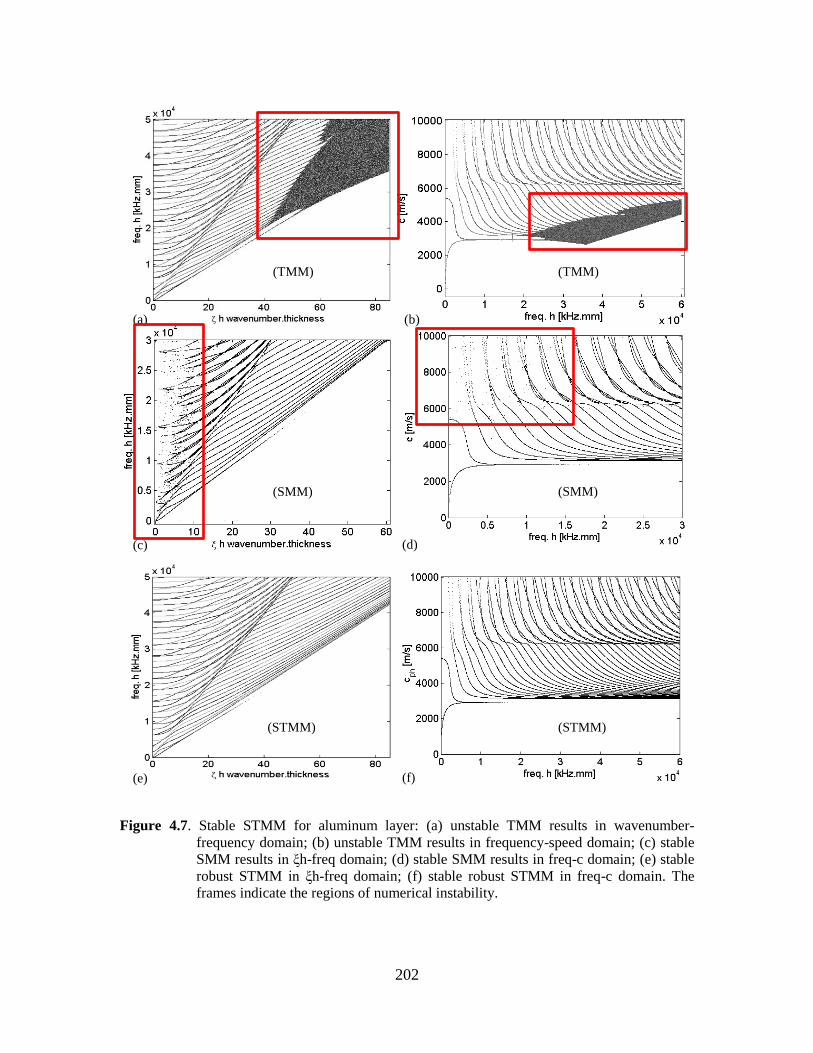
202
Figure 4.7. Stable STMM for aluminum layer: (a) unstable TMM results in wavenumber-
frequency domain; (b) unstable TMM results in frequency-speed domain; (c) stable
SMM results in ξh-freq domain; (d) stable SMM results in freq-c domain; (e) stable
robust STMM in ξh-freq domain; (f) stable robust STMM in freq-c domain. The
frames indicate the regions of numerical instability.
(c) (d)
(e) (f)
(SMM) (SMM)
(STMM) (STMM)
(a)
(TMM)
(b)
(TMM)
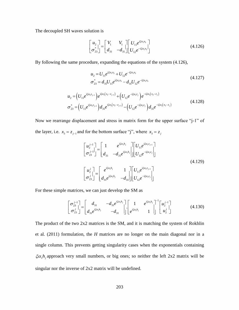
203
The decoupled SH waves solution is
1 3
1 3
2 1 1 11
*
23 31 31 12
i x
i x
u V V U e
d d U e
(4.126)
By following the same procedure, expanding the equations of the system (4.126),
1 3 1 3
1 3 1 3
2 11 12
*
23 31 11 31 12
i x i x
i x i x
u U e U e
d U e d U e
(4.127)
1 3 1 1 31 1 1
1 3 1 1 31 1 1
2 11 12
*
23 11 31 12 31
j jj j
j jj j
i x z i x zi z i z
i x z i x zi z i z
u U e e U e e
U e d e U e d e
(4.128)
Now we rearrange displacement and stress in matrix form for the upper surface “j-1” of
the layer, i.e. 3 1jx z and for the bottom surface “j”, where
3 jx z
1 1 1
1 1
1 1 1
1 1
1112
1
23 31 31 12
112
23 31 31 12
1
1
j j
j j
j j
j j
i h i zj
j i h i z
i h i zj
j i h i z
e U eu
d d e U e
e U eu
d e d U e
(4.129)
For these simple matrices, we can just develop the SM as
1 1
1 1
11 1
31 3123 2
23 231 31
1.
1
j j
j j
i h i hj j
j ji h i h
d d e e u
ud e d e
(4.130)
The product of the two 2x2 matrices is the SM, and it is matching the system of Rokhlin
et al. (2011) formulation, the H matrices are no longer on the main diagonal nor in a
single column. This prevents getting singularity cases when the exponentials containing
1 jh approach very small numbers, or big ones; so neither the left 2x2 matrix will be
singular nor the inverse of 2x2 matrix will be undefined.
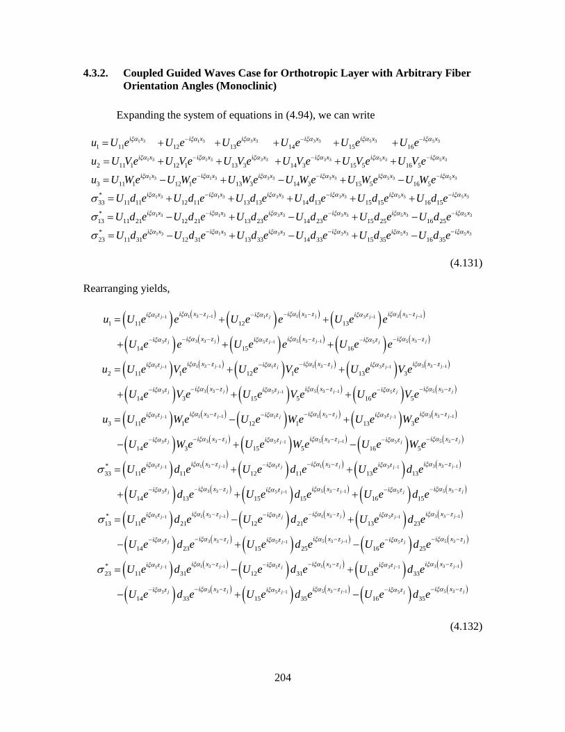
204
Coupled Guided Waves Case for Orthotropic Layer with Arbitrary Fiber 4.3.2.
Orientation Angles (Monoclinic)
Expanding the system of equations in (4.94), we can write
1 3 1 3 3 3 3 3 5 3 5 3
1 3 1 3 3 3 3 3 5 3 5 3
1 3 1 3
1 11 12 13 14 15 16
2 11 1 12 1 13 3 14 3 15 5 16 5
3 11 1 12 1
i x i x i x i x i x i x
i x i x i x i x i x i x
i x i x
u U e U e U e U e U e U e
u U V e U V e U V e U V e U V e U V e
u U W e U W e
3 3 3 3 5 3 5 3
1 3 1 3 3 3 3 3 5 3 5 3
1 3 1 3 3 3
13 3 14 3 15 5 16 5
*
33 11 11 12 11 13 13 14 13 15 15 16 15
*
13 11 21 12 21 13 23 14 23
i x i x i x i x
i x i x i x i x i x i x
i x i x i x
U W e U W e U W e U W e
U d e U d e U d e U d e U d e U d e
U d e U d e U d e U d e
3 3 5 3 5 3
1 3 1 3 3 3 3 3 5 3 5 3
15 25 16 25
*
23 11 31 12 31 13 33 14 33 15 35 16 35
i x i x i x
i x i x i x i x i x i x
U d e U d e
U d e U d e U d e U d e U d e U d e
(4.131)
Rearranging yields,
1 3 1 1 3 3 3 11 1 1 3 1
3 3 5 3 1 5 33 5 1 5
1 3 1 1 31 1 1
1 11 12 13
14 15 16
2 11 1 12 1
j j jj j j
j j jj j j
j jj j
i x z i x z i x zi z i z i z
i x z i x z i x zi z i z i z
i x z i x zi z i z
u U e e U e e U e e
U e e U e e U e e
u U e V e U e V e
3 3 13 1
3 3 5 3 1 5 33 5 1 5
1 3 1 1 3 3 3 11 1 1 3 1
3
13 3
14 3 15 5 16 5
3 11 1 12 1 13 3
14 3
jj
j j jj j j
j j jj j j
j
i x zi z
i x z i x z i x zi z i z i z
i x z i x z i x zi z i z i z
i z
U e V e
U e V e U e V e U e V e
u U e W e U e W e U e W e
U e W e
3 3 5 3 1 5 35 1 5
1 3 1 1 3 3 3 11 1 1 3 1
3 3 5 33 5 1
15 5 16 5
*
33 11 11 12 11 13 13
14 13 15 15
j j jj j
j j jj j j
j jj j
i x z i x z i x zi z i z
i x z i x z i x zi z i z i z
i x z i x zi z i z
U e W e U e W e
U e d e U e d e U e d e
U e d e U e d e
1 5 35
1 3 1 1 3 3 3 11 1 1 3 1
3 3 5 3 1 5 33 5 1 5
16 15
*
13 11 21 12 21 13 23
14 23 15 25 16 25
*
23
jj
j j jj j j
j j jj j j
i x zi z
i x z i x z i x zi z i z i z
i x z i x z i x zi z i z i z
U e d e
U e d e U e d e U e d e
U e d e U e d e U e d e
U
1 3 1 1 3 3 3 11 1 1 3 1
3 3 5 3 1 5 33 5 1 5
11 31 12 31 13 33
14 33 15 35 16 35
j j jj j j
j j jj j j
i x z i x z i x zi z i z i z
i x z i x z i x zi z i z i z
e d e U e d e U e d e
U e d e U e d e U e d e
(4.132)
205
Rearranging the displacements and stresses of Eq. (4.132) in a matrix form, we obtain:
For the top surface “j-1” of the layer, i.e., 3 1jx z ,
1 3 5
1 3 5
1 3 5
11 3 5
1
1
1
1
1
2 1 1 3 3 5 5
1
3 1 1 3 3 5 5
*
11 11 13 13 15 1533
*21 2113
*
23
1 1 1j j j
j j j
j j j
jj j j
j
j
i h i h i hj
i h i h i hj
i h i h i hj
i h i h i h
i
u e e e
u V V e V V e V V e
u W W e W W e W W e
d d e d d e d d e
d d e
1 1
1
3 1
3
1 3 5 5 1
1 3 5 5
11
12
13
14
23 23 25 25 15
31 31 33 33 35 35 16
j
j
j
j
j j j j
j j j j
i z
i z
i z
i z
h i h i h i z
i h i h i h i z
U e
U e
U e
U e
d d e d d e U e
d d e d d e d d e U e
(4.133)
For the bottom surface “j”, i.e., 3 jx z ,
1 3 5
1 3 5
1 3 5
1 3 5
1
1
2 1 1 3 3 5 5
3 1 1 3 3 5 5
*
11 11 13 13 15 1533
*21 21 2313
*
23
1 1 1j j j
j j j
j j j
jj j j
jj
j
i h i h i hj
i h i h i hj
i h i h i hj
i h i h i h
i h i
u e e e
u V e V V e V V e V
u W e W W e W W e W
d e d d e d d e d
d e d d e
1 1
1
3 1
3
3 5 5 1
1 3 5 5
11
12
13
14
23 25 25 15
31 31 33 33 35 35 16
j
j
j
j
j j j
j j j j
i z
i z
i z
i z
h i h i z
i h i h i h i z
U e
U e
U e
U e
d d e d U e
d e d d e d d e d U e
(4.134)
The right hand side array of the partial wave amplitudes is always the same and will be
eliminated later. Equations (4.133), (4.134) are rearranged such that we keep
exponentials containing the layer thickness at one side of the matrix. This is done by
rearranging the elements of the partial wave amplitudes array without changing the rows
sequence of left hand side arrays, Eq. (4.133) will be rearranged as
206
1 3 5
1 3 5
1 3 5
11 3 5
1
1
1
1
1
2 1 3 5 1 3 5
1
3 1 3 5 1 3 5
*
11 13 15 11 13 1533
*21 23 2513
*
23
1 1 1 j j j
j j j
j j j
jj j j
j
j
i h i h i hj
i h i h i hj
i h i h i hj
i h i h i h
u e e e
u V V V V e V e V e
u W W W W e W e W e
d d d d e d e d e
d d d
1 1
3 1
5 1
1
1 3 5 3
1 3 5 5
11
13
15
12
21 23 25 14
31 33 35 31 33 35 16
j
j
j
j
j j j j
j j j j
i z
i z
i z
i z
i h i h i h i z
i h i h i h i z
U e
U e
U e
U e
d e d e d e U e
d d d d e d e d e U e
(4.135)
Call the modified array of partial wave amplitudes { }U . We kept the elements of { }U
array to show how they are rearranged. Equation (4.134) will be rearranged in the same
was as follows
1 3 5
1 3 5
1 3 5
1 3 5
1 3
1
2 1 3 5 1 3 5
3 1 3 5 1 3 5
*
11 13 15 11 13 1533
*21 2313
*
23
1 1 1j j j
j j j
j j j
jj j j
jj j
j
i h i h i hj
i h i h i hj
i h i h i hj
i h i h i h
i h i h
u e e e
u V e V e V e V V V
u W e W e W e W W W
d e d e d e d d d
d e d e d
5
1 3 5
25 21 23 25
31 33 35 31 33 35
{U}
j
j j j
i h
i h i h i h
e d d d
d e d e d e d d d
(4.136)
So far, the instability sources still exist by having H sub matrices, i.e., elements with
exponentials containing layer thickness jh in complete columns; however, when we
formulate the SM by collecting all the stresses in one array and all the displacements in
another array, we get
207
11 3 5
11 3 5
11 3 5
1 3
*
33 11 13 15 11 13 15
*
13 21 23 25 21 23 25
*
23 31 33 35 31 33 35
*
11 1333
*
13
*
23
jj j j
jj j j
jj j j
jj
j
j
i h i h i h
i h i h i h
i h i h i h
i h i
d d d d e d e d e
d d d d e d e d e
d d d d e d e d e
d e d e
5
1 3 5
1 3 5
1 3 5
1 3 5
1
15 11 13 15
21 23 25 21 23 25
31 33 35 31 33 35
1 3 5 1 3 5
1 3 5 1
.
1 1 1
j j
j j j
j j j
j j j
j j j
h i h
i h i h i h
i h i h i h
i h i h i h
i h i h i h
i h
d e d d d
d e d e d e d d d
d e d e d e d d d
e e e
V V V V e V e V e
W W W W e
3 5
1 3 5
1 3 5
1 3 5
1
1
1
1
2
13 5 3
1
21 3 5 1 3 5
31 3 5 1 3 5
1 1 1
j j j
j j j
j j j
j j j
j
j
i h i h j
ji h i h i h
ji h i h i h
ji h i h i h
u
u
W e W e u
ue e e
uV e V e V e V V Vu
W e W e W e W W W
(4.137)
The product of the two 6x6 matrices is the SM. Comparing the system with Rokhlin et al.
(2011) formulation, the system condenses to
1
1 1j j
j jj j
uD D H P P H
uD H D P H P
(4.138)
4.4. FRAMEWORK OF STMM AND SEPARATING MODES BY MODE TRACING
Root solving methods are mostly numerical and iterative; it was reported in Lowe
(1995); Pavlakovic and Lowe (2003) that roots can be determined in a robust way by
varying the phase velocity at fixed frequency or vice versa. An initial guess is needed and
root tracing is achieved by linear extrapolation of two roots. Afterwards, when sufficient
number of roots is determined, a quadratic extrapolation is used. We used this approach
on our roots to get initial separation for individual modes; later on, mode shapes can be
used to identify similar wave types, e.g. symmetric Lamb waves, antisymmetric Lamb
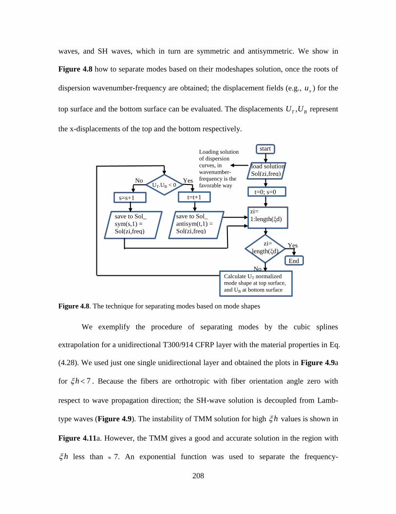
208
waves, and SH waves, which in turn are symmetric and antisymmetric. We show in
Figure 4.8 how to separate modes based on their modeshapes solution, once the roots of
dispersion wavenumber-frequency are obtained; the displacement fields (e.g., xu ) for the
top surface and the bottom surface can be evaluated. The displacements ,T BU U represent
the x-displacements of the top and the bottom respectively.
Figure 4.8. The technique for separating modes based on mode shapes
We exemplify the procedure of separating modes by the cubic splines
extrapolation for a unidirectional T300/914 CFRP layer with the material properties in Eq.
(4.28). We used just one single unidirectional layer and obtained the plots in Figure 4.9a
for 7h . Because the fibers are orthotropic with fiber orientation angle zero with
respect to wave propagation direction; the SH-wave solution is decoupled from Lamb-
type waves (Figure 4.9). The instability of TMM solution for high h values is shown in
Figure 4.11a. However, the TMM gives a good and accurate solution in the region with
h less than 7. An exponential function was used to separate the frequency-
start
load solution
Sol(zi,freq)
t=0; s=0
zi=
length(ξd) Yes
No
zi=
1:length(ξd) save to Sol_
antisym(t,1) =
Sol(zi,freq)
Loading solution
of dispersion
curves, in
wavenumber-
frequency is the
favorable way
Calculate UT normalized
mode shape at top surface,
and UB at bottom surface
End
UT.UB < 0 Yes
t=t+1 s=s+1
No
save to Sol_
sym(s,1) =
Sol(zi,freq)
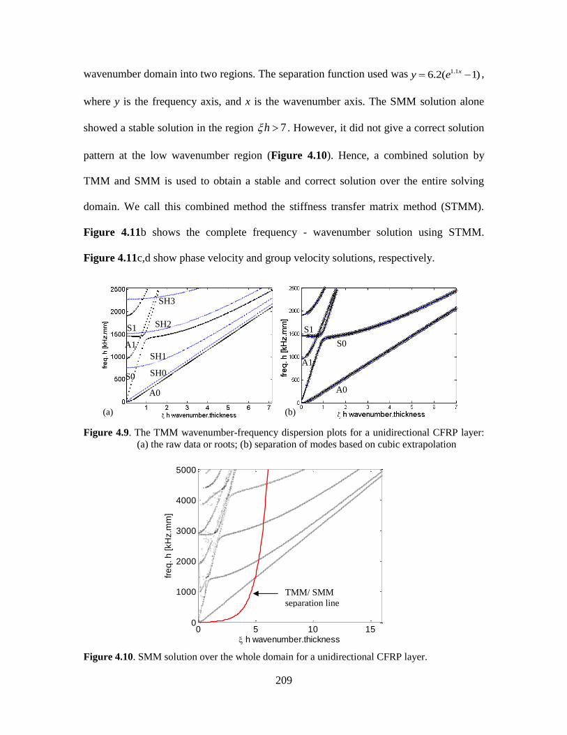
209
wavenumber domain into two regions. The separation function used was 1.16.2( 1)xy e ,
where y is the frequency axis, and x is the wavenumber axis. The SMM solution alone
showed a stable solution in the region 7h . However, it did not give a correct solution
pattern at the low wavenumber region (Figure 4.10). Hence, a combined solution by
TMM and SMM is used to obtain a stable and correct solution over the entire solving
domain. We call this combined method the stiffness transfer matrix method (STMM).
Figure 4.11b shows the complete frequency - wavenumber solution using STMM.
Figure 4.11c,d show phase velocity and group velocity solutions, respectively.
Figure 4.9. The TMM wavenumber-frequency dispersion plots for a unidirectional CFRP layer:
(a) the raw data or roots; (b) separation of modes based on cubic extrapolation
Figure 4.10. SMM solution over the whole domain for a unidirectional CFRP layer.
0 5 10 150
1000
2000
3000
4000
5000
h wavenumber.thickness
fre
q. h
[kH
z.m
m]
(b) (a)
A0
SH0 S0
SH1 A1
S1 SH2
SH3
A0
S0
A1
S1
TMM/ SMM
separation line
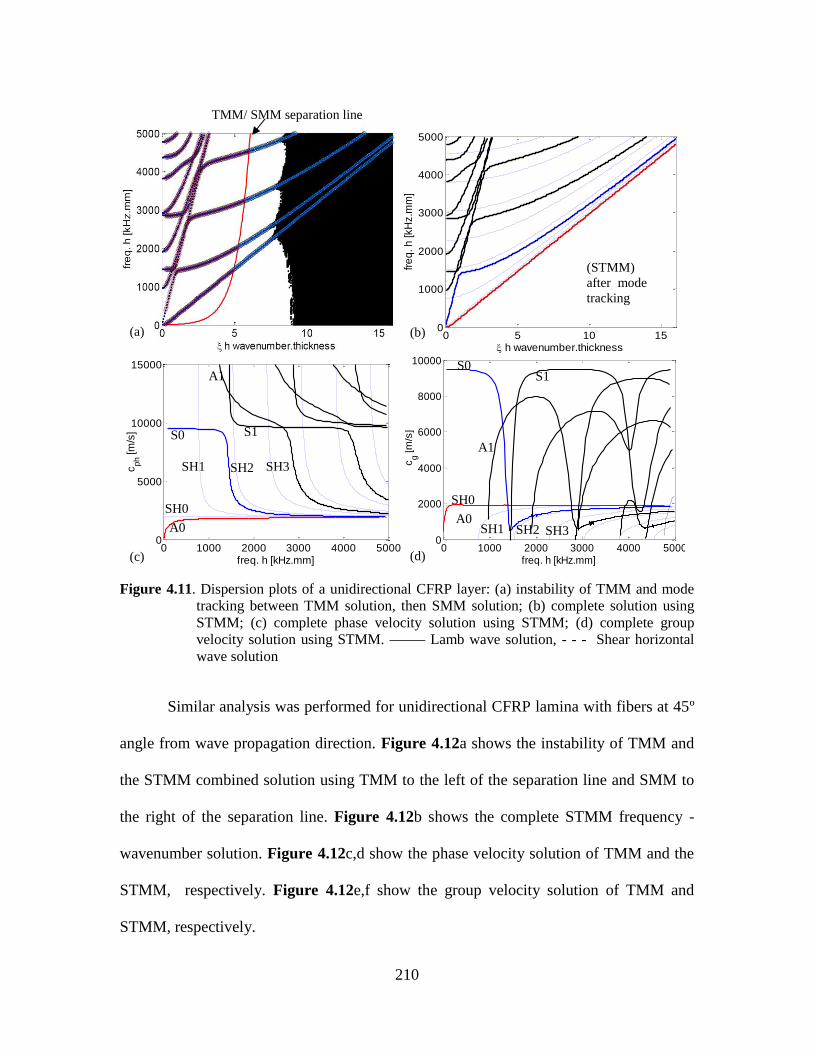
210
Figure 4.11. Dispersion plots of a unidirectional CFRP layer: (a) instability of TMM and mode
tracking between TMM solution, then SMM solution; (b) complete solution using
STMM; (c) complete phase velocity solution using STMM; (d) complete group
velocity solution using STMM. Lamb wave solution, - - - Shear horizontal
wave solution
Similar analysis was performed for unidirectional CFRP lamina with fibers at 45º
angle from wave propagation direction. Figure 4.12a shows the instability of TMM and
the STMM combined solution using TMM to the left of the separation line and SMM to
the right of the separation line. Figure 4.12b shows the complete STMM frequency -
wavenumber solution. Figure 4.12c,d show the phase velocity solution of TMM and the
STMM, respectively. Figure 4.12e,f show the group velocity solution of TMM and
STMM, respectively.
0 1000 2000 3000 4000 50000
2000
4000
6000
8000
10000
freq. h [kHz.mm]
cg [m
/s]
0 5 10 150
1000
2000
3000
4000
5000
h wavenumber.thickness
fre
q. h
[kH
z.m
m]
0 1000 2000 3000 4000 50000
5000
10000
15000
freq. h [kHz.mm]
cph [m
/s]
(c)
(b) (a)
(d)
A0
SH0
S0
SH1
A1
S1
SH2 SH3
A0
SH0
S0
SH1
A1
S1
SH2 SH3
TMM/ SMM separation line
(STMM)
after mode
tracking
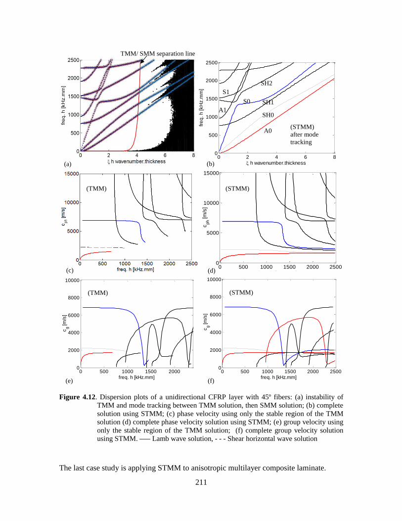
211
Figure 4.12. Dispersion plots of a unidirectional CFRP layer with 45º fibers: (a) instability of
TMM and mode tracking between TMM solution, then SMM solution; (b) complete
solution using STMM; (c) phase velocity using only the stable region of the TMM
solution (d) complete phase velocity solution using STMM; (e) group velocity using
only the stable region of the TMM solution; (f) complete group velocity solution
using STMM. Lamb wave solution, - - - Shear horizontal wave solution
The last case study is applying STMM to anisotropic multilayer composite laminate.
0 2 4 6 80
500
1000
1500
2000
2500
h wavenumber.thickness
fre
q. h
[kH
z.m
m]
0 500 1000 1500 2000 25000
5000
10000
15000
freq. h [kHz.mm]
cph [m
/s]
0 500 1000 1500 2000 25000
2000
4000
6000
8000
10000
freq. h [kHz.mm]
cg [m
/s]
0 500 1000 1500 20000
2000
4000
6000
8000
10000
freq. h [kHz.mm]
cg [m
/s]
(c)
(b) (a)
(d)
(e) (f)
A0
SH0
S0 SH1 A1
S1 SH2
TMM/ SMM separation line
(STMM)
after mode
tracking
(STMM)
(STMM) (TMM)
(TMM)
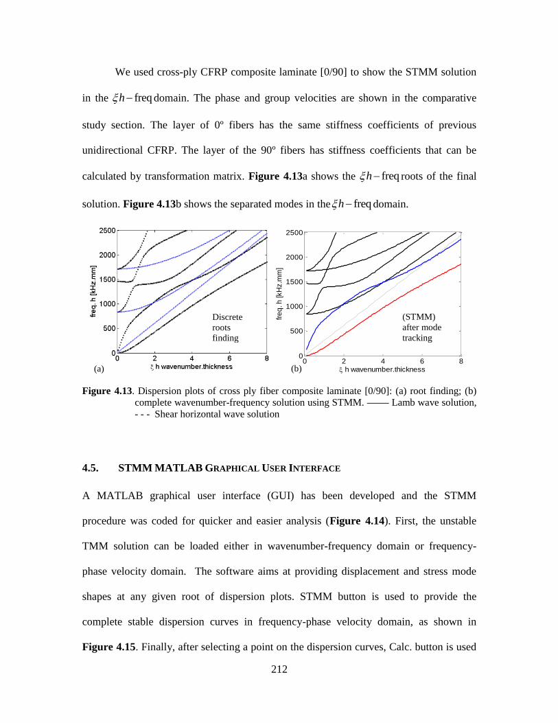
212
We used cross-ply CFRP composite laminate [0/90] to show the STMM solution
in the freqh domain. The phase and group velocities are shown in the comparative
study section. The layer of 0º fibers has the same stiffness coefficients of previous
unidirectional CFRP. The layer of the 90º fibers has stiffness coefficients that can be
calculated by transformation matrix. Figure 4.13a shows the freqh roots of the final
solution. Figure 4.13b shows the separated modes in the freqh domain.
Figure 4.13. Dispersion plots of cross ply fiber composite laminate [0/90]: (a) root finding; (b)
complete wavenumber-frequency solution using STMM. Lamb wave solution,
- - - Shear horizontal wave solution
4.5. STMM MATLAB GRAPHICAL USER INTERFACE
A MATLAB graphical user interface (GUI) has been developed and the STMM
procedure was coded for quicker and easier analysis (Figure 4.14). First, the unstable
TMM solution can be loaded either in wavenumber-frequency domain or frequency-
phase velocity domain. The software aims at providing displacement and stress mode
shapes at any given root of dispersion plots. STMM button is used to provide the
complete stable dispersion curves in frequency-phase velocity domain, as shown in
Figure 4.15. Finally, after selecting a point on the dispersion curves, Calc. button is used
0 2 4 6 80
500
1000
1500
2000
2500
h wavenumber.thickness
fre
q. h
[kH
z.m
m]
(b) (a)
(STMM)
after mode
tracking
Discrete
roots
finding
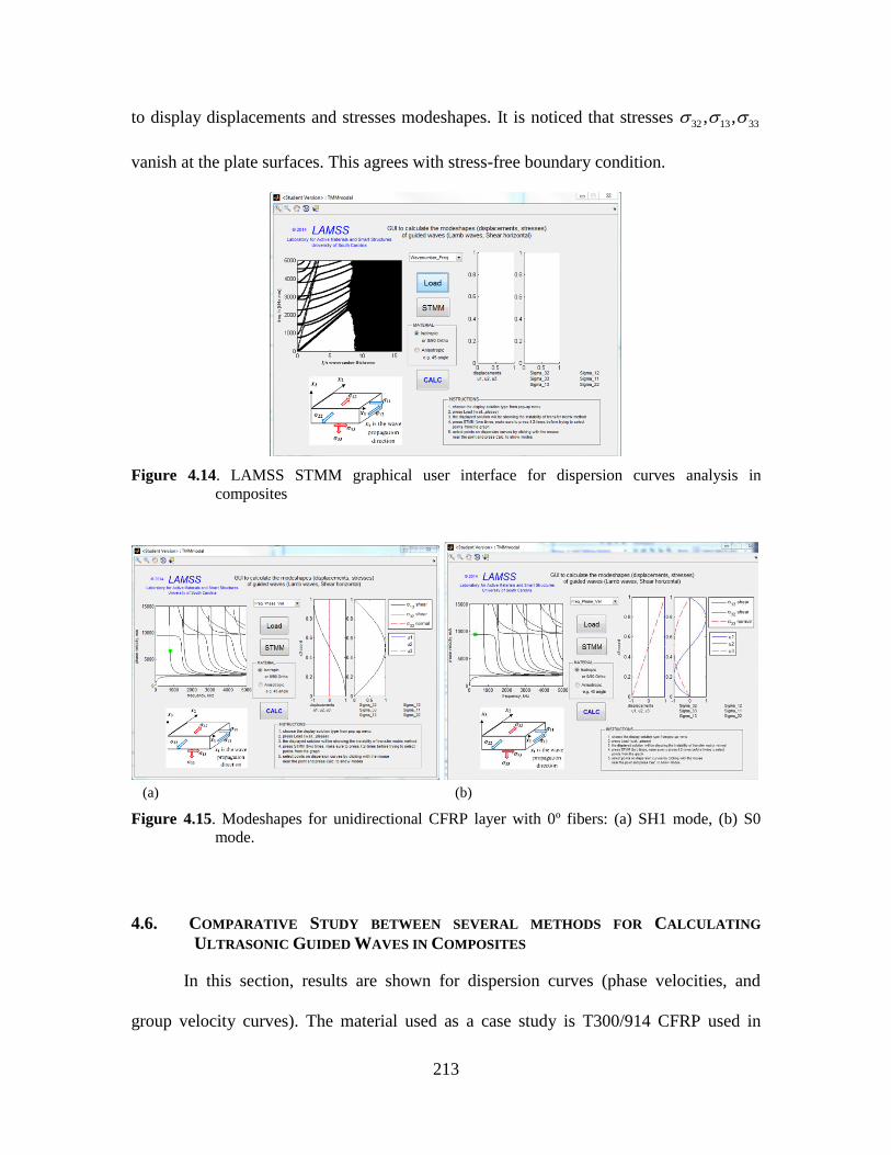
213
to display displacements and stresses modeshapes. It is noticed that stresses 32 13 33, ,
vanish at the plate surfaces. This agrees with stress-free boundary condition.
Figure 4.14. LAMSS STMM graphical user interface for dispersion curves analysis in
composites
Figure 4.15. Modeshapes for unidirectional CFRP layer with 0º fibers: (a) SH1 mode, (b) S0
mode.
4.6. COMPARATIVE STUDY BETWEEN SEVERAL METHODS FOR CALCULATING
ULTRASONIC GUIDED WAVES IN COMPOSITES
In this section, results are shown for dispersion curves (phase velocities, and
group velocity curves). The material used as a case study is T300/914 CFRP used in
(a) (b)
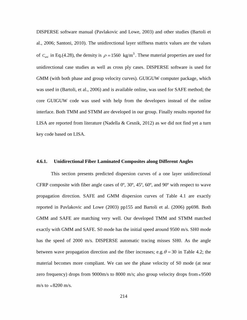
214
DISPERSE software manual (Pavlakovic and Lowe, 2003) and other studies (Bartoli et
al., 2006; Santoni, 2010). The unidirectional layer stiffness matrix values are the values
of uniC in Eq.(4.28), the density is 31560 kg/m . These material properties are used for
unidirectional case studies as well as cross ply cases. DISPERSE software is used for
GMM (with both phase and group velocity curves). GUIGUW computer package, which
was used in (Bartoli, et al., 2006) and is available online, was used for SAFE method; the
core GUIGUW code was used with help from the developers instead of the online
interface. Both TMM and STMM are developed in our group. Finally results reported for
LISA are reported from literature (Nadella & Cesnik, 2012) as we did not find yet a turn
key code based on LISA.
Unidirectional Fiber Laminated Composites along Different Angles 4.6.1.
This section presents predicted dispersion curves of a one layer unidirectional
CFRP composite with fiber angle cases of 0º, 30º, 45º, 60º, and 90º with respect to wave
propagation direction. SAFE and GMM dispersion curves of Table 4.1 are exactly
reported in Pavlakovic and Lowe (2003) pp155 and Bartoli et al. (2006) pp698. Both
GMM and SAFE are matching very well. Our developed TMM and STMM matched
exactly with GMM and SAFE. S0 mode has the initial speed around 9500 m/s. SH0 mode
has the speed of 2000 m/s. DISPERSE automatic tracing misses SH0. As the angle
between wave propagation direction and the fiber increases; e.g. 30 in Table 4.2; the
material becomes more compliant. We can see the phase velocity of S0 mode (at near
zero frequency) drops from 9000m/s to 8000 m/s; also group velocity drops from 9500
m/s to 8200 m/s.
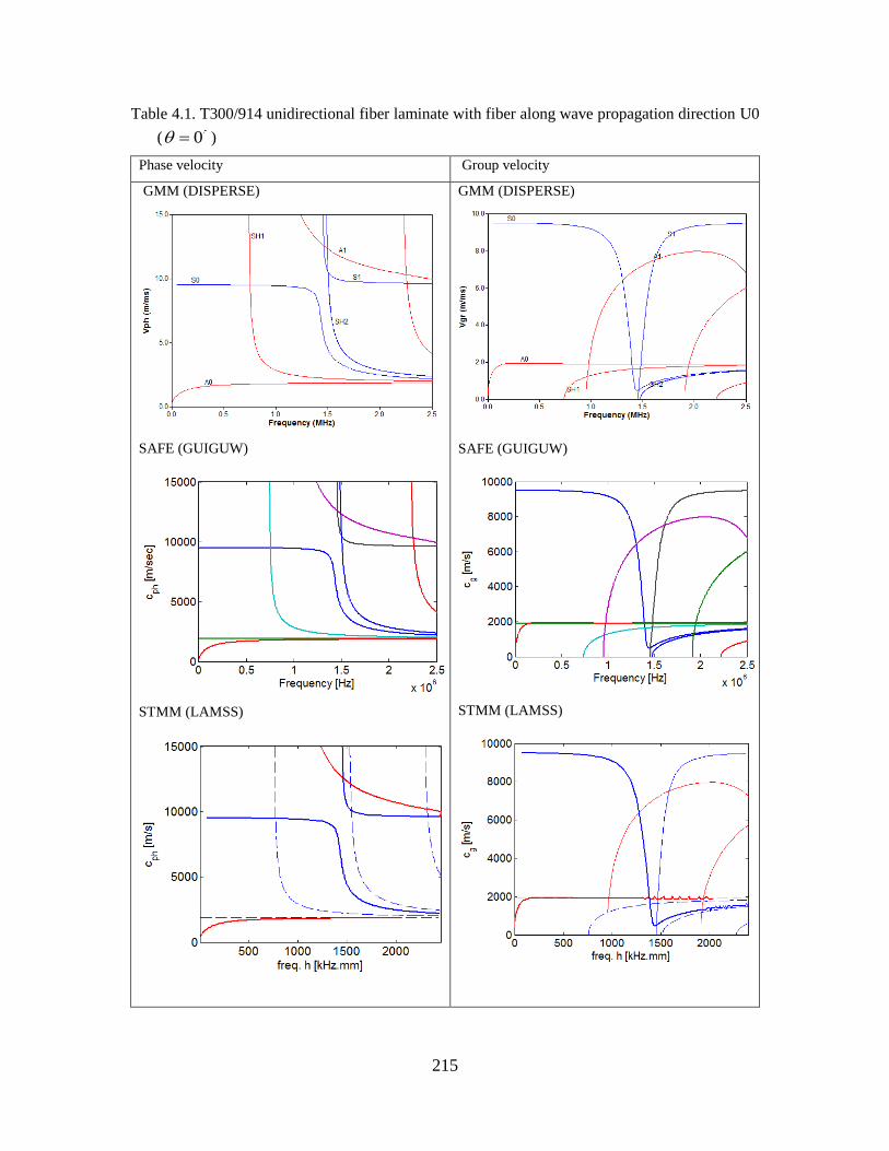
215
Table 4.1. T300/914 unidirectional fiber laminate with fiber along wave propagation direction U0
( 0 )
Phase velocity Group velocity
GMM (DISPERSE)
SAFE (GUIGUW)
STMM (LAMSS)
GMM (DISPERSE)
SAFE (GUIGUW)
STMM (LAMSS)
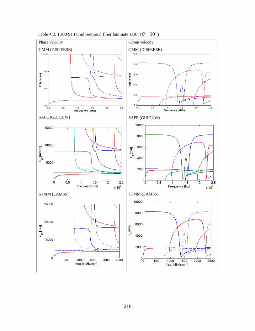
216
Table 4.2. T300/914 unidirectional fiber laminate U30 ( 30 )
Phase velocity Group velocity
GMM (DISPERSE)
SAFE (GUIGUW)
STMM (LAMSS)
GMM (DISPERSE)
SAFE (GUIGUW)
STMM (LAMSS)
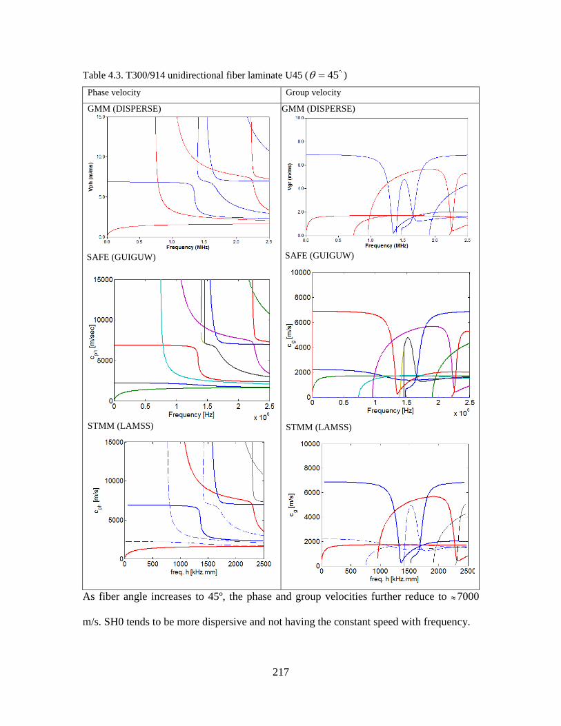
217
Table 4.3. T300/914 unidirectional fiber laminate U45 ( 45 )
Phase velocity Group velocity
GMM (DISPERSE)
SAFE (GUIGUW)
STMM (LAMSS)
GMM (DISPERSE)
SAFE (GUIGUW)
STMM (LAMSS)
As fiber angle increases to 45º, the phase and group velocities further reduce to 7000
m/s. SH0 tends to be more dispersive and not having the constant speed with frequency.
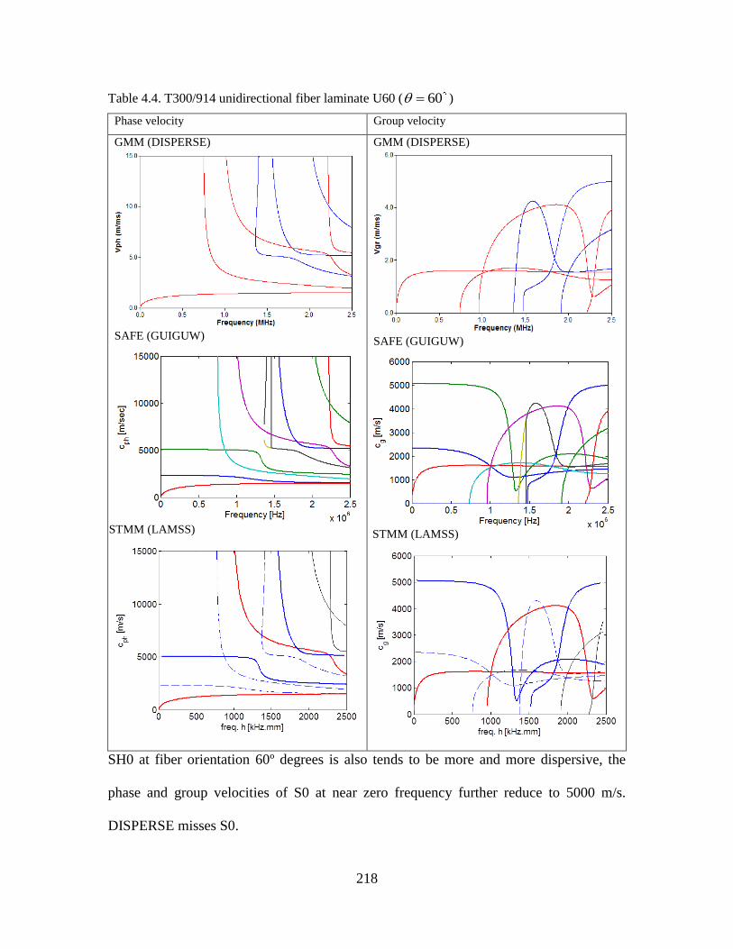
218
Table 4.4. T300/914 unidirectional fiber laminate U60 ( 60 )
Phase velocity Group velocity
GMM (DISPERSE)
SAFE (GUIGUW)
STMM (LAMSS)
GMM (DISPERSE)
SAFE (GUIGUW)
STMM (LAMSS)
SH0 at fiber orientation 60º degrees is also tends to be more and more dispersive, the
phase and group velocities of S0 at near zero frequency further reduce to 5000 m/s.
DISPERSE misses S0.
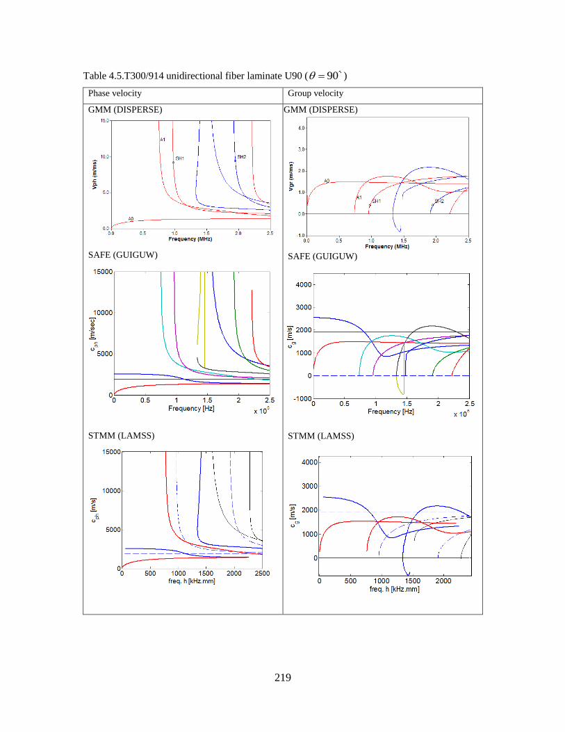
219
Table 4.5.T300/914 unidirectional fiber laminate U90 ( 90 )
Phase velocity Group velocity
GMM (DISPERSE)
SAFE (GUIGUW)
STMM (LAMSS)
GMM (DISPERSE)
SAFE (GUIGUW)
STMM (LAMSS)
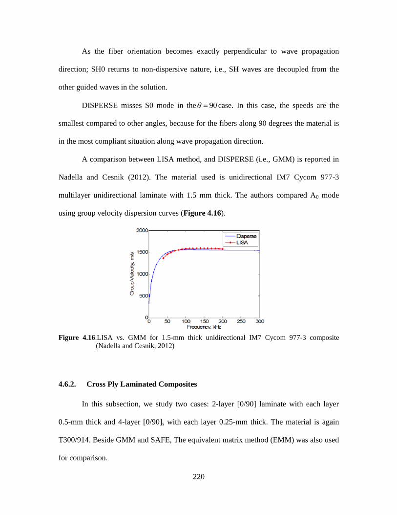
220
As the fiber orientation becomes exactly perpendicular to wave propagation
direction; SH0 returns to non-dispersive nature, i.e., SH waves are decoupled from the
other guided waves in the solution.
DISPERSE misses S0 mode in the 90 case. In this case, the speeds are the
smallest compared to other angles, because for the fibers along 90 degrees the material is
in the most compliant situation along wave propagation direction.
A comparison between LISA method, and DISPERSE (i.e., GMM) is reported in
Nadella and Cesnik (2012). The material used is unidirectional IM7 Cycom 977-3
multilayer unidirectional laminate with 1.5 mm thick. The authors compared A0 mode
using group velocity dispersion curves (Figure 4.16).
Figure 4.16.LISA vs. GMM for 1.5-mm thick unidirectional IM7 Cycom 977-3 composite
(Nadella and Cesnik, 2012)
Cross Ply Laminated Composites 4.6.2.
In this subsection, we study two cases: 2-layer [0/90] laminate with each layer
0.5-mm thick and 4-layer [0/90]s with each layer 0.25-mm thick. The material is again
T300/914. Beside GMM and SAFE, The equivalent matrix method (EMM) was also used
for comparison.
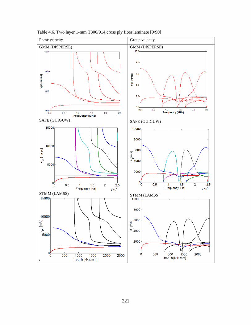
221
Table 4.6. Two layer 1-mm T300/914 cross ply fiber laminate [0/90]
Phase velocity Group velocity
GMM (DISPERSE)
SAFE (GUIGUW)
STMM (LAMSS)
GMM (DISPERSE)
SAFE (GUIGUW)
STMM (LAMSS)
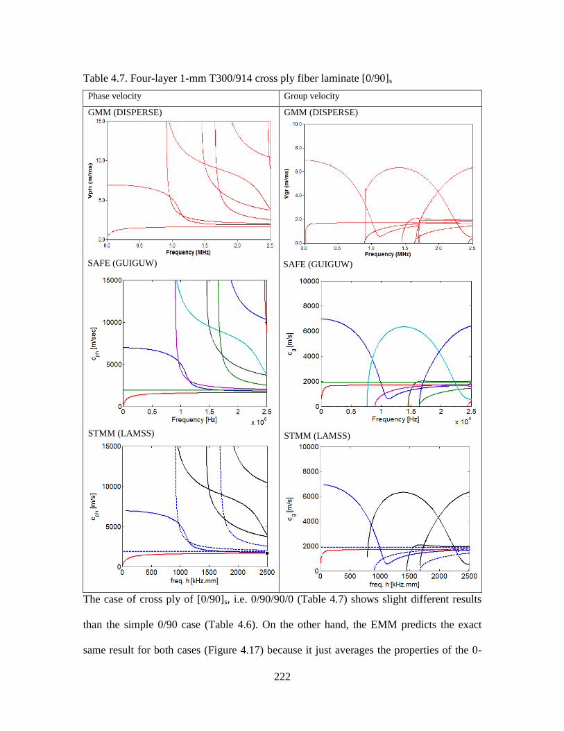
222
Table 4.7. Four-layer 1-mm T300/914 cross ply fiber laminate [0/90]s
Phase velocity Group velocity
GMM (DISPERSE)
SAFE (GUIGUW)
STMM (LAMSS)
GMM (DISPERSE)
SAFE (GUIGUW)
STMM (LAMSS)
The case of cross ply of [0/90]s, i.e. 0/90/90/0 (Table 4.7) shows slight different results
than the simple 0/90 case (Table 4.6). On the other hand, the EMM predicts the exact
same result for both cases (Figure 4.17) because it just averages the properties of the 0-
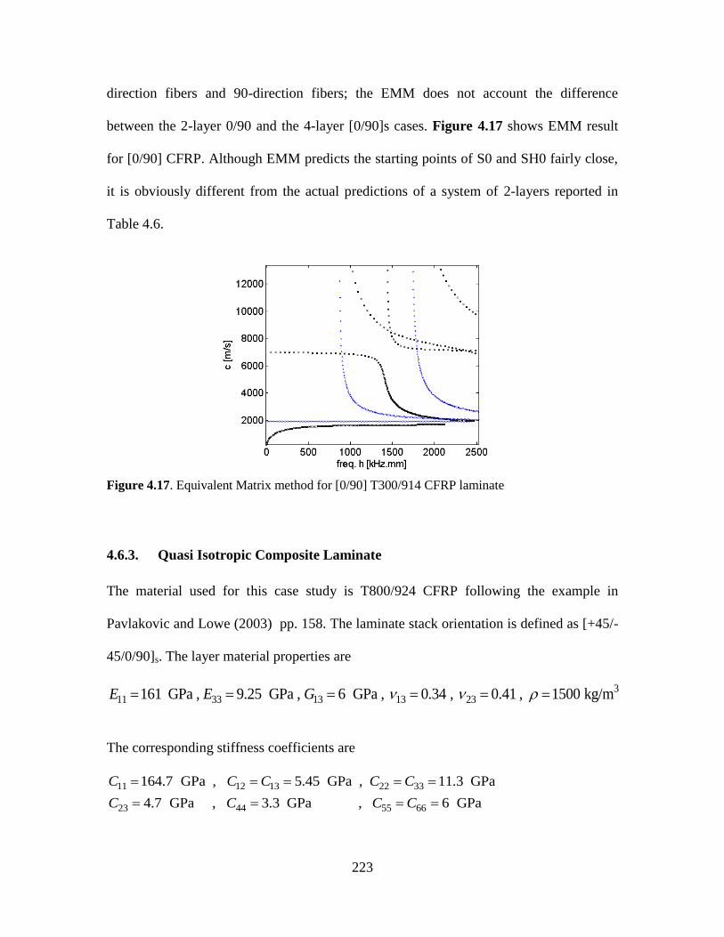
223
direction fibers and 90-direction fibers; the EMM does not account the difference
between the 2-layer 0/90 and the 4-layer [0/90]s cases. Figure 4.17 shows EMM result
for [0/90] CFRP. Although EMM predicts the starting points of S0 and SH0 fairly close,
it is obviously different from the actual predictions of a system of 2-layers reported in
Table 4.6.
Figure 4.17. Equivalent Matrix method for [0/90] T300/914 CFRP laminate
Quasi Isotropic Composite Laminate 4.6.3.
The material used for this case study is T800/924 CFRP following the example in
Pavlakovic and Lowe (2003) pp. 158. The laminate stack orientation is defined as [+45/-
45/0/90]s. The layer material properties are
311 33 13 13 23161 GPa , 9.25 GPa , 6 GPa , 0.34 , 0.41 , 1500 kg/mE E G
The corresponding stiffness coefficients are
11 12 13 22 33
23 44 55 66
164.7 GPa , 5.45 GPa , 11.3 GPa
4.7 GPa , 3.3 GPa , 6 GPa
C C C C C
C C C C
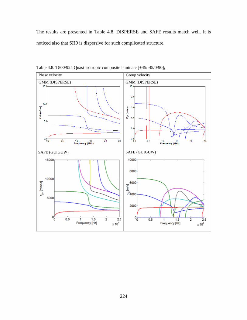
224
The results are presented in Table 4.8. DISPERSE and SAFE results match well. It is
noticed also that SH0 is dispersive for such complicated structure.
Table 4.8. T800/924 Quasi isotropic composite laminate [+45/-45/0/90]S
Phase velocity Group velocity
GMM (DISPERSE)
SAFE (GUIGUW)
GMM (DISPERSE)
SAFE (GUIGUW)
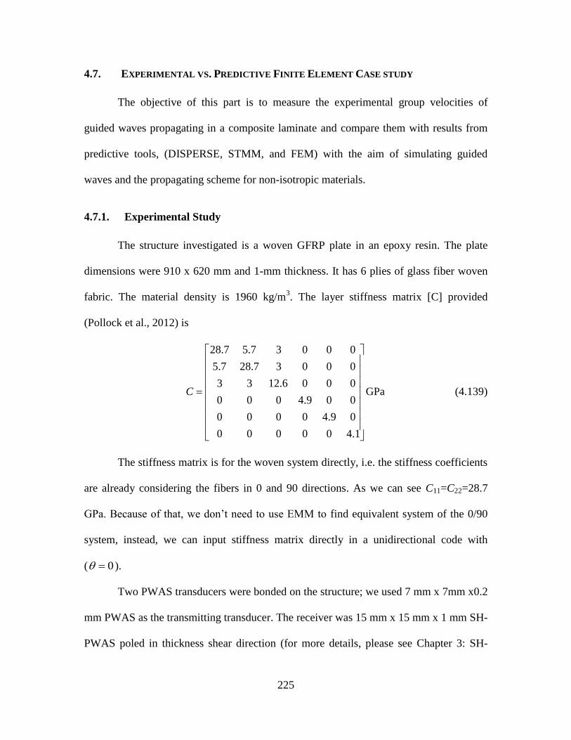
225
4.7. EXPERIMENTAL VS. PREDICTIVE FINITE ELEMENT CASE STUDY
The objective of this part is to measure the experimental group velocities of
guided waves propagating in a composite laminate and compare them with results from
predictive tools, (DISPERSE, STMM, and FEM) with the aim of simulating guided
waves and the propagating scheme for non-isotropic materials.
Experimental Study 4.7.1.
The structure investigated is a woven GFRP plate in an epoxy resin. The plate
dimensions were 910 x 620 mm and 1-mm thickness. It has 6 plies of glass fiber woven
fabric. The material density is 1960 kg/m3. The layer stiffness matrix [C] provided
(Pollock et al., 2012) is
28.7 5.7 3 0 0 0
5.7 28.7 3 0 0 0
3 3 12.6 0 0 0GPa
0 0 0 4.9 0 0
0 0 0 0 4.9 0
0 0 0 0 0 4.1
C
(4.139)
The stiffness matrix is for the woven system directly, i.e. the stiffness coefficients
are already considering the fibers in 0 and 90 directions. As we can see C11=C22=28.7
GPa. Because of that, we don’t need to use EMM to find equivalent system of the 0/90
system, instead, we can input stiffness matrix directly in a unidirectional code with
( 0 ).
Two PWAS transducers were bonded on the structure; we used 7 mm x 7mm x0.2
mm PWAS as the transmitting transducer. The receiver was 15 mm x 15 mm x 1 mm SH-
PWAS poled in thickness shear direction (for more details, please see Chapter 3: SH-
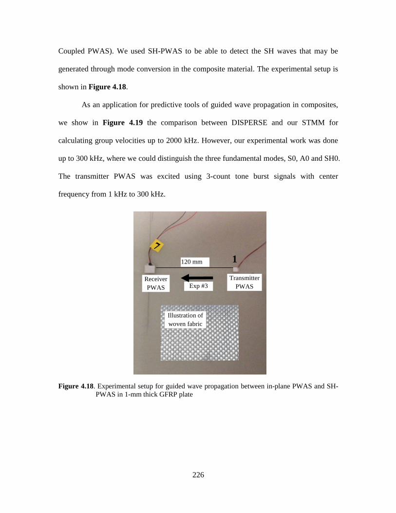
226
Coupled PWAS). We used SH-PWAS to be able to detect the SH waves that may be
generated through mode conversion in the composite material. The experimental setup is
shown in Figure 4.18.
As an application for predictive tools of guided wave propagation in composites,
we show in Figure 4.19 the comparison between DISPERSE and our STMM for
calculating group velocities up to 2000 kHz. However, our experimental work was done
up to 300 kHz, where we could distinguish the three fundamental modes, S0, A0 and SH0.
The transmitter PWAS was excited using 3-count tone burst signals with center
frequency from 1 kHz to 300 kHz.
Figure 4.18. Experimental setup for guided wave propagation between in-plane PWAS and SH-
PWAS in 1-mm thick GFRP plate
120 mm
Exp #3
1
Transmitter
PWAS Receiver
PWAS
Illustration of
woven fabric
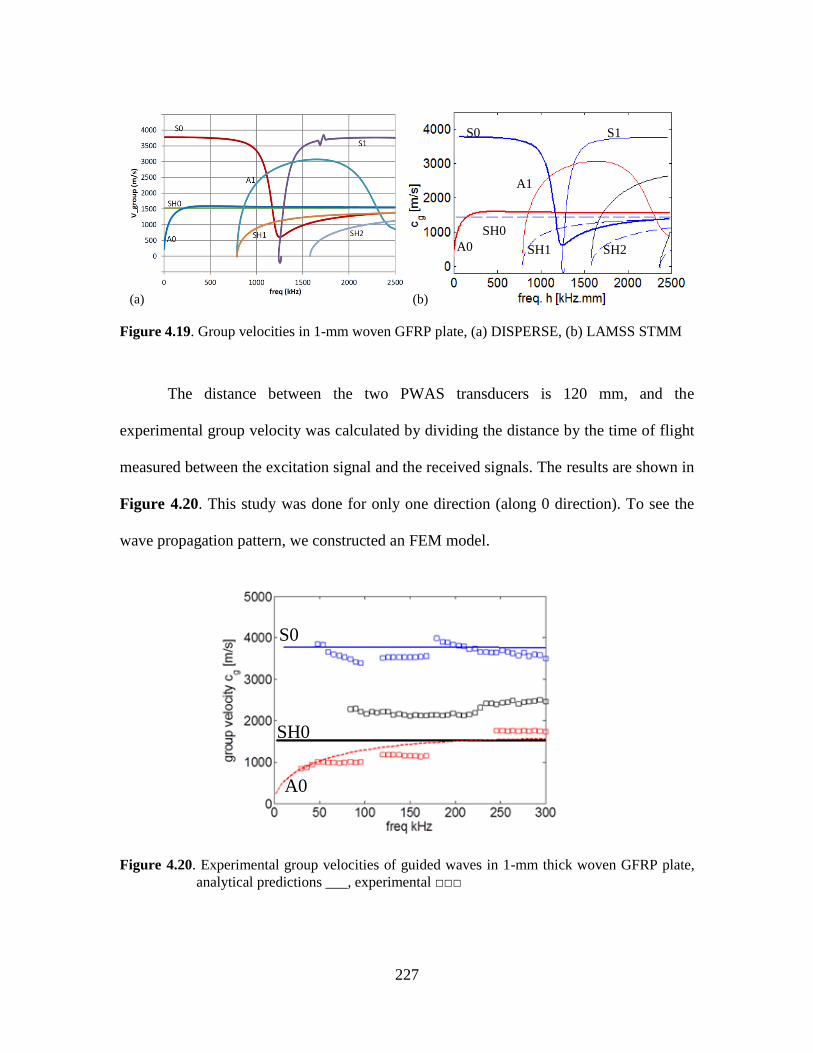
227
Figure 4.19. Group velocities in 1-mm woven GFRP plate, (a) DISPERSE, (b) LAMSS STMM
The distance between the two PWAS transducers is 120 mm, and the
experimental group velocity was calculated by dividing the distance by the time of flight
measured between the excitation signal and the received signals. The results are shown in
Figure 4.20. This study was done for only one direction (along 0 direction). To see the
wave propagation pattern, we constructed an FEM model.
Figure 4.20. Experimental group velocities of guided waves in 1-mm thick woven GFRP plate,
analytical predictions ___, experimental □□□
(b)
A0 SH0
S0
SH1
A1
S1
SH2
(a)
S0
SH0
A0
228
Finite Element Model for Guided Wave Propagation in GFRP 4.7.2.
The finite element model plate dimensions were 450 mm x 450 mm x 1-mm. The
material was GFRP. Two PWAS transducers were bonded in the middle as shown in
Figure 4.21. We used COMSOL Multiphysics coupled-field element for piezoelectric
transducers; this allowed us to apply excitation voltage as the input excitation and receive
the signal at the SH-receiver PWAS as voltage (rather than input a mechanical wave
excitation or force excitation). The excitation signal was 3-count tone burst with 10 V
signal amplitude and center frequency of 48 kHz. The reason for selecting this relatively
low frequency is to satisfy convergence and accuracy requirements with the available
computational resources. The model was run for 200 μs with 0.5 μs time step. The
structure domain was divided into 9 domains as shown in Figure 4.21 such that the
meshing of the domain in the middle was done by free mesh and then extruded by two
elements through the thickness (i.e. 0.5-mm mesh size through thickness). The meshing
of the other external domains was done by structural mesh and was extruded as two
elements through thickness. The mesh size that was used in this study was 3-mm for
GFRP material. Coupled field elements for the PWAS transducers were meshed by 1-mm
mesh size and 4 elements through the thickness of each PWAS (i.e. 0.25-mm mesh size
through the thickness of 1-mm thick SH-PWAS, and 0.05-mm mesh size through the
thickness of the 0.2-mm PWAS1.)
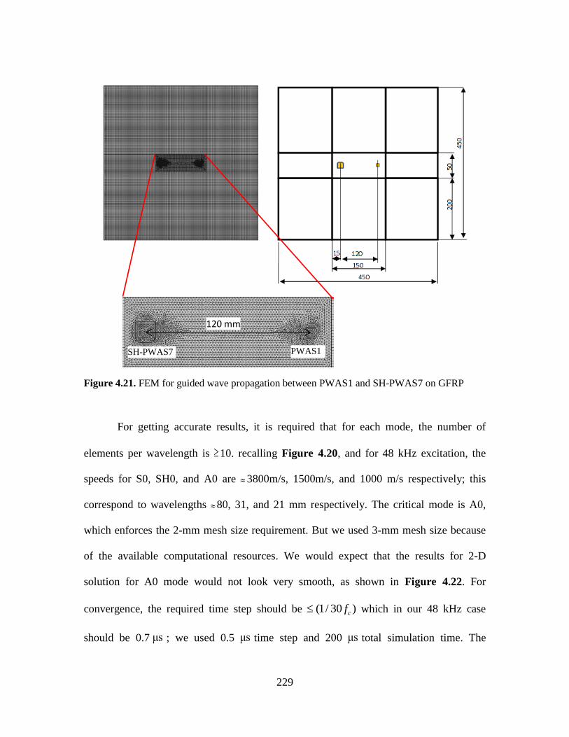
229
Figure 4.21. FEM for guided wave propagation between PWAS1 and SH-PWAS7 on GFRP
For getting accurate results, it is required that for each mode, the number of
elements per wavelength is 10. recalling Figure 4.20, and for 48 kHz excitation, the
speeds for S0, SH0, and A0 are 3800m/s, 1500m/s, and 1000 m/s respectively; this
correspond to wavelengths 80, 31, and 21 mm respectively. The critical mode is A0,
which enforces the 2-mm mesh size requirement. But we used 3-mm mesh size because
of the available computational resources. We would expect that the results for 2-D
solution for A0 mode would not look very smooth, as shown in Figure 4.22. For
convergence, the required time step should be (1/ 30 )cf which in our 48 kHz case
should be 0.7 μs ; we used 0.5 μs time step and 200 μs total simulation time. The
PWAS1 SH-PWAS7
120 mm
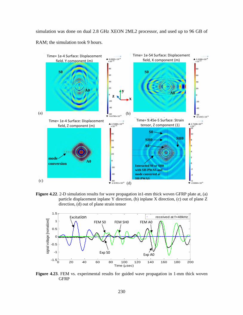
230
simulation was done on dual 2.8 GHz XEON 2ML2 processor, and used up to 96 GB of
RAM; the simulation took 9 hours.
Figure 4.22. 2-D simulation results for wave propagation in1-mm thick woven GFRP plate at, (a)
particle displacement inplane Y direction, (b) inplane X direction, (c) out of plane Z
direction, (d) out of plane strain tensor
Figure 4.23. FEM vs. experimental results for guided wave propagation in 1-mm thick woven
GFRP
Time= 1e-4 Surface: Displacement field, Y component (m)
Time= 1e-4 Surface: Displacement field, Z component (m)
Time= 1e-54 Surface: Displacement field, X component (m)
Time= 9.45e-5 Surface: Strain tensor, Z component (1)
S0
S0
A0 mode
conversion
A0
SH0
A0
Interacted S0 or SH0
with SH-PWAS and
mode converted at
SH-PWAS
SH0
S0
A0
(b) (a)
(d) (c)
y z
x
0 20 40 60 80 100 120 140 160 180 200-1.5
-1
-0.5
0
0.5
1
1.5
sig
na
l vo
ltag
e [n
om
aliz
ed
]
Time (sec)
received at f=48kHzExcitation
Exp S0
FEM SH0
Exp A0
FEM S0 FEM A0
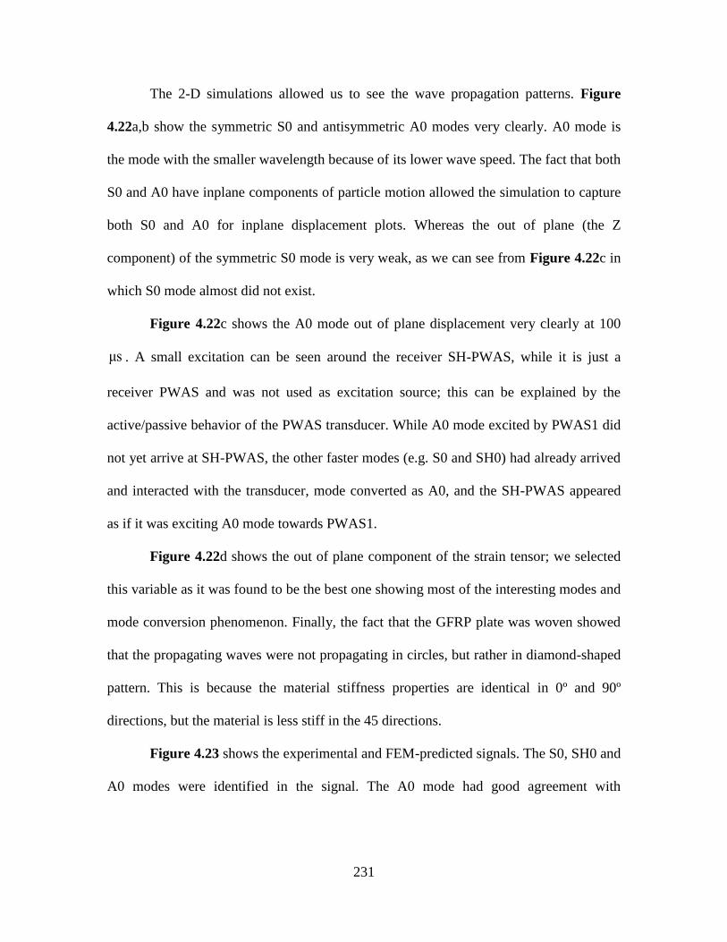
231
The 2-D simulations allowed us to see the wave propagation patterns. Figure
4.22a,b show the symmetric S0 and antisymmetric A0 modes very clearly. A0 mode is
the mode with the smaller wavelength because of its lower wave speed. The fact that both
S0 and A0 have inplane components of particle motion allowed the simulation to capture
both S0 and A0 for inplane displacement plots. Whereas the out of plane (the Z
component) of the symmetric S0 mode is very weak, as we can see from Figure 4.22c in
which S0 mode almost did not exist.
Figure 4.22c shows the A0 mode out of plane displacement very clearly at 100
μs . A small excitation can be seen around the receiver SH-PWAS, while it is just a
receiver PWAS and was not used as excitation source; this can be explained by the
active/passive behavior of the PWAS transducer. While A0 mode excited by PWAS1 did
not yet arrive at SH-PWAS, the other faster modes (e.g. S0 and SH0) had already arrived
and interacted with the transducer, mode converted as A0, and the SH-PWAS appeared
as if it was exciting A0 mode towards PWAS1.
Figure 4.22d shows the out of plane component of the strain tensor; we selected
this variable as it was found to be the best one showing most of the interesting modes and
mode conversion phenomenon. Finally, the fact that the GFRP plate was woven showed
that the propagating waves were not propagating in circles, but rather in diamond-shaped
pattern. This is because the material stiffness properties are identical in 0º and 90º
directions, but the material is less stiff in the 45 directions.
Figure 4.23 shows the experimental and FEM-predicted signals. The S0, SH0 and
A0 modes were identified in the signal. The A0 mode had good agreement with
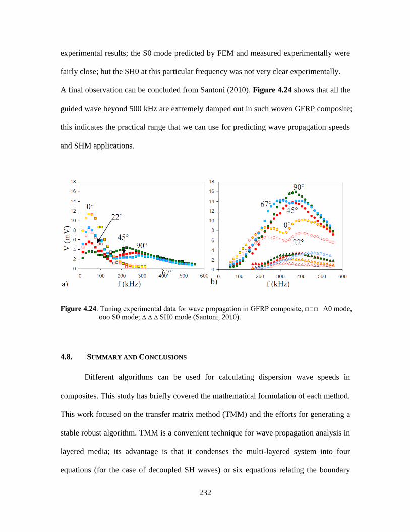
232
experimental results; the S0 mode predicted by FEM and measured experimentally were
fairly close; but the SH0 at this particular frequency was not very clear experimentally.
A final observation can be concluded from Santoni (2010). Figure 4.24 shows that all the
guided wave beyond 500 kHz are extremely damped out in such woven GFRP composite;
this indicates the practical range that we can use for predicting wave propagation speeds
and SHM applications.
Figure 4.24. Tuning experimental data for wave propagation in GFRP composite, □□□ A0 mode,
ooo S0 mode; Δ Δ Δ SH0 mode (Santoni, 2010).
4.8. SUMMARY AND CONCLUSIONS
Different algorithms can be used for calculating dispersion wave speeds in
composites. This study has briefly covered the mathematical formulation of each method.
This work focused on the transfer matrix method (TMM) and the efforts for generating a
stable robust algorithm. TMM is a convenient technique for wave propagation analysis in
layered media; its advantage is that it condenses the multi-layered system into four
equations (for the case of decoupled SH waves) or six equations relating the boundary
233
conditions at the first and the last interfaces. It eliminates all other intermediate interfaces;
this saves a lot in terms of computation and complexity. One drawback TMM suffers is
the numerical instability of the solution at large frequency-thickness product values.
There have been many publications proposing reformulation of TM equations to avoid
this problem. One method is based on using stiffness matrix (SM) instead of TM; this is
done by rearranging terms of the TM such that displacements at both the top and the
bottom of the layer are in a single column matrix, and similarly the stresses.
Global matrix method (GMM) combines stresses and displacements at the
boundaries of each layer with the overall system boundary conditions and assembles
them in one single matrix. GMM has the advantage that it remains stable at high
frequency-thickness products. The disadvantage is that the GM turns out to be a large
matrix for laminates with large numbers of layers. Semi Analytical Finite Element (SAFE)
discretizes the structure cross section allowing different cross sections to be analyzed
because of the finite element discretizing in cross section. In the same time it solves
analytically in the wave propagation direction; this makes SAFE more efficient in terms
of computational time and memory than a complete FEM. In general, the material is
defined in FEM by stiffness matrix; this makes SAFE method a very straight forward for
application for anisotropic materials. SAFE is becoming popular for analyzing guided
wave propagation in composites. Local Interaction Simulation Approach (LISA)
discretizes the system into a lattice like the finite difference method; its formulation is
based on the elastodynamic equations. The advantage of LISA appears when
discontinuities or changes need to be applied to the material properties; those changes are
treated by modifying the properties of the lattice at the corresponding locations.
234
Equivalent matrix method (EMM) is a quick approach for analyzing cross ply laminates
due to the fact that transformation matrix between 0 and 90 degrees is straight forward
and can be done manually. However it does not catch the differences between different
layup sequences of 0 and 90 fiber layers, such as 0/90/0/90 and 0/90/90/0.
The instability of TMM was discussed in details, and the mathematical
formulation of stiffness matrix method (SMM) was presented. It was shown that SMM
gives a stable solution at the high frequency- thickness products. But SMM does not give
correct roots pattern at low wavenumber and low frequency domain. Hence, a combined
stiffness transfer matrix method (STMM) was proposed and used to obtain correct and
stable results over the entire domain of interest.
The study presented case studies for unidirectional composites with wave
propagation along different angles. GMM and SAFE methods had very good agreement
with our STMM in terms of cut off frequencies and speeds values (both phase and group
velocities). Next, we presented case studies on cross-ply laminates; in this case, results
were compared with EMM method as well. EMM predicted both [0/90] and [0/90/90/0]
in the same way, although their dispersion curves are actually different. This highlights
one drawback of EMM: it gives generally a good approximation but not accurate
predictions. The chapter also presented comparisons on quasi-isotropic laminates and it
showed good agreement between GMM and SAFE methods.
Finally, experimental and finite element studies on a GFRP woven composite
specimen were discussed. PWAS transducers were used for pitch catch experiments using
tone burst excitation signals. Experimental dispersion group velocities showed good
agreement with the theory. COMSOL Multiphysics finite element model was constructed

235
using coupled-field elements for the PWAS; this allowed simulation of the input
excitation and output response in voltage directly. FEM showed the propagation pattern
of guided waves in composites. For the specific case of a woven GFRP composite, the
wave propagation along 0 and 90 degrees was similar, but was different along 45 degrees,
which resulted in diamond pattern instead of the conventional propagation in circles
obtained for isotropic materials. New methods need to be designed for even complex
sandwich composites with complex filling structures (e.g. honeycomb).

236
PART II APPLICATIONS
237
CHAPTER 5: SHEAR HORIZONTAL PWAS FOR COMPOSITES SHM
In this chapter, we apply the material studied in Chapter 3 (SH waves and SH-PWAS)
and Chapter 4 (guided wave propagation in composites) on two case studies: (a) a woven
GFRP plate with installed SH-PWAS network; (b) quasi-isotropic [0/45/45/0]s CFRP
with each layer as woven ply. The goal of this study is to establish the experimental and
predictive modeling procedures for testing and modeling the SH-PWAS impedance
spectroscopy and guided wave propagation in composites. The ultimate goal is to discuss
the challenges and applicability of using the SH-PWAS for SHM of polymer composite
materials in structural components. Both electromechanical impedance spectroscopy
(EMIS) technique and guided wave propagation methods are good candidates for SHM
systems. The first part of this study is the modeling of EMIS with finite element analysis
tools; then comparing FEM results with experimental measurements. The second part
covers SH wave propagation between different transducers: SH-coupled PWAS and
regular extensional-mode PWAS transducers, followed by FEM case studies to show 2-D
wave propagation. A similar FEM studies were performed on aluminum (Zhou et al.,
2013) and SH piezoelectric transducers were used for excitation.
5.1. MATERIALS
The first material under investigation is 1-mm thick woven GFRP plate with
dimensions 910 mm x 620 mm. It has 6 plies of woven fabric. The material density is

238
31960 kg/m .The provided stiffness matrix [C] (Pollock et al., 2012) is
28.7 5.7 3 0 0 0
5.7 28.7 3 0 0 0
3 3 12.6 0 0 0GPa
0 0 0 4.9 0 0
0 0 0 0 4.9 0
0 0 0 0 0 4.1
C
For modeling purpose, we use Rayleigh damping with the mass proportional coefficient
M is 0.2 rad/s and the stiffness proportional coefficient K is 810s/rad.
The 2-mm thick CFRP plate consists of woven prepreg carbon fabrics in epoxy
resin. There are 8 layers with orientation [0/45/45/0]s. The material density is
31605 kg/m . The material properties for the 0-direction ply was provided by Hexcel
manufacturer as
E11 E22 E33 n12 n13 n23 G12 G13 G23
65 GPa 67 GPa 8.6 GPa 0.09 0.09 0.3 5 GPa 5 GPa 5 GPa
The corresponding stiffness [C] is
65.6 5.5 1 0 0 0
5.5 58.2 2.7 0 0 0
1 2.7 8.7 0 0 0GPa
0 0 0 5 0 0
0 0 0 0 5 0
0 0 0 0 0 5
C
However a previous study by Gresil and Giurgiutiu (2013) showed that the manufacturer
properties may be overestimated and the updated material properties are
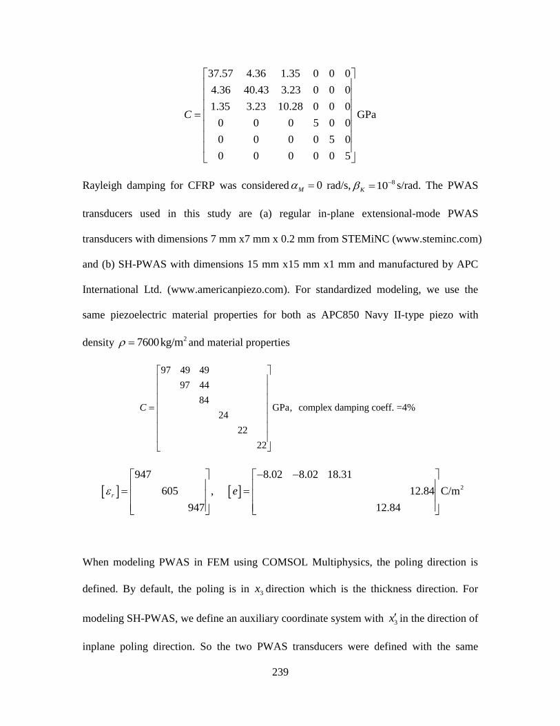
239
37.57 4.36 1.35 0 0 0
4.36 40.43 3.23 0 0 0
1.35 3.23 10.28 0 0 0GPa
0 0 0 5 0 0
0 0 0 0 5 0
0 0 0 0 0 5
C
Rayleigh damping for CFRP was considered 0M rad/s, 810K s/rad. The PWAS
transducers used in this study are (a) regular in-plane extensional-mode PWAS
transducers with dimensions 7 mm x7 mm x 0.2 mm from STEMiNC (www.steminc.com)
and (b) SH-PWAS with dimensions 15 mm x15 mm x1 mm and manufactured by APC
International Ltd. (www.americanpiezo.com). For standardized modeling, we use the
same piezoelectric material properties for both as APC850 Navy II-type piezo with
density 27600kg/m and material properties
97 49 49
97 44
84GPa, complex damping coeff. =4%
24
22
22
C
2
947 8.02 8.02 18.31
605 , 12.84 C/m
947 12.84
r e
When modeling PWAS in FEM using COMSOL Multiphysics, the poling direction is
defined. By default, the poling is in 3x direction which is the thickness direction. For
modeling SH-PWAS, we define an auxiliary coordinate system with 3x in the direction of
inplane poling direction. So the two PWAS transducers were defined with the same
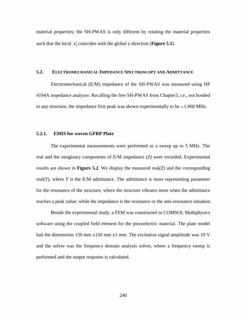
240
material properties; the SH-PWAS is only different by rotating the material properties
such that the local 3x coincides with the global y direction (Figure 5.1).
5.2. ELECTROMECHANICAL IMPEDANCE SPECTROSCOPY AND ADMITTANCE
Electromechanical (E/M) impedance of the SH-PWAS was measured using HP
4194A impedance analyzer. Recalling the free SH-PWAS from Chapter3, i.e., not bonded
to any structure, the impedance first peak was shown experimentally to be 1.060 MHz.
EMIS for woven GFRP Plate 5.2.1.
The experimental measurements were performed as a sweep up to 5 MHz. The
real and the imaginary components of E/M impedance (Z) were recorded. Experimental
results are shown in Figure 5.2. We display the measured real(Z) and the corresponding
real(Y), where Y is the E/M admittance. The admittance is more representing parameter
for the resonance of the structure, where the structure vibrates more when the admittance
reaches a peak value; while the impedance is the resistance or the anti-resonance situation.
Beside the experimental study, a FEM was constructed in COMSOL Multiphysics
software using the coupled field element for the piezoelectric material. The plate model
had the dimensions 150 mm x150 mm x1 mm. The excitation signal amplitude was 10 V
and the solver was the frequency domain analysis solver, where a frequency sweep is
performed and the output response is calculated.
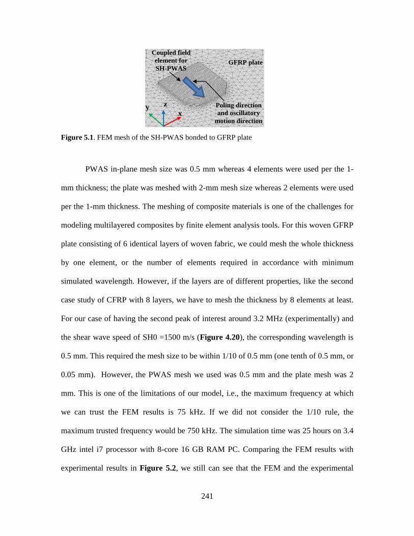
241
Figure 5.1. FEM mesh of the SH-PWAS bonded to GFRP plate
PWAS in-plane mesh size was 0.5 mm whereas 4 elements were used per the 1-
mm thickness; the plate was meshed with 2-mm mesh size whereas 2 elements were used
per the 1-mm thickness. The meshing of composite materials is one of the challenges for
modeling multilayered composites by finite element analysis tools. For this woven GFRP
plate consisting of 6 identical layers of woven fabric, we could mesh the whole thickness
by one element, or the number of elements required in accordance with minimum
simulated wavelength. However, if the layers are of different properties, like the second
case study of CFRP with 8 layers, we have to mesh the thickness by 8 elements at least.
For our case of having the second peak of interest around 3.2 MHz (experimentally) and
the shear wave speed of SH0 =1500 m/s (Figure 4.20), the corresponding wavelength is
0.5 mm. This required the mesh size to be within 1/10 of 0.5 mm (one tenth of 0.5 mm, or
0.05 mm). However, the PWAS mesh we used was 0.5 mm and the plate mesh was 2
mm. This is one of the limitations of our model, i.e., the maximum frequency at which
we can trust the FEM results is 75 kHz. If we did not consider the 1/10 rule, the
maximum trusted frequency would be 750 kHz. The simulation time was 25 hours on 3.4
GHz intel i7 processor with 8-core 16 GB RAM PC. Comparing the FEM results with
experimental results in Figure 5.2, we still can see that the FEM and the experimental
y z
x
Coupled field
element for
SH-PWAS
Poling direction
and oscillatory
motion direction
GFRP plate
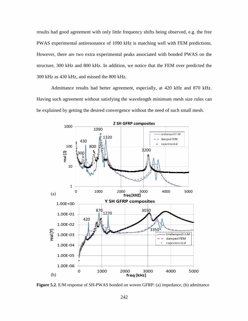
242
results had good agreement with only little frequency shifts being observed, e.g. the free
PWAS experimental antiresonance of 1090 kHz is matching well with FEM predictions.
However, there are two extra experimental peaks associated with bonded PWAS on the
structure, 300 kHz and 800 kHz. In addition, we notice that the FEM over predicted the
300 kHz as 430 kHz, and missed the 800 kHz.
Admittance results had better agreement, especially, at 420 kHz and 870 kHz.
Having such agreement without satisfying the wavelength minimum mesh size rules can
be explained by getting the desired convergence without the need of such small mesh.
Figure 5.2. E/M response of SH-PWAS bonded on woven GFRP: (a) impedance, (b) admittance
430 800
1090
1320
870
300 3200
420
1270
3350
3030
(a)
(b)
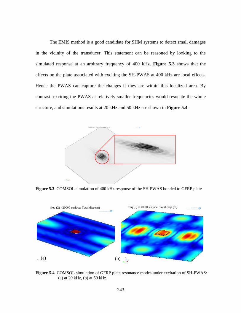
243
The EMIS method is a good candidate for SHM systems to detect small damages
in the vicinity of the transducer. This statement can be reasoned by looking to the
simulated response at an arbitrary frequency of 400 kHz. Figure 5.3 shows that the
effects on the plate associated with exciting the SH-PWAS at 400 kHz are local effects.
Hence the PWAS can capture the changes if they are within this localized area. By
contrast, exciting the PWAS at relatively smaller frequencies would resonate the whole
structure, and simulations results at 20 kHz and 50 kHz are shown in Figure 5.4.
Figure 5.3. COMSOL simulation of 400 kHz response of the SH-PWAS bonded to GFRP plate
Figure 5.4. COMSOL simulation of GFRP plate resonance modes under excitation of SH-PWAS:
(a) at 20 kHz, (b) at 50 kHz.
(a) (b)
freq (2) =20000 surface: Total disp (m) freq (5) =50000 surface: Total disp (m)
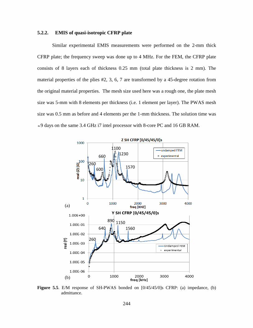
244
EMIS of quasi-isotropic CFRP plate 5.2.2.
Similar experimental EMIS measurements were performed on the 2-mm thick
CFRP plate; the frequency sweep was done up to 4 MHz. For the FEM, the CFRP plate
consists of 8 layers each of thickness 0.25 mm (total plate thickness is 2 mm). The
material properties of the plies #2, 3, 6, 7 are transformed by a 45-degree rotation from
the original material properties. The mesh size used here was a rough one, the plate mesh
size was 5-mm with 8 elements per thickness (i.e. 1 element per layer). The PWAS mesh
size was 0.5 mm as before and 4 elements per the 1-mm thickness. The solution time was
9 days on the same 3.4 GHz i7 intel processor with 8-core PC and 16 GB RAM.
Figure 5.5. E/M response of SH-PWAS bonded on [0/45/45/0]s CFRP: (a) impedance, (b)
admittance.
1100
660 1230
1570 600 260
260
640
890 1150
1560
(a)
(b)
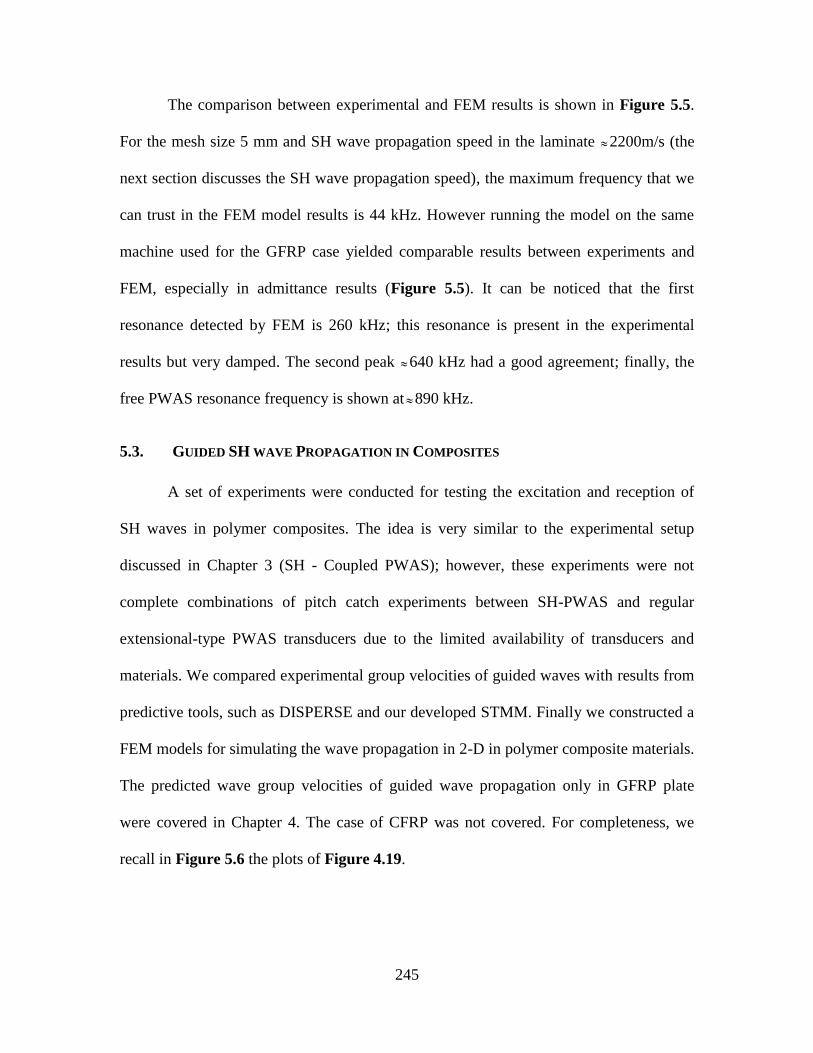
245
The comparison between experimental and FEM results is shown in Figure 5.5.
For the mesh size 5 mm and SH wave propagation speed in the laminate 2200m/s (the
next section discusses the SH wave propagation speed), the maximum frequency that we
can trust in the FEM model results is 44 kHz. However running the model on the same
machine used for the GFRP case yielded comparable results between experiments and
FEM, especially in admittance results (Figure 5.5). It can be noticed that the first
resonance detected by FEM is 260 kHz; this resonance is present in the experimental
results but very damped. The second peak 640 kHz had a good agreement; finally, the
free PWAS resonance frequency is shown at 890 kHz.
5.3. GUIDED SH WAVE PROPAGATION IN COMPOSITES
A set of experiments were conducted for testing the excitation and reception of
SH waves in polymer composites. The idea is very similar to the experimental setup
discussed in Chapter 3 (SH - Coupled PWAS); however, these experiments were not
complete combinations of pitch catch experiments between SH-PWAS and regular
extensional-type PWAS transducers due to the limited availability of transducers and
materials. We compared experimental group velocities of guided waves with results from
predictive tools, such as DISPERSE and our developed STMM. Finally we constructed a
FEM models for simulating the wave propagation in 2-D in polymer composite materials.
The predicted wave group velocities of guided wave propagation only in GFRP plate
were covered in Chapter 4. The case of CFRP was not covered. For completeness, we
recall in Figure 5.6 the plots of Figure 4.19.
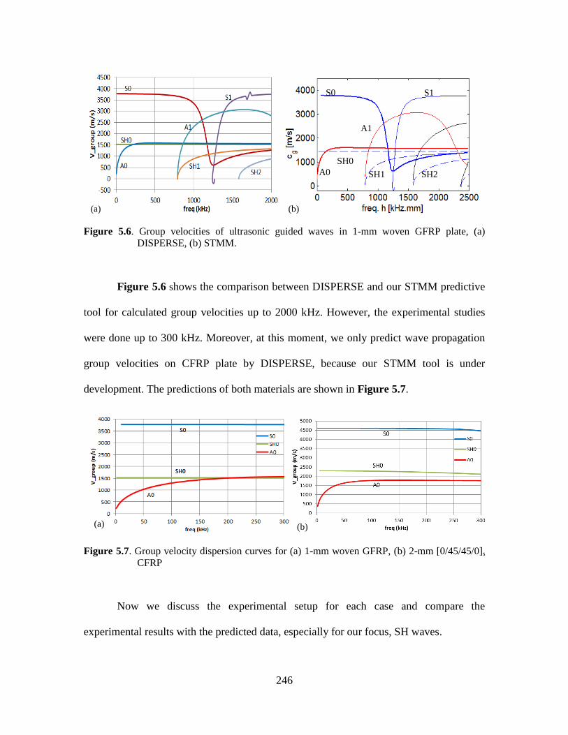
246
Figure 5.6. Group velocities of ultrasonic guided waves in 1-mm woven GFRP plate, (a)
DISPERSE, (b) STMM.
Figure 5.6 shows the comparison between DISPERSE and our STMM predictive
tool for calculated group velocities up to 2000 kHz. However, the experimental studies
were done up to 300 kHz. Moreover, at this moment, we only predict wave propagation
group velocities on CFRP plate by DISPERSE, because our STMM tool is under
development. The predictions of both materials are shown in Figure 5.7.
Figure 5.7. Group velocity dispersion curves for (a) 1-mm woven GFRP, (b) 2-mm [0/45/45/0]s
CFRP
Now we discuss the experimental setup for each case and compare the
experimental results with the predicted data, especially for our focus, SH waves.
(b) (a)
A0 SH0
S0
SH1
A1
S1
SH2
(a) (b)
247
Experimental Study for GFRP 5.3.1.
The schematic setup (Figure 5.8) shows two installed SH-PWAS (#7 and #8) and
two regular PWAS (#1 and #2). The distance between PWAS transducers is 120 mm.
Pitch catch experiments were conducted by exciting PWAS transducers in turns with 3-
count tone burst signals with 10V amplitude and sweep the center frequency up to 300
kHz.
Experiment-1 was done between the two SH-PWAS transducers, #7 and #8, by
exciting SH-PWAS7 and receiving at SH-PWAS8; three types of waves were picked at
the receiver SH-PWAS8, symmetric S0, antisymmetric A0 and SH0 (Figure 5.10a).
In experiment-2, the excitation was done by SH-PWAS7 and reception by
PWAS1; we can see from Figure 5.10c that PWAS1 picked up SH0 waves as well as the
expected S0 and A0. This interesting feature was also observed in isotropic aluminum
plate. In experiment-3, the excitation was done by the regular PWAS1; the receiver SH-
PWAS7 picked up SH waves. PWAS1 is supposed to excite only Lamb-type waves;
however, SH0 waves were picked up by SH-PWAS7. Experiment-3 was exactly identical
to experiment-2 (Figure 5.10c).
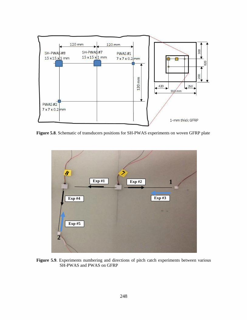
248
Figure 5.8. Schematic of transducers positions for SH-PWAS experiments on woven GFRP plate
Figure 5.9. Experiments numbering and directions of pitch catch experiments between various
SH-PWAS and PWAS on GFRP
Exp #2 Exp #1
Exp #5
Exp #3
2
1
Exp #4
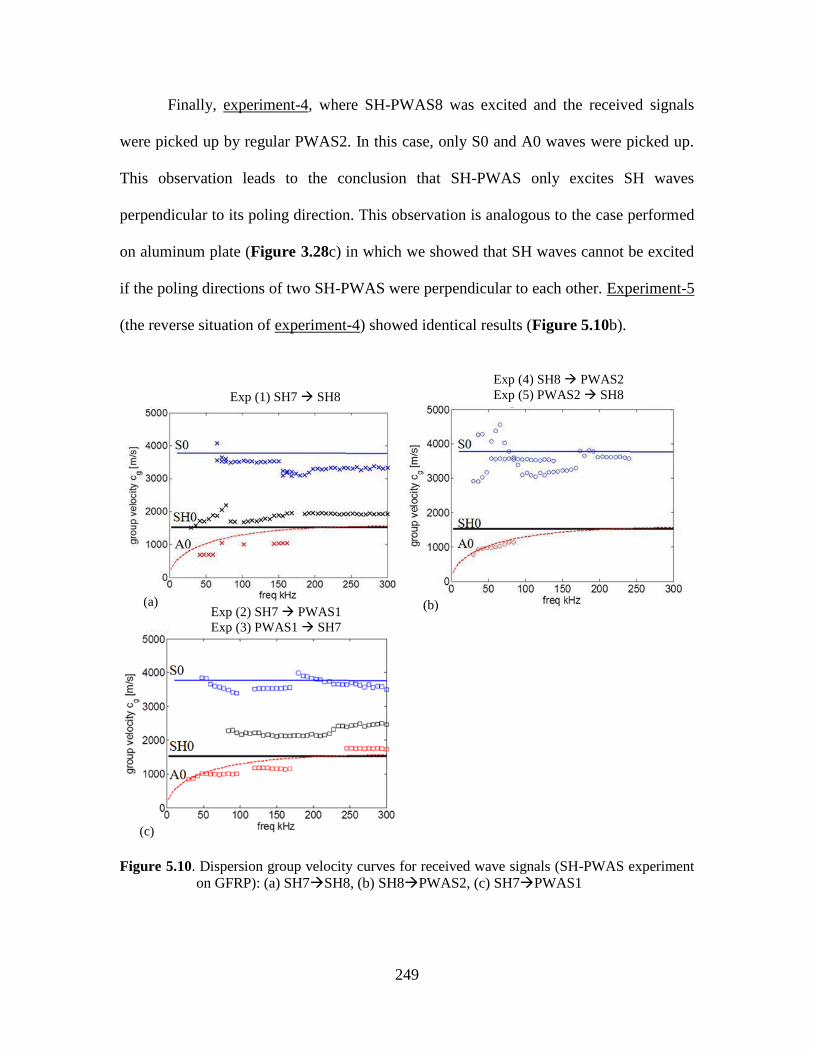
249
Finally, experiment-4, where SH-PWAS8 was excited and the received signals
were picked up by regular PWAS2. In this case, only S0 and A0 waves were picked up.
This observation leads to the conclusion that SH-PWAS only excites SH waves
perpendicular to its poling direction. This observation is analogous to the case performed
on aluminum plate (Figure 3.28c) in which we showed that SH waves cannot be excited
if the poling directions of two SH-PWAS were perpendicular to each other. Experiment-5
(the reverse situation of experiment-4) showed identical results (Figure 5.10b).
Figure 5.10. Dispersion group velocity curves for received wave signals (SH-PWAS experiment
on GFRP): (a) SH7SH8, (b) SH8PWAS2, (c) SH7PWAS1
(a) (b)
Exp (4) SH8 PWAS2
Exp (5) PWAS2 SH8 Exp (1) SH7 SH8
(c)
Exp (2) SH7 PWAS1
Exp (3) PWAS1 SH7
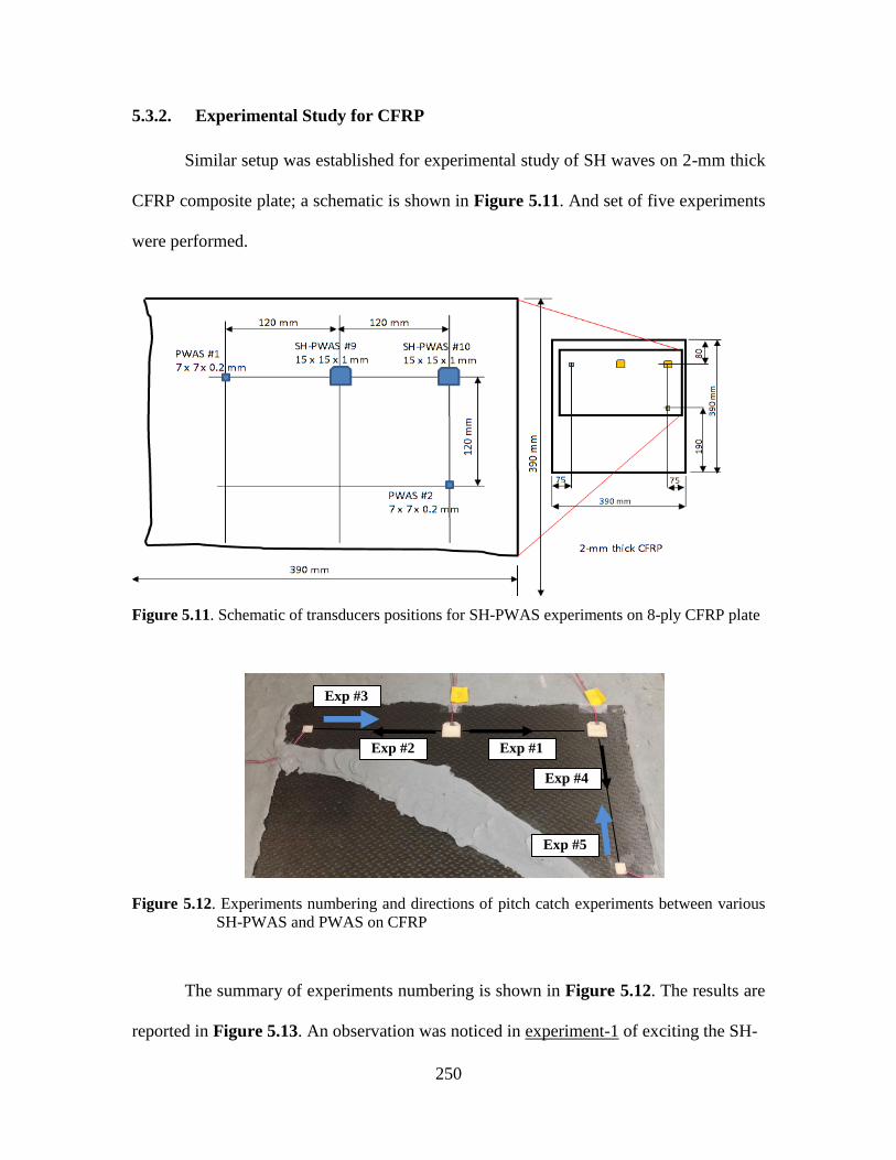
250
Experimental Study for CFRP 5.3.2.
Similar setup was established for experimental study of SH waves on 2-mm thick
CFRP composite plate; a schematic is shown in Figure 5.11. And set of five experiments
were performed.
Figure 5.11. Schematic of transducers positions for SH-PWAS experiments on 8-ply CFRP plate
Figure 5.12. Experiments numbering and directions of pitch catch experiments between various
SH-PWAS and PWAS on CFRP
The summary of experiments numbering is shown in Figure 5.12. The results are
reported in Figure 5.13. An observation was noticed in experiment-1 of exciting the SH-
Exp #2 Exp #1
Exp #3
Exp #4
Exp #5
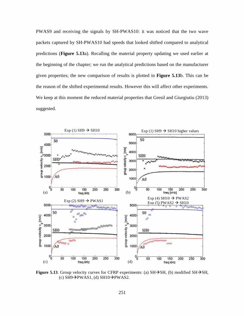
251
PWAS9 and receiving the signals by SH-PWAS10: it was noticed that the two wave
packets captured by SH-PWAS10 had speeds that looked shifted compared to analytical
predictions (Figure 5.13a). Recalling the material property updating we used earlier at
the beginning of the chapter; we run the analytical predictions based on the manufacturer
given properties; the new comparison of results is plotted in Figure 5.13b. This can be
the reason of the shifted experimental results. However this will affect other experiments.
We keep at this moment the reduced material properties that Gresil and Giurgiutiu (2013)
suggested.
Figure 5.13. Group velocity curves for CFRP experiments: (a) SHSH, (b) modified SHSH,
(c) SH9PWAS1, (d) SH10PWAS2.
(c) (d)
(a) (b)
Exp (4) SH10 PWAS2 Exp (5) PWAS2 SH10
Exp (1) SH9 SH10 higher values Exp (1) SH9 SH10
Exp (2) SH9 PWAS1
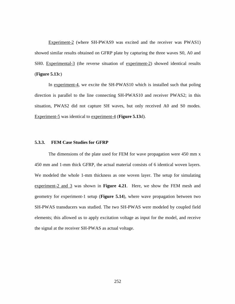
252
Experiment-2 (where SH-PWAS9 was excited and the receiver was PWAS1)
showed similar results obtained on GFRP plate by capturing the three waves S0, A0 and
SH0. Experimental-3 (the reverse situation of experiment-2) showed identical results
(Figure 5.13c)
In experiment-4, we excite the SH-PWAS10 which is installed such that poling
direction is parallel to the line connecting SH-PWAS10 and receiver PWAS2; in this
situation, PWAS2 did not capture SH waves, but only received A0 and S0 modes.
Experiment-5 was identical to experiment-4 (Figure 5.13d).
FEM Case Studies for GFRP 5.3.3.
The dimensions of the plate used for FEM for wave propagation were 450 mm x
450 mm and 1-mm thick GFRP, the actual material consists of 6 identical woven layers.
We modeled the whole 1-mm thickness as one woven layer. The setup for simulating
experiment-2 and 3 was shown in Figure 4.21. Here, we show the FEM mesh and
geometry for experiment-1 setup (Figure 5.14), where wave propagation between two
SH-PWAS transducers was studied. The two SH-PWAS were modeled by coupled field
elements; this allowed us to apply excitation voltage as input for the model, and receive
the signal at the receiver SH-PWAS as actual voltage.
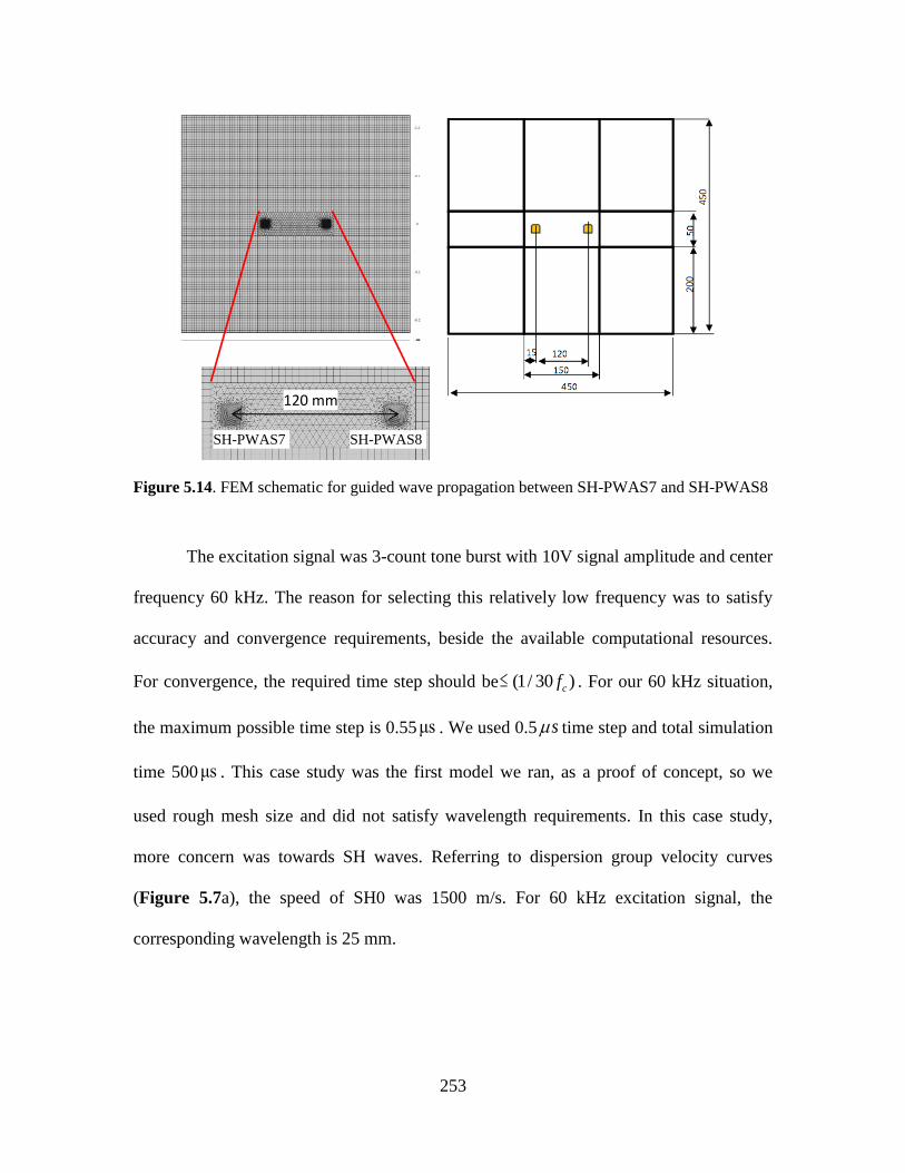
253
Figure 5.14. FEM schematic for guided wave propagation between SH-PWAS7 and SH-PWAS8
The excitation signal was 3-count tone burst with 10V signal amplitude and center
frequency 60 kHz. The reason for selecting this relatively low frequency was to satisfy
accuracy and convergence requirements, beside the available computational resources.
For convergence, the required time step should be (1/ 30 )cf . For our 60 kHz situation,
the maximum possible time step is 0.55μs . We used 0.5 s time step and total simulation
time 500μs . This case study was the first model we ran, as a proof of concept, so we
used rough mesh size and did not satisfy wavelength requirements. In this case study,
more concern was towards SH waves. Referring to dispersion group velocity curves
(Figure 5.7a), the speed of SH0 was 1500 m/s. For 60 kHz excitation signal, the
corresponding wavelength is 25 mm.
SH-PWAS7
120 mm
SH-PWAS8
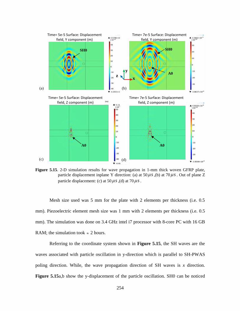
254
Figure 5.15. 2-D simulation results for wave propagation in 1-mm thick woven GFRP plate,
particle displacement inplane Y direction: (a) at 50 s ,(b) at 70 s . Out of plane Z
particle displacement: (c) at 50 s ,(d) at 70 s .
Mesh size used was 5 mm for the plate with 2 elements per thickness (i.e. 0.5
mm). Piezoelectric element mesh size was 1 mm with 2 elements per thickness (i.e. 0.5
mm). The simulation was done on 3.4 GHz intel i7 processor with 8-core PC with 16 GB
RAM; the simulation took 2 hours.
Referring to the coordinate system shown in Figure 5.15, the SH waves are the
waves associated with particle oscillation in y-direction which is parallel to SH-PWAS
poling direction. While, the wave propagation direction of SH waves is x direction.
Figure 5.15a,b show the y-displacement of the particle oscillation. SH0 can be noticed
Time= 5e-5 Surface: Displacement field, Y component (m)
Time= 5e-5 Surface: Displacement field, Z component (m)
Time= 7e-5 Surface: Displacement field, Y component (m)
Time= 7e-5 Surface: Displacement field, Z component (m)
SH0
A0 A0
SH0
A0
(b) (a)
(d) (c)
y z
x
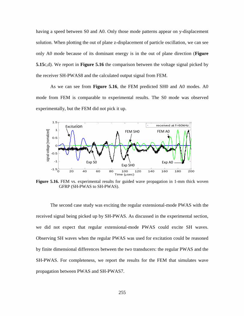
255
having a speed between S0 and A0. Only those mode patterns appear on y-displacement
solution. When plotting the out of plane z-displacement of particle oscillation, we can see
only A0 mode because of its dominant energy is in the out of plane direction (Figure
5.15c,d). We report in Figure 5.16 the comparison between the voltage signal picked by
the receiver SH-PWAS8 and the calculated output signal from FEM.
As we can see from Figure 5.16, the FEM predicted SH0 and A0 modes. A0
mode from FEM is comparable to experimental results. The S0 mode was observed
experimentally, but the FEM did not pick it up.
Figure 5.16. FEM vs. experimental results for guided wave propagation in 1-mm thick woven
GFRP (SH-PWAS to SH-PWAS).
The second case study was exciting the regular extensional-mode PWAS with the
received signal being picked up by SH-PWAS. As discussed in the experimental section,
we did not expect that regular extensional-mode PWAS could excite SH waves.
Observing SH waves when the regular PWAS was used for excitation could be reasoned
by finite dimensional differences between the two transducers: the regular PWAS and the
SH-PWAS. For completeness, we report the results for the FEM that simulates wave
propagation between PWAS and SH-PWAS7.
0 20 40 60 80 100 120 140 160 180 200-1.5
-1
-0.5
0
0.5
1
1.5
sign
al v
olta
ge [n
omal
ized
]
Time (sec)
received at f=60kHz
Exp A0
FEM A0 FEM SH0
Exp SH0 Exp S0
Excitation
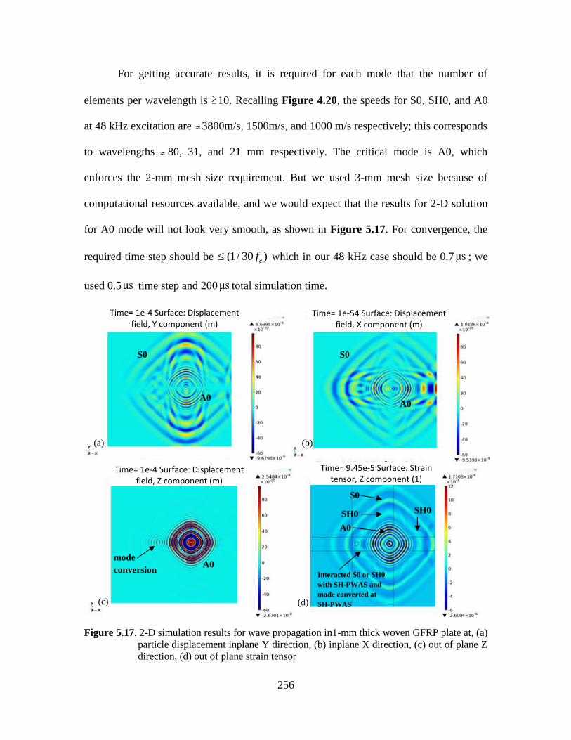
256
For getting accurate results, it is required for each mode that the number of
elements per wavelength is 10. Recalling Figure 4.20, the speeds for S0, SH0, and A0
at 48 kHz excitation are 3800m/s, 1500m/s, and 1000 m/s respectively; this corresponds
to wavelengths 80, 31, and 21 mm respectively. The critical mode is A0, which
enforces the 2-mm mesh size requirement. But we used 3-mm mesh size because of
computational resources available, and we would expect that the results for 2-D solution
for A0 mode will not look very smooth, as shown in Figure 5.17. For convergence, the
required time step should be (1/ 30 )cf which in our 48 kHz case should be 0.7μs ; we
used 0.5μs time step and 200μs total simulation time.
Figure 5.17. 2-D simulation results for wave propagation in1-mm thick woven GFRP plate at, (a)
particle displacement inplane Y direction, (b) inplane X direction, (c) out of plane Z
direction, (d) out of plane strain tensor
Time= 1e-4 Surface: Displacement field, Y component (m)
Time= 1e-4 Surface: Displacement field, Z component (m)
Time= 1e-54 Surface: Displacement field, X component (m)
Time= 9.45e-5 Surface: Strain tensor, Z component (1)
S0
S0
A0 mode
conversion
A0
SH0
A0
Interacted S0 or SH0
with SH-PWAS and
mode converted at
SH-PWAS
SH0
S0
A0
(b) (a)
(d) (c)
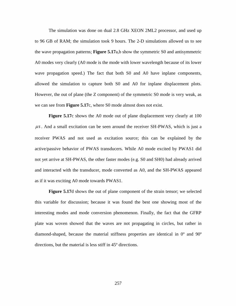
257
The simulation was done on dual 2.8 GHz XEON 2ML2 processor, and used up
to 96 GB of RAM; the simulation took 9 hours. The 2-D simulations allowed us to see
the wave propagation patterns; Figure 5.17a,b show the symmetric S0 and antisymmetric
A0 modes very clearly (A0 mode is the mode with lower wavelength because of its lower
wave propagation speed.) The fact that both S0 and A0 have inplane components,
allowed the simulation to capture both S0 and A0 for inplane displacement plots.
However, the out of plane (the Z component) of the symmetric S0 mode is very weak, as
we can see from Figure 5.17c, where S0 mode almost does not exist.
Figure 5.17c shows the A0 mode out of plane displacement very clearly at 100
s . And a small excitation can be seen around the receiver SH-PWAS, which is just a
receiver PWAS and not used as excitation source; this can be explained by the
active/passive behavior of PWAS transducers. While A0 mode excited by PWAS1 did
not yet arrive at SH-PWAS, the other faster modes (e.g. S0 and SH0) had already arrived
and interacted with the transducer, mode converted as A0, and the SH-PWAS appeared
as if it was exciting A0 mode towards PWAS1.
Figure 5.17d shows the out of plane component of the strain tensor; we selected
this variable for discussion; because it was found the best one showing most of the
interesting modes and mode conversion phenomenon. Finally, the fact that the GFRP
plate was woven showed that the waves are not propagating in circles, but rather in
diamond-shaped, because the material stiffness properties are identical in 0º and 90º
directions, but the material is less stiff in 45º directions.
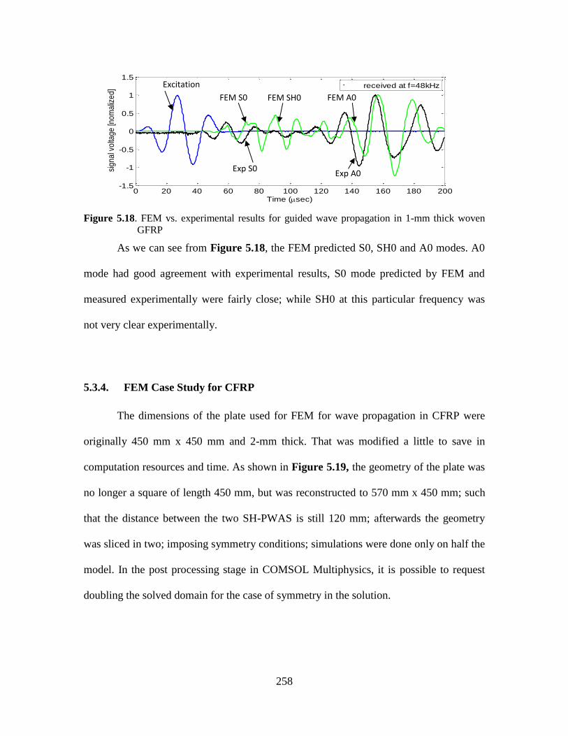
258
Figure 5.18. FEM vs. experimental results for guided wave propagation in 1-mm thick woven
GFRP
As we can see from Figure 5.18, the FEM predicted S0, SH0 and A0 modes. A0
mode had good agreement with experimental results, S0 mode predicted by FEM and
measured experimentally were fairly close; while SH0 at this particular frequency was
not very clear experimentally.
FEM Case Study for CFRP 5.3.4.
The dimensions of the plate used for FEM for wave propagation in CFRP were
originally 450 mm x 450 mm and 2-mm thick. That was modified a little to save in
computation resources and time. As shown in Figure 5.19, the geometry of the plate was
no longer a square of length 450 mm, but was reconstructed to 570 mm x 450 mm; such
that the distance between the two SH-PWAS is still 120 mm; afterwards the geometry
was sliced in two; imposing symmetry conditions; simulations were done only on half the
model. In the post processing stage in COMSOL Multiphysics, it is possible to request
doubling the solved domain for the case of symmetry in the solution.
0 20 40 60 80 100 120 140 160 180 200-1.5
-1
-0.5
0
0.5
1
1.5
sig
na
l vo
ltag
e [n
om
aliz
ed
]
Time (sec)
received at f=48kHzExcitation
Exp S0
FEM SH0
Exp A0
FEM S0 FEM A0
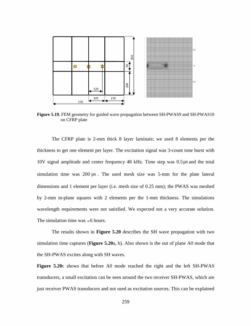
259
Figure 5.19. FEM geometry for guided wave propagation between SH-PWAS9 and SH-PWAS10
on CFRP plate
The CFRP plate is 2-mm thick 8 layer laminate; we used 8 elements per the
thickness to get one element per layer. The excitation signal was 3-count tone burst with
10V signal amplitude and center frequency 48 kHz. Time step was 0.5μs and the total
simulation time was 200 μs . The used mesh size was 5-mm for the plate lateral
dimensions and 1 element per layer (i.e. mesh size of 0.25 mm); the PWAS was meshed
by 2-mm in-plane squares with 2 elements per the 1-mm thickness. The simulations
wavelength requirements were not satisfied. We expected not a very accurate solution.
The simulation time was 6 hours.
The results shown in Figure 5.20 describes the SH wave propagation with two
simulation time captures (Figure 5.20a, b). Also shown is the out of plane A0 mode that
the SH-PWAS excites along with SH waves.
Figure 5.20c shows that before A0 mode reached the right and the left SH-PWAS
transducers, a small excitation can be seen around the two receiver SH-PWAS, which are
just receiver PWAS transducers and not used as excitation sources. This can be explained
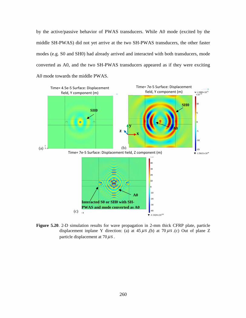
260
by the active/passive behavior of PWAS transducers. While A0 mode (excited by the
middle SH-PWAS) did not yet arrive at the two SH-PWAS transducers, the other faster
modes (e.g. S0 and SH0) had already arrived and interacted with both transducers, mode
converted as A0, and the two SH-PWAS transducers appeared as if they were exciting
A0 mode towards the middle PWAS.
Figure 5.20. 2-D simulation results for wave propagation in 2-mm thick CFRP plate, particle
displacement inplane Y direction: (a) at 45 s ,(b) at 70 s .(c) Out of plane Z
particle displacement at 70 s .
Time= 4.5e-5 Surface: Displacement field, Y component (m)
Time= 7e-5 Surface: Displacement field, Y component (m)
Time= 7e-5 Surface: Displacement field, Z component (m)
SH0
Interacted S0 or SH0 with SH-
PWAS and mode converted as A0
A0
SH0
A0
(b) (a)
(c)
y z
x
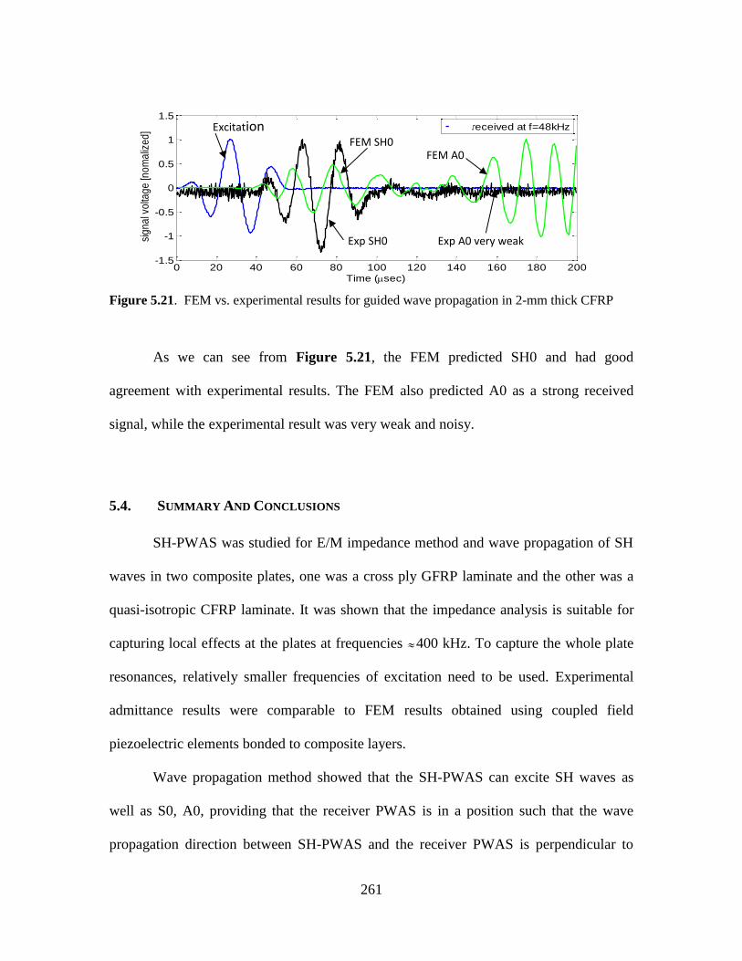
261
Figure 5.21. FEM vs. experimental results for guided wave propagation in 2-mm thick CFRP
As we can see from Figure 5.21, the FEM predicted SH0 and had good
agreement with experimental results. The FEM also predicted A0 as a strong received
signal, while the experimental result was very weak and noisy.
5.4. SUMMARY AND CONCLUSIONS
SH-PWAS was studied for E/M impedance method and wave propagation of SH
waves in two composite plates, one was a cross ply GFRP laminate and the other was a
quasi-isotropic CFRP laminate. It was shown that the impedance analysis is suitable for
capturing local effects at the plates at frequencies 400 kHz. To capture the whole plate
resonances, relatively smaller frequencies of excitation need to be used. Experimental
admittance results were comparable to FEM results obtained using coupled field
piezoelectric elements bonded to composite layers.
Wave propagation method showed that the SH-PWAS can excite SH waves as
well as S0, A0, providing that the receiver PWAS is in a position such that the wave
propagation direction between SH-PWAS and the receiver PWAS is perpendicular to
0 20 40 60 80 100 120 140 160 180 200-1.5
-1
-0.5
0
0.5
1
1.5
sig
na
l vo
ltag
e [n
om
aliz
ed
]
Time (sec)
received at f=48kHzExcitation
Exp SH0
FEM SH0
Exp A0 very weak
FEM A0

262
SH-PWAS poling direction. If we excite SH-PWAS and receive the signal along a
direction parallel to the poling direction, only A0 and S0 waves were captured. These
phenomena were observed in both GFRP cross ply laminate and CFRP quasi-isotropic
laminate.
2-D FEM wave propagation simulation showed the wave propagation patterns of
SH waves. The mesh size used was not satisfying the accuracy conditions of wavelength
and mesh size because of our limited computational resources; nevertheless, the overall
wave propagation showed consistent results with our expectations. The received signals
predicted by FEM were compared with experimentally measured voltage signals. For the
experiment between two SH-PWAS in GFRP, there was a little shift between received
SH0 waves, but a good match for A0 mode. Predictive models of transmitted waves from
a regular PWAS showed three waves: A0, S0 and SH0; however the experimental results
did not show a strong SH0 signal.
Moreover, for CFRP simulations, there was a good match between SH0 mode
predicted by FEM and measured experimentally. On the other hand, A0 was captured by
FEM, but it was not detected experimentally.
SH-PWAS is a good transducer for generating SH waves in composite materials,
and it is way less expensive than EMAT transducers; this makes it a potential candidate
for composites SHM.
263
CHAPTER 6: GUIDED WAVE DAMAGE DETECTION IN AN AEROSPACE
PANEL
The objective of this chapter is to test and to apply the basic theory that was covered in
previous chapters on a realistic complex structure for detecting simulated damages. Of
course, this will require more advanced system with some damage detection algorithms.
We used a realistic aging aircraft specimen that was fabricated at Sandia National Lab
with simulated aging-like induced damage. We presented the SHM system we used; it
was developed by Metis Design (www.metisdesign.com). Brief description of sensors
installation and system operation was addressed. Finally we proposed the tests that we
will perform.
6.1. MATERIALS
The aging aircraft specimen was fabricated at Sandia National Lab with simulated
aging-like induced damage (cracks and corrosion). It is made of 1-mm ( 0.040 ) 2024-T3
Al-clad sheets assembled with 4.2-mm ( 0.166 ) diameter countersunk rivets, with a U-
shaped (BAC 1498-152 stringer), as shown in Figure 6.1.

264
Figure 6.1. Image of the 2024-T3 Al plate under test
This plate was used before for testing certain simulated damages that were
included in the blue print (Figure 6.2) developed at Sandia National Laboratory. The
detailed experimental setup and results were reported in Giurgiutiu et al. (2002).
Figure 6.2. Blue print of the experimental panel developed at Sandia National Lab.
6.2. EXPERIMENTAL SET UP FOR MD7 ANALOG SENSOR-ASSEMBLE SYSTEM
The hardware is developed by Metis Design (www.metisdesign.com) and it
includes (1) piezoelectric-based damage localization sensors (MD7 VectorLocator™), (2)
distributed digitization hardware (MD7 IntelliConnector™), and (3) a data accumulation
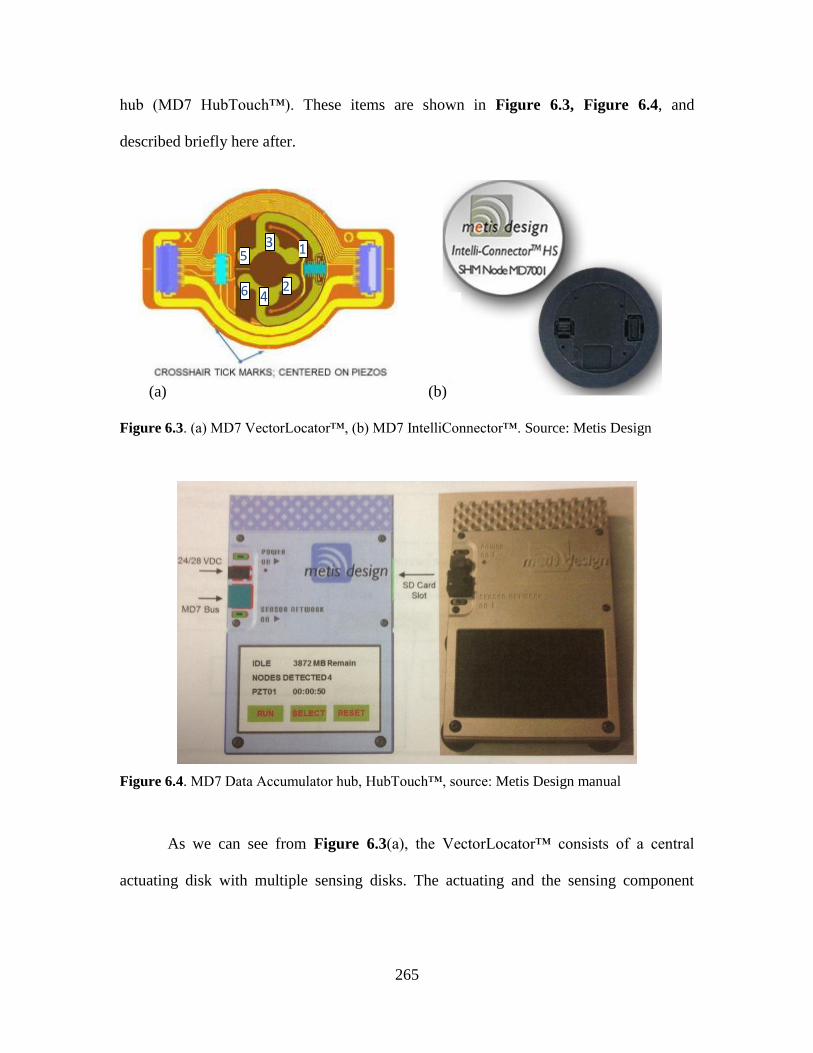
265
hub (MD7 HubTouch™). These items are shown in Figure 6.3, Figure 6.4, and
described briefly here after.
Figure 6.3. (a) MD7 VectorLocator™, (b) MD7 IntelliConnector™. Source: Metis Design
Figure 6.4. MD7 Data Accumulator hub, HubTouch™, source: Metis Design manual
As we can see from Figure 6.3(a), the VectorLocator™ consists of a central
actuating disk with multiple sensing disks. The actuating and the sensing component
1 3 5
2 4 6
(a) (b)
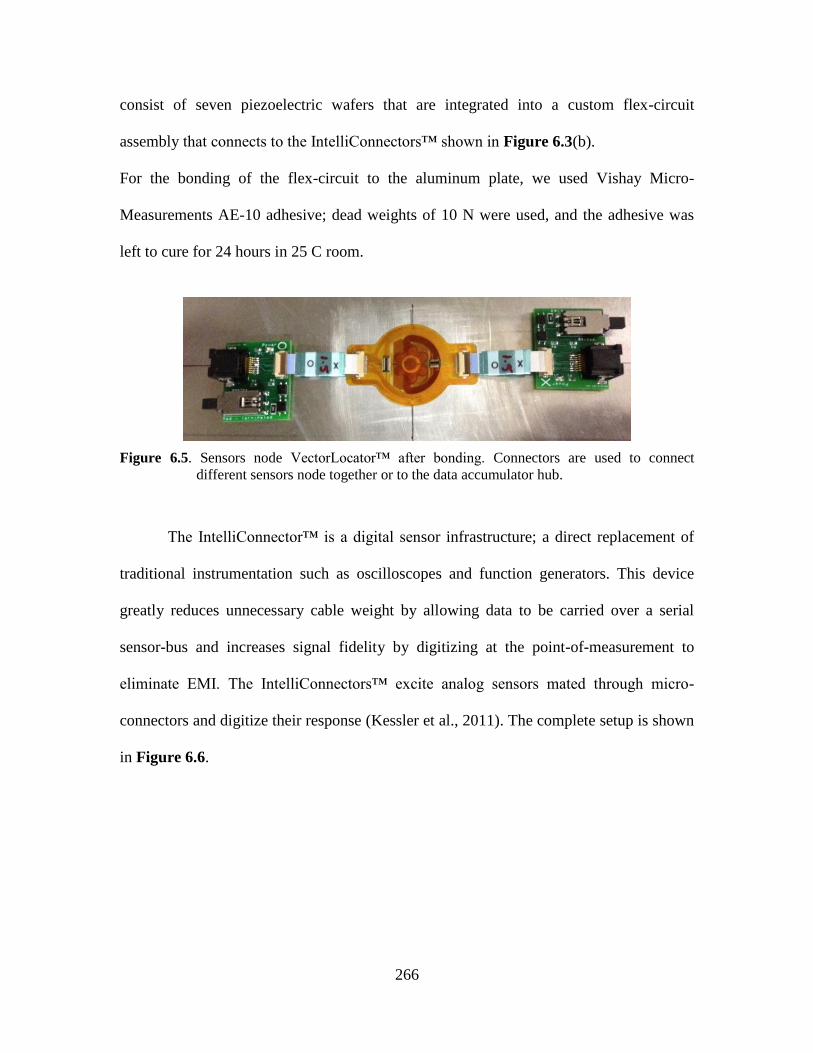
266
consist of seven piezoelectric wafers that are integrated into a custom flex-circuit
assembly that connects to the IntelliConnectors™ shown in Figure 6.3(b).
For the bonding of the flex-circuit to the aluminum plate, we used Vishay Micro-
Measurements AE-10 adhesive; dead weights of 10 N were used, and the adhesive was
left to cure for 24 hours in 25 C room.
Figure 6.5. Sensors node VectorLocator™ after bonding. Connectors are used to connect
different sensors node together or to the data accumulator hub.
The IntelliConnector™ is a digital sensor infrastructure; a direct replacement of
traditional instrumentation such as oscilloscopes and function generators. This device
greatly reduces unnecessary cable weight by allowing data to be carried over a serial
sensor-bus and increases signal fidelity by digitizing at the point-of-measurement to
eliminate EMI. The IntelliConnectors™ excite analog sensors mated through micro-
connectors and digitize their response (Kessler et al., 2011). The complete setup is shown
in Figure 6.6.
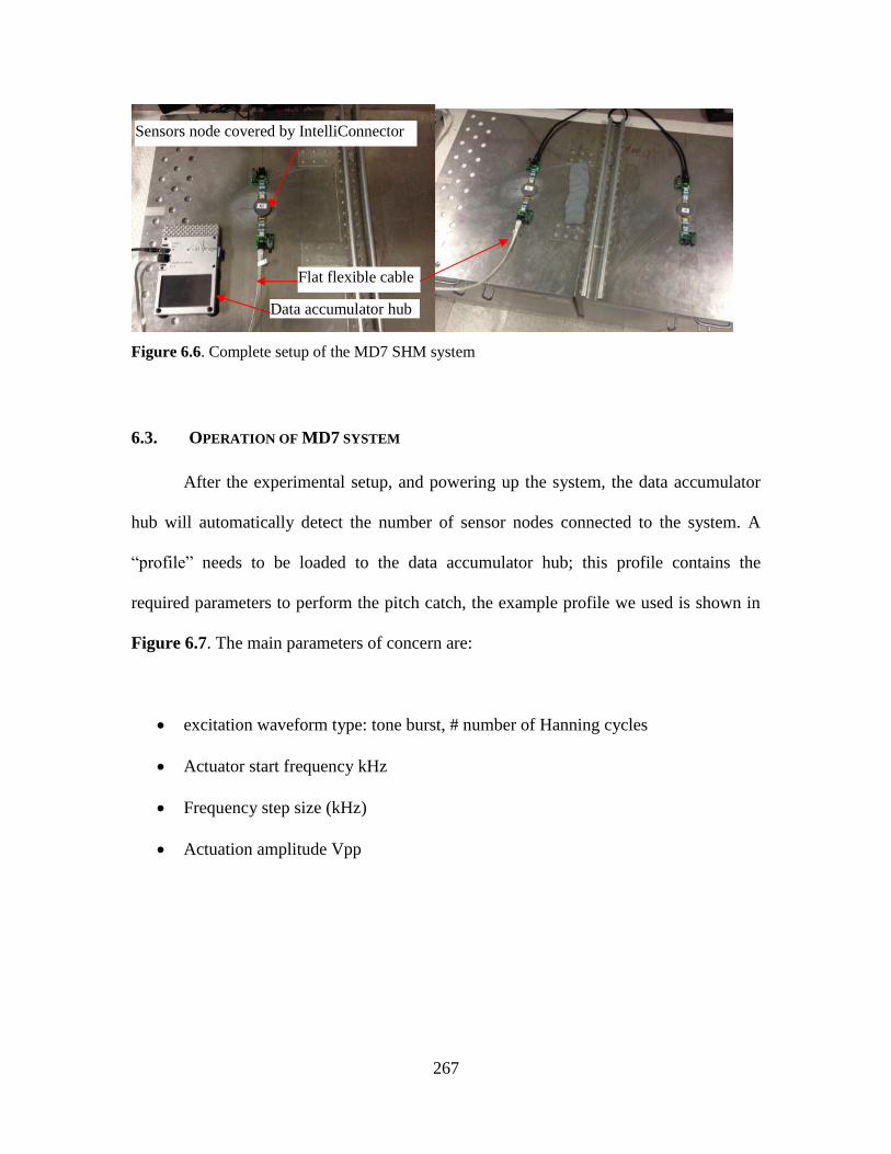
267
Figure 6.6. Complete setup of the MD7 SHM system
6.3. OPERATION OF MD7 SYSTEM
After the experimental setup, and powering up the system, the data accumulator
hub will automatically detect the number of sensor nodes connected to the system. A
“profile” needs to be loaded to the data accumulator hub; this profile contains the
required parameters to perform the pitch catch, the example profile we used is shown in
Figure 6.7. The main parameters of concern are:
excitation waveform type: tone burst, # number of Hanning cycles
Actuator start frequency kHz
Frequency step size (kHz)
Actuation amplitude Vpp
Data accumulator hub
Sensors node covered by IntelliConnector
Flat flexible cable
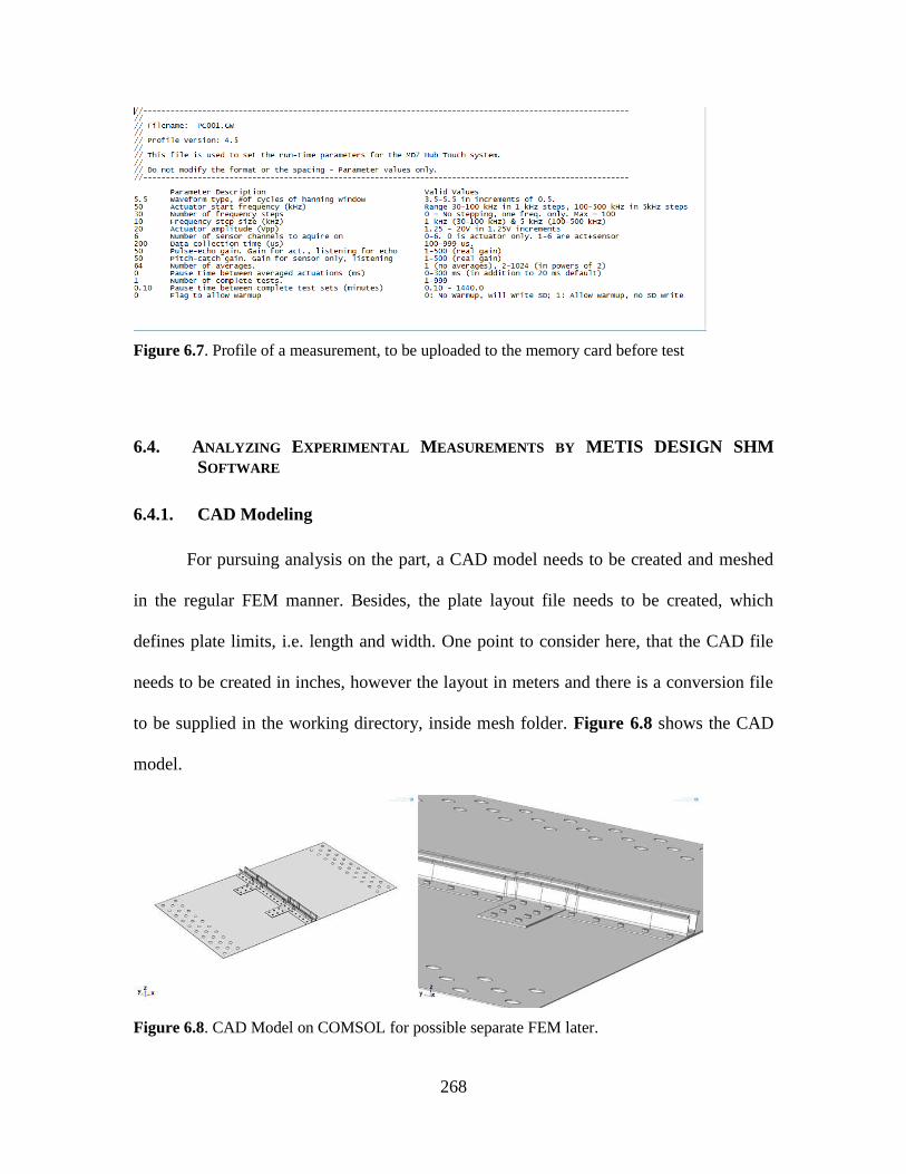
268
Figure 6.7. Profile of a measurement, to be uploaded to the memory card before test
6.4. ANALYZING EXPERIMENTAL MEASUREMENTS BY METIS DESIGN SHM
SOFTWARE
CAD Modeling 6.4.1.
For pursuing analysis on the part, a CAD model needs to be created and meshed
in the regular FEM manner. Besides, the plate layout file needs to be created, which
defines plate limits, i.e. length and width. One point to consider here, that the CAD file
needs to be created in inches, however the layout in meters and there is a conversion file
to be supplied in the working directory, inside mesh folder. Figure 6.8 shows the CAD
model.
Figure 6.8. CAD Model on COMSOL for possible separate FEM later.

269
FEM Meshing 6.4.2.
The CAD file is then imported into a finite element modeling software package
for automatic meshing, typically ANSYS is the software that the Metis Design uses with
the help of ANSYS script to perform meshing directly.
Typical exported mesh files are (1) the nodes list which specifies the node number and its
coordinates, (2) the elements list, which specifies the element number and its connectivity
with nodes (Figure 6.9).
Figure 6.9. Exported mesh files and move.txt file for relative position, rotation and unit
conversion
Once the mesh files are generated, it is ready to use the Metis Design software
package for SHM, the starting windows is shown in Figure 6.10.

270
Figure 6.10. Module launcher for Metis Design software package
Our main focus here is not about DAQ optimization and modeling, neither the
optimal sensor placement. But in general, the purpose of the DAQ optimization module is
to import preliminary data from small set of sensors and the measured pitch-catch data
for example; for the goal of optimizing the full scale testing. Also it aims to estimate
statistical model parameters for sensors, e.g. the frequency at which the signals are
having the maximum average, the global maxima, and the global standard deviations.
This is used to calculate the frequency at which the signal to noise ratio (SNR) is the
maximum.
Optimal sensor placement module:
The purpose of this module is to determine the optimal arrangement of specified
number of sensors, given the statistical signal model parameters from previous module.
This module exports to the layout file that is needed for the damage detection module.
However at this stage, we designed our layout ourselves.

271
Damage Detection and Visualization 6.4.3.
We installed two nodes of sensors, node 3 and node 4, the layout file provided is
Figure 6.11. Layout of the sensor nodes
The working directory contains the following files
Figure 6.12. Required files in the working directory of the software.
The file we meshed and imported in the damage detection and visualization
module is shown in Figure 6.13.

272
Figure 6.13. Damage detection and visualization module, after importing our test structure.
6.5. PROPOSED WORK
The SHM system developed by Metis Design is based on the baseline
measurements concept. This means that when we installed the sensors nodes and run the
pitch catch experiments between basically the 12 sensors within the two nodes, we have a
baseline measurement Run001. Whatever damages that were induced in the plate (e.g.
corrosion, slit cracks), this is the baseline measurement. We propose inducing some
simulated damages, either by using the strong magnet attached to the plate with two
magnets from both sides of the plate, or cover a part of the plate by clay as a wave
absorption domain. After that we run another measurement run and save it as Run002. As
shown in Figure 6.13, it is required to load reference measurement, then another
measurement that is after inducing damage. As an illustration for the method, we
installed a chunk of clay as shown in Figure 6.6, and the resulted output analysis is
shown in Figure 6.14.
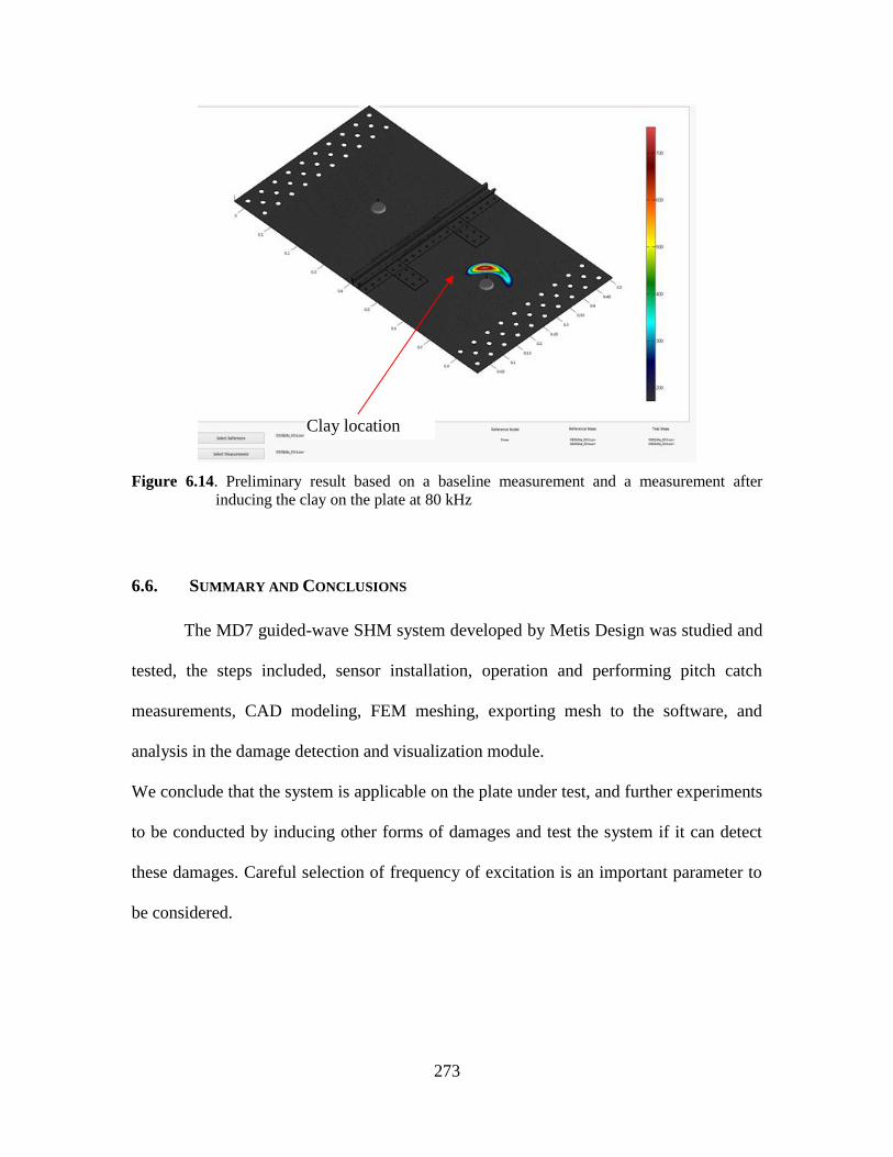
273
Figure 6.14. Preliminary result based on a baseline measurement and a measurement after
inducing the clay on the plate at 80 kHz
6.6. SUMMARY AND CONCLUSIONS
The MD7 guided-wave SHM system developed by Metis Design was studied and
tested, the steps included, sensor installation, operation and performing pitch catch
measurements, CAD modeling, FEM meshing, exporting mesh to the software, and
analysis in the damage detection and visualization module.
We conclude that the system is applicable on the plate under test, and further experiments
to be conducted by inducing other forms of damages and test the system if it can detect
these damages. Careful selection of frequency of excitation is an important parameter to
be considered.
Clay location

274
CHAPTER 7: SHM OF VARIABLE STIFFNESS CFRP PLATE
In this Chapter, we study the wave propagation in a CFRP plate with variable fiber
orientations along plate width and length at every layer. This type of structure was
studied by Tatting and Gurdal (2003); Blom (2010). The objectives here are: (1) to find
experimentally the dispersion wave propagation speeds and (2) to discuss the challenges
for getting accurate results. The methods involved for finding wave propagation speeds in
this study are time of flight (TOF) with using Hilbert envelops over the signals, and short
time Fourier transform (STFT). We installed eight PWAS transducers on the plate and
performed pitch catch experiments between different transducers to investigate wave
propagation along different fiber orientation angles, (keeping in mind that the fiber
orientation is not homogenous at every x and y position.) This fiber orientation pattern
leads to varying the plate stiffness as function of x, and y dimensions. Hence we refer to
this plate as variable stiffness (VS) plate.
7.1. MATERIALS
The plate we used is a 140x 390 mm CFRP plate with a variable thickness that is
ranging from 2.9 mm at edges to 3.4 mm in the middle. This plate was fabricated and
studied by Tatting and Gurdal (2003). Figure 7.1 shows the plate during fabrication stage.
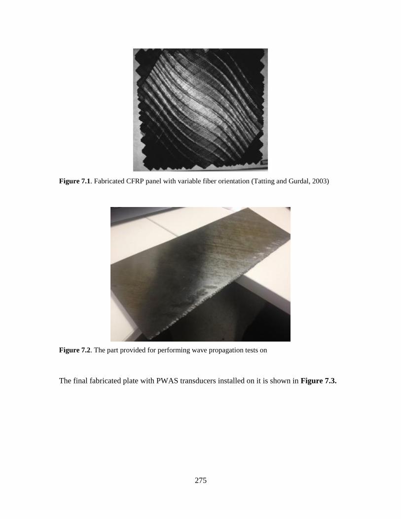
275
Figure 7.1. Fabricated CFRP panel with variable fiber orientation (Tatting and Gurdal, 2003)
Figure 7.2. The part provided for performing wave propagation tests on
The final fabricated plate with PWAS transducers installed on it is shown in Figure 7.3.
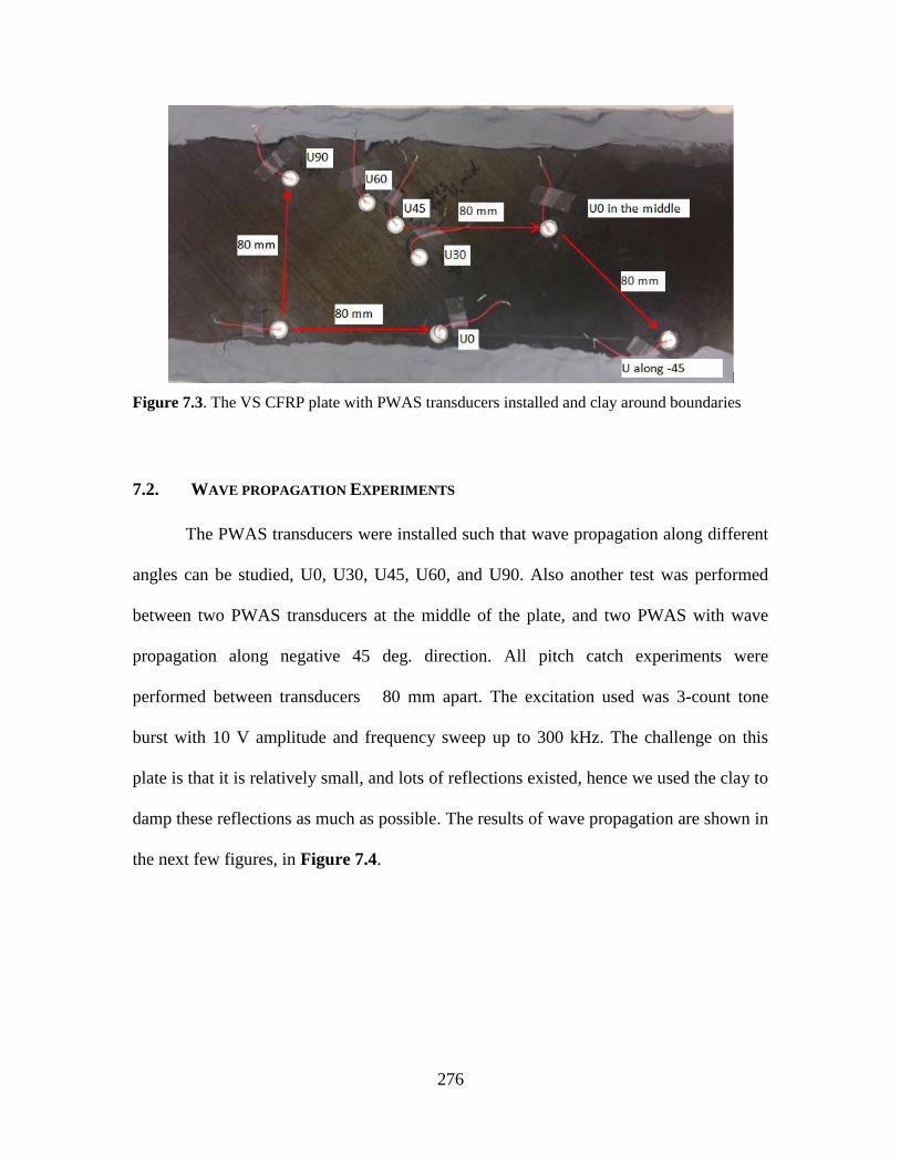
276
Figure 7.3. The VS CFRP plate with PWAS transducers installed and clay around boundaries
7.2. WAVE PROPAGATION EXPERIMENTS
The PWAS transducers were installed such that wave propagation along different
angles can be studied, U0, U30, U45, U60, and U90. Also another test was performed
between two PWAS transducers at the middle of the plate, and two PWAS with wave
propagation along negative 45 deg. direction. All pitch catch experiments were
performed between transducers 80 mm apart. The excitation used was 3-count tone
burst with 10 V amplitude and frequency sweep up to 300 kHz. The challenge on this
plate is that it is relatively small, and lots of reflections existed, hence we used the clay to
damp these reflections as much as possible. The results of wave propagation are shown in
the next few figures, in Figure 7.4.

277
Figure 7.4. Experimental results of dispersion wave propagation group velocities for CFRP VS
plate
As we can see from Figure 7.4a, the wave propagation along the same direction
U0 but at two different locations of the plate are not the same; A0 is almost a constant
and is having a speed around 1500 m/s, while S0 showed some differences. Figure 7.4b,c
show that the wave propagation speeds along 45 deg. and -45 deg. directions were the
maximum, probably because of the maximum stiffness at this part was along the 45 deg.
directions.
S0 symmetric
A0 antisymmetric
A0 antisymmetric
S0 symmetric
S0 symmetric
A0 antisymmetric
S0 symmetric
Exp (1) U0 near edge
Exp (2) U30 Exp (3) U45
Exp (4) U60 Exp (5) U90
A0 antisymmetric
(a)
(b)
(c)
(d)
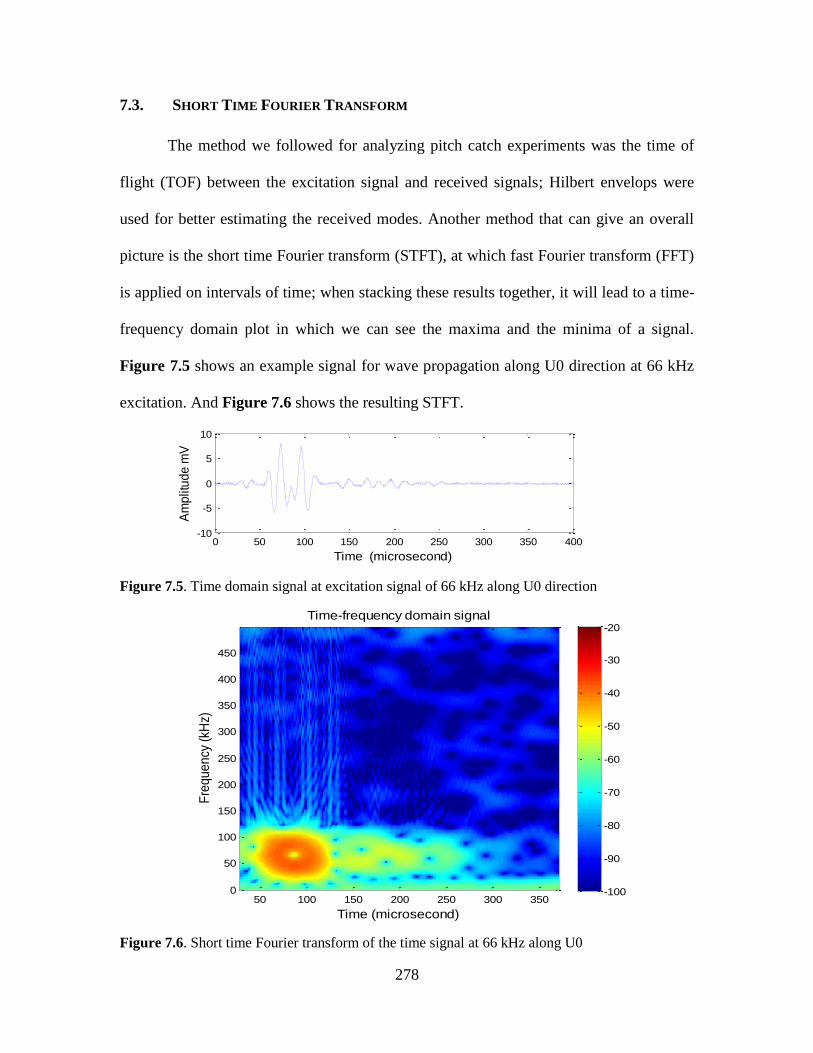
278
7.3. SHORT TIME FOURIER TRANSFORM
The method we followed for analyzing pitch catch experiments was the time of
flight (TOF) between the excitation signal and received signals; Hilbert envelops were
used for better estimating the received modes. Another method that can give an overall
picture is the short time Fourier transform (STFT), at which fast Fourier transform (FFT)
is applied on intervals of time; when stacking these results together, it will lead to a time-
frequency domain plot in which we can see the maxima and the minima of a signal.
Figure 7.5 shows an example signal for wave propagation along U0 direction at 66 kHz
excitation. And Figure 7.6 shows the resulting STFT.
Figure 7.5. Time domain signal at excitation signal of 66 kHz along U0 direction
Figure 7.6. Short time Fourier transform of the time signal at 66 kHz along U0
0 50 100 150 200 250 300 350 400-10
-5
0
5
10Time domain signal
Time (microsecond)
Am
plit
ud
e m
V
Time-frequency domain signal
Time (microsecond)
Fre
qu
en
cy (
kHz)
50 100 150 200 250 300 3500
50
100
150
200
250
300
350
400
450
-100
-90
-80
-70
-60
-50
-40
-30
-20
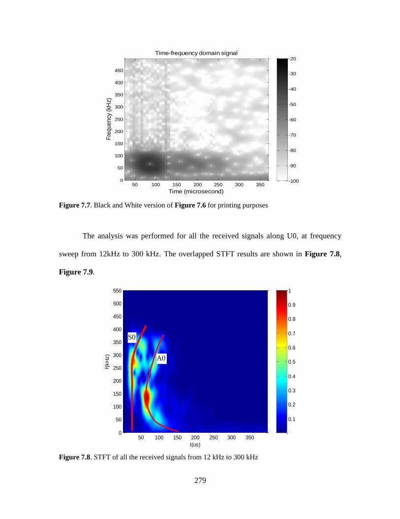
279
Figure 7.7. Black and White version of Figure 7.6 for printing purposes
The analysis was performed for all the received signals along U0, at frequency
sweep from 12kHz to 300 kHz. The overlapped STFT results are shown in Figure 7.8,
Figure 7.9.
Figure 7.8. STFT of all the received signals from 12 kHz to 300 kHz
Time-frequency domain signal
Time (microsecond)
Fre
qu
en
cy (
kHz)
50 100 150 200 250 300 3500
50
100
150
200
250
300
350
400
450
-100
-90
-80
-70
-60
-50
-40
-30
-20
t(us)
f(kH
z)
50 100 150 200 250 300 3500
50
100
150
200
250
300
350
400
450
500
550
0.1
0.2
0.3
0.4
0.5
0.6
0.7
0.8
0.9
1
A0
S0
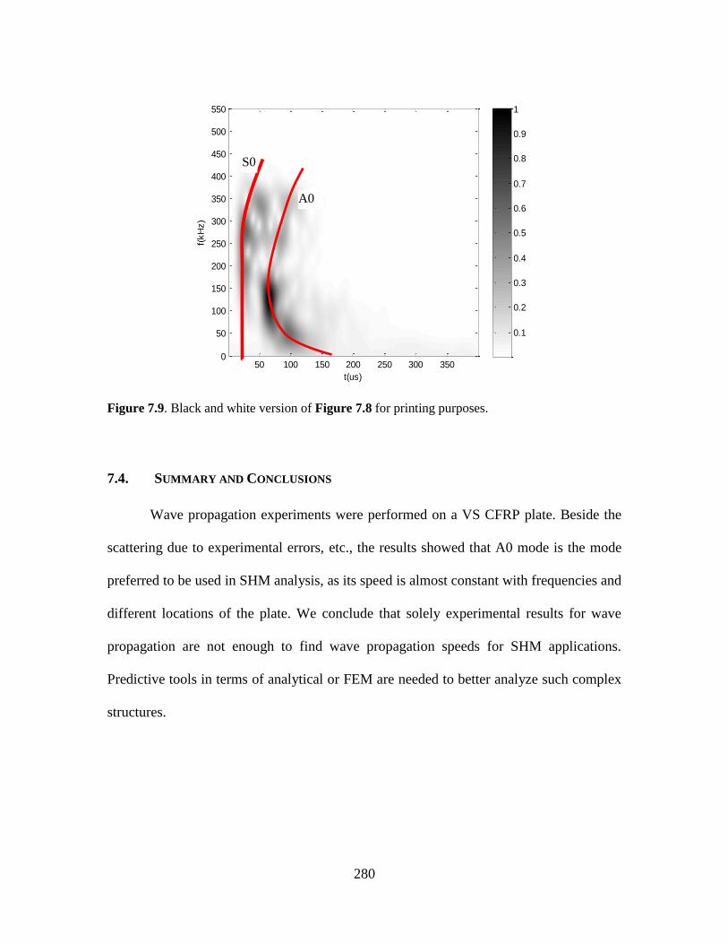
280
Figure 7.9. Black and white version of Figure 7.8 for printing purposes.
7.4. SUMMARY AND CONCLUSIONS
Wave propagation experiments were performed on a VS CFRP plate. Beside the
scattering due to experimental errors, etc., the results showed that A0 mode is the mode
preferred to be used in SHM analysis, as its speed is almost constant with frequencies and
different locations of the plate. We conclude that solely experimental results for wave
propagation are not enough to find wave propagation speeds for SHM applications.
Predictive tools in terms of analytical or FEM are needed to better analyze such complex
structures.
t(us)
f(kH
z)
50 100 150 200 250 300 3500
50
100
150
200
250
300
350
400
450
500
550
0.1
0.2
0.3
0.4
0.5
0.6
0.7
0.8
0.9
1
A0
S0
281
CHAPTER 8: CONCLUSIONS AND FUTURE WORK
This dissertation has addressed analytical and numerical predictive models for ultrasonics
transduction in metallic and composite structures using piezoelectric wafer active sensors
(PWAS) for structural health monitoring (SHM). The key themes for this dissertation are
power and energy; ultrasonic shear horizontal waves; wave propagation in composites.
The dissertation started with a background of ultrasonic guided waves in plates,
PWAS as an active/passive transducer, and various ways in which PWAS are used for
SHM applications. A predictive model of power and energy transduction between PWAS
and the structure has been developed based on exact Lamb wave solution. The aim was
optimizing guided wave mode tuning, PWAS electromechanical (E/M) impedance, and
PWAS size for having power-efficient SHM systems. The power and energy models
were applicable on multimodal Lamb wave situations that exist at high frequency
ultrasonics and/or relatively thick structures. Experimental validation was conducted
using scanning laser Doppler vibrometer (SLDV).
The dissertation continued with investigating the excitation and reception of shear
horizontal (SH) guided waves in plates. A special type of PWAS was used, which is
poled in the thickness-shear direction ( 35d mode), we called it SH-PWAS. The E/M
impedance of the free and the bonded SH-PWAS transducer have been developed
analytically and by finite element modeling (FEM). The predictive models of the E/M
282
impedance have been validated experimentally. Next, wave propagation experimental
and FEM studies were conducted between different combinations of SH-PWAS and
regular inplane PWAS transducers. The excitability of SH waves and the directivity of
the SH-PWAS were investigated. Finally, we presented simulations of our developed
analytical models of SH waves’ power and energy, along with a MATLAB graphical user
interface (GUI) for the analysis of SH-waves including: dispersion phase and group
velocities, mode shapes, and wave energy.
In order to investigate SH waves excitation and reception in composites; we
needed a stable robust method for determining dispersion curves in composites. The
transfer matrix method (TMM) has been used to calculate dispersion curves of guided
waves in composites. TMM suffers numerical instability at high frequency-thickness
values, especially in multilayered composites. A method of using stiffness matrix method
(SMM) was investigated to overcome instability. A combined stiffness transfer matrix
method (STMM) was proposed to obtain correct and stable results over the entire domain
of interest. STMM procedure was coded in a MATLAB graphical user interface that also
allows displaying modeshapes at any selected root of interest. This was followed by a
comparative study between commonly used methods for the calculation of ultrasonic
guided waves in composites, e.g. global matrix method (GMM), semi–analytical finite
element (SAFE).
Furthermore, the dissertation presented three SHM applications: (1) using the SH-
PWAS for case studies on composites, (2) testing of SHM industrial system for damage
detection in an aluminum aerospace-like structure panel, and (3) measuring dispersion
wave propagation speeds in a variable stiffness CFRP plate.
283
8.1. RESEARCH CONCLUSIONS
Power and Energy 8.1.1.
Exact Lamb wave theory was used to model the power and energy transduction
between PWAS transducer and hosted structures. The model was developed based on the
normal mode expansion (NME) theory and straight-crested harmonic waves. The pin-
force model was used to simulate perfect bonding between the PWAS and the structure.
The model is applicable on multi-modal situations, for example, a half-inch thick steel
plate, where three symmetric and three antisymmetric modes exist within the 500 kHz
excitation window. Modal participation factors were developed to predict how much each
mode contributes to the final power.
It was noticed that the transmitter reactive power (i.e., the power that depends on
the capacitive behavior of the PWAS) was directly proportional to the transmitter
admittance. The power transducted by the PWAS has an extra component, which is the
transmitter active power, i.e., the power converted into the ultrasonic waves. A
remarkable variation of active power with frequency was observed, and we noticed that
the active power was not monotonic with frequency, but manifested peaks and valleys.
As a result, the ratio between the reactive and active powers was not constant, but
presented the peaks and valleys. The increase and decrease of active power with
frequency corresponds to the PWAS tuning of various ultrasonic waves traveling into the
structure. The developed model for Lamb waves case was compared with the axial and
flexural waves, that approximate Lamb waves at relatively low frequencies and the two
simulations showed good agreement. Next, a parametric study was performed to optimize
the transducer size and excitation frequency to guarantee maximum energy transfer
284
between the source and the examined structure. Finally, an experimental study was
performed using the scanning laser vibrometer to compare the out-of-plane structural
oscillation at receiver PWAS transducers bonded on aluminum plates with analytical
predictions, as well as the received voltage through the piezoelectric effects. The results
have shown good agreement.
Shear Horizontal Coupled PWAS 8.1.2.
The shear-horizontal piezoelectric wafer active sensor (SH-PWAS) was presented
as a candidate for SHM compared to other-state-of-the-art transducers. Characterization
of the SH-PWAS includes the analytical development of the free transducer (in 35d
mode). We developed the E/M impedance and admittance of the free transducer based on
the constant electric field assumption and based on the constant electric displacement
assumption. The analytical model with the constant electric field assumption is more
representative of the experimental case and FEM. The first resonance frequency of the free
transducer is 900 kHz. We also extended the analytical development to the constrained
SH-PWAS case, where the transducer is bonded to structures in the form of beams. The
interaction between the SH-PWAS and the structure was studied. The analytical model
was compared with experimental results and finite element analysis. It was shown that
the analytical model predicts well the finite element and experimental results in the
situation where the transducer – to – structure mass ratio is < 5%. It was also shown that
the SH-PWAS has directivity effects, where an axial-flexural response is obtained when
the transducer poling direction is parallel to the beam length. When the transducer poling
direction is perpendicular to the beam length, the SH response is obtained.
285
The study then discussed the excitation and reception of SH waves using the SH-
PWAS. Excitation of SH waves was analyzed by finite element simulations and
experiments. SH0 non-dispersive waves were captured in aluminum plates. Multiple
experiments were performed to show the SH waves excitation and receiving capabilities
of both SH-PWAS and regular inplane PWAS transducers. It was shown that positioning
and orientation of the SH-PWAS affects the generation of SH waves: (1) SH-PWAS
excites SH waves in the direction perpendicular to its poling direction; (2) Regular
inplane PWAS can sense SH waves; (3) SH-PWAS transducers can sense A0 and S0
Lamb waves. Directivity analysis showed that excited SH wave amplitude gradually
decreases as the measuring direction deviates from the maximum received amplitude
direction. Finally, we presented simulations of our developed wave power and energy
analytical models along with a MATLAB graphical user interface (GUI) for the analysis
of SH-waves including dispersion phase and group velocities, mode shapes, and wave
energy.
Guided Wave Propagation in Composites 8.1.3.
Different algorithms for calculating dispersion wave speeds in composites were
reviewed. This work focused on the transfer matrix method (TMM) and the efforts for
generating a stable robust algorithm. A combined stiffness transfer matrix method
(STMM) was proposed to obtain correct and stable results over the entire domain of
interest. STMM procedure was coded in a MATLAB graphical user interface that also
allows displaying modeshapes at any selected root of interest. This was followed by a
comparative study between commonly used methods for the calculation of ultrasonic
286
guided waves in composites, e.g. global matrix method (GMM), semi–analytical finite
element (SAFE). Case studies were presented for an isotropic plate; a unidirectional fiber
composite layer with fibers along 0º or 90º degrees w.r.t wave propagation direction; a
unidirectional fiber composite layer with arbitrary fiber angles; multilayered
unidirectional composite with fibers along 0º direction; and cross-ply composites. For
each of the preceding cases, we obtained phase velocities, group velocities, and
wavenumber-frequency domain solutions. Some observations we noticed include: as
fibers angle increase from 0º towards 90º with respect to wave propagation direction, the
phase and group velocities reduce; because for the fibers along 90º the material is in the
most compliant case along wave propagation direction. Another observation regarding
the equivalent matrix method (EMM) is that: the case of cross ply of [0/90]s, i.e.
0/90/90/0 shows slight different results than the simple 0/90 case. The EMM predicted
the exact same result for both cases because it just averages the properties of the 0-
direction fibers and 90-direction fibers; hence the EMM does not account the difference
between the 2-layer 0/90 and the 4-layer [0/90]s cases.
Afterwards, a comparable study was established between the STMM results and
results from commercially available software, e.g. DISPERSE software based on GMM,
and GUIGUW software based on SAFE. This was followed by experimental and FEM
studies on a glass fiber reinforced polymer (GFRP) woven composite. PWAS transducers
were used for pitch catch experiments using tone burst excitation signals. Experimental
dispersion group velocities showed good agreement with the theory. COMSOL
Multiphysics finite element model was constructed using coupled-field elements for the
PWAS; this allowed simulation of the input excitation and output response in voltage
287
directly. FEM showed the propagation pattern of guided waves in composites. For the
specific case of a woven GFRP composite, the wave propagation along 0 and 90 degrees
was similar, but was different along 45 degrees, which resulted in diamond pattern
instead of the conventional propagation in circles obtained for isotropic materials.
SH-PWAS for Exciting SH Waves in Composites 8.1.4.
SH-PWAS was studied for the E/M impedance method and wave propagation of
SH waves in two composite plates, one was cross ply GFRP woven composite and the
other was quasi-isotropic [0/45/45/0] carbon fiber reinforced polymer (CFRP) composite
with woven prepreg. Admittance experimental results were comparable to FEM built
using coupled field piezoelectric elements bonded to composite layers. Wave propagation
method showed that the SH-PWAS can excite SH waves as well as S0, A0, providing
that the receiver PWAS is in a position such that the wave propagation direction between
SH-PWAS and the receiver PWAS is perpendicular to SH-PWAS poling direction. If we
excite SH-PWAS and receive the signal along a direction parallel to the poling direction,
only A0 and S0 waves were captured. FEM models showed well the wave propagation
pattern in woven GFRP plate and quasi-isotropic CFRP composite plate, however, lack of
accuracy existed in the received signals due to limited computational resources.

288
Guided Wave Damage Detection in an Aerospace-Like 8.1.5.
The MD7 guided-wave SHM system developed by Metis Design was studied and
tested. It is concluded that the system is applicable on the plate under test. Careful
selection of frequency of excitation is an important parameter to be considered.
SHM of Variable Stiffness CFRP Plate 8.1.6.
Wave propagation experiments were performed on a VS CFRP plate. Besides the
scattering due to experimental errors, the experimentally-measured wave speeds of the S0
mode were more scattered than A0 mode. We concluded that A0 mode is the more
preferred mode to be used in SHM analysis; its speed was almost constant with
frequencies and different locations of the plate. A general conclusion is that solely
experimental results for wave propagation are not enough to find wave propagation
speeds for SHM applications. Predictive tools in terms of analytical or FEM are needed
to better analyze such complex structures.
8.2. MAJOR CONTRIBUTIONS
The dissertation has contributed to the fundamental studies of using ultrasonics in
SHM. The list of the major contributions includes
1. Development of the analytical models of ultrasonic waves power and energy
based on the exact Lamb wave modes.
2. Predicting the power partitioning between multimodal Lamb waves (three
symmetric and three antisymmetric modes) for a thick structure application.

289
3. Characterization of the SH-PWAS as a candidate for exciting SH waves in SHM
applications, including:
a) Modeling the E/M impedance of a bonded SH-PWAS to the structure
analytically for the first time.
b) Performing a comprehensive experimental and FEM studies to investigate
excitation and reception of SH waves and the directivity of the SH-PWAS.
4. The development of a MATLAB-based graphical user interface (GUI) for SH
waves analysis, including: dispersion curves, modeshapes and wave energy.
5. A novel approach (STMM) was proposed for obtaining a stable and correct
solution of dispersion curves in composites over the entire solving domain.
6. The development a MATLAB-based GUI for a quicker and easier analysis of the
dispersion curves in composites, including:
a) Loading the unstable results of the transfer matrix method (TMM).
b) Displaying the complete stable stiffness transfer matrix method (STMM).
c) Calculating displacements and stresses modeshapes at any given root on the
dispersion curves.
7. Performing comprehensive pitch catch experiments and FEM between SH-PWAS
and regular in-plane PWAS for investigating SH wave excitation and reception in
composites.

290
8.3. RECOMMENDATION FOR FUTURE WORK
The dissertation has addressed analytical and numerical models to advance
fundamental understanding of using ultrasonics for SHM of metallic and composite
materials. The recommended future work includes:
1. Extending power and energy transduction models for situations of bonded PWAS
on composite materials.
2. Performing more experimental studies to validate power and energy models;
power need to be a parameter in the measurements.
3. Performing scanning laser vibrometer measurements to capture the shear
horizontal response of the SH-PWAS.
4. Continue developing the stiffness transfer matrix method (STMM) and predict
dispersion curves for more complex composite layups.
5. Performing more experiments of the wave propagation in composites and
investigating types of damages, SH-PWAS is capable to detect.
291
REFERENCES
APC International Ltd, Physical and Piezoelectric Properties of APC Materials. [Online]
Available at: http://www.americanpiezo.com
Aldrin, J.; Knopp, J.; Judd, D.; Mandeville, J.; Lindgren, E. (2006) Spiral Creeping
Waves in Ultrasonic Angled‐Beam Shear Wave Inspection of Fastener Holes in
Multilayer Structures, AIP Conf. Proc. 820, pp. 187-194.
Aldrin, J.; Kropas-Hughes, C.V.; Knopp, J.; Mandeville, J.; Judd, D.; Lindgren, E. (2006)
Advanced echo-dynamic measures for the characterisation of multiple ultrasonic
signals in aircraft structures. Insight: Non-Destructive Testing & Condition
Monitoring, 48(3), pp. 144-148.
Alleyne, D.; Cawley, P. (1992) The Interaction of Lamb Waves With Defects. IEEE
Trans. Ultrason. Ferroelectr. Freq. Control, 39(3), pp. 381-396.
Auld, B. (1990) Acoustic Fields and waves in solids. New York: John Wiley & Son.
Baillargeon, P.B. (2003) Active Vibration Suppression of Smart Structures Using
Piezoelectric Shear Actuators, University of Maine Electronic Dissertation.
Banerjee, S.; Ricci, F.; Monaco, E.; Mal, A. (2008) A wave propagation and vibration-
based approach for damage identification in structural components. Journal of
Sound and Vibration, 322(1-2), pp. 167-183.
Bartoli, I.; Marzani, A.; Lanza di Scalea, F.; Viola, E. (2006)Modeling Wave Propagation
in Damped Waveguides of Arbitrary Cross-section. J. Sound & Vibration, 295, pp.
685-707.
292
Benjeddou, A.; Trindade, M.A.; Ohayon, R. (1997) A Unified Beam Finite Element
Model for Extension and Shear Piezoelectric Actuation Mechanisms. J. Intelligent
Mat. Syst. Struct., 8(12), pp. 1012-1025.
Blom, A. (2010) Structural performance of fiber-placed, variable-stiffness composite
conical and cylindrical shells, Ph. D. Thesis, Delft University of Technology.
Bocchini, P.; Marzani, A.; Viola, E. (2011) Graphical User Interface for Guided Acoustic
Waves. Journal of Comput. Civ. Eng., 25(3), pp. 202-201.
Centolanza, L.R.; Smith, E.C.; Munsky, B. (2002) Induced-shear piezoelectric actuators
for rotor blade trailing edge flaps. J. Smart Mater. Struct, 11, pp. 24-35.
Chang, F. (1998) Smart layer: built-in diagnostics for composite structures. Proc. of the
4th European Conference on Smart Materials and Structures.
Cheng, C.; Chen, S.; Zhang, Z.; Lin, Y. (2007) Analysis and experiment for the
deflection of a shear-mode PZT actuator. Smart Mater. Struct., 16, pp. 230-36.
Chinthalapudi, A.; Hassan, H. (2005) Investigation of Methods to Detect Defects in Thin
Layered Materials, Karlskrona, Master's Degree Thesis, Blekinge Institute of
Technology, Sweden.
Delsanto, P.P.; Schechter, R.S.; Mignogna, R.B. (1997) Connection machine simulation
of ultrasonic wave propagation in materials III: The three-dimensional case. Wave
Motion, 26(4), pp. 329-339.
Ferroperm Piezoceramics, [Online] Available at: www.ferroperm-piezo.com/
Flynn, E.; Todd, M.; Kessler, S.; Dunn, C. (2011) Identifying Scatter Targets in 2D Space
using In Situ Phased-Arrays for Guided Wave Structural Health Monitoring. The
8th Int. Workshop on Structural Health Monitoring Stanford, CA.

293
Fortunko, C.M.; King, R.B.; Tan, M. (1982) Nondestructive Evaluation of Planar Defects
in Plates Using Low-Frequency Shear Horizontal Waves. J. Applied Physics, 53,
pp. 3450-3458.
Gao, H.; Ali, S.; Lopez, B. (2010) Inspection of Austenitic Weld with EMAT, Review of
Progress in Quantitative Nondestructive Evaluation 29B, pp. 1175-1181.
Gavric, L. (1995) Computation of Propagative Waves in Free Rail Using a Finite
Element Technique. Journal of Sound and Vibration, 185(3), pp. 531-543.
Giurgiutiu, V. (2005) Tuned Lamb wave excitation and detection with piezoelectric
wafer active sensors for structural health monitoring. J.Intell. Mat. Syst. Struct.,
16, pp. 291-305.
Giurgiutiu, V. (2008) Structural Health Monitoring with Piezoelectric Wafer Active
Sensors. Amsterdam: Elsevier Academic Press.
Giurgiutiu, V.; Santoni, G. (2011) Structural Health Monitoring of Composite Structures
with Piezoelectric-Wafer Active Sensors. AIAA Journal , 49(3), pp. 565-581.
Giurgiutiu, V.; Zagrai, A. (2000) Characterization of piezoelectric wafer active sensors.
J.Intell. Mater. Sys. Struct., 11, pp. 959-976.
Giurgiutiu, V.; Zagrai, A.; Bao, J. (2002) Piezoelectric wafer embedded active sensors for
aging aircraft structural health monitoring. Structural Health Monitoring, 1, pp.
41-61.
Glazounov, A.; Zhang, Q. (1998) Piezoelectric actuator generating torsional displacement
from piezoelectric d15 shear response. J. Applied Physics Letters, 72, pp. 2526-28.
294
Glushkov, E.; Glushkova, N.; Eremin, A. (2011) Forced wave propagation and energy
distribution in anisotropic laminate composites. Journal Acoust. Soc. America,
129(5), pp. 2923-2934.
Glushkov, E.; Glushkova, N.; Kvasha, O.; Seemann, W. (2007) Integral equation based
modeling of the interaction between piezoelectric patch actuators and an elastic
substrate. Smart Materials and Structures, 16(3), pp. 650-664.
Glushkov, E.; Glushkova, N.; Seemann, W.; Kvasha, O. (2006) Elastic wave excitation in
a layer by piezoceramic patch actuators. Acoustical Physics, 52(4), pp. 398-407.
Graff, K. (1991) Wave motion in elastic solids. New York: Dover Publications Inc.
Gresil, M.; Giurgiutiu, V. (2013) Guided wave propagation in carbon composite laminate
using piezoelectric wafer active sensors. SPIE NDE proc., March 10-14, San
Diego, CA, pp. 869577-1:15.
Gresil, M.; Yu, L.; Giurgiutiu, V.; Sutton, M. (2012) Predictive modeling of
electromechanical impedance spectroscopy for composite materials. Structural
Health Monitoring, 11(6), pp. 671-683.
Haskell, N. (1953) The dispersion of surface waves on multi-layered media. Bulletin of
the Seismological Society of America, 43(1), pp. 17-34.
Hayashi, T.; Song, W.-J.; Rose, J. L. (2003) Guided wave dispersion curves for a bar
with an arbitrary cross-section, a rod and rail example. Ultrasonics, 41, pp. 175-
183.
Heeg, J. (1993) Analytical and experimental investigation of flutter suppression by
piezoelectric actuation, NASA Technical paper 3241 Langley Research Center, ,
Hampton, Virginia.
295
Ji, W.; Shen, L.-j. (2005) Exact thickness-shear resonance frequency of electroded
piezoelectric crystal plates. J. Zhejiang Univ. Sci, 6A(9), pp. 980-985.
Jones, R. (1999) Mechanics of composite materials. London: Taylor & Francis.
Kamal, A.; Lin, B.; Giurgiutiu, V. (2013) Energy and power modeling of multi mode
lamb waves propagating in structure bonded with piezoelectric wafer active
sensors. AIP Conf. Proc, 1511, Denver, CO, pp. 183-190.
Kamal, A.; Lin, B.; Giurgiutiu, V. (2013) Predictive modeling of PWAS-coupled shear
horizontal waves. SPIE NDE pro, March 10-14, San Diego, CA., pp. (86950F-
1:15).
Kamas, T.; Lin, B.; Giurgiutiu, V. (2013) Analytical modeling of PWAS in-plane and
out-of-plane electromechanicalimpedance spectroscopy (EMIS). SPIE NDE proc.
March 10-14, San Diego, CA, pp. 869227-1:13.
Kessler, S.; Flynn, E.; Dunn, C.; Todd, M. (2011) A Structural Health Monitoring
Software Tool for Optimization, Diagnostics and Prognostics. 3rd Annual
Conference of the Prognostics and Health Management Society, 25-29 Sept. 2011,
Montreal, Quebec.
Knopoff, L., 1964. A matrix method for elastic wave problems. Bulletin of the
Seismological Society of America, Volume 54, pp. 431-438.
Koh, Y.; Chiu, W.; Rajic, N. (2002) Effects of local stiffness changes and delamination
on Lamb wave transmission using surface-mounted piezoelectric transducers.
Composite Structures, 57, pp. 437-443.

296
Kural, A.; Pullin, R; Featherston, C; Pager, C; Holford, K. (2011) Wireless power
transmission using ultrasonic guided waves. Journal of Physics, Conference
Series 305( 012088), pp. 1-11.
Le Crom, B.; Castaings, M. (2010) Shear horizontal guided wave modes to infer the shear
stiffness of adhesive bond layers. J. Acoust. Society of America., 127(4), pp.
2220-2230.
Lee, B.C.; Staszewski, W.J. (2003) Modelling of Lamb waves for damage detection in
metallic structures: Part I. Wave propagation. Smart Mat. Str., 12, pp. 804-814.
Lee, J.; Kim, Y.; Cho, S.; (2009) Beam-focused shear-horizontal wave generation in a
plate by a circular magnetostrictive patch transducer employing a planar solenoid
array. J. Smart Mater. Struct, 18, pp. 015009.
Li, F.; Murayama, H.; Kageyama, K. (2009) Guided Wave and Damage Detection in
Composite Laminates Using Different Fiber Optic Sensors. Sensors, 9(5), pp.
4005-4021.
Lin, B.; Giurgiutiu, V. (2012) Power and Energy Transduction Analysis of Piezoelectric
Wafer Active Sensors for Structural Health Monitoring. Structural Health
Monitoring – An International Journal, 11(1), pp. 109-121.
Lin, B.; Giurgiutiu, V.; Kamal, A. (2012) The Use of Exact Lamb Waves Modes for
Modelling the Power and Energy Transduction of Structurally- Bonded
Piezoelectric Wafer Active Sensors. SPIE NDE proc. March 11-15, San Diego,
CA., pp. 83450A-1:12.
297
Lowe, M. (1995) Matrix techniques for modeling ultrasonic waves in multilayered media,
Ultrasonics Ferroelectrics and Frequency Control, IEEE Transactions, 42(4), pp.
525-542.
Milyutin, E.; Gentil, S.; Muralt, P. (2008) Shear mode bulk acoustic wave resonator
based on c-axis oriented AIN thin film. J. Applied Physics, 104, pp. 084508.
Milyutin, E.; Muralt, P. (2011) Electro-mechanical coupling in shear-mode FBAR with
piezoelectric modulated thin film. Ultrasonics Ferroelectrics and Frequency
Control, IEEE Transactions, 58, pp. 685-688.
Monnier, T. (2006) Lamb Waves-based Impact Damage Monitoring of a Stiffened
Aircraft Panel using Piezoelectric Transducers. J. Int. Mat. Sys. and Structures, 17,
pp. 411-421.
Moser, F.; Jacobs, L.J.; Qu, J. (1999) Modeling elastic wave propagation in waveguides
with the finite element method. NDT & E International, 32(4), pp. 225-234.
Mueller, V.; Zhang, Q. (1998) Shear response of lead zirconate titanate piezoceramics. J.
Applied Physics, 83, pp. 3754.
Nadella, K.; Cesnik, C. (2012) Numerical simulation of wave propagation in composite
plates. SPIE NDE proc. March, San Diego, CA, 8348, 83480L.
Nadella, K.; Cesnik, C. (2012) Simulation of Guided Wave Propagation in Isotropic and
Composite Structures using LISA, 53rd AIAA/ASME/ASCE/AHS/ASC Structures,
Structural Dynamics and Materials Conference.
Nayfeh, A. (1995) Wave Propagation in Layered Anisotropic Media. New York: Elsevier.

298
Park, G.; Rosing, T.; Todd, M.D.; Farrar, C.R.; Hodgkiss, W. (2007) Energy Harvesting
for Structural Health Monitoring Sensor Networks, LA 14314-M8 Los Alamos
National Laboratory Report.
Pavlakovic, B.; Lowe, M. (2003). DISPERSE Manual, London: Imperial College.
Pollock, P.; Yu, L; Sutton, M.A; Guo, S.; Majumdar, P.; Gresil, M. (2012) Full-Field
Measurements for Determining Orthotropic Elastic Parameters of Woven Glass-
Epoxy Composites Using Off-Axis Tensile Specimens. Experimental Techniques.
Rokhlin, S.; Chimenti, D.; Nagy, P. (2011) Physical Ultrasonics of Composites, Oxford
University Press.
Rose, J.(1999) Ultrasonic Waves in Solid Media. New York, Cambridge University Press.
Rose, J.; Pelts, S.; Li, J. (2000) Quantitative Guided Wave NDE. 15th World Conference
on Non-Destructive Testing Rome, Italy.
Ruzzene, M.; Jeong, S.M.; Michaels, T.E.; Michaels, J.E.; Mi, B. (2005) Simulation and
measurement of ultrasonic waves in elastic plates using laser vibrometry, Green
Bay, Wisconsin, AIP Conf. Proc., 24, pp. 172-179.
Santoni, G. (2010) Fundamental Studies in the Lamb-Wave Interaction Between
Piezoelectric Wafer Active Sensor and Host Structure During Structural Health
Monitoring, Dissertation, University of South Carolina.
Santoni, G.; Chrysochoidis, N.A.; Giurgiutiu, V.; Saravanos, D.A. (2007) Analytical and
Experimental Evaluation of Piezoelectric Wafer Active Sensors Performances for
Lamb Waves based Structural Health Monitoring in Composite Laminates. SPIE
NDE proc. March 19-22, San Diego, CA, pp. 6532-22.

299
Schmidt, H.; Jensen, F.B. (1985) A full wave solution for propagation in multilayered
viscoelastic media with application to Gaussian beam reflection at fluid-solid
interfaces. Journal Acoust. Soc. America, 77(3), pp. 813-825.
Sherrit, S.; Djrbashian, A.; Bradford, S. (2013) Analysis of the impedance resonance of
piezoelectric multi-fiber composite stacks. SPIE NDE proc. March 10-14, San
Diego, CA, pp. 868904-1:12.
Sohoni, V. (1995) A new smooth step function for ADAMS mscsoftware. [Online]
Available at: http://webcache.googleusercontent.com/search?q=cache:fZ-a--
O62ksJ:web.mscsoftware.com/support/library/conf/adams/na/1995/UC950030.P
DF+&cd=1&hl=en&ct=clnk&gl=us [Accessed June 2014].
Sorohan, S.; Constantin, N.; Gavan, M.; Anghel, V. (2011) Extraction of dispersion
curves for waves propagating in free complex waveguides by standard finite
element codes. Ultrasonics, 51, pp. 503-515.
STEMiNC, Steiner & Martins, Inc. [Online] Available at: http://www.steminc.com/
Sun, C.; Zhang, X. (1995) Use of thickness-shear mode in adaptive sandwich structures. J.
Smart Mater Struct, 4, pp. 202-206.
Su, Z.; Yang, C.; Pan, N.; Ye, L.; Zhou, L. (2007) Assessment of delamination in
composite beams using shear horizontal (SH) wave mode. Composites Science
and Technology, 67(2), pp. 244-251.
Su, Z.; Ye, L.; Lu, Y. (2006) Guided Lamb waves for identification of damage in
composite structures: A review. J. of Sound and Vibration, 295(3-5), pp. 753-780.
Tatting, B.; Gurdal, Z. (2003) Automated finite element analysis of elastically-tailored
plates, Technical Report, NASA/CR-2003-212679.
300
Thomson, W. (1950) Transmission of elastic waves through a stratified solid medium.
journal of Applied Physics, 21, pp. 89-93.
Viktorov, I. (1967) Rayleigh and Lamb waves - physical theory and applications. New
York: Plenum Press.
Wang, L.; Rokhlin, S. (2001) Stable reformulation of transfer matrix method for wave
propagation in layered anisotropic media. J. Ultrasonics, 39, pp. 407–418.
Wilcox, P.; Lowe, M.; Cawley, P. (2001) Mode and Transducer Selection for Long
Range Lamb Wave Inspection. Journal of Intelligent Material Systems and
Structures, 12, pp. 553-565.
Yanagitani, T. (2011) Shear Mode Piezoelectric Thin Film Resonators. In: Acoustic
Waves – From Microdevices to Helioseismology, M. G. Beghi, ed. InTech, Japan
pp. 501-520.
Zhou, W.; Li, H.; Yuan, F. (2013) Guided wave generation, sensing, and damage
detection using in-plane shear piezoelectric wafer. SPIE NDE proc. March 10-14,
San Diego, CA , pp. 869225-1:12.


![[VII]. Regulation of Gene Expression Via Signal Transduction Reading List VII: Signal transduction Signal transduction in biological systems](https://img.pdfslide.us/doc/110x75/56649e385503460f94b28319/vii-regulation-of-gene-expression-via-signal-transduction-reading-list-vii.jpg)