Extensional Reasoning

Timothy L. Hinrichs and Michael R. GeneserethStanford University

{thinrich,genesereth}@cs.stanford.edu

Abstract

Relational databases have had great industrial success in computer science, theirpower evidenced by theoretical analysis and widespread adoption. Often, automatedtheorem provers do not take advantage of database query engines and thereforedo not routinely leverage that source of power. Extensional Reasoning is a novelapproach to automated theorem proving where the system automatically translatesa logical entailment query into a query about a database system so that the answersto the two queries are the same. This paper discusses the framework for ExtensionalReasoning, describes algorithms that enable a theorem prover to leverage the powerof the database in the case of axiomatically complete theories, and discusses theoryresolution for handling incomplete theories.

1 Introduction

Relational database systems have been built to answer questions about enormous amountsof data, yet it is rare today for a theorem prover (Cyc’s inference engine [MG03] a notableexception) to exploit those systems when confronted with large theories. ExtensionalReasoning (ER) is an approach to automated theorem proving where the system trans-forms a logical entailment query into a database (a set of extensionally defined tables),a set of view definitions (a set of intensionally defined tables), and a database query.

For example, the map coloring problem is often stated as follows: given a map and aset of colors, paint each region of the map so that no two adjacent regions are the samecolor. One very natural way to encode this problem (according to the introductory logicstudents at Stanford who offer up this formulation year after year) centers around thefollowing constraints.

color(x, y) ⇒ region(x) ∧ hue(y)color(x, y) ∧ adj(x, z) ⇒ ¬color(z, y)

These constraints are the same regardless the map and the colors, i.e. regardless thedefinitions for region, hue, and adj; moreover, the definitions for these three predicatesare often complete. For example, for the graph illustrated in Fig. 1, we would have thefollowing definitions.

region(x) ⇔ (x = r1 ∨ x = r2 ∨ x = r3)hue(x) ⇔ (x = red ∨ x = blue)adj(x, y) ⇔ ((x = r1 ∧ y = r2) ∨ (x = r2 ∧ y = r3))

Query: next(x, y) ∧ next(y, z)

Database:next

red blueblue red

Figure 1: A 3-node graph and its corresponding database query

It so happens that the database formulation of this problem studied in, for example,[McC82] is quite different from the one above and is shown in Fig. 1. Given a table,next, that contains all the possible pairs of adjacent colors, the query for the threeregion graph would be

next(x, y) ∧ next(y, z)

where x represents the hue for r1, y the hue for r2, and z the hue for r3.The key difference between the formulations is that the database version entails all

the valid colorings, whereas the classical version is only consistent with each valid col-oring individually. In Extensional Reasoning, the transformation from one formulationinto the other happens automatically.

A relational database corresponds to a special kind of logical theory—one that isaxiomatically complete. Such theories are rare, and even when the theory is complete,recognizing that fact and constructing the appropriate database is nontrivial. Sincethe logical formulation of map coloring comprises an incomplete theory, to transformit into the database formulation we must first complete it. Because theory-completionin the context of Extensional Reasoning is performed solely for the sake of efficiency, atheory must be completed so that any entailment query about the original theory canbe transformed into an entailment query about the completed theory where the answersto the queries are the same, another nontrivial problem.

Sometimes the work is worth the effort. A database can sometimes solve the databaseversion of the query orders of magnitude faster than traditional techniques solve theclassical version; moreover, the cost of a database query is bounded (polynomial inthe size of the data and exponential in the size of the query), making the performancemore predictable, sometimes an important feature from the users’ perspective. Thesebenefits appear to have several causes. First, the portion of the logical theory that isrepresented extensionally can be indexed very efficiently both for lookup and retrieval.Second, negation is treated with Negation as Failure, which can cause large reductionsin the search space. Finally, if there is a solution to a problem, the candidates can bechecked one at a time, which is in contrast to the theorem proving environment wheredisjunctive answers would require checking each subset of possible answers.

While we hope Extensional Reasoning will eventually be applied to a wide varietyof logics, for the time being we have elected to focus on theories in a decidable logic,placing the issue of efficiency front and center. The particular logic we are studyingis a fragment of first-order logic that is a perennial problem in the theorem provingcommunity: it includes the domain closure axiom, which guarantees decidability whileallowing arbitrary quantification. This logic, to which the example above belongs, allows

us to avoid issues of undecidability at this early stage in the development of ExtensionalReasoning, while at the same time giving us the opportunity to make progress on animportant class of problems.

Orthogonal to the choice of logic, Extensional Reasoning could be applied in a varietyof settings that differ in the way efficiency is measured. Our work thus far measuresefficiency the same way the theorem proving community does. Once the machine hasbeen given a premise set and a query the clock starts; the clock stops once the machinereturns an answer. We do not amortize reformulation costs over multiple queries, andwe do not assume the premises or query have ever been seen before or will ever be seenagain.

The bulk of this paper examines Extensional Reasoning in the case of completetheories and introduces algorithms for recognizing completeness and transforming acomplete theory into a database system. For incomplete theories, some results on theoryresolution are introduced. Further work on the incomplete case can be found in acompanion paper [HG07]. Our technical contributions occur in the sections on Completetheories (3) and Incomplete theories (4). The necessary background is given in Sect. 2.

2 Background

In our investigations of Extensional Reasoning thus far, the logic we have considered isfunction-free first-order logic with equality, unique names axioms (UNA), and a domainclosure axiom (DCA). The UNA state that every pair of distinct object constants inthe vocabulary is unequal. The DCA states that every object in the universe must beone of the object constants in the vocabulary. Together, the UNA and DCA ensurethat the only models that satisfy a given set of sentences are the Herbrand modelsof those sentences, and because the language is function-free, every such model has afinite universe. We call this logic Finite Herbrand Logic (FHL). It is noteworthy thatentailment in FHL is decidable.

Besides the existence of UNA and a DCA, the definitions for FHL are the same asthose for function-free first-order logic with equality. Terms and sentences are defined asusual. We say a sentence is closed whenever it has no free variables, and open wheneverit has at least one free variable. The definition for a model is the usual one, but becauseall the models of FHL are isomorphic to finite Herbrand models, it is often convenientto treat a model as a set of ground atoms. When we do that, satisfaction is defined asfollows.

Definition 1 (FHL Satisfaction). The definition for the satisfaction of closed sen-tences, where the model M is represented as a set of ground atoms, is as follows.

|=M s = t if and only if s and t are syntactically identical.

|=M p(t1, . . . , tn) if and only if p(t1, . . . , tn) ∈M

|=M ¬ψ if and only if 6|=M ψ

|=M ψ1 ∧ ψ2 if and only if |=M ψ1 and |=M ψ2

|=M ∀x.ψ(x) if and only if |=M ψ(a) for every object constant a.

An open sentence ψ(x1, . . . , xn) with free variables x1, . . . , xn is satisfied by M if andonly if ∀x1 . . . xn.ψ(x1, . . . , xn) is satisfied by M according to the above definition.

A set of sentences in FHL constitutes an incomplete theory whenever there is morethan one Herbrand model that satisfies it. A set of sentences in FHL constitutes acomplete theory whenever there is at most one Herbrand model that satisfies it. Logicalentailment is defined as usual: ∆ |= φ in FHL if and only if every model that satisfies∆ also satisfies φ.

The language used in this paper for representing database systems is nonrecursivedatalog with negation, denoted datalog¬ , which is equivalent in expressive power torelational algebra and SQL. This particular language has been chosen because it is well-understood and because some of the algorithms for processing it are very similar toalgorithms for processing classical logic, which allows for relatively clean comparisons.

A datalog¬ system consists of (1) a set of tables, named using the ExtensionalDatabase predicates (EDB predicates) and (2) a set of datalog rules whose heads usethe Intensional Database predicates (IDB predicates). The EDB predicates and IDBpredicates are disjoint. A datalog rule is an implication, where :− is used in place of⇐.

h :− b1 ∧ · · · ∧ bnh, the head of the rule, is an atomic sentence. Each bi is a literal, and the conjunctionof bis is called the body of the rule. Every rule must be safe: every variable thatoccurs in the head or in a negative literal must occur in a positive literal in the body.Collectively, the rule set must be non-recursive, which can be defined in terms of therules’ dependency graph. The dependency graph for a rule set consists of one node perpredicate and an edge from u to v exactly when there is a rule with u in the head andv in the body, labelled with ¬ if v occurs in a negative literal. To be nonrecursive, thedependency graph for a rule set must be acyclic.

A model for a datalog¬ system is the same as that for FHL: a set of ground atoms.We use the standard stratified semantics. A consequence of these definitions is thatevery datalog¬ system is satisfied by exactly one Herbrand model, or more precisely,a database system is a representation of a single model. A database query is trueexactly when the query is true in that model, written Γ ∪ Λ |= φ, where Γ consistsof the extensional tables and Λ the view definitions. When confusion may arise, wewill subscript |= with FHL and D to indicate the semantics for FHL and datalog¬ ,respectively.

Because every datalog¬ system represents a single model, the logical theory corre-sponding to a database system is one that is axiomatically complete.

Definition 2 (Axiomatic Completeness). A satisfiable set of sentences ∆ is ax-iomatically complete with respect to language L if and only if for every closed sentences in L, either ∆ |= s or ∆ |= ¬s. ∆ is complete with respect to vocabulary V if and onlyif it is complete with respect to the set of all first-order sentences that can be formedfrom V .

3 Complete Theories

A satisfiable set of sentences in Finite Herbrand Logic can always be transformed intodatalog¬ while preserving logical equivalence if those sentences constitute a completetheory. In this section, we discuss algorithms for recognizing that a set of sentences iscomplete and algorithms for transforming such a sentence set into a datalog¬ system.

3.1 Recognizing Complete Theories

In Finite Herbrand Logic, a satisfiable, complete theory is satisfied by exactly one Her-brand model—by exactly one set of ground literals. Entailment in FHL is decidablebecause there is a fixed, finite bound on the size of the universe. Consequently, checkingwhether a satisfiable FHL theory is complete is decidable. For each ground atom a inthe language (of which there are finitely many), check whether ∆ entails a or ∆ entails¬a. If for some a, neither is entailed, the theory is incomplete; otherwise, the theory iscomplete.

This decision algorithm relies on entailment queries to determine whether the the-ory is complete, but entailment is the very problem Extensional Reasoning is meant toconfront. For this reason we developed an alternate algorithm that has more of a syn-tactic flavor—one that performs some inexpensive tests that are sufficient for ensuringcompleteness.

Complete theories have been studied in the nonmonotonic reasoning literature. Pred-icate completion, for example, was one of the early techniques used to define the seman-tics of Negation as Failure in Logic Programming [Llo84]. When applied to a set ofnonrecursive rules, predicate completion produces a set of nonrecursive biconditionalsentences, e.g.

p(x) ⇔ (q(x) ∧ r(x)) (1)q(x) ⇔ (x = a ∨ x = b)r(x) ⇔ (x = e ∨ x = f)

With some small caveats, a nonrecursive set of biconditional definitions is guaranteedto comprise a complete theory.

Definition 3 (Biconditional Definition). A biconditional definition is a sentence ofthe form r(x) ⇔ φ(x), where r is a relation constant, x is a sequence of non-repeatingvariables, and φ(x) is a sentence with free variables x.

Definition 4 (Nonrecursive biconditional definitions). A set of biconditional def-initions ∆ is nonrecursive if and only if the dependency graph 〈V,E〉 is acyclic.

V : the set of predicates in ∆

E : 〈u, v〉 is a directed edge if and only if there is a biconditional in ∆ with u in thehead and v in the body.

Theorem 1 (Biconditional Completeness). Suppose ∆ is a finite set of nonrecur-sive, biconditional definitions in FHL, where there is exactly one definition for eachpredicate in ∆ and no definition for =. ∆ is complete.

In this paper we examine algorithms that attempt to reformulate a sentence set intoa logically-equivalent set of nonrecursive biconditional definitions. Though incomplete,these algorithms run in low-order polynomial time, making them practical for certainclasses of theories. These algorithms perform the recognition task by partitioning thesentence set and examining each partition individually. If each partition can be writ-ten as a single biconditional then by the way the partitions are chosen, the theory isguaranteed to be complete.

To partition the sentences, we ask the following question. Suppose the sentence setwere originally written as nonrecursive, biconditional definitions. Further suppose thateach definition were then rewritten independently of all the others without introducingany additional predicates while preserving logical equivalence. For each predicate p,how do we find all those sentences that were produced from the biconditional definitionfor p?

For example, the following set of clauses were produced by converting the nonrecur-sive, biconditional definitions for p, q, and r in Formula 1 into clausal form.

p(x) ∨ ¬q(x) ∨ ¬r(x)¬p(x) ∨ q(x)¬p(x) ∨ r(x)q(x) ∨ x 6= aq(x) ∨ x 6= b¬q(x) ∨ x = a ∨ x = br(x) ∨ x 6= er(x) ∨ x 6= f¬r(x) ∨ x = e ∨ x = f

How does one determine which clause came from which definition?Because the original biconditionals were nonrecursive, there must be at least one of

them whose body is expressed entirely in terms of equality; call each such biconditionala base table definition. All those clauses that contain one predicate besides equalitymust have originated in base table definitions. Within that set of clauses, all those thatconstrain the same predicate must have come from the definition for that predicate.

In the example above, applying this observation selects two sets of sentences.

q(x) ∨ x 6= aq(x) ∨ x 6= b¬q(x) ∨ x = a ∨ x = b

and

r(x) ∨ x 6= er(x) ∨ x 6= f¬r(x) ∨ x = e ∨ x = f

The first is the set of sentences that came from the definition for q, and the secondis the set of sentences that came from the definition for r.

The partitioning algorithm recurses on the remaining sentences, this time looking forsentences with a single predicate besides = and the base table predicates. At iteration i,

the sentences that originated from definitions for predicates p1, . . . , pj have been foundand the algorithm looks for sentences with a single predicate besides {p1, . . . , pj ,=}.This is a variation on the context-free grammar (CFG) marking algorithm: when thepartition is found for predicate p, all occurrences of p in the remaining sentences aremarked, and when a sentence has all but one of its predicates marked, it is added to thepartition corresponding to the remaining predicate.

In the example, the remaining sentences are

p(x) ∨ ¬q(x) ∨ ¬r(x)¬p(x) ∨ q(x)¬p(x) ∨ r(x)

and since each contains one predicate, p, besides the predicates {q, r,=}, all of thesesentences are grouped into the partition corresponding to the biconditional for p.

Alg. 1 embodies the approach outlined here. Each recursive call selects all thosesentences with the same unmarked predicate p and calls reformulate-to-bicond onthose sentences. If they entail a biconditional for p, that biconditional is deemed to bethe definition for p, and the algorithm recurses. If no such biconditional is entailed, thealgorithm finds a different unmarked predicate and tries again. If there is no bicondi-tional entailed for any of the unmarked predicates, the theory is incomplete.

Algorithm 1 to-biconds(∆, basepreds)

1: sents := {〈p, d〉|d ∈ ∆ and p 6∈ basepreds and Preds[d] is p plus a subset of basepreds}2: preds := {p|〈p, d〉 ∈ sents}3: bicond := NIL4: for all p ∈ preds do5: partition := {d|〈p, d〉 ∈ sents}6: bicond := reformulate-to-bicond(partition, p)7: pred := p8: when bicond then exit for all9: end for

10: when not(bicond) then return NIL11: remaining := ∆− partition12: when remaining = ∅ then return cons(bicond,NIL)13: rest := to-biconds(remaining, basepreds ∪ {pred})14: when rest then return cons(bicond, rest)15: return NIL

to-biconds runs in O(n2(m + r)), where n is the number of predicates in ∆, mis the size of ∆, and r is the cost of reformulate-to-bicond. Under the conditionsmentioned above, to-biconds is sound and complete as long as reformulate-to-bicond is sound and complete.

Theorem 2 (Soundness of TO-BICONDS). Under the conditions listed below, ifto-biconds(∆, {=}) returns the non-NIL Γ, then Γ is a set of nonrecursive bicondition-als with one definition per predicate in ∆ besides equality and ∆ is logically equivalentto Γ.

• ∆ is a satisfiable sentence set in FHL

• reformulate-to-bicond is sound, i.e. if reformulate-to-bicond(Σ, p) re-turns p(x) ⇔ φ(x) then the result is a biconditional definition for p entailed byΣ.

Theorem 3 (Completeness of TO-BICONDS). Under the conditions listed below,if ∆ is a complete theory in FHL then to-biconds(∆, {=}) does not return NIL.

• ∆ is a satisfiable, nonempty sentence set that can be partitioned into sets so thatthere is one set per relation constant in ∆ besides equality: Sr1 , . . . , Srn.

• ∆ is logically equivalent to a set of nonrecursive biconditionals with one definitionper relation constant besides equality: {βr1 , . . . , βrn}

• βri is logically equivalent to Sri and Preds[βri ] = Preds[Sri ], for every i

• reformulate-to-bicond is complete, i.e. if Σ entails some nonrecursive bicon-ditional definition p(x) ⇔ φ(x) then reformulate-to-bicond(Σ, p) returns anequivalent biconditional definition for p; otherwise, it returns NIL.

to-biconds relies on reformulate-to-bicond, an algorithm for checking whethera given set of sentences entails a biconditional definition. There are many such algo-rithms, which form a spectrum of inexpensive syntactic checks to expensive semanticchecks. Our approach lies closer to the inexpensive end of the spectrum: it attemptsto rewrite the sentences of a partition into sufficient conditions for p, p(x) ⇐ φ(x),and necessary conditions for p, p(x) ⇒ ψ(x). It then tests whether φ(x) and ψ(x) arelogically equivalent, and again there is a spectrum of algorithms for checking logicalequivalence.

To finish the example, the sentences of the last partition can be written as

p(x) ⇐ (q(x) ∧ r(x))p(x) ⇒ (q(x) ∧ r(x))

Clearly there is a biconditional definition entailed by these two impications; likewisefor the other partitions in the example. Notice that because of the way the partitionswere constructed, the resulting set of biconditionals must be nonrecursive.

p(x) ⇔ (q(x) ∧ r(x))q(x) ⇔ (x = a ∨ x = b)r(x) ⇔ (x = e ∨ x = f)

3.2 Translating Complete Theories into Datalog

One of the benefits of the recognition algorithm described in the last section is that whensuccessful, the algorithm produces a formulation of the theory, a set of nonrecursivebiconditionals, that is amenable to translation into datalog¬ ; that transformation is thesubject of this section.

The translation takes place in two steps. First, the set of nonrecursive biconditionaldefinitions is partitioned into the portion that is turned into data (extensional tables)

and the portion that is turned into views (intensional tables). Second, the extensionalportion is converted into explicit tables and the intensional portion is converted intodatalog¬ view definitions.

The approach reported in this paper for partitioning the set of biconditionals is asimple one. As mentioned in the last section, every set of biconditional definitions mustinclude at least one definition whose body is expressed entirely in terms of equality.Our partitioning algorithm assigns all such definitions to the extensional portion of thetheory and all the remaining definitions to the intensional portion. More sophisticatedpartitioning algorithms are the subject of future work.

Regardless of what algorithm is used to split the set of biconditional definitionsinto the extensional and the intensional portions, the algorithms for transforming thosebiconditionals into datalog¬ are fairly straightforward.

Turning a biconditional definition into a datalog¬ view definition can be performedusing a typical recursive walk of the sentence and a post-processing step at the end.The walk turns ∀ into ¬∃¬; it introduces new predicates when negation and ∃ areencountered; boolean connectives are treated as usual. We demonstrate by showing astep-by-step transformation of r(x) ⇔ ∀y.(¬p(y) ∨ q(x, y)).

r(x) ⇔ ∀y.(¬p(y) ∨ q(x, y))r(x) :− ∀y.(¬p(y) ∨ q(x, y)) (⇔ turned into :− )r(x) :− ¬∃y.¬(¬p(y) ∨ q(x, y)) (∀ turned into ¬∃¬)r(x) :− ¬∃y.(p(y) ∧ ¬q(x, y)) (¬ pushed through)(1) r(x) :− not(newreln(x)) (new predicate invented)where newreln(x) ⇔ ∃y.(p(y) ∧ ¬q(x, y))newreln(x) :− ∃y.p(y) ∧ ¬q(x, y) (⇔ turned into :− )(2)newreln(x) :− p(y) ∧ ¬q(x, y) (drop ∃)

The result is two rules (1) and (2), one for r and one for newreln. Notice thatneither rule is safe—there are variables in negative literals that do not occur in positiveliterals. To be valid datalog¬ , safety must be ensured. To achieve this, we introducea new predicate univ that is true of all the object constants in the vocabulary, i.e. allthe objects in the universe. Then we add univ(x) for every variable x that is not safein some rule. The result is shown below.

r(x) :− not(newreln(x)) ∧ univ(x)newreln(x) :− p(y) ∧ not(q(x, y)) ∧ univ(x)

Because the biconditional definitions are nonrecursive, the algorithm illustratedabove, which we will refer to as views-to-datalog, is guaranteed to produce a setof safe, stratified datalog¬ rules. The algorithm used for converting the body of the rulewill convert any sentence into datalog¬ ; it will be called sentence-to-datalog.

views-to-datalog can also be used to convert a biconditional into a table of data.Suppose we convert all the biconditionals, both those destined to become data and thosedestined to become views, into datalog¬ views using views-to-datalog, treating = asan uninterpreted predicate. We can then add in a table for =, which has one row perelement in the universe. Then we can materialize a table by constructing the appropriatedatalog¬ query and running it through a standard deductive database engine. In thecase of very large theories, here again, we are relying on database algorithms to do what

they do best—manipulate large amounts of data. We will refer to the algorithm forconverting a biconditional into an extensional table with the name materialize.

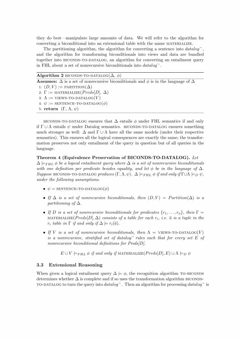
The partitioning algorithm, the algorithm for converting a sentence into datalog¬ ,and the algorithm for transforming biconditionals into views and data are bundledtogether into biconds-to-datalog, an algorithm for converting an entailment queryin FHL about a set of nonrecursive biconditionals into datalog¬ .

Algorithm 2 biconds-to-datalog(∆, φ)

Assumes: ∆ is a set of nonrecursive biconditionals and φ is in the language of ∆1: (D,V ) := partition(∆)2: Γ := materialize(Preds[D], ∆)3: Λ := views-to-datalog(V )4: ψ := sentence-to-datalog(φ)5: return (Γ, Λ, ψ)

biconds-to-datalog ensures that ∆ entails φ under FHL semantics if and onlyif Γ ∪ Λ entails ψ under Datalog semantics. biconds-to-datalog ensures somethingmuch stronger as well: ∆ and Γ ∪ Λ have all the same models (under their respectivesemantics). This ensures all the logical consequences are exactly the same; the transfor-mation preserves not only entailment of the query in question but of all queries in thelanguage.

Theorem 4 (Equivalence Preservation of BICONDS-TO-DATALOG). Let∆ |=FHL φ be a logical entailment query where ∆ is a set of nonrecursive biconditionalswith one definition per predicate besides equality, and let φ be in the language of ∆.Suppose biconds-to-datalog produces (Γ,Λ, ψ). ∆ |=FHL φ if and only if Γ∪Λ |=D ψ,under the following assumptions.

• ψ = sentence-to-datalog(φ)

• If ∆ is a set of nonrecursive biconditionals, then (D,V ) = Partition(∆) is apartitioning of ∆.

• If D is a set of nonrecursive biconditionals for predicates {r1, . . . , rn}, then Γ =materialize(Preds[D],∆) consists of a table for each ri, i.e. a is a tuple in theri table in Γ if and only if ∆ |= ri(a).

• If V is a set of nonrecursive biconditionals, then Λ = views-to-datalog(V )is a nonrecursive, stratified set of datalog¬ rules such that for every set E ofnonrecursive biconditional definitions for Preds[D],

E ∪ V |=FHL φ if and only if materialize(Preds[D], E) ∪ Λ |=D ψ

3.3 Extensional Reasoning

When given a logical entailment query ∆ |= φ, the recognition algorithm to-bicondsdetermines whether ∆ is complete and if so uses the transformation algorithm biconds-to-datalog to turn the query into datalog¬ . Then an algorithm for processing datalog¬ is

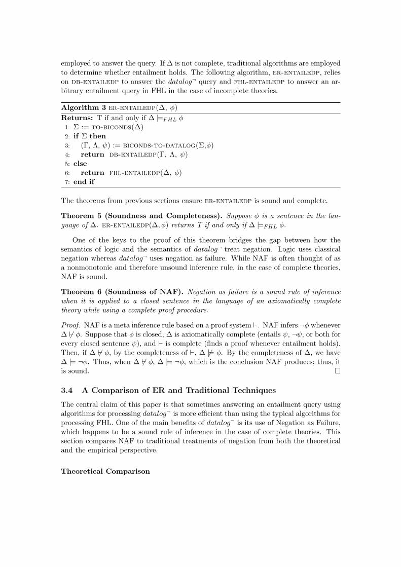
employed to answer the query. If ∆ is not complete, traditional algorithms are employedto determine whether entailment holds. The following algorithm, er-entailedp, relieson db-entailedp to answer the datalog¬ query and fhl-entailedp to answer an ar-bitrary entailment query in FHL in the case of incomplete theories.

Algorithm 3 er-entailedp(∆, φ)

Returns: T if and only if ∆ |=FHL φ1: Σ := to-biconds(∆)2: if Σ then3: (Γ, Λ, ψ) := biconds-to-datalog(Σ,φ)4: return db-entailedp(Γ, Λ, ψ)5: else6: return fhl-entailedp(∆, φ)7: end if

The theorems from previous sections ensure er-entailedp is sound and complete.

Theorem 5 (Soundness and Completeness). Suppose φ is a sentence in the lan-guage of ∆. er-entailedp(∆, φ) returns T if and only if ∆ |=FHL φ.

One of the keys to the proof of this theorem bridges the gap between how thesemantics of logic and the semantics of datalog¬ treat negation. Logic uses classicalnegation whereas datalog¬ uses negation as failure. While NAF is often thought of asa nonmonotonic and therefore unsound inference rule, in the case of complete theories,NAF is sound.

Theorem 6 (Soundness of NAF). Negation as failure is a sound rule of inferencewhen it is applied to a closed sentence in the language of an axiomatically completetheory while using a complete proof procedure.

Proof. NAF is a meta inference rule based on a proof system `. NAF infers ¬φ whenever∆ 6` φ. Suppose that φ is closed, ∆ is axiomatically complete (entails ψ, ¬ψ, or both forevery closed sentence ψ), and ` is complete (finds a proof whenever entailment holds).Then, if ∆ 6` φ, by the completeness of `, ∆ 6|= φ. By the completeness of ∆, we have∆ |= ¬φ. Thus, when ∆ 6` φ, ∆ |= ¬φ, which is the conclusion NAF produces; thus, itis sound.

3.4 A Comparison of ER and Traditional Techniques

The central claim of this paper is that sometimes answering an entailment query usingalgorithms for processing datalog¬ is more efficient than using the typical algorithms forprocessing FHL. One of the main benefits of datalog¬ is its use of Negation as Failure,which happens to be a sound rule of inference in the case of complete theories. Thissection compares NAF to traditional treatments of negation from both the theoreticaland the empirical perspective.

Theoretical Comparison

To demonstrate the power of NAF, we start by comparing SLDNF resolution andmodel elimination on an example, a fair comparison since the two proof procedures differmainly in how they treat negation. SLDNF uses NAF, whereas model elimination usesclassical negation. Consider the following biconditional definition for p.

p(x) ⇔

(p1(x) ∧ p2(x) ∧ p3(x)) ∨(p4(x) ∧ p5(x) ∧ p6(x)) ∨(p7(x) ∧ p8(x) ∧ p9(x)))

Converting the biconditional above to view definitions using the algorithms of the lastsection basically amounts to dropping the ⇒.

p(x) :− p1(x) ∧ p2(x) ∧ p3(x)p(x) :− p4(x) ∧ p5(x) ∧ p6(x)p(x) :− p7(x) ∧ p8(x) ∧ p9(x)

In contrast, converting the biconditional to clausal form produces the implications abovealong with implications for ¬p(x). In this example, there are 27 possible ways to prove¬p(t) for a particular t, which is exponential in the size of the biconditional. The naiveclausal form conversion will construct one clause for each one. (Structure-preservingclausal form conversion, which can be found in chapters 5 and 6 of [RV01], ensures thenumber of clauses is polynomial in the size of the original sentence set, but as we willsee the size of the search space can still be exponential.)

¬p(x) ⇐ ¬p1(x) ∧ ¬p4(x) ∧ ¬p7(x)¬p(x) ⇐ ¬p1(x) ∧ ¬p4(x) ∧ ¬p8(x)¬p(x) ⇐ ¬p1(x) ∧ ¬p4(x) ∧ ¬p9(x)

...¬p(x) ⇐ ¬p3(x) ∧ ¬p6(x) ∧ ¬p9(x)

We compare SLDNF resolution on the datalog¬ with model elimination on theclauses. For the entailment query ∃x.p(x), the two perform identically (assuming weturn off the reduction operation [AS92] for model elimination); however, for the query∃x.¬p(x), the two techniques differ significantly. SLDNF resolution uses the rules withp(x) in the head to look for a t such that the proof for p(t) fails. Model elimination usesthe rules with ¬p(x) in the head to look for a t such that ¬p(t) has a proof. Dependingon the relative sizes of the universe, the search space for p(x), and the search space for¬p(x), proving ¬p(t) by exhausting the search space for p(t) can be far less expensivethan finding a proof in the search space for ¬p(t).

Information theoretically, it is not surprising that for complete theories, NAF some-times answers queries more quickly than methods for classical negation. NAF can beviewed as a mechanism for reasoning about complete theories, whereas methods for clas-sical negation are mechanisms for reasoning about incomplete theories. NAF implicitlyleverages the fact that the theory is complete, but methods for classical negation do not.

More tangibly, the tradeoff between NAF and classical negation can be seen as atradeoff of search spaces. Often the space for ¬p is larger than the space for p, andit is this case that NAF takes advantage of. As opposed to classical negation, NAF

avoids searching the large space and instead searches just the small space. (We mightadditionally consider Truth as Failure to handle the case where the space for p is verylarge but the space for ¬p is very small.)

As mentioned earlier, structure-preserving clausal-form conversion will avoid enu-merating the exponential number of rules with ¬p in the head, but that does not nec-essarily prevent resolution from enumerating an exponential search space. Moreover,with certain assumptions placed on what it means to convert to clausal form, one canshow that regardless of which clausal form conversion is used, there is an infinite classof biconditionals such that resolution has the potential to generate exponentially manyclauses in the size of the biconditional, assuming that the implementation of resolutionis generatively complete.

Lemma 1. Consider the following biconditional β.

p(x) ⇔

(p11(x) ∧ · · · ∧ p1n1(x)) ∨...(pm1(x) ∧ · · · ∧ pmnm(x))

When applying the naive clausal form conversion to β, the number of clauses with anegative p literal is the product of the lengths of the disjunctions:

∏i ni.

¬p(x) ∨ p11(x) ∨ p21(x) ∨ · · · ∨ pm1(x)¬p(x) ∨ p11(x) ∨ p21(x) ∨ · · · ∨ pm2(x)

...¬p(x) ∨ p1n1(x) ∨ p2n2(x) ∨ · · · ∨ pmnm(x)

Suppose a clausal form conversion algorithm converts β into Γ. Further suppose Γ itis logically equivalent to β with respect to the predicates in β, i.e. for every sentenceσ whose predicates are a subset of those in β, Γ |= σ iff β |= σ. Suppose Res is animplementation of resolution that is generatively complete.

Res[Γ ∪ {p(t)}] will produce at least∏

i ni clauses.

Proof. Here we argue somewhat informally. Consider an arbitrary clause with a negativep literal.

¬p(x) ∨ p1j1(x) ∨ p2j2(x) ∨ · · · ∨ pmjm(x)

This clause, which is entailed by β, entails

p(t) ⇒ p1j1(t) ∨ p2j2(t) ∨ · · · ∨ pmjm(t)

Consequently Γ entails it as well. Thus, Γ ∪ {p(t)} entails

p1j1(t) ∨ p2j2(t) ∨ · · · ∨ pmjm(t)

Since Res is generatively complete up to subsumption, Res[Γ ∪ {p(t)}] must includeeither this disjunction, or some clause that subsumes it. No clause that subsumes thisone is entailed by Γ ∪ {p(t)}; hence, this clause must appear in the closure. Since theclause was chosen arbitrarily, the same holds for all clauses. Since there are

∏i ni of

these clauses, the resolution closure must contain at least that many clauses.

The above lemma guarantees a local property about resolution—that given a singlebiconditional and a query, the resolution closure is exponentially large in the numberof disjunctions. When other sentences are included, the lemma makes no guarantees.For example, if resolution were given a biconditional for p(x) along with the sentence¬p(x), resolution could find a proof without enumerating the exponential number ofconsequences described above.

To truly understand a technique it is important to find its limitations. ExtensionalReasoning is not always superior to traditional techniques. Consider a satisfiable, com-plete premise set that consists of a single sentence ∀xy.p(x, y), which when convertedto clausal form is just p(x, y). The query ∀xy.p(x, y) when negated and converted toclausal form is ¬p(k1, k2). Resolution finds a proof in a single step, regardless of howlarge the universe is.

In Extensional Reasoning, if the decision is made to materialize p, the databaseincludes n2 tuples for p, where n is the size of the universe. Using SLDNF resolution,the proof attempt ∀xy.p(x, y) is performed by attempting to find elements k1 and k2

such that ¬p(k1, k2) is true. Since every attempt fails, even assuming perfect indexing,the proof costs n2.

Thus, in some cases Extensional Reasoning can find proofs in complete theories moreefficiently than traditional techniques, but this last example demonstrates that this isnot always the case. An important next step is to investigate algorithms that predictwhich approach will find a proof (or fail to find a proof) more quickly; such algorithmsare the subject of future work.

Empirical Comparison

Next we report on experiments designed to compare Extensional Reasoning tech-niques to traditional techniques in the case of complete theories. Since the algorithmsfor detecting completeness presented in this paper produce a set of nonrecursive bi-conditional definitions, all the tests we performed were on such sentence sets. Theresults demonstrate what is predicted above. When negation occurs in the sentences,the datalog¬ implementation, which uses Negation as Failure, is significantly faster thantechniques that do not employ NAF.

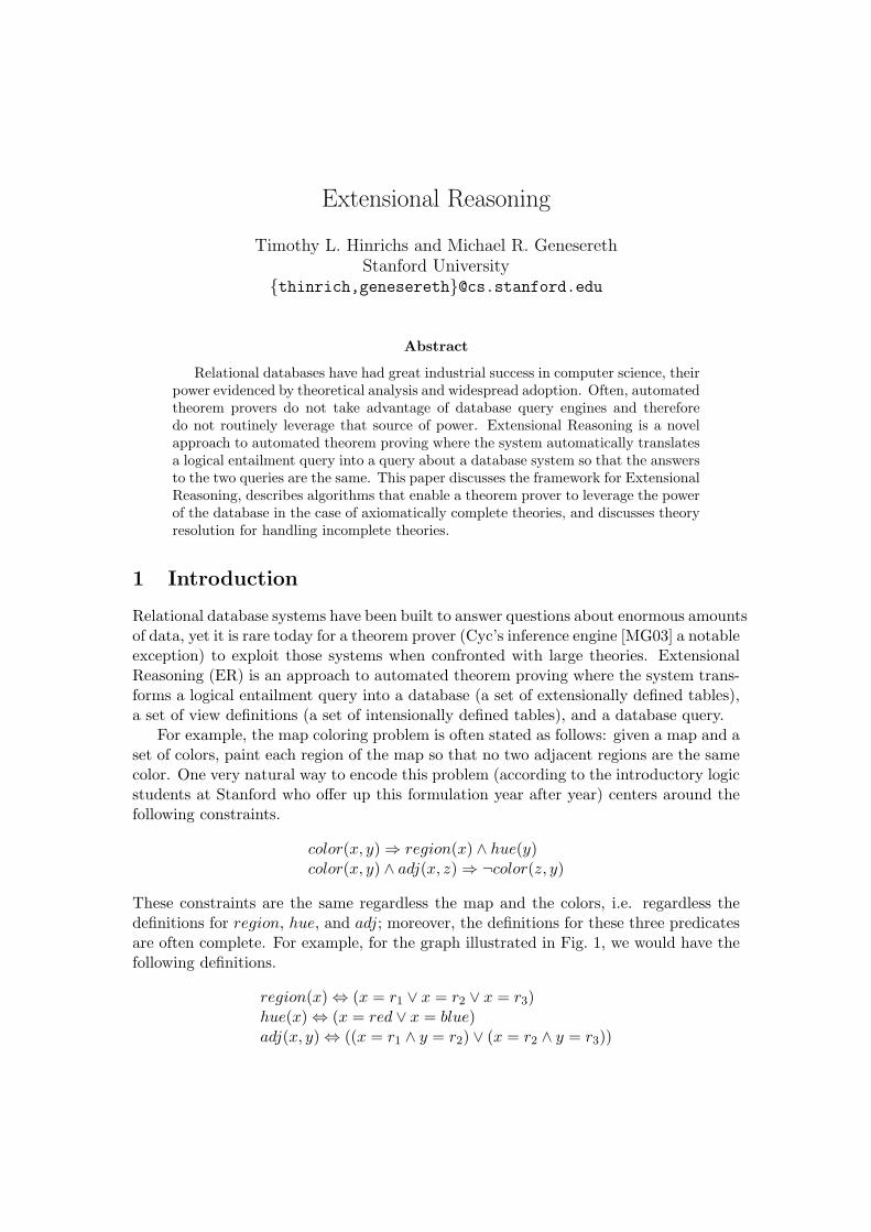
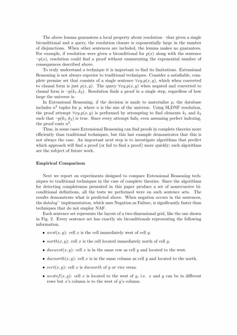
Each sentence set represents the layout of a two-dimensional grid, like the one shownin Fig. 2. Every sentence set has exactly six biconditionals representing the followinginformation.

• west(x, y): cell x is the cell immediately west of cell y.

• north(x, y): cell x is the cell located immediately north of cell y.

• duewest(x, y): cell x is in the same row as cell y and located to the west.

• duenorth(x, y): cell x is in the same column as cell y and located to the north.

• vert(x, y): cell x is duenorth of y or vice versa.

• westof(x, y): cell x is located to the west of y, i.e. x and y can be in differentrows but x’s column is to the west of y’s column.

Figure 2: A 4× 4 grid, corresponding to the theory in the appendix.

An axiomatization for the 4× 4 case can be found in the appendix.The tests varied the dimensions of the grid, starting at 4× 4 and ending at 20× 20.

The queries were of the form westof(t, u) and ¬westof(t, u), where t and u were alwaysground. Every query tested was entailed. The results of the positive queries are reportedseparately from the results of the negative queries because negation plays a prevalentrole in the negative queries but not the positive. The positive queries provide a baselinefor comparing techniques on how well they handle nonrecursive biconditional definitions.The negative queries illustrate how NAF can affect performance.

We compared our implementation of Extensional Reasoning for the case of completetheories, DBD (Datalog Based Deduction), with Vampire 8.1, Darwin, and Epilog (theStanford Logic Group’s model-elimination implementation1). Vampire and Darwin wererun using SystemOnTPTP, and Epilog and DBD were run in Macintosh Common Lispon a 1.5 GHz G4 Powerbook with 1.25 GB of RAM.

As expected, DBD, the system built to reason about towers of biconditionals, outper-formed the three general-purpose systems on both the positive and the negative queries.Each system had 1000 seconds to find a proof. Most of the systems performed fairlysimilarly until the last or second-to-last grid size they solved under the time limit.

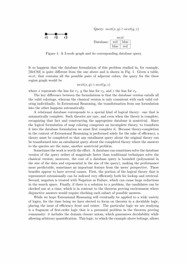
For the positive queries (Fig. 3), Epilog and Darwin performed similarly, both failingto find a proof in 1000 seconds for the 16 × 16 grid. Vampire failed to find a proof at20× 20; DBD solved the 20× 20 in 126 seconds. These tests were run without the DCAor the UNA since entailment did not require them; thus, these tests primarily illustratehow the various systems cope with the potentially large number of clauses generated byconverting biconditionals to clausal form.

1For completeness, model elimination and therefore Epilog require all contrapositives of the clausesetto be explored. For these experiments, only those clauses produced by a typical clausal form conversionwere used.

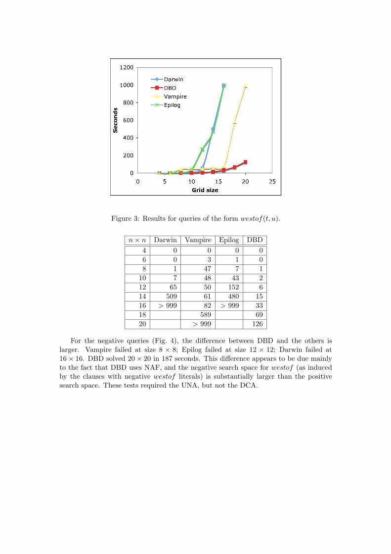
Figure 3: Results for queries of the form westof(t, u).

n× n Darwin Vampire Epilog DBD4 0 0 0 06 0 3 1 08 1 47 7 1

10 7 48 43 212 65 50 152 614 509 61 480 1516 > 999 82 > 999 3318 589 6920 > 999 126

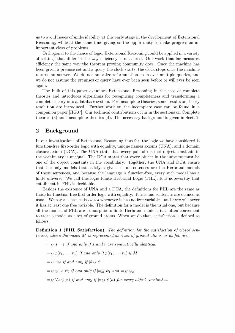
For the negative queries (Fig. 4), the difference between DBD and the others islarger. Vampire failed at size 8 × 8; Epilog failed at size 12 × 12; Darwin failed at16× 16. DBD solved 20× 20 in 187 seconds. This difference appears to be due mainlyto the fact that DBD uses NAF, and the negative search space for westof (as inducedby the clauses with negative westof literals) is substantially larger than the positivesearch space. These tests required the UNA, but not the DCA.

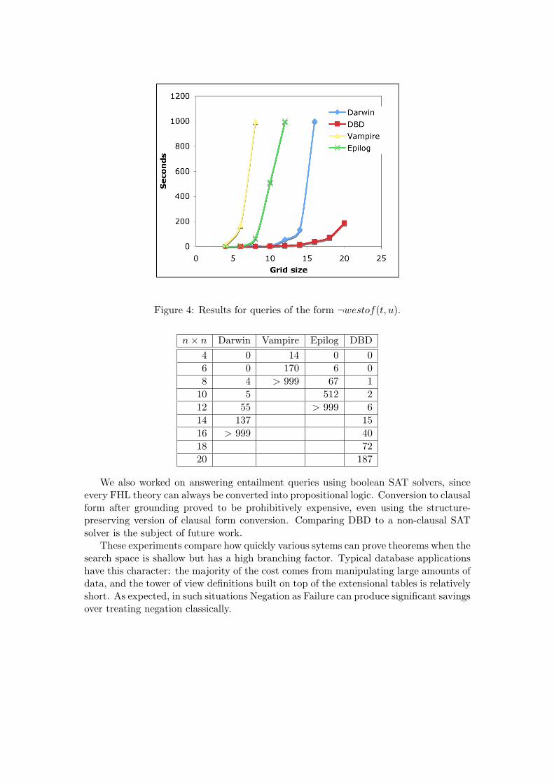
Figure 4: Results for queries of the form ¬westof(t, u).

n× n Darwin Vampire Epilog DBD4 0 14 0 06 0 170 6 08 4 > 999 67 1

10 5 512 212 55 > 999 614 137 1516 > 999 4018 7220 187

We also worked on answering entailment queries using boolean SAT solvers, sinceevery FHL theory can always be converted into propositional logic. Conversion to clausalform after grounding proved to be prohibitively expensive, even using the structure-preserving version of clausal form conversion. Comparing DBD to a non-clausal SATsolver is the subject of future work.

These experiments compare how quickly various sytems can prove theorems when thesearch space is shallow but has a high branching factor. Typical database applicationshave this character: the majority of the cost comes from manipulating large amounts ofdata, and the tower of view definitions built on top of the extensional tables is relativelyshort. As expected, in such situations Negation as Failure can produce significant savingsover treating negation classically.

4 Incomplete Theories

Complete theories have powerful properties, but incomplete theories are the norm. Thelast section detailed techniques for reasoning efficiently about complete theories usingdatabase techniques. However, if one were to add even just a small amount of incom-pleteness into a complete theory by including new predicates, those techniques could nolonger be applied. This is unfortunate since the speedups in the complete case seem tobe large enough to absorb some extra overhead for dealing with theories that have asmall amount of incompleteness.

For example, suppose we take any complete theory and add in the following sen-tences, where p and q are new predicates.

p(a) ∨ p(b) ∨ p(c)q(d) ∨ q(e) ∨ q(f)

Supposing the complete theory had a definition for the binary predicate r, a reason-able entailment query might be

∀xy.(p(x) ∧ q(y) ⇒ r(x, y)). (2)

When the definitions for r are large enough to warrant using a database system, weprobably still want to use that database system in spite of the fact that we now havean incomplete theory.

Theory resolution [Sti85] is one approach to dealing with such situations, wherepart of the theory can be effectively represented and reasoned about with a specializedprocedure. If a theory were partitioned into the complete portion C and the incompleteportion I, theory resolution would allow us to use a database system to represent Cwhile answering queries about C ∪ I using resolution.

One of the benefits of the to-biconds algorithm shown in Alg. 1 is that with a two-line change, it can be used to find the portion of the theory that is complete, partitioningthe theory as required for theory resolution. This change consists of replacing lines (14)and (15) so that once the algorithm fails to find a new biconditional definition, it returnsall the biconditionals it has found so far. Alg. 4 gives this new algorithm, to-biconds-max. It is noteworthy that to-biconds-max can be turned into an anytime algorithm,allowing the user or system designer to determine how much time to spend trying tofind a complete subtheory.

With the partitioning algorithm in place, we can now focus on theory resolution.Because C is complete, we can think of it as being a set of ground literals such thatevery ground atom or its negation is included. For the case where the incomplete portionI is in ∀∗, i.e. where when I is written in prenex normal form the quantifiers are alluniversal, theory resolution takes a particularly simple form. Suppose p is a predicatethat belongs to the complete portion, i.e. every ground p literal or its negation belongsto C. Then if there were some clause

{p(t)} ∪ Φ,

resolution would produce a resolvent for every literal ¬p(a) where p(a) unifies with p(t):

Φσ, where σ is the mgu of p(a) and p(t)

Algorithm 4 to-biconds-max(∆, basepreds)

1: sents := {〈p, d〉|d ∈ ∆ and p 6∈ basepreds and Preds[d] is p and some subset of basepreds}2: preds := {p|〈p, d〉 ∈ sents}3: bicond := NIL4: for all p ∈ preds do5: partition := {d|〈p, d〉 ∈ sents}6: bicond := reformulate-to-bicond(partition, p)7: pred := p8: when bicond then exit for all9: end for

10: when not(bicond) then return NIL11: remaining := ∆− partition12: when remaining = ∅ then return cons(bicond,NIL)13: rest := to-biconds-max(remaining, basepreds ∪ {pred})14: return cons(bicond, rest)

For completeness, theory resolution must produce all such clauses.

Definition 5 (Complete Theory Resolution). Complete Theory Resolution (CTR)is the following rule of inference. When it is added to the usual resolution inference rules,we denote the closure of clauses S using all those rules by CTRRes(C,S). Suppose Cis a complete theory with a definition for predicate p.

±p(t) ∪ ΦLet {σ1, . . . , σn} be the set of all mgus σ such that ∓p(t)σ is entailed by C.

Φσ1...Φσn

∓p(t)σ has the opposite sign of ±p(t).

In general, for FHL the DCA, UNA, and x = x must be added to a set of clauses forstandard implementations of resolution equipped with paramodulation to be sound andcomplete; however, in the case where the clauses are in ∀∗, it has been shown [Rei80]that neither the DCA nor paramodulation are necessary for completeness. This factsimplifies the completeness proof below.

Theorem 7 (CTRRes Soundness and Completeness for ∀∗). Suppose ∆ = C ∪ Iis a finite set of FHL sentences, where C is a satisfiable, complete theory with definitionsfor predicates P , and I is in ∀∗. ∆ is unsatisfiable if and only if CTRRes(C, I) containsthe empty clause.

Proof. (Soundness) Every resolution inference rule is sound, which means we need onlyshow CTR is sound. But this is immediate because CTR is simply n applications ofresolution, using literals from C.

(Completeness) A database system compactly represents C, which is semanticallya finite set of ground literals. We show that CTRRes is complete by showing that

every inference step that could occur using resolution between C, represented as a setof ground literals, and I will also occur in CTRRes(C, I).

Because C is a set of ground literals, it is in ∀∗, and I is in ∀∗ by assumption;thus, C ∪ I is in ∀∗, which means neither the DCA nor paramodulation are necessaryfor resolution to be complete. Thus, the only necessary rules of inference are binaryresolution and factoring; moreover, only those inferences that use as a premise someliteral from C could cause incompleteness.

If ∆ is unsatisfiable then there is a resolution proof of the empty clause from C ∪ I.Consider any step in which one of the literals from C is resolved with a non-unary clause.

±p(t) ∪ Φ∓p(a) (from C)

Φσ, where σ is the mgu of p(t) and p(a)

In CTRRes(C, I), this resolvent is one of many produced when CTR is applied to thefirst clause above. CTR finds all variable assignments ρ1, . . . , ρm so that ∓p(t)ρi belongsto C. Because every literal in C is ground, the unifier σ is a variable assignment suchthat p(t)σ belongs to C, i.e. σ is one of the ρi. Since CTR produces all Φρ and σ issome ρi, CTR certainly produces Φσ.

For every resolution between some literal in C and some other literal, we know thatthe other literal could not have come from C because that would make C unsatisfiable;the above argument applies to this case as well, which guarantees no binary resolutioninferences are lost by using CTRRes.

Hiding C does not result in the loss of any factoring step since factoring does notapply to unit clauses. Altogether, every inference rule application using resolution canbe mirrored using CTRRes.

In effect, this result is a practical approach to enlarging Reiter’s result [Rei80] thateliminates the need for paramodulation in the case of ∀∗. Here we have shown thatregardless what prefix class the complete portion of the theory belongs to, we can avoidparamodulation as long as the remaining sentences are in ∀∗.

We have speculated on inference rules for performing theory resolution when theincomplete sentences do not belong to ∀∗. The difficulty is that skolems exist, whichmust be dealt with by the database; moreover, the proof of completeness is complicatedby the fact that paramodulation is necessary. Here we simply illustrate the issues andpoint toward an avenue with promise.

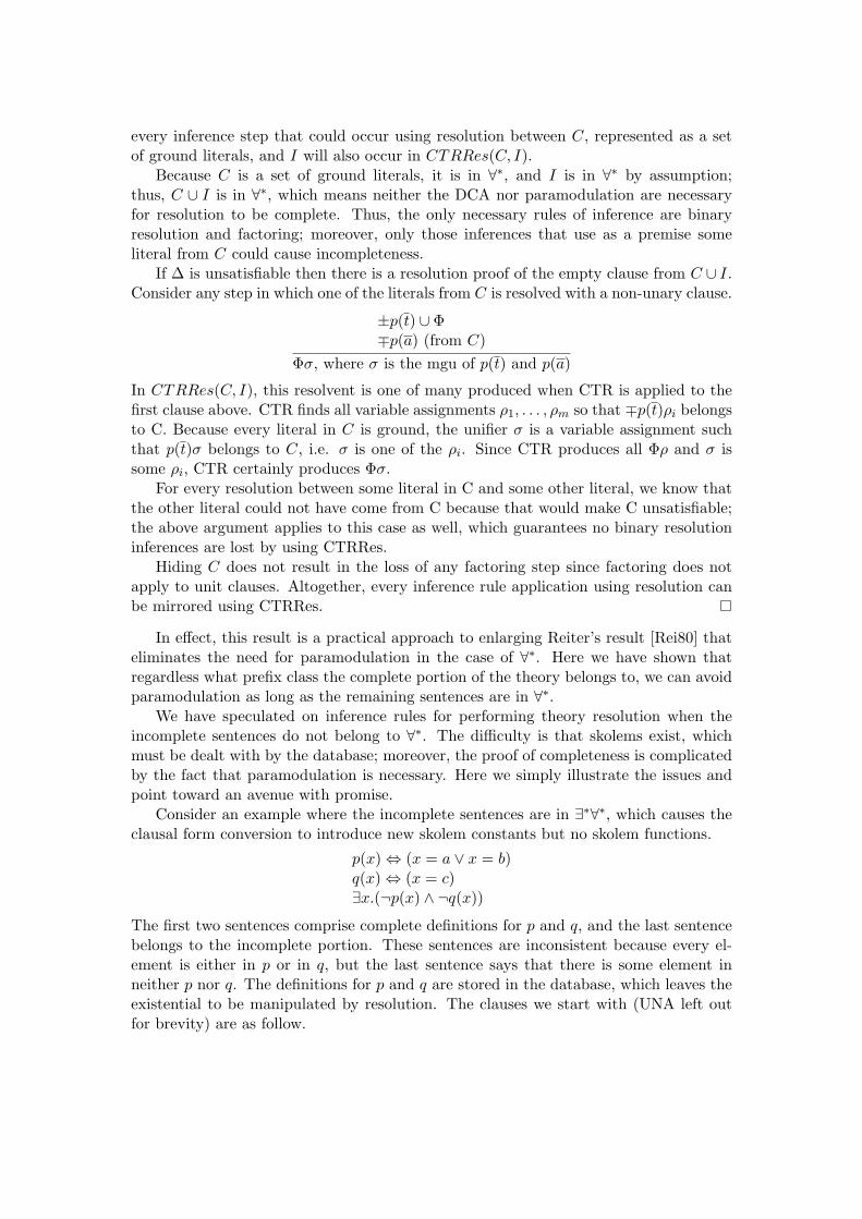
Consider an example where the incomplete sentences are in ∃∗∀∗, which causes theclausal form conversion to introduce new skolem constants but no skolem functions.

p(x) ⇔ (x = a ∨ x = b)q(x) ⇔ (x = c)∃x.(¬p(x) ∧ ¬q(x))

The first two sentences comprise complete definitions for p and q, and the last sentencebelongs to the incomplete portion. These sentences are inconsistent because every el-ement is either in p or in q, but the last sentence says that there is some element inneither p nor q. The definitions for p and q are stored in the database, which leaves theexistential to be manipulated by resolution. The clauses we start with (UNA left outfor brevity) are as follow.

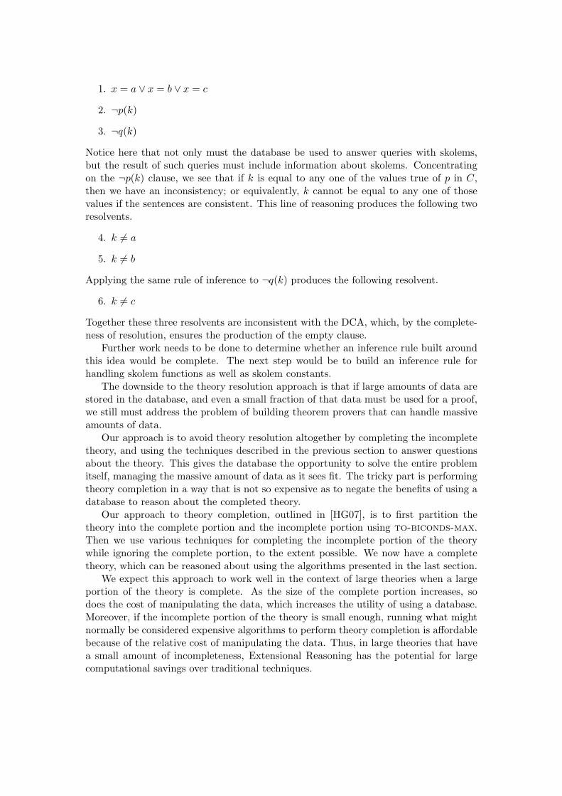
1. x = a ∨ x = b ∨ x = c

2. ¬p(k)

3. ¬q(k)

Notice here that not only must the database be used to answer queries with skolems,but the result of such queries must include information about skolems. Concentratingon the ¬p(k) clause, we see that if k is equal to any one of the values true of p in C,then we have an inconsistency; or equivalently, k cannot be equal to any one of thosevalues if the sentences are consistent. This line of reasoning produces the following tworesolvents.

4. k 6= a

5. k 6= b

Applying the same rule of inference to ¬q(k) produces the following resolvent.

6. k 6= c

Together these three resolvents are inconsistent with the DCA, which, by the complete-ness of resolution, ensures the production of the empty clause.

Further work needs to be done to determine whether an inference rule built aroundthis idea would be complete. The next step would be to build an inference rule forhandling skolem functions as well as skolem constants.

The downside to the theory resolution approach is that if large amounts of data arestored in the database, and even a small fraction of that data must be used for a proof,we still must address the problem of building theorem provers that can handle massiveamounts of data.

Our approach is to avoid theory resolution altogether by completing the incompletetheory, and using the techniques described in the previous section to answer questionsabout the theory. This gives the database the opportunity to solve the entire problemitself, managing the massive amount of data as it sees fit. The tricky part is performingtheory completion in a way that is not so expensive as to negate the benefits of using adatabase to reason about the completed theory.

Our approach to theory completion, outlined in [HG07], is to first partition thetheory into the complete portion and the incomplete portion using to-biconds-max.Then we use various techniques for completing the incomplete portion of the theorywhile ignoring the complete portion, to the extent possible. We now have a completetheory, which can be reasoned about using the algorithms presented in the last section.

We expect this approach to work well in the context of large theories when a largeportion of the theory is complete. As the size of the complete portion increases, sodoes the cost of manipulating the data, which increases the utility of using a database.Moreover, if the incomplete portion of the theory is small enough, running what mightnormally be considered expensive algorithms to perform theory completion is affordablebecause of the relative cost of manipulating the data. Thus, in large theories that havea small amount of incompleteness, Extensional Reasoning has the potential for largecomputational savings over traditional techniques.

5 Conclusion and Future Work

This paper presents Extensional Reasoning for both complete theories and incompletetheories. In the complete case it introduces a quadratic-time partitioning algorithm forrewriting a class of complete theories into a set of nonrecursive biconditional definitionsand discusses issues regarding the transformation of those definitions into datalog¬ .For the incomplete case, it introduces an anytime algorithm for finding the portion ofa theory that can be transformed into a set of nonrecursive biconditionals, and theoryresolution techniques that allow the complete portion to be represented with a databasesystem. The theory resolution techniques are sound and complete when the incompleteportion of the theory is in ∀∗. Empirically, Extensional Reasoning techniques performbetter than traditional theorem proving techniques when the theory consists of nonre-cursive biconditional definitions.

Besides enlarging the class of complete theories that we can detect, the first extensionto the work presented here is a better algorithm for finding a biconditional that isentailed by a given set of sentences. This problem is unlike the traditional theoremproving problem because the entailment query is a metalevel query: do these sentencesentail a sentence of the form p(x) ⇔ φ(x)? We have done some work on metalevel logic[HG05] and made preliminary investigations into meta-resolution, a variant of resolutionthat targets metalevel logic.

Second, the algorithm illustrated in section 3 for converting a set of nonrecursivebiconditional definitions into datalog¬ is straightforward, but in those cases where theresulting rules are unsafe, we introduce the univ relation, which is true of every objectconstant in the language. Minimizing the cases where univ is used can have drasticeffects on run time. Because such domain-dependent queries are often explicitly disal-lowed in the traditional database setting, standard database query optimizers will nottake advantage of the semantics of univ. ER will reap large benefits from augmentedquery-optimization algorithms.

Third, the policy we currently use for determining which portion of the theory toturn into extensional tables and which portion to turn into intensional tables needsfurther study. The database community has studied view materialization [Hal01] andview construction [Chi02] in depth, and those results can surely inform if not entirelyaddress this issue.

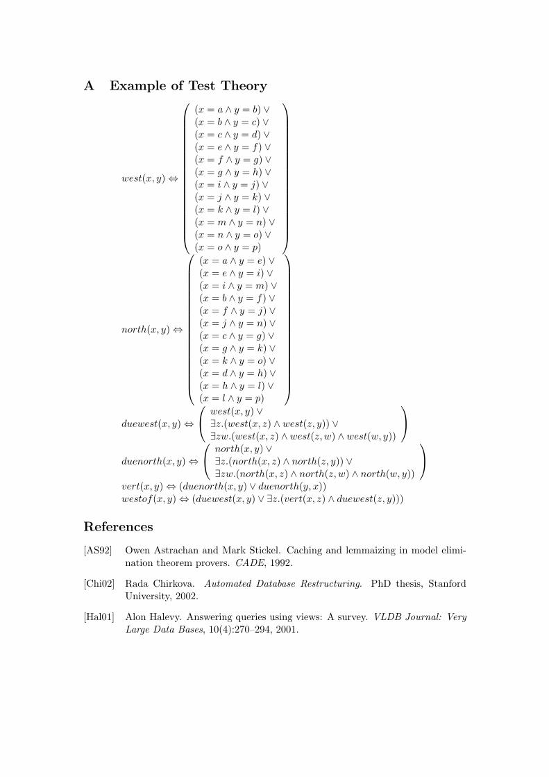
A Example of Test Theory

west(x, y) ⇔

(x = a ∧ y = b) ∨(x = b ∧ y = c) ∨(x = c ∧ y = d) ∨(x = e ∧ y = f) ∨(x = f ∧ y = g) ∨(x = g ∧ y = h) ∨(x = i ∧ y = j) ∨(x = j ∧ y = k) ∨(x = k ∧ y = l) ∨(x = m ∧ y = n) ∨(x = n ∧ y = o) ∨(x = o ∧ y = p)

north(x, y) ⇔

(x = a ∧ y = e) ∨(x = e ∧ y = i) ∨(x = i ∧ y = m) ∨(x = b ∧ y = f) ∨(x = f ∧ y = j) ∨(x = j ∧ y = n) ∨(x = c ∧ y = g) ∨(x = g ∧ y = k) ∨(x = k ∧ y = o) ∨(x = d ∧ y = h) ∨(x = h ∧ y = l) ∨(x = l ∧ y = p)

duewest(x, y) ⇔

west(x, y) ∨∃z.(west(x, z) ∧ west(z, y)) ∨∃zw.(west(x, z) ∧ west(z, w) ∧ west(w, y))

duenorth(x, y) ⇔

north(x, y) ∨∃z.(north(x, z) ∧ north(z, y)) ∨∃zw.(north(x, z) ∧ north(z, w) ∧ north(w, y))

vert(x, y) ⇔ (duenorth(x, y) ∨ duenorth(y, x))westof(x, y) ⇔ (duewest(x, y) ∨ ∃z.(vert(x, z) ∧ duewest(z, y)))

References

[AS92] Owen Astrachan and Mark Stickel. Caching and lemmaizing in model elimi-nation theorem provers. CADE, 1992.

[Chi02] Rada Chirkova. Automated Database Restructuring. PhD thesis, StanfordUniversity, 2002.

[Hal01] Alon Halevy. Answering queries using views: A survey. VLDB Journal: VeryLarge Data Bases, 10(4):270–294, 2001.

[HG05] Timothy L. Hinrichs and Michael R. Genesereth. Axiom schemata as metalevelaxioms. AAAI, 2005.

[HG07] Timothy L. Hinrichs and Michael R. Genesereth. Reformulation for extensionalreasoning. Proceedings of the Symposium on Abstraction, Reformulation, andApproximation, 2007.

[Llo84] John Lloyd. Foundations of Logic Programming. Springer Verlag, 1984.

[McC82] John McCarthy. Coloring maps and the Kowalski doctrine. Stanford TechnicalReport, 1982.

[MG03] James Masters and Zelai Gungordu. Structured knowledge source integration:A progress report. Integration of Knowledge Intensive Multiagent Systems,2003.

[Rei80] Raymond Reiter. Equality and domain closure in first-order databases. Journalof the ACM, 27(2):235–249, 1980.

[RV01] Alan Robinson and Andrei Voronkov. Handbook of Automated Reasoning. MITPress and Elsevier Science, 2001.

[Sti85] Mark Stickel. Automated deduction by theory resolution. Journal of Auto-mated Reasoning, 1:333–356, 1985.