U. S. DEPARTMENT OF COMMERCENATIONAL OCEANIC AND ATMOSPHERIC ADMiINISTRATION

NATIONAL WEATHER SERVICE

TECHNICAL NOTE

PERFORMANCE OF TECHNIQUESUSED TO DERIVE OCEAN,

SURFACE WINDS

WILLIAM H. GEMMILL, TSANN W. YU,AND DAVID M. FEIT

APRIL 1987

THIS IS AN UNREVIEWED MANUSCRIPT, PRIMARILY INTENDED FOR INFORMALEXCHANGE OF INFORMATION

OPC Contribution No. 14NMC Office Note No;.- 330

OPC CONTRIBUTIONS

No. 1. Burroughs, L. D., 1986: Development of Forecast Guidance for

Santa Ana Conditions. National Weather Digest. (in press)

No. 2. Richardson, W. S., D. J. Schwab, Y. Y. Chao, and D. I.

Wright, 1986: Lake Erie Wave Height Forecasts Generated by

Empirical and Dynamical Methods -- Comparison and Verification.

Ocean Products-Center Technical Note, 23pp. -

No. 3. Auer, S. J., 1986: Determination of Errors in LFM Forecasts

Surface Lows Over the Northwest Atlantic Ocean. Ocean Products

Center Technical Note/NMC Office9t Note N 313, 17pp.

No. 4. Rao, D. B., S. D. Steenrod, and B. V. Sanchez, 1987: A Method

of Calculating the Total Flow from A Given Sea Surface

Topography. NASA Technical Memorandum 87799., l9pp.

No. 5. Feit, D. H., 1986: Compendium of Marine Meteorological

and Oceanographic Products of the Ocean Products Center. NOAA

Technical Memorandum NWS NMC 68, 98pp.

No. 6. Auer, S. J., 1986: A Comparison of the LFM, Spectral, and

ECKVF Numerical Model Forecasts of Deepening Oceanic Cyclones

During One Cool Season. Ocean Products Center Technical

Note/NMC Office Note No. 312, 20pp.-

No. 7. Burroughs, L. D., 1986: Development of Open Fog Forecasting

Regions. Ocean Products Center Technical Note/NMC Office

Note. No. 323., 36pp.

No. 8. Yu, T., 1986: A Technique of Deducing Wind Direction from

Altimeter Wind Speed Measurements. Mon. Wea. Rev.

(Submitted).

No. 9. Auer, S. J., 1986: A 5-Year Climatological Survey of the Gulf

Stream and Its Associated Ring Movements. Journal of

Geophysical Research. (Submitted).

No. 10. Chao, Y. Y., 1987: Forecasting Wave Conditions Affected by

Currents and Bottom Topography. Ocean Products Center

Technical Note, 11pp.

No. 11. Esteva, D. C., 1987: The Editing and Averaging of Altimeter

Wave and Wind Data. Ocean Products Center Technical Note. 4pp.

No. 12. Feit, D. N., 1987: Forecasting Superstructure Icing for

Alaskan Waters. National Weather Digest. (Submitted).

No. 13. Rao, D. B., B. V. Sanchez, S. D. Steenrod, 1986: Tidal

Estimation in the Atlantic and Indian Oceans. Marine

Geodesy, 309-350pp.

TABLE OF CONTENTS

Abstract

I. Introduction

II. Description of TechniquesA. Geostrophic windB. Simple lawC. NMC 1000 mb windD. Ekman slab model

1) Linear solution2) Non-linear solution

E. Marine boundary layer modelof Cardone

F. Marine boundary layer modelof Clarke and Hess

H. Summary comments concerningthe techniques

III. Winds from Analyses and Forecasts Models

IV. Sources of Validation Data

A. Ship weather reportsB. Buoy reports

V. Statistical Procedures

VI. Discussion

VII. Summary

VIII. References

i

Abstract

Various techniques used to derive analyses and forecastsof ocean surface winds were compared. These techniques are thegeostrophic relation, a simple law, an Ekman slab model, NMCforecast model 1000 mb winds, the Cardone (1969; model winds, theClarke and Hess (1975) model winds, and the marine winds fromFleet Numerical Ocean Oceanographic Command (FNOC). Statisticalcomparisons of model winds with those from ships and buoys weremade for wind speed, wind direction and the vector wind. Thestatistics suggest that none of the techniques was clearlybetter. The study did indicate that model wind speeds and inflowangles compare better with buoy data than ship data. For highwind speeds (>22.5 m/s) observed by ships, all models were toolow. Overall, the Cardone model appears to produce slightly bet-ter verification results when both the analyses and 24 hourforecasts are compared with observations from the buoys.

ii

1) Introduction

Over the past 30 years, advances in operational numericalweather prediction have significantly improved the ability toforecast the large scale synoptic features of the atmosphere.However, because of computer limitations and time constraints withinthe operational environment, numerical weather prediction modelsmust compromise horizontal and vertical resolutions, and details ofphysics in order to produce timely predictions. Such atmosphericvariables as wind, temperature and moisture are computed at themidpoint of the model layers and boundary layer physics isparameterized so that depiction of the detailed structure of the at-mospheric boundary layer is not possible. In order to obtain thesevariables at the sea surface, it is necessary to apply further con-siderations of boundary layer physics.

In practice, operational forecasts of surface variables are madeusing statistical regression techniques which relate the modelforecast parameters to surface weather observations (Burroughs,1982). In order to apply the statistical approach, a continuousrecord of accurate observations at "fixed" weather stations isrequired. The resulting forecasts include the influence of localeffects, as well as corrections for systematic forecast modelerrors. Unfortunately, the number of oceanic "fixed" observationplatforms with sufficiently long records is limited and confinedmostly to ocean regions near the continents.

In order to develop oceanographic and marine guidance productswhich provide forecasts of ocean waves, ice movement, upwelling,ocean mixing, fog, vessel icing and boundary layer clouds, it isnecessary to have accurate forecasts of, among other parameters,ocean surface wind speed and direction. This report compares ob-served ocean surface winds with those derived from 1) large scalemeteorological model fields using "diagnostic" methods, 2) NMC(National Meteorological Center) 1000 mb winds, and 3) FNOC (FleetNumerical Oceanographic Center) marine winds.

The term "diagnostic" is used here to catagorize those methodswhich relate information from the large scale meteorologicalanalyses and forecasts to ocean surface wind speed and direction.These techniques can be considered indirect approaches and are basedon physical theories which assume a steady state wind, and empiricalrelationships. Further, they are applied grid point by grid point,with no one grid point influencing any other.

1

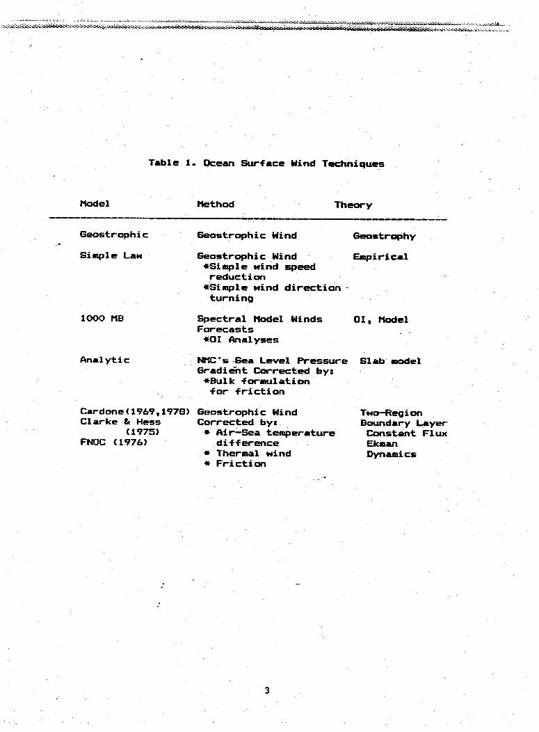
The different models evaluated were A) the geostrophic wind, B) a

simple wind law (Larson, 1975), C) NMC 1000 mb winds, D) an Ekman

slab model, E) Boundary layer model of Cardone (1969), F) boundary

layer model of Clarke and Hess (1975), and G) FNOC winds (Mihok and

Kaitala, 1976). A brief discussion of these wind models is given

below. A summary is presented in Table 1.

II) Description of Techniques

A. Geostrophic Wind

Sea level geostrophic winds were determined from the gridded

analyses and forecasts of sea level pressure and temperature using

the standard relations:

Ug = - (RT/fp) (p/ay) A.l.a

Vg = (RT/fp) Qp/<x) A.l.b

G = (Ug + Vg )'/ A.2

where: Ug = x-component of the geostrophic wind,Vg = y-component of the geostrophic wind,G = geostrophic wind speed,

and: R = universal gas constant,T = temperature(K),f = coriolis parameter,p = sea level pressure.

B. Simple Law

Operational forecasters commonly determine ocean surface

winds by simply reducing the geostrophic wind speed by a constant

factor and rotating the direction towards low pressure by a constant

angle. Larson (1975) proposed a slightly more complex formulation

in his study of time series of marine winds. The reduction factor

is allowed to vary as a function of latitude and the cross-isobaric

angle (or inflow angle) of the wind is permitted to vary as a func-

tion of wind speed and latitude.

The appropriate equations are:

B = 0.6045 + 0.186(0/25) for < 25 B.I.a

B = 0.7905 25 K e < 45 B.l.b

B = 0.6975 + 0.093*(90-G)/45 45 < B..c

where: B = wind reduction factor,G = latitude

2

4 w ,-. I- - - -S I- - A -- -- -. I I II.

Table 1. Ocean Surface Wind Techniques

Method Theory

Geostrophic

Simple Law

6eostrophic Wind

Geostrophic Wind*Simple wind speedreduction*Simple wind direction -turning

Geostrophy

Empirical

Spectral Model WindsForecasts

*OI Analyses

OI, Model

Analytic

Cardone(1969,1978)Clarke & Hess

(1975)FNOC (1976)

NMC's-Sea Level PressureGradient Corrected by:*Bulk formulationfor friction

Geostrophic WindCorrected by:

* Air-Sea temperaturedifference

* Thermal wind* Friction

Slab model

Two-Reg ionBoundary LayerConstant FluxEkmanDynamics

3

Model

1000 MB

and the surface wind speed is given by:

Vs = B*S B .2

where: 6 - geostrophic wind,

and the inflow angle (%) is given by the relations

O( (1.475/(1+sinO ))(22.5 - 0.0175Vs ) B.3

C) NMC Model 1000 mb winds

Analyses of 1000 mb winds were obtained from the NMC global dataassimilation system (Dey and Morone, 1985). The system providesanalyses of meteorological variables; height, temperature, windsand moisture using both conventional station observations taken

on the synoptic periods (OOz, 06z, 12z, and lz), and synoptic datafrom aircraft, satellite, etc. The analyses are made every six

hours using a two step procedure. A six hour forecast . is made,which is used as a first guess for the analysis. Current data are

then used to update the first guess by applying multi-variatethree-dimensional optimum interpolation on isobaric surfaces. Overthe ocean, both surface wind and pressure observations are used toproduce the 1000 mb wind analysis. In contrast, over the landsurface wind observations are not used.

Forecasts of the 1000 mb winds were obtained from the NMCMedium Range Forecast model which was run once per day during theOOZ operational cycle (Sela, 1982). The initial analysis is obtainedfrom the global data assimilation system. This model has 18 equallayers, each 28 mb thick (Since October 1986, unequal sigma levels- -have been incorporated into the model, with the'lowest layer havinga thickness of 11 mb). The boundary layer physics is the GFDLE-physics (Miyakoda and Sirutis, 1983). The 1000 lb winds were ob-tained from the forecast model sigma coordinate system byinterpolation. Figure I illustrates a schematic of the model levelsin relation to the mandatory observational level.

D) Ekman Slab Method

Ocean winds may be derived using a simple boundary layer slabmodel. The equations of motion, assuming steady state conditionsmay be written:

u a u/ax + v u/iy - fv - -p/ax - a(uw')/z D 1.a

u v/ax + v av/ay + fu - -Ka P/aY - C(v"w-)/~z D.1.b

4

Figure 1. Vertical distribution of modellayers, mandatory levels, and parameters.P* is the surface.-pressure, and SO, SI,etc., are the successive sigma levels.

I

III700mfb I… ~~~~~~~. III

I ETC

850 mb I- - - - - - - - - - - - - - - - - - - - - - - - - - - -

I ss3 _ (3)I s2 (2)I ISi (__ _1l)

1000 mb I- - - - - - - - - - - - - - - - - - - - - - - - -Surface I---- sO - - (0)-

5

.Iq: .:" .~~~~~~~~~~~~~~~k

If one parameterizes the momentum fluxes (u'w') (v'w') at the

ocean surface in terms of u and v and the pressure gradient at the

surface is given, then the above non-linear equations are solved as

a system of two equations with two unknowns through an iterativeprocess for u and v.

(1) Linear Solution

The linear system expresses a balance between the pressuregradient, coriolis, and friction forces in the atmospheric boundarylayer. The boundary layer is assumed to be a slab of constant depth(h). The momentum fluxes at the ocean surface are parameterized bya bulk transfer formula with a drag coefficient (CD) and thebalance of forces may be expressed as:

--dp/x + fv - (CD/h) Islu - 0 D.2.a

-- cap/ay - fu - (CD/h) IStv 0 D.2.b

In the above equations, it was assumed that the stress at the top

of the boundary layer (at zRh) is zero. Through algebraicmanipulation, D.2.a and D.2.b can be combined to give a fourth or-

der equation for (S):

IL.2. 2-LCD' S + f S - (Qp/X) + (a p/ ay) ) - 0 D

2. 2. Lwhere: S = u v and CD' CD/h 2.0 x 10

The solution for S is given by:

S C-fL + [f4+ 4CDt'o iiP/x + ~p/Y )] i}t/( CD') D.4

Thus, from equation D.4, one can calculate wind speed, given the

pressure gradient, coriolis parameter and the frictional drag

coefficient. Once S is calculated, substitution into the

original equations enables u and v to be determined.

(2) Non-linear Solution

The surface wind speed and direction were also determined by

adding the non-linear (advective) terms to the above linear Ekman

solution. Equations D.2. a and D.2.b are now written to include the

non-linear terms.

fv - ikap/ax - CD'Su u au/ax + vau/ay D 5 a

- fu - i ap/Iy - CD'Sv = uav/ix + v a v/ay D.5.b

6

~~~~~~~~~~~~~~~~~~~~~~~~~~~~:. .%-

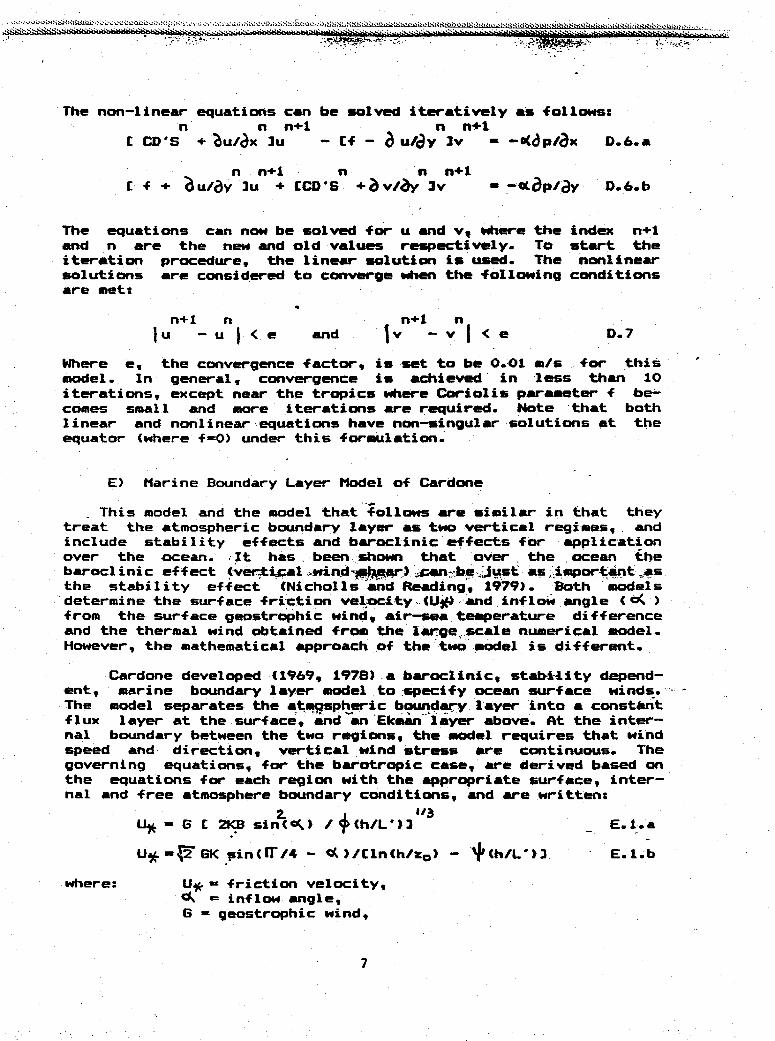
The non-linear equations can be solved iteratively as followsn n n41 n n+l

£ CD'S + ~u/<x 3u - if - a u/¥y Iv -' -dp/x D. 6

n n+1 - n n+lE +; aU/ay 3u * ECD~ 5 2+v/) 3Iv m- py D. 6. b

The equations can now be solved for u and vn W'here the index n+1and n are the new and old values respectively. To start theiteration procedure, the linear solution is used. The nonlinearsolutions are considered to converge when the following conditionsare met - -

,u -, - u |< e and IV - v < e D 7

Where e, the convergence factor, is set to be 0.01 m/s ..for thismodel. In general, convergence is achieved' in less than 10iterations, except near the tropics where Coriolis parameter f be-comes small and more iterations are required. Note 'that bothlinear and nonlinear equations have non-singular solutions at theequator (where f=0) under this formulation.

E) Marine Boundary Layer Model of Cardone

This model and the model that follows are similar in that theytreat the atmospheric boundary layer as two vertical regimes, andinclude stability effects and baroclinic effects for applicationover the ocean. .It has. been shown that over the ocean thebaroclinic effect (vertiq'al~wind . ..n-be u..as .Aiporta'nt:4sthe stability effect (Nicholls and Reading, 1979). .Both 'modelsdetermine the surface friction veloci-ty¥(U4 and inflow angle (cQ from the surface geostrophic winds air-sea temperature differenceand the thermal wind obtained from the large scale numerical model.However, the mathematical approach of the two model is different.

Cardone developed (1969t 1978) a barocllnics stabi-&ity depend-ent, marine boundary layer model to specify ocean surface winds. --The model separates the atmrspheric boundary layer into a constantflux layer at the surface, and an Ekean layer above. At the inter-nal boundary between the two regions, the model requires that windspeed and direction, vertical wind stress are continuous. Thegoverning equations, {or the barotropic case, are derived based onthe equations for each region with the appropriate surface, inter-nal and free atmosphere boundary conditions, and are written:

U - G E 2KB sin(CK.) / (h/L')] E.l a

U*,-.,'GK Din(gy/4 - rA)/Eln(h/zo) - *(+h/L')3 - E.l.b'where: U* - friction velocity,

Ak - inflow angle,G - geostrophic wind,

7

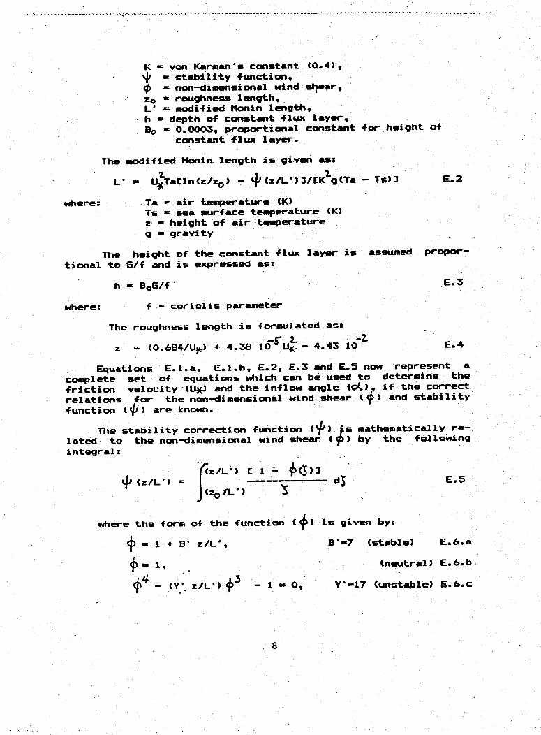
K - von Karman's constant (0.4),' stability function,= non-dimensional wind shear,

zo roughness length,L' modified Monin length,h = depth of constant flux layer,Bo = 0.0003, proportional constant

constant flux layer.

The modified Monin. length is gi-ven as:

for height of

where:

2. 2.L' - UyTaCln(z/zO) - +(z/L')]/£K g(Ta - Ts)]

Ta - air temperature (K)Ts = sea surface temperature (K)z - height of air temperatureg - gravity

The height of the constant flux layer istional to G/f and is expressed as:

assumed

E.2

propor-

E. 3h - BoG/f

where: f - coriolis parameter

The roughness length is formulated as:

z = (0.684U) + 43 10 U_ 443 10z- (o. 664/u .) + 4.3 10 U' 4.4 10' E.4

Equations E.I.a, E.L.b, E.2, E.3 and E.5 now represent acomplete set of equations which can be used to determine the

friction velocity (U*3 and the inflow angle (0C), if the correct

relations for the non-dimensional wind shear ( ) and stabilityfunction (4) are known.

The stability correction function () 's mathematically re-lated to the non-dimensional wind shear ( ) by the followingintegral:

) (z/L') =(z/L E 1) - )J(z0 /L') S

where the form of the function ( +) is given by:

I = 1 + B' z/L',

1) Y 1,

+4 (y. z/L' ) +

B'-7 (stable) E. 6. a

(neutral) E.6. b.

- 1 - 0, Y'-17 (unstable) E.&.c

8

dS E.5

..~' '~;:; -.... : 'h'' " ' ~ i ':s?; A ~' .'."'i't~ ~':' hc'' *~iSS~b'E'Lt~~S i S~:b ~ bSS8S`SS~`~S.''ti~t;;;S^:~ `~ ~ . ```~ t ` t ~ .i'iii; ;! *.~-h

6iven U¥, z o, and 4 (z/L'), the wind can now be specifiedat height z, within the constant layer, which for this study isat 10 m, and is given by:

U(z) = (U/K)Cln(z/zo ) - I(z/L')] E. 3

There are three parameters that are important to this bound-ary layer model, but whose relationships must be empiricallydetermined from field measurement studies. These parameters arethe stability dependent non-dimensional wind shear ( 4' ), thesurface roughness (zo) as a function of surface stress, and thescaling factor (B0 ) for the height of the internal boundarylayer.

For the full baroclinic case, equations E.l.a and E.I.b arereformulated with the inclusion of the non-dimensional wind shear(thermal wind) parameter:s_

ddG/dzI/f E.9 -

and the angle between the wind shear vector and the surfacegeostrophic wind. In this case the equations become more complexand can be found in Cardone(1969).

F) Marine Boundary Layer Model of Clarke and Hess

Clarke and Hess (1975) have also developed a marine boundarymodel, based on similarity theory, which incorporates baroclinicand stability effects. The atmospheric boundary layer is assumed tobe divided into two distinct regions, the inner layer (which isabout 50 m thick), and the outer region which extends to the top ofthe boundary which is 1-2 km. The inner layer is a constant fluxlayer and the outer layer is the Ekman layer. The equations for thetwo layers along with the boundary conditions are similar to theCardone model. However, the mathematical basis of this technique isthe asymptotic matching of wind from the constant flux layer to theEkman layer across the interior height h, through dynamicsimilarity scaling arguments. This approach provides equations thatlink the #external parameters of the free atmosphere such asgeostrophic wind, thermal wind, and air-sea temperature differenceto the 'internal" parameters of surface stress and inflow angle,without direct knowledge of internal boundary height and the top ofthe boundary layer.

The Rossby number similarity theory is applied to the govern-ing atmospheric equations, which are written:

K Ug'/U*C ln(U*/fzO) - A F.l.a

K Vg'/U* = BIf[/f F.l.b

where: Ug' = component of geostrophic wind in thedirection of U

9

Vg' component of geostrophic wind 90 degreesto the left of U

U* - friction velocityf - coriolis parameterzo = roughness lengthK von Karman s constant (0.4)A, B - similarity functions

By combining equations F.1.a and F.1.b with some algebraic

manipulation, a new equation, F.2. a, is obtained. Further, equationF.1.b can be rewritten, using the trigonometric relation

Yg' - 6 sin(O'),

to obtain equation F.2.b. The inflow angle (C) is the directional

difference between the geostrophic wind and surface stress.Equations F.2.a and F.2.b can be solved for the two unknowns offriction velocity (U*), and inflow angle (K) given the geostrophicwind speed and stability. The height of the internal boundary isnot a required variable in the solution.

ln(R0) A - In(U,/G) + (K6/U* - B I F.2.a

= sirnl (BUM/KG) - F.2.b

where the Rossby number is defined as:

RO = G/(fzo )F.3

the roughness length is specified as:

Zo = 0.016 U* /g F. 4

where g - gravity

and G = geostrophic wind speed

The similarity functions A, B are dependent upon stability.Extensive field experiments and research has been conducted to

determine these universal functions. Clarke and Hess (1975)

modified the Rossby number similarity theory to include the

baroclinic effect and also to include the ocean surface current as

a function of friction velocity. Equations F.1.a and F.l.b are

rewritten as:

K(Ug - Us')/U* ln(U/(fz) - A(Us) F5a

K(Vg - Vs)/U, -B y,,s)ifI/f F.5.b

where the sea surface current is specified to be the friction

velocity (LL) and its relative components are:

Us = UM cos(04 ) F.6.a

10

. ' -:, : .~. .' :.:.:.:.:S!>'.:'.'i: !.: :'.' i , ;'i!.', '::: .:. .' .' . .' . ' ' : . .; :: ----

Vs' = sinCO ). F.6.b

Agadn combining the U a ndV cmanents of the Rossby numbersimilarity theory equation and after some algebraic anipulations,UX and ck can be determined from the two equations that {ollowt

In(.). - A(fgs) - ln(6/U - CK'(6/*- 1) - 9.1,5) - 0 F.7

C(- sin CEijs)/C(K(6/L.- 1))] F.8

where the stability parameter is given bys

- gK(Ta -Ts) / (fGTa) F.9Ta - air temperature (K)Ts - sea surface temperature (K)

and the baroclinic parameters are given by:

s = (sxL + sy ? ')'L F.10

~- sx - (K/f) Ug "az, F.lI.a

sy - (f aVg'z F. l1.b

The similarity functinons .. Ws) and BR ,s) have been derivedas:

AC(,s) A(1J) + A(s) + Ao F.12.a~~~~~~~~~~~~~~~~~~~~~. 2.a

B(C,s) - B(. + B(s) + B0 F. 12.b

where A0 - 1.1 and B0 -- 4;3 are the neutral barotropic values for Aand B. AY) and BJ) +are the contributions due to stability. A(s)and B(s) are the ,contributions due to the baroclinic effect.Clarke and Uess used the following relations;

A( ) - -0. 10 - o.oolt F 13 a

B( ) - 0.13 - 0.001Pi F.13.b

A(s) - 0.20sx - 0.04sy F. 14.a

A(s) - -0.32dx + 0.3Ssy F.14.b

G) FNOC Marine Winds

Unlike the NHC's 1000 ob winds which are analyzed on fixedisobaric surfaces using optimum interpolation analysis, the FNOCwinds are analyzed at the oceean surface using a variationalanalysis method (hihok and Kaitala, 1976, and L. Clark CFNOC), 1986personal communication). Forecast winds are derived from outputfrom the NOGAPS model. 11

- x -- -- - ---------

H) Summary comments concerning the models

The techniques that were evaluated have been p resEnted in or--der of complexity. These techniques are -diagnostic models, whichdetermine ocean surface winds from the large scale atmosphericanalyses and forecasts. The simplest method for obtaining oceansurface winds is to directly calculate the geostrophic wind.lHowever, it is well known the actual surface winds are lss thangeostrophic and are turned toward lower pressure. The Simple Law is

based on. empirical equations uhich provide the surface wind speedand direction from the qeostrophic wind. This technique willproduce the general pattern of the large scale wind field

However, the simple empirical law is just that, a simple em-pirical adjustment to the geostrophic wind. Theoretical modelsprovide a logical framework to progress from the simple to the com-plex with an orderly physical interpretation. The one-layer slab

model was designed on the premise that simple Ekman theory could be

used to deduce surface winds, given the sea level pressure

analysis. This technique was formulated to be well behaved- at theequator unlike the geostrophic wind relation. A deficiency of thisslab model, is the use of a constant drag coefficient. Although,

the diabatic and baroclinic effects were not included in the model,

it was extended to include the non-linear advection terms. However,

inclusion of the nonlinear terms in this formulation did not ap-

preciably improve the ocean surface winds.

The next level of complexity treats the atmospheric boundarylayer as two regions and includes stability and baroclinic effects.In this study, two representative models were evaluated; one whichdetermines the surface stress and surface inflow angle based on asystem of equations for each region with boundary conditions at theocean surface, top of the constant flux layer, and top of theboundary layer (Cardone), and the other that determines the surfacestress and inflow angle using the appropriate equations and bound-ary conditions based on dynamic similarity scaling theory (Clarkeand Hess). Because a boundary layer theory does not present closed

set of equations, the Cardone model requires empirical knowledge ofthe non-dimensional wind shear function 4 and height of the inter-nal boundary layer (through the constant Be), and Clarke and Hessrequire knowledge of the similarity {unctions A and B. Both models

require functional .relation between the surface stress and the sur-face roughness. It has been shown by Krishna (1981) that if the.equations from two layer analytical model are written in the formof similarity equations (for barotropic case), t"e similarity func-tions can be expressed in terms of B0 , %' andy). Krishna scaledthe internal boundary height on U*/f rather than 6/f, whichresults in the constant B, instead of Bo . The similarity {unc-tions have been determined {rom extensive field experiments in or-der to determine empirical relations for a range of stability and

12

- ~ ~ ~ ~ ~ ~ ~ - -- - - - - - - - -- - -- -- -- ---- ---- ---- ----

Vs' - L sin( CO() F.6.bAgain combining the U and V components of the Rossby numbersimilarity theory equation and after some algebraic manipulations,UK and cO can be determined from the two equations that follow:ln( ) -A(0,s) -ln(G/U)- -[K1(i/U* --B tjs)] -0 F.7

c~= sin CB(Ujs)/((K(B/U -- 1)M] F.8where the stability parameter is given by:

J e gK(Ta - Ts) / (fGTa) F.9Ta - air temperature (K)Ts - sea surface temperature (K)

and the baroclinic parameters are given by:

s = (sx + sy )I/ F. 10

sx (K /f) Ug z,FaX U9 Z, ~~~~~~~~~~F. lt.a

sy = (KZ/f) (vg /az F.Il.b

The similarity functibns'.Aw,s) and B 9j,s) have-been derivedas:

A(js) A(Fj) + A(s) + AO F. 12. a

B(jJ,s) = B(J) +- B(s) + B0 F. 12. bwhere A0 - 1.1 and B0o- 4.3 are the neutral barotropic values for Aand B. A(p) and B ) are the contributions due to stability. A(s)and B(s) are the -contributions due to the baroclinic effect.Clarke and Hess used the following relations;

A( ) = -0. 10op - 0.0012. F. 13.aB( ) - 0. 13J - 0.001 F.13.bA(s) - 0.20sx - 0.04sy F.14.aA(s) - -0.32sx + 0.35sy F. 14.b

G) FNOC Marine Winds

Unlike the NMC's 1000 mb winds which are analyzed on fixedisobaric surfaces using optimum interpolation analysis, the FNOCwinds are analyzed at the ocean surface using a variationalanalysis method (Mihok and Kaitala, 1976, and L. Clark (FNOC), 1996personal communication). Forecast winds are derived from outputfrom the NOGAPS model.

'11

H) Summary comments concerning the models

The techniques that were evaluated have been presented in or-der of complexity. These techniques are "diagnostic" models whichdetermine ocean surface winds from the large scale atmospheric

analyses and forecasts. The simplest method for obtaining oceansurface winds is to directly calculate the geostrophic wind.

However, it is well known the actual surface winds are less thangeostrophic and are turned toward lower pressure. The Simple Law is

based on empirical equations which provide the surface wind speed

and direction from the geostrophic wind. This technique willproduce the general pattern of the large scale wind field.

However, the simple empirical law is just that, a simple em-

pirical adjustment to the geostrophic wind. Theoretical models

provide a logical framework to progress from the simple to the com-

plex with an orderly physical interpretation. The one-layer slab

model was designed on the premise that simple Ekman theory could be

used to deduce surface winds, given the sea level pressureanalysis. This technique was formulated to be well behaved at the

equator unlike the geostrophic wind relation. A deficiency of thisslab model, is the use of a constant drag coefficient. Although,the diabatic and baroclinic effects were not included in the model, it was extended to include the nonlinear advection terms. However,inclusion of the nonlinear terms in this formulation did

not ap-

preciably improve the ocean surface winds.

The next level of complexity treats the atmospheric boundary

layer as two regions and includes stability and baroclinic effects.

In this study, two representative models were evaluated; one which

determines the surface stress and surface inflow angle based on a

system of equations for each region with boundary conditions at the

ocean surface, top of the constant flux layer, and top of the

boundary layer (Cardone}, and the other that determines the surface

stress and inflow angle using the appropriate equations and bound-

ary conditions based on dynamic similarity scaling theory (Clarke

and Hess). Because a boundary layer theory does not present closedset of equations, the Cardone model requires empirical knowledge ofthe non-dimensional wind shear function p and height of the inter-nal boundary layer (through the constant Be), and Clarke and Hess

require knowledge of the similarity functions A and B. Both models

require functional relation between the surface stress and the sur-{ace roughness. It has been shown by Krishna (1981) that if theequations from two layer analytical model are written in the form

of similarity equations (for barotropic case), tqe similarity func-tions can be expressed in terms of Bo , ) and * Krishna scaledthe internal boundary height on U*/f rather than G/f, whichresults in the constant B, instead of Bo. The similarity func-tions have been determined from extensive field experiments in or-der to determine empirical relations for a range of stability and

12

thermal wind conditions. Both two-layer analytic models andsimilarity theory models have been used in numerical prediction.However, while the similarity theory does not require the height ofthe internal boundary layer, it is not as straight forward to in-clude more complex physics as in the two layer analytic models.

III) Winds from Analysis and Forecast Models

The wind models were run daily for 0000 UTC from December 3,1985 through January 6, 1986 to generate wind fields on a 2.5 by2.5 latitude/longitude grid for analyses (meteorological variablesobtained from the NMC global data assimilation system) and 24 hourforecasts (obtained from the NMC spectral atmospheric forecastmodel). The comparison study covers 35 days of early winterconditions. During that period, 28 days of FNOC winds were avail-able for comparison. Observations were matched, with interpolatedmodel winds, for analyses and forecasts.

The data distribution for the 35 day period of reports taken at0000 UTC and received over the GTS for the areas used in the studyare shown in Figure 2. The location of the data buoys used in thestudy are presented in Figure 3. The typical global distribution ofship reports taken at the synoptic hour of 0000 UTC on 12 December1985 is shown in figure 4. It is evident that the coverage of sur-face 'data is insufficient for providing an adequate analysis formany regions over the ocean.

IV) Sources of Validation Data

A. Ship Weather Reports

Two types of observations were used as standards to measurethe accuracy of the models - ship weather reports and data ob-tained from the NWS fixed buoy network.

Meteorological observations from ships at sea are preparedby deck officers as part of their routine duties. The observa-tions are recorded in a weather log and transmitted to coastalreceiving stations via radio in an internationally agreed uponWorld Meteorological Organization ¢WMO) code. This code consistsof up to 20 weather parameter groups one of which contains areport of wind speed and direction. These reports are dissemi-nated world wide in real time via the Global TelecommunicationsSystem (GTS).

Wind speed and direction are estimated either indirectly bythe observer using the sea state and the feel of the wind ordirectly by anemometer if the vessel is so equipped. Based upondata compiled by Earle (1985) for the period 1980-19q83 46X ofship reports in the Pacific and 44% of Atlantic ship reportswere from vessels without anemometers. Dischel and Pierson(1986) discuss the characteristics of wind observations made withand without anemometers. They note that errors from anemometer

13

Figure 2. Ship data distribution for

investigation period, December 3, 1985

through' January 6, 1986 for OOZ. Coastal

reports (less than 50 km from land) were

excluded. Data were received vie the GTS.

VC SNIP M MTSMISOSO0 1 "OIOUwCALL SION

I laud IIIM"I~IlIN

Figure 3. Location of fixed buoys.Coastal buoys were excluded.

:2

AtS~~~~~~~~~~~~~~~~~~~~~~~~~~~~~~~~~~~~~~~~~~~0

flat 1~O~ 12M i~fl~ SOC 101 17C IO 1 7Q A11 flo0 Iog AMI, OM JIG AQI W II Ill I l O# I m- low

3.,

06~~~~~~

:;. ~ ~~~~~~~~~~~~~~~~~~ S~ 1

UP,~~~~~8

U ./ .. .

S~~~~~~S m S-41 -4MIgA IAM3Ut 11D mlw7

'S. ~ ~ ~ I arSX msii sUUG 3`3 11 V11N

'5~~~~ctLso

'S/ fj~~~~~~~~

I

Figure 4. Distribution for all wind reports

for one synoptic period, OOZ, December 12, 1985.

z

.3'i7,f;

-f

X

,I

2

i

r

I.1;I

Y.

"Ij.1Z

2

t

.1

j

measurements can be introduced by poor instrument exposure, im-proper reading of the wind speed and direction indicators, andvessel motion. In addition wind instruments exposed to severemarine meteorological conditions can lose their calibration.

Estimated wind observations are also subject to a widevariety of errors. Such reports are often made by the observerby first determining the wind speed parameter in terms of theBeaufort scale where each scale number represents a range of pos-sible wind speeds. From this a single speed is chosen forreporting purposes. Furthermore the .scale is based, for the mostpart, on the appearance of the state of the sea. However, it iswell known that there may be a substantial time lag for the seato reach a state that truly reflects the concurrent wind forceconditions. In addition, it is obvious that night time windreports based upon visual sea state observations are subject togreat error.

Ship wind observations were collected from reports trans-mitted over the GTS, which have been processed at NMC with onlyminimal quality control error checking. There is no distinctionmade between whether the report is estimated or measured.Further, for measured winds there is no correction for varyinganemometer heights.

B. Fixed Buoy Reports

Since 1967 moored buoys, equipped with meteorological in-struments, have provided surface atmospheric and oceanographicdata for marine use. Buoys can be expected to provide improveddata compared to that reported by ships for several reasons.First, each sensor location is carefully considered to avoid ex-posure problems. Second, measurement sampling frequencies andaveraging periods are determined after accounting for buoymotion. Third, duplicate sensors are used and each is calibratedbefore deployment. Finally, all data are monitored in near realtime to detect instrument errors. Gilhousen (1986) reported thatthe buoys are presently providing measurements which are withinthe original accuracy specifications. Table 2 (National ClimatcData Center, 1983) shows the specified buoy system accuracy forwind speed and direction.

Table 2

Reporting Sampling Averaging Total SystemRange Interval Period Accuracy

Speed 0 - 155kt 1 sec 8.5 min SD +/- 1.9 ktor o10%.

Direction 0 - 360 deg 1 sec 8.5 min Sd +/- 10 deg

Remark: Sensor heights vary between 5 and 10 meters abovethe water.

17

V) Statistical Procedures

The statistical comparisons are made for wind speed, wind

direction and vector wind, for both analyses and 24 hour forecasts

with ship and buoy data.

Because wind direction is a circular function (0 - 360

degrees), standard statistical methods for linear data sets can not

be used directly. For instance, Turner (1986) has discussedseveral methods to determine the standard deviation of wind direc-tion as well as its mean direction. In this paper, wind direction

statistics were determined relative to the cross isobaric angle

(inflow angle toward lower pressure), in order to eliminate the

cross over problem of wind direction at 360°. The evaluation of in-

flow angle is important because of its relation to low level

convergence.

Standard statistical measures were used in order to compare

and evaluate the models with observations. Willmott (1982) has

discussed the use of difference measures in order to evaluate model

performance, and states that no one measure can be expected to

provide satisfactory information. In this study we used a similar

set of statistical difference measures. However, wind is a vector so

that standard scalar measures are not complete, and additional vec-

tor statistical measures have been included.

The measures used for this study are given by the following

definitions:

Wind speed:

Correlation coefficient:

(N SoSm Sof- S m '/~

C ENENS - (Eds0 3"IENSM - ( 3Pm 1 6.1

Average absolute difference:

lso - S.m/IN S.2

Average algebraic difference:

(S- Sm)/N .3~~~~~~~~~~S. 3

and the Root mean square difference:

.E(SO - SM) /N] S.4

where SO = observed wind speed

18

Sm - model wind speed,N - number of comparisons

Wind direction:

Average inflow angle:

g(o -C(g) IN

Aver-ge absolute diff-erence:

IF loco -& I IN/

Average algebraic difference:

cO<o - C) IN

S.5

6.6

S.7and the Root mean square difference:

c . 6 -_O?'-L/N, vwhere

S.6

g - direction of the isobars with low pressure to theleft (direction of the geostrophic wind),

o - direction of the observed wind, andm - direction of the model wind.

Vector wind:

Average vector wind difference

Ruo-um)o + (vo-v) n2 iNeRoot Mean Square vector wind difference:

{ ZE(uo-u) * c(vo-vm= itNI

S.9

SjrloA wind vector correlation coefficient was calculated using the

formulation developed by Court (1958). In the formulation,. thecorrelation between two sets of wind vectors, Wl and W2, can bedetermined by a combination of expresslons containing the -scalarwind components. The wind vector W1 is composed of a component (ul)toward the east and -(vl) toward the north, and the wind vector W2 iscomposed of. & component (u2) toward the east and (v2) toward thenorth. The following expression has been used to determine the windvector correlation. coefficient (R WIWZ.)s

L -2 L Z. LR WI Nt- C CGvI (Gulu2 + S9iu2 ) + Su1 (<ulv2 + Gvlv2 )- 2Su2v2(Sulu2 Sulv2 + Sv1u2 Gvlv2 )2 /

[2 2.Sul 22.E(Sul *- Svi )(Su2.Sv2

The relations for the wind_1tSul - Z(ul - ul) IN

-82v2 -- BU2v2 ) 3}

vector correlation are of the form:· ulv2 - ;(ul - ul)(v2 - v2)/N1 9

S. 11.

VI) Discussion

Wind speed data distributions (number of observations and per-cent) at 1m/sec intervals are presented in Table 3. The mean wind

speed for ship data was 10.1 /sece, with a standard deviation of 5.4

m/sec, and for buoy data the mean was 7.4 m/sec with a standarddeviation of 3.4 i/sec. The mean wind speed data and and the wind

speed distribution data indicated that major store activity did notaffect the regions of the fixed buoys, but that ships, WhMse routescover a much wider part of the ocean-did encounter some major stormactivity. But, it was also suspected that high wind speeds may be

overestimated by observers on ship. Ships reporting high wind speeds

were subjectively compared with the Northern Hemisphere Surface

Analysis to determine whether the reports were reasonable or not. Itwas found that some of the high wind speeds were obviously erroneous(i. e. not supported by the synoptic pattern), but others were lo-cated in frontal zones, squalls, or within intense cyclonic

systems

which may be reasonable but can not be resolved by the large scale

model. Those wind reports that were identified as erroneous have

been eliminated from the evaluation.

Comparisons of model winds with observations are presented in

Tables 4 through 9, for wind speed, wind direction and vector wind,

for both analyses and 24 hour forecasts. The tables separate the

data by type, ship and buoy; and by region, northern hemisphere (>

17 N), east coast (25N to 50N, the coast out to 55W), and westcoast (20N to 65W, 10W to the coast) The regions are identifiedin Figure 2. Tables 10 and 11 show the average algebraic difference

and RMS difference as a function of wind speed. The data used to

produce these tables do not include reports within 50km of land ordata over lakes. Wind speed data were rejected when the geostrophicwind and model wind differed by more than 40kts, and wind directiondata when the model direction differed from observation by more

than 105 degrees for analyses (165 degrees for 24 hour forecasts).

Inspection of the tables indicates the no one model is superiorto the others in all respects. However, a few general comments canbe made concerning the statistics. The models verify better againstthe buoys than ships. This is not unexpected. Reports from fixedbuoys are closely monitored and quality controlled in order toprovide reliable data (Gilhousen, 19B6), Whereas the quality ofship reports has-' been shown to be questionable (Dischell andPierson, 1986, and Earle, 1985), Hence, the following discussion

will be primarily concerned with comparing the model winds with

buoys. Another point to be made is that the Models verify betterwith the east coast buoys than With the west coast. This possiblyreflects a poorer quality analysis over the Northeast Pacific com-pared with the Northwest Atlantic.

20

2 3435 5133.1 3.7

33 473.8 5.4

13 14626 4794.5 3.41e 7

2.1 0.8

23 2495 460.7 0.3

33 340 10 <0.1

47705.6

566.5

156594.66

0.725360.3

353

<0. 1

5 6919 10816.6 7.8

95 11210.9 12.9

16 17180 3221.3 2.3

1 4

0.1 0.5

26 2728 19

0.2 0.1

36 370 10 <0.1

Table 3. Data distribution by ships and buoys at intervalsof 1 m/s such that the wind speed is the truncated speed,for example 5 is the range 5 to <6 m/s, 6 is 6 to < 7 m/s,and so forth. Mean wind speed for ships is 10.1 m/s withstandard deviation of 5.4 m/s. Mean wind speed for buoys is7.4 m/s with standard deviation of 3.4 m/s.

21

813249.6145

16.7

91107S.0778.9

SourceShips

(X)Buoys(%)

SourceShips(%)

Buoys(%)

SourceShips(%)

Buoys(7)

SourceShips(x)

Calm1511.1141.6

1010497.648

5.5

202241.600

3010

0.1

>017

0.13

0.3

117695.635

4.8

21850.6

00

316

<0. 1

>11981.422

2.5

129436.840

4.6

22690.5

1

0.1

324

<0. 1

711068.099

11.4

183462.53

0.3

2814

0.1

3800

192181.6

20.2

2916

0.1

3900

. I . . - - - - - - - - - - - - - -- - - -- - - - - - - - - - - - - - - .- - 7 7 - - .- - . I - -

. s ; aes o s~9;t......... 8: !; i,.<:v>x.:xs:>.s:s~x .................. s. :as - . < A s .. :.... --...... , .. .' ::. . ;.-. - .... . '. ...v I'.: :I..i.'.:-.::.:

I- I-. I I II ICorrelationI Ave. Abs. I Ave. Alg. 'I RfSD I

I MODEL I I Diff. I Diff. I I

I I NH WC ECI NH wC ECI NH WC ECI NH WC ECII- -- -1 1 . ... I

I Ship 1.66 .71 .7113.8 4.0 3.4-0.9-1.7 0.615.0 5.2 4.51

I Geostrophic I I I I I

I Buoy 1.70 .77 .7913.5 4.9 2.7-2.3-4.3-1.614.6 6.1 3.5I

I- '- - 1- I - II Ship 1.66 .71 .7113.4 3.2 3.7-1.4 0.9 2.514.5 4.2 4.81I Simple Law I I I 1 1

I Buoy 1.71 .77 .7912.4 2.9 2.010.2 1.8 0.313.1 3.7 2.51

I -I .- 1 I - 1- .--------1I Ship 1.68 .72 .7413.4 3.5 3.4-0.6-i.4-0.014.5 4.6 4.01

I 1000 mb I I I I I

I Buoy 1.71 .77 .7813.1 4.0 2.5-2.1-3.6-1.514.0 5.0 3.21I-- 1-- I 1- I --' II Ship 1.63 .68 .6713.5 3.4 3.4-0.1-0.6-1.314.6 4.5 4.41

I Yu I I I I I

I Buoy 1.68 .73 .7813.0 3.8 2.4-1.8-3.2-1.213.8 4.8 3.01

I- -- I I I I I- II Ship 1.61 .63 .6813.7 3.6 3.9-2.1 2.0 2.914.8 4.7 5.11

ICardone I I I I I

I Buoy 1.67 .70 .7512.5 2.4 2.210.2-0.6 0.1:3.2 3.2 2.91

I -- - I I I -'I Ship 1.65 .70 .7313,3 3.0 3.410.9-0.6 1.614.3 4.0 4.11

I Clarke/Hess I I I I I

I Buoy 1.67 .77 .7712.5 3.1 1.9-0.6-2.3-0.613.2 3.9 2.51I- -I I L a

Ship 1.69 .72 .7513.1 3.0 2.910.5-0.0 1.614.1 4.0 4.01

FNOC I I I I I

Buoy 1.74 .75 .8212.3 3.1 1.8-0.9-2.3-0.513.2 4.2 2.6I.~-I I I- 1.I -- I

Table 4. Ships/Buoys vs Models (Analyses) Comparisonsfor Wind Speed (m/sec). NH: Northern hemi-sphere > 17N, WC: West Coast and ECt EastCoast

22

I.I

III

I �. . �

MODEL

ShipBeostrophi c

Buoy

ShipSimple Law

Buoy

Shipmb

Buoy1000

Yu

Cardone

I Clarl

I

I FNOC--

II FNOCII~

I-I i -I' I " IICorrelationl Ave. Abs. I Ave. Alg. I RMSD II I Diff. I Diff. I II NH WC ECI NH WC ECI NH WC ECI Ni WC ECI-I ·' I- I ......I I1.59 .61 .6814.2 4.6 3.7-1.0-1.7 0.015.5 5.9 4.91I I I I I1.61 .66 .7013.9 4.9 4.0-2.5-4.0-2.815.1 6.3 5.31

-I I I I I1.59 .60 .6813.8 3,8 3.711.4 0.9 2.114.9 5.0 4.01I I I I I1.61 .66 .7012.9 3.3 2.8-0.3-1.6-0.713.7 4.2 3.5I15-I I I I- I1.58 .59 .6813.6 3.9 3,310.0-0.6 0.214.B 5.1 4.4II

I. 60

Ship 1.56I

Buoy . 59

ke/H

1 ---Ship 1.60

I

Buoy 1. 65- -- I----Ship 1.59less I

Buoy I.60

Ship 1.52I -

Buoy 1.45- I -I

I I I I.64 .6713.3 4.2 3.4-2.1-3.2-2.614.3 5.3 4.5I

I I - I I.59 .65I3.8 4.0 3.5-0.2-0.6 0.915.0 5.2 4.61

I I I- I.64 .7013.5 4.0 3.2-1.9-3.0-2.014.4 5.0 4.01

- I-- I I - -- I.61 .7013.8 3.7 3.7+2.2 2.1 2.5I4.9 4.9 4.8I

I I I I.68 .7912.6 2.5 2.410.3-0.3-0.6I3.3 3.1 3.01-I -- I --- I.62 .7013.6 3.5 3.4 1.3 1.0 0.914.7 4.9 4.4I

I I I I.68 .7012.6 2.8 2.6-0.4-1.4-1.113.4 3.6 3.2I

I I l -I -I.53 .5213.8 3.8 4.2 1.3 1.0 2.214.9 4.9 5.41

I I I I.51 .4113.1 3.3 3.3-.3-1.4 -0.213.9 4.1 3.9I

I I - -I I

Ships/BuoysComparisons

vs Hodels (24 hour forecasts)for Wind Speed (m/sec).

23

I

I

I

I

I

I

I

I

I

I

I

I

I

II

I

I

I

I

I

I

I

I

I

I

Table 5.

; ·. .. . . < , . ; .,. .. , .i .... ...:`:<`.`..`::`.``*`<<``:`~`~`~`:~`:`:`.```::`.`~`.`.``x:`~-~>`> `~`q>`:`.`.:*:`~:``~ . ;.~.~4~j ~ `%.~ ;`~`s%~ .` ~ ;;~:`.:~~;;;;~ `L~`.``.`.

'.

i- - I ... i- I ~ , I , I

I IInflow I Ave. Abs. I Ave. Ailg. I R:SD I

I MODEL I Angle I Diff. I Diff. I I

I I NH WC ECI NH WC ECI NH WC ECI NH WC ECI

I- - . I-I I I II Ship I 0 0 0 I 30 27 32 1*21 16 24 *1 37 34 39 I

I Seostrophic I I I* *I I

I Buoy I 0 0 0 I 31 24 361*24 17 34 *I 38 31 42 I

I- - I I I I-II Ship I 19 lB 19 I 2322 24 i 2 -2 5 I 31 30 32 I

ISimple Law I I I I I

I Buoy I 19 17 1 9 I 22 18 23 I 5 0 14 I 30 26 29 I

I -. I - I I ---- II Ship I 17 17 21 I 21 21 24 I 4 3 3 I 29 29 32 I

I 1000 mb I I I I I

I Buoy I 20 12 28 I 19 17 17 I 4 5 6 I 27 25 22 I

I- . . I I - - I - II Ship I 17 17 15 I 23 22 24 1 4-1 9 I 31 30 32 I

I Yu I I I I I

I Buoy I 16 15 13 I 23 19 25 I 8 2 20 I 31 27 32 I

I- - - - - I- I-- - I1- I- - -I

I Ship I 16 14 16 I 23 22 24 I 5 2 8 I 30 30 24 I

I Cardone I I I I I

I Buoy I 18 14 19 I 21 18 21 I 6 3 15 I 29 26 26 I

I ---- I-------I- I -- I --.-.-- I --- .II Ship I 19 19 18 I 23 22 24 I 2-3 6 I 31 30 32 I

I Clarke/Hess I I I I I

I Buoy I 22 19 21 I 21 19 17 I 2 -2 14 I 29 26 24 I

I -----. I- I-- I --I II Ship I 20 17 19 I 21 20 21 I 1 -1 5 I 29 29 31 I

I FNOC I I I I I

I .Buoy I 21 17 22 I 18 16 17 I 3 0 12 I 26 23 24 II- ------ -.-.- I -- -I--I-I- --- -ITable 6. Ships/Buoys vs Models (Analyses) Comparisons

for Wind Direction (Degrees). The computedinflow angles between observation directionand geostrophic direction is presented as thestatistic under average algebraic differenceFor the geostrophic model.

24

I-

III

I i I I I

IInflow I Ave. Abs. I Ave. Alg. I RMSD IMODEL I Angle I Diff. I Diff. I I

I NH WC ECI NH WC ECI NH WC ECI NH WC ECII- . . .I ---- I- I I - II Ship I 0 0 I 37 37 35 I 17 15 18 I 49 50 45 II Geostrophic I I I I I

I Buoy I 0 0 0 I 35 33 32 I 18 11 26 I 45 45 38 II---- - I- I -I I -- II Ship I 19 17 19 I 32 34 29 I -2 2 -1 I 46 47 42 II Simple Law I I I I I

I Buoy I 19 17 19 1 28 31 21 I -1-6 8 I 40 4429 II--- - I -.---- I------ . ..--I---------I ------II Ship I 21 15 16 I 32 33 30 I -4 0 2 I 46 48 42 II 1000 mb I I I I - I

I Buoy 1 21 12 23 I 28 31 21 I -3 -1 3 I 40 44 29 III-------------- I-------- I -- --- I----------III Ship I 17 17 16 I 33 34 30 I 0 -2 2 I 46 48 42 IIYu I I ' I I I

I Buoy I 164 14 15 I 28 31 22 I 2-3 12 I 40 43 30 II------------ -I . ---- I ---------- I----------I - II Ship I 15 15 16 I 32 34 29 I 2 0 2 I 46 47 41 II Cardone I I I I I

I Buoy I 18 15 18 I 28 30 20 I 1 -4 8 I 40 44 28 1I -------------- ------ I ---- --- I…. --…-I… -------I

I Ship I 19 20 17 I 32 33 29 I -2 -5 1 I 45 48 41 II Clarke/Hess I I I I I

I .Buoy I 21 2219 I 28 31 21 I -3 -11 7 I 41 45 28 II---- --------- ------ I ------ --- I -- II Ship I 14 15 9 I 37 38 40 I 3 0 9 I 52 54 54 II FNOC I I I I I

I Buoy I 12 11 7 I 40 37 43 I 6 0 19 I 55 53 59 II------------- --- - I I - ------- I

Table 7. Ships/Buoys vs Models (24 hour forecasts)Comparisons for Wind Directions (Degrees).

25

I .. I -i 1 II I Vector I Vect. Err.I Vect. Err.I

I MODEL ICorrelationl lagn. I RMS I

I I NH WC ECI NH WC ECI NH WC ECI

I -- I I I II Ship 1.72 .75 .7017.4 7.3 7.0i9.1 9.0 8.71I Geostrophic I I I I

I Buoy 1.73 .62 .7916.4 6.1 6.217.7 7.8 7.51

I -I-I- I I

I Ship 1.72 .74 .6815.7 5.5 5.817.2 7.0 7.3II Simple Law I I I I

I Buoy 1.74 .83 .8014.4 4.2 4.115.5 5.0 4.81I- I: II II Ship 1.76 .77 .73I5.8 5.9 5.417.4 7.5 7.11

I 1000 mb I I I I

I Buoy 1.79 .84 .8314.7 5.3 3.915.8 6.1 4.61

I ..- I - I I :. II Ship 1.72 .74 .6916.1 6.0 5.817.6 7.5 7.41

I Yu I I I I

I Buoy 1.74 .81 .8015.2 5.3 4.716.3 6.1 5.5I

I --- I I I I

I - Ship 1.70 .72 .6715.8 5.6 5.717.1 7.0 7.11

I Cardone I I I I

I Buoy 1.73 .81 .7914.2 3.7 3.815.3 4.4 4.6I

I -I I I II Ship 1.72 .74 .7015.7 5.6 5.517.2 7.1 7.01

I Clarke/Hess I I I I

I Buoy 1.74 .82 .8014.4 4.5 3.615.5 5.3 4.21........ I- I I

Ship 1.75 .76 .7215.3 5.2 5.016.9 6.9 6.8I

FNOC I I I I

Buoy 1.78 .84 .8513.9 4.3 3.31I5.3 5.3 4.3II-I - I ... I

Table 8. Ships/Buoys vs Models (Analyses) Comparisonsfor Wind Vector (m/sec).

26

I.IIII-

-, 11.1. � � Q "

,7 _I

I MODELI

ShipGeostrophic

Buoy

-I -i .... I II Vector I Vect. Err.I Vect. Err.IICorrelationI Hagn. I RIS II NH WC ECI NH WC ECI NH WC ECI- I I I I1.65 .62 .6418.1 8.6 7.419.8 0.5 9.21I I I I

1.69 .71 .7816.6 7.3 6.518.1 8.7 7.9II---- . .....I- I - I I

I Ship 1.64 .61 .6216.7 7.0 6.318.2 6.7 7.91I Simple Law I I I I

I Buoy 1.69 .71 .7915.0 5.4 4.316.1 6.3 5.11I - I I I I II

I Ship 1.66 .62 .6516.8 7.4 6.318.4 9.1 8.0II 1000 mb I I I I

I Buoy 1.70 .70 .7815.6 6.4 5.116.8 7.4 6.0II---- ----- I-- I- I II Ship 1.65 .62 .6217.1 7.4 6.41I.6 9.1 8.11I Yu I I I I

I Buoy 1.69 .70 .7915.8 6.2 4.916.9 7.2 5.61II

I

I

I

I

I

I

I

I

I

I

I

[ -.... I -----I - 'LShip 1.64 .61 .6216.5 6.7 6.117.9 8.2 7.71

Cardone I I I I

Buoy 1.69 .71 .BO14.6 4.5 3.815.6 5.4 4.41-------------- -- I I- -I

Ship 1.64 .62 .63I6.5 6.8 6.118.0 8.4 7.8IC1 arke/Hess I I I I

Buoy 1.69 .72 .78I4.9 5.0 4.115.9 5.9 4.7I[--- .....-I I -- I I

[ ~ Ship 1.60 .59 .4917.1 7.3 7.51iB.6 8.9 8.91FNOC I I I I

1* Buoy 1.59 .62 .6215.9 5.9 6.016.9 6.8 6.7I..... I---- ~ I- -I- I

Table 9. Ships/Buoys vs Models (24 hour forecasts)Comparisons for Wind Vector (m/sec).

27

In order to compare the change in performance of the models

from analyses to 24 hour forecasts, an additional statisticalmeasure was defined: the Average of the RMS Differences (ARMSD)

from all the models (except geostrophic) for the northernhemispheric buoys for analyses and for forecasts.

Comparisons of the analyses of model wind speeds with buoys(Table 4) shows that the geostrophic wind speeds are too high by2.3 m/s, and have an RMS difference of 4.6 I/s. But, the 1000 mbwind speeds are also high by 2.1 m/s with an RaS difference of 4.0m/s. The diagnostic models reduce the wind speed in agreement with

theory, as the average bias of the models (excluding thegeostrophic) was reduced to 0.8 m/s too high and the ARMSD was 3.4m/s. The model performance statistics do not indicate which of the

models is best.

When comparing the 24 hour wind speed forecasts with buoys(Table 5), the model performances show a slight deterioration, theARMSD increases from 3.4 m/s for analyses to 3.8 m/s for forecasts.

Cardone's model has a slight statistical edge for forecasts, it's

RMS difference was lowest at 3.3 m/s.

The inflow angle of the buoy wind direction is computed rela-

tive to the geostrophic wind direction and is given by the-average

algebraic difference of the geostrophic wind (Table 6). The inflow

angle is found to be twice as large for the east coast as for the

west coast. Air masses along the west coast have had a long trajec-tory over the ocean and are near neutrally stable conditions,whereas along the east coast cold air masses from the continentmove eastward over the warmer coastal and Gulf Stream watersproducing an unstable boundary layer, and as theory predicts, a

larger inflow angle.

Comparison of the wind directions indicate that there is littledifference between models (Tables 6 & 7). Again, the geostrophic

wind does the poorest when compared with the buoys with an RMS dif-ference of 38 degrees, whereas the ARMSD was 29 degrees. However,along the east coast the 1000 mb winds were closest (average al-gebraic difference was smallest) to the buoy wind directions. The

tendency of the models is not to turn the windes enough, especiallywhen large inflow angles are computed. The 24 hour forecast ARSDfor wind direction increased to 43 degrees, with FNOC wind direc-tion RMS difference was greatest at 55 degrees. Again the best winddirection forecasts were along the east coast where the average RMSdifference was about 30 degrees (excluding FNOC winds andgeostrophic winds).

These statistics point out several problems concerning theevaluation of inflow angle from the models. Inflow angles are on

the order of 10 to 30 degrees which is small when compared with

the natural variability of the wind and errors in its reported

measurement. Wind directions are reported to the nearest 10 degrees

and the fixed buoy sensor accuracy is + 10 degrees. Thus, althoughthe absolute wind direction can be determined reasonably ac-curately, the inflow angle correction is small when compared with

28

the uncertainty of the wind direction measurement. Therefore, it isdifficult to differentiate model performance on the basis of inflowangle.

The comparison of the wind vector statistics (Tables 8 & 9)

lead to a similar conclusion about the wind models as noted above.

Analyses of geostrophic winds exhibit the largest vector dif-ferences when compared with buoys (RMS difference was 7.7 m/s),

whereas the ARMSD was 5.6 m/s. For 24 hour forecasts the vector er-

ror RMS was 8.1 m/s for geostrophic winds, and the ARMSD was 6.3m/s. Cardone wind forecasts were slightly better (vector RMS dif-ference is 5.6 m/s which is lowest) than the other models. The

average vector RMS difference of the models along the east coastalso indicates more accurate forecasts of wind direction ( 5.4m/s).

Tables 10 and 11 are presented to identify model performance interms of bias and RMS as a function of wind speed. At high wind

speeds (above 15 m/s) the mean model wind speeds begin to deviate

from the mean buoy wind speeds, with Cardone under specifying the

wind the most. Although, at speeds above 22.5 m/s there were no

buoy speeds for comparison, ship speeds are much larger-than the

model wind speed. The large-scale models seem to be incapable of

specifying the high wind speeds. The discrepancy between models and

observations at high wind speed is related to the coarse resolution

(2.5 x 2.5 degrees) of the analyses and forecast fields on one hand

and the tendency for observers to over estimate high winds, on the

other.

VII) Summary

A study has been made to compare various techniques for deriv-

ing wind fields at the ocean surface. Over the past 20 years a num-

ber of approaches have been proposed, based on application of

boundary layer physics. Table 1 presents a brief summary of the

techniques reviewed, and investigated in this study. Although

statistics were included for both ship and buoy data, it was evi-

dent that only buoy data were suitable for use as "ground truth"

for the comparisons. This conclusion has been, also, has beenreported by several recent-studies.

It was found that the model wind speeds verify better with buoy

data than ship data, and verify better with east coast buoys than

west coast buoys. Comparisons of wind direction indicates that the

accuracy of models are about the same (except for the geostrophiccase which is clearly the poorest). The inflow angle is small rela-

tive to the variability and measurement of wind direction.

This study showed that for northern hemispheric analyses, the

wind models, when compared with buoys, were able to specify wind

speed with an ARMSD of 3.4 m/s, wind direction of 29 degrees and

vectors with 5.6 m/s. The 24 hour forecast RMS differences for wind

speed were 3.8 m/s, for wind direction were 43 degrees, for windvector 6.3 m/s.

29

1 ' - - I---- -' i --- I- - I I

I I Algebraic difference II

I10-45 0-5 5-10

I ---- I-I Ship I-0.9-2.6-1.3I Geostrophic I

I Buoy I-2.3-2.0 -2.1

I .-.-..-.-.-- II Ship I 1.5 1.4 0.6

I Simple Law I

I Buoy 1-0.2-1.0 0.0I--- -I

1 ~ Ship 1-0.7-2.3-1.3I 1000 mb I

I Buoy I-2.1-2.0-2.1I ~--- -- I-I Ship I 0.0-2.5-1.0

I Yu I

I Buoy 1-1.8-2.2-1.8I-- ---- - I--

I Ship I2.1-1.1 1.0I Cardone I

I Buoy I 0.2-0.8 0.2I-- -I-I Ship I 1.0-2.0 0.0

I Clarke/HessI Buoy

I

1-0.6-1.7-0.6I-- -----I-I Ship I 0.5-1.8-0.2I FNOC I

-I Buoy 1-0.9-1.2-0.9

Table 10.

10-15 15-Z

-0.7

-3.6

2.1

-0.2-0.7

-2.6

0.4

-1.8

2.9

0.5

1.7

0.0

1.0

-1.1

Z2.5 22.5-30 30-45

0.4 3.8 16.1

-0.7 - -4.1 8.4 19.3

3.4

1.1 5.3 17.8

2.2 - -2.7 7.6 18.9

2.2 -

5.6 11.1 21.0

5.3 -

4.4 8.7 20.1

2.7 -

2.8 7.0 17.3

1.9 -Ships/Buoys vs Models (analyses).of Biases (algebraic differences)

Wind Speeds (m/sec)

!I-I

II

-IIII-IIII-IIII

--IIII--IIII-I III-I

Comparisonsvs Various

30

I MODELI -

- -

-

-

- - -

. , , ,..,,.. ...... ! -,- '.I.'.^:-,,

. �-.. ..

I-- --- I i I I I~I I ,*~ R?~MS difference I

I MODEL I II 10-45 0-5 5-10 10-15 15-22.5 22.5-30 30-45 II I II Ship I 5.3 4.6 4.4 5.2 6.3 9.5 19.0 II Geostrophic I II Buoy I 4.6 3.7 4.3 6.3 4.9 - -II-- I II Ship I 4.7 3,3 3.3 4.6 6.5 10.9 20.8 II Simple Law I I

I Buoy I 3.1 2.6 2.9 4.0 5.1 II ---- I I

I Ship I 4.7 4.1 3.8 4.5 5.7 9.0 19.3 I

I 1000 mb I I

I Buoy I 4.0 3.3 3.8 4.9 5.2 -- - II-.. …...I -- -- II Ship I 4.6 4.3 3.8 4.4 5.8 10.2 20.4 I

IYu I I

I ..Buoy I 3.8 3.6 3.7 4.6 4.3 - -- I

I----- -------I -- - -II Ship I 5.1 3.0 3.3 4.9 7.3 12.7 21.9 I

I Cardone I I

I Buoy I 3.2 2.4 2.9 4.4 6.4 - - I

I ----- I .---- II Ship I 4.6 3.7 3.3 4.2 6.0 10.6 21.2 II Clarke/Hess I I

I Buoy I 3.2 3.1 3.0 3.8 4.4 -- - I

I--- --- -I -- I

I Ship I 4.3 3.6 3.4 4.0 5.6 9.5 19.4 II FNOC I I

I Buoy 1.3.2 2.6 2.9 4.5 4.1 - I_______ -- I

Table 11. Ships/Buoys vs Models (analysis)of RMS vs Various Wind Speeds.

Comparisons

31

I

The results of the study point out the difficulty of specifyingand verifying winds over the oceans using boundary layer modelswith limited physics, reduced vertical resolution and lack of sig-nificant, accurate measurements at sea. The future lies in generat-ing ocean surface wind fields using aore complex boundary layerformulation schemes. At present the lowest layer in the NNC modelis 11 mb thick and it is possible that future models will have evensmaller thicknesses thereby possibly eliminating the need {for spe-cial boundary layer models. The data issue will have to wait orsatellite measurements to provide a comprehensive coverage of theglobal oceans.

32

.... I -.- --- I.I.-.I.. I...,.�.111,�,.,.�",,..'�.1.11.11.1.,.".���--",Z,.,.,.",.�"..��'...,.,:,.l.I 1111.1.1 . . I I I

REFERENCES

Burroughs, L. D., 1982. Coastal wind forecasts based on modeloutput statistics. 9th Conference Weather Forecasting andAnalysis Preprints, June 28 - July 1, 1986, Seattle, WA,pp 351-354.

Cardone,V.J. 1969.Specification of the wind field distribu-tion in the marine boundary layer for wave forecasting.Report TR-69-1,6eophys. Sci.Lab., New York University.Available from NTIS AD*702-490.

Cardone, V. J. 1978. Specification and prediction of the vectorwind one United States Continental shelf for applications toan oil slick trajectory forecast program. Final Report,Contract T-35430. The City College of the City Universityof New York.

Clark, L., 1986. Personal Communications, FNOC.

Clarke, R. H. and G. D. Hess, 1975. On the relation betweensurface wind and pressure gradient, especially in lowerlatitudes. Boundary Layer Meteorol. 9, pp 325-339.

Court, A. 1958. Wind correlation and regression. Sci. Report 3,Contract Afl9(604)-2060. AFCRC, Hanscom Field, Bedford,Mass.

Dey, C. H. and L. L. Morone 1985. Evolution of the NationalMeteorological Center global data assimilation system:January-1982-December 1983, Mon. Wea. Rev., 113, pp 304-317.

Dischel, R. S. and W. J. Pierson 1986. Comparison of windreports by ships and data buoys. Proceeding of the MarineData Systems Symposium, Marine Technology Society, NewOrleans, LA.

Earle, M. D. 1965. Statistical comparisons of ship and buoy datamarine observations. Report MEC-85-B, MEC SystemsCorporation, Manassas, Virginia

Gilhousen, D. B. 1986. An accuracy statement for meteorologicalmeasurements obtained from NDBC moored buoys. Proc. MDS,1986. Marine Data Systems International Symposium, MarineTech. Soc. April 30-lay 2,19B6, New Orleans, LA. pp 198-204.

Krishna, K., 1981. A two-layer first-order closure model for thestudy of the baroclinic atmospheric boundary layer. J.Atmosp. Sci., 38, pp 1401-1417.

Larson, S. E. 1975. A 26-year time series of monthly mean winds

over the ocean, part 1. A statistical verification of com-

puted surface winds over the North Pacific and North

Atlantic. Tech. Paper No. 8-75, Envirn. Pred. Res. Fac.,

Naval Postgraduate School, Monterey, CA.

Mihok, W. F. and J. E. Kaitala, 1976. U. S. Navy Fleet Numerical

Weather Central operational five-level global fourth-order

primative-equation model, Mon. Wea. Rev, 104, pp. 1528-1550.

Miyakoda, K. and J. Sirutis, 1983. Manual of the E-Physics.

Geophysical Fluid Dynamics Lab., NOAA. Princeton Univ., P.

O. Box 308 Princeton, N. J., 03540.

National Climatic Data Center, 1983. Climatic summaries for NOA

databuoys. National Weather Service,NOAA, U.S. Department

of Commerce, 214 pp.

Nicholls, S. and C. J. Reading 1979. Aircraft observations of the

structure of the lower boundary layer over the sea, Quart.

J. Roy. Meteorol. Soc., 105, pp. 785-802.

Sela, J. G. 1982. The NMC spectral model. NOAA Tech. Report

NWS-30. U. S. Dept. of Commerce.,- NOAA, NWS.

Turner, D, B, 1986. Comparison of three methods for calculating

the standard deviation of wind direction. J. Climate Appl.

Meteorol., 25, pp 703-707.

Willmott, C. J. 1982. Some Comments on the Evaluation of Model

Performance. Bull. Am. Meteorol. Soc., 63, pp 1309-1313.

34