Brazilian J. Oceanogr.., 49(1/2):13-28, 2001

Measurement and modeling of wind waves at the northern coast of Santa Catarina, Brazil

José Henrique G. M. Alves & Eloi Melo

Laboratório de Hidráulica Marítima, UFSC Programa de Pós-Graduação, Engenharia Ambiental

(Caixa Postal 5039, 88040-970 Campus Trindade, Florianópolis, SC, Brasil)

• Abstract: Directional measurements of wind-wave spectra made during the year of 1996 are used in a preliminary investigation of the wind-wave climate and its transformation at the São Francisco do Sul island, northern coast of the Santa Catarina state. Four major sea states and associated meteorological conditions are identified through analyses of joint distributions of observed wave parameters. Transformations of these main sea-state patterns due to refraction and shoaling are investigated through a numerical modeling approach that allows the reconstruction of the wave field within extensive coastal areas, using single point measurements of the wave spectrum in shallow waters. Cross-validation of measured and reconstructed spectra at the study site yield consistent results, suggesting that the proposed methodology works well for the São Francisco do Sul coast.

• Resumo: Medições do espectro direcional de ondas geradas pelo vento realizadas em 1996

são utilizadas em uma investigação preliminar do clima de ondas no litoral norte de Santa Catarina, Brasil. Quatro estados de mar predominantes são identificados, em conjunto com os padrões meteorológicos associados a sua ocorrência, através de análises estatísticas. As transformações desses quatro estados de mar devido a refração e empinamento são investigadas através de modelos numéricos, que permitem obter estimativas do campo de ondas em áreas extensas a partir de medições pontuais feitas em águas rasas. Comparações entre espectros medidos e modelados produzem resultados consistentes, sugerindo que a metodologia proposta é válida para a costa de São Francisco do Sul.

• Descriptors: Wind-waves, Spectral wave refraction, Numerical models, Wave climate.

• Descritores: Propagação de ondas oceânicas de vento, Refração espectral, Modelos

numéricos, Clima de ondas. Introduction

The island of São Francisco do Sul in Santa Catarina is a popular beach resort well known for its pristine beaches which attract tourists engaged in nautical sports and other recreational activities. Besides tourism related enterprises, the island also shelters a maritime facility operated by Companhia de Petróleo Brasileiro S/A. (PETROBRAS). The facility consists of several inland storage tanks connected through an underwater duct to a large offshore buoy where oil tankers anchor to unload

their cargo. A small port was also built around Enseada Headland to provide support for sea operations (see Fig. 1).

In 1996, environmental issues concerning the operation of this facility led PETROBRAS to sponsor a comprehensive field measurement campaign intended to collect oceanographic and meteorological data in the area. This campaign, carried out by the Federal University of Santa Catarina, included measurements of waves, currents, tides, sea-water temperature and salinity and several meteorological parameters near the PETROBRAS facility.

Brazilian J. Oceanogr., 49(1/2), 2001

Our work reports some preliminary results derived from the wave measurements performed at the São Francisco do Sul coast. The objectives are to identify the main sea-state regimes off São Francisco do Sul Island and to validate a method to obtain deep-water estimates of wave spectra measured close to the coast using numerical modeling. The innovative aspects of this work include a first contribution towards wave-climate studies using directional wave measurements made at southern Brazil, and the use of a back-refraction wave model to investigate the transformation of wave spectra.

We begin in section 2 by describing the instrument used for the wave measurements and by giving a brief outline of the techniques used for data analysis and interpretation. Next, in section 3, we present some preliminary results on the main sea-state regimes found in the area. A methodology for extrapolating single-point shallow-water wave measurements to a large coastal area is described in section 4. It consists of a back-refraction model that is used to produce estimates of the wave field in deep water, combined with a second wave model used to forward-refract the deep-water spectra towards an extense area in the vicinity of the measurement site. In section 5, this back- and forward-refraction approach is used to investigate the impact of bottom refraction on wave spectra transformation at the São Francisco do Sul coast. Concluding remarks are made in section 6.

Fig. 1. Location of the study site at São Francisco do Sul

Island. The positions of the Enseada Beach (PE) and Headland (EH), of the Waverider buoy (triangle labeled WR), of the meteorological station (cross labeled MS), of Praia Grande (PG) extending southwest from Enseada Headland and of the offshore docking buoy operated by PETROBRAS (star labeled MB) are indicated. Depth contours are indicated at five-meter intervals.

Wave measurements

Measurements of directional wind-wave spectra were performed by the Marine Hydraulics Laboratory (Laboratório de Hidráulica Marítima - LaHiMar), of the Federal University of Santa Catarina (UFSC) at São Francisco do Sul during 1996. Wave observations were made with a Datawell Directional Waverider deployed 1.5 km offshore from Praia Grande at a depth of approximately 20 m (Fig. 1). The Waverider is a spherical buoy of 0.9 m diameter containing an inertia stabilized platform equipped with three accelerometers oriented orthogonally in one vertical and two horizontal directions from which vertical and horizontal (eastward and northward) displacements are obtained. Data were transmitted from the buoy by radio and stored in a computer installed in a land-based facility in Praia Grande.

Wave measurements started on January 1996 and lasted till September 1996, when the Waverider buoy was dragged to the shore during a storm. The Waverider was set to measure 20-minute-long records eight times a day at three hour intervals. A total of 930 records were obtained over a period of eight months. Due to the remote location of the land-based data-storage facility, problems with power supply and other logistical mishaps caused loss of data during part of February and March and, unfortunately, during the whole month of July and parts of June and September.

Waverider buoy measurements consist of a set of three independent time series of sea surface displacements,

(1)

where Xz refers to the vertical elevation and XN and XE to the north (N) and east (E) horizontal displacements. According to the manufacturer Datawell, measurements made with the Directional Waverider have a resolution of 1 cm for measurements of the vertical displacement Xz and a directional resolution of 1.5o.

Directional spectra at the measurement site were obtained from cross spectra calculated from the time series (1) using the Welch method with 32 degrees of freedom and 25% overlap between segments. Details of the analysis techniques are beyond the scope of the present work. The interested reader is referred to Alves & Melo (1999) for a recent review of the subject.

Directional wave spectra provide a complete description of a given sea state and are useful for calculating the transformations of the wave field as it propagates to the shore (see section 4). However, it is

(t)(t),X(t),X XX(t) ENz=

ALVES & MELO: Wind waves at the northern coast of Santa Catarina

still common practice to characterize a sea state in simpler terms by means of the following three parameters: (i) the significant wave height Hs, (ii) the peak period Tp and (iii) the dominant direction θm.

The significant wave height Hs represents the average of the highest 1/3 of all waves from an arbitrary wave field. This parameter has historical significance, as it appeared to correlate well with visual estimates of wave height made by experienced observers. According to Longuet-Higgins (1952), individual wave heights are random variables that follow closely the Rayleigh statistical distribution. Consequently, Hs may be derived from the total energy or variance of the wave field, and thus the wave spectrum, as follows:

2/104mH s = (2)

with the total energy m0 calculated by integration of the one-dimensional frequency spectrum S(ω)

∫=max

00 )(ω

ωω dSm (3)

where ωmax = π∆t is a limiting frequency.

The peak period Tp = 2π /ωp corresponds to the frequency with the highest energy density present in S(ω).

The dominant direction θm is calculated from (Longuet-Higgins, 1963)

zN

zE

mQ

Q1tan −=θ (4)

where QzN and QzE are the quadrature spectra of Xz(t) with XN(t) and XE(t), given by

∫

∫=

=

π

π

θθθωω

θθθωω

2

0

2

0

)sen(),()(

)cos(),()(

dEkQ

dEkQ

zE

zN

(5)

where θ is the direction of propagation of individual spectral components and E(ω,θ) is the two-dimensional frequency-directional spectrum, defined in terms of S(ω) as

),()(),( θωωθω DSE = (6)

In the previous equation, D(ω,θ) is a

directional spreading function. In our study, D(ω,θ) is determined according to a model-free formulation described in details by Alves & Melo (1999).

Synoptic properties of the wind fields over the South Atlantic Ocean during the campaign, an

important piece of information for identifying the typical sea states, were inferred from the analysis of atmospheric surface pressure charts made available by the Brazilian Navy. Information on the local wind speed and direction, collected by an automatic meteorological station as indicated in Figure 1, was also used in the analysis. Although the length of the wave measurement campaign fell short of what was initially intended, we believe that the available data were long enough to identify the main wave patterns expected to exist in the area, as supported by evidence discussed in the next section. Main sea-state regimes

A good starting point for understanding some basic features of the waves at São Francisco do Sul is to find out what regions of the ocean may act as sources of waves for this area. Through a simple inspection of a world map and recalling that swell waves propagate across the oceans along great circle routes, one sees that the major wave source area for that part of our littoral is the South Atlantic Ocean. In fact, the broad shape of the northeastern part of the South American continent prevents swell generated in the North Atlantic from reaching the southern shores of Brazil.

Furthermore, despite the existence of a large “window” to the Indian Ocean between southern Africa and Antarctica, swell from that ocean would be a nearly negligible contribution to the wave climate of South America because those waves would have to propagate from the east, against the dominant wind and storm directions. Swell from the Pacific coming through the Drake Passage must also be ruled out since no great circle can reach the coast of Brazil from that window, as shown by Alves (1991).

Winds over the South Atlantic are highly influenced by the existence of a semi-permanent high-pressure system centered over the ocean. The eastern branch of the associated anti-cyclonic gyre gives rise to fairly persistent winds from the northeast along the southeastern and southern coasts of Brazil. This basic pattern, however, is regularly disturbed by the passage of cold fronts that typically travel along the coast towards the northeast. The passage of such disturbances is accompanied by migrating high and low pressure centers which perturb the basic air flow producing significant winds and waves from the south and east quadrants.

As Taljaard (1967), Nimer (1989) and Lima & Satyamurti (1992) have pointed out, meteorological patterns over the southern Brazilian coast occur with great regularity all year round regardless of seasonality. Seasonal differences appear to affect the intensity and frequency of these systems rather than their characteristics. This observation is in

Brazilian J. Oceanogr., 49(1/2), 2001

accordance with a remarkable feature of the South Atlantic weather system, namely, the total absence of hurricanes and tropical storms over the tropical ocean. In fact, as opposed to its northern counterpart, the South Atlantic Ocean experiences no hurricane season and, consequently, no hurricane-generated waves.

The basic environmental features pointed out above encouraged us to regard the somewhat limited data set that we have at our disposal as representative for the main sea states expected to exist at the study

site. A summary of the available measurements is presented in Figure 2, showing time series of the characteristic sea-state parameters Hs, Tp and θm, along with the maximum recorded wave height Hmax and local wind speed and direction at 10 m height, U10 and θU. We note first that the restrictions imposed by the orientation of the coastline confine the dominant direction θm to a sector between 174o (approximately south) and 40o (approximately northeast).

Fig. 2. Time series of (a) significant wave heights Hs, maximum wave heights Hmax, peak periods Tp, dominant directions θm, wind directions θU, wind speeds at 10 m height U10. Both θm and θU follow the meteorological convention indicating arrival directions.

ALVES & MELO: Wind waves at the northern coast of Santa Catarina

From Figure 2(b) it is found that the maximum observed individual wave height Hmax during the measurement period was 5.59 m, corresponding to a maximum Hs of 3.44 m [Fig. 2(a)]. Figure 2(c) records a maximum observed peak period Tp of 16.67 s, associated with the arrival of long traveled southeasterly swell. Mean values for the whole campaign were as follows: Hs = 1.02 m, Tp = 8.91 s and θm = 112.41o.

Figure 3 shows joint plots of [Hs and Tp], [Hs and θm], [Tp and θm] and histograms of Hs, Tp and θm. Contours in Figure 3, panels (a), (b) and (c), correspond to joint probability levels of .001, .005, .01, .025, .05 and .075. The number of observations per class of joint values are also shown within the contour lines. The data shown in the histograms are organized into 25 classes.

In spite of the limitedness of our data set, it is possible to identify some general properties of the wave climate and, consequently, the main observed

sea states. Figure 3(c) shows at least three different clusters of data with distinct joint peak period and directional properties. These clusters are centered in [Tp = 6 s and θm = 140o], [Tp = 8 s and θm = 100 o] and [Tp = 13 s and θm = 130 o].

The cluster can also be seen in the histograms shown in Figure 3, panels (e) and (f), which quantify the relative frequency of Tp and θm. It is clear, for example, that most of the waves reaching the coast are predominantly from the east and southeast. The reasons for this are not only the constraints on direction due to the coastline orientation, but also the effects of refraction, that tends to reduce the directional range of incoming swell towards direction that is perpendicular to depth contours (Alves, 1996). The histogram corresponding to Tp reveals finer details about the characteristics of the main sea states. Four clusters are seen at classes centered at 6, 8, 11 and 13 s.

Fig. 3. Joint and individual distributions of wave climate parameters significant wave height Hs, peak period Tp and dominant direction θm. Panels corresponding to joint distributions of Hs versus Tp (a), Hs versus θm (b), and θm versus Tp (c) indicate contours with probability levels of .001, .005, .01, .025, .05 and .075 and number of occurences per class. Histograms in panels (d) to (f) show the percentage of occurrence of Hs, Tp and θm.

Brazilian J. Oceanogr., 49(1/2), 2001

Further indications for identifying the predominant sea states may be obtained by organizing the data into directional bins corresponding to five directions of origin: east-northeast (40o ≤ θm ≤ 78.75o), east (78.75o < θm ≤ 101.25o), east-southeast (101.25o < θm ≤ 123.75o), southeast (123.75o < θm ≤ 146.24o) and south-southeast (146.25o < θm ≤ 180o). Histograms of Hs and Tp for these directional bins are shown in Figure 4.

Combining the statistical information provided by the data set (Figs 3 and 4) with the knowledge of the typical wind patterns known to occur over the oceanic area that act as source of waves for the São Francisco do Sul coast, we identified four predominant sea-state patterns: (i) local wind seas from ENE; (ii) local wind seas from SSE; (iii) easterly waves; and (iv) southeasterly swell. The characteristics of each pattern will be presented and discussed next.

East-northeast (ENE) wind seas

East-northeast (ENE) seas were mainly observed during summer, accounting for approximately 10% of the overall observations. Peak periods varied typically in the range 3 s < Tp < 8 s, while significant wave heights averaged 0.75 m, ranging within 0.5 m < Hs < 1.5 m. Their generation was associated with the intensification of northeasterly winds at the boundary of the semi-permanent South Atlantic high pressure system. Intensification usually preceded the passage of frontal systems due to the development of strong pressure gradients over the study site. Figure 4, panels (a) and (b), shows the distributions of Tp and Hs associated with ENE wind seas.

Fig. 4. Histograms of significant wave height Hs and peak period Tp divided into five directions of origin: (a) and (b) east-northeast (40o < θm ≤ 78.75o); (c) and (d) east (78.75o < θm ≤ 101.25o); (e) and (f) east-southeast (101.25o < θm ≤ 123.75o); (g) and (h) southeast (123.75o < θm ≤ 146.24o); and (i) and (j) south-southeast (146.25o < θm ≤ 180o).

ALVES & MELO: Wind waves at the northern coast of Santa Catarina

South-southeast (SSE) wind seas

South-southeast (SSE) wind seas correspond to approximately 10% of the observed wave climate regimes. They were the most severe sea state in terms of significant wave heights, typical values ranging within 1 m < Hs < 3.5 m. Peak periods varied typically in the range 4 s < Tp < 8 s. In Figure 4, the climatic characteristics of SSE seas appear mixed with those from southeasterly swell, since the histograms are grouped by directional ranges shared by both types of events. SSE seas would correspond to the lower Tp and larger Hs values in Figure 4, panels (g) to (j). The maximum observed value of Hs = 3.44 m is associated with a SSE sea event that can be seen as a small contribution to the class centered at 3.25 m in Figure 4(g).

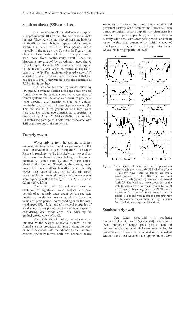
SSE seas are generated by winds caused by low-pressure systems carried along the coast by cold fronts. Due to the typical speed of progression of frontal systems and the associated pressure gradients, wind direction and intensity change very quickly within the area, as seen in Figure 5, panels (a) and (b). This fact results in the generation of a local wave field that has strong two-dimensional properties, as discussed by Alves & Melo (1999). Figure 6(a) illustrates the passage of a cold front associated with SSE seas observed at the study site. Easterly waves

Waves arriving from the east and southeast dominate the local wave climate (approximately 50% of all observations), as seen in Figure 3. As seen in Figure 4, panels (c) to (f), it is likely that waves from these two directional sectors belong to the same population, since both Tp and Hs have almost identical distributions. Therefore, they are grouped under the same pattern hereafter called easterly waves. The range of peak periods and significant wave heights observed during easterly wave events were typically within the ranges 6 s < Tp < 11 s and 0.5 m < Hs < 1.5 m.

Figure 5, panels (c) and (d), shows the evolution of significant wave heights and peak periods of an easterly wave event. As the sea state builds up, conditions progress gradually from low values of peak periods corresponding with the local wind speed [Fig. 5, (e) and (f)], typical properties of wind seas, to peak periods well above those expected considering local winds only, thus indicating the gradual development of swell.

The evolution of easterly wave events is initiated by the passage of frontal systems. As the frontal systems propagate northward along the coast or move eastwards into the Atlantic Ocean, an anti-cyclone gradually moves north and becomes nearly

stationary for several days, producing a lengthy and persistent easterly wind fetch off the study site. Such a meteorological scenario explains the characteristics observed in Figure 5, panels (c) to (f), resulting in easterly wind seas with short peak periods and small wave heights that dominate the initial stages of development, progressively evolving into larger waves that have properties of swell.

Fig. 5. Time series of wind and wave parameters

corresponding to: (a) and (b) SSE wind sea; (c) to (f) easterly waves; and (g) and (h) SE swell. Wind properties of the SSE wind sea event shown in panels (a) and (b) were recorded around April 25. The wind and wave properties of the easterly waves event shown in panels (c) to (f) were observed beginning February 29. The wave properties from the SE swell event shown in panels (g) and (h) were recorded beginning May 7. The abscissa scales show the lags in hours from the indicated days and local times.

Southeasterly swell

Sea states associated with southeast directions [Fig. 4, panels (g) and (h)] have mainly swell properties: longer peak periods and no connection with the local wind speed or direction. In our data set, SE swell is the second most persistent feature of the local wave climate (approximately 25%

Brazilian J. Oceanogr., 49(1/2), 2001

of the observations), presenting Tp ranging from 7 to 16 s and Hs varying between 0.5 and 2.0 m.

Alves (1996) identifies two main sources of SE swell to the São Francisco do Sul coast. The first is associated with storms that sometimes propagate along the South American coast and deviate into the ocean within the 20oS and 40oS latitude band at distances in excess of 1000 km from the study site. Whenever these storms become slow moving systems, persistent southeasterly wind fetches develop along with strong pressure gradients as they migrate into areas dominated by warm air mass systems, resulting in strong wind fields.

The second swell sources are storms that migrate from the Southern Ocean northwards along the Argentinian coast near Patagonia, deviating towards the east into the Atlantic Ocean south of 40oS. Figure 6(d) shows part of one such storm centered over the Drake Passage, between the Antarctic Peninsula and the Falklands (Malvinas) Islands. The swell generated by this particular storm was observed at the São Francisco do Sul coast about three days after the peak of the storm and displayed the progressive decay in wave periods characteristic of the dispersive arrival of long traveled swell.

Fig. 6. Surface pressure charts [Diretoria de Hidrografia e Navegação (DHN), Brazilian Navy] indicating (a) the passage of a frontal system (diagonal line with triangles crossing the extra tropical low near the center of the panel) over the study site (25/04/96 12 h GMT); (b) and (c) a stationary high pressure system (labeled with the letter “A”) expanding over the study site (26/04/96 12 h GMT and 27/04/96 12 h GMT); and (d) a mid-latitude storm centered southeast from the Falkland Islands (the storm has closely spaced isobars forming a semi-circle at the bottom of the figure; 06/05/96 12 h GMT). The study site is approximately in the center-point of each panel.

ALVES & MELO: Wind waves at the northern coast of Santa Catarina

In fact, Figure 5, panels (g) and (h), illustrates well the onset of the swell event mentioned above. Curiously, the arrival of this swell did not alter much the sea conditions in terms of Hs [panel (g)], but caused a remarkable change in the peak period of the sea state [panel (h)]. After rising quickly to 16s, Tp slowly decreased for the following hours. The dispersive arrival of swell systems generated by distant storms is one of the most conspicuous features of wind waves that have been reported since the pioneering contribution of Barber & Ursell (1948) and Snodgrass et al. (1966). Melo & Alves (1993) and Melo et al. (1995) used a similar approach to describe the arrival of long traveled swell to the Brazilian Coast.

A record of the time evolution of the peak period at a coastal station allows one to estimate the distance traveled by the incoming swell through a very simple calculation based on linear wave theory. Following Melo & Alves (1993), the distance between São Francisco do Sul and the generating storm (Xs) may be estimated by means of the expression:

tTT

TTg

f

tgX

p

s ∆

−≈

∆

∆=

21

21

44 ππ (7)

where g is the acceleration of gravity, T1 and T2 are the periods of swell components observed at times t = 1 and t = 2, respectively, ∆t is the elapsed time between the arrival of successive swell components and ∆fp the difference between their peak frequencies fp = 1/ Tp.

Figure 5 provides an average value of ∆fp / ∆t = 2 × 10-7 s-2. Plugging this into equation (7), one readily obtains a distance of 3900 km from the São Francisco do Sul coast, which is consistent with the approximate location of the southerly wind storm fetches seen in Figure 6(d) extending towards the Drake Passage. Transformation of wave spectra

Theory and experiments have demonstrated that surface gravity waves are unaffected by the bottom whenever the depth of water is greater than approximately half the wavelength (see, for example, Dean & Dalrymple, 1984). The depth at the measurement site in São Francisco do Sul was about 20 m. Thus, it is expected that spectral components representing lengths equal to or smaller than approximately 40 m, which correspond to waves with periods less than about 6 s to 7 s, would not “feel” the bottom.

This being so, short period wind seas will remain unaffected by refraction over bottom topography as they propagate from deeper waters

towards the measurement site. Consequently, the majority of spectra associated with ENE and SSE wind seas may be directly extrapolated to surrounding areas with depths greater than 20 m. The wave field at shallower positions may be determined through a forward spectral refraction model, using the measured spectrum as initial/boundary conditions.

Easterly waves and SE swell with considerable energy in period bands longer than 6 s are expected to undergo transformation by bottom refraction before reaching the measurement site, rendering a direct extrapolation of the measured wave field to surrounding areas invalid. This limitation may be overcome through a two-step technique using numerical propagation models. The first step consists in estimating the spectra in deep waters, where the wave field should be spatially homogeneous, by back-refracting the measured shallow-water spectra. As a second step, the deep-water spectra are forward-refracted to provide the desired extrapolation of the actual measurements to a regional scale.

Longuet-Higgins (1955, 1956) showed that for linear waves the energy initially concentrated around an arbitrary range of the directional wind-wave spectrum keeps itself bound to the same frequency throughout the entire refraction process. Therefore, it is possible to establish a direct relationship between the energy density of an initially undisturbed spectral component E0 (f,θ0) and the refracted energy density E (f,θ), as long as dissipation, diffraction and nonlinear processes are negligible.

The governing equation relating initial and refracted spectra is

[ ]),(,),( 00

0

θθ ffEc

c

k

kfE

g

gΓ= (8)

where the directional spectrum E (f,θ) is defined in terms of components with frequency f, direction of propagation θ, wave number k and group velocity cg. The subscripts 0 denote properties related to the spectrum before refraction. Wave numbers and group velocities of any given component are related to its frequency through the linear dispersion relation

)tanh(2khgk=ω (9)

where ω = 2πf, k = 2π / L is the wavenumber and h is the local water depth.

The gamma function Γ(f,θ) relates initial and refracted directions, as follows

),(0 θθ fΓ= (10)

Brazilian J. Oceanogr., 49(1/2), 2001

Equation (8) is valid along a ray path. For an orthogonal Cartesian frame, rays are defined by the following equations (Munk & Arthur, 1951)

−=

=

=

θθθ

θ

θ

cossen

sen

cos

dy

dc

dx

dc

dt

d

cdt

dy

cdt

dx

gg

g

g

(11)

The present study uses a numerical model

based on equations (8) to (11) to calculate the deep water spectra E0 (f,θ0) from the measured shallow-water spectra E (f,θ). Since the procedure is done in reverse order from the actual wave propagation sense (which is deep-to-shallow water), it is called back or inverse refraction. Techniques based on equation (8) are also called spectral mapping (O'Reilly, 1991; O'Reilly & Guza, 1998).

Fig. 7. Diagram showing the fan of back-refracted ray paths

departing from the measurement location. This example shows the back-refracted rays of a spectral component with f = 0.05 Hz. Only rays that reach deep water are retained in the computations (i.e., rays reaching land boundaries are eliminated). Also shown are the depth contours from 10m to 100m at a 10m interval (dash-dotted lines) and the following key geographical landmarks, from top to bottom: Parangua Bay (BP), São Francisco do Sul Island (SFI) and Porto Belo (PB).

The practical application of this procedure is as follows. For any given frequency, one performs the back-refraction of a set of equally spaced rays (the “ray fan”) within a range of directions pointing offshore all departing from the measurement site and ending at the corresponding deep water depth. Figure 7 illustrates such a result for the São Francisco do Sul coast for a component with frequency of 0.05 Hz. The tracing of rays allows the construction of the function Γ(f,θ), which maps the shallow-water directions θ of all spectral components resolved in the model into their deep-water unrefracted directions θ0. Values of θ0 = Γ(f,θ) are obtained through integration of the ray equations (11). Further details of these calculations are found in Alves (1996).

The extrapolation of the estimated deep-water spectrum to the surroundings of the measurement site is computed by a simple forward-propagation model, based on two other properties derived from refraction theory, namely, the wave number irrotationality and the energy flux conservation conditions. For a continental shelf with smooth bottom contours (as in São Francisco do Sul) and in the absence of significant currents, changes in the wave number vector k of any given spectral component may be calculated by applying the wave number irrotationality condition, which reads

0=×∇ k (12) where ∇ stands for the horizontal gradient operator.

The associated wave height variations due to refraction are calculated through the energy flux conservation equation

( ) 0=•∇ Ecg (13)

where E(f,θ) is the energy density of an arbitrary spectral component.

The spectral forward-refraction model used in the present study is a spectral version of the monochromatic wave refraction model presented in Dalrymple (1988). The model solves numerically the coupled system of equations (12) and (13), allowing the use of grids covering large areas. Details of the numerical solution method are presented in the Appendix. Further information may be found in Alves (1996).

Before applying the model to a real case, two tests were made to assess the performance of the forward-propagation model. The first test compared the analytical solution of monochromatic wave propagation with several angles of incidence over a beach with plane parallel depth contours (see Dean & Dalrymple, 1984) to the model calculations. Throughout all these preliminary test cases (not

ALVES & MELO: Wind waves at the northern coast of Santa Catarina

shown) the model reproduced the exact analytical solution (Alves, 1996).

The second test compared the model results with those from a laboratory experiment described in Mase & Kirby (1992). In this test case, a two-dimensional wave field defined by a frequency-direction wave spectrum was propagated over a beach with plane parallel depth contours. An algorithm to calculate wave breaking based on statistical properties of the wave field as proposed by Thornton & Guza (1983) was included in the forward-refraction model to provide the energy decay within the surf zone.

Fig. 8. Comparison between laboratory results from Mase

& Kirby (1992) (triangles) and model calculation (continuous line).

The model validation made at 12 equally

spaced points along the domain in the x direction is summarized in Figure 8. Before the onset of breaking (locations 1 to 8) experiment and model agree with less than 5% relative error. The agreement is still good at locations 9 (0.43%) and 10 (5.02%), but becomes progressively poorer inside the breaking zone, probably due to non-linear effects not included in the model. Since our simulations exclude the breaking zone, these results indicated that the model was adequate for the present purposes. Impact of refraction on spectral

transformation

Four observed frequency-direction spectra, representing different stages of a SE swell event recorded at the measurement site on September 1996, were initially used to assess the impact of refraction on the propagation of swell spectra. Using the ray-tracing inverse-refraction model described in the previous section, deep-water spectra were obtained for each of the four cases considered: the initial, two intermediate and the final stages of the SE swell event. All spectra were discretized into 12 frequency bands with 30 directional bins each and a rectangular 186 km by 185 km grid with ∆x = ∆y = 250 m was used in the calculations.

Figure 9 shows an example of the differences between the measured shallow water one-dimensional spectrum at an intermediate stage of the event and its corresponding deep water estimate. The remarkable difference seen in the energy levels around the peak frequency indicates the importance of refraction for this case. Considering the four cases, the differences in significant wave height between shallow and deep water were always greater than 20%. Directional computations (not shown) also caused transformations in the main direction θm in excess of 20o (Alves, 1996).

Fig. 9. Shallow- (dashed line) and deep-water (continuous

line) frequency spectra illustrating the transformation due to refraction of a SE swell event observed on May 8, 1996, at 7 AM local time.

The four deep-water swell spectra were then

used as initial conditions for the forward propagation model, yielding sea-state predictions that covered the whole northern coast of Santa Catarina state. A new rectangular depth grid with 136 km (x direction) by 185 km (y direction) and ∆x = ∆y = 250 m was used in the forward-refraction computations. As a check for the full methodology, the forward-propagated spectra predicted at the location where the waverider was deployed (see Fig. 1) were compared to the original measured spectra. This might seem an obvious comparison. However, this is not the case. Although both back- and forward-refraction models are based on similar general physical assumptions, they are developed using different mathematical approaches, as outlined in section 4.

Measured and numerically reconstructed directional one-dimensional frequency spectra were in very good agreement, with differences in Hs of less than 4%. Figure 10 shows this comparison for the case with strongest refraction effects, observed on May 8th, 1996, 7AM local time. A comparison between measured and computed directional slices of the two-dimensional frequency-direction spectrum at the spectral peak frequency E(fp,θ) is presented in Figure 11 for the same test case. This figure demonstrates that the calculated directional

Brazilian J. Oceanogr., 49(1/2), 2001

distribution reproduced remarkably well the unsmoothed measured distribution, calculated using the maximum entropy technique described in Alves & Melo (1999).

Fig. 10. Comparison between measured (continuous line)

and calculated (dashed line) frequency spectra for swell waves recorded on May 8, 1996, 7 AM local time.

The same back- and forward-refraction approach was applied to assess the impact of refraction on the propagation of selected spectra from locally-generated ENE and SSE wind-seas and easterly waves. Overall results are summarized in Table 1. The degree of transformations due to refraction and shoaling were assessed in terms of observed and computed significant wave heights Hs and main directions θm, indicated respectively in Table 1 by superscripts obs and dw.

Other parameters listed in Table 1 for each selected event are the type of sea-state pattern, the date and time of its observation, the spectral peak period Tp, the percentage difference ∆Hs between Hs

obs and Hsdw relative to Hs

dw and the absolute difference in degrees ∆θm between θm

obs and θmdw.

Diagnostic parameters indicating the degree of transformations due to refraction and shoaling are the variations ∆Hs and ∆θm.

The negligible effects of refraction on locally generated wind seas are illustrated by the first two cases listed in Table 1, corresponding to SSE and ENE, seas respectively. As expected, variations in wave height and direction are under 5% and 5o, both lower than typical instrumental errors or sampling variability effects (see e.g., Krogstad, 1991; Donelan & Pierson, 1987 and Allender et al., 1989).

Transformations due to refraction were also negligible during the easterly waves events listed

in Table 1. Variations in wave height and direction were under 5% and 5o, despite their longer measured peak periods. This can be explained by the fact that easterly waves propagate in directions that are approximately perpendicular to the smooth depth contours that characterize the bottom topography offshore from the study site. Consequently, refraction of easterly waves is negligible due to the absence of depth gradients along crests of individual wave components of this sea-state pattern. Although shoaling still occurs closer to the shoreline, it was not a noticeable effect at the depth in which the measurements were made.

The four cases of SE swell listed in Table 1 were associated with a single long traveled swell event, as discussed previously in this section. The evolution of this event illustrates well how the combined values of Tp and θm determine the magnitude of transformations due to refraction, indicated by the resulting values of ∆Hs and ∆θm.

When the SE swell event first becomes noticeable the periods are high (16.67s) and the measured waves propagate from SE. In deep water the computed direction is shifted by 14o towards SSE. Wave heights decrease by approximately 20% as the waves propagate from deep water towards the observation point. As the event evolves in time, the peak periods fall progressively with a corresponding weakening of the transformation process, until this transformation becomes negligible with the variations falling within typical values of instrumental errors.

Fig. 11. Directional distribution of amplitudes at the peak

frequency from a spectrum measured on May 8, 1996, at 7 AM. Shown are the unsmoothed measured spectrum (continuous line) and the spectrum calculated by the wave model (dashed line).

ALVES & MELO: Wind waves at the northern coast of Santa Catarina

Table 1. Effects of refraction on significant wave height Hs and peak periods Tp of selected occurences of local wind seas, swell and easterly waves. Measurements are indicated as Hs

obs, Tp and θmobs. Deep-water

values computed with an inverse refraction model are indicated as Hsdw and θm

dw. The percentage variation of Hs is indicated by ∆Hs = (Hs

obs- Hsdw )/ Hs

dw and the absolute variation in propagation angles by ∆θm = θm

obs - θmdw.

Type of

Event

Date Time Tp

(s)

Hsobs

(m)

Hsdw

(m)

∆Hs

(%)

θmobs

θmdw

∆θm

SSE sea 25/04/96 22:00 5.88 1.38 1.45 -4.83 159o 162o -3o

ENE sea 01/02/96 04:00 6.67 0.59 0.62 -4.84 71o 73o 2o

Easterly 01/03/96 22:00 7.14 1.67 1.74 -4.02 95o 93o 2o

Easterly 03/03/96 22:00 8.60 1.63 1.70 -4.12 103o 104o -1o

SE swell 08/05/96 01:00 16.67 0.69 0.83 -16.87 131o 145o -14o

SE swell 08/05/96 07:00 14.29 0.76 0.92 -17.39 130o 141o -11o

SE swell 08/05/96 22:00 12.50 0.57 0.65 -12.31 134o 142o -8o

SE swell 09/05/96 10:00 10.00 0.50 0.54 -7.41 113o 112o 1o

Concluding Remarks

This study presents a preliminary investigation of the wind-wave climate and its transformation off São Francisco do Sul island, at the northern coast of the Santa Catarina state, using directional measurements of wind-wave spectra made during the year of 1996. Analyses of joint distributions of Hs, Tp and θm, combined with a study of the typical wind patterns found over the South Atlantic Ocean allowed the identification of the following four major sea states and associated meteorological conditions:

• East-northeast (ENE) wind seas; • South-southeast (SSE) wind seas; • Easterly waves; • Southeasterly swell.

Transformations of these main sea-state patterns

due to refraction and shoaling are investigated through a numerical modeling approach that allows the reconstruction of the wave field within extensive coastal areas, using single point measurements of the wave spectrum in shallow waters. The methodology consists of first estimating deep-water spectra using an inverse-refraction model, initialized with observed shallow water spectra. The wave field is then reconstructed within an extense area around the measurement site using a forward-refraction model. A comparison between measured and reconstructed spectra at the deployment site yielded consistent results, suggesting that the proposed methodology works well for the São Francisco do Sul coast.

A summary of results concerning the transformation of the main sea states due to depth induced refraction and shoaling is presented. This final summary presents selected cases representative of the four major sea states, allowing a first assessment of the general characteristics and magnitudes of wave climate transformations in the northern coast of Santa Catarina, Brazil.

In closing, we wish to point out that the ideal test for the wave transformation methodology presented herein would be to compare the estimated deep water spectra with actual deep water measurements. That, of course, would require simultaneous measurements of directional wave spectra at a shallow and a deep-water site which, unfortunately, exceeded our economical and logistical possibilities at the time. Although the difficulties involved in such a double measurement operation are still very challenging, this remains as a goal to be achieved in our future work. APPENDIX

Forward refraction model

The forward spectral wave refraction model developed by Alves (1996) and used in the present study is based on the technique described in Dalrymple (1988) to study monochromatic waves. The spectral model version solves the coupled system of equations (12) and (13) explicitly using a finite difference method. The numerical solution uses a discretization module shifted in the y direction, resembling a zig-zag shape (Fig. 12).

Brazilian J. Oceanogr., 49(1/2), 2001

The solution progresses in y from left to right or vice-versa, depending on the initial direction θ of each component at the outer boundary (in this appendix, azimuthal directions used throughout the paper are converted into grid directions referenced to the westward-pointing x axis). The whole spectrum is solved after the discretization module has swept all grid points for a fixed x position. The solution progresses in the cross-shore x direction line by line.

For a Cartesian system of reference, equation (12) is rewritten as

0=∂

∂−

∂

∂

yx

nn βα (14)

where αn = ky = kn sin θn and βn = ky = kn cos θn are the orthogonal projections of the wave number modulus kn. For the sake of simplicity, the subscript n, identifying an arbitrary component of the wave spectrum E(f,θ), will be dropped hereafter. By definition, β can be related to α by

( ) 2/122 αβ −= k (15)

The wave number modulus is related to the

frequency by the dispersion relation ω = {g k tanh(kh)}1/2, where g is the acceleration due to gravity and h is the local water depth. Therefore, the wave number is calculated directly from the frequency at each grid point considering only the local depth.

Equation (14) is discretized using central differences along the x and y axis, with equally spaced intervals ∆x and ∆y. The partial differentials in x are solved at an intermediate point (i+1/2,j). The resulting expressions for the x and y partial derivatives are

[ ]1,1,1,1, −+++ −+−=

∂

∂jijijijir

yββββ

β (16)

and

∂

∂+=+

yjiji

βαα ,,1 (17)

where r = ∆x / 2∆y. Using the relation (15) it is possible to eliminate the β terms with subscript (i+1,j), which identify unknown quantities. After some algebra, the resulting expression is

02 ,12

,1 =++ ++ cb jiji αα (18)

where

( )2

,,1,1,1

1 r

rb

jijijiji

+

−+−=

+−+ αβββ (19)

and

[ ]2

2,1

222

1

)1(

r

krbrc

ji

+

−+=

+ (20)

The positive root of equation (18) gives the

solution for the α terms at each new grid point as the solution progresses in space. The β terms are obtained directly through the relation (15). The angle of propagation at each grid point is, therefore

= −

ji

ji

ji

,

,1, tan

β

αθ . (21)

The numerical solution of the energy

conservation equation (13) is obtained similarly. Using equation (14), now with ε = E cg cos θ and φ = - E cg sin θ , the resulting expressions to be solved are

( )( )

jiji

jijijiji

jir

r

,1,1

,1,1,1,,1 cos/sen1 ++

+−+

++

+−+=

θθ

φφφεε (22)

and

=

+

+

++

ji

ji

jiji

,1

,1,1,1 cos

sen

θ

θεφ (23)

where the group velocity is given by

Fig. 12. Detail of the numerical mesh and of the discretization module. The slashes on the lower right corner illustrate wave crests and the angle of propagation.

ALVES & MELO: Wind waves at the northern coast of Santa Catarina

+==

)2senh(

21)tanh(

2 kh

khkh

k

g

dk

dcg

ω (24)

The numerical model outputs amplitude and

angle of propagation of individual spectral components. Since the entire spectrum is solved progressing line by line toward the x direction, it is also possible to compute statistical parameters of the wave field at each grid point. The main parameter used for applications is the significant wave height Hs, obtained from the model calculations through the expression

( )[ ] 2/12

,2

jins HH ∑= (25)

where the wave height Hn of individual components is defined as

( )( )

( )jing

jin

jinc

H,

,

, cos

8

θ

ε= (26)

and ε is the energy flux in the x direction (equation 22). Acknowledgements

The authors are grateful to Dr. William O'Reilly for providing the inverse refraction code. We also thank Davide Franco, Nei Seixas, Renato Martins, Cesar Ribeiro and Eliane Truccollo for providing technical support and a proper scientific environment for discussions that much enriched the contents of this manuscript. This study was made possible through the financial support and research grants provided by PETROBRAS and Conselho Nacional de Desenvolvimento Científico e Tecnológico (CNPq). References Allender, J.; Audunson, T.; Barstow, S. F.; Bjerken,

S.; Krogstad, H. E.; Steinbakke, P.; Vartdal, L.; Borgman, L. & Graham, C. 1989. The WADIC Project: a comprehensive field evaluation of directional wave instrumentation. Ocean Engng., 16(5-6):505-536.

Alves, J. H. G. M. 1991. Considerations on the arrival

at the Rio de Janeiro coast of South Pacific swell propagating through the Drake Passage. Bachelor of Oceanography Final Monograph. Rio de Janeiro State University (UERJ), Oceanography Department. 71p. (in Portuguese).

Alves, J. H. G. M. 1996. Refraction of wind-wave spectra in shallow waters: Applications to the Coast of São Francisco do Sul, SC, Brazil. M.Sc Thesis. Federal University of Santa Catarina (UFSC), 89p. (in Portuguese).

Alves, J. H. G. M. & Melo, E. 1999. On the measurement of directional wave spectra at the Southern Brazilian coast. Appl. Ocean. Res., 21(6):295-309.

Barber, N. F. & Ursell, F. 1948. The generation and propagation of ocean waves and swell. Phil. Trans. R. Soc., A240(824):527-560.

Dalrymple, R. A. 1988. Model for refraction of water

waves. J. Watway Port. coast. Ocean Engng., 114(4):423-435.

Dean, R. G. & Dalrymple, R. A. 1984. Water wave

mechanics for engineers and scientists. 4th ed. Singapore, World Scientific. 353p.

Donelan, M. A. & Pierson, W. J. 1987. Radar scattering and equilibrium ranges in wind-generated waves with application to scatterometry. J. geophys. Res., 92(C5):4971-5029.

Krogstad, H. E. 1991. Reliability and resolution of directional wave spectra from heave, pitch and roll buoy wave data. In: Beal, R. C. ed. Directional ocean wave spectra. Baltimore, The Johns Hopkins University Press. p.66-71.

Lima, L. C. E. & Satyamurti, H. E. 1992. An

observational study of formation and trajectory of extratropical cyclones in South America. In: BRAZILIAN CONGRESS OF METEOROLOGY, 7. Rio de Janeiro, 1992. Proceedings. Rio de Janeiro, SBMet., 2:706-710.

Longuet-Higgins, M. S. 1952. On the statistical distribution of heights of sea waves, J. mar. Res., 11:245-266.

Longuet-Higgins, M. S. 1955. The refraction of sea

waves in shallow water, J. Fluid. Mech., 1:163-176.

Longuet-Higgins, M. S. 1956. On the transformation

of a continuous spectrum by refraction. Proc. Cambridge Phyl. Soc., 53(1):226-229.

Brazilian J. Oceanogr., 49(1/2), 2001

Longuet-Higgins, M. S.; Cartwright, D. E. & Smith, N. D. 1963. Observations of the directional spectrum of sea waves using the motions of a floating buoy. In: Admiral, R. & Stephan, E. C. eds. Ocean wave spectra. New Jersey, Pretice-Hall. p.111-136.

Mase, H. & Kirby, J. T. 1992. Modified frequency-

domain KdV equation for random wave shoaling. Proc. 23rd ICCE, ASCE, p.474-487.

Melo, E. & Alves, J. H. G. M. 1993. A note on the

arrival of long traveled swell at the Brazilian Coast. In: SIMPÓSIO BRASILEIRO DE RECURSOS HÍDRICOS, 10. Gramado, 1993. Proceedings. Porto Alegre, UFRGS/ABRH, 5:362-369.

Melo, E. 1995. Instrumental confirmation of the

arrival of North Atlantic swell to the Ceara coast. In: INTERNATIONAL CONFERENCE COASTAL AND PORT ENGINEERING IN DEVELOPING COUNTRIES. COPEDEC, 4. Rio de Janeiro, 1995. Proceedings. Rio de Janeiro, ABRH, 3: 1984-1996.

Munk, W. H. & Arthur, R. S. 1951. Wave intensity

along a refracted ray. Scripps Institute of Oceanography Wave Report, 95, Ref. 51-7. 18p.

Nimer, E. 1989. Climatology of Brazil. Rio de Janeiro, IBGE, Natural Resources and Environmental Studies Departament. 421p. (in Portuguese)

O'Reilly, W. 1991. Modeling surface gravity waves

in the Southern California Bight. PhD Thesis. San Diego, Scripps Institute of Oceanography/UCSD. 89p.

O'Reilly, W. & Guza, R. T. 1998. Assimilating

coastal wave observations in regional swell predictions. Part 1: Inverse methods. J. phys. Oceanogr., 28(4):679-691.

Snodgrass, F. E.; Groves, G. W.; Hasselmann, K. F.;

Miller, G. R.; Munk, W. H. & Powers, W. M. 1966. Propagation of swell across the Pacific. Phil. Trans. R. Soc., A259(1103):431-497.

Taljaard, J. J. 1967. Development, distribution and

movement of cyclones and anticyclones in the Southern Hemisphere during the IGY. J. appl. Met., (6):973-987.

Thornton, E. B. & Guza, R. T. 1983. Transformation

of wave height distribution. J. geophys. Res., 88(C10):5925-5938.

(Manuscript received 27 March 2001; revised

18 October 2001; accepted 12 December 2001)