Two simple tests for normality with high power - DiVA Portal

U.U.D.M. Report 2010:13

Department of MathematicsUppsala University

Two simple tests for normality with high power

Måns Eriksson

Two simple tests for normality with high power

Mans Eriksson1

Abstract

We derive explicit expressions for the correlation coefficients between X and S2 andX and n

(n−1)(n−2)

∑ni=1(Xi−X)3 in terms of sample moments. Using these we show

that two tests for normality, proposed by Lin and Mudholkar [14] and Mudholkaret al. [16], can be simplified by using moment estimators; particularly the sampleskewness and kurtosis; rather than the jackknife estimators previously used. In anextensive simulation power study the tests exhibit higher power than some commontests for normality against a wide range of distributions.Keywords: Goodness-of-fit; Kurtosis; Skewness; Test for normality.

1 Introduction

The assumption of normality is the basis of many of the most common statistical meth-ods. Tests for normality, used to assess the normality assumption, is therefore a widelystudied field. Tests based on, for instance, moment conditions, distance measures andregression have been proposed. Thode [19] provides an overview of the field.

Another group of tests uses characterizations of the normal distribution. This ap-proach can be found in some recent papers; Ahmad and Mugdadi [1] constructed a testusing that X1 and X2 are normal if and only if X1 +X2 and X1 −X2 are independent;Bontemps and Meddahi [4] based a test on the Stein equation characterization of thenormal distribution and Arcones and Wang [2] presented two tests based on the Levycharacterization. Another example is Vasicek’s test [20], which uses the entropy charac-terization of the normal distribution. Reviews of characterization results related to thenormal distribution are found in the books by Bryc [6] and Kagan, Linnik and Rao [12].

A well-known characterization is that the sample mean X and sample variance S2

are independent if and only if the underlying population is normal. Similarly, X andn−1

∑ni=1(Xi − X)3 are independent if and only if X is normal; see [12], Sections 4.2

and 4.7.Lin and Mudholkar proposed a test based on the independence of X and S2 in

[14]. They noted that it is difficult to test the independence of X and S2 but that thecorrelation coefficient between the two is possible to estimate. They used a jackknifeprocedure to estimate ρ(X, S2), and used this for a test for normality against asymmetric

1Department of Mathematics, Uppsala University, P.O.Box 480, 751 06 Uppsala, Sweden.Phone: +46(0)184713389; Fax: +46(0)184713201; E-mail: [email protected]

1

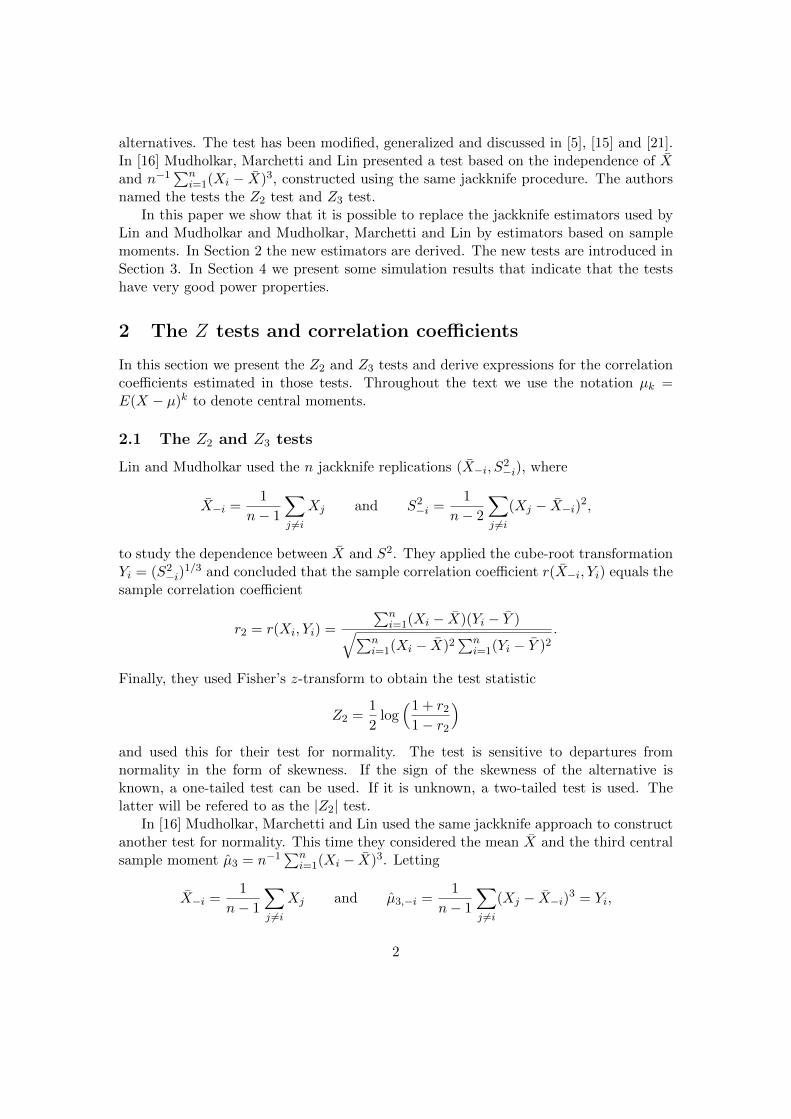
alternatives. The test has been modified, generalized and discussed in [5], [15] and [21].In [16] Mudholkar, Marchetti and Lin presented a test based on the independence of Xand n−1

∑ni=1(Xi − X)3, constructed using the same jackknife procedure. The authors

named the tests the Z2 test and Z3 test.In this paper we show that it is possible to replace the jackknife estimators used by

Lin and Mudholkar and Mudholkar, Marchetti and Lin by estimators based on samplemoments. In Section 2 the new estimators are derived. The new tests are introduced inSection 3. In Section 4 we present some simulation results that indicate that the testshave very good power properties.

2 The Z tests and correlation coefficients

In this section we present the Z2 and Z3 tests and derive expressions for the correlationcoefficients estimated in those tests. Throughout the text we use the notation µk =E(X − µ)k to denote central moments.

2.1 The Z2 and Z3 tests

Lin and Mudholkar used the n jackknife replications (X−i, S2−i), where

X−i =1

n− 1

∑j 6=i

Xj and S2−i =

1

n− 2

∑j 6=i

(Xj − X−i)2,

to study the dependence between X and S2. They applied the cube-root transformationYi = (S2

−i)1/3 and concluded that the sample correlation coefficient r(X−i, Yi) equals the

sample correlation coefficient

r2 = r(Xi, Yi) =

∑ni=1(Xi − X)(Yi − Y )√∑n

i=1(Xi − X)2∑n

i=1(Yi − Y )2.

Finally, they used Fisher’s z-transform to obtain the test statistic

Z2 =1

2log(1 + r2

1− r2

)and used this for their test for normality. The test is sensitive to departures fromnormality in the form of skewness. If the sign of the skewness of the alternative isknown, a one-tailed test can be used. If it is unknown, a two-tailed test is used. Thelatter will be refered to as the |Z2| test.

In [16] Mudholkar, Marchetti and Lin used the same jackknife approach to constructanother test for normality. This time they considered the mean X and the third centralsample moment µ3 = n−1

∑ni=1(Xi − X)3. Letting

X−i =1

n− 1

∑j 6=i

Xj and µ3,−i =1

n− 1

∑j 6=i

(Xj − X−i)3 = Yi,

2

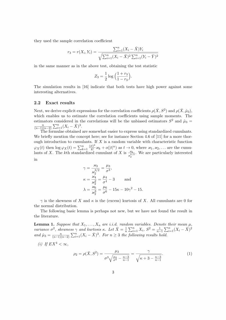
they used the sample correlation coefficient

r3 = r(Xi, Yi) =

∑ni=1(Xi − X)Yi√∑n

i=1(Xi − X)2∑n

i=1(Yi − Y )2

in the same manner as in the above test, obtaining the test statistic

Z3 =1

2log(1 + r3

1− r3

).

The simulation results in [16] indicate that both tests have high power against someinteresting alternatives.

2.2 Exact results

Next, we derive explicit expressions for the correlation coefficients ρ(X, S2) and ρ(X, µ3),which enables us to estimate the correlation coefficients using sample moments. Theestimators considered in the correlations will be the unbiased estimators S2 and µ3 =

n(n−1)(n−2)

∑ni=1(Xi − X)3.

The formulae obtained are somewhat easier to express using standardized cumulants.We briefly mention the concept here; see for instance Section 4.6 of [11] for a more thor-ough introduction to cumulants. If X is a random variable with characteristic function

ϕX(t) then logϕX(t) =∑n

k=1(it)k

k! κk + o(|t|n) as t→ 0, where κ1,κ2, . . . are the cumu-lants of X. The kth standardized cumulant of X is κk

κk/22

. We are particularly interested

in

γ =κ3

κ3/22

=µ3

σ3,

κ =κ4

κ22

=µ4

σ4− 3 and

λ =κ6

κ32

=µ6

σ6− 15κ− 10γ2 − 15.

γ is the skewness of X and κ is the (excess) kurtosis of X. All cumulants are 0 forthe normal distribution.

The following basic lemma is perhaps not new, but we have not found the result inthe literature.

Lemma 1. Suppose that X1, . . . , Xn are i.i.d. random variables. Denote their mean µ,variance σ2, skewness γ and kurtosis κ. Let X = 1

n

∑ni=1Xi, S

2 = 1n−1

∑ni=1(Xi − X)2

and µ3 = n(n−1)(n−2)

∑ni=1(Xi − X)3. For n ≥ 3 the following results hold.

(i) If EX4 <∞,

ρ2 = ρ(X, S2) =µ3

σ3√

µ4σ4 − n−3

n−1

=γ√

κ+ 3− n−3n−1

. (1)

3

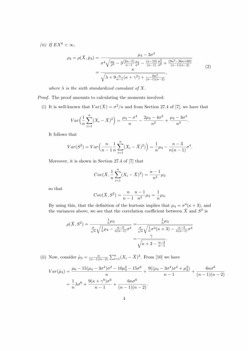
(ii) If EX6 <∞,

ρ3 = ρ(X, µ3) =µ4 − 3σ4

σ4

√µ6σ6 − 3 (2n−5)

n−1µ4σ4 − (n−10)

(n−1)µ23σ6 + (9n2−36n+60)

(n−1)(n−2)

=κ√

λ+ 9 nn−1(κ+ γ2) + 6n2

(n−1)(n−2)

,(2)

where λ is the sixth standardized cumulant of X.

Proof. The proof amounts to calculating the moments involved:

(i) It is well-known that V ar(X) = σ2/n and from Section 27.4 of [7], we have that

V ar( 1

n

n∑i=1

(Xi − X)2)

=µ4 − σ4

n− 2µ4 − 4σ2

n2+µ4 − 3σ4

n3.

It follows that

V ar(S2) = V ar( n

n− 1

1

n

n∑i=1

(Xi − X)2))

=1

nµ4 −

n− 3

n(n− 1)σ4.

Moreover, it is shown in Section 27.4 of [7] that

Cov(X,1

n

n∑i=1

(Xi − X)2) =n− 1

n2µ3

so that

Cov(X, S2) =n

n− 1

n− 1

n2µ3 =

1

nµ3.

By using this, that the definition of the kurtosis implies that µ4 = σ4(κ+ 3), andthe variances above, we see that the correlation coefficient between X and S2 is

ρ(X, S2) =1nµ3

σ√n

√1nµ4 − n−3

n(n−1)σ4

=1nµ3

σ√n

√1nσ

4(κ+ 3)− n−3n(n−1)σ

4

=γ√

κ+ 3− n−3n−1

.

(ii) Now, consider µ3 = n(n−1)(n−2)

∑ni=1(Xi − X)3. From [10] we have

V ar(µ3) =µ6 − 15(µ4 − 3σ4)σ2 − 10µ2

3 − 15σ6

n+

9((µ4 − 3σ4)σ2 + µ23)

n− 1+

6nσ6

(n− 1)(n− 2)

=1

nλσ6 +

9(κ+ γ6)σ6

n− 1+

6nσ6

(n− 1)(n− 2).

4

Furthermore,

Cov(X, µ3) = E((X − µ)µ3)− E((X − µ)µ3) = E((X − µ)µ3),

but this expression does not depend on µ, so we can study the case where µ = 0without loss of generality. Then

Cov(X, µ3) = E(Xµ3) =n2

(n− 1)(n− 2)E(X

1

n

(∑i

X3i − 3X

∑i

X2i + 3X2

∑i

Xi − X3))

=n2

(n− 1)(n− 2)

(E(X

1

n

∑i

X3i )− 3E(X2 1

n

∑i

X2i ) + 2E(X4)

).

The three expectations above are all found in Sections 27.4 and 27.5 of [7]. Insertingtheir values, the expression becomes

n2

(n− 1)(n− 2)

(µ4

n− 3

µ4 + (n− 1)σ4

n2+ 2

µ4 + 3(n− 1)σ4

n3

)=

n2

(n− 1)(n− 2)

(n2 − 3n+ 2)µ4 + 3(n− 1)(2− n)σ4

n3

=n2

(n− 1)(n− 2)

(n− 1)(n− 2)µ4 + 3(n− 1)(2− n)σ4

n3

=µ4 − 3σ4

n.

Thus

ρ(X, µ3) =µ4−3σ4

n√1nσ

2√

1nλσ

6 + 9(κ+γ6)σ6

n−1 + 6nσ6

(n−1)(n−2)

=µ4 − 3σ4

√σ2√λσ6 + 9n(κ+γ6)σ6

n−1 + 6n2σ6

(n−1)(n−2)

=µ4 − 3σ4

σ4√λ+ 9n(κ+γ6)

n−1 + 6n2

(n−1)(n−2)

=κ√

λ+ 9 nn−1(κ+ γ2) + 6n2

(n−1)(n−2)

=µ4 − 3σ4

σ4

√µ6σ6 − 3 (2n−5)

n−1µ4σ4 − (n−10)

(n−1)µ23σ6 + (9n2−36n+60)

(n−1)(n−2)

.

Remark 1. Kendall and Stuart [13], Section 31.3, present the asymptotic result thatρ(X, S2)→ γ√

κ+2.

Next, we wish to study ρ2 and ρ3 as functions of the standardized cumulants. Thefollowing little-known lemma, relating the standardized cumulants to each other, tellsus what the possible values of (γ, κ, λ) are. Naturally, it suffices to study ρ2 and ρ3 forvalues that (γ, κ, λ) can attain.

5

Lemma 2. Let X,X1, X2, . . . be i.i.d. random variables that satisfy the conditions inLemma 1. Then

(i) γ2 ≤ κ+ 2, with equality if and only if X has a two-point distribution.

(ii) κ2 ≤ λ+ 9(κ+ γ2) + 6, with equality if X has a two-point distribution.

The inequality in (i) was first shown in [8]. The entire statement was later shown in[17]. (ii) follows from expression (13) in [8] when γ2 < κ + 2. It is readily verifiedthat equality holds for two-point distributions. We have not found an X distributedon more than two points for which equality holds in (ii), and therefore conjecture thatκ2 = λ+ 9(κ+ γ2) + 6 only if X has a two-point distribution.

We are now ready to prove a smoothness lemma.

Lemma 3. Let ρ2 and ρ3 be the correlation coefficients given in (1) and (2). Then

(i) ρ2 is a smooth function of γ and κ, for (γ, κ) : γ ∈ R, γ2 ≤ κ+ 2.

(ii) ρ3 is a smooth function of γ, κ and λ, for (γ, κ, λ) : γ ∈ R, γ2 ≤ κ + 2, κ2 ≤λ+ 9(κ+ γ2) + 6.

Proof. (i) When γ2 ≤ κ + 2 we have κ ≥ −2 and√κ+ 3− n−3

n−1 > 0, so that ρ2 is a

well-defined real function. It is clearly continuous. The partial derivatives are

∂kρ2

∂γl∂κk−l=I(l = 1)γI(l=0)(−1)k−l

(κ+ 3− n−3n−1)

2(k−l)+12

.

Since these exist and are continuous for all k, ρ2 is differentiable for all k and hencesmooth.

(ii) The proof runs along the same line as above. The conditions give λ + 9 nn−1(κ +

γ2) + 6n2

(n−1)(n−2) > 0. ρ3 is a well-defined real function and the partial derivativeswith respect to γ, κ and λ exists and are continuous. Thus ρ3 is smooth.

Remark 2. Incidentally, Lemma 2 can be used to verify that ρ2 and ρ3 are bounded by

−1 and 1. Since κ + 2 ≥ γ2 we have |γ|/√κ+ 3− n−3

n−1 < |γ|/√κ+ 2 ≤ 1 and hence

|ρ2| < 1, as expected. We see that the correlation coefficient never equals ±1. Lookingat ρ3 we similarly get |ρ3| < 1 since κ2 ≤ λ+ 9(κ+ γ2) + 6. Conversely, the fact that ρ2

and ρ3 must be bounded by −1 and 1 can be used as a partial proof of Lemma 2.

6

2.3 Estimators

Given the smoothness of ρ2 and ρ3, the moment estimators of the two correlation coef-ficients are now obtained by replacing the moments by their sample counterparts

γ =1n

∑ni=1(xi − x)3(

1n

∑ni=1(xi − x)2

)3/2,

κ =1n

∑ni=1(xi − x)4(

1n

∑ni=1(xi − x)2

)2 − 3 and

λ =1n

∑ni=1(xi − x)6(

1n

∑ni=1(xi − x)2

)3 − 15κ− 10γ2 − 15.

The estimators are thus defined as

ρ2 = γ√κ+3−n−3

n−1

and (3)

ρ3 = κ√λ+9 n

n−1(κ+γ2)+ 6n2

(n−1)(n−2)

. (4)

Next, we describe the properties of the estimators ρk.

Theorem 1. Let X,X1, X2, . . . be i.i.d. random variables that satisfy the conditions inLemma 1 and ρ2 and ρ3 be the estimators given in (3) and (4), respectively. Then

(a) ρ2 and ρ3 are scale and location invariant, i.e. independent of µ and σ.

Moreover, the following results hold as n→∞,

(b) ρ2 − ρ2p−→ 0 and ρ3 − ρ3

p−→ 0,

(c)√n ρ2−ρ(X,S2)

σρ2 σ3√κ+3−n−3

n−1

d−→ N(0, 1) and√n ρ3−ρ(X,µ3)

σρ3 σ4√λ+9 n

n−1(κ+γ2)+ 6n2

(n−1)(n−2)

d−→ N(0, 1),

where σρk is the standard deviation of (Xi − X)k+1.

Proof. (a) Follows immediately since all sample moments involved in the estimatorsare scale and location invariant.

(b) The consistency of the sample cumulants is well-known, so since the fourth moment

is finite, γp−→ γ and κ

p−→ κ as n → ∞. The continuity of 1/√x+ 3− n−3

n−1

for x ≥ −2 ensures that 1/√κ+ 3− n−3

n−1

p−→ 1/√κ+ 2. Thus the first part of

(b) follows from the Cramer-Slutsky lemma. Similarly, the second part followsusing continuity properties, Cramer-Slutsky and the additional assumption thatEX6 <∞, so that λ

p−→ λ.

(c) The asymptotic normality for∑

(Xi− X)k is shown in [7], Section 28.2. As in (b)the result follows from continuity properties and the Cramer-Slutsky lemma.

7

3 The new tests

From Lemma 1 we conclude that ρ2 is large when the underlying distribution has highskewness, and that high kurtosis brings the correlation coefficient closer to 0. Whenusing ρ2 as test statistic for a normality test, we should thus reject the null hypothesisof normality if, when the alternative distribution has positive skewness, ρ2 is unusuallylarge, or if, when the alternative distribution has negative skewness, ρ2 is negative andunusually large. If the sign of the skewness of the alternative is unknown, |ρ2| can bestudied instead.

Similarly, the hypothesis of normality should be rejected if ρ3 is far from 0. If thesign of the kurtosis of the alternative is known, a one-tailed test should be used.

Part (b) of Theorem 1 shows that the ρ2 test is consistent against alternatives withγ 6= 0 and that the ρ3 test is consistent against alternatives with κ 6= 0.

We could use part (c) of Theorem 1 to approximate the distributions of ρ2 and ρ3,but simulation results indicate that the approximation is poor for small sample sizes.However, part (a) of Theorem 1 ensures that we can find good approximations of thenull distributions of the two estimators by Monte Carlo simulation.

The test procedure is thus as follows. Given a sample x1, x2, . . . , xn for which the testshall be used, calculate ρk = ρk,obs. Generate B random samples of size n from the stan-dard normal distribution. For each such sample calculate ρk so that ρk,1, ρk,2, . . . , ρk,Bare obtained. The p-value for the test is now obtained by comparing ρk,obs to the distri-bution of the ρk,1, ρk,2, . . . , ρk,B. For instance, if large values of ρk imply non-normality,

the p-value is#{ρk,i:ρk,i≥ρk,obs,i=1,...,B}

B .An R implementation of the test is found in the cornormtest package, available from

the author.

4 Power studies

To evalute the performance of the tests a simulation power study was performed, wherethe |ρ2|, ρ2 and ρ3 test were compared to the |Z2|, Z2 and Z3 tests, one-tailed versions ofthe sample moment tests

√b1 = γ and b2 = κ, the Shapiro-Wilk test W [18], Vasicek’s

test K [20] and the Jarque-Bera test LM [3]. The latter test has performed poorly inprevious comparisons of power, but is nevertheless popular in econometrics. It is of someinterest to us since it is based on the sample skewness and kurtosis; the test statistic isLM = n(1

6 γ2 + 1

24 κ2).

The tests were studied for χ2, Weibull, lognormal, beta, Student’s t, Laplace, logis-tic and normal mixture alternatives and were thus compared for both symmetric andasymmetric distributions as well as short-tailed and long-tailed ones. The skewness,kurtosis and limit correlation coefficients of the alternatives are given in Table 1. To es-timate their powers against the various alternative distributions at the significance levelα = 0.05, the tests were applied to 1,000,000 simulated random samples of size n =10,20 and 50 from each distribution.

It should be noted that the Student’s t distributions considered in the study don’t

8

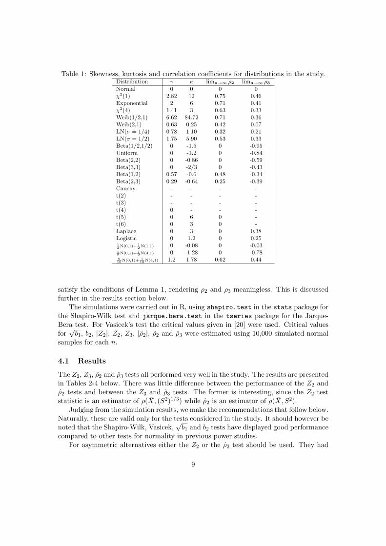
Table 1: Skewness, kurtosis and correlation coefficients for distributions in the study.Distribution γ κ limn→∞ ρ2 limn→∞ ρ3Normal 0 0 0 0χ2(1) 2.82 12 0.75 0.46Exponential 2 6 0.71 0.41χ2(4) 1.41 3 0.63 0.33Weib(1/2,1) 6.62 84.72 0.71 0.36Weib(2,1) 0.63 0.25 0.42 0.07LN(σ = 1/4) 0.78 1.10 0.32 0.21LN(σ = 1/2) 1.75 5.90 0.53 0.33Beta(1/2,1/2) 0 -1.5 0 -0.95Uniform 0 -1.2 0 -0.84Beta(2,2) 0 -0.86 0 -0.59Beta(3,3) 0 -2/3 0 -0.43Beta(1,2) 0.57 -0.6 0.48 -0.34Beta(2,3) 0.29 -0.64 0.25 -0.39Cauchy - - - -t(2) - - - -t(3) - - - -t(4) 0 - - -t(5) 0 6 0 -t(6) 0 3 0 -Laplace 0 3 0 0.38Logistic 0 1.2 0 0.2512N(0,1)+ 1

2N(1,1) 0 -0.08 0 -0.03

12N(0,1)+ 1

2N(4,1) 0 -1.28 0 -0.78

910

N(0,1)+ 110

N(4,1) 1.2 1.78 0.62 0.44

satisfy the conditions of Lemma 1, rendering ρ2 and ρ3 meaningless. This is discussedfurther in the results section below.

The simulations were carried out in R, using shapiro.test in the stats package forthe Shapiro-Wilk test and jarque.bera.test in the tseries package for the Jarque-Bera test. For Vasicek’s test the critical values given in [20] were used. Critical valuesfor√b1, b2, |Z2|, Z2, Z3, |ρ2|, ρ2 and ρ3 were estimated using 10,000 simulated normal

samples for each n.

4.1 Results

The Z2, Z3, ρ2 and ρ3 tests all performed very well in the study. The results are presentedin Tables 2-4 below. There was little difference between the performance of the Z2 andρ2 tests and between the Z3 and ρ3 tests. The former is interesting, since the Z2 teststatistic is an estimator of ρ(X, (S2)1/3) while ρ2 is an estimator of ρ(X, S2).

Judging from the simulation results, we make the recommendations that follow below.Naturally, these are valid only for the tests considered in the study. It should however benoted that the Shapiro-Wilk, Vasicek,

√b1 and b2 tests have displayed good performance

compared to other tests for normality in previous power studies.For asymmetric alternatives either the Z2 or the ρ2 test should be used. They had

9

the highest power against most asymmetric alternatives in the study, and power closeto that of the best test whenever they didn’t have the highest power. The one-sidedtests are particularly powerful, but the two-sided tests are often more powerful than thecompeting tests.

For symmetric alternatives either the Z3 or the ρ3 test can be recommended, both forplatykurtic (κ < 0) and leptokurtic (κ > 0) distributions. Vasicek’s test and the b2 testare more powerful against some alternatives and should be considered to be interestingalternatives to the Z3 or the ρ3 tests. It would be of some interest to compare thesetests in a larger power study.

When choosing between the Z and the ρ tests, it seems reasonable to choose thelatter, as the relative simplicity of the ρ tests speaks in their favor.

As for the Student’s t distributions studied, we note that ρ2 is undefined for thedistributions with 4 or fewer degrees of freedom and that ρ3 is undefined for all six dis-tributions. Nevertheless, both tests perform quite well against those alternatives. Thisis perhaps not unexpected, since the heavy tails of those distributions will cause obser-vations that are so large that they dominate

∑i(xi− x)k completely. Such observations

force ρ2 to be close to either -1 or 1 and ρ3 to be close to 1.

4.2 Concluding remarks

In many situations of practical interest the practitioner has some idea about the type ofnon-normality that can occur – ideas about the sign of the skewness of the alternativeand whether or not is has long or short tails. Similarly, it might be of interest to guardagainst some special class of alternatives. For instance, leptokurtic alternatives withκ > 0 are often considered to be a greater problem than platykurtic alternatives withκ < 0. Judging from the simulation results presented here, the one-tailed ρ2 and ρ3 testscan be recommended above some of the most common tests for normality in such cases.

The good performance of the Z and ρ tests and the fact that the jackknife approachyields tests with essentially the same power as the ”exact” tests is encouraging. Jack-knifing or bootstraping to estimate correlations – or other quantities – could perhaps beused for other independence characterizations as well, as mentioned in [21]. Brown et al.studied some sub- and resampling based tests based on independence characterizationsin [5] and noted that the bootstrap and jackknife tests seemed to complement each other.

In [9] Eriksson described a bootstrap procedure for estimating ρ2 and ρ3, similarto the jackknife procedure used by Lin and Mudholkar. Even for a small number ofbootstrap samples the performance of the bootstrap ρ tests was close to that of the ρtests presented in the present paper. In this particular case, bootstrap and jackknifetests do not seem to complement each other.

The author is currently preparing a manuscript concerning a multivariate general-ization of the ρ tests.

10

References

[1] Ahmad, I., Mugdadi, A.R. (2003), Testing Normality Using Kernel Methods, Journal of Nonpara-metric Statistics, Vol. 15, pp. 273-288

[2] Arcones, M.A., Wang, Y. (2006), Some New Tests for Normality Based on U-processes, Statistics& Probability Letters, Vol. 76, pp. 69-82

[3] Bera, A.K., Jarque, C.M. (1987), A Test for Normality of Observations and Regression Residuals,International Statistical Review, Vol. 55, pp. 163-172

[4] Bontemps, C., Meddahi, N. (2005), Testing Normality: a GMM Approach, Journal of Econometrics,Vol. 124, pp. 149-186

[5] Brown, L, DasGupta, A., Marden, J., Politis, D. (2004), Characterizations, Sub and Resampling,and Goodness of Fit, Lecture Notes-Monograph Series, Vol. 45, A Festschrift for Herman Rubin,IMS, pp. 180-206

[6] Bryc, W. (1995), The Normal Distribution: Characterizations with Applications, Springer-Verlag,ISBN 0-387-97990-5

[7] Cramer, H. (1946), Mathematical Methods of Statistics, Princeton University Press, ISBN 0-691-00547-8

[8] Dubkov, A. A., Malakhov, A. N. (1976), Properties and Interdependence of the Cumulants of aRandom Variable, Radiophysics and Quantum Electronics, Vol. 19, pp. 833-839

[9] Eriksson, M. (2010), Tests for Normality Using a Bootstrap Estimator, pre-print, Uppsala Univer-sity

[10] Fisher, R.A. (1930), Moments and Product Moments of Sampling Distributions, Proceedings of theLondon Mathematical Society, Vol. 2, pp. 199-238

[11] Gut, A. (2005), Probability: A Graduate Course, Springer-Verlag, ISBN 978-0-387-22833-4

[12] Kagan, A.M., Linnik, Y.V., Rao, C.R. (1973), Characterization Problems in Mathematical Statis-tics, Wiley, ISBN 0-471-45421-4

[13] Kendall, M.G., Stuart, A. (1967), The Advanced Theory of Statistics vol. 2, Griffin, ISBN 0-387-98864-5

[14] Lin, C.-C., Mudholkar, G.S. (1980), A Simple Test for Normality Against Asymmetric Alternatives,Biometrika, Vol. 67, pp. 455-461

[15] Mudholkar, G.S., McDermott, M., Srivastava, D.K. (1992), A Test of p-Variate Normality,Biometrika, Vol. 79, pp. 850-854

[16] Mudholkar, G.S., Marchetti, C.E., Lin, C.T. (2002), Independence Characterizations and TestingNormality Against Restricted Skewness-Kurtosis Alternatives, Journal of Statistical Planning andInference, Vol. 104, pp. 485-501

[17] Rohatgi, V., Szekely, G.J. (1989), Sharp Inequalities Between Skewness and Kurtosis, Statistics &Probability Letters, Vol. 8, pp. 297-299

[18] Shapiro, S.S., Wilk, M.B. (1965), An Analysis of Variance Test for Normality, Biometrika, Vol.52, pp. 591-611

11

[19] Thode, H.C. (2002), Testing for Normality, Marcel Dekker, ISBN 0-8247-9613-6

[20] Vasicek, O. (1976), A Test for Normality Based on Sample Entropy, Journal of the Royal StatisticalSociety B, Vol. 38, pp. 54-59

[21] Wilding, G.E., Mudholkar, G.S. (2007), Some Modifications of the Z-Tests of Normality and TheirIsotones, Statistical Methodology, Vol. 5, pp. 397-409

12

Table 2: Power of normality tests against some alternatives, α = 0.05, n = 10.n = 10 W K LM

√b1 b2 |Z2| Z2 Z3 |ρ2| ρ2 ρ3

χ2(1) 0.73 0.79 0.27 0.68 0.39 0.69 0.79 0.38 0.67 0.78 0.38Exponential 0.44 0.42 0.15 0.48 0.26 0.44 0.57 0.23 0.46 0.56 0.25χ2(4) 0.24 0.19 0.08 0.32 0.17 0.25 0.37 0.14 0.27 0.36 0.16Weib(1/2,1) 0.90 0.93 0.46 0.83 0.56 0.86 0.93 0.58 0.86 0.91 0.55Weib(2,1) 0.08 0.08 0.03 0.14 0.07 0.09 0.15 0.06 0.09 0.15 0.07LN(σ = 1/4) 0.10 0.08 0.03 0.17 0.10 0.11 0.17 0.08 0.12 0.17 0.10LN(σ = 1/2) 0.25 0.18 0.09 0.34 0.20 0.26 0.37 0.17 0.28 0.37 0.19Beta(1/2,1/2) 0.30 0.51 0.01 0.04 0.38 0.12 0.10 0.41 0.10 0.08 0.39Uniform 0.08 0.17 0.00 0.02 0.20 0.05 0.05 0.20 0.04 0.04 0.20Beta(2,2) 0.04 0.08 0.00 0.03 0.11 0.03 0.04 0.10 0.03 0.03 0.11Beta(3,3) 0.04 0.06 0.00 0.03 0.08 0.03 0.04 0.08 0.04 0.04 0.08Beta(1,2) 0.13 0.18 0.01 0.14 0.12 0.12 0.20 0.12 0.12 0.19 0.12Beta(2,3) 0.05 0.08 0.01 0.06 0.09 0.03 0.08 0.09 0.05 0.08 0.09Cauchy 0.59 0.43 0.43 0.32 0.61 0.55 0.31 0.62 0.55 0.31 0.61t(2) 0.30 0.17 0.19 0.20 0.35 0.29 0.19 0.34 0.30 0.19 0.35t(3) 0.19 0.10 0.10 0.15 0.23 0.19 0.14 0.23 0.20 0.14 0.24t(4) 0.14 0.07 0.07 0.12 0.18 0.14 0.11 0.17 0.15 0.11 0.18t(5) 0.11 0.06 0.05 0.10 0.15 0.12 0.10 0.14 0.12 0.10 0.15t(6) 0.10 0.06 0.04 0.09 0.13 0.10 0.09 0.12 0.11 0.09 0.13Laplace 0.15 0.07 0.06 0.13 0.20 0.16 0.12 0.20 0.16 0.12 0.20Logistic 0.08 0.05 0.03 0.08 0.11 0.09 0.08 0.10 0.08 0.08 0.1112N(0,1)+ 1

2N(1,1) 0.05 0.05 0.01 0.05 0.05 0.05 0.05 0.05 0.05 0.05 0.05

12N(0,1)+ 1

2N(4,1) 0.18 0.26 0.01 0.04 0.31 0.09 0.08 0.27 0.08 0.09 0.29

910

N(0,1)+ 110

N(4,1) 0.25 0.12 0.10 0.36 0.23 0.27 0.36 0.22 0.26 0.37 0.22


√b1 b2 |Z2| Z2 Z3 |ρ2| ρ2 ρ3


2N(1,1) 0.05 0.05 0.02 0.05 0.05 0.05 0.05 0.06 0.04 0.05 0.05

12N(0,1)+ 1

2N(4,1) 0.40 0.55 0.00 0.02 0.61 0.09 0.08 0.58 0.09 0.08 0.55

910

N(0,1)+ 110

N(4,1) 0.53 0.27 0.35 0.65 0.38 0.53 0.64 0.42 0.53 0.64 0.40

13


√b1 b2 |Z2| Z2 Z3 |ρ2| ρ2 ρ3


2N(1,1) 0.05 0.05 0.03 0.05 0.06 0.04 0.04 0.06 0.04 0.05 0.06

12N(0,1)+ 1

2N(4,1) 0.90 0.92 0.00 0.01 0.96 0.09 0.07 0.94 0.08 0.08 0.94

910

N(0,1)+ 110

N(4,1) 0.91 0.72 0.87 0.95 0.65 0.90 0.94 0.74 0.89 0.94 0.73

14

Documents

Two simple tests for normality with high power - DiVA Portal