Dr. John Mellor-Crummey

Department of Computer ScienceRice University

johnmc@cs.rice.edu

Two-Factor Full Factorial Designwith Replications

COMP 528 Lecture 17 22 March 2005

2

Goals for Today

Understand• Two-factor Full Factorial Design with Replications

—motivation & model—model properties—estimating model parameters—estimating experimental errors—allocating variation to factors and interactions—analyzing significance of factors and interactions—confidence intervals for effects—confidence intervals for interactions

3

Two-factor Design with Replications

• Motivation—two-factor full factorial design without replications

– helps estimate the effect of each of two factors varied– assumes negligible interaction between factors

• effects of interactions are ignored as errors—two-factor full factorial design with replications

– enables separation of experimental errors from interactions• Example: compare several processors using several workloads

—factor A: processor type factor B: workload type—no limits on number of levels each factor can take—full factorial design → study all workloads x processors

• Model: yijk = µ + αj+ βi + γij + eijk—yijk - response with factor A at level j and factor B at level i—µ - mean response—αj - effect of level j for factor A—βi - effect of level i for factor B—γij - effect of interaction of factor A at level j with B at level i—eijk - error term

4

• Effects—sums are 0

• Interactions—row sums are 0

—column sums are 0

• Errors—errors in each experiment sum to 0

!

" j

j

# = 0, $ii

# = 0

!

"1 j =

j=1

a

# "2 j =

j=1

a

# ... = " bj =j=1

a

# 0

Model Properties

!

"i1

=i=1

b

# "i2

=i=1

b

# ... = "ia

=i=1

b

# 0

!

eijkk=1

r

" = 0, #i, j

5

Estimating Model Parameters I

• Organize measured data for two-factor full factorial design as— b x a matrix of cells: (i,j) = factor B at level i and factor A at level j

columns = levels of factor A rows = levels of factor B—each cell contains r replications

• Begin by computing averages—observations in each cell

—each row

—each column

—overall

!

y ij. = µ +" j + #i + $ ij

!

y i.. = µ + " i

!

y . j . = µ +" j

!

y ...

= µ

(∑ errors = 0)

(∑ column effects, errors, and interactions = 0)

(∑ row effects, errors, and interactions = 0)

(∑ row & column effects, errors, and interactions = 0)

6

Estimating Model Parameters II

• Estimate effects from equations for averages—mean

—effect of factor A at level j

—effect of factor B at level i

—overall

• How to compute model parameter estimates?—use table as for two-factor full factorial design without replications,

except use cell means to compute row and column effects!

y ij. = µ +" j + #i + $ ij % $ ij = y ij. & y . j. & y i.. + y

...

!

y i.. = µ + " i # " i = y i.. $ y ...

!

y . j . = µ +" j # " j = y

. j . $ y ...

!

µ = y ...

7

• Code size for 5 different workloads on 4 different processors• Codes written by 3 programmers with similar backgrounds

• What kind of model is needed: additive or multiplicative?

Example: Workload Code Size vs. Processor

Workload W X Y Z

I 7006 12042 29061 9903

6593 11794 27045 9206

7302 13074 30057 10035

J 3207 5123 8960 4153

2883 5632 8064 4257

3523 4608 9677 4065

K 4707 9407 19740 7089

4935 8933 19345 6982

4465 9964 21122 6678

L 5107 5613 22340 5356

5508 5947 23102 5734

4743 5161 21446 4965

M 6807 12243 28560 9803

6392 11995 26846 9306

7208 12974 30559 10233

8

Transformed data (log10)

Example: Workload Code Size vs. Processor

Workload W X Y Z

I 3.8455 4.0807 4.4633 3.9958

3.8191 4.0717 4.4321 3.9641

3.8634 4.1164 4.4779 4.0015

J 3.5061 3.7095 3.9523 3.6184

3.4598 3.7507 3.9066 3.6291

3.5469 3.6635 3.9857 3.6091

K 3.6727 3.9735 4.2953 3.8506

3.6933 3.9510 4.2866 3.8440

3.6498 3.9984 4.3247 3.8246

L 3.7082 3.7492 4.3491 3.7288

3.7410 3.7743 4.3636 3.7585

3.6761 3.7127 4.3313 3.6959

M 3.8330 4.0879 4.4558 3.9914

3.8056 4.0790 4.4289 3.9688

3.8578 4.1131 4.4851 4.0100

9

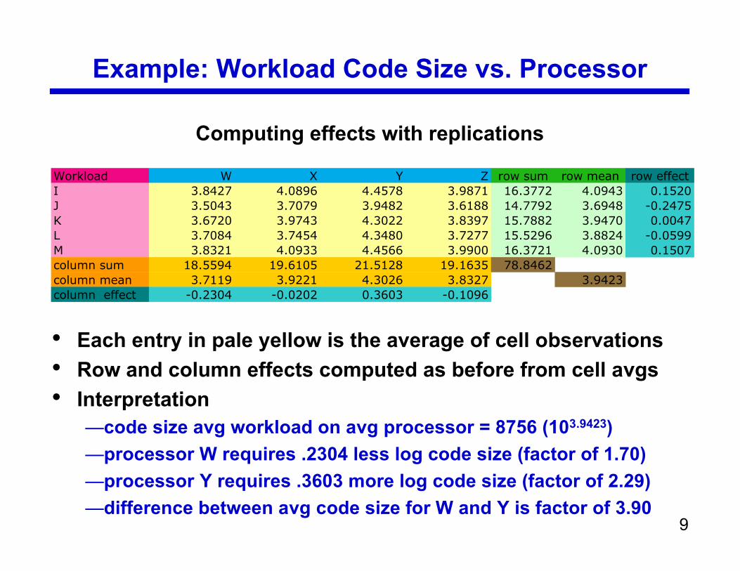
Computing effects with replications

• Each entry in pale yellow is the average of cell observations• Row and column effects computed as before from cell avgs• Interpretation

—code size avg workload on avg processor = 8756 (103.9423)—processor W requires .2304 less log code size (factor of 1.70)—processor Y requires .3603 more log code size (factor of 2.29)—difference between avg code size for W and Y is factor of 3.90

Example: Workload Code Size vs. Processor

Workload W X Y Z row sum row mean row effect

I 3.8427 4.0896 4.4578 3.9871 16.3772 4.0943 0.1520

J 3.5043 3.7079 3.9482 3.6188 14.7792 3.6948 -0.2475

K 3.6720 3.9743 4.3022 3.8397 15.7882 3.9470 0.0047

L 3.7084 3.7454 4.3480 3.7277 15.5296 3.8824 -0.0599

M 3.8321 4.0933 4.4566 3.9900 16.3721 4.0930 0.1507

column sum 18.5594 19.6105 21.5128 19.1635 78.8462

column mean 3.7119 3.9221 4.3026 3.8327 3.9423

column effect -0.2304 -0.0202 0.3603 -0.1096

10

Example: Workload Code Size vs. Processor

Compute interactions as

• Interaction constraints: row and column sums are 0• Interpretation

—interaction of I & W requires factor of 10.0212 < code than avg workload on W—interaction of I & W requires factor of 10.0212 < code than I on avg processor

Workload W X Y Z

I -0.0212 0.0155 0.0032 0.0024

J 0.0399 0.0333 -0.1069 0.0337

K -0.0447 0.0475 -0.0051 0.0023

L 0.0564 -0.1168 0.1054 -0.0450

M -0.0305 0.0205 0.0033 0.0066

Workload W X Y Z row sum row mean row effect

I 3.8427 4.0896 4.4578 3.9871 16.3772 4.0943 0.1520

J 3.5043 3.7079 3.9482 3.6188 14.7792 3.6948 -0.2475

K 3.6720 3.9743 4.3022 3.8397 15.7882 3.9470 0.0047

L 3.7084 3.7454 4.3480 3.7277 15.5296 3.8824 -0.0599

M 3.8321 4.0933 4.4566 3.9900 16.3721 4.0930 0.1507

column sum 18.5594 19.6105 21.5128 19.1635 78.8462

column mean 3.7119 3.9221 4.3026 3.8327 3.9423

column effect -0.2304 -0.0202 0.3603 -0.1096

10.0212 = 1.05

!

" ij = y ij. # (µ +$ j + %i)

11

Estimating Experimental Errors

• Predicted response of (i,j)th experiment

• Prediction error = observation - cell mean

!

ˆ y ij = µ +" j + # i + $ ij = y ij.

!

eijk = yijk " ˆ y ij = yijk " y ij.

12

Allocating Variation

• Total variation of y can be allocated to—the two factors—their interactions—errors

• Square both sides of model equation

• Total variation

• Compute SSE (easiest from other sums of squares)

• Percent variation for each factor, interaction and errors—factor A: 100(SSA/SST) factor B: 100(SSB/SST)—interactions: 100(SSAB/SST) error: 100(SSE/SST)

!

yijk2

i, j ,k

" = abrµ2 + br # j

2

j

" + ar $ i

2

i

" + r % ij2

i, j

" + eijk2

i, j,k

" +cross

productterms

(all = 0)SSY = SS0 + SSA + SSB + SSAB + SSE

SST = SSY - SS0 = SSA + SSB + SSAB + SSE

SSE = SSY - SS0 - SSA - SSB - SSAB

13

Allocating Variation for Code Size Study

% workload = 100*SSA/SST = 100*2.93/4.44 = 66.0%

Workload W X Y Z

I 3.8455 4.0807 4.4633 3.9958

3.8191 4.0717 4.4321 3.9641

3.8634 4.1164 4.4779 4.0015

J 3.5061 3.7095 3.9523 3.6184

3.4598 3.7507 3.9066 3.6291

3.5469 3.6635 3.9857 3.6091

K 3.6727 3.9735 4.2953 3.8506

3.6933 3.9510 4.2866 3.8440

3.6498 3.9984 4.3247 3.8246

L 3.7082 3.7492 4.3491 3.7288

3.7410 3.7743 4.3636 3.7585

3.6761 3.7127 4.3313 3.6959

M 3.8330 4.0879 4.4558 3.9914

3.8056 4.0790 4.4289 3.9688

3.8578 4.1131 4.4851 4.0100

3.9423

row effect

0.1520

-0.2475

0.0047

-0.0599

0.1507

column effect -0.2304 -0.0202 0.3603 -0.1096

!

SSY = yijk2

i, j ,k

" = (3.8455)2

+ (3.8191)2

+ ...+ (4.0100)2

= 936.95

!

SST = SSY " SS0 = 936.95 " 932.51= 4.44

!

SSA = br " j

2

j

# = (5)(3)(($.2304)2 + ($.0202)2 + (.3603)2

+ ($.1096)2) = 2.93

!

SS0 = abrµ2 = (5)(4)(3)(3.9423)2 = 932.51

!

SSB = ar " j

2

j

# = (4)(3)((.1520)2

+ ($.2475)2 + (.0047)2

+ ($.0599)2 + (.1507)2) =1.33

!

SSAB = r " ij2

i, j

# = (3)(($.0212)2 + (.0399)2

+ ...+ (.0066)2) = .1548

Workload W X Y Z

I -0.0212 0.0155 0.0032 0.0024

J 0.0399 0.0333 -0.1069 0.0337

K -0.0447 0.0475 -0.0051 0.0023

L 0.0564 -0.1168 0.1054 -0.0450

M -0.0305 0.0205 0.0033 0.0066

% interaction = 100*SSAB/SST = 100*.1548/4.44 = 3.48%

% procs = 100*SSB/SST = 100*1.33/4.44 = 29.9%

14

Degrees of Freedom

• Degrees of freedom SSY = SS0 + SSA + SSB + +SSAB + SSE abr = 1 + (a-1) + (b-1) + (a-1)(b-1) + ab(r-1)

sum of abr obs.all independent

single term µ2:repeated abr times

sum of (αj)2:a-1 independent

(∑αj = 0)

sum of (γij)2,(a-1)(b-1)

independent0 across row,down column

sum of (βi)2:b-1 independent

(∑βi = 0)

sum of (eijk)2:ab(r-1)

independent

15

Analyzing Significance

• Divide each sum of squares by its DOF to get meansquares—MSA = SSA/(a-1)—MSB = SSB/(b-1)—MSAB = SSAB/((a-1)(b-1))—MSE = SSE/(ab(r-1))

• Are effects of factors and interactions significant at α level?—Test MSA/MSE against F-distribution F[1-α; a-1; ab(r-1)]

—Test MSB/MSE against F-distribution F[1-α; b-1; ab(r-1)]

—Test MSAB/MSE against F-distribution F[1-α; (a-1)(b-1); ab(r-1)]

!

se

= MSE

Sum of

Squares % var DOF

Mean

Square

F

computed

F

table

processors 2.929504 65.96 3 0.9765 1340.0121 2.23

workloads 1.328183 29.9 4 0.332 455.65256 2.09

interactions 0.154789 3.48 12 0.0129 17.700875 1.71

errors 0.029149 0.66 40 0.0007

forα=.1

16

Variance for µ

• Expression for µ in terms of random variables yij’s

!

µ =1

abryijk

k=1

r

"j=1

a

"i=1

b

"

Assuming errors normally distributedzero mean, variance (σe)2

What is the variance for µ?

!

"µ

2 = abr1

abr

#

$ %

&

' (

2#

$ % %

&

' ( ( " e

2

=1

abr"e

2

!

Var(µ) =Var1

abryijk

k=1

r

"j=1

a

"i=1

b

"#

$ % %

&

' ( (

17

Variance for αj

• Expression for αj in terms of random variables yij’s

• What is the coefficient aikj for each yilk for αj?

!

" j = y . j . # y

...=1

bryijk

k=1

r

$ #1

abryilk

k=1

r

$l=1

a

$i=1

b

$i=1

b

$

!

ailk =

1

br"1

abr

"1

abr

l = j

otherwise

#

$ %

& %

Assuming errors normally distributedzero mean, variance (σe)2

What is the variance for αj?

!

"# j

2 = br1

br$1

abr

%

& '

(

) *

2

+ abr $ br( )1

abr

%

& '

(

) *

2%

& ' '

(

) * * " e

2

=(a $1)

abr" e

2

18

Parameter Estimation for Two Factors w/ Repl

!

Parameter Estimate Varianceµ y ... se

2 /abr

" j y .j. # y ... se

2(a #1) /abr

$ i y i.. # y ... se

2(b #1) /abr

% ij y ij. - y i.. # y .j. + y ... se

2(a #1)(b #1) /abr

h j" j , h j = 0j=1

a

&j=1

a

& h jy .j.j=1

a

& se

2h j

2

j=1

a

& /br

hi$i, hi = 0i=1

b

&i=1

b

& hiy i..i=1

b

& se

2hi

2

i=1

b

& /ar

se2

eijk2&( ) /(ab(r #1))

DOF of errors = ab(r-1)

19

Confidence Intervals for Effects

• Variance of processor effects

• Error degrees of freedom = ab(r-1) = 5 x 4 x 2 = 40—can use unit normal variate rather than t-variate since DOF large

• For 90% confidence level: z.95 = 1.645

—example:

does not include 0: effect is significant

!

s" j= se

(a #1)

abr= .0267

4 #1

4 $ 5 $ 3= .0060

!

" j ± z.95s" j

!

"1 ± z.95s"1 = #.2304 ± (1.645)(.0060) = (#.2406,#.2203)

for processor W

20

Confidence Intervals for Effectsparameter mean effect std deviation confidence interval

Mu 3.9423 0.0035 ( 3.9366 , 3.9480 )

processors

W -0.2304 0.0070 ( -0.2419 , -0.2190 )

X -0.0202 0.0070 ( -0.0317 , -0.0087 )

Y 0.3603 0.0070 ( 0.3488 , 0.3717 )

Z -0.1096 0.0070 ( -0.1211 , -0.0982 )

workloads

I 0.1520 0.0060 ( 0.1420 , 0.1619 )

J -0.2475 0.0060 ( -0.2574 , -0.2376 )

K 0.0047 0.0060 ( -0.0052 , 0.0147 )

L -0.0599 0.0060 ( -0.0698 , -0.0500 )

M 0.1507 0.0060 ( 0.1408 , 0.1606 )

pink cells are not significant

21

Confidence Intervals for Interactions

• 90% confidence interval for interaction effect—γij ± z.95 sγij

—pink cells are not significant

!

s" ij = se (a #1)(b #1) /abr

Workload W X Y Z

I ( -0.0411 , -0.0013 ) ( -0.0043 , 0.0354 ) ( -0.0166 , 0.0231 ) ( -0.0174 , 0.0223 )

J ( 0.0200 , 0.0598 ) ( 0.0134 , 0.0532 ) ( -0.1267 , -0.0870 ) ( 0.0138 , 0.0535 )

K ( -0.0645 , -0.0248 ) ( 0.0276 , 0.0673 ) ( -0.0249 , 0.0148 ) ( -0.0176 , 0.0222 )

L ( 0.0366 , 0.0763 ) ( -0.1366 , -0.0969 ) ( 0.0855 , 0.1252 ) ( -0.0649 , -0.0252 )

M ( -0.0503 , -0.0106 ) ( 0.0006 , 0.0404 ) ( -0.0165 , 0.0232 ) ( -0.0132 , 0.0265 )

22

Prediction Error for Code Size Study

23

Quantile-Quantile Plot for Code Size Study