Embed Size (px)
Citation preview

Two-Factor Factorial Analysis
STAT:5201
Week 9 - Lecture 1
1 / 40
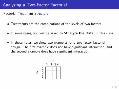
Analyzing a Two-Factor Factorial
Factorial Treatment Structure
Treatments are the combinations of the levels of two factors.
In some cases, you will be asked to ‘Analyze the Data’ in this class.
In these notes, we show two examples for a two-factor factorialdesign. The first example does not have significant interaction, andthe second example does have significant interaction.
2 / 40
Analyzing a Two-Factor Factorial
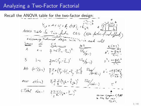
Recall the ANOVA table for the two-factor design:1~/1''')a.. I 2··. h
v,J k '" Ai + G-f -' ~. +fy# )'" + ~I~I~ .. , b A 2
i d ~
AN'OIJIt f~ J" IwD-~ tR.{) (6.f-tt ld.r5J;t.Jf,Idr);f~SJ~/~ bJ~ dh/~ Lu~'II~ e~ ~
~~ d-f: 5S ;\II S E(MS)-
I I T It
'/,I
A
8 b -I
3 / 40
Analyzing a Two-Factor Factorial
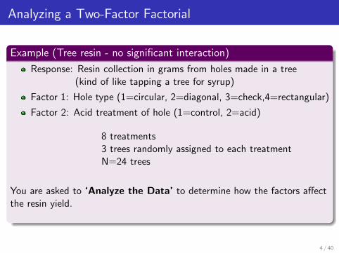
Example (Tree resin - no significant interaction)
Response: Resin collection in grams from holes made in a tree(kind of like tapping a tree for syrup)
Factor 1: Hole type (1=circular, 2=diagonal, 3=check,4=rectangular)
Factor 2: Acid treatment of hole (1=control, 2=acid)
8 treatments3 trees randomly assigned to each treatmentN=24 trees
You are asked to ‘Analyze the Data’ to determine how the factors affectthe resin yield.
4 / 40
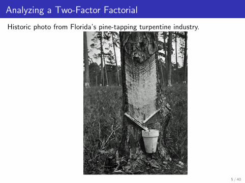
Analyzing a Two-Factor Factorial
Historic photo from Florida’s pine-tapping turpentine industry.
5 / 40
Analyzing a Two-Factor Factorial
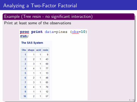
Example (Tree resin - no significant interaction)
Print at least some of the observations
6 / 40
Analyzing a Two-Factor Factorial
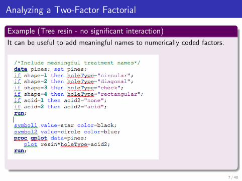
Example (Tree resin - no significant interaction)
It can be useful to add meaningful names to numerically coded factors.
7 / 40
Analyzing a Two-Factor Factorial
Example (Tree resin - no significant interaction)
8 / 40
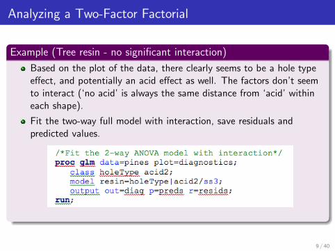
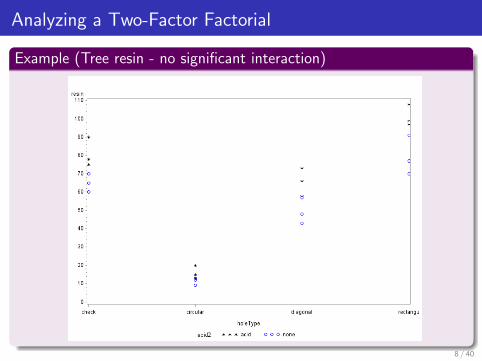
Analyzing a Two-Factor Factorial
Example (Tree resin - no significant interaction)
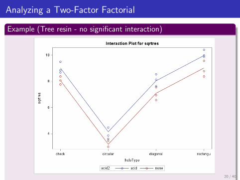
Based on the plot of the data, there clearly seems to be a hole typeeffect, and potentially an acid effect as well. The factors don’t seemto interact (‘no acid’ is always the same distance from ‘acid’ withineach shape).
Fit the two-way full model with interaction, save residuals andpredicted values.
9 / 40
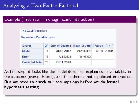
Analyzing a Two-Factor Factorial
Example (Tree resin - no significant interaction)
As first step, it looks like the model does help explain some variability inthe outcome (overall F-test), and that there is not significant interaction.But we need to check our assumptions before we do formalhypothesis testing.
10 / 40
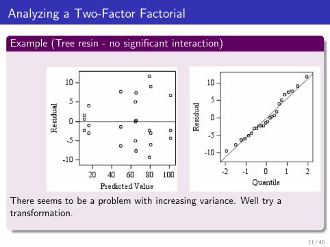
Analyzing a Two-Factor Factorial
Example (Tree resin - no significant interaction)
There seems to be a problem with increasing variance. Well try atransformation.
11 / 40
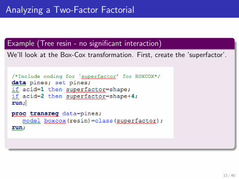
Analyzing a Two-Factor Factorial
Example (Tree resin - no significant interaction)
We’ll look at the Box-Cox transformation. First, create the ’superfactor’.
12 / 40
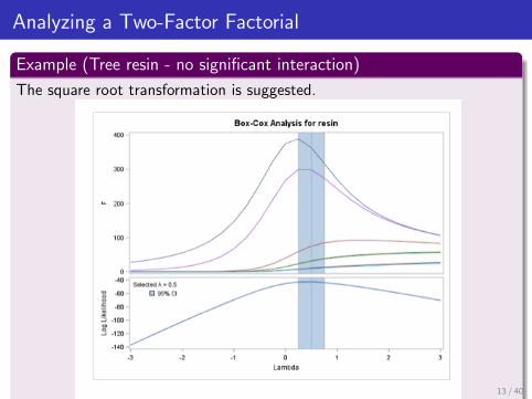
Analyzing a Two-Factor Factorial
Example (Tree resin - no significant interaction)
The square root transformation is suggested.
13 / 40
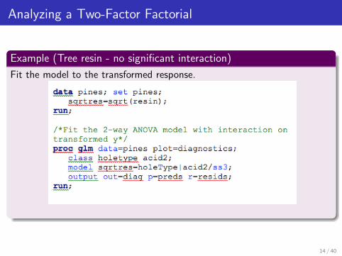
Analyzing a Two-Factor Factorial
Example (Tree resin - no significant interaction)
Fit the model to the transformed response.
14 / 40
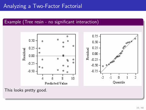
Analyzing a Two-Factor Factorial
Example (Tree resin - no significant interaction)
This looks pretty good.
15 / 40
Analyzing a Two-Factor Factorial
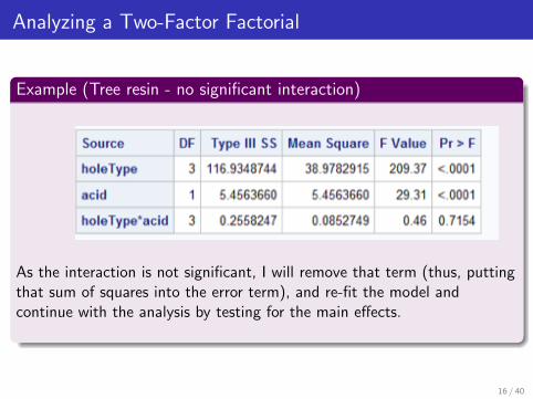
Example (Tree resin - no significant interaction)
As the interaction is not significant, I will remove that term (thus, puttingthat sum of squares into the error term), and re-fit the model andcontinue with the analysis by testing for the main effects.
16 / 40
Analyzing a Two-Factor Factorial
NOTE: There are two camps regarding what to do when an interaction isnot significant... to pool or not to pool...
If the interaction does not exist, then pooling the interaction terminto the error increases the degrees of freedom for error and it alsosimplifies our model.
On the other hand, if there really is interaction (but it wasntsignificant), and we pool it into the error term, then we are inflatingour MSE, which will decrease our power. So, some people feel youshould still leave the interaction term in the model, and then test formain effects. The downside is that your mean structure will stillcontain the interaction effects, and it wont look quite like an additivemodel.
Here, I remove the interaction and re-analyze.
17 / 40
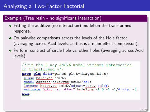
Analyzing a Two-Factor Factorial
Example (Tree resin - no significant interaction)
Fitting the additive (no interaction) model on the transformedresponse.
Do pairwise comparisons across the levels of the Hole factor(averaging across Acid levels, as this is a main-effect comparison).
Perform contrast of circle hole vs. other holes (averaging across Acidlevels).
18 / 40
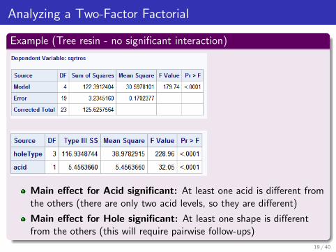
Analyzing a Two-Factor Factorial
Example (Tree resin - no significant interaction)
Main effect for Acid significant: At least one acid is different fromthe others (there are only two acid levels, so they are different)
Main effect for Hole significant: At least one shape is differentfrom the others (this will require pairwise follow-ups)
19 / 40
Analyzing a Two-Factor Factorial
Example (Tree resin - no significant interaction)
20 / 40
Analyzing a Two-Factor Factorial
Example (Tree resin - no significant interaction)
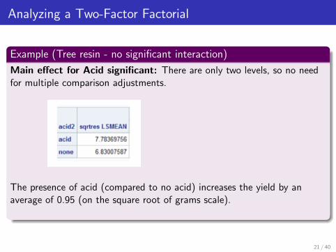
Main effect for Acid significant: There are only two levels, so no needfor multiple comparison adjustments.
The presence of acid (compared to no acid) increases the yield by anaverage of 0.95 (on the square root of grams scale).
21 / 40
Analyzing a Two-Factor Factorial
Example (Tree resin - no significant interaction)
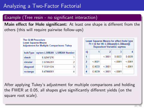
Main effect for Hole significant: At least one shape is different from theothers (this will require pairwise follow-ups)
After applying Tukey’s adjustment for multiple comparisons and holdingthe FWER at 0.05, all shapes give significantly different yields (on thesquare root scale).
22 / 40
Analyzing a Two-Factor Factorial
Example (Tree resin - no significant interaction)
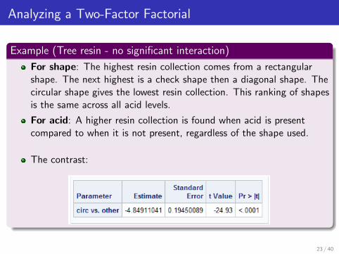
For shape: The highest resin collection comes from a rectangularshape. The next highest is a check shape then a diagonal shape. Thecircular shape gives the lowest resin collection. This ranking of shapesis the same across all acid levels.
For acid: A higher resin collection is found when acid is presentcompared to when it is not present, regardless of the shape used.
The contrast:
23 / 40
Analyzing a Two-Factor Factorial
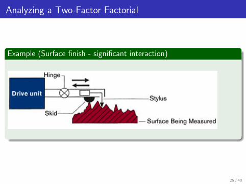
Example (Surface finish - significant interaction)
Response: Surface finish measurement of a metal part(a measure of roughness, lower is better)
Factor 1: Feed rate, inches/minute (0.20, 0.25, 0.30)
Factor 2: Depth of cut, inches (0.15, 0.18, 0.20, 0.25)
12 treatments3 runs randomly assigned to each treatmentN=36 runs
You are asked to ‘Analyze the Data’ to determine how the factors affectthe surface finish measurement.
24 / 40
Analyzing a Two-Factor Factorial
Example (Surface finish - significant interaction)
25 / 40
Analyzing a Two-Factor Factorial
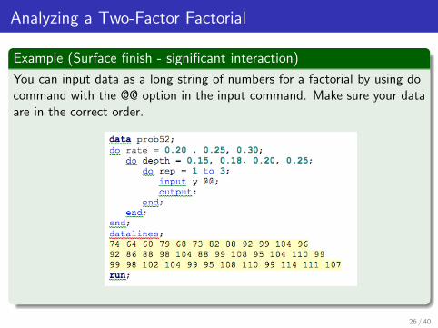
Example (Surface finish - significant interaction)
You can input data as a long string of numbers for a factorial by using docommand with the @@ option in the input command. Make sure your dataare in the correct order.
26 / 40
Analyzing a Two-Factor Factorial
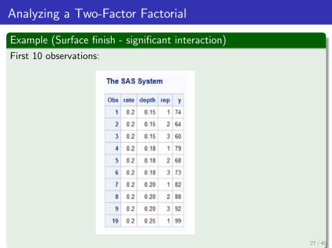
Example (Surface finish - significant interaction)
First 10 observations:
27 / 40
Analyzing a Two-Factor Factorial
Example (Surface finish - significant interaction)
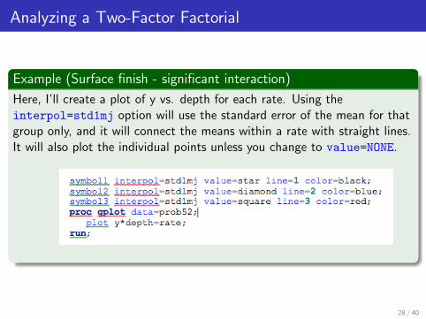
Here, I’ll create a plot of y vs. depth for each rate. Using theinterpol=std1mj option will use the standard error of the mean for thatgroup only, and it will connect the means within a rate with straight lines.It will also plot the individual points unless you change to value=NONE.
28 / 40
Analyzing a Two-Factor Factorial
Example (Surface finish - significant interaction)
29 / 40
Analyzing a Two-Factor Factorial
Example (Surface finish - significant interaction)
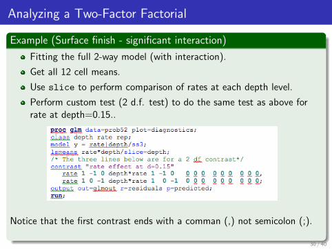
Fitting the full 2-way model (with interaction).
Get all 12 cell means.
Use slice to perform comparison of rates at each depth level.
Perform custom test (2 d.f. test) to do the same test as above forrate at depth=0.15..
Notice that the first contrast ends with a comman (,) not semicolon (;).
30 / 40
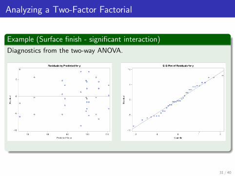
Analyzing a Two-Factor Factorial
Example (Surface finish - significant interaction)
Diagnostics from the two-way ANOVA.
31 / 40
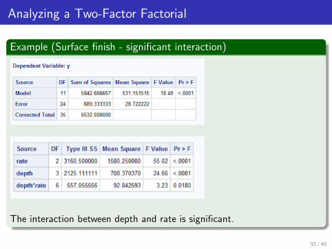
Analyzing a Two-Factor Factorial
Example (Surface finish - significant interaction)
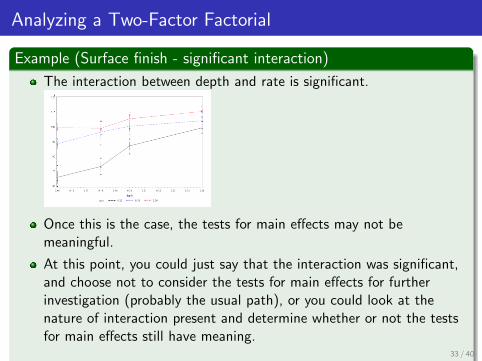
The interaction between depth and rate is significant.
32 / 40
Analyzing a Two-Factor Factorial
Example (Surface finish - significant interaction)
The interaction between depth and rate is significant.
Once this is the case, the tests for main effects may not bemeaningful.
At this point, you could just say that the interaction was significant,and choose not to consider the tests for main effects for furtherinvestigation (probably the usual path), or you could look at thenature of interaction present and determine whether or not the testsfor main effects still have meaning.
33 / 40
Analyzing a Two-Factor Factorial
Example (Surface finish - significant interaction)
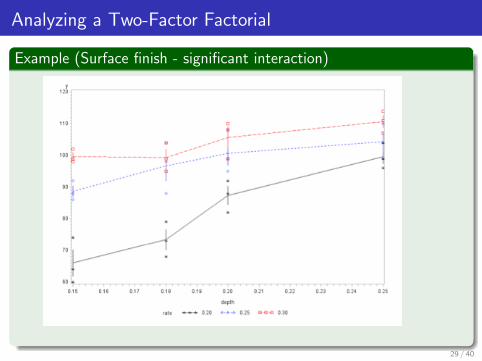
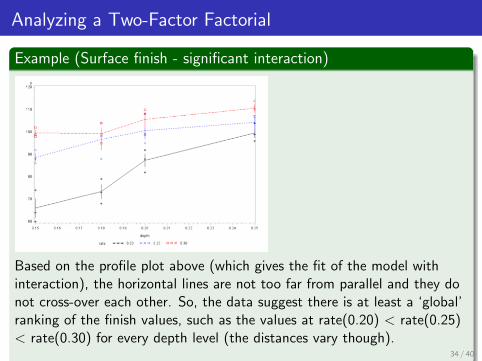
Based on the profile plot above (which gives the fit of the model withinteraction), the horizontal lines are not too far from parallel and they donot cross-over each other. So, the data suggest there is at least a ‘global’ranking of the finish values, such as the values at rate(0.20) < rate(0.25)< rate(0.30) for every depth level (the distances vary though).
34 / 40
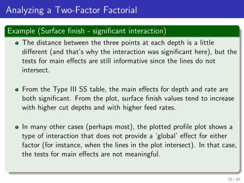
Analyzing a Two-Factor Factorial
Example (Surface finish - significant interaction)
The distance between the three points at each depth is a littledifferent (and that’s why the interaction was significant here), but thetests for main effects are still informative since the lines do notintersect.
From the Type III SS table, the main effects for depth and rate areboth significant. From the plot, surface finish values tend to increasewith higher cut depths and with higher feed rates.
In many other cases (perhaps most), the plotted profile plot shows atype of interaction that does not provide a ‘global’ effect for eitherfactor (for instance, when the lines in the plot intersect). In that case,the tests for main effects are not meaningful.
35 / 40
Analyzing a Two-Factor Factorial
Example (Surface finish - significant interaction)
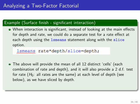
When interaction is significant, instead of looking at the main effectsfor depth and rate, we could do a separate test for a rate effect ateach depth using the lsmeans statement along with the slice
option.
The above will provide the mean of all 12 distinct ‘cells’ (eachcombination of rate and depth), and it will also provide a 2 d.f. testfor rate (H0: all rates are the same) at each level of depth (seebelow), as we have sliced by depth.
36 / 40
Analyzing a Two-Factor Factorial
Example (Surface finish - significant interaction)
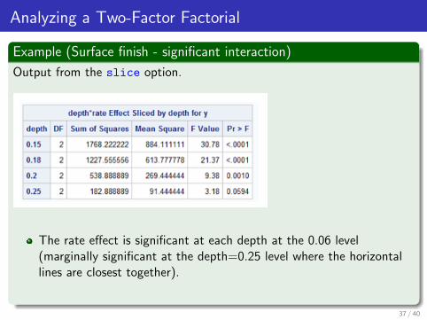
Output from the slice option.
The rate effect is significant at each depth at the 0.06 level(marginally significant at the depth=0.25 level where the horizontallines are closest together).
37 / 40
Analyzing a Two-Factor Factorial
Example (Surface finish - significant interaction)
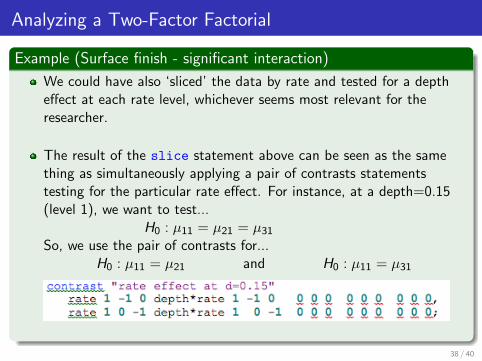
We could have also ‘sliced’ the data by rate and tested for a deptheffect at each rate level, whichever seems most relevant for theresearcher.
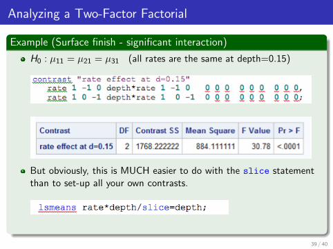
The result of the slice statement above can be seen as the samething as simultaneously applying a pair of contrasts statementstesting for the particular rate effect. For instance, at a depth=0.15(level 1), we want to test...
H0 : µ11 = µ21 = µ31So, we use the pair of contrasts for...
H0 : µ11 = µ21 and H0 : µ11 = µ31
38 / 40
Analyzing a Two-Factor Factorial
Example (Surface finish - significant interaction)
H0 : µ11 = µ21 = µ31 (all rates are the same at depth=0.15)
But obviously, this is MUCH easier to do with the slice statementthan to set-up all your own contrasts.
39 / 40
Analyzing a Two-Factor Factorial
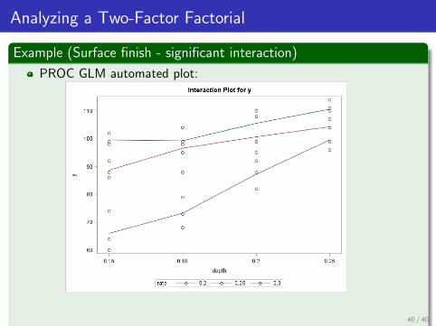
Example (Surface finish - significant interaction)
PROC GLM automated plot:
40 / 40