Tutorialby Ma’ayan Fishelson

Changes made by Anna Tzemach

The Given Problem

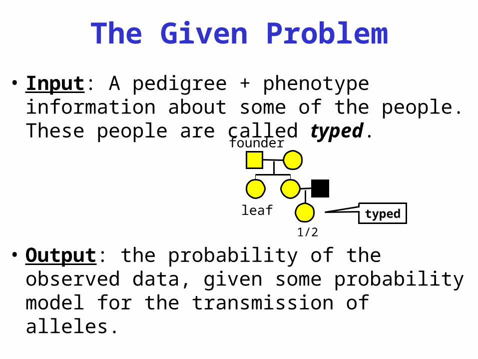
• Input: A pedigree + phenotype information about some of the people. These people are called typed.

• Output: the probability of the observed data, given some probability model for the transmission of alleles.

founder

leaf

1/2type

d

Q: What is the probability of theobserved data composed of ?

A: There are three types of probability functions: founder probabilities, penetrance probabilities, and transmission probabilities.

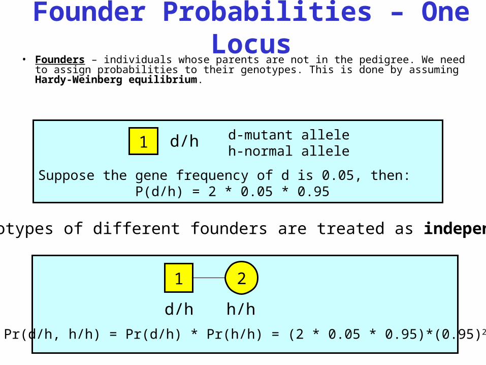
Suppose the gene frequency of d is 0.05, then:P(d/h) = 2 * 0.05 * 0.95

Founder Probabilities – One Locus

• Founders – individuals whose parents are not in the pedigree. We need to assign probabilities to their genotypes. This is done by assuming Hardy-Weinberg equilibrium.

1 d/h d-mutant alleleh-normal allele

Pr(d/h, h/h) = Pr(d/h) * Pr(h/h) = (2 * 0.05 * 0.95)*(0.95)2

1

d/h

2

h/h

• Genotypes of different founders are treated as independent:

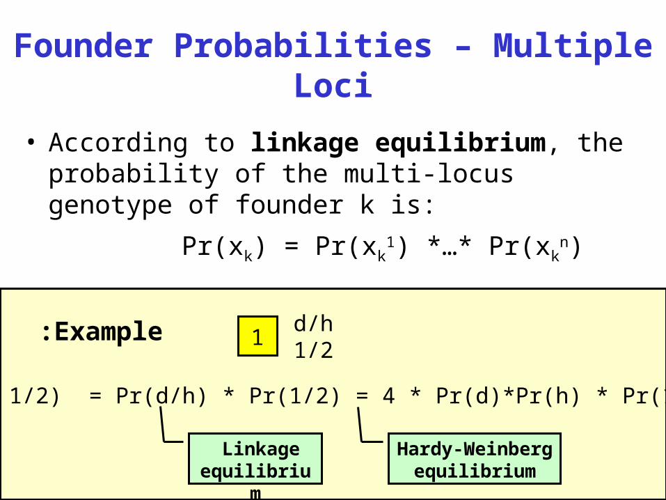
Founder Probabilities – Multiple Loci

• According to linkage equilibrium, the probability of the multi-locus genotype of founder k is:

Pr(xk) = Pr(xk1) *…* Pr(xk

n)

1d/h1/2

Pr(d/h, 1/2) = Pr(d/h) * Pr(1/2) = 4 * Pr(d)*Pr(h) * Pr(1)*Pr(2)

Linkage equilibrium

Hardy-Weinberg

equilibrium

Example:

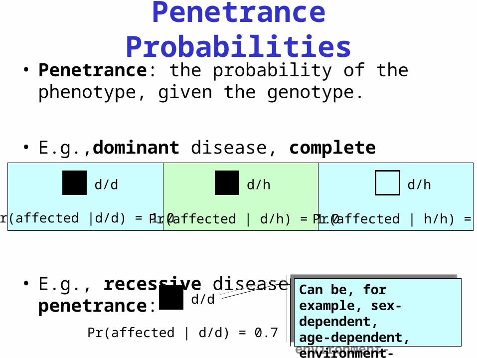
Penetrance Probabilities

• Penetrance: the probability of the phenotype, given the genotype.

• E.g.,dominant disease, complete penetrance:

• E.g., recessive disease, incomplete penetrance: d/d

Pr(affected | d/d) = 0.7

Can be, for example, sex-dependent, age-dependent, environment-dependent.

Can be, for example, sex-dependent, age-dependent, environment-dependent.

d/d

Pr(affected |d/d) = 1.0

d/h

Pr(affected | d/h) = 1.0

d/h

Pr(affected | h/h) = 0

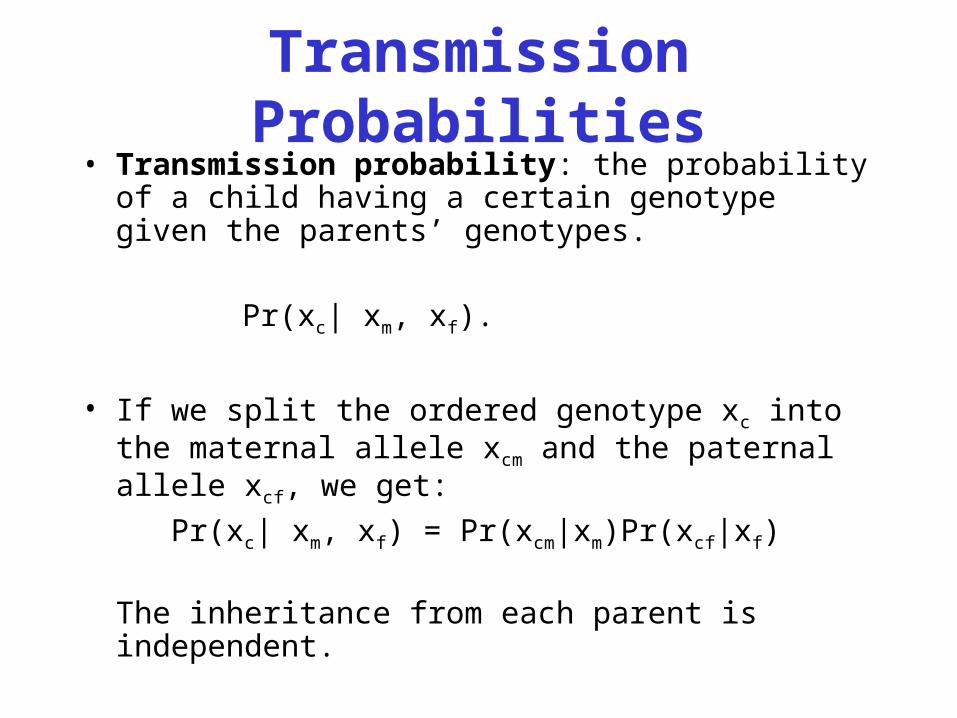
Transmission Probabilities

• Transmission probability: the probability of a child having a certain genotype given the parents’ genotypes.

Pr(xc| xm, xf).

• If we split the ordered genotype xc into the maternal allele xcm and the paternal allele xcf, we get:

Pr(xc| xm, xf) = Pr(xcm|xm)Pr(xcf|xf)

The inheritance from each parent is independent.

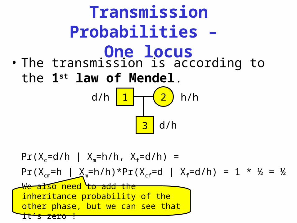
Transmission Probabilities –

One locus• The transmission is according to the 1st

law of Mendel.

Pr(Xc=d/h | Xm=h/h, Xf=d/h) =

Pr(Xcm=h | Xm=h/h)*Pr(Xcf=d | Xf=d/h) = 1 * ½ = ½

1d/h 2 h/h

3 d/h

We also need to add the inheritance probability of the other phase, but we can see that it’s zero !

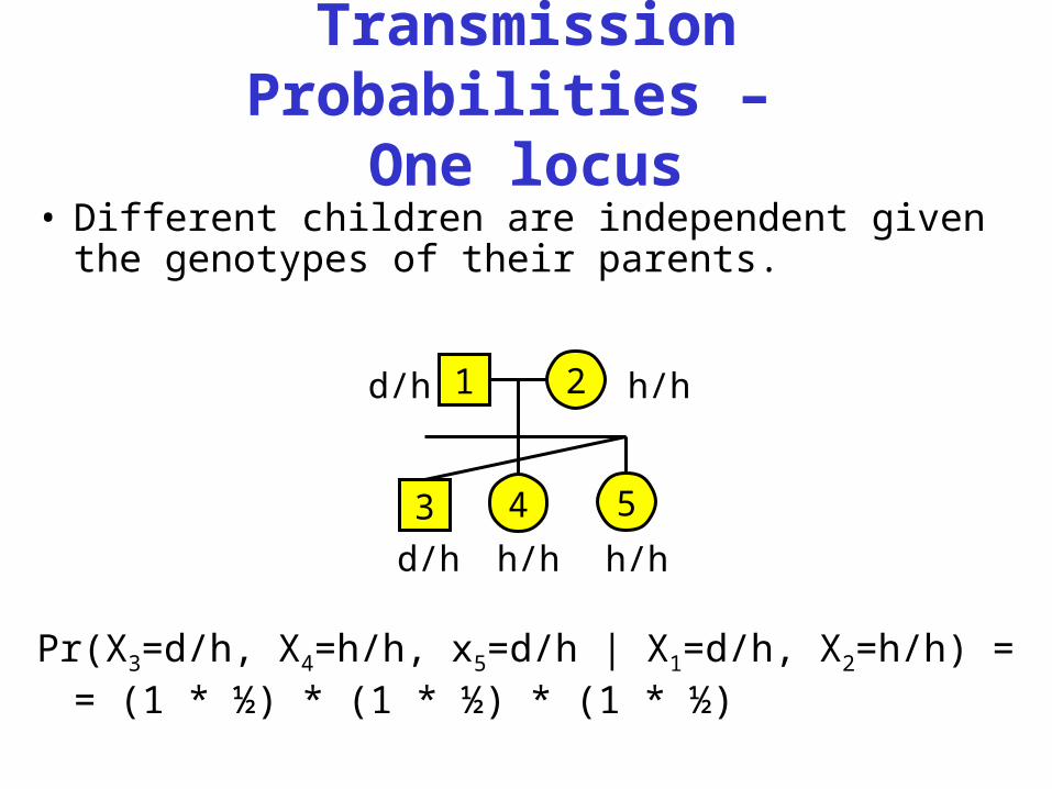
Transmission Probabilities –

One locus• Different children are independent given the

genotypes of their parents.

Pr(X3=d/h, X4=h/h, x5=d/h | X1=d/h, X2=h/h) == (1 * ½) * (1 * ½) * (1 * ½)

1d/h 2 h/h

3

d/h

4 5h/h h/h

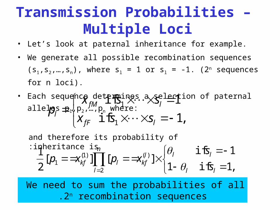
Transmission Probabilities – Multiple Loci

• Let’s look at paternal inheritance for example.

• We generate all possible recombination sequences (s1,s2,

…,sn), where sl = 1 or sl = -1. (2n sequences for n loci).

• Each sequence determines a selection of paternal alleles

p1,p2,…,pn where:

,1 if

1 if

1

1

lfF

lfMl ssx

ssxp

,1 if 1

1 if][][

2

1 )(

2

)1(1

ll

lllkf

n

llkf s

sxpxp

and therefore its probability of inheritance is:

We need to sum the probabilities of all 2n recombination sequences.

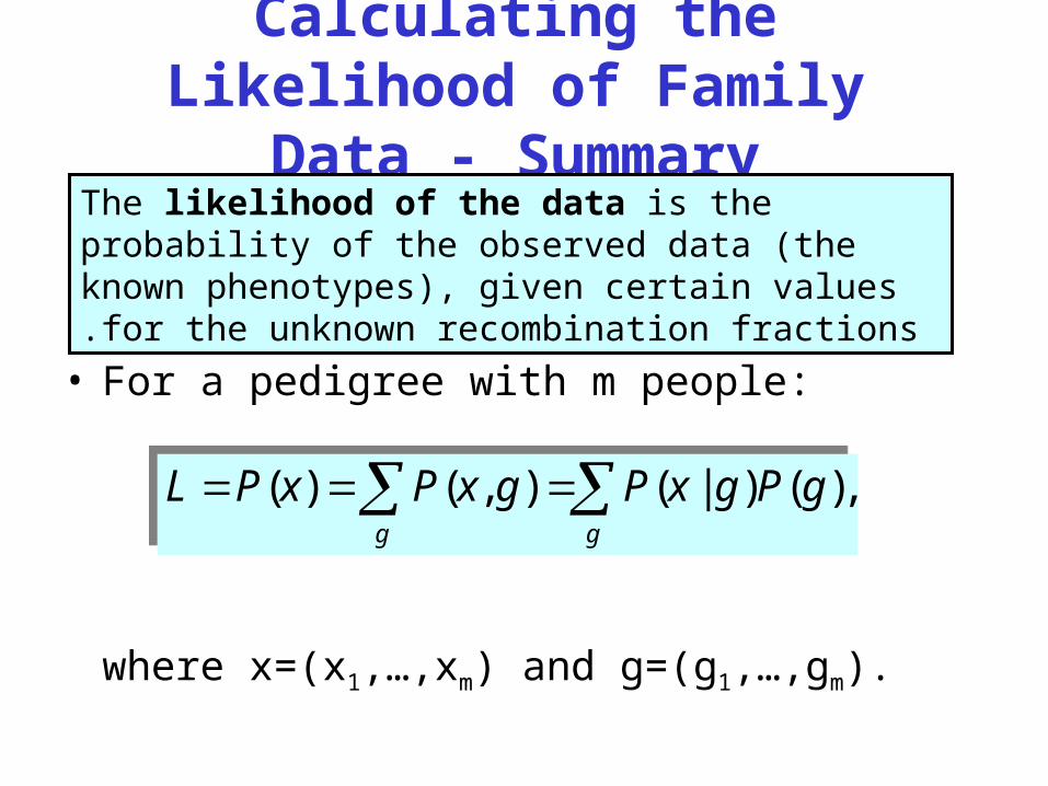
Calculating the Likelihood of Family Data - Summary

• For a pedigree with m people:

where x=(x1,…,xm) and g=(g1,…,gm).

The likelihood of the data is the probability of the observed data (the known phenotypes), given certain values for the unknown recombination fractions.

,)()|(),()( gg

gPgxPgxPxPL ,)()|(),()( gg

gPgxPgxPxPL

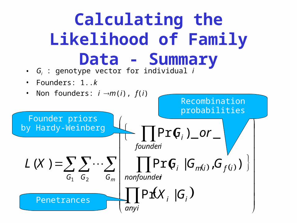
Calculating the Likelihood of Family Data - Summary

• Gi : genotype vector for individual i

• Founders: 1..k

• Non founders: im(i), f(i)

mG

ianyii

inonfounderifimi

ifounderi

G G

GX

GGG

orG

XL

|Pr

),|Pr(

__)Pr(

)(1 2

Founder priorsby Hardy-Weinberg

Recombinationprobabilities

Penetrances

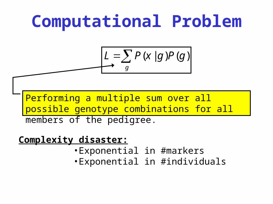
Computational Problem

g

gPgxPL )()|(

Complexity disaster:•Exponential in #markers•Exponential in #individuals

Performing a multiple sum over all possible genotype combinations for all members of the pedigree.

Elston-Stewart algorithm

The Elston-Stewart algorithm provides a means for evaluating the multiple sum in a streamlined fashion, for simple pedigrees.

More efficient computation•Exponential in #markers•Linear in #individuals

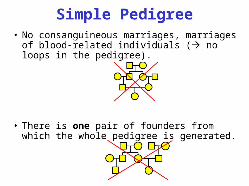
Simple Pedigree• No consanguineous marriages, marriages of

blood-related individuals ( no loops in the pedigree).

• There is one pair of founders from which the whole pedigree is generated.

Simple Pedigree

• There is exactly one nuclear family T at the top generation.

• Every other nuclear family has exactly one parent who is a direct descendant of the two parents in family T and one parent who has no ancestors in the pedigree (such a person is called a founder).

• There are no multiple marriages.• One of the parents in T is treated as the proband.

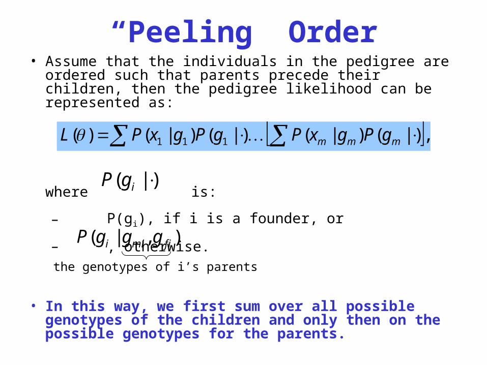
“Peeling” Order• Assume that the individuals in the pedigree are

ordered such that parents precede their children, then the pedigree likelihood can be represented as:

where is:

– P(gi), if i is a founder, or

– , otherwise.

• In this way, we first sum over all possible genotypes of the children and only then on the possible genotypes for the parents.

,)|()|()|()|()( 111 mmm gPgxPgPgxPL

)|( igP

),|( fimii gggP

the genotypes of i’s parents

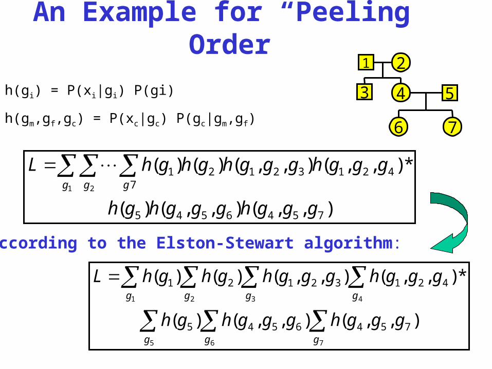
An Example for “Peeling” Order

),,(),,()(

*),,(),,()()(

7546545

42132127

1

1 2

ggghggghgh

ggghggghghghLg g g

1 2

3 4 5

76

),,(),,()(

*),,(),,()()(

7546545

42132121

75 6

431 2

ggghggghgh

ggghggghghghL

gg g

ggg g

According to the Elston-Stewart algorithm:

h(gi) = P(xi|gi) P(gi)

h(gm,gf,gc) = P(xc|gc) P(gc|gm,gf)

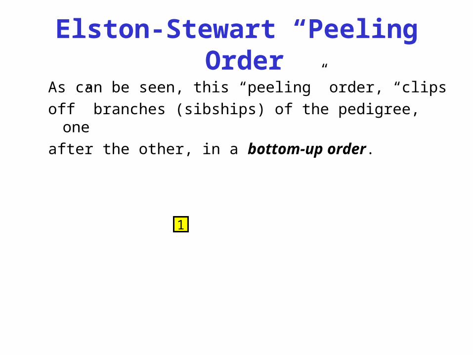
Elston-Stewart “Peeling” Order

As can be seen, this “peeling” order, “clipsoff” branches (sibships) of the pedigree, oneafter the other, in a bottom-up order.

1 2

3 4 5

76

1 2

3 4 5

6

1 2

3 4 5

1 2

3 4

1 2

3

1 21

Elston-Stewart – Computational Complexity

• The computational complexity of the algorithm is linear in the number of people but exponential in the number of loci.

• The computational complexity of the algorithm is linear in the number of people but exponential in the number of loci.

Variation on the Elston-Stewart

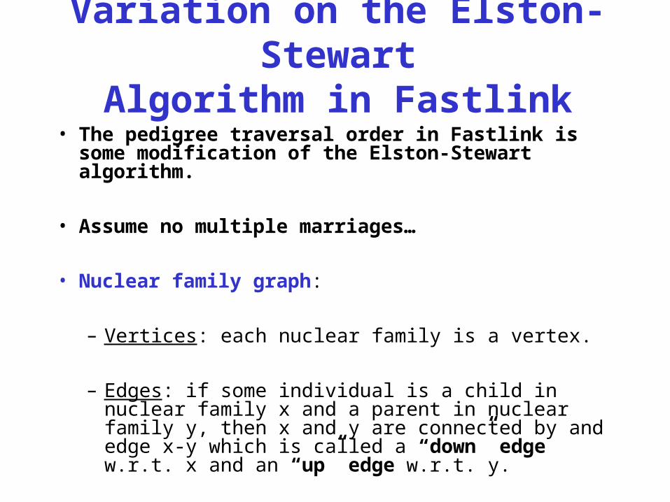
Algorithm in Fastlink• The pedigree traversal order in Fastlink is

some modification of the Elston-Stewart algorithm.

• Assume no multiple marriages…

• Nuclear family graph:

– Vertices: each nuclear family is a vertex.

– Edges: if some individual is a child in nuclear family x and a parent in nuclear family y, then x and y are connected by and edge x-y which is called a “down” edge w.r.t. x and an “up” edge w.r.t. y.

Traversal Order

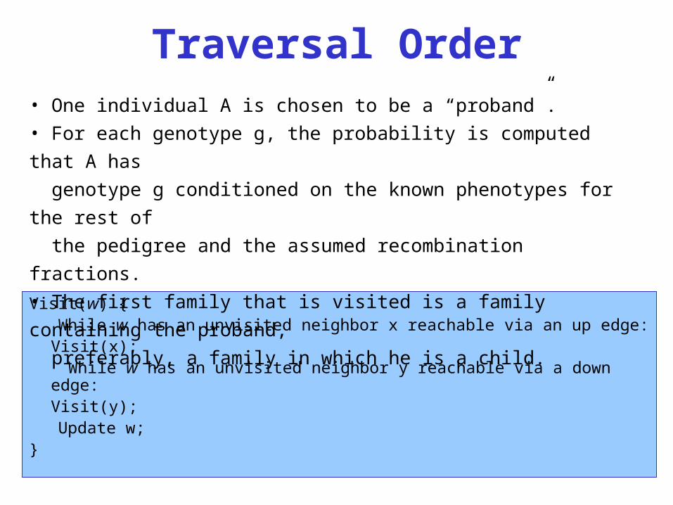
Visit(w) {While w has an unvisited neighbor x reachable via an up edge:

Visit(x); While w has an unvisited neighbor y reachable via a down edge:

Visit(y);Update w;

}

• One individual A is chosen to be a “proband”.• For each genotype g, the probability is computed that A has

genotype g conditioned on the known phenotypes for the rest

of

the pedigree and the assumed recombination fractions.• The first family that is visited is a family containing the

proband,

preferably, a family in which he is a child.

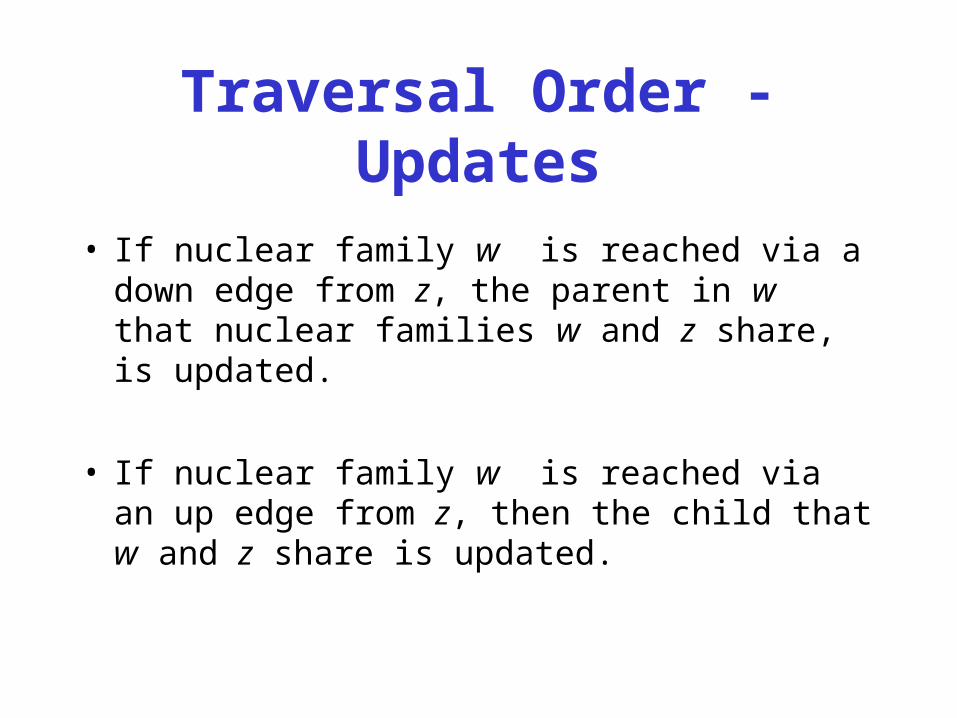
Traversal Order - Updates

• If nuclear family w is reached via a down edge from z, the parent in w that nuclear families w and z share, is updated.

• If nuclear family w is reached via an up edge from z, then the child that w and z share is updated.

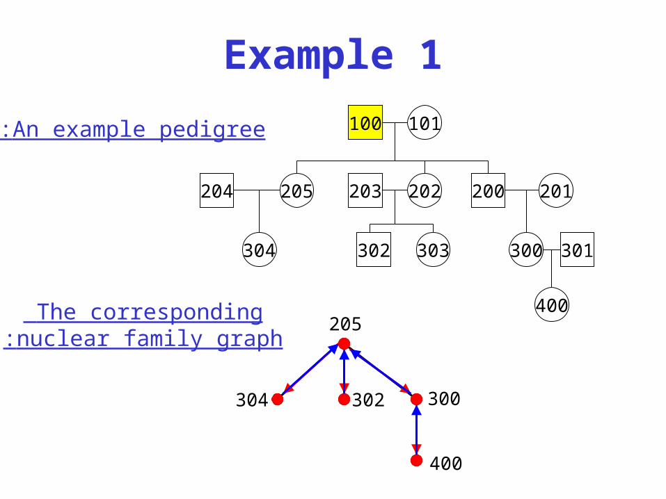
Example 1

100 101

204 205 202203 200 201

304 302 303 300 301

400205

300

400

302304

An example pedigree:

The corresponding nuclear family graph:

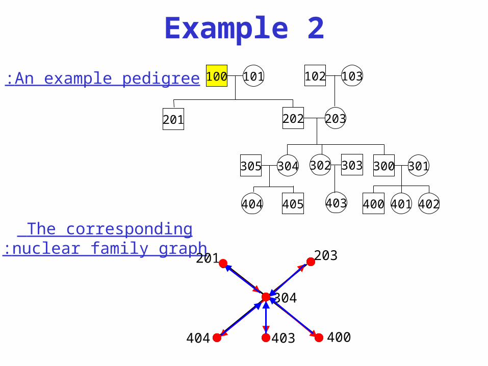
Example 2

The corresponding nuclear family graph:

An example pedigree: 100 101

304305

202 203

405404

302 303

403

201

102 103

300 301

400 401 402

400

203

403404

201

304