Tube-wave reflections in cased borehole

Alexandrov D.V.Saint-Petersburg State University

Department of PhysicsLaboratory of Elastic Media Dynamic

April 13, 2008

Summary

At low frequencies tube or Stoneley waves represent a dominant arrival propagating along boreholes.They can be excited by the source in a well or by external source due to conversion from other wavetypes. Tube wave experiences reflection at the bed boundaries, borehole diameter changes and frac-tures or permeable zones. It was proven in previous studies that 1D effective wavenumber approachprovides simple and accurate low-frequency description of tube-wave propagation in open boreholessurrounded by radially homogeneous formation. Tube waves become even more dominant in casedboreholes, but casing further modifies wave propagation and reflection/transmission phenomena. Inthis study we apply 1D effective wavenumber approach to radially inhomogeneous media and demon-strate that it still provides excellent description of low-frequency tube-wave propagation. In particu-lar, we focus on three models representative of cased boreholes: reflection from geological interfacesbehind casing, reflection from corroded casing section and reflection from idealized disk-shaped per-foration in cased hole. In all three cases frequency-dependent reflection coefficient obtained by 1Deffective method and by finite-difference computations show excellent agreement.

1 Introduction

Tube (Stoneley) waves are useful for characterizing near-wellbore space since they are sensitive toborehole diameter changes, variations in elastic properties and permeability of the surrounding for-mations. The main part of tube-wave energy is concentrated inside the well. In open-hole acousticlogging higher-frequency tube waves are used to detect and characterize fractures as well as to obtaina permeability profile (Winkler et al., 1989; Krauklis and Krauklis, 2005). In cased boreholes low-frequency tube-wave reflections can be used for estimation of quality and parameters of hydraulicfractures (Medlin and Schmitt, 1994; Paige et el., 1995) as well as other purposes. We are interestedin the latter applications for cased boreholes where surrounding media is radially inhomogeneous(casing, cement, formation). Currently only numerical finite-difference methods can handle the re-flection/transmission problem for such systems. Finite-difference method provides little physicalinsight into the problem. Approximate methods are useful for gaining better understanding of theproblem of tube-wave reflections in cased boreholes. In this study we utilize 1D effective wavenum-ber approach suggested by White (1983) and extended by Tang and Cheng (1993). This approachwas originally developed for low-frequency tube waves in radially homogeneous formations and wasverified numerically for an open hole surrounded by elastic (Tezuka et al, 1997) and poroelastic for-mations (Bakulin et al., 2005). Here we extend this approach to radially inhomogeneous media withparticular focus to cased boreholes.

1

2 1D effective wavenumber approach

The problem of acoustic logging can be considered either from the point of exact analytical solution orusing numerical modelling. Good understanding of physical processes can be obtained from analyti-cal solutionis, however the main disadvantage is the fact that amount of models which can be solvedanalytically is rather limited. Such models are the simplest like borehole in homogenous isotropicor anisotropic media. Therefor, more complex models, like fluid-filled wells with varying diameter,or cased boreholes, are usually solved with numerical methods or approximate analytical methods.The last ones need to be examined for adaptability and one of the simplest and most effective is tocompare results of approximate analytical methods with correspondent numerical modelling.

Approximate analytical method I have used in this work is 1D effective wavenumber approach.Original formulation of 1D approach by White (1983) and later generalization by Tang and Cheng(1993) assumed radial homogeneity of the media surrounding the fluid column. This was appropri-ate to describe open-hole acoustic logging. While change in diameter (washout) could be treated,no radial layering was assumed beyond the fluid-formation interface. Our interest lies in analyzinginteraction of tube waves with borehole structures in cased wells. Casing (and cement) representsanother radial layer with very distinct parameters that substantially alters the properties of the tubewave (velocity, dispersion, attenuation) and ultimately modifies the reflection and transmission phe-nomena in an unknown manner. It seems that only numerical methods, like finite-difference, cancorrectly handle these interactions. Nevertheless, presence of elastic or poroelastic radial layeringwithout additional fluid layers still supports only one propagating tube wave albeit with modifiedproperties. Thus, it appears reasonable to assume that at least at low frequencies extension of 1Dapproach should still be applicable. Let us verify this hypothesis by means of a series of numericaltests.

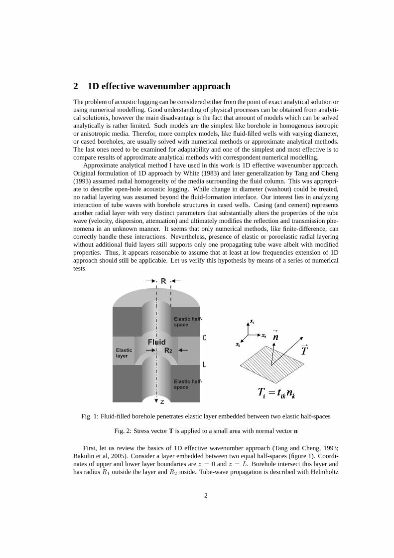
Fig. 1: Fluid-filled borehole penetrates elastic layer embedded between two elastic half-spaces

Fig. 2: Stress vectorT is applied to a small area with normal vectorn

First, let us review the basics of 1D effective wavenumber approach (Tang and Cheng, 1993;Bakulin et al, 2005). Consider a layer embedded between two equal half-spaces (figure 1). Coordi-nates of upper and lower layer boundaries arez = 0 andz = L. Borehole intersect this layer andhas radiusR1 outside the layer andR2 inside. Tube-wave propagation is described with Helmholtz

2

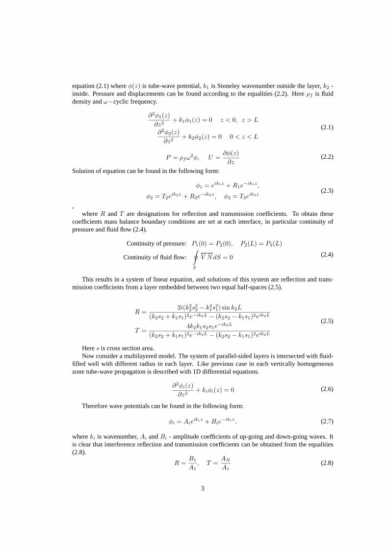
equation (2.1) whereφ(z) is tube-wave potential,k1 is Stoneley wavenumber outside the layer,k2 -inside. Pressure and displacements can be found according to the equalities (2.2). Hereρf is fluiddensity andω - cyclic frequency.

∂2φ1(z)∂z2

+ k1φ1(z) = 0 z < 0, z > L

∂2φ2(z)∂z2

+ k2φ2(z) = 0 0 < z < L

(2.1)

P = ρfω2φ, U =∂φ(z)

∂z(2.2)

Solution of equation can be found in the following form:

φ1 = eik1z + R1e−ik1z,

φ2 = T2eik2z + R2e

−ik2z, φ3 = T3eik3z

(2.3)

,whereR and T are designations for reflection and transmission coefficients. To obtain these

coefficients mass balance boundary conditions are set at each interface, in particular continuity ofpressure and fluid flow (2.4).

Continuity of pressure:P1(0) = P2(0), P2(L) = P3(L)

Continuity of fluid flow:∮S

−→V−→NdS = 0 (2.4)

This results in a system of linear equation, and solutions of this system are reflection and trans-mission coefficients from a layer embedded between two equal half-spaces (2.5).

R =2i(k2

2s22 − k2

1s21) sin k2L

(k2s2 + k1s1)2e−ik2L − (k2s2 − k1s1)2eik2L

T =4k2k1s2s1e

−ik2L

(k2s2 + k1s1)2e−ik2L − (k2s2 − k1s1)2eik2L

(2.5)

Heres is cross section area.Now consider a multilayered model. The system of parallel-sided layers is intersected with fluid-

filled well with different radius in each layer. Like previous case in each vertically homogeneouszone tube-wave propagation is described with 1D differential equations.

∂2φi(z)∂z2

+ kiφi(z) = 0 (2.6)

Therefore wave potentials can be found in the following form:

φi = Aieikiz + Bie

−ikiz, (2.7)

whereki is wavenumber,Ai andBi - amplitude coefficients of up-going and down-going waves. Itis clear that interference reflection and transmission coefficients can be obtained from the equalities(2.8).

R =B1

A1, T =

AN

A1(2.8)

3

Boundary conditions are the same as in the previous case, and we obtain a system of linearequations where G is a propagation matrix (2.10).

Continuity of pressure:Pi−1(zi) = Pi(zi)

Continuity of fluid flow:∮Si

−→V−→NdS = 0 (2.9)

(Bi

Ai

)= Gi

(Bi+1

Ai+1

)(

B1

A1

)= G1

(B2

A2

)= ... = G1G2...GN−1

(BN

AN

):= GT

(BN

AN

) (2.10)

R =(GT )12(GT )22

, T =1

(GT )22(2.11)

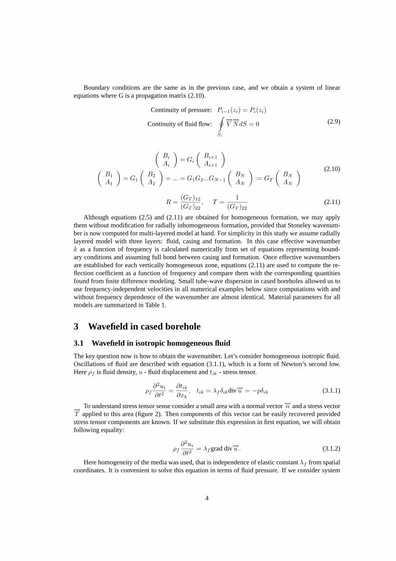
Although equations (2.5) and (2.11) are obtained for homogeneous formation, we may applythem without modification for radially inhomogeneous formation, provided that Stoneley wavenum-ber is now computed for multi-layered model at hand. For simplicity in this study we assume radiallylayered model with three layers: fluid, casing and formation. In this case effective wavenumberk as a function of frequency is calculated numerically from set of equations representing bound-ary conditions and assuming full bond between casing and formation. Once effective wavenumbersare established for each vertically homogeneous zone, equations (2.11) are used to compute the re-flection coefficient as a function of frequency and compare them with the corresponding quantitiesfound from finite difference modeling. Small tube-wave dispersion in cased boreholes allowed us touse frequency-independent velocities in all numerical examples below since computations with andwithout frequency dependence of the wavenumber are almost identical. Material parameters for allmodels are summarized in Table 1.

3 Wavefield in cased borehole

3.1 Wavefield in isotropic homogeneous fluid

The key question now is how to obtain the wavenumber. Let’s consider homogeneous isotropic fluid.Oscillations of fluid are described with equation (3.1.1), which is a form of Newton’s second low.Hereρf is fluid density,u - fluid displacement andtik - stress tensor.

ρf∂2ui

∂t2=

∂tik∂xk

, tik = λfδikdiv−→u = −pδik (3.1.1)

To understand stress tensor sense consider a small area with a normal vector−→n and a stress vector−→T applied to this area (figure 2). Then components of this vector can be easily recovered providedstress tensor components are known. If we substitute this expression in first equation, we will obtainfollowing equality:

ρf∂2ui

∂t2= λf grad div−→u . (3.1.2)

Here homogeneity of the media was used, that is independence of elastic constantλf from spatialcoordinates. It is convenient to solve this equation in terms of fluid pressure. If we consider system

4

with point source, than we should put delta-function in the right side of the equation.

∆p(x, y, z, t)− 1v2

f

p(x, y, z, t) = δ(t)δ(x, y, z), p = −div−→u ,1v2

f

=λf

ρf(3.1.3)

∆P (r, k, ω)− ω2

v2f

P (r, k, ω) = δ(r) (3.1.4)

Time and Spatial Fourier transform leads to the equation (3.1.4). For the system has axial sym-metry, one can rewrite this equation in cylindrical coordinates and obtain so-called Bessel equationof zero-order. Solution of this equation are Bessel- and Hankel-function of zero-order. Solutions forpressure and for displacement are presented below.

P (r, k, ω) = CfJ0(−iαfr) +i

4H

(2)0 (−iαfr), αf = ω

√k2

ω2− 1

v2f

, r =√

x2 + y2 (3.1.5)

(Ur

Uz

)= Cf

(αfJ1(−iαfr)−kJ0(−iαfr)

)− 1

4ρfω2

(αfH

(2)1 (−iαfr)

−kH(2)0 (−iαfr)

)(3.1.6)

One can see that for infinite fluid with point source we have one unknown constantCf (indepen-dent from spatial coordinates). Herek is wavenumber.

3.2 Wavefield in isotropic homogeneous elastic media

Now consider infinite homogeneous elastic media.

ρf∂2ui

∂t2=

∂tik∂xk

, tik = λfδikdiv−→u + 2µεik (3.2.1)

For such media additional component appears in stress tensor (3.2.1). It contains strain tensorεik,which for small deformations has following form:

εik =12

( ∂ui

∂xk+

∂uk

∂xi

)(3.2.2)

ρf∂2ui

∂t2= (λ + 2µ)grad div−→u − rot rot−→u (3.2.3)

In this case motion equation becomes more complicated (3.2.3), but it still can be solved. Aftertime- and spatial fourier transform we will again obtain Bessel equation. But now there will be twokinds of waves: p-wave (from primal) and s-wave (from secondary).(

Ur

Uz

)= Cp

(αpH

(2)1 (−iαpr)

−kH(2)0 (−iαpr)

)+ Cs

(αsH

(2)1 (−iαsr)

−kH(2)0 (−iαsr)

)(3.2.4)

3.3 Boundary conditions

Now we should construct solution for the model we are interested in: cased borehole in homogeneousmedia (figure 3).

Casing, a steel pipe, has thicknessa and inner radiusR. Solutions in previous sections wereobtained for infinite media and thus contain only outgoing waves. It’s clear that inside the casingwavefield will be described with expression from the previous (3.2.4), but there will be also waves

5

Fig. 3: Cased borehole in homogeneous elastic media

going in negative r-direction. Thus we have seven unknown constants: one in fluid, four in casingand two in surrounding elastic media. To obtain them we should set boundary conditions at eachinterface. They are:

• continuity of r-component of displacement on the boundary between fluid and casing:Ur(R + 0) = Ur(R− 0),

• continuity of displacement on the boundary between casing and surrounding media:−→U (R + a + 0) =

−→U (R + a− 0),

• continuity of stress-vector components:trr|R+0 = trr|R−0, trr|R+a+0 = trr|R+a−0,trz|R+0 = trz|R−0, trz|R+a+0 = trz|R+a−0.

There is no necessity in continuity of z-component of displacement because oscillation of fluidand casing in z-direction are independent - fluid is nonviscous and therefore there is no friction onthe boundary between fluid and casing.

So, we have seven constants to find and a system of seven linear algebraic equations. After weinverse matrix of this system we can obtain them as functions of frequency, wavenumber and mediaelastic parameters.

M−→C =

−→D =⇒

−→C =

M̂

det M

−→D

−→C = {Cf , Cc

p+,Ccp−, Cc

s+, Ccs−, Ce

p+, Cep−}

(3.3.1)

But if determinant of this matrix is equal to zero for some values of parameters, then a singularitywill appear. This condition (det M = 0) leads to an equation, called ”dispersion equation”. Fromdispersion equation one can obtain wavenumber as function of frequency for several wave modes.The slowest one is tube wave.

6

4 Modelling results

4.1 Reflection from geological interfaces behind casing

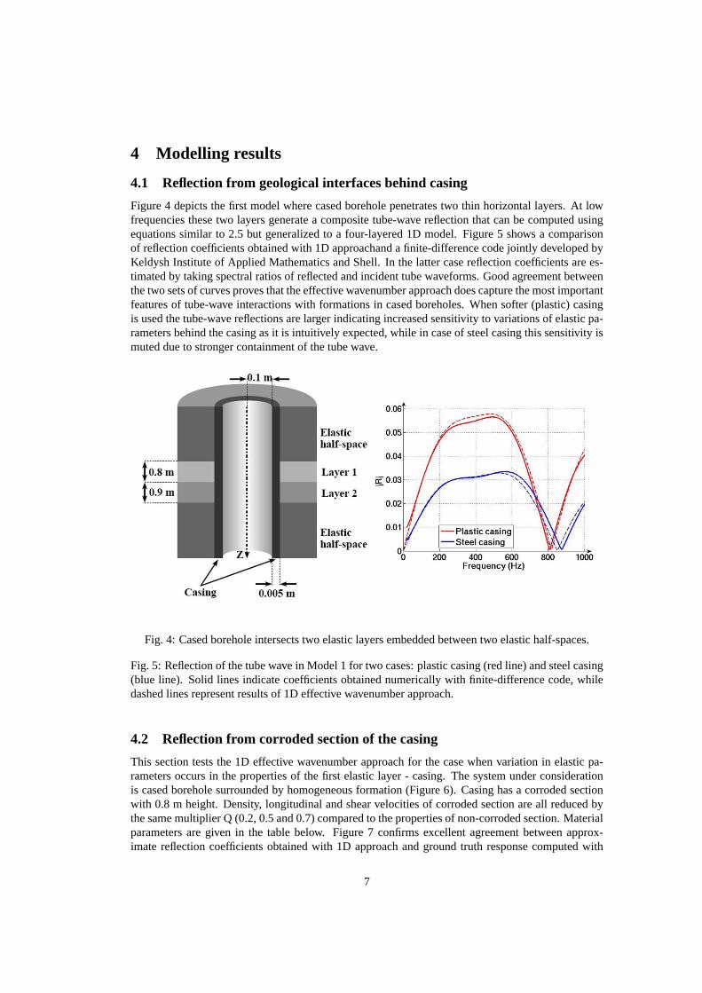
Figure 4 depicts the first model where cased borehole penetrates two thin horizontal layers. At lowfrequencies these two layers generate a composite tube-wave reflection that can be computed usingequations similar to 2.5 but generalized to a four-layered 1D model. Figure 5 shows a comparisonof reflection coefficients obtained with 1D approachand a finite-difference code jointly developed byKeldysh Institute of Applied Mathematics and Shell. In the latter case reflection coefficients are es-timated by taking spectral ratios of reflected and incident tube waveforms. Good agreement betweenthe two sets of curves proves that the effective wavenumber approach does capture the most importantfeatures of tube-wave interactions with formations in cased boreholes. When softer (plastic) casingis used the tube-wave reflections are larger indicating increased sensitivity to variations of elastic pa-rameters behind the casing as it is intuitively expected, while in case of steel casing this sensitivity ismuted due to stronger containment of the tube wave.

Fig. 4: Cased borehole intersects two elastic layers embedded between two elastic half-spaces.

Fig. 5: Reflection of the tube wave in Model 1 for two cases: plastic casing (red line) and steel casing(blue line). Solid lines indicate coefficients obtained numerically with finite-difference code, whiledashed lines represent results of 1D effective wavenumber approach.

4.2 Reflection from corroded section of the casing

This section tests the 1D effective wavenumber approach for the case when variation in elastic pa-rameters occurs in the properties of the first elastic layer - casing. The system under considerationis cased borehole surrounded by homogeneous formation (Figure 6). Casing has a corroded sectionwith 0.8 m height. Density, longitudinal and shear velocities of corroded section are all reduced bythe same multiplier Q (0.2, 0.5 and 0.7) compared to the properties of non-corroded section. Materialparameters are given in the table below. Figure 7 confirms excellent agreement between approx-imate reflection coefficients obtained with 1D approach and ground truth response computed with

7

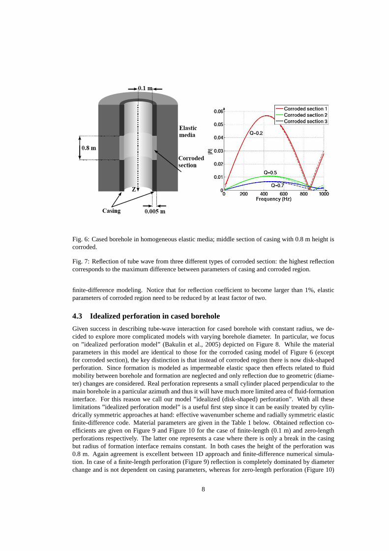
Fig. 6: Cased borehole in homogeneous elastic media; middle section of casing with 0.8 m height iscorroded.

Fig. 7: Reflection of tube wave from three different types of corroded section: the highest reflectioncorresponds to the maximum difference between parameters of casing and corroded region.

finite-difference modeling. Notice that for reflection coefficient to become larger than 1%, elasticparameters of corroded region need to be reduced by at least factor of two.

4.3 Idealized perforation in cased borehole

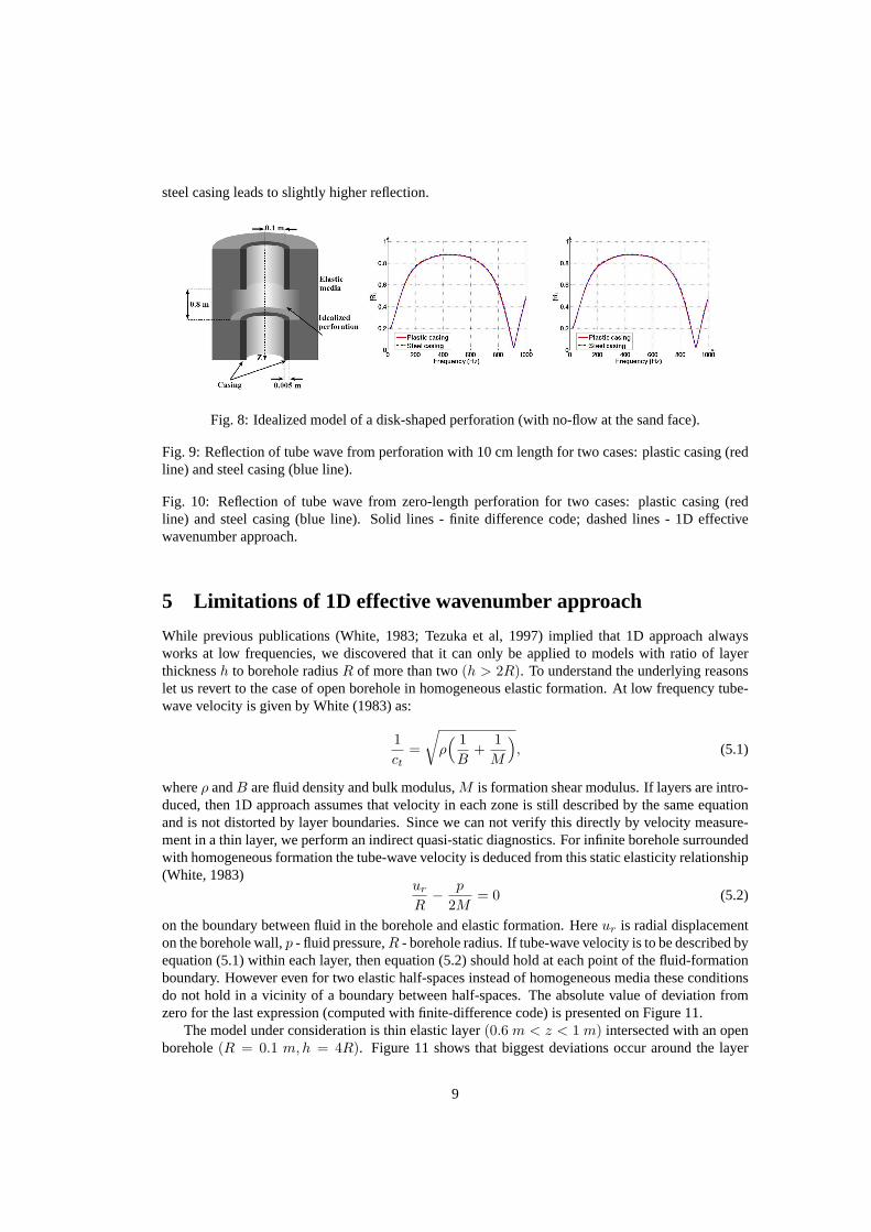
Given success in describing tube-wave interaction for cased borehole with constant radius, we de-cided to explore more complicated models with varying borehole diameter. In particular, we focuson ”idealized perforation model” (Bakulin et al., 2005) depicted on Figure 8. While the materialparameters in this model are identical to those for the corroded casing model of Figure 6 (exceptfor corroded section), the key distinction is that instead of corroded region there is now disk-shapedperforation. Since formation is modeled as impermeable elastic space then effects related to fluidmobility between borehole and formation are neglected and only reflection due to geometric (diame-ter) changes are considered. Real perforation represents a small cylinder placed perpendicular to themain borehole in a particular azimuth and thus it will have much more limited area of fluid-formationinterface. For this reason we call our model ”idealized (disk-shaped) perforation”. With all theselimitations ”idealized perforation model” is a useful first step since it can be easily treated by cylin-drically symmetric approaches at hand: effective wavenumber scheme and radially symmetric elasticfinite-difference code. Material parameters are given in the Table 1 below. Obtained reflection co-efficients are given on Figure 9 and Figure 10 for the case of finite-length (0.1 m) and zero-lengthperforations respectively. The latter one represents a case where there is only a break in the casingbut radius of formation interface remains constant. In both cases the height of the perforation was0.8 m. Again agreement is excellent between 1D approach and finite-difference numerical simula-tion. In case of a finite-length perforation (Figure 9) reflection is completely dominated by diameterchange and is not dependent on casing parameters, whereas for zero-length perforation (Figure 10)

8

steel casing leads to slightly higher reflection.

Fig. 8: Idealized model of a disk-shaped perforation (with no-flow at the sand face).

Fig. 9: Reflection of tube wave from perforation with 10 cm length for two cases: plastic casing (redline) and steel casing (blue line).

Fig. 10: Reflection of tube wave from zero-length perforation for two cases: plastic casing (redline) and steel casing (blue line). Solid lines - finite difference code; dashed lines - 1D effectivewavenumber approach.

5 Limitations of 1D effective wavenumber approach

While previous publications (White, 1983; Tezuka et al, 1997) implied that 1D approach alwaysworks at low frequencies, we discovered that it can only be applied to models with ratio of layerthicknessh to borehole radiusR of more than two(h > 2R). To understand the underlying reasonslet us revert to the case of open borehole in homogeneous elastic formation. At low frequency tube-wave velocity is given by White (1983) as:

1ct

=

√ρ( 1

B+

1M

), (5.1)

whereρ andB are fluid density and bulk modulus,M is formation shear modulus. If layers are intro-duced, then 1D approach assumes that velocity in each zone is still described by the same equationand is not distorted by layer boundaries. Since we can not verify this directly by velocity measure-ment in a thin layer, we perform an indirect quasi-static diagnostics. For infinite borehole surroundedwith homogeneous formation the tube-wave velocity is deduced from this static elasticity relationship(White, 1983)

ur

R− p

2M= 0 (5.2)

on the boundary between fluid in the borehole and elastic formation. Hereur is radial displacementon the borehole wall,p - fluid pressure,R - borehole radius. If tube-wave velocity is to be described byequation (5.1) within each layer, then equation (5.2) should hold at each point of the fluid-formationboundary. However even for two elastic half-spaces instead of homogeneous media these conditionsdo not hold in a vicinity of a boundary between half-spaces. The absolute value of deviation fromzero for the last expression (computed with finite-difference code) is presented on Figure 11.

The model under consideration is thin elastic layer(0.6 m < z < 1 m) intersected with an openborehole(R = 0.1 m,h = 4R). Figure 11 shows that biggest deviations occur around the layer

9

Fig. 11: Deviation(

|ur/R−p/2M |max |ur/R−p/2M |

)from static formula (5.2) for a case of thin layer between two

half-spaces.

Fig. 12: Relative error of 1D approach in respect to finite-difference modelling as a function ofrelative layer thickness

boundaries and two symmetric peaks overlap in the middle of the thin layer. Most likely mismatch ofacoustic properties between fully bonded layers of different materials invalidate relation (5.2) near theinterface. For two half-space model or this model withh = 4R 1D this deviation is not essential and1D approach still produces reflection response that is close to finite-difference computation. Whenlayer thickness is further reduced, the deviation in the middle of the layer is enhanced by strongerinterference of the approaching peaks. For thicknessesh < 2R we observe consistent and substantialmismatches between the 1D approach and finite difference responses. It is clear that formula (5.2) isno longer valid within the layer and thus equation (5.1) does not represent a tube-wave velocity insidethe bed with very close boundaries. We can interpret that that ”effective” tube-wave velocity insidethe thin layer is altered and is no longer described by (5.1), thus leading to a mismatch. Presence ofmultiple closely spaced geological interfaces between contrasting beds can break the approximations(5.2) and (5.1) in a larger depth interval. Therefore 1D wavenumber approach can not be applied tothe case of very thin layers(h < 2R).

6 Conclusions

We extended 1D effective wavenumber approach to treat the interactions of low-frequency tube waveswith various borehole structures in a radially inhomogeneous media that supports single tube-wavemode. In particular, we have shown good agreement between responses obtained with 1D approachand finite-difference computations in cased boreholes with vertical variation in properties of casingor formation layers. We further tested this method for simplest model of idealized (disk-shaped)perforation with no-flow boundary at the sand face. In this case change in diameter is additionallyintroduced. We also demonstrate that 1D approach becomes inaccurate for very thin layers(h < 2R)and thus very thin layers or small perforations can not be treated properly. We predict that in caseof poroelastic structures 1D effective wavenumber approach would also account for fluid flow effectsand correctly describe tube-wave interaction with radially inhomogeneous permeable formations.

10

References

1. Bakulin A., Gurevich, B., Ciz, R., Ziatdinov S., 2005, Tube-wave reflection from a porouspermeable layer with an idealized perforation: 75th Annual Meeting, Society of ExplorationGeophysicists, Expanded Abstract, 332-335.

2. Krauklis, P. V., and A. P. Krauklis, 2005, Tube Wave Reflection and Transmission on the Frac-ture: 67th Meeting, EAGE, Expanded Abstracts, P217.

3. Medlin, W.L., Schmitt, D.P., 1994, Fracture diagnostics with tube-wave reflections logs: Jour-nal of Petroleum Technology, March, 239-248.

4. Paige, R.W., L.R. Murray, and J.D.M. Roberts, 1995, Field applications of hydraulic impedancetesting for fracture measurements: SPE Production and Facilities, February, 7-12.

5. Tang, X. M., and C. H. Cheng, 1993, Borehole Stoneley waves propagation across permeablestructures: Geophysical Prospecting, 41, 165-187.

6. Tezuka, K., C.H. Cheng, and X.M. Tang, 1997, Modeling of low-frequency Stoneley-wavepropagation in an irregular borehole: Geophysics, 62, 1047-1058.

7. White, J. E., 1983, Underground sound, Elsevier.

8. Winkler, K. W., H. Liu, and D.L. Johnson, 1989, Permeability and borehole Stoneley waves:Comparison between experiment and theory: Geophysics, 54, 66-75.

11

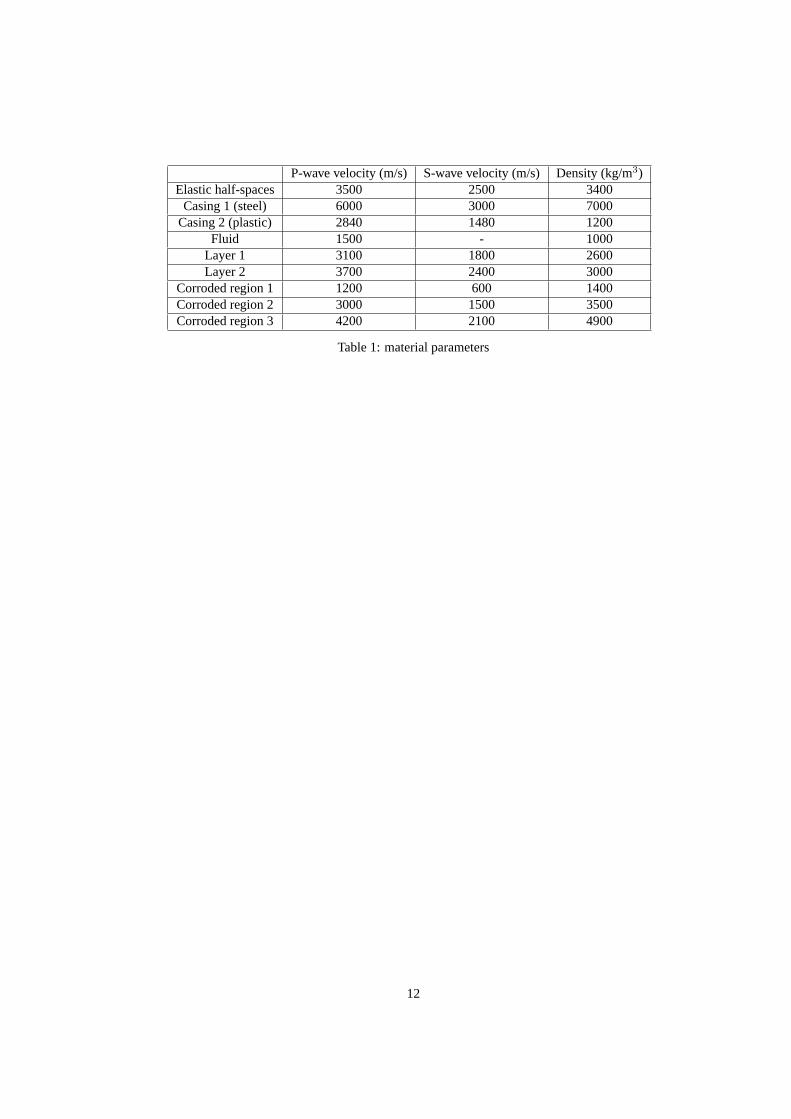
P-wave velocity (m/s) S-wave velocity (m/s) Density (kg/m3)Elastic half-spaces 3500 2500 3400

Casing 1 (steel) 6000 3000 7000Casing 2 (plastic) 2840 1480 1200

Fluid 1500 - 1000Layer 1 3100 1800 2600Layer 2 3700 2400 3000

Corroded region 1 1200 600 1400Corroded region 2 3000 1500 3500Corroded region 3 4200 2100 4900

Table 1: material parameters

12