True images: a calibration technique to reproduce images as recorded

Corey Manders and Steve MannElectrical and Computer Engineering

University of Toronto10 King’s College Rd., Toronto, Canada

manders@ieee.org and mann@eecg.utoronto.ca

Abstract

When the user of a digital camera records an image,there is some presumption that when displayed, there is anaccurate tonal representation. However, this is almost neverthe case. The paper shows how capture and tonal repro-duction of an image rarely match, as well as the historyas to why this is true. Techniques for calibrating digitalcameras tonally as well as calibrating viewing devices arepresented. The paper demonstrates a method of recoveringcamera response curves easily and with precision. Monitorcalibration is demonstrated in a means that allows an ac-curate display of light-linear images. Ultimately, the papershows how the proposed methods of calibration for digitalcameras and display devices results in the accurate repre-sentation of images.

1. Introduction

Since the advent of television, the capture and trans-mission of images has always involved range compression[17][13]. This follows from the fact that televisions throughtheir very nature are range expanders. A signal of vary-ing voltage is exponentially expanded in the process of dis-play. To compensate for this fact, television cameras wereconstructed to be range compressors. Coincidentally, theeye (and most of the human sensory system) is also a rangecompressor. This is largely why sound intensity is measuredin the logarithmic unit of decibels. Similarly, to perceiveone light as being twice as bright as another, the energy pro-duced by the brighter light must be more than double thatof the dimmer.

Producers of digital cameras have long known about thebenefits of range compression. Because of the non-linearnature of this phenomena, we are less likely to notice quan-tization artifacts as the range compression of images closelymatches the range compression present in our visual system.Because of this match, reasonably coarse quantization may

be applied, reducing the file size of the image stored. How-ever, more has been done by the camera manufacturers thansimply applying a logarithmic curve to the response of acamera. Camera manufactures typically tailor the responseof the camera to result in images that the human viewer willfind more appealing than the image actually taken. Simi-larly, many file formats increase the contrast of an imageby increasing the gamma correction applied in the storageof the image (for example png). The overall result of thisprocess is that the chance of accurately displaying an imagecaptured by a digital camera is unlikely. The techniquesapplied by manufacturers of digital ca meras and displaydevices confounds the possibility of achieving an accuratedisplay, even though a viewer of the result may be visuallyimpressed by the outcome.

Thankfully, research has been done to recover the re-sponse curves of digital cameras [14][3][4][11], howeverall techniques are tedious and do not always reliable be-cause of such phenomena as comperiodicity [13] or fractalambiguity[8]. Another vehicle which may be used is a re-cent development in digital cameras. Specifically the factthat several digital SLR cameras allow the output of unpro-cessed data from their sensor arrays. In the case of Nikoncameras, this corresponds to the output of NEF files. Simi-larly, in the case of Canon cameras, this corresponds to theoutput of CRW files. In both cases, the output contained inboth file formats has been shown to be linear with respect tothe amount of light impinging on the sensor elements[10].

At first glance, it may seem that only a camera whichproduces non-linear file types (such as JPEG) as well as lin-ear file types (such as NEF or CRW) will allow for the cam-era response to be recovered[11]. However, we will showhow using the linear response available in one camera maybe used to solve for the non-linear responses in other cam-eras. We will also demonstrate how to calibrate display de-vices using a “known” camera and ultimately show how thecombination of these techniques may be used to produce“true” images. That is to say, the image that is displayedon the viewing device is as tonally close as possible to the

image captured by a given digital camera.

2 Why Range Compression Exists

Most cameras do not provide an output which varies lin-early with light input. Instead, most cameras contain a dy-namic range compressor, as illustrated in figure 1. His-torically the dynamic range compressor in video camerasarose because it was found that televisions did not producea linear response to the video signal. In particular, it wasfound that early cathode ray screens provided a light out-put approximately equal to the voltage raised to the expo-nent 2.5. Rather than build a circuit into every televisionto compensate for this nonlinearity, a partial compensation(exponent of 1/2.22) was introduced into the television cam-era at much lesser cost, since there were far more televi-sions than television cameras. Indeed, early television sta-tions, with names such as “American Broadcasting Corpo-ration” and “National Broadcasting Corporation” suggesta one-to-many mapping (one camera to many televisionsacross a whole country). Clearly, it was easier to introducean inverse mapping into the camera than to fix all of thetelevisions[13] [17].

Through a fortunate and amazing coincidence, the log-arithmic response of human visual perception is approxi-mately the same as the inverse of the response of the televi-sion tube (i.e. human visual response is approximately thesame as the response of the television camera). For this rea-son, processing done on typical video signals could be on aperceptually relevant tone scale. Moreover any quantizationon such a video signal (e.g. quantization into 8 bits) couldbe close to ideal in the sense that each step of the quan-tizer could have associated with it roughly equal perceptualchange in perceptual units.

3 Related Background

The recovery of the response function (dynamic rangecompression function) was first attempted by Mann andPicard[15]. Mann used sets of differently exposed imagesto recover the response function comparametrically. Shortlyafter, mention of range compression as well as aspects of thehistory are discussed by Poynton in [17]. Note that thoughPoynton does mention the implications of range compres-sion as well as its history, he does not mention any methodin which one may recover the compression function. Oneyear after Poynton’s discussion, Debevec published somework involving the recovery of camera response functionsin [5]. Debevec’s recovery of the function requires the solu-tion of a system of quadratic equations. Shortly after, Mit-sunaga showed a method of modeling the camera response(or radiometric response as he termed it) as a high-order

polynomial, and solving for a series of ratios of polynomi-als which reflected differently exposed images of the samesubject matter[16]. The basic setup was similar to that ofMann’s original setup, but used a different model for theresponse function resulted in a different manner of solvingthe problem. Developing Mann’s notion of solving for cam-era response functions through a method of comparametricequations, Candocia used simple piecewise linear functionsto approximate camera response function in [3] and [1].Later, a more stable method of solving a system of equa-tions arising from differently illuminated images (knownas a superposimetric method) was developed by Manders,Aimone, and Mann[10]. When a number of digital cam-eras appeared on the market which offered the possibility ofsimultaneously obtaining range compressed images alongwith their linear counterparts, Manders and Mann showeda simple method of quickly solving for the response accu-rately in [11].

The subject of tonally calibrating display devices such asmonitor has not been studied academically nearly as muchas it has been dealt with commercially. Companies such asColorvision have developed devices which attach directly tomonitors for the purpose of calibrating colours. Other thanthe colorvision product, the subject of monitor calibration isnot a well studied area. This may be because most devicessuch as monitors still employ a relatively simple f = qγ

model in their approach.

4 Developing a Scientific Light MeasuringDevice

The advent of cameras which allow for the output lin-ear values with respect to the quantity of light as inputgreatly eases the complexity of the problem. A programdeveloped by Dave Coffin entitled dcraw allows for the de-coding of Nikon’s and Canon’s proprietary image formatswhich encode the raw sensor response data. It is avail-able at http://www.cybercom.net/∼dcoffin/dcraw/. Cof-fin employs a method of Bayer interpolation [9][2] whichhe argues is superior to that used in the respective dig-ital cameras. However, for our purpose in developinga scientific light measuring device, it would be ideal ifthere was no Bayer interpolation present. Rather, wewould like the raw linear sensor output from the cam-era. For this reason, a modified version of Coffin’s pro-gram is available called dcraw nointerp is available athttp://www.eyetap.org/∼corey/CODE. This program leaveseach colour in its uninterpolated position in the Bayer pat-tern in a single 16-bit ppm file (the data uses 12 of the 16bits). Another program, bayer16tobayer3 (also availablefrom http://www.eyetap.org/∼corey/CODE) will split thesingle file into three files containing the red, green, and bluecomponents. Finally the programs ppm16squish bayer red,

CAMERA

compressor

sensor noise image noise

expander

DISPLAYstorage,transmission,processing, ...

subjectmatter

degraded depictionof subject matter

sens

or"le

ns"

lightrays

every camera equiv.to ideal photoq. camerawith noise and distortion

cathode ray tube

nq nf

fq q̂1f f−1

~

Figure 1. Typical camera and display. Light from subject matter passes through lens and is quantifiedin q units by a sensor array where noise nq is also added to produce an output that is compressedin dynamic range by an unknown function f . Further noise is introduced by the camera electronics,including quantization noise and compression noise if the camera produces a compressed outputsuch as a JPEG image, giving rise to the output image f1(x, y). The apparatus that converts lightrays into f1(x, y) is labeled CAMERA. The image f1 is transmitted or recorded and played back intoa DISPLAY system, where the dynamic range is expanded again. Most cathode ray tubes exhibita nonlinear response to voltage, and this nonlinear response is the expander. The block labeled“expander” is therefore not usually a separate device. Typical print media also exhibits a nonlinearresponse that embodies an implicit expander

ppm16squish bayer grn and ppm16 squish bayer blue willreduce the files from the original size into compact fileswith simply the respective red, green, and blue data. Inthis state, without the Bayer interpolation, each one of thecolour channels may be used as a linear measure of lightintensities with respect to the red, green, and blue sensitiv-ities of the camera. Thus, a digital SLR camera capable oflinear output is able to be used as a scientific device for thepurpose of quantifying light.

4.1 Calibrating a Monitor

Given that we have created a system for the scientificquantification of light using a digital SLR camera and theprocedure described in the last section, we may now usethe raw output of the camera to calibrate a monitor to accu-rately display a known amount of light at each pixel. Usingthe linear output of a digital SLR camera, the procedure isrelatively simple.

Assuming that the camera used is PTP (Picture TransferProtocol) compliant, the camera may be actuated using acomputer issuing PTP transactions to the camera. This factcoupled with an openGL routine which displays a singlecolour as graphics output allows for the easy calibration of amonitor. Once again, a C program which does exactly that is

available at http://www.eyetap.org/∼corey/CODE. Essen-tially, the program sets the color (glColor3f parameter) toa value starting from 0 and ending at 1 in 100 equal incre-ments. At each step, the camera is actuated by the programand the raw image is transfered to the computer. After theprogram is complete, the pixels of each of the images areaveraged giving an accurate photoquantimetric[13] value toeach of the 100 pixel intensities displayed by the monitor.Each colour channel was considered separately giving riseto the results shown in figures 2, 3, and 4. Note that in eachcolour channel, the results show the effect of a monitor be-ing a range expander. The test results closely follow thepower equation axγ . Thus, to show a set intensities whichvary linearly from 0 (the lowest intensity) to 1 (the highestintensity), we must use the correction:

photoq =(

1ax

) 1γ

(1)

which is the inverse of the expansion effect of the moni-tor.

4.2 Using a calibrated monitor

Once the parameters are known for a specific monitor,we may undo the expanding effect by applying equation 1 to

0 0.2 0.4 0.6 0.8 10

200

400

600

800

1000

1200

1400Apple 17’ LCD Monitor test results (green channel)

linea

r lig

htsp

ace

valu

e

openGL glColor3F parameter

test results1329*x2.602

Figure 2. Green channel test results. Valuesare found in varying the glColor3f parame-ter from 0 to 1. The green photoquantimet-ric values range from 0 to 1329 following thegamma correction equation x2.6.

0 0.2 0.4 0.6 0.8 10

50

100

150

200

250

300

openGL glColor3F parameter

linea

r lig

htsp

ace

valu

e

Apple 17’ LCD Monitor test results (blue channel)

test results248.6*x2.496

Figure 3. Blue channel test results. Valuesare found in varying the glColor3f parame-ter from 0 to 1. The blue photoquantimet-ric values range from 0 to 248.6 following thegamma correction equations x2.5.

the glColor3f parameter, which will linearize the output. Ifwe now use the corrected glColor3f parameter when usingthe monitor calibration program, we will be displaying 100linearly varying intensities and actuating the camera at ev-ery step. Thus the monitor calibration program may now beused to recover the compression curves for cameras whichdo not have the option for output of raw sensor data.

0 0.1 0.2 0.3 0.4 0.5 0.6 0.7 0.8 0.9 10

50

100

150

200

250

300

350

400

openGL glColor3F parameter

linea

r lig

htsp

ace

valu

e

Apple 17’ LCD Monitor test results (red channel)

test results352.1*x2.483

Figure 4. Red channel test results. Valuesare found in varying the glColor3f parame-ter from 0 to 1. The red photoquantigraphicvalues range from 0 to 352.1 following thegamma correction equation x2.5.

Essentially, by applying equation 1 to the monitor cali-bration program, we have created a simple linear test proce-dure in using this calibrated monitor. We may use this testprogram to recover the camera response curve for virtuallyany camera by pointing it at the monitor and taking one pic-ture every time the monitor changes intensity. This may bedone manually, or be done automatically in the case of PTP-compliant cameras. After a simple analysis of the data fromeach intensity, we may plot and model the response curveswith ease. Obviously, this is much simpler than the meth-ods presented in [15][5][3], or virtually any of the derivativework.

4.3 Confirming the correctness of thecamera response function by homo-geneity

Once the calibrated monitor method has been employedto recover the response of a given camera, it is now possibleto assess the accuracy of the recovered function, and com-pare the proposed method to other methods. As we havestated earlier in the work, many methods of recovering therange compression function of a camera have been imple-mented by other authors. Obviously we cannot implementeach of them to test their accuracy against the calibratedmonitor method. However, we have implemented a few ofthe other techniques and compared the results against thecalibrated monitor method.

The methods we compared the calibrated monitormethod against were Mann’s original comparametric

method [12], Mitsunaga’s high-order polynomial method[16], Manders, Aimone, and Mann’s superposimetricmethod [10], and Manders and Mann’s method where boththe range-compressed and uncompressed data are available[11]. All methods were used on a Nikon D70 camera witha Nikkor 18-70mm lens.

The first measure to test the accuracy of a method istermed a homogeneity-test of the camera response func-tion. The test is valid regardless of how the camera responsefunction was obtained. That is to say, we may have recov-ered the response function using a superposimetric method,or any other method. However, we may still test the accu-racy of the response using this homogeneity method. Thehomogeneity-test requires two differently exposed pictures(by a scalar factor of k), f(q) and f(kq), of the same subjectmatter.

To conduct the test, the dark image f(q) is lightened, andthen tested to see how close it is in the mean squared errorsense to f(kq). The mean-squared difference is termed thehomogeneity error. To lighten the dark image, it is first con-verted from imagespace f to lightspace, q, by computingf−1(f(q)). Then the photoquantities q are multiplied by aconstant value, k. Finally, we convert it back to images-pace, by applying f . Alternatively we could apply f−1 toboth images and multiply the first by k and compare themin lightspace [13](as photoquantities).

4.4 Confirming the correctness of thecamera response function by superpo-sition

Another test of a camera response function, termed thesuperposition-test, requires three pictures pa = f(qa), pb =f(qb) and pc = f(qa+b). In less mathematical terms pa isan imagespace image in which a single light (light “a”) ison, pb is an imagespace image in which a different lightis on (light ”b”), and finally pc is an imagespace image inwhich both lights “a” and “b” are on. The inverse responsefunction is applied to pa and pb and the resulting photo-quantities qa and qb are added. We now compare this sum(in either imagespace, i.e. range-compressed pixel values orlightspace, i.e. light-linear values) with pc (or qc). The re-sulting mean squared difference is the superposition error.

4.5 Comparing homogeneity and super-position errors in response functionsfound by each of various methods

The results of comparison of homogeneity and superpo-sition errors in response functions found by various meth-ods (including previous published work) are compared intable 1. As expected, the direct method using the raw dataproduces the lowest error (the method is almost akin to

Method used to Super- Homo-determine the position geneityresponse function Error ErrorCalibrated Monitortechnique 7.5044 8.2199Direct solutionfrom Raw Data [11] 7.2018 8.1201Mann comparametric [12] 8.8096 9.9827Manders, Aimone, MannHomogeneity usingsuperposimetric technique [10] 8.6751 9.4011Manders, Aimone, MannSuperposition usingsuperposimetric tecnique [10] 8.5450 9.5361Mitsunaga high-orderpolynomial [16] 9.8341 10.664

Table 1. This table shows the per-pixel errorsobserved in using lookup tables arising fromseveral methods of calculating f and f−1.The leftmost column denotes the methodused to determine the response function.The middle column denotes how well the re-sulting response function superimposes im-ages, based on testing the candidate re-sponse function on pictures of subject mat-ter taken under different lighting positions.The rightmost column denotes how wellthe resulting response function amplitude-scales images, and was determined basedon using differently exposed pictures of thesame subject matter. The entries in the right-most two columns are mean squared error di-vided by the number of pixels in an image.

knowing the solution). Note however that the error is not0 due to the noise imposed primarily by the lossy compres-sion of JPEG data. The use of a calibrated monitor producedresults comparable to the direct method.

5 Displaying images as recorded

When we went about recording test images for the pur-pose of analysis, the Bayer interpolation was disabled sothat the sensor data would be uncorrupted. Each reading wegot from a red, green, or blue sensor was just that. No fur-ther processing had taken place. However, for the purposeof displaying a captured image, we decided accept the pro-cess of Bayer interpolation (for simplicity). Alternatively,we could segment the pixels into 2×2 squares. Each squarewould contain one red and blue reading each, and two green

readings. The two green readings are averaged to produceone pixel value with a red, green, and blue component. Athird option of interpolation is a technique presented in [7].In this case, multiple images which contain sub-pixel shiftsare used to fill in the red, green, and blue components of asingle pixel location.

We created a program which simply reads a 16-bit ppmfile in which the pixels are expected to be in red, green,blue order. Thus, the input file is a typical 16-bit ppmfile. It is assumed that the maximum value of the ppm isthe maximum values of a 12-bit linear camera file, 4095.However, this value is easily changed in the code. Theprogram is a simple openGL program, similar to the pro-gram used to display the camera test images. The com-putation used to correct for the monitor non-linearity isused to properly display the image. The program, re-alView, is available at the same website as the test code athttp://www.eyetap.org/∼corey/code.html. The source codeis available, and the parameters used for the monitor ad-justment are easily changed to accommodate the findingsfrom tests on other monitors. Given that the images takenare raw files with no range compression, or have been lin-earized using the inverse of the camera response functionrecovered using our technique, the display program may beused to display the image as captured. The techniques usedavoid the range compression which has been present in dig-ital imaging from the beginning of its existence. As well,any contrast enhancements which occur due to gamma cor-rection differences between the storage and display of animage are removed.

6 Consequences to image processing

To this point, the focus of the work has been to recordand display images without range compression. However,this results in images that are ideal for image processing.Typical image processing assumes that that the underlyingdata is linear. Many processes, such as blurring, or filter-ing in general hold this linearity assumption. However, us-ing range compressed pixels is contrary to this assumption,even though one may argue that the range-compressed datalies in a perceptually relevant space. However, when an im-age is blurred due to the point-spread function in a particu-lar lens, the blurring does not occur in the range compressedspace. Rather, the blurring occurs in lightspace. Thus, fil-tering operations will benefit from operations in a linear do-maini (or at least be closer to the physical counterpart). Thisis shown quite clearly in [6].

6.1 Post-processing in linear space

Aside from filtering being more appropriate on linear im-ages rather than range compressed images, the process of

lightening or darkening an image has a physical meaning,rather than another process such as gamma correction. It isnot unusual for an experienced photographer to lighten ordarken an image at the time it is taken by either increasingthe width of a camera’s aperture, or increasing the exposuretime to the film or sensor array. The consequence of in-creasing the aperture width is to reduce the depth of field.However, if we consider the other option, increasing the ex-posure time, the photographer is exposing the film or sensorarray to the incident light for a longer amount of time. If weassume that the subject matter is not changing, this is akinto integrating a constant function over a longer period oftime. If the amount of light is being recorded linearly, asit is in the case of the raw file format, the resulting imagediffers from other exposure times by a scalar constant (if wedisregard the effect of noise). Therefore, given an image inraw format, we may retroactively simulate other exposuretimes simply by multiplying the linear image values by ascalar constant.

To simplify the multiplication of the image before dis-play, again we have created a simple program with a ba-sic user interface. The program employs a “slider” whichmay be used to multiply the raw image before the moni-tor correction is applied. The application is shown in fig-ure 5 with the slider in differing positions. The applicationwhich is able to scale the raw image, and then display theimage with the appropriate monitor calibration is availableat http://www.eyetap.org/∼corey/code.html.

7 Results

When images are typically captured and later displayed,many techniques are employed to dynamically enhance theimage. The manner in which the range compression is ex-panded typically is done to expand the contrast and dynamicrange of the image. For this reason, the results of the re-alView and multiplicative scaling programs looked dull incomparison. Ironically, even though the methods proposedin the paper lead to images which are an accurate represen-tation of what was photographed, typical images look lessdramatic in comparison to their range-compressed counter-parts. As one may expect, though an accurate representationof what was imaged is being displayed, without the meth-ods implicit in the file storage of typical formats (for exam-ple JPEG or PNG images), the artificial contrast which isused to make images more appealing is lost. However, thiswas not the intent of the paper. Rather, the intent was todisplay images as taken without the implied image process-ing techniques (for example contrast enhancement) inherentin range-compressed images. For that reason, it should beno surprise that images displayed using our technique doappear dull.

Figure 5. An image viewing program that al-lows for multiplicative scaling on raw imagedata. The range slider on the right side ofthe application allows the user to view theimage as it would look taken at various ex-posure times. After the scaling is done onthe raw image values, equation 1 is appliedbefore the image is displayed. The result is arange compression free result.

8 Conclusion

We have offered a system of capturing and displayingimages without the use of range compression. Unlike othermethods of capturing and displaying images, the proposedand implemented technique does not use any range com-pression. Compared to images which employ range com-pression in storage and display, the non-range compressedimages did appear dull in comparison. Using raw images al-lowed for proper linear filtering as well as easy retroactivegain control. The paper showed how to accurately calibratea monitor using a “known” camera. After the calibrationof the monitor was achieved, it was shown that the moni-tor along with program made available, could solve for therange response curves of unknown cameras. The methodfor recovering the response function using a calibrated mon-itor was shown to be almost as accurate as a method inwhich both range compressed and non-range compresseddata were available.

References

[1] A. Barros and F. M. Candocia. Image registrationin range using a constrained piecewise linear model.IEEE ICASSP, IV:3345–3348, May 13-17 2002. avail. athttp://iul.eng.fiu.edu/candocia/Publications/Publications.htm.

[2] B. Bayer. Color imaging array, 1976. U.S. Patent 3,971,065.[3] F. M. Candocia. A least squares approach for the

joint domain and range registration of images. IEEEICASSP, IV:3237–3240, May 13-17 2002. avail. athttp://iul.eng.fiu.edu/candocia/Publications/Publications.htm.

[4] F. M. Candocia. Synthesizing a panoramic scenewith a common exposure via the simultaneous regis-tration of images. FCRAR, May 23-24 2002. avail. athttp://iul.eng.fiu.edu/candocia/Publications/Publications.htm.

[5] P. E. Debevec and J. Malik. Recovering high dynamic rangeradiance maps from photographs. SIGGRAPH, 1997.

[6] H. Faraji and W. Maclean. Adaptive suppression of ccdsignal-dependent noise in light space. In Proceedings of theIEEE International Conference on Acoustics, Speech, andSignal Processing, Montreal, Canada, May 17-21 2004.

[7] J. Fung and S. Mann. Projective demosaicing using mul-tiple overlapping images. In Proceedings of the IEEE firstInternational Symposium on Intelligent Multimedia, pages190–193, Hong Kong, Oct. 20-22 2004.

[8] M. D. Grossberg and S. K. Nayar. What can be known aboutthe radiometric response function from images ? Proc. ofEuropean Conference on Computer Vision (ECCV) Copen-hagen, May, 2002.

[9] A. Lukin and D. Kubasov. High-quality algorithm forbayer interpolation. Programming and Computer Software,30(6):347–358, 2004. Translated from Programmirovanie,Vol. 30, No.6, 2004.

[10] C. Manders, C. Aimone, and S. Mann. Camera response re-covery from different illuminations of identical subject mat-ter. In Proceedings of the IEEE International Conference on

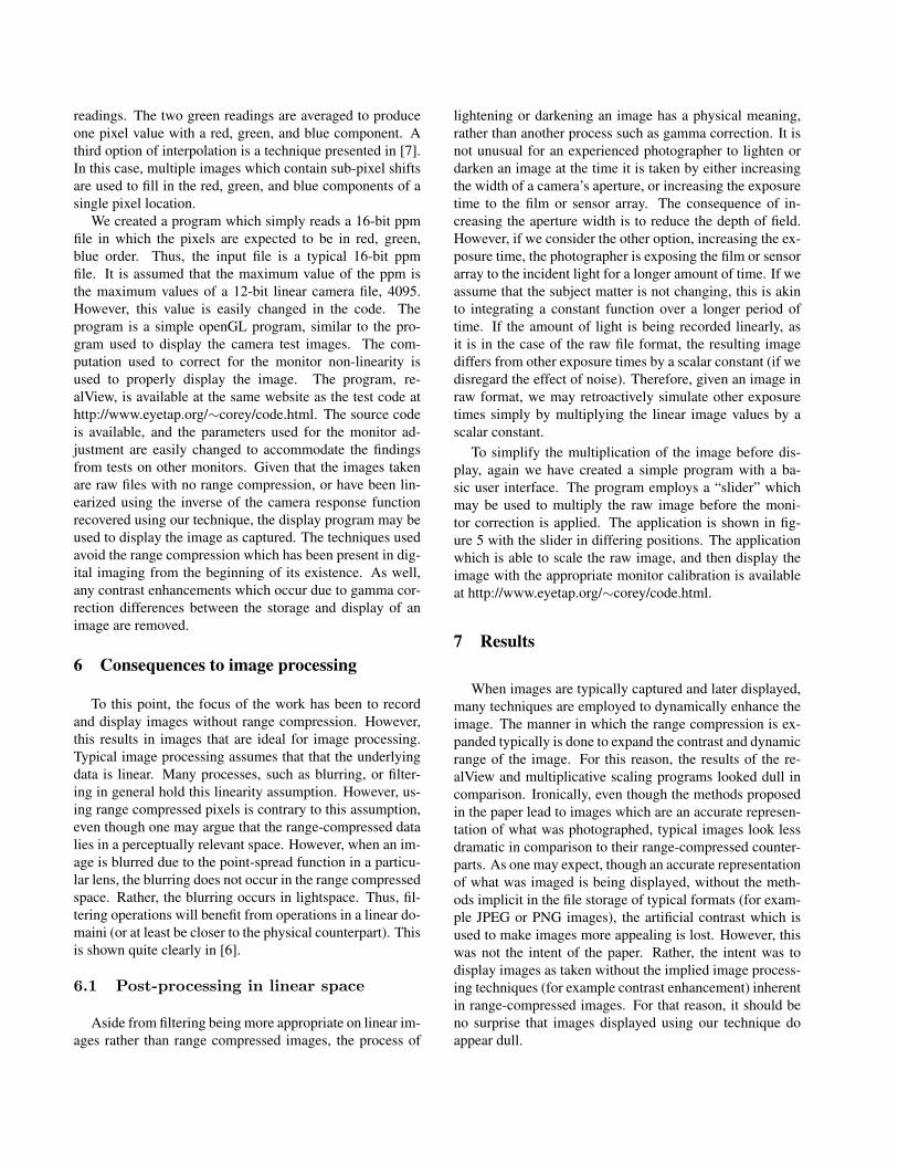
Figure 6. Capturing and displaying imageswithout range compression.

Image Processing, pages 2965–2968, Singapore, Oct. 24-272004.

[11] C. Manders and S. Mann. Determining camera responsefunctions from comparagrams of images with their rawdatafile counterparts. In Proceedings of the IEEE first Inter-national Symposium on Intelligent Multimedia, pages 418–421, Hong Kong, Oct. 20-22 2004.

[12] S. Mann. Comparametric equations with practical applica-tions in quantigraphic image processing. IEEE Trans. ImageProc., 9(8):1389–1406, August 2000. ISSN 1057-7149.

[13] S. Mann. Intelligent Image Processing. John Wiley andSons, November 2 2001. ISBN: 0-471-40637-6.

[14] S. Mann and R. Mann. Quantigraphic imaging: Estimatingthe camera response and exposures from differently exposedimages. CVPR, pages 842–849, December 11-13 2001.

[15] S. Mann and R. W. Picard. Virtual bellows: constructinghigh-quality images from video. In Proceedings of the IEEE

first international conference on image processing, pages363–367, Austin, Texas, Nov. 13-16 1994.

[16] T. Mitsunaga and S. K. Nayar. Radiometric self calibration.Proceedings of IEEE Conference on Computer Vision andPattern Recognition, June 1999.

[17] C. Poynton. A technical introduction to digital video. JohnWiley & Sons, 1996.