Multi-view shape reconstruction

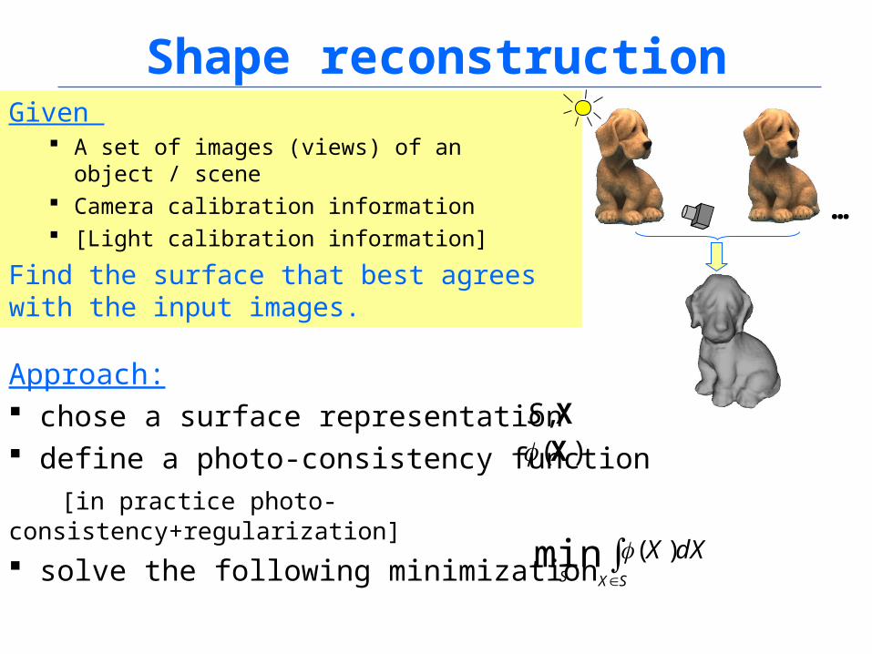
Shape reconstructionGiven A set of images (views) of an object / scene Camera calibration information [Light calibration information]

Find the surface that best agrees with the input images.

…

Approach: chose a surface representation define a photo-consistency function

[in practice photo-consistency+regularization]

solve the following minimization

X,S)(X

SXS

dXX )(min

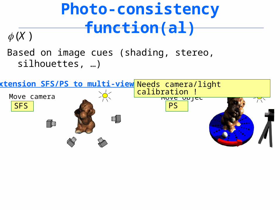
Photo-consistency function(al)

Based on image cues (shading, stereo, silhouettes, …)

)(X

Extension SFS/PS to multi-view:

SFSMove camera Move object

PS

Needs camera/light calibration !

Surface representation

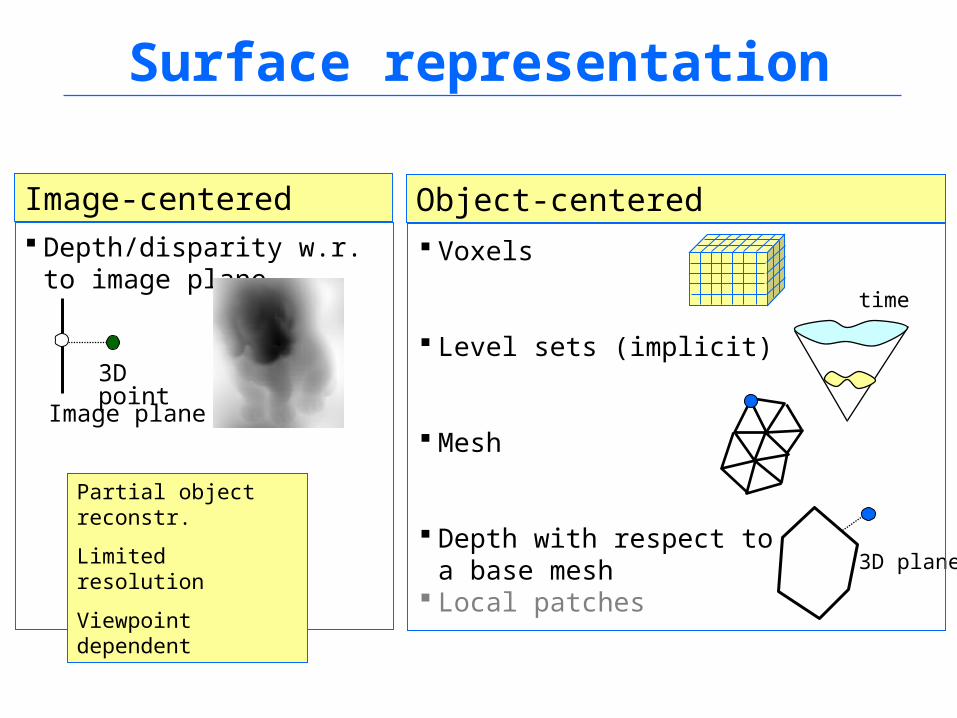
Image-centered Depth/disparity w.r. to image

plane

Image plane

3D point

Voxels

Level sets (implicit)

Mesh

Depth with respect to a base mesh Local patches

3D plane

Object-centered

time

Partial object reconstr.

Limited resolution

Viewpoint dependent

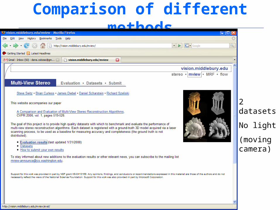
Comparison of different methods

2 datasets

No light

(moving camera)

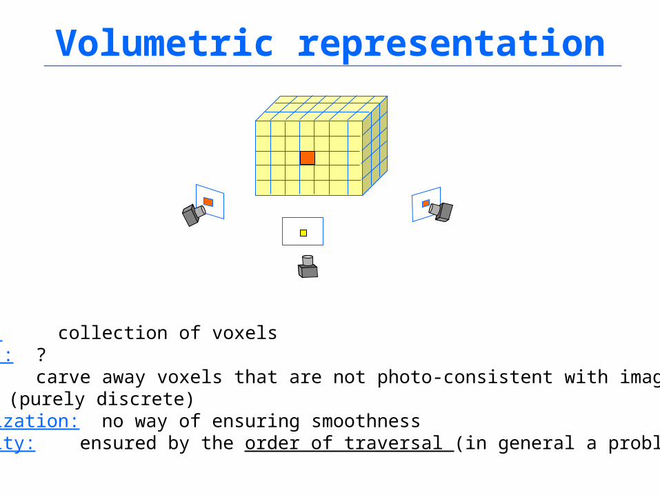
Volumetric representation

Object : collection of voxelsNormals : ?Method: carve away voxels that are not photo-consistent with images

(purely discrete)Regularization: no way of ensuring smoothnessVisibility: ensured by the order of traversal (in general a problem!)

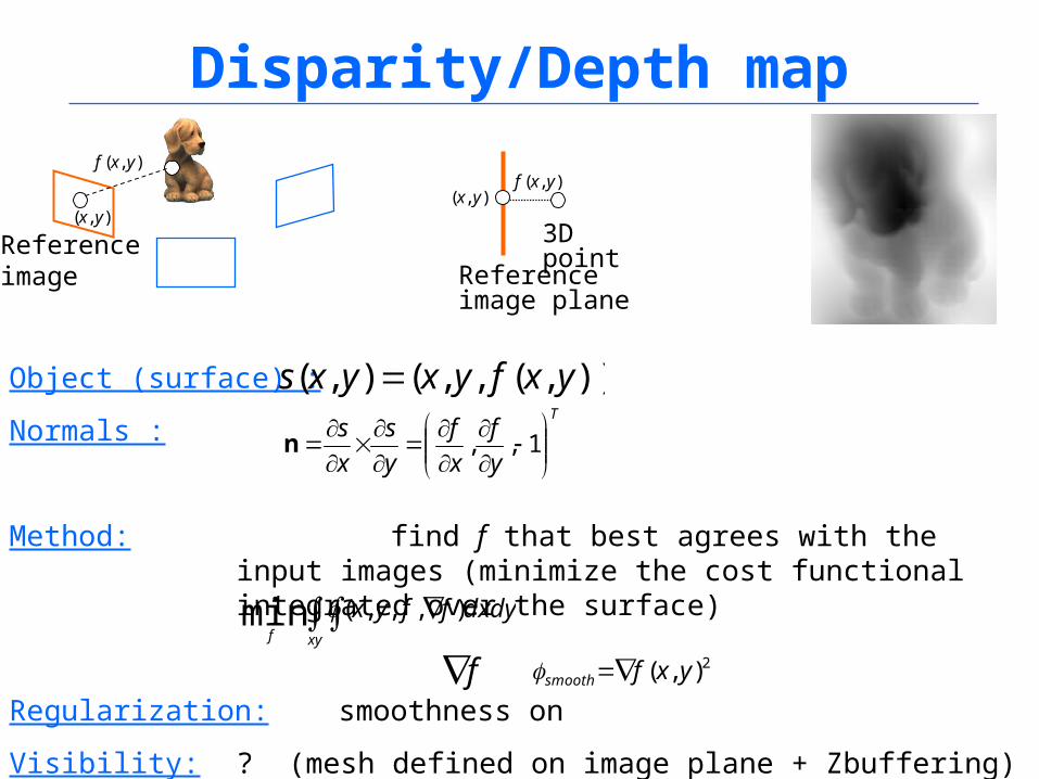
Disparity/Depth map

Reference image plane

3D pointReferenceimage

Object (surface) :

Normals :

Method: find f that best agrees with the input images (minimize the cost functional integrated over the surface)

Regularization: smoothness on

Visibility: ? (mesh defined on image plane + Zbuffering)

)),(,,(),( yxfyxyxs

),( yx

),( yxf

T

y

f

x

f

y

s

x

s

1,,n

xyf

dxdyffyx ),,,(min

),( yx

),( yxf

2),( yxfsmooth f

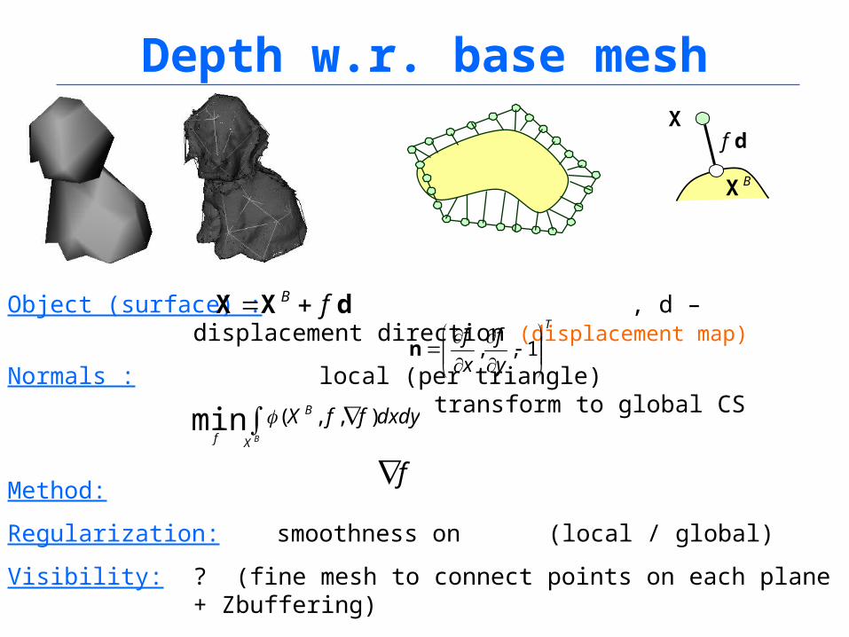
Depth w.r. base mesh

Object (surface) : , d – displacement direction (displacement map)

Normals : local (per triangle) transform to global CS

Method:

Regularization: smoothness on (local / global)

Visibility: ? (fine mesh to connect points on each plane + Zbuffering)

How to deal with boundaries ?

dXX fB

X

BX

df

T

y

f

x

f

1,,n

dxdyffX B

Xf B

),,(min

f

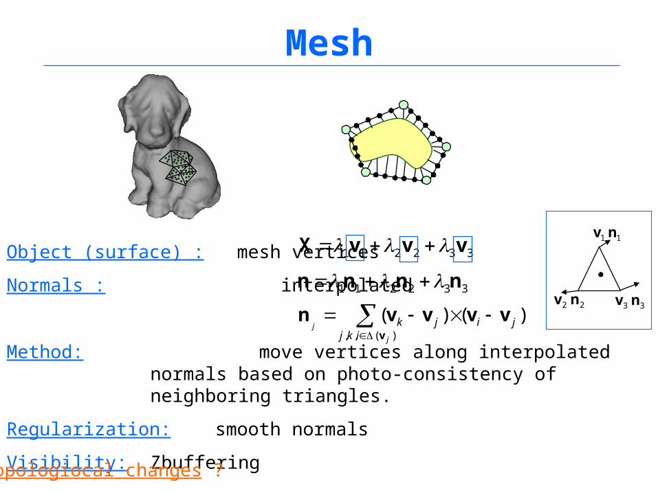
Mesh

Object (surface) : mesh vertices

Normals : interpolated

Method: move vertices along interpolated normals based on photo-consistency of neighboring triangles.

Regularization: smooth normals

Visibility: Zbuffering

332211 nnnn

)()()(,,

jiikj

jk

j

jvvvvn

v

332211 vvvX 11 nv

22 nv 33 nv

Topologiocal changes ?

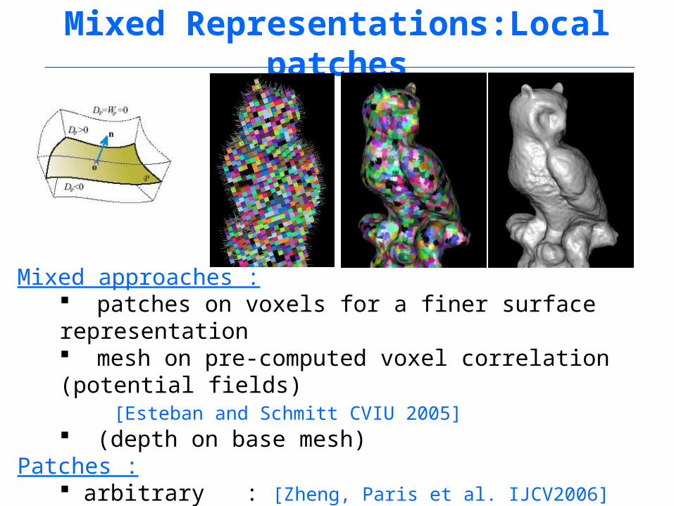
Mixed Representations:Local patches

Mixed approaches : patches on voxels for a finer surface representation mesh on pre-computed voxel correlation (potential fields) [Esteban and Schmitt CVIU 2005] (depth on base mesh)

Patches : arbitrary : [Zheng, Paris et al. IJCV2006] quadratic : surfels [Carceroni and Kutulakos IJCV 2002]

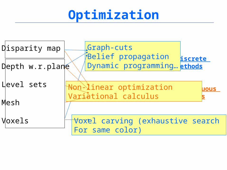
Optimization

Disparity map

Depth w.r.plane

Level sets

Mesh

Voxels

Discrete methods

Graph-cutsBelief propagationDynamic programming…

Voxel carving (exhaustive search For same color)

Continuous methods

Non-linear optimizationVariational calculus

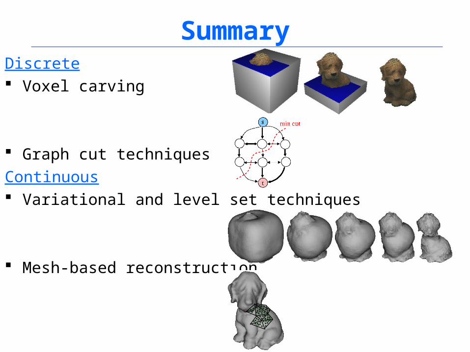
Discrete Voxel carving

Graph cut techniques

Continuous Variational and level set techniques

Mesh-based reconstruction

Summary

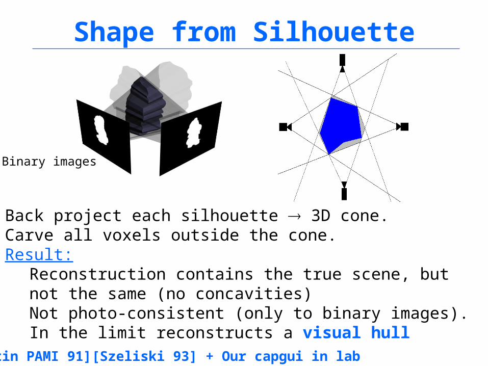
Shape from Silhouette

Binary images

Back project each silhouette 3D cone.Carve all voxels outside the cone. Result:

Reconstruction contains the true scene, but not the same (no concavities) Not photo-consistent (only to binary images).In the limit reconstructs a visual hull

[Martin PAMI 91][Szeliski 93] + Our capgui in lab

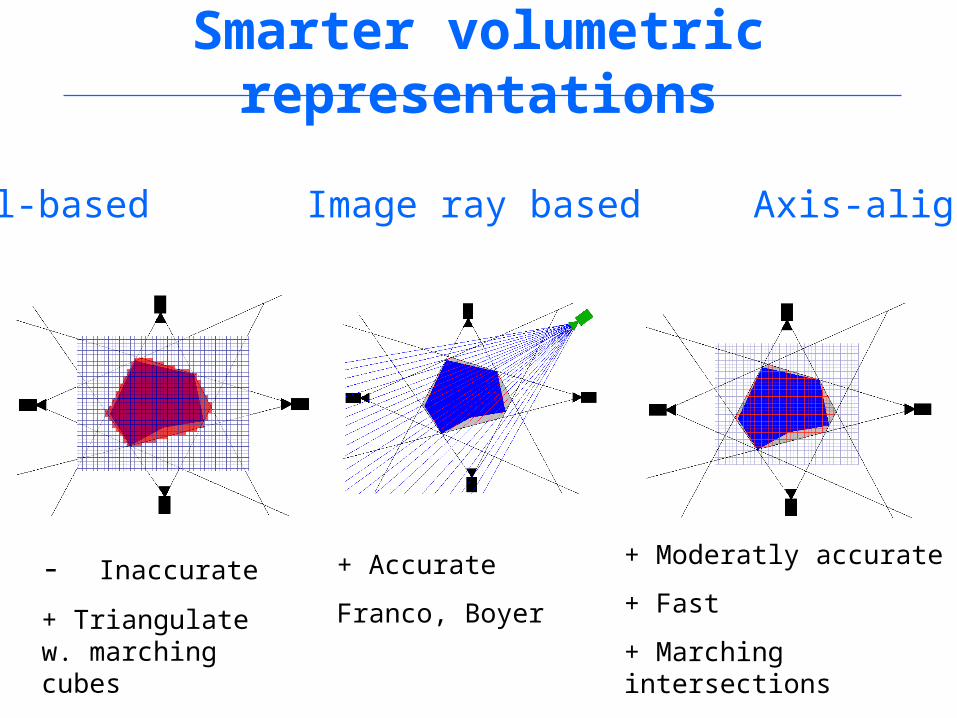
Smarter volumetric representations

- Inaccurate

+ Triangulate w. marching cubes

+ Accurate

Franco, Boyer

+ Moderatly accurate

+ Fast

+ Marching intersections

Tarini’01 + our Capgui

Voxel-based Image ray based Axis-aligned

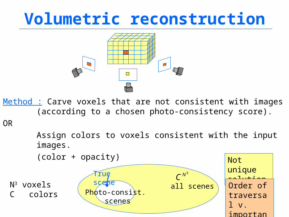
Volumetric reconstruction

Method : Carve voxels that are not consistent with images (according to a chosen photo-consistency score).

OR

Assign colors to voxels consistent with the input images.

(color + opacity)

N3 voxelsC colors

3NCall scenes

Photo-consist. scenes

True scene

Not unique solution

Order of traversal v. important

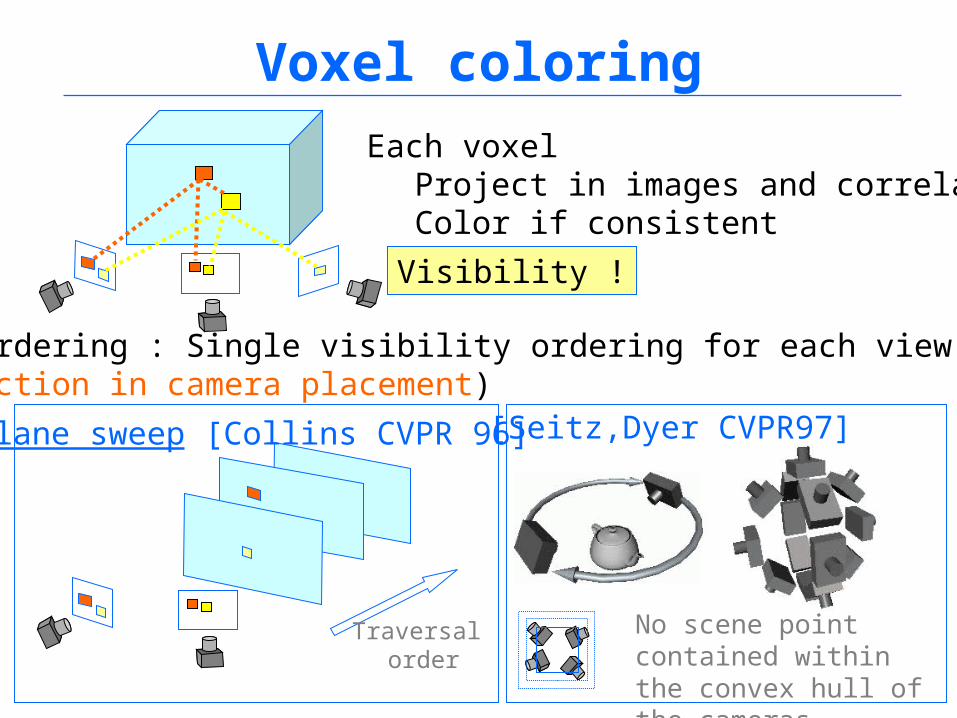
Voxel coloring

Each voxelProject in images and correlateColor if consistent

Visibility !

Depth ordering : Single visibility ordering for each view(Restriction in camera placement)

Traversal order

[Seitz,Dyer CVPR97]Plane sweep [Collins CVPR 96]

No scene point contained within the convex hull of the cameras

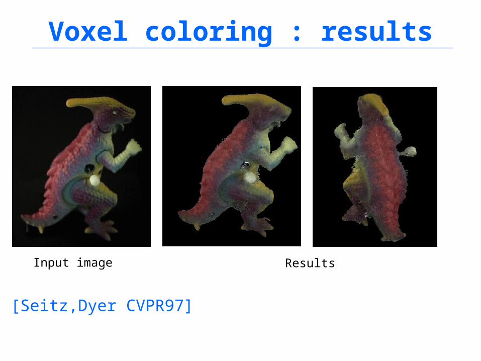
Voxel coloring : results

Input image Results

[Seitz,Dyer CVPR97]

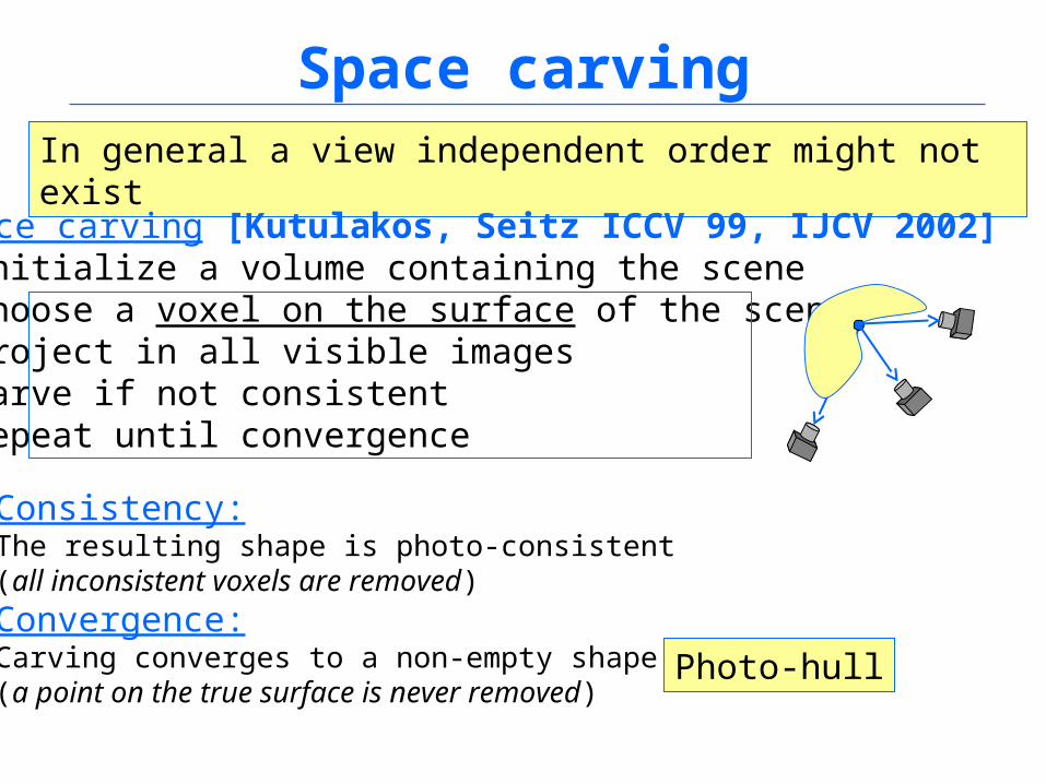
Space carvingIn general a view independent order might not exist

Space carving [Kutulakos, Seitz ICCV 99, IJCV 2002] initialize a volume containing the scene Choose a voxel on the surface of the scene Project in all visible images Carve if not consistent Repeat until convergence

Consistency:The resulting shape is photo-consistent(all inconsistent voxels are removed)

Convergence:Carving converges to a non-empty shape(a point on the true surface is never removed)

Photo-hull

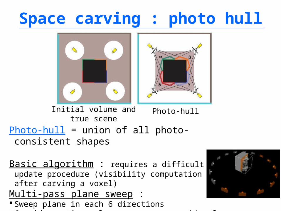
Space carving : photo hull

Initial volume andtrue scene

Photo-hull

Photo-hull = union of all photo-consistent shapes

Basic algorithm : requires a difficult update procedure (visibility computation after carving a voxel)

Multi-pass plane sweep : Sweep plane in each 6 directionsConsider active only cameras on one side of the plane

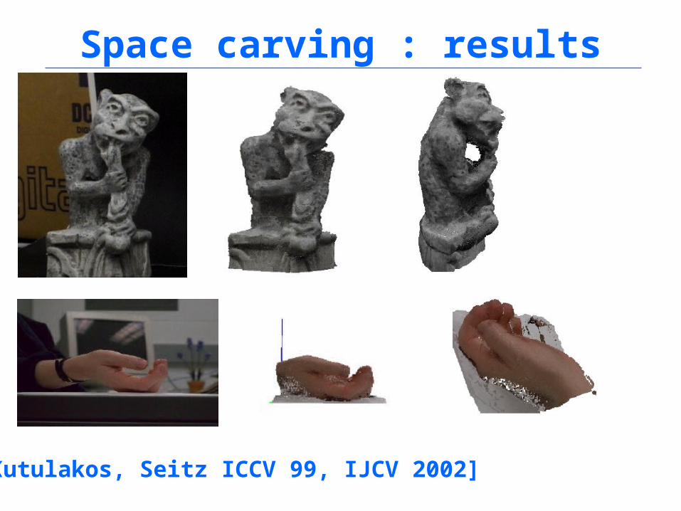
Space carving : results

[Kutulakos, Seitz ICCV 99, IJCV 2002]

Graph cuts for multi-view reconstruction Discrete surface reconstruction Graph cut Graph cuts as hypersurfaces Example: [Paris, Sillion, Quan IJCV 05]

Types of energies minimized with graph cut

[Kolmogorov Zabih ECCV 2002]

Graph cuts for multi-labeling

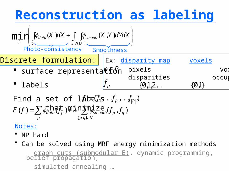
Reconstruction as labeling

S XN

smooth

S

dataS

dYdXYXdXX)(

),()(min

Discrete formulation: surface representation

labels

Find a set of labels that minimize

Pp

),...,,...,( 1 Pp ffff

p Nqp

qpsmoothpdata ffffE},{

),()()(

pf

Ex: disparity map voxels pixels voxels disparities occupancy

...}2,1,0{ }1,0{

Notes: NP hard Can be solved using MRF energy minimization methods

graph cuts (submodular E), dynamic programming, belief propagation,

simulated annealing …

Photo-consistency Smoothness

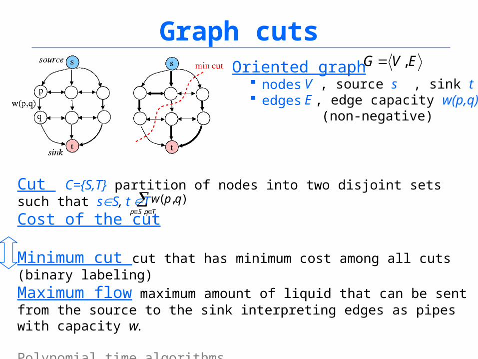
Graph cutsOriented graph nodes edges

EVG ,

V , source s , sink t E , edge capacity w(p,q) (non-negative)

Cut C={S,T} partition of nodes into two disjoint sets such that sS, t T

Cost of the cut

Minimum cut cut that has minimum cost among all cuts (binary labeling)

Maximum flow maximum amount of liquid that can be sent from the source to the sink interpreting edges as pipes with capacity w.

Polynomial time algorithmsAugmenting paths [Ford & Fulkerson, 1962]Push-relabel [Goldberg-Tarjan, 1986]

TqSp

qpw,

),(

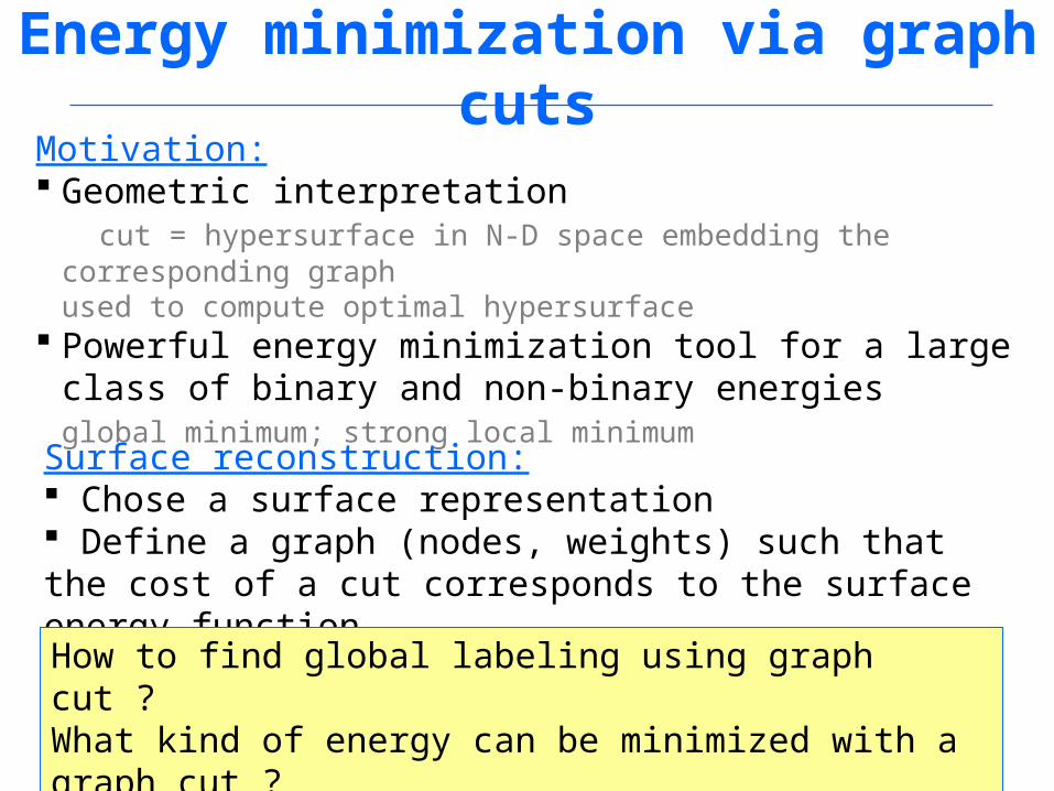
Energy minimization via graph cutsMotivation: Geometric interpretation cut = hypersurface in N-D space embedding the corresponding graph

used to compute optimal hypersurface Powerful energy minimization tool for a large class of binary

and non-binary energiesglobal minimum; strong local minimum

Surface reconstruction: Chose a surface representation Define a graph (nodes, weights) such that the cost of a cut corresponds to the surface energy function.

How to find global labeling using graph cut ? What kind of energy can be minimized with a graph cut ?

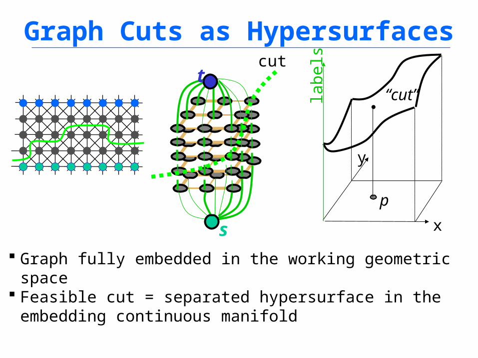
Graph Cuts as Hypersurfaces

s

tcut

p

“cut”

x

y

lab

els

Graph fully embedded in the working geometric space Feasible cut = separated hypersurface in the embedding

continuous manifold

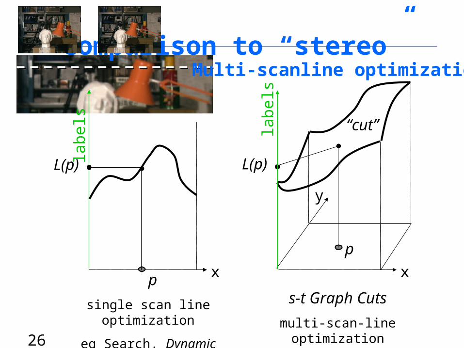
Comparison to “stereo”

26

Multi-scanline optimization

L(p)

p

“cut”

x

y

lab

els

labels

x

L(p)

p

single scan line optimization

eg Search, Dynamic Programming

s-t Graph Cuts

multi-scan-line optimization

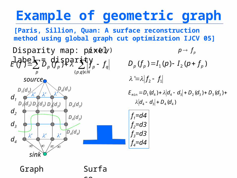
Example of geometric graph

p Nqp

qppp fffDfE},{

)()(

Disparity map: pixel label = disparity),( yxp

[Paris, Sillion, Quan: A surface reconstruction method using global graph cut optimization IJCV 05]

source

sink

d1

d3

D1(d1)

d2

d4

D4(d1)

)()()( 21 ppp fpIpIfD

D3(d2) D4(d2)

D4(d3)

D4(d4)

D2(d2)D1(d2)

’ ’’

’’ ’

Graph Surface

12' ff

)(

)()()(

4434

33323441min

dDdd

dDdDdddDE

pfp

f1=d4f2=d3f3=d3f4=d4

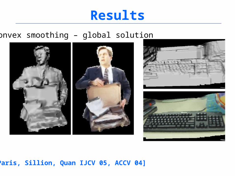
ResultsConvex smoothing – global solution

[Paris, Sillion, Quan IJCV 05, ACCV 04]

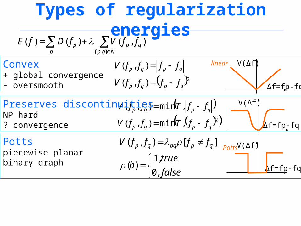
Types of regularization energies

p Nqp

qpp ffVfDfE},{

),()()(

Convex+ global convergence- oversmooth

false

trueb

ffffV qppqqp

,0

,1)(

][),(

2),(

),(

qpqp

qpqp

ffffV

ffffV

2,min),(

,min),(

qpqp

qpqp

ffTffV

ffTffV

V(Δf)

Δf=fp-fq

Pottspiecewise planarbinary graph

Preserves discontinuitiesNP hard? convergence

V(Δf)

Δf=fp-fq

V(Δf)

Δf=fp-fq

linear

Potts

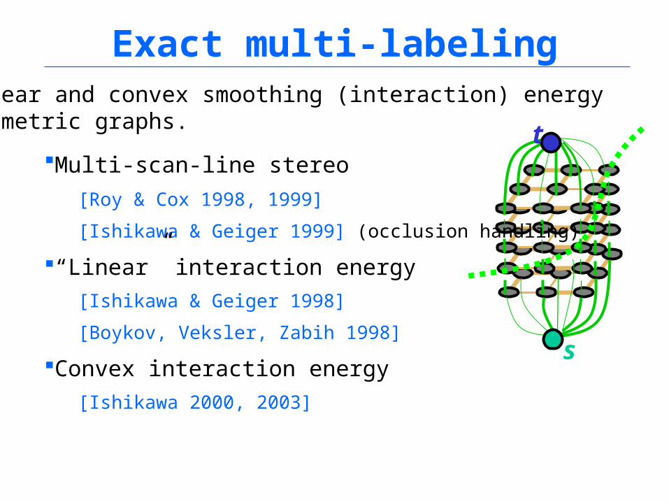
Exact multi-labelingLinear and convex smoothing (interaction) energy Geometric graphs.

s

tMulti-scan-line stereo

[Roy & Cox 1998, 1999]

[Ishikawa & Geiger 1999] (occlusion handling)

“Linear” interaction energy

[Ishikawa & Geiger 1998]

[Boykov, Veksler, Zabih 1998]

Convex interaction energy

[Ishikawa 2000, 2003]

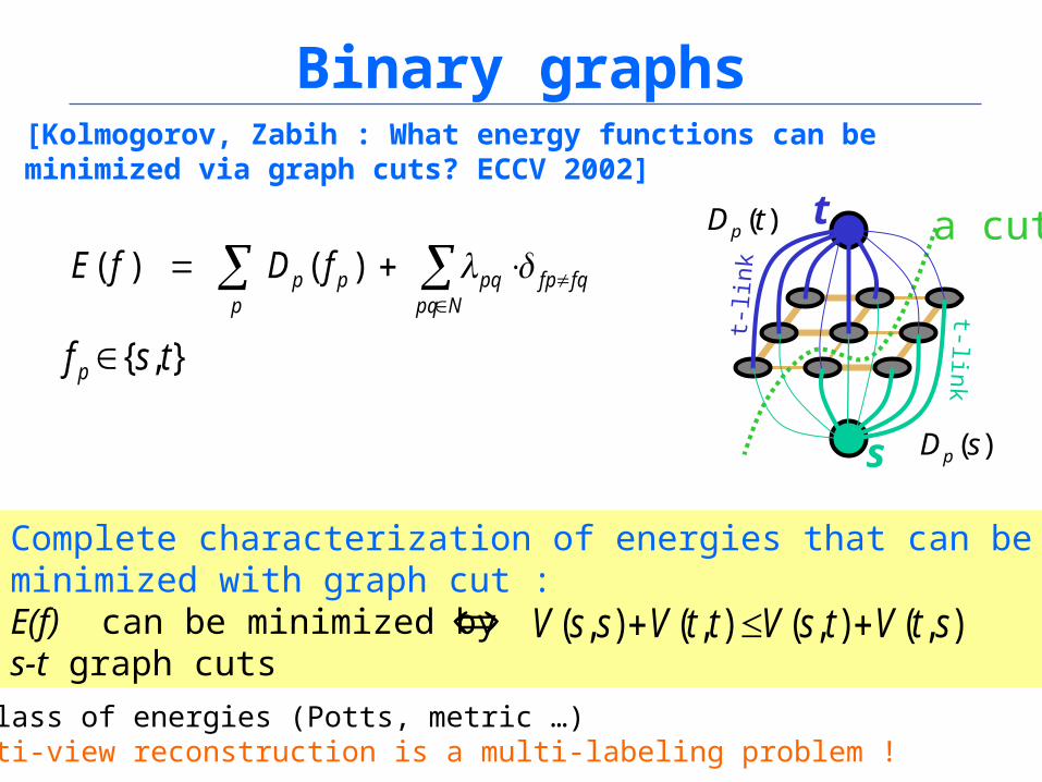
Binary graphs[Kolmogorov, Zabih : What energy functions can be minimized via graph cuts? ECCV 2002]

Npq

fqfppqp

pp fDfE )()(

},{ tsf p

Complete characterization of energies that can be minimized with graph cut : E(f) can be minimized by s-t graph cuts

pqw

n-links

s

t a cut)(tDp

t-lin

k

t-link

)(sDp

),(),(),(),( stVtsVttVssV

Large class of energies (Potts, metric …)BUT multi-view reconstruction is a multi-labeling problem !

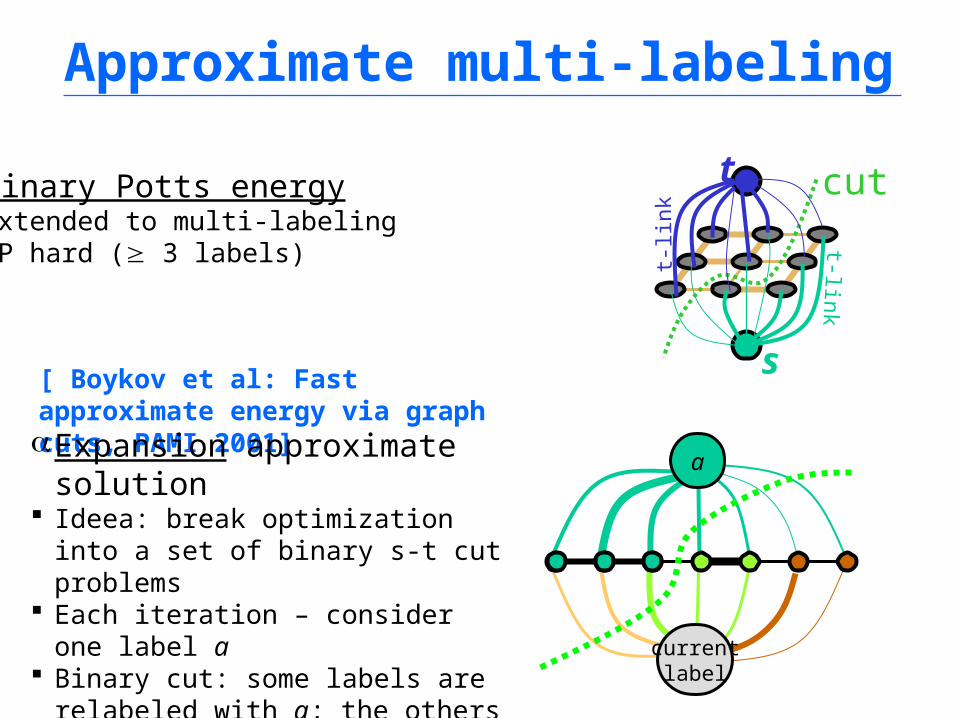
Approximate multi-labeling

Binary Potts energyExtended to multi-labelingNP hard ( 3 labels)

pqw

n-links

s

t cut

t-lin

k

t-link

currentlabel

a

[ Boykov et al: Fast approximate energy via graph cuts, PAMI 2001]Expansion approximate

solution Ideea: break optimization into a

set of binary s-t cut problems Each iteration – consider one

label a Binary cut: some labels are

relabeled with a; the others remain unchanged

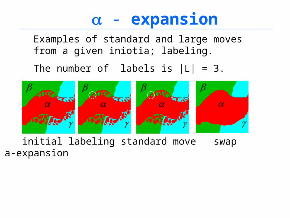
- expansion

initial labeling standard move swap a-expansion

Examples of standard and large moves from a given iniotia; labeling.

The number of labels is |L| = 3.

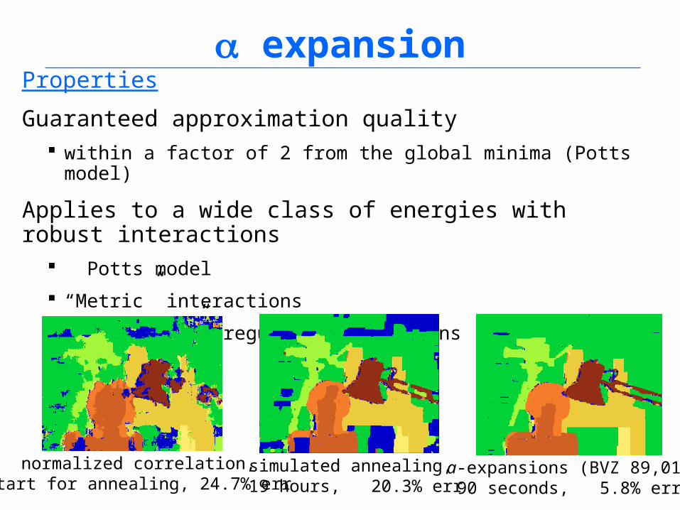
expansionProperties

Guaranteed approximation quality within a factor of 2 from the global minima (Potts model)

Applies to a wide class of energies with robust interactions Potts model

“Metric” interactions

“Submodular” (regular) interactions

simulated annealing, 19 hours, 20.3% err

a-expansions (BVZ 89,01)90 seconds, 5.8% err

normalized correlation,start for annealing, 24.7% err

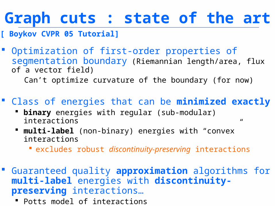
Graph cuts : state of the art

Optimization of first-order properties of segmentation boundary (Riemannian length/area, flux of a vector field)

Can’t optimize curvature of the boundary (for now)

Class of energies that can be minimized exactly binary energies with regular (sub-modular) interactions multi-label (non-binary) energies with “convex” interactions excludes robust discontinuity-preserving interactions

Guaranteed quality approximation algorithms for multi-label energies with discontinuity-preserving interactions… Potts model of interactions Metric interactions Regular (sub-modular) interactions

[ Boykov CVPR 05 Tutorial]

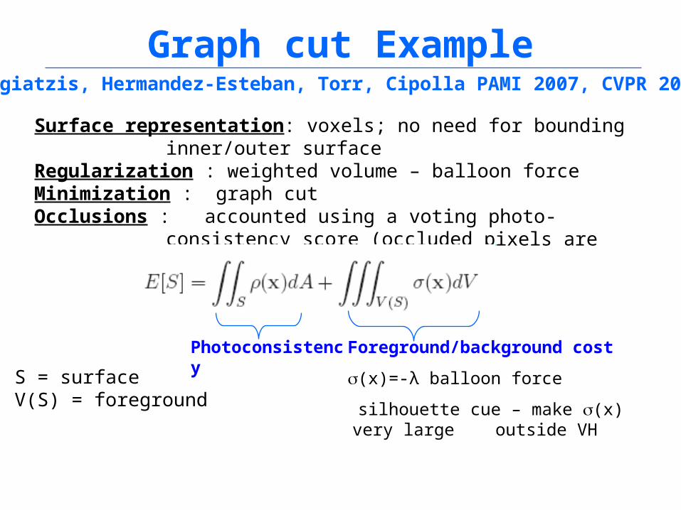
Graph cut Example[ Vogiatzis, Hermandez-Esteban, Torr, Cipolla PAMI 2007, CVPR 2005 ]

Surface representation: voxels; no need for bounding inner/outer surfaceRegularization : weighted volume – balloon force Minimization : graph cutOcclusions : accounted using a voting photo-consistency score

(occluded pixels are treated as outliers)

S = surfaceV(S) = foreground

Photoconsistency Foreground/background cost

(x)=-λ balloon force

silhouette cue – make (x) very large outside VH

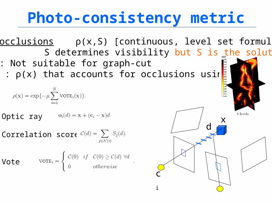
Photo-consistency metric

Account occlusions ρ(x,S) [continuous, level set formulations]S determines visibility but S is the solution!

Problem : Not suitable for graph-cutSolution : ρ(x) that accounts for occlusions using NCC

xOptic ray

Correlation scores

Vote

ci

d

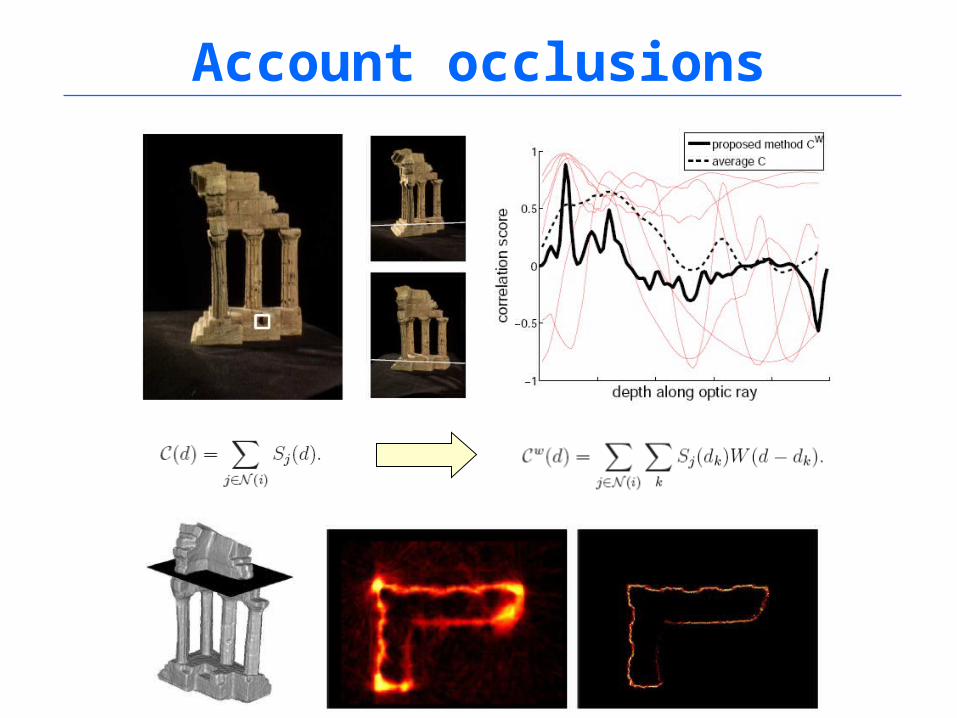
Account occlusions

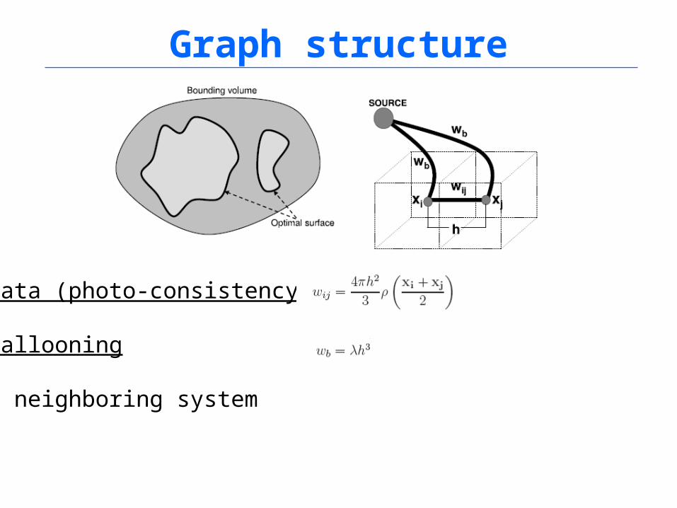
Graph structure

Data (photo-consistency)

Ballooning

6 neighboring system

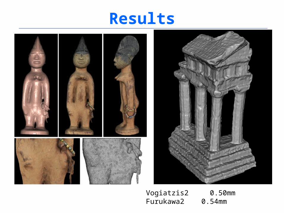
Results

Vogiatzis2 0.50mmFurukawa2 0.54mm

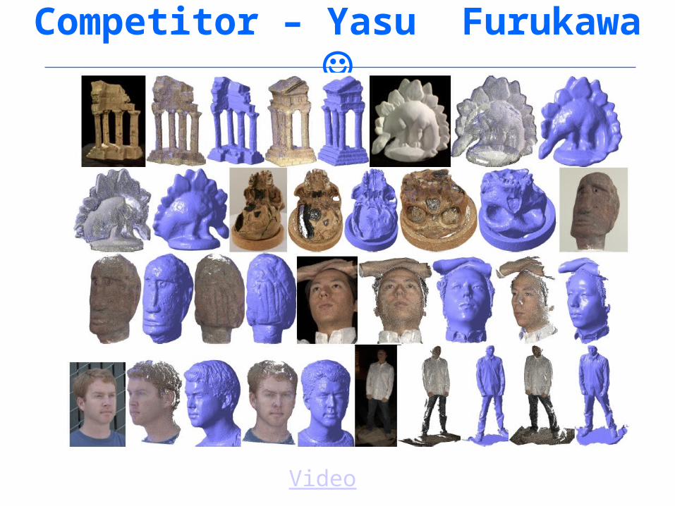
Competitor – Yasu Furukawa

Video

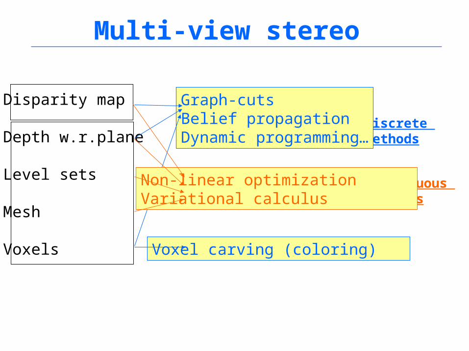
Multi-view stereo

Disparity map

Depth w.r.plane

Level sets

Mesh

Voxels

Discrete methods

Graph-cutsBelief propagationDynamic programming…

Voxel carving (coloring)

Continuous methods

Non-linear optimizationVariational calculus

Continuous multi-view methods Regular surface and surface evolution Level set methods Example of mesh-based reconstruction

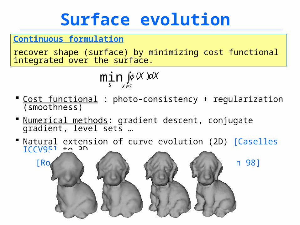
Surface evolution

SXS

dXX )(min

Continuous formulation

recover shape (surface) by minimizing cost functional integrated over the surface.

Cost functional : photo-consistency + regularization (smoothness)

Numerical methods: gradient descent, conjugate gradient, level sets …

Natural extension of curve evolution (2D) [Caselles ICCV95] to 3D

[Robert,Deriche ECCV 96][Faugeras Kerivan 98]

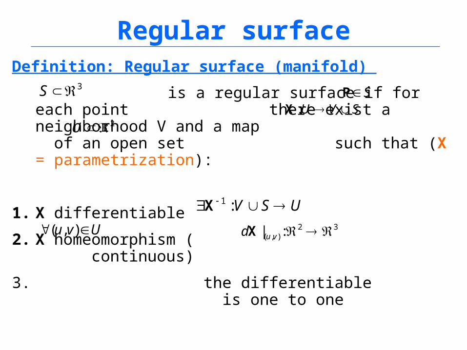
Regular surfaceDefinition: Regular surface (manifold)

is a regular surface if for each point there exist a neighborhood V and a map of an open set such that (X = parametrization):

1. X differentiable

2. X homeomorphism ( continuous)

3. the differentiable is one to one

3S SPSVU :X

2U

USV :1X

Uvu ),( 32),( :| vudX

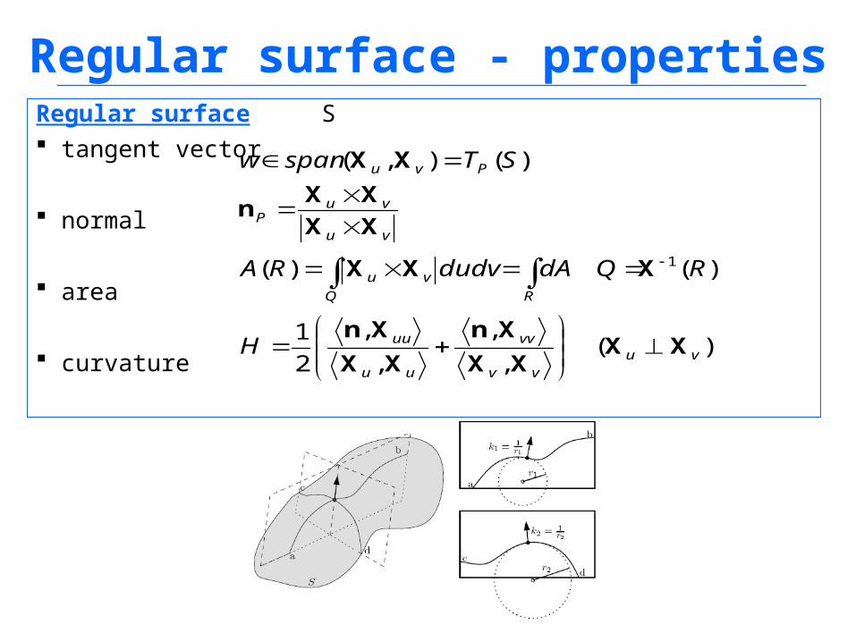
Regular surface - propertiesRegular surface S tangent vector

normal

area

curvature )(

,

,

,

,

2

1

)()(

)(),(

1

vuvv

vv

uu

uu

Q R

vu

vu

vuP

Pvu

H

RQdAdudvRA

STspanw

XXXX

Xn

XX

Xn

XXX

XX

XXn

XX

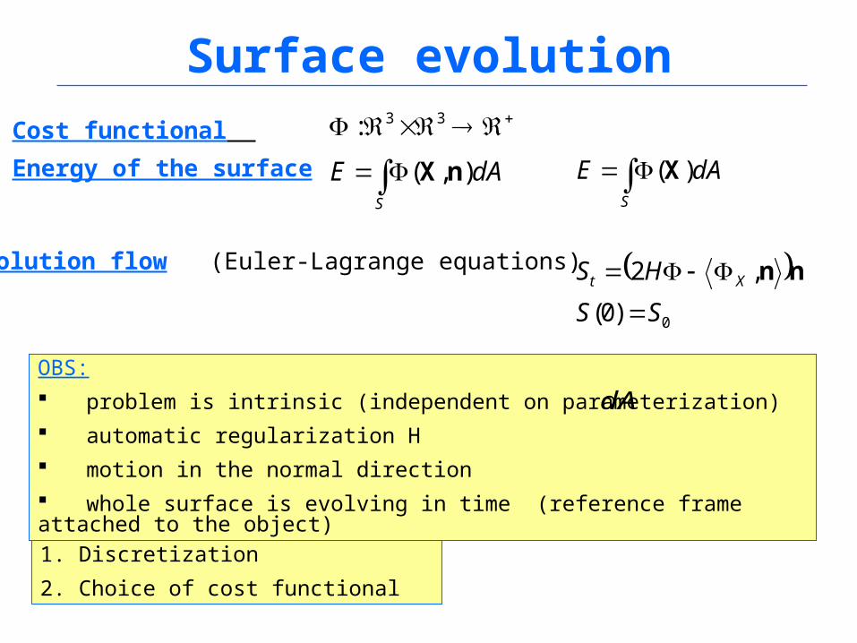
Surface evolutionCost functional

Energy of the surface

S

dAE ),(

: 33

nX

Evolution flow (Euler-Lagrange equations) 0)0(

,2

)(

SS

HS

dAE

Xt

S

nn

X

OBS:

problem is intrinsic (independent on parameterization)

automatic regularization H

motion in the normal direction

whole surface is evolving in time (reference frame attached to the object)

dA

1. Discretization

2. Choice of cost functional

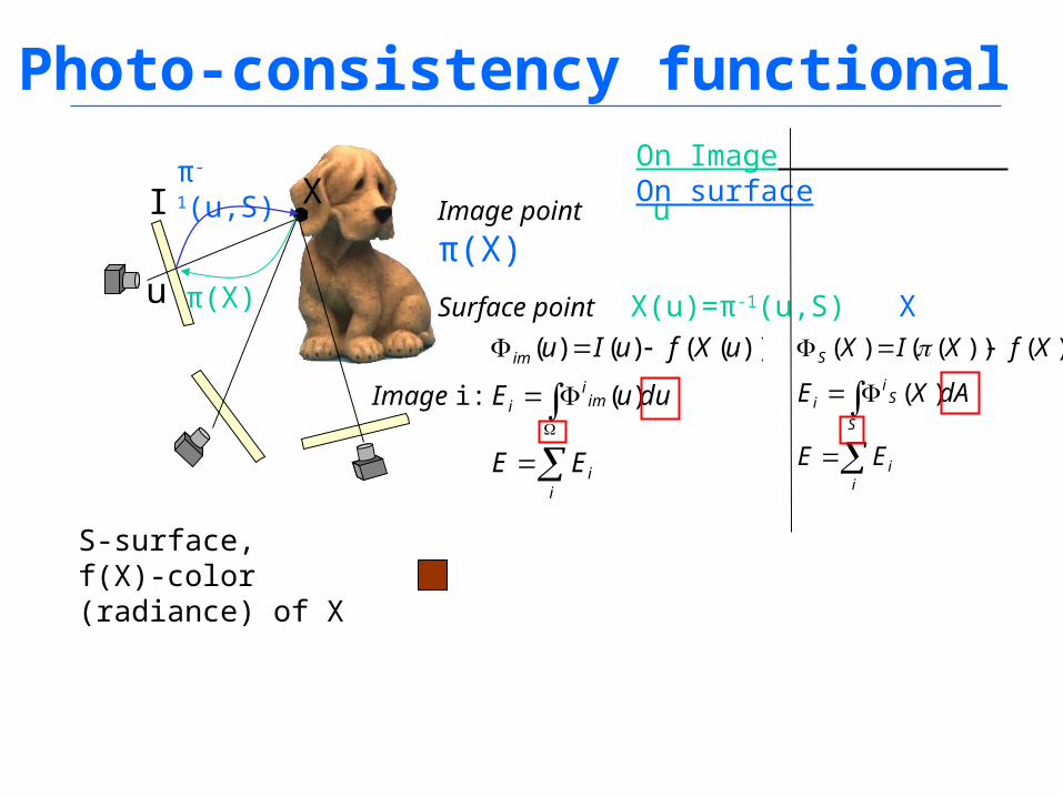
Photo-consistency functional

ii

imi

i

im

EE

duuE

uXfuIu

)(

))(()()(

X

u

I Image point u π(X)

Surface point X(u)=π-1(u,S) X

On Image On surfaceπ-1(u,S)

S-surface, f(X)-color (radiance) of X

π(X)

ii

S

Si

i

S

EE

dAXE

XfXIX

)(

)())(()(

Image i:

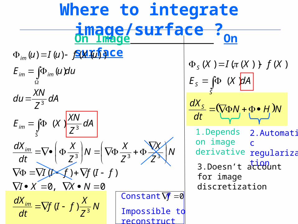
Where to integrate image/surface ?On Image On surface

NZ

XfIf

dt

dX

NXXI

fIffII

NZ

X

Z

XN

Z

X

dt

dX

dAZ

XNXE

dAZ

XNdu

duuE

uXfuIu

im

im

S

im

imim

im

3

333

3

3

)(

0,0

)()(

)(

)(

))(()()(

NHNdt

dX

dAXE

XfXIX

S

S

S

S

)(

)())(()(

0fConstant f

Impossible to reconstruct

2.Automatic regularization

1.Depends on image derivative

3.Doesn’t account for image discretization

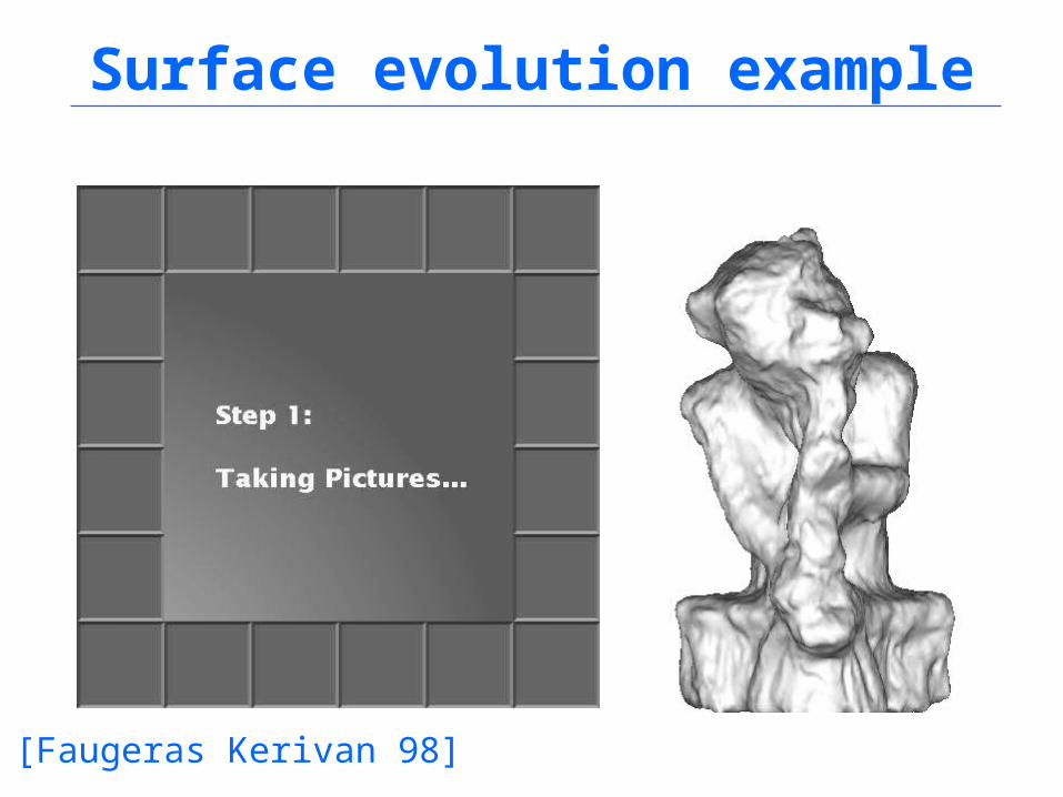
Surface evolution example

[Faugeras Kerivan 98]

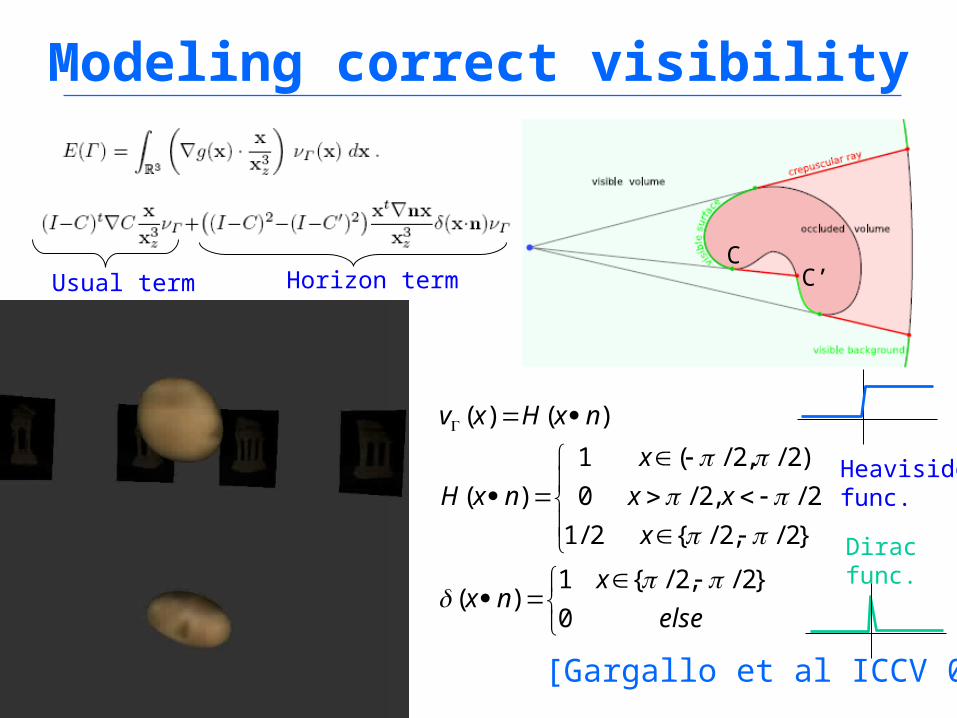
Modeling correct visibility

CC’

[Gargallo et al ICCV 07]

Horizon termUsual term

else

xnx

x

xx

x

nxH

nxHxv

0

}2/,2/{1)(

}2/,2/{2/1

2/,2/0

)2/,2/(1

)(

)()(

Heaviside

func.

Dirac func.

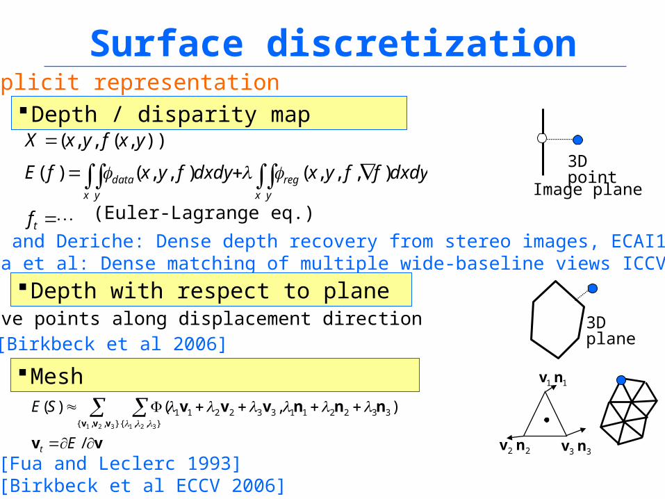
Surface discretization

Depth / disparity map

Image plane

3D point

Explicit representation

t

x y

reg

x y

data

f

dxdyffyxdxdyfyxfE

yxfyxX

),,,(),,()(

)),(,,(

[Robert and Deriche: Dense depth recovery from stereo images, ECAI1992][Strecha et al: Dense matching of multiple wide-baseline views ICCV 2003]Depth with respect to plane

3D plane[Birkbeck et al 2006]

(Euler-Lagrange eq.)

Mesh

Move points along displacement direction

vv

nnnvvvvvv

/

),()( 332211332211},,{ },,{321 321

E

SE

t

11 nv

22 nv 33 nv[Fua and Leclerc 1993][Birkbeck et al ECCV 2006]

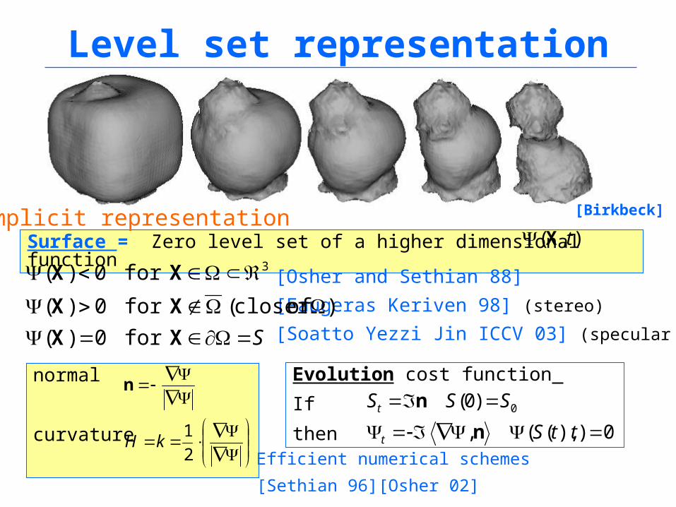
Level set representation

Surface = Zero level set of a higher dimensional function

[Osher and Sethian 88]

[Faugeras Keriven 98] (stereo)

[Soatto Yezzi Jin ICCV 03] (specular refl.)S

XX

XX

XX

for0)(

)ofcloser(for0)(

for0)( 3

normal

curvature

),( tX

2

1kH

nEvolution cost function

If

then 0)),((,

)0( 0

ttS

SSS

t

t

n

n

Efficient numerical schemes

[Sethian 96][Osher 02]

[Birkbeck]Implicit representation

Cost functional

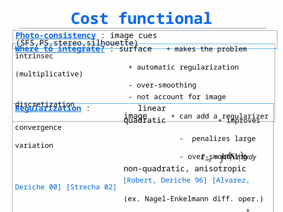
Regularization : linear

quadratic + improves convergence

- penalizes large variation

- over-smoothing

non-quadratic, anisotropic

[Robert, Deriche 96] [Alvarez, Deriche 00] [Strecha 02]

(ex. Nagel-Enkelmann diff. oper.)

+ preserves discontinuities

Photo-consistency : image cues (SFS,PS,stereo,silhouette)

dxdyzEreg

Where to integrate? : surface + makes the problem intrinsec

+ automatic regularization (multiplicative)

- over-smoothing

- not account for image discretization

image + can add a regularizer

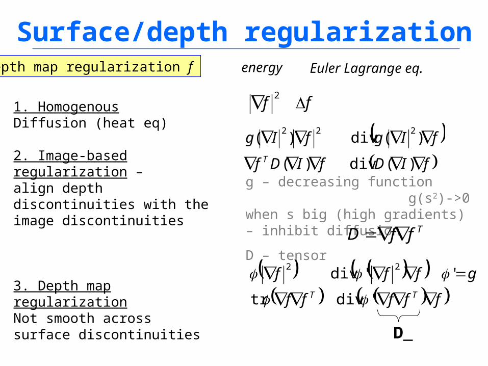
Surface/depth regularization

ff 2

fIDfIDf

fIgfIgT

)(div)(

)(div)(222

fffff

gfffTT

'divtr

''div22

Depth map regularization f

1. HomogenousDiffusion (heat eq)

2. Image-based regularization – align depth discontinuities with the image discontinuities

3. Depth map regularization Not smooth across surface discontinuities

energy Euler Lagrange eq.

g – decreasing function g(s2)->0 when s big (high gradients) – inhibit diffusion

D – tensor

D

TffD

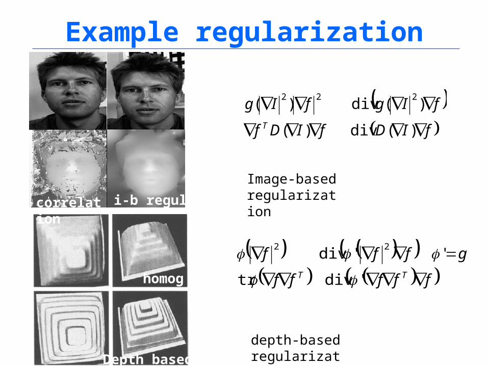
Example regularization

fIDfIDf

fIgfIgT

)(div)(

)(div)(222

Image-based regularizationcorrelation i-b regul.

homog

Depth based

depth-based regularization

fffff

gfffTT

'divtr

''div22

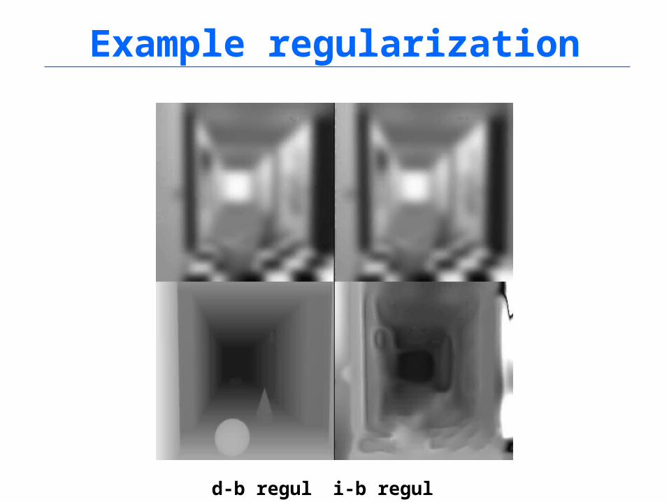
Example regularization

i-b regul.d-b regul

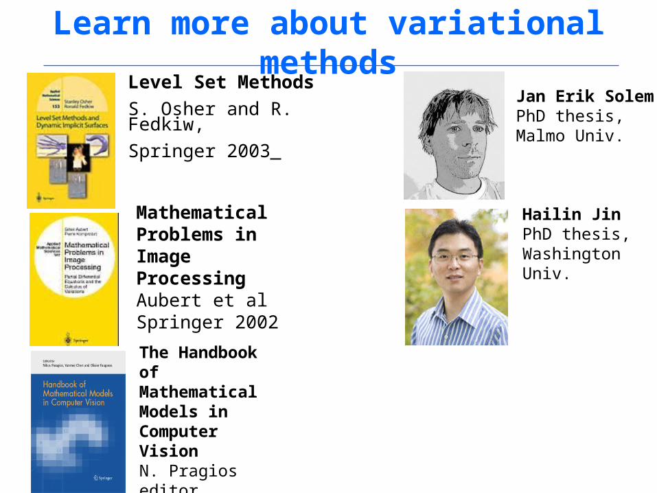
Learn more about variational methods

Jan Erik Solem PhD thesis, Malmo Univ.

Level Set Methods

S. Osher and R. Fedkiw,

Springer 2003

Mathematical Problems in Image Processing Aubert et alSpringer 2002

Hailin Jin PhD thesis, Washington Univ.

The Handbook of Mathematical Models in Computer Vision N. Pragios editorSpringer 2005

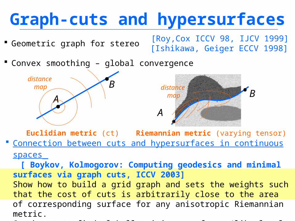
Graph-cuts and hypersurfaces Geometric graph for stereo

Convex smoothing – global convergence

[Ishikawa, Geiger ECCV 1998][Roy,Cox ICCV 98, IJCV 1999]

Connection between cuts and hypersurfaces in continuous spaces [ Boykov, Kolmogorov: Computing geodesics and minimal surfaces via

graph cuts, ICCV 2003]Show how to build a grid graph and sets the weights such that the cost of cuts is arbitrarily close to the area of corresponding surface for any anisotropic Riemannian metric. Graph cut to find globally minimum surfaces (like level sets) under arbitrary Riemannian metric.

Riemannian metric (varying tensor)Euclidian metric (ct)

A

Bdistance

map

A

Bdistance

map

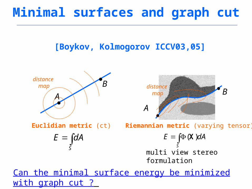
Minimal surfaces and graph cut

S

dAE

Riemannian metric (varying tensor)Euclidian metric (ct)

A

Bdistance

map

A

Bdistance

map

S

dAE )(X

Can the minimal surface energy be minimized with graph cut ?

[Boykov, Kolmogorov ICCV03,05]

multi view stereo formulation

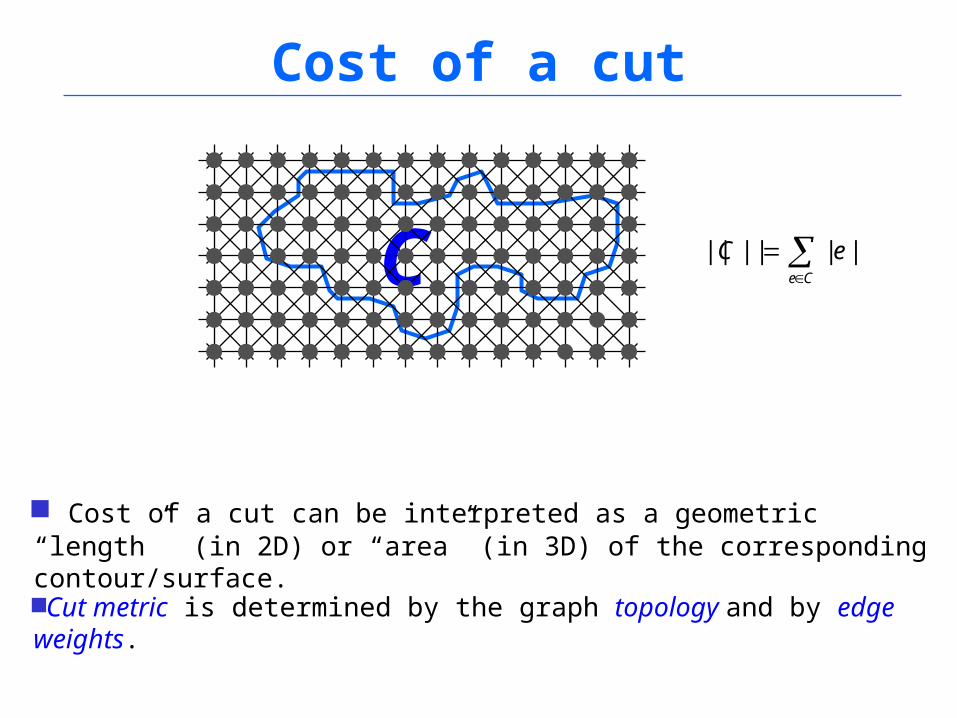
Cost of a cut

C

Cut metric is determined by the graph topology and by edge weights.

Ce

eC ||||||

Cost of a cut can be interpreted as a geometric “length” (in 2D) or “area” (in 3D) of the corresponding contour/surface.

Riemanian metric

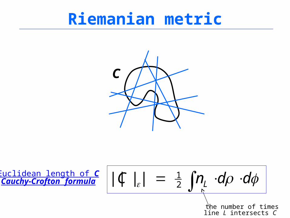
ddnC L21||||Euclidean length of C

Cauchy-Crofton formula

the number of times line L intersects C

C

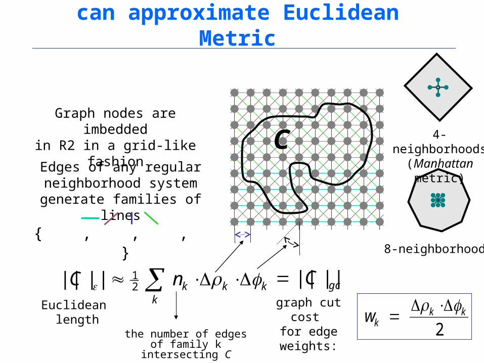
Cut Metric on gridscan approximate Euclidean Metric

C

k

kkknC 21||||

Euclidean length

2kk

kw

gcC ||||graph cut cost

for edge weights:the number of edges of family k intersecting C

Edges of any regular neighborhood system

generate families of lines

{ , , , }

Graph nodes are imbeddedin R2 in a grid-like fashion

8-neighborhoods

4-neighborhoods(Manhattan metric)

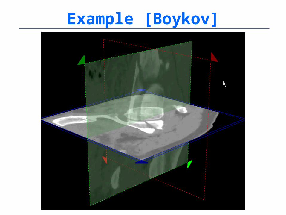
Example [Boykov]

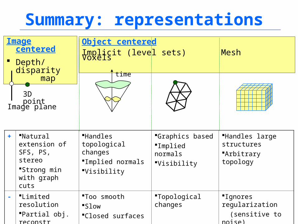
Summary: representations Image centered

Depth/disparity map

Object centeredImplicit (level sets) Mesh Voxels

Image plane

3D point

+ Natural extension of SFS, PS, stereoStrong min with graph cuts

Handles topological changesImplied normalsVisibility

Graphics basedImplied normalsVisibility

Handles large structuresArbitrary topology

- Limited resolution Partial obj. reconstrViewpoint dependent

Too smoothSlowClosed surfaces

Topological changes

Ignores regularization

(sensitive to noise)Limited resolutionOcclusion handling

time

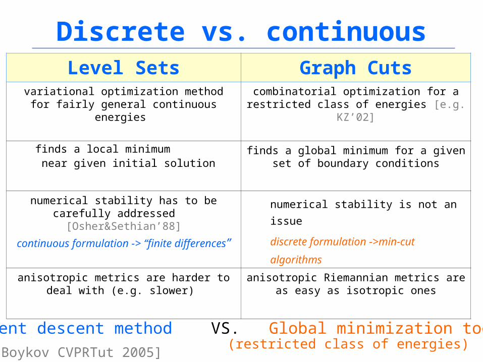
Discrete vs. continuousLevel Sets Graph Cuts

variational optimization method for fairly general continuous energies

combinatorial optimization for a restricted class of energies [e.g. KZ’02]

finds a local minimum near given initial solution

finds a global minimum for a given set of boundary conditions

numerical stability has to be carefully addressed [Osher&Sethian’88]

continuous formulation -> “finite differences”

numerical stability is not an issue

discrete formulation ->min-cut algorithms

anisotropic metrics are harder to deal with (e.g. slower)

anisotropic Riemannian metrics are as easy as isotropic ones

Gradient descent method VS. Global minimization tool(restricted class of energies)

[Boykov CVPRTut 2005]

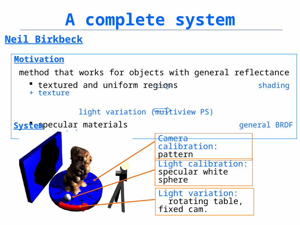
A complete systemNeil Birkbeck

Motivation

method that works for objects with general reflectance textured and uniform regions shading + texture

light variation (multiview PS)

specular materials general BRDF – parametric

System

Camera calibration: pattern

Light calibration: specular white sphere

Light variation: rotating table, fixed cam.

i

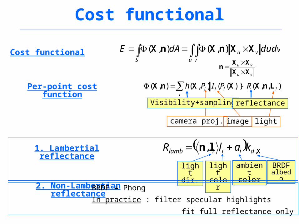
iiii RPIPh ),,())((),(),( LnXXXnX

Cost functional

dudvdAES u v

vu XXnXnX ),(),(Cost functional

vu

vu

XX

XXn

camera proj. image light

Per-point cost function

Visibility+sampling reflectance

1. Lambertial reflectance Xln ,, diiilamb kalR

light color

light dir.

ambient color

BRDFalbedo

2. Non-Lambertian reflectance BRDF = Phong

In practice : filter specular highlights

fit full reflectance only at the end

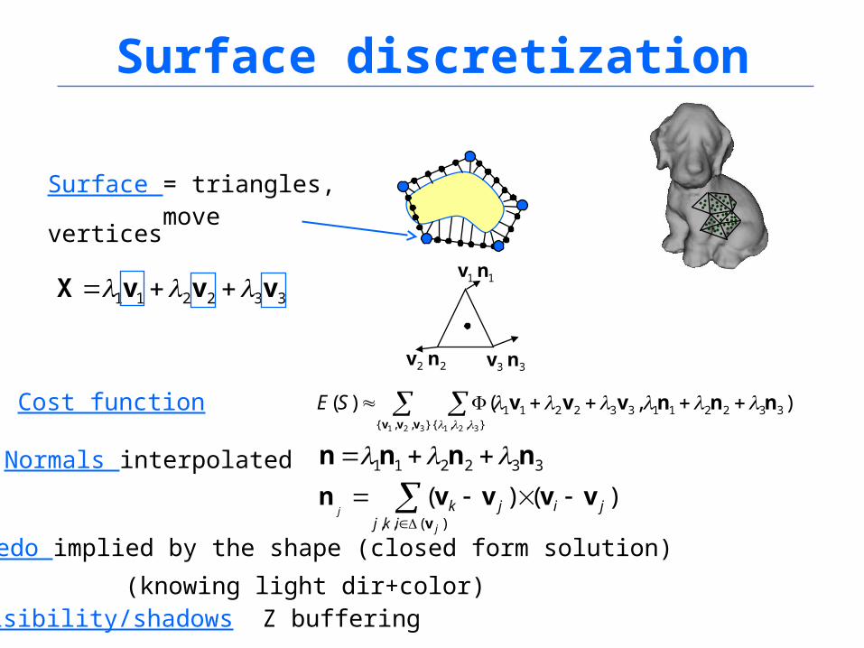
Surface discretization

Surface = triangles, move vertices

332211 vvvX 11 nv

22 nv 33 nv

Normals interpolated 332211 nnnn

Albedo implied by the shape (closed form solution)

(knowing light dir+color)

)()()(,,

jiikj

jk

j

jvvvvn

v

Visibility/shadows Z buffering

Cost function ),()( 332211332211},,{ },,{321 321

nnnvvvvvv

SE

Surface discretization

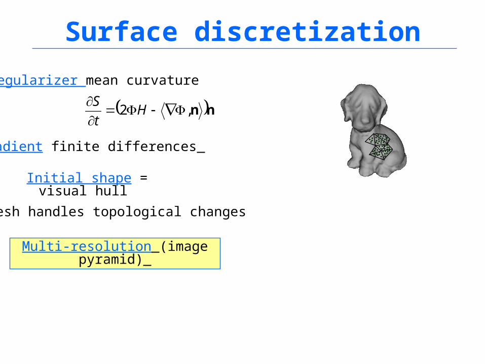
Regularizer mean curvature

Gradient finite differences

nn,2

Ht

S

Multi-resolution (image pyramid)

Mesh handles topological changes

Initial shape = visual hull

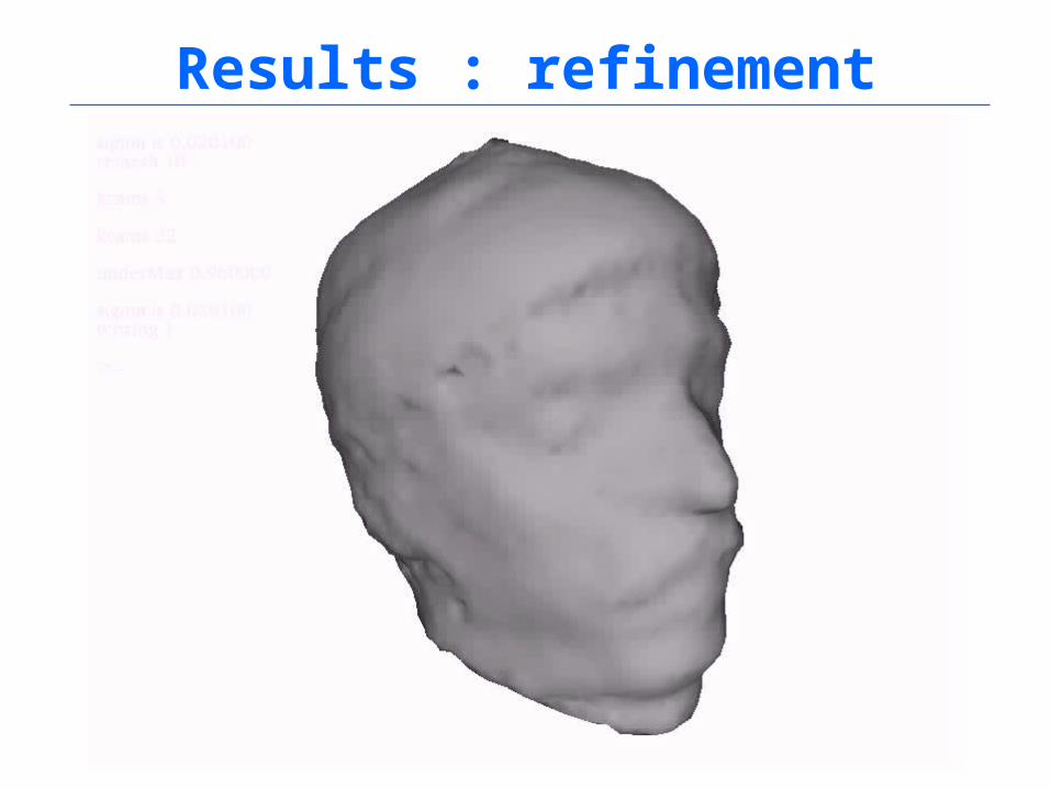
Results : refinement

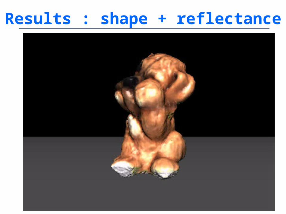
Results : shape + reflectance

Improvements Better light model – no need for calibration

Model background ? no need to extract silhouette (foreground) – Mumford-Shah functional

Discontinuities – anisotropic regularization; discontinuous mesh

Incorporate noise ?

Capture system Shape from silhouette Dynamic texture