Embed Size (px)
Citation preview

Numerical Simulation of the Fluid-Structure Interaction
of a Surface Effect Ship Bow Seal
Andrew L. Bloxom
Dissertation submitted to the faculty of the Virginia Polytechnic Institute and State
University in partial fulfillment of the requirements for the degree of
Doctor of Philosophy
in
Aerospace Engineering
Wayne L. Neu, Chairman
Leigh S. McCue-Weil
Christopher J. Roy
Solomon C. Yim
September 12, 2014
Blacksburg, VA
Keywords: Surface Effect Ship, Bow Seal, Finite Volume, Finite Element, Fluid-
Structure Interaction, Iterative Partitioned Coupling
©2014

Numerical Simulation of the Fluid Structure Interaction
of a Surface Effect Ship Bow Seal
Andrew L. Bloxom
Abstract
Numerical simulations of fluid-structure interaction (FSI) problems were performed in an effort
to verify and validate a commercially available FSI tool. This tool uses an iterative partitioned
coupling scheme between CD-adapco’s STAR-CCM+ finite volume fluid solver and Simulia’s
Abaqus finite element structural solver to simulate the FSI response of a system. Preliminary
verification and validation work (V&V) was carried out to understand the numerical behavior of
the codes individually and together as a FSI tool.
Verification and Validation work that was completed included code order verification of the
respective fluid and structural solvers with Couette-Poiseuille flow and Euler-Bernoulli beam
theory. These results confirmed the 2nd order accuracy of the spatial discretizations used.
Following that, a mixture of solution verifications and model calibrations was performed with
the inclusion of the physics models implemented in the solution of the FSI problems. Solution
verifications were completed for fluid and structural stand-alone models as well as for the
coupled FSI solutions. These results re-confirmed the spatial order of accuracy but for more
complex flows and physics models as well as the order of accuracy of the temporal
discretizations. In lieu of a good material definition, model calibration is performed to reproduce
the experimental results. This work used model calibration for both instances of hyperelastic
materials which were presented in the literature as validation cases because these materials were
defined as linear elastic.
Calibrated, three dimensional models of the bow seal on the University of Michigan bow seal
test platform showed the ability to reproduce the experimental results qualitatively through
averaging of the forces and seal displacements. These simulations represent the only current 3D
results for this case. One significant result of this study is the ability to visualize the flow around
the seal and to directly measure the seal resistances at varying cushion pressures, seal
immersions, forward speeds, and different seal materials. SES design analysis could greatly
benefit from the inclusion of flexible seals in simulations, and this work is a positive step in that
direction. In future work, the inclusion of more complex seal geometries and contact will further
enhance the capability of this tool.

iii
For my parents, Elliott and Susan

iv
Acknowledgements
I want to thank Wayne Neu for his advisement over the last 10 years, two years as my undergraduate
advisor and the other six during my graduate studies at Virginia Tech. I joined the Ocean Engineering
program in 2005 and his mentorship has been a major influence in my education. Over the years we have
had a great time studying interesting problems, sharing our work, and trying to understand the underlying
physics in the problems we’ve encountered. The additional committee members also played a role in
shaping my work through their constructive comments and shared knowledge. Leigh McCue-Weil is an
awesome scientist/educator who takes on challenging problems in ship dynamics and ocean engineering
and over the years gave me a strong appreciation for the elegance of the applied mathematics in our field.
Chris Roy is widely recognized as a top expert in Verification and Validation and is working to improve
the predictive capability and increase confidence in numerical simulations. I have certainly gained an
appreciation for V&V work in my final year and a half as I’ve toiled to apply those principles to my
simulations. Solomon Yim is a professor of civil engineering at Oregon State University and agreed to be
a member of my committee as we worked together in a summer research program hosted by Naval
Surface Warfare Research Center-Carderock Division. His advice and encouragement related to finite
elements and fluid-structure interaction were greatly appreciated.
I also want to thank Steve Edwards for his tireless efforts in providing high performance computing
support which was critical to the results presented in this work. He cares about the research that is
ongoing in our department and that is reflected in his work to provide us the best resources possible. Also
to the staff of the Advanced Research Computing center for providing the Ithaca and BlueRidge clusters
and support for the hardware.
Along the way, there have been a lot of people who have provided me a home away from home and
reminded me that what I was doing would be worth it. Thanks to all my friends. Lastly, I want to thank
my wife Lyndsey for moral support during the past two years. She is a mad scientist and an even better
friend.

v
Contents
Abstract ............................................................................................................................................ i
Acknowledgements ........................................................................................................................ iv
List of Figures .............................................................................................................................. viii
List of Tables ............................................................................................................................... xiii
List of Abbreviations ................................................................................................................... xiv
Chapter 1 ......................................................................................................................................... 1
Introduction ................................................................................................................................. 1
1.1 Motivation .................................................................................................................... 1
1.2 Introduction to Fluid-Structure Interaction................................................................... 3
1.3 Review of Literature ..................................................................................................... 5
1.3.1 SES Design ............................................................................................................ 5
1.3.2 FSI Solution Algorithms ....................................................................................... 9
1.3.3 Simulations of SES.............................................................................................. 13
1.3.4 FEM for Fabric Reinforced Rubber .................................................................... 21
1.4 Approach .................................................................................................................... 22
Chapter 2 ....................................................................................................................................... 25
Physical Model Experiments .................................................................................................... 25
2.1 ONR T-Craft at NSWCCD ......................................................................................... 26
2.2 University of Michigan Bow Seal Experiment........................................................... 28
2.3 Sloshing Tank Fluid-Structure Interaction Experiment at Universidad Polytechnica de
Madrid ................................................................................................................................... 32
2.4 Seal Material Calibration Experiment ........................................................................ 38
Chapter 3 ....................................................................................................................................... 41
Computational Methodology .................................................................................................... 41
3.1 Computational Fluid Dynamics .................................................................................. 42
vi
3.1.1 STAR-CCM+ ...................................................................................................... 42
3.1.2 Finite Volume Method ........................................................................................ 43
3.1.3 Reynolds-Averaged Navier-Stokes (RANS) Equations ...................................... 44
3.1.4 Volume of Fluid Method ..................................................................................... 46
3.1.5 Grid Generation ................................................................................................... 47
3.1.6 Lift Fan Model .................................................................................................... 48
3.2 Finite Element Analysis.............................................................................................. 50
3.2.1 Abaqus ................................................................................................................. 50
3.2.2 Implicit vs. Explicit Solver.................................................................................. 52
3.2.3 General element overview ................................................................................... 52
3.2.4 Continuum elements ............................................................................................ 54
3.2.5 Shell Elements ..................................................................................................... 57
3.2.6 Membrane Elements ............................................................................................ 58
3.2.7 Nonlinearities ...................................................................................................... 59
3.2.8 Nonlinear Dynamics Formulation ....................................................................... 61
3.2.9 Linear Elasticity .................................................................................................. 63
3.2.10 Hyperelasticity ................................................................................................. 64
3.3 Partitioned Coupling for Fluid-Structure Interaction ................................................. 67
3.3.1 Data Mapping and Transfer................................................................................. 67
3.3.2 Partitioned Solution Algorithm ........................................................................... 69
3.3.3 Grid Motion ......................................................................................................... 72
3.3.4 Stabilization Techniques ..................................................................................... 73
3.3.5 Remeshing/Restarting ......................................................................................... 77
3.4 Implementing JAVA macros for Automated Workflow ................................................ 79
Chapter 4 ....................................................................................................................................... 82
Verification and Validation....................................................................................................... 82
4.1 V&V Methodology ..................................................................................................... 83
4.2 Order Verification....................................................................................................... 88
4.2.1 Couette flow ........................................................................................................ 89
4.2.2 Euler-Bernoulli Theory: Cantilevered Beam ..................................................... 92
4.3 Solution Verification .................................................................................................. 96

vii
4.3.1 SES with Rigid Seals........................................................................................... 97
4.3.2 Sloshing Tank with neoprene beam .................................................................. 100
4.3.3 Static Hanging Seal ........................................................................................... 108
4.3.4 SES Bow Seal Test Platform Drag on Static Seal ............................................. 113
4.3.5 SES Bow Seal Test Platform Drag on Dynamic Seal ....................................... 120
4.4 Model Calibration ......................................................................................................... 121
4.4.1 Sloshing tank neoprene beam: material definition ............................................ 121
4.4.2 SES bow seal: material definition ..................................................................... 123
4.5 Model Validation ...................................................................................................... 125
4.5.1 Sloshing Tank FSI ............................................................................................. 125
4.6 V&V Conclusions..................................................................................................... 131
Chapter 5 ..................................................................................................................................... 133
Results & Discussion .............................................................................................................. 133
5.1 SES Test Craft Bow Seal .......................................................................................... 133
5.1.1 SES flat plate bow seal model ........................................................................... 134
5.1.2 Accuracy of Dynamic Seal Motion ................................................................... 136
5.2 Model Validation: Steady Bow Seal Hydrodynamics .............................................. 137
5.2.1 Bow Seal Displacement ......................................................................................... 140
5.2.2 Hydrodynamic Seal Resistance ......................................................................... 154
5.2.3 Bow Seal Pressure and Skin Friction Distribution ................................................ 159
Summary ................................................................................................................................. 165
References ................................................................................................................................... 168
Appendix A –JAVA macro code: Automated SES Bow Seal Co-Simulation Workflow .......... 179
Appendix B – University of Michigan Bow Seal Experiment: Summary of Modeled Runs ..... 195
Appendix C – ARC Cluster PBS submission script ................................................................... 196
Appendix D – Example Abaqus input ........................................................................................ 198

viii
List of Figures
Figure 1 - Bow sidewall immersion for a typical SES over a range of Fn. Increased bow
immersion between Fn = 0.2-0.4 is due to bow down pitch motion. (2) ................................ 8
Figure 2 - Drag force time histories on the seal for both the implicit and explicit coupling
algorithms for ∆t = 0.0001 s and 2nd order time discretization in the fluid (31). ................ 12
Figure 3 - Simulation of SES using Volume of Fluid method for calm water resistance test with
full length rigid seals (32). .................................................................................................... 15
Figure 4 - Head seas run with shortened rigid seals experiences high added resistance in waves
(32). ....................................................................................................................................... 16
Figure 5 - Bow immersion data for the rigid seal SES take-off.................................................... 17
Figure 6 - Resistance, pitch, and heave for 2.25 lbf constant thrust take-off. .............................. 18
Figure 7 - Rigid seal SES during take-off top) at Fn = 0.369, and impact of 1st transverse wave,
middle) at Fn = 0.387, and passing through of 1st transverse wave and, bottom) at Fn =
0.434, and impact of 2nd transverse wave. ........................................................................... 20
Figure 8 - NSWCCD Model Number 5887, generic T-Craft SES model with finger type bowl
seal (left). A view of the underside of the craft showing the bow seal, transverse mid-
cushion seal, and stern seal (right) (12). ............................................................................... 26
Figure 9 - CAD Model of the UM bow seal test platform (14) .................................................... 30
Figure 10 - Internal view of the membrane bow seal with description of modeling simplifications
(14). ....................................................................................................................................... 30
Figure 11 - Tank dimensions (in mm) for the experimental sloshing tank with hanging neoprene
beam. Tank is 39mm thick and gaps between beam and sidewalls are 2.9 mm. The beam is
4mm thick. Rotation is prescribed about the center of rotation and displacements are
measured in the rotating coordinate system. ......................................................................... 33
Figure 12 - Roll angle history comparison between benchmark (17) and Tracker analysis. ........ 35
Figure 13 - Comparison of displacements at 100% length (tip) between the benchmark (17) and
Tracker analysis with perspective filter applied. .................................................................. 36
Figure 14 - Comparison between numerical results and experimental data for a) the original input
roll history and b) the new roll history from Tracker and shifting other authors results by t =
0.2 s (30; 61). ........................................................................................................................ 37
Figure 15 - Experimental test set-up for static and dynamic tests of rubberized fabric material. 39

ix
Figure 16 - Raw experimental results highlighting the pre-stress state of the sample in two
configurations and the average displacement for the 45° case. ............................................ 40
Figure 17 – Comparison between the experimental and numerical cushion pressure probe time
histories for momentum source lift fan model for the T-Craft SES model (33). .................. 49
Figure 18 - Visualization of the pressure rise across the momentum source due to a constant
strength source term. ............................................................................................................. 50
Figure 19 - Node and face numbering scheme for 8 and 20 node three-dimensional solid
elements. (68) ........................................................................................................................ 54
Figure 20 – 8 and 20 node Fully integrated elements with integration point numbering scheme.
(68) ........................................................................................................................................ 55
Figure 21 – 8 and 20 node Reduced integration elements with integration point numbering
scheme. (68) .......................................................................................................................... 56
Figure 22 - Schematic of Shell element modeling types. (68) ...................................................... 58
Figure 23 – Nonlinear stress vs. strain relationship for a vulcanized neoprene rubber. (69) ....... 59
Figure 24 – Co-simulation workflow showing the primary steps of running the solvers, checking
convergence criteria, and transfer and mapping of data. ...................................................... 68
Figure 25 – Order of solver runs for a single coupling step with implicit solvers. ...................... 69
Figure 26 – Iterative partitioned coupling schematic with Aitken’s relaxation applied to
accelerate the convergence of the coupling iterations. ......................................................... 71
Figure 27 – Normalized iterative residuals during a co-simulation with 5 inner iterations. ........ 72
Figure 28 – Pressure ramping is used in the simulation to slowly raise the loading toward the full
value. This is especially useful when the initial load is exaggerated based on initial
conditions. t_zero is when the pressures are first exported and T_couple is when the full
load is realized. (64) .............................................................................................................. 76
Figure 29 - Skewed cells resulting from large displacement and morphing near the co-simulation
interface. ................................................................................................................................ 77
Figure 30 – Example of the remeshing process for an SES bow seal simulation: a) After 5
seconds of co-simulation the grid below and above the near seal region is highly distorted,
and b) the remeshed domain with a new grid aligned with the deformed geometry but
including some discrepancy due to grid resolution and solution interpolation..................... 78
Figure 31 - Couette flow description with approximate flow profiles for different values of
dimensionless pressure jump defined in Eq. 4. The top wall moves with constant velocity
no-slip BC, the fixed bottom uses a no-slip BC, and there are periodic boundaries on the
ends. ...................................................................................................................................... 90
Figure 32 – Schematic of the cantilevered beam with end load which was used for order
verification purposes of the finite element solver. ................................................................ 93

x
Figure 33 – Fixed displacement boundary conditions applied at x = 0 and two end loads on the
corner nodes at x=L. ............................................................................................................. 94
Figure 34 – Coarse grid cantilevered beam, dx = 0.01m. ............................................................. 94
Figure 35 – Medium grid cantilevered beam, dx = 0.005 m. ........................................................ 95
Figure 36 – Fine grid cantilevered beam, dx = 0.0025 m. ............................................................ 95
Figure 37 - Three dimensional perspectives of the SES geometry. .............................................. 98
Figure 38 - Coarse grid on the symmetry plane. (74) ................................................................... 99
Figure 39 - Fine grid on the symmetry plane. (74) ....................................................................... 99
Figure 40 - Fn 0.6 inviscid averaged drag results vs. normalized grid spacing. (74) ................. 100
Figure 41 - Finite volume grid of 839,753 cells: top) Overview of the grid refinement where
waves and spray are located, bottom-left) the prism layer cells on the beam, and bottom-
right) the prism layer in the corner of the tank walls. ......................................................... 102
Figure 42 – A relative comparison for system response quantity, f, the beam tip displacement. It
is presented as a difference in tip displacements between the three grid levels (f4, f3, f2) and
the reference solution (f1) in the first two seconds of the time history for the FSI response of
the neoprene beam. ............................................................................................................. 106
Figure 43 - Influence of thickness based refinement in the quadratic finite elements on the FSI
response of the sloshing tank hanging beam. ...................................................................... 107
Figure 44 - Influence of the fluid temporal discretization on the FSI response of the sloshing tank
hanging beam. ..................................................................................................................... 108
Figure 45 - Static seal deflections for four grid resolutions with refinement along the length of
the seal. ............................................................................................................................... 111
Figure 46 - Convergence of the tip deflection for the hanging static seal with four levels of grid
refinement. Level 1 is the finest and Level 4 is the coarsest. ............................................. 112
Figure 47 - Overview of the SES bow seal test platform grid architecture with a general
refinement region around the craft, isotropic refinement in the cushion and bow seal
regions, and extruded growth cells moving away from the primary region of interest. ..... 114
Figure 48 - Close-up of the bow seal, bow wave, and spray refinement regions of the SES bow
seal test platform model’s grid architecture. ....................................................................... 115
Figure 49 – Close-up of the boundary layer grid for the SES bow seal test platform model. .... 115
Figure 50 - Region directly beneath the bow seal at the three grid refinement levels a) coarse, b)
medium, and c) fine, showing flow discrepancy arising from the refinement and the
allowance of air leakage. ..................................................................................................... 117
Figure 51 - Wetting on the upstream side of the seal at the a) coarse, b) medium, and c) fine grid
levels which highlights and increased level of air leakage as the grid is coarsened for a static
seal case. ............................................................................................................................. 119

xi
Figure 52 – Resultant seal displacements for the solution verification study of the FSI response.
............................................................................................................................................. 120
Figure 53 - Comparison of experimental seal profile with the numerical result after model
calibration of the material stiffness. .................................................................................... 124
Figure 54 - Model calibration results with increased Young's modulus. .................................... 126
Figure 55 – Beam tip displacement at four reference locations compared with exp. E = 4.0 MPa.
............................................................................................................................................. 127
Figure 56 - Beam tip displacement at four reference locations compared with exp. E = 20.0 MPa.
............................................................................................................................................. 127
Figure 57 - Qualitative comparison for numerical results with linear elasticity and E = 20.0 MPa.
Video frames at t = 0.76, 1.64, 2.4, 2.68, 2.96, 3.32, 3.4, 3.56, 3.80, 3.84, 4, and 4.16
seconds (17). ....................................................................................................................... 128
Figure 58 – Qualitative validation results for a new 5 parameter Mooney-Rivlin material model.
............................................................................................................................................. 130
Figure 59 - Final finite element grid for the flat plate SES bow seal comprised of 14,592
elements. ............................................................................................................................. 134
Figure 60 - Schematic cross sectional cut of the SES flat plate bow seal finite element model. 135
Figure 61 - Run 1058: Visualization of free surface profile and bow seal displacement. .......... 139
Figure 62 – Run 1026 steady bow seal displacement after 20 seconds on the fine grid. The
forward velocity of the craft and cushion pressure are, U = 1.82 m/s and Pcushion = 567 Pa.
............................................................................................................................................. 142
Figure 63 – Run 1051 steady bow seal displacement displacement after 20 seconds on the fine
grid. The forward velocity of the craft and cushion pressure are, U = 2.43 m/s and Pcushion =
252 Pa. ................................................................................................................................. 143
Figure 64 – Run 1058 steady bow seal displacement displacement after 20 seconds on the fine
grid. The forward velocity of the craft and cushion pressure are U = 2.43 m/s and Pcushion =
475 Pa. Also included are results of remeshing the domain after initial 5 seconds of
displacement. ...................................................................................................................... 144
Figure 65 - Run 1114 steady bow seal displacement displacement after 20 seconds on the fine
grid. The forward velocity of the craft and cushion pressure are U = 2.43 m/s and Pcushion =
953 Pa. ................................................................................................................................. 145
Figure 66 - Run 1121 steady bow seal displacement displacement after 20 seconds on the fine
grid. The forward velocity of the craft and cushion pressure are U = 2.43 m/s and Pcushion =
997 Pa. For this case, the starndard deviations have been presented individually for the low,
medium, and high measurement locations because they were significantly different. ....... 146
Figure 67 - Run 1128 steady bow seal displacement displacement after 20 seconds on the fine
grid. The forward velocity of the craft and cushion pressure are U = 2.43 m/s and Pcushion =

xii
1050 Pa. For this case, the starndard deviations have been presented individually for the
low, medium, and high measurement locations because they were significantly different. 147
Figure 68 - Run 1142 steady bow seal displacement displacement after 20 seconds on the fine
grid. The forward velocity of the craft and cushion pressure are U = 2.74 m/s and Pcushion =
625 Pa. ................................................................................................................................. 148
Figure 69 – Run 1412 steady bow seal displacement displacement after remeshing the domain
after initial 5 seconds of displacement and running to 20 seconds on the fine grid. The
forward velocity of the craft and cushion pressure are U = 3.04 m/s and Pcushion = 625 Pa. 149
Figure 70 – Run 1058, U = 2.43 m/s, Pc = 475 Pa. Comparison of the average seal z-coordinate
at the three measurement locations and standard deviations for numerical results with
stabilization removed (top). (2nd order time in fluid, transient fidelity in solid, and no
Rayleigh damping). Zoomed in comparison displaying the relative difference (bottom). . 153
Figure 71 – Schematic of the forces acting on the bow seal. Cushion pressure (orange) acts on
the aft side of the seal and is balanced by the hydrodynamic forces (blue) and the skin
friction (green). The seal’s weight (red) and the reaction forces and moment are also shown
at the red circle where the seal is clamped. ......................................................................... 155
Figure 72 – Non-dimensional seal resistance versus non-dimensional cushion pressure for a seal
immersion based Froude number = 1.6. Bc is the cushion beam, δs is the static seal
immersion. Comparison with experimental values (14). .................................................... 159
Figure 73 – Progression of bow seal pressure distributions normalized by the interior cushion
pressure and displacements for the Fn = 1.6 series. The cushion pressures going from the
top to bottom are 252, 475, 953, 997, and 1050 Pa at a forward speed of 2.43 m/s. .......... 161
Figure 74 – Scalar values of the pressure distribution on the forward side of the bow seal for Run
1058. U = 2.43 m/s, Pc = 475 m/s. ...................................................................................... 162
Figure 75 – X component of the skin friction acting on the upstream side at the centerline of the
seal for Run 1058. U = 2.43 m/s, Pc = 475 m/s. ................................................................. 162
Figure 76 – Free surface elevation wake profiles for Runs 1051 (Pc = 252), 1058 (Pc = 475 Pa),
and 1114 (Pc = 953 Pa) highlight the deepening of the free surface inside the cushion and
the rise of the bow wave with increasing cushion pressure at constant forward speed. ..... 163

xiii
List of Tables
Table 1 - T-Craft Model Characteristics ....................................................................................... 27
Table 2 - The default Parameters for the HHT integrator for both the Transient fidelity and
moderate dissipation settings, both of which were used in the present work. ...................... 63
Table 3 – Code verification results for the observed order of accuracy using the laminar Couette
flow exact solution. ............................................................................................................... 92
Table 4 – Principle dimensions and values for the cantilevered beam with end load case. ......... 93
Table 5 – Order verification results for Abaqus with cantilevered beam with end load.
Displacement of free beam end is measured for each grid. .................................................. 96
Table 6 - Grid Refinement Specifics. ........................................................................................... 98
Table 7- Grid refinement data for the sloshing tank FSI simulations. ........................................ 102
Table 8 – L2 norm of the discretization error, observed order of accuracy, and error reduction
ratio for the temporal solution verification. ........................................................................ 103
Table 9 - L2 norm of the discretization error, observed order of accuracy, and error reduction
ratio for the spatial solution verification. ............................................................................ 103
Table 10 - L2 norm of the discretization error, observed order of accuracy, and error reduction
ratio for the combined spatial and temporal solution verification. ..................................... 104
Table 11 - L2 norm of the discretization error in the tip displacement, observed order of
accuracy, and error reduction ratio for the combined FSI response solution verification. . 105
Table 12- Grid refinement properties for static hanging seal ..................................................... 111
Table 13 – Solution verification results for the static hanging seal refinement study ................ 112
Table 14 – Grid characteristics for the bow seal drag solution verification ............................... 116
Table 15 – Solution verification results for the seal drag in a dynamic FSI simulation after 20
seconds. Using three grid levels provides one estimate of the observed order of accuracy.
............................................................................................................................................. 120
Table 16 – Fabric reinforced vulcanized neoprene model definition after model calibration .... 125
Table 17 – Average seal force data in the last 5 seconds of simulation for a static seal immersion
based Froude number =1.6 at varying cushion pressures. .................................................. 157

xiv
List of Abbreviations
SES – Surface effect ship
ACV – Air cushion vehicle
ONR – Office of Naval Research
FSI – Fluid-structure interaction
T-Craft – Transformable Craft
CFD – Computational Fluid Dynamics
CSM – Computational Structural Mechanics
AAME – Artificial added mass effect
CFL – Courant-Friedrichs-Lewy number
VOF – Volume of fluid
HPC – High performance computing
SRQ – system response quantity
V&V – Verification and Validation

1
Chapter 1
Introduction
1.1 Motivation
The Office of Naval Research (ONR) began looking into technologies at the turn of the century
to compliment the current Landing Craft Air Cushion (LCAC) craft that serve the Navy and
Marines as a ship to shore landing/supply craft. At that time, the overarching theme in naval
strategy was pushing toward a sea-base concept where a joint floating port and airfield would be
positioned offshore near a location to support sea and land forces as required. One key
requirement for such a system is an intermediary vessel which can transit the open ocean,
provide good seakeeping performance during load transfer, perform at high speed under full load
in shallow water, and also transform into an amphibious mode for “boots dry” offloading. The
ONR, through the Innovative Naval Prototype (INP) program developed government and
industry prototype designs, and the T-Craft Tool Development Program was created as a joint
effort with the addition of academic research teams. The objective of this program was to explore
and develop key technologies and design tools which would aid in the design of this 21st century
naval craft (1).

2
The initial T-Craft prototype concepts combined the best elements of the Surface Effect Ship
(SES), Air Cushion Vehicle (ACV), and catamaran design features. This advanced design
allowed for academic and industry research in materials, propulsion, seakeeping, hydrodynamics,
and control. Advances in computer-aided engineering allowed computational design tools to be
explored seriously as a means to compliment model testing and prototype construction plans.
Additionally, a team of subject matter experts came together to share their historical knowledge
of SES and ACV design from their heyday in the late 1960’s. This insight was invaluable as it
pointed out the remaining technology gaps to be addressed in order to fully realize the T-Craft
and to further ACV technology in general through a collaborative exchange.
A common denominator between an ACV and SES is the use of highly flexible seals to maintain
a cushion pressure under the craft which lifts it, reduces wetted surface area, and as a result
decreases the frictional drag on the craft (which scales with the square of the velocity). The
seals’ interactions with the water surface during take-off, maneuvering, and transit, including the
dynamics and fatigue of the seals were identified as a key technology gap to be addressed.
Improper design of the seals can affect the motions of the craft, the total lifespan of the seal
material, the fuel-efficiency of the propulsion system, and the safety of the crew onboard. There
are hydrodynamic phenomena related to the cushion and seal design which needed to be
explored (2). Specifically, seal resistance and dynamics, and their effect on the overall craft
dynamics is an area which has been historically difficult to address in model and full scale
testing. However, model tests have since been performed with state of the art experimental
techniques to gain insight into these issues.
With modern advances in computational power and algorithm development, new approaches to
solve these old problems are currently being investigated. Typical computational approaches

3
treat marine craft as rigid structures to analyze the hydrodynamic performance and predict loads
which are applied to a structural model. This approach can work well for ships and boats in small
to moderate seas, whose structural response is relatively decoupled from the fluid motion. In
these instances, the maximum design loads and resultant stresses are of interest. In more extreme
scenarios, ships encountering heavy seas can experience slamming and hydroelastic phenomena
resulting from these transient loads and would require an approach which included the
deformation of the structure. This is especially true with light flexible structures like ACV seals.
Fluid loads can deform flexible structures to a degree that also affects the fluid response and
therefore the fluid and structural response must be solved together in a coupled fashion to
capture these interactions. Efforts to model the T-Craft have previously been performed with
rigid seal structures and will be described shortly. A key predictive capability is lost in these
simulations however, as the information on seal drag and dynamics is neglected. This deficiency
will be highlighted and provide motivation for the goals of this work.
1.2 Introduction to Fluid-Structure Interaction
Fluid-Structure Interaction is a field of study which bridges the divide between fluid flow and
structural motion in response to some loading. Historically speaking, a large number of human
constructs were and are still built to a level of rigidity so that interactions with the flow of fluids
or gases are negligible to the design. Pyramids and other buildings made from stone are not
easily swayed by the winds. Only long weathering or an earthquake would make them move. But
as civilization grew and progressed, a keen interest in implementing technologies to improve the
standard of life, increase profit, or just provided sheer entertainment has increased.. With
innovation came radical inventions, new materials, and the rise of an industrialized civilization

4
full of interactions with the world around us. Thanks to the scientific revolution, everything
changed when the ability to analyze structures and fluid flow with mathematical equations
became a reality. FSI was becoming more important as structures grew larger and upwards.
Gustav Eiffel performed load analysis on the Eiffel Tower taking into account the wind forces
(3). On the other hand, almost a century later the Tacoma Narrows Bridge collapse stands out as
a case of not giving enough attention to the FSI effects. The cause of that unfortunate incident
was vortex-induced vibration (VIV), a potentially dangerous form of FSI where the wind and its
shed wake off the bridge interact with the natural frequency of the suspended bridge’s
oscillation. This event brought aeroelasticity (4) into the public eye and through years of
research, trial and error, these effects have become the target of great effort to reduce their
negative impacts.
Generally, there are two classifications of FSI problems. The first are loosely coupled problems
where the time dependent response of the structure is not influenced by the fluid flow around it.
Second, are strongly coupled problems where the properties of the structure are such that it does
have a time dependent response which is influenced by the surrounding fluid flow. The design
analysis of the Eiffel Tower is a good example of an early loosely coupled FSI problem. The
structural details were designed, and then an analysis was performed to ensure that even with
wind loads, the structural elements which comprised the tower would be able to withstand the
stress. Eiffel was one of the first structural engineers to begin using wind drag coefficients for
shapes to obtain estimates of the natural loading on a design. The overall displacement of the tip
of the tower in wind should be small compared to say the overall height of the tower. A majority
of engineering problems typically reside in this classification.

5
The second classification of strongly coupled problems is more relevant today than ever.
Structures are being built stronger, lighter, and with new materials. Membrane structures (i.e.
parachutes, air bags, tents), bridge design, aerodynamic flutter, tires, biological tissues and blood
flow (5), biomimetic devices, ship/offshore design, and renewable energy harvesting are just a
few fields which have seen strong interest by the FSI community. As designs become more
advanced, so to do the tools which are used to analyze them. Problems in FSI are now within the
grasp of high fidelity computer simulation prediction, where before they were limited to study
through empirically based models, analytical solutions, and scale model experiments.
Simulations have the ability to provide information that is difficult to visualize and measure
experimentally. These important problems are now being explored with state of the art
approaches and modern computational power and can be found in every field of engineering.
1.3 Review of Literature
1.3.1 SES Design
Surface Effect Ships were brought into the high speed marine vehicle world as a hybrid of a
traditional air-cushion vehicle, a catamaran, and the Captured Air Bubble concept (6; 7). A
typical SES design has a catamaran-type pair of side-hulls with flexible seals which contain a
cushion pressure provided by lift fans pumping air into the void between the hulls. SES’s are
able to achieve higher speeds with less thrust by taking advantage of the reduced wetted surface
area from lifting the hull to minimize frictional drag. At the same time, an increase in directional
stability over a typical ACV is provided by the side hulls, as well as improved seakeeping
performance and less cushion pressure leakage compared to the typical losses in the peripheral
seals of ACV’s. Due to the highly flexible nature of these seals and the complex wake

6
interactions inside the hulls, the free surface is in constant interaction with them, causing
increased drag, and additional material fatigue. ACV’s are normally limited to favorable sea
conditions due to the likelihood of the cushion pressure leakage resulting from large motions in
higher wave amplitudes (8). The SES design allows the craft to seal the cushion pressure in
along the length of the craft hulls, but still has flexible seals fore and aft to maintain cushion
pressure and allow smoother interaction of the craft with waves. Some designs omit the rear seal
entirely and still maintain a cushion pressure.
Beginning in the mid 1960’s and continuing well through the next decade, SES work largely
followed a design, build, test, iterate paradigm. Rohr Industries, Textron Marine, Bell Aerospace,
and the David Taylor Model Basin (DTMB) produced a number of prototype test craft for the
United States Navy. Many of the early seal and hull design iterations were tested in Froude
scaled prototypes at DTMB (9). The vision for these craft pushed toward a 100-kt navy and fast
trans-oceanic passages. Significant research went into super-cavitating propellers and water-jet
propulsion in order to reach such high speeds. Many things were learned about the nature of
these craft through both model tests and full scale prototype testing which advanced the state of
the art and provided a craft which was very useful for transiting quickly in littoral environments.
Notable uses include high speed ferries and the Norwegian Skjold-class littoral patrol craft (8;
10). Due to the nature of the cushion and twin hulls, and the inability to visually observe the
dynamics between the hulls during operation, the true nature of the free surface dynamics and
their interaction with the seals was never fully understood. An anecdote told by an early SES
designer, Bob Wilson, tells of a Navy Captain who nearly lost his life strapped to the inner
cushion wet-deck of a prototype SES in order to get a better look at the free surface dynamics
inside the cushion (2)!

7
Much of the design guidance which is found in texts like (8) and (10) provide a wealth of
empirical data from historical SES and ACV designs from the 1960’s onward. They also present
many studies based on theoretical work using control volume analysis and models of air cushions
and craft dynamics. Many of the early problems and their solutions are outlined, along with some
of the remaining challenges to future SES designers. SES design still has some areas of open
research that have the potential to improve the performance characteristics. A good review and
discussion of the issues with respect to current day research was conducted in (11). Specifically,
key targets of research include the implementation of new, lightweight and high strength
materials, improved understanding of hydrodynamics through simulation and experiments, novel
propulsion systems, multi-body interactions, and dynamics and control. The end result will be
the shift from art to science in SES design.
ACV/SES helmsmen are often referred to as pilots, since the craft tend to “fly” on top of the
water. For this reason, the acceleration of the craft from rest to operating speed is typically called
take-off. SES’s during take-off have been noted to encounter negative performance effects due to
the complex interaction of the wave systems and the seals. The resistance curve of an SES
typically has a primary and secondary hump due to these effects. The secondary hump occurs at
approximately Fn = 0.38 when the craft is riding with a wave crest located at the bow and the
stern. The stern wave crest has the potential for serious interaction with the stern seal. If the stern
seal is relatively rigid and the bow seal is flexible, the craft can tend to pitch bow down in this
situation, further increasing the drag on the craft. Early SES designs which did not account for
these effects were often unable to take-off and reach design speed.
Experimental research into SES dynamics during acceleration (2) also shows a bow down pitch
motion around the Froude number where the wavemaking drag shows a hump. This bow down
8
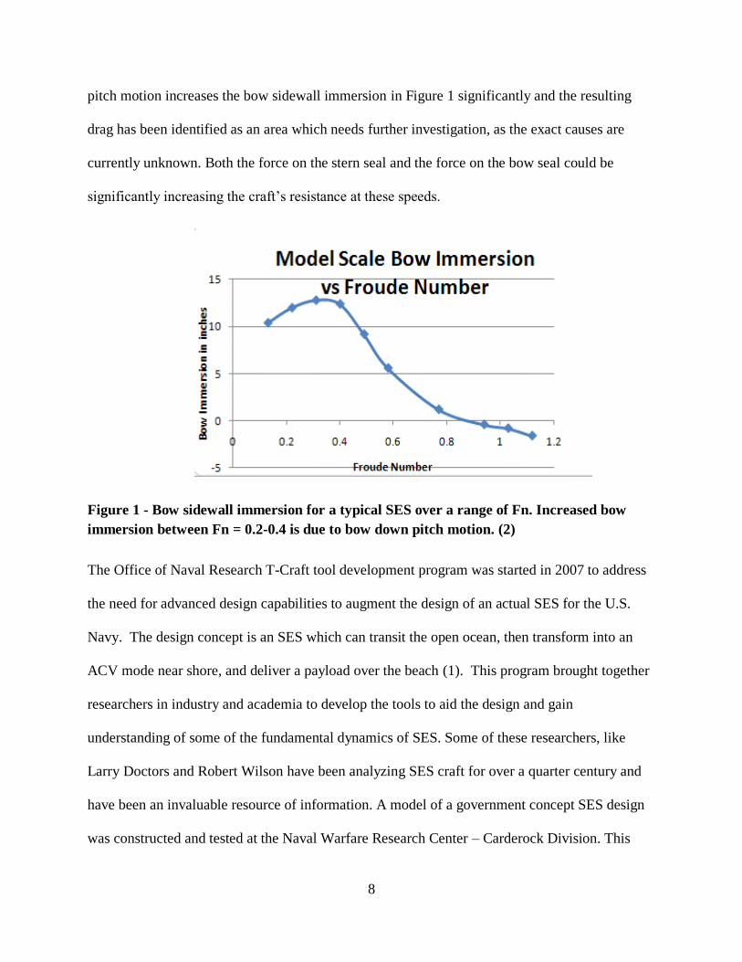
pitch motion increases the bow sidewall immersion in Figure 1 significantly and the resulting
drag has been identified as an area which needs further investigation, as the exact causes are
currently unknown. Both the force on the stern seal and the force on the bow seal could be
significantly increasing the craft’s resistance at these speeds.
Figure 1 - Bow sidewall immersion for a typical SES over a range of Fn. Increased bow
immersion between Fn = 0.2-0.4 is due to bow down pitch motion. (2)
The Office of Naval Research T-Craft tool development program was started in 2007 to address
the need for advanced design capabilities to augment the design of an actual SES for the U.S.
Navy. The design concept is an SES which can transit the open ocean, then transform into an
ACV mode near shore, and deliver a payload over the beach (1). This program brought together
researchers in industry and academia to develop the tools to aid the design and gain
understanding of some of the fundamental dynamics of SES. Some of these researchers, like
Larry Doctors and Robert Wilson have been analyzing SES craft for over a quarter century and
have been an invaluable resource of information. A model of a government concept SES design
was constructed and tested at the Naval Warfare Research Center – Carderock Division. This

9
model was tested in the Maneuvering and Seakeeping Basin at NSWCCD to provide basic data
for validation of ship motion simulations (12). These tests were performed in calm water, waves,
at various cushion pressure/weight ratios, and in multi-body configurations with a larger cargo
ship model.
Another contemporary experimental test program was carried out specifically to address the
hydrodynamics of the bow seal system and its interactions with the free surface (13; 14; 15).
Initially, a medium scale craft was tested in the Marine Hydromechanics Laboratory at
University of Michigan with a planing seal and finger type seals. Results from that series of tests
guided the efforts for a second, larger and more instrumented bow seal test platform at the Large
Cavitation Channel (a NSWCCD resource) in Memphis, TN. Some of the key results of those
tests were the measurement of seal forces and deflections, as well as detailed experimental
visualization and analysis of the buckling of the bow seal where it interacts with the free surface.
These experiments will be described in more detail later with regards to the validation efforts of
this work.
1.3.2 FSI Solution Algorithms
Fluid-structure interaction (FSI) simulation efforts aimed at modeling the hydroelastic and
aeroelastic response of thin, highly flexible structures has increased significantly in the past two
decades. Design challenges and novel ideas existed that were once only within the realm of a
design, build, and test paradigm. Membrane structures (i.e. parachutes, air bags, tents),
aerodynamic flutter, tires, biological tissues and blood flow (5), biomimetic devices, and
ship/offshore design are just a few fields which have seen much interest by the FSI community.
A good review of the current state of the art in FSI is provided in (16). With a range of varying
fidelity computational tools at hand, some of these difficult problems in fluid-structure

10
interaction are being solved. This has been enabled by the rise in High Performance Computing
(HPC) resource availability as well as significant efforts in code development to improve current
FSI tools on both the fluid and structural side. In order to use state of the art computational tools
effectively, verification and validation efforts should be carried out to assess the predictive
capability of the method for the intended purposes. It is important to have canonical or
experimental data sets for FSI problems that provide a solid foundation for this assessment. This
is critical because analytical solutions for V&V of FSI problems are essentially non-existent.
Fortunately, there is a growing body of experimental and numerical benchmark data on relevant
problems provided specifically for FSI code validation (17; 18; 19; 14; 20).
Fluid-structure interaction simulations solve for both fluid flow and structural motion to capture
the behavior of a system interacting with the environment and the loads placed on it. Generally
there are two ways to approach this. In a monolithic approach, the governing equations for the
fluid and structure are written together and solved simultaneously in one solver. Alternatively, in
a partitioned approach, the fluid and structural systems are solved within distinct solvers and
there is an exchange of interfacial data between them at coordinated times. The monolithic
approach is generally more accurate and preferred for problems where the coupling between the
fluid and structure is strong (21). However, the solution of the monolithic system is costly
because of the nonlinear nature of the coupling and the large total number of unknowns (22). The
partitioned approach is more amenable to using independent solvers together which may be
tailored for specific target applications, but requires some efforts in algorithm design in order to
stabilize the numerical solution of strongly coupled problems. Often the partitioned approach is
desirable due to the amount of development, verification and validation, and focused research
spent refining the solvers for the target applications.

11
Partitioned FSI can be done either with one way coupling, where the dynamic response is not
sought, or with a two way coupling where information is continually exchanged in order to
capture dynamic phenomena. One way coupling has been used extensively in design where
estimates of the loads on a structure are made, then given to a structural engineer to analyze the
structure and ensure it meets requirements (23). Efficient two-way coupling is a more recent
capability in FSI, made possible in part by the advances in computational resources over the past
two decades. This work focuses on two way coupling between finite volume CFD and finite
element CSM codes. It can be performed with explicit coupling (loose), using one force-
displacement exchange per coupling time step, or it can be performed with implicit coupling
(strong) where there is an iterative exchange which utilizes Aitken’s relaxation until the co-
simulation interface conditions have converged for a given coupling step. The structural
displacements calculated in the finite element solution are passed to the fluid domain where they
are applied throughout the grid via an interpolation method. Handling this grid deformation
dynamically in a simulation can be a difficult task, especially in strongly coupled systems.
Explicit coupling in partitioned simulations can result in an instability that is a result of the
continuous motion of the coupling boundary being represented in a discretized fashion with a
grid flux term included for the surface’s velocity. If the interface surface moves too far in one
time step, then the Space Conservation Law (SCL) can be violated (24; 25). This is analogous to
the Courant-Friedrichs-Lewy (CFL) stability condition for the convection of fluid in grid cells.
Mass sources can be created in cells where this large deformation is occurring (24). By using a
non-converged prediction of the displacement in a single exchange, the displacement can create
an unrealistically large pressure spike, which pushes the seal in the opposite direction, creating a
pressure spike on the other side. In this way, the pressure response on the seal cascades out of

12
control, until either the structural solver fails to converge or the grid deformation model can no
longer handle the severity of the displacement. Because of physical added mass effects, the fluid
and solid solutions need to be converged together toward a coupling independent solution. In the
literature, this is referred to as the artificial added mass effect (AAME) and is a well-known
instability for partitioned FSI methods (26; 27; 28). Problems involving high fluid velocities,
incompressible flow, low stiffness materials, and large displacements are particularly sensitive to
the AAME.
An implicit partitioned coupling algorithm was first implemented in STAR-CCM+ in version
7.04. The force-displacement transfer is allowed multiple passes during a step using successive
substitution with Aitken’s relaxation until the calculated co-simulation displacement has
converged within a given coupling step. Similar methods have been shown to be successful for
the calculation of FSI problems in application to free surface flow (29; 30).
Figure 2 - Drag force time histories on the seal for both the implicit and explicit coupling
algorithms for ∆t = 0.0001 s and 2nd order time discretization in the fluid (31).
-200-175-150-125-100-75-50-25
0255075
100125150175200225250
0
100
200
300
400
500
600
700
800
900
1000
1100
1200
1300
Sea
l D
rag F
orc
e (l
bf)
Inner Iterations
Explicit

13
Figure 2 highlights the advantage of using the implicit coupling scheme for a strongly coupled
FSI problem. Instead of predicting wildly oscillating forces which cause the FSI solution to
diverge, the implicit scheme nicely stabilizes the calculation.
1.3.3 Simulations of SES
Numerical simulations of SES focused on the resistance, sea-keeping performance, and
dynamics & control of simplified geometries have been performed previously. Among those
simulations in the literature, there are varying degrees of fidelity with respect to the modeling of
the craft and the complexity of the physics. Because full physics simulations are expensive both
computationally and in time, many of these efforts pursued reduced order modeling and
approximations to reap the most information possible. The primary approximation revolves
around the handling of the seal system. The second major approximation is in the modeling of
fluid flow, e.g. potential flow, control volume analysis, Reynolds Averaged Navier-Stokes
equations, or frequency domain simulations. Past simplifications of the seals include: rigid
bodies (32; 33), total neglect, torsional spring and hinged flap approximations which can respond
to wave motions while still providing a more accurate prediction of resistance and overall craft
motions (34; 35), implementing pressure elements at the free surface (36; 37; 38; 39), or
including a term for seal drag based on empirical or numerical approximations. The latter
represent the seal’s influence on the overall performance of the craft without actually modeling
the seals and their interactions (34; 40; 41).
The groups which focused on reduced order modeling of craft motions and performance in order
to provide timely information to design teams were typically using boundary element and panel
method calculations of the flow around the ship. With models for cushion pressure and seal
effect, these simulations are much less computationally intensive than Navier-Stokes simulations

14
which capture the finer details and viscous effects in the flow. They can be useful for exploring
large design spaces and for obtaining response amplitude operators for sea-keeping analysis
while keeping in mind their limitations and deficiencies. These are referred to as low-fidelity
simulations. However, to capture the interaction of the seals with the craft wake and bow wave,
it becomes necessary to use more advanced CFD methods. Only in the past decade have
numerical codes and fluid structure interaction research provided the capability to model the
complex behavior of an ACV seal interacting with the free surface.
Simulations which employ more in-depth models of viscous fluid flow are referred to as high
fidelity simulations. The advantage to numerical testing of SES is the wealth of data which
would be otherwise very difficult to obtain, however the physical experiment is still very
relevant in gaining insight and providing validation data to modelers. A high fidelity simulation
of SES does not necessarily calculate the FSI response of the seals, but can still provide a good
estimate of the calm water drag and simple motion analyses. Finite volume CFD simulations of
SES have been very popular due to the better description of the flow field and more accurate
calculation of forces on the craft (33; 34; 42).
A third distinction is made to indicate simulations which calculate the actual FSI response of the
structure within a high fidelity simulation. Figure 3 shows how a rigid seal approximation over-
predicts drag and motions due to increased forces on the seals because of the enlarged bow wave
and associated drag increase. Shortened rigid seals allow basic resistance calculation and
motions studies, but still present a problem in waves which is highlighted in the transient drag
response from a simulation shown in Figure 4. Low-fidelity and high-fidelity simulations
without FSI may miss dynamic phenomena related to seal issues that affect the overall
performance of the vehicle. There is a need to model flexible seals in simulation to properly

15
account for the dynamics of the vehicle when interacting with steep waves in the near shore
environment, transiting the open ocean, and predicting seal drag forces across the operational
envelope.
Few studies have been performed on the transient dynamics of actual seal geometries for ACVs
and SES. Due to the challenges of coupled FSI on finite volume grids, a number of researchers
have pursued alternative methods. One study used Smoothed Particle Hydrodynamics coupled
with the finite element method to calculate two-dimensional simulations of an SES bow seal test
platform (43; 44). The deflections calculated with SPH/FEM were compared with experiment
and represented the first attempt to match the experimental data. The development of that work is
ongoing to make the simulations three-dimensional, parallelized, and have faster FEM solvers. In
a similar but different approach, the Particle Finite Element Method was used to model the
government T-Craft model which was tested at Carderock with seal dynamics included (45). To
date, a time accurate, high fidelity simulation with a fully appended, realistic geometry of an SES
in waves has yet to be achieved. This work will hope to further progress toward that goal with a
respect for the inherent challenge of the task.
Figure 3 - Simulation of SES using Volume of Fluid method for calm water resistance test
with full length rigid seals (32).

16
Figure 4 - Head seas run with shortened rigid seals experiences high added resistance in
waves (32).
After Donnelly’s initial work, simulations were also run as part of this work to explore the rigid
seal SES free surface profiles and the forces/moments on the model and attempt to understand
the underlying causes of the bow down pitch motion as the craft accelerates through the hump
speed. It is unclear whether the actual seal dynamics influence this behavior, but using a
simplified rigid seal model will partially neglect certain aspects of the seal’s contribution to the
dynamics of the craft. The computational domain for these simulations consists of a half model
of the T-Craft geometry with roughly 300,000 cells. Formal solution verification was not
performed for this problem.
The bow immersion was also estimated from these runs by looking at the free surface elevation,
the pitch and heave of the craft, and the initial immersion of the sidewalls. Figure 5 presents this
immersion data versus Fn. Comparing this with Figure 1, there does appear to be a similarity in
the trends where the immersion increases going through the secondary resistance hump and then
gradually decreases.
0
0.05
0.1
0.15
0.2
0 0.5 1 1.5 2 2.5 3 3.5 4
Norm
ali
zed
Dra
g,
D/W
Time, s
Sim: Drag
Run599,
Channel 60

17
Figure 5 - Bow immersion data for the rigid seal SES take-off
The simulation of SES take-off must include the transient free surface effects as the craft
interacts with its own wave system. Figure 6 presents the important data for a SES take-off with
a constant 2.25 lbf thrust force. The drag, pitch angle, and heave are all plotted on the same
graph. These along with images of the interaction of the SES with its wave system provide a way
to visualize the effects of the wave system. As can be seen from the blue drag curve, there is
some noise-like variation in the drag, but the secondary and primary resistance humps are
evident. Three images are presented in conjunction with Figure 6 and their corresponding take
off Froude numbers are given. These significant points in the drag are highlighted with the
colored markers on the drag plot.
0.000 0.500 1.000 1.500
0
0.5
1
1.5
2
2.5
3
3.5
4
4.5
Fn
Bow
Im
mer
sion
(in
)

18
Figure 6 - Resistance, pitch, and heave for 2.25 lbf constant thrust take-off.
The top view in Figure 7 (green triangle in Figure 6) corresponds with the impact of the first
internal cushion transverse wave with the rear seal surface. From the figure it is clear when this
occurs, first the resistance increases, then the craft heaves upwards, and as it is falling also
pitches bow down. This is certainly caused by the moment produced from the impact of the wave
and the added buoyancy at the stern. The middle view of Figure 7 (red triangle in Figure 6)
corresponds with the passing of the 1st transverse wave out the rear seal and the accompanying
reduction in drag. The bottom view in Figure 7 (yellow triangle in Figure 6) corresponds with the
impact of the 2nd internal cushion transverse wave with the rear seal surface. Now the craft is
riding between two wave crests, and experiences a rise in drag due to both the impact of this
wave, and the traditional wavemaking increase associated with this condition in a craft’s wave
0
0.005
0.01
0.015
0.02
0.025
0.03
0.035
0.04
-0.5
0
0.5
1
1.5
2
2.5
0 5 10 15 20
Hea
ve
(m)
Dra
g F
orc
e (l
bf)
& P
itch
(deg
)
t (sec)
DragPitchFirst WavePassing ThroughSecond WaveHeave

19
system. This primary hump is earlier than suggested by Yun and Bliault (10) who provided Fn =
0.56 as the typical location of primary resistance humps.
The importance of studying the transient progression of the internal wave interactions is evident
by looking at the impact of waves with the stern seal surface. The bow down pitch motion and
the increased resistance due to this wave impacting the rear seal are important phenomena to
capture in simulation. The level that this wave impact affects the total drag on a flexible lobe
type seal versus the rigid approximation used in these simulations remains to be understood. The
flexible seal may make it easier to mitigate the impact of this transverse wave. The flexible bow
seal may also be critical to the modeling of this take-off event. However, despite these
deficiencies, the model still predicts the typical characteristics of the SES take-off.

20
Figure 7 - Rigid seal SES during take-off top) at Fn = 0.369, and impact of 1st transverse
wave, middle) at Fn = 0.387, and passing through of 1st transverse wave and, bottom) at Fn
= 0.434, and impact of 2nd transverse wave.

21
1.3.4 FEM for Fabric Reinforced Rubber
Simulation of rubber has long been a challenge with large deformations and nonlinear behavior
as well as visco/thermo-elastic properties. Similarly, fabrics which are inextensible yet have very
low flexural rigidity haven been modeled with reduced complexity models that aim to generalize
their behavior. While there is much literature on characterization of rubber materials in finite
element constitutive models and different approaches to inextensible fabric modeling and fabric
drape, the combination of the two fields into rubber composite materials has seen less
widespread attention due to the difficulty in obtaining material characteristics.
A brief survey of literature on rubber, elastomer, and nonlinear hyperelastic material modeling
yields a number of significant application and advances. Beginning with the work of Mooney,
Rivlin, and Saunders (46; 47) in the 1940-1950’s and Ogden (48; 49) to characterize the behavior
of rubber during large deformations, the theory of hyperelasticity has come a long way in more
than a half a century of work. The theory and models based on their initial work in strain energy
density functions for nonlinear, elastic rubbers have increased in complexity over the years from
the simple phenomenological models to more complex models which start to capture the
behavior of the rubber chain structure at the micro level.
Fabric simulations are also readily available in the textile industry, both for consumer and
industrial applications. Some of the relevant modeling applications include sail design for boats
(50), clothing drape (51; 52) and computer graphics for animation of fabrics (53), blast strength
for military style tents, inflatable structures such as balloons and airbags, and industrial textiles
production modeling (54). With these materials, the response is anisotropic and nonlinear. They

22
can support high load in tension then buckle under the slightest compression and have very little
bending rigidity.
Automobile tire research is one area where finite element analysis of reinforced rubber
composite materials is being performed (55; 56). The rubber in tires is reinforced with corded
fabric layers which are often modeled with rebar type elements in a similar approach to modeling
reinforced concrete. There have been some analyses of SES seal materials in terms of fatigue at
the joints and failure, specifically in China where SES are popular as commercial ferries.
However, the material in that case was considered isotropic and a hyperelastic model was used to
account for both the rubber and the fabric behavior (57).
The application of similar models to the design of marine vehicles and systems is currently an
active field of research. Whether it is a seal on an air cushion vehicle (31), a biomimetic
propulsor on an autonomous underwater vehicle (58), or a mobile inflatable causeway (59), the
need for advanced computational approaches for these highly flexible, nonlinear response
materials is present.
1.4 Approach
One of the major challenges for the T-Craft Program and with SES design in general is in
understanding the dynamics of the craft in severe conditions, the near shore environment, and the
influence of seal drag and motion on the powering and sea-keeping performance. To gain a full
understanding of the interesting flow phenomena, a full SES including dynamic seals must be
tested. Full scale trials, historical information, and scale experiments provide a great resource of
data, but it is difficult to instrument and test an SES and get the same information which can be

23
extracted from a simulation regarding drag breakdowns and flow visualization. The challenge
becomes to simulate the total SES and include the flow around the craft as well as the dynamic
displacement of the seals. A design tool that can do this effectively and efficiently would be
applicable across a range of related problems in FSI and high speed marine vehicle design. High
fidelity simulations using Reynold’s Averaged Navier-Stokes CFD coupled with FEA has the
potential to be such a tool.
This work aims to qualify a commercially available tool for performing partitioned FSI
simulations to predict the dynamic displacement of the bow seal and study important SES
phenomena within a numerical towing tank. To complete the process, verification of the code
order of accuracy, verification of the individual solutions, and validation of stand-alone models
for the vehicle and seal will be performed. In addition, seal material and composites models will
be implemented to advance the complexity of the physical models used for the craft. In the end,
the results will be used in a validation study of an SES bow seal system in comparison with an
experiment conducted at the Univ. of Michigan which was devised to study seal resistance and
interaction as well as to provide a data set for validation of numerical methods.
It is important to note that FSI simulations of SES are quite challenging and are limited by the
following characteristics which can affect the stability of the coupled solution: high fluid
velocities leading to large forces on the seal, density ratio between the structure and fluid very
near unity (a light structure interacting with a heavy fluid makes for a very tightly coupled FSI
problem), and the stiffness of the structural material (more flexible materials will displace a
greater amount in response to the same loads). Also, SES seals present a complex surface
topology which has many inherent computational challenges to overcome such as self-contact,

24
rigid body contact, gap opening/closure, buckling behavior, and composite/hyperelastic material
modeling. The main thrust of this work will be to produce stable calculations of a simplified
geometry and extract valuable SES design performance characteristics to validate the co-
simulation tool.

25
Chapter 2
Physical Model Experiments
Three physical model tests, which were conducted outside of Virginia Tech, will be utilized as
validation data with which to assess the predictive capability of the fluid-structure interaction
simulation tool. All three of the experiments were designed with validation data for numerical
simulations in mind, but also to provide basic insight and understanding about the relevant
problems and physical phenomena associated with each. Since these experiments were not the
work of the author, the information provided here will serve to explain the important aspects
which are vital to a basic understanding of the experimental design, the nature of the validation
data, and the subsequent set-up and selection of test cases for a numerical simulation. Refer to
the original sources for more detailed descriptions of the experimental technique, design, and full
data sets. A fourth physical test was carried out as part of this work on a sample of the seal
material from the SES bow seal test for model calibration purposes.

26
2.1 ONR T-Craft at NSWCCD
Figure 8 - NSWCCD Model Number 5887, generic T-Craft SES model with finger type
bowl seal (left). A view of the underside of the craft showing the bow seal, transverse mid-
cushion seal, and stern seal (right) (12).
Figure 8a shows Naval Surface Warfare Center Carderock Division (NSWCCD) Model Number
5887, a generic T-Craft SES model with finger type bow seal, transverse mid-cushion finger
seals, and a lobed-bag stern seal sitting at rest on cushion. The design includes features from
each of three contract hull designs from Alion, Umoe Mandal, and Textron Marine. In the
experiments the model was operated at various cushion load ratios, in calm water and head seas
tests, and in tandem configurations in waves with a larger LMSR cargo ship model to ascertain
relative motions. Figure 8 shows the underside of the model, with the bow seal in the foreground,
looking at the transverse midcushion finger seals and the stern seal in the bottom of the image.
The model has rigid catamaran hulls and the mid-cushion seals separate the plenum into fore and
aft sections. This allows for the use of the plenum as a pitch control mechanism. Two flange
mount blower fans mounted on the deck pump air into the plenum to achieve the desired cushion
pressure. The outlets for the air blow down the front of the bow seal, into the mid-cushion seal,
a) b)

27
just ahead of the stern seal, and directly into the stern bag to pressurize it. Principal
characteristics of the model are presented in Table 1.
Table 1 - T-Craft Model Characteristics
Linear Scale 1: 30.209
Length Overall 2.5273 m
Length Waterline (off cushion) 2.4892 m
Length Waterline (on cushion) 2.352 m
Beam Max 0.7366 m
Cushion Width 0.5461 m
Cushion length 2.2225 m
Displacement 54 kg
LCG, forward of wet deck transom 1.2316 m
VCG, below deck 0.0023 m
Moment of Inertia in Pitch 27.9 kg-m2

28
During August through October in 2008, model tests were performed in the Maneuvering and
Seakeeping Basin (MASK).The model was instrumented for a number of measurements
including drag force, ship motions, and pressure inside the cushion. Only the calm water and
head seas cases with the T-Craft model alone were modeled to provide information about the
baseline performance characteristics and to test the feasibility of using the selected numerical
method for SES design analysis. Model runs that were simulated include calm seas at Froude
numbers of 0.08, 0.2, 0.4, and 0.6, corresponding to a full scale speed of 4, 10, 20, and 30 knots,
and two regular waves head seas conditions at a Froude number of 0.6 (33). Additionally, based
on previous reports and correspondence self-propelled accelerating runs were performed to
compare steady state speed runs against those with transient effects in a dynamic take-off
maneuver. Through those preliminary simulations, the interaction of the interior craft wake
resulting from the combined influence of the seal systems, cushion pressure, and side hulls was
identified as a major source of drag during take-off. Also, because these interactions between the
seals and wake produced increased drag, the case for performing FSI on the seals was further
supported.
2.2 University of Michigan Bow Seal Experiment
The aforementioned canonical SES bow seal tests were carried out in 2008-2009 at the
University of Michigan Hydromechanics Laboratory Towing Tank (14). The geometry of the rig
used was designed to accommodate different seal designs at the bow, and had a lobed stern seal.
The model, seen in Figure 9, had thin metal plate sidewalls to minimize hull induced waves and
effectively remove that interaction from the study. A number of tests were run in which initial

29
seal immersion, cushion pressure, seal design, and forward speed were varied. The two seal
designs selected for testing were a canonical flat plate type seal, and a finger type bow seal
design. The finger seal design shown on Figure 8b on the NSWCCD Model Number 5887 is
common in production SES, and the single flap design is more a canonical test case. Both were
constructed of 3.175 mm thick vulcanized neoprene rubber with a nylon fabric inner layer. The
material was tested in a simple bending test to obtain a flexural rigidity, which was used to
calculate the Young’s modulus of 16.9 MPa. The density of the material is 1096 kg/m3. Figure
10 is a view of the interior cushion volume of the test rig. Inside it was instrumented with a scale
grid and cameras having good visibility of the seal and wake, taut string potentiometers to
measure the seal displacement along the centerline plane, load cells to measure the net forces
where the upper rigid seal plate meets the craft, and blower fans to provide variable cushion
pressure. Three fiberglass rod stiffeners were mounted along the back surface of the planing seal
to force its deformation to remain relatively two-dimensional in nature. Additionally, Figure 10
highlights what was included and what was neglected in the design of the numerical model.
During an experimental run, the craft was held fixed to the carriage over the towing tank, and the
only degree of freedom was in surge (x-direction, down the tank). A run started with the
pressurization of the cushion and initialization of the data collection equipment, then the rig was
accelerated to test speed and data was collected during a roughly ten second window of attained
constant speed. To obtain the seal resistance, the entire bow seal and front face of the craft was
mounted to two rails which interacted pushed the assembly against a thrust plate with load cell.
The cushion pressure was integrated over the total projected area based on the seal’s
displacement, and a rough estimate was made of the aerodynamic drag on the rigid bow section
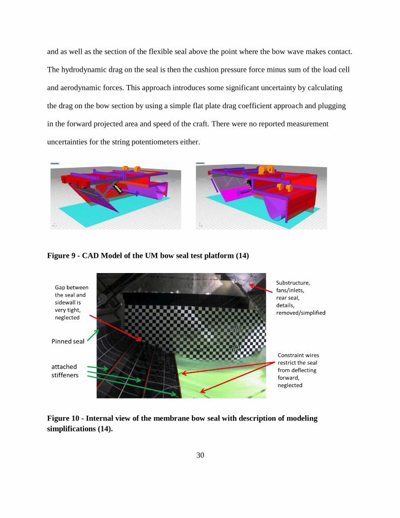
30
and as well as the section of the flexible seal above the point where the bow wave makes contact.
The hydrodynamic drag on the seal is then the cushion pressure force minus sum of the load cell
and aerodynamic forces. This approach introduces some significant uncertainty by calculating
the drag on the bow section by using a simple flat plate drag coefficient approach and plugging
in the forward projected area and speed of the craft. There were no reported measurement
uncertainties for the string potentiometers either.
Figure 9 - CAD Model of the UM bow seal test platform (14)
Figure 10 - Internal view of the membrane bow seal with description of modeling
simplifications (14).

31
One of the other issues is in the presentation of the data itself. Raw data as well as calculation
sheets were made available on a joint project research site. Some graphical data was also
available in a paper presented at the 2010 Naval Hydrodynamics Symposium (14). There was a
discrepancy between the calculation of the seal resistance between these two locations. The
website data shows the seal resistance as the load cell values minus the cushion force minus the
aerodynamics forces. The data presented in the paper is the correct approach. If the formula were
kept more general without signs or assumed directions of forces, this would not be an issue and it
would be a straightforward summation of forces. Their expression for the seal resistance is:
𝑅𝑠𝑒𝑎𝑙 = 𝑅𝑐𝑢𝑠ℎ𝑖𝑜𝑛 − 𝑅𝑙𝑜𝑎𝑑𝑐𝑒𝑙𝑙 − 𝑅𝑎𝑒𝑟𝑜𝑑𝑟𝑎𝑔 1
where 𝑅𝑐𝑢𝑠ℎ𝑖𝑜𝑛 is the total integrated force on the seal in the x-direction due to the cushion
pressure, 𝑅𝑙𝑜𝑎𝑑𝑐𝑒𝑙𝑙 is the force measured by the summation of the two loadcells, and 𝑅𝑎𝑒𝑟𝑜𝑑𝑟𝑎𝑔 is
the aerodynamic drag estimated for a flat plate of the same dimensions as the bow of the test
craft.
The flat plate bow seal design was chosen as the test case for this numerical study primarily to
remove the complexity of contact modeling and volume cell deletion and creation that would
result from the interaction of the finger type seals with each other and the SES sidewalls. To
model the thin gap between the flat seal and the rigid sidewalls of the craft would be very
computationally intensive, even without contact between the seal and sidewall. This is because
the grid cells in the thin gap would be highly distorted when the seal undergoes large
displacements and would require remeshing of the domain. The fluid domain boundary in the

32
following work does not account for the gap and the seal geometry extends all the way to the
sidewall. The structural model constrains the seal with a displacement boundary condition in the
transverse direction to remain flush with the sidewall.
Appendix B provides an overview of the experimental test runs which were selected for
simulation efforts. Simulations were run for a range of test speeds and cushion pressures
representative of the scope of the experiments.
2.3 Sloshing Tank Fluid-Structure Interaction Experiment at
Universidad Polytechnica de Madrid
The goal of this experimental FSI validation case was to track the FSI response of a 4mm thick,
neoprene beam hanging in a rotationally oscillating tank that is partially filled with water. The
calm free surface is set at the tip of the beam. A coordinate system was defined which moves
with the tank. A schematic of the experimental set-up is shown in Figure 11. The blue and red
colors represent the initial water and air distributions, respectively. The neoprene was stated to
have a density of 1900 kg/m3 and Young's Modulus of E = 4.0 MPa. Details of this experiment
are presented in (17; 60; 61). Some additional notes on the set-up specifically geared toward
modeling the problem are made below.
The experimental beam behavior as the tank oscillates and develops a sloshing free surface can
be described as follows. In the first two seconds, the beam gently sways back and forth with the
tank oscillation and has very little interaction with the free surface. As the sloshing waves
develop, the first strong interaction occurs around 2.4 seconds. The beam is swept outward to a
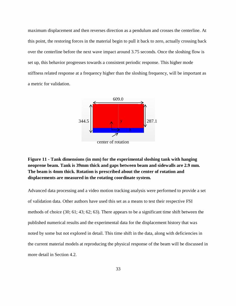
33
maximum displacement and then reverses direction as a pendulum and crosses the centerline. At
this point, the restoring forces in the material begin to pull it back to zero, actually crossing back
over the centerline before the next wave impact around 3.75 seconds. Once the sloshing flow is
set up, this behavior progresses towards a consistent periodic response. This higher mode
stiffness related response at a frequency higher than the sloshing frequency, will be important as
a metric for validation.
Figure 11 - Tank dimensions (in mm) for the experimental sloshing tank with hanging
neoprene beam. Tank is 39mm thick and gaps between beam and sidewalls are 2.9 mm.
The beam is 4mm thick. Rotation is prescribed about the center of rotation and
displacements are measured in the rotating coordinate system.
Advanced data processing and a video motion tracking analysis were performed to provide a set
of validation data. Other authors have used this set as a means to test their respective FSI
methods of choice (30; 61; 43; 62; 63). There appears to be a significant time shift between the
published numerical results and the experimental data for the displacement history that was
noted by some but not explored in detail. This time shift in the data, along with deficiencies in
the current material models at reproducing the physical response of the beam will be discussed in
more detail in Section 4.2.
x
y 344.5 287.1
609.0
center of rotation

34
A new motion tracking video analysis of the original 25 frames per second benchmark data
video was performed in this study with the video analysis tool, Tracker v4.84 (a free product of
opensourcephysics.org). The re-analysis was inspired by the aforementioned shift in the
numerical validations published for this case and a discrepancy in the reported frame rate of the
experimental video between (17) and (61). (The shift is evident in the tip displacement time
histories shown in Figure 14a.) All of the numerical results used the same input roll history and
showed the same shift away from the experimental data as time progressed.
Tracker allows both automatic and manual tracking of objects or markers which are moving in a
fixed field of view in successive frames of a video. The first step is to calibrate the image scale
by marking the pixel to true length ratio and then setting the origin of the axes. The aspect ratio
of the tank appeared to be distorted (either lens distortion or post-processing of the video aspect
ratio), so a perspective filter was added which corrected this distortion and recovered the correct
aspect ratio based on the published tank dimensions. Displacements were recorded at four
locations: 25%, 50%, 75%, and 100% of the length of the beam as in the benchmark data. An
additional point was tracked on the rotating tank in order to recalculate the roll angle history and
confirm that it was synced with the video frames.
It was determined that the video and published benchmark roll angle history (60; 17; 61) were
not synced properly and an additional 0.2 seconds of zero tank motion exists prior to the
commencement of the oscillation which was unaccounted for in the published roll angle history.
Additionally, some clipping of the peaks in the benchmark roll angle history was found in the
reanalysis which may be due to measurement uncertainty but could also point to less than ideal
dynamics of the test rig. It is not directly apparent whether or not these were smoothed out by the

35
data processing algorithms developed for this experimental set-up (60). This comparison
between the previously published roll angle history and this reanalysis is shown in Figure 12.
Figure 12 - Roll angle history comparison between benchmark (17) and Tracker analysis.
The inclusion of the perspective filter also modifies the beam displacement histories significantly
around the local absolute maxima/minima of the beam displacements. This effect is shown in
Figure 13. Also of note is that in the first 0.5 seconds of the experiment, it is apparent that the
seal actually has some prestrain which causes the initial seal position to not be on the centerline.
The motion in that first 0.5 seconds is a results of the beam dynamics and the initiation of the
motion from the top of the tank down which at first moves the beam back toward the centerline.

36
Figure 13 - Comparison of displacements at 100% length (tip) between the benchmark (17)
and Tracker analysis with perspective filter applied.
It is important to show that using the new roll angle history from the Tracker analysis improves
the validation comparisons of the previously published results, as well as the current work.
Figure 14a shows all of the available numerical results using the prescribed roll history, and
Figure 14b shows that same comparison using the new roll angle history in the current
calculation and adding 0.2 seconds to the beginning of the other numerical results to account for
the time when the tank had not yet begun its motion. Fortunately this correction is easy to make
to all of the previous results because there is no missing behavior at the beginning of each run.
The improvement in the data comparison provides clear evidence to support using the new video
reanalysis as the roll angle history input for the simulation.

37
Figure 14 - Comparison between numerical results and experimental data for a) the
original input roll history and b) the new roll history from Tracker and shifting other
authors results by t = 0.2 s (30; 61).
a)
)
b)
)

38
However, while the primary frequency of oscillation of the beam is captured, some secondary
effects are absent between the maxima in the displacement history. The secondary response peak
at approximately 3.8-3.9 seconds is representative of this restoring type behavior before the
sloshing wave impacts the tip of the beam and sends it toward an outward maximum at around
4.0-4.1 seconds.
2.4 Seal Material Calibration Experiment
The primary objective of this study is to produce the most physically accurate model for
simulating the displacements of an SES bow seal that the selected tools can provide. Limited
information is available on the material properties of the vulcanized neoprene reinforced with
nylon fabric because appropriate tests were never conducted as part of the SES bow seal
experiment to characterize its response. A small rectangular sample of the material provided for
our own inspection and use. Traditionally, standard hyperelastic test data would be obtained and
used to fit the coefficients for the model. In this study, there were no means to physically
separate the vulcanized neoprene from the inner fabric and determine the individual
characteristics of the constituent materials. Advanced material characterization is outside the
scope of this dissertation. The following represents our basic method to calibrate an FEM model
of this material in the absence of accurate material property definitions.
A static deflection experiment was devised for testing the sample in order to provide some
information about its bending characteristics and to provide a set of experimental baseline data
that could be used in calibration of the FE model. The set-up allows for the measurement of the
final static deflection of the sample when clamped on one end and allowed to hang at an initial
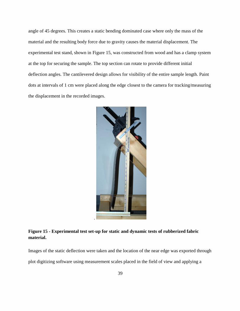
39
angle of 45 degrees. This creates a static bending dominated case where only the mass of the
material and the resulting body force due to gravity causes the material displacement. The
experimental test stand, shown in Figure 15, was constructed from wood and has a clamp system
at the top for securing the sample. The top section can rotate to provide different initial
deflection angles. The cantilevered design allows for visibility of the entire sample length. Paint
dots at intervals of 1 cm were placed along the edge closest to the camera for tracking/measuring
the displacement in the recorded images.
.
Figure 15 - Experimental test set-up for static and dynamic tests of rubberized fabric
material.
Images of the static deflection were taken and the location of the near edge was exported through
plot digitizing software using measurement scales placed in the field of view and applying a

40
correction for the distance between the sample and the scale, as well as a correction for the lens
distortion. Two tests were done at an initial angle of 45 degrees. Because of the pre-stress in the
material and a resulting initial permanent displacement, each angle was run with the seal in two
orientations to ensure the displacement in the upper portion of the seal was independent of the
pre-stress displacement. Figure 16 shows the final static displacements for the 45 degree initial
angle case. The inward and outward profiles show the effect of the initial pre-stress in the
material. However, the upper displacements of the two tests show that the two displacements
agree in the region that is dominated by bending. An average displacement based on the inward
and outward profiles was calculated and will serve as the comparison between experimental and
numerical work. The horizontal scale is exaggerated here to highlight the discrepancy due to the
pre-stress state.
Figure 16 - Raw experimental results highlighting the pre-stress state of the sample in two
configurations and the average displacement for the 45° case.
0
0.05
0.1
0.15
0.2
0.25
0.3
0.35
0.4
0.45
0.5
0 0.05 0.1 0.15 0.2 0.25
z (m
)
x (m)
Inward
Outward
45 avg

41
Chapter 3
Computational Methodology
Computational studies on the performance of marine vehicles have evolved concurrently with
advances in computer science and fluid dynamics over the last half century. In the old days, ship
designers drew plans for ships by hand. A new hullform was tested against geometrically similar
models in a towing tank to gain insight into its performance characteristics. Then it would be
constructed by master boat builders into its final hydrodynamic shape. Throughout this process,
engineers and designers have been making use of the computer from very early on to aid with
design calculations which would have otherwise been extremely labor intensive or impossible
with human computers and early electronic computers. Early stage concept design might use
resistance and powering estimates based on empirical data and regression analyses. Such
methods contain inherent uncertainties which must be allowed for early on so that the final ship
will be within the design margins. The end result of large uncertainties is a higher cost to the ship
owner, whether it is in increased fuel consumption, shorter design life, or downtime due to
unsafe conditions outside of the operating envelope.
Even in today’s world of computers, model testing is still a very critical tool in modern ship
design. State of the art data measurements and signal processing techniques with good
uncertainty estimates are still the most reliable tool for qualifying ship designs and providing

42
data to validate numerical models. However, model testing is expensive, time consuming and
often carried out at scales much smaller than the intended design. The model basin is a very
valuable tool to designers for studies, but each year as computational power grows, the numerical
model basin becomes a more attractive solution to exploring design spaces and localized flow
phenomena. With the integration of high fidelity physics simulations and verification and
validation efforts, it is now possible to provide real world answers to complex physical problems
which previously were not computationally feasible. It is the goal of this work to provide
guidance and information about the capabilities of the selected computational approaches, and
not to develop wholly new algorithms and computational methods themselves. With that in
mind, the computational approaches will be described in detail as tools which can further the
usefulness of numerical model basin approaches to ship design analysis.
3.1 Computational Fluid Dynamics
The initial body of work which led to the current simulations was performed using
Computational Fluid Dynamics (CFD) as a standalone tool for analyzing performance
characteristics of SES designs. CFD encompasses a large array of numerical methods for
predicting the flow of gas and fluid. The central idea is to take a geometrical representation of a
body of interest, discretize the governing equations of fluid flow onto a surrounding
computational grid, apply boundary conditions, and solve for the fluid velocities, densities, and
pressures in the domain of interest.
3.1.1 STAR-CCM+
STAR-CCM+ is a commercial software package developed by CD-adapco. It is a finite volume
solver with significant multi-physics capabilities including tools for FSI, rigid body dynamics,

43
and free surface flow. The main methods used by STAR-CCM+ in the present calculations are
described below. An entire simulation workflow can start and end in STAR-CCM+, however it
also has the added benefit of being able to interface with third party packages to enhance its
capabilities further and being integrated as a black box CFD solver within a FSI framework.
3.1.2 Finite Volume Method
At the core of STAR-CCM+ is a finite volume solver which calculates solution values at a finite
number of control volumes whose size and distribution are defined by the generation of a
computational grid throughout the volume of interest. The integral formulation of the governing
conservation equations are discretized and then applied at each cell. The variables are stored at
the cell centers and numerical interpolation, integration, and differentiation are used to get the
values and fluxes at cell faces. The resulting algebraic equation for each cell is a function of the
solution variables in neighboring cells and previous time steps. Here we choose to solve the
Reynolds Averaged Navier-Stokes (RANS) equations. These nonlinear equations are iteratively
solved with Algebraic Multigrid (AMG) using a collocated variable arrangement, Rhie and
Chow-type velocity-pressure coupling, and a SIMPLE-type algorithm. In general, 2nd order
temporal and spatial discretizations are employed. When initial conditions require extra
dissipation, 1st order temporal schemes have been used as recommended in (64).
The general Navier-Stokes equations for conservation of mass and momentum may be expressed
in the following integral forms:
𝑑
𝑑𝑡∫ 𝜌 𝑑𝑉 + ∮ 𝜌 (𝒗 − 𝒗𝑔) ∙ 𝑑𝒂
𝐴𝑉
= 0 2

44
𝑑
𝑑𝑡∫ 𝜌𝒗 𝑑𝑉 + ∮ 𝜌𝒗 × (𝒗 − 𝒗𝑔) ∙ 𝑑𝒂
𝐴𝑉
= ∮ 𝑝𝑰 ∙ 𝑑𝒂
𝐴
+ ∮ 𝑻 ∙ 𝑑𝒂
𝐴
+ ∫ (𝒇𝑟
𝑉
+ 𝒇𝑟 + 𝒇𝑟 + 𝒇𝑟)𝑑𝑉 3
Equation 2 is the conservation of mass in integral form with density, ρ, and fluid velocity, v. The
equations are written to account for the motion of the entire grid as a whole (rigid body) or
relative to the grid (grid deformation), and therefore vg is the velocity of the cell. The left hand
side of Equation 3 contains the transient term and convective flux for momentum. The right hand
side includes terms for the pressure gradient, the viscous flux, and any additional body force
terms such as a gravitational field. T is the viscous stress tensor.
3.1.3 Reynolds-Averaged Navier-Stokes (RANS) Equations
When calculating CFD solutions for practical problems in design and engineering, often times it
is unnecessary to capture the complex turbulent flow structures at the smallest scales. Design
analysis typically requires integral quantities such as averaged force on a body or pressure
distributions on a wetted hull which can be predicted without the full resolution of turbulent
structures in the flow. The Reynolds-averaged approach takes all of the unsteadiness in the flow
and averages it out and considers it part of the turbulence. The averaging process combined with
the nonlinear nature of the equations includes turbulent production and dissipation terms which
must be modeled in simulation. These terms are modeled because of the disparity that exists
between the true turbulent length scales and the grid size in the computational domain and
regions of viscous flow.
The central idea in Reynolds-averaging is that for an unsteady flow, ensemble averaging can be
used to write any flow variable in terms of an average value and a fluctuation about that average.
For some value, ϕ:

45
𝝓(𝑥𝑖) = �̅�(𝒙𝑖) + 𝝓′(𝒙𝑖, 𝑡) 4
This approach is applied to the terms in the continuity and momentum equations and through
ensemble averaging of nonlinear terms, two separate terms arise; one from the product of the
average and a covariance. Omitting the details of the derivations, this leads to the incompressible
RANS equations shown here in differential form with tensor notation,
𝜕(𝜌�̅�𝑖)
𝜕𝒙𝑖 = 0 5
𝜕(𝜌�̅�𝑖)
𝜕𝑡+
𝜕
𝜕𝒙𝑗 (𝜌�̅�𝑖�̅�𝑗 + 𝜌𝒖′𝑖𝒖′𝑗̅̅ ̅̅ ̅̅ ̅) =
𝜕�̅�
𝜕𝒙𝑖+
𝜕�̅�𝑖𝑗
𝜕𝒙𝑗 6
The Reynolds stresses, 𝜌𝒖′𝑖𝒖′𝑗̅̅ ̅̅ ̅̅ ̅, and the turbulent scalar flux, 𝜌𝒖′𝑖𝝓′̅̅ ̅̅ ̅̅ ̅, are two such terms that
arise and must be modeled numerically. These additional terms are additional unknowns in the
equations and therefore the equations must be closed by approximating them with a turbulence
model, introducing another equation to the system. Turbulence models vary in complexity from
one to two equation models, and various forms of handling the additional terms.
Based on the complexity of the grid morphing and the highly mixed flow in the region of the
bow seal, a conscious decision was made to accept a higher level of approximation by using a
one equation turbulence closure model, the Spalart-Almaras model (65).
Turbulence models are greatly influenced by the near wall spacing of the grid near walls and
regions of viscous flow where a wall model is applied. Prims layers or boundary layer fitted
grids are normally placed there with spacing such that y+ values near the wall are close to unity.
However, in the morphing procedure described shortly, the near wall grid spacing also can

46
negatively impact the stability of a partitioned FSI simulation and limit the stable coupling step
size in simulation. Due to this difficulty in selecting a grid size suitable for a more accurate
turbulence model, it was decided to just use the SA model and accept some level of numerical
error based on the grid size in the viscous flow regions. Results will later support this decision by
observing the ratio of frictional force on the seal to that of hydrodynamic and cushion pressure.
3.1.4 Volume of Fluid Method
When solving for fluid solutions to multiphase problems with RANS equations, there are two
general classifications of solution techniques. The first class, named interface tracking methods,
explicitly follow the interface between the fluids as a solution boundary on which the free
surface boundary conditions are imposed. The second class is interface capturing methods where
the interface is captured by the calculation of a volume fraction. Any cell can have a volume
fraction between 0 and 1 which prescribes its mixture of the two fluids. Through interpolation, a
surface can be placed along the interface between the two fluids where the volume fraction is
equal to 0.5 as an approximation of the free surface location.
The Volume of Fluid (VOF) method (66) for interface capturing modifies the solution scheme by
adding an additional transport equation for the volume fraction of fluids within the domain. This
is analogous to the transport of any scalar values in the domain through the use of the Reynolds
Transport theorem.
𝑑
𝑑𝑡∫ 𝛼𝑖 𝑑𝑉 + ∮ 𝛼𝑖 (𝒗 − 𝒗𝑔) ∙ 𝑑𝒂
𝐴𝑉
= ∫ 𝑆𝛼𝑖 𝑑𝑉
𝑉
7
The assumption that all fluids which are present in a single cell share velocity, pressure, and
temperature fields allows the transport equations to be solved with an equivalent fluid definition

47
which is calculated as a function of the properties of the individual fluids and their volume
fractions.
Additionally, in the region near the interface, special treatment is provided through the High-
Resolution Interface Capturing (HRIC) scheme. The HRIC scheme was developed to mimic the
convection processes between multiphase fluid components and maintain a sharp interface. This
is achieved by modifying the cell face values through a blending of discretization schemes as a
function of local CFL number and the relationship of the cell face to the interface position and
properties (67).
3.1.5 Grid Generation
STAR-CCM+ has region based meshing as well as parts based meshing models for generating
the computational grid. The automation of the meshing process, while still producing quality
grids, has significantly affected the CFD industry where before the grid generation and attention
to detail accounted for a major portion of project time. In the current workflow, the geometry of
interest is imported, its faces spit into appropriate boundaries, manual grid sizes are applied as
surface or volume refinement, and then an automated mesh solver produces the computational
grid. For relatively simple geometries this process can be very hands-off. With tighter tolerances
and more complex geometries, more user intervention is required to clean up irregularities and
low quality cells.
For free surface applications using VOF multiphase flow, Cartesian cells aligned with the calm
water free surface are desirable. This grid architecture allows for much sharper capturing of the
air-water interface and its convection through the domain. It also allows for straightforward
refinement in the vertical direction to resolve any generated waves. The mesh solver produces a

48
general template of hexahedral cells which are orthogonal and aligned with the initial free
surface position. Cells which contain arbitrary solid boundaries are trimmed at the boundary
resulting in irregular polygons. A near wall prism layer was added with spacing set so that the
wall y+ < 40. This value is appropriate for the “all y+ wall model” and SA turbulence model
(37).
Another grid model which was implemented was the Extruder model. This model takes the
generalized outer domain boundaries and extrudes them along the outward normal, producing
prismatic cells with specified growth factors. This is useful especially in free surface problems to
handle the propagation of gravity waves out of the region of interest without reflection back into
the domain. The growth of the cells in the extrusion acts as a numerical beach to damp the wave
energy and reduce the sensitivity of the solution to the boundary conditions and position.
3.1.6 Lift Fan Model
The cushion pressure in full scale craft and in the model tests is provided by centrifugal blower
fans. The interaction between the fans’ performance characteristics, the ducting and plenum, and
varying free surface profile create a dynamic system which usually requires a feedback control
system to maintain the desired cushion pressure. In calm water, the cushion pressure achieves a
steady state with some small fluctuations about the average value. This behavior is shown in
Figure 17 by the blue curves, which represent the cushion pressures in the T-Craft model tested
at NSWCCD. The forward and aft pressure probes highlight a significant differential in the
cushion pressure between these two regions.
In order to reduce computational complexity, the details of the sub-structure, ducting, and blower
fans are neglected in the SES simulations. Instead, a constant strength momentum source lift fan

49
model was implemented to provide the interior cushion pressure. This concept was first explored
in (33). In those simulations, the actual placement and geometry of the inlets replicated those of
the experimental model. The momentum source numerically imparts momentum into the flow
and provides a very consistent cushion pressure. Figure 17 also shows the numerical cushion
pressure probe time history from a corresponding simulation and the smoother pressure response
is evident in the red curves. The pressure differential is also present, and a result of applying
different values of momentum source strength to match the correct pressures as seen in the
experiment. While the pressures disagree slightly between the experiment and simulation, the
momentum source strength can be calibrated to achieve the desired pressure, and the consistency
of the pressure affirms that this model provides a good approximation.
Figure 17 – Comparison between the experimental and numerical cushion pressure probe
time histories for momentum source lift fan model for the T-Craft SES model (33).
This method will tend to produce less accurate results when the dynamics of the system are
important. Phenomena like cobble-stoning and motion damping due to the cushion pressure and
lift fan system will not be captured. The primary simulations shown in this work are calm water
0
50
100
150
200
250
0 1 2 3 4 5
Pre
ssu
re,
Pa
Time, s
Sim: Fwd Cush
Sim: Trans Seal
Sim: Aft Cush
Run 595, Channel 38:
Fwd Cush
Run 595, Channel 39:
Trans Seal
Run 595, Channel 40:
Aft Cush

50
towing tank tests in a simplified SES geometry. This work models the lift fan as a large
rectangular momentum source which spans most of the deck above the cushion.
Figure 18 - Visualization of the pressure rise across the momentum source due to a
constant strength source term.
3.2 Finite Element Analysis
3.2.1 Abaqus
An Abaqus model is the compilation of input components which detail the physical problem
under consideration, the solution methodology, and the types of information that are required for
further analysis. At the core of every finite element analysis is the geometry of interest. The
overall geometry is subdivided into a discrete number of finite elements. Each element is
comprised of nodes, and shares them with other interconnected elements immediately
surrounding it. Together, all of the elements and nodes form a grid which defines the discretized
structure. Appropriate spatial discretization is critical to the accurate prediction of stresses and

51
displacements with finite element analysis and will be discussed later. If the mathematical
models for the solvers have been verified, then the model should approach a unique solution with
grid refinement. If the approximations made in the model setup are good and error sources have
been minimized, then the model should also approach the physical solution. Elements may have
additional geometric information beyond just the nodal locations. These element section
properties describe features such as layers in composites or fiber directions, the homogeneity of
the material, or the element type. Elements can simply be three-dimensional homogeneous
continuum elements, two-dimensional plane stress/strain elements, or one-dimensional rods, etc.
Populating the elements with material data provides the necessary information to reproduce the
material's behavior. The quality of the material data directly affects the ability of the simulation
to make an accurate prediction of a structural response. The structural response and stress
distribution under a given load is generally the goal of finite element analysis. In this work, fluid
forces (pressure and shear stress), and gravitational body force are acting on the structure. The
physical model is generally constrained in some way unless rigid body motion is under
consideration. Both situations require boundary conditions to either define nodes which are fixed
or that have some prescribed displacement, velocity, or acceleration. The type of analysis is
specified and determines the solver to employ for the application (e.g.- static, dynamic, or a
modal analysis). The solver assembles the information that comprises the model and forms the
discretized equations which must be solved. Output can be specified at a number of locations in
reference to the model and individual elements to be used in further analysis of the response. In
this chapter, the relevant formulations and solvers used in the presented finite element models
will be described.

52
3.2.2 Implicit vs. Explicit Solver
The primary division in Abaqus analyses is whether the discretized system is solved implicitly or
explicitly. The different nature and timescales of the physical phenomena require certain
characteristics from the selected numerical solution technique. Problems like elastic wave
propagation in solids occur over short timescales at very high speeds. They are suited to explicit
schemes which advance the solution without iteration and calculate the new state based wholly
on the previous increment by calculating the accelerations at the current time and integrating
forward to the new time level. Explicit methods are conditionally stable and generally require
very small time steps. There is a trade-off between problem size and solution efficiency between
the two methods. A large implicit analysis requires the iterative solution of a costly system of
equations, but can be more accurate for smooth nonlinear problems. They are also
unconditionally stable. The solution of an increment with the implicit method requires the
inversion of the global stiffness matrix which can be costly for large numbers of degrees of
freedom. An explicit analysis can sometimes perform more efficiently for large numbers of
degrees of freedom in the model.
3.2.3 General element overview
The finite elements used to discretize the structural geometry have five aspects which affect the
behavior of the element and as a result, the overall solution. The first of these is the element
family which describes the type of problem being solved and the level of fidelity in the model.
The major families of elements include 3D continuum, shell, beam, rigid, truss, and membrane
elements. Each is geared towards a specific state of stress or structure which is being modeled.
There are also special purpose elements for springs, connectors, and dashpots. The second
feature of an element is its degrees of freedom. They are the primary solution variables which are

53
solved for at the nodes of the model. In a stress/displacement analysis, the degrees of freedom
are the displacements of the nodes. Rotations and temperature can also be a degrees of freedom
in certain element families. The total number of degrees of freedom in all the connected elements
is dependent on the third feature, the total number of nodes and the order of interpolation. The
solution variables are only solved for at the nodes of the model, and therefore to obtain the
solution at an arbitrary point requires the interpolation of the nodal solution values to that
location. The order of interpolation is determined by the total number of nodes in the element.
The two primary element types are linear (1st order interpolation) and quadratic (2nd order
interpolation). For 3D continuum elements, linear elements have 8 nodes and quadratic have 20
nodes. The fourth and fifth features of an element are its formulation and integration. At the
highest level, stress/displacement elements use a Lagrangian formulation which tracks the
displacement of material following the material trajectory and motion. An element preserves its
given material during the course of a step in the absence of any adaptive remeshing. Alternative
formulations are provided for elements which capture certain behaviors with respect to material
compressibility and bending behavior. The integration of quantities within the elemental volumes
is determined by the integration scheme. Typically, Gaussian quadrature is used but a choice can
be made to use full or reduced integration when evaluating these integrals at the specific
integration points of an element.

54
3.2.4 Continuum elements
Figure 19 - Node and face numbering scheme for 8 and 20 node three-dimensional solid
elements. (68)
The three-dimensional continuum elements shown in Figure 19 are solid bricks and include both
linear and quadratic interpolations with full and reduced integration. They also support hybrid
and incompatible mode formulations. The accuracy of a finite element model relies heavily on
the selection of the element and properties with respect to the problem of interest. Fully
integrated linear 3D elements have eight nodes and eight integration points. Conversely, a fully
integrated quadratic element has 20 nodes and 27 integration points. The integration point
numbering scheme near face 1 is shown in Figure 20.

55
Figure 20 – 8 and 20 node Fully integrated elements with integration point numbering
scheme. (68)
The relative accuracy of fully integrated elements can be observed by setting up a model of a
cantilevered beam and comparing the tip displacement to the exact solution from beam theory.
This will be shown in more detail later but the main result is that the linear, fully integrated
elements under predict the tip displacement because the elements are too stiff in bending. This is
result of a numerical error caused by shear locking of the elements. Shear locking exists because
of the discretization of a solid into orthogonal brick elements. In pure bending of a beam, the
lines parallel to the horizontal axis will deform with constant curvature. With a linear element the
edges are unable to curve and this deformation cannot be represented by the element. Normally
the shear stress in a pure bending situation is zero throughout the structure. When the linear
element distorts, the lack of curvature forces the material to undergo shear stress at the
integration points. Some locking may still occur in fully integrated quadratic elements as well in

56
states of high distortion or areas of high stress gradients. Volumetric locking can also occur with
nearly incompressible materials and produces overly stiff behavior when a displacement should
not induce any volumetric change.
Figure 21 – 8 and 20 node Reduced integration elements with integration point numbering
scheme. (68)
In comparison, Figure 21 shows the nodal positions in both the linear and quadratic reduced
integration elements. Now the reduced integration linear 3D elements have eight nodes and one
integration point. Conversely, a reduced integration quadratic element has 20 nodes and 8
integration points. The same solution verification procedure can be performed to show that
linear, reduced integration elements are generally too flexible due to another numerical error
known as hour-glassing. With hour-glassing, an integration point will now be at the centroid of
the element for the linear case and the lines which run through and element do not change in
length. This results in a zero-energy state inside the element even though the element is distorted.

57
Using these elements can result in meaningless deformation predictions. Hourglass stiffness is
introduced for these elements which allow them to be used, albeit with very fine grids.
Specifically, in bending dominated problems, care should be made to ensure an appropriate
number of elements through the thickness to ensure that the bending stresses may be resolved.
The quadratic reduced integration elements are generally free of locking and are a good general
purpose element for stress/displacement analysis. Best practice guidelines recommend using
quadratic reduced integration in most cases unless very large strains are encountered, in which
case the fully integrated elements are preferable. (68)
The hybrid formulation is used when the material behavior is incompressible or very close to it.
This corresponds to a Poisson ration close to 0.5. Undergoing a uniform pressure will produced
no volume change in this type of material, and the pressure stress can no longer be determined
strictly from the displacement field. Since flexible rubber materials are the subject of this work,
the use of the hybrid formulation will be investigated.
3.2.5 Shell Elements
Two distinct shell element types are available in Abaqus. They are conventional 2D shell
elements and 3D continuum shell elements. The conventional shell element discretizes a planar
surface with a surface normal and curvature to represent the 3D surface. The thickness is not
defined through the nodes but instead through a section property. Conversely, the 3D continuum
shell element does define the surface with the nodal positions, but has a formulation that has
similar constitutive and kinematic behavior to the conventional element. The 2D conventional
shell element will be utilized to model the fiberglass stiffener rods placed transversely across the
back of the seal.

58
Figure 22 - Schematic of Shell element modeling types. (68)
The shell thickness must be specified for the cross-section which defines the locations of the
numerical integration points through the thickness of the shell. The fiberglass stiffeners used in
the University of Michigan seal experiment should respond in the linear elastic regime and
therefore some approximations have been made. The cylindrical fiberglass rods will be modeled
with a rectangular shell element with the same cross-sectional area. The sectional area moment
of inertia will be different, but for the purposes of keeping the seal deformation relatively two-
dimensional in nature, this should be acceptable. The primary reason for this approximation is to
create a stiffener whose nodes line up with the nodes of the continuum elements on the seal to
ease the creation of tie constraints between the two surfaces and reduce model complexity.
3.2.6 Membrane Elements
Membrane elements are used to model thin materials and surfaces that provide strength in the
in-plane direction but have little to no bending stiffness. Examples of these materials are cloth or
fabric used in tents, parachutes, airbags, or thin sheets of latex in balloons and gloves. The inner
nylon fabric layer of the SES seal material also falls into this category. It provides the composite
material with the strength to make it inextensible in plane, but does not affect the overall bending

59
rigidity. A four node reduced integration element, M3D4R, is implemented in the current work
for this purpose.
3.2.7 Nonlinearities
In continuum structural dynamics, there are three sources of nonlinearity in the solution. They
are material, boundary, and geometric nonlinearities. Material nonlinearity arises from the
constitutive behavior of the material with regards to stress vs. strain. Generally metals will
respond linearly to stress for low strains but can yield and become nonlinear and plastic. Rubber
materials such as the vulcanized neoprene on SES seals exhibit a nonlinear relationship between
stress and strain even at low strains as shown in Figure 23. These differences are related to the
micro-structure of the materials. Rubbers have cross-linked polymers which behave differently
once stretched and loaded whereas metals have a crystalline lattice structure which behaves
much more uniformly.
Figure 23 – Nonlinear stress vs. strain relationship for a vulcanized neoprene rubber. (69)

60
Boundary nonlinearity arises when the boundary conditions change during the middle of an
analysis. An example of this is during contact analysis or fluid-structure interaction when the
structure encounters a rigid body or changing loading conditions which in turn affect the
response.
Geometric nonlinearities typically arise when a structure undergoes large deformations to the
point that the displacements affect the response of the structure. For large deformations, both the
shape of the structure can change altering the section stiffness or the action of the load can be
vastly different than the initial loading. For a cantilevered beam, an end load which is initially
perpendicular may, after some time has passed, be resolved into an axial and tangential
component to the tip of the beam. Snap through and initial stress distributions are also sources of
geometric nonlinearity. The vulcanized neoprene is prone to carrying a pre-stress from its
manufacturing or time spent in the roll of material.
For nonlinear problems Abaqus uses a Newton-Raphson method where the loads are ramped
over a loading increment until the external loading and internal forces are in balance. This can
often take several iterations to converge for a given load increment. The general hierarchy of an
analysis is broken up into steps, increments, and iterations. A step is an overarching time period
where loads and boundary conditions are applied. Each step is broken up into increments where
the loading is applied to the nodes in a gradual fashion. Likewise, an increment is further
subdivided into iterations using an implicit method. The iterations continue until the solution
satisfies the equilibrium conditions at which point the increment is complete.

61
3.2.8 Nonlinear Dynamics Formulation
The displacement-based finite element formulation is based on the principal of virtual work. The
goal is to find an approximate solution for the state variables (i.e. displacement, deformations,
stresses) of a solid body which is subjected to some loading. To solve such a problem, the force
and moment equilibrium must be satisfied within an arbitrary volume of that body. The finite
element method approximates the equilibrium condition by applying that condition in a weaker
sense, that the equilibrium must be maintained as an average over a finite number of divisions of
the body. The discretized equilibrium equations are,
𝑴𝑁𝑀�̈�𝑀 − 𝑷𝑁 + 𝑰𝑁 = 0 8
where 𝑷𝑁 is the external force vector, 𝑰𝑁 is the internal force vector developed from the stresses
in the interior of the element, 𝑴𝑁𝑀is the consistent mass matrix, �̈�𝑀 is the element acceleration,
and 𝑴𝑁𝑀�̈�𝑀together is the force vector arising from material inertia.
The internal forces are given by the following relation,
𝐼𝑁 = ∫ 𝜷𝑁
𝑉
: 𝝈 𝑑𝑉0 9
where 𝑉0 is the undeformed volume of the model, 𝝈 is the stress tensor at a point in the model,
and 𝜷𝑵is the strain rate-displacment rate transformation defined by the constitutive material
property stated in the element definition. This term is where the use of a linear elastic or
hyperelastic model is made distinct in the model.
The internal force vector 𝑷𝑁 is given by,
𝑷𝑁 = ∫ 𝑵𝑁
𝑆
∙ 𝒕 𝑑𝑆 + ∫ 𝑵𝑁
𝑆
∙ 𝑭 𝑑𝑉 10

62
where 𝑵𝑁are the element shape functions, 𝒕 is the traction vector on the surface S, and 𝑭 is the
externally prescribed body force vector.
The dynamic procedure employs a generalized Hilbert-Hughes-Taylor solver in the transient
fidelity setting for the temporal integration. This integrator is an extension of the Newmark-β
method and adds controllable numerical damping which is beneficial when automatic time
stepping scheme is used. The numerical damping has the effect of damping or eliminating the
numerical noise which is produced when the scheme modifies the time step. The dynamic
implicit time integration procedure was used with an initial increment size of 0.00001 seconds,
sub-cycling enabled, and auto-incrementation to control the size of the increment. Because the
operator is implicit, its matrix must be inverted and a set of simultaneous nonlinear equilibrium
equations has to be solved during each increment. The inner solution of the nonlinear
equilibrium equations is performed with Newton’s method. The HHT operator replaces the
equilibrium statement with an expression for the balance between the d’Alembert forces at the
end of a time step with a weighted average of the static forces between the beginning and the end
of a step:
𝑴𝑁𝑀�̈�𝑀|𝑡+∆𝑡 + (1 + 𝛼)(𝑰𝑁|𝑡+∆𝑡 − 𝑷𝑁|𝑡+∆𝑡) − 𝛼(𝑰𝑁|𝑡 − 𝑷𝑁|𝑡) + 𝑳𝑁|𝑡+∆𝑡 = 0 11
where 𝐿𝑁|𝑡+∆𝑡 is the sum of the Lagrange multiplier forces associated with the degree of freedom
N. To complete the operator definition, the Newmark formulas for velocity and displacement are:
𝒖|𝑡+∆𝑡 = 𝒖|𝑡 + ∆𝑡�̇�|𝑡 + ∆𝑡2 ((1
2− 𝛽) �̈�|𝑡 + 𝛽�̈�|𝑡+∆𝑡) 12
and
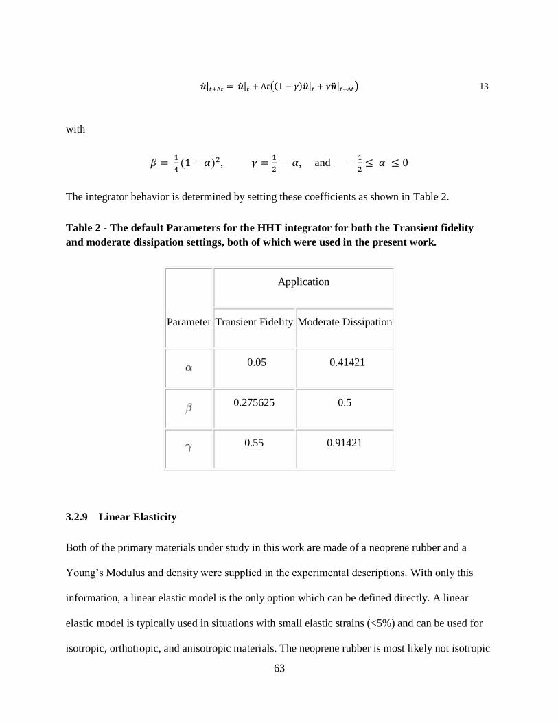
63
�̇�|𝑡+∆𝑡 = �̇�|𝑡 + ∆𝑡((1 − 𝛾)�̈�|𝑡 + 𝛾�̈�|𝑡+∆𝑡) 13
with
𝛽 = 1
4(1 − 𝛼)2, 𝛾 =
1
2− 𝛼, and −
1
2≤ 𝛼 ≤ 0
The integrator behavior is determined by setting these coefficients as shown in Table 2.
Table 2 - The default Parameters for the HHT integrator for both the Transient fidelity
and moderate dissipation settings, both of which were used in the present work.
Parameter
Application
Transient Fidelity Moderate Dissipation
–0.05 –0.41421
0.275625 0.5
0.55 0.91421
3.2.9 Linear Elasticity
Both of the primary materials under study in this work are made of a neoprene rubber and a
Young’s Modulus and density were supplied in the experimental descriptions. With only this
information, a linear elastic model is the only option which can be defined directly. A linear
elastic model is typically used in situations with small elastic strains (<5%) and can be used for
isotropic, orthotropic, and anisotropic materials. The neoprene rubber is most likely not isotropic

64
due to the nature of rubber chemistry and the long polymer chains which define its molecular
structure. In the absence of any information pertaining to the directional dependencies of its
behavior, an isotropic, linear elastic model is defined however. Here the total stress, σ, is defined
with the total elastic strain, εel,
𝝈 = 𝑫𝒆𝒍𝜺𝒆𝒍 14
where 𝑫𝒆𝒍 is the fourth-order elasticity tensor. This material definition is not recommended when
the elastic strains become large. This model will be used for solution verification studies and
initial comparisons of the displacements. The Poisson ratio was not provided, but other authors
have assumed a value of 0.49 which is typical of rubber-like materials which are fully or nearly
incompressible.
3.2.10 Hyperelasticity
Rubber behaves differently than linear elasticity predicts and has a nonlinear stress-strain
relationship, large deformations, and often hysteresis effects during loading cycles. Hyperelastic
material models need specific test data to define their model coefficients or at the very least good
estimates thereof to be used effectively. When very large strains are encountered as is common
with hyperelastic materials, the stress-strain relationship derived in linear elasticity is no longer
valid. A strain energy potential can describe a hyperelastic material and defines the strain energy
stored per unit of reference volume as a function of the strains at that location. The stress-strain
relationship for the solid is defined by specifying the strain energy density 𝑊as a function of the
deformation gradient, 𝑊 = �̅�(𝐹). To set up the analysis, some deformation measures will be

65
defined below. For a solid which is subjected to a displacement field, 𝑢𝑖(𝑥𝑘), the deformation
gradient, 𝐹 is,
𝑭𝑖𝑗 = 𝜹𝑖𝑗 +𝜕𝒖𝑖
𝜕𝒙𝑗 15
and its Jacobian is,
𝐽 = det (𝑭) 16
Then the Left Cauchy-Green deformation tensor, 𝑪, can be defined which will be used as a
deformation measure for the deformed material.
𝑪𝑖𝑗 = 𝑭𝑖𝑘𝑭𝑗𝑘 17
In order for the constitutive equation to be objective, the strain energy density should be a
function of the invariants of 𝑩. These are defined as,
�̅�1 = 𝑪𝑘𝑘
𝐽2/3 18
�̅�2 = 1
2(𝐼1̅
2 −𝐶𝑖𝑘𝑪𝑘𝑖
𝐽4/3) 19
𝐽 = √det (𝑪) 20
In order to get the true Cauchy stress, σ, the constitutive law must be formed which relates the
strain energy density to the three invariants of 𝐵,

66
𝝈𝑖𝑗 = 2
𝐽[
1
𝐽2/3 (𝜕�̅�
𝜕�̅�1
+ 𝐼 ̅1
𝜕�̅�
𝜕�̅�2
) 𝑩𝑖𝑗 − (�̅�1
𝜕�̅�
𝜕�̅�1
+ 2�̅�2
𝜕�̅�
𝜕�̅�2
)𝜹𝑖𝑗
3−
1
𝐽4/3
𝜕�̅�
𝜕�̅�2
𝑩𝑖𝑘𝑩𝑘𝑗] +𝜕�̅�
𝜕𝐽𝜹𝑖𝑗 21
Abaqus has a range of models to represent the strain-energy potential of rubber materials. The
generalized polynomial rubber elasticity potential provides a phenomenological basis for a
hyperelastic model which represents observed behavior of rubber elasticity (46). The strain
energy density, �̅�, is a function of the invariants of the deformation tensor, 𝐼1̅, 𝐼2̅, and 𝐽.
�̅� = ∑ 𝐶𝑖𝑗(�̅�1 − 3)𝑖(
𝑁
𝑖+𝑗=1
�̅�2 − 3)𝑗 + ∑𝐷𝑖
2(𝐽 − 1)2𝑖
𝑁
𝑖=1
22
The generalized polynomial model is implemented in many codes and often is simplified into
two other common models which are special cases found by setting 𝑁 = 1 and choosing the 𝐶𝑖𝑗
appropriately. These are the Mooney-Rivlin (47) and Neo-Hookean models, respectively.
�̅� = 𝐶10(�̅�1 − 3) + 𝐶01(�̅�2 − 3) + 1
𝐷1
(𝐽 − 1)2 23
�̅� = 𝐶10(�̅�1 − 3) + 1
𝐷1
(𝐽 − 1)2 24
In order to use the strain energy potential the coefficients need to be populated and can be set
with the following relations relating the shear modulus, 𝜇, and the bulk modulus, 𝐾, to the
components of the left Cauchy-Green deformation tensor:
𝜇0 = 2(𝐶01 + 𝐶10) 25

67
𝐾0 = 2
𝐷1 26
These values are either calculated to fit a battery of experimental test data or must be
approximated if no such data is available. (68)
3.3 Partitioned Coupling for Fluid-Structure Interaction
The co-simulation tool has seen several significant advances over the past four years. Starting as
a file based transfer tool for one way coupling, the implementation of more advanced algorithms
based on iterative exchange of force and displacement has enabled the solution of strongly
coupled FSI problems.
3.3.1 Data Mapping and Transfer
The simulation work flow at the highest level proceeds as shown in Figure 24. One simulation is
chosen as the leading simulation while the other lags behind in the exchange of information.

68
Figure 24 – Co-simulation workflow showing the primary steps of running the solvers,
checking convergence criteria, and transfer and mapping of data.
The green triangles in Figure 24 represent the exchange of data between the two respective
codes. Data mapping must be performed because the two unique computational grids share the
same source surfaces, but they are not required to be conformal, i.e., node to node matching on
the coupling boundary surface. At the beginning of the simulation, the fluid boundary and
structure surface must match within a specified tolerance in order to proceed with the co-
simulation.
By specifying a reference configuration, the co-simulation mappers are able to create the field
import and export mapper functions which define the relationship between the fluid cell centers
and the finite element nodal locations. The reference configuration can either be specified as the

69
original (un-deformed) surfaces, or the current (deformed) coordinates. This is useful when
starting with a pre-deformed structure or restarting a co-simulation.
In the simulations presented in this work, the exchanged fields are the fluid pressure and shear
stress on walls from the CFD simulation, and the structural nodal displacements from the CSM
simulation. The pressure and shear stress at cell centers are mapped to an equivalent traction
vector applied at each of the surface nodes of the finite elements. In turn, the displacements at
the nodes are mapped to displacements at the vertices of the cells and applied through the use of
a grid morphing algorithm, to be described shortly.
3.3.2 Partitioned Solution Algorithm
When both of the codes are run with implicit solvers, as is the case here, then Abaqus is typically
run as the lead simulation. Considering a single coupling step, the procedure is shown in Figure
25.
Figure 25 – Order of solver runs for a single coupling step with implicit solvers.
In this way the response calculated in the increment for the structural solver influences the
response of the fluid solver during that same increment in step 2. As a result, the procedure must
become iterative within an increment and the solutions should be passed back and forth until the
solution converges towards equilibrium otherwise instability can occur. This effect was

70
described previously in Section 1.3.2. The general scheme now looks more like that shown in
Figure 26. The structural code runs first with initial conditions from the fluid domain and gets an
initial estimate of the displacement. The dynamic boundary condition on the coupling surface
which relates the interaction traction on the fluid interface to the mapped concentrated nodal
loading is,
𝝈𝛤𝑆 ∙ 𝒏 = 𝝈𝛤
𝐹 ∙ 𝒏 27
The nodal displacements at the interface, 𝒅𝛤, are passed to the fluid grid morphing algorithm
which then generates an interpolation field everywhere in the interior of the fluid domain. This
field is applied to all of the fluid domain vertices and corrections are made for consistency near
boundaries based on morphing boundary types and condition. Next the fluid solver advances the
solution with the kinematic boundary condition that,
𝒖𝛤 =𝑑𝒅𝛤
𝑑𝑡 28
which states that the velocity of the coupling surface, 𝒖𝛤, is equal to the time rate of change of
the nodal displacements based on the current coupling step size. The fluid solver obtains the
pressure and shear stress and the cycle continues. This velocity is applied via a grid flux term and
is the primary coupling variable at the interface. It can be thought of as representing the volume
swept by a face during a step or the velocity of the structure as a boundary condition in the fluid
domain and gives rise to the coupled response.
The iterative process is accelerated by applying Aitken’s Relaxation which weights the new
update to the solution at a given step with the value from the last iteration based on a

71
displacement residual between the fluid and structure. This residual is the difference between the
actual structural displacement and the fluid interface displacement as derived from the grid flux
term.
𝒓𝑁+1 = 𝒅𝑆,𝑁+1 − 𝒅𝐹,𝑁+1 29
where 𝑁 is the time increment and then 𝑘 will be the iteration count. The new iterate then for the
displacement within the coupling step is:
𝒅𝑁+1𝑘+1 = 𝒅𝑁+1
𝑘 + 𝜔(𝒓𝑁+1𝑘 ) 30
The entire process can be summarized by Figure 26
Figure 26 – Iterative partitioned coupling schematic with Aitken’s relaxation applied to
accelerate the convergence of the coupling iterations.
Fluid
Structure
Fluid
Structure
1
3
2
d
P,τ
P,τ
d
∆t ∆t ∆t ∆t
Iterate w/ Aitken’s Relaxation until FSI
interface convergence achieved
1
3
2
4
time
1
3
2
P,τ
d 1
3
2
P,τ
d 1
3
2
P,τ
d
d
P,τ
1
3
2
4
d
P,τ
1
3
2
4
d
P,τ
1
3
2
4

72
Figure 27 – Normalized iterative residuals during a co-simulation with 5 inner iterations.
3.3.3 Grid Motion
The coupled boundaries at the fluid-solid interface are moved according to the displacements
calculated by Abaqus. All of the fluid domain grid vertices must also be moved to maintain the
quality of the cells in the region surrounding the coupled boundaries and avoid squashed cells. In
STAR-CCM+, grid motion is referred to as mesh morphing. The mesh morphing solver collects
the displacements of all control points, calculates an interpolation field throughout the domain
using multiquadric interpolation theory, and then applies the field to all the vertices to get the
new grid.
Mesh morphing can also be used in a more general sense to model moving boundary conditions
by applying rigid body grid motion to the grid vertices. In the case of the sloshing tank, the rigid
body rotation of the tank walls is applied with this solver. The angular displacement time history
is input into STAR-CCM+ as a table and then linearly interpolated to determine the angular
position at any time within the history.

73
Together the grid deformation due to the fluid-structure interaction and the rigid body rotation of
the tank are superimposed to arrive at the final morphed grid. For large deformations or non-
periodic motions, it may be advisable to remesh the fluid domain periodically or use an overset
grid combined with mesh morphing.
3.3.4 Stabilization Techniques
As previously discussed, the calculation of the response of a tightly coupled FSI problems can be
challenging when the mass ratio between the fluid and the solid is near one, the stiffness of the
solid is low, or high velocities in the fluid and subsequent high loading are encountered. As a
result, certain approximations or adjustments in the model must be made to maintain numerical
stability and also to keep the simulation runtimes feasible. Whether or not these stabilization
methods affect the overall solution is the subject of the next chapter.
Separate time step sizes can be specified for both the fluid and structural solver. For the coupling
time step, options exist to use the maximum or minimum of the fluid and structure time step, or
to use some specified coupling step size to address the numerical instabilities in strongly coupled
FSI. The time step for the final fluid runs was 0.0025 seconds. Typically, the structural solver
will initially demand a smaller time step, and the coupling step size will gradually ramp towards
the fluid time step. It is important to limit the time step in the fluid to reduce excessive motion of
the fluid grid during a single time step. Exchanges were performed after each fluid inner iteration
with a total of five inner iterations per time step. An option to halt exchanges when the co-
simulation displacement residual falls below the convergence criterion was also used.
Choosing the appropriate time step can be difficult when various criteria are simultaneously
affecting the stability of the calculation. The time step can be chosen based on any of the

74
following criteria; a) the time step based on the turbulence model and the near wall prism layer
spacing, b) the time step based on the max permissible CFL number in the domain, c) the time
step based on the SCL and the maximum grid flux value, d) or a time step based on the structural
calculation. The implicit fluid solver does allow some freedom when selecting the time step
based on fluid properties, especially when a steady state solution is sought. The most important
criteria is that which keeps the FSI calculation stable which ensures that the coupling step size
remains below the limit which would produce the artificial added mass effect due to the SCL. By
allowing the co-simulation to choose between either the structural time step or some maximum
allowable time step in the fluid domain ensures this condition. For most simulations, the
maximum time step size is limited to by the following relationship: minimum (∆tCFD = 0.001
sec., auto incrementation w/∆tCSM,initial = 0.00001 sec).
Using the 1st order temporal discretization for the implicit unsteady fluid solver is very
stabilizing due to the dissipation it produces numerically. A simulation of the bow seal of an SES
is initialized at full forward speed run for 20 seconds while the seal remains rigid. After this
initial period, the FSI response is calculated from the 20 second mark. This initial condition
encountered in the co-simulation is typically far from reality, with exaggerated loads developed
on the upstream side of the rigid seal. The stabilizing effect of the 1st order discretization allows
larger time steps to be used and reduces the overall runtime. The potential disadvantages to this
choice are that the time accuracy of transient behaviors will be sacrificed, the final displacements
may be incorrect, or the resolution of the free surface and the hydrodynamics forces will be
degraded by not using the 2nd order discretization. Similarly, the HHT-α integrator coefficients
can be modified in the structural solver to also achieve some numerical dissipation which speeds
up the co-simulation by allowing larger time steps and fewer equilibrium iterations in the finite

75
element calculation. The preset Moderate Dissipation settings were used according to the values
in Table 2.
There also exists an option to under-relax the grid flux terms on the interface in the fluid
calculation to help stabilize the calculation if a steady state is sought. Experience with this under-
relaxation factor showed that without the grid flux terms, the forward seal did not experience
suction pressures if it was pushed back from its initial position which kept it attached to the free
surface. Additionally, the free surface is convected with the grid velocity creating an unnatural
situation. With high initial forces, the seal would often deflect unhindered all the way back into
the momentum source region which represents the lift fan and cause the simulation to crash.
Rayleigh damping provides a means for adding mass and stiffness proportional damping terms
into the finite element calculation. Rayleigh damping adds two terms into the equations which
together make up a damping matrix. The 𝛼 term is proportional to the mass matrix and the 𝛽
term is proportional to the stiffness matrix. The damping matrix, 𝑪, is thus,
𝑪 = 𝛼𝑴 + 𝛽𝑲 31
where M is the mass matrix and K is the stiffness matrix.
The finite element model itself includes no damping and therefore the dynamic response may
suffer. However, with the additional stabilization methods, the dynamic response is
compromised regardless, and adding the damping only works to further speed up and stabilize
the calculation. The actual neoprene material would have some level of damping, but values
were not provided experimentally and only rough estimates were made for the purpose of these

76
calculations based on back of the envelope approximations of the natural frequency of oscillation
of a sample piece of the reinforced neoprene seal material.
𝛼 = 0.215; 𝛽 = 0.86 32
Figure 28 – Pressure ramping is used in the simulation to slowly raise the loading toward
the full value. This is especially useful when the initial load is exaggerated based on initial
conditions. t_zero is when the pressures are first exported and T_couple is when the full
load is realized. (64)
The last stabilization method is used only in the first 0.5 seconds of the co-simulation and ramps
the exported pressures at the beginning of the simulation when the loading is extremely high
from the initially rigid seal configuration. The pressure ramping is handled as shown in Figure
28.

77
3.3.5 Remeshing/Restarting
One significant downside to the finite volume approach for the fluid domain is the distorted cells
which are the result of applying the interface displacements throughout the entire domain’s grid
via the grid morphing procedure. Figure 29 shows an example of this behavior in the region near
a co-simulation coupling boundary surface.
\
Figure 29 - Skewed cells resulting from large displacement and morphing near the co-
simulation interface.
Remeshing the deformed geometry and restarting the FSI analysis is necessary to maintain
aligned cells and this capability just became available in late 2013. The restart requires an
updated reference configuration for the initial co-simulation boundary mapper search. The
current coordinates of the deformed structure are specified along with a restart file. The new co-
simulation step then begins with a small error arising from the new surface discretization and
interpolation of the solution onto the new fluid grid. The effect of remeshing the domain and
restarting with a new grid aligned with the deformed geometry will be explored in more detail
and an example is shown in Figure 30.

78
Figure 30 – Example of the remeshing process for an SES bow seal simulation: a) After 5
seconds of co-simulation the grid below and above the near seal region is highly distorted,
and b) the remeshed domain with a new grid aligned with the deformed geometry but
including some discrepancy due to grid resolution and solution interpolation.
a)
b)

79
3.4 Implementing JAVA macros for Automated Workflow
STAR-CCM+ runs a Java based Graphical User Interface (GUI). This feature allows the user to
record and write scripts which control the GUI through the use of the specific Java API. This is
extremely advantageous when there are either a large number or runs to complete or a number of
parameter changes which must be made mid-simulation. The following pseudo-code describes
the algorithm for completing an entire case simulation of a bow seal on the University of
Michigan experiment. The Java macro can be run coincidentally with STAR-CCM+ to make
changes to parameters in the simulation file, using the object-oriented handles of the GUI.
Required files in the directory:
- initial.sim (STAR-CCM+ input file)
- 1.inp (Abaqus input file)
- Run_BowSealFSI.java (Java macro runtime control)
- Submit_date.sh (HPC run script)
- Dataprocessing.m (Data post-processing MATLAB script)
- UMICH_case#.txt (run parameters and relevant comparison data)
- Initial.dbs (boundary geometry file)
Call STAR-CCM+ in qsub script.sh with macro keyword
Run_BowSealFSI.java
Class: Initial Conditions (case.txt, delt, inners, max time, etc)
- Start with blank .sim file with initial geometry and boundaries (un-extruded)
- Read in "case".txt file with the case number and run parameters
○ Run #
○ Cushion Pressure
○ Fwd Speed
○ Initial Immersion Depth
- Update all variables based on input from "case".txt
○ Calc. momentum source strength

80
○ Set Physics initial conditions
○ Set velocity inlet
○ Set water height
- Run 20 sec. of simulation time with cosimulation and morpher frozen to initialize the
flow around a rigid seal
○ ∆t = 0.01s
○ inner iters = 5
○ max time = 20 s
○ No scene saves
○ Disable cosim displacement stopping criterion
- Save simulation
- Save as simname_cosim.sim
- Take care of plot/scene save auto location
Class: Co-simulation #1
- Update simulation tree for cosim
○ Change ∆t = 0.001 s
○ Set input file
○ Set Executable name for BlueRidge
○ Set Reference configuration = Original Coordinates
○ Unfreeze Cosimulation solver
○ Unfreeze Morpher Solver
○ Enable Cosim Disp Stopping Criterion
○ Change max physical time = 27 s
○ Max inner iters = 45
○ Set up scene/plot save to files with addresses
- Run 20 seconds
- Save simulation
- Delete surface reps
- Extract boundary
- Import and swap domain boundaries
- Remesh

81
Class: Co-simulation #2
- Update simulation tree for cosim
○ Set input file and restart file
○ Set Reference configuration = Current Coordinates
○ Change max physical time =XX s
○ Remove pressure ramping
○ Take away Abaqus damping
Call Dataprocessing.m from qsub script and save figures to work directory
○ Take seal position history, calculate mean and variance of position and plot with
experimental values from UMICH
○ Export seal resistance
○ Calculate numerical uncertainties and add to plot
END
Because the typical run time is on the order of 2-5 days depending on the selected grid and
timestep, speed up is realized through automation of user inputs. Remeshing requires the ability
to restart a co-simulation seamlessly and this can be at any hour of the day. Therefore the macro
script is very useful in HPC computing. Appendix A contains the macro runtime script
implemented for these simulations.

82
Chapter 4
Verification and Validation
Advanced models of fluid flow, fluid-structure interaction, and detailed physics are being
implemented and tested to further expand current capabilities in numerical simulation and
prediction of loads and resultant displacements. With any numerical method, the fundamental
models represent approximations to reality through mathematical descriptions of nature. As such,
they will inherently carry some error based on the level of modeling fidelity and the formulations
when compared against physical reality.
To use a numerical method with confidence it becomes necessary to understand the numerical
error from the approximations made and how it affects the quantities of interest in the simulation.
This process is known as Verification and Validation (V&V). Verification refers to the procedure
by which a numerical method’s implementation is checked for correctness and accuracy with
respect to the underlying mathematical formulations. Validation refers to the procedure which
compares the numerical predictions to experimental data and defines the relationship between the
model and reality. This chapter aims to show the nature of the numerical simulations presented
herein and provide an estimate of the errors and resulting uncertainties.

83
4.1 V&V Methodology
To assess the predictive capability of the selected tools, simulations were run to quantify the
numerical errors following the recommendations of (70; 71), a text which well summarizes the
state of the art methods in V&V in scientific computing applications. The nomenclature
conventions defined in this text will be used here. Some additional concepts concerning the Grid
Convergence Index (GCI) (72) will also be included. This task is made challenging by the
partitioned nature of the fluid-structure interaction simulation. A multistep procedure will be
performed including the verification and validation of the individual codes as well as an attempt
to apply the same principles to the FSI solution. Specific tests are carried out to quantify the
sources of numerical error, including round-off, iterative, and discretization error.
First it is helpful to note a few ideas from (70) which are relevant to this FSI validation case. One
key point is that V&V work is ultimately the responsibility of the code user and the objective is
not necessarily to show how good the agreement between a model and reality is, but to
rigorously assess the accuracy in a straightforward and honest manner. This is important when
using commercial code, as this information is usually not readily available. The STAR-CCM+
developers do release a “Verification Suite” (64), which consists of numerical benchmarks,
version repeatability tests, and qualitative assessments to show good engineering accuracy.
Similarly, the Abaqus documentation also provides some verification and benchmark cases.
Abaqus does additional information to the code user by presenting some grid refinement and
element selection tests for the case of a simply supported beam. These results highlight some of
the deficiencies of certain low order elements and guide the user in selecting appropriate
elements for the application. However, these sources do not fully satisfy the rigorous skepticism
inherent in the V&V process.

84
For rigorous V&V, certain criteria should be met to ensure the validity of the assessment (70).
Some of these criteria are not easily met when performing a validation of a numerical model
outside of a joint experimental/computational V&V research program. Ideally, there should be
some level of independence between the experiment and the computations. This ensures that the
numerical modeler does not have an idea of what the system response quantities (SRQ’s) look
like ahead of time, and that no calibration was performed before the validation. This is
challenging because often experimental validation cases are published with results included and
the code user likely sees this information prior to constructing the simulation. Additionally, the
experiment must provide full details concerning the input parameters, experimental uncertainties,
and exact geometries as constructed to eliminate error sources which stem from differences
between the model and experimental inputs.
The various modeling and numerical error sources will now be described, as well as the
procedures employed to estimate or calculate them. The first of these is round-off error, which
arises from the finite number of digits used to represent real numbers in a digital format.
Regardless of the specific mathematical formulations used in the calculations, round-off error
will always be present. Digital numbers are stored in memory using either single or double
precision formats. Higher precision is also available, but the large memory requirements make it
nearly infeasible with all but the largest HPC resources. When calculations and arithmetic
operations are made within the algorithm, the numbers are rounded off to keep the total stored
information with the maximum number of digits using the selected precision. To estimate the
round-off error the simulation is first run with desired precision. Then the exact simulation is re-
run at a higher precision. The solutions with each precision must be iteratively converged down

85
to machine precision, i.e., until the iterative residuals can no longer be reduced due to iterative
round off error.
Iterative error arises from iterative solution of algebraic equations common in the discretization
of mathematical models and is defined as the difference between the current approximate
solution to an equation or system of equations and the exact solution. The solution of transient
nonlinear systems requires an implicit algorithm's iterative methods. The iterative error is
defined as:
𝜀ℎ𝑘 = 𝑓ℎ
𝑘 − 𝑓ℎ 33
where 𝑓ℎ is the exact solution to the discrete equations, i.e., what the numerical solutions are
converging toward, and 𝑓ℎ𝑘
is the approximate solution at iteration level k. Often times, the exact
solution to the discrete equations is not known in advance and, as a result, estimates of iterative
error can be made by establishing a relationship between the iterative residual and the iterative
error. The iterative residual is found through subsitution of the newly calculated solution field
into the discrete system operator Lℎ,
Rk+1 = Lℎ(uhk+1) 34
where Rk+1 is the iterative residual and indicates the convergence of the solution. The key is to
find the scaling between the iterative error and residual since the iterative error cannot be directly
calculated without already knowing the exact solution to the discrete equations. The process for
calculating the iterative error starts with running the simulation until the residuals are converged.
86
That is, they are no longer decreasing and are oscillatory about a number near the same
magnitude as the precision of the numbers.
𝜀ℎ𝑘 = 𝑓ℎ
𝑘 − 𝑓ℎ𝑘→∞ 35
Iterative and round-off errors should be 100 times smaller than the discretization error levels in
code verification or discretization error studies to keep them from affecting the SRQ’s (70).
Discretization error is the difference between the exact solution to the discrete equations and the
exact solution to the mathematical model.
𝜀ℎ = 𝑢ℎ − �̃�
36
This is generally the most important and the most difficult to estimate with certainty because of
the complex interaction between the mathematical models, the grid, and the behavior of the
solution. The division of the domain into discrete cells and the calculations for variables and
fluxes through the equations gives rise to the discretization error which can be both spatial and
temporal in nature. For the finite volume method, the formal order of accuracy is related to the
approximations used to represent the cell and face averages. Flux quadrature interpolates the face
values from the neighboring cells. For steady flow problems, the grid should be refined in order
to achieve spatial discretization which captures the extent of flow features. For unsteady
problems we also need to discretize in the time direction by employing an appropriate timestep
for both numerical stability and the characteristic frequency of the important flow features.
Richardson Extrapolation (RE) is a common approach to estimate the discretization error using
discrete solutions on systematically refined grids. This requires that the solutions lie in the

87
asymptotic range, necessitating solutions on a minimum of three grid refinement levels. It is
common to use the Grid Convergence Index (GCI) to convert the error estimate from RE into a
numerical uncertainty for a given grid size (72).The generalized Richardson Extrapolation
procedure generally requires that solutions be run with the following requirements being met:
Be in the asymptotic range
Use uniform grid spacing
Contain systematic refinement
Exhibit smooth solutions
Minimize other numerical error sources
The primary foundation of RE is that the observed order of accuracy (rate of convergence) has
been shown through verification to match the formal order. With that requirement and the
solution of the discrete equations on at least two grid refinement levels, an estimate of the exact
solution to the mathematical model can be made through a Taylor series analysis with respect to
grid spacing. If all the requirements have been satisfied thoroughly, then the discretization error
estimate can be used to correct solutions. Otherwise, this numerical error must be carried along
and converted to a numerical uncertainty for the SRQ’s on a given grid.
The generalized RE estimate for the solution,𝑓,̅ is:
𝑓̅ = 𝑓ℎ −𝑓ℎ − 𝑓𝑟ℎ
𝑟𝑝 − 1 37
and the estimate of the actual discretization error, 𝜀ℎ̅, is,
𝜀ℎ̅ = −𝑓ℎ − 𝑓𝑟ℎ
𝑟𝑝 − 1 38

88
where r is the grid refinement factor, h is the grid spacing and �̂� is the observed order of
accuracy.
The observed order of accuracy of the scheme can be calculated as follows,
ˆ rh hln
pln r
39
where ε is the discretization error, rh is the grid level with r being the refinement factor and h the
fine grid size.
The GCI is defined as,
𝐺𝐶𝐼 =𝐹𝑆
𝑟𝑃 − 1|𝑓2 − 𝑓1
𝑓1| 40
where 𝐹𝑆is a factor of safety equal to 1.25 when the observed and formal orders of accuracy
match and equal to 3 otherwise providing a more conservative estimate. Using the absolute
relative difference |𝑓2−𝑓1
𝑓1| provides an uncertainty estimate as a percentage of the fine grid
solution.
4.2 Order Verification
The V&V approach begins with code verification to ensure that the code is correctly solving the
governing mathematical equations. Code verification requires a reference solution, the best of
which is an exact analytical solution to the governing equations. Using the reference solution, the
difference between the numerical and reference solution can be used to compute an overall error
norm in the domain. Comparing error norms with simulations using different levels of grid
refinement provides a way to analyze the behavior of the solution and verify the formal order of

89
accuracy of the computational scheme. When the observed order of accuracy matches the formal
order of accuracy of the scheme, then code verification for the relevant model is complete. This
procedure will be performed for a fluid solution and also a solid solution to test both of the
respective codes individually.
4.2.1 Couette flow
Exact analytical solutions of the Navier-Stokes equations are not plentiful, but they exist and the
Couette flow solution will be used for this task. This is flow between two infinite parallel plates
where one plate has a tangential velocity and the other is fixed. A constant pressure gradient is
present across the domain. The exact solution is a function of the wall velocity, geometry, and
the pressure gradient.
The Navier-Stokes equations for this case can be simplified in the x-direction to:
2
2
p u
x x
41
The exact solution for the velocity field is,
21 2
wall
y pu U y hy
h x
42
The shape of the velocity profile given by the curves in Figure 31 is represented by the non-
dimensional parameter P,
2
2 wall
h pP
U x
43

90
Code verification results are presented here modeling the laminar Couette flow in a 1x1x1 m
domain with symmetry planes on the front and back, periodic boundaries on the sides
(simulating infinite extent), and Uwall = 0.001 m/s on the top. A pressure jump of 5e-6 Pa was
specified across the length. The P value for this pressure jump is -2.86 and corresponds with a
backflow region in the lower domain. The case was run at spatial grid resolutions of 0.3333, 0.2,
and 0.1 meters using both the single and double precision versions of the code. Running on both
precisions allows for an estimate of the round-off error using single precision. The exact solution
for the velocity directly between the two plates is -2.033e-4 m/s and the round-off error is
approximately +/- 9.4 e-10 m/s. This round-off error is in the right range for single precision
which carries approximately seven significant digits in the calculation.
Figure 31 - Couette flow description with approximate flow profiles for different values of
dimensionless pressure jump defined in Eq. 4. The top wall moves with constant velocity
no-slip BC, the fixed bottom uses a no-slip BC, and there are periodic boundaries on the
ends.
The code order verification will compare the exact analytical solution to the numerical solution
at the cell-centered variable locations at three grid refinement levels. This provides a means for
analyzing the convergence of the solution with spatial refinement and quantifying the
discretization error in the numerical results. The discretization error is defined as the difference

91
between the exact solution to the discrete equations and the exact solution to the mathematical
model (70). Because the exact solution to the discrete equations is typically unknown due to
iterative and round-off error, these two error sources must remain at least 100 times smaller than
the discretization error so that the converged numerical solution can be used as a surrogate for
the exact solution to the discrete equations. In this case, the exact solution is known. For a linear
velocity profile (P = 0), the discretization is able to resolve the solution very well, and as a result
the discretization error is of the same order of magnitude as the iterative and round-off errors.
The code order verification analysis cannot calculate an observed order of accuracy using the
Couette flow solution when P = 0.
Including the pressure gradient across the domain, the velocity field takes a parabolic profile and
the iterative and round-off errors become much smaller in magnitude than the discretization
error. By taking the L1 and L2 norms of the velocity at cell centers throughout the domain and
comparing these for all grid levels, the observed order of accuracy of the scheme can be
calculated.
With the steady Couette flow, we are only able to test the spatial accuracy of the solver. The
results for the code order verification are presented in Table 3. It can be seen that the formal
order of accuracy (2) is almost achieved for the L1 norm of the velocity field error. For the L2
norm of the error, both values are close to the formal order but at increased resolution the
observed order decreases. This is likely due to some numerical error addition or boundary
condition influence at those specific grid resolutions.

92
Table 3 – Code verification results for the observed order of accuracy using the laminar
Couette flow exact solution.
h δx (m) |ε|L1 (m/s) |ε|L2 (m/s) ˆL1p ˆ
L2p
3 0.333 1.2155E-04 1.3783E-04
2 0.200 4.6031E-05 4.8823E-05 1.901 2.032
1 0.100 1.2305E-05 1.4064E-05 1.903 1.796
4.2.2 Euler-Bernoulli Theory: Cantilevered Beam
For code order verification of the finite element spatial convergence, a cantilevered beam with
end load, shown in Figure 32, was tested stand-alone in Abaqus and compared with the
analytical result from Euler-Bernoulli beam theory. The tip displacement of the beam end will be
used as a metric to measure the convergence of the finite element model towards the exact
solution, wmax, given by:
𝑤𝑚𝑎𝑥 = 𝑃𝐿3
3𝐸𝐼 44
where P is the magnitude of the end load, L is the length of the beam, E is the modulus of
elasticity, and I is the cross-sectional moment of inertia about the neutral axis of the beam.

93
Figure 32 – Schematic of the cantilevered beam with end load which was used for order
verification purposes of the finite element solver.
Table 4 – Principle dimensions and values for the cantilevered beam with end load case.
height=width 0.01 m
P 100 N
L 0.2 m
E 68.9 GPa
I 8.33e-10 m4
wmax 0.004644 m
To test the quadratic element shape functions of the C3D20 element formulation for spatial
convergence, the beam was discretized three times with 1, 2, and 4 elements through the
thickness of the beam. The elements had an aspect ratio of 1 and were cubic in shape. The
loading and boundary conditions are shown in Figure 33 and the three finite element grids can be
seen in Figure 34, Figure 35, and Figure 36.
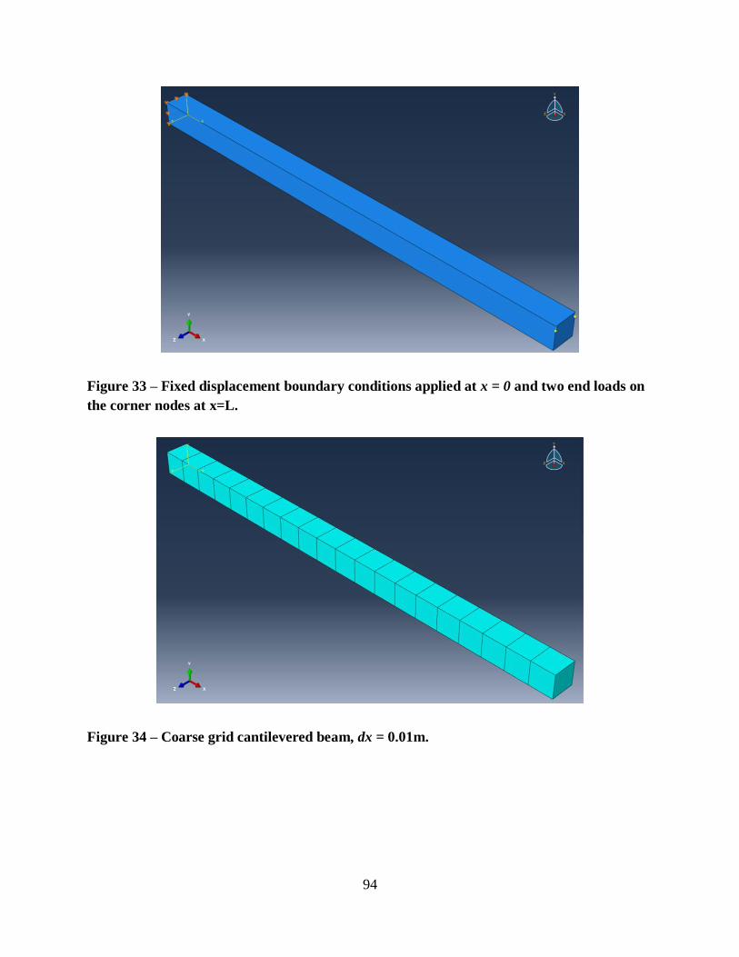
94
Figure 33 – Fixed displacement boundary conditions applied at x = 0 and two end loads on
the corner nodes at x=L.
Figure 34 – Coarse grid cantilevered beam, dx = 0.01m.

95
Figure 35 – Medium grid cantilevered beam, dx = 0.005 m.
Figure 36 – Fine grid cantilevered beam, dx = 0.0025 m.
After obtaining the solutions on the three grids, the solutions for the displacement of the tip of
the beam were compared against the exact analytical solution to enable the calculation of the
observed order of accuracy. Additionally, the GCI was calculated for each grid. The results are
presented in Table 5 and show that the finite element spatial discretization is approaching the

96
formal order of accuracy (2) with a value of 1.92 on the fine grid and that the GCI values are
low, less than one percent (0.3%) for even the coarse grid. This indicates that the solutions are in
the asymptotic range.
Table 5 – Order verification results for Abaqus with cantilevered beam with end load.
Displacement of free beam end is measured for each grid.
Displacement
(m)
Discretization Error
(m) �̂� GCI %
coarse 0.004603 0.000041
0.372
med 0.004631 0.000013 1.637307 0.170
fine 0.004641 0.000004 1.922305 0.034
4.3 Solution Verification
Solution verification follows the same procedure as with code order verification, with the
exception that now more physics have been added, and no exact solution exists. The exact
solution to the discrete equations will be replaced with an estimate which will be the converged
solution on a very fine grid. This is referred to as a fine grid reference solution. The purpose of
solution verification is to show that the temporal and spatial observed orders of accuracy match
the formal orders of accuracy. The convergence of solution variables is observed with added
levels of refinement. Including added physics models which cannot be verified with exact
analytical solutions and instead must use a fine-grid reference solution. Additionally, since the
code order verification was a steady problem, the temporal discretization error will be estimated
as well. Some work with the T-Craft model will be presented, and the numerical simulations of
the sloshing tank experiment will be presented to provide a simpler FSI V&V case.

97
One challenge in generating FSI solutions is gathering all required model inputs. This includes
boundary conditions and material definitions which can be difficult to obtain for certain
materials and problems. This is specifically the case for reinforced rubbers which display some
mixture of hyperelastic behavior with linear elastic behavior of the reinforcing layer. Many of
the FSI validation experiments in the literature fall short in providing all of the necessary
information which is needed as input in numerical simulation. As a result the validation process
typically fails to produce a definitive answer as to the predictive capability of the codes.
4.3.1 SES with Rigid Seals
The rigid seal T-Craft model has been studied for calm water and head seas drag cases,
accelerating craft, and shallow water cases. The original work by Dave Donnelly (33) using
RANS calculations to observe the free surface dynamics in the interior of the cushion between
the side-hulls showed promise toward identifying interesting and important physical phenomena.
However, as mentioned before, the rigid seal approximation broke down in waves and when the
seals would normally have critical interactions with the free surface. Solution verification was
performed using systematically refined grids in order to quantify the error in the steady state drag
calculations on the desired grid level (73). The grids employed for that study were refined by a
factor of ( 4 2 ). In the three initial grid levels, the convergence was oscillatory, but additional
refinement levels did achieve monotone convergence. The details of the five grid levels are
presented in Table 6.
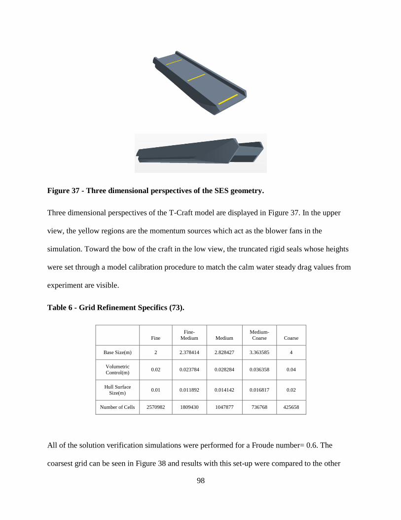
98
Figure 37 - Three dimensional perspectives of the SES geometry.
Three dimensional perspectives of the T-Craft model are displayed in Figure 37. In the upper
view, the yellow regions are the momentum sources which act as the blower fans in the
simulation. Toward the bow of the craft in the low view, the truncated rigid seals whose heights
were set through a model calibration procedure to match the calm water steady drag values from
experiment are visible.
Table 6 - Grid Refinement Specifics (73).
Fine
Fine-
Medium Medium
Medium-
Coarse Coarse
Base Size(m) 2 2.378414 2.828427 3.363585 4
Volumetric
Control(m) 0.02 0.023784 0.028284 0.036358 0.04
Hull Surface
Size(m) 0.01 0.011892 0.014142 0.016817 0.02
Number of Cells 2570982 1809430 1047877 736768 425658
All of the solution verification simulations were performed for a Froude number= 0.6. The
coarsest grid can be seen in Figure 38 and results with this set-up were compared to the other

99
refinement levels including the fine grid shown in Figure 39. After four seconds of runtime, the
converged drag values were collected and the results for the various refinement levels as seen in
Figure 40
Figure 38 - Coarse grid on the symmetry plane. (73)
Figure 39 - Fine grid on the symmetry plane. (73)

100
Figure 40 - Fn 0.6 inviscid averaged drag results vs. normalized grid spacing. (73)
The observed order of accuracy from the rigid seal drag solution verification was calculated to be
2.16, just larger than the formal order of accuracy of 2 (73). The generalized relative error for
the fine grid solution is 4%. For turbulent multiphase flow simulations of rigid seal SES these
should be acceptable levels of discretization error with good solution behavior with respect to
grid refinement.
4.3.2 Sloshing Tank with neoprene beam
The sloshing tank experiment presents a good FSI validation case and the simple geometry
makes it very easy to model. However, its similarity to the SES bow seal problem through the
exploration of free surfaces interacting with thin neoprene structures provides a very good basic
problem for solution verification. Formally testing the behavior of the additional physics models
in a free surface FSI problem with positive results can instill a higher level of confidence moving
forward to full SES bow seal simulations. The details of this solution verification exercise are
presented in this section.
4
5
6
7
8
9
1 10D
rag l
bf
Grid Spacing h

101
The final grid construction was an intuitive, iterative procedure based on observations of the
sloshing flow and spray generated from wave impacts with the sidewalls. Figure 41 shows three
key aspects of the fine grid used in these studies. Figure 41 (top) shows a high level overview of
the grid and refinement in the free surface region, as well as along the sidewalls to capture spray
from wave impacts. Figure 41 (bottom-left) shows the prism layer near wall grid at the tip of the
beam and Figure 41 (bottom-right) highlights the same along the tank walls. The grids which
were used in the verification tests were comprised of uniform hexahedral cells and do not include
the fine prism layers in the near wall regions or any distinction in grid sizes between the air and
water regions. This decision was made in an attempt to conform more closely with the
requirement of uniform grid size and systematic refinement.
In order to perform solution verification on the sloshing tank the beam is removed from the
simulation and the water is allowed to slosh inside the empty tank. For this verification, it is
important to use error norms of global variables or integral quantities on simulation boundaries
as opposed to observing a local variable at a single point in the domain. The error in a variable
measured at a single point can display behavior which deviates from the overall order of
accuracy of the method due to the influence of boundary conditions and error propagation (70).
The measured system response quantity will be the integral of the mean kinetic energy per unit
volume over a plane which bisects the center of the tank. This quantity is important to capture in
the FSI solution because a portion of that kinetic energy in the fluid is then transferred to the
beam during wave impacts. The time history of this quantity is recorded and compared with that
from the other grid refinement levels.

102
Figure 41 - Finite volume grid of 839,753 cells: top) Overview of the grid refinement where
waves and spray are located, bottom-left) the prism layer cells on the beam, and bottom-
right) the prism layer in the corner of the tank walls.
Table 7 - Grid refinement data for the sloshing tank FSI simulations.
Base Size(m) Refinement(m) Total Cells Timestep(s)
Coarse 0.016 0.008 91,616 0.005
Medium 0.008 0.004 196,492 0.0025
Fine 0.004 0.002 837,153 0.00125
VeryFine 0.002 0.001 3,804,158 0.000625

103
The solution verification process allows for the independent confirmation of both the spatial and
temporal orders of accuracy, as well as an overall order through a combined analysis. The
solvers used in this simulation are formally 2nd order accurate in both time and space. With three
levels of refinement in space and time, one estimate of the observed order of accuracy is
obtained by using the finest solution as a reference.
First, solutions were computed on the fine grid (δx = 0.005 m) with time steps of 0.01, 0.005, and
0.0025 seconds to calculate the observed temporal order of accuracy. The results of those
computations are summarized in Table 8.
Table 8 – L2 norm of the discretization error, observed order of accuracy, and error
reduction ratio for the temporal solution verification.
|ε31|L2 |ε21|L2 ˆL2p ratio
0.02783 0.00893 1.639 3.114
Second, solutions were computed with the fine time step (δt = 0.0025 seconds) with grid sizes of
0.02, 0.01, and 0.005 m to calculate the observed spatial order of accuracy. The results of those
computations are summarized in
Table 9.
Table 9 - L2 norm of the discretization error, observed order of accuracy, and error
reduction ratio for the spatial solution verification.
|ε31|L2 |ε21|L2 ˆL2p ratio
0.20534 0.04622 2.151 4.442

104
Finally, solutions were computed with corresponding grid size and time step refinement factors
(δt = 0.01 s, δx = 0.02 m; δt = 0.005 s, δx = 0.01 m; δt = 0.0025 s, δx = 0.005m) to show an
overall observed order of accuracy. The results of those computations are summarized in Table
10.
Table 10 - L2 norm of the discretization error, observed order of accuracy, and error
reduction ratio for the combined spatial and temporal solution verification.
|ε31|L2 |ε21|L2 ˆL2p ratio
0.21816 0.05227 2.061 4.174
The observed temporal order of accuracy was calculated to be 1.639. This is slightly less than the
formal value of 2 for the code. Boundary conditions at the domain extents typically are 1st order
approximations and will degrade the overall order of accuracy (70). The observed spatial order
of accuracy was much closer to the expected value of 2 at 2.151. This indicates that the kinetic
energy in the cross section is converging appropriately with increasing grid refinement. The third
test for the overall combined order of accuracy gave a final estimate of the observed order of
accuracy of 2.061. A GCI (72) with a factor of safety of 1.25 was calculated for the medium grid
with a value of 3.67%. This represents an uncertainty estimate for the mean kinetic energy per
unit volume for the medium grid solution. With these values, the models and medium grid for the
fluid calculation should be acceptable.
Solution verification for the full FSI problem in the first two seconds of oscillation will now be
considered. Using three base cell sizes, δx, of 0.016, 0.008, and 0.004 meters, three
corresponding time steps, δt, of 0.005, 0.0025, and 0.00125 seconds were run. These were
compared with a reference solution on a very fine grid with δx = 0.002 m and δt = 0.000625s.

105
For each grid, the resolution in the free surface region was refined to one quarter of the base cell
edge length, but the refinement was uniform and consistent. An indication of convergence can be
obtained by examining the L2-norm of the difference between the predicted tip displacements of
the very fine grid reference solution and the three coarser grid solutions for the first two seconds
of the time history. These differences are plotted in Figure 6. Beyond two seconds, the
convergence is unclear due to the accumulation of error and history dependent behavior. A value
for the observed order of accuracy of this FSI scheme can be obtained. Table 11 shows results of
this analysis.
Table 11 - L2 norm of the discretization error in the tip displacement, observed order of
accuracy, and error reduction ratio for the combined FSI response solution verification.
|ε31|L2 |ε21|L2 ˆL2p ratio
0.00140 0.00039 1.890 3.707
Performing the solution verification procedure on the FSI response on the flexible beam
estimated the observed order of accuracy of the method at 1.89. This value is slightly under the
expected value of 2, but well within expectations considering the mixed codes and interpolations
occurring in the FSI procedure. Both codes are formally 2nd order in space and time, but the
exchange of interface values (interpolation) and the presence of cumulative iterative error likely
degrade the overall observed order. Since the observed and formal orders presented are in
reasonable agreement, the discretization errors on the selected grid can be used to estimate the
overall numerical uncertainty.

106
Figure 42 – A relative comparison for system response quantity, f, the beam tip
displacement. It is presented as a difference in tip displacements between the three grid
levels (f4, f3, f2) and the reference solution (f1) in the first two seconds of the time history
for the FSI response of the neoprene beam.
To ensure that refinement in the thickness direction was not an issue, grid constructions with
one, two, and five layers were made to look at the solution behavior. The results show that the
quadratic elements do a good job at modelling the through thickness stresses and additional
elements do not significantly affect the overall response. Figure 43 presents the tip displacement
history using 1, 2, and 5 layers of elements through the thickness of the neoprene beam. The
response is consistent for the three spatial refinement levels and only shows some small
discrepancies in the motions at the extremes. The response frequency and overarching behavior
is the same for all three levels. Despite this good qualitative agreement, formal solution
verification with this refinement was inconclusive.

107
Similarly, the 1st order vs. 2nd order fluid temporal discretization was tested to see if the
dissipation it added to stabilize the partitioned FSI solution had a large effect on the overall
solution behavior. These tests were performed because the eventual simulations of the SES bow
seal do use 1st order temporal discretizations whereas in the sloshing tank simulations, 2nd order
temporal discretization are generally used because they are less susceptible to numerical
instability because of smaller forces. Comparison of the tip displacement between the two
discretizations is presented in Figure 44.
Figure 43 - Influence of thickness based refinement in the quadratic finite elements on the
FSI response of the sloshing tank hanging beam.

108
Figure 44 - Influence of the fluid temporal discretization on the FSI response of the
sloshing tank hanging beam.
Here again the overall solution behavior is consistent with respect to the response frequency and
the overall behavior for δt= 0.005 sec. The 1st order scheme does shows some smaller local tip
displacements around the maxima of the tip displacements likely from the dissipation it adds to
the scheme.
4.3.3 Static Hanging Seal
Following similar work on modeling composite rubber/fiber materials in tire research (55), a
sandwiched finite element model construction was selected for the fabric reinforced rubber. An
inner layer of two dimensional membrane elements representing the fabric was constrained with
tie nodes to the outer three dimensional continuum stress elements for the rubber. The inner
fabric layer comprised of M3D4 membrane elements was prescribed a linear elastic model with a
Young’s Modulus of a typical nylon fabric. The membrane formulation provides no stiffness in
bending and compression was neglected in the membrane to account for the buckling behavior

109
under compressive loads which is typical of fabrics. The tensional behavior is more critical to
capture and provides the inextensible characteristics of the composite fabric reinforced rubber.
C3D20R quadratic continuum elements with a hyperelastic material definition provide the
bending stiffness that the rubber gives to the structure. The bending is localized to the uppermost
portion of the structure and the elements were refined with a biased growth function near the top
to ensure that the high curvature due to bending would be resolved. The choice of final grid
construction will be discussed in more detail below in relation to a grid convergence study.
The reinforced vulcanized neoprene used in this study was used in an experimental study of SES
seals. That study was intended to provide numerical modelers with a set up validation data for
fluid-structure interaction simulations. Unfortunately, the material data given by experimentalists
were for a linear elastic isotropic material. Only the density and Young’s Modulus were
provided. Using that information alone, properly modelling the accurate displacements of the
bow seal would be difficult to impossible. However, static tests were performed as a simple way
to populate the hyperelastic constants and calibrate the material stiffness in the absence of more
detailed information.
Initial attempts at using the material definition from the experiments failed to reproduce the
displacements of the static hanging seal in simulation. A detailed solution verification to rule out
spatial discretization as a cause of that modeling error was not completed at the time. Instead,
model calibration was conducted for the material definition initially and then solution
verification with that material model was performed. This procedure does not adhere to the
requirements outlined for the independence of the results and therefore a formal model validation
of the material model cannot be made. Regardless, the solution verification was completed for

110
the elements with the calibrated material definition and convergence of those models for the
static hanging seal case is presented.
After setting the hyperelastic constants through model calibration (to be described in Sec 4.4.2, a
grid refinement study was conducted in order to provide solution verification results concerning
the element selections and to guide the final element grid construction. Due to the grid
construction using a growth function on the lengthwise edge, a systematic, uniform grid
refinement was not performed. The finest grid used a reference solution was comprised of
elements with an aspect ratio (AR) of one (hexahedral cube elements). The aspect ratio here
refers to the ratio between the thickness of the element and its length and width. The widths of
the elements remained constant for all grids since the bending is two dimensional in nature and
very little variation in displacement across the transverse direction is expected. The three grids
used for the refinement study are of a different architecture and are detailed in Table 12. Instead
of uniform element spacing, the elements were coarsened progressively down the length of the
seal away from the fixed end. This local element refinement process implemented a growth
function in the area with the highest bending and curvature near the fixed attachment point. Each
grid grew to the same resultant AR=10 toward the tip. Figure 45 shows the positions of points
along the seal edge for the four grids with C3D20R quadratic elements. As the beam model is
refined, the solutions are approaching the fine grid reference solution.

111
Figure 45 - Static seal deflections for four grid resolutions with refinement along the length
of the seal.
Table 12 - Grid refinement properties for static hanging seal
Base Size (m) Start AR Final AR Total Elements
Coarse 0.003 4 10 2499
Medium 0.003 2 10 3264
Fine 0.003 1 10 4131
Very Fine 0.003 1 1 166,080
It should also be noted that the three grids all have the same number of elements through the
thickness. Refinement in this direction was avoided to help minimize the total elements, and
solution verification of element refinement in the thickness direction was presented earlier in
regards to a similar vulcanized neoprene material without the internal fabric reinforcement layer.

112
The results of those tests showed that even one layer through the thickness of the quadratic
elements could reproduce the bending of thin beams.
Figure 46 shows the seal’s tip x-coordinate for all four grids which display asymptotic behavior
with refinement which seems to be converging toward the very fine uniform grid value.
Figure 46 - Convergence of the tip deflection for the hanging static seal with four levels of
grid refinement. Level 1 is the finest and Level 4 is the coarsest.
Table 13 – Solution verification results for the static hanging seal refinement study.
𝜀41 𝜀31 𝜀21 �̂�432 �̂�321 GCIfine
-0.00163 -0.00068 -0.00022 1.27 1.60 0.11%

113
Two estimates of the observed order of accuracy are calculated using the four solutions. Between
the coarse, medium, and fine grids, the observed order is 1.27. Between the medium, fine, and
reference solution, the observed order is 1.60. These values appear to be approaching the formal
order of 2 but there is still some significant discrepancy which is most likely due to the lack of
refinement in the thickness direction during this study. Future refinement studies on elements in
bending should definitely include refinement in this direction.
4.3.4 SES Bow Seal Test Platform Drag on Static Seal
An attempt to perform solution verification on the drag values was undertaken for the SES bow
seal test platform model. The study included the effects of temporal and spatial refinement on the
unsteady average drag after displacing the seal in an FSI simulation. In other words, it was a
comparison of the developed forces on a pre-deformed static seal. This was done primarily to
provide independent solution verification on the fluid and solid partitions of the FSI scheme.
However, these results were less than ideal and some of the downfalls of this approach will be
described.
The grids used for the SES bow seal test platform model were constructed based on intuition
with respect to a craft moving on a free surface, best practice guidelines, and trial and error. The
mesh morphing algorithm can be very sensitive to the grid. A general overview of this final grid
architecture is provided in Figure 47. Much of the structure is specifically geared toward
capturing the free surface accurately.

114
Figure 47 - Overview of the SES bow seal test platform grid architecture with a general
refinement region around the craft, isotropic refinement in the cushion and bow seal
regions, and extruded growth cells moving away from the primary region of interest.
Zooming in to view the region surrounding the bow seal in Figure 48, isotropic refinement is
added in the cushion region, and even higher isotropic refinement is added directly forward of
the bow seal. This region of flow contains the bow wave that forms and spray that is generated
above the bow wave where the free surface meets the seal. To the right side of the image, the
anisotropic refinement in the vertical direction which keeps the incoming free surface sharp is
visible.

115
Figure 48 - Close-up of the bow seal, bow wave, and spray refinement regions of the SES
bow seal test platform model’s grid architecture.
Figure 49 – Close-up of the boundary layer grid for the SES bow seal test platform model.
In Figure 49, the boundary layer grid on the forward side of the bow seal is visible. The
boundary layer grid is only placed on the forward side to capture the skin friction from the flow
of water across it. The rear of the seal is unwetted and acted upon only by the interior cushion
pressure and whatever dynamic flow exists. The shear stress on the back should be much smaller

116
than on the front and for this reason, the boundary layer grid was omitted to save on the total cell
number. The thickness of the first layer is critical to the success of the grid morphing process
when the seal is undergoing large displacements or accelerations. The values of the near wall cell
thickness were not allowed to be less than 0.0005 m.
The extrusion of the grid away from the region of interest works to damp out wave energy
propagating toward the pressure outlet boundary and prevent reflection back into the region
around the SES test platform.
For the solution verification, a co-simulation was first conducted with the medium grid to obtain
the pre-deformed state to use in the grid refinement study. Then two additional grids were
created by halving and doubling the base size in the domain to get a fine and coarse grid. The
simulations were run with the grid characteristics in Table 14, and run until an averaged drag
force on the seal could be computed. The 1st order temporal discretization, used for the co-
simulation was tested with timesteps which corresponds with the refined grids. Typically, this
was on the order of 20 seconds runtime.
Table 14 – Grid characteristics for the bow seal drag solution verification.
Total Cells Timestep(s) Spray Cell Size(m) Drag (lbf)
Coarse 927,154 0.005 0.02 12.728
Med 2,335,262 0.0025 0.01 13.128
Fine 13,107,788 0.00125 0.005 8.659
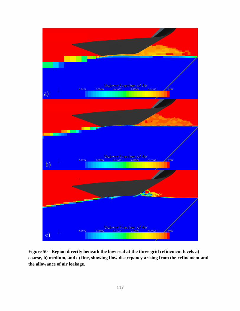
117
Figure 50 - Region directly beneath the bow seal at the three grid refinement levels a)
coarse, b) medium, and c) fine, showing flow discrepancy arising from the refinement and
the allowance of air leakage.
a)
b)
c)

118
Unfortunately, this approach to solution verification for an SES did not produce any valid results
due to changes in the flow around the bow seal and the lack of response by the seal to the
changing flow conditions. The drag forces on the seal do not display any monotonic convergence
when observing the values in Table 14. To better understand the difference it is helpful to
visualize the flow in the region around the wetted side of the seal, and to observed the wetting
itself through the volume fractions on the seal.
Figure 50 displays the flow in the region directly underneath the bow seal for the three levels of
refinement. Note that the medium grid was used to calculate the displacement of the seal. When
coarsened in part a, the flow of air cushion pressure is allowed to push forward and jet out of the
bow of the craft. The medium grid has a smaller amount of leakage. When refined in part c, the
water on the upstream side of the seal impacts it more and doesn’t let any leakage out. This
cushion pressure leakage is also apparent when looking at the wetting on the upstream side of the
seal. Since the seal cannot respond and close the gap, it is very difficult to achieve a solution
verification result for the drag force on the seal.
The wetting on the upstream side of the seal displays the level of air leakage by showing the
volume fractions on the seal surface. The overall trend which is displayed in Figure 51 is that
with coarsening of the grid the air leakage increases. This makes it extremely difficult to capture
the true drag force on the seal in this type of simulation. It is troubling because the initial shape
of the seal was determined through the medium grid FSI solution, but the forces and wetting will
not remain constant on the static seal during this post FSI run. This is further evidence of the true
strong coupling that exists for the problem of bow seal FSI.

119
Figure 51 - Wetting on the upstream side of the seal at the a) coarse, b) medium, and c) fine
grid levels which highlights and increased level of air leakage as the grid is coarsened for a
static seal case.

120
4.3.5 SES Bow Seal Test Platform Drag on Dynamic Seal
A solution verification was also performed on the FSI response and the resultant seal drag for
three levels of refinement using Run 1058. Table 15 presents the results for this study. The
spatial and temporal refinement factors were equal to 1.5 and the results displayed an observed
order of accuracy of 1.009. Due to the mixed order of the combined discretization, for the 1st
order temporal discretization, the refinement factor in time should have been set equal to 3 to
achieve the same level of error reduction between the temporal and spatial refinement.
Table 15 – Solution verification results for the seal drag in a dynamic FSI simulation after
20 seconds. Using three grid levels provides one estimate of the observed order of accuracy.
dx dt Seal Drag (lbf) �̂�
Coarse 1.125 0.005 -10.82
Medium 0.75 0.0025 -8.146 1.009
Fine 0.5 0.00125 -6.37
Figure 52 – Resultant seal displacements for the solution verification study of the FSI
response.

121
Because the temporal refinement factor is in error for this study, the discretization error estimate
made with these results are not reliable. Simulations with the appropriate time steps should be
run to make an accurate estimate of the discretization error.
Figure 52 present the three instantaneous seal displacements after 20 seconds of simulation at the
different grid levels. As the grid is refined, the forward section of the seal moves down and the
aft section comes up as the forces are resolved more accurately.
4.4 Model Calibration
4.4.1 Sloshing tank neoprene beam: material definition
The primary goal of the V&V process is to check that the numerical grids employed are
converging toward a grid independent solution. Secondly, the numerical solution should be
compared against a known data set to ensure that the grid independent solution is approaching
the physical solution. The outcome of the solution verification work showed convergent results
for refinement of both the temporal and spatial discretization which were close to the formal
order of accuracy of the methods. The model validation process discovered a significant error in
beam response highlighted by the numerical results using a linear elastic material model with
Young’s modulus, E = 4.0 MPa.
It is apparent that the provided material characteristics do not properly replicate the behavior of
the neoprene beam. A comparison of the simulated restoring motion of the beam to the
experiment indicates that the simulated beam behaves less stiffly than was observed in the
experiment. The validation work shown in Figure 14b is representative of the agreement between
the numerical and experimental cases using the published benchmark material data. Model

122
calibration will be performed to try and recover some of the missing behavior due to the
incomplete material definition.
A new material stiffness was estimated by comparing results found by iteratively increasing the
Young’s modulus. Through this calibration of the material stiffness, the restoring behavior is
significantly improved as shown in Figure 54.
The beam in these new results has been given a Young’s modulus, E = 20.0 MPa, which is five
times larger than that provided by the tension test in the benchmark data. Looking at the first
cycle of oscillations, the beam response much more closely matches the experimental
displacement. While the restoring behavior is improved, this behavior is still the feature of the
beam response showing the largest discrepancy in the comparison.
Figure 54 shows clearly that the errors arising from the material information are much larger
than the errors from temporal and spatial resolution established above. With this in mind, it is
instructive to examine the time histories of the Tracker analysis of beam deflection at each of the
four measurement locations with the simulations. In Figure 55 the data is presented for each
measurement location and compared to the simulation with an elastic beam with E = 4.0 MPa.
Starting at the top, the 25% length position of the experiment shows a regular oscillation but in
the simulations, high frequency noise likely from vibrations along the length of the beam cause a
deviation from the experimental displacements. The same results are shown at the 50% length
location. Progressing towards the tip, the numerical behavior deviates further from the
experimental response.
A comparison of the same data with the simulation using an elastic beam with E = 20 MPa is
shown in Figure 56. Of particular note is that, at the bottom two measurement locations, the
recovery of the snap-back behavior is clear and the results are in much better agreement with the

123
experiment. There is still some error at the higher measurement locations as well as in the
amplitude of the maximum and minimum beam deflections at the tip. The simulation appears to
agree well with the zero crossing points and the overall frequency of the response.
4.4.2 SES bow seal: material definition
The hyperelastic constants, C10, C01, and D1, define the behavior of the hyperelastic material.
Normally, a battery of tests is conducted to define the model coefficients and these standard tests
are normally done for an isotropic sample. The reinforced rubber cannot be tested in the same
way because of the composite nature and the inability to separate and attribute the results to each
specific constituent material. To determine the coefficients, they were modified so that the
numerical displacements in the upper region of the sample matched the experimental as best as
possible. This is by no means a rigorous method, but without further material definition, it should
provide a better estimate than the alternative of using the published data on the material
describing it as linear elastic.
This comparison was performed on the finest element grid and the agreement can be seen in
Figure 53 below. The displacements deviate strongly towards the bottom due to the pre-strain in
the material sample and the averaging that was performed on the inward and outward facing
orientations to arrive at the static displacement of the seal. This is an acceptable failure because
the primary goal of this work is to ensure that the bending behavior is properly accounted for at
the top, where it is concentrated. This qualitative agreement should at least provide a reasonable
guess to the hyperelastic coefficients, which should in turn provide a better approximation of the
reinforced rubber than a linear elastic model.

124
Figure 53 - Comparison of experimental seal profile with the numerical result after model
calibration of the material stiffness.
The hyperelastic constants were modified in an iterative approach after initial estimates were to
convert the linear elastic properties into the C01, C10, and D1 coefficients. The end result is a
material definition which can replicate the bending of a static hanging sample of the seal
material. This material definition is summarized in Table 16.
-0.2
-0.1
0
0.1
0.2
0.3
0.4
0.3 0.32 0.34
Z(m
)
X(m)
Experimental
Very Fine (AR=1)

125
Table 16 – Fabric reinforced vulcanized neoprene model definition after model calibration
Linear Elastic Density (kg/m^3) E (GPa) ν
Fiberglass Stiffeners 1936 41.3 0.33
Nylon Fabric 50 0.2 0.33
Hyperelastic C10 C01 D1
Vulcanized Neoprene 1.30E+06 0 2.00E-08
4.5 Model Validation
4.5.1 Sloshing Tank FSI
With the current reanalysis, this experimental FSI validation case becomes much more useful to
the community. The partitioned approach using the prescribed Young’s Modulus captures the
temporal behavior of the primary motion of the beam which is correlated with the sloshing
frequency but fails to predict the higher mode oscillations seen during the zero crossing points in
the time history.
The tension test for the neoprene material provided the initial slope of the stress/strain
relationship but this alone will not describe the bending behavior of a hyperelastic material. It
has been acknowledged that this value may contain an uncertainty of roughly 10-20% (A. Souto-
Iglesias, personal communication). The new elastic modulus which is five times larger is not
realistic either. Because of its hyperelastic nature, it is not expected that a simulation using a
linear elastic material model will accurately reproduce the experimental beam response except

126
for small displacements. With more information gathered from a battery of hyperelastic-specific
material tests, a more physical model could be implemented which accounts for the unique
behavior of neoprene rubber. At the time of writing, material tests are underway to define an
incompressible hyperelastic material model which holds some promise toward an improved
validation (L. Lobovsky, personal communication).
By artificially stiffening the structure in the computation through model calibration, some of the
lost behavior is recovered. The STAR-CCM+/Abaqus Co-Simulation tool has been shown here
to provide comparable predictive performance to the other published results on this case, and all
validations are improved by the shifting of the results to account for the 0.2 seconds that the tank
stationary at the beginning of the experiment. However, the published results could not be
adjusted to include the effects of the discrepancy in the roll history amplitudes.
Figure 54 - Model calibration results with increased Young's modulus.

127
Figure 55 – Beam tip displacement at four
reference locations compared with exp. E =
4.0 MPa.
Figure 56 - Beam tip displacement at four
reference locations compared with exp. E =
20.0 MPa.

128
Figure 57 - Qualitative comparison for numerical results with linear elasticity and E = 20.0
MPa. Video frames at t = 0.76, 1.64, 2.4, 2.68, 2.96, 3.32, 3.4, 3.56, 3.80, 3.84, 4, and 4.16
seconds (17).

129
Figure 57 shows a typical frame by frame comparison between the video and the simulation
using the linear elastic material model with E = 20.0 MPa. Using the updated roll history the
comparison between the frames is improved. The free surface profile matches well for each
instant of time and shows that the sloshing flow is being reproduced well. The recovery of
behaviors shown in Figure 55 is identifiable in this qualitative comparison. The general response
of the experimental beam follows a pattern wherein there is a restoring motion which occurs
after the beam reaches its maximum displacement and before the next wave impacts. The
validation results presented previously fail to reproduce this behavior using linear elastic models
with E = 4.0 MPa.
Figure 14b shows that all of the methods roughly predict the same behavior for this case. The
present commercial code method using finite volume CFD and finite element CSM is very
similar to the method presented by (30). These two methods should and do agree reasonably. The
Particle Finite Element Method (PFEM) presented in (17; 61) is quite different from the other
two fundamentally, but also exhibits very similar behavior. The important trend to take note of is
the lack of the secondary beam tip displacement that occurs as the beam crosses zero from its
major excursions. The results of (63), not shown in Figure 14, have a much better agreement
than any of the other results. They were differentiated by the use of Rayleigh damping in the
finite element calculation, however no information was provided about the model calibration or
the time shift in the experimental roll angle history. It is likely that a combination of Rayleigh
damping and material stiffening would lead to a better approximation of the neoprene rubber if
using a linear elastic material model is the only option.
In this work, using the linear elastic model, taking into account the time shift and lens distortion,
and ruling out other major error sources through V&V, the numerical beam tip displacements

130
with E = 4.0 MPa still follow a path that does not include the oscillatory restoring behavior at the
centerline crossing points seen in the experimental behavior. Because this behavior is so far from
the experimental results and information regarding the material characteristics is incomplete, the
validation of the method cannot be authoritatively stated using the provided inputs. However, the
inclusion of the model calibration does enhance the performance of the method for this
challenging problem while accepting a higher level of physical approximation.
Tests were conducted (69) to better characterize the hyperelastic material used in these tests.
Time was only available to conduct one simulation with the new material data but the qualitative
validation results are promising and show that taking the time to improve the material definition
goes a long way toward validating the response in numerical simulations. These results are
highlighted in Figure 58. Similar results were obtained in (44).
Figure 58 – Qualitative validation results for a new 5 parameter Mooney-Rivlin material
model.
131
4.6 V&V Conclusions
The results from grid refinement studies to ascertain the spatial observed order of accuracy of
both the fluid and structural solvers exhibited convergent behavior towards 2nd order accuracy.
This was expected from the commercial product’s discretizations, but the independent
verification by the code user is an important aspect of the V&V methodology.
The fluid spatial discretization was tested by using the Couette flow exact solution in a 1x1x1m
domain. The observed order of accuracy using the L1 norm of the velocity in the domain was
1.9. Estimates were also made of the round-off and iterative errors which were both very small
compared to the discretization error.
The solid spatial discretization was tested using the Euler-Bernoulli solution of a cantilevered
beam with an end load. The observed order of accuracy calculated by observing the tip deflection
of the beam with uniform grid refinement was converging toward the formal order of two. The
estimate produced by the two finer grids was 1.92. GCI’s calculated for these results showed the
solutions were in the asymptotic range.
A number of additional solution verification studies were undertaken in order to observe the
solution behavior of the solver independently and for FSI cases with the more complete physics
definitions. For these cases, no exact solutions are available, and fine grid reference solutions
were used as surrogates in the calculation of the numerical error. This approach works well if it
can be confirmed that the solutions are in the asymptotic range, however this can be difficult to
achieve realistically when considering the computational time for the simulations. However,
efforts were made to quantify the observed order of accuracy and deficiencies were highlighted.
The solution verifications discussed included a rigid seal SES drag calculation, sloshing tank

132
FSI, a static hanging seal, and the bow seal drag force on the test platform model. With the
exception of the bow seal drag solutions, all of the other cases displayed error reduction with
grid refinement which was close to the formal observed order of the schemes.
Formal validations with error bars have not been produced, but the quantification of
discretization errors was attempted. The preceding section will provide a validation of the
partitioned FSI procedure for the case of the flexible SES bow seal and hopefully provide some
insightful new information relevant to SES seal design.

133
Chapter 5
Results & Discussion
5.1 SES Test Craft Bow Seal
The main focus of this chapter will be the evaluation of the presented FSI procedure for
simulating the flat plate bow seal from the University of Michigan SES experiment. The results
presented should provide some estimate of the predictive capability even though the formal
validation criteria will be difficult to meet for the FSI simulations. Appendix B provides an
overview of the experimental runs which were simulated in this study. These runs represent
approximately one-fifth of the total runs in that experiment, and span a range of test speeds and
cushion pressures that is representative of the conditions tested.
The series of numerical runs was made using the fine grid from the solution verification studies
in Chapter 4. Each of these simulations took approximately 3-4 days for 20 seconds of
simulation time on the BlueRidge cluster of Virginia Tech’s Advanced Research Computing
center. Additional physics models, approximations, and other simulations details not previously
described will be discussed here prior to the presentation of the numerical bow seal results for
these cases.

134
5.1.1 SES flat plate bow seal model
The final finite element grid to be used for the flexible SES bow seal was developed taking into
account some of the lessons learned in the solution verification and model calibration for the
static hanging seal. The finite element grid uses the same edge biased growth function
architecture developed for static hanging seal simulations with a sandwiched element
construction for the fabric reinforced rubber. A visual example of this, shown in Figure 59,
shows the primary grid refinement toward the fixed end of the hanging seal along the top edge,
growing to larger elements toward the bottom where there is less bending. The red lines indicate
the position of the fiberglass stiffeners. The stiffeners provide some transverse resistance to
bending and maintain a relatively two dimensional displacement profile.
Figure 59 - Final finite element grid for the flat plate SES bow seal comprised of 14,592
elements.

135
This final grid architecture was developed based on similar approaches used in tire modeling and
composite materials. The primary grid is comprised of three layers, two outer layers of 3D
continuum stress elements with hyperelastic material definition sandwiching an inner layer of
membrane elements with a linear elastic definition for the nylon fabric reinforcement. Three
beams comprised of shell elements with linear elastic definitions for fiberglass are affixed on the
downstream side of the seal. Another approach would be to define an anisotropic composite
layer material model which would require only a single layer of elements, but without good
material data this simple approach provided a means to estimate the individual material
properties apart from their combined behavior.
Figure 60 - Schematic cross sectional cut of the SES flat plate bow seal finite element
model.
A cross sectional cut of the sandwiched finite element model is presented schematically in Figure
60. The best case scenario for populating the material definitions would be to test each
constituent material individually in an appropriate manner for the type of material and the class
of structural behavior exhibited. Then supply these material definitions into the overall model,
and perform some solution verification and model validation to show this input data can properly
represent the observed behavior of the physical specimen.

136
Without such material information, as is the case here, model calibration had to be performed to
obtain the hyperelastic coefficients. This process was performed in Sec 4.4.2 until the numerical
results matched the static displacement of a hanging sample of the material. The neoprene rubber
layers are only comprised of one layer of quadratic continuum finite elements. The refinement
studies showed that for these elements even one layer could effectively model the through
thickness stress distributions to a degree which matched the experimental displacements. This
also saves an approximately 4-8 times increase in the number of elements. Refining the seal
through the thickness would likely slow down the simulations greatly without a significant
increase in solution accuracy.
5.1.2 Accuracy of Dynamic Seal Motion
The iterative partitioned nature of the FSI solution algorithm using implicit fluid and solid
solvers with a large number of degrees of freedom creates a computationally expensive
simulation. Early results showed that the partitioned approach took significant effort to stabilize
numerically. These simulations begin with an exaggerated loading on the upstream side of the
seal because it is fixed in the un-deflected configuration in order to initialize a flow field around
the craft. This stabilization comes at the price of time accuracy. The biggest factor was the
temporal discretization used on both sides of the FSI solution. The fluid solver was run with a 1st
order time integration, and the solid solver used the moderate dissipation settings in the HHT
integrator to control instabilities arising from the coupled solution. Without these stabilizing
features, what is currently a 3-4 days of computational time for 20 seconds of simulation time
could be on the order of one month. To account for the dynamic phenomena would require finite
element time increments which were a function of the elastic wave speed in the neoprene rubber.

137
The coupling timestep itself would need to be small enough control the magnitude of large
motions at the coupling boundaries during one step. As a result the fluid domain would also see
higher grid fluxes at the co-simulation interface and require smaller timesteps.
For these reasons, computational efficiency was often preferred over time accuracy. While the
time accurate dynamic response of an SES bow seal would certainly be a significant
achievement, even steady state deflections and bow seal resistance estimates using a more
approximate approach can provide useful information for SES design. This is especially true for
the case of the SES bow seal because it has been shown to be extremely difficult to get good
characterizations of the flow and measurements of the forces specifically acting on the seal
systems alone. The FSI solutions have the ability to provide some of this hard to get information
by describing the environment directly surrounding the seal and the direct extraction of forces on
the seal surface.
5.2 Model Validation: Steady Bow Seal Hydrodynamics
In this section, the data extracted from the FSI simulations of the University of Michigan bow
seal experiment will be presented in comparison with the experimental results. Some of the
characteristic features of the bow seal system will be studied including metrics like seal
displacement, surface pressure and shear stress distributions, and the total force balance for the
system found by looking at average forces.
The objective of this study will be to examine the steady state conditions for the bow seal. To
achieve this, the average forces over the last five seconds of a simulation will be calculated to
arrive at an approximation of the steady forces acting on the seal. The experimental seal

138
oscillated with some unsteadiness due to the bow wave, spray, and aerated incoming free surface
flow. The simulations are run for 20 seconds to allow the seal to reach a steady state
displacement. Figure 61 provides a visualization of the free surface flow and seal displacement
in this final condition for Run 1058. In the top view, the total extents of the simulation domain
and the free surface are visible along with the craft’s Kelvin wake pattern interacting with the
sidewalls of the towing tank. The dissipative effect of the extruded cells toward the boundaries
can be seen as the wave heights in the wake diminish as it moves toward the left pressure outlet
boundary. Zooming in closer, the middle view displays the free surface profile inside the cushion
and gives some indication of the level of bow seal displacement and wave rise just upstream of
the seal. In the bottom view, the deflected seal is shown from the side with a sharp separation off
the trailing edge of the seal and a smooth free surface profile.

139
Figure 61 - Run 1058: Visualization of free surface profile and bow seal displacement.

140
5.2.1 Bow Seal Displacement
The displacement of the bow seal or what could be referred to as the steady state planing shape
of the bow seal along the centerline was one of the primary measurements in the experiment. The
shape of the seal is critical to capture in a numerical simulation because it is represents the
culmination of all the forces acting on the seal which bring it into a final equilibrium shape.
Without properly resolving the fluid forces, the numerical displacements could not be expected
to compare reasonably. Relative comparisons of the seal displacements can give both a rough
qualitative assessment of the validity of the models as well as a foundation to a simple validation
effort. By comparing the actual values of displacement and taking into account the numerical
uncertainties, a basic validation of the model can be made. The results will be presented for each
run individually and some discussion of the trends in each case will be made. One case in
particular was given more attention, Run 1058. This run was initially selected as a representative
condition for testing the partitioned FSI scheme during the troubleshooting, development, and
V&V phases of the model.
Initial runs in the study were conducted for only seven seconds total runtime on coarse grids. At
the time, it was thought that this would be a sufficient period of time for the seal to achieve a
steady state deflection. Later, lengthened simulations on the medium grid showed that indeed the
seal had not yet converged to equilibrium and the total simulation time was increased to 20
seconds. Some of the runs presented were only run for seven seconds and final displacements
will not be shown for these. In the succeeding sections, only the simulations which were run for
20 seconds will be discussed.

141
The experimental displacement values at three locations were presented as averages over the data
window when the test craft had achieved a steady velocity. On the contrary, the simulation
displacements are presented as instantaneous values at the end of the 20 second simulations. This
failure to present the averaged seal position is due to a lack of planning with regard to the desired
output of the simulations. The original intent was to take the final seal position as the steady state
value, and the simulations were run without recording the time history of all of the points on the
seal to calculate the average displacement.
The experimental values are also presented with their standard deviation. These standard
deviations are the measurement of the unsteadiness in the experimental results and no
experimental measurement uncertainties were provided. For certain runs, the standard deviation
is presented individually at each measurement location when they varied significantly. In
hindsight, the simulations should also have calculated an average and standard deviation of the
displacement. However, because we are interested in the steady state condition, the dynamics of
the seal have been sacrificed for solution stability, and it is unlikely that the standard deviations
would match as a result. It should be noted that these simulations currently represent the only
three-dimensional numerical results presented for this set of experiments and also contain the
highest fidelity simulation of the fluid environment around an SES bow seal system.

142
Figure 62 – Run 1026 steady bow seal displacement after 20 seconds on the fine grid. The
forward velocity of the craft and cushion pressure are, U = 1.82 m/s and Pcushion = 567 Pa.

143
Figure 63 – Run 1051 steady bow seal displacement displacement after 20 seconds on the
fine grid. The forward velocity of the craft and cushion pressure are, U = 2.43 m/s and
Pcushion = 252 Pa.
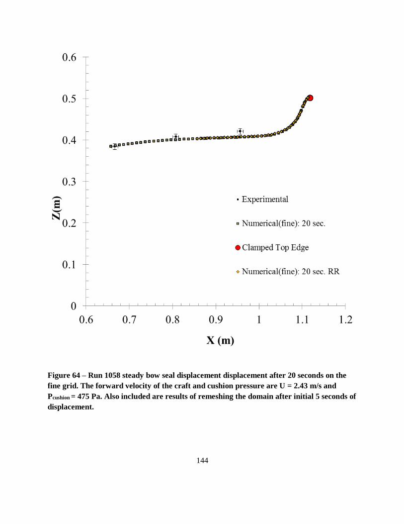
144
Figure 64 – Run 1058 steady bow seal displacement displacement after 20 seconds on the
fine grid. The forward velocity of the craft and cushion pressure are U = 2.43 m/s and
Pcushion = 475 Pa. Also included are results of remeshing the domain after initial 5 seconds of
displacement.

145
Figure 65 - Run 1114 steady bow seal displacement displacement after 20 seconds on the
fine grid. The forward velocity of the craft and cushion pressure are U = 2.43 m/s and
Pcushion = 953 Pa.

146
Figure 66 - Run 1121 steady bow seal displacement displacement after 20 seconds on the
fine grid. The forward velocity of the craft and cushion pressure are U = 2.43 m/s and
Pcushion = 997 Pa. For this case, the starndard deviations have been presented individually
for the low, medium, and high measurement locations because they were significantly
different.

147
Figure 67 - Run 1128 steady bow seal displacement displacement after 20 seconds on the
fine grid. The forward velocity of the craft and cushion pressure are U = 2.43 m/s and
Pcushion = 1050 Pa. For this case, the starndard deviations have been presented individually
for the low, medium, and high measurement locations because they were significantly
different.

148
Figure 68 - Run 1142 steady bow seal displacement displacement after 20 seconds on the
fine grid. The forward velocity of the craft and cushion pressure are U = 2.74 m/s and
Pcushion = 625 Pa.

149
Figure 69 – Run 1412 steady bow seal displacement displacement after remeshing the
domain after initial 5 seconds of displacement and running to 20 seconds on the fine grid.
The forward velocity of the craft and cushion pressure are U = 3.04 m/s and Pcushion = 625
Pa.

150
For the majority of these runs, there is a good level of qualitative agreement between the 20
second simulations on the fine grid and the experimental average displacements. One challenge
in comparing these experimental and numerical results is the resolution of the seal
displacements. With only three measurement locations on the seal, it is difficult to understand the
full nature of the seal displacement experimentally. This is especially apparent when considering
the bulging of the flat plate style seal in the upper portion which greatly affects the longitudinal
location of the seal tip. Also it is important to keep in mind that these comparisons will be
between the experimental averages and the instantaneous numerical seal displacements at the end
of 20 seconds of simulation time.
Figure 62 presents the seal displacement for Run 1026 which was at a forward speed of 1.82 m/s
and a cushion pressure of 567 Pa. Overall, this would be considered a slower speed and medium
cushion pressure. The product of this speed and pressure produces a seal displacement which is
plowing through the calm water and results in a deeply running seal tip and deeper free surface
profile in the cushion.
Figure 63 presents the seal displacement for Run 1051 at a forward speed of 2.43 m/s and a
cushion pressure of 252 Pa. A series of runs at this forward speed and various cushion pressures
were made to observe the behavior of the seal resistance versus cushion pressure. At 252 Pa, this
is a very low cushion pressure. The seal displacement behavior at lower cushion pressures for the
fixed SES test platform generally produces a shape which is heavily deflected after and rides
nearly at the calm free surface level of z = 0.381 m. The low internal cushion pressure cannot
overcome the hydrodynamic forces developed on the front of the seal and the seal folds back in
response.

151
Figure 64 presented the deal displacement for Run 1058 at a forward speed of 2.43 m/s and a
cushion pressure of 475 Pa. This run was the basis for many of the V&V runs and the initial
model development. At a slightly higher cushion pressure than Run 1051, the seal pushes down
on the incoming free surface and the tip displacements is deeper in the water. The experimental
standard deviations provide some insight into the unsteadiness of the seal during each run and for
these early cases, the standard deviations are small and the seal shapes is fairly constant.
The cushion pressure is increased further and the seal displacement makes a transformation back
to the behavior seen in Run 1026. Figure 65, Figure 66, and Figure 67 present the displacements
for Runs 1114, 1121, and 1128. These runs were all at 2.43 m/s forward speed, and cushion
pressures of 953, 997, and 1050 Pa, respectively. The seal displacement again pushes deep into
the water at these increased pressures. Figure 66 and Figure 67 both present the experimental
measurement standard deviation for each location individually. It is clear from these values that
the seal is fluctuating in position much more than at the lower cushion pressures. The
combination of the higher pressure and the forces on the front of the seal from the bow wave and
aerated flow induce this unsteadiness. As a result, the instantaneous seal displacements after 20
seconds are further from the experimental values.
Figure 68 and Figure 69 present the seal displacements for Runs 1142 and 1412 which were at a
cushion pressure of 625 Pa and forward speeds of 2.74 m/s and 3.04 m/s, respectively. These two
runs highlight the changes in seal shape that occur for a constant cushion pressure and an
increase in the forward speed. The increased forward speed in Run 1412 creates a larger bow
wave which results in a higher running position.

152
In most of these cases, the final seal displacement matches well at the two higher measurement
locations, but the largest error is at the seal tip. The tip fluctuates the most and it could be
expected that these instantaneous seal shapes would not match well in the lower region of the
seal. In some cases, like that shown in Figure 63 for Run 1051, the difference is more subtle. In
that case, the lower two measurement locations appear to match better. However, some
knowledge from the experiment can be useful in assessing the quality of the agreement. It was
noted in the experiments that flat plate seal tended to bulge forward because of the lack of
forward restraint which is inherent in the finger type seals. In fact, the experimental seal
displacements were even “corrected” in (14) to account for this deviation from their planing seal
theory assumptions and to improve their own validations.
At the lower cushion pressures in Figure 63 and Figure 64, the seal appears to deflect more and
have less influence the free surface profile. This transition can be seen between Figure 63-Figure
65 as the cushion pressure is approximately doubled from 1 in H2O to 2 in. H2O to 4 in. H2O for
the same speed (8 ft/s) and static seal immersion (9 in.).
Two additional simulations were run once the ability to remesh and restart the simulations was
available. Most runs were completed prior to this, but two cases were run to observe the effect of
this procedure on the final steady displacement of the seal. In Figure 64 for Run 1058, the
remeshing of the domain was performed after 5 seconds of co-simulation and the then was
restarted and allowed to run for an additional 15 seconds. The displacements matched almost
exactly between that remesh/restart run and the standard 20 second simulation without
remeshing. This can be considered as evidence that the FSI solutions on the morphed grids are
still properly resolving the forces on the seal. For the second case shown in Figure 69 of Run

153
1412, an exact comparison cannot be made because of the early termination of the 20 second
standard run.
Figure 70 – Run 1058, U = 2.43 m/s, Pc = 475 Pa. Comparison of the average seal z-
coordinate at the three measurement locations and standard deviations for numerical
results with stabilization removed (top). (2nd order time in fluid, transient fidelity in solid,
and no Rayleigh damping). Zoomed in comparison displaying the relative difference
(bottom).

154
An additional simulation for Run 1058 was completed after the initial 20 second co-simulation.
The domain was remeshed, the 2nd order temporal discretization in the fluid was used, the
transient fidelity settings in the solid solver were selected, and the Rayleigh damping was
removed. The simulation was run for an additional 20 seconds. This run was set-up to monitor
the time histories of locations on the numerical seal which correspond with the three
experimental measurement locations. Through this, the average seal displacements can be
compared directly between the simulation and experiment. Figure 70 present these averaged
results for Run 1058. The average seal values agree much more closely with the experimental
seal displacements, although the standard deviation in the numerical response is approximately
two times smaller. This shows that the simulated seal is oscillating at smaller amplitudes than the
experimental seal.
5.2.2 Hydrodynamic Seal Resistance
The characterization of the hydrodynamic seal resistance represents one of the chief goals of
many SES studies, both experimentally and numerically. This information is highly desirable for
design engineers because of the difficulty in obtaining it coupled with its large influence on the
craft, and has been calculated in a number of different ways including using boundary element
and potential flow methods (37) as well as empirically based estimates (8). The University of
Michigan experiment was one such effort to isolate the seal forces experimentally and observe
their behavior over a range of operating conditions.
The primary forces acting on the bow seal are schematically shown in Figure 71. The area
between the sidewalls is raised to a cushion pressure above atmospheric pressure and this

155
constant pressure acts on the aft side of the bow seal. As the craft moves at some forward speed,
hydrodynamic forces are generated on the forward wetted portion of the seal, as well as some
aerodynamic forces above the waterline on the un-wetted portion. Additionally, some skin
friction is also generated in the boundary layer on the forward side of the seal.
Figure 71 – Schematic of the forces acting on the bow seal. Cushion pressure (orange) acts
on the aft side of the seal and is balanced by the hydrodynamic forces (blue) and the skin
friction (green). The seal’s weight (red) and the reaction forces and moment are also shown
at the red circle where the seal is clamped.
Because there is little tangential flow developed on the aft side of the seal, any skin friction that
may arise there is neglected. All of these are the forces are captured on the fluid side of the
calculation. On the structural side, the reactions at the clamped edge and the weight of the
material are the only external forces.
This study is concerned with the steady hydrodynamic drag on the bow seal. As a result, only the
components of those forces which act in the x-direction will be considered in the following

156
analysis. A detailed understanding of this force balance and the distribution on the seal has yet to
be shown in previous work, either experimentally or numerically. This shortcoming is the result
of the direct challenge of computing the FSI response numerically or directly measuring the
force components experimentally. Attempting to measure the forces numerically on a static seal
which has been deflected to a steady running condition will not properly capture the forces and
lower fidelity methods cannot recreate the complex flow in the bow seal region. To check the
validity of using the averaged forces as a steady state representation of the forces acting on the
seal, the assumption is that the summation of all the forces equals zero and the seal is in
equilibrium.
∑ �̅�𝑥 = 0: �̅�𝑝ℎ𝑦𝑑𝑟𝑜+ �̅�𝑝𝑐𝑢𝑠ℎ𝑖𝑜𝑛
+ �̅�𝜏𝑤+ �̅�𝑅𝑥
= 0 45
This steady force balance in the x-direction is between the hydrodynamic seal resistance,
�̅�𝑝ℎ𝑦𝑑𝑟𝑜, the cushion pressure force acting on the projected internal area, �̅�𝑝𝑐𝑢𝑠ℎ𝑖𝑜𝑛
, the skin
friction component in the x-direction, �̅�𝜏𝑤, and the reaction forces at the fixed end of the seal,
�̅�𝑅𝑥.
Experimentally, the force distribution is difficult to measure. The UM SES bow seal experiment
aimed to directly measure the hydrodynamic and skin friction forces acting on the seal by means
described in Section 2.2 University of Michigan Bow Seal Experiment. This force
measurement system introduced approximations to the forces on the bow of the craft due to the
aerodynamic drag and likely did not accurately reflect the true forces on the seal. Since no
estimate of uncertainty in the drag measurements was provided, it will be difficult to say exactly

157
how well the present numerical results compare to the experimental results for the steady drag of
the bow seal. However, a qualitative validation of these results will be made regardless. In our
simulations, what is considered bow seal resistance is all equal to the sum of the (�̅�𝑝ℎ𝑦𝑑𝑟𝑜+
�̅�𝜏𝑤) terms of the numerical force breakdown. The components of resistance on the bow seal
system are presented in Table 17.
The seal resistance values in the experimental study (14) were presented for constant Froude
numbers which were calculated as in Equation 46 for the forward speed of the craft, 𝑈, and the
reference length chosen as the static seal immersion depth, 𝑑𝑠𝑒𝑎𝑙.
𝐹𝑛 = 𝑈
√𝑔𝑑𝑠𝑒𝑎𝑙
46
One series of numerical runs at a seal immersion based Froude number of 1.6 was completed to
obtain a comparison of the hydrodynamic forces between the FSI solutions and the experimental
values. The presented values from that study (14) were digitized and used here for comparison.
Table 17 – Average seal force data in the last 5 seconds of simulation for a static seal
immersion based Froude number =1.6 at varying cushion pressures.
In Table 17, the breakdown of the average forces is presented for this series of runs at Fn=1.6.
The overall skin friction forces, which increase with increasing cushion pressure, are seen to be
Run Fn Pc (Pa) τ w, avg. (lbf) p hydro, avg. (lbf) p cushion, avg. (lbf) R x (lbf) Seal Dra g (lbf)
1051 1.600 252.384 -0.099 -2.453 9.939 -7.446 -0.059 -2.552
1058 1.600 475.493 -0.229 -7.396 20.113 -12.759 -0.271 -7.625
1114 1.600 953.429 -0.735 -64.639 70.578 -6.009 -0.805 -65.374
1121 1.600 997.695 -0.717 -68.561 74.593 -6.126 -0.811 -69.278
1128 1.600 1050.328 -0.776 -77.410 83.015 -5.895 -1.066 -78.186

158
much smaller than the other components. With increasing cushion pressure the pressure forces
increase significantly on the forward side of the seal as the additional pressure on the aft side
presses the seal further into the incoming flow. The average reaction forces, Rx are also presented
for these cases, as well as the average net force acting on the seal in the x-direction. If the steady
state approximation is correct, this net force should be close to zero, which it is. The net force
rises on the seal with increasing cushion pressure to a maximum of one pound of force. This net
force is 1-2% of the opposing forces on the seal, and the steady state averaging of the forces can
be assumed to be representative of the steady force balance.
Figure 72 is a graph of the non-dimensional seal resistance versus non-dimensional cushion
pressure for a seal immersion based Froude number =1.6. The non-dimensionalization is
performed using the cushion beam and the static seal immersion depth. Comparing with the
experimental values (14), the lower cushion pressure seal resistances match well, but at higher
speeds some discrepancy develops while still capturing the general upward trend with increased
cushion pressure.

159
Figure 72 – Non-dimensional seal resistance versus non-dimensional cushion pressure for a
seal immersion based Froude number = 1.6. Bc is the cushion beam, δs is the static seal
immersion. Comparison with experimental values (14).
5.2.3 Bow Seal Pressure and Skin Friction Distribution
The progression of the bow seal pressure distribution is shown in Figure 73 for the series of runs
at Fn = 1.6. These plots were produced by multiplying the scalar pressure values at the seal
surface cell centers by their unit normal vectors facing out from the seal to obtain a “pressure
vector” to visualize the seal’s pressure distribution in a meaningful way.
At the lower cushion pressures, the seal tucks back and finds an equilibrium which is closer to
the calm free surface height. Increasing the pressure moves the center of pressure forward which
can be visualized between Run 1051 and Run 1058. The latter three runs are much closer in
cushion pressure with values ranging from 950-1,050 Pa and they display a much more uniform

160
pressure on the forward side of the seal because of the total immersion of the seal below the bow
wave in those cases.
As a simple check that the seal pressure distributions are two dimensional in nature and that the
assumptions of the experimental methodology are valid, Figure 74 shows scalar values of the
pressure on the forward side of the seal looking across the beam. While the profile is mostly
uniform across the width, the pressure does rise where the cushion meets the sidewalls due to a
blockage effect in this region. The location of the peak pressure appears to define the buckle
point of the seal due to the local force imbalance.
The skin friction on the seal follows a pattern shown in Figure 75. This pattern identifies the
direction of the flow in the near wall region. The point where the skin friction goes to zero is the
seal’s stagnation point. Forward of the stagnation point the flow moves in the forward direction
resulting in the generation of spray from this contact point.

161
Figure 73 – Progression of bow seal pressure distributions normalized by the interior
cushion pressure and displacements for the Fn = 1.6 series. The cushion pressures going
from the top to bottom are 252, 475, 953, 997, and 1050 Pa at a forward speed of 2.43 m/s.

162
Figure 74 – Scalar values of the pressure distribution on the forward side of the bow seal
for Run 1058. U = 2.43 m/s, Pc = 475 m/s.
Figure 75 – X component of the skin friction acting on the upstream side at the centerline
of the seal for Run 1058. U = 2.43 m/s, Pc = 475 m/s.

163
Figure 76 – Free surface elevation wake profiles for Runs 1051 (Pc = 252), 1058 (Pc = 475
Pa), and 1114 (Pc = 953 Pa) highlight the deepening of the free surface inside the cushion
and the rise of the bow wave with increasing cushion pressure at constant forward speed.

164
An interesting result can be observed through the visualization of the free surface elevations
around the craft with increasing cushion pressure at a fixed forward speed. Figure 76 presents a
birds-eye view of the free surface elevations for these three runs. As the cushion pressure is
increased, the location of the Kelvin wake peaks and troughs remains constant while the
amplitude of the wave system amplifies. This increased forces acting on the seal could be related
back to the energy required to generate these higher amplitude waves.

165
Summary
Numerical simulations of fluid-structure interaction problems were performed in an effort to
verify and validate a commercially available FSI tool. This tool uses an iterative partitioned
coupling scheme between CD-adapco’s STAR-CCM+ finite volume fluid solver and Simulia’s
Abaqus finite element structural solver to simulate the FSI response of a system. These fluid and
structural codes, along with the associated FSI algorithm were implemented for the solution of
strongly coupled physical problems. Additionally, a large component of this work was to
understand the accuracy of this method and recognize its shortcomings.
The application of Verification and Validation principles to FSI solution methodologies is still a
research frontier. Many of the approaches for assessing code accuracy are limited in their
application to uniform grids and simplified problems. The V&V work presented in this work
included code order verification of the respective fluid and structural solvers with Couette-
Poiseuille flow and Euler-Bernoulli beam theory. These results confirmed the 2nd order accuracy
of the spatial discretizations used. Following that, a mixture of solution verifications and model
calibrations was performed with the inclusion of the physics models implemented in the solution
of the FSI problems. Solution verifications were completed for fluid and structural stand-alone
models as well as for the coupled FSI solutions. These results re-confirmed the spatial order of
accuracy but for more complex flows and physics models as well as the order of accuracy of the
temporal discretizations. This approach of studying the codes independently and then together as

166
a tool was able to aid in the identification of experimental errors and missing material
information.
One of the more challenging aspects of generating FSI solutions is gathering all of the required
model inputs. This includes boundary conditions and material definitions which can be difficult
to obtain for certain materials and problems. This is specifically the case for reinforced rubbers
which display some mixture of hyperelastic behavior with linear elastic behavior of the
reinforcing layer. Many of the FSI validation experiments in the literature fall short in providing
all of the information needed as input in numerical simulation, and as a result the validation
process typically fails to produce a definitive answer as to the predictive capability of the codes.
In lieu of a good material definition, model calibration was performed to reproduce the
experimental results. At varying combinations of input parameters the calibration still provided
displacements which agreed well with the experimental results. This work used model
calibration for two instances of hyperelastic materials which were presented as experimental FSI
validation cases because these materials were defined as linear elastic in published model inputs.
While this concession in the validation effort due to the inclusion of model calibration is less
than ideal, the results are still meaningful.
Calibrated three dimensional models of the bow seal on the University of Michigan bow seal test
platform showed the ability to reproduce the experimental results to a good degree of qualitative
comparison and represents what is currently the first and only three-dimensional results for this
FSI validation case. Some of the significant results of that study are the ability to directly
measure the seal resistance forces at varying cushion pressures, seal immersions, forward speeds,

167
and different seal materials. Additionally, the visualization of the pressure distribution on the
bow seal and the breakdown of the steady forces are significant contributions. This information
is highly desirable to the SES design community.
The FSI community needs more strong validation cases as simulations grow more complex with
respect to materials and the behaviors they aim to predict. No analytical solutions for general FSI
problems exist. Because of that, it is important to have good experiments with a goal of
providing data to modelers for validations purposes. In return the modelers can provide feedback
on the experimental procedure and additional insight into physical phenomena that are readily
visualized in computational results. There exists a stigma around the idea of using model
calibration, however, performing V&V work to justify that the model calibration is necessary in
order o remove this negative association. The experimental and modeling efforts thus far are
positive steps toward this goal of multidisciplinary research collaboration.

168
References
1. Cooper, K. Sea Base Enabler Innovative Naval Prototype Transformable Craft (T-Craft). s.l. : SD-5 Panel Brief,
Office of Naval Research, 2009.
2. Personal Correspondence. Wilson, B. s.l. : ONR T-Craft Tool Development Program Review, 2012.
3. Model equations for the Eiffel Tower profile: historical perspective and new results. P. Weidman, I. Pinelis. s.l. :
C.R. Mecanique 332 (2004) 571-584.
4. R.L. Bisplinghoff, H. Ashley, R.L. Halfman. Aeroelasticity. Cambridge, Mass. : Addison-Wesley Pub. Co., 1955.
5. Space-time and ALE-VMS Techniques for Patient-Specific Cardiovascular Fluid-Structure Interaction Modeling.
K. Takizawa, Y. Bazilevs, T.E. Tezduyar. s.l. : Arch. Comput. Methods Eng., 19, 171-225, 2012.
6. Ford, A.G. Progress in Air Cushion Vehicles. David Taylor Model Basin Report 2280. Carderock, Md : s.n.,
October 1966.
7. —. Captured Air Bubble Over-Water Vehicle Concept. Naval Engineers Journal. April 1964. Vols. Vol. 76, Issue 2,
pp. 223-230.
8. Faltinsen, O. M. Hydrodynamics of High-Speed Marine Vehicles. New York : Cambridge University Press, 2005.
9. Wilson, R.A. Captured Air Bubble Vehicle Stability Tests. AIAA/SNAME Advanced Marine Vehicle Meeting.
May 1964.
10. L. Yun, A. Bliault. Theory and Design of Air Cushion Vehicles. Burlington, MA : Elsevier, 2005.
11. T-Craft- What, Why & How? A. Skolnick, R.A. Wilson. Honolulu, HI : 11th Int. Conf. on Fast Sea Transport,
September 2011.
12. R. C. Bishop, A. L. Silver, D. Tahmasian, S. S. Lee, J. T. Park, L. A. Snyder, J. Kim. T-craft Seabase Seakeeping
Model Test Data Report - Update. s.l. : NSWCCD Technical Report (50-TR-2010-062), 2010.
13. Development of a Large Scale Surface Effect Ship Bow Seal Testing Platform. A. Wiggins, S. Zalek, M. Perlin,
S. Ceccio,L. Doctors, R. Etter. Honolulu, HI : 11th Int. Conf. on Fast Sea Transport, September 2011.
14. Experimental Study of the Resistance of Surfac-Effect-Ship Seals. S. Zalek, L. Doctors. s.l. : 28th Symposium on
Naval Hydrodynamics, 2010.
15. Wiggins, A.D. Hydroelastic Response of Surface-Effect Ship Bow Seals: Large-Scale Experiments and Post-
Buckling Analysis . Ph.D Dissertation. s.l. : University of Michigan, Naval Architecture and Marine Engineering,
2014.
16. Numerical Methods for Fluid-Structure Interaction - A Review. G. Hou, J. Wang, A. Layton. s.l. : Commun.
Comput. Phys., Vol. 12, No. 2 337-377, 2012.

169
17. Modeling of Free Surface Flows with Elastic Bodies Interactions. A. Souto-Iglesias, S.R. Idelsohn, J. Martín, R.
Zamora-Rodríguez, E. Oñate. s.l. : 27th Symposium on Naval Hydrodynamics, Seal, Korea, 5-10 Oct. 2008.
18. S. Turek, J. Hron. Proposal for numerical benchmarking of fluid-structure interaction between an elastic object
and laminar incompressible flow. Fluid-structure interaction. Berlin : Springer, 2006.
19. Some manufactured solutions for verification of fluid-structure interaction codes. S. Étienne, A. Garon, D.
Pelletier. s.l. : Computers and Structures, 106-107, 56-57, 2012.
20. Benchmark problems for incompressible flows with structural interactions. K. Bathe, G.A. Ledezma. s.l. :
Computers and Structures, 85, 628-644, 2007.
21. A monolithic approach to fluid-structure interaction using space-time finite elements. B. Hubner, E. Walhorn,
D. Dinkler. s.l. : Comput. Methods Appl. Engrg. 193 (2004) 2087-2104.
22. A monolithic Lagrangian approach for fluid-structure interaction. P.B. Ryzhakov, R. Rossi, S.R. Idelsohn, E.
Oñate. s.l. : Comput. Mech., 46, 883-899, 2010.
23. Hydroelastic impact of a wedge-shaped body. K. Maki, D. Lee, A. Troesch, N. Vlahopoulos. s.l. : Ocean
Engineering 38 (2011) 621-629.
24. J.H. Ferziger, M. Peric. Computational Methods for Fluid Dynamics. Berlin : Springer, 2002. 3-540-42074-6.
25. Geometric Conservation Law and Its Application to Flow Computations on Moving Grids. P.D. Thomas, C.K.
Lombard. s.l. : AIAA Journal, vol. 17, No. 10, 1030-1037.
26. Added-mass effect in the design of partitioned algorithms for fluid-structure problems. P. Causin, J.F. Gerbeau,
F. Nobile. s.l. : Comput. Methods Appl. Mech. Engrg., 194, 4506-4527, 2005.
27. Fluid-structure interaction problems with strong added-mass effect. S.R. Idelsohn, F. Del Pin, R. Rossi, E.
Oñate. s.l. : Int. J. Numer. Meth. Engng., 80, 1261-1294, 2009.
28. Fluid-structure Interaction: Applied Numerical Methods. H. Morand, R. Ohayon. s.l. : John Wiley and Sons,
1995.
29. Partitioned solution to fluid-structure interaction problem in application to free-surface flows. C. Kassiotis, A.
Ibrahimbegovic, H. Matthies. s.l. : European Journal of Mechanics B/Fluids.
30. Partitioned simulation of the interaction between an elastic structure and free surface flow. J. Degroote, A.
Souto-Iglesias, W. Van Paepegem, S. Annerel,P. Bruuggeman,J. Vierendeels. s.l. : Comp. Meth. in App. Mech. &
Eng., 199, 2085-2098, 2010.
31. Fluid-Structure Interactionof a Surface Effect Ship Bow Seal and a Free Surface. Bloxom, A. L. Orlando, Fl :
CD-Adapco STAR Global Conference, 2013.
32. Numerical Simulation of Flow About a Surface Effect Ship. D. Donnelly, W.L. Neu. Honolulu, HI : 11th
International Conference on Fast Sea Transportation, 2011.
33. Donnelly, D.J. Numerical Simulation of Surface Effect Ship Air Cushion and Free Surface Interaction. M.S.
Thesis. s.l. : Virginia Tech, Aerospace and Ocean Engineering, 2010.

170
34. T-Craft Calm Water Resistance and Mothions, and Seakeeping in Regular Waves. S. Bhushan, F. Stern, L.
Doctors,. Honolulu, Hi : Proc. 11th International Conference on Fast Sea Transportation, 2011.
35. W.M. Lin, S. Zhang, K. Weems. Numerical Simulations of Surface Effect Ship in Waves. s.l. : Science
Applications International Corporation.
36. The Resistance Components of a Surface-Effect Ship. L. Doctors, C. McKesson. Rome, Italy : Twenty-Sixth
Symposium on Naval Hydrodynamics, 2006.
37. Near-field hydrodynamics of a surface-effect ship. Doctors, L. s.l. : Journal of Ship Research, 2012, Vols. 56, pp.
183-196.
38. The wave resistance of an air-cushion vehicle in a stead and accelerated motion. L. Doctors, S.D. Sharma. s.l. :
Journal of Ship Research, 1972, Vols. 16, pp. 248-260.
39. Kramer, M.R. Numerical Investigation of the Steady-State Interaction Between Surface Effect Ship Seals, Air
Cushion, Free-Surface Waves, and Vessel Motion. Ph.D. Dissertation. s.l. : University of Michigan, Naval
Architecture and Marine Engineering, 2013.
40. Single and Multi-body Surface Effect Ship Simulation for T-Craft Design Evaluation. B. Connell, W. Milewski,
B. Goldman, D. Kring. Honolulu, HI : 11th Int. Conf. on Fast Sea Transportation, September 2011.
41. Oliphant, L.L. Real Time Simulation and Control 3000 ton Surface Effect Ship with Negative Drag
Characteristics in Sea State. Monterey, CA : Naval Postgraduate School, 1980.
42. Numerical investigation of the components of calm-water resistance of a surface effect ship. K.J. Maki, R.
Broglia, L.J. Doctors, A. Di Mascio. s.l. : Ocean Engineering, 2013, Vols. 72, 375-385.
43. Free-surface flow interactions with deformable stuctures using an SPH-FEM model. Q. Yang, V. Jones, L.
McCue. s.l. : Ocean Engineering, 55, 136-147, 2012.
44. Yang, Q. SPH Simulation of Fluid-Structure Interaction Problems with Application to Hovercraft. Ph.D.
Dissertation. s.l. : Virginia Tech, Aerospace and Ocean Engineering, 2011.
45. Advances in the Development of a FEM Model for Evaluation of a Surface Effect Ship (SES) Inlcuding Skirt
Dynamics. J. Garcia-Espinosa, B. Servan, D. Di Capua, P. Ubach, E. Onate. s.l. : SNAMES 34th Annual Journal,
2012/2013.
46. Large Elastic Deformations of Isotropic Materials VII. Experiments on the Deformation of Rubber. R.S. Rivlin,
D.W. Saunders. s.l. : Phil. Trans. of the Roy. Soc. of London, Series A, Math. and Phys. Sciences, 243, 251-288, 1951.
47. A theory of large elastic deformation. Mooney, M. s.l. : Journal of Applied Physics, 11(9) (1940) 582-592.
48. Large Deformation Isotropic Elasticity - On the Correlation of Theory and Experiment for Incompressible
Rubberlike Solids. Ogden, R.W. s.l. : Proceeding of the Royal Society of London, Series A, Mathematical and
Physical Scienes, Vol. 326, No 1567 (1972) 565-584.
49. Ogden, R.W. Mechanics of Rubberlike Solids. [book auth.] T.A. Kowalewski W. Gutkowski. Mechanics of the
21st Century. Netherlands : Springer, 263-274, 2005.
50. A finite element model for wrinkled curved elastic membranes, and it application to sails. Muttin, F. s.l. :
Commincations in Numerical Methods in Engineering, Vol. 12 (1996), 775-785.

171
51. Finite-Element Modeling and Control of Flexible Fabric Parts. J. Eischen, S. Deng, T. Clapp. s.l. : Computer
Graphics in Textlies and Apparel, September 1996.
52. Solid-mechanics finite element simulations of the draping of fabrics: a sensitivity analysis. L. Dong, C. Lekakou,
M.G. Bader. s.l. : Composites: Part A 31 (200) 639-652.
53. Efficient Simulation of Inextensible Cloth. R. Goldenthal, D. Harmon, R. Fattal, M. Bercovier, E. Grinspun.
s.l. : Proceedings of SIGRAPH 2007, ACM Transaction on Graphics.
54. FE analysis of large deformations of membranes with wrinkling. Stanuszek, M. s.l. : Finite Elements in Analysis
and Design 39 (2003) 599-618.
55. A new 3-D finite element model for cord-reinforced rubber composites- Application to analysis of automobile
tires. P. Helnwein, C.H. Liu, G. Meschke, H.A. Mang. s.l. : Finite Elements in Analysis and Design, 14, 1-16, 1993.
56. Finite Element Analysis of a Tire Steady Rolling on the Drum and Comparison with Experiment. N. Korunovic,
M. Trajanovic, D. Misic, J. Milovanovic. s.l. : Journal of Mechanical Engineering, 57(2011)12, 888-897.
57. Nonlinear FEM Simulations of Air Cushion Vehicle (ACV) Skirt Joint Under Tension Loading. J. Zhou, J. Guo.
W. Tang, S. Zhang. s.l. : Naval Engineers Journal, 2, 91-97, 2009.
58. A biologically inspired artificial fish using flexible matrix composite actuators: analysis and experiment. Z.
Zhang, M. Philen, W. Neu. 9, s.l. : Smart Materials and Structures, 2010, Vol. 19.
59. Testing of Inflatable Structures for Rapidly Deployable Port Infrastructures. A. Bloxom, S. Yim, A. Medellin, C.
Vince. s.l. : Proceedings of 30th International Conference on Ocean, Offshore, and Arctic Engineering, Vol. 6: Ocean
Engineering (2011).
60. A set of canonical problems in sloshing. Part 0: Experimental setup and data processing. A. Souto-Iglesias, E.
Botia-Vera, A. Martín, F. Pérez-Arribas. s.l. : Ocean Engineering, 38, 1823-1830, 2011.
61. Interaction between an elastic structure and free-surface flows: experimental versus numerical comparisons using
the PFEM. S. Idelsohn, J. Marti, A. Souto-Iglesias, E. Oñate. 2008, Computational Mechanics , Vol. 43, pp. 125–132.
62. A coupled FDM-FEM method for free surface flow interaction with thin elastic plate. K. Liao, C. Hu. s.l. : J.
Mar. Sci. Technol.,18,1-11, 2013.
63. Fluid-structure interaction for an elastic structure interacting with free surface in a rolling tank. K. Paik, P.
Carrica. s.l. : Ocean Engineering, Vol. 84, 1 July 2014, pp. 201-212.
64. STAR-CCM+ v8.04 Documentation. s.l. : CD-adapco, Melville, NY, information available at www.cd-adapco.com.
65. A one-equation turbulence model for aerodynamic flows. P.R. Spalart, S.R. Allmaras. s.l. : AIAA-92-0439, 1992.
66. Volume of fluid (VOF) method for dynamics of free boundaries. Hirt, C.W., Nicholls, B.D. s.l. : J. of Comput.
Phys., 39, 201-221, 1981.
67. Computation of free surface flows using interface-tracking and interface-capturing methods. Muzaferija,
S.,Peric, M. s.l. : In O. Mahrenholtz, M. Markiewicz (eds.), Nonlinear Water Waves Interaction, Chap. 2, 59-100,
WIT Press, Southhampton.
68. Abaqus v6.13 Documentation. s.l. : SIMULIA, Providence, RI, Information available at www.3ds.com.

172
69. Personal Communication, e-mail, June 3, 2014. Lobovsky, L.
70. W.L. Oberkampf, C.J. Roy. Verification and Validation in Scientific Computing. Cambridge : Cambridge
University Press, 2012.
71. Navy, Secretary of the. SECNAVINST 5200.40: Verification, Validation, and Accredidation of Models and
Simulations. Washington, D.C. : s.n., 1999.
72. Roache, P.J. Quantification of Uncertainty in Computational Fluid Dynamics. s.l. : Annu. Rev. Fluid. Mechan.,
29:123-160, 1997.
73. Comparison of Single and Overset Grid Techniques for Simulations of a Surface Effect Ship. C. Clark, D. Lyons,
W. Neu. s.l. : Proceedings of the ASME 2014, 33rd International Conference on OMAE, San Francisco, CA, 2014.
74. Artifical added mass instabilities in sequential staggered coupling of nonlinear structures and incompressible
viscous flows. C. Forster, W.A. Wall, E. Ramm. s.l. : Comput. Methods Appl. Mech. Engrg., 196, 1278-1293, 2007.
75. On the geometric conservation law in transient flow calculations on deforming domains. C. Forster, W.A. Wall,
E. Ramm. s.l. : Int. J. Numer. Meth. Fluids, 50, 1369-1379, 2006.
76. Partitioned Simulation of Fluid-Structure Interaction. Degroote, J. s.l. : Arch. Comput. Methods Eng., 20, 185-
238, 2013.
77. A stable partitioned FSI algorithm for incompressible flow and structural shells. J.W. Banks, W.D. Henshaw,
D.W. Schwendeman. s.l. : Preprint submitted to Elsevier, Aug. 28. 2013.
78. Fixed-point fluid-structure interaction solvers with dynamic relaxation. U. Kuttler, W.A. Wall. s.l. : Comput.
Mech., 43, 61-72, 2008.
79. Performance of partitioned procedures in fluid-structure interaction. J. Degroote, R. Haelterman, S. Annerel, P.
Bruggerman, J. Vierendeels. s.l. : Comnputers and Structures, 88, 446-457, 2010.
80. Multi-solver alogirthms for the partioned simulation of fluid-structure interaction. J. Degroote, J. Vierendeels.
s.l. : Comput. Methods Appl. Mech. Engrg., 200, 2195-2210, 2011.
81. Factors of Safety for Richardson Extrapolation. T. Xing, F. Stern. s.l. : Jouranl of Fluids Engineering, 132,
2010.
82. Goal-oriented error estimation in the analysis of fluid flows with structural interactions. T. Gratsch, K. Bathe.
s.l. : Comput. Methods Appl. Mech. Engrg., 195, 5673-5684, 2006.
83. Simulation of Maneuvering in Waves for a High-Speed Surface Effect Ship. Kring, D., et al. Honolulu, Hi :
Proc. 11th International Conference on Fast Sea Transportation, 2011.
84. The Challenges of Fluid Structure Interaction. Mueller, A. s.l. : Presentation to the 19th Annual HP CAE
Symposium, 2008.
85. Mueller, A. Strategies for Improving Stability of Explicit Coupling. s.l. : CD-Adapco, 2011.
86. Dassult Systems, SIMULIA. Multiphysics Simulation Using Abaqus and MpCCI. 2010.

173
Appendix A –JAVA macro code: Automated
SES Bow Seal Co-Simulation Workflow
// STAR-CCM+ macro: SEScosim.java
package sescosimmacro;
import java.io.BufferedReader;
import java.io.BufferedWriter;
import java.io.File;
import java.io.FileInputStream;
import java.io.FileNotFoundException;
import java.io.FileWriter;
import java.io.IOException;
import java.io.InputStream;
import java.io.InputStreamReader;
import java.util.*;
import java.util.logging.Level;
import java.util.logging.Logger;
import star.common.*;
import star.base.neo.*;
import star.base.report.MaxReport;
import star.resurfacer.*;
import star.vis.*;
import star.cosimulation.common.*;
import star.cosimulation.abaqus.*;
import star.flow.MomentumUserSource;
import star.meshing.*;
import star.morpher.MovingMeshSolver;
import star.post.SolutionHistory;
import star.vof.FlatVofWave;
import star.vof.VofWave;
import star.vof.VofWaveModel;

174
public class SEScosim extends StarMacro {
public static SurfaceRep initial, extracted, remeshed, imported;
public static SurfaceRepRegion mombound, rigbound;
public static Simulation sim;
public static Solution sol;
public static AbaqusCoSimulation Cosim;
public static PhysicalTimeStoppingCriterion maxtime;
public static StepStoppingCriterion maxsteps;
public static AbaqusExecution abq;
public static FvRepresentation volume;
public static Region rig, mom, Body1;
public static MeshContinuum mesh;
public static MeshPipelineController mesher;
public static AbaqusCoSimulationSolver cosimsolver;
public static MovingMeshSolver morphsolver;
public static Continuum Physics;
public static VofWaveModel vof;
public static MomentumUserSource momsource;
public static FlatVofWave FS;
public static ImplicitUnsteadySolver ImpSolver;
public static MonitorIterationStoppingCriterion CosimDispCrit;
public static InnerIterationStoppingCriterion InnerIterCrit;
double Run;
int abqfile;
public String location;
public XYPlot sealdisp;
public MonitorPlot sealforce, ztip, elapstime;
public PlotUpdate sealdispupdate, ztipupdate, sealforceupdate, elapstimeupdate;
public SceneUpdate vofsceneupdate;
public Scene vofscene;
@Override
public void execute() {
execute0();
}
private void execute0() {
// Initialsteprun();

175
// Cosimstep1run();
RemeshRestart();
}
public void Initialsteprun() {
sim = getActiveSimulation();
location = sim.getSessionDir();
//Read in run data from UMICH.txt
try {
InputStream fis = new FileInputStream(location + "/UMICH.txt");
BufferedReader reader = new BufferedReader(new InputStreamReader(fis));
int lines = 0;
try {
while (reader.readLine() != null) {
lines++;
}
} catch (IOException ex) {
Logger.getLogger(SEScosim.class.getName()).log(Level.SEVERE, null, ex);
}
InputStream fis2 = new FileInputStream(location + "/UMICH.txt");
BufferedReader reader2 = new BufferedReader(new InputStreamReader(fis2));
double[] line = new double[lines];
for (int i = 0; i < lines; i++) {
try {
line[i] = Double.parseDouble(reader2.readLine());
} catch (IOException ex) {
Logger.getLogger(SEScosim.class.getName()).log(Level.SEVERE, null, ex);
}
System.out.println(line[i]);
}
//Run parameters
Run = line[0];
double pc = line[1];
double vfwd = line[2];
double di = line[3];

176
//Update case parameters in STAR-CCM+
double pressure_cushion = 249.0 * pc;
double fwd_V = 0.3048 * vfwd;
double height = 0.1524 + di * .0254;
double strength = pressure_cushion / .4;
Physics = sim.getContinuumManager().getContinuum("Physics 1");
vof = Physics.getModelManager().getModel(VofWaveModel.class);
FS = (FlatVofWave) vof.getVofWaveManager().getObject("FlatVofWave 1");
FS.getCurrent().setComponents(-fwd_V, 0.0, 0.0);
FS.getWind().setComponents(-fwd_V, 0.0, 0.0);
FS.getPointOnLevel().setComponents(0.0, 0.0, height);
mom = sim.getRegionManager().getRegion("Mom. Source");
momsource = mom.getValues().get(MomentumUserSource.class);
momsource.getMethod(ConstantVectorProfileMethod.class).getQuantity().setComponents(0.0, 0.0, -strength);
// Update solver settings for initial 20 second rigid seal initialization
// Initialize objects
ImpSolver = sim.getSolverManager().getSolver(ImplicitUnsteadySolver.class);
CosimDispCrit = (MonitorIterationStoppingCriterion) sim.getSolverStoppingCriterionManager().getSolverStoppingCriterion("Co-Simulation Displacement Criterion");
InnerIterCrit = ((InnerIterationStoppingCriterion) sim.getSolverStoppingCriterionManager().getSolverStoppingCriterion("Maximum Inner Iterations"));
maxtime = ((PhysicalTimeStoppingCriterion) sim.getSolverStoppingCriterionManager().getSolverStoppingCriterion("Maximum Physical Time"));
morphsolver = ((MovingMeshSolver) sim.getSolverManager().getSolver(MovingMeshSolver.class));
cosimsolver = ((AbaqusCoSimulationSolver) sim.getSolverManager().getSolver(AbaqusCoSimulationSolver.class));
cosimsolver.setFrozen(true);
morphsolver.setFrozen(true);
//Set values
ImpSolver.getTimeStep().setValue(0.010);
CosimDispCrit.setIsUsed(false);
InnerIterCrit.setMaximumNumberInnerIterations(5);
maxtime.getMaximumTime().setValue(20.0);
//Image update, save files
sealdisp = ((XYPlot) sim.getPlotManager().getPlot("Copy of Mid-seal Displacement"));
sealdispupdate = sealdisp.getPlotUpdate();

177
sealdispupdate.setSaveAnimation(true);
sealdispupdate.setAnimationFilePath(resolvePath(location + "/seal"));
sealdispupdate.getUpdateModeOption().setSelected(StarUpdateModeOption.DELTATIME);
DeltaTimeUpdateFrequency dTseal =
sealdispupdate.getDeltaTimeUpdateFrequency();
dTseal.getDeltaTime().setValue(0.1);
sealforce = ((MonitorPlot) sim.getPlotManager().getPlot("Seal Force"));
sealforceupdate = sealforce.getPlotUpdate();
sealforceupdate.setSaveAnimation(true);
sealforceupdate.getUpdateModeOption().setSelected(StarUpdateModeOption.DELTATIME);
sealforceupdate.setAnimationFilePath(resolvePath(location + "/force"));
DeltaTimeUpdateFrequency dTsealforce =
sealforceupdate.getDeltaTimeUpdateFrequency();
dTsealforce.getDeltaTime().setValue(0.1);
elapstime = ((MonitorPlot) sim.getPlotManager().getPlot("Solver Elapsed Time per Time Step Monitor Plot"));
elapstimeupdate = elapstime.getPlotUpdate();
elapstimeupdate.setSaveAnimation(true);
elapstimeupdate.setAnimationFilePath(resolvePath(location + "/time"));
elapstimeupdate.getUpdateModeOption().setSelected(StarUpdateModeOption.DELTATIME);
DeltaTimeUpdateFrequency dTet =
elapstimeupdate.getDeltaTimeUpdateFrequency();
dTet.getDeltaTime().setValue(0.1);
ztip = ((MonitorPlot) sim.getPlotManager().getPlot("Z Tip History Monitor Plot"));
ztipupdate = ztip.getPlotUpdate();
ztipupdate.setSaveAnimation(true);
ztipupdate.setAnimationFilePath(resolvePath(location + "/tip"));
ztipupdate.getUpdateModeOption().setSelected(StarUpdateModeOption.DELTATIME);
DeltaTimeUpdateFrequency dTztip =
ztipupdate.getDeltaTimeUpdateFrequency();
dTztip.getDeltaTime().setValue(0.1);
vofscene = sim.getSceneManager().getScene("Scalar Scene 1");
vofsceneupdate = vofscene.getSceneUpdate();
vofsceneupdate.setSaveAnimation(true);
vofsceneupdate.setAnimationFilePath(resolvePath(location + "/vof"));
vofsceneupdate.getUpdateModeOption().setSelected(StarUpdateModeOption.DELTATIME);
DeltaTimeUpdateFrequency dTvof =

178
vofsceneupdate.getDeltaTimeUpdateFrequency();
dTvof.getDeltaTime().setValue(0.1);
sim.initializeSolution();
sim.getSimulationIterator().run();
sim.saveState(resolvePath(location + "/" + Double.toString(Run) + "_initial.sim"));
} catch (FileNotFoundException ex) {
Logger.getLogger(SEScosim.class.getName()).log(Level.SEVERE, null, ex);
}
}
// Run a cosimulation step for 20 seconds to equilibrium
public void Cosimstep1run() {
//Get simulation active
sim = getActiveSimulation();
location = sim.getSessionDir();
sol = sim.getSolution();
sim.saveState(resolvePath(location + "/" + Double.toString(Run) + "_cosimstep1.sim"));
// sim.saveState(resolvePath(location + "/" + "1058" + "_cosim.sim"));
//Initialize objects
ImpSolver = sim.getSolverManager().getSolver(ImplicitUnsteadySolver.class);
CosimDispCrit = (MonitorIterationStoppingCriterion) sim.getSolverStoppingCriterionManager().getSolverStoppingCriterion("Co-Simulation Displacement Criterion");
InnerIterCrit = ((InnerIterationStoppingCriterion) sim.getSolverStoppingCriterionManager().getSolverStoppingCriterion("Maximum Inner Iterations"));
maxtime = ((PhysicalTimeStoppingCriterion) sim.getSolverStoppingCriterionManager().getSolverStoppingCriterion("Maximum Physical Time"));
morphsolver = ((MovingMeshSolver) sim.getSolverManager().getSolver(MovingMeshSolver.class));
cosimsolver = ((AbaqusCoSimulationSolver) sim.getSolverManager().getSolver(AbaqusCoSimulationSolver.class));
Cosim = ((AbaqusCoSimulation) sim.get(CoSimulationManager.class).getObject("Abaqus Co-Simulation 1"));
// Update solver settings for 7 second seal cosimulation
//ImpSolver.getTimeStep().setValue(0.05);
// ImpSolver.getTimeDiscretizationOption().setSelected(TimeDiscretizationOption.FIRST_ORDER);
// CosimDispCrit.setIsUsed(false);
// InnerIterCrit.setMaximumNumberInnerIterations(5);
maxtime.getMaximumTime().setValue(40.0);
ScalarPhysicalQuantity tmax = maxtime.getMaximumTime();

179
cosimsolver.setFrozen(false);
morphsolver.setFrozen(false);
morphsolver.setSolveInnerIterations(true);
// FieldExchangeControls fieldEx =
// cosimsolver.getFieldExchangeControls();
//fieldEx.setNumIterations(1);
//fieldEx.setFieldConvergeTol(0.0050);
//Image update, save files
sealdisp = ((XYPlot) sim.getPlotManager().getPlot("Copy of Mid-seal Displacement"));
sealdispupdate = sealdisp.getPlotUpdate();
sealdispupdate.setSaveAnimation(true);
sealdispupdate.setAnimationFilePath(resolvePath(location + "/seal"));
DeltaTimeUpdateFrequency dTseal =
sealdispupdate.getDeltaTimeUpdateFrequency();
dTseal.getDeltaTime().setValue(0.01);
sealforce = ((MonitorPlot) sim.getPlotManager().getPlot("Seal Force"));
sealforceupdate = sealforce.getPlotUpdate();
sealforceupdate.setSaveAnimation(true);
sealforceupdate.setAnimationFilePath(resolvePath(location + "/force"));
DeltaTimeUpdateFrequency dTsealforce =
sealforceupdate.getDeltaTimeUpdateFrequency();
dTsealforce.getDeltaTime().setValue(0.01);
elapstime = ((MonitorPlot) sim.getPlotManager().getPlot("Solver Elapsed Time per Time Step Monitor Plot"));
elapstimeupdate = elapstime.getPlotUpdate();
elapstimeupdate.setSaveAnimation(true);
elapstimeupdate.setAnimationFilePath(resolvePath(location + "/time"));
DeltaTimeUpdateFrequency dTet =
elapstimeupdate.getDeltaTimeUpdateFrequency();
dTet.getDeltaTime().setValue(0.01);
ztip = ((MonitorPlot) sim.getPlotManager().getPlot("Z Tip History Monitor Plot"));
ztipupdate = ztip.getPlotUpdate();
ztipupdate.setSaveAnimation(true);
ztipupdate.setAnimationFilePath(resolvePath(location + "/tip"));
DeltaTimeUpdateFrequency dTztip =
ztipupdate.getDeltaTimeUpdateFrequency();

180
dTztip.getDeltaTime().setValue(0.01);
vofscene = sim.getSceneManager().getScene("Scalar Scene 1");
vofsceneupdate = vofscene.getSceneUpdate();
vofsceneupdate.setSaveAnimation(true);
vofsceneupdate.setAnimationFilePath(resolvePath(location + "/vof"));
DeltaTimeUpdateFrequency dTvof =
vofsceneupdate.getDeltaTimeUpdateFrequency();
dTvof.getDeltaTime().setValue(0.01);
//Update Abaqus execution
// abq = Cosim.getAbaqusExecution();
// abq.setJobFileNameSilently(resolvePath(location + "/1.inp"));
// abq.setExecutableName("/opt/apps/abaqus/6.13_1/6.13-1/code/bin/abq6131");
// abq.setNumCpus(4);
// MapperSettings mapper = Cosim.getMapperSettings();
// mapper.getMapperRefConfig().setSelected(MapperRefConfigOptions.ORIGINAL);
//
//while (sol.getPhysicalTime() < tmax.getValue()) {
sim.getSimulationIterator().run();
// MaxReport GFmax =
// ((MaxReport) sim.getReportManager().getReport("GFmax"));
//
// double gfm = GFmax.getValue();
//ImpSolver.getTimeStep().setDefinition("1.2e-8/$GFmaxReport");
// if (gfm > 0) {
// ImpSolver.getTimeStep().setDefinition("1.2e-8/$GFmaxReport");
// } else {
// ImpSolver.getTimeStep().setValue(.001);
// }
//}
}
public void RemeshRestart() {
sim = getActiveSimulation();

181
location = sim.getSessionDir();
// sim.saveState(resolvePath(location + "/" + Double.toString(Run) + "_cosimstep2.sim"));
sim.saveState(resolvePath(location + "/" + "Restart1.sim"));
//Initialize objects
ImpSolver = sim.getSolverManager().getSolver(ImplicitUnsteadySolver.class);
CosimDispCrit = (MonitorIterationStoppingCriterion) sim.getSolverStoppingCriterionManager().getSolverStoppingCriterion("Co-Simulation Displacement Criterion");
InnerIterCrit = ((InnerIterationStoppingCriterion) sim.getSolverStoppingCriterionManager().getSolverStoppingCriterion("Maximum Inner Iterations"));
maxtime = ((PhysicalTimeStoppingCriterion) sim.getSolverStoppingCriterionManager().getSolverStoppingCriterion("Maximum Physical Time"));
morphsolver = ((MovingMeshSolver) sim.getSolverManager().getSolver(MovingMeshSolver.class));
cosimsolver = ((AbaqusCoSimulationSolver) sim.getSolverManager().getSolver(AbaqusCoSimulationSolver.class));
Cosim = ((AbaqusCoSimulation) sim.get(CoSimulationManager.class).getObject("Abaqus Co-Simulation 1"));
// Run a cosimulation step without damping
sol = sim.getSolution();
morphsolver = ((MovingMeshSolver) sim.getSolverManager().getSolver(MovingMeshSolver.class));
cosimsolver = ((AbaqusCoSimulationSolver) sim.getSolverManager().getSolver(AbaqusCoSimulationSolver.class));
Cosim = ((AbaqusCoSimulation) sim.get(CoSimulationManager.class).getObject("Abaqus Co-Simulation 1"));
maxtime = ((PhysicalTimeStoppingCriterion) sim.getSolverStoppingCriterionManager().getSolverStoppingCriterion("Maximum Physical Time"));
// Update solver settings for 20 second high-fidelity restart co-simulation
ImpSolver.getTimeStep().setValue(0.005);
ImpSolver.getTimeDiscretizationOption().setSelected(TimeDiscretizationOption.SECOND_ORDER);
CosimDispCrit.setIsUsed(false);
InnerIterCrit.setMaximumNumberInnerIterations(5);
maxtime.getMaximumTime().setValue(60.0);
ScalarPhysicalQuantity tmax = maxtime.getMaximumTime();
// volume.extractBoundarySurface(new NeoObjectVector(new Object[]{rig, mom}));
initial = ((SurfaceRep) sim.getRepresentationManager().getObject("Initial Surface"));
remeshed = ((SurfaceRep) sim.getRepresentationManager().getObject("Remeshed Surface"));
sim.getRepresentationManager().removeObjects(initial, remeshed);
volume = ((FvRepresentation) sim.getRepresentationManager().getObject("Volume Mesh"));
mom = sim.getRegionManager().getRegion("Mom. Source");
rig = sim.getRegionManager().getRegion("Rig");
volume.extractBoundarySurface(new NeoObjectVector(new Object[]{mom, rig}));
//Export the mom source surface

182
extracted = ((SurfaceRep) sim.getRepresentationManager().getObject("Extracted Surface"));
mombound = ((SurfaceRepRegion) extracted.getSurfaceRepRegionManager().getObject("Mom. Source"));
mombound.exportDbsRegion(resolvePath(location + "/Momsource.dbs"), 1, "");
//Export the rig boundaries except the outer domain walls
rigbound = ((SurfaceRepRegion) extracted.getSurfaceRepRegionManager().getObject("Rig"));
SurfaceRepBoundary surfaceRepBoundary_0 =
((SurfaceRepBoundary) rigbound.getSurfaceBoundaries().getObject("Mom. Source Boundary - Top"));
SurfaceRepBoundary surfaceRepBoundary_1 =
((SurfaceRepBoundary) rigbound.getSurfaceBoundaries().getObject("Rear Seal"));
SurfaceRepBoundary surfaceRepBoundary_2 =
((SurfaceRepBoundary) rigbound.getSurfaceBoundaries().getObject("Mom. Source Boundary - Bottom [In-place 1]"));
SurfaceRepBoundary surfaceRepBoundary_3 =
((SurfaceRepBoundary) rigbound.getSurfaceBoundaries().getObject("Mom. Source Boundary - Bottom"));
SurfaceRepBoundary surfaceRepBoundary_4 =
((SurfaceRepBoundary) rigbound.getSurfaceBoundaries().getObject("Rig"));
SurfaceRepBoundary surfaceRepBoundary_5 =
((SurfaceRepBoundary) rigbound.getSurfaceBoundaries().getObject("Mom. Source Boundary - Top [In-place 2]"));
SurfaceRepBoundary surfaceRepBoundary_6 =
((SurfaceRepBoundary) rigbound.getSurfaceBoundaries().getObject("RigOutsidePort"));
SurfaceRepBoundary surfaceRepBoundary_7 =
((SurfaceRepBoundary) rigbound.getSurfaceBoundaries().getObject("RigOutsideStbd"));
SurfaceRepBoundary surfaceRepBoundary_8 =
((SurfaceRepBoundary) rigbound.getSurfaceBoundaries().getObject("RigSide-Stb"));
SurfaceRepBoundary surfaceRepBoundary_9 =
((SurfaceRepBoundary) rigbound.getSurfaceBoundaries().getObject("RigSide_Port"));
SurfaceRepBoundary surfaceRepBoundary_10 =
((SurfaceRepBoundary) rigbound.getSurfaceBoundaries().getObject("SKIRT:Back"));
SurfaceRepBoundary surfaceRepBoundary_11 =

183
((SurfaceRepBoundary) rigbound.getSurfaceBoundaries().getObject("SKIRT:Bottom"));
SurfaceRepBoundary surfaceRepBoundary_12 =
((SurfaceRepBoundary) rigbound.getSurfaceBoundaries().getObject("SKIRT:Front"));
surfaceRepBoundary_0.exportDbsBoundary(new NeoObjectVector(new Object[]{surfaceRepBoundary_0, surfaceRepBoundary_1, surfaceRepBoundary_2, surfaceRepBoundary_3, surfaceRepBoundary_4, surfaceRepBoundary_5, surfaceRepBoundary_6, surfaceRepBoundary_7, surfaceRepBoundary_8, surfaceRepBoundary_9, surfaceRepBoundary_10, surfaceRepBoundary_11, surfaceRepBoundary_12}), resolvePath(location + "/Rig.dbs"), 1, "");
sim.getRepresentationManager().removeObjects(extracted);
// Import in the extracted bounaries to make the new initial mesh
Units units_0 =
sim.getUnitsManager().getPreferredUnits(new IntVector(new int[]{0, 1, 0, 0, 0, 0, 0, 0, 0, 0, 0, 0, 0, 0, 0, 0, 0, 0, 0, 0, 0, 0, 0, 0}));
PartImportManager partImportManager_0 =
sim.get(PartImportManager.class);
partImportManager_0.importDbsPart(resolvePath(location+"/Boundaries.dbs"), "OneSurfacePerPatch", "OnePartPerFile", true, units_0, 1);
partImportManager_0.importDbsPart(resolvePath(location + "/Rig.dbs"), "OneSurfacePerPatch", "OnePartPerFile", true, units_0, 1);
partImportManager_0.importDbsPart(resolvePath(location + "/Momsource.dbs"), "OneSurfacePerPatch", "OnePartPerFile", true, units_0, 1);
LeafMeshPart leafMeshPart_0 =
((LeafMeshPart) sim.get(SimulationPartManager.class).getPart("Boundaries"));
LeafMeshPart leafMeshPart_1 =
((LeafMeshPart) sim.get(SimulationPartManager.class).getPart("Rig"));
rig.getPartGroup().setObjects(leafMeshPart_0, leafMeshPart_1);
LeafMeshPart leafMeshPart_2 =
((LeafMeshPart) sim.get(SimulationPartManager.class).getPart("Momsource"));
mom.getPartGroup().setObjects(leafMeshPart_2);
// Run the Volume Mesh pipeline

184
mesher = sim.get(MeshPipelineController.class);
mesher.initializeMeshPipeline();
mesher.generateVolumeMesh();
// Update co-simulation parameters
abq = Cosim.getAbaqusExecution();
// abq.setExecutableName("/opt/apps/abaqus/6.13_1/6.13-1/code/bin/abq6131");
abq.setExecutableName("/aoe/abaqus/v6.13/6.13-1/code/bin/abq6131");
String restartfile = location + "/" + "Restart.inp";
abqfile = 1;
abqfile = abqfile + 1;
//String fname = location + "/" + Integer.toString(abqfile) + ".inp";
//writeAbqFile(abqfile, fname, restartfile);
abq.setJobName(Integer.toString(abqfile));
abq.getRestartOptions().setSelected(AbaqusRestartOptions.NEWSTEP);
MapperSettings mapper = Cosim.getMapperSettings();
mapper.getMapperRefConfig().setSelected(MapperRefConfigOptions.CURRENT);
abq.setOldJobName(Integer.toString(abqfile - 1));
abq.setJobFileNameSilently(resolvePath(restartfile));
//Restart
// sim.getSimulationIterator().run();
}
// public void CosimstepDRM() {
//
// sim.saveState(resolvePath(location + "/" + Double.toString(Run) + "_cosimstep2.sim"));
// sim = getActiveSimulation();
// location = sim.getSessionDir();
//
// // Run a cosimulation step with damping for 7 seconds to get to equilibrium remesh or remesh during the run w/ disp. criteria
// sol = sim.getSolution();
// morphsolver = ((MovingMeshSolver) sim.getSolverManager().getSolver(MovingMeshSolver.class));
// cosimsolver = ((AbaqusCoSimulationSolver) sim.getSolverManager().getSolver(AbaqusCoSimulationSolver.class));
// Cosim = ((AbaqusCoSimulation) sim.get(CoSimulationManager.class).getObject("Abaqus Co-Simulation 1"));
// maxtime = ((PhysicalTimeStoppingCriterion) sim.getSolverStoppingCriterionManager().getSolverStoppingCriterion("Maximum Physical Time"));

185
//
// // Update solver settings for 7 second seal cosimulation
// ImpSolver.getTimeStep().setValue(0.0010);
// CosimDispCrit.setIsUsed(true);
// InnerIterCrit.setMaximumNumberInnerIterations(45);
// maxtime.getMaximumTime().setValue(32.0);
//
//// sealdispupdate.setSaveAnimation(true);
//// sealforceupdate.setSaveAnimation(true);
//// elapstimeupdate.setSaveAnimation(true);
//// ztipupdate.setSaveAnimation(true);
//// vofsceneupdate.setSaveAnimation(true);
////
//// abq = Cosim.getAbaqusExecution();
//// abq.setJobFileNameSilently(resolvePath(location + "1.inp"));
//// abq.setExecutableName("/opt/apps/abaqus/6.12_1/6.12-1/code/bin/abq6121.ex");
//// MapperSettings mapper = Cosim.getMapperSettings();
//// mapper.getMapperRefConfig().setSelected(MapperRefConfigOptions.ORIGINAL);
//// cosimsolver.setFrozen(false);
//// morphsolver.setFrozen(false);
//// String restartfile = location + "2.inp";
//
//// // Dynamic Remeshing (comment to line 241 for single cosim step)
//// double disp_tol = 0.005;
//// double tmax = 27.0;
//// int abqfile = 1;
////
//// while (sol.getPhysicalTime() < tmax) {
////
//// maxtime.setIsUsed(false);
//// // Run nSteps to next remesh
//// try {
//// //sim.initializeSolution();
//// sim.getSimulationIterator().run(1);
//// } catch (Exception e) {
//// sim.println("MACRO: FATAL ERROR: STOPPING SIMULATION");
//// return;
//// }
////
//// double MaxNodDisp = sim.getReportManager().getReport("MaxNodDisp").getReportMonitorValue();

186
//// if (MaxNodDisp >= disp_tol) {
//// try {
//// Cosim.terminate();
//// } catch (InterruptedException ex) {
//// Logger.getLogger(SEScosim.class.getName()).log(Level.SEVERE, null, ex);
//// } catch (IOException ex) {
//// Logger.getLogger(SEScosim.class.getName()).log(Level.SEVERE, null, ex);
//// }
//// // Remesh
// // Extract the surface of volume mesh, and remesh the volume cells with the extracted surface representation
// extracted = ((SurfaceRep) sim.getRepresentationManager().getObject("Extracted Surface"));
// remeshed = ((SurfaceRep) sim.getRepresentationManager().getObject("Remeshed Surface"));
// sim.getRepresentationManager().removeObjects(extracted, remeshed);
// volume = ((FvRepresentation) sim.getRepresentationManager().getObject("Volume Mesh"));
// //Body1 = sim.getRegionManager().getRegion("Body 1");
// rig = sim.getRegionManager().getRegion("Mom. Source");
// mom = sim.getRegionManager().getRegion("Rig");
// volume.extractBoundarySurface(new NeoObjectVector(new Object[]{rig, mom}));
// mesh = ((MeshContinuum) sim.getContinuumManager().getContinuum("Domain"));
// mesher = sim.get(MeshPipelineController.class);
// mesher.generateVolumeMesh();
//
// // Update co-simulation parameters
// abqfile = abqfile + 1;
// String fname = location + Integer.toString(abqfile) + ".inp";
//
// writeAbqFile(abqfile, fname, restartfile);
// abq = Cosim.getAbaqusExecution();
// abq.setJobName(Integer.toString(abqfile));
// abq.getRestartOptions().setSelected(AbaqusRestartOptions.NEWSTEP);
// abq.setOldJobName(Integer.toString(abqfile - 1));
// abq.setJobFileNameSilently(fname);
// }
// }
// }
// public static void writeAbqFile(int AbqFile, String filename, String restart) {
//
// InputStream fis = null;
// BufferedReader reader = null;
// InputStream fis2 = null;

187
// BufferedReader reader2 = null;
//
// try {
// fis = new FileInputStream(restart);
// reader = new BufferedReader(new InputStreamReader(fis));
// // System.out.println("Reading File line by line using BufferedReader");
//
// int lines = 0;
// while (reader.readLine() != null) {
// lines++;
// }
//
// fis2 = new FileInputStream(restart);
// reader2 = new BufferedReader(new InputStreamReader(fis2));
// String[] line = new String[lines];
// for (int i = 0; i < lines; i++) {
// line[i] = reader2.readLine();
// // System.out.println(line[i]);
//
// }
//
// // line[5] = line[5].replace("=0","="+Integer.toString(AbqFile-1));
// //line[5] = line[5].replace("=0","=1");
// // System.out.println(line[5]);
// // line[8] = line[8].replace("Step-0","Step-1");//+Integer.toString(AbqFile));
// // System.out.println(line[8]);
// // line[10] = line[10].replace("Step-0","Step-1");//+Integer.toString(AbqFile));
// // System.out.println(line[10]);
//
// for (int i = 0; i < lines; i++) {
// try {
// BufferedWriter bw = new BufferedWriter(new FileWriter(new File(filename), true));
// bw.write(line[i]);
// bw.newLine();
// bw.close();
// // System.out.print("line" + Integer.toString(i));
// } catch (IOException ex) {
// Logger.getLogger(SEScosim.class.getName()).log(Level.SEVERE, null, ex);
// }
// }

188
//
// } catch (FileNotFoundException ex) {
// Logger.getLogger(SEScosim.class.getName()).log(Level.SEVERE, null, ex);
// } catch (IOException ex) {
// Logger.getLogger(SEScosim.class.getName()).log(Level.SEVERE, null, ex);
//
// } finally {
// try {
// reader.close();
// fis.close();
// } catch (IOException ex) {
// Logger.getLogger(SEScosim.class.getName()).log(Level.SEVERE, null, ex);
// }
// }
//
// }
}

189
Appendix B – University of Michigan Bow Seal
Experiment: Summary of Modeled Runs
Summary of the test data for the SES bow seal platform test at Univeristy of Michigan Marine Hydrodynamics Laboratory (14)
Test No Data File Name
Speed
(ft/s) F_n
Seal Imm.
Depth (in)
P1 (in
H2O)
P2 (in
H2O)
P3 (in
H2O)
P4 (in
H2O)
X Low
(in)
Z Low
(in)
X
Med
(in)
Z Med
(in)
X High
(in)
Z High
(in)
X Top
(in)
Z Top
(in)
Load
Cell (lbf)
Cushion
Force (lbf)
Air
Resist
(lbf)
Water
Resist (lbf)
Wave
Ht (in) Pc_av Pc(Pa)
Mom.
Source
Strength
Seal
Resist
(lbf)
7 test_run_09-10-14_1026 6.0 0.160 9.0 2.40 2.19 2.29 2.23 27.58 10.20 32.96 12.40 38.63 14.61 44.00 19.75 122.7 170.9 19.6 -63.2 3.55 2.28 567.1517 1417.8792 28.6
10 test_run_09-10-14_1051 8.0 0.284 9.0 1.11 0.97 1.01 0.97 26.72 15.44 32.43 15.97 38.36 16.27 44.00 19.75 58.6 109.4 35.0 -38.8 -0.03 1.01 252.3843 630.96079 15.8
11 test_run_09-10-14_1058 8.0 0.284 9.0 2.06 1.81 1.91 1.86 26.59 15.25 32.28 15.90 37.96 16.52 44.00 19.75 109.1 178.0 35.0 -44.4 2.08 1.91 475.4932 1188.7329 33.9
13 test_run_09-10-14_1114 8.0 0.284 9.0 3.83 3.78 3.92 3.78 26.53 12.02 31.95 13.71 37.42 15.83 44.00 19.75 196.1 295.5 35.2 -103.5 6.00 3.83 953.4291 2383.5727 64.2
14 test_run_09-10-14_1121 8.0 0.284 9.0 4.00 3.97 4.10 3.95 26.06 12.37 31.99 14.36 37.53 16.05 44.00 19.75 200.2 296.1 35.1 -108.6 5.48 4.01 997.6945 2494.2364 60.9
15 test_run_09-10-14_1128 8.0 0.284 9.0 4.23 4.18 4.31 4.16 27.04 11.45 32.54 13.23 37.93 15.49 44.00 19.75 213.6 314.6 35.2 -118.1 5.86 4.22 1050.328 2625.8207 65.8
17 test_run_09-10-14_1142 9.0 0.360 9.0 2.62 2.44 2.53 2.46 26.30 15.99 32.08 16.39 37.66 17.05 44.00 19.75 137.8 166.8 44.7 -58.6 3.87 2.51 625.3319 1563.3298 -15.6
19 test_run_09-10-14_1154 9.0 0.360 9.0 4.44 4.40 4.52 4.37 25.82 13.82 31.44 15.41 37.26 16.90 44.00 19.75 215.9 308.4 44.4 -117.2 6.03 4.43 1103.356 2758.3906 48.1
23 test_run_09-10-14_1412 10.0 0.444 9.0 2.63 2.44 2.53 2.45 26.01 15.67 31.52 16.54 37.85 16.70 44.00 19.75 135.8 174.1 54.7 -72.6 3.25 2.51 625.8716 1564.679 -16.5
24 test_run_09-10-14_1418 10.0 0.444 9.0 3.63 3.56 3.69 3.56 25.25 15.90 31.30 16.62 37.10 16.91 44.00 19.75 197.4 283.8 54.8 -76.4 3.85 3.61 899.0779 2247.6947 31.6
26 test_run_09-10-14_1435 10.0 0.444 9.0 4.25 4.20 4.34 4.19 25.03 16.08 31.09 16.87 37.07 17.54 44.00 19.75 214.1 337.8 54.8 -96.3 3.85 4.25 1057.009 2642.5227 68.9

190
Appendix C – ARC Cluster PBS
submission script
#!/bin/bash
#PBS -l walltime=96:00:00
#PBS -l nodes=8:ppn=16
##PBS -l nodes=7:ppn=16:highmem
# Access group
#PBS -W group_list=blueridge
#PBS -q normal_q
#PBS -A ARCNeuCFD
#PBS -M [email protected]
#PBS -m bea
module load abaqus/6.13_1
## Calculate the number of processors requested so we can
## automatically fill in the "np" parameter for mpiexec commands
NUM_PROCS=`/bin/cat $PBS_NODEFILE | /usr/bin/wc -l | /bin/sed "s/ //g"`
## Below here enter the commands
## to start your job
cd $PBS_O_WORKDIR
# Multiple node multi-core command line.
##/home/abloxom/CD-adapco/STAR-CCM+9.04.009_01/STAR-CCM+9.04.009/star/bin/starccm+ -batch-report -
licpath [email protected] -power -podkey fv3XaTTnv+Pb/IOHi9Q8hQ -mppflags "-prot" -machinefile
$PBS_NODEFILE -np $NUM_PROCS -rsh ssh -batch SEScosim_fix.java -cpubind off -time
1058_7614_fine_initial.sim >&output.txt

191
/home/abloxom/CD-adapco/STAR-CCM+9.02.005_01/STAR-CCM+9.02.005/star/bin/starccm+ -batch-report -
licpath [email protected] -power -podkey fv3XaTTnv+Pb/IOHi9Q8hQ -mppflags "-prot" -machinefile
$PBS_NODEFILE -np $NUM_PROCS -rsh ssh -batch SEScosim_fix.java -cpubind off -time
1058_medium_FSI_SV.sim >&output.txt
exit;

192
Appendix D – Example Abaqus input
*Heading
** Job name: 1_new Model name: Model-1
** Generated by: Abaqus/CAE 6.13-1
*Preprint, echo=NO, model=NO, history=NO, contact=NO
**
** PARTS
Definitions omitted
**ASSEMBLY
Definitions omitted
*End Assembly
**
** ELEMENT CONTROLS
**
*Section Controls, name=EC-1, second order accuracy=YES
1., 1., 1.
**
** MATERIALS
**
*Material, name=Fabric
*Density
1.,
*Elastic
2e+08, 0.33
*No Compression
*Material, name=Fiberglass
*Density
1936.,
*Elastic
4.138e+10, 0.33
*Material, name="Vulcanized Neoprene"
*Damping, alpha=0.215, beta=0.86
*Density
1088.,
*Hyperelastic
1.3e+06, 0., 2e-08
** ----------------------------------------------------------------
** STEP: Step-1
**

193
*Step, name=Step-1, nlgeom=YES, inc=100000
*Dynamic,application=moderate dissipation,initial=NO
0.0001,20.0,1e-08
**
**BOUNDARY CONDITIONS
**
** Name: Sides Type: Displacement/Rotation
*Boundary
Set-2, 2, 2
** Name: Top Type: Displacement/Rotation
*Boundary
Set-1, 1, 1
Set-1, 2, 2
Set-1, 3, 3
**
** LOADS
**
** Name: Load-1 Type: Gravity
*Dload
, GRAV, 9.81, 0., 0., -1.
**
** OUTPUT REQUESTS
**
*Restart, write, overlay, frequency=1
**
*Node Print, Nset=Set-2,Frequency=100,Totals=yes
RF
**
** FIELD OUTPUT: F-Output-1
**
*Output, field, variable=PRESELECT
**
** HISTORY OUTPUT: H-Output-1
**
*Output, history, variable=PRESELECT
*Co-simulation, name="Co-simulation with STAR-CCM+", program=MULTIPHYSICS
*Co-simulation Region, type=SURFACE, import
ASSEMBLY_Wetted, CF
*Co-simulation Region, type=SURFACE, export
ASSEMBLY_Wetted, U
*End Step


![PRINCIPLES OF MIMETIC DISCRETIZATIONS OFpbboche/papers_pdf/2006IMA.pdf · 2010-06-02 · PRINCIPLES OF MIMETIC DISCRETIZATIONS 91 al. [3] which define canonical procedures for building](https://img.pdfslide.us/doc/110x75/5e7afb7712688672b777ed59/principles-of-mimetic-discretizations-of-pbbochepaperspdf2006imapdf-2010-06-02.jpg)