Tropical Intraseasonal Variability in Version 3 of the

Tropical Intraseasonal Variability in Version 3 of the GFDL Atmosphere Model

JAMES J. BENEDICT AND ERIC D. MALONEY

Department of Atmospheric Science, Colorado State University, Fort Collins, Colorado

ADAM H. SOBEL

Department of Applied Mathematics, Department of Earth and Environmental Sciences, and Lamont-Doherty

Earth Observatory, Columbia University, New York, New York

DARGAN M. FRIERSON

Department of Atmospheric Sciences, University of Washington, Seattle, Washington

LEO J. DONNER

NOAA/Geophysical Fluid Dynamics Laboratory, Princeton, New Jersey

(Manuscript received 24 February 2012, in final form 3 July 2012)

ABSTRACT

Tropical intraseasonal variability is examined in version 3 of the Geophysical Fluid Dynamics Labo-

ratory AtmosphereModel (AM3). In contrast to its predecessor AM2, AM3 uses a new treatment of deep

and shallow cumulus convection and mesoscale clouds. The AM3 cumulus parameterization is a mass-

flux-based scheme but also, unlike that in AM2, incorporates subgrid-scale vertical velocities; these play

a key role in cumulus microphysical processes. The AM3 convection scheme allows multiphase water

substance produced in deep cumuli to be transported directly into mesoscale clouds, which strongly in-

fluence large-scale moisture and radiation fields. The authors examine four AM3 simulations using

a control model and three versions with different modifications to the deep convection scheme. In the

control AM3, using a convective closure based on CAPE relaxation, both MJO and Kelvin waves are

weak relative to those in observations. By modifying the convective closure and trigger assumptions

to inhibit deep cumuli, AM3 produces reasonable intraseasonal variability but a degraded mean state.

MJO-like disturbances in the modified AM3 propagate eastward at roughly the observed speed in the

Indian Ocean but up to 2 times the observed speed in the west Pacific Ocean. Distinct differences in

intraseasonal convective organization and propagation exist among the modified AM3 versions. Dif-

ferences in vertical diabatic heating profiles associated with the MJO are also found. The two AM3

versions with the strongest intraseasonal signals have a more prominent ‘‘bottom heavy’’ heating profile

leading the disturbance center and ‘‘top heavy’’ heating profile following the disturbance. The more realistic

heating structures are associated with an improved depiction of moisture convergence and intraseasonal

convective organization in AM3.

1. Introduction

In the tropical atmosphere, variability on 20–100-day

time scales (hereafter, ‘‘intraseasonal’’) is dominated by

theMadden–Julian oscillation (MJO) (Madden and Julian

1971).Kelvin and equatorialRossbywavesmodify tropical

precipitation and wind distributions on shorter time scales.

In the Indo-Pacific region, these disturbances typically

involve a coupling between moist convection and the

large-scale flow field. General circulation models (GCMs)

use parameterizations to represent the bulk effects of these

convective clouds on grid-scale heat, moisture, and mo-

mentum budgets. GCM simulations are often strongly

sensitive to the choice of convective parameterization

and parameter variations within a given parameterization

scheme (e.g.,Maloney andHartmann2001).The challenges

of accurately simulating subgrid-scale clouds and the

Corresponding author address: Jim Benedict, Department of

Atmospheric Science, Colorado State University, Fort Collins, CO

80523-1371.

E-mail: [email protected]

426 JOURNAL OF CL IMATE VOLUME 26

DOI: 10.1175/JCLI-D-12-00103.1

� 2013 American Meteorological Society

sensitivity to the convective parameterizations used have

contributed to a poor depiction of intraseasonal convec-

tive systems in many GCMs (Slingo et al. 1996; Lin et al.

2006; Kim et al. 2009).

In this study, we examine intraseasonal convective

disturbances in version 3 of the Geophysical Fluid Dy-

namics Laboratory (GFDL) AtmosphereModel (AM3)

(Donner et al. 2011). For selected diagnostics, we also

compare the AM3 results with those of its predecessor,

AM2 (Anderson et al. 2004). Two important differences

distinguish AM3 from AM2: 1) the AM3 deep convec-

tive parameterization utilizes plume momentum bud-

gets to compute cumulus cell-scale updraft speeds and 2)

AM3 uses a separate parameterization to assess the im-

pact of dynamically active mesoscale anvil clouds on the

large-scale heat and moisture budgets following Donner

(1993). Vertical air motion within cumulus cells is closely

linked to microphysical processes that in turn play a pri-

mary role in determining the rate of condensate forma-

tion in the cumulus cells. This condensate in cumuli is the

dominant source of water substance for neighboring anvil

clouds, which are a common feature of tropical convec-

tive systems and can significantly affect the local radiation

budget (Houze 1982). Observational studies suggest that

a substantial portion (20%–60%) of total tropical pre-

cipitation is associated with stratiform mesoscale cloud

systems (Houze 1989; Schumacher andHouze 2003; Yuan

and Houze 2010). Whereas conventional convective pa-

rameterizations treat only direct interactions between

cumuli and their grid-scale environment, theAM3 scheme

accounts for mesoscale circulations that modulate the

exchange of water substance as well as the radiative,

dynamic, and thermodynamic properties within the

cloud–environment system.

Aside from the changes to the deep convective param-

eterization mentioned above, the AM3 also implements

advanced treatments of shallow convection, cloud–aerosol

interactions, and stratosphere–troposphere coupling re-

lative to AM2. Full details of the standard AM3 simu-

lations are provided in Donner et al. (2011), but here we

highlight results relevant to this study. The AM3 param-

eterizations are tuned to produce an optimal mean state,

but some climatological biases remain including ex-

cessive deep convection in the Indian Ocean and west

Pacific regions. Tropical interannual variability is broadly

consistent with observations (see Fig. 18 in Donner et al.

2011), but subseasonal features such as Kelvin waves,

the MJO, and tropical cyclones are poorly simulated.

Donner et al. indicate that modifications made to the

convective closure and trigger assumptions improve

aspects of intraseasonal convection but also increase

mean state biases, a common trade-off found in most

GCMs (e.g., Kim et al. 2011).Wewill examine additional

details of this and other modified AM3 simulations in

section 3.

A key linkage between parameterized convection and

the depiction in GCMs of intraseasonal convective dis-

turbances involves spatial structures of moistening and

diabatic heating. In nature, convectively active regions

often exhibit a top-heavy heating structure with a peak

occurring between 400 and 500 hPa (e.g., Yanai et al.

1973). In a time mean sense, this profile is known to

result from the combined effects of deep convective,

stratiform, and shallow convective heating (Houze 1982;

Lin and Johnson 1996; Lau and Wu 2010). However,

cloud systems evolve on hourly to intraseasonal time

scales with characteristic heating profiles during each

phase of their life cycle. Lin et al. (2004) noted that the

structure of maximum diabatic heating tilts westward

with height for MJO disturbances and that this tilt was

associated with a progression of shallow to deep to

stratiform cloud types. This westward tilt with height is

a common feature of many organized tropical convec-

tive systems as discussed in numerous observational and

theoretical studies (e.g., Moncrieff 1992, 2004; Kiladis

et al. 2005). Lau and Wu (2010) used the Tropical Rain-

fall Measuring Mission (TRMM; Kummerow et al. 2000)

precipitation radar to highlight the cumulus deepening

and the transition to stratiform clouds during different

MJO stages. A similar evolution in cloud populations and

their associated heating structures is seen in many other

convectively coupled equatorial waves (Kiladis et al.

2009). These heating structures can drive multiscale cir-

culations that broadly impact moisture availability and

atmospheric stability, and thus the probability and char-

acteristics of future convection. Numerous theories re-

lated to such feedbacks between convective heating and

large-scale circulations have been proposed (e.g.,

Hayashi 1970; Emanuel 1987; Neelin et al. 1987; Wang

1988; Emanuel 1993), but an accurate, comprehensive

model has yet to be established.

Several modeling studies have investigated the re-

lationships between heating structures and intraseasonal

convection. It is clear that simulated intraseasonal con-

vective systems are sensitive to the vertical structure of

diabatic heating, but exactly what type of heating struc-

ture is most favorable for generating and sustaining such

disturbances in GCMs remains under debate. Some

studies show that simulated MJO intensity and propa-

gation can be improved if the contributions to the total

heating profile by grid-scale stratiform heating become

larger (Fu and Wang 2009; Seo and Wang 2010). Others

have emphasized bottom-heavy shallow convective

heating rather than top-heavy stratiform heating as be-

ing a primary contributor to tropical intraseasonal dis-

turbances (Wu 2003; Zhang and Mu 2005; Li et al. 2009;

15 JANUARY 2013 BENED I CT ET AL . 427

Jia et al. 2010). The balance of evidence suggests that

each heating structure—shallow, deep, and stratiform—

contributes in some way to the observed space–time

patterns of intraseasonal convective disturbances. Re-

cent work has underscored the importance of three-

dimensional heating in MJO simulations. In one GCM

study, the vertical heating profile is artificially adjusted

to determine the optimal profile required for a realistic

MJO simulation (Lappen and Schumacher 2012). The

authors conclude that an accurate representation of the

horizontal variation in the shape of the vertical heating

profile—rather than a single representative vertical heat-

ing structure—is critical to generate a realistic MJO. The

prominent role that spatially varying vertical heating

profiles play in the simulation of intraseasonal convec-

tive systems is also noted in reduced-complexity models

(Khouider andMajda 2007; Kuang 2008; Khouider et al.

2011).

The purpose of this study is to investigate changes to

the depiction of intraseasonal convective systems that

result from adjustments made to the deep convective

parameterization scheme of the GFDLAM3. Our study

complements the preliminary results of the AM3 simu-

lation reported in Donner et al. (2011), but also examines

in much greater detail the ability of modified versions of

themodel to produce realistic intraseasonal disturbances.

Questions that we seek to address include the following:

1) What are the space–time and spectral characteristics

of intraseasonal variability in the control AM3 and how

does this compare to previous results from AM2 simula-

tions? 2) Can we tune the AM3 to produce more realistic

intraseasonal variability by making convection more in-

hibited, as is typical of many other GCMs (e.g., Tokioka

et al. 1988)? If so, does the tuning degrade the mean

state as in many other GCMs (e.g., Kim et al. 2011)? 3)

Do moisture convergence and vertical heating profiles

associated with the simulated intraseasonal disturbances

vary systematically across our ensemble of modified

AM3 simulations?

A description of the AM3, modifications made to its

deep convection scheme, and the validation datasets used

in this study are provided in section 2. We review the

simulation results in section 3. In section 4, we discuss the

mechanisms associated with changes to the intraseasonal

convective systems in the modified AM3 simulations.

Concluding remarks are given in section 5.

2. Data and model description

We analyze daily averaged output from two simula-

tions of the AM2 and four simulations of the AM3 to

investigate how modifying parameters of the deep con-

vection scheme influences the tropical mean state and

subseasonal variability. Each model is run for 11 years

with the first year of output discarded to account formodel

spinup. All simulations are forced by observed long-

term seasonal cycle monthly means in sea surface tem-

peratures (SSTs) and sea ice concentrations.1

The AM2 simulations examined in this study are

identical to those used by Sobel et al. (2010). AM2 uti-

lizes a hydrostatic, finite-difference dynamical core run

on a staggeredArakawaB horizontal grid with 28 latitudeand 2.58 longitude resolution. A 24-level hybrid sigma-

pressure coordinate system is used in the vertical, with

nine levels in the lowest 1.5 km of the atmosphere and

a 3-hPa top. All moist convection is parameterized using

a modified version of the relaxed Arakawa–Schubert

scheme (RAS) of Moorthi and Suarez (1992). In this

scheme, a spectrum of convective plumes exists, and each

member has a characteristic lateral entrainment rate.

Closure of the system of equations is based on a relax-

ation of the cloud work function [or convective available

potential energy (CAPE) for a nonentraining parcel]

back to a reference value over a specified time scale

[Arakawa and Schubert (1974); see Eq. (2) inWilcox and

Donner (2007)]. The version of RAS used in the AM2

simulations shown in this study does not parameterize

convective downdrafts. We note that this exclusionmight

hinder AM2’s ability to correctly simulate MJO distur-

bances, as evidenced in Maloney and Hartmann (2001),

who found that intraseasonal variability increases (be-

comes more realistic) when convective downdrafts are

activated in the RAS scheme. Convective momentum

transport (CMT) is represented by including an addi-

tional term Kcu } gMC in the vertical momentum diffu-

sion coefficient, where MC is the total cumulus mass flux

and g is a dimensionless constantwhose value is chosen to

minimize errors in mean and interannual tropical pre-

cipitation patterns while still being within a range sug-

gested by cloud-resolving modeling studies [see Eq. (1)

in Anderson et al. (2004)]. The downgradient diffusive

treatment of CMT ensures numerical stability but strongly

reduces tropical transient eddy activity relative to more

conventional mass-flux-based formulations. This degra-

dation is partially alleviated by suppressing deep convec-

tive formation for updrafts with lateral entrainment rates

below a minimum threshold mmin 5 a/D, where a is

a positive constant and D is the planetary boundary

1 AM2 is forced by the 1981–99 mean annual cycle derived from

version 2 of the NOAA optimum interpolation SST and sea ice

dataset (OI.v2) (Reynolds et al. 2002), while AM3 uses the 1981–

2000 mean annual cycle from a data product that combines OI.v2

with version 1 of the Hadley Centre SST and sea ice dataset

(Hurrell et al. 2008). For the purposes of our simulations, the two

datasets are nearly identical.


layer depth (Tokioka et al. 1988). In practice, a can be

increased or reduced to make suppression of deep con-

vection stronger or weaker, respectively (e.g., Hannah

and Maloney 2011). Stronger suppression of convection

in this manner tends to increase the overall rate of sub-

seasonal transient eddies in the tropics (e.g., Tokioka et al.

1988; Kim et al. 2011). Additional details of the AM2

setup are provided in Anderson et al. (2004).

Many features of AM3 differ markedly from those of

AM2. AM3 has a finite volume dynamical core on a

cubed-sphere horizontal grid. The use of a cubed-sphere

configuration, characterized by horizontal grid cell sizes

ranging from 163 to 231 km, greatly increases compu-

tational efficiency. Although the standard version of

AM3 used in Donner et al. (2011) uses 48 levels and an

advanced treatment of chemistry, the version used here

has 32 levels and implements a simplified chemistry

scheme as described in Salzmann et al. (2010) to increase

computational efficiency. This ‘‘simplified’’ AM3 has

more stratospheric levels than the AM2, but fewer than

the standard AM3 (Donner et al. 2011).

Compared to AM2, AM3 implements new parame-

terizations for shallow and deep convection. Shallow

convection is represented by a modified version of the

Bretherton et al. (2004) scheme (see Zhao et al. 2009).

Interactions among vertically dominant deep convective

cells,2 their associated horizontally dominant mesoscale

anvil clouds, and the environment are parameterized

as described in Donner (1993), Donner et al. (2001), and

Wilcox andDonner (2007). Because anvil clouds can have

a substantial impact on precipitation and the radiation

budget in the tropics (Houze 1982, 1989), some repre-

sentation ofmesoscale cloud effects, even if simplified, is

desirable. The Donner formulation incorporates both

cumulus cell-scale vertical momentum dynamics as well

as traditionally implemented mass fluxes to diagnose

the multiphase water budget of the cloud–environment

system. Cumulus microphysical processes are strongly

dependent on vertical velocityw within convective cells,

and the condensate produced within these cells is the

dominant source of water substance to neighboring anvil

clouds. Cumulus-scalew is computed using a steady-state

equation in which vertical advection of vertical momen-

tum is changed by entrainment, condensate loading, and

buoyancy [see Eq. (6) in Donner 1993]. Figure 1 depicts

graphically the vapor and condensate pathways handled

by the Donner deep convection scheme, although we

note that two simplified versions of the AM3 discussed

below do not treat all pathways. Within each member of

a spectrum of cumulus plumes with characteristic entrain-

ment rates, condensate can be formed within convective

updrafts (CU), evaporated directly into the environment

near the cloud top (ECE), evaporated within convective

downdrafts (ECD), removed from the cloud as pre-

cipitation (RC), or transferred to an adjacent anvil cloud

as liquid (CA) or vapor (Q 9mf). Water substance supplied

by cumulus cells to the dynamically active anvil cloud

can undergo additional phase changes: condensate can

be formed within mesoscale updrafts (CMU), removed as

precipitation (RM), or evaporated into the GCM grid-

scale environment from mesoscale updrafts (EME) or

downdrafts (EMD). We note that ECD 5 0 for two sim-

plified versions of the AM3 (AM3-CTL and AM3-A).

Numerous simplifying assumptions within theDonner

scheme are a direct result of the limited number of ob-

servations describing the physical processes within the

cloud systems. For example, themoisture budget partitioning

outlined above uses a semiempirical approach based on a

very limited number of tropical convective system case

studies from Leary and Houze (1980). Vertical profiles of

evaporation and sublimation within cumulus updrafts

and downdrafts also remain highly uncertain. Further

details of the AM3 model setup can be found in Donner

et al. (2011) and references therein.

We summarize key differences among the deep con-

vection parameterizations in Table 1. The two AM2

simulations are identical except that the minimum

entrainment parameter mmin is 4 times as large in

the AM2-TOK simulation than in the AM2 control

run (AM2-CTL). A larger mmin essentially represents

stronger suppression of the deepest convective plumes,

which has been shown to improve the depiction of in-

traseasonal convective disturbances in some GCMs

(Tokioka et al. 1988; Hannah andMaloney 2011). In the

AM2, nonprecipitated condensate is transferred to grid-

scale stratiform clouds. Evaporation of some (or all) of

the condensate is then possible depending on the envi-

ronment and history of the stratiform clouds, which are

prognostically parameterized. Additionally, a CAPE

relaxation closure assumption is used as described pre-

viously [Eq. (2) in Wilcox and Donner 2007].

Although the control AM3 simulation, AM3-CTL,

uses the same type of closure assumption as in the AM2

runs, the convective parameterization is based upon the

scheme of Donner (1993). In AM3-CTL, activation of

deep cumulus formation is precluded if convective in-

hibition (CIN) is above 100 J kg21. Additionally, a single

CAPE threshold (1000 J kg21) and relaxation time scale

are applied to the entire cumulus ensemble, whereas in

AM2 the thresholds are assigned by each subensemble

2 A requirement for activation of the deep convection parame-

terization is that a rising air parcel must exhibit a pressure differ-

ence of at least 500 hPa between its level of free convection and

level of neutral buoyancy.


member. The AM3-CTL is tuned such that 10% of

nonprecipitated condensate formed in convective up-

drafts is exposed to the environment and possibly

evaporated while the remaining 90% is transported into

mesoscale clouds. AM3-A uses condensate partitioning

identical to AM3-CTL but with modified convective

closure and trigger assumptions. The modified closure

assumption (Zhang 2002) is based on the idea that CAPE

fluctuations associated with free-tropospheric tempera-

ture fluctuations driven by large-scale processes are

balanced by changes in CAPE due to cumulus activity

[see Eq. (3) inWilcox andDonner (2007)]. In addition to

the CAPE and CIN thresholds used to restrict deep

convection activation in AM3-CTL, each AM3 experi-

mental simulation employs a triggering mechanism re-

quiring that time-integrated low-level ascentmust exceed

a selected value in order for deep cumuli to form [see

Eqs. (6) and (7) in Donner et al. (2001)]. AM3-B is

identical to AM3-A but incorporates a new partitioning

of cumulus condensate for which 25% of nonprecipitated

condensate is evaporated within convective downdrafts,

13% is evaporated directly into the environment, and

62% is entrained into mesoscale updrafts. The numeri-

cal values of the partitioning are based on observations

of tropical convective systems as reported in Leary and

Houze (1980). As a final modification in the experi-

mental suite, AM3-C implements amore realistic CAPE

calculation. For simplicity, CAPE is typically computed

under the assumption that no mixing occurs between

a rising parcel and its environment (‘‘undilute’’ CAPE).

This zero-entrainment assumption results in an unreal-

istically weak sensitivity of CAPE to free-tropospheric

FIG. 1. Diagram of selected physical processes represented in the Donner deep convection

scheme. Clouds associated with the cumulus (mesoscale) parameterizations are shaded gray

(dark blue). For any member of a spectrum of cumuli, condensate can be formed within con-

vective updrafts (CU), evaporated directly into the environment (ECE) within the cloud-top

zone, evaporatedwithin convective downdrafts (ECD), removed from the cloud as precipitation

(RC), or transported to a mesoscale anvil cloud as liquid (CA) or vapor (Q 9mf). Water substance

provided by cumuli to the subgrid-scale anvil can undergo phase changes: condensate can be

formed within mesoscale updrafts (CMU), removed as precipitation (RM), or evaporated into

the grid-scale environment from mesoscale updrafts (EME) or downdrafts (EMD). The cloud-

top zone, defined for each cumulus subensemble, is the region from 50 hPa below cloud top (pt)

to 10 hPa above pt (ptt). The cloud-top pressure of the most penetrative cumulus plume is ptt(d).

The mesoscale cloud updraft base pressure pzm occurs whereQ 9mf first becomes positive for the

least penetrative cumulus plume; its top extends to pztm, where pztm is set at the level of zero

buoyancy (LZB) or pLZB 2 10 hPa, if pt for the deepest cell is less than pLZB. Also, pztm is

restricted to be no less than the pressure at the temperature minimum taken as an indicator of

the local tropopause. Sublimation associated with mesoscale downdrafts occurs in the layer

from pzm to the surface (pg), and light blue shading fading to white represents the reduction in

relative humidity as mixing with environmental air occurs. Mesoscale downdrafts can exist

between pzm and pg, and their associated fluxes of moisture and temperature are distributed as

functions of height between pmd and cumulus cloud-base pressure pb and uniformly between

pzm and pmd and between pb and pg.


humidity and temperature (Donner and Phillips 2003;

Holloway and Neelin 2009). Versions 3 and 4 of the

National Center for Atmospheric Research Community

Climate System Model (CCSM) have shown a more re-

alistic depiction of intraseasonal variability with the di-

lute CAPE approach (Neale et al. 2008; Subramanian

et al. 2011; Zhou et al. 2012). In AM3-C, all CAPE cal-

culations involve parcel–environment mixing whose

strength is dependent on an assumed fractional entrain-

ment rate m5 23 1024 m21 that is constant with height.

This choice ofm is representative ofweakly entraining deep

convection (Romps 2010). To experiment with changes in

evaporation from convective cells and CAPE relaxation,

AM3-B and AM3-C use a cloud model with higher verti-

cal resolution in the deep convection parameterization,

which has been coded to allow for these experiments.3 The

changes in the parameterization for deep cumulus con-

vection associated with the higher-resolution cloud model

are summarized in section 3e of Donner et al. (2011). In

addition, the least-entraining member of the cumulus en-

sembles in AM3-B and AM3-C occurs only 45% as fre-

quently as in AM3-A andAM3-CTL, with an entrainment

coefficient 54% larger.

We use several data sources for validation of our results.

Two types of comparisons are conducted: (i) long-term

climatological comparisons and (ii) comparisons of intra-

seasonal convective disturbances. Because the AM simu-

lations are forced by ;1980–2000 seasonal cycle SSTs,

we compare climatologies of simulated precipitation

and 850-hPa zonal wind with 1980–2000 mean Global

Precipitation Climatology Project (GPCP) (Adler et al.

2003) rainfall and interim European Centre for Medium-

Range Weather Forecasts Re-Analysis (ERA-Interim,

hereafter abbreviated ERAI; Berrisford et al. 2009)

winds.

The statistical behavior and physical structure of intra-

seasonal convective disturbances simulated by the AM2

and AM3 are compared with several validation datasets

that span the 1999–2008 time window. Although this val-

idation period is mostly outside of the 1980–2000 window

used to construct the mean seasonal cycle SSTs that drive

the AM simulations, it does allow us to utilize daily grid-

ded precipitation products from the Tropical Rainfall

Measuring Mission (TRMM) that are available only after

late 1997. The 1999–2008 time window exhibits a slightly

stronger El Nino SST pattern compared to the 1980–2000

window (not shown), but the differences are not substantial,

and we believe that observed intraseasonal disturbances

sampled from the 1999–2008 window are representative

of the MJO. Total precipitation for the 1999–2008 period

is taken from the TRMM 3B42 version 6 product, which

blends spaceborne microwave and infrared retrievals

and also scales the resulting 3-h precipitation estimates to

be consistent with monthly rain gauge measurements

(Huffman et al. 2007). Outgoing longwave radiation

(OLR) data are derived from the NOAA suite of polar

orbiting satellites (Liebmann and Smith 1996). All re-

maining dynamic and thermodynamic variables are taken

from ERAI. For a uniform comparison, all data are daily

averaged, linearly interpolated to a 2.58 horizontal grid,and resampled to the 27 ERAI standard pressure levels.

3. Results

a. Global energy budget

We examine the net energy budget at the earth’s

surface (SFC) and the top of the atmosphere (TOA) for

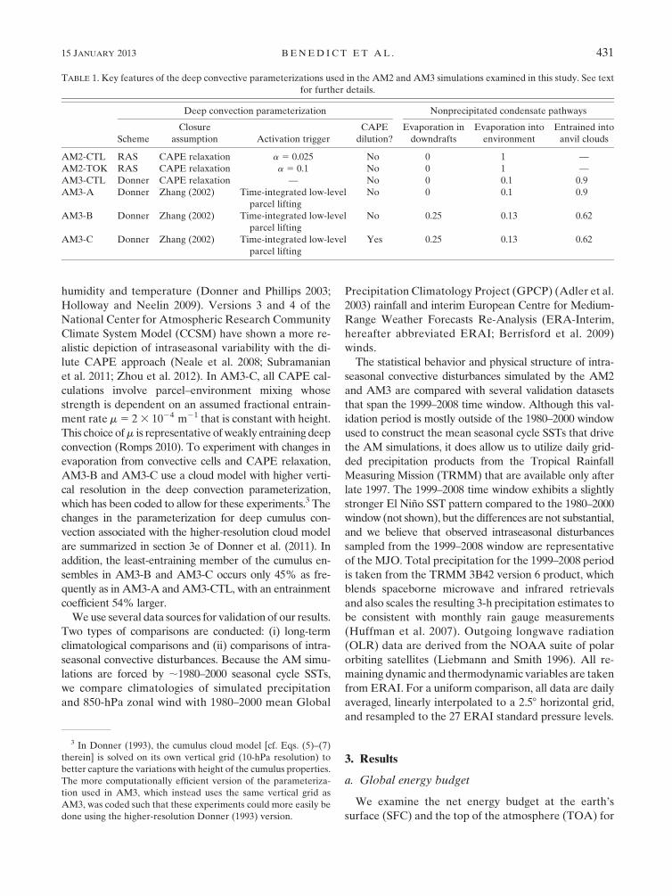
TABLE 1. Key features of the deep convective parameterizations used in the AM2 and AM3 simulations examined in this study. See text

for further details.

Deep convection parameterization Nonprecipitated condensate pathways

Scheme

Closure

assumption Activation trigger

CAPE

dilution?

Evaporation in

downdrafts

Evaporation into

environment

Entrained into

anvil clouds

AM2-CTL RAS CAPE relaxation a 5 0.025 No 0 1 —

AM2-TOK RAS CAPE relaxation a 5 0.1 No 0 1 —

AM3-CTL Donner CAPE relaxation — No 0 0.1 0.9

AM3-A Donner Zhang (2002) Time-integrated low-level

parcel lifting

No 0 0.1 0.9

AM3-B Donner Zhang (2002) Time-integrated low-level

parcel lifting

No 0.25 0.13 0.62

AM3-C Donner Zhang (2002) Time-integrated low-level

parcel lifting

Yes 0.25 0.13 0.62

3 In Donner (1993), the cumulus cloud model [cf. Eqs. (5)–(7)

therein] is solved on its own vertical grid (10-hPa resolution) to

better capture the variations with height of the cumulus properties.

The more computationally efficient version of the parameteriza-

tion used in AM3, which instead uses the same vertical grid as

AM3, was coded such that these experiments could more easily be

done using the higher-resolution Donner (1993) version.


observations and the AM simulations in Table 2. Only

small differences in the net surface longwave and sen-

sible heat fluxes are found between the different AM

versions. Modifications of AM convective parameteri-

zations examined in this study have a larger impact on net

surface shortwave and latent heat fluxes. For example,

globally averaged surface shortwave flux increases (be-

comes more negative, indicating a larger flux into the

surface) but is partially compensated by an increase in

latent heat flux. At the atmosphere top, the modified

versions of the AM3 have enhanced net shortwave that

is mostly offset by increasedOLR.With the exception of

AM3-B, net energy budget residuals at the SFC and

TOA are less than j4 W m22j. All AM versions exam-

ined indicate net atmospheric column energy budget

residuals less than about j0.1 W m22j.b. Boreal winter means

Observed intraseasonal convective disturbances are

influenced by the climatological state in which they exist

(e.g., Hendon and Salby 1994). A review of many GCM

simulations reveals that models with excessive mean

precipitation in the equatorial west Pacific often gener-

ate larger intraseasonal precipitation variability (Slingo

et al. 1996; Kim et al. 2011). Additionally, several GCM

experiments indicate a link between the accurate depic-

tion of tropical time-mean zonal winds and realistic MJO

eastward propagation (Inness et al. 2003; Sperber at al.

2005). Figure 2 illustrates climatological boreal winter

(November–April) precipitation for the 20-yr GPCP

dataset (Fig. 2a) as well as the biases for all AM simu-

lations (Figs. 2b–g). The AM2 and AM3 overestimate

globally averaged annual precipitation by about 10%–

20%. In the boreal winter, these biases are largest in the

western Indian and Pacific Ocean basins, the Pacific

intertropical convergence zone, and the South Ameri-

can west coast. A weak dry bias is noted near and west of

Java in most AM simulations examined. In AM3-CTL,

AM3-A, and AM3-C, a dry bias also appears in the

equatorial west Pacific.

Recent analyses of global energy balances and cloud

and aerosol properties based on the Cloud–Aerosol Lidar

and InfraredPathfinder SatelliteObservations (CALIPSO),

CloudSat, and Moderate Resolution Imaging Spectror-

adiometer (MODIS) satellites indicate that GPCP global

mean precipitation could be biased low.Kato et al. (2011)

show net surface irradiances consistent with globalmean

precipitation 15%–20%more thanGPCP and still within

estimated GPCP uncertainty (their Fig. 15). Accordingly,

the precipitation overestimates relative toGPCP inAM2

and AM3, which increase in the modified AM3 versions

examined in this study, may not be consequential.

A comparison of climatological boreal winter 850-hPa

zonal winds (hereafter, U850) between 1980–2000 ERAI

and the 10-yr AM simulations (Fig. 3) indicates that

AM2-CTL and AM3-CTL are able to reproduce the strip

of equatorial low-level westerlies across the Indian Ocean,

but that this region does not extend far enough into the

west Pacific. For example,U850westerlies extend to 1758Ein ERAI but only to 1358 and 1508E in the AM3-CTL and

TABLE 2. Global-mean energy budgets at the top of atmosphere (TOA) and earth surface (SFC) for observational estimates (Trenberth

et al. 2009) and all AM2 and AM3 simulations. Observational estimates reported in Trenberth et al. (2009) are derived from satellite

retrievals [Clouds and the Earth’s Radiant Energy System (CERES), International Satellite Cloud Climatology Project (ISCCP), and

GPCP], climate models [Community Land Model, version 3 (CLM3)], and various reanalysis products [e.g., National Centers for En-

vironmental Prediction (NCEP); see Trenberth et al. (2009) for further details]. Net flux components are also shown, including shortwave

(SW) and longwave (LW) radiation, surface latent heat flux (LH, includes column heating from snow formation), and surface sensible heat

flux (SH). Positive fluxes are into the atmospheric column; units are watts per meter squared.

Obs AM2-CTL AM2-TOK AM3-CTL AM3-A AM3-B AM3-C

Time range

2000–04 10 yr 10 yr 10 yr 10 yr 10 yr 10 yr

SFC

Net SW 2161.2 2162.1 2159.1 2161.6 2167.3 2163.5 2168.7

Net LH 180.0 185.6 187.7 188.5 192.1 195.0 193.7

Net LW 163.0 157.0 156.3 155.2 156.6 156.1 157.3

Net SH 117.0 118.8 118.9 116.5 117.9 118.5 118.2

NET SFC 20.9 20.7 13.7 21.4 20.7 16.2 10.6

TOA

Net SW 1239.4 1238.0 1235.1 1236.0 1241.1 1237.6 1242.0

Net LW 2238.5 2237.4 2238.8 2234.6 2240.4 2243.8 2242.6

NET TOA 10.9 10.6 23.8 11.4 10.7 26.2 20.6

NET column 0.0 20.1 20.1 0.0 0.0 0.0 0.0


AM2-CTL, respectively. The modified versions of the

AM2 and AM3 tend to improve the eastward extension

of low-level westerlies (e.g., to 1608E in AM2-TOK and

1558E in AM3-C) but also underestimate their strength

over the eastern Indian Ocean where magnitudes drop

to less than 1 m s21 as compared with 3–4 m s21 in

ERAI. In the extreme case, AM3-B actually produces

U850 easterlies of ;0.5 m s21 over the eastern Indian

FIG. 2. (a) Boreal winter mean (November–April) GPCP pre-

cipitation (1980–2000) and (b)–(g) the difference in boreal winter

mean precipitation between the GPCP dataset and each AM

simulation. Pattern correlations for the domain (208S–208N, 508E–1208W) are shown to the upper right of each difference panel.

FIG. 3. Climatological borealwintermean (November–April) 850-hPa

zonal wind U850 from (a) ERAI (1980–2000) and (b)–(g) the AM

simulations analyzed. The zero contour is shownwith a thick black line.


Ocean (Fig. 3f). For all AM simulations, low-level bo-

real winter mean easterlies are too strong across south-

ern Asia, the subtropical Pacific, and Central America.

Figure 4 shows boreal winter mean vertical profiles of

relative humidity between 608 and 1608E for ERAI and

the humidity differences between each AM simulation

and ERAI. Although only relative humidity profiles are

displayed here, comments on other variables are included

in this discussion. As documented in previous studies, the

cool-troposphere and warm-stratosphere temperature

biases in the AM2-CTL are reduced in the AM3-CTL

(see middle column of Table 3; Anderson et al. 2004;

Donner et al. 2011). Cool biases of 2–4 K in the middle

to upper troposphere of the climatological deep con-

vecting region (108S–58N, 608E–1808) are evident in the

AM2-TOK and all modifiedAM3 simulations, however,

while tropical boundary layer temperatures are within

a few tenths of a degree from the values indicated by

ERAI (Table 3). Zero (for AM3) or weakly positive (for

AM2) biases in boundary layer relative humidity are

noted in Fig. 4. A moist bias above 500 hPa in AM3-CTL

(Fig. 4d) is strongly reduced and even reverses sign in

the modified AM3 versions. For example, Fig. 4g shows

relative humidity values that are nearly 20% lower than

ERAI (Fig. 4a) in the equatorial midtroposphere. The

cool and dry biases in the modified AM3 are likely

linked to deep convection suppression that results from

the changes made to the convective parameterization.

Regarding vertical profiles of convective heatingQ1 [see

Eq. (1) from Lin and Johnson (1996)] using identical

FIG. 4. Boreal winter mean (November–April) relative humidity averaged between 608 and 1608E for (a) ERAI, and (b)–(g) the (model2ERAI) humidity difference for each AM simulation.

TABLE 3. Climatological November–April temperature biases

for the AM simulations. Biases are computed as the simulation

differences from reanalysis, averaged horizontally within the re-

gion (108S–58N, 608E–1808) and vertically within the noted pres-

sure levels.

Averaged T bias (K)

Simulation 200–500 hPa (8 levels) 900–1000 hPa (5 levels)

AM2-CTL 21.79 10.01

AM2-TOK 23.85 20.03

AM3-CTL 10.22 10.18

AM3-A 22.17 10.32

AM3-B 22.24 20.10

AM3-C 23.49 10.31


space–time averaging as in Fig. 4, the levels and magni-

tudes of maximum heating among the reanalysis andAM

simulations are qualitatively similar.4 One exception is

that the maximum of November–April mean heating

shifts from the Northern Hemisphere (58N) in AM3-CTL

to the Southern Hemisphere (2.58S) in all modified

versions of AM3 (not shown). All AM simulations tend

to overestimate heating and rising motion north of the

equator and underestimate heating south of the equator

during boreal winter. A persistent and unrealistic sec-

ondary maximum of convective heating near 125 hPa is

also noted in the AM within 108 of the equator (not

shown).

c. Zonal wavenumber–frequency spectra

Decomposing a total field into its zonal wavenumber

and frequency components allows a succinct view of

tropical wave activity. We compute such spectra for the

AM2 andAM3 output data using themethods ofWheeler

and Kiladis (1999). Figure 5 depicts power spectra of the

symmetric component of tropical precipitation for ob-

servations and a selection of AM simulations. Figures

5a–f each consist of a pair of plots showing the base-10

logarithm of the summation of spectral power from 158Sto 158N (‘‘raw’’ spectrum, top) and the raw spectrum di-

vided by a smoothed background spectrum (‘‘significant’’

spectrum, bottom). Negative zonal wavenumbers are as-

sociated with disturbances that propagate westward and

positive wavenumbers with those that propagate eastward.

Figure 6 shows the same spectra as Fig. 5 but zoomed into

the MJO spectral region. Relative to the AM2-CTL (not

shown), AM2-TOK exhibits a shift of the maximum in-

traseasonal power from westward to eastward propagat-

ing disturbances but continues to lack Kelvin wave activity

that is prevalent in nature (Fig. 5a). As in AM2-TOK,

previous modeling studies have also reported that MJO

variability generally becomesmore realistic through theuse

of strongermoisture triggers—more stringent requirements

for high humidity to be present in some layer in order for

parameterized deep convection to occur—in the deep con-

vection parameterization (e.g., Lin et al. 2008). Stronger

triggers were found to increase the contributions of large-

scale condensation, making model convection more sensi-

tive to environmental moisture. Lin et al. attribute the

slower and more intense disturbances to a reduction in

gross moist stability, as was demonstrated in earlier

studies using an idealized moist GCM (Frierson 2007).

The modifications made to the AM3 convective pa-

rameterization generally have a positive impact on the

depiction of tropical precipitation variability relative to

the control simulation, at the expense of a degraded

mean state as seen in Fig. 2 and noted in Donner et al.

(2011). Implementation of a modified convective closure

(Zhang 2002) and trigger (Donner et al. 2001) dramat-

ically improves precipitation variability associated with

Kelvin waves, the MJO, inertio–gravity waves (e.g.,

Figs. 5d and 6d), and mixed Rossby–gravity waves (not

shown) compared toAM3-CTL (Fig. 5c). Consistent with

Fig. 5, maps of variance of MJO-filtered precipitation

(not shown) show a marked improvement for the mod-

ified AM3 compared to AM3-CTL despite an over-

estimation of variability in the Northern Hemisphere

ITCZ. As in the case of AM2, the peak in intraseasonal

power shifts from a westward to eastward propagation

preference in AM3 when a convective parameterization

that suppresses deep cumuli is implemented. In the an-

tisymmetric precipitation spectra (not shown), modified

AM3 versions have improved (larger) power in theMJO

region but the signal-to-noise ratio is not significant.

Despite these improvements, several differences between

the observed and modified AM3 precipitation spectra

are evident. Overall, total variance is overestimated in

themodified versions ofAM3, consistent with the findings

of Kim et al. (2011). Raw power for westward propagat-

ing disturbances on subseasonal time scales (;6–90 days)

is overestimated as well. The power within the MJO

spectral region (zonal wavenumbers 11 to 15, periods

20–90 days) is also moderately overestimated and ex-

hibits a maximum closer to a 25–35-day period com-

pared to the observed;45 day period (Fig. 6, seeTable 4).

Additionally, the significant spectra show that Kelvin

wave power shifts to smaller equivalent depths (slower

phase speeds) and lower frequencies in the AM3 simu-

lations that incorporate more stringent convective trig-

gers (Figs. 5d,e), in agreement with Frierson et al.

(2011). In AM3-C, low-frequency eastward propagating

disturbances resemble convectively coupled Kelvin

waves rather than the MJO, as is shown here in Figs. 5

and 6 (and later in Fig. 8). The ability of AM3-A to

simulate the combination of equatorial Rossby and

Kelvin waves and MJO disturbances makes it an ap-

pealing test bed for future studies of tropical intraseasonal

variability.

RecentworkbyRoundy (2012a,b) suggests that innature

there is a smooth transition of spectral power between the

MJO and Kelvin bands in regions of climatological low-

level westerlies, in contrast to the spectral gap that arises

within the dominant easterly trade regime. In the mod-

ified AM3, Kelvin power shifts to lower frequencies and

smaller equivalent depths (slower phase speeds) and the

4 The accuracy of computing the pressure level of peak con-

vective heating is complicated by the model’s vertical resolution in

the midtroposphere. Approximate layer-midpoint pressures in this

area are 392, 461, 532, and 600 hPa.


FIG. 5. Frequency–zonal wavenumber power spectra of the symmetric component (about the equator) of pre-

cipitation for observations and a selection of AM simulations. For each panel, a pair of plots display the (top) base-10

logarithm of the summation of power between 158S and 158N (raw spectrum) and (bottom) raw spectrum divided by

a smoothed background spectrum. Thick black lines represent dispersion curves for equivalent depths of 12, 25, and

50 m for equatorial Rossby (ER), Kelvin, and eastward and westward inertio–gravity waves (EIG and WIG, re-

spectively) and the MJO. Negative zonal wavenumbers correspond to westward propagation.


gap between MJO and Kelvin spectral peaks is less no-

ticeable, particularly for AM3-C. However, the low-level

westerlies—the presence of which contribute to the

smooth MJO–Kelvin transition in Roundy (2012b)—are

weaker in themodifiedAM3 compared toAM3-CTL (cf.

Fig. 3), and the smooth MJO–Kelvin transition follows

the h5 12 m shallow water equivalent depth line rather

than h 5 5 m as in Roundy (2012b).

FIG. 6. As in Fig. 5 but zoomed in to the MJO spectral region.


We present zonal wavenumber–frequency spectra of

U850 for ERAI, AM2-TOK, and AM3-C in Figs. 7a–c,

respectively. Both AM2 and AM3 generate zonal wind

variability associated with equatorial Rossby and Kelvin

waves and the MJO, but several biases exist. AM2-CTL

and AM3-CTL underestimate power for low-frequency

Kelvin waves and the MJO (not shown). All AM simu-

lations overestimate zonal wind variability in the spectral

area where high-frequency Kelvin waves merge with

eastward inertia–gravity waves. AM2-TOK produces

Kelvin waves with much higher phase speeds (larger

equivalent depths) relative to ERAI, likely due to the

absence of sufficient convective coupling (cf. Figs. 7a,b).

A persistent bias of the AM3 is the enhanced zonal wind

variability of low-frequency Kelvin waves that is evident

when the background spectrum is removed (bottom plot

of Fig. 7c). The clear separation of zonal wind spectral

power between the MJO and low-frequency Kelvin

waves near a 16-day period in ERAI (Fig. 7a) is seen in

AM2-TOK (Fig. 7b) but not in any of the AM3 simu-

lations (e.g., Fig. 7c; AM3-A and AM3-B U850 spectra

are qualitatively similar to AM3-C and so are omitted

from Fig. 7). The absence of an MJO–Kelvin spectral

gap in U850 occurs despite no enhancement of clima-

tological low-level westerlies over the Indo-Pacific re-

gion in theAM3 compared toAM2 (seeRoundy 2012b).

Modified versions of the AM3 do, however, produce

slower and more realistic Kelvin wave phase speeds, sug-

gesting an improvement in the coupling between tropical

convection and dynamics in AM3. A reduction in Kelvin

wave phase speed is noted when the dilute CAPE ap-

proximation is implemented in theAM3, compared to the

nondilute CAPE case. The dilute CAPE approach is as-

sumed to represent a more inhibiting convective trigger in

that, relative to the undilutedCAPE case, more instability

is required to reach the CAPE threshold for deep con-

vection (1000 J kg21). Our findings support the con-

clusions of Frierson (2007) and Frierson et al. (2011),

who showed that slower Kelvin waves developed with

more inhibiting convective triggers due to a reduction in

gross moist stability.

d. Lag correlation

We present lag correlations between rainfall and U850

in Fig. 8. To construct these plots, we first apply a 20–100-

day bandpass filter to anomalous precipitation and U850,

where the anomaly is a departure from the smoothed

calendar-day mean at each grid point. The data are then

latitudinally averaged between 158S and 158N. We cor-

relate the time series of precipitation at either 908E or

1508E (left and right columns of Fig. 8, respectively) with

U850 over a range of time lags and longitudes. Results

TABLE 4. Summary of intraseasonal convective disturbances and warm pool mean state biases for ERAI and the AM simulations.

Columns include U850 (qualitative bias description and eastward extent of boreal winter mean U850 equatorial westerlies), RH [relative

humidity bias description in the upper andmiddle troposphere (approximately 200–400 hPa and 400–600 hPa, respectively) and boundary

layer (BL; 900–1000 hPa)], T (temperature bias description), MJO E/W [ratio of eastward to westward spectral power for the symmetric

component of precipitation in the MJO spectral region (periods 32–96 days, zonal wavenumbers from11 to13 (eastward) or from21 to

23 (westward)], Kelvin (qualitative comparison of Kelvin waves between simulation and reanalysis based on significant power spectra in Fig.

5), MJO [qualitative MJO comparison between simulations and reanalysis based on significant power spectra in Fig. 6, where the ap-

proximate zonal wavenumber (zwn) and period (t) of the peak power are indicated], and Speed (approximate intraseasonal disturbance

phase speed based on Fig. 8). Other abbreviations in the table include IO (Indian Ocean), WP (west Pacific), and trop (troposphere).

Boreal winter mean biases Intraseasonal disturbances

U850 RH T

MJO

E/W Kelvin MJO

Speed

(m s21)

ERAI 1758E — — 2.4 — — 5–6

AM2-CTL Realistic, 1508E Up-trop: dry Mid-trop: cool 0.9 Very weak zwn 2–3, t;45 d —

Mid-trop: moist

BL: moist

AM2-TOK Weak IO, realistic

WP, 1608EUp-trop: dry Mid-trop: very

cool

1.4 Very weak zwn 3, t;45 d 5

Mid-trop: dry

BL: moist

AM3-CTL Realistic, 1358 Up-trop: moist Small T biases 0.9 Weak zwn 3, t;45 d —

AM3-A Weak, 1408E Up-trop: moist Mid-trop: cool 1.5 Slow zwn 2, t;30 d 6–10

Mid-trop: dry BL: warm

AM3-B Very weak

(IO easterlies),

1608E

Mid-trop: very dry Mid-trop: cool 1.4 Slow zwn 1, t;35 d 5–7

AM3-C Weak, 1558E Mid-trop: dry Mid-trop: very

cool

1.6 Slow, merged

with MJO

signal

zwn 1–2, t;20–30 d 6–11

BL: warm


from the AM2-CTL and AM3-CTL are not shown owing

to the inability of those models to produce realistic

eastward-propagating intraseasonal convection. Among

the modified AM simulations shown, the coupling be-

tween rainfall (which is approximately proportional to the

vertically integrated diabatic heating) and U850 (which

we take to be largely a dynamical response to the diabatic

heating) is stronger in theAM3-A andAM3-C.Although

AM2-TOK produces realistic phase speeds for distur-

bances in the west Pacific, it has difficulty depicting a

strong signal in the Indian Ocean (cf. Figs. 8c,d). The

modified AM2 and AM3 simulations tend to have a sta-

tionary or westward-moving U850 signal to the west of

the regression base point at 908E (Fig. 8, left column), in

contrast to reanalysis. The signal generated by AM3-A

in the Indian Ocean (Fig. 8e) suggests that this model is

able to simulate MJO phase speeds in that region better

than AM3-B and AM3-C. However, a general tendency

exists for disturbances in the modifiedAM3 simulations to

propagate too quickly, particularly when deep convection

is moving across the west Pacific region. For example,

estimated phase speeds in the west Pacific are about

5 m s21 in AM2-TOK but closer to 11 m s21 in AM3-C

(see Table 4). This rapid propagation of convective

disturbances in the modified AM3 may be partially at-

tributed to the use of prescribed SSTs in the model.

More realistic air–sea interactions, even in an idealized

framework, have been shown to reduce the phase speed

and enhance organization of the MJO in some GCMs

(Zhang et al. 2006). The faster speeds in the AM3-C are

consistent with the poorly distinguished separation be-

tween the MJO and Kelvin spectral peaks in Figs. 6f

and 7c and suggest that, particularly in the Pacific, the

disturbances produced by the modified AM3 versions

have characteristics more reminiscent of low-frequency

convectively coupled Kelvin waves (Straub et al. 2010).

This assertion is supported by noting that, in the modi-

fied AM3, the pattern of low-level zonal wind anomalies

differs from the observed MJO pattern in the Pacific

(Fig. 8b) such that a negative correlation exists between

intraseasonal rainfall and U850, and peak low-level

easterlies occur only a few days before the precipitation

FIG. 7. As in Fig. 5 but for 850-hPa zonal winds for (a) ERAI, (b) AM2-TOK, and (c) AM3-C.


maximum (Figs. 8f,h,j). This structure is more consistent

with observed convectively coupled Kelvin waves

(Wheeler et al. 2000) than with the MJO (Kiladis et al.

2005; Benedict and Randall 2007).

e. Lag regression

We present longitudinal cross sections of specific hu-

midity for ERAI and several AM simulations in Fig. 9.

FIG. 8. Lag correlations of 850-hPa zonal wind U850 with precipitation at (left) 908E and (right) 1508E. Both fields are

bandpass filtered (20–100days) and averagedbetween 158S and 158N.Solid (dashed) contours represent positive (negative)

correlations that are shadeddark (light) gray if they exceed the 95%statistical significance level.WeuseERAIandTRMM

for the observed wind and rainfall fields. In the left panels, the index reference longitudes and the 5 m s21 phase speed are

marked by vertical and slanted thick lines, respectively. The right panels also contain the 10 m s21 phase speed line.


FIG. 9. Lag-0 longitudinal cross sections of specific humidity anomalies linearly regressed onto

a standardized 20–100-day filtered precipitation index time series at (left) 908E and (right) 1508E.Humidity anomalies are departures from a smoothed calendar-day mean, and anomaly values rep-

resent a one standard deviation change in the index. Both fields are averaged between 158S and 158N.

Positive (negative) anomalies that exceed the 95% statistical significance levels are shaded dark

(light) gray. We use ERAI and TRMM for the observed specific humidity and rainfall fields. Index

reference longitudes are marked by thick vertical lines. Contour interval is 60.1 g kg21, and the

60.05 g kg21 contour is also shown. No zero contour is drawn.


Anomalous specific humidity is linearly regressed onto

a standardized version of the precipitation index defined

in section 3d and then averaged between 158S and 158N.

Plotted values represent humidity anomalies associated

with a one standard deviation change in the precipitation

index at zero time lag. All modified AM versions un-

derpredict the longitudinal extent and maximum value

of positive humidity anomalies relative to ERAI. The

longitudinal structure of moisture appears to be strongly

associated with the ability of the AM to realistically

simulate eastward propagation of intraseasonal con-

vective systems, as seen in Fig. 8. In particular, the

models that perform best at producing these distur-

bances (Figs. 9d,e,i,j) show some evidence of shallow

moistening that leads deep moistening. Low-level

moistening leading deep moistening is apparent in the

ERAI results (Figs. 9a,b) and in previous reanalysis- and

radiosonde-based studies of the observed MJO (Kiladis

et al. 2005; Kemball-Cook and Weare 2001) and other

convectively coupled equatorial waves (Kiladis et al.

2009).

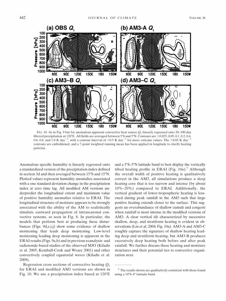
Regression cross sections of convective heating Q1

for ERAI and modified AM3 versions are shown in

Fig. 10. We use a precipitation index based at 1208E

and a 58S–58N latitude band to best display the vertically

tilted heating profile in ERAI (Fig. 10a).5 Although

the overall width of positive heating is qualitatively

correct in the AM3, all simulations produce a deep

heating core that is too narrow and intense (by about

10%–20%) compared to ERAI. Additionally, the

vertical gradient of lower-tropospheric heating is less-

ened during peak rainfall in the AM3 such that large

positive heating extends closer to the surface. This sug-

gests an overabundance of shallow cumuli and congesti

when rainfall is most intense in the modified versions of

AM3. A clear vertical tilt characterized by successive

shallow, deep, and stratiform heating is evident in ob-

servations (Lin et al. 2004; Fig. 10a). AM3-A and AM3-C

roughly capture the signature of shallow heating lead-

ing deep and stratiform heating, but AM3-B produces

excessively deep heating both before and after peak

rainfall. We further discuss these heating and moisture

structures and their potential ties to convective organi-

zation next.

FIG. 10. As in Fig. 9 but for anomalous apparent convective heat source Q1 linearly regressed onto 20–100-day

filtered precipitation at 1208E. All fields are averaged between 58S and 58N. Contours are60.025, 0.05, 0.1, 0.2, 0.4,

0.6, 0.8, and 1.0 K day21, with a contour interval of 60.5 K day21 for more extreme values. The 60.05 K day21

contours are emboldened, and a 7-point weighted running mean has been applied in longitude to clarify heating

patterns.

5 The results shown are qualitatively consistent with those found

using a 108S–08 latitude band.


4. Discussion

Salient features and biases of the AM simulations

are summarized in Table 4. The results discussed in

section 3 indicate that an improved depiction of eastward-

propagating intraseasonal disturbances is achieved when

mechanisms that suppress deep convection are imple-

mented in the AM3. This GCM behavior is not unique to

the GFDL AM and is documented extensively in the

modeling literature (e.g., Tokioka et al. 1988; Hannah

and Maloney 2011; Kim et al. 2011). The improvements

made to convectively coupled Kelvin waves and the

MJO come at the cost of a degraded mean state that

includes a drying and cooling of the tropical tropo-

sphere and a possible overestimation of equatorial total

precipitation. Additionally, phase speeds of the AM3-

simulated eastward-propagating convective systems are

faster than the observed MJO phase speed, particularly

for disturbances in the west Pacific region (see Table 4).

Despite these deficiencies, the AM3 simulations provide

new and useful information that may contribute to a

better understanding of the physical processes associated

with intraseasonal convective systems. Our preliminary

examination of themodifiedAM3 suggests a link between

the degree of organization of intraseasonal disturbances

and their corresponding heating and moisture structures

(Figs. 9 and 10). In this section, we investigate in greater

detail how differences in these structures might impact the

intraseasonal convective signals seen in the AM3.

Some GCM studies show that MJO simulation can be

improved if the fraction of stratiform (grid scale) to total

precipitation is increased (Fu and Wang 2009; Seo and

Wang 2010). In these studies, MJO-like disturbances

become much weaker when turbulent entrainment and

detrainment along the edges of either deep or shallow

convective plumes are set to zero [i.e., Eu(1) 5 Du

(1) 5 0

in Eq. (12) of Tiedtke (1989)]. The authors assert that

detrainment from convective clouds moistens the grid-

scale environment and promotes grid-scale precipitation.

The results of Fu and Wang emphasize the direct inter-

action between grid-scale precipitation heating and low-

frequency disturbances, and their explanation of more

vigorous MJO events invokes stratiform instability ar-

guments (Mapes 2000; Kuang 2008). To investigate the

applicability of this hypothesis to the AM3, we present

longitudinal cross sections of boreal winter mean total

precipitation (Fig. 11a) and large-scale6 precipitation as

a percentage of total precipitation (Fig. 11b). In both

AM2 and AM3, modifications that suppress deep con-

vection and increase the percentage of time-mean grid-

scale precipitation (Fig. 11b) are associatedwith enhanced

intraseasonal variability (cf. Fig. 6). Returning to Fig. 4,

AM3-B is drier thanAM3-A andAM3-C above 700 hPa

but has equal or slightly higher humidity below 700 hPa.

This is qualitatively consistent with Fig. 8a of Fu and

Wang (2009) and suggests that, in a comparison of AM3

simulations with identical convective closure and trigger

assumptions, a drier midtroposphere is associated with

weaker intraseasonal disturbances. Importantly, how-

ever, simply increasing the percentage of time-mean

grid-scale precipitation does not necessarily improve

intraseasonal convective organization in theAM3. Figure 8

indicates that AM3-A and AM3-C have more robust and

coherent signals of intraseasonal convective disturbances

FIG. 11. Longitudinal cross sections of boreal winter mean (a)

total precipitation and (b) stratiform (grid scale) precipitation as

a percentage of total precipitation for all AM simulations. Lat-

itudinal bounds are 108S–108N. Stratiform rainfall fraction was

computed for each day prior to space–time averaging.

6 ‘‘Large-scale’’ precipitation reported in AM3 is from grid-scale

stratiform clouds only and does not include contributions from

mesoscale anvils, so a direct comparison to observed percentages

of stratiform to total precipitation (e.g., Schumacher and Houze

2003) is not recommended.


in comparison with AM3-B despite the fact that per-

centages of grid-scale precipitation, at least in the time

mean, are larger in AM3-B (Fig. 11b). We also exam-

ined the behavior of grid-scale precipitation fraction in

an intraseasonal context. To do this, we produced plots of

anomalous daily grid-scale rainfall fraction regressed onto

an MJO total precipitation index at various longitudes

between 608E and 1808. These results (not shown) agree

with those depicted in Fig. 11b and indicate a greater grid-

scale rainfall fraction in AM3-B compared to AM3-A

or AM3-C. Additional work is needed to clarify the in-

teractions among humidity, grid-scale precipitation, and

the depiction of intraseasonal disturbances in the AM3.

We further investigate the link between convection

and large-scale circulations by examining Indo-Pacific

boreal winter mean convective mass fluxes that are out-

put directly from the AM3 convective parameterizations

(i.e., are not computed using grid-scale vertical velocities;

Fig. 12). Our modifications to the convective closure and

trigger assumptions strongly reduce upward mass fluxes

by deep convective cells (second row of Fig. 12). Upward

mass fluxes within mesoscale anvils are also reduced in

step with the weakened deep cumuli because these cu-

muli act as a main source of water substance for the anvil

clouds. In response to the suppressed deep convection,

activity from the shallow convective scheme increases in

the lower troposphere and expands upward (top row of

Fig. 12). Shallow convection is particularly enhanced in

AM3-A andAM3-C relative toAM3-B.Wenote that the

shallow convection scheme is that of a highly entraining

plume, where the cloud top is a function of plume

buoyancy. As such, modifications applied to the AM3

that limit the ability of deep convection to reduce in-

stability ultimately result in stronger and deeper plumes

FIG. 12. Boreal winter mean (November–April) parameterized mass fluxes from the (top) shallow convection scheme UW_CONV,

(middle) deep convection scheme (upward only, CELL_UP), and (bottom) mesoscale cloud scheme (upward only, MESO_UP) for all

AM3 simulations.


produced by the shallow convection parameterization.

The interplay between stratiform (grid scale) and shallow

convective activity in the AM3 is evident in a compari-

son of boreal winter mean rainfall associated with large-

scale and shallow convective processes (not shown). In

the AM3 simulations with robust intraseasonal vari-

ability (AM3-A and AM3-C), time-mean shallow con-

vection increases as grid-scale precipitation decreases.

The opposite behavior occurs in the AM3 version with

weaker intraseasonal variability (AM3-B).

Shallow convective activity may be stronger in a time-

mean sense in the AM3-A and AM3-C simulations, but

are these differences in diabatic heating manifested on

intraseasonal scales as well? Figure 13 depicts the ver-

tical structure of the effective heat source, Q1 (Yanai

et al. 1973), taken from the linear regressions of Fig. 10

and averaged over selected longitude ranges to capture

the dominant heating signatures to the west and east of

peak rainfall at 1208E. We omit heating profiles at the

longitude of peak rainfall because they are qualitatively

similar among the models, with the exception that the

modified AM3 version with weaker intraseasonal distur-

bances (AM3-B) has a slightly weaker upper-tropospheric

heating maximum (and thus a slightly less top-heavy

profile) compared to AM3-A and AM3-C. In Fig. 13b,

the observed heating profile over the west Pacific is

bottom heavy with a peak heating near 850 hPa and

cooling in the midtroposphere, in agreement with the

TRMM-based results of Lau and Wu (2010). A similar

structure is noted for AM3-A and AM3-C, but AM3-B

reveals a shallow heating peak closer to 725 hPa and

a lack of cooling anywhere in the troposphere. Similar

differences between the AM3-B heating profiles and the

TRMM results of Lau and Wu (2010) are seen to the

west of maximum rainfall where stratiform processes

are expected to dominate (Fig. 13a). Here, top-heavy

heating is evident in ERAI, with a peak near 450 hPa

and aminimum in the lower troposphere. The upper-level

heating is too weak in all AM3 versions, but the modified

AM3 versions with more robust intraseasonal distur-

bances (AM3-A and AM3-C) produce a much stronger

reduction in low-level heating (and thus a larger vertical

heating gradient in the middle troposphere) compared

to AM3-B.

The shape of the vertical heating profile can impact

the large-scale flow and thus the distribution of moisture

and degree of atmospheric stability. Wu (2003) argues

that a bottom-heavy heating profile associated with

shallow convection generates stronger near-surface cir-

culations and enhances low-level moisture convergence

to the east of deep convection, and that this shallow

heating can sustainMJO-like systems against dissipation.

Figure 14 depicts anomalies of 2$ � qvh regressed onto

a standardized precipitation index at 1208E, where q is

FIG. 13. Vertical profiles of regressed apparent convective heating Q1 taken from Fig. 10 and

averaged between (a) 808 and 1008E, (b) 1508E and 1808.


specific humidity and vh is horizontal vector wind. Both

fields are averaged between 158S and 158N. In ERAI

(Fig. 14a), positive moisture convergence anomalies de-

velop within the boundary layer during the suppressed

convective phase (i.e., in the west Pacific) and then gradu-

ally deepen toward thedisturbance center.A similar pattern

is seen in AM3-A and AM3-C—the two modified AM3

versions with more robust intraseasonal disturbances—but

the suppressed-phase moisture convergence in AM3-B

is irregular and weak. Boundary layer moistening along

the leading (eastern) edge of the disturbance is mainly

associated with meridional convergence (not shown).

This suggests that the convergence may be primarily

frictional in origin, a process whose importance to the

MJO has been debated (e.g., Wang 1988; Moskowitz

and Bretherton 2000).

Figures 13 and 14 indicate a clear link between the

vertical heating profiles and large-scale circulations as-

sociated with intraseasonal convective disturbances in

the AM3. In the two modified AM3 versions with the

strongest inhibition of deep convection (AM3-A and

AM3-C), time-mean shallow convective activity is en-

hanced relative to a third modified AM3 version with

weaker deep convective suppression (AM3-B). These

differences in heating profiles are associated with sub-

seasonal variability rather than simply being features of

the time means. In AM3-A and AM3-C, the peak of

shallow convective heating is more prominent and the

vertical gradient of heating in the lower to midtropo-

sphere is larger ahead of the intraseasonal deep convec-

tive center (Fig. 13). This sharper heating peak effectively

drives low-level circulations and moisture convergence

that can promote subsequent convective development.

A larger vertical gradient of upper-tropospheric heating

associated with stratiform processes is also seen inAM3-A

and AM3-C relative to AM3-B (Fig. 13). It is unclear

exactly why the stratiform signal trailing the deep con-

vective center is enhanced in themodifiedAM3 versions

with stronger deep convective suppression (AM3-A and

AM3-C), although it seems plausible that the overall

improved strength and organization of the disturbances

themselves somehow promote improved organization of

the heating. Lau and Wu (2010) assert that horizontal

variability of the vertical heating profile likely contrib-

utes to the modulation of intraseasonal deep convection

and the transition of MJO phases. For example, those

authors demonstrate that shallow cumulus heating pre-

conditions the environment ahead of the MJO while

stratiform heating entrains dry midtropospheric air and

suppresses deep convection following the MJO. To-

gether, the differences in the distributions of the simu-

lated heating structures and their associated circulations

are related to the degree of organization of intraseasonal

convective disturbances in the AM3.

5. Conclusions

Intraseasonal variability in four GFDL AM3 simula-

tions is examined and compared to previous simulations

of the AM2. In contrast to AM2, AM3 employs new

treatments of deep and shallow convection. In particular,

cloud–aerosol interactions are introduced by computing

cumulus cell-scale vertical velocities, and the param-

eterization of convective cloud systems now includes

dynamically active mesoscale clouds that modulate the

transfer of water substance between cumuli and their

FIG. 14. As in Fig. 10 but for anomalous moisture convergence,

2$ � qvh, linearly regressed onto 20–100-day filtered precipitation

at 1208E. All fields are averaged between 158S and 158N. Here q is

specific humidity and vh is horizontal vector wind. We use ERAI

and TRMM for the observed wind, specific humidity, and rainfall

fields.


environment. The default AM3 generates a realistic

mean state but lacks intraseasonal variability. Changes

made to the deep convective closure and trigger as-

sumptions inhibit themost penetrative cumuli and result

in a substantial increase in the amplitude of eastward-

propagating intraseasonal disturbances. As is typical of

many other GCMs (Kim et al. 2011), the improved sim-

ulation of intraseasonal variability comes at the cost of

a degraded mean state that includes possible wet biases

in equatorial precipitation and a weakening of low-level

westerlies in the Indo-Pacific region.

The eastward-propagating intraseasonal features pro-

duced by the modified AM3 versions have unrealistically

narrow longitudinal scales and propagate at speeds closer

to those of convectively coupled Kelvin waves in the west

Pacific (Wheeler et al. 2000). Notable differences in the

degree of convective organization and signal coherence

exist among the modified AM3 simulations and may be

associated with intraseasonal heating structures and their

impact on low-level circulation and moisture availability,

particularly for those processes related to shallow con-

vection. In the two versions of theAM3with the strongest

MJO-like signal (AM3-A and AM3-C), a more prom-

inent peak in shallow heating occurs with enhanced low-

level convergence that increases moisture accumulation

ahead of the deep convective center. The tropospheric

heating gradient and low-level convergence leading the

convective center are substantially weaker in the AM3

version with more disorganized intraseasonal convec-

tion (AM3-B). Following the deep convective center,

AM3-A and AM3-C depict a more pronounced strati-

form heating signal relative to AM3-B. Stratiform cloud

processes can modulate intraseasonal deep convection

and the transition of MJO phases (Lau and Wu 2010)

and may also be contributing to the differences among

the modified AM3 simulations in addition to shallow

heating differences.

Although we have provided new insight into the

mechanisms that contribute to intraseasonal convective

organization within the GFDL AM3, many issues have

yet to be addressed. One such issue is the inability of the

AM3 to produce a realistic mean state concurrent with

a reasonable degree of intraseasonal variability. Another

involves the dilemma by which intraseasonal convection

is improved. On one hand, we have found that suppress-

ing deep convection enhances intraseasonal variability;

however, deep convection suppression also limits the

source of water substance for the mesoscale clouds that

are clearly important in simulated and observed MJOs

(Fu and Wang 2009; Lau and Wu 2010). Additionally,

our use of prescribed SSTs in the AM simulations pre-

cludes realistic air–sea interactions that strongly modu-

late intraseasonal convection in GCMs (Waliser et al.

1999) and in nature (Roundy and Kiladis 2006). Fur-

ther research is warranted to explore these and other

issues related to simulated intraseasonal convection in

the AM3.

Acknowledgments. We thank J.-L. Lin and three

anonymous reviewers for their helpful comments on

this manuscript. This work was supported by award

NA08OAR4320893 (JJB, EDM) and NA08OAR4320912

(AHS) from the National Oceanic and Atmospheric Ad-

ministration, U.S. Department of Commerce, and by the

Climate and Large-Scale Dynamics Program of the Na-

tional Science Foundation under Grants AGS-1025584

(EDM) and ATM-1062161 (EDM). The statements, find-

ings, conclusions, and recommendations do not necessarily

reflect the views of NSF, NOAA, or the Department of

Commerce.

REFERENCES

Adler, R. F., and Coauthors, 2003: The version-2 Global Pre-

cipitation Climatology Project (GPCP) monthly precipitation

analysis (1979–present). J. Hydrometeor., 4, 1147–1167.

Anderson, J. L., and Coauthors, 2004: The new GFDL global at-

mosphere and land model AM2–LM2: Evaluation with pre-

scribed SST simulations. J. Climate, 17, 4641–4673.

Arakawa, A., and W. H. Schubert, 1974: Interaction of a cumulus

cloud ensemble with the large-scale environment, Part I.

J. Atmos. Sci., 31, 674–701.

Benedict, J. J., andD.A.Randall, 2007:Observed characteristics of

the MJO relative to maximum rainfall. J. Atmos. Sci., 64,

2332–2354.

Berrisford, P., D. Dee, K. Fielding, M. Fuentes, P. Kallberg,

S. Kobayashi, and S. Uppala, 2009: The ERA-Interim archive.

ECMWFTech. Rep. 1, 16 pp. [Available online at http://www.

ecmwf.int/publications/library/do/references/show?id589203.]

Bretherton, C. S., J. R. McCaa, and H. Grenier, 2004: A new pa-

rameterization for shallow cumulus convection and its appli-

cation to marine subtropical cloud-topped boundary layers.

Part I: Description and 1D results. Mon. Wea. Rev., 132, 864–

882.

Donner, L. J., 1993: A cumulus parameterization including mass

fluxes, vertical momentum dynamics, and mesoscale effects.

J. Atmos. Sci., 50, 889–906.

——, and V. T. Phillips, 2003: Boundary layer control on convec-

tive available potential energy: Implications for cumulus pa-

rameterization. J. Geophys. Res., 108, 4701, doi:10.1029/

2003JD003773.

——, C. J. Seman, R. S. Hemler, and S. Fan, 2001: A cumulus

parameterization including mass fluxes, convective vertical

velocities, and mesoscale effects: Thermodynamic and hy-

drological aspects in a general circulation model. J. Climate,

14, 3444–3463.

——, and Coauthors, 2011: The dynamical core, physical parame-

terizations, and basic simulation characteristics of the atmo-

spheric component AM3 of the GFDL global coupled model

CM3. J. Climate, 24, 3484–3519.Emanuel, K. A., 1987: An air–sea interaction model of intra-

seasonal oscillations in the tropics. J. Atmos. Sci., 44, 2324–

2340.


——, 1993: The effect of convective response time on WISHE

modes. J. Atmos. Sci., 50, 1763–1776.

Frierson, D. M.W., 2007: Convectively coupled Kelvin waves in an

idealized moist general circulation model. J. Atmos. Sci., 64,2076–2090.

——, D. Kim, I.-S. Kang, M.-I. Lee, and J. Lin, 2011: Structure of

AGCM-simulated convectively coupled Kelvin waves and

sensitivity to convective parameterization. J. Atmos. Sci., 68,26–45.

Fu, X., and B.Wang, 2009: Critical roles of the stratiform rainfall in

sustaining the Madden–Julian oscillation: GCM experiments.

J. Climate, 22, 3939–3959.Hannah, W. M., and E. D. Maloney, 2011: The role of moisture–

convection feedbacks in simulating the Madden–Julian oscil-

lation. J. Climate, 24, 2754–2770.Hayashi, Y., 1970: A theory of large-scale equatorial waves gen-

erated by condensation heat and accelerating the zonal wind.

J. Meteor. Soc. Japan, 48, 140–160.

Hendon, H. H., and M. L. Salby, 1994: The life cycle of the

Madden–Julian oscillation. J. Atmos. Sci., 51, 2225–2237.

Holloway, C. E., and J. D. Neelin, 2009:Moisture vertical structure,

column water vapor, and tropical deep convection. J. Atmos.

Sci., 66, 1665–1683.Houze, R. A., Jr., 1982: Cloud clusters and large-scale vertical

motion in the tropics. J. Meteor. Soc. Japan, 60, 396–410.

——, 1989: Observed structure of mesoscale convective systems

and implications for large-scale heating.Quart. J. Roy.Meteor.

Soc., 115, 425–461.

Huffman, G. J., and Coauthors, 2007: The TRMM Multisatellite

Precipitation Analysis (TMPA): Quasi-global, multiyear, com-

bined-sensor precipitation estimates at fine scales. J. Hydrol., 8,

38–55.

Hurrell, J. W., J. J. Hack, D. Shea, J. M. Caron, and J. Rosinski,

2008: A new sea surface temperature and sea ice boundary

dataset for the Community AtmosphereModel. J. Climate, 21,

5145–5153.

Inness, P. M., J. M. Slingo, E. Guilyardi, and J. Cole, 2003: Simula-

tion of the Madden–Julian oscillation in a coupled general

circulationmodel. Part II: The role of the basic state. J. Climate,

16, 365–382.

Jia, X., C. Li, N. Zhou, and J. Ling, 2010: The MJO in an AGCM

with three different cumulus parameterization schemes. Dyn.

Atmos. Oceans, 49, 141–163.

Kato, S., and Coauthors, 2011: Improvements of top-of-atmosphere

and surface irradiance computations with CALIPSO-, CloudSat-,

and MODIS-derived cloud and aerosol properties. J. Geophys.

Res., 116, D19209, doi:10.1029/2011JD016050.

Kemball-Cook, S. R., and B. C. Weare, 2001: The onset of convec-

tion in the Madden–Julian oscillation. J. Climate, 14, 780–793.Khouider, B., and A. J. Majda, 2007: A simple multicloud param-

eterization for convectively coupled tropical waves. Part II:

Nonlinear simulations. J. Atmos. Sci., 64, 381–400.——, A. St-Cyr, A. J. Majda, and J. Tribbia, 2011: The MJO and

convectively coupled waves in a coarse-resolution GCM with a

simple multicloud parameterization. J. Atmos. Sci., 68, 240–264.

Kiladis, G. N., K. H. Straub, and P. T. Haertel, 2005: Zonal and

vertical structure of the Madden–Julian oscillation. J. Atmos.

Sci., 62, 2790–2809.

——,M. C.Wheeler, P. T. Haertel, K. H. Straub, and P. E. Roundy,

2009: Convectively coupled equatorial waves. Rev. Geophys.,

47, RG2003, doi:10.1029/2008RG000266.

Kim, D., and Coauthors, 2009: Application of MJO simulation

diagnostics to climate models. J. Climate, 22, 6413–6436.

——,A.H. Sobel, E.D.Maloney,D.M.W. Frierson, and I.-S.Kang,

2011: A systematic relationship between intraseasonal vari-

ability and mean state bias in AGCM simulations. J. Climate,

24, 5506–5520.Kuang, Z., 2008: A moisture-stratiform instability for convectively

coupled waves. J. Atmos. Sci., 65, 834–854.

Kummerow, C., and Coauthors, 2000: The status of the Tropical

Rainfall Measuring Mission (TRMM) after two years in orbit.

J. Appl. Meteor., 39, 1965–1982.

Lappen, C.-L., and C. Schumacher, 2012: Heating in the tropical

atmosphere: What level of detail is critical for acurate MJO

simulations in GCMs? Climate Dyn., 39, 2547–2568.Lau, K.-M., and H.-T. Wu, 2010: Characteristics of precipitation,

cloud, and latent heating associated with the Madden–Julian

oscillation. J. Climate, 23, 504–518.Leary, C. A., andR.A.Houze, 1980: The contribution ofmesoscale

motions to the mass and heat fluxes of an intense tropical

convective system. J. Atmos. Sci., 37, 784–796.

Li, C., X. Jia, J. Ling, W. Zhou, and C. Zhang, 2009: Sensitivity of

MJO simulations to diabatic heating profiles. Climate Dyn.,

32, 167–187.

Liebmann, B., and C. A. Smith, 1996: Description of a complete

(interpolated) outgoing longwave radiation dataset. Bull.

Amer. Meteor. Soc., 77, 1275–1277.

Lin, J., B. Mapes, M. Zhang, and M. Newman, 2004: Stratiform

precipitation, vertical heating profiles, and theMadden–Julian

oscillation. J. Atmos. Sci., 61, 296–309.

——, and Coauthors, 2006: Tropical intraseasonal variability in 14

IPCC AR4 climate models. Part I: Convective signals. J. Cli-

mate, 19, 2665–2690.——, M.-I. Lee, D. Kim, I.-S. Kang, and D. M. W. Frierson, 2008:

The impacts of convective parameterization and moisture

triggering on AGCM-simulated convectively coupled equa-

torial waves. J. Climate, 21, 883–909.Lin, X., and R. H. Johnson, 1996: Heating, moistening, and rainfall

over the western Pacific warm pool during TOGA COARE.

J. Atmos. Sci., 53, 3367–3383.Madden, R. A., and P. R. Julian, 1971: Detection of a 40–50 day

oscillation in the zonal wind in the tropical Pacific. J. Atmos.

Sci., 28, 702–708.

Maloney, E. D., and D. L. Hartmann, 2001: The sensitivity of in-

traseasonal variability in the NCAR CCM3 to changes in

convective parameterization. J. Climate, 14, 2015–2034.

Mapes, B. E., 2000: Convective inhibition, subgrid-scale triggering

energy, and stratiform instability in a toy tropical wave model.

J. Atmos. Sci., 57, 1515–1535.

Moncrieff, M. W., 1992: Organized convective systems: Arche-

typal dynamical models, mass and momentum flux theory, and

parametrization. Quart. J. Roy. Meteor. Soc., 118, 819–850.——, 2004: Analytic representation of the large-scale organization

of tropical convection. J. Atmos. Sci., 61, 1521–1538.

Moorthi, S., andM. J. Suarez, 1992: RelaxedArakawa-Schubert: A

parameterization of moist convection for general circulation

models. Mon. Wea. Rev., 120, 978–1002.

Moskowitz, B. M., and C. S. Bretherton, 2000: An analysis of fric-

tional feedback on a moist equatorial Kelvin mode. J. Atmos.

Sci., 57, 2188–2206.

Neale, R. B., J. H. Richter, and M. Jochum, 2008: The impact of

convection on ENSO: From a delayed oscillator to a series of

events. J. Climate, 21, 5904–5924.Neelin, J. D., I. M. Held, and K. H. Cook, 1987: Evaporation–wind

feedback and low-frequency variability in the tropical atmo-

sphere. J. Atmos. Sci., 44, 2341–2348.


Reynolds, R. W., N. A. Rayner, T. M. Smith, D. C. Stokes, and

W.Wang, 2002: An improved in situ and satellite SST analysis

for climate. J. Climate, 15, 1609–1625.

Romps, D. M., 2010: A direct measure of entrainment. J. Atmos.

Sci., 67, 1908–1927.

Roundy, P. E., 2012a: Observed structure of convectively coupled

waves as a function of equivalent depth: Kelvin waves and the

Madden–Julian oscillation. J. Atmos. Sci., 69, 2097–2106.——, 2012b: The spectrum of convectively coupled Kelvin waves

and the Madden–Julian oscillation in regions of low-level

easterly and westerly background flow. J. Atmos. Sci., 69,

2107–2111.

——, and G. N. Kiladis, 2006: Observed relationships between

oceanic Kelvin waves and atmospheric forcing. J. Climate, 19,

5253–5272.

Salzmann, M., Y. Ming, J.-C. Golaz, P. A. Ginoux, H. Morrison,

A.Gettelman,M.Kramer, andL. J. Donner, 2010: Two-moment

bulk stratiform cloud microphysics in the GFDL AM3 GCM:

Description, evaluation, and sensitivity tests. Atmos. Chem.

Phys., 10, 8037–8064.

Schumacher, C., and R. A. Houze, 2003: The TRMM precipitation

radar’s view of shallow, isolated rain. J. Appl. Meteor., 42,

1519–1524.

Seo, K.-H., and W. Wang, 2010: The Madden–Julian oscillation

simulated in the NCEP Climate Forecast System model: The

importance of stratiform heating. J. Climate, 23, 4770–4793.Slingo, J. M., and Coauthors, 1996: Intraseasonal oscillations in 15

atmospheric general circulation models: Results from an

AMIP diagnostic subproject. Climate Dyn., 12, 325–357.

Sobel, A. H., E. D. Maloney, G. Bellon, and D. M. Frierson, 2010:

Surface fluxes and tropical intraseasonal variability: A re-

assessment. J. Adv. Model. Earth Syst., 2 (2), doi:10.3894/

JAMES.2010.2.2.

Sperber, K., S. Gualdi, S. Legutke, and V. Gayler, 2005: The

Madden–Julian oscillation in ECHAM4 coupled and un-

coupled general circulation models. Climate Dyn., 25, 117–

140.

Straub, K. H., P. T. Haertel, and G. N. Kiladis, 2010: An analysis of

convectively coupledKelvin waves in 20WCRPCMIP3 global

coupled climate models. J. Climate, 23, 3031–3056.

Subramanian,A. C.,M. Jochum,A. J.Miller, R.Murtugudde, R. B.

Neale, and D. E. Waliser, 2011: The Madden–Julian oscilla-

tion in CCSM4. J. Climate, 24, 6261–6282.

Tiedtke, M., 1989: A comprehensive mass flux scheme for cumulus

parameterization in large-scale models. Mon. Wea. Rev., 117,1779–1800.

Tokioka, T., K. Yamazaki, A. Kitoh, and T. Ose, 1988: The

equatorial 30-60 day oscillation and the Arakawa–Schubert

penetrative cumulus parameterization. J. Meteor. Soc. Japan,

66, 883–901.

Trenberth, K. E., J. T. Fasullo, and J. Kiehl, 2009: Earth’s global

energy budget. Bull. Amer. Meteor. Soc., 90, 311–323.Waliser, D. E., K. M. Lau, and J. H. Kim, 1999: The influence of

coupled sea surface temperatures on the Madden–Julian os-

cillation: A model perturbation experiment. J. Atmos. Sci., 56,

333–358.

Wang, B., 1988: Dynamics of tropical low-frequency waves: An

analysis of the moist Kelvin wave. J. Atmos. Sci., 45, 2051–

2065.

Wheeler, M., and G. N. Kiladis, 1999: Convectively coupled

equatorial waves: Analysis of clouds and temperature in the

wavenumber–frequency domain. J. Atmos. Sci., 56, 374–399.

——, ——, and P. J. Webster, 2000: Large-scale dynamical fields

associated with convectively coupled equatorial waves.

J. Atmos. Sci., 57, 613–640.

Wilcox, E. M., and L. J. Donner, 2007: The frequency of extreme

rain events in satellite rain-rate estimates and an atmospheric

general circulation model. J. Climate, 20, 53–69.

Wu, Z., 2003:A shallowCISK, deep equilibriummechanism for the

interaction between large-scale convection and large-scale

circulations in the tropics. J. Atmos. Sci., 60, 377–392.Yanai, M., S. Esbensen, and J.-H. Chu, 1973: Determination of

bulk properties of tropical cloud clusters from large-scale heat

and moisture budgets. J. Atmos. Sci., 30, 611–627.Yuan, J., and R. A. Houze, 2010: Global variability of mesoscale

convective system anvil structure from A-Train satellite data.

J. Climate, 23, 5864–5888.

Zhang, C., and Coauthors, 2006: Simulations of theMadden–Julian

oscillation in four pairs of coupled and uncoupled global

models. Climate Dyn., 27, 573–592.

Zhang, G. J., 2002: Convective quasi-equilibrium in midlatitude

continental environment and its effect on convective param-

eterization. J. Geophys. Res., 107, 4220, doi:10.1029/

2001JD001005.

——, and M. Mu, 2005: Simulation of the Madden–Julian oscilla-

tion in the NCAR CCM3 using a revised Zhang–McFarlane

convection parameterization scheme. J. Climate, 18, 4046–

4064.

Zhao, M., I. M. Held, S. J. Lin, andG. A. Vecchi, 2009: Simulations

of global hurricane climatology, interannual variability, and

response to global warming using a 50-km resolution GCM.

J. Climate, 22, 6653–6678.

Zhou, L., R. Neale, M. Jochum, and R. Murtugudde, 2012: Im-

proved Madden–Julian oscillations with improved physics:

The impact of modified convection parameterizations.

J. Climate, 25, 1116–1136.


Documents

Tropical Intraseasonal Variability in Version 3 of the