Embed Size (px)
Citation preview
August 2011
Travel Demand Model
Model Development and
Validation Report
Lincoln Metropolitan
Planning Organization
LINCOLN MPO TRAVEL DEMAND MODEL
Travel Demand Model Update and Enhancement ii
TABLE OF CONTENTS
EXECUTIVE SUMMARY ...................................................................... 1
PROCESS OVERVIEW .................................................................................................... 1 VALIDATION OVERVIEW ................................................................................................ 3
CHAPTER 1: ROADWAY NETWORK ................................................... 1-1
CONTEXT AND BACKGROUND ...................................................................................... 1-1 ROADWAY NETWORK DEVELOPMENT ........................................................................... 1-1
Transfer of Network Attributes ............................................................................................................. 1-2 Centroid Connectors .............................................................................................................................. 1-2 Link Consolidation ................................................................................................................................. 1-2 GIS Consistency ...................................................................................................................................... 1-3 Turn Penalties ........................................................................................................................................ 1-4 Grade Separation ................................................................................................................................... 1-4
ROADWAY NETWORK STRUCTURE ................................................................................ 1-5 INPUT AND OUTPUT NETWORKS .................................................................................. 1-6 MULTI-YEAR AND ALTERNATIVE NETWORK STRUCTURE .................................................... 1-8
Representation of Networks by Year..................................................................................................... 1-8 Representation of New Facilities ........................................................................................................... 1-9 Representation of Network Alternatives ............................................................................................... 1-9 Network Attribute Selection ................................................................................................................ 1-11
NETWORK ATTRIBUTE LIST ....................................................................................... 1-13 FUNCTIONAL CLASSIFICATION / FACILITY TYPE ............................................................... 1-15 AREA TYPE ........................................................................................................... 1-22
Area Type Specification ....................................................................................................................... 1-22
LINK SPEEDS ......................................................................................................... 1-25 Estimating Link Speeds ........................................................................................................................ 1-25 Travel Time .......................................................................................................................................... 1-26
LINK CAPACITIES .................................................................................................... 1-27 Freeways .............................................................................................................................................. 1-27 Collectors and Arterials ....................................................................................................................... 1-29 Resulting Capacity Model .................................................................................................................... 1-32
ROUTABLE NETWORK .............................................................................................. 1-33
LINCOLN MPO TRAVEL DEMAND MODEL
Travel Demand Model Update and Enhancement iii
CHAPTER 2: TRIP GENERATION ....................................................... 2-1 CONTEXT AND BACKGROUND ...................................................................................... 2-1
TRAFFIC ANALYSIS ZONE STRUCTURE ............................................................................ 2-1
HOUSEHOLD DISAGGREGATION MODELS ....................................................................... 2-5
Household Size Disaggregation Model .................................................................................................. 2-5 Household Income Disaggregation Model ............................................................................................ 2-6 TAZ-Level Bivariate Data ........................................................................................................................ 2-7
DATA SOURCES ....................................................................................................... 2-8
TRIP PURPOSES ....................................................................................................... 2-9
PRODUCTION RATES ............................................................................................... 2-12
Income Groups .................................................................................................................................... 2-12 Cross Classified Trip Rates ................................................................................................................... 2-12 Production Rate Summary ................................................................................................................... 2-17
ATTRACTION RATES ................................................................................................ 2-18
NON-HOME-BASED PRODUCTION ALLOCATION MODELS ................................................ 2-22
UNIVERSITY SPECIAL GENERATOR AND PRODUCTION ALLOCATION ..................................... 2-23
University Definition ............................................................................................................................ 2-23 Trip Types at Universities .................................................................................................................... 2-24 Special Generator Survey Adaptation ................................................................................................. 2-24 University Production Allocation ......................................................................................................... 2-29
EXTERNAL TRIPS .................................................................................................... 2-31
External Station Volumes .................................................................................................................... 2-31 Internal-External and External-Internal Trips ...................................................................................... 2-34 External-External Trips ........................................................................................................................ 2-34
TRIP BALANCING .................................................................................................... 2-36
CHAPTER 3: TRIP DISTRIBUTION ...................................................... 3-1 CONTEXT AND BACKGROUND ...................................................................................... 3-1
PEAK AND OFF-PEAK PERIOD DEFINITIONS ..................................................................... 3-2
ROADWAY NETWORK SHORTEST PATH .......................................................................... 3-2
Terminal Times ...................................................................................................................................... 3-3 Intrazonal Impedance ............................................................................................................................ 3-3
FRICTION FACTORS ................................................................................................... 3-3
Trip Lengths ........................................................................................................................................... 3-6 Intrazonal Trips ...................................................................................................................................... 3-7
LINCOLN MPO TRAVEL DEMAND MODEL
Travel Demand Model Update and Enhancement iv
CHAPTER 4: MODE MODELS .......................................................... 4-1 CONTEXT AND BACKGROUND ...................................................................................... 4-1
NON-MOTORIZED MODE SPLIT ................................................................................... 4-1
TRANSIT ................................................................................................................. 4-3
AUTO OCCUPANCY ................................................................................................... 4-7
CHAPTER 5: TRIP ASSIGNMENT ....................................................... 5-1
CONTEXT AND BACKGROUND ...................................................................................... 5-1
TIME OF DAY .......................................................................................................... 5-1
TRIP ASSIGNMENT .................................................................................................... 5-3
Assignment Algorithms .......................................................................................................................... 5-3 Closure Criteria ...................................................................................................................................... 5-4 Impedance Calculations ......................................................................................................................... 5-4 Volume-Delay Functions ........................................................................................................................ 5-5
SPEED FEEDBACK ..................................................................................................... 5-6
Methodology ......................................................................................................................................... 5-6 Convergence Criteria ............................................................................................................................. 5-8 Application of Speed Feedback for Alternatives Analysis ..................................................................... 5-9
TRAFFIC ASSIGNMENT VALIDATION ............................................................................ 5-10
Traffic Count Data ................................................................................................................................ 5-10 Overall Activity Level ........................................................................................................................... 5-11 Screenlines ........................................................................................................................................... 5-12 Measures of Error ................................................................................................................................ 5-15
CHAPTER 6: DYNAMIC VALIDATION.................................................. 6-1
CONTEXT AND BACKGROUND ...................................................................................... 6-1
LAND USE DATA ADJUSTMENTS .................................................................................. 6-1
Household Changes ............................................................................................................................... 6-3 Non-Residential Changes ....................................................................................................................... 6-3 Wholesale Changes................................................................................................................................ 6-4
ROADWAY NETWORK CHANGES .................................................................................. 6-5
Link Removal .......................................................................................................................................... 6-5
LINCOLN MPO TRAVEL DEMAND MODEL
Travel Demand Model Update and Enhancement v
LIST OF TABLES Table ES.1: Summarized Trip Productions per Household ....................................................................... 3 Table ES.2: Distribution of Trips by Purpose ............................................................................................ 3 Table ES.3: Modeled Average Trip Lengths .............................................................................................. 4 Table ES.4: Intrazonal Trip Percentages ................................................................................................... 5 Table ES.5: Mode Share Targets and Results............................................................................................ 5 Table ES.6: Regional Activity Validation ................................................................................................... 6 Table ES.7: Model % Root Mean Square Error ......................................................................................... 6 Table 1.1: Network Attributes Transferred from the Previous Model ................................................ 1-2 Table 1.2: Attributes Monitored during Link Consolidation ................................................................ 1-3 Table 1.3: Input Network Link Fields ................................................................................................. 1-13 Table 1.4: Input Network Node Fields ............................................................................................... 1-14 Table 1.5: Functional Classification / Facility Type Values ................................................................. 1-16 Table 1.6: Area Types ......................................................................................................................... 1-22 Table 1.7: Ratio of Freeflow Speed (Off-Peak) to Speed Limit .......................................................... 1-25 Table 1.8: Speed Limit to Freeflow Speed Conversion Factors.......................................................... 1-26 Table 1.9: Centroid Connector Freeflow Speeds ............................................................................... 1-26 Table 1.10: Ideal and Adjusted Capacities for Freeways and Expressways based on HCM 2000 ....... 1-29 Table 1.11: Link Capacity Adjustment Factors and Resulting Capacity ............................................... 1-30 Table 1.12: Parking Adjustment Factors .............................................................................................. 1-32 Table 1.13: Roadway Capacities (vehicles per hour per lane, upper-limit LOS E) ............................... 1-32 Table 2.1: Income Group Definitions ................................................................................................... 2-6 Table 2.2: Bivariate Household Distribution for Lancaster County ..................................................... 2-7 Table 2.3: Trip Purposes....................................................................................................................... 2-9 Table 2.4: Weighted Trips by Purpose ............................................................................................... 2-10 Table 2.5: Trip Purpose Definitions Based on Reported Activity ....................................................... 2-11 Table 2.6: Household Trip Production Rates by Income Category .................................................... 2-12 Table 2.7A: Initial HBW Trip Production Rates (Person trips per household)...................................... 2-13 Table 2.8A: Initial HBS Trip Production Rates (Person trips per household) ....................................... 2-13 Table 2.9A: Initial HBR Trip Production Rates (Person trips per household) ....................................... 2-13 Table 2.10A: Initial HBO Trip Production Rates (Person trips per household) ...................................... 2-14 Table 2.11A: Initial WBO Trip Production Rates (Person trips per household) ..................................... 2-14 Table 2.12A: Initial OBO Trip Production Rates (Person trips per household) ...................................... 2-14 Table 2.13A: Initial Trip Production Rates – All Purposes (Person trips per household) ....................... 2-14 Table 2.7B: Final Adjusted HBW Trip Production Rates (Person trips per household) ........................ 2-15 Table 2.8B: Final Adjusted HBS Trip Production Rates (Person trips per household) ......................... 2-15 Table 2.9B: Final Adjusted HBR Trip Production Rates (Person trips per household) ......................... 2-15 Table 2.10B: Final Adjusted HBO Trip Production Rates (Person trips per household)......................... 2-15 Table 2.11B: Final Adjusted WBO Trip Production Rates (Person trips per household) ....................... 2-16 Table 2.12B: Final Adjusted OBO Trip Production Rates (Person trips per household) ........................ 2-16 Table 2.13B: Final Adjusted Trip Production Rates – All Purposes (Person trips per household) ......... 2-16 Table 2.14: Summarized Trip Productions per Household .................................................................. 2-17 Table 2.15: Distribution of Trips by Purpose ....................................................................................... 2-17 Table 2.16: HBW Trip Attraction Rates ................................................................................................ 2-19 Table 2.17: HBS Trip Attraction Rates .................................................................................................. 2-19 Table 2.18: HBR Trip Attraction Rates ................................................................................................. 2-20
LINCOLN MPO TRAVEL DEMAND MODEL
Travel Demand Model Update and Enhancement vi
Table 2.19: HBO Trip Attraction Rates ................................................................................................. 2-20 Table 2.20: WBO Trip Attraction Rates ................................................................................................ 2-21 Table 2.21: OBO Trip Attraction Rates ................................................................................................. 2-21 Table 2.22: Total Trip Attraction Rates ................................................................................................ 2-22 Table 2.23: WBO Production Allocation Rates .................................................................................... 2-22 Table 2.24: University of Nebraska at Lincoln Employment Data ....................................................... 2-25 Table 2.25: University Enrollment Summary ....................................................................................... 2-25 Table 2.26: University Special Generator Values ................................................................................. 2-25 Table 2.27: Total Intra-Campus Trips ................................................................................................... 2-26 Table 2.28A: Intra-University HBU Production/Attraction Trip Table (Simplified Assumptions) .......... 2-26 Table 2.28B: Intra-University OBO Production/Attraction Trip Table (Simplified Assumptions) .......... 2-26 Table 2.29A: Intra-University HBU Production/Attraction Trip Table (Adjusted Assumptions) ............ 2-27 Table 2.29B: Intra-University OBO Production/Attraction Trip Table (Adjusted Assumptions) ............ 2-27 Table 2.30: Allocation of UNL Trips by Campus ................................................................................... 2-27 Table 2.31: Allocation of UNL City Campus Productions by TAZ ......................................................... 2-28 Table 2.32: Allocation of UNL City Campus Attractions by TAZ ........................................................... 2-28 Table 2.33: External Travel Assumptions ............................................................................................. 2-33 Table 2.34: IE/EI Trips by Trip Purpose and Direction ......................................................................... 2-34 Table 2.35: EE Trip Table Seed Values ................................................................................................. 2-35 Table 2.36: 24-Hour EE Trip Table ....................................................................................................... 2-35 Table 3.1: Peak and Off-Peak Trip Percentages by Purpose ................................................................ 3-2 Table 3.2: Terminal Penalties by Area Type ......................................................................................... 3-3 Table 3.3: Friction Factors .................................................................................................................... 3-6 Table 3.4: Modeled Average Trip Lengths ........................................................................................... 3-7 Table 3.5: Intrazonal Trip Percentages ................................................................................................ 3-7 Table 4.1: Non-Motorized Mode Shares – San Luis Obispo, California ............................................... 4-2 Table 4.2: Non-Motorized Mode Share Targets – Lincoln Model........................................................ 4-2 Table 4.3: Initial Non-Motorized Mode Split Models .......................................................................... 4-3 Table 4.4: Transit Availability Scores ................................................................................................... 4-4 Table 4.5: Transit Boarding/Trip Target ............................................................................................... 4-7 Table 4.6: Transit Ridership Factors ..................................................................................................... 4-7 Table 4.7: Auto Occupancy .................................................................................................................. 4-8 Table 5.1: Peak Period Definitions ....................................................................................................... 5-1 Table 5.2: Time of Day Factors (Based on 24 hours) ........................................................................... 5-3 Table 5.3: Pre-Distribution Time of Day Factors .................................................................................. 5-3 Table 5.4: Pre-Assignment Time of Day Factors .................................................................................. 5-3 Table 5.5: Volume Delay Parameters Alpha and Beta ......................................................................... 5-6 Table 5.6: Traffic Count Data Sources ................................................................................................ 5-11 Table 5.7: Regional Activity Validation .............................................................................................. 5-12 Table 5.8: VMT and VHT Totals .......................................................................................................... 5-12 Table 5.9: Screenline Data ................................................................................................................. 5-15 Table 5.10: Model % Root Mean Square Error .................................................................................... 5-16 Table 5.11: % Root Mean Square Error by Volume Group .................................................................. 5-17 Table 6.1: Household Sensitivity Test Results ...................................................................................... 6-3 Table 6.2: Non-Residential Sensitivity Test Results ............................................................................. 6-4 Table 6.3: Forecast Year Model Sensitivity Test Results ...................................................................... 6-4 Table 6.4: Link Removal Sensitivity Test Results .................................................................................. 6-5
LINCOLN MPO TRAVEL DEMAND MODEL
Travel Demand Model Update and Enhancement vii
LIST OF FIGURES Lincoln MPO Travel Model Process Flowchart ............................................................................................. 2 Figure ES.1: Trip Length Distribution Curves ............................................................................................. 4 Figure ES.2: Screenline Error Values .......................................................................................................... 7 Figure ES.3: Model Count/Volume Comparison ........................................................................................ 7 Figure 1.1: Example Model Run Directory Structure ............................................................................ 1-7 Figure 1.2a: 2009 Facility Type Designations (Regionwide) .................................................................. 1-17 Figure 1.2b: Facility Type Designations (Urban Area Detail) ................................................................. 1-18 Figure 1.2c: Facility Type Designations (CBD Detail) ............................................................................ 1-19 Figure 1.3: Roadway Facility Type Hierarchy ...................................................................................... 1-20 Figure 1.4a: Area Type Designations (Regional) ................................................................................... 1-23 Figure 1.4b: Area Type Designations (CBD Detail) ................................................................................ 1-24 Figure 2.1A: Traffic Analysis Zones .......................................................................................................... 2-2 Figure 2.1B: Traffic Analysis Zones (Urban Area Detail) .......................................................................... 2-3 Figure 2.1C: Traffic Analysis Zones (CBD) ................................................................................................ 2-4 Figure 2.2: Household Size Disaggregation Curves ............................................................................... 2-6 Figure 2.3: Household Income Disaggregation Model .......................................................................... 2-7 Figure 2.4: Trip Generation for Single-Family and Multi-Family Households ..................................... 2-18 Figure 2.5: University of Nebraska, Lincoln Campus Locations .......................................................... 2-23 Figure 2.6: City Campus TAZ Numbers ................................................................................................ 2-28 Figure 2.7: Geocoded UNL Student Addresses (Aggregated to TAZ) .................................................. 2-30 Figure 2.8: External Station Locations ................................................................................................. 2-32 Figure 3.1: HBW Trip Time Distribution ................................................................................................ 3-5 Figure 3.2: Friction Factors .................................................................................................................... 3-6 Figure 4.1: Existing Fixed Route Transit Level of Service ...................................................................... 4-5 Figure 4.2: Transit Zones/Districts ........................................................................................................ 4-6 Figure 5.1: Screenline Locations ......................................................................................................... 5-13 Figure 5.2: Screenline Error Values ..................................................................................................... 5-14 Figure 5.3: Model Count/Volume Comparison ................................................................................... 5-16 Figure 6.1: Traffic Analysis Zones for Sensitivity Testing ...................................................................... 6-2 Figure 6.2: Traffic Assignment Changes due to the Removal of an Urban Link .................................... 6-6

LINCOLN MPO TRAVEL DEMAND MODEL
Executive Summary 1
EXECUTIVE SUMMARY
Process Overview
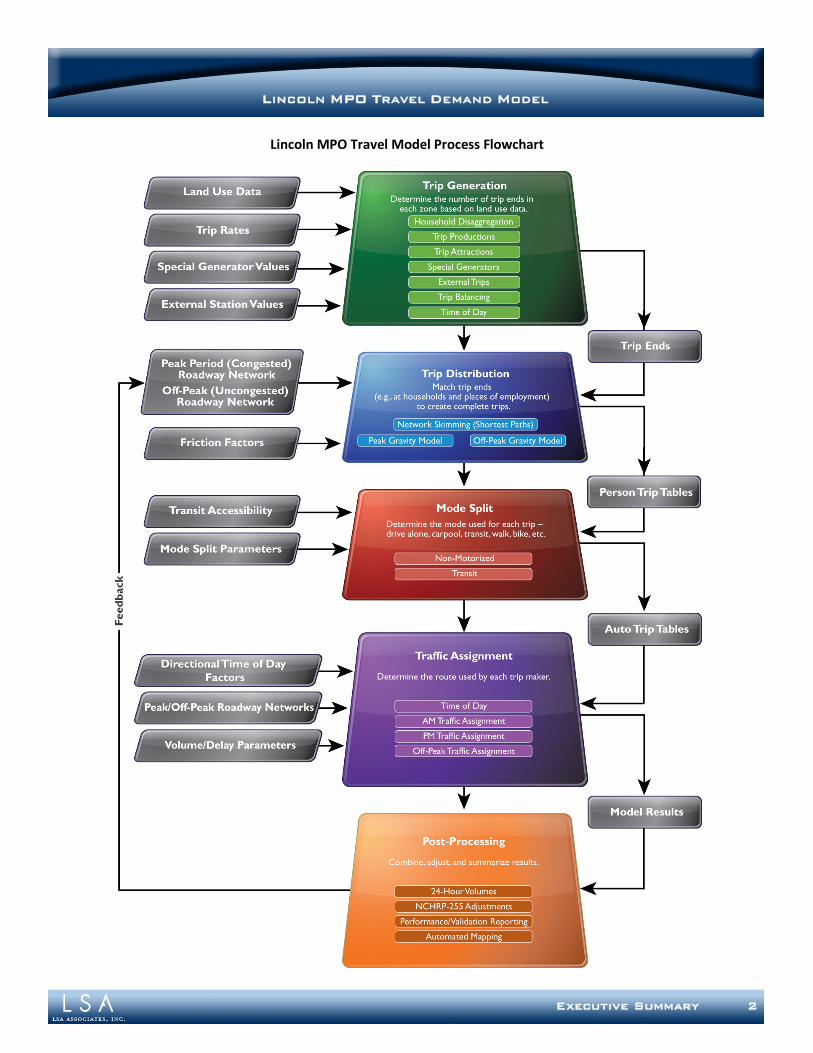
The Lincoln MPO Travel Model is a tool used by the Lincoln MPO to forecast travel patterns in the City of Lincoln and the surrounding areas in Lancaster County. The primary purpose of the travel model is to support the development of the MPO’s long-range transportation plan. The travel model can also be used to test the outcomes of specific land use or roadway changes in the short- or long-term. The model also includes limited transit and non-motorized analysis capabilities. The base year selected for the model is 2009, with a forecast year of 2040 and an interim year of 2025. The Lincoln MPO Travel Model utilizes a traditional four-step modeling process, as demonstrated in the flowchart on the following page. This process addresses all person trips, including trips made using transit and non-motorized modes (walk and bicycle). The updated model includes AM and PM peak periods and an off-peak period, which are combined to produce total daily traffic volumes. Post processing tools produce useful information, such as a summary report, adjusted model volumes, and intersection turn movement estimates. The entire process is automated and can be managed from a scenario management system within the TransCAD software platform. Automation has been implemented using GISDK, TransCAD’s programming language. This document provides detailed information about the processes and parameters contained in the Lincoln MPO Travel Model. Each chapter focuses on a specific model input or model step, beginning with the input roadway network and continuing with descriptions of the four-step modeling process (Trip Generation, Trip Distribution, Mode Split, and Traffic Assignment). Base year model validation measures associated with each of the four model steps are discussed in the corresponding chapters, with a dynamic validation process described in a separate chapter. In addition, a User’s Guide is provided under a separate cover. The User’s Guide provides detailed information about using the travel model software and datasets.
LINCOLN MPO TRAVEL DEMAND MODEL
Executive Summary 2
Lincoln MPO Travel Model Process Flowchart
Executive Summary 3
LINCOLN MPO TRAVEL DEMAND MODEL
Validation Overview
The chapters in this report describe the parameters, process, and validation for each model step. Validation results are summarized here for easy reference. Trip Generation Validation
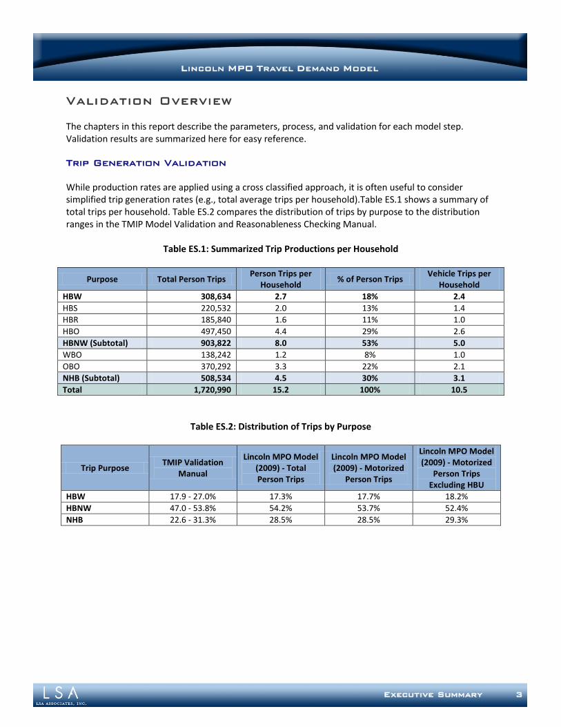
While production rates are applied using a cross classified approach, it is often useful to consider simplified trip generation rates (e.g., total average trips per household).Table ES.1 shows a summary of total trips per household. Table ES.2 compares the distribution of trips by purpose to the distribution ranges in the TMIP Model Validation and Reasonableness Checking Manual.
Table ES.1: Summarized Trip Productions per Household
Purpose Total Person Trips Person Trips per
Household % of Person Trips
Vehicle Trips per Household
HBW 308,634 2.7 18% 2.4
HBS 220,532 2.0 13% 1.4
HBR 185,840 1.6 11% 1.0
HBO 497,450 4.4 29% 2.6
HBNW (Subtotal) 903,822 8.0 53% 5.0
WBO 138,242 1.2 8% 1.0
OBO 370,292 3.3 22% 2.1
NHB (Subtotal) 508,534 4.5 30% 3.1
Total 1,720,990 15.2 100% 10.5
Table ES.2: Distribution of Trips by Purpose
Trip Purpose TMIP Validation
Manual
Lincoln MPO Model (2009) - Total Person Trips
Lincoln MPO Model (2009) - Motorized
Person Trips
Lincoln MPO Model (2009) - Motorized
Person Trips Excluding HBU
HBW 17.9 - 27.0% 17.3% 17.7% 18.2%
HBNW 47.0 - 53.8% 54.2% 53.7% 52.4%
NHB 22.6 - 31.3% 28.5% 28.5% 29.3%
Executive Summary 4
LINCOLN MPO TRAVEL DEMAND MODEL
Trip Distribution Validation
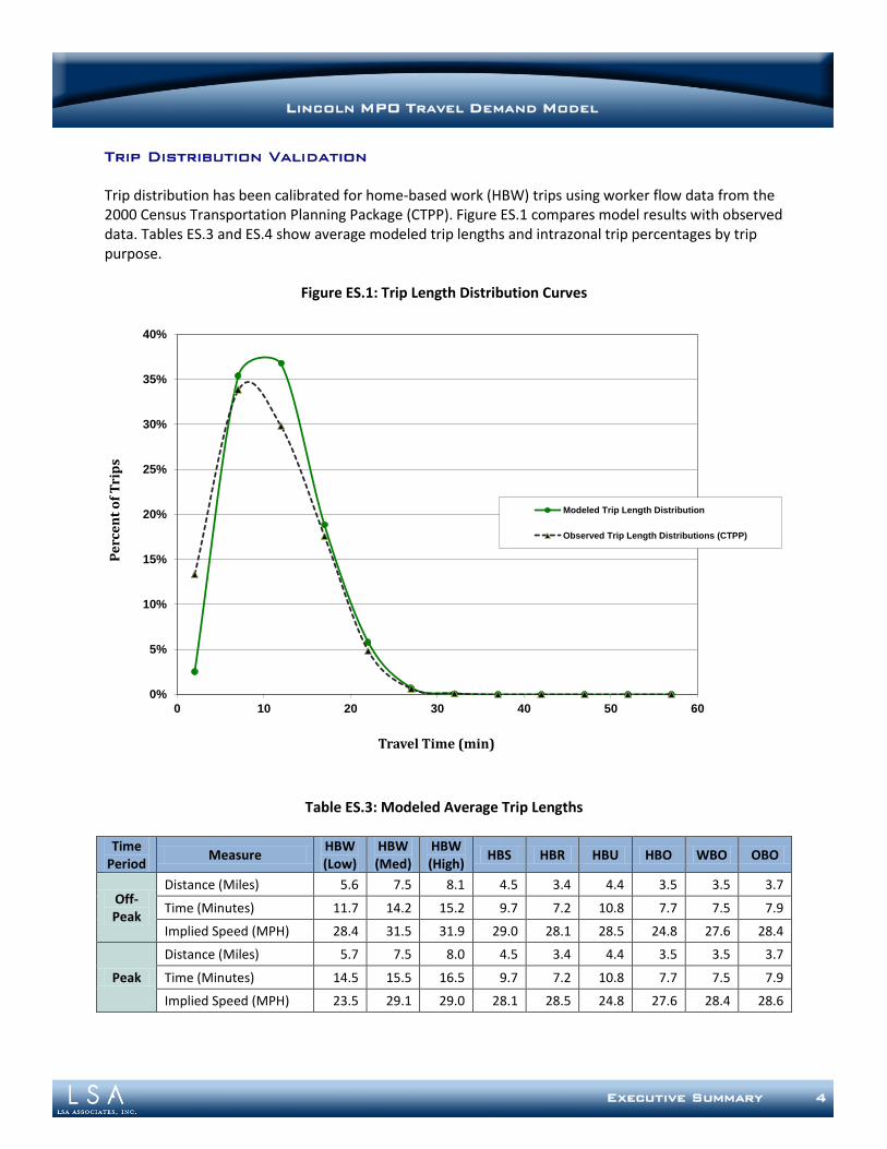
Trip distribution has been calibrated for home-based work (HBW) trips using worker flow data from the 2000 Census Transportation Planning Package (CTPP). Figure ES.1 compares model results with observed data. Tables ES.3 and ES.4 show average modeled trip lengths and intrazonal trip percentages by trip purpose.
Figure ES.1: Trip Length Distribution Curves
Table ES.3: Modeled Average Trip Lengths
Time Period
Measure HBW (Low)
HBW (Med)
HBW (High)
HBS HBR HBU HBO WBO OBO
Off-Peak
Distance (Miles) 5.6 7.5 8.1 4.5 3.4 4.4 3.5 3.5 3.7
Time (Minutes) 11.7 14.2 15.2 9.7 7.2 10.8 7.7 7.5 7.9
Implied Speed (MPH) 28.4 31.5 31.9 29.0 28.1 28.5 24.8 27.6 28.4
Peak
Distance (Miles) 5.7 7.5 8.0 4.5 3.4 4.4 3.5 3.5 3.7
Time (Minutes) 14.5 15.5 16.5 9.7 7.2 10.8 7.7 7.5 7.9
Implied Speed (MPH) 23.5 29.1 29.0 28.1 28.5 24.8 27.6 28.4 28.6
0%
5%
10%
15%
20%
25%
30%
35%
40%
0 10 20 30 40 50 60
Pe
rce
nt
of
Tri
ps
Travel Time (min)
Trip Time Distribution - HBW
Modeled Trip Length Distribution
Observed Trip Length Distributions (CTPP)
Executive Summary 5
LINCOLN MPO TRAVEL DEMAND MODEL
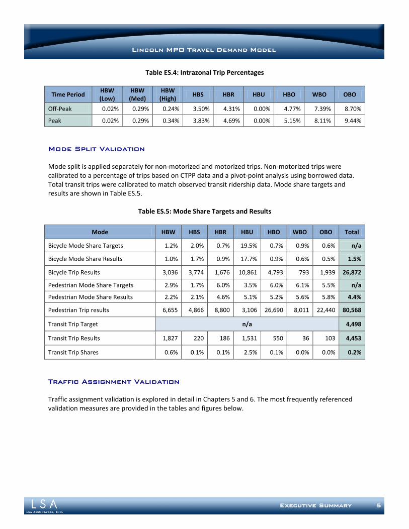
Table ES.4: Intrazonal Trip Percentages
Time Period HBW (Low)
HBW (Med)
HBW (High)
HBS HBR HBU HBO WBO OBO
Off-Peak 0.02% 0.29% 0.24% 3.50% 4.31% 0.00% 4.77% 7.39% 8.70%
Peak 0.02% 0.29% 0.34% 3.83% 4.69% 0.00% 5.15% 8.11% 9.44%
Mode Split Validation
Mode split is applied separately for non-motorized and motorized trips. Non-motorized trips were calibrated to a percentage of trips based on CTPP data and a pivot-point analysis using borrowed data. Total transit trips were calibrated to match observed transit ridership data. Mode share targets and results are shown in Table ES.5.
Table ES.5: Mode Share Targets and Results
Mode HBW HBS HBR HBU HBO WBO OBO Total
Bicycle Mode Share Targets 1.2% 2.0% 0.7% 19.5% 0.7% 0.9% 0.6% n/a
Bicycle Mode Share Results 1.0% 1.7% 0.9% 17.7% 0.9% 0.6% 0.5% 1.5%
Bicycle Trip Results 3,036 3,774 1,676 10,861 4,793 793 1,939 26,872
Pedestrian Mode Share Targets 2.9% 1.7% 6.0% 3.5% 6.0% 6.1% 5.5% n/a
Pedestrian Mode Share Results 2.2% 2.1% 4.6% 5.1% 5.2% 5.6% 5.8% 4.4%
Pedestrian Trip results 6,655 4,866 8,800 3,106 26,690 8,011 22,440 80,568
Transit Trip Target n/a 4,498
Transit Trip Results 1,827 220 186 1,531 550 36 103 4,453
Transit Trip Shares 0.6% 0.1% 0.1% 2.5% 0.1% 0.0% 0.0% 0.2%
Traffic Assignment Validation
Traffic assignment validation is explored in detail in Chapters 5 and 6. The most frequently referenced validation measures are provided in the tables and figures below.
Executive Summary 6
LINCOLN MPO TRAVEL DEMAND MODEL
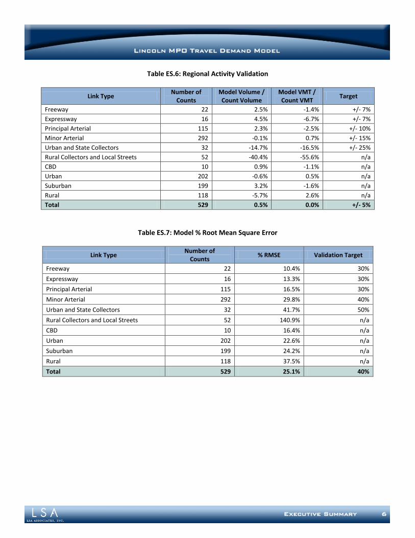
Table ES.6: Regional Activity Validation
Link Type Number of
Counts Model Volume / Count Volume
Model VMT / Count VMT
Target
Freeway 22 2.5% -1.4% +/- 7%
Expressway 16 4.5% -6.7% +/- 7%
Principal Arterial 115 2.3% -2.5% +/- 10%
Minor Arterial 292 -0.1% 0.7% +/- 15%
Urban and State Collectors 32 -14.7% -16.5% +/- 25%
Rural Collectors and Local Streets 52 -40.4% -55.6% n/a
CBD 10 0.9% -1.1% n/a
Urban 202 -0.6% 0.5% n/a
Suburban 199 3.2% -1.6% n/a
Rural 118 -5.7% 2.6% n/a
Total 529 0.5% 0.0% +/- 5%
Table ES.7: Model % Root Mean Square Error
Link Type Number of
Counts % RMSE Validation Target
Freeway 22 10.4% 30%
Expressway 16 13.3% 30%
Principal Arterial 115 16.5% 30%
Minor Arterial 292 29.8% 40%
Urban and State Collectors 32 41.7% 50%
Rural Collectors and Local Streets 52 140.9% n/a
CBD 10 16.4% n/a
Urban 202 22.6% n/a
Suburban 199 24.2% n/a
Rural 118 37.5% n/a
Total 529 25.1% 40%
Executive Summary 7
LINCOLN MPO TRAVEL DEMAND MODEL
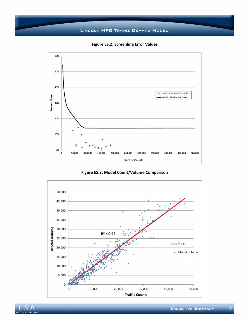
Figure ES.2: Screenline Error Values
Figure ES.3: Model Count/Volume Comparison
0%
10%
20%
30%
40%
50%
60%
0 50,000 100,000 150,000 200,000 250,000 300,000 350,000 400,000 450,000 500,000
Pe
rce
nt
Erro
r
Sum of Counts
Lincoln Screenline Percent Error
NCHRP 255 Allowable Curve
0
5,000
10,000
15,000
20,000
25,000
30,000
35,000
40,000
45,000
50,000
0 10,000 20,000 30,000 40,000 50,000
Mo
del
Vo
lum
e
Traffic Counts
Y = X
Model Volume
R2 = 0.92
Chapter 1 – Roadway Network 1-1
LINCOLN MPO TRAVEL DEMAND MODEL
Chapter 1: Roadway Network
CONTEXT AND BACKGROUND
The roadway network contains basic input information for use in the travel demand model and represents real-world conditions for the 2009 base year. The roadway networks are used in the model to distribute both motorized and non-motorized trips and to route automobile trips. In the GIS environment used by the model, the networks are databases in which assorted information can be stored and managed. In addition, the networks provide a foundation for system performance analysis including vehicle miles of travel, congestion delay, level of service, and other performance criteria. This chapter describes the network attributes and lookup tables for the roadway networks used in the Lincoln MPO Travel Model. The assumptions and parameters identified herein were identified during development of the model’s 2009 base year network, but generally apply to all model year networks. The roadway network is a GIS-based representation of the street and highway system in the Lincoln area. It operates both as an input database containing roadway characteristics (such as facility type, number of lanes, area type, etc.) and as a data repository that can be used to store and view travel model results. The roadway network is one of the foundational components of the Lincoln MPO Travel Model as it represents the supply side of the travel demand/transportation system relationship. As such, establishing and reviewing detailed network attribute data was critical to the model development. The Lincoln MPO Travel Model roadway network contains the 2009 base year network, but is structured to contain data for multiple timeframes and can be expanded to include forecast year improvements or alternatives. It is designed to accommodate future horizon year networks, including 2040 and other interim years, as desired. The model is capable of representing the 2009 base year, existing plus committed networks, plan forecast networks, interim horizon year networks, and any other network scenarios within a single network database. In addition, the network is structured so that localized alternatives can be represented within the same file. These alternatives can be activated and deactivated based on the year of analysis and the desired infrastructure scenario using the scenario management system that forms the basis of the travel model user interface.
ROADWAY NETWORK DEVELOPMENT
The 2009 roadway network is based on the street centerline layer maintained by Lincoln/Lancaster GIS and on the roadway network from the previous version of the model. The underlying network geography is based on a snapshot of the Lincoln/Lancaster GIS street centerline file from August 2010, which was then populated with network variables from the previous model roadway network using a spatial join. Centroid connectors were then added to the roadway network and the resulting network was processed to include turn prohibitions, to combine multiple short links into longer links where appropriate, and to properly represent grade separations.
Chapter 1 – Roadway Network 1-2
LINCOLN MPO TRAVEL DEMAND MODEL
Transfer of Network Attributes
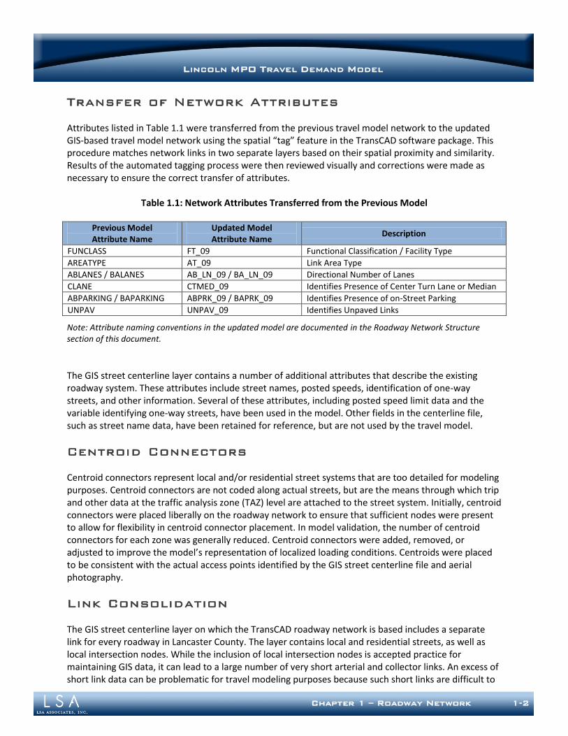
Attributes listed in Table 1.1 were transferred from the previous travel model network to the updated GIS-based travel model network using the spatial “tag” feature in the TransCAD software package. This procedure matches network links in two separate layers based on their spatial proximity and similarity. Results of the automated tagging process were then reviewed visually and corrections were made as necessary to ensure the correct transfer of attributes.
Table 1.1: Network Attributes Transferred from the Previous Model
Previous Model Attribute Name
Updated Model Attribute Name
Description
FUNCLASS FT_09 Functional Classification / Facility Type
AREATYPE AT_09 Link Area Type
ABLANES / BALANES AB_LN_09 / BA_LN_09 Directional Number of Lanes
CLANE CTMED_09 Identifies Presence of Center Turn Lane or Median
ABPARKING / BAPARKING ABPRK_09 / BAPRK_09 Identifies Presence of on-Street Parking
UNPAV UNPAV_09 Identifies Unpaved Links
Note: Attribute naming conventions in the updated model are documented in the Roadway Network Structure section of this document.
The GIS street centerline layer contains a number of additional attributes that describe the existing roadway system. These attributes include street names, posted speeds, identification of one-way streets, and other information. Several of these attributes, including posted speed limit data and the variable identifying one-way streets, have been used in the model. Other fields in the centerline file, such as street name data, have been retained for reference, but are not used by the travel model.
Centroid Connectors
Centroid connectors represent local and/or residential street systems that are too detailed for modeling purposes. Centroid connectors are not coded along actual streets, but are the means through which trip and other data at the traffic analysis zone (TAZ) level are attached to the street system. Initially, centroid connectors were placed liberally on the roadway network to ensure that sufficient nodes were present to allow for flexibility in centroid connector placement. In model validation, the number of centroid connectors for each zone was generally reduced. Centroid connectors were added, removed, or adjusted to improve the model’s representation of localized loading conditions. Centroids were placed to be consistent with the actual access points identified by the GIS street centerline file and aerial photography.
Link Consolidation
The GIS street centerline layer on which the TransCAD roadway network is based includes a separate link for every roadway in Lancaster County. The layer contains local and residential streets, as well as local intersection nodes. While the inclusion of local intersection nodes is accepted practice for maintaining GIS data, it can lead to a large number of very short arterial and collector links. An excess of short link data can be problematic for travel modeling purposes because such short links are difficult to
Chapter 1 – Roadway Network 1-3
LINCOLN MPO TRAVEL DEMAND MODEL
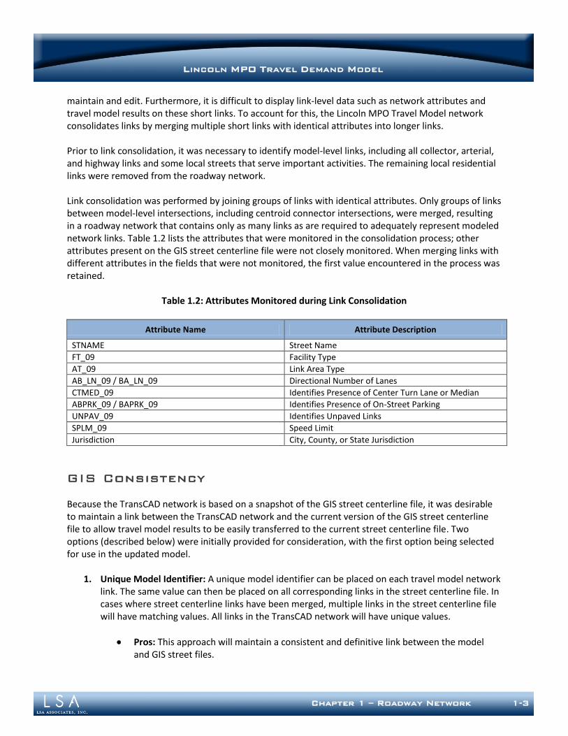
maintain and edit. Furthermore, it is difficult to display link-level data such as network attributes and travel model results on these short links. To account for this, the Lincoln MPO Travel Model network consolidates links by merging multiple short links with identical attributes into longer links. Prior to link consolidation, it was necessary to identify model-level links, including all collector, arterial, and highway links and some local streets that serve important activities. The remaining local residential links were removed from the roadway network. Link consolidation was performed by joining groups of links with identical attributes. Only groups of links between model-level intersections, including centroid connector intersections, were merged, resulting in a roadway network that contains only as many links as are required to adequately represent modeled network links. Table 1.2 lists the attributes that were monitored in the consolidation process; other attributes present on the GIS street centerline file were not closely monitored. When merging links with different attributes in the fields that were not monitored, the first value encountered in the process was retained.
Table 1.2: Attributes Monitored during Link Consolidation
Attribute Name Attribute Description
STNAME Street Name
FT_09 Facility Type
AT_09 Link Area Type
AB_LN_09 / BA_LN_09 Directional Number of Lanes
CTMED_09 Identifies Presence of Center Turn Lane or Median
ABPRK_09 / BAPRK_09 Identifies Presence of On-Street Parking
UNPAV_09 Identifies Unpaved Links
SPLM_09 Speed Limit
Jurisdiction City, County, or State Jurisdiction
GIS Consistency
Because the TransCAD network is based on a snapshot of the GIS street centerline file, it was desirable to maintain a link between the TransCAD network and the current version of the GIS street centerline file to allow travel model results to be easily transferred to the current street centerline file. Two options (described below) were initially provided for consideration, with the first option being selected for use in the updated model.
1. Unique Model Identifier: A unique model identifier can be placed on each travel model network link. The same value can then be placed on all corresponding links in the street centerline file. In cases where street centerline links have been merged, multiple links in the street centerline file will have matching values. All links in the TransCAD network will have unique values.
Pros: This approach will maintain a consistent and definitive link between the model and GIS street files.
Chapter 1 – Roadway Network 1-4
LINCOLN MPO TRAVEL DEMAND MODEL
Cons: This approach will require careful maintenance of both the model and GIS street files. If links are split in the travel model, it will be necessary to update the unique model identifier in both the TransCAD network and the Lincoln/Lancaster GIS street centerline file. A set of network editing protocols can be developed to ensure that consistency is maintained.
2. Spatial Join: A spatial join or TransCAD “tag” can be used to place TransCAD model values on the GIS street centerline layer on an as-needed basis.
Pros: This method will not require coordination between the Lincoln MPO and Lincoln/Lancaster GIS each time model network edits require splitting or adding of links.
Cons: It is possible that a small number of links will not be filled properly using this approach. The potential for errors increases with splitting, joining, and relocation of links. A set of network editing protocols can be developed to reduce the potential for errors.
Turn Penalties
Two primary types of turn penalties can be included in the network. Specific (localized) turn penalties represent known turn penalties or prohibitions at individual locations. Global turn penalties represent the increased amount of time required to make a left or right turn rather than traveling straight through an intersection. The updated model does not utilize global turn penalties, but does prohibit U-turns. The inclusion of specific turn penalties in the roadway network is described below. The Lincoln MPO Travel Model has been calibrated and validated without the use of specific turn penalties. When used, individual turn penalties represent the existing level of congestion at particular intersections that may or may not exist in the future, especially if operational improvements are made. While it is possible to adjust specific turn penalties for future conditions based on planned intersection or signal timing improvements, this task is beyond the capability or desire of most planning agencies. Maintenance of specific turn penalties can be a time consuming task, and detailed plans for intersections and traffic signal timings in a 30-year forecast scenario do not often exist. Turn prohibitions, meanwhile, are a valuable addition to a travel model. Turn prohibitions are used in locations where turns (typically lefts) are prohibited entirely. An inventory of existing turn prohibitions was provided by Lincoln/Lancaster GIS. This turn penalty data was transferred to a TransCAD turn penalty file for use in the model.
Grade Separation
The GIS street centerline file does not inherently represent grade separation. At locations where grade separations are present (e.g., freeway overpasses), the centerline file represents the intersections with a simple connected node. While this representation is common in GIS street files, the TransCAD model requires that these nodes to be disconnected to prevent the model from routing vehicles through these nodes as if they were at-grade intersections. The locations of grade separations are maintained by Lincoln/Lancaster GIS in a separate layer. This information was transferred to the TransCAD network and used to modify the network structure accordingly.
Chapter 1 – Roadway Network 1-5
LINCOLN MPO TRAVEL DEMAND MODEL
The modified geographic file contains the following types of nodes:
Intersection Nodes – Nodes at which all connected links intersect.
Grade Separated Nodes (Removed) – Nodes at which one or more grade separated facilities exist. In most cases, nodes have been removed entirely at these locations, leaving two disconnected links.
Grade Separated Nodes (Retained) – Nodes at which one or more grade separated facilities exist. Wherever possible, nodes have been removed entirely at these locations, leaving two disconnected links. However, in some cases, it was necessary to retain one or more nodes in the network at grade-separated locations to accurately maintain network data.
Shape Nodes – Nodes to which only two links are connected. Grade separation does not occur at any of these nodes.
Endpoint Nodes – Nodes to which only one link is connected. Grade separation does not occur at these nodes.
ROADWAY NETWORK STRUCTURE
The structure of the Lincoln MPO roadway network was designed to be a flexible data repository and to host input and output data required by the travel model. This section describes the network file structure and defines attributes that are populated on the network. Input attributes and some output attributes are discussed herein. Additional output variables created by subsequent model steps are discussed in the associated chapters. Input network attributes used by the travel model include facility type, area type, number of lanes, speed limit, parking availability, pavement status, and direction of flow. Each of these variables is addressed in the sections that follow. Values for these attributes have been populated on the roadway network file for the year 2009. The roadway network is structured to consolidate data from multiple years and scenarios in a single TransCAD geographic file. A description of the organizational scheme used to accomplish this consolidation is provided. Several illustrative examples are also provided. Year-specific input data is used to compute freeflow speed, travel time, and capacity on each link in the roadway network. Methods used to develop and compute these values are discussed and specific values are documented herein. This information is placed on a copy of the network rather than the original input file. The creation of a routable network as required by several TransCAD processes is also discussed.

Chapter 1 – Roadway Network 1-6
LINCOLN MPO TRAVEL DEMAND MODEL
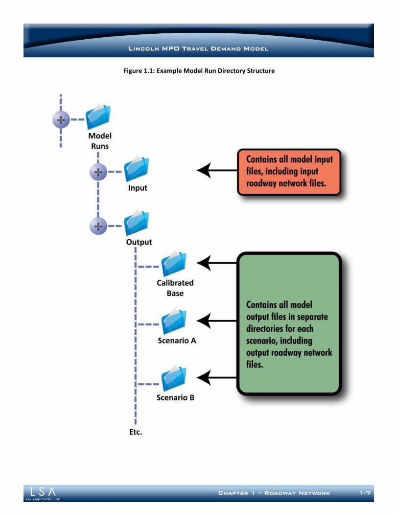
INPUT AND OUTPUT NETWORKS
The roadway network file contains travel model input data, and acts as a repository for both intermediate (e.g., speed feedback data) and final (e.g., traffic volumes) model data. For this reason, a separate output model network is created for each model scenario. This output network is created by making a copy of the input network and then modifying the network to contain the data and results specific to each model run. This copy of the roadway network is created and modified automatically by a network initialization step when the travel model is run. The model’s directory structure allows multiple model output directories to exist alongside a single input directory. Each time the travel model is run, files located in the input directory are not modified by model macros. Instead, if a file is to be modified it will be copied to an output directory and only the copy will be modified. This approach has several benefits, including the following:
1. All input files are located in one standardized location, making it easy to identify files when edits are required.
2. Because input files are not modified by the travel model macros, important data present within
input files will not be inadvertently overwritten by travel model macros. 3. Since all output files related to a particular model run will be maintained in a single directory,
there will be no confusion about which model scenario is represented by each file. An example directory structure containing travel model input and output files is shown in Figure 1.1.
Chapter 1 – Roadway Network 1-7
LINCOLN MPO TRAVEL DEMAND MODEL
Figure 1.1: Example Model Run Directory Structure

Chapter 1 – Roadway Network 1-8
LINCOLN MPO TRAVEL DEMAND MODEL
MULTI-YEAR AND ALTERNATIVE
NETWORK STRUCTURE
The Lincoln MPO roadway network is designed to store roadway data representing different years in one consolidated network layer. To accomplish this, selected network attribute names are appended with a two- through four-digit suffix representing a particular year. By representing multiple networks in one network file, consistency between baseline and forecast networks is enforced. Furthermore, this approach eliminates the need to edit multiple network files when making changes to a baseline or interim year network. In addition, the network structure allows for the representation of alternative roadway projects such as roadway widening, realignments, and new facilities that are not tied to a specific network year. These alternatives can be activated or deactivated individually or in groups, regardless of the network year that has been selected. While there are some limitations with respect to alternatives sharing the same link, this capability can be a valuable tool when evaluating alternatives with the travel model. These limitations and strategies to overcome them are described below.
Representation of Networks by Year
Each attribute that can vary from year to year (e.g., facility type, area type, number of lanes, direction of flow, etc.) is represented in the roadway network by an attribute containing a two- through four-digit numerical suffix. When a particular network is selected for use in the travel model, only those attributes with a suffix matching the selected year are used by the travel model. Of utmost importance is the facility type attribute. If this attribute is blank on a link for a particular year, that link will be “closed” to traffic (i.e., will not exist) in the network when that year is selected. If a valid facility type value is found, then the remaining attributes specified for that year will be referenced by the travel model. The roadway network initially contained data only for the year 2009; ultimately, the network will contain forecast year data consistent with the MPO’s 2040 Long Range Transportation Plan (LRTP). It is often necessary to consider multiple interim or buildout year networks (e.g., 2012 or 2050) in addition to the existing and plan forecast networks. Additional network years can be added at any time using the following steps:
1. Add new columns to the network link and node tables that will represent the additional network year (e.g., FT_12, AT_12, etc.);
2. Move these columns so that they are in a convenient location (e.g., between the 2009 and 2040 data columns);
3. Fill these columns with data from the corresponding attributes for either 2009 or 2040; and
4. Adjust the data as necessary.
Chapter 1 – Roadway Network 1-9
LINCOLN MPO TRAVEL DEMAND MODEL
Because this is a commonly performed task, a utility was developed that automatically performs steps 1 thorough 3 listed above. If alternatives are present in the network file, the utility will also allow the user to select the alternatives to include in a newly created network year. The utility can also be used to delete all attributes associated with a particular year. The “Edit Network Year” utility is accessible from the model dialog box.
Representation of New Facilities
The network structure allows for the representation of roadway facilities that do not currently exist in the network but are planned for future construction. For example, if a new roadway is planned to be built by 2040, it could be represented in the 2040 roadway network but not in the base year roadway network. To implement this, the roadway is added as a new link to the network layer. The new link is not assigned a facility type for the base year, but is assigned a facility type for the year 2040. When the travel model is run, only links with a valid facility type are considered by model components that reference the roadway network.
Representation of Network Alternatives
Roadway network alternatives provide a mechanism for testing localized network changes either individually or in combination without creating an additional network. Roadway network alternatives are specified by a set of attributes with the suffix AL (e.g., FT_AL, AT_AL, etc.) and by attributes named ALT and ALT2, as follows:
The fields with an AL suffix represent the network attributes used when an alternative is activated; and
The “ALT” and “ALT2” fields identify the alternative number associated with each link. If a particular alternative has been activated prior to a model run, the values in fields containing the AL suffix will override other network attributes on links where ALT or ALT2 match a selected alternative. The sidebar entitled, “Network Structure Example” further illustrates the application of network alternatives. The Network Attribute Selection section describes the stepwise procedure used to process network attributes.

Chapter 1 – Roadway Network 1-10
LINCOLN MPO TRAVEL DEMAND MODEL
Network alternatives can represent scenarios in which roadway attributes differ or scenarios in which roadways are constructed or removed. For example, an alternative might represent a proposed roadway widening project that is not included in the 2040 roadway network, but could be included as an alternative for testing purposes. After adding this one alternative, model scenarios could then be created that:
1. Represent the base-year network without the roadway widening, 2. Represent the base-year network with the roadway widening, 3. Represent the 2040 network without the roadway widening, or 4. Represent the 2040 network with the roadway widening.
As with network attributes that vary by year, absence of facility type data will result in a link being omitted from consideration in the travel model. It is possible to represent the closure of a roadway by activating an alternative with a null value for FT_AL on a particular roadway link. This method is also useful to simulate a roadway that is realigned. This structure does have some limitations. Only two alternatives can occupy the same link, as limited by the two fields “ALT” and “ALT2.” Also, only one set of alternative attributes can occupy the same link, as limited by the one set of attributes with an “AL” suffix.
NETWORK STRUCTURE EXAMPLE
To illustrate the concept behind the network structure, a simplified example link data table is shown below. This table only shows facility type information. Lane, speed override, and area type information follow a similar theme. In this example network:
Link 100 exists as a principal arterial (FT = 3) in 2009 and all subsequent years.
Link 200 is programmed as a principal arterial (exists in 2012 and later).
Link 300 is planned to be built as a minor arterial (FT = 4) by 2040.
Link 300 is instead built as a collector (FT = 5) if Alternative 1 is activated.
Link 400 is a new facility to be built as a minor arterial if Alternative 2 is activated.
Link 500 exists in 2009 and all future years as a minor arterial, but is closed if Alternative 3 is activated.
EXAMPLE LINK DATASET
ID FT_09 FT_12 FT_40 FT_AL ALT
100 3 3 3 -- --
200 -- 3 3 -- --
300 -- -- 4 5 1
400 -- -- -- 4 2
500 4 4 4 -- 3
Chapter 1 – Roadway Network 1-11
LINCOLN MPO TRAVEL DEMAND MODEL
These limitations are of particular concern in a scenario in which a road currently exists as a 2-lane facility and is being considered for widening to 4 or 6 lanes. While this scenario cannot be readily represented in the network alternative structure, it can be represented using either one of two suggested options:
1. Create a separate network year (e.g., “09W4” or "40W4”) that represents the road as a 4-lane facility. Create an alternative that represents the road as a 6-lane facility; or
2. Create an alternative that represents the facility as a 4-lane facility. To run the alternative as a 6-
lane facility, make a copy of the network and change the number of lanes (in the “AL” attributes) to six before running the model.
Network Attribute Selection
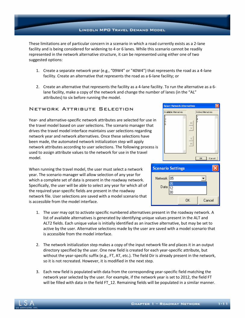
Year- and alternative-specific network attributes are selected for use in the travel model based on user selections. The scenario manager that drives the travel model interface maintains user selections regarding network year and network alternatives. Once these selections have been made, the automated network initialization step will apply network attributes according to user selections. The following process is used to assign attribute values to the network for use in the travel model.
When running the travel model, the user must select a network year. The scenario manager will allow selection of any year for which a complete set of data is present in the roadway network. Specifically, the user will be able to select any year for which all of the required year-specific fields are present in the roadway network file. User selections are saved with a model scenario that is accessible from the model interface.
1. The user may opt to activate specific numbered alternatives present in the roadway network. A list of available alternatives is generated by identifying unique values present in the ALT and ALT2 fields. Each unique value is initially identified as an inactive alternative, but may be set to active by the user. Alternative selections made by the user are saved with a model scenario that is accessible from the model interface.
2. The network initialization step makes a copy of the input network file and places it in an output
directory specified by the user. One new field is created for each year-specific attribute, but without the year-specific suffix (e.g., FT, AT, etc.). The field Dir is already present in the network, so it is not recreated. However, it is modified in the next step.
3. Each new field is populated with data from the corresponding year-specific field matching the
network year selected by the user. For example, if the network year is set to 2012, the field FT will be filled with data in the field FT_12. Remaining fields will be populated in a similar manner.
Chapter 1 – Roadway Network 1-12
LINCOLN MPO TRAVEL DEMAND MODEL
4. If any alternatives have been activated, a selection set consisting only of links where either ALT or ALT2 matches an active alternative is created. Attributes for links in the selection set are filled with data from the corresponding field ending in “_AL” which overwrites any data previously populated from the year-specific fields. For example, if Alternative 1 is selected, all links where ALT = 1 or ALT2 = 1 will be selected. For these links only, data in the FT field will be replaced with data in the FT_AL attribute, overwriting data previously read from the FT_12 attribute. Remaining fields would be populated in a similar manner.
5. Data in the fields that do not include a suffix (e.g., FT, AT, etc.) are referenced for all subsequent
model steps, including the speed, capacity, and volume-delay lookup procedures.
DIRECTION OF FLOW
Direction of flow does not fit within the attribute management scheme as well as other variables because the TransCAD software requires that direction of flow be maintained in the network field “Dir” at all times. While this requirement fits within the process used to run the model, it can cause difficulties if not addressed when editing the network. The following points must be remembered if the direction of flow varies on a link in different year or alternative networks:
To display directional arrows for a particular network year, fill the column “Dir” with the value from the appropriate attribute (e.g., Dir_09).
The Dir field and year-specific Dir fields should be populated with a 1, -1, or 0, even for network years for which links are not active (i.e., year-specific FT is null). The Dir_AL field can be null, but only if FT_AL is also null.
Note that these concerns apply only if the Dir attribute varies from year to year.
Chapter 1 – Roadway Network 1-13
LINCOLN MPO TRAVEL DEMAND MODEL
NETWORK ATTRIBUTE L IST
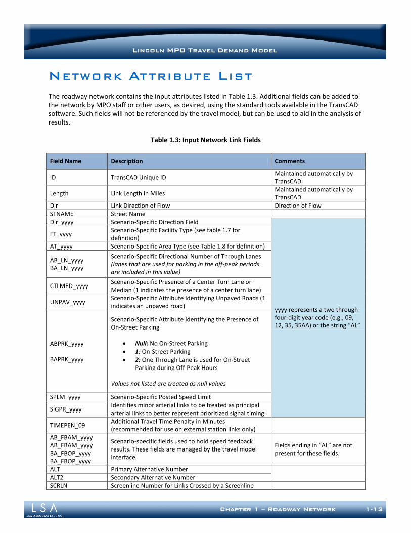
The roadway network contains the input attributes listed in Table 1.3. Additional fields can be added to the network by MPO staff or other users, as desired, using the standard tools available in the TransCAD software. Such fields will not be referenced by the travel model, but can be used to aid in the analysis of results.
Table 1.3: Input Network Link Fields
Field Name Description Comments
ID TransCAD Unique ID Maintained automatically by TransCAD
Length Link Length in Miles Maintained automatically by TransCAD
Dir Link Direction of Flow Direction of Flow STNAME Street Name Dir_yyyy Scenario-Specific Direction Field
yyyy represents a two through four-digit year code (e.g., 09, 12, 35, 35AA) or the string “AL”
FT_yyyy Scenario-Specific Facility Type (see table 1.7 for definition)
AT_yyyy Scenario-Specific Area Type (see Table 1.8 for definition)
AB_LN_yyyy BA_LN_yyyy
Scenario-Specific Directional Number of Through Lanes (lanes that are used for parking in the off-peak periods are included in this value)
CTLMED_yyyy Scenario-Specific Presence of a Center Turn Lane or Median (1 indicates the presence of a center turn lane)
UNPAV_yyyy Scenario-Specific Attribute Identifying Unpaved Roads (1 indicates an unpaved road)
ABPRK_yyyy BAPRK_yyyy
Scenario-Specific Attribute Identifying the Presence of On-Street Parking
Null: No On-Street Parking 1: On-Street Parking 2: One Through Lane is used for On-Street
Parking during Off-Peak Hours Values not listed are treated as null values
SPLM_yyyy Scenario-Specific Posted Speed Limit
SIGPR_yyyy Identifies minor arterial links to be treated as principal arterial links to better represent prioritized signal timing.
TIMEPEN_09 Additional Travel Time Penalty in Minutes (recommended for use on external station links only)
AB_FBAM_yyyy AB_FBAM_yyyy BA_FBOP_yyyy BA_FBOP_yyyy
Scenario-specific fields used to hold speed feedback results. These fields are managed by the travel model interface.
Fields ending in “AL” are not present for these fields.
ALT Primary Alternative Number
ALT2 Secondary Alternative Number SCRLN Screenline Number for Links Crossed by a Screenline
Chapter 1 – Roadway Network 1-14
LINCOLN MPO TRAVEL DEMAND MODEL
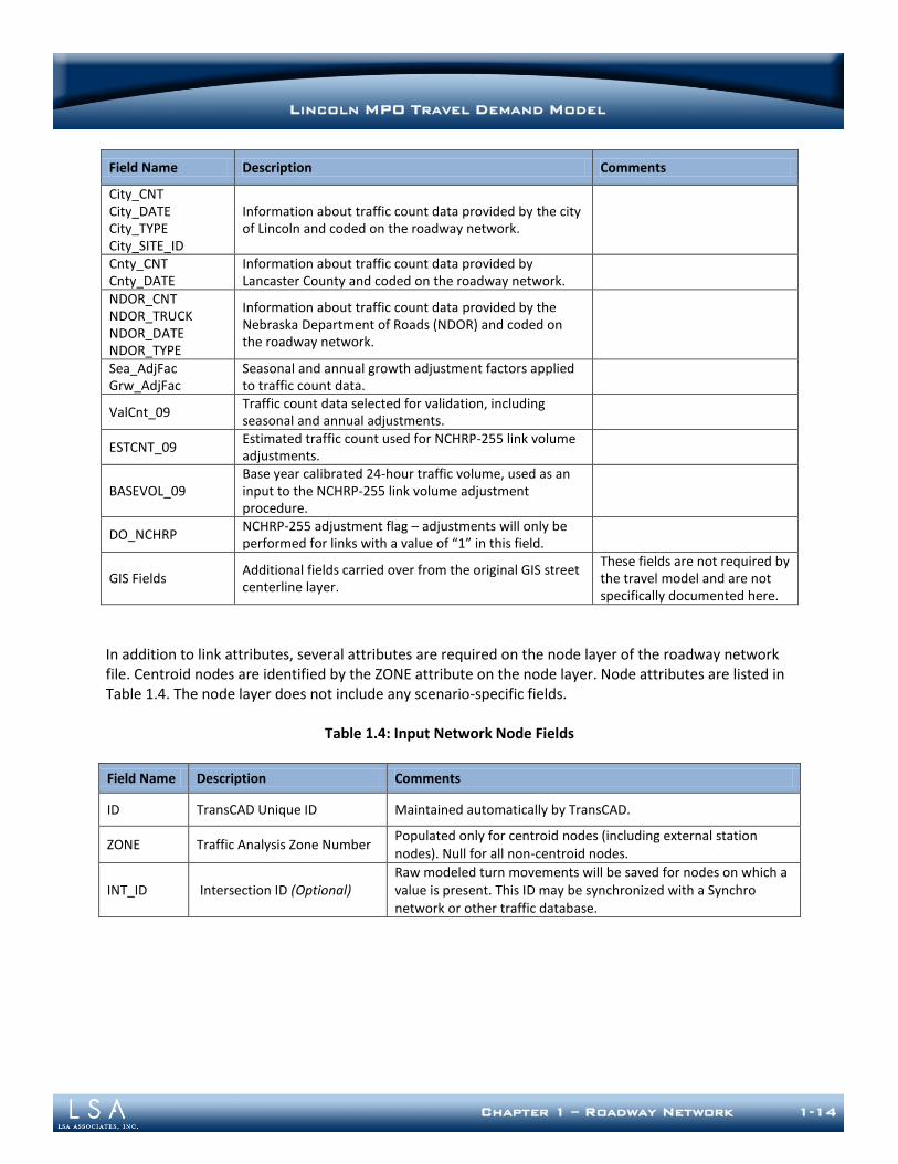
Field Name Description Comments
City_CNT City_DATE City_TYPE City_SITE_ID
Information about traffic count data provided by the city of Lincoln and coded on the roadway network.
Cnty_CNT Cnty_DATE
Information about traffic count data provided by Lancaster County and coded on the roadway network.
NDOR_CNT NDOR_TRUCK NDOR_DATE NDOR_TYPE
Information about traffic count data provided by the Nebraska Department of Roads (NDOR) and coded on the roadway network.
Sea_AdjFac Grw_AdjFac
Seasonal and annual growth adjustment factors applied to traffic count data.
ValCnt_09 Traffic count data selected for validation, including seasonal and annual adjustments.
ESTCNT_09 Estimated traffic count used for NCHRP-255 link volume adjustments.
BASEVOL_09 Base year calibrated 24-hour traffic volume, used as an input to the NCHRP-255 link volume adjustment procedure.
DO_NCHRP NCHRP-255 adjustment flag – adjustments will only be performed for links with a value of “1” in this field.
GIS Fields Additional fields carried over from the original GIS street centerline layer.
These fields are not required by the travel model and are not specifically documented here.
In addition to link attributes, several attributes are required on the node layer of the roadway network file. Centroid nodes are identified by the ZONE attribute on the node layer. Node attributes are listed in Table 1.4. The node layer does not include any scenario-specific fields.
Table 1.4: Input Network Node Fields
Field Name Description Comments
ID TransCAD Unique ID Maintained automatically by TransCAD.
ZONE Traffic Analysis Zone Number Populated only for centroid nodes (including external station nodes). Null for all non-centroid nodes.
INT_ID Intersection ID (Optional) Raw modeled turn movements will be saved for nodes on which a value is present. This ID may be synchronized with a Synchro network or other traffic database.
Chapter 1 – Roadway Network 1-15
LINCOLN MPO TRAVEL DEMAND MODEL
FUNCTIONAL CLASSIFICATION /
FACILITY TYPE
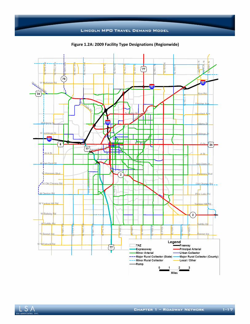
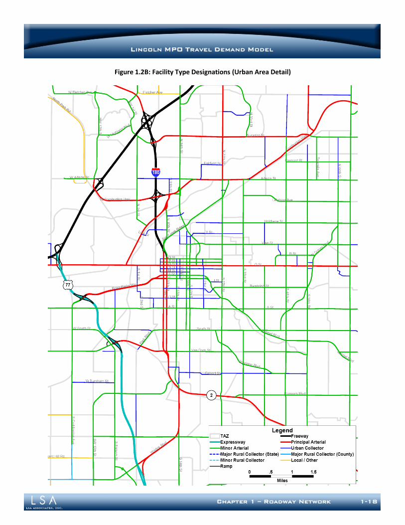
The functional classification of each roadway link reflects its role in the street and highway system. The term “functional classification” has specific implications with regards to the administration of federal-aid highway programs; but travel model networks do not always adhere to these definitions. The functional classification maintained on the previous model network has been applied to the current model network and is maintained under the variable FUNCLASS. An additional variable named Facility Type (FT) has been added to the network for use in speed, capacity, and volume delay parameter look-up. This additional variable will allow the facility type to be changed if necessary while keeping a record of the functional class. Model data may still be summarized using either the FT or FUNCLASS variables. Functional class / facility type values used in the Lincoln MPO Travel Model are listed in Table 1.5. Base year facility type values in the updated model are shown in Figures 1.2A through 1.2C. As shown in Table 1.5, the numbering scheme has been revised from the previous model. Two additional categories, expressway and freeway/freeway ramp, have been added. Further, the distinction between divided and undivided principal arterials has been removed from the facility type classification numbers and is instead represented using a separate variable.
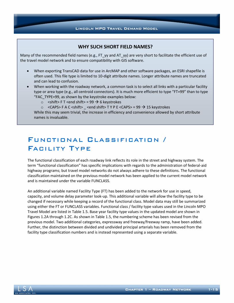
WHY SUCH SHORT FIELD NAMES?
Many of the recommended field names (e.g., FT_yy and AT_yy) are very short to facilitate the efficient use of the travel model network and to ensure compatibility with GIS software.
When exporting TransCAD data for use in ArcMAP and other software packages, an ESRI shapefile is often used. This file type is limited to 10-digit attribute names. Longer attribute names are truncated and can lead to confusion.
When working with the roadway network, a common task is to select all links with a particular facility type or area type (e.g., all centroid connectors). It is much more efficient to type “FT=99” than to type “FAC_TYPE=99, as shown by the keystroke examples below:
o <shift> F T <end shift> = 99 6 keystrokes o <CAPS> F A C <shift> _ <end shift> T Y P E <CAPS> = 99 15 keystrokes
While this may seem trivial, the increase in efficiency and convenience allowed by short attribute names is invaluable.
Chapter 1 – Roadway Network 1-16
LINCOLN MPO TRAVEL DEMAND MODEL
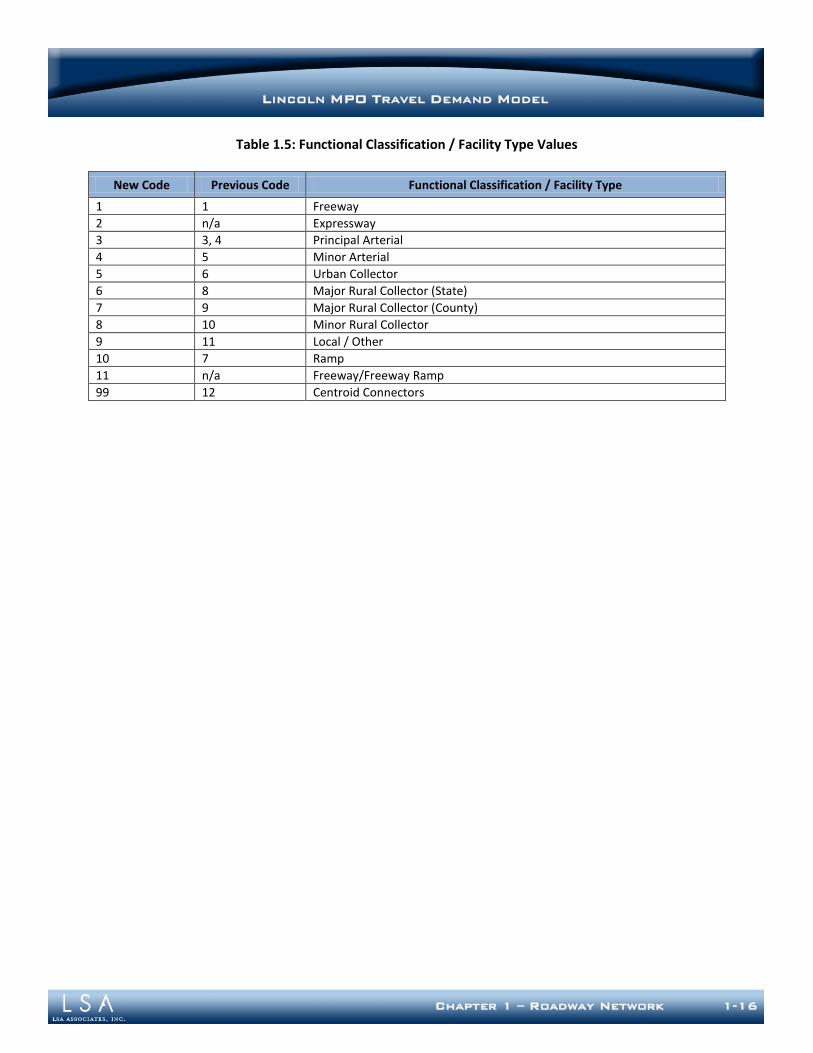
Table 1.5: Functional Classification / Facility Type Values
New Code Previous Code Functional Classification / Facility Type
1 1 Freeway
2 n/a Expressway
3 3, 4 Principal Arterial
4 5 Minor Arterial
5 6 Urban Collector
6 8 Major Rural Collector (State)
7 9 Major Rural Collector (County)
8 10 Minor Rural Collector
9 11 Local / Other
10 7 Ramp
11 n/a Freeway/Freeway Ramp
99 12 Centroid Connectors
Chapter 1 – Roadway Network 1-17
LINCOLN MPO TRAVEL DEMAND MODEL
Figure 1.2A: 2009 Facility Type Designations (Regionwide)
Chapter 1 – Roadway Network 1-18
LINCOLN MPO TRAVEL DEMAND MODEL
Figure 1.2B: Facility Type Designations (Urban Area Detail)
Chapter 1 – Roadway Network 1-19
LINCOLN MPO TRAVEL DEMAND MODEL
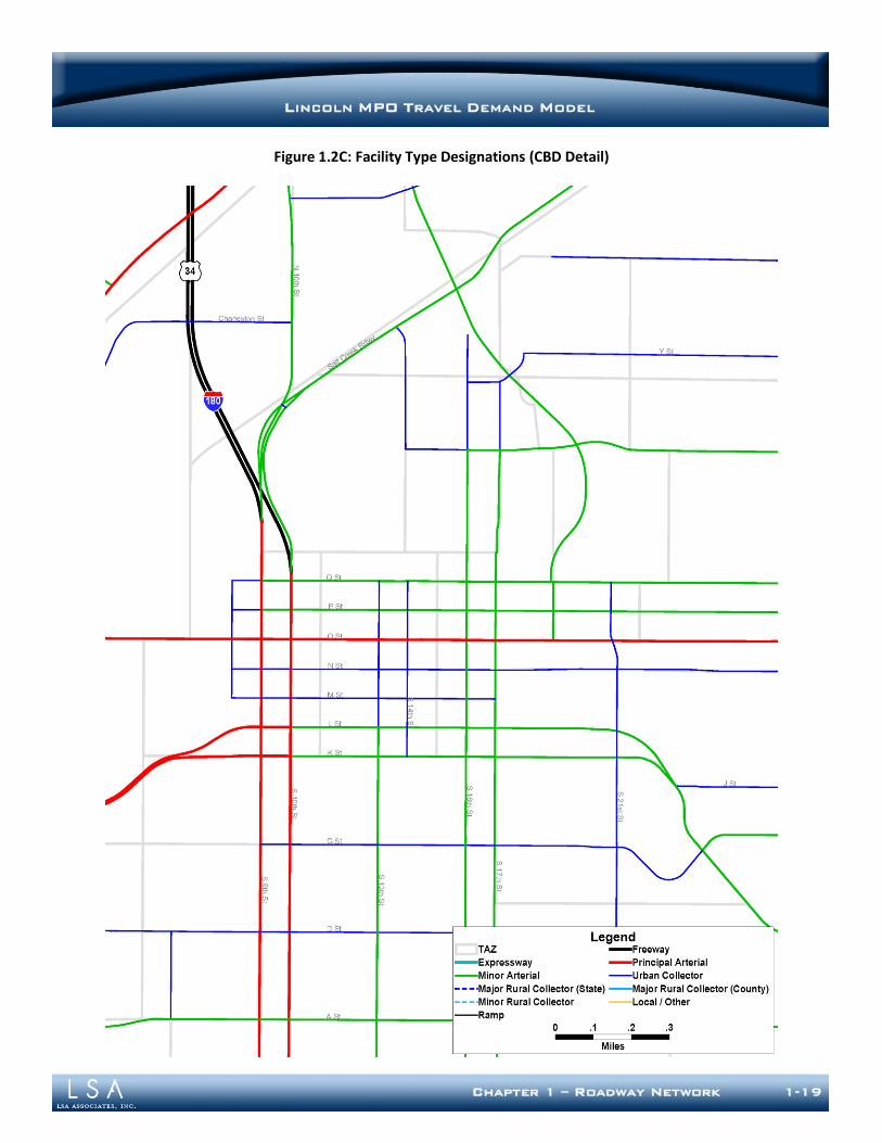
Figure 1.2C: Facility Type Designations (CBD Detail)
Chapter 1 – Roadway Network 1-20
LINCOLN MPO TRAVEL DEMAND MODEL
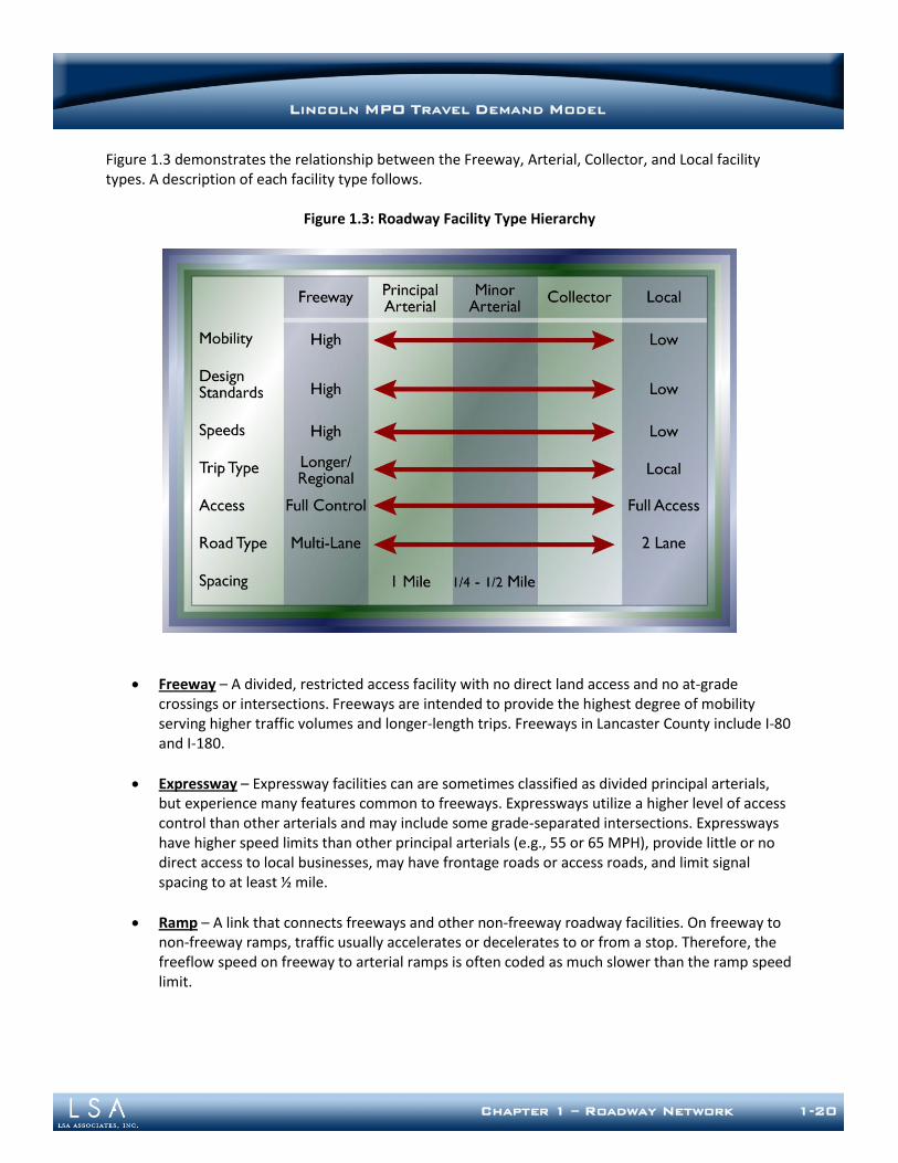
Figure 1.3 demonstrates the relationship between the Freeway, Arterial, Collector, and Local facility types. A description of each facility type follows.
Figure 1.3: Roadway Facility Type Hierarchy
Freeway – A divided, restricted access facility with no direct land access and no at-grade crossings or intersections. Freeways are intended to provide the highest degree of mobility serving higher traffic volumes and longer-length trips. Freeways in Lancaster County include I-80 and I-180.
Expressway – Expressway facilities can are sometimes classified as divided principal arterials, but experience many features common to freeways. Expressways utilize a higher level of access control than other arterials and may include some grade-separated intersections. Expressways have higher speed limits than other principal arterials (e.g., 55 or 65 MPH), provide little or no direct access to local businesses, may have frontage roads or access roads, and limit signal spacing to at least ½ mile.
Ramp – A link that connects freeways and other non-freeway roadway facilities. On freeway to non-freeway ramps, traffic usually accelerates or decelerates to or from a stop. Therefore, the freeflow speed on freeway to arterial ramps is often coded as much slower than the ramp speed limit.

Chapter 1 – Roadway Network 1-21
LINCOLN MPO TRAVEL DEMAND MODEL
Freeway to Freeway Ramp – Movements between freeways are handled using this facility type. These ramps directly connect two freeway facilities with no intervening traffic controls. Use of a separate freeway to freeway ramp facility type is beneficial because ramp speed represents the average speed on a ramp link. On ramps connecting freeways, traffic typically travels near the speed limit for the length of the link. In some cases, the freeway to freeway ramp facility type is used to represent ramps connecting freeways to expressways or principal arterials when both ends of the ramp facility terminate with a merge operation.
Principal Arterial– These facility types permit traffic flow through and within urban areas and between major destinations. Principal arterials are of great importance in the transportation system since they provide local land access by connecting major traffic generators, such as central business districts and universities, to other major activity centers. Principal arterials carry a high proportion of the total urban travel on minimal roadway mileage. They typically receive priority in traffic signal systems (i.e., have a high level of coordination and receive longer green times than other facility types). Divided principal arterials have turn bays at intersections, include medians or center turn lanes, and sometimes contain grade separations and other higher-type design features. State and U.S. highways are typically designated as principal arterials unless they are classified as freeways.
Minor Arterial – Minor arterials collect and distribute traffic from principal arterials, freeways, and expressways to streets of lower classification and, in some cases, allow traffic to directly access destinations. They serve secondary traffic generators, such as community business centers, neighborhood shopping centers, multifamily residential areas, and traffic between neighborhoods. Access to land use activities is generally permitted, but should be consolidated, shared, or limited to larger-scale users. Minor arterials generally have slower speed limits than principal arterials, may or may not have medians and center turn lanes, and receive lower signal priority than other facility types (i.e., are only coordinated to the extent that principal arterials are not disrupted and receive shorter green times than principal arterials).
Collector Street – Collectors provide for land access and traffic circulation within and between residential neighborhoods and commercial and industrial areas. They distribute traffic movements from these areas to arterial streets. Except in rural areas, collectors do not typically accommodate long through trips and are not continuous for long distances. The cross-section of a collector street may vary widely depending on the scale and density of adjacent land uses and the character of the local area. Left turn lanes sometimes occur on collector streets adjacent to nonresidential development. Collector streets should generally be limited to two lanes, but sometimes have 4-lane sections. In rural areas, major collectors act similarly to minor arterials, while rural minor collectors fit more closely with the characterizations described here.
Centroid Connector – These facilities represent local and/or residential street systems that are too detailed for modeling purposes. Centroid connectors are not coded along actual streets, but are the means through which trip and other data at the traffic analysis zone (TAZ) level are attached to the street system.
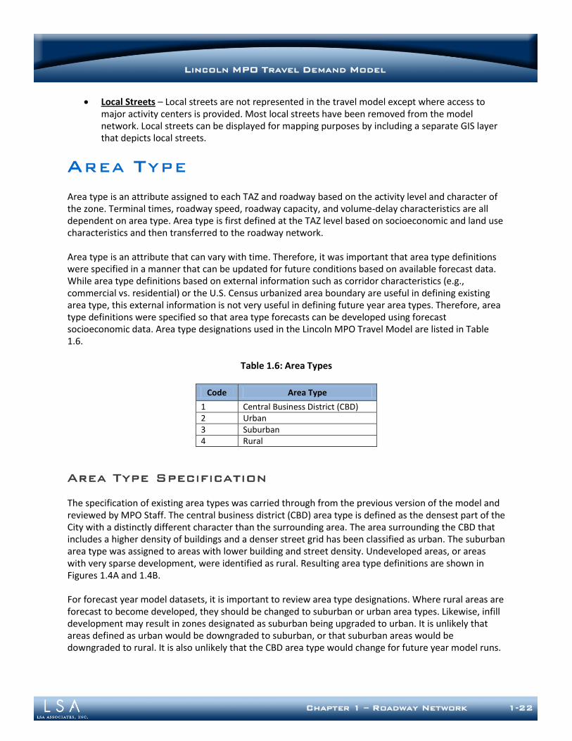
Chapter 1 – Roadway Network 1-22
LINCOLN MPO TRAVEL DEMAND MODEL
Local Streets – Local streets are not represented in the travel model except where access to major activity centers is provided. Most local streets have been removed from the model network. Local streets can be displayed for mapping purposes by including a separate GIS layer that depicts local streets.
AREA TYPE
Area type is an attribute assigned to each TAZ and roadway based on the activity level and character of the zone. Terminal times, roadway speed, roadway capacity, and volume-delay characteristics are all dependent on area type. Area type is first defined at the TAZ level based on socioeconomic and land use characteristics and then transferred to the roadway network. Area type is an attribute that can vary with time. Therefore, it was important that area type definitions were specified in a manner that can be updated for future conditions based on available forecast data. While area type definitions based on external information such as corridor characteristics (e.g., commercial vs. residential) or the U.S. Census urbanized area boundary are useful in defining existing area type, this external information is not very useful in defining future year area types. Therefore, area type definitions were specified so that area type forecasts can be developed using forecast socioeconomic data. Area type designations used in the Lincoln MPO Travel Model are listed in Table 1.6.
Table 1.6: Area Types
Code Area Type
1 Central Business District (CBD) 2 Urban 3 Suburban 4 Rural
Area Type Specification
The specification of existing area types was carried through from the previous version of the model and reviewed by MPO Staff. The central business district (CBD) area type is defined as the densest part of the City with a distinctly different character than the surrounding area. The area surrounding the CBD that includes a higher density of buildings and a denser street grid has been classified as urban. The suburban area type was assigned to areas with lower building and street density. Undeveloped areas, or areas with very sparse development, were identified as rural. Resulting area type definitions are shown in Figures 1.4A and 1.4B. For forecast year model datasets, it is important to review area type designations. Where rural areas are forecast to become developed, they should be changed to suburban or urban area types. Likewise, infill development may result in zones designated as suburban being upgraded to urban. It is unlikely that areas defined as urban would be downgraded to suburban, or that suburban areas would be downgraded to rural. It is also unlikely that the CBD area type would change for future year model runs.
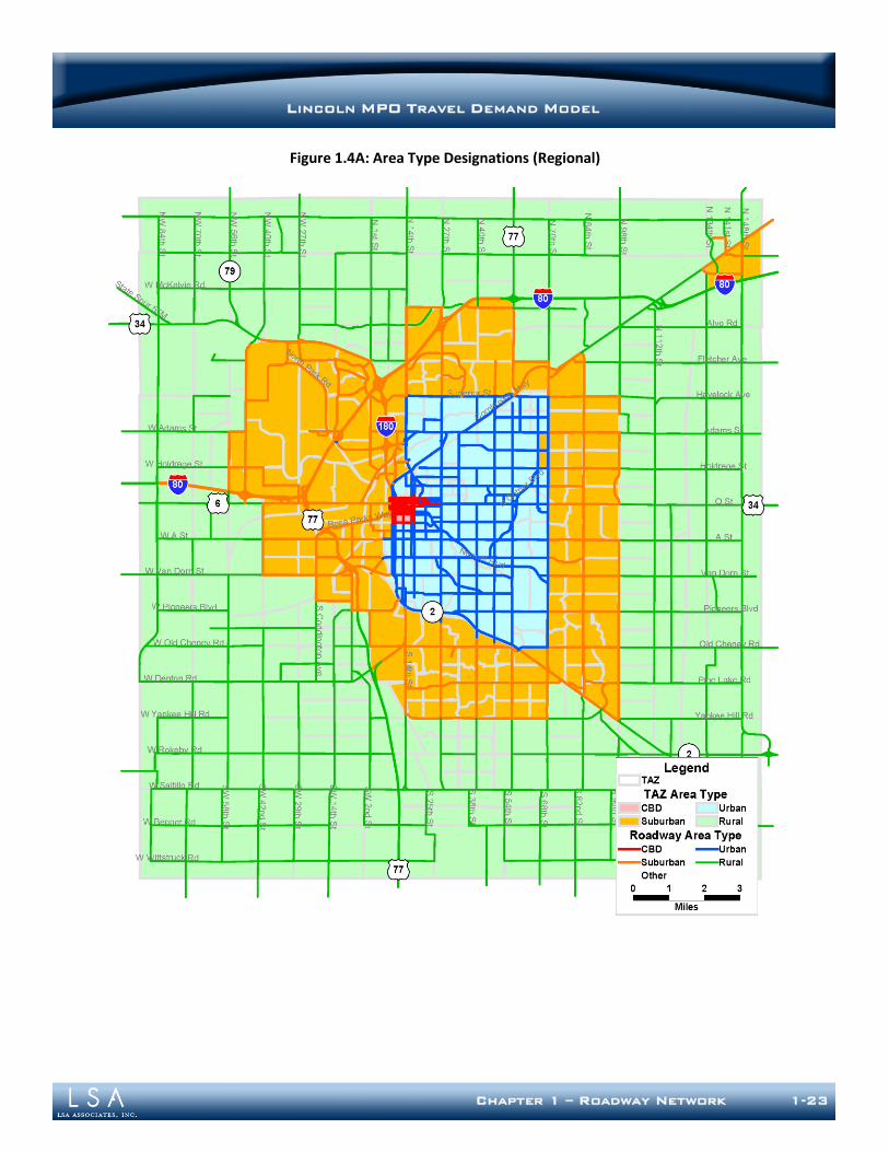
Chapter 1 – Roadway Network 1-23
LINCOLN MPO TRAVEL DEMAND MODEL
Figure 1.4A: Area Type Designations (Regional)
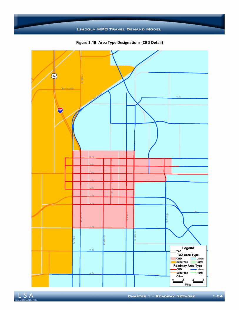
Chapter 1 – Roadway Network 1-24
LINCOLN MPO TRAVEL DEMAND MODEL
Figure 1.4B: Area Type Designations (CBD Detail)

Chapter 1 – Roadway Network 1-25
LINCOLN MPO TRAVEL DEMAND MODEL
L INK SPEEDS
Network speeds are used in the trip distribution model to distribute trips throughout the region and in the trip assignment model to route traffic on the roadway network. Link freeflow speeds represent the average travel time, including intersection delay, needed to traverse the distance of a link with little or no traffic (i.e., no congestion effects). These speeds are calculated as a function of the speed limit, functional class, and area type. Freeflow speeds are typically lower than the speed limit to account for intersection delay on arterials, collectors, and ramps. On other facility types, the speed limit and freeflow speed may be the same.
Estimating Link Speeds
Speed limit data is available for all roadway links in the network and can be used in combination with corridor travel time survey data to approximate a freeflow speed on each network link. Because the travel model freeflow speed must include intersection delay experienced in uncongested conditions, freeflow speed is typically lower than the posted speed limit. The relationship between speed limit and freeflow speed has been observed to vary by characteristics such as facility type and area type. No local data is available to facilitate the development of a model relating posted speed limit, facility type, and area type to freeflow speed. To estimate such a model using local data, a comprehensive and current travel time survey would be necessary. A comprehensive speed survey conducted in the Colorado North Front Range1 provides sufficient information to estimate such a model. The North Front Range survey contains off-peak (approximately freeflow) speed data as well as speed limit data for a large number of corridors around the region. Analysis of this survey’s data results in the relationships shown in Table 1.7.
Table 1.7: Ratio of Freeflow Speed (Off-Peak) to Speed Limit
Fort Collins CBD Other CBD Urban Suburban Rural
Freeway n/a n/a n/a n/a 1.00
Expressway n/a n/a 0.96* 1.02 1.01
Principal Arterial 0.95* 0.73
+ 0.83
+ 0.87
+ 0.94
Minor Arterial n/a 0.63* 0.94 0.90+ 0.94
Collector n/a n/a 0.82* 0.93
* 0.95
* Very Small Sample Size + Very Large Sample Size Not Indicated: Moderate Sample Size Source: 2005 (Colorado) North Front Range Regional Speed Study
1 2005 North Front Range Regional Speed Study (North Front Range Metropolitan Planning Organization, 2005)
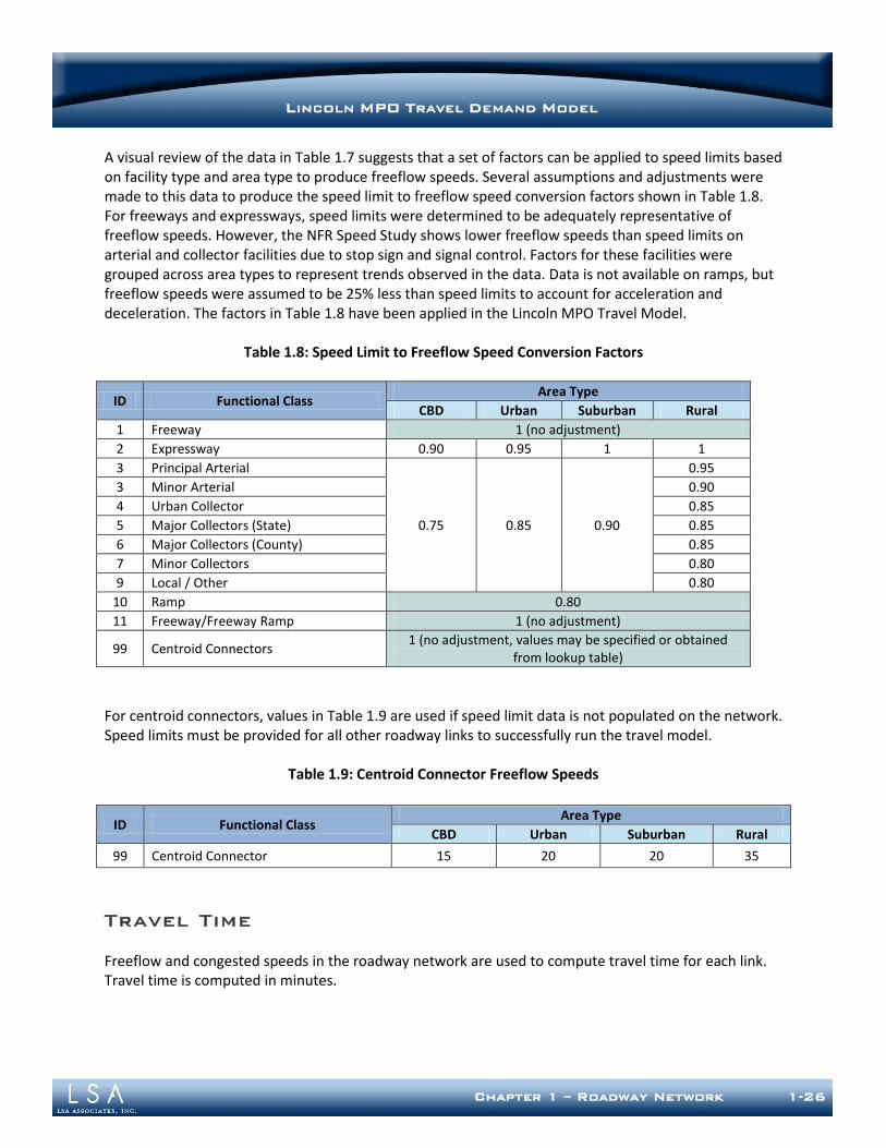
Chapter 1 – Roadway Network 1-26
LINCOLN MPO TRAVEL DEMAND MODEL
A visual review of the data in Table 1.7 suggests that a set of factors can be applied to speed limits based on facility type and area type to produce freeflow speeds. Several assumptions and adjustments were made to this data to produce the speed limit to freeflow speed conversion factors shown in Table 1.8. For freeways and expressways, speed limits were determined to be adequately representative of freeflow speeds. However, the NFR Speed Study shows lower freeflow speeds than speed limits on arterial and collector facilities due to stop sign and signal control. Factors for these facilities were grouped across area types to represent trends observed in the data. Data is not available on ramps, but freeflow speeds were assumed to be 25% less than speed limits to account for acceleration and deceleration. The factors in Table 1.8 have been applied in the Lincoln MPO Travel Model.
Table 1.8: Speed Limit to Freeflow Speed Conversion Factors
ID Functional Class Area Type
CBD Urban Suburban Rural
1 Freeway 1 (no adjustment)
2 Expressway 0.90 0.95 1 1
3 Principal Arterial
0.75 0.85 0.90
0.95
3 Minor Arterial 0.90
4 Urban Collector 0.85
5 Major Collectors (State) 0.85
6 Major Collectors (County) 0.85
7 Minor Collectors 0.80
9 Local / Other 0.80
10 Ramp 0.80
11 Freeway/Freeway Ramp 1 (no adjustment)
99 Centroid Connectors 1 (no adjustment, values may be specified or obtained
from lookup table)
For centroid connectors, values in Table 1.9 are used if speed limit data is not populated on the network. Speed limits must be provided for all other roadway links to successfully run the travel model.
Table 1.9: Centroid Connector Freeflow Speeds
ID Functional Class Area Type
CBD Urban Suburban Rural
99 Centroid Connector 15 20 20 35
Travel Time
Freeflow and congested speeds in the roadway network are used to compute travel time for each link. Travel time is computed in minutes.
Chapter 1 – Roadway Network 1-27
LINCOLN MPO TRAVEL DEMAND MODEL
L INK CAPACITIES
Traffic assignment, especially capacity constrained traffic assignment, requires accurate roadway capacity values. Capacity is used in the model to measure congestion and to determine route diversion due to congestion. This calculation is accomplished through the use of volume-delay equations that are defined and applied in the traffic assignment model. In the model, per-lane capacity values are retrieved from a lookup table based on the facility type and area type of each link in the roadway network. This approach eliminates opportunities for error in defining capacities at the link level and enforces consistent application of capacity values. Hourly per-lane capacities are retrieved from a lookup table that is stored in an Access database. These hourly lane capacities are used in combination with the number of lane information present on the network to define hourly directional capacity. The Highway Capacity Manual (HCM or HCM 2000)2 provides guidance on the definition of roadway capacity. The HCM provides link-level capacity guidelines for freeways and rural highways, but does not provide detailed link-level capacity guidelines for urban and suburban collector and arterial streets. Therefore, HCM intersection capacity was used in place of link capacity to develop capacities for these other facilities.
Freeways
Capacity guidelines for freeways and expressways are provided in Chapters 21 and 23 of HCM 2000. Unadjusted, or ideal, per-lane capacities based on freeflow speed are provided, which must then be adjusted for various conditions. The conditions for which adjustments can be applied are described below.
Heavy Vehicle Adjustment Factor – The heavy vehicle adjustment factor accounts for passenger car equivalents for trucks, buses, and recreational vehicles. HCM 2000 recommends default values of 10% heavy vehicles in rural areas and 5% heavy vehicles in non-rural areas unless additional data is available. Capacities in the Lincoln MPO Travel Model assume 5% heavy vehicles on all facilities.
Driver Population Factor – The driver population factor represents the familiarity of drivers with roadway facilities. Because the model represents traffic on a typical weekday when school is in session, normal driver familiarity was assumed. Driver population factors are typically used for weekend conditions or in areas with a high amount of tourist/recreational activity.
Peak Hour Factor – A peak hour factor (PHF) represents the variation of traffic volumes within an hour. Default values of 0.88 for rural area types and 0.92 for non-rural area types were applied3.
2 Highway Capacity Manual. Transportation Research Board, 2000.
3 HCM 2000, p. 13-11
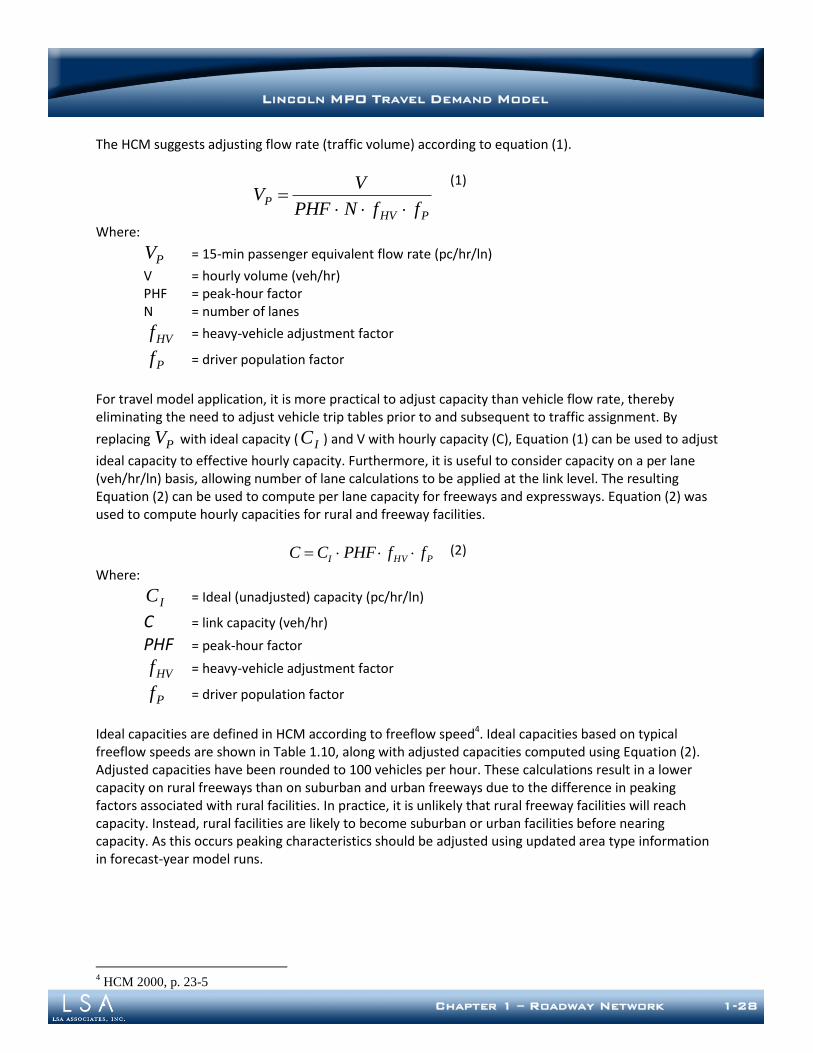
Chapter 1 – Roadway Network 1-28
LINCOLN MPO TRAVEL DEMAND MODEL
The HCM suggests adjusting flow rate (traffic volume) according to equation (1).
PHV
PffNPHF
VV
(1)
Where:
PV = 15-min passenger equivalent flow rate (pc/hr/ln)
V = hourly volume (veh/hr) PHF = peak-hour factor N = number of lanes
HVf = heavy-vehicle adjustment factor
Pf = driver population factor
For travel model application, it is more practical to adjust capacity than vehicle flow rate, thereby eliminating the need to adjust vehicle trip tables prior to and subsequent to traffic assignment. By
replacing PV with ideal capacity ( IC ) and V with hourly capacity (C), Equation (1) can be used to adjust
ideal capacity to effective hourly capacity. Furthermore, it is useful to consider capacity on a per lane (veh/hr/ln) basis, allowing number of lane calculations to be applied at the link level. The resulting Equation (2) can be used to compute per lane capacity for freeways and expressways. Equation (2) was used to compute hourly capacities for rural and freeway facilities.
PHVI ffPHFCC (2)
Where:
IC = Ideal (unadjusted) capacity (pc/hr/ln)
C = link capacity (veh/hr)
PHF = peak-hour factor
HVf = heavy-vehicle adjustment factor
Pf = driver population factor
Ideal capacities are defined in HCM according to freeflow speed4. Ideal capacities based on typical freeflow speeds are shown in Table 1.10, along with adjusted capacities computed using Equation (2). Adjusted capacities have been rounded to 100 vehicles per hour. These calculations result in a lower capacity on rural freeways than on suburban and urban freeways due to the difference in peaking factors associated with rural facilities. In practice, it is unlikely that rural freeway facilities will reach capacity. Instead, rural facilities are likely to become suburban or urban facilities before nearing capacity. As this occurs peaking characteristics should be adjusted using updated area type information in forecast-year model runs.
4 HCM 2000, p. 23-5
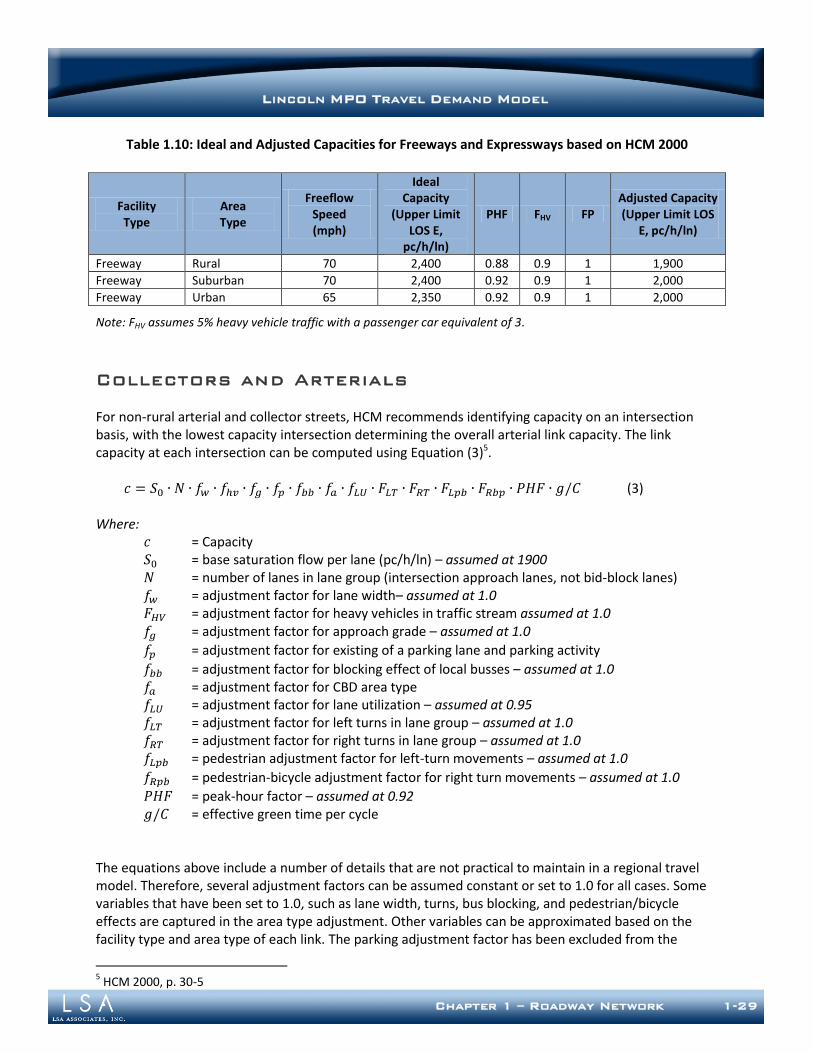
Chapter 1 – Roadway Network 1-29
LINCOLN MPO TRAVEL DEMAND MODEL
Table 1.10: Ideal and Adjusted Capacities for Freeways and Expressways based on HCM 2000
Facility Type
Area Type
Freeflow Speed (mph)
Ideal Capacity
(Upper Limit LOS E,
pc/h/ln)
PHF FHV FP Adjusted Capacity (Upper Limit LOS
E, pc/h/ln)
Freeway Rural 70 2,400 0.88 0.9 1 1,900
Freeway Suburban 70 2,400 0.92 0.9 1 2,000
Freeway Urban 65 2,350 0.92 0.9 1 2,000
Note: FHV assumes 5% heavy vehicle traffic with a passenger car equivalent of 3.
Collectors and Arterials
For non-rural arterial and collector streets, HCM recommends identifying capacity on an intersection basis, with the lowest capacity intersection determining the overall arterial link capacity. The link capacity at each intersection can be computed using Equation (3)5.
(3)
Where: = Capacity
= base saturation flow per lane (pc/h/ln) – assumed at 1900 = number of lanes in lane group (intersection approach lanes, not bid-block lanes) = adjustment factor for lane width– assumed at 1.0
= adjustment factor for heavy vehicles in traffic stream assumed at 1.0 = adjustment factor for approach grade – assumed at 1.0
= adjustment factor for existing of a parking lane and parking activity
= adjustment factor for blocking effect of local busses – assumed at 1.0 = adjustment factor for CBD area type
= adjustment factor for lane utilization – assumed at 0.95 = adjustment factor for left turns in lane group – assumed at 1.0 = adjustment factor for right turns in lane group – assumed at 1.0 = pedestrian adjustment factor for left-turn movements – assumed at 1.0
= pedestrian-bicycle adjustment factor for right turn movements – assumed at 1.0
= peak-hour factor – assumed at 0.92 = effective green time per cycle
The equations above include a number of details that are not practical to maintain in a regional travel model. Therefore, several adjustment factors can be assumed constant or set to 1.0 for all cases. Some variables that have been set to 1.0, such as lane width, turns, bus blocking, and pedestrian/bicycle effects are captured in the area type adjustment. Other variables can be approximated based on the facility type and area type of each link. The parking adjustment factor has been excluded from the
5 HCM 2000, p. 30-5
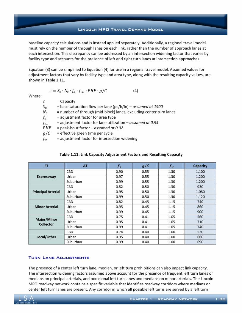
Chapter 1 – Roadway Network 1-30
LINCOLN MPO TRAVEL DEMAND MODEL
baseline capacity calculations and is instead applied separately. Additionally, a regional travel model must rely on the number of through lanes on each link, rather than the number of approach lanes at each intersection. This discrepancy can be addressed by an intersection widening factor that varies by facility type and accounts for the presence of left and right turn lanes at intersection approaches. Equation (3) can be simplified to Equation (4) for use in a regional travel model. Assumed values for adjustment factors that vary by facility type and area type, along with the resulting capacity values, are shown in Table 1.11.
(4) Where:
= Capacity = base saturation flow per lane (pc/h/ln) – assumed at 1900 = number of through (mid-block) lanes, excluding center turn lanes = adjustment factor for area type
= adjustment factor for lane utilization – assumed at 0.95 = peak-hour factor – assumed at 0.92
= effective green time per cycle = adjustment factor for intersection widening
Table 1.11: Link Capacity Adjustment Factors and Resulting Capacity
FT AT Capacity
Expressway
CBD 0.90 0.55 1.30 1,100
Urban 0.97 0.55 1.30 1,200
Suburban 0.99 0.55 1.30 1,200
Principal Arterial
CBD 0.82 0.50 1.30 930
Urban 0.95 0.50 1.30 1,080
Suburban 0.99 0.50 1.30 1,120
Minor Arterial
CBD 0.82 0.45 1.15 740
Urban 0.95 0.45 1.15 860
Suburban 0.99 0.45 1.15 900
Major/Minor Collector
CBD 0.75 0.41 1.05 560
Urban 0.95 0.41 1.05 710
Suburban 0.99 0.41 1.05 740
Local/Other
CBD 0.74 0.40 1.00 520
Urban 0.95 0.40 1.00 660
Suburban 0.99 0.40 1.00 690
Turn Lane Adjustments
The presence of a center left turn lane, median, or left turn prohibitions can also impact link capacity. The intersection widening factors assumed above account for the presence of frequent left turn lanes or medians on principal arterials, and occasional left turn lanes and medians on minor arterials. The Lincoln MPO roadway network contains a specific variable that identifies roadway corridors where medians or center left turn lanes are present. Any corridor in which all possible left turns are served by a left turn

Chapter 1 – Roadway Network 1-31
LINCOLN MPO TRAVEL DEMAND MODEL
lane is identified by this variable. To account for center left turn lanes, the number of lanes used to compute total directional flow is adjusted as follows:
Principal Arterial: o Left turn lane present: Add 0.25 lanes (0.125 lanes in each direction) o No left turn lane present: Subtract 0.5 lanes (0.25 lanes in each direction)
Minor Arterial: o Left turn lane present Add 0.5 lanes (0.25 lanes in each direction) o No left turn lane present: Subtract 0.25 lanes (0.125 lanes in each direction)
No center turn lane or median adjustments are made on expressway, collector, or local facilities. Parking Adjustments
The capacity assumptions listed above do not account for on-street parking where it exists. In the Lincoln area, on-street parking is allowed in parts of the CBD and the surrounding urban areas. In some places, on-street parking is only permitted in the off-peak hours. During the peak hours, on-street parking is prohibited and the parking lane is used as a travel lane. Discussions with MPO staff indicate that these lanes are fully utilized during the peak periods. Therefore, the roadway network has been coded to include these off-peak parking lanes as through lanes. On links where on-street parking is allowed, two capacity adjustments can be applied.
1. For links with off-peak parking only, the total number of lanes is reduced by one during the off-peak period, and
2. For all links with on-street parking, the capacity is reduced to account for the increased friction associated with parking maneuvers. The adjustment is only applied to periods in which on-street parking is permitted.
The reduction in capacity resulting from on-street parking is calculated based on guidance from HCM 20006. Equation (5) defines the parking adjustment.
(5)
Where: = Capacity adjustment factor for on-street parking
= Number of lanes in lane group = Number of parking maneuvers per hour (up to 180; assumed to be 20 for the Lincoln
MPO Model) Resulting parking adjustments are applied to arterial streets only. Collector streets already include significant capacity reductions and on-street parking is generally prohibited on expressways. Parking adjustments (shown in Table 1.12) are applied based on the number of directional lanes on a roadway.
6 HCM 2000, p. 16-11
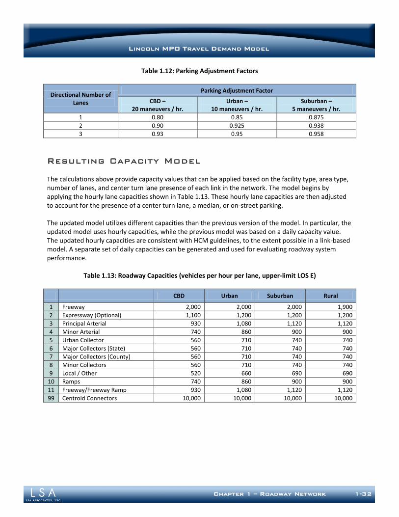
Chapter 1 – Roadway Network 1-32
LINCOLN MPO TRAVEL DEMAND MODEL
Table 1.12: Parking Adjustment Factors
Directional Number of Lanes
Parking Adjustment Factor
CBD – 20 maneuvers / hr.
Urban – 10 maneuvers / hr.
Suburban – 5 maneuvers / hr.
1 0.80 0.85 0.875
2 0.90 0.925 0.938
3 0.93 0.95 0.958
Resulting Capacity Model
The calculations above provide capacity values that can be applied based on the facility type, area type, number of lanes, and center turn lane presence of each link in the network. The model begins by applying the hourly lane capacities shown in Table 1.13. These hourly lane capacities are then adjusted to account for the presence of a center turn lane, a median, or on-street parking. The updated model utilizes different capacities than the previous version of the model. In particular, the updated model uses hourly capacities, while the previous model was based on a daily capacity value. The updated hourly capacities are consistent with HCM guidelines, to the extent possible in a link-based model. A separate set of daily capacities can be generated and used for evaluating roadway system performance.
Table 1.13: Roadway Capacities (vehicles per hour per lane, upper-limit LOS E)
CBD Urban Suburban Rural
1 Freeway 2,000 2,000 2,000 1,900
2 Expressway (Optional) 1,100 1,200 1,200 1,200
3 Principal Arterial 930 1,080 1,120 1,120
4 Minor Arterial 740 860 900 900
5 Urban Collector 560 710 740 740
6 Major Collectors (State) 560 710 740 740
7 Major Collectors (County) 560 710 740 740
8 Minor Collectors 560 710 740 740
9 Local / Other 520 660 690 690
10 Ramps 740 860 900 900
11 Freeway/Freeway Ramp 930 1,080 1,120 1,120
99 Centroid Connectors 10,000 10,000 10,000 10,000

Chapter 1 – Roadway Network 1-33
LINCOLN MPO TRAVEL DEMAND MODEL
ROUTABLE NETWORK
Many functions in TransCAD require the creation of a routable network file, identified by a “.net” extension. For the Lincoln MPO Travel Model, the pathbuilding/skimming and traffic assignment procedures require a routable network. Length and travel time information for each link is stored in the routable network file, as are turn prohibitions. Specific turn prohibitions are initially stored in a separate file that is referenced when creating the routable network. An appropriate routable network file is created during the automated network initialization step. Routable network files are also required when performing interactive pathbuilding; these routable networks can be created using the TransCAD interface designed for this purpose. The routable network file also contains information about centroid connectors to prevent the pathbuilder and traffic assignment algorithms from routing trips through centroids. The model automatically creates a selection of centroid nodes and identifies these nodes as centroids in the routable network file.
Chapter 2 – Trip Generation 2-1
LINCOLN MPO TRAVEL DEMAND MODEL
Chapter 2: Trip Generation
CONTEXT AND BACKGROUND
This chapter describes the process used to develop the Trip Generation component of the Lincoln MPO Travel Model. Trip production and attraction rates, special generators, allocation models, balancing methods, trip purpose, external travel, and other information related to the trip generation model are addressed herein. Trip generation rates are expressed as daily person trips for all modes, including auto/truck, bus transit, pedestrian, and bicycle. Trip generation is the first phase of the traditional four-step travel demand modeling process. It identifies the trip ends (productions and attractions) that correspond to the places where activities occur according to land use and socioeconomic data. Productions and attractions are estimated for each TAZ by trip purpose, and then balanced at the regional level so that total productions and attractions are equal. In some cases, production and attraction allocation sub-models are applied to better represent the geographic locations at which these trip ends occur. The resulting productions and attractions by trip purpose and TAZ are subsequently used by the Trip Distribution model to estimate zone-to-zone travel patterns. The trip generation model is defined such that trips are produced at home and are generally attracted to other places of activity (non-residential land uses). Hence, the terms “productions” and “attractions” are the fundamental variables for defining the trip ends associated with travel. Productions generally occur at the home end of a trip; and attractions are typically associated with non-residential activity. Some exceptions are described in the following sections, but this method of defining productions and attractions is generally used for trips internal to (within) the modeling area. For travel outside the modeling area, external trips are defined as: 1) external-external (EE) if both trip ends are outside of the modeling area, and 2) internal-external or external-internal (IE/EI) if one end of the trip is inside and the other end is outside of the modeling area. This chapter opens with a summary of TAZ inputs to the trip generation model followed by a discussion of trip rate data sources, trip purposes, and an explanation of how trip production and attraction rates are established. Then, sub-allocation models, special generators, and trip balancing are explained followed by a description of external trips, including trips to, from, and through the region.
TRAFFIC ANALYSIS ZONE STRUCTURE
TAZs are small areas containing the land use data that form the foundation for trip-making in the travel model. For the Lincoln MPO Travel Model, the TAZ layer is maintained to be consistent with US Census TAZ boundaries. The TAZ structure is formatted as a polygon layer in TransCAD’s GIS structure. The TAZs are attached to the network using zone centroids and centroid connectors that allow travelers access to the transportation system by simulating local and neighborhood streets. The TAZ layer is shown in Figures 2.1A through 2.1C.
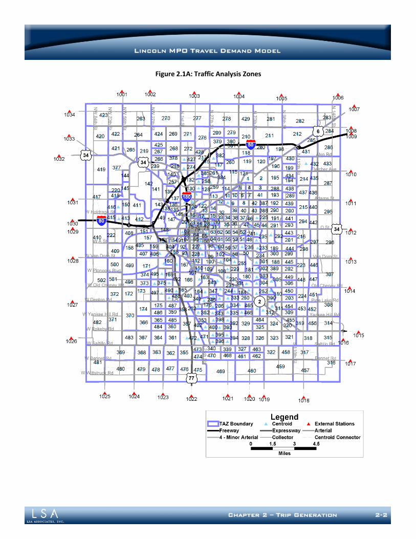
Chapter 2 – Trip Generation 2-2
LINCOLN MPO TRAVEL DEMAND MODEL
Figure 2.1A: Traffic Analysis Zones
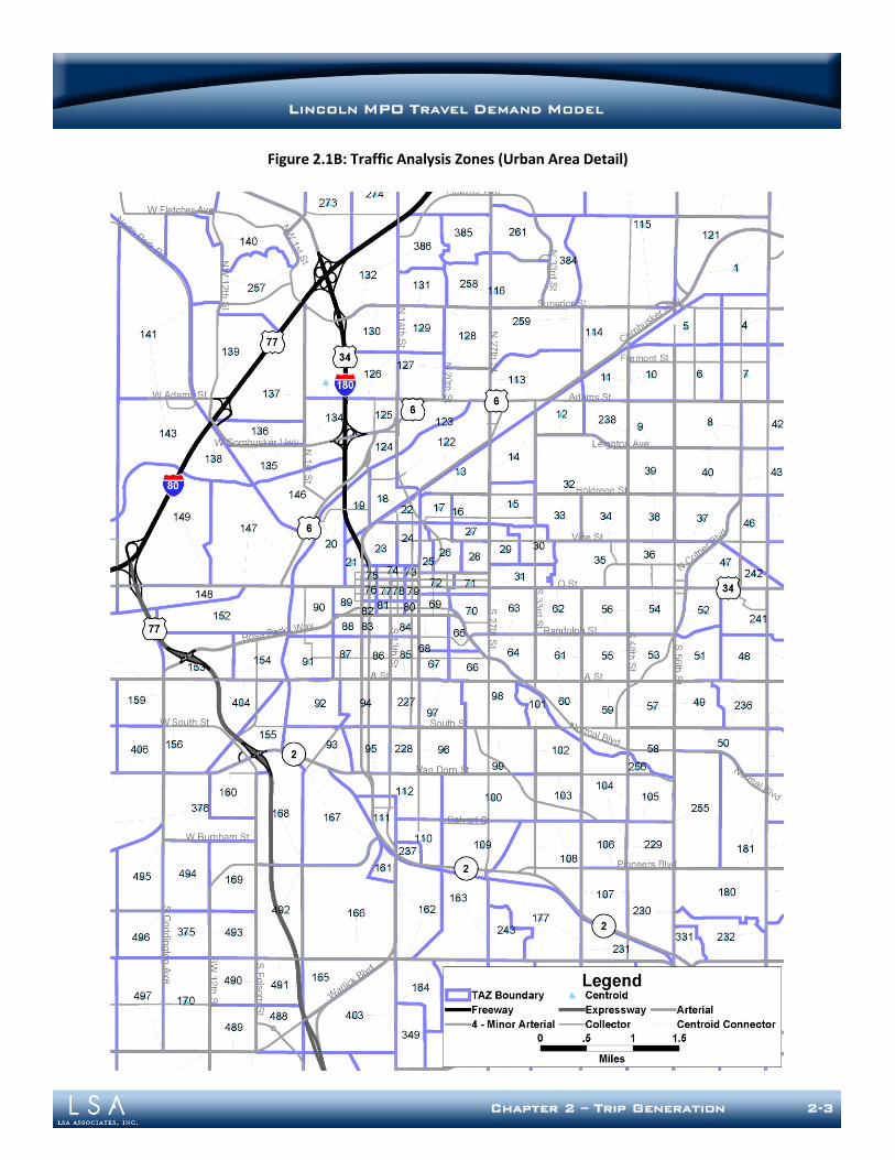
Chapter 2 – Trip Generation 2-3
LINCOLN MPO TRAVEL DEMAND MODEL
Figure 2.1B: Traffic Analysis Zones (Urban Area Detail)
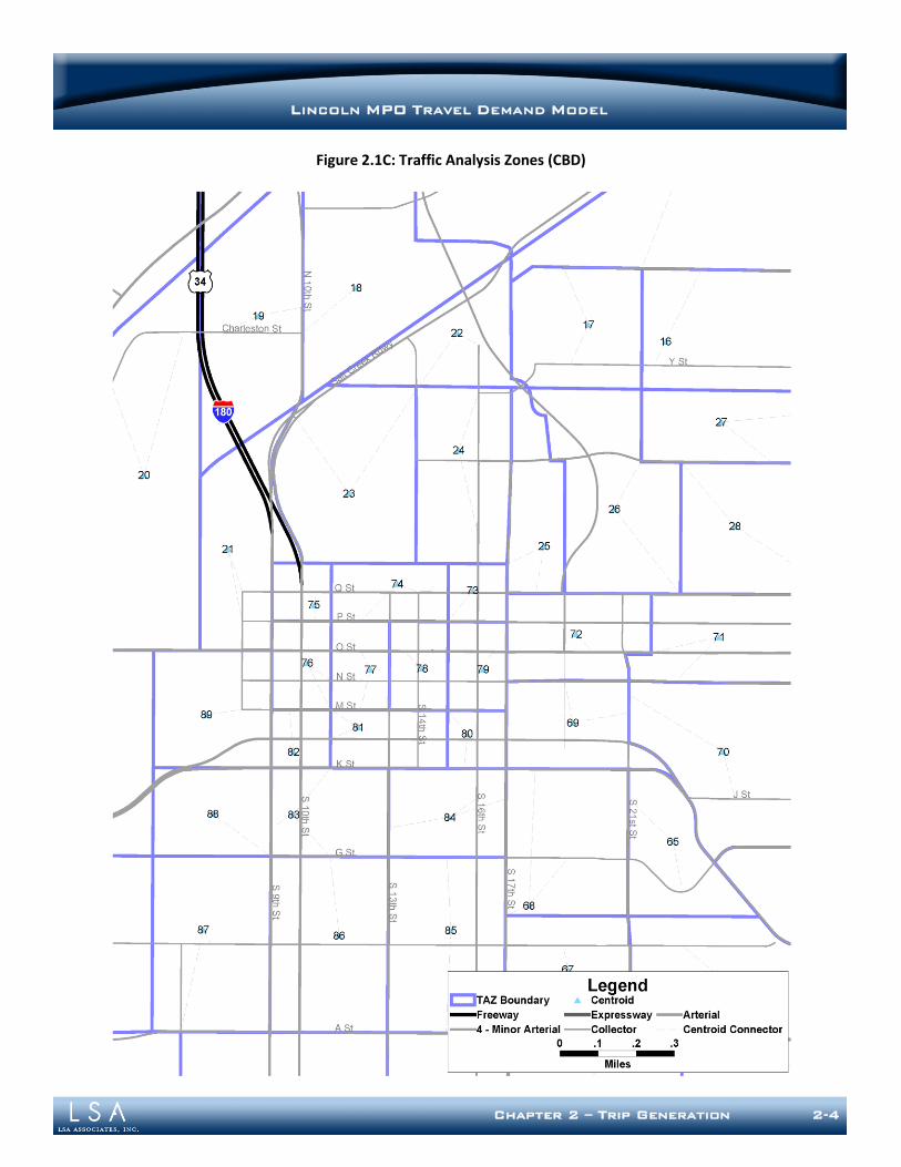
Chapter 2 – Trip Generation 2-4
LINCOLN MPO TRAVEL DEMAND MODEL
Figure 2.1C: Traffic Analysis Zones (CBD)
Chapter 2 – Trip Generation 2-5
LINCOLN MPO TRAVEL DEMAND MODEL
TAZs are ideally, but not always, sized and shaped to encompass a relatively homogeneous level and type of activity within each zone. TAZ delineations traditionally follow the natural and manmade boundaries that segregate different land uses. These boundaries include water features, roads, railroads, and other lines that form logical land use boundaries. Often, jurisdictional and census boundaries are not used to define TAZ boundaries because they can be arbitrary and may not follow logical boundaries; but they are usually desirable for data development and reporting.
HOUSEHOLD D ISAGGREGATION MODELS
The land use input data includes information about single- and multi-family dwelling units. To supplement this data, the average household size and income for each TAZ has been obtained from US Census data. The model then uses household disaggregation models to estimate the univariate distribution of households by size and by income group for each TAZ. Once these distributions have been estimated, the model uses an iterative proportional factoring process to develop bi-variate distributions of households by income and size for each TAZ. Household disaggregation models use known variables to determine the distribution of households by classification. For example, a zone with an average household size of 1 person would be comprised entirely of 1-person households (by definition). Conversely, a zone with an average household size of 4 people would be modeled as a combination of 1, 2, 3, 4, and 5+ person households. Distributions are represented by hand-fitted curves based on US Census data aggregated to each TAZ. It is important that the distribution curves always sum to 100% and that, for the household size model, the results are consistent with the input value when averaged. Hand-fitted curves have been adjusted to fit the observed data points, sum to 100%, and produce the appropriate average. The household income model is expressed as a percentage of regional income rather than an income value in dollars to allow for median income data to be input in any chosen units, so long as the units are consistent for all zones. Data may be input in 1999 dollars (consistent with the 2000 Census), or in some other unit if desired.
Household Size Disaggregation Model
Model trip rates are classified by five (5) household size groups. The portion of households in each group can be approximated for any given TAZ based on the average household size. Disaggregation curves, along with the Census data, are shown in Figure 2.2. The resulting model is defined as a lookup table and is provided with the travel model input dataset.
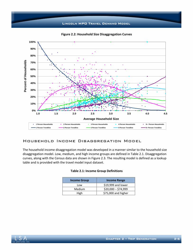
Chapter 2 – Trip Generation 2-6
LINCOLN MPO TRAVEL DEMAND MODEL
Figure 2.2: Household Size Disaggregation Curves
Household Income Disaggregation Model
The household income disaggregation model was developed in a manner similar to the household size disaggregation model. Low, medium, and high income groups are defined in Table 2.1. Disaggregation curves, along with the Census data are shown in Figure 2.3. The resulting model is defined as a lookup table and is provided with the travel model input dataset.
Table 2.1: Income Group Definitions
Income Group Income Range
Low $19,999 and lower
Medium $20,000 – $74,999
High $75,000 and higher
0%
10%
20%
30%
40%
50%
60%
70%
80%
90%
100%
1.0 1.5 2.0 2.5 3.0 3.5 4.0 4.5
Perc
en
t o
f H
ou
seh
old
s
Average Household Size
Lincoln MPO Household Size Distribution
1 Person Households 2 Person Households 3 Person Households 4 Person Households 5+ Person Households
1 Person Trendline 2 Person Trendline 3 Person Trendline 4 Person Trendline 5+ Person Trendline
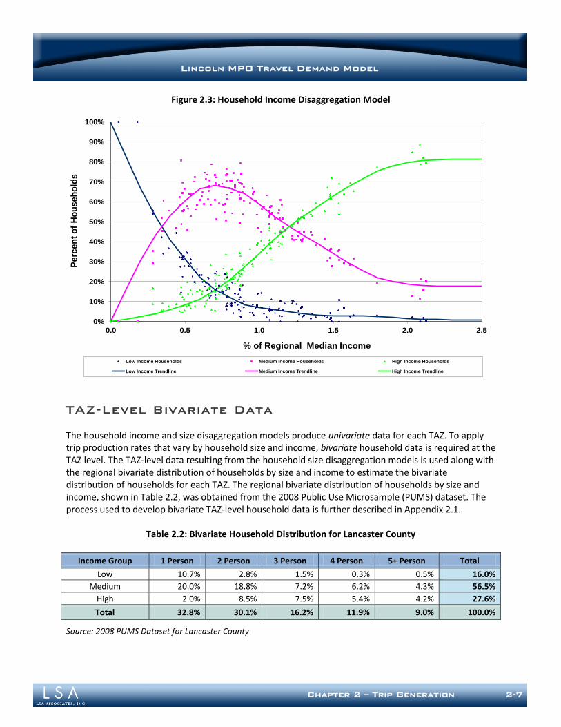
Chapter 2 – Trip Generation 2-7
LINCOLN MPO TRAVEL DEMAND MODEL
Figure 2.3: Household Income Disaggregation Model
TAZ-Level Bivariate Data
The household income and size disaggregation models produce univariate data for each TAZ. To apply trip production rates that vary by household size and income, bivariate household data is required at the TAZ level. The TAZ-level data resulting from the household size disaggregation models is used along with the regional bivariate distribution of households by size and income to estimate the bivariate distribution of households for each TAZ. The regional bivariate distribution of households by size and income, shown in Table 2.2, was obtained from the 2008 Public Use Microsample (PUMS) dataset. The process used to develop bivariate TAZ-level household data is further described in Appendix 2.1.
Table 2.2: Bivariate Household Distribution for Lancaster County
Income Group 1 Person 2 Person 3 Person 4 Person 5+ Person Total
Low 10.7% 2.8% 1.5% 0.3% 0.5% 16.0%
Medium 20.0% 18.8% 7.2% 6.2% 4.3% 56.5%
High 2.0% 8.5% 7.5% 5.4% 4.2% 27.6%
Total 32.8% 30.1% 16.2% 11.9% 9.0% 100.0%
Source: 2008 PUMS Dataset for Lancaster County
0%
10%
20%
30%
40%
50%
60%
70%
80%
90%
100%
0.0 0.5 1.0 1.5 2.0 2.5
Perc
en
t o
f H
ou
seh
old
s
% of Regional Median Income
Lincoln MPO Household Income Distribution
Low Income Households Medium Income Households High Income Households
Low Income Trendline Medium Income Trendline High Income Trendline

Chapter 2 – Trip Generation 2-8
LINCOLN MPO TRAVEL DEMAND MODEL
DATA SOURCES
The primary data source for estimating trip production and attraction rates is the household-based travel diary survey. These household-based surveys usually have three components – household, person, and trip – and provide excellent information with regard to household trip-making. Therefore, household travel surveys are especially well suited for estimating trip production rates. The person component of the survey records information about attraction trip ends, which helps to estimate trip attraction rates. The trip component of the survey includes information about the activities (i.e., purpose) of each trip as well as the facility type at the origin and destination of each trip record. Because a local dataset is not available, several datasets were investigated for possible transfer to the Lincoln MPO Travel Model. Initially, the 2009 National Household Travel Survey (NHTS) dataset was investigated as a source for trip generation rates in the Lincoln area. However, the NHTS includes only limited data for the Lincoln area, so an attempt was made to utilize NHTS data from all urbanized areas with a population between 100,000 and 300,000. An evaluation of the data at the cross-classified level suggested problems with the preliminary weighting factors that were available when the analysis was conducted. Revised weighting and expansion factors under development when the analysis was conducted will likely resolve the observed problems. The NHTS includes add-on data for small- and medium-sized urban areas, including Cedar Rapids, IA and Rapid City, SD. An attempt was made to utilize data from the Cedar Rapids add-on dataset. While Cedar Rapids is similar in size and character to Lincoln and Lancaster County, a review of the data by income group raised concerns with the accuracy of the initial weighting factors provided with the dataset. These draft weighting factors were under review during development of the Lincoln MPO model. Use of Rapid City data was also considered, but differences in size and character between Rapid City and Lincoln and Lancaster County eliminated this area from consideration. The Colorado Front Range is currently conducting a household travel survey throughout the region. The first phase of this survey encompassed the North Front Range (NFR), including the cities of Fort Collins, Greeley, and Loveland. The NFR survey dataset was analyzed to produce trip rates by household size and income. A review of these trip rates showed that they were reasonably similar to trip rates developed for other areas such as Ann Arbor, MI and San Luis Obispo, CA. The NFR region includes two urbanized areas, the Fort Collins/Loveland area (population of approximately 230,000) and Greeley area (population of approximately 87,000). The NFR also includes two universities. With a population of approximately 250,000 and a major university, Lincoln and Lancaster County can be considered reasonably similar to the NFR region. Therefore, trip rates based on the NFR household survey dataset were applied to the updated Lincoln MPO model.

Chapter 2 – Trip Generation 2-9
LINCOLN MPO TRAVEL DEMAND MODEL
TRIP PURPOSES
Trip purpose is used in travel models to categorize various types of household-based trips with similar characteristics, such as location of production or attraction end, trip length, auto occupancy, and others. In this manner, trip rates by trip purpose are sensitive to the specific socioeconomic data associated with each trip type. In general, trips by trip purpose should be disaggregated only to the point that the base and horizon year activity data can support them. The previous model utilized five trip purposes to describe personal trip-making. For this model update, the number of trip purposes was expanded to seven by further disaggregating home-based other and non-home-based trips as shown in Table 2.3.
Table 2.3: Trip Purposes
Previous Model Updated Model
Home-Based Work (HBW) Home-Based Work (HBW)
Home-Based Shop (HBS) Home-Based Shop (HBS)
Home-Based Recreational (HBR) Home-Based Recreational (HBR)
Home-Based Other (HBO) Home-Based University (HBU)
Home-Based Other (HBO)
Non-Home-Based (NHB) Work-Based-Other (WBO)
Other-Based-Other (OBO)
Generally, a trip is defined as a distinct travel movement from one clearly identifiable starting place/activity to another with a distance of more than one block. In some cases, two or more trips may be linked to reflect the true trip purpose and to factor out convenience stops, such as stopping for gas on the way from home to work. In these cases, the model represents the linked trip as two separate trips. The specific trip purpose definitions are as follows:
Home-Based Work (HBW) - Commute trips between home and work and vice versa (e.g., includes trips between work and home).
Home-Based Shop (HBS) - Trips between home and shopping locations for the purpose of
shopping.
Home-Based Recreational (HBR) - Trips between home and social or recreational activities such as restaurants, entertainment venues, or the homes of friends or relatives.
Home-Based University (HBU) - Trips between home and the university campus for school related purposes by people not employed by the University (i.e., students and visitors).
Home-Based Other (HBO) - All other trips that have one end at home, including trips between
home and appointment, home and recreation, etc.
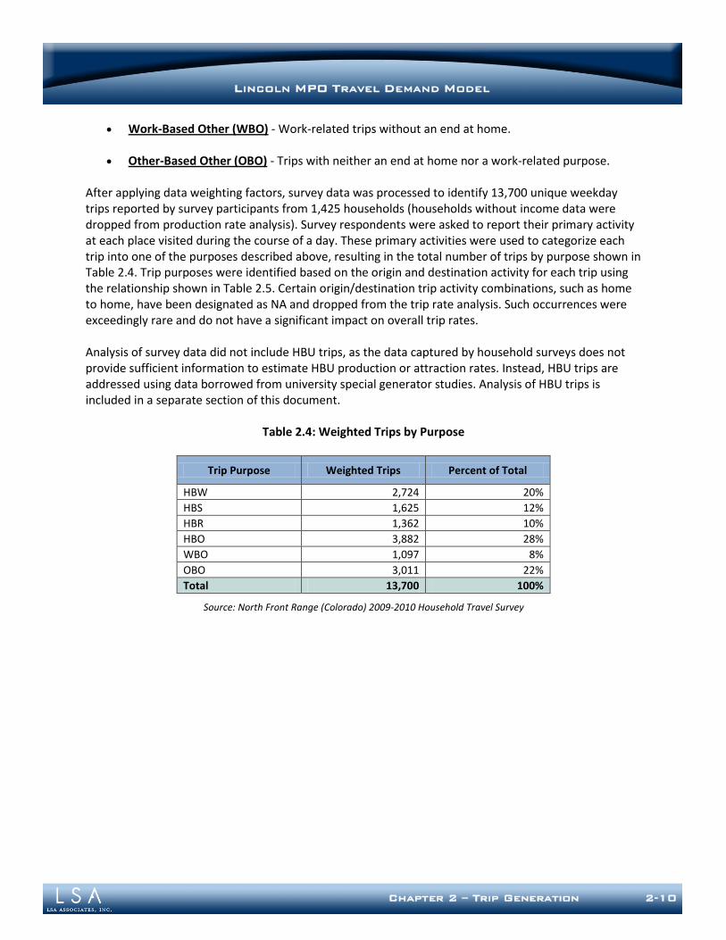
Chapter 2 – Trip Generation 2-10
LINCOLN MPO TRAVEL DEMAND MODEL
Work-Based Other (WBO) - Work-related trips without an end at home.
Other-Based Other (OBO) - Trips with neither an end at home nor a work-related purpose. After applying data weighting factors, survey data was processed to identify 13,700 unique weekday trips reported by survey participants from 1,425 households (households without income data were dropped from production rate analysis). Survey respondents were asked to report their primary activity at each place visited during the course of a day. These primary activities were used to categorize each trip into one of the purposes described above, resulting in the total number of trips by purpose shown in Table 2.4. Trip purposes were identified based on the origin and destination activity for each trip using the relationship shown in Table 2.5. Certain origin/destination trip activity combinations, such as home to home, have been designated as NA and dropped from the trip rate analysis. Such occurrences were exceedingly rare and do not have a significant impact on overall trip rates. Analysis of survey data did not include HBU trips, as the data captured by household surveys does not provide sufficient information to estimate HBU production or attraction rates. Instead, HBU trips are addressed using data borrowed from university special generator studies. Analysis of HBU trips is included in a separate section of this document.
Table 2.4: Weighted Trips by Purpose
Trip Purpose Weighted Trips Percent of Total
HBW 2,724 20%
HBS 1,625 12%
HBR 1,362 10%
HBO 3,882 28%
WBO 1,097 8%
OBO 3,011 22%
Total 13,700 100%
Source: North Front Range (Colorado) 2009-2010 Household Travel Survey
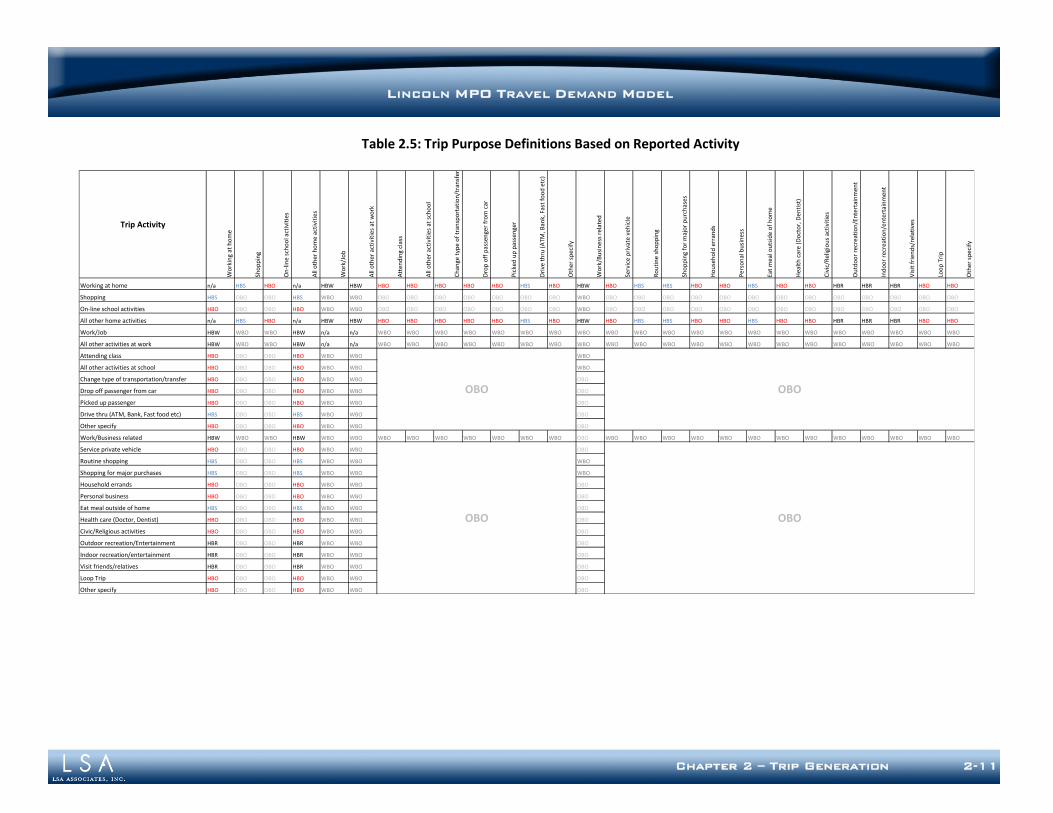
LINCOLN MPO TRAVEL DEMAND MODEL
Chapter 2 – Trip Generation 2-11
Table 2.5: Trip Purpose Definitions Based on Reported Activity
Trip ActivityW
ork
ing
at h
om
e
Sho
pp
ing
On
-lin
e sc
ho
ol a
ctiv
itie
s
All
oth
er h
om
e ac
tivi
ties
Wo
rk/J
ob
All
oth
er a
ctiv
itie
s at
wo
rk
Att
end
ing
clas
s
All
oth
er a
ctiv
itie
s at
sch
oo
l
Ch
ange
typ
e o
f tr
ansp
ort
atio
n/t
ran
sfer
Dro
p o
ff p
asse
nge
r fr
om
car
Pic
ked
up
pas
sen
ger
Dri
ve t
hru
(A
TM, B
ank,
Fas
t fo
od
etc
)
Oth
er s
pec
ify
Wo
rk/B
usi
nes
s re
late
d
Serv
ice
pri
vate
veh
icle
Ro
uti
ne
sho
pp
ing
Sho
pp
ing
for
maj
or
pu
rch
ases
Ho
use
ho
ld e
rran
ds
Per
son
al b
usi
nes
s
Eat
mea
l ou
tsid
e o
f h
om
e
He
alth
car
e (
Do
cto
r, D
enti
st)
Civ
ic/R
elig
iou
s ac
tivi
ties
Ou
tdo
or
recr
eat
ion
/En
tert
ain
men
t
Ind
oo
r re
cre
atio
n/e
nte
rtai
nm
ent
Vis
it f
rien
ds/
rela
tive
s
Loo
p T
rip
Oth
er s
pec
ify
Working at home n/a HBS HBO n/a HBW HBW HBO HBO HBO HBO HBO HBS HBO HBW HBO HBS HBS HBO HBO HBS HBO HBO HBR HBR HBR HBO HBO
Shopping HBS OBO OBO HBS WBO WBO OBO OBO OBO OBO OBO OBO OBO WBO OBO OBO OBO OBO OBO OBO OBO OBO OBO OBO OBO OBO OBO
On-line school activities HBO OBO OBO HBO WBO WBO OBO OBO OBO OBO OBO OBO OBO WBO OBO OBO OBO OBO OBO OBO OBO OBO OBO OBO OBO OBO OBO
All other home activities n/a HBS HBO n/a HBW HBW HBO HBO HBO HBO HBO HBS HBO HBW HBO HBS HBS HBO HBO HBS HBO HBO HBR HBR HBR HBO HBO
Work/Job HBW WBO WBO HBW n/a n/a WBO WBO WBO WBO WBO WBO WBO WBO WBO WBO WBO WBO WBO WBO WBO WBO WBO WBO WBO WBO WBO
All other activities at work HBW WBO WBO HBW n/a n/a WBO WBO WBO WBO WBO WBO WBO WBO WBO WBO WBO WBO WBO WBO WBO WBO WBO WBO WBO WBO WBO
Attending class HBO OBO OBO HBO WBO WBO WBO
All other activities at school HBO OBO OBO HBO WBO WBO WBO
Change type of transportation/transfer HBO OBO OBO HBO WBO WBO OBO
Drop off passenger from car HBO OBO OBO HBO WBO WBO OBO
Picked up passenger HBO OBO OBO HBO WBO WBO OBO
Drive thru (ATM, Bank, Fast food etc) HBS OBO OBO HBS WBO WBO OBO
Other specify HBO OBO OBO HBO WBO WBO OBO
Work/Business related HBW WBO WBO HBW WBO WBO WBO WBO WBO WBO WBO WBO WBO OBO WBO WBO WBO WBO WBO WBO WBO WBO WBO WBO WBO WBO WBO
Service private vehicle HBO OBO OBO HBO WBO WBO OBO
Routine shopping HBS OBO OBO HBS WBO WBO WBO
Shopping for major purchases HBS OBO OBO HBS WBO WBO WBO
Household errands HBO OBO OBO HBO WBO WBO OBO
Personal business HBO OBO OBO HBO WBO WBO OBO
Eat meal outside of home HBS OBO OBO HBS WBO WBO OBO
Health care (Doctor, Dentist) HBO OBO OBO HBO WBO WBO OBO
Civic/Religious activities HBO OBO OBO HBO WBO WBO OBO
Outdoor recreation/Entertainment HBR OBO OBO HBR WBO WBO OBO
Indoor recreation/entertainment HBR OBO OBO HBR WBO WBO OBO
Visit friends/relatives HBR OBO OBO HBR WBO WBO OBO
Loop Trip HBO OBO OBO HBO WBO WBO OBO
Other specify HBO OBO OBO HBO WBO WBO OBO
OBO
OBO OBO
OBO
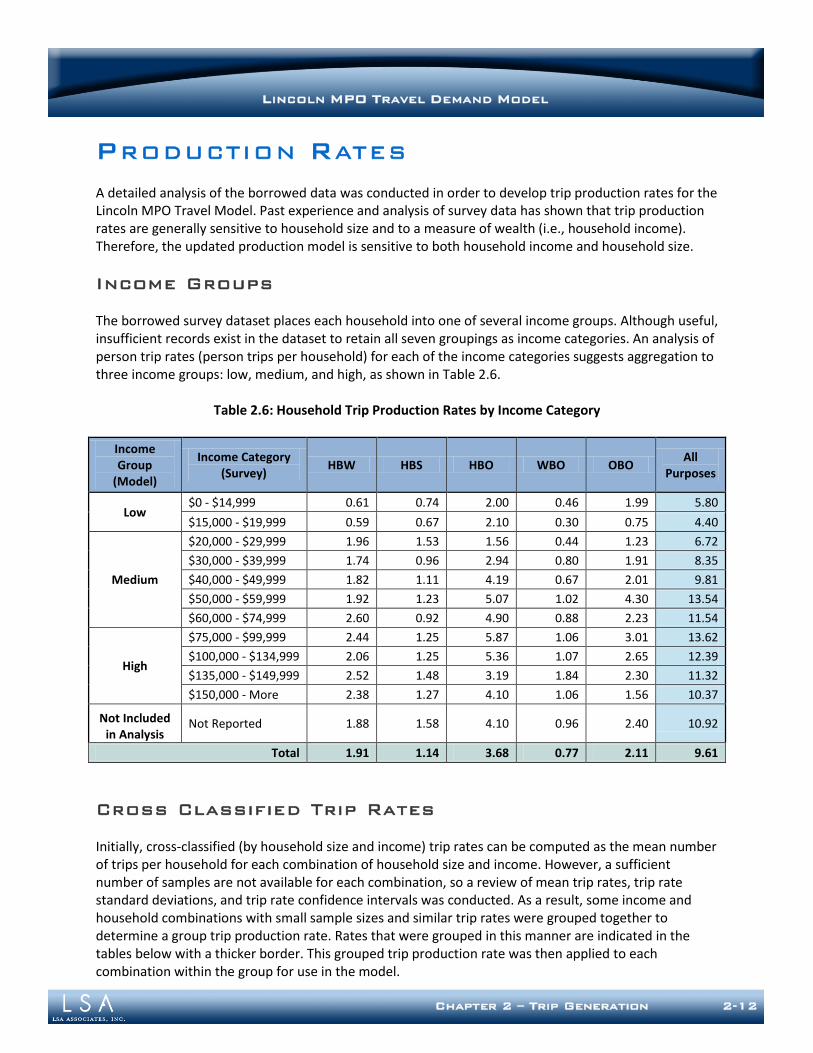
Chapter 2 – Trip Generation 2-12
LINCOLN MPO TRAVEL DEMAND MODEL
PRODUCTION RATES
A detailed analysis of the borrowed data was conducted in order to develop trip production rates for the Lincoln MPO Travel Model. Past experience and analysis of survey data has shown that trip production rates are generally sensitive to household size and to a measure of wealth (i.e., household income). Therefore, the updated production model is sensitive to both household income and household size.
Income Groups
The borrowed survey dataset places each household into one of several income groups. Although useful, insufficient records exist in the dataset to retain all seven groupings as income categories. An analysis of person trip rates (person trips per household) for each of the income categories suggests aggregation to three income groups: low, medium, and high, as shown in Table 2.6.
Table 2.6: Household Trip Production Rates by Income Category
Income Group
(Model)
Income Category (Survey)
HBW HBS HBO WBO OBO All
Purposes
Low $0 - $14,999 0.61 0.74 2.00 0.46 1.99 5.80
$15,000 - $19,999 0.59 0.67 2.10 0.30 0.75 4.40
Medium
$20,000 - $29,999 1.96 1.53 1.56 0.44 1.23 6.72
$30,000 - $39,999 1.74 0.96 2.94 0.80 1.91 8.35
$40,000 - $49,999 1.82 1.11 4.19 0.67 2.01 9.81
$50,000 - $59,999 1.92 1.23 5.07 1.02 4.30 13.54
$60,000 - $74,999 2.60 0.92 4.90 0.88 2.23 11.54
High
$75,000 - $99,999 2.44 1.25 5.87 1.06 3.01 13.62
$100,000 - $134,999 2.06 1.25 5.36 1.07 2.65 12.39
$135,000 - $149,999 2.52 1.48 3.19 1.84 2.30 11.32
$150,000 - More 2.38 1.27 4.10 1.06 1.56 10.37
Not Included in Analysis
Not Reported 1.88 1.58 4.10 0.96 2.40 10.92
Total 1.91 1.14 3.68 0.77 2.11 9.61
Cross Classified Trip Rates
Initially, cross-classified (by household size and income) trip rates can be computed as the mean number of trips per household for each combination of household size and income. However, a sufficient number of samples are not available for each combination, so a review of mean trip rates, trip rate standard deviations, and trip rate confidence intervals was conducted. As a result, some income and household combinations with small sample sizes and similar trip rates were grouped together to determine a group trip production rate. Rates that were grouped in this manner are indicated in the tables below with a thicker border. This grouped trip production rate was then applied to each combination within the group for use in the model.
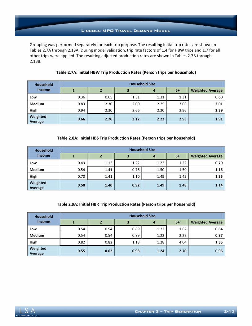
Chapter 2 – Trip Generation 2-13
LINCOLN MPO TRAVEL DEMAND MODEL
Grouping was performed separately for each trip purpose. The resulting initial trip rates are shown in Tables 2.7A through 2.13A. During model validation, trip rate factors of 1.4 for HBW trips and 1.7 for all other trips were applied. The resulting adjusted production rates are shown in Tables 2.7B through 2.13B.
Table 2.7A: Initial HBW Trip Production Rates (Person trips per household)
Household Income
Household Size
1 2 3 4 5+ Weighted Average
Low 0.36 0.65 1.31 1.31 1.31 0.60
Medium 0.83 2.30 2.00 2.25 3.03 2.01
High 0.94 2.30 2.66 2.20 2.96 2.39
Weighted Average
0.66 2.20 2.12 2.22 2.93 1.91
Table 2.8A: Initial HBS Trip Production Rates (Person trips per household)
Household Income
Household Size
1 2 3 4 5+ Weighted Average
Low 0.43 1.12 1.22 1.22 1.22 0.70
Medium 0.54 1.41 0.76 1.50 1.50 1.16
High 0.70 1.41 1.10 1.49 1.49 1.35
Weighted Average
0.50 1.40 0.92 1.49 1.48 1.14
Table 2.9A: Initial HBR Trip Production Rates (Person trips per household)
Household Income
Household Size
1 2 3 4 5+ Weighted Average
Low 0.54 0.54 0.89 1.22 1.62 0.64
Medium 0.54 0.54 0.89 1.22 2.22 0.87
High 0.82 0.82 1.18 1.28 4.04 1.35
Weighted Average
0.55 0.62 0.98 1.24 2.70 0.96
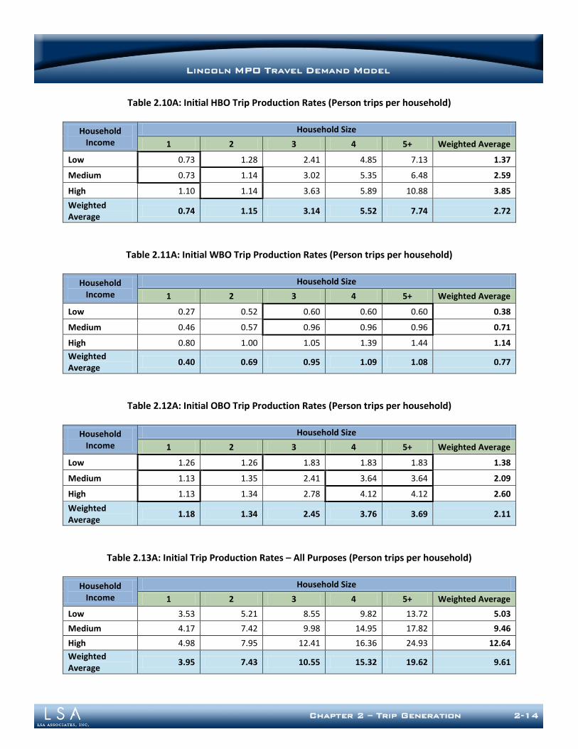
Chapter 2 – Trip Generation 2-14
LINCOLN MPO TRAVEL DEMAND MODEL
Table 2.10A: Initial HBO Trip Production Rates (Person trips per household)
Household Income
Household Size
1 2 3 4 5+ Weighted Average
Low 0.73 1.28 2.41 4.85 7.13 1.37
Medium 0.73 1.14 3.02 5.35 6.48 2.59
High 1.10 1.14 3.63 5.89 10.88 3.85
Weighted Average
0.74 1.15 3.14 5.52 7.74 2.72
Table 2.11A: Initial WBO Trip Production Rates (Person trips per household)
Household Income
Household Size
1 2 3 4 5+ Weighted Average
Low 0.27 0.52 0.60 0.60 0.60 0.38
Medium 0.46 0.57 0.96 0.96 0.96 0.71
High 0.80 1.00 1.05 1.39 1.44 1.14
Weighted Average
0.40 0.69 0.95 1.09 1.08 0.77
Table 2.12A: Initial OBO Trip Production Rates (Person trips per household)
Household Income
Household Size
1 2 3 4 5+ Weighted Average
Low 1.26 1.26 1.83 1.83 1.83 1.38
Medium 1.13 1.35 2.41 3.64 3.64 2.09
High 1.13 1.34 2.78 4.12 4.12 2.60
Weighted Average
1.18 1.34 2.45 3.76 3.69 2.11
Table 2.13A: Initial Trip Production Rates – All Purposes (Person trips per household)
Household Income
Household Size
1 2 3 4 5+ Weighted Average
Low 3.53 5.21 8.55 9.82 13.72 5.03
Medium 4.17 7.42 9.98 14.95 17.82 9.46
High 4.98 7.95 12.41 16.36 24.93 12.64
Weighted Average
3.95 7.43 10.55 15.32 19.62 9.61
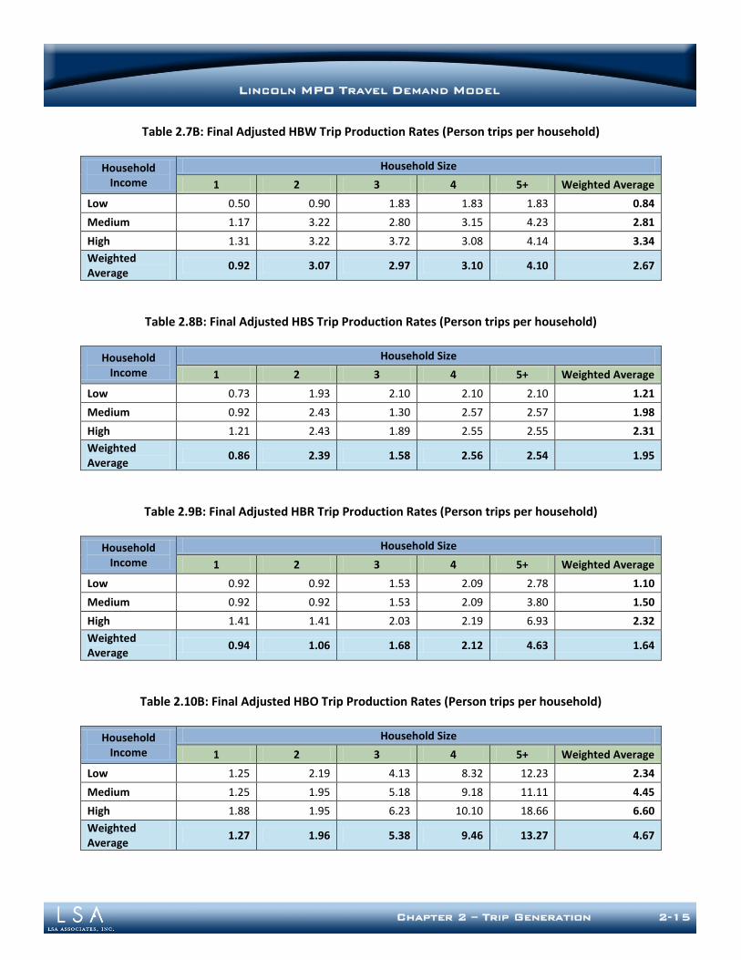
Chapter 2 – Trip Generation 2-15
LINCOLN MPO TRAVEL DEMAND MODEL
Table 2.7B: Final Adjusted HBW Trip Production Rates (Person trips per household)
Household Income
Household Size
1 2 3 4 5+ Weighted Average
Low 0.50 0.90 1.83 1.83 1.83 0.84
Medium 1.17 3.22 2.80 3.15 4.23 2.81
High 1.31 3.22 3.72 3.08 4.14 3.34
Weighted Average
0.92 3.07 2.97 3.10 4.10 2.67
Table 2.8B: Final Adjusted HBS Trip Production Rates (Person trips per household)
Household Income
Household Size
1 2 3 4 5+ Weighted Average
Low 0.73 1.93 2.10 2.10 2.10 1.21
Medium 0.92 2.43 1.30 2.57 2.57 1.98
High 1.21 2.43 1.89 2.55 2.55 2.31
Weighted Average
0.86 2.39 1.58 2.56 2.54 1.95
Table 2.9B: Final Adjusted HBR Trip Production Rates (Person trips per household)
Household Income
Household Size
1 2 3 4 5+ Weighted Average
Low 0.92 0.92 1.53 2.09 2.78 1.10
Medium 0.92 0.92 1.53 2.09 3.80 1.50
High 1.41 1.41 2.03 2.19 6.93 2.32
Weighted Average
0.94 1.06 1.68 2.12 4.63 1.64
Table 2.10B: Final Adjusted HBO Trip Production Rates (Person trips per household)
Household Income
Household Size
1 2 3 4 5+ Weighted Average
Low 1.25 2.19 4.13 8.32 12.23 2.34
Medium 1.25 1.95 5.18 9.18 11.11 4.45
High 1.88 1.95 6.23 10.10 18.66 6.60
Weighted Average
1.27 1.96 5.38 9.46 13.27 4.67
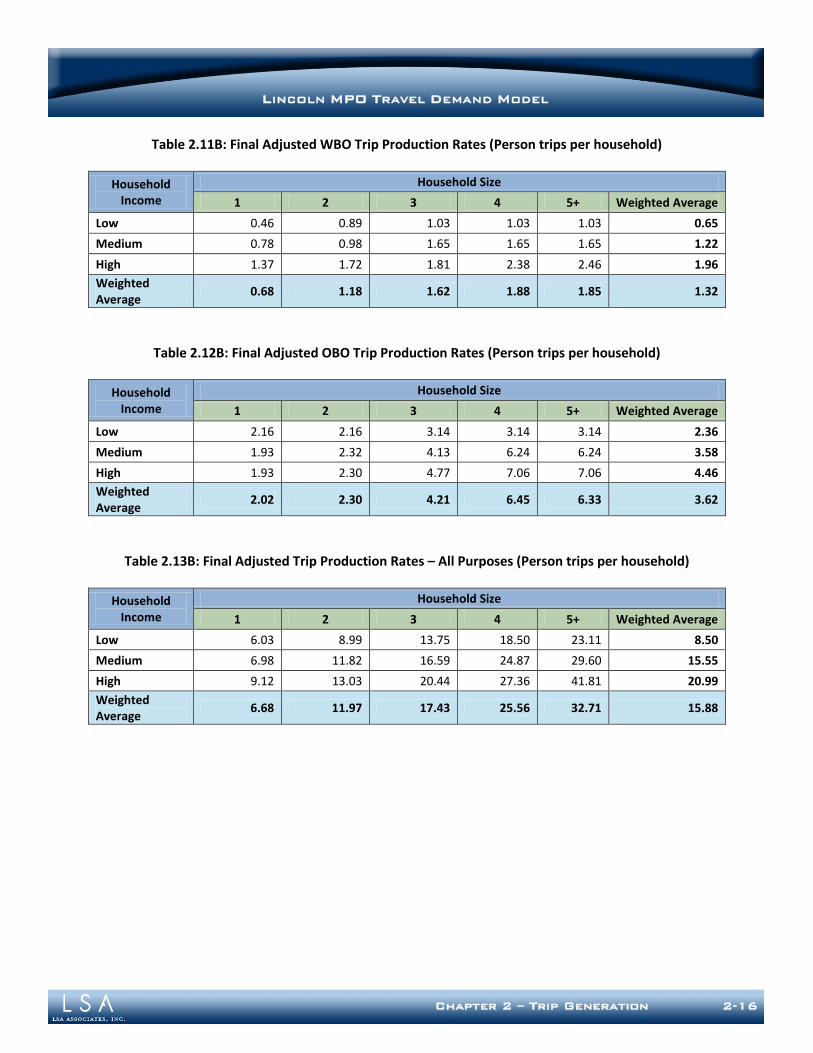
Chapter 2 – Trip Generation 2-16
LINCOLN MPO TRAVEL DEMAND MODEL
Table 2.11B: Final Adjusted WBO Trip Production Rates (Person trips per household)
Household Income
Household Size
1 2 3 4 5+ Weighted Average
Low 0.46 0.89 1.03 1.03 1.03 0.65
Medium 0.78 0.98 1.65 1.65 1.65 1.22
High 1.37 1.72 1.81 2.38 2.46 1.96
Weighted Average
0.68 1.18 1.62 1.88 1.85 1.32
Table 2.12B: Final Adjusted OBO Trip Production Rates (Person trips per household)
Household Income
Household Size
1 2 3 4 5+ Weighted Average
Low 2.16 2.16 3.14 3.14 3.14 2.36
Medium 1.93 2.32 4.13 6.24 6.24 3.58
High 1.93 2.30 4.77 7.06 7.06 4.46
Weighted Average
2.02 2.30 4.21 6.45 6.33 3.62
Table 2.13B: Final Adjusted Trip Production Rates – All Purposes (Person trips per household)
Household Income
Household Size
1 2 3 4 5+ Weighted Average
Low 6.03 8.99 13.75 18.50 23.11 8.50
Medium 6.98 11.82 16.59 24.87 29.60 15.55
High 9.12 13.03 20.44 27.36 41.81 20.99
Weighted Average
6.68 11.97 17.43 25.56 32.71 15.88
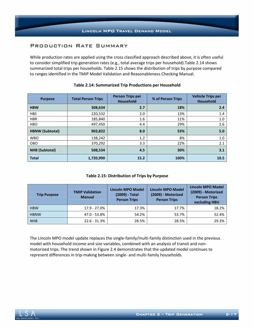
Chapter 2 – Trip Generation 2-17
LINCOLN MPO TRAVEL DEMAND MODEL
Production Rate Summary
While production rates are applied using the cross classified approach described above, it is often useful to consider simplified trip generation rates (e.g., total average trips per household).Table 2.14 shows summarized total trips per households. Table 2.15 shows the distribution of trips by purpose compared to ranges identified in the TMIP Model Validation and Reasonableness Checking Manual.
Table 2.14: Summarized Trip Productions per Household
Purpose Total Person Trips Person Trips per
Household % of Person Trips
Vehicle Trips per Household
HBW 308,634 2.7 18% 2.4
HBS 220,532 2.0 13% 1.4
HBR 185,840 1.6 11% 1.0
HBO 497,450 4.4 29% 2.6
HBNW (Subtotal) 903,822 8.0 53% 5.0
WBO 138,242 1.2 8% 1.0
OBO 370,292 3.3 22% 2.1
NHB (Subtotal) 508,534 4.5 30% 3.1
Total 1,720,990 15.2 100% 10.5
Table 2.15: Distribution of Trips by Purpose
Trip Purpose TMIP Validation
Manual
Lincoln MPO Model (2009) - Total Person Trips
Lincoln MPO Model (2009) - Motorized
Person Trips
Lincoln MPO Model (2009) - Motorized
Person Trips excluding HBU
HBW 17.9 - 27.0% 17.3% 17.7% 18.2%
HBNW 47.0 - 53.8% 54.2% 53.7% 52.4%
NHB 22.6 - 31.3% 28.5% 28.5% 29.3%
The Lincoln MPO model update replaces the single-family/multi-family distinction used in the previous model with household income and size variables, combined with an analysis of transit and non-motorized trips. The trend shown in Figure 2.4 demonstrates that the updated model continues to represent differences in trip-making between single- and multi-family households.
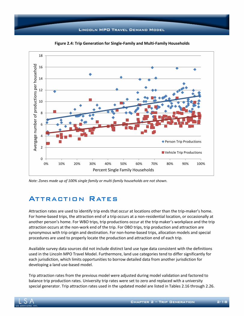
Chapter 2 – Trip Generation 2-18
LINCOLN MPO TRAVEL DEMAND MODEL
Figure 2.4: Trip Generation for Single-Family and Multi-Family Households
Note: Zones made up of 100% single family or multi-family households are not shown.
ATTRACTION RATES
Attraction rates are used to identify trip ends that occur at locations other than the trip-maker’s home. For home-based trips, the attraction end of a trip occurs at a non-residential location, or occasionally at another person’s home. For WBO trips, trip productions occur at the trip maker’s workplace and the trip attraction occurs at the non-work end of the trip. For OBO trips, trip production and attraction are synonymous with trip origin and destination. For non-home-based trips, allocation models and special procedures are used to properly locate the production and attraction end of each trip. Available survey data sources did not include distinct land use type data consistent with the definitions used in the Lincoln MPO Travel Model. Furthermore, land use categories tend to differ significantly for each jurisdiction, which limits opportunities to borrow detailed data from another jurisdiction for developing a land use-based model. Trip attraction rates from the previous model were adjusted during model validation and factored to balance trip production rates. University trip rates were set to zero and replaced with a university special generator. Trip attraction rates used in the updated model are listed in Tables 2.16 through 2.26.
0
2
4
6
8
10
12
14
16
18
0% 10% 20% 30% 40% 50% 60% 70% 80% 90% 100%
Ave
rgag
e n
um
ber
of
pro
du
ctio
ns
per
ho
use
ho
ld
Percent Single Family Households
Person Trip Productions
Vehicle Trip Productions
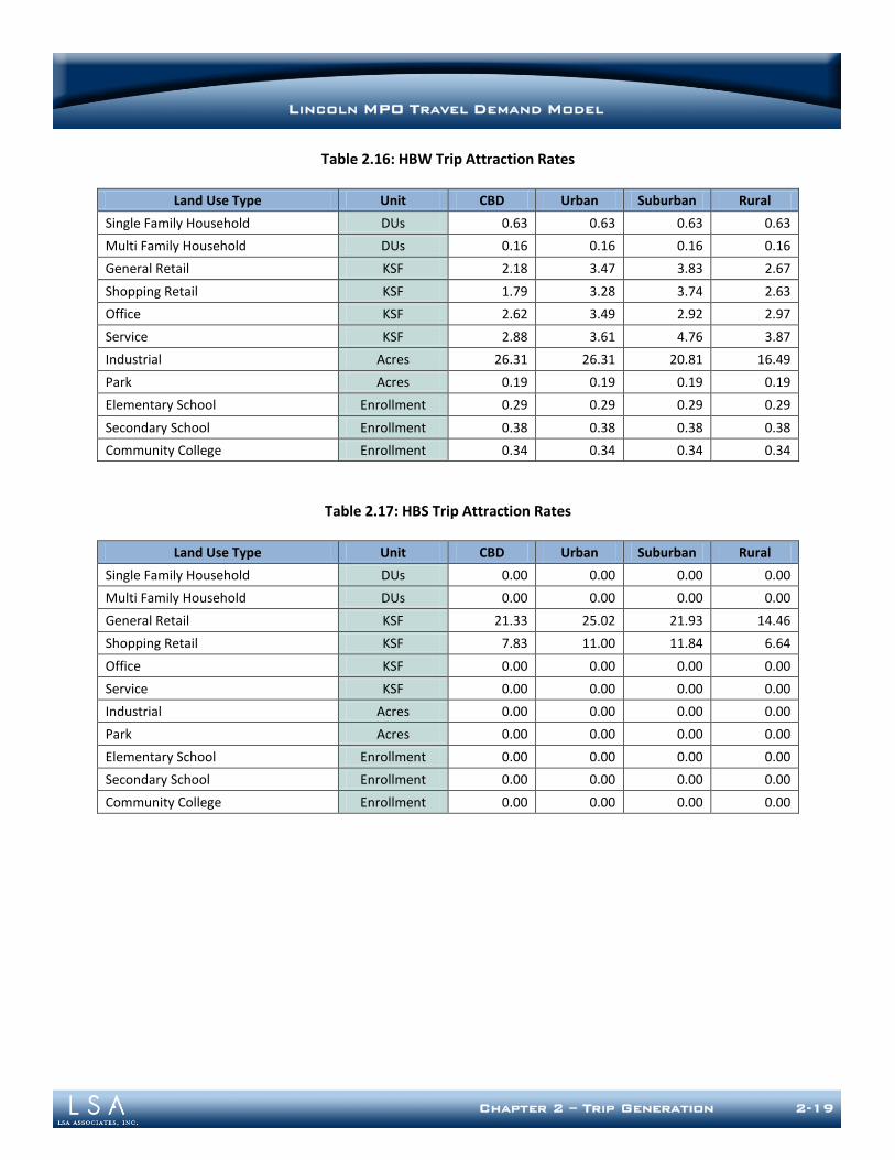
Chapter 2 – Trip Generation 2-19
LINCOLN MPO TRAVEL DEMAND MODEL
Table 2.16: HBW Trip Attraction Rates
Land Use Type Unit CBD Urban Suburban Rural
Single Family Household DUs 0.63 0.63 0.63 0.63
Multi Family Household DUs 0.16 0.16 0.16 0.16
General Retail KSF 2.18 3.47 3.83 2.67
Shopping Retail KSF 1.79 3.28 3.74 2.63
Office KSF 2.62 3.49 2.92 2.97
Service KSF 2.88 3.61 4.76 3.87
Industrial Acres 26.31 26.31 20.81 16.49
Park Acres 0.19 0.19 0.19 0.19
Elementary School Enrollment 0.29 0.29 0.29 0.29
Secondary School Enrollment 0.38 0.38 0.38 0.38
Community College Enrollment 0.34 0.34 0.34 0.34
Table 2.17: HBS Trip Attraction Rates
Land Use Type Unit CBD Urban Suburban Rural
Single Family Household DUs 0.00 0.00 0.00 0.00
Multi Family Household DUs 0.00 0.00 0.00 0.00
General Retail KSF 21.33 25.02 21.93 14.46
Shopping Retail KSF 7.83 11.00 11.84 6.64
Office KSF 0.00 0.00 0.00 0.00
Service KSF 0.00 0.00 0.00 0.00
Industrial Acres 0.00 0.00 0.00 0.00
Park Acres 0.00 0.00 0.00 0.00
Elementary School Enrollment 0.00 0.00 0.00 0.00
Secondary School Enrollment 0.00 0.00 0.00 0.00
Community College Enrollment 0.00 0.00 0.00 0.00
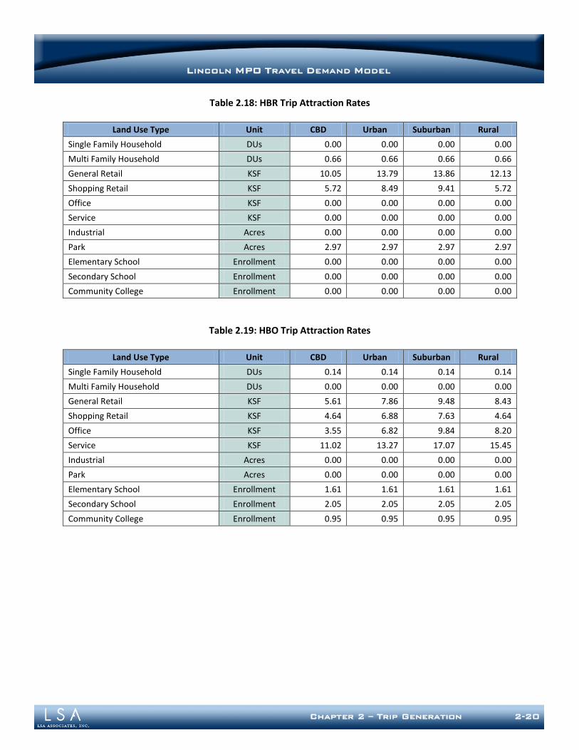
Chapter 2 – Trip Generation 2-20
LINCOLN MPO TRAVEL DEMAND MODEL
Table 2.18: HBR Trip Attraction Rates
Land Use Type Unit CBD Urban Suburban Rural
Single Family Household DUs 0.00 0.00 0.00 0.00
Multi Family Household DUs 0.66 0.66 0.66 0.66
General Retail KSF 10.05 13.79 13.86 12.13
Shopping Retail KSF 5.72 8.49 9.41 5.72
Office KSF 0.00 0.00 0.00 0.00
Service KSF 0.00 0.00 0.00 0.00
Industrial Acres 0.00 0.00 0.00 0.00
Park Acres 2.97 2.97 2.97 2.97
Elementary School Enrollment 0.00 0.00 0.00 0.00
Secondary School Enrollment 0.00 0.00 0.00 0.00
Community College Enrollment 0.00 0.00 0.00 0.00
Table 2.19: HBO Trip Attraction Rates
Land Use Type Unit CBD Urban Suburban Rural
Single Family Household DUs 0.14 0.14 0.14 0.14
Multi Family Household DUs 0.00 0.00 0.00 0.00
General Retail KSF 5.61 7.86 9.48 8.43
Shopping Retail KSF 4.64 6.88 7.63 4.64
Office KSF 3.55 6.82 9.84 8.20
Service KSF 11.02 13.27 17.07 15.45
Industrial Acres 0.00 0.00 0.00 0.00
Park Acres 0.00 0.00 0.00 0.00
Elementary School Enrollment 1.61 1.61 1.61 1.61
Secondary School Enrollment 2.05 2.05 2.05 2.05
Community College Enrollment 0.95 0.95 0.95 0.95
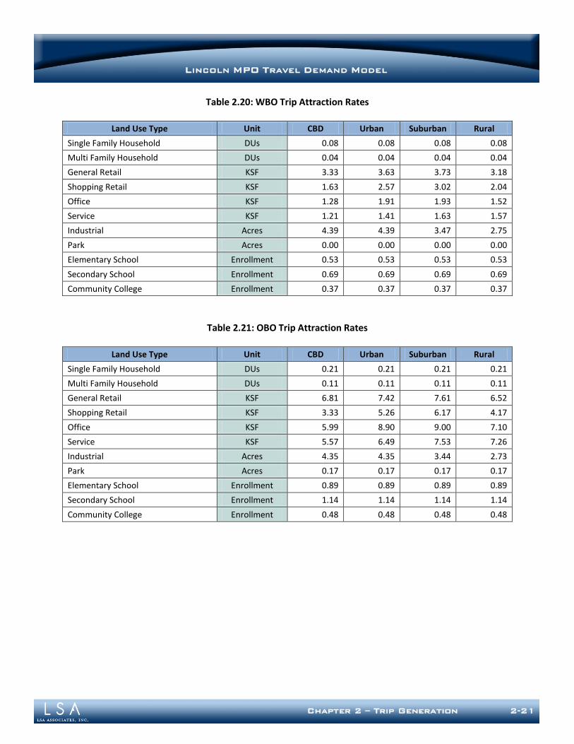
Chapter 2 – Trip Generation 2-21
LINCOLN MPO TRAVEL DEMAND MODEL
Table 2.20: WBO Trip Attraction Rates
Land Use Type Unit CBD Urban Suburban Rural
Single Family Household DUs 0.08 0.08 0.08 0.08
Multi Family Household DUs 0.04 0.04 0.04 0.04
General Retail KSF 3.33 3.63 3.73 3.18
Shopping Retail KSF 1.63 2.57 3.02 2.04
Office KSF 1.28 1.91 1.93 1.52
Service KSF 1.21 1.41 1.63 1.57
Industrial Acres 4.39 4.39 3.47 2.75
Park Acres 0.00 0.00 0.00 0.00
Elementary School Enrollment 0.53 0.53 0.53 0.53
Secondary School Enrollment 0.69 0.69 0.69 0.69
Community College Enrollment 0.37 0.37 0.37 0.37
Table 2.21: OBO Trip Attraction Rates
Land Use Type Unit CBD Urban Suburban Rural
Single Family Household DUs 0.21 0.21 0.21 0.21
Multi Family Household DUs 0.11 0.11 0.11 0.11
General Retail KSF 6.81 7.42 7.61 6.52
Shopping Retail KSF 3.33 5.26 6.17 4.17
Office KSF 5.99 8.90 9.00 7.10
Service KSF 5.57 6.49 7.53 7.26
Industrial Acres 4.35 4.35 3.44 2.73
Park Acres 0.17 0.17 0.17 0.17
Elementary School Enrollment 0.89 0.89 0.89 0.89
Secondary School Enrollment 1.14 1.14 1.14 1.14
Community College Enrollment 0.48 0.48 0.48 0.48
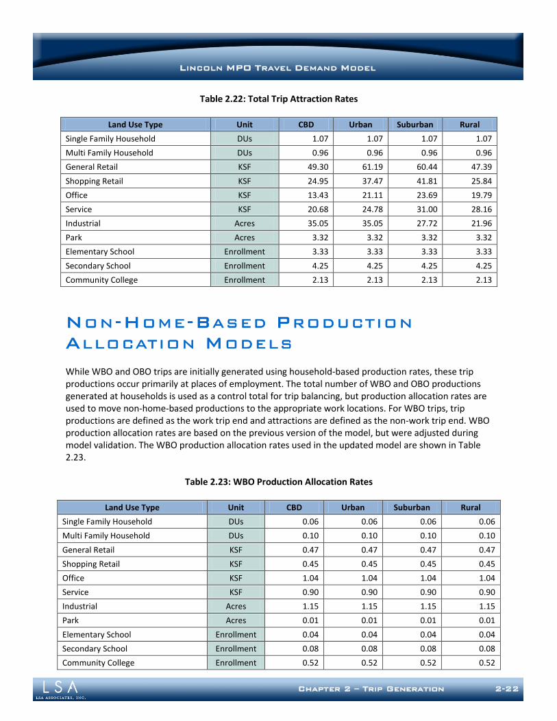
Chapter 2 – Trip Generation 2-22
LINCOLN MPO TRAVEL DEMAND MODEL
Table 2.22: Total Trip Attraction Rates
Land Use Type Unit CBD Urban Suburban Rural
Single Family Household DUs 1.07 1.07 1.07 1.07
Multi Family Household DUs 0.96 0.96 0.96 0.96
General Retail KSF 49.30 61.19 60.44 47.39
Shopping Retail KSF 24.95 37.47 41.81 25.84
Office KSF 13.43 21.11 23.69 19.79
Service KSF 20.68 24.78 31.00 28.16
Industrial Acres 35.05 35.05 27.72 21.96
Park Acres 3.32 3.32 3.32 3.32
Elementary School Enrollment 3.33 3.33 3.33 3.33
Secondary School Enrollment 4.25 4.25 4.25 4.25
Community College Enrollment 2.13 2.13 2.13 2.13
NON-HOME-BASED PRODUCTION
ALLOCATION MODELS
While WBO and OBO trips are initially generated using household-based production rates, these trip productions occur primarily at places of employment. The total number of WBO and OBO productions generated at households is used as a control total for trip balancing, but production allocation rates are used to move non-home-based productions to the appropriate work locations. For WBO trips, trip productions are defined as the work trip end and attractions are defined as the non-work trip end. WBO production allocation rates are based on the previous version of the model, but were adjusted during model validation. The WBO production allocation rates used in the updated model are shown in Table 2.23.
Table 2.23: WBO Production Allocation Rates
Land Use Type Unit CBD Urban Suburban Rural
Single Family Household DUs 0.06 0.06 0.06 0.06
Multi Family Household DUs 0.10 0.10 0.10 0.10
General Retail KSF 0.47 0.47 0.47 0.47
Shopping Retail KSF 0.45 0.45 0.45 0.45
Office KSF 1.04 1.04 1.04 1.04
Service KSF 0.90 0.90 0.90 0.90
Industrial Acres 1.15 1.15 1.15 1.15
Park Acres 0.01 0.01 0.01 0.01
Elementary School Enrollment 0.04 0.04 0.04 0.04
Secondary School Enrollment 0.08 0.08 0.08 0.08
Community College Enrollment 0.52 0.52 0.52 0.52

Chapter 2 – Trip Generation 2-23
LINCOLN MPO TRAVEL DEMAND MODEL
A simpler approach was taken for OBO trips. For OBO trips, OBO production allocation rates are identical to OBO attraction rates because there is no distinct difference between OBO productions and attractions. OBO productions and attractions are all non-home, non-work locations.
UNIVERSITY SPECIAL GENERATOR AND
PRODUCTION ALLOCATION
Lancaster County is home to the University of Nebraska, Lincoln (UNL), a traditional 4-year university that generates a significant amount of trip activity. Students attending the university tend to be concentrated at households near the university or live on campus, suggesting that a special university trip purpose and allocation model can improve representation of the university in the travel model.
University Definition
UNL is separated into two main campuses: the City Campus and the East campus. All TAZs within these two campuses are considered to be part of the UNL special generator shown in Figure 2.5. Off-campus research and administration facilities associated with UNL are not included in the special generator analysis, but are represented by the normal trip generation process, described above.
Figure 2.5: University of Nebraska, Lincoln Campus Locations

Chapter 2 – Trip Generation 2-24
LINCOLN MPO TRAVEL DEMAND MODEL
Trip Types at Universities
Because universities do not fall into the normal trip patterns used by the model, special considerations are given to university trip types. In particular, the Home-Based University (HBU) trip purpose is defined as a trip by a university student or visitor between home and any location on the university campus. University trip ends are associated with University faculty and staff, students living on campus, and students and visitors living off campus and described as follows:
HBW, HBS, HBR, and HBO Productions - These production trip ends can occur only for students living on campus.
HBW Attractions and WBO Productions - These trip ends can occur only for University faculty and staff.
WBO Attractions and all OBO Trips - These trip ends can only occur for students and visitors living off campus.
HBS, HBR, and HBO Attractions - These trip ends cannot occur at the University. All home-based trips to the University by students and visitors are considered HBU trips and all home-based trips to the University by faculty and staff is considered HBW trips.
HBU Productions - Trips within each university campus are not modeled, so only limited HBU productions occur on campus. Only HBU trips between campuses are included in the on-campus HBU trip productions.
HBU Attractions - HBU attractions can occur only for students and visitors living off campus or for students who live on campus traveling between the two campuses.
Special Generator Survey Adaptation
Detailed survey data was not available for UNL, but use of university special generator surveys from other jurisdictions were useful in specifying a special generator model for UNL. The updated model includes a special generator model based on special generator studies conducted for Colorado State University (CSU)7 and the University of Northern Colorado (UNC)8. The special generator model was originally developed for the Colorado North Front Range Regional Travel Model (NFR RTM). Employment Data
Total employment at UNL was available from the UNL website and is summarized in Table 2.24. Both the UNC and CSU special generator values were developed based on full time equivalent (FTE) University employment, not including employment at third-party vendors. Therefore, special generator adaptation is based on FTE employment data from the UNL website. FTE employment for UNL was estimated by multiplying part time employment by 50% and adding 100% of full time employment.
7 1999 Colorado State University Special Generator Study, City of Fort Collins, 2000.
8 2004 University of Northern Colorado Special Generator Study, North Front Range MPO, 2004.
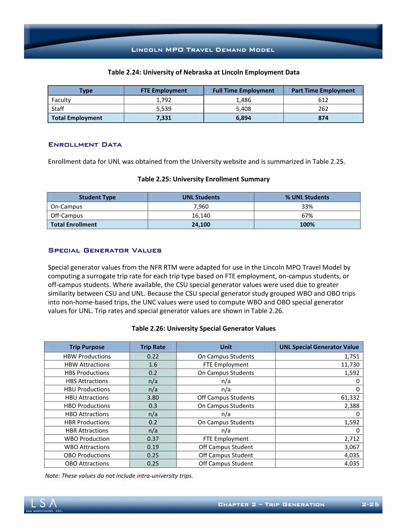
Chapter 2 – Trip Generation 2-25
LINCOLN MPO TRAVEL DEMAND MODEL
Table 2.24: University of Nebraska at Lincoln Employment Data
Type FTE Employment Full Time Employment Part Time Employment
Faculty 1,792 1,486 612
Staff 5,539 5,408 262
Total Employment 7,331 6,894 874
Enrollment Data
Enrollment data for UNL was obtained from the University website and is summarized in Table 2.25.
Table 2.25: University Enrollment Summary
Student Type UNL Students % UNL Students
On-Campus 7,960 33%
Off-Campus 16,140 67%
Total Enrollment 24,100 100%
Special Generator Values
Special generator values from the NFR RTM were adapted for use in the Lincoln MPO Travel Model by computing a surrogate trip rate for each trip type based on FTE employment, on-campus students, or off-campus students. Where available, the CSU special generator values were used due to greater similarity between CSU and UNL. Because the CSU special generator study grouped WBO and OBO trips into non-home-based trips, the UNC values were used to compute WBO and OBO special generator values for UNL. Trip rates and special generator values are shown in Table 2.26.
Table 2.26: University Special Generator Values
Trip Purpose Trip Rate Unit UNL Special Generator Value
HBW Productions 0.22 On Campus Students 1,751 HBW Attractions 1.6 FTE Employment 11,730 HBS Productions 0.2 On Campus Students 1,592 HBS Attractions n/a n/a 0
HBU Productions n/a n/a 0 HBU Attractions 3.80 Off Campus Students 61,332 HBO Productions 0.3 On Campus Students 2,388 HBO Attractions n/a n/a 0 HBR Productions 0.2 On Campus Students 1,592 HBR Attractions n/a n/a 0 WBO Production 0.37 FTE Employment 2,712 WBO Attractions 0.19 Off Campus Student 3,067 OBO Productions 0.25 Off Campus Student 4,035 OBO Attractions 0.25 Off Campus Student 4,035
Note: These values do not include intra-university trips.
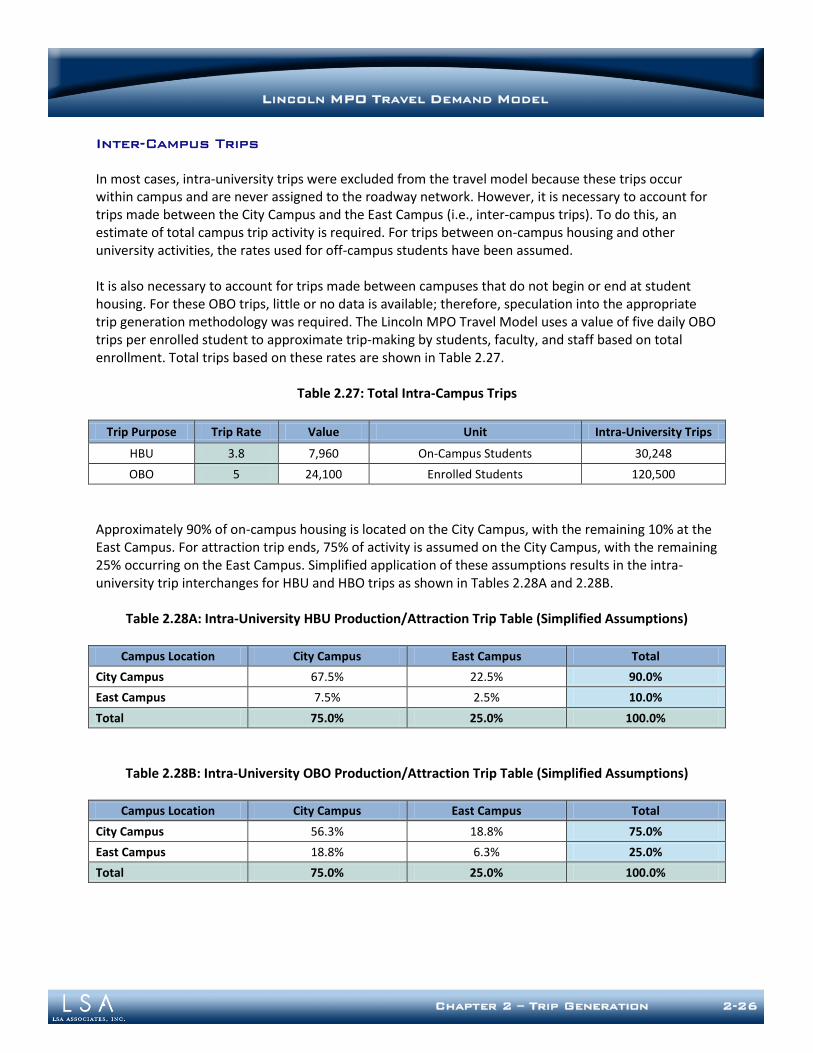
Chapter 2 – Trip Generation 2-26
LINCOLN MPO TRAVEL DEMAND MODEL
Inter-Campus Trips
In most cases, intra-university trips were excluded from the travel model because these trips occur within campus and are never assigned to the roadway network. However, it is necessary to account for trips made between the City Campus and the East Campus (i.e., inter-campus trips). To do this, an estimate of total campus trip activity is required. For trips between on-campus housing and other university activities, the rates used for off-campus students have been assumed. It is also necessary to account for trips made between campuses that do not begin or end at student housing. For these OBO trips, little or no data is available; therefore, speculation into the appropriate trip generation methodology was required. The Lincoln MPO Travel Model uses a value of five daily OBO trips per enrolled student to approximate trip-making by students, faculty, and staff based on total enrollment. Total trips based on these rates are shown in Table 2.27.
Table 2.27: Total Intra-Campus Trips
Trip Purpose Trip Rate Value Unit Intra-University Trips
HBU 3.8 7,960 On-Campus Students 30,248
OBO 5 24,100 Enrolled Students 120,500
Approximately 90% of on-campus housing is located on the City Campus, with the remaining 10% at the East Campus. For attraction trip ends, 75% of activity is assumed on the City Campus, with the remaining 25% occurring on the East Campus. Simplified application of these assumptions results in the intra-university trip interchanges for HBU and HBO trips as shown in Tables 2.28A and 2.28B.
Table 2.28A: Intra-University HBU Production/Attraction Trip Table (Simplified Assumptions)
Campus Location City Campus East Campus Total
City Campus 67.5% 22.5% 90.0%
East Campus 7.5% 2.5% 10.0%
Total 75.0% 25.0% 100.0%
Table 2.28B: Intra-University OBO Production/Attraction Trip Table (Simplified Assumptions)
Campus Location City Campus East Campus Total
City Campus 56.3% 18.8% 75.0%
East Campus 18.8% 6.3% 25.0%
Total 75.0% 25.0% 100.0%
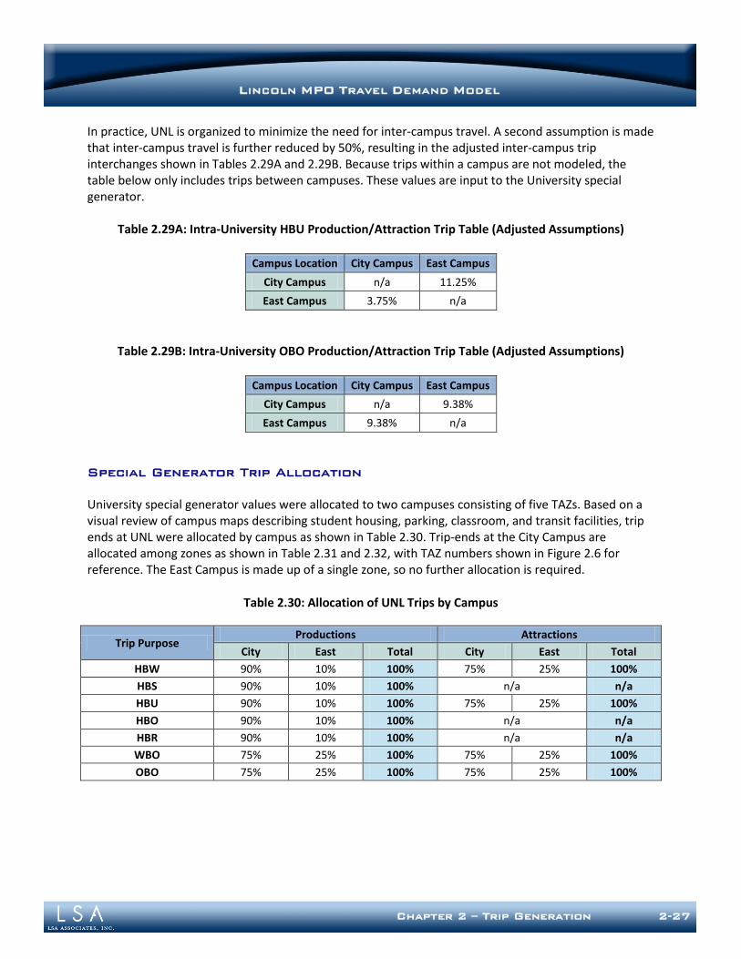
Chapter 2 – Trip Generation 2-27
LINCOLN MPO TRAVEL DEMAND MODEL
In practice, UNL is organized to minimize the need for inter-campus travel. A second assumption is made that inter-campus travel is further reduced by 50%, resulting in the adjusted inter-campus trip interchanges shown in Tables 2.29A and 2.29B. Because trips within a campus are not modeled, the table below only includes trips between campuses. These values are input to the University special generator.
Table 2.29A: Intra-University HBU Production/Attraction Trip Table (Adjusted Assumptions)
Campus Location City Campus East Campus
City Campus n/a 11.25%
East Campus 3.75% n/a
Table 2.29B: Intra-University OBO Production/Attraction Trip Table (Adjusted Assumptions)
Campus Location City Campus East Campus
City Campus n/a 9.38%
East Campus 9.38% n/a
Special Generator Trip Allocation
University special generator values were allocated to two campuses consisting of five TAZs. Based on a visual review of campus maps describing student housing, parking, classroom, and transit facilities, trip ends at UNL were allocated by campus as shown in Table 2.30. Trip-ends at the City Campus are allocated among zones as shown in Table 2.31 and 2.32, with TAZ numbers shown in Figure 2.6 for reference. The East Campus is made up of a single zone, so no further allocation is required.
Table 2.30: Allocation of UNL Trips by Campus
Trip Purpose Productions Attractions
City East Total City East Total
HBW 90% 10% 100% 75% 25% 100%
HBS 90% 10% 100% n/a n/a
HBU 90% 10% 100% 75% 25% 100%
HBO 90% 10% 100% n/a n/a
HBR 90% 10% 100% n/a n/a
WBO 75% 25% 100% 75% 25% 100%
OBO 75% 25% 100% 75% 25% 100%
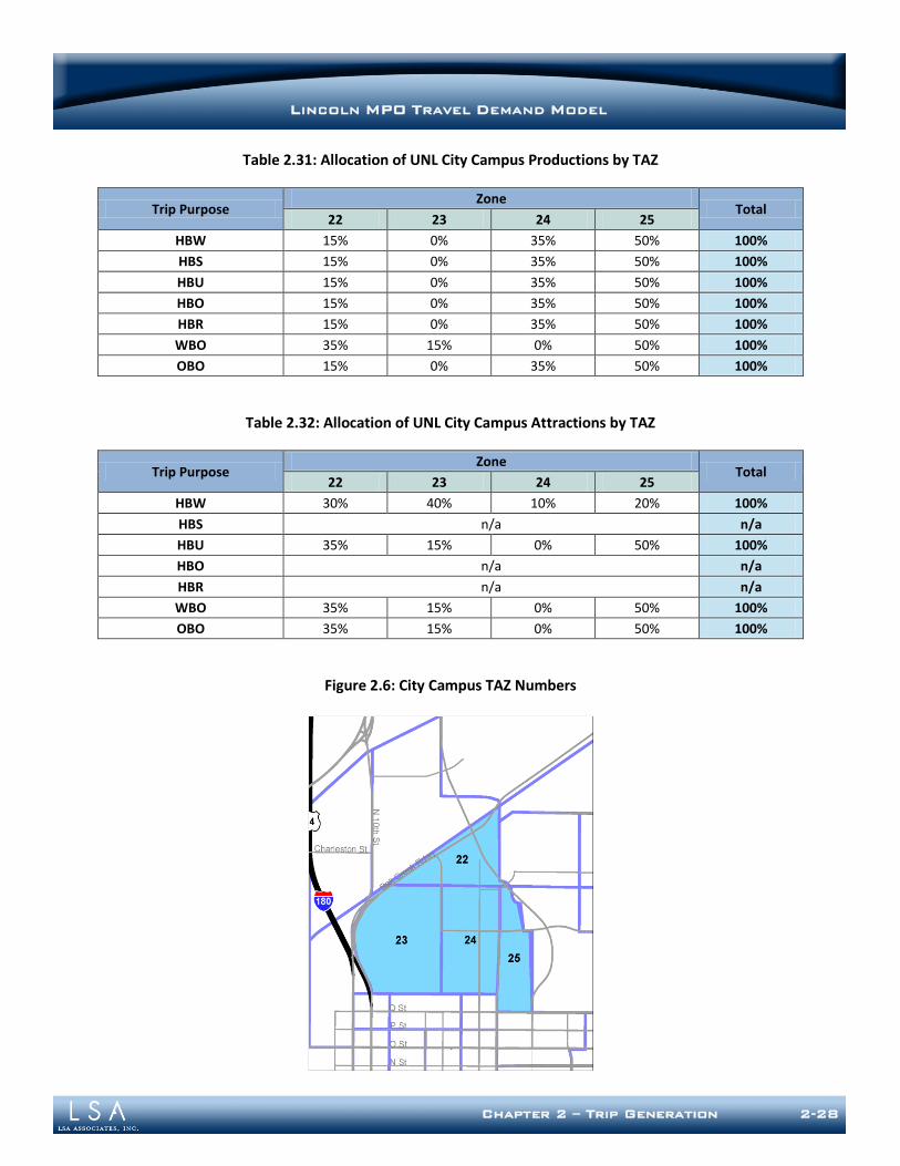
Chapter 2 – Trip Generation 2-28
LINCOLN MPO TRAVEL DEMAND MODEL
Table 2.31: Allocation of UNL City Campus Productions by TAZ
Trip Purpose Zone
Total 22 23 24 25
HBW 15% 0% 35% 50% 100%
HBS 15% 0% 35% 50% 100%
HBU 15% 0% 35% 50% 100%
HBO 15% 0% 35% 50% 100%
HBR 15% 0% 35% 50% 100%
WBO 35% 15% 0% 50% 100%
OBO 15% 0% 35% 50% 100%
Table 2.32: Allocation of UNL City Campus Attractions by TAZ
Trip Purpose Zone
Total 22 23 24 25
HBW 30% 40% 10% 20% 100%
HBS n/a n/a
HBU 35% 15% 0% 50% 100%
HBO n/a n/a
HBR n/a n/a
WBO 35% 15% 0% 50% 100%
OBO 35% 15% 0% 50% 100%
Figure 2.6: City Campus TAZ Numbers

Chapter 2 – Trip Generation 2-29
LINCOLN MPO TRAVEL DEMAND MODEL
University Production Allocation
The production end of each off-campus HBU trip will occur at a household, most likely near the university. The university provided student address data aggregated to a square-mile grid to assist in development of a HBU production allocation model. These addresses were then aggregated to the model TAZs using a simple area-based overlay. The calibration parameters in Equation (6) were adjusted iteratively until the resulting production allocation model matched the allocation of geocoded student address data. The geocoded trips allocated to TAZ are shown in Figure 2.7 as a dot density map.
[Allocation Factor] = HH * a*(Db )*(edistance *c ) (6)
Where: HH = Total households in zone D = Right angle distance to university (mi) a = Calibration Parameter (70) b = Calibration Parameter (-0.951) c = Calibration Parameter (-0.09)
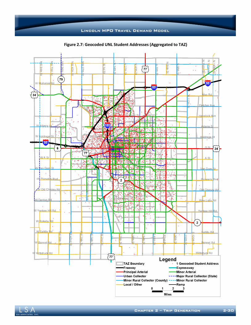
Chapter 2 – Trip Generation 2-30
LINCOLN MPO TRAVEL DEMAND MODEL
Figure 2.7: Geocoded UNL Student Addresses (Aggregated to TAZ)
Chapter 2 – Trip Generation 2-31
LINCOLN MPO TRAVEL DEMAND MODEL
EXTERNAL TRIPS
In addition to the internal-internal trips that occur entirely within the modeling area, the model must also include external travel from outside of the region. Trips with one end inside the modeling area and the other outside of the area are called Internal-External (IE) and External-Internal (EI) trips. Through trips, or External-External (EE) trips, are those that pass through the county modeling area without stopping (or with only short convenience stops). External travel is modeled explicitly at the external stations where roadways cross the model boundary. The 34 external stations are shown in Figure 2.8.
External Station Volumes
The first step in estimating external travel is to determine the average weekday traffic at each external station in the base year. The weekday traffic values were obtained from the Nebraska Department of Roads (NDOR) and Lancaster County and are shown in Table 2.33 along with other information. Because NDOR provides average annual daily traffic, NDOR traffic data was adjusted to represent an average weekday in March, April, September, October, and November in order to represent an “average weekday when school is in session.” In addition, seasonal and annual growth adjustments were applied to counts provided by Lancaster County. Next, it was necessary to determine the split between the EE and IE/EI trips at each external station using guidance provided in NCHRP Report 3659 along with a manual review of external station locations, volumes, and connections to other regions. The resulting split between EE and IE/EI trips for each external station is shown in Table 2.33. Total volumes at each external station represent a single trip-end, with the matched trip end occurring either within the modeling area (for IE/EI trips) or at another external station (for EE trips). Only a few external stations are assumed to carry a significant number of EE trips. In this model adjustment, external stations have been renumbered as zones 1001 through 1034 to simplify identification of external stations and allow for easier zone splits as necessary for focused subarea modeling. In addition, external station 1015 (SH 2 East) was relocated east of the newly constructed interchange with SH 43 South. A new external station, numbered 1016 (SH 43 South) has been added to represent the south leg of this newly constructed interchange.
9 National Cooperative Highway Research Program (NCHRP) Report 365: Travel Estimation Techniques for Urban
Planning, Transportation Research Board, 1998.
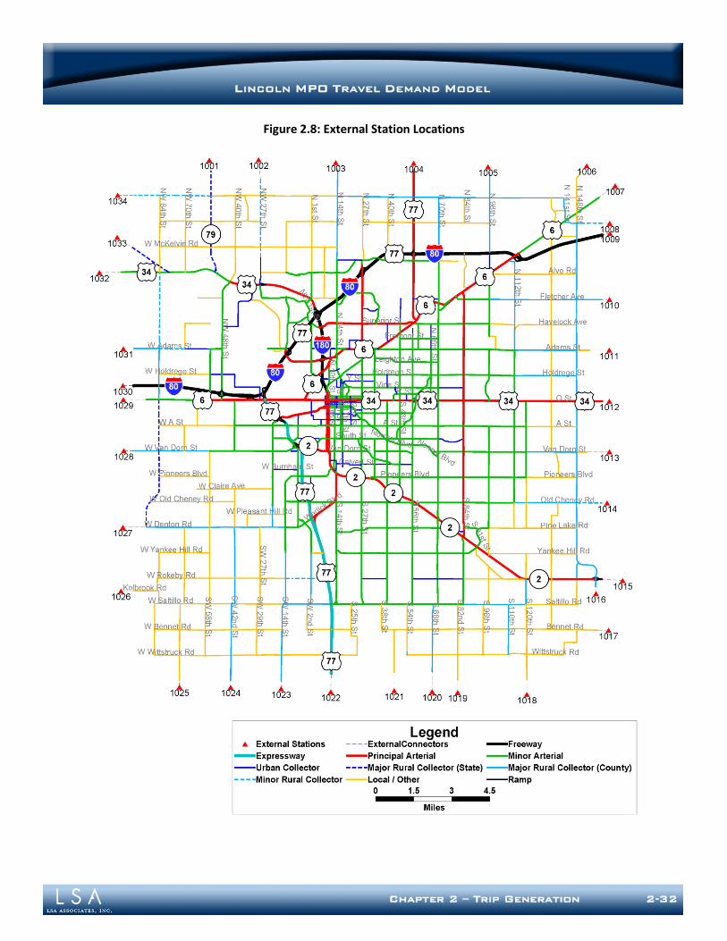
Chapter 2 – Trip Generation 2-32
LINCOLN MPO TRAVEL DEMAND MODEL
Figure 2.8: External Station Locations
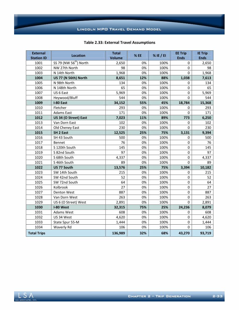
Chapter 2 – Trip Generation 2-33
LINCOLN MPO TRAVEL DEMAND MODEL
Table 2.33: External Travel Assumptions
External
Station ID Location
Total Volume
% EE % IE / EI EE Trip Ends
IE Trip Ends
1001 SS 79 (NW 56th
) North 2,650 0% 100% 0 2,650
1002 NW 27th North 98 0% 100% 0 98
1003 N 14th North 1,968 0% 100% 0 1,968
1004 US 77 (N 56th) North 8,651 12% 88% 1,038 7,613
1005 N 98th North 134 0% 100% 0 134
1006 N 148th North 65 0% 100% 0 65
1007 US 6 East 5,969 0% 100% 0 5,969
1008 Heywood/Bluff 544 0% 100% 0 544
1009 I-80 East 34,152 55% 45% 18,784 15,368
1010 Fletcher 293 0% 100% 0 293
1011 Adams East 171 0% 100% 0 171
1012 US 34 (O Street) East 7,023 11% 89% 773 6,250
1013 Van Dorn East 102 0% 100% 0 102
1014 Old Cheney East 230 0% 100% 0 230
1015 SH 2 East 12,525 25% 75% 3,131 9,394
1016 SH 43 South 500 0% 100% 0 500
1017 Bennet 76 0% 100% 0 76
1018 S 120th South 145 0% 100% 0 145
1019 S 82nd South 97 0% 100% 0 97
1020 S 68th South 4,337 0% 100% 0 4,337
1021 S 46th South 89 0% 100% 0 89
1022 US 77 South 13,576 25% 75% 3,394 10,182
1023 SW 14th South 215 0% 100% 0 215
1024 SW 42nd South 52 0% 100% 0 52
1025 SW 72nd South 64 0% 100% 0 64
1026 Kolbrook 27 0% 100% 0 27
1027 Denton West 887 0% 100% 0 887
1028 Van Dorn West 263 0% 100% 0 263
1029 US 6 (O Street) West 2,891 0% 100% 0 2,891
1030 I-80 West 32,315 75% 25% 24,236 8,079
1031 Adams West 608 0% 100% 0 608
1032 US 34 West 4,620 0% 100% 0 4,620
1033 State Spur 55-M 1,444 0% 100% 0 1,444
1034 Waverly Rd 106 0% 100% 0 106
Total Trips 136,989 32% 68% 43,270 93,719
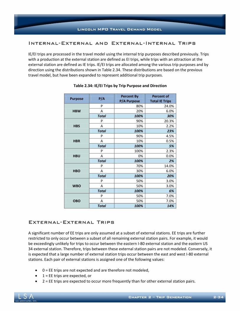
Chapter 2 – Trip Generation 2-34
LINCOLN MPO TRAVEL DEMAND MODEL
Internal-External and External-Internal Trips
IE/EI trips are processed in the travel model using the internal trip purposes described previously. Trips with a production at the external station are defined as EI trips, while trips with an attraction at the external station are defined as IE trips. IE/EI trips are allocated among the various trip purposes and by direction using the distributions shown in Table 2.34. These distributions are based on the previous travel model, but have been expanded to represent additional trip purposes.
Table 2.34: IE/EI Trips by Trip Purpose and Direction
Purpose P/A Percent By
P/A Purpose Percent of
Total IE Trips
HBW
P 80% 24.0%
A 20% 6.0%
Total 100% 30%
HBS
P 90% 20.3%
A 10% 2.2%
Total 100% 23%
HBR
P 90% 4.5%
A 10% 0.5%
Total 100% 5%
HBU
P 100% 2.3%
A 0% 0.0%
Total 100% 2%
HBO
P 70% 14.0%
A 30% 6.0%
Total 100% 20%
WBO
P 50% 3.0%
A 50% 3.0%
Total 100% 6%
OBO
P 50% 7.0%
A 50% 7.0%
Total 100% 14%
External-External Trips
A significant number of EE trips are only assumed at a subset of external stations. EE trips are further restricted to only occur between a subset of all remaining external station pairs. For example, it would be exceedingly unlikely for trips to occur between the eastern I-80 external station and the eastern US 34 external station. Therefore, trips between these external station pairs are not modeled. Conversely, it is expected that a large number of external station trips occur between the east and west I-80 external stations. Each pair of external stations is assigned one of the following values:
0 = EE trips are not expected and are therefore not modeled,
1 = EE trips are expected, or
2 = EE trips are expected to occur more frequently than for other external station pairs.
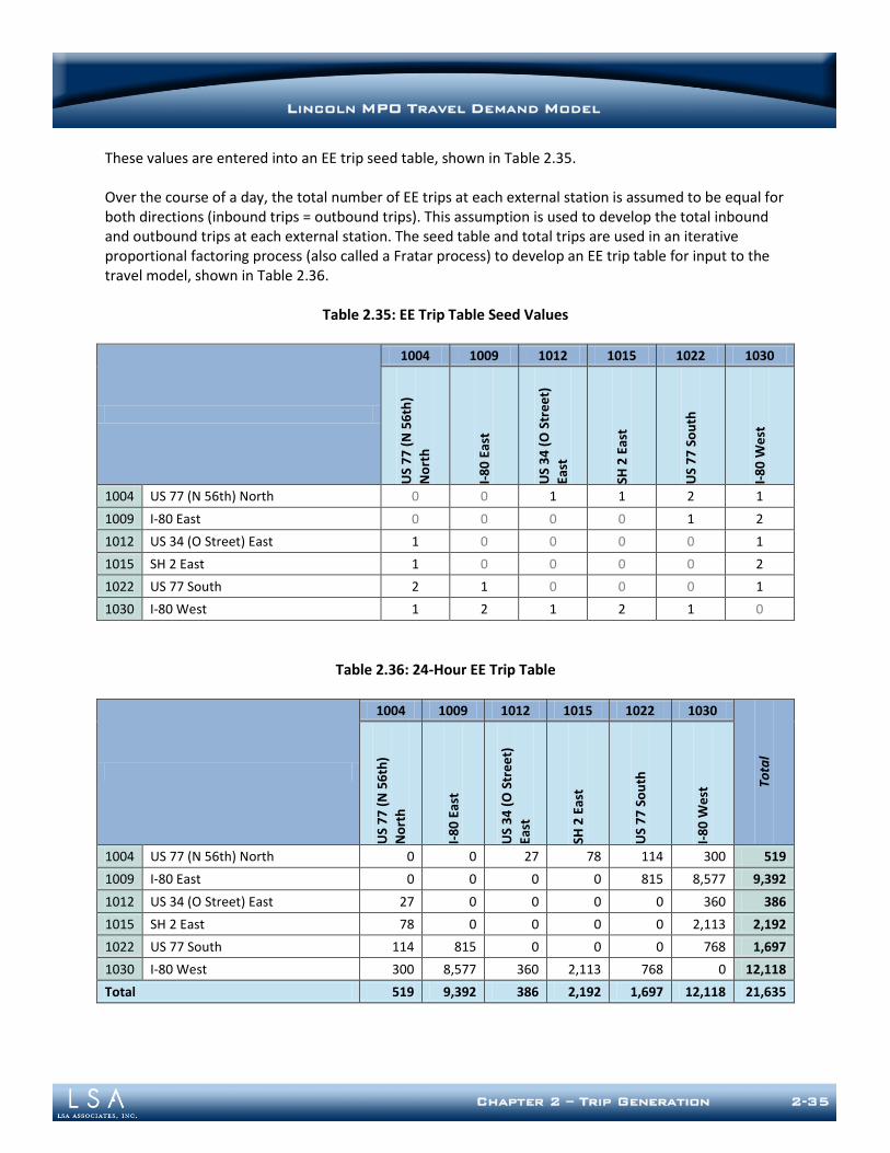
Chapter 2 – Trip Generation 2-35
LINCOLN MPO TRAVEL DEMAND MODEL
These values are entered into an EE trip seed table, shown in Table 2.35. Over the course of a day, the total number of EE trips at each external station is assumed to be equal for both directions (inbound trips = outbound trips). This assumption is used to develop the total inbound and outbound trips at each external station. The seed table and total trips are used in an iterative proportional factoring process (also called a Fratar process) to develop an EE trip table for input to the travel model, shown in Table 2.36.
Table 2.35: EE Trip Table Seed Values
1004 1009 1012 1015 1022 1030
US
77
(N
56
th)
No
rth
I-8
0 E
ast
US
34
(O
Str
ee
t)
East
SH 2
Eas
t
US
77
So
uth
I-8
0 W
est
1004 US 77 (N 56th) North 0 0 1 1 2 1
1009 I-80 East 0 0 0 0 1 2
1012 US 34 (O Street) East 1 0 0 0 0 1
1015 SH 2 East 1 0 0 0 0 2
1022 US 77 South 2 1 0 0 0 1
1030 I-80 West 1 2 1 2 1 0
Table 2.36: 24-Hour EE Trip Table
1004 1009 1012 1015 1022 1030
Tota
l
US
77
(N
56
th)
No
rth
I-8
0 E
ast
US
34
(O
Str
ee
t)
East
SH 2
Eas
t
US
77
So
uth
I-8
0 W
est
1004 US 77 (N 56th) North 0 0 27 78 114 300 519
1009 I-80 East 0 0 0 0 815 8,577 9,392
1012 US 34 (O Street) East 27 0 0 0 0 360 386
1015 SH 2 East 78 0 0 0 0 2,113 2,192
1022 US 77 South 114 815 0 0 0 768 1,697
1030 I-80 West 300 8,577 360 2,113 768 0 12,118
Total 519 9,392 386 2,192 1,697 12,118 21,635
Chapter 2 – Trip Generation 2-36
LINCOLN MPO TRAVEL DEMAND MODEL
TRIP BALANCING
Trip productions and attractions are estimated separately by purpose using the trip rates and allocation models previously described. While an attempt is made to make the initial estimate of productions equal to the initial estimate of attractions, it is not feasible to make them exactly equal in all scenarios. However, to ensure conservation of trips in the model, the number of productions and attractions must be equal. The balancing process conserves the total number of trips in the model by making the productions and attractions equal. Balancing depends on the level of confidence associated with the initial estimate of productions and attractions. Since (borrowed) household survey data was used to estimate trip production rates, the home-based trip purposes are balanced to trip productions. One exception to this is the HBU trip purpose. The special generator studies and cordon counts upon which the UNL estimates are based provided increased reliability for HBU trip attractions to the university campus, so HBU productions are balanced to attractions rather than productions. Non-Home-Based trips (WBO and OBO) are also balanced to productions. These trips are balanced to the initial estimate of productions from the basic trip rates in the cross-classified trip production model. Then, the productions are re-allocated using the allocation models previously discussed.
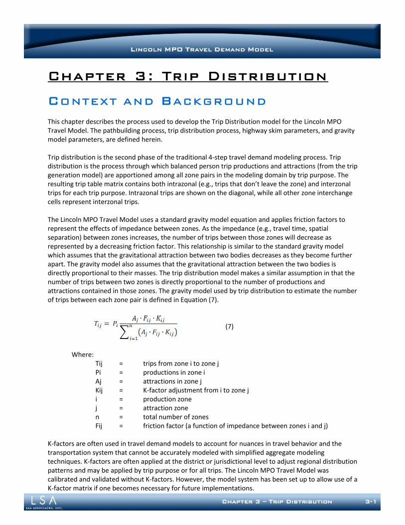
LINCOLN MPO TRAVEL DEMAND MODEL
Chapter 3 – Trip Distribution 3-1
Chapter 3: Trip Distribution
CONTEXT AND BACKGROUND
This chapter describes the process used to develop the Trip Distribution model for the Lincoln MPO Travel Model. The pathbuilding process, trip distribution process, highway skim parameters, and gravity model parameters, are defined herein. Trip distribution is the second phase of the traditional 4-step travel demand modeling process. Trip distribution is the process through which balanced person trip productions and attractions (from the trip generation model) are apportioned among all zone pairs in the modeling domain by trip purpose. The resulting trip table matrix contains both intrazonal (e.g., trips that don’t leave the zone) and interzonal trips for each trip purpose. Intrazonal trips are shown on the diagonal, while all other zone interchange cells represent interzonal trips. The Lincoln MPO Travel Model uses a standard gravity model equation and applies friction factors to represent the effects of impedance between zones. As the impedance (e.g., travel time, spatial separation) between zones increases, the number of trips between those zones will decrease as represented by a decreasing friction factor. This relationship is similar to the standard gravity model which assumes that the gravitational attraction between two bodies decreases as they become further apart. The gravity model also assumes that the gravitational attraction between the two bodies is directly proportional to their masses. The trip distribution model makes a similar assumption in that the number of trips between two zones is directly proportional to the number of productions and attractions contained in those zones. The gravity model used by trip distribution to estimate the number of trips between each zone pair is defined in Equation (7).
(7)
Where: Tij = trips from zone i to zone j Pi = productions in zone i Aj = attractions in zone j Kij = K-factor adjustment from i to zone j i = production zone j = attraction zone n = total number of zones Fij = friction factor (a function of impedance between zones i and j)
K-factors are often used in travel demand models to account for nuances in travel behavior and the transportation system that cannot be accurately modeled with simplified aggregate modeling techniques. K-factors are often applied at the district or jurisdictional level to adjust regional distribution patterns and may be applied by trip purpose or for all trips. The Lincoln MPO Travel Model was calibrated and validated without K-factors. However, the model system has been set up to allow use of a K-factor matrix if one becomes necessary for future implementations.
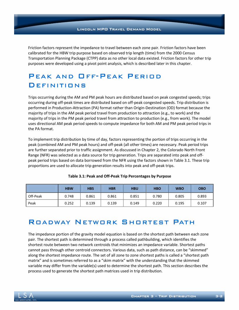
LINCOLN MPO TRAVEL DEMAND MODEL
Chapter 3 – Trip Distribution 3-2
Friction factors represent the impedance to travel between each zone pair. Friction factors have been calibrated for the HBW trip purpose based on observed trip length (time) from the 2000 Census Transportation Planning Package (CTPP) data as no other local data existed. Friction factors for other trip purposes were developed using a pivot point analysis, which is described later in this chapter.
PEAK AND OFF-PEAK PERIOD
DEFINITIONS
Trips occurring during the AM and PM peak hours are distributed based on peak congested speeds; trips occurring during off-peak times are distributed based on off-peak congested speeds. Trip distribution is performed in Production-Attraction (PA) format rather than Origin-Destination (OD) format because the majority of trips in the AM peak period travel from production to attraction (e.g., to work) and the majority of trips in the PM peak period travel from attraction to production (e.g., from work). The model uses directional AM peak period speeds to compute impedance for both AM and PM peak period trips in the PA format. To implement trip distribution by time of day, factors representing the portion of trips occurring in the peak (combined AM and PM peak hours) and off-peak (all other times) are necessary. Peak period trips are further separated prior to traffic assignment. As discussed in Chapter 2, the Colorado North Front Range (NFR) was selected as a data source for trip generation. Trips are separated into peak and off-peak period trips based on data borrowed from the NFR using the factors shown in Table 3.1. These trip proportions are used to allocate trip generation results into peak and off-peak trips.
Table 3.1: Peak and Off-Peak Trip Percentages by Purpose
HBW HBS HBR HBU HBO WBO OBO
Off-Peak 0.748 0.861 0.861 0.851 0.780 0.805 0.893
Peak 0.252 0.139 0.139 0.149 0.220 0.195 0.107
ROADWAY NETWORK SHORTEST PATH
The impedance portion of the gravity model equation is based on the shortest path between each zone pair. The shortest path is determined through a process called pathbuilding, which identifies the shortest route between two network centroids that minimizes an impedance variable. Shortest paths cannot pass through other centroid connectors. Various data, such as path distance, can be “skimmed” along the shortest impedance route. The set of all zone to zone shortest paths is called a “shortest path matrix” and is sometimes referred to as a “skim matrix” with the understanding that the skimmed variable may differ from the variable(s) used to determine the shortest path. This section describes the process used to generate the shortest path matrices used in trip distribution.
LINCOLN MPO TRAVEL DEMAND MODEL
Chapter 3 – Trip Distribution 3-3
The Lincoln MPO Travel Model finds the shortest paths between each zone pair based on peak or off-peak congested travel time. Peak travel time is defined as the AM peak hour directional travel time, while off-peak travel time is defined as the off-peak period congested travel time. Travel times are calculated using a speed feedback process, which will be described further in Chapter 5, Traffic Assignment.
Terminal Times
In the model, terminal penalties are applied to the shortest paths, in order to simulate several travel-related variables, such as the time to locate a parking space, walking to a final destination, paying for a parking space, etc. Terminal penalties, shown in Table 3-2, are added to both the production and attraction end of each zone pair based on the area type of each zone.
Table 3.2: Terminal Penalties by Area Type
Area Type Terminal Time
1 CBD 1.5
2 Urban 1
3 Suburban 1
4 Rural 0.75
Intrazonal Impedance
Impedance, or travel time, for trips within a zone (intrazonal impedance) is not generated in the zone to zone pathbuilding process because the roadway network is not detailed enough for a sub-TAZ level analysis. Instead, the nearest neighbor rule is used to estimate intrazonal impedance. The nearest neighbor rule is applied by taking an average of the nearest TAZs and multiplying that average by a factor. Rather than using the average travel time to multiple nearby zones, intrazonal travel time for the Lincoln MPO model has been calculated by multiplying the distance to the single nearest neighbor by 75%.
FRICTION FACTORS
Friction factors represent the impedance to travel between each zone pair. The Lincoln MPO Travel Model applies the friction factors in the form of gamma functions for each trip purpose. The gamma function is defined by Equation (8).
(8)
Where:
Fij = friction factor between zones i and j t = travel time
= calibration parameters
t
ij etF
,,
LINCOLN MPO TRAVEL DEMAND MODEL
Chapter 3 – Trip Distribution 3-4
Friction factors for the HBW trip purpose were calibrated to the zone to zone trip data obtained from the 2000 CTPP (worker flow data). A trip table created from the CTPP worker flow data was used in combination with the freeflow shortest path matrix from the model to create a trip length distribution calibration target. The CTPP data includes a reported work commute time, which was also reviewed. However, the reported commute time is often longer than the observed commute time due to reporting bias. The calibration target, model results for HBW trips, and reported travel time are all shown in Figure 3.1. In addition to friction factor adjustments, other model variables and parameters including terminal penalties, intrazonal travel times, volume/delay equations, and K-factors can affect calibration of trip length distribution curves. However, it was not necessary to make further adjustments to these parameters during model validation. Although local data from the CTPP can be used to estimate HBW friction factors, no local data exists to calibrate friction factors for other trip purposes. For these purposes, the relationship between the HBW trip lengths and the trip lengths for other trip purposes from the NFR model were used as a benchmark for estimating trip lengths for the Lincoln MPO model. With the estimated average trip times and the general shape of the trip length distributions for each trip purpose, the remaining friction factors could be calibrated. Because the NFR MPO model does not include the HBR trip purpose, the same friction factor parameters were used for both HBO and HBR trips. Figure 3.2 shows the friction factors for each trip purpose. Table 3.3 contains the calibrated gamma function parameters.
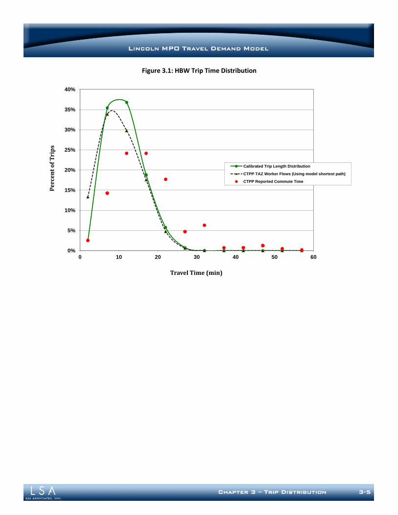
LINCOLN MPO TRAVEL DEMAND MODEL
Chapter 3 – Trip Distribution 3-5
Figure 3.1: HBW Trip Time Distribution
0%
5%
10%
15%
20%
25%
30%
35%
40%
0 10 20 30 40 50 60
Pe
rce
nt
of
Tri
ps
Travel Time (min)
Trip Time Distribution - HBW
Calibrated Trip Length Distribution
CTPP TAZ Worker Flows (Using model shortest path)
CTPP Reported Commute Time
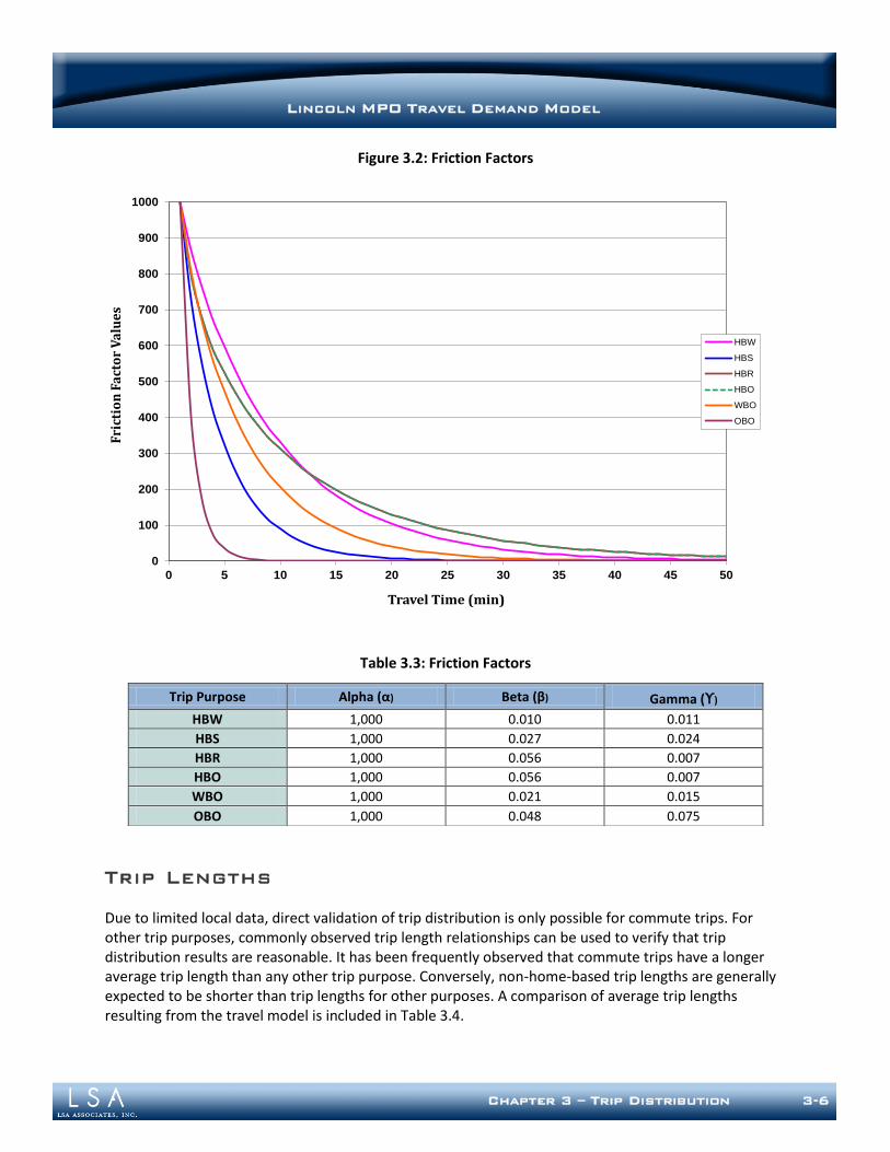
LINCOLN MPO TRAVEL DEMAND MODEL
Chapter 3 – Trip Distribution 3-6
Figure 3.2: Friction Factors
Table 3.3: Friction Factors
Trip Lengths
Due to limited local data, direct validation of trip distribution is only possible for commute trips. For other trip purposes, commonly observed trip length relationships can be used to verify that trip distribution results are reasonable. It has been frequently observed that commute trips have a longer average trip length than any other trip purpose. Conversely, non-home-based trip lengths are generally expected to be shorter than trip lengths for other purposes. A comparison of average trip lengths resulting from the travel model is included in Table 3.4.
0
100
200
300
400
500
600
700
800
900
1000
0 5 10 15 20 25 30 35 40 45 50
Fri
ctio
n F
act
or
Va
lue
s
Travel Time (min)
Friction Factors by Trip Type
HBW
HBS
HBR
HBO
WBO
OBO
Trip Purpose Alpha (α) Beta (β) Gamma (ϒ)
HBW 1,000 0.010 0.011
HBS 1,000 0.027 0.024
HBR 1,000 0.056 0.007
HBO 1,000 0.056 0.007
WBO 1,000 0.021 0.015
OBO 1,000 0.048 0.075
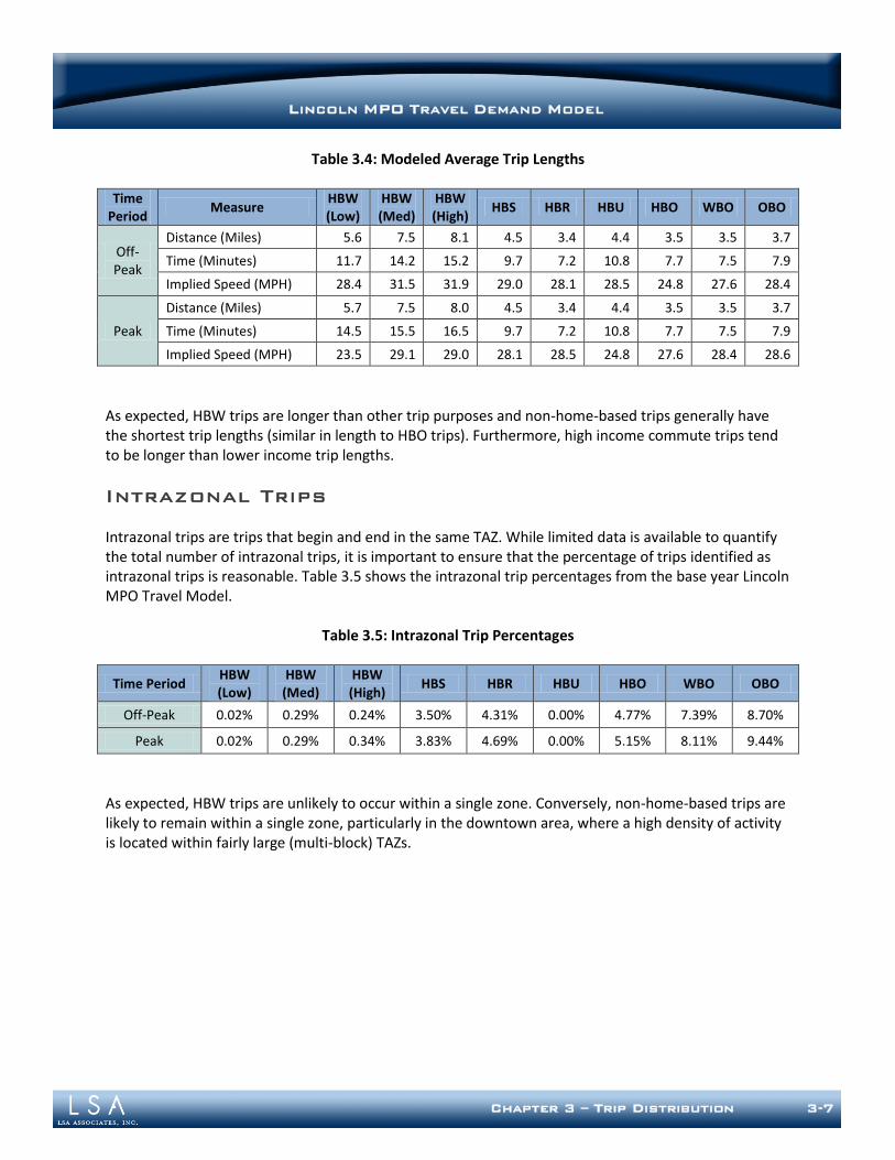
LINCOLN MPO TRAVEL DEMAND MODEL
Chapter 3 – Trip Distribution 3-7
Table 3.4: Modeled Average Trip Lengths
Time Period
Measure HBW (Low)
HBW (Med)
HBW (High)
HBS HBR HBU HBO WBO OBO
Off-Peak
Distance (Miles) 5.6 7.5 8.1 4.5 3.4 4.4 3.5 3.5 3.7
Time (Minutes) 11.7 14.2 15.2 9.7 7.2 10.8 7.7 7.5 7.9
Implied Speed (MPH) 28.4 31.5 31.9 29.0 28.1 28.5 24.8 27.6 28.4
Peak
Distance (Miles) 5.7 7.5 8.0 4.5 3.4 4.4 3.5 3.5 3.7
Time (Minutes) 14.5 15.5 16.5 9.7 7.2 10.8 7.7 7.5 7.9
Implied Speed (MPH) 23.5 29.1 29.0 28.1 28.5 24.8 27.6 28.4 28.6
As expected, HBW trips are longer than other trip purposes and non-home-based trips generally have the shortest trip lengths (similar in length to HBO trips). Furthermore, high income commute trips tend to be longer than lower income trip lengths.
Intrazonal Trips
Intrazonal trips are trips that begin and end in the same TAZ. While limited data is available to quantify the total number of intrazonal trips, it is important to ensure that the percentage of trips identified as intrazonal trips is reasonable. Table 3.5 shows the intrazonal trip percentages from the base year Lincoln MPO Travel Model.
Table 3.5: Intrazonal Trip Percentages
Time Period HBW (Low)
HBW (Med)
HBW (High)
HBS HBR HBU HBO WBO OBO
Off-Peak 0.02% 0.29% 0.24% 3.50% 4.31% 0.00% 4.77% 7.39% 8.70%
Peak 0.02% 0.29% 0.34% 3.83% 4.69% 0.00% 5.15% 8.11% 9.44%
As expected, HBW trips are unlikely to occur within a single zone. Conversely, non-home-based trips are likely to remain within a single zone, particularly in the downtown area, where a high density of activity is located within fairly large (multi-block) TAZs.
LINCOLN MPO TRAVEL DEMAND MODEL
Chapter 4 – Mode Models 4-1
Chapter 4: Mode Models
CONTEXT AND BACKGROUND
This chapter describes the process used to develop the Mode Split and Auto Occupancy components of the Lincoln MPO Travel Model. Mode analysis is the third phase of the traditional 4-step travel demand modeling process, converting person trips from the trip generation and distribution models into vehicle trips for assignment to the roadway network. The mode analysis steps identify non-motorized trips and transit trips based on trip distance and proximity to transit service. After the non-motorized and transit trips are split from the person trip table, the remaining auto-driver and auto-passenger trips are converted to vehicle trips. Transit and non-motorized trip tables are retained for further analysis, but are not further processed by the Lincoln MPO Travel Model. The Lincoln MPO Travel Model does not include a more complicated mode choice step, which would estimate transit usage based on a detailed representation of the region’s transit service. Because trip generation and distribution include all person trips, a mode choice component could be added at a later time, if desired. The algorithms used in this model provide limited information about transit usage in the region, but cannot be used to perform detailed transit forecasts.
NON-MOTORIZED MODE SPLIT
The first step in the mode analysis process is non-motorized mode split. Walk and bicycle trips are identified using a distance-based approach that targets shorter trips. Local data available for this purpose comes from the 2000 CTPP data for Lancaster County. While useful, the CTPP only reports mode use for commute trips, which are defined similar to but not exactly the same as the home-based work trips (HBW) in the Lincoln MPO Travel Model. No local information is available for mode use on the other trip purposes. Mode share targets for HBW trips in the Lincoln area are based on CTPP data for Lancaster County. For the remaining trip purposes, data was borrowed from another region. After reviewing available data sources, including NHTS data, San Luis Obispo, CA was selected as the source model for non-motorized trip shares (non-motorized results from the recent NFR household travel survey were not yet available). Like Lincoln, San Luis Obispo is home to a major university and experiences similar non-motorized trip shares according to a review of the CTPP data. Local household survey data in San Luis Obispo County was used to develop detailed non-motorized mode shares by trip purpose. Non-motorized shares from San Luis Obispo were adjusted based on the relative differences in non-motorized shares for Lincoln and San Luis Obispo. Mode shares from the San Luis Obispo model are shown in Table 4.1. Data adjusted for use in the Lincoln MPO Travel Model, along with model results, are shown in Table 4.2.
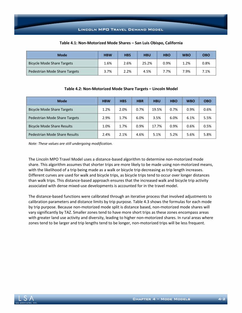
LINCOLN MPO TRAVEL DEMAND MODEL
Chapter 4 – Mode Models 4-2
Table 4.1: Non-Motorized Mode Shares – San Luis Obispo, California
Mode HBW HBS HBU HBO WBO OBO
Bicycle Mode Share Targets 1.6% 2.6% 25.2% 0.9% 1.2% 0.8%
Pedestrian Mode Share Targets 3.7% 2.2% 4.5% 7.7% 7.9% 7.1%
Table 4.2: Non-Motorized Mode Share Targets – Lincoln Model
Mode HBW HBS HBR HBU HBO WBO OBO
Bicycle Mode Share Targets 1.2% 2.0% 0.7% 19.5% 0.7% 0.9% 0.6%
Pedestrian Mode Share Targets 2.9% 1.7% 6.0% 3.5% 6.0% 6.1% 5.5%
Bicycle Mode Share Results 1.0% 1.7% 0.9% 17.7% 0.9% 0.6% 0.5%
Pedestrian Mode Share Results 2.4% 2.1% 4.6% 5.1% 5.2% 5.6% 5.8%
Note: These values are still undergoing modification.
The Lincoln MPO Travel Model uses a distance-based algorithm to determine non-motorized mode share. This algorithm assumes that shorter trips are more likely to be made using non-motorized means, with the likelihood of a trip being made as a walk or bicycle trip decreasing as trip length increases. Different curves are used for walk and bicycle trips, as bicycle trips tend to occur over longer distances than walk trips. This distance-based approach ensures that the increased walk and bicycle trip activity associated with dense mixed-use developments is accounted for in the travel model. The distance-based functions were calibrated through an iterative process that involved adjustments to calibration parameters and distance limits by trip purpose. Table 4.3 shows the formulas for each mode by trip purpose. Because non-motorized mode split is distance based, non-motorized mode shares will vary significantly by TAZ. Smaller zones tend to have more short trips as these zones encompass areas with greater land use activity and diversity, leading to higher non-motorized shares. In rural areas where zones tend to be larger and trip lengths tend to be longer, non-motorized trips will be less frequent.
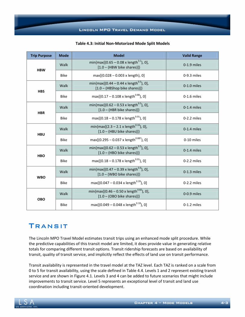
LINCOLN MPO TRAVEL DEMAND MODEL
Chapter 4 – Mode Models 4-3
Table 4.3: Initial Non-Motorized Mode Split Models
Trip Purpose Mode Model Valid Range
HBW
Walk min{max[(0.65 – 0.08 x length
3.1), 0],
[1.0 – (HBW bike shares)]} 0-1.9 miles
Bike max[(0.028 – 0.003 x length), 0] 0-9.3 miles
HBS
Walk min{max[(0.44 – 0.44 x length
0.5), 0],
[1.0 – (HBShop bike shares)]} 0-1.0 miles
Bike max[(0.17 – 0.108 x length0.88
), 0] 0-1.6 miles
HBR
Walk min{max[(0.62 – 0.53 x length
0.5), 0],
[1.0 – (HBR bike shares)]} 0-1.4 miles
Bike max[(0.18 – 0.178 x length0.01
), 0] 0-2.2 miles
HBU
Walk min{max[(2.3 – 2.1 x length
0.16), 0],
[1.0 – (HBU bike shares)]} 0-1.4 miles
Bike max[(0.295 – 0.037 x length0.887
), 0] 0-10 miles
HBO
Walk min{max[(0.62 – 0.53 x length
0.5), 0],
[1.0 – (HBO bike shares)]} 0-1.4 miles
Bike max[(0.18 – 0.178 x length0.01
), 0] 0-2.2 miles
WBO
Walk min{max[(0.47 – 0.39 x length
0.6), 0],
[1.0 – (WBO bike shares)]} 0-1.3 miles
Bike max[(0.047 – 0.034 x length0.39
), 0] 0-2.2 miles
OBO
Walk min{max[(0.46 – 0.50 x length
0.82), 0],
[1.0 – (OBO bike shares)]} 0-0.9 miles
Bike max[(0.049 – 0.048 x length0.18
), 0] 0-1.2 miles
TRANSIT
The Lincoln MPO Travel Model estimates transit trips using an enhanced mode split procedure. While the predictive capabilities of this transit model are limited, it does provide value in generating relative totals for comparing different transit options. Transit ridership forecasts are based on availability of transit, quality of transit service, and implicitly reflect the effects of land use on transit performance. Transit availability is represented in the travel model at the TAZ level. Each TAZ is ranked on a scale from 0 to 5 for transit availability, using the scale defined in Table 4.4. Levels 1 and 2 represent existing transit service and are shown in Figure 4.1. Levels 3 and 4 can be added to future scenarios that might include improvements to transit service. Level 5 represents an exceptional level of transit and land use coordination including transit-oriented development.
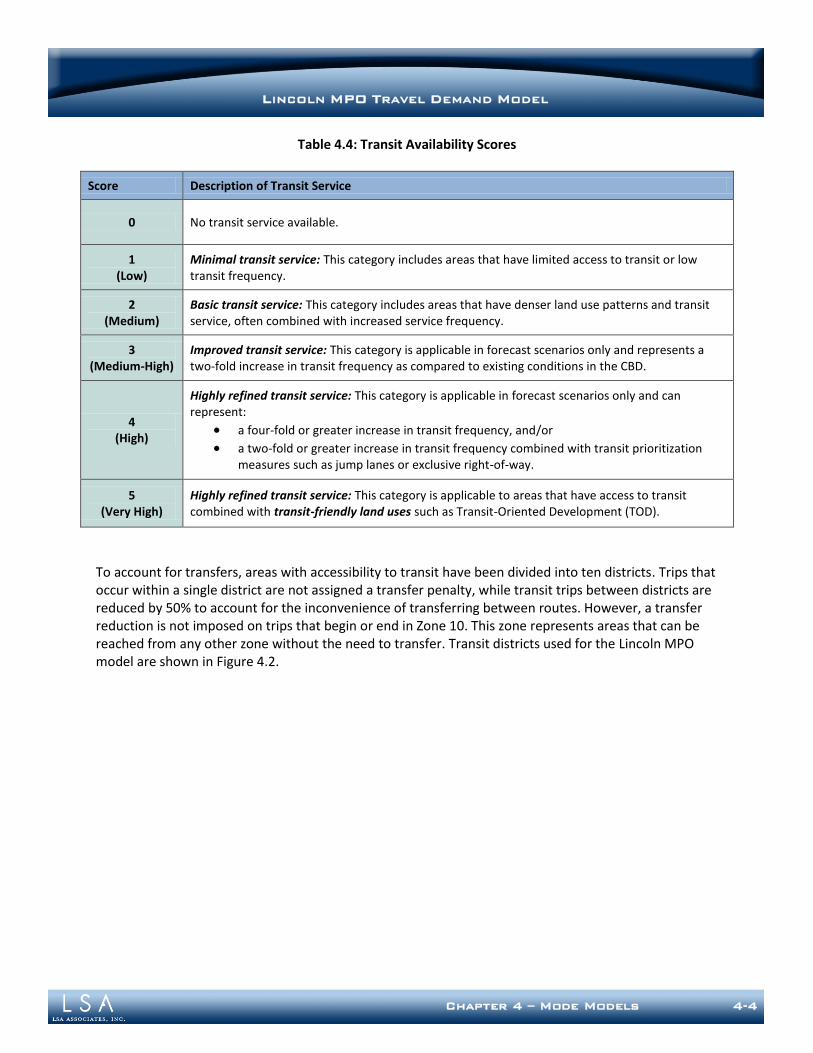
LINCOLN MPO TRAVEL DEMAND MODEL
Chapter 4 – Mode Models 4-4
Table 4.4: Transit Availability Scores
Score Description of Transit Service
0 No transit service available.
1 (Low)
Minimal transit service: This category includes areas that have limited access to transit or low transit frequency.
2 (Medium)
Basic transit service: This category includes areas that have denser land use patterns and transit service, often combined with increased service frequency.
3 (Medium-High)
Improved transit service: This category is applicable in forecast scenarios only and represents a two-fold increase in transit frequency as compared to existing conditions in the CBD.
4 (High)
Highly refined transit service: This category is applicable in forecast scenarios only and can represent:
a four-fold or greater increase in transit frequency, and/or
a two-fold or greater increase in transit frequency combined with transit prioritization measures such as jump lanes or exclusive right-of-way.
5 (Very High)
Highly refined transit service: This category is applicable to areas that have access to transit combined with transit-friendly land uses such as Transit-Oriented Development (TOD).
To account for transfers, areas with accessibility to transit have been divided into ten districts. Trips that occur within a single district are not assigned a transfer penalty, while transit trips between districts are reduced by 50% to account for the inconvenience of transferring between routes. However, a transfer reduction is not imposed on trips that begin or end in Zone 10. This zone represents areas that can be reached from any other zone without the need to transfer. Transit districts used for the Lincoln MPO model are shown in Figure 4.2.
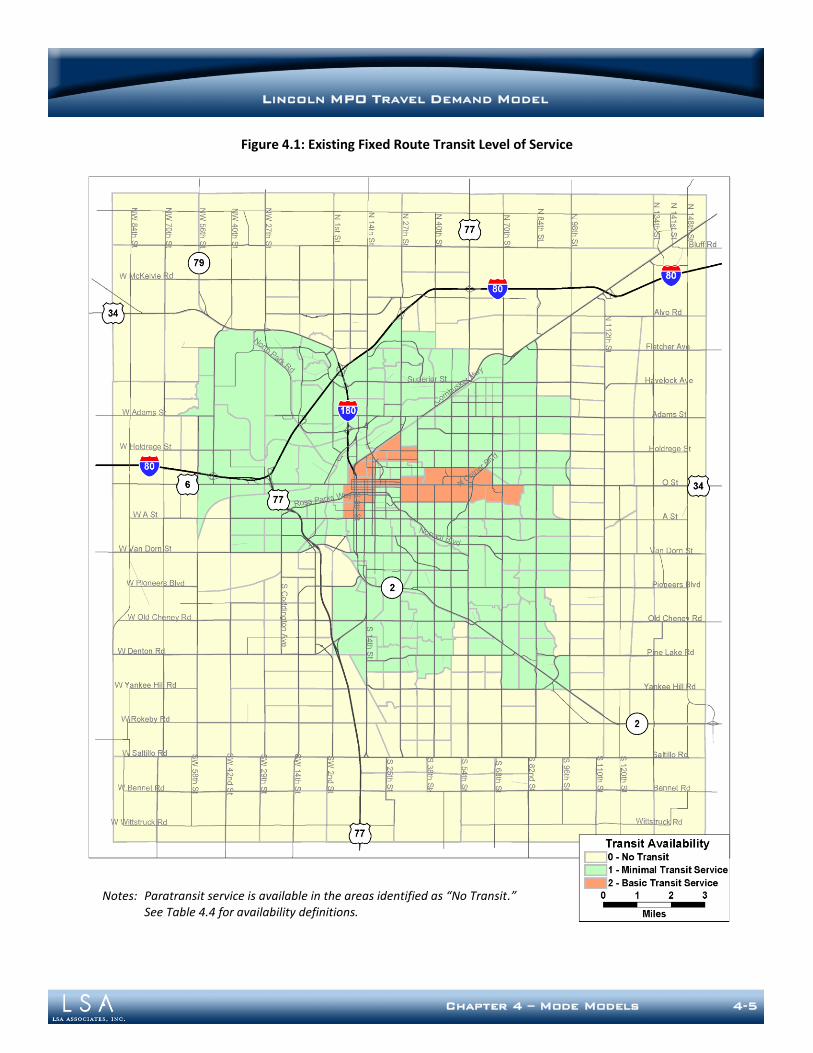
LINCOLN MPO TRAVEL DEMAND MODEL
Chapter 4 – Mode Models 4-5
Figure 4.1: Existing Fixed Route Transit Level of Service
Notes: Paratransit service is available in the areas identified as “No Transit.” See Table 4.4 for availability definitions.
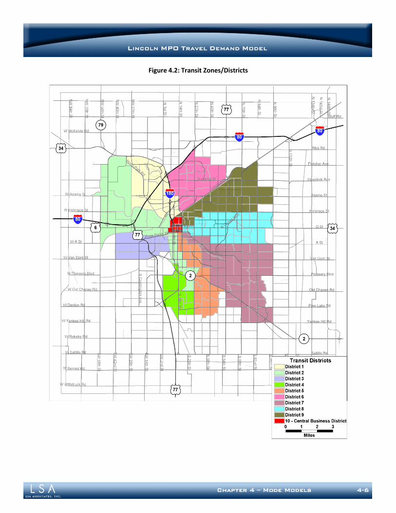
LINCOLN MPO TRAVEL DEMAND MODEL
Chapter 4 – Mode Models 4-6
Figure 4.2: Transit Zones/Districts
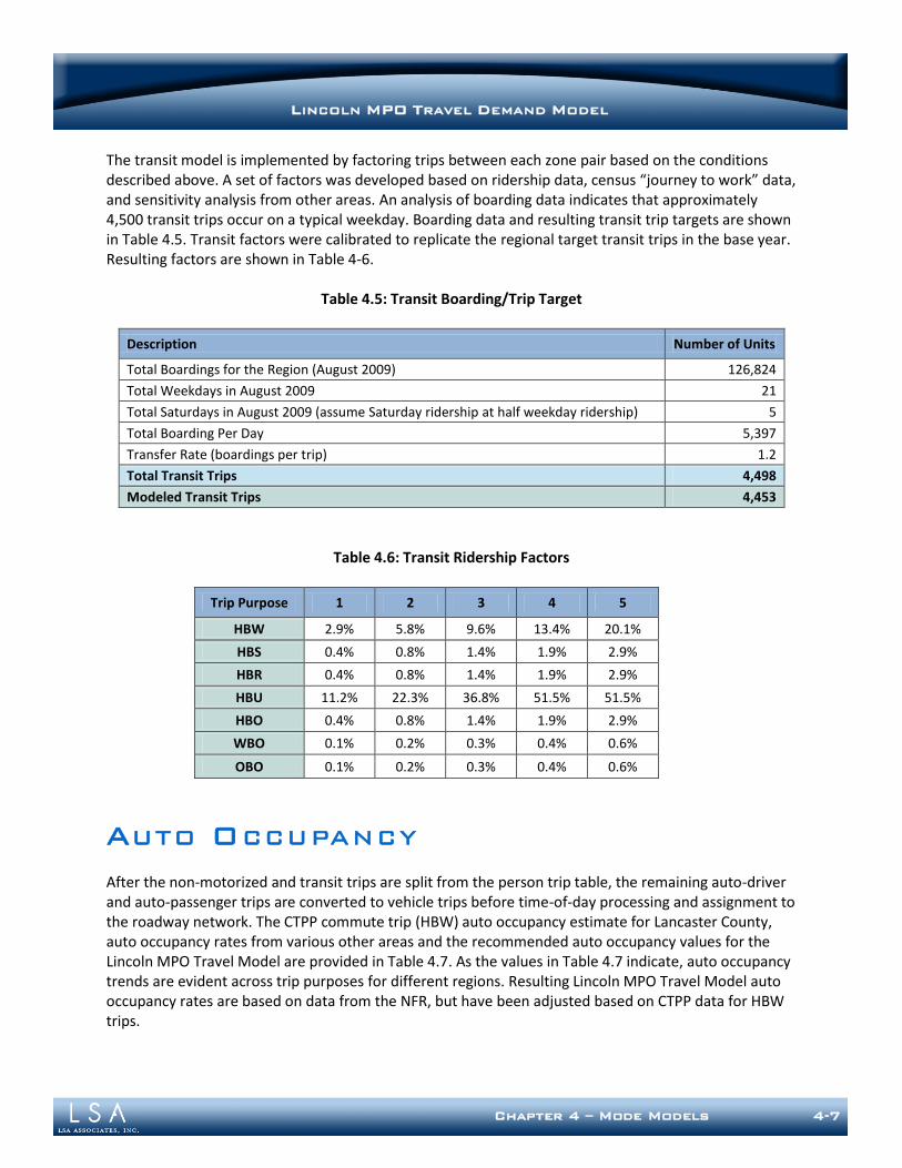
LINCOLN MPO TRAVEL DEMAND MODEL
Chapter 4 – Mode Models 4-7
The transit model is implemented by factoring trips between each zone pair based on the conditions described above. A set of factors was developed based on ridership data, census “journey to work” data, and sensitivity analysis from other areas. An analysis of boarding data indicates that approximately 4,500 transit trips occur on a typical weekday. Boarding data and resulting transit trip targets are shown in Table 4.5. Transit factors were calibrated to replicate the regional target transit trips in the base year. Resulting factors are shown in Table 4-6.
Table 4.5: Transit Boarding/Trip Target
Description Number of Units
Total Boardings for the Region (August 2009) 126,824
Total Weekdays in August 2009 21
Total Saturdays in August 2009 (assume Saturday ridership at half weekday ridership) 5
Total Boarding Per Day 5,397
Transfer Rate (boardings per trip) 1.2
Total Transit Trips 4,498
Modeled Transit Trips 4,453
Table 4.6: Transit Ridership Factors
Trip Purpose 1 2 3 4 5
HBW 2.9% 5.8% 9.6% 13.4% 20.1%
HBS 0.4% 0.8% 1.4% 1.9% 2.9%
HBR 0.4% 0.8% 1.4% 1.9% 2.9%
HBU 11.2% 22.3% 36.8% 51.5% 51.5%
HBO 0.4% 0.8% 1.4% 1.9% 2.9%
WBO 0.1% 0.2% 0.3% 0.4% 0.6%
OBO 0.1% 0.2% 0.3% 0.4% 0.6%
AUTO OCCUPANCY
After the non-motorized and transit trips are split from the person trip table, the remaining auto-driver and auto-passenger trips are converted to vehicle trips before time-of-day processing and assignment to the roadway network. The CTPP commute trip (HBW) auto occupancy estimate for Lancaster County, auto occupancy rates from various other areas and the recommended auto occupancy values for the Lincoln MPO Travel Model are provided in Table 4.7. As the values in Table 4.7 indicate, auto occupancy trends are evident across trip purposes for different regions. Resulting Lincoln MPO Travel Model auto occupancy rates are based on data from the NFR, but have been adjusted based on CTPP data for HBW trips.
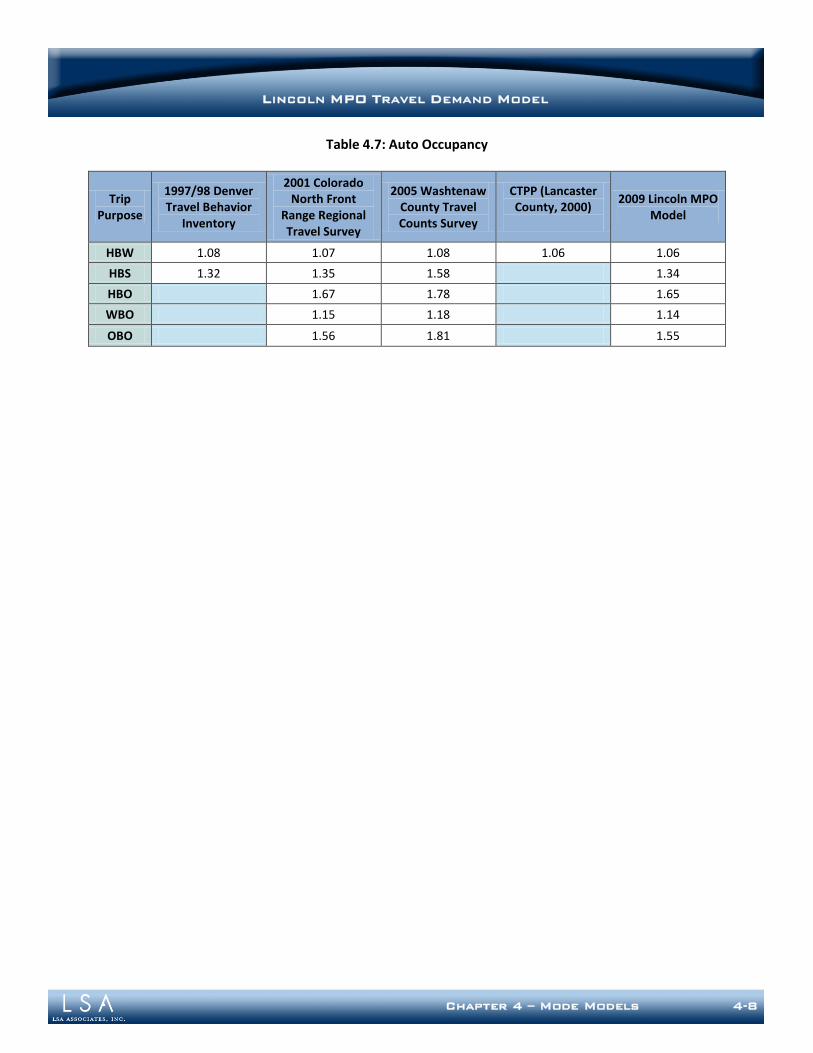
LINCOLN MPO TRAVEL DEMAND MODEL
Chapter 4 – Mode Models 4-8
Table 4.7: Auto Occupancy
Trip Purpose
1997/98 Denver Travel Behavior
Inventory
2001 Colorado North Front
Range Regional Travel Survey
2005 Washtenaw County Travel Counts Survey
CTPP (Lancaster County, 2000)
2009 Lincoln MPO Model
HBW 1.08 1.07 1.08 1.06 1.06
HBS 1.32 1.35 1.58 1.34
HBO 1.67 1.78 1.65
WBO 1.15 1.18 1.14
OBO 1.56 1.81 1.55

LINCOLN MPO TRAVEL DEMAND MODEL
Chapter 5 – Trip Assignment 5-1
Chapter 5: Trip Assignment
CONTEXT AND BACKGROUND
This chapter describes the traffic assignment model for the Lincoln MPO Travel Model, including the time of day process used to convert trips from production-attraction (PA) format to origin-destination (OD) format and the iterative speed feedback process. In the time of day model component, the vehicle trip tables by trip purpose from the mode split process are converted from PA to OD format and factored into time periods for roadway network assignment. The time of day process is not considered a separate phase in the 4-step travel modeling process, but is instead grouped with the traffic assignment model. In the remaining traffic assignment model steps, vehicle trip tables by time of day are assigned for the off-peak period. After traffic assignment is completed, resulting travel times are fed back into trip distribution and the model is run iteratively until speeds input to trip distribution are reasonable and relatively consistent with speeds resulting from traffic assignment.
T IME OF DAY
In the early days of travel demand modeling, models were either set up directly as peak hour models or were established as 24-hour models that were post-processed to obtain peak hour directional design year traffic volumes. With the dramatic increase in processing speeds and electronic storage capability, disaggregation of the models occurred at a faster pace with more traffic analysis zones, larger modeling areas, and more detail in the modeling process. Combined with the need for time-specific traffic volumes and congested speed detail to assess air quality conformity, these influences made detailed time of day modeling commonplace. Based on the analysis of hourly traffic count data, the AM and PM peak hours were defined as shown in Table 5.1. The peak hour definitions are consistent with the traditional morning and evening peak hours observed in many similarly-sized areas.
Table 5.1: Peak Period Definitions
Period Name Period Definition
AM Peak Hour 7:00 AM – 8:00 AM
PM Peak Hour 4:30 PM – 5:30 PM
Off-Peak Period All Remaining Time (22 hours)
Directional time of day factors are used to convert trips from PA to OD format and allocate them into peak and off-peak time periods used in the model. This process is based on extensive data indicating that trips are made directionally by time of day. For example, HBW trips generally occur from the production to the attraction (i.e., from home to work) in the AM peak hour and from the attraction to

LINCOLN MPO TRAVEL DEMAND MODEL
Chapter 5 – Trip Assignment 5-2
the production (i.e., from work to home) in the PM peak hour. However, some trips are made in the reverse of this pattern and many trips are made outside of the peak periods. Although traffic count data can be used to identify peak hours and to validate the model for peak hours, it is not particularly useful in defining time of day PA to OD conversion factors. Traffic count data does not include information about trip purpose or trip direction which is necessary for developing model parameters. Therefore, time of day data used in the Lincoln MPO Travel Model is borrowed from the NFR. In the model, time of day factors are applied directly to the purpose-specific vehicle trip tables created by the mode split model. As described in Chapter 3 - Trip Distribution, daily trip tables are separated into peak period (combined AM and PM peak periods) and off-peak period trips prior to trip distribution and mode split. The traffic assignment time of day module further separates peak period trips into AM and PM peak hour trips. At the same time, all trip tables are converted from PA to OD format. Time of day factors shown in Table 5.2 demonstrate the portion of trips by purpose and direction assigned to each time period. These factors are applied in a two stage process: first in a pre-distribution time of day module and second in a pre-assignment time of day module. The pre-distribution time of day parameters are defined in Chapter 3 - Trip Distribution and are repeated in Table 5.3 for reference. The pre-assignment time of day parameters are shown in Table 5.4. Pre-distribution time of day factors are computed based on the 24-hour time of day factors. For the off-peak period, the distribution time of day factor is simply the sum of the PA and AP factors. For the peak period, the distribution time of day factor is the sum of the PA and AP factors for the AM and PM peak periods. Distribution time-of-day factors are applied by simple multiplication of the time of day factors and the trip tables. Because they are applied to trip tables that have already been separated into peak and off-peak periods, pre-assignment time of day factors are computed by dividing 24-hour factors by the pre-distribution factors for each period and trip purpose. The pre-assignment time of day factors are applied to the peak and off-peak PA tables using Equation (9). Because EE trips are not processed through trip distribution or mode choice, EE time of day is applied prior to trip distribution. EE time of day is computed by simply multiplying time of day factors by the 24-hour EE trip tables.
(9)
Where:
= OD trip-table for the AM or PM hour (or for the off-peak period) = PA trip-table for the peak or off-peak period = Transposed PA trip-table for the peak or off-peak period
= Pre-assignment time of day factor for the PA direction = Pre-assignment time of day factor for the AP direction
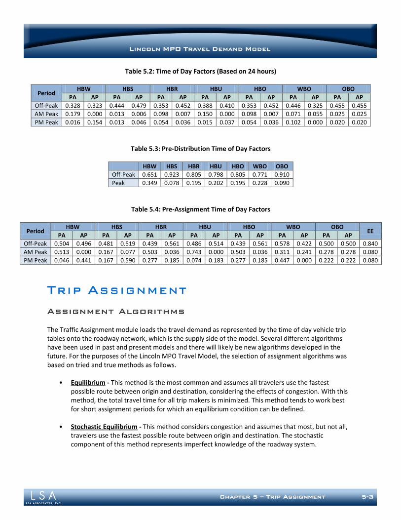
LINCOLN MPO TRAVEL DEMAND MODEL
Chapter 5 – Trip Assignment 5-3
Table 5.2: Time of Day Factors (Based on 24 hours)
Period HBW HBS HBR HBU HBO WBO OBO
PA AP PA AP PA AP PA AP PA AP PA AP PA AP
Off-Peak 0.328 0.323 0.444 0.479 0.353 0.452 0.388 0.410 0.353 0.452 0.446 0.325 0.455 0.455
AM Peak 0.179 0.000 0.013 0.006 0.098 0.007 0.150 0.000 0.098 0.007 0.071 0.055 0.025 0.025
PM Peak 0.016 0.154 0.013 0.046 0.054 0.036 0.015 0.037 0.054 0.036 0.102 0.000 0.020 0.020
Table 5.3: Pre-Distribution Time of Day Factors
HBW HBS HBR HBU HBO WBO OBO
Off-Peak 0.651 0.923 0.805 0.798 0.805 0.771 0.910
Peak 0.349 0.078 0.195 0.202 0.195 0.228 0.090
Table 5.4: Pre-Assignment Time of Day Factors
Period HBW HBS HBR HBU HBO WBO OBO
EE PA AP PA AP PA AP PA AP PA AP PA AP PA AP
Off-Peak 0.504 0.496 0.481 0.519 0.439 0.561 0.486 0.514 0.439 0.561 0.578 0.422 0.500 0.500 0.840
AM Peak 0.513 0.000 0.167 0.077 0.503 0.036 0.743 0.000 0.503 0.036 0.311 0.241 0.278 0.278 0.080
PM Peak 0.046 0.441 0.167 0.590 0.277 0.185 0.074 0.183 0.277 0.185 0.447 0.000 0.222 0.222 0.080
TRIP ASSIGNMENT
Assignment Algorithms
The Traffic Assignment module loads the travel demand as represented by the time of day vehicle trip tables onto the roadway network, which is the supply side of the model. Several different algorithms have been used in past and present models and there will likely be new algorithms developed in the future. For the purposes of the Lincoln MPO Travel Model, the selection of assignment algorithms was based on tried and true methods as follows.
• Equilibrium - This method is the most common and assumes all travelers use the fastest possible route between origin and destination, considering the effects of congestion. With this method, the total travel time for all trip makers is minimized. This method tends to work best for short assignment periods for which an equilibrium condition can be defined.
• Stochastic Equilibrium - This method considers congestion and assumes that most, but not all, travelers use the fastest possible route between origin and destination. The stochastic component of this method represents imperfect knowledge of the roadway system.
LINCOLN MPO TRAVEL DEMAND MODEL
Chapter 5 – Trip Assignment 5-4
• All-or-Nothing - This method does not consider congestion and assigns all trips to the fastest possible route between origin and destination. It is not appropriate for congested networks because it does not consider congestion effects and thus tends to overload some facilities and under-load others.
• Stochastic - This method does not consider congestion and assigns most, but not all, trips to the fastest possible route between origin and destination. For similar reasons as the all-or-nothing assignment, the stochastic assignment method is not appropriate for congested networks.
• Incremental Capacity-Restrained Assignment - With this method, the vehicle trip table is assigned incrementally. Network travel times are updated after each increment is assigned, so congestion effects are considered. With a very large number of increments, this method can approximate an equilibrium assignment. This method is very efficient and includes consideration of congestion effects. However, it has largely fallen out of favor because modern computing power allows for more widespread application of the equilibrium assignment process, which is less efficient computationally, but is theoretically a more valid algorithm.
Because the Lincoln area experiences congestion, only the equilibrium and stochastic equilibrium assignment methods were considered. Based on previous experience, the equilibrium assignment method is preferred over the stochastic equilibrium method except in cases where specific problems are encountered. Therefore, the Lincoln MPO Travel Model uses the equilibrium traffic assignment method.
Closure Criteria
When equilibrium traffic assignment is used, oscillations between equilibrium iterations can sometimes result in unstable assignment results. If closure criteria are not sufficient, two very similar model runs (e.g., with only one small adjustment to the roadway network) can produce un-intuitive results. These results generally occur when the equilibrium traffic assignment algorithm converges at a different number of iterations – sometimes only one apart – for each run. Even when equilibrium traffic assignment converges after the same number of iterations, alternating oscillations in traffic volumes can sometimes be observed in traffic assignment results based on slightly different model networks. While oscillations introduced by the equilibrium traffic assignment procedure can be of concern, they can be managed through introduction of a very tight closure criterion. Traffic assignment is performed with a closure gap of 0.0001 (10-4) and a maximum number of iterations of 500.
Impedance Calculations
In the Traffic Assignment Model, the impedance used for determining the shortest path can take many forms, but typically it includes one or more of the following – travel time, travel distance, and tolls. If more than one impedance variable is used, a generalized cost function is necessary so that the relevant variables can be added together into a single impedance function expression. Since tolls are not an issue in the Lincoln area, they were not seriously considered for the impedance function. Furthermore, experience has shown that distance is less important than travel time; and including distance is problematic because it results in double-counting the emphasis on this variable since distance is also inherent in the travel time calculations.
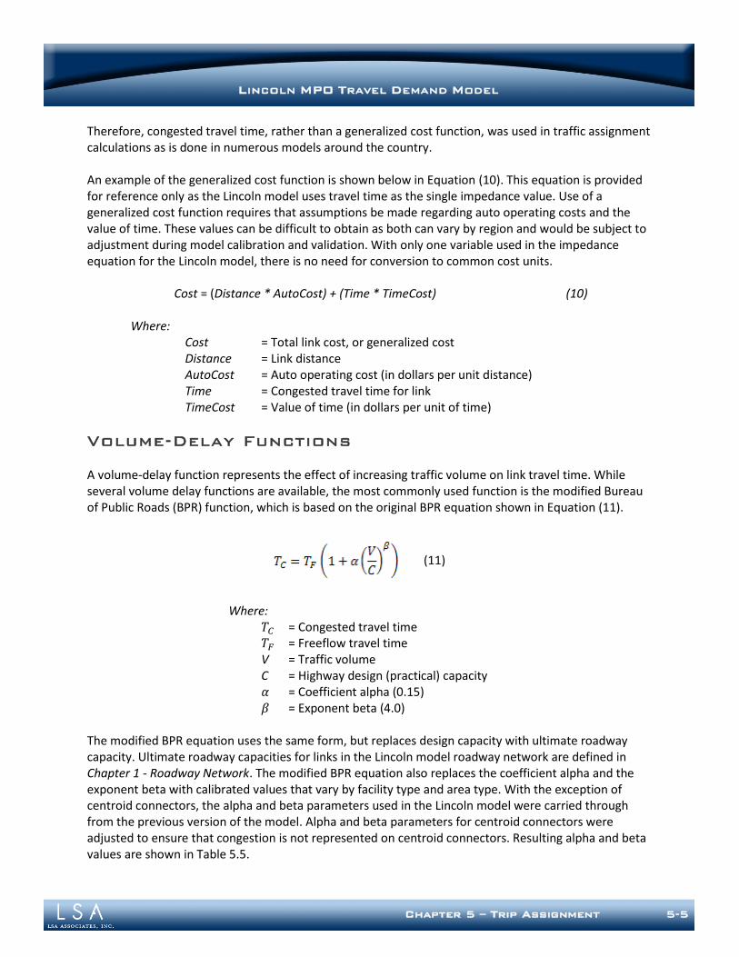
LINCOLN MPO TRAVEL DEMAND MODEL
Chapter 5 – Trip Assignment 5-5
Therefore, congested travel time, rather than a generalized cost function, was used in traffic assignment calculations as is done in numerous models around the country. An example of the generalized cost function is shown below in Equation (10). This equation is provided for reference only as the Lincoln model uses travel time as the single impedance value. Use of a generalized cost function requires that assumptions be made regarding auto operating costs and the value of time. These values can be difficult to obtain as both can vary by region and would be subject to adjustment during model calibration and validation. With only one variable used in the impedance equation for the Lincoln model, there is no need for conversion to common cost units.
Cost = (Distance * AutoCost) + (Time * TimeCost) (10) Where: Cost = Total link cost, or generalized cost Distance = Link distance AutoCost = Auto operating cost (in dollars per unit distance) Time = Congested travel time for link TimeCost = Value of time (in dollars per unit of time)
Volume-Delay Functions
A volume-delay function represents the effect of increasing traffic volume on link travel time. While several volume delay functions are available, the most commonly used function is the modified Bureau of Public Roads (BPR) function, which is based on the original BPR equation shown in Equation (11).
(11)
Where: = Congested travel time = Freeflow travel time V = Traffic volume C = Highway design (practical) capacity = Coefficient alpha (0.15) = Exponent beta (4.0)
The modified BPR equation uses the same form, but replaces design capacity with ultimate roadway capacity. Ultimate roadway capacities for links in the Lincoln model roadway network are defined in Chapter 1 - Roadway Network. The modified BPR equation also replaces the coefficient alpha and the exponent beta with calibrated values that vary by facility type and area type. With the exception of centroid connectors, the alpha and beta parameters used in the Lincoln model were carried through from the previous version of the model. Alpha and beta parameters for centroid connectors were adjusted to ensure that congestion is not represented on centroid connectors. Resulting alpha and beta values are shown in Table 5.5.
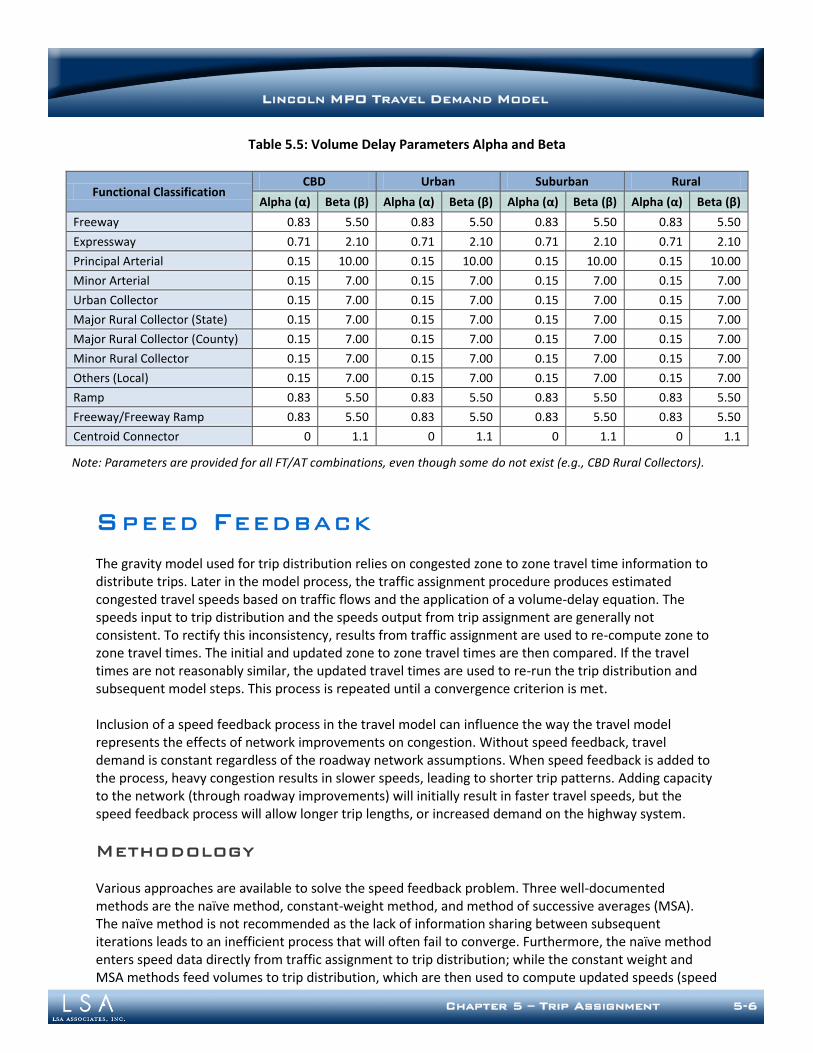
LINCOLN MPO TRAVEL DEMAND MODEL
Chapter 5 – Trip Assignment 5-6
Table 5.5: Volume Delay Parameters Alpha and Beta
Functional Classification CBD Urban Suburban Rural
Alpha (α) Beta (β) Alpha (α) Beta (β) Alpha (α) Beta (β) Alpha (α) Beta (β)
Freeway 0.83 5.50 0.83 5.50 0.83 5.50 0.83 5.50
Expressway 0.71 2.10 0.71 2.10 0.71 2.10 0.71 2.10
Principal Arterial 0.15 10.00 0.15 10.00 0.15 10.00 0.15 10.00
Minor Arterial 0.15 7.00 0.15 7.00 0.15 7.00 0.15 7.00
Urban Collector 0.15 7.00 0.15 7.00 0.15 7.00 0.15 7.00
Major Rural Collector (State) 0.15 7.00 0.15 7.00 0.15 7.00 0.15 7.00
Major Rural Collector (County) 0.15 7.00 0.15 7.00 0.15 7.00 0.15 7.00
Minor Rural Collector 0.15 7.00 0.15 7.00 0.15 7.00 0.15 7.00
Others (Local) 0.15 7.00 0.15 7.00 0.15 7.00 0.15 7.00
Ramp 0.83 5.50 0.83 5.50 0.83 5.50 0.83 5.50
Freeway/Freeway Ramp 0.83 5.50 0.83 5.50 0.83 5.50 0.83 5.50
Centroid Connector 0 1.1 0 1.1 0 1.1 0 1.1
Note: Parameters are provided for all FT/AT combinations, even though some do not exist (e.g., CBD Rural Collectors).
SPEED FEEDBACK
The gravity model used for trip distribution relies on congested zone to zone travel time information to distribute trips. Later in the model process, the traffic assignment procedure produces estimated congested travel speeds based on traffic flows and the application of a volume-delay equation. The speeds input to trip distribution and the speeds output from trip assignment are generally not consistent. To rectify this inconsistency, results from traffic assignment are used to re-compute zone to zone travel times. The initial and updated zone to zone travel times are then compared. If the travel times are not reasonably similar, the updated travel times are used to re-run the trip distribution and subsequent model steps. This process is repeated until a convergence criterion is met. Inclusion of a speed feedback process in the travel model can influence the way the travel model represents the effects of network improvements on congestion. Without speed feedback, travel demand is constant regardless of the roadway network assumptions. When speed feedback is added to the process, heavy congestion results in slower speeds, leading to shorter trip patterns. Adding capacity to the network (through roadway improvements) will initially result in faster travel speeds, but the speed feedback process will allow longer trip lengths, or increased demand on the highway system.
Methodology
Various approaches are available to solve the speed feedback problem. Three well-documented methods are the naïve method, constant-weight method, and method of successive averages (MSA). The naïve method is not recommended as the lack of information sharing between subsequent iterations leads to an inefficient process that will often fail to converge. Furthermore, the naïve method enters speed data directly from traffic assignment to trip distribution; while the constant weight and MSA methods feed volumes to trip distribution, which are then used to compute updated speeds (speed
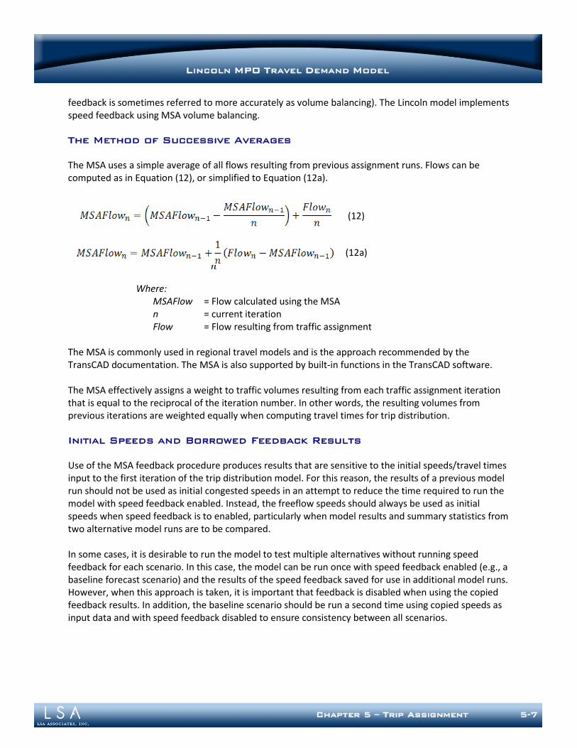
LINCOLN MPO TRAVEL DEMAND MODEL
Chapter 5 – Trip Assignment 5-7
feedback is sometimes referred to more accurately as volume balancing). The Lincoln model implements speed feedback using MSA volume balancing. The Method of Successive Averages
The MSA uses a simple average of all flows resulting from previous assignment runs. Flows can be computed as in Equation (12), or simplified to Equation (12a).
(12)
(12a)
Where:
MSAFlow = Flow calculated using the MSA n = current iteration Flow = Flow resulting from traffic assignment
The MSA is commonly used in regional travel models and is the approach recommended by the TransCAD documentation. The MSA is also supported by built-in functions in the TransCAD software. The MSA effectively assigns a weight to traffic volumes resulting from each traffic assignment iteration that is equal to the reciprocal of the iteration number. In other words, the resulting volumes from previous iterations are weighted equally when computing travel times for trip distribution. Initial Speeds and Borrowed Feedback Results
Use of the MSA feedback procedure produces results that are sensitive to the initial speeds/travel times input to the first iteration of the trip distribution model. For this reason, the results of a previous model run should not be used as initial congested speeds in an attempt to reduce the time required to run the model with speed feedback enabled. Instead, the freeflow speeds should always be used as initial speeds when speed feedback is to enabled, particularly when model results and summary statistics from two alternative model runs are to be compared. In some cases, it is desirable to run the model to test multiple alternatives without running speed feedback for each scenario. In this case, the model can be run once with speed feedback enabled (e.g., a baseline forecast scenario) and the results of the speed feedback saved for use in additional model runs. However, when this approach is taken, it is important that feedback is disabled when using the copied feedback results. In addition, the baseline scenario should be run a second time using copied speeds as input data and with speed feedback disabled to ensure consistency between all scenarios.
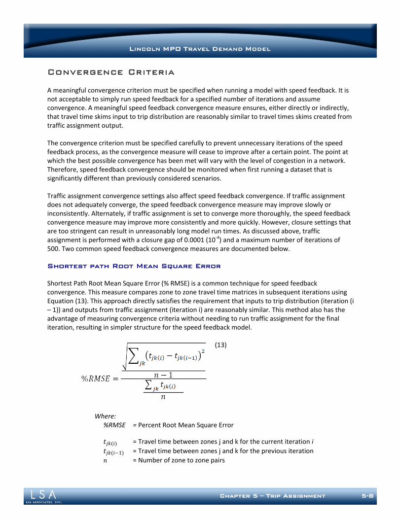
LINCOLN MPO TRAVEL DEMAND MODEL
Chapter 5 – Trip Assignment 5-8
Convergence Criteria
A meaningful convergence criterion must be specified when running a model with speed feedback. It is not acceptable to simply run speed feedback for a specified number of iterations and assume convergence. A meaningful speed feedback convergence measure ensures, either directly or indirectly, that travel time skims input to trip distribution are reasonably similar to travel times skims created from traffic assignment output. The convergence criterion must be specified carefully to prevent unnecessary iterations of the speed feedback process, as the convergence measure will cease to improve after a certain point. The point at which the best possible convergence has been met will vary with the level of congestion in a network. Therefore, speed feedback convergence should be monitored when first running a dataset that is significantly different than previously considered scenarios. Traffic assignment convergence settings also affect speed feedback convergence. If traffic assignment does not adequately converge, the speed feedback convergence measure may improve slowly or inconsistently. Alternately, if traffic assignment is set to converge more thoroughly, the speed feedback convergence measure may improve more consistently and more quickly. However, closure settings that are too stringent can result in unreasonably long model run times. As discussed above, traffic assignment is performed with a closure gap of 0.0001 (10-4) and a maximum number of iterations of 500. Two common speed feedback convergence measures are documented below. Shortest path Root Mean Square Error
Shortest Path Root Mean Square Error (% RMSE) is a common technique for speed feedback convergence. This measure compares zone to zone travel time matrices in subsequent iterations using Equation (13). This approach directly satisfies the requirement that inputs to trip distribution (iteration (i – 1)) and outputs from traffic assignment (iteration i) are reasonably similar. This method also has the advantage of measuring convergence criteria without needing to run traffic assignment for the final iteration, resulting in simpler structure for the speed feedback model.
(13)
Where: %RMSE = Percent Root Mean Square Error
= Travel time between zones j and k for the current iteration i
= Travel time between zones j and k for the previous iteration
= Number of zone to zone pairs
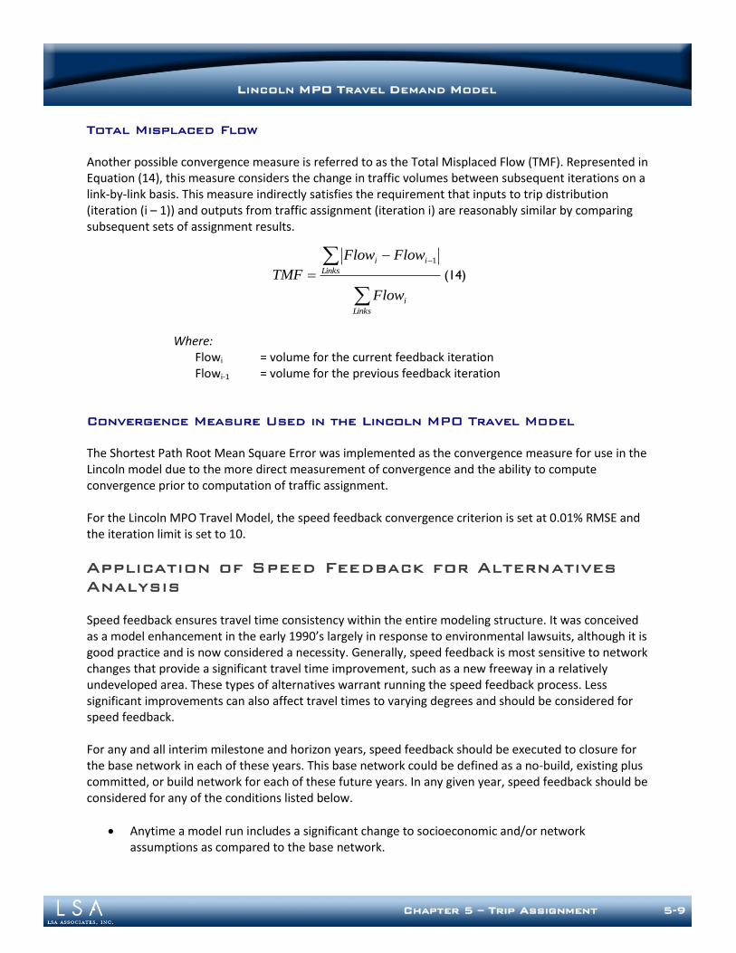
LINCOLN MPO TRAVEL DEMAND MODEL
Chapter 5 – Trip Assignment 5-9
Total Misplaced Flow
Another possible convergence measure is referred to as the Total Misplaced Flow (TMF). Represented in Equation (14), this measure considers the change in traffic volumes between subsequent iterations on a link-by-link basis. This measure indirectly satisfies the requirement that inputs to trip distribution (iteration (i – 1)) and outputs from traffic assignment (iteration i) are reasonably similar by comparing subsequent sets of assignment results.
Links
i
Links
ii
Flow
FlowFlow
TMF1
(14)
Where:
Flowi = volume for the current feedback iteration Flowi-1 = volume for the previous feedback iteration
Convergence Measure Used in the Lincoln MPO Travel Model
The Shortest Path Root Mean Square Error was implemented as the convergence measure for use in the Lincoln model due to the more direct measurement of convergence and the ability to compute convergence prior to computation of traffic assignment. For the Lincoln MPO Travel Model, the speed feedback convergence criterion is set at 0.01% RMSE and the iteration limit is set to 10.
Application of Speed Feedback for Alternatives
Analysis
Speed feedback ensures travel time consistency within the entire modeling structure. It was conceived as a model enhancement in the early 1990’s largely in response to environmental lawsuits, although it is good practice and is now considered a necessity. Generally, speed feedback is most sensitive to network changes that provide a significant travel time improvement, such as a new freeway in a relatively undeveloped area. These types of alternatives warrant running the speed feedback process. Less significant improvements can also affect travel times to varying degrees and should be considered for speed feedback. For any and all interim milestone and horizon years, speed feedback should be executed to closure for the base network in each of these years. This base network could be defined as a no-build, existing plus committed, or build network for each of these future years. In any given year, speed feedback should be considered for any of the conditions listed below.
Anytime a model run includes a significant change to socioeconomic and/or network assumptions as compared to the base network.
LINCOLN MPO TRAVEL DEMAND MODEL
Chapter 5 – Trip Assignment 5-10
A significant new roadway alternative (i.e., new or greatly improved access) over the base network, including new access to areas that are undeveloped, developing, or already developed. For undeveloped areas, the effect is likely more significant in later years. Examples include new freeway interchanges, new freeways and arterials, and, in limited cases, new collector roads.
Less significant roadway improvements, including roadway widenings or corridor improvements that imply functional class, speed, or capacity changes, might warrant running speed feedback. . Improvements limited to a short section of roadway or an intersection generally would not warrant speed feedback.
A significant change to socioeconomic assumptions over the base case. This change is more likely to be necessary over a larger area involving significant demographic shifts, but could conceivably be limited to one or a small number of zones with very high activity. Socioeconomic changes should also include an update to area type assumptions.
Significant changes to external trip assumptions.
Significant changes to special generator assumptions.
Any model run in which a change in congestion on any corridor is anticipated. This criterion is largely covered by those above.
Changes to model parameters, factors, coefficients, etc. – Note: These changes should only be made in conjunction with model calibration and validation, but any tests of changes to parameters should include running the feedback process.
If in doubt, the relatively small amount of time necessary to run the Lincoln model suggests that it may be prudent to run the feedback mechanism for all conditions.
TRAFFIC ASSIGNMENT VALIDATION
Roadway volumes resulting from traffic assignment were compared against traffic count data. This process, called traffic assignment validation, ensures that the model is reasonably representing observed traffic patterns. Traffic count data was obtained from various sources and placed on the roadway network. Travel model results were then compared to traffic count data using a variety of techniques, including regional comparisons, screenline comparisons, and visual inspection of individual link data.
Traffic Count Data
The roadway network has been populated with traffic count data provided by the sources listed in Table 5.6. Due to differences in the way various agencies provide traffic data, some adjustments were made to the original data, which has been retained on the roadway network for reference. For model validation, traffic count data must represent a “typical weekday when school is in session.” This condition allows model results to reflect volumes that would be consistent with traffic counts taken during this time period.
LINCOLN MPO TRAVEL DEMAND MODEL
Chapter 5 – Trip Assignment 5-11
This approach is also important for long range transportation planning purposes. The long range transportation planning process focuses on the urbanized area in and around the city of Lincoln. In the urbanized area, deficiencies in the transportation system are most frequently observed on weekdays. Due to the increased level of activity when the University is in session, it is also important to plan for the time period when school is in session.
Table 5.6: Traffic Count Data Sources
Source Data Formats
City of Lincoln Average Daily Traffic on a particular day, with the date and day of week noted.
Estimated Average Daily Traffic
Lancaster County Average Daily Traffic (weekday)
Nebraska Department of Roads Average Annual Daily Traffic (AADT)
Detailed Traffic Count Data, including data for a specific day or time period.
All traffic count data was adjusted to represent 2009 conditions for use in model validation. Count data for the years 2006 through 2008 was adjusted to represent 2009 conditions using growth rates provided by NDOR. AADT provided by NDOR was adjusted to represent weekday travel and to represent an approximate average for the months of March, April, September, October, and November by applying traffic count adjustment factors provided by NDOR. Because these factors are typically used to factor raw count data to reflect AADT, the factors were applied in reverse.
Overall Activity Level
Overall vehicle trip activity was validated by comparing count data to model results on all links where count data is available using two statistics: the Model Volume as compared to Count Volume and the Model VMT as compared to Count VMT. These statistics were reviewed at the facility type, area type, and regional level and are shown in Table 5.7. In addition, regional daily VMT and VHT are shown in Table 5.8.
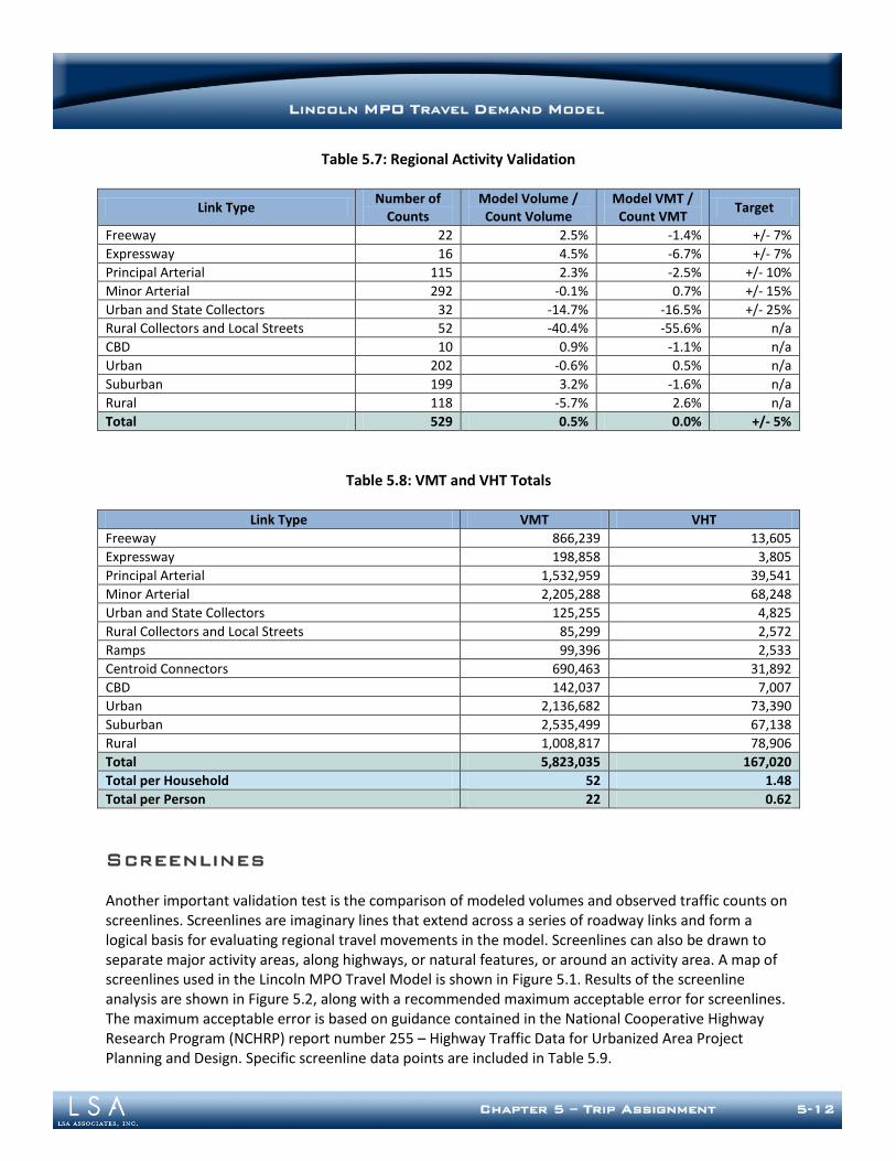
LINCOLN MPO TRAVEL DEMAND MODEL
Chapter 5 – Trip Assignment 5-12
Table 5.7: Regional Activity Validation
Link Type Number of
Counts Model Volume / Count Volume
Model VMT / Count VMT
Target
Freeway 22 2.5% -1.4% +/- 7%
Expressway 16 4.5% -6.7% +/- 7%
Principal Arterial 115 2.3% -2.5% +/- 10%
Minor Arterial 292 -0.1% 0.7% +/- 15%
Urban and State Collectors 32 -14.7% -16.5% +/- 25%
Rural Collectors and Local Streets 52 -40.4% -55.6% n/a
CBD 10 0.9% -1.1% n/a
Urban 202 -0.6% 0.5% n/a
Suburban 199 3.2% -1.6% n/a
Rural 118 -5.7% 2.6% n/a
Total 529 0.5% 0.0% +/- 5%
Table 5.8: VMT and VHT Totals
Link Type VMT VHT
Freeway 866,239 13,605
Expressway 198,858 3,805
Principal Arterial 1,532,959 39,541
Minor Arterial 2,205,288 68,248
Urban and State Collectors 125,255 4,825
Rural Collectors and Local Streets 85,299 2,572
Ramps 99,396 2,533
Centroid Connectors 690,463 31,892
CBD 142,037 7,007
Urban 2,136,682 73,390
Suburban 2,535,499 67,138
Rural 1,008,817 78,906
Total 5,823,035 167,020
Total per Household 52 1.48
Total per Person 22 0.62
Screenlines
Another important validation test is the comparison of modeled volumes and observed traffic counts on screenlines. Screenlines are imaginary lines that extend across a series of roadway links and form a logical basis for evaluating regional travel movements in the model. Screenlines can also be drawn to separate major activity areas, along highways, or natural features, or around an activity area. A map of screenlines used in the Lincoln MPO Travel Model is shown in Figure 5.1. Results of the screenline analysis are shown in Figure 5.2, along with a recommended maximum acceptable error for screenlines. The maximum acceptable error is based on guidance contained in the National Cooperative Highway Research Program (NCHRP) report number 255 – Highway Traffic Data for Urbanized Area Project Planning and Design. Specific screenline data points are included in Table 5.9.
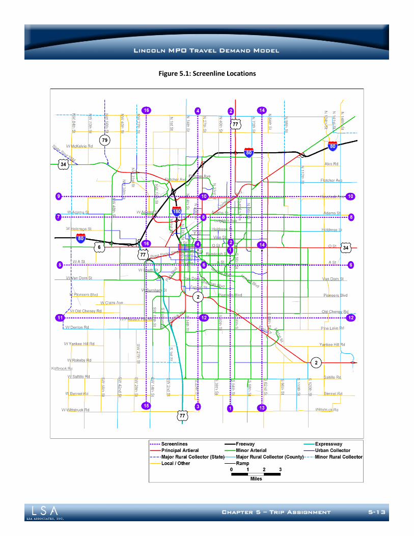
LINCOLN MPO TRAVEL DEMAND MODEL
Chapter 5 – Trip Assignment 5-13
Figure 5.1: Screenline Locations
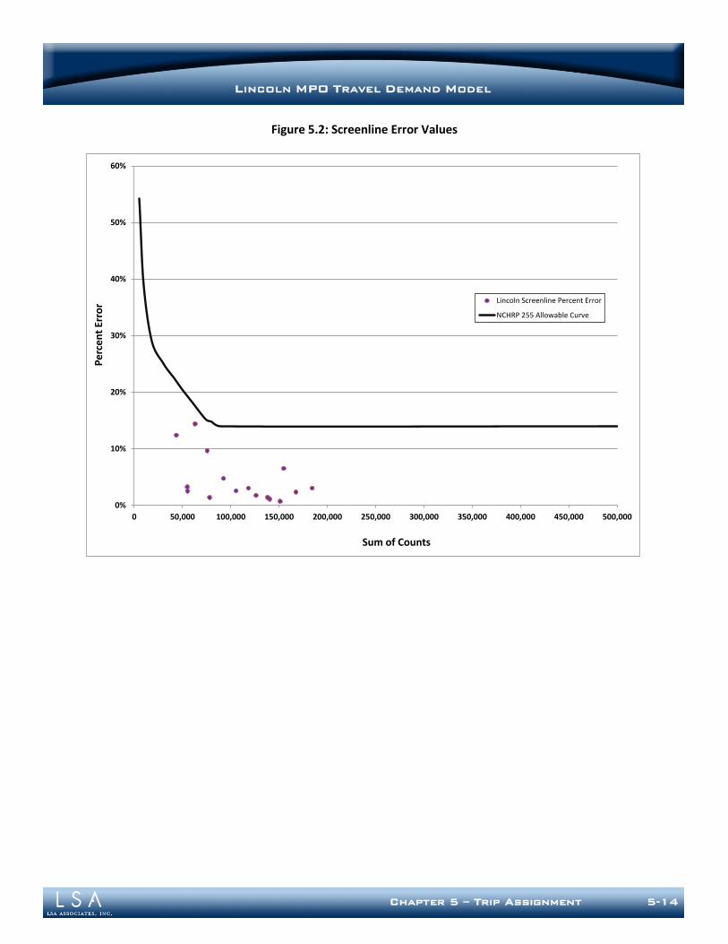
LINCOLN MPO TRAVEL DEMAND MODEL
Chapter 5 – Trip Assignment 5-14
Figure 5.2: Screenline Error Values
0%
10%
20%
30%
40%
50%
60%
0 50,000 100,000 150,000 200,000 250,000 300,000 350,000 400,000 450,000 500,000
Pe
rce
nt
Erro
r
Sum of Counts
Lincoln Screenline Percent Error
NCHRP 255 Allowable Curve
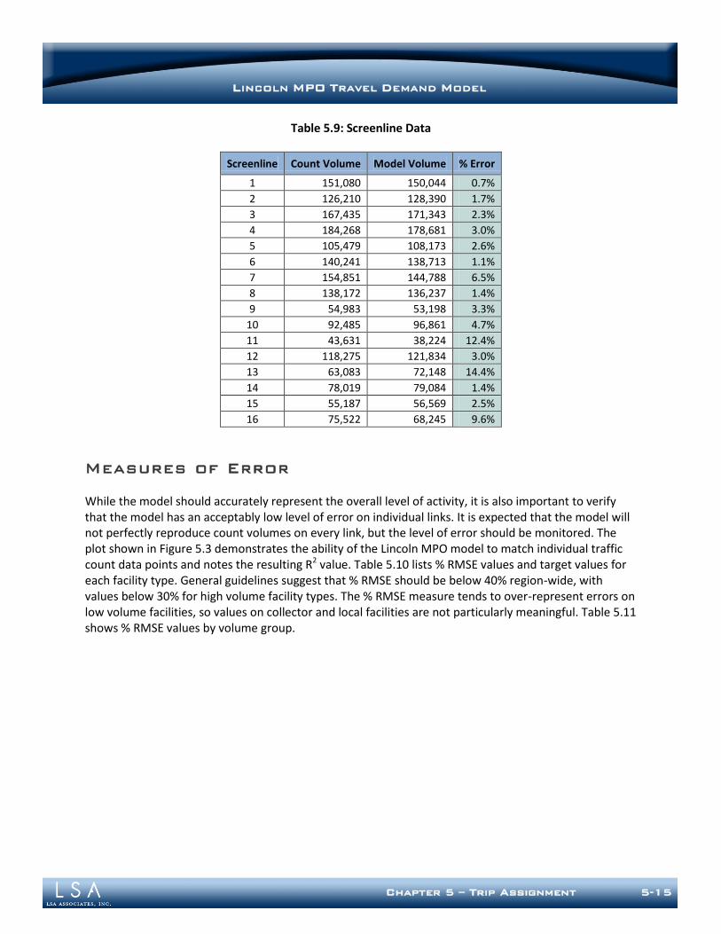
LINCOLN MPO TRAVEL DEMAND MODEL
Chapter 5 – Trip Assignment 5-15
Table 5.9: Screenline Data
Screenline Count Volume Model Volume % Error
1 151,080 150,044 0.7%
2 126,210 128,390 1.7%
3 167,435 171,343 2.3%
4 184,268 178,681 3.0%
5 105,479 108,173 2.6%
6 140,241 138,713 1.1%
7 154,851 144,788 6.5%
8 138,172 136,237 1.4%
9 54,983 53,198 3.3%
10 92,485 96,861 4.7%
11 43,631 38,224 12.4%
12 118,275 121,834 3.0%
13 63,083 72,148 14.4%
14 78,019 79,084 1.4%
15 55,187 56,569 2.5%
16 75,522 68,245 9.6%
Measures of Error
While the model should accurately represent the overall level of activity, it is also important to verify that the model has an acceptably low level of error on individual links. It is expected that the model will not perfectly reproduce count volumes on every link, but the level of error should be monitored. The plot shown in Figure 5.3 demonstrates the ability of the Lincoln MPO model to match individual traffic count data points and notes the resulting R2 value. Table 5.10 lists % RMSE values and target values for each facility type. General guidelines suggest that % RMSE should be below 40% region-wide, with values below 30% for high volume facility types. The % RMSE measure tends to over-represent errors on low volume facilities, so values on collector and local facilities are not particularly meaningful. Table 5.11 shows % RMSE values by volume group.
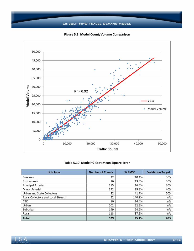
LINCOLN MPO TRAVEL DEMAND MODEL
Chapter 5 – Trip Assignment 5-16
Figure 5.3: Model Count/Volume Comparison
Table 5.10: Model % Root Mean Square Error
Link Type Number of Counts % RMSE Validation Target
Freeway 22 10.4% 30%
Expressway 16 13.3% 30%
Principal Arterial 115 16.5% 30%
Minor Arterial 292 29.8% 40%
Urban and State Collectors 32 41.7% 50%
Rural Collectors and Local Streets 52 140.9% n/a
CBD 10 16.4% n/a
Urban 202 22.6% n/a
Suburban 199 24.2% n/a
Rural 118 37.5% n/a
Total 529 25.1% 40%
0
5,000
10,000
15,000
20,000
25,000
30,000
35,000
40,000
45,000
50,000
0 10,000 20,000 30,000 40,000 50,000
Mo
del
Vo
lum
e
Traffic Counts
Y = X
Model Volume
R2 = 0.92
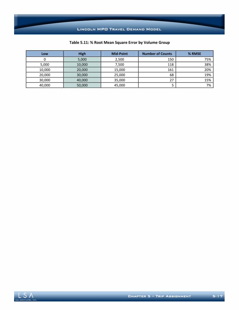
LINCOLN MPO TRAVEL DEMAND MODEL
Chapter 5 – Trip Assignment 5-17
Table 5.11: % Root Mean Square Error by Volume Group
Low High Mid-Point Number of Counts % RMSE
0 5,000 2,500 150 75%
5,000 10,000 7,500 118 38%
10,000 20,000 15,000 161 20%
20,000 30,000 25,000 68 19%
30,000 40,000 35,000 27 15%
40,000 50,000 45,000 5 7%

LINCOLN MPO TRAVEL DEMAND MODEL
Chapter 6 – Dynamic Validation 6-1
Chapter 6: Dynamic Validation
CONTEXT AND BACKGROUND
The base year validation measures described in the preceding chapters of this report are critical in ensuring the validity of the Lincoln MPO Travel Model. These measures show that the model adequately reproduces observed trip generation, distribution, mode split, and assignment patterns. In addition, the measures show that parameters such as trip rates and trip lengths are reasonable when compared to other sources of data and guidance documents. However, the base year validation measures are static – they do not demonstrate the sensitivity of the model. This chapter describes a dynamic validation process in which the model is run through a series of simple sensitivity tests. These tests show that the model provides appropriate sensitivity to variables that are important in the forecasting and planning process.
LAND USE DATA ADJUSTMENTS
The addition of new land use data to a TAZ is expected to affect the total number of trips made, and the regional total VMT and VHT. The type and location of new land use data may impact the type of change seen. For example, addition of new land use data in the fringe areas surrounding the suburban area would be expected to result in higher VMT increases than addition of data in a developed urban area (e.g., infill development). Land use sensitivity tests were performed in two TAZs – numbered 61 (urban area) and 298 (newly developing suburban area). These zones are shown in Figure 6.1.
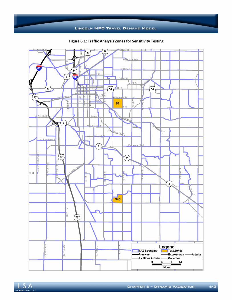
LINCOLN MPO TRAVEL DEMAND MODEL
Chapter 6 – Dynamic Validation 6-2
Figure 6.1: Traffic Analysis Zones for Sensitivity Testing
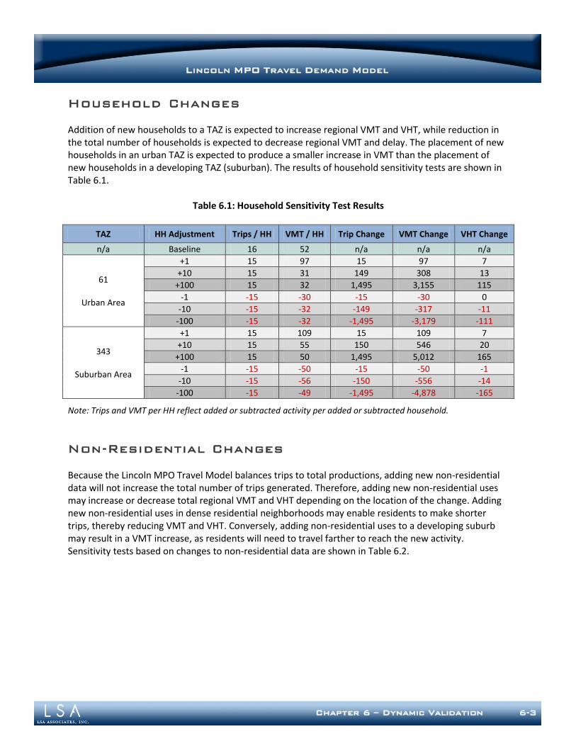
LINCOLN MPO TRAVEL DEMAND MODEL
Chapter 6 – Dynamic Validation 6-3
Household Changes
Addition of new households to a TAZ is expected to increase regional VMT and VHT, while reduction in the total number of households is expected to decrease regional VMT and delay. The placement of new households in an urban TAZ is expected to produce a smaller increase in VMT than the placement of new households in a developing TAZ (suburban). The results of household sensitivity tests are shown in Table 6.1.
Table 6.1: Household Sensitivity Test Results
TAZ HH Adjustment Trips / HH VMT / HH Trip Change VMT Change VHT Change
n/a Baseline 16 52 n/a n/a n/a
61
Urban Area
+1 15 97 15 97 7
+10 15 31 149 308 13
+100 15 32 1,495 3,155 115
-1 -15 -30 -15 -30 0
-10 -15 -32 -149 -317 -11
-100 -15 -32 -1,495 -3,179 -111
343
Suburban Area
+1 15 109 15 109 7
+10 15 55 150 546 20
+100 15 50 1,495 5,012 165
-1 -15 -50 -15 -50 -1
-10 -15 -56 -150 -556 -14
-100 -15 -49 -1,495 -4,878 -165
Note: Trips and VMT per HH reflect added or subtracted activity per added or subtracted household.
Non-Residential Changes
Because the Lincoln MPO Travel Model balances trips to total productions, adding new non-residential data will not increase the total number of trips generated. Therefore, adding new non-residential uses may increase or decrease total regional VMT and VHT depending on the location of the change. Adding new non-residential uses in dense residential neighborhoods may enable residents to make shorter trips, thereby reducing VMT and VHT. Conversely, adding non-residential uses to a developing suburb may result in a VMT increase, as residents will need to travel farther to reach the new activity. Sensitivity tests based on changes to non-residential data are shown in Table 6.2.
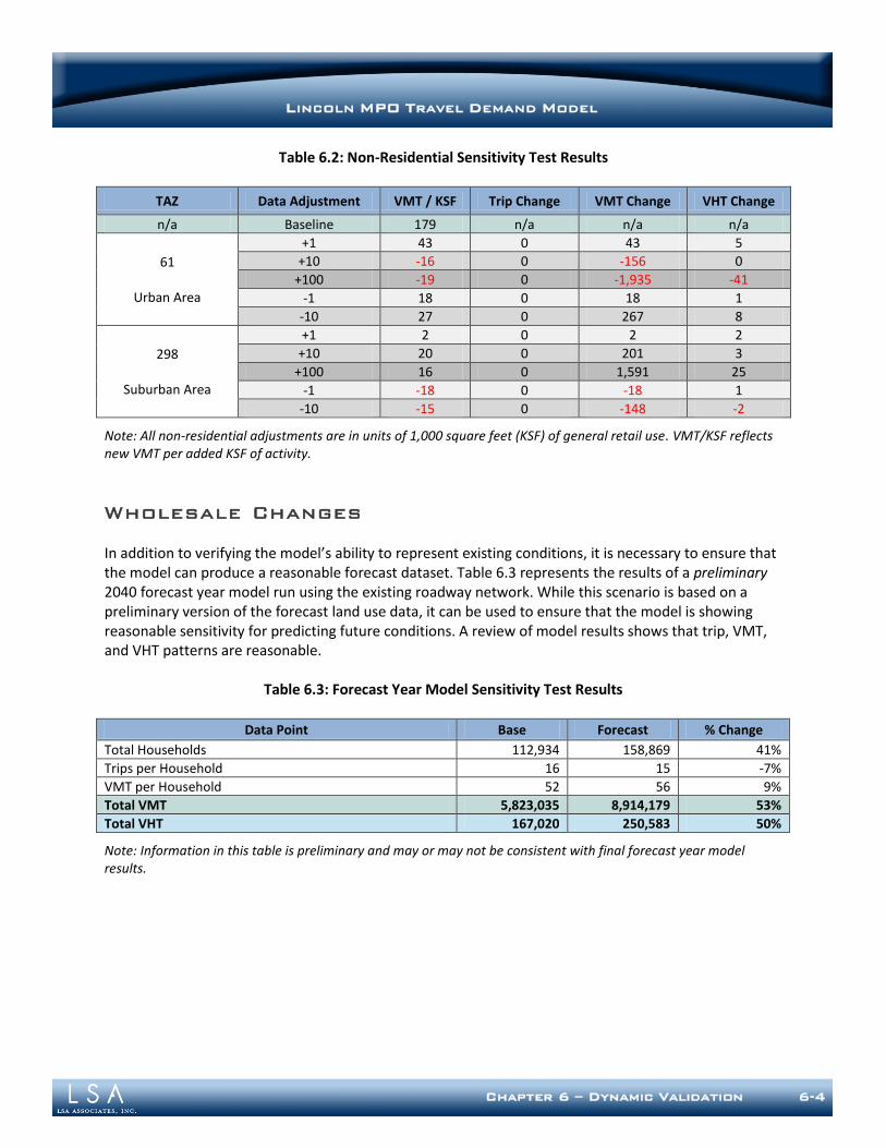
LINCOLN MPO TRAVEL DEMAND MODEL
Chapter 6 – Dynamic Validation 6-4
Table 6.2: Non-Residential Sensitivity Test Results
TAZ Data Adjustment VMT / KSF Trip Change VMT Change VHT Change
n/a Baseline 179 n/a n/a n/a
61
Urban Area
+1 43 0 43 5
+10 -16 0 -156 0
+100 -19 0 -1,935 -41
-1 18 0 18 1
-10 27 0 267 8
298
Suburban Area
+1 2 0 2 2
+10 20 0 201 3
+100 16 0 1,591 25
-1 -18 0 -18 1
-10 -15 0 -148 -2
Note: All non-residential adjustments are in units of 1,000 square feet (KSF) of general retail use. VMT/KSF reflects new VMT per added KSF of activity.
Wholesale Changes
In addition to verifying the model’s ability to represent existing conditions, it is necessary to ensure that the model can produce a reasonable forecast dataset. Table 6.3 represents the results of a preliminary 2040 forecast year model run using the existing roadway network. While this scenario is based on a preliminary version of the forecast land use data, it can be used to ensure that the model is showing reasonable sensitivity for predicting future conditions. A review of model results shows that trip, VMT, and VHT patterns are reasonable.
Table 6.3: Forecast Year Model Sensitivity Test Results
Data Point Base Forecast % Change
Total Households 112,934 158,869 41%
Trips per Household 16 15 -7%
VMT per Household 52 56 9%
Total VMT 5,823,035 8,914,179 53%
Total VHT 167,020 250,583 50%
Note: Information in this table is preliminary and may or may not be consistent with final forecast year model results.
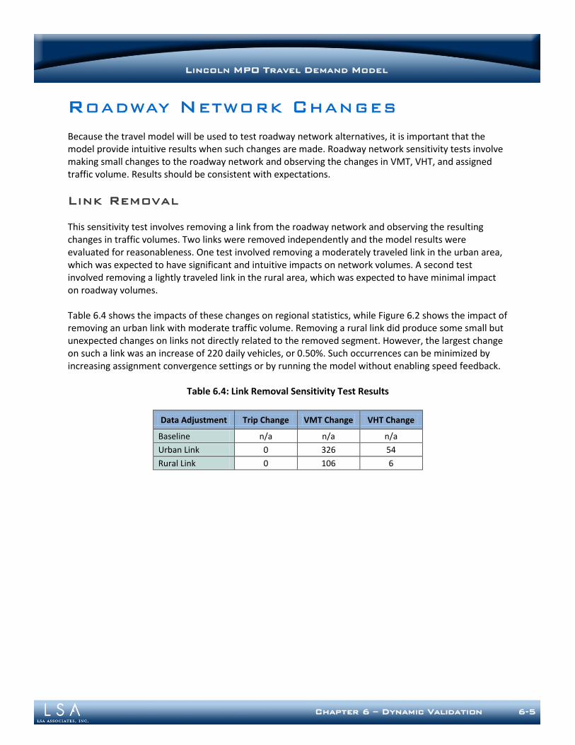
LINCOLN MPO TRAVEL DEMAND MODEL
Chapter 6 – Dynamic Validation 6-5
ROADWAY NETWORK CHANGES
Because the travel model will be used to test roadway network alternatives, it is important that the model provide intuitive results when such changes are made. Roadway network sensitivity tests involve making small changes to the roadway network and observing the changes in VMT, VHT, and assigned traffic volume. Results should be consistent with expectations.
Link Removal
This sensitivity test involves removing a link from the roadway network and observing the resulting changes in traffic volumes. Two links were removed independently and the model results were evaluated for reasonableness. One test involved removing a moderately traveled link in the urban area, which was expected to have significant and intuitive impacts on network volumes. A second test involved removing a lightly traveled link in the rural area, which was expected to have minimal impact on roadway volumes. Table 6.4 shows the impacts of these changes on regional statistics, while Figure 6.2 shows the impact of removing an urban link with moderate traffic volume. Removing a rural link did produce some small but unexpected changes on links not directly related to the removed segment. However, the largest change on such a link was an increase of 220 daily vehicles, or 0.50%. Such occurrences can be minimized by increasing assignment convergence settings or by running the model without enabling speed feedback.
Table 6.4: Link Removal Sensitivity Test Results
Data Adjustment Trip Change VMT Change VHT Change
Baseline n/a n/a n/a
Urban Link 0 326 54
Rural Link 0 106 6

LINCOLN MPO TRAVEL DEMAND MODEL
Chapter 6 – Dynamic Validation 6-6
Figure 6.2: Traffic Assignment Changes due to the Removal of an Urban Link