Embed Size (px)
Citation preview

University of New MexicoUNM Digital Repository
Physics & Astronomy ETDs Electronic Theses and Dissertations
1-30-2013
Transport theoretical studies of some microscopicand macroscopic systemsAlden Astwood
Follow this and additional works at: https://digitalrepository.unm.edu/phyc_etds
This Dissertation is brought to you for free and open access by the Electronic Theses and Dissertations at UNM Digital Repository. It has beenaccepted for inclusion in Physics & Astronomy ETDs by an authorized administrator of UNM Digital Repository. For more information, please [email protected].
Recommended CitationAstwood, Alden. "Transport theoretical studies of some microscopic and macroscopic systems." (2013).https://digitalrepository.unm.edu/phyc_etds/6

!" # # $ % & ' ( ) * + , ' - . / / ' $ + 0 + . % 1 2 % 3 3 . + + ' ' 4 5 6 7 8 9 : ; < : = > ?

Transport Theoretical Studies of SomeMicroscopic and Macroscopic Systems
by
Alden Matthew Astwood
B.S., Texas Tech University, 2008
DISSERTATION
Submitted in Partial Fulfillment of the
Requirements for the Degree of
Doctor of Philosophy,
Physics
The University of New Mexico
Albuquerque, New Mexico
December, 2012

c©2012, Alden Matthew Astwood
iii

Dedication
To my parents.
iv

Acknowledgments
I would like to express my great appreciation to my advisor Professor V. M. Kenkrefor much guidance and support during my time at the University of New Mexico.It was a great pleasure to be his student, and I am extremely grateful for all histeachings and advice.
Advice and suggestions given by my collaborator Michael Raghib were a greathelp during the writing of this thesis.
I would also like to offer thanks to my other teachers in the Department of Physicsand Astronomy at UNM, especially Profs. David Dunlap, Rouzbeh Allahverdi, KevinCahill, and Daniel Finley, for excellent and challenging courses.
It was a great benefit to be a part of the Consortium of the Americas for Interdis-ciplinary Science. I thank its members and visitors for many interesting discussions.
Finally, I would like to thank my family, especially my parents, for their supportand encouragement during the preparation of this thesis.
This work was supported in part by the Air Force Research Laboratory at KirtlandAir Force Base, and by the Department of Energy at Los Alamos National Laboratory.
v

Transport Theoretical Studies of SomeMicroscopic and Macroscopic Systems
by
Alden Matthew Astwood
B.S., Texas Tech University, 2008
Ph.D., Physics, University of New Mexico, 2012
Abstract
This dissertation is a report on theoretical transport studies of two systems of vastly
different sizes. The first topic is electronic motion in quantum wires. In recent years, it
has become possible to fabricate wires that are so small that quantum effects become
important. The conduction properties of these wires are quite different than those of
macroscopic wires. In this dissertation, we seek to understand scattering effects in
quantum wires in a simple way. Some of the existing formalisms for studying trans-
port in quantum wires are reviewed, and one such formalism is applied to calculate
conductance in some simple systems. The second topic concerns animals which move
in groups, such as flocking birds or schooling fish. Exact analytic calculations of the
transport properties of such systems are very difficult because a flock is a system that
is far from equilibrium and consists of many interacting particles. We introduce two
simplified models of flocking which are amenable to analytic study. The first model
consists of a set of overdamped Brownian particles that interact via spring forces. The
exact solution for the probability distribution is calculated, and equations of motion
for continuous coarse-grained quantities, such as the density, are obtained from the
full solution. The second model consists of particles which move in one dimension
vi

at constant speed, but which change their directions at random. The flipping rates
are constructed in such a way that particles tend to align their directions with each
other. The model is solved exactly for one and two particles, the first two moments
are obtained, and equations of motion for continuous coarse-grained quantities are
written. The model cannot be solved exactly for many particles, but the first and
second moments are calculated. Finally, two additional topics are briefly discussed.
The first is transport in disordered lattices, and the second is a static magnetic model
of flocking.
vii

Contents
List of Figures xii
1 Introduction 1
2 Review of Some Existing Formalisms of Quantum Transport 6
2.1 Introduction . . . . . . . . . . . . . . . . . . . . . . . . . . . . . . . . 6
2.2 Transmission Formalism . . . . . . . . . . . . . . . . . . . . . . . . . 7
2.2.1 1D Ballistic Conductor . . . . . . . . . . . . . . . . . . . . . . 8
2.2.2 Mutli-Mode Ballistic Conductor . . . . . . . . . . . . . . . . . 12
2.2.3 Relation between Transmission and Conductance . . . . . . . 15
2.2.4 Transmission and the Green’s Function . . . . . . . . . . . . . 18
2.3 Wigner Function Approach . . . . . . . . . . . . . . . . . . . . . . . . 20
2.3.1 Wigner Functions for Infinite Square Well Confinement . . . . 27
2.3.2 Wigner Functions for Harmonic Confinement . . . . . . . . . . 27
2.4 Kenkre, Biscarini, Bustamante Scanning Tunneling Microscope For-
malism . . . . . . . . . . . . . . . . . . . . . . . . . . . . . . . . . . 28
viii

Contents
2.4.1 Derivation of Formulae for Calculating Current . . . . . . . . 29
2.4.2 Generalized Master Equation for Modeling Partially Coherent
Motion . . . . . . . . . . . . . . . . . . . . . . . . . . . . . . . 36
2.5 Lyo and Huang Boltzmann Equation Solution . . . . . . . . . . . . . 39
2.6 Remarks . . . . . . . . . . . . . . . . . . . . . . . . . . . . . . . . . . 41
3 Application of the Transmission Formalism to Simple 1D Conductors
45
3.1 Introduction . . . . . . . . . . . . . . . . . . . . . . . . . . . . . . . . 45
3.2 Single-Site Conductor . . . . . . . . . . . . . . . . . . . . . . . . . . . 46
3.2.1 Textbook Calculation of the Transmission Function . . . . . . 48
3.2.2 Transmission from the Green’s Function . . . . . . . . . . . . 50
3.2.3 Discussion of the One-Level Conductor . . . . . . . . . . . . . 52
3.3 Two-Level Systems . . . . . . . . . . . . . . . . . . . . . . . . . . . . 56
3.3.1 Calculation of the Transmission . . . . . . . . . . . . . . . . . 56
3.3.2 Discussion . . . . . . . . . . . . . . . . . . . . . . . . . . . . . 58
3.4 N-Level Degenerate System . . . . . . . . . . . . . . . . . . . . . . . 61
3.5 A Different Two-Level Conductor . . . . . . . . . . . . . . . . . . . . 63
3.6 Single-Site Conductor Coupled to Oscillator . . . . . . . . . . . . . . 66
3.7 Summary . . . . . . . . . . . . . . . . . . . . . . . . . . . . . . . . . 70
4 Collective Motion of Macroscopic Objects: A Model with Centering
72
ix
Contents
4.1 Description of the Model . . . . . . . . . . . . . . . . . . . . . . . . . 74
4.2 Deterministic Dynamics . . . . . . . . . . . . . . . . . . . . . . . . . 77
4.3 Noisy Dynamics . . . . . . . . . . . . . . . . . . . . . . . . . . . . . . 79
4.4 A Mean Field Approach in the Presence of Noise . . . . . . . . . . . 90
4.5 Time Evolution of the Density . . . . . . . . . . . . . . . . . . . . . . 93
4.5.1 Initial Conditions . . . . . . . . . . . . . . . . . . . . . . . . . 94
4.5.2 Linear Evolution Equations from the Green’s Function . . . . 98
4.5.3 Evolution of the Density in the Absence of Bias . . . . . . . . 102
4.5.4 Evolution of the Density with Bias . . . . . . . . . . . . . . . 107
4.6 Remarks . . . . . . . . . . . . . . . . . . . . . . . . . . . . . . . . . . 111
5 Collective Motion of Macroscopic Objects: A Model with Alignment
113
5.1 Single-Particle Model . . . . . . . . . . . . . . . . . . . . . . . . . . . 114
5.2 Two-Particle Model . . . . . . . . . . . . . . . . . . . . . . . . . . . . 126
5.3 Generalization to Many Particles . . . . . . . . . . . . . . . . . . . . 140
5.3.1 Average Positions . . . . . . . . . . . . . . . . . . . . . . . . . 144
5.3.2 Second Moments . . . . . . . . . . . . . . . . . . . . . . . . . 147
5.4 Remarks . . . . . . . . . . . . . . . . . . . . . . . . . . . . . . . . . . 154
6 Miscellaneous Topics and Conclusions 157
6.1 Transport in Disordered Lattices and Effective Medium Theory . . . 157
x

Contents
6.2 A Magnetic Model of Flocking . . . . . . . . . . . . . . . . . . . . . . 163
6.3 Closing Remarks . . . . . . . . . . . . . . . . . . . . . . . . . . . . . 167
References 171
xi

List of Figures
2.1 Example energy diagram for a quasi-1D conductor with multiple sub-
bands. Each line represents a single sub-band. . . . . . . . . . . . . 14
2.2 Illustration of a how current may be driven through an elastic scat-
terer. The scatterer with transmission function T (E) is connected
to two 1D ballistic source and drain leads. The leads are in turn
connected to source and drain reservoirs held respectively at electro-
chemical potentials µS and µD. . . . . . . . . . . . . . . . . . . . . 15
2.3 Wigner Functions for the first four eigenstates of the infinite square
well. . . . . . . . . . . . . . . . . . . . . . . . . . . . . . . . . . . . . 43
2.4 Wigner Functions for the first four eigenstates of the harmonic os-
cillator potential. The lower axes are the dimensionless quantities
Y ≡√
m∗ωhx and PY ≡
√1
m∗hωpy. . . . . . . . . . . . . . . . . . . . 44
3.1 A conductor consisting of a single site (blue) connected to two semi-
infinite tight binding leads (black). The strength of the coupling from
the conductor to the leads ηV (orange) is allowed to differ from the
intersite coupling within the leads V . . . . . . . . . . . . . . . . . . 47
3.2 Transmission function versus energy for the one-level conductor with
η = 1 for different values of a ≡ EA/(2V ). . . . . . . . . . . . . . . 53
xii

List of Figures
3.3 Transmission function versus energy for the one-level conductor with
a = EA/(2V ) = 0.5 for different coupling strengths η. . . . . . . . . 54
3.4 Transmission function versus energy for the one-level conductor with
a = EA/(2V ) = 1.5 for different coupling strengths η. . . . . . . . . 55
3.5 A conductor consisting of a two-levels (blue) connected to two semi-
infinite tight binding leads (black). . . . . . . . . . . . . . . . . . . . 56
3.6 Transmission function versus energy for the two-level conductor de-
scribed in Section 3.3 when EA = −EB for different values of a ≡
EA/(2V ). . . . . . . . . . . . . . . . . . . . . . . . . . . . . . . . . . 59
3.7 Transmission function versus energy for the two-level conductor de-
scribed in Section 3.3 when EB = 0 for different values of a ≡ EA/(2V ). 60
3.8 Transmission function versus energy for the two-level conductor de-
scribed in Section 3.3 for different values of b ≡ EB/(2V ) for fixed
EA = V . . . . . . . . . . . . . . . . . . . . . . . . . . . . . . . . . . . 61
3.9 A conductor consisting of a 4 degenerate levels (blue), each of which
are connected to two semi-infinite tight binding leads (black). . . . . 62
3.10 A conductor consisting of two states (blue). Only the |A〉 state is
connected to the two semi-infinite tight binding leads (black). There
is an interaction between the two conductor states of strength VAB. . 64
3.11 Transmission function versus energy for the two-level conductor de-
scribed in Section 3.5 for different values of b ≡ EB/(2V ) for fixed
EA = V and VAB = V . . . . . . . . . . . . . . . . . . . . . . . . . . . 66
3.12 First order correction to the transmission for a one-level conductor
coupled to a harmonic oscillator, with hω/(2V ) = 4 and for different
values of a ≡ E0/(2V ). . . . . . . . . . . . . . . . . . . . . . . . . . . 70
xiii
List of Figures
4.1 Density per particle as a function of time in the simple model of
centering without bias for a delta function initial condition. . . . . . 103
4.2 Density per particle as a function of time in the simple model of
centering when the bias is present for a delta function initial condition.
In this case, the individuals are either uninformed vm = 0 or informed
vm = v. The concentration of informed individuals is a = 0.2. . . . 108
5.1 Sample path of a particle moving at speed c which flips directions at
random. . . . . . . . . . . . . . . . . . . . . . . . . . . . . . . . . . 115
5.2 Probability to find a randomly flipping particle pointing to the left
or right as a function of time, given that the particle was initially
pointing to the right. . . . . . . . . . . . . . . . . . . . . . . . . . . 118
5.3 The average position versus time of a randomly flipping particle mov-
ing at speed c, given that the particle was initially pointing to the
right. . . . . . . . . . . . . . . . . . . . . . . . . . . . . . . . . . . . 120
5.4 Mean square displacement versus time of a randomly flipping particle
which moves at constant speed c on a log-log scale to illustrate the
change from t2 growth to t growth. . . . . . . . . . . . . . . . . . . . 123
5.5 The solution to the telegrapher’s equation for different times for a
delta function initial condition. The vertical arrows represent delta
functions, with the length of the arrow representing the amplitude of
the delta function. . . . . . . . . . . . . . . . . . . . . . . . . . . . . 125
5.6 Illustration of the flipping rates for the two-particle alignment model. 128
5.7 Solutions of σ∗ = tanh(βJ0zσ∗) versus 1/(βJ0z). . . . . . . . . . . . 146
5.8 The effective diffusion constant versus temperature in the ordered
phase for the N particle alignment model. . . . . . . . . . . . . . . . 155
xiv

List of Figures
6.1 Left and right hand sides of the mean field equation m = (1 −
a) tanh(bm) + a tanh(bm + c)f for a = 0.4, b = 15, c = 10. The
intersections of the two curves represent are solutions of the mean
field equation. . . . . . . . . . . . . . . . . . . . . . . . . . . . . . . 165
6.2 Magnetization (both stable and unstable solutions) versus tempera-
ture at fixed field c/b = 0.5 and fixed concentration of informed spins
a = 0.4. . . . . . . . . . . . . . . . . . . . . . . . . . . . . . . . . . . 167
6.3 Magnetization (both stable and unstable solutions) versus field at
fixed inverse temperature b = 15 and fixed concentration of informed
spins a = 0.4. . . . . . . . . . . . . . . . . . . . . . . . . . . . . . . . 168
6.4 Stability diagrams showing the total number of solutions in different
regions of parameter space. . . . . . . . . . . . . . . . . . . . . . . . 170
xv

Chapter 1
Introduction
In our everyday lives we encounter many objects, both large and small, that move from
one place to another. Several tools have been developed over the years in transport
theory, the branch of statistical physics dealing with entities in motion, which are
useful for modeling such objects.
This thesis is in two parts. In the first part we study the motion of very small
objects: electrons moving in tiny wires with sizes on the order of hundreds of nanome-
ters to microns. In the second part, we look at much larger objects: animals, such as
birds or fish, moving together in groups.
One way to model electronic motion in solids is to simply treat the electrons and
ions as point particles and apply kinetic theory to calculate the desired transport
properties. This is the basis of the Drude-Sommerfeld theory described in many
textbooks on solid state physics (for example ref. [1]). In such a theory, the heavier
ions are assumed to be stationary, and the electrons move in straight lines according
to Newton’s laws until they collide with an ion and scatter. Long range electron-
electron interactions and electron-ion interactions are ignored, and collisions happen
instantaneously with a constant probability per unit time.
1

Chapter 1. Introduction
In this simple picture, the current density J in the solid is directly proportional
to the applied electric field E,
J = σE (1.1)
where the proportionality constant σ is called the conductivity. This relation is simply
Ohm’s law, which can be written in terms of the total current I and the voltage
difference V across the conductor as
I = GV. (1.2)
The proportionality constant G is called the conductance and for a three-dimensional
conductor is related to the conductivity by
G =σA
L(1.3)
where A is the cross-sectional area of the conductor and L is its length. In the
Drude-Sommerfeld model, the conductance σ is independent of the dimensions of the
conductor, but the conductivity G is not.
Although the largely classical Drude-Sommerfeld theory has been relatively suc-
cessful in qualitatively describing some of the observed properties of macroscopic
solids, in the past few decades it has become possible to fabricate devices which
are so small that the crude form of the theory must be abandoned in favor of more
sophisticated quantum mechanical models.
Quantum mechanics tells us that electrons and ions are certainly not point par-
ticles with definite position and momentum; they must instead be described by a
wavefunction. In macroscopic conductors, electrons scatter many times, and after
they have traveled a distance which is small compared to the size of the conductor
any information about the phase of their wavefunctions is destroyed and interference
effects are washed out. This is not the case in small high mobility conductors where
electrons are only scattered a few times, or not at all, as they move through the
2

Chapter 1. Introduction
device. The conductance in very small systems with low scattering can therefore be
quite different than in macroscopic systems. For example, in a ballistic conductor
(i.e. a conductor in which the electrons move without being scattered at all), the
conductance G is not proportional to the width of the device, as it is in the classical
expression (1.3). Instead, as the width of a ballistic conductor is increased the con-
ductance can remain constant, then suddenly jump to a higher value. This behavior,
called conductance quantization, has been observed experimentally (see refs. [2–4])
and is well understood in terms of current quantum theories of transport.
This effect can be seen in devices called heterostructures, which consist of two
different materials, such as GaAs and GaAlAs, in contact with each other. If the two
materials have different electrochemical potentials, when the two materials are put in
contact with each other, in order to equalize the electrochemical potential, electrons
spill over and the bands “bend” at the interface. In some cases, the conduction band
edge on one side of the interface can dip below the electrochemical potential, resulting
in the formation of a high mobility two-dimensional electron gas at the interface. The
device can be made into a field-effect transistor by etching a gate onto the structure.
The effective width of the conductor, and thus its conductance, can then be varied
by changing the gate voltage.
A topic of present interest in the literature is when the electronic motion is neither
completely ballistic nor completely classical. The subject of Chapter 2 is a review of
some of the existing formalisms developed by various authors for studying quantum
transport, and the origin of conductance quantization in ballistic conductors will be
addressed. In Chapter 3, one of these formalisms, the Landauer-Buttiker transmission
theory, will be applied to some simple one-dimensional systems with scattering.
The second part of this thesis concerns motion on a much larger scale. It is often
advantageous for biological organisms to move together in cohesive groups. This is
termed flocking or collective motion and occurs in many different kinds of biological
systems such as the motion of bacteria [5–10], flocking of birds [11–15], schooling of
3

Chapter 1. Introduction
fish and other marine life [16–19], insect motion [20, 21], and even human behavior
[22, 23].
The problem of collective motion presents several interesting challenges from a
theoretical perspective. A flock is a non-equilibrium system consisting of a large, but
finite, number of objects which can interact in complicated ways. Furthermore, since
the constituents of flock are biological organisms, they can sometimes move in ways
which are difficult to predict. These challenges can make analytic calculations of the
transport properties quite difficult.
One method of avoiding the difficulties of analytic calculations is to simply perform
numerical simulations. Typically, one begins with a model of individual behavior (i.e.
a description of how each member of the flock moves and interacts with others),
simulates this behavior on a computer, and looks at the results. The quantities of
interest are usually coarse-grained quantities such as the average position and velocity
of the whole flock, its size, its angular momentum, and whether or not there is a phase
transition from coherent to incoherent motion. One disadvantage of this approach
is that if the parameters of the individual-level model (such as interaction strength
between individuals or amount of noise) are changed, the simulation must be run
again.
An example of an individual-level model is the one devised by Mikhailov and
Zanette [24]. In this model, the members of the flock are taken to be point particles
which move in one dimension. Biological entities like birds and fish are able to propel
themselves, so in this model each particle is subject to a force which drives its speed
to a constant, nonzero value. The particles interact simply via spring forces which
pull all particles toward all others. Finally, a stochastic force is added to account for
random perturbations. The equation of motion for the evolution of the position of
the mth particle is
xm + (x2m − 1)xm +
a
N
∑n
(xm − xn) = Γm(t). (1.4)
4
Chapter 1. Introduction
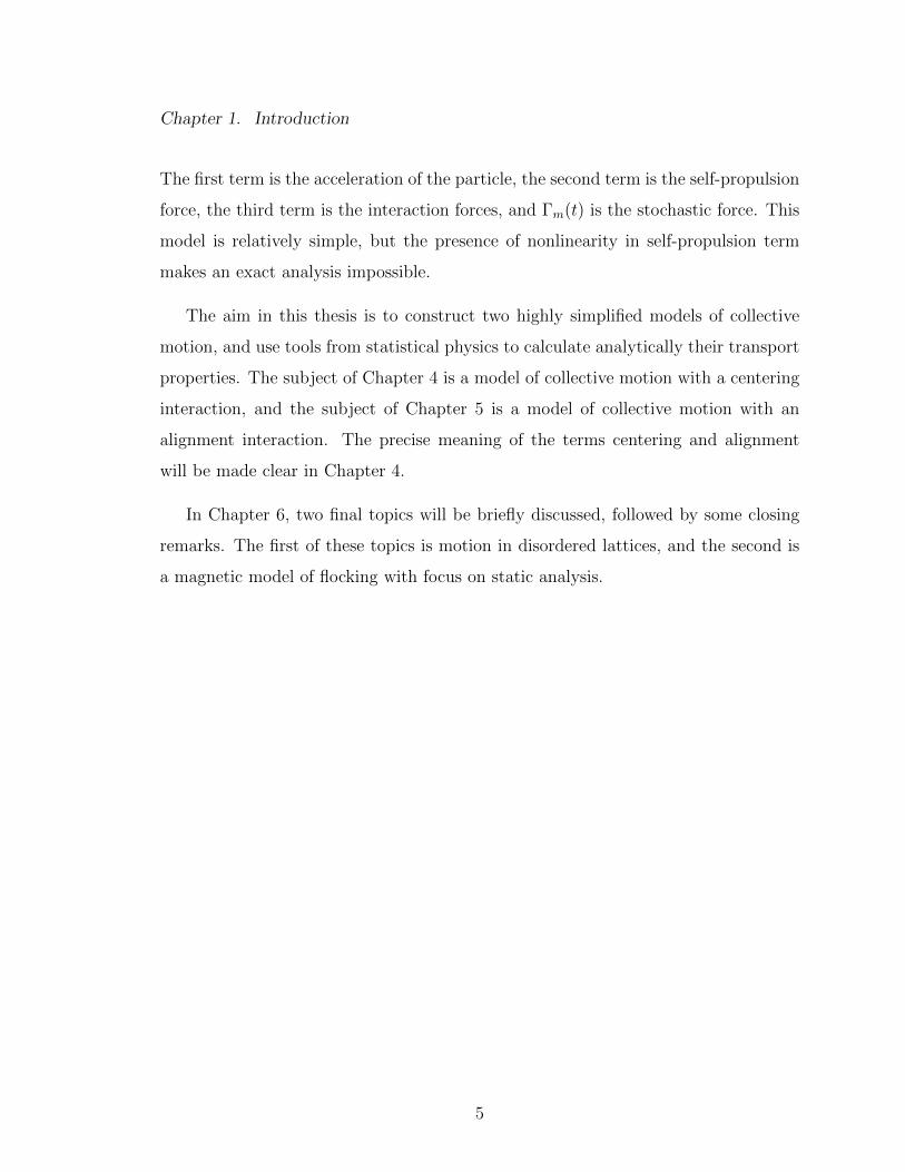
The first term is the acceleration of the particle, the second term is the self-propulsion
force, the third term is the interaction forces, and Γm(t) is the stochastic force. This
model is relatively simple, but the presence of nonlinearity in self-propulsion term
makes an exact analysis impossible.
The aim in this thesis is to construct two highly simplified models of collective
motion, and use tools from statistical physics to calculate analytically their transport
properties. The subject of Chapter 4 is a model of collective motion with a centering
interaction, and the subject of Chapter 5 is a model of collective motion with an
alignment interaction. The precise meaning of the terms centering and alignment
will be made clear in Chapter 4.
In Chapter 6, two final topics will be briefly discussed, followed by some closing
remarks. The first of these topics is motion in disordered lattices, and the second is
a magnetic model of flocking with focus on static analysis.
5

Chapter 2
Review of Some Existing
Formalisms of Quantum Transport
2.1 Introduction
In this chapter several existing formalisms which have been used in the literature
to study electronic quantum transport will be reviewed, beginning with the trans-
mission formalism developed by Landauer [25–27] and others [28–30] (for a textbook
introduction to the subject, see ref. [31]). Landauer’s first paper on the subject was
published in 1957, but the connection between transmission and conductance was not
well understood until further publications in the 1970s and 1980s. Here we will first
show the derivation of the well known expressions for the current in one-dimensional
(1D) and quasi-1D ballistic conductors and obtain the relationship between conduc-
tance and transmission for a 1D conductor with elastic scattering. We then show
how the transmission can be calculated from the single-particle Green’s function and
explain the connection to the non-equilibrium Green’s function formalism.
Next we will discuss a formalism based on quantum quasi-distribution functions
known as Wigner functions [32], emphasizing their similarity to classical distribution
6

Chapter 2. Review of Some Existing Formalisms of Quantum Transport
functions. Although Wigner first introduced the functions in 1932, it was not until
the 1980s that authors began to apply Wigner functions to study quantum transport
in mesoscopic devices [33–37]. Here we will provide a brief description of Wigner
functions and their properties. Next, we calculate the conductance of a quasi-1D
ballistic conductor from the Wigner function and show the conductance obtained in
this fashion is equivalent to the Landauer result.
Thirdly, we review an approach for studying current flow of arbitrary degree of
coherence in scanning tunneling microscopes developed by Kenkre, Biscarini, and
Bustamante in the 1990s [38–43]. The basic formulas for the current will be derived
here, and it will be shown how partially coherent motion can be modeled with a
generalized Master equation.
Finally, we briefly discuss an approach developed by Lyo and Huang in the early
2000s which uses a formal solution to the Boltzmann equation for studying different
kinds of scattering [44–47].
2.2 Transmission Formalism
One intuitively expects the resistance of a device to depend on the ease with which
carriers may pass through the device. If it is difficult to move a carrier through the
device, for example due to the presence of scatterers, it is reasonable to expect a higher
resistance than if there were no scattering. For a device in which carriers are only
scattered elastically, this idea can be made more precise by introducing a quantity
called the transmission function. The transmission function T (E) is defined as the
probability that a carrier with energy E incident from one terminal will pass through
the conductor and reach the other terminal. The transmission formalism developed
by Landauer, Imry, and Buttiker and others indeed expresses the current, and thus
the conductance, in a simple way in terms of the transmission function [25–30].
7

Chapter 2. Review of Some Existing Formalisms of Quantum Transport
Several review articles [48–50] and books [29, 31, 51–53] are available on the
subject. We will follow here mainly the standard development as in Datta [31].
First, a 1D conductor in which the charge carriers are not scattered at all will be
considered. Surprisingly, the conductance G = 1/R is found to be finite. It will
be seen that this finite conductance is a result of the coupling to the contacts. The
result is then generalized to a two-dimensional conductor in which the carriers are
confined in the dimension perpendicular to current flow. Finally, formulae relating
transmission to conductance will be obtained in the 1D case.
2.2.1 1D Ballistic Conductor
Consider now the 1D conductor in which carriers move ballistically (without scat-
tering). The device must be connected to at least two reservoirs for current to flow
through it. Suppose that one end of the device is connected to a source reservoir
held at constant temperature T and electrochemical potential µS, and the other end
is connected to a drain reservoir held at temperature T and electrochemical potential
µD. We will take the source reservoir to be on the left of the device and the drain
reservoir to be on right of the device. The difference in electrochemical potentials is
related to the voltage difference φ by
µS − µD = qφ (2.1)
with q being the carrier charge. This difference in chemical potentials is responsible for
the injection of carriers into the device from the source reservoir and the corresponding
removal in the drain reservoir, causing a net flow of current. The conductor will never
reach electrochemical equilibrium with either of the reservoirs, but arguments can be
made about which states in the conductor are filled when a steady state is reached. It
is generally assumed that a rightward moving carrier may exit into the drain reservoir
without being reflected, and that similarly a leftward moving carrier may exit into the
source reservoir without reflection (see ref. [31] for example for discussion). Under
8

Chapter 2. Review of Some Existing Formalisms of Quantum Transport
this assumption, in the steady state, positive k (rightward moving) states must have
originated in the source reservoir, and are thus distributed according to the Fermi
function at chemical potential µS:
fS(E) =1
1 + e(E−µS)/(kT ). (2.2)
Similarly, in the steady state, all negative k (leftward moving) must have originated
in the drain reservoir and are distributed according to the Fermi function at electro-
chemical potential µD,
fD(E) =1
1 + e(E−µS)/(kT ). (2.3)
Knowing the steady state distribution of states in the conductor, the current may
now be calculated. The current carried by a single state with wavenumber k is two
(for spin) times the carrier charge q times the probability current j(k) carried by the
state:
i(k) = 2qj(k). (2.4)
The total current in the conductor is then the current carried by each k state times
the probability that the state is occupied, multiplied by the k-space density of states
ρk(k) and integrated over all k. There is no phase relationship between the carriers
originating in the source reservoir and carriers originating in the drain reservoir so
that leftward and rightward moving waves do not interfere with each other. This
allows us to simply add up the currents from the leftward and rightward moving
carriers. The total current carried by the positive k states is
I+ =
∫ ∞0
i(k)fS(E(k))ρk(k)dk = 2q
∫ ∞0
j(k)fS(E(k))ρk(k)dk (2.5)
with E(k) being the energy of a state with wavenumber k. Similarly, the current
carried by the negative k states is
I− = −∫ ∞
0
i(k)fD(E(k))ρk(k)dk = −2q
∫ ∞0
j(k)fD(E(k))ρk(k)dk (2.6)
9

Chapter 2. Review of Some Existing Formalisms of Quantum Transport
with a minus sign since the carriers are moving to the left. The net current is then
I = 2q
∫ ∞0
j(k)[fS(E(k))− fD(E(k))]ρk(k)dk. (2.7)
Let us now calculate the probability current j(k) and k-space density of states a
1D conductor. Instead of writing a Hamiltonian which explicitly includes a potential
due to interaction of the carriers with atoms in the lattice, we will take simply a 1D
effective mass Hamiltonian which treats the carriers as free particles,
H = E0 +p2
2m∗(2.8)
with E0 being the energy at the bottom of the band. The mass m∗ is not the carrier
mass; it is an effective mass which is related to the curvature at the bottom of the
band. In typical solids the band will not be parabolic, but this can still be used as
an approximation near the bottom of the band (i.e. when k is small).
The eigenfunctions of the effective mass Hamiltonian are
ψn(x) =eikmx√L
(2.9)
where
kn ≡2πm
L(2.10)
and with L being the length of the conductor and m being any integer. The corre-
sponding energy eigenvalues are
E(km) = E0 +h2k2
m
2m∗= E0 +
h2(2πm)2
2m∗L2. (2.11)
The probability current is given by [54]
j(km) =h
2m∗i
(ψ∗m
∂ψm∂x− ψm
∂ψ∗m∂x
)=hkmm∗L
. (2.12)
In the limit as L becomes large, the discrete set of k states becomes a continuum, and
sums over states m can be converted to integrals over k via the usual prescription∑m
→ L
2π
∫dk (2.13)
10
Chapter 2. Review of Some Existing Formalisms of Quantum Transport
so the k-space density of states is
ρk(k) =L
2π. (2.14)
Using these, the current becomes
I = 2qL
2π
h
m∗L
∫ ∞0
[fS(E(k))− fD(E(k))]kdk. (2.15)
This can be converted to an integral over energy using
dE
dk=h2k
m∗. (2.16)
The current is finally
I =2q
h
∫ ∞E0
[fS(E)− fD(E)]dE. (2.17)
In deriving this result, we have used a parabolic effective mass band; however, similar
calculations can be done for other systems. For example, if the conductor consists of
a 1D tight binding chain the result is the same, except the upper bound of the energy
integral becomes the upper band edge energy [53].
In the limit of zero temperature, the Fermi functions are step-like so states with
energies below the electrochemical potential are filled and states with energies above
µ are empty. Thus, if the electrochemical potentials µS and µD are below the energy
at the bottom of the band E0, then the reservoirs are unable to inject any electrons
into the conductor, and no current flows. If however the electrochemical potentials
are greater than E0, then we have
I =2q
h(µS − µD) =
2q2
hφ (2.18)
and thus the conductance is
G ≡ I
φ=
2q2
h≡ G0. (2.19)
The quantity G0 ≡ 2q2/h when q is taken to be the electron charge is sometimes
known as the “quantum of conductance” for reasons which will soon become clear.
11
Chapter 2. Review of Some Existing Formalisms of Quantum Transport
The numerical value of 1/G0 is approximately 12.9 kΩ and represents the minimum
possible resistance for a 1D conductor.
It should also be noted that in this limit, only carriers with energies between µS
and µD are responsible for current flow. Although leftward moving states are filled
below µD, their current flow is exactly canceled by filled rightward moving states
below µD.
Why is the resistance nonzero if the charge carriers move ballistically? A thorough
discussion and explanation of this point may be found in the literature. Authors such
as Imry [29] have pointed out that the resistance in fact depends on how the voltage
difference φ is measured. If the voltage difference is measured between two different
points inside the conductor, then it is found to be zero, and thus the resistance is also
zero. However, the resistance is nonzero if the voltage difference is measured between
two points in the source and drain reservoirs, as we have defined it to be. For this
reason, this resistance is sometimes known as the “contact resistance” since it arises
from coupling to the contacts. Although carriers may exit from the conductor into
the reservoirs without scattering, the reverse is not likely true [31]. The source and
drain reservoirs typically contain many more states than the conductor, and thus
some carriers in the reservoirs must be reflected back rather than entering into the
conductor, resulting in a finite resistance.
2.2.2 Mutli-Mode Ballistic Conductor
Next, consider a two-dimensional conductor in which carriers are confined in the
direction perpendicular to current flow. Coordinates will be labeled x and y, with x
measuring the coordinate along the direction of current flow and y being perpendicular
to x. We take an effective mass Hamiltonian of the form
H =p2x
2m∗+
p2y
2m∗+ V (y) (2.20)
12

Chapter 2. Review of Some Existing Formalisms of Quantum Transport
where V (y) is a potential which confines the carriers in the y direction. Again, we
treat the carriers as free particles with an effective mass m∗ rather than modeling the
interaction with the atomic lattice explicitly. In devices such as field effect transistors,
the strength of the confinement potential V (y), and thus the effective width of the
conductor, may be controlled through use of an electric field. The eigenfunctions are
of the form
ψm,n(x, y) =eikmx√Lφn(y) (2.21)
with again km ≡ 2πm/L for integer m, and φn(y) being eigenfunctions of the y part
of the Hamiltonian with eigenvalues En,[p2y
2m∗+ V (y)
]φn(y) = Enφn(y). (2.22)
The corresponding eigenvalues for the total eigenfunctions ψm,n are then
E(km, n) =h2k2
m
2m∗+ En. (2.23)
The energy levels are illustrated in Figure 2.1. Rather than one single parabolic
band, we now have one for each En. These are sometimes known as “sub-bands”,
“channels”, or “modes”.
The preceding calculation for the 1D conductor may now be repeated for each
mode. In the low temperature limit, every mode which is occupied contributes G0 to
the conductance, thus the total conductance becomes
G =2q2
hM = G0M (2.24)
where M is the integer number of occupied modes which participate in transport, i.e.
the number of modes for which En is less that µD. The separation between the sub-
band edges may be controlled by changing the strength of the confinement potential
V (y). If the source and drain electrochemical potentials are held constant, this then
changes the number of occupied modes M . The observed conductance thus jumps in
steps of G0 = 2q2/h. This is the origin of the term quantum of conductance.
13

Chapter 2. Review of Some Existing Formalisms of Quantum Transport
E k,n
k
Quasi-1D Conductor Energy Levels
Figure 2.1: Example energy diagram for a quasi-1D conductor with multiple sub-bands. Each line represents a single sub-band.
The same effect can be achieved as the strength of an external magnetic field is
varied. The mechanism for this is similar to the Shubnikov-de Haas effect [55]. In
the presence of a sufficiently strong magnetic field, the electron levels become Landau
levels with energies En = hωc(n+ 1
2
)where ωc is the cyclotron frequency. As the
strength of the field is increased (or decreased), the separation between successive
sub-bands increases (or decreases). If the chemical potential is held constant, this
causes depletion (or filling) of modes.
This is not a true quantization (as in the case of charge quantization, for example)
because the conductance may be less than G0M , for instance if there is scattering in
the conductor. This “quantization” has been observed experimentally in split gate
heterostructures [2–4].
14

Chapter 2. Review of Some Existing Formalisms of Quantum Transport
T (E)Source Lead Drain LeadSource µS Drain µD
Carrier Flow
Figure 2.2: Illustration of a how current may be driven through an elastic scatterer.The scatterer with transmission function T (E) is connected to two 1D ballistic sourceand drain leads. The leads are in turn connected to source and drain reservoirs heldrespectively at electrochemical potentials µS and µD.
2.2.3 Relation between Transmission and Conductance
We will now return to the 1D conductor in the presence of elastic scattering and
determine the relationship between the conductance G and the transmission function
T (E). We follow here again the standard development as given in ref. [31]. The
elastic scatterer is connected to two 1D ballistic leads, which in turn are connected
to reservoirs so that a current may be passed through the device as in Figure 2.2.
Charge carriers flow into the leads from source and drain reservoirs held at differing
electrochemical potentials µS and µD. Again, carriers are allowed to exit from the
leads into the source and drain without reflection.
In the source lead, there are:
• Rightward moving (positive k) carriers injected from the source reservoir
• Leftward moving (negative k) carriers which originated in the source reservoir
and were reflected in the conductor
• Leftward moving (negative k) carriers which originated in the drain reservoir
and were transmitted through the conductor
15

Chapter 2. Review of Some Existing Formalisms of Quantum Transport
Assuming again that the k states from source and drain have random phases and
thus do not interfere with each other, the total current in the source lead can be
written as the sum of the currents due to incident, reflected, and transmitted beams.
The total current carried in the incident beam II is then the current carried by each
state k, times the distribution of incoming states from the source fS(E(k)), times the
k-space density of states ρk(k) and integrated over all positive (rightward moving) k
states:
II = 2q
∫ ∞0
j(k)fS(E(k))ρk(k)dk (2.25)
where fS is again the Fermi function at electrochemical potential µS. Similarly, the
current in the source lead due to the reflected beam is
IR = −2q
∫ ∞0
j(k)R(E(k))fS(E(k))ρk(k)dk (2.26)
with a negative sign since the carriers are traveling to the left, and with R(E(k))
being the probability that a carrier with energy E(k) is reflected. The current in the
source lead due to transmitted carriers originating in the drain is
ID = −2q
∫ ∞0
j(k)T (E(k))fD(E(k))ρk(k)dk (2.27)
with fD(Ek) being again the Fermi distribution at the drain electrochemical potential
µD. Adding these, the total current in the source terminal is
I = II + IR + ID = 2q
∫ ∞0
j(k)[fS(E(k))− fD(E(k))]T (E(k))ρk(k)dk (2.28)
where we have used the fact that since the scattering is elastic R(E(k))+T (E(k)) = 1
(i.e. the carrier must be either transmitted through the conductor or reflected back;
it cannot be absorbed).
Using our earlier results for the probability current j(k) and the k-space density
of states ρk(k), and changing integration variables to E, we have finally
I =2q
h
∫ ∞E0
T (E)[fS(E)− fD(E)]dE. (2.29)
16

Chapter 2. Review of Some Existing Formalisms of Quantum Transport
In the limit of small bias, we can write
I =2q
h(µS − µD)
∫ ∞E0
T (E)
[−dfDdE
]dE (2.30)
Additionally, in the limit of low temperature, −dFD/dE ≈ δ(E − µD) and we have
approximately
I =2q
h(µS − µD)T (µD). (2.31)
The conductance is then
G =I
φ=
2q2
hT (µD) = G0T (µD). (2.32)
This formula relating the conductance to the transmission function is the simplest
version of what is known as the Landauer formula [26]. As expected, a higher trans-
mission means a higher conductance, with the ballistic result being recovered in the
limiting case T = 1.
In the case where there are multiple sub-bands, such as the two-dimensional con-
ductor discussed earlier, then the generalized version of the Landauer formula (when
potential difference is measured between the reservoirs) is
G = G0Tr(tt†) (2.33)
where t is the matrix of transmission amplitudes.
More generalizations may be displayed, in particular there is a formula for mul-
tiple terminals derived in ref. [28]. Phase breaking scattering processes can then be
incorporated into the theory by introducing a “scattering” terminal which removes
electrons and reinjects them with different energies. The transmission formalism has
been successfully applied in the literature to understand conductance in mesoscopic
semiconductors. In the following chapter, the transmission formalism will be applied
to calculate the conductance for various kinds of elastic scatterers.
17

Chapter 2. Review of Some Existing Formalisms of Quantum Transport
2.2.4 Transmission and the Green’s Function
So far we have not yet discussed how the transmission function T (E) can be calcu-
lated. One simple method, oft found in quantum mechanics textbooks (see ref. [54]),
is to take an incoming wave of the form eikx to the left of the scatterer, a reflected
wave re−ikx to the left of the scatterer, and a transmitted wave teikx to the right of
the scatterer. The amplitudes r and t are then calculated by matching the wavefunc-
tion at the boundaries of the scatterer so that the Schrodinger equation is everywhere
satisfied. If the group velocities are the same on either side of the scatterer, the
transmission and reflection functions are R = |r|2 and T = |t|2.
In certain cases, it may be more convenient to calculate the transmission function
from the single-particle Green’s function. The Green’s function is defined as [56]
G(E) ≡ 1
E −H. (2.34)
It can be shown that only the part of the Green’s function for the conductor subsys-
tem (i.e. the elements 〈m|G(E)|n〉 where |m〉, |n〉 are conductor states) is needed to
calculate the transmission function. The effect of the coupling to reservoirs may be
incorporated into the conductor Green’s function by introducing a complex energy
dependent function Σ(E) known as the self energy. This may be done as follows
[56]. Suppose for now that only one contact is connected to the conductor. Divid-
ing the Hilbert space into conductor and reservoir subspaces and writing the total
Hamiltonian for the total system as a block matrix gives
H =
HR τ †
τ Hc
(2.35)
where HR and Hc are respectively the Hamiltonians for the isolated reservoir and con-
ductor and τ represents the coupling between reservoir and conductor. The Green’s
function obeys (E −H)G = 1, so as block matrices,E −HR −τ †
−τ E −Hc
GRR GRc
GcR Gcc
=
1 0
0 1
. (2.36)
18

Chapter 2. Review of Some Existing Formalisms of Quantum Transport
Multiplying the two block matrices on the left hand side,
(E −HR)GRR + τ †GcR = 1 (2.37)
(E −HR)GRc + τ †Gcc = 0 (2.38)
τGRR + (E −Hc)GcR = 0 (2.39)
τGRc + (E −Hc)Gcc = 1 (2.40)
If we are only interested in the part of the Green’s function for the conductor subspace,
Gcc, we can combine the second equation with the fourth equation to write
Gcc(E) =1
E −Hc − Σ(E)(2.41)
with the self energy Σ(E) given by1
Σ(E) = τGRτ† (2.42)
where GR is the Green’s function for the isolated reservoir, GR = [E −HR]−1. In the
case where multiple terminals are connected, it may be shown that the resulting self
energies add, provided that the leads do not interact with each other.
The transmission function T (E) may be expressed in terms of the conductor
Green’s function, even when there are multiple terminals and multiple channels per
lead. The details of the derivation may be found in textbooks such as [31, 56]. For
the special case of two terminals, the result is
T (E) = TrΓSGΓDG† (2.43)
where the trace runs over conductor states and the quantities Γ are related to the self
energies by
Γ(E) ≡ i[Σ(E)− Σ†(E)]. (2.44)
1When H has a continuous spectrum, G has a branch cut along the real axis and musttherefore be defined through a limiting process. In these expressions, G(E) should be takento mean G+(E) ≡ limη→0+ G(E + iη) [56].
19

Chapter 2. Review of Some Existing Formalisms of Quantum Transport
This is sometimes known as the Fisher-Lee relation [57].
In addition to providing another way to calculate the transmission function, this
relation also connects the transmission theory to the non-equilibrium Green’s function
(NEGF) formalism. The NEGF approach, developed by Keldysh [58], Kadanoff and
Baym [59], and others, is completely equivalent to the transmission theory when the
motion is coherent. However, rather than incorporating incoherent scattering effects
phenomenologically as in the Landauer-Buttiker theory, scattering can be modeled
microscopically. Scattering is introduced into the Green’s function through additional
self energy terms Σ. As the Green’s function depends on the self energies, these self
energy terms typically will depend on the Green’s function itself. This necessitates
an iterative procedure whereby a self-consistent solution can be arrived at.
2.3 Wigner Function Approach
Although the transmission theory and the NEGF formalism have been successfully
used in the literature, they are quite different from the classical theory of conduc-
tance based on the kinetic Boltzmann equation. Some authors have used so called
Wigner functions to study quantum transport because of certain similarities to clas-
sical transport theory. A Wigner function, first introduced by Eugene Wigner in 1932
[32], like the classical probability distribution, is a quantity defined on phase space,
yet it completely describes the quantum state of the system. It obeys an equation
of motion which is similar to the semi-classical Boltzmann transport equation, and
observables are calculated in a similar manner.
Many review and tutorial articles are available in the literature, see refs. [60–64]
and references therein. We follow here a similar development as in ref. [64].
In classical transport theory, the state of a system can be described by a distribu-
tion function f(x,p, t) defined on phase space which describes the density of particles
20

Chapter 2. Review of Some Existing Formalisms of Quantum Transport
with position x and momentum p at time t. The time evolution of the distribution
function f is governed by the Boltzmann equation [65],
∂f
∂t+
p
m· ∇rf + F · ∇pf =
(∂f
∂t
)coll
(2.45)
where the term on the right hand side accounts for the change in the distribution
function due to collisions. To find the expectation value of an observable quantity
O(x,p), the distribution function is multiplied by the observable and integrated over
all phase space,
〈O〉 =
∫ ∫O(x,p)f(x,p, t)dxdp. (2.46)
In a quantum system, because of the uncertainty principle, the momentum and
position of a particle cannot be simultaneously specified, and the semi-classical dis-
tribution function f cannot be used. Instead, for a quantum mechanical system in
a statistical mixture of states, the density operator ρ is used to describe the com-
plete state of the system. The density operator may be defined as (see any standard
quantum mechanics textbook, e.g. [54])
ρ =∑m
pm|ψm〉〈ψm| (2.47)
where pm is the statistical weight to find the system in state |ψm〉. In the Schrodinger
picture, states evolve as
|ψ(t)〉 = e−iHt/h|ψ(0)〉, (2.48)
so the density matrix evolves as
ρ(t) =∑m
pme−iHt/h|ψm(0)〉〈ψm(0)|e+iHt/h. (2.49)
Taking a time derivative, we have
∂ρ
∂t=∑m
pm
(H
ih|ψm(t)〉〈ψm(t)| − |ψm(t)〉〈ψm(t)|H
ih
). (2.50)
21

Chapter 2. Review of Some Existing Formalisms of Quantum Transport
The density operator thus obeys
∂ρ
∂t=
1
ih[H, ρ]. (2.51)
This is the quantum mechanical analogue of the Liouville equation and is known as
the von Neumann equation or Liouville-von Neumann equation.
For a system in a pure quantum mechanical state |ψ〉, the expectation value of
an observable O is given by 〈O〉 = 〈ψ|O|ψ〉. When in a statistical mixture of states,
the expectation value is averaged over possible states, weighted by the statistical
probability to be in each state,
〈O〉 =∑m
pm〈ψm|O|ψm〉. (2.52)
Inserting a complete set of states, (assuming the |ψm〉 are normalized so that
〈ψm|ψn〉 = δmn), we have
〈O〉 =∑n,m
pm〈ψm|O|ψn〉〈ψn|ψm〉 =∑n,m
pn〈ψm|O|ψn〉〈ψn|ψm〉 (2.53)
where pn has been substituted for pm, which is valid since the only nonzero terms in
the double sum have m = n. Using the definition for the density operator, this is just
〈O〉 =∑m
〈ψm|Oρ|ψm〉 ≡ TrOρ (2.54)
where Tr denotes the trace.
The statements made thus far apply in any representation. If we have a set of
position states, |x〉, such that
〈x|x′〉 = δ(x− x′) (2.55)
and for any state |ψ(t)〉,
〈x|ψ(t)〉 = ψ(x, t), (2.56)
22

Chapter 2. Review of Some Existing Formalisms of Quantum Transport
the density operator may then be defined as a function of two position variables (and
time) via
ρ(x,x′, t) ≡ 〈x′|ρ|x〉 =∑m
pmψ∗m(x, t)ψm(x′, t). (2.57)
The Wigner function in d dimensions is defined by changing to mean and relative
coordinates, and Fourier transforming on the relative coordinate,
W (x,p, t) ≡ 1
(πh)d
∫ρ(x + y,x− y, t)e2i(p·y)/hddy. (2.58)
To derive the evolution equation for the Wigner function, the von Neumann equa-
tion in the position representation will first be written and then transformed to obtain
the evolution equation for the Wigner function. Using equation (2.57), the von Neu-
mann equation becomes
ih∂
∂tρ(x,x′, t) =
∑m
pm
[ihψm(x′, t)
∂
∂tψ∗m(x, t) + ihψ∗m(x, t)
∂
∂tψm(x′, t)
].
(2.59)
For a Hamiltonian of the form H = p2/(2m) + V (x), the Schrodinger equation and
its complex conjugate can be used to rewrite this as
ih∂
∂tρ(x,x′, t) =
∑m
pm
[(h2
2m∇2
x − V (x)
)+
(−h2
2m∇2
x′ + V (x′)
)]ψ∗m(x, t)ψm(x′, t). (2.60)
Again using equation (2.57), the von Neumann equation in the position representation
is
ih∂
∂tρ(x,x′, t) =
[− h2
2m∇2
x′ +h2
2m∇2
x + V (x′)− V (x)
]ρ(x,x′, t). (2.61)
Changing to centered and relative coordinates, this is
ih∂
∂tρ(x + y,x− y, t) =
[h2
2m∇x · ∇y + V (x− y)
− V (x + y)
]ρ(x + y,x− y, t) (2.62)
23

Chapter 2. Review of Some Existing Formalisms of Quantum Transport
Fourier transforming, integrating the first term by parts and using the convolution
theorem for the second term, the evolution of the Wigner function is finally given by
∂W
∂t= − p
m· ∇xW (x,p, t) +
∫χ(x,p− p′)W (x,p′, t)ddp′ (2.63)
with χ given by
χ(x,p) ≡ 1
ih
1
(πh)d
∫[V (x− y)− V (x + y)]e2ip·y/hddy. (2.64)
This equation, known sometimes as Moyal’s evolution equation [66], is superficially
similar to the Boltzmann equation (2.45), except now with a term which is nonlocal
in momentum space. Again, since all transforms are invertible, this is completely
equivalent to the fully quantum von Neumann equation, thus this equation completely
describes the evolution of the quantum system. Additional terms may be added to
account for incoherent scattering effects.
Next, it will be shown how the expectation value of any observable can be calcu-
lated. Starting from (2.54), and taking the trace over position states,
〈O〉 = TrOρ =
∫〈x|Oρ|x〉ddx. (2.65)
Inserting a complete set of position states,
〈O〉 =
∫ ∫〈x|O|x′〉〈x′|ρ|x〉ddxddx′. (2.66)
Next, changing to centered and relative coordinates,
〈O〉 = 2d∫ ∫
〈x + y|O|x− y〉〈x− y|ρ|x + y〉ddxddy. (2.67)
Using the properties of Fourier transforms, this can be rewritten as
〈O〉 =
∫ ∫O(x,p)W (x,p, t)ddxddp (2.68)
where O is said to be the Wigner-Weyl transform of the operator O, defined by
O(x,p) ≡ 2d∫〈x− y|O|x + y〉e2ip·y/hddy. (2.69)
24

Chapter 2. Review of Some Existing Formalisms of Quantum Transport
Equation (2.68) is analogous to the classical expression (2.46) used for calculating
observables.
To apply the Wigner function formalism to quantum transport, one must solve
equation (2.63) subject to appropriate boundary conditions. In [51] the problems of
specifying the correct boundary conditions are discussed, and it is suggested that an
appropriate method is to extend the domain of the problem far from the source of
quantum effects (i.e. into the reservoirs) so that a semi-classical distribution may be
used at the boundaries. In the literature, the Wigner function formalism has been
successfully applied by a few authors to simple systems, such as the 1D resonant
tunneling diode (RTD), in particular see [33–37].
Next, the equivalence of the Landauer transmission theory and the Wigner func-
tion theory for the two-dimensional ballistic conductor discussed earlier will be demon-
strated. Instead of solving (2.63) directly, the steady-state Wigner function can be
found from the steady-state density matrix. Knowing the Wigner function, the cur-
rent can then be calculated using (2.68). The result is equivalent to the Landauer
result.
Starting with the same effective mass Hamiltonian,
H =p2x
2m∗+
p2y
2m∗+ V (y) (2.70)
recall that the rightward moving k states are filled according to the source distribution
function, and leftward moving k states are filled according to the drain distribution
function. The steady state density matrix in the position representation is then
ρ(x,x′) =1
2π
∑n
∫ ∞0
fS(Ekx,n)φ∗n(y)φn(y′)e−ikx(x−x′)dkx
+1
2π
∑n
∫ 0
−∞fD(Ekx,n)φ∗n(y)φn(y′)e−ikx(x−x′)dkx (2.71)
with Ekx,n = h2k2/(2m∗) + En being the energy eigenvalue associated with a state
ψkx,n(x, y) =eikx√Lφn(y) (2.72)
25

Chapter 2. Review of Some Existing Formalisms of Quantum Transport
with φn(y) an eigenfunction of the y part of the Hamiltonian with eigenvalue En.
Changing coordinates, this becomes
ρ(x + u,x− u) =1
2π
∑n
∫ ∞0
fS(Ekx,n)φ∗n(y + uy)φn(y − uy)e−2ikxuxdkx
+1
2π
∑n
∫ 0
−∞fD(Ekx,n)φ∗n(y + uy)φn(y − uy)e−2ikxuxdkx.
(2.73)
Fourier transforming, the Wigner function in the steady state is
W (x,p) =1
h
∑n
[fS(Epx/h,n)Θ(px) + fD(Epx/h,n)Θ(−px)
]Wn(y, py) (2.74)
where Θ is the Heaviside step function and Wn is the Wigner function associated with
the nth eigenfunction of the y Hamiltonian φn(y),
Wn(y, py) ≡1
πh
∫φ∗n(y + uy)φn(y − uy)e2ipyuy/hduy. (2.75)
The current operator is
I =2q
m∗Lpx, (2.76)
and its Wigner-Weyl transform is
I(x,p) = hδ(py)2q
m∗Lpx. (2.77)
We then have for the current
〈I〉 =2q
m∗h
∑n
∫ ∞0
[fS(Epx,n)− fD(Epx,n)]pxdpx. (2.78)
Converting to an integral over energy gives
〈I〉 =2q
h
∑n
∫ ∞En
[fS(E)− fD(E)]dE . (2.79)
In the low temperature, low bias limit, this reduces to the Landauer result,
〈I〉 =2q
h(µS − µD)M. (2.80)
26

Chapter 2. Review of Some Existing Formalisms of Quantum Transport
Although the current depends only on the number of occupied sub-bands at a
particular energy, not the specific form of the y part of the Wigner function, we
display here the Wigner functions Wn(y, py) for the two most commonly used types
of confinement: square well and harmonic.
2.3.1 Wigner Functions for Infinite Square Well Confinement
For the infinite square well the potential is
V (y) =
0 if 0 < y < Ly
∞ otherwise(2.81)
and the eigenfunctions are
φn(y) =
√
2Ly
sin(nπLyy)
if 0 < y < Ly
0 otherwise
(2.82)
with energies
En =h2π2
2m∗L2y
n2. (2.83)
The associated Wigner functions are [67]
Wn(y, py) =
(2
πhLy
)sin[2(py/h− nπ/Ly)y]
4(py/h− nπ/Ly)+
sin[2(py/h+ nπ/Ly)y]
4(py/h+ nπ/Ly)
− cos
(2nπy
Ly
)sin(2pyy/h)
(2py/h)
(2.84)
for y < Ly/2 and Wn(y, py) = Wn(Ly − y, py) for y > Ly/2. The functions Wn(y, py)
are plotted for n = 1 through n = 4 in Figure (2.3).
2.3.2 Wigner Functions for Harmonic Confinement
For harmonic confinement, we have for the potential
V (y) =1
2m∗ω2y2 (2.85)
27

Chapter 2. Review of Some Existing Formalisms of Quantum Transport
and the eigenfunctions are [54]
φn(y) =
(m∗ω
πh
)1/41√2nn!
Hn
(√m∗ω
hy
)e−mωy
2/2h2
(2.86)
where Hn is the nth Hermite polynomial. The energies are
En =
(n+
1
2
)hω. (2.87)
The corresponding Wigner functions are [61]
Wn(y, py) =2
h(−1)ne−2H(y,py)/hωLn
(4H(y, py)
hω
)(2.88)
where Ln is the nth Laguerre polynomial and
H(y, py) ≡p2y
2m∗+
1
2m∗ω2y2. (2.89)
Explicitly, the first few are
W0(y, py) = +2
he−2H(y,py)/hω, (2.90)
W1(y, py) = −2
he−2H(y,py)/hω
[−4H(y, py)
hω+ 1
], (2.91)
W2(y, py) = +2
he−2H(y,py)/hω
[1
2
(4H(y, py)
hω
)2
− 2
(4H(y, py)
hω
)+ 1
]. (2.92)
The functions Wn(y, py) are plotted for n = 0 through n = 3 in Figure (2.4).
2.4 Kenkre, Biscarini, Bustamante Scanning Tun-
neling Microscope Formalism
Motivated by a desire to understand partially coherent transport in scanning tunnel-
ing microscope (STM) junctions in a simple fashion, Kenkre, Biscarini, and Busta-
mante formulated a theory of quantum transport using generalized Master equations
28

Chapter 2. Review of Some Existing Formalisms of Quantum Transport
(GMEs) to study transport of with an arbitrary degree of coherence [38–43]. Scatter-
ing effects are not modeled microscopically; they are instead introduced phenomeno-
logically through the use of stochastic Liouville equations (SLEs). One advantage of
this approach is that one can make use of several exact solutions to SLEs that have
already been published in the literature (see for example refs. [68–70]).
2.4.1 Derivation of Formulae for Calculating Current
The current will be calculated here for the simplest case, following the same procedure
as described in detail in ref. [41], but relaxing the assumption that there is no transient
net buildup of charge in the conductor. Suppose we have a conductor which consists of
a discrete set of states with labels m. When the conductor is isolated (not connected
to any contacts), suppose that the probabilities obey a generalized Master equation
(GME), i.e.
∂Pm∂t
= −∑n
∫ t
0
Amn(t− t′)Pn(t′)dt′. (2.93)
Later in this section, it will be shown how a GME may be used to model coherent
(quantum mechanical) motion, incoherent (classical) motion, and partially coherent
motion.
Next, suppose that only a single state m = S is connected to a source reservoir
and a single state m = D is connected to a drain reservoir. The source and drain will
be assumed to be held at equal temperatures, but differing electrochemical potentials
µS and µD. This results in a flow of probability into the source state at a rate which
will be denoted RS(t), and a removal of probability from drain state at a rate RD(t).
In the steady state, there should be no accumulation of charge, thus RS(t) = RD(t)
at long times. The steady state current is then the carrier charge q times the number
of carriers nc times the probability flux out of the conductor,
I(t) = qncRD(t) = qncRS(t). (2.94)
29

Chapter 2. Review of Some Existing Formalisms of Quantum Transport
When the conductor is connected to source and drain terminals, the generalized
Master equation for the open system becomes
dPmdt
= −∑n
∫ t
0
Amn(t− t′)Pn(t′)dt′ + δm,SRS(t)− δm,DRD(t). (2.95)
Laplace transforming, this is
εPm(ε)− Pm(0) = −∑n
Amn(ε)Pn(ε) + δm,SRS(ε)− δm,DRD(ε) (2.96)
where the Laplace transform of a function f is
f(ε) ≡ Lεf(t) ≡∫ ∞
0
f(t)e−εtdt. (2.97)
The solution is
Pm(ε) = ηm(ε) + ΠmS(ε)RS(ε)− ΠmD(ε)RD(ε) (2.98)
where ηm is the solution to the Master equation for the isolated conductor,
ηm(ε) =∑n
Πmn(ε)Pn(0). (2.99)
The Πs are the propagators of the isolated conductor, i.e. Πmn(t) is the probability of
finding the particle at state m at time t given that it began at state n. The Laplace
transformed propagators Πmn(ε) are given in terms of the rates Amn(ε) through the
matrix equation
Π(ε) = [εI + A(ε)]−1. (2.100)
To proceed, the form that the rates RS and RD should take must now be deter-
mined. The rates must depend on the probabilities in some way, since for example
if the conductor were in equilibrium with only the source (or drain), then RS (or
RD) should vanish. Ideally, this dependence on the probabilities should be linear.
The interaction with the reservoir should attempt to drive the state connected to the
30

Chapter 2. Review of Some Existing Formalisms of Quantum Transport
reservoir to its thermal value. Thus, it is reasonable to assume that the rates should
take the simple form
RS(t) =P thS − PS(t)
τS, (2.101)
RD(t) = −PthD − PD(t)
τD. (2.102)
Here P thS is the probability to find a carrier at the source state S if the conductor
were in equilibrium with the source reservoir alone. P thD is similarly defined; it is the
probability to find a carrier at the drain state D if the conductor were in equilibrium
with only the drain reservoir. τS and τD are constants with the dimensions of time
which describe respectively the strength of the coupling to the source and drain
reservoirs, with a smaller τ meaning a stronger coupling.
Returning to (2.98) and writing out explicitly the equations for m = S and m = D
gives
PS(ε) = ηS(ε) + ΠSS(ε)RS(ε)− ΠSD(ε)RD(ε), (2.103)
PD(ε) = ηD(ε) + ΠDS(ε)RS(ε)− ΠDD(ε)RD(ε). (2.104)
Equations (2.101) and (2.102) may now be used to eliminate PS and PD in favor of
RS and RD, giving
P thS /ε− τSRS(ε) = ηS(ε) + ΠSS(ε)RS(ε)− ΠSD(ε)RD(ε), (2.105)
P thD /ε+ τDRD(ε) = ηD(ε) + ΠDS(ε)RS(ε)− ΠDD(ε)RD(ε). (2.106)
This is now a set of two coupled equations in two unknowns, the rates RS and RD,
which we may be easily solved. After some rearrangement,
−(ΠSS(ε) + τS)RS(ε) + ΠSD(ε)RD(ε) = [ηS(ε)− P thS /ε], (2.107)
−ΠDS(ε)RS(ε) + (ΠDD(ε) + τD)RD(ε) = [ηD(ε)− P thD /ε]. (2.108)
Using Cramer’s rule to solve this system gives the rates explicitly in the Laplace
31
Chapter 2. Review of Some Existing Formalisms of Quantum Transport
domain,
RS(ε) =[ηD(ε)− P th
D /ε][ΠSD(ε)]− [ηS(ε)− P thS /ε][ΠDD(ε) + τD]
[ΠDD(ε) + τD][ΠSS(ε) + τS]− ΠSD(ε)ΠDS(ε), (2.109)
RD(ε) =[ηD(ε)− P th
D /ε][ΠSS(ε) + τS]− [ηS(ε)− P thS /ε][ΠDS(ε)]
[ΠDD(ε) + τD][ΠSS(ε) + τS]− ΠSD(ε)ΠDS(ε). (2.110)
The steady state current may now be obtained using the final value theorem for
Laplace transforms,
limt→∞
f(t) = limε→0
εf(ε). (2.111)
For RS we have
RS(∞) = limε→0
[εηD(ε)− P thD ][εΠSD(ε)]− [εηS(ε)− P th
S ][εΠDD(ε) + ετD]
ε[ΠDD(ε) + τD][ΠSS(ε) + τS]− εΠSD(ε)ΠDS(ε)(2.112)
where we have multiplied top and bottom by ε.
If the conductor were isolated, we should expect it to reach the same final state
regardless of whatever the initial condition is. Using the same notation as (ref), let
ηthm = limt→∞ ηm(t) = limε→0 εηm(ε) be the probability to find a particle at state m at
long times in the isolated conductor. We may then write
limε→0
εΠmn(ε) = ηthm , (2.113)
again since the final state is independent of initial condition. This should hold pro-
vided that any state m may be reached from any other state n (i.e. there are no
states or sets of states which are totally cut off from the rest of the conductor). Using
this, we have in the numerator
limε→0
[εηD(ε)− P thD ][εΠSD(ε)]− [εηS(ε)− P th
S ][εΠDD(ε) + ετD]
=[ηthD − P th
D ]ηthS − [ηth
S − P thS ]ηth
D
=ηthDP
thS − ηth
S PthD (2.114)
32

Chapter 2. Review of Some Existing Formalisms of Quantum Transport
In the denominator we have
limε→0
ε[ΠDD(ε) + τD][ΠSS(ε) + τS]− εΠSD(ε)ΠDS(ε)
= limε→0
εΠDD(ε)ΠSS(ε)− εΠSD(ε)ΠDS(ε) + ετDΠSS(ε) + ετSΠDD(ε) + ετDτS
= limε→0
εΠDD(ε)ΠSS(ε)− εΠSD(ε)ΠDS(ε) + τDηthS + τSη
thD . (2.115)
We must proceed with care here since the Laplace transformed propagators have poles
at the origin in the complex ε plane, as a consequence of probability conservation in
the isolated conductor. However, due to the preceding argument, we know that the
residue of Πmn at zero is just the thermal value ηthm . Thus writing ΠDD as
ΠDD(ε) = [ΠDD(ε)− ηthD /ε] + ηth
D /ε (2.116)
and similarly for ΠSS, gives
εΠDD(ε)ΠSS(ε) = ε[ΠDD(ε)− ηthD /ε][ΠSS(ε)− ηth
S /ε] + ηthD [ΠSS(ε)− ηth
S /ε]
+ ηthS [ΠDD(ε)− ηth
D /ε] + ηthD η
thS /ε. (2.117)
Similarly, we have also
εΠDS(ε)ΠSD(ε) = ε[ΠDS(ε)− ηthD /ε][ΠSD(ε)− ηth
S /ε] + ηthD [ΠSD(ε)− ηth
S /ε]
+ ηthS [ΠDS(ε)− ηth
D /ε] + ηthD η
thS /ε. (2.118)
Subtracting the two yields
εΠDD(ε)ΠSS(ε)− εΠDS(ε)ΠSD(ε) = ε[ΠDD(ε)− ηthD /ε][ΠSS(ε)− ηth
S /ε]
− ε[ΠDS(ε)− ηthD /ε][ΠSD(ε)− ηth
S /ε] + ηthD [ΠSS(ε)− ΠSD(ε)]
+ ηthS [ΠDD(ε)− ΠDS(ε)]. (2.119)
The limit ε→ 0 may now be taken. The first term (and similarly the second term) on
the right hand side vanishes in the limit since neither ΠDD(ε)−ηthD /ε nor ΠDD(ε)−ηth
D /ε
have poles at zero (we have subtracted them out). The third and fourth terms may
appear infinite since the Π’s have poles at zero; however, ΠSS and ΠSD have the same
33

Chapter 2. Review of Some Existing Formalisms of Quantum Transport
residue at zero (ηthS ), thus the difference is finite in the limit. Similarly, the fourth
term also remains finite, and we have
limε→0
ε[ΠDD(ε) + τD][ΠSS(ε) + τS]− εΠSD(ε)ΠDS(ε)
= ηthD [ΠSS(0)− ΠSD(0) + τS] + ηth
S [ΠDD(0)− ΠDS(0) + τD]. (2.120)
Finally, we have for the steady state rate
RS(∞) =ηthDP
thS − ηth
S PthD
ηthD [ΠSS(0)− ΠSD(0) + τS] + ηth
S [ΠDD(0)− ΠDS(0) + τD]. (2.121)
A similar calculation for RD shows that indeed in the steady state RD = RS, as
expected. The differences of propagators in the denominator may also be rewritten
in terms of time integrals using the fact that from the definition of the Laplace
transform
f(0) =
∫ ∞0
f(t)dt. (2.122)
The result (2.121) differs slightly from the result obtained by Kenkre, Biscarini, and
Bustamante in ref. [41] due to the face that here it was not assumed that RS(t) =
RD(t) for all times. In situations where the source and drain are coupled not to a single
state each, but to multiple states, Kenkre, Biscarini, and Bustamante also obtain
approximate expressions in terms of averages of probability propagators. Details may
be found in ref. [41].
Although this approach may be used for incoherent or partially coherent motion,
we found that it does not reproduce the Landauer result in the fully coherent limit.
The reason appears to be the fact that level broadening of the conductor states due
to the coupling to the contacts has not been included in the STM theory. Such a
possibility is pointed out in ref. [53]. We follow closely that argument in the following.
Consider a conductor which consists only of a single state with energy E0. This
single state is connected to both the source and drain reservoirs. The Master equation
for the evolution of the probability P to find an electron in the conductor is then
dP
dt=P thS − Pτ
+P thD − Pτ
(2.123)
34

Chapter 2. Review of Some Existing Formalisms of Quantum Transport
where for simplicity, the time constants have been set equal, τS = τD = τ . In the
steady state, the probability to find an electron in the conductor is simply the average
of the source and drain thermal probabilities,
P =P thS + P th
D
2, (2.124)
and the rate at which probability flows out of (and into) the conductor is
RD = RS =P thS − P th
D
2τ. (2.125)
From this expression, is appears that an arbitrarily large amount of current could be
passed through the device; however, we have seen earlier that there is a maximum
amount of current that may be passed through a 1D conductor, Imax = V G0.
To see how level broadening can decrease the amount of current that can be passed
through the device, consider the zero temperature limit. In this case P thS is zero if
the energy of the conductor state E0 is above the source chemical potential µS and
one if E0 is below µS. Similarly P thD is zero for E0 > µD and one if E0 < µD. Thus
if E0 is below both the source and drain chemical potentials, both reservoirs try to
inject electrons into the conductor, and no net current flows. Similarly, if E0 is larger
than both source and drain potentials, then no current flows since neither reservoir
has electrons with high enough energies to enter into the conductor.
Is is only when the energy of the conductor state is between source and drain
potentials, µD < E0 < µS, that net current flows. However, the stronger the conductor
is coupled to the contacts, the broader its energy level becomes, part of which leaks
out from between µD and µS, thus decreasing the amount of current that flows.
This problem also arises in other coherent conductors (this is discussed briefly for
a two site conductor in ref. [39]) where the current is proportional to 1/τ . Although
broadening effects can be incorporated into the one level conductor, it remains un-
clear, at least to us at the moment, how they can be included in a Master equation
approach with many sites or energy levels. This remains an issue in the STM for-
malism for perfectly coherent motion; however, in the presence of sufficiently strong
35

Chapter 2. Review of Some Existing Formalisms of Quantum Transport
scattering or phase breaking processes, the contribution to the resistance due to the
coupling to the contacts is typically small and the formulae would become valid.
2.4.2 Generalized Master Equation for Modeling Partially
Coherent Motion
We will now discuss briefly how a generalized Master equation can be used to model
coherent and partially coherent motion following the analyses of Kenkre [68, 71, 72].
We will begin with a discussion of stochastic Liouville equations (SLEs) and show
[73] how they can be converted into generalized Master equations via a projection
technique.
As discussed earlier, the state of a quantum system is described by the density ma-
trix ρ, which obeys the quantum version of the Liouville equation, the von Neumann
equation,
ih∂ρ
∂t= [H, ρ]. (2.126)
The diagonal elements ρmm ≡ 〈m|ρ|m〉 represent the probabilities to find the system
in a state |m〉. The off diagonal elements of the density matrix ρmn arise when the
system is in a quantum superposition of states and are related to the relative phases.
To illustrate this, consider a two state system consisting of states |1〉 and |2〉.
If an ensemble is prepared in such a way that each member has statistical prob-
ability 1/2 to be in state |1〉 and probability 1/2 to be in state |2〉, then the density
matrix is
ρ =1
2|1〉〈1|+ 1
2|2〉〈2| (2.127)
If however, the ensemble is prepared so that each member has probability one to
be in a quantum superposition of states |1〉 and |2〉 given by
|+〉 =|1〉+ |2〉√
2, (2.128)
36
Chapter 2. Review of Some Existing Formalisms of Quantum Transport
then the resulting density matrix is
ρ =1
2|1〉〈1|+ 1
2|1〉〈2|+ 1
2|2〉〈1|+ 1
2|2〉〈2|. (2.129)
The diagonal elements are the same, so an observer measuring in the |1〉, |2〉 basis
measures |1〉 with probability 1/2 and |2〉 with probability 1/2. The difference here
is that an observer measuring |+〉 will find it with probability 1 in this case, but only
with probability 1/2 in the previous case.
When the system is put in interaction with a bath or incoherent scattering is
introduced, we should expect the system to evolve toward a classical statistical mix-
ture of states in which the density matrix is diagonal in the energy basis. Thus, one
may approximate the interaction with a reservoir in a simple way by adding to the
von Neumann equation a term which causes the off diagonal elements of the density
matrix to decay, such as [68]
ih∂ρmn∂t
= [H, ρ]mn − ihα(1− δmn)ρmn (2.130)
with α being a constant representing the strength of the incoherence, α = 0 meaning
that the motion is perfectly coherent and α→∞ meaning totally incoherent, or clas-
sical motion. This is the simplest form of the stochastic Liouville equation. Although
strictly speaking the off diagonal elements should only vanish in the energy represen-
tation, this simple approach may be used approximately in other representations such
as when the |m〉s are tight binding states. More sophisticated SLEs exist, and may
be found in the literature (see for example [68–70, 74, 75] and references therein).
We have seen how an SLE may be used to introduce incoherent scattering effects
in a simple phenomenological way. Now let us look at how we can pass [73] from an
SLE to a generalized Master equation to be used in the STM formalism described
above, following the projection approach as described by Zwanzig and Nakajima [76–
78]. First, define a Liouville superoperator L and write the evolution of the density
matrix as
∂ρ
∂t= −iLρ (2.131)
37

Chapter 2. Review of Some Existing Formalisms of Quantum Transport
where the action of L on an operator is defined according to the von Neumann equa-
tion or SLE equation being used. For the simple SLE (2.130), L on an operator f
is
(Lf)mn = (L0f)mn + (Lαf)mn =1
h[H, f ]mn − iα(1− δmn)fmn (2.132)
where L0 and Lα are superoperators which produce respectively the commutator and
the off-diagonal part,
(L0f)mn ≡1
h[H, f ]mn, (2.133)
(Lαf)mn ≡ −iα(1− δmn). (2.134)
Next, define a time independent, idempotent (P2 = 1) projection superoperator P .
Since we are interested in the evolution of the probabilities Pm = ρmm (in a particular
representation), an appropriate choice is a P which when acted on the density matrix
projects away the off diagonal elements,
(Pρ)mn = δmnρmn. (2.135)
We would like write an evolution equation for the projected part of the density matrix
alone, Pρ. To this end, we formally solve for the evolution of the remaining part,
(1− P)ρ. Applying P and (1− P) to (2.131) and writing ρ = Pρ+ (1− P)ρ gives
∂
∂tPρ = −iPLPρ− iPL(1− P)ρ, (2.136)
∂
∂t(1− P)ρ = −i(1− P)LPρ− i(1− P)L(1− P)ρ. (2.137)
Solving the second equation formally for (1 − P)ρ, treating Pρ as an independent
quantity gives
(1− P)ρ(t) = e−i(1−P)Lt(1− P)ρ(0)− i∫ t
0
e−i(1−P)L(t−t′)(1− P)LPρ(t′)dt′.
(2.138)
38

Chapter 2. Review of Some Existing Formalisms of Quantum Transport
Inserting this into the first equation now gives an equation which depends on the
projected part Pρ and only the initial condition of the non-projected part (1−P)ρ(0),
∂
∂tPρ = −iPLPρ− PL
∫ t
0
e−i(1−P)L(t−t′)(1− P)LPρ(t′)dt′ + I(t) (2.139)
with the initial condition term given by
I(t) ≡ −iPL(1− P)e−i(1−P)Lt(1− P)ρ(0). (2.140)
If the initial condition term vanishes or can otherwise be neglected, we have success-
fully obtained a closed generalized Master equation for the probabilities, as we set
out to do. The generalized Master equation can be written in gain-loss form as
d
dtPm(t) =
∑n
∫ t
0
[Wmn(t− t′)Pn(t′)−Wnm(t− t′)Pm(t′)]dt′ (2.141)
where Pm is the probability to be in state m and the quantitiesWmn(t−t′) are known
as the memories or memory functions since they connect the evolution of the system
at time t with the state of the system at earlier times.
For the Liouville superoperator in equation (2.132), L = L0 +Lα, Kenkre showed
in ref. [73] that the total memory is simply the coherent memory function multiplied
by a factor e−αt, i.e.
Wmn(t) = e−αtW0mn(t) (2.142)
where W0 is the memory obtained from the coherent part L0 alone.
2.5 Lyo and Huang Boltzmann Equation Solution
Although the semi-classical distribution function does not contain information about
the full quantum state of the system, a Boltzmann equation approach can may be
useful to help understand the effects of scattering in quantum devices. In particular,
Lyo and Huang have applied a Boltzmann equation approach to study the effects of
39

Chapter 2. Review of Some Existing Formalisms of Quantum Transport
different kinds of scattering in quantum wires [44–47]. Their approach, as described
in more detail in [44] and [45] is to begin with a Boltzmann equation,
vj +2π
h
∑j′
|Vj,j′ |2(gj′ − gj)δ(Ej − E ′j) + Pj +Qj = 0. (2.143)
Here j is used to represent a set of quantum numbers. For instance, in the two-
dimensional conductor an appropriate set of quantum numbers is the sub-band index
n and the wave number in the direction of current flow, kx. vj represents the group
velocity in the direction of current flow,
vj =1
h
∂Ej∂k
. (2.144)
The quantities Vj,j′ represent matrix elements of the elastic scattering matrix. gj is the
non-equilibrium component of the distribution function, defined implicitly through
fj = f0(Ej) + gj[−f ′0(Ej)]qE, (2.145)
f0 being the equilibrium distribution function. Additional terms may be added for
electron-electron scattering and electron-phonon scattering. Implicit in writing this
equation are the assumptions firstly that a Boltzmann equation is valid (i.e. that
the off diagonal elements of the density matrix decay quickly) and secondly that
the scattering is small so that Fermi Golden Rule transition rates may be used. A
careful analysis of the particular system under consideration should be performed to
determine the validity of these assumptions.
Lyo and Huang write the conductance in terms of the distribution function g,
G =2q2
hL
∫ ∞0
dE [−f ′0(E)]∑ν
sνgν . (2.146)
Here ν are the quantum numbers for which Eν = E, and sν represents the sign of the
velocity for a state with quantum numbers ν. Lyo and Huang refer to these points
as “Fermi points”.
Next, they formally solve the Boltzmann equation (2.143) and write
G = −2q2
hL
∫ ∞0
dE [−f ′0(E)]s†u−1s (2.147)
40

Chapter 2. Review of Some Existing Formalisms of Quantum Transport
where s is a column vector whose elements sν give the sign of the velocity for a state
with quantum numbers ν and u is defined from the scattering matrix elements by
uν,ν′ ≡
Lh2
|Vν,ν′ |2
|vνvν′ |if ν 6= ν ′
−∑
ν′ 6=ν uν,ν′ otherwise. (2.148)
One row and column are deleted from u to make the matrix nonsingular, but it is
shown that the result does not depend on the removed part.
Lyo and Huang are then able to calculate the elements of the matrix u to study
how different types of scattering affect the conductance. One interesting result in
particular they have predicted in [44] is the behavior conductance as the strength of
an applied magnetic field is strikingly different when scattering is present than when
the motion is ballistic.
2.6 Remarks
In this chapter several formalisms of quantum transport have been reviewed, each
with advantages and disadvantages, summarized here.
The Landauer-Buttiker theory is popular in the literature for analyzing quan-
tum transport, but incoherent scattering is introduced only phenomenologically. The
NEGF formalism is valid even for strong bias and incoherent scattering effects may be
modeled from microscopic considerations, but it typically requires iterative numerical
solution.
Wigner functions are desirable because of their similarity to classical distribution
functions, but difficulties can arise when attempting to determine the correct bound-
ary conditions in nontrivial systems. Furthermore, they obey an equation of motion
which is nonlocal in momentum space which may be difficult to solve for certain
potentials.
41

Chapter 2. Review of Some Existing Formalisms of Quantum Transport
The STM theory of Kenkre, Biscarini, and Bustamante provides a simple way
to study motion of any degree of coherence, but needs to be extended to include
broadening effects before it can be connected to the Landauer theory when the motion
is fully coherent.
The approach by Lyo and Huang using a Boltzmann equation, but the procedure
of calculating the scattering matrix and its inverse can be computationally difficult.
Furthermore, a careful analysis should be made to examine the validity of the ap-
proximations made.
42

Chapter 2. Review of Some Existing Formalisms of Quantum Transport
Figure 2.3: Wigner Functions for the first four eigenstates of the infinite square well.
43

Chapter 2. Review of Some Existing Formalisms of Quantum Transport
Figure 2.4: Wigner Functions for the first four eigenstates of the harmonic oscillator
potential. The lower axes are the dimensionless quantities Y ≡√
m∗ωhx and PY ≡√
1m∗hω
py.
44

Chapter 3
Application of the Transmission
Formalism to Simple 1D
Conductors
3.1 Introduction
In Chapter 2, it was shown that the conductance of an elastic scatterer is related to the
transmission function T (E) through the scatterer. In this chapter, the transmission
function through several different kinds of conductors will be calculated. Two meth-
ods will be used for calculating the transmission function. Firstly, the “textbook”
method of taking an incoming and reflected wave in one lead and a transmitted wave
in the other and calculating the amplitudes by ensuring that the Schrodinger equa-
tion is everywhere satisfied will be applied (see ref. [54] for example). Secondly, the
relation between Green’s function and transmission function,
T (E) = TrΓSGΓDG† (3.1)
will be used.
45

Chapter 3. Application of the Transmission Formalism to Simple 1D Conductors
The first system to be considered is a conductor consisting of a single site. It will
be coupled to two semi-infinite 1D ballistic tight binding leads which are in contact
with reservoirs held at different electrochemical potentials. Although the result is
well known in the literature, the transmission function T (E) will be derived again
here for purposes of comparison with more complicated systems and to demonstrate
both methods of calculating the transmission function.
Next to be considered is a two-level system where both states are connected to
both leads and there is no interaction between the two conductor states. It will be
shown that when the two-levels are degenerate, the result is related to to the one-level
conductor with a stronger coupling to the leads. The result is then extended to N
degenerate levels, with each connected to both leads, and it is shown again that the
result is related to the one-level result.
Another two-level system of a different configuration will then be analyzed. Only
one of the two states is connected to the leads, but an interaction between the two
conductor states is added.
Finally, a one-level system in interaction with a harmonic oscillator is examined.
This could be looked at as a simplified model of electron-phonon interaction.
3.2 Single-Site Conductor
First, consider a conductor which consists only of a single lattice site. This problem
has already been examined in the literature, see for example [79] or section 9.5 in
[53].
The conductor will be coupled to two semi-infinite 1D tight binding chains, repre-
senting the leads. Let V be the magnitude of the matrix element connecting adjacent
sites within the leads, and let the matrix element coupling the reservoirs to the con-
ductor be ηV . Let the site energies of all the sites in the contacts to be zero and the
46

Chapter 3. Application of the Transmission Formalism to Simple 1D Conductors
| − 3〉 | − 2〉 | − 1〉 |1〉 |2〉 |3〉|0〉
VVVVV VηV ηV
Figure 3.1: A conductor consisting of a single site (blue) connected to two semi-infinite tight binding leads (black). The strength of the coupling from the conductorto the leads ηV (orange) is allowed to differ from the intersite coupling within theleads V .
site energy of the conductor to be E0. The situation is illustrated in Figure (3.1).
Suppose that the tight binding states are labeled as |m〉 with m being the integer
index of the site that the state is centered on. The conductor site will be labeled
as m = 0, thus all sites with m < 0 belong to the left (source) lead, and all sites
m > 0 belong to the right (drain) lead. The Hamiltonian for the total system can be
decomposed as follows,
H = Hc +HS +HD + τS + τ †S + τD + τ †D. (3.2)
Here Hc is the Hamiltonian for the isolated conductor,
Hc = E0|0〉〈0|, (3.3)
HS and HD are the Hamiltonians for the isolated left and right leads,
HS = V∑m<−1
[|m〉〈m+ 1|+ |m+ 1〉〈m|], (3.4)
HD = V∑m>1
[|m〉〈m+ 1|+ |m+ 1〉〈m|], (3.5)
and τS and τD are the couplings from conductor to the left and right leads,
τS = ηV |0〉〈−1|, (3.6)
τD = ηV |0〉〈+1|. (3.7)
47

Chapter 3. Application of the Transmission Formalism to Simple 1D Conductors
3.2.1 Textbook Calculation of the Transmission Function
First, the transmission function T (E) will be calculated in the traditional textbook
way, by looking for eigenstates |ψk〉 of the total Hamiltonian H with wavenumber k
which consist of an incoming and reflected wave to the left of the conductor and a
transmitted wave to the right of the conductor. Defining ψkm as the projection of |ψk〉
onto the state |m〉,
ψkm ≡ 〈m|ψk〉, (3.8)
to the left of the conductor, for m < 0, ψkm is
ψkm = eikm + re−ikm (3.9)
where r is the amplitude of the reflected wave, and to the right of the conductor
(m > 0) is it
ψkm = te−ikm (3.10)
with t being the amplitude of the transmitted wave. Away from the conductor, this
is an eigenstate of the Hamiltonian with eigenvalue
Ek = 2V cos k. (3.11)
The values of the reflection and transmission amplitudes r and t as well as the wave-
function inside the conductor ψk0 = 〈0|ψk〉 which ensure that the Schrodinger equation
is satisfied everywhere must now be determined.
The Schrodinger equation for the conductor and the two adjacent sites is
Ekψk−1 = V ψk−2 + ηV ψk0 , (3.12)
Ekψk0 = E0ψk0 + ηV ψk−1 + ηV ψk1 , (3.13)
Ekψk1 = ηV ψk0 + V ψk2 . (3.14)
48

Chapter 3. Application of the Transmission Formalism to Simple 1D Conductors
Using equations (3.9) and (3.10) for ψkm for the sites in the left and right leads, these
three equations become
Ek(e−ik + reik) = V (e−2ik + re2ik) + ηV ψk0 , (3.15)
Ekψk0 = E0ψk0 + ηV (e−ik + reik) + ηV teik, (3.16)
Ekteik = ηV ψk0 + V te2ik. (3.17)
The three unknowns (ψk0 , r, and t) must now be found which satisfy these three
equations. Rearranging,
ηV ψk0 = Eke−ik − V e−2ik + r(Ekeik − V e2ik), (3.18)
(Ek − E0)ψk0 = ηV (e−ik + reik) + ηV teik, (3.19)
ηV ψk0 = t(Ekeik − V e2ik). (3.20)
Combining the first and third equations, and solving for t,
t = r +Eke−ik − V e−2ik
Ekeik − V e2ik= r + 1 (3.21)
where the second equality follows since Ek = 2V cos k. Now using the second equation
and eliminating r,
(Ek − E0)ψ0 = ηV [e−ik + (t− 1)eik] + ηV teik = −2iηV sin k + 2tηV eik. (3.22)
Using again the third equation to eliminate ψk0 and solving for t finally gives
t =−2iη2V 2 sin k
(Ek − E0)− 2η2V eik. (3.23)
The transmission function is then
T (Ek) = |t|2 =[2η2V sin k]2
[Ek − E0 − 2η2V cos k]2 + [2η2V sin k]2. (3.24)
The carrier velocity is given by [31]
v(E) =1
h
dE
dk= −2V sin k (3.25)
49

Chapter 3. Application of the Transmission Formalism to Simple 1D Conductors
so the transmission function can now be written
T (E) =η4[hv(E)]2
[E(1− η2)− E0]2 + η4[hv(E)]2. (3.26)
where Ek = 2V cos k has been used to completely eliminate k. The squared velocity
as a function of energy is
[hv(E)]2 = 4V 2 sin2 k = 4V 2 − E2. (3.27)
3.2.2 Transmission from the Green’s Function
Before the properties of (3.26) are examined further, the transmission function will
now be obtained from the Green’s function using equation (2.43),
T (E) = TrΓSGΓDG† (3.28)
to illustrate the equivalence to the preceding method.
The first step in this process is to calculate the self energies which result from the
coupling to the leads. The self energy for the source lead is
ΣS = τSGSτ†S (3.29)
where τS is the coupling between lead and channel and GS is the (retarded) Green’s
function for the isolated lead,
GS = [(E + iη)I −HS]−1.
The self energy is a matrix, but for this single-site system is is only a 1x1 matrix,
ΣS(E) = η2V 2(〈−1|GS(E)| − 1〉)|0〉〈0| (3.30)
Since the coupling τS couples only the end of the reservoir chain to the conductor,
only the self propagator for the site at the end of the chain, 〈−1|GS(E)|−1〉 is needed.
50
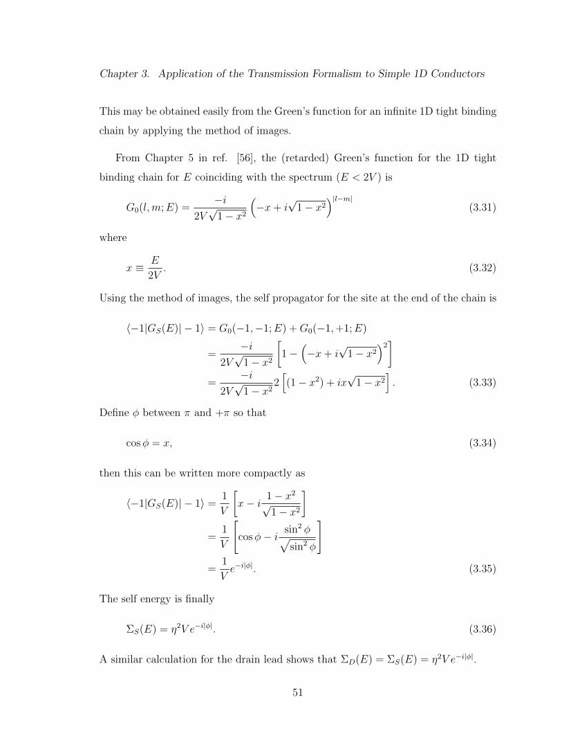
Chapter 3. Application of the Transmission Formalism to Simple 1D Conductors
This may be obtained easily from the Green’s function for an infinite 1D tight binding
chain by applying the method of images.
From Chapter 5 in ref. [56], the (retarded) Green’s function for the 1D tight
binding chain for E coinciding with the spectrum (E < 2V ) is
G0(l,m;E) =−i
2V√
1− x2
(−x+ i
√1− x2
)|l−m|(3.31)
where
x ≡ E
2V. (3.32)
Using the method of images, the self propagator for the site at the end of the chain is
〈−1|GS(E)| − 1〉 = G0(−1,−1;E) +G0(−1,+1;E)
=−i
2V√
1− x2
[1−
(−x+ i
√1− x2
)2]
=−i
2V√
1− x22[(1− x2) + ix
√1− x2
]. (3.33)
Define φ between π and +π so that
cosφ = x, (3.34)
then this can be written more compactly as
〈−1|GS(E)| − 1〉 =1
V
[x− i 1− x2
√1− x2
]=
1
V
[cosφ− i sin2 φ√
sin2 φ
]=
1
Ve−i|φ|. (3.35)
The self energy is finally
ΣS(E) = η2V e−i|φ|. (3.36)
A similar calculation for the drain lead shows that ΣD(E) = ΣS(E) = η2V e−i|φ|.
51

Chapter 3. Application of the Transmission Formalism to Simple 1D Conductors
The matrices ΓS and ΓD may now be calculated. They are
ΓS = ΓD = i[ΣD − Σ†D] = 2η2V sin |φ|. (3.37)
The next step is to write the Green’s function for the channel subsystem. Since
the conductor only consists of a single site this is easily done as it is only a 1x1 matrix:
G(E) = [E −H − ΣS − ΣD]−1
=|0〉〈0|
E − E0 − 2η2V e−i|φ|. (3.38)
The energy dependent transmission function through the conductor is then
T (E) = TrΓSGΓDG†
=[2η2V sin |φ|]2
[E − E0 − 2η2V e−i|φ|][E − E0 − 2η2V e+i|φ|]
=[2η2V sin |φ|]2
[E − E0 − 2η2V cosφ]2 + [2η2V sin |φ|]2. (3.39)
Using 2V cosφ = E and hv(E) = ∂E∂k
the transmission function when E is inside the
band is
T (E) =η4[hv(E)]2
[E(1− η2)− E0]2 + η4[hv(E)]2(3.40)
(and zero outside the band). This is exactly the result obtained earlier through a
different method.
3.2.3 Discussion of the One-Level Conductor
First consider the special case when the coupling from the leads to the conductor
is equal to the intersite coupling within the leads, i.e. η = 1. In this case, the
transmission function becomes
T (E) = |t|2 =[hv(E)]2
E20 + [hv(E)]2
(3.41)
52

Chapter 3. Application of the Transmission Formalism to Simple 1D Conductors
0
0.2
0.4
0.6
0.8
1
-1 -0.5 0 0.5 1
T(E)
E/(2V)
Transmission Function versus Energy for the One-Level Conductor, η=1
a=0 a=0.1 a=0.5 a=1.0 a=2.0
Figure 3.2: Transmission function versus energy for the one-level conductor withη = 1 for different values of a ≡ EA/(2V ).
If additionally the conductor site energy E0 vanishes, then it is easy to see that the
incoming waves are not scattered at all and T = 1. As the magnitude of the site energy
|E0| is increased, the transmission function everywhere decreases. In particular, at the
band edges E = ±2V , the velocity vanishes, so the transmission also goes to zero.
The maximum transmission is at the center of the band E = 0, and its value is
Tmax =1
1 +E2
0
4V 2
. (3.42)
Furthermore, for this special case, η = 1, the transmission function is not sensitive
to the sign of E0, and T (E) is symmetric around E = 0. This is illustrated in Figure
53

Chapter 3. Application of the Transmission Formalism to Simple 1D Conductors
0
0.2
0.4
0.6
0.8
1
-1 -0.5 0 0.5 1
T(E)
E/(2V)
Transmission Function versus Energy for the One-Level Conductor, a = 0.5
η=0.1 η=0.5 η=1.0 η=2 η=5
Figure 3.3: Transmission function versus energy for the one-level conductor witha = EA/(2V ) = 0.5 for different coupling strengths η.
3.2.
If the coupling to the leads is strong (η large), then the transmission function is
T (E) = 1− E2
4V 2+O(1/η2). (3.43)
In this limit, the transmission function is parabolic, with T = 1 at the center of the
band and again T = 0 at the edges, independent of the strength of E0.
In the general case, T (E) still vanishes at the band edges, but it loses its symmetry
around E = 0. If η 6= 1 and the value E0/(1− η2) is within the band, i.e.
|E0/(1− η2)| < 2V, (3.44)
maximum transmission occurs at that energy and is unity. Otherwise, maximum
54

Chapter 3. Application of the Transmission Formalism to Simple 1D Conductors
0
0.2
0.4
0.6
0.8
1
-1 -0.5 0 0.5 1
T(E)
E/(2V)
Transmission Function versus Energy for the One-Level Conductor, a = 1.5
η=0.1 η=0.5 η=1.0 η=2 η=5
Figure 3.4: Transmission function versus energy for the one-level conductor witha = EA/(2V ) = 1.5 for different coupling strengths η.
transmission occurs at
E = (1− η2)4V 2
E0
(3.45)
and is less than unity,
Tmax =η4
2η2 − 1 +E2
0
4V 2
. (3.46)
The transmission function versus energy for different values of η for constant EA is
displayed in Figures (3.3) and (3.4).
55

Chapter 3. Application of the Transmission Formalism to Simple 1D Conductors
| − 3〉 | − 2〉 | − 1〉 |1〉 |2〉 |3〉
|A〉
|B〉
VVVVV VV V
V V
Figure 3.5: A conductor consisting of a two-levels (blue) connected to two semi-infinitetight binding leads (black).
3.3 Two-Level Systems
There are various different configurations of two-level conductors and different ways
of connecting them to the leads. First, consider a two-level system with Hamiltonian
H = EA|A〉〈A|+ EB|B〉〈B|
where |A〉 and |B〉 are the energy eigenstates of H and EA and EB their energies.
There is no matrix element coupling the two states |A〉 and |B〉. Now suppose that
both A and B are connected to both leads (the same 1D semi-infinite chains as before)
with a coupling strength V which is the same as the intersite coupling V within the
leads. This is illustrated in Figure (3.5).
3.3.1 Calculation of the Transmission
The transmission function will now be calculated using the Green’s function method
to illustrate its use for a system consisting of more than one state. Again, the first
step is to calculate the self energies due to the coupling to the leads.
The coupling τS from the conductor to the source lead is
τS = V (|A〉〈−1|+ |B〉〈−1|) (3.47)
56

Chapter 3. Application of the Transmission Formalism to Simple 1D Conductors
where | − 1〉 is the state on the end of the contact chain. Then the self energy is
ΣS = τSGSτ†S (3.48)
= V 2〈−1|GS| − 1〉(|A〉〈A|+ |A〉〈B|+ |B〉〈A|+ |B〉〈B|). (3.49)
The matrix element 〈−1|GS| − 1〉 was already calculated in the previous section, it is
〈−1|GS| − 1〉 =1
Ve−i|φ| (3.50)
where again cosφ = E/(2V ) and is between −π and π. The self energy written as a
matrix is then
Σs = V e−i|φ|
1 1
1 1
. (3.51)
A similar calculation for the drain lead yields ΣD = ΣS. The Γ matrices are
ΓS = ΓD = i(ΣS − Σ†S) = 2V sin |φ|
1 1
1 1
. (3.52)
The Green’s function for the conductor subsystem is
G(E) = [E −H − ΣS − ΣD]−1
=
E 0
0 E
−EA 0
0 EB
− 2V e−i|φ|
1 1
1 1
−1
=
E − EA − 2V e−i|φ| −2V e−i|φ|
−2V e−i|φ| E − EB − 2V e−i|φ|
−1
. (3.53)
The inverse on the right hand side may be easily calculated, and the result is
G(E)
E−EB−2V e−i|φ|
(E−EA)(E−EB)−2V e−i|φ|[2E−EA−EB ]2V e−i|φ|
(E−EA)(E−EB)−2V e−i|φ|[2E−EA−EB ]
2V e−i|φ|
(E−EA)(E−EB)−2V e−i|φ|[2E−EA−EB ]E−EA−2V e−i|φ|
(E−EA)(E−EB)−2V e−i|φ|[2E−EA−EB ]
.
(3.54)
The transmission function may now be calculated. It is
T (E) = TrΓSGΓDG†
=[hv(E)]2(
E2−EAEB2E−EA−EB
)2
+ [hv(E)]2. (3.55)
57

Chapter 3. Application of the Transmission Formalism to Simple 1D Conductors
3.3.2 Discussion
Now let us examine the properties of equation (3.55). First, the following special
cases will be considered:
• The two-levels are degenerate EA = EB.
• The two energies have the same magnitude, but opposite signs, EA = −EB.
• One of the energies is zero, EB = 0.
If the two sites are degenerate, EA = EB = E0, then the transmission function
becomes
T (E) =[hv(E)]2
(E+E0)2
4+ [hv(E)]2
. (3.56)
This is exactly the same as for the one site conductor, equation (3.26), if η is set to√
2 in that expression, and all the comments made about that system apply here also.
The effect of adding a degenerate site with the same coupling is therefore equivalent
to increasing the strength of the coupling for a one-level conductor.
Next, consider the special case where EA = −EB. The transmission function is
T (E) =[hv(E)]2(
E2+E2A
2E
)2
+ [hv(E)]2. (3.57)
The conductor is opaque (T = 0) at the center of the band (provided the energies are
nonzero) as well as at the band edges, and the transmission function is symmetric
around E = 0. The maximum transmission occurs at
E = ± EA/2V√2( EA
2V
)2+ 1
(3.58)
and has the value
Tmax =1
1 +( EA
2V
)2+( EA
2V
)4 . (3.59)
58

Chapter 3. Application of the Transmission Formalism to Simple 1D Conductors
0
0.2
0.4
0.6
0.8
1
-1 -0.5 0 0.5 1
T(E)
E/(2V)
Transmission Function versus Energy for the Two-Level Conductor, EA = -EB
a=0.1 a=0.5 a=1.0 a=2.0
Figure 3.6: Transmission function versus energy for the two-level conductor describedin Section 3.3 when EA = −EB for different values of a ≡ EA/(2V ).
The maximum transmission is always less than one for EA nonzero and decreases
sharply as EA is moved further outside of the band. This is illustrated in Figure (3.6).
Next, consider the case where one of the energies is zero. Since it does not matter
which one, let EB = 0. The transmission function is then given by
T (E) =[hv(E)]2(
E2
2E−EA
)2
+ [hv(E)]2. (3.60)
The conductor becomes transparent at the center of the band, E = 0, but the trans-
mission function is no longer a symmetric function of energy. If EA/2 is within the
band, then the conductor becomes opaque (T = 0) at E = EA/2. If EA is moved far
outside the band, then transmission function becomes nearly one everywhere inside
the band. This is illustrated in Figure (3.7).
59

Chapter 3. Application of the Transmission Formalism to Simple 1D Conductors
0
0.2
0.4
0.6
0.8
1
-1 -0.5 0 0.5 1
T(E)
E/(2V)
Transmission Function versus Energy for the Two-Level Conductor, EB = 0
a=0.1 a=0.5 a=1.0 a=2.0
Figure 3.7: Transmission function versus energy for the two-level conductor describedin Section 3.3 when EB = 0 for different values of a ≡ EA/(2V ).
Now some comments can be made about the general case. As with the one-level
conductor, the transmission function vanishes at the band edges, E = ±2V . If EAand EB both have the same sign, and if
√EAEB is within the band, then the conductor
becomes transparent at plus and minus the geometric mean of the site energies,
E = ±√EAEB. (3.61)
On the other hand, at the arithmetic mean of the site energies,
E =EA + EB
2(3.62)
the conductor becomes opaque (T = 0), provided EA 6= EB. For certain values of
EA and EB, the arithmetic and geometric means are close to one another, causing
60
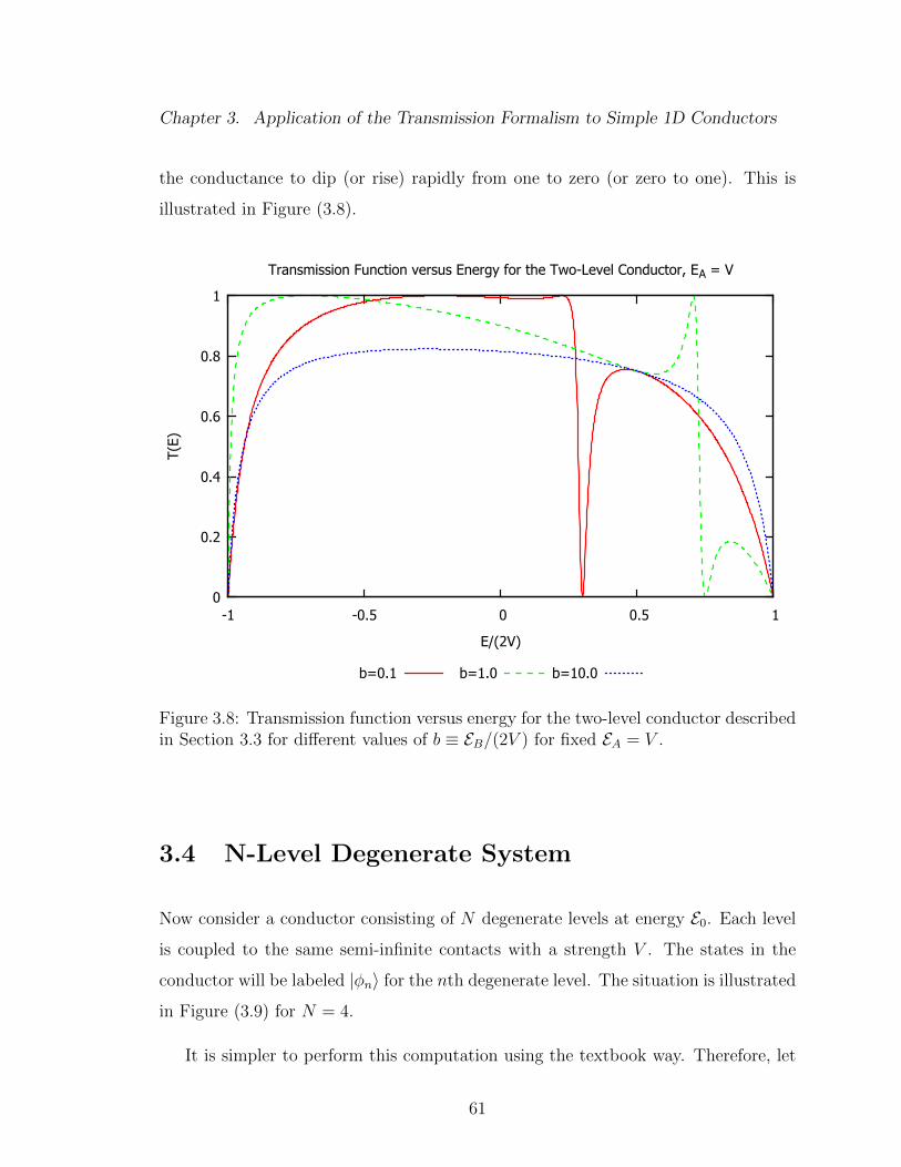
Chapter 3. Application of the Transmission Formalism to Simple 1D Conductors
the conductance to dip (or rise) rapidly from one to zero (or zero to one). This is
illustrated in Figure (3.8).
0
0.2
0.4
0.6
0.8
1
-1 -0.5 0 0.5 1
T(E)
E/(2V)
Transmission Function versus Energy for the Two-Level Conductor, EA = V
b=0.1 b=1.0 b=10.0
Figure 3.8: Transmission function versus energy for the two-level conductor describedin Section 3.3 for different values of b ≡ EB/(2V ) for fixed EA = V .
3.4 N-Level Degenerate System
Now consider a conductor consisting of N degenerate levels at energy E0. Each level
is coupled to the same semi-infinite contacts with a strength V . The states in the
conductor will be labeled |φn〉 for the nth degenerate level. The situation is illustrated
in Figure (3.9) for N = 4.
It is simpler to perform this computation using the textbook way. Therefore, let
61

Chapter 3. Application of the Transmission Formalism to Simple 1D Conductors
| − 3〉 | − 2〉 | − 1〉 |1〉 |2〉 |3〉
|φ0〉
|φ1〉
|φ2〉
|φ3〉
VVVVV V
V V
V V
V V
V V
Figure 3.9: A conductor consisting of a 4 degenerate levels (blue), each of which areconnected to two semi-infinite tight binding leads (black).
us take again an incoming and reflected wave to the left, and a transmitted wave to
the right,
ψkm =
eikm + re−ikm m < 0
te−ikm m > 0. (3.63)
The reflection and transmission amplitudes |r| and |t|, as well as the wavefunction
inside the conductor |φ〉 must now be determined so that the Schrodinger equation is
everywhere satisfied. The Schrodinger equation for the conductor states and the two
lead states to the left and right of the conductor is
Eψ−1 = V
(ψ−2 +
∑n
cn
), (3.64)
Eψ+1 = V
(ψ+2 +
∑n
cn
), (3.65)
Ecn = E0cn + V (ψ−1 + ψ+1), (3.66)
where cn is the amplitude of the wavefunction in the nth conductor state, cn ≡ 〈φn|φ〉.
From the third equation, all the amplitudes cn must evidently be the same, i.e. cn = A
62

Chapter 3. Application of the Transmission Formalism to Simple 1D Conductors
for all n, and inserting this the Schrodinger equation becomes
E(e−ik + reik) = V(e−2ik + re2ik +NA
)(3.67)
E(teik) = V(te2ik +NA
)(3.68)
EA = E0A+ V (e−ik + reik + teik). (3.69)
Using the first two gives t = r + 1, and eliminating r from the third,
(E − E0)A = V (e−ik + teik − eik + teik)
= V (−2i sin k + 2teik). (3.70)
Combining this with the second equation to eliminate A,
(E − E0)tV = V 2N(−2i sin k + 2teik). (3.71)
Finally, solving for the transmission amplitude t,
t =−2iNV sin k
E − E0 − 2NV eik(3.72)
so the transmission function is
T (E) = |t|2 =[hv(E)]2
[(1−N)E−E0]2
N2 + [hv(E)]2. (3.73)
This is exactly equivalent to the transmission function obtained earlier for the one-
level system under the replacement η2 = N . Thus, adding degenerate levels has
the same effect as increasing the strength of the coupling to the leads in a one-level
system.
3.5 A Different Two-Level Conductor
Now consider again a two-level conductor, but suppose that only one of the states
is coupled to the contacts, and add a coupling between the two states. Let the
Hamiltonian for the isolated conductor be
H = EA|A〉〈A|+ EB|B〉〈B|+ VAB (|B〉〈A|+ |A〉〈B|) , (3.74)
63
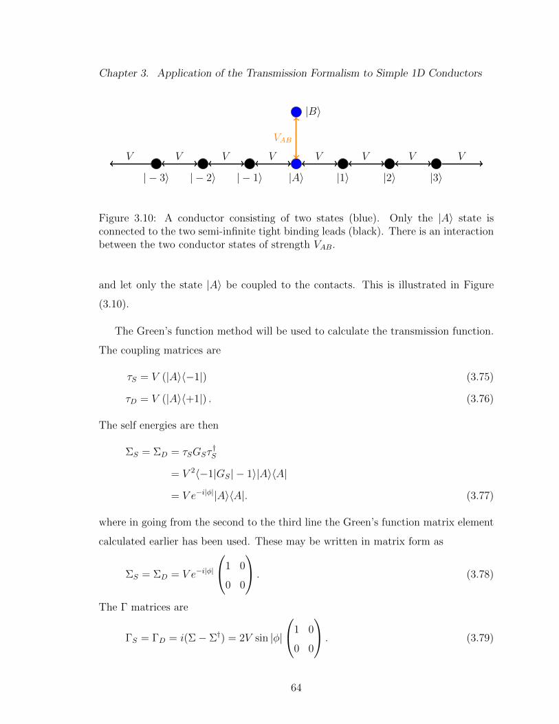
Chapter 3. Application of the Transmission Formalism to Simple 1D Conductors
| − 3〉 | − 2〉 | − 1〉 |1〉 |2〉 |3〉|A〉
|B〉
VVVVV VV V
VAB
Figure 3.10: A conductor consisting of two states (blue). Only the |A〉 state isconnected to the two semi-infinite tight binding leads (black). There is an interactionbetween the two conductor states of strength VAB.
and let only the state |A〉 be coupled to the contacts. This is illustrated in Figure
(3.10).
The Green’s function method will be used to calculate the transmission function.
The coupling matrices are
τS = V (|A〉〈−1|) (3.75)
τD = V (|A〉〈+1|) . (3.76)
The self energies are then
ΣS = ΣD = τSGSτ†S
= V 2〈−1|GS| − 1〉|A〉〈A|
= V e−i|φ||A〉〈A|. (3.77)
where in going from the second to the third line the Green’s function matrix element
calculated earlier has been used. These may be written in matrix form as
ΣS = ΣD = V e−i|φ|
1 0
0 0
. (3.78)
The Γ matrices are
ΓS = ΓD = i(Σ− Σ†) = 2V sin |φ|
1 0
0 0
. (3.79)
64

Chapter 3. Application of the Transmission Formalism to Simple 1D Conductors
The Green’s function inside the conductor is
G(E) = [EI −H − ΣS − ΣD]1
=
E 0
0 E
− EA VAB
VAB EB
− 2V e−i|φ|
1 0
0 0
−1
= 1(E−EA−2V e−i|φ|)(E−EB)−V 2
AB
E − EB VAB
VAB E − EA − 2V e−i|φ|.
. (3.80)
The transmission function is finally
T (E) = TrΓGΓG† =[hv(E)]2(
EA +V 2AB
(E−EB)
)2
+ [hv(E)]2.
It is worth pointing out that this calculation could have been done in a simpler way,
by noting that the Green’s function for the A subsystem (which is all that is needed
when computing the trace since the leads are only coupled to A) is
GA(E) =1
E − EA − ΣB − ΣS − ΣD
(3.81)
where ΣB is the self energy resulting from coupling to the |B〉 state,
ΣB(E) =V 2AB
E − EB. (3.82)
Let us now discuss the properties of the transmission as a function of energy.
Again, the transmission vanishes at the band edges, and it is not in general a sym-
metric function of energy. If EB is within the band, the the conductor becomes opaque
at E = EB. At
E = EB −V 2AB
EA, (3.83)
the conductor becomes transparent, provided this energy is within the band. As the
magnitude of EB becomes very large compared to VAB, the transmission function
approaches the single-site value, i.e. it behaves as if the site |B〉 were not there. This
is illustrated in Figure (3.11).
65

Chapter 3. Application of the Transmission Formalism to Simple 1D Conductors
0
0.2
0.4
0.6
0.8
1
-1 -0.5 0 0.5 1
T(E)
E/(2V)
Transmission Function versus Energy for the Two-Level Conductor, EA = 2V, VAB = V
b=0.1 b=0.2 b=1.0 b=5.0
Figure 3.11: Transmission function versus energy for the two-level conductor de-scribed in Section 3.5 for different values of b ≡ EB/(2V ) for fixed EA = V andVAB = V .
3.6 Single-Site Conductor Coupled to Oscillator
Now consider a one-level conductor which is placed in interaction with a harmonic
oscillator. This could be looked at as a highly simplified model of electron-phonon
scattering. The total Hamiltonian exists in the product space of the electron and
boson spaces, and consists of the following parts:
• Hamiltonians for the isolated source and drain leads.
• Coupling between leads and the conductor.
• Hamiltonian for the isolated conductor.
66

Chapter 3. Application of the Transmission Formalism to Simple 1D Conductors
• Hamiltonian for the isolated oscillator.
• Interaction between conductor and oscillator.
The Hamiltonians for the isolated leads and the coupling between leads and conductor
may be written in total as
Hleads = V
∞∑m=−∞
(|m〉〈m+ 1|+ |m+ 1〉〈m|)⊗ Ib (3.84)
Here V is the intersite interaction energy in the leads as well as the coupling strength
from leads to conductor. The states |m〉 are electronic states with |0〉 being the
conductor state, and the operator Ib is the identity operator in the boson space.
Next, the Hamiltonian for the isolated conductor is
Hconductor = E0|0〉〈0| ⊗ Ib (3.85)
where E0 is the site energy of the conductor site relative to the site energies in the
leads. The Hamiltonian for the isolated oscillator is
Hoscillator = Ie ⊗ hω(
1
2Ib + b†b
). (3.86)
Here Ie is the identity operator in the electron space, ω is the frequency of the
oscillator, and b† and b are the raising and lowering operators in the oscillator space.
Finally, let the interaction between oscillator and conductor to be
|0〉〈0| ⊗ ghω(b+ b†) (3.87)
where g is a dimensionless constant which determines the strength of the interaction.
This type of interaction between conductor and oscillator changes the effective energy
of the |0〉 state based on the position of the oscillator.
Putting everything together, the total Hamiltonian is
H = V
∞∑m=−∞
(|m〉〈m+ 1|+ |m+ 1〉〈m|)⊗ Ib + E0|0〉〈0| ⊗ Ib
+ Ie ⊗ hω(
1
2Ib + b†b
)+ |0〉〈0| ⊗ ghω(b+ b†). (3.88)
67
Chapter 3. Application of the Transmission Formalism to Simple 1D Conductors
If the temperature in source and drain reservoirs is low enough, the oscillator
should be in its (non-shifted) ground state |φ0〉 before the electron passes through the
junction, so for the incoming wave take
|ψi〉 =∑m<0
eik0m|m〉 ⊗ |φ0〉 (3.89)
where the energy of the incoming electron is Ee = 2V cos k0 and |φ0〉 is the ground
state of the isolated oscillator. Because of the interaction, as the electron passes
through the conductor it may create one or more excitations in the oscillator, so the
reflected and transmitted waves must be of the form
reflected wave: |ψr〉 =∑m<0
∑n
rne−iknm|m〉 ⊗ |φn〉, (3.90)
transmitted wave: |ψt〉 =∑m>0
∑n
tne−knm|m〉 ⊗ |φn〉. (3.91)
where rn and tn are reflection and transmission amplitudes for modes with n bosons
in the oscillator. The |φn〉’s are n boson eigenstates of the non-shifted oscillator.
Since the incoming wave only has enough energy to create a finite number of bosons,
some of the kn’s will necessarily be complex, and part of the electron wavefunction
will be exponentially localized around the conductor.
Enforcing H|ψ〉 = E|ψ〉 with |ψ〉 consisting of the sum of incoming, reflected, and
transmitted waves, it is possible to show that the kn’s are determined by
Etotal = 2V cos k0 +hω
2= 2V cos kn + hω
(n+
1
2
)(3.92)
and the reflection and transmission amplitudes are
δn,0 + rn = tn = −2iV sin k0〈φn|G(E)|φ0〉 (3.93)
and the Green’s function G is
G(E) ≡ [E −H0 −H1 − 2Σ(E)]−1 (3.94)
68

Chapter 3. Application of the Transmission Formalism to Simple 1D Conductors
with
H0 ≡ ε0 + hω
(b†b+
1
2
), (3.95)
H1 ≡ ghω(b+ b†), (3.96)
Σ(E) ≡ V∑n
eikn|φn〉〈φn|. (3.97)
If we restrict ourselves to the special case hω > 4V , then the incoming electron
does not have enough energy to create a boson and keep propagating, so all kn’s for
n > 0 will be complex, and the transmission function is only affected by t0,
T = |t0|2 = [2V sin k0]2〈φ0|G(E)|φ0〉〈φ0|G†(E)|φ0〉. (3.98)
Due to the difficulty in calculating G(E) exactly, we have considered the limit of
weak coupling g. Expanding equation (3.94), we have [56]
G = G0 +G0H1G0 +G0H1G0H1G0 + ... (3.99)
where
G0(E) = [E −H0 − 2Σ(E)]−1 =∑n
|φn〉〈φn|E − ε0 − hω(n+ 1/2)− 2V eikn
. (3.100)
Using this approximation, the transmission when hω > 4V to order g2 as a func-
tion of electron energy Ee is
T (Ee) ≈[hv(Ee)]
2
E20 + [hv(Ee)]2
+ g2h(Ee) (3.101)
where the correction term is
h(Ee) ≡2E0h
2ω2h2v2(Ee)[E2
0 + h2v2(Ee)]2 [E0 +
√h2ω2 − 2Eehω − h2v2(Ee)
] (3.102)
and with v(Ee) again the velocity as a function of the electron energy, [hv(Ee)]2 =
4V 2 − E2e .
This correction term may be positive or negative depending on the sign of ε0, and
it is not symmetric around Ee = 0. Interestingly, h(Ee) also vanishes if the site energy
E0 is zero. The function h(Ee) is plotted in figure (3.12).
69
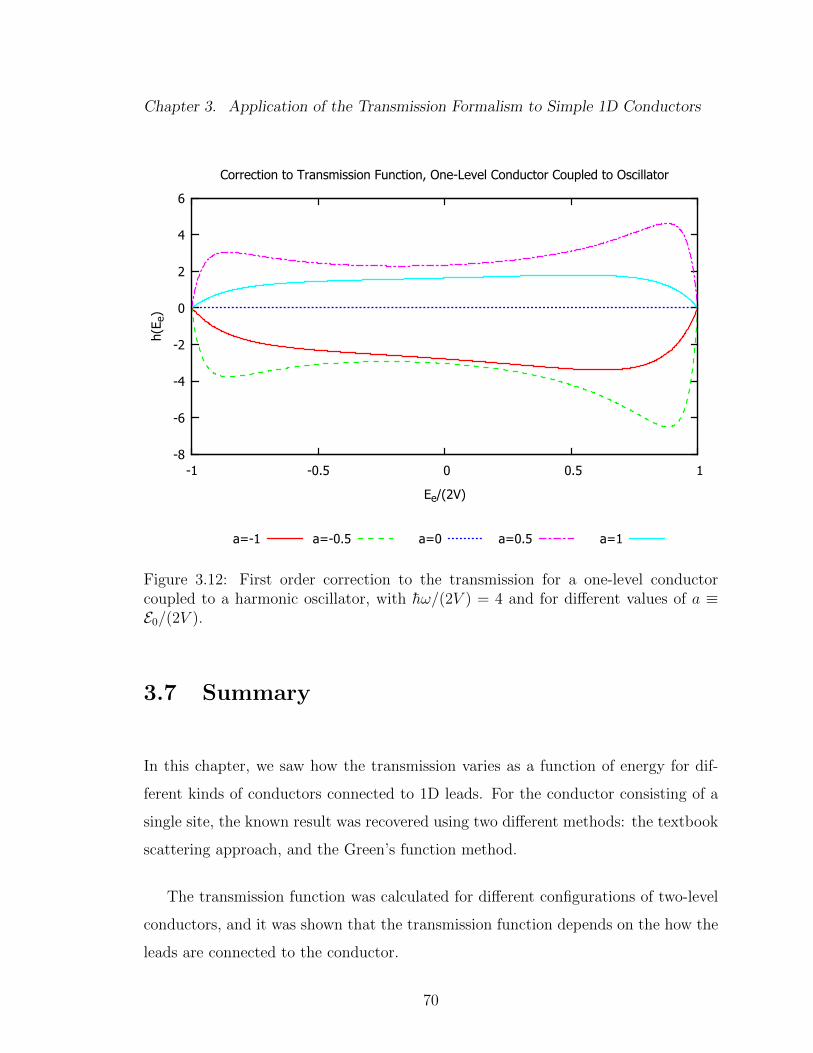
Chapter 3. Application of the Transmission Formalism to Simple 1D Conductors
-8
-6
-4
-2
0
2
4
6
-1 -0.5 0 0.5 1
h(E e
)
Ee/(2V)
Correction to Transmission Function, One-Level Conductor Coupled to Oscillator
a=-1 a=-0.5 a=0 a=0.5 a=1
Figure 3.12: First order correction to the transmission for a one-level conductorcoupled to a harmonic oscillator, with hω/(2V ) = 4 and for different values of a ≡E0/(2V ).
3.7 Summary
In this chapter, we saw how the transmission varies as a function of energy for dif-
ferent kinds of conductors connected to 1D leads. For the conductor consisting of a
single site, the known result was recovered using two different methods: the textbook
scattering approach, and the Green’s function method.
The transmission function was calculated for different configurations of two-level
conductors, and it was shown that the transmission function depends on the how the
leads are connected to the conductor.
70

Chapter 3. Application of the Transmission Formalism to Simple 1D Conductors
For a conductor consisting of N degenerate levels at energy E0, each connected to
the leads with interaction strength V , it was shown that the transmission is equivalent
to a one-level system at the same energy E0 but with a stronger coupling strength√NV .
Finally, for a one-level conductor in interaction with an oscillator, although the
problem could not be solved exactly, to lowest order it was found that the interaction
can enhance or reduce the transmission function, depending on the sign of the site
energy E0.
71

Chapter 4
Collective Motion of Macroscopic
Objects: A Model with Centering
Several different approaches have been used in the literature for modeling the cooper-
ative motion of various biological organisms. One approach is to explicitly model the
motion of every member of the group by specifying how the positions and velocities
of each individual evolve in time. One way to do this is to simply construct equa-
tions of motion for each individual’s position and velocity. Such models are known as
Lagrangian or dynamical models [10, 24, 80–82]. Other authors prefer to make time
discrete in order to make it easier to perform computer simulations. In these discrete
time models, at each time step a set of rules is used to determine the state of system
in the next time step based on the current state of the system. These are typically
known as rule-based models or cellular automata [17, 83–93].
Yet another approach is to construct equations of motion for continuous functions
of space and time such as the density and velocity fields. This is a coarse-grained
description since the motion of individual particles is not modeled explicitly. This is
known as the continuum or fluid dynamics approach [94–100].
In the realm of collective motion, due to the difficulties inherent in studying sys-
72

Chapter 4. Collective Motion of Macroscopic Objects: A Model with Centering
tems of many interacting particles, very few authors have been able to analytically
connect a description where each particle is modeled individually (a rule-based or
dynamical model) to a coarse-grained continuum description. A notable exception
is the 1999 paper by Czirok et al. [97] where approximate continuum equations of
motion for the density and velocity fields are constructed from a rule-based model.
Recently, some authors have used hybrid approaches to help bridge the gap be-
tween individual-level descriptions and continuum descriptions [101–109]. In such
approaches, a model of individual behavior is chosen and numerical simulations are
performed. Next, equations of motion are postulated for continuous coarse-grained
quantities. The undetermined parameters in the equations of motion are then esti-
mated from simulations. In particular, in a recent 2010 paper Raghib et al. [108]
used an advection-diffusion equation with memory for the evolution of the center of
mass distribution. An advection-diffusion equation with memory is a generalization
of the advection-diffusion equation which is non-local in time in the sense that the
evolution at time t depends on the state of the system at previous times. In one
dimension, the advection-diffusion equation with memory has the form
∂
∂tP (x, t) = −
∫ t
0
V(t− t′) ∂∂xP (x, t′)dt′ +
∫ t
0
D(t− t′) ∂2
∂x2P (x, t′)dt′. (4.1)
Raghib et al. postulate a form for the memory, and fit the unknown parameters using
simulation of a rule-based model.
Although this procedure can produce coarse-grained equations of motion which
fit well with simulation, it does not make clear why the memory has the particular
form found. The presence of a memory at least should not be surprising. In Chapter
2 it was shown that for a quantity ρ which obeys
∂ρ
∂t= −iLρ (4.2)
where L is a linear (super)operator, the Zwanzig-Nakajima projection approach [76–
78] shows that the projected quantity Pρ naturally obeys a memory equation of the
73

Chapter 4. Collective Motion of Macroscopic Objects: A Model with Centering
form
∂
∂tPρ = −iPLPρ− PL
∫ t
0
e−i(1−P)L(t−t′)(1− P)LPρ(t′)dt′ + I(t) (4.3)
where I is a term which depends on initial conditions. This expression formally
gives the memory in terms of the projection and evolution operators, but it is not
very useful for practical calculations of the memory, since calculating the operator
e−i(1−P)Lt can be difficult even for extremely simple systems [72].
In this chapter, we construct a simplified dynamical model of collective motion
and obtain exact equations of motion for a few continuum quantities. We begin by
writing stochastic differential equations of motion for the positions of each particle in
the system. We then construct and solve the corresponding equation of motion for
the probability distribution function using standard techniques. Next, we perform
coarse-graining to find the evolution of continuous quantities such as the center of
mass distribution function and the density.
For one particular coarse-grained quantity, the density, we find that even in this
simple system an advection-diffusion equation with memory cannot completely cap-
ture the dynamics. The full dynamics are described via an evolution equation which
is non-local in space as well as time.
4.1 Description of the Model
Models of collective motion typically consist of several ingredients. The majority of
these ingredients can be classified as either self-propulsion, interaction, or noise. We
will define each of these in turn.
Self-propulsion is the tendency for each individual to move at a particular speed.
Self-propulsion can be incorporated into dynamical models by introducing a force
which drives the speed of each particle to a given value. In rule based models, self-
74

Chapter 4. Collective Motion of Macroscopic Objects: A Model with Centering
propulsion is typically included simply by specifying that the particles move at a
given constant speed and using a set of rules which only modifies the directions of
the particles.
Collective motion is a result of interaction between individuals in a group. The
most common kinds of interaction included in models of collective motion are:
• Short Range Collision Avoidance: The tendency for individuals to move away
from each other if they are too close together.
• Centering : The tendency for individuals to move toward other nearby individ-
uals.
• Alignment : The tendency for individuals to align their directions with the di-
rections of nearby individuals.
Biological organisms can change speed or direction in apparently random ways.
This is taken into account in models of collective motion through noise. Noise is
typically included in dynamical models by introducing a stochastic force acting on
the particles, or in rule-based models by randomly perturbing the direction of each
particle at every time step.
Finally, one may also introduce a preferred direction. A group of organisms may
have a preferred direction if, for example, a food source lies in that direction. One
topic of interest in the literature is the idea of collective decision making [90, 92, 110,
111]. In the simplest approaches, the flock is divided into two groups: one group
consisting of individuals which are “informed” and have a preferred direction, and
the other group consisting of individuals which are “uninformed” and do not have
any such preferred direction.
As an example of a model including some of these ingredients, the dynamical
model of Mikhailov and Zanette [24] has self-propulsion, a centering interaction, and
75

Chapter 4. Collective Motion of Macroscopic Objects: A Model with Centering
noise. Their equation of motion for the position of the mth particle is
xm + (x2m − 1)xm +
a
N
∑n
(xm − xn) = Γm(t). (4.4)
The first term on the left hand side is inertia, the second term is a self-propulsion
force which drives the speed of the particle to −1 or +1, and the third term represents
a centering interaction. The particular kind of centering interaction they have chosen
is to simply couple all particles to all other particles with spring forces. Finally,
the term on the right hand side, Γm(t), represents a stochastic noise force, which
they take to be delta-correlated white noise with a given strength. Although the
model of Mikhailov and Zanette is relatively simple, the presence of the nonlinear
self-propulsion term precludes exact analysis.
The simplified model of collective motion we construct and analyze in this chapter
is similar to the model of Mikhailov and Zanette, but does not contain any self-
propulsion. We do however allow for a preferred direction. Our simplified model thus
consists of three ingredients: a centering interaction, noise, and a bias. The model
can be solved exactly. The entire joint probability distribution as a function of time
can be found and any observable dependent on the distribution can be calculated
explicitly.
We begin with a description of the model and a discussion of the dynamics when
there is no noise. Next, we find the evolution of the probability distribution when the
dynamics are noisy. We then look at the evolution of coarse-grained quantities and
write continuum equations of motion.
The model consists of N identical overdamped Brownian point particles in one
dimension. As in the model by Mikhailov and Zanette, the centering interaction is
introduced by coupling each particle to all others with spring forces of equal strengths.
We take the springs to all have zero equilibrium length.
Next, we introduce a bias, i.e. a directional feature in the motion of the particles.
Furthermore, to include the idea of informed and uninformed individuals, we allow
76
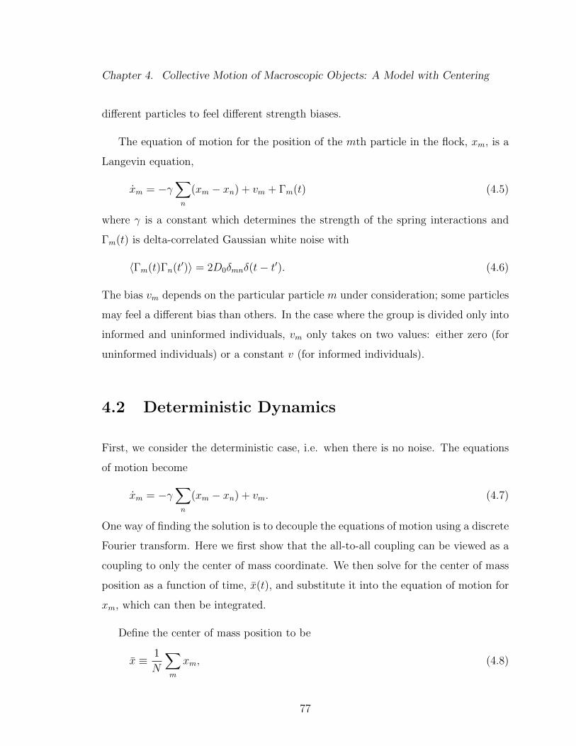
Chapter 4. Collective Motion of Macroscopic Objects: A Model with Centering
different particles to feel different strength biases.
The equation of motion for the position of the mth particle in the flock, xm, is a
Langevin equation,
xm = −γ∑n
(xm − xn) + vm + Γm(t) (4.5)
where γ is a constant which determines the strength of the spring interactions and
Γm(t) is delta-correlated Gaussian white noise with
〈Γm(t)Γn(t′)〉 = 2D0δmnδ(t− t′). (4.6)
The bias vm depends on the particular particle m under consideration; some particles
may feel a different bias than others. In the case where the group is divided only into
informed and uninformed individuals, vm only takes on two values: either zero (for
uninformed individuals) or a constant v (for informed individuals).
4.2 Deterministic Dynamics
First, we consider the deterministic case, i.e. when there is no noise. The equations
of motion become
xm = −γ∑n
(xm − xn) + vm. (4.7)
One way of finding the solution is to decouple the equations of motion using a discrete
Fourier transform. Here we first show that the all-to-all coupling can be viewed as a
coupling to only the center of mass coordinate. We then solve for the center of mass
position as a function of time, x(t), and substitute it into the equation of motion for
xm, which can then be integrated.
Define the center of mass position to be
x ≡ 1
N
∑m
xm, (4.8)
77

Chapter 4. Collective Motion of Macroscopic Objects: A Model with Centering
and rewrite the equations of motion as
xm = −Nγ(xm − x) + vm. (4.9)
Written in this form, it is easy to see that the mth particle is only coupled to the
center of mass position. The spring interactions exert no net force on the center of
mass; it only affected by the bias. This can be seen explicitly by summing equation
(4.9) over m, which gives
˙x = v (4.10)
where v ≡ 1N
∑m vm is the mean of the vms. The center of mass position as a function
of time is then
x(t) = x(0) + vt. (4.11)
Substituting this into (4.9) gives an equation for xm and t alone,
xm = −Nγ(xm − x(0)− vt) + vm. (4.12)
The solution to this equation is
xm(t) = xm(0)e−Nγt + vt+
(x(0) +
vm − vNγ
)(1− e−Nγt). (4.13)
When t is much less than 1/(Nγ), the right hand side can be expanded in a Taylor
series as
xm(t) = xm(0) + vmt+ (Nγt)[x(0)− xm(0)] +O(t2). (4.14)
At short times, the mth particle drifts at a velocity which is the sum of the bias it
feels vm and an amount which is proportional to its initial separation from the center
of mass.
At times t 1/(Nγ) the position becomes
xm(t) ≈ vt+ x(0) +vm − vNγ
. (4.15)
78

Chapter 4. Collective Motion of Macroscopic Objects: A Model with Centering
At long times, each particle drifts at a velocity v and is displaced from the center
of mass by an amount which depends on the difference between the bias it feels vm
and the mean bias v. For the special case when vm is either zero (for uninformed
individuals) or v (for informed individuals), the particles collect into two clusters.
The informed birds cluster ahead of the center of mass at x = x + (1 − a)v/(Nγ)
where a is the fraction of informed birds, and the uninformed birds cluster behind the
center of mass at x = x− a/(Nγ). The informed and uninformed birds are therefore
separated from each other by a distance v/(Nγ).
4.3 Noisy Dynamics
We now add noise to the system. Although the Langevin equations (4.5) can be
solved directly, it is simpler for the purposes of calculating observables to construct
and solve the corresponding equation of motion for the evolution of the probability
distribution function. We define the probability distribution function W (x1, ..., xN , t)
so that at time t the probability to find particle 1 in a small interval between x1 and
x1 + dx1, particle 2 between x2 and x2 + dx2, et cetera is
W (x1, ..., xN , t)dx1 · · · dxN . (4.16)
The partial differential equation of motion for the distribution function W is
known as a Fokker-Planck equation [112, 113]. The Fokker-Planck equation can be
constructed from the Langevin equations (4.5) using standard techniques (see e.g.
Chapter 4 in Risken [114] for a detailed discussion). For this system, the Fokker-
Planck equation is
∂W
∂t= γ
∑m
∂
∂xm
∑n
(xm − xn)W −∑m
vm∂W
∂xm+D0
∑m
∂2W
∂x2m
. (4.17)
We proceed by first performing a coordinate transformation to a frame where the
bias does not appear explicitly in the equations of motion. The transformed Fokker-
79

Chapter 4. Collective Motion of Macroscopic Objects: A Model with Centering
Planck equation can be solved with the standard techniques described in the book by
Risken [114].
Motivated by the long time solution in the deterministic case, equation (4.15),
define um to be
um ≡ xm − vt−vm − vNγ
. (4.18)
In the deterministic case, each um(t) at long times goes to a constant, x(0), indepen-
dent of m. For the evolution of the ums we have
um = xm − v = −γ∑n
(um +
vmNγ− un −
vnNγ
)+ vm − v + Γm(t). (4.19)
Since the mean velocity is v = 1N
∑n vn, this simplifies to
um = −γ∑n
(um − un) + Γm(t). (4.20)
The equations of motion for the um variables do not explicitly contain any bias.
The Fokker-Planck equation for evolution of the probability distribution function in
terms of the new variables um may be obtained either by constructing it from the
transformed Langevin equations, or by transforming the partial derivatives in the
untransformed Fokker-Planck equation [114]. In either case, the result is
∂W ′
∂t= γ
∑m
∂
∂um
∑n
(um − un)W ′ +D0
∑m
∂2
∂u2m
W ′. (4.21)
The prime is used here simply as a reminder that we have changed to a different
coordinate frame.
Before we proceed to find the solution, let us first recall the single particle Orstein-
Uhlenbeck process [115, 116], which is just an overdamped harmonic oscillator with
noise,
x = −γx+ Γ(t) (4.22)
80

Chapter 4. Collective Motion of Macroscopic Objects: A Model with Centering
again where Γ(t) is delta-correlated Gaussian white noise with 〈Γ(t)Γ(t′)〉 = 2D0δ(t−
t′). The corresponding Fokker-Planck equation is
∂W
∂t= γ
∂
∂x(xW ) +D0
∂2W
∂x2. (4.23)
The standard method of solving this is to Fourier transform and solve the resulting
first order partial differential equation with the method of characteristics. The solu-
tion G(x, x′, t) subject to a delta function initial condition G(x, x′, 0) = δ(x− x′) is a
Gaussian distribution [114],
G(x, x′, t) =
√γ
2πD0(1− e−2γt)exp
[− γ(x− x′e−γt)2
2D0(1− e−2γt)
]. (4.24)
At long times any information about the initial condition of the system is lost and
the distribution is centered around x = 0 due to the spring force pulling the particle
to the origin. The variance σ2 at short times is σ2 = 2D0t, like in an ordinary
diffusive process, but at long times becomes constant because the spring force limits
the distribution from spreading further.
The Ornstein-Uhlenbeck process can be generalized to higher dimensions. A
stochastic process with linear drift and constant diffusion in any number of dimen-
sions can be called an Ornstein-Uhlenbeck process. The most general form of the
Fokker-Planck equation describing such a process is [114]
∂W
∂t=∑ij
αij∂
∂xi(xjW ) +
∑ij
Dij∂2W
∂xi∂xj. (4.25)
The system described by equation (4.21), in which all particles are coupled to all
others with equal strengths, is indeed a particular special case of the multivariate
Ornstein-Uhlenbeck process.
One method of solving equations of this form, as described by Wang and Uhlen-
beck [116] is to transform to normal mode coordinates (i.e. transform to a basis in
which the matrix α is diagonal), then Fourier transform the Fokker-Planck equation
and solve the resulting first order partial differential equation using the method of
81
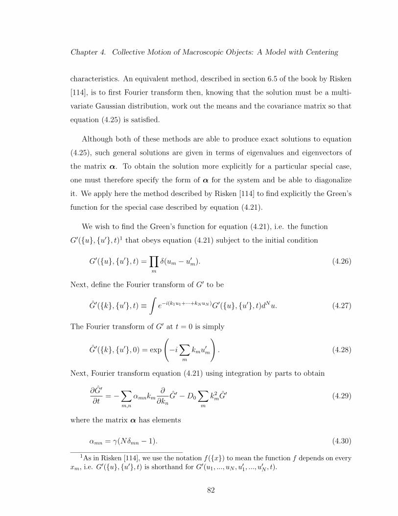
Chapter 4. Collective Motion of Macroscopic Objects: A Model with Centering
characteristics. An equivalent method, described in section 6.5 of the book by Risken
[114], is to first Fourier transform then, knowing that the solution must be a multi-
variate Gaussian distribution, work out the means and the covariance matrix so that
equation (4.25) is satisfied.
Although both of these methods are able to produce exact solutions to equation
(4.25), such general solutions are given in terms of eigenvalues and eigenvectors of
the matrix α. To obtain the solution more explicitly for a particular special case,
one must therefore specify the form of α for the system and be able to diagonalize
it. We apply here the method described by Risken [114] to find explicitly the Green’s
function for the special case described by equation (4.21).
We wish to find the Green’s function for equation (4.21), i.e. the function
G′(u, u′, t)1 that obeys equation (4.21) subject to the initial condition
G′(u, u′, t) =∏m
δ(um − u′m). (4.26)
Next, define the Fourier transform of G′ to be
G′(k, u′, t) ≡∫e−i(k1u1+···+kNuN )G′(u, u′, t)dNu. (4.27)
The Fourier transform of G′ at t = 0 is simply
G′(k, u′, 0) = exp
(−i∑m
kmu′m
). (4.28)
Next, Fourier transform equation (4.21) using integration by parts to obtain
∂G′
∂t= −
∑m,n
αmnkm∂
∂knG′ −D0
∑m
k2mG
′ (4.29)
where the matrix α has elements
αmn = γ(Nδmn − 1). (4.30)
1As in Risken [114], we use the notation f(x) to mean the function f depends on everyxm, i.e. G′(u, u′, t) is shorthand for G′(u1, ..., uN , u
′1, ..., u
′N , t).
82

Chapter 4. Collective Motion of Macroscopic Objects: A Model with Centering
It can be shown [114] that the solution must be a Gaussian, therefore G′ has the form
G′(k, u′, t) = exp
[−i∑m
kmMm(t)− 1
2
∑m,n
kmknσmn(t)
](4.31)
where Mm and σmn are functions of time which must be chosen so that equation
(4.29) is satisfied. Taking a derivative with respect to kn, we have
∂
∂knG′(k, u′, t) =
[−i∑m
kmMm −1
2
∑m,n
kmknσmn
]G′(k, u′, t). (4.32)
Substituting this into equation (4.29) and dividing by G′ gives
− i∑m
kmMm −1
2
∑m,n
kmknσmn =
−∑m,n
αmnkm
[−iMn −
1
2
∑l
kl(σln + σnl)
]−D0k
2m. (4.33)
Rearranging, this becomes
i∑m
km
[Mm +
∑n
αmnMn
]
=∑m,n
kmkn
[− σmn
2−∑l
αmlσln + σnl
2+D0δmn
]. (4.34)
For this to be true for any set of kms, Mn and σmn must be solutions to
Mm = −∑n
αmnMn = −γ∑n
[Mm −Mn], (4.35)
σmn = −∑l
αml(σln + σnl) +D0δmn. (4.36)
At time t = 0, the Green’s function must reduce to equation (4.28), so the initial
conditions for Mm and σmn are
Mm(0) = u′m. (4.37)
σmn(0) = 0. (4.38)
83

Chapter 4. Collective Motion of Macroscopic Objects: A Model with Centering
The Mm(t)s are evidently solutions to the deterministic problem,
Mm(t) =∑n
gmn(t)u′m (4.39)
where gmn is given by
gmn(t) = δmne−Nγt +
1
N(1− e−Nγt). (4.40)
The solution to the equation for the σmns with initial condition σmn(0) = 0 is [114]
σmn(t) =∑j,l
2D0δjl
∫ t
0
gmj(t′)gnl(t
′)dt′ = 2D0
∑l
∫ t
0
gml(t′)gln(t′)dt′ (4.41)
Using the gmn given above, this is
σmn(t) = 2D0
[δmn
1− e−2Nγt
2Nγ+
1
N
(t− 1− e−2Nγt
2Nγ
)]. (4.42)
The Fourier transform may be inverted to obtain the Green’s function in real
space. The Fourier inverse is
G′(u, u′, t) =1
(2π)N
∫G′(k, u′, t) exp(ikTu)dNk (4.43)
where k and u are column vectors so that kTu means∑
m kmum. Plugging in equation
(4.31), this becomes
G′(u, u′, t) =1
(2π)N
∫exp
(−ikTM− 1
2kTσk
)exp(ikTu)dNk. (4.44)
The integration can be done using the standard formula for multidimensional Gaus-
sian integrals,∫exp
(−1
2xTAx + BTx
)dNx =
√(2π)N
det Aexp
(1
2BTA−1B
). (4.45)
Using this, we have for the Green’s function in real space
G′(u, u′, t) =1√
(2π)N detσexp
(−1
2(u−M)Tσ−1(u−M)
). (4.46)
84

Chapter 4. Collective Motion of Macroscopic Objects: A Model with Centering
The determinant and inverse of the matrix σ can be calculated explicitly for this
system. The matrix σ can be written as
σ = 2D0
(1− e−2Nγt
2Nγ
)IN + 2D0
1
N
(t− 1− e−2Nγt
2Nγ
)JN . (4.47)
where IN is the NxN identity matrix and JN is an NxN matrix with each element
equal to one, (JN)mn = 1. Using the fact that det(cA) = cN det A for a constant c,
we have
detσ = (2D0)N(
1− e−2Nγt
2Nγ
)Ndet
[IN +
1
N
(2Nγt
(1− e−2Nγt)− 1
)JN
]. (4.48)
Next, consider determinants of the form
det(IN + αJN). (4.49)
The determinant of a matrix may be written as a the product of its eigenvalues, while
the trace of the matrix can be written as the sum of its eigenvalues. We can therefore
write
det(IN + αJN) = etr[ln(IN+αJN )] (4.50)
where tr denotes the trace. Using the power series expansion for ln(1 + x), we have
det(IN + αJN) = exp
tr
[−∞∑n=1
(−1)n(αJN)n
n
]. (4.51)
We have for the elements of J2N
(J2N)mn =
∑l
(JN)ml(JN)ln =∑l
1 = N (4.52)
therefore J2N = NJN . Then, by induction we have JnN = Nn−1JN for integer n ≥ 1.
Putting this in, we have
det(IN + αJN) = exp
−∞∑n=1
(−1)n(αN)n
n
tr JNN
. (4.53)
85

Chapter 4. Collective Motion of Macroscopic Objects: A Model with Centering
The trace of JN is N , so
det(IN + αJN) = exp
−∞∑n=1
(−1)n(αN)n
n
= exp ln(1 + αN) . (4.54)
Using this identity, we have finally for the determinant of σ,
detσ = (2D0t)
(2D0
(1− e−2Nγt)
2Nγ
)N−1
. (4.55)
Next, we calculate the inverse of σ. We have
σ−1 =1
2D01−e−2Nγt
2Nγ
[IN +
1
N
(2Nγt
1− e−2Nγt− 1
)JN
]−1
. (4.56)
Consider now inverses of the form [IN + αJN ]−1. Expanding this in a power series
gives
[IN + αJN ]−1 =∞∑n=0
(−1)n(αJN)n. (4.57)
Using J0N = IN and JnN = Nn−1JN for n ≥ 1, this becomes
[IN + αJN ]−1 = IN +JNN
∞∑n=1
(−1)n(αN)n. (4.58)
Summing the series gives
[IN + αJN ]−1 = IN +JNN
[∞∑n=0
(−1)n(αN)n − 1
]
= IN +JNN
[−αN
1 + αN
]. (4.59)
Using this to compute the inverse of σ gives finally
σ−1 =2Nγ
2D0(1− e−2Nγt)
(IN −
JNN
)+
JN2ND0t
. (4.60)
Inserting Mm(t) = u′me−Nγt + u′(1− e−Nγt) where u′ ≡ 1
N
∑m u′m and the results for
86

Chapter 4. Collective Motion of Macroscopic Objects: A Model with Centering
detσ and σ−1 into equation (4.46), the Green’s function in real (um) space is finally
G′(u, u′, t) =1√
4πD0t(
2πD01−e−2Nγt
Nγ
)N−1
· exp
− Nγ
2D0(1− e−2Nγt)
∑m
[um − u′me−Nγt − u′(1− e−Nγt)
]2−(
1
4D0t− Nγ
2D0(1− e−2Nγt)
)1
N
(∑m
um − u′me−Nγt − u′(1− e−Nγt)
)2.
(4.61)
Since the Jacobian matrix of the transformation from xm variables to um variables
has unit determinant, the Green’s function back in xm coordinates may be found now
simply by substituting back
um = xm − vt−vm − vNγ
. (4.62)
Although the general expression (4.46) for the real space Green’s function for a
multivariate Ornstein-Uhlenbeck process in terms of the covariance matrix σ and the
vector M can be found in earlier literature (see page 156 in ref. [114]), the author
does not know of any published work containing the explicit expressions for detσ,
σ−1, and the real space Green’s function, equations (4.55), (4.60), and (4.61), for the
particular system described here.
Now that the Green’s function is known, for any given initial condition W (x, 0)
the probability distribution as a function of time can be determined from
W (x, t) =
∫G(x, x′, t)W (x′, t)dNx, (4.63)
and the average of any observable O can be calculated from
〈O〉 =
∫O(x)W (x, t)dNx. (4.64)
To gain a better understanding of noisy dynamics, let us now look at two coarse-
grained quantities: the center of mass distribution function and the single particle
distribution functions.
87

Chapter 4. Collective Motion of Macroscopic Objects: A Model with Centering
The center of mass distribution function P (x, t) we define so that the probability
to find the center of mass x ≡ 1N
∑m xm in a small interval between x and x+ dx at
time t is P (x, t)dx.
We can determine the evolution of the center of mass distribution function easily
by returning to the Langevin equations. Summing equation (4.5) on m, and dividing
by 1/N , we have
˙x = v + Γ(t) (4.65)
where Γ(t) ≡ 1N
∑m Γm(t). Since 〈Γ(t)Γ(t′)〉 = 2D0
Nδ(t − t′), the center of mass
distribution obeys simply an advection diffusion equation,
∂
∂tP (x, t) = −v ∂
∂xP (x, t) +
D0
N
∂2
∂x2P (x, t). (4.66)
For a delta function initial condition, the distribution as a function of time is a
Gaussian centered at x = x′ + vt with a variance which increases proportional to
time, σ2 = 2D0t/N .
Next, consider the single particle distribution functions P(1)m (x, t). We define these
so that P(1)m (x, t)dxm is the probability to find the mth particle in a small interval
between xm and xm + dxm at time t, regardless of where any of the other particles
are found. These can be obtained from the full distribution function by integrating
out all variables except for one,
P (1)m (x, t) =
∫δ(x− xm)W (x, t)dNx. (4.67)
We will calculate now the single particle distribution functions for a delta function
initial condition. Instead of performing a difficult integral on equation (4.61), it is
simpler to return to the Fourier transformed expression, set every kn except km to
zero, then invert the remaining transform. This works because the Fourier transform
of a function f at k = 0 is simply its integral,
f(k = 0) =
∫ ∞−∞
f(x)dx. (4.68)
88

Chapter 4. Collective Motion of Macroscopic Objects: A Model with Centering
Furthermore, we can use the expressions in um coordinates and change back to xm
coordinates at the end since each um is related to each xm by only a translation.
Using equation (4.31) and setting all but one km to zero, we have
P′(1)m = exp
(−ikmMm −
1
2k2mσmm
). (4.69)
(with a prime to remind us that we are still in um coordinates). Inverting the Fourier
transform gives
P′(1)m =
1√2σmm
exp
(−(um −Mm)2
2σmm
). (4.70)
Finally, inserting the values calculated earlier for Mm and σmm and changing back to
xm coordinates, the single particle distribution function for the mth particle is
P (1)m (x, t) =
exp(−[xm−x′me−Nγt−x′(1−e−Nγt)−vmτ−v(t−τ)]2
2S(t)
)√
2πS(t)(4.71)
where we have defined the variance S(t) to be
S(t) ≡ 2D0
[t
N+ (1− 1/N)
1− e−2Nγt
2Nγ
](4.72)
and τ has units of time and is related to t by
τ ≡ 1− e−Nγt
Nγ. (4.73)
Our expression (4.71) for the single particle distribution function for this particu-
lar system, which follows from the known result (4.31) by inserting the M and σ
calculated here, is apparently a new result.
At short times τ ≈ t, but at long times τ goes to a constant, 1/(Nγ). The
distribution is again a Gaussian, centered at the position where the particle would be
deterministically, xm = x′me−Nγt + x′(1− e−Nγt) + vmτ + v(t− τ). At short times, the
variance is
S(t) ≈ 2D0t, (4.74)
89

Chapter 4. Collective Motion of Macroscopic Objects: A Model with Centering
which is characteristic of diffusive motion with an effective diffusion constant D0. At
long times; however, the variance becomes
S(t) ≈ 2D0t
N+ constant (4.75)
so the effective diffusion constant at long times is reduced to D0/N . This is due
to the fact that the internal spring coordinates have stopped spreading (as in the
1D Orstein-Uhlenbeck process), but the center of mass is still diffusing with effective
diffusion constant D0/N .
4.4 A Mean Field Approach in the Presence of
Noise
We will now rederive our results for the center of mass and single particle distribution
functions in a different manner. In our calculation of the deterministic dynamics we
already showed that we could view each particle as being coupled only to the center
of mass. Instead of solving the full N particle problem, we now treat the group as
an effective two particle system consisting of a single particle from the group and a
center of mass particle. This is reminiscent of “mean field” calculations in statistical
mechanics in which the interaction with other particles is replaced with a mean field
(in this case, the center of mass acts as the field). In this system, since each particle
is coupled to all others, there is no need to make any approximations; the calculation
is exact.
The Langevin equations for the evolution of the position of the mth particle in
the group, xm, and the center of mass position are
xm = −Nγ(xm − x) + vm + Γm(t), (4.76)
˙x = v + Γ(t) (4.77)
90

Chapter 4. Collective Motion of Macroscopic Objects: A Model with Centering
where Γ(t) ≡ 1N
∑m Γm(t). We treat this now as a two variable (xm and x) system.
Care must be taken when constructing the Fokker-Planck equation for this system
since the noises Γm and Γ are correlated,
〈Γm(t)Γ(t′)〉 = 〈Γ(t)Γm(t′)〉
=1
N
∑n
〈Γm(t)Γn(t′)〉
=2D0
Nδ(t− t′) (4.78)
where we have used 〈Γm(t)Γn(t′)〉 = 2D0δmnδ(t− t′).
Using this, the Fokker-Planck equation for the distribution W (xm, x, t) is
∂W
∂t=
∂
∂xm(Nγxm −Nγx− vm)W − v ∂
∂xW
+D0∂2
∂x2m
W +D0
N
∂2
∂x2W +
2D0
N
∂2
∂xm∂xW. (4.79)
The mixed partial derivative term is a consequence of the nonzero correlation between
Γm and Γ. This Fokker-Planck equation can be solved by performing two change of
variable transformations. Firstly, we use again our transformation to um variables to
remove the bias,
um ≡ xm − vt−vm − vNγ
. (4.80)
The Langevin equations for um and u become
um = −Nγ(um − u) + Γm(t), (4.81)
˙u = Γ(t). (4.82)
The transformed Fokker-Planck equation (which again may be obtained either by
transforming the partial derivatives in the old Fokker-Planck equation, or constructed
directly from the transformed Langevin equations) is
∂W ′
∂t= Nγ
∂
∂um(um − u)W ′ +D0
∂2
∂u2m
W ′ +D0
N
∂2
∂u2W ′ +
2D0
N
∂2
∂um∂uW ′.
(4.83)
91

Chapter 4. Collective Motion of Macroscopic Objects: A Model with Centering
The prime is used as a reminder that we have changed to a different set of variables.
This is again classified as an Ornstein-Uhlenbeck process, but with only two variables
instead of N as before. Although this Fokker-Planck equation can be solved directly
using standard methods, it is simpler to perform one further change of variables by
introducing the displacement y between um and u,
y ≡ um − u (4.84)
which obeys the equation of motion
y = −Nγy + Γm(t)− Γ(t). (4.85)
The Fokker-Planck equation in y and u coordinates is then
∂W ′′
∂t= Nγ
∂2
∂y2yW ′′ +D0
(1− 1
N
)∂2
∂y2W ′′ +
D0
N
∂2
∂u2W ′′ (4.86)
where we have written two primes since we have changed variables twice. This Fokker-
Planck equation is much easier to solve, since through the transformations we have
removed both the bias and the mixed partial derivative terms. Since the right hand
side is a sum of terms which contain only y and u separately, the solution can be
written as a product. The y part is an ordinary 1D Ornstein-Uhlenbeck process, and
the u part is simply a Wiener (diffusion) process. The Green’s function can be written
down from the known solutions for the two processes,
G′′(y, u, y′, u′, t) = 1√2πSy(t)
exp[− (y−y′e−Nγt)2
2Sy(t)
]1√
2πSu(t)exp
[− (u−u′)2
2Su(t)
]. (4.87)
where
Sy(t) ≡D0(1− 1/N)(1− e−2Nγt)
Nγ, (4.88)
Su(t) ≡2D0t
N. (4.89)
Integrating out the y variable and changing from u to x reproduces the same
center of mass distribution as calculated earlier, a Gaussian drifting at velocity v
with variance 2D0t/N .
92

Chapter 4. Collective Motion of Macroscopic Objects: A Model with Centering
To obtain the single particle distribution, we should first return to um and u
coordinates since y depends on u,
G′(um, u, u′m, u
′, t) =1√
2πSy(t)exp
[− [um − u− (u′m − u′)e−Nγt]2
2Sy(t)
]· 1√
2πSu(t)exp
[−(u− u′)2
2Su(t)
]. (4.90)
Now u can be integrated out using a Gaussian integral. The result is∫∞−∞G
′(um, u, u′m, u
′, t)du = 1√2πS(t)
exp[− [um−u′me−Nγt+u′(1−e−Nγt)]2
2S(t)
](4.91)
with S(t) as defined earlier,
S(t) ≡ 2D0
[t
N+ (1− 1/N)
1− e−2Nγt
2Nγ
]. (4.92)
Finally, changing back to xm coordinates, we obtain the same result as before for the
single particle distribution functions,
P (1)m (x, t) =
exp(−[xm−x′me−Nγt−x′(1−e−Nγt)−vmτ−v(t−τ)]2
2S(t)
)√
2πS(t)(4.93)
with again τ ≡ (1− e−Nγt)/(Nγ).
Although we derived again the same results for the center of mass distribution
and the single particle distributions in a simpler way, this method does not allow for
the calculation of two particle observables, for example 〈xmxn〉. To calculate such
observables, one must use the full solution derived in the previous section.
This “mean field” calculation could be used as a starting point for constructing
approximate solutions when the full problem cannot be solved exactly, for example
when the interactions are more complicated.
4.5 Time Evolution of the Density
Next, we look at another coarse-grained quantity: the density. Like the center of mass
distribution and the single particle distributions, the density ρ(x, t) is a continuous
93

Chapter 4. Collective Motion of Macroscopic Objects: A Model with Centering
function of space and time. We define the density per particle ρ(x, t) so that the
probability to find any particle in a small interval between x and x + dx divided by
the total number of particles N is ρ(x, t)dx. Defined in this way, the density is simply
the average of the single particle distribution functions,
ρ(x, t) =1
N
∑m
P (1)m (x, t) =
1
N
∑m
∫δ(x− xm)W (x, t)dNx. (4.94)
In order to connect this model with continuum models in the literature, we seek to
write a continuum equation of motion for the evolution of the density. One method of
doing this is to determine a linear, time independent, idempotent projection operator
P which performs the coarse graining, then apply the Zwanzig projection operator
approach described in Chapter 2 to write an equation of motion for the coarse grained
quantity PW . Although such a projection operator can be constructed, it remains
difficult to calculate explicitly the evolution equation using this method. Instead, we
use our full solution to write the density as a function of time, then work backwards
to find an equation of motion which it obeys. Before we do this however, we must
pause and discuss initial conditions.
4.5.1 Initial Conditions
Since the density per particle ρ(x, t) is a coarse-grained quantity, it should not be
surprising that the density at time t = 0, ρ(x, 0) is not enough to uniquely determine
the density at all later times ρ(x, t); the full initial distribution W (x, 0) must be
known. We will see this explicitly by looking at two types of initial distributions
W (x, 0) which give the same initial density ρ(x, 0) but different densities at later
times.
What sort of initial condition should we use? We should not give any particular
particle special treatment, so the initial condition should be symmetric in every xm.
Furthermore, if we wish to write an evolution equation which is linear, the density as
94

Chapter 4. Collective Motion of Macroscopic Objects: A Model with Centering
a function of time must depend linearly on the initial density. We will see that for a
particular class of initial conditions, the evolution is indeed linear.
One obvious distribution which is symmetric in every xm is simply a product:
W (x, 0) =∏m
f(xm) (4.95)
where f is a function with unit integral,∫ ∞−∞
f(x)dx = 1. (4.96)
It is easy to see that the single particle distribution functions are initially P(1)m (x, 0) =
f(x), and so the density per particle at time t = 0 is also
ρ(x, 0) = f(x). (4.97)
For this type of initial condition, the positions of any two particles are uncorrelated
at time t = 0 in the sense that
〈xmxn〉 − 〈xm〉〈xn〉 = 0. (4.98)
The evolution of the probability distribution for this class of initial conditions is
W (x, t) =
∫G(x, x′, t)
∏m
f(xm)dNx′ (4.99)
and the density evolves in time as
ρ(x, t) =
∫g(x, x′, t)
∏m
ρ(xm, 0)dNx′ (4.100)
where g depends on x, every x′m, and time, and is related to the full Green’s function
G through
g(x, x′, t) =1
N
∑m
∫δ(x− xm)G(x, x′, t)dNx. (4.101)
For this class of initial condition, we see that the density at later times depends
nonlinearly on the initial density. Consequently, it will be impossible to write a linear
equation of motion for the density in this case.
95

Chapter 4. Collective Motion of Macroscopic Objects: A Model with Centering
We will now look at a different class of initial conditions and show that it does
result in the density evolving linearly. Consider initial conditions of the form
W (x, 0) = f(x1)N−1∏m=1
δ(xm+1 − xm) (4.102)
where f is again a normalized function. Again, this initial condition gives the same
single particle distribution functions at time t = 0, P(1)m (x, t) = f(x), and therefore
the same initial density
ρ(x, 0) = f(x). (4.103)
How does this differ from the previous case? For this kind of initial distribution, the
delta functions ensure that at time 0 if any particle m is found at some position x,
all other particles must be found there as well, i.e. the particles all exist together in
a cluster. The location of the cluster of particles itself is determined by the function
f . In this case, the correlation 〈xmxn〉 − 〈xm〉〈xn〉 does not vanish at t = 0.
Let us make this more clear by looking at a specific example for N = 2 particles.
Choose the function f to be simply a sum of two delta functions,
f(x) =1
2δ(x− a) +
1
2δ(x− b). (4.104)
For the first kind of initial condition, we have
W (x1, x2, 0) = f(x1)f(x2) =1
4[δ(x1 − a)δ(x2 − a) + δ(x1 − a)δ(x2 − b)
+ δ(x1 − b)δ(x2 − a) + δ(x1 − b)δ(x2 − b)].
(4.105)
Each of the following have a 1/4 probability to occur:
• Both particles at x = a
• Both particles at x = b
• Particle 1 at x = a and particle 2 at x = b
96

Chapter 4. Collective Motion of Macroscopic Objects: A Model with Centering
• Particle 2 at x = a and particle 1 at x = b
For the second kind of initial condition with the same f , the initial distribution
becomes
W (x1, x2, 0) = f(x1)δ(x1 − x2)
=1
2[δ(x1 − a)δ(x2 − a) + δ(x1 − b)δ(x2 − b)]. (4.106)
In this case, only two possibilities can occur (each with probability 1/2):
• Both particles at x = a
• Both particles at x = b
Unlike in the previous case, the particles cannot be found physically separated from
each other at time t = 0; they must be found together.
We show now that the second kind of initial condition results in the density
evolving linearly in time. For the initial condition W (x, 0) = f(x1)∏N−1
m=1 δ(xm+1−
xm), the distribution evolves as
∂W
∂t=
∫G(x1, ..., xN , x
′, ..., x′, t)f(x′)dx′, (4.107)
and the density as a function of time is
ρ(x, t) =
∫ ∞−∞G(x, x′, t)ρ(x′, 0)dx′ (4.108)
where the function G is related to the full Green’s function through
G(x, x′, t) =1
N
∑m
∫δ(x− xm)G(x1, ..., xN , x
′, ..., x′, t)dNx. (4.109)
We have found two different classes of initial conditions, both of which give the
same density at time t = 0, but different densities at later times. The second type
results in a linear evolution of the density, equation (4.108). This is not necessarily
the only class of initial conditions which gives linear evolution of the density, but it
does seem to be the simplest.
97

Chapter 4. Collective Motion of Macroscopic Objects: A Model with Centering
4.5.2 Linear Evolution Equations from the Green’s Function
Before we proceed to calculate G for this model, let us first see how a linear evolution
equation can be written once the Green’s function G is known. There are two equiv-
alent ways to do this: a time-dependent way and memory way. The precise meaning
of these terms will soon become clear. This discussion is based on work by Kenkre
and Sevilla [117].
We assume that the system is translationally invariant, i.e. the entire system can
be translated by an arbitrary amount without changing the dynamics. In this case
G(x, x′, t) depends only on x− x′ and t, and equation (4.108) becomes
ρ(x, t) =
∫ ∞−∞G(x− x′, t)ρ(x′, 0)dx′. (4.110)
For a function ρ which depends on x and t and evolves linearly according to
equation (4.110), a completely general equation of motion is
∂
∂tρ(x, t) =
∫ ∞−∞K(x− x′, t)ρ(x′, t)dx′. (4.111)
This is the time-dependent way of writing the evolution. We will prove that this is
indeed general by showing that the kernel K can be expressed in terms of the Green’s
function G. First, Fourier transform equation (4.110) to obtain
ρ(k, t) = G(k, t)ρ(0) (4.112)
where we have used the fact that a convolution in x-space becomes a product in
k-space. Taking a time derivative gives
∂
∂tρ(k, t) = ρ(0)
∂
∂tG(k, t) = ρ(k, t)
1
G(k, t)
∂
∂tG(k, t). (4.113)
where equation (4.112) has been used to eliminate ρ(k, 0). On the other hand, Fourier
transforming equation (4.111) gives
∂
∂tρ(k, t) = K(k, t)ρ(k, t). (4.114)
98

Chapter 4. Collective Motion of Macroscopic Objects: A Model with Centering
Comparing the two, the kernel must be related to the Green’s function in the Fourier
domain by
K(k, t) =1
G(k, t)
∂
∂tG(k, t) =
∂
∂tln G(k, t). (4.115)
In order to connect with existing work in the literature in which an advection-
diffusion equation with memory is used as a continuum equation of motion, we have
also investigated equations of motion with memory. The most general equation ofw
motion with memory when the evolution is linear and translationally invariant is
∂
∂tρ(x, t) =
∫ t
0
∫ ∞−∞M(x− x′, t− t′)ρ(x′, t′)dx′dt′. (4.116)
The function M is a kind of memory as it connects the evolution at time t with the
state of the system at previous times. Again, we show that this is indeed completely
general by expressing the memoryM in terms of the Green’s function G. Fourier and
Laplace transforming (4.110) gives
ρ(k, ε) = G(k, ε)ρ(k, 0) (4.117)
where the breve denotes joint Fourier-Laplace transform. Multiply by ε and subtract
ρ(k, 0) to obtain
ερ(k, ε)− ρ(k, 0) = [εG(k, ε)− 1]ρ(k, 0) =[εG(k, ε)− 1]
G(k, ε)ρ(k, ε) (4.118)
where equation (4.117) has been used to eliminate ρ(k, 0) on the right hand side.
Now, compare this with the Fourier-Laplace transform of equation (4.116),
ερ(k, ε)− ρ(k, 0) = M(k, ε)ρ(k, ε) (4.119)
to see that the memoryM is related to the Green’s function G in the Fourier-Laplace
domain by
M(k, ε) = ε− 1
G(k, ε). (4.120)
99

Chapter 4. Collective Motion of Macroscopic Objects: A Model with Centering
We may furthermore relate the time-dependent kernel K to the memory M by
first solving equation (4.115) for G,
G(k, t) = exp
[∫ t
0
K(k, t′)dt′]
(4.121)
then Laplace transforming it,
G(k, ε) =
∫ ∞0
e−εt exp
[∫ t
0
K(k, t′)dt′]dt (4.122)
and substituting into equation (4.120),
M(k, ε) = ε− 1∫∞0e−εt exp
[∫ t0K(k, t′)dt′
]dt. (4.123)
In both of these cases, the evolution can be expressed in a more familiar form, in
terms of x derivatives of ρ, by Fourier transforming and expanding in powers of ik.
Doing this for both the time-dependent and memory versions, we have
∂
∂tρ(k, t) =
∞∑m=0
(ik)m
m!
∂mK(k, t)
∂(ik)m
∣∣∣∣k=0
ρ(k, t), (4.124)
∂
∂tρ(k, t) =
∫ t
0
∞∑m=0
(ik)m
m!
∂mM(k, t− t′)∂(ik)m
∣∣∣∣k=0
ρ(k, t′)dt′. (4.125)
The Fourier transform can be inverted since
∂m
∂xmρ(x, t) =
∂m
∂xm1
2π
∫ ∞−∞
eikxρ(k, t)dk =1
2π
∫ ∞−∞
(ik)meikxρ(k, t)dk, (4.126)
so we have
∂
∂tρ(x, t) =
∞∑m=0
1
m!
∂mK(k, t)
∂(ik)m
∣∣∣∣k=0
∂mρ(x, t′)
∂xm, (4.127)
∂
∂tρ(x, t) =
∫ t
0
∞∑m=0
1
m!
∂mM(k, t− t′)∂(ik)m
∣∣∣∣k=0
∂mρ(x, t′)
∂xmdt′. (4.128)
Since the integral of ρ over all space must remain constant in time (because of con-
servation of probability), the m = 0 term must vanish in both cases. We can also
express the expansion coefficients in terms of moments with the identity
∂m
∂(ik)mf(k)
∣∣∣∣k=0
=∂m
∂(ik)m
∫ ∞−∞
e−ikxf(x)dx
∣∣∣∣k=0
=
∫ ∞−∞
(−x)mf(x)dx. (4.129)
100

Chapter 4. Collective Motion of Macroscopic Objects: A Model with Centering
Using this, the expansion coefficients can be written
∂mK(k, t)
∂(ik)m
∣∣∣∣k=0
=
∫ ∞−∞
(−x)mK(x, t)dx, (4.130)
∂mM(k, t− t′)∂(ik)m
∣∣∣∣k=0
=
∫ ∞−∞
(−x)mM(x, t− t′)dx. (4.131)
We have succeeded in constructing two different linear equations of motion which
can be constructed from the Green’s function G. Although both approaches are
equally valid and yield equivalent dynamics, one representation may be more conve-
nient, for example if one of the series (4.127) or (4.128) terminates after a finite number
of terms. According to the Pawula theorem [118], the series in the time-dependent
case, equation (4.127), either terminates after one or two terms or contains infinitely
many terms. The author does not know at present whether a similar result exists
for the memory evolution, equation (4.128). It was however shown in ref. [117] that
except in certain very special cases, if one of the series terminates, the other does not.
This can be seen from equation (4.123). One of the representations (the one with
a terminating series) may therefore be more convenient depending on the particular
system under consideration.
In some cases, as we will see, neither series terminates after a finite number of
terms. However, approximate equations of motion can always be written simply by
dropping all terms past the second derivative. In both cases, doing this preserves
the first and second moments of ρ, but higher moments can be wrong. This can be
seen by formally solving equations (4.111) and (4.116) and showing that the first two
moments depend only on the first two expansion coefficients (and higher moments
depend on higher order expansion coefficients).
It should be noted that the two truncated series will in general result in different
evolution for ρ depending on which version is used. The truncated versions of (4.127)
and (4.128) are approximate equations of motion which in general are not equivalent,
so the two truncated series should therefore be viewed as two completely different
101
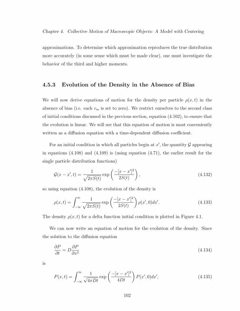
Chapter 4. Collective Motion of Macroscopic Objects: A Model with Centering
approximations. To determine which approximation reproduces the true distribution
more accurately (in some sense which must be made clear), one must investigate the
behavior of the third and higher moments.
4.5.3 Evolution of the Density in the Absence of Bias
We will now derive equations of motion for the density per particle ρ(x, t) in the
absence of bias (i.e. each vm is set to zero). We restrict ourselves to the second class
of initial conditions discussed in the previous section, equation (4.102), to ensure that
the evolution is linear. We will see that this equation of motion is most conveniently
written as a diffusion equation with a time-dependent diffusion coefficient.
For an initial condition in which all particles begin at x′, the quantity G appearing
in equations (4.108) and (4.109) is (using equation (4.71), the earlier result for the
single particle distribution functions)
G(x− x′, t) =1√
2πS(t)exp
(−[x− x′]2
2S(t)
), (4.132)
so using equation (4.108), the evolution of the density is
ρ(x, t) =
∫ ∞−∞
1√2πS(t)
exp
(−[x− x′]2
2S(t)
)ρ(x′, 0)dx′. (4.133)
The density ρ(x, t) for a delta function initial condition is plotted in Figure 4.1.
We can now write an equation of motion for the evolution of the density. Since
the solution to the diffusion equation
∂P
∂t= D
∂P
∂x2(4.134)
is
P (x, t) =
∫ ∞−∞
1√4πDt
exp
(−[x− x′]2
4Dt
)P (x′, 0)dx′, (4.135)
102

Chapter 4. Collective Motion of Macroscopic Objects: A Model with Centering
Figure 4.1: Density per particle as a function of time in the simple model of centeringwithout bias for a delta function initial condition.
it is easy to see that the density obeys
∂ρ
∂S=
1
2
∂2ρ
∂x2. (4.136)
Using the chain rule, we can rewrite this as a diffusion equation with a time dependent
diffusion coefficient,
∂ρ
∂t= D0χ(t)
∂2ρ
∂x2(4.137)
with
χ(t) =1
2D0
dS
dt= e−2Nγt +
1
N(1− e−2Nγt). (4.138)
As we saw earlier, at short times the effective diffusion constant is D0, but at
long times the springs counteract the spreading caused by the thermal noise, and the
effective diffusion constant is reduced to D0/N (since the center of mass still diffuses).
We could have derived this in a different way using the expressions obtained in
103

Chapter 4. Collective Motion of Macroscopic Objects: A Model with Centering
the previous section. The Fourier transformed Green’s function is
G(k, t) = exp
[−k
2S(t)
2
](4.139)
so using equation (4.115), we have
K(k, t) =∂
∂tln G(k, t) = −k2 1
2
dS
dt. (4.140)
Inserting this into the expansion (4.127) gives again equation (4.137).
In this case, it is more convenient to write the evolution equation as a time-
dependent diffusion equation; however, using the results from the previous section we
can reformulate the evolution as a memory equation. To do this, we must calculate
the joint Fourier-Laplace transform of the Green’s function,
G(k, ε) =
∫ ∞0
e−εtG(k, t)dt =
∫ ∞0
e−εt exp
[−k
2S(t)
2
]dt
=
∫ ∞0
exp
[−εt−D0k
2
(t
N+ (1− 1/N)
1− e−2Nγt
2Nγ
)]dt. (4.141)
This integral can be written in terms of the incomplete gamma function. First change
variables to κ = 2Nγt to get
G(k, ε) =e−
D0k2
2Nγ(1−1/N)
2Nγ
∫ t
0
exp
[−
(ε+ D0k2
N
2Nγ
)κ+
D0k2
2Nγ(1− 1/N)e−κ
]dκ.
(4.142)
Now consider integrals of the form∫ ∞0
e−atebe−tdt. (4.143)
Substitute u = −be−t to get∫ ∞0
e−atebe−tdt =
∫ 0
−b(−u/b)ae−u−du
u
= (−b)−a∫ −b
0
ua−1e−udu
= (−b)−aγinc(a,−b) (4.144)
104

Chapter 4. Collective Motion of Macroscopic Objects: A Model with Centering
where γinc(a, x) is the lower incomplete gamma function,
γinc(a, x) ≡∫ x
0
ta−1e−tdt. (4.145)
Using this, the Fourier-Laplace transformed Green’s function is
G(k, ε) =e−µ(k)
2Nγ[−µ(k)]−ν(k,ε) γinc
(ν(k, ε),−µ(k)
)(4.146)
where we have defined
µ(k) ≡ D0k2
2Nγ(1− 1/N), (4.147)
ν(k, ε) ≡ε+ D0k2
2Nγ
2Nγ. (4.148)
Using equation (4.120), the memory is
M(k, ε) = ε− 1
G(k, ε)
= ε−e−µ(k)
2Nγ[−µ(k)]−ν(k,ε) γinc
(ν(k, ε),−µ(k)
)−1
. (4.149)
We have now explicitly obtained an expression for the memory, at least in the Fourier-
Laplace domain.
This completes the calculation of two equivalent equations of motion for the den-
sity per particle ρ. The time-dependent evolution equation for ρ is local in space
in the sense that the time derivative of ρ(x, t) depends only on the second spatial
derivative at x, whereas the memory evolution equation is necessarily non-local in
space in the sense that the time derivative of ρ(x, t) depends on on ρ(x, t) at points
in space away from x.
We end this section with a calculation of an approximate memory evolution equa-
tion for ρ using the method described in the previous section. Instead of calculating
the expansion coefficients directly from equation (4.149), it is simpler to return to
equation (4.120). The m = 0 term necessarily vanishes due to conservation of prob-
ability, and in this case the m = 1 term vanishes since there is no bias in either
105

Chapter 4. Collective Motion of Macroscopic Objects: A Model with Centering
direction. The m = 2 term in the Laplace domain is
−1
2
∂2
∂k2M(k, ε)
∣∣∣∣k=0
=1
2
∂2
∂k2
1
G(k, ε)
∣∣∣∣k=0
=1
[G(0, ε)]3
[∂
∂kG(k, ε)
]2 ∣∣∣∣k=0
− 1
2[G(0, ε)]2∂2
∂k2G(k, ε)
∣∣∣∣k=0
.
(4.150)
Since the distribution is normalized to unity, we have G(0, t) = 1 and thus G(0, ε) =
1/ε. The first term vanishes since G is symmetric in x, so we have
−1
2
∂2
∂k2M(k, ε)
∣∣∣∣k=0
= −ε2
2
∫ ∞0
e−εt∂2
∂k2G(k, t)dt
∣∣∣∣k=0
. (4.151)
Using the Fourier transformed Green’s function, equation (4.139), this becomes
−1
2
∂2
∂k2M(k, ε)
∣∣∣∣k=0
=ε2S(ε)
2. (4.152)
The right hand side may be rewritten as
−1
2
∂2
∂k2M(k, ε)
∣∣∣∣k=0
=ε2S(ε)− εS(0)− S(0) + S (0)
2(4.153)
since S(0) = 0. Inverting the Laplace transform using the identity
Lf(t)(ε) = ε2f(ε)− εf(0)− f(0) (4.154)
gives
−1
2
∂2
∂k2M(k, t)
∣∣∣∣k=0
=1
2S(t) +
1
2δ(t)S(0). (4.155)
Plugging in for S(t) gives explicitly
−1
2
∂2
∂k2M(k, t)
∣∣∣∣k=0
= −2D0γe−2Nγt(N − 1) +D0δ(t). (4.156)
Our approximate memory equation of motion for the density is therefore
∂
∂tρ(x, t) = D0
∂
∂x2ρ(x, t)− 2D0γ(N − 1)
∫ t
0
e−2Nγ(t−t′) ∂2
∂x2ρ(x, t′)dt′. (4.157)
106

Chapter 4. Collective Motion of Macroscopic Objects: A Model with Centering
4.5.4 Evolution of the Density with Bias
Next, we analyze the case when bias vm is present. For the cluster initial condition
described earlier, equation (4.102), the single particle distribution functions evolve as
P (1)m (x, t) =
∫ ∞−∞
G(1)m (x− x′, t)P (1)
m (x′, 0)dx (4.158)
with G(1)m (x− x′, t) calculated from equation (4.71) by setting x′m = x′ for all m,
G(1)m (x− x′, t) =
1√2πS(t)
. exp
(−[xm − x′ − vmτ − v(t− τ)]2
2S(t)
). (4.159)
Fourier transforming, we have
G(1)m (k, t) = exp
−ik[vmτ + v(t− τ)]− k2S(t)
2
. (4.160)
Each individual single particle distribution therefore obeys an advection-diffusion
equation with time-dependent coefficients,
∂
∂tP (1)m (x, t) = −[vme
−Nγt + v(1− e−Nγt)] ∂∂xP (1)m (x, t) +D0χ(t)
∂2
∂x2P (1)m (x, t)
(4.161)
where we have used τ(t) = e−Nγt and S(t)/2 = D0χ(t).
The density per particle ρ(x, t), which is the sum of the single particle distribution
functions divided by N , obeys neither an advection-diffusion equation with time-
dependent coefficients nor an advection diffusion equation with memory unless every
vm is the same. The non-local in space versions, equations (4.111) and (4.116) must
be used.
The Green’s function for the evolution of the density in this case is
G(x− x′, t) =1
N
∑m
1√2πS(t)
exp
(−[x− x′ − vmτ − v(t− τ)]2
2S(t)
). (4.162)
The density per particle as a function of time when the bias is present is plotted in
Figure (4.2).
107

Chapter 4. Collective Motion of Macroscopic Objects: A Model with Centering
Figure 4.2: Density per particle as a function of time in the simple model of centeringwhen the bias is present for a delta function initial condition. In this case, theindividuals are either uninformed vm = 0 or informed vm = v. The concentration ofinformed individuals is a = 0.2.
In general, the neither equation (4.127) nor equation (4.128) terminate after a
finite number of terms. The evolution is thus necessarily non-local in space, no
matter which formulation, time-dependent or memory, is used to write the equation
of motion.
The time-dependent kernel K may at least be calculated explicitly in the Fourier
domain. We will also derive approximate equations of motion in both the time-
dependent and memory formulations.
The Fourier transform of the Green’s function in equation (4.162) is
G(k, t) =1
N
∑m
exp
[−ik [vmτ + v(t− τ)]− k2S(t)
2
]. (4.163)
Using this in equation (4.115), the time-dependent kernel K is
K(k, t) =
1N
∑m
[−ik[vmτ+v(1−τ)]− k
2S(t)2
]exp
[−ik[vmτ+v(t−τ)]− k
2S(t)2
]1N
∑m exp
[−ik[vmτ+v(t−τ)]− k
2S(t)2
] . (4.164)
108

Chapter 4. Collective Motion of Macroscopic Objects: A Model with Centering
We now calculate the expansion coefficients and write approximate equations of
motion which are local in space, beginning with the time-dependent formulation.
Again the m = 0 term vanishes because of conservation of probability. The m = 1
term is
∂
∂(ik)K(k, t)
∣∣∣∣k=0
=∂
∂t
1
G(k, t)
∂
∂(ik)G(k, t)
∣∣∣∣k=0
= − ∂
∂t
1
N
∑m
[vmτ + v(t− τ)] = −v. (4.165)
where we have used v = 1N
∑m vm and G(0, t) = 1. The m = 2 term is
1
2
∂2
∂(ik)2K(k, t)
∣∣∣∣k=0
=1
2
∂
∂t
[∂2
∂(ik)2G(k, t)
∣∣∣∣k=0
−(
∂
∂(ik)G(k, t)
)2 ∣∣∣∣k=0
]=
1
2S(t) + τ τσ2
v
= D0χ(t) + e−Nγtτσ2v (4.166)
with χ as defined earlier,
χ(t) = e−Nγt +1
Ne−Nγt (4.167)
and where σ2v is related to the spread of the vms,
σ2v ≡
1
N
∑m
v2m − v2. (4.168)
Using these results, an approximate space-local time-dependent equation of motion
for the density is
∂
∂tρ(x, t) = −v ∂
∂xρ(x, t) + [D0χ(t) + e−Nγtτσ2
v ]∂2
∂x2ρ(x, t). (4.169)
Next, we calculate an approximate equation of motion with memory. The m = 1
expansion coefficient in the Laplace domain is
∂
∂(ik)M(k, ε) = − ∂
∂(ik)
1
G(k, ε)
∣∣∣∣k=0
= ε2∂
∂(ik)
∫ ∞0
e−εtG(k, t)dt
∣∣∣∣k=0
= −vε2∫ ∞
0
e−εttdt = −v. (4.170)
109

Chapter 4. Collective Motion of Macroscopic Objects: A Model with Centering
Inverting the Laplace transform, this is
∂
∂(ik)M(k, t) = −vδ(t). (4.171)
The m = 2 term in the expansion in the Laplace domain is
−1
2
∂2
∂k2M(k, ε)
∣∣∣∣k=0
=1
[G(0, ε)]3
[∂
∂kG(k, ε)
]2 ∣∣∣∣k=0
− 1
2[G(0, ε)]2∂2
∂k2G(k, ε)
∣∣∣∣k=0
.
(4.172)
We have
∂
∂kG(k, ε)
∣∣∣∣k=0
=
∫ ∞0
e−εt∂
∂kG(k, t)dt
∣∣∣∣k=0
= −iv∫ ∞
0
e−εttdt = −iv 1
ε2(4.173)
and
1
2
∂2
∂k2G(k, ε)
∣∣∣∣k=0
=1
2
∫ ∞0
e−εt∂2
∂k2G(k, t)dt
∣∣∣∣k=0
= −1
2
∫ ∞0
e−εt1
N
∑m
S(t) + [vmτ + v(t− τ)]2
= −1
2S(ε)− σ2
v
2
∫ ∞0
e−εtτ 2dt− v2
ε3(4.174)
Using these along with G(0, ε) = 1/ε we have
−1
2
∂2
∂k2M(k, ε)
∣∣∣∣k=0
=ε2S(ε) + σ2
vε2∫∞
0e−εtτ 2dt
2. (4.175)
Using the definition of τ ,
τ 2 =1
(Nγ)2(1− 2e−Nγt + e−2Nγt) (4.176)
so
ε2∫ ∞
0
e−εtτ 2dt =ε2
(Nγ)2
(1
ε− 2
ε+Nγt+
1
ε+ 2Nγt
)=
1
(Nγ)2
2ε2(Nγ)2
(ε+Nγ)(ε+ 2Nγ)
=4
ε+ 2Nγ− 2
ε+Nγ. (4.177)
110

Chapter 4. Collective Motion of Macroscopic Objects: A Model with Centering
where we have performed a partial fraction decomposition in the last step. Inverting
the Laplace transform, we have for the m = 2 term in the expansion
−1
2
∂2
∂k2M(k, ε)
∣∣∣∣k=0
=1
2S(t) +
1
2δ(t)S(0) + σ2
v [2e−2Nγt − e−Nγt]
= −2D0γe−2Nγt(N − 1) +D0δ(t) + σ2
v [2e−2Nγt − e−Nγt].
(4.178)
The approximate memory equation of motion for the density is finally
∂
∂tρ(x, t) = −v ∂
∂xρ(x, t) +D0
∂
∂x2ρ(x, t)
−∫ t
0
[2D0γ(N − 1)− σ2v(2− eNγ(t−t′))]e−2Nγ(t−t′) ∂
2
∂x2ρ(x, t′)dt′.
(4.179)
4.6 Remarks
Let us summarize what we have found in this chapter. We have calculated exactly the
probability distribution as a function of time for a simple model of flocking consisting
only of a centering interaction, noise, and a bias. In the absence of noise, each particle
moves at the same speed but is displaced from the center of mass by an amount which
depends on the strength of the bias the particle feels. The noisy dynamics, analyzed
with a Fokker-Planck equation, are similar, but there is a spread in the particles
positions. At long times the distribution spreads more slowly due to the spring forces
counteracting the thermal noise. We saw also how a “mean-field” calculation could
be used to calculate the center of mass and single particle distribution functions in a
simpler way.
Next, we calculated another coarse-grained quantity: the density. It was shown
that for a certain class of initial conditions in which the particles are found clustered
together that the evolution of the density is linear, and we wrote continuum equations
of motion for the evolution of the density.
111

Chapter 4. Collective Motion of Macroscopic Objects: A Model with Centering
We saw that in the absence of bias, the evolution of the density is naturally
described by a diffusion equation with a time-dependent diffusion constant. We then
showed that the evolution equation can be recast as a memory equation, but in doing
so we found that the memory must be non-local in space as well as time.
In the presence of bias, it was shown that the density does not obey simply an
advection-diffusion equation with time-dependent coefficients (although the single
particle distributions themselves do). Instead, the density obeys time-dependent evo-
lution equation which is non-local in space. An equivalent memory equation, also
non-local in space, was found as well.
This simple model has proven to be amenable to analytic calculations, and we were
successfully able to write continuum equations of motion for coarse-grained quantities
starting from a dynamical description of the motion of each individual particle.
112
Chapter 5
Collective Motion of Macroscopic
Objects: A Model with Alignment
In the previous chapter, we constructed a simple model of collective motion which
consisted of a centering interaction, noise, and a bias. Although the model could
be exactly solved, it lacks an important feature present in many models of collective
motion: self-propulsion.
In this chapter, we construct and analyze another simple model of collective mo-
tion with a slightly different set of ingredients: self-propulsion, an alignment interac-
tion, and noise.
A heavily cited model in the literature with self-propulsion, alignment, and noise
is the model by Vicsek et al. [85]. Their model is rule-based with the following single
rule:
at each time step a given particle driven with a constant absolute velocity
assumes the average direction of motion of the particles in its neighbor-
hood of radius r with some random perturbation added.
113

Chapter 5. Collective Motion of Macroscopic Objects: A Model with Alignment
The model discussed in this chapter is based on Vicsek’s central idea. However, we
will treat it in a simplified form and, to allow for analytic calculations to be done, we
will make a crucial assumption: we will take the alignment interaction have infinite
range. We begin with the known single-particle version of the model and generalize
first to two-particles, then to many particles.
The one- and two-particle versions can be solved exactly, and we calculate the
first two moments and write equations of motion for some coarse-grained continuous
quantities. The many-particle version cannot be solved exactly, but we do calculate
the first two moments.
5.1 Single-Particle Model
First, consider a single particle which moves in one dimension at a constant speed
c, but which changes directions at random. Suppose that the probability per unit
time for the particle to flip is a constant, which we will call F . One possible path
of such a particle is illustrated in Figure 5.1. This simple model is already known
in the literature, see for example refs. [117, 119–122]. We will reproduce here the
main results from the single-particle model, then generalize the model to more than
one-particle and introduce an interaction.
The complete state of the particle can be described by two functions of space and
time which we will call Q+(x, t) and Q−(x, t). We define Q+ so that Q+(x, t)dx is the
probability to find the particle moving to the right in a small interval between x and
x+ dx at time t. Similarly, Q−(x, t)dx is the probability to find the particle moving
to the left in a small interval between x and x+ dx at time t.
What equations of motion do Q+ and Q− obey? If the particle did not flip (F = 0)
114

Chapter 5. Collective Motion of Macroscopic Objects: A Model with Alignment
0
2
4
6
8
10
-4 -3 -2 -1 0 1 2 3 4
Ft
x/c
Sample Path, Single Flipping Particle
Figure 5.1: Sample path of a particle moving at speed c which flips directions atrandom.
then the equations of motion would simply be advection equations,
∂
∂tQ+ = −c ∂
∂xQ+, (5.1)
∂
∂tQ− = +c
∂
∂xQ−. (5.2)
On the other hand, if the particles were stationary, then the equations of motion
would simply resemble the Master equation for a two-state system,
∂
∂tQ+ = F [Q− −Q+], (5.3)
∂
∂tQ− = F [Q+ −Q−]. (5.4)
115
Chapter 5. Collective Motion of Macroscopic Objects: A Model with Alignment
Combining these, when the particle is not stationary and does flip, the equations of
motion are
∂
∂tQ+ = −c ∂
∂xQ+ + F [Q− −Q+], (5.5)
∂
∂tQ− = +c
∂
∂xQ− + F [Q− −Q+]. (5.6)
This set of equations can be solved by Fourier and Laplace transforming and solving
the resulting system of linear equations. We again define the Fourier transform of a
function f which depends on space as
f(k) ≡∫ ∞−∞
f(x)e−ikxdx (5.7)
and the Laplace transform of a function g which depends on time as
g(ε) ≡∫ ∞
0
g(t)e−εtdt. (5.8)
The joint Fourier-Laplace transform of a function h which depends on both space and
time, which we label with a breve, is
h(k, ε) =
∫ ∞0
∫ ∞−∞
h(x, t)e−ikxe−εtdxdt. (5.9)
We have for the joint Fourier-Laplace transform of the equations of motion (5.5) and
(5.6)
εQ+(k, ε)− Q+(k, 0) = −ikcQ+(k, ε) + F [Q−(k, ε)− Q+(k, ε)], (5.10)
εQ−(k, ε)− Q−(k, 0) = ikcQ−(k, ε) + F [Q+(k, ε)− Q−(k, ε)]. (5.11)
Rearranging and rewriting as a matrix equation, this becomesε+ F + ikc −F
−F ε+ F − ikc
Q+(k, ε)
Q−(k, ε)
=
Q+(k, 0)
Q−(k, 0)
. (5.12)
Inverting the matrix on the left hand side then gives the solution asQ+(k, ε)
Q−(k, ε)
=1
ε2 + 2Fε+ k2
ε+ F − ikc F
F ε+ F + ikc
Q+(k, 0)
Q−(k, 0)
.
(5.13)
116

Chapter 5. Collective Motion of Macroscopic Objects: A Model with Alignment
We will see later that the solution in real space and time can be written in terms of
modified Bessel functions.
For now we will calculate some coarse-grained quantities. The total probability to
find the particle pointing to the right, which we will call P+, can be obtained simply
by integrating Q+ over all space,
P+(t) =
∫ ∞−∞
Q+(x, t)dx = Q(0, t). (5.14)
Similarly, the probability to find the particle pointing to the left, P−, is found by
integrating Q− over all space. We have constructed the model so that the flipping
occurs independently of where the particle is located, so P+ and P− obey the Master
equation
d
dtP+ = F [P− − P+], (5.15)
d
dtP− = F [P+ − P−]. (5.16)
This can be seen explicitly by integrating the equations of motion for Q+ and Q−
over all space.
Using P+ + P− = 1, the solution is
P+(t) = P+(0)e−2Ft +1
2(1− e−2Ft), (5.17)
P−(t) = P−(0)e−2Ft +1
2(1− e−2Ft), (5.18)
so at times t 1/(2F ), it is equally likely to find the particle pointing in either
direction. The evolution of P+ and P− for a particle initially pointing to the right is
plotted in Figure 5.2.
Now let us calculate the average position 〈x〉. Define Q to be the sum of Q+ and
Q−;
Q(x, t) ≡ Q+(x, t) +Q−(x, t). (5.19)
117

Chapter 5. Collective Motion of Macroscopic Objects: A Model with Alignment
0
0.5
1
0 1 2 3 4 5 6
Prob
abili
ty
2Ft
P+ and P-, particle initially pointing right
P+(t)P-(t)
Figure 5.2: Probability to find a randomly flipping particle pointing to the left orright as a function of time, given that the particle was initially pointing to the right.
The probability to find the particle in a small interval between x and x+ dx going in
either direction at time t is then Q(x, t)dx. The average position is then
〈x〉 =
∫ ∞−∞
xQ(x, t)dx =
∫ ∞−∞
x[Q+(x, t) +Q−(x, t)]dx. (5.20)
Fourier transforming equations (5.5) and (5.6) gives
∂
∂tQ+ = −c(ik)Q+ + F [Q− − Q+], (5.21)
∂
∂tQ− = +c(ik)Q+ + F [Q+ − Q−]. (5.22)
118

Chapter 5. Collective Motion of Macroscopic Objects: A Model with Alignment
Adding these, we have
∂
∂tQ = −c(ik)[Q+ − Q−]. (5.23)
Since the Fourier transform of Q is given by Q(k, t) ≡∫e−ikxQ(x, t)dx, the nth
moment can be computed by taking k-space derivatives of Q;
〈xn〉 ≡∫ ∞−∞
xnQ(x, t)dx =∂nQ
∂(−ik)n
∣∣∣∣k=0
, (5.24)
so using this in equation (5.23) gives the evolution of 〈x〉,
d
dt〈x(t)〉 = c[P+(t)− P−(t)]. (5.25)
The quantity P+(t)−P−(t) is the average direction the particle is pointing in at time t.
This can be seen by defining a stochastic variable σ(t) which represents the direction
of the particle and can take on only the values −1 or +1. Then the average direction
is
〈σ(t)〉 =∑
σ=−1,+1
σPσ(t) = P+(t)− P−(t). (5.26)
We can therefore write the evolution of the first moment as
d
dt〈x(t)〉 = c〈σ(t)〉. (5.27)
In words, this equation states simply that the time derivative of the average position
is the speed c times the average direction. From equations (5.17) and (5.18), the
average direction decays exponentially from its initial value,
〈σ(t)〉 = 〈σ(0)〉e−2Ft. (5.28)
Substituting this into equation (5.27) and integrating gives the average position as
〈x(t)〉 = 〈x(0)〉+ c〈σ(0)〉1− e−2Ft
2F. (5.29)
For short times, t 1/(2F ), the particle simply drifts at speed c in whichever
direction it is initially pointing in,
〈x(t)〉 ≈ 〈x(0)〉+ c〈σ(0)〉t. (5.30)
119

Chapter 5. Collective Motion of Macroscopic Objects: A Model with Alignment
0
0.2
0.4
0.6
0.8
1
0 1 2 3 4 5 6
(<x>
-<x(
0)>
)(2F
/c)
2Ft
Single Particle <x> vs t, Initially Pointing Right
Figure 5.3: The average position versus time of a randomly flipping particle movingat speed c, given that the particle was initially pointing to the right.
At long times, t 1/(2F ), the probability to find the particle pointing to the left
is equal to the probability to find the particle pointing to the right, so the average
direction is zero and the first moment becomes a constant,
〈x(t)〉 ≈ 〈x(0)〉+ c〈σ(0)〉 1
2F. (5.31)
The average position for an initial condition in which the particle is pointing to the
right is displayed in Figure 5.3.
Now let us calculate the second moment. Using equation (5.23), we have
d
dt〈x2〉 =
d
dt
∂2
∂(−ik)2Q
∣∣∣∣k=0
= 2c
[∂
∂(−ik)Q+
∣∣∣∣k=0
− ∂
∂(−ik)Q+
∣∣∣∣k=0
]. (5.32)
120

Chapter 5. Collective Motion of Macroscopic Objects: A Model with Alignment
Define
〈x+〉 =∂
∂(−ik)Q+
∣∣∣∣k=0
, (5.33)
〈x−〉 =∂
∂(−ik)Q−
∣∣∣∣k=0
. (5.34)
From the equations of motion for Q+ and Q−, we have
d
dt[〈x+〉 − 〈x−〉] = c[Q+(0, t) + Q−(0, t)]− 2F [〈x+〉 − 〈x−〉]. (5.35)
Because of normalization, Q(0, t) = Q+(0, t) + Q−(0, t) = 1 so
〈x+(t)〉 − 〈x−(t)〉 = [〈x+(0)〉 − 〈x−(0)〉]e−2Ft +c
2F(1− e−2Ft). (5.36)
Substituting,
∂
∂t〈x2〉 = 2c2 (1− e−2Ft)
2F+ 2ce−2Ft[〈x+(0)〉 − 〈x−(0)〉]. (5.37)
Integrating,
〈x2(t)〉−〈x2(0)〉 = 2c2 2Ft− (1− e−2Ft)
(2F )2+ 2c
1− e−2Ft
2F[〈x+(0)〉−〈x−(0)〉]. (5.38)
To see what happens for a simple initial condition, suppose that at time t = 0 the
particle is located at x = 0 and has a random direction. In terms of the Qs, this
means
Q+(x, 0) = Q−(x, 0) =1
2δ(x). (5.39)
We then have 〈x+(0)〉 = 〈x−(0)〉 = 0, 〈x2(0)〉 = 0, and 〈x(t)〉 = 0, and the second
moment is
〈x2(t)〉 = 2c2 2Ft− (1− e−2Ft)
(2F )2. (5.40)
At short times, t 1/(2F ), the second moment is proportional to t2, and the motion
is said to be ballistic,
〈x2(t)〉 ≈ (ct)2. (5.41)
121

Chapter 5. Collective Motion of Macroscopic Objects: A Model with Alignment
At long times, t 1/(2F ), the second moment is proportional to t, and the motion
is said to be diffusive,
〈x2(t)〉 ≈ 2c2
2Ft− 2c2
(2F )2. (5.42)
The effective diffusion constant, which can be defined as
Deff =1
2
d
dt
(〈x2(t)〉 − 〈x(t)〉2
), (5.43)
is
Deff =c2
2F. (5.44)
The second moment as a function of time is illustrated in Figure 5.4.
Now let us look at continuous coarse-grained quantities. Since there is only one
particle, the density, center of mass distribution, and single particle distribution are
all the same:
ρ(x, t) = Qcm(x, t) = Q(x, t) = Q+(x, t) +Q−(x, t). (5.45)
What equation of motion does Q obey? We could follow our procedure as discussed in
the previous chapter for constructing equations of motion from the Green’s function,
but it is simpler to use the following procedure as described in ref. [122]. First, take
the sum and difference of the equations of motion for Q+ and Q−, equations (5.5)
and (5.6), to obtain
∂
∂tQ = −c ∂
∂xR (5.46)
∂
∂tR = −c ∂
∂xQ− 2FR. (5.47)
where R is defined to be
R(x, t) ≡ Q+(x, t)−Q−(x, t). (5.48)
122

Chapter 5. Collective Motion of Macroscopic Objects: A Model with Alignment
10-4
10-3
10-2
10-1
100
101
102
10-2 10-1 100 101 102
Mea
n Sq
uare
d D
ispl
acem
ent
Time
Single Particle Mean Squared Displacement, c=F=1
Figure 5.4: Mean square displacement versus time of a randomly flipping particlewhich moves at constant speed c on a log-log scale to illustrate the change from t2
growth to t growth.
Take a time derivative of the first and substitute the second in the right hand side to
obtain
∂2
∂t2Q = −c ∂
∂x
∂
∂tR = c2 ∂
2
∂x2Q+ 2Fc
∂
∂xR. (5.49)
Finally, eliminate R from the right hand side using again equation (5.46) to obtain a
closed equation for Q,
∂2
∂t2Q+ 2F
∂
∂tQ = c2 ∂
2
∂x2Q. (5.50)
This partial differential equation, which is second order in time, is known as the
123

Chapter 5. Collective Motion of Macroscopic Objects: A Model with Alignment
telegrapher’s equation. If there were no flipping, F = 0, Q would obey simply the
wave equation. On the other hand, if the first term were not present, Q would obey
a diffusion equation with diffusion constant D = c2/(2F ).
Since this is a second order in time equation, both Q and Q must be specified at
time t = 0. Using the definition of Q, we have simply
Q(x, 0) = Q+(x, 0) +Q−(x, 0), (5.51)
and using equation (5.46), Q(x, 0) is
Q(x, 0) = −c ∂∂x
[Q+(x, 0)−Q−(x, 0)] . (5.52)
The solution to the telegrapher’s equation (5.50) can be obtained by standard
techniques (see for example ref. [123]), and has been applied in diverse areas ranging
from particle transport to stress distribution in granular compacts [124–126]. For an
initial condition Q(x, 0) = δ(x), Q(x, 0) = 0 (i.e. the particle starts at x = 0 with a
random direction), the solution is
Q(x, t) = e−Ftδ(x− ct) + δ(x+ ct)
2+F
2ce−FtH(ct− |x|)
[I0(Λ) +
Ft
ΛI1(Λ)
](5.53)
where H is the unit step function, the Is are modified Bessel functions, and
Λ ≡ F
c
√c2t2 − x2. (5.54)
How does Q evolve in time? The distribution Q(x, t) is zero for |x| > ct due to the fact
that the particle moves at a constant speed c, so it cannot be found anywhere with
|x| > ct (since it would have to move faster than c to get there). The delta functions
in the first term represent the motion of the particle if it has not flipped. They are
multiplied by a factor e−Ft because the probability that the particle has not flipped
decays exponentially in time. The second term is nonzero in the interior region |x| < ct
and is a result of the flipping. Using the asymptotic properties of the modified Bessel
124

Chapter 5. Collective Motion of Macroscopic Objects: A Model with Alignment
0
0.25
0.5
0.75
1
-5 -4 -3 -2 -1 0 1 2 3 4 5
Q(x
,t)
x
Telegrapher's Equation Solution, c=F=1
t=0 t=1 t=2 t=4 t=6
Figure 5.5: The solution to the telegrapher’s equation for different times for a deltafunction initial condition. The vertical arrows represent delta functions, with thelength of the arrow representing the amplitude of the delta function.
functions it can be shown that at long times, Q becomes approximately a Gaussian
[122]. The solution is illustrated in Figure 5.5.
Instead of a second order in time partial differential equation, the evolution of
Q may also be written as a first order in time partial differential equation with a
memory [117]. Formally solving equation (5.47) for R in terms of Q gives
R(x, t) = e−2FtR(x, 0)− c∫ t
0
e−2F (t−t′) ∂
∂xQ(x, t′)dt′. (5.55)
Substituting into (5.46) gives an equation which is closed in Q except for a term which
125

Chapter 5. Collective Motion of Macroscopic Objects: A Model with Alignment
depends on R at time t = 0,
∂
∂tQ(x, t) = −ce−2Ft ∂
∂xR(x, 0) + c2
∫ t
0
e−2F (t−t′) ∂2
∂x2Q(x, t′)dt′. (5.56)
5.2 Two-Particle Model
Next, we generalize the model constructed in the previous section to two interacting
particles. The particles still flip randomly, but we construct the flipping rates so
that the particles tend to point in the same direction. This is a kind of alignment
interaction. An important simplification we will use is to make the interaction infinite
ranged, in the sense that the strength of the alignment interaction is independent of
the distance between the particles.
Since there are four total configurations, the state of the system may be described
by four functions of two spatial variables (the positions of each of the two-particles)
and time which we will denote Q++, Q+−, Q−+ and Q−−. Define Q++ so that the
probability to find both particles pointing to the right with the first particle in a small
interval between x1 and x1 + dx1 and the second particle in a small interval between
x2 and x2 + dx2 is
Q++(x1, x2, t)dx1dx2. (5.57)
Similarly define Q+− (except with the first particle pointing to the right and the
second to the left), Q−+ (first pointing to the left, second to the right), and Q−−
(both particles pointing to the left).
Before we construct the equations of motion for the Qs, let us first construct
equations of motion for the probabilities to find the particles in a given configuration,
which we will denote P++, P+−, P−+, and P−−. The quantity P++(t) is the total
probability to find both particles pointing to the right at time t, and is related to
126
Chapter 5. Collective Motion of Macroscopic Objects: A Model with Alignment
Q++ by integrating over the positions of the two-particles,
P++(t) =
∫ ∞−∞
∫ ∞−∞
Q++(x1, x2, t)dx1dx2. (5.58)
The remaining quantities P+−, P−+, and P−− are similarly related to Q+−, Q−+, and
Q−−.
Since we have assumed that the strength of the alignment interaction does not
depend on the relative distance between the two-particles, the directions of the par-
ticles evolve independently of the positions and closed equations of motion can be
written for the P s. We assume that their evolution can be described by a Master
equation, and we introduce alignment by constructing the rates in such a way that
the aligned states are favored. More precisely, let F by the probability per unit time
for the system to change from an unaligned state to an aligned state (e.g. −+ to ++
or −+ to −−), and let f < F be the probability per unit time to flip from an aligned
state to an unaligned state. The situation is illustrated in Figure 5.6. The Master
equation for the evolution of the P s is
dP++
dt= F [P+− + P−+]− 2fP++, (5.59)
dP−−dt
= F [P+− + P−+]− 2fP−−, (5.60)
dP+−
dt= f [P++ + P−−]− 2FP+−, (5.61)
dP−+
dt= f [P++ + P−−]− 2FP−+. (5.62)
This system of equations can be solved in the following way. This procedure is
equivalent to diagonalizing the interaction matrix. Adding all four equations together,
we have simply conservation of total probability:
d
dt[P++ + P−− + P+− + P−+] = 0. (5.63)
Subtracting the second from the first and the fourth from the third,
d
dt[P++ − P−−] = −2f [P++ − P−−], (5.64)
d
dt[P+− − P−+] = −2F [P+− − P−+], (5.65)
127

Chapter 5. Collective Motion of Macroscopic Objects: A Model with Alignment
++
+−−+
−−
Ff
Ff
Ff
Ff
Figure 5.6: Illustration of the flipping rates for the two-particle alignment model.
which can be solved as
[P++(t)− P−−(t)] = e−2ft[P++(0)− P−−(0)], (5.66)
[P+−(t)− P−+(t)] = e−2Ft[P+−(0)− P−+(0)]. (5.67)
Finally, combining all four equations we also have
d
dt[2f(P+++P−−)−2F (P+−+P−+)] = −(2f+2F )[2f(P+++P−−)−2F (P+−+P−+)]
(5.68)
which can be solved as
2f [P++(t) + P−−(t)]− 2F [P+−(t) + P−+(t)]
= e−(2f+2F )t2f [P++(0) + P−−(0)]− 2F [P+−(0) + P−+(0)]. (5.69)
128

Chapter 5. Collective Motion of Macroscopic Objects: A Model with Alignment
If we now solve for P++, P−−, P+−, P−+, we have
P++(t) =1
2e−2ft[P++(0)− P−−(0)]
+1
2e−2(F+f)t[P++(0) + P−−(0)] +
1
2
F
F + f(1− e−2(F+f)t) (5.70)
P−−(t) =1
2e−2ft[P−−(0)− P++(0)]
+1
2e−2(F+f)t[P++(0) + P−−(0)] +
1
2
F
F + f(1− e−2(F+f)t) (5.71)
P+−(t) =1
2e−2Ft[P+−(0)− P−+(0)]
+1
2e−2(F+f)t[P+−(0) + P−+(0)] +
1
2
f
F + f(1− e−2(F+f)t) (5.72)
P−+(t) =1
2e−2Ft[P−+(0)− P+−(0)]
+1
2e−2(F+f)t[P+−(0) + P−+(0)] +
1
2
f
F + f(1− e−2(F+f)t) (5.73)
In the steady state, the probabilities become
P++ = P−− =1
2
F
F + f, (5.74)
P+− = P−+ =1
2
f
F + f. (5.75)
Since we have chosen F > f , the probability to find the particles in the aligned states
++ and −− is larger than the probability to find them in the unaligned states +−
and −+.
We now construct equations of motion for the four Qs. We do this simply by
keeping the flipping terms the same (again, since we have made the simplification
that the interaction does not depend on the separation between the particles) and
129

Chapter 5. Collective Motion of Macroscopic Objects: A Model with Alignment
adding drift terms,
∂Q++
∂t= −c∂Q++
∂x1
− c∂Q++
∂x2
+ F [Q+− +Q−+]− 2f [Q++], (5.76)
∂Q−−∂t
= +c∂Q−−∂x1
+ c∂Q−−∂x2
+ F [Q+− +Q−+]− 2f [Q−−], (5.77)
∂Q+−
∂t= −c∂Q+−
∂x1
+ c∂Q+−
∂x2
+ f [Q++ +Q−−]− 2F [Q+−], (5.78)
∂Q−+
∂t= +c
∂Q−+
∂x1
− c∂Q−+
∂x2
+ f [Q++ +Q−−]− 2F [Q−+]. (5.79)
It is possible to solve the equations of motion exactly by Fourier transforming and
solving the resulting set of linear ordinary differential equations by diagonalizing a
4x4 matrix, i.e. write
∂
∂tQ(k1, k2, t) = −A(k1, k2)Q(k1, k2, t) (5.80)
where Q(k1, k2, t) is a vector which contains the Fourier transformed distributions,
Q(k1, k2, t) ≡
Q++(k1, k2, t)
Q−−(k1, k2, t)
Q+−(k1, k2, t)
Q−+(k1, k2, t)
(5.81)
and the matrix A(k1, k2) is
A(k1, k2) =
ic(k1 + k2) + 2f 0 −F −F
0 −ic(k1 + k2) + 2f −F −F
−f −f ic(k1 − k2) + 2F 0
−f −f 0 ic(k2 − k1) + 2F
. (5.82)
The solution can be formally written as
Q(k1, k2, t) = exp[−A(k1, k2)t]Q(k1, k2, 0), (5.83)
or in the Laplace domain as
Q(k1, k2, ε) = [εI + A(k1, k2)]−1Q(k1, k2, 0). (5.84)
130

Chapter 5. Collective Motion of Macroscopic Objects: A Model with Alignment
Explicit expressions can be found by diagonalizing the 4x4 matrix A to calculate the
exponential (in the time domain), or inverting εI+A (in the Laplace domain). These
operations can be performed in computer algebra systems, but the resulting expression
are too large to reproduce here. Instead, we calculate the first two moments, and some
continuous coarse-grained quantities.
One way to calculate the first two moments is to follow the same procedure as
in the single-particle case: Fourier transform the equations of motion for the Qs and
take k-space derivatives to obtain equations of motion for the moments. A simpler
method which we will apply here is to write stochastic differential equations for the
positions of the two-particles, and calculate the moments from them by ensemble
averaging. The velocity of the mth particle is simply the speed c times the direction
the particle is moving in σm,
xm(t) = cσm(t). (5.85)
Since σm is a stochastic variable (and therefore xm is as well), these are stochastic
differential equations, but not necessarily Langevin equations since σm does not rep-
resent Gaussian white noise. However, since the interaction strength does not depend
on the positions, the statistical properties of the directions are defined simply through
the Master equation (5.59)–(5.62). Ensemble averaging equation (5.85), we have an
equation of motion for the first moment 〈xm〉.
d
dt〈xm(t)〉 = c〈σm(t)〉. (5.86)
This may also be derived directly from the equations of motion for the Qs.
How does the average direction 〈σm(t)〉 evolve in time? The total probability for
the first particle to be pointing to the right is P++ + P+−, and the total probability
for the first particle to be pointing to the left is P−+ + P−−, therefore the average
direction of the first particle is
〈σ1(t)〉 = [P++(t) + P+−(t)]− [P−+(t) + P−−(t)]. (5.87)
131

Chapter 5. Collective Motion of Macroscopic Objects: A Model with Alignment
Similarly, the average direction of the second particle is
〈σ2(t)〉 = [P++(t) + P−+(t)]− [P+−(t) + P−−(t)]. (5.88)
Using equations (5.66) and (5.67) average directions evolve as
〈σ1(t)〉 = e−2ft 〈σ1(0)〉+ 〈σ2(0)〉2
+ e−2Ft 〈σ1(0)〉 − 〈σ2(0)〉2
, (5.89)
〈σ2(t)〉 = e−2ft 〈σ1(0)〉+ 〈σ2(0)〉2
− e−2Ft 〈σ1(0)〉 − 〈σ2(0)〉2
. (5.90)
Substituting into equation (5.86) and integrating, the average positions of the first
and second particles are
〈x1(t)〉 − 〈x1(0)〉c
=1− e−2ft
2f
〈σ1(0)〉+ 〈σ2(0)〉2
+1− e−2Ft
2F
〈σ1(0)〉 − 〈σ2(0)〉2
,
(5.91)
〈x2(t)〉 − 〈x2(0)〉c
=1− e−2ft
2f
〈σ1(0)〉+ 〈σ2(0)〉2
− 1− e−2Ft
2F
〈σ1(0)〉 − 〈σ2(0)〉2
.
(5.92)
At short times, the particles simply drift in whichever direction they are initially
pointing in,
〈x1(t)〉 ≈ 〈x1(0)〉+ c〈σ1(0)〉t, (5.93)
〈x2(t)〉 ≈ 〈x2(0)〉+ c〈σ2(0)〉t. (5.94)
At long times, both 〈x1〉 and 〈x2〉 go to a constant, since even though the particles
tend to align, there is no preferred direction for them to point in (i.e. the ++ state
is just as likely as the −− state).
The alignment interaction does affect the average positions at intermediate times.
For example, consider the case when at time t = 0 the direction of the first particle
is random, 〈σ1(0)〉 = 0, but the second particle is pointing to the right, 〈σ2(0)〉 = 1.
In this case, we have
〈x1(t)〉 = 〈x1(0)〉+c
2
(1− e−2ft
2f− 1− e−2Ft
2F
), (5.95)
〈x2(t)〉 = 〈x2(0)〉+c
2
(1− e−2ft
2f+
1− e−2Ft
2F
). (5.96)
132

Chapter 5. Collective Motion of Macroscopic Objects: A Model with Alignment
At short times, the first particle is stationary, and the second particle drifts to the
right at speed c, but at intermediate times, the first particle also begins to drift to
the right due to the alignment interaction.
Now let us calculate the second moments. Again, these may be calculated direction
from the equations of motion for the Qs, but instead we calculate starting from the
stochastic differential equations for the positions. Integrating equation (5.85), we
have
xm(t) = xm(0) + c
∫ t
0
σm(t′)dt′. (5.97)
Multiplying by xn(t) and ensemble averaging,
〈xm(t)xn(t)〉 = 〈xm(0)xn(0)〉+ c
∫ t
0
〈xm(0)σn(t′)〉dt′ + c
∫ t
0
〈xn(0)σm(t′)〉dt′
+ c2
∫ t
0
∫ t
0
〈σm(t′)σn(t′′)〉dt′dt′′. (5.98)
The two-time correlation function on the right hand side may be written as [127, 128]
〈σm(t)σn(t+ t′)〉 =∑σ
∑σ′
Pσ(t)σmPσ|σ′(t′)σ′n (5.99)
where σ represents an entire configuration (i.e. for this two-particle system ++, −+,
+−, or −−), Pσ(t) is the probability to find the particles in that configuration at
time t, and Pσ|σ′(t′) is the conditional probability for finding the configuration σ′ at
time t′ given that the particles began in a configuration σ. We have∑σ′
Pσ|σ′(τ)σ′n = 〈σn(τ)〉σ (5.100)
where the right hand side means the average value of the nth direction at time τ
given that the system began in a configuration σ. Using equations (5.89) and (5.90),
these are
〈σ1(t′)〉σ =e−2ft′ + e−2Ft′
2σ1 +
e−2ft′ − e−2Ft′
2σ2, (5.101)
〈σ2(t′)〉σ =e−2ft′ − e−2Ft′
2σ1 +
e−2ft′ + e−2Ft′
2σ2. (5.102)
133

Chapter 5. Collective Motion of Macroscopic Objects: A Model with Alignment
Using σ21 = σ2
2 = 1, we have
〈σ1(t)σ1(t+ t′)〉 = 〈σ2(t)σ2(t+ t′)〉
=e−2ft′ + e−2Ft′
2+e−2ft′ − e−2Ft′
2〈σ1(t)σ2(t)〉 (5.103)
and
〈σ1(t)σ2(t+ t′)〉 = 〈σ2(t)σ1(t+ t′)〉
=e−2ft′ − e−2Ft′
2+e−2ft′ + e−2Ft′
2〈σ1(t)σ2(t)〉. (5.104)
We must now calculate the equal-time pair correlation function 〈σ1(t)σ2(t)〉. We have
〈σ1(t)σ2(t)〉 =∑σ
σ1σ2Pσ(t) = P++(t) + P−−(t)− P+−(t)− P−+(t). (5.105)
Using equations (5.70) through (5.73), the equal time pair correlation function is
〈σ1(t)σ2(t)〉 = e−2(F+f)t〈σ1(0)σ2(0)〉+F − fF + f
(1− e−2(F+f)t). (5.106)
Now, let us simplify to the case where both particles start at x = 0 with random
directions. In this case 〈xm(0)σn(t)〉 = 0, 〈xm(0)xn(0)〉 = 0, 〈σ1(0)σ2(0)〉 = 0, and
equation (5.98) reduces to
〈xm(t)xn(t)〉 = c2
∫ t
0
∫ t
0
〈σm(t′)σn(t′′)〉dt′dt′′. (5.107)
Rewriting the double integral on the right hand side and using the fact that nothing
changes in this system if σ1 and σ2 are interchanged,
〈xm(t)xn(t)〉 = 2c2
∫ t
0
∫ t−t′
0
〈σm(t′)σn(t′ + t′′)〉dt′′dt′. (5.108)
Substituting and performing the integration, we have
〈x21(t)〉 = 〈x2
2(t)〉 = 2c2
[(1− e−2Ft
2F− 1− e−2ft
2f
)(F − f
4F (F + f)
)−(
1− e−2(F+f)t
2(F + f)
)(F 2 + f 2
4Ff(F + f)
)+
2ft− (1− e−2ft)
(2f)2
F
F + f+
2Ft− (1− e−2Ft)
(2F )2
f
F + f
].
(5.109)
134
Chapter 5. Collective Motion of Macroscopic Objects: A Model with Alignment
and
〈x1(t)x2(t)〉 = 2c2
[F − f
8Ff(F + f)
(e−2Ft + e−2ft − e−2(F+f)t − 1
)2ft− (1− e−2ft)
(2f)2
F
F + f− 2Ft− (1− e−2Ft)
(2F )2
f
F + f
](5.110)
At short times, we have 〈x21(t)〉 ≈ (ct)2 (ballistic motion), and at long times the
second moment is proportional to time,
〈x21(t)〉 ≈ const + c2 F 2 + f 2
Ff(F + f)t, (5.111)
which is characteristic of diffusive motion with an effective diffusion constant
Deff = c2 F 2 + f 2
2Ff(F + f)(5.112)
This is similar to the one-particle (telegrapher) case. In fact, if we set f = F , i.e.
both particles flip independently and we get the same effective diffusion constant as
in the one-particle case, Deff = c2/(2F ).
If F and f are switched, then for this initial condition, 〈x21〉 and 〈x2
2〉 do not
change, i.e. it does not matter for 〈x21〉 and 〈x2
2〉 if the birds tend to align or antialign
because the interaction has infinite range.
To see the effect of the alignment, we must look at two-particle observables such
as the mixed moment 〈x1x2〉. This is a measure of how strongly the positions of the
two-particles are correlated. At long times the positions are positively correlated so
long as F > f ,
〈x1x2〉 ≈ const + c2 F 2 − f 2
Ff(F + f)t. (5.113)
For F = f , the correlation vanishes for all times since the particles then flip indepen-
dently of each other.
We now look at coarse-grained continuum quantities, starting with the joint dis-
135

Chapter 5. Collective Motion of Macroscopic Objects: A Model with Alignment
tribution function defined by
Q(x1, x2, t) ≡ Q++(x1, x2, t) +Q+−(x1, x2, t) +Q−+(x1, x2, t) +Q−−(x1, x2, t).
(5.114)
Defined in this way, Q(x1, x2, t)dx1dx2 is the total probability to find the first particle
in a small interval between x1 and x1 +dx1 and the second particle in a small interval
between x2 and x2 + dx2 at time t with either particle pointing in any direction.
We take an initial condition in which the directions of both particles are random,
i.e.
Q++(x1, x2, 0) = Q+−(x1, x2, 0) = Q−+(x1, x2, 0) = Q−−(x1, x2, 0) = Q(x1,x2,0)4 .
(5.115)
Using a computer algebra system to perform coarse-graining on the full solution, the
evolution of Q in the Fourier-Laplace domain for this initial condition is
Q(k1, k2, ε) =1
ε− M(k1, k2, ε)Q(k1, k2, 0) (5.116)
where the memory M is, in the transformed domain,
M(k1, k2, ε) ≡−c2[(ε2+3Fε+4F 2)k2
++(3fε+4f2)k2−+c2(k+k−)2]
8Ff(F+f)+4(F 2+f2)ε+4(F+f)ε2+12Ffε+c2Fk2++c2fk2
−+c2ε(k2++k2
−)/2+ε3.
(5.117)
with
k+ ≡ k1 + k2, (5.118)
k− ≡ k1 − k2. (5.119)
Since the series expansion of M(k1, k2, ε) in powers of k1 and k2 has infinitely
many terms, the joint distribution Q obeys an equation of motion which is non-local
in both space and time,
∂
∂tQ(x1, x2, t) =
∫ ∞−∞
∫ ∞−∞
∫ t
0
M(x1 − x′1, x2 − x′2, t− t′)Q(x′1, x′2, t)dt
′dx′1dx′2.
(5.120)
136

Chapter 5. Collective Motion of Macroscopic Objects: A Model with Alignment
From the joint distribution Q, we can coarse-grain further to the single-particle
distributions by integrating out one of the position variables,
Q(1)1 (x, t) ≡
∫ ∞−∞
Q(x, x2, t)dx2, (5.121)
Q(1)2 (x, t) ≡
∫ ∞−∞
Q(x1, x, t)dx1. (5.122)
For the same initial condition, we have
Q(1)1 (k, ε) =
1
ε− M1(k, ε)Q
(1)1 (k, 0) (5.123)
Q(1)2 (k, ε) =
1
ε− M1(k, ε)Q
(1)2 (k, 0) (5.124)
with
M1(k, ε) = M(k, 0, ε) = M(0, k, ε)
= −c2[(4F 2+4f2+3Fε+3fε+ε2+c2k2)k2]8Ff(F+f)+4(F 2+f2)ε+4(F+f)ε2+12Ffε+c2(F+f)k2+c2k2ε+ε3
. (5.125)
The memory M1 is again non-local in both space and time, and the single-particle
distributions obey
∂
∂tQ(1)(x, t) =
∫ ∞−∞
∫ t
0
M1(x− x′, t− t′)Q(1)(x′, t′)dt′dx′. (5.126)
Finally, we calculate the center of mass distribution. We define Qcm(x, t)dx as the
probability to find the center of mass xcm = (x1 +x2)/2 between x and x+dx at time
t. This can be obtained from the joint distribution by changing to coordinates
x+ =x1 + x2
2(5.127)
x− =x1 − x2
2(5.128)
and integrating out x−. For the same initial condition, the evolution of the center of
mass distribution in the Fourier-Laplace domain is
Qcm(k, ε) =1
ε− Mcm(k, ε)Qcm(k, 0) (5.129)
137

Chapter 5. Collective Motion of Macroscopic Objects: A Model with Alignment
with the memory given by
Mcm(k, ε) =−c2k2(4F + ε)
8f(F + f) + 4ε(F + 2f) + c2k2 + 2ε2. (5.130)
The center of mass distribution again obeys an equation of motion which is non-local
in both space in time,
∂
∂tQcm(x, t) =
∫ ∞−∞
∫ t
0
Mcm(x− x′, t− t′)Qcm(x′, t′)dt′dx′ (5.131)
Since memory for the center of mass distribution Mcm is relatively simple, let us
look at it in more detail.
We can use the methods described in section 4.5.2 to write an approximate evo-
lution equation which is local in space. We have for the first expansion coefficient in
the Laplace domain
−1
2
∂2
∂k2Mcm(k, ε)
∣∣∣∣k=0
=c2(4F + ε)
8f(F + f) + 4ε(F + 2f) + 2ε2. (5.132)
The Laplace transform can be inverted with a partial fraction decomposition. The
result is
−1
2
∂2
∂k2Mcm(k, t)
∣∣∣∣k=0
=1
2c2e−(F+2f)t
[cosh(Ft) +
3F − 2f
Fsinh(Ft)
]. (5.133)
This is the approximate space local memory. For large t, it decays exponentially like
e−2ft, but since the derivative at t = 0 is c2(F − 2f) it can grow or decay at short
times depending on whether f is smaller or larger than F/2.
Now let us try to gain some insight into the spatial dependence of the memory.
The series expansion of M in powers of k does not contain any terms of order lower
than k2, so we can rewrite the evolution as
∂
∂tQcm(x, t) =
∫ ∞−∞
∫ t
0
D(x− x′, t− t′) ∂2
∂x′2Qcm(x′, t′)dt′dx′ (5.134)
with D related to Mcm by
D(k, t) =−1
k2Mcm(k, t) =
c2(4F + ε)
8f(F + f) + 4ε(F + 2f) + c2k2 + 2ε2. (5.135)
138

Chapter 5. Collective Motion of Macroscopic Objects: A Model with Alignment
The Fourier transform can be inverted by using the fact that the Fourier transform
of e−a|x| is
F [e−a|x|](k) =
∫ ∞−∞
e−a|x|e−ikxdx =2a
a2 + k2. (5.136)
Then in the real space-Laplace domain, we have
D(x, ε) = c(4F+ε)
2√
8f(F+f)+4ε(F+2f)+2ε2exp
(− |x|c
√8f(F + f) + 4ε(F + 2f) + 2ε2
). (5.137)
Although we cannot invert the Laplace transform we can gain some understanding of
the long time dynamics by making the so-called Markovian approximation, in which
the memory is replaced with a delta function times its integral,
D(x, t) ≈ δ(t)
∫ ∞0
D(x, t′)dt′. (5.138)
Using equation (5.137) gives for the integral on the right hand side∫ ∞0
D(x, t′)dt′ = D(x, 0) =cF√
2f(F + f)exp
(−|x|c
√8f(F + f)
). (5.139)
In this limit, the memory decays exponentially with distance at rate which depends
on the speed c and the flipping rates F and f .
What about the short time dynamics? Suppose that we have an initial condition
where both particles start at x = 0 with random directions. At short times, before
the particles have had a chance to flip, there is probability 1/2 to have one particle
pointing right and one particle pointing left. Therefore the center of mass does not
move. Otherwise, with probability 1/4 each, we have both particles pointing to the
right (in which case the center of mass moves to the right at speed c) or both particles
pointing to the left (in which case the center of mass moves to the left at speed c).
The Green’s function for the center of mass at short times is thus
Gcm(x, 0, t) ≈ 1
2δ(x) +
1
4δ(x− ct) +
1
4δ(x+ ct). (5.140)
Using the formalism developed in Section 4.5.2, the memory is approximately
Mcm(k, ε) = ε− 1
G(k, ε)≈ −(ck)2 ε
2ε2 + (ck)2(5.141)
139

Chapter 5. Collective Motion of Macroscopic Objects: A Model with Alignment
in which case D is approximately
D(k, ε) ≈ c2 ε
2ε2 + (ck)2. (5.142)
Inverting both the Laplace and Fourier transforms gives the short time memory as
D(x, t) ≈ c2
4
[δ
(x− ct√
2
)+ δ
(x− ct√
2
)]. (5.143)
The memory at short times thus connects the evolution of distribution at a point x
at time t only to the distribution at different positions within the range |x| < ct/√
2.
This is entirely expected and represents ballistic motion at short times.
5.3 Generalization to Many Particles
We now generalize the model to N particles. Again, the particles move in one di-
mension at a constant speed c, but with directions that change randomly, with the
flipping rates constructed so that there is an alignment effect. We will make use of
an existing model, Glauber dynamics for the Ising model, to construct the rates. The
interaction will again be infinite ranged in the sense that the tendency for particles
to align is not affected by the relative distance between them.
We will describe the complete state of the system using 2N functions which depend
on N spatial variables (the positions of the particles) and time. Generalizing our
earlier notation, we denote these by Qσ(x, t). The quantity σ represents a complete
set of directions, i.e. it is a quantity with N components with the nth component,
σn, representing the direction of the nth particle (either −1 or +1). The quantity x is
an N dimensional vector with the nth component xn representing the position of the
nth particle. Let Qσ(x, t)dNx be the probability to find the system in a state with
directions given by σ and particle 1 between x1 and x1 + dx1, particle 2 between x2
and x2 + dx2 et cetera at time t.
140

Chapter 5. Collective Motion of Macroscopic Objects: A Model with Alignment
For the evolution of Qσ(x, t) we take the general form
∂
∂tQσ(x, t) = −c
∑n
σn∂
∂xnQσ(x, t)+
∑σ′
[wσ,σ′Qσ′(x, t)− wσ′,σQσ(x, t)] (5.144)
where the sum over σ′ means to sum on all possible configurations σ′, i.e. sum over
σ′1 = −1,+1, σ′2 = −1,+1 et cetera, and wσ,σ′ is the probability per unit time to flip
from a configuration σ′ to a configuration σ.
The first term on the right hand side represents the motion of the particles at speed
c in the directions specified by σ, and the next two terms represent the directional
flipping.
The probabilities Pσ to find the particles in with a set of directions σ no matter
where they are located are obtained by integrating out the positions,
Pσ(t) =
∫Qσ(x, t)dNx = Qσ(k = 0, t). (5.145)
These evolve in time simply as
d
dtPσ(t) =
∑σ′
[wσ,σ′Pσ′(t)− wσ′,σPσ(t)] . (5.146)
Again, we can see explicitly that since the interaction is infinite ranted, the direction
flipping dynamics is completely independent of the positions of the particles.
We will now construct the flipping rates wσ′,σ. The directions of the particles
are similar to spins in an Ising model [129] in the sense that each spin or direction
can take on only two values. Discussion of the Ising model can be found in many
introductory textbooks on statistical physics, see for example refs. [130, 131].
In a ferromagnetic Ising model, aligning two interacting spins lowers the inter-
action energy between those two spins, but the Ising model itself has no intrinsic
dynamics so gives us no insight into how to construct the flipping rates. There are
however ways to add dynamics to the Ising model. The approach applicable to this
system, due to Glauber [127], is to construct equations of motion for the probabilities
141

Chapter 5. Collective Motion of Macroscopic Objects: A Model with Alignment
to find the system in a given spin configuration, the quantities which we have here
written as Pσ.
We construct the rates following Glauber’s procedure. The procedure will only be
outlined here, more detail can be found in the papers by Glauber [127] and Suzuki
and Kubo [128]. First we take an Ising model Hamiltonian (with no field),
H(σ) = −∑m<n
Jmnσmσn (5.147)
where the interaction matrix Jmn determines which particles interact with each other
and how strongly. We suppose that the system is in contact with a heat bath at tem-
perature T which causes the particles to flip directions stochastically. We only allow
only one-particle to flip at a time, so that wσ′,σ is zero unless the initial configuration
σ and the final configuration σ′ differ by a only single direction flip. In the steady
state, the probabilities Pσ(t) to form a Boltzmann distribution,
Pσ(t)→ 1
Ze−βH(σ) (5.148)
where Z is the partition function,
Z =∑σ
e−βH(σ). (5.149)
In the steady state, we must also have
d
dtPσ(t) = 0 =
∑σ′
[wσ,σ′Pσ′(t)− wσ′,σPσ(t)] . (5.150)
Knowing the Pσs in the steady state is still not enough to determine the rates uniquely.
To determine them uniquely, we make the assumption of detailed balance, i.e. that
every term in the sum in equation (5.150) vanishes. We then have in the steady state
0 = wσ,σ′Pσ′(t)− wσ′,σPσ(t) (5.151)
and thus
wσ,σ′
wσ′,σ=Pσ(t)
Pσ′(t)=e−βH(σ)
e−βH(σ′)(5.152)
142

Chapter 5. Collective Motion of Macroscopic Objects: A Model with Alignment
(provided that σ′ and σ differ only by a single spin flip). In the literature some
authors use the notation wm(σm) to mean the probability per unit time that the
mth particle flips from σm to −σm. Although we write this as a function of σm,
this quantity really depends on the configuration of the rest of the particles as well.
Similarly, wm(−σm) is the probability per time that the mth particle flips back from
−σm to σm. Using this notation, we have
w(σm)
w(−σm)=e−βEmσm
eβEmσm=
1− σm tanh(βEm)
1 + σm tanh(βEm)(5.153)
with
Em ≡∑n
Jmnσn. (5.154)
We then choose
wm(σm) =1
2τ[1− σm tanh(βEm)] (5.155)
where τ is a constant with dimensions of time and determines the timescale of the
dynamics.
We must now decide on the form of the interaction matrix Jmn. There are two situ-
ations in which it is possible to obtain analytic results. The first is the case analyzed
by Glauber [127] where the interactions between particles form a one-dimensional
lattice, i.e. the nth particle only interacts with the (n+ 1)th and (n− 1)th particles.
The second case where analytic results can be obtained is the “mean field” or
“molecular field” limit of a large number of particles with each particle interacting
with all others. The dynamics near the critical point are analyzed by Suzuki and
Kubo [128].
The second case is more applicable to this system since because the particles
are allowed to move, so the particles may not be found in order according to their
labels. For example, the n = 3 particle may be found in between the n = 1 and
143

Chapter 5. Collective Motion of Macroscopic Objects: A Model with Alignment
n = 2 particles. Thus, in this simplified case when the interaction does not depend
on distance, it makes more sense to have all particles interacting with all others.
As it does not matter what the diagonal elements of the interaction matrix are,
we simply set them to zero. Let all the off diagonal elements have the same strength
J0z/(N−1) where J0 is a constant. We have modulated the strength of the interaction
by a factor z/(N − 1) where z is an effective number of other particles each particle
is interacting with (and N − 1 is the actual number). This interaction matrix can be
written
Jmn = (1− δmn)J0z
N − 1. (5.156)
To summarize, we have a set of Ising spins which all interact with each other
with equal strengths. The spins evolve in time from some initial configuration to
a Boltzmann distribution via Glauber dynamics. The timescale of the flipping dy-
namics is determined by a single parameter τ . The other parameters relevant to the
flipping dynamics are the inverse temperature β and the effective interaction strength
J0z. What we call temperature here does not necessarily mean temperature in the
thermodynamic sense; it should be thought of simply as a parameter which controls
the strength of the noise. In addition, the particles all move at a constant speed c
(as such, they are self-propelled) in the positive x direction for “spin” +1, or in the
negative x direction for spin -1.
5.3.1 Average Positions
Although we cannot solve for Qσ(x, t) exactly for systems larger than N = 2, it is
possible to calculate at least the first two moments. We apply the same procedure used
for calculating the moments. Using equation (5.86), the average value of the position
of the nth particle, 〈xn〉, is related to the average direction of the nth particle by
〈xn(t)〉 − 〈xn(0)〉 = c
∫ t
0
〈σn(t′)〉dt′. (5.157)
144

Chapter 5. Collective Motion of Macroscopic Objects: A Model with Alignment
Multiplying the equation for the evolution of the Pσs, equation (5.146), by σn and
summing over all configurations σ, the evolution of the average direction of the nth
particle when the rates are given by equation (5.155) can be shown to be [127, 128]
d
dt〈σn(t)〉 =
d
dt
∑σ
σnPσ(t) =1
τ[−〈σm〉+ 〈tanh(βEm)〉] (5.158)
with
〈tanh(βEm)〉 ≡∑σ
tanh(βEm)Pσ(t). (5.159)
We proceed to analyze the dynamics near the critical point following Suzuki and
Kubo [128]. In the mean field limit we move the ensemble average inside the hyper-
bolic tangent,
〈tanh(βEm)〉 ≈ tanh(β〈Em〉) (5.160)
and furthermore we make the approximation that all the average directions are the
same, i.e. that 〈σm〉 = 〈σ〉. Then using Jmn = (1− δmn)J0z/(N − 1), we have
τd
dt〈σ〉 = −〈σ〉+ tanh(βJ0z〈σ〉). (5.161)
In the steady state, we have the familiar mean field equation
〈σ〉 = tanh(βJ0z〈σ〉). (5.162)
The solutions are plotted in Figure 5.7. There is a phase transition at βJ0z = 1.
When βJ0z < 1 there is only one solution, 〈σ〉 = 0, which is stable in the sense
that perturbations away from zero will decay. For βJ0z > 1, zero is still a solution,
but it becomes unstable in the sense that perturbations will grow. Furthermore, two
additional nonzero solutions with opposite signs appear for βJ0z > 1, and they are
stable. These nonzero solutions correspond to phases with magnetic ordering.
Near the critical temperature, the argument of the hyperbolic tangent in equation
(5.161) is small, so we expand it in a power series and keep terms up to 〈σ〉3,
τd
dt〈σ〉 = −〈σ〉+ βJ0z〈σ〉 −
1
3(βJ0z〈σ〉)3. (5.163)
145
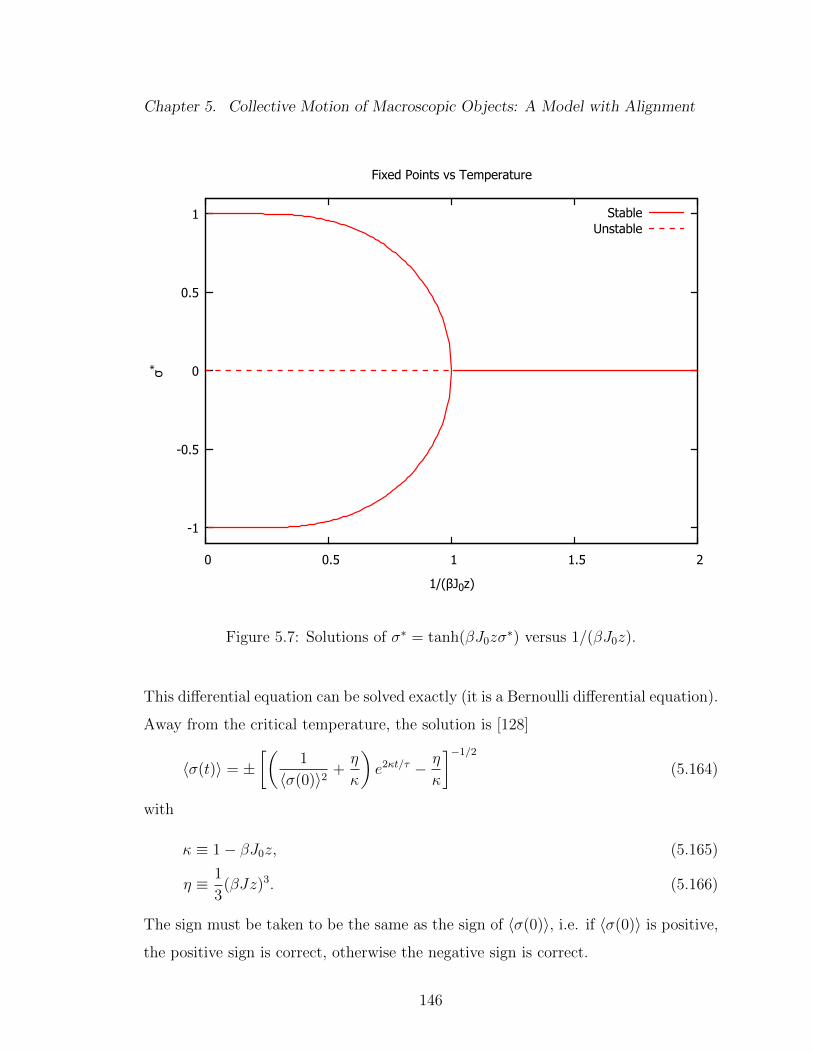
Chapter 5. Collective Motion of Macroscopic Objects: A Model with Alignment
-1
-0.5
0
0.5
1
0 0.5 1 1.5 2
σ*
1/(βJ0z)
Fixed Points vs Temperature
StableUnstable
Figure 5.7: Solutions of σ∗ = tanh(βJ0zσ∗) versus 1/(βJ0z).
This differential equation can be solved exactly (it is a Bernoulli differential equation).
Away from the critical temperature, the solution is [128]
〈σ(t)〉 = ±[(
1
〈σ(0)〉2+η
κ
)e2κt/τ − η
κ
]−1/2
(5.164)
with
κ ≡ 1− βJ0z, (5.165)
η ≡ 1
3(βJz)3. (5.166)
The sign must be taken to be the same as the sign of 〈σ(0)〉, i.e. if 〈σ(0)〉 is positive,
the positive sign is correct, otherwise the negative sign is correct.
146

Chapter 5. Collective Motion of Macroscopic Objects: A Model with Alignment
Above the critical temperature (βJ0z < 1), 〈σ〉 decays from its initial value to
zero. This means that the average positions, 〈xm〉 can increase or decrease at short
times but eventually saturate to a constant value, as in the two-particle case.
Below the critical temperature (βJ0z > 1), if 〈σ〉 starts at zero, then it remains
at zero. However since zero is unstable, if the system is perturbed it will go to one of
the stable solutions, 〈σ〉 = ±√−κ/η.
At the critical point, βJ0z = 1, the solution becomes [128]
〈σ(t)〉 =
[1
〈σ(0)〉2+
2ηt
τ
]−1/2
. (5.167)
The average direction decays from its initial value to zero at long times, but it does
so much slower (like 1/√t) than it does away from the critical point.
For the mean position at the critical point, we have
〈x(t)〉 − 〈x(0)〉 =cτ
η〈σ(0)〉
[√1 +
2η〈σ(0)〉2τ
t− 1
](5.168)
which surprisingly still increases at long times like√t if 〈σ(0)〉 is nonzero.
5.3.2 Second Moments
We now calculate the second moments 〈x2m〉 and the mixed moments 〈xmxn〉. For an
initial condition in which all particles start at x = 0 we have again
〈xm(t)xn(t)〉 = 2c2
∫ t
0
∫ t−t′
0
〈σm(t′)σn(t′ + t′′)〉dt′′dt′. (5.169)
We analyze separately the dynamics in the disordered and ordered phases.
147

Chapter 5. Collective Motion of Macroscopic Objects: A Model with Alignment
Disordered Phase, βJ0z < 1
We can calculate the two time spin correlation function following the procedure de-
scribed by Glauber [127] and Suzuki and Kubo [128]. We have again
〈σm(t)σn(t+ t′)〉 =∑σ,σ′
σmσ′nPσ(t)Pσ|σ′(t
′) (5.170)
where Pσ|σ′(t′) is the conditional probability to find the spins in a configuration σ′
at time t′ given that they began at a configuration σ. We can write∑σ′
σ′nPσ|σ′(t′) = 〈σn(t′)〉σ (5.171)
where 〈σn(t′)〉σ means the average value of σn at time t′ given that the spins began in
a configuration σ. In the mean field, we have again for the evolution of the average
directions
τd
dt〈σn〉 = −〈σn〉+ tanh(β〈En〉). (5.172)
We do not assume here that all the average directions are the same. Above the critical
temperature, we expect the argument of the tanh to be small, so we expand the right
hand side and this time only keep the linear term,
τd
dt〈σn〉 = −〈σn〉+ βJnl
∑l
〈σl〉 = −〈σn〉+ βJ0z1
N − 1
∑l 6=n
〈σl〉. (5.173)
For large N , the right hand side can be rewritten approximately as
τd
dt〈σn〉 = −〈σn〉+ βJ0z
1
N
∑l
〈σl〉. (5.174)
The solution for an initial condition σ is
〈σn(t)〉σ =∑l
Πnl(t)σl (5.175)
with
Πnl(t) =
(δnl −
1
N
)e−t/τ +
1
Ne−κt/τ (5.176)
148

Chapter 5. Collective Motion of Macroscopic Objects: A Model with Alignment
with κ = (1− βJ0z) as defined earlier.
We now have
〈σm(t)σn(t+ t′)〉 =∑l
Πnl(t′)∑σ
σmσlPσ(t) =∑l
Πnl(t′)〈σm(t)σl(t)〉 (5.177)
so we have related the spin correlation function at unequal times to the spin correla-
tion function at equal times.
We now calculate the equal time pair correlation function 〈σm(t)σn(t)〉 in the mean
field limit, following once again Suzuki and Kubo [128]. The pair correlation function
obeys (this can be derived from the evolution equation of the Pσs),
τd
dt〈σmσn〉 = −2〈σmσn〉+ 〈σm tanh βEn〉+ 〈σn tanh βEm〉. (5.178)
Since σm and σn can only be ±1, they can be brought inside the tanh. Next, the
ensemble average is brought inside the tanh in the mean field approximation,
τd
dt〈σmσn〉 = −2〈σmσn〉+ tanh〈βσmEn〉+ tanh〈βσnEm〉. (5.179)
For m = n, 〈σ2m〉 = 1, and for m 6= n linearize the right hand side around zero to find
τd
dt〈σmσn〉 = −2〈σmσn〉+ β
∑l
Jnl〈σmσl〉+ β∑l
Jml〈σnσl〉. (5.180)
Next, define Gml = 〈σmσn〉 for m 6= n, then
τd
dtGmn = −2Gmn + β
∑l 6=n
JnlGln + β∑l 6=m
JmlGln + 2βJmn. (5.181)
For an initial condition in which is translationally invariant (i.e. Gmn(0) only depends
on |m− n|), Gmn remains translationally invariant for all time (since the interaction
matrix we have chosen is also translationally invariant). We can then discrete Fourier
transform to get
τd
dtGq = −2Gq + 2βJqGq + 2βJq (5.182)
149

Chapter 5. Collective Motion of Macroscopic Objects: A Model with Alignment
where
Gq ≡∑n6=l
Gnleiq(n−l), Jq ≡
∑n6=l
Jnleiq(n−l). (5.183)
The solution is
Gq(t) = Gq(0)e−2(1−βJq)t/τ +βJq
1− βJq[1− e−2(1−βJq)t/τ] . (5.184)
For an initial condition where the directions are random, Gq(0) = 0. For the interac-
tion matrix defined earlier, we have
Jq =∑n6=l
Jnleiq(n−l) =
J0z
N − 1
∑n6=l
eiq(n−l) = J0zδq,0 (5.185)
so
Gq(t) = δq,01− κκ
[1− e−2κt/τ
]. (5.186)
Inverting the discrete Fourier transform then gives
Gmn(t) =1
(N − 1)
1− κκ
[1− e−2κt/τ
]. (5.187)
We then have∫ t−t′
0
〈σm(t′)σn(t′ + t′′)〉dt′′ =∑l
〈σm(t′)σl(t′)〉∫ t−t′
0
Πnl(t′′)dt′′
= τ∑l
〈σm(t′)σl(t′)〉[(δnl −
1
N
)[1− e−(t−t′)/τ ] +
1
N
1− e−κ(t−t′)/τ
κ
]. (5.188)
Using∑
l〈σm(t′)σl(t′)〉 = 1 +Gq=0, this becomes∫ t−t′
0
〈σm(t′)σn(t′ + t′′)〉dt′′ = τ〈σm(t′)σn(t′)〉[1− e−(t−t′)/τ ]
+τ
N
[1− e−κ(t−t′)/τ
κ− [1− e−(t−t′)/τ ]
]·[1 +
1− κκ
[1− e−2κt′/τ ]
]. (5.189)
150

Chapter 5. Collective Motion of Macroscopic Objects: A Model with Alignment
To find the second moments, we need to integrate this expression over t′ from 0
to t. Let us focus on the long time behavior. At long times, the integrals of the
exponential terms become constants, and for m = n, we have
〈x2m(t)〉 ≈ 2c2τt
[1 +
1
N
1− κκ2
]+ constant (5.190)
and for m 6= n,
〈xm(t)xn(t)〉 ≈ 2c2τt1− κκ
[1
N − 1+
1
N
1
κ
]+ constant
≈ 2c2τt1− κ2
Nκ2+ constant (5.191)
for large N .
The second moments 〈x2m(t)〉 scale like t in the disordered phase, characteristic of
diffusive motion. The effective diffusion constant is
Deff = c2τ
(1 +
1
N
1− κκ2
). (5.192)
For large N and away from the critical point at κ = 0, the second term is small
compared to the first term, so Deff ≈ c2τ .
As in the two-particle case, the correlations 〈xmxn〉 scale with time; however, the
rate of growth scales like 1/N and is therefore very small away from the critical point.
Ordered Phase, βJ0z > 1
We can also do a linear mean field analysis below the critical temperature. We have
again in the mean field
τd
dt〈σn〉 = −〈σn〉+ tanh(β〈En〉). (5.193)
Above the critical point, we proceeded by linearizing the tanh around zero. Below the
critical point, we linearize the tanh around one of the stable fixed points σ∗. Since
there is no preferred direction, −σ∗ is also a stable fixed point. We assume here the
151

Chapter 5. Collective Motion of Macroscopic Objects: A Model with Alignment
system is perturbed from the unstable fixed point so that it moves toward the positive
fixed point σ∗. The fixed point σ∗ satisfies
0 = −σ∗ + tanh(βJ0zσ∗) (5.194)
so we have
τd
dt〈σn〉 = −〈σn〉+ tanh
(βJ0z
N − 1
∑l 6=n
〈σl〉
)
≈ −〈σn〉+ σ∗ + βJ0z
(1
N − 1
∑l 6=n
〈σl〉 − σ∗)
[1− (σ∗)2] (5.195)
using sech2(βJ0zσ∗) = 1− tanh2(βJ0zσ
∗) = 1− (σ∗)2. For large N , we the sum can
be rewritten approximately as
1
N − 1
∑l 6=n
〈σl〉 ≈1
N
∑l
〈σl〉. (5.196)
The solution for an initial condition σ is
〈σn(t)〉σ = σne−t/τ + σ∗(1− e−t/τ ) +
(1
N
∑l
σl − σ∗)
[e−λt/τ − e−t/τ ] (5.197)
with
λ ≡ 1− βJ0z[1− (σ∗)2]. (5.198)
At zero temperature (β = ∞) λ goes to one, and at the critical point (βJ0z = 1) λ
vanishes. The two-time correlation function is
〈σm(t)σn(t+ t′)〉 = 〈σm(t)σn(t)〉e−t′/τ + 〈σm(t)〉σ∗(1− e−t′/τ )
+
(1
N
∑l
〈σm(t)σl(t)〉 − 〈σm(t)〉σ∗)
[e−λt′/τ − e−t′/τ ]. (5.199)
Now we need to calculate the equal time correlation function 〈σm(t)σn(t)〉. If we
are only interested in the long time behavior, we only need calculate the steady state
152

Chapter 5. Collective Motion of Macroscopic Objects: A Model with Alignment
value. For m = n we have always 〈σ2m〉 = 1, and in the steady state, in the mean field
we have for m 6= n,
0 = −2Gmn + 2 tanh
(βJ0z
N − 1
∑l 6=n
Gln +βJ0z
N − 1
)(5.200)
where again Gmn ≡ 〈σmσn〉 for m 6= n. In the global coupling case, we should expect
Gmn to equal some G∗ independent of m and n. Then
0 = −2G∗ + 2 tanh
(βJ0zG
∗ +βJ0z
N − 1
). (5.201)
For large N the second term inside the tanh is small, so we have approximately
G∗ ≈ σ∗. (5.202)
Except for the second term in equation (5.199), 〈σm〉 and 〈σmσl〉 can be replaced
with their steady state values in the long time limit, so we have
〈σm(t′)σn(t′ + t′′)〉 = e−t′′/τ + (σ∗)2(1− e−λt′/τ )(1− e−t′′/τ )
+[σ∗ − (σ∗)2
][e−λt
′′/τ − e−t′′/τ ]. (5.203)
Integrating over t′′, this is∫ t−t′
0
〈σm(t′)σn(t′ + t′′)〉dt′′ = τ(1− e−(t−t′)/τ )
+ (σ∗)2(1− e−λt′/τ )[t− t′ − τ(1− e−(t−t′)/τ )]
+ τ[σ∗ − (σ∗)2
] [1− e−λ(t−t′)/τ
λ− (1− e−(t−t′)/τ )
]. (5.204)
Integrating over t′ and taking the limit of large t we finally have
〈x2m〉 = (cσ∗t)2 + 2c2τt
(1− σ∗ +
σ∗ − 2(σ∗)2
λ
)+ constant. (5.205)
A similar calculation for m 6= n gives at long times
〈xmxn〉 = (cσ∗t)2 + 2c2τt
(σ∗ − 2(σ∗)2
λ
)+ constant. (5.206)
153
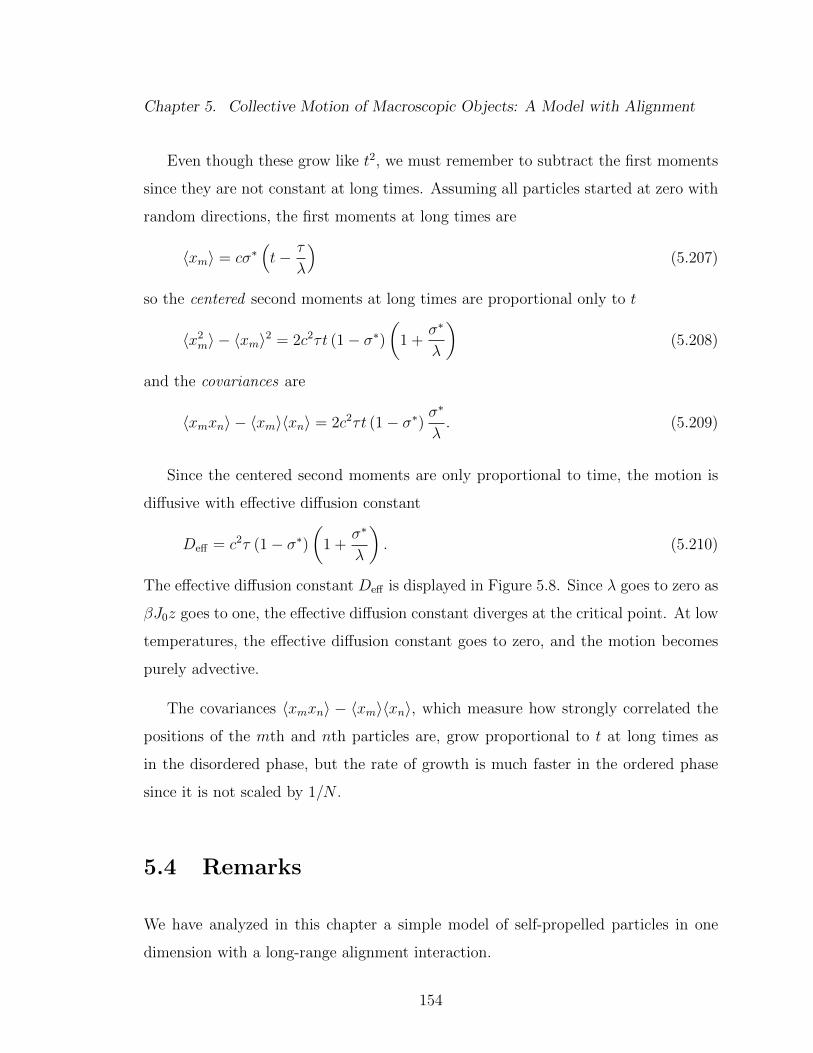
Chapter 5. Collective Motion of Macroscopic Objects: A Model with Alignment
Even though these grow like t2, we must remember to subtract the first moments
since they are not constant at long times. Assuming all particles started at zero with
random directions, the first moments at long times are
〈xm〉 = cσ∗(t− τ
λ
)(5.207)
so the centered second moments at long times are proportional only to t
〈x2m〉 − 〈xm〉2 = 2c2τt (1− σ∗)
(1 +
σ∗
λ
)(5.208)
and the covariances are
〈xmxn〉 − 〈xm〉〈xn〉 = 2c2τt (1− σ∗) σ∗
λ. (5.209)
Since the centered second moments are only proportional to time, the motion is
diffusive with effective diffusion constant
Deff = c2τ (1− σ∗)(
1 +σ∗
λ
). (5.210)
The effective diffusion constant Deff is displayed in Figure 5.8. Since λ goes to zero as
βJ0z goes to one, the effective diffusion constant diverges at the critical point. At low
temperatures, the effective diffusion constant goes to zero, and the motion becomes
purely advective.
The covariances 〈xmxn〉 − 〈xm〉〈xn〉, which measure how strongly correlated the
positions of the mth and nth particles are, grow proportional to t at long times as
in the disordered phase, but the rate of growth is much faster in the ordered phase
since it is not scaled by 1/N .
5.4 Remarks
We have analyzed in this chapter a simple model of self-propelled particles in one
dimension with a long-range alignment interaction.
154

Chapter 5. Collective Motion of Macroscopic Objects: A Model with Alignment
0
2
4
6
8
10
0 0.2 0.4 0.6 0.8 1
Deff/
(c2 τ
)
1/(βJ0z)
Effective Diffusion Constant, Ordered Phase
Figure 5.8: The effective diffusion constant versus temperature in the ordered phasefor the N particle alignment model.
The single-particle version of this model is known in the literature. At short times,
the motion is ballistic (mean squared displacement proportional to t2), but changes
to diffusive (mean squared displacement proportional to t) at long times. We saw
that the the density obeys the evolution equation (5.56) which is local in space, but
non-local in time with an exponential memory.
We generalized the analysis to two particles by constructing flipping rates which
cause the particles to align on average. By calculating the mean squared displace-
ment, given by equation (5.109), we found that the motion is again ballistic at short
times but diffusive at long times. The positions of the two-particles were found
155

Chapter 5. Collective Motion of Macroscopic Objects: A Model with Alignment
to be correlated, as a result of the alignment. We also calculated some continuous
coarse-grained quantities and saw that, unlike in the single-particle case, the evolution
equations (5.120), (5.126), and (5.130) are non-local in space.
Finally, we generalized the analysis further to many particles by building upon
Glauber dynamics. Although the model could not be solved exactly, in sections 5.3.1
and 5.3.2 we were able to calculate the first two moments in the mean field limit. The
many-particle model exhibits a phase transition from a disordered phase to an ordered
phase at a particular strength of the noise. In the ordered phase, the particles can
experience a net drift to left or right at long times, with the direction chosen depending
on initial conditions, an effect which did not happen in the one and two-particle
versions. The mean squared displacement given by equations (5.190) and (5.208)
grows proportional to t at long times in both phases, indicative of diffusive motion.
We found in both phases that the positions of any two particles are correlated, and
the correlation in the ordered phase, equation (5.209), is independent of the number
of particles N while the correlation in the disordered phase, equation (5.191), scales
like 1/N .
156

Chapter 6
Miscellaneous Topics and
Conclusions
The study of two additional problems in transport theory related only incidentally to
the investigations described in the preceding chapters were undertaken in the course
of this thesis work. The first of these is motion in disordered one-dimensional lattices,
and the second is a magnetic model of flocking. We will give a brief description of
our work on these two problems and then close with some final comments.
6.1 Transport in Disordered Lattices and Effective
Medium Theory
Consider a one-dimensional disordered system which obeys a Master equation of the
form
dPmdt
= Fm+1[Pm+1 − Pm] + Fm[Pm−1 − Pm] (6.1)
where Pm is the probability to be in the mth state and the Fms are transfer rates.
We have chosen the rates to be nearest-neighbor, i.e. the mth site is only connected
157
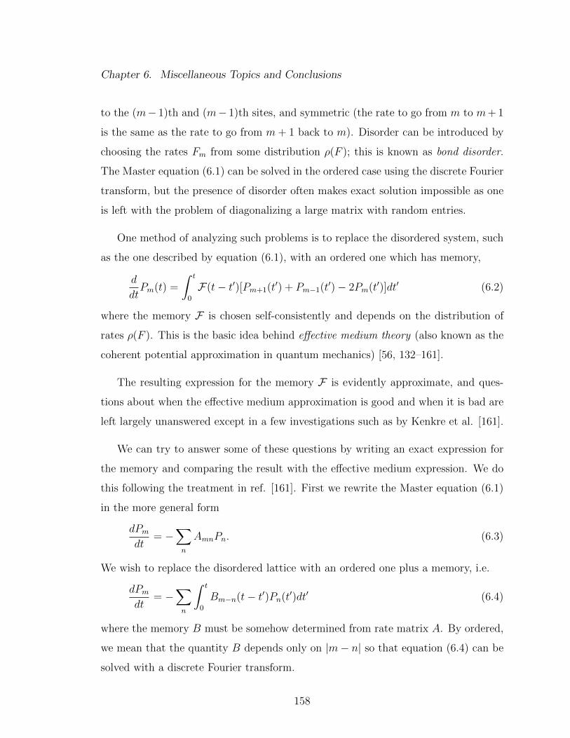
Chapter 6. Miscellaneous Topics and Conclusions
to the (m− 1)th and (m− 1)th sites, and symmetric (the rate to go from m to m+ 1
is the same as the rate to go from m+ 1 back to m). Disorder can be introduced by
choosing the rates Fm from some distribution ρ(F ); this is known as bond disorder.
The Master equation (6.1) can be solved in the ordered case using the discrete Fourier
transform, but the presence of disorder often makes exact solution impossible as one
is left with the problem of diagonalizing a large matrix with random entries.
One method of analyzing such problems is to replace the disordered system, such
as the one described by equation (6.1), with an ordered one which has memory,
d
dtPm(t) =
∫ t
0
F(t− t′)[Pm+1(t′) + Pm−1(t′)− 2Pm(t′)]dt′ (6.2)
where the memory F is chosen self-consistently and depends on the distribution of
rates ρ(F ). This is the basic idea behind effective medium theory (also known as the
coherent potential approximation in quantum mechanics) [56, 132–161].
The resulting expression for the memory F is evidently approximate, and ques-
tions about when the effective medium approximation is good and when it is bad are
left largely unanswered except in a few investigations such as by Kenkre et al. [161].
We can try to answer some of these questions by writing an exact expression for
the memory and comparing the result with the effective medium expression. We do
this following the treatment in ref. [161]. First we rewrite the Master equation (6.1)
in the more general form
dPmdt
= −∑n
AmnPn. (6.3)
We wish to replace the disordered lattice with an ordered one plus a memory, i.e.
dPmdt
= −∑n
∫ t
0
Bm−n(t− t′)Pn(t′)dt′ (6.4)
where the memory B must be somehow determined from rate matrix A. By ordered,
we mean that the quantity B depends only on |m− n| so that equation (6.4) can be
solved with a discrete Fourier transform.
158

Chapter 6. Miscellaneous Topics and Conclusions
The formal solution to (6.3) in the Laplace domain is
Pm(ε) =∑n
[εI + A]−1mnPn(0) (6.5)
where [εI + A]−1mn means the m,n element of the matrix [εI + A]−1. Discrete
Fourier transforming,
P k(ε) =∑m
∑n
[εI + A]−1mnPn(0)eikm (6.6)
where P k ≡∑
m Pmeikm. A similar calculation gives the solution to (6.4) as
P k(ε) =P k(0)
ε+ Bk(ε). (6.7)
Solving for Bk and plugging in P k(ε) from (6.6) we have now a formula for B in terms
of A in the transformed domain
Bk(ε) =P k(0)∑
m
∑n[εI + A]−1mnPn(0)eikm
− ε. (6.8)
Note that this expression has the rather undesirable property that the memory B
depends on the initial conditions Pm(0).
The dependence on initial conditions can be removed in the following way. Sup-
pose that we have an ensemble of disordered lattices with different realizations of the
disorder. For an ensemble member labeled ξ, let ξPm be the probability to find the
system in a state m in that ensemble member, and let ξA be the rate matrix for the
particular realization of the disorder in that ensemble member.
For each ensemble member we have
ξPm(ε) =∑n
[εI + ξA]−1mn
ξPn(0). (6.9)
Next, define define the ensemble average over realizations of the disorder 〈f〉 of any
quantity ξf as
〈f〉 ≡∑ξ
ξfP (ξ) (6.10)
159

Chapter 6. Miscellaneous Topics and Conclusions
where P (ξ) is the probability of generating the ensemble member ξ. Ensemble aver-
aging equation (6.9) and assuming that each ensemble member starts with the same
initial condition ξPm(0) = Pm(0) gives
〈Pm(ε)〉 =∑n
〈[εI + A]−1〉mnPn(0). (6.11)
For bond disorder as described earlier, the ensemble averaged propagator 〈[εI+A]−1〉
becomes translationally invariant even though the propagators for individual ensemble
members are not. We can then discrete Fourier transform to find
〈P k(ε)〉 = 〈[εI + A]−1〉kP k(0) (6.12)
with
〈[εI + A]−1〉k =∑m
〈[εI + A]−1〉mneik(m−n). (6.13)
Using equation (6.8), the ensemble averaged probabilities 〈Pm〉 therefore obey
d〈Pm〉dt
= −∑n
∫ t
0
Bm−n(t− t′)〈Pn(t′)〉dt′ (6.14)
with a memory which is now independent of the initial conditions,
Bk(ε) =1
〈[εI + A]−1〉k− ε. (6.15)
This expression for the memory is exact, but it requires the computation of the propa-
gator of each disordered lattice in the ensemble: exactly the task the effective medium
theory seeks to avoid. We can however glean a few insights from this expression.
Firstly, we note there is no guarantee that the memory B will be nearest-neighbor
even if the rates in every ensemble member are nearest neighbor, a fact pointed out
already in ref. [161]. Secondly, we can compute the exact memory for small (i.e.
N = 3, N = 4 et cetera) lattices. The exact memory can then be compared to the
approximate one obtained through effective medium theory.
160

Chapter 6. Miscellaneous Topics and Conclusions
We will perform here the calculation of the exact memory for a 4 site chain with
random nearest neighbor rates all drawn from some distribution ρ(F ). In general,
the rate matrix for a 4 site chain with nearest neighbor rates is
A =
F1 + F2 −F2 0 −F1
−F2 F2 + F3 −F3 0
0 −F3 F3 + F4 −F4
−F1 0 −F4 F4 + F1
. (6.16)
The discrete Fourier transformed ensemble averaged propagator in the Laplace do-
main is (a computer algebra system is useful for this computation)
⟨[εI + A]−1
⟩k=0=
1
ε, (6.17)⟨
[εI + A]−1⟩k=π/2
=
⟨ε2 + 4F1ε+ 4F1F2 + 4F1F3
∆(ε)
⟩=⟨[εI + A]−1
⟩k=3π/2,
(6.18)⟨[εI + A]−1
⟩k=π=
⟨ε2 + 4F1ε+ 4F1F2
∆(ε)
⟩. (6.19)
with
∆(ε) ≡ ε3 + 2ε2(F1 + F2 + F3 + F4)
+ ε[3(F1F2 + F2F3 + F3F4 + F4F1) + 4(F1F3 + F2F4)]
+ 4[F1F2F3 + F2F3F4 + F3F4F1 + F4F1F2]. (6.20)
Simplifications have been made using the fact that all the rates (F1, F2, F3 and F4) are
chosen from the same distribution ρ(F ) so we can permute labels inside the ensemble
averages.
Using equation (6.15) we have for the discrete Fourier transformed memory in the
161

Chapter 6. Miscellaneous Topics and Conclusions
Laplace domain
Bk=0(ε) = 0, (6.21)
Bk=π/2(ε) =1⟨
ε2+4F1ε+4F1F2+4F1F3
∆(ε)
⟩ − ε = Bk=3π/2(ε), (6.22)
Bk=π(ε) =1⟨
ε2+4F1ε+4F1F2
∆(ε)
⟩ − ε. (6.23)
What does this tell us? The k = 0 part is simply a result of conservation of probability.
Is the exact memory nearest-neighbor? A nearest-neighbor memory would have the
form Bk(ε) = 2F(ε)(1− cos k), but in general the computed Bk(ε) does not have this
form.
To compare with effective medium theory, we now take the Markovian limit, i.e.
replace the memory with its integral times a delta function,
Bm−n(t) ≈ δ(t)
∫ ∞0
Bm−n(t′)dt′ = δ(t)Bm−n(0). (6.24)
In this limit we have
Bk=0(0) = 0, (6.25)
Bk=π/2(0) =1⟨
8F1F2
∆(0)
⟩ = Bk=3π/2(0), (6.26)
Bk=π(0) =1⟨
4F1F2
∆(0)
⟩ − ε (6.27)
where we have used the fact that 〈F1F3/∆(0)〉 is equal to 〈F1F2/∆(0)〉 since again we
can freely permute indices inside the ensemble average. This is of the nearest-neighbor
form with the effective nearest-neighbor hopping rate
F exacteff =
[4
⟨F1F2
F1F2F3 + F2F3F4 + F3F4F1 + F4F1F2
⟩]−1
. (6.28)
How does this compare to the effective medium result? For a finite lattice, the
effective nearest-neighbor hopping rate F emteff is given implicitly by [161]
1
F emteff
=N
N − 1
∫ ∞0
ρ(F )
F +F emt
eff
N−1
dF. (6.29)
162

Chapter 6. Miscellaneous Topics and Conclusions
To compare the two, a particular distribution of the rates ρ(F ) must be chosen.
We will not proceed any further here, but suffice it to say that even in the Markovian
limit the effective hopping rate given by effective medium theory, equation (6.29),
does indeed differ from the exact result (6.28) for nontrivial distributions.
6.2 A Magnetic Model of Flocking
In Chapter 4, we discussed collective motion the idea of information transfer from
informed to uninformed individuals (see refs. [90, 92, 110, 111]). In this section we
will briefly analyze a simple magnetic model of the same phenomenon. In this model
we will have only static ingredients, i.e. there will be no motion undergone by the
elements.
As in the model discussed in Chapter 5, we will again treat the members of the
flock as Ising spins, but we now apply a field. The strength of the field is not uniform:
we designate a certain fraction a of individuals as “informed” which feel a magnetic
field of strength h, and the remaining fraction as “uninformed” which do not feel a
magnetic field. We reiterate that here the particles do not move, unlike the particles
in Chapter 5. We study only the equilibrium properties of the magnetic system.
The standard Ising model Hamiltonian is:
H = −∑i<j
Jijσiσj −∑i
hiσi (6.30)
where the σis are a set of N spin variables which can either be −1 or −1, the Jij’s
are exchange energies, and hi is the magnetic field on the ith site.
The partition function in the one-dimensional case can likely be solved exactly
with transfer matrices, but the system in one dimension does not exhibit a phase
transition. Exact calculations are prohibitively difficult in higher dimensions, so we
simply perform a mean field analysis. The standard set of N mean field equations
163

Chapter 6. Miscellaneous Topics and Conclusions
are
〈σi〉 = tanh
(β∑j
Jij〈σj〉+ βhi
)(6.31)
where β ≡ 1/kT is the inverse temperature. If the dimensionality of the lattice is
very large, then we may assume that∑
j Jij〈σj〉 is independent of i, and replace it
with J0zm where J0 is the pair exchange energy, z is the configuration number of the
lattice, and m is the magnetization per spin of the entire system,
m ≡ 1
N
∑j
〈σj〉. (6.32)
We are now left with only two equations:
〈σi〉 = tanh (βJ0zm) (6.33)
if there is no magnetic field on site i, or
〈σi〉 = tanh (βJ0zm+ βh) (6.34)
if there is a magnetic field on site i. We can now obtain a single self consistent mean
field equation for the magnetization m:
m =1
N
∑j
〈σj〉 = (1− a) tanh(βJ0zm) + a tanh(βJ0zm+ βh) (6.35)
where a is again the fraction of spins affected by the field. Note that the spatial
configuration of spins which are affected by the magnetic field does not matter in
the mean field analysis. It is convenient to introduce the dimensionless quantities
b ≡ βJ0z and c ≡ βh, so that the equation for m can be written more simply as
m = (1− a) tanh(bm) + a tanh(bm+ c). (6.36)
It can be seen graphically that equation (6.36) can have between one and five solu-
tions. The left and right hand sides for a particular choice of a, b, and c are plotted
in Figure 6.1.
164

Chapter 6. Miscellaneous Topics and Conclusions
-1
-0.5
0
0.5
1
-1.5 -1 -0.5 0 0.5 1 1.5
m
m
Mean Field Equation, a = 0.4, b = 15, c = 10
m (1-a)tanh(bm) + a tanh(bm+c)
Figure 6.1: Left and right hand sides of the mean field equationm = (1−a) tanh(bm)+a tanh(bm + c)f for a = 0.4, b = 15, c = 10. The intersections of the two curvesrepresent are solutions of the mean field equation.
First let us analyze the solutions at very low temperature (b 1). At low
temperatures the hyperbolic tangents become step-like and the mean field equation
is approximately
m ≈
+1 m > 0
2a− 1 −c/b < m < 0
−1 m < −c/b
. (6.37)
The three stable (or at least metastable) solutions for h > 0 are
165

Chapter 6. Miscellaneous Topics and Conclusions
• m = +1: all spins aligned in the direction of the field.
• m = −1: all spins aligned opposite the direction of the field. Only a solution
for sufficiently weak field, c < b.
• m = 2a − 1: informed spins aligned with the field; uninformed spins aligned
opposite the field. Only a solution for certain fractions of informed spins 1−c/b2
<
a < 12.
For certain ranges of parameters, we have solutions where all the particles ignore the
field or where only uninformed spins ignore the field.
What about at nonzero temperatures? To gain some insight we can make several
kinds of plots. One kind of plot that can be made is that of magnetization (found
numerically) versus temperature at fixed field, for different fractions of informed birds.
One such plot is shown in Figure 6.2.
Alternatively, the magnetization versus field at fixed temperature and concentra-
tion can be plotted. One such plot is given in Figure 6.3.
Another kind of diagram that can be made is called a stability diagram (see ref.
[162]) and shows how many solutions there are in different regions of parameter space.
These can be made by noting that the number of solutions to (6.36) changes exactly
when m is tangent to (1− a) tanh(bm) + a tanh(bm + c). Setting their slopes equal,
we obtain
1 = (1− a)b sech2(bm) + ab sech2(bm+ c). (6.38)
This, together with equation (6.36) form a system of two coupled equations which for
fixed a and b can be solved for the values of m and c where a change in the number
of solutions occurs. This can be done numerically, and the results for different values
of a are shown in 6.4.
166

Chapter 6. Miscellaneous Topics and Conclusions
-1
-0.5
0
0.5
1
0 0.5 1 1.5 2
m
1/b
Magnetization versus Temperature, a = 0.4, c/b = 0.5
Figure 6.2: Magnetization (both stable and unstable solutions) versus temperatureat fixed field c/b = 0.5 and fixed concentration of informed spins a = 0.4.
For a > 1/2, the behavior is qualitatively similar to the ordinary Ising model and
there can be only one or three solutions. Only for a < 1/2 can five solutions appear.
6.3 Closing Remarks
The two main problems studied in this thesis, electrons moving in mesoscopic devices
and macroscopic biological entities such as birds moving collectively, are certainly
quite different from each other, but despite the vast difference in scale, we did en-
167
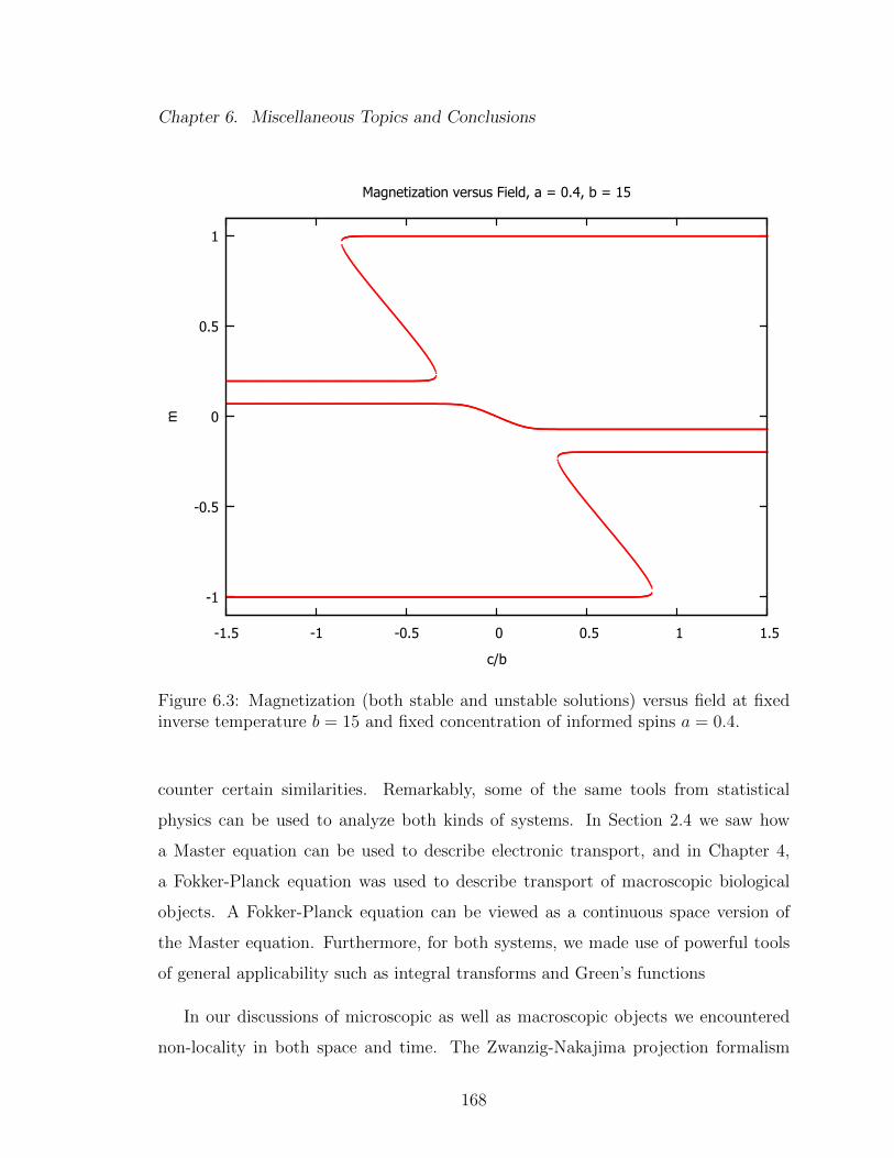
Chapter 6. Miscellaneous Topics and Conclusions
-1
-0.5
0
0.5
1
-1.5 -1 -0.5 0 0.5 1 1.5
m
c/b
Magnetization versus Field, a = 0.4, b = 15
Figure 6.3: Magnetization (both stable and unstable solutions) versus field at fixedinverse temperature b = 15 and fixed concentration of informed spins a = 0.4.
counter certain similarities. Remarkably, some of the same tools from statistical
physics can be used to analyze both kinds of systems. In Section 2.4 we saw how
a Master equation can be used to describe electronic transport, and in Chapter 4,
a Fokker-Planck equation was used to describe transport of macroscopic biological
objects. A Fokker-Planck equation can be viewed as a continuous space version of
the Master equation. Furthermore, for both systems, we made use of powerful tools
of general applicability such as integral transforms and Green’s functions
In our discussions of microscopic as well as macroscopic objects we encountered
non-locality in both space and time. The Zwanzig-Nakajima projection formalism
168

Chapter 6. Miscellaneous Topics and Conclusions
shows how coarse-graining results in non-locality in time, but the projection formalism
does not make clear that coarse-graining can also give rise to non-locality in space.
In the macroscopic systems described in Chapters 4 and 5, we saw explicitly several
coarse-grained quantities which obey equations of motion which are non-local in space.
In Section 6.1 we saw in a microscopic system how a different kind of coarse-graining,
ensemble averaging over different realizations of disorder, also produces spatially long-
range effects. A few other examples of spatially long-range memories can be found in
the literature, in particular see refs. [69, 163].
The models of microscopic and macroscopic transport discussed in this thesis
were quite simple from a mathematical standpoint. These simple models certainly
do not capture all the details of the real systems, but they are amenable to analytic
calculations. The author hopes the analyses presented here can thereby provide a
better understanding of certain aspects of the difficult problems in transport theory.
169

Chapter 6. Miscellaneous Topics and Conclusions
Figure 6.4: Stability diagrams showing the total number of solutions in differentregions of parameter space.
170
References
[1] Neil W. Ashcroft and N. David Mermin. Solid state physics. Holt, Rinehartand Winston, 1976.
[2] D. A. Wharam, T. J. Thornton, R. Newbury, M. Pepper, H. Ahmed, J. E. F.Frost, D. G. Hasko, D. C. Peacock, D. A. Ritchie, and G. A. C. Jones. One-dimensional transport and the quantisation of the ballistic resistance. Journalof Physics C: Solid State Physics, 21(8):L209–L214, March 1988.
[3] B. J. van Wees, L. P. Kouwenhoven, H. van Houten, C. W. J. Beenakker, J. E.Mooij, C. T. Foxon, and J. J. Harris. Quantized conductance of magnetoelectricsubbands in ballistic point contacts. Physical Review B, 38(5):3625–3627, 1988.
[4] B. J. van Wees, H. van Houten, C. W. J. Beenakker, J. G. Williamson, L. P.Kouwenhoven, D. van der Marel, and C. T. Foxon. Quantized conductanceof point contacts in a two-dimensional electron gas. Physical Review Letters,60(9):848–850, February 1988.
[5] Theodosius Dobzhansky, Jeffery R. Powell, Charles E. Taylor, and Michael An-dregg. Ecological variables affecting the dispersal behavior of drosophila pseu-doobscura and its relatives. The American Naturalist, 114(3):325–334, Septem-ber 1979.
[6] Hiroshi Fujikawa and Mitsugu Matsushita. Fractal growth of bacillus subtilis onagar plates. Journal of the Physical Society of Japan, 58(11):3875–3878, 1989.
[7] Eshel Ben-Jacob, Adam Tenenbaum, Ofer Shochet, and Orna Avidan. Holo-transformations of bacterial colonies and genome cybernetics. Physica A: Sta-tistical Mechanics and its Applications, 202(1–2):1–47, January 1994.
[8] Eshel Ben-Jacob, Ofer Schochet, Adam Tenenbaum, Inon Cohen, AndrasCzirok, and Tamas Vicsek. Generic modelling of cooperative growth patternsin bacterial colonies. Nature, 368(6466):46–49, March 1994.
171

REFERENCES
[9] Eshel Ben-Jacob, Inon Cohen, Ofer Shochet, Adam Tenenbaum, Andras Czirok,and Tamas Vicsek. Cooperative formation of chiral patterns during growth ofbacterial colonies. Physical Review Letters, 75(15):2899–2902, October 1995.
[10] Andras Czirok, Eshel Ben-Jacob, Inon Cohen, and Tamas Vicsek. Formationof complex bacterial colonies via self-generated vortices. Physical Review E,54(2):1791–1801, August 1996.
[11] M. Ballerini, N. Cabibbo, R. Candelier, A. Cavagna, E. Cisbani, I. Giardina,V. Lecomte, A. Orlandi, G. Parisi, A. Procaccini, M. Viale, and V. Zdravkovic.Interaction ruling animal collective behavior depends on topological rather thanmetric distance: Evidence from a field study. Proceedings of the NationalAcademy of Sciences, 105(4):1232 –1237, January 2008.
[12] Michele Ballerini, Nicola Cabibbo, Raphael Candelier, Andrea Cavagna,Evaristo Cisbani, Irene Giardina, Alberto Orlandi, Giorgio Parisi, Andrea Pro-caccini, Massimiliano Viale, and Vladimir Zdravkovic. Empirical investigationof starling flocks: a benchmark study in collective animal behaviour. AnimalBehaviour, 76(1):201–215, July 2008.
[13] Andrea Cavagna, Alessio Cimarelli, Irene Giardina, Giorgio Parisi, RaffaeleSantagati, Fabio Stefanini, and Massimiliano Viale. Scale-free correlations instarling flocks. Proceedings of the National Academy of Sciences, 107(26):11865–11870, June 2010.
[14] Andrea Cavagna, Alessio Cimarelli, Irene Giardina, Giorgio Parisi, RaffaeleSantagati, Fabio Stefanini, and Raffaele Tavarone. From empirical data tointer-individual interactions: unveiling the rules of collective animal behavior.Mathematical Models and Methods in Applied Sciences, 20:1491–1510, Septem-ber 2010.
[15] William Bialek, Andrea Cavagna, Irene Giardina, Thierry Mora, Edmondo Sil-vestri, Massimiliano Viale, and Aleksandra M. Walczak. Statistical mechanicsfor natural flocks of birds. Proceedings of the National Academy of Sciences,109(13):4786–4791, March 2012.
[16] D. P. O’Brien. Analysis of the internal arrangement of individuals within crus-tacean aggregations (Euphausiacea, mysidacea). Journal of Experimental Ma-rine Biology and Ecology, 128(1):1–30, June 1989.
[17] Andreas Huth and Christian Wissel. The simulation of the movement of fishschools. Journal of Theoretical Biology, 156(3):365–385, June 1992.
[18] Andreas Huth and Christian Wissel. The simulation of fish schools in compar-ison with experimental data. Ecological Modelling, 75–76:135–146, September1994.
172

REFERENCES
[19] Yael Katz, Kolbjørn Tunstrøm, Christos C. Ioannou, Cristian Huepe, andIain D. Couzin. Inferring the structure and dynamics of interactions in school-ing fish. Proceedings of the National Academy of Sciences, 108(46):18720–18725,November 2011.
[20] Wolfgang Alt. Elements of a systematic search in animal behavior and modelsimulations. Biosystems, 34(1–3):11–26, 1995.
[21] J. Buhl, D. J. T. Sumpter, I. D. Couzin, J. J. Hale, E. Despland, E. R. Miller,and S. J. Simpson. From disorder to order in marching locusts. Science,312(5778):1402 –1406, June 2006.
[22] Dirk Helbing, Joachim Keltsch, and Peter Molnar. Modelling the evolution ofhuman trail systems. Nature, 388(6637):47–50, July 1997.
[23] Dirk Helbing, Frank Schweitzer, Joachim Keltsch, and Peter Molnar. Activewalker model for the formation of human and animal trail systems. PhysicalReview E, 56(3):2527–2539, September 1997.
[24] Alexander S. Mikhailov and Damian H. Zanette. Noise-induced breakdownof coherent collective motion in swarms. Physical Review E, 60(4):4571–4575,October 1999.
[25] R. Landauer. Spatial variation of currents and fields due to localized scatterersin metallic conduction. IBM Journal of Research and Development, 1(3):223–231, July 1957.
[26] Rolf Landauer. Electrical resistance of disordered one-dimensional lattices.Philosophical Magazine, 21(172):863–867, 1970.
[27] R. Landauer. Electrical transport in open and closed systems. Zeitschrift furPhysik B Condensed Matter, 68(2):217–228, 1987.
[28] M. Buttiker, Y. Imry, R. Landauer, and S. Pinhas. Generalized many-channelconductance formula with application to small rings. Physical Review B,31(10):6207–6215, May 1985.
[29] Yoseph Imry. Physics of mesoscopic systems. In Geoffrey Grinstein and GeneMazenko, editors, Directions in condensed matter physics: memorial volume inhonor of Prof. S.K. Ma. World Scientific, 1986.
[30] M. Buttiker. Role of quantum coherence in series resistors. Physical Review B,33(5):3020–3026, March 1986.
[31] Supriyo Datta. Electronic Transport in Mesoscopic Systems. Cambridge Uni-versity Press, May 1997.
173

REFERENCES
[32] E. Wigner. On the quantum correction for thermodynamic equilibrium. PhysicalReview, 40(5):749–759, June 1932.
[33] Umberto Ravaioli, Mohamed A. Osman, Walter Potz, Norman Kluksdahl, andDavid K. Ferry. Investigation of ballistic transport through resonant-tunnellingquantum wells using Wigner function approach. Physica B+C, 134(1–3):36–40,November 1985.
[34] N. Kluksdahl, W. Potz, U. Ravaioli, and D.K. Ferry. Wigner function studyof a double quantum barrier resonant tunnelling diode. Superlattices and Mi-crostructures, 3(1):41–45, 1987.
[35] William R. Frensley. Wigner-function model of a resonant-tunneling semicon-ductor device. Physical Review B, 36(3):1570–1580, July 1987.
[36] A. M. Kriman, N. C. Kluksdahl, and D. K. Ferry. Scattering states and dis-tribution functions for microstructures. Physical Review B, 36(11):5953–5959,October 1987.
[37] N. C. Kluksdahl, A. M. Kriman, D. K. Ferry, and C. Ringhofer. Self-consistentstudy of the resonant-tunneling diode. Physical Review B, 39(11):7720–7735,April 1989.
[38] V. M. Kenkre, F. Biscarini, and C. Bustamante. Theoretical framework forthe interpretation of STM images of adsorbates. Ultramicroscopy, 42–44, Part1:122–127, July 1992.
[39] Fabio Biscarini. Theory of Electron Transport in Scanning Tunneling Mi-croscopy and Applications to the Simulation of Images of Metal Surfaces andAdsorbed Molecules. PhD thesis, University of Oregon, 1993.
[40] F. Biscarini, C. Bustamante, and V. M. Kenkre. Cluster models for the simula-tion of STM images of adsorbates: Origin of non-topographical features. ICEM,13:581, 1994.
[41] V. M. Kenkre, F. Biscarini, and C. Bustamante. Scanning tunneling mi-croscopy. I. Theoretical framework and coherence effects. Physical Review B,51(16):11074–11088, April 1995.
[42] F. Biscarini, C. Bustamante, and V. M. Kenkre. Scanning tunneling microscopy.II. Calculation of images of atomic and molecular adsorbates. Physical ReviewB, 51(16):11089–11102, April 1995.
[43] F. Biscarini and V.M. Kenkre. Quantum coherence effects in the scanningtunneling microscope: a simple interpretation of contact resistance experiments.Surface Science, 426(3):336–344, May 1999.
174

REFERENCES
[44] S. K. Lyo and Danhong Huang. Multisublevel magnetoquantum conductancein single and coupled double quantum wires. Physical Review B, 64(11):115320,2001.
[45] S. K. Lyo and Danhong Huang. Magnetoquantum oscillations of thermoelec-tric power in multisublevel quantum wires. Physical Review B, 66(15):155307,October 2002.
[46] S. K. Lyo and Danhong Huang. Temperature-dependent magnetoconduc-tance in quantum wires: Effect of phonon scattering. Physical Review B,68(11):115317, 2003.
[47] S. K. Lyo and Danhong Huang. Effect of electron-electron scattering on theconductance of a quantum wire studied with the boltzman transport equation.Physical Review B, 73(20):205336, May 2006.
[48] R Landauer. Conductance determined by transmission: probes and quantisedconstriction resistance. Journal of Physics: Condensed Matter, 1(43):8099–8110, October 1989.
[49] Henk van Houten and Carlo Beenakker. Quantum point contacts. PhysicsToday, 49(7):22–27, 1996.
[50] Yoseph Imry and Rolf Landauer. Conductance viewed as transmission. Reviewsof Modern Physics, 71(2):S306–S312, March 1999.
[51] David K. Ferry and Stephen M. Goodnick. Transport in Nanostructures. Cam-bridge University Press, 1997.
[52] Yoseph Imry. Introduction to Mesoscopic Physics. Oxford University Press,February 2002.
[53] Supriyo Datta. Quantum Transport: Atom To Transistor. Cambridge Univer-sity Press, June 2005.
[54] Albert Messiah. Quantum Mechanics. Dover Publications, July 1999.
[55] L. Shubnikov and W. J. de Haas. Magnetische widerstandsvergrosserung ineinkristallen von wismut bei tiefen temperaturen. Communications from thePhysical Laboratory at the University of Leiden, 207a, 1930.
[56] Eleftherios N. Economou. Green’s Functions in Quantum Physics. Springer,3rd edition, February 2010.
[57] Daniel S. Fisher and Patrick A. Lee. Relation between conductivity and trans-mission matrix. Physical Review B, 23(12):6851–6854, June 1981.
175

REFERENCES
[58] L. V. Keldysh. Diagram technique for non-equilibrium processes. Soviet PhysicsJETP, 20:1018, 1965.
[59] Leo P. Kadanoff and Gordon Baym. Quantum statistical mechanics: Green’sfunction methods in equilibrium and nonequilibrium problems. W.A. Benjamin,1962.
[60] John Snygg. Use of operator wave functions to construct a refined correspon-dence principle via the quantum mechanics of Wigner and Moyal. AmericanJournal of Physics, 48(11):964, 1980.
[61] M. Hillery, R.F. O’Connell, M.O. Scully, and E.P. Wigner. Distribution func-tions in physics: Fundamentals. Physics Reports, 106(3):121–167, April 1984.
[62] N.L. Balazs and B.K. Jennings. Wigner’s function and other distribution func-tions in mock phase spaces. Physics Reports, 104(6):347–391, February 1984.
[63] Hai-Woong Lee. Theory and application of the quantum phase-space distribu-tion functions. Physics Reports, 259(3):147–211, August 1995.
[64] William B. Case. Wigner functions and Weyl transforms for pedestrians. Amer-ican Journal of Physics, 76(10):937, 2008.
[65] John M. Ziman. Principles of the Theory of Solids. Cambridge University Press,November 1979.
[66] J. E. Moyal. Quantum mechanics as a statistical theory. Mathematical Proceed-ings of the Cambridge Philosophical Society, 45(01):99–124, 1949.
[67] M. Belloni, M. A. Doncheski, and R. W. Robinett. Wigner quasi-probabilitydistribution for the infinite square well: Energy eigenstates and time-dependentwave packets. American Journal of Physics, 72(9):1183, 2004.
[68] V. M. Kenkre and Peter Reineker. Exciton dynamics in molecular crystals andaggregates. Springer-Verlag, 1982.
[69] V.M. Kenkre and S.M. Phatak. Exact probability propagators for motion witharbitrary degree of transport coherence. Physics Letters A, 100(2):101–104,January 1984.
[70] V. M. Kenkre and D. W. Brown. Exact solution of the stochastic Liouvilleequation and application to an evaluation of the neutron scattering function.Physical Review B, 31(4):2479–2487, February 1985.
[71] V. M. Kenkre. Mathematical methods for the description of energy transfer.In B. DiBartolo, editor, Proceedings of the NATO Advance Study Institute onEnergy Transfer, Erice, Italy. Plenum, New York, 1984.
176

REFERENCES
[72] V. M. Kenkre and Katja Lindenberg. Modern challenges in statistical mechan-ics: patterns, noise, and the interplay of nonlinearity and complexity : PanAmerican Advanced Studies Institute, Bariloche, Argentina, 2-15 June, 2002.American Institute of Physics, March 2003.
[73] V. M. Kenkre. Generalization to spatially extended systems of the relation be-tween stochastic Liouville equations and generalized master equations. PhysicsLetters A, 65(5–6):391–392, April 1978.
[74] P. Avakian, V. Ern, R. E. Merrifield, and A. Suna. Spectroscopic approachto triplet exciton dynamics in anthracene. Physical Review, 165(3):974–980,January 1968.
[75] Yu Kagan and M. I. Klinger. Theory of quantum diffusion of atoms in crystals.Journal of Physics C: Solid State Physics, 7(16):2791–2807, August 1974.
[76] Sadao Nakajima. On quantum theory of transport phenomena. Progress ofTheoretical Physics, 20(6):948–959, 1958.
[77] Robert Zwanzig. Ensemble method in the theory of irreversibility. The Journalof Chemical Physics, 33(5):1338–1341, November 1960.
[78] Robert Zwanzig. On the identity of three generalized master equations. Physica,30(6):1109–1123, June 1964.
[79] P. Sautet and C. Joachim. Electronic transmission coefficient for the single-impurity problem in the scattering-matrix approach. Physical Review B,38(17):12238–12247, December 1988.
[80] Herbert Levine, Wouter-Jan Rappel, and Inon Cohen. Self-organization in sys-tems of self-propelled particles. Physical Review E, 63(1):017101, December2000.
[81] Udo Erdmann, Werner Ebeling, and Alexander S. Mikhailov. Noise-inducedtransition from translational to rotational motion of swarms. Physical ReviewE, 71(5):051904, May 2005.
[82] V. Dossetti, F. J. Sevilla, and V. M. Kenkre. Phase transitions induced bycomplex nonlinear noise in a system of self-propelled agents. Physical ReviewE, 79(5):051115, May 2009.
[83] Craig W. Reynolds. Flocks, herds and schools: A distributed behavioral model.In Proceedings of the 14th annual conference on Computer graphics and inter-active techniques, SIGGRAPH ’87, page 25–34, New York, NY, USA, 1987.ACM.
177

REFERENCES
[84] G. Bard Ermentrout and Leah Edelstein-Keshet. Cellular automata approachesto biological modeling. Journal of Theoretical Biology, 160(1):97–133, January1993.
[85] Tamas Vicsek, Andras Czirok, Eshel Ben-Jacob, Inon Cohen, and Ofer Shochet.Novel type of phase transition in a system of self-driven particles. PhysicalReview Letters, 75(6):1226–1229, 1995.
[86] J Hemmingsson. Modellization of self-propelling particles with a coupled maplattice model. Journal of Physics A: Mathematical and General, 28(15):4245–4250, August 1995.
[87] Y. Limon Duparcmeur, H. Herrmann, and J. P. Troadec. Spontaneous forma-tion of vortex in a system of self motorised particles. Journal de Physique I,5(9):1119–1128, September 1995.
[88] Zoltan Csahok and Tamas Vicsek. Lattice-gas model for collective biologicalmotion. Physical Review E, 52(5):5297–5303, November 1995.
[89] Andras Czirok, H. Eugene Stanley, and Tamas Vicsek. Spontaneously orderedmotion of self-propelled particles. Journal of Physics A: Mathematical andGeneral, 30(5):1375–1385, March 1997.
[90] Iain D. Couzin, Jens Krause, Richard James, Graeme D. Ruxton, and Nigel R.Franks. Collective memory and spatial sorting in animal groups. Journal ofTheoretical Biology, 218(1):1–11, September 2002.
[91] Guillaume Gregoire and Hugues Chate. Onset of collective and cohesive motion.Physical Review Letters, 92(2):025702, January 2004.
[92] Iain D. Couzin, Jens Krause, Nigel R. Franks, and Simon A. Levin. Effec-tive leadership and decision-making in animal groups on the move. Nature,433(7025):513–516, February 2005.
[93] M. Aldana, V. Dossetti, C. Huepe, V. M. Kenkre, and H. Larralde. Phase tran-sitions in systems of self-propelled agents and related network models. PhysicalReview Letters, 98(9):095702, March 2007.
[94] Akira Okubo. Dynamical aspects of animal grouping: Swarms, schools, flocks,and herds. Advances in Biophysics, 22:1–94, 1986.
[95] John Toner and Yuhai Tu. Long-range order in a two-dimensional dynamicalXY model: How birds fly together. Physical Review Letters, 75(23):4326–4329,December 1995.
178

REFERENCES
[96] John Toner and Yuhai Tu. Flocks, herds, and schools: A quantitative theoryof flocking. Physical Review E, 58(4):4828–4858, October 1998.
[97] Andras Czirok, Albert-Laszlo Barabasi, and Tamas Vicsek. Collective motionof self-propelled particles: Kinetic phase transition in one dimension. PhysicalReview Letters, 82(1):209–212, January 1999.
[98] Alexander Mogilner and Leah Edelstein-Keshet. A non-local model for a swarm.Journal of Mathematical Biology, 38(6):534–570, June 1999.
[99] John Toner, Yuhai Tu, and Sriram Ramaswamy. Hydrodynamics and phases offlocks. Annals of Physics, 318(1):170–244, July 2005.
[100] Chad M. Topaz, Andrea L. Bertozzi, and Mark A. Lewis. A nonlocal continuummodel for biological aggregation. Bulletin of Mathematical Biology, 68(7):1601–1623, July 2006.
[101] C. William Gear. Equation-free, coarse-grained multiscale computation: En-abling microscopic simulators to perform system-level analysis. Communica-tions in Mathematical Sciences, 1(4):715–762, December 2003.
[102] Radek Erban, Ioannis G. Kevrekidis, and Hans G. Othmer. An equation-free computational approach for extracting population-level behavior fromindividual-based models of biological dispersal. Physica D: Nonlinear Phenom-ena, 215(1):1–24, March 2006.
[103] Allison Kolpas, Jeff Moehlis, and Ioannis G. Kevrekidis. Coarse-grained analysisof stochasticity-induced switching between collective motion states. Proceedingsof the National Academy of Sciences, 104(14):5931–5935, April 2007.
[104] Sung Joon Moon, B. Nabet, Naomi E. Leonard, Simon A. Levin, and I. G.Kevrekidis. Heterogeneous animal group models and their group-level align-ment dynamics: An equation-free approach. Journal of Theoretical Biology,246(1):100–112, May 2007.
[105] Daniel Grunbaum, Karen Chan, Elizabeth Tobin, and Michael T. Nishizaki.Non-linear advection–diffusion equations approximate swarming but not school-ing populations. Mathematical Biosciences, 214(1–2):38–48, July 2008.
[106] R. R. Coifman, I. G. Kevrekidis, S. Lafon, M. Maggioni, and B. Nadler. Diffu-sion maps, reduction coordinates and low dimensional representation of stochas-tic systems. Multiscale Modeling and Simulation, 7(2):842–864, 2008.
[107] Christian A. Yates, Radek Erban, Carlos Escudero, Iain D. Couzin, JeromeBuhl, Ioannis G. Kevrekidis, Philip K. Maini, and David J. T. Sumpter. In-herent noise can facilitate coherence in collective swarm motion. Proceedings ofthe National Academy of Sciences, 106(14):5464–5469, April 2009.
179

REFERENCES
[108] M. Raghib, S. A. Levin, and I. G. Kevrekidis. Multiscale analysis of collectivemotion and decision-making in swarms: An advection–diffusion equation withmemory approach. Journal of Theoretical Biology, 264(3):893–913, June 2010.
[109] Thomas A. Frewen, Iain D. Couzin, Allison Kolpas, Jeff Moehlis, Ronald Coif-man, and Ioannis G. Kevrekidis. Coarse collective dynamics of animal groups.In Alexander N. Gorban and Dirk Roose, editors, Coping with Complexity:Model Reduction and Data Analysis, volume 75, pages 299–309. Springer BerlinHeidelberg, Berlin, Heidelberg, 2011.
[110] Iain D. Couzin, Christos C. Ioannou, Guven Demirel, Thilo Gross, Colin J.Torney, Andrew Hartnett, Larissa Conradt, Simon A. Levin, and Naomi E.Leonard. Uninformed individuals promote democratic consensus in animalgroups. Science, 334(6062):1578–1580, December 2011.
[111] Naomi E. Leonard, Tian Shen, Benjamin Nabet, Luca Scardovi, Iain D. Couzin,and Simon A. Levin. Decision versus compromise for animal groups in motion.Proceedings of the National Academy of Sciences, 109(1):227–232, January 2012.
[112] A. D. Fokker. Die mittlere energie rotierender elektrischer dipole im strahlungs-feld. Annalen der Physik, 348(5):810–820, 1914.
[113] M. Planck. Sitzungsberichte der Preussischen Akademie der Wissenschaften,page 324, 1917.
[114] Hannes Risken. The Fokker-Planck equation: methods of solution and applica-tions. Springer, 1996.
[115] G. E. Uhlenbeck and L. S. Ornstein. On the theory of the Brownian motion.Physical Review, 36(5):823–841, 1930.
[116] Ming Chen Wang and G. E. Uhlenbeck. On the theory of the Brownian motionII. Reviews of Modern Physics, 17(2-3):323–342, April 1945.
[117] V. M. Kenkre and F. Sevilla. Thoughts about anomalous diffusion: Time-dependent coefficients versus memory functions. In T. S. Ali and K. B. Sinha,editors, Contributions to Mathematical Physics: a Tribute to Gerard G. Emch,pages 147–160. Hindustan Book Agency, New Delhi, October 2007.
[118] R. F. Pawula. Approximation of the linear Boltzmann equation by the Fokker-Planck equation. Physical Review, 162(1):186–188, October 1967.
[119] G. I. Taylor. Diffusion by continuous movements. Proceedings of the LondonMathematical Society, s2-20(1):196–212, January 1922.
180

REFERENCES
[120] S. Goldstein. On diffusion by discontinuous movements, and on the tele-graph equation. The Quarterly Journal of Mechanics and Applied Mathematics,4(2):129–156, January 1951.
[121] Mark Kac. A stochastic model related to the telegrapher’s equation. RockyMountain Journal of Mathematics, 4(3):497–510, September 1974.
[122] H. G. Othmer, S. R. Dunbar, and W. Alt. Models of dispersal in biologicalsystems. Journal of Mathematical Biology, 26(3):263–298, June 1988.
[123] Philip McCord Morse and Herman Feshbach. Methods of Theoretical Physics,Part I. McGraw-Hill Science/Engineering/Math, June 1953.
[124] J. E. Scott, V. M. Kenkre, E. A. Pease, and A. J. Hurd. Compaction stress infine powders. MRS Online Proceedings Library, 520, 1998.
[125] V. M. Kenkre, J. E. Scott, E. A. Pease, and A. J. Hurd. Nonlocal approachto the analysis of the stress distribution in granular systems. I. Theoreticalframework. Physical Review E, 57(5):5841–5849, May 1998.
[126] J. E. Scott, V. M. Kenkre, and A. J. Hurd. Nonlocal approach to the analysisof the stress distribution in granular systems. II. application to experiment.Physical Review E, 57(5):5850–5857, May 1998.
[127] Roy J. Glauber. Time-Dependent statistics of the Ising model. Journal ofMathematical Physics, 4(2):294–307, February 1963.
[128] Masuo Suzuki and Ryogo Kubo. Dynamics of the Ising model near the criticalpoint. I. Journal of the Physical Society of Japan, 24(1):51–60, 1968.
[129] Ernst Ising. Beitrag zur theorie des ferromagnetismus. Zeitschrift fur Physik,31(1):253–258, February 1925.
[130] Ralph Baierlein. Thermal Physics. Cambridge University Press, July 1999.
[131] Daniel V. Schroeder. An Introduction to Thermal Physics. Addison Wesley, 1edition, August 1999.
[132] D. A. G. Bruggeman. Berechnung verschiedener physikalischer konstanten vonheterogenen substanzen. I. Dielektrizitatskonstanten und leitfahigkeiten dermischkorper aus isotropen substanzen. Annalen der Physik, 416(7):636–664,1935.
[133] D. A. G. Bruggeman. Berechnung verschiedener physikalischer konstanten vonheterogenen substanzen. II. dielektrizitatskonstanten und leitfahigkeiten vonvielkristallen der nichtregularen systeme. Annalen der Physik, 417(7):645–672,1936.
181
REFERENCES
[134] D. A. G. Bruggeman. Berechnung verschiedener physikalischer konstanten vonheterogenen substanzen. III. die elastischen konstanten der quasiisotropen mis-chkorper aus isotropen substanzen. Annalen der Physik, 421(2):160–178, 1937.
[135] Paul Soven. Coherent-potential model of substitutional disordered alloys. Phys-ical Review, 156(3):809–813, April 1967.
[136] D. W. Taylor. Vibrational properties of imperfect crystals with large defectconcentrations. Physical Review, 156(3):1017–1029, April 1967.
[137] P. L. Leath. Self-consistent-field approximations in disordered alloys. PhysicalReview, 171(3):725–727, July 1968.
[138] R. N. Aiyer, R. J. Elliott, J. A. Krumhansl, and P. L. Leath. Pair effects andself-consistent corrections in disordered alloys. Physical Review, 181(3):1006–1014, May 1969.
[139] Scott Kirkpatrick. Classical transport in disordered media: Scaling andeffective-medium theories. Physical Review Letters, 27(25):1722–1725, Decem-ber 1971.
[140] Fumiko Yonezawa and Kazuo Morigaki. Coherent potential approximation.Progress of Theoretical Physics Supplement, 53:1–76, 1973.
[141] Scott Kirkpatrick. Percolation and conduction. Reviews of Modern Physics,45(4):574–588, October 1973.
[142] J. Bernasconi. Conduction in anisotropic disordered systems: Effective-mediumtheory. Physical Review B, 9(10):4575–4579, May 1974.
[143] R. J. Elliott, J. A. Krumhansl, and P. L. Leath. The theory and properties ofrandomly disordered crystals and related physical systems. Reviews of ModernPhysics, 46(3):465–543, July 1974.
[144] Motoo Hori and Fumiko Yonezawa. Statistical theory of effective electrical, ther-mal, and magnetic properties of random heterogeneous materials. IV. effective-medium theory and cumulant expansion method. Journal of MathematicalPhysics, 16(2):352–364, February 1975.
[145] J. Bernasconi and H. J. Wiesmann. Effective-medium theories for site-disordered resistance networks. Physical Review B, 13(3):1131–1139, February1976.
[146] C. T. White and E. N. Economou. Self-consistent approach to alloys exhibitingpartial order. Physical Review B, 15(8):3742–3758, April 1977.
182

REFERENCES
[147] Rolf Landauer. Electrical conductivity in inhomogeneous media. AIP Confer-ence Proceedings, 40(1):2–45, April 1978.
[148] James G. Berryman. Long-wavelength propagation in composite elastic me-dia I. Spherical inclusions. The Journal of the Acoustical Society of America,68(6):1809–1819, 1980.
[149] S. Alexander, J. Bernasconi, W. R. Schneider, and R. Orbach. Excitationdynamics in random one-dimensional systems. Reviews of Modern Physics,53(2):175–198, April 1981.
[150] T. Odagaki and M. Lax. Coherent-medium approximation in the stochastictransport theory of random media. Physical Review B, 24(9):5284–5294, Novem-ber 1981.
[151] Itzhak Webman. Effective-medium approximation for diffusion on a randomlattice. Physical Review Letters, 47(21):1496–1499, November 1981.
[152] Joseph W. Haus, Klaus W. Kehr, and Kazuo Kitahara. Long-time tail effects onparticle diffusion in a disordered system. Physical Review B, 25(7):4918–4921,April 1982.
[153] Muhammad Sahimi, Barry D. Hughes, L. E. Scriven, and H. Ted Davis. Real-space renormalization and effective-medium approximation to the percolationconduction problem. Physical Review B, 28(1):307–311, July 1983.
[154] T. Odagaki, M. Lax, and A. Puri. Hopping conduction in the d-dimensional lat-tice bond-percolation problem. Physical Review B, 28(5):2755–2765, September1983.
[155] P. E. Parris. Site-diagonal t-matrix expansion for anisotropic transport andpercolation on bond-disordered lattices. Physical Review B, 36(10):5437–5445,October 1987.
[156] K. R. McCall, D. L. Johnson, and R. A. Guyer. Magnetization evolution inconnected pore systems. Physical Review B, 44(14):7344–7355, October 1991.
[157] David J. Bergman and David Stroud. Physical properties of macroscopicallyinhomogeneous media. In Solid State Physics, volume 46, pages 147–269. Aca-demic Press, 1992.
[158] Jeppe C. Dyre and Thomas B. Schrøder. Universality of ac conduction indisordered solids. Reviews of Modern Physics, 72(3):873–892, July 2000.
[159] V. M. Kenkre. Spatial memories and correlation functions in the theory ofstress distribution in granular materials. Granular Matter, 3(1-2):23–28, Jan-uary 2001.
183

REFERENCES
[160] Z. Kalay, P. E. Parris, and V. M. Kenkre. Effects of disorder in location and sizeof fence barriers on molecular motion in cell membranes. Journal of Physics:Condensed Matter, 20(24):245105, June 2008.
[161] V. M. Kenkre, Z. Kalay, and P. E. Parris. Extensions of effective-medium theoryof transport in disordered systems. Physical Review E, 79(1):011114, January2009.
[162] Steven H. Strogatz. Nonlinear Dynamics And Chaos: With Applications ToPhysics, Biology, Chemistry, And Engineering. Da Capo Press, January 2001.
[163] V. M. Kenkre. Theory of exciton transport in the limit of strong intersite cou-pling. I. Emergence of long-range transfer rates. Physical Review B, 18(8):4064–4076, October 1978.
184