Embed Size (px)
Citation preview
Quantum field-theoretical methods in transport theory of metals'
J. Rammer
NORDITA, Blegdamsvej f7, DK-2f OO Copenhagen B, Denmark
H. Smith
Physics Laboratory I, H. C. usted Institute, Universitetsparken 5, DK-2fOO Copenhagen 6, Denmark
The authors review the Keldysh method of obtaining kinetic equations for normal and superconductingmetals. The use of the method is illustrated by examples involving electron-impurity, electron-phonon, andelectron-electron scattering, both within and beyond the quasiclassical approximation.
CONTENTSI. Introduction
A. A brief historyB. Survey of previous work
1. Transport properties of normal metals2. Nonequilibrium superconductivity3. Fermi liquids
4. Other applicationsC. Summary of content
II. Nonequilibrium Statistical MechanicsA. Careen's functions and perturbation theory
1. Green's functions2. Perturbation theory
B. The Keldysh formulationC. Feynman rules
D. Dyson equationsE. Kinetic equations,
1. The gradient expansion2. The Boltzmann equation for impurity scattering3. Currents and densities
III. The guasiclassical Limit and BeyondA. The quasiclassical approximationB. .The particle representationC. An example: Electron-phonon renormalization of the
ac conductivityD. The excitation representation
1. The kinetic equation2. Densities and currents —the conservation law
E. Beyond the quasiclassical limit
F. An example: Electron-phonon renormalization of thehigh-field Nernst-Ettingshausen coefficient
IV. Kinetic Equations for Normal MetalsA. Impurity scattering and weak localization
1. Linear-response theory2. The kinetic equation
B. Electron-electron scatteringC. Electron-electron and electron-impurity scattering
1. The model of disorder2. Electron-electron interaction in weakly disordered
conductors3. Electron-electron collision rate
V. Kinetic Equations for Superconducting MetalsA. The quasiclassical description
323323324324324325325325325325326326327328330330330331333333333334
336336337337338
339340340340344346347347
348348350350
*Based on part of a thesis sUbmitted by J. Rammer for the de-gree of Lic. Scient. at the University of Copenhagen (November1984).
B. The dirty limit1. The equation of motion2. Generalized densities of states in the static limit3. Dirty-limit kinetic equation in the static limit
C. An example: Impurity scattering in the presence ofsuperAow and a temperature gradient
VI. ConclusionsAcknowledgments
Appendix: Vertices, self-energies, and the collision integralReferences
352352353353
354356356356358
I. INTRODUCTION
A. A brief history
The purpose of this tutorial review is to give an accountof the use of real-time Green's-function methods in thetransport theory of metals and to discuss the relevance ofthese methods for some problems of current interest. Inso doing, we shall follow the formulation due to Keldysh(1964) because of its simplicity, although alternative for-mulations also exist in the literature. We shall deal withdifferent transport phenomena by deriving the appropri-ate kinetic equations, starting from the Dyson equation inits general form. This method has the advantage ofgreater generality than linear-response theory by allowingnonlinear situations to be considered, and facilitates com-parison with the conventional Boltzmann equation ap-proach. In some cases, however, linear-response theory ismore convenient to use, as we shall discuss below inspecific cases.
The introduction of quantum field-theoretical methodsin nonequilibrium statistical mechanics, in the form weadopt here, dates back to Martin and Schwinger (1959)and Schwinger (1961). Significant further developmentswere due to Kadanoff and Baym (1962). Parallel to thisdevelopment in the USA was the work in the USSR byKonstantinov and Perel (1960), Dzyaloshinski (1962),Keldysh (1964), Abrikosov, Cxorkov, and Dzyaloshinski(1965), Eliashberg (1971),and others.
Our main purpose in writing this review is to give aself-contained presentation of nonequilibrium theorywhich may be understood with the knmvledge of standard
Reviews of Modern Physics, Vol. 58, No. 2, April 1986 Copyright 1986 The American Physical Society 323
324 J. Rammer and H. Smith: Field-theoretical methods in transport theory
equilibrium Greens-function theory. For this purpose,the technique employed by Keldysh (1964) is particularlyconvenient, since the level of complication is reduced tothat of standard quantum field theory for systems inequilibrium. To illustrate how the method works, wehave chosen a few representative examples involvingtransport phenomena in normal and superconductingmetals.
B. Survey of previous work
equation in a magnetic field. Interaction effects in weaklydisordered metals were treated in a series of important pa-pers by Altshuler and Aronov (1978a,l979a, l979b) withthe Keldysh method, and also with the use of temperatureGreen's functions (Altshuler and Aronov, 1979c). Wemention, in addition, work by Jauho and Wilkins (1983),who employed Langreth's formulation to investigate non-linear effects of an electric field on the scattering of elec-trons from resonant impurities.
2. Nonequilibrium superconductivity
We summarize below the previous work in which tech-niques identical or similar to those introduced by Keldysh(1964) have been employed. For brevity, we refer to thesetechniques as the Keldysh method, although they are theresults of related or independent developments involvingthe work of a number of authors, as already indicated. '
The purpose of this survey of previous work is to give thereader a sense of the scope and potential of the Keldyshmethod. In our survey we thus deliberately focus on theformalism employed, which inherently puts a bias on ourselection of references. Even so, we cannot hope to pro-vide the reader with an exhaustive hst, but only to includethe important areas in which the Keldysh method hasbeen utilized. We shall group the references by area ofapplication.
1. Transport properties of normal metals
The transport equation for electrons interacting withphonons was discussed by Konstantinov and Perel (1960)by a diagrammatic technique. In his 1964 paper, Keldyshapplied his technique to the derivation of the kineticequation for electrons interacting with phonons in equili-brium. The early paper by Prange and Kadanoff (1964)has had a lasting influence on the transport theory of nor-mal metals. Using the formulation due to Kadanoff andBaym (1962), these authors derived the transport equa-tions beyond perturbation theory for the case of interact-ing electrons and phonons, a subject that we treat in detailin Sec. III. Fleurov and Kozlov (1978) employed the Kel-dysh formulation for the derivation of the transport equa-tion for electrons in a metal. Derivations of the electron-phonon transport equation using the Kadanoff-Baymmethod have also been given by Hansch and Mahan(1983a) and by Jauho (1983). An application of theKadanoff-Baym formulation was used to treat spin reso-nance and diffusion- in dilute magnetic alloys by Langrethand Wilkins (1972). A generalization of the Kadanoff-Baym formulation has been given by Langreth (1976),who also considered (1966) the' derivation of the transport
~In particular, we emphasize the significance of the paper bySchwinger (1961), in which the so-called "closed time pathGreen's function" was first introduced.
The Keldysh technique has been used extensively in re-cent years to derive kinetic equations for superconductors.A derivation of the quasiparticle kinetic equation by theKeldysh method has been given by Aronov and Gurevich(1974) and Aronov et al. (1981). The quasiparticle kineticequation was also derived by Tremblay et al. (1980) usingthe Langreth formulation. Starting with the work of deGennes (1964,1966), the use of quasiclassical methods wasshown to be a powerful tool for studying equilibrium
properties under conditions when the simple quasiparticlepicture could not be applied. The use of the quasiclassicalmethod to describe transport phenomena in superconduc-tors was brought to full maturity through the work ofEilenberger (1968), Larkin and Ovchinnikov(1968,1975,1977), Eliashberg (1971), and Schmid andSchon (1975a). Some of these authors used temperatureGreen s functions as a starting point instead of real-timeGreen's functions. It turns out, however, that the use ofthe Keldysh technique, based on real-time Green's func-tions, allows the nonequilibrium theory to be formulatedrather elegantly. This is demonstrated in the review arti-cle by Schmid (1981), who discussed the application ofthe kinetic equations obtained by the Keldysh techniqueto various nonequilibrium phenomena in dirty supercon-ductors. Further details regarding the use of the methodare given by Hu (1980). A different, but equivalent, set ofkinetic equations was obtained by Shelankov (1980). Thekinetic equations were solved under various conditions bySchmid and Schon (1975a) at temperatures close to thetransition temperature. Approximate collision operatorsappropriate to lower temperatures were discussed by Eck-ern and Schon (1978). Solutions to the kinetic equationdescribing charge imbalance were obtained at arbitrarytemperatures by Beyer Nielsen et al. (1982). The case ofthermal conductivity was treated by Beyer Nielsen andSmith (1982,1985), who also considered strong couplingeffects on both charge imbalance and thermal conductivi-ty. The transition between the clean and dirty limits inthe presence of supercurrents was discussed by Schon(1981) and by Beyer Nielsen et al. (1982,1986). Furtherapplications of the kinetic equations include the study ofcollective modes (Schmid and Schon, 1975b), frequency-dependent conductivity (Ovchinnikov, Schmid, andSchon, 1981; Beyer Nielsen, Smith, and Yang, 1984), and
gap relaxation (see the review by Schmid, 1981). An at-tempt to generalize the quasiclassical method by usingsingle-particle Green's functions integrated over the
Rev. Mod. Phys. , Vol. 58, No. 2, April 1986
J. Rarnmer and H. Smith: Field-theoretical methods in transport theory 325
chemical potential instead of the magnitude of the rela-tive momentum was made by Eckern and Schmid (1981).
3. Fermi liquids
The kinetic equation of a normal Fermi liquid has beenderived 'with the use of Green's-function methods byAbrikosov, Gorkov, and Dzyaloshinski (1965), who usedtemperature Green's functions requiring analytic con-tinuation from imaginary frequencies. The kinetic equa-tion for a slightly nonideal Fermi gas was derived withthe Keldysh technique by Lifshitz and Pitaevskii (1981).The review by Serene and Rainer (1983) on the quasiclas-sical approach to normal and superfluid He contains aderivation by the Keldysh method of the kinetic equationappropriate to . He. The kinetic equation for the A phaseof He has also been discussed by Kopnin (1978) and byEckern (1981,1982) on the basis of the Keldysh technique.When pair breaking may be neglected, the kinetic equa-tion for superfluid He reduces to the Landau-Boltzmanntransport equation, which has been used extensively todiscuss nonequilibrium phenomena in superfluid Fermiliquids (see, for example, the review by Pethick andSmith, 1977). When one considers low-frequency proper-ties of superfluid He, one does not need to use kineticequations of more general validity. than the Landau-Boltzmann equation, due to the smallness of the pair-breaking effects. However, when external frequencies arecomparable to the magnitude of the gap, as may be thecase for zero sound propagation, it is necessary to usemore general quantum-kinetic equations. The work inthis area has been reviewed by Wolfle (1978) and bySerene and Rainer (1983).
4. Other applications
The review by Langreth (1976) discusses applications ofthe Kadanoff-Baym method to photoemission and relatedprocesses, in which it is necessary to go beyond linearresponse in the treatment of the photon field (Chang and
Langreth, 1972,1973; Yue and Doniach, 1973; McMullenand Bergersen, 1972; Caroli et al. , 1973). Blandin et al.(1976) have used the Keldysh formalism to treat problemsin surface physics, when a nonperturbative treatment oftime-dependent potentials is essential. The method wasused by Caroli et.al. (1971) to discuss the effect of inelas-
ticity on the tunneling current between normal metals.The Keldysh technique was used by Artemenko and
Volkov (1981a,l981b) and by Eckern (1986) to derive ki-netic equations for quasi-one-dimensional conductorswith a charge-density wave resulting from the Peierls in-stabi'ity. The self-consistent method used by these au-thors is closely related to that used in superconductivitytheory and requires for its validity that the fluctuations benegligible.
Altshuler and Aronov (1978b) employed the Keldyshmethod to study electron-electron collisions in a weaklyioni. zed plasma. Similar methods have also been applied
to relativistic plasmas (Bezzerides and DuBois, 1972), nu-clear collisions (Danielewicz, 1984), and quark-gluon plas-rnas (Heinz, 1983). Other applications to nonequilibriumproblems include derivation of Langevin equations bySchmid (1982) for a particle in a dissipative environment,and by Zhou et al. (1980) in the context of criticaldynamics. A review of functional methods employing theKeldysh technique has recently been published by Chouet al. (1985). We also mention the work of Korenman(1966), who applied the method introduced by Schwinger(1961) to a model of a gas laser.
C. Summary of content
The outline of this review is as follows. In Sec. II weintroduce the Green s-function theory of nonequilibriumstatistical mechanics in a form due to Langreth (1976)and describe the Keldysh formulation. We derive the ap-propriate Feynman rules and show how the kinetic equa-tion is obtained from the Dyson equations. Section IIIdiscusses the important quasiclassical approximation andthe connection between the excitation and particle repre-sentations. As an example of the use of the quasiclassicalapproximation, we derive the electron-phonon renormali-zation of the ac optical conductivity in the limit of highfrequencies, when collisions may be neglected. Whenparticle-hole asymmetry is important, as in the case ofthermoelectric effects, one must abandon the quasiclassi-cal scheme. As an example, we consider the electron-phonon renormalization of the Nernst-Ettingshausen ef-fect in high magnetic fields. In addition, we indicate howthe effects of a periodic potential may be included in thekinetic equation. For the derivation we refer the reader tothe thesis by Rammer (1984).
In Sec. IV we discuss some recent applications of themethod to transport problems in normal metals. We con-sider localization and interaction effects arising fromelectron-impurity and electron-electron scattering, whichmay be treated within the framework of kinetic equations,although it is often simpler to use linear-response theory.A recent review of the effects of localization and interac-tion in disordered electronic systems has been given byLee and Ramakrishnan (1985).
In Sec. V we obtain kinetic equations for superconduc-tors within the quasiclassical limit and discuss the dirtylimit when impurity scattering dominates. The techniqueis illustrated by studying the charge imbalance generatedby thermal gradients. In Sec. VI we summarize our dis-cussion of the Keldysh method in relation to linear-response theory and the conventional Boltzmann equationapproach.
I l. NONEQUILI BRIUM STATISTICAL MECHANICS
A. Green's functions and perturbation theory
Let us consider a physical system represented by thetime-independent Hamiltonian
Rev. Mod. Phys. , Vol. 58, No. 2, April 1986
J. Rammer and H. Smith: Field-theoretical methods in transport theory
H =Ho+H', (2.1) G(1,1')= —i (T,(/+1)/+1')) ), (2.6)
where Ho represents free particles and H' the interactionbetween the particles.
In thermodynamic equilibrium, the state of the systemis described by the statistical operator p given by
(H)=(Tre ~ ) 'e ~ P=T (2.2)
(we use the grand canonical ensemble and measure parti-cle energies from the chemical potential p).
We now employ the standard device for obtaining anonequilibrium state: At time to, prior to which the sys-tem is assumed to be in thermodynamic equilibrium witha reservoir, the system is disconnected from the reservoirand exposed to a disturbance represented by the contribu-tion H'(t) to the Hamiltonian. The total Hamiltonian isthus given by
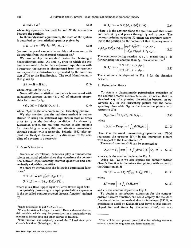
where c is the contour along the real-time axis that startsand ends at to and passes through t& and t& once. Thecontour-ordering operator T, orders the operators accord-ing to the position on the contour of their time arguments
r
(/+ 1 )Q+t 1 P))4& 0@ 1 c 1
+PA (2.7)
G(1, 1')= .(2.8)G ~(1,1') t) &,t)
The contour c is depicted in Fig. 1 for the situation~1 + c t 1'.
The contour-ordering relation t] &,t~ means that t& isfurther along the contour than t, . We observe that
G (1,1') t, &,t, ,
~( t) =H +H'(t), (2.3) 2. Perturbation theory
where H'(t) =0 for t & toNonequilibrium statistical mechanics is concerned with
calculating average values (O~(t)) of physical observ-ables for times t &to,
( 0 (t) ) =Tr[p(H)O (t)], (2.4)
Green's functions
Green's or correlation, functions play a fundamentalrole in statistical physics since they constitute the connec-tion between experimentally relevant quantities and con-veniently calculable quantities.
We start by introducing the following correlation func-tions:
where O~(t) is the observable in the Heisenberg picture.We also mention that the real-time method is not re-
stricted to using the statistical equilibrium state at timesprior to to as the boundary condition. As shown byKorenman (1966), the real-time method is also suitablefor describing a nonequilibrium situation maintainedthrough contact with a reservoir. Schmid (1982) also ap-plied the KeMysh technique to a discussion of the cou-pling of a system to a reservoir.
To obtain a diagrammatic perturbation expansion ofthe contour-ordered Green's function, we notice that thestandard way of expressing the relation between an ob-servable Q~ in the Heisenberg picture and the corre-sponding observable O~ in the interaction picture withrespect to H is
O~(t) =Q (t ro)O~(t)u (t, to)
where
(2.9)
u (t, to) =T exp i J dt'HH—(t')0
(2.10)
Here T is the usual time-ordering operator and H~(t)«presents the operator H'(r) in the interaction picturewith respect to the Hamiltonian H.
The transformation (2.9) can be expressed as
G (1,1')= i ( T,(S, Q—H(1)QH(1')) ), (2.12)
O~(t) = T exp —i I ri~HH(~) O~(t) (2 11)
where c, is the contour depicted in Fig. 2.Using Eq. (2.11) we can express the contour-ordered
Green's function in the interaction picture with respect tothe Hamiltonian H
(2.5)
S~=exp i dr H—II(&)C
(2.13)where f is a Bose (upper sign) or Fermi (lower sign) field.
A quantity possessing a simple perturbation expansionis the so-called contour-ordered Green's function defined
2Units are chosen to put 6=k~ ——c =1.The abbreviation 1=—(tl, x~} is used. Here x denotes the spa-
tial variable, which may be generalized in a straightforwardmanner to include spin and other degrees of freedom.
4This function was originally named the "closed time pathCareen's function" (Schwinger, 1961}.
and e is the contour depicted in Fig. 1.To obtain a perturbation expansion for the contour-
ordered Green's function, we could employ the standardfunctional derivative method due to Schwinger (1951), asexplained in detail by Kadanoff and Baym (1962) and em-ployed for real times by Korenman (1966; see also
5This will be our general prescription for relating contour-ordered quantities to greater and lesser quantities.
Rev. Mod. Phys. , Vol. 58, No. 2, April 1986
J. Rammer and H. . Smith: Field-theoretical methods in transport. theory
to tp
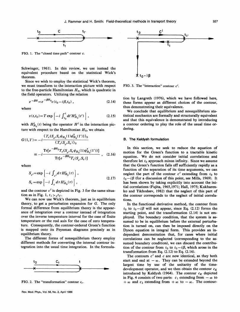
FIG. 1. The "closed time path" contour c.
Schwinger, 1961). In this review, we use instead theequivalent procedure based on the statistical Wick'stheorem.
Since we wish to employ the statistical Wick's theorem,we must transform to the interaction picture with respectto the free-particle Hamiltonian Ho, which is quadratic inthe field operators. Utilizing the relation
e =e U(to —ip to),-pe -»o
where
(2.14)
wherer
S;=exp i f .d—~HJI (z)
S~ =exp(2.17)
and the contour c is depicted in Fig. 3 for the same situa-tion as in Fig. 1, t ~ ~,i] .
We can now use Wick's theorem, just as in equilibriumtheory, to get a perturbation expansion for G. The onlyformal difference from equilibrium theory is the appear-ance of integration over a contour instead of integrationover the inverse temperature interval for the case of finitetemperature or the real axis for the case of zero tempera-ture. Consequently, the contour-ordered Green's functionis mapped onto its Feynman diagrams precisely as inequilibrium theory.
The different forms of nonequilibrium theory employdifferent methods for converting the internal contour in-tegration into the usual time integration. In the formula-
c,
FIG. 2. The "transformation" contour c,.
tU(t, to) =T exp i I dt'HH —(t')
0
with H~ (t) being the operator H' in the interaction pic-
ture with respect to the Hamiltonian Ho, we obtain
( T, (S,; S,p~, (1)f~,(1')))0G(1,1')= i—
(T,(S,;S,))0
Tr[e 'T, (S,;S,QH, (1)g~~ (1'))](2.16)
Tr[e T, (S;S,)]
FIG. 3. The "interaction" contour c'.
tion by I.angreth (1976), which we have followed here,these forms appear as different choices of the contour,thus demonstrating their equivalence.
We conclude that equilibrium and nonequilibrium sta-tistical mechanics are formally and structurally equivalentand that this equivalence is demonstrated by introducinga contour ordering to play the role of the usual time or-dering.
B. The Keldysh formulation
In this section, we seek to reduce the equation ofmotion for the Green's function to a tractable kineticequation. We do not consider initial correlations andtherefore let to approach minus infinity. Since we assumethat the Green's function falls off sufficiently rapidly as afunction of the separation of its time arguments, we canneglect the part of the contour c' extending from to toro —iP (for a discussion of this point, see Mills, 1969}. Ithas been shown by taking explicitly into account the ini-tial correlations (Fujita, 1965,1971;Hall, 1975; Kukharen-ko and Tikhodeev, 1982) that the neglect of this part ofthe contour corresponds to the neglect of initial correla-tions.
In the functional derivative method, the contour fromro to tp —iP will not appear, since Eq. (2.12) forms thestarting point, and the transformation (2.14) is not em-ployed. The boundary condition, that the system is as-sumed to be in equilibrium before the external perturba-tion is turned on, can then be imposed directly on theDyson equation in integral form. This provides an in-dependent demonstration that, for cases where initialcorrelations can be neglected (corresponding to the as-sumed boundary condition), we can discard the contribu-tion of the contour from to to to —ig, which arose in thetransformation from Eq. (2.12}to Eq. (2.16).
The contours c' and c are now identical, as they bothstart and end at —oo. They can be extended beyond thelargest time by use of the unitarity of the time-development operator, and we then obtain the contour c~introduced by Keldysh (1964). The contour cx depictedin Fig. 4 consists of two parts: c~ extending from —00 to+ oo and cz extending from + 00 to —oo. The contour-
Rev. Mod. Phys. , Vol. 58, No. 2, April 1986

328 J. Rammer and H. Smith: Field-theoretical methods in transport theory
C)
FIG. 4. The Keldysh contour c~.
central to the nonequilibrium formulation of Keldysh.For many purposes there exists a more convenient rep-
resentation of 6, introduced by Larkin and Ovchinnikov
(1975). It has the advantage that the matrix structure inKeldysh space of a one-body coupling is the simplest pos-sible. To obtain this representation we first perform atransformation in Keldysh space
ordered Crreen's function 6, specified by the Keldysh
contour can then be mapped onto the Keldysh space,
G= r—G,followed by a rotation
(2.23)
6, (1,1')~6=. Giz
Gzi Gzz(2.18)
G =LGL~,
where
(2.24)
(2.25)by the prescription that the ij component of 6 be definedas 6, (1,1') for ti and ti residing on c; and cj, respec-
tively. Writing out the components, we observe
Gi)(1, 1')= i ( T—(g~(1)/@1'))),
Gi2(1, 1')=6~(1,1'),
62i(1, 1')=6 ~(1,1'),
622(1, 1')= —(iT(lp~ 1)y~ 1')) ) .
(2.19)
The components of 6 are not linearly independent, and
by performing a rotation in Keldysh space it is possible toremove part of the redundancy. In the original article,Keldysh (1964) used the linear transformation
With the help of the following identities,
6~(1,1')=Gii(1, 1')—Gip(1, 1')
=62 i (1,1')—622 (1,1'),
6"(1,1')=Gii(1, 1')—62i(1,1')
=6 ip(1, 1')—Gg2(1, 1'),
6 (1,1')=62i(1,1')+Gi2(1, 1')
=6 i i (1,1')+G22( 1,1'),
which are easily proved, we obtain
(2.26)
O GAGI
GR GK (2.20)
GRG='
,0
GK
GA(2.27)
where, besides the usual retarded and advanced Green'sfunctions,
The representation (2.27) with one off-diagonal element
equal to zero will be used below.
C. Feynman rules
(2.21)
= —8(ti ti )[G ~(1,1') —6 ~(—1,1')],we encounter the function
G~(1, 1')=6~(1,1')+6 ~(1,1')
The ordering along the contour c& is given by the usual time-ordering operator T, while the ordering along c~ is given by theanti-time-ordering operator T according to
T(g(1)g (1'))= ~
[+f (1')$(1)
7We riote that the original article by Keldysh (1964) contains
the misprint of interchanging the definition of retarded and ad-
vanced.
In order to establish the Feynman rules in Keldyshspace it is sufficient to consider simple diagrams. Aspointed out in Sec. II.A.2 we need only add to the stan-dard Feynman rules the additional features brought about
by the contour. In addition we note that the cancellationof the unlinked diagrams is obtained automatically in theKeldysh technique. Let us start with the simplest exam-
ple, coupling to an external potential U. In standard no-tation we have the diagrammatic expansion of 6, shown
in Fig. 5 with the crosses denoting the external potential.The first-order term in U is given by the second dia-
gram in the infinite series shown in Fig. 5,
We use 8 (i =0,1,2,3) instead of o' to designate the Pauli ma-
trices, to stress that they have nothing to do with spin degrees offreedom (r is the unit matrix).
Rev. Mod. Phys. , Vol. 58, No. 2, April 1986
J. Rammer and H. Smith: Field-theoretical methods in transport theory 329
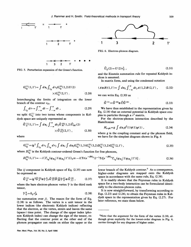
FIG. 6. Electron-phonon diagram.
V
1 3 2+ o o- ~
FICi. 5. Perturbation expansion of the Green's function. Uij(2) = U(2)rg~j, (2.31)
and the Einstein summation rule for repeated Keldysh in-dices is assumed.
In matrix form, and using the condensed notation
G,"'(l, l')= f dx2f dr2G, ' '(1,2)U(2)
XG(0)(2 1~) (2.28)
(A B)(1, 1')=f dxz f dt2A (1,2)B (2, 1'),
we can write Eq. (2.30) as
(2.32)
where
XG k ji(2, 1'), (2.30)
Interchanging the limits of integration on the lowerbranch of the contour cz.,
f d~ f" dr f"—dr, (2.29)
we split G,'" into two terms whose components in Kel-
dysh space are uniquely represented as
G,',"(l, l )=f dx, f dI, G(„"(1,2)vkk. (2)
G (1) G (0)g UG (0) (2.33)
H, &~——g x~ ~ 1 1y1 (2.34)
where g is the coupling constant and q& the phonon field,we have for the simplest diagram shown in Fig. 6
We have thus established in the representation given byEq. (2.18) that an external potential in Keldysh space cou-ples to particles through a 2 matrix.
For the electron-phonon interaction described by theHamiltonian
G,'"=ig~ f d~3 f d~2 f dx3 f dx2G,' '(1,3)G,' '(3,2)D,' '(3,2)G,' '(2, 1'),
where D,' ' is the Keldysh contour-ordered Careen's function for free phonons,
(2.35)
D,' '(l, l')= I (T, (y—I! (1)yH (1')))0= I(Tr(e ))—'Tr[e T, (IjjH (1)y Ir(1'))] . (2.36)
The ij component in Keldysh space of Eq. (2.35) can nowbe expressed as
Gij =Ig Gii' 9 i'I GI'! kkT'Ij' j'j ~( i) 2 ~ (p) k ~ (0) ~ (p) kp ~ (p) (2.37)
where the bare electron-phonon vertex y is the third ranktensor,
9 lj ~l ~jjk (2.38)
(no summation over j). The reason for the form of Eq.(2.38) is as follows. The vertex is a unit tensor in thelower indices (the electronic Keldysh indices) reflectingthat the electron, at the vertex, enters and leaves the same(space-) time point. The change of the upper index (pho-non Keldysh index) can change the sign of the tensor, re-flecting that the contour point at the other end of thephonon propagator can reside on either the upper or the
lower branch of the Keldysh contour. As a consequence,higher-order diagrams are mapped onto the Keldyshspace in accordance with the same rule, Eq. (2.38).
It is readily shown that the Feynman rules in Keldyshspace for a two-body interaction can be formulated identi-cally to the electron-phonon rules.
It is now straightforward, by transforming according toEqs. (2.23) and (2.24), to obtain the Feynman rules in Kel-dysh space in the representation given by Eq. (2.27). Forlater reference, we state them below.
9Note that the argument for the form of the vertex (2.38), al-though given explicitly for the lowest-order diagram in Fig. 6,carries through for any diagram of higher order.
Rev. Mod. Phys. , Vol. 68, No. 2, April 1986
330 J. Rammer and H. Smith: Field-theoretical methods in transport theory
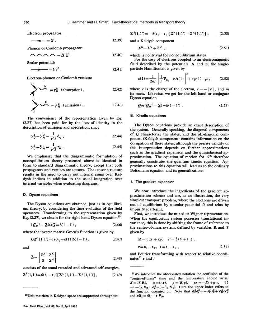
Electron propagator:
Phonon or Coulomb propagator:
X"(1,1')= —B(t i —t, )[X~ ( 1, 1')—X «(1,1')],and a Keldysh component
yK @++y(
(2.50)
(2.51)
Scalar potential:
=D, V. (2.40)
(2.41)
which is nontrivial for nonequilibrium states.For the case of electrons coupled to an electromagnetic
field described by the potentials A and p, the single-particle Hamiltonian is given by
2
Electron-phonon or Coulomb vertices: s(1)= —.V„—e A(1) +ey(1)—p,1 1
2ln i(2.52)
=y,".
J (absorption), (2.42) where e is the charge of the electron, e = —~
e ~, and mits mass. Likewise, we get for the left-hand or conjugateDyson equation
=y kj (emission) . (2.43) Ge(GO ' —X)=&(1—1') . (2.53)
The convenience of the representation given by Eq.(2.27) has been paid for by the loss of identity in thedescription of emission and absorption, since
(2.44)
1 1
27 gJ ~ (2.45)
D. Dyson equations
The Dyson equations are obtained, just as in equilibri-um theory, by considering the time evolution of the fieldoperators. Transforming to the representation given byEq. (2.27), we obtain for the right-hand Dyson equation'
(Go ' —X)SG=5(1—1'), (2.46)
where the inverse matrix Green's function is given by
We emphasize that the diagrammatic formulation ofnonequilibrium theory presented above is identical inform to standard diagrammatic theory, except that bothpropagators and vertices are tensors. The tensor structureresults in the need to carry out internal sums over Kel-dysh indices in addition to the usual integration overinternal variables when evaluating diagrams.
E. Kinetic equations
The Dyson equations provide an exact description ofthe system. Generally speaking, the diagonal componentsof G characterize the states, and the off-diagonal com-ponent (Keldysh component) contains information on theoccupation of these states, although the precise validity ofthis interpretation depends on further approximationssuch as the gradient expansion and the quasiclassical ap-proximation. The equation of motion for G thereforegenerally constitutes the quantum-kinetic equation. Ap-proximations to this equation will lead us to the ordinaryBoltzmann equation and its generalizations.
1. The gradient expansion
We now introduce the ingredients of the gradient ap-proximation scheme and use, as an illustration, the verysimplest transport problem, where the electrons are drivenout of equilibrium by a scalar potential U and relax byimpurity scattering.
First, we introduce the mixed or Wigner representation.When the equilibrium system possesses translational in-variance, this is done by shifting the frame of reference tothe center-of-mass system, defined by variables R and Tgiven by
and
Go '(l, l')=[iB,, —e(l)]5(1—1'), (2.47) R= —,'(xi+xi ), T= —,'(ti+ti ),r=xI —xi, t =t& —ti (2.54)
yR yKX=0 yA (2.48)
and Fourier transforming with respect to relative coordi-nates" r and t
consists of the usual retarded and advanced self-energies,
(2.49)
Unit matrices in Keldysh space are suppressed throughout.
~IWe introduce the abbreviated notation (no confusion of the"center-of-mass" time and the temperature should arise)X =(T,R), x =(t, r), p =(E,p), px = —Et +p-r, B~
VR ) &p = ( &E Vp ) Here the upper index refers tothe function operated on. Note that B~B~=—B~B~+VR.V~and xB~——tBT+r VR.
Rev. Mod. Phys. , Val. 58, No. 2, April 1986
J. Ramrner and H. Smith: Field-theoretical methods in transport theory 331
6(X,p) =f dx e '~"G(X+ x/2, X—x/2) . (2.55) of Green's functions, we have'
Performing a Taylor expansion, we observe that theconvolution A 8 in this representation is given by
Go (p) =Ito(E)[Go (p) —Gc (p)],with the consequence
(2.66)
g ~ax~a~ —a~a~ i/2(ASB)(X,p)=e ~ ~ A(X,p)B(X,p) . (2.56) &f(p) =&p(E)[&o(p)—&o(p)], (2.67)
Physical quantities such as densities and particle currentsmay be expressed in terms of the equal-time, one-particledensity matrix, which is essentially our Green's function6 in the mixed representation integrated over E. How-ever, the Dyson equation cannot be reduced to one involv-
ing equal-time Green's functions. As a first step towardsobtaining an equation that may be integrated over E, wesubtract the Dyson equation and its conjugate, whereuponwe obtain
ho(E) =tanh —,' PE . (2.68)
Thus the two terms on the right-hand side of Eq. (2.60)cancel in equilibrium, while the left-hand side is triviallyzero in equilibrium. The gradient approximation is ob-tained from (2.56) by keeping the first two terms in theexpansion of the exponential function in (2.56). We thushave
[Go ' —XG] =0,
where, in the mixed representation,
Gp ' E —gp
———U(R, T),and, since we consider a free electron model below,
P~&=2m
(2.57)
(2.58)
(2.59)
[AB]+ =2AB,
i [A—B] = [A,B]p,
where the generalized Poisson brackets is defined as
[A,B],=a"Aa,'B —a,"Aa'B
(gAg8 gAgB PA PB+PA.PB)AB
(2.69)
(2.70)
=—[X~eA]+——[I'eG ]+, (2.60)
where we have introduced the spectral weight function
A =i(G"—6")together with the other abbreviations
(2.61)
To obtain a kinetic equation, we consider the Keldyshcomponent of Eq. (2.57),
[6 ' —ReXII 6 ] —[X ReG]
2. The Boltzmann equationfor impurity scattering
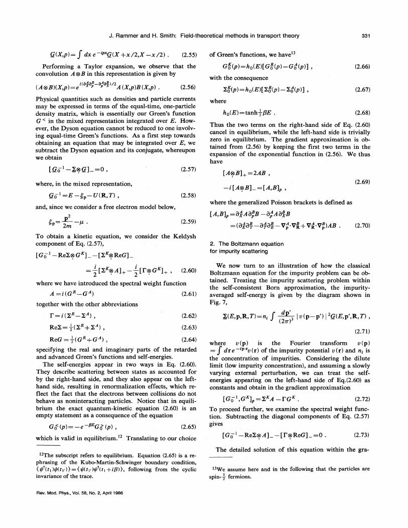
We now turn to an illustration of how the classicalBoltzmann equation for the impurity problem can be ob-tained. Treating the impurity scattering problem withinthe self-consistent Born approximation, the impurity-averaged self-energy is given by the diagram shown inFig. 7,
i (yR yA)
Rex =-,' (X'+r"),(2.62)
(2.63)
X(E,p, R, T)=n; f i u(p —p')i
6(E,p', R, T),(2m)
(2.71)ReG = —,'(6 +G"), (2.64)
specifying the real and imaginary parts of the retardedand advanced Green's functions and self-energies.
The self-energies appear in two ways in Eq. (2.60).They describe scattering between states as accounted forby the right-hand side, and they also appear on the left-hand side, resulting in renormalization effects, which re-flect the fact that the electrons between collisions do notbehave as noninteracting particles. Notice that in equili-brium the exact quantum-kinetic equation (2.60) is anempty statement as a consequence of the equation
Go (p)= —e Go (p), - (2.65)
which is valid'in equilibrium. ' Translating to our choice
The subscript refers to equilibrium. Equation (2.65) is a re-phrasing of the Kubo-Martin-Schwinger boundary condition,(g (&~)g(r~ ))=(g(t~ )f (r~+iP)), following from the cyclicinvarianee of the trace.
[6, ' —ReXe A] —[I"eReG] =0 . (2.73)
The detailed solution of this equation within the gra-
We assume here and in the following that the particles are
spin- 2 fermions.
where u (p) is the Fourier transform u (p)=f dre 't"u(r) of the impurity potential u(r) and n; isthe concentration of impurities. Considering the dilutelimit (low impurity concentration), and assuming a slowlyvarying external perturbation, we can treat the self-energies appearing on the left-hand side of Eq.(2.60) asconstants and obtain in the gradient approximation
[6,6 ],=X A —rG . (2.72)
To proceed further, we examine the spectral weight func-tion. Subtracting th'e diagonal components of Eq. (2.57)gives
Rev. Mod. Phys. , Vol. 58, No. 2, April 1986
332 J. Rammer and H. Smith: Field-theoretical methods in transport theory
where v= Vpg is the (group) velocity.The dilute-limit approximation that went into the
derivation of Eq. (2.80) is equivalent to the usual criterionfor the validity of the Boltzmann equation for a degen-erate Fermi gas,
FIG. 7. Impurity self-energy diagram. 1 «p p (2.81)
dient approximation is given by Kadanoff and Baym(1962). One finds that the solution has the same form asin equilibrium,
I(E —
gp—ReX —U) +(I /2)~
(2.74)
The spectral weight function thus approaches a deltafunction in the dilute limit
3 =2m5(E —gp
—U) . (2.75)
X5(gp —g'p )(hp —hp ), (2.76)
where (suppressing space and time arguments) we have in-troduced the distribution function
and a free-particle form for the spectral weight, corre-sponding to
G = 2~i 5(E —gp
——U)h p,has been inserted in the self-energies.
Introducing the more familiar distribution function
(2.78)
fp ———,' (1—hp), (2.79)
which reduces to the Fermi function in equilibrium, weobtain the Boltzmann equation for impurity scattering
(~T+«.VR VRU. V,)f, —
2~n; f —~U(p —p')
~5(gp —g, )(f —f, ),
(2.80)
~4Notice that the first term on the left-hand side of Eq. (2.76)is exact and so is the second, insofar as the dispersion is qua-dratic.
This is also seen by observing that the solution to Eq.(2.73), in the case where the self-energies are neglected, isthe function given by Eq. (2.75); in other words, Go ' and3 given by Eq. (2.75) commute.
Exploiting the delta-function character of the spectralweight and the similarly peaked character of 6, we caneasily integrate Eq. (2.72) with respect to E from minus toplus infinity and obtain'
"dTh+Vpg VRh VRU Vph—
where I/r is the impurity scattering rate at the Fermisurface (p =p'=k~),
—=2~nI&O U p —p'dp4m
(2.82)
Here Xo ——mkz/2m is the density of states per spin at theFermi energy and kF the Fermi momentum. Further-more, the gradient approximation is valid when the exter-nal perturbation is slowly varying in space and time, sothat its characteristic frequency co and wave vector qsatisfy the conditions
cu «p, q «k+ . (2.83)
The condition (2.83) for a degenerate Fermi gas is suffi-cient to ensure the validity of the gradient expansion. Itis not necessary, however, to assume that the external fre-quency is small in the sense of co «1/r or co « T, as thequestion of the magnitude of the frequency with respectto the collision rate or the temperature never enters theapproximations leading to Eq. (2.72). Slow variations intime are therefore, within the context of the impurityproblem, to be understood in the sense of the conditions(2.83). In subsequent sections, the condition q «k~ canbe used throughout, while the restriction on co may de-pend on the particular system under consideration. Thusin discussing the electron-phonon problem (Sec. III.B), weassume m « T, while in the context of superconductivity(Sec. V), the inclusion of an external frequency within thegradient expansion would require co «A. The validity ofthe gradient expansion, as far as the external frequency isconcerned, will therefore depend on the physical systemunder consideration. It should be noted, however, that itis never necessary to assume the frequency to be small incomparison to the collision rate, as one would also expectfrom the simple physical arguments that lead to the semi-classical Boltzmann equation.
Since we, in our approximations, have freed the Green'sfunctions from their quantum-mechanical origin, it is nosurprise that we have obtained a classical equation (2.80).However, the absence of any feature due to quantumstatistics is a well-known property of impurity scattering.If we had treated electron-phonon scattering by the samelowest-order perturbation treatment, we would have en-countered the characteristics of Fermi-Dirac and Bose-Einstein statistics. %"e note that, except for this statisticalfeature, integration of the quantum-kinetic equation withrespect to E leads to the classical Boltzmann equation.The basic approximation was the use of the free-particleform of the spectral weight in Eq. (2.78).
Rev. Mod. Phys. , Vol. 58, No. 2, Aprif 1986
J. Rammer and H. Smith: Field-theoretical methods in transport theory 333
3. Currents and densities
The physical quantities we shall encounter are expressi-ble in terms of the Green's function G~: the fermioncharge density p,
p(1)= —2iG ~(1,1),and the electric current density j,
(2.84)
We have assumed spin independence, which accounts forfactors of 2. To change to our choice of basic Green'sfunctions we observe that
(2.86)
j(1)=— IVi —Vi.—ie[A(l)+A(1')]IG (1,1')~
i.m
(2.85)
equation involving only equal-time quantities cannot beobtained by integration with respect to E. It is wellknown that the electron-phonon interaction leads to animportant structure in the functions ReX and I as func-tions of the variable E. In contrast, as noted by Migdal(1958), the momentum dependence is very weak as aconsequence of the phonon energy's being small comparedto the Fermi energy. The spectral function thus becomesa peaked function in the variable g. We shall use thispeaked character to restrict all other quantities in con-junction with the spectral weight function to the Fermisurface. ' Just as the subtraction of the Dyson equationsin Eq. (2.57) eliminated the strong E dependence, it alsoeliminated the strong g dependence. Utilizing the peakedcharacter of the spectral weight function and neglectingthe momentum dependence of the self-energy, it is there-fore possible to integrate the left-right subtrac-ted Dyson equation with respect to g and obtain
The spectral weight A in Eq. (2.86) represents a contribu-tion to Eqs. (2.84) and (2.85) that does not depend on thestate of the system and shall henceforth be dropped when
nonequilibrium contributions are considered.
III. THE QUASICLASSICAL LIMITAND BEYONO
[g p +Ec70g] =O&
where
1 —1 0g o =go
with
gp' —— 8,, +vF [VR .ie A(—R, ti )]+icy(R, ti )
(3.2)
(3.3)
A. The quasiclassical approximation
The breakdown of the quasiparticle approximation isassociated with the deviation from a delta function of thespectral weight function
I(E —g—ReX)z+(I /2)2
(3.1)
If A differs significantly from a delta function, a kinetic
I
This scheme was first applied by Prange and Kadanoff(1964) in their treatment of transport phenomena in theelectron-phonon system, although they did not use the namequasiclassical. It was later extended to describe transport phe-nomena in superfluid systems by Eilenberger (196&).
There exists a consistent and self-contained approxima-tion scheme for a degenerate Fermi system, valid fordescribing a wide range of phenomena, that does not em-
ploy a restrictive quasiparticle approximation such as Eq.(2.78). It is called the quasiclassical approximation' andis of interest since it allows one to obtain simple transportequations even in cases where the quasiparticle approxi-mation fails. As an example of this approximationscheme, we derive in this section the electronic kineticequation for the case of electron-phonon interaction. In alater section (V) we treat the related case of superconduc-tors with large pair breaking.
2
[A(R, ti)] 5(ti —ti ),27?l
(3.4)
where v~ denotes the Fermi velocity, while g is thequasiclassical Green's function
g(R,p, ti, ti )=—I dg G(R, p, ti, ti ) .ITj
(3.5)
In doing so, we are, for instance, unable to account for theLorentz force effect of the magnetic field on the electronicmotion.
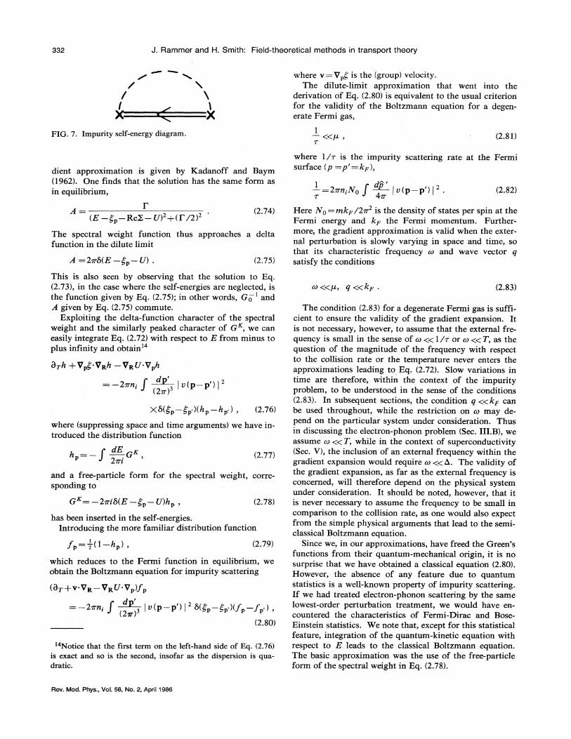
One often refers to g as the f-integrated Crreen's function.The integrand in Eq. (3.5) is not well behaved for largevalues of g, since it falls off only as 1/g. A high-energycutoff must therefore be introduced, as discussed by, forexample, Serene and Rainer (1983). Equivalently, we canuse the decomposition employed by Eilenberger (1968)and illustrated diagrammatically in Fig. 8. The integra-tion over g in Fig. 8 from —co to +' oo is replaced bytwo closed semicircles [Fig. 8(a)] yielding the low-energycontribution of physical interest, provided the cutoff ener-
gy is suitably chosen. The remaining high-energy contri-bution [Fig. 8(b)] contains terms that do not depend onthe nonequilibrium state and therefore can be dropped inthe equation of motion (3.2). The quasiclassical equationsmay also be derived without explicit use of g integration,as shown by Shelankov (1985).
In obtaining an equation which only involves thecenter-of-mass spatial coordinates, it has been assumed
Rev. Mod. Phys. , Vol. 58, No. 2, April 1986
334 J. Rammer and H. Smith: Field-theoretical methods in transport theory
time integration. In order to have a closed set of equa-tions and a complete quasiclassical theory we must makesure that the self-energy can be expressed solely in termsof the quasiclassical Careen's function and thus accountfor the transformation X[6]~cr[g],X being a functionalof G and o being a functional of g.
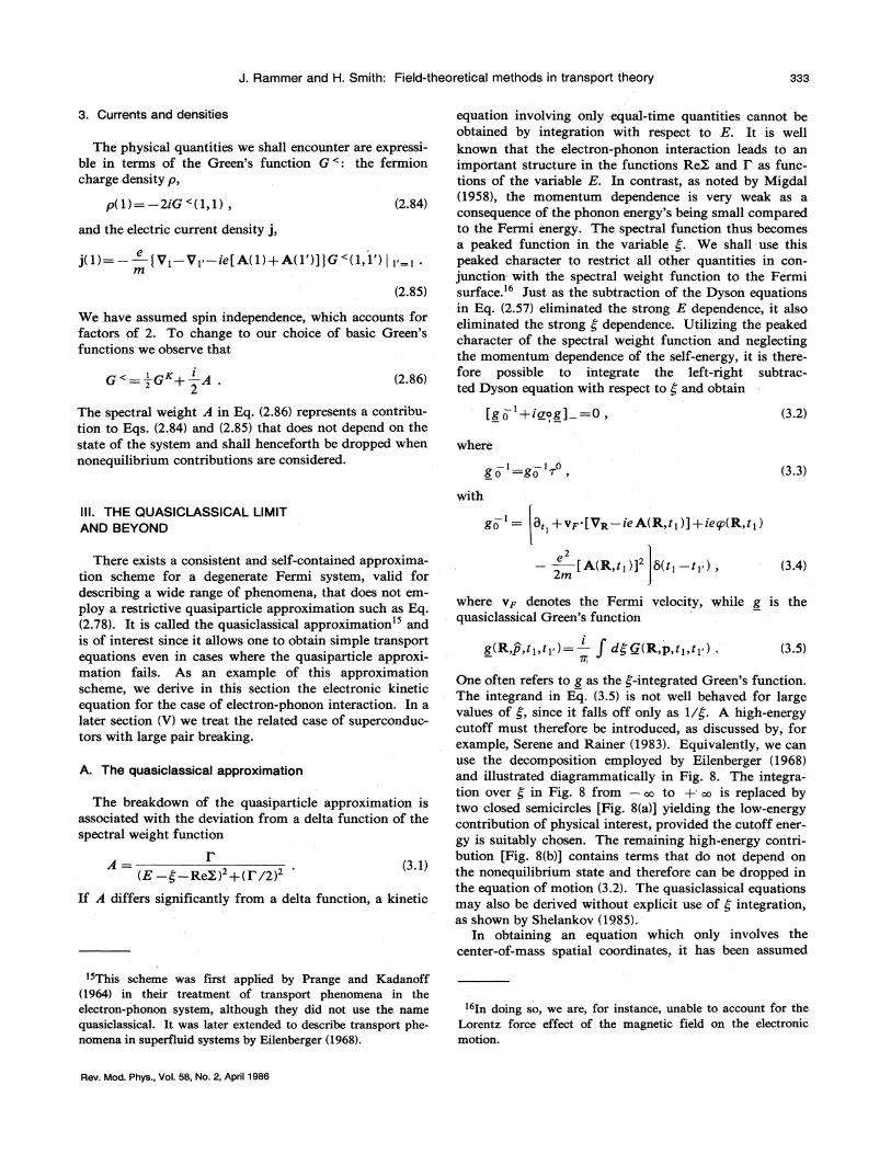
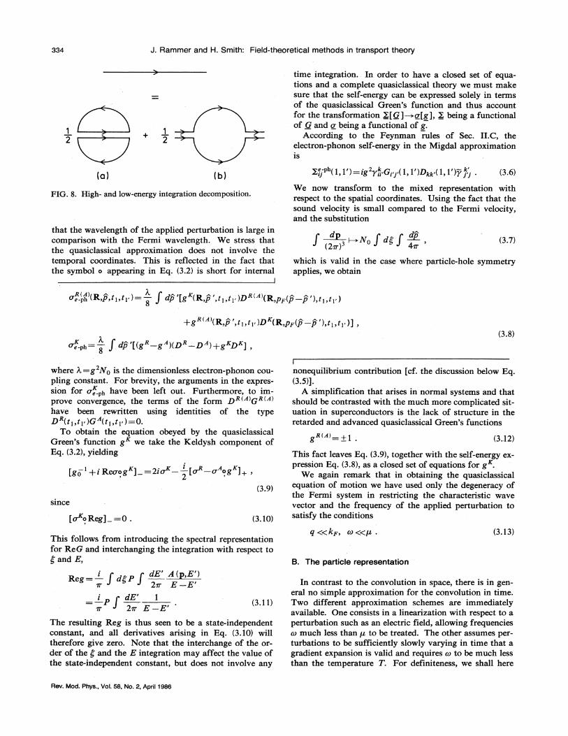
According to the Feynman rules of Sec. II.C, theelectron-phonon self-energy in the Migdal approximation1s
(a) XJ""(1,1')=ig y,"G; J ( 1,1')Dkk (1,1')y Jkj . (3.6)
FIG. 8. High- and 1ow-energy integration decomposition.
that the wavelength of the applied perturbation is large incomparison with the Fermi wavelength. %'e stress thatthe quasiclassical approximation does not involve thetemporal coordinates. This is reflected in the fact thatthe symbol a appearing in Eq. (3.2) is short for internal
l
We now transform to the mixed representation withrespect to the spatial coordinates. Using the fact that thesound velocity is small compared to the Fermi velocity,and the substitution
f "Pj ~ fdgf P, (3.7)
which is valid in the case where particle-hole symmetryapplies, we obtain
-ph p 1 I') f p'[g (R,p', ti, ti )D '"'(R,p~(p —p'), ti, t, )
+g '"'(RP', ti, ti )Dx(Rp+(P —P'), t„t,)],~..ph= —f dp'[(g' g")(D' —D")+g —D ],
(3.8)
[go +i Reo'og ] =2icr —[o' ——~ &g ]+ ~
since
(3.9)
[cr oReg] =0. (3.10)
where A, =g No is the dimensionless electron-phonon cou-pling constant. For brevity, the arguments in the expres-sion for cr, ~h have been left out. Furthermore, to im-prove convergence, the terms of the form D '"'Ghave been rewritten using identities of the typeD (ti, ti )G"(ti,ti )=0.
To obtain the equation obeyed by the quasiclassicalGreen's function g we take the Keldysh component ofEq. (3.2), yielding
I
nonequilibrium contribution [cf. the discussion below Eq.(3.5)].
A simplification that arises in normal systems and thatshould be contrasted with the much more complicated sit-uation in superconductors is the lack of structure in theretarded and advanced quasiclassical Green's functions
(3.12)
This fact leaves Eq. (3.9), together with the self-energy ex-pression Eq. (3.8), as a closed set of equations for g~.
We again remark that in obtaining the quasiclassicalequation of motion we have used only the degeneracy ofthe Fermi system in restricting the characteristic wavevector and the frequency of the applied perturbation tosatisfy the conditions
This follows from introducing the spectral representationfor ReG and interchanging the integration with respect topand E,
q ((kF, co ((p .
B. The particle representation
(3.13)
R = i f dgP f dE' A(p, E')7T' 2m E —E'i E' I=—P
2m E —E' (3.11)
The resulting Reg is thus seen to be a state-independentconstant, and all derivatives arising in Eq. (3.10) willtherefore give zero. Note that the interchange of the or-der of the g and the E integration may affect the value ofthe state-independent constant, but does not involve any
In contrast to the convolution in space, there is in gen-eral no simple approximation for the convolution in time.Two different approximation schemes are immediatelyavailable. One consists in a linearization with respect to aperturbation such as an electric field, allowing frequenciesco much less than p to be treated. The other assumes per-turbations to be sufficiently slowly varying in time that agradient expansion is valid and requires u to be much lessthan the temperature T. For definiteness, we shall here
Rev. Mod. Phys. , Vol. 58, No. 2, April 1986
J. Rarnmer and H. Smith: Field-theoretical methods in transport theory 335
employ the second scheme. In order to reduce Eq. (3.9) toa simpler looking transport equation, we introduce themixed representation with respect to the temporal coordi-nates and perform a gradient expansion as in Sec. II.E.This approximation restricts us to frequencies smallerthan the characteristic frequency of the system, in thiscase the temperature. After transformation to a gaugewhere the vector potential is absent, Eq. (3.9) is reduced to
[(1—BzReo)Br+BrReoBz+vz. VR+eBzyB ]g =I,
f= —,'(1—h),and the Bose distribution X,, given by
(3.22)
N(E) = ——1 —coth1 E2 2T
(3.23)
the kinetic equation takes the form
If we introduce the distribution function f, whichreduces to the Fermi distribution in equilibrium,
where the collision integral is
(3.14) [(1—a,R~g, +a,Reoaz+vz. v„+ed'.yBz]f =I, zh[f]., (3.24)
with
y=i(o —o") .
(3.15)
(3.16)
with the collision integral
w p
I, zh[f]= —2m f f dE'p(P p', E E—')Rzz;—&-, ,
The two terms in the collision integral constitute thescattering-in and -out terms, respectively. According toEq. (3.8) they are determined by (space and time coordi-nates suppressed) Rz,'~-, =[1+N (E —E')]f(E,P)[I —f(E',P ') ]
(3.25)
N(E E—')[1 f—(E,p)]—f(E',P ') . (3.26)&o, ph(@P) = ~ f —f dE'p('pF(p p'), E —E')—
4m
coth h (E',p ') 1—El2T
Finally, to introduce a distribution function that is in-variant with respect to gauge transformations, we makethe replacement
(3.17)P g
y(E,p) =—m. f f dE'p(pz(p p'), E E—')—4m.
EIX coth —h (E',p ')
2T
f(E)=f(E —ep)
(cf. Sec. III.E), whereby Eq. (3.24) becomes
[(1—8 Reg)Bz+ BzReoBz+v (Vit+eEBz)]f
(3.27)
(3.18)
p(q E)= [Do (q E)—Do (q E)liN& lgq I z (3.19)
and we have introduced the distribution function
h = —,g K (3.20)
We have further assumed the phonons to be in thermalequilibrium (although this is not necessary) and utilizedthe equilibrium property
Do =(Do —Do )coth2T
(3.21)
The Fermi-surface average of the function p is the Eliash-berg function n I" well known from superconductivity.
i7At this point we aBow for a more general eIectron-phonon
coupling than before. The coupling is denoted by gq, corre-
sponding to a momentum transfer q. In the model described by(2.34) we have
~ g~ ~=g (co~/2)'~~, where co~ is the phonon fre-
quency.
=I.ph[f]-
where E=—Vy. Here we have dropped the tilde on f forconvenience.
As noted previously, we have split off the self-energyterms in the kinetic equation. The terms on the right-hand side describe scattering, whereas the self-energyterms on the left-hand side, which are absent in the usualelectron-phonon Boltzmann equation, describe the renor-malizatiori effects due to the electron-phonon interaction.Another difference from the usual electron-phononBoltzmann equation is the dependence of the distributionfunction on energy and position on the Fermi surface (be-sides space and time). This feature of the kinetic equationis characteristic of the quasiclassical theory and refiectsthe fact that we do not rely on a definite relation between
energy and momentum, that is, the validity of the quasi-particle description.
Prom the kinetic equation (3.24), Prange and Kadanoff(1964) drew the conclusion that many-body effects can beseen only in time-dependent transport properties and thatstatic transport coefficients, such as dc conductivity andthermal conductivity, are correctly given by the usualBoltzmann result. However, there is a restriction to thegenerality of this statement. In deriving the quasiclassicalequation of motion we assumed particle-hole, symmetry.
Rev. Mod. Phys. , Vol. 58, No. 2, April 1986
336 J. Rammer and H. Smith: Field-theoretical methods in transport theory
Within the quasiclassical theory, all thermoelectric coeffi-cients therefore vanish, and no conclusions can be drawnabout many-body effects on the thermoelectric properties.We shall see in Sec. III.F, by going beyond the quasiclas-sical limit, how the thermoelectric properties do get re-normalized by the electron-phonon interaction.
Before proceeding to consider physical problems, weexpress the electric charge and current densities in termsof the quasiclassical Green's function.
Referring to Sec. II.E.3 we get the following expressionfor the charge density in the mixed representation:
A, r
Reo = 2%0 f f dE'~g,
~
ilg(p', E',R, T)
X R.eD (pp —p„',E E'),— (3.33)
where
(1 —8@Reer)8Th —BTReoBgho+ev~. EBEho 0——. (3.32)
Except for a real constant (renormalizing the chemicalpotential), we have by using the Feynman rules of Sec.II.C
p(R, t)= 2eN—, —f p f dEgx(E,p, R, T)1 dp
+ey(R, T) (3.29)
ReD = ,'(D +—D ) .
Letting the applied electric field E be
E(t) =Eoe
(3.34)
(3.35)
we seek a solution to Eq. (3.32) of the form h =ho+hiwith
(3.36)h ~——aeE-vy Bghp,
where the constant a remains to be determined. InsertingEq. (3.36) into Eq. (3.32) we obtain
1
—ice(1+i.*) (3.37)
j(R,T)= —, eNO f f—dEvFg4m
(3.30)where
The second term in Eq. (3.29) stems from energies farfrom the Fermi surface and is thus not accounted for bythe quasiclassical Green's function. This is establisheddirectly (see Eliashberg, 1971) or by invoking the ap-propriate symmetry, which here is gauge invariance.
For the electric current density we have in the mixedrepresentation
Here the high-energy contribution is cancelled by what issometimes called the diamagnetic current (as we shall ver-ify in a specific case in Sec. IV.A).
The origin of the form of Eqs. (3.29) and (3.30) is theinterchange of the order of integration over E and g,brought about by the use of the quasiclassical Green'sfunction. This reverses the sequence of integration fromthe correct one, in which the E integration is done first.Later, in the context of superconductivity, we shall useEq. (3.29) and interpret p as the difference between thecharge density of a nonequilibrium superconducting stateand that of the normal state in equilibrium. Such a sub-traction procedure ensures the validity of the interchangeof the order of integration.
C. An example: Electron-phononrenormaiization of the ac conductivity
A, '=2K, f '(1—PP') .
47K cop~-pF(3.38)
We can now evaluate the current and obtain for theconductivity
ne
COm-opt(3.39)
where n is the number density of electrons and the opticalmass m,p, is renormalized according to
m, ~, =m(1+I,') . (3.40)
This result was originally obtained by Holstein (1964).We note that it is the nonequilibrium electron contribu-tion to the real part of the self-energy that makes the opti-cal mass renormalization different from the specific-heatmass renormalization.
As an example of electron-phonon renormalization oftime-dependent transport coefficients we shall considerthe ac conductivity in the frequency range given by
(3.31)
where y denotes the electron-phonon scattering rate atthermal excitation energies. For definiteness, we also con-sider the temperature to be low compared to the Debyetemperature 8&.
The inequality (3.31) enables us to neglect the collisionintegral. The linearized kinetic equation then takes thesimple form
D. The excitation representation
The quasiclassical theory leads to equations that aremore general than the usual Boltzmann equation. Wehave shown that the basic variables, besides space andtime, are energy and position on the Fermi surface. Al-though the electron-phonon interaction does not permitthe quasiparticle approximation a priori, we shall here re-capitulate the derivation by Prange and Kadanoff (1964),showing that it is still possible to cast the electron-phononproblem in the Landau-Boltzmann form.
Rev. Mod. Phys. , Vol. 58, No. 2, April 1986
J. Rammer and H. Smith: Field-theoretical methods in transport theory
1. The kinetic equation
We start by defining a quasiparticle energy Ep, whichis given implicitly' by
In transforming the collision integral we have utilized thesubstitution
N f ~ fdEmN f ~ fog, .
Ep =gp+Recr(Ep+ey, P,R, T) .
This satisfies the equations
(3.41)I f P, Z,
(2m)3(3.54)
Vkp =ZpVp&p
VRE =Z ( VRlpdzReo'+VRReo')~ z
P
d E =Z (ed q&BzRecr+BTReo) ~z z +,p,
(3.42)
(3.43)
(3.44)
Since the sound velocity is much less than the Fermivelocity, the phonon damping is negligible, and the pho-non spectral weight function therefore has a delta-function character
S (p —p')=Np lgp p I'[@Ep—Ep —~p-p)
Zp=(1 —BzReo) '~ z z +, (3A5)
We now set E equal to E&+ey in the kinetic equation(3.24) and introduce the distribution function
where in (3.42) we have neglected any angular dependenceof the real part of the self-energy and introduced thewave-function renormalization constant
—6(Ep Ep +co—p p )], (3.55)
where coq denotes the phonon frequency. We can thenwrite the kinetic equation in the final form
[dr+VpEp VR VR(Ep+—ep) Vp]np I, ph——[n], (3.56)
with
np——f( Ep, R, T)~ z {3.46) I, p„[n]= 2n f— , ZpZp i gp p i
Il pp
(2~)By using the relations'
Vpn =VpEp(dzf)I z=z, +.p
Van =[VRf+VR(Ep+eq»dzf] I z=z, + ~
d" =[d.f+d.(Ep+.~)~zf] I z=;+...
(3.47)
(3.48)
(3A9)
I, h[n]= — Z p(p —p')RP,277 dp(2)' ' (3.51)
ApP——[1+N(Ep —Ep )]np(1 np )—
and Eqs. (3.42)—(3.44), we obtain
Z '[dr+Vs .VR VR(E +—eq&).V ]n =I, h[n],
(3.50)where
X[5(Ep—Ep —pip p)
—5(Ep Ep +p)p —p)] . (3.57)
This has the form of the familiar Boltzmann equation, ex-cept for the fact that the matrix elements are renormal-ized.
%'e stress that only the quasiclassical approximationwas used to derive the above kinetic equation. In particu-lar, we have not assumed any relation between the scatter-ing rate y and the temperature. This would have beennecessary for invoking a quasiparticle description in orderto justify the existence of long-lived electronic momentumstates. It has thus been established from microscopictheory that the validity of the Boltzmann description ofthe electron-phonon system is determined not by thePeierls criterion (y « T), but by the Landau criterion,
N(Ep Ep )(1——np)np- ,
f(I —P') = [D (y —I'
Ep —Ep )INp (gp p
2m'
(3.52) 'V«P .
2. Densities and currents —theconservation law
(3.58)
—D"(p—p', Ep —Ep )] .
(3.53)
We shall suppress the space-time variables and use the short-hand notation E~ =E(p,R, T).
In using {3.47) to transform the gradient term in (3.24) we
have ignored the explicit dependence of f on P. This is neces-
sary to preserve consistency in the quasiclassical scheme in thepresent form, where the momentum is fixed at the Fermi sur-
face, cf. (3.5).
j(R,T)=2 f ~ V+pnp .(2m )
(3.60)
The collision integral [Eq. (3.57)] has the invariant
f d p Iq ph[ n ]=0, (3.61)
The Landau-Boltzmann expressions for the density andcurrent density have the well-known form
n(R, T)=2 f & npdp
(2~)
and
Rev. Mod. Phys. , Vol. 58, No. 2, April 1986
338 J. Rammer and H. Smith: Field-theoretical methods in transport theory
n=2NO f f dEf(E,P) —ey4m
=2ND dE E+eyp (3.63)
The last equality seems to require that ey «T. How-ever, this is an artifact of our choice of representation.We could equally well have represented the electric fieldin a gauge where the scalar potential is absent.
which expresses the conservation of the number of parti-cles.
Integrating the kinetic equation (3.56) with respect tothe momentum shows that the density and current-density expressions (3.59) and (3.60) satisfy the continuityequation
(3.62)
In order to establish that Eqs. (3.59) and (3.60) areindeed the correctly identified densities (in the excitationrepresentation), we should connect one of them with themicroscopic expression. According to Sec. III.B we havefor the density in the particle representation (we suppressspace-time variables)
In order to compare the particle and the excitation rep-resentations, we transform Eq. (3.59) to the particle repre-sentation by using Eqs. (3.41) and (3.54) and obtain
2 f — n =2ND f f dE(1 —BERea')f(E,p)(2m ) 4~
Since Eqs. (3.63) and (3.64) appear to be different, wealso transform Eq. (3.60) to the particle representation
2 f Vp&np 2eN——O f f dEvFf(E, p) .4n.(3.65)
Comparing Eq. (3.65) with Eq. (3.30), we observe that thisis identical to the quasiclassical current-density expres-sion. The only possibility for the above-mentioneddiscrepancy not to lead to a violation of the continuityequation is the existence of the identity
B f dP f dEf(E,p)B Reer(E,p)=0. (3.66)
We shall now prove this identity. Inserting the expressionfrom Eq. (3.33) into the left-hand side of Eq. (3.66) we areled to consider
f dp f dE f dP' f dE'~g,~
ReD(pz —p+, E E')[BTf(Ep)B—Ff(E',P') —BEf(Ep)B f(E',p')] . (3.67)
By interchanging the variables E,p and E',p' one seesthat Eq. (3.67) vanishes and the identity (3.66) is thus es-
'
tablished.
[Go ' —XG] =0 (3.68)
with G 0 given by Eqs. (2.47) and (2.52). A distributionfunction is introduced by the ansatz20
E. Beyond the quasiclassical lirfait GK GRp I GA (3.69)
The quasiclassical description of transport phenomenahas some limitations. It relies on the assumption ofparticle-hole symmetry and it is unable to account for theLorentz force due to a magnetic field. In this section weshall show how these limitations can be avoided withinthe gradient approximation, using results due to Langreth(1966) and Altshuler (1978). In the next section we treat,as an example, thermoelectric effects in a magnetic field.We only mention here that the effects of a periodic poten-tial may also be included within the present framework.As shown by Rammer (1984), the kq representation (Zak,1972) may be used in conjunction with field-theoreticalmethods to derive transport equations for Bloch electrons.One finds, as expected, that the velocity v in the Lorentzforce is replaced by the group velocity Bs„(k)/Bk,wheree„(k)is the band energy, provided the distribution matrixis assumed to be diagonal in the band index ri. In thegeneral case, the transport equation obtained by thismethod contains interband terms and a more complicatedform of the Lorentz force. For details the reader is re-ferred to Rammer (1984).
We start from the general equation (2.57)
To obtain a kinetic equation we take the Keldysh com-ponent of Eq. (3.68). Utilizing the equation of motion forthe diagonal (retarded and advanced) components of Eq.(3.68) and the property that the composition is associa-tive, we can write the equation in the form
where
B[h]= i [GO' —R—eXh] + ,
' [I @h]+ —iXx . —(3.71)
In the gradient. approximation we obtain
(G"—G")B+[B,ReG]p ——0 .
Inserting the solution of the equation
(G"—G")B=0
(3.72)
(3.73)
In the desired approximation, such a representation is alwayspossible. In the mixed representation we have 6=(G"—G")h +i [ReG, h]~
Rev. Mod. Phys. , Vol. 58, No. 2, April 1986
J. Rammer and H. Smith: Field-theoretical methods in transport, theory 339
into Eq. (3.72) we observe that the second term of Eq.(3.72) has the form of a double Poisson bracket and thuscan be dropped in the gradient approximation. %"e thusseek solutions of the equation
[A»] =()zA I()T+u Vit+[eE.u —(BzA) t]TA]B
+[eE+evXH+(BEA) 'VRA] VpIB,
(3.82)
B[h]=0 . (3.74) with
However, since the distribution function is not gaugeinvariant, we shall not succeed in obtaining an appropri-ate kinetic equation with the usual expression for theLorentz force. Performing a gradient expansion of theterm in (3.71) containing Go, we obtain in the mixedrepresentation
i [G—O 'Sh] =[E—e(p —g'p, &,h]
u=((]EA) 'VpA . (3.83)
The kinetic equation thus has the form
[(1—(]EReX)(]T+Br ReXB@+v*.(VR+eE()E )
+(eE+ev'XH). Vp]h =I[h], (3.84)
where the collision integral is given by
h(Q, P,R, T)=h (E,p, R,T),by the change of variables
(3.76)
a result first derived by Langreth (1966).%'ithin the gradient approximation, we thus can intro-
duce a gauge-invariant distribution function h, defined by
1[h]=+iX~ rh .—
F. An example: Electron-phononrenorrnalization of the high-fieldNernst-Ettingshausen coefficient
(3.85)
P=p —e A(R, T), Q=E ey(R, T—) . (3.77)
As a result of the transformation, we observe that it is thekinematic (not the canonical) momentum that enters thekinetic equation, as one would expect. Using the identi-ty ' (Langreth, 1966)
[A,B]p E [A,B]p n—+eE (dnA VpB —BnBVpA )
+eH (VpA XVpB), (3.78)
where H=rotA and E= —Vy —dA/dt, and A and Bare related to A and B by equations analogous to Eq.(3.76), we get the following driving terms in the gradientapproximation:
X &&~c ~(3.86)
where y is the collision rate and co, is the cyclotron fre-quency co, =
~e ~Hlm, so that the collision integral can
be neglected. The kinetic equation (3.84) then reduces to
As an example of electron-phonon renormalization of astatic transport coefficient we shall consider the high-fieldNernst-Ettingshausen coefficient, which relates thecurrent density to the vector product of the temperaturegradient and the magnetic field. For now, we shallneglect any momentum dependence of the self-energy.The system is driven out of equilibrium by a temperaturegradient. The magnetic field is assumed to satisfy thecondition
—i [Go ' —ReXeh] =[Q—gp —ReX, h]p n [v VR+e(vXH). Vp]h =0. (3.87)
+eE [(1—BnReX)Vph+v'Bnh] It follows from Eq. (2.85) that the electric current den-sity in the gradient approximation is given by
+ev XH Vph,
where we have introduced
(3.79)j=—e f 3 f v(Ah —[ReG,h]p) .
(2~)3(3.88)
v' =Vp[gp+ ReX(Q, P,R, T)] . (3.80)In accordance with Eqs. (3.86) and (3.87) the last term inEq. (3.88) can be neglected, since
We could equally well, following Altshuler (1978), havechosen to introduce the mixed representation
G (X ) f d& &ir [p+eA(x)]+i—t[E+eq&(x)]G (X x)
(3.81)
whereupon, in accordance with Eq. (3.78), we can expressthe Poisson bracket as
[ReG, h]& —— VpReG V—Rh +eH .(VpReG X Vph. )
(3 ReG[v VRh+e(vxH) Vp]
ag
(3.89)
Inserting the solution of Eq. (3.87),
W'e have changed the subscript on the Poisson bracket to in-dicate the variables with respect to which the derivatives aretaken.
2~Describing the kinetics in the momentum representation as-sumes we are not in the quantum limit, that is, m, && T.
Rev. Mod. Phys. , Vol. 58, No. 2, April 1986
340 J. Rammer and H. Smith: Field-theoretical methods in transport theory
h =ho— ~PT [Bh,
eHT " BEpE (3.90)A. Impurity scattering and weaklocalization
into the current expression and performing a Sommerfeldexpansion, we obtain
(1+A,)S {3.91)
where
B ReXE =O,p=p+
(3.92)
and S is the free-electron entropy. In the modeldescribed by Eq. (2.34) one has A, =g No. Thus theenhancement of the high-field thermoelectric current inEq. (3.91) is seen to be identical to the enhancement of theequilibrium specific heat. This result was conjectured byLyo (1977) and demonstrated microscopically by Hanschand Mahan (1983b).
Up to this point, we have not considered the possiblemomentum dependence of the self-energy. Taking thisinto account, we find that Eqs. (3.84)—(3.88) lead tocorrection terms to the coefficient in Eq. (3.91) of thetype VpReX
~ p p . However, the nonequilibrium contri-
bution to the spectral weight is difficult to extract. A cal-culation within the context of Fermi-liquid theory leadsto the appearance of two VpReX-dependent terms that ex-actly cancel each other, thus suggesting the resultingequation (3.91) to be generally valid (further details maybe found in Rammer, 1984).
Thermopower measurements by Opsal, Thaler, andBass (1976) and Fletcher (1976) agree with the calculatedmass enhancement in Eq. (3.91) due to the electron-phonon interaction.
IV. KINETIC EQUATIONS FOR NORMAL METALS
23The coefficient relating the current density j to VT~II is
the Nernst-Ettingshausen coefficient.
As examples of the use of field-theoretical methods forobtaining kinetic equations, we now discuss some effectsof impurity scattering that have attracted considerable in-
terest over the last few years. Recent reviews of these ef-fects on localization and interaction in disordered systemshave been given by Altshuler et al. (1982), Bergmann(1984), Altshuler and Aronov (1985), and Lee andRamakrishnan (1985). Most of the work on these prob-lems have taken the point of view of linear-responsetheory. Our objective here is to show how such effectsmay be incorporated in the kinetic equation derived bythe Keldysh technique. We emphasize, however, that thelinear-response method is often more convenient than thekinetic equation for deriving the results discussed below,and we shall therefore show how linear-response theory isformulated using the Keldysh technique.
The subject of weak localization in metals dates back tothe pioneer work of Abrahams, Anderson, Licciardello,and Ramakrishnan (1979), who proposed a scaling theoryfor conductivity in disordered metals based on earlierideas of Thouless (1977). A large amount of subsequenttheoretical and experimental work has given support tothe scaling approach to localization. Here we first discussweak localization within linear-response theory using Kel-dysh propagators. Subsequently, we demonstrate how theeffects of weak localization may be included in the kineticequation derived by use of the Keldysh technique. Welimit ourselves to considering the effects of weak localiza-tion on the frequency-dependent conductivity, as first ob-tained by Gorkov, Larkin, and Khmel'nitskii (1979), whoused diagrammatic methods within linear-responsetheory. The Keldysh technique was employed by Vasko(1983) to treat nonlinear effects of the electric field. Thederivation given in Sec. IV.A.2 essentially follows his ap-proach.
1. Linear-response theory
In this section, we employ the linear-response methodusing Keldysh propagators to determine the effects ofweak localization on the frequency-dependent conductivi-ty. In the following section (IV.A.2), we derive the sameresult by the kinetic equation method. The latter is themore general method, since it allows, in principle, all non-linear effects to be considered.
As a model for the impurities, we take a random poten-tial u (r) with zero mean value and a correlator(u(r)u {r')) with white-noise character, corresponding tothe relations
(u) =0, (u(r)u(r')) =u'5(r —r'), (4.1)
where ( ) denotes the impurity averaging. The constantu is a convenient measure of the strength of the impurityscattering, u being equal to the square of the matrix ele-ment for scattering from a single impurity times the num-ber of impurities per volume.
Linear-response theory may be formulated quite simplyin terms of Keldysh propagators, since the current, Eq.(2.85) via Eq. (2.86), is determined by calciilating thechange in the Keldysh component of the matrix propaga-tor to linear order in the external field, as we shall nowdemonstrate.
The use of Keldysh propagators makes the formulationat finite temperature analogous to the one used at zerotemperature (cf. Abrikosov et al. , 1965). It is convenientto express the electric field by a vector potentialA=A e ' ', where A~=K/ice. The vector potentialcontributes a term of the form j A to the Hamiltonian.In order to determine the corresponding first-order contri-bution G~ to the Keldysh component of the Green's
Rev. Mod. Phys. , Vol. 58, No. 2, April 1986
J. Rammer and H. Smith: Field-theoretical methods in transport theory 341
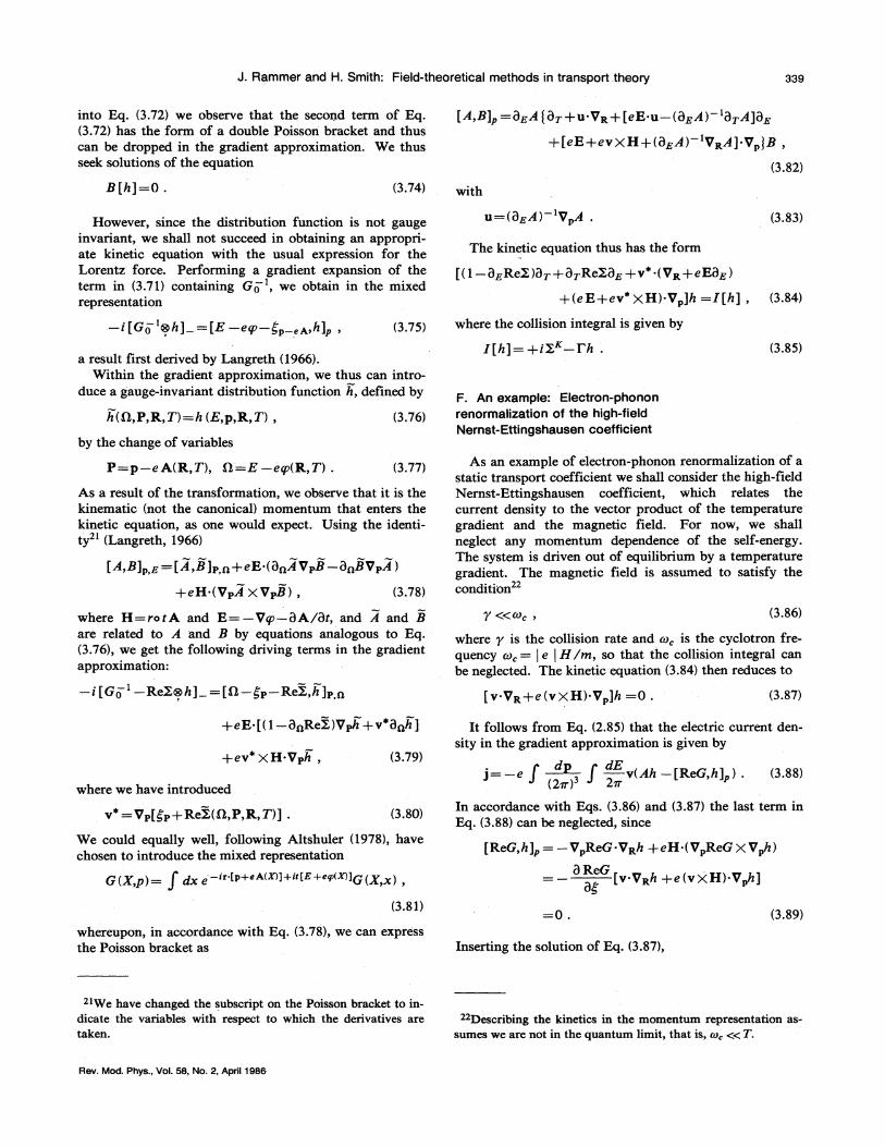
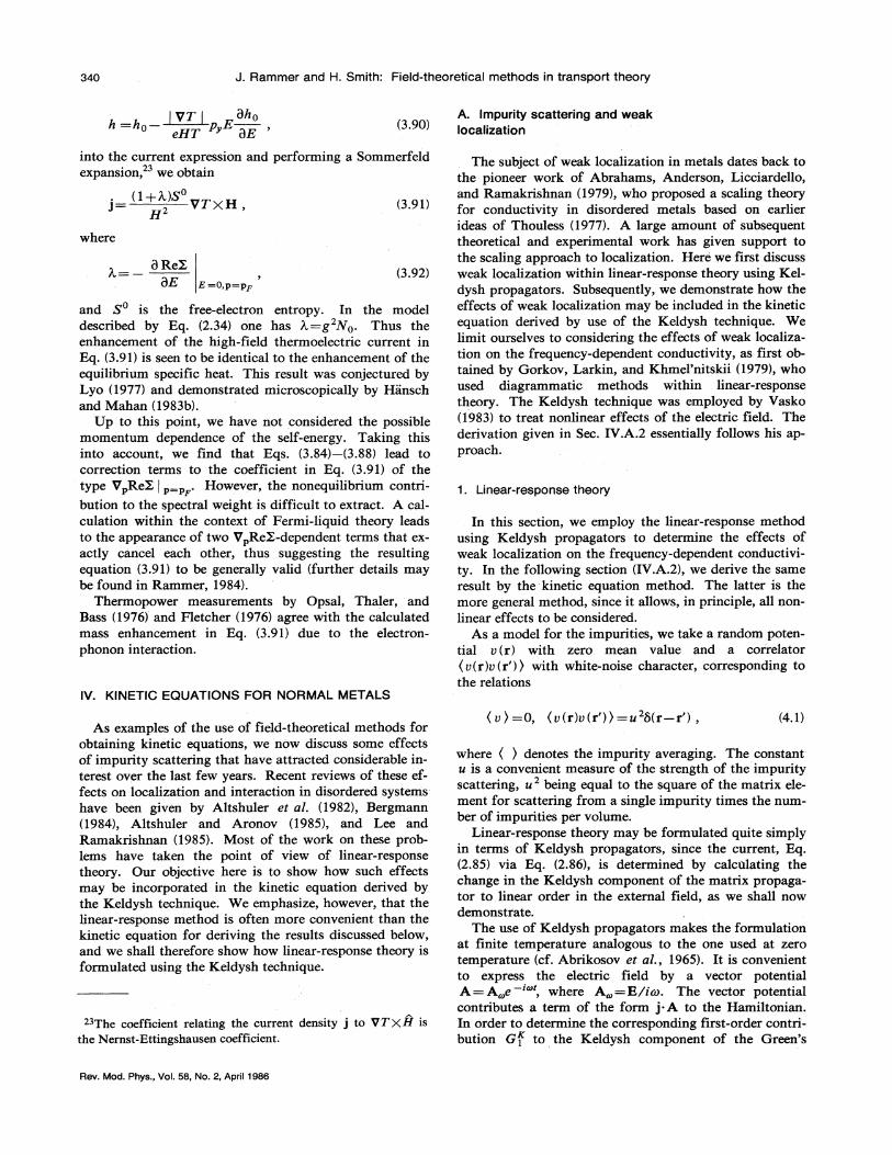
FIG. 9. The conductivity diagram. FIG. 10. The classical conductivity diagram.
function, we include for the moment the impurity poten-tial in the free-particle Hamiltonian Ho, and since we donot consider interaction effects, we have H'=0 and
S,;=1 in Eq. (2.16). Then we can repeat the steps given
in Sec. II.C, Eqs. (2.28)—(2.30), with the vector potentialreplacing the scalar potential, as we expand the operator
exp i —f dr f dxj. A
Eq. (2.17), to first order in A and express the current j insecond-quantized form (within linear response, we needonly consider the paramagnetic term in j). As a result,we get
Gf(1,1')= Tr ri f d2 A(2)[(V„—V„,)G(1,2')G(2, 1')]22m
(4.2)
I
The trace in Keldysh space and the v' matrix have been introduced to pick out the Keldysh component. To linear orderin the electric field the current is thus
2
Ji(1)= (Vi —Vi )Gi (1,1')~ i i — A,
2m m(4.3)
where the last term is the usual diamagnetic current (cf. Abrikosov et al. , 1965). We now Fourier-transform Eq. (4.3)with the result
l.e2 neJi(co)= 2Tr ~' f dE+ pG(p, p', E+co)A„.p'G(p', p, E) — A„.
2R'm I m(4.4)
Under isotropic conditions, the conductivity cr(co) then becomes
2o(co)= Tr r' f dE gp. p'(G(p, p', E+co)G(p', p,E))
2&dm co I
ne
t tom(4.5)
In Eq. (4.5) we have introduced the impurity averaging denoted by ( ).We have thus demonstrated that, within the Keldysh formulation of linear response, the Feynman rules for interpret-
ing the standard conductivity diagrams need only to be supplemented in accordance with the matrix structure in Keldyshspace, where lines and vertices are interpreted as tensors, as explained in Sec. II. The structure of the first term in Eq.(4.5) is illustrated diagrammatically in Fig. 9. Note that in the representation given by Eq. (2.27) the Keldysh structureof the driving and measuring vertex in Fig. 9 is represented by
(4.6)
2
, f (dp)p~[(hEO+„hEO)G~+~G~" +G~—+~6~"(1 hEO+„)+G~—+~6~~(hEO 1)], —dco m
in accordance with Eq. (4.2). Finally, the closed loop implies that the trace in Keldysh space is to be taken.The last term on the right-hand side of Eq. (4.5) diverges as co—+0 and must cancel a similar term appearing in the first
part of Eq. (4.5). To verify the cancellation of these terms, it is sufficient to consider the simplest diagram, depicted inFig. 10, for which we obtain
neo(~)+ .l corn
In this section we use the shorthand notation
where d is the dimension.
Rev. Mod. Phys. , Vol. 5S, No. 2, April 1986
342 J. Rammer and H. Smith: Field-theoreticaI methods in transport theory
whereq =(O, co) . (4.8)
P~P
(4.10)which forms a useful starting point for calculations of theconductivity.
Before considering the quantum correction, we showhow the classical conductivity given by the diagram inFig. 10 is obtained. From Eq. (4.10), it follows that
22dm
The retarded and advanced impurity-averaged Green'sfunctions are given by (Abrikosov et a/. , 1965)
1Gk, E
R(A) (4.12)E —4(+-)
227
where 1A is the impurity scattering rate
—=2nu Nd(0) .1
7
In Eq. (4.13), Xq(0) denotes the density of states for a sin-gle spin at the Fermi energy in d dimensions.
In the limit cu «p that we consider, the main contribu-tion to the momentum integration in Eq. (4.11) comesfrom the region near the Fermi surface. We perform themomentum integration and then the energy integration,and obtain the Drude result
(4.13)
Opo(co) =
1 —l$7where the static conductivity o.
p is
Ple
(4.14)
(4.15)m
In the s-wave approximation we are considering, thereis no difference between the transport time occurring inthe conductivity and the lifetime ~ occurring in theGreen's function (4.12), since the contribution to the con-ductivity from the particle-hole ladder gives zero in thiscase (see, for example, Abrikosov et al. , 1965).
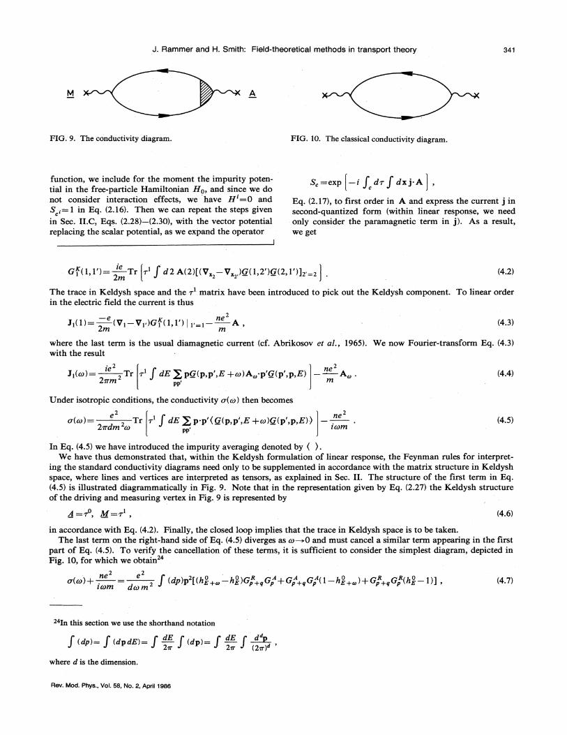
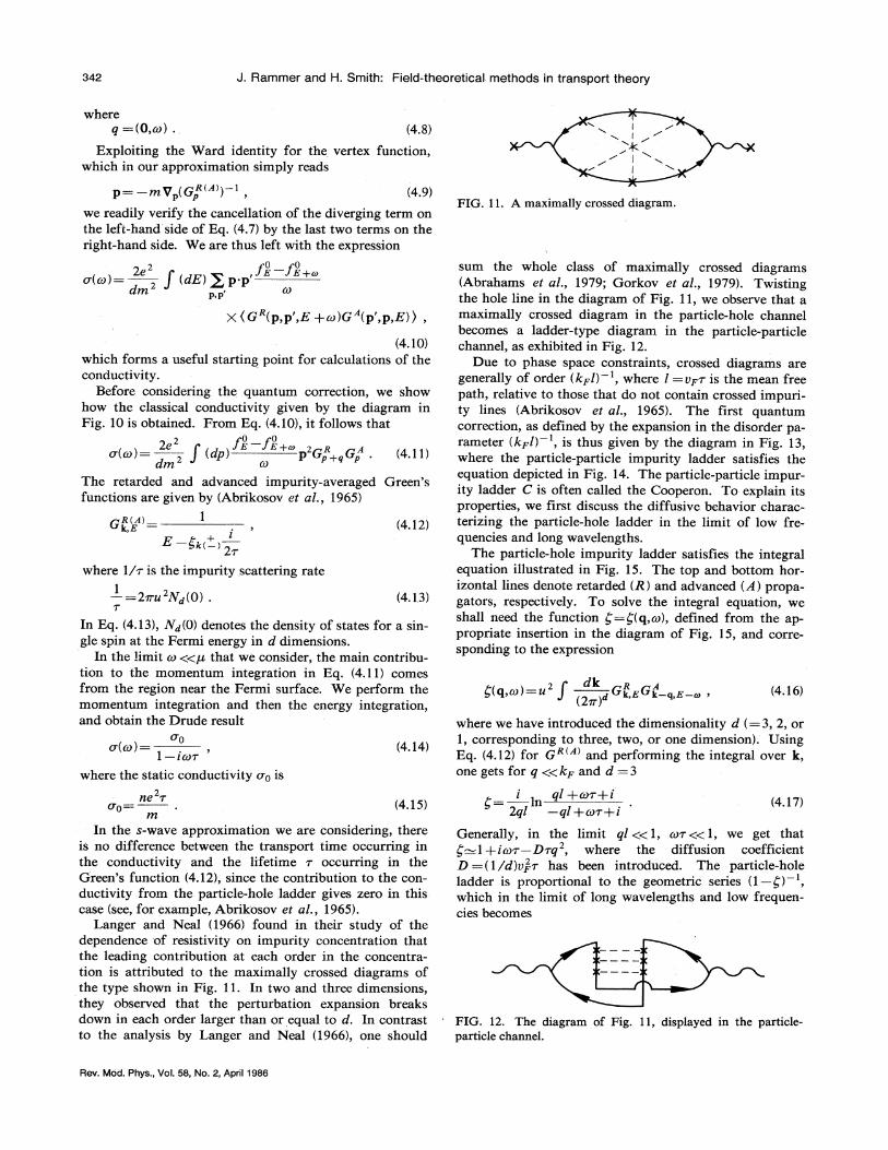
Langer and Neal (1966) found in their study of thedependence of resistivity on impurity concentration thatthe leading contribution at each order in the concentra-tion is attributed to the maximally crossed diagrams ofthe type shown in Fig. 11. In two and three dimensions,they observed that the perturbation expansion breaksdown in each order larger than or equal to d. In contrastto the analysis by Langer and Neal (1966), one should
Exploiting the Ward identity for the vertex function,which in our approximation simply reads
p mP (GR(A)) —1
we readily verify the cancellation of the diverging term onthe left-hand side of Eq. (4.7) by the last two terms on theright-hand side. We are thus left with the expression
FICx. 11. A maximally crossed diagram.
2 d~ R Ag(q, co) =u(2~)d Gk, EGk —q, E—co ~ (4.16)
where we have introduced the dimensionality d (=3, 2, or1, corresponding to three, two, or one dimension). UsingEq. (4.12) for G ~ ~ and performing the integral over k,one gets for q «kF and d =3
i ql +cur+i2ql —ql +co~+i
(4.17)
Generally, in the limit ql « 1, mw « 1, we get thatg= 1 +i d'or Drq, wh—ere the diffusion coefficientD = (1jd )UF 7 has been introduced. The particle-holeladder is proportional to the geometric series (1—g)which in the limit of long wavelengths and low frequen-cies becomes
FICx. 12. The diagram of Fig. 11, displayed in the particle-particle channel.
sum the whole class of maximally crossed diagrams(Abrahams et al. , 1979; Gorkov et al. , 1979). Twistingthe hole line in the diagram of Fig. 11, we observe that amaximally crossed diagram in the particle-hole channelbecomes a ladder-type diagram in the particle-particlechannel, as exhibited in Fig. 12.
Due to phase space constraints, crossed diagrams aregenerally of order (k~l) ', where l =U~r is the mean freepath, relative to those that do not contain crossed impuri-ty lines (Abrikosov et al. , 1965). The first quantumcorrection, as defined by the expansion in the disorder pa-rameter (kFl), is thus given by the diagram in Fig. 13,where the particle-particle i~purity ladder satisfies theequation depicted in Fig. 14. The particle-particle impur-ity ladder C is often called the Cooperon. To explain itsproperties, we first discuss the diffusive behavior charac-terizing the particle-hole ladder in the limit of low fre-quencies and long wavelengths.
The particle-hole impurity ladder satisfies the integralequation illustrated in Fig. 15. The top and bottom hor-izontal lines denote retarded (R) and advanced (A) propa-gators, respectively. To solve the integral equation, weshall need the function g=g(q, co), defined from the ap-propriate insertion in the diagram of Fig. 15, and corre-sponding to the expression
Rev. Mod. Phys. , Vol. 58, No. 2, April 1986
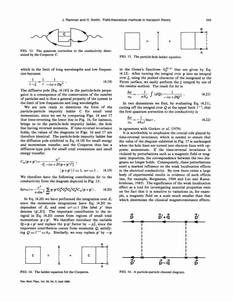
J. Rammer and H. Smith: Field-theoretical methods in transport theory 343
FIG. 13. The quantum correction to the conductivity deter-mined by the Cooperon C.
XI
I
lI
I
I
I
X
FIG. 15. The particle-hole ladder equation.
RX
I
I
I
I
XA
which in the limit of long wavelengths and low frequen-cies becomes
1 1 1
iso+�—
Dq'(4.18)
QC (p+p')=~[ ico+D(p+—p') ]
ip+p'
il « 1, cow « 1 . (4.19)
We therefore have the following contribution 5cr to theconductivity from the diagram depicted in Fig. 13:
2
5'(ro) = g p.p'Gz Gz Gz"Gz"C„(p+p') .Wdm2
pp
(4.20)
In Eq. (4.20) we have performed the integration over E,since the momentum integrations leave Eq. (4.20) in-dependent of E, and used co~&&1 [the label p' thusdenotes (p', E)]. The important contribution to the in-tegral in Eq. (4.20) comes from regions of small totalmomentum p+p'. We therefore introduce the variableQ=p+p' and replace the p.p' factor by —pg, since theimportant contribution comes from momenta Q, satisfy-ing Q « l «kF. Similarly, we may replace p' by —p
The diffusive pole [Eq. (4.18)] in the particle-hole propa-gator is a consequence of the conservation of the numberof particles and is thus a general property of the system inthe limit of low frequencies and long wavelengths.
We are now ready to determine the form of theparticle-particle impurity ladder C for small totalmomentum, since we see by comparing Figs. 16 and 17that time-reversing the lower line in Fig. 16, for instance,brings us to the particle-hole impurity ladder, the holeline having reversed momenta. If time-reversal invarianceholds, the values of the diagrams in Figs. 16 and 17 aretherefore identical. The particle-hole impurity ladder hasthe diffusion pole exhibited in Eq. (4.18) for small energyand momentum transfer, and the Cooperon thus has adiffusion-type pole for small total momentum and smallenergy transfer:
0(dQ)
ice+ D—Q(4.21)
In two dimensions we find, by evaluating Eq. (4.21),cutting off the integral over Q at the upper limit l ', thatthe first quantum correction to the conductivity is
1lnC07
IT F(4.22)
in agreement with Gorkov et al. (1979).It is worthwhile to emphasize the crucial role played by
time-reversal invariance, which is needed to ensure thatthe value of the diagram exhibited in Fig. 17 is unchangedwhen the hole lines are turned into electron lines with op-posite momentum. If the time-reversal invariance isviolated by perturbations such as a magnetic field or mag-netic impurities, the correspondence between the two dia-grams no longer holds. Consequently, these perturbationsexert a marked influence on the weak localization effectsin the electrical conductivity. By now there exists a largebody of experimental results in evidence of such effects(see, for example, Bergmann, 1984 and Lee and Rama-krishnan, 1985). The significance of the weak localizationeffect as a tool for investigating material properties restson the fact that it is sensitive to variations in, for exam-ple, a magnetic field on a scale much smaller than thatwhich determines the classical magnetoresistance effects.
0+0
in the Green*s functions Gz'"' that are given by Eq.
(4.12). After turning the integral over p into an integralover g, using the peaked character of the integrand at theFermi surface, we easily perform the g integral by use ofthe residue method. The result for 5cr is
l
I
I
I1
X
FIG. 14. The ladder equation for the Cooperon.
RXI
II.I
I
I
XA
FIG. 16. A particle-particle channel diagram.
Rev. Mod. Phys. , Val. 58, No. 2, April 1986
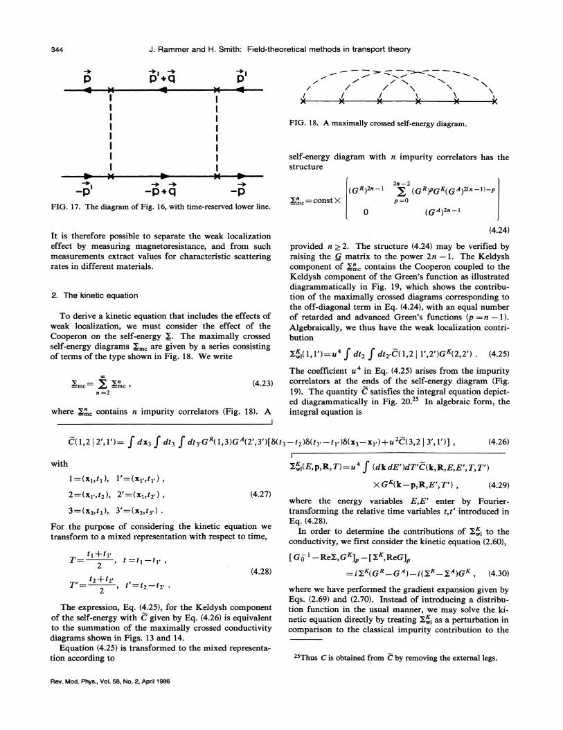
J. Ramrner and H. Smith: Field-theoretical methods in transport theory
FIG. 18. A maximally crossed self-energy diagram.
self-energy diagram with n impurity correlators has thestructure
FIG. 17. The diagram of Fig. 16, with time-reserved lower line.X",=const X
2' —2(gR)2n —i g (Gii)pgx(GA)2(n —1)—p
p=0
(g A)2n —1
It is therefore possible to separate the weak localizationeffect by measuring magnetoresistance, and from suchmeasurements extract values for characteristic scatteringrates in different materials.
2. The kinetic equation
71 =2(4.23)
where X", contains n impurity correlators (Fig. 18). A
To derive a kinetic equation that includes the effects ofweak localization, we must consider the effect of theCooperon on the self-energy X. The maximally crossedself-energy diagrams X, are given by a series consistingof terms of the type shown in Fig. 18. We write
(4.24)
provided n )2. The structure (4.24) may be verified byraising the G matrix to the power 2n —1. The Keldyshcomponent of X", contains the Cooperon coupled to theKeldysh component of the Green's function as illustrateddiagrammatically in Fig. 19, which shows the contribu-tion of the maximally crossed diagrams corresponding tothe off-diagonal term in Eq. (4.24), with an equal numberof retarded and advanced Green's functions (p =n —1).Algebraically, we thus have the weak localization contri-bution
X i(1,1')=u f dt2 f dt2 C(1,2i1',2')6 (2,2') . (4.25)
The coefficient u in Eq. (4.25) arises from the impuritycorrelators at the ends of the self-energy diagram (Fig.19). The quantity C satisfies the integral equation depict-ed diagrammatically in Fig. 20. In algebraic form, theintegral equation is
C(1,2~2', 1')= f dx, f dt, f dts6"(1,3)6"(2',3')[5(t, —t2)5(t; —t, )5(x,—x, )+u C(3,2~ 3, 1 )], (4.26)
With
l=(xi, ti), 1'=(xi, ti ),2=(xi, t2), 2'=(xl, t2 ),3=(x3 t3), 3'=(x3 i3') .
(4.27)
For the purpose of considering the kinetic equation wetransform to a mixed representation with respect to time,
I
Xxi(E,p, R, T)=u' f (dkdE')dT'C(k, R,E,E', T, T )
XG (k —p, R,E', T'), (4.29)
where the energy variables E,E' enter by Fourier-transforming the relative time variables t, t' introduced inEq. (4.28).
In order to detertnine the contributions of X~~ to theconductivity, we first consider the kinetic equation (2.60),
&i+&iT=, t=t2
(4.28)
[60 ' —ReX, G+]p —[X,Reg]~
= l Xx(G~ G") l (X~ —X")G—, (4—.30)
The expression, Eq. (4.25), for the Keldysh componentof the self-energy with C given by Eq. (4.26) is equivalentto the summation of the maximally crossed conductivitydiagrams shown in Figs. 13 aDD I4.
Equation (4.25) is transformed to the niixed representa-tion according to
where we have performed the gradient expansion given byEqs. (2.69) and (2.70). Instead of introducing a distribu-tion function in the usual manner, we may solve the ki-netic equation directly by treating X ~ as a perturbation incomparison to the classical impurity contribution to the
Thus C is obtained from C by removing the external legs.
Rev. Mod. Phys. , Vol. 58, No. 2, April 1986
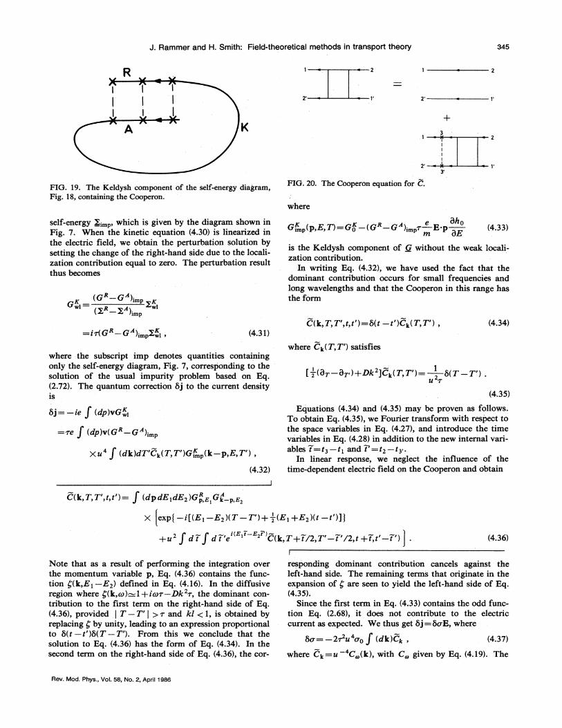
J. Rarnmer and H. Smith: Field-theoretical methods in transport theory 345
l
l
I
FKx. 19. The Keldysh component of the self-energy diagram,Fig. 18, containing the Cooperon.
2'
FICr. 20. The Cooperon equation for C.
where
3I
I
I
I
3l
self-energy X;mz, which is given by the diagram shown inFig. 7. When the kinetic equation (4.30) is linearized inthe electric field, we obtain the perturbation solution bysetting the change of the right-hand side due to the locali-zation contribution equal to zero. The perturbation resultthus becomes
6 = Xxwl (~il ~g) wl
GE ( E T) GE (Gii GA) &e E.p1111P (4.33)
is the Keldysh coinponent of G without the weak locali-zation contnbution.
In writing Eq. (4.32), we have used the fact that thedominant contribution occurs for small frequencies andlong wavelengths and that the Cooperon in this range hasthe form
=i r( G G");—mpawl, (4.31)C(k, T, T', r, r') =5(r r')C„(T,—T'),
where Cl,(T, T') satisfies
(4.34)
where the subscript imp denotes quantities containingonly the self-energy diagram, Fig. 7, corresponding to thesolution of the usual impurity problem based on Eq.(2.72). The quantum correction 5j to the current density1S
[—,'(BT—Bz-)+Dk ] CI, ( T,T')= 5(T —T') .
Q 'T
(4.35)
5j= ie f (dp)—vG,
=re f (dp)v(G" —G"); z
Xu f (dk)dT'Cl, (T,T')G; ~(k p, E,T')—,
(4.32)
Equations (4.34) and (4.35) may be proven as follows.To obtain Eq. (4.35), we Fourier transform with respect tothe space variables in Eq. (4.27), and introduce the timevariables in Eq. (4.28) in addition to the new internal vari-ables t=t3 —t) and t'=t2 —t3.
In linear response, we neglect the infiuence of thetime-dependent electric field on the Cooperon and obtain
C(k, T, T', t, t')= f (dpdE, dE2)G~aE Gl, ,E, —r
X expI —i [(E, E,)(T T')+ —,' (E, +E—, )(r —t'—)]I
+u~ f dr f dt'e ' ' C(k, T+t j2,T' t'l2, r+t, r' r')— — (4.36)
Note that as a result of performing the integration overthe moinentum variable p, Eq (4.36) co. ntains the func-tion g(k, E, —Ez) defined in Eq. (4.16). In the diffusiveregion where g(k, co)=1+icos Dk w, the dom—inant con-tribution to the first term on the right-hand side of Eq.(4.36), provided
tT —T'
t& ~ and kl & 1, is obtained by
replacing g by unity, leading to an expression proportionalto 5(t —t')5(T —T'). From this we conclude that thesolution to Eq. (4.36) has the form of Eq. (4.34). In thesecond term on the right-hand side of Eq. (4.36), the cor-
responding dominant contribution cancels against theleft-hand side. The remaining terms that originate in theexpansion of g are seen to yield the left-hand side of Eq.(4.35).
Since the first term in Eq. (4.33) contains the odd func-tion Eq. (2.68), it does not contribute to the electriccurrent as expected. We thus get 5j=5oE, where
5cr= —22u oo f (dk)Ck, (4.37)
where Ci, ——u C (k), with C„given by Eq. (4.19). The
Rev. Mod. Phys. , Vol. 58, No. 2, April 1986
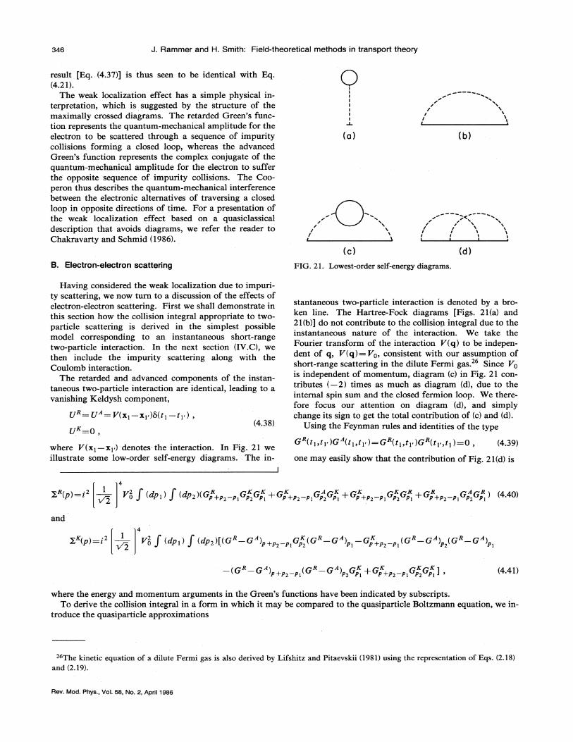
346 J. Rammer and H. Smith: Field-theoretical methods in transport theory
result [Eq. . (4.37)] is thus seen to be identical with Eq.(4.21).
The weak localization effect has a simple physical in-terpretation, which is suggested by the structure of themaximally crossed diagrams. The retarded Green's func-tion represents the quantum-mechanical amplitude for theelectron to be scattered through a sequence of impuritycollisions forming a closed loop, whereas the advancedGreen's function represents the complex conjugate of thequantum-mechanical amplitude for the electron to sufferthe opposite sequence of impurity collisions. The Coo-peron thus describes the quantum-mechanical interferencebetween the electronic alternatives of traversing a closedloop in opposite directions of time. For a presentation ofthe weak localization effect based on a quasiclassicaldescription that avoids diagrams, we refer the reader toChakravarty and Schmid (1986).
IIIIIIII
(c)
//
II \
(b)
~ss
//
/I II 1I I I
B. Electron-electron scattering FIG. 21. Lowest-order self-energy diagrams.
U = U"= V(xi —xi )5(ti ti ), —U =0.,
(4.38)
where V(x~ —x&) denotes the interaction. In Fig. 21 weillustrate some low-order self-energy diagrams. The in-
Having considered the weak localization due to impuri-ty scattering, we now turn to a discussion of the effects ofelectron-electron scattering. First we shall demonstrate inthis section how the collision integral appropriate to two-particle scattering is derived in the simplest possiblemodel corresponding to an instantaneous short-rangetwo-particle interaction. In the next section (IV.C), wethen include the impurity scattering along with theCoulomb interaction.
The retarded and advanced components of the instan-taneous two-particle interaction are identical, leading to avanishing Keldysh component,
G (~$, r$ )G"(&$,&$ )=G (r$, t$ )G~(tr, t$)=0, (4.39)
one may easily show that the contribution of Fig. 21(d) is
stantaneous two-particle interaction is denoted by a bro-ken line. The Hartree-Fock diagrams [Figs. 21(a) and21(b)] do not contribute to the collision integral due to theinstantaneous nature of the interaction. We take theFourier transform of the interaction V(q) to be indepen-dent of q, V(q)= Vo, consistent with our assumption ofshort-range scattering in the dilute Fermi gas. Since Vois independent of momentum, diagram (c) in Fig. 21 con-tributes ( —2) times as much as diagram (d), due to theinternal spin sum and the closed fermion loop. We there-fore focus our attention on diagram (d), and simplychange its sign to get the total contribution of (c) and (d).
Using the Feynman rules and identities of the type
x (p) =i4
Vo f (dp)) f (dp2)(GP+P, P, GP, GP, +GP+P, P, GP",GP, +GP+P, P, GP, GP, +GP+P, P, GP",GP", ) (440)
x (p) =i4
Vo f (dp)) f (dp2)[(G —G")p+p, p, Gp, (G G")p, Gp+p, —p, (G —G")p,(G G"—
)p,—
)P+P P(G G )P GP —+ P+P PGP GP ]—(4.41)
where the energy and momentum arguments in the Green's functions have been indicated by subscripts.To derive the collision integral in a form in which it may be compared to the quasiparticle Boltzmann equation, we in-
troduce the quasiparticle approximations
The kinetic equation of a dilute Fermi gas is also derived by Lifshitz and Pitaevskii (1981)using the representation of Eqs. (2.18)and (2.19).
Rev. Mod. Phys. , Vol. 58, No. 2, April 1986
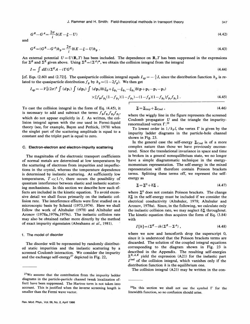
J. Rammer and H. Smith: Field-theoretical methods in transport theory 347
and
(4.42)
G =(G"—G")I = "S(E—g —U)hl
(4.43)
An external potential U = U(R, T) has been included. The dependence on R, T has been suppressed in the expressionsfor X" and X given above. Using X =(X"),we obtain the collision integral from the integral
I= f dE(ir ~ —irG~) (4.44)
[cf. Eqs. (2.60) and (2.72)]. The quasiparticle collision integral equals Iqz ————,I, since the distribution function h& is re-lated to the quasiparticle distribution fz by h~ = (1—2'). We then get
I = —Vo(2m) f (dpi) f (dpi') f (dp3N(gp+gp, —gp,
—gp, )5(p+pp —pi —p3)
(4.45)
To cast the collision integral in the form of Eq. (4.45), itis necessary to add and subtract the terms fez, f~ fz, ,which do not appear explicitly in I. As written, the col-lision integral agrees with the one used in Fermi-liquidtheory (see, for example, Baym and Pethick, 1978) whenthe singlet part of the scattering amplitude is equal to aconstant and the triplet part is equal to zero.
C. Electron-electron and electron-impurity scattering
The magnitudes of the electronic transport coefficientsof normal metals are determined at low temperatures bythe scattering of electrons from impurities and imperfec-tions in the crystal, whereas the temperature dependenceis determined by inelastic scattering. At sufficiently lowtemperatures, T«1/r, there occurs the possibility ofquantum interference between elastic and inelastic scatter-ing mechanisms. In this section we describe how such ef-fects are included in the kinetic equation. To avoid exces-sive detail we shall focus primarily on the inelastic col-lision rate. The interference effects were first studied on amicroscopic basis by Schmid (1973,1974). Here we shallfollow the work of Altshuler (1978) and Altshuler andAronov (1978a,1979a,1979c). The inelastic collision ratemay also be obtained rather more directly by the methodof exact impurity eigenstates (Abraharns et a/. , 1981).
r =r p+r=c-] (4.46)
where the wiggly line in the figure represents the screenedCoulomb propagator U and the triangle the impurity-renormalized vertex I . 8
To lowest order in 1/kzl, the vertex I is given by theimpurity ladder diagrams in the particle-hole channelshown in Fig. 23.
In the general case the self-energy Xc,„& is of a morecomplex nature than those we have previously encoun-tered. Since the translational invariance in space and timeis broken in a general nonequilibrium state, we no longerhave a simple diagrammatic technique in the energy-momentum representation. The self-energy in the mixedrepresentation will therefore contain Poisson bracketsterms. Splitting these terms off, we represent the self-energy as
r=a'+sr, (4.47)
I[h]=iX ih(X ——X ), (4.48)
where Xo does not contain Poisson brackets. The change5X in the self-energy must be included if we consider theelectrical conductivity (Altshuler, 1978; Altshuler andAronov, 1978a). Since, in the following, we calculate onlythe inelastic collision rate, we may neglect 6X throughout.The kinetic equation thus acquires the form of Eq. (3.84)with
1. The model of disorder
The disorder will be represented by randomly distribut-ed static impurities and the inelastic scattering by ascreened Coulomb interaction. We consider the im.purityand the exchange self-energy depicted in Fig. 22,
We assume that the contribution from the impurity ladderdiagrams in the particle-particle channel (weak localization ef-fect) have been suppressed. The Hartree term is not taken intoaccount. This is justified when the inverse screening length issmaller than the Fermi wave vector.
where we now and henceforth drop the superscript 0,since it is understood that the Poisson brackets terms arediscarded. The solution of the coupled integral equationscorresponding to the diagram shown in Fig. 23 isdescribed in the Appendix. The resulting self-energiesX '"' yield the expression (A21) for the inelastic partI'"" of the collision integral, which vanishes only if thedistribution function h is the equilibrium one.
The collision integral (A21) may be written in the con-
SIn this section we shall not use the symbol I for thelinewidth function, so no confusion should arise.
Rev. Mod. Phys. , Vol. 58, No. 2, April 1986
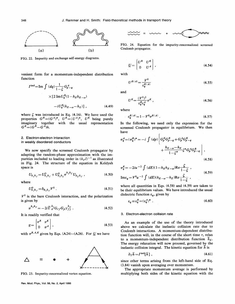
J. Rammer and H. Smith: Field-theoretical methods in transport theory
rr/
/I \
(a)
FIG. 24. Equation for the impurity-renormahzed screenedCoulomb propagator.
FIG. 22. Impurity and exchange self-energy diagrams.
venient form - for a momentum-independent distributionfunction
I'"' =Im f (dq) GA
X[21mU (1—h h )
with
and
UR UK
0 U
R(A)Eq
(4.54)
(4.55)
(4.56)
i Uq (—hE „hE)]—, (4.49)where
where g was introduced in Eq. (4.16). We have used theproperties g =(G")*, U =(U"), U being purelyimaginary together with the usual representationgK—(gR gA)h
2. Electron-electron interactionin weakly disordered conductors
ER(A) 1 go~(A) (4.57)
In the following, we need only the expression for thescreened Coulomb propagator in equilibrium. We thenhave
A (~)e ~ f (d ) gKGR +gAgK
We now specify the screened Coulomb propagator byadapting the random-phase approximation with the im-purities included to leading order in (kFl) ' as illustratedin Fig. 24. The structure of the equation in Keldyshspace is
E —co E e A R+1 —g'
~=—2ig f (dE)(1—hEhE „)Re
(4.58)
where
0 0 k2kk&k(. k)k&. + k)k2 k2. kl. ~ (4.50)
Ime~=&~ ' f (d&)(hE ~ hE)Re—(4.59)
Uk k, —5k, k (4.51)
V is the bare Coulomb interaction, and the polarizationis given by ER (EA)+ (4.60)
where all quantities in Eqs. (4.58) and (4.59) are taken tobe their equilibrium values. We have introduced the usualdielectric function E~, given by
k2k2. —k~ k2,77 2EPfp Gp j GjI&j j
It is readily verified that
(4.52)
3. Electron-electron collision rate
(4.53)LT— 0 m.A
with m" given by Eqs. (A24)—(A26). For Uwe have
As an example of the use of the theory introducedabove we calculate the inelastic collision rate due toCoulomb interactions. A momentum-dependent distribu-tion function will, in the course of the short time r, relaxto a momentum-independent distribution function hE.The energy relaxation will now proceed, governed by theinelastic collision integral. The kinetic equation for h is
(4.61)
FICx. 23. Impurity-renormalized vertex equation.
since other terms arising from the left-hand side of Eq.(3.84) vanish upon averaging over momentum.
The appropriate momentum average is performed bymultiplying both sides of the kinetic equation with the
Rev. Mod. Phys. , Vol. 58, No. 2, April 1986
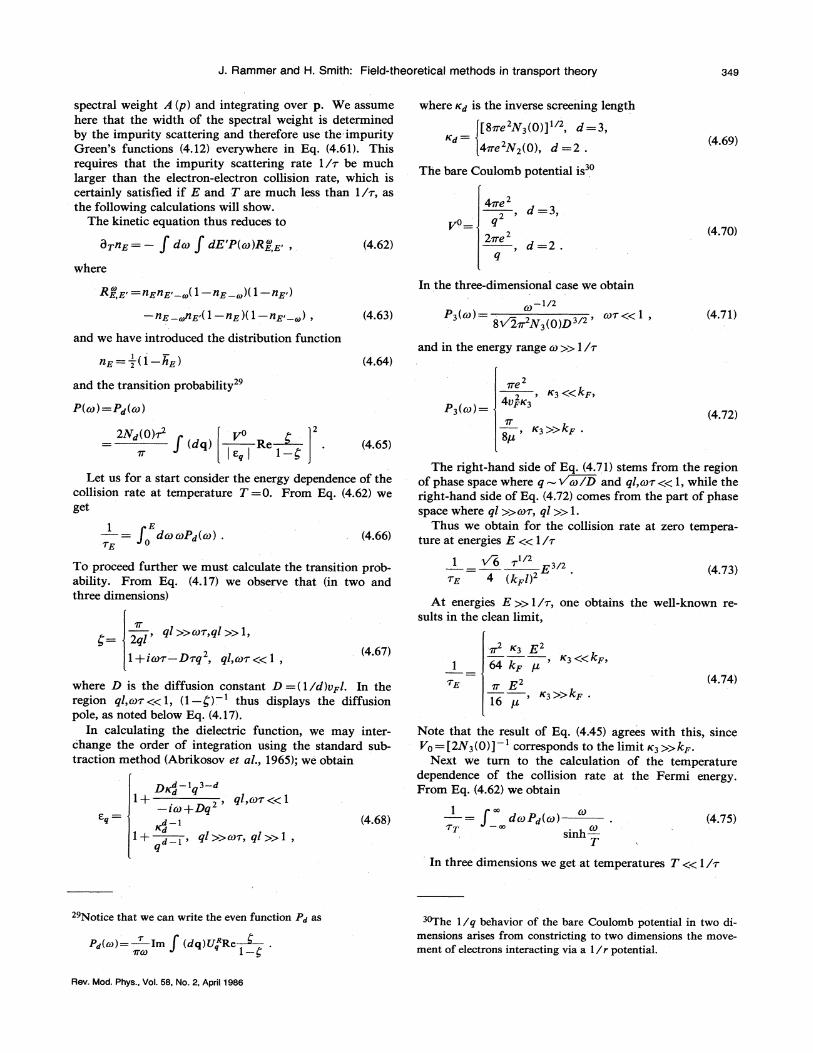
J. Rammer and H. Smith: Field-theoretical methods in transport theory
spectral weight /I (p) and integrating over p. We assumehere that the width of the spectral weight is determinedby the impurity scattering and therefore use the impurityGreen's functions (4.12) everywhere in Eq. (4.61). Thisrequires that the impurity scattering rate 1/r be muchlarger than the electron-electron collision rate, which iscertainly satisfied if E and T are much less than I/r, asthe following calculations will show.
The kinetic equation thus reduces to
BTnz ———f dco f dE'P(c0)Rzz (4.62)
where ~d is the inverse screening length
[See N3(0)]'/, d =3,Kd =
4m.e2X2(0), d =2.The bare Coulomb potential is
24me2v'=
227Te
(4.69)
(4.70)
Rz z nznz——~(1—nz „)(1 nz —)nz „n—z (1—nz)(1 —nz „),
and we have introduced the distribution function
nz ———,' (1—hz)
(4.63)
(4.64)
In the three-dimensional case we obtain—1/2
P3(C0) = 3, CO~ && 1,SV'2m %3(0)D /
and in the energy range co » I /r
(4.71)
and the transition probability
P(co) =P~(c0)
2Nd(0)v yo(4.65)
&eK3 «kF~
P ( )4UF'K3
K3 ))kFSp'(4.72)
Let us for a start consider the energy dependence of thecollision rate at temperature T =0. From Eq. (4.62) weget
tEE= f de COPd(CO) . (4.66)
ql »cor, ql »1,2ql
'
1+icot—Dtq, q/, cot « 1, (4.67)
where D is the diffusion constant D=(1/d)UFI. In theregion ql, cor«1, (1—g) ' thus displays the diffusionpole, as noted below Eq. (4.17).
In calculating the dielectric function, we may inter-change the order of integration using the standard sub-traction method (Abrikosov et al. , 1965); we obtain
d —1 3—dDKd1+,q/, « 1—in)+DqiCd
d —1
1 + d 1 q/ »cot q/ » 1qd —1'
(4.6S)
To proceed further we must calculate the transition prob-ability. From Eq. (4.17) we observe that (in two andthree dimensions)
~' ~3 E'K3 «kF&64 kF P
m EK3 &)kF16 p
(4.74)
Note that the result of Eq. (4.45) agrees with this, sinceVo ——[2%3(0)] ' corresponds to the limit lc3 »kF.
Next we turn to the calculation of the temperaturedependence of the collision rate at the Fermi energy.From Eq. (4.62) we obtain
= f dcoPd(co)CO81nh-T
(4.75)
In three dimensions we get at temperatures T« I/r
The right-hand side of Eq. (4.71) stems from the regionof phase space where q -V'co/D and ql, cur « 1, while theright-hand side of Eq. (4.72) comes from the part of phasespace where q/ »cot, ql »1.
Thus we obtain for the collision rate at zero tempera-ture at energies E « I /r
1/2E3/2 (4.73)4 (kF l)
At energies E» I/r, one obtains the well-known re-sults in the clean limit,
Notice that we can write the even function I'q as
Pq(co) = Im (dq}U~"Re%CO
3oThe 1/q behavior of the bare Coulomb potential in two di-mensions arises from constricting to two dimensions the move-ment of electrons interacting via a 1/r potential.
Rev. Mod. Phys. , Vol. 58, No. 2, April 1986
350 J. Rarnmer and H. Smith: Field-theoretical methods in transport theory
1/2 T3/2
16 kFl pr(4.76)
] codco
ZT 2kFI COsinh—T
(4.82)
7T e T, K3 (gkF~SUFK3
32T ~ K3 ))kF
16@
(4.77)
Calculating the same quantities for the two-dimensional case we obtain '
1P2(co)= —,cur«1 .Sp7 co
(4.78)
where g is the Riemann zeta function.At temperatures T »1/r, we have the results of the
clean limit,
T T1ln
2mD T(4.83)
At temperatures T »1/r, the same state of affairs pre-vails as in the result stated in Eq. (4.81). We state the re-sult by Hodges et al. (1971)for completeness
To cure this infrared divergence one should considerterms of next order in the coupling constant e as notedby Abrahams et al. (1981). This leads to a lower cutoff atcop=4T /Tf, where T& (2——mD) Daz and an inelastic col-lision rate
The inelastic collision rate at ener'gies E« 1/r is thusgiven by 2&@ T (4.84)
E4kFI
(4.79)
This result is in agreement with Abrahams et al. (1981)to within a factor of 2. We note that a missing factor of 2has also been reported by Lopes dos Santos (1983), whoconsidered the temperature dependence of the inelasticcollision rate.
When calculating the transition probability at energiesco» 1/r, we encounter the logarithmically divergent ex-pressions
&z(~)=
2k~dg 2 ~ K2))kF~
n. N2(0)e00 1
UF dg K2 Q(kFq(q+a2)
(4.80)
1 2 EE ln-Smp p
(4.81)
Turning to the temperature dependence of the inelasticcollision rate, we obtain at temperatures T« 1/r
The reason for the appearance of this singularity in theforward scattering is our use of momentum states that aredetermined only to within the inverse impurity mean freepath. Instead, we approach the problem from the cleanlimit and obtain the Boltzmann equation for two-particlescattering. We then refer to Hodges et al. (1971), whocalculated the inelastic collision rate. Their result is
In conclusion, we note that the results of this sectionshow that diffusion renormalization enhances theelectron-electron interaction. The interpretation of thisenhancement is given in terms of the breaking of transla-tional invariance due to the presence of the disorder. Theviolation of momentum conservation gives more phasespace for final states.
V. KINETIC EQUATIONSFOR SUPERCONOUGTING METALS
In this section we shall give an account of the quasi-classical description of transport phenomena in supercon-ductors. The development of the quasiclassical method todescribe transport phenomena in-superfIuids is due pri-marily to Eilenberger (1968), Larkin and Ovchinnikov(1968,1975,1977), Eliashberg (1971), and Schmid andSchon (1975a).
A. The quasiclassical description
The basic feature of the superconducting state, the pair-ing interaction, is made compatible with the standardFeynman diagrammatics by introducing the Nambu pseu-dospinor field
(5.1)
3~%'e note that the Coulomb interaction in a weakly disorderedmetal can be considered two dimensional when the samplethickness a satisfies D/a~maxIE, TI && l.
32Notice that Lopes dos Santos (1983) used a definition of theinverse lifetime differing from the inelastic collision rate by afactor of 2.
Then the only additional feature of the Feynman rulesis the interpretation of the components of the electronicCareen's function in Keldysh space as (2 X2)-matrixCareen's functions in particle-hole (or Nambu) space(Nambu, 1960; Schrieffer, 1964).
We introduce the basic Green's functions in particle-
Rev. Mod. Phys. , Vol. 58, No. 2, April 1986
J. Rammer and H. Smith: Field-theoretical methods in transport theory 351
hole space gog=5(t( t)—) . (5.13)
&q, (1)y,(1') & &1(,(1)y,(1') &
&1(t(1)y,(1)& &@,(1)y,(1)&
&1i',(1)y'„(I)& &q, (1)y',(1)&
(5.3)
G() '(l, l')=G() '(l)5(1 —1'),
G;((I)=id',,—e(1),
(5 5)
(5.6)
The results of Sec. II are immediately taken over andwe obtain the equation of motion
[ Go ' —XI SG =5(1—1'), (5.4)
where
K gR I iogA (5.14)
The important feature, that the coefficient on theright-hand side of Eq. (5.13) is independent of the spacecoordinates, was established by Eilenberger (1968) andLarkin and Ovchinnikov (1968) for the static case. It wasnoted by Larkin and Ovchinnikov (1975), by taking thespatial derivative of Eq. (5.13), that the normalizationcondition is in general compatible with the equation ofmotion. The normalization condition for the general,nonstationary case was discussed recently by Shelankov(1985).
The normalization condition allows us to representthe Keldysh component in terms of a distribution matrixh,
E( 1)= — 8 +eq&(1 )—p,1 2 (5.7) Equation (5.10) consists of three coupled equations,
[g1 +i (rR ( A )og
R ( A )] 0 (5.15)B(1)=V„ier—A(1) . (5'.8)
The matrix structure is the tensorial product of Kel-dysh and particle-hole space (unit matrices aresuppressed). Thus r appearing in Eqs. (5.6) and (5.8)denotes
~3 00
Similarly, we have the conjugate equation
G(g) IG() ' —XI =5(I—1') . (5.9)
The arguments that bring us from the above equationsof motion to the quasiclassical ones are identical withthose we used for the normal state. Subtracting the twoDyson equations (5.4) and (5.9) we can, as in the normalstate, introduce the quasiclassical Green s function satis-ying
[go '+i~;g] =o (5.10)
g() '(p, R,t„tt)=go—'(p, R, t()5(tt —t) ),g() '(p, R, t) )=r r), +vR [VR ier A(R, t—) )]
(5.11)
+icy(R, t() . (5.12)
For the case of inelastic interactions, Eq. (5.10) was firstobtained by Eliashberg (1971).
In the superconducting state, the components of the re-tarded and advanced Green's functions in particle-holespace will not reduce to numbers as in the normal state[cf. Eq. (3.12)]. Equation (5.10) thus constitutes a compli-cated set of equations describing the coupling betweenstates (g '"') and the occupation (g ) of these states. Animportant simplifying feature, when it comes to reducingEq. (5.10) to a more solvable form, is the existence of anormalization condition
and
gR g g gA 0 (5.16)
~e-ph+ imp+ sf (5.18)
The expressions for the components of Lr' )'" are identicalin form to Eq. (3.8),
rrR ( A ) dp ~(g KD R ( A ) + R ( A )L)K)~e-p~e-ph =
~K ~p~~ gR gA DR DA +gKDKeph 8
Furthermore
(5.19)
Lr' = —i~)t(Xo~
U(P'P')~
2g(RP' t) t( )4m
(5.20)
o' = — ~ g Rp', t],t]sf l dP'
3
2w, 4m(5.21)
B= rr +h o rr cr o h +—[go 'o h ] (5.17)
The equation for g"'"' determines the states of the sys-tem, while the equation for h determines the occupationof these states. In obtaining Eq. (5.16) from the Keldyshcomponent of Eq. (5.10) we have utilized the equationsfor g"'"' and the fact that the composition o is associa-tive.
To get a closed set of equations we must specify theself-energy. Apart from the inherent electron-phonon in-teraction, we shall allow for impurity scattering in theBorn approximation, including spin flip. The self-energyo. is given by
The third Pauli matrix, operating in particle-hole space, isdenoted by ~. No confusion with our notation in Keldyshspace should arise.
34This choice is not unique. A choice maQing the resemblance
between the Boltzmann equation and Eq. (5.16) immediate in
the quasiparticle approximation has been introduced by Shelan-
kov (1980).
Rev. Mod. Phys. , Vol. 58, No. 2, April 1986
352 J. Rammer and H. Smith: Field-theoretical methods in transport theory
where we have treated the spin-flip scattering in the s-wave approximation corresponding to the spin-flipscattering rate
=2m n, tNpS (S + 1)(ust(p'p')
(4m
(5.22)
Here n, t is the concentration of spin-flip impurities, Stheir spin and u,t(p.p ') the interaction. For later use weintroduce the normal impurity scattering rate given by
B. The dirty limit
In the dirty limit, ~T, &&1, we can reduce the integralequation with respect to the non-spin-flip impurityscattering to a differential equation of diffusion type. Inthe dirty limit the Green s function will be almost isotro-pic. We therefore make an expansion in spherical har-monics keeping only the s- and p-wave parts (Usadel,1970),
g(p, R, t(, t1 )=g, (R, t), t1 )+p ~g(R, t(, t(. ) .(5.23)
The self-energy
(5.34)
To elucidate the information contained in Eq. (5.15),we solve it in equilibrium and take the BCS limit, obtain-ing
a(p, R, t), t( )=o,(R, t(, t) )+p oF(R., t(, t( )
is given by
(5.35)
R(A) R(A)P+ ~R(A) 1
~R(A) =(+)N, (E)+is,(E),P '"'=N2(E)(+)F2(E),
(5.25)
(5.26)
ICT—S r g, r +og'rh,
7$
lo's = — gs+LTs ~2r— (5.36)
(5.37)
where
N1(E)= 8(E —b, ),(E2 g2)1/2
2 2(n(g2 E2)1j2
R2(E)=—N1(E),
R1(E)= — N2(E),
(5.27)
(5.28)
(5.29)
(5.30)
A. p
p oF ———inn;Np~
u(PP')~
p'~g4m
(5.38)
Performing the angular average on the right-hand sideof Eq. (5.38) gives
lCT
2(5.39)
where ~« is the impurity transport lifetime,
and, since the non-spin-flip impurity scattering is as-sumed to be dominant,
with 6 being the BCS energy gap.In the static case it follows from Eq. (5.15) that gR'
is traceless, so that=2mn;Np J ~
u(p.p')~
[1—(p P')] . (5.40)4~
R(A) ~R(A) 3+pR(A) 1+ R(A)P (5.31)We also rewrite (without approximations) the inverse
propagator gp—' in s- and p-wave form,
In applications to time-dependent phenomena, the trace-less form in Eq. (5.31) has so far proved to be sufficientlygeneral.
The quantities a, p, and y denote the generalized densi-ties of states, and we recognize N1 in the BCS limit as theusual normalized BCS density of states.
We only have to consider one set of generalized densi-ties of states, since from the general equality (e denotescomplex conjugation and t denotes Hermitian conjuga-tion)
with
g—I g
—1 +p~.g—1
gP ' ——(r B,, +ie(P)5(t( t1 ), —
gp =uFd ~P
B=(VR ier A)5(t( —t1 ) . —
(5.41)
(5.42)
(5.43)
(5.44)
G (1,1')=r (G (1',1))V
it follows that
(5.32)
1. The equation of motion
In the dirty limit we can split the equation of motion(5.10) into an even and odd part with respect to p,
~A (~R)+ pA (pR)e +A ( R)e (5.33)[g p +i& ogq] + 3 uF[BogF] =0, (5.45)
We shall not consider Eq. (5.16) in its full generality, butderive the collision integral for the case of a dirty super-conductor.
The subscript on o,'P" designates that it is only a functionalof g, .
Rev. Mod. Phys. , Vol. 58, No. 2, April 1986
J. Rammer and H. Smith: Field-theoretical methods in transport theory 353
1[g,og, ] +URQog. ]-=0
tr(5.46)
2. Generalized densities of statesin the static limit
g, og, =5(t) —t, ), (5.47)
[gsogp]+=0 ~ (5.48)
Using the s- and p-wave parts of the normalizationcondition,
In this section we shall further reduce the diagonalcomponents of Eq. (S.S1) by considering the static limit.We shall treat the pairing effect (contained in Reo"'")) inthe BCS approximation and approximate the electronicdamping by the equilibrium expression. Then the retard-ed (advanced) electron-phonon self-energy reduces to
r
we can solve Eq. (5.46) for gR(A) l
cog ph— AE(+)
+111(5.53)
g p= —ig.o Mop, ] (5.49)
with the gap matrix
where / is the impurity mean free path, (5.54)
I =VF1tr . (5.50) where (from now on we drop the s-wave subscript)
Inserting Eq. (5.49) into Eq. (5.45) we obtain for the s-wave part
I dE Tr[(~' —iH)g ]8 1+X
(S.55)
[g o +io,' DBog, o—Bog, ] =0,
where D is the diffusion constant,
D= 3Vgl .
(5.51)
(5.52)
is the order parameter, and coD is the Debye frequency.The renormalization factor is ( 1+A, ) and the inelasticscattering rate is denoted by 1/r;„.
%'e now perform a Taylor expansion to lowest order inthe equation
Equation (5.51) is the starting point for consideringgeneral nonequilibrium phenomena in a dirty supercon-ductor.
—i+ ~ R(A) Dg R(A) g g A ] ()7
(5.56)
and obtain for the off-diagonal components of Eq. (5.56)
' D[a~2(P iy) (P &y)P2 a]R(A)
,' D[a&*—(p+iy ) (p+i y —)VRa] —iE( )+ 1
1Il
R(A)
(p i y ) ha+ —a(p —i y )—Ts
R(A)
(p+i y ) b,*a+ a(p+i—y )
(5.57)
(5.58)
where we have neglected terms involving time derivatives,since we consider only the static limit. We have further-more introduced the gauge-invariant derivative
g o8 —n'og =0 (5.61)
gR(A) and the fact that the composition 0 is associative,we can bring it to the form
M=VR 2ieA . —
Together with the normalization condition
a2+ p2+ y2
(5.59)
(5.60)
with
B[h]= (go ) 'oh —ho (go )' io, ph—
—DBog o[Boh] —D[Boh] og"oB,
where
(5.62)
Eqs. (5.57) and (5.58) determine the generalized densitiesof states in the static limit. For brevity we have in Eq.(5.60) and the following denoted a by a, P by P, and yby y.
(g(R)'")-'= ized'+ icy—+ap R(A) 3 R(A) 31
lQ mph ~Vg 7
7$(5.63)
3. Dirty-limit kinetic equationin the static limit
To obtain a kinetic equation we take the Keldysh com-ponent of Eq. (5.51). Using the equation of motion for
In the static limit considered we can choose the distribu-tion matrix h to be diagonal,
6Tr denotes trace in particle-hole space.7The prime on the electron-phonon self-energy indicates that
it does not include the order-parameter term.
Rev. Mod. Phys. , Vol. 58, No. 2, April 1986
354 J. Rammer and H. Smith: Field-theoretical methods in transport theory
h =h)~ +h2~ (S 64) —DVR™)(E,E)VRh, +DVRh2
We now perform a Taylor expansion in Eq. (5.61) andlinearize the equation with respect to h& —ho and h2.Subsequently, we take the trace of this equation and thetrace of the equation multiplied by ~ . For the phenome-na considered below, we may set the y term in Eq. (5.31)equal to zero. This ansatz is valid in many physical situa-tions (see Schmid, 1981 for further discussion). In addi-tion, we choose a gauge in which 5 is real:
+4N2R2e A'VR&2 ——K) [it ) ] (5.65)
DVR™2(EiE)VRh2 +2~Nplt2
+4DN2R2e A VRh, =K2[h2], (5.66)
where
K; [h; ]= — f dE'p(E E')M;—(E,E')1+1,
h; (E)cosh —h;(E')cosh2T 2T
~ hE —E' E Esinh cosh cosh2T 2T
(5.67)
Here p is the Fermi-surface average of the function poccurring in (3.18) and
N)(E)N)(E') —Rp(E)R2(E'), i =1,N)(E)N((E')+Np(E)Np(E'), i =2 . (S.68)
Together with the expressions for the charge andcurrent density,
M;(E,E')= .
p= eNo 2eq—o+ —, f dETrg (5.69)
j=— f dETr(r gz), (5.70)
the kinetic equations (5.65) and (5.66) supplemented withEqs. (5.57) and (5.58) for the generalized densities ofstates, the gap equation (5.55) and Maxwell's equations, .
constitute a complete description of a dirty superconduc-tor in the static limit.
C. An example: Impurity scatteringin the presence of superflo~and a temperature gradient
As shown in the previous section, the dirty limitpresents a particularly simple case, since the Green'sfunctions are nearly isotropic due to the dominance of im-purity scattering. This makes it possible to obtain an ex-pansion in s and p waves. The resulting kinetic equationsare not necessarily restricted to the dirty limit for validity.%'hen pair breaking is negligible, the kinetic equations(5.65) and (5.66) reduce to the quasiparticle Boltzmannequation, as demonstrated in detail by Beyer Nielsenet al. (1982). In the presence of superflow, the anisotropyassociated with the moving condensate becomes impor-tant, and one must investigate in detail the meaning of thedirty limit and the validity of the quasiparticle Boltzmannequation. This section illustrates how the transition be-tween these two extremes is accomplished for the case ofimpurity scattering in the presence of superflow.
In the example discussed below we investigate the non-equilibrium distribution set up by a temperature gradientfor the case when a supercurrent is present. To keep thediscussion simple, we neglect electron-phonon scattering
go ——r (E —p.v, )+t V —ep .—1 3 ~ PI (5.71)
Here, E is the energy variable, p=pFp the momentum, v,the superfluid velocity, and g the electrostatic potential.We neglect for simplicity the effects of phonon renormali-zation, although they may be included readily (BeyerNielsen et al. , 1982). The gap parameter 6 occurring inEq. (5.54) is taken to be real, in accordance with ourneglect of lifetime effects. The retarded part o~ of theself-energy is then
R g 1+ R (5.72)
where cr; ~ is the retarded component of Eq. (5.20). Tosolve the equation of motion (5.10) we use the ansatzy=0 in Eq. (5.31), corresponding to the normalizationcondition a +P =1. The kinetic equation is obtainedfrom the component of Eq. (5.10) which is off-diagonal inKeldysh space, and proportional to ~ in Nambu space,
T I 3[(g —& &)g& IcgA gE(g 1.A)—+gR X]~ (5.73)
When go' and cr are inserted from Eqs. (5.71) and (5.72),
together with Eq. (5.14) for g, with h given by Eq.(5.64), the following kinetic equation results:
I
and treat only impurity scattering. The simultaneouspresence of a temperature gradient and a supercurrentgives rise to a charge imbalance that may be observed byuse of a tunneling probe (Clarke, 1972; Tinkham, 1972).This particular effect was first proposed by Pethick andSmith (1979) and subsequently observed by Clarke,Fjordb@ge, and I.indelof (1979). The role of impurityscattering has been considered by Schmid and Schon(1979), Clarke and Tinkham (1980), and Beyer Nielsenet al. (1980).
The general equation of motion (5.10) contains the in-verse of the noninteracting Green's function go
' given inEq. (3.3). In the present case, go
' is a 2X2 matrix inNambu space, which is given by Eq. (5.12),
Rev. Mod. Phys. , Vol. 58, No. 2, April 1986
J. Rarnmer and H. Smith: Field-theoretical methods in transport theory 355
Ni .Vf = ——[(Ni (Ni )+N2(Nz) }f (5.81) and the normalization condition
a2+p2 (5.82)N—i(Nif ) —Np(N2f )]
2b,N—Q (5.74)
where ( ) here denotes an average over the direction ofthe momentum p. We have introduced the distributionfunctions f and f (Schmid and Schon, 1975a), whichare connected with hi and hz by the definitionshi =1 2f, h—2 2f . T——he integral equation (5.74) is se-parable and may readily be solved once f =f (E) is in-serted on the left-hand side. When v, is parallel to VT,Eq. (5.74) may be written as
c (E)Nix = (Ni (Ni ) +N2 (N2) )fr
Ni (Nif ) —N2 (N2f ) +yo Nzf
(5.75) or (5.83)
The transition from the clean limit to the dirty limithas been discussed extensively by Schon (1981) and byBeyer Nielsen et al. (1982). The effect of impurities isfound to depend strongly on energy. For the case of weakimpurity scattering one finds that the charge relaxationrate for states in the pocket with energy
p—„u,&E &6,+pzu, is of the order (1/r)(p~u, /6)'Pair breaking in the pocket region cannot be treated assmall when the charge relaxation rate is comparable to atypical quasiparticle energy, measured with respect to thegap b, . Thus for energies near 5 the transition betweenclean and dirty behavior occurs when
1/21 PFUs
~PFg
with x=P VT, yo ——1/2rb and c(E)=uzi~VT
~(E/
T)(Bf /BE). We can now find the averages (Nif ) and
(N,f'x),1 PF~s
' 1/2
(Ni '7 x)+y (oNi x)(Ni N27)Nif =c
1 —(Ni '7.)
and
(5.76)
For~
E~
b, pFu, &—&pF—u, Beyer Nielsen et al (198. 2).found for the quantity of importance in the expression forthe charge imbalance, Eq. (5.79),
(Nif )=—rv, VT uzp~—E Bf
+(N, f'&(N -. &,
where the quantity 7. is defined as
(5.77)
(N,fTx) = c((N, '7x')+yo(Nix)(N, N, '7x)) " (E~ g )2+2(E2 g~)1 2+ ' I 4
(Ez —b2+ I.2)2(Ez b 2)
(5.84)
(N i (N i ) +N2 (N2 ) + y-o 'N2 ) . (5.78)
and
Q =2No f dE(N, f (5.79)
The results of Eqs. (5.76)—(5.78) are obtained most easilyby eliminating (N2f ) by averaging Eq. (5.75) over an-gle. From the averages [Eqs. (5.76) and (5.77)] the chargeimbalance Q' and heat current j,h are determined accord-ing to
Q =i5 Noppvgrv, . —I (I /T),4 VT
(5.85)
where I =1/2r. This result shows that the transition be-tween the clean and dirty limits occurs when(E b, )'~ =1/2w—. Close to T„the region where
~
E~
—b, —p~v, &pFu, contributes little to the charge im-balance, and to leading order in 5 the charge imbalance,in Eq. (5.79) may be obtained by integrating over E thehigh-energy expression (5.84) with 5 put equal to zero.One finds
j,h——2No vF I dE E (N if x ) . (5.80) where
As discussed by Schmid (1981), for example, the chargeimbalance of Eq. (5.79) is directly observable in a tunnel-ing experiment (Clarke, 1972,1981).
Although formally the problem is solved by these re-sults, one must know X~ and X2 as functions of energyand angle in order to carry out the integrals over thesetwo variables. The component of Eq. (5.10) diagonal inKeldysh space yields one equation which a and p mustsatisfy,
I(I /T) =2+7yg'( —,' +y)+4y'g"( —,
' +y), (5.86)
while in the dirty limit I=5 and Q' is given by
where y =I /(2~T), and g' and P" are the trigammafunction and its derivative. In the clean limit (I /T —+0),I=2 and Q* is given by
8 PTis m, VF~, .
(E pFu, cos8)p i ha+— ((a)p ——(p)a) =0 .1
27(5.81) 4 TT
3 ~OUF~ '~
The functions a and p are obtained as solutions of Eq. The transition between these two limiting behaviors is
Rev. Mod. Phys. , Vol. 58, No. 2, April 1986
356 J. Rammer and H. Smith: Field-theoretical methods in transport theory
given by the function I (1 /T), which increases monotoni-cally with increasing I /T.
Vl. CONCLUSIONS
determine the -self-energy X and derive the collision in-tegral.
We first write out the self-energy Xc,„~correspondingto Fig. 22(b),
The use of quantum field-theoretical methods in trans-port theory serves a dual purpose: it provides a micro-scopic justification for the use of a semiclassicalBoltzmann equation, and it allows one to generalize thisapproach to take renormalization and lifetime effects intoaccount in a systematic manner. The Keldysh formula-tion, which we have reviewed here, provides g convenientand general framework for deriving kinetic equations. Inthe context of certain applications, such as those involv-
ing localization and interaction effects in dirty metals, theuse of a kinetic equation may be quite cumbersome. Insuch cases, the Keldysh technique may be used as a con-venient starting point for linear-response theory, which al-lows answers to be obtained more directly. The advantageof the kinetic equation method over linear-responsetheory is that it allows one to consider situations wherenonlinearities are important, and in addition provides adirect link to a description at the level of the semiclassicalBoltzmann equation.
ACKNOWLEDGMENTS
It is a pleasure to acknowledge a number of fruitful andstimulating discussions with A. Schmid. %'e also thankC. J. Pethick for a critical reading of the manuscript andJ. Beyer, C. J. Pethick, D. Rainer, and P. Wolfle for dis-cussions.
gcjo&(1 1')=' f d2 f d3 f d4 f d51,';(5;1,3)Ukk'(»4)
X G; '(3,2)I " (4;2, 1' }.
U(5, 4) = U(5 —4) . (A2)
%'e introduce the Fourier transformations
I (5;1,3)= f (dq)e ' ' 1 (q'1, 3), (A3)
I (4;2, 1') = f (dq)e 1 (q;2, 1'), (A4)
and obtain
&c „&(1,1')=i f d2 f d3 f (dq)U(q)e'
X I ( —q;1,3)G(3,2)
X 1"(+q;2,1') . (A5)
Transforming to the mixed representation and neglect-
ing the gradient terms leads to
~J' (»p)=E f (dq)Ukk(q)I, ';( q;p, X)—
(Al)
For calculating the inelastic collision rate, we can use theequilibrium value of the screened Coulomb propagator U,so that
APPENDIX: VERTICES, SELF-ENERG IES,AND THE COLLISION INTEGRAL X G; J (p q,X)I J"'j(q;p—,X) . (A6)
In this appendix we solve the algebraic equations forthe vertex function I corresponding to Fig. 23. We then
The absorption vertex I,J is determined by the integral
equation (cf. Fig. 23)
I;"1( q;Xp) =p,"J +—f (dk)~
u (p —k)~
'G, ; (X,k)I,"', ( q;X, k)G, ,(X—,k q), — (A7)
where~u(p)
~
is the Fourier transform with respect to r —r' of the correlator (u(r)u(r')). A similar equation holds forthe emission vertex I .
For simplicity we treat the impurity scattering in the s-wave approximation, so
i u(p)i=u (AS)
[cf. Eq. (4.1)]. In that case the integral equations for the vertices will reduce to algebraic equations that are readilysolved:
1
r'( —q;X,E)= 0
~RK+ ~KA
RA
1(A9)
I ( —q;XE)=~2(1 AR) ]
1 —nAR+nKRnRK+ nKK+nKAnAKRA
AK
Rev. Mod. Phys. , Vol. 58, No. 2, April 1986
J. Rammer and H. Smith: Field-theoretical methods in transport theory
I '( —q;X,E)=I ( —q;X,E)/
„
I ( —q;X,E)=l"'(—q;X,E)i
„
where (we suppress the spatial dependence)
=«Iqz ——u f (dk)gkgg q,
q I'=q, ~ =u' f (dk)g„,gg,
(Al 1)
(A13)
and a,P=R, A,K. These vertices have considerably more components in Keldysh space than the bare vertices, and theself-energies will accordingly be quite lengthy:
r —KR RIC
+ AR 1 + AR (1 ~RA)(1 AR)
KRE R A R+ Uq Gp-q+Uq1 —g
AK1
—KA
—AE+ Uq Gp-q+Uq AR Gp-q
K A R 9 A
~ AR (A16)
r
AR ~KR—RE —KE+ EA—AK AK —RK EAyE (X ) (d ) URgR ) + 1 9 +9 ) ) +URGE / + 9 + ) UKGRCow ~P =2 9 q p —q (1 —~R)(1— R")'9 —71 '9 '9
~KR —EA ~KR . ~RK ~ AE+Uq Gp-q+ AR Uq Gp-q RA+ AR Uq Gp q+ RA Uq Gp" q AR1 —g 1 —g 1 —g 1 —g . 1 —g
RK+ EA '
1 ~AR+ ~ER~RE+ ~EE+~KAYAK+1 —7l
UEGA + USGA(1—g )(1—g )AR RA (A17)
We can now write down the collision integral I, but beforehand we divide it into two parts, depending on the presenceof the Coulomb propagator,
I =limP+&COull ~
where I; ~ and 5C,&I originate in X; ~ and X C,„I,respectively.The impurity collision integral has the form
I; p u f (dk)i(gk —G— )(kh —khan),
(A18)
(A19)
as obtained from Eqs. (2.71) and (3.8S). It vanishes when h is only a function of the energy, and therefore does not con-tribute to the inelastic collision integral.
The increment to the collision integral 5c „~Ican be divided into an inelastic part I that only vanishes if h is theequilibrium distribution, and an elastic part I"that vanishes whenever h is only a function of the energy,
(A20)
As we shall see, this separation requires the addition and subtraction of the terms involving u explicitly in Eqs. (A21)and (A22) below.
Using Eqs. (A1S)—(A17) we obtain
—RE+—EAI =2 f (dq) Uq Gz q+Uq Gz" q+U«RG& q 2h&Re(U« Gz q+U«RG& q)+2Re Uq Gz q
Q+2 Re Uq"G~"q 1 — f (dk)gk Gk qhkhz «)1—
and
Q+ 2Re1
Uq GR q f (dk)gk Gk qhRhk q (A21)
Rev. Mod. Phys. , Vol. 58, No. 2, April 1986
358 J. Rammer and H. Smith: Field-theoretical methods in transport theory
I"=f (dq) Re Uq"Gp"q
~KR~RK+ ~KK+ ~KA AK KRQ
hp q+ f (dk)Gk Gk qhkhk q
RK—AK
+Re URG~p
AK u2hp q hp —f «k)gkgk" qhkh-k q-
1 — ' 1— (A22)
where the expressions have been simplified by noting that
-aa aa( aa)g R & R, CE=A
a=A . (A23)
This completes the derivation of the collision integrals. We shall in addition need the polarization given in Eq. (4.52).Using the Feynman rules we obtain for the components of Eq. (4.53) the result
fiji (d )(GRgE +GKGA +—IcRGItgR +~ AKgAGA ) (A24)
—RK+—KA
p p q p p q1 ge p p
(d ) Gggg +—KRGKGR +GKGK +—AKGAGK1—
—AR —KR—RK —KK —KA—AK'I ~ ~'I ~'I "I 6AGR1 —g' P JJ —0
(A25)
(A26)
Note that the various inter-relations between the expressions appearing in this appendix constitute a useful check on theircorrectness.
REFERENCES
Abrahams, E., P. W. Anderson, P. A. Lee, and T. V. Ramak-rishnan, 1981,Phys. Rev. 8 24, 6783.
Abrahams, E., P. W. Anderson, D. C. Licciardello, and T. V.Ramakrishnan, 1979, Phys. Rev. Lett. 42, 673.
Abrikosov, A. A., L. P. Gorkov, and I. E. Dzyaloshinski, 1965,Quantum Field Theoretical Methods in Statistical Physics, 2nded. (Pergamon, New York).
Altshuler, B. L., 1978, Zh. Eksp. Teor. Fiz. 75, 1330 [Sov.Phys. —JETP 48, 670 (1978)].
Altshuler, B. L., and A. G. Aronov, 1978a, Pis'ma Zh. Eksp.Teor. Fiz. 27, 700 [JETP Lett. 27, 662 (1978)].
Altshuler, B. L., and A. G. Aronov, 1978b, Zh. Eksp. Teor. Fiz.75, 1610 [Sov. Phys. —JETP 48, 812 (1978)].
Altshuler, B. L., and A. G. Aronov, 1979a, Pis'ma, Zh. Eksp.Teor. Fiz. ,30, 514 [JETP Lett. 30, 482 (1979)].
Altshuler, B. L., and A. G. Aronov, 197-9b, Solid State Com-mun. 30, 115.
Altshuler, B. L., and A. G. Aronov, 1979c, Zh. Eksp. Teor. Fiz.77, 2028 [Sov. Phys. —JETP 50, 968 (1979)].
Altshuler, B. L., and A. G. Aronov, 1985, in Electron-ElectronInteractions in Disordered Systems, edited by A. L. Efros andM. Pollak (Elsevier Science, Amsterdam), p. 1.
Altshuler, B. L., A. G. Aronov, D. E. Khmel'nitskii, and A. I.Larkin, 1982, in Quantum Theory of Solids, edited by I. M.
Lifshitz (MIR, Moscow), p. 130.Aronov, A. G., Yu.M. Gal'perin, V. L. Gurevich, and V. I. Ko-
zub, 1981, Adv. Phys. 30, 539.Aronov, A. G., and V. L. Gurevich, 1974, Fiz. Tverd. Tela
(Leningrad) 16, 2656 [Sov. Phys. —Solid State 16, 1722 (1974)].Artemenko, S. N. , and A. F. Volkov, 1981a, Zh. Eksp. Teor.Fiz. 80, 2018 [Sov. Phys. —JETP 53, 1050 (1981)].
Artemenko, S. N. , and A. F. Volkov, 19811, Zh. Eksp. Teor.Fiz. 81, 1872 [Sov. Phys. —JETP 54, 992 (1981)].
Baym, G., and C. J. Pethick, 1978, in The Physics of Liquid andSolid Helium, Part II, edited by K. H. Bennemann and J. B.Ketterson (Wiley, New York), p. 1.
Bergmann, G., 1984, Phys. Rep. 107, 1.Beyer, J., C. J. Pethick, J. Rammer, and H. Smith, 1986, in
Ãonequilibrium Superconductivity, edited by D. N. Langenbergand A. I. Larkin (North-Holland, Amsterdam), p. 129.
Beyer Nielsen, J., Y. A. Ono, C. J. Pethick, and H. Smith, 1980,Solid State Commun. 33, 925.
Beyer Nielsen, J., C. J. Pethick, J. Rammer, and H. Smith,1982, J. Low Temp. Phys. 46, 565.
Beyer Nielsen, J., and H. Smith, 1982, Phys. Rev. Lett. 49, 689.Beyer Nielsen, J., and H. Smith, 1985, Phys. Rev. B 31, 2831.Beyer Nielsen, J., H. Smith, and S. R. Yang, 1984, J. Low
Temp. Phys. 51, 81.Bezzerides, B., and D. F. DuBois, 1972, Ann. Phys. (N.Y.) 70,
10.Blandin, A. , A. Nourtier, and D. W. Hone, 1976, J. Phys.
Rev. Mod. Phys. , Yol. 58, No. 2, April 1986
J. Rammer and H.- Smith: Field-theoretical methods in transport theory
(Paris) 37, 369.Caroli, C., R. Combescot, P. Nozieres, and D. Saint-James,
1971,J. Phys. C 4, 916.Caroli, C., D. Lederer-Rosenblatt, B. Roulet, and D. Saint-
James, 1973, Phys. Rev. 8 8, 4552.Chakravarty, S., and A. Schmid, 1986, Phys. Rep. , in press.Chang, J. J., and D. C. Langreth, 1972, Phys. Rev. 8 5, 3512.Chang, J. J., and D. C. Langreth, 1973, Phys. Rev. 8 8, 4638.Chou, Kuang-chao, Zhao-bin Su, Bai-lin Hao, and Lu Yu, 1985,
Phys. Rep. 118, 1.Clarke, J., 1972, Phys. Rev. Lett. 28, 1363.Clarke, J., 1981, in Nonequilibrium Superconductiuity, Phonons,
and Kapitza Boundaries, NATO Advanced Study InstituteSeries 8, Vol. 65, edited by K. E. Gray (Plenum, NewYork/London), p. 353.
Clarke, J., 8. Fjordb@ge, and P. E. Lindelof, 1979, Phys. Rev.Lett. 43, 642.
Clarke, J. and M. Tinkham, 1980, Phys. Rev. Lett. 44, 106.Danielewicz, P., 1984, Ann. Phys. (N.Y.) 152, 239,305.de Gennes, P. G., 1964, Rev. Mod. Phys. 36, 225.de Gennes, P.G., 1966, Superconductivity of Metals and Alloys
(Benjamin, New York).Dzyaloshinski, 1. E., 1962, Zh. Eksp. Teor. Fiz. 42, 1126 [Sov.
Phys. —JETP 15, 778 (1962)].Eckern, U. , 1981,Ann. Phys. (N.Y.) 133, 390.Eckern, U. , 1982, J. Low Temp. Phys. 50, 489.Eckern, U. , 1986, J. Low Temp. Phys. 62, 525.Eckern, U. , and A. Schmid, 1981,J. Low Temp. Phys. 45, 137.Eckern, U. , and G. Schon, 1978, J. Low Temp. Phys. 32, 821.Eilenberger, G., 1968, Z. Phys. 214, 195.Eliashberg, G. M. , 1971, Zh. Eksp. Teor. Fiz. 61, 1254 [Sov.
Phys. —JETP 34, 668 (1972)].Fletcher, R., 1976, Phys. Rev. 8 14, 4329.Fleurov, V. N. , and A. N. Kozlov, 1978, J. Phys. F 8, 1899.Fujita, S., 1965, J. Math. Phys. 6, 1877.Fujita, S., 1971,Phys. Rev. A 4, 1114.Gorkov, L. P., A. I. Larkin, and D. E. Khmel'nitskii, 1979,
Pis'ma, Zh. Eksp. Teor. Fiz. 30, 248 [JETP Lett. 30, 228(1979)].
Hall, A. G., 1975, J. Phys. A 8, 214.Hansch, W. , and G. D. Mahan, 1983a, Phys. Rev. 8 28, 1902.Hansch, W. , and G. D. Mahan, 1983b, Phys. Rev. 8 28, 1886.Heinz, U. , 19&3, Phys. Rev. Lett. 51, 351.Hodges, C., H. Smith, and J. W. Wilkins, 1971,Phys. Rev. 8 4,
302.Holstein, T., 1964, Ann. Phys. (Paris) 29, 410.Hu, C. R., 1980, Phys. Rev. 8 21, 2775.Jauho, A. P., 1983, J. Phys. F 13, L203.Jauho, A. P., and J. W. Wilkins, 1983, Phys. Rev. 8 29, 1919.Kadanoff, L. P., and G. Baym, 1962, Quantum StatisticalMechanics (Benjamin, New York).
Keldysh, L. V., 1964, Zh. Eksp. Teor. Fiz. 47, 1515 [Sov.Phys. —JETP 20, 1018 (1965)].
Konstantinov, O. V., and V. I. Perel, 1960, Zh. Eksp. Teor. Fiz.39, 197 [Sov. Phys. —JETP 12, 142 (1961)].
Kopnin, N. V., 1978, Zh. Eksp. Teor. Fiz. 74, 1538 [Sov.Phys. —JETP 47, 804 (1978)].
Korenman, V., 1966, Ann. Phys. (Paris) 39, 72.Kukharenko, Yu.A. , and S. G. Tikhodeev, 1982, Zh. Eksp.Teor. Fiz. 83, 1444 [Sov. Phys. —JETP 56, 831 (1982)].
Langer, J. S., and T. Neal, 1966, Phys. Rev. Lett. 16, 984.Langreth, D. C., 1966, Phys. Rev. 148, 707.Langreth, D. C., 1976, in Linear and Nonlinear Electron Trans-port in Solids, NATO Advanced Study Institute Series 8, Vol.
17, edited by J. T. Devreese and E. van Doren (Plenum, NewYork/London), p. 3.
Langreth, D. C., and J. W. Wilkins, 1972, Phys. Rev. 8 6, 3189.Larkin, A. I., and Yu.N. Ovchinnikov, 1968, Zh. Eksp. Teor.Fiz. 55, 2262 [Sov. Phys. —JETP 28, 1200 (1969)].
Larkin, A. I., and Yu.N. Ovchinnikov, 1975, Zh. Eksp. Teor.Fiz. 68, 1915 [Sov. Phys. —JETP 41, 960 (1975)].
Larkin, A. I., and Yu.N. Ovchinnikov, 1977, Zh. Eksp. Teor.Fiz. 73, 299 [Sov. Phys. —JETP 46, 155 (1977)].
Lee, P. A. , and T. V. Ramakrishnan, 1985, Rev. Mod. Phys. 57,287.
Lifshitz, E. M. , and L. P. Pitaevskii, 1981, Physical Kinetics(Pergamon, New York).
Lopes dos Santos, J. M. B., 1983, Phys. Rev. 8 28, 1189.Lyo, S. K., 1977, Phys. Rev, 8 17, 2546.Martin, P. C., and J. Schwinger, 1959, Phys. Rev. 115, 1342.McMullen, T., and B. Bergersen, 1972, Can. J. Phys. 50, 1002.Migdal, A. B., 1958, Zh. Eksp. Teor. Fiz. 34, 1438 [Sov.
Phys. —JETP 7, 996 (1958)].Mills, R., 1969, Propagators for Many Particl-e Systems (Gordon
and Breach, New York).Nambu, Y., 1960, Phys. Rev. 117, 648.Opsal, J. L., B.J. Thaler, and J. Bass, 1976, Phys. Rev. Lett. 36,
1211.Ovchinnikov, Yu.N. , A. Schmid, and G. Schon, 1981, Phys.
Rev. Lett. 46, 1013.Pethick, C. J., and H. Smith, 1977, Physica 8 90, 107.Pethick, C. J., and H. Smith, 1979, Phys. Rev. Lett. 43, 640.Prange, R. E., and L. P. Kadanoff, 1964, Phys. Rev. 134, A566.Rammer, J., 1984, Lic. Scient. thesis (University of
Copenhagen).Schmid, A. , 1973, Z. Phys. 259, 421.Schmid, A. , 1974, Z. Phys. 271, 251.Schmid, A. , 1981, in Nonequilibrium Superconductiuity, Pho-
nons, and Kapitza Boundaries, NATO Advanced Study Insti-tute Series 8, Vol. 65, edited by K. E. Gray {Plenum, NewYork/London), p. 423.
Schmid, A. , 1982, J. Low Temp. Phys. 49, 609.Schmid, A., and G. Schon, 1975a, J. Low Temp. Phys. 20, 207.Schmid, A., and G. Schon, 1975b, Phys. Rev. Lett. 34, 941.Schmid, A., and G. Schon, 1979, Phys. Rev. Lett. 43, 793.Schon, G., 1981,Festkorperprobleme 21, 341.Sehrieffer, J. R, , 1964, The Theory of Superconductivity (Benja-
min New York).Schwinger, J., 1951,Proc. Natl. Acad. Sci. U.S.A. 37, 452.Schwinger, J., 1961,J. Math. Phys. {N.Y.) 2, 407.Serene, J. W., and D. Rainer, 1983, Phys. Rep. 101, 221.Shelankov, A. L., 1980, Zh. Eksp. Teor. Fiz. 78, 2359 [Sov.
Phys. —JETP 51, 1186 (1980)].Shelankov, A. L., 1985, J. Low Temp. Phys. 60, 29.Thouless, D. J., 1977, Phys. Rev. Lett. 39, 1167.Tinkham, M., 1972, Phys. Rev. B 6, 1747.Tremblay, A. M., B. R. Patton, and P. C. Martin, 1980, Ann.
Phys. (N.Y.) 124, 401.Usadel, K., 1970, Phys. Rev. Lett. 25, 507.Vasko, F. T., 1983, Fiz. Tverd. Tela (Leningrad) 25, 20 [Sov.
Phys. —Solid State 25, 10 (1983)].Wolfle, P., 1978, Prog. Low Temp. Phys. 7, 191.Yue, J. T., and S. Doniach, 1973, Phys. Rev. 8 8, 4578.Zak, J., 1972, in Solid State Physics, Vol. 27, edited by H.
Ehrenreich, F. Seitz, and D. Turnbull (Academic, New York),p. 1.
Zhou, Guang-Zhao, Zhao-bin Su, Bai-lin Hao, and Lu Yu,1980, Phys. Rev. 8 22, 3385.
Rev. Mod. Phys. , Vol. 58, No. 2, Aprii 1986


![Introduction to [Theoretical] Quantum Optics · 2019-12-18 · Introduction to [Theoretical] Quantum Optics P. Zoller Institute for Theoretical Physics, Univ of Innsbruck, and Institute](https://img.pdfslide.us/doc/110x75/5fb5da242a096e027d3e892d/introduction-to-theoretical-quantum-optics-2019-12-18-introduction-to-theoretical.jpg)