Transmission Line Fundamentals by - Chris Angove · Transmission Lines Page1 of 21 5 May 2011 Transmission Line Fundamentals by Chris Angove DISCLAIMER The Author makes no …

Transmission Lines Page 1 of 215 May 2011

Transmission Line Fundamentals

by

Chris Angove

DISCLAIMER

The Author makes no representation or warranties with respect to the accuracy orcompleteness of the contents of this paper and specifically disclaims any implied

warranties of merchantability or fitness for any particular purpose and shall in no event beliable for any loss of profit or any other commercial damage, including but not limited tospecial, incidental, consequential or other damages. Any opinions expressed are thosepersonal opinions of the Author only and they do not necessarily imply that any detailed

and accredited engineering tests have been performed to arrive at them.

The reader is advised to check the information given, formulas and derivations againstother sources before using them because the Author cannot guarantee them to be free

from errors.


Accronym Meaningµm micrometerdB decibelDC direct currentRF radio frequencyTE transverse electricTEM transverse electric magneticTM transverse magneticVSWR voltage standing wave ratio


Contents

1 Transmission lines 41.1 What is an Electrical Transmission Line? 41.2 History 41.3 The Elements of a Practical Uniform TEM Transmission Line 51.4 The Total Voltage Wave 61.5 The Total Current Wave 71.6 Characteristic Impedance 81.7 Voltage Reflection Coefficient, Voltage Standing Wave Ratio and Return Loss 81.8 The Variation of Impedance Along a Practical (Lossy) Mismatched Transmission Line 101.9 The Loss-Free Transmission Line 111.9.1 The Loss-Free Transmission Line Equation 111.9.2 Phase Constant and Phase Velocity 112 Waveguides 132.1 The Rectangular Waveguide [2] 133 References 21

Figures

Figure 1-1 The fundamental element section of a uniform TEM transmission line ........................................... 5Figure 1-2 The fundamental transmission line configuration............................................................................. 8Figure 2-1 The rectangular co-ordinate system used with rectangular waveguides ....................................... 14


1 TRANSMISSION LINES

1.1 What is an Electrical Transmission Line?

An electrical transmission line is a device for transferring electrical energy from onelocation to another. This must usually be achieved with the highest possible efficiency.Transmission lines have been developed for operation at practically all frequencies fromDC to optical. There are three common types of transmission line used in radio frequency(RF) and microwave engineering:

Transverse electric-magnetic (TEM) transmission lines.

Conductor waveguides.

Dielectric waveguides.

TEM transmission lines have separate conductors for the forward and return electriccurrent paths and include open wire lines, twisted wire lines, coaxial cables and stripline.The common transmission line known as microstrip departs slightly from pure TEM as thefield associated with the line is shared between the substrate material and the air above,so this line is sometimes called a quasi-TEM transmission line. A TEM transmission linewill operate at frequencies from DC upwards. In practice however, there is an upperfrequency limit determined by when the wavelength becomes sufficiently short that non-TEM modes start to occur. These are known as waveguide modes and comprise eithertransverse electric (TE) or transverse magnetic (TM) modes.

Conductor waveguides take the form of precision rigid pipes comprising insulator coresbound by electrical conductors. They allow propagation of electrical energy in the form ofnon-TEM wave modes supported by electrical currents circulating on the inside walls ofthe guide and the resulting magnetic and electric fields. The modes are again specificorders of TE or TM modes.

Dielectric waveguides comprise cores of low loss dielectric material surrounded by a shellof another similar dielectric material but with a slightly higher dielectric constant.Transmission occurs by a series of reflections at the dielectric boundaries. The mostcommon example of the dielectric waveguide is the fiber optic cable, typically used for thepropagation of infrared wavelengths around 1.5 μm

1.2 History

The theory of transmission lines developed from work performed by James Clerk Maxwell,Lord Kelvin and Oliver Heaviside. In 1855 Lord Kelvin performed the first distributedanalysis of a transmission line [1]. He modelled the type of pulsed current then used inlong distance telegraph cables and correctly predicted the poor performance of the trans-Atlantic submarine cable which was laid in 1858. In 1885 Heaviside published the firstpapers which analysed the propagation of telegraph-like signals, arriving at thetelegrapher’s equations. These will be described in Section 1.3

Early telegraph lines were very crude, each one comprising a single iron conductor carriedby overhead telegraph poles and forming an electrical circuit using an earth return path.The choice of an electrical conductor with such a relatively high resistivity would seem oddtoday, but in the mid-nineteenth century very little research had been done is this area andiron was plentiful and relatively cheap. After the invention of the telephone at the end ofthe nineteenth century, attempts to transmit reasonable quality audio frequencies (knownas telephony) over telegraph lines were not successful. Two separate wires were found tobe much more effective, the second providing the current return path instead of a route


through the ground. It was soon discovered that using copper wires, a much betterelectrical conductor than iron, reduced the series loss affecting the signal. Heaviside alsoshowed that the addition of series inductors, regularly spaced every mile or so,compensated for the capacitance of the line, increased its effectiveness and allowed afiner gauge of wire to be used between the inductors than previously.

1.3 The Elements of a Practical Uniform TEM Transmission Line

Even today the principle of the transmission line has not changed significantly fromHeaviside’s time. It comprises elements of serial capacitance, inductance, resistance andconductance distributed as evenly as possible along the line. The resistance andconductance require minimising as they cause unwanted attenuation of the signal. Thecapacitance and inductance require careful control to ‘balance’ each other out as much aspossible.

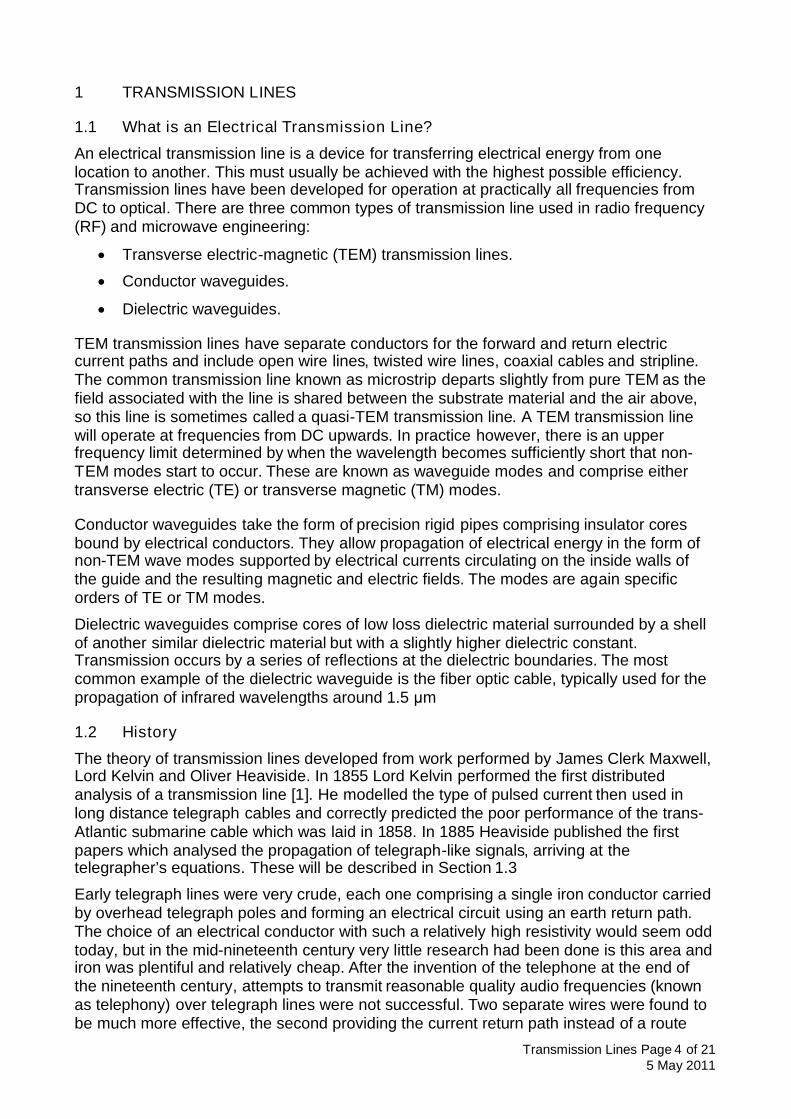
A practical TEM transmission line will contain elements of series resistance R , seriesinductance L , parallel conductance G and parallel capacitance C distributed along theline. Consider a small element of such a transmission line of short elementary length z ,as shown in Figure 1-1. The lower case z represents the distance measured along theline which is also the direction of propagation. Figure 1-1 represents the section from anunbalanced transmission line, such as a coaxial cable which is the most common form oftransmission line. In unbalanced transmission lines the ‘return’ path comprises a metallicscreen surrounding the inner coaxial conductor used for the forward path. In this case thereturn path will have low resistance and inductance, which is assumed negligible andtherefore not shown in Figure 1-1.

Figure 1-1 The fundamental element section of a uniform TEM transmission line

Many such elementary sections may be cascaded to form a section of a practical, uniformtransmission line. The units of the elementary parameters are defined per unit length asfollows:

' R ' Ohms per metre ( / m );

' L ' Henries per metre ( /H m);

' G ' Siemens per metre ( /S m );

' C ' Farads per metre ( /F m);

The impedance of the series section represented by Z , with an upper case Z , not to beconfused with the length which is a lower case z is:

Z R j L (1.1)


and the admittance of the section is represented by Y , where

Y G j C (1.2)

In (1.1) and (1.2) the term is the angular frequency of the applied sinusoidal waveformin radians per second ( /rad s ). is related to the frequency in hertz ( Hz ) of the waveformby:

2 f (1.3)

By Kirchoff’s laws using the definitions of voltages and current shown in Figure 1-1:

2 1 1V V I Z z (1.4)

2 1 2I I V Y z (1.5)

If the voltage difference therefore across z is V

2 1 1V V V I Z z (1.6)

1

lim0

VI Z

zV V IZ

zz z

(1.7)

Similarly

IYV

z

(1.8)

Differentiating (1.7) with respect to z :2

2

2

2

( )

0

V IZ Z YV YZVz z

V YZVz

(1.9)

This differential equation expresses the voltage variation along the line in terms of position.Similarly, the following differential equation may be derived in terms of the current.

2

2 0I YZIz

(1.10)

1.4 The Total Voltage Wave

A practical linear transmission line will simply comprise a cascade of networks of the typeshown in Figure 1-1. It will have some loss because finite values for resistance R andconductance G . Each of these parameters will dissipate heat and therefore waste some ofthe power intended for propagation along the transmission line. Each will also change withfrequency, the resistance and conductance tending to increase with increasing frequencybecause of the skin effect. Excessive heat dissipation is not usually a problem at lowpower levels but may become so at high power levels if, for example, the transmission linewas used to feed an antenna from a high power transmitter. Inductance also changes withfrequency, tending to increase with increasing frequency.

Using a transmission line at high powers also increases the risk of breakdown and/oroverheating. Breakdown can occur very quickly, often being initiated by a very narrowpulse of high instantaneous peak power. Overheating is normally the direct result of


excessive mean power being dissipated in the R and G elements. Either can causepermanent damage to the transmission line.

The series element can be represented as an impedance Z , given by:

Z R j L (1.11)

and the parallel element can be represented by an admittance Y given by:

Y G j C (1.12)

(1.9) is a differential equation which has an exponential solution of the typez zV Ae Be (1.13)

where A and B are constants and is the complex quantity given by

ZY R j L G j C (1.14)

Furthermore is known as the propagation constant and is given by

j (1.15)

where is the attenuation constant expressed in Nepers per metre ( /Np m ) and is thephase constant expressed in radians per metre ( /rad m ).

A Neper is a logarithmic way of expressing a power ratio, with a similar definition to thedecibel, but using a natural logarithm instead of a common logarithm. The bases oflogarithms may be changed using the following equation:

10

10

logln

logb

be

(1.16)

Thus (1.16) may be used to convert Nepers to decibels.

(1.13) is the expression for the total voltage on the transmission line, the sum of theforward ( FV ) and reverse ( RV ) waves. Therefore

zFV Ae (1.17)

zRV Be (1.18)

F RV V V (1.19)

1.5 The Total Current Wave

Differentiating the total voltage from (1.13) with respect to z gives:

z zVAe Be

z

(1.20)

But

VIZ

z

(1.21)

Therefore, using (1.14), (1.20) and (1.21), the total current waveform is given by:z zAe Be

IZ ZY Y

(1.22)


1.6 Characteristic Impedance

Another way of writing the total current waveform in terms of FV and RV is:

0 F RIZ V V (1.23)

where 0Z is known as the characteristic impedance of the transmission line and is definedas:

0

Z R j LZ

Y G j C

(1.24)

As 0Z is an impedance it has dimensions of Ohms (). For some transmission linesoperating at modest radio frequencies, R and G are negligible compared to themagnitudes of j L and j C , so

0R j L LZG j C C

(1.25)

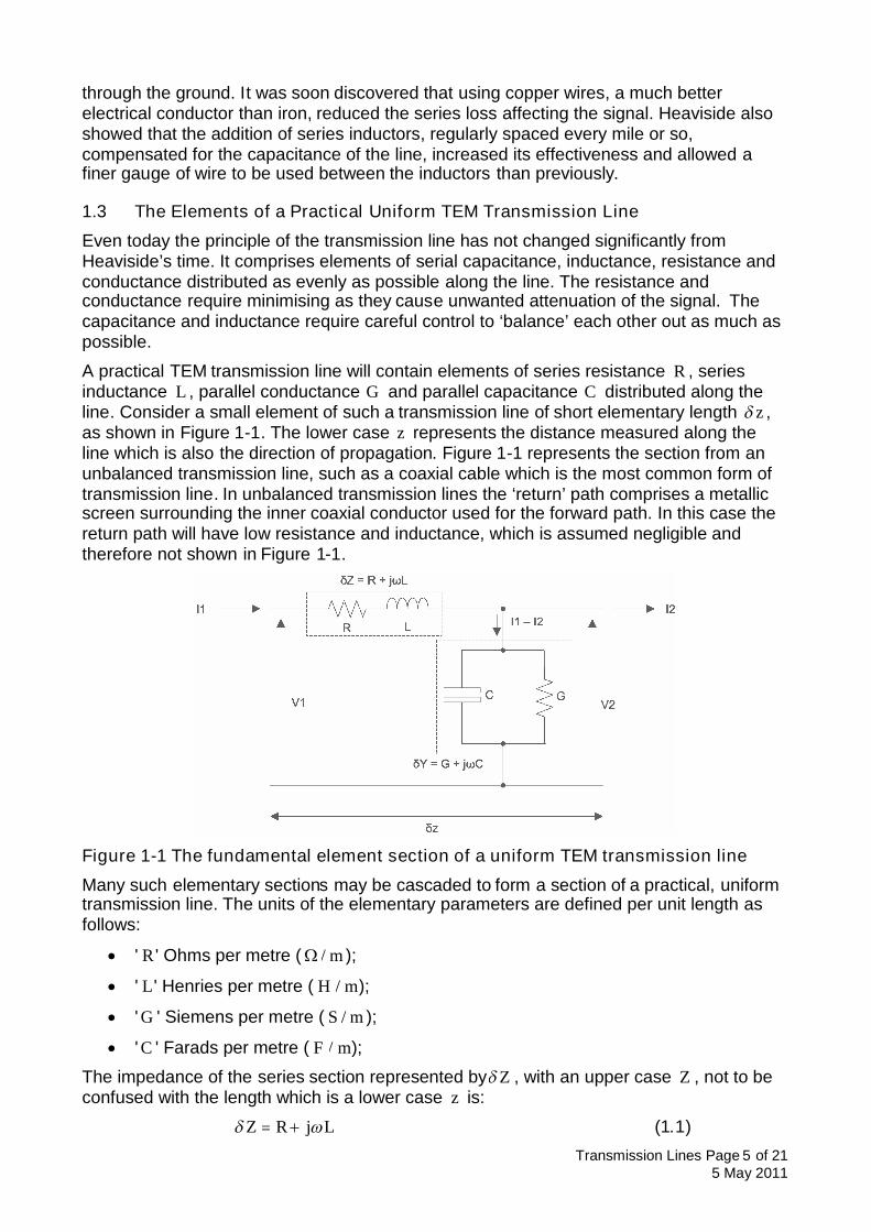
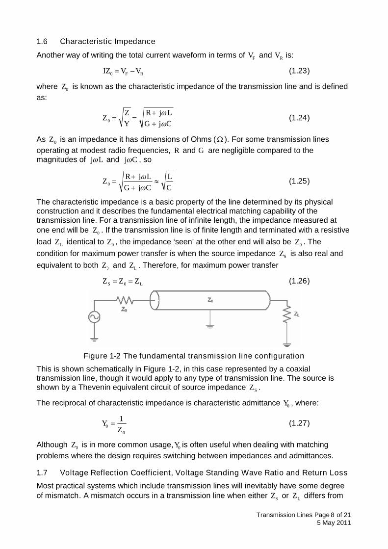
The characteristic impedance is a basic property of the line determined by its physicalconstruction and it describes the fundamental electrical matching capability of thetransmission line. For a transmission line of infinite length, the impedance measured atone end will be 0Z . If the transmission line is of finite length and terminated with a resistiveload LZ identical to 0Z , the impedance ‘seen’ at the other end will also be 0Z . Thecondition for maximum power transfer is when the source impedance SZ is also real andequivalent to both 0Z and LZ . Therefore, for maximum power transfer

0S LZ Z Z (1.26)

Figure 1-2 The fundamental transmission line configuration

This is shown schematically in Figure 1-2, in this case represented by a coaxialtransmission line, though it would apply to any type of transmission line. The source isshown by a Thevenin equivalent circuit of source impedance SZ .

The reciprocal of characteristic impedance is characteristic admittance 0Y , where:

00

1YZ

(1.27)

Although 0Z is in more common usage, 0Y is often useful when dealing with matchingproblems where the design requires switching between impedances and admittances.

1.7 Voltage Reflection Coefficient, Voltage Standing Wave Ratio and Return Loss

Most practical systems which include transmission lines will inevitably have some degreeof mismatch. A mismatch occurs in a transmission line when either SZ or LZ differs from


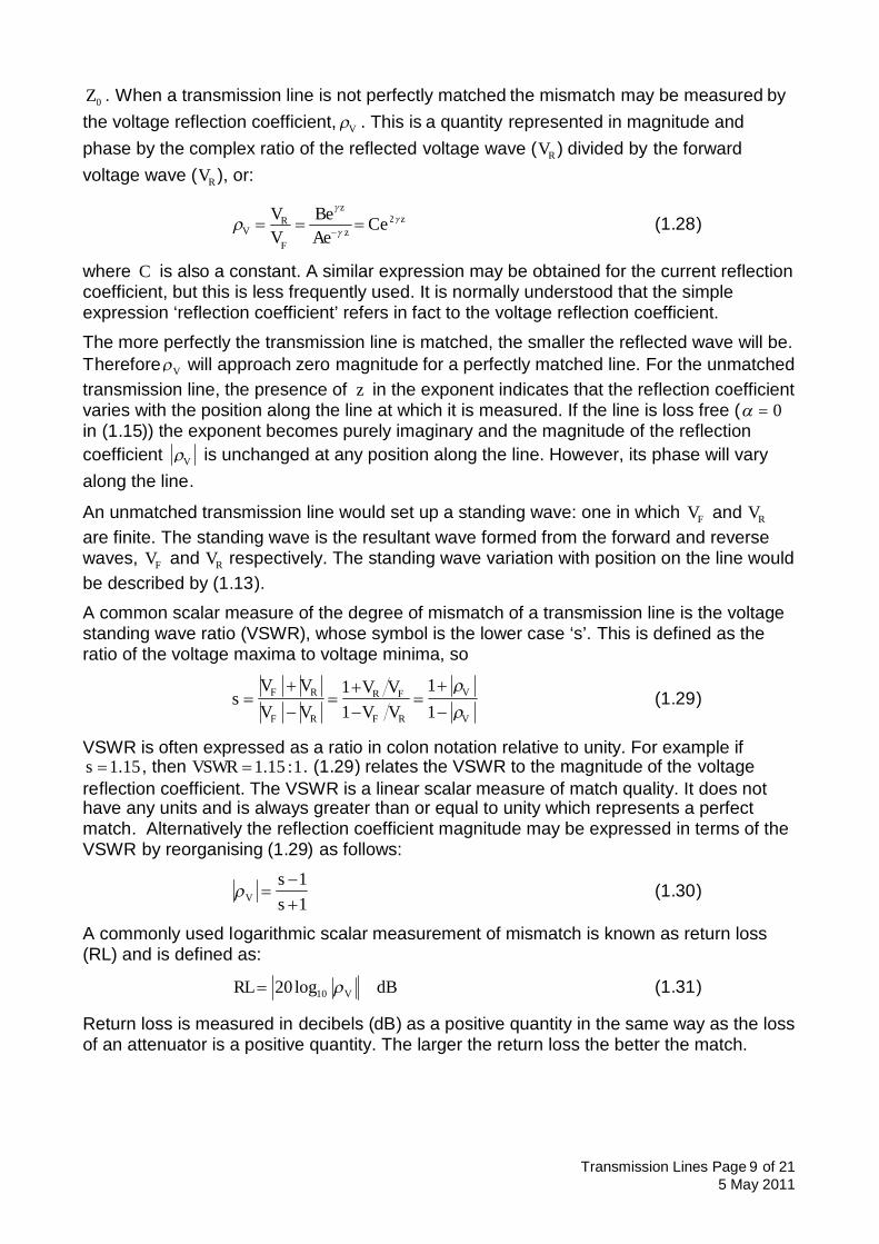
0Z . When a transmission line is not perfectly matched the mismatch may be measured bythe voltage reflection coefficient, V . This is a quantity represented in magnitude andphase by the complex ratio of the reflected voltage wave ( RV ) divided by the forwardvoltage wave ( RV ), or:

2z

zRV z

F

V Be CeV Ae

(1.28)

where C is also a constant. A similar expression may be obtained for the current reflectioncoefficient, but this is less frequently used. It is normally understood that the simpleexpression ‘reflection coefficient’ refers in fact to the voltage reflection coefficient.

The more perfectly the transmission line is matched, the smaller the reflected wave will be.Therefore V will approach zero magnitude for a perfectly matched line. For the unmatchedtransmission line, the presence of z in the exponent indicates that the reflection coefficientvaries with the position along the line at which it is measured. If the line is loss free ( 0in (1.15)) the exponent becomes purely imaginary and the magnitude of the reflectioncoefficient V is unchanged at any position along the line. However, its phase will varyalong the line.

An unmatched transmission line would set up a standing wave: one in which FV and RVare finite. The standing wave is the resultant wave formed from the forward and reversewaves, FV and RV respectively. The standing wave variation with position on the line wouldbe described by (1.13).

A common scalar measure of the degree of mismatch of a transmission line is the voltagestanding wave ratio (VSWR), whose symbol is the lower case ‘s’. This is defined as theratio of the voltage maxima to voltage minima, so

111 1

F R VR F

F R F R V

V V V Vs

V V V V

(1.29)

VSWR is often expressed as a ratio in colon notation relative to unity. For example if1.15s , then 1.15 :1VSWR . (1.29) relates the VSWR to the magnitude of the voltage

reflection coefficient. The VSWR is a linear scalar measure of match quality. It does nothave any units and is always greater than or equal to unity which represents a perfectmatch. Alternatively the reflection coefficient magnitude may be expressed in terms of theVSWR by reorganising (1.29) as follows:

11V

ss

(1.30)

A commonly used logarithmic scalar measurement of mismatch is known as return loss(RL) and is defined as:

1020log VRL dB (1.31)

Return loss is measured in decibels (dB) as a positive quantity in the same way as the lossof an attenuator is a positive quantity. The larger the return loss the better the match.


1.8 The Variation of Impedance Along a Practical (Lossy) MismatchedTransmission Line

For a practical (lossy) transmission line, mismatched at the distant end, the voltagereflection coefficient will vary at points along the line in both magnitude and phase.

If the length of the line is l , then substitution into (1.28) for 0z and z l will yield thefollowing equation for the reflection coefficient measured at the input to the line ( 0) interms of the reflection coefficient at the load connected to the end of the line ( T).

20

lT e (1.32)

Dividing (1.19) by (1.23) gives the general expression relating the impedanceTZ connected to the end of the line with the forward and reflected waves FV and RV

respectively.

0 0

1111

R

T F R F T

RF R T

F

VZ V V VV

VZ I Z V VV

(1.33)

Notice that all terms in this equation are actual complex quantities. In terms of T (1.33)becomes:

0

0

TT

T

Z ZZ Z

(1.34)

Substituting for T into (1.32) gives

20

0

lTl

T

Z Ze

Z Z

(1.35)

where l is the reflection coefficient at the input of a line of length l terminated in animpedance TZ . A similar equation to may be written but this time relating the inputimpedance of line INZ to the associated reflection coefficient 0:

0

0 0

11

INZZ

(1.36)

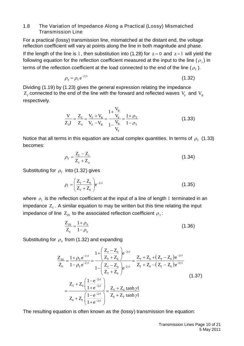
Substituting for 0 from (1.32) and expanding

2022

0 002 2

0 0 020

0

2

0 20

20

0 2

111

1

11 tanh

tanh11

lTll

T TTIN Tl l

T T TlT

T

l

T lT

lT

T l

Z Z eZ Z Z Z eZ ZZ e

Z e Z Z Z Z eZ Z eZ Z

eZ Z

e Z Z lZ Z le

Z Ze

(1.37)

The resulting equation is often known as the (lossy) transmission line equation:


00

0

tanhtanh

TIN

T

Z Z lZ Z

Z Z l

(1.38)

This is used to calculate the input impedance of a lossy transmission line of characteristicimpedance 0Z , length l , propagation coefficient whilst it is terminated with animpedance TZ .

1.9 The Loss-Free Transmission Line

1.9.1 The Loss-Free Transmission Line Equation

Often in transmission line problems it is adequate to assume the line to be loss free as thisadds several very welcome simplifications in the algebra such as dealing withtrigonometric functions instead of hyperbolic functions.

For a loss free transmission line the attenuation constant will be zero, so (1.15)becomes

j j (1.39)

Substituting for j in the loss-free case and using the Euler identities

2cos

2 sin

jx jx

jx jx

e e x

e e j x

(1.40)

the hyperbolic tangent simplifies as follows2 2

2 2

1 1tanh1 1

2 sin2cos

tan

l j l

l j l

j l j l

j l j l

e ele e

e e j le e lj l

(1.41)

Performing this substitution yields the transmission line equation for the loss-free case

00

0

tantan

TIN

T

Z jZ lZ Z

Z jZ l

(1.42)

This may be used to calculate the impedance looking into a loss-free transmission line ofcharacteristic impedance 0Z , length l and terminated at the distant end with animpedance of TZ .

1.9.2 Phase Constant and Phase Velocity

In this case the phase constant is given by

2/rad m

(1.43)

where is the wavelength within the transmission line. This equation is used to determinethe spatial phase variation ( l ) along a transmission line.

For the loss free case 0R and 0G therefore, by equating (1.14) with (1.39):


2 2j j LC

LC

(1.44)

Therefore, equating (1.43) with (1.44) and using the relationship relating temporal andangular frequency:

2 f (1.45)

yields

2

2 2

1

1p

LC

f LC

LCf

v fLC

(1.46)

where Pv is the phase velocity of propagation within the transmission line. If thetransmission line is air spaced then Pv is identical to the velocity of electromagneticradiation in free space ( pv c ). If it includes a solid dielectric of relative permittivity

(dielectric constant) r, then Pv is related to c by

pr

cv

(1.47)

If the dielectric is partially air-spaced, then it may be assigned an effective dielectricconstant effk where

p

cv

k (1.48)

The value of k would be found by measurement to be a value between unity (air onlydielectric) and r (solid dielectric).

The assumption in these definitions is that the phase velocity is constant and not afunction of frequency.


2 WAVEGUIDES

A waveguide is a transmission line constructed to guide electromagnetic energy from onelocation to another. There are two forms of practical waveguide: dielectric-conductor anddielectric-dielectric. The dielectric-conductor waveguide comprises a conductorsurrounding a dielectric through which the radio frequency (RF) energy is directed. Adielectric-dielectric waveguide is of similar construction with one of the dielectricssurrounding the other, and the two dielectrics have differing refractive indices, relativepermittivities or dielectric constants.

2.1 The Rectangular Waveguide [2]

The rectangular waveguide is a form of very low loss transmission line used across therange of microwave frequencies from approximately typically from about 1 GHz to over220 GHz. It comprises a rigid, precision rectangular hollow pipe constructed from a goodelectrical conductor with the inner hollow formed from a dielectric material. The dielectricmust exhibit a suitably low loss at the maximum frequency to be propagated through thewaveguide. Typically this might be dry air at normal atmospheric pressure or another gassuch as dry nitrogen at a slightly elevated pressure compared to atmospheric. The wallsare often constructed from copper, as this is a good electrical conductor, relatively cheapand chemically stable. Sometimes the internal walls may be plated with silver. Silver is abetter electrical conductor that copper and, provided that the plating thickness is sufficient,the transmission loss will be slightly less that that with an equivalent copper waveguide.Although rectangular waveguide is expensive and bulky compared to the alternativetransmission lines such as microstrip or coaxial cables, it is used widely for high powertransmitter feeds, millimetre wave components and precision measuring equipment.

A difference between a waveguide and a TEM transmission line of the type described inSection 1.3 is that the waveguide comprises a single conductor so there is no possiblepath to form an electrical circuit requiring separate ‘go’ and ‘return’ current paths. It cannottherefore support TEM waves. Unlike TEM waves which propagate down to DC, arectangular waveguide will only support frequencies above a threshold and then only in theform or transverse electric (TE) waves or transverse magnetic (TM) waves.

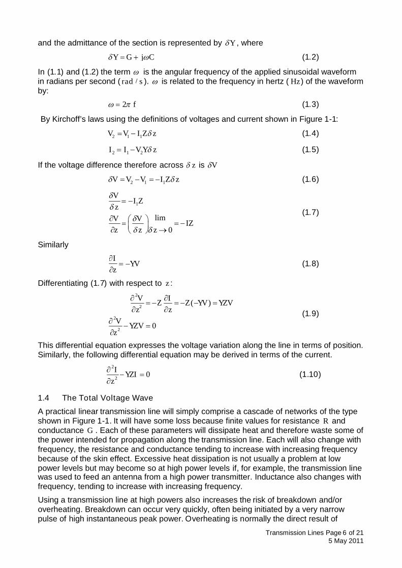
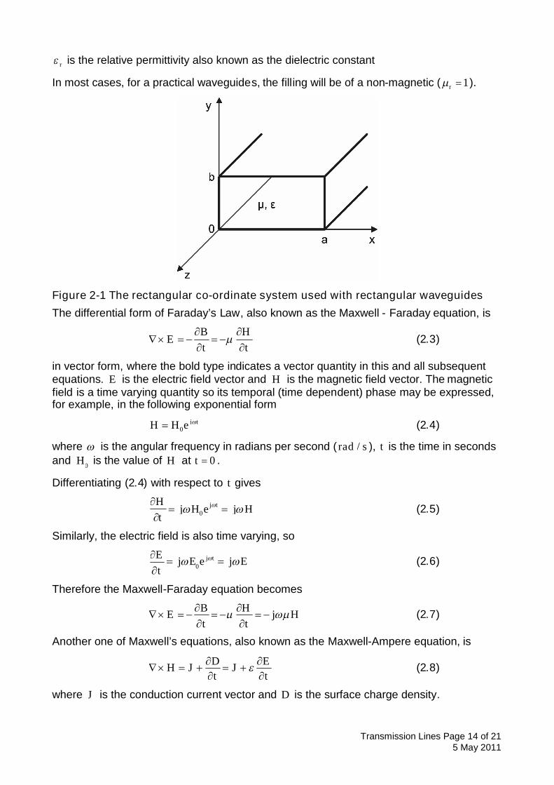
The geometry of a cross section of the rectangular waveguide is shown in Figure 2-1. Thelonger and the shorter internal transverse dimensions are a and b respectively ( a b ).For the most common type of rectangular waveguide 2a b . The x and y axes are alignedwith the longer and shorter dimensions respectively. The direction of propagation throughthe waveguide, is parallel to the z axis and mutually perpendicular to both the x and yaxes. The electrical properties of the material within the guide are described by itspermittivity and permeability , where

0 r (2.1)

and

0 r (2.2)

In (2.1) and (2.2)

0 is the absolute permeability

r is the relative permeability

0 is the absolute permittivity


r is the relative permittivity also known as the dielectric constant

In most cases, for a practical waveguides, the filling will be of a non-magnetic ( 1r ).

Figure 2-1 The rectangular co-ordinate system used with rectangular waveguides

The differential form of Faraday’s Law, also known as the Maxwell - Faraday equation, is

t t

B H

E (2.3)

in vector form, where the bold type indicates a vector quantity in this and all subsequentequations. E is the electric field vector and H is the magnetic field vector. The magneticfield is a time varying quantity so its temporal (time dependent) phase may be expressed,for example, in the following exponential form

0j tH H e (2.4)

where is the angular frequency in radians per second ( /rad s ), t is the time in secondsand 0H is the value of H at 0t .

Differentiating (2.4) with respect to t gives

0j tH

j H e j Ht

(2.5)

Similarly, the electric field is also time varying, so

0j tE j E e j E

t

(2.6)

Therefore the Maxwell-Faraday equation becomes

jt t

B HE H (2.7)

Another one of Maxwell’s equations, also known as the Maxwell-Ampere equation, is

t

D EH J Jt

(2.8)

where J is the conduction current vector and D is the surface charge density.


For the dielectric in the hollow section of a rectangular waveguide, no conduction currentcan flow but an alternating current can, also known as a convection current. Therefore

0J and (2.8) simplifies to

jt

D E

H Et

(2.9)

(2.7) and (2.9) are used to derive the differential equations that describe transversecomponents of both the electrical and magnetic fields as described in the next section.

2.1.1.1 Transverse Electric and Transverse Magnetic Fields

By expanding the curl expression in (2.7) and expressing the H field in terms of itsrectangular vector components xH , yH and zH :

x y z

x y z

j H H Hy z

E E E

x y z

x y z

a a a

E a a ax

(2.10)

where xa , ya and za are the unit vectors in the x , y and z directions respectively.

As propagation is in the z direction, the spatial phase dependence is also in the z direction,so a similar simplification that was adopted with the temporal part in (2.6) may be appliedto the spatial part. An electric field E may be represented in the exponential spatial phaseformat as:

0j zE E e (2.11)

Differentiating this with respect to z gives

0j zE j E e j E

z

(2.12)

The vector curl equation in (2.10) may be expanded and substitutions made from (2.6) and(2.12) for the x , y and z coefficients of E and H , followed by equating coefficients foreach of the unit vectors to yield the following six equations.

zy x

E j E j Hy

(2.13)

zx y

Ej E j Hx

(2.14)

y xz

E Ej H

x y

(2.15)

zy x

H j H j Ey

(2.16)

zx y

Hj H j Ex

(2.17)

y xz

H Hj E

x y

(2.18)


Equations (2.13) to (2.18) may be solved for the transverse field components of E ( xEand yE ) and H ( xH and yH ) to give the following

2z z

xc

E HjE

k x y

(2.19)

2z z

yc

E HjE

k y x

(2.20)

2z z

xc

E HjH

k y x

(2.21)

2z z

yc

E HjH

k x y

(2.22)

where2 2 2

ck k (2.23)

ck is the cutoff wavenumber or phase constant specific to the waveguide.

k is the phase constant of a plane (TEM) wave propagating in an unbounded mediumelectrically described by and .

is the phase constant in the direction of propagation along the waveguide. Equation(2.23) may be expressed in terms of wavelengths by

2 2 2

1 1 1

c g (2.24)

where

c is the cutoff wavelength for the rectangular waveguide under consideration.

is the TEM wavelength for an equivalent unbounded plane wave considered aspropagating through the medium described by and .

g is the guide wavelength in the direction of propagation.

The results presented in (2.19) through (2.22) are the differential equations which definetransverse electric (TE) fields and transverse magnetic (TM) fields.

2.1.1.2 Transverse Electric Waves

Transverse electric (TE) waves, by definition, are those for which 0zE and 0zH so thedifferential terms of zE in (2.19) through (2.22) become zero, giving the followingequations

2z

xc

HjE

k y

(2.25)

2z

yc

HjE

k x

(2.26)


2z

xc

HjHk x

(2.27)

2z

yc

HjHk y

(2.28)

2.1.1.3 Transverse Magnetic Waves

Transverse magnetic (TM) waves, by definition, are those for which 0zE and 0zH sothe differential terms of zH in (2.19) through (2.22) become zero, giving the followingequations

2z

xc

EjE

k x

(2.29)

2z

yc

EjE

k y

(2.30)

2z

xc

EjH

k y

(2.31)

2z

yc

EjH

k x

(2.32)

2.1.1.4 TE and TM Modes

To examine the modes that may be supported by rectangular waveguides, we need to firstreturn to the modified version of the Maxwell-Faraday equation (2.7).

Taking the curl of both sides of (2.7) and substituting the modified version of the Maxwell-Ampere equation from (2.9):

2j j j E H E E (2.33)

The next step is to apply the following vector identity for a general vector A to (2.33).

2 A A A (2.34)

giving

2 2E E = E (2.35)

Since there is no stored charge, the volumetric charge density becomes zero ( 0 ) andthe Maxwell Gauss equation D also becomes zero, so

0 E (2.36)

and

0 E (2.37)

Substituting (2.37) into (2.35) gives the Helmholtz wave equation in terms of electric field:2 2 0 E E (2.38)

A similar Helmholtz expression in terms of the magnetic field H can be obtained startingwith the Maxwell-Ampere equation (2.8) applied to the internal medium of the waveguide


which is an insulator so 0J and the modified version (2.9) is used. A further substitutionfrom (2.7) produces the result

2 2 0 H H (2.39)

(2.39) may be reduced to its rectangular components since, for the left hand side2 2 2 2

x y zH H H x y zH a a a (2.40)

and

x y zH H H x y zH a a a (2.41)

To apply the equations for the TE waves (2.25) to (2.28), the zH component of theHelmholtz equation must be extracted from (2.40) and (2.41):

2 2 22

2 2 2 0zk Hx y z

(2.42)

The spatial phase dependence of zH in the z direction may be described by

, , ( , ) j zz zH x y z h x y e (2.43)

Since zh is not actually a function of z , it may be treated as a constant whendifferentiating zH with respect to z , so

2

2z

z

HH

z

(2.44)

Substituting (2.44) into (2.42) and also using 2 2 2ck k (2.23) gives the result

2 2

22 2 , 0c zk h x y

x y

(2.45)

The partial differential equation (2.45) may be solved by the method known as ‘separationof the variables’, letting

,zh x y X x Y y (2.46)

then2 2

2 2zh X

Yx x

(2.47)

2 2

2 2zh Y

Xy y

(2.48)

Substituting (2.46), (2.47) and (2.48) into (2.45) gives the following result2 2

22 2

1 10c

d X d Yk

X dx Y dy (2.49)

The principle of separation of the variables requires each of the terms in (2.49) to be equalto a constant thus generating two more differential equations

22

2 0x

d X k Xdx

(2.50)


22

2 0y

d Yk Y

dy (2.51)

where xk and yk are constants such that

2 2 2x y ck k k (2.52)

The solutions of (2.50) and (2.51) are

cos sinx xX A k x B k x (2.53)

and

cos siny yY C k y D k y (2.54)

where A , B , C and D are constants, so

( , ) ( cos sin )( cos sin )z x x y yh x y XY A k x B k x C k y D k y (2.55)

2.1.1.5 Boundary Conditions for TE Modes

The waveguide walls are very good conductors so will not support any tangentialcomponents of electric field. Using the rectangular coordinate system given in Figure 2-1,this must occur at the waveguide walls as follows:

( , ) 0 0xe x y at y and y b (2.56)

( , ) 0 0ye x y at x and x b (2.57)

xe and ye are obtained by differentiating (2.55) with respect to both x and y and usingresults in (2.26) and (2.25) respectively.

( sin cos )( cos cos )zx x x y y

hk A k x B k x C k y D k y

x

(2.58)

( cos sin )( sin cos )zy x x y y

hk A k x B k x C k y D k y

y

(2.59)

By substituting (2.58) and (2.59) into (2.26) and (2.25) respectively, the solutions for xeand ye are

2 ( cos sin )( sin cos )x y x x y yc

je k A k x B k x C k y D k y

k

(2.60)

2 ( sin cos )( cos cos )y x x x y yc

je k A k x B k x C k y D k y

k

(2.61)

Using the boundary conditions in (2.56) and (2.57), from (2.60), 0D and

0,1, 2...ynk for nb (2.62)

Similarly, from (2.61), 0B and

0,1,2...x

mk for ma (2.63)

Using (2.43) the solution for zH is therefore


( , , ) cos cos j zz mn

m x n yH x y z A ea b

(2.64)

where mnA is a constant originating from the constants A and C .

The solutions for the transverse E and H components are obtained by differentiating(2.64) with respect to x or y as appropriate and substituting into (2.25), (2.26), (2.27) and(2.28) to give the following equations.

2 cos sin j zx mn

c

j n m x n yE A e

k b a b (2.65)

2 sin cos j zy mn

c

j m m x n yE A e

k a a b

(2.66)

2 sin cos j zx mn

c

j m m x n yH A e

k a a b (2.67)

2 cos sin j zy mn

c

j n m x n yH A e

k b a b (2.68)

These equations will describe the mnTE mode.

The propagation constant, from (2.23) by substituting (2.62) and (2.63) is

2 22 2 2

c

m nk k k

a b

(2.69)

The propagation constant is real when

ck k (2.70)

and the cutoff condition is

2 2

c

m nka b

(2.71)

The general expression for the cutoff frequency cmnf for any combination of m and n is

2 21

2 2c

cmnk m nf

a b

(2.72)

The fundamental mode is that with 1, 1m n , known as 10TE , so

101

2cf

a (2.73)


3 REFERENCES1. Chipman, Robert A.; Transmission Lines; Schaum’s Outline Series in Engineering;

McGraw Hill Book Company;2. Pozar, David M.; Microwave Engineering - Third Edition; John Wiley & Sons Inc;

ISBN 0-471-44878-8 (2005); pp 106 - 117.

Documents

Transmission Line Fundamentals by - Chris Angove · Transmission Lines Page1 of 21 5 May 2011 Transmission Line Fundamentals by Chris Angove DISCLAIMER The Author makes no …