Embed Size (px)
Citation preview

1
Transmission Lines
Chris Allen ([email protected])
Course website URL people.eecs.ku.edu/~callen/713/EECS713.htm

2
Transmission linesUsed to transmit signals point-to-point
Requirements• Preserve signal fidelity (low distortion)
signal voltage levelssignal bandwidthsignal phase / timing properties
• Minimum of radiation (EMI)• Minimum of crosstalk
Parameters of interest• Useful frequencies of operation (f1 – f2)
• Attenuation (dB @ MHz)• Velocity of propagation or delay (vp = X cm/ns, D = Y ns/cm)
• Dispersion (vp(f), frequency-dependent propagation velocity)
• Characteristic impedance (Zo, )
• Size, volume, weight• Manufacturability or cost (tolerances, complex geometries)

3
Transmission linesTransmission line types
There are a large variety of transmission line types

4
Transmission linesTransmission line types
All depend on electromagnetic phenomenaElectric fields, magnetic fields, currents
EM analysis tells us about attenuation vs. frequency propagation velocity vs. frequencyZo characteristic impedance
relative dimensions
Parameters contributing to these characteristics conductivity of metalsr′ real part of relative permittivityr″ imaginary part of relative permittivityr relative permaebility (usually ~ 1)
structure dimensionsh heightw widtht thickness

5
Transmission linesEffects of transmission line parameters on system performance
Attenuation vs. frequencyAttenuation – reduces signal amplitude, reduces noise marginFreq-dependent attenuation – reduces higher frequency components,
increasing Tr
Propagation velocity vs. frequencyvelocity – determines propagation delay between components
reduces max operating frequencyFreq-dependent velocity – distorts signal shape (dispersion)
may broaden the pulse duration
Characteristic impedance – ratio of V/I or E/Hdetermines drive requirementsrelates to electromagnetic interference (EMI)mismatches lead to signal reflections

6
Transmission line modelingCircuit model for incremental length of transmission line
It can be shown that for a sinusoidal signal, = 2f, Vs = A ej(t+)
is analogous to
where is complex, = + j is the propagation constant
the real part, is the attenuation constant [Np / m : Np = Nepers]
the imaginary part, , is the phase constant [rad / m : rad = radians]
CjGLjR
axiszalongnpropagatioeVV zSO
npropagatiowaveplaneinjj
zjzSO eeVV
amplitude change phase change

7
Transmission line modelingFor a loss-less transmission line (R 0, G 0)
so
for the argument to be constant requires
therefore the propagation velocity is
Similarly, for the general case (R, G > 0)
The characteristic impedance, Zo is
and for the low-loss case (R 0, G 0)
CLjj
zCLtjztjO eAeeAV
CL1tzorCLzt
1vorCL1v pp
CjGLjR Re
CjGLjRIVZ SSo
oo ZorCLZ

8
Transmission line modelingTransmission line loss mechanisms
non-zero R, G result in > 0
R relates to ohmic losses in the conductorsG relates to dielectric losses
Ohmic lossesAll conductors have resistivity, (-m)
copper, = 1.67x10⁻⁸ -m
Resistance is related to the material’s resistanceand to the conductor’s geometry (Length, Thickness, Width)
CjGLjR Re

9
Transmission line modelingOhmic losses in a printed circuit trace
Consider a trace 10 mils wide (0.010”) or W = 254 m2” long (2.000”) or L = 50.8 mm, made with 1 ounce copper,T = 1.35 mil (0.00135”) or T = 34.3 m(1 oz. = weight per square foot)
For this 2” trace the DC resistance is R = 97.4 m
Skin effectAt DC, the current is uniformly distributed through the conductor
At higher frequencies, the current density, J, is highest on the surface and decays exponentially with distance from the surface (due to inductance)
The average current depth or skin depth, where = resistivity = 1/ (conductivity)
= radian frequency (rad/s) = 2f = magnetic permeability (H/m) = or
o = 4 x 10⁻⁷ H/m
is frequency dependent
(m)2 ,
10
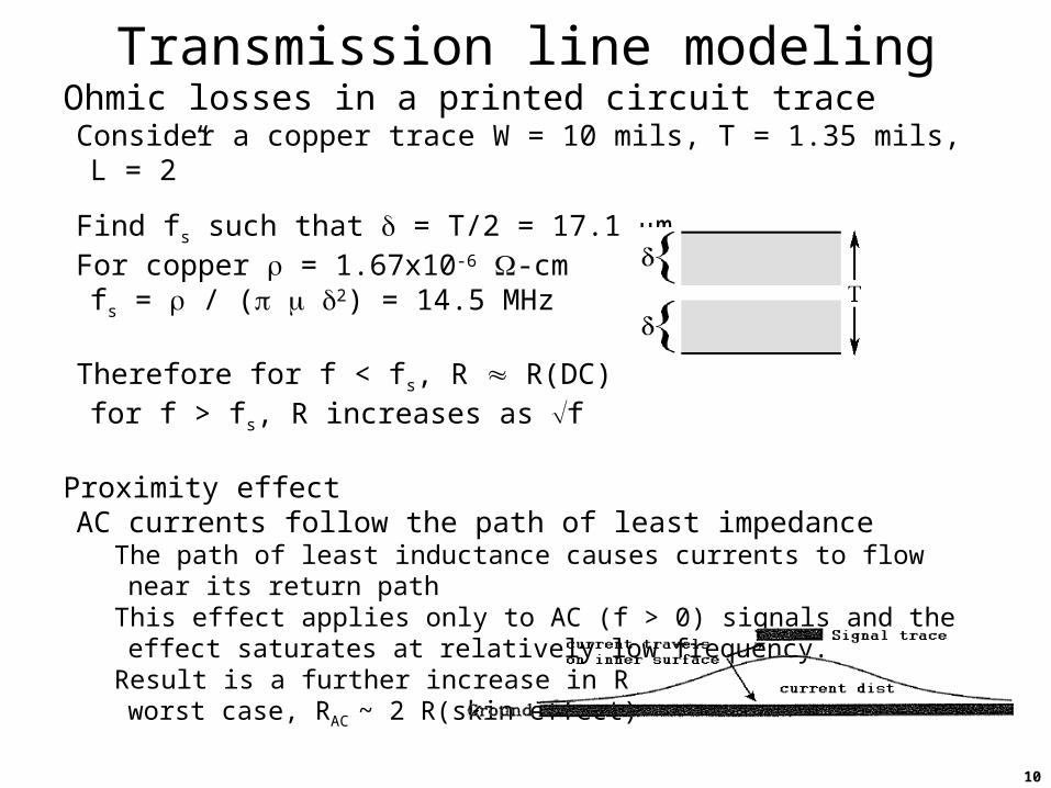
Transmission line modelingOhmic losses in a printed circuit traceConsider a copper trace W = 10 mils, T = 1.35 mils, L = 2”
Find fs such that = T/2 = 17.1 mFor copper = 1.67x10⁻⁶ -cmfs = / ( 2) = 14.5 MHz
Therefore for f < fs, R R(DC)for f > fs, R increases as f
Proximity effectAC currents follow the path of least impedance
The path of least inductance causes currents to flow near its return pathThis effect applies only to AC (f > 0) signals and the effect saturates at relatively low frequency.
Result is a further increase in Rworst case, RAC ~ 2 R(skin effect)

11
Transmission line modelingOhmic losses in a printed circuit traceFor the 2” long trace, (W = 10 mils, T = 1.35 mils), find fp such that = T = 34.3 m
fp = / ( 2) = 3.6 MHz
for f < fp, R R(DC)for f > fs, R increases as f
Since AC currents flow on the metal’s surface (skin effect) and on the surface near its return path (proximity effect), plating traces on a circuit board with a very good conductor (e.g., silver) will not reduce its ohmic loss.

12
Transmission line modelingConductor loss example (part 1 of 3)
Consider the broadside-coupledtransmission line* as shown.
Find the signal attenuation (dB/m) at 1500 MHz if the 1-oz. copper traces are 17 mils wide, the substrate’s relative dielectric constant (εr)
is 3.5, and the characteristic impedance (Zo) is 62 Ω.
We know
So to solve for (dB/m) first find per unit length values for R, L, C
RCjLCReCjLjRRem/Np 2
RCI,LCRwhereIjRRem/Npor x2
xxx
xx1
x2x
2xxxx RItanPandIRMand2PcosMm/Npor
mNp686.8mdB
*
* Also known as the “parallel-plane transmission line” or the “double-sided parallel strip line”

13
Transmission line modelingConductor loss example (part 2 of 3)
Resistance, R, is found using
where ρ (copper) = 1.67x10⁻⁸ -m, L = 1 m, W = 432 m, and is the 1500-MHz skin depth.
For a 1-m length of transmission line (L = 1 m), W = 17 mils (W = 432 m) and = 1.71 m, we get R = 22.6 Ω/m.
To find C and L over a 1-m length, we know
W
LR
CL1vands/m10x6.1cv p8
rp
CLZand62Z oo
m/F10x01.1Zv
1Candm/H10x87.3
v
ZLSo 10
op
7
p
o

14
Transmission line modelingConductor loss example (part 3 of 3)
R = 22.6 Ω/m, L = 387 nH/m, C = 101 pF/m
Rx = -3206, Ix = 20.64, Mx = 3206, Px = 3.14
= 0.182 Np/m or 1.58 dB/m
Conversely, for low-loss transmission lines (i.e., R « ωL) the attenuation can be accurately approximated using
m/dB58.1orm/Np182.0622
m6.22
Z2
RmNp
1
o

15
Transmission line modelingDielectric lossFor a dielectric with a non-zero conductivity ( > 0) (i.e., a non-infinite resistivity, < ), losses in the dielectric also attenuate the signal
permittivity becomes complex,with being the real part the imaginary part
= / (conductivity of dielectric / 2f)
Sometimes specified as the loss tangent, tan , (the material characteristics table)
To find , = tan
The term loss tangent refers to the angle between two current components: displacement current (like capacitor current) conductor current (I = V/R)
Don’t confuse loss tangent (tan ) with skin depth ()
j
tan
ESR: equiv. series resistance

16
Transmission line modelingDielectric lossFrom electromagnetic analysis we can relate to
o = free-space wavelength = c/f, c = speed of lighto = free-space permittivity = 8.854 x 10⁻¹² F/m
d (attenuation due to lossy dielectric) is frequency dependent (1/o) and it increases with frequency (heating of dielectric)
Transmission line loss has two components, = c + d
Attenuation is present and it increases with frequency
Can distort the signalreduces the signal level, Vo = Vs e-z
reduces high-frequency components more than low-frequency components, increasing rise time
Length is also a factor – for short distances (relative to ) may be very small
)m/Neper(,1tan12
221
2
oo

17
Transmission line modelingPropagation velocity, vp (or Delay)
from circuit model, (D = 1/vp)
as long as L and C (or and ) are frequency independent, vp is frequency independent
CL
1vp
1vp

18
Transmission line modelingCharacteristic impedance, Zo
ratio of voltage to current, V/I = Z
From transmission line model
typically G (conductance) is very small 0, so
At low frequencies, R >> L when f << R/(2L)the transmission line behaves as an R-C circuit
Zo is complexZo is frequency dependent
At high frequencies, L >> R when f >> R/(2L)
Zo is realZo is frequency independent
CjG
LjRZo
Cj
LjRZo
Cj
RZo
C
LZo

19
Transmission line modelingCharacteristic impedance example
Consider a transmission line with R = 0.1 / inch = 3.9 / mL = 6.35 nH / inch = 250 nH / m C = 2.54 pF / inch = 100 pF / m
From these parameters we know,vp = 2 x 10⁸ m/s = 0.67 c r = 2.25
f1 = R/(2L) = 63.7 kHz
For f f1,
f = 100 Hz, |Zo| 1.26 kf = 1 kHz, |Zo| 400 f = 10 kHz, |Zo| 126
For f >> f1,
Zo = 50
45f
k612
Cj
RZo
.

20
Transmission line modelingTraveling waves
For frequencies above f1 (and frequency components above f1),
Zo is real and frequency independent
For a transmission line with a matched load (RL = Zo), when ‘looking’ into a
transmission line, the source initially ‘sees’ a resistive load
or
21
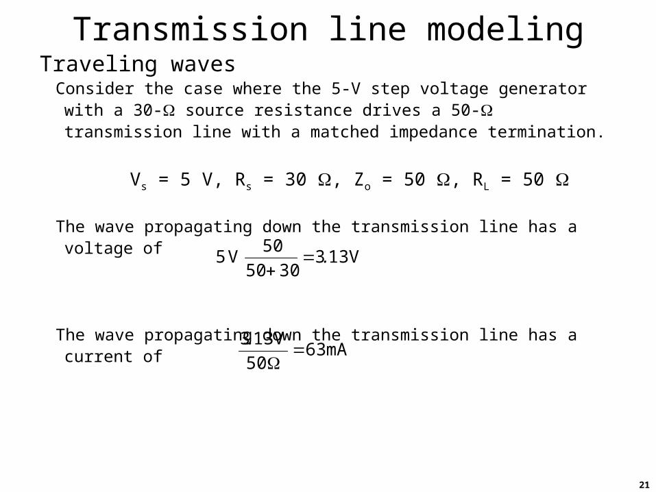
Transmission line modelingTraveling waves
Consider the case where the 5-V step voltage generator with a 30- source resistance drives a 50- transmission line with a matched impedance termination.
Vs = 5 V, Rs = 30 , Zo = 50 , RL = 50
The wave propagating down the transmission line has a voltage of
The wave propagating down the transmission line has a current of
V1333050
50V5 .
mA6350
V133
.

22
Transmission line modelingTraveling waves
Now consider the more general case with impedance mismatchesFirst consider the source end
for Rs = Zo, VA = Vs/2
for Rs Zo,
The wave travels down the transmission line and arrives at B at time t = ℓ/vp where the impedance mismatch causes a
reflected wave with reflection coefficient, L
wave voltage = VA L
Special cases• if RL = Zo (matched impedance), then L = 0
• if RL = 0 (short circuit), then L = –1
• if RL = (open circuit), then L = +1
oS
oSA ZR
ZVV
oL
oLL ZR
ZR

23
Transmission line modelingTraveling waves
The reflected signal then travels back down the transmission line and arrives at A at time t = 2ℓ/vp where another impedance
mismatch causes a reflected wave with reflection coefficient, S
wave voltage = VA L S
This reflected signal again travels down the transmission line …
For complex loads, the reflection coefficient is complex
In general
oS
oSS ZR
ZR
oL
oL
ZZ
ZZ
or
1
1
Z
Z
o
L

24
Transmission line modelingTraveling waves
Example, Zo = 60 , ZS = 20 , ZL = 180 , T = ℓ / vp
L = +1/2, S = –1/2, VS = 8 V, VA = 6 V
+6 V
+3 V
-1.5 V
-0.75 V
Multiple reflections result when Rs Zo , RL Zo
Ringing results when L and S are of opposite polarity
Ideally we’d like no reflections, = 0Realistically, some reflections exist
How much can we tolerate?Answer depends on noise margin
Zo = 60 VA = 6 V, I = 100 mA
RL = 180 VA = 6 V, I = 33.3 mA
Excess current 66.7 mA

25
Transmission line modelingReflections and noise margin
Consider the ECL noise margin
Terminal voltage is the sum of incident wave and reflected wave vi(1+)
noise margin ~ max max for ECL ~ 15 %
, evaluate for = 0.15
or 1.35 Zo > RL > 0.74 Zo
For Zo = 50 , 67.5 > RL > 37 however Zo variations also contribute to If RT = 50 ( 10 %), then Zo = 50 (+22 % or -19 %)
If RT = 50 ( 5 %), then Zo = 50 (+28 % or -23 %)
%%%
minmax
maxmin16100
1830870
8701025100
VV
VV
OLOH
IHOH
1
1
Z
R
o
L
740Z
R351
151
850
Z
R
850
151
o
L
o
L ...
.
.
.

26
Transmission line modelingReflectionsHow long does it take for transients to settle?
Settling criterion : mag. of change rel. to original wave < some value, aV: magnitude of traveling wave, A: magnitude of original wave|V/A| < a
The signal amplitude just before the termination vs. time
t . V .T A(L S)0
3T A(L S)1
5T A(L S)2
From this pattern we know
for a given a, L, S, solve for ta,
Example, S = 0.8, L = 0.15, a = 10%, T = 10 ns ta = 3.17 T ~ 30 ns
To reduce ta, must reduce either S, L, or T (or ℓ)
aA
V2
Tt1
SL
1
a2Tt
SLa ln
ln
CLvT p

27
Transmission line structuresCoaxial cable
attenuation in dB/m is 8.686 (c + d)
,ln
a
b60Z
r
o
smcv rp ,
mNeper
mNepera
1
b
1
Z4
R
o
rd
o
sc
dc
,tan
,
frequencyindependent
frequencydependent
o = c/f, free-space wavelength
RS is sheet resistivity ( per square or /)
RS = /T, = resistivity, T = thickness
sometimes written as R
real units are , “square” is unitless
R = RS L/W
Assuming the skin depth determines T
oo
S
oo
ff
R
f
2T
28
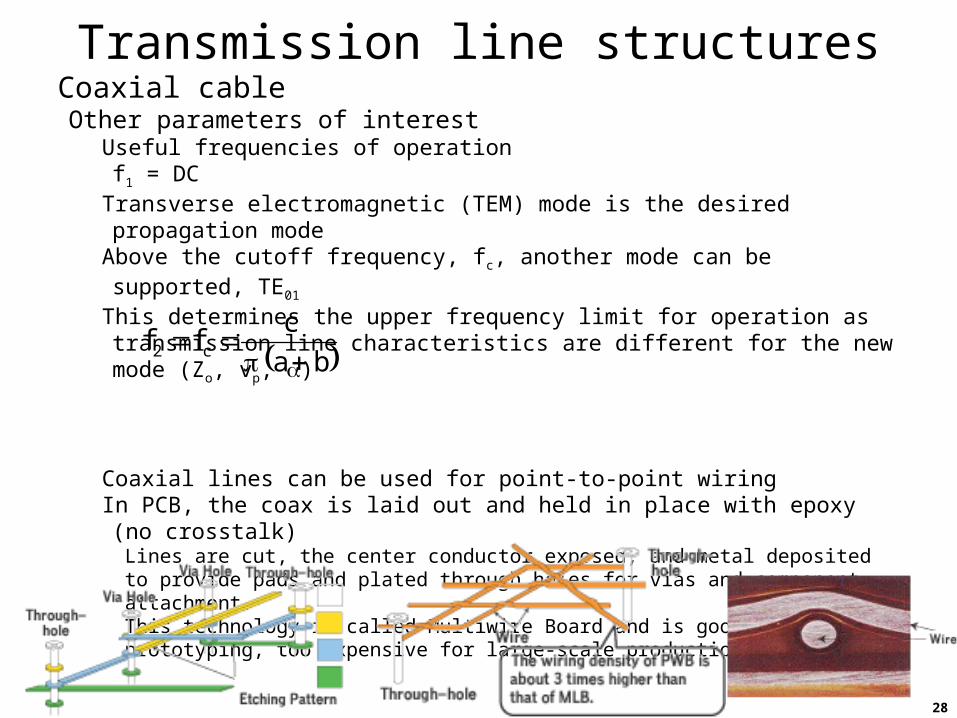
Transmission line structuresCoaxial cableOther parameters of interest
Useful frequencies of operationf1 = DC
Transverse electromagnetic (TEM) mode is the desired propagation modeAbove the cutoff frequency, fc, another mode can be supported, TE01
This determines the upper frequency limit for operation as transmission line characteristics are different for the new mode (Zo, vp, )
Coaxial lines can be used for point-to-point wiringIn PCB, the coax is laid out and held in place with epoxy (no crosstalk)
Lines are cut, the center conductor exposed, and metal deposited to provide pads and plated through holes for vias and component attachment.This technology is called Multiwire Board and is good for prototyping, too expensive for large-scale production.
ba
cff c2

29
Transmission line structuresStripline
f1 = DC, f2 = f (r, b, w, t)
Expressions are provided in supplemental information on course website
Simpler expressions for Zo available– Found in other sources
e.g., eqn. 4.92 on pg 188 in text, Appendix C of text pgs 436-439
– Less accurate– Only applicable for certain range of geometries (e.g., w/b ratios)
iprelationshcomplexb,w,,tfZ ro
rp
cv
fwtbZf orc ,,,,,,
ff rd ,tan,
250btand350bwfortw80
b9160Z
r
o ..,.
.ln

30
Transmission line structuresMicrostrip linessimilar to stripline
re = effective r for transmission line
similar relations for c and d
f1 = DC
Expressions are provided in supplemental information on course website
Simpler expressions for Zo available– Found in other sources
e.g., eqn 4.90 on pg 187 in text, Appendix C of text pgs 430-435
– Less accurate– Only applicable for certain range of geometries (e.g., w/h ratios)
w,h,,tfZ ro
rep
cv
fvaspossibledispersionftwhf prre ,,,,
151and02hw10fortw80
h985
411
87Z r
r
o
..,.
.ln
.

31
Transmission line structuresCoplanar strips
Coplanar waveguide
These structures are useful in interconnect systems board-to-board and chip-to-board
Expressions for Zo, c, d, and re are provided in supplemental information on
course website
kKkK30
Zre
o
k25.01.011.0k7.004.0hwk75.1whln775.0tanh2
1r
rre
1k7.0fork1
k12ln
1
7.0k0fork1
k12ln
1
kK
kK
1
2k1kandw2s
skwhere
kKkK120
Zre
o

32
Transmission line structuresEffects of manufacturing variations on electrical performanceSpecific values for transmission line parameters from design equations
t, r, w, b or h Zo, vp,
However manufacturing processes are not perfectfabrication errors introduced
Example – the trace width is specified to be 10 milsdue to process variations the fabricated trace width is
w = 10 mils 2.5 mils (3 variation 99.5% of traces lie within these limits)The board manufacturer specifies r = 4 0.1 (3) and h = 10 mil 0.2 mil
(3)
These uncertainties contribute to electrical performance variationsZo Zo , vp vp
These effects must be considered
So given t, r, w, h, how is Zo found ?

33
Transmission line structuresEffects of manufacturing variations on electrical performance
Various techniques available for finding Zo due to t, w, r • Monte-Carlo simulation
Let each parameter independently vary randomly and find the Zo
Repeat a large number of trialsFind the mean and standard deviation of the Zo results
• Find the sensitivity of Zo to variations in each parameter (t, r, w, h)
For example find Zo/t to find the sensitivity to thickness variations about
the nominal values
For small perturbations () treat the relationship Zo(t, r, w, h) as linear with
respect to each parameter
ho
h|Z
r
o|Z
wo
w|Z
to
t|Z
h
Z
Z
w
Z
t
Z
o
rro
o
o
where Zo/t is found through numerical differentiation
combine the various Zo terms in a root-sum-square (RSS) fashion
t
h,w,,tZh,w,,ttZ
t
Z roroo
2h|Z
2w|Z
2|Z
2t|ZZ oorooo
oZooro 3nomZZdeterminetonomnomtnomZ ...,,,

34
Transmission line summaryOverview of transmission lines
Requirements and characteristics of interestTypes of transmission linesParameters that contribute to characteristics of interest
Transmission line modelingCircuit modelRelating R, L, C, G to Zo, vp, Conductive loss factors
• Resistivity, skin effect, proximity effect
Dielectric loss factors• Conduction loss, polarization loss loss tangent
Wave propagation and reflections• Reflections at source and load ends• Voltage on transmission line vs. time
Design equations for transmission line structuresCoaxial cable, stripline, microstrip, coplanar strips and waveguide
Analysis of impact of manufacturing variations on Zo

35
Transmission line bonusWhy are 50- transmission lines used?
For coaxial cable –It is the result of a compromise between minimum insertion loss and maximum power handling capability
Insertion loss is minimum at: Zo ~ 77 for r = 1 (air)
Zo ~ 64 for r = 1.43 (PTFE foam)
Zo ~ 50 for r = 2.2 (solid PTFE)
Power handling is maximum at Zo = 30 Voltage handling is maximum at Zo ~ 60
For printed-circuit board transmission lines –Near-field EMI height above plane, hCrosstalk h2
Impedance hHigher impedance lines are difficult to fabricate (especially for small h)