Transition Modeling for General CFD Applications in ...€¦ · Transition Modeling for General CFD Applications in Aeronautics ... Re x = Reynolds number, ρLU ref /µ Re ... In

American Institute of Aeronautics and Astronautics

1

Transition Modeling for General CFD Applications in

Aeronautics

R.B. Langtry* and F.R. Menter

†

ANSYS CFX Germany, 83624 Otterfing, Germany

A new correlation-based transition model has been developed, which is built strictly on

local variables. As a result, the transition model is compatible with modern CFD techniques

such as unstructured grids and massively parallel execution. The model is based on two

transport equations, one for intermittency and one for a transition onset criterion in terms

of momentum thickness Reynolds number. The proposed transport equations do not

attempt to model the physics of the transition process (unlike e.g. turbulence models), but

form a framework for the implementation of transition correlations into general-purpose

CFD methods. The transition model was initially developed for turbomachinery flows. The

main goal of the present paper is to validate the model for predicting transition in

aeronautical flows. An incremental approach was used to validate the model, first on 2D

airfoils and then on progressively more complicated test cases such as a 3-element flap, a 3D

transonic wing and a full helicopter configuration. In all cases good agreement with the

available experimental data was observed. The authors believe that the current formulation

is a significant step forward in engineering transition modeling, as it allows the combination

of transition correlations with general purpose CFD codes. There is a strong potential that

the model will allow the 1st order effects of transition to be included in everyday industrial

CFD simulations.

Nomenclature

AoA = Angle of attach (deg.)

Cf = skin friction coefficient, τ/(0.5ρUref2)

FSTI = freestream turbulence intensity (percent), 100(2k/3)1/2

/Uref

k = turbulent kinetic energy

Rex = Reynolds number, ρLUref/µ

Reθ = momentum thickness Reynolds number, ρθU0/µ

Reθt = transition onset momentum thickness Reynolds number (based on freestream conditions), ρθtU0/µ

tθeR~ = local transition onset momentum thickness Reynolds number (obtained from a transport equation)

RT = viscosity ratio

Ry = wall-distance based turbulent Reynolds number

Rv = vorticity Reynolds number

S = absolute value of strain rate, (2SijSij)1/2

Sij = strain rate tensor, 0.5(∂ui/∂xj + ∂uj/∂xi)

Tu = turbulence intensity, 100(2k/3)1/2

/U U = local velocity

Uo = local freestream velocity

Uref = inlet reference velocity

u’ = local fluctuating streamwise velocity

x/C = axial distance over axial chord

y = distance to nearest wall

y+ = distance in wall coordinates, ρyµτ/µ

δ = boundary layer thickness

* Development, Staudenfeldweg 12, 83624 Otterfing, Germany.

† Head of Development, Staudenfeldweg 12, 83624 Otterfing, Germany.

AIAA 2005-522


2

θ = momentum thickness

λθ = pressure gradient parameter, (ρθ2/µ)(dU/ds)

µ = molecular viscosity

µt = eddy viscosity

ρ = density

τ = wall shear stress

Ω = absolute value of vorticity, (2ΩijΩij)1/2

Ωij = vorticity tensor, 0.5(∂ui/∂xj - ∂uj/∂xi)

ω = specific turbulence dissipation rate

Subscripts t = transition onset

s = streamline

I. Introduction

HE location of the onset and extent of transition are of major importance in the design and performance of many

aerospace devices where the wall-shear-stress or wall heat transfer is of interest. The transition process can also

have a strong influence on the separation behavior of boundary layers. As a result, transition can have a large effect

on the performance of airfoils and bluff bodies. In addition, the transition on any hypersonic vehicle has a significant

influence on the design of the thermal protection system and the allowable flight trajectories (Thompson et al.,

1998). For all these reasons, the performance, weight and costs associated with many aerospace vehicles can be

affected by transition.

There are a number of different transition mechanisms depending on the turbulence level of the external flow, the

pressure gradient along the laminar boundary layer, the geometrical details, the surface roughness and the freestream

Mach number. It is generally assumed that the most common transition mechanism on a vehicle in flight is natural

transition, which occurs due to the growth of unstable Tollmien-Schlichting waves. A transition mechanism that has

also received heightened attention - is the so-called bypass transition. Bypass transition is imposed on the boundary

layer by high levels of turbulence in the free-stream. This can occur when an airfoil encounters the wake from an

upstream device. Examples of bypass transition that can occur in flight are on the tail surfaces located in the wake

of a fuselage, or on flaps of a multi-element airfoil. Bypass transition is a complex phenomenon that depends

mainly on the turbulence intensity and the status of the boundary layer due to pressure gradients and separation.

There is also some empirical evidence suggesting that the structure of the turbulence (length scale) can have an

impact on the transition location (Mayle, 1991). As linear methods cannot be applied to bypass transition, there is

only a limited range of predictive engineering tools available, most of which are empirical (Savill, 1993, Savill

1996).

At present, there are mainly three concepts used to model transition in industry. The first is the application of low-

Reynolds number turbulence models. However, the ability of low-Re turbulence models to predict transition seems

to be coincidental. This is because the calibration of the damping functions is based on reproducing the viscous

sublayer behavior, not on predicting transition from laminar to turbulent flow. It is now generally accepted that the

use of turbulence models without any coupling to an intermittency equation appears to be a very delicate and often

unreliable method of predicting transition. In addition, low-Re turbulence models can only be applied to bypass

transition and are therefore not suitable for aerodynamic flows.

The second approach is the so-called eN method. It is based on the local, linear stability theory and the parallel flow

assumption in order to calculate the growth of the disturbance amplitude from the boundary layer neutral point to the

transition location (Smith and Gamberoni, 1956 and van Ingen, 1956). Once the disturbance amplitude ratio (eN)

exceeds the limiting N factor transition is assumed to start. The limiting N factor is not known in advance and must

be determined by calibration to wind tunnel or flight tests, hence the eN approach is considered a semi-empirical

method. For isolated airfoils, the eN method has been shown to produce very good transition predictions compared

to wind tunnel measurements (Stock and Haase, 2000). However, there remain some formidable barriers towards

applying the eN method to general aerospace applications. The first is that since the e

N method is based on linear

stability theory it cannot predict transition due to non-linear effects such as high freestream turbulence or surface

T


3

roughness. In addition, typical industrial Navier-Stokes solutions are not accurate enough to evaluate the stability

equations. As a result, the Navier-Stokes solution must be coupled to an accurate boundary layer code (Stock and

Haase, 2000). Finally, the need to track the growth of the disturbance amplitude ratio along the streamline results in

a significant issue for 3-dimensional flows where the streamline direction is not aligned with the grid. Because of

this limitation, the present authors are not aware of any instance in the open literature where the eN method has been

successfully applied to predict transition on a full 3-dimensional aircraft configuration. This is not to argue against

methods based on the stability analysis of the boundary layer. They are a central approach in the required spectrum

of transition models. However, they are not compatible with general-purpose CFD methods and cannot easily be

applied to arbitrary geometries.

The third approach to predicting transition, which is favored by the gas turbine industry, is the use of experimental

correlations. The correlations usually relate the free-stream turbulence intensity, Tu, and the local pressure gradient

to the transition momentum thickness Reynolds number. A typical example is the Abu-Ghannam and Shaw (1980)

correlation, which is based on a large number of experimental observations. While this method proves sufficiently

accurate, it poses numerical and programming challenges in Navier-Stokes codes. For classical correlation based

transition models, it is necessary to compare the actual momentum-thickness Reynolds numbers (Reθ) to the

transition value from the correlation (Reθt). This is not an easy task in a Navier-Stokes environment because the

boundary layer edge is not well defined and the integration will therefore depend on the implementation of a search

algorithm. The difficulties associated with non-local formulations are exaggerated by modern CFD methods that are

based on unstructured grids and massive parallel execution. Unstructured grids do not easily provide the

infrastructure needed to integrate global boundary layer parameters because the grid lines normal to the surface

cannot be easily identified. In the case of a general parallelised CFD code, the boundary layer can be split between

different CPUs making the integration tedious to perform in parallel. The use of correlation based transition criteria

is therefore incompatible with modern CFD codes.

In the present paper, a recent method for transition prediction (Menter et. Al. 2002, Menter et al. 2004, Langtry et al.

2004) will be described and extended to aeronautical flows. The model is based on two transport equations using

only local information and is therefore fully compatible with modern CFD codes. One of the central variables in the

formulation of model is the strain-rate (or sometimes vorticity, Van Driest and Blumer (1963)) Reynolds number:

Sy

y

uyv

µ

ρ

µ

ρ 22

Re =∂

∂= (1)

where y is the wall distance, ρ is the density, µ is the molecular viscosity and S is the absolute value of the strain

rate. The importance of ReV lies in the relation of its maximum value inside the boundary layer to the momentum

thickness Reynolds number ReΘ, of Blasius (or more generally Falkner-Skan) profiles (Menter et al. 2002):

:

)(Re193.2~)~,(Re max xyxV Θ (2)

where y~ is the location where ReV has its maximum. The function Reν can be used on physical reasoning, by

arguing that the combination of y2S is responsible for the growth of disturbances inside the boundary layer, whereas

ρµν /= is responsible for their damping. As y2S grows with the thickness of the boundary layer and ν stays

constant, transition will take place once a critical value of Reν is reached. The connection between the growth of

disturbances and the function Reν was shown by Van Driest and Blumer (1963) in comparison with experimental

data. The model proposed by Langtry & Sjolander (2002) and Walters & Leylek, (2002) use Reν in physics-based

arguments. These models appear superior to conventional low-Re models, as they implicitly contain information of

the thickness of the boundary layer. Nevertheless, the close integration of viscous sublayer damping and transition

prediction does not allow an independent calibration of both sub-models.

In an alternative approach, Menter et al. (2002), Menter et al. (2004) and Langtry et al. (2004) proposed a

combination of the strain-rate Reynolds number with experimental transition correlations using standard transport

equations. Due to the separation of viscous sublayer damping and transition prediction, the new method has

provided the flexibility for introducing additional transition effects with relative ease. Currently, the main missing

extensions are cross-flow instabilities and high-speed flow correlations and these do not pose any significant


4

obstacles. The concept of linking the transition model with experimental data has proven to be an essential strength

of the model and this is difficult to achieve with closures based on a physical modeling of these diverse phenomena.

The present transition model is built on a transport equation for intermittency, which can be used to trigger transition

locally. In addition, to the transport equation for the intermittency, a second transport equation is solved for the

transition onset momentum-thickness Reynolds number. This is required in order to capture the non-local influence

of the turbulence intensity, which changes due to the decay of the turbulence kinetic energy in the free-stream, as

well as due to changes in the free-stream velocity outside the boundary layer. This second transport equation is an

essential part of the model as it ties the empirical correlation to the onset criteria in the intermittency equation. It

thereby allows the models use in general geometries and over multiple airfoils, without additional information on

the geometry. The intermittency function is coupled with the SST k-ω based turbulence model (Menter 1994). It is

used to turn on the production term of the turbulent kinetic energy downstream of the transition point based on the

relation between transition momentum-thickness and strain-rate Reynolds number. As the strain-rate Reynolds

number is a local property, the present formulation avoids another very severe shortcoming of the correlation-based

models, namely their limitation to 2D flows. It therefore allows the simulation of transition in 3D flows originating

from different walls. The formulation of the intermittency equation has also been extended to account for the rapid

onset of transition caused by separation of the laminar boundary layer. In addition, the model can be fully calibrated

with internal or proprietary transition onset and transition length correlations. The correlations can also be extended

to flows with rough walls or to flows with cross-flow instability. It should be stressed that the proposed transport

equations do not attempt to model the physics of the transition process (unlike e.g. turbulence models), but form a

framework for the implementation of correlation-based models into general-purpose CFD methods. In order to

distinguish the present concept from physics based transport modeling, it is named LCTM – Local Correlation-based

Transition Modeling.

The present transition model was first presented at the IGTI 2004 conference in two separate papers (Menter et al.,

2004 and Langtry et al., 2004). The first paper described the mathematical formulation of the model and some of the

basic building block experiments for its calibration. The second paper detailed many of the industrial test cases that

were used to validate the model including 3D and unsteady test cases, which before have been outside the realm of

empirical correlation based transition models. Most of these test cases where for turbomachinery applications where

bypass transition was the dominant transition mode.

The goal of the present paper is to demonstrate some modifications that have been made to the transition model that

have improved the predictions of natural transition and to validate the model for predicting transition on full 3-

dimensional aerospace vehicle configurations.

II. Transition Model Formulation

The present transition model formulation is described very briefly for completeness, a detailed description of the

model can be found in Menter et al., 2004 and Langtry et al., 2004. It should be noted that a few changes have been

made to the model in order to improve the predictions of natural transition. These include:

1. An improved transition onset correlation that results in improved predictions for both natural and bypass

transition.

2. A modification to the separation induced transition modification that prevents it from causing early

transition near the separation point.

3. Some adjustments of the model coefficients in order to better account for flow history effects on the

transition onset location.

It was expected that different groups will make numerous improvements to the model and consequently a naming

convention was introduced in Menter et al. (2004) in order to keep track of the various model versions. The basic

model framework (transport equations without any correlations) was called the γ-Reθ transition model. The version

number given in Menter et al. (2004) was called CFX-v-1.0. Based on this naming convention, the present model

with the above modifications will be referred to as the γ-Reθ model, CFX-v-1.1. The present transition model is

briefly summarized in the following pages.


5

The transport equation for the intermittency, γ, reads:

( ) ( )

∂

∂

+

∂

∂+−+−=

∂

∂+

∂

∂

j

t

jj

j

xxEPEP

x

U

t

γ

σ

µµ

γρργ

γ

γγγγ 2211 (3)

The transition sources are defined as follows:

[ ] γγρ γγγα

11111 ; PcEFScFP e

c

onsetalength == (4)

where S is the strain rate magnitude. Flength is an empirical correlation that controls the length of the transition

region. The destruction/relaminarization sources are defined as follows:

γγρ γγγ 22222 ; PcEFcP eturba =Ω= (5)

where Ω is the vorticity magnitude. The transition onset is controlled by the following functions:

µω

ρ

µ

ρ kR

SyTV == ;Re

2

(6)

( )( )0.2,,maxmin;Re193.2

Re 4

1121 onsetonsetonset

c

vonset FFFF =

⋅=

θ

(7)

( )4

4

32

3

3 ;0,max;0,5.2

1max

−

=−=

−=

TR

turbonsetonsetonsetT

onset eFFFFR

F (8)

Reθc is the critical Reynolds number where the intermittency first starts to increase in the boundary layer. This

occurs upstream of the transition Reynolds number, tθeR

~, and the difference between the two must be obtained

from an empirical correlation. Both the Flength and Reθc correlations are functions of tθeR

~.

The constants for the intermittency equation are:

;0.1;06.0;50;5.0;0.2;0.1 2211 ====== γα σaeae ccccc (9)

The modification for separation-induced transition is:

( )sepeff

R

reattachtreattach

c

vsep

T

eFFF γγγγ θ

θ

,max;;2,0,1Re235.3

Remax2min

4

20 ==

−

⋅=

−

(10)

The model constants in Equ. 10 have been adjusted from those of Menter et al (2004) in order to improve the

predictions of separated flow transition. The main difference is the constant that controls the relation between Rev

and Reθc was changed from 2.193, it’s value for a Blasius boundary layer, to 3.235, the value at a separation point

where the shape factor is 3.5 (see for example Figure 2 in Menter et al, 2004). The boundary condition for γ at a

wall is zero normal flux while for an inlet γ is equal to 1.0.


6

The transport equation for the transition momentum thickness Reynolds number, tθeR

~, reads:

( ) ( )

( )

∂

∂+

∂

∂+=

∂

∂+

∂

∂

j

ttt

j

t

j

tjt

xxP

x

U

t

θθθ

θθ µµσρρ eR

~eR

~eR

~ (11)

The source term is defined as follows:

( )( )2

500;0.1eR

~Re

UtF

tcP ttttt

ρ

µρθθθθθ =−−= (12)

−

−−⋅=

−

0.1,/10.1

/10.1,maxmin

2

2

2

4

e

e

y

waketc

ceFF

γδθ

(13)

BLBLBL

tBL

U

y

Uδδθδ

ρ

µθ θ ⋅

Ω===

50;

2

15;

eR~

(14)

2

51

Re2

;Re

+−

== E

wake eFy

ω

µ

ρωω

(15)

The model constants for the tθeR

~ equation are:

0.2;03.0 == ttc θθ σ (16)

The boundary condition for tθeR

~ at a wall is zero flux. The boundary condition for

tθeR~

at an inlet should be

calculated from the empirical correlation based on the inlet turbulence intensity.

The model contains three empirical correlations. ReΘt is the transition onset as observed in experiments. This has

been modified from Menter et al. (2004) in order to improve the predictions for natural transition. It is used in

Eq.12. Flength is the length of the transition zone and goes into Eq. 4. ReΘc is the point where the model is activated in

order to match both, ReΘt and Flength, it goes into Eq. 7. At present these empirical correlations are proprietary and

are not given in the paper.

( ) ( ) ( )tctlengtht ffFTuf ΘΘΘΘ === eR~

Re;eR~

;,Re λ (17)

The first empirical correlation is a function of the local turbulence intensity, Tu, and the Thwaites’ pressure gradient

coefficient λθ defined as:

λθ = (θ2/ν)dU/ds (18)

where dU/ds is the acceleration in the streamwise direction.


7

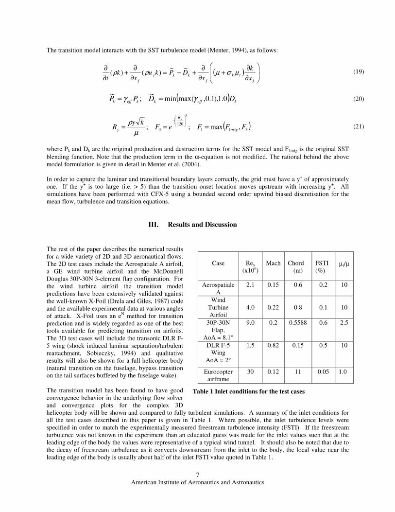
The transition model interacts with the SST turbulence model (Menter, 1994), as follows:

( )

∂

∂+

∂

∂+−=

∂

∂+

∂

∂

j

tk

j

kkj

j x

k

xDPku

xk

tµσµρρ

~~)()( (19)

( )keffkkeffk DDPP 0.1),1.0,max(min

~;

~γγ == (20)

( )311

120

3 ,max;;

8

FFFeFky

R orig

R

y

y

===

−

µ

ρ (21)

where Pk and Dk are the original production and destruction terms for the SST model and F1orig is the original SST

blending function. Note that the production term in the ω-equation is not modified. The rational behind the above

model formulation is given in detail in Menter et al. (2004).

In order to capture the laminar and transitional boundary layers correctly, the grid must have a y+ of approximately

one. If the y+ is too large (i.e. > 5) than the transition onset location moves upstream with increasing y

+. All

simulations have been performed with CFX-5 using a bounded second order upwind biased discretisation for the

mean flow, turbulence and transition equations.

III. Results and Discussion

The rest of the paper describes the numerical results

for a wide variety of 2D and 3D aeronautical flows.

The 2D test cases include the Aerospatiale A airfoil,

a GE wind turbine airfoil and the McDonnell

Douglas 30P-30N 3-element flap configuration. For

the wind turbine airfoil the transition model

predictions have been extensively validated against

the well-known X-Foil (Drela and Giles, 1987) code

and the available experimental data at various angles

of attack. X-Foil uses an eN method for transition

prediction and is widely regarded as one of the best

tools available for predicting transition on airfoils.

The 3D test cases will include the transonic DLR F-

5 wing (shock induced laminar separation/turbulent

reattachment, Sobieczky, 1994) and qualitative

results will also be shown for a full helicopter body

(natural transition on the fuselage, bypass transition

on the tail surfaces buffeted by the fuselage wake).

The transition model has been found to have good

convergence behavior in the underlying flow solver

and convergence plots for the complex 3D

helicopter body will be shown and compared to fully turbulent simulations. A summary of the inlet conditions for

all the test cases described in this paper is given in Table 1. Where possible, the inlet turbulence levels were

specified in order to match the experimentally measured freestream turbulence intensity (FSTI). If the freestream

turbulence was not known in the experiment than an educated guess was made for the inlet values such that at the

leading edge of the body the values were representative of a typical wind tunnel. It should also be noted that due to

the decay of freestream turbulence as it convects downstream from the inlet to the body, the local value near the

leading edge of the body is usually about half of the inlet FSTI value quoted in Table 1.

Case

Rex

(x106)

Mach

Chord

(m)

FSTI

(%)

µt/µ

Aerospatiale

A

2.1 0.15 0.6 0.2 10

Wind

Turbine

Airfoil

4.0

0.22

0.8

0.1

10

30P-30N

Flap,

AoA = 8.1°

9.0 0.2 0.5588 0.6 2.5

DLR F-5

Wing

AoA = 2°

1.5 0.82 0.15 0.5 10

Eurocopter

airframe

30 0.12 11 0.05 1.0

Table 1 Inlet conditions for the test cases


8

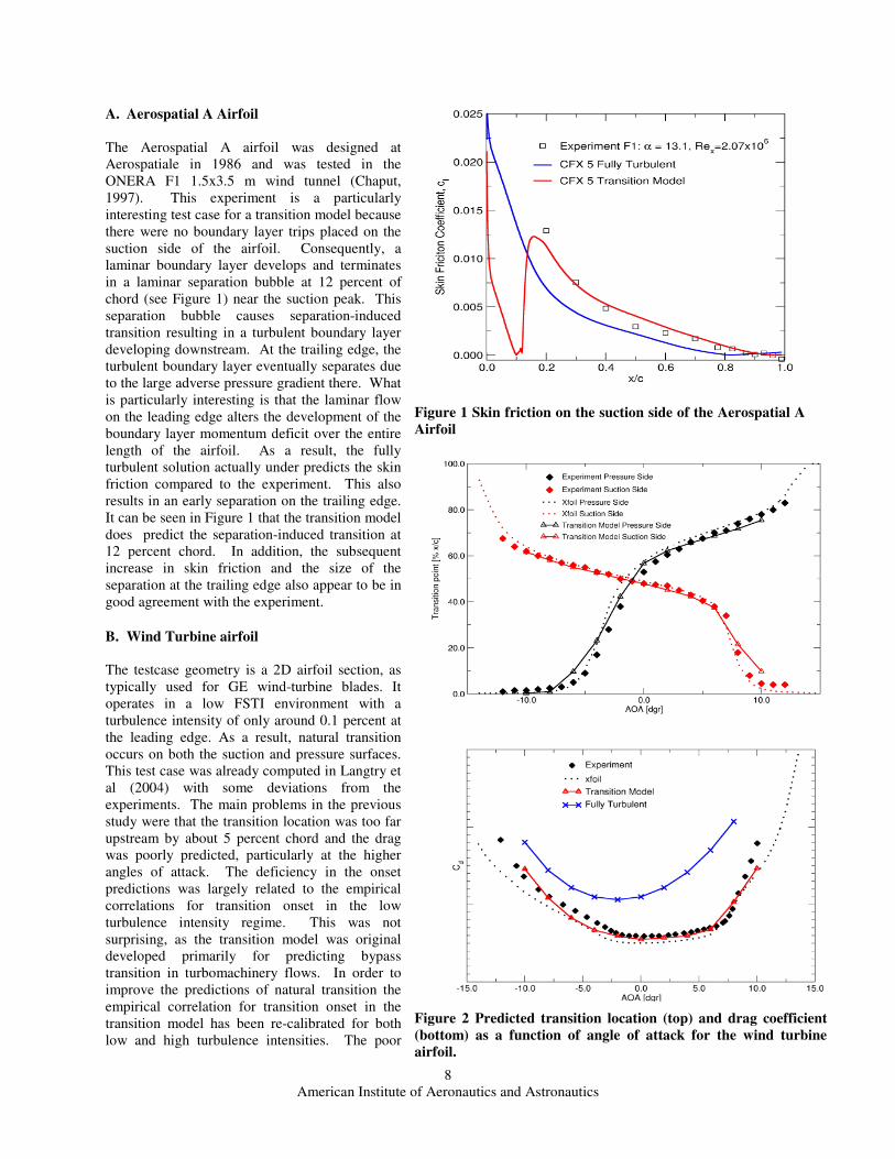
A. Aerospatial A Airfoil

The Aerospatial A airfoil was designed at

Aerospatiale in 1986 and was tested in the

ONERA F1 1.5x3.5 m wind tunnel (Chaput,

1997). This experiment is a particularly

interesting test case for a transition model because

there were no boundary layer trips placed on the

suction side of the airfoil. Consequently, a

laminar boundary layer develops and terminates

in a laminar separation bubble at 12 percent of

chord (see Figure 1) near the suction peak. This

separation bubble causes separation-induced

transition resulting in a turbulent boundary layer

developing downstream. At the trailing edge, the

turbulent boundary layer eventually separates due

to the large adverse pressure gradient there. What

is particularly interesting is that the laminar flow

on the leading edge alters the development of the

boundary layer momentum deficit over the entire

length of the airfoil. As a result, the fully

turbulent solution actually under predicts the skin

friction compared to the experiment. This also

results in an early separation on the trailing edge.

It can be seen in Figure 1 that the transition model

does predict the separation-induced transition at

12 percent chord. In addition, the subsequent

increase in skin friction and the size of the

separation at the trailing edge also appear to be in

good agreement with the experiment.

B. Wind Turbine airfoil

The testcase geometry is a 2D airfoil section, as

typically used for GE wind-turbine blades. It

operates in a low FSTI environment with a

turbulence intensity of only around 0.1 percent at

the leading edge. As a result, natural transition

occurs on both the suction and pressure surfaces.

This test case was already computed in Langtry et

al (2004) with some deviations from the

experiments. The main problems in the previous

study were that the transition location was too far

upstream by about 5 percent chord and the drag

was poorly predicted, particularly at the higher

angles of attack. The deficiency in the onset

predictions was largely related to the empirical

correlations for transition onset in the low

turbulence intensity regime. This was not

surprising, as the transition model was original

developed primarily for predicting bypass

transition in turbomachinery flows. In order to

improve the predictions of natural transition the

empirical correlation for transition onset in the

transition model has been re-calibrated for both

low and high turbulence intensities. The poor

Figure 1 Skin friction on the suction side of the Aerospatial A

Airfoil

Figure 2 Predicted transition location (top) and drag coefficient

(bottom) as a function of angle of attack for the wind turbine

airfoil.


9

predictions of the drag coefficient were caused by inadequate grid resolution in the trailing edge region of the airfoil.

In the present paper a refined grid has been used, resulting in much better drag predictions for all angles of attack.

The inlet conditions for k and ω have been selected as to match the transition location for zero angle of attack. They

have than been kept at these values for all other angle of attack simulations. This is a similar calibration for wind-

tunnel conditions as typically also used for the eN method. The transition locations vs. angle of attack predicted by

the transition model are shown in Figure 2 (top). Wind tunnel results and XFOIL (v6.8) predictions (where transition

is predicted by the eN method) are plotted for comparison. The experimental data were obtained using a stethoscope

method. With the new empirical correlations, the transition model captures the dependence of the transition location

on the angle of attack in good agreement with the data. Figure 2 (bottom) shows the predicted drag coefficient as a

function of angle of attack. Included are results from a transitional computation using the XFOIL code and from

fully turbulent simulations. Clearly, the drag coefficient predictions from the transitional computation are in good

agreement with the experimentally measured drag.

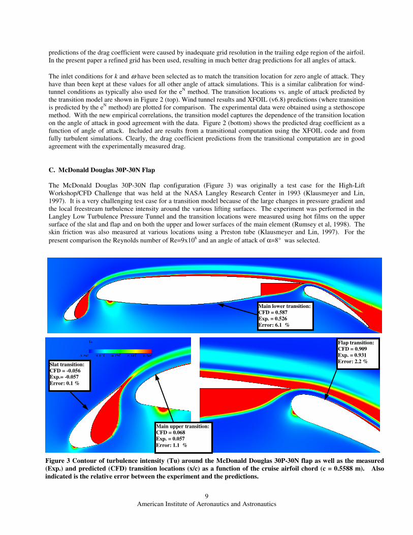
C. McDonald Douglas 30P-30N Flap

The McDonald Douglas 30P-30N flap configuration (Figure 3) was originally a test case for the High-Lift

Workshop/CFD Challenge that was held at the NASA Langley Research Center in 1993 (Klausmeyer and Lin,

1997). It is a very challenging test case for a transition model because of the large changes in pressure gradient and

the local freestream turbulence intensity around the various lifting surfaces. The experiment was performed in the

Langley Low Turbulence Pressure Tunnel and the transition locations were measured using hot films on the upper

surface of the slat and flap and on both the upper and lower surfaces of the main element (Rumsey et al, 1998). The

skin friction was also measured at various locations using a Preston tube (Klausmeyer and Lin, 1997). For the

present comparison the Reynolds number of Re=9x106 and an angle of attack of α=8° was selected.

Figure 3 Contour of turbulence intensity (Tu) around the McDonald Douglas 30P-30N flap as well as the measured

(Exp.) and predicted (CFD) transition locations (x/c) as a function of the cruise airfoil chord (c = 0.5588 m). Also

indicated is the relative error between the experiment and the predictions.

Slat transition:

CFD = -0.056

Exp.= -0.057

Error: 0.1 %

Main upper transition:

CFD = 0.068

Exp. = 0.057

Error: 1.1 %

Main lower transition:

CFD = 0.587

Exp. = 0.526

Error: 6.1 %

Flap transition:

CFD = 0.909

Exp. = 0.931

Error: 2.2 %


10

A contour plot of the predicted turbulence

intensity around the flap is shown in Figure 3.

Also indicated are the various transition

locations that were measured in the experiment

(Exp.) as well as the locations that were

predicted by the transition model (CFD). As no

information was available on the freestream

turbulence level in the experiment, the inlet

turbulence values for this case were estimated

so that the slat transition location matched the

experiment. The transition locations on the

main element and the flap are the outcome of

selecting that freestream turbulence level. In

the computations, the onset of transition was

judged as the location were the skin friction

first started to increase due to the production of

turbulent kinetic energy in the boundary layer.

In general the agreement between the measured

and predicted transition locations is good. The

worst error was on the lower surface of the

main element were the predicted transition

location was too far downstream by

approximately 6 percent of the cruise airfoil

chord, c.

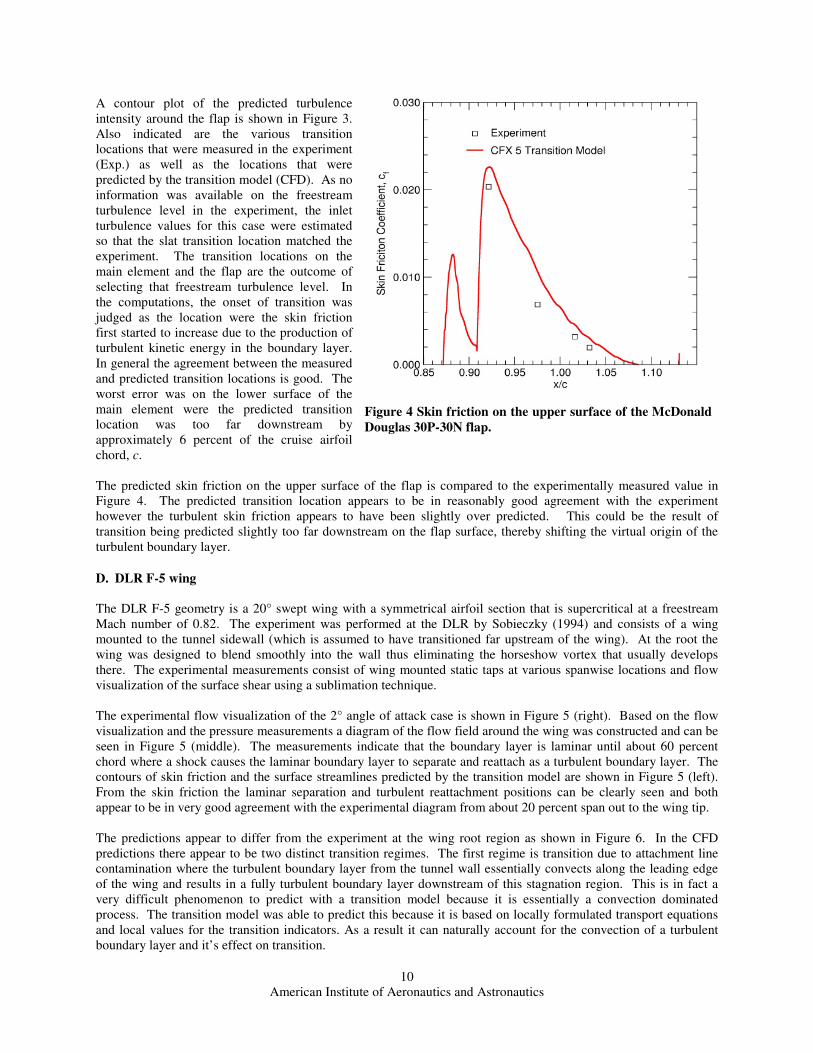
The predicted skin friction on the upper surface of the flap is compared to the experimentally measured value in

Figure 4. The predicted transition location appears to be in reasonably good agreement with the experiment

however the turbulent skin friction appears to have been slightly over predicted. This could be the result of

transition being predicted slightly too far downstream on the flap surface, thereby shifting the virtual origin of the

turbulent boundary layer.

D. DLR F-5 wing

The DLR F-5 geometry is a 20° swept wing with a symmetrical airfoil section that is supercritical at a freestream

Mach number of 0.82. The experiment was performed at the DLR by Sobieczky (1994) and consists of a wing

mounted to the tunnel sidewall (which is assumed to have transitioned far upstream of the wing). At the root the

wing was designed to blend smoothly into the wall thus eliminating the horseshow vortex that usually develops

there. The experimental measurements consist of wing mounted static taps at various spanwise locations and flow

visualization of the surface shear using a sublimation technique.

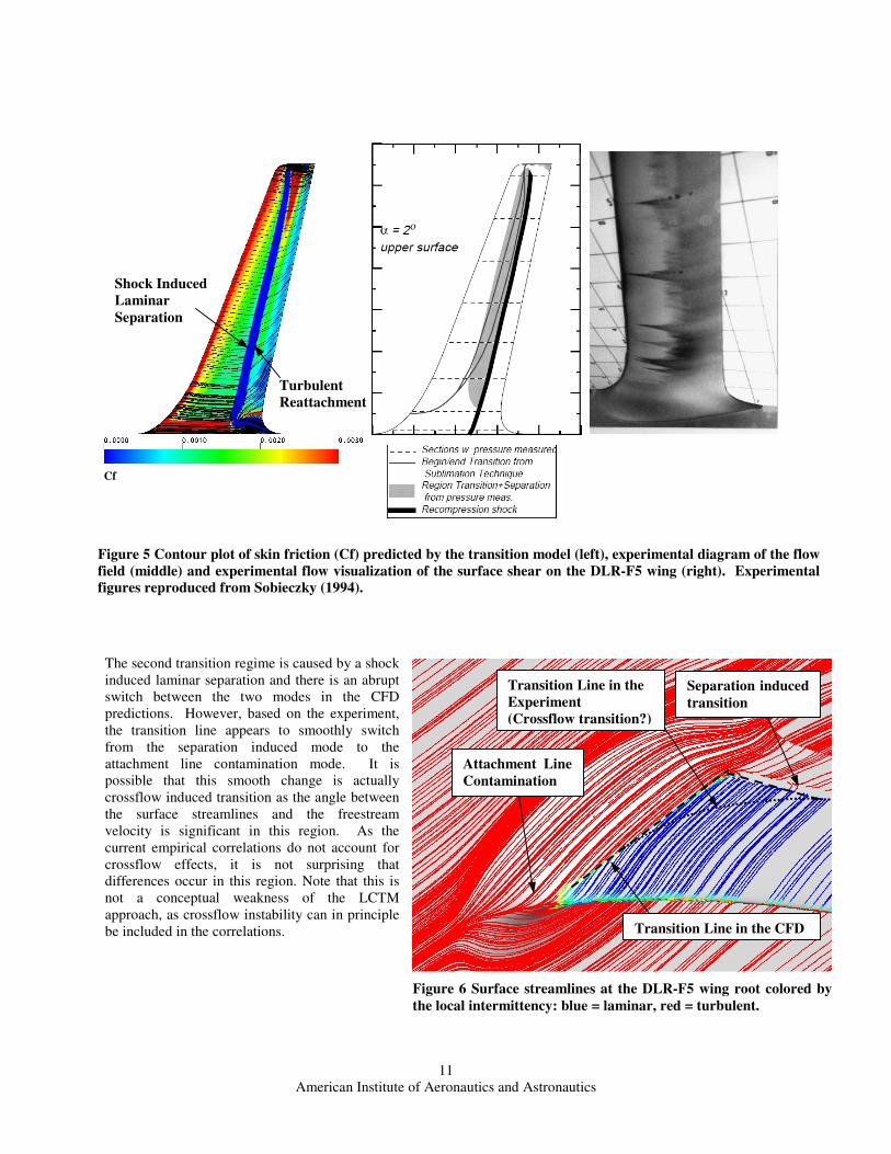
The experimental flow visualization of the 2° angle of attack case is shown in Figure 5 (right). Based on the flow

visualization and the pressure measurements a diagram of the flow field around the wing was constructed and can be

seen in Figure 5 (middle). The measurements indicate that the boundary layer is laminar until about 60 percent

chord where a shock causes the laminar boundary layer to separate and reattach as a turbulent boundary layer. The

contours of skin friction and the surface streamlines predicted by the transition model are shown in Figure 5 (left).

From the skin friction the laminar separation and turbulent reattachment positions can be clearly seen and both

appear to be in very good agreement with the experimental diagram from about 20 percent span out to the wing tip.

The predictions appear to differ from the experiment at the wing root region as shown in Figure 6. In the CFD

predictions there appear to be two distinct transition regimes. The first regime is transition due to attachment line

contamination where the turbulent boundary layer from the tunnel wall essentially convects along the leading edge

of the wing and results in a fully turbulent boundary layer downstream of this stagnation region. This is in fact a

very difficult phenomenon to predict with a transition model because it is essentially a convection dominated

process. The transition model was able to predict this because it is based on locally formulated transport equations

and local values for the transition indicators. As a result it can naturally account for the convection of a turbulent

boundary layer and it’s effect on transition.

Figure 4 Skin friction on the upper surface of the McDonald

Douglas 30P-30N flap.


11

The second transition regime is caused by a shock

induced laminar separation and there is an abrupt

switch between the two modes in the CFD

predictions. However, based on the experiment,

the transition line appears to smoothly switch

from the separation induced mode to the

attachment line contamination mode. It is

possible that this smooth change is actually

crossflow induced transition as the angle between

the surface streamlines and the freestream

velocity is significant in this region. As the

current empirical correlations do not account for

crossflow effects, it is not surprising that

differences occur in this region. Note that this is

not a conceptual weakness of the LCTM

approach, as crossflow instability can in principle

be included in the correlations.

Figure 5 Contour plot of skin friction (Cf) predicted by the transition model (left), experimental diagram of the flow

field (middle) and experimental flow visualization of the surface shear on the DLR-F5 wing (right). Experimental

figures reproduced from Sobieczky (1994).

Figure 6 Surface streamlines at the DLR-F5 wing root colored by

the local intermittency: blue = laminar, red = turbulent.

Shock Induced

Laminar

Separation

Turbulent

Reattachment

Cf

Attachment Line

Contamination

Transition Line in the

Experiment

(Crossflow transition?)

Separation induced

transition

Transition Line in the CFD


12

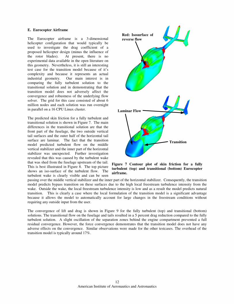
E. Eurocopter Airframe

The Eurocopter airframe is a 3-dimensional

helicopter configuration that would typically be

used to investigate the drag coefficient of a

proposed helicopter design (minus the influence of

the rotor blades). At present, there is no

experimental data available in the open literature on

this geometry. Nevertheless, it is still an interesting

test case for the transition model because of it’s

complexity and because it represents an actual

industrial geometry. Our main interest is in

comparing the fully turbulent solution to the

transitional solution and in demonstrating that the

transition model does not adversely affect the

convergence and robustness of the underlying flow

solver. The grid for this case consisted of about 6

million nodes and each solution was run overnight

in parallel on a 16 CPU Linux cluster.

The predicted skin friction for a fully turbulent and

transitional solution is shown in Figure 7. The main

differences in the transitional solution are that the

front part of the fuselage, the two outside vertical

tail surfaces and the outer half of the horizontal tail

surface are laminar. The fact that the transition

model predicted turbulent flow on the middle

vertical stabilizer and the inner part of the horizontal

stabilizer was unexpected. Further investigation

revealed that this was caused by the turbulent wake

that was shed from the fuselage upstream of the tail.

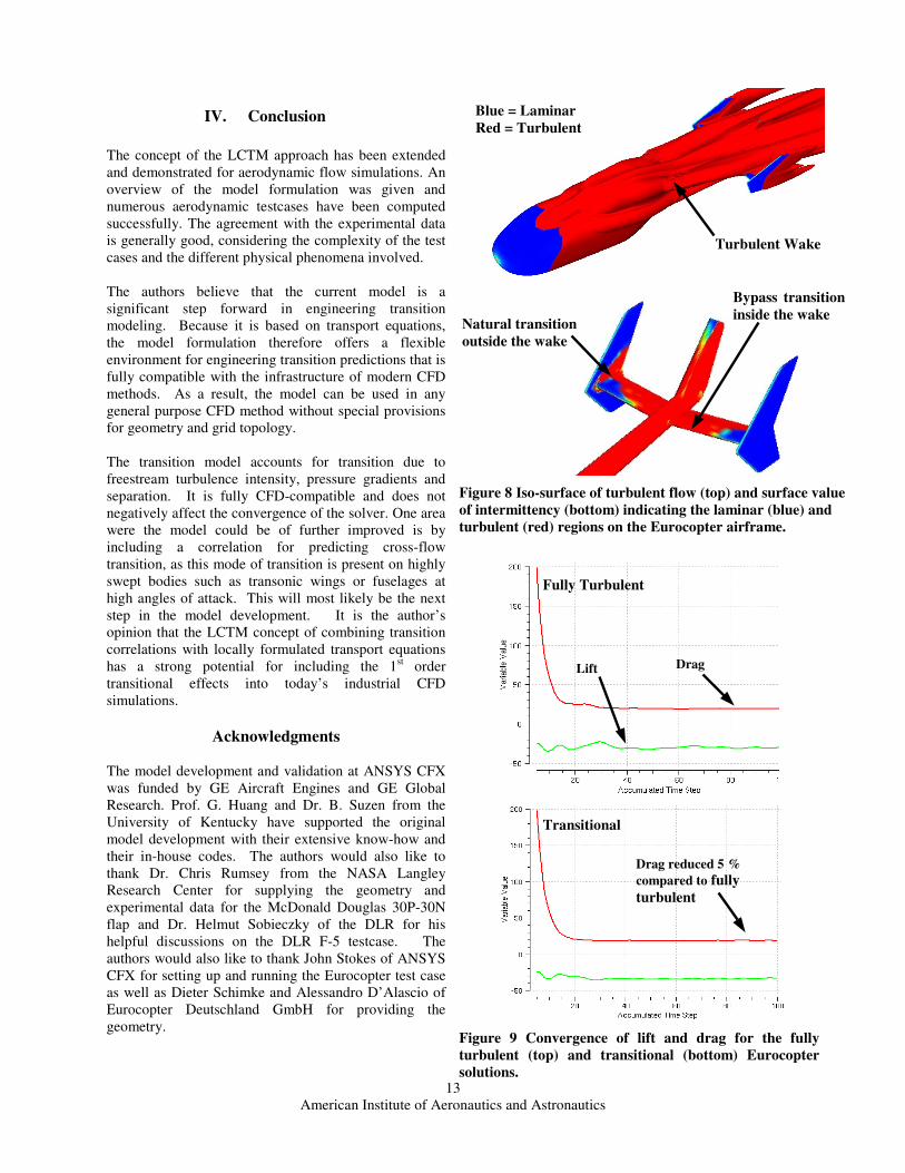
This is best illustrated in Figure 8. The top picture

shows an iso-surface of the turbulent flow. The

turbulent wake is clearly visible and can be seen

passing over the middle vertical stabilizer and the inner part of the horizontal stabilizer. Consequently, the transition

model predicts bypass transition on these surfaces due to the high local freestream turbulence intensity from the

wake. Outside the wake, the local freestream turbulence intensity is low and as a result the model predicts natural

transition. This is clearly a case where the local formulation of the transition model is a significant advantage

because it allows the model to automatically account for large changes in the freestream conditions without

requiring any outside input from the user.

The convergence of lift and drag is shown in Figure 9 for the fully turbulent (top) and transitional (bottom)

solutions. The transitional flow on the fuselage and tails resulted in a 5 percent drag reduction compared to the fully

turbulent solution. A slight oscillation of the separation zones behind the engine compartment prevented a full

residual convergence. However, the force convergence demonstrates that the transition model does not have any

adverse effects on the convergence. Similar observations were made for the other testcases. The overhead of the

transition model is typically around 17%.

Figure 7 Contour plot of skin friction for a fully

turbulent (top) and transitional (bottom) Eurocopter

airframe.

Red: Isosurface of

reverse flow

Laminar Flow

Transition


13

IV. Conclusion

The concept of the LCTM approach has been extended

and demonstrated for aerodynamic flow simulations. An

overview of the model formulation was given and

numerous aerodynamic testcases have been computed

successfully. The agreement with the experimental data

is generally good, considering the complexity of the test

cases and the different physical phenomena involved.

The authors believe that the current model is a

significant step forward in engineering transition

modeling. Because it is based on transport equations,

the model formulation therefore offers a flexible

environment for engineering transition predictions that is

fully compatible with the infrastructure of modern CFD

methods. As a result, the model can be used in any

general purpose CFD method without special provisions

for geometry and grid topology.

The transition model accounts for transition due to

freestream turbulence intensity, pressure gradients and

separation. It is fully CFD-compatible and does not

negatively affect the convergence of the solver. One area

were the model could be of further improved is by

including a correlation for predicting cross-flow

transition, as this mode of transition is present on highly

swept bodies such as transonic wings or fuselages at

high angles of attack. This will most likely be the next

step in the model development. It is the author’s

opinion that the LCTM concept of combining transition

correlations with locally formulated transport equations

has a strong potential for including the 1st order

transitional effects into today’s industrial CFD

simulations.

Acknowledgments

The model development and validation at ANSYS CFX

was funded by GE Aircraft Engines and GE Global

Research. Prof. G. Huang and Dr. B. Suzen from the

University of Kentucky have supported the original

model development with their extensive know-how and

their in-house codes. The authors would also like to

thank Dr. Chris Rumsey from the NASA Langley

Research Center for supplying the geometry and

experimental data for the McDonald Douglas 30P-30N

flap and Dr. Helmut Sobieczky of the DLR for his

helpful discussions on the DLR F-5 testcase. The

authors would also like to thank John Stokes of ANSYS

CFX for setting up and running the Eurocopter test case

as well as Dieter Schimke and Alessandro D’Alascio of

Eurocopter Deutschland GmbH for providing the

geometry.

Figure 8 Iso-surface of turbulent flow (top) and surface value

of intermittency (bottom) indicating the laminar (blue) and

turbulent (red) regions on the Eurocopter airframe.

Figure 9 Convergence of lift and drag for the fully

turbulent (top) and transitional (bottom) Eurocopter

solutions.

Blue = Laminar

Red = Turbulent

Turbulent Wake

Bypass transition

inside the wake Natural transition

outside the wake

Fully Turbulent

Transitional

Drag reduced 5 %

compared to fully

turbulent

Drag Lift


14

References

1Thompson, R.A., Hamilton II, H.H, Berry, S.A., Horvath, T.J., and Nowak, R.J., “Hypersonic Boundary-Layer Transition

for X-33 Phase II Vehicle” AIAA-1998-0867, 36th Aerospace Sciences Meeting & Exhibit, 1998. 2Mayle, R.E., “The Role of Laminar-Turbulent Transition in Gas Turbine Engines,” ASME Journal of Turbomachinery, Vol.

113, 1991, pp. 509-537. 3Savill, A.M., “Some recent progress in the turbulence modelling of by-pass transition”, In: R.M.C. So, C.G. Speziale and

B.E. Launder, Eds.: Near-Wall Turbulent Flows, Elsevier, 1993, pp. 829. 4Savill, A.M., “One-point closures applied to transition, Turbulence and Transition Modelling”, M. Hallbäck et al., eds.,

Kluwer, 1996, pp. 233-268. 5Smith, A.M.O. and Gamberoni, N., “Transition, Pressure Gradient and Stability Theory,” Douglas Aircraft Company, Long

Beach, Calif. Rep. ES 26388, 1956. 6Van Ingen, J.L., “A suggested Semi-Empirical Method for the Calculation of the Boundary Layer Transition Region,” Univ.

of Delft, Dept. Aerospace Engineering, Delft, The Netherlands, Rep. VTH-74, 1956. 7Stock, H.W. and Haase, W., “Navier-Stokes Airfoil Computations with eN Transition Prediction Including Transitional Flow

Regions,” AIAA Journal, Vol. 38, No. 11, 2000, pp. 2059 – 2066. 8Abu-Ghannam, B.J. and Shaw, R., “Natural Transition of Boundary Layers-The Effects of Turbulence, Pressure Gradient,

and Flow History,” Journal of Mechanical Engineering Science, Vol. 22, No. 5, 1980, pp. 213 – 228. 9Van Driest, E.R. and Blumer, C.B., “Boundary Layer Transition: Freestream Turbulence and Pressure Gradient Effects,”

AIAA Journal, Vol. 1, No. 6, June 1963, pp. 1303-1306. 10Langtry, R.B., and Sjolander, S.A., “Prediction of Transition for Attached and Separated Shear Layers in Turbomachinery”,

AIAA-2002-3643, 38th AIAA/ASME/SAE/ASEE Joint Propulsion Conference and Exhibit, 2002. 12Walters, D.K and Leylek, J.H. “A New Model for Boundary-Layer Transition Using a Single-Point Rans Approach”. ASME

IMECE’02, IMECE2002-HT-32740, 2002. 13Menter, F. R., Esch, T. and Kubacki, S., “Transition Modelling Based on Local Variables”, 5th International Symposium on

Turbulence Modeling and Measurements, Spain, 2002. 14Menter, F.R., Two-equation eddy-viscosity turbulence models for engineering applications, AIAA Journal, Vol. 32, No. 8,

1994, pp. 1598-1605. 15Menter, F.R., Langtry, R.B., Likki, S.R., Suzen, Y.B., Huang, P.G., and Völker, S., "A Correlation based Transition Model

using Local Variables Part 1- Model Formulation ASME-GT2004-53452, ASME TURBO EXPO 2004, Vienna, Austria. 16Langtry, R.B., Menter, F.R., Likki, S.R., Suzen, Y.B., Huang, P.G., and Völker, S., "A Correlation based Transition Model

using Local Variables Part 2 – Test Cases and Industrial Applications ASME-GT2004-53454, ASME TURBO EXPO 2004,

Vienna, Austria. 17Drela, M., and Giles, M. B., “Viscous-Inviscid Analysis of Transonic and Low Reynolds Number Airfoils,” AIAA Journal,

Vol. 25, No. 10, October 1987, pp. 1347 – 1355. 18Sobieczky, H., “ DLR – F5: Test Wing for CFD and Applied Aerodynamics”, Test Case B-5 in AGARD FDP Advisory

Report AR 303: Test Cases for CFD Validation, 1994. 19Chaput, E., “Chapter 3: Application-Oriented Synthesis of Work Presented in Chapter II”, Notes on Numerical Fluid

Mechanics, Vol. 58, Vieweg Braunschweig.Wiesbaden, 1997, pp. 327-346.

20Klausmeyer, S.M. and Lin, J.C., “Comparative Results From a CFD Challenge Over a 2D Three-Element High-Lift

Airfoil” NASA Technical Memorandum 112858, 1997.

21Rumsey, C.L., Gatski, T.B., Ying, S.X. and Bertelrud,A., “Prediction of High-Lift Flows Using Turbulent Closure Models”

AIAA Journal, Vol. 36, No. 5, 1998.

Documents

Transition Modeling for General CFD Applications in ...€¦ · Transition Modeling for General CFD Applications in Aeronautics ... Re x = Reynolds number, ρLU ref /µ Re ... In