Embed Size (px)
Citation preview
Analysis of the flux Analysis of the flux of biogenic substances of biogenic substances on water eutrophication on water eutrophication in the Sulejin the Sulejoow Reservoirw Reservoir
M.Sc. Aleksandra Ziemińska-Stolarska
Supervisor: Prof. Jerzy Skrzypski
Lodz University of Technology, Poland
Faculty of Process and Environmental Engineering


Plan of presentation
1. Aim of the thesis
2. Study area – Sulejow Reservoir
3. 3D CFD model of flow hydrodynamic in the Sulejow Reservoir
4. Verification of CFD model
5. Analysis of water quality in the Sulejow Resrevoir (WASP)
6. Conclusions
3
4
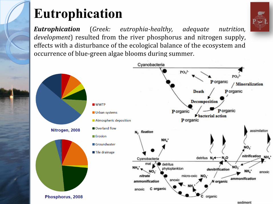
EutrophicationEutrophication (Greek: eutrophia-healthy, adequate nutrition, development) resulted from the river phosphorus and nitrogen supply, effects with a disturbance of the ecological balance of the ecosystem and occurrence of blue-green algae blooms during summer.
Eutrophication
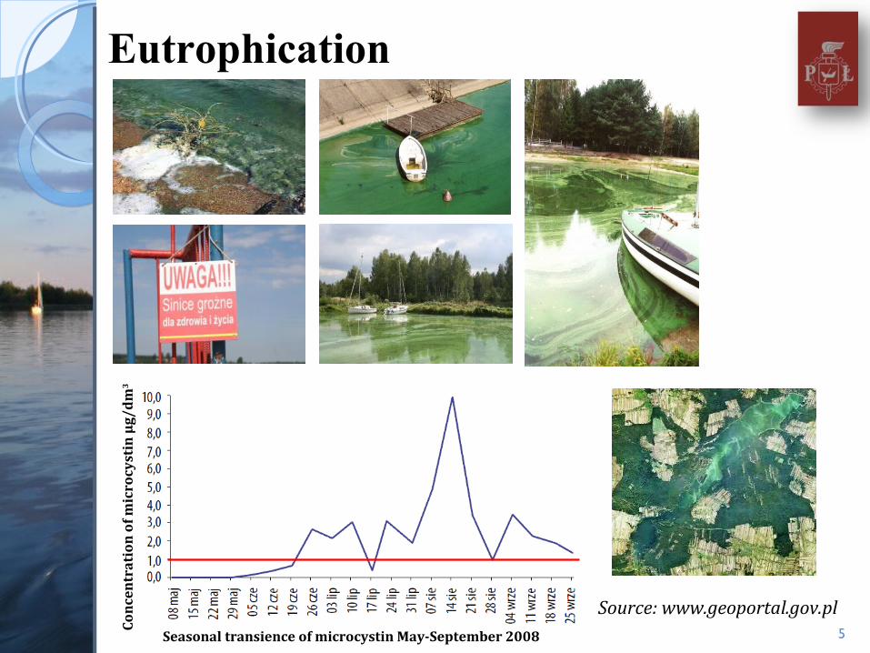
5Seasonal transience of microcystin May-September 2008
Con
cen
trat
ion
of m
icro
cyst
in μ
g/d
m3
Source: www.geoportal.gov.pl
Aim of the study
Application of coupled CFD and WASP models allows to obtain a full picture
of the ecological status of the reservoir and will enable the identification of
areas with the highest accumulation biogenic components and thus areas
particularly vulnerable to the formation of cyanobacterial blooms
Develop three dimensional model of flow hydrodynamic in the Sulejow
Reservoir using CFD technique.
Perform calculations of water quality in the Sulejow Reservoir with the use
of the WASP (Water Analysis Simulation Program) program for which
hydrodynamic data were supplied by my own CFD model. It allows to
obtain an realistic image of the distribution of temperatures, flow
velocities and concentrations of main substances responsible for the
eutrophication process.
6

7
Application areaApplication area Associated studiesAssociated studies
Flow-field prediction
Fang and Rodi (2003), Fangkai et al. (2007),
Zinke et al. (2010), Wang et al. (2010),
Khosronejad (2010),
Analysis of particulate behaviour Stovin and Saul (1996;2000),
Adamson et al. (2003),Bridgeman et al. (2009)
Prediction of water surface profiles Ta and Brignal (1998),
Kouyi et al.(2005),Lau et al. (2007),
Anderson et al. (2013)
Residence time distribution (RTD) Faram et al. (2004),
Kennedy et al. (2006), Lau et al. (2007)
Sediment transport pattern
Faram and Harwood (2003), Dargahi (2004),
Gupta et al. (2005), Stovin et al. (2005),Townsend (2007)
State of the art
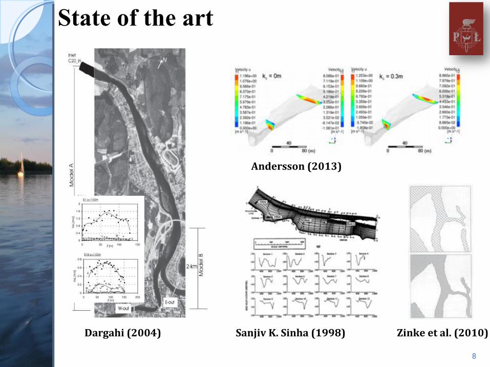
State of the art
8
Dargahi (2004) Sanjiv K. Sinha (1998) Zinke et al. (2010)
Andersson (2013)
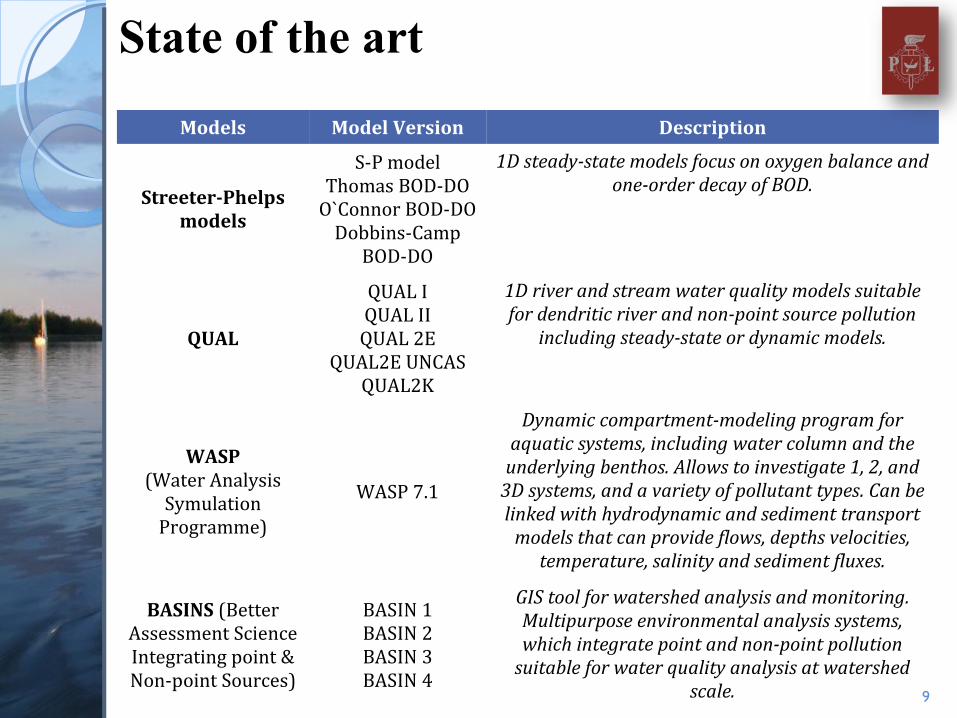
9
Models Model Version Description
Streeter-Phelps models
S-P modelThomas BOD-DO
O`Connor BOD-DODobbins-Camp
BOD-DO
1D steady-state models focus on oxygen balance and one-order decay of BOD.
QUAL
QUAL IQUAL II
QUAL 2EQUAL2E UNCAS
QUAL2K
1D river and stream water quality models suitable for dendritic river and non-point source pollution
including steady-state or dynamic models.
WASP(Water Analysis
Symulation Programme)
WASP 7.1
Dynamic compartment-modeling program for aquatic systems, including water column and the
underlying benthos. Allows to investigate 1, 2, and 3D systems, and a variety of pollutant types. Can be linked with hydrodynamic and sediment transport
models that can provide flows, depths velocities, temperature, salinity and sediment fluxes.
BASINS (Better Assessment Science Integrating point & Non-point Sources)
BASIN 1BASIN 2BASIN 3BASIN 4
GIS tool for watershed analysis and monitoring. Multipurpose environmental analysis systems, which integrate point and non-point pollution
suitable for water quality analysis at watershed scale.
State of the art
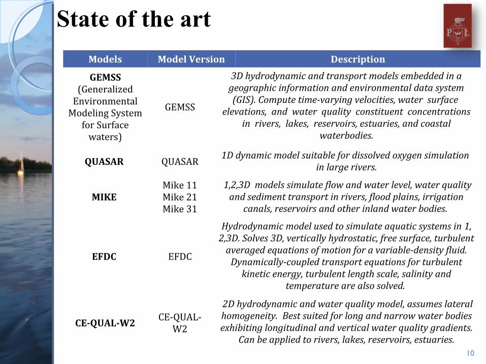
GEMSS(Generalized
Environmental Modeling System
for Surface waters)
GEMSS
3D hydrodynamic and transport models embedded in a geographic information and environmental data system (GIS). Compute time-varying velocities, water surface
elevations, and water quality constituent concentrations in rivers, lakes, reservoirs, estuaries, and coastal
waterbodies.
QUASAR QUASAR1D dynamic model suitable for dissolved oxygen simulation
in large rivers.
MIKE Mike 11Mike 21Mike 31
1,2,3D models simulate flow and water level, water quality and sediment transport in rivers, flood plains, irrigation
canals, reservoirs and other inland water bodies.
EFDC EFDC
Hydrodynamic model used to simulate aquatic systems in 1, 2,3D. Solves 3D, vertically hydrostatic, free surface, turbulent
averaged equations of motion for a variable-density fluid. Dynamically-coupled transport equations for turbulent
kinetic energy, turbulent length scale, salinity and temperature are also solved.
CE-QUAL-W2CE-QUAL-
W2
2D hydrodynamic and water quality model, assumes lateral homogeneity. Best suited for long and narrow water bodies exhibiting longitudinal and vertical water quality gradients.
Can be applied to rivers, lakes, reservoirs, estuaries.10
Models Model Version Description
State of the art
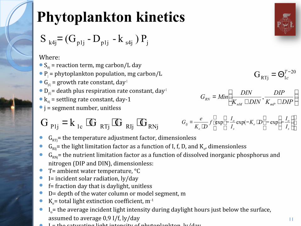
Phytoplankton kinetics
Where:Sk4j = reaction term, mg carbon/L dayPj = phytoplankton population, mg carbon/LGp1j = growth rate constant, day-1
Dp1j = death plus respiration rate constant, day-1
ks4j = settling rate constant, day-1j = segment number, unitless
11
GRTj= the temperature adjustment factor, dimensionless GRIj= the light limitation factor as a function of I, f, D, and Ke, dimensionless GRNj= the nutrient limitation factor as a function of dissolved inorganic phosphorus and
nitrogen (DIP and DIN), dimensionless: T= ambient water temperature, °C I= incident solar radiation, ly/day f= fraction day that is daylight, unitless D= depth of the water column or model segment, m Ke= total light extinction coefficient, m-1
Io= the average incident light intensity during daylight hours just below the surface, assumed to average 0,9 I/f, ly/day
Is= the saturating light intensity of phytoplankton, ly/day
js4j p1jp1jk4j P ) k -D - (G S =
RNjRIj RTj1c P1j G G G k G ⋅⋅⋅=
201RTjG −Θ= Tc
++
=DIPK
DIP
DINK
DINMinG
mPnMRN ,
−−
⋅−−⋅
=s
oe
s
o
eIj I
IDK
I
If
DK
eG expexp(exp
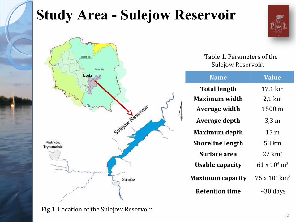
Study Area - Sulejow Reservoir
12
Lodz Name Value
Total length 17,1 km
Maximum width 2,1 km
Average width 1500 m
Average depth 3,3 m
Maximum depth 15 m
Shoreline length 58 km
Surface area 22 km2
Usable capacity 61 x 106 m3
Maximum capacity 75 x 106 km3
Retention time ~30 days
Table 1. Parameters of the Sulejow Reservoir.
Fig.1. Location of the Sulejow Reservoir.
Study Area - Sulejow Reservoir
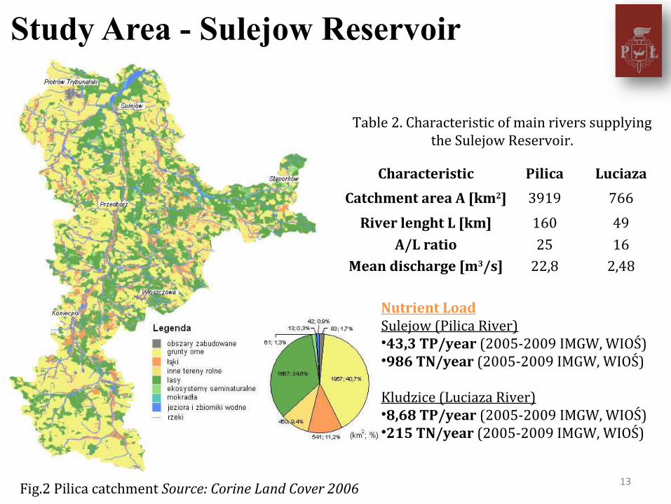
Fig.2 Pilica catchment Source: Corine Land Cover 2006 13
Characteristic Pilica Luciaza
Catchment area A [km2] 3919 766
River lenght L [km] 160 49A/L ratio 25 16
Mean discharge [m3/s] 22,8 2,48
Table 2. Characteristic of main rivers supplying the Sulejow Reservoir.
Nutrient LoadSulejow (Pilica River)•43,3 TP/year (2005-2009 IMGW, WIOŚ)•986 TN/year (2005-2009 IMGW, WIOŚ)
Kludzice (Luciaza River)•8,68 TP/year (2005-2009 IMGW, WIOŚ)•215 TN/year (2005-2009 IMGW, WIOŚ)
3D CFD MODEL OF HYDRODYNAMIC IN THE
SULEJOW RESERVOIR
14
15
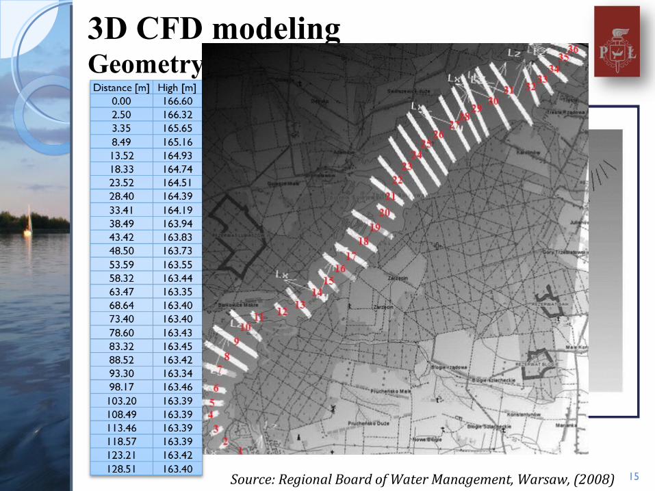
3D CFD modeling Geometry modeling & Grid generation
Fig.5. 36 cross section profiles of the Sulejow Reservoir.
Source: Regional Board of Water Management, Warsaw, (2008)
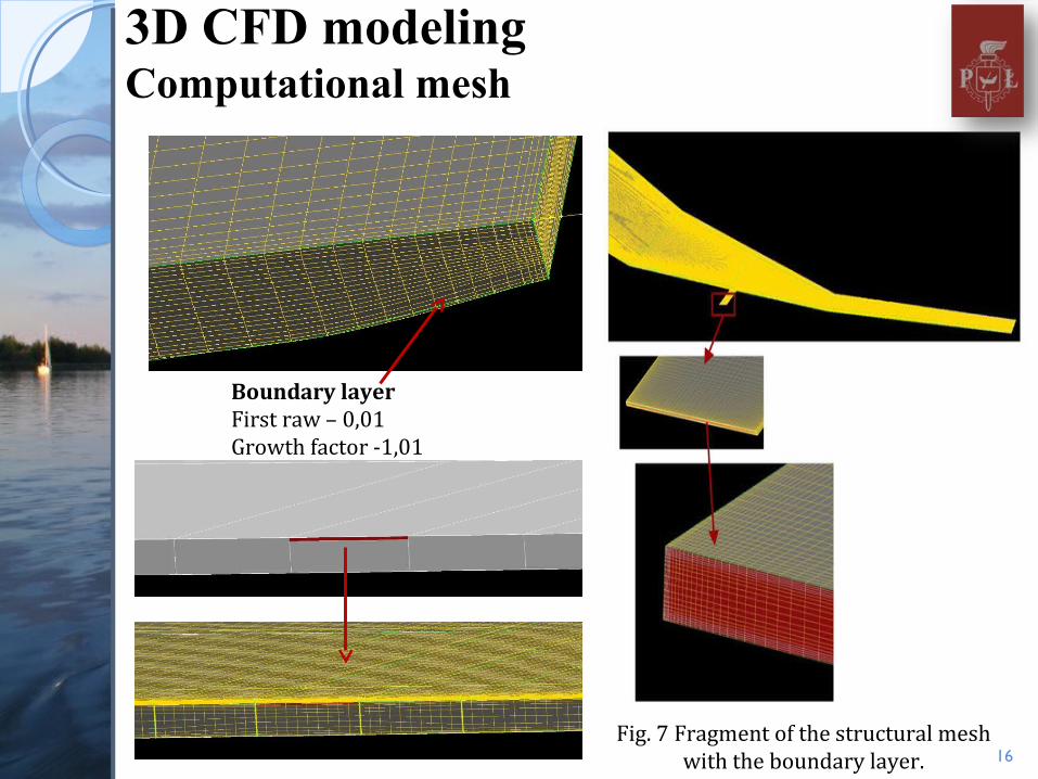
3D CFD modeling Computational mesh
16
air
Fig. 7 Fragment of the structural mesh with the boundary layer.
Boundary layerFirst raw – 0,01Growth factor -1,01
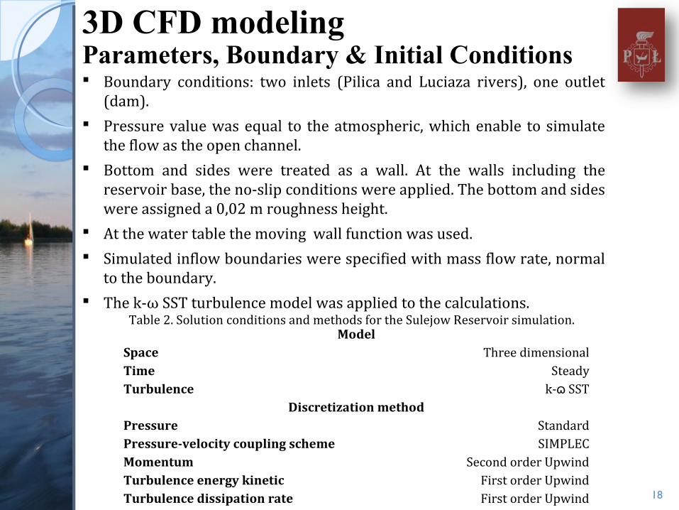
3D CFD modeling Parameters, Boundary & Initial Conditions
18
Boundary conditions: two inlets (Pilica and Luciaza rivers), one outlet (dam).
Pressure value was equal to the atmospheric, which enable to simulate the flow as the open channel.
Bottom and sides were treated as a wall. At the walls including the reservoir base, the no-slip conditions were applied. The bottom and sides were assigned a 0,02 m roughness height.
At the water table the moving wall function was used. Simulated inflow boundaries were specified with mass flow rate, normal
to the boundary. The k-ω SST turbulence model was applied to the calculations.
ModelSpace Three dimensionalTime SteadyTurbulence k- SSTɷ
Discretization methodPressure StandardPressure-velocity coupling scheme SIMPLECMomentum Second order UpwindTurbulence energy kinetic First order UpwindTurbulence dissipation rate First order Upwind
Table 2. Solution conditions and methods for the Sulejow Reservoir simulation.
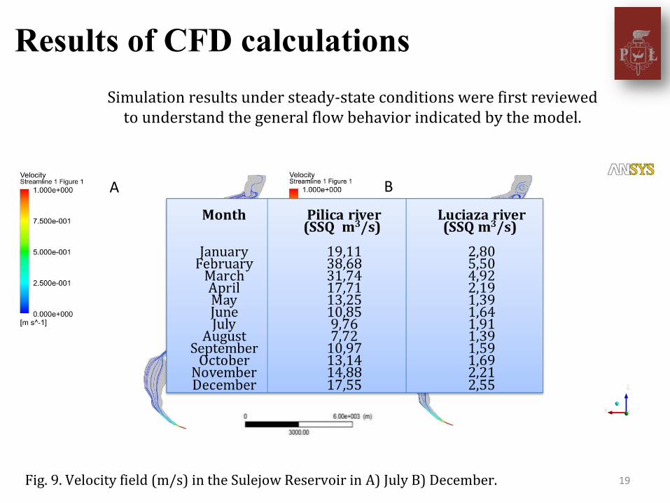
Results of CFD calculations
19Fig. 9. Velocity field (m/s) in the Sulejow Reservoir in A) July B) December.
Simulation results under steady-state conditions were first reviewed to understand the general flow behavior indicated by the model.
A B
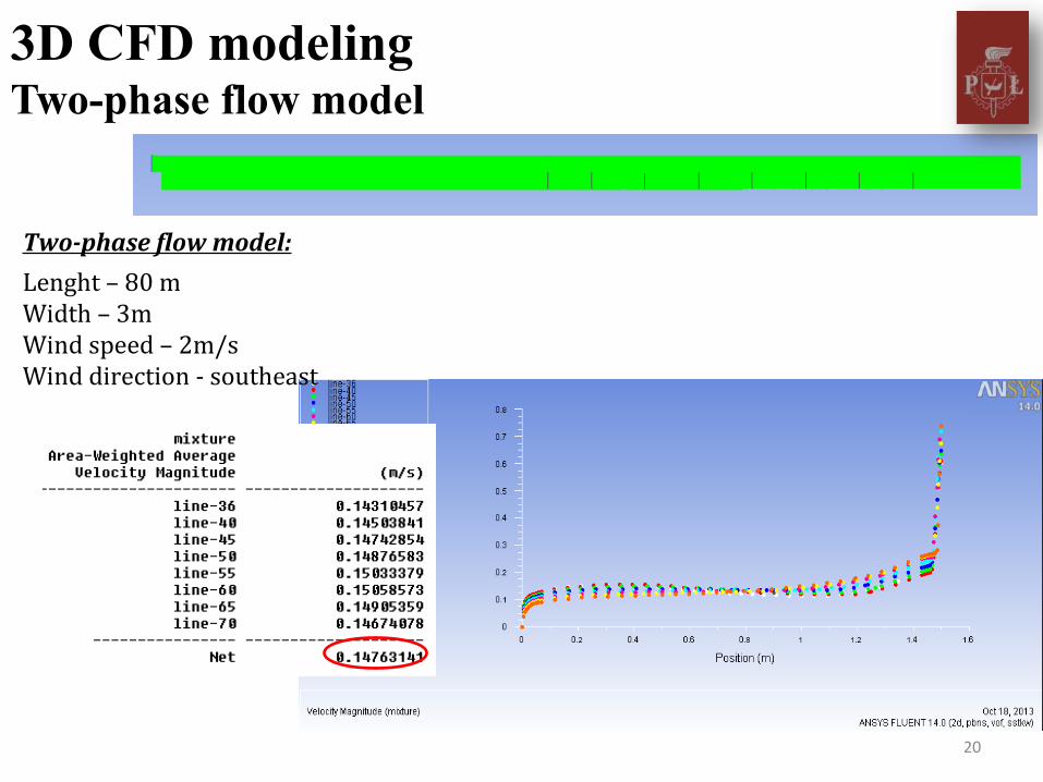
3D CFD modelingTwo-phase flow model
20
Two-phase flow model:
Lenght – 80 mWidth – 3mWind speed – 2m/sWind direction - southeast
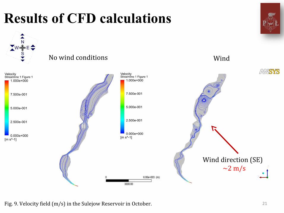
Results of CFD calculations
21Fig. 9. Velocity field (m/s) in the Sulejow Reservoir in October.
No wind conditions Wind
Wind direction (SE)~2 m/s
22
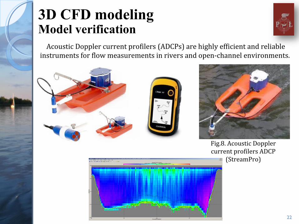
Acoustic Doppler current profilers (ADCPs) are highly efficient and reliable instruments for flow measurements in rivers and open-channel environments.
Fig.8. Acoustic Doppler current profilers ADCP
(StreamPro)
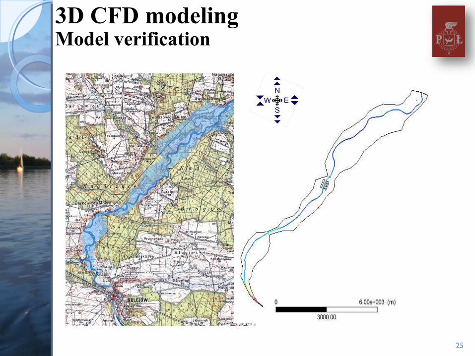
3D CFD modeling Model verification
3D CFD modeling Model verification
23
1
2
3 4
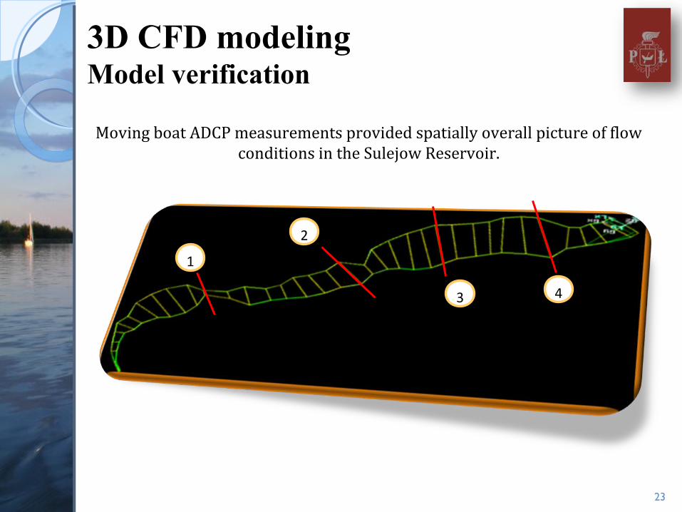
Moving boat ADCP measurements provided spatially overall picture of flow conditions in the Sulejow Reservoir.
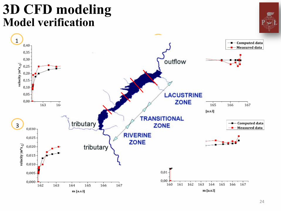
3D CFD modeling Model verification
24
3 4
21
25
3D CFD modeling Model verification
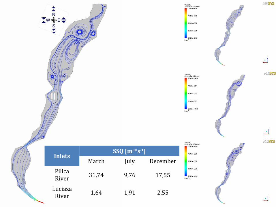
26
InletsSSQ [m3*s-1]
March July December
Pilica River 31,74 9,76 17,55
Luciaza River 1,64 1,91 2,55
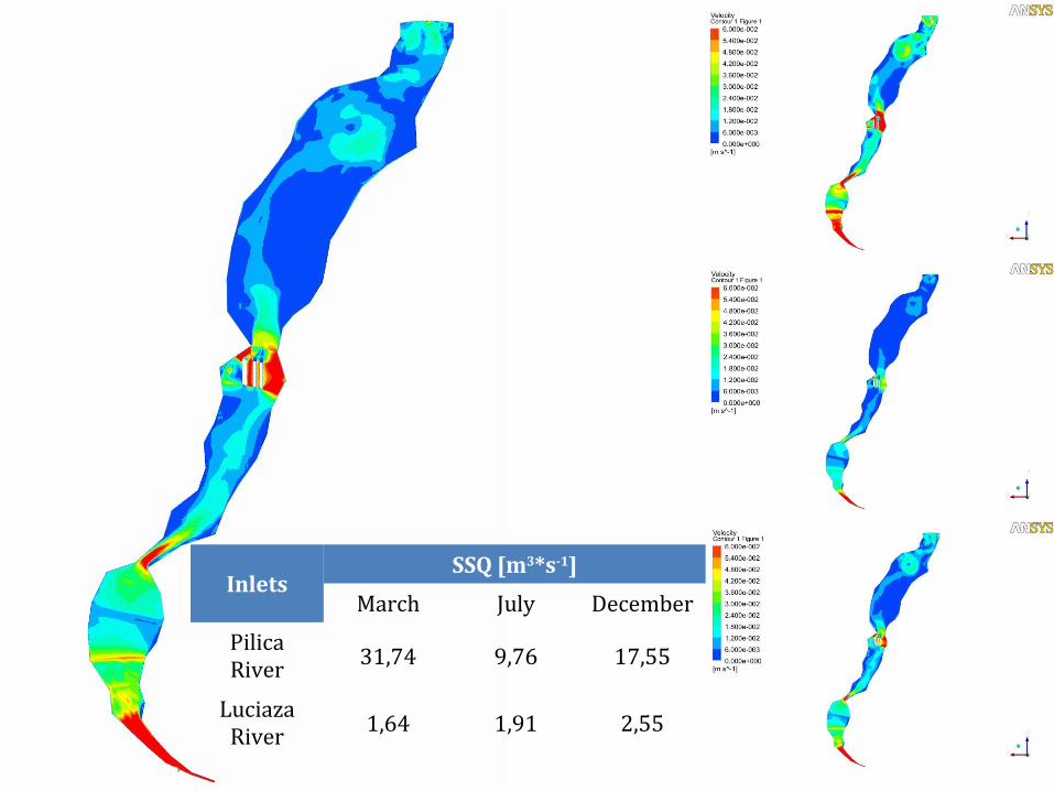
27
InletsSSQ [m3*s-1]
March July December
Pilica River 31,74 9,76 17,55
Luciaza River 1,64 1,91 2,55
WATER ANALYSIS SIMULATION PROGRAME
(WASP)
28
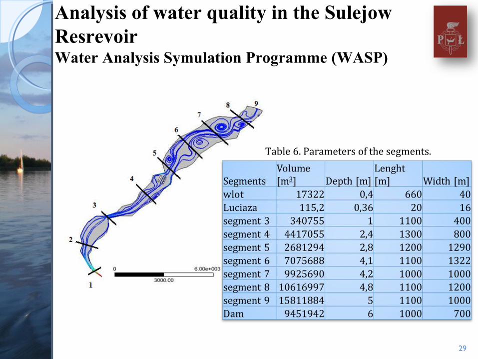
Analysis of water quality in the Sulejow ResrevoirWater Analysis Symulation Programme (WASP)
29
Table 6. Parameters of the segments.
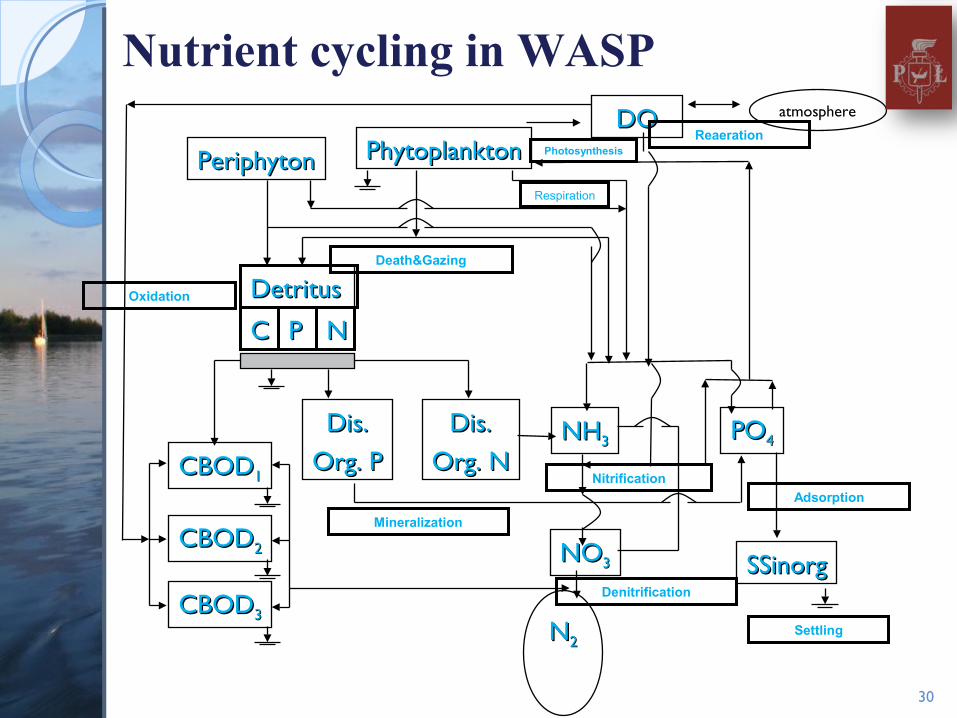
Nutrient cycling in WASP
30
PhytoplanktonPhytoplankton
NHNH33
Respiration
Dis.Dis.Org. POrg. P
Dis.Dis.Org. NOrg. NCBODCBOD11
CBODCBOD22
CBODCBOD33
POPO44
SSinorgSSinorg
Settling
Photosynthesis
Denitrification
Nitrification
atmosphereDODO
NONO33
Adsorption
Oxidation
Mineralization
Reaeration
NN22
NNPPCC
DetritusDetritus
PeriphytonPeriphyton
Death&Gazing

Nitrogen
31
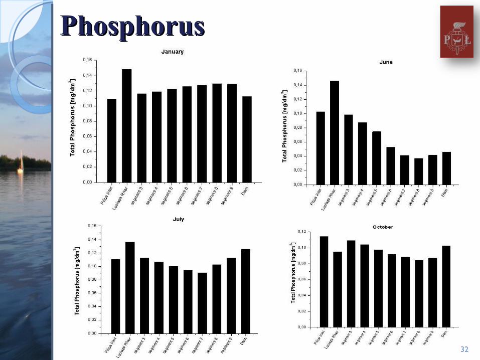
PhosphorusPhosphorus
32
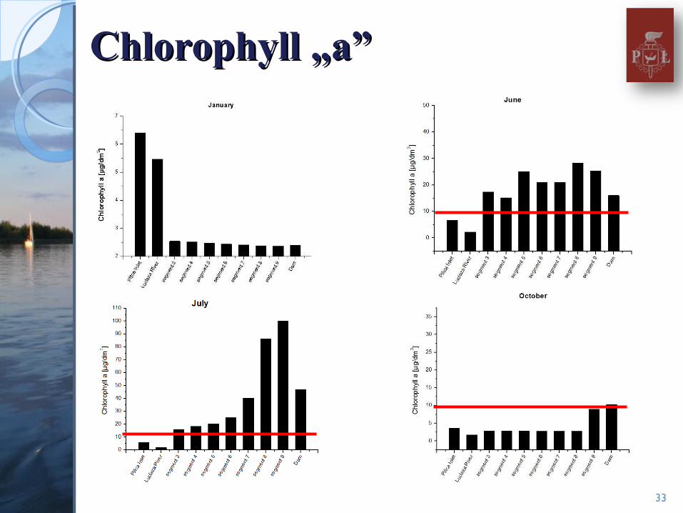
Chlorophyll „a”Chlorophyll „a”
33
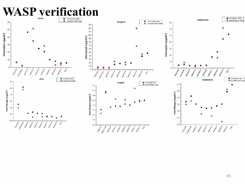
WASP verification
34
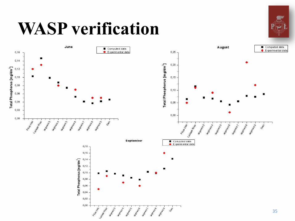
WASP verification
35
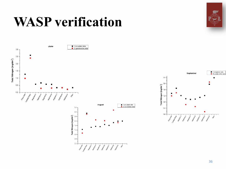
WASP verification
36
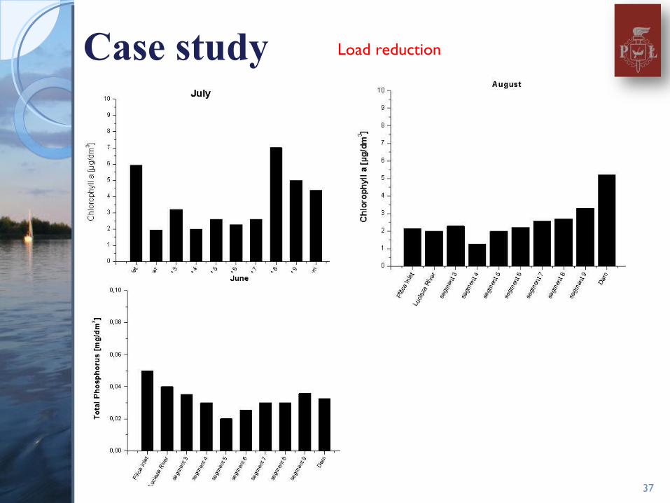
Case study
37
Load reduction
SummarySummary
A 3D single-phase CFD model of flow hydrodynamic in the Sulejow Reservoir with accurate depiction of basin bathymetry was developed and verified.
The results generated by the model indicate that the flow field in the Sulejow Reservoir is transient in nature, containing turbulent structures and swirl flow. Analysis of the flow velocities show that main path of flow is approximately along the bad of the Pilica River.
The WASP eutrophication model was applied to simulate the complex nutrient transport and cycling in the Sulejow Reservoir.
Proper correlation between the measured and calculated values ware obtained, which is a result of application a realistic hydrodynamics in the lake, determined from the CFD calculations in the WASP analysis.
Analysis of the results shown correlation between hydrodynamics and concentrations of selected nutrients in the reservoir.
The resulting model is accurate, robust and the methodology develop in the frame of this work can be applied to all types of storage reservoir configurations, characteristics, and hydraulic conditions.
38

THANK YOU FOR YOUR ATTENTION
39