Trajectory generation for a four

axis robot with linear kinematics

S.N. van den Brink

DCT 2005.69

Traineeship report

The work in this report is part of the NewMotion project

Coaches: Dr. ir. N. van de Wouw †

Ir. W.C.M. Pancras ‡

Supervisor: Prof. dr. H. Nijmeijer †

† Technische Universiteit EindhovenDepartment Mechanical EngineeringDynamics and Control Group

‡ Nyquist Industrial Control B.V.Department Development and EngineeringMotion Engineering

Eindhoven, 5th July 2005

Abstra tCurrently, for every robot and often for every purpose, a new trajectory generator is developed.These specific trajectory generators use the capacity of a robot almost to its full extent and theresulting trajectories are very fast.The capacity of any robot is limited by the maximum velocity, acceleration and jerk that the con-struction, the actuators and the process of the robot can withstand. These limitations are calledconstraints. The constraints have their reflection on the trajectory; the maximum velocity, accel-eration and jerk in a motion robot may not violate the constraints.However, as developing new trajectory generators is expensive, there is a need for generic tra-jectory generators who efficiently handle the constraints. This is one of the objectives of theNewMotion project.

In this report, the requirements for trajectory generation for a specific pick and place robot, calledModular Robot System (MRS), are defined. An algorithm fulfilling the requirements to a large ex-tent is developed and implemented in a Matlab environment.

First, the MRS is described. An inventory of the demands for a trajectory generator regardingthe MRS is made. These demands are transformed into requirements for a generic trajectorygeneration algorithm. The major requirements relate to time-optimality within the constraintsand second-order continuity of the trajectory.

In the second part of this report, the algorithm is treated in depth. The path in Cartesian spaceis defined by setpoints. The setpoints are connected by splines. As a spline contains no timeinformation, such time information must be added on the spline path. For this purpose, thespline parameter is transformed into a function of time by a time mapping function. The endtime of the motion is determined by the most critical constraint at a certain time instant.The result of the proposed algorithm is a second-order continuous trajectory. All setpoints arecrossed exactly. The constraints are never violated and at one time instant one constraint is ac-tive. The trajectory is not time-optimal within the constraints. However, by calculating a piecewisesecond-order continuous time mapping, better results regarding this demand are possible.

In the third part of this report, the implementation of the algorithm in Matlab is presentedand several results are given. To show the effectiveness of the proposed trajectory generatingalgorithm, an example of a path with a piecewise second-order continuous time mapping is givenfor the MRS.

i

ii

Abstra t (Dut h)Tegenwoordig wordt voor elke robot en vaak voor elke toepassing, een nieuwe traject generatorontwikkeld. Deze toepassingsgerichte traject generatoren benutten de capaciteit van de robotbijna volledig en de gegenereerde trajectorie zijn erg snel.De capaciteit van elke robot is beperkt; elke robot heeft een maximale snelheid, acceleratie en rukdie de constructie, de actuatoren en het proces van de robot kunnen verdragen. Deze beperkin-gen hebben hun weerslag op de trajectorie; de snelheid, acceleratie of ruk tijdens een bewegingmogen de beperkingen niet overschrijden.Het ontwikkelen van traject generatoren is een dure aangelegenheid. Er is behoefte aan generie-ke traject generatoren die efficient omgaan met de beperkingen. Dit is een van de doelstellingenvan het NewMotion project.

In dit rapport zijn de specificaties voor traject generatie voor een specifieke pick-and-place robotgenaamd Modular Robot System (MRS) gedefinieerd. Een algoritme dat in ruime mate voldoetaan de specificaties is ontwikkeld en geïmplementeerd in Matlab .

Ter inleiding is de MRS beschreven. Tevens zijn de eisen met betrekking tot traject generatievoor de MRS geïnventariseerd en zijn deze eisen omgezet in specificaties voor een generiek tra-ject generatie algoritme. De belangrijkste specificaties zijn een tijd-optimale trajectorie binnende beperkingen en dat de gegenereerde trajectorie tweede orde continue zijn.

In het tweede deel van dit rapport is het algoritme verder uitgewerkt. De baan in Cartesischecoördinaten wordt gedefinieerd door een aantal punten in de ruimte. Deze punten worden metelkaar verbonden door middel van ”splines”. Een spline beschrijft een baan zonder dat dezetijd-informatie bevat, de tijd moet nog worden toegevoegd. Hiervoor wordt de spline parametergeschreven als een functie van de tijd. De eindtijd van de beweging wordt bepaald de meestkritische beperking op één bepaald tijdstipHet resultaat van het voorgestelde algoritme is een tweede orde continue trajectorie. De baangaat exact door alle voorgeschreven punten. De beperkingen worden nooit overschreden en opéén tijdstip is één beperking actief. De trajectorie is niet tijd-optimaal binnen de beperkingen.Echter, door de tijd functie op te splitsen en tweede orde continue te houden, zijn betere resulta-ten mogelijk met betrekking tot tijd-optimaliteit.

In het derde deel van dit rapport wordt de implementatie in Matlab beschreven. Om de effectiviteitvan het voorgestelde algoritme te tonen, is een voorbeeld van een baan met een gedeelde tijd-fitfunctie gegeven voor de MRS. iii

iv

ContentsAbstract i

Abstract (Dutch) iii

Contents v

1 Introduction 1

1.1 The need for trajectory generation . . . . . . . . . . . . . . . . . . . . . . . . . . 11.2 The NewMotion project . . . . . . . . . . . . . . . . . . . . . . . . . . . . . . . . 11.3 Definition of the project objectives . . . . . . . . . . . . . . . . . . . . . . . . . . 21.4 Report overview . . . . . . . . . . . . . . . . . . . . . . . . . . . . . . . . . . . . 2

2 Modular Robot System 3

2.1 Description of the MRS . . . . . . . . . . . . . . . . . . . . . . . . . . . . . . . . 32.2 Coordinate systems . . . . . . . . . . . . . . . . . . . . . . . . . . . . . . . . . . 5

2.2.1 Kinematics . . . . . . . . . . . . . . . . . . . . . . . . . . . . . . . . . . . 52.2.2 Constraints . . . . . . . . . . . . . . . . . . . . . . . . . . . . . . . . . . . 6

3 Trajectory generating requirements and algorithm proposal 7

3.1 List of demands . . . . . . . . . . . . . . . . . . . . . . . . . . . . . . . . . . . . 73.1.1 Requirements regarding the MRS functionality . . . . . . . . . . . . . . . 73.1.2 Requirements regarding the trajectory generator functionality . . . . . . . 8

3.2 Trajectory planning strategy . . . . . . . . . . . . . . . . . . . . . . . . . . . . . . 83.3 Proposed trajectory generating algorithm . . . . . . . . . . . . . . . . . . . . . . 11

3.3.1 Input . . . . . . . . . . . . . . . . . . . . . . . . . . . . . . . . . . . . . . 133.3.2 Output . . . . . . . . . . . . . . . . . . . . . . . . . . . . . . . . . . . . . 14

3.4 Discussion . . . . . . . . . . . . . . . . . . . . . . . . . . . . . . . . . . . . . . . 144 Generating the path and the time mapping 15

4.1 Representing the path . . . . . . . . . . . . . . . . . . . . . . . . . . . . . . . . . 154.1.1 Spline representation of the path . . . . . . . . . . . . . . . . . . . . . . . 154.1.2 Domains and spaces . . . . . . . . . . . . . . . . . . . . . . . . . . . . . . 16

4.2 Proposed time mapping function . . . . . . . . . . . . . . . . . . . . . . . . . . . 174.3 Path derivatives . . . . . . . . . . . . . . . . . . . . . . . . . . . . . . . . . . . . . 18

4.3.1 Velocity . . . . . . . . . . . . . . . . . . . . . . . . . . . . . . . . . . . . . 184.3.2 Acceleration . . . . . . . . . . . . . . . . . . . . . . . . . . . . . . . . . . 194.3.3 Jerk . . . . . . . . . . . . . . . . . . . . . . . . . . . . . . . . . . . . . . . 19v

4.4 Activating a constraint . . . . . . . . . . . . . . . . . . . . . . . . . . . . . . . . . 194.4.1 Determining the maxima of each profile . . . . . . . . . . . . . . . . . . . 204.4.2 Iteration of the active constraint . . . . . . . . . . . . . . . . . . . . . . . 21

4.5 Improving the time-optimality of a time-independent path . . . . . . . . . . . . . 224.6 Feasibility of a time-dependent path . . . . . . . . . . . . . . . . . . . . . . . . . 23

5 Implementation and results 25

5.1 Setup of the implementation in Matlab . . . . . . . . . . . . . . . . . . . . . . . . 255.2 Results of the Matlab algorithm . . . . . . . . . . . . . . . . . . . . . . . . . . . 26

5.2.1 Generating the path . . . . . . . . . . . . . . . . . . . . . . . . . . . . . . 265.2.2 Time mapping . . . . . . . . . . . . . . . . . . . . . . . . . . . . . . . . . 295.2.3 Improving the mapping . . . . . . . . . . . . . . . . . . . . . . . . . . . . 30

5.3 Discussion . . . . . . . . . . . . . . . . . . . . . . . . . . . . . . . . . . . . . . . 326 Conclusions and recommendations 33

6.1 Conclusions . . . . . . . . . . . . . . . . . . . . . . . . . . . . . . . . . . . . . . 336.2 Recommendations . . . . . . . . . . . . . . . . . . . . . . . . . . . . . . . . . . . 34

Bibliography 35

A MRS data sheet 37

A.1 Motion transfer . . . . . . . . . . . . . . . . . . . . . . . . . . . . . . . . . . . . . 37A.2 Control compartment . . . . . . . . . . . . . . . . . . . . . . . . . . . . . . . . . 38A.3 Kinematic constants . . . . . . . . . . . . . . . . . . . . . . . . . . . . . . . . . . 39A.4 Constraints . . . . . . . . . . . . . . . . . . . . . . . . . . . . . . . . . . . . . . . 40

B Trajectory planning strategies 41

B.1 Point-to-point motion . . . . . . . . . . . . . . . . . . . . . . . . . . . . . . . . . 41B.2 Catch-up profile . . . . . . . . . . . . . . . . . . . . . . . . . . . . . . . . . . . . 42

C Reflection on the requirements 43

D Spline theory 45

D.1 Hermite splines . . . . . . . . . . . . . . . . . . . . . . . . . . . . . . . . . . . . 45D.2 Natural cubic splines . . . . . . . . . . . . . . . . . . . . . . . . . . . . . . . . . . 46D.3 Directional cubic splines . . . . . . . . . . . . . . . . . . . . . . . . . . . . . . . . 47D.4 Mixed cubic splines . . . . . . . . . . . . . . . . . . . . . . . . . . . . . . . . . . 48

E Determining the mapping 49

E.1 Calculating the mapping parameters . . . . . . . . . . . . . . . . . . . . . . . . . 49E.2 Velocity boundary conditions . . . . . . . . . . . . . . . . . . . . . . . . . . . . . 49

F Derivation of path derivatives with respect to time 51

F.1 Acceleration . . . . . . . . . . . . . . . . . . . . . . . . . . . . . . . . . . . . . . 51F.2 Jerk . . . . . . . . . . . . . . . . . . . . . . . . . . . . . . . . . . . . . . . . . . . 52vi

G Additional results of the implementation in Matlab 53G.1 Additional figures of trajectories . . . . . . . . . . . . . . . . . . . . . . . . . . . 53G.2 Output generated to the Matlab command window . . . . . . . . . . . . . . . . . 55

H Implementation of the algorithm in Matlab 57H.1 Description of the Matlab files . . . . . . . . . . . . . . . . . . . . . . . . . . . . 57H.2 Master file . . . . . . . . . . . . . . . . . . . . . . . . . . . . . . . . . . . . . . . 59H.3 Define kinematics . . . . . . . . . . . . . . . . . . . . . . . . . . . . . . . . . . . 60H.4 Define constraints . . . . . . . . . . . . . . . . . . . . . . . . . . . . . . . . . . . 61H.5 Define setpoints . . . . . . . . . . . . . . . . . . . . . . . . . . . . . . . . . . . . 62H.6 Generate spline path . . . . . . . . . . . . . . . . . . . . . . . . . . . . . . . . . . 63H.7 Convert path from CS to JS . . . . . . . . . . . . . . . . . . . . . . . . . . . . . . 66H.8 Time mapping master file . . . . . . . . . . . . . . . . . . . . . . . . . . . . . . . 67H.9 Calculate mapping parameters . . . . . . . . . . . . . . . . . . . . . . . . . . . . 69H.10 Calculate time derivatives of spline for given mapping . . . . . . . . . . . . . . . 70H.11 Select active constraint and update end time . . . . . . . . . . . . . . . . . . . . . 71H.12 Iterate to piecewise time mapping . . . . . . . . . . . . . . . . . . . . . . . . . . 74

vii

viii

Chapter 1Introdu tion1.1 The need for traje tory generationIn general, a robot is built to simplify the job of man. In order to fulfil its tasks, the robot mustperform a certain motion. The robot’s user or developer should tell the robot what to do. Acontroller ensures that the robot indeed performs the motion it is commanded to perform. Ingeneral, this is what motion control is about. Motion control of robotics is a well-known practisein industry these days.

To make the control of a motion easier, the motion should be smooth to some extent. Moreover,to make a robot profitable, it should work as fast as possible. Finally, to prevent damage ordynamical excitation of the robot, the robot should work within its constraints. Constraints definethe limitations of the robot, the actuators and the process. A trajectory planning algorithm shouldcombine the desired motion with the constraints to a smooth and time optimal trajectory.

Currently, for every robot and often for every purpose, a new trajectory generator is developed.In general these trajectory generators are designed using an ad-hoc approach. As a result, theyhandle constraints very well and the resulting trajectories and motions are very fast.

If however, the desired path of a robot changes over time, for example due to changing processrequirements, the trajectory generator should be able to handle such varying demands. Thisoccurs for example within pick-and-place robots. Moreover, it would be convenient if a trajectorygenerator could be used for multiple purposes (possibly with some small adjustments). Thisrequires for generic trajectory generator strategies.

A simple approach to generate a trajectory is to use very conservative constraints; this way itbecomes practically impossible to violate any constraints. However, a disadvantage is the lowerthe capacity of the robot and this is for this reason undesirable. In generic trajectory generation,it is not the aim that the user defines the velocities, accelerations and jerks of a motion. Thegenerator itself should determine the motion from the path and the constraints, making use ofthe kinematics and dynamics of the robot. This is one of the goals of the NewMotion project.1.2 The NewMotion proje tNyquist Industrial Control develops and sells motion control systems for industrial purposes. To-gether with FEI Company and the Technische Universiteit Eindhoven, Nyquist is cooperating in theNewMotion project. This project is on the development of high-end control, actuator and motionsystems for advanced industrial robots and stages.1

2 Introdu tionAs part of the NewMotion project, new generic trajectory generation algorithms will be developed.This report is the first step to explore the trajectory generation problem.1.3 Definition of the proje t obje tivesThe main target of this project is to explore the problems which will be confronted during thedevelopment of an advanced trajectory generation algorithm for a specific robot. The robot con-sidered in this project is a pick-and-place robot, calledModular Robot System (MRS). The objectivesof the project are threefold.

• Make an inventory of demands for a trajectory generator for the MRS. Moreover, an inven-tory of the requirements regarding the desired functionality of the MRS has to be made.These requirements will be transferred into trajectory generator requirements.

• Determine an approach to handle constraints in multiple domains. The limits of the mo-tions of the robot as well as those of the actuators are called constraints. Under no circum-stance the constraints may be violated. However, for economical reasons it is desired tomake the robot move as fast as possible. This means that as often as possible, at least oneconstraints must be active, i.e. critical.

• Generate an algorithm for trajectory planning with the desired flexibility and maximumuse of the constraints. This algorithm must be implemented in Matlab to check theeffectiveness and limitations of the chosen approach.

In this report there is a distinction between a trajectory and a path. With a trajectory we indicatethe position, velocity, acceleration and jerk profiles of every actuator as a function of time. With apath, the subsequent positions of every actuator without time information is indicated.1.4 Report overviewThis report is organized as follows.

MRS stands for Modular Robot System. In chapter 2, the MRS is described. The coordinatesystems will be defined, the constraints will be given and the kinematics will be derived.

Chapter 3 presents the requirements regarding the trajectory generator, specifically for the MRS.The trajectory generation algorithm is presented and the way it handles the requirements is ex-plained. Moreover, the possibilities and restrictions of the algorithm will be pointed out.

The path of theMRS in Cartesian space is described by cubic splines. Splines do not hold any timeinformation; consequently the path does not contain time information either. For this reason, atime function must be mapped on the path. As constraints (in multiple domains) are given asa function of time, the time mapping should be able to cope with the constraints. This will betreated in chapter 4; together with the handling of the boundary conditions of the path.

In chapter 5 the implementation of the algorithm in Matlab code is presented. The general setupand the outcome of the code is described and the results of the application of the algorithm to amodel of the MRS system will be discussed.

Chapter 6 contains the conclusions on the obtained results and gives recommendations for futureresearch and topics to focus on for making the algorithm applicable in practice.

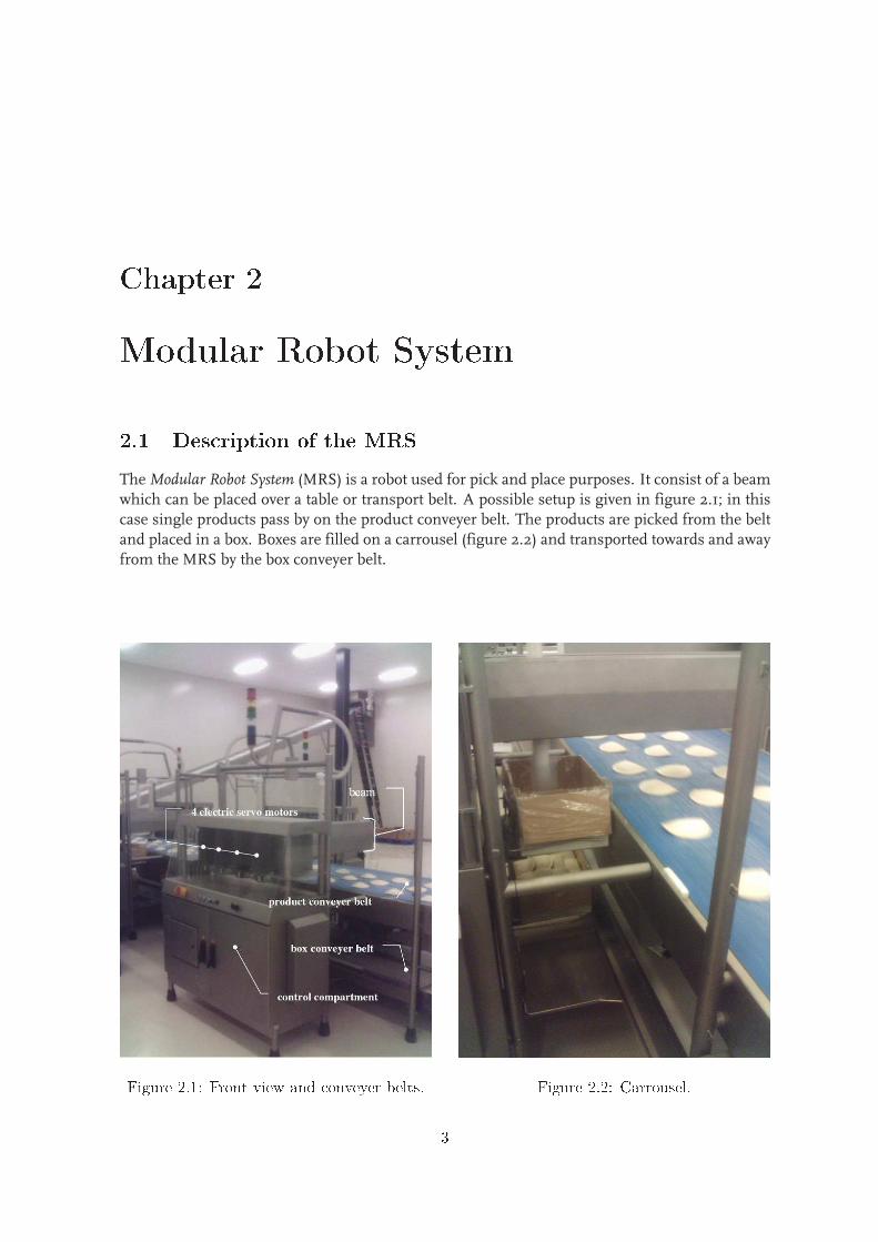
Chapter 2Modular Robot System2.1 Des ription of the MRSTheModular Robot System (MRS) is a robot used for pick and place purposes. It consist of a beamwhich can be placed over a table or transport belt. A possible setup is given in figure 2.1; in thiscase single products pass by on the product conveyer belt. The products are picked from the beltand placed in a box. Boxes are filled on a carrousel (figure 2.2) and transported towards and awayfrom the MRS by the box conveyer belt.

Figure 2.1: Front view and onveyer belts. Figure 2.2: Carrousel.3

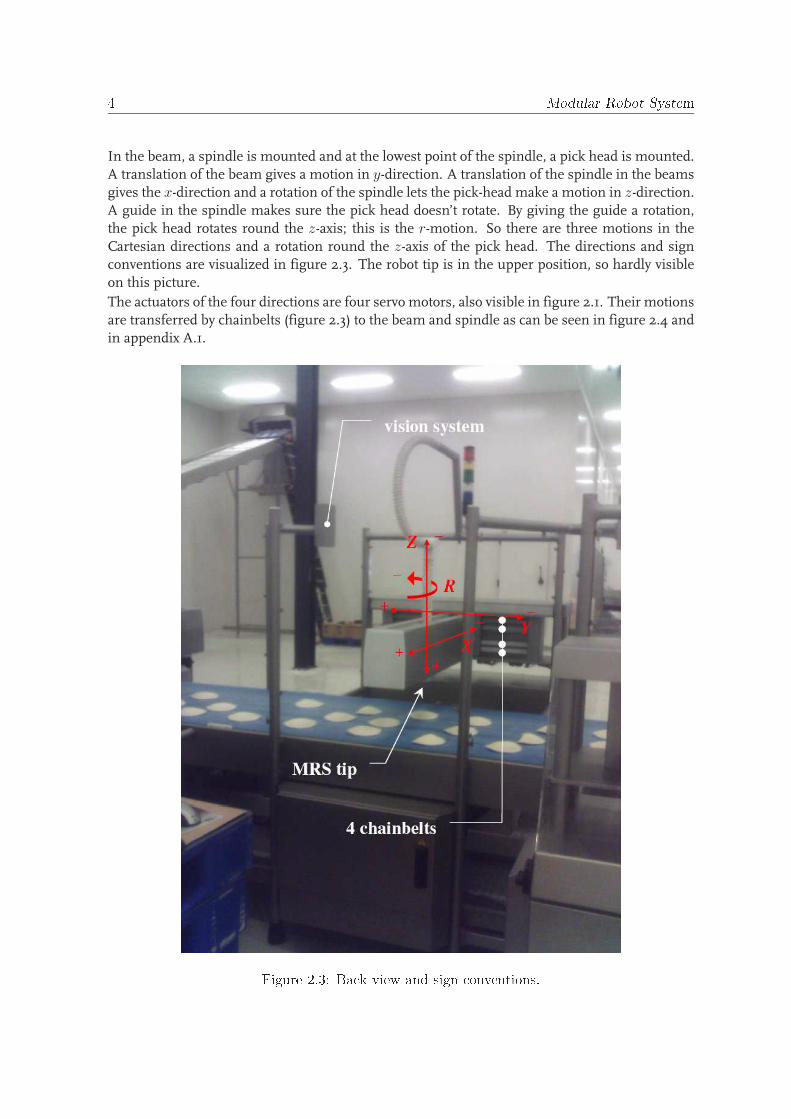
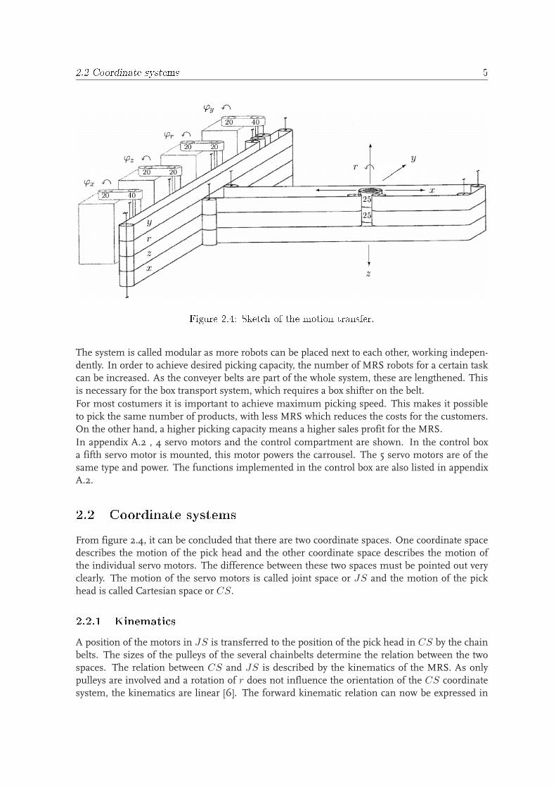
4 Modular Robot SystemIn the beam, a spindle is mounted and at the lowest point of the spindle, a pick head is mounted.A translation of the beam gives a motion in y-direction. A translation of the spindle in the beamsgives the x-direction and a rotation of the spindle lets the pick-head make a motion in z-direction.A guide in the spindle makes sure the pick head doesn’t rotate. By giving the guide a rotation,the pick head rotates round the z-axis; this is the r-motion. So there are three motions in theCartesian directions and a rotation round the z-axis of the pick head. The directions and signconventions are visualized in figure 2.3. The robot tip is in the upper position, so hardly visibleon this picture.

The actuators of the four directions are four servo motors, also visible in figure 2.1. Their motionsare transferred by chainbelts (figure 2.3) to the beam and spindle as can be seen in figure 2.4 andin appendix A.1.

Figure 2.3: Ba k view and sign onventions.

2.2 Coordinate systems 5

Figure 2.4: Sket h of the motion transfer.The system is called modular as more robots can be placed next to each other, working indepen-dently. In order to achieve desired picking capacity, the number of MRS robots for a certain taskcan be increased. As the conveyer belts are part of the whole system, these are lengthened. Thisis necessary for the box transport system, which requires a box shifter on the belt.

For most costumers it is important to achieve maximum picking speed. This makes it possibleto pick the same number of products, with less MRS which reduces the costs for the customers.On the other hand, a higher picking capacity means a higher sales profit for the MRS.

In appendix A.2 , 4 servo motors and the control compartment are shown. In the control boxa fifth servo motor is mounted, this motor powers the carrousel. The 5 servo motors are of thesame type and power. The functions implemented in the control box are also listed in appendixA.2.2.2 Coordinate systemsFrom figure 2.4, it can be concluded that there are two coordinate spaces. One coordinate spacedescribes the motion of the pick head and the other coordinate space describes the motion ofthe individual servo motors. The difference between these two spaces must be pointed out veryclearly. The motion of the servo motors is called joint space or JS and the motion of the pickhead is called Cartesian space or CS.2.2.1 Kinemati sA position of the motors in JS is transferred to the position of the pick head in CS by the chainbelts. The sizes of the pulleys of the several chainbelts determine the relation between the twospaces. The relation between CS and JS is described by the kinematics of the MRS. As onlypulleys are involved and a rotation of r does not influence the orientation of the CS coordinatesystem, the kinematics are linear [6]. The forward kinematic relation can now be expressed in

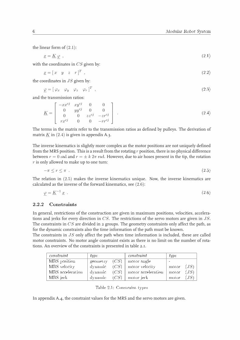
6 Modular Robot Systemthe linear form of (2.1):

x = K ϕ , (2.1)with the coordinates in CS given by:

x = [ x y z r ]T , (2.2)the coordinates in JS given by:

ϕ = [ ϕx ϕy ϕz ϕr ]T , (2.3)and the transmission ratios:

K =

−xxcj xycj 0 00 yycj 0 00 0 zzcj −zrcj

rxcj 0 0 −rrcj

. (2.4)The terms in the matrix refer to the transmission ratios as defined by pulleys. The derivation ofmatrix K in (2.4) is given in appendix A.3.

The inverse kinematics is slightly more complex as the motor positions are not uniquely definedfrom theMRS position. This is a result from the rotating r position, there is no physical differencebetween r = 0 rad and r = ± k 2π rad. However, due to air hoses present in the tip, the rotationr is only allowed to make up to one turn:

−π ≤ r ≤ π . (2.5)The relation in (2.5) makes the inverse kinematics unique. Now, the inverse kinematics arecalculated as the inverse of the forward kinematics, see (2.6):

ϕ = K−1 x . (2.6)2.2.2 ConstraintsIn general, restrictions of the construction are given in maximum positions, velocities, accelera-tions and jerks for every direction in CS. The restrictions of the servo motors are given in JS.The constraints in CS are divided in 2 groups. The geometry constraints only affect the path, asfor the dynamic constraints also the time information of the path must be known.The constraints in JS only affect the path when time information is included, these are calledmotor constraints. No motor angle constraint exists as there is no limit on the number of rota-tions. An overview of the constraints is presented in table 2.1. onstraint type onstraint typeMRS position geometry (CS) motor angle -MRS velo ity dynami (CS) motor velo ity motor (JS)MRS a eleration dynami (CS) motor a eleration motor (JS)MRS jerk dynami (CS) motor jerk motor (JS)Table 2.1: Constraint typesIn appendix A.4, the constraint values for the MRS and the servo motors are given.

Chapter 3Traje tory generating requirementsand algorithm proposalThe trajectory generator should be able to provide the desired functionality of the MRS. Also re-garding the trajectory generator itself, several demands will be stated. In this chapter, first theresults of the inventory of all demands will be presented. In the larger framework of the New-Motion project, this is important to know. Next the structure of the trajectory planning algorithmand the way in which it copes with the list of demands, will be sketched. Finally, the possibilitiesand restrictions of the chosen algorithm will be discussed.3.1 List of demands3.1.1 Requirements regarding the MRS fun tionalityFrom the MRS manufacturer point of view, the input for the path generator should consist ofsetpoints. These setpoints have to be crossed, possibly within a certain range. The avoidance ofconstraint area’s is simply done by giving in certain setpoints. Themanufacturer has to determinethe optimal setpoints by hand and check whether the trajectory is satisfying. This also means thatthe number of setpoints to provide might be relatively large.As a result of this approach, the MRS manufacturer may sell a MRS for a certain purpose. How-ever, the pick and place positions may be varied by the end-user within a certain range, the posi-tions in between can not. All demands are listed below:

1. Time critical within the constraints.

2. Input (and obstacle avoidance) by declaring setpoints in Cartesian space.

3. Define a waiting position. The MRS must pick a product, even when no place position isavailable (i.e. there is no box on the carrousel or the current box is full). The picked productmust be picked and held in the robot pick head in the wait position until a place position isavailable.

4. Instead of the current pick head, other more complex tools can be mounted on the MRS.These may have additional kinematics; it should be possible to account for this.

5. It must be possible to pick and place products having a time-dependant position. Thisrequires for the MRS to move synchronized with these pick and place positions.7

8 Traje tory generating requirements and algorithm proposal6. As the products approach the MRS in a random way, the MRS should pick those products

yielding the highest picking capacity.

7. The mass of the picked product may influence dynamic constraints of the MRS. For thisreason, the constraints might be defined as a function of the picked mass. On the otherhand, this calls for using of the dynamics instead of the kinematics.3.1.2 Requirements regarding the traje tory generator fun tionality

For the inventory of the desired functionality of the trajectory generator (TG), several personsinvolved in the development of the current trajectory generator for the MRS are interviewed.Besides the requirements in the list above, new requirements came up:

1. Using the setpoint and dynamic constraint data, feasible profiles for all axes have to be cal-culated. Profiles of higher order than three are not very interesting as the Nyquist controllerinterpolates profiles towards third-order profiles.

2. The synchronization of the four axes is of great importance. The tip has to make correctmovements, especially when picking and placing products.

3. Real time synchronization / adjustment of the path should be possible.

4. Picking and placing under different orientations. Currently, products are picked and placedfrom above, this should also be possible by for example a sliding motion of a tray.

5. The beam mounted on the MRS can have different lengths. As this influences the con-straints, these should be adjustable.

6. A path must be defined by providing the TG with a number of (Cartesian) coordinates.

7. In the setpoints, the definition of the velocity must be optional.

8. Constraints on velocity, acceleration and jerk must be met in joint space as well as in Carte-sian space.

9. The path must be continuous in the acceleration.

10. It must be possible to define actions (I/O events) on defined positions along the trajectory,for example to enable functions built in in the pick head, or to assure that the pick head isout of range of the carrousel so it can start rotating.3.2 Traje tory planning strategy

One very clear point is the need for giving in setpoints and the TG to construct the intermediatepath. For this kind of trajectory generation, several options are open. It is important to selectan algorithm that provides great flexibility and functionality. Five possibilities for connectingsetpoints are considered:Cubi splines: setpoints (or nodes) are connected by cubic splines. A cubic spline is a piece-

wise continuous third-order function. Piecewise means, that for every section between twonodes another function is valid. Besides cubic splines, also other spline types might beused. The theory on splines will be treated in appendix D. Five properties of splines arestated below.

3.2 Traje tory planning strategy 9• A spline is second-order continuous in the nodes, every node is crossed by the spline.

• the spline itself does not contain any time information. The trajectory is defined along onespline parameter k for a motion through space.

• A disadvantage of splines is the tendency for the path to show oscillations when nodes arelocated close to each other.

• The trajectory may move out of the area spanned by the nodes.

• A spline is curved, other line types (straight lines) are difficult to define.p2p: point to point method; two setpoints are connected individually by a piecewise second-order continuous profile. One p2p motion consist of up to 7 sections. A one axis exampleis given in appendix B.1, made with the Matlab toolbox Ref3 [5]. Three properties of a pathdescription with p2p are stated below.

• Every provided setpoint is crossed by the path.

• A drawback is the zero velocity at the two setpoints. In case of combining multiple p2pmotions, the MRS stops at every provided setpoint.

• The path between two setpoints is a straight line in space. Preventing the path frommovingout of the area spanned by the geometry constraints is easy. Even moving on the geometryconstraints is possible.Rounding p2p: Similar to p2p; but in order to assure a continuous velocity; the motion tothe next setpoint may start before the current setpoint is reached. A disadvantage is thatsetpoints are not reached exactly.State diagram type: With this method the TG chooses between several predefined p2p mo-tions. When a given position is reached, the TG checks a number of conditions or I/O ports.Depending on the conditions, a p2p-motion towards a new setpoint is selected. When thisnew setpoint is reached, another p2p motion is selected, etc . . .

This is a rather ad hoc method, not very suitable for generic trajectory planning. An exam-ple is the commercial available trajectory generator Step 7 [4]. This is a program developedby Simatic (Siemens), used for programming programmable controllers.Cat h up profile: A method developed by Nyquist for picking moving products. This is cur-rently used in the TG for picking products in a synchronized manner. The catch up profileis a p2p motion with variable begin and end velocities. Also the start and end accelerationmay be defined. An graphical example is given in appendix B.2.

The decision for the trajectory generation strategy is made for a combination of three of the abovedescribed strategies. Because of the demand of being second-order continuous and making timeoptimal motions; the cubic spline method fulfills the demands the best for motions in space.However, as a spline is not defined as a function of time, a time function must be mapped on thespline parameter. For making predescribed or synchronized motions, splines are not useful. Forthis type of motions, the catch-up profile is selected. Finally, to assure that the pick head makes asteady, direct rotation; the rotation of the pick head will be defined by a p2p algorithm.The three strategies (splines, p2p and catch-up) must be connected and combined in such a waythat the motions remain second-order continuous. This is possible since a p2p motion can bewritten in spline representation using a specific combination of path and time function. As thecatch-up profile is a derivative of a p2p motion, this also counts for the catch-up profile.

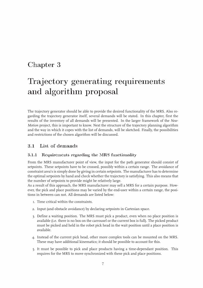
10 Traje tory generating requirements and algorithm proposal

PSfrag repla ements

1

2

3

4

5

6

78

9 9

10

11

start

end

A

A

B

C

D

EF

G

II

Iyesyes yes yes no

notime lefttime short onstraint a tive?Improved end time?

time riti al?

Use ubi spline to generatex, y and z path in kCSUse P2P to generate

r path in kCS

Compute path length, nodepositions; he k geometryCompute the path in kJSin spline representation Kinemati sTake a fifth-order timemapping and map on spline I End time estimateII End time from end position

Cal ulate mappingparametersDetermine most riti al onstraint; adjust timemapping onsequently this onstraint be omes a tive Update end time

Iteration step: splittime mapping

hange timing andupdate positionsInfeasible

Add at h-up profile

Add I/O timing and positions

Figure 3.1: Flow hart representing the traje tory generator stru ture.

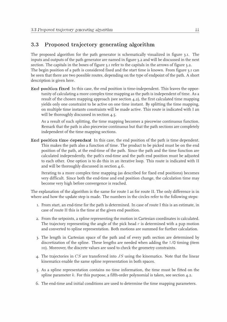
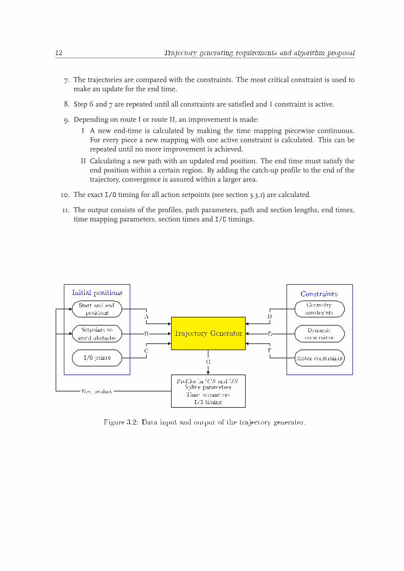
3.3 Proposed traje tory generating algorithm 113.3 Proposed traje tory generating algorithmThe proposed algorithm for the path generator is schematically visualized in figure 3.1. Theinputs and outputs of the path generator are named in figure 3.2 and will be discussed in the nextsection. The capitals in the boxes of figure 3.1 refer to the capitals in the arrows of figure 3.2.The begin position of a path is considered fixed and the start time is known. From figure 3.1 canbe seen that there are two possible routes, depending on the type of endpoint of the path. A shortdescription is given here.End position fixed In this case, the end position is time-independent. This leaves the oppor-

tunity of calculating a more complex time mapping as the path is independent of time. As aresult of the chosen mapping approach (see section 4.2), the first calculated time mappingyields only one constraint to be active on one time instant. By splitting the time mapping,on multiple time instants constraints will be made active. This route is indicated with I anwill be thoroughly discussed in section 4.5.

As a result of such splitting, the time mapping becomes a piecewise continuous function.Remark that the path is also piecewise continuous but that the path sections are completelyindependent of the time mapping sections.End position time dependant In this case, the end position of the path is time dependent.This makes the path also a function of time. The product to be picked must be on the endposition of the path, at the end-time of the path. Since the path and the time function arecalculated independently, the path’s end-time and the path end position must be adjustedto each other. One option is to do this in an iterative loop. This route is indicated with IIand will be thoroughly discussed in section 4.6.

Iterating to a more complex time mapping (as described for fixed end positions) becomesvery difficult. Since both the end-time and end position change, the calculation time maybecome very high before convergence is reached.

The explanation of the algorithm is the same for route I as for route II. The only difference is inwhere and how the update step is made. The numbers in the circles refer to the following steps:

1. From start, an end-time for the path is determined. In case of route I this is an estimate, incase of route II this is the time at the given end position.

2. From the setpoints, a spline representing the motion in Cartesian coordinates is calculated.The trajectory representing the angle of the pick head r is determined with a p2p motionand converted to spline representation. Both motions are summed for further calculation.

3. The length in Cartesian space of the path and of every path section are determined bydiscretization of the spline. These lengths are needed when adding the I/O timing (item10). Moreover, the discrete values are used to check the geometry constraints.

4. The trajectories in CS are transferred into JS using the kinematics. Note that the linearkinematics enable the same spline representation in both spaces.

5. As a spline representation contains no time information, the time must be fitted on thespline parameter k. For this purpose, a fifth-order polynomial is taken, see section 4.2.

6. The end-time and initial conditions are used to determine the time mapping parameters.

12 Traje tory generating requirements and algorithm proposal7. The trajectories are compared with the constraints. The most critical constraint is used to

make an update for the end time.

8. Step 6 and 7 are repeated until all constraints are satisfied and 1 constraint is active.

9. Depending on route I or route II, an improvement is made:

I A new end-time is calculated by making the time mapping piecewise continuous.For every piece a new mapping with one active constraint is calculated. This can berepeated until no more improvement is achieved.

II Calculating a new path with an updated end position. The end time must satisfy theend position within a certain region. By adding the catch-up profile to the end of thetrajectory, convergence is assured within a larger area.

10. The exact I/O timing for all action setpoints (see section 3.3.1) are calculated.

11. The output consists of the profiles, path parameters, path and section lengths, end times,time mapping parameters, section times and I/O timings.

PSfrag repla ements

ABCDEFGTraje tory GeneratorInitial positionsStart and endpositionsSetpoints toavoid obsta lesI/O points

ConstraintsGeometry onstraintsDynami onstraintsMotor onstraintsProfiles in tCS and tJSSpline parametersTime parametersI/O timingNext produ tFigure 3.2: Data input and output of the traje tory generator.

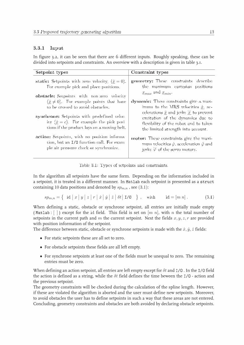
3.3 Proposed traje tory generating algorithm 133.3.1 InputIn figure 3.2, it can be seen that there are 6 different inputs. Roughly speaking, these can bedivided into setpoints and constraints. An overview with a description is given in table 3.1.Setpoint types Constraint typesstati : Setpoints with zero velo ity, (x = 0).For example pi k and pla e positions.obsta le: Setpoints with non-zero velo ity(x 6= 0). For example points that haveto be rossed to avoid obsta les.syn hrone: Setpoints with predefined velo -ity (x = c). For example the pi k posi-tions if the produ t lays on a moving belt.a tion: Setpoints, with no position informa-tion, but an I/O fun tion all. For exam-ple air pressure he k or syn hronize.

geometry: These onstraints des ribethe maximum artesian positionsxmax and xmin.dynami : These onstraints give a max-imum to the MRS velo ities x, a - elerations x and jerks ...x to preventex itation of the dynami s due toflexibility of the robot and to takenthe limited strength into a ount.motor: These onstraints give the maxi-mum velo ities ϕ, a eleration ϕ andjerks ...ϕ of the servo motors.Table 3.1: Types of setpoints and onstraints.

In the algorithm all setpoints have the same form. Depending on the information included ina setpoint, it is treated in a different manner. In Matlab each setpoint is presented as a stru tcontaining 10 data positions and denoted by spm,n , see (3.1):

spm,n ={ id x y z r x y z δt I/O }

, with id = [m n] . (3.1)When defining a static, obstacle or synchrone setpoint, all entries are initially made empty( Matlab : [ ] ) except for the id field. This field is set on [m n], with n the total number ofsetpoints in the current path and m the current setpoint. Next the fields x, y, z, r are providedwith position information of the setpoint.The difference between static, obstacle or synchrone setpoints is made with the x, y, z fields:

• For static setpoints these are all set to zero.

• For obstacle setpoints these fields are all left empty.

• For synchrone setpoints at least one of the fields must be unequal to zero. The remainingentries must be zero.

When defining an action setpoint, all entries are left empty except for δt and I/O . In the I/O fieldthe action is defined as a string, while the δt field defines the time beween the I/O - action andthe previous setpoint.The geometry constraints will be checked during the calculation of the spline length. However,if these are violated the algorithm is aborted and the user must define new setpoints. Moreover,to avoid obstacles the user has to define setpoints in such a way that these areas are not entered.Concluding, geometry constraints and obstacles are both avoided by declaring obstacle setpoints.

14 Traje tory generating requirements and algorithm proposal3.3.2 OutputThe output mainly consists of parameters and a number of timings. Parameters for the splinedescription and parameters for the time mapping. From these parameters, every possible profilecan be reconstructed, in time as well as in the spline index k.From these profiles, every interesting visualization while designing the trajectory, can be calcu-lated. For example: 3D image describing the calculated trajectory in CS (including orientation ofthe gripper), 3D animation of the gripper moving along the trajectory, cycle time, product count,time of picking product, etc. . .

For practical reasons, in a runtime environment the parameters in JS aremost interesting. In theend, the trajectories are sent to the actuators. The trajectories are calculated inCS and transferredto JS. The calculation of the active constraint however happens in CS as well as in JS. Thereis no practical advantage in making a conversion from CS to JS or vice versa. Only one activeconstraint will come out and this one is bounding, independent of the space.3.4 Dis ussionIn this section, the proposed design of the trajectory generation algorithm is compared with therequirements of the MRS and TG as stated in section 3.1. Moreover, several restrictions of thechosen approach are mentioned.

The algorithm should fulfill the demands to the greatest possible extent. This is checked bycomparing the demands with the properties of the proposed algorithm. In table C.1, the demandsregarding the MRS are evaluated, in table C.2 the demands regarding the TG are evaluated.It can be seen that most requirements are met. Some requirements are not directly taken intoaccount in the algorithm, but with some minor additions, they can easily be fulfilled.

The algorithm needs the motions of all axis to depend on one parameter k as the time is mappedon this parameter. Moreover, the domain of k must be equal for every axis.The main conclusion however, is the demand of being time optimal is not met. In the chosenapproach, the timemapping will not guarantee of having one constraint active all the time. In fact,during a motion only on a few moments, a constraint will be active. This is explained in section4.2. To guarantee a constraint to be active more often, the time mapping can be calculated in adifferent way. Several options are:

• take a higher-order mapping polynomial;

• a different mapping function, for example a combination of exponential functions;

• integration of the constraints along the path and map the time by applying look ahead feed.This is applied to first-order continuous functions in [7].

However, the fifth-order k(t) mapping is a good approach to start with.

Chapter 4Generating the path and the timemappingIn this chapter the mathematical formulation of algorithm as treated in section 3.3 will be elab-orated. The path generation within both spaces will be treated in section 4.1. In section 4.2the time is mapped on the path. In the remaining sections of this chapter, the handling of theconstraints and time-optimality will be treated.4.1 Representing the pathFrom the proposed algorithm, the path Cartesian space (x, y, z) is defined by splines. The angleof the pick head is given by r. The theory on splines is described in appendix D.4.1.1 Spline representation of the pathThe path in spline representation xi(k) is mathematically defined as:

xi(k) = (Xi(k), Yi(k), Zi(k)) , with i = 1, 2, . . . , n − 1 . (4.1)Each spline is defined in between n setpoints yielding n − 1 spline segments. The position inx(k) is defined by the polynomial Xi(k) and is defined in (D.2) as:

Xi(k) = axi + bx

i k + cxi k2 + dx

i k3 , with i = 1, 2, . . . , n − 1 . (4.2)The path variable k ∈ [0, 1] is non-uniform defined along the spline segment, this property isillustrated by (4.3).

X(k1) − X(k2) 6= X(k1 + δ) − X(k2 + δ) (4.3)For the rotation r, a point to point algorithm is used. It is known that a p2p motion can bewritten into a spline formulation, using the same definition for k and i as in (4.2). To make thetheory unambiguous with the definitions in section 2.2.1, (4.1) is completed with the positioninformation r.

xi(k) = (Xi(k), Yi(k), Zi(k), Ri(k))T , with i = 1, 2, . . . , n . (4.4)From now on, the path is no longer represented by the formulation of (4.1), but the notation of(4.4) will be used. 15

16 Generating the path and the time mapping4.1.2 Domains and spa esThe desired output of the trajectory generator is in JS and in the time domain. The path isdefined in CS and in the spline domain. The dynamic constraints are defined in CS and in thetime domain. To keep an eye on all domains and spaces, in table 4.1 an overview is presented. Inthis table the notation of each combination of domain and space is given and we define the wayin which a position in the each domain and space is represented.

CS time domain CS spline domain JS time domain JS spline domainnotation tCS kCS tJS kJSposition x(t) x(k) ϕ(t) ϕ(k)Table 4.1: Representation of positions, domains and spa es.From this table, it can be concluded that a certain CS position x can be defined both as a functionof k and as a function of t.

Rewriting from tJS to tCS , only involves the kinematics; the same applies to a conversion fromkJS and kCS . The kinematic relations are defined in section 2.2.1. Rewriting a path from thetime-domain to the spline-domain involves a relation between k and t. This is the time mappingwhich is defined by the function k = k(t).

The path in kCS can be given in a linear relation by combining (4.2) and (4.4):

xi(k) =

axi + bx

i k + cxi k2 + dx

i k3

ayi + by

i k + cyi k

2 + dyi k

3

azi + bz

i k + czi k

2 + dzi k

3

ari + br

i k + cri k

2 + dri k

3

=

axi bx

i cxi dx

i

ayi by

i cyi dy

i

azi bz

i czi dz

i

ari br

i cri dr

i

1kk2

k3

= P i k , (4.5)with k = [ 1 k k2 k3 ]T .

By combining (2.6) and (4.5) the conversion of the path from kCS to kJS is given by

ϕi(k) = Φi k , (4.6)

with

Φi = K−1 P i . (4.7)From (4.7), it can be seen that the positions in each segment in kJS is still determined by 16coefficients. Since both the kinematics and the path in kCS can be defined in a linear form, alsothe path in kJS can be represented in a linear form.

The path as a function of time in both tCS and tJS is now easily derived by substituting k(t) ink.

4.2 Proposed time mapping fun tion 174.2 Proposed time mapping fun tionAs is stated in section 3.4, there are several options for the k(t) mapping. At this time, the relationbetween k and t is taken as a fifth-order polynomial function:

k(t) = p0 + p1 t + p2 t2 + p3 t3 + p4 t4 + p5 t5 =5

∑

i=0

pi ti . (4.8)

The time mapping k(t) is defined for k ∈ [0, n] and must be strictly increasing. Although thespline is divided in segments, the mapping is not. This way, the path is kept second-order con-tinuous.

The reason to take a fifth-order polynomial function is simple. The mapping in (4.8) has 6unknown parameters (p0 to p5). The mapping must fulfill 6 boundary conditions:

t0 → k = 0 ,

t0 → dkdt

=(

dkdt

)

0,

t0 → d2kdt2

= 0 ,

tn → k = n ,

tn → dkdt

=(

dkdt

)

n,

tn → d2kdt2

= 0 .

(4.9)These conditions define the 6 parameters of the mapping k(t) .

How to derive the values for the mapping parameters (p0 to p5) making use of (4.9) is elaboratedin appendix E.1. When defining the begin and end position as static or synchrone setpoints, thetrajectory is not second-order continuous at the begin and end position. By setting the values for(

d2kdt2

)

0and

(

d2kdt2

)

nto zero, the demand of being second-order continuous is fulfilled.

In section 3.1, it is stated that it should be possible to give the path a direction and speed at thebegin and end nodes. Subsequently, in appendix D.3, it is shown that it is possible to cope with

this demand. However, how to derive the values for(

∂x∂k

)

0and

(

∂x∂k

)

nhas not been stated yet.

Also the derivation of the boundary conditions(

dkdt

)

0and

(

dkdt

)

nin (4.9) is not stated yet. In

appendix E.2 the relation between these derivatives and(

dxdt

)

0and

(

dxdt

)

nas defined in (3.1) is

elaborated.

In case the first setpoint is a static setpoint, (E.8) and (E.7) are used respectively. The relation

for(

∂x∂k

)

0and

(

dkdt

)

0can be stated as:

(

∂x

∂k

)

0

=

(

dx

dt

)

0

= 0 , (4.10)(

dk

dt

)

0

= 0 . (4.11)

18 Generating the path and the time mappingIn case the final setpoint is a synchrone setpoint, respectively (E.8) and (E.6) are used. The

relation for(

∂x∂k

)

nand

(

dkdt

)

ncan be stated as:

(

∂x

∂k

)

n

=

(

dx

dt

)

n

, (4.12)(

dk

dt

)

n

= 1 . (4.13)With the theory in appendix E.1 the time mapping is calculated. Applying the time mapping tothe path gives the trajectory.The path is defined as a piecewise function with the parameter k ∈ [0, 1]. This means that for thetime instants t that k(t) = i with i = 1, 2, . . . , n − 1, the continuation of the path is given by thepath segment i + 1. To calculate the path correctly from the time, these time instants must beknown. These are determined by using a zero f inder; e.g. the Matlab function fzero [3].

Finally, the end time tn is determined by either the velocity, acceleration or jerk profile in tCS ortJS . These profiles are compared with the constraints. The most critical profile determines tn.To calculate the profiles, the time derivatives are needed; this is treated in section 4.3. How todetermine tn is elaborated in section 4.4.4.3 Path derivativesThe time derivatives of the path determine the velocity, acceleration and jerk profiles. These4 profiles are needed in tCS and tJS , allowing for the evaluation of the dynamic and motorconstraints. The calculation of the derivatives is elaborated in this section, see also [2]. Thenotation of the derivatives is simplified by:

dx

dt(t) = x(t) , (4.14)

∂x

∂k(k) = x′(k) . (4.15)4.3.1 Velo ity

The first derivative of xi from (4.5) with respect to k is given by:

x′i(k) = P i k′ , (4.16)

with k′ = ∂k∂k

= [ 0 1 2k 3k2 ]T .

The first derivative of the path in JS: ϕiwith respect to k can be derived using (4.6)

ϕ′

i(k) = Φi k′ . (4.17)

From (4.16) and (4.17) the first derivative of xi and ϕiwith respect to t can be calculated by

applying the chain rule, which leads to

xi(t) = x′i(k)

(

dkdt

)

= P i k′(

dkdt

)

, (4.18)ϕ

i(t) = ϕ′

i(k)

(

dkdt

)

= Φi k′(

dkdt

)

, (4.19)respectively.

4.4 A tivating a onstraint 194.3.2 A elerationUsing (4.5) and (4.6), the second derivative of xi and ϕ

iwith respect to k is given by:

x′′i (k) = P i k′′ , (4.20)

ϕ′′

i(k) = Φi k′′ , (4.21)

respectively, with k′′ = [ 0 0 2 6k ]T .

From (4.18), the acceleration of the path in tCS is given by:

xi(t) = P i

{

k′′

(

dk

dt

)2

+ k′

(

d2k

dt2

)

}

. (4.22)This equation is derived in appendix F.1.

Using (4.7), the expression in (4.22) can easily be transformed to the acceleration in tJS :

ϕi(t) = Φi

{

k′′

(

dk

dt

)2

+ k′

(

d2k

dt2

)

}

. (4.23)4.3.3 JerkFinally, the relation for the third derivative of xi and ϕ

iwith respect to k in respectively kCS and

kJS is given by:

x′′′i (k) = P i k′′′ , (4.24)

ϕ′′′

i(k) = Φi k′′′ , (4.25)

respectively, with k′′′ = [ 0 0 0 6 ]T .

The jerk of the path in tCS is derived in appendix F.2 and can be formulated as:...x i(t) = P i

{

k′′′

(

dk

dt

)3

+ 3k′′

(

dk

dt

) (

d2k

dt2

)

+ k′

(

d3k

dt3

)

}

. (4.26)Using (4.7), the expression in (4.26) can easily be transformed to the jerk in tJS :...

ϕi(t) = Φi

{

k′′′

(

dk

dt

)3

+ 3k′′

(

dk

dt

) (

d2k

dt2

)

+ k′

(

d3k

dt3

)

}

. (4.27)4.4 A tivating a onstraintOne of the requirements of the trajectory generator is time-optimality. To meet this requirement,the next step in the algorithm is to assure that at least one constraint is active. This is done byiterating the end time tn. The first step involves choosing an end time tn or to take the end timebelonging to the end position of the spline. For this end time, the mapping k(t) is calculated inthe way described in appendix E.1 and mapped on the path. This yields x(t) .

20 Generating the path and the time mapping4.4.1 Determining the maxima of ea h profileThe derivatives of x(t) (from now called profiles) are calculated as described in section 4.3. Untilthis point, the path and the mapping are given by parameters. By applying these parametersin the correct function, for every time, every profile value can be calculated. To determine theactive constraint however, the maximum absolute value of every profile must be known. Thesemaximum values must be within the constraints and for one derivative, the constraint must beactive. There are two options to determine the maximum absolute value:

1. Calculate the positions where the derivative of each profile is zero and pick the positionswhere the absolute value of every maxima is maximal. This approach is exact in theory. Inpractice however, a numerical zero finder is needed. As the path x(t) is a fifteenth-orderpolynomial function of time, this approach will be very slow. It is also difficult to implementand may lead to convergence problems of the zero finder.

2. Calculate the profile values for a discrete number of positions and pick the time wherethe profile value is maximal. The accuracy is limited by the discretization step, the con-straints may be crossed in between two discrete positions. Around a maximum, both theconstraints and the profile have a derivative of 0. As a result, the amount of crossing ofthe constraint is limited when a sufficiently large number of discrete positions are used.Moreover, the exact amount crossing of the constraint is not of much importance; mostconstraints are formulated within a certain safety margin. For this approach a lot of calcu-lation is needed, however, it is easy to implement.

Concluding, the second method is preferred.

The discretization is performed for each spline section, i.e. for every spline section the profilesvalues are calculated for s positions. The s discrete positions are derived from s discrete timeinstants. The timing at the begin (ti,0) and end (ti,1) of each path section i is known by using azero f inder as is explained at the end of section 4.2. The discrete time instants (Ti,j) are given by:

∆Ti =ti,1−ti,0

s−1with i = 1, 2, . . . , n ,

Ti,j = ti,0 + (j − 1) ∆Ti with j = 1, 2, . . . , s .(4.28)

The chosen form of the discretization, has two advantages:

1. The values of the profiles are calculated two times at the nodes; once on every side of thespline. As the jerk profile shows a step in time, in this way both values are calculated.

2. Some spline segments may be shorter than others. As every spline segment is divided in spositions, every spline is taken into account. If the complete path was divided in a numberof positions, some spline sections could be very coarsely populated or in extreme cases evencompletely be skipped by the discretization.

The polynomial formulation of the path limits the number of maxima in each segment. No ex-tremely high number of discrete positions are needed to assure the maximum to be found.

For the time instants Ti,j the position and profile values are calculated in tCS and tJS and storedin a stru t. This stru t has (4 ·6 ·n · s) data entries. Next step is to find the maximum absolutevalue for each constraint. This leaves 24 data entries:

[

xmax xmax

...xmax ϕ

maxϕ

max

...ϕ

max

]

. (4.29)

4.4 A tivating a onstraint 214.4.2 Iteration of the a tive onstraintFor each of the 24 data entries in (4.29), the relative error e with respect to the constraint iscalculated, see (4.30). Note that the division in the first three equations indicate an element-wisedivision of the column entries. The 24 data entries in (4.29) are now converted into 24 relativeerrors, divided over 6 columns:

eCS,1 = (a − xmax) / a with a = CS velo ity onstraints;eCS,2 = (b − xmax) / b with b = CS a eleration onstraints;eCS,3 = (c − ...

xmax) / c with c = CS jerk onstraints;eJS,1 = (α − ϕ

max) / α with α = JS velo ity onstraint;

eJS,2 = (β − ϕmax

) / β with β = JS a eleration onstraint;eJS,3 = (γ −

...ϕ

max) / γ with γ = JS jerk onstraint. (4.30)The relative error indicates the the relative difference between a maximum and the constraint.Three cases can be defined:

e > 0 the maximum is within the onstraint;e = 0 the maximum is on the onstraint;e < 0 the maximum rosses the onstraint.

When e ≈ 0, for one constraint while all others e > 0, the iteration should be terminated. Thisis a good stopping criterion. The iteration of the end time tn should converge to this criterion. Atstep k + 1 of the iteration, the old end time tn,k is updated by multiplying it with a factor ν:

tn,k+1 = ν tn,k . (4.31)On first thought, ν should be some function of the smallest relative error. While simulating thealgorithm; it is noticed that ν must not only depend on the smallest relative error. The factor νis given as the maximum of three update factors u1, u2 and u3. The relation for calculating theupdate factors u1 to u3 is empirically determined for each order of the time derivative of the path.This is shown in (4.32) and (4.33):

ν = max ( u1 , u2 , u3 ) , (4.32)u1 = 1 − e1 with e1 = min (

eCS,1 , eJS,1

)

,

u2 =√

1 − e2 with e2 = min (

eCS,2 , eJS,2

)

,

u3 = 3√

1 − e3 with e3 = min (

eCS,3 , eJS,3

)

.

(4.33)As can be seen, the space of the constraint is of no importance regarding the calculation of ν. Apath with one active constraint is the result. In case of all boundary conditions except k(tn) in(4.9) being equal to zero and k(tn) = n, convergence will reached in one step.

22 Generating the path and the time mapping4.5 Improving the time-optimality of a time-independent pathThe major part of the algorithm as given in section 3.3 is now treated. The only parts left are theimproving step as defined by 9-I and 9-II. Item 9-I will be treated in this section, item 9-II willbe treated in section 4.6.

Route 9-I supposes a fixed (time independent) end position. This iteration loop is given by thefollowing steps:

1. A path x(k) and a second-order continuous time mapping k(t) are calculated as is shownin the previous paragraphs. These result in a trajectory.

2. From this trajectory the position with an active constraint arises. The values of k, dkdt

and d2kdt2

at this position are fixed and stored. The fixed values will function as additional boundaryconditions for the new piecewise second-order continuous time mapping k2(t) .

3. The old mapping k(t) is replaced by a piecewise time mapping k2(t) . The path x(t) is notchanged. Item 6 in figure 3.1 is called two times to calculate the mapping k2(t) :

(a) The first mapping is in between the original starting position and the fixed position;

(b) The second mapping is in between the fixed position and the original end position.

4. Also the new calculated mappings can be split, giving 4 k(t) mappings, etc. . .

The main difficulty in this scheme is to avoid the recalculation of the already found position withan active constraint. This may happen when item 8 is called in loop 9-I. The time mappingiteration schema (8 in figure 3.1) aborts when one relative error becomes zero. As the fixed posi-tion (with an active constraint) already has a relative error zero, the iteration aborts immediately.There are three possibilities to avoid this; all of them are not completely satisfying:

1. While determining a new maximum, every maximum with the same characteristics as thealready active constraint is not taken in to account. The characteristics of the found con-straint are given by:

(a) the path segment where the fixed position is in;

(b) the sign of the constraint at the fixed position, indicating a maximum or a minimum;

(c) the type of the of the active constraint, i.e. velocity, acceleration or jerk constraint;

(d) the axis of the active constraint, i.e. the x, y, z, r, ϕx, ϕy, ϕz or ϕr axis.

2. This method is the same as the previous one, but with one addition. It is possible thatblocking the constraint with the characteristics as given above, becomes violated at anotherposition. To prevent this, the constraint characteristics are only blocked within a safety mar-gin around the fixed position found in the previous iteration. The success of this additionwill largely depend on the size of the safety margin.

3. In the third method the new estimated end time for the time mapping in each section,is taken to be very short. This forces the mapping to violate other constraints, while theposition on the border of the time sections remains only active. Now the constraint withthe largest relative error will be used for iterating. However, convergence is not guaranteedas the fixed position (on the border of the mapping section) may still become recalculated.

4.6 Feasibility of a time-dependent path 23The first two methods require a strict accounting of the constraint characteristics at the fixedposition(s). Coping with the already found fixed position(s), requires corrections on the stan-dard procedure as explained in section 4.4. These corrections make the iteration scheme ratherchaotic.

When calling iteration loop 9-I more then twice, most new mapping sections have two constraintinstants (at the start and at end of the each time mapping section). Handling both these activeconstraint instants (correcting two times), will complicate the iteration scheme further.

In chapter 5, the implementation of the algorithm in Matlab is discussed. In the implementation,methods 1 and 3 are used to avoid recalculation of the fixed position.4.6 Feasibility of a time-dependent pathRoute 9-II supposes a time dependent end position. This has not been implemented in Matlab yet.However, some things about the convergence of the iteration can be noted.

The problem concerns a moving product on a belt. The end position of the belt should be reachedat the moment a product to pick is passing by. In advance, little is known about the length of thepath and the time it takes to reach the end position. The following iteration is proposed:

1. Take an estimated end position. The time at which the product to pick will pass that positioncan be calculated from the product’s (constant) velocity and current position.

2. Calculate a path x(t) .

3. Calculate a time mapping k(t) , use the end position’s time as the estimated end time forcalculating k(t) .

4. Iterating the k(t) mapping results in one constraint te become active on one position. Thisyields a new end time for the path.

5. Calculate the position of the product at the end time of the k(t) mapping, calculated in theprevious step. Use this new end position for recalculating the path, perform a new timemapping, etc. . .

6. When the end time and end position match within a certain area, the pick-up profile iscalled. This profile assures that the pick head catches the product and ensures the appro-priate pick action.

For the starting pick position estimate and the accompanying end time, there are two options:

1. Taking a safe guess for the first end position: the boundary of the picking area; i.e. thelatest possible pick position. Now start iterating backwards to a feasible position and endtime. In this way infeasible product picks are filtered out immediately.

2. Pick a first estimate based on previous information about motion times. This results in lesscalculation time but infeasible product picks are not noticed within the first iteration loop.

24 Generating the path and the time mappingAnother option for handling time dependant end positions is to insert iteration loop 9-I intoiteration loop 9-II. First, loop 9-I is called once for generating a time mapping consisting of twopiecewise continuous functions. This yields a constraint to be active on 3 time instants. Next,loop 9-II is called to update the end position with the new end time. Again, loop 9-I is called onceand loop 9-II, etc . . .A time dependant path with on more time instants an active constraint can be determined. How-ever, at this point we can conclude little about the calculation time and the convergence of theproblem in this case.

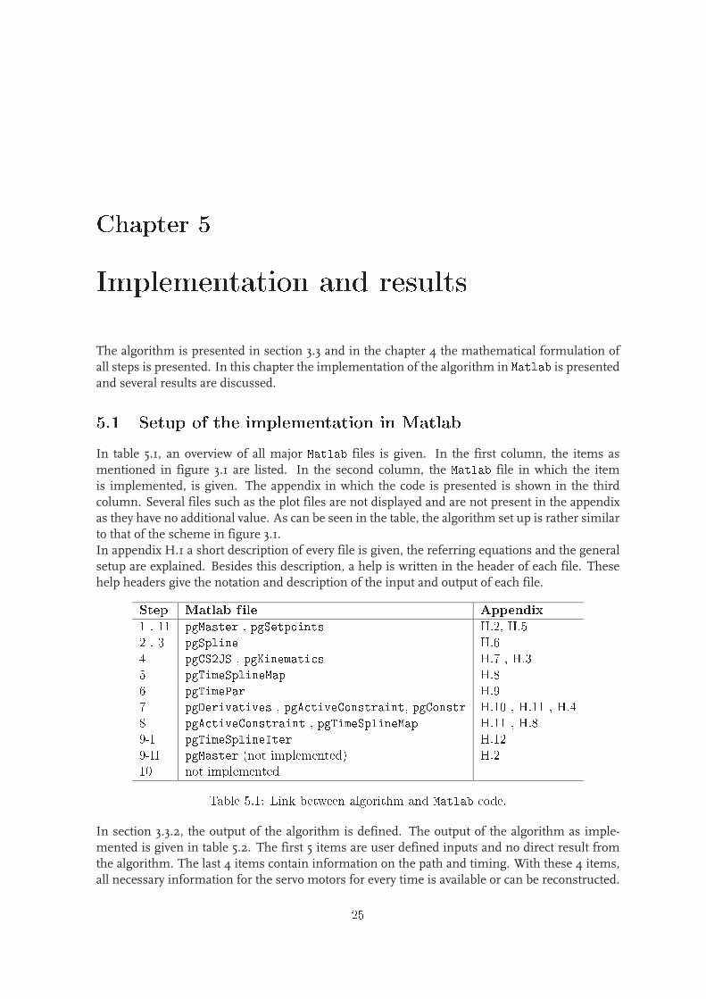
Chapter 5Implementation and resultsThe algorithm is presented in section 3.3 and in the chapter 4 the mathematical formulation ofall steps is presented. In this chapter the implementation of the algorithm in Matlab is presentedand several results are discussed.5.1 Setup of the implementation in MatlabIn table 5.1, an overview of all major Matlab files is given. In the first column, the items asmentioned in figure 3.1 are listed. In the second column, the Matlab file in which the itemis implemented, is given. The appendix in which the code is presented is shown in the thirdcolumn. Several files such as the plot files are not displayed and are not present in the appendixas they have no additional value. As can be seen in the table, the algorithm set up is rather similarto that of the scheme in figure 3.1.In appendix H.1 a short description of every file is given, the referring equations and the generalsetup are explained. Besides this description, a help is written in the header of each file. Thesehelp headers give the notation and description of the input and output of each file.Step Matlab file Appendix1 , 11 pgMaster , pgSetpoints H.2, H.52 , 3 pgSpline H.64 pgCS2JS , pgKinemati s H.7 , H.35 pgTimeSplineMap H.86 pgTimePar H.97 pgDerivatives , pgA tiveConstraint, pgConstr H.10 , H.11 , H.48 pgA tiveConstraint , pgTimeSplineMap H.11 , H.89-I pgTimeSplineIter H.129-II pgMaster (not implemented) H.210 not implementedTable 5.1: Link between algorithm and Matlab ode.In section 3.3.2, the output of the algorithm is defined. The output of the algorithm as imple-mented is given in table 5.2. The first 5 items are user defined inputs and no direct result fromthe algorithm. The last 4 items contain information on the path and timing. With these 4 items,all necessary information for the servo motors for every time is available or can be reconstructed.25

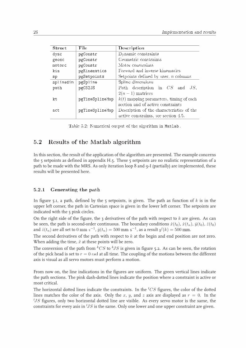
26 Implementation and resultsStru t File Des riptiondyn pgConstr Dynami onstraintsgeom pgConstr Geometri onstraintsmotor pgConstr Motor onstraintskin pgKinemati s Forward and inverse kinemati ssp pgSetpoints Setpoints defined by user, n olumnssplinedim pgSpline Spline dimensionspath pgCS2JS Path des ription in CS and JS,2(n − 1) matri eskt pgTimeSplineMap k(t) mapping parameters, timing of ea hse tion and of a tive onstraintsa t pgTimeSplineMap Des ription of the hara teristi s of thea tive onstraints, see se tion 4.5.Table 5.2: Numeri al output of the algorithm in Matlab .5.2 Results of the Matlab algorithm

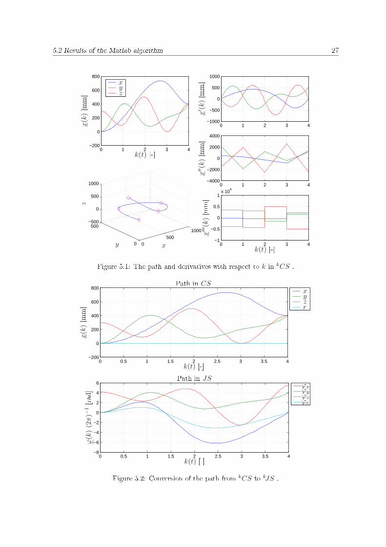
In this section, the result of the application of the algorithm are presented. The example concernsthe 5 setpoints as defined in appendix H.5. These 5 setpoints are no realistic representation of apath to be made with the MRS. As only iteration loop 8 and 9-I (partially) are implemented, theseresults will be presented here.5.2.1 Generating the pathIn figure 5.1, a path, defined by the 5 setpoints, is given. The path as function of k is in theupper left corner, the path in Cartesian space is given in the lower left corner. The setpoints areindicated with the 5 pink circles.

On the right side of the figure, the 3 derivatives of the path with respect to k are given. As canbe seen, the path is second-order continuous. The boundary conditions x(t0), x(tn), y(t0), z(t0)and z(tn) are all set to 0 mm s−1, y(tn) = 500 mm s−1, as a result y′(k) = 500 mm.

The second derivatives of the path with respect to k at the begin and end position are not zero.When adding the time, x at these points will be zero.

The conversion of the path from kCS to kJS is given in figure 5.2. As can be seen, the rotationof the pick head is set to r = 0 rad at all time. The coupling of the motions between the differentaxis is visual as all servo motors must perform a motion.

From now on, the line indications in the figures are uniform. The green vertical lines indicatethe path sections. The pink dash-dotted lines indicate the position where a constraint is active ormost critical.

The horizontal dotted lines indicate the constraints. In the tCS figures, the color of the dottedlines matches the color of the axis. Only the x, y, and z axis are displayed as r = 0. In thetJS figures, only two horizontal dotted line are visible. As every servo motor is the same, theconstraints for every axis in tJS is the same. Only one lower and one upper constraint are given.

5.2 Results of the Matlab algorithm 27

0 1 2 3 4−200

0

200

400

600

800

0500

1000

0

500−500

0

500

1000

0 1 2 3 4−1000

−500

0

500

1000

0 1 2 3 4−4000

−2000

0

2000

4000

0 1 2 3 4−1

−0.5

0

0.5

1x 10

4

PSfrag repla ements

x

x

y

yz

z[s℄

k(t) [-℄k(t) [-℄

[s ℄[s ℄[s ℄ x(k

)

[mm℄

x′ (k)

[mm℄

x′′(k

)

[mm℄x′′′ (k)

[mm℄[mm℄[mm s ℄[mm s ℄... [mm s ℄[rad℄[rad℄[rad s ℄[rad s ℄... [rad s ℄ Figure 5.1: The path and derivatives with respe t to k in kCS .0 0.5 1 1.5 2 2.5 3 3.5 4

−200

0

200

400

600

800

0 0.5 1 1.5 2 2.5 3 3.5 4−8

−6

−4

−2

0

2

4

6

PSfrag repla ementsx

ϕx

y

ϕy

z

ϕz

r

ϕr

[s℄

k(t) [-℄k(t) [-℄

[s ℄[s ℄[s ℄

x(k

)

[mm℄[mm℄[mm℄[mm℄[mm℄[mm s ℄[mm s ℄... [mm s ℄

ϕ(k

)(2

π)−

1

[rad℄[rad℄[rad s ℄[rad s ℄... [rad s ℄

Path in CS

Path in JS

Figure 5.2: Conversion of the path from kCS to kJS .

28 Implementation and results

0 2 4 6 8 100

1

2

3

4

0 2 4 6 8 10−0.2

0

0.2

0.4

0.6

0.8

1

1.2

0 2 4 6 8 100

0.05

0.1

0.15

0.2

0 2 4 6 8 10−0.15

−0.1

−0.05

0

0.05

PSfrag repla ements

t [s℄t [s℄t [s℄t [s℄k

(t)

[-℄

dk

dt

[s−1 ℄d2k

dt2

[s−2 ℄d3k

dt3

[s−3 ℄[mm℄[mm℄[mm℄[mm℄[mm℄[mm s ℄[mm s ℄... [mm s ℄[rad℄[rad℄[rad s ℄[rad s ℄... [rad s ℄ Figure 5.3: Time mapping for tn = 10 s.

0 0.5 1 1.5 2 2.50

1

2

3

4

0 0.5 1 1.5 2 2.5−0.5

0

0.5

1

1.5

2

2.5

3

0 0.5 1 1.5 2 2.5−3

−2

−1

0

1

2

3

4

0 0.5 1 1.5 2 2.5−10

−5

0

5

10

15

20

PSfrag repla ements

t [s℄t [s℄t [s℄t [s℄k

(t)

[-℄

dk

dt

[s−1 ℄

d2k

dt2

[s−2 ℄

d3k

dt3

[s−3 ℄[mm℄[mm℄[mm℄[mm℄[mm℄[mm s ℄[mm s ℄... [mm s ℄[rad℄[rad℄[rad s ℄[rad s ℄... [rad s ℄ Figure 5.4: Time mapping for tn = 2.2383 s.

5.2 Results of the Matlab algorithm 29

0 0.5 1 1.5 2 2.5−200

0

200

400

600

800

0500

1000

0

500−500

0

500

1000

0 0.5 1 1.5 2 2.5−5000

0

5000

0 0.5 1 1.5 2 2.5−1

−0.5

0

0.5

1x 10

5

0 0.5 1 1.5 2 2.5−2

−1

0

1

2x 10

6

PSfrag repla ementsx

x

y

y

z

z

r

t [s℄

t [s℄[-℄[s ℄[s ℄[s ℄[mm℄[mm℄[mm℄[mm℄

x(t

)

[mm℄ x(t

)

[mms−1 ℄

x(t

)

[mms−2 ℄

... x(t

)

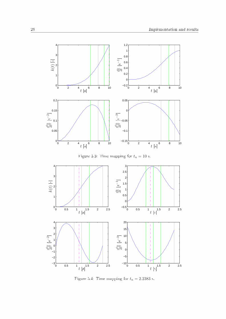
[mms−3 ℄[rad℄[rad℄[rad s ℄[rad s ℄... [rad s ℄ Figure 5.5: Traje tory in tCS with tn = 2.2383 s.5.2.2 Time mappingOn the path, the time must be mapped with the function k(t). The first estimated end time is setto tn = 10 s. The resulting k(t) mapping function is given in figure 5.3.

The green section lines indicate that the path is not symmetric, this is only the case whenk(t0) = k(tn). Since the last setpoint is defined with y(tn) = 500 mm s−1, the boundary con-ditions for k(t) are k(t0) = 0 s−1 and k(tn) = 1 s−1; yielding no symmetric time mapping.

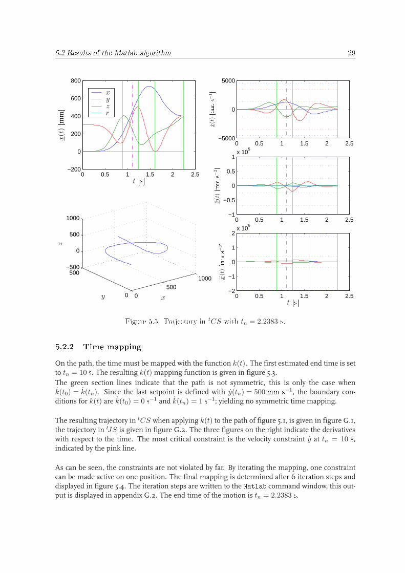
The resulting trajectory in tCS when applying k(t) to the path of figure 5.1, is given in figure G.1,the trajectory in tJS is given in figure G.2. The three figures on the right indicate the derivativeswith respect to the time. The most critical constraint is the velocity constraint y at tn = 10 s,indicated by the pink line.

As can be seen, the constraints are not violated by far. By iterating the mapping, one constraintcan be made active on one position. The final mapping is determined after 6 iteration steps anddisplayed in figure 5.4. The iteration steps are written to the Matlab command window, this out-put is displayed in appendix G.2. The end time of the motion is tn = 2.2383 s.

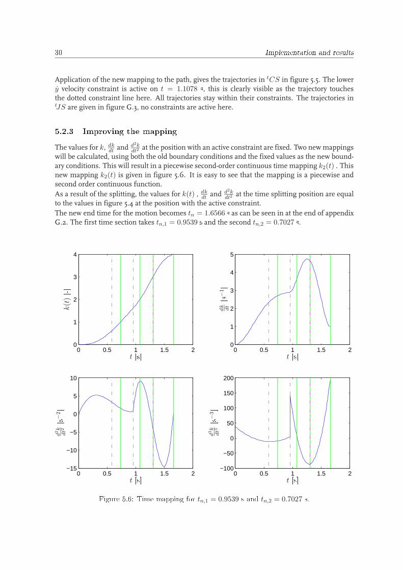
30 Implementation and resultsApplication of the new mapping to the path, gives the trajectories in tCS in figure 5.5. The lowery velocity constraint is active on t = 1.1078 s, this is clearly visible as the trajectory touchesthe dotted constraint line here. All trajectories stay within their constraints. The trajectories intJS are given in figure G.3, no constraints are active here.5.2.3 Improving the mappingThe values for k, dk

dtand d2k

dt2at the position with an active constraint are fixed. Two newmappings

will be calculated, using both the old boundary conditions and the fixed values as the new bound-ary conditions. This will result in a piecewise second-order continuous time mapping k2(t) . Thisnew mapping k2(t) is given in figure 5.6. It is easy to see that the mapping is a piecewise andsecond order continuous function.

As a result of the splitting, the values for k(t) , dkdt

and d2kdt2

at the time splitting position are equalto the values in figure 5.4 at the position with the active constraint.

The new end time for the motion becomes tn = 1.6566 s as can be seen in at the end of appendixG.2. The first time section takes tn,1 = 0.9539 s and the second tn,2 = 0.7027 s.

0 0.5 1 1.5 20

1

2

3

4

0 0.5 1 1.5 20

1

2

3

4

5

0 0.5 1 1.5 2−15

−10

−5

0

5

10

0 0.5 1 1.5 2−100

−50

0

50

100

150

200

PSfrag repla ements

t [s℄t [s℄

t [s℄t [s℄

k(t

)

[-℄dk

dt

[s−1 ℄

d2k

dt2

[s−2 ℄

d3k

dt3

[s−3 ℄[mm℄[mm℄[mm℄[mm℄[mm℄[mm s ℄[mm s ℄... [mm s ℄[rad℄[rad℄[rad s ℄[rad s ℄... [rad s ℄ Figure 5.6: Time mapping for tn,1 = 0.9539 s and tn,2 = 0.7027 s.

5.2 Results of the Matlab algorithm 31

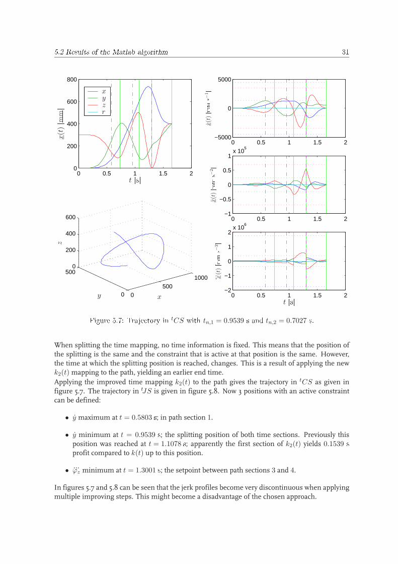
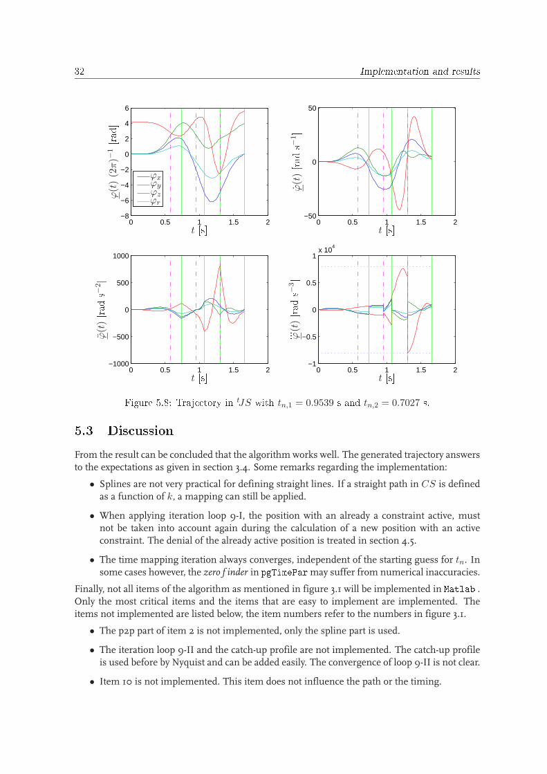
0 0.5 1 1.5 20

200

400

600

800

0500

1000

0

5000

200

400

600

0 0.5 1 1.5 2−5000

0

5000

0 0.5 1 1.5 2−1

−0.5

0

0.5

1x 10

5

0 0.5 1 1.5 2−2

−1

0

1

2x 10

6

PSfrag repla ementsx

x

y

y

z

z

r

t [s℄

t [s℄[-℄[s ℄[s ℄[s ℄[mm℄[mm℄[mm℄[mm℄

x(t

)

[mm℄ x(t

)

[mms−1 ℄

x(t

)

[mms−2 ℄

... x(t

)

[mms−3 ℄[rad℄[rad℄[rad s ℄[rad s ℄... [rad s ℄ Figure 5.7: Traje tory in tCS with tn,1 = 0.9539 s and tn,2 = 0.7027 s.When splitting the time mapping, no time information is fixed. This means that the position ofthe splitting is the same and the constraint that is active at that position is the same. However,the time at which the splitting position is reached, changes. This is a result of applying the newk2(t) mapping to the path, yielding an earlier end time.

Applying the improved time mapping k2(t) to the path gives the trajectory in tCS as given infigure 5.7. The trajectory in tJS is given in figure 5.8. Now 3 positions with an active constraintcan be defined:

• y maximum at t = 0.5803 s; in path section 1.

• y minimum at t = 0.9539 s; the splitting position of both time sections. Previously thisposition was reached at t = 1.1078 s; apparently the first section of k2(t) yields 0.1539 sprofit compared to k(t) up to this position.

• ...ϕz minimum at t = 1.3001 s; the setpoint between path sections 3 and 4.

In figures 5.7 and 5.8 can be seen that the jerk profiles become very discontinuous when applyingmultiple improving steps. This might become a disadvantage of the chosen approach.

32 Implementation and results

0 0.5 1 1.5 2−8

−6

−4

−2

0

2

4

6

0 0.5 1 1.5 2−50

0

50

0 0.5 1 1.5 2−1000

−500

0

500

1000

0 0.5 1 1.5 2−1

−0.5

0

0.5

1x 10

4

PSfrag repla ementsϕxϕyϕzϕr

t [s℄t [s℄

t [s℄t [s℄[-℄[s ℄[s ℄[s ℄[mm℄[mm℄[mm℄[mm℄[mm℄[mm s ℄[mm s ℄... [mm s ℄[rad℄

ϕ(t

)(2

π)−

1

[rad℄

ϕ(t

)

[rads−1 ℄ϕ(t

)

[rads−2 ℄ ... ϕ(t

)

[rads−3 ℄Figure 5.8: Traje tory in tJS with tn,1 = 0.9539 s and tn,2 = 0.7027 s.5.3 Dis ussion

From the result can be concluded that the algorithm works well. The generated trajectory answersto the expectations as given in section 3.4. Some remarks regarding the implementation:

• Splines are not very practical for defining straight lines. If a straight path in CS is definedas a function of k, a mapping can still be applied.

• When applying iteration loop 9-I, the position with an already a constraint active, mustnot be taken into account again during the calculation of a new position with an activeconstraint. The denial of the already active position is treated in section 4.5.

• The time mapping iteration always converges, independent of the starting guess for tn. Insome cases however, the zero f inder in pgTimeParmay suffer from numerical inaccuracies.

Finally, not all items of the algorithm as mentioned in figure 3.1 will be implemented in Matlab .Only the most critical items and the items that are easy to implement are implemented. Theitems not implemented are listed below, the item numbers refer to the numbers in figure 3.1.

• The p2p part of item 2 is not implemented, only the spline part is used.

• The iteration loop 9-II and the catch-up profile are not implemented. The catch-up profileis used before by Nyquist and can be added easily. The convergence of loop 9-II is not clear.

• Item 10 is not implemented. This item does not influence the path or the timing.

Chapter 6Con lusions and re ommendationsIn this project, the requirements for trajectory generation for a specific robot are considered. Analgorithm fulfilling the requirements has been developed and is implemented in a Matlab pro-gram. The following conclusions and recommendations can be made.6.1 Con lusionsThe first objective of this project, i.e. to make an inventory of demands of a trajectory gener-ator regarding a specific robot, has been met by taking several interviews. The result of theseinterviews are transformed into a list of demands regarding a trajectory generator. From thesedemands an algorithm in a flow chart form is formulated. The requirements as stated are validfor any type of robot. However, additional requirements might be needed for specific robots. Thealgorithm starts with defining the path for all axes. To achieve synchronization between all axes,positions are defined by the path variable k. By writing k as a function of time t yielding k(t) , thetime is mapped on the path. The path as a function of time is called the trajectory.

The time mapping function k(t) is chosen as a fifth-order polynomial function. The mappingfunction is suitable if and only if k(t) is a strictly increasing function, this is a necessary condition.As the parameters of the mapping function depend on the boundary conditions, the necessarycondition is difficult to guarantee.

There is a lot of space for improvement of the k(t) function yielding a more time-optimal trajec-tory. For example by considering other types of mapping functions.

The constraints in multiple domains are handled by evaluating them in their own domain. Theconversion between the domains is defined by the kinematics. The constraints are not converted,only the path. In this way, the kinematics are called only once. In case of more complex kine-matics, this is a desirable feature. When the path is known in both joint space and Cartesianspace, the time mapping is performed on both paths. The time derivatives are calculated after-wards. When the time derivatives are known, the constraints are compared with the profile theconstraint relates to.

The chosen approach does not lead to a constraint being active permanently. Only on one or on afew positions within one motion, a constraint will be active. No constraints will be crossed. Theactive constraint is determined in an iterative loop; the variable which is iterated is the end timeof the motion. The motion can be made faster by allowing constraints to be active at more andmore time instants. 33

34 Con lusions and re ommendationsThe algorithm is partially implemented in a Matlab program. Two different iterative loops aredefined, depending on the time-dependency of the path. In both cases a third iterative loop iscalled for determining the timing mapping function k(t) .The algorithm for a time-independent path is proven to work. In this case, a loop is requiredaround the k(t) loop. However, no good stopping criterion has been formulated and its applica-bility is limited; it is difficult to avoid the recalculation of positions with an active constraint.The algorithm for a time-dependent path is not implemented and no updating step has beenformulated. At this point, it is difficult to say whether the proposed algorithm will work; this willdepend largely on the strategy to gain convergence and the kind of update step, that is chosen.Moreover, only one constraint will be active along the complete motion.6.2 Re ommendationsConsidering the time mapping, a different method instead of picking a certain type of function,might be used. Iterating the constraints along the path will yield a better result with a perma-nently active constraint. This method has proven to work for first-order continuous functions[7]. Research for second- or higher-order continuous functions would be worthwhile. There aretwo additional advantages; firstly, no iteration loop for determining the end time of a motion isneeded anymore and secondly, the demand of for a strictly increasing function is easy to handle.

The path in space is defined with cubic splines; this limits the type of possible motions. Forexample, with cubic splines it is not possible to represent straight lines. As a result, other pathformulations should be considered; i.e. straight lines, circles, etc. . . It must be possible to repre-sent these formulations with the path parameter k(t) . The same can be said with respect to thetime mapping k(t) ; namely for the mapping also other representations can be considered.

The path of cubic splines is second-order continuous. In order to make even smoother paths,higher-order splines can be used. This causes less excitation of the dynamics of the robot and itmakes the motions more accurate and easier to control.

How ”generic” a generic path generation should be, must be investigated. In some cases, robotsneed to make very specific motions for which it is hard to give a generic formulation. It is easierto generate the main part of a trajectory with a generic algorithm and to add some very specificpath sections specially written for the robot.

With the current definition of a setpoint, it is not possible to define a start or end direction ofthe path, independent of the velocity. At this point, the direction can be influenced by definingadditional setpoints. In case a boundary velocity is zero, it might be convenient to define theaccelerations at this position. Concluding, it would be worthwhile to investigate a different wayof defining setpoints with independent direction and velocity.

Finally, the current representation of the path with the parameter k(t) has two drawbacks. Firstlyevery segment is defined for k(t) ∈ [0, 1]; it would be better to define k(t) ∈ [0, s]with s ameasurefor the Euclidian distance. Secondly k(t) is not proportionally distributed within a segment; betterwould be a linear relation between k and the position, yielding smoother splines. These twodrawbacks result in unnecessary high maxima in the profiles.As the end time of the time mapping is determined by the maxima of the profiles, it is desired tokeep them as low as possible. If k would be linear in with the position, much quicker mappingscould be determined using the fifth-order k(t) mapping.

Bibliography[1] R.H. Bartels, J.C. Beatty, and B.A. Barsky. An introduction to splines for use in computer graphics

& geometric modeling. Morgan Kaufmann Publishers, 1987.

[2] D. Constantinescu and E.A. Croft. Smooth and time-optimal trajectory planning for industrialmanipulators along specified paths. Journal of Robotic Systems, 17(5):233 – 249, July 2000.

[3] The Mathworks Inc. Using Matlab Revised for MATLAB 6 (Release 12). The Mathworks Inc,Natick, United States of America, 5 edition, November 2000.

[4] Simatic Industrial Software. Step 7. Siemens. http://www2.automation.siemens.com/simatic/industriesoftware/html_76/produkte/software-step7.htm.

[5] M.J.G. van de Molengraft. Third-degree path generator for MATLAB 6 (Release 12). EindhovenUniversity of Technology. http://www.dct.tue.nl/home_of_ref3.htm.

[6] N. van de Wouw. Multibody Dynamica - 4J400. Eindhoven University of Technology, 2003.lecture notes: 4816.

[7] F. van Tuijl, S. Lagewaard, S. Rienstra, and A. Reusken. Toward look-ahead feed and cubichermite interpolation, version 3.0. Philips Machine Tool Controls, April 16, 1991.

35

36 BIBLIOGRAPHY

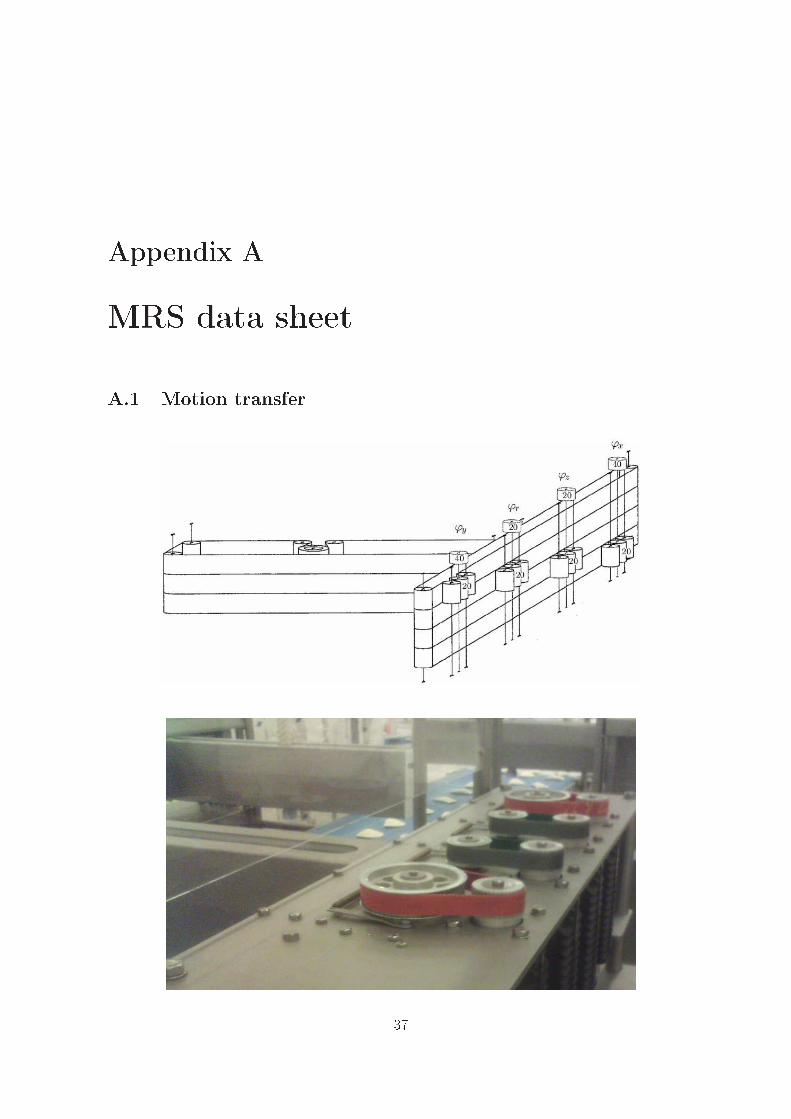
Appendix AMRS data sheetA.1 Motion transfer

37

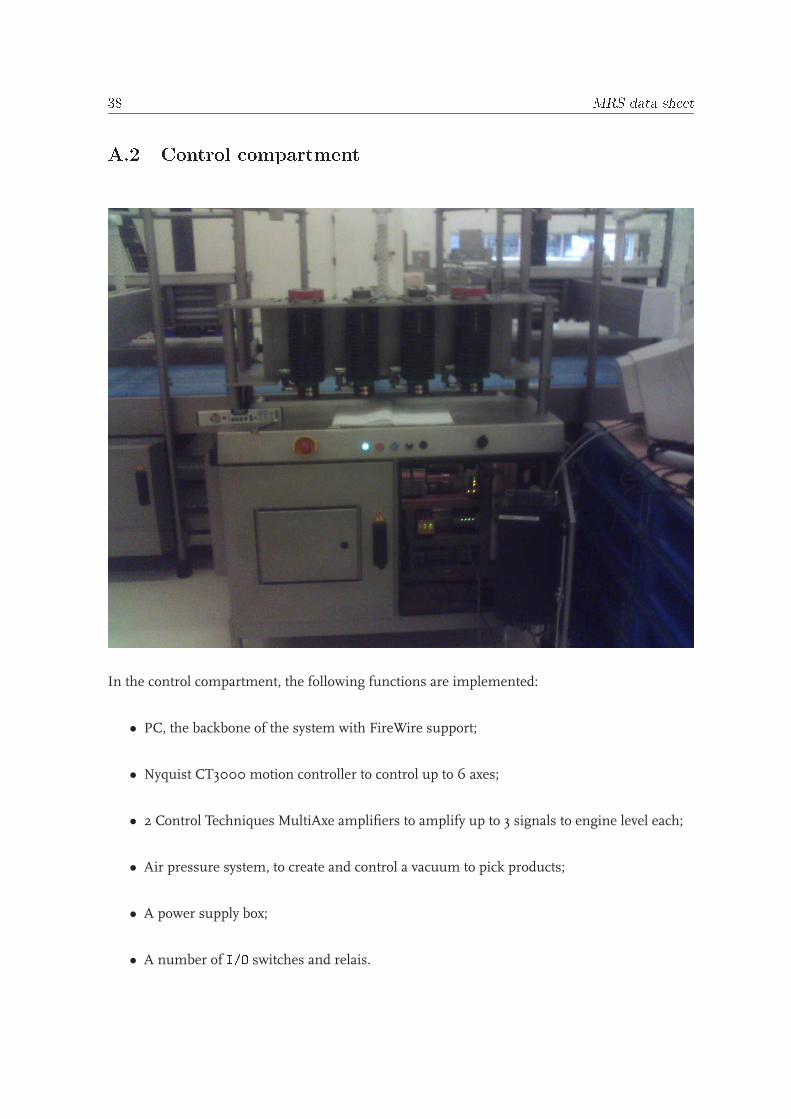
38 MRS data sheetA.2 Control ompartment

In the control compartment, the following functions are implemented:

• PC, the backbone of the system with FireWire support;

• Nyquist CT3000 motion controller to control up to 6 axes;

• 2 Control Techniques MultiAxe amplifiers to amplify up to 3 signals to engine level each;

• Air pressure system, to create and control a vacuum to pick products;

• A power supply box;

• A number of I/O switches and relais.

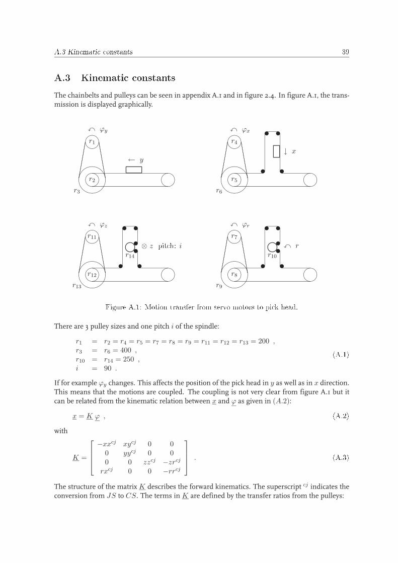
A.3 Kinemati onstants 39A.3 Kinemati onstantsThe chainbelts and pulleys can be seen in appendix A.1 and in figure 2.4. In figure A.1, the trans-mission is displayed graphically.

x ϕy

µ´¶³r1

&%'$

µ´¶³r2 µ´¶³

r3

← y

x ϕx

µ´¶³r4

&%'$

µ´¶³r5 µ´¶³

r6

u u

u u↓ x

x ϕz

µ´¶³r11

&%'$

µ´¶³r12 µ´¶³

r13

u u

u uuum

r14

⊗ z pit h: i

x ϕr

µ´¶³r7

&%'$

µ´¶³r8 µ´¶³

r9

u u

u uuum

r10

x r

Figure A.1: Motion transfer from servo motors to pi k head.There are 3 pulley sizes and one pitch i of the spindle:

r1 = r2 = r4 = r5 = r7 = r8 = r9 = r11 = r12 = r13 = 200 ,r3 = r6 = 400 ,r10 = r14 = 250 ,i = 90 .

(A.1)If for example ϕy changes. This affects the position of the pick head in y as well as in x direction.This means that the motions are coupled. The coupling is not very clear from figure A.1 but itcan be related from the kinematic relation between x and ϕ as given in (A.2):

x = K ϕ , (A.2)with

K =

−xxcj xycj 0 00 yycj 0 00 0 zzcj −zrcj

rxcj 0 0 −rrcj

. (A.3)The structure of the matrix K describes the forward kinematics. The superscript cj indicates theconversion from JS to CS. The terms in K are defined by the transfer ratios from the pulleys:

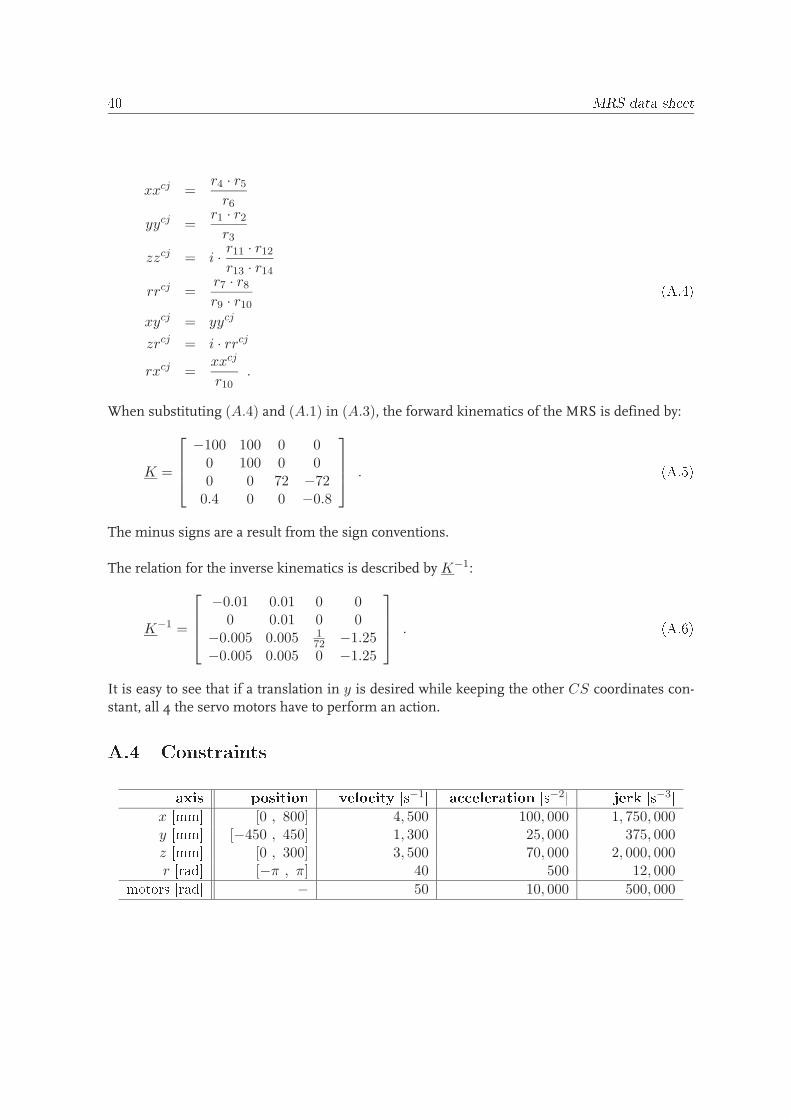
40 MRS data sheetxxcj =

r4 · r5

r6

yycj =r1 · r2

r3

zzcj = i · r11 · r12

r13 · r14

rrcj =r7 · r8

r9 · r10

(A.4)xycj = yycj

zrcj = i · rrcj

rxcj =xxcj

r10

.

When substituting (A.4) and (A.1) in (A.3), the forward kinematics of the MRS is defined by:

K =

−100 100 0 00 100 0 00 0 72 −72

0.4 0 0 −0.8

. (A.5)The minus signs are a result from the sign conventions.

The relation for the inverse kinematics is described by K−1:

K−1 =

−0.01 0.01 0 00 0.01 0 0

−0.005 0.005 1

72−1.25

−0.005 0.005 0 −1.25

. (A.6)It is easy to see that if a translation in y is desired while keeping the other CS coordinates con-stant, all 4 the servo motors have to perform an action.A.4 Constraintsaxis position velo ity [s−1℄ a eleration [s−2℄ jerk [s−3℄

x [mm℄ [0 , 800] 4, 500 100, 000 1, 750, 000y [mm℄ [−450 , 450] 1, 300 25, 000 375, 000z [mm℄ [0 , 300] 3, 500 70, 000 2, 000, 000r [rad℄ [−π , π] 40 500 12, 000motors [rad℄ − 50 10, 000 500, 000

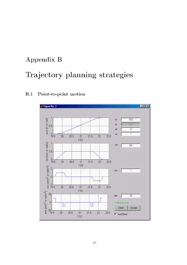
Appendix BTraje tory planning strategiesB.1 Point-to-point motion

41

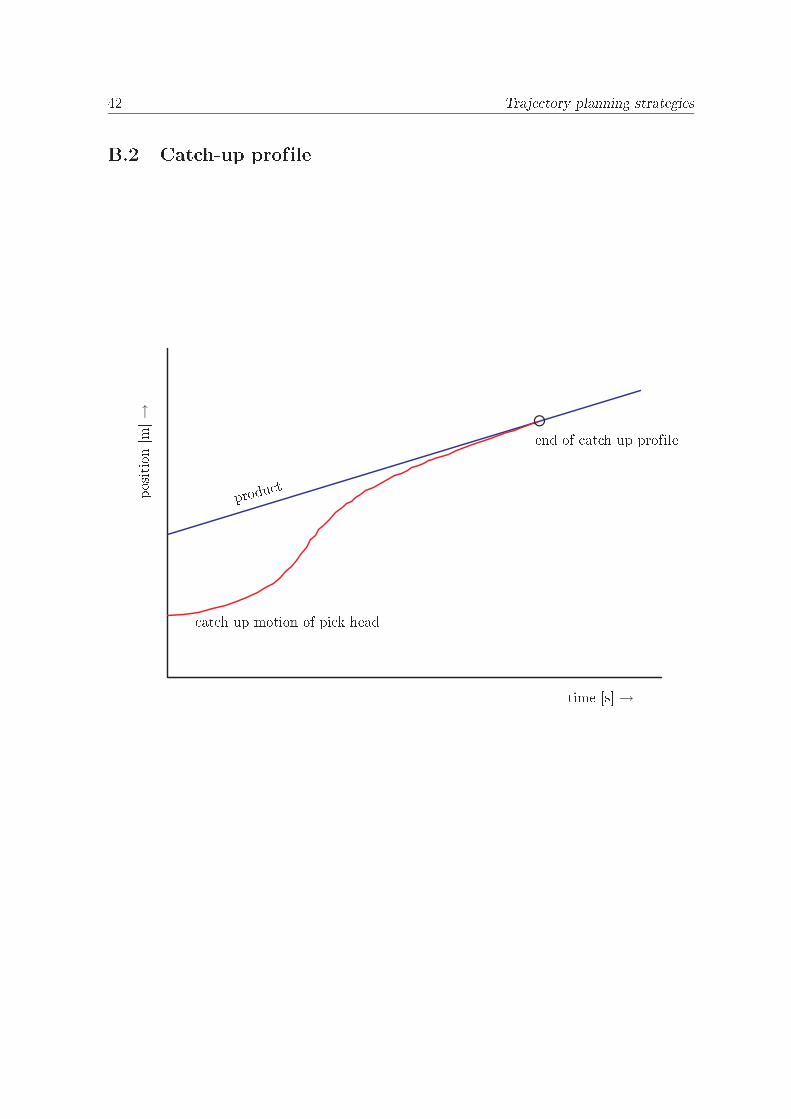
42 Traje tory planning strategiesB.2 Cat h-up profile

PSfrag repla ementstime [s℄ →

position[m℄

→

produ t at h up motion of pi k head

end of at h up profile◦

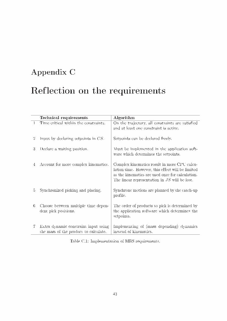
Appendix CRefle tion on the requirementsTe hni al requirements Algorithm1 Time riti al within the onstraints. On the traje tory, all onstraints are satisfiedand at least one onstraint is a tive.2 Input by de laring setpoints in CS. Setpoints an be de lared freely.3 De lare a waiting position. Must be implemented in the appli ation soft-ware whi h determines the setpoints.4 A ount for more omplex kinemati s. Complex kinemati s result in more CPU al u-lation time. However, this effe t will be limitedas the kinemati s are used on e for al ulation.The linear representation in JS will be lost.5 Syn hronized pi king and pla ing. Syn hrone motions are planned by the at h-upprofile.6 Choose between multiple time depen-dent pi k positions. The order of produ ts to pi k is determined bythe appli ation software whi h determines thesetpoints.7 Extra dynami onstraint input usingthe mass of the produ t to al ulate. Implementing of (mass depending) dynami sinstead of kinemati s.Table C.1: Implementation of MRS requirements.

43

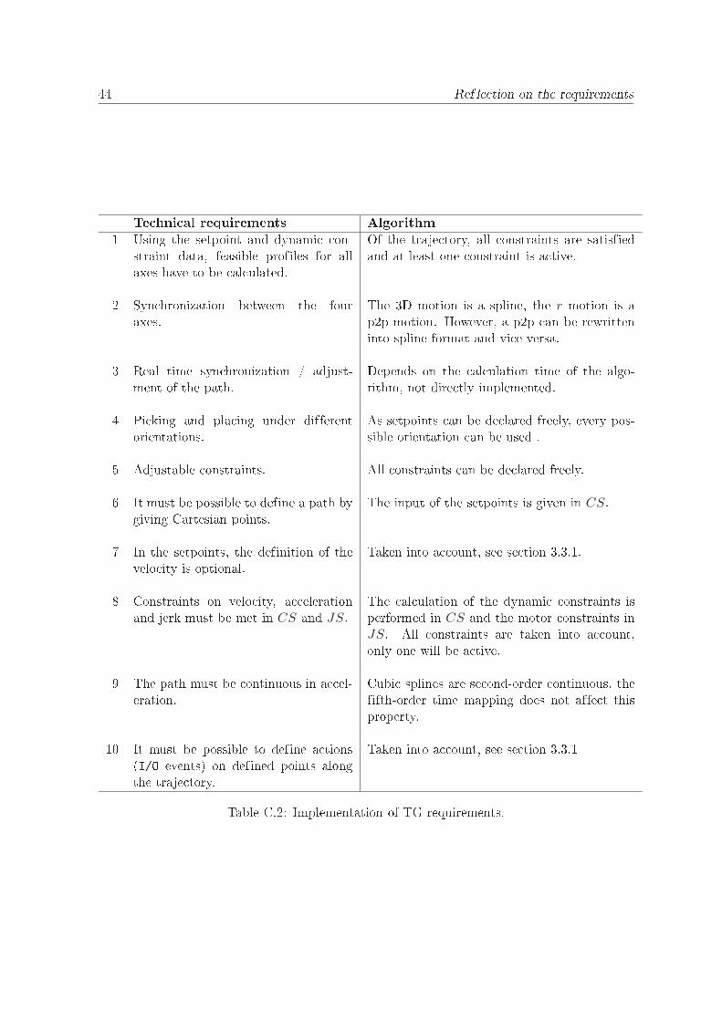
44 Ref le tion on the requirementsTe hni al requirements Algorithm1 Using the setpoint and dynami on-straint data, feasible profiles for allaxes have to be al ulated. Of the traje tory, all onstraints are satisfiedand at least one onstraint is a tive.2 Syn hronization between the fouraxes. The 3D motion is a spline, the r motion is ap2p motion. However, a p2p an be rewritteninto spline format and vi e versa.3 Real time syn hronization / adjust-ment of the path. Depends on the al ulation time of the algo-rithm, not dire tly implemented.4 Pi king and pla ing under differentorientations. As setpoints an be de lared freely, every pos-sible orientation an be used .5 Adjustable onstraints. All onstraints an be de lared freely.6 It must be possible to define a path bygiving Cartesian points. The input of the setpoints is given in CS.7 In the setpoints, the definition of thevelo ity is optional. Taken into a ount, see se tion 3.3.1.8 Constraints on velo ity, a elerationand jerk must be met in CS and JS. The al ulation of the dynami onstraints isperformed in CS and the motor onstraints in

JS. All onstraints are taken into a ount,only one will be a tive.9 The path must be ontinuous in a el-eration. Cubi splines are se ond-order ontinuous, thefifth-order time mapping does not affe t thisproperty.10 It must be possible to define a tions(I/O events) on defined points alongthe traje tory. Taken into a ount, see se tion 3.3.1Table C.2: Implementation of TG requirements.

Appendix DSpline theoryAs a large part of the path, is generated as a spline, splines will be treated in this chapter. A splinexi(k) is constructed of n − 1 piecewise third-order polynomials which pass through n nodesSi = (xi, yi, zi), with i = 1, . . . , n. The polynomial segments can be represented parametricallyas:

xi(k) = (Xi(k), Yi(k), Zi(k)) , with i = 1, . . . , n − 1 . (D.1)Variable k ∈ [0, 1] is defined along the spline segment. In general, Xi(k) is determined solely bythe x-coordinates x1, . . . , xn, Yi(k) is determined solely by the y-coordinates y1, . . . , yn, etc. AsXi(k) , Yi(k) and Zi(k) are treated in the same way, only the derivation of Xi(k) is discussed. Athorough discussion of spline theory is present in [1].D.1 Hermite splinesConsider the 1-dimensional spline for a set of n nodes (x1, x2, . . . , xn)with n−1 spline segments.The equation for spline segment i = 1, . . . , n − 1 is given by:

Xi(k) = ai + bik + cik2 + dik

3 , (D.2)with ai, bi, ci and di constant coefficients. The begin and end position of each spline segment aregiven by:

Xi(0) = xi = ai (D.3)Xi(1) = xi+1 = ai + bi + ci + di . (D.4)

Similar to (D.3) and (D.14), the first derivative of the begin (Di) and end position (Di−1) of eachspline segment are given by:

X ′i(0) = Di = bi (D.5)

X ′i(1) = Di+1 = bi + 2ci + 3di . (D.6)

To be able to determine Xi(k) completely, the four coefficients have to be determined. Solving(D.3) to (D.6) for ai, bi, ci and di gives:

ai = xi (D.7)bi = Di (D.8)ci = 3(xi+1 − xi) − 2Di − Di+1 (D.9)di = 2(xi − xi+1) + Di + Di+1 . (D.10)45

46 Spline theoryThese 4 equations can be solved if the variables xi and Di are known. The values for xi aredefined by the node Si. An easy way is to do determine Di, is to define a value x′

i to the firstderivative of every node:

Di = x′i . (D.11)

In a hermite spline, the first derivative at the left end of a spline segment is equal to the firstderivative at the right end of the previous spline segment. This way the hermite spline has acontinuous first derivative at each node, equal to the predefined value of (D.11):

Di = X ′i−1(1) = X ′

i(0) = x′i . (D.12)D.2 Natural ubi splines

To achieve not only first-order but also second-order continuous derivatives at the nodes of aspline, cubic splines can be used. Consider a cubic spline existing of n − 1 segments, with foreach segment a third-order polynomial determined by 4 coefficients.

For cubic splines, the interior nodes (i = 2, 3, . . . , n − 1) are subjected to four conditions:

Xi−1(1) = xi

Xi(0) = xi

X ′i−1(1) = X ′

i(0)X ′′

i−1(1) = X ′′i (0) .

(D.13)The end nodes (i = 1 and i = n) are given by:

X1(0) = x1

Xn−1(1) = xn .(D.14)

Compared to hermite splines, in a cubic spline the first derivatives Di are not defined. So, therelation stated in (D.11) is not valid for cubic splines. Instead Di must be calculated such thatthe spline is second-order continuous.

The number of conditions is given by (n − 2) spline segments constructed from (D.13) and 2from (D.14). Resuming, there are 4(n − 2) + 2 = 4n − 6 equations and 4(n − 1) unknowns. Toobtain a well-defined problem, two additional equations are needed. These may be chosen in anumber of ways.In case of a natural cubic spline, the second derivatives at the extends of the spline are simply setto zero:

X ′′1 (0) = 0 (D.15)

X ′′n−1(1) = 0 . (D.16)

The solution to this set of equations is now derived for n nodes. The second derivatives of (D.2)at each node are given by:

X ′′i−1(1) = 2ci−1 + 6di−1 (D.17)X ′′

i (0) = 2ci . (D.18)

D.3 Dire tional ubi splines 47Taking the fourth condition in (D.13) and substituting (D.17) and (D.18) for the internal nodes,we obtain:

2ci−1 + 6di−1 = 2ci . (D.19)Substituting (D.9) and (D.10) and rearranging terms gives the (n − 2) unknowns Di:

2[3(xi − xi−1) − 2Di−1 − Di] + 6[2(xi−1 − xi) + Di−1 + Di] =

[3(xi+1 − xi) − 2Di − Di+1]

Di−1 + 4Di + Di+1 = 3(xi+1 − xi−1) , with i = 2, 3, . . . , (n − 1) . (D.20)As there are (n − 2) internal nodes, there are (n − 2) (D.20).

The boundary condition in (D.15) require the second-order derivative of the begin node of thespline to be zero. Substituting (D.9) and (D.18) in (D.15) and rearranging terms gives:

2c1 = 0

2[3(x2 − x1) − 2D1 − D2] = 0

2D1 + D2 = 3(x2 − x1) . (D.21)Similarly, for the end node of the spline it holds that:

Dn−1 + 2Dn = 3(xn − xn−1) . (D.22)Representing (D.20), (D.21) and (D.22) in a matrix yields the linear system:

2 11 4 1

1 4 1. . .

. . .. . .

1 4 11 4 1

1 2

D1

D2

D3

...Dn−2

Dn−1

Dn

=

3(x2 − x1)3(x3 − x1)3(x4 − x2)

...3(xn−1 − xn−3)3(xn − xn−2)3(xn − xn−1)

. (D.23)This tridiagonal linear relation can be solved very easily. Finally the using the relations in (D.7) to(D.10), the values for ai, bi, ci and di for each spline segment can be determined. Every positionon the spline can now be calculated by varying k for each spline segment.D.3 Dire tional ubi splinesTo complete the set of equations, also other conditions can be formulated. Not only second-orderderivatives are an option, also conditions concerning the first derivatives may be defined. Anytwo linear relations that are independent from the equations provided in (D.20) will do.A possible option might be to take the cubic spline formulation but with the hermite spline

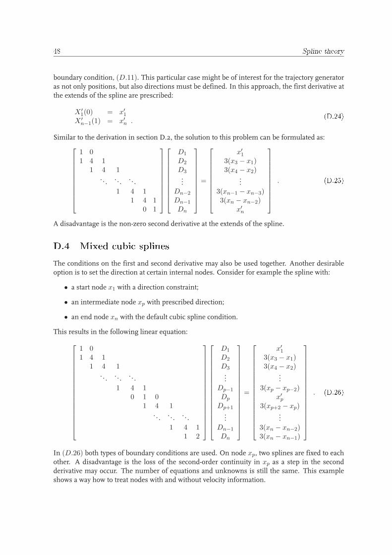
48 Spline theoryboundary condition, (D.11). This particular case might be of interest for the trajectory generatoras not only positions, but also directions must be defined. In this approach, the first derivative atthe extends of the spline are prescribed:

X ′1(0) = x′

1

X ′n−1(1) = x′

n .(D.24)

Similar to the derivation in section D.2, the solution to this problem can be formulated as:

1 01 4 1

1 4 1. . .

. . .. . .

1 4 11 4 1

0 1

D1

D2

D3

...Dn−2

Dn−1

Dn

=

x′1

3(x3 − x1)3(x4 − x2)

...3(xn−1 − xn−3)3(xn − xn−2)

x′n

. (D.25)A disadvantage is the non-zero second derivative at the extends of the spline.D.4 Mixed ubi splinesThe conditions on the first and second derivative may also be used together. Another desirableoption is to set the direction at certain internal nodes. Consider for example the spline with:

• a start node x1 with a direction constraint;

• an intermediate node xp with prescribed direction;

• an end node xn with the default cubic spline condition.

This results in the following linear equation:

1 01 4 1

1 4 1. . .

. . .. . .

1 4 10 1 0

1 4 1. . .

. . .. . .

1 4 11 2

D1

D2

D3

...Dp−1

Dp

Dp+1

...Dn−1

Dn

=

x′1

3(x3 − x1)3(x4 − x2)

...3(xp − xp−2)

x′p

3(xp+2 − xp)...

3(xn − xn−2)3(xn − xn−1)

. (D.26)In (D.26) both types of boundary conditions are used. On node xp, two splines are fixed to eachother. A disadvantage is the loss of the second-order continuity in xp as a step in the secondderivative may occur. The number of equations and unknowns is still the same. This exampleshows a way how to treat nodes with and without velocity information.

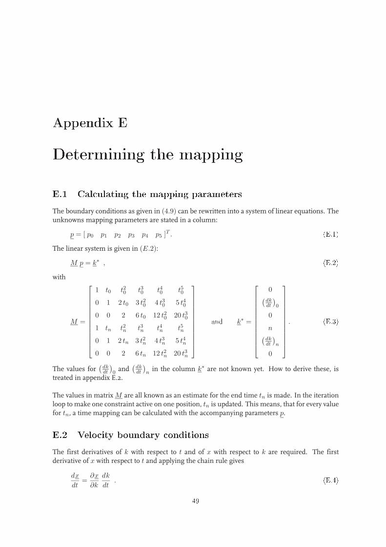
Appendix EDetermining the mappingE.1 Cal ulating the mapping parametersThe boundary conditions as given in (4.9) can be rewritten into a system of linear equations. Theunknowns mapping parameters are stated in a column:

p = [ p0 p1 p2 p3 p4 p5 ]T . (E.1)The linear system is given in (E.2):

M p = k∗ , (E.2)with

M =

1 t0 t20 t30 t40 t50

0 1 2 t0 3 t20 4 t30 5 t40

0 0 2 6 t0 12 t20 20 t30

1 tn t2n t3n t4n t5n

0 1 2 tn 3 t2n 4 t3n 5 t4n

0 0 2 6 tn 12 t2n 20 t3n

and k∗ =

0(

dkdt

)

0

0

n(

dkdt

)

n

0

. (E.3)The values for

(

dkdt

)

0and

(

dkdt

)

nin the column k∗ are not known yet. How to derive these, is

treated in appendix E.2.

The values in matrix M are all known as an estimate for the end time tn is made. In the iterationloop to make one constraint active on one position, tn is updated. This means, that for every valuefor tn, a time mapping can be calculated with the accompanying parameters p.E.2 Velo ity boundary onditionsThe first derivatives of k with respect to t and of x with respect to k are required. The firstderivative of x with respect to t and applying the chain rule gives

dx

dt=

∂x

∂k

dk

dt. (E.4)49

50 Determining the mappingThe values for dx

dtare defined by the user when providing the setpoints (3.1). To determine the

relation between ∂x∂k

and dkdt, another equation is needed. Very common is the choice to normalize

the direction of the spline vector ∂x∂k

, [7]:

∂x

∂k=

dx

dt

∥

∥

∥

∥

dx

dt

∥

∥

∥

∥

−1

2

. (E.5)The sign of the dx

dtindicates the direction of the motion at the setpoint, this information is still

included in ∂x∂k

.

Substituting (E.5) in (E.4) yields dkdt

=∥

∥

∥

dxdt

∥

∥

∥

2. As a result, dk

dtdepends on the variable dx

dt.

The necessary condition for the time mapping k(t) is being strictly increasing. Whether thiscondition is fulfilled, depends on the time mapping boundary conditions in (E.2).Empirically is noticed that when using (E.5), the necessary condition is not guaranteed. For anyboundary condition k >> n in combination with the defined boundary conditions in (E.2), thetime mapping k(t) most likely will not fulfill the necessary condition.This is a result of the large numerical values of de velocity (for example x = 400 mm s−1) andthe relative small maximum value of k (for example k(te) = n = 5). To avoid dk

dtfrom getting

relatively large numerical values, dkdt

must be independent of dxdt.

To make dkdt

independent of dxdt, another approach is needed. In case of a synchrone setpoint (see

table 3.1, x = c ), the following choice has been made:

dk

dt= 1 . (E.6)

In case of a static setpoint (see table 3.1, x = 0 ), both derivatives (right side of (E.4)) may be zero.This is interesting as it yields an earlier end time of the motion (empirically). In this case (E.6)will be stated as:

dk

dt= 0 . (E.7)

In both cases, ∂x∂k

can be stated as:

∂x

∂k=

dx

dt. (E.8)

Concluding, in case of a static setpoint∥

∥

∥

dxdt

∥

∥

∥

2=

∥

∥

∥

∂x∂k

∥

∥

∥

2= dk

dt= 0 , (E.9)

while in a synchrone setpoint∥

∥

∥

dxdt

∥

∥

∥

2=

∥

∥

∥

∂x∂k

∥

∥

∥

26= 0 . (E.10)

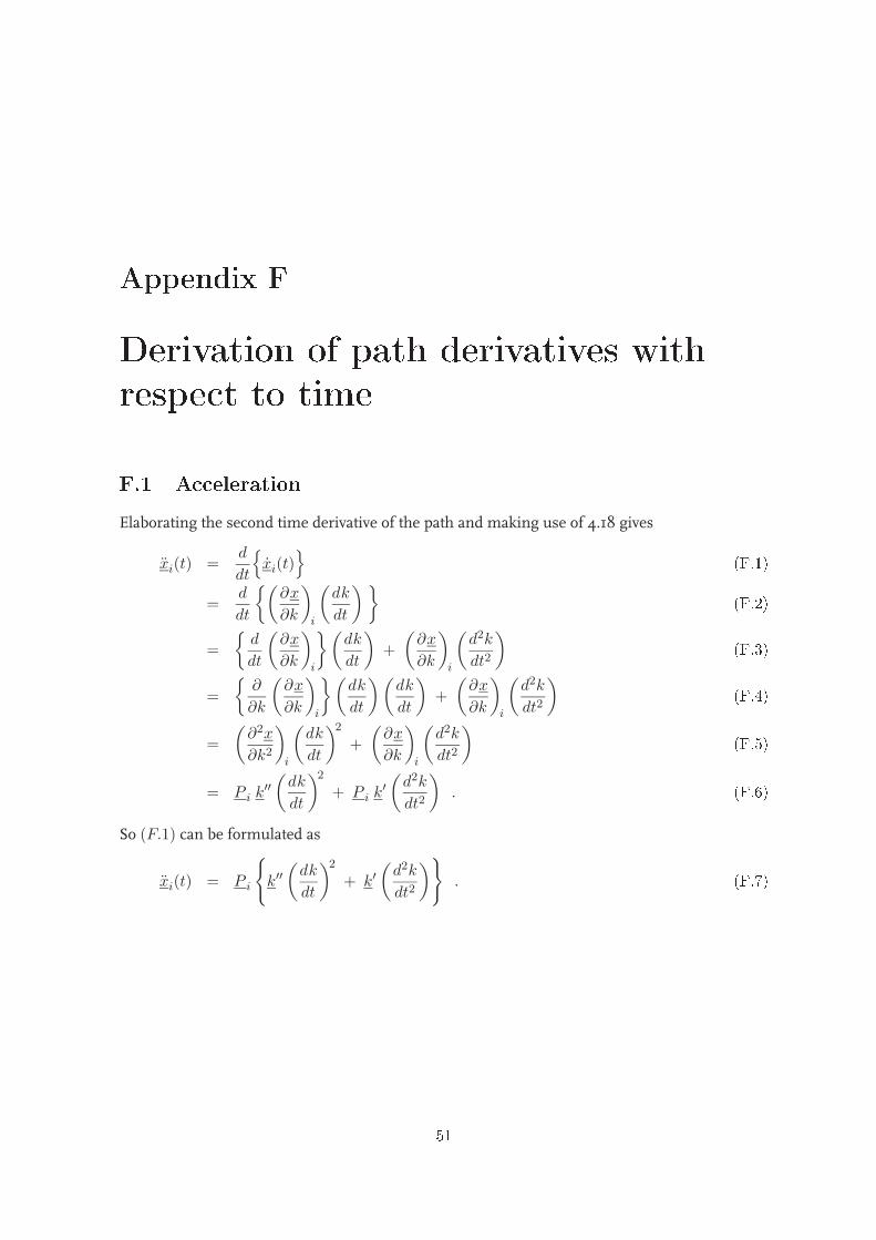
Appendix FDerivation of path derivatives withrespe t to timeF.1 A elerationElaborating the second time derivative of the path and making use of 4.18 gives

xi(t) =d

dt

{

xi(t)} (F.1)

=d

dt

{(

∂x

∂k

)

i

(

dk

dt

) } (F.2)=

{

d

dt

(

∂x

∂k

)

i

} (

dk

dt

)

+

(

∂x

∂k

)

i

(

d2k

dt2

) (F.3)=

{

∂

∂k

(

∂x

∂k

)

i

} (

dk

dt

) (

dk

dt

)

+

(

∂x

∂k

)

i

(

d2k

dt2

) (F.4)=

(

∂2x

∂k2

)

i

(

dk

dt

)2

+

(

∂x

∂k

)

i

(

d2k

dt2

) (F.5)= P i k′′

(

dk

dt

)2

+ P i k′

(

d2k

dt2

)

. (F.6)So (F.1) can be formulated as

xi(t) = P i

{

k′′

(

dk

dt

)2

+ k′

(

d2k

dt2

)

}

. (F.7)

51

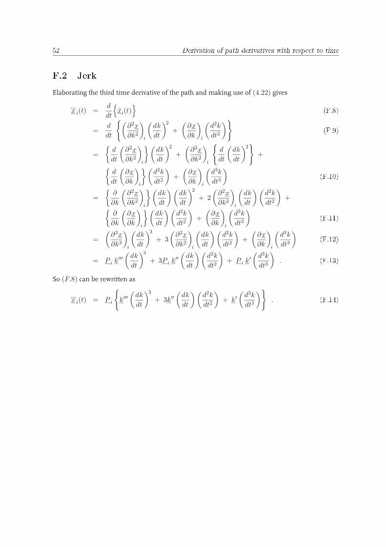
52 Derivation of path derivatives with respe t to timeF.2 JerkElaborating the third time derivative of the path and making use of (4.22) gives...

x i(t) =d

dt

{

xi(t)} (F.8)

=d

dt

{

(

∂2x

∂k2

)

i

(

dk

dt

)2

+

(

∂x

∂k

)

i

(

d2k

dt2

)

} (F.9)=

{

d

dt

(

∂2x

∂k2

)

i

} (

dk

dt

)2

+

(

∂2x

∂k2

)

i

{

d

dt

(

dk

dt

)2}

+

{

d

dt

(

∂x

∂k

)

i

} (

d2k

dt2

)

+

(

∂x

∂k

)

i

(

d3k

dt3

) (F.10)=

{

∂

∂k

(

∂2x

∂k2

)

i

} (

dk

dt

) (

dk

dt

)2

+ 2

(

∂2x

∂k2

)

i

(

dk

dt

) (

d2k

dt2

)

+

{

∂

∂k

(

∂x

∂k

)

i

} (

dk

dt

) (

d2k

dt2

)

+

(

∂x

∂k

)

i

(

d3k

dt3

) (F.11)=

(

∂3x

∂k3

)

i

(

dk

dt

)3

+ 3

(

∂2x

∂k2

)

i

(

dk

dt

) (

d2k

dt2

)

+

(

∂x

∂k

)

i

(

d3k

dt3

) (F.12)= P i k′′′

(

dk

dt

)3

+ 3P i k′′

(

dk

dt

) (

d2k

dt2

)

+ P i k′

(

d3k

dt3

)

. (F.13)So (F.8) can be rewritten as...

x i(t) = P i

{

k′′′

(

dk

dt

)3

+ 3k′′

(

dk

dt

) (

d2k

dt2

)

+ k′

(

d3k

dt3

)

}

. (F.14)

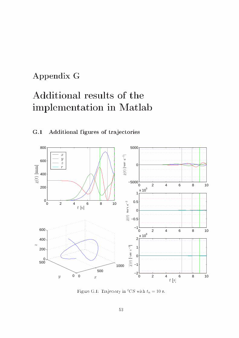
Appendix GAdditional results of theimplementation in MatlabG.1 Additional figures of traje tories

0 2 4 6 8 100

200

400

600

800

0500

1000

0

5000

200

400

600

0 2 4 6 8 10−5000

0

5000

0 2 4 6 8 10−1

−0.5

0

0.5

1x 10

5

0 2 4 6 8 10−2

−1

0

1

2x 10

6

PSfrag repla ementsx

x

y

y

z

z

r

t [s℄

t [s℄[-℄[s ℄[s ℄[s ℄[mm℄[mm℄[mm℄[mm℄

x(t

)

[mm℄ x(t

)

[mms−1 ℄x(t

)

[mms−2 ℄

... x(t

)

[mms−3 ℄[rad℄[rad℄[rad s ℄[rad s ℄... [rad s ℄ Figure G.1: Traje tory in tCS with tn = 10 s.53

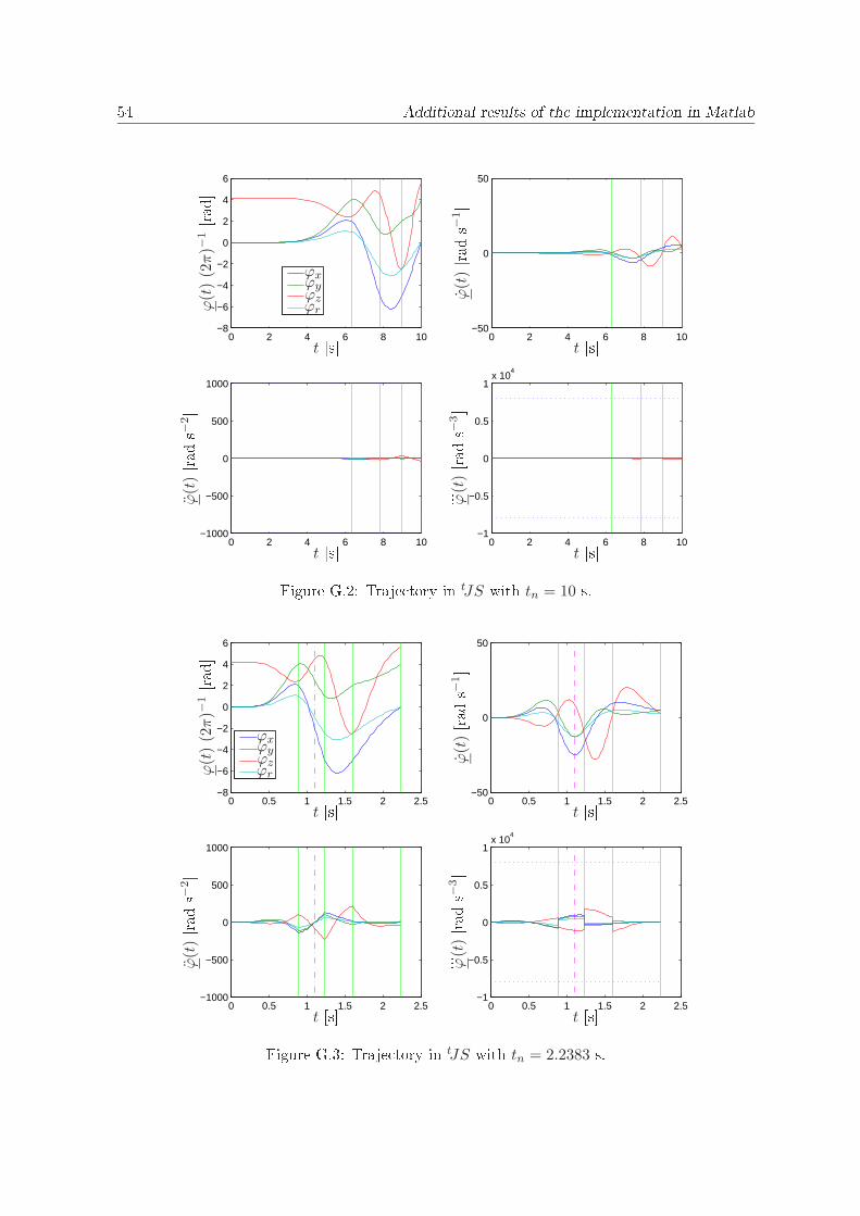
54 Additional results of the implementation in Matlab

0 2 4 6 8 10−8

−6

−4

−2

0

2

4

6

0 2 4 6 8 10−50

0

50

0 2 4 6 8 10−1000

−500

0

500

1000

0 2 4 6 8 10−1

−0.5

0

0.5

1x 10

4

PSfrag repla ements

ϕxϕyϕzϕr

t [s℄t [s℄t [s℄t [s℄

[-℄[s ℄[s ℄[s ℄[mm℄[mm℄[mm℄[mm℄[mm℄[mm s ℄[mm s ℄... [mm s ℄[rad℄

ϕ(t

)(2

π)−

1

[rad℄

ϕ(t

)

[rads−1 ℄ϕ(t

)

[rads−2 ℄ ... ϕ(t

)[rads−3 ℄

Figure G.2: Traje tory in tJS with tn = 10 s.0 0.5 1 1.5 2 2.5

−8

−6

−4

−2

0

2

4

6

0 0.5 1 1.5 2 2.5−50

0

50

0 0.5 1 1.5 2 2.5−1000

−500

0

500

1000

0 0.5 1 1.5 2 2.5−1

−0.5

0

0.5

1x 10

4

PSfrag repla ements

ϕxϕyϕzϕr

t [s℄t [s℄t [s℄t [s℄

[-℄[s ℄[s ℄[s ℄[mm℄[mm℄[mm℄[mm℄[mm℄[mm s ℄[mm s ℄... [mm s ℄[rad℄

ϕ(t

)(2

π)−

1

[rad℄ϕ(t

)

[rads−1 ℄

ϕ(t

)

[rads−2 ℄ ... ϕ(t

)

[rads−3 ℄Figure G.3: Traje tory in tJS with tn = 2.2383 s.

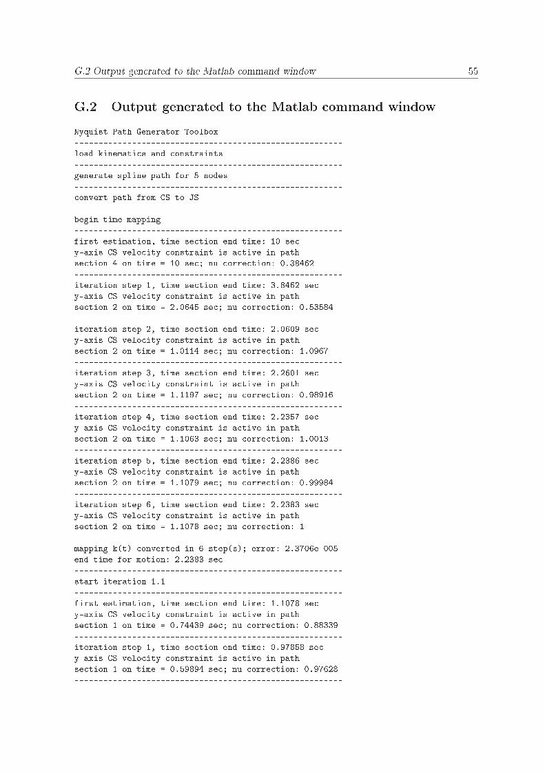
G.2 Output generated to the Matlab ommand window 55G.2 Output generated to the Matlab ommand windowNyquist Path Generator Toolbox--------------------------------------------------------load kinemati s and onstraints--------------------------------------------------------generate spline path for 5 nodes-------------------------------------------------------- onvert path from CS to JS--------------------------------------------------------begin time mapping--------------------------------------------------------first estimation, time se tion end time: 10 se y-axis CS velo ity onstraint is a tive in pathse tion 4 on time = 10 se ; nu orre tion: 0.38462--------------------------------------------------------iteration step 1, time se tion end time: 3.8462 se y-axis CS velo ity onstraint is a tive in pathse tion 2 on time = 2.0645 se ; nu orre tion: 0.53584--------------------------------------------------------iteration step 2, time se tion end time: 2.0609 se y-axis CS velo ity onstraint is a tive in pathse tion 2 on time = 1.0114 se ; nu orre tion: 1.0967--------------------------------------------------------iteration step 3, time se tion end time: 2.2601 se y-axis CS velo ity onstraint is a tive in pathse tion 2 on time = 1.1197 se ; nu orre tion: 0.98916--------------------------------------------------------iteration step 4, time se tion end time: 2.2357 se y-axis CS velo ity onstraint is a tive in pathse tion 2 on time = 1.1063 se ; nu orre tion: 1.0013--------------------------------------------------------iteration step 5, time se tion end time: 2.2386 se y-axis CS velo ity onstraint is a tive in pathse tion 2 on time = 1.1079 se ; nu orre tion: 0.99984--------------------------------------------------------iteration step 6, time se tion end time: 2.2383 se y-axis CS velo ity onstraint is a tive in pathse tion 2 on time = 1.1078 se ; nu orre tion: 1--------------------------------------------------------mapping k(t) onverted in 6 step(s); error: 2.3706e-005end time for motion: 2.2383 se --------------------------------------------------------start iteration 1.1--------------------------------------------------------first estimation, time se tion end time: 1.1078 se y-axis CS velo ity onstraint is a tive in pathse tion 1 on time = 0.74439 se ; nu orre tion: 0.88339--------------------------------------------------------iteration step 1, time se tion end time: 0.97858 se y-axis CS velo ity onstraint is a tive in pathse tion 1 on time = 0.59894 se ; nu orre tion: 0.97628--------------------------------------------------------

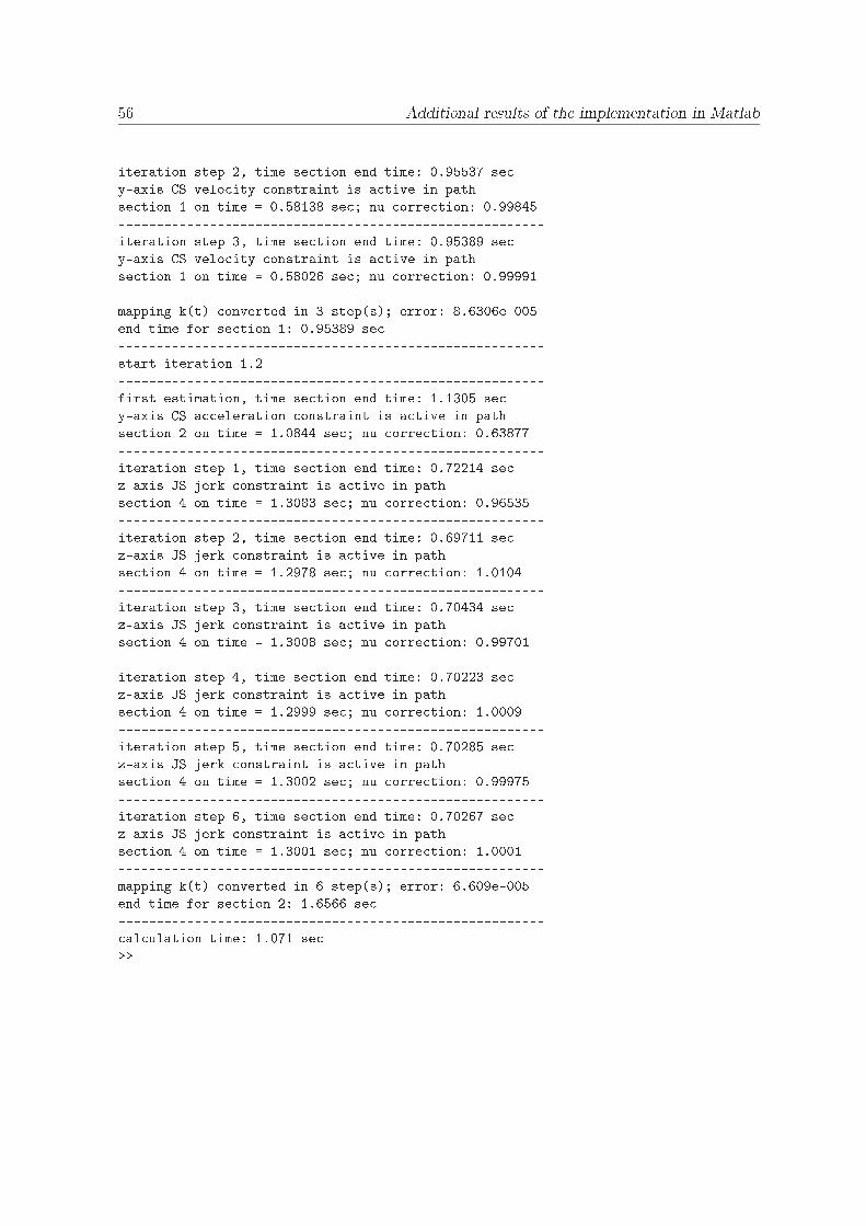
56 Additional results of the implementation in Matlabiteration step 2, time se tion end time: 0.95537 se y-axis CS velo ity onstraint is a tive in pathse tion 1 on time = 0.58138 se ; nu orre tion: 0.99845--------------------------------------------------------iteration step 3, time se tion end time: 0.95389 se y-axis CS velo ity onstraint is a tive in pathse tion 1 on time = 0.58026 se ; nu orre tion: 0.99991--------------------------------------------------------mapping k(t) onverted in 3 step(s); error: 8.6306e-005end time for se tion 1: 0.95389 se --------------------------------------------------------start iteration 1.2--------------------------------------------------------first estimation, time se tion end time: 1.1305 se y-axis CS a eleration onstraint is a tive in pathse tion 2 on time = 1.0844 se ; nu orre tion: 0.63877--------------------------------------------------------iteration step 1, time se tion end time: 0.72214 se z-axis JS jerk onstraint is a tive in pathse tion 4 on time = 1.3083 se ; nu orre tion: 0.96535--------------------------------------------------------iteration step 2, time se tion end time: 0.69711 se z-axis JS jerk onstraint is a tive in pathse tion 4 on time = 1.2978 se ; nu orre tion: 1.0104--------------------------------------------------------iteration step 3, time se tion end time: 0.70434 se z-axis JS jerk onstraint is a tive in pathse tion 4 on time = 1.3008 se ; nu orre tion: 0.99701--------------------------------------------------------iteration step 4, time se tion end time: 0.70223 se z-axis JS jerk onstraint is a tive in pathse tion 4 on time = 1.2999 se ; nu orre tion: 1.0009--------------------------------------------------------iteration step 5, time se tion end time: 0.70285 se z-axis JS jerk onstraint is a tive in pathse tion 4 on time = 1.3002 se ; nu orre tion: 0.99975--------------------------------------------------------iteration step 6, time se tion end time: 0.70267 se z-axis JS jerk onstraint is a tive in pathse tion 4 on time = 1.3001 se ; nu orre tion: 1.0001--------------------------------------------------------mapping k(t) onverted in 6 step(s); error: 6.609e-005end time for se tion 2: 1.6566 se -------------------------------------------------------- al ulation time: 1.071 se >>

Appendix HImplementation of the algorithm inMatlabH.1 Des ription of the Matlab filesTo avoid problems with standard Matlab files, all filenames start with pg, then the function name is added.For all files, a help is written in the header. This help gives the notation and description of the input andoutput of each file. It is tried to keep the names for the variables the same throughout all the files. As canbe seen, most files are written as fun tions; in this way the number of variables can be kept small. Thefiles will be discussed briefly and difficulties will be mentioned.pgMasterThe Matlab code is presented in H.2. The algorithm is started by calling the master file in Matlab. Thedesired graphical output is set by adjusting switches in the functions called in this file.The algorithm is initialized by loading the kinematics and constraints as defined by the user. Next, iterationscheme II is initialized. For a time independent end position, this iteration scheme is run only once.The (time dependant) setpoints are loaded and in between these setpoints a path is calculated. The path inkCS is converted to kJS and the time is mapped on the path, handeling constraints in both tCS end tJS .If iteration scheme II is used, the convergence is determined. Finally the catch-up profile is added and thetiming for the I/O setpoints is calculated.

The algorithm master file only calculates one trajectory. To let the algorithm continuously calculate newtrajectories, another layer is needed calling the master file. The setpoints for each path should now bepicked from several (time depending) matrices. In this case, the resulting trajectories must be stored in amatrix, struct or sent to the servo motors.pgKinemati sThe Matlab code is presented in H.3. In this function the forward kinematics are calculated from the ratiosof the pulleys. The inverse kinematics are derived by inverting the forward kinematics. Both matrices arestored in the struct kin and returned to the master file.pgConstrThe Matlab code is presented in H.4. The constraints are already treated in section 2.2.2 and appendixA.4. This file contains all constraints in CS and JS. They are stored in the structs: dyn , geom andmotor and returned to the master file. 57

58 Implementation of the algorithm in MatlabpgSetpointsThe Matlab code is presented in H.5. The setpoints are defined in the same way as declared in (3.1) andstored in the struct sp. For testing the algorithm, 5 setpoints are defined. The begin position is static, theend position has a velocity. This means that 3 types of setpoints are called, see section 3.3.1: setpoint 1 is astatic setpoint, setpoints 2, 3 and 4 are obstacle setpoints and setpoint 5 is a synchrone setpoint.pgSplineThe Matlab code is presented in H.6. Now, all input for the algorithm is available. First the path isdefined in x, y and z in kCS , using a spline representation. The path in r should defined by using a p2pdescription. In this file however, the path parameters of r, are all set to zero. This yields a constant pickhead angle of r = 0. The first part of the file follows the theory of chapter D. The matrices P

idescribing

the path parameters for each section as defined in (4.5) are stored in the struct path and returned to themaster file.In the second part of the file, the length of the path in space is approximated. This is done by discretizationof the path and calculating the Euclidean distance between two discrete positions. The number of discretepositions for each spline section can be adjusted. The length of the total path and of each section is storedin the struct splinedim and returned to the master file.pgCS2JSThe Matlab code is presented in H.7. The path in kCS is converted to kJS by applying (4.7) to matrixP

ifor every section of the path. The new matrices Φ

iare added to the already existing struct path and

returned to the master file.pgTimeSplineMapThe Matlab code is presented in H.8. This file works as the master file for the iteration loop to map thetime on the path and to determine the active constraint. In figure 3.1, this is indicated by step 8. Theiteration scheme is initialized by declaring the boundary conditions and end time estimate. The functionpgTimePar is called to calculate the k(t) parameters ( p0 to p5 ) for the estimated end time.The next step is to find a critical constraint to bematched with the timemapping. In order to do this, valuesfor the time derivatives along the path must be known. The position with the most critical constraint isdetermined from a discrete number of time derivatives. The discretization and the way of determiningthis position, is discussed in section 4.4.1.The discretization is implemented as defined in (4.28). The discrete time instants are defined in this filein the column T. For a correct calculation of the time derivatives, also the path section of every time instantis needed. These sections are stored in the column S.The derivatives are now determined by calling the function pgDerivatives and the most critical derivativeis selected with the function pgA tiveConstraint. From the most critical constraint, the update factorfor the end time is calculated. The k(t) parameters are recalculated for the updated end time. When themost critical constraint is active, the iteration loop is aborted.The function pgTimeSplineMap returns the structs KT and ACT to the master file. For improving thetrajectory, the file pgTimeSplineItermay be called to split the mapping at the active constraint as definedin step 9-I in figure 3.1.pgTimeParThe Matlab code is presented in H.9. In this function, the k(t) parameters are determined using thetheory as discussed in appendix E.1. The time of each section is determined by making use of the zerofinder function fzero to the function k(t) for the values: k(t) = 2, 3, . . . , n − 1. The time for k = 1 andk = n follow from the boundary conditions and are added afterwards. The mapping parameters are storedin the struct KT together with the time of each path section and returned to pgTimeSplineMap.

H.2 Master f ile 59pgDerivativesThe Matlab code is presented in H.10. The time derivatives of the path are calculated for a discrete numberof times, defined in the column T. To this extent, the theory as discussed in sections 4.3.1, 4.3.2 and 4.3.3is implemented in this function. The output consists of the struct X with values of the derivatives for eachdiscrete time instant which is returned to pgTimeSplineMap.When calling this function, also the string CS or JSmust be defined. This is necessary to select the correctmatrix from the struct path.pgA tiveConstraintThe Matlab code is presented in H.11. This function consists of 3 parts. First the 24 absolute maximumvalues for al constraints are determined as defined in (4.29) yielding 6 columns.The second part is only used in iteration loop 9-I. One or two values (depending on the iteration step) ofthe 24 maximum values are interchanged to avoid the recalculation of positions which already have anactive constraint. The interchanging depends on the active constraint characteristics as defined in section4.5.In the third part, the minimum relative error and the maximum update factor ν is calculated from the 6(updated) columns making use of the theory as treated in section 4.4.2.The output of pgA tiveConstraint consist of 4 structs: the update factor ν, the remaining relative error,information on the position with an active constraint and the characteristics of the active constraint.

In the implementation of pgA tiveConstraint can be seen that much use is made of index numbers(variables starting with i). This is done to collect all characteristics of the active constraint. This makes theimplementation a little less obvious, compared to the theory.Also the function is not suited yet for handeling the case of two active constraints (both boundaries of thetime section). This means that iteration loop 9-I can be called only once.pgTimeSplineIterThe Matlab code is presented in H.12. This file is called at the end of pgTimeSplineMap to apply theiteration loop 9-I. Looking at the file, it is rather similar to pgTimeSplineMap. The difference is that oneiteration loop is added around the time mapping loop. At the begin of the file, new boundary conditionsare generated from the old ones and at the position with the active constraint. The calculation of eachmapping is similar to the first one, only more complex as a result of index numbers.No stopping criteria has been implemented yet, the loop is aborted after running once for reasons givenin at the end of the description of pgA tiveConstraint. The newly found time mapping and constraintsare also stored in respectively KT and ACT and returned to the master file.H.2 Master file% Nyquist Path Generator Toolbox% Path Generator master file% Nyquist, Mar h 2005% Programmed by sbr%% Calls for pgKinemati s.m, pgConstr.m, pgSetpoints.m,% pgSpline.m, pgCS2JS.m, pgTimeSplineMap.m%format short e lear, lose all, l disp('Nyquist Path Generator Toolbox')disp('--------------------------------------------------------')ti

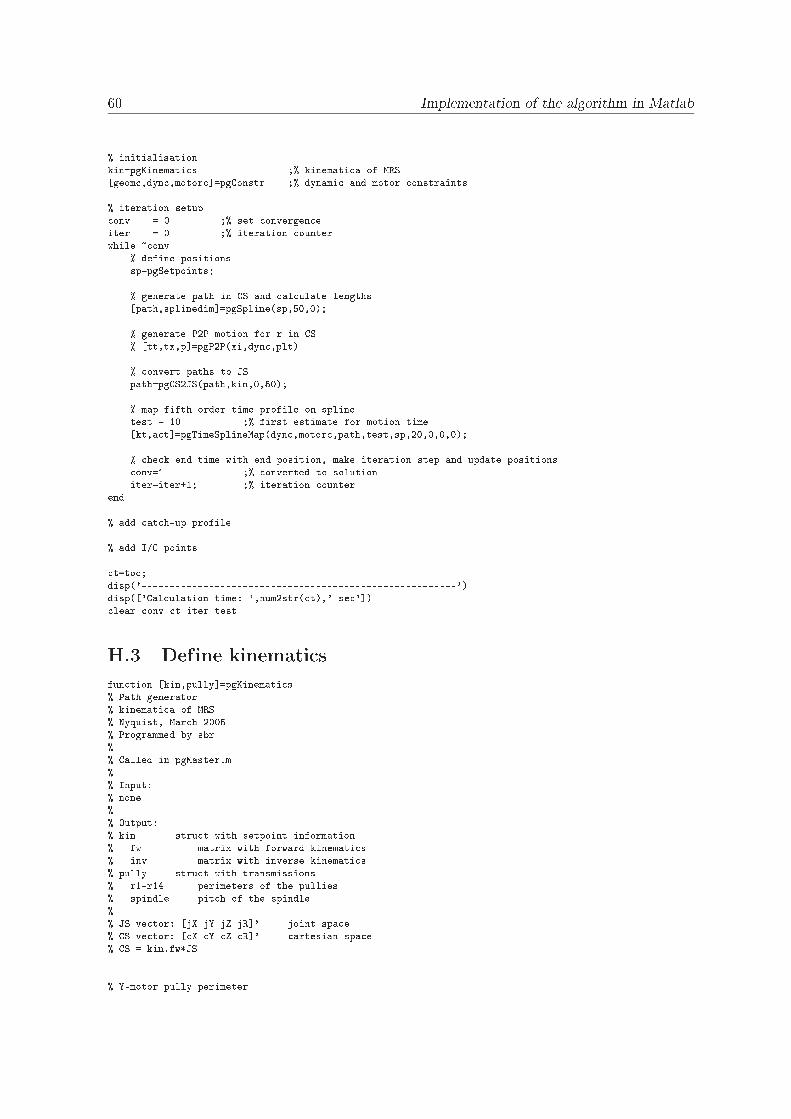
60 Implementation of the algorithm in Matlab% initialisationkin=pgKinemati s ;% kinemati a of MRS[geom ,dyn ,motor ℄=pgConstr ;% dynami and motor onstraints% iteration setup onv = 0 ;% set onvergen eiter = 0 ;% iteration ounterwhile ~ onv% define positionssp=pgSetpoints;% generate path in CS and al ulate lengths[path,splinedim℄=pgSpline(sp,50,0);% generate P2P motion for r in CS% [tt,tx,p℄=pgP2P(xi,dyn ,plt)% onvert paths to JSpath=pgCS2JS(path,kin,0,50);% map fifth order time profile on splinetest = 10 ;% first estimate for motion time[kt,a t℄=pgTimeSplineMap(dyn ,motor ,path,test,sp,20,0,0,0);% he k end time with end position, make iteration step and update positions onv=1 ;% onverted to solutioniter=iter+1; ;% iteration ounterend% add at h-up profile% add I/O points t=to ;disp('--------------------------------------------------------')disp(['Cal ulation time: ',num2str( t),' se '℄) lear onv t iter testH.3 Define kinemati sfun tion [kin,pully℄=pgKinemati s% Path generator% kinemati a of MRS% Nyquist, Mar h 2005% Programmed by sbr%% Called in pgMaster.m%% Input:% none%% Output:% kin stru t with setpoint information% fw matrix with forward kinemati s% inv matrix with inverse kinemati s% pully stru t with transmissions% r1-r14 perimeters of the pullies% spindle pit h of the spindle%% JS ve tor: [jX jY jZ jR℄' joint spa e% CS ve tor: [ X Y Z R℄' artesian spa e% CS = kin.fw*JS% Y-motor pully perimeter

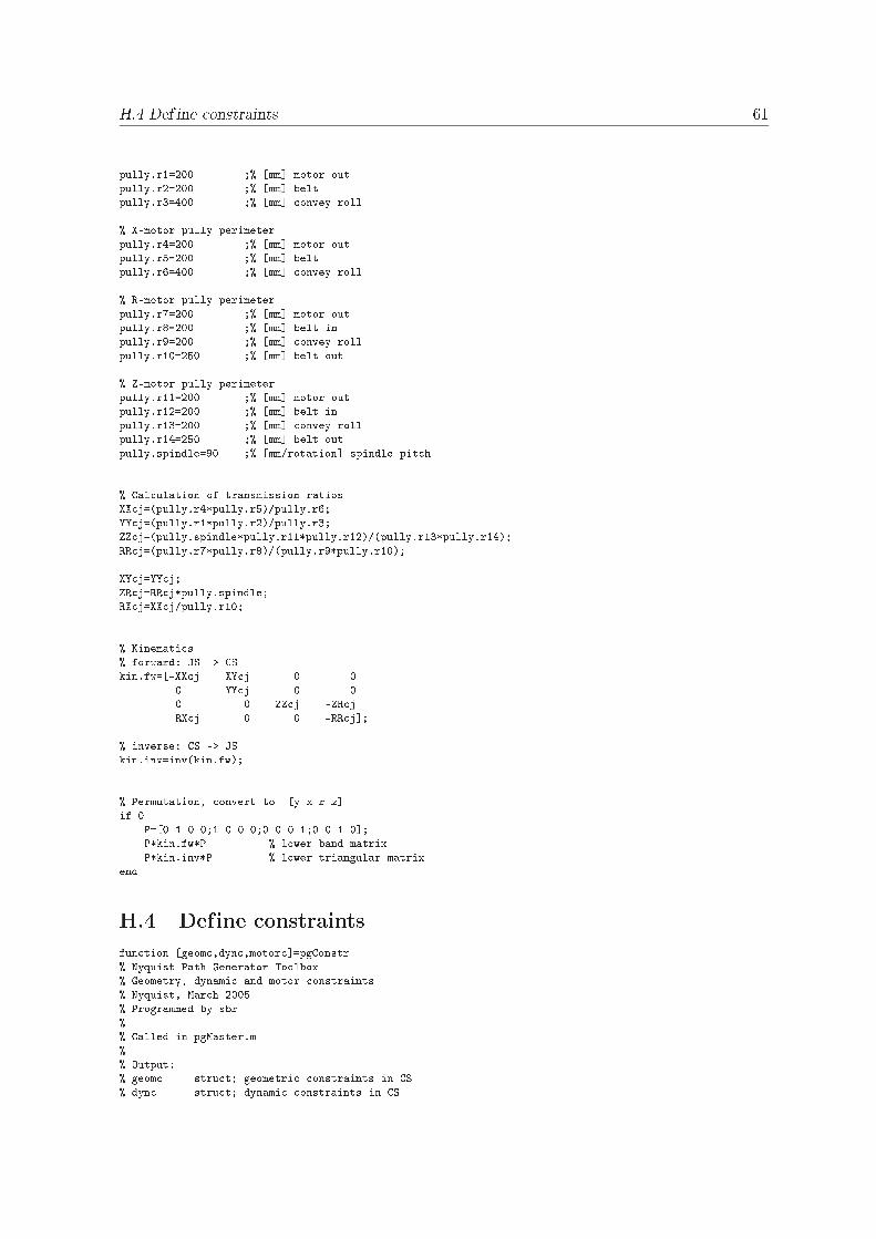
H.4 Def ine onstraints 61pully.r1=200 ;% [mm℄ motor outpully.r2=200 ;% [mm℄ beltpully.r3=400 ;% [mm℄ onvey roll% X-motor pully perimeterpully.r4=200 ;% [mm℄ motor outpully.r5=200 ;% [mm℄ beltpully.r6=400 ;% [mm℄ onvey roll% R-motor pully perimeterpully.r7=200 ;% [mm℄ motor outpully.r8=200 ;% [mm℄ belt inpully.r9=200 ;% [mm℄ onvey rollpully.r10=250 ;% [mm℄ belt out% Z-motor pully perimeterpully.r11=200 ;% [mm℄ motor outpully.r12=200 ;% [mm℄ belt inpully.r13=200 ;% [mm℄ onvey rollpully.r14=250 ;% [mm℄ belt outpully.spindle=90 ;% [mm/rotation℄ spindle pit h% Cal ulation of transmission ratiosXX j=(pully.r4*pully.r5)/pully.r6;YY j=(pully.r1*pully.r2)/pully.r3;ZZ j=(pully.spindle*pully.r11*pully.r12)/(pully.r13*pully.r14);RR j=(pully.r7*pully.r8)/(pully.r9*pully.r10);XY j=YY j;ZR j=RR j*pully.spindle;RX j=XX j/pully.r10;% Kinemati s% forward: JS -> CSkin.fw=[-XX j XY j 0 00 YY j 0 00 0 ZZ j -ZR jRX j 0 0 -RR j℄;% inverse: CS -> JSkin.inv=inv(kin.fw);% Permutation, onvert to [y x r z℄if 0P=[0 1 0 0;1 0 0 0;0 0 0 1;0 0 1 0℄;P*kin.fw*P % lower band matrixP*kin.inv*P % lower triangular matrixendH.4 Define onstraintsfun tion [geom ,dyn ,motor ℄=pgConstr% Nyquist Path Generator Toolbox% Geometry, dynami and motor onstraints% Nyquist, Mar h 2005% Programmed by sbr%% Called in pgMaster.m%% Output:% geom stru t; geometri onstraints in CS% dyn stru t; dynami onstraints in CS

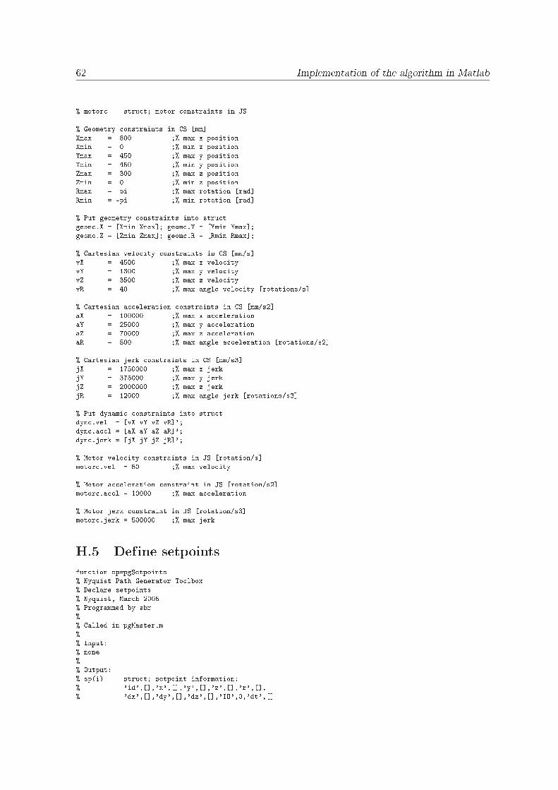
62 Implementation of the algorithm in Matlab% motor stru t; motor onstraints in JS% Geometry onstraints in CS [mm℄Xmax = 800 ;% max x positionXmin = 0 ;% min x positionYmax = 450 ;% max y positionYmin = -450 ;% min y positionZmax = 300 ;% max z positionZmin = 0 ;% min z positionRmax = pi ;% max rotation [rad℄Rmin = -pi ;% min rotation [rad℄% Put geometry onstraints into stru tgeom .X = [Xmin Xmax℄; geom .Y = [Ymin Ymax℄;geom .Z = [Zmin Zmax℄; geom .R = [Rmin Rmax℄;% Cartesian velo ity onstraints in CS [mm/s℄vX = 4500 ;% max x velo ityvY = 1300 ;% max y velo ityvZ = 3500 ;% max z velo ityvR = 40 ;% max angle velo ity [rotations/s℄% Cartesian a eleration onstraints in CS [mm/s2℄aX = 100000 ;% max x a elerationaY = 25000 ;% max y a elerationaZ = 70000 ;% max z a elerationaR = 500 ;% max angle a eleration [rotations/s2℄% Cartesian jerk onstraints in CS [mm/s3℄jX = 1750000 ;% max x jerkjY = 375000 ;% max y jerkjZ = 2000000 ;% max z jerkjR = 12000 ;% max angle jerk [rotations/s3℄% Put dynami onstraints into stru tdyn .vel = [vX vY vZ vR℄';dyn .a l = [aX aY aZ aR℄';dyn .jerk = [jX jY jZ jR℄';% Motor velo ity onstraints in JS [rotation/s℄motor .vel = 50 ;% max velo ity% Motor a eleration onstraint in JS [rotation/s2℄motor .a l = 10000 ;% max a eleration% Motor jerk onstraint in JS [rotation/s3℄motor .jerk = 500000 ;% max jerkH.5 Define setpointsfun tion sp=pgSetpoints% Nyquist Path Generator Toolbox% De lare setpoints% Nyquist, Mar h 2005% Programmed by sbr%% Called in pgMaster.m%% Input:% none%% Output:% sp(i) stru t; setpoint information:% 'id',[℄,'x',[℄,'y',[℄,'z',[℄,'r',[℄,% 'dx',[℄,'dy',[℄,'dz',[℄,'IO',0,'dt',[℄

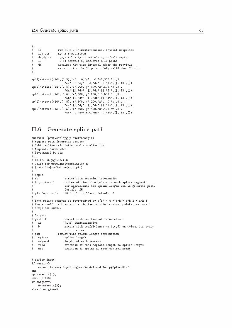
H.6 Generate spline path 63%% id row [i n℄, i=identifi ation, n=total setpoints% x,y,z,r x,y,z,r positions% dx,dy,dz x,y,z velovity at setpoints, default empty% IO [0 1℄ default 0, de lares a IO point% dt de alres the time interval after the previous% setpoint for the IO point. Only valid when IO = 1.%sp(1)=stru t('id',[1 5℄,'x', 0,'y', 0,'z',300,'r',0,...'dx', 0,'dy', 0,'dz', 0,'dt',[℄,'IO',[℄);sp(2)=stru t('id',[2 5℄,'x',200,'y',400,'z',100,'r',0,...'dx',[℄,'dy', [℄,'dz',[℄,'dt',[℄,'IO',[℄);sp(3)=stru t('id',[3 5℄,'x',600,'y',100,'z',500,'r',0,...'dx',[℄,'dy', [℄,'dz',[℄,'dt',[℄,'IO',[℄);sp(4)=stru t('id',[4 5℄,'x',700,'y',200,'z', 0,'r',0,...'dx',[℄,'dy', [℄,'dz',[℄,'dt',[℄,'IO',[℄);sp(5)=stru t('id',[5 5℄,'x',400,'y',400,'z',400,'r',0,...'dx', 0,'dy',500,'dz', 0,'dt',[℄,'IO',[℄);H.6 Generate spline pathfun tion [path,dim℄=pgSpline(varargin)% Nyquist Path Generator Toolbox% Cubi spline al ulation and visualisation% Nyquist, Mar h 2005% Programmed by sbr%% Called in pgMaster.m% Calls for pgSplineIterpolation.m% [path,dim℄=pgSpline(sp,N,plt)%% Input:% sp stru t with setpoint information% N (optional) number of iteration points in ea h spline segment,% for approximate the spline length and to generate plot.% Default: 25% plt (optional) [0 1℄ plot splines, default: 0%% Ea h spline segment is represented by p(k) = a + b*k + *k^2 + d*k^3% The a oeffi ient is similar to the provided ontrol points, so: ax=x0% ay=y0 and az=z0.%% Output:% path(i) stru t with oeffi ient information% id [i n℄ identifi ation% P matrix with oeffi ients (a,b, ,d) on olumn for every% axis one row.% dim stru t with spline length information% spline spline length% segment length of ea h segment% fra fra tion of ea h segment length to spline length% se fra tion of spline at ea h ontrol point% define inputif nargin>3error('To many input arguments defined for pgSplineDir')endsp=varargin{1};N=25; plt=0;if nargin==2N=varargin{2};elseif nargin==3

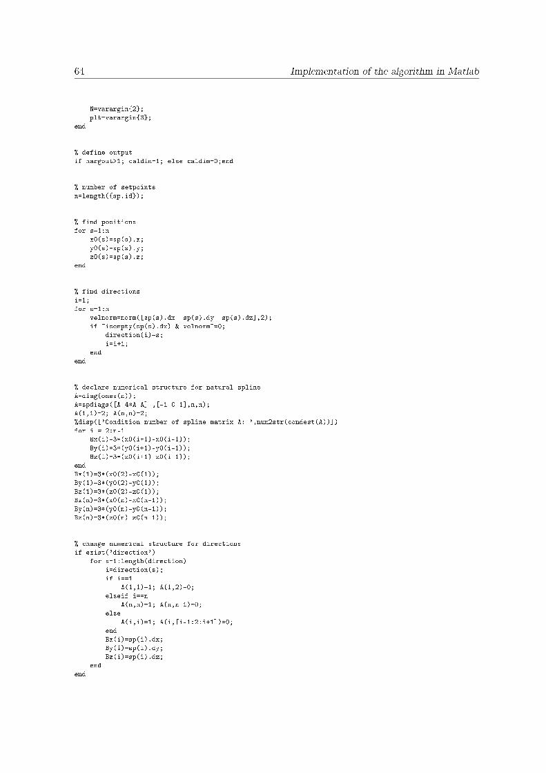
64 Implementation of the algorithm in MatlabN=varargin{2};plt=varargin{3};end% define outputif nargout>1; aldim=1; else aldim=0;end% number of setpointsn=length({sp.id});% find positionsfor s=1:nx0(s)=sp(s).x;y0(s)=sp(s).y;z0(s)=sp(s).z;end% find dire tionsi=1;for s=1:nvelnorm=norm([sp(s).dx sp(s).dy sp(s).dz℄,2);if ~isempty(sp(s).dx) & velnorm~=0;dire tion(i)=s;i=i+1;endend% de lare numeri al stru ture for natural splineA=diag(ones(n));A=spdiags([A 4*A A℄ ,[-1 0 1℄,n,n);A(1,1)=2; A(n,n)=2;%disp(['Condition number of spline matrix A: ',num2str( ondest(A))℄)for i = 2:n-1Bx(i)=3*(x0(i+1)-x0(i-1));By(i)=3*(y0(i+1)-y0(i-1));Bz(i)=3*(z0(i+1)-z0(i-1));endBx(1)=3*(x0(2)-x0(1));By(1)=3*(y0(2)-y0(1));Bz(1)=3*(z0(2)-z0(1));Bx(n)=3*(x0(n)-x0(n-1));By(n)=3*(y0(n)-y0(n-1));Bz(n)=3*(z0(n)-z0(n-1));% hange numeri al stru ture for dire tionsif exist('dire tion')for s=1:length(dire tion)i=dire tion(s);if i==1A(1,1)=1; A(1,2)=0;elseif i==nA(n,n)=1; A(n,n-1)=0;elseA(i,i)=1; A(i,[i-1:2:i+1℄)=0;endBx(i)=sp(i).dx;By(i)=sp(i).dy;Bz(i)=sp(i).dz;endend

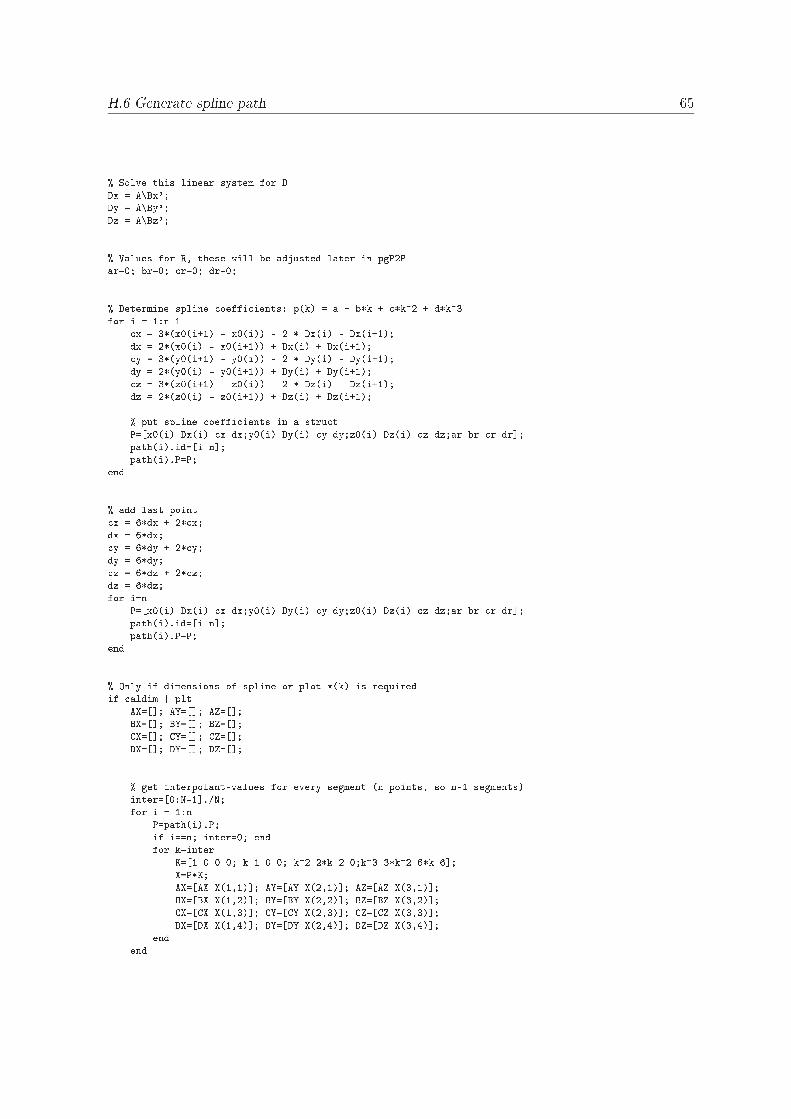
H.6 Generate spline path 65% Solve this linear system for DDx = A\Bx';Dy = A\By';Dz = A\Bz';% Values for R, these will be adjusted later in pgP2Par=0; br=0; r=0; dr=0;% Determine spline oeffi ients: p(k) = a + b*k + *k^2 + d*k^3for i = 1:n-1 x = 3*(x0(i+1) - x0(i)) - 2 * Dx(i) - Dx(i+1);dx = 2*(x0(i) - x0(i+1)) + Dx(i) + Dx(i+1); y = 3*(y0(i+1) - y0(i)) - 2 * Dy(i) - Dy(i+1);dy = 2*(y0(i) - y0(i+1)) + Dy(i) + Dy(i+1); z = 3*(z0(i+1) - z0(i)) - 2 * Dz(i) - Dz(i+1);dz = 2*(z0(i) - z0(i+1)) + Dz(i) + Dz(i+1);% put spline oeffi ients in a stru tP=[x0(i) Dx(i) x dx;y0(i) Dy(i) y dy;z0(i) Dz(i) z dz;ar br r dr℄;path(i).id=[i n℄;path(i).P=P;end% add last point x = 6*dx + 2* x;dx = 6*dx; y = 6*dy + 2* y;dy = 6*dy; z = 6*dz + 2* z;dz = 6*dz;for i=nP=[x0(i) Dx(i) x dx;y0(i) Dy(i) y dy;z0(i) Dz(i) z dz;ar br r dr℄;path(i).id=[i n℄;path(i).P=P;end% Only if dimensions of spline or plot x(k) is requiredif aldim | pltAX=[℄; AY=[℄; AZ=[℄;BX=[℄; BY=[℄; BZ=[℄;CX=[℄; CY=[℄; CZ=[℄;DX=[℄; DY=[℄; DZ=[℄;% get interpolant-values for every segment (n points, so n-1 segments)inter=[0:N-1℄./N;for i = 1:nP=path(i).P;if i==n; inter=0; endfor k=interK=[1 0 0 0; k 1 0 0; k^2 2*k 2 0;k^3 3*k^2 6*k 6℄;X=P*K;AX=[AX X(1,1)℄; AY=[AY X(2,1)℄; AZ=[AZ X(3,1)℄;BX=[BX X(1,2)℄; BY=[BY X(2,2)℄; BZ=[BZ X(3,2)℄;CX=[CX X(1,3)℄; CY=[CY X(2,3)℄; CZ=[CZ X(3,3)℄;DX=[DX X(1,4)℄; DY=[DY X(2,4)℄; DZ=[DZ X(3,4)℄;endend

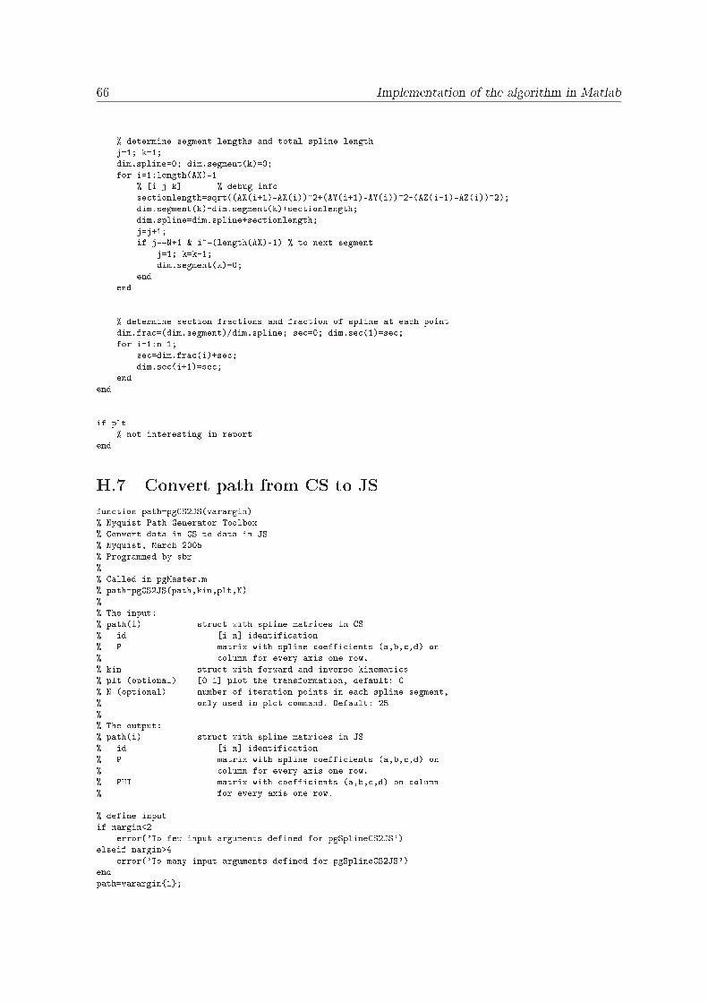
66 Implementation of the algorithm in Matlab% determine segment lengths and total spline lengthj=1; k=1;dim.spline=0; dim.segment(k)=0;for i=1:length(AX)-1% [i j k℄ % debug infose tionlength=sqrt((AX(i+1)-AX(i))^2+(AY(i+1)-AY(i))^2+(AZ(i+1)-AZ(i))^2);dim.segment(k)=dim.segment(k)+se tionlength;dim.spline=dim.spline+se tionlength;j=j+1;if j==N+1 & i~=(length(AX)-1) % to next segmentj=1; k=k+1;dim.segment(k)=0;endend% determine se tion fra tions and fra tion of spline at ea h pointdim.fra =(dim.segment)/dim.spline; se =0; dim.se (1)=se ;for i=1:n-1;se =dim.fra (i)+se ;dim.se (i+1)=se ;endendif plt% not interesting in reportendH.7 Convert path from CS to JSfun tion path=pgCS2JS(varargin)% Nyquist Path Generator Toolbox% Convert data in CS to data in JS% Nyquist, Mar h 2005% Programmed by sbr%% Called in pgMaster.m% path=pgCS2JS(path,kin,plt,N)%% The input:% path(i) stru t with spline matri es in CS% id [i n℄ identifi ation% P matrix with spline oeffi ients (a,b, ,d) on% olumn for every axis one row.% kin stru t with forward and inverse kinemati s% plt (optional) [0 1℄ plot the transformation, default: 0% N (optional) number of iteration points in ea h spline segment,% only used in plot ommand. Default: 25%% The output:% path(i) stru t with spline matri es in JS% id [i n℄ identifi ation% P matrix with spline oeffi ients (a,b, ,d) on% olumn for every axis one row.% PHI matrix with oeffi ients (a,b, ,d) on olumn% for every axis one row.% define inputif nargin<2error('To few input arguments defined for pgSplineCS2JS')elseif nargin>4error('To many input arguments defined for pgSplineCS2JS')endpath=varargin{1};

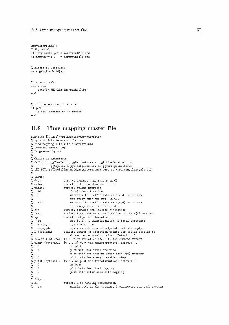
H.8 Time mapping master f ile 67kin=varargin{2};N=25; plt=0;if nargin>=3; plt = varargin{3}; endif nargin>=4; N = varargin{4}; end% number of setpointsn=length({path.id});% onvert pathfor i=1:npath(i).PHI=kin.inv*path(i).P;end% plot onversion if requiredif plt% not interesting in reportendH.8 Time mapping master filefun tion [KT,ACT℄=pgTimeSplineMap(varargin)% Nyquist Path Generator Toolbox% Find mapping k(t) within onstraints% Nyquist, Mar h 2005% Programmed by sbr%% Called in pgMaster.m% Calls for pgTimePar.m, pgDerivatives.m, pgA tiveConstraint.m,% pgMapPlot.m pgTimeSplinePlot.m, pgTimeSplineIter.m% [KT,ACT℄=pgTimeSplineMap(dyn ,motor ,path,test,sp,N,s reen,pltxt,plotkt)%% Input:% dyn stru t; dynami onstraints in CS% motor stru t; motor onstraints in JS% path(i) stru t; spline matri es% id [i n℄ identifi ation% P matrix with oeffi ients (a,b, ,d) on olumn% for every axis one row. In CS.% PHI matrix with oeffi ients (a,b, ,d) on olumn% for every axis one row. In JS.% kin stru t; forward and inverse kinemati s% test s alar; first estimate the duration of the k(t) mapping% sp stru t; setpoint information% id row [i n℄, i=identifi ation, n=total setpoints% x,y,z,r x,y,z positions% dx,dy,dz x,y,z orientation of setpoint, default empty% N (optional) s alar; number of iteration points per spline se tion to% determine onstraint points. Default: 10% s reen (optional) [0 1℄ plot iteration steps to the ommand window% pltxt (optional) [0 1 2 3℄ plot the transformation, default: 0% 0 no plot% 1 plot x(t) for final end time% 2 plot x(t) for endtime after ea h k(t) mapping% 3 plot x(t) for every iteration step% pltkt (optional) [0 1 2 3℄ plot the transformation, default: 0% 0 no plot% 1 plot k(t) for final mapping% 2 plot k(t) after ea h k(t) mapping%% Output:% KT stru t; k(t) mapping information% map matrix with in the olumns, 6 parameters for ea h mapping

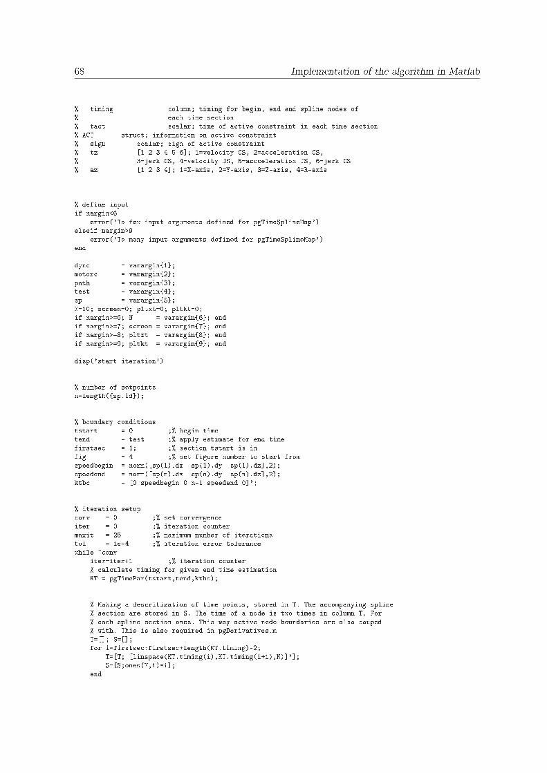
68 Implementation of the algorithm in Matlab% timing olumn; timing for begin, end and spline nodes of% ea h time se tion% ta t s alar; time of a tive onstraint in ea h time se tion% ACT stru t; information on a tive onstraint% sign s alar; sign of a tive onstraint% tz [1 2 3 4 5 6℄; 1=velo ity CS, 2=a eleration CS,% 3=jerk CS, 4=velo ity JS, 5=a eleration JS, 6=jerk CS% az [1 2 3 4℄; 1=X-axis, 2=Y-axis, 3=Z-axis, 4=R-axis% define inputif nargin<6error('To few input arguments defined for pgTimeSplineMap')elseif nargin>9error('To many input arguments defined for pgTimeSplineMap')enddyn = varargin{1};motor = varargin{2};path = varargin{3};test = varargin{4};sp = varargin{5};N=10; s reen=0; pltxt=0; pltkt=0;if nargin>=6; N = varargin{6}; endif nargin>=7; s reen = varargin{7}; endif nargin>=8; pltxt = varargin{8}; endif nargin>=9; pltkt = varargin{9}; enddisp('start iteration')% number of setpointsn=length({sp.id});% boundary onditionststart = 0 ;% begin timetend = test ;% apply estimate for end timefirstse = 1; ;% se tion tstart is infig = 4 ;% set figure number to start fromspeedbegin = norm([sp(1).dx sp(1).dy sp(1).dz℄,2);speedend = norm([sp(n).dx sp(n).dy sp(n).dz℄,2);ktb = [0 speedbegin 0 n-1 speedend 0℄';% iteration setup onv = 0 ;% set onvergen eiter = 0 ;% iteration ountermaxit = 25 ;% maximum number of iterationstol = 1e-4 ;% iteration error toleran ewhile ~ onviter=iter+1 ;% iteration ounter% al ulate timing for given end time estimationKT = pgTimePar(tstart,tend,ktb );% Making a des ritization of time points, stored in T. The a ompanying spline% se tion are stored in S. The time of a node is two times in olumn T. For% ea h spline se tion ones. This way a tive node boundaries are also ouped% with. This is also required in pgDerivatives.mT=[℄; S=[℄;for i=firstse :firstse +length(KT.timing)-2;T=[T; [linspa e(KT.timing(i),KT.timing(i+1),N)℄'℄;S=[S;ones(N,1)*i℄;end

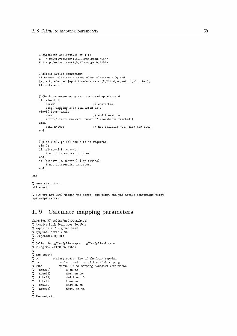
H.9 Cal ulate mapping parameters 69% al ulate derivatives of x(t)X = pgDerivatives(T,S,KT.map,path,'CS');Phi = pgDerivatives(T,S,KT.map,path,'JS');% sele t a tive onstraintif s reen; plotiter = iter; else; plotiter = 0; end[z,ta t,reler,a t℄=pgA tiveConstraint(X,Phi,dyn ,motor ,plotiter);KT.ta t=ta t;% Che k onvergen e, give output and update tendif reler<tol onv=1 ;% onverteddisp('mapping k(t) onverted in')elseif iter==maxit onv=1 ;% end iterationerror('Error: maximum number of iterations rea hed')elsetend=z*tend ;% not solution yet, pi k new time.end% plot x(t), phi(t) and k(t) if requiredfig=4;if (pltkt==2 & onv==1)% not interesting in reportendif (pltxt==2 & onv==1) | (pltxt==3)% not interesting in reportendend% generate outputACT = a t;% Fit two new k(t) within the begin, end point and the a tive onstraint pointpgTimeSplineIterH.9 Cal ulate mapping parametersfun tion KT=pgTimePar(t0,tn,ktb )% Nyquist Path Generator Toolbox% map t on k for given tend% Nyquist, Mar h 2005% Programmed by sbr%% Called in pgTimeSplineMap.m, pgTimeSplineIter.m% KT=pgTimePar(t0,tn,ktb )%% The input:% t0 s alar; start time of the k(t) mapping% tn s alar; end time of the k(t) mapping% ktb ve tor; k(t) mapping boundary onditions% ktb (1) k on t0% ktb (2) dkdt on t0% ktb (3) dkdt2 on t0% ktb (4) k on tn% ktb (5) dkdt on tn% ktb (6) dkdt2 on tn%% The output:

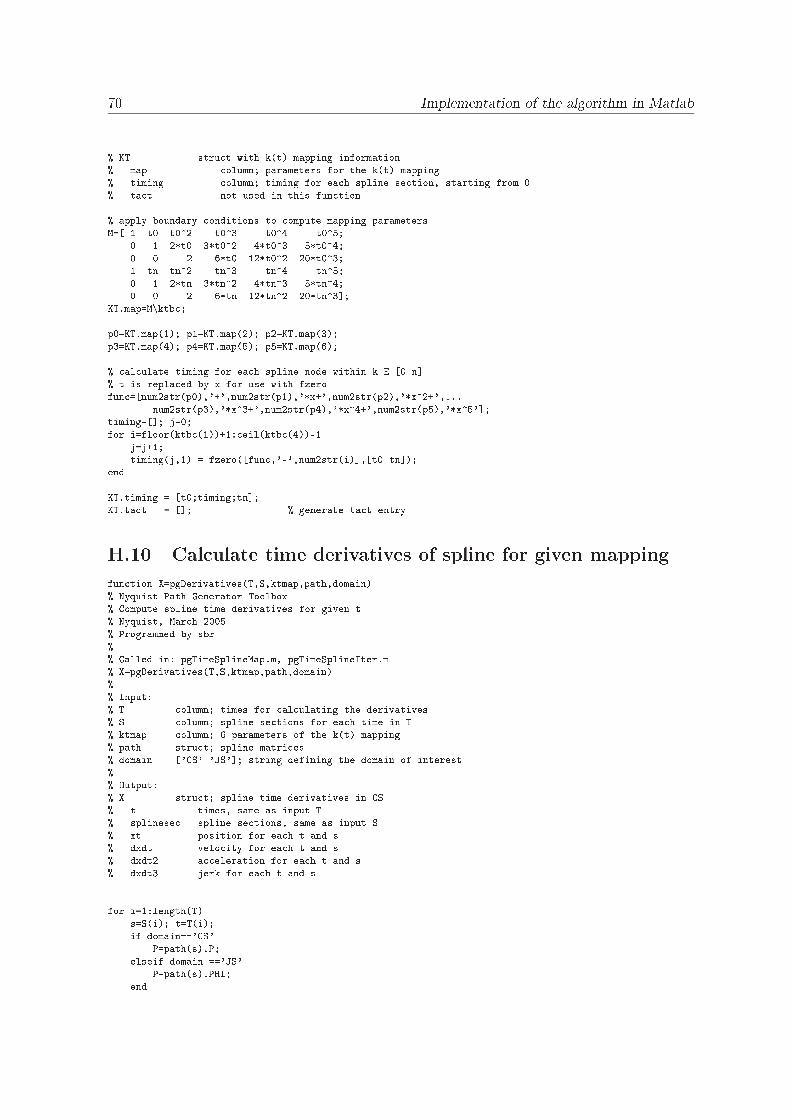
70 Implementation of the algorithm in Matlab% KT stru t with k(t) mapping information% map olumn; parameters for the k(t) mapping% timing olumn; timing for ea h spline se tion, starting from 0% ta t not used in this fun tion% apply boundary onditions to ompute mapping parametersM=[ 1 t0 t0^2 t0^3 t0^4 t0^5;0 1 2*t0 3*t0^2 4*t0^3 5*t0^4;0 0 2 6*t0 12*t0^2 20*t0^3;1 tn tn^2 tn^3 tn^4 tn^5;0 1 2*tn 3*tn^2 4*tn^3 5*tn^4;0 0 2 6*tn 12*tn^2 20*tn^3℄;KT.map=M\ktb ;p0=KT.map(1); p1=KT.map(2); p2=KT.map(3);p3=KT.map(4); p4=KT.map(5); p5=KT.map(6);% al ulate timing for ea h spline node within k E [0 n℄% t is repla ed by x for use with fzerofun =[num2str(p0),'+',num2str(p1),'*x+',num2str(p2),'*x^2+',...num2str(p3),'*x^3+',num2str(p4),'*x^4+',num2str(p5),'*x^5'℄;timing=[℄; j=0;for i=floor(ktb (1))+1: eil(ktb (4))-1j=j+1;timing(j,1) = fzero([fun ,'-',num2str(i)℄,[t0 tn℄);endKT.timing = [t0;timing;tn℄;KT.ta t = [℄; % generate ta t entryH.10 Cal ulate time derivatives of spline for given mappingfun tion X=pgDerivatives(T,S,ktmap,path,domain)% Nyquist Path Generator Toolbox% Compute spline time derivatives for given t% Nyquist, Mar h 2005% Programmed by sbr%% Called in: pgTimeSplineMap.m, pgTimeSplineIter.m% X=pgDerivatives(T,S,ktmap,path,domain)%% Input:% T olumn; times for al ulating the derivatives% S olumn; spline se tions for ea h time in T% ktmap olumn; 6 parameters of the k(t) mapping% path stru t; spline matri es% domain ['CS' 'JS'℄; string defining the domain of interest%% Output:% X stru t; spline time derivatives in CS% t times, same as input T% splinese spline se tions, same as input S% xt position for ea h t and s% dxdt velo ity for ea h t and s% dxdt2 a eleration for ea h t and s% dxdt3 jerk for ea h t and sfor i=1:length(T)s=S(i); t=T(i);if domain=='CS'P=path(s).P;elseif domain =='JS'P=path(s).PHI;end

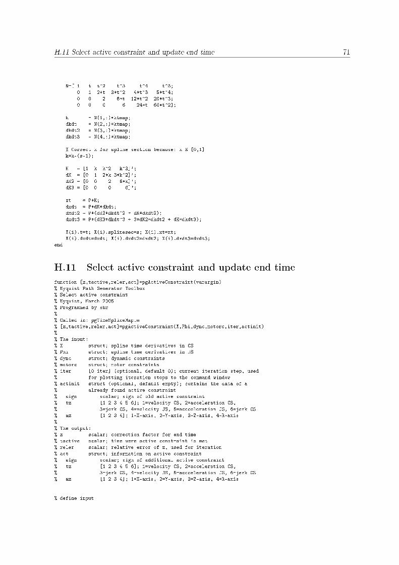
H.11 Sele t a tive onstraint and update end time 71N=[ 1 t t^2 t^3 t^4 t^5;0 1 2*t 3*t^2 4*t^3 5*t^4;0 0 2 6*t 12*t^2 20*t^3;0 0 0 6 24*t 60*t^2℄;k = N(1,:)*ktmap;dkdt = N(2,:)*ktmap;dkdt2 = N(3,:)*ktmap;dkdt3 = N(4,:)*ktmap;% Corre t k for spline se tion be ause: k E [0,1℄k=k-(s-1);K = [1 k k^2 k^3℄';dK = [0 1 2*k 3*k^2℄';dK2 = [0 0 2 6*k℄';dK3 = [0 0 0 6℄';xt = P*K;dxdt = P*dK*dkdt;dxdt2 = P*(dK2*dkdt^2 + dK*dkdt2);dxdt3 = P*(dK3*dkdt^3 + 3*dK2*dkdt2 + dK*dkdt3);X(i).t=t; X(i).splinese =s; X(i).xt=xt;X(i).dxdt=dxdt; X(i).dxdt2=dxdt2; X(i).dxdt3=dxdt3;endH.11 Sele t a tive onstraint and update end timefun tion [z,ta tive,reler,a t℄=pgA tiveConstraint(varargin)% Nyquist Path Generator Toolbox% Sele t a tive onstraint% Nyquist, Mar h 2005% Programmed by sbr%% Called in: pgTimeSplineMap.m% [z,ta tive,reler,a t℄=pgA tiveConstraint(X,Phi,dyn ,motor ,iter,a tinit)%% The input:% X stru t; spline time derivatives in CS% Phi stru t; spline time derivatives in JS% dyn stru t; dynami onstraints% motor stru t; motor onstraints% iter [0 iter℄ (optional, default 0); urrent iteration step, used% for plotting iteration steps to the ommand window% a tinit stru t (optional, default empty); ontains the data of a% already found a tive onstraint% sign s alar; sign of old a tive onstraint% tz [1 2 3 4 5 6℄; 1=velo ity CS, 2=a eleration CS,% 3=jerk CS, 4=velo ity JS, 5=a eleration JS, 6=jerk CS% az [1 2 3 4℄; 1=X-axis, 2=Y-axis, 3=Z-axis, 4=R-axis%% The output:% z s alar; orre tion fa tor for end time% ta tive s alar; time were a tive onstraint is met% reler s alar; relative error of z, used for iteration% a t stru t; information on a tive onstraint% sign s alar; sign of additional a tive onstraint% tz [1 2 3 4 5 6℄; 1=velo ity CS, 2=a eleration CS,% 3=jerk CS, 4=velo ity JS, 5=a eleration JS, 6=jerk CS% az [1 2 3 4℄; 1=X-axis, 2=Y-axis, 3=Z-axis, 4=R-axis% define input

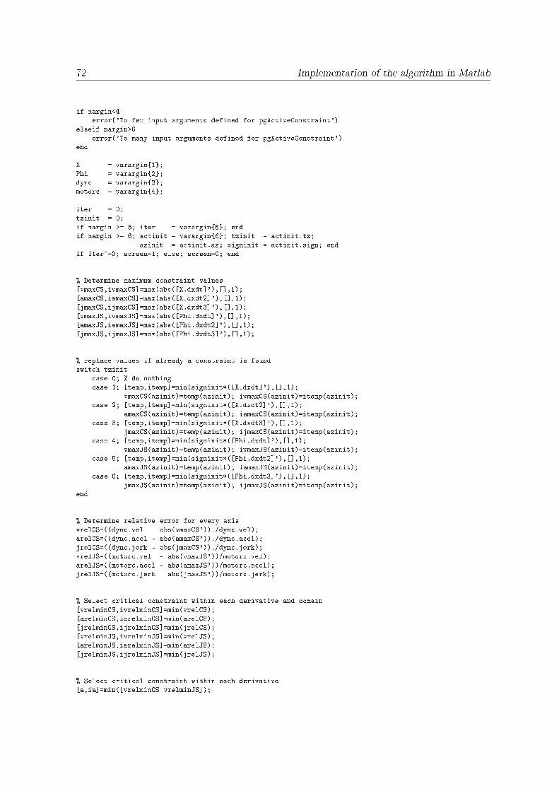
72 Implementation of the algorithm in Matlabif nargin<4error('To few input arguments defined for pgA tiveConstraint')elseif nargin>6error('To many input arguments defined for pgA tiveConstraint')endX = varargin{1};Phi = varargin{2};dyn = varargin{3};motor = varargin{4};iter = 0;tzinit = 0;if nargin >= 5; iter = varargin{5}; endif nargin >= 6; a tinit = varargin{6}; tzinit = a tinit.tz;azinit = a tinit.az; signinit = a tinit.sign; endif iter~=0; s reen=1; else; s reen=0; end% Determine maximum onstraint values[vmaxCS,ivmaxCS℄=max(abs([X.dxdt℄'),[℄,1);[amaxCS,iamaxCS℄=max(abs([X.dxdt2℄'),[℄,1);[jmaxCS,ijmaxCS℄=max(abs([X.dxdt3℄'),[℄,1);[vmaxJS,ivmaxJS℄=max(abs([Phi.dxdt℄'),[℄,1);[amaxJS,iamaxJS℄=max(abs([Phi.dxdt2℄'),[℄,1);[jmaxJS,ijmaxJS℄=max(abs([Phi.dxdt3℄'),[℄,1);% repla e values if already a onstraint is foundswit h tzinit ase 0; % do nothing ase 1; [temp,itemp℄=min(signinit*([X.dxdt℄'),[℄,1);vmaxCS(azinit)=temp(azinit); ivmaxCS(azinit)=itemp(azinit); ase 2; [temp,itemp℄=min(signinit*([X.dxdt2℄'),[℄,1);amaxCS(azinit)=temp(azinit); iamaxCS(azinit)=itemp(azinit); ase 3; [temp,itemp℄=min(signinit*([X.dxdt3℄'),[℄,1);jmaxCS(azinit)=temp(azinit); ijmaxCS(azinit)=itemp(azinit); ase 4; [temp,itemp℄=min(signinit*([Phi.dxdt℄'),[℄,1);vmaxJS(azinit)=temp(azinit); ivmaxJS(azinit)=itemp(azinit); ase 5; [temp,itemp℄=min(signinit*([Phi.dxdt2℄'),[℄,1);amaxJS(azinit)=temp(azinit); iamaxJS(azinit)=itemp(azinit); ase 6; [temp,itemp℄=min(signinit*([Phi.dxdt3℄'),[℄,1);jmaxJS(azinit)=temp(azinit); ijmaxJS(azinit)=itemp(azinit);end% Determine relative error for every axisvrelCS=((dyn .vel - abs(vmaxCS'))./dyn .vel);arelCS=((dyn .a l - abs(amaxCS'))./dyn .a l);jrelCS=((dyn .jerk - abs(jmaxCS'))./dyn .jerk);vrelJS=((motor .vel - abs(vmaxJS'))/motor .vel);arelJS=((motor .a l - abs(amaxJS'))/motor .a l);jrelJS=((motor .jerk - abs(jmaxJS'))/motor .jerk);% Sele t riti al onstraint within ea h derivative and domain[vrelminCS,ivrelminCS℄=min(vrelCS);[arelminCS,iarelminCS℄=min(arelCS);[jrelminCS,ijrelminCS℄=min(jrelCS);[vrelminJS,ivrelminJS℄=min(vrelJS);[arelminJS,iarelminJS℄=min(arelJS);[jrelminJS,ijrelminJS℄=min(jrelJS);% Sele t riti al onstraint within ea h derivative[a,ia℄=min([vrelminCS vrelminJS℄);

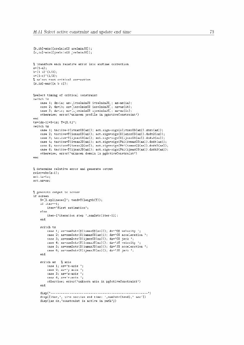
H.11 Sele t a tive onstraint and update end time 73[b,ib℄=min([arelminCS arelminJS℄);[ ,i ℄=min([jrelminCS jrelminJS℄);% transform ea h relative error into endtime orre tiona=(1-a);b=(1-b)^(1/2); =(1- )^(1/3);% sele t most riti al orre tion[z,iz℄=max([a b ℄);%sele t timing of riti al onstraintswit h iz ase 1; dz=ia; az=[ivrelminCS ivrelminJS℄; az=az(ia); ase 2; dz=ib; az=[iarelminCS iarelminJS℄; az=az(ib); ase 3; dz=i ; az=[ijrelminCS ijrelminJS℄; az=az(i );otherwise; error('unknown profile in pgA tiveConstraint')endtz=(dz-1)*3+iz; T=[X.t℄';swit h tz ase 1; ta tive=T(ivmaxCS(az)); a t.sign=sign(X(ivmaxCS(az)).dxdt(az)); ase 2; ta tive=T(iamaxCS(az)); a t.sign=sign(X(iamaxCS(az)).dxdt2(az)); ase 3; ta tive=T(ijmaxCS(az)); a t.sign=sign(X(ijmaxCS(az)).dxdt3(az)); ase 4; ta tive=T(ivmaxJS(az)); a t.sign=sign(Phi(ivmaxCS(az)).dxdt(az)); ase 5; ta tive=T(iamaxJS(az)); a t.sign=sign(Phi(iamaxCS(az)).dxdt2(az)); ase 6; ta tive=T(ijmaxJS(az)); a t.sign=sign(Phi(ijmaxCS(az)).dxdt3(az));otherwise; error('unknown domain in pgA tiveConstraint')end% determine relative error and generate outputreler=abs(z-1);a t.tz=tz;a t.az=az;% generate output to s reenif s reenS=[X.splinese ℄'; tend=T(length(T));if iter==1;iter='first estimation';elseiter=['iteration step ',num2str(iter-1)℄;endswit h tz ase 1; as=num2str(S(ivmaxCS(az))); dz='CS velo ity '; ase 2; as=num2str(S(iamaxCS(az))); dz='CS a eleration '; ase 3; as=num2str(S(ijmaxCS(az))); dz='CS jerk '; ase 4; as=num2str(S(ivmaxJS(az))); dz='JS velo ity '; ase 5; as=num2str(S(iamaxJS(az))); dz='JS a eleration '; ase 6; as=num2str(S(ijmaxJS(az))); dz='JS jerk ';endswit h az % axis ase 1; az='x-axis '; ase 2; az='y-axis '; ase 3; az='z-axis '; ase 4; az='r-axis ';otherwise; error('unknown axis in pgA tiveConstraint')enddisp('--------------------------------------------------------')disp([iter,', time se tion end time: ',num2str(tend),' se '℄)disp([az dz,' onstraint is a tive in path'℄)

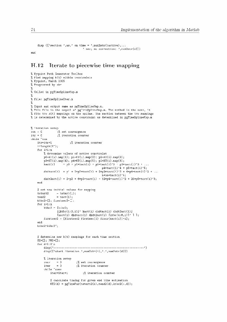
74 Implementation of the algorithm in Matlabdisp (['se tion ',as,' on time = ',num2str(ta tive),...' se ; nu orre tion: ',num2str(z)℄)endH.12 Iterate to pie ewise time mapping% Nyquist Path Generator Toolbox% Find mapping k(t) within onstraints% Nyquist, Mar h 2005% Programmed by sbr%% Called in pgTimeSplineMap.m%% file: pgTimeSplineIter.m%% Input and output same as pgTimeSplineMap.m.% This file is the sequel of pgTimeSplineMap.m. The method is the same, it% fits two k(t) mappings on the spline. The se tion between the two mappings% is determined by the a tive onstraint as determined in pgTimeSplineMap.m% iteration setup on = 0 ;% set onvergen eitr = 0 ;% iteration ounterwhile ~ onitr=itr+1 ;% iteration ounterm=length(KT);for i=1:m% determine values of a tive onstraintp0=KT(i).map(1); p1=KT(i).map(2); p2=KT(i).map(3);p3=KT(i).map(4); p4=KT(i).map(5); p5=KT(i).map(6);ka t(i) = p0 + p1*ta t(i) + p2*ta t(i)^2 + p3*ta t(i)^3 + ...p4*ta t(i)^4 + p5*ta t(i)^5;dkdta t(i) = p1 + 2*p2*ta t(i) + 3*p3*ta t(i)^2 + 4*p4*ta t(i)^3 + ...5*p5*ta t(i)^4;dkdt2a t(i) = 2*p2 + 6*p3*ta t(i) + 12*p4*ta t(i)^2 + 20*p5*ta t(i)^3;end% set new initial values for mappingtstart2 = tstart(1);tend2 = ta t(1);ktb 2=[℄; firstse 2=[℄;for i=1:mktb 2 = [ktb 2;[[ktb (1:3,i)℄' ka t(i) dkdta t(i) dkdt2a t(i)℄[ka t(i) dkdta t(i) dkdt2a t(i) [ktb (4:6,i)℄' ℄ ℄;firstse 2 = [firstse 2 firstse (i) floor(ka t(i))+1℄;endktb 2=ktb 2';% determine new k(t) mappings for ea h time se tionXX=[℄; PHI=[℄;for d=1:2^mdisp('--------------------------------------------------------')disp(['start iteration ',num2str(m),'.',num2str(d)℄)% iteration setup onv = 0 ;% set onvergen eiter = 0 ;% iteration ounterwhile ~ onviter=iter+1 ;% iteration ounter% al ulate timing for given end time estimationKT2(d) = pgTimePar(tstart2(d),tend2(d),ktb 2(:,d));

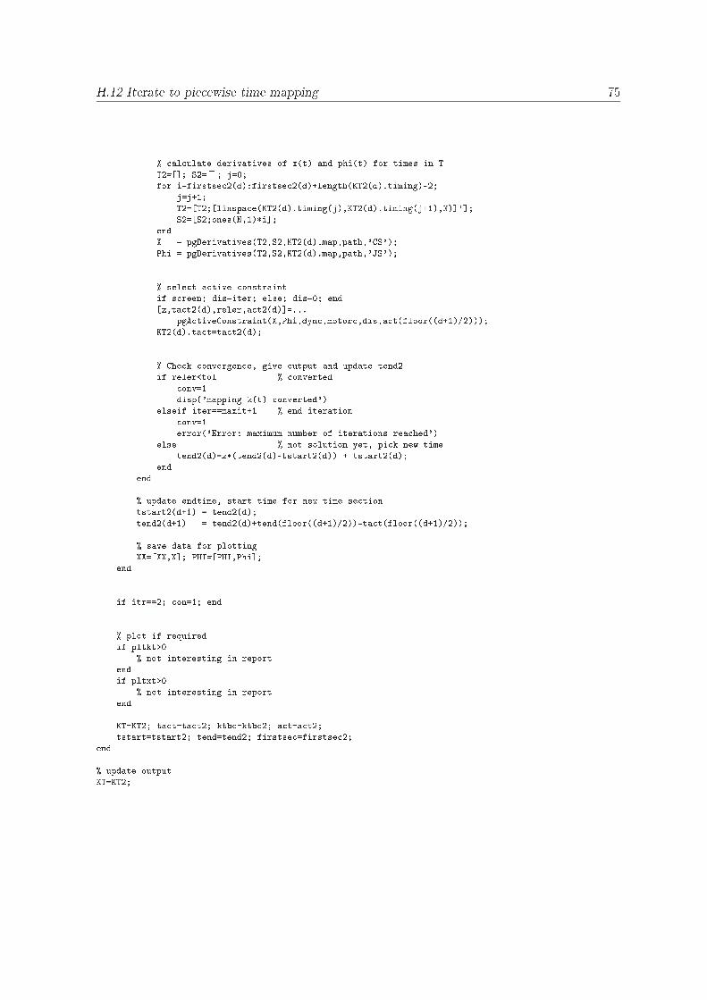
H.12 Iterate to pie ewise time mapping 75% al ulate derivatives of x(t) and phi(t) for times in TT2=[℄; S2=[℄; j=0;for i=firstse 2(d):firstse 2(d)+length(KT2(d).timing)-2;j=j+1;T2=[T2;[linspa e(KT2(d).timing(j),KT2(d).timing(j+1),N)℄'℄;S2=[S2;ones(N,1)*i℄;endX = pgDerivatives(T2,S2,KT2(d).map,path,'CS');Phi = pgDerivatives(T2,S2,KT2(d).map,path,'JS');% sele t a tive onstraintif s reen; dis=iter; else; dis=0; end[z,ta t2(d),reler,a t2(d)℄=...pgA tiveConstraint(X,Phi,dyn ,motor ,dis,a t(floor((d+1)/2)));KT2(d).ta t=ta t2(d);% Che k onvergen e, give output and update tend2if reler<tol % onverted onv=1disp('mapping k(t) onverted')elseif iter==maxit+1 % end iteration onv=1error('Error: maximum number of iterations rea hed')else % not solution yet, pi k new timetend2(d)=z*(tend2(d)-tstart2(d)) + tstart2(d);endend% update endtime, start time for new time se tiontstart2(d+1) = tend2(d);tend2(d+1) = tend2(d)+tend(floor((d+1)/2))-ta t(floor((d+1)/2));% save data for plottingXX=[XX,X℄; PHI=[PHI,Phi℄;endif itr==2; on=1; end% plot if requiredif pltkt>0% not interesting in reportendif pltxt>0% not interesting in reportendKT=KT2; ta t=ta t2; ktb =ktb 2; a t=a t2;tstart=tstart2; tend=tend2; firstse =firstse 2;end% update outputKT=KT2;

76 Implementation of the algorithm in Matlab