Embed Size (px)
Citation preview
TIME OPTIMAL TRAJECTORY GENERATION FOR A
DIFFERENTIAL DRIVE ROBOT
by
Subramaniam V. Iyer
8/13/08
A thesis submitted to
the Faculty of the Graduate School of
State University of New York at Buffalo
in partial fulfillment of the requirements for the degree of
Master of Science
Department of Mechanical & Aerospace Engineering
To My Grandfather the late V.Venkiteswaran
ii
Acknowledgment
I would like to express my sincere gratitude to my advisor Dr.Puneet Singla
who gave me this wonderful opportunity to work under his able guidance. I would
like to thank him for being patient and providing me with all the resources that made
this thesis possible. I would like to thank my committee members Dr.V.Krovi and
Dr.T.Singh for their valuable inputs. I would also like to acknowledge other professors
in the department who taught me the basics of controls and helped me to reach till
here. Their wide knowledge has been of great value for me.
I would like to extend my gratitude to my parents, my grand parents and my
brother who encouraged me all the way in my journey. I also like to thank all of my
lab mates, room mates and friends who helped me in my work.
I would also like to thank the Mechanical Engineering Department and the
New York state who supported me financially for my education here.
iii
Contents
Acknowledgement iii
Abstract . . . . . . . . . . . . . . . . . . . . . . . . . . . . . . . . . . . . . viii
1 Introduction 1
2 Time Optimal Control Problem for Three Wheeled Differential-
Drive Ground Vehicle 7
2.1 Introduction . . . . . . . . . . . . . . . . . . . . . . . . . . . . . . . . 7
2.2 Derivation of Equation of motion . . . . . . . . . . . . . . . . . . . . 8
2.3 Optimal Trajectory Generation . . . . . . . . . . . . . . . . . . . . . 10
2.4 Pontrygins Maximum Principle . . . . . . . . . . . . . . . . . . . . . 11
3 Time Optimal Path Planning for three-wheeled differential-drive
robot using Sequential Linear Programming(SLP) 14
3.1 Introduction . . . . . . . . . . . . . . . . . . . . . . . . . . . . . . . . 14
iv
Contents v
3.1.1 Road Map Techniques: . . . . . . . . . . . . . . . . . . . . . . 15
3.1.2 Cell Decomposition: . . . . . . . . . . . . . . . . . . . . . . . 16
3.1.3 Artificial Potential field methods: . . . . . . . . . . . . . . . . 17
3.1.4 Continuous Path Planning . . . . . . . . . . . . . . . . . . . . 18
3.1.5 Sequential Linear Programming : . . . . . . . . . . . . . . . . 20
3.2 Time Optimal Path Planning using Sequential Linear Programming(SLP) 23
3.3 Numerical Simulation & Results . . . . . . . . . . . . . . . . . . . . . 28
3.3.1 Case 1 . . . . . . . . . . . . . . . . . . . . . . . . . . . . . . . 28
3.3.2 Case 2 . . . . . . . . . . . . . . . . . . . . . . . . . . . . . . . 30
3.3.3 Case 3 . . . . . . . . . . . . . . . . . . . . . . . . . . . . . . . 30
3.3.4 Case 4 . . . . . . . . . . . . . . . . . . . . . . . . . . . . . . . 33
3.3.5 Case 5 . . . . . . . . . . . . . . . . . . . . . . . . . . . . . . . 35
3.3.6 Case 6 . . . . . . . . . . . . . . . . . . . . . . . . . . . . . . . 35
4 GLOMAP 37
4.1 Introduction . . . . . . . . . . . . . . . . . . . . . . . . . . . . . . . . 37
4.2 Solution to Optimal Control Problem with
GLOMAP Approach . . . . . . . . . . . . . . . . . . . . . . . . . . . 38
4.2.1 Problem Statement . . . . . . . . . . . . . . . . . . . . . . . . 41
Contents vi
4.3 Numerical Simulation and Results . . . . . . . . . . . . . . . . . . . . 46
4.3.1 Case 1 : . . . . . . . . . . . . . . . . . . . . . . . . . . . . . . 47
4.3.2 Case 2: . . . . . . . . . . . . . . . . . . . . . . . . . . . . . . 47
4.3.3 Case 3: . . . . . . . . . . . . . . . . . . . . . . . . . . . . . . . 52
4.3.4 Case 4 : . . . . . . . . . . . . . . . . . . . . . . . . . . . . . . 53
4.3.5 Case 5 : . . . . . . . . . . . . . . . . . . . . . . . . . . . . . . 55
4.4 Conclusion . . . . . . . . . . . . . . . . . . . . . . . . . . . . . . . . . 57
5 Real testing 58
5.1 Hardware Used . . . . . . . . . . . . . . . . . . . . . . . . . . . . . . 58
5.2 Player And Stage . . . . . . . . . . . . . . . . . . . . . . . . . . . . . 59
5.2.1 Player: . . . . . . . . . . . . . . . . . . . . . . . . . . . . . . . 59
5.2.2 Features of Player . . . . . . . . . . . . . . . . . . . . . . . . . 60
5.2.3 Stage: . . . . . . . . . . . . . . . . . . . . . . . . . . . . . . . 60
5.3 Laser mapping . . . . . . . . . . . . . . . . . . . . . . . . . . . . . . 61
5.4 Player-Stage Simulation . . . . . . . . . . . . . . . . . . . . . . . . . 61
5.5 Real Run . . . . . . . . . . . . . . . . . . . . . . . . . . . . . . . . . 67
5.5.1 Case1: . . . . . . . . . . . . . . . . . . . . . . . . . . . . . . . 67
5.5.2 Case2: . . . . . . . . . . . . . . . . . . . . . . . . . . . . . . . 71

Contents vii
6 Conclusion 76
6.1 Future Scope . . . . . . . . . . . . . . . . . . . . . . . . . . . . . . . 77
Bibliography 78
Abstract
Trajectory generation or motion planning is one of the critical steps in the con-
trol design for autonomous robots. The problem of shortest trajectory or time optimal
trajectory has been a topic of active research. In this, thesis Sequential Linear Pro-
gramming algorithm (SLP) and Global Local Mapping (Glomap) are the two methods
used to solve the optimal trajectory generation problem for a differential drive robot.
The time optimal path planning problem is posed as a linear programming problem
which is solved using the SLP algorithm. In the Glomap approach the time domain is
broken into smaller domains. The trajectory is generated for each local domain and
then merged into a global trajectory. In both these methods potential functions are
used to represent the obstacles in the configuration space. The trajectory generation
methods are implemented in Matlab and validated on a robotic platform. Though
the methods mentioned here are used for path planning for a differential drive robot
they may be used for other systems with little or no modifications
viii
Chapter 1
Introduction
In the near future with the increasing automation and development in robotics,
it is evident that robots will be a part of the natural landscape. One of the challenges
faced by these robots will be to interact with objects, humans and the terrain. The
most basic step for such robots would be to reach their assigned (or desired) position
autonomously while negotiating obstacles in the vicinity. Thus, motion planning is a
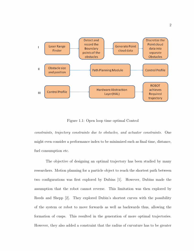
critical step in the control design for robots. Motion planning for a robot include three
main steps namely mapping of the environment, computing the trajectory given initial
and final configurations of the robot and computing the control profile required for the
transition of the robot from the initial configuration to the final as shown in Fig. 1.1.
The knowledge of the environment can be obtained by using various sensors (sonar,
laser range finders, etc). The initial and final configurations are usually given. An
important challenge is: How to plan a trajectory while incorporating system dynamics
1
2
Figure 1.1: Open loop time optimal Control
constraints, trajectory constraints due to obstacles, and actuator constraints. One
might even consider a performance index to be minimized such as final time, distance,
fuel consumption etc.
The objective of designing an optimal trajectory has been studied by many
researchers. Motion planning for a particle object to reach the shortest path between
two configurations was first explored by Dubins [1]. However, Dubins made the
assumption that the robot cannot reverse. This limitation was then explored by
Reeds and Shepp [2]. They explored Dubin’s shortest curves with the possibility
of the system or robot to move forwards as well as backwards thus, allowing the
formation of cusps. This resulted in the generation of more optimal trajectories.
However, they also added a constraint that the radius of curvature has to be greater
3
than or equal to one. The above mentioned system is also known as the Reed and
Shepp robot. In Ref. [3], it has been suggested every non-trivial optimal trajectory of
a differential-drive vehicle with bounded velocity can be composed of as many as five
actions (four are enough). Each action may comprise of straight segments or turns in
either direction about the robot’s center. It is shown that the solution would always
be bang-bang, i.e. the acceleration of each of the wheels will be at maximum in one
or the other direction.
Although analytical solutions have been obtained to find the shortest or time
optimal trajectory between two given configurations, these methods do not explicitly
take into consideration the presence of obstacles in the configuration space. In such
cases an analytical solution may not always exist. Many numerical methods [4, 5]
have been discussed in literature to find an optimal trajectory between two config-
uration points while explicitly taking care of path constraints due to obstacles. A
general strategy is to parameterize the optimal trajectory at discrete intervals of time
and the optimal trajectory generation problem is solved as a nonlinear programming
problem (NLP) [6–8]. Several methods [9] including direct collocation [7, 10, 11],
pseudo-spectral methods [12–15] and spline approximations [5,16,17] have been pro-
posed to solve the resulting nonlinear programming problem. Methods based on
direct collocation methods lead to an inefficient representation of the optimal control
problem and often result in large optimization problem. In pseudo-spectral methods,
Legendre or Chebyshev polynomials are used as basis functions which demonstrate
4
the Gibbs phenomenon [18, 19] and are not suitable to approximate bang-bang type
of solution.
In spline based methods [5,16,17], the trajectory is assumed to be a composite
of polynomial pieces stitched together and smoothness conditions at break points is
enforced implicitly by using B-Splines as basis functions. Although B-Splines offer
local support but, the approximation is done with polynomials of the same order and
lacks variability. As a consequence of this, the basis functions used to obtain differ-
ent local approximation can not be independent from each other without introducing
discontinuity across the boundary of different local regions. If the configuration space
is nonlinear in nature, as is often the case in real world scenarios, the level of nonlin-
earity over the space need not be constant. In Ref. [15], a method to parameterize
a globally smooth function based on local approximations is proposed. A recently
developed novel Global-Local Orthogonal Mapping (GLOMAP) approach [15,20,21]
is used to construct overlapping, shifted independent local approximations and av-
erage these approximations in the overlapped region in such a way that prescribed
consistency/continuity conditions are automatically accommodated, without im-
posing continuity constraints directly on the local approximations. Thus,
the freedom to incorporate any local approximations, to create a global trajectory, is
the strength of the approach and offers a more generalized framework for trajectory
generation and allows greater flexibility.
Furthermore, in Ref. [22, 23], a sequentially linear programming approach is
5
proposed to solve the generic optimal control problem making use of the sensitivities of
the system dynamics with respect to the states and control vector. The sensitivities
are used to determine a time-varying linear model which is used to pose a linear
programming (LP) problem to exploit the strength of solver for LP problems. The
solution of the LP problem is used to update the initial estimate of the control profile.
This process continues till the terminal constraints are satisfied. A bisection algorithm
is used to converge to the optimal cost.
The main objective of this thesis is to develop and test an efficient optimal
trajectory planning technique while incorporating vehicle dynamics constraints, path
constraints due to obstacles, actuation constraints and boundary constraints. The
sequential linear programming technique is compared with the GLOMAP based tran-
scription method for the design of optimal trajectories while minimizing a cost index
subject to system dynamics, path and actuation constraints. Although the trajec-
tory planning problem considered here is for a differential drive system, the approach
developed here is generic enough to be applied to other problems as well.
The outline of this thesis is as follows: First, an overview of the kinematic
model of the differential drive vehicle is presented. In the following chapters, the
application of sequential linear programming and GLOMAP methods to solve the time
optimal control problem is discussed. Several numerical examples are considered to
validate and compared the performance of both the methods. Both un-cluttered and
cluttered environments are considered for the numerical simulations. Furthermore,
6
robotic simulation software package Player and Stage is used to validate both the
methods. Finally, the algorithms are tested on the three-wheeled differential-drive
vehicle and the results are discussed.
Chapter 2
Time Optimal Control Problem for
Three Wheeled Differential-Drive
Ground Vehicle
2.1 Introduction
In this chapter the kinematic model of a differential drive robot is discussed.
The system equations are derived and the constraints are imposed. Motion planning
is posed as a optimal control problem. The hamiltonian equations of the system are
discussed and Pontrygins maximum principle [24] is applied to develop an analyti-
cal solution to the problem as discussed in Ref. [3]. Other numerical solutions are
suggested and briefly discussed.
7
2.2 Derivation of Equation of motion 8
2.2 Derivation of Equation of motion
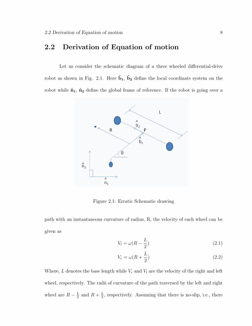
Let us consider the schematic diagram of a three wheeled differential-drive
robot as shown in Fig. 2.1. Here b1, b2 define the local coordinate system on the
robot while n1, n2 define the global frame of reference. If the robot is going over a
Figure 2.1: Erratic Schematic drawing
path with an instantaneous curvature of radius, R, the velocity of each wheel can be
given as
Vl = ω(R− L
2) (2.1)
Vr = ω(R +L
2) (2.2)
Where, L denotes the base length while Vr and Vl are the velocity of the right and left
wheel, respectively. The radii of curvature of the path traversed by the left and right
wheel are R − L2
and R + L2, respectively. Assuming that there is no-slip, i.e., there
2.2 Derivation of Equation of motion 9
is no component of the velocity of the robot in the direction of b2 , we can write.
VP.b2 = 0 (2.3)
Where VP is the velocity vector of point P on the robot and can be expressed as
VP = xn1 + yn2 (2.4a)
= x(cosθb1 − sinθb2) + y(sinθb1 + cosθb2) (2.4b)
We can write Eq. (2.4) in terms of the local co-ordinate system by substituting for
n1 and n2 in terms of b1 and b2. Where, x, y denote the cartesian co-ordinates of
robot and θ represents the orientation of the robot with respect to n1 and n2. x, y
and θ are time derivatives of x, y and θ, respectively
VP = (xcosθ + ysinθ)b1 + (−xsinθ + ycosθ)b2 (2.5)
Substitution of Eq. (2.5) in Eq. (2.3) we get
VP.b2 = [(xcosθ + ysinθ)b1 + (−xsinθ + ycosθ)b2].b2 = 0 (2.6)
= (−xsinθ + ycosθ) = 0 (2.7)
Furthermore let V be the translational velocity of the robot in the direction b1, then
the components of V along the global co-ordinate axes are given as
x = V cosθ (2.8)
y = V sinθ (2.9)

2.3 Optimal Trajectory Generation 10
It should be noticed that Eqs. (2.8) and (2.9) always satisfy the no-slip condition
given by Eq. (2.7) . Finally, the system equations are then given as
x = V cosθ (2.10a)
y = V sinθ (2.10b)
θ = ω (2.10c)
Where, ω is turn-rate of the robot
2.3 Optimal Trajectory Generation
In order to generate a time optimal path, given the initial and final states, we
pose the following optimal control problem.
min J =
∫ tf
0
dt (2.11a)
subject to
System Dynamics : q = f(q,u) (2.11b)
Boundry Condition : q(t0) = q0 and q(tf ) = qf (2.12a)
Actuator Constraints : ul ≤ ut ≤ uu,∀t (2.12b)
Where,
q =
[x y θ
]Tu =
[V ω
]T

2.4 Pontrygins Maximum Principle 11
q = f(q,u) =
[V cosθ V sinθ ω
]T(2.13a)
V is given in m/sec and ω is in rad/sec
We now briefly discuss the analytical solution of the above mentioned optimal
control problem as discussed in detail in Ref. [3]. Given the equations of motion of
the three-wheeled differential drive Eqs. (2.10a) - (2.10c) the hamiltonian H is given
by the inner product of the co-state vector with the state derivative.
H = λxV cosθ + λyV sinθ + λθω (2.14a)
Where, λx, λy, λθ are the co-states.
2.4 Pontrygins Maximum Principle
Pontrygins maximum principle [24] states that if the trajectory q(t) with cor-
responding control u(t) is time optimal then the following conditions must hold.
For the time optimal control sequence u(t) the hamiltonian is minimum at all
given time(t).
H(λ(t),q(t),u(t)) = minuεU
H(λ(t),q(t),u(t)) (2.15)
Eq. (2.15) is known as the minimization equation [3]. There exists an adjoint function
a continuous function of time that is non-trivial.
λ(t) =
[λx(t) λy(t) λθ(t)
](2.16)
2.4 Pontrygins Maximum Principle 12
The adjoint function satisfies the adjoint equation given as
λ = − ∂
∂qH (2.17)
Also the adjoint equation can be given as
λ = − ∂
∂qH = −(0, 0, λxV sinθ − λyV cosθ) (2.18)
The set of equations generated by Eq. (2.18) are also known as the co-state equations.
Integrating the equations to solve for λ
λx = c1; (2.19a)
λy = c2; (2.19b)
λθ = c1y − c2x+ c3; (2.19c)
Let us for simplicity assume
c12 + c2
2 = 1 (2.20)
2.4 Pontrygins Maximum Principle 13
Then the hamiltonian can be written as
H = λxV cosθ + λyV sinθ + λθω (2.21a)
H = Vc1cosθ + c2sinθ√
c21 + c22
+ c1y − c2x+ c3ω (2.21b)
Let c1y − c2x+ c3 = η(x, y)
−H = V cos(β)− η(x, y)ω (2.22a)
Where, β = θ − tan−1(c2c1
) (2.22b)
By maximizing −H, we can calculate the control profile for the time optimal path.
In Ref. [3] the analytical solution has been discussed to get the optimal trajectory
by maximizing −H. It is shown that an optimal trajectory can be reached using
a combination of five or less actions. However, when there are obstacles present in
the system’s configuration space, no analytical solution is available. It is possible to
generate the optimal trajectory even when there are obstacles in the configuration
space using various numerical methods. In the following chapters, two such numerical
methods (SLP & GLOMAP) are discussed.
Chapter 3
Time Optimal Path Planning for
three-wheeled differential-drive
robot using Sequential Linear
Programming(SLP)
3.1 Introduction
In the previous chapter, we discussed the formulation of the motion planning
problem for a differential drive robot as an optimal control problem. As shown in
the previous chapter, there exits an analytical solution for the time optimal control
problem when the system environment is uncluttered. However, in the presence of
14
3.1 Introduction 15
path constraints due to obstacles an analytical solution may not be feasible. Many
numerical methods such as nonlinear programming [6], Runge-Kutta based methods
[4], parameter optimization techniques [7] have been discussed in detail. A good detail
of these methods can be found in Ref. [25]. In sections below we briefly discuss some
of these methods.
3.1.1 Road Map Techniques:
Road map techniques as discussed in Ref. [25] like visibility graphs, voronoi
diagrams, freeway nets, silhouettes are some of the approaches proposed for motion
planning in a cluttered environment. Road map approach is based upon the idea of
capturing the connectivity of robot’s free-space, in a network of 1-D curves, called
road-maps. Once a road-map is constructed it is used as a set of standardized paths.
There are two main methods proposed in this category.
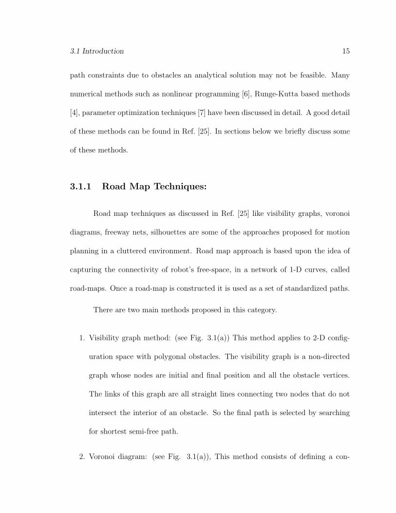
1. Visibility graph method: (see Fig. 3.1(a)) This method applies to 2-D config-
uration space with polygonal obstacles. The visibility graph is a non-directed
graph whose nodes are initial and final position and all the obstacle vertices.
The links of this graph are all straight lines connecting two nodes that do not
intersect the interior of an obstacle. So the final path is selected by searching
for shortest semi-free path.
2. Voronoi diagram: (see Fig. 3.1(a)), This method consists of defining a con-
3.1 Introduction 16
(a) Visibility Graph (b) Voronoi Diagram
Figure 3.1: Road Map Techniques
tinuous function of free-space (obstacle free region) onto a 1-D subset of itself
such that restriction of this function to this subset is the identity map. In 2-D
configuration space the retracted region is known as Voronoi diagram. The ad-
vantage of this approach is that it yields free paths which tend to maximize the
clearance from the obstacles.
3.1.2 Cell Decomposition:
This method consists of decomposing the robot’s free space into simple re-
gions called cells. A graph representing the adjacency relation between two cells is
constructed and searched. The node of this graph are extracted from the free space
and two adjacent cells are connected by a link. Generally cell decomposition meth-
ods are broken down into exact and approximate methods. Exact cell decomposition
methods decompose the free space into cells whose union is exactly the free space [25].
3.1 Introduction 17
On the contrary, approximate cell decomposition methods produce cells of predefined
shape whose union is strictly included in the free space [25]. An approximate cell
decomposition method operates in a hierarchal way by using a coarse resolution at
the beginning, and refining it until a desired path is obtained.
3.1.3 Artificial Potential field methods:
Artificial Potential field methods have also been proposed to solve the motion
planning problem in a cluttered environment. Many researchers have proposed differ-
ent ways of using the representation of obstacles [26]- [27]. The basic idea is that the
robot moves in a field of forces. The position to be reached (goal) is an attractive pole
for the robot while obstacles are repulsive surfaces for the robot. Various types of
potential functions for example attractive and repulsive potential Eqs. (3.1a) - (3.1b)
have been suggested [25], [28], [29]. In these methods the derivative of the potential
is often used for determining the direction of motion of an obstacle at any given time.
Attractive Potential :Patt =1
2ξsρ
2goal(q) (3.1a)
Repulsive Potential :Prep =1
2ηs(
1
ρq− 1
ρ0
)2; ρq ≤ ρ0 (3.1b)
= 0; ρq ≥ ρ0 (3.1c)
Where, ρ is a measure of the distance from either the goal or the obstacle, while ξs ηs
are scaling factors. Main advantage of this approach is that the robot needs to know
3.1 Introduction 18
(a) (b)
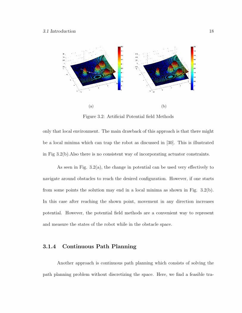
Figure 3.2: Artificial Potential field Methods
only that local environment. The main drawback of this approach is that there might
be a local minima which can trap the robot as discussed in [30]. This is illustrated
in Fig 3.2(b).Also there is no consistent way of incorporating actuator constraints.
As seen in Fig. 3.2(a), the change in potential can be used very effectively to
navigate around obstacles to reach the desired configuration. However, if one starts
from some points the solution may end in a local minima as shown in Fig. 3.2(b).
In this case after reaching the shown point, movement in any direction increases
potential. However, the potential field methods are a convenient way to represent
and measure the states of the robot while in the obstacle space.
3.1.4 Continuous Path Planning
Another approach is continuous path planning which consists of solving the
path planning problem without discretizing the space. Here, we find a feasible tra-
3.1 Introduction 19
jectory by minimizing a cost function. This cost function can be a jerk function or
torque model. In our current case the cost function is final time. This approach
is similar to variational calculus approach. The main advantage of this approach is
that variational methods provide a unifying framework for dealing with equality and
inequality constraints on both state and control variables. Moreover, system dynam-
ics can be taken into account and problem like actuator redundancy can be dealt
with. Main disadvantage is here we need to solve nonlinear constrained optimization
problem. So we need efficient numerical tools.
It should be noted that variational path planning can be combined with po-
tential field methods. Potential field and continuous path planning methods do not
include an initial processing step aimed at capturing the connectivity of free space in
a concise representation. Instead, they search a much larger graph representing the
adjacency among the patches contained in robot’s configuration space. Also poten-
tial field methods are known as local methods while cell decomposition and road-map
methods are called global methods. However, potential field method can be posed as
a global method if potential function is designed to avoid local minima, as computing
such a function require the knowledge of the geometry of whole space. Similarly, cell
decomposition methods can be posed as local methods by restricting their application
to a subset of configuration space. A path is then generated in an iterative fashion
by concatenating the different sub-paths.

3.1 Introduction 20
3.1.5 Sequential Linear Programming :
In this chapter and the next chapter, we explore the application of two opti-
mization techniques to implement the variational approach in combination with the
potential field approach. In Ref. [22], a sequentially linear programming approach is
proposed to solve the generic optimal control problem making use of the sensitivities
of the system dynamics with respect to the states and control vector. The sensi-
tivities are used to determine a time-varying linear model which is used to pose a
linear programming (LP) problem to exploit the strength of solver for LP problems.
The solution of the LP problem is used to update the initial estimate of the control
profile. This process continues till the terminal constraints are satisfied. A bisection
algorithm is used to converge to the optimal cost.
Obstacle representation using Potential Functions
The obstacles are to be represented as high potential areas as the performance
index would include the integral of potential state over time. It is desired to allow
all other configurations including those just outside the boundary of the obstacle in
the feasible set of solutions so that the limitation mentioned above can be eliminated.
It is thus, desired that the potential function used to represent an obstacle have the
following properties
1. The configurations within the obstacle must have a high potential value.
3.1 Introduction 21
2. The value for the potential must go to zero at all other configurations including
just outside the boundary.
3. The potential function must be continuous at all points including the boundary
of the obstacle.
4. The higher derivatives of the potential function must also be continuous at all
points and go to zero at the boundary of the obstacle.
In Ref. [20] a generic expression(as given in Eq. (3.2a)) has been developed for
mathematical functions which satisfies the aforementioned requirements. It is hence
used to represent the obstacles in this approach.
Pt = 1− ηm+1{((2m+ 1)!(−1)m
(m!)2)
m∑k=0
(−1)k
(2m− k + 1)
m
Ckηm−k} (3.2a)
Where,m is the degree of continuity of the potential function and η is a function of x
and y given by
η = (1/ro)((x− xo)2 + (y − yo)2)1/2 (3.3a)
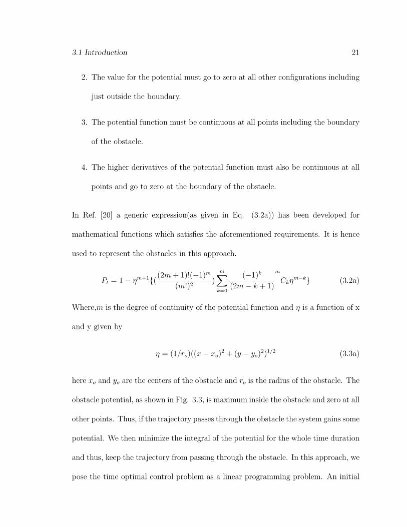
here xo and yo are the centers of the obstacle and ro is the radius of the obstacle. The
obstacle potential, as shown in Fig. 3.3, is maximum inside the obstacle and zero at all
other points. Thus, if the trajectory passes through the obstacle the system gains some
potential. We then minimize the integral of the potential for the whole time duration
and thus, keep the trajectory from passing through the obstacle. In this approach, we
pose the time optimal control problem as a linear programming problem. An initial
3.1 Introduction 22
Figure 3.3: Potential
guess is made for the final time and the time space is discritized with a finite number
of time steps. The time optimal control profile is computed iteratively by assuming an
initial control profile u0 ,and determining the corresponding evolution of the states.
In order to use this approach we linearize the system equations about the current
states at each time step. We now proceed to apply SLP algorithm(as explained in
Ref. [22]) to the differential drive robot mentioned in the previous chapter.
3.2 Time Optimal Path Planning using Sequential Linear Programming(SLP) 23
3.2 Time Optimal Path Planning using Sequential
Linear Programming(SLP)
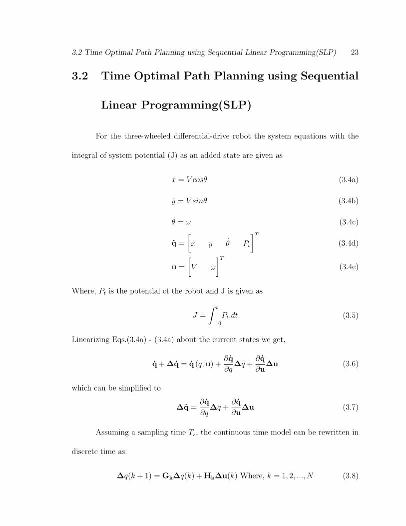
For the three-wheeled differential-drive robot the system equations with the
integral of system potential (J) as an added state are given as
x = V cosθ (3.4a)
y = V sinθ (3.4b)
θ = ω (3.4c)
q =
[x y θ Pt
]T(3.4d)
u =
[V ω
]T(3.4e)
Where, Pt is the potential of the robot and J is given as
J =
∫ t
0
Pt.dt (3.5)
Linearizing Eqs.(3.4a) - (3.4a) about the current states we get,
q + ∆q = q (q,u) +∂q
∂q∆q +
∂q
∂u∆u (3.6)
which can be simplified to
∆q =∂q
∂q∆q +
∂q
∂u∆u (3.7)
Assuming a sampling time Ts, the continuous time model can be rewritten in
discrete time as:
∆q(k + 1) = Gk∆q(k) + Hk∆u(k) Where, k = 1, 2, ..., N (3.8)

3.2 Time Optimal Path Planning using Sequential Linear Programming(SLP) 24
Gk =
1 0 −TsV sin(θk)
0 1 TsV cos(θk)
0 0 1
Hk =
Tscos(θk) −1
2Ts
2V sin(θk)
Tssin(θk)12Ts
2V cos(θk)
0 Ts
Where, ∆q is the perturbation state vector and ∆u is the perturbation control input.
The state response for the control input ∆u(k) is
∆q(k + 1) = Gk∆q(1) +k∑i=1
Gk−iHk∆u(i) (3.9)
Where, ∆q(1) represents the initial perturbation state of the system and is zero, since
the initial condition are prescribed. To solve the control problem with specified initial
and final states, in addition to the final time (tf ), the final state constraint can be
represented as
∆q(N + 1) =N∑i=1
GN−iH∆u(i) (3.10)
A linear programming problem can now be posed as
Minimize:aT∆u (3.11)
subject to,
A∆u = b (3.12)
ul − u ≤∆u ≤ uu − u (3.13)
3.2 Time Optimal Path Planning using Sequential Linear Programming(SLP) 25
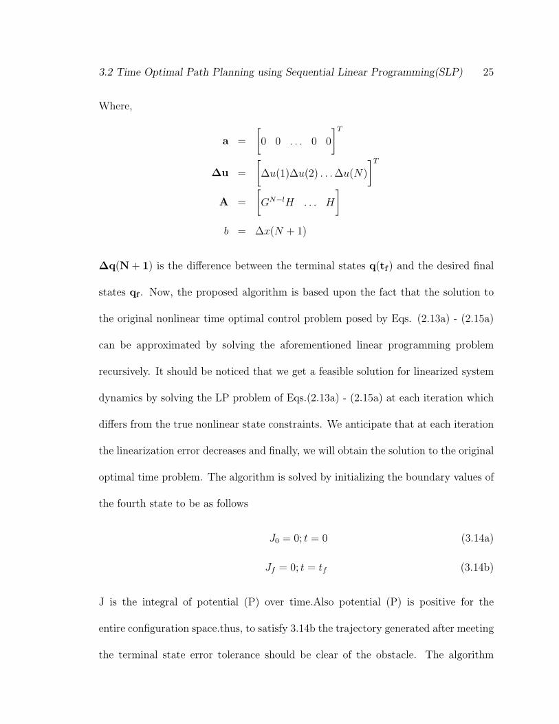
Where,
a =
[0 0 . . . 0 0
]T∆u =
[∆u(1)∆u(2) . . .∆u(N)
]TA =
[GN−lH . . . H
]b = ∆x(N + 1)
∆q(N + 1) is the difference between the terminal states q(tf ) and the desired final
states qf . Now, the proposed algorithm is based upon the fact that the solution to
the original nonlinear time optimal control problem posed by Eqs. (2.13a) - (2.15a)
can be approximated by solving the aforementioned linear programming problem
recursively. It should be noticed that we get a feasible solution for linearized system
dynamics by solving the LP problem of Eqs.(2.13a) - (2.15a) at each iteration which
differs from the true nonlinear state constraints. We anticipate that at each iteration
the linearization error decreases and finally, we will obtain the solution to the original
optimal time problem. The algorithm is solved by initializing the boundary values of
the fourth state to be as follows
J0 = 0; t = 0 (3.14a)
Jf = 0; t = tf (3.14b)
J is the integral of potential (P) over time.Also potential (P) is positive for the
entire configuration space.thus, to satisfy 3.14b the trajectory generated after meeting
the terminal state error tolerance should be clear of the obstacle. The algorithm
3.2 Time Optimal Path Planning using Sequential Linear Programming(SLP) 26
mentioned can be implemented for path planning in a cluttered environment for a
time optimal trajectory. The following steps are followed to solve the problem
1. Guess the bounds for final time, tlf and tuf .
2. Initialize tf =tlf+tuf
2and divide the time interval [0 − tf ] into pre-specified N
intervals and guess the value for control variable u(i), i ∈ [1, N ] compatible
with actuator constraints given by Eq. (3.13).
3. Integrate the nonlinear system dynamics Eq. (2.11b), to compute q(tf ) and if
the terminal state constraints of Eq. (2.12a), are satisfied then decrease the
value of final time according to bisection algorithm and Go to Step 2.
4. Else linearize the nonlinear dynamics system and find a feasible solution by
solving the LP problem posed by Eqs. (3.11)-(3.13).
5. If the solution to LP problem (Eqs. (3.11)-(3.13)) exists, then modify the initial
guess for control unew(i) = uold(i) + ∆u(i) and Go To Step 3.
6. Else, increase the value of tf according to the bisection algorithm. and Go To
Step 2.
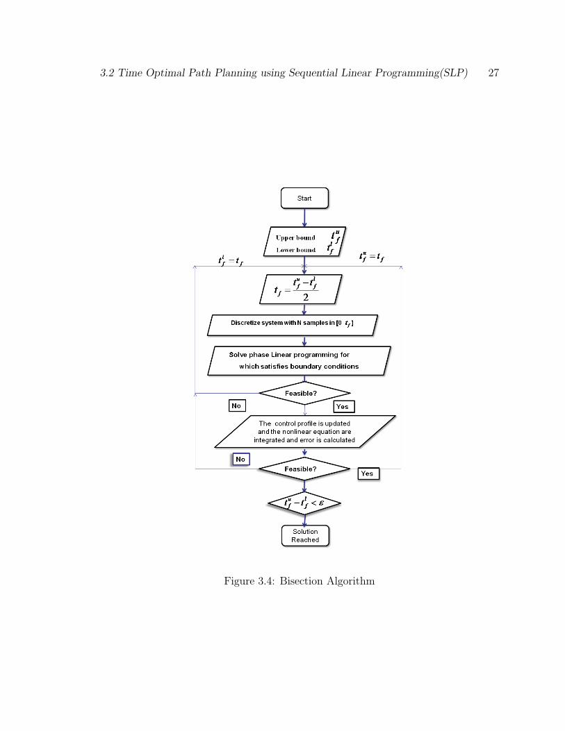
3.2 Time Optimal Path Planning using Sequential Linear Programming(SLP) 27
Figure 3.4: Bisection Algorithm

3.3 Numerical Simulation & Results 28
3.3 Numerical Simulation & Results
The algorithm is tested by running simulations for various scenarios with and
without obstacles. The first three cases deal with path planning for various initial
and final configurations. The last two cases consider the presence of obstacles in the
configuration space. For all the cases considered the control constraints are as follows
−1m/s ≤ V ≤ 1m/s (3.15a)
−50deg/s ≤ ω ≤ 50deg/s (3.15b)
Also the tuning parameters for all the simulations are as given
Time Toleranace, (εt) = 1× 10⁻⁶ (3.16a)
State Error Toleranace, (εs) = 1× 10⁻⁶ (3.16b)
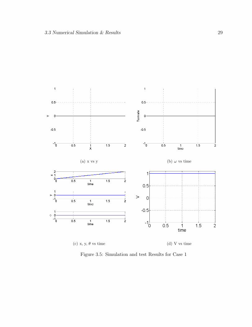
3.3.1 Case 1
The algorithm is run for an initial configuration of [x = 0, y = 0, θ = 0] to a
final configuration of [2,0,0]. As expected the trajectory generated is a straight line
along the X axis. The control profile is seen to be bang-bang with the linear velocity
at a maximum of 1m/sec and the turn rate holding a constant value of zero. The
minimum time as expected is 2 seconds. The trajectory can be seen as shown in Fig.
3.5(a). The control plots are as shown in Fig. 3.5(d) to Fig. 3.5(b) .
3.3 Numerical Simulation & Results 29
(a) x vs y (b) ω vs time
(c) x, y, θ vs time (d) V vs time
Figure 3.5: Simulation and test Results for Case 1
3.3 Numerical Simulation & Results 30
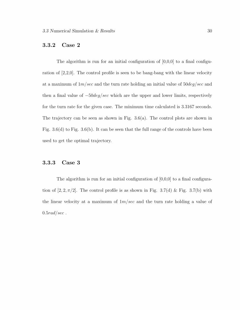
3.3.2 Case 2
The algorithm is run for an initial configuration of [0,0,0] to a final configu-
ration of [2,2,0]. The control profile is seen to be bang-bang with the linear velocity
at a maximum of 1m/sec and the turn rate holding an initial value of 50deg/sec and
then a final value of −50deg/sec which are the upper and lower limits, respectively
for the turn rate for the given case. The minimum time calculated is 3.3167 seconds.
The trajectory can be seen as shown in Fig. 3.6(a). The control plots are shown in
Fig. 3.6(d) to Fig. 3.6(b). It can be seen that the full range of the controls have been
used to get the optimal trajectory.
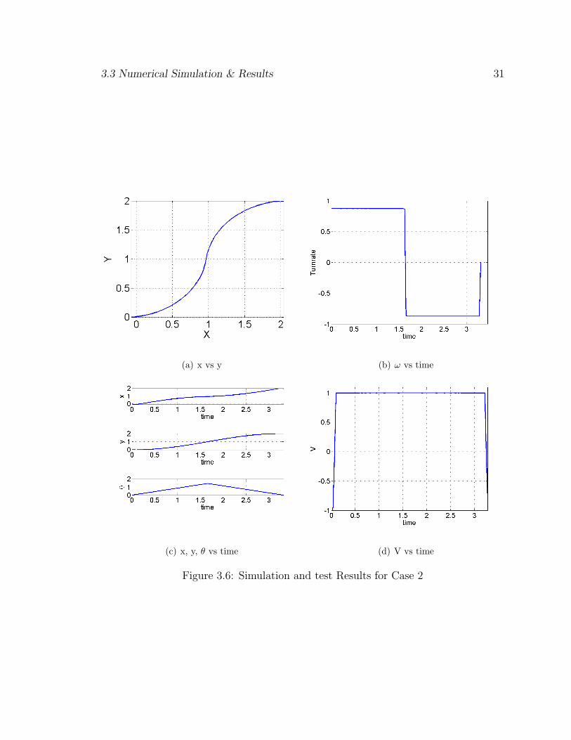
3.3.3 Case 3
The algorithm is run for an initial configuration of [0,0,0] to a final configura-
tion of [2, 2, π/2]. The control profile is as shown in Fig. 3.7(d) & Fig. 3.7(b) with
the linear velocity at a maximum of 1m/sec and the turn rate holding a value of
0.5rad/sec .
3.3 Numerical Simulation & Results 31
(a) x vs y (b) ω vs time
(c) x, y, θ vs time (d) V vs time
Figure 3.6: Simulation and test Results for Case 2
3.3 Numerical Simulation & Results 32
(a) x vs y (b) ω vs time
(c) x, y, θ vs time (d) V vs time
Figure 3.7: Simulation and test Results for Case 3

3.3 Numerical Simulation & Results 33
The minimum time calculated is 3.1421 seconds. It is seen that as one would
expect the shortest path which would not contradict the no-slip condition would be
a long arc of a circle with center at [2,0] and radius of 2 m. The trajectory can
be seen as shown in Fig.(3.7(a)). The control plots ares as shown in Fig. 3.7(d) to
Fig. 3.7(b). In the above cases we have considered an uncluttered environment. The
following examples consider the presence of obstacles in the systems configuration
space.
3.3.4 Case 4
The algorithm is run for an initial configuration of [0,0,0] to a final configura-
tion of [2,0,0] with an obstacle at [0.5,0.2] and has a radius of 0.25m. As it can be seen
a path similar to case 1 would lead in a collision of the robot with the object. The
control profile is not bang-bang with the linear velocity at a maximum of 1m/sec and
the turn rate varying as shown between a value of 50deg/sec an −50deg/sec. The
minimum time calculated is 2.198242 seconds. It is seen that even after the robot is
past the obstacle, it does not immediately turn around the obstacle rather uses the
maximum linear velocity to cover more ground in the direction of the target while
varying the turn rate so that the no-slip condition is not violated. The trajectory can
be seen as shown in Fig. 3.8(a). The control plots are as shown in Fig. 3.8(d) Fig.
3.8(b)).
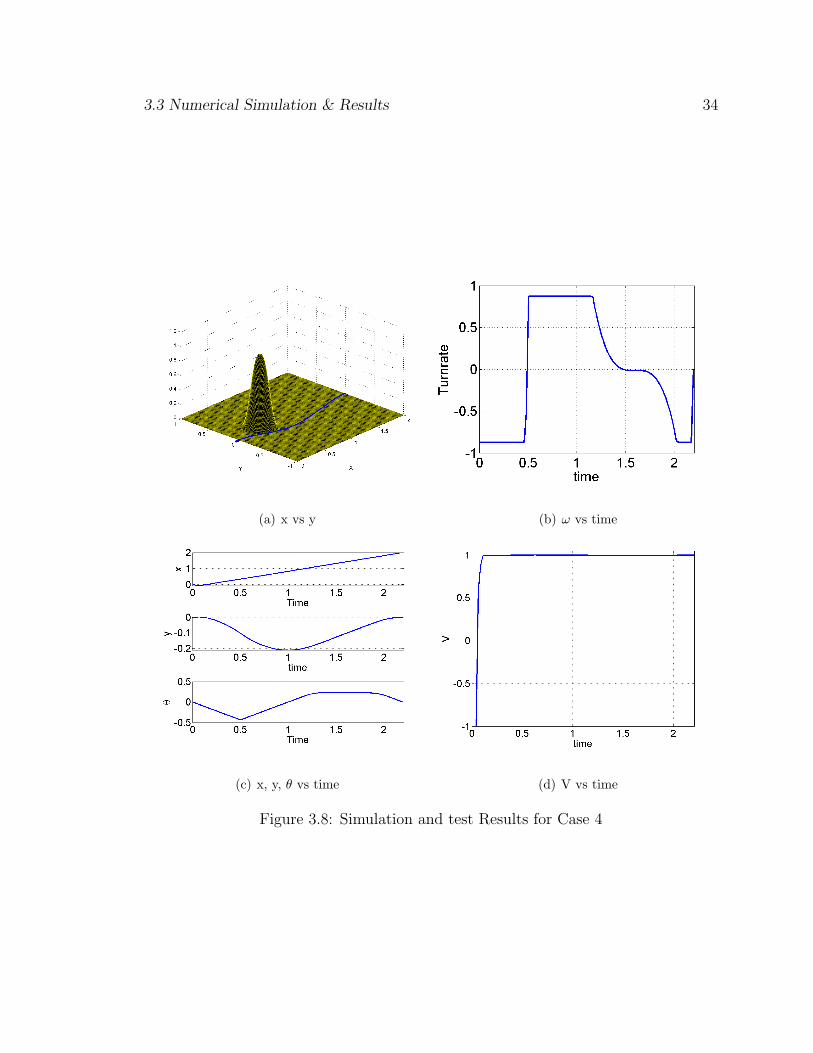
3.3 Numerical Simulation & Results 34
(a) x vs y (b) ω vs time
(c) x, y, θ vs time (d) V vs time
Figure 3.8: Simulation and test Results for Case 4
3.3 Numerical Simulation & Results 35
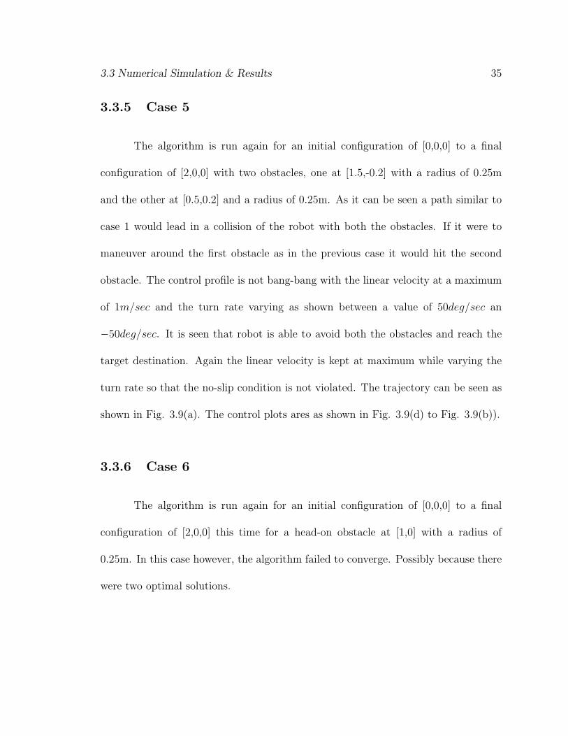
3.3.5 Case 5
The algorithm is run again for an initial configuration of [0,0,0] to a final
configuration of [2,0,0] with two obstacles, one at [1.5,-0.2] with a radius of 0.25m
and the other at [0.5,0.2] and a radius of 0.25m. As it can be seen a path similar to
case 1 would lead in a collision of the robot with both the obstacles. If it were to
maneuver around the first obstacle as in the previous case it would hit the second
obstacle. The control profile is not bang-bang with the linear velocity at a maximum
of 1m/sec and the turn rate varying as shown between a value of 50deg/sec an
−50deg/sec. It is seen that robot is able to avoid both the obstacles and reach the
target destination. Again the linear velocity is kept at maximum while varying the
turn rate so that the no-slip condition is not violated. The trajectory can be seen as
shown in Fig. 3.9(a). The control plots ares as shown in Fig. 3.9(d) to Fig. 3.9(b)).
3.3.6 Case 6
The algorithm is run again for an initial configuration of [0,0,0] to a final
configuration of [2,0,0] this time for a head-on obstacle at [1,0] with a radius of
0.25m. In this case however, the algorithm failed to converge. Possibly because there
were two optimal solutions.
3.3 Numerical Simulation & Results 36
(a) x vs y (b) ω vs time
(c) x, y, θ vs time (d) V vs time
Figure 3.9: Simulation and test Results for Case 5

Chapter 4
GLOMAP
4.1 Introduction
In the previous chapter, SLP was implemented to perform path planning for
a differential drive robot in both cluttered and uncluttered environments. However,
the limitation with this and other such methods is the resolution of the solution. If
we need a higher resolution we have to solve for higher number of variables which
increases computational load and complexity. However, instead of capturing the
control variables as a step function of time, if we can capture the solution as a
continuous function, then control inputs can be computed at much higher resolution.
As mentioned in the first chapter, in order to better cope with the varying level
of nonlinearity in the configuration space it would be more efficient to solve the
path planning problems in smaller local domains. The local trajectories can then be
37

4.2 Solution to Optimal Control Problem with GLOMAP Approach 38
aggregated into a global continuous trajectory which can be expressed as a function
of time. In this chapter we shall solve the optimal control problem using Global Local
Mapping (GLOMAP) approach.
4.2 Solution to Optimal Control Problem with
GLOMAP Approach
The optimal trajectory for nonlinear systems can be highly nonlinear. To
solve for such trajectories and control profiles can be computationally very expensive.
The trajectories can be nonlinear but the degree of nonlinearity may vary in time and
space. By breaking the entire time domain into small parts, it may be possible to very
accurately approximate a highly nonlinear trajectory with a lower order system. For
sufficiently large number of time steps even a linear system can capture the dynamics
of the non-linear system, thus, reducing the complexity of the system. We generate a
global continuous function for the states and their derivatives by merging the smaller
local functions. In this approach the states, x, y, θ, are approximated to be continuous
functions of time. The time range is divided into N parts. For the ith time sections,
the states x, y, θ are defined by local nth order polynomial functions fxi(t), fyi
(t),
4.2 Solution to Optimal Control Problem with GLOMAP Approach 39
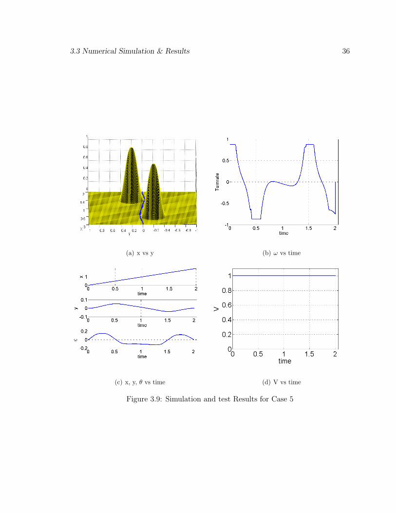
(a) Local and Global Trajectories (b) Weight functions
Figure 4.1: Glomap
fθi(t) as given
fxi(t) =
n∑j=0
axjtj (4.1a)
fyi(t) =
n∑j=0
ayjtj (4.1b)
fθi(t) =
n∑j=0
aθjtj (4.1c)
Where, axj, ayj
, aθjare constants.
A global function is then constructed for each of the states by blending the
local functions for each state. It is done by taking the sum of the products of the
local functions and their corresponding weighting functions. The weight function for
a given local function is defined such that, it takes a maximum value of one at the
center of the local time domain for which the function is defined and goes to zero for
any value beyond the range of the local domain. Therefore the local function is most
dominant at the point about which it is centered and least dominant at the edges of
4.2 Solution to Optimal Control Problem with GLOMAP Approach 40
the boundary for which it is defined. For e.g. in Fig. 4.1(b) we can see three local
functions shown by the red, blue and green curves. Now, F1 is 3rd order, F2 is 2rd
order, F3 is 1rd order. The three functions are discontinuous at the end of their local
range .This can be resolved by using weighing functions such that these weighing
function have a value of one at their centroid and zero at the extremes of the local
range. Also in the area of overlap the sum of the weighting functions is 1. They
can be merged into a global function (shown by the black solid line) using weighting
functions. It can be seen that each function coincides with the global function at
the midpoints of their domains A, B, and C, respectively. The global function is
continuous over the entire range of the solution. The derivatives are also continuous
as per the order of the weighing function. An example of weighting functions are
shown in Fig. 4.1(a).
xt =N∑i=0
wi(t)fxi(t) (4.2a)
yt =N∑i=0
wi(t)fyi(t) (4.2b)
θt =N∑i=0
wi(t)fθi(t) (4.2c)
Thus, the functions used to approximate the states at a time ‘t’ can be given by Eqs.
4.2 Solution to Optimal Control Problem with GLOMAP Approach 41
(4.2a) - (4.2c)
xt =N∑i=0
wi(t)fxi(t) +
N∑i=0
wi(t)fxi(t) (4.3a)
yt =N∑i=0
wi(t)fyi(t) +
N∑i=0
wi(t)fyi(t) (4.3b)
θt =N∑i=0
wi(t)fθi(t) +
N∑i=0
wi(t)fθi(t) (4.3c)
The time derivatives can then be defined as given by Eqs. (4.3a) - (4.3c).
Where,
wi(t) = 1− τm+1{((2m+ 1)!(−1)m
(m!)2)
m∑k=0
(−1)k
(2m− k + 1)
m
Ckτm−k} (4.4a)
τ ≡ t;−1 < τ < 1 (4.4b)
Where, ‘m’ is the order of the weight function if continuity is desired in the derivatives,
a higher order weighing function should be chosen accordingly. In this case ‘m’ should
be greater than or equal to 2 as a 2nd order continuity is desired in this case.
V = xtcos(θt) + ytsin(θt) (4.5a)
ω = θt (4.5b)
The control inputs can be defined as given by Eq. (4.5b)
4.2.1 Problem Statement
Thus, the path planning problem can then be posed as an optimization prob-
lem as given below,

4.2 Solution to Optimal Control Problem with GLOMAP Approach 42
To minimize
J =
∫ tf
0
Ptdt (4.6a)
Where, potential, Pt, of the robot is defined as given
Pt = 1− ηm+1{((2m+ 1)!(−1)m
(m!)2)
m∑k=0
(−1)k
(2m− k + 1)
m
Ckηm−k} (4.7a)
Where, η is a function of x and y given by
η = (1/ro)((x− xo)2 + (y − yo)2)1/2 (4.8a)
here xo and yo are the centers of the obstacle and ro is the radius of the obstacle.
xtsinθ + ytcosθ = 0 (4.9a)
− 1 < V < 1 (4.10a)
− 50 < ω < 50 (4.10b)
the constraints for velocity can be given as in Eq. (4.10b) where, V is in m/s and ω
is in deg/sec. Therefore, the objective is to minimize Eq. (4.6a) subject to system
dynamics given by Eqs. (4.2a) - (4.5b) and state constraints as given by Eqs. (4.9a)
- (4.10b).
A nonlinear optimizer is used to solve the problem. A time bisection loop is
implemented to find the minimum time for which a solution exits. To use the nonlinear
optimizer fmincon the problem is restructured. First the number of approximations
4.2 Solution to Optimal Control Problem with GLOMAP Approach 43
(N) is decided and then the grid points are calculated on the time scale about which
each of the functions fx,i(t) are centered. Where,
fx,i(t) = ax.iφx,i(t) i = 1, 2, 3, ....N (4.11a)
ax,i =
[a0,i a1,i a2,i a3,i ...... an,i
](4.11b)
φx,i(t) =
[1 t t2 t3 . . . . tn
]T(4.11c)
Similarly, for y and θ. Now, If Ax and P matrix are given as below and wi(t)
corresponds to the value of the weight function corresponding to the ith approximation
at time t, then equation 4.2a can be implemented as shown below.
ψx,t =
w1(t)φx,1
w2(t)φx,2
w3(t)φx,3
w4(t)φx,4
.
.
.
.
wN(t)φx,N
Ax =
ax,1
ax,2
ax,3
.
.
.
.
ax,N
T
(4.12a)
xt = Axψx,t (4.12b)
Similarly, equations Eq. (4.2b) and Eq. (4.2c) can be implemented. To implement
4.2 Solution to Optimal Control Problem with GLOMAP Approach 44
the end conditions, we apply linear equality constraints as shown below
Axψx,t0 = x0 Axψx,tf = xf (4.13a)
Ayψy,t0 = y0 Ayψy,tf = yf (4.13b)
Aθψθ,t0 = θ0 Aθψθ,tf = θf (4.13c)
The velocity constraints are applied as linear and nonlinear constraints. θ can be ex-
pressed as a linear constraint and V and no-slip condition are provided as a nonlinear
constraint as shown.
ωmin deg /sec < Aθψθ,t0 < ωmax deg /sec (4.14a)
Vminm/sec < xtcos(θt) + ytsin(θt) < Vmaxm/sec (4.14b)
xtsin(θt) + ytcos(θt) = 0 (4.14c)
As in any nonlinear optimization problem, the initial guess is important. A second-
order function is used to fit the trajectory so that the end conditions are satisfied.
The coefficients are then back calculated and assigned as the initial guess for the
coefficients. For the initial condition a second order curve is fit between the end
conditions and the coefficients Ax, Ay, Aθ are generated as given as below.
Ax = (ψ′xψx)−1ψ′xxapp (4.15a)
Ay = (ψ′yψy)−1ψ′yyapp (4.15b)
Aθ = (ψ′θψθ)−1ψ′θθapp (4.15c)
With this as the initial condition the optimization problem is solved for the solution
with minimum time by applying the time bisection. In the case of the cluttered

4.2 Solution to Optimal Control Problem with GLOMAP Approach 45
Figure 4.2: Flowchart for the Glomap Algorithm

4.3 Numerical Simulation and Results 46
environment the value of J(cost) is checked before reducing final time. If the value
of J is less that 1 × 10⁻⁶ then the final time is reduced otherwise the final time is
increased. Thus, the following steps are followed to solve the problem
1. Guess the bounds for final time, tlf and tuf .
2. Initialize tf =tlf+tuf
2and divide the time interval [0 − tf ] into pre-specified N
intervals and initialize the value for the coefficients using Eqs. (4.15a) - (4.15c)
so that the end conditions given by Eq. (4.13c) are satisfied.
3. Solve for the coefficients using fmincon for a given accuracy to minimize the
cost as given by Eq. (4.6a)
4. If cost is less than the threshold value set tu = tf and tf = (tu+tu)2
and pass the
calculated value of the coefficients as the initial guess in step(2)
5. Else, set tu = tf and tf = (tu+tu)2
and go to step(2)
6. Repeat steps (2) to (5) till tu − tl < time tolerance
4.3 Numerical Simulation and Results
For all the cases considered the control constraints are as follows
−1m/s ≤ V ≤ 1m/s (4.16a)
−50deg/s ≤ ω ≤ 50deg/s (4.16b)

4.3 Numerical Simulation and Results 47
Also the tuning parameters for all the simulations are as given
Time Toleranace, (εt) = 1× 10⁻⁶ (4.17a)
State Error Toleranace, (εs) = 1× 10⁻⁶ (4.17b)
Potential Toleranace, (εp) = 1× 10⁻⁶ (4.17c)
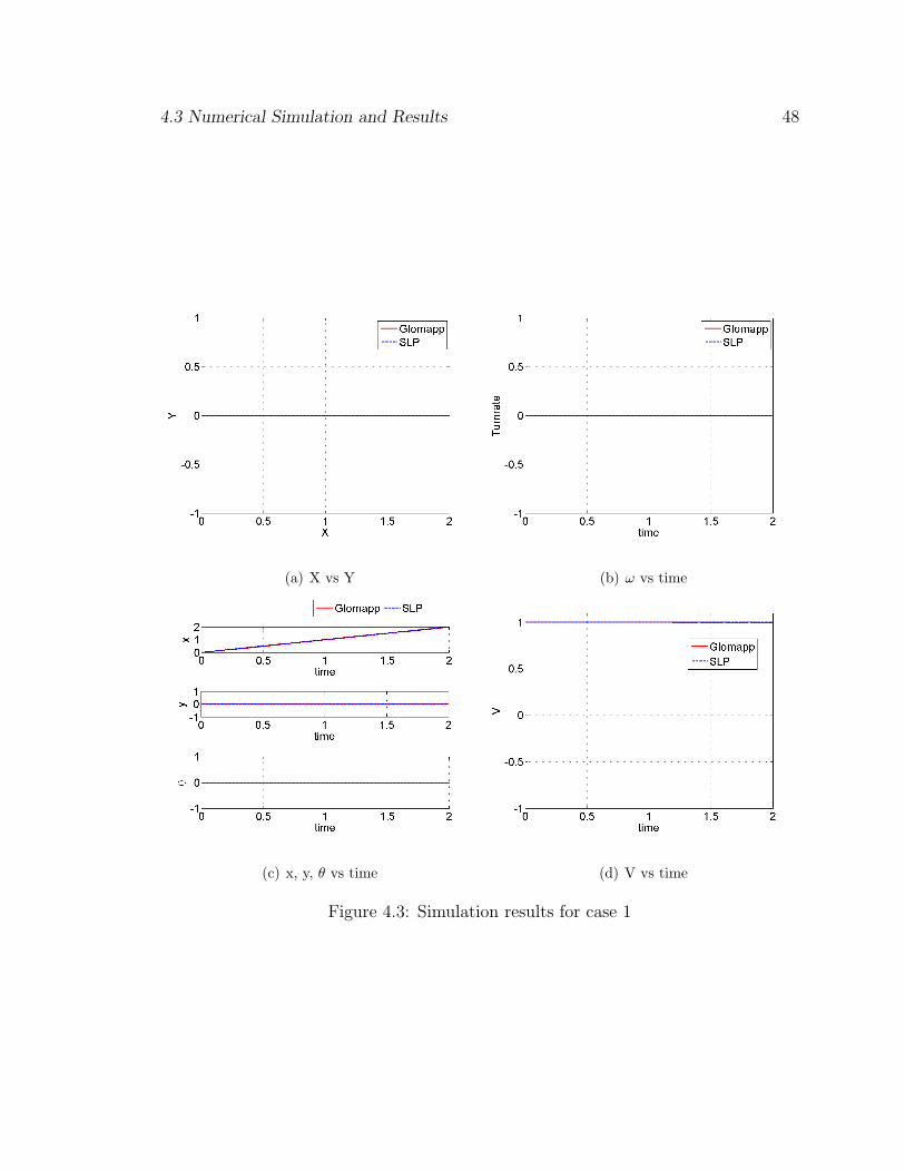
4.3.1 Case 1 :
Initially a simple simulation is run with the starting point at [x=0 y=0 θ=0]
and ending point at [2 0 0] . The number of approximations selected are 6 and the
degree of the polynomials for x, y, θ are 3, 3 and 3, respectively. The solution is bang-
bang as expected with the velocity profile being constant at the maximum value as
seen in the Fig. 4.3(d). The coefficients that are obtained by the Glomap approach are
used to generate the control profiles and then integrated with the original nonlinear
equations of motion and the norm of the terminal error is found to be 6.5440× 10⁻⁶
which is very small. It is seen that the states match the SLP solution quite well. The
minimum time in this case also as in SLP is 2 sec.
4.3.2 Case 2:
A simulation with the starting point at [0 0 0] and ending point at [2 2 0] is
run. The number of approximations selected are 40 and the degree of the polynomials
for x, y, θ are 3, 3 and 2, respectively. The solution is bang-bang as seen in the Fig.
4.3 Numerical Simulation and Results 48
(a) X vs Y (b) ω vs time
(c) x, y, θ vs time (d) V vs time
Figure 4.3: Simulation results for case 1
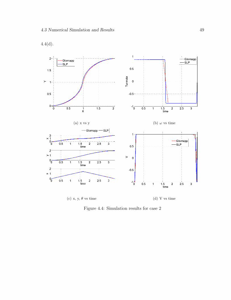
4.3 Numerical Simulation and Results 49
4.4(d).
(a) x vs y (b) ω vs time
(c) x, y, θ vs time (d) V vs time
Figure 4.4: Simulation results for case 2
4.3 Numerical Simulation and Results 50
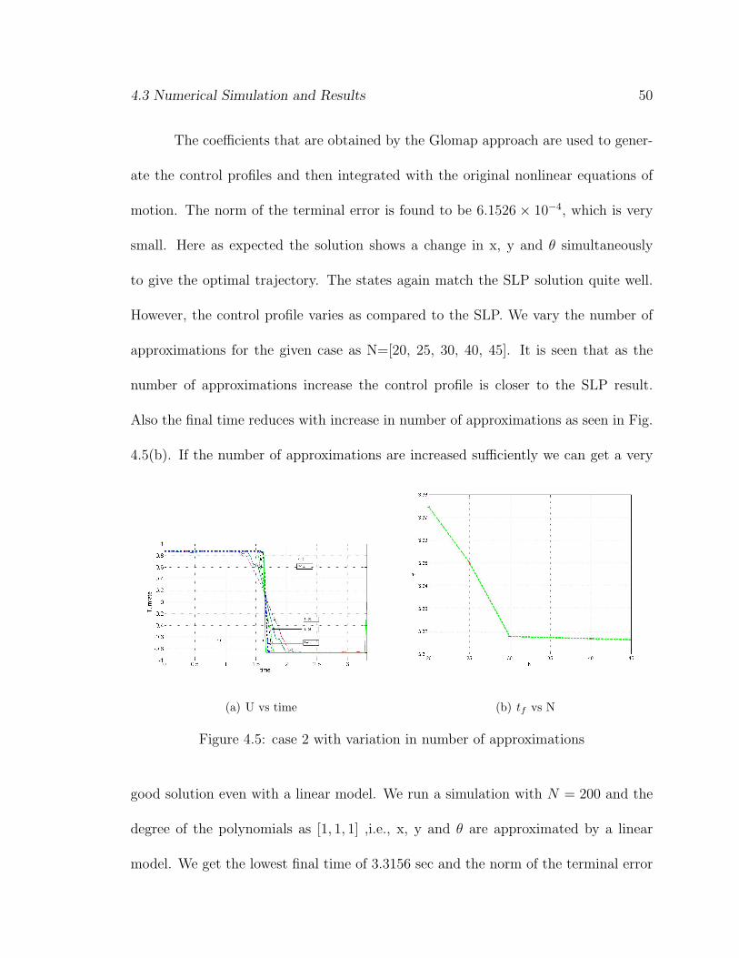
The coefficients that are obtained by the Glomap approach are used to gener-
ate the control profiles and then integrated with the original nonlinear equations of
motion. The norm of the terminal error is found to be 6.1526 × 10⁻⁴, which is very
small. Here as expected the solution shows a change in x, y and θ simultaneously
to give the optimal trajectory. The states again match the SLP solution quite well.
However, the control profile varies as compared to the SLP. We vary the number of
approximations for the given case as N=[20, 25, 30, 40, 45]. It is seen that as the
number of approximations increase the control profile is closer to the SLP result.
Also the final time reduces with increase in number of approximations as seen in Fig.
4.5(b). If the number of approximations are increased sufficiently we can get a very
(a) U vs time (b) tf vs N
Figure 4.5: case 2 with variation in number of approximations
good solution even with a linear model. We run a simulation with N = 200 and the
degree of the polynomials as [1, 1, 1] ,i.e., x, y and θ are approximated by a linear
model. We get the lowest final time of 3.3156 sec and the norm of the terminal error
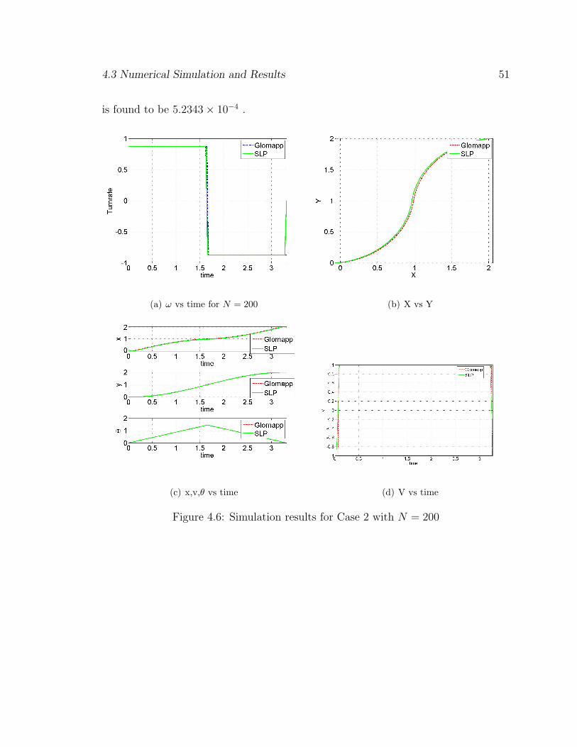
4.3 Numerical Simulation and Results 51
is found to be 5.2343× 10⁻⁴ .
(a) ω vs time for N = 200 (b) X vs Y
(c) x,v,θ vs time (d) V vs time
Figure 4.6: Simulation results for Case 2 with N = 200
4.3 Numerical Simulation and Results 52
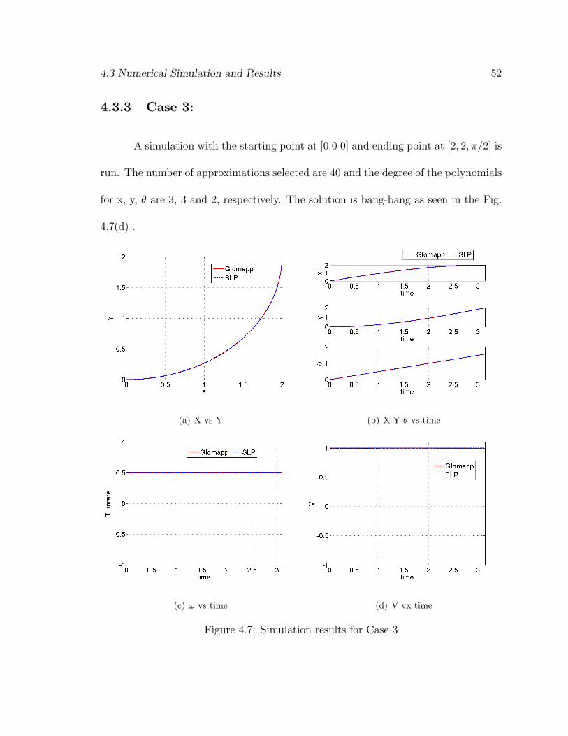
4.3.3 Case 3:
A simulation with the starting point at [0 0 0] and ending point at [2, 2, π/2] is
run. The number of approximations selected are 40 and the degree of the polynomials
for x, y, θ are 3, 3 and 2, respectively. The solution is bang-bang as seen in the Fig.
4.7(d) .
(a) X vs Y (b) X Y θ vs time
(c) ω vs time (d) V vx time
Figure 4.7: Simulation results for Case 3
4.3 Numerical Simulation and Results 53
The coefficients that are obtained by the Glomap approach are used to generate
the control profiles and then integrated with the original nonlinear equations of motion
and the norm of the terminal error is found to be 4.4157× 10⁻⁵, which is very small.
Here again the solution agrees well with the SLP solution.
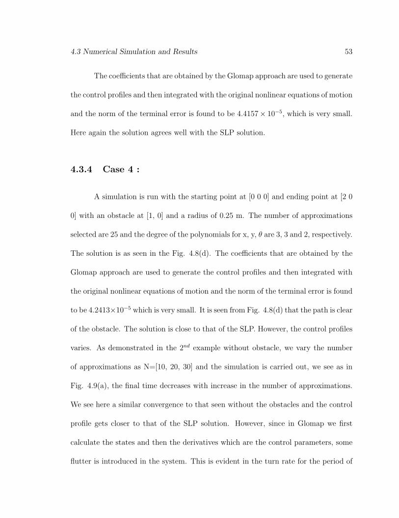
4.3.4 Case 4 :
A simulation is run with the starting point at [0 0 0] and ending point at [2 0
0] with an obstacle at [1, 0] and a radius of 0.25 m. The number of approximations
selected are 25 and the degree of the polynomials for x, y, θ are 3, 3 and 2, respectively.
The solution is as seen in the Fig. 4.8(d). The coefficients that are obtained by the
Glomap approach are used to generate the control profiles and then integrated with
the original nonlinear equations of motion and the norm of the terminal error is found
to be 4.2413×10⁻⁵ which is very small. It is seen from Fig. 4.8(d) that the path is clear
of the obstacle. The solution is close to that of the SLP. However, the control profiles
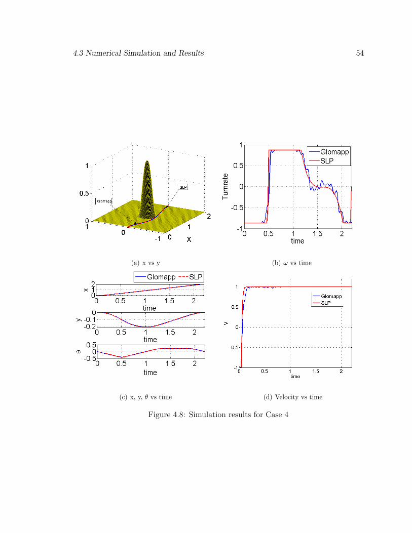
varies. As demonstrated in the 2nd example without obstacle, we vary the number
of approximations as N=[10, 20, 30] and the simulation is carried out, we see as in
Fig. 4.9(a), the final time decreases with increase in the number of approximations.
We see here a similar convergence to that seen without the obstacles and the control
profile gets closer to that of the SLP solution. However, since in Glomap we first
calculate the states and then the derivatives which are the control parameters, some
flutter is introduced in the system. This is evident in the turn rate for the period of
4.3 Numerical Simulation and Results 54
(a) x vs y (b) ω vs time
(c) x, y, θ vs time (d) Velocity vs time
Figure 4.8: Simulation results for Case 4
4.3 Numerical Simulation and Results 55
time for which the orientation θ is seen to be constant.
(a) tf vs N (b) ω vs time
Figure 4.9: Variation in number of approximations
4.3.5 Case 5 :
A simulation is run with the starting point at [0 0 0] and ending point at
[10 0 0]. In Fig. 4.10(a) we can see that there are many obstacles of different sizes
creating a cluttered environment. The algorithm still finds the optimal path and finds
a trajectory through the cluttered environment as seen in Fig. 4.10(a). The number
of approximations selected are 30 and the degree of the polynomials for x, y, and θ are
3,3 and 2, respectively. The coefficients that are obtained by the Glomap approach are
used to generate the control profiles and then integrated with the original nonlinear
equations of motion and the norm of the terminal error is found to be 1.5340× 10⁻⁵
which is very small.

4.3 Numerical Simulation and Results 56
Here we have introduced an obstacle right in front of the robot and it manages
to find its way around it as well as other obstacles in its path and reach its target.
(a) X vs Y (b) x, y, θ vs time
(c) ω vs time (d) V vs time
Figure 4.10: Simulation results for case 5
4.4 Conclusion 57
4.4 Conclusion
It is seen that, with just polynomial functions we can achieve results as shown
above. Depending on the level of accuracy desired the number of approximations
can be increased or decreased. One may also increase the order of the polynomials
to increase accuracy. The advantage with this method is that it is not limited to
polynomial functions only. Also, here we have considered equal time divisions which
need not be the case. We can have fewer number of approximations where the control
profile is simpler and more number of approximations for a highly nonlinear control
profile.
Chapter 5
Real testing
In order to verify the performance of the algorithms discussed in the earlier
chapters, we test the algorithms on real systems. The algorithms developed are used
to perform motion planning on a virtual robot in the Player-Stage environment, as
well as, on the actual three wheeled differential drive robot Erratic [31]. The various
experiments are run and the results are discussed.
5.1 Hardware Used
The hardware used for the experiments is a three wheeled robot called Erratic
developed by VIDERE DESIGN c© [31]. The three wheeled robot is equipped with
two independently driven motors and a trailing castor. It has an onboard CPU
equipped with a 1.6 Gz Intel processor, 1 Gb ram ,2 usb 2.0 ports and an firewire
58

5.2 Player And Stage 59
port. It is also equipped with a LIDAR , stereo vision camera , and two IR sensors
at the base.
Figure 5.1: Erratic Robot Base
5.2 Player And Stage
5.2.1 Player:
Player [32] is a network server used for robot control. Player is hardware
abstraction layer and acts as an interface to the robot’s sensors and actuators. Player
can be used to read data from sensors, write commands to actuators, and configure
other devices on the robot. Player was originally tested on the ActivMedia Pioneer
2 family, but can be used on many other robots sensors and devices. Player is an
open source software and has an active user/developer community that contributes
5.2 Player And Stage 60
new drivers. Player is designed to run on Linux (PC and embedded) and Solaris.
5.2.2 Features of Player
The main features of player are as follows
1. It is language and platform independent. .
2. It allows multiple devices to present the same interface.
3. It can be used with stage to simulate real sensors and robot response.
4. It is designed to support any number of clients thus, enabling collaboration in
robots and sharing of sensor information.
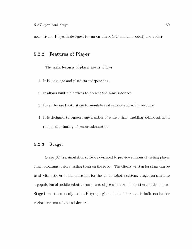
5.2.3 Stage:
Stage [32] is a simulation software designed to provide a means of testing player
client programs, before testing them on the robot. The clients written for stage can be
used with little or no modifications for the actual robotic system. Stage can simulate
a population of mobile robots, sensors and objects in a two-dimensional environment.
Stage is most commonly used a Player plugin module. There are in built models for
various sensors robot and devices.
5.3 Laser mapping 61
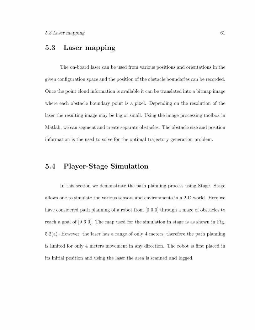
5.3 Laser mapping
The on-board laser can be used from various positions and orientations in the
given configuration space and the position of the obstacle boundaries can be recorded.
Once the point cloud information is available it can be translated into a bitmap image
where each obstacle boundary point is a pixel. Depending on the resolution of the
laser the resulting image may be big or small. Using the image processing toolbox in
Matlab, we can segment and create separate obstacles. The obstacle size and position
information is the used to solve for the optimal trajectory generation problem.
5.4 Player-Stage Simulation
In this section we demonstrate the path planning process using Stage. Stage
allows one to simulate the various sensors and environments in a 2-D world. Here we
have considered path planning of a robot from [0 0 0] through a maze of obstacles to
reach a goal of [9 6 0]. The map used for the simulation in stage is as shown in Fig.
5.2(a). However, the laser has a range of only 4 meters, therefore the path planning
is limited for only 4 meters movement in any direction. The robot is first placed in
its initial position and using the laser the area is scanned and logged.
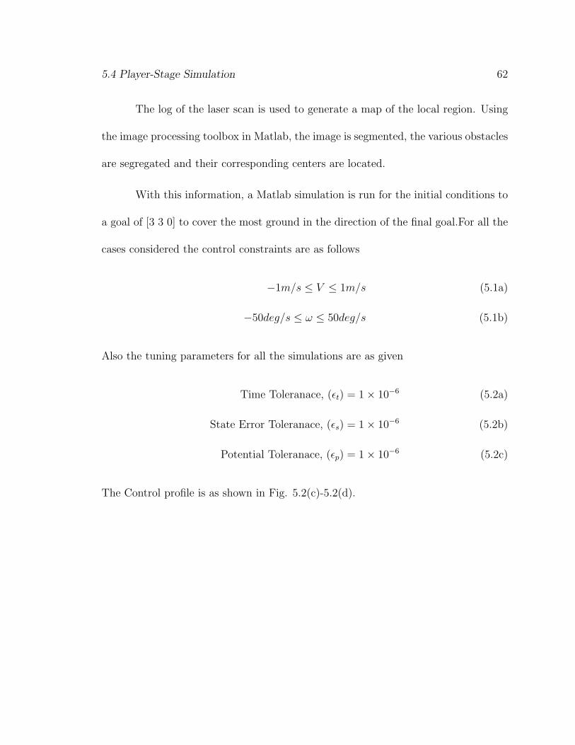
5.4 Player-Stage Simulation 62
The log of the laser scan is used to generate a map of the local region. Using
the image processing toolbox in Matlab, the image is segmented, the various obstacles
are segregated and their corresponding centers are located.
With this information, a Matlab simulation is run for the initial conditions to
a goal of [3 3 0] to cover the most ground in the direction of the final goal.For all the
cases considered the control constraints are as follows
−1m/s ≤ V ≤ 1m/s (5.1a)
−50deg/s ≤ ω ≤ 50deg/s (5.1b)
Also the tuning parameters for all the simulations are as given
Time Toleranace, (εt) = 1× 10⁻⁶ (5.2a)
State Error Toleranace, (εs) = 1× 10⁻⁶ (5.2b)
Potential Toleranace, (εp) = 1× 10⁻⁶ (5.2c)
The Control profile is as shown in Fig. 5.2(c)-5.2(d).
5.4 Player-Stage Simulation 63
(a) (b)
(c) V vs time (d) ω vs time
Figure 5.2: Laser based mapping and simulation for Part 1

5.4 Player-Stage Simulation 64
The velocity vectors of the solution are logged and applied to the stage robot.
The path followed is as shown in Fig. 5.3(a). The process is repeated this time for a
goal of [6 3 0]. The velocity vectors as shown in Fig. 5.3(c)-5.3(d). are logged again
and applied to the stage robot.
(a) (b)
(c) V vs time (d) ω vs time
Figure 5.3: Laser based mapping and simulation for Part 2
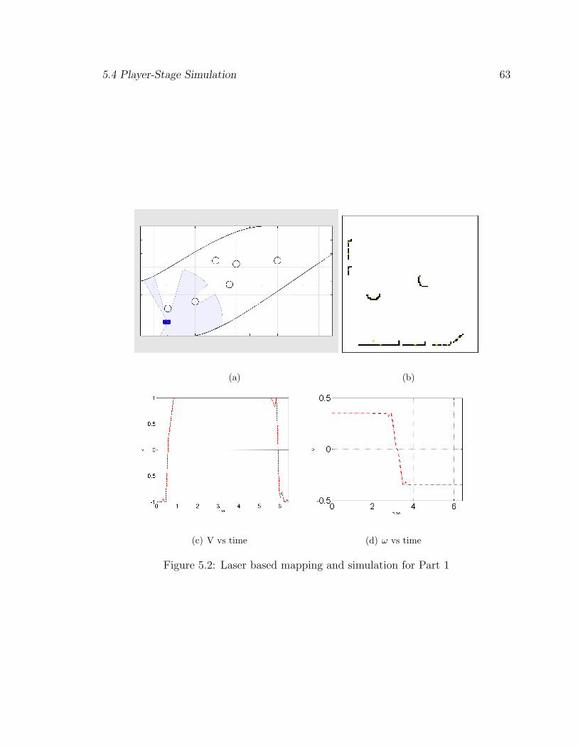
5.4 Player-Stage Simulation 65
The path followed is as shown in Fig. 5.4(a).The process is repeated this time
for a goal of [9 6 0]. The velocity vectors as shown in Fig. 5.4(c)-5.4(d). are logged
again and applied to the stage robot.The velocity vectors are logged again and applied
to the stage robot.
(a) (b)
(c) V vs time (d) ω vs time
Figure 5.4: Laser based mapping and simulation for Part 3

5.4 Player-Stage Simulation 66
The path followed is as shown in Fig. 5.4(a). Thus, the path planning problem
is solved for the final goal in three steps. In each step the local area is learnt and
path planning is done accordingly. Thus, this simulation leads to the conclusion that
it is possible to do path planning using the above mentioned procedure. This is
further tested by trying the procedure to solve the path planning problem in a real
case scenario, using a real robot mounted with a laser range finder in the presence of
obstacles.
(a)
(b)
Figure 5.5: Stage Simulation
5.5 Real Run 67
5.5 Real Run
Finally, we test the algorithm and the mapping technique in the real world.
We look at two cases,one, where the entire range is in the scope of the sensors and
the other when the sensors have a limited range smaller that the final goal.
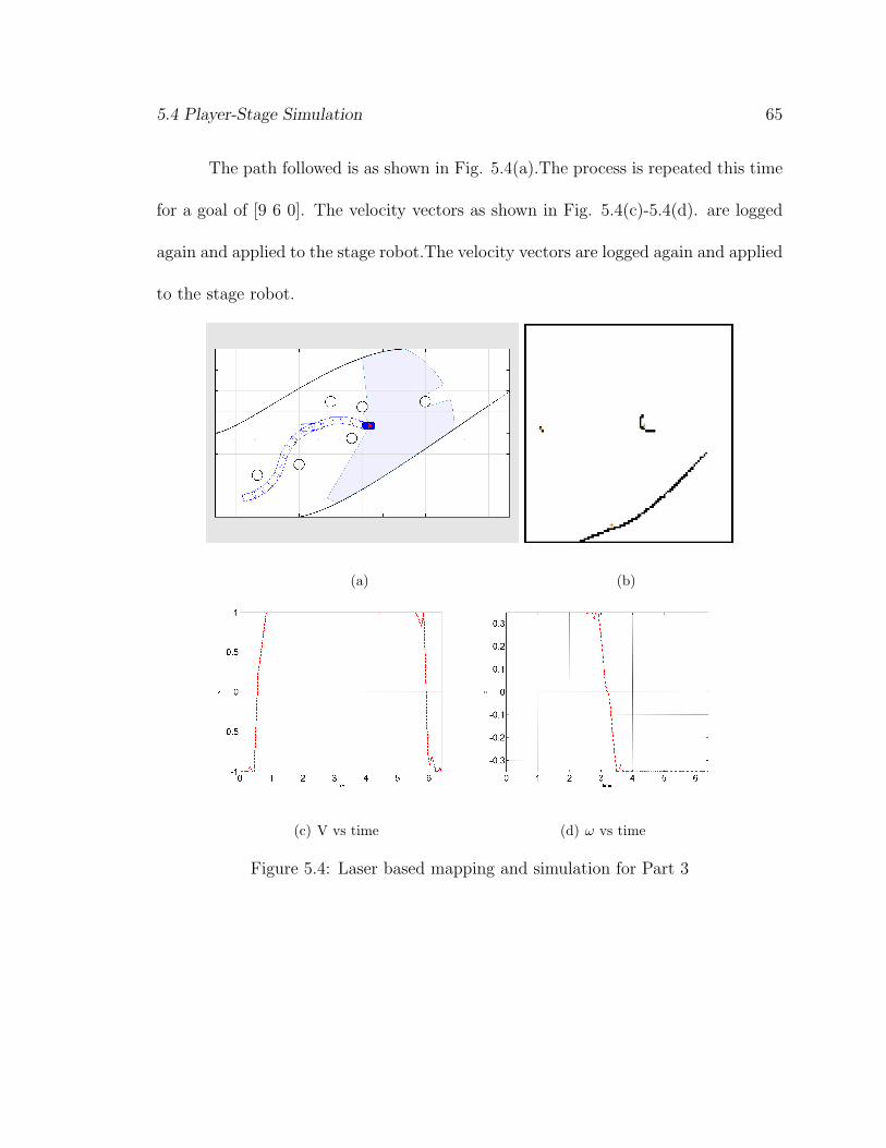
5.5.1 Case1:
In this case the entire configuration space is in the range of the robots sensors.
The robot ERRATIC is placed at a defined zero-zero position, and the obstacles are
placed in front of the robot. As discussed earlier, the first step is mapping the local
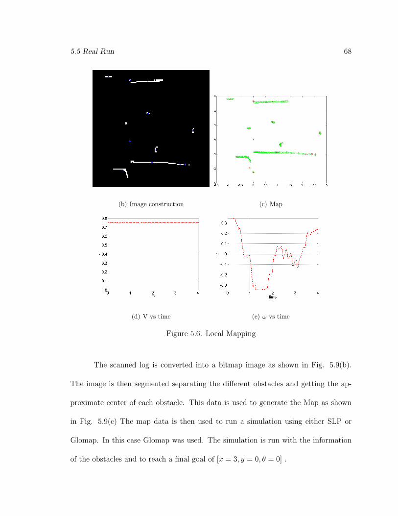
area. The laser is used to scan the area as shown in Fig. 5.9(a) and the scan is logged.
(a) Laser scan
5.5 Real Run 68
(b) Image construction (c) Map
(d) V vs time (e) ω vs time
Figure 5.6: Local Mapping
The scanned log is converted into a bitmap image as shown in Fig. 5.9(b).
The image is then segmented separating the different obstacles and getting the ap-
proximate center of each obstacle. This data is used to generate the Map as shown
in Fig. 5.9(c) The map data is then used to run a simulation using either SLP or
Glomap. In this case Glomap was used. The simulation is run with the information
of the obstacles and to reach a final goal of [x = 3, y = 0, θ = 0] .

5.5 Real Run 69
The control profiles are as shown in Fig. 5.6(d)-5.6(e). The solution achieved
is as shown in Fig. 5.7(a). For all the cases considered the control constraints are as
follows
−1m/s ≤ V ≤ 1m/s;−50deg/s ≤ ω ≤ 50deg/s (5.3a)
Also the tuning parameters for all the simulations are as given
Time Toleranace, (εt) = 1× 10⁻⁶; State Error Toleranace, (εs) = 1× 10⁻⁶ (5.4a)
Potential Toleranace, (εp) = 1× 10⁻⁶ (5.4b)
(a)
Figure 5.7: Matlab Simulation
5.5 Real Run 70
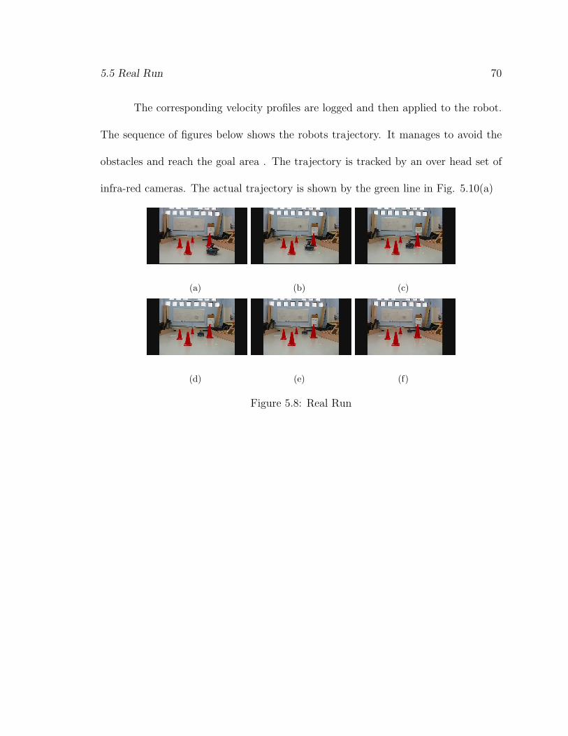
The corresponding velocity profiles are logged and then applied to the robot.
The sequence of figures below shows the robots trajectory. It manages to avoid the
obstacles and reach the goal area . The trajectory is tracked by an over head set of
infra-red cameras. The actual trajectory is shown by the green line in Fig. 5.10(a)
(a) (b) (c)
(d) (e) (f)
Figure 5.8: Real Run
5.5 Real Run 71
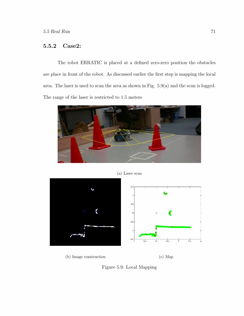
5.5.2 Case2:
The robot ERRATIC is placed at a defined zero-zero position the obstacles
are place in front of the robot. As discussed earlier the first step is mapping the local
area. The laser is used to scan the area as shown in Fig. 5.9(a) and the scan is logged.
The range of the laser is restricted to 1.5 meters
(a) Laser scan
(b) Image construction (c) Map
Figure 5.9: Local Mapping
5.5 Real Run 72
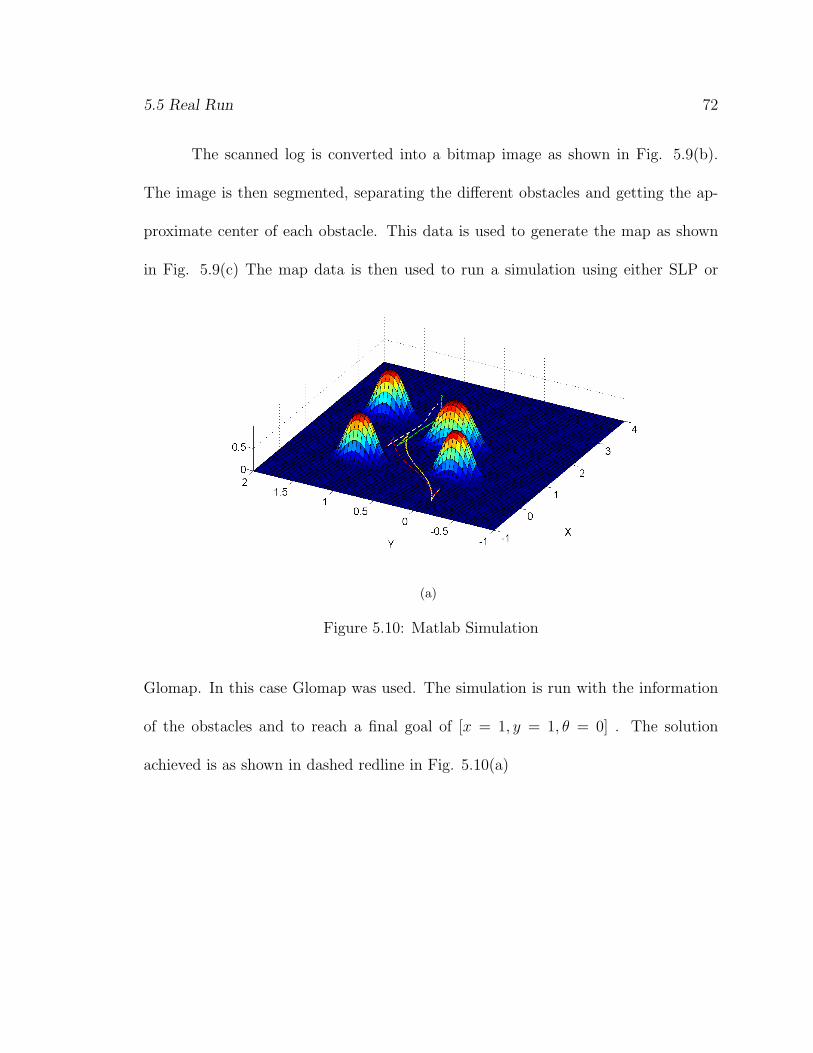
The scanned log is converted into a bitmap image as shown in Fig. 5.9(b).
The image is then segmented, separating the different obstacles and getting the ap-
proximate center of each obstacle. This data is used to generate the map as shown
in Fig. 5.9(c) The map data is then used to run a simulation using either SLP or
(a)
Figure 5.10: Matlab Simulation
Glomap. In this case Glomap was used. The simulation is run with the information
of the obstacles and to reach a final goal of [x = 1, y = 1, θ = 0] . The solution
achieved is as shown in dashed redline in Fig. 5.10(a)
5.5 Real Run 73
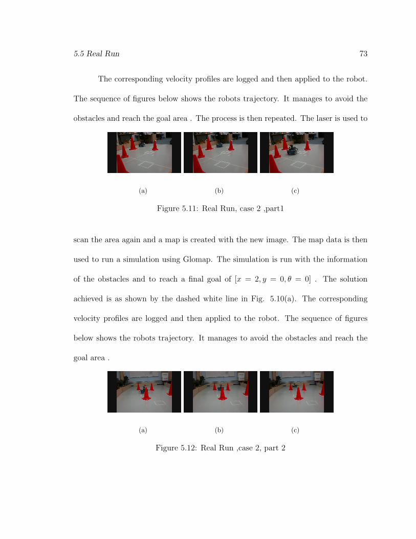
The corresponding velocity profiles are logged and then applied to the robot.
The sequence of figures below shows the robots trajectory. It manages to avoid the
obstacles and reach the goal area . The process is then repeated. The laser is used to
(a) (b) (c)
Figure 5.11: Real Run, case 2 ,part1
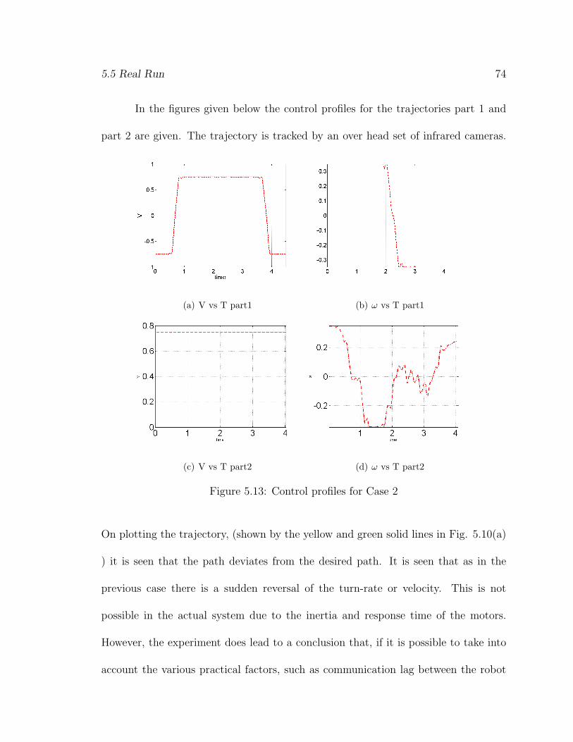
scan the area again and a map is created with the new image. The map data is then
used to run a simulation using Glomap. The simulation is run with the information
of the obstacles and to reach a final goal of [x = 2, y = 0, θ = 0] . The solution
achieved is as shown by the dashed white line in Fig. 5.10(a). The corresponding
velocity profiles are logged and then applied to the robot. The sequence of figures
below shows the robots trajectory. It manages to avoid the obstacles and reach the
goal area .
(a) (b) (c)
Figure 5.12: Real Run ,case 2, part 2
5.5 Real Run 74
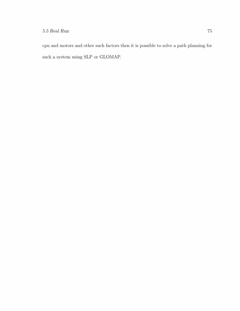
In the figures given below the control profiles for the trajectories part 1 and
part 2 are given. The trajectory is tracked by an over head set of infrared cameras.
(a) V vs T part1 (b) ω vs T part1
(c) V vs T part2 (d) ω vs T part2
Figure 5.13: Control profiles for Case 2
On plotting the trajectory, (shown by the yellow and green solid lines in Fig. 5.10(a)
) it is seen that the path deviates from the desired path. It is seen that as in the
previous case there is a sudden reversal of the turn-rate or velocity. This is not
possible in the actual system due to the inertia and response time of the motors.
However, the experiment does lead to a conclusion that, if it is possible to take into
account the various practical factors, such as communication lag between the robot
5.5 Real Run 75
cpu and motors and other such factors then it is possible to solve a path planning for
such a system using SLP or GLOMAP.
Chapter 6
Conclusion
The time optimal trajectory generation problem has been successfully imple-
mented using both SLP and Glomap. It is seen that in the presence of obstacles
both the algorithms converge to an optimal solution. The results of both SLP and
Glomap are very close. It is seen that using Glomap a solution similar to SLP can be
reached with a much lesser number of variables. In ‘case 4’ in ‘chapter 4’ Glomap had
to solve for only 360 variables to get the same solution as that of the SLP solution.
The the SLP solution required 500 grid points. At each grid points the two control
parameters were to be computed. Thus, Slp had to solve for a total of 1000 variables
as compared to Glomap which required only 360 variables. Therefore, with lesser
number of variables the computational load is also less. With Glomap the solution of
the control parameters is a continuous function of time. Thus, the control parameters
can be computed at a much higher resolution.
76
6.1 Future Scope 77
6.1 Future Scope
It was seen from the practical experiments that the trajectory of the robot in
real time varied from that of the matlab simulation. This can be corrected by using
system identification to compensate for the system parameters like inertia and system
noise. In all the cases that have been discussed the states were always expressed as
polynomial functions of time. This need not be the case, Glomap can be expanded
to work with a library of other functions. A combination of Glomap and SLP may
also be used. The methods discussed we applied only to a differential drive robot,
however, the methods are generic enough to be applied to other systems with little
or no modifications.
Bibliography
[1] L. E. Dubins. On curves of minimal length with a constraint on average curva-
ture, and with prescribed initial and terminal positions and tangents. American
Journal of Mathematics, 79(3):497–516, 1957.
[2] J. A. REEDS and L. A. SHEPP. Optimal paths for a car that goes both forwards
and backwards. Pacific Journal of Mathematics, 145,(2):367–392, 1990.
[3] Devin J. Balkcom & Matthew T. Mason. Time optimal trajectories for bounded
velocity differential drive vehicles. IEEE International Conference on Robotics
and Automation, 4(1-2):1–8, 2002.
[4] A. L. Schwartz. Theory and implementation of numerical methods based on
runge-kutta integration for solving optimal control problems. PhD thesis, U.C.
Berkeley, 1996.
[5] Mark B. Milam, Kudah Mushambi, and Richard M. Murray. A new compu-
tational approach to real-time trajectory generation for constrained mechanical
systems. In IEEE Conference on Decision and Control, 2000.
78

Bibliography 79
[6] C. R. Hargraves and S.W. Paris. Direct trajectory optimization using nonlinear
programming and collocation. Journal of Guidance, Control, and Dynamics,
10(4):338–342, 1987.
[7] D. G. Hull. Conversion of optimal control problems into parameter optimization
problems. In Guidance, Navigation and Control Conference, San Francisco, CA,
Aug. 15-18 1996.
[8] A. L. Herman and B. A. Conway. Direct optimization using collocation based
on high-order gauss-lobatto quadrature rules. Journal of Guidance, Control, and
Dynamics, 19(3):592–599, 1996.
[9] J. T. Betts. Survey of Numerical Methods for Trajectory Optimization. Journal
of Guidance, Control, and Dynamics, 21(2):193–207, 1998.
[10] C. R. Hargraves and S.W. Paris. Direct trajectory optimization using nonlinear
programming and collocation. Journal of Guidance, Control, and Dynamics,
10(4):338–342, 1987.
[11] A. L. Herman and B. A. Conway. Direct optimization using collocation based on
high-order Gauss-Lobatto quadrature rules. Journal of Guidance, Control, and
Dynamics, 19(3):592–599, 1996.
[12] J. Vlassenbroeck and R. Van Dooren. A Chebyshev Technique for Solving Non-
linear Optimal Control Problem. IEEE Transactions on Automatic Control,
33(4):333–340, 1988.
Bibliography 80
[13] F. Fariba and M.I Ross. Direct Trajectory Optimization by a Chebyshev Pseu-
dospectral Method. Journal of Guidance, Control, and Dynamics, 25(1):160–166,
2002.
[14] F. Fariba and M.I Ross. Legendre Pseudospectral Approximations of Optimal
Control Problems. Lecture Notes in Control and Information Sciences, 295, 2004.
[15] Raktim Bhattacharya and Puneet Singla. Nonlinear trajectory generation using
global local approximations. 45th IEEE Conference on Decision and Control,
2006.
[16] Bostjan Potocnik Marko Leptic; Gregor Klancar Igor skranjac, Drago Matko.
Optimal path design in robot soccer environment. IEEE International Confer-
ence on Industrial Technology, pages 778–782, 2003.
[17] A. L. Schwartz. Theory and Implementation of Numerical Methods Based on
Runge-Kutta Integration for Solving Optimal Control Problems. PhD thesis,
U.C. Berkeley, 1996.
[18] G. Arfken. Mathematical Methods for Physicists. Academic Press, Orlando, FL,
3 edition, 1985.
[19] J. W. Gibbs. Fourier series. Nature, 59(200 & 606), 1899.
Bibliography 81
[20] P. Singla. Multi-Resolution Methods for High Fidelity Modeling and Control
Allocation in Large-Scale Dynamical Systems. Ph.d dissertation, Texas A&M
University, College Station, TX, May 2006.
[21] John L. Junkins & Puneet Singla. Multi-resolution Methods for Modeling And
Control of Dynamical Systems. Chapman & Hall, July 2008.
[22] T. Singh and P. Singla. Sequential linear programming for design of time optimal
controllers. 46th IEEE Conference on Decision and Control, 52(1-2):1–8, 2007.
[23] S. G. Manyam P. Singla, T. Singh. Input shaping design using sequential linear
programming (slp) for non-linear systems. American Control Conference, (11-
13):3275–3280, 2008.
[24] Arthur E. Bryson. Applied optimal control : optimization, estimation, and con-
trol. Hemisphere Pub. Corp., 1975.
[25] Jean-Claud Latombe. Robot Motion Planning. KAP, 7 edition, 2003.
[26] Oussama Khatib. Real-time obstacle avoidance for manipulators and mobile
robots. The International Journal of Robotics Research, 5(1):90–98, 1986.
[27] S. S. Ge and Y. J. Cui. New potential functions for mobile robot path planning.
IEEE Transactions on Robotics and Automation, 16:615–620, 2000.
[28] Huchinson Kantor Bugard Kavraki Choset, lynch and Thrun. Principles of robot
motion. MIT Press, pages 80–100, 2005.
Bibliography 82
[29] Charles W. Warren. Global path planning using artificial potential fields. Pro-
ceedings, IEEE International Conference on Robotics and Automation, pages
316–321, 1989.
[30] Yoram Koren and Johann Borenstein. Potential field methods and their inherent
limitations for mobile robot navigation. Proceedings,IEEE International Confer-
ence on Robotics and Automation, 2:1398–1404, 1991.
[31] http://www.videredesign.com.
[32] http://playerstage.sourceforge.net.


![[EN-A-073] Robust Optimal Trajectory Planning under](https://img.pdfslide.us/doc/110x75/6211df51e743c86aea630c41/en-a-073-robust-optimal-trajectory-planning-under-.jpg)