Trajectory Forecast as a Rapid Response to the Deepwater

Trajectory Forecast as a Rapid Response to the Deepwater Horizon Oil Spill

Yonggang Liu, Robert H. Weisberg, Chuanmin Hu, and Lianyuan Zheng

College of Marine Science, University of South Florida, St. Petersburg, Florida, USA

In response to the Gulf of Mexico Deepwater Horizon oil spill, a Lagrangiantrajectory modeling system was implemented immediately upon spill onset bymarshaling numerical model and satellite remote sensing resources available fromexisting coastal ocean-observing activities. Surface oil locations inferred fromsatellite imagery were used to re-initialize the positions of virtual particles in thisensemble of trajectory models, and the particles were tracked using forecast surfacecurrents, with new particles added to simulate the continual release of oil from thewell. A challenge to this modeling effort was that much information remainedunknown throughout the spill event, with additional uncertainty due to intensivemitigation activities. By frequently re-initializing the trajectory models with satellite-inferred locations, the effects of in situ mitigation and forecast error growth wereimplicitly accounted for and minimized. The simulated surface oil trajectories werecompared to the satellite observations in subsequent forecast cycles for veracitytesting. Although similar results were obtained, in general, differences were seen inthe simulated trajectories by different models. However, no one model performedconsistently better or worse than the others throughout the event with one excep-tion. The lessons learned from the event may be useful in preparing rapid trajectoryforecast systems in the future.

1. INTRODUCTION

The Deepwater Horizon drill rig, located southeast of theMississippi River delta within the Mississippi Canyon Block252, exploded on 20 April 2010. The subsequent sinking on22 April 2010 resulted in the largest offshore oil spill in U.S.history. This spill, which continued for 3 months, presentedan unprecedented threat to the Gulf of Mexico (GOM), itscoastal zone and living marine resources [e.g.,Mearns et al.,2010; Jernelöv, 2010;Hu et al., 2011], and possibly to that ofthe southeastern United States of America [e.g., Maltrud etal., 2010]. Needed for mitigation efforts and for guidingscientific investigations was a system for tracking the oil,both at the surface and at depth.

The fate of oil spilled into the ocean depends on manyfactors, including transport and dispersion by the ocean cir-culation, physical weathering (evaporation, emulsification),other chemical transformations, and biological consumption[e.g., Spaulding, 1988; Yapa, 1996; Reed et al., 1999; Li,2000; Ji et al., 2004]. Here we focus on the conservativeaspects (the ocean circulation) because these are fundamentalto all else, and they are the most readily implemented withinexisting coastal ocean-observing and modeling systems [e.g.,Weisberg et al., 2009]. The ocean circulation is also whatdetermines either landfall or movement toward biologicallysensitive areas in both deep and shallow water regions [e.g.,Weisberg, 2011; Ji et al., this volume].Along with chemical and biological processes, the mitiga-

tion activities that were ongoing throughout the DeepwaterHorizon oil spill, for instance, the use of dispersants [e.g.,Kujawinski et al., 2011], containment, and fire at sea [e.g.,Crout, 2011], and off-loading to, or skimming by, boatsadded further uncertainty to oil spill trajectory modelingefforts. Information on the locations and effects of these

Monitoring and Modeling the Deepwater Horizon Oil Spill:A Record-Breaking EnterpriseGeophysical Monograph Series 195Copyright 2011 by the American Geophysical Union.10.1029/2011GM001121

153

actions were generally unknown throughout the spillduration.The Deepwater Horizon oil spill also differed from previ-

ous spills in many ways. Crude oil was introduced at theocean bottom in 1500 m of water, a depth that was muchdeeper than those of previous oil spills. For instance, theIXTOC-1 oil spill was in 50 m deep water [e.g., Jernelöv andLindén, 1981]. Three months of flow, ending with the cap-ping of the wellhead on 15 July 2010, further distinguishedthis event from major tanker incidents, e.g., the Prestige[e.g., Abasca et al., 2009; Jordi et al., 2006] and the ExxonValdez [e.g., Koburger, 1989]. Moreover, the amount ofhydrocarbons being released remained unknown throughoutthe event. All of these factors complicated traditional oiltrajectory model forecasts [e.g., Aamo et al., 1997; Danielet al., 2004]. These challenges called for an effective, rapidlyimplemented oil spill tracking/predicting system to augmentthe work of the agencies and industries comprising the Inci-dent Command.Such a response system [Liu et al., 2011a] was implemen-

ted at the University of South Florida (USF) immediatelyupon spill onset, by marshaling numerical model and satelliteremote sensing resources available from existing coastalocean-observing activities [e.g., Weisberg et al., 2009]. Theconcept of this system was briefly reported in the work of Liuet al. [2011a], and its methodology was later explained in thework of Liu et al. [2011b]. Here in this paper, we provide afuller description of the oil spill trajectory model develop-ment, along with model/data comparisons. The purpose is notto hindcast the oil spill trajectory for the entire event; rather, itis to summarize our use of the available coastal modeling andobserving resources and to provide some performance mea-sures. The goal is to offer lessons learned that may be useful inresponses to future events, recognizing the increasing demandfor oil production from deep water regions.The next section 2 describes the evolution of our surface

oil trajectory modeling system. Section 3 then discussestrajectory model veracity testing by comparing the simulatedsurface oil trajectories with satellite imagery-inferred oillocations. The purpose is to see which models, if any, mayhave performed better or worse than others. Challenges tosuch modeling efforts and lessons learned throughout theevent are discussed in section 4.

2. THE SURFACE OIL TRAJECTORYMODELING SYSTEM

2.1. Numerical Ocean Circulation Models

The Deepwater Horizon rig site, located less than 100 kmfrom the Mississippi River delta is on the GOM continental

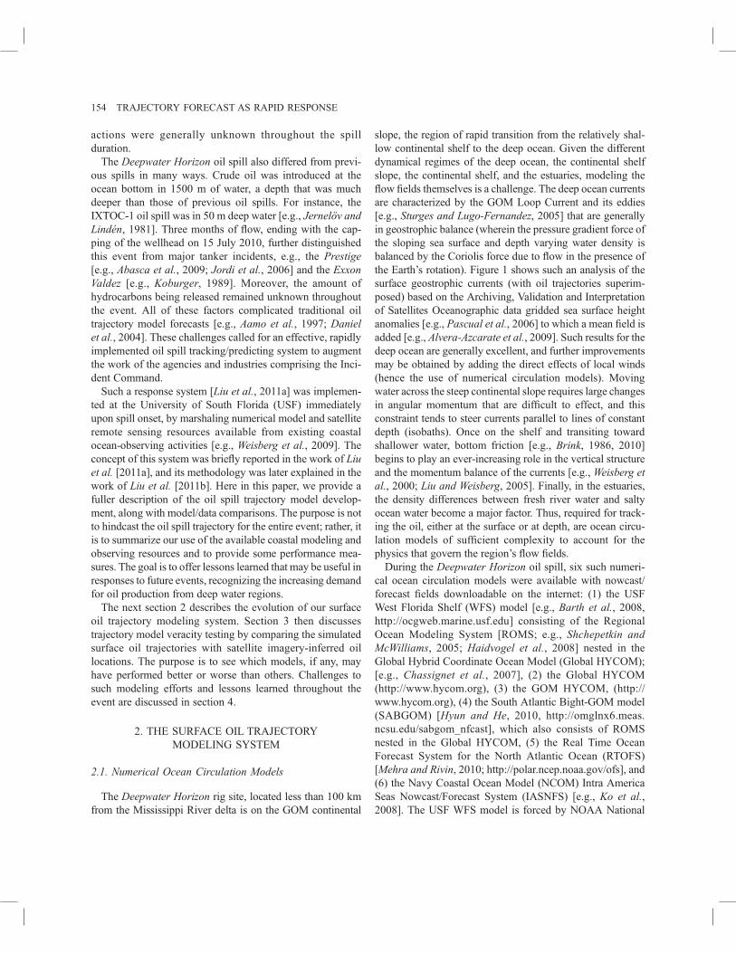
slope, the region of rapid transition from the relatively shal-low continental shelf to the deep ocean. Given the differentdynamical regimes of the deep ocean, the continental shelfslope, the continental shelf, and the estuaries, modeling theflow fields themselves is a challenge. The deep ocean currentsare characterized by the GOM Loop Current and its eddies[e.g., Sturges and Lugo-Fernandez, 2005] that are generallyin geostrophic balance (wherein the pressure gradient force ofthe sloping sea surface and depth varying water density isbalanced by the Coriolis force due to flow in the presence ofthe Earth’s rotation). Figure 1 shows such an analysis of thesurface geostrophic currents (with oil trajectories superim-posed) based on the Archiving, Validation and Interpretationof Satellites Oceanographic data gridded sea surface heightanomalies [e.g., Pascual et al., 2006] to which a mean field isadded [e.g., Alvera-Azcarate et al., 2009]. Such results for thedeep ocean are generally excellent, and further improvementsmay be obtained by adding the direct effects of local winds(hence the use of numerical circulation models). Movingwater across the steep continental slope requires large changesin angular momentum that are difficult to effect, and thisconstraint tends to steer currents parallel to lines of constantdepth (isobaths). Once on the shelf and transiting towardshallower water, bottom friction [e.g., Brink, 1986, 2010]begins to play an ever-increasing role in the vertical structureand the momentum balance of the currents [e.g., Weisberg etal., 2000; Liu and Weisberg, 2005]. Finally, in the estuaries,the density differences between fresh river water and saltyocean water become a major factor. Thus, required for track-ing the oil, either at the surface or at depth, are ocean circu-lation models of sufficient complexity to account for thephysics that govern the region’s flow fields.During the Deepwater Horizon oil spill, six such numeri-

cal ocean circulation models were available with nowcast/forecast fields downloadable on the internet: (1) the USFWest Florida Shelf (WFS) model [e.g., Barth et al., 2008,http://ocgweb.marine.usf.edu] consisting of the RegionalOcean Modeling System [ROMS; e.g., Shchepetkin andMcWilliams, 2005; Haidvogel et al., 2008] nested in theGlobal Hybrid Coordinate Ocean Model (Global HYCOM);[e.g., Chassignet et al., 2007], (2) the Global HYCOM(http://www.hycom.org), (3) the GOM HYCOM, (http://www.hycom.org), (4) the South Atlantic Bight-GOM model(SABGOM) [Hyun and He, 2010, http://omglnx6.meas.ncsu.edu/sabgom_nfcast], which also consists of ROMSnested in the Global HYCOM, (5) the Real Time OceanForecast System for the North Atlantic Ocean (RTOFS)[Mehra and Rivin, 2010; http://polar.ncep.noaa.gov/ofs], and(6) the Navy Coastal Ocean Model (NCOM) Intra AmericaSeas Nowcast/Forecast System (IASNFS) [e.g., Ko et al.,2008]. The USF WFS model is forced by NOAA National

154 TRAJECTORY FORECAST AS RAPID RESPONSE

Centers for Environmental Prediction (NCEP), North Amer-ican Mesoscale Model reanalysis (http://www.emc.ncep.noaa.gov) and forecast winds and heat fluxes modified byblending with observed winds and SST for improving theaccuracy of the coastal ocean circulation simulations [Heet al., 2004]. The SABGOM model, operated at the NorthCarolina State University, is forced by NOAA NationalOperational Model Archive and Distribution System windsand heat fluxes [Rutledge et al., 2006]. Both the GlobalHYCOM and GOM HYCOM, maintained by the NavalResearch Laboratory and the HYCOM Consortium, areforced by Navy Operational Global Atmospheric PredictionSystem surface fluxes [Rosmond et al., 2002] and use theNavy Coupled Ocean Data Assimilation system [Cummings,

2005]. The RTOFS, operated by NOAA/NCEP, is a dataassimilative Atlantic basin-scale ocean forecast system basedon HYCOM. The NCOM IASNFS is operated at the NavalResearch Laboratory with output served through the North-ern Gulf Institute (http://www.northerngulfinstitute.org). Allof these models (in their state of readiness at the time) arecapable of considering the transitions from the deep ocean tothe continental shelf. None, however, are constructed to treatthe estuaries.Our starting point for these analyses was the USF WFS

model because we had immediate access to it, and our now-cast/forecast system was readily adaptable to the new situa-tion. Within a day of the rig sinking, we added additionalparticle tracking sites to the suite of existing sites in use for

Figure 1. A snapshot of the surface oil location (black) inferred from Moderate Resolution Imaging Spectroradiometer(MODIS) imagery, superimposed on the satellite altimetry-derived surface geostrophic currents (vectors) and Geostation-ary Operational Environmental Satellites (GOES)-derived sea surface temperature (SST) on 18 May 2011. Note theentrainment of the oil into the Gulf of Mexico Loop Current at this time and therefore the potential for oil to be advectedthrough the Florida Straits. The shedding of an eddy within 2 days of this snapshot, broke the connection between the wellsite and the Florida Straits thereby sparing most of Florida from the direct impacts of the Deepwater Horizon oil. Alsoshown are the well site (o) and National Data Buoy Center (NDBC) Buoy 42040 (x). Geostrophic velocities are computedwith sea level gradients derived from satellite sea surface height analyses plus a model mean field, following a procedure inthe works of Alvera-Azcárate et al. [2009] and Liu et al. [this volume].

LIU ET AL. 155

search and rescue readiness. We then contacted NOAA Haz-mat (G. Watabayashi, personal communication, 2010), andwithin a week or so, we were providing our results for theirinclusion in the Incident Command forecasts in which ourUSF contributions were subsequently acknowledged on adaily basis. With time, we then refined our analysis schemeand added additional models as their information becameavailable to us. The order of inclusion was: (1) USF WFS,(2) Global HYCOM, (3) RTOFS, (4) SABGOM, (5) GOMHYCOM, and (6) NCOM IASNFS.

2.2. Satellite Data

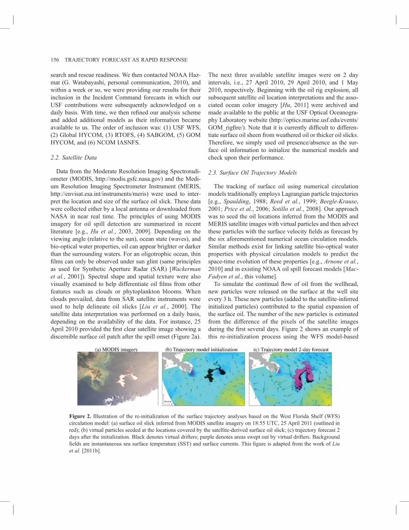
Data from the Moderate Resolution Imaging Spectroradi-ometer (MODIS, http://modis.gsfc.nasa.gov) and the Medi-um Resolution Imaging Spectrometer Instrument (MERIS,http://envisat.esa.int/instruments/meris) were used to inter-pret the location and size of the surface oil slick. These datawere collected either by a local antenna or downloaded fromNASA in near real time. The principles of using MODISimagery for oil spill detection are summarized in recentliterature [e.g., Hu et al., 2003, 2009]. Depending on theviewing angle (relative to the sun), ocean state (waves), andbio-optical water properties, oil can appear brighter or darkerthan the surrounding waters. For an oligotrophic ocean, thinfilms can only be observed under sun glint (same principlesas used for Synthetic Aperture Radar (SAR) [Wackermanet al., 2001]). Spectral shape and spatial texture were alsovisually examined to help differentiate oil films from otherfeatures such as clouds or phytoplankton blooms. Whenclouds prevailed, data from SAR satellite instruments wereused to help delineate oil slicks [Liu et al., 2000]. Thesatellite data interpretation was performed on a daily basis,depending on the availability of the data. For instance, 25April 2010 provided the first clear satellite image showing adiscernible surface oil patch after the spill onset (Figure 2a).

The next three available satellite images were on 2 dayintervals, i.e., 27 April 2010, 29 April 2010, and 1 May2010, respectively. Beginning with the oil rig explosion, allsubsequent satellite oil location interpretations and the asso-ciated ocean color imagery [Hu, 2011] were archived andmade available to the public at the USF Optical Oceanogra-phy Laboratory website (http://optics.marine.usf.edu/events/GOM_rigfire/). Note that it is currently difficult to differen-tiate surface oil sheen from weathered oil or thicker oil slicks.Therefore, we simply used oil presence/absence as the sur-face oil information to initialize the numerical models andcheck upon their performance.

2.3. Surface Oil Trajectory Models

The tracking of surface oil using numerical circulationmodels traditionally employs Lagrangian particle trajectories[e.g., Spaulding, 1988; Reed et al., 1999; Beegle-Krause,2001; Price et al., 2006; Sotillo et al., 2008]. Our approachwas to seed the oil locations inferred from the MODIS andMERIS satellite images with virtual particles and then advectthese particles with the surface velocity fields as forecast bythe six aforementioned numerical ocean circulation models.Similar methods exist for linking satellite bio-optical waterproperties with physical circulation models to predict thespace-time evolution of these properties [e.g., Arnone et al.,2010] and in existing NOAA oil spill forecast models [Mac-Fadyen et al., this volume].To simulate the continual flow of oil from the wellhead,

new particles were released on the surface at the well siteevery 3 h. These new particles (added to the satellite-inferredinitialized particles) contributed to the spatial expansion ofthe surface oil. The number of the new particles is estimatedfrom the difference of the pixels of the satellite imagesduring the first several days. Figure 2 shows an example ofthis re-initialization process using the WFS model-based

Figure 2. Illustration of the re-initialization of the surface trajectory analyses based on the West Florida Shelf (WFS)circulation model: (a) surface oil slick inferred from MODIS satellite imagery on 18:55 UTC, 25 April 2011 (outlined inred); (b) virtual particles seeded at the locations covered by the satellite-derived surface oil slick; (c) trajectory forecast 2days after the initialization. Black denotes virtual drifters; purple denotes areas swept out by virtual drifters. Backgroundfields are instantaneous sea surface temperature (SST) and surface currents. This figure is adapted from the work of Liuet al. [2011b].


Lagrangian trajectory model. New trajectory forecasts weremade daily and re-initialized whenever new satellite imageinterpretations permitted. The frequent re-initialization of oillocation controlled trajectory error growth, especially giventhe unknown effects from mitigation activities. The com-bined effects of weathering, consumption, and mitigation aretherefore implicit in the re-initializations.Upon the spill onset, both the WFS- and the HYCOM-

simulated surface currents were available, and they wereimmediately and successively used to set up surface trajec-tory analyses without the re-initialization. On 25 April 2010,the satellite imagery, showing a discernible size of surfaceoil, was used to re-initialize these surface trajectories. The re-initialization process was repeated when the next satelliteimages became available on 27 April 2010, 29 April 2010,and 1 May 2010, and so forth. On 1 May 2010, the RTOFS-based surface trajectory analyses were added to the system,and on 4 May 2010, the SABGOM-based trajectory analyseswere also included. The GOM HYCOM-based trajectoryanalyses began on 11 May 2010 after the Global HYCOMstopped updating its forecast for about a week. The sixth andfinal trajectory analyses based on the NCOM IASNFS wasadded on 23 June. In essence, we added analyses as soon aswe could access their surface velocity fields.

3. COMPARISON OF MODELED SURFACETRAJECTORIES WITH SATELLITE IMAGERY

3.1. Forecast for Different Days

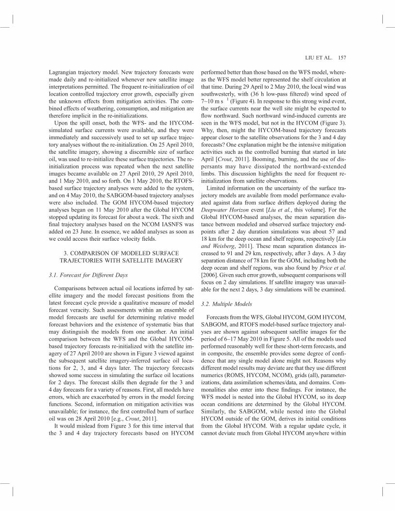
Comparisons between actual oil locations inferred by sat-ellite imagery and the model forecast positions from thelatest forecast cycle provide a qualitative measure of modelforecast veracity. Such assessments within an ensemble ofmodel forecasts are useful for determining relative modelforecast behaviors and the existence of systematic bias thatmay distinguish the models from one another. An initialcomparison between the WFS and the Global HYCOM-based trajectory forecasts re-initialized with the satellite im-agery of 27 April 2010 are shown in Figure 3 viewed againstthe subsequent satellite imagery-inferred surface oil loca-tions for 2, 3, and 4 days later. The trajectory forecastsshowed some success in simulating the surface oil locationsfor 2 days. The forecast skills then degrade for the 3 and4 day forecasts for a variety of reasons. First, all models haveerrors, which are exacerbated by errors in the model forcingfunctions. Second, information on mitigation activities wasunavailable; for instance, the first controlled burn of surfaceoil was on 28 April 2010 [e.g., Crout, 2011].It would mislead from Figure 3 for this time interval that

the 3 and 4 day trajectory forecasts based on HYCOM

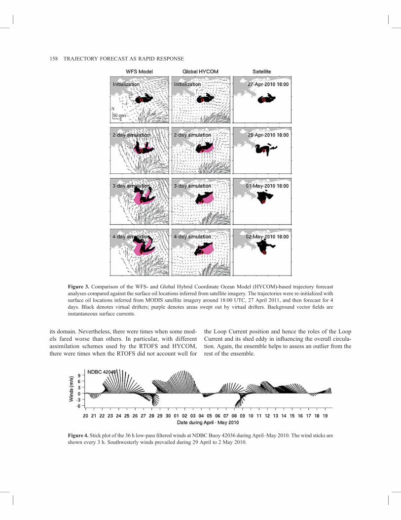
performed better than those based on theWFS model, where-as the WFS model better represented the shelf circulation atthat time. During 29 April to 2 May 2010, the local wind wassouthwesterly, with (36 h low-pass filtered) wind speed of7~10 m s�1 (Figure 4). In response to this strong wind event,the surface currents near the well site might be expected toflow northward. Such northward wind-induced currents areseen in the WFS model, but not in the HYCOM (Figure 3).Why, then, might the HYCOM-based trajectory forecastsappear closer to the satellite observations for the 3 and 4 dayforecasts? One explanation might be the intensive mitigationactivities such as the controlled burning that started in lateApril [Crout, 2011]. Booming, burning, and the use of dis-persants may have dissipated the northward-extendedlimbs. This discussion highlights the need for frequent re-initialization from satellite observations.Limited information on the uncertainty of the surface tra-

jectory models are available from model performance evalu-ated against data from surface drifters deployed during theDeepwater Horizon event [Liu et al., this volume]. For theGlobal HYCOM-based analyses, the mean separation dis-tance between modeled and observed surface trajectory end-points after 2 day duration simulations was about 57 and18 km for the deep ocean and shelf regions, respectively [Liuand Weisberg, 2011]. These mean separation distances in-creased to 91 and 29 km, respectively, after 3 days. A 3 dayseparation distance of 78 km for the GOM, including both thedeep ocean and shelf regions, was also found by Price et al.[2006]. Given such error growth, subsequent comparisons willfocus on 2 day simulations. If satellite imagery was unavail-able for the next 2 days, 3 day simulations will be examined.

3.2. Multiple Models

Forecasts from theWFS, Global HYCOM,GOMHYCOM,SABGOM, and RTOFS model-based surface trajectory anal-yses are shown against subsequent satellite images for theperiod of 6–17 May 2010 in Figure 5. All of the models usedperformed reasonably well for these short-term forecasts, andin composite, the ensemble provides some degree of confi-dence that any single model alone might not. Reasons whydifferent model results may deviate are that they use differentnumerics (ROMS, HYCOM, NCOM), grids (all), parameter-izations, data assimilation schemes/data, and domains. Com-monalities also enter into these findings. For instance, theWFS model is nested into the Global HYCOM, so its deepocean conditions are determined by the Global HYCOM.Similarly, the SABGOM, while nested into the GlobalHYCOM outside of the GOM, derives its initial conditionsfrom the Global HYCOM. With a regular update cycle, itcannot deviate much from Global HYCOM anywhere within

LIU ET AL. 157

its domain. Nevertheless, there were times when some mod-els fared worse than others. In particular, with differentassimilation schemes used by the RTOFS and HYCOM,there were times when the RTOFS did not account well for

the Loop Current position and hence the roles of the LoopCurrent and its shed eddy in influencing the overall circula-tion. Again, the ensemble helps to assess an outlier from therest of the ensemble.

Figure 4. Stick plot of the 36 h low-pass filtered winds at NDBC Buoy 42036 during April–May 2010. The wind sticks areshown every 3 h. Southwesterly winds prevailed during 29 April to 2 May 2010.

Figure 3. Comparison of the WFS- and Global Hybrid Coordinate Ocean Model (HYCOM)-based trajectory forecastanalyses compared against the surface oil locations inferred from satellite imagery. The trajectories were re-initialized withsurface oil locations inferred from MODIS satellite imagery around 18:00 UTC, 27 April 2011, and then forecast for 4days. Black denotes virtual drifters; purple denotes areas swept out by virtual drifters. Background vector fields areinstantaneous surface currents.


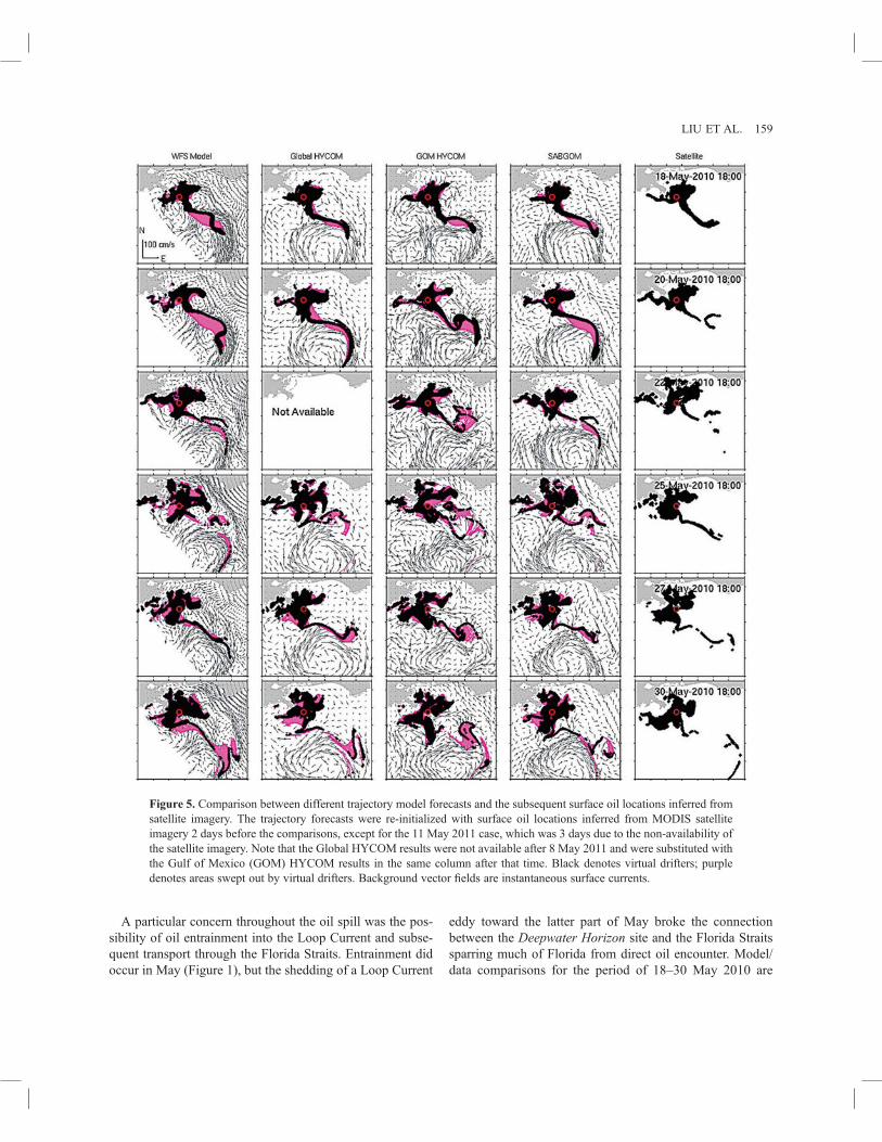
A particular concern throughout the oil spill was the pos-sibility of oil entrainment into the Loop Current and subse-quent transport through the Florida Straits. Entrainment didoccur in May (Figure 1), but the shedding of a Loop Current

eddy toward the latter part of May broke the connectionbetween the Deepwater Horizon site and the Florida Straitssparring much of Florida from direct oil encounter. Model/data comparisons for the period of 18–30 May 2010 are

Figure 5. Comparison between different trajectory model forecasts and the subsequent surface oil locations inferred fromsatellite imagery. The trajectory forecasts were re-initialized with surface oil locations inferred from MODIS satelliteimagery 2 days before the comparisons, except for the 11 May 2011 case, which was 3 days due to the non-availability ofthe satellite imagery. Note that the Global HYCOM results were not available after 8 May 2011 and were substituted withthe Gulf of Mexico (GOM) HYCOM results in the same column after that time. Black denotes virtual drifters; purpledenotes areas swept out by virtual drifters. Background vector fields are instantaneous surface currents.

LIU ET AL. 159

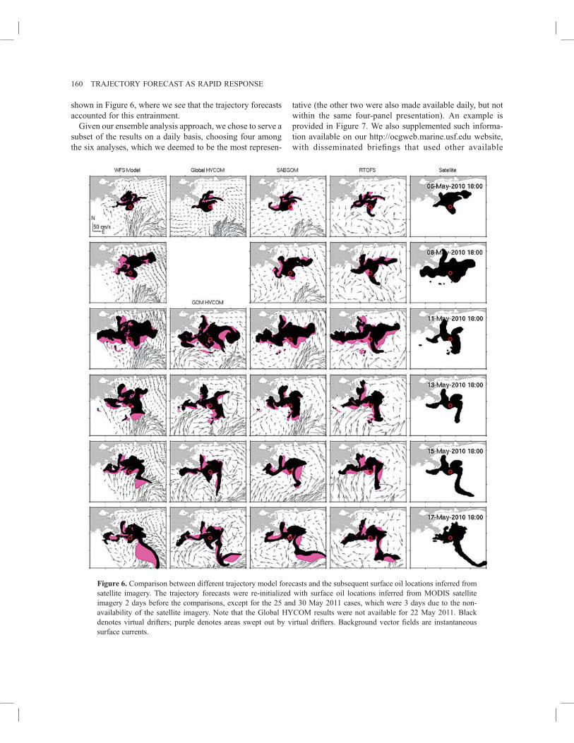
shown in Figure 6, where we see that the trajectory forecastsaccounted for this entrainment.Given our ensemble analysis approach, we chose to serve a

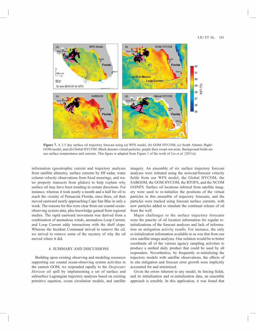
subset of the results on a daily basis, choosing four amongthe six analyses, which we deemed to be the most represen-

tative (the other two were also made available daily, but notwithin the same four-panel presentation). An example isprovided in Figure 7. We also supplemented such informa-tion available on our http://ocgweb.marine.usf.edu website,with disseminated briefings that used other available

Figure 6. Comparison between different trajectory model forecasts and the subsequent surface oil locations inferred fromsatellite imagery. The trajectory forecasts were re-initialized with surface oil locations inferred from MODIS satelliteimagery 2 days before the comparisons, except for the 25 and 30 May 2011 cases, which were 3 days due to the non-availability of the satellite imagery. Note that the Global HYCOM results were not available for 22 May 2011. Blackdenotes virtual drifters; purple denotes areas swept out by virtual drifters. Background vector fields are instantaneoussurface currents.


information (geostrophic current and trajectory analysesfrom satellite altimetry, surface currents by HF-radar, watercolumn velocity observations from fixed moorings, and wa-ter property transects from gliders) to help explain whysurface oil may have been trending in certain directions. Forinstance, whereas it took nearly a month and a half for oil toreach the vicinity of Pensacola Florida, once there, oil thenmoved eastward nearly approaching Cape San Blas in only aweek. The reasons for this were clear from our coastal ocean-observing system data, plus knowledge gained from regionalstudies. The rapid eastward movement was derived from acombination of anomalous winds, anomalous Loop Current,and Loop Current eddy interactions with the shelf slope.Whereas the Incident Command strived to remove the oil,we strived to remove some of the mystery of why the oilmoved where it did.

4. SUMMARY AND DISCUSSIONS

Building upon existing observing and modeling resourcessupporting our coastal ocean-observing system activities inthe eastern GOM, we responded rapidly to the DeepwaterHorizon oil spill by implementing a set of surface andsubsurface Lagrangian trajectory analyses based on existingprimitive equation, ocean circulation models, and satellite

imagery. An ensemble of six surface trajectory forecastanalyses were initiated using the nowcast/forecast velocityfields from our WFS model, the Global HYCOM, theSABGOM, the GOM HYCOM, the RTOFS, and the NCOMIASNFS. Surface oil locations inferred from satellite imag-ery were used to re-initialize the positions of the virtualparticles in this ensemble of trajectory forecasts, and theparticles were tracked using forecast surface currents, withnew particles added to simulate the continual release of oilfrom the well.Major challenges to the surface trajectory forecasts

were the paucity of oil location information for regular re-initializations of the forecast analyses and lack of informa-tion on mitigation activity results. For instance, the onlyre-initialization information available to us was that from ourown satellite image analyses. One solution would be to bettercoordinate all of the various agency sampling activities toproduce a unified daily product that could be used by allresponders. Nevertheless, by frequently re-initializing thetrajectory models with satellite observations, the effects ofin situ mitigation and forecast error growth were implicitlyaccounted for and minimized.Given the errors inherent to any model, its forcing fields,

and its initialization and re-initialization data, an ensembleapproach is sensible. In this application, it was found that

Figure 7. A 3.5 day surface oil trajectory forecast using (a) WFS model, (b) GOM HYCOM, (c) South Atlantic Bight-GOMmodel, and (d) Global HYCOM. Black denotes virtual particles, purple their swept-out areas. Background fields aresea surface temperatures and currents. This figure is adapted from Figure 1 of the work of Liu et al. [2011a].

LIU ET AL. 161

no single model outperformed any other with any consis-tency, and when an outlier was found, that finding waswithin the context of the ensemble. Here for instance, twoobservations warrant mention. The first is that the GlobalHYCOM performance was found to improve as more ob-servations (F. Bub, personal communication, 2010) wereobtained for assimilation into the model. The second is thatthe RTOFS performance improved after adjustments weremade to its satellite altimetry assimilation. Whereas thesestatements are qualitative, they do reinforce the concept ofusing an ensemble of models versus relying on any singlemodel.Our trajectory models did not consider the physical-

chemical weathering of crude oil [e.g., Zheng et al.,2002] or biological consumption [e.g., Atlas, 1981; Venosaand Holder, 2007; Adcroft et al., 2010], as simplified inmany previous oil spill forecast systems [e.g., Jordi et al.,2006; Howlett et al., 2008; Sotillo et al., 2008; Chang etal., 2011]. We also excluded any additional parameterizedwind drift of oil relative to the sea surface [e.g., Price etal., 2006; Abascal et al., 2009] for two reasons. First,when comparing forecast cycle results with observations,the model performance was satisfactory. Second, by usingrelatively high resolution, 3-D, density-dependent data as-similative models or models nested into data assimilativemodels, it was unclear whether or not such parameteriza-tions (designed for lower resolution, less physically com-plete models) would be applicable, and subsequently,Huntley et al. [this volume] showed that parameterizedwind effects were generally negligible away from thecoastal areas. Wave-induced Stokes drift was also notincluded, although under strong winds and waves of largeslope, this has been argued to be important [Sobey andBarker, 1997; Giarrusso et al., 2001]. Carratelli et al. [thisvolume] subsequently showed that Stokes drift had a non-negligible influence on the average movement of oil slicks.Oil droplet size [e.g., Li and Garrett, 1998; North et al.,this volume] has also been argued to be a factor. Theseeffects all warrant possible inclusion in future trajectorymodels. Notwithstanding these other omissions, it must bestressed that deep ocean models require data assimilation torepresent the strong currents such as the Loop current andits eddies that are controlling of the flow fields there andthat also impact the continental shelf through interactionswith the shelf slope.Whereas most of the attention on the Deepwater Horizon

oil focused on the surface distribution, there was amplereason to believe that a portion of the hydrocarbons emanat-ing from the ruptured wellhead some 1500 m below thesurface would remain in the water column [e.g., Adcroft etal., 2010; Socolofsky et al., 2011]. Our analyses therefore

included subsurface trajectory forecasts based on the WFSmodel [see Weisberg et al., this volume]. The combinedsurface and subsurface trajectory modeling results were con-sistent with certain findings by others [e.g., Schrope, 2010;Camilli et al., 2010] and was helpful in guiding some of ourcolleagues in their sampling campaigns [e.g., Hollanderet al., 2010]. A limitation for subsurface trajectory modeling,however, was the scarcity of observations. In responses toany future environmental disaster, there should be provisionmade for systematic 3-D mapping of important environmen-tal variables so that, in combination with models, we canbetter assess the distributions of materials throughout thewater column.In many respects, much of Florida and the Southeastern

United States were spared the direct impact of DeepwaterHorizon oil because the Loop Current, by shedding an eddy1 month into the 3-month spill, broke its connection with theFlorida Current and Gulf Stream. This kept the oil in thenorthern GOM and away from other equally sensitive re-gions. Finally, helpful for all coastal ocean matters of envi-ronment concern would be models that are capable ofdownscaling from the deep ocean, across the continentalshelf and into the estuaries themselves. We were not awareof any such models that were available regionally at the timeof the Deepwater Horizon event.

Acknowledgments. This work did not initiate based on any directsource of funding. We did benefit, however, from several existinggrants, and midway through the effort, we received support from theGulf Research Institute (GRI) set up by British Petroleum (BP). Wewere in a position to respond immediately to the Deepwater Hori-zon rig explosion and ensuing oil spill due to grants in support of acoordinated coastal ocean-observing and modeling activity byOcean Circulation Group, College of Marine Science, Universityof South Florida. Contributing and active at the time were ONRgrants: N00014-05-1-0483, N00014-10-0785, and N00014-10-1-0794; NOAA Ecohab grant NA06NOS4780246; NSF grant OCE-0741705; and support from South Carolina Seagrant as passthrough from the NOAA IOOS Program Office, NOAA grantNA07NOS4730409. Subsequent support from British Petroleumcame as a grant from the Florida Institute of Oceanography FIO-BPgrant 4710-1101-05. Support for satellite work was provided by theUS NASA Ocean Biology and Biogeochemistry Program and Gulfof Mexico Program. The HYCOM Consortium, NOAA, NorthCarolina State University (NCSU), and Naval Oceanographic Of-fice provided model fields for ensemble forecasts. Satellite datawere provided by NASA and NOAA. We particularly thank A.Barth and A. Alvera-Azcarate (University of Liège), E. Chassignet(Florida State University), R. He and K. H. Hyun (NCSU), O. M.Smedstad and P. Hogan (HYCOM Consortium), C. Lozano(NOAA), and F. Bub (Naval Oceanographic Office) for providingmodel results and F. Muller-Karger (USF) for assisting with satelliteimagery. This is CPR Contribution 19.


REFERENCES

Aamo, O. M., M. Reed, and A. Lewis (1997), Regional contingencyplanning using the OSCAR Oil Spill Contingency and ResponseModel, in Proc. 1997 Oil Spill Conference, Ft. Lauderdale, Fla.,pp. 429–438, Am. Petrol. Inst., Washington, D. C.

Abascal, A. J., S. Castanedo, F. J. Mendez, R. Medina, and I. J.Losada (2009), Calibration of a Lagrangian transport modelusing drifting buoys deployed during the Prestige oil spill,J. Coastal Res., 25, 80–90.

Adcroft, A., R. Hallberg, J. P. Dunne, B. L. Samuels, J. A. Galt, C.H. Barker, and D. Payton (2010), Simulations of underwaterplumes of dissolved oil in the Gulf of Mexico, Geophys. Res.Lett., 37, L18605, doi:10.1029/2010GL044689.

Alvera-Azcárate, A., A. Barth, and R. H. Weisberg (2009), Thesurface circulation of the Caribbean Sea and the Gulf of Mex-ico as inferred from satellite altimetry, J. Phys. Oceanogr., 39,640–657.

Arnone, R., B. Casey, S. Ladner, and D. S. Ko (2010), Forecastingthe coastal optical properties using satellite ocean color, inOcean-ography from Space, edited by V. Barale, J. F. R. Gower, and L.Alberotanza, pp. 335–348, Springer, Heidelberg, Germany.

Atlas, R. M. (1981), Microbial degradation of petroleum hydro-carbons: An environmental perspective, Microbiol. Rev., 45,180–209.

Barth, A., A. Alvera-Azcárate, and R. H. Weisberg (2008), A nestedmodel study of the Loop Current generated variability and itsimpact on the West Florida Shelf, J. Geophys. Res., 113, C05009,doi:10.1029/2007JC004492.

Beegle-Krause, C. J. (2001), General NOAA oil modelling envi-ronment (GNOME): A new spill trajectory model, in Proc. Int.Oil Spill Conference 2001, 26–29 March, pp. 865–871, MiraDigital, St. Louis, Mo.

Brink, K. H. (1986), Topographic drag due to barotropic flow overthe continental shelf and slope, J. Phys. Oceanogr., 16(12),2150–2158.

Brink, K. H. (2010), Topographic rectification in a forced, dissipa-tive, barotropic ocean, J. Mar. Res., 68, 337–368.

Camilli, R., C. M. Reddy, D. R. Yoerger, B. A. S. Van Mooy, M. V.Jakuba, J. C. Kinsey, C. P. McIntyre, S. P. Sylva, and J. V.Maloney (2010), Tracking hydrocarbon plume transport andbiodegradation at Deepwater Horizon, Science, 330(6001),201–204, doi:10.1126/science.1195223.

Chang, Y.-L., L. Oey, F.-H. Xu, H.-F. Lu, and A. Fujisaki (2011),2010 oil spill: Trajectory projections based on ensemble drifteranalyses, Ocean Dyn., 61, 829–839, doi:10.1007/s10236-011-0397-4.

Chassignet, E. P., H. E. Hurlburt, O. M. Smedstad, G. R. Halliwell,P. J. Hogan, A. J. Wallcraft, R. Baraille, and R. Bleck (2007), TheHYCOM (HYbrid Coordinate Ocean Model) data assimilativesystem, J. Mar. Syst., 65, 60–83.

Crout, R. L. (2011), Measurement in support of the DeepwaterHorizon (MC-252) oil spill response, Proc. SPIE, 8030,80300J, doi:10.1117/12.888006.

Cummings, J. A. (2005), Operational multivariate ocean dataassimilation, Q. J. R. Meteorol. Soc., Part C, 131(613), 3583–3604.

Daniel, P., P. Josse, P. Dandin, J.-M. Lefecre, G. Lery, F. Cabioch,and V. Gouriou (2004), Forecasting the prestige oil spills [CD-ROM], in paper 402 presented at Interspill 2004 Conference,NOSCA, SYCOPOL and UKSpill, Trondheim, Norway.

Giarrusso, C. C., E. P. Carratelli, and G. Spulsi (2001), On theeffects of wave drift on the dispersion of floating pollutants,Ocean Eng., 28(10), 1339–1348.

Haidvogel, D. B., et al. (2008), Ocean forecasting in terrain-following coordinates: Formulation and skill assessment of theRegional Ocean Modeling System, J. Comput. Phys., 227,3595–3624.

He, R., Y. Liu, and R. H. Weisberg (2004), Coastal ocean windfields gauged against the performance of an ocean circulation model,Geophys. Res. Lett., 31, L14303, doi:10.1029/2003GL019261.

Hollander, D. J., K. H. Freeman, G. Ellis, A. F. Diefendorf, E. B.Peebles, and J. Paul (2010), Long-lived, subsurface layers oftoxic oil in the deep-sea, Abstract OS21G-02 presented at 2010AGU Fall Meeting, San Francisco, Calif., 13–17 Dec.

Howlett, E., K. Jayko, T. Isaji, P. Anid, G. Mocke, and F. Smit(2008), Marine forecasting and oil spill modeling in Dubai andthe Gulf region, paper presented at 31st AMOP Technical Sem-inar on Environmental Contamination and Response, COPEDECVII, Dubai, UAE.

Hu, C. (2011), An empirical approach to derive MODIS ocean colorpatterns under severe sun glint, Geophys. Res. Lett., 38, L01603,doi:10.1029/2010GL045422.

Hu, C., F. E. Müller-Karger, C. Taylor, D. Myhre, B. Murch, A. L.Odriozola, and G. Godoy (2003), MODIS detects oil spills inLake Maracaibo, Venezuela, Eos Trans. AGU, 84(33), 313,doi:10.1029/2003EO330002.

Hu, C., X. Li, W. G. Pichel, and F. E. Muller-Karger (2009),Detection of natural oil slicks in the NW Gulf of Mexico usingMODIS imagery, Geophys. Res. Lett., 36, L01604, doi:10.1029/2008GL036119.

Hu, C., R. H. Weisberg, Y. Liu, L. Zheng, K. L. Daly, D. C. English,J. Zhao, and G. A. Vargo (2011), Did the northeastern Gulf ofMexico become greener after the Deepwater Horizon oil spill?,Geophys. Res. Lett., 38, L09601, doi:10.1029/2011GL047184.

Huntley, H. S., B. L. Lipphardt Jr., and A. D. Kirwan Jr. (2011),Surface drift predictions of the Deepwater Horizon spill: TheLagrangian perspective, in Monitoring and Modeling the Deep-water Horizon Oil Spill: A Record-Breaking Enterprise, Geophys.Monogr. Ser., doi:10.1029/2011GM001097, this volume.

Hyun, K. H., and R. He (2010), Coastal upwelling in the SouthAtlantic Bight: A revisit of the 2003 cold event using longterm observations and model hindcast solutions, J. Mar. Syst.,83, 1–13.

Jernelöv, A. (2010), The threats from oil sills: Now, then, and in thefuture, Ambio, 39(5–6), 353–366.

Jernelö, A., and O. Lindén (1981), Ixtoc I: A case study of theworld’s largest oil spill, Ambio, 10, 299–306.

LIU ET AL. 163

Ji, Z.-G., W. R. Johnson, and C. F. Marshall (2004), Deepwater oil-spill modeling for assessing environmental impacts, in CoastalEnvironment V, edited by C. A. Brebbia et al., pp. 349–358, WITPress, Southampton, U. K.

Ji, Z.-G., W. R. Johnson, and Z. Li (2011), Oil Spill RiskAnalysis model and its application to the Deepwater Horizonoil spill using historical current and wind data, in Monitoringand Modeling the Deepwater Horizon Oil Spill: A Record-Breaking Enterprise, Geophys. Monogr. Ser., doi:10.1029/2011GM001117, this volume.

Jordi, A., et al. (2006), Scientific management of Mediterraneancoastal zone: A hybrid ocean forecasting system for oil spill andsearch and rescue operations, Mar. Pollut. Bull., 53, 361–368.

Ko, D. S., P. J. Martin, C. D. Rowley, and R. H. Preller (2008), Areal-time coastal ocean prediction experiment for MREA04,J. Mar. Syst., 69, 17–28.

Koburger, C. W., Jr. (1989), Exxon Valdez—End of an era?, SeaTechnol., 30(7), 25–28.

Kujawinski, E. B., M. C. Kido Soule, D. L. Valentine, A. K.Boysen, K. Longnecker, and M. C. Redmond (2011), Fate ofdispersants associated with the Deepwater Horizon oil spill,Environ. Sci. Technol., 45(4), 1298–1306.

Li, M. (2000), Estimating horizontal dispersion of floating particlesin wind-driven upper ocean, Spill Sci. Technol., 6, 255–261.

Li, M., and C. Garrett (1998), The relationship between oildroplet size and upper ocean turbulence, Mar. Pollut. Bull., 36,961–970.

Liu, A. K., S. Y. Wu, W. Y. Teng, and W. G. Pichel (2000), Waveletanalysis of SAR images for coastal monitoring, Can. J. RemoteSens., 26(6), 494–500.

Liu, Y., and R. H. Weisberg (2005), Momentum balance diagnosesfor the West Florida Shelf, Cont. Shelf Res., 25, 2054–2074.

Liu, Y., and R. H. Weisberg (2011), Evaluation of trajectory mod-eling in different dynamic regions using normalized cumulativeLagrangian separation, J. Geophys. Res., 116, C09013, doi:10.1029/2010JC006837.

Liu, Y., R. H. Weisberg, C. Hu, C. Kovach, and R. Riethmüller(2011), Evolution of the Loop Current system during the Deep-water Horizon oil spill event as observed with drifters and satel-lites, in Monitoring and Modeling the Deepwater Horizon OilSpill: A Record-Breaking Enterprise, Geophys. Monogr. Ser.,doi:10.1029/2011GM001127, this volume.

Liu, Y., R. H. Weisberg, C. Hu, and L. Zheng (2011a), Tracking theDeepwater Horizon oil spill: A modeling perspective, Eos Trans.AGU, 92(6), 45, doi:10.1029/2011EO060001.

Liu, Y., R. H. Weisberg, C. Hu, and L. Zheng (2011b), Combiningnumerical ocean circulation models with satellite observations ina trajectory forecast system: A rapid response to the DeepwaterHorizon oil spill, Proc. SPIE, 8030, 80300K, doi:10.1117/12.887983.

MacFadyen, A., G. Y. Watabayashi, C. H. Barker, and C. J. Beegle-Krause (2011), Tactical modeling of surface oil transport duringthe Deepwater Horizon spill response, in Monitoring and Model-ing the Deepwater Horizon Oil Spill: A Record-Breaking

Enterprise, Geophys. Monogr. Ser., doi:10.1029/2011GM001128,this volume.

Maltrud, M., S. Peacock, and M. Visbeck (2010), On the possiblelong-term fate of oil released in the Deepwater Horizon inci-dent, estimated using ensembles of dye release simulations,Environ. Res. Lett., 5(3), 035301, doi:10.1088/1748-9326/5/3/035301.

Mearns, A. J., D. J. Reish, P. S. Oshida, and T. Ginn (2010), Effectsof pollution on marine organisms, Water Environ. Res., 82(10),2001–2046.

Mehra, A., and I. Rivin (2010), A real time ocean forecast systemfor the North Atlantic Ocean, Terr. Atmos. Ocean. Sci., 21, 211–228, doi:10.3319/TAO.2009.04.16.01(IWNOP).

North, E. W., E. E. Adams, Z. Schlag, C. R. Sherwood, R. He, K. H.Hyun, and S. A. Socolofsky (2011), Simulating oil droplet dis-persal from the Deepwater Horizon spill with a Lagrangianapproach, in Monitoring and Modeling the Deepwater HorizonOil Spill: A Record-Breaking Enterprise, Geophys. Monogr. Ser.,doi:10.1029/2011GM001102, this volume.

Pascual, A., Y. Faugère, G. Larnicol, and P.-Y. Le Traon (2006),Improved description of the ocean mesoscale variability by com-bining four satellite altimeters, Geophys. Res. Lett., 33, L02611,doi:10.1029/2005GL024633.

Price, J. M., M. Reed, M. K. Howard, W. R. Johnson, Z.-G. Ji, C. F.Marshall, N. L. Guinasso Jr., and G. B. Rainey (2006), Prelimi-nary assessment of an oil-spill trajectory model using satellite-tracked, oil-spill-simulating drifters, Environ. Modell. Software,21, 258–270.

Pugliese Carratelli, E., F. Dentale, and F. Reale (2011), On theeffects of wave-induced drift and dispersion in the DeepwaterHorizon oil spill, in Monitoring and Modeling the DeepwaterHorizon Oil Spill: A Record-Breaking Enterprise, Geophys.Monogr. Ser., doi:10.1029/2011GM001109, this volume.

Reed, M., Ø. Johansen, P. J. Brandvik, P. Daling, A. Lewis, R.Fiocco, D. Mackay, and R. Prentki (1999), Oil spill modelingtowards the close of the 20th century: Overview of the state of theart, Spill Sci. Technol. Bull., 5(1), 3–16.

Rosmond, T. E., J. Teixeira, M. Peng, T. F. Hogan, and R. Pauley(2002), Navy Operational Global Atmospheric Prediction System(NOGAPS): Forcing for ocean models,Oceanography, 15, 99–108.

Rutledge, G. K., J. Alpert, and W. Ebuisaki (2006), NOMADS: Aclimate and weather model archive at the National Oceanicand Atmospheric Administration, Bull. Am. Meteorol. Soc., 87,327–341.

Schrope, M. (2010), Oil cruise finds deep-sea plume, Nature, 465(7296), 274–275, doi:10.1038/465274a.

Shchepetkin, A. F., and J. C. McWilliams (2005), The RegionalOcean Modeling System (ROMS): A split-explicit, free-surface,topography-following-coordinate oceanic model,Ocean Modell.,9, 347–404, doi:10.1016/j.ocemod.2004.08.002.

Sobey, R. J., and C. H. Barker (1997), Wave-driven transport ofsurface oil, J. Coastal Res., 13, 490–496.

Socolofsky, S. A., E. E. Adams, and C. R. Sherwood (2011),Formation dynamics of subsurface hydrocarbon intrusions


following the Deepwater Horizon blowout, Geophys. Res. Lett.,38, L09602, doi:10.1029/2011GL047174.

Sotillo, M. G., et al. (2008), Towards an operational system foroil-spill forecast over Spanish waters: Initial developmentsand implementation test, Mar. Pollut. Bull., 56, 686–703.

Spaulding, M. L. (1988), A state-of-the-art review of oil spilltrajectory and fate modeling, Oil Chem. Pollut., 4, 39–55.

Sturges, W., and A. Lugo-Fernandez (Eds.) (2005), Circulation inthe Gulf of Mexico: Observations and Models,Geophys. Monogr.Ser., vol. 161, 360 pp., AGU, Washington, D. C.

Venosa, A. D., and E. L. Holder (2007), Biodegradability of dis-persed crude oil at two different temperatures, Mar. Pollut. Bull.,54, 545–553, doi:10.1016/j.marpolbul.2006.12.013.

Wackerman, C. C., K. S. Friedman, W. G. Pichel, P. Clemente-Colon, and X. Li (2001), Automatic detection of ships inRADARSAT-1 SAR imagery, Can. J. Remote Sens., 27, 568–577.

Weisberg, R. H. (2011), Coastal ocean pollution, water quality andecology: A commentary, Mar. Technol. Soc. J., 45(2), 35–42.

Weisberg, R. H., B. Black, and Z. Li (2000), An upwelling casestudy on Florida’s west coast, J. Geophys. Res., 105, 11,459–11,469.

Weisberg, R. H., A. Barth, A. Alvera-Azcárate., and L. Zheng(2009), A coordinated coastal ocean observing and modelingsystem for the West Florida Continental Shelf, Harmful Algae,8, 585–597, doi:10.1016/j.hal.2008.11.003.

Weisberg, R. H., L. Zheng, and Y. Liu (2011), Tracking subsurfaceoil in the aftermath of the Deepwater Horizon well blowout, inMonitoring and Modeling the Deepwater Horizon Oil Spill:A Record-Breaking Enterprise, Geophys. Monogr. Ser., doi:10.1029/2011GM001131, this volume.

Yapa, P. D. (1996), Sate-or-the-art review of modeling transport andfate of oil spills, J. Hydraul. Eng., 112(11), 594–609.

Zheng, L., P. D. Yapa, and F. Chen (2002), Behavior of oil and gasfrom deepwater blowouts, J. Hydraul. Eng., 41(4), 339–351.

C. Hu, Y. Liu, R. H. Weisberg, and L. Zheng, College of MarineScience, University of South Florida, St. Petersburg, FL 33701,USA. ([email protected])

LIU ET AL. 165

Documents

Trajectory Forecast as a Rapid Response to the Deepwater