Board of Governors of the Federal Reserve System

International Finance Discussion Papers

Number 864

August 2006

Trade Integration, Competition, and the Decline in Exchange-Rate Pass-Through

Christopher Gust, Sylvain Leduc, and Robert J. Vigfusson

NOTE: International Finance Discussion Papers are preliminary materials circulated to stimulate discussion and critical comment. References in publications to International Finance Discussion Papers (other than an acknowledgment that the writer has had access to unpublished material) should be cleared with the author or authors. Recent IFDPs are available on the Web at www.federalreserve.gov/pubs/ifdp/. This paper can be downloaded without charge from Social Science Research Network electronic library at http://www.ssrn.com/.

Trade Integration, Competition, and the Decline inExchange-Rate Pass-Through∗

Christopher Gust, Sylvain Leduc†, and Robert J. VigfussonFederal Reserve Board

August 2006

Abstract

Over the past twenty years, U.S. import prices have become less responsive to theexchange rate. We propose that a significant portion of this decline is a result of increasedtrade integration. To illustrate this effect, we develop an open economy DGE model inwhich trade occurs along both the intensive and extensive margins. The key element weintroduce into this environment is strategic complementarity in price setting. As a result,a firm’s pricing decision depends on the prices set by its competitors. This feature impliesthat a foreign exporter finds it optimal to vary its markup in response to shocks thatchange the exchange rate, insulating import prices from exchange rate movements. Withincreased trade integration, exporters have become more responsive to the prices of theircompetitors and this change in pricing behavior accounts for a significant portion of theobserved decline in the sensitivity of U.S import prices to the exchange rate.

JEL classification: F15, F41

Keywords: Pass-through, trade integration, strategic complementarity

∗We thank Jeannine Bailliu, Martin Bodenstein, Jeff Campbell, Luca Dedola, Joe Gagnon, Jordi Galí,Luca Guerrieri, and seminar participants at the Federal Reserve Board, Federal Reserve Bank of Chicago,Bank of Canada, and Université Laval for helpful comments. The views expressed in this paper are solely theresponsibility of the authors and should not be interpreted as reflecting the views of the Board of Governors ofthe Federal Reserve System or of any other person associated with the Federal Reserve System.

†Corresponding Author: Sylvain Leduc, Telephone 202-452-2399, Fax 202-736-5638. Email addresses:christopher.gust@frb.gov, sylvain.leduc@frb.gov, robert.vigfusson@frb.gov.

1

1 Introduction

An important factor influencing trade balance dynamics and the transmission of business cycle

across countries is the responsiveness of import prices to exchange-rate movements. To the

extent that exchange-rate pass-through to import prices is low, currency fluctuations will be

accompanied by small changes in trade prices and quantities, muting the international spillover

effects of shocks on domestic activity and prices. As a consequence, exchange-rate pass-through

is particularly relevant for monetary policymakers interested in maintaining price stability.1

Furthermore, in a low pass-through environment, the effects of a dollar depreciation on the trade

balance may be limited, which has important ramifications for the ongoing debate concerning

how adjustment of the current U.S. trade deficit may be resolved.2

What is the extent of exchange-rate pass-through (pass-through herein) to import prices?

Consistent with the evidence surveyed in Goldberg and Knetter (1997), our estimate of pass-

through for the 1980s is roughly 55 percent for the United States. This estimate implies that,

following a 10 percent depreciation of the dollar, a foreign exporter selling to the U.S. market

would raise its price in the United States by 5.5 percent. In the 1990s, however, we document

that there has been a considerable decline in pass-through, as fluctuations in import prices have

moderated substantially relative to exchange rate fluctuations.3

In this paper, we develop a novel approach that links this fall in pass-through to an

increase in trade integration spurred by lower tariffs, transport costs, and changes in relative

productivities across countries. Following the recent international trade literature, we build a

real, open economy model with endogenous entry and exit of exporters so that trade occurs

along both the intensive and extensive margins.4 We study incomplete pass-through building on

the work of Kimball (1995) and more recently, Dotsey and King (2005). These papers allow for

strategic complementarity in price setting using demand curves for which (the absolute value)

of the demand elasticity is increasing in a firm’s price relative to the price of its competitors.5

1 See, for example, Corsetti and Pesenti (2005) and Devereux and Engel (2003), who show how optimalmonetary policy depends on the extent of exchange-rate pass-through.

2 See Gust and Sheets (2006) for a discussion of how trade balance dynamics change in a low pass-throughenvironment.

3 Our empirical evidence is in line with the work of Olivei (2002) and Marazzi, Sheets, and Vigfusson (2005)for the United States. Ihrig, Marazzi, and Rothenberg (2006) also document a fall in pass-through in other G-7economies, and Otani, Shiratsuka, and Shirota (2003) find a decline in exchange rate pass-through in Japan.

4 As in Melitz (2003), Ghironi and Melitz (2005), Bergin and Glick (2005), and Alessandria and Choi (2006),we postulate that monopolistically competitive firms face fixed costs of exporting and only a fraction of firmschoose to export.

5 We follow Woodford (2003) and define pricing decisions to be strategic complements if an increase in theprices charged for other goods increases a firm’s own optimal price. For a similar approach to modelling the

2

This feature implies that a firm’s pricing decision depends not only on its marginal cost but also

on the prices of its competitors. Because a foreign exporter does not want its price to deviate

too far from its competitors, it is optimal for the exporter to increase its markup in response to

a dollar appreciation that lowers its costs in dollars. Accordingly, pass-through of exchange-rate

changes to import prices is incomplete in an environment with strategic complementarity in

price setting.

It is well known that models with strategic complementarity have incomplete pass-

through. Our main contribution is to show that, in a model with strategic complementarity,

factors that lead to greater trade integration may reduce pass-through. In our model, lower

per-unit trade costs or higher productivity improve the relative competitiveness of a foreign

exporter in the domestic market — allowing the foreign firm to increase its relative markup over

costs.6 With strategic complementarity, the foreign exporter’s price becomes more responsive

to the prices of its competitors as its markup increases, and the firm finds it optimal to vary

its markup more and its price less in response to an exchange rate movement, i.e., lower pass-

through. In our model, strategic complementarity thus induces an exporter to set a relatively

high and variable markup when its costs are lower than its competitors and a low and unrespon-

sive markup when its costs are relatively high. We show that this mechanism has a significant

impact on the pricing behavior of exporting firms. In our benchmark calibration, lower trade

costs and higher foreign productivity account for about one third of the observed decline in

pass-through since the early 1990s.

We also assess the importance of exporters’ entry decisions for trade integration and

exchange-rate pass-through. With endogenous entry, the model is better able to account for

the rise in the U.S. import share over the last 25 years. Similar to Dornbusch (1987), the entry

of foreign exporters, other things equal, leads to a rise in exchange-rate pass-through. However,

we show that following a reduction in the cost of exporting the effects of markups adjustments

that arise only along the intensive margin largely dominate the impact of entry on pass-through.

Another implication of our model is that factors that increase trade integration induce

an economy to become more competitive. Because lower trade costs reduce the prices of for-

eign exports relative to domestic producers, domestic producers lose market share. Strategic

complementarity in price setting induces these producers to reduce their markups in response

strategic complementarity in an open economy, see Bergin and Feenstra (2001). For a game-theoretic approach,see, for example, Atkeson and Burstein (2005), Bernard, Eaton, Jensen, and Kortum (2003), or Bodnar, Dumas,and Marston (2002).

6 In contrast, markups would be constant for a CES demand curves where there is no strategic complemen-tarity.

3

to the decline in the prices of foreign exporters.7 The approach developed in this paper is thus

in line with the view that trade integration has reduced the market power of U.S. producers

and squeezed their profit margins.

Finally, to support our theoretical findings, we provide empirical evidence linking the

fall in pass-through to lower trade costs. Using industry specific measures of pass-through and

trade costs, we show that industries in which the decline in trade costs has been relatively large

have also experienced relatively large declines in pass-through.

The paper is organized as follows. The next section presents evidence on the decline in

pass-through in the United States, while Section 3 describes the time-series properties of trade

costs and documents changes in productivities in different regions of the world. The model is

described in Section 4, and we relate our statistical measure of pass-through to the model in

Section 5. Section 6 discusses the model’s calibration and our results are presented in Section

7. The last section concludes.

2 U.S. Import Prices and the Real Exchange Rate

We first examine the statistical relationship between import prices and the exchange rate and

document the increasing disconnect between these variables.

In our analysis, we focus on imports that are included in the end-use categories of auto-

motive products, consumer goods, and capital goods, excluding computers and semiconductors.

We will refer to these categories as finished goods, which account for 45 percent of the nominal

value of total imports since 1987.

We concentrate on this more narrowly defined measure of import prices for two reasons.

First, we exclude import prices of services, computers, and semiconductors because of concerns

about price measurement. Prices for services are notoriously hard to measure. In addition,

over time, different kinds of services have been added to the measured series and thus their

composition is particularly unstable. We also exclude computers and semiconductors since their

hedonic prices are heavily influenced by rapid increases in technology.

Second, our preferred measure excludes import prices of foods, feeds, beverages, and

industrial supplies, because we view our model as less applicable to these categories.8 In par-

ticular, we model the determination of import prices as arising from the decisions of firms that

7 This result is consistent with the evidence in Chen, Imbs, and Scott (2004) who estimate that markupshave fallen in the European Union since 1990.

8 Industrial supplies include oil, natural gas, non-fuel primary commodities, such as copper, and moreprocessed items, such as chemicals.

4

are monopolistic competitors and have the ability to price discriminate across countries. In the

context of our model, excluding these goods is sensible since many of these goods are homoge-

neous and are traded on organized exchanges, so that the extent of monopolistic behavior and

price discrimination is limited.

We argue that the decline in pass-through can be understood using a real model and

thus focus on real import prices and real exchange rates. Accordingly, we define the real price

of imports as the ratio of the finished goods import price deflator to the U.S. CPI deflator.

Henceforth we will refer to our relative price index of finished goods as the relative price of

imports. For our measure of the real exchange rate, we use the Federal Reserve’s real effective

exchange rate, which is constructed from data on nominal exchange rates and consumer price

indices for 39 countries.

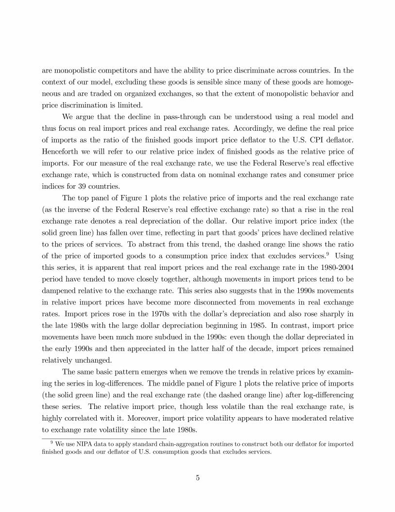
The top panel of Figure 1 plots the relative price of imports and the real exchange rate

(as the inverse of the Federal Reserve’s real effective exchange rate) so that a rise in the real

exchange rate denotes a real depreciation of the dollar. Our relative import price index (the

solid green line) has fallen over time, reflecting in part that goods’ prices have declined relative

to the prices of services. To abstract from this trend, the dashed orange line shows the ratio

of the price of imported goods to a consumption price index that excludes services.9 Using

this series, it is apparent that real import prices and the real exchange rate in the 1980-2004

period have tended to move closely together, although movements in import prices tend to be

dampened relative to the exchange rate. This series also suggests that in the 1990s movements

in relative import prices have become more disconnected from movements in real exchange

rates. Import prices rose in the 1970s with the dollar’s depreciation and also rose sharply in

the late 1980s with the large dollar depreciation beginning in 1985. In contrast, import price

movements have been much more subdued in the 1990s: even though the dollar depreciated in

the early 1990s and then appreciated in the latter half of the decade, import prices remained

relatively unchanged.

The same basic pattern emerges when we remove the trends in relative prices by examin-

ing the series in log-differences. The middle panel of Figure 1 plots the relative price of imports

(the solid green line) and the real exchange rate (the dashed orange line) after log-differencing

these series. The relative import price, though less volatile than the real exchange rate, is

highly correlated with it. Moreover, import price volatility appears to have moderated relative

to exchange rate volatility since the late 1980s.

9 We use NIPA data to apply standard chain-aggregation routines to construct both our deflator for importedfinished goods and our deflator of U.S. consumption goods that excludes services.

5

Table 1 summarizes these findings by comparing the volatility and correlation of the

relative import price and the real exchange rate over different subsamples. The top panel

shows the results for the data in differences and the bottom panel for HP-filtered data. Both

the HP-filtered and differenced data show a marked decline in the ratio of the standard deviation

of import prices, σpm, to the standard deviation of the exchange rate, σq, in the latter half of our

sample. The correlation of the relative import price with the real exchange rate has declined

noticeably as well.

Another important statistic summarizing the relationship between these two series is:

βpm,q =cov(pm, q)

σ2q= corr(pm, q)

σpmσq

, (1)

where pm denotes the relative price of imports and q denotes the real exchange rate. This

statistic takes into account the correlation between the two series as well as their relative

volatility and can be derived as the estimate from a univariate least squares regression of the

real exchange rate on the relative import price. As shown in Table 1, our estimate of βpm,q

has declined in the 1990s, reflecting both the decline in the relative volatility of import prices

and the lower correlation between the two series. Further evidence of the increasing disconnect

between these variable is shown in the bottom panel of Figure 1 which plots estimates of βpm,q

for the log-differenced data based on 10-year, rolling windows (The line with stars indicates

the point estimate and the shaded region denotes the 95 percent confidence region.) There is a

gradual decline in βpm,q beginning in the mid-1980s.

We view the decline in βpm,q as a useful way of summarizing the increasing disconnect

between the relative import price and the real exchange rate. Our summary statistic, βpm,q,

is closely related to estimates of pass-through in empirical studies. One notable difference

is that these studies typically estimate a specification for import prices with the exchange

rate controlling for a number of other factors influencing import prices. A recent paper that

follows this approach is Marazzi, Sheets, and Vigfusson (2005), who argue that pass-through

of exchange rate changes to import prices has fallen from about 0.5 in the 1980s to a current

estimate of 0.2. One reason we choose to use the statistic βpm,q is that it eases comparisons

between the model and the data. However, we note that we get comparable estimates to

Marazzi, Sheets, and Vigfusson (2005) regarding the change in the relationship between import

prices and the exchange rate.10

10 When estimating pass-through, Marazzi, Sheets, and Vigfusson (2005) control for movements in marginalcosts using foreign CPIs and commodity prices. The results are also similar if different control variables are

6

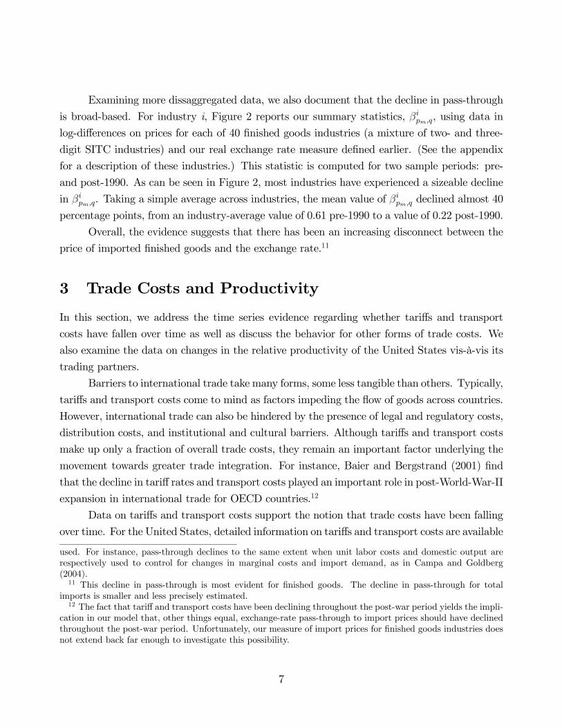
Examining more dissaggregated data, we also document that the decline in pass-through

is broad-based. For industry i, Figure 2 reports our summary statistics, βipm,q, using data in

log-differences on prices for each of 40 finished goods industries (a mixture of two- and three-

digit SITC industries) and our real exchange rate measure defined earlier. (See the appendix

for a description of these industries.) This statistic is computed for two sample periods: pre-

and post-1990. As can be seen in Figure 2, most industries have experienced a sizeable decline

in βipm,q. Taking a simple average across industries, the mean value of βipm,q declined almost 40

percentage points, from an industry-average value of 0.61 pre-1990 to a value of 0.22 post-1990.

Overall, the evidence suggests that there has been an increasing disconnect between the

price of imported finished goods and the exchange rate.11

3 Trade Costs and Productivity

In this section, we address the time series evidence regarding whether tariffs and transport

costs have fallen over time as well as discuss the behavior for other forms of trade costs. We

also examine the data on changes in the relative productivity of the United States vis-à-vis its

trading partners.

Barriers to international trade take many forms, some less tangible than others. Typically,

tariffs and transport costs come to mind as factors impeding the flow of goods across countries.

However, international trade can also be hindered by the presence of legal and regulatory costs,

distribution costs, and institutional and cultural barriers. Although tariffs and transport costs

make up only a fraction of overall trade costs, they remain an important factor underlying the

movement towards greater trade integration. For instance, Baier and Bergstrand (2001) find

that the decline in tariff rates and transport costs played an important role in post-World-War-II

expansion in international trade for OECD countries.12

Data on tariffs and transport costs support the notion that trade costs have been falling

over time. For the United States, detailed information on tariffs and transport costs are available

used. For instance, pass-through declines to the same extent when unit labor costs and domestic output arerespectively used to control for changes in marginal costs and import demand, as in Campa and Goldberg(2004).11 This decline in pass-through is most evident for finished goods. The decline in pass-through for total

imports is smaller and less precisely estimated.12 The fact that tariff and transport costs have been declining throughout the post-war period yields the impli-

cation in our model that, other things equal, exchange-rate pass-through to import prices should have declinedthroughout the post-war period. Unfortunately, our measure of import prices for finished goods industries doesnot extend back far enough to investigate this possibility.

7

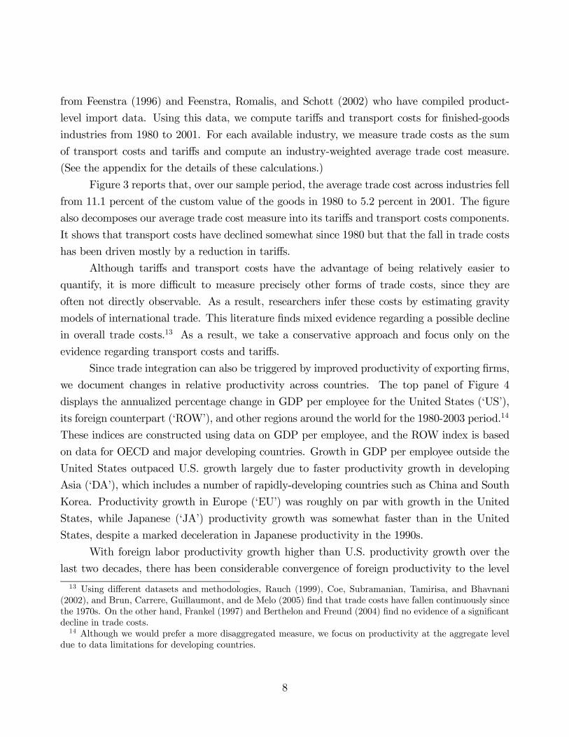
from Feenstra (1996) and Feenstra, Romalis, and Schott (2002) who have compiled product-

level import data. Using this data, we compute tariffs and transport costs for finished-goods

industries from 1980 to 2001. For each available industry, we measure trade costs as the sum

of transport costs and tariffs and compute an industry-weighted average trade cost measure.

(See the appendix for the details of these calculations.)

Figure 3 reports that, over our sample period, the average trade cost across industries fell

from 11.1 percent of the custom value of the goods in 1980 to 5.2 percent in 2001. The figure

also decomposes our average trade cost measure into its tariffs and transport costs components.

It shows that transport costs have declined somewhat since 1980 but that the fall in trade costs

has been driven mostly by a reduction in tariffs.

Although tariffs and transport costs have the advantage of being relatively easier to

quantify, it is more difficult to measure precisely other forms of trade costs, since they are

often not directly observable. As a result, researchers infer these costs by estimating gravity

models of international trade. This literature finds mixed evidence regarding a possible decline

in overall trade costs.13 As a result, we take a conservative approach and focus only on the

evidence regarding transport costs and tariffs.

Since trade integration can also be triggered by improved productivity of exporting firms,

we document changes in relative productivity across countries. The top panel of Figure 4

displays the annualized percentage change in GDP per employee for the United States (‘US’),

its foreign counterpart (‘ROW’), and other regions around the world for the 1980-2003 period.14

These indices are constructed using data on GDP per employee, and the ROW index is based

on data for OECD and major developing countries. Growth in GDP per employee outside the

United States outpaced U.S. growth largely due to faster productivity growth in developing

Asia (‘DA’), which includes a number of rapidly-developing countries such as China and South

Korea. Productivity growth in Europe (‘EU’) was roughly on par with growth in the United

States, while Japanese (‘JA’) productivity growth was somewhat faster than in the United

States, despite a marked deceleration in Japanese productivity in the 1990s.

With foreign labor productivity growth higher than U.S. productivity growth over the

last two decades, there has been considerable convergence of foreign productivity to the level

13 Using different datasets and methodologies, Rauch (1999), Coe, Subramanian, Tamirisa, and Bhavnani(2002), and Brun, Carrere, Guillaumont, and de Melo (2005) find that trade costs have fallen continuously sincethe 1970s. On the other hand, Frankel (1997) and Berthelon and Freund (2004) find no evidence of a significantdecline in trade costs.14 Although we would prefer a more disaggregated measure, we focus on productivity at the aggregate level

due to data limitations for developing countries.

8

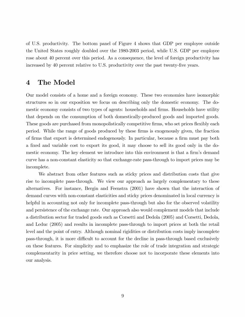
of U.S. productivity. The bottom panel of Figure 4 shows that GDP per employee outside

the United States roughly doubled over the 1980-2003 period, while U.S. GDP per employee

rose about 40 percent over this period. As a consequence, the level of foreign productivity has

increased by 40 percent relative to U.S. productivity over the past twenty-five years.

4 The Model

Our model consists of a home and a foreign economy. These two economies have isomorphic

structures so in our exposition we focus on describing only the domestic economy. The do-

mestic economy consists of two types of agents: households and firms. Households have utility

that depends on the consumption of both domestically-produced goods and imported goods.

These goods are purchased from monopolistically competitive firms, who set prices flexibly each

period. While the range of goods produced by these firms is exogenously given, the fraction

of firms that export is determined endogenously. In particular, because a firm must pay both

a fixed and variable cost to export its good, it may choose to sell its good only in the do-

mestic economy. The key element we introduce into this environment is that a firm’s demand

curve has a non-constant elasticity so that exchange-rate pass-through to import prices may be

incomplete.

We abstract from other features such as sticky prices and distribution costs that give

rise to incomplete pass-through. We view our approach as largely complementary to these

alternatives. For instance, Bergin and Feenstra (2001) have shown that the interaction of

demand curves with non-constant elasticities and sticky prices denominated in local currency is

helpful in accounting not only for incomplete pass-through but also for the observed volatility

and persistence of the exchange rate. Our approach also would complement models that include

a distribution sector for traded goods such as Corsetti and Dedola (2005) and Corsetti, Dedola,

and Leduc (2005) and results in incomplete pass-through to import prices at both the retail

level and the point of entry. Although nominal rigidities or distribution costs imply incomplete

pass-through, it is more difficult to account for the decline in pass-through based exclusively

on these features. For simplicity and to emphasize the role of trade integration and strategic

complementarity in price setting, we therefore choose not to incorporate these elements into

our analysis.

9

4.1 Households

The utility function of the representative household in the home country is

Et

∞Xj=0

βjlog (Ct+j)− χ0L1+χt+j

1 + χ, (2)

where the discount factor β satisfies 0 < β < 1 and Et is the expectation operator conditional

on information available at time t. The period utility function depends on consumption Ct and

labor Lt. A household also purchases state-contingent assets bt+1 that are traded internationally

so that asset markets are complete.

Household’s receive income fromworking and an aliquot share of profits of all the domestic

firms, Ωt. In choosing its contingency plans for Ct, Lt, bt+1, a household takes into account its

budget constraint at each date:

Ct +

Zs

pbt,t+1bt+1 − bt = wtLt + Ωt. (3)

In equation (3), wt =Wt

Ptis household’s real wage and pbt,t+1 denotes the price of an asset that

pays one unit of the domestic consumption good in a particular state of nature at date t + 1.

(For convenience, we have suppressed that variables depend on the state of nature.).

4.2 Demand Aggregator

There is a continuum of goods indexed by i ∈ [0, 1] produced in each economy. While a domestichousehold purchases all of the domestically-produced goods, there are only i ∈ [0, ω∗t ] that areavailable for imports, where ω∗t denotes the endogenously determined fraction of traded foreign

goods. A household chooses domestically-produced goods, Cdt(i), and imported goods, Cmt(i),

to minimize their total expenditures:∙Z 1

0

Pdt(i)Cdt(i)di+

Z ω∗t

0

Pmt(i)Cmt(i)di

¸, (4)

subject to D³Cdt(i)Ct

, Cmt(i)Ct

´= 1. In minimizing its expenditures, a household takes the prices of

the domestic, Pdt(i), and imported goods, Pmt(i), as given. (For convenience, we denote these

prices in nominal terms, although prices are flexible in the model and we solve only for real

variables.) In our model, there are no distribution services required to sell the imported goods

10

to households. Accordingly, Pmt(i) denotes both the retail import price for good i and price

charged at the point of entry.

The function, D³Cdt(i)Ct

, Cmt(i)Ct

´, is a household’s demand aggregator for producing a unit

of Ct and is defined by:

D

µCdt(i)

Ct,Cmt(i)

Ct

¶=

∙1

1 + ω∗tV

1ρ

dt +ω∗t

1 + ω∗tV

1ρ

mt

¸ρ− 1

(1 + η)γ+ 1, (5)

In this expression, Vdt is an aggregator for domestic goods given by:

Vdt =

Z 1

0

1

(1 + ω∗t )(1 + η)γ

∙(1 + ω∗t )(1 + η)

Cdt(i)

Ct− η

¸γdi, (6)

and Vmt is an aggregator for imported goods given by:

Vmt =1

ω∗t

Z ω∗t

0

1

(1 + ω∗t )(1 + η)γ

∙(1 + ω∗t )(1 + η)

Cmt(i)

Ct− η

¸γdi. (7)

Our demand aggregator adapts the one discussed in Dotsey and King (2005) to an inter-

national environment. It shares the central feature that the elasticity of demand is nonconstant

(NCES) with η 6= 0, and the (absolute value of the) demand elasticity can be expressed as anincreasing function of a firm’s relative price when η < 0.15 This feature has proven useful in

the sticky price literature, because it helps mitigate a firm’s incentive to raise its price after

an expansionary monetary shock in the context of a model in which other firms have already

preset their prices. It is also consistent with the evidence that firms tend to change their prices

more in response to cost increases than decreases (see, for instance, Peltzman (2000)). Another

important implication of this aggregator, discussed below, is that exchange-rate pass-through to

import prices will be incomplete when the elasticity of demand is increasing in a firm’s relative

price.

Expenditure minimization by a domestic household implies that the demand curve for

15 When η = 0, our demand aggregator can be thought of as the combination of a Dixit-Stiglitz and Armingtonaggregator. To see this, note that in this case we can rewrite our aggregator as:

Ct = (1 + ω∗t )

∙1

1 + ω∗tC

γρ

dt +ω∗t

1 + ω∗tC

γρ

mt

¸ ργ

,

where Cdt =³R 1

0Cdt(i)

γdi´ 1γ

and Cmt =³1ω∗t

R ω∗t0

Cmt(i)γdi´ 1γ

. Our specification of the demand aggregator

also rules out the “love of variety” effect.

11

an imported good is given by:

Cmt(i)

Ct=

1

1 + ω∗t

"1

1 + η

µPmt(i)

Γt

¶ 1γ−1µPmt

Γt

¶ γγ−ρ

ρ−1γ−1

+η

1 + η

#. (8)

In the above, Γt is a price index consisting of the prices of a firm’s competitors defined as:

Γt =

∙µ1

1 + ω∗t

¶P

γγ−ρdt +

µω∗t

1 + ω∗t

¶P

γγ−ρmt

¸γ−ργ

, (9)

and Pdt and Pmt are indices of domestic and import prices defined as:

Pdt =

µZ 1

0

Pdt(i)γ

γ−1di

¶γ−1γ

, (10)

Pmt =

µ1

ω∗t

Z ω∗t

0

Pmt(i)γ

γ−1di

¶γ−1γ

. (11)

Expenditure minimization also implies an analagous expression for the demand curve of do-

mestic good i, which depends on prices, Pdt(i), Pdt, and Γt.

A property of these demand curves is that the elasticity of substitution between a home

and foreign good can differ from the demand elasticity for two home goods. This separate

elasticity for goods occurs when ρ 6= 1, which gives the model more flexibility to match estimatesof the elasticity of substitution between home and foreign tradeables as well as estimates of

economy-wide markups. More importantly, when η 6= 0, the demand curve has an additive

linear term, which implies that the elasticity of demand depends on the price of good i relative

to other prices. It is this feature that helps give rise to incomplete pass-through to import prices

and implies that pass-through depends on the economy’s structure including the underlying

shocks.

The aggregate consumer price level is given by

Pt =1

1 + ηΓt +

η

1 + η

∙1

1 + ω∗t

Z 1

0

Pdt(i)di+1

1 + ω∗t

Z ω∗t

0

Pmt(i)di

¸. (12)

From this expression, it is clear that the consumer price level is equal to the competitive pricing

bundle, Γt, when η = 0. In general, the consumer price level is the sum of Γt with a linear

aggregator of prices for individual goods.16

16 The consumer price level can be derived from equating equation (4) to PtCt and substituting in the relative

12

4.3 Firms

The production function for firm i is linear in labor so that

Yt(i) = ZtLt(i). (13)

In the above, Zt is an aggregate, iid technology shock that affects the production function for

all firms in the home country. A firm hires labor in a competitive market in which labor is

completely mobile within a country but immobile across countries. Marginal cost is therefore

the same for all firms in the home country so that real marginal cost of firm i is given by wtZt.

Firms in each country are monopolistically competitive and each firm sells its good to

households located in its country. Profit maximization implies that a firm chooses to set its

price as a markup over marginal cost. As a result, the price of good i in the domestic market

satisfies:

Pdt(i)

Pt= μdt(i)

wt

Zt, i ∈ [0, 1] , (14)

with μdt(i) ≥ 1. The markup μdt(i) can be expressed as:

μdt(i) = μdt =

∙1− 1

| dt|

¸−1=

"γ + η(γ − 1)

µPdt

Γt

¶ ρρ−γ#−1

, (15)

where | dt|, is the absolute value of the elasticity of a domestic good given by:

dt =

"(γ − 1)

Ã1 + η

µPdt

Γt

¶ ρρ−γ!#−1

. (16)

In the above, we have dropped the index i, since we restrict our attention to a symmetric

equilibrium in which all firms set the same price in the domestic market (i.e., Pdt(i) = Pdt,

dt(i) = dt, and μdt(i) = μdt.)

Equation (15) shows that a firm’s markup depends on the price it sets relative to its

competitors price Γt. When the (absolute value of) the demand elasticity is increasing inPdtΓt, the markup will be a decreasing function of this relative price. Consequently, a firm will

respond to a fall in the price of its competitors by lowering its markup and price. A firm finds it

desirable to do so, because otherwise it will experience a relatively large fall in its market share.

demand curves. The price Γt can be derived from substituting the relative demand curves into equation (5).

13

An important exception to this pricing behavior is the CES demand curve in which η = 0. In

this case, a firm’s markup does not depend on the relative price of its competitors.

We view our setup with variable markups as a tractable way to capture the strategic

complementarity amongst price-setting firms. Although we do not explicitly model strategic

behavior using a game-theoretic framework, our setup has similar implications to those of

Bodnar, Dumas, andMarston (2002), Bernard, Eaton, Jensen, and Kortum (2003), and Atkeson

and Burstein (2005) who model the strategic complementarity that arises between firms through

Cournot or Bertrand competition. These alternative setups, like ours, give rise to a markup

that is increasing in a firm’s market share or decreasing in its price relative to those of its

competitors.

Following Melitz (2003), Ghironi and Melitz (2005) and Bergin and Glick (2005), we allow

for the endogenous entry and exit of firms into the export market. In particular, we assume

that each period a firm faces a fixed and per-unit export cost and decides whether to export

or not. Unlike these previous papers, which allow productivity to vary with a good’s type, we

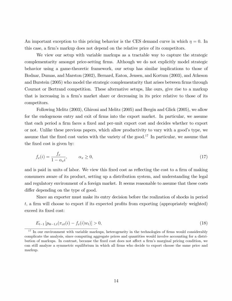
assume that the fixed cost varies with the variety of the good.17 In particular, we assume that

the fixed cost is given by:

fx(i) =fx

1− αxi, αx ≥ 0, (17)

and is paid in units of labor. We view this fixed cost as reflecting the cost to a firm of making

consumers aware of its product, setting up a distribution system, and understanding the legal

and regulatory environment of a foreign market. It seems reasonable to assume that these costs

differ depending on the type of good.

Since an exporter must make its entry decision before the realization of shocks in period

t, a firm will choose to export if its expected profits from exporting (appropriately weighted)

exceed its fixed cost:

Et−1 [pbt−1,t(πxt(i)− fx(i)wt)] > 0, (18)

17 In our environment with variable markups, heterogeneity in the technologies of firms would considerablycomplicate the analysis, since computing aggregate prices and quantities would involve accounting for a distri-bution of markups. In contrast, because the fixed cost does not affect a firm’s marginal pricing condition, wecan still analyze a symmetric equilibrium in which all firms who decide to export choose the same price andmarkup.

14

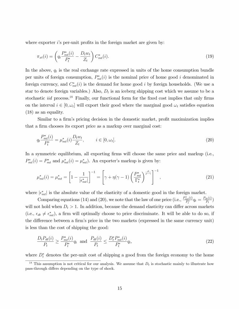
where exporter i’s per-unit profits in the foreign market are given by:

πxt(i) =

µqtP ∗mt(i)

P ∗t− Dtwt

Zt

¶C∗mt(i). (19)

In the above, qt is the real exchange rate expressed in units of the home consumption bundle

per units of foreign consumption, P ∗mt(i) is the nominal price of home good i denominated in

foreign currency, and C∗mt(i) is the demand for home good i by foreign households. (We use a

star to denote foreign variables.) Also, Dt is an iceberg shipping cost which we assume to be a

stochastic iid process.18 Finally, our functional form for the fixed cost implies that only firms

on the interval i ∈ [0, ωt] will export their good where the marginal good ωt satisfies equation

(18) as an equality.

Similar to a firm’s pricing decision in the domestic market, profit maximization implies

that a firm chooses its export price as a markup over marginal cost:

qtP ∗mt(i)

P ∗t= μ∗mt(i)

Dtwt

Zt, i ∈ [0, ωt]. (20)

In a symmetric equilibrium, all exporting firms will choose the same price and markup (i.e.,

P ∗mt(i) = P ∗mt and μ∗mt(i) = μ∗mt). An exporter’s markup is given by:

μ∗mt(i) = μ∗mt =

∙1− 1

| ∗mt|

¸−1=

"γ + η(γ − 1)

µP ∗mt

Γ∗t

¶ ρρ−γ#−1

, (21)

where | ∗mt| is the absolute value of the elasticity of a domestic good in the foreign market.Comparing equations (14) and (20), we note that the law of one price (i.e., P

∗mt(i)

P ∗tqt =

Pdt(i)Pt)

will not hold when Dt > 1. In addition, because the demand elasticity can differ across markets

(i.e., dt 6= ∗mt), a firm will optimally choose to price discriminate. It will be able to do so, if

the difference between a firm’s price in the two markets (expressed in the same currency unit)

is less than the cost of shipping the good:

DtPdt(i)

Pt≥ P ∗mt(i)

P ∗tqt and

Pdt(i)

Pt≤ D∗

tP∗mt(i)

P ∗tqt, (22)

where D∗t denotes the per-unit cost of shipping a good from the foreign economy to the home

18 This assumption is not critical for our analysis. We assume that Dt is stochastic mainly to illustrate howpass-through differs depending on the type of shock.

15

economy.19 The first condition ensures that a foreign household can not buy the good for less

in the domestic market inclusive of the cost of shipping the good. The second condition ensures

that a domestic household can not buy the good for less abroad. Later, we verify that these

conditions and their counterparts for the prices set by foreign firms are satisfied.

4.4 Market Clearing

The home economy’s aggregate resource constraint can be written as:Z 1

0

Cdt(i)

Ztdi+

Z ωt

0

DtC∗mt(i)

Ztdi+

Z ωt

0

fx(i)di = Lt. (23)

Given that we focus on a symmetric equilibrium, we define aggregate output as Yt = ZtLt.

Finally, we note that the foreign economy has an isomorphic structure to the home economy

and differs only in its level of trade costs and technology.

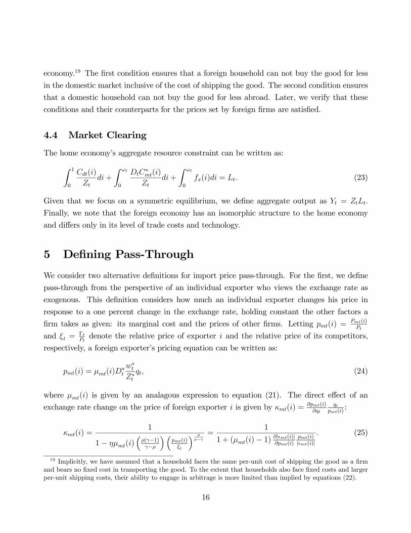
5 Defining Pass-Through

We consider two alternative definitions for import price pass-through. For the first, we define

pass-through from the perspective of an individual exporter who views the exchange rate as

exogenous. This definition considers how much an individual exporter changes his price in

response to a one percent change in the exchange rate, holding constant the other factors a

firm takes as given: its marginal cost and the prices of other firms. Letting pmt(i) =Pmt(i)Pt

and ξt =ΓtPtdenote the relative price of exporter i and the relative price of its competitors,

respectively, a foreign exporter’s pricing equation can be written as:

pmt(i) = μmt(i)D∗t

w∗tZ∗t

qt, (24)

where μmt(i) is given by an analagous expression to equation (21). The direct effect of an

exchange rate change on the price of foreign exporter i is given by κmt(i) =∂pmt(i)∂qt

qtpmt(i)

:

κmt(i) =1

1− ημmt(i)³ρ(γ−1)γ−ρ

´³pmt(i)ξt

´ ρρ−γ

=1

1 + (μmt(i)− 1) ∂| mt(i)|∂pmt(i)

pmt(i)| mt(i)|

. (25)

19 Implicitly, we have assumed that a household faces the same per-unit cost of shipping the good as a firmand bears no fixed cost in transporting the good. To the extent that households also face fixed costs and largerper-unit shipping costs, their ability to engage in arbitrage is more limited than implied by equations (22).

16

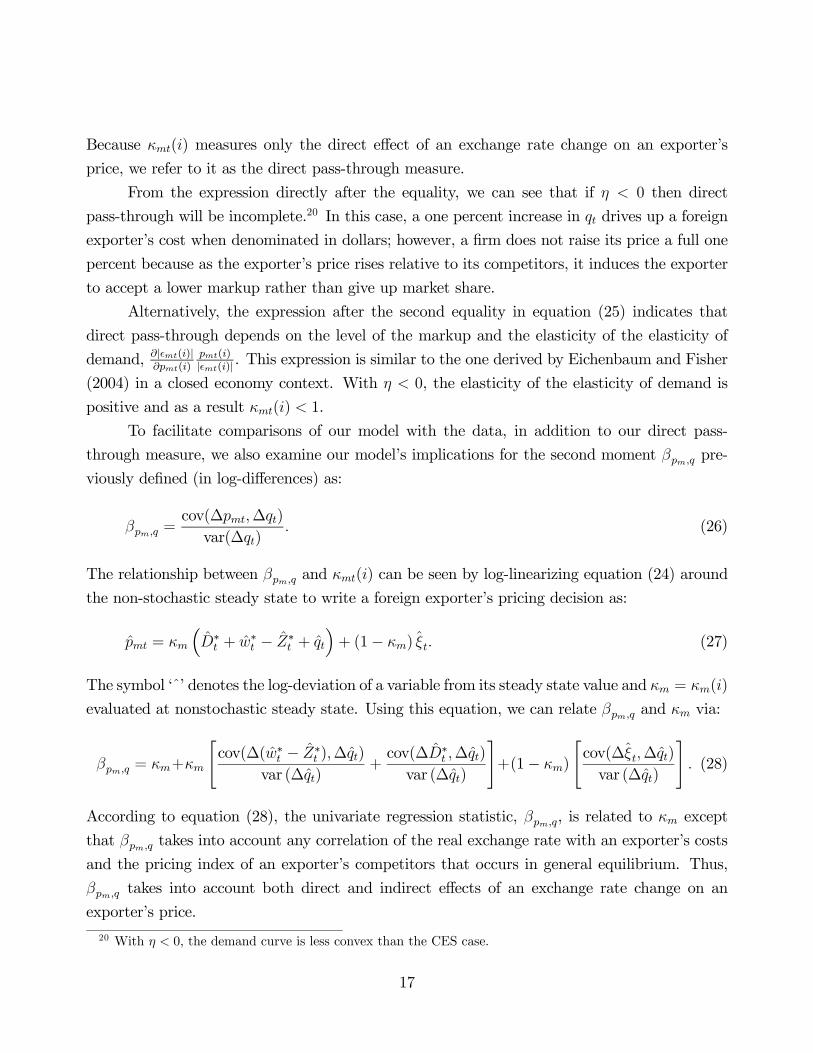
Because κmt(i) measures only the direct effect of an exchange rate change on an exporter’s

price, we refer to it as the direct pass-through measure.

From the expression directly after the equality, we can see that if η < 0 then direct

pass-through will be incomplete.20 In this case, a one percent increase in qt drives up a foreign

exporter’s cost when denominated in dollars; however, a firm does not raise its price a full one

percent because as the exporter’s price rises relative to its competitors, it induces the exporter

to accept a lower markup rather than give up market share.

Alternatively, the expression after the second equality in equation (25) indicates that

direct pass-through depends on the level of the markup and the elasticity of the elasticity of

demand, ∂| mt(i)|∂pmt(i)

pmt(i)| mt(i)| . This expression is similar to the one derived by Eichenbaum and Fisher

(2004) in a closed economy context. With η < 0, the elasticity of the elasticity of demand is

positive and as a result κmt(i) < 1.

To facilitate comparisons of our model with the data, in addition to our direct pass-

through measure, we also examine our model’s implications for the second moment βpm,q pre-

viously defined (in log-differences) as:

βpm,q =cov(∆pmt,∆qt)

var(∆qt). (26)

The relationship between βpm,q and κmt(i) can be seen by log-linearizing equation (24) around

the non-stochastic steady state to write a foreign exporter’s pricing decision as:

pmt = κm³D∗

t + w∗t − Z∗t + qt´+ (1− κm) ξt. (27)

The symbol ‘ˆ’ denotes the log-deviation of a variable from its steady state value and κm = κm(i)

evaluated at nonstochastic steady state. Using this equation, we can relate βpm,q and κm via:

βpm,q = κm+κm

"cov(∆(w∗t − Z∗t ),∆qt)

var (∆qt)+cov(∆D∗

t ,∆qt)

var (∆qt)

#+(1− κm)

"cov(∆ξt,∆qt)

var (∆qt)

#. (28)

According to equation (28), the univariate regression statistic, βpm,q, is related to κm except

that βpm,q takes into account any correlation of the real exchange rate with an exporter’s costs

and the pricing index of an exporter’s competitors that occurs in general equilibrium. Thus,

βpm,q takes into account both direct and indirect effects of an exchange rate change on an

exporter’s price.

20 With η < 0, the demand curve is less convex than the CES case.

17

In our analysis, we focus on comparing our model results to the data for βpm,q rather than

κm. This reflects that βpm,q is a second moment that is easily measured in the data. In contrast,

measuring κm is complicated by finding good measures of marginal costs and the prices of a

firm’s competitors as well as correctly specifying the equations for estimating κm and dealing

with the endogeneity of the exchange rate and the prices of other firms.

6 Calibration

In order to investigate the role of trade costs and productivity differentials on pass-through, we

log-linearize and solve the model around two different steady states. In the first, the home and

foreign economies are identical, and both economies have relatively high trade costs. We call

this our benchmark calibration. In the second, we lower trade costs as well as raise the level

of foreign productivity, keeping the remaining parameters constant.21 We call this the 2004

calibration.

The value of η, which governs the curvature of the demand curve, is critical for our

analysis. Faced with sparse independent evidence regarding this parameter, we calibrate it as

a part of a simulated method of moments procedure. Specifically, we choose η along with the

standard deviations of the iid technology and trade cost shocks so that the model’s implications

for the volatility of output, the ratio of the volatility of relative import prices to the real exchange

rate, and the correlation between relative import prices and the real exchange rate match those

observed in the 1980-1989 period. In doing so, we constrain the standard deviation of the

technology shocks and trade costs shocks to be the same in both countries (i.e., σz = σ∗z and

σD = σD∗). By construction, our model matches the observed value of βpm,q for the 1980s.

With η pinned down based on the pre-1990s data, we then examine the fall in βpm,q arising

from a fall in trade costs and a higher level of foreign productivity.

Tables 2 show our calibrated value of η as well as the calibrated values of other important

parameters of the model. We choose γ to be consistent with an exporter’s markup over marginal

cost of around 20 percent in the benchmark calibration. We set ρ = 0.85, which implies

21 While the level of foreign productivity is actually lower than U.S. productivity, for simplicity we begin witha calibration in which the two economies are identical. This simplification seems reasonable, since our results forthe decline in pass-through depend critically on the change in relative productivity in the two countries ratherthan their initial levels.

18

an aggregate trade-price elasticity for the benchmark calibration of 2.22 The discount factor

β = 1.03−0.25, and the utility function parameter χ is set to 1.5, which implies a Frisch elasticity

of labor supply of 2/3. We set χ0 and χ∗0 to imply L = L∗ = 1 in the benchmark calibration.

For the initial levels of technology, we choose Z = Z∗ = 1. As discussed earlier, foreign

technology rose about 40 percent relative to the level of U.S. productivity over the past 25

years. For the 2004 calibration, we choose a more conservative 35 percent increase in relative

productivity by setting Z∗ = 1.35. Consistent with Figure 3, we set D = D∗ = 1.1 in the

benchmark calibration and lowered D = D∗ = 1.05 in the 2004 calibration.

For the fixed costs of trade we set fx = f∗x = 0.46 which implies that the import share in

the home economy is about 10 percent. Since we assume that trade is balanced in the initial

steady state, the foreign economy has the same import share. We choose αx = α∗x = 2.5 so

that after the fall in trade costs and increase in foreign productivity the home country’s import

share rises about 4 percentage points.

We also compare our benchmark calibration to one with CES preferences (i.e., η = 0).

Table 2 reports the parameter values used for the CES calibration, which were selected in

an analogous manner to our benchmark calibration. Table 3 shows that both the CES and

benchmark calibration (by construction) match the observed volatility of output and correlation

between import prices and the exchange rate in the 1980s. However, only the benchmark

calibration with η 6= 0 has the flexibility to match the observed value of βpm,q in the 1980s.

Although the benchmark calibration implies slightly more exchange rate volatility than the CES

calibration, both versions of the model understate the amount of volatility relative to the data.

Thus, while the NCES demand curves better account for the observed relationship between

the relative import price and the real exchange rate, they do not by themselves explain other

important aspects of the data emphasized in the international business cycle literature.23

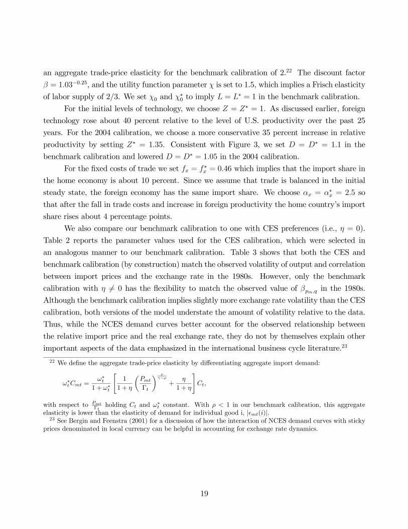
22 We define the aggregate trade-price elasticity by differentiating aggregate import demand:

ω∗tCmt =ω∗t

1 + ω∗t

"1

1 + η

µPmt

Γt

¶ ργ−ρ

+η

1 + η

#Ct,

with respect to Pmt

Γtholding Ct and ω∗t constant. With ρ < 1 in our benchmark calibration, this aggregate

elasticity is lower than the elasticity of demand for individual good i, | mt(i)|.23 See Bergin and Feenstra (2001) for a discussion of how the interaction of NCES demand curves with sticky

prices denominated in local currency can be helpful in accounting for exchange rate dynamics.

19

7 Results

To gain intuition for our main results, we first illustrate the implications of our setup for

pass-through in partial equilibrium. We then demonstrate how our preferred measure of pass-

through, βpm,q, depends on the economy’s shocks. Finally, we discuss our main findings re-

garding the effects of falling trade costs and higher foreign productivity on pass-through. In

doing so, we pay particular attention to the influence of both the intensive and extensive trade

margins.

7.1 A Partial Equilibrium Explanation for Declining Pass-Through

The upper left panel of Figure 5 plots our calibrated demand curve of import good i and

compares it to the CES demand curve. The absolute value of the demand elasticity for good

i, | mt(i)|, is shown in the upper right panel. Our calibrated demand curve is consistent withstrategic complementarity in price setting, as the absolute value of the elasticity is increasing

in an exporter’s relative price. Therefore, an exporter finds it optimal to reduce its markup

rather than increase its prices, and, hence, direct pass-through, κmt(i), is incomplete.

Another important implication of our demand curve is that pass-through will fall with

a decline in the cost of exporting. Thus, our model will be able to account for a declining

pass-through via either a fall in trade costs or a rise in foreign productivity relative to U.S.

productivity. We now discuss the intuition for this result.

We begin by noting that foreign exporter i ’s marginal revenue satisfies:

MRmt(i) =Pmt(i)

μmt(i)= Pmt(i)

∙1− 1

| mt(i)|

¸. (29)

The lower left panel of Figure 5 displays marginal revenue (in logs and scaled by Γt) as a function

of the relative price Pmt(i)Γt. As a firm increases its price relative to the price of its competitors,

marginal revenue exhibits diminishing returns. At a low relative price, the demand elasticity

is also low and an increase in exporter i ’s relative price boosts marginal revenue because of a)

the direct effect of the rise in the firm’s price and b) the increase in the demand elasticity as

an exporter’s price rises relative to its competitors. However, as the exporter’s relative price

increases and the demand elasticity becomes high enough, the latter effect becomes negligible

and the increase in marginal revenue is limited to only the direct effect of the increase in price.

(As the demand elasticity approaches infinity, a firm is essentially setting its price equal to

marginal cost.) Thus, the effect of strategic complementarity in price setting diminishes as the

20

elasticity rises, and, as displayed in the lower right panel of Figure 5, an exporter’s markup is

more responsive to Pmt(i)Γt

at a low elasticity (i.e., high markup) and less responsive to Pmt(i)Γt

at

a high elasticity (i.e., low markup).

A consequence of the concavity of the marginal revenue schedule is that a fall in an

exporter’s costs will result in a decline in direct pass-through. To illustrate this point, consider

the dashed blue line, labelled mcH , of the lower left panel, which shows the logarithm of

the exporter’s marginal cost denominated in domestic currency units (also scaled by Γt). At

this portion of the marginal revenue schedule, a real (exogenous) depreciation of the domestic

currency that results in a 3 percent increase in firm i ’s marginal cost (mc0H) only results in

about a 1 percent increase in a firm’s relative price, so that direct pass-through is roughly 33

percent. Now, suppose a fall in trade costs shifts the firm’s marginal costs down to mcL. In this

case, a 3 percent real depreciation of the domestic currency increases the exporter’s costs from

mcL to mc0L and results in only about a 0.45 percent increase in relative price, so that direct

pass-through is roughly 15 percent. Pass through is lower for a low-cost producer because a cost

increase requires a smaller increase in price, since the associated rise in the demand elasticity

provides an extra boost to marginal revenue.

In comparison, under CES demand curves direct pass-through of exchange-rate changes

will be complete: A two percent home currency depreciation results in a two percent increase

in price regardless of an exporter’s costs. This reflects the fact that the demand elasticity, and

thus the markup, do not vary with a monopolist’s relative price.

7.2 The Effects of Different Shocks on Pass-Through

We now show that productivity and trade-cost shocks have different effects on our two measures

of pass-through. An important difference between the two measures is that κm is independent

of the economy’s iid shocks, while βpm,q is not. To illustrate this, the second column of Table

4 shows the effects of a one standard deviation increase in home technology for the benchmark

calibration. Home technology shocks induce a real depreciation of the home currency (i.e., a

rise in qt) and put upward pressure on the real marginal cost of foreign firms, as foreign labor

supply contracts and real wages rise abroad. Import prices at home increase, though by less

than the rise in qt, since foreign exporters react by lowering their markups. Accordingly, our

measure of pass-through, βpm,q, will be positive following a technology shock, as import prices

rise with the real exchange rate.

The implications of a change in trade costs on pass-through differ substantially from

21

those triggered by changes in technology. The third column of the table shows that following

an increase in the foreign exporter’s per-unit cost D∗t pass-through will be negative: because

of the fall in the demand for foreign goods, the increase in foreign trade costs leads to an

appreciation of the domestic currency, while import prices simultaneously rise as the cost of

exporting increases. Note that import prices do not rise as much as the increase in foreign real

marginal costs since foreign exporters decide to lower their markups.

Overall, our calibration procedure implies that the bulk of the variation in the real ex-

change rate and the relative import price are driven primarily by technology shocks. As a

consequence, the values of βpm,q reported in Table 3 for the benchmark calibration mainly

reflect the influence of technology shocks.24

7.3 Trade Integration and Declining Pass-Through

Table 5 shows the effects of lowering trade costs and higher foreign productivity on pass-through

and important steady state prices and quantities. The table shows the value of the variables in

steady state except for βpm,q, which is obtained from log-linearizing the model and computing

the population moments of the model’s variables given the shock processes. We start by looking

at the effects of changing one variable at a time (columns 2, 3 and 5), before analyzing their

combined impacts (last column). As shown in the second column, a five percentage point fall in

the trade costs of foreign exporters reduces the real marginal cost of exporting (denominated in

terms of the home consumption bundle) by 3.5 percent. Note that the fall in foreign exporters’

real marginal cost, qD∗w∗Z∗ , is less than the decline in D∗ as increased demand for the foreign

good puts upward pressure on the real exchange rate, q, and on foreign wages. With lower costs,

foreign exporters reduce their prices and the home country’s import share rises 0.7 percentage

point. Because foreign exporters’ prices fall relative to their competitors - the domestic firms,

they are able to increase their markups and still gain market share. Conversely, the prices for

domestic goods rise relative to their competitors, and domestic firms are forced to cut their

markups in reaction to stiffer competition from abroad.

With higher markups on foreign goods, the strategic complementarity intensifies and

foreign exporters become more willing to vary their markups in response to cost shocks (see

the lower left panel of Figure 5). Thus, the 5 percentage point decline in trade costs causes the

24 It is interesting to note that the cyclicality of the domestic producers’ markups in the home marketdepends on the source of the shock. Domestic markups are countercyclical conditional on changes in trade costsfaced by home exporters and procyclical with respect to the other shocks. The domestic markup is procyclicalunconditionally, reflecting the importance of technology shocks. Incorporating nominal rigidities in domesticprices would imply a countercyclical markup.

22

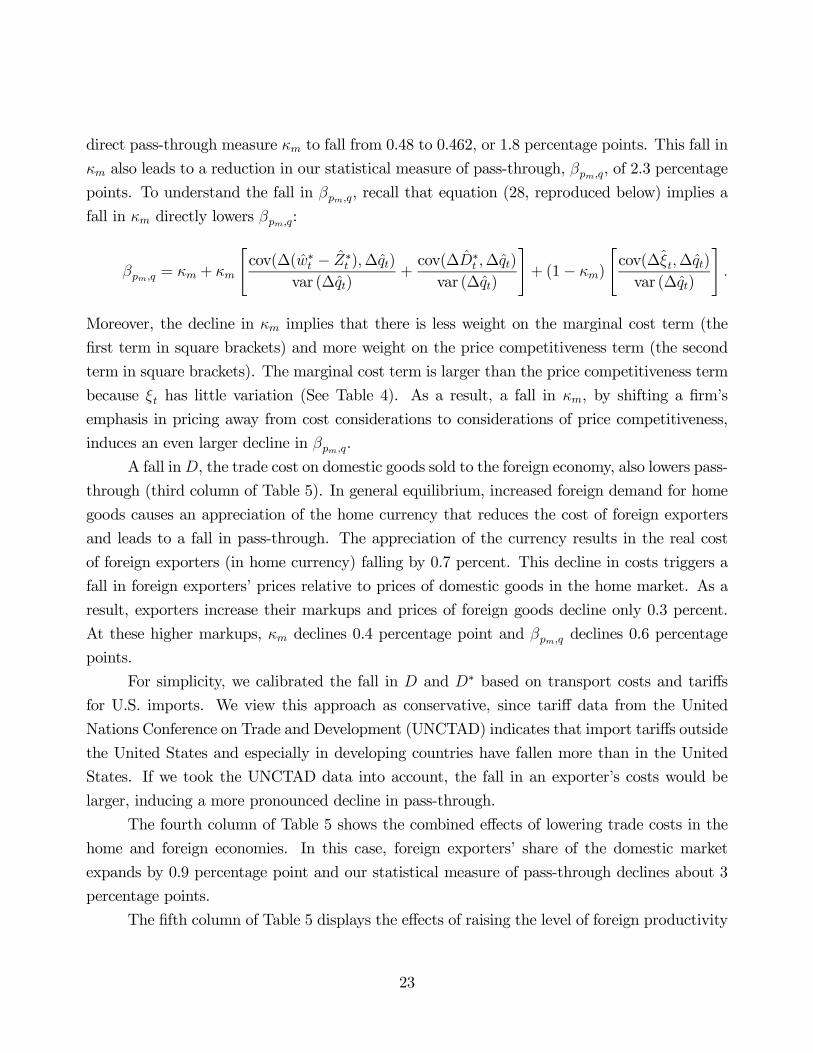
direct pass-through measure κm to fall from 0.48 to 0.462, or 1.8 percentage points. This fall in

κm also leads to a reduction in our statistical measure of pass-through, βpm,q, of 2.3 percentage

points. To understand the fall in βpm,q, recall that equation (28, reproduced below) implies a

fall in κm directly lowers βpm,q:

βpm,q = κm + κm

"cov(∆(w∗t − Z∗t ),∆qt)

var (∆qt)+cov(∆D∗

t ,∆qt)

var (∆qt)

#+ (1− κm)

"cov(∆ξt,∆qt)

var (∆qt)

#.

Moreover, the decline in κm implies that there is less weight on the marginal cost term (the

first term in square brackets) and more weight on the price competitiveness term (the second

term in square brackets). The marginal cost term is larger than the price competitiveness term

because ξt has little variation (See Table 4). As a result, a fall in κm, by shifting a firm’s

emphasis in pricing away from cost considerations to considerations of price competitiveness,

induces an even larger decline in βpm,q.

A fall inD, the trade cost on domestic goods sold to the foreign economy, also lowers pass-

through (third column of Table 5). In general equilibrium, increased foreign demand for home

goods causes an appreciation of the home currency that reduces the cost of foreign exporters

and leads to a fall in pass-through. The appreciation of the currency results in the real cost

of foreign exporters (in home currency) falling by 0.7 percent. This decline in costs triggers a

fall in foreign exporters’ prices relative to prices of domestic goods in the home market. As a

result, exporters increase their markups and prices of foreign goods decline only 0.3 percent.

At these higher markups, κm declines 0.4 percentage point and βpm,q declines 0.6 percentage

points.

For simplicity, we calibrated the fall in D and D∗ based on transport costs and tariffs

for U.S. imports. We view this approach as conservative, since tariff data from the United

Nations Conference on Trade and Development (UNCTAD) indicates that import tariffs outside

the United States and especially in developing countries have fallen more than in the United

States. If we took the UNCTAD data into account, the fall in an exporter’s costs would be

larger, inducing a more pronounced decline in pass-through.

The fourth column of Table 5 shows the combined effects of lowering trade costs in the

home and foreign economies. In this case, foreign exporters’ share of the domestic market

expands by 0.9 percentage point and our statistical measure of pass-through declines about 3

percentage points.

The fifth column of Table 5 displays the effects of raising the level of foreign productivity

23

by 35 percent. Although there is a substantial increase in foreign real wages in response to

the higher level of productivity, marginal costs in foreign currency fall. The foreign currency

also depreciates; so, an exporter’s marginal cost in home currency units falls almost 19 percent.

This large decline in foreign costs allows foreign exporters to both substantially reduce prices

and expand their markups at the expense of their domestic competitors. Consequently, the

decline in βpm,q is a sizeable 12.5 percentage points.

The last column of Table 5 displays the decline in pass-through from the benchmark

calibration to 2004 calibration in which the increase in foreign productivity is combined with

the decline in D and D∗. Higher productivity and lower trade costs have a substantial impact

on pass-through. Overall, βpm,q falls almost 15 percentage points, which accounts for about one

third of the observed decline. The fall in pass-through occurs even though the home market

is simultaneously becoming more competitive: markups on domestic goods fall 1.7 percentage

points (see Table 2 for a more detailed comparison of the properties of the benchmark and 2004

calibrations). These results broadly capture the view that pass-through has fallen in the United

States because of increased foreign competition, which in turn has reduced profit margins of

domestic producers in the U.S. market.

The positive relationship between trade costs and pass-through emphasized in our model

is broadly in line with U.S. industry-level data since the early 1980s. Figure 6 relates the

changes in industry-specific pass-through (reported in Section 2) to the changes in industry-

specific trade cost (discussed in Section 3). The figure indicates that declines in trade costs are

correlated with declines in pass-through. As indicated by the solid line, a 1 percentage point

decline in trade costs is associated with a 0.7 percentage point decline in pass-through, about

the same magnitude as in our benchmark calibration. This estimate is based on data from both

2- and 3-digit industries. Estimation using only the more disaggregated industries implies a

slope coefficient of 2.3 (the dashed line).

Although the model is able to explain a significant part of the decline in pass-through,

it does not account for the observed decline in the correlation between import prices and the

exchange rate. As shown in Table 3, βpm,q has declined due to both falls in the relative volatility

of import prices and the correlation of import prices with the exchange rate. In comparison,

the model is only able to account for the decline in the relative volatility of import prices. As a

result, other factors such as changes in the magnitudes and types of shocks are also important

in explaining the decline in pass-through, and we leave a more thorough understanding of the

reduced correlation between import prices and the exchange rate to future research.

Finally, we note that with producers engaging in price discrimination, a household might

24

find it profitable to exploit deviations in the law of one price. However, we verified that in the

benchmark calibration households have no incentive to do so because deviations from the law

of one price (as measured by |pd − p∗mq|) are less than 10 percent, which is the cost of tradinggoods across countries. Deviations from the law of one price are less than the level of the trade

cost, because a monopolist must take into account the influence of its competitors’ prices on

its own price setting behavior: in the market where its costs are low, a producer sets a high

markup, while in the market where its costs are high, it sets a low markup. Thus, the strategic

complementarity in price setting acts to offset deviations from the law of one price arising from

the presence of trade costs.

The strategic complementarity also implies that the degree of price discrimination declines

in response to a fall in trade costs. Given lower trade costs, a firm increases its markup abroad

and lowers it in its own market and, as such, markups converge. These changes in markup,

however, do mute the degree to which prices change in response to the fall in trade costs. For

example, the 5 percentage point fall inD andD∗ only results in about a 2 percentage point con-

vergence in prices. This result is consistent with the evidence that notwithstanding an increase

in trade integration, price convergence remained muted in comparison.25 In comparison, in an

economy with constant markups, deviations from the law of one price would decline one-for-one

with the fall in trade costs.

7.4 The Impact of Entry on Pass-Through

We now assess the interaction of the intensive and extensive trade margins with the strategic

complementarity and their role in accounting for the decline in pass-through. To do this,

we consider a version of our model that abstracts from entry altogether and then consider a

version in which only foreign exporters make entry decisions. In each case, we consider a fall in

domestic and foreign trade costs of 5 percentage points and an increase in foreign productivity

of 35 percent.

To better understand the relative importance of the intensive and extensive margins,

Figure 7 plots a number of key variables as a function of the number of foreign exporters. We

do so for three different cases: the benchmark calibration with relatively high trade costs and

low foreign productivity (the dashed blue line), the 2004 calibration with low trade costs and

high foreign productivity (the dotted red line), and the 2004 calibration except only foreign

25 See Engel and Rogers (2004) and Bergin and Glick (2005). Bergin and Glick (2005) also report puzzlinginstances in which price dispersion increased over time as barriers to trade fell.

25

exporters make entry decisions (the dashed-dotted green line). The corresponding numerical

results to Figure 7 are shown in Table 6.

Consider first the dashed blue lines in each panel. As the number of foreign exporters

increases, per-unit profits of export good i decline due to lower demand for each individual good

and a decline in an exporter’s markup. This markup decline reflects that an increase in the

number of foreign exporters drives up wages and production costs in the foreign economy, in-

ducing a real home currency deprecation and a rise in the relative import price, pm. Conversely,

the markups of domestic firms in the domestic market increase.

Both measures of pass-through increase as the number of foreign exporters rises. As

discussed earlier, this increase reflects that a reduction in an exporter’s markup is associated

with an increase in direct pass-through, κm. Also, an increase in the number of exporters in

the domestic economy implies that there are more firms who change their prices in response

to exchange-rate movements, which also increases pass-through in general equilibrium, βpm,q.

Thus, as in Dornbusch (1987), our model implies that other things equal, an increase in the

number of foreign exporters leads to higher pass-through of exchange rate changes to import

prices.26

Returning to the upper left panel, the equilibrium number of foreign exporters in the

benchmark calibration is given by point A where per-unit profits intersect with the fixed cost

(the solid black line). What happens when we lower trade costs and raise foreign productivity

but completely abstract from the extensive trade margin? The equilibrium shifts from point A

to point B, as the fall in export production costs raises the demand for an exporter’s good as

well as his profits. As shown in the upper right panel, the import share in the home economy

also rises from about 10 percent to 10.7 percent. Lower production costs are also associated

with an increase in the markups of foreign exporters and, as shown in the second column of

Table 6, a decline in pass-through of about 15.1 percentage points. Consequently, most of the

decline in pass-through occurs along the intensive trade margin.

Now consider the case in which we allow for the entry of foreign exporters in response to

the decline in the cost of exporting. In this case, the equilibrium shifts from point B to point

C, as the increase in profits induces more exporters to pay their fixed entry cost. Accordingly,

26 Our model implies that the import share gained through the intensive margin lowers pass-through, whereasimport share gained through the extensive margin increases pass-through. These two effects may help explainthe empirical results of Feenstra, Gagnon, and Knetter (1996) for automotive exporters. At low levels of marketshare, they estimate that pass-through declines as market share increases. Whereas, for a high market share,pass-through rises with an increase in market share. See Alessandria (2004) for an alternative theoretical analysisbased on search costs that can also account for the observed U-shaped relationship between market share andpass-through.

26

the import share now rises to about 14.6 percent and there is some decline in the markups of

foreign exporters. While the two measures of pass-through rise, the effect is small relative to

the decline in pass-through associated with the intensive margin.

When we further endogenize home exporters’ entry decisions, the equilibrium moves from

point C to point D, which corresponds to the last column in Table 6. Since foreign firms are 35

percent more productive than in the initial equilibrium (point A), foreign demand for domestic

goods falls and domestic exporters decide to exit the foreign market. Table 6 shows that this

reduction in the number of domestic exporters implies a smaller appreciation of the domestic

real exchange rate and as a result the profit and markup functions for a foreign exporter shifts

down to the red dotted line. At equilibrium point D, foreign exporters markups are smaller

and, in turn, the direct measure of pass-through, κm, is higher than at point C. Despite this

increase in κm, βpm,q falls, reflecting that there is less co-movement between the real exchange

rate and foreign marginal cost (see equation (28)) with a decline in the number of domestic

exporters in the foreign economy.

Overall, we conclude that ceteris paribus a rise in the number of foreign exporters raises

pass-through. However, this effect is small relative to the decline in pass-through that results

from strategic complementarity along the intensive margin in response to factors that increase

trade integration.

8 Conclusion

In this paper, we proposed a new explanation for the decline in exchange-rate pass-through

to import prices that emphasized the role of trade integration and strategic complementarity.

When firms face strategic complementarity in setting prices, a fall in exporters’ marginal costs

may lower pass-through. Using conservative estimates of declines in per-unit trade costs and

increases in foreign productivity, we show that this mechanism is able to account for about one

third of the observed decline in pass-through.

To isolate and emphasize the role of strategic complementarity in price setting, we ab-

stracted from another feature that may also lead to a decline in pass-through in response to

greater trade integration. Increasing trade in intermediate goods could also lower the respon-

siveness of import prices to exchange rate fluctuations. In our model, introducing imported

intermediate goods should reinforce the effect of trade integration on pass-through, as declining

export costs increases their demand. We leave the exploration of this issue to future research.

27

References

Alessandria, G. (2004). International deviations from the law of on price: the role of searchfrictions and market share. International Economic Review 45, 1263—91.

Alessandria, G. and H. Choi (2006). Do sunk costs of exporting matter for net export dy-namics? mimeo, Federal Reserve Bank of Philadelphia.

Atkeson, A. and A. Burstein (2005). Trade costs, pricing to market, and international relativeprices. mimeo, University of California at Los Angeles.

Baier, S. L. and J. H. Bergstrand (2001). The growth of world trade: Tariffs, transport costs,and income similarity. Journal of International Economics 53, 1—27.

Bergin, P. R. and R. C. Feenstra (2001). Pricing-to-market, staggered contracts, and realexchange rate persistence. Journal of International Economics 54, 333—59.

Bergin, P. R. and R. Glick (2005). Tradability, productivity, and understanding internationaleconomic integration. National Bureau of Economic Research Working Paper 11637.

Bernard, A. B., J. Eaton, J. B. Jensen, and S. Kortum (2003). Plants and productivity ininternational trade. American Economic Review 93, 1668—90.

Bernard, A. B., J. B. Jensen, and P. K. Schott (2003). Falling trade costs, heterogeneousfirms, and industry dynamics. National Bureau of Economic Research Working Paper9639.

Berthelon, M. and C. Freund (2004). On the conservation of distance in international trade.World Bank Policy Research Working Paper 3293.

Bodnar, G. M., B. Dumas, and R. D. Marston (2002). Pass through and exposure. Journalof Finance 57, 199—231.

Brun, J.-F., C. Carrere, P. Guillaumont, and J. de Melo (2005). Has distance died? evidencefrom a panel gravity model. World Bank Economic Review 19, 99—120.

Campa, J. M. and L. S. Goldberg (2004). Exchange rate pass-through into import prices.Centre for Economic Policy Research Discussion Papers 4391.

Chen, N., J. Imbs, and A. Scott (2004). Competition, globalization and the decline of infla-tion. Centre for Economic Policy Research Discussion Papers 4695.

Coe, D. T., A. Subramanian, N. T. Tamirisa, and R. Bhavnani (2002). The missing global-ization puzzle. International Monetary Fund Working Paper 02/171.

Corsetti, G. and L. Dedola (2005). A macroeconomic model of international price discrimi-nation. Journal of International Economics 67, 129—155.

Corsetti, G., L. Dedola, and S. Leduc (2005). Dsge models of high exchange-rate volatilityand low pass-through. Board of Governors of the Federal Reserve System InternationalFinance Discussion Papers 845.

28

Corsetti, G. and P. Pesenti (2005). International dimensions of optimal monetary policy.Journal of Monetary Economics 52, 281—305.

Devereux, M. B. and C. Engel (2003). Monetary policy in the open economy revisited: Pricesetting and exchange rate flexibility. Review of Economic Studies 70, 765—783.

Dornbusch, R. (1987). Exchange rates and prices. American Economic Review 77, 93—106.

Dotsey, M. and R. G. King (2005). Implications of state-dependent pricing for dynamicmacroeconomic models. Journal of Monetary Economics 52, 213—42.

Eichenbaum, M. and J. D. M. Fisher (2004). Evaluating the calvo model of sticky prices.National Bureau of Economic Research Working Paper 10617.

Engel, C. and J. H. Rogers (2004). European product market integration after the euro.Economic Policy 39, 347—84.

Feenstra, R. C. (1996). U.s. imports 1972-1994: Data and concordances. National Bureau ofEconomic Research Working Paper 5515.

Feenstra, R. C., J. E. Gagnon, and M. M. Knetter (1996). Market share and exchange ratepass-through in world automobile trade. Journal of International Economics 40, 187—207.

Feenstra, R. C., J. Romalis, and P. Schott (2002). U.s. imports, exports and tariff data,1989-2001. National Bureau of Economic Research Working Paper 9387.

Frankel, J. A. (1997). Regional Trading Blocs in the World Economic System. Washington,D.C.: Institute for International Economics.

Ghironi, F. and M. J. Melitz (2005). International trade and macroeconomic dynamics withheterogeneous firms. Quarterly Journal of Economics 120, 865—915.

Goldberg, P. K. and M. M. Knetter (1997). Goods prices and exchange rates: What have welearned? Journal of Economic Literature 35, 1243—72.

Gust, C. and N. Sheets (2006). The adjustment of global external imbalances: Does partialexchange rate pass-through to trade prices matter? Board of Governors of the FederalReserve System International Finance Discussion Papers 850.

Ihrig, J. E., M. Marazzi, and A. D. Rothenberg (2006). Exchange-rate pass-through in theg-7 countries. Board of Governors of the Federal Reserve System International FinanceDiscussion Papers 851.

Kimball, M. S. (1995). The quantitative analytics of the noemonetarist model. Journal ofMoney, Credit, and Banking 27, 1241—77.

Marazzi, M., N. Sheets, and R. J. Vigfusson (2005). Exchange rate pass-through to u.s.import prices: Some new evidence. Board of Governors of the Federal Reserve SystemInternational Finance Discussion Papers 833.

Melitz, M. J. (2003). The impact of trade on intra-industry reallocations and aggregateindustry productivity. Econometrica 71, 1695—1725.

29

Olivei, G. P. (2002). Exchange rates and the prices of manufacturing products imported intothe united states. Federal Reserve Bank of Boston New England Economic Review 0,3—18.

Otani, A., S. Shiratsuka, and T. Shirota (2003). The decline in the exchange rate pass-through: Evidence from japanese import prices. Monetary and Economic Studies 21,53—81.

Peltzman, S. (2000). Prices rise faster than they fall. Journal of Political Economy 108,466—502.

Rauch, J. E. (1999). Networks versus markets in international trade. Journal of InternationalEconomics 48, 7—35.

Woodford, M. (2003). Interest & Prices: Foundations of a Theory of Monetary Policy. Prince-ton: Princeton University Press.

30

Data Appendix

A Trade costs

We use product-level (ten-digit harmonized system) U.S. import data from U.S. customs’ re-ports to compute a measure of trade costs. We respectively measure transport costs and tariffsusing the shares of freight and insurance expenditure, F , and collected duty, T ,in terms ofcustoms value of the goods, V , which is the value on which duties are assessed in the UnitedStates. Freight expenditure represents Feenstra, Romalis, and Schott (2002)’s measure of Im-port Charges: “...the aggregate cost of all freight, insurance and other charges (excluding importduties) incurred in bringing the merchandise from alongside the carrier at the port of expor-tation and placing it alongside the carrier at the first port of entry in the United States.”Inturn, customs values reflects “...the value of imports as appraised by the U.S. Customs Service.This value is generally defined as the price actually paid or payable for merchandise when soldfor exportation to the United States, excluding U.S. import duties,freight, insurance and othercharges incurred in bringing the merchandise to the United States.”

For each available finished-goods industry (starting at the four-digit SITC level), wefollow Bernard, Jensen, and Schott (2003) and compute industry-level trade costs, dit, as:

dit =Tit + Fit

Vit,

from 1980 to 2001. We then compute an average trade cost measure, dt, by weighting anindustry’s trade cost measure by that industry’s share of total customs value of finished goods:

dt =NXi=1

Vit³PNj=1 Vjt

´dit,where N is the total number of finished-goods industries.

B Trade Prices

We report results for two different (but related) kinds of trade price indexes. First, we con-structed the price index of finished goods as the chain-weighted price deflator constructed forimports of capital goods excluding computers and semiconductors, automotive products andconsumer goods. The underlying data comes from the National Income and Product Accountsas reported by the Bureau of Economic Analysis. The price index for consumer goods is like-wise based on a chain-weighted aggregation over the NIPA categories of consumer durables andnondurables.

We also reported results using industry-level price indexes for imports of finished goodsas classified by two— and three-digit SITC code. We used two-digit industry only when the

31

underlying three-digit industries’ price indexes did not begin in the 1980s. These price indexesare published monthly by the Bureau of Labor Statistics. Within finished goods, we reportedresults for 40 industries. These 40 industries are listed in Table 7.

C Productivity

The productivity indices are constructed using GDP in 1990 U.S. dollars at purchasing powerparity. The data are from the Groningen Growth andDevelopment Centre (http://www.ggdc.net).We define labor productivity based on GDP per employee rather than GDP per hour, since theformer index allows for greater country coverage. This aggregate is constructed using data onAustralia, Austria, Belgium, Canada, Denmark, Finland, France, Germany, Greece, Iceland,Ireland, Italy, Japan, Luxembourg, the Netherlands, New Zealand, Norway, Portugal, Spain,Sweden, Switzerland, Turkey, the United Kingdom, China, India, Indonesia, Malaysia, SouthKorea, Taiwan, Thailand, Argentina, Brazil, and Mexico. Note that we arrived a slightly largerproductivity differential if we use GDP per hour worked and fewer countries for our foreignaggregate.

32

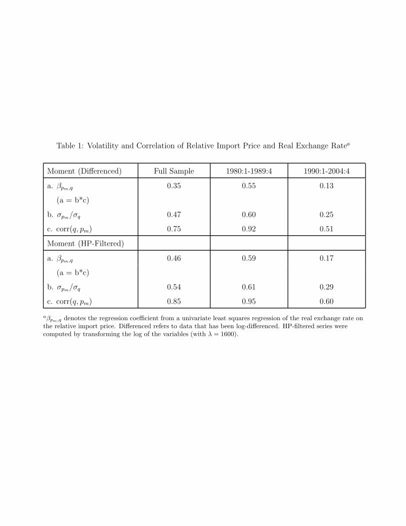
Table 1: Volatility and Correlation of Relative Import Price and Real Exchange Ratea

Moment (Differenced) Full Sample 1980:1-1989:4 1990:1-2004:4

a. βpm,q 0.35 0.55 0.13

(a = b*c)

b. σpm/σq 0.47 0.60 0.25

c. corr(q, pm) 0.75 0.92 0.51

Moment (HP-Filtered)

a. βpm,q 0.46 0.59 0.17

(a = b*c)

b. σpm/σq 0.54 0.61 0.29

c. corr(q, pm) 0.85 0.95 0.60

aβpm,q denotes the regression coefficient from a univariate least squares regression of the real exchange rate onthe relative import price. Differenced refers to data that has been log-differenced. HP-filtered series werecomputed by transforming the log of the variables (with λ = 1600).

38

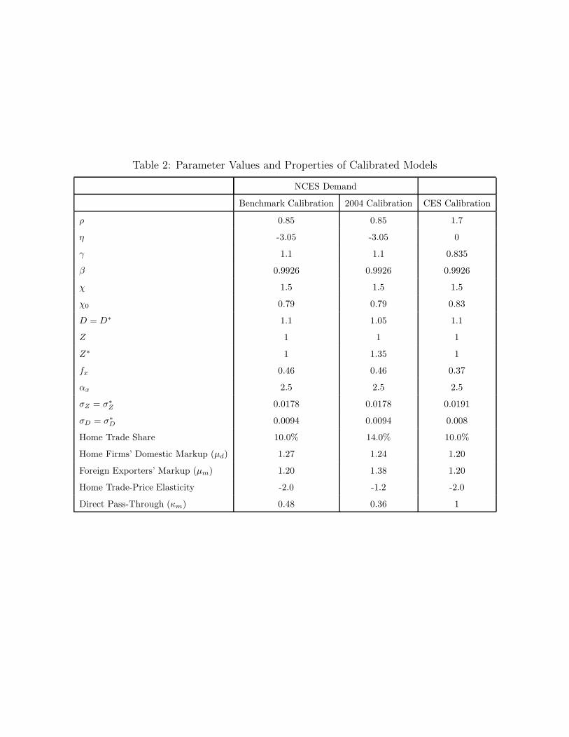
Table 2: Parameter Values and Properties of Calibrated Models

NCES Demand

Benchmark Calibration 2004 Calibration CES Calibration

ρ 0.85 0.85 1.7

η -3.05 -3.05 0

γ 1.1 1.1 0.835

β 0.9926 0.9926 0.9926

χ 1.5 1.5 1.5

χ0 0.79 0.79 0.83

D = D∗ 1.1 1.05 1.1

Z 1 1 1

Z∗ 1 1.35 1

fx 0.46 0.46 0.37

αx 2.5 2.5 2.5

σZ = σ∗Z 0.0178 0.0178 0.0191

σD = σ∗D 0.0094 0.0094 0.008

Home Trade Share 10.0% 14.0% 10.0%

Home Firms’ Domestic Markup (μd) 1.27 1.24 1.20

Foreign Exporters’ Markup (μm) 1.20 1.38 1.20

Home Trade-Price Elasticity -2.0 -1.2 -2.0

Direct Pass-Through (κm) 0.48 0.36 1

39

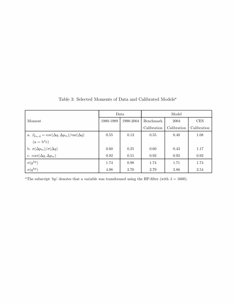
Table 3: Selected Moments of Data and Calibrated Modelsa

Data Model

Moment 1980-1989 1990-2004 Benchmark 2004 CES

Calibration Calibration Calibration

a. βpm,q = cov(Δq, Δpm)/var(Δq) 0.55 0.13 0.55 0.40 1.08

(a = b*c)

b. σ(Δpm)/σ(Δq) 0.60 0.25 0.60 0.43 1.17

c. corr(Δq, Δpm) 0.92 0.51 0.92 0.92 0.92

σ(yhp) 1.74 0.98 1.74 1.71 1.74

σ(qhp) 4.98 2.70 2.79 2.86 2.54

aThe subscript ‘hp’ denotes that a variable was transformed using the HP-filter (with λ = 1600).

40

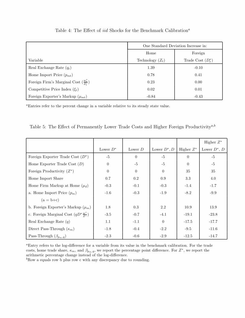
Table 4: The Effect of iid Shocks for the Benchmark Calibrationa

One Standard Deviation Increase in:

Home Foreign

Variable Technology (Zt) Trade Cost (D∗t )

Real Exchange Rate (qt) 1.39 -0.10

Home Import Price (pmt) 0.78 0.41

Foreign Firm’s Marginal Cost (w∗t

Z∗t) 0.23 0.00

Competitive Price Index (ξt) 0.02 0.01

Foreign Exporter’s Markup (μmt) -0.84 -0.43

aEntries refer to the percent change in a variable relative to its steady state value.

Table 5: The Effect of Permanently Lower Trade Costs and Higher Foreign Productivitya,b

Higher Z∗

Lower D∗ Lower D Lower D∗, D Higher Z∗ Lower D∗, D

Foreign Exporter Trade Cost (D∗) -5 0 -5 0 -5

Home Exporter Trade Cost (D) 0 -5 -5 0 -5

Foreign Productivity (Z∗) 0 0 0 35 35

Home Import Share 0.7 0.2 0.9 3.3 4.0

Home Firm Markup at Home (μd) -0.3 -0.1 -0.3 -1.4 -1.7

a. Home Import Price (pm) -1.6 -0.3 -1.9 -8.2 -9.9

(a = b+c)

b. Foreign Exporter’s Markup (μm) 1.8 0.3 2.2 10.9 13.9

c. Foreign Marginal Cost (qD∗ w∗Z∗ ) -3.5 -0.7 -4.1 -19.1 -23.8

Real Exchange Rate (q) 1.1 -1.1 0 -17.5 -17.7

Direct Pass-Through (κm) -1.8 -0.4 -2.2 -9.5 -11.6

Pass-Through (βpm,q) -2.3 -0.6 -2.9 -12.5 -14.7

aEntry refers to the log-difference for a variable from its value in the benchmark calibration. For the tradecosts, home trade share, κm, and βpm,q, we report the percentage point difference. For Z∗, we report thearithmetic percentage change instead of the log-difference.bRow a equals row b plus row c with any discrepancy due to rounding.

41

Table 6: The Effect of Permanently Lower Trade Costs and Higher Foreign Productivity

for Alternative Model Versionsa,b

Without With Only Foreign With

Entry Exporter Entry Entry

Foreign Exporter Trade Cost (D∗) -5 -5 -5

Home Exporter Trade Cost (D) -5 -5 -5

Foreign Productivity (Z∗) 35 35 35

Home Import Share 0.7 4.6 4.0

Home Firm Markup at Home (μd) -1.7 -1.9 -1.7

a. Home Import Price (pm) -12.9 -11.0 -9.9

(a = b+c)

b. Foreign Exporter’s Markup (μm) 19.8 16.1 13.9

c. Foreign Marginal Cost (qD∗ w∗Z∗ ) -23.7 -19.2 -17.7

Real Exchange Rate (q) -15.2 -13.0 -11.6

Direct Pass-Through (κm) -15.2 -13.0 -11.6

Pass-Through (βpm,q) -15.1 -13.4 -14.7

aEntry refers to the log-difference for a variable from its value in the benchmark calibration. For the tradecosts, home trade share, κm, and βpm,q, we report the percentage point difference. For Z∗, we report thearithmetic percentage change instead of the log-difference.bRow a equals row b plus row c with any discrepancy due to rounding.

42

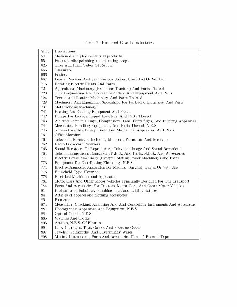
Table 7: Finished Goods Industries

SITC Descriptions54 Medicinal and pharmaceutical products55 Essential oils; polishing and cleansing preps625 Tires And Inner Tubes Of Rubber665 Glassware666 Pottery667 Pearls, Precious And Semiprecious Stones, Unworked Or Worked716 Rotating Electric Plants And Parts721 Agricultural Machinery (Excluding Tractors) And Parts Thereof723 Civil Engineering And Contractors’ Plant And Equipment And Parts724 Textile And Leather Machinery, And Parts Thereof728 Machinery And Equipment Specialized For Particular Industries, And Parts73 Metalworking machinery741 Heating And Cooling Equipment And Parts742 Pumps For Liquids; Liquid Elevators; And Parts Thereof743 Air And Vacuum Pumps, Compressors, Fans, Centrifuges, And Filtering Apparatus744 Mechanical Handling Equipment, And Parts Thereof, N.E.S.745 Nonelectrical Machinery, Tools And Mechanical Apparatus, And Parts751 Office Machines761 Television Receivers, Including Monitors, Projectors And Receivers762 Radio Broadcast Receivers763 Sound Recorders Or Reproducers; Television Image And Sound Recorders764 Telecommunications Equipment, N.E.S.; And Parts, N.E.S., And Accessories771 Electric Power Machinery (Except Rotating Power Machinery) and Parts773 Equipment For Distributing Electricity, N.E.S.774 Electro-Diagnostic Apparatus For Medical, Surgical, Dental Or Vet. Use775 Household Type Electrical778 Electrical Machinery and Apparatus781 Motor Cars And Other Motor Vehicles Principally Designed For The Transport784 Parts And Accessories For Tractors, Motor Cars, And Other Motor Vehicles81 Prefabricated buildings; plumbing, heat and lighting fixtures84 Articles of apparel and clothing accessories85 Footwear874 Measuring, Checking, Analysing And And Controlling Instruments And Apparatus881 Photographic Apparatus And Equipment, N.E.S.884 Optical Goods, N.E.S.885 Watches And Clocks893 Articles, N.E.S. Of Plastics894 Baby Carriages, Toys, Games And Sporting Goods897 Jewelry, Goldsmiths’ And Silversmiths’ Wares898 Musical Instruments, Parts And Accessories Thereof; Records Tapes

43

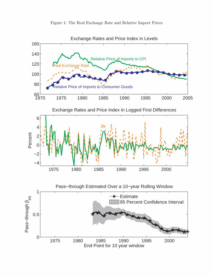
Figure 1: The Real Exchange Rate and Relative Import Prices

1970 1975 1980 1985 1990 1995 2000 200560

80

100

120

140

160

Relative Price of Imports to CPI

Relative Price of Imports to Consumer Goods

Real Exchange Rate

Exchange Rates and Price Index in Levels

1975 1980 1985 1990 1995 2000−4

−2

0

2

4

6

Per

cent

Exchange Rates and Price Index in Logged First Differences

1975 1980 1985 1990 1995 20000

0.5

1Pass−through Estimated Over a 10−year Rolling Window

End Point for 10 year window

Pas

s−th

roug

hβ pq

Estimate95 Percent Confidence Interval

44

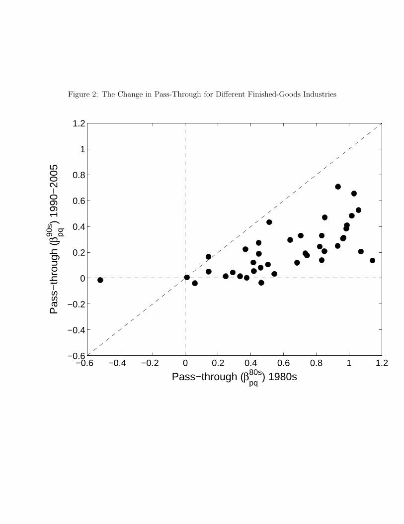
Figure 2: The Change in Pass-Through for Different Finished-Goods Industries

−0.6 −0.4 −0.2 0 0.2 0.4 0.6 0.8 1 1.2−0.6

−0.4

−0.2

0

0.2

0.4

0.6

0.8

1

1.2

Pass−through (βpq80s) 1980s

Pas

s−th

roug

h (β

pq90s )

1990

−20

05

45

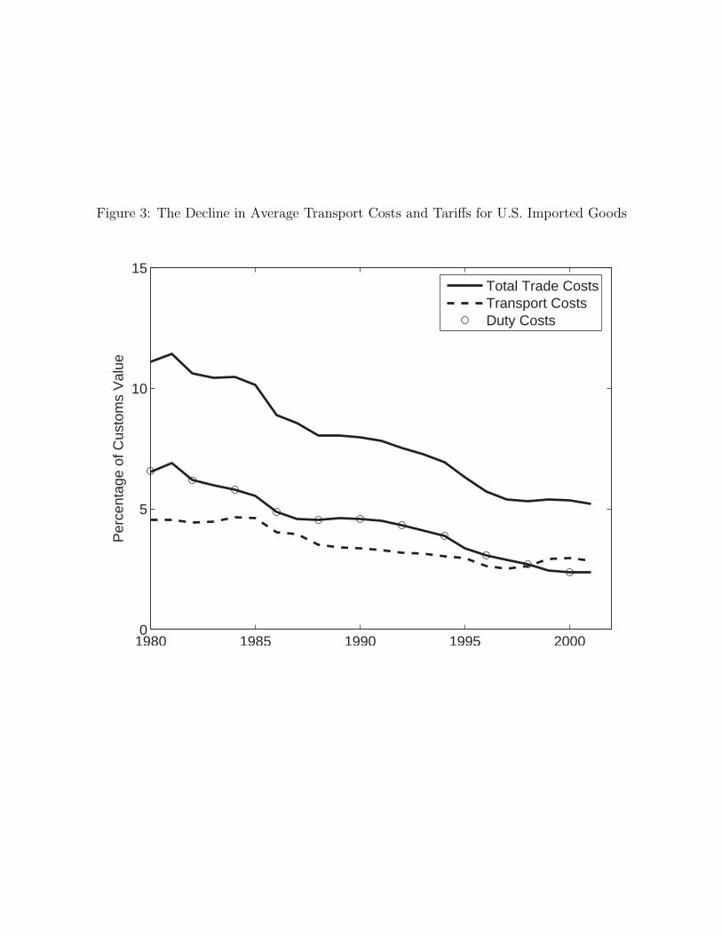
Figure 3: The Decline in Average Transport Costs and Tariffs for U.S. Imported Goods

1980 1985 1990 1995 20000

5

10

15

Per

cent

age

of C

usto

ms

Val

ue

Total Trade CostsTransport CostsDuty Costs

46

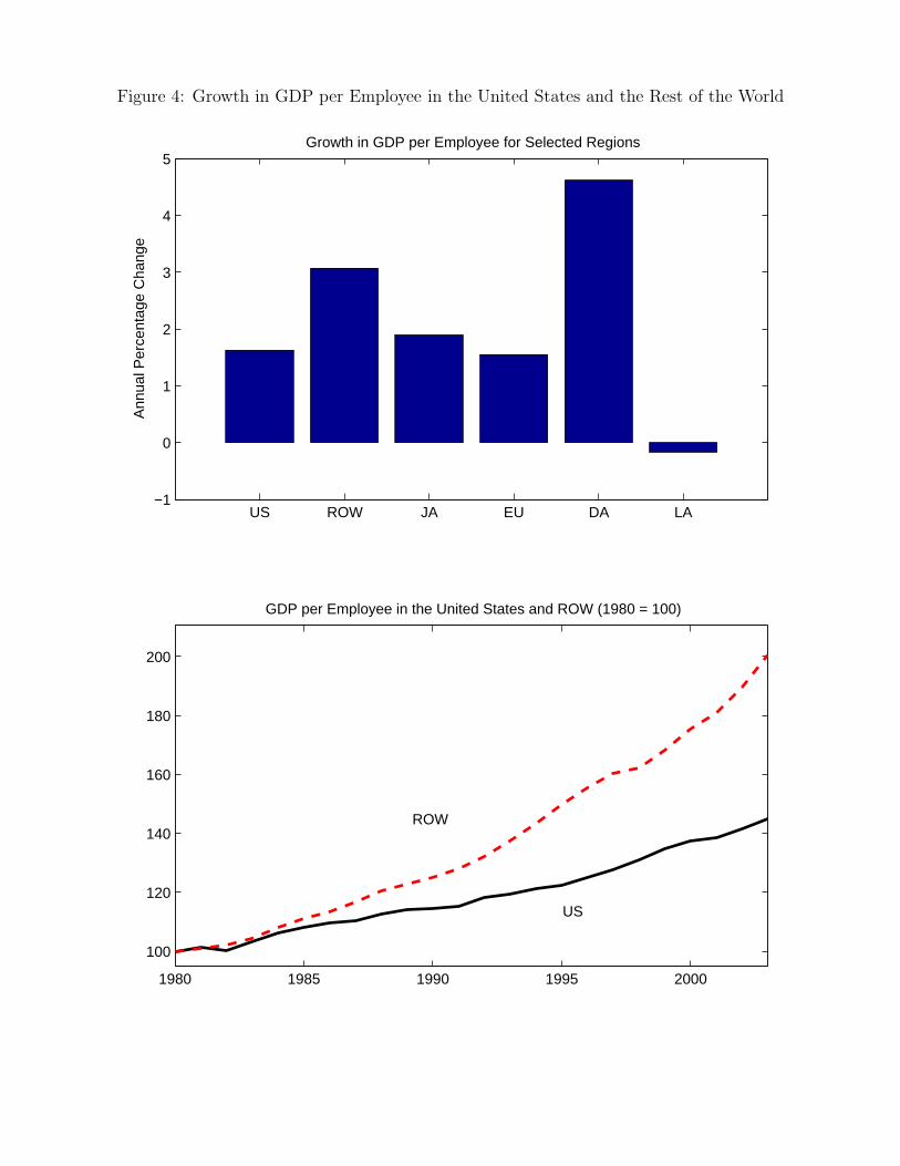
Figure 4: Growth in GDP per Employee in the United States and the Rest of the World

US ROW JA EU DA LA−1

0

1

2

3

4

5A

nnua

l Per

cent

age

Cha

nge

Growth in GDP per Employee for Selected Regions

1980 1985 1990 1995 2000

100

120

140

160

180

200

GDP per Employee in the United States and ROW (1980 = 100)

ROW

US

47

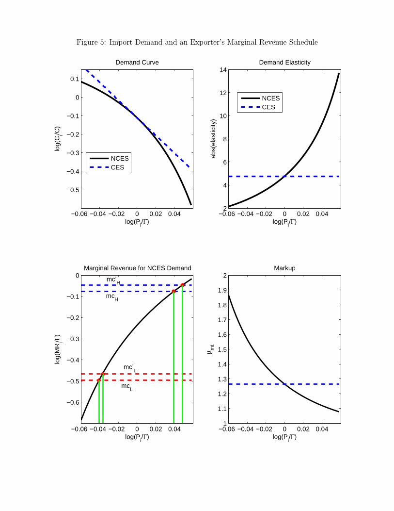
Figure 5: Import Demand and an Exporter’s Marginal Revenue Schedule

−0.06 −0.04 −0.02 0 0.02 0.04

−0.5

−0.4

−0.3

−0.2

−0.1

0

0.1

log(Pi/Γ)

log(

Ci/C

)Demand Curve

NCESCES

−0.06 −0.04 −0.02 0 0.02 0.042

4

6

8

10

12

14

log(Pi/Γ)

abs(

elas

ticity

)

Demand Elasticity

NCESCES

−0.06 −0.04 −0.02 0 0.02 0.041

1.1

1.2

1.3

1.4

1.5

1.6

1.7

1.8

1.9

2

log(Pi/Γ)

μ mt

Markup

−0.06 −0.04 −0.02 0 0.02 0.04

−0.6

−0.5

−0.4

−0.3

−0.2

−0.1

0

log(Pi/Γ)

log(

MR

i/Γ)

Marginal Revenue for NCES Demand

mcL

mc’L

mcH

mc’H

48

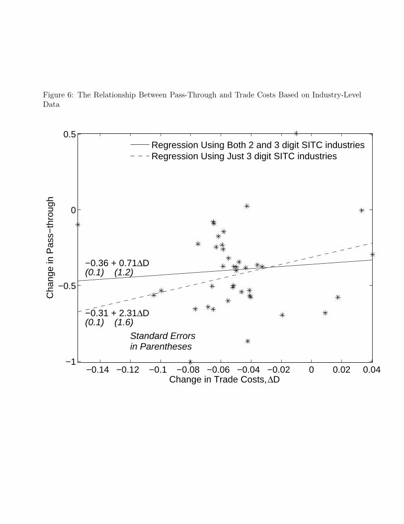
Figure 6: The Relationship Between Pass-Through and Trade Costs Based on Industry-LevelData

−0.14 −0.12 −0.1 −0.08 −0.06 −0.04 −0.02 0 0.02 0.04−1

−0.5

0

0.5

Change in Trade Costs, ΔD

Cha

nge

in P

ass−

thro

ugh

−0.36 + 0.71ΔD(0.1) (1.2)

−0.31 + 2.31ΔD(0.1) (1.6)

Regression Using Both 2 and 3 digit SITC industriesRegression Using Just 3 digit SITC industries

Standard Errorsin Parentheses

49

Figure 7: The Effect of the Intensive and Extensive Entry Margins on Pass-Through

0.12 0.14 0.16

0.1

0.15

0.2

0.25

0.3

0.35

Percentage of Exporting Firms

Foreign Export Profits

0.12 0.14 0.16

0.1

0.11

0.12

0.13

0.14

Percentage of Exporting Firms

Import Share

Initial ValuesNew ValuesNew Values (Only Foreign Exporter Entry)

0.12 0.14 0.16

1.15

1.2

1.25

1.3

1.35

1.4

1.45

Percentage of Exporting Firms

Foreign Exporter Markup

0.12 0.14 0.16

1.25

1.26

1.27

1.28

1.29

1.3

Percentage of Exporting Firms

Domestic Firm Markup

0.12 0.14 0.16

0.35

0.4

0.45

0.5

0.55

Percentage of Exporting Firms

Direct Pass−Through

0.12 0.14 0.16

0.4

0.45

0.5

0.55

0.6

Percentage of Exporting Firms

General Equilibrium Pass−Through

0.12 0.14 0.16

0.35

0.4

0.45

0.5

0.55

Percentage of Exporting Firms

Direct Pass−Through

FixedCost

A

B

D

C

A

B

C

D

A

B C

D

B

A

CD

B

A

C

D

A

BC

D

50