Computationally Efficient Multiphase Heuristicsfor Simulation-Based Optimization

Christoph Bodenstein, Thomas Dietrich, and Armin ZimmermannSystems & Software Engineering, Ilmenau University of Technology, P.O. Box 100 565, 98684 Ilmenau, Germany

{Christoph.Bodenstein, Thomas.Dietrich, Armin.Zimmermann}@tu-ilmenau.de

Keywords: SCPN, Petri nets, simulation, optimization

Abstract: Stochastic colored Petri nets are an established model for the specification and quantitative evaluation of com-plex systems. Automated design-space optimization for such models can help in the design phase to find goodvariants and parameter settings. However, since only indirect heuristic optimization based on simulation isusually possible, and the design space may be huge, the computational effort of such an algorithm is oftenprohibitively high. This paper extends earlier work on accuracy-adaptive simulation to speed up the overalloptimization task. A local optimization heuristic in a “divide-and-conquer” approach is combined with vary-ing simulation accuracy to save CPU time when the response surface contains local optima. An applicationexample is analyzed with our recently implemented software tool to validate the advantages of the approach.

1 INTRODUCTION

Stochastic Colored Petri nets (SCPN, [Zenie,1985, Zimmermann, 2007]) are well-known for theirrich modeling and event-based simulation capabilitiesfor complex systems. A realistic simulation modelcan assist in finding the right set of design parametersettings. To find the optimal configuration, so-calledoptimization by simulation (or indirect optimization)can be applied. This is a commonly used approach inthe literature [Fu, 1994b,Carson and Maria, 1997,Fu,1994a, Biel et al., 2011, Kunzli, 2006]. The data flowof its usual setup is depicted in Figure 1. The designspace for optimization is defined by the number of pa-rameters and their individual value ranges.

This design space can be very large or even infi-nite, and because each parameter set has to be evalu-ated with a simulation that may require several min-utes of CPU time, the overall time for a full designspace scan is intractable. Heuristics such as simulatedannealing, hill climbing, genetic algorithms etc. aresolutions for this problem that exchange some resultaccuracy for a significant speedup in many practicalexamples.

There is often not one design-space optimiza-tion heuristic that fits the whole solution process: inthe beginning, a rough global search for a promis-ing region is beneficial, while the accuracy of thefinal result can be improved by a fine-grained localsearch at the end. Two-phased heuristics are there-

fore used [Schoen, 2002] and mix, for instance, simu-lated annealing for the start with a hill-climbing localsearch at the end.

However, despite this combination of heuristicsand the development of many specialized heuris-tics, another idea (that may be combined with it) isto also take into consideration the accuracy of themodel analysis. This uses explicitly the trade-off be-tween solution accuracy and computational effort. Afirst step is a two-phase approach for instance takenin [Rodriguez et al., 2004, Zimmermann et al., 2001],where the detailed stochastic Petri net models of man-ufacturing systems are approximately and rapidly an-alyzed during the first phase (based on performancebounds), while a correct detailed simulation is donefinally.

In our current work we aim at extending this vari-ant of the two-phase idea towards adaptively control-ling the evaluation accuracy based on the result qual-ity that the heuristic currently needs [Zimmermannand Bodenstein, 2011]. The contribution of this ideais a tighter integration between the two modules of in-

Sim. Output

Parameter set

Optimization heuristic

Simulation

Figure 1: Common black box optimization, see [Carson andMaria, 1997]

direct optimization and its use for algorithm speedup.There are many ways to control the accuracy of eval-uation — a first simple method is to adapt the dis-cretization step of the design parameters (adaptingmodel detail granularity or refinement quality wasproposed for this in [Zimmermann and Bodenstein,2011], but without an automated tool implementa-tion).

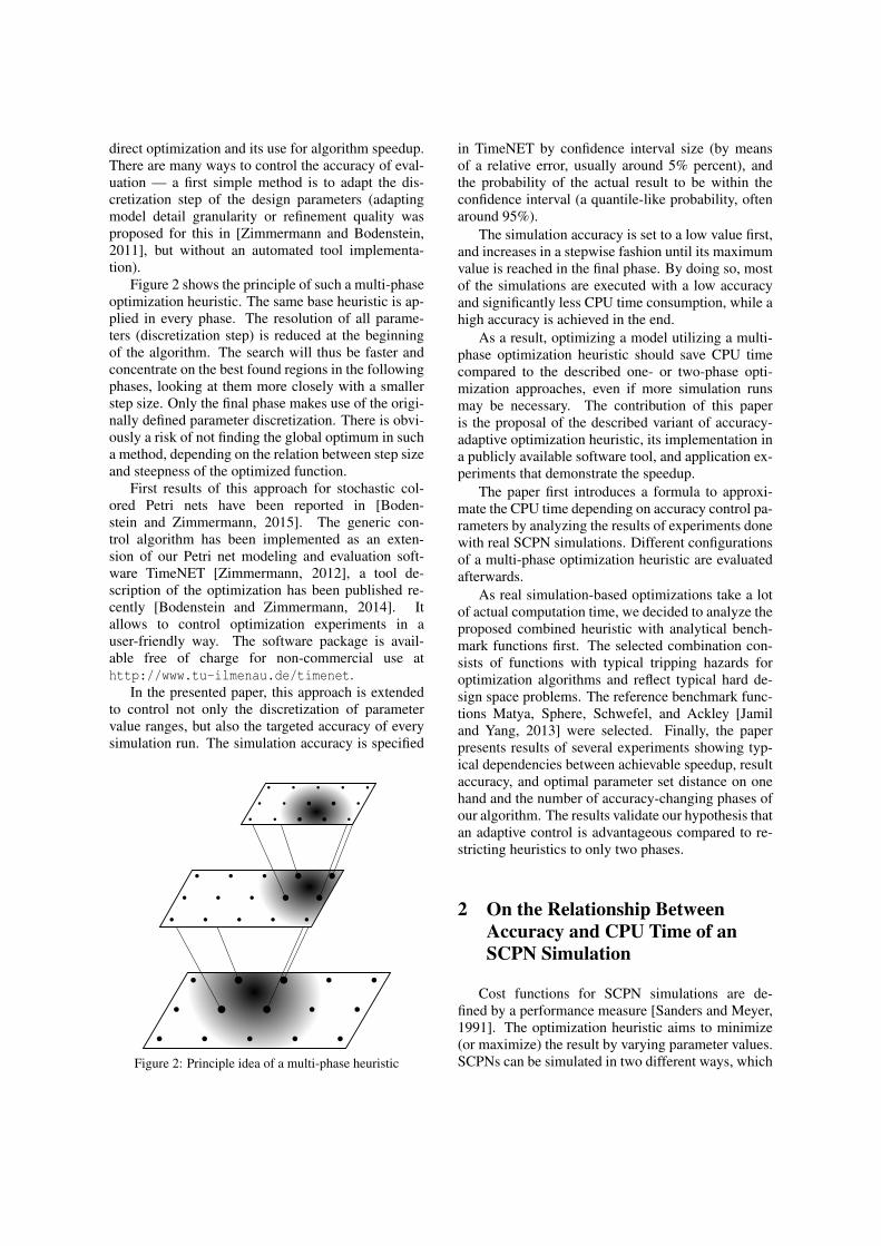
Figure 2 shows the principle of such a multi-phaseoptimization heuristic. The same base heuristic is ap-plied in every phase. The resolution of all parame-ters (discretization step) is reduced at the beginningof the algorithm. The search will thus be faster andconcentrate on the best found regions in the followingphases, looking at them more closely with a smallerstep size. Only the final phase makes use of the origi-nally defined parameter discretization. There is obvi-ously a risk of not finding the global optimum in sucha method, depending on the relation between step sizeand steepness of the optimized function.

First results of this approach for stochastic col-ored Petri nets have been reported in [Boden-stein and Zimmermann, 2015]. The generic con-trol algorithm has been implemented as an exten-sion of our Petri net modeling and evaluation soft-ware TimeNET [Zimmermann, 2012], a tool de-scription of the optimization has been published re-cently [Bodenstein and Zimmermann, 2014]. Itallows to control optimization experiments in auser-friendly way. The software package is avail-able free of charge for non-commercial use athttp://www.tu-ilmenau.de/timenet.

In the presented paper, this approach is extendedto control not only the discretization of parametervalue ranges, but also the targeted accuracy of everysimulation run. The simulation accuracy is specified

Figure 2: Principle idea of a multi-phase heuristic

in TimeNET by confidence interval size (by meansof a relative error, usually around 5% percent), andthe probability of the actual result to be within theconfidence interval (a quantile-like probability, oftenaround 95%).

The simulation accuracy is set to a low value first,and increases in a stepwise fashion until its maximumvalue is reached in the final phase. By doing so, mostof the simulations are executed with a low accuracyand significantly less CPU time consumption, while ahigh accuracy is achieved in the end.

As a result, optimizing a model utilizing a multi-phase optimization heuristic should save CPU timecompared to the described one- or two-phase opti-mization approaches, even if more simulation runsmay be necessary. The contribution of this paperis the proposal of the described variant of accuracy-adaptive optimization heuristic, its implementation ina publicly available software tool, and application ex-periments that demonstrate the speedup.

The paper first introduces a formula to approxi-mate the CPU time depending on accuracy control pa-rameters by analyzing the results of experiments donewith real SCPN simulations. Different configurationsof a multi-phase optimization heuristic are evaluatedafterwards.

As real simulation-based optimizations take a lotof actual computation time, we decided to analyze theproposed combined heuristic with analytical bench-mark functions first. The selected combination con-sists of functions with typical tripping hazards foroptimization algorithms and reflect typical hard de-sign space problems. The reference benchmark func-tions Matya, Sphere, Schwefel, and Ackley [Jamiland Yang, 2013] were selected. Finally, the paperpresents results of several experiments showing typ-ical dependencies between achievable speedup, resultaccuracy, and optimal parameter set distance on onehand and the number of accuracy-changing phases ofour algorithm. The results validate our hypothesis thatan adaptive control is advantageous compared to re-stricting heuristics to only two phases.

2 On the Relationship BetweenAccuracy and CPU Time of anSCPN Simulation

Cost functions for SCPN simulations are de-fined by a performance measure [Sanders and Meyer,1991]. The optimization heuristic aims to minimize(or maximize) the result by varying parameter values.SCPNs can be simulated in two different ways, which

are also supported by the tool TimeNET: The first isa transient analysis where the user defines the simu-lation end time. The simulation is executed repeat-edly and the measurements are calculated at specificpoints in simulation time. The simulation is stoppedif all measures at all defined points in simulation timereached their required accuracy.

The second type is a stationary simulation. Amodel is simulated until all measures meet the prede-fined accuracy constraints. The model must not havedead states in this case.

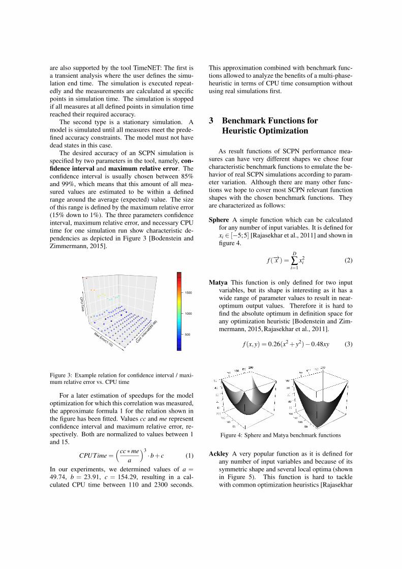
The desired accuracy of an SCPN simulation isspecified by two parameters in the tool, namely, con-fidence interval and maximum relative error. Theconfidence interval is usually chosen between 85%and 99%, which means that this amount of all mea-sured values are estimated to be within a definedrange around the average (expected) value. The sizeof this range is defined by the maximum relative error(15% down to 1%). The three parameters confidenceinterval, maximum relative error, and necessary CPUtime for one simulation run show characteristic de-pendencies as depicted in Figure 3 [Bodenstein andZimmermann, 2015].

Conf.-Intervall(85-99)

Max Error(1-10)

CPU-Tim

e

++

+

+

+ +

+

++

+

++ +++

+

++ +

+

++

++

+

++

++

++++++

+

++

++

+

+

++

+

++ +

+

++

+

+++

+

+

++

+

+++

++

+

++

+

++++++

+++++

+

++

+

++ ++

+

++

+

++ ++ ++

+

++ ++++

++ ++++

++ ++ ++ +++ ++ ++ ++ ++ ++ ++ + ++ ++ + + ++ + + ++ + ++ ++

500

1000

1500

Figure 3: Example relation for confidence interval / maxi-mum relative error vs. CPU time

For a later estimation of speedups for the modeloptimization for which this correlation was measured,the approximate formula 1 for the relation shown inthe figure has been fitted. Values cc and me representconfidence interval and maximum relative error, re-spectively. Both are normalized to values between 1and 15.

CPUTime =(cc∗me

a

)3·b+ c (1)

In our experiments, we determined values of a =49.74, b = 23.91, c = 154.29, resulting in a cal-culated CPU time between 110 and 2300 seconds.

This approximation combined with benchmark func-tions allowed to analyze the benefits of a multi-phase-heuristic in terms of CPU time consumption withoutusing real simulations first.

3 Benchmark Functions forHeuristic Optimization

As result functions of SCPN performance mea-sures can have very different shapes we chose fourcharacteristic benchmark functions to emulate the be-havior of real SCPN simulations according to param-eter variation. Although there are many other func-tions we hope to cover most SCPN relevant functionshapes with the chosen benchmark functions. Theyare characterized as follows:

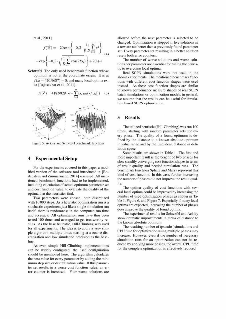
Sphere A simple function which can be calculatedfor any number of input variables. It is defined forxi ∈ [−5;5] [Rajasekhar et al., 2011] and shown infigure 4.

f (−→x ) =D

∑i=1

x2i (2)

Matya This function is only defined for two inputvariables, but its shape is interesting as it has awide range of parameter values to result in near-optimum output values. Therefore it is hard tofind the absolute optimum in definition space forany optimization heuristic [Bodenstein and Zim-mermann, 2015, Rajasekhar et al., 2011].

f (x,y) = 0.26(x2 + y2)−0.48xy (3)

Figure 4: Sphere and Matya benchmark functions

Ackley A very popular function as it is defined forany number of input variables and because of itssymmetric shape and several local optima (shownin Figure 5). This function is hard to tacklewith common optimization heuristics [Rajasekhar

et al., 2011].

f (−→x ) =−20exp

{−0,2 ·

√1D

D

∑i=1

x2i

}

−exp

{−0,2 ·

√1D

D

∑i=1

cos(2πxi)

}+20+ e

(4)

Schwefel The only used benchmark function whoseoptimum is not at the coordinate origin. It is atf (−−−−−−−−−→xi = 420.9687) = 0, and many local optima ex-

ist [Rajasekhar et al., 2011].

f (−→x ) = 418.9829 ·n−n

∑i=1

(xi sin(√|xi|)) (5)

Figure 5: Ackley and Schwefel benchmark functions

4 Experimental Setup

For the experiments covered in this paper a mod-ified version of the software tool introduced in [Bo-denstein and Zimmermann, 2014] was used. All men-tioned benchmark functions had to be implemented,including calculation of actual optimum parameter setand cost function value, to evaluate the quality of theoptima that the heuristics find.

Two parameters were chosen, both discretizedwith 10 000 steps. As a heuristic optimization run is astochastic experiment just like a single simulation runitself, there is randomness in the computed run timeand accuracy. All optimization runs have thus beentested 100 times and averaged to get trustworthy re-sults. As the base heuristic, Hill-Climbing was usedfor all experiments. The idea is to apply a very sim-ple algorithm multiple times starting at a coarse dis-cretization and low simulation precision as the base-line.

As even simple Hill-Climbing implementationscan be widely configured, the used configurationshould be mentioned here. The algorithm calculatesthe next value for every parameter by adding the min-imum step size or discretization value. If this parame-ter set results in a worse cost function value, an er-ror counter is increased. Four worse solutions are

allowed before the next parameter is selected to bechanged. Optimization is stopped if five solutions ina row are not better then a previously found parameterset. Every parameter set resulting in a better solutionresets both error counters.

The number of worse solutions and worse solu-tions per parameter are essential for tuning the heuris-tic to overcome local optima.

Real SCPN simulations were not used in theshown experiments. The mentioned benchmark func-tions with different cost function shapes were usedinstead. As these cost function shapes are similarto known performance measure shapes of real SCPNbatch simulations or optimization models in general,we assume that the results can be useful for simula-tion based SCPN optimization.

5 Results

The utilized heuristic (Hill-Climbing) was run 100times, starting with random parameter sets for ev-ery phase. The quality of a found optimum is de-fined by the distance to a known absolute optimumin value range and by the Euclidean distance in defi-nition space.

Some results are shown in Table 1. The first andmost important result is the benefit of two phases forslow steadily converging cost function shapes in termsof result quality and needed simulation runs. Thebenchmark functions Sphere and Matya represent thiskind of cost function. In this case, further increasingthe number of phases did not improve the result qual-ity.

The optima quality of cost functions with sev-eral local optima could be improved by increasing thenumber of used optimization phases as shown in Ta-ble 1, Figure 6, and Figure 7. Especially if many localoptima are expected, increasing the number of phasesdoes improve the quality of found optima.

The experimental results for Schwefel and Ackleyshow dramatic improvements in terms of distance tothe known absolute optimum.

The resulting number of (pseudo-)simulations andCPU time for optimization using multiple phases mayincrease. However, even if the number of necessarysimulation runs for an optimization can not be re-duced by applying more phases, the overall CPU timefor the complete optimization is effectively reduced.

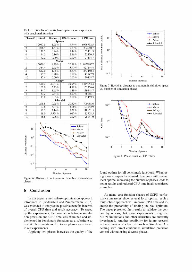
Table 1: Results of multi-phase optimization experimentwith benchmark function

Phase-# Sim-# Distance DS-Distance CPU timeSphere

1 2947.5 1.75% 19.74% 6976732.52 256.9 1.47% 10.83% 202660.73 171.5 0.44% 5.44% 55401.34 44.5 0.16% 2.16% 23450.510 72.2 0.00% 0.02% 27434.7

Matya1 5056.1 9.29% 20.19% 11967788772 384.4 2.95% 5.97% 421244.43 622.0 1.05% 2.37% 283450.44 179.9 0.28% 1.82% 47842.910 87.6 0.00% 0.02% 30468.7

Ackley1 570.2 42.61% 29.95% 1349663.42 102.0 3.73% 4.11% 153356.63 84.7 1.65% 1.89% 139848.74 53.2 2.64% 2.27% 68165.110 73.8 0.03% 0.02% 27459.3

Schwefel1 295.8 10.95% 20.82% 700158.62 67.8 15.07% 13.06% 123082.93 82.2 12.14% 5.21% 118661.54 68.0 5.574% 1.917% 33708.510 76.8 0.06% 0.02% 28141.0

0 2 4 6 8 10

10−3

10−2

10−1

100

101

Number of phases

Dis

tanc

eto

optim

um

SphereMatyaAckleySchwefel

Figure 6: Distance to optimum vs. Number of simulationphases

6 Conclusion

In this paper a multi-phase optimization approachintroduced in [Bodenstein and Zimmermann, 2015]was extended to analyze the possible benefits in termsof overall CPU time and result accuracy. To speedup the experiments, the correlation between simula-tion precision and CPU time was examined and im-plemented in benchmark functions as a substitute toreal SCPN simulations. Up to ten phases were testedin our experiments.

Applying two phases increases the quality of the

0 2 4 6 8 1010−2

10−1

100

101

Number of phases

Euk

liddi

stan

ceto

optim

um(i

nD

S)

SphereMatyaAckleySchwefel

Figure 7: Euclidian distance to optimum in definition spacevs. number of simulation phases

0 2 4 6 8 10

104.5

105

105.5

Number of phases

CPU

timeSphereMatyaAckleySchwefel

Figure 8: Phase count vs. CPU Time

found optima for all benchmark functions. When us-ing more complex benchmark functions with severallocal optima, increasing the number of phases leads tobetter results and reduced CPU time in all consideredexamples.

As many cost function shapes of SCPN perfor-mance measures show several local optima, such amulti-phase approach will improve CPU time and in-crease the probability of finding the real optimum.The paper presented first results to validate the gen-eral hypothesis, but more experiments using realSCPN simulations and other heuristics are currentlyinvestigated. Another possibility for future researchis the extension of a heuristic such as Simulated An-nealing with direct continuous simulation precisioncontrol without using discrete phases.

ACKNOWLEDGEMENTS

This paper is based on work funded by the FederalMinistry for Education and Research of Germany un-der grant number 01S13031A.

REFERENCES

Biel, J., Macias, E., and Perez de la Parte, M. (2011).Simulation-based optimization for the design ofdiscrete event systems modeled by parametricPetri nets. In Computer Modeling and Simula-tion (EMS), 2011 Fifth UKSim European Sym-posium on, pages 150–155.

Bodenstein, C. and Zimmermann, A. (2014).TimeNET optimization environment. In Pro-ceedings of the 8th International Conferenceon Performance Evaluation Methodologies andTools.

Bodenstein, C. and Zimmermann, A. (2015). Extend-ing design space optimization heuristics for usewith stochastic colored petri nets. In 2015 IEEEInternational Systems Conference (IEEE SysCon2015), Vancouver, Canada. (accepted for publi-cation).

Carson, Y. and Maria, A. (1997). Simulation opti-mization: Methods and applications. In Proceed-ings of the 29th Conference on Winter Simula-tion, WSC ’97, pages 118–126.

Fu, M. C. (1994a). Optimization via simulation: areview. Annals of Operations Research, pages199–248.

Fu, M. C. (1994b). A tutorial overview of optimiza-tion via discrete-event simulation. In Cohen, G.and Quadrat, J.-P., editors, 11th Int. Conf. onAnalysis and Optimization of Systems, volume199 of Lecture Notes in Control and Informa-tion Sciences, pages 409–418, Sophia-Antipolis.Springer-Verlag.

Jamil, M. and Yang, X.-S. (2013). A Literature Sur-vey of Benchmark Functions For Global Opti-mization Problems. ArXiv e-prints.

Kunzli, S. (2006). Efficient Design Space Explorationfor Embedded Systems. Phd thesis, ETH Zurich.

Rajasekhar, A., Abraham, A., and Pant, M. (2011).Levy mutated artificial bee colony algorithm forglobal optimization. In Systems, Man, and Cy-bernetics (SMC), 2011 IEEE International Con-ference on, pages 655–662.

Rodriguez, D., Zimmermann, A., and Silva, M.(2004). Two heuristics for the improvement of a

two-phase optimization method for manufactur-ing systems. In Proc. Int. Conf. Systems, Man,and Cybernetics (SMC’04), pages 1686–1692,The Hague, Netherlands.

Sanders, W. H. and Meyer, J. F. (1991). A unified ap-proach for specifying measures of performance,dependability, and performability. In Avizie-nis, A. and Laprie, J., editors, Dependable Com-puting for Critical Applications, volume 4 ofDependable Computing and Fault-Tolerant Sys-tems, pages 215–237. Springer Verlag.

Schoen, F. (2002). Two-phase methods for global op-timization. In Handbook of global optimization,pages 151–177. Springer US.

Zenie, A. (1985). Colored stochastic Petri nets. InProc. 1st Int. Workshop on Petri Nets and Per-formance Models, pages 262–271.

Zimmermann, A. (2007). Stochastic Discrete EventSystems - Modeling, Evaluation, Applications.Springer-Verlag New York Incorporated.

Zimmermann, A. (2012). Modeling and evaluation ofstochastic Petri nets with TimeNET 4.1. In Per-formance Evaluation Methodologies and Tools(VALUETOOLS), 2012 6th Int. Conf. on, pages54–63.

Zimmermann, A. and Bodenstein, C. (2011). To-wards accuracy-adaptive simulation for efficientdesign-space optimization. In Systems, Man,and Cybernetics (SMC), 2011 IEEE Interna-tional Conference on, pages 1230 –1237.

Zimmermann, A., Rodriguez, D., and Silva, M.(2001). A two-phase optimisation methodfor Petri net models of manufacturing sys-tems. Journal of Intelligent Manufacturing,12(5/6):409–420. Special issue ”Global Opti-mization Meta-Heuristics for Industrial SystemsDesign and Management”.