Board of Governors of the Federal Reserve System

International Finance Discussion Papers

Number 1031

October 2011

Oil Efficiency, Demand, and Prices:

a Tale of Ups and Downs

Martin Bodenstein

Luca Guerrieri

NOTE: International Finance Discussion Papers are preliminary materials circulated to stimulate discus-sion and critical comment. References in publications to International Finance Discussion Papers (otherthan an acknowledgement that the writer has had access to unpublished material) should be cleared withthe author or authors. Recent IFDPs are available on the Web at www.federalreserve.gov/pubs/ifdp/.This paper can be downloaded without charge from Social Science Research Network electronic libraryat http://www.ssrn.com/.

Oil Efficiency, Demand, and Prices: a Tale of Ups and Downs∗

Martin Bodenstein and Luca Guerrieri∗∗

Federal Reserve Board

October 2011

Abstract

The macroeconomic implications of oil price fluctuations vary according to their sources. Ourestimated two-country DSGE model distinguishes between country-specific oil supply shocks, variousdomestic and foreign activity shocks, and oil efficiency shocks. Changes in foreign oil efficiency,modeled as factor-augmenting technology, were the key driver of fluctuations in oil prices between1984 and 2008, but have modest effects on U.S. activity. A pickup in foreign activity played animportant role in the 2003-2008 oil price runup. Beyond quantifying the responses of oil pricesand economic activity, our model informs about the propagation mechanisms. We find evidencethat nonoil trade linkages are an important transmission channel for shocks that affect oil prices.Conversely, nominal rigidities and monetary policy are not.

Keywords: oil shocks, DSGE models, Maximum Likelihood

JEL Classification: F32, F41

∗ We thank Mario Crucini, James Hamilton, Matteo Iacoviello, Lutz Kilian, Sylvain Leduc, David Lopez-Salido, John Rogers, Rob Vigfusson, and seminar participants at the Federal Reserve Bank of Atlanta, FederalReserve Board, Federal Reserve Bank of San Francisco, and University of Michigan. This draft replaces aprevious version of this paper circulated under the title:“On the Sources of Oil Price Fluctuations.” The viewsexpressed in this paper are solely the responsibility of the authors and should not be interpreted as reflectingthe views of the Board of Governors of the Federal Reserve System or of any other person associated with theFederal Reserve System.

∗∗ Contact Information: Telephone (202) 452 2550. E-mail Luca.Guerrieri@frb.gov.

1 Introduction

Not all oil price fluctuations have the same macroeconomic repercussions. If oil demand and

oil prices rise because of strong foreign aggregate demand, worldwide activity expands rather

than contracting, as it would for price increases stemming from foreign oil supply disruptions.

Similarly, U.S. activity reacts differently to oil price movements that originate in the U.S.

rather than abroad. Disagreement persists regarding the relative importance of oil supply

and demand factors in determining oil prices. For instance, Hamilton (1983, 2003, 2009)

emphasizes oil supply disruptions in explaining major runups in oil prices, while Kilian (2009)

argues that shocks to oil demand have driven oil prices historically.

In addition to the challenges of identifying empirically the sources of fluctuations - domestic

or foreign, demand or supply - studying the macroeconomic effects of oil price movements is

further complicated by the response of monetary policy. Monetary authorities are often seen

as contributing to the slowdown in economic activity associated with oil price increases by

raising policy interest rates. Perhaps most prominently, Bernanke, Gertler, and Watson (1997)

argued that the output decline that coincided with the oil price hikes of the 1970s and early

1980s could have been largely reduced by an alternative policy response.1

The international dimension of oil trade matters beyond distinguishing whether oil price

fluctuations originate at home or abroad. Due to intertemporal consumption smoothing, an

oil-importing country, such as the United States, offsets oil deficits associated with oil price

increases by expanding nonoil trade. The expansion of nonoil net exports buffers the response

of gross domestic product and is accompanied by a depreciation of the dollar that affects

import prices and inflation.

1 The approach and conclusions in Bernanke, Gertler, and Watson (1997) have subsequently been challenged by Hamiltonand Herrera (2004), Leduc and Sill (2004), and Kilian and Lewis (2010).

1

To disentangle domestic and foreign sources of oil price fluctuations, to evaluate their

repercussions on economic activity and inflation, and to assess the role of monetary policy

in an internally consistent framework, we estimate a dynamic stochastic general equilibrium

model (DSGE) using full information maximum likelihood. In the model, oil is both a factor

of production and a direct input in consumption. Building on the work of Backus and Crucini

(1998), the model allows for trade in oil and nonoil goods and encompasses U.S. and foreign

trade blocs. Drawing on the monetary policy literature, the model incorporates nominal wage

and price rigidities, as well as real rigidities. Following Smets and Wouters (2007), cyclical

fluctuations are linked to a rich stochastic structure. Previous estimates of the sources of

oil price fluctuations and their macroeconomic effects have disregarded the nature of oil as a

globally traded commodity, or have taken econometric approaches that do not allow explaining

the transmission channels and the role of monetary policy, or both.2

Our analysis distinguishes between country-specific shocks associated with oil supply and

demand. On the demand side, we allow for numerous sources of variation that influence

oil demand indirectly through economic activity. The indirect demand sources reflect the

dependence of oil demand on broader macroeconomic events, such as shifts in productivity,

changes in government spending, or, possibly, the conduct of monetary policy. Our results

assign a relatively modest role to these factors in explaining oil prices in dollar terms for the

period between 1984 and 2003. However, a pickup in economic activity in the foreign bloc of

the model plays an important role in explaining the increase in oil demand and prices between

2003 and 2008.

In our model, oil demand is also influenced directly by changes in oil efficiency, modeled

2 Others have estimated DSGE models that include oil inputs. Nakov and Pescatori (2010) abstracted from the openeconomy links and restricted key parameters such as the oil price elasticity of demand. Balke, Brown, and Yucel (2010)focused on the open economy dimension, but excluded a role for monetary policy.

2

as a factor-augmenting technology. Movements in oil efficiency may capture changes in con-

sumption patterns or production processes. Examples include a shift towards motorization in

emerging Asia, continuing industrialization of China, or energy-efficient cars becoming more

popular in the United States.

We find that movements in foreign oil efficiency are of principal importance in the deter-

mination of oil demand and prices over the period 1984 to 2008 both at business-cycle and

longer frequencies. Between 1984 and the late 1990s the real dollar price of oil (measured

by the U.S. refiners’ acquisition costs for imported crude deflated by the U.S. GDP deflator)

dropped by 140% as oil efficiency sharply improved in the industrialized countries and around

the globe. Since the late 1990s, improvements in oil efficiency have slowed down and oil prices

have been catching up to levels that would have prevailed absent the earlier gains.

Going beyond the focus on an aggregate foreign bloc of our DSGE model, we construct mea-

sures of oil efficiency for individual foreign countries using the approach of growth-accounting

studies in the style of Solow (1957) and Griliches and Jorgenson (1966). Starting from the

oil demand equations in our model, we show that the growth rate of oil efficiency can be

expressed in terms of directly observable quantities and parameters, such as the rate of trend

growth in efficiency and the oil price elasticity of demand. To construct country-by-country

measures of oil efficiency consistent with the foreign aggregate included in the DSGE model,

we use disaggregate data in conjunction with the parameter estimates obtained for the entire

foreign bloc of the model. Our results imply that the inverted U-shaped pattern for the evo-

lution of foreign oil efficiency over the sample is not merely a consequence of aggregation. On

the contrary, that pattern is shared by all the foreign industrialized economies and by many

developing countries.

3

While our results highlight the importance of shocks that affect oil demand, oil supply

shocks are estimated to play a small role in driving oil price fluctuations. Disentangling oil

demand and supply sources of fluctuations based solely on observed equilibrium quantities

is no easy task. In our case, this task is facilitated by the rich stochastic structure of the

model and by the information provided by an equally rich set of observed variables. Over our

sample, global oil supply displays relatively little volatility. For oil supply sources to account

for a large share of the volatility in oil prices, oil demand would have to be price insensitive.

We estimate the oil price elasticity of demand to be -0.41. In our model, a more inelastic

oil demand would imply a larger role not only for oil supply shocks, but also for many other

sources of fluctuations. In that case, the volatility in oil prices implied by the model would

be counterfactually high relative to the volatility in oil prices in the observed data.

One of the transmission channels scrutinized by the literature on the macroeconomic effects

of oil shocks is the response of monetary policy.3 For the period between 1984 and 2008,

our analysis finds no evidence that monetary policy played a quantitatively important role

in shaping the response of economic activity to oil price fluctuations. We assess the role

of monetary policy through the lens of a potential economy with flexible prices and wages

and show that output levels in the actual and potential economy differ only slightly when

conditioning on the smoothed estimates of oil supply and oil efficiency shocks. Even after

ascribing most of the variation in oil prices to foreign sources, there remains the possibility

that U.S. monetary policy may have raised the volatility of oil prices. We also dispel this

argument as the price of oil in our model with nominal rigidities and a role for monetary

policy evolves similarly to its counterpart in the potential economy.

3 An overview is offered in Kilian and Lewis (2010).

4

Jones, Leiby, and Paik (2004), Hamilton (2008), Kilian (2008) surveyed the broad literature

on the macroeconomic impact of oil price fluctuations. Ramey and Vine (2011) gave an

overview of the transmission channels typically embedded in DSGE models with a closed-

economy focus. The review in Bodenstein, Erceg, and Guerrieri (2011) placed a greater

emphasis on work that captured the international nature of oil trade.

2 Model Description

Like the model in Backus and Crucini (1998), our model encompasses international trade in

oil and nonoil goods. We extend the model in Backus and Crucini (1998) by incorporating

the nominal and real rigidities that Smets and Wouters (2007) and Christiano, Eichenbaum,

and Evans (2005) have found to be empirically relevant in closed economy models. As in

Bodenstein, Erceg, and Guerrieri (2011), the assumption of incomplete asset markets across

countries is a key ingredient in generating country-specific wealth effects in reaction to shocks

that affect the price of oil.

There are two countries, country 1, the home country, and country 2, the foreign country.

We estimate the model using U.S. data for the home country and aggregate data for the

principal trading partners of the United States for the foreign bloc. Because the structure

of the country blocs is symmetric, we focus on the home country in describing the model.

Country specific values for the parameters allow for differences in population size, oil shares

in production and consumption, oil endowments, expenditures shares and in nonoil and oil

trade flows.

In each country, a continuum of firms produces differentiated varieties of an intermediate

good under monopolistic competition. These firms use capital, labor, and oil as factor inputs.

5

Goods prices are determined by Calvo-Yun staggered contracts. Trade occurs at the level

of intermediate goods and within each country the varieties are aggregated into a (nonoil)

consumption and an investment good. Households consume oil, the nonoil consumption good,

save and invest, and supply differentiated labor services under monopolistic competition.

Wages are determined by Calvo-Yun staggered contracts. While asset markets are complete

at the country level, asset markets are incomplete internationally. The two country-blocs are

endowed with a nonstorable supply of oil each period. Finally, to allow for a balanced growth

path, the oil efficiency must grow over time to bridge the gap between the growth rates of

labor augmenting technology and oil supply.

2.1 Households and Firms

The preferences of the representative household are given by:

Et

∞∑j=0

βj1

{1

1− σ1

(Zc

1,tC1,t+j − κ1CA1,t+j−1

)1−σ1+

χ0,1

1− χ1

(1− L1,t+j)1−χ1

}. (1)

Et denotes the expectations conditional on information available at time t. The variables

C1,t and L1,t represent consumption and hours worked, respectively. The parameter σ1 is

used for determining the intertemporal elasticity of substitution, χ1 for the Frisch elasticity

of labor supply, and χ0,1 for the number of hours worked along the balanced growth path.

The term Zc1,t+j models a preference shock to consumption. In addition, a household’s utility

from consumption is affected by the presence of external consumption habits, parameterized

by κ1. CA1,t−1 is the per capita aggregate consumption level.

The time t budget constraint of the household states that the combined expenditures on

6

goods and the net accumulation of financial assets must equal disposable income:

P c1,tC1,t + P i

1,tI1,t +e1,tP

b2,tB1,t

φb1,t

+

∫

S

P d1,t,t+1D1,t,t+1(h)−D1,t−1,t

= W1,tL1,t + Rk1,tK1,t−1 + Γ1,t + P o

1,tYo1,t + T1,t + e1,tB1,t−1. (2)

Final consumption and investment goods, C1,t and I1,t, are purchased at the prices P c1,t and

P i1,t, respectively. The household earns labor income W1,tL1,t and capital income Rk

1,tK1,t−1.

The household also receives an aliquot share Γ1,t of firm and union profits, a share of the

country’s (unrefined) oil endowment P o1,tY

o1,t, and net transfers of T1,t.

Households accumulate financial assets by purchasing state-contingent domestic bonds,

and a non state-contingent foreign bond. The state contingent domestic bonds are denoted

by D1,t,t+1. The term B1,t+1 in the budget constraint represents the quantity of the non state-

contingent bond purchased by a typical household that pays one unit of foreign currency in the

subsequent period, P b2,t is the foreign currency price of the bond, and e1,t is the exchange rate

expressed in units of home currency per unit of foreign currency. φb1,t captures intermediation

costs incurred to purchase the foreign bond and render the dynamics of B1,t+1 stationary.4

The evolution of the capital stock follows:

K1,t = (1− δ1) K1,t−1 + Zi1,tI1,t

(1− 1

2ψi

1

(I1,t

I1,t−1

− µz

)2)

, (3)

where δ1 is the depreciation rate of capital. For ψi1 > 0, changing the level of gross investment

from the previous period is costly, so that the acceleration in the capital stock is penalized.

The term Zi1,t captures an investment-specific technology shock. µz is the deterministic growth

rate of labor augmenting technological change discussed below.

4 See Bodenstein (2011) for a detailed discussion of stationarity inducing devices in linearized models with incompleteasset markets.

7

In every period t, household h maximizes the utility functional (1) with respect to con-

sumption, labor supply, investment, end-of-period capital stock, and holdings of domestic and

foreign bonds, subject the budget constraint (2), and the transition equation for capital (3).

In doing so, prices, wages, and net transfers are taken as given.

Labor Bundling

As in Smets and Wouters (2007), households supply their homogenous labor to intermediate

labor unions. These unions introduce distinguishing characteristics on the labor services and

resell them to intermediate labor bundlers. The unions use Calvo contracts to set the wages

charged to the intermediate bundlers. In turn, firms purchase a labor bundle Ld1,t from the

labor bundlers.

The labor bundle demanded by firms takes the from:

Ld1,t =

[∫ 1

0

L1,t(h)1

1+θw1,t dh

]1+θw1,t

, (4)

where θw1,t is time-varying reflecting shocks to the wage markup.

The labor bundlers buy the labor services L1,t(h) from unions, combine them to obtain Ld1,t,

and resell them to the intermediate goods producers at wage W1,t. In a perfectly competitive

environment, profit maximization by the bundlers implies:

L1,t(h) =

[W1,t(h)

W1,t

]− 1+θw1,t

θw1,t

Ld1,t, (5)

and the zero-profit condition yields:

W1,t =

[∫ 1

0

W1,t(h)− 1

θw1,t dh

]−θw1,t

. (6)

Labor bundlers purchase labor from the unions that intermediate between the households

and the labor bundlers. The unions allocate and differentiate the labor services from the

8

households and have market power, i.e., they choose a wage subject to the labor demand

equation. We denote the real wage desired by the household W f1,t+j/P1,t+j which reflects the

marginal rate of substitution between leisure and consumption.

Labor unions take W f1,t+j/P1,t+j as the cost of labor services in their negotiations with the

labor bundlers. The markup above the marginal disutility is distributed to the households.

However, unions are subject to nominal rigidities as in Calvo. A union can readjust a wage

with probability 1− ξw1 in each period. For those unions which cannot adjust wages in a given

period, wages grow by a geometric average of last period’s nominal wage inflation and the

wage inflation rate along the balanced growth path. The problem of a union h is given by:

maxWt(h)

Et

∞∑j=0

(ξw1 )jψt,t+j

[(1 + τw

1 )ωlt,jWt(h)Lt+j(h)−W f

t+jLt+j(h)]

(7)

s.t.

L1,t(h) =

[W1,t(h)

W1,t

]− 1+θw1,t

θw1,t

Ld1,t, (8)

ωlt,j =

j∏s=1

{(ωt−1+s)

ιw (π∗)1−ιw}

. (9)

The subsidy τw1 guarantees the efficient level of labor supply along the balanced growth path.

Bundlers of Varieties

A continuum of representative bundlers combines differentiated intermediate products (whose

production is described below) into a composite home-produced good Y1,t according to:

Y d1,t =

[∫ 1

0

Y1,t (i)1

1+θp1,t di

]1+θp1,t

, (10)

where Y d1,t is used as the domestic input in producing all final use goods, including exports.

The term θp1,t represents a domestic mark-up shock. The optimal bundle of intermediate goods

minimizes the cost of producing Y d1,t taking the price of each intermediate good as given. One

9

unit of the sectoral output index sells at the price:

P d1,t =

[∫ 1

0

P d1,t (i)

−1

θp1,t di

]−θp1,t

. (11)

Under producer currency pricing, the exports sell at the foreign price Pm2,t = P d

1,t/e1,t.

Production of Domestic Intermediate Goods

There is a continuum of differentiated intermediate goods indexed by i ∈ [0, 1], each of which

is produced by a single monopolistically competitive firm.

Firm i faces a demand function that varies inversely with its output price P1,t(i) and

directly with aggregate demand Y d1,t for country 1’s products:

Y1,t(i) =

[P1,t(i)

P d1,t

]− 1+θp1,t

θp1,t

Y d1,t, (12)

where θp1,t > 0 is time-varying in order to allow for price mark-up shocks.

Each firm utilizes capital, labor, and oil and acts in perfectly competitive factor markets.

The production technology is given by a nested constant-elasticity of substitution specification.

Since capital is owned by households and rented out to firms, the cost minimization problem

of firm i that intends to produce overall output Y1,t(i) can be written as:

minK1,t−1(i),L1,t(i),

Oy1,t(i),V1,t(i)

Rk1,tK1,t−1 (i) + W1,tL1,t (i) + P o

1,tOy1,t (i) (13)

s.t.

Y1,t (i) =

((ωvy

1 )ρo1

1+ρo1 (V1,t (i))

11+ρo

1 + (ωoy1 )

ρo1

1+ρo1

(µt

zoZo1,tO

y1,t (i)

) 11+ρo

1

)1+ρo1

(14)

V1,t (i) =

((ωk

1

) ρv1

1+ρv1

(Ks

1,t (i)) 1

1+ρv1 +

(ωl

1

) ρv1

1+ρv1

(µt

zZ1,tL1,t (i)) 1

1+ρv1

)1+ρv1

. (15)

Utilizing capital Ks1,t(i) and labor services L1,t(i), the firm produces a value-added input

V1,t(i), which is then combined with oil Oy1,t(i) to produce the domestic nonoil variety Y1,t(i).

10

In equilibrium, aggregating over firms, overall demand for the various factor inputs needs to

clear the quantities of each input available for rent from households and unions.

The quasi-share parameter ωoy1 determines the importance of oil purchases in the firm’s

output, and the parameter ρo1 determines the price elasticity of demand for oil. The substi-

tutability between capital and labor is measured by ρv1. The term Z1,t represents a stochastic

process for the evolution of technology while µz denotes constant labor augmenting techno-

logical progress. Oil efficiency is also modeled as a factor-augmenting technology. The term

Zo1,t represents a stochastic process that influences the oil efficiency in production while µt

zo

denotes a constant rate of oil efficiency gains.

The prices of intermediate goods P1,t(i) are determined by Calvo-style staggered contracts,

see Calvo (1983) and Yun (1996). Each period, a firm faces a constant probability, 1 − ξp1,

to reoptimize its price P1,t(i), that is common across destinations under producer currency

pricing without pricing-to-market. These probabilities are independent across firms, time,

and countries. Firms that do not reoptimize their price partially index it to the inflation rate

in the aggregate price P d1,t. The indexation scheme for prices is analogous to that for wages

in Equation (9). For prices, the indexation weight is denoted by ιp.

Production of Consumption Goods

The consumption basket C1,t that enters the household’s budget constraint is produced by

perfectly competitive consumption distributors whose production function mirrors the prefer-

ences of households over home and foreign nonoil goods and oil. For convenience, we suppress

firm-specific indices as all the distributors behave identically in equilibrium. The cost mini-

11

mization problem of a representative distributor that produces C1,t can be written as:

minCd

1,t,Mc1,t

Cne1,t,O

c1,t

P d1,tC

d1,t + Pm

1,tMc1,t + P o

1,tOc1,t (16)

s.t.

C1,t =

((ωcc

1 )ρo1

1+ρo1

(Cne

1,t

) 11+ρo

1 + (ωoc1 )

ρo1

1+ρo1

(µt

zoZo1,tO

c1,t

) 11+ρo

1

)1+ρo1

(17)

Cne1,t =

((ωc

1)ρc1

1+ρc1

(Cd

1,t

) 11+ρc

1 + (ωmc1 )

ρc1

1+ρc1

(Zm

1,tMc1,t

) 11+ρc

1

)1+ρc1

. (18)

Each distribution firm produces a nonoil aggregate Cne1,t from the home and foreign interme-

diate consumption aggregates Cd1,t and M c

1,t, which is then combined with oil Oc1,t to produce

the final consumption good in the home country C1,t and sold under perfect competition.

The parameter ωoc1 determines the ratio of oil purchases to the output of the firm. The

price elasticity of oil demand ρo1 in the consumption aggregate (17) coincides with the one in

the production function (14). The same shock Zo1,t that affects oil efficiency in production also

affects the oil efficiency of consumption. µtzo denotes a constant rate of oil efficiency gains.

The quasi-share ωmc1 determines the importance of nonoil imports in the nonoil aggregate.

The elasticity of substitution between the home and foreign intermediate good is denoted by

ρc1. The term Zm

1,t captures an import preference shock. In our estimation, this shock accounts

for the volatility of nonoil goods trade that is not explained by the remaining shocks.

The price of the consumption aggregate P c1,t coincides with the Lagrange multiplier on

Equation (17) in the cost minimization problem of a distributor. The price of the nonoil

consumption good Cne1,t is referred to as the “core” price level P ne

1,t .

Production of Investment Goods

The investment good is also produced by perfectly competitive distributors. In contrast to

the consumption distributors, however, the production of the investment aggregate does not

12

require oil as input. The cost minimization of a representative investment distributor is:

minId1,t,M

i1,t

P d1,tI

d1,t + Pm

1,tMi1,t (19)

s.t.

I1,t =

((ωi

1

) ρc1

1+ρc1

(Id1,t

) 11+ρc

1 +(ωmi

1

) ρc1

1+ρc1

(Zm

1,tMi1,t

) 11+ρc

1

)1+ρc1

. (20)

The quasi-share parameter ωmi1 determines the importance of nonoil imports in the investment

aggregate. The same import preference shock Zm1,t also affects investment imports. The La-

grangian from the problem of investment distributors determines the price of new investment

goods P i1,t, that appears in the household’s budget constraint.

2.2 The Oil Market

Each period the home and foreign countries are endowed with exogenous supplies of oil Y o1,t

and Y o2,t, respectively. The two endowments are governed by distinct stochastic processes.

With both domestic and foreign oil supply determined exogenously, the oil price P o1,t adjusts

endogenously to clear the world oil market:

Y o1,t +

1

ζ1

Y o2,t = O1,t +

1

ζ1

O2,t, (21)

where Oi,t = Oyi,t + Oc

i,t. To clear the oil market, the sum of home and foreign oil production

must equal the sum of home and foreign oil consumption by firms and households. Because

all variables are expressed in per capita terms, foreign variables are scaled by the relative

population size of the home country 1ζ1

.

13

2.3 Fiscal Policy

The government purchases some of the domestic nonoil good Y d1,t but the import content

of government purchases is zero. Government purchases have no direct effect on household

utility and are given by:

Gd1,t = g1Z

g1,tY

d1,t. (22)

The share of government spending in value added along the balanced growth path is denoted

by g1. The stochastic component to this autonomous spending is Zg1,t.

Given the Ricardian structure of our model, net lump-sum transfers T1,t are assumed to

adjust each period to balance the government receipts and revenues, so that:

P d1,tG

d1,t + T1,t = 0. (23)

2.4 Monetary Policy

Monetary policy follows a modified version of the interest rate reaction function suggested by

Taylor (1993):

i1,t = i1 +γi1(i1,t−1− i1)+(1−γi

1)[(πcore

1,t − πcore1 ) + γπ

1 (πcore1,t − πcore

1 − πcore1,t ) + γy

1ygap1,t

]. (24)

The terms i1 and πcore1 are the steady state values for the nominal interest rate and inflation,

respectively. The inflation rate πcore1,t is expressed as the logarithmic percentage change of the

core price level, i.e., inflation in nonoil consumer prices πcore1,t = log(P ne

1,t/Pne1,t−1). The term

ygap1,t denotes the log deviation of gross output from the value of gross output in a model that

excludes nominal rigidities, but is otherwise identical to the one described.5 The parameter

γi1 allows for interest rate smoothing. The term πcore

1,t reflects a time varying inflation target.

5 Notice that the capital stock in the parallel model with flexible prices and wages is not imposed to be identical to thecapital stock in the model with nominal rigidities.

14

2.5 Resource Constraints for Nonoil Goods and Net Foreign Assets

The resource constraint for the nonoil goods sector of the home economy can be written as:

Y d1,t = Cd

1,t + Id1,t + Gd

1,t +1

ζ1

(M c

2,t + M i2,t

), (25)

where M2,t = M c2,t+M i

2,t denotes the per capita imports of the foreign country, which accounts

for the population scaling factor 1ζ1

.

The evolution of net foreign assets can be expressed as:

e1,tPb2,tB1,t

φb1,t

= e1,tB1,t−1+1

ζ1

e1,tPm2,t

(M c

2,t + M i2,t

)−Pm1,t

(M c

1,t + M i1,t

)+P o

1,t

(Y o

1,t −O1,t

). (26)

This expression can be derived by combining the budget constraint for households, the gov-

ernment budget constraint, and the definition of firm profits. Market clearing for the non-

state-contingent bond requires B1,t + B2,t = 0.

2.6 Balanced Growth Path

Our model is consistent with a balanced steady state growth path driven by a labor-augmenting

technological progress, increases in oil supply, and increases in oil efficiency. All growth rates

are common across countries. The growth rate of labor productivity is denoted by µz while oil

supply grows at the rate µo. To allow for a balanced growth path, oil efficiency must improve

over time to bridge the gap between labor augmenting technological progress and oil supply

growth at the rate µzo = µz

µo. Consequently, the price of oil is expected to grow at the rate µzo

unconditionally.6

6 Focusing exclusively on trend growth in real oil prices, recent work by Stefanski (2011) investigates the link betweenoil prices and structural change in Asia in a multi-sector model.

15

3 Model Solution and Estimation Strategy

The model is linearized around its balanced growth path and solved using the algorithm of

Anderson and Moore (1985). The estimation by the method of maximum likelihood uses

fifteen observed series: the log of U.S. and foreign GDP, U.S. and foreign oil production, the

U.S. dollar price of oil (deflated by the U.S. GDP deflator), U.S. hours worked per capita,

and the real dollar trade-weighted exchange rate; the GDP share of U.S. private consumption

expenditures, the GDP share of U.S. oil imports, the GDP share of U.S. nonoil goods imports,

the GDP share of U.S. goods exports, the GDP share of U.S. fixed investment; the level of

U.S. core PCE inflation, U.S. wage inflation (demeaned), and the U.S. federal funds rate

(demeaned). An appendix provides further details on data sources. The data are quarterly

and run between 1984 and 2008. A presample that starts in 1974 trains the Kalman filter

used to form the likelihood. The sample stops in the fall of 2008 to avoid a break in U.S.

monetary policy associated with the zero bound on nominal interest rates.7

The model is just identified, as it also contains fifteen exogenous shock processes: U.S. and

foreign productivity (Z1,t and Z2,t), U.S. and foreign oil supply (Y o1,t and Y o

2,t), U.S. and foreign

oil efficiency (Zo1,t and Zo

2,t), U.S. autonomous spending (Zg1,t), U.S. and foreign consumption

preferences (Zc1,t and Zc

2,t), U.S. and foreign import preferences (Zm1,t and Zm

2,t), U.S. investment

specific technology (Zi1,t), U.S. price markup (θp

1,t), U.S. labor supply (θw1,t), and U.S. inflation

target (πcore1,t ). Our first estimation attempt involved specifying all shock processes as auto-

regressive of order one. However, the estimates of the parameters governing some of the shock

processes chafed against the upper bound of the unit circle, imposed to ensure stationarity.

7 To maximize the likelihood, we employ a combination of optimization algorithms. We rely on simulated annealingto identify a candidate global maximum and refine the estimates through Nelder-Meade and Newton-Raphson algorithms.The candidate global maximum needs to then survive repeated calls to the simulated annealing algorithm with a high initialtemperature and slow cooling process.

16

To avoid constraining the shock processes arbitrarily, we introduced AR(2) processes for the

following shocks: domestic and foreign productivity, domestic and foreign oil supply, domestic

and foreign oil efficiency, domestic and foreign import preferences. While allowing for distinct

estimates of the size of the standard deviation of the innovation to the shock process, we

constrained the autoregressive parameters for the home and foreign shocks to be the same in

the case of the shocks to: productivity, oil efficiency, consumption preferences, and import

preferences. Table 1 summarizes the stochastic processes of the shocks and the data.

In the case of the home economy, we have adhered closely to the choice of observed series

of closed-economy estimation exercises such as Smets and Wouters (2007) and Justiniano

and Primiceri (2008). The asymmetry between the observed series for the home and foreign

economies is dictated by data limitations. However, with regard to the home economy, the

open-economy nature of our model avoids shortcuts taken by papers with a narrower one-

sector, closed-economy focus. For instance, Smets and Wouters (2007) include investment and

consumption measures not deflated by their own NIPA deflators, but rather by the overall

GDP deflator – a sensible choice given that their model only implies one relative price. We

prefer to observe consumption and investment as a share of GDP because our model has

multiple relative prices, i.e., oil and import prices. A similar parallel to the closed-economy

literature inspired our choice of stochastic processes. However, in our model the shock to

autonomous spending has a different interpretation. As observations on trade data inform

the likelihood, autonomous spending captures movements in the components of GDP not

directly observed, specifically, government spending and inventory investment. By contrast,

in closed-economy models, Chari, Kehoe, and McGrattan (2009) noticed that the shock to

autonomous spending would also have to capture the bulk of fluctuations in the trade balance.

17

We estimate all the parameters governing the shock processes listed in Table 1. We also

estimate all behavioral parameters in the model with the exception of: the depreciation rate

of capital, δ1, fixed at 0.025; the intertemporal elasticity for consumption σ1, fixed at 1; the

curvature of the intermediation cost for foreign bonds, φ1,b, fixed at 0.0001; and the discount

factor β1, fixed so that taking into account the estimate for trend productivity growth, the

real interest rate along the balanced growth path is 4% per year. Following Ireland (2004),

this calibration of β1 avoids the systematic over-prediction of the historical returns on U.S.

Treasury bills in representative agent models to that Weil (1989) calls “the risk free rate

puzzle.” The foreign parameters take on the same values as for the home country.

Table 2 summarizes parameters and the values for ratios (along the balanced growth path)

that enter the linearized conditions for our model. Values for government spending g1, and

ωk1 are consistent with data from the National Income and Product Accounts (NIPA). The

parmeter ζ1 implies that nonoil production in the home country is half the size of nonoil

production in the foreign country.

Values for ωoy1 and ωoc

1 are determined by the overall oil share of output, and the ratios of

the quantity of oil used as an intermediate input in production relative to the quantity used

as a final input in consumption. Based on data from the Energy Information Administration

of the U.S. Department of Energy for 2008, the overall oil share of the domestic economy is

set to 4.2 percent of GDP. The relative size of oil use in consumption and production is sized

using the U.S. Input-Output Use tables. Over the period 2002-2008, for which the tables are

available annually, the Use tables point to a low in 2002 of 0.30 and a peak in 2008 of 0.39.

We settle on a calibration equal to the average over the last ten years in the sample of 0.35,

which implies that ωoy1 and ωoc

1 are equal to 0.026 and 0.021, respectively.

18

The oil imports of the home country are set to 70 percent of total demand in the steady

state, implying that 30 percent of oil demand is satisfied by domestic production. This

estimate is based on 2008 NIPA data. In the foreign bloc, the overall oil share is set to 8.2

percent. The oil endowment abroad is 9.5 percent of foreign GDP, based on oil supply data

from the Energy Information Administration. The common trend growth rate for oil supply

µo is fixed at 1.0026, implying 0.26 percent growth per quarter, the average growth rate of

world oil supply over the sample period.

Turning to the parameters determining trade flows, the parameter ωmc1 and ωmi

1 are chosen

to reflect NIPA data for nonoil imports while equalizing the nonoil import-intensity of con-

sumption and investment. This calibration implies a ratio of nonoil goods imports relative to

GDP for the home country of about 12 percent and values of for both ωmc1 and ωmi

1 equal to

0.15. Given that trade is balanced in along the balanced growth path, and that the oil import

share for the home country is 3 percent of GDP, the goods export share is 15 percent of GDP.

3.1 Parameter Estimates and Empirical Fit

Table 3 reports estimates of the main behavioral parameters and confidence intervals.8 Start-

ing from the trends, the growth rate of productivity for the home and foreign economies, µz, is

estimated at 0.6 percent per quarter, or 2.4 percent per year, lower than the 2.9 average U.S.

GDP growth over the sample and the 3.5 average foreign GDP growth. As world oil supply

expands at the quarterly rate of 0.26 percent, oil efficiency improves at the quarterly rate of

0.32 percent along the balanced growth path given the relationship µzo = µz

µo. Consequently,

the trend growth in the real price of oil is also 0.32 percent per quarter, or roughly 1.3 percent

8 The 95% confidence interval reported in the table is obtained by repeating the maximum likelihood estimation exerciseon 1000 bootstrap samples of length equal to that of the observed estimation sample. The bootstrap samples were generatedtaking the point estimates in Table 3 as pseudo-true values for the parameters in the model.

19

per year. The U.S. steady state inflation rate, πcore, is estimated at 1.1 percent per quarter,

which is a close match to the 3.84 average for U.S. core PCE inflation over the sample.

Turning to substitution elasticities, we estimate the oil substitution elasticity,1+ρo

1

ρo1

, to be

0.42. Notice that, in our model, substitution elasticities map one for one into price elasticities

of demand. Perhaps the closest results to ours are those of Kilian and Murphy (2010), who

gauge the price elasticity of oil demand as the ratio of the impact response of oil production

to the impact response of the real price of oil conditional on an oil supply shock. The ab-

solute value of their posterior median estimate is 0.44. From the same type of calculation,

Baumeister and Peersman (2009) estimate the price elasticity at 0.38. In our model such a

ratio is influenced not only by the price elasticity of oil demand, but also by the contempora-

neous response of consumption and gross output (the activity variables driving oil demand).

However, since the response of consumption and gross output to a foreign oil supply shock is

of a different order of magnitude relative to the response of the real dollar price of oil, and

given the theoretical restriction that the activity elasticity is 1, the ratio of oil supply to the

the price of oil on impact is 0.40 in our model.

On the nonoil goods trade side, the estimate of the elasticity of substitution between

domestic and foreign goods, at 1.8 is also close to other estimates based on aggregate data.

For instance, Hooper, Johnson, and Marquez (2000) estimated trade price elasticities using

data for G-7 countries and reported an export price elasticity of 1.5 for the United States.

The model has two parameters governing real rigidities. The parameter for consumption

habits, κ1, is estimated at 0.65. This estimate is in line with values typically reported by

studies with a closed economy focus such as Smets and Wouters (2007), who show a posterior

distribution with a mean and a mode of 0.71. Our estimate for the adjustment costs of

20

investment ψi1, at 3.5, is also in line with other authors’ estimates of this parameter in DSGE

models. For comparison, Christiano, Eichenbaum, and Evans (2005) report an estimate of the

curvature of the adjustment cost function equal to 4, well within the 95% confidence interval

for our estimate.

The estimates of parameters in the monetary policy rule indicate a stronger weight on

inflation than the output gap. The weight on inflation is γπ1 = 0.2, the estimated weight on

the output gap is γy1 = 0.9 We find evidence for substantial interest rate smoothing, as our

estimate of the smoothing parameter is γi1 = 0.66.

Moving to the wage- and price-setting equations, the Calvo parameter for wages, ξw1 , is

estimated at 0.89. The Calvo parameter for prices, ξp1, is estimated at 0.81. We find little

evidence in favor of lagged indexation for either prices or wages. Following Eichenbaum and

Fisher (2007) and Guerrieri, Gust, and Lopez-Salido (2010) one could reinterpret the estimate

of the slope of marginal cost in the Phillips curve, determined by the parameters β1 and ξp1 in

our model, through the lens of a more general aggregator for intermediate goods such as the

one suggested by Kimball (1995). That aggregator allows for the possibility that the elasticity

of demand for the product of an intermediate firm is increasing in its price. The results in

Guerrieri, Gust, and Lopez-Salido (2010) for the curvature of the elasticity with respect to

price suggest that our estimate of ξp1 implies an average contract duration below 2 quarters,

in line with the micro evidence in Klenow and Krytsov (2008).

While Table 3 reports estimates of the parameters governing all the shock processes, to

interpret these estimates, we prefer to focus on Table 4. The latter table shows a break-down

by shock of the population variance of key variables. The table focuses on decomposing pop-

9 Notice that the Taylor principle is satisfied given the form of the interest rate rule in Equation 24.

21

ulation variances over the business cycle, obtained by isolating oscillations with a periodicity

between 6 and 36 quarters.10

Focusing on the price of oil, domestic shocks play a negligible role. The bulk of the

population variance, 88%, is explained by foreign oil efficiency shocks, with foreign oil supply

shocks playing a non-negligible role. Despite the finding that most of the variance of oil shocks

is explained by oil efficiency shocks, the price of oil is not the only channel for the transmission

of those shocks. For instance, foreign oil efficiency shocks, account for 19% of the population

variance of the real dollar exchange rate. This finding underscores the importance of general

equilibrium effects for the transmission of shocks that are specific to the oil market and is in

line with previous results in Bodenstein, Erceg, and Guerrieri (2011).

Moving to U.S. nonoil gross output and its components, shocks that are directly related

to the oil market, play a negligible role in explaining population variances. Altogether, those

shocks account for only 3% of the population variance of U.S. output. They play a slightly

larger role for consumption and the trade balance, respectively, 6% and 10% in total. Not

surprisingly, oil shocks have a larger effect on foreign output. The data imply that oil is

a proportionately more substantial input in foreign production and consumption, and is a

sizable source of exports. Accordingly, foreign oil efficiency shocks account for about 33% of

the population variance of foreign nonoil gross output.

Comparing the sources of fluctuation for domestic and foreign output in Table 4 under-

scores a substantial asymmetry. Economy-wide productivity shocks account for the prevalent

share of the population movements for foreign output, about 60%. By contrast, in the home

economy, economy-wide and investment-specific productivity shocks account for about 30%

10 Given that the model is stationary, we used its numerical solution to form the correlogram and could then constructa bandbass filter by integrating the spectrum analytically.

22

of output fluctuations and are less important than labor supply shocks. It is hard to gauge

to what extent the differences on the determinants of domestic and foreign business cycles

are extant or artificially driven by the exclusion of foreign labor supply shocks in the model.

Without series for foreign hours worked – and to our knowledge, only few countries maintain

statistics on hours worked – it is infeasible to separately identify labor supply and produc-

tivity shocks for the foreign bloc. However, when we excluded U.S. hours worked from the

observations in the likelihood (and removed the labor supply shock from the U.S. bloc of the

model), the asymmetries on the role of technology shocks in the domestic and foreign blocs

were practically eliminated.

It is not straight-forward to relate some of our estimates to those in exercises with a

closed economy focus on U.S. data. Our model implies additional channels that influence the

variability of wages deflated by consumption prices. Closed economy models miss variation

stemming from import prices and oil prices. Given these additional sources of variation for

real wages, it may not be surprising that our estimate for the Frisch elasticity of labor supply

is already deemed unlikely by the prior used in Smets and Wouters (2007). Their Normal

prior with a mean of 2 is more than two prior standard deviations away from our estimate.

3.2 Cyclical Properties

Our estimated model captures the business cycle properties of key variables. For those vari-

ables that are directly observed in the estimation, Table 5 reports the 2.5th percentile, 97.5th

percentile, and the median of the standard deviations and autocorrelations implied by the

model, along with their sample estimates in the data.11 In most cases, the statistic derived

11 The statistics are computed from 10000 simulated series each of length 138, the same length as the observed data. Thebusiness cycle component of each simulated series is extracted using the bandpass filter, retaining only oscillations with

23

from the observed data lies between the 2.5th and the 97.5th percentile of the model implied

distribution. In a similar fashion, the table also reports contemporaneous correlations of the

price of oil with other observed variables.12 We conclude that the model is consistent with a

remarkable array of sample moments.

3.3 Interpreting Oil Efficiency Shocks

While oil efficiency shocks are meant to capture fundamental changes in the demand for

oil – such as a shift towards motorization in emerging Asia, continuing industrialization of

China, or energy-efficient cars becoming more popular in the United States – we would like to

exclude the possibility that the efficiency shocks are nothing but a catchall for all unmodeled

disturbances that can affect oil demand.

Accordingly, we conduct a simple exogeneity test for our estimated oil efficiency innovations

εzo1,t and εzo

2,t following the exercise in Evans (1992) for technology shocks. Let

εzoi,t = Ai(L)εzo

i,t−1 + Bi(L)xt−1 + νi,t, (27)

where νi,t is a mean zero, i.i.d random variable, Ai(L) and Bi(L) are polynomials in the lag

operator L, x is a vector that includes potential explanatory variables for oil demand. Ideally,

none of the variables included in xt−1 should Granger cause the innovations εzo1,t and εzo

2,t.

Unmodeled determinants of oil demand that we would like to see assessed as unimpor-

tant for our measure of oil efficiency are: (i) log-changes in oil inventories (OECD and U.S.

inventory data), (ii) log-changes of the price of oil substitutes in energy generation (price of

coal), (iii) financial market activities (log-changes in oil futures, real stock market returns),

amplitude between 6 and 32 quarters.12 Others have compared the fit of the model with that of a vector auto-regression. Given the large number of observed

variables and relatively small sample, we would have to restrict the lag length of the VAR to such an extent that thecomparison would not be informative.

24

(iv) changes in and the level of activity-driven demand for all commodities (index proposed

in Kilian (2009)) as these should already be captured by our GDP measures.13

When including each of the variables separately with up to three lags, the null hypothesis

of exogeneity, B2(L) = 0, was never rejected for the foreign oil efficiency shocks at the 5%

significance level.14 For the U.S. oil efficiency shock, the null hypothesis was rejected at

the 5% level of significance for log-changes in OECD oil inventories and changes in Kilian’s

shipping index. Yet, the adjusted R2 never exceeds 11%. With up to three lags in the VAR,

no combination of variables ever implied a rejection of the null hypothesis at conventional

significance levels for the foreign oil efficiency shock (up to 10%). Moreover, the adjusted R2

never exceeds 12%. For the U.S. oil efficiency shock, the most challenging combination of

variables is given by the set of changes in Kilian’s activity measure, and log-changes in OECD

and U.S. oil inventories. In this case, the null hypothesis of block exogeneity is rejected at the

1% significance level for each lag-length up to three lags. However, with adjusted R2 values

not exceeding 15%, the combined explanatory power of these variables is low. We conclude

that none of the combinations we tested poses an important challenge to our interpretation

of the oil efficiency shocks.15

13 The variables in xt−1 in Equation (27) enter either as a return or in growth rates. The data sources are as follows.Oil inventory: U.S. Energy Information Administration; given the lack of data on crude oil inventories for countries otherthan the United States, we construct OECD crude oil inventories by scaling OECD petroleum stocks over U.S. petroleumstocks for each period as suggested in Hamilton (2009), and Kilian and Murphy (2010). Price of coal: Australian Coal,World Bank Commodity Price Data (Pink Sheet). Oil futures: three months NYMAX contract, U.S. Energy InformationAdministration. Stock market index: S&P 500, FRED database St. Louis Fed. World commodity demand: index of globalreal economic activity in industrial commodity markets, available at http://www-personal.umich.edu/ lkilian/reaupdate.txt.

14 A detailed description of Granger causality tests in a multivariate context is given in Hamilton (1994), chapter 11.Let σνi(0) be the estimate of the variance of the innovations, σνi under the null hypothesis and σνi be the unrestrictedestimate. The test statistic T{ln|σνi(0)| − ln|σνi |} follows a χ2 distribution with the degrees of freedom, df, given by theproduct of the number of lags and the number of variables included in x. If the test statistic exceeds the α% critical valuefor χ2(df), the block exogeneity assumption is rejected at the α% level of significance.

15 Further increases in the lag-length not only did not overturn our overall assessment, but reinforced it, instead.

25

4 Foreign Oil Efficiency Shocks

Based on the decompositions of the population variance, foreign oil efficiency shocks are the

key determinant of movements in oil prices. The effects of an innovation to the shock that

governs foreign oil efficiency highlight the propagation mechanisms in the model. The reaction

of domestic production cannot be understood without considering the general equilibrium

repercussions through trade channels, as well as the reaction of inflation and the systematic

role of monetary policy. However important, efficiency shocks are not the only determinant of

movements in the price of oil or even oil demand. Comparing the implications of the shocks

in the model, it emerges that there is no such a thing as a typical oil price shock and that the

impact of the oil price fluctuations remarkably varies depending on the underlying source.

4.1 The Effects of an Oil Efficiency Shock

Figure 1 illustrates the effects of a two-standard deviation shock that reduces foreign oil

efficiency, Zo2,t. As foreign oil demand expands, the price of oil increases. Initially, the price

rises 30%. The half life of the response is close to 5 years. Home oil demand contracts as both

households and firms substitute away from the more expensive oil input. Since the oil price

elasticity of demand is estimated close to 1/3, the decline in demand is also approximately

1/3 of the price increase.

Eventually, the decline in oil use has effects on gross nonoil output, the expenditure com-

ponents, and the real interest rate that resemble those of a highly persistent decline in pro-

ductivity. Lower oil use leads to a fall in the current and future marginal product of capital,

causing investment, consumption, and gross output to fall. However, in the short run, the

shock does not unequivocally lead to a fall in output. Real rigidities prevent both consumption

26

and investment from adjusting immediately, as can be evinced from the response of domestic

absorption. Furthermore, the response of net nonoil exports, as well as the role of nominal

rigidities and monetary policy need to be taken into account.

Focusing on trade, for an oil importer with a low oil price elasticity, an oil price increase

results in a marked deterioration of the oil balance. With incomplete international financial

markets, the deterioration in the oil balance is linked to substantial differences in wealth

effects across countries. As the negative wealth effect is relatively larger for the oil importer,

the home nonoil terms of trade worsen and induce an expansion in nonoil net exports.16

Apart from net exports, nominal rigidities, and monetary policy also play an important

role in shaping the short-term response. In Figure 1, realized output expands whereas poten-

tial output contracts. The differences in the responses of the realized real interest rate and

the potential real interest rate are stark. In the presence of pronounced real rigidities that

make the economy relative insensitive to movements in the real interest rate in the short run,

very large swings in the real interest rate occur in the potential economy in order to curb

domestic absorption. Consequently, potential absorption drops more substantially than real-

ized absorption. By contrast, the smoothing component of the estimated historical monetary

policy rule generates a gradual increase in real rates that ends up overshooting the increase

in potential rates after a couple of quarters. The relative movements of realized and potential

output mirror those of the interest rate movements. After a couple of quarters, as potential

real rates fall more sharply than realized rates, potential output recovers more quickly and

“leapfrogs” realized output. The figure also reveals that the initial expansion in realized out-

put is associated with an expansion in hours worked. By contrast, the demand for oil and

16 As shown in Bodenstein, Erceg, and Guerrieri (2011), these effects occur regardless of the presence of nominal rigidities.

27

capital falls uniformly.

Core inflation rises above domestic inflation, as the terms of trade worsen and import prices

rise. The rise in domestic inflation is related to the rise in marginal cost. In turn the rise in

marginal cost is mostly linked to the gap between the marginal product of labor and the real

wage. As firms shift away from using more expensive oil, they push up the relative demand

for other factor inputs. The labor input is the only factor that can be adjusted immediately,

so hours worked increase and the marginal product of labor falls below the real wage. Sticky

nominal wages ward off a large immediate rise in the rental rate for labor, but they also hinder

subsequent downward adjustment towards the marginal product. The resulting persistent gap

between the real wage and the marginal product of labor is the key contributor to the rise in

marginal cost and domestic price inflation. Eventually, as oil prices come down, the effects

on inflation are reversed and inflation turns negative. However, the core and domestic price

levels remain persistently elevated.

4.2 Output Responses

Figure 2 showcases the richness of our model by highlighting how the broad array of shocks

influences the price of oil. All the shocks considered are sized at two standard deviations and

their sign is chosen to induce an increase in the price of oil. The figure paints stark differences

regarding the magnitude and dynamic response of oil prices depending on whether the sources

of fluctuations are domestic or foreign. Furthermore, it shows that drastically different results

obtain depending on the specific source of activity shocks.

The explicit open economy nature of our model distinguishes between domestic and foreign

sources of fluctuations. Apart from size differences, the response of the oil price to domestic

28

and foreign efficiency shocks appear similar. However, the impact on gross output is quite

different. Abstracting from short-lived impact differences, the price responses differ by about

a factor of 10, while the output responses only differ by a factor of about 2.5. This asymmetry

occurs because, a fall in oil efficiency at home pushes up home oil demand despite an increase

in oil prices. Consequently, conditioning on the same price increase, the associated negative

wealth effect is larger for the home country. Aggregation of sources of fluctuation does lead

to an loss in important details.

Moving to oil supply shocks, we can also distinguish between domestic and foreign sources.

We estimate markedly different processes for domestic and foreign shocks that translate into

quite different price paths for oil. In particular, the domestic shock is much closer to resembling

a unit root process and almost leads to one-time shift in oil prices.17 Accordingly, gross output

contracts almost permanently in response to the domestic shock.

The right panels of Figure 2 focus on shocks that affect oil prices through broader move-

ments in activity. Aside from disentangling the domestic or foreign source, we illustrate a

wide array of distinct activity shocks. Apart from differences in magnitudes and rates of

decay, striking differences in sign are apparent. All of the shocks shown are sized to induce

an increase in the price of oil, but these shocks do not all induce an expansion in activity. For

example, a negative domestic consumption preference shock contracts home activity, reduces

overall oil demand, yet a depreciation of the dollar raises the price of oil in dollar terms. Simi-

lar effects obtain for a contraction in foreign activity because of offsetting changes in exchange

rates. By contrast, a domestic technology shock increases domestic activity and pushes up

the demand for oil. The resulting increase in the price of oil is reinforced by the depreciation

17 The processes are literally stationary, but return to the balanced growth path at horizons beyond the one shown inthe figure.

29

of the domestic currency.

Thus, explicit modeling of oil as an internationally traded commodity leads to complica-

tions in the formulation of sign restrictions that can identify supply and demand shocks. In

particular, the increase in the price of oil (in dollar terms) is associated with a decrease in

oil demand and contradicts the typical sign restrictions applied to disentangle demand and

supply movements implemented in Lippi and Nobili (2010), or in Kilian and Murphy (2009).

5 Historical Decompositions

The estimates in this section alternatively apportion movements in the observed series to a

rotating cast of shocks. The goal is to learn which types of shocks are good candidates to

explain the behavior of oil prices and U.S. oil demand over the sample. Since the model is

linear in the size of shocks, isolating the role of any arbitrary subset of shocks in explaining

the observed data comes without loss of information and the contributions to the observed

series associated with different groups of shocks are additive.

Use of the Kalman filter ensures that the smoothed estimates of the shocks, together with

trends and estimated initial conditions yield an exact match for the series observed. As we

choose to ignore trend and initial conditions, the series produced when all shocks are turned

on can be interpreted as a detrended measure of the series observed.

5.1 What Moves Oil Prices and Oil Demand?

The top panel in the first column of Figure 3 parses out the role of oil shocks and nonoil shocks

in determining the observed movements in the detrended real price of oil, i.e. the observed

dollar price deflated by the U.S. GDP deflator. The term “oil shocks” refers to oil supply and

30

efficiency shocks both at home and abroad combined. All other shocks are grouped in the

category “nonoil shocks.” The dashed line, shows the path of oil conditional on nonoil shocks

only. Mostly because productivity growth in the foreign bloc is on average above trend over

the sample, nonoil shocks have tended to push oil prices above the estimated oil trend.

By contrast, oil shocks have tended to depress oil prices, on average. The dash-dotted

line reports the path of the oil price conditional on the occurrence of oil shocks only. The

cumulative effects of persistent shocks can generate protracted deviations from the balanced

growth path. Since the path of oil that obtains with oil shocks follows the detrended observed

price closely (the solid line), oil shocks are the major determinant of fluctuations in the price

of oil over the sample period. Nonetheless, nonoil shocks play a non-negligible role. For

instance, between 2003 and 2008, when the detrended real price of oil in log terms rose about

120%, if only nonoil shocks had occurred, the oil price would have risen 40%.18

The bottom panel in the first column of Figure 3 de-constructs the oil price further. In

focusing on two subsets of the oil shocks. The dotted dashed line shows the path of the

oil price that would obtain with home and foreign oil supply shocks only. The dashed line

shows the price of oil conditional on home and foreign oil efficiency shocks only. For ease

of comparison, the solid line shows the path of oil conditional on both demand and supply

shocks (and matches the “oil shocks” line in the top left panel). The proximity of the dashed

and solid lines indicates that among oil shocks, oil efficiency shocks play a pivotal role. This

result is the sample counterpart of our finding that oil efficiency shocks are the single largest

source of variation in population.

The rich structure of our model allows us to decompose the sources of fluctuations in oil

18 By construction, the relationship between the lines shown in the panel is such that the the broken lines, denotingcontributions of particular groups of shocks, sum to the solid line, denoting the observed data excluding contributions ofthe trends and initial conditions.

31

prices further. The second column in Figure 3 shows the price of oil conditional on domestic

and foreign determinants. As the path of oil price conditional on shocks of foreign origin hugs

the observed price closely in the top panel, the bulk of fluctuations in oil prices is explained

by foreign shocks. The panel below shows that among foreign shocks, foreign activity shocks

have played a relatively minor role on average. However, over particular episodes, they made

a non-negligible contribution. Focusing again on the 2003-2008 oil price runup, of the 120%

increase in the log of detrended real oil prices, a 35% increase was due to foreign activity

shocks.

The remaining columns of Figure 3 shift the focus away from prices, and onto the demand

for oil. The solid lines in the third column of the figure show U.S. oil demand. The solid lines

in the fourth column show foreign demand. It is immediately apparent that detrended oil

demand is less volatile than detrended oil prices (notice the different scales). This observation

gives an intuitive justification for our estimate of a price elasticity of demand below unity. In

the right columns oil demand is decomposed alternatively into contributions of domestic and

foreign shocks (the top panels) and into contributions of efficiency shocks and other shocks

(the bottom panels). From the top panels, one can see that foreign shocks play a pivotal role

in shaping both U.S. and foreign oil demand, just as for the oil price.

Moving to the bottom panels, the component that isolates oil efficiency shocks hugs the

detrended demand closely for both country blocs. While remaining important, the role of

efficiency shocks is not preponderant for the period between 2003 and 2008. Of the 20%

increase in detrended foreign oil demand in that period, roughly half the increase is accounted

for by declines in efficiency and half by other shocks. A finer decomposition of the other shocks

reveals an important role for technology shocks. Faster productivity growth in the foreign

32

bloc brought up foreign oil demand over that period. Interestingly, the effects of the foreign

productivity increases on the detrended price of oil in dollar terms were offset by the effects

on the dollar exchange rate, as in isolation, those shocks tend to appreciate the U.S. dollar.

5.2 Monetary Policy

One of the fundamental themes that has beguiled the literature on the macroeconomic effects

of oil shocks is the role of monetary policy in influencing the relationship between U.S. activity

and oil prices.19 Figure 4 considers the effects on realized and potential output of all the shocks

specific to the oil market retrieved from our estimation, which include oil efficiency and oil

supply shocks both in the United States and abroad. The solid line in the top panel shows

the movements in U.S. gross output conditional on the smoothed estimates of oil demand and

supply shocks both at home and abroad. The bottom panel isolates the oil price movements

associated with the same shocks. In both panels, the dotted lines denote the responses in

the potential economy without nominal rigidities. The price responses in the realized and

potential economies appear indistinguishable. We interpret this finding as evidence that U.S.

monetary policy plays no role in shaping the evolution of oil prices.

However, monetary policy does have consequences for the transmission of oil shocks to the

macroeconomy. The “leapfrogging” of potential and realized output highlighted in the discus-

sion of Figure 1 is a feature that comes through for the full set of the oil shocks throughout the

sample. This feature is associated with the response to lagged interest rates in the estimated

monetary policy rule. The interest rate smoothing is so strong that monetary policy first

cushions the effects of oil shocks on output. However, when monetary policy does respond,

19 For instance, see Bernanke, Gertler, and Watson (1997), Leduc and Sill (2004).

33

it responds in a fashion that is too protracted. Nonetheless, the gaps between potential and

realized output appear modest in magnitude, relative to the overall effects on potential out-

put. Accordingly, we conclude that monetary policy and nominal rigidities did not have a

quantitatively important role in magnifying the effects of oil demand and supply shocks for

U.S. economic activity through the estimation sample.

5.3 A Look Beyond the Model

As shown in Figure 3, the detrended real oil price fell 140% over the first part of the estimation

sample, from 1984 to 1998. However, over the second half of the sample, the oil price moved

back up and by 2008 it had surpassed its 1984 level. One of the main results to emerge from

the estimation of our DSGE model is that foreign oil efficiency is the major driver of the price

of oil at business-cycle and longer frequencies. The top left panel of Figure 5 shows that the

cumulative growth in foreign oil efficiency outpaced its trend µzo over the first half of the

sample when oil prices declined.20 Since the late 1990s, improvements in oil efficiency have

slowed down and oil prices have been catching up to levels that would have prevailed absent

the earlier gains in oil efficiency.

While our estimation restricted attention to an aggregate foreign bloc, we can construct

measures of oil efficiency for individual foreign countries using the approach of growth-

accounting studies in the style of Solow (1957) and Griliches and Jorgenson (1966). Starting

from the oil demand equations, we show that the growth rate of oil efficiency can be expressed

in terms of directly observable quantities. However, our theoretically-founded concept of ef-

ficiency, also depends on parameters, such as the rate of trend growth in efficiency and the

20To facilitate comparison across panels, foreign oil efficiency is plotted relative to its value in 1984.

34

oil price elasticity of demand. To construct country-by-country measures of oil efficiency con-

sistent with the foreign aggregate included in the DSGE model, we use disaggregate data in

conjunction with the parameter estimates obtained for the entire foreign bloc of the model.

Using the first order conditions for oil use by foreign firms Oy2,t and households Oc

2,t derived

from problems (13) and (16), respectively, foreign oil efficiency growth can be written as:

ln

(Zo

2,t

Zo2,t−1

)+ (µzo − 1)

= ρo2 ln

(O2,t

O2,t−1

)+ (1 + ρo

2) ln

(P o

1,t

P o1,t−1

)

+ ln

(GDP2,t

GDP2,t−1

)− (1 + ρo

2) ln

(e1,tP

gdp2,t GDP2,t

e1,t−1Pgdp2,t−1GDP2,t−1

)+ ln

(S2,t

S2,t−1

). (28)

Along the balanced growth path, oil efficiency grows at the constant rate µzo. Growth in

efficiency relative to the balanced growth path is measured by the term ln(

Zo2,t

Zo2,t−1

). In sum-

mary, oil efficiency is measured by those changes in oil demand that cannot be explained by

movements in the oil price or movements in a broad measure of economic activity. Finally,

the term ln(

S2,t

S2,t−1

)corrects for changes in the composition of aggregate oil demand.21

Some intuitive measures of oil efficiency emerge as special cases of our approach. Abstract-

ing from composition effects captured by the term ln(

S2,t

S2,t−1

), if the elasticity of substitution

between oil and other factor inputs were zero, oil efficiency would collapse to the ratio of real

oil demand to real GDP. With a unitary price elasticity, our measure would coincide with the

nominal oil share in GDP.22 Ultimately, we do not find these alternative intuitive measures

21 The level term ln (S2,t) is given by

ln (S2,t) =Oy∗

2,0

O∗2,0

[ln

(Y2,t

GDP2,t

)− (1 + ρo

2) ln

(P d

2,tY2,t

P gdp2,t GDP2,t

)− (1 + ρo

2) ln

(MC2,t

P d2,t

)]

+

(1− Oy∗

2,0

O∗2,0

)[ln

(C2,t

GDP2,t

)− (1 + ρo

2) ln

(P c

2,tC2,t

P gdp2,t GDP2,t

)]. (29)

22 Eurostat and the U.S. Energy Information Administration compute energy efficiency by dividing total primary energy

35

compelling, since reconciling them with economic theory relies on assumptions regarding the

price elasticity of oil demand that are refuted empirically.

We use annual data for oil consumption from the BP Statistical Review of World Energy

2011 and the refiners’ acquisition costs for imported crude from the U.S. Energy Information

Administration. Data for nominal (in U.S. dollars) and real GDP and consumption are taken

from the World Bank’s World Development Indicators (WDI) database. We construct gross

output measures based on GDP and oil shares. As we use annual data, we simplify the

analysis by abstracting from nominal rigidities and taking real marginal costs to be constant.

Figure 5 plots the cumulative change in oil efficiency net of its balanced growth path rate

µzo for various foreign countries starting in 1984. For each country, the log-level of oil efficiency

is normalized to zero at the beginning of the sample. Foreign industrialized economies across

the board showed strong improvements in oil efficiency between 1984 and 1998. Among

the emerging economies, Brazil, Korea, and India stand out for not having experienced the

pronounced increases in efficiency in the first part of the sample, or having registered almost

monotonic declines through the sample relative to trend. In Mexico and China, however, as

in the foreign industrialized countries, oil efficiency showed significant faster growth than µzo

in the first half of the sample. After the late 1990s, foreign efficiency improvements slowed

down and the gap between actual oil efficiency and cumulative trend growth in oil efficiency

narrowed. Hence, the inverted U-shaped pattern for the evolution of foreign oil efficiency over

the sample is shared by many countries and is not merely a consequence of aggregation.

The bottom panels of the figure show a decomposition of the growth rate of world oil

efficiency by region and the shares of oil consumption by region. The decomposition apportions

consumption in British thermal units through real GDP. Stefanski (2011) refers to the nominal oil share in GDP as ameasure oil efficiency/intensity.

36

the average annual growth in world oil efficiency relative to trend to regional contributions

based on regional consumption shares and regional growth rates of efficiency.23 For ease of

presentation, we show results for groups of aggregates: the OECD countries (excluding South

Korea), Emerging Asia (including South Korea), and the rest of the world bloc. Consistent

with the country-specific evidence and our estimation results, between 1984 and 1998, oil

efficiency grew faster than predicted by the balanced growth rate both in the aggregate and

in each bloc. Afterwards, actual oil efficiency growth fell below the balanced growth rate µzo.

The industrialized countries accounted for the bulk of the improvements in world oil ef-

ficiency.24 Due to its relatively low share in world oil consumption, Emerging Asia played a

modest role in driving oil efficiency at the beginning of the sample. However, as oil demand

expanded faster there than elsewhere, this group’s share in world oil consumption has climbed

from less than 10% between 1984-1988 to more than 20%. Accordingly, Emerging Asia has

made a larger contribution to the slowdown in oil efficiency growth between 2004 and 2008.

6 Conclusion

We broadened the study of changes in crude oil prices to consider their global macroeco-

nomic sources. Using an estimated two-country DSGE model, we used observations from 15

aggregate time series to decompose fluctuations in the price of oil into components driven

by country-specific oil supply shocks, oil efficiency shocks, and various domestic and foreign

23 We used data for Australia, Canada, France, Germany, Italy, Japan, South Korea, the United Kingdom, the UnitedStates, an aggregate of the remaining OECD members (see WDI category OEC); China, India, Indonesia, Malaysia, thePhilippines, Thailand, an aggregate of the remaining countries in Emerging Asia (see WDI category EAS (East Asia));Brazil, Mexico; an aggregate of the rest of the world. Oil efficiency growth rates by country are weighted by a country’sshare in world oil consumption when computing country bloc contributions to world oil efficiency growth.

24 Further investigation of the large contribution from the rest of the world bloc between 1983-1988 reveals that thosegains in efficiency occurred in the Soviet Union and its satellite countries.

37

shocks that affect the price of oil indirectly through activity. Foreign oil efficiency shocks were

the key driver of fluctuations in oil prices between 1984 and 2008. Our analysis shows that

oil efficiency grew above trend around the globe from 1984 to the mid-nineties and oil prices

fell below trend. When oil efficiency growth slowed down, oil prices caught up to levels that

would have prevailed absent the earlier gains.

Our economic model has the distinct advantage of being explicit on the transmission

channels of all the shocks considered. We find evidence that shocks that affect oil demand

or supply do not only transmit through oil prices, but also through nonoil trade and related

exchange rate movements. For instance, shocks that led to a pick up in foreign activity

played an important role in boosting foreign oil demand between 2003 and 2008. However,

their effects on the price of oil in dollar terms were not proportional to the increase in global

demand since they also had the partial effect of appreciating the dollar exchange rate.

Previous estimates have disregarded the nature of oil as a globally traded commodity, or

have taken an econometric approach that does not allow to explain the transmission channels,

or both. The conduct of monetary policy has often been indicated as a likely candidate for

the amplification of the macroeconomic effects of shocks that affect the price of oil. We found

no evidence that monetary policy had an important effect in magnifying the macroeconomic

spillovers of oil efficiency and oil supply shocks for the United States. Furthermore, we

found no evidence that U.S. monetary policy had a quantitatively important influence on the

evolution of oil prices.

38

References

Anderson, G. and G. Moore (1985). A Linear Algebraic Procedure for Solving Linear PerfectForesight Models. Economic Letters 17, 247–52.

Backus, D. and M. Crucini (1998). Oil Prices and the Terms of Trade. Journal of Interna-tional Economics 50, 185–213.

Balke, N., S. P. A. Brown, and M. K. Yucel (2010). Oil Price Shocks and U.S. EconomicActivity: An International Perspective. Mimeo, Federal Reserve Bank of Dallas.

Baumeister, C. and G. Peersman (2009). Sources of the Volatility Puzzle in the Crude OilMarket. Mimeo, Ghent University.

Bernanke, B., M. Gertler, and M. Watson (1997). Systematic Monetary Policy and theEffects of Oil Price Shocks. Brookings Papers on Economics Activity (1), 91–142.

Bodenstein, M. (2011). Closing Large Open Economy Models. Journal of InternationalEconomics 84 (2), 160–177.

Bodenstein, M., C. Erceg, and L. Guerrieri (2011). Oil Shocks and External Adjustment.Journal of International Economics 83 (1), 168–184.

Chari, V. V., P. J. Kehoe, and E. R. McGrattan (2009). New Keynesian Models: NotYet Useful for Policy Analysis. American Economic Journal: Macroeconomics 1 (1),242–266.

Christiano, L. J., M. Eichenbaum, and C. L. Evans (2005). Nominal Rigidities and theDynamic Effects of a Shock to Monetary Policy. Journal of Political Economy 113 (1),1–45.

Eichenbaum, M. and J. D. M. Fisher (2007). Estimating the frequency of price re-optimization in Calvo-style Models. Journal of Monetary Economics , 2032–2047.

Evans, C. L. (1992). Productivity Shocks and Real Business Cycles. Journal of MonetaryEconomics 29, 191–208.

Griliches, Z. and D. W. Jorgenson (1966). Sources of Measured Productivity Change: Cap-ital Input. The American Economic Review 56 (1/2), 50–61.

Guerrieri, L., C. Gust, and J. D. Lopez-Salido (2010). International Competition andInflation: A New Keynesian Perspective. American Economic Journal: Macroeco-nomics 2 (4), 247–80.

Hamilton, J. (1983). Oil and the Macroeconomy since World War II. Journal of PoliticalEconomy 91 (2), 228–48.

Hamilton, J. (1994). Time Series Analysis. Princeton, NJ: Princeton University Press.

Hamilton, J. (2003). What Is an Oil Shock. Journal of Econometrics 113, 363–98.

Hamilton, J. (2008). The New Palgrave Dictionary of Economics, Chapter Oil and theMacroeconomy. Palgrave Macmillan Ltd.

Hamilton, J. (2009). Causes and Consequences of the Oil Shock of 2007-08. BrookingsPapers on Economic Activity (1), 215–84.

Hamilton, J. and C. Herrera (2004). Oil Shocks and Aggregate Macroeconomic Behavior:The Role of Monetary Policy: Comment. Journal of Money, Credit, Banking 36 (2),265–86.

Hooper, P., K. Johnson, and J. Marquez (2000). Trade Elasticities for the G-7 Countries.Princeton Studies in International Economics.

39

Ireland, P. N. (2004). Technology Shocks in the New Keynesian Model. The Review ofEconomics and Statistics 86 (4), 923–936.

Jones, D. W., P. Leiby, and I. K. Paik (2004). Oil Price Shocks and the Macroeconomy:What Has Been Learned Since 1996. Energy Journal 25 (2), page 1–32.

Justiniano, A. and G. Primiceri (2008). The Time Varying Volatility of MacroeconomicFluctuations. American Economic Review 98 (3), 604–641.

Kilian, L. (2008). The Economic Effects of Energy Price Shocks. Journal of EconomicLiterature 46 (4), 871–909.

Kilian, L. (2009). Not All Price Shocks Are Alike: Disentangling Demand and SupplyShocks in the Crude Oil Market. American Economic Review 99 (3), 1053–69.

Kilian, L. and L. Lewis (2010). Does the Fed Respond to Oil Price Shocks? Forthcomingin The Economic Journal.

Kilian, L. and D. Murphy (2009). Why Agnostic Sign Restrictions Are Not Enough: Un-derstanding the Dynamics of Oil Market VAR Models. Forthcoming in the Journal ofthe European Economic Association.

Kilian, L. and D. Murphy (2010). The Role of Inventories and Speculative Trading in theGlobal Market for Crude Oil. Mimeo, University of Michigan.

Kimball, M. (1995). The quantitative analytics of the basic neomonetarist model. Journalof Money, Credit, and Banking 27 (4), 1241–1277.

Klenow, P. and O. Krytsov (2008). State-Dependent or Time-Dependent Pricing: Does itMatter for Recent U.S. Inflation. Quarterly Journal of Economics 123 (3).

Leduc, S. and K. Sill (2004). A Quantitative Analysis of Oil-Price Shocks, SystematicMonetary Policy, and Economic Downturns. Journal of Monetary Economics 51, 781–808.

Lippi, F. and A. Nobili (2010). Oil and the macroeconomy: A quantitative structuralanalysis. EIEF Working Papers Series 1009, Einaudi Institute for Economic and Finance(EIEF).

Nakov, A. and A. Pescatori (2010). Oil and the Great Moderation. Economic Jour-nal 120 (543), 131–156.

Ramey, V. A. and D. J. Vine (2011). Oil, Automobiles, and the U.S. Economy: How MuchHave Things Really Changed? In NBER Macroconomics Annual 2010, Volume 25, pp.333–367. National Bureau of Economic Research, Inc.

Smets, F. and R. Wouters (2007). Shocks and Frictions in US Business Cycles: A BayesianDSGE Approach. American Economic Review 97 (3), 586–606.

Solow, R. (1957). Technical change and the aggregate production function. Review of Eco-nomics and Statistics 39 (3), 312–320.

Stefanski, R. (2011). Structural Transformation and the Oil Price. Oxford University, Ox-Carre Research Paper 48.

Taylor, J. B. (1993). Discretion versus Policy Rules in Practice. Carnegie-Rochester Con-ference Series on Public Policy 39, 195–214.

Weil, P. (1989). The equity premium puzzle and the risk-free rate puzzle. Journal of Mon-etary Economics 24 (3), 401–421.

40

Table 1: Shocks and Data

Shock Stochastic Process Data SeriesHome Shocksneutral technology ln(Z1,t) = (1 + ρz

1 − ρz2)ln(Z1,t−1)− ρz

1ln(Z1,t−2) + σz1ε

z1,t U.S. GDP

investment ln(Zi1,t) = ρzi

1 ln(Zi1,t−1) + σzi

1 εz1,t U.S. fixed invest. (GDP share)

consumption ln(Zc1,t) = ρzc

1 ln(Zc1,t−1) + σzc

1 εz1,t U.S. consumption (GDP share)

spending ln(Zg1,t) = ρzg

1 ln(Zg1,t−1) + σzg

1 εz1,t U.S. hours worked

price markup θp

1,t = ρp1θ

p

1,t−1 + σp1ε

p1,t U.S. core inflation

wage markup θw

1,t = ρw1 θ

w

1,t−1 + σw1 εw

1,t U.S. wage inflationmonetary policy πcore

1,t = ρπ1 πcore

1,t−1 + σπ1 επ

1,t U.S. federal fundsOil Shockshome oil supply ln(Y o

1,t) = (1 + ρyo11 − ρyo

21)ln(Y o1,t−1)− ρyo

11ln(Y oj,t−2) + σyo

1 εyo1,t U.S. oil production

foreign oil supply ln(Y o2,t) = (1 + ρyo

12 − ρyo22)ln(Y o

2,t−1)− ρyo12ln(Y o

2,t−2) + σyo2 εyo

2,t for. oil productionhome oil efficiency ln(Zo

1,t) = (1 + ρzo1 − ρzo

2 )ln(Zo1,t−1)− ρzo

1 ln(Zo1,t−2) + σzo

1 εzo1,t U.S. oil imports (GDP share)

for. oil efficiency ln(Zo2,t) = (1 + ρzo

1 − ρzo2 )ln(Zo

2,t−1)− ρzo1 ln(Zo

2,t−2) + σzo2 εzo

2,t real oil priceOther Open-Economy Shocksfor. neutral tech. ln(Z2,t) = (1 + ρz

1 − ρz2)ln(Z2,t−1)− ρz

1ln(Z2,t−2) + σz2ε

z2,t for. trade-weighted GDP

home import ln(Zm1,t) = (1 + ρzm

1 − ρzm2 )ln(Zm

1,t−1)− ρzm1 ln(Zm

1,t−2) + σzm1 εzm

1,t U.S. imports (share GDP)foreign import ln(Zm

2,t) = (1 + ρzm1 − ρzm

2 )ln(Zm2,t−1)− ρzm

1 ln(Zm2,t−2) + σzm

2 εzm2,t U.S. exports (share GDP)

foreign consumption ln(Zc2,t) = ρzcln(Zc

2,t−1) + σzc2 εz

2,t exch. rate (real, t.w.)For shock-types that occur in both countries, we impose that the autoregressive coefficients are identical except for the case of oil supply shocks.

Table 2: Steady State Ratios and Calibrated Parameters

Parameter Used to Determine Parameter Used to DetermineParameters common across countries

β = 0.99 discount factor σ = 1 intertemporal consumption elasticityδ = 0.025 depreciation rate of capital ρv = −2 K-L sub. elasticity (0.5)g = 0.18 steady state gov. cons. share of GDP Nss = 0.33 steady state labor share to fix χ0

µo = 1.0026 trend growth in oil supplyParameters not common across countriesωk = 1.54 parameter on K in value added (home) ω∗k = 1.60 parameter on K in value added (foreign)

ωoy = 0.026 weight on oil in production (home) ω∗oy = 0.057 weight on oil in production (foreign)ωoc = 0.021 weight on oil in consumption (home) ω∗oc = 0.041 weight on oil in consumption (foreign)ωmc = 0.068 weight on imports in consumption (home) ω∗mc = 0.039 weight on imports in consumption (foreign)ωmi = 0.40 weight on imports in investment (home) ω∗mi = 0.25 weight on imports in investment (foreign)Parameters specific to home country

ζ = 1/2 relative size of home country Y 1Oss

O1Y ss+O1

Css= 0.3 steady state ratio oil prod. to cons. (home)

φb = 0.0001 curvature of bond intermed. cost

41

Tab

le3:

Est

imat

ion

Res

ult

s

Est

imat

eC

onf.

Inte

rval

Est

imat

eC

onf.

Inte

rval

ρz 1,Tec

hnol

ogy,

grow

thA

Rco

ef.

0.21

630.

1736

-0.3

001

σzm

1,U

.S.Im

port

,st

.de

v.of

inno

v.0.

0263

0.02

24-0

.031

1

ρz 2,Tec

hnol

ogy,

leve

ler

ror

corr

.co

ef.

0.00

010.

0001

-0.0

214

σzm

1,Fo

r.Im

port

,st

.de

v.of

inno

v.0.

0412

0.03

54-0

.048

3

σz 1,U

.S.Tec

hnol

ogy,

st.

dev.

ofin

nov.

0.00

660.

0058

-0.0

121

ρw 1,U

.S.W

age

Mar

kup,

AR

(1)

coef

.0.

9768

0.94

81-0

.994

3

σz 1,Fo

r.Tec

hnol

ogy,

st.

dev.

ofin

nov.

0.01

080.

0096

-0.0

140

σw 1,U

.S.W

age

Mar

kup,

st.

dev.

ofin

nov.

3.69

883.

1693

-3.9

912

ρzi

1,U

.S.In

vest

men

tTec

hnol

ogy,

AR

coef

.0.

9059

0.80

00-0

.993

1ρ

p 1,U

.S.P

rice

Mar

kup,

AR

(1)

coef

.0.

7401

0.62

06-0

.815

3

σzi

1,U

.S.In

v.Tec

h.st

.de

v.of

inno

v.0.

0269

0.02

31-0

.059

9σ

p 1,U

.S.P

rice

Mar

kup,

st.

dev.

ofin

nov.

0.47

740.

4292

-0.6

043

ρzg

1,U

.S.G

over

nmen

tE

xpen

ditu

re,A

Rco

ef.

0.99

800.

9591

-0.9

989

ρπ 1,U

.S.M

onet

ary

Pol

icy,

AR

(1)

coef

.0.

4026

0.33

38-0

.473

9

σzg

1,U

.S.G

ov.

Exp

.st

.de

v.of

inno

v.0.

0246

0.02

13-0

.028

8σ

π 1,U

.S.M

onet

ary

Pol

icy,

st.

dev.

ofin

nov.

0.02

170.

0180

-0.0

409

ρyo

11,U

.S.O

ilSu

pply

,gr

owth

AR

coef

.0.

1236

0.06

50-0

.207

01+

ρo 1

ρo 1

,O

ilSu

bst.

Ela

stic

ity

0.42

250.

4009

-0.4

540

ρyo

21,U

.S.O

ilSu

pply

,le

veler

ror

corr

.co

ef.

0.00

010.

0001

-0.0

414

1+

ρc 1

ρc 1

,Tra

deSu

bst.

Ela

stic

ity

1.75

701.

6755

-1.8

567

σyo

1,U

.S.O

ilSu

pply

,st

.de

v.of

inno

v.0.

0253

0.02

22-0

.029

9µ

z,G

row

thR

ate

ofTec

hnol

ogy

(gro

ss)

1.00

581.

0000

-1.0

070

ρyo

12,Fo

r.O

ilSu

pply

,gr

owth

AR

coef

.0.

0001

0.00

01-0

.068

9κ

1,H

abit

sin

Con

sum

ptio

n0.

6512

0.59

65-0

.691

5

ρyo

22,Fo

r.O

ilSu

pply

,le

veler

ror

corr

.co

ef.

0.03

780.

0005

-0.0

308

γi 1,Pol

icy

Rat

eSm

ooth

ing

0.65

530.

6314

-0.6

920

σyo

1,Fo

r.O

ilSu

pply

,st

.de

v.of

inno

v.0.

0181

0.01

63-0

.023

4γ

π 1,W

eigh

ton

Infla

tion

inM

on.

Pol

.R

ule

0.19

070.

1444

-0.2

371

ρzo

11,O

ilE

ffici

ency

,gr

owth

AR

coef

.0.

0001

0.00

01-0

.056

5γ

y 1,W

eigh

ton

Out

put

Gap

inM

on.

Pol

.R

ule

0.00

000.

0000

-0.0

574

ρzo

21,O

ilE

ffici

ency

,le

veler

ror

corr

.co

ef.

0.01

450.

0061

-0.0

461

ξp 1,C

alvo

Pri

cePar

amet

er0.

8140

0.78

04-0

.843

4

σzo

1,U

.S.O

ilE

ffici

ency

,st

.de

v.of

inno

v.0.

0470

0.04

11-0

.058

6ξp 1

,C

alvo

Wag

ePar

amet

er0.

8900

0.87

43-0

.930

0

σzo

2,Fo

r.O

ilE

ffici

ency

,st

.de

v.of

inno

v.0.

1269

0.10

87-0

.151

4ι p

,Lag

ged

Pri

ceIn

dexa

tion

0.00

000.

0000

-0.0

748

ρzc

1,C

onsu

mpt

ion

Shoc

k,A

R(1

)co

ef.

0.91

880.

8882

-0.9

512

ι w,Lag

ged

Wag

eIn

dexa

tion

0.00

000.

0000

-0.0

617

σzc

1,U

.S.C

onsu

mpt

ion,

st.

dev.

ofin

nov.

0.64

840.

5931

-0.7

894

πcore

1,St

eady

Stat

eIn

flati

on1.

0114

0.99

93-1

.012

5

σzc

2,Fo

r.C

onsu

mpt

ion,

st.

dev.

ofin

nov.

0.71

740.

6827

-0.8

838

ψi 1,In

vest

men

tA

djus

tmen

tC

ost

3.51

543.

1631

-4.4

161

ρzm

1,Im

port

,gr

owth

AR

coef

.0.

0001

0.00

01-0

.047

6ξ,

Det

erm

ines

Lab

.Su

pply

El.

(1 2ξ)

59.5

402

49.7

207-

64.1

135

ρzm

1,Im

port

,le

veler

ror

corr

.co

ef.

0.00

190.

0003

-0.0

082

The

low

erbo

und

for

the

coeffi

cien

ton

the

leve

ler

ror

corr

ecti

onco

mpo

nent

sis

0.00

01.

The

95%

confi

denc

ein

terv

alre

port

edin

the

tabl

eis

obta

ined

byre

peat

ing

the

max

imum

likel

ihoo

des

tim

atio

nex

erci

seon

1000

boot

stra

psa

mpl

esof

leng

theq

ualto

that

ofth

eob

serv

edes

tim

atio

nsa

mpl

e.

42

Tab

le4:

Dec

ompos

itio

nof

Pop

ula

tion

Var

iance

atB

usi

nes

s-C

ycl

eFre

quen

cies

Oil

Pri

ceD

olla

rO

utpu

tC

onsu

mp-

Inve

st-

Cor

eO

utpu

tO

vera

ll

(rea

l)E

xch.

Rat

e(r

eal)

tion

men

tIn

fla-

Fore

ign

Goo

dsB

al.

(rea

l)(G

DP

shar

e)(G

DP

shar

e)ti

on(r

eal)

(GD

Psh

are)

Zg 1,t

0.00

0.01

0.02

0.08

0.00

0.00

0.00

0.01

Z1,t

0.00

0.01

0.27

0.10

0.10

0.01

0.00

0.02

Zi 1,t

0.00

0.02

0.02

0.06

0.63

0.21

0.00

0.14

Yo 1,t

0.00

0.00

0.00

0.00

0.00

0.00

0.00

0.00

Zo 1,t

0.01

0.00

0.00

0.01

0.00

0.00

0.00

0.03

Zc 1,t

0.00

0.03

0.03

0.38

0.03

0.15

0.00

0.29

Zm 1,t

0.00

0.22

0.00

0.09

0.01

0.12

0.00

0.02

Z2,t

0.01

0.01

0.00

0.01

0.00

0.01

0.59

0.04

Yo 2,t

0.07

0.00

0.00

0.00

0.00

0.00

0.01

0.01

Zo 2,t

0.88

0.19

0.03

0.05

0.01

0.03

0.33

0.06

Zc 2,t

0.01

0.04

0.01

0.07

0.02

0.10

0.06

0.30

Zm 2,t

0.00

0.43

0.00

0.02

0.00

0.06

0.00

0.02

θp 1,t

0.00

0.01

0.13

0.02

0.04

0.15

0.00

0.02

θw 1,t

0.00

0.02

0.37

0.08

0.14

0.01

0.00

0.02

π1,t

0.00

0.01

0.09

0.02

0.01

0.14

0.00

0.02

∗Z

g 1,t

U.S

.aut

onom

ous

spen

ding

;Z1,t,U

.S.n

eutr

alte

chno

logy

;Zi 1,t,U

.S.i

nves

tmen

tte

chno

logy

;Yo 1,t,U

.S.o

ilsu

pply

;Zo 1,t,U

.S.o

ileffi

cien

cy;Z

c 1,t,U

.S.

cons

umpt

ion;

Zm 1,t,U

.S.im

port

;Z

2,t

fore

ign

neut

ralte

chno

logy

;Y

o 2,t,fo

reig

noi

lsu

pply

;Z

o 2,t,fo

reig

noi

leffi

cien

cy;Z

c 2,t,fo

reig

nco

nsum

ptio

n;Z

m 2,t,

fore

ign

impo

rt;θp 1

,t,U

.S.pr

ice

mar

kup;

θw 1,t,U

.S.w

age

mar

kup;

π1,t,U

.S.in

flati

onta

rget

.

43

Table 5: Key Moments at Business Cycle Frequencies: Data Observations and Model ImplicationsStandard Deviations 2.5% 97.5% Median DataU.S. GDP 0.95 1.81 1.32 1.26Foreign GDP 0.98 1.94 1.39 0.70U.S. Oil Production 2.23 4.20 3.10 1.97Foreign Oil Production 1.47 2.70 1.99 2.23U.S. Oil Imports (GDP share) 0.18 0.33 0.24 0.16Real Oil Price 12.28 22.13 16.55 15.65U.S. Nonoil Goods Imports (GDP share) 0.23 0.44 0.32 0.32U.S. Goods Exports (GDP share) 0.35 0.68 0.49 0.32U.S. Real Exchange Rate 1.96 3.59 2.68 2.80U.S. Private Consumption (GDP share) 0.55 1.15 0.80 0.37U.S. Fixed Investment (GDP share) 0.44 1.01 0.68 0.55U.S. Core Inflation (qr) 0.33 0.55 0.43 0.15U.S. Federal Funds Rate (qr) 0.24 0.45 0.33 0.31U.S. Wage Inflation (qr) 0.84 1.38 1.09 0.33U.S. Hours Worked (PC) 1.02 1.87 1.40 1.52U.S. Overall Goods Balance (GDP share) 0.40 0.80 0.57 0.36U.S. Nonoil Goods Balance (GDP share) 0.40 0.78 0.56 0.38AutocorrelationsU.S. GDP 0.86 0.94 0.90 0.93Foreign GDP 0.87 0.95 0.92 0.89U.S. Oil Production 0.84 0.94 0.90 0.90Foreign Oil Production 0.84 0.93 0.89 0.90U.S. Oil Imports (GDP share) 0.83 0.93 0.89 0.88Real Oil Price 0.83 0.93 0.89 0.88U.S. Nonoil Goods Imports (GDP share) 0.85 0.94 0.90 0.89U.S. Goods Exports (GDP share) 0.85 0.94 0.91 0.92U.S. Real Exchange Rate 0.84 0.93 0.89 0.91U.S. Private Consumption (GDP share) 0.87 0.95 0.92 0.88U.S. Fixed Investment (GDP share) 0.90 0.96 0.94 0.94U.S. Core Inflation (qr) 0.79 0.90 0.85 0.87U.S. Federal Funds Rate (qr) 0.85 0.93 0.90 0.89U.S. Wage Inflation (qr) 0.80 0.90 0.86 0.81U.S. Hours Worked (PC) 0.85 0.93 0.90 0.92U.S. Overall Goods Balance (GDP share) 0.87 0.95 0.92 0.92U.S. Nonoil Goods Balance (GDP share) 0.86 0.94 0.91 0.94Correlation with Oil PriceU.S. GDP -0.30 0.52 0.13 0.04Foreign GDP -0.70 0.00 -0.40 0.51U.S. Real Exchange Rate 0.16 0.77 0.54 0.11U.S. Core Inflation (qr) -0.33 0.40 0.05 0.24U.S. Federal Funds Rate (qr) -0.34 0.47 0.09 0.37U.S. Overall Goods Balance (GDP share) -0.54 0.31 -0.14 -0.02U.S. Nonoil Goods Balance (GDP share) -0.22 0.60 0.23 0.32

44

Figure 1: The Effects of a Two-Standard Deviation Decrease in Foreign Oil Efficiency: Deviations from

the Balanced Growth Path

5 10 15 20 25 30

−10

0

10

20

30

Per

cent

Dev

.

Oil Price and Demand

5 10 15 20 25 30−0.4

−0.3

−0.2

−0.1

0

0.1

Per

cent

Dev

.

Output and Potential

5 10 15 20 25 300

2

4

6

8

10

Per

cent

age

Poi

nt D

ev.

Real Interest Rate and Potential (AR)

5 10 15 20 25 30

−0.2

0

0.2

0.4

0.6

Per

cent

age

Poi

nt D

ev.

Policy Rate and Inflation (AR)

5 10 15 20 25 30

−1

−0.8

−0.6

−0.4

Per

cent

Dev

.

Domestic Absorption and Potential

5 10 15 20 25 30

−0.3

−0.2

−0.1

0

0.1

Per

cent

age

Poi

nt D

ev.

Trade Balance (GDP Share)

5 10 15 20 25 30

0

0.2

0.4

0.6

Per

cent

Dev

.

Hours Worked and Potential

Quarters5 10 15 20 25 30

0.5

1

1.5

2

Per

cent

Dev

.

International Relative Prices

Quarters

Oil Price

Oil Demand

Potential Output

Output

Potential Real Interest Rate

Real Interest Rate

Potential Domestic Absorption

Domestic Absorption

Nonoil Goods Balance

Oil Balance

Overall Balance

Hours Worked

Potential Hours Worked

Real Exchange Rate (cons. based)

Terms of Trade for Nonoil Goods

Core PCE Inflation

Policy Interest Rate

Domestic Goods Inflation

45

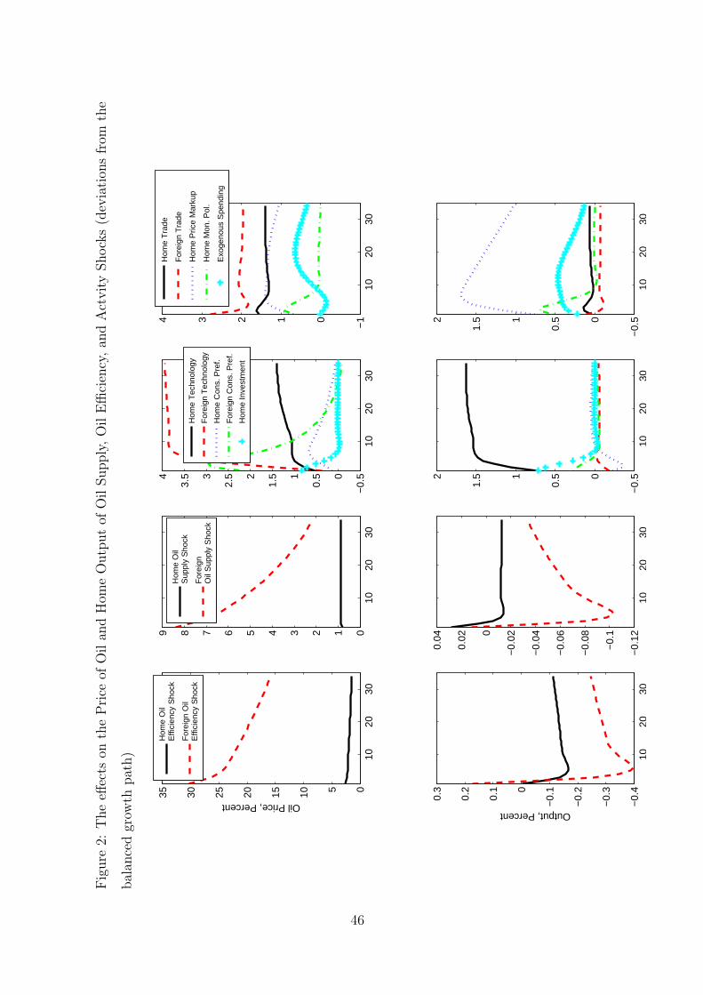
Fig

ure

2:T

he

effec

tson

the

Pri

ceof

Oil

and

Hom

eO

utp

ut

ofO

ilSupply

,O

ilE

ffici

ency

,an

dA

ctvity

Shock

s(d

evia

tion

sfr

omth

e

bal

ance

dgr

owth

pat

h)

1020

300123456789

1020

30−

0.12

−0.

1

−0.

08

−0.

06

−0.

04

−0.

020

0.02

0.04

Hom

e O

ilS

uppl

y S

hock

For

eign

Oil

Sup

ply

Sho

ck

1020

3005101520253035

Oil Price, Percent

1020

30−

0.4

−0.

3

−0.

2

−0.

10

0.1

0.2

0.3

Output, Percent

Hom

e O

ilE

ffici

ency

Sho

ck

For

eign

Oil

Effi

cien

cy S

hock

1020

30−

0.50

0.51

1.52

2.53

3.54

1020

30−

0.50

0.51

1.52

Hom

e T

echn

olog

y

For

eign

Tec

hnol

ogy

Hom

e C

ons.

Pre

f.

For

eign

Con

s. P

ref.

Hom

e In

vest

men

t

1020

30−

101234

1020

30−

0.50

0.51

1.52

Hom

e T

rade

For

eign

Tra

de

Hom

e P

rice

Mar

kup

Hom

e M

on. P

ol.

Exo

geno

us S

pend

ing

46

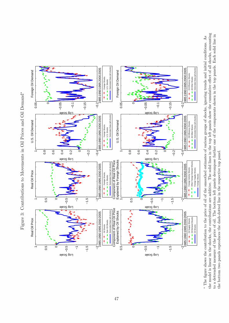
Fig

ure

3:C

ontr

ibuti

ons

toM

ovem

ents

inO

ilP

rice

san

dO

ilD

eman

d∗

1985

1990

1995

2000

2005

−2

−1.

5

−1

−0.

50

0.51

Rea

l Oil

Pric

e

Log Scale

Oil

Sho

cks

Non

−O

il S

hock

s

Det

rend

ed D

ata

(all

shoc

ks)

1985

1990

1995

2000

2005

−2

−1.

5

−1

−0.

50

0.51

Rea

l Oil

Pric

e

Log Scale

For

eign

Sho

cks

U.S

. Sho

cks

Det

rend

ed D

ata

(all

shoc

ks)

1985

1990

1995

2000

2005

−2

−1.

5

−1

−0.

50

0.5C

ompo

nent

of R

eal O

il P

rice

Exp

lain

ed b

y O

il S

hock

s

Log Scale

Oil

Sup

ply

Sho

cks

Oil

Dem

and

Sho

cks

Oil

Sho

cks

1985

1990

1995

2000

2005

−2

−1.

5

−1

−0.

50

0.51C

ompo

nent

of R

eal O

il P

rice

Exp

lain

ed b

y F

orei

gn S

hock

sLog Scale

For

eign

Act

ivity

Sho

cks

Oth

er F

orei

gn D

eman

d S

hock

s

For

eign

Sup

ply

Sho

cks

For

eign

Sho

cks

1985

1990

1995

2000

2005

−0.

4

−0.

20

0.2

0.4

0.6

0.81

U.S

. Oil

Dem

and

Log Scale

Oil

Effi

cien

cy S

hock

s

All

Oth

er S

hock

s

Det

rend

ed D

ata

(all

shoc

ks)

1985

1990

1995

2000

2005

−0.

4

−0.

20

0.2

0.4

0.6

0.81

U.S

. Oil

Dem

and

Log Scale

For

eign

Sho

cks

U.S

. Sho

cks

Det

rend

ed D

ata

(all

shoc

ks)

1985

1990

1995

2000

2005

−0.

2

−0.

15

−0.

1

−0.

050

0.05

For

eign

Oil

Dem

and

Log Scale

Oil

Effi

cien

cy S

hock

s

All

Oth

er S

hock

s

Det

rend

ed D

ata

(all

shoc

ks)

1985

1990

1995

2000

2005

−0.

2

−0.

15

−0.

1

−0.

050

0.05

For

eign

Oil

Dem

and

Log Scale

For

eign

Sho

cks

U.S

. Sho

cks

Det

rend

ed D

ata

(all

shoc

ks)

∗T

hefig

ure

show

sth

eco

ntri

buti

onto

the

pric

eof

oilof

the

smoo

thed

esti

mat

esof

vari

ous

grou

psof

shoc

ks,ig

nori

ngtr

ends

and

init

ialco

ndit

ions

.A

sth

em

odel

islin

ear

inth

esh

ocks

,the

cont

ribu

tion

sar

ead

diti

ve.

The

solid

lines

inth

eto

ple

ftpa

nels

show

the

cum

ulat

ive

effec

tof

alls

hock

s,am

ount

ing

toa

detr

ende

dm

easu

reof

the

pric

eof

oil.

The

bott

omle

ftpa

nels

deco

mpo

sefu

rthe

ron

eof

the

com

pone

nts

show

nin

the

top

pane

ls.

Eac

hso

lidlin

ein

the

bott

omtw

opa

nels

repr

oduc

esth

eda

sh-d

otte

dlin

ein

the

resp

ecti

veto

ppa

nel.

47

Figure 4: Contributions of Oil Demand and Supply Shocks (both at home and abroad) to Movements in

Gross Output∗

1985 1990 1995 2000 2005−0.005

0

0.005

0.01

0.015

0.02

0.025

0.03

0.035Detrended Gross Output

Log

Sca

le

Oil ShocksOil Shocks, Potential

1985 1990 1995 2000 2005−2

−1.5

−1

−0.5

0

0.5Detrended Real Oil Price

Log

Sca

le

Oil ShocksOil Shocks, Potential

∗ “Oil Shocks” include oil supply and oil efficiency shocks both at home and abroad. The label “Potential” refers tooutcomes in the model without nominal rigidities (but otherwise identical). “Detrended” refers to the exclusion of theestimated trends in productivity, oil supply, and oil prices as detailed in Section 2.

48

Fig

ure

5:O

ilE

ffici

ency

Acr

oss

For

eign

Cou

ntr

ies∗

1985

1990

1995

2000

2005

−1

−0.

50

0.51

1.5

Log Scale

Qua

rter

ly M

easu

re o

f For

eign

Oil

Effi

cien

cy in

the

Mod

el

1985

1990

1995

2000

2005

−1

−0.

50

0.51

1.5

Log Scale

Ann

ual O

il E

ffici

ency

Mea

sure

for

Am

eric

a

Can

ada

Bra

sil

Mex

ico

1985

1990

1995

2000

2005

−1

−0.

50

0.51

1.5

Log Scale

Ann

ual O

il E

ffici

ency

Mea

sure

for

Eur

ope

Ger

man

y

Fra

nce

Italy

Uni

ted

Kin

gdom

1985

1990

1995

2000

2005

−1

−0.

50

0.51

1.5

Log Scale

Ann

ual O

il E

ffici

ency

Mea

sure

for

Asi

a

Chi

na

Indi

a

Kor

ea

Japa

n

1984

−88

1989

−93

1994

−98

1999

−03

2004

−08

−20

−1001020

Percent

Con

trib

utio

ns to

Oil

Effi

cien

cy G

row

th R

elat

ive

to T

rend

O

EC

D e

xcl.

S. K

orea

Em

ergi

ng A

sia

incl

. S. K

orea

Res

t of W

orld

1984

−88

1989

−93

1994

−98

1999

−03

2004

−08

0204060

Percent

Sha

re in

Wor

ld O

il C

onsu

mpt

ion

∗T

hefig

ure

plot

sth

ech

ange

sin

oileffi

cien

cyne

tof

the

bala

nced

grow

thpa

thra

te.

The

aggr

egat

em

easu

rede

rive

dfr

omth

em

odel

isth

esm

ooth

edes

tim

ate

offo

reig

noi

leffi

cien

cy;co

untr

ym

easu

res

are

deri

ved

usin

gan

nual

data

inco

mbi

nati

onw

ith

the

mod

el’s

oilde

man

deq

uati

on.

Whe

npl

otti

ngcu

mul

ativ

egr

owth

rate

s,th

elo

g-le

velof

oileffi

cien

cyis

norm

aliz

edto

zero

in19

84.

Whe

nag

greg

atin

gac

ross

coun

try

regi

ons,

coun

try-

spec

ific

oil

effici

ency

grow

thra

tes

wer

ew

eigh

ted

bya

coun

try’

ssh

are

inw

orld

oilco

nsum

ptio

n.

49