Trafficking Networks and the Mexican Drug War∗

Melissa Dell

Harvard

August, 2014

Abstract: Drug trade-related violence has escalated dramatically in Mexico since 2007,and recent years have also witnessed large-scale efforts to combat trafficking, spearheadedby Mexico’s conservative PAN party. This study examines the direct and spillover effectsof Mexican policy towards the drug trade. Regression discontinuity estimates show thatdrug-related violence increases substantially after close elections of PAN mayors. Empiricalevidence suggests that the violence reflects rival traffickers’ attempts to usurp territoriesafter crackdowns have weakened incumbent criminals. Moreover, the study uses a networkmodel of trafficking routes to show that PAN victories divert drug traffic, increasing violencealong alternative drug routes.

Keywords : Drug trafficking, networks, violence.

∗I am grateful to Daron Acemoglu and Ben Olken for their extensive feedback on this project. I alsothank Arturo Aguilar, Abhijit Banerjee, Ernesto Dal Bo, Dave Donaldson, Esther Duflo, Ray Fisman, RachelGlennerster, Gordon Hanson, Austin Huang, Panle Jia, Chappell Lawson, Nick Ryan, Andreas Schulz, JakeShapiro, and seminar participants at Bocconi University, the Brown University Networks conference, ChicagoBooth, CIDE, Colegio de Mexico, Columbia, CU Boulder, George Mason, Harvard, the Inter-AmericanDevelopment Bank, ITAM, the Mexican Security in Comparative Perspective conference (Stanford), MIT,the NBER Political Economy Meeting, NEUDC, Princeton, Stanford, University of British Columbia, UCBerkeley Haas School of Business, UC San Diego, University of Chicago, University of Leicester, Universityof Maryland, US Customs and Border Patrol, the World Bank, and Yale for extremely helpful commentsand suggestions. Contact email: melissadell@fas.harvard.edu, address: Harvard University Department ofEconomics, Littauer Center M-24, Cambridge MA 02138.

1 Introduction

Drug trade-related violence has escalated dramatically in Mexico since 2007, claiming over

60,000 lives and raising concerns about the capacity of the state to monopolize violence.

Recent years have also witnessed large scale efforts to combat drug trafficking, spearheaded

by Mexico’s conservative National Action Party (PAN). These efforts have cost around 9

billion USD per annum, nearly as much as the government expends on social development.1

Yet there is limited causal evidence about the impacts of crackdowns. This study uses

plausibly exogenous variation from close Mexican mayoral elections, a network model of drug

trafficking, and confidential data on the drug trade to identify how crackdowns have affected

violence and trafficking. It examines both the direct effects of crackdowns in the places

experiencing them and the spillover effects they exert by diverting drug traffic elsewhere.

Mexico is the largest supplier to the U.S. illicit drug market, with Mexican traffickers

earning approximately 25 billion USD each year in wholesale U.S. drug markets (U.N. World

Drug Report, 2011). Official data described later in this study document that in 2008, drug

trafficking organizations maintained operations in two thirds of Mexico’s municipalities, and

illicit drugs were cultivated in 14% of municipalities.

While Mexico is a major player in the drug trade, its high levels of drug violence and

drug enforcement expenditures are not unique. Global annual drug enforcement spending

exceeds 100 billion USD, and traffickers in Central America, West Africa, and elsewhere

use violent tactics and often belong to the same transnational trafficking organizations that

operate in Mexico (Economics Briefing, 2013). Because law enforcement does not randomly

decide where to crack down, the existing evidence on drug enforcement impacts consists

primarily of correlations. While often the best evidence available, these can be non-trivial

to interpret. For example, a positive cross-sectional correlation between violence and drug

enforcement could result because areas with higher violence attribute it to drug consumption

and thus expend more fighting the drug trade, and a positive correlation in a panel could

occur because governments crack down in places where they expect violence to later increase.

This study isolates plausibly exogenous variation in drug enforcement policy by exploiting

the outcomes of 2007-2010 close mayoral elections involving the PAN party.2 The PAN

federal government’s role in spearheading the war on drug trafficking, as well as qualitative

evidence that PAN mayors have contributed to these efforts, motivate this empirical strategy.

While municipalities where PAN candidates win and lose by wide margins are likely to be

1See Estados Unidos de Mexico, Gobierno Federal (2010) and Keefer and Loayza (2010). Social devel-opment encompasses a variety of anti-poverty programs, the most prominent of which is the extensivelyevaluated Progresa/Oportunidades conditional cash transfer program.

2See Lee, Moretti, and Butler (2004) for a pioneering example of a regression discontinuity design ex-ploiting close elections. A number of studies have used discontinuous changes in policies, in the cross-sectionor over time, to examine illicit behavior. See Zitzewitz (2011) for a detailed review.

1

different, when focusing on close elections it becomes plausible that election outcomes are

driven by idiosyncratic factors. The study shows that the outcomes of close elections are in

fact uncorrelated with baseline municipal characteristics and violence trends.

Regression discontinuity estimates document that there are 27 to 33 more drug trade-

related homicides per 100,000 municipal inhabitants per annum after a PAN mayor takes

office in a municipality than after a non-PAN mayor takes office, and these effects persist

throughout the mayor’s term and plausibly beyond. Relative to the pre-period, drug trade-

related violence increases by a factor of 5.5 in municipalities with a close PAN victory,

as compared to doubling in municipalities with a PAN loss. These results are robust to

alternative specifications, samples, and lengths of the analysis period and to using the overall

homicide rate, which is balanced throughout the 17 years of available pre-period data. Most

of these homicides were not prosecuted, as just under 20% of homicides in Mexico result in

an arrest (Mexico Evalua, 2012). Homicide is typically in the jurisdiction of Mexico’s state-

level criminal justice systems, and in several of the most violent states the clearance rate for

homicide is only three to seven percent. RD evidence also documents that police-criminal

confrontations increase substantially following PAN inaugurations.

Over 90% of the violence consists of drug traffickers killing each other, and the increases

in violence are concentrated in municipalities that are plausibly the most valuable for drug

trafficking organizations to control. Analysis using information on the industrial organization

of trafficking suggests that the violence reflects rival traffickers’ attempts to wrest control of

territories after crackdowns initiated by PAN mayors have weakened the incumbent traffick-

ers. The violence does not appear to be explained by differences in corruption between the

PAN and other parties or by several other alternative hypotheses that are explored.

These results provide novel evidence that crackdowns caused large and sustained increases

in the homicide rate. They contribute to a literature - consisting primarily of cross-sectional

and panel correlations across countries or cities/states, particularly within the US - which

on balance documents a positive relationship between drug enforcement and violence. Miron

(forthcoming), Werb et al. (2011), and Keefer and Loayza (2010) offer detailed reviews.3

The study’s results also compliment qualitative and descriptive studies arguing that Mex-

ican government policy has been the primary cause of the large spike in violence in recent

years (Guerrero, 2011; Escalante, 2011; Merino, 2011), as well as recent work by Durante

and Gutierrez (2014), who use close Mexican elections to argue that coordination across

municipalities can reduce drug violence.4 The findings contrast with studies arguing that

3Examples of cross-country studies include Miron (2001) and Fajnzylber, Lederman, and Loayza (1998).Examples of studies within the U.S. include Brumm and Cloninger (1995); Miron (1999); and Rasmussen,Benson, and Sollars (1993).

4Guerrero compiles extensive qualitative and descriptive evidence suggesting that government policieshave ignited violent conflicts between traffickers. Escalante documents a state level correlation between

2

the increase in Mexican violence can primarily be explained by the diversification of drug

trafficking organizations into new criminal activities, by increased arms availability, by in-

creased U.S. deportation of immigrants with a criminal record, by job loss, or by cultural

shifts in morality (see Williams, 2012; Escalante et al, 2011, Rios, 2011a for a discussion).

Finally, the results on mechanisms relate to work by Angrist and Kugler (2008) document-

ing that exogenous increases in coca prices spurred violence in rural districts in Colombia

because combatant groups fought over the additional rents. In Mexico, crackdowns likely re-

duce rents from criminal activities while in effect, but by weakening the incumbent criminals

they also reduce the costs of taking control of a municipality. Controlling territory plausibly

offers substantial rents from trafficking and a variety of other criminal activities once the

crackdown and its violent aftermath subside. While the study shows that the violent effects

of crackdowns are sustained in the medium run, trafficking organizations may have a longer

run horizon or might have underestimated how long gang wars would last.

When policy leads one location to become less conducive to illicit activity, organized

crime may relocate elsewhere, affecting violence in other municipalities.5 Examining these

spillovers is central to understanding the broader impacts of crackdowns. A number of

studies have examined the drug trade and organized crime, but to the best of my knowledge

this study is the first to empirically identify spillover patterns in drug trade activity.6 To do

so, the study develops a network model of trafficking routes that predicts where drug traffic

- and potentially drug violence - is diverted following crackdowns.

Traffickers’ objective is to minimize the costs of transporting drugs from producing mu-

nicipalities in Mexico across the road network to U.S. entry points. In the simplest version of

the model, traffickers take the most direct route to the U.S. that avoids municipalities with

a closely elected PAN mayor. PAN victories increase the costs of trafficking drugs through a

municipality, diverting least cost routes elsewhere. Because elections occur at different times

during the sample period, this generates plausibly exogenous within-municipality variation

in predicted routes throughout Mexico. This variation from close elections is essential to

identifying spillovers because it breaks the well-known reflection problem, allowing spillovers

homicides and the deployment of the Mexican military and federal police, and Merino expands Escalante’sanalysis by using a matching strategy to argue that Mexican homicides in 2008-2009 would have totaled14,000 rather than 19,000 in the absence of intervention.

5For example, in a non drug-related context, work by Di Tella and Schargrodsky (2004) documents thatthe allocation of police officers to Jewish institutions in Buenos Aires substantially reduced auto theft in theimmediate vicinity but may also have diverted some theft to as close as two blocks away.

6Studies of the economics of organized crime include Levitt and Venkatesh’s analysis of the finances ofa U.S. drug gang (2000); Gambetta’s economic analysis of the Sicilian mafia (1996); Pinotti’s (2012) studyof the economic costs of organized crime in southern Italy; Bandiera (2003), Dimico et al. (2012) andBuonanno et al.’s (2012) investigations of the historical origins of the Sicilian mafia; Varese’s (2005) andFrye and Zhuravskaya’s (2000) analyses of the rise of the Russian mafia; and Mastrobuoni and Patacchini’s(2010) study of the network structure of crime syndicates.

3

to be isolated from correlations (Manski, 1993). Traffickers may care about the routes other

traffickers take, and thus the study also estimates a richer model that imposes congestion

costs when routes coincide. The approach is illustrated in Figure 1, and predicted routes for

the beginning of the sample period are shown in Figure 2.

When a municipality acquires a predicted route, the monthly probability that a drug

trade-related homicide occurs increases from a baseline probability of 4.8% to 6.2%, and for

each additional route the drug trade-related homicide rate increases by 0.54 per 100,000.

There is some evidence that violence spillovers are concentrated in municipalities where

multiple routes coincide. While the magnitudes of violence spillovers are typically small

compared to the direct effects of crackdowns, they are nevertheless important given the

gravity of homicides.

The study also examines how within-municipality variation in predicted routes compares

to within-municipality variation in actual illicit drug seizures. This exercise can validate

whether the trafficking model is predictive, as changes in drug confiscations are not used to

estimate the routes. The value of drug seizures increases by 18% when a municipality acquires

a predicted trafficking route, and this estimate is significant at the 1% level. Robustness and

placebo checks also support the validity of the network approach.

In addition to validating the model, the drug seizures results can shed some light on the

“diversion hypothesis”, which argues that when the government cracks down in one place,

drug activity is partially diverted elsewhere without being substantially reduced. The di-

version hypothesis plays a major role in debates over the War on Drugs and is a leading

explanation popularly given for why - despite a massive increase in drug enforcement ex-

penditures globally over the past forty years - drug markets have continued to expand and

drug use has not declined (UNODC, 2010; Reuter and Trautmann, 2009; ODCPP, 2002).

For example, descriptive evidence suggests that coca eradication policies in Bolivia and Peru

during the late 1990s led cultivation to shift to Colombia, and large-scale coca eradication

in Colombia in the early 2000s has since led cultivation to re-expand in Peru and Bolivia,

with total coca cultivation unchanged (Isacson, 2010; Leech, 2000; UN Office on Drugs and

Crime 1999-2009). In the context of the Mexican Drug War, the shares of Mexican heroin

and possibly other Mexican drugs in the U.S. market actually increased during the Calderon

crackdown (Dıaz-Briseno, 2010). While the counterfactual is not clear - a problem that more

generally plagues the predominantly descriptive and anecdotal evidence about the diversion

hypothesis - this hypothesis is a potential explanation.

Estimating the share of drugs diverted and the share no longer trafficked through Mexico

would require making potentially untenable assumptions about drug cultivation and seizure

rates. Nevertheless, the study’s results document that the diversion of drug traffic following

crackdowns was large enough to substantially increase illicit drug seizures along predicted

4

alternative routes. Combined with the fact that some law enforcement resources used for

drug seizures and eradication were re-directed during the Calderon administration to focus

on steeply increasing rates of violence (National Drug Intelligence Center, 2010), these results

suggest that it is unlikely that the Mexican Drug War led to large, sustained reductions in

the supply or consumption of illicit drugs.

While there are a variety of outcomes that could be affected by drug crackdowns, this

study focuses on violence and the diversion of drug traffic since these are particularly central

to policy and academic debates about the War on Drugs. It does briefly examines economic

outcomes - finding negative impacts of crackdowns on informal sector earnings and female

labor force participation. Formal sector wages and male labor force participation are not sig-

nificantly affected. While the economic effects are noisily estimated, they are consistent with

qualitative evidence that drug trafficking organizations not only set up smuggling operations

but also extort informal sector producers via protection rackets.

This study’s results document that the costs of the drug war, in terms of lives lost,

have been high and sustained. Beyond the violence costs, there are also opportunity costs

of the Mexican government expending approximately nine billion USD per annum fighting

drug trafficking. While evidence is imperfect and the existence of countervailing benefits

that outweigh these costs - such as impacts on drug consumption, corruption, or wages -

cannot be disproved, available evidence does not indicate that large positive impacts on

these outcomes are particularly probable. The results of the study overall suggest policies

aimed at deterring violence, enforcing homicide laws, and confronting other challenges, as

opposed to policies whose primary objective is to reduce drug trafficking.

The next section provides an overview of Mexican drug trafficking. Section 3 then tests

whether the outcomes of close elections affect violence in the municipalities experiencing

these elections and examines the economic mechanisms underlying the results. Section 4

develops the network model of drug trafficking and tests whether PAN victories exert drug

trafficking and violence spillovers. Finally, Section 5 concludes.

2 Drugs and Violence in Mexico

2.1 The Drug Trafficking Industry

Mexican drug traffickers dominate the wholesale illicit drug market in the United States,

earning between 14 and 48 billion USD annually.7 According to the U.N. World Drug Report,

7Estimates are from the U.S. State Department (2009). Estimates by U.S. Immigration and CustomsEnforcement, the U.S. Drug Enforcement Agency, and the Mexican Secretarıa de Seguridad Publica arebroadly similar and also contain a large margin of error.

5

Mexico is the largest supplier of heroin to U.S. markets and the largest foreign supplier

of marijuana and methamphetamine. Official Mexican government data, obtained from

confidential sources, document that fourteen percent of Mexico’s municipalities regularly

produce opium poppy seed (heroin) or cannabis. Moreover, 60 to 90 percent of cocaine

consumed in the U.S. transits through Mexico (U.S. Drug Enforcement Agency, 2011). The

U.S. market provides substantially more revenue than Mexico’s domestic drug market, which

is worth an estimated 560 million USD annually (Secretarıa de Seguridad Publica, 2010).8

At the beginning of this study’s sample period, in December 2006, there were six major

drug trafficking organizations (DTOs) in Mexico. Official data obtained from confidential

sources document that 68 percent of Mexico’s 2,456 municipalities were known to have a

major DTO or local drug gang operating within their limits in early 2008. These data

also estimate that 49 percent of drug producing municipalities were controlled by a major

trafficking organization, with the remaining controlled by local gangs.

The term ‘cartel’, used colloquially to refer to DTOs, is a misnomer, as these organizations

do not collude to reduce illicit drug production or to set prices. Alliances between DTOs

are highly unstable, and there is considerable decentralization and conflict within DTOs

(Williams, 2012; Guerrero, 2011, p. 10, 106-108). Decisions about day-to-day operations are

typically made by local cells, as this ensures that no single trafficker will be able to reveal

extensive information if captured by authorities. Moreover, the number of major DTOs

increased from six in 2007 to 16 by 2011, with groups splitting over leadership disputes.

In addition to trafficking drugs, Mexican DTOs engage in a host of illicit activities that

range from protection rackets, kidnapping, human smuggling, and prostitution to oil and fuel

theft, money laundering, weapons trafficking, arson, and auto theft (Guerrero, 2011, p. 10).

Notably, protection rackets involving the general population have increased substantially in

recent years (Rios, 2011b; Secretariado Ejecutivo del Sistema Nacional de Seguridad Publica,

2011). The poor, who have limited recourse to state protection, are particularly likely to be

extorted (Dıaz-Cayeros et al., 2011).

The second half of the 2000s witnessed large, rapid increases in drug trade-related vi-

olence. Over 50,000 people were killed by drug trade-related violence between 2007 and

2012, and homicides increased by at least 30% per year during most of this period (Rios,

2011b). By 2010, violent civilian deaths per capita had reached levels higher than in Iraq

and Afghanistan during the same period, higher than in Russia during the 1990s, and higher

than in Sicily following the Second World War (Williams, 2012). Over 85 percent of the

drug violence consisted of people involved in the drug trade killing each other, 95 percent of

8According to the U.S. National Survey on Drug Use and Health, 14.2 percent of Americans (35.5 millionpeople) have used illicit drugs during the past year, as contrasted to 1.4 percent of the Mexican population(1.1 million people) (National Addiction Survey, 2008).

6

the victims were male, and 45 percent were under age 30. The violence has been public and

brutal, with bodies hung from busy overpasses and severed heads placed in public spaces

(Williams, 2012). Public displays of brutality and activities such as kidnapping and extor-

tion affect the general public, and 2011 public opinion surveys found that security was more

likely than the economy to be chosen as the largest problem facing the country.

2.2 Mexico’s War on Drug Trafficking

Combating drug trafficking has been a major priority of the Mexican federal government in

recent years. Notably, President Felipe Calderon (December 2006 - 2012) of the conservative

National Action Party (PAN) made fighting organized crime the centerpiece of his adminis-

tration. During his second week in office, Calderon deployed 6,500 federal troops to combat

trafficking, and by the close of his presidency approximately 45,000 troops were involved.

For most of the 20th century, a single party, the PRI (Institutionalized Revolutionary

Party), dominated Mexican politics. The PRI historically took a passive stance towards

the drug trade, and widespread drug-related corruption is well-documented (Shannon, 1988;

Chabat, 2010). Mexicans elected their first opposition president in 2000, and today Mex-

ico has three major parties: the PAN on the right, the PRI, and the PRD (Party of the

Democratic Revolution) on the left. While presidents Ernesto Zedillo (1994-2000, PRI)

and Vicente Fox (2000-2006, PAN) did implement security reforms and crackdowns (Cha-

bat, 2010), these were on a lesser scale than Calderon’s. Calderon’s crackdown appears to

have been unanticipated, as the 2006 presidential election - decided by an extremely narrow

margin - made limited mention of security issues (Aguilar and Castaneda, 2009).

Mexico’s crackdown on trafficking has focused on arrests and enforcement against traffick-

ers, whereas illicit crop eradication has declined somewhat as resources have been diverted to

respond to violence (National Drug Intelligence Center, 2010). Drug seizures and high level

arrests are typically made by the federal police and military, who have the requisite training

and weaponry to fight heavily armed traffickers. Municipal police are relevant because they

can provide local information for federal interventions, which often target specific actors

about whom reliable information is available (Chabat, 2010). Municipal police also serve as

valuable allies for traffickers, collecting information on who is passing through a town. This

information is essential for protecting criminal operations and anticipating attacks by federal

authorities and rivals.9 Municipal police form the largest group of public servants killed by

drug-related violence (Guerrero, 2011).

Mayors name the municipal police chief and set policies regarding police conduct. Thus,

PAN mayors could assist Calderon’s drug war by appointing amenable law enforcement au-

9See for example El Pais, August 26 2010.

7

thorities and by encouraging them to share information with the PAN federal government.

Qualitative evidence indicates that PAN mayors under Calderon were more likely to request

law enforcement assistance from the PAN federal government than their non-PAN counter-

parts and also suggests that operations involving the federal police and military have been

most effective when local authorities are politically aligned with the federal government

(Guerrero, 2011, p. 70).10

PAN mayors may have been more likely to aid Calderon’s war on drugs because author-

ities from the same party cooperate more effectively, because of differences in corruption, or

because of ideology. For example, Nathan Jones (2012) argues based on fieldwork conducted

in Baja California that PAN politicians not only received more military assistance than their

non-PAN counterparts but also were provided with newer, more sophisticated military hard-

ware. Corruption will be discussed quantitatively later in this study. Moreover, PAN mayors

plausibly had strong career incentives to cooperate. Mexican mayors are barred from con-

secutive reelection and securing a subsequent political post typically requires support from

party leaders.11 For example, the mayorship is a common stepping stone to national politics,

and a substantial part of the Mexican Congress is elected from closed party lists.12 PAN

party leaders choose these lists, and if a candidate is placed high enough, she will enter

the legislature (Langston, 2008; Wuhs, 2006). Parties likewise distribute millions of pesos

in public campaign resources, and the federal government controls thousands of appointed

posts (Langston, 2008).

The criminal justice system is also relevant for understanding the effects of crackdowns.

Like the U.S., Mexico has state and federal criminal justice systems, and homicides are

typically in the jurisdiction of the states. The clearance rate for homicides in Mexico is

low, with just under 20% of homicides resulting in an arrest (Mexico Evalua, 2012), and the

national average masks substantial regional variation. In the state of Chihuahua, only 3.6%

of homicides in 2010 resulted in an arrest by the end of the following year, with Durango

and Sinaloa close behind at 4.6% and 7%, respectively. In contrast, Yucatan had a clearance

rate of 100% for the 34 homicides that it experienced in 2010 and Baja California Sur had

a clearance rate of 90%. States with the lowest clearance rates tend to be the most violent.

For comparison, the clearance rate for homicides in the U.S. is around 67%, ranging from

10For example, while drug trade-related violence initially increased in Baja California in response to alarge federal intervention, the violence has since declined, and the state is frequently showcased as a federalintervention success story (Guerrero, 2011). The governor of Baja California belonged to the PAN, and thefederal intervention began under the auspices of a PAN mayor in Tijuana. On the other hand, in CiudadJuarez both the mayor and governor belonged to the opposing PRI party, and conflicts and mistrust betweenmunicipal and federal police have been rampant.

11The PAN controlled the mayorship in around a third of municipalities at the beginning of the sample.12 In a survey of 1,400 representatives who had served in Mexico’s lower house of Congress, 77% of the

PAN legislators had previously been involved in municipal politics (Langston, 2008). 200 of the 500 seats inthe lower house of Congress and 32 of the 128 Senate seats are filled from the party lists.

8

a low of 52% in Michigan to a high of 89% in Wyoming (FBI Uniform Crime Statistics,

2013). Low clearance rates in Mexico result from difficulties in both investigating homicides

and apprehending suspects. Only 36% of warrants result in an arrest, with the arrest rate

ranging from 14% to 76% across Mexican states (Mexico Evalua, 2012 and 2010). The federal

government passed major judicial reforms in 2008, but the system remains weak.

These statistics, however, should not be interpreted as evidence that the Mexican federal

government is incapable of arresting wanted criminals in a targeted manner. Drug-related

crimes and organized criminal activity are often federal offenses, and nearly half of all federal

inmates are charged with drug-related crimes (Zepeda, 2013; Mexico Evalua, 2013). Having

the cooperation of local authorities can be central in making drug trade-related arrests, and

confidential data on high level drug arrests shows that - while rare - they are about twice as

common following close PAN victories as compared to close PAN losses.

These facts can plausibly help explain why violence has increased dramatically in Mexico

in recent years. With the help of municipal authorities, the federal government has used

a targeted strategy to arrest drug traffickers on federal drug-related or organized crime

charges, plausibly destabilizing drug gangs. Rival gangs knew they could violently exploit

this weakness without much risk of being prosecuted by state criminal justice systems for

homicide, at least in Mexico’s most violent states. This equilibrium has influenced some

policymakers and scholars, such as Mark Kleinman (2011), to argue that the Mexican federal

government should explicitly target its drug enforcement strategy towards the most violent

traffickers, rather than targeting drug trafficking activity per se. The results of the current

study plausibly support this position.

3 Direct Effects of Close PAN Victories on Violence

This section uses a regression discontinuity approach to test whether the outcomes of close

mayoral elections affect violence in the municipalities experiencing these elections. It first

describes the data and identification strategy. Then it examines the relationship between

PAN victories and violence, as well as the economic mechanisms underlying this relationship.

3.1 Data

The analysis uses official government data on drug trade-related outcomes, obtained from

confidential sources unless otherwise noted. Data on drug trade-related homicides occurring

between December of 2006 and October of 2011 were compiled by a committee with repre-

sentatives from all ministries that are members of the National Council of Public Security.13

13The Mexican government stopped compiling these data after October of 2011.

9

This committee met each week to classify which homicides from the past week were drug

trade-related.14 Drug trade-related homicides are defined as any instance in which a civil-

ian kills another civilian, with at least one of the parties involved in the drug trade. The

classification is made using information in the police reports and validated whenever pos-

sible using newspapers. The committee also maintains a database of those killed in armed

clashes between police and organized criminals. Month x municipality data on all homicides

occurring between 1990 and 2012 were obtained from the National Institute of Statistics

and Geography (INEGI) and allow examination of a longer pre and post period than the

drug trade-related homicide data. The overall homicide data are drawn from vital statistics

compiled by state government authorities in each of Mexico’s 31 states and federal district.

Month x municipality confidential data on high level drug arrests are also employed.15

Moreover, this section uses official government data on which of Mexico’s 2456 municipal-

ities had a DTO or local drug gang operating within their limits in early 2008. This offers the

closest available approximation to pre-period DTO presence, as systematic municipal-level

data about DTOs were not collected before this time.

Finally, electoral data for elections occurring during 2007-2010 were obtained from the

electoral authorities in each of Mexico’s states. The sources for a number of other variables,

used to examine whether the RD sample is balanced, are listed in the notes to Table 1.

3.2 Econometric Framework

This study uses a regression discontinuity (RD) approach to estimate the impact of PAN

victories on violence. The RD strategy exploits the fact that the party affiliation of a

municipality’s mayor changes discontinuously at the threshold between a PAN victory and

loss. Municipalities where the PAN wins by a large margin are likely to be different from

municipalities where the PAN loses by a wide margin. However, when we narrow our focus to

the set of municipalities with close elections, it becomes more plausible that election outcomes

are determined by idiosyncratic factors and not by systematic municipal characteristics that

could also affect violence. Thus, under certain conditions municipalities where the PAN

barely lost can serve as a reasonable counterfactual for municipalities where they barely

won. This section examines the plausibility of the RD identifying assumptions in detail, but

first it is helpful to specify the regression form. The baseline analysis estimates the following

regression model within a narrow window around the PAN win-loss threshold:

ym = α0+α1PANwinm+α2PANwinm×f(spreadm)+α3(1−PANwinm)×f(spreadm)+εm (1)

14Previous homicides are also considered for reclassification if new information becomes available.15High level traffickers include DTO kingpins, regional lieutenants, assassins, and financiers.

10

where ym is the outcome of interest in municipality m. PANwinm is an indicator equal

to 1 if the PAN candidate won the election, and spreadm is the margin of PAN victory.

The study examines robustness to different functional forms, f(·), for the RD polynomial,

which is estimated separately on either side of the PAN win-loss threshold. Some robustness

specifications also include region fixed effects and baseline controls.

Elections in Mexico occur at different times throughout the sample period. The study

considers two samples: close elections occurring in 2007-2008 and close elections occurring in

2007-2010. The former provides a longer post-inauguration period but fewer municipalities.

In order to be able to check for violence pre-trends, both samples are limited to municipalities

with at least half a year of drug-trade related homicide data prior to the elections. The

samples are also limited to municipalities with at least a year of post-inauguration data, so

that violence effects can be examined in the medium-term.

Identification requires that all relevant factors besides treatment vary smoothly at the

threshold between a PAN victory and loss. Formally, letting y1 and y0 denote poten-

tial outcomes under a PAN victory and loss, identification requires that E[y1|spread] and

E[y0|spread] are continuous at the win-loss threshold. This assumption is needed for mu-

nicipalities where the PAN barely lost to be an appropriate counterfactual for those where

they barely won. This assumption would be violated if the outcomes of close elections were

determined not by idiosyncratic factors but by a systematic advantage of winners.16

To assess the plausibility of the identifying assumptions, Table 1 examines whether 25

political, economic, demographic, road network, and geographic pre-characteristics are bal-

anced across the PAN win-loss threshold. The next section considers violence trends prior to

the relevant elections. The body of the study focuses on the baseline 2007-2008 elections sam-

ple for municipalities with a vote spread of five percentage points or less, and the appendix

provides analogous results for the 2007-2010 elections and for alternative bandwidths.17

Column (1) reports the mean value of each characteristic in municipalities where the PAN

won, column (2) does the same for municipalities where they lost, and column (3) reports the

t-statistic on the difference. In no case are there statistically significant differences, including

for political characteristics such as turnout and the party of the incumbent.18 I also estimate

the RD specification given by equation (1) using each of the baseline characteristics as the

dependent variable. The coefficients on PAN win are reported in column (4) and t-statistics

in column (5). While some of the coefficients are noisily estimated, they are statistically

identical to zero. Appendix Figures A-2 through A-5 show analogous RD plots for each

characteristic. Regional characteristics could also differ across the PAN win-loss threshold,

16For example, Caughey and Sekhon (2011) show that in U.S. House elections between 1942 and 2008,close winners have financial and incumbency advantages.

17 Figure A-1 shows a map of the close election municipalities, which are located throughout Mexico.18The economically large difference in surface area is driven by a single large municipality, Ensenada.

11

and thus I calculate the average of each baseline characteristic in the municipalities that

border each municipality in the RD sample. Columns (6) and (7) repeat the RD analysis

using these characteristics as the dependent variable. Again, while some coefficients are

noisy, nearly all are statistically insignificant.

To provide a more complete view of how pre-characteristics vary around the threshold,

Appendix Tables A-1 through A-4 repeat this analysis limiting the sample to vote spread

bandwidths of 4%, 3%, 2%, and 13.3% (the Imbens-Kalyanaraman bandwidth), respectively,

and Tables A-5 through A-9 do the same for the 2007-2010 close election sample. These tables

document qualitatively similar patterns.19

When all pre-characteristics are combined into a single measure based on their ability to

predict post-period violence - providing a higher powered test of whether pre-characteristics

are balanced - there likewise is not a discontinuity at the PAN win-loss threshold. Specif-

ically, I regress average violence during the post-period - which lasts for the duration of a

mayor’s term - on all the characteristics from Table 1, as well as on average violence during

the pre-period. Both the average monthly probability that at least one homicide occurs

and the average homicide rate are considered. I then use the coefficients from this regres-

sion to predict post-period violence, and Figure A-6 plots the predicted violence measures

against the PAN margin of victory. Panel A examines the predicted drug-related homicide

probability, Panel B the predicted drug-related homicide rate, Panel C the predicted overall

homicide probability, and Panel D the predicted overall homicide rate. In no case is there a

statistically significant discontinuity, and the magnitude of the discontinuity is modest.

Identification also requires the absence of selective sorting around the PAN win-loss

threshold. This assumption would be violated, for example, if elections were rigged in

favor of the PAN in municipalities that would later experience an increase in violence. To

formally test for sorting, I implement McCrary’s (2008) test by collapsing the election data

to one percentage point vote spread bins and using the observation count in each bin as the

dependent variable in equation (1). Appendix Figures A-7 and A-8 show that there is not

a discontinuous change at the PAN win-loss threshold for either the 2007-2008 or 2007-2010

close election samples. In other words, neither the PAN nor its opponents systematically

win close elections. For manipulation of the threshold to be consistent with these figures

and Table 1, there would need to be an equal number of elections rigged in favor of and

against the PAN, and the pre-characteristics would need to be the same on average for these

municipalities and their neighbors, a scenario that is unlikely.

The absence of selective sorting is also institutionally plausible. Elections in Mexico

19Regressions using the Imbens-Kalyanaraman bandwidth use a triangular kernel such that the weightgiven to each observation decays with distance from the threshold. This is the standard approach forimplementing the Imbens-Kalyanaraman bandwidth - which is estimated assuming that kernel weightingwill be used. The other bandwidths produce very similar estimates when combined with kernel weighting.

12

are coordinated by a multi-partisan state commission, and genuine recourse exists in the

case of suspected fraud. While traffickers may have incentives to intimidate voters and

candidates, recall that mayors prior to the Calderon administration had limited capacity

to challenge heavily armed traffickers given the absence of a widespread federal crackdown.

The elections, particularly for the 2007-2008 sample, are at the beginning of Calderon’s

crackdown, when traffickers were unlikely to have anticipated how sustained it would be and

the role mayors would play. Thus, they may not have found it worthwhile to influence local

elections. Consistent with this conjecture, systematic killings of mayors by traffickers began

only after the federal crackdown had been sustained for several years.

3.3 Graphical Analysis of Violence Patterns

This section graphically analyzes the relationship between close election outcomes and vi-

olence, documenting that violence is similar prior to elections but diverges significantly

thereafter. The main body of the paper focuses on the 2007-2008 close election sample, in

which the post-inauguration period encompasses the mayor’s three year term.

Figure 3 examines the probability that at least one drug trade-related homicide occurs

in a given month and the homicide rate, both averaged across the pre-election, lame duck,

and post-election periods. It plots the violence measures against the PAN margin of victory,

with a negative margin indicating a PAN loss. Each point represents average violence in 0.5

percentage point vote spread bins. The solid line plots predicted values from a regression of

violence on a quadratic polynomial in the vote spread, estimated separately on either side

of the PAN win-loss threshold, and the dashed lines show 95% confidence intervals.

While close PAN victories do not significantly increase the average probability that drug

trade-related violence occurs during the mayor’s subsequent term (Panel A), the drug-related

homicide rate increases by around 40 per 100,000 following a close PAN victory, as compared

to a close PAN loss (Panel B). At the threshold, violence is around three times higher in PAN

municipalities. In contrast, Panel C (Panel D) shows that the drug trade-related homicide

probability (rate) during the 2 to 5 month period following the election but prior to the

inauguration of new authorities is similar regardless of whether the PAN barely won or lost.

Finally, Panels E and F document the absence of a violence discontinuity at the PAN win-loss

threshold during the six months prior to the elections, providing additional evidence that the

RD sample is balanced. Appendix Figure A-9 presents an analogous figure for the 2007-2010

elections, documenting similar patterns.20 Violence is somewhat higher nearer the threshold,

on both sides, in the pre as well as post-periods.21 This is plausibly explained by the fact

20Appendix Figure A-11 shows that both the 2007-2008 and 2007-2010 estimates are similar in magnitudewhen a negative binomial model is used to account for the count nature of the homicide rate.

21 See Appendix Table A-46 for an examination of the relationship between the absolute value of the vote

13

that drug trade-related violence is concentrated in larger, more urban municipalities, which

are more likely to have very close elections (see Appendix Figure A-2).

Figure 4 provides an analogous exercise for overall homicides, in order to address two

potential concerns with the drug trade-related homicide data. First, while homicides are

classified as drug trade-related by a national committee, it is possible that the police reports

used to make this classification systematically differ across municipalities. Moreover, the

pre-period in the drug trade-related homicide data is relatively short since the data were

not collected prior to President Calderon’s inauguration in December of 2006. The overall

homicide data are available for 1990-2012 and hence offer a much longer pre-period.

The patterns documented in Figure 4 are similar to those in Figure 3. There is a signifi-

cant increase in the overall homicide rate following the inauguration of PAN mayors (Panel

B), whereas violence during the pre-period - which in this case extends over 17 years - is

balanced.22 Appendix Figure A-10 documents analogous overall homicide patterns in the

2007-2010 close election sample.23 Since it is quite unlikely that homicide differences of this

magnitude would be driven by differences in reporting, these results provide strong evidence

that there is a genuine increase in violence following PAN victories. The overall homicide

estimates tend to be somewhat larger in magnitude than the drug trade-related homicide es-

timates, and the positive correlation between changes from month-to-month in drug-related

homicides and overall homicides net drug-related homicides suggests that some homicides

related to drug gang wars may not have been classified as such.

To uncover more detail about the relationship between violence and PAN victories, I

estimate equation (1) separately for each quarter prior to the election and following the

inauguration of new authorities. Figure 5 plots the PAN win coefficients against time, which

is defined relative to each municipality’s election and inauguration. The thin lines plot

95% confidence intervals, and the thick lines plot 90% confidence intervals. Quarterly data

are used to improve the legibility of the plots, and similar patterns are documented using

monthly data in Appendix Figure A-13.

Panel A documents that the probability that at least one drug-related homicide occurs

in a given month increases for one to two quarters following the mayor’s inauguration, but

the difference between PAN and non-PAN municipalities converges back to zero after this.24

In contrast, the drug trade-related homicide rate increases in the first quarter following

the inauguration of a new PAN mayor and remains higher than in non-PAN municipalities

spread and violence.22Results (available upon request) are also similar when overall homicides are considered using the same

period as for the drug trade-related homicides.23Figure A-12 documents similar results for the homicide rate using a negative binomial model.24Whether the impact is statistically significant in the second quarter varies with the specification used,

though coefficient magnitudes are similar across specifications.

14

throughout the remainder of the mayor’s term. Drug violence in the pre-election period is

balanced for both the extensive margin and homicide rate. Likewise, Panel C shows that the

overall homicide rate is balanced throughout the seventeen years prior to the relevant elec-

tions. The homicide rate increases following the inaugurations of PAN mayors and remains

significantly higher in PAN municipalities for as long as data are available. The violence dif-

ferences do not subside when new mayors take office in 2010 and 2011.25 Appendix Figures

A-15-A-23 show that these results are robust to using different bandwidths (4%, 3%, 2%,

and 13.3%, the Imbens-Kalyanaraman bandwidth) and controls, and Appendix Figure A-24

documents that violence is also balanced in neighboring municipalities prior to the elections.

3.4 Further Results and Robustness

Tables 2 and 3 estimate the RD specification given in equation (1) - using either a linear or

quadratic RD polynomial - for the 2007-2008 and 2007-2010 close election samples.26 The

coefficients on PAN win in the specification using the quadratic RD polynomial estimate the

discontinuities in Figures 3 and 4, and the linear polynomial provides a robustness check.

Panel A considers drug trade-related homicides and Panel B overall homicides.

Table 2 documents that close PAN victories increase the drug trade-related homicide rate

by between 33 (s.e. = 9) and 42 (s.e. = 8) homicides per 100,000 per annum during the

mayor’s three year term. Table 3 considers close elections occurring between 2007 and 2010,

estimating that PAN victories increases the drug-related homicide rate by 18 (s.e.= 6) to 27

(s.e.= 9) homicides per 100,000 during the one year following the mayor’s inauguration. The

difference between these estimates is explained by the post-period lengths. When the anal-

ysis examining 2007-2008 elections uses a one year post-inauguration period, the estimated

impact of close PAN victories is 22 per 100,000. The estimates for the overall homicide rate

show a similar pattern but are somewhat larger in magnitude, as discussed above. Columns

(1) through (6) of both tables document that close PAN victories do not have a sustained

impact on the violence extensive margin.

Back of the envelope calculations suggest that crackdowns are responsible for at least

half of the increase in homicides in Mexico in recent years. When using 2007-2008 elections

to compare the drug trade-related homicide rate in the pre and post periods, the homicide

rate approximately doubles in municipalities where the PAN barely loses and increases by

a factor of 5.5 in places where the PAN barely wins. Similarly, the overall homicide rate in

municipalities with close PAN elections in 2007-2008 nearly doubles in municipalities with

25The probability of at least one homicide occurring in a given month is also balanced across the full 17year period prior to the elections, see Figure A-14.

26The homicide rate is more noisily measured in smaller municipalities. Thus, following the standardapproach in the crime literature, regressions use inverse variance weighting.

15

a PAN loss and increases by a factor of four in municipalities with a PAN victory. These

estimates are likely a lower bound since the party of the mayor is not the sole determinant

of federal security assistance.

The appendix conducts a number of additional robustness checks. First, Appendix Ta-

bles A-10 and A-11 examine the robustness of the drug trade-related homicide rate estimates

to using alternative bandwidths (5%, 4%, 3%, 2%, and 13.3% - the Imbens-Kalyanaraman

bandwidth), alternative RD polynomials (linear, quadratic, cubic, and quartic, estimated

separately on either side of the PAN win-loss threshold), and alternative inclusions of con-

trols, for the 2007-2008 and 2007-2010 samples respectively. Appendix Tables A-12 and A-13

perform an analogous exercise for the overall homicide rate. The coefficients reported in the

main text fall towards the middle of the distribution of the 132 coefficients reported in each

of the analogous robustness tables and tend to be statistically similar. Moreover, Appendix

Figures A-25 and A-26 document that PAN victories robustly increase the homicide rate,

regardless of the length of the analysis period.27 I focus on close elections because they allow

for causal identification. For completeness, Table A-14 reports that when all PAN elections

are included in the sample, effects on violence are positive but only statistically significant

for the overall homicide rate.

If violence before the elections is balanced, a differences-in-differences specification will

estimate PAN win effects that are similar to the RD coefficients. Appendix Tables A-15-A-24

- which each explore a different vote spread bandwidth (5%, 4%, 3%, 2%, and 13.3%) and

dependent variable (the drug trade-related or overall homicide rate) - document that this

approach does indeed produce estimates similar to those from the RD, for both the 2007-

2008 and 2007-2010 close election samples. This remains true even when the differences-in-

differences specifications control for municipality-specific time trends.

3.5 Interpretation

This section examines the mechanisms through which PAN victories affect drug trade-related

violence, over 85% of which consists of traffickers killing each other. The evidence suggests

that PAN victories lead to crackdowns that weaken incumbent criminals, spurring violence

between traffickers.

First, consider whether PAN victories lead to crackdowns. Municipality level data on mil-

itary and federal police deployments cannot be released to individuals outside these organi-

27 Figure A-25 shows that results using the drug trade-related homicide rate are robust to varying thepre-period from one to six months, the lame duck period from one to five months, and the post-period fromtwo to thirty-five months. Figure A-26 shows analogously that results for the overall homicide rate arerobust to varying the pre-period from one to 205 months (≈ 17 years), the lame duck period from one tofive months, and the post-period from two to over 50 months.

16

zations, but other available evidence suggests that PAN mayors are more likely to crack down

on the drug trade. Appendix Table A-25 examines police-criminal confrontation causalities.

Using the RD specification in equation (1), it documents that casualties are significantly

higher in PAN than in non-PAN municipalities, for both the 2007-2008 and 2007-2010 elec-

tion samples. In contrast, casualties are balanced in the pre-period. Arrests of high level

drug traffickers, while rare, likewise occur more frequently following PAN victories.28

Table 4 examines whether the patterns of heterogeneity in the data are consistent with the

hypothesis that crackdowns spur conflicts between traffickers. Columns (1) and (5) reproduce

the baseline post-inauguration results for the 2007-2008 and 2007-2010 close election samples,

respectively. Columns (2) and (6) examine whether effects are larger in municipalities that

are closer to the U.S., where most illicit drugs are consumed. These municipalities are

plausibly more valuable for traffickers to control and potentially more worth fighting over.

I interact PAN win, spread, and PAN win × spread with an indicator equal to one if the

municipality is greater than median distance from the U.S. In both the 2007-2008 and 2007-

2010 close election samples, the effect of PAN victories on the post-inauguration homicide

rate is large and positive in municipalities closer to the U.S. and smaller and statistically

insignificant in municipalities further from the U.S. Appendix Tables A-26 - A-34 document

robustness across different bandwidths and measures of the homicide rate (drug trade-related

and overall homicides).

Columns (3) and (7) perform a similar exercise, interacting the PAN win indicator and

RD polynomial with an indicator equal to 1 if the municipality had a below average homicide

rate prior to Calderon’s presidency. It is plausible that municipalities more valuable to the

drug trade were already experiencing baseline violent conflict prior to the Mexican Drug War,

and the extensive and intensive margin results in Tables 2 and 3 suggest that the sustained

violence effects are concentrated in places that would have experienced some violence in any

case. The heterogeneity results in Table 4 document that sustained increases in violence

during the post-inauguration period are in fact concentrated in municipalities with an above

average pre-period homicide rate. Results are similar regardless of the bandwidth or homicide

measure used (Tables A-26 - A-34).

Crackdowns could plausibly ignite conflicts within DTOs if members fight to be promoted

to the positions of higher level traffickers who have been arrested or killed. Crackdowns could

also weaken the incumbent DTO, creating incentives for rival DTOs to violently wrest control

of a territory while the incumbent is vulnerable. Incentives to usurp territory are plausibly

greatest when the territory is nearby, as controlling an entire region allows traffickers to

28The federal government does not maintain a database of all drug-related arrests. During the post-inauguration period, high level arrests happened twice as often in places where the PAN barely won.

17

monopolize the many criminal activities in which they engage.29 To shed light on these

hypotheses, I categorize municipalities into four groups using confidential data on DTOs:

1) municipalities controlled by a major DTO that border territory controlled by a rival

2) municipalities controlled by a major DTO that do not border territory controlled by a

rival DTO 3) municipalities controlled by a local drug gang, and 4) no known drug trade

presence.30 Municipalities with no known drug trade presence had not experienced drug

trade-related homicides or illicit drug confiscations at the time the DTO data were compiled,

and local authorities had not reported the presence of a drug trade-related group.

Columns (4) and (8) of Table 4 interact these indicators with the RD terms, provid-

ing robust evidence that violence effects are concentrated where the control of territory is

fragmented. PAN win effects are large, positive, and statistically significant in municipali-

ties with a major DTO that border territory controlled by a rival, and Tables A-26 - A-34

show that these effects are highly robust across RD samples. There is also some evidence

that PAN victories increase the homicide rate in municipalities controlled by a major DTO

that border territory controlled by allies, although estimates are not statistically significant

across all samples. With the 5% bandwidth, which is used in the main text, impacts are not

statistically significant, but the coefficients are broadly similar to those estimated using the

bandwidths examined in the appendix, which do tend to be statistically significant. These

estimates suggest that PAN victories increase the drug-related homicide rate by between 5

and 16 per 100,000 in municipalities that border an ally, as compared to effects of around 35

per 100,000 in municipalities that border a rival. The effects for municipalities with a local

drug gang and with no known drug trade presence are small and statistically insignificant.

Why would a rival DTO want to wrest control of territory experiencing a crackdown,

as crackdowns and their violent aftermath could make the territory less profitable? Crack-

downs are unlikely to persist in the long-run, and their violent aftermath plausibly also fades

eventually. While the study finds that the violent effects of crackdowns are sustained in the

medium-term, DTOs are multi-billion dollar businesses and may make long-run investment

decisions that are expected to pay out only over a longer period than has elapsed since the

start of the Mexican Drug War. Moreover, the level of drug violence in Mexico in recent

years, as well as the widespread recruitment of ex-military special forces personnel by drug

gangs, is unprecedented (Guerrero, 2011). Given recent changes in the weaponry and mili-

tary strategies used to wage gang wars, DTOs may have underestimated the time and costs

required to monopolize a territory after the incumbent DTO was weakened.

While this evidence suggests that crackdowns spur violence between traffickers, there are

29For example, a DTO can charge higher prices for prostitution if it controls brothels throughout a regionthan if it has to compete with a rival group.

30The major DTOs during the sample period are Beltran, Familia Michoacana, Golfo, Juarez, Sinaloa,Tijuana, and Zetas.

18

other potential explanations of the PAN win effects that will be considered in turn. First,

a PAN victory is more likely to signal a change in the party controlling the mayorship,

which could spur violence by disrupting the status quo. The PAN is the incumbent party

in around 30% of the 2007-2008 election sample and 37% of the 2007-2010 election sample,

whereas the PRI is the incumbent party in around half of municipalities. This hypothesis

is examined in Table 5. The dependent variable is the drug trade-related homicide rate in

the post-inauguration period, with columns (1) through (6) examining the 2007-2008 close

election sample and columns (7) through (12) the 2007-2010 close election sample.

Columns (1) and (7) report the baseline RD estimates, whereas columns (2) and (8)

distinguish whether the PAN was the incumbent party. This specification includes the same

terms as the baseline and also interacts PAN win, spread, and PAN win × spread with the in-

cumbency dummy. Column (2) estimates that in municipalities with a non-PAN incumbent,

close PAN victories increase the drug homicide rate during the mayor’s subsequent term by

30 homicides per 100,000 (s.e. = 8), whereas the estimated impact in municipalities with a

PAN mayor previously is -3 (s.e. = 5).31 For the 2007-2010 elections, the impact of PAN

victories in municipalities without a PAN incumbent is 33 (s.e. = 10), whereas the impact

in municipalities with a PAN incumbent is 0.5 (s.e. = 4). Appendix Tables A-35 - A-43

document that these patterns are robust to bandwidth selection and to different homicide

measures (drug trade-related and overall homicides).

Columns (3) and (9) interact the RD terms with an indicator equal to one if the party

controlling the mayorship changed.32 The impact of an alternation on violence is smaller

and statistically insignificant. While violence increases when the party switches to the PAN,

it does not increase when the party switches to the PRI or PRD, so the average effect of an

alternation is small.

As a further check, I examine close elections between the PRI and PRD. If alternations

between parties spur violence, we would expect to see an impact of alternations in the PRI-

PRD sample, whereas if the violence effects are driven by the PAN, alternations should

not influence violence in this sample. Results are consistent with the latter scenario. For

comparison purposes, columns (4) and (10) run the standard RD specification comparing

municipalities where the PRI or PRD barely won or lost, and the PRI win coefficient is

positive but not statistically significant. Columns (5) and (11) examine whether alternations

in this sample affect violence. The violence effects are small, equaling 4.4 (s.e.= 4.1) and

-3.9 (s.e.= 7.2) in columns (5) and (11), respectively. These results are robust across the

samples and homicide measures examined in Appendix Tables A-35 - A-43.

31The coefficient in column (1) (column (7)) is not a simple weighted average of the coefficients in column(2) (column(8)) because the latter estimates the RD polynomial separately for municipalities with a PANand non-PAN incumbent.

32Vote spread is negative when the party stays the same and positive when it changes.

19

Governors control the deployment of state police and disbursement of state funds. An-

other alternative explanation is that security assistance from PAN governors - and not the

PAN federal government - drives the results. This explanation is unlikely since less than 10%

of the sample is in a state with a PAN governor, and columns (6) and (12) of Table 5 show

that the impact of PAN victories on violence is similar regardless of the governor’s party.33

Beyond security assistance, PAN mayors could also in theory receive more economic

assistance from the PAN federal government, which traffickers might fight to siphon off

through extortion. While 90 percent of Mexican state and local spending are financed by

federal transfers, economic resources are allocated transparently using formulas (Haggard

and Webb, 2006). Since the RD sample is balanced on the characteristics used in these

formulas, economic transfers do not differ between PAN and non-PAN municipalities.34

A final alternative hypothesis is that the violence effects result from differences in corrup-

tion between PAN and non-PAN mayors. While this hypothesis cannot be completely ruled

out due to difficulties in observing corruption, the available evidence more strongly suggests

that violence effects are driven by PAN mayors receiving federal security assistance. Official

government data on mayoral corruption in 2008 offer unique insight into corruption at the

local level, documenting around 25% of mayors in the RD sample engaging in corruption.

The data are available for mayors who had taken office by 2008, providing 102 observations

for the 5% vote spread bandwidth. Table A-44 examines the relationship between PAN vic-

tories and an indicator equal to 1 if the mayor was corrupt, with Panel A reporting a simple

means comparison and Panel B including a linear RD polynomial. Estimates for five differ-

ent bandwidths are reported. The coefficient on PAN win is typically small, relative to high

mean levels of corruption, although the estimates become noisier once the vote spread trends

are included. The most precise estimates use the 13.3% (Imbens-Kalyanaraman) bandwidth,

and equal 0.007 (s.e.= 0.055) and -0.005 (s.e.= 0.091) for the means comparison and RD.

Elections involving the PRI and PRD can provide an additional test of this hypothesis,

and also suggest that corruption differences are unlikely to generate the violence results. The

outcomes of PRI-PRD elections should matter for violence if the corruption hypothesis is

true and there are significant differences in these parties’ propensities to engage in corruption.

The corruption data suggest that the PRI is more corrupt than the PRD, but columns (4)

and (10) of Table 5 document that if anything violence is higher in places that barely elect

33Because few states have a PAN governor, caution must be used in interpreting these results when narrowbandwidths are used in the appendix.

34Municipalities receive federal resources through two main funds: the Fondo para la Infraestructura SocialMunicipal, which is distributed proportionally to the number of households living in extreme poverty, andthe Fondo de Aportaciones para el Fortalecimiento de los Municipios, which is distributed proportionally topopulation. Resource transfers from state to local governments are less transparent, but recall that I do notfind differences by the party of the state governor.

20

a PRI mayor, although the differences are not statistically significant.35

4 A Network Analysis of Spillover Effects

Thus far the analysis has focused on how crackdowns in a given municipality affect that

location, but crackdowns may also impact other municipalities by motivating traffickers to

relocate their operations. This section utilizes a network model of drug trafficking to provide

insight into where spillovers are likely to occur. It first specifies the baseline model and uses

data on drug confiscations to test whether the model predicts the diversion of drug traffic

following close PAN victories. It then examines whether close PAN victories increase violence

along alternative trafficking routes and finally develops several extensions of the model.

4.1 A Network Model of Drug Trafficking

In order to test whether crackdowns affect violence and drug trafficking elsewhere, it is nec-

essary to specify a model of where spillovers are likely to occur. DTOs are profit-maximizing

entities who face economic constraints, and the trafficking model captures this in a simple

and transparent way. In the model, traffickers minimize the costs of transporting drugs from

producing municipalities in Mexico across the road network to U.S. points of entry. They

incur costs from the physical distance traversed and from crackdowns and thus take the

most direct route to the U.S. that avoids municipalities with crackdowns. This framework

provides a starting point for examining patterns in the data without having to first develop

extensive theoretical or empirical machinery. Section 4.3 will specify and estimate richer

versions of the model that include congestion and other costs.

The model setup is as follows: let N = (V , E) be an undirected graph representing

the Mexican road network, which consists of sets V of vertices and E of edges. Traffickers

transport drugs across the network from a set of origins to a set of destinations. The

routes are calculated using Dijkstra’s algorithm (Dijkstra, 1959), an application of Bellman’s

principal of optimality. The appendix provides a formal statement of the problem.

Destinations consist of Mexico - U.S. border crossings and major Mexican ports. While

drugs may also enter the United States between terrestrial border crossings, the large amount

of legitimate commerce between Mexico and the United States offers ample opportunities

for drug traffickers to smuggle large quantities of drugs through border crossings and ports

35RD estimates of the impact of PRI victories on corruption (available upon request) are positive andstatistically significant regardless of the bandwidth used. When using the five standard bandwidths employedthroughout this study, two of the five means comparison estimates are statistically significant.

21

(U.S. Drug Enforcement Agency, 2011).36 All destinations pay the same international price

for a unit of smuggled drugs.

Each origin i produces drugs and has a trafficker whose objective is to minimize the

cost of trafficking these drugs to U.S. entry points. Producing municipalities are identified

from confidential Mexican government data on drug cultivation (heroin and marijuana) and

major drug labs (methamphetamine). In practice we know little about the quantity of drugs

cultivated, and hence I make the simplifying assumption that each origin produces a single

unit of drugs. Opium poppy seed and marijuana have a long history of production in specific

regions with particularly suitable conditions, and thus the origins for domestically produced

drugs are relatively stable throughout the sample period. In contrast, cocaine - which can

only be produced in the Andean region - typically enters Mexico along the Pacific coast

via small vessels at locations that are flexible and less well-known (U.S. Drug Enforcement

Agency, 2011). Thus, I focus on trafficking routes for domestically produced drugs.

In the baseline spillovers analysis, I assume that close PAN victories increase the costs

of trafficking drugs through a municipality to infinity when the PAN mayor takes office.

Because mayors take office at different times throughout the sample period, close elections

generate plausibly exogenous within-municipality variation in predicted routes across Mexico.

If the aim of the exercise were purely predictive, routes in the baseline specification could

also vary with landslide elections and other time varying characteristics. However, such an

approach would not identify spillovers, due to the well-known reflection problem (Manski,

1993). For example, support for the PAN and drug trafficking activity could be growing in

tandem in a region because of economic factors, generating correlations between politics in

one municipality and violence nearby. In contrast, Table 1 and Figure A-24 show that the

outcomes of close elections are uncorrelated with neighbors’ characteristics and pre-period

violence trends. For completeness, Section 4.3 nevertheless examines robustness to imposing

costs to pass through all PAN municipalities.

There is a large and growing literature examining conflict and crime on networks. These

studies tend to emphasize local bilateral interactions. For example, Ballester et al. (2006,

2010) model bilateral interactions between criminals on a network, identifying which player(s)

should be arrested in order to reduce crime the most, and Konig et al. (2014) apply a similar

key player analysis of bilateral interactions to insurgent groups in the Congo War. Baccara

and Bar-Isaac (2008) use network tools to model how the information flow within criminal

organizations might change in response to law enforcement strategies that target specific

parts of the network, and Kovenock and Roberson (2012) employ a network to model the

36There are 370 million entries into the U.S. through terrestrial border crossings each year, and 116 millionvehicles cross the land borders with Canada and Mexico (U.S. Drug Enforcement Agency, 2011). Each yearmore than 90,000 merchant and passenger ships dock at U.S. ports, and these ships carry more than 9 millionshipping containers. Commerce between the U.S. and Mexico exceeds a billion dollars a day.

22

relationships between conflicts on multiple battlefields. Brown, Carlyle, Salmeron and Wood

(2005) examine how networks can be made less vulnerable to attack by terrorists, and Goyal

and Vigier (2010) develop a related model where a designer chooses a network and an attacker

chooses an attack strategy. Allocating defense budgets to a node of the network can prevent

the attack from spreading locally to other nodes.

Core to the trafficking model is a global optimization decision - choosing a path across

a congested network - whereas the networks literature in economics has focused largely on

local bilateral interactions, for example between a farmer and his agricultural contacts or

between criminal associates in the mafia. It would be appropriate to apply such a model to

the trafficking problem if traffickers sold drugs to their associates in the next municipality

over based on what was locally optimal, and these associates in turn sold the drugs to their

locally optimal associates and so forth until the drugs were sold to a consumer in the United

States. Instead, a single trafficker makes a global decision about how to transport drugs

across a network, which is the problem that the routing model was designed to solve.

4.2 Baseline Results

To shed light on whether this simple model provides reasonable predictions of where spillovers

are likely to occur, this section examines the relationship between model predicted routes

and actual illicit drug confiscations using the following empirical specification:

confmst = β0 + β1Routesmst + ψst + δm + εmst (2)

where confmst is confiscations of domestically produced drugs (marijuana, heroin, and

methamphetamine) in municipality m, state s, month t. Official government data on confis-

cations of different types of drugs were obtained from confidential sources. Both an indicator

and a continuous measure are examined. Routesmst is a measure of predicted trafficking

routes, ψst is a month x state fixed effect, and δm is a municipality fixed effect. The error

term is clustered simultaneously by municipality and state-month to address spatial corre-

lation (Cameron, Gelbach, and Miller, 2011), and the sample excludes municipalities that

themselves experience a close election.37 The main text focuses on the 2007-2008 close elec-

tion sample, and the baseline sample period extends through 2009, when mayors from all

the 2007-2008 elections have taken office. To examine robustness to extending the length

of the sample period, the appendix predicts trafficking routes using close elections between

2007 and 2010. The empirical approach is summarized in Figure 1.

37It also excludes producing municipalities, since much of the analysis focuses on the extensive margin oftrafficking routes and producing municipalities mechanically contain a predicted trafficking route. Results(available upon request) are robust to including these municipalities.

23

The municipality fixed effect ensures that β1 is identified from within municipality vari-

ation. Thus, if enforcement is constant within municipalities over time, confiscations will

provide a proxy for actual drug traffic. Typically, local politics does not change when a

municipality acquires a predicted route, and thus relatively constant enforcement appears

plausible. This assumption will be further examined in the empirical analysis.

Panel A of Table 6 reports estimates from equation (2). In column (1), the dependent

variable is an indicator equal to one if domestically produced drugs (marijuana, heroin, or

methamphetamine) were confiscated in the municipality-month and the routes measure is

an indicator equal to one if the municipality had at least one predicted route in that month.

When a municipality acquires a predicted route, the probability of confiscating drugs during

a given month increases from a baseline of 5.4% to 7%, and the effect is significant at the

1% level. In column (2), the dependent variable equals the log value (in US dollars) of drug

seizures if they are positive and equals zero otherwise. This measure is always non-negative,

as even the smallest confiscations are worth hundreds of dollars.38 Acquiring a predicted

trafficking route is associated with an 18% increase in the total value of confiscated domestic

drugs, and again the correlation is significant at the 1% level. Finally, column (3) uses a

count measure of predicted routes, estimating that each predicted route increases the value

of illicit drug confiscations by slightly over 2%. Appendix Table A-47 examines robustness

to using the 2007-2010 election sample and period. Results are broadly similar, although

the relationship between confiscation value and the predicted routes dummy is no longer

statistically significant.

These results suggest that the model can predict the diversion of drug traffic following

PAN victories. However, if alternative routes traverse nearby municipalities and if the mili-

tary or federal police become active throughout a region when deployed to PAN municipali-

ties, this could generate a correlation between changes in predicted routes and confiscations

that is unrelated to the diversion of drug traffic. In contrast, it is difficult to tell a plausible

story in which PAN victories directly affect confiscations along alternative routes located

further away. Columns (4)-(6) examine whether the model is predictive when I exclude mu-

nicipalities bordering those with close PAN victories. The estimated coefficients are similar

to those in columns (1)-(3) and remain statistically significant.39

Another concern is that authorities along alternative routes may have increased enforce-

ment efforts in response to a small increase in drug traffic. In this case the model would

38Working in logs is attractive because drug confiscations are highly right-skewed, with several drug bustsconfiscating tens of millions of dollars of drugs.

39This contrasts to the 2007-2010 results, which are not significant for the limited sample. The limitedsample offers little power for the 2007-2010 exercise since many more municipalities border a 2007-2010 closeelection municipality than border a 2007-2008 close election municipality. Moreover, some of the extensionsin the following section will improve the fit for this sample.

24

correctly identify the locations of spillovers, which is its central aim, but the confiscations

data would exaggerate the magnitudes. To assess this possibility, I examine whether pre-

dicted domestic drug routes are correlated with cocaine confiscations. While cocaine and

domestic routes ultimately intersect before reaching the U.S., in general they are different

since cocaine entry points and drug producing municipalities are in distinct locations. When

domestic drug traffic changes in a town that also contains a cocaine route, its cocaine route

often will be unaffected by the change in local politics that diverted domestic drug traffic.

Thus, if enforcement is constant, cocaine confiscations will on average change little when

a municipality acquires or loses a domestic route. In contrast, if changes in enforcement

drive most of the large increases in domestic drug confiscations that occur when a munic-

ipality acquires a predicted route, cocaine confiscations should also increase. Columns (7)

through (9) document that within-municipality variation in predicted domestic routes is in

fact uncorrelated with variation in the presence and value of cocaine confiscations.40

As a final check on the model, I show that the strong correlation between predicted

routes and actual confiscations that Table 6 documents is unlikely to have arisen by chance.

I randomly assign placebo close PAN victories such that the number of randomly selected

municipalities that are infinitely costly to traverse increases each month by the number of

close PAN inaugurations that actually occurred that month. I calculate predicted routes

and regress confiscations on an indicator for the presence of a predicted route (along with

municipality and state x month fixed effects), repeating this exercise 1000 times and plotting

the coefficients in Appendix Figure A-27. Only six of the coefficients are statistically different

from zero at the 5% level, and the coefficient from column (2) of Table 6 is in the far right

tail of the coefficient distribution, more than three standard deviations above the mean.

Modeling the diversion of drug trafficking activity can shed some light on the “diversion

hypothesis”, which argues that when the government cracks down in one place, drug activity

is partially diverted elsewhere without being substantially reduced. The diversion hypothesis

plays a major role in debates over the War on Drugs and is a leading explanation popularly

given for why - despite a massive increase in drug enforcement expenditure globally over

the past forty years - drug markets have continued to expand and drug use has not declined

(UNODC, 2010; Reuter and Trautmann, 2009; ODCPP, 2002). In the context of the Mexican

Drug War, the shares of Mexican heroin and possibly other Mexican drugs in the U.S. market

increased during the Calderon crackdown (Dıaz-Briseno, 2010). In this case, as with the other

mostly qualitative and anecdotal evidence about the diversion hypothesis, the correlations

are consistent with the diversion hypothesis but it is difficult to know the counterfactual.

40Results are similar when I limit the sample to municipalities with cocaine confiscations during thebeginning of the sample period. Because of the municipality fixed effects, municipalities without cocaineconfiscations only affect the routes coefficient through their influence on the fixed effects estimation.

25

The current study addresses this concern by providing causal evidence about the diversion

of drug traffic. While it would ideally quantify what percentage of drugs are diverted by

crackdowns, what percentage continue to be trafficked along the original routes, and what

percentage are no longer grown in Mexico, this would require making potentially untenable

assumptions about drug cultivation and seizure rates. I am not aware of data that could

be used to calculate how seizure rates vary across space before and after crackdowns - they

plausibly change in the midst of a crackdown, which is why the study does not examine the

direct effects of crackdowns on confiscations - nor are there data that quantify how many

drugs were initially trafficked along each route. Nevertheless, the diversion of drug traffic

following PAN victories is substantial enough to increase the value of illicit drug seizures

by around 18% along each predicted alternative route. Combined with the fact that law

enforcement resources used for drug seizures and eradication were ultimately re-directed

during the Calderon administration to focus on steeply increasing rates of violence (National

Drug Intelligence Center, 2010), these results suggest that it is unlikely that the Mexican

Drug War led to large sustained reductions in the supply or consumption of illicit drugs.

Given that the trafficking model predicts the diversion of drug traffic following crack-

downs, it can be used as an empirical tool to assess whether crackdowns affect violence by

diverting illicit activity elsewhere. Specifically, Table 7 employs the panel specification from

equation (2) to test whether homicides change when a municipality acquires a predicted traf-

ficking route. Panel A, column (1) estimates that the presence of a predicted route increases

the monthly drug trade-related homicide probability from a baseline of 4.8% to 6.2%, and

the effect is statistically significant at the 1% level. Column (2) does not find a statistically

significantly relationship between the homicide rate and the predicted routes indicator, al-

though the coefficient is positive, whereas column (3) uses the count measure of predicted

routes and finds that each predicted route increases the homicide rate by 0.54 per 100,000

(s.e.= 0.3). Columns (4) and (5) distinguish whether the municipality contains none, one,

or more than one predicted route. The coefficients on the one and more than one route

indicators are positive and statistically identical for the homicide probability in column (4),

but when examining the homicide rate in column (5), violence increases are concentrated

in municipalities with more than one route.41 The coefficient on the more than one route

indicator is large and statistically significant at the 5% level. This is consistent with the

view that crackdowns spur conflicts between traffickers by diverting drug traffic to routes

that are already in use.

Next, columns (6) through (10) examine the limited sample that excludes municipalities

bordering a close PAN victory. While the effects are no longer statistically significant, the

41Results for both confiscations and violence are similar when I control for having a PAN mayor (TablesA-49 and A-50.

26

routes coefficients in the full and limited samples are not statistically different. The exten-

sions developed in the next section will improve the predictive power of the limited sample.

Finally, Table A-48 documents broadly similar results for the 2007-2010 close election sample,

particularly for the homicide rate measure.42

The straightforward model of drug trafficking offers additional traction over a reduced

form approach. Tables A-51 and A-52 document that the trafficking model outperforms a

reduced form model that counts a municipality as treated if it borders a municipality that

has inaugurated a closely elected PAN mayor during the sample period. Neither confiscations

nor violence is statistically significantly correlated with the reduced form treatment, and the

coefficients are smaller than when the trafficking model is used to predict drug traffic.

While the violence spillovers are relatively small in magnitude, even a modest increase in

a city’s homicide rate due to other municipalities’ crackdowns is likely to be of relevance due

to the seriousness of the offense. The overall effects of spillovers are relatively small because

the violence impacts of acquiring an additional trafficking route are substantially less than

the direct effects of crackdowns, and the number of municipalities who acquire an additional

route as a result of crackdowns - net of those who lose a route - is also modest. Back of the

envelope calculations suggest that the direct effects of crackdowns are about 30 times larger

than the spillover effects, though this is plausibly a lower bound since the network model is

an imperfect predictor of where spillovers occur.

4.3 Extensions

This section develops several extensions of the spillovers analysis. First, it introduces more

realism into the model by incorporating congestion costs and costs for transporting drugs

through rival DTOs’ territories. It also estimates the cost and duration of PAN crackdowns

and examines additional outcomes. Finally, while the main objective of the trafficking model

is to locate the spillover effects of crackdowns, the model has more general applications to

problems where understanding the economics of trafficking is important. One particularly

interesting application, to the allocation of law enforcement resources, is briefly developed.

4.3.1 Congestion Costs

This section introduces more realism into the shortest paths model by incorporating con-

gestion costs when trafficking routes coincide. There are several reasons why edge latencies

may depend on drug flows: as drug traffic increases, the probability of conflict with other

traffickers may change; the quality of hiding places may decline, particularly at U.S. entry

points; and law enforcement may direct more or less attention per unit of traffic.

42Impacts on the homicide probability are not statistically significant.

27

The setup for the model with congestion costs is as follows: as in the shortest paths model,

every origin produces a unit of drugs and has a trafficker who decides how to transport those

drugs to U.S. entry points, which have a size given by the number of commercial lanes for

terrestrial border crossings and the container capacity for ports. All U.S. entry points pay the

same international price for a unit of drugs. Each edge e has a cost function ce(le, xe), where

le is the length of the edge and xe is the total drug flow on edge e. A trafficker’s objective

is to minimize the costs of transporting his municipality’s drugs, taking aggregate flows as

given. Recall that most trafficking decisions are made within local cells, so the assumption

that traffickers are small is reasonable and simplifies the analysis. This assumption is relaxed

later as a robustness check.

In equilibrium, the costs of all routes used to transport drugs from a producing munici-

pality to the U.S. are equal and less than the cost that would be experienced by reallocating

traffic to an unused route. These conditions were first formalized by John Wardrop (1952)

and characterize the Nash equilibrium of the game. Formally, an equilibrium satisfies:

1. For all p, p′ ∈ Pi with xp, xp′ > 0,∑

e∈p′ ce(xe, le) =∑

e∈p ce(xe, le).

2. For all p, p′ ∈ Pi with xp > 0 xp′ = 0,∑

e∈p′ ce(xe, le) ≥∑

e∈p ce(xe, le).

where Pi denotes the set of all possible paths between producing municipality i and U.S.

entry points and xp denotes the flow on path p. An equilibrium routing pattern always

exists, and if each ce is strictly increasing, it is unique. The equilibrium is not typically

socially optimal, since traffickers do not internalize the congestion externalities. Note that

the shortest paths model is a special case of the more general model where congestion costs

are assumed to be zero.

Beckmann, McGuire, and Winsten (1956) proved that the equilibrium can be character-

ized by a straightforward optimization problem, which is stated in the estimation appendix.

For a given network, set of supplies, and specification of the congestion costs ce(·), the

problem can be solved using numerical methods, also detailed in the appendix.

Edge costs in this more general model are not directly observed. To make progress, the

study assumes that congestion costs take a Cobb-Douglas form. In the most parsimonious

specification, traffickers incur costs to enter the U.S. that depend on the amount of drug

traffic using the entry point, normalized by the entry point’s size. Formally, edges con-

necting Mexico to the U.S. (which by definition are of length zero) impose costs equal to

φt(flowe/lanes)δ for terrestrial border crossings and φp(flowe/containers)

δ for ports, where

{φt, φp, δ} are parameters that will be estimated, lanes is the number of commercial crossing

lanes, and containers is the port container capacity. δ captures the shape of congestion

costs, and {φt, φp} scale these costs to the same units as physical distance. Interior edges

are not congested: cinte (le, xe) = le. The appendix also estimates a more flexible specification

28

with six φ parameters for different sizes of terrestrial crossings and ports, as well as a speci-

fication with congestion costs on crossing and interior edges: cinte = le(1 + φintflowγe ), where

φint and γ are parameters whose interpretations are analogous to φt/φp and δ.43 Congestion

costs, particularly in the most flexible models, should be interpreted broadly. For example,

if traffickers prefer large crossings because they are closer to U.S. population centers, this

will appear as lower estimated congestion costs for large crossings.

The above parameters, as well as a scaling parameter κ that maps model-predicted flows

to model-predicted confiscations, are estimated using the simulated method of moments

(SMM).44 Every choice of the model’s parameters generates a set of moments that summarize

model-predicted confiscations, and the study estimates the parameters by matching these

moments to their counterparts calculated from cross-sectional data on actual illicit drug

confiscations during the beginning of the sample period.45 The estimation appendix specifies

the SMM objective, lists the moments, and discusses inference.46

Appendix Table A-53 reports the parameter estimates.47 All three specifications esti-

mate convex congestion costs on U.S. entry points (δ > 1), and interior congestion appears

modest, with total congestion costs at U.S. entry points 39 times larger than total interior

congestion costs. This appears plausible, as U.S. entry points are bottlenecks with a large

law enforcement presence. All specifications estimate that total congestion costs are nearly

as large as total distance costs. Predicted pre-period routes are shown in Figure 2

As expected given the SMM approach, model predicted and actual pre-period confisca-

tions are highly correlated. The more challenging test is whether the model, fitted using

pre-period data, can predict changes in confiscations during later periods. I examine this

by using the panel specification given in equation (2) to compare within-municipality varia-

tion in predicted routes and actual confiscations. The routes are calculated using the three

congestion parameters in column (1) of Table A-53, and Appendix Tables A-54 and A-55

document robustness to using alternative parameterizations of congestion.

Panel B of Table 6 shows that the estimates using the congestion model are similar

to those using the shortest path model. Columns (1) through (3) estimate that when a

municipality acquires a predicted route, the probability of confiscations increases by 1.3

percentage points (s.e.= 0.005), and the value of confiscations increases by around 15% (s.e.=

43Results are robust to specifying interior costs as le + φintflowγe .

44κ likely varies with the local environment, but it is not possible to estimate this dependence.45This lasts from December 2006, when the data become available, until the first authorities elected during

the sample period took office in July 2007.46As is often the case with choice problems, the SMM objective is not globally convex. Thus I minimize

the objective using simulated annealing. It is not possible to guarantee that an estimation procedure will findthe global minimum of a non-convex objective, but Monte Carlo type simulations suggest that the traffickingproblem is well-behaved.

47Conley standard errors are in brackets, and robust standard errors are in parentheses.

29

0.057). There is not a statistically significant relationship between the count of predicted

routes and the value of confiscations. Columns (4) through (6) document robustness to

excluding municipalities bordering a municipality that has experienced a close PAN victory,

and columns (7) through (9) show that the correlations between predicted domestic routes

and the presence/value of cocaine confiscations are low. Results are also robust to assuming

that traffickers are non-atomic.48 The similarity between the shortest paths and congestion

results is consistent with a world in which the risk of confiscations by authorities and other

criminals increases with time on the road, and hence traffickers prefer to use direct routes.

The shortest path and congested routing models also estimate similar violence spillovers.

Panel B of Table 7 reports that the probability of drug trade-related violence increases by

1.7 percentage points (s.e.= 0.005) when a municipality acquires a predicted route, and the

homicide rate increases by around 2 per 100,000 (s.e.= 0.8). Columns (6) through (10)

document that estimates are similar in the limited sample, which drops municipalities that

border a close PAN victory.49

Thus far, the model has not imposed costs for transporting drugs through territory con-

trolled by a rival DTO. For several reasons, I focus on this as a robustness check and not

as the main specification. With ideal data, one could estimate these costs by matching

predicted routes for each DTO to confiscations made from that DTO. However, DTO x mu-

nicipality confiscations data are not available. Additionally, 51% of producing municipalities

are controlled by local gangs, and there is not information on which larger organizations,

if any, these groups coordinate with to transport drugs. Finally, DTO costs impose player-

specific edge latencies, and a trafficking equilibrium may not exist (Gairing, Monien, and

Tiemann, 2011). In any case, least cost routes between producing municipalities controlled

by a major DTO and U.S. entry points tend to pass primarily through territory controlled

by that DTO, so territorial costs may not influence the trafficking equilibrium much.

In the territorial costs robustness check, decisionmakers - consisting of a single repre-

sentative for each DTO and drug producing gang - minimize the costs of transporting their

group’s drugs to the U.S. Costs are incurred from passing through another DTO’s territory,

as well as from distance or distance and congestion.50 Table A-56 shows that the coeffi-

cients from regressing actual confiscations or drug-related homicides on the predicted routes

48When I assume that non-atomic DTOs and local gangs make trafficking decisions, with a single decision-maker for each DTO, predicted routes are still statistically significantly correlated with actual confiscations,but these predicted routes lose a horse race to the atomic decisionmaker predicted routes. This is consistentwith the qualitative evidence that most decisions within DTOs are decentralized.

49The violence results are weaker for the 2007-2010 sample (Table A-48), but the next section will showthat they become stronger when the cost and duration of PAN crackdowns are estimated.

50To solve the routing game for a given set of parameters, the best response functions are iterated toconvergence. Although an equilibrium is not guaranteed to exist, simulations show that the best responsesalways converge to a unique equilibrium regardless of the starting point. Parameters are estimated usingSMM, and the moments are listed in the appendix.

30

dummy are positive and often - though not always - significant, regardless of whether conges-

tion costs are estimated or assumed to be zero. When I regress actual confiscations on both

the routes dummy from this model and the routes dummy from the model without territo-

rial costs, only the coefficient on the latter is large and statistically significant (regardless of

whether congestion costs are included), suggesting that territorial costs are noisily inferred

from available data.

4.3.2 Estimating the costs and duration of PAN crackdowns

The baseline model assumes that crackdowns impose infinite costs on trafficking drugs

through a municipality and persist through the end of the sample period. In order to exam-

ine robustness to these assumptions, I use the simulated method of moments to estimate the

cost and duration of PAN crackdowns. Specifically, I match confiscations to predicted routes

using data from all available periods, choosing the crackdown cost and duration parameters

such that the evolution of confiscations matches the evolution of predicted trafficking routes

as closely as possible. Unlike in the baseline model - where the congestion parameters are

estimated using a single cross-section - the PAN cost and duration parameters are identified

from changes in confiscation patterns when the PAN takes office. I cannot validate the richer

model by comparing changes in predicted routes to changes in confiscations because they

match by construction, and for this reason I examine this model as a robustness check and

not as a main specification. The estimates of the violence spillovers of crackdowns are similar

to the baseline model, as the PAN cost parameter is sufficiently high that most drug traffic

circumvents PAN municipalities, and the crackdown duration parameter is not binding for

most municipalities. Since the direct effects of PAN crackdowns on violence also persist for

as long as data are available, the direct and spillover results appear quite consistent.

If the effects of PAN victories on trafficking are similar regardless of the margin of victory,

the model’s predictions could plausibly be improved by imposing a cost to pass through all

municipalities with a PAN mayor. Using the approach outlined above, I estimate the cost

and duration of PAN victories using the close elections and then plug these parameters in

for all municipalities that elect a PAN mayor, regardless of the margin of victory. Estimates

using routes predicted by the richer model are presented in Appendix Table A-57. Estimates

are similar to the baseline model when 2007-2008 elections are used, whereas the fit improves

substantially when 2007-2010 elections are examined.

4.3.3 Additional outcomes

In order to assess the full effects of the Mexican Drug War, one would ideally examine

an extensive range of outcomes, including drug consumption, drug prices, and economic

31

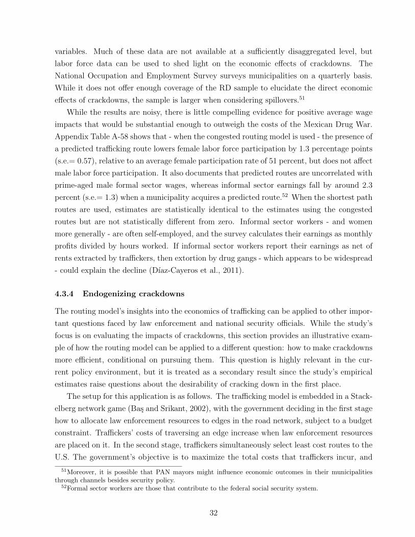
variables. Much of these data are not available at a sufficiently disaggregated level, but

labor force data can be used to shed light on the economic effects of crackdowns. The

National Occupation and Employment Survey surveys municipalities on a quarterly basis.

While it does not offer enough coverage of the RD sample to elucidate the direct economic

effects of crackdowns, the sample is larger when considering spillovers.51

While the results are noisy, there is little compelling evidence for positive average wage

impacts that would be substantial enough to outweigh the costs of the Mexican Drug War.

Appendix Table A-58 shows that - when the congested routing model is used - the presence of

a predicted trafficking route lowers female labor force participation by 1.3 percentage points

(s.e.= 0.57), relative to an average female participation rate of 51 percent, but does not affect

male labor force participation. It also documents that predicted routes are uncorrelated with

prime-aged male formal sector wages, whereas informal sector earnings fall by around 2.3

percent (s.e.= 1.3) when a municipality acquires a predicted route.52 When the shortest path

routes are used, estimates are statistically identical to the estimates using the congested

routes but are not statistically different from zero. Informal sector workers - and women

more generally - are often self-employed, and the survey calculates their earnings as monthly

profits divided by hours worked. If informal sector workers report their earnings as net of

rents extracted by traffickers, then extortion by drug gangs - which appears to be widespread

- could explain the decline (Dıaz-Cayeros et al., 2011).

4.3.4 Endogenizing crackdowns

The routing model’s insights into the economics of trafficking can be applied to other impor-

tant questions faced by law enforcement and national security officials. While the study’s

focus is on evaluating the impacts of crackdowns, this section provides an illustrative exam-

ple of how the routing model can be applied to a different question: how to make crackdowns

more efficient, conditional on pursuing them. This question is highly relevant in the cur-

rent policy environment, but it is treated as a secondary result since the study’s empirical

estimates raise questions about the desirability of cracking down in the first place.

The setup for this application is as follows. The trafficking model is embedded in a Stack-

elberg network game (Bas and Srikant, 2002), with the government deciding in the first stage

how to allocate law enforcement resources to edges in the road network, subject to a budget

constraint. Traffickers’ costs of traversing an edge increase when law enforcement resources

are placed on it. In the second stage, traffickers simultaneously select least cost routes to the

U.S. The government’s objective is to maximize the total costs that traffickers incur, and

51Moreover, it is possible that PAN mayors might influence economic outcomes in their municipalitiesthrough channels besides security policy.

52Formal sector workers are those that contribute to the federal social security system.

32

each trafficker minimizes his own costs. This framework can accommodate multiple types of

resources with deployment costs that vary by edge. The most closely related work method-

ologically is a study by Israeli and Wood (2002), which develops an efficient algorithm to

solve for which k edges to remove in the context of a non-congested shortest path problem

on a directed graph with a single origin and destination. This study’s problem examines an

enriched setting with congestion and multiple origins and destinations.53

There are several things to note about how the network structure conditions the equi-

librium allocation of law enforcement resources. First, while a naive policy might allocate

law enforcement to edges with the most drug traffic, the network model highlights that the

extent to which law enforcement affects trafficking costs depends on available detours. In

fact, increasing an edge’s latency can decrease total trafficking costs if there are externali-

ties from congestion. This result, known as Braess’s paradox (1968), occurs for 15% of the

edges in the congested trafficking equilibrium. Moreover, the effects of law enforcement in

different locations are interconnected through the network structure, implying that resource

allocation decisions should be made jointly rather than on a location-by-location basis.

The online appendix provides an illustrative example of how this framework can be

used to inform the allocation of scarce law enforcement resources. It first shows that the

government’s allocation problem is NP hard, which implies that the time required to solve

for the optimum increases quickly as the size of the problem grows. Intuitively, the problem

is challenging because allocating resources to two edges at the same time might increase the

government’s objective function more than the summation of changes in the objective when

resources are allocated to each edge separately. Hence the order in which a solution algorithm

proceeds may matter. The estimation appendix develops an algorithm for solving the game,

and Appendix Table A-59 documents robustness to changing the algorithm’s details.

If the government has enough resources to triple the latencies on 25 edges (this is the

factor by which PAN victories are estimated to increase edge costs), this will increase traf-

fickers’ total predicted costs by 17%. This exercise illustrates how the network model can

contribute unique information to interdiction efforts, as the 25 edges chosen differ from the

25 most trafficked edges.

This exercise is a simplified illustrative example, but with appropriate data it would

be straightforward to extend the model to make it more realistic. Multiple types of law

enforcement resources could be incorporated, as well as deployment costs that vary by edge.

Future work could also examine mixed strategies by law enforcement, which may be desirable

but are beyond the scope of the current study.

53While there are other studies that focus on removing key nodes or edges from a network - notablyBallester et al. (2006, 2010) - since the network interactions modeled by these studies are different thetechniques for solving them are likewise quite distinct.

33

5 Conclusion

This study examines the direct and spillover effects of Mexican crackdowns on the drug

trade, documenting the following results. First, regression discontinuity estimates show that

violence in a municipality increases substantially after the close election of a PAN mayor and

remains higher throughout the mayor’s term and beyond. The empirical evidence suggests

that the violence largely reflects rival traffickers’ attempts to wrest control of territories after

crackdowns initiated by PAN mayors have challenged the incumbent criminals. Moreover,

an economic model of equilibrium trafficking routes predicts the diversion of drug traffic

following close PAN victories. This diversion is large enough to make a substantial difference

in illicit drug seizures along alternative routes, and when drug traffic is diverted to other

municipalities, violence in these municipalities increases.

These results demonstrate how traffickers’ economic objectives and constraints imposed

by the routes network have conditioned the policy outcomes of the Mexican Drug War.

While further research is needed to identify the causal effects of crackdowns on additional

outcomes and in alternative contexts, overall the study’s results suggest policies aimed at

deterring violence, enforcing homicide laws, and confronting other challenges, as opposed to

policies whose primary objective is to reduce drug trafficking.

34

References

Angrist, J. and A. Kugler (2008): “Rural windfall or a new resource curse? Coca,income, and civil conflict in Colombia,” The Review of Economics and Statistics, 90, 191–215.

Beckmann, M., C. McGuire, and C. Winston (1956): Studies in the Economics ofTransportation, Yale University Press.

Braess, D. (1968): “Uber ein Paradoxon aus der Verkehrsplanung,” Mathematical Methodsof Operations Research, 12, 258–268.

Brumm, H. J. and D. O. Cloninger (1995): “Violent crime and punishment: an appli-cation of the LISREL model 1,” Applied Economics, 27, 719–725.

Cameron, A. C., J. B. Gelbach, and D. L. Miller (2011): “Robust inference withmultiway clustering,” Journal of Business & Economic Statistics, 29.

Dıaz-Cayeros, A., B. Magaloni, A. Matanock, and V. Romero (2011): “Livingin Fear: Mapping the Social Embeddedness of Drug Gangs and Violence in Mexico,”Manuscript: University of California at San Diego.

Dijkstra, E. (1959): “A note on two problems in connection with graphs,” Numerischemathematik, 1, 269–271.

Eaton, G., C. Davies, L. English, A. Lodwick, M. A. Bellis, and J. McVeigh(2007): United Kingdom drug situation: annual report to the European Monitoring Centrefor Drugs and Drug Addiction 2007.

Estados Unidos de Mexico, Gobierno Federal (2010): Oportunidades: A Programof Results.

Fajnzylber, P., D. Lederman, and N. Loayza (1998): Determinants of crime ratesin Latin America and the world: an empirical assessment, vol. 1 of World Bank LatinAmerican and Caribbean studies, World Bank Publications.

Gambetta, D. (1993): The Sicilian Mafia, Harvard University Press.

Guerrero-Gutierrez, E. (2011): “Security, Drugs, and Violence in Mexico: A Survey,”7th North American Forum, Washington D.C.

Imbens, G. and K. Kalyanaraman (2012): “Optimal bandwidth choice for the regressiondiscontinuity estimator,” The Review of Economic Studies, 79, 933–959.

Isacson, A. (2010): “Colombia: Don’t Call it a Model,” Policy Document: WashingtonOffice on Latin America.

Keefer, P. and N. Loayza (2010): Innocent bystanders: developing countries and thewar on drugs, World Bank Publications.

35

Lee, D., E. Moretti, and M. Butler (2004): “Do voters affect or elect policies?Evidence from the US House,” The Quarterly Journal of Economics, 119, 807–859.

Leech, G. (2000): “The Failure of Coca Eradication in Peru and Bolivia,” Colombia Jour-nal.

Levitt, S. and S. Venkatesh (2000): “An Economic Analysis of a Drug-Selling Gang’sFinances,” The Quarterly Journal of Economics, 115, 755–789.

Manski, C. (1993): “Identification of endogenous social effects: The reflection problem,”The Review of Economic Studies, 60, 531–542.

Mexico Evalua (2010): Indice de desempeno del sistema penal.

——— (2012): Seguridad y Justicia Penal en los Estados: 25 Indicadores de Nuestra debil-idad institucional.

——— (2013): La Carcel en Mexico: Para que.

Miron, J. A. (1999): “Violence and the U.S. Prohibitions of Drugs and Alcohol,” AmericanLaw and Economics Review, Fall, 78–114.

——— (2001a): “The Economics of Drug Prohibition and Drug Legalization,” Social Re-search, 3, 835–855.

——— (2001b): “Violence, Guns, and Drugs: A Cross-Country Analysis,” Journal of Lawand Economics, 2, 615–634.

——— (2010): “The Budgetary Implications of Drug Prohibition,” 1–39.

——— (Forthcoming): “Drugs and Violence,” Report for World Bank Project on Crime andViolence in Central America.

Rasmussen, D. W., B. L. Benson, and D. L. Sollars (1993): “Spatial competitionin illicit drug markets: The consequences of increased drug law enforcement,” The Reviewof Regional Studies, 23, 219–236.

Reuter, P. and F. Trautmann (2009): A Report on Global Illicit Drug Markets 1998-2007.

Rios, V. (2011): “Understanding Mexico’s Drug War,” Manuscript: Harvard UniversityDepartment of Government.

——— (2013): “Why did Mexico become so violent? A self-reinforcing violent equilibriumcaused by competition and enforcement,” Trends in Organized Crime, 16.

Secretarıa de Salud, CONADIC (2008): National Addictions Survey.

Secretarıa de Seguridad Publica (2010): Informe del Estado de la Seguridad Publicaen Mexico.

36

Shannon, E. (1988): Desperados: Latin drug lords, US lawmen, and the war America can’twin, Viking.

Shirk, D. A. (2012): “Drug Violence and State Responses in Mexico,” Manuscript: Uni-versity of San Diego Department of Political Science.

The White House Office of National Drug Control Policy (2010): NationalDrug Control Strategy.

United Nations International Drug Control Programme and United NationsOffice on Drugs and United Nations Office for Drug Control and CrimePrevention (2011): World Drug Report, United Nations Publications.

United Nations Office for Drug Control and Crime Prevention (2002): Studieson Drugs and Crime: Global Illicit Drug Trends 2002, United Nations Publications.

United Nations Office on Drugs and Crime (2010): World Drug Report 2010.

——— (2011): World Drug Report 2011.

United States Drug Enforcement Agency (2011): Drug Trafficking in the UnitedStates.

Varese, F. (2005): The Russian Mafia: private protection in a new market economy, OxfordUniversity Press.

Wardrop, J. (1952): “Some Theoretical Aspects of Road Traffic Research,” Proceedings ofthe Institution of Civil Engineers, 1, 325–378.

Werb, D., G. Rowell, G. Guyatt, T. Kerr, J. Montaner, and E. Wood (2011):“Effect of drug law enforcement on drug market violence: A systematic review,” Interna-tional Journal of Drug Policy, 22, 87–94.

Zepeda Lecuona, G. (2013): Situacion y desafıos del sistema penitenciario mexicano.

Zitzewitz, E. (2012): “Forensic economics,” Journal of Economic Literature, 50, 731–769.

37

Table 1: Baseline Characteristics

(1) (2) (3) (4) (5) (6) (7)

Own municipality Neighboring muns.

5% vote spread t-stat on t-stat on t-stat onPAN PAN means RD RD RD RDwon lost difference estimate estimate estimate estimate

Political characteristicsMun. taxes per capita (2005) 59.84 56.75 (0.23) 40.96 (0.86) 10.80 (0.42)Turnout 0.61 0.59 (0.99) 0.05 (0.77) 0.02 (0.42)PAN incumbent 0.27 0.32 (-0.61) -0.05 (-0.22) 0.14 (1.52)PRD incumbent 0.17 0.13 (0.63) -0.02 (-0.12) -0.16 (-1.42)% alternations (1976-2006) 0.31 0.31 (-0.01) 0.06 (0.70) 0.01 (0.25)PRI never lost (1976-2006) 0.07 0.07 (-0.04) -0.21 (-1.64) -0.15 (-1.61)Demographic characteristicsPopulation (2005) 6.03 5.10 (0.35) 5.08 (0.60) -1.37 (-0.62)Population density (2005) 220.23 191.05 (0.42) -374.00 (-1.42) -186.70 (-1.19)Migrants per capita (2005) 0.02 0.02 (-0.69) 0.00 (-0.06) 0.00 (-0.77)Economic characteristicsIncome per capita (2005) 4.29 4.48 (-0.53) -0.69 (-0.56) 0.10 (0.15)Malnutrition (2005) 32.76 31.20 (0.53) 3.90 (0.50) -5.23 (-0.89)Mean years schooling (2005) 6.26 6.19 (0.32) -0.55 (-0.77) -0.10 (-0.22)Infant mortality (2005) 22.54 22.26 (0.22) 0.80 (0.22) 0.39 (0.17)HH w/o access to sewage (2005) 8.51 8.44 (0.05) 0.80 (0.26) -1.53 (-0.52)HH w/o access to water (2005) 16.14 18.22 (-0.62) -8.35 (-1.06) -6.45 (-0.97)Marginality index (2005) -0.15 -0.12 (-0.23) -0.05 (-0.13) -0.23 (-0.73)Road network characteristicsDetour length (km) 26.15 22.48 (0.19) -53.47 (-1.29) -14.63 (-0.90)Road density 0.15 0.13 (0.98) -0.06 (-1.08) -0.04 (-0.86)Distance U.S. (km) 708.27 735.49 (-0.55) -126.82 (-0.86) -135.29 (-0.92)Geographic characteristicsElevation (m) 1403.42 1367.95 (0.26) 547.41 (1.29) 487.19 (1.24)Slope (degrees) 3.62 3.19 (1.02) 0.26 (0.22) -0.17 (-0.18)Surface area (km2) 1787.36 725.37 (1.36) 1808.90 (1.61) 544.10 (0.65)Average min. temperature, C 7.17 7.59 (-0.46) -4.56 (-1.60) -4.04 (-1.51)Average max. temperature, C 22.54 22.90 (-0.53) -3.44 (-1.58) -3.24* (-1.66)Average precipitation, cm 1164.40 1084.63 (0.65) -93.64 (-0.32) -90.74 (-0.32)Observations 70 82 152 152

Notes: Data on population, population density, mean years of schooling, and migrants per capita are from II Conteode Poblacion y Vivienda, INEGI (National Institute of Statistics and Geography, 2005). Data on municipal taxcollection are from Sistema de Cuentas Municipales, INEGI. Data on household access to sewage and water are fromCONAPO (National Population Council) (2005). Data on malnutrition are from CONEVAL (National Council forEvaluating Social Development Policy), Indice de Reazgo Social (2005). Data on infant mortality are from PNUDMexico (UN Development Program, 2005). The marginality index is from CONAPO (2005). Data on distance to theU.S. and other road network characteristics are from the author’s own calculations. Electoral data are from MexicoElectoral-Banamex and electoral results published by the Electoral Tribunals of each state. For 11 states, data onthe total number of eligible voters, required to calculate turnout, are not reported. The geographic characteristics arefrom Acemoglu and Dell (2009). Columns (1) through (5) examine these variables for municipalities with closeelections. Column (6) and (7) examine these characteristics for municipalities that border a municipality with a closeelection. Column (3) reports the t-statistic on the difference in means between municipalities where the PAN barelywon and where they barely lost. Columns (4) and (6) report the coefficient on PAN win from a standard RDspecification where the respective characteristic is used as the dependent variable, and columns (5) and (7) reportthe respective t-statistic. * significant at 10%, ** significant at 5%, *** significant at 1%.

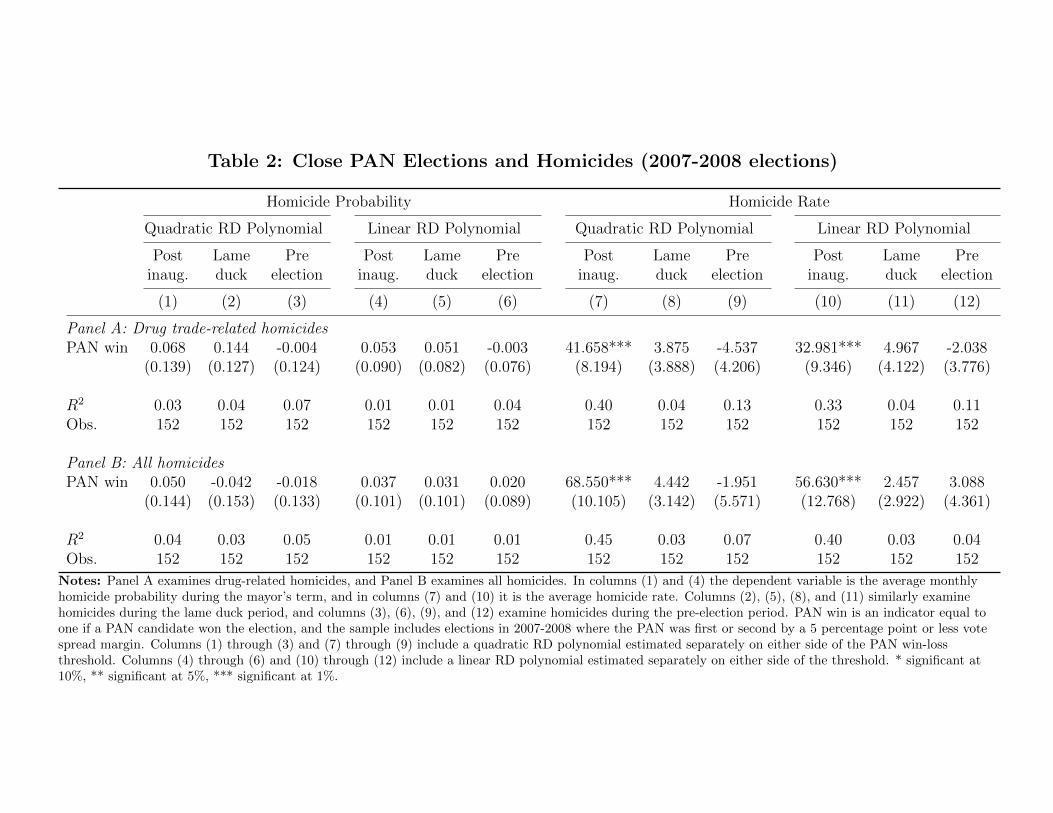
Table 2: Close PAN Elections and Homicides (2007-2008 elections)

Homicide Probability Homicide Rate

Quadratic RD Polynomial Linear RD Polynomial Quadratic RD Polynomial Linear RD Polynomial

Post Lame Pre Post Lame Pre Post Lame Pre Post Lame Preinaug. duck election inaug. duck election inaug. duck election inaug. duck election

(1) (2) (3) (4) (5) (6) (7) (8) (9) (10) (11) (12)

Panel A: Drug trade-related homicidesPAN win 0.068 0.144 -0.004 0.053 0.051 -0.003 41.658*** 3.875 -4.537 32.981*** 4.967 -2.038

(0.139) (0.127) (0.124) (0.090) (0.082) (0.076) (8.194) (3.888) (4.206) (9.346) (4.122) (3.776)

R2 0.03 0.04 0.07 0.01 0.01 0.04 0.40 0.04 0.13 0.33 0.04 0.11Obs. 152 152 152 152 152 152 152 152 152 152 152 152

Panel B: All homicidesPAN win 0.050 -0.042 -0.018 0.037 0.031 0.020 68.550*** 4.442 -1.951 56.630*** 2.457 3.088

(0.144) (0.153) (0.133) (0.101) (0.101) (0.089) (10.105) (3.142) (5.571) (12.768) (2.922) (4.361)

R2 0.04 0.03 0.05 0.01 0.01 0.01 0.45 0.03 0.07 0.40 0.03 0.04Obs. 152 152 152 152 152 152 152 152 152 152 152 152

Notes: Panel A examines drug-related homicides, and Panel B examines all homicides. In columns (1) and (4) the dependent variable is the average monthlyhomicide probability during the mayor’s term, and in columns (7) and (10) it is the average homicide rate. Columns (2), (5), (8), and (11) similarly examinehomicides during the lame duck period, and columns (3), (6), (9), and (12) examine homicides during the pre-election period. PAN win is an indicator equal toone if a PAN candidate won the election, and the sample includes elections in 2007-2008 where the PAN was first or second by a 5 percentage point or less votespread margin. Columns (1) through (3) and (7) through (9) include a quadratic RD polynomial estimated separately on either side of the PAN win-lossthreshold. Columns (4) through (6) and (10) through (12) include a linear RD polynomial estimated separately on either side of the threshold. * significant at10%, ** significant at 5%, *** significant at 1%.

Table 3: Close PAN Elections and Homicides (2007-2010 elections)

Homicide Probability Homicide Rate

Quadratic RD Polynomial Linear RD Polynomial Quadratic RD Polynomial Linear RD Polynomial

Post Lame Pre Post Lame Pre Post Lame Pre Post Lame Preinaug. duck election inaug. duck election inaug. duck election inaug. duck election

(1) (2) (3) (4) (5) (6) (7) (8) (9) (10) (11) (12)

Panel A: Drug trade-related homicidesPAN win 0.004 0.032 -0.036 0.042 0.030 0.027 17.635*** 1.132 -4.574 26.735*** 6.331 3.830

(0.085) (0.085) (0.079) (0.054) (0.054) (0.050) (6.489) (4.895) (4.774) (8.560) (5.212) (4.688)

R2 0.04 0.01 0.02 0.02 0.01 0.01 0.13 0.01 0.02 0.10 0.01 0.01Clusters 307 307 307 307 307 307 307 307 307 307 307 307Obs. 310 310 310 310 310 310 310 310 310 310 310 310

Panel B: All homicidesPAN win -0.014 -0.108 -0.016 0.053 0.001 0.039 35.970*** -2.048 -0.669 44.820*** 6.622 4.740

(0.097) (0.106) (0.085) (0.064) (0.071) (0.054) (9.351) (5.665) (4.767) (12.289) (6.665) (3.498)

R2 0.03 0.02 0.04 0.02 0.01 0.03 0.27 0.02 0.07 0.24 0.01 0.03Clusters 307 307 307 307 307 307 307 307 307 307 307 307Obs. 310 310 310 310 310 310 310 310 310 310 310 310

Notes: Panel A examines drug-related homicides, and Panel B examines all homicides. In columns (1) and (4) the dependent variable is the average monthlyhomicide probability during the one year following the mayor’s inauguration, and in columns (7) and (10) it is the average homicide rate. Columns (2), (5), (8),and (11) similarly examine homicides during the lame duck period, and columns (3), (6), (9), and (12) examine homicides during the pre-election period. PANwin is an indicator equal to one if a PAN candidate won the election, and the sample includes elections in 2007-2010 where the PAN was first or second by a 5percentage point or less vote spread margin. Columns (1) through (3) and (7) through (9) include a quadratic RD polynomial estimated separately on eitherside of the PAN win-loss threshold. Columns (4) through (6) and (10) through (12) include a linear RD polynomial estimated separately on either side of thethreshold. Standard errors are clustered by municipality. * significant at 10%, ** significant at 5%, *** significant at 1%.

Table 4: Heterogeneity

Dependent variable: drug-related homicide rate

2007-2008 elections 2007-2010 elections

(1) (2) (3) (4) (5) (6) (7) (8)

PAN win 32.981*** 37.699*** 37.333*** -2.344 26.735*** 32.594*** 30.333*** -0.781(9.346) (9.000) (9.752) (4.020) (8.560) (10.261) (8.725) (8.164)

PAN win x -49.364*** -34.487***far from U.S. (12.674) (11.231)

PAN win x -51.267*** -38.262***low violence (11.524) (9.709)

PAN win x 0.331 1.000local gang (14.867) (9.978)

PAN win x 33.747*** 33.680**rival (10.827) (16.747)

PAN win x 11.522 4.900ally (10.992) (9.405)

R-squared 0.326 0.433 0.443 0.504 0.102 0.201 0.216 0.220Clusters 152 152 152 152 307 307 307 307Observations 152 152 152 152 310 310 310 310PAN win effect -11.670 -1.892

(far from US) (8.924) (4.566)PAN win effect -13.930** -7.928*

(low violence) (6.140) (4.259)PAN win effect -2.013 0.219

(local gang) (14.310) (5.736)PAN win effect 31.400*** 32.900**

(rival) (10.050) (14.620)PAN win effect 9.178 4.119

(ally) (10.230) (4.669)

Notes: PAN win is an indicator equal to one if a PAN candidate won the election, far from U.S. is an indicator equal to 1 if the municipality is above mediandistance from the U.S., low violence is an indicator equal to 1 if the municipality had a below median homicide rate during 2004-2006, local gang is an indicatorequal to one if the municipality contains only a local gang, rival is an indicator equal to one if it contains a major DTO and borders territory controlled by arival DTO, and ally is an indicator equal to one if it contains a major DTO and does not border territory controlled by a rival DTO. All columns limit thesample to municipalities where a PAN candidate was the winner or runner-up by less than a five percentage point vote spread margin and include a linear RDpolynomial estimated separately on either side of the PAN win-loss threshold. In addition to the interactions, main effects are also included. Standard errors,clustered by municipality, are in parentheses. * significant at 10%, ** significant at 5%, *** significant at 1%.

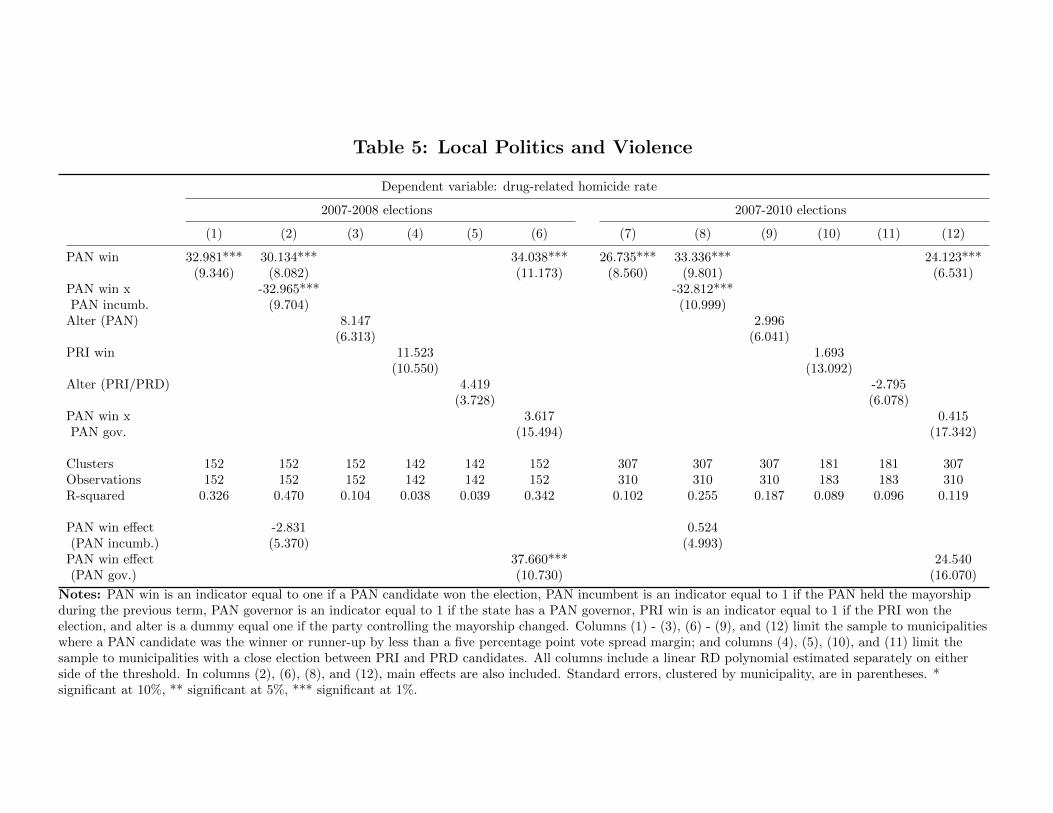
Table 5: Local Politics and Violence

Dependent variable: drug-related homicide rate

2007-2008 elections 2007-2010 elections

(1) (2) (3) (4) (5) (6) (7) (8) (9) (10) (11) (12)

PAN win 32.981*** 30.134*** 34.038*** 26.735*** 33.336*** 24.123***(9.346) (8.082) (11.173) (8.560) (9.801) (6.531)

PAN win x -32.965*** -32.812***PAN incumb. (9.704) (10.999)

Alter (PAN) 8.147 2.996(6.313) (6.041)

PRI win 11.523 1.693(10.550) (13.092)

Alter (PRI/PRD) 4.419 -2.795(3.728) (6.078)

PAN win x 3.617 0.415PAN gov. (15.494) (17.342)

Clusters 152 152 152 142 142 152 307 307 307 181 181 307Observations 152 152 152 142 142 152 310 310 310 183 183 310R-squared 0.326 0.470 0.104 0.038 0.039 0.342 0.102 0.255 0.187 0.089 0.096 0.119

PAN win effect -2.831 0.524(PAN incumb.) (5.370) (4.993)

PAN win effect 37.660*** 24.540(PAN gov.) (10.730) (16.070)

Notes: PAN win is an indicator equal to one if a PAN candidate won the election, PAN incumbent is an indicator equal to 1 if the PAN held the mayorshipduring the previous term, PAN governor is an indicator equal to 1 if the state has a PAN governor, PRI win is an indicator equal to 1 if the PRI won theelection, and alter is a dummy equal one if the party controlling the mayorship changed. Columns (1) - (3), (6) - (9), and (12) limit the sample to municipalitieswhere a PAN candidate was the winner or runner-up by less than a five percentage point vote spread margin; and columns (4), (5), (10), and (11) limit thesample to municipalities with a close election between PRI and PRD candidates. All columns include a linear RD polynomial estimated separately on eitherside of the threshold. In columns (2), (6), (8), and (12), main effects are also included. Standard errors, clustered by municipality, are in parentheses. *significant at 10%, ** significant at 5%, *** significant at 1%.

Table 6: The Diversion of Drug Traffic

Dep. var.: Domestic Illicit Drug Confiscations Cocaine ConfiscationsDummy Value Value Dummy Value Value Dummy Value Value

Full Sample Limited Sample Full Sample

(1) (2) (3) (4) (5) (6) (7) (8) (9)

Panel A: Shortest PathsPredicted 0.016*** 0.170*** 0.016** 0.169*** 0.004 0.028routes dummy (0.005) (0.050) (0.007) (0.065) (0.004) (0.020)

Predicted 0.021*** 0.015* 0.006routes count (0.008) (0.009) (0.006)

Panel B: Model with Congestion CostsPredicted 0.013** 0.149*** 0.011* 0.129** 0.002 0.009routes dummy (0.005) (0.057) (0.006) (0.065) (0.004) (0.025)

Predicted 0.004 0.002 0.001routes count (0.004) (0.004) (0.002)

Municipalities 1869 1869 1869 1562 1562 1562 1869 1869 1869Observations 69,153 69,153 69,153 57,794 57,794 57,794 69,153 69,153 69,153

Notes: The dependent variable in columns (1) and (4) is an indicator equal to 1 if domestic illicit drug confiscations are made in a givenmunicipality-month; the dependent variable in columns (2), (3), (5), and (6) is the log value of domestic illicit drug confiscations (or 0 if noconfiscations are made); the dependent variable in column (7) is an indicator equal to 1 if cocaine confiscations are made in a givenmunicipality-month; and the dependent variable in columns (8) and (9) is the log value of confiscated cocaine (or 0 if no confiscations aremade). Columns (4) through (6) limit the sample to municipalities that do not border a municipality that has experienced a close PANvictory. Panel A predicts trafficking routes using the shortest paths model, and Panel B uses the model with congestion costs. All columnsinclude month x state and municipality fixed effects. Standard errors clustered by municipality and month x state are reported inparentheses. * significant at 10%, ** significant at 5%, *** significant at 1%.

Table 7: Violence Spillovers

Dep var: drug trade-related homicidedummy rate rate dummy rate dummy rate rate dummy rate

Full sample Limited sample

(1) (2) (3) (4) (5) (6) (7) (8) (9) (10)

Panel A: Shortest PathsPredicted 0.014*** 1.163 0.006 -0.702routes dummy (0.005) (1.251) (0.006) (1.199)

Predicted 0.542* 0.456routes count (0.308) (0.290)

One route 0.017** -6.180 0.014 -5.530(0.007) (3.779) (0.010) (3.449)

More than 0.011 10.314** -0.000 6.164one route (0.008) (4.746) (0.010) (4.511)

Panel B: Model with Congestion CostsPredicted 0.017*** 1.870** 0.019*** 1.831**routes dummy (0.005) (0.811) (0.006) (0.930)

Predicted -0.005 0.002routes count (0.015) (0.013)

One route 0.010 2.188 0.010 1.399(0.006) (1.631) (0.007) (0.943)

More than 0.020*** 1.746* 0.023*** 2.019*one route (0.006) (1.058) (0.007) (1.034)

Municipalities 1869 1869 1869 1869 1869 1562 1562 1562 1562 1562Observations 69,153 69,153 69,153 69,153 69,153 57,794 57,794 57,794 57,794 57,794

Notes: The dependent variable in columns (1), (4), (6) and (9) is an indicator equal to 1 if a drug trade-related homicide occurred in a givenmunicipality-month, and the dependent variable in columns (2), (3), (5), (7), (8), and (10) is the drug trade-related homicide rate per 100,000municipal inhabitants. Columns (6) through (10) limit the sample to municipalities that do not border a municipality that has experienced aclose PAN victory. All columns include month x state and municipality fixed effects. Standard errors clustered by municipality and month xstate are reported in parentheses. * significant at 10%, ** significant at 5%, *** significant at 1%.

Figure 1: Illustration of Spillovers Methodology

(a) Legend (b) Basic environment (c) Close PAN victory increases costs;routes change

(d) Do confiscation patterns alsochange?

Figure 2: Road Network and Predicted Trafficking Routes

Notes: The least cost routes plotted in this figure are predicted using the network model with congestion costs.

Figure 3: Drug trade-related homicides RD figures0

.2.4

.6.8

1M

onth

ly p

roba

bilit

y of

dru

g−re

late

d ho

mic

ide

−.05 0 .05PAN margin of victory

(a) Post-inauguration (extensive margin)

−20

020

4060

80D

rug

hom

icid

e ra

te

−.05 0 .05PAN margin of victory

(b) Post-inauguration (homicide rate)

0.2

.4.6

.81

Mon

thly

pro

babi

lity

of d

rug−

rela

ted

hom

icid

e

−.05 0 .05PAN margin of victory

(c) Lame duck (extensive margin)

−20

020

4060

80D

rug

hom

icid

e ra

te

−.05 0 .05PAN margin of victory

(d) Lame duck (homicide rate)

0.2

.4.6

.81

Mon

thly

pro

babi

lity

of d

rug−

rela

ted

hom

icid

e

−.05 0 .05PAN margin of victory

(e) Pre-election (extensive margin)

−20

020

4060

80D

rug

hom

icid

e ra

te

−.05 0 .05PAN margin of victory

(f) Pre-election (homicide rate)

Notes: This figure plots violence measures against the PAN margin of victory, with a negative margin indicating aPAN loss. Each point represents the average value of the outcome in vote spread bins of width one half of apercentage point. The solid line plots predicted values, with separate quadratic vote spread trends estimated oneither side of the PAN win-loss threshold. The dashed lines show 95% confidence intervals.

Figure 4: All homicides RD figures0

.2.4

.6.8

1M

onth

ly p

roba

bilit

y of

hom

icid

e oc

curr

ing

−.05 0 .05PAN margin of victory

(a) Post-inauguration (extensive margin)

−20

020

4060

8010

012

0O

vera

ll ho

mic

ide

rate

−.05 0 .05PAN margin of victory

(b) Post-inauguration (homicide rate)

0.2

.4.6

.81

Mon

thly

pro

babi

lity

of h

omic

ide

occu

rrin

g

−.05 0 .05PAN margin of victory

(c) Lame duck (extensive margin)

−20

020

4060

8010

012

0O

vera

ll ho

mic

ide

rate

−.05 0 .05PAN margin of victory

(d) Lame duck (homicide rate)

0.2

.4.6

.81

Mon

thly

pro

babi

lity

of h

omic

ide

occu

rrin

g

−.05 0 .05PAN margin of victory

(e) Pre-election (extensive margin)

−20

020

4060

8010

012

0O

vera

ll ho

mic

ide

rate

−.05 0 .05PAN margin of victory

(f) Pre-election (homicide rate)

Notes: This figure plots violence measures against the PAN margin of victory, with a negative margin indicating aPAN loss. Each point represents the average value of the outcome in vote spread bins of width one half of apercentage point. The solid line plots predicted values, with separate quadratic vote spread trends estimated oneither side of the PAN win-loss threshold. The dashed lines show 95% confidence intervals.

Figure 5: Homicide RD figures

●●

●●

● ●●

●

●

●

●

● ●

−0.25

0.00

0.25

0.50

−2 −1 LD 1 2 3 4 5 6 7 8 9 LDQuarter

Hom

icid

e P

roba

bilit

y

Period

●

●

●

●

Pre−period

Lame Duck 1

Post−period

Lame Duck 2

(a) Drug-related homicides (extensive margin)

●

●

● ●

●

●●

●

●

●

●

●

●

0

40

80

−2 −1 LD 1 2 3 4 5 6 7 8 9 LDQuarter

Hom

icid

e R

ate Period

●

●

●

●

Pre−period

Lame Duck 1

Post−period

Lame Duck 2

(b) Drug-related homicide rate

●●●●

●●●●

●●● ●●●●●●●●●●● ●●●●●●●●●●●

●●●●●●●●●●●

●●●●

●●

●●●

●●

●

●●●●●

●●●

●●●●● ●

●

●

●

●

●●

●●

●

●

●

●●

●

●

●

●

−50

0

50

100

150

200

−69 −65 −60 −55 −50 −45 −40 −35 −30 −25 −20 −15 −10 −5 LD1 4 8 LD1 4 7Quarter

Hom

icid

e R

ate

Period

●

●

●

●

●

Pre−period

Lame Duck 1

Post Term 1

Lame Duck 2

Post Term 2

(c) Overall homicide rate

Notes: In Panel A, each point plots a separate RD estimate of the impact of close PAN victories on the average probability that a drug trade-relatedhomicide occurred. In Panel B, each point plots a separate RD estimate of the impact of close PAN victories on the drug-related homicide rate in a givenquarter. In Panel C, each point plots a separate RD estimate of the impact of close PAN victories on the overall homicide rate in a given quarter. Allregressions include a quadratic RD polynomial, estimated separately on either side of the PAN win-loss threshold. The thin lines plot 95% confidenceintervals, and the thick lines plot 90% confidence intervals.