Trafficking Networks and the Mexican Drug War∗

Melissa Dell

Harvard

December, 2012

Abstract: Drug trade-related violence has escalated dramatically in Mexico since 2007,and recent years have also witnessed large-scale efforts to combat trafficking, spearheadedby Mexico’s conservative PAN party. This study examines the direct and spillover effectsof Mexican policy towards the drug trade. Regression discontinuity estimates show thatdrug-related violence increases substantially after close elections of PAN mayors. Empiricalevidence suggests that the violence reflects rival traffickers’ attempts to usurp territoriesafter crackdowns have weakened incumbent criminals. Moreover, the study uses a networkmodel of trafficking routes to show that PAN victories divert drug traffic, increasing violencealong alternative drug routes.

Keywords : Drug trafficking, networks, violence.

∗I am grateful to Daron Acemoglu and Ben Olken for their extensive feedback on this project. I alsothank Arturo Aguilar, Abhijit Banerjee, Ernesto Dal Bo, Dave Donaldson, Esther Duflo, Ray Fisman, RachelGlennerster, Gordon Hanson, Austin Huang, Panle Jia, Chappell Lawson, Nick Ryan, Andreas Schulz, JakeShapiro, and seminar participants at Bocconi University, the Brown University Networks conference, ChicagoBooth, CIDE, Colegio de Mexico, Columbia, CU Boulder, George Mason, Harvard, the Inter-AmericanDevelopment Bank, ITAM, the Mexican Security in Comparative Perspective conference (Stanford), MIT,the NBER Political Economy Meeting, NEUDC, Princeton, Stanford, University of British Columbia, UCBerkeley Haas School of Business, UC San Diego, University of Chicago, University of Leicester, Universityof Maryland, US Customs and Border Patrol, the World Bank, and Yale for extremely helpful commentsand suggestions. Contact email: melissadell@fas.harvard.edu, address: Harvard University Department ofEconomics, Littauer Center M-24, Cambridge MA 02138.

1 Introduction

Drug trade-related violence has escalated dramatically in Mexico since 2007, claiming over

50,000 lives and raising concerns about the capacity of the Mexican state to monopolize

violence. Recent years have also witnessed large scale efforts to combat drug trafficking,

spearheaded by Mexico’s conservative National Action Party (PAN). While drug traffickers

are economic actors with clear profit maximization motives, there is little empirical evidence

on how traffickers’ economic objectives have conditioned the outcomes of Mexico’s war on

drug trafficking. More basically, it remains controversial whether government policies have

caused the marked increase in violence, or whether violence would have risen substantially

in any case (Guerrero, 2011; Rios, 2011a; Shirk, 2011). This study uses variation from close

mayoral elections and a network model of drug trafficking to examine the direct and spillover

effects of Mexican crackdowns on the drug trade.

Mexico is the largest supplier to the U.S. illicit drug market, with Mexican drug traffickers

earning approximately 25 billion USD each year in wholesale U.S. drug markets (U.N. World

Drug Report, 2011). In addition to drugs, Mexican trafficking organizations engage in a

wide variety of illicit activities including protection rackets, kidnapping, human smuggling,

prostitution, oil and fuel theft, money laundering, weapons trafficking, arson, and auto theft

(Guerrero, 2011, p. 10). Official data described later in this study document that in 2008,

drug trafficking organizations maintained operations in two thirds of Mexico’s municipalities,

and illicit drugs were cultivated in 14% of municipalities.

The study uses three main inputs to analyze how crackdowns affect violence and drug

trafficking routes: a network model of trafficking routes, plausibly exogenous variation in

local drug policy, and confidential data on the drug trade. In the network routes model,

traffickers’ objective is to minimize the costs of transporting drugs from producing munic-

ipalities in Mexico across the road network to U.S. entry points. In the simplest version,

traffickers take the shortest route to the U.S. that avoids municipalities experiencing crack-

downs. I also specify and estimate richer versions of the model in which trafficking costs are

a function of additional relevant factors.

The state does not randomly combat drug trafficking in some places but not others, and

the government may choose to crack down in municipalities where violence is expected to

increase. In order to isolate plausibly exogenous variation in local policy towards the drug

trade, I exploit the outcomes of close mayoral elections in 2007 and 2008 involving the PAN

party.1 The PAN’s role in spearheading the war on drug trafficking, as well as qualitative

evidence that PAN mayors have contributed to these efforts, motivate this empirical strategy.

1See Lee, Moretti, and Butler (2004) for a pioneering example of a regression discontinuity design ex-ploiting close elections. A number of studies have used discontinuous changes in policies, in the cross-sectionor over time, to examine illicit behavior. See Zitzewitz (2011) for a detailed review.

1

While municipalities where PAN candidates win and lose by wide margins are likely to be

different, when we focus on close elections it becomes plausible that election outcomes are

driven by idiosyncratic factors that do not themselves affect violence. I show that the

outcomes of close elections are in fact uncorrelated with baseline municipal characteristics.

The network model, variation from close mayoral elections, and data on drug trade-

related outcomes are used to examine three sets of questions. First, the study tests whether

the outcomes of close mayoral elections involving the PAN affect drug trade-related violence

in the municipalities experiencing these elections. It also examines the economic mechanisms

mediating this relationship. Second, it tests whether trafficking routes are diverted to other

municipalities following close PAN victories and examines whether the diversion of drug

traffic is accompanied by violence spillovers. Finally, it discusses policy applications and

uses the trafficking model to examine the allocation of law enforcement resources.

Regression discontinuity (RD) estimates document that the monthly drug trade-related

homicide probability is 8.4 percentage points higher after a PAN mayor takes office than after

a non-PAN mayor takes office. This compares to a sample average monthly probability of

drug-related homicide equal to six percent. The drug trade-related homicide rate is likewise

higher after PAN inaugurations: drug-related violence declines slightly following PAN losses,

whereas it increases sharply following PAN victories. In contrast, the non-drug homicide rate

is uncorrelated with the outcomes of close elections. The homicide response to PAN victories

consists primarily of individuals involved in the drug trade killing each other. Analysis using

information on the industrial organization of trafficking suggests that the violence reflects

rival traffickers’ attempts to wrest control of territories after crackdowns initiated by PAN

mayors have weakened the incumbent traffickers.

These results support qualitative and descriptive studies arguing that Mexican govern-

ment policy has been the primary cause of the large increase in violence in recent years.

Guerrero (2011) compiles extensive qualitative and descriptive evidence suggesting that gov-

ernment policies have ignited violent conflicts between traffickers. Escalante (2011) docu-

ments a strong state level correlation between homicides and deployment of the Mexican

military and federal police, and Merino (2011) expands Escalante’s analysis by using state

level data and a matching strategy to argue that Mexican homicides in 2008-2009 would have

totaled 14,000 rather than 19,000 in the absence of federal law enforcement intervention. This

study’s findings contrast with other studies arguing that the increase in violence in recent

years can primarily be explained by the diversification of drug trafficking organizations into

new criminal activities, by increased arms availability, by increased U.S. deportation of im-

migrants with a criminal record, by job loss, or by cultural shifts in morality (see Williams,

2012; Escalante et al, 2011, Rios, 2011a for a discussion). The results also relate to work

by Angrist and Kugler (2008) documenting that exogenous increases in coca prices increase

2

violence in rural districts in Colombia because combatant groups fight over the additional

rents. In Mexico, crackdowns likely reduce rents from criminal activities while in effect, but

by weakening the incumbent criminal group they also reduce the costs of taking control of a

municipality. Controlling territory is likely to offer substantial rents from trafficking and a

variety of other criminal activities once the crackdown subsides.

The study’s second set of results examines whether close PAN victories exert spillover ef-

fects. When policy leads one location to become less conducive to illicit activities, organized

crime may relocate elsewhere. For example, descriptive evidence suggests that coca eradica-

tion policies in Bolivia and Peru during the late 1990s led cultivation to shift to Colombia,

and large-scale coca eradication in Colombia in the early 2000s has since led cultivation to

re-expand in Peru and Bolivia, with total coca cultivation unchanged between 1999 and 2009

(Isacson, 2010; Leech, 2000; UN Office on Drugs and Crime 1999-2009). On a local level,

work by Di Tella and Schargrodsky (2004) documents that the allocation of police officers to

Jewish institutions in Buenos Aires substantially reduced auto theft in the immediate vicin-

ity but may also have diverted some theft to as close as two blocks away. While a number

of studies have examined the drug trade and organized crime, to the best of my knowledge

this study is the first to empirically estimate spillover patterns in drug trafficking activity.2

I use the network routes model to locate municipalities where violence spillovers are likely

to occur. In the model, close PAN victories increase the costs of trafficking drugs through a

municipality, diverting least cost routes elsewhere.3 Elections occur at different times during

the sample period, generating plausibly exogenous within-municipality variation in predicted

routes throughout Mexico. To assess whether the model is reasonable, within-municipality

variation in model predicted routes is compared to within-municipality variation in actual

illicit drug confiscations, as illustrated in Figure 1. Illicit drug confiscations increase by

18.5% when a municipality acquires a predicted shortest path route, and this estimate is

significant at the 1% level. Traffickers may care about the routes other traffickers take, and

thus I also estimate a richer model that imposes congestion costs when routes coincide. The

richer model is similarly predictive, and further robustness and placebo checks also support

the validity of the network approach as a tool for locating spillovers. Predicted routes for

the beginning of the sample period are shown in Figure 2.

After showing that the network routes model is predictive, the study provides evidence

2Studies of the economics of organized crime include Levitt and Venkatesh’s analysis of the finances ofa U.S. drug gang (2000); Gambetta’s economic analysis of the Sicilian mafia (1996); Pinotti’s (2012) studyof the economic costs of organized crime in southern Italy; Bandiera (2003), Dimico et al. (2012) andBuonanno et al.’s (2012) investigations of the historical origins of the Sicilian mafia; Varese’s (2005) andFrye and Zhuravskaya’s (2000) analyses of the rise of the Russian mafia; and Mastrobuoni and Patacchini’s(2010) study of the network structure of crime syndicates.

3The model exploits close election outcomes because they allow spillovers to be isolated from correlationsthat are due to environmental factors (Manski, 1993).

3

that crackdowns increase violence along alternative routes. When a municipality acquires a

predicted route, the monthly probability that a drug trade-related homicide occurs increases

by around 1.4 percentage points, relative to a baseline probability of 4.4%. There is some

evidence that violence spillovers are concentrated in municipalities where multiple routes

coincide. I also show that the trafficking model provides more insight into where violence

spillovers are likely to occur than looking at areas adjacent to crackdowns, a common reduced

form approach for locating crime spillovers.

Finally, I discuss policy interpretations and extend the trafficking model to include the

government’s law enforcement allocation problem. In addition to endogenizing crackdowns, I

consider how the costs of violence can be incorporated into this problem and how the violent

response to crackdowns may be reduced. While we would not expect there to be easy solu-

tions to the challenges facing Mexico, the network framework provides unique information

with the potential to contribute to a more economically informed law enforcement policy.

The next section provides an overview of Mexican drug trafficking, and Section 3 devel-

ops the network trafficking model. Section 4 tests whether the outcomes of close elections

affect violence in the municipalities experiencing these elections and examines the economic

mechanisms underlying the relationship between PAN victories and violence. Section 5 tests

whether PAN victories exert spillovers on drug trafficking activity and violence. Finally,

Section 6 discusses policy applications, and Section 7 concludes.

2 Drugs and Violence in Mexico

2.1 The Drug Trafficking Industry

Mexican drug traffickers dominate the wholesale illicit drug market in the United States,

earning between 14 and 48 billion USD annually.4 According to the U.N. World Drug Report,

Mexico is the largest supplier of heroin to U.S. markets and the largest foreign supplier

of marijuana and methamphetamine. Official Mexican government data, obtained from

confidential sources, document that fourteen percent of Mexico’s municipalities regularly

produce opium poppy seed (heroin) or cannabis. Moreover, 60 to 90 percent of cocaine

consumed in the U.S. transits through Mexico (U.S. Drug Enforcement Agency, 2011). The

U.S. market provides substantially more revenue than Mexico’s domestic drug market, which

is worth an estimated 560 million USD annually (Secretarıa de Seguridad Publica, 2010).5

4Estimates are from the U.S. State Department (2009). Estimates by U.S. Immigration and CustomsEnforcement, the U.S. Drug Enforcement Agency, and the Mexican Secretarıa de Seguridad Publica arebroadly similar and also contain a large margin of error.

5According to the U.S. National Survey on Drug Use and Health, 14.2 percent of Americans (35.5 millionpeople) have used illicit drugs during the past year, as contrasted to 1.4 percent of the Mexican population

4

At the beginning of this study’s sample period, in December 2006, there were six major

drug trafficking organizations (DTOs) in Mexico. Official data obtained from confidential

sources document that 68 percent of Mexico’s 2,456 municipalities were known to have a

major DTO or local drug gang operating within their limits in early 2008. These data

also estimate that 49 percent of drug producing municipalities were controlled by a major

trafficking organization, with the remaining controlled by local gangs.

The term ‘cartel’, used colloquially to refer to DTOs, is a misnomer, as these organizations

do not collude to reduce illicit drug production or to set prices. Alliances between DTOs

are highly unstable, and there is considerable decentralization and conflict within DTOs

(Williams, 2012; Guerrero, 2011, p. 10, 106-108). Decisions about day-to-day operations are

typically made by local cells, as this ensures that no single trafficker will be able to reveal

extensive information if captured by authorities. Moreover, the number of major DTOs

increased from six in 2007 to 16 by 2011, with groups splitting over leadership disputes.

In addition to trafficking drugs, Mexican DTOs engage in a host of illicit activities that

range from protection rackets, kidnapping, human smuggling, and prostitution to oil and fuel

theft, money laundering, weapons trafficking, arson, and auto theft (Guerrero, 2011, p. 10).

Notably, protection rackets involving the general population have increased substantially in

recent years (Rios, 2011b; Secretariado Ejecutivo del Sistema Nacional de Seguridad Publica,

2011). The poor, who have limited recourse to state protection, are particularly likely to be

extorted (Dıaz-Cayeros et al., 2011).

The second half of the 2000s witnessed large, rapid increases in drug trade-related vi-

olence. Over 50,000 people were killed by drug trade-related violence between 2007 and

2012, and homicides increased by at least 30% per year during most of this period (Rios,

2011b). By 2010, violent civilian deaths per capita had reached levels higher than in Iraq

and Afghanistan during the same period, higher than in Russia during the 1990s, and higher

than in Sicily following the Second World War (Williams, 2012). Over 85 percent of the

drug violence consisted of people involved in the drug trade killing each other, 95 percent of

the victims were male, and 45 percent were under age 30. The violence has been public and

brutal, with bodies hung from busy overpasses and severed heads placed in public spaces

(Williams, 2012). Public displays of brutality and activities such as kidnapping and extor-

tion affect the general public, and 2011 public opinion surveys found that security was more

likely than the economy to be chosen as the largest problem facing the country.

(1.1 million people) (National Addiction Survey, 2008).

5

2.2 Mexico’s War on Drug Trafficking

Combating drug trafficking has been a major priority of the Mexican federal government in

recent years. Notably, President Felipe Calderon (December 2006 - 2012) of the conservative

National Action Party (PAN) made fighting organized crime the centerpiece of his adminis-

tration. During his second week in office, Calderon deployed 6,500 federal troops to combat

trafficking, and by the close of his presidency approximately 45,000 troops were involved.

For most of the 20th century, a single party, the PRI (Institutionalized Revolutionary

Party), dominated Mexican politics. The PRI historically took a passive stance towards

the drug trade, and widespread drug-related corruption is well-documented (Shannon, 1988;

Chabat, 2010). Mexicans elected their first opposition president in 2000, and today Mex-

ico has three major parties: the PAN on the right, the PRI, and the PRD (Party of the

Democratic Revolution) on the left. While presidents Ernesto Zedillo (1994-2000, PRI) and

Vicente Fox (2000-2006, PAN) did implement some security reforms and crackdowns (Cha-

bat, 2010), these were on a lesser scale than Calderon’s. Calderon’s crackdown appears to

have been unanticipated, as the 2006 presidential election - decided by an extremely narrow

margin - made limited mention of security issues (Aguilar and Castaneda, 2009).

Mexico’s crackdown on trafficking has focused on arrests and interdiction, whereas crop

eradication has declined somewhat as resources have been diverted to respond to violence

(National Drug Intelligence Center, 2010). Confiscations and high level arrests are typically

made by the federal police and military, who have the requisite training and weaponry to

fight heavily armed traffickers. Municipal police are relevant because they can provide local

information for federal interventions, which often target specific actors about whom reliable

information is available (Chabat, 2010). Municipal police also serve as valuable allies for

traffickers, collecting information on who is passing through a town. This information is

essential for protecting criminal operations and anticipating attacks by federal authorities

and rivals.6 Municipal police form the largest group of public servants killed by drug-related

violence (Guerrero, 2011).

The federal government passed major judicial reforms in 2008, but the Mexican criminal

justice system remains weak. It is estimated that during the 2000s only 2% of felony crimes

were prosecuted, and trafficking operations can be run from prison (Shirk, 2011). Prison

fights in which dozens are killed have become common, and in one instance prison guards

provided arms and transport to an imprisoned death squad and released them nightly to kill

(Garcia de la Garza, 2012).

Mayors name the municipal police chief and set policies regarding police conduct. Thus,

PAN mayors could assist Calderon’s drug war by appointing amenable law enforcement

6See for example El Pais, August 26 2010.

6

authorities and by encouraging them to share information with the PAN federal government.

PAN mayors may have been more likely to aid Calderon’s war on drugs because authorities

from the same party cooperate more effectively, because of differences in corruption, or

because of ideology.7 Moreover, they plausibly had strong career incentives to cooperate.

Mexican mayors are barred from consecutive reelection and securing a subsequent political

post typically requires support from party leaders.8 For example, the mayorship is a common

stepping stone to national politics, and a substantial part of the Mexican Congress is elected

from closed party lists.9 PAN party leaders choose these lists, and if a candidate is placed

high enough, she will enter the legislature (Langston, 2008; Wuhs, 2006). Parties likewise

distribute millions of pesos in public campaign resources, and the federal government controls

thousands of appointed posts (Langston, 2008). Qualitative evidence indicates that PAN

mayors under Calderon were more likely to request law enforcement assistance from the

PAN federal government than their non-PAN counterparts and also suggests that operations

involving the federal police and military have been most effective when local authorities are

politically aligned with the federal government (Guerrero, 2011, p. 70).10

3 A Network Model of Drug Trafficking

This section develops a simple model of the network structure of drug trafficking that will

serve as an empirical tool for analyzing the direct and spillover effects of local drug trafficking

policy. In this model, traffickers minimize the costs of transporting drugs from producing

municipalities in Mexico across the road network to U.S. points of entry. They incur costs

from the physical distance traversed and from crackdowns and thus take the shortest route to

the U.S. that avoids municipalities with crackdowns. This baseline model provides a starting

point for examining patterns in the data without having to first develop extensive theoretical

or empirical machinery. In Section 5, I specify and estimate a richer version that imposes

congestion costs when trafficking routes coincide and also examine additional extensions,

7I have analyzed official data on corruption, made available by confidential sources. These data recorddrug trade-related corruption of mayors in 2008, as measured by intercepted calls from traffickers to officials.Corruption was no more common in municipalities where a PAN candidate barely won versus lost.

8The PAN controlled the mayorship in around a third of municipalities at the beginning of the sample.9In a survey of 1,400 representatives who had served in Mexico’s lower house of Congress, 77% of the

PAN legislators had previously been involved in municipal politics (Langston, 2008). 200 of the 500 seats inthe lower house of Congress and 32 of the 128 Senate seats are filled from the party lists.

10For example, while drug trade-related violence initially increased in Baja California in response to alarge federal intervention, the violence has since declined, and the state is frequently showcased as a federalintervention success story (Guerrero, 2011). The governor of Baja California belonged to the PAN, and thefederal intervention began under the auspices of a PAN mayor in Tijuana. On the other hand, in CiudadJuarez both the mayor and governor belonged to the opposing PRI party, and conflicts and mistrust betweenmunicipal and federal police have been rampant.

7

such as territorial ownership by DTOs.

The model setup is as follows: let N = (V , E) be an undirected graph representing

the Mexican road network, which consists of sets V of vertices and E of edges. Traffickers

transport drugs across the network from a set of origins to a set of destinations. The

routes are calculated using Dijkstra’s algorithm (Dijkstra, 1959), an application of Bellman’s

principal of optimality. The appendix provides a formal statement of the problem.

Destinations consist of Mexico - U.S. border crossings and major Mexican ports. While

drugs may also enter the United States between terrestrial border crossings, the large amount

of legitimate commerce between Mexico and the United States offers ample opportunities

for drug traffickers to smuggle large quantities of drugs through border crossings and ports

(U.S. Drug Enforcement Agency, 2011).11 All destinations pay the same international price

for a unit of smuggled drugs.

Each origin i produces drugs and has a trafficker whose objective is to minimize the

cost of trafficking these drugs to U.S. entry points. Producing municipalities are identified

from confidential Mexican government data on drug cultivation (heroin and marijuana) and

major drug labs (methamphetamine). In practice we know little about the quantity of drugs

cultivated, and hence I make the simplifying assumption that each origin produces a single

unit of drugs. Opium poppy seed and marijuana have a long history of production in specific

regions with particularly suitable conditions, and thus the origins for domestically produced

drugs are relatively stable throughout the sample period. In contrast, cocaine - which can

only be produced in the Andean region - typically enters Mexico along the Pacific coast

via small vessels at locations that are flexible and less well-known (U.S. Drug Enforcement

Agency, 2011). Thus, I focus on trafficking routes for domestically produced drugs.

In the baseline spillovers analysis, I assume that close PAN victories increase the costs of

trafficking drugs through a municipality to infinity, diverting drug traffic elsewhere. I also

examine robustness to assuming non-infinite costs and to estimating costs imposed by PAN

victories. I focus on close victories because they allow spillovers in trafficking activity and

violence to be identified, but for completeness I also estimate a specification in which all

municipalities with PAN victories become more costly to traverse.

4 Direct Effects of Close PAN Victories on Violence

This section uses a regression discontinuity approach to test whether the outcomes of close

mayoral elections affect violence in the municipalities experiencing these elections. It first

11There are 370 million entries into the U.S. through terrestrial border crossings each year, and 116 millionvehicles cross the land borders with Canada and Mexico (U.S. Drug Enforcement Agency, 2011). Each yearmore than 90,000 merchant and passenger ships dock at U.S. ports, and these ships carry more than 9 millionshipping containers. Commerce between the U.S. and Mexico exceeds a billion dollars a day.

8

describes the data and identification strategy. Then it examines the relationship between

PAN victories and violence, as well as the economic mechanisms underlying this relationship.

4.1 Data

The analysis uses official government data on drug trade-related outcomes, obtained from

confidential sources unless otherwise noted. Data on drug trade-related homicides occurring

between December of 2006 and 2009 were compiled by a committee with representatives from

all ministries that are members of the National Council of Public Security. This committee

meets each week to classify which homicides from the past week are drug trade-related.12

Drug trade-related homicides are defined as any instance in which a civilian kills another

civilian, with at least one of the parties involved in the drug trade. The classification is made

using information in the police reports and validated whenever possible using newspapers.

The committee also maintains a database of how many people have been killed in armed

clashes between police and organized criminals. Month x municipality confidential daily data

on all homicides occurring between 1990 and 2008 were obtained from the National Institute

of Statistics and Geography (INEGI). Month x municipality confidential data on high level

drug arrests occurring between December of 2006 and 2009 are also employed.13

This section also uses official government data on which of Mexico’s 2456 municipali-

ties had a DTO or local drug gang operating within their limits in early 2008. This of-

fers the closest available approximation to pre-period DTO presence, given that systematic

municipal-level data about DTOs were not collected before this time.

Finally, electoral data for elections occurring during 2007-2008 were obtained from the

electoral authorities in each of Mexico’s states. The sources for a number of other variables,

used to examine whether the RD sample is balanced, are listed in the notes to Table 1.

4.2 Econometric Framework

This study uses a regression discontinuity (RD) approach to estimate the impact of PAN

victories on violence. The RD strategy exploits the fact that the party affiliation of a

municipality’s mayor changes discontinuously at the threshold between a PAN victory and

loss. Municipalities where the PAN wins by a large margin are likely to be different from

municipalities where they lose by a wide margin. However, when we narrow our focus to the

set of municipalities with close elections, it becomes more plausible that election outcomes

are determined by idiosyncratic factors and not by systematic municipal characteristics that

could also affect violence. Thus, under certain conditions municipalities where the PAN

12Previous homicides are also considered for reclassification if new information becomes available.13High level traffickers include DTO kingpins, regional lieutenants, assassins, and financiers.

9

barely lost can serve as a reasonable counterfactual for municipalities where they barely

won. This section examines the plausibility of the RD identifying assumptions in detail, but

first it is helpful to specify the regression form. The baseline analysis estimates the following

local linear regression model within a narrow window around the PAN win-loss threshold:

yms = α0 + α1PANwinms + α2PANwinms × spreadms+ α3(1− PANwinms)× spreadms + δX ′

ms + βX ′msPANwinms + αs + εms (1)

where yms is the outcome of interest in municipality m in state s. PANwinms is an indicator

equal to 1 if the PAN candidate won the election, and spreadms is the margin of PAN victory.

Some specifications also include αs, a state-specific intercept and X ′ms, demeaned baseline

controls. While baseline controls and fixed effects are not necessary for identification, their

inclusion improves the precision of the estimates. A triangular kernel is used to ensure that

the weight given to each observation decays with distance from the threshold. The sample

includes elections occurring throughout 2007 and 2008 in which the PAN won or came in

second. I limit the sample to municipalities with at least half a year of violence data prior

to the elections, in order to be able to check for violence pre-trends.14

Identification requires that all relevant factors besides treatment vary smoothly at the

threshold between a PAN victory and loss. Formally, letting y1 and y0 denote poten-

tial outcomes under a PAN victory and loss, identification requires that E[y1|spread] and

E[y0|spread] are continuous at the win-loss threshold. This assumption is needed for mu-

nicipalities where the PAN barely lost to be an appropriate counterfactual for those where

they barely won. This assumption would be violated if the outcomes of close elections were

determined not by idiosyncratic factors but by a systematic advantage of winners.15

To assess its plausibility, Table 1 compares 28 crime, political, economic, demographic,

road network, and geographic characteristics across the PAN win-loss threshold. The sample

is limited to elections with a vote spread of five percentage points or less. Appendix Figure

A1 shows a map of the close election municipalities, which are located throughout Mexico.

Column (1) reports the mean value of each characteristic in municipalities where the PAN

won, column (2) does the same for municipalities where they lost, and column (3) reports the

t-statistic on the difference. In no case are there statistically significant differences, including

for political characteristics such as turnout and the party of the incumbent.16 Drug trade-

14I show in Appendix Table A3 and Appendix Figure A13 that results are similar when I include the fewmunicipalities that have elections early in 2007 and thus do not have a half year of pre-election data.

15For example, Caughey and Sekhon (2011) show that in U.S. House elections between 1942 and 2008,close winners have financial and incumbency advantages.

16The economically large difference in surface area is driven by a single large municipality, Ensenada.

10

related violence during the pre-period is also balanced.17 Appendix Table A1 performs the

same exercise limiting the sample to municipalities with a vote spread of four, three, and

two percentage points or less, documenting similar patterns.

I also estimate the RD specification given by equation (1) using each of the baseline

characteristics as the dependent variable and the Imbens-Kalyanaraman optimal RD band-

width (2012). The coefficients on PAN win are in column (4) and t-statistics in column

(5). The coefficients tend to be small and statistically identical to zero. RD plots for each

characteristic are shown in Appendix Figures A2 - A9, and Appendix Table A2 documents

that results are similar when I use bandwidths of 5, 4, 3, and 2 percentage points.

Regional characteristics could also differ across the PAN win-loss threshold, and thus I

calculate the average of each baseline characteristic in the municipalities that border each

municipality in the RD sample. Columns (6) and (7) repeat the local linear regression

analysis using these average neighbor characteristics as the dependent variable. Only 1 of

the 28 coefficients on PAN win is statistically significant at the ten percent level, providing

strong evidence that neighbors’ observable characteristics are balanced.

Identification also requires the absence of selective sorting around the PAN win-loss

threshold. This assumption would be violated, for example, if elections were rigged in

favor of the PAN in municipalities that would later experience an increase in violence. To

formally test for sorting, I implement McCrary’s (2008) test by collapsing the election data

to one percentage point vote spread bins and using the observation count in each bin as the

dependent variable in equation (1). Appendix Figure A10 shows that the density does not

change discontinuously at the threshold, documenting that neither the PAN nor its opponents

systematically win close elections. For manipulation of the threshold to be consistent with

Figure A10 and Table 1, there would need to be an equal number of elections rigged in favor

of and against the PAN, and the characteristics in Table 1 would need to be the same on

average in these municipalities and their neighbors, a scenario that appears unlikely.

The absence of selective sorting is also institutionally plausible. Elections in Mexico are

coordinated by a multi-partisan state commission, and genuine recourse exists in the case of

suspected fraud. While traffickers may have incentives to intimidate voters and candidates,

recall that mayors prior to the Calderon administration had limited capacity to challenge

heavily armed traffickers given the absence of a widespread federal crackdown.18 The sample

period is at the beginning of Calderon’s crackdown, when traffickers were unlikely to have

anticipated how sustained it would be and the role mayors would play. Thus, they may

not have found it worthwhile to influence local elections. Consistent with this conjecture,

17This lasts from December of 2006, when these data were first collected, to June of 2007, when the firstauthorities elected during the sample period were inaugurated.

18I will show later that the outcomes of close elections prior to the Calderon administration are uncorrelatedwith subsequent violence.

11

systematic killings of mayors by traffickers began only after the federal crackdown had been

sustained for several years, after this study’s sample period.

4.3 Graphical Analysis

I begin by graphically analyzing the relationship between close election outcomes and vio-

lence. Figure 3 examines average homicides during the months following the inauguration

and preceding the election of new authorities. It plots violence against the PAN margin of

victory, with a negative margin indicating a PAN loss. Each point represents the average

value of the outcome in vote spread bins that are one quarter of a percentage point wide.

The solid line plots predicted values from a local linear regression, with separate vote spread

trends estimated on either side of the win-loss threshold, and the dashed lines show 95%

confidence intervals.

Panel A documents that the average probability that a drug trade-related homicide occurs

in a given month during the five months following the inauguration of new authorities is

around nine percentage points higher after a PAN mayor takes office than after a non-PAN

mayor takes office. This compares to a sample average monthly homicide probability of

six percent. Panel B shows that violence during the one to five month period between the

election and inauguration of new authorities is similar regardless of whether the PAN won

or lost.19 Finally, Panel C examines the average monthly probability of drug trade-related

homicides during the half year prior to elections. This placebo check documents the absence

of a discontinuity at the PAN win-loss threshold prior to the relevant elections, providing

additional evidence that the RD sample is balanced.20 Appendix Figure A11 shows that

these patterns are similar for the drug trade-related homicide rate.

While homicides are classified as drug trade-related by a national committee, it is possible

that the police reports used to make this classification systematically differ across municipali-

ties. To explore whether the discontinuity in Panel A reflects the reclassification of homicides

as drug trade-related by PAN authorities, Panels D through F examine the non-drug trade-

related monthly homicide rate per 10,000 municipal inhabitants, for the post-inauguration,

lame duck, and pre-election periods, respectively. There are no statistically significant dis-

continuities, and Appendix Table A4 documents that this is also the case when an indicator

measure of non-drug related homicide is used. During the sample period, about half of

Mexican homicides were drug trade-related. As will be discussed subsequently, it is likewise

implausible that PAN authorities discovered enough additional bodies to explain the effects.

To uncover more detail about the relationship between violence and PAN victories, I

19The length of this lame duck period varies by state.20The probably of drug trade-related violence tends to be higher on either side of the threshold than

further away from the threshold because population is also higher; see Appendix Figures A4-d and A5-a.

12

next estimate equation (1) separately for each month prior to the election and following the

inauguration of new authorities. Time is defined relative to each municipality’s election and

inauguration. Figure 4 plots the coefficients on PAN win as well as 95% confidence intervals

against time. The lame duck period is excluded due to its varying length by state.

In Panel A, the dependent variable is an indicator equal to one if a drug trade-related

homicide occurred in a municipality-month. Prior to the elections, drug trade-related homi-

cides occurred with similar frequency in places where the PAN would later lose and win.

In contrast, the PAN win coefficients are large, positive, and statistically significant in all

periods following the inauguration of new authorities, except for six months after.21

As an additional check, I explore the relationship from an alternative perspective that

exploits the full panel variation in the homicide data. Panel B of Figure 4 plots the γτ

coefficients from the following differences-in-differences specification against time:

ymst = β0 +

Tms∑τ=−Tms

βτζτm +

Tms∑τ=−Tms

γτζτmPANwinms + f(spreadms)Postmst + ψst + δm + εmst (2)

where {ζτ} is a set of months-to-election and months-since-inauguration indicators, Postmst

is an indicator equal to 1 for all periods t in which the new authorities have assumed power,

f(·) is the RD polynomial, which is assumed to take a quadratic form, ψst are state x month

fixed effects, and δm are municipality fixed effects. εmst is clustered by municipality.

Panel B shows that the magnitudes of the γτ coefficients are similar to the cross-sectional

RD estimates, and Appendix Figure A11 documents that the results are robust to using

the drug trade-related homicide rate. Finally, Panels C and D repeat the cross-sectional

and panel specifications for non-drug homicides. Both document the absence of differences

across the PAN win-loss threshold, before and after the inauguration of new authorities.

4.4 Further Results and Robustness

Table 2 further examines the relationship between PAN victories and violence. The depen-

dent variable is the average monthly drug trade-related homicide probability in Panel A and

the drug trade-related homicide rate in Panel B.22 Using the RD specification from equation

(1), Column 1 estimates that the average probability that at least one drug-related homicide

occurs in a municipality in a given month is 8.4 percentage points higher after a PAN mayor

takes office than after a non-PAN mayor takes office, and this effect is statistically signifi-

21Appendix Figure A12 shows that when the post-period is extended to a year following the inauguration,the coefficients are more volatile during the latter half of this period. Whether this is due to PAN authoritiessuccessfully deterring crime or results from them being co-opted is not possible to establish definitively.

22Analysis of the non-drug trade-related homicide rate robustly shows no discontinuity at the PAN win-lossthreshold and due to space constraints is presented in Table A4.

13

cant at the one percent level.23 The drug trade-related homicide rate per 10,000 municipal

inhabitants is around 0.05 (s.e. = 0.02) higher following a close PAN victory, which can be

compared to the average monthly homicide rate of 0.06. In contrast, columns (2) and (3)

show that the PAN win effects during the lame duck and pre-inauguration periods are small

and statistically insignificant.24 Columns (4) and (5) document that the PAN win effect is

robust to excluding state fixed effects as well as both fixed effects and controls.25

Next, I use the panel specification, replacing the series of months until election and

months since inauguration dummies in equation (2) with a lame duck dummy and a post-

inauguration dummy. Pre-election is the omitted category. Column (6) specifies the RD

polynomial as linear, estimating that the probability of drug-related violence is 14.7 per-

centage points higher after a PAN inauguration than after a non-PAN inauguration. The

coefficient on lame duck × PAN win is smaller and statistically insignificant.

While the RD figures suggest that the data are reasonably approximated by a linear

functional form, columns (7), (9), and (11) estimate the cross-sectional specification and

columns (8), (10), and (12) estimate the panel specification using quadratic, cubic, and

quartic vote spread polynomials, respectively. The estimated effects of close PAN victories

are large, positive, and statistically significant, with coefficients tending to increase when

higher order terms are used. Appendix Table A5 documents that alternative vote spread

bandwidths yield similar estimates.26

Next, Table 3 examines whether violence following the inauguration of PAN mayors could

result from some other political characteristic correlated with PAN victories. The dependent

variable is the average monthly probability of drug trade-related homicides during the post-

inauguration period, and coefficients are estimated using local linear regression.27 Column

(1) reports the baseline result from Table 2, column (1), whereas column (2) distinguishes

whether the PAN was the incumbent party. Since Mexican mayors cannot run for re-election,

a new mayor takes office each electoral cycle. This specification includes the same terms as

the baseline and also interacts PAN win, spread, and PAN win × spread with the incum-

bency dummy. The estimated violence effect is large and statistically significant, regardless

of whether the PAN held the mayorship previously. Violence increased sharply after the

inauguration of PAN mayors and decreased slightly following the inauguration of non-PAN

23The post-inauguration period extends for five months, beyond which the violence effects become morevolatile (Figure A12). The baseline controls are from Table 1. I omit households without water and electricity,since marginality is constructed from these, as well as PRI never lost, which is highly correlated with historicalalternations of the mayorship.

24The pre-election period extends to six months prior to the election.25The estimated effects for the lame duck and pre-election periods are also similar when state fixed effects

and baseline controls are excluded.26When bandwidths of less than 3 percentage points are used, the estimates become extremely noisy.27Appendix Table A6 documents that results are similar when I instead use a panel data specification.

14

mayors, whether or not the PAN held the incumbency.28

There are at least two plausible explanations for these patterns. First, recall that may-

ors typically require assistance from higher levels of government to combat heavily armed

traffickers. Incumbent mayors were elected in 2004 and 2005, before the sustained federal

crackdown, and thus it would have been difficult for them to initiate crackdowns at the

beginning of their terms. Consistent with this conjecture, Appendix Figure A14 shows that

between 2004 and 2006, the outcomes of close elections were uncorrelated with the subse-

quent homicide rate. Unable to crack down initially, some incumbent mayors may have been

corrupted by the time Calderon took office. Recall also that mayors typically depend on

patrons at higher levels of government for their next political position. It is possible that

PAN incumbents, all elected during the administration of PAN President Vicente Fox, were

more likely to have patrons in Fox’s faction of the PAN, whereas those elected during the

Calderon administration were more likely to have patrons in Calderon’s faction.29 If so, PAN

incumbent mayors may have had weaker career incentives to aid Calderon’s war on drugs.

State governors control the deployment of state police, disbursement of state funds, and

appointment of various civil service posts. Column (3) shows, subject to limited statistical

power, that the impact of PAN victories on violence is similar regardless of the governor’s

party.30 Next, column (4) reports a specification that distinguishes whether the PAN faced

an opponent from the PRI, which opposed the PAN in around three quarters of elections.

The PAN win effect does not statistically differ with the party of the opponent.

Next, column (5) considers close elections where the PRI and PRD - Mexico’s other major

parties - received the two highest vote shares, replacing the PAN win indicator with a PRI

win indicator. While the coefficient on PRI win is positive, it is about half the magnitude

of the baseline PAN win coefficient and is not statistically significant. Column (6) considers

all close elections (including those in which the PAN was not the winner or runner-up),

replacing the PAN win indicator with an indicator equal to one if there was an alternation in

political party. The alternation effect is small and statistically insignificant. Overall, these

results show that the effects in Table 2 are driven by PAN mayors taking office and not by

changes in the party controlling the mayorship.

I have focused on close elections because they allow for identification of causal effects.

Nevertheless, for the sake of completeness column (7) examines all municipalities with elec-

tions in 2007 and 2008, reporting results from an ordinary least squares regression of the

28Prior to the elections, the monthly probability of drug trade-related violence was modestly higher inmunicipalities with a PAN incumbent (0.067 as compared to 0.048).

29The PAN contains traditional, more ideological members and more pragmatic, less ideological members.Fox belongs to the latter group, whereas Calderon belongs to the former (Beer, 2006). Fox supportedCalderon’s opponent in the primary.

30Only around ten percent of municipalities with close PAN elections in 2007-2008 had a PAN governorduring the mayor’s subsequent term.

15

average drug-related homicide probability during the post-inauguration period on a PAN

win indicator, controls, and state fixed effects. While the correlation between PAN victories

and violence is large and positive, it is imprecisely estimated.

4.5 Interpretation

This section first examines whether crackdowns occur following PAN inaugurations. Munic-

ipality level data on military and federal police deployment cannot be released to individuals

outside these organizations, complicating efforts to test for crackdowns directly. Instead, I

examine confidential data on police and military causalities. While these are rare, occurring

during the sample period in only 12 municipalities with a vote spread of less than 5%, they

are the best available measure.31

Deaths in police-criminal confrontations are ten times higher during the post-

inauguration period in municipalities where the PAN barely won as compared to where

they barely lost. When I estimate the baseline specification with the average number of

post-inauguration confrontation deaths per 10,000 municipal inhabitants as the dependent

variable, the PAN win effect of 0.07 (s.e.=0.06) is large, as compared to a sample mean

of 0.06 deaths, but noisily estimated. In contrast, the effect in the pre-election period is a

precisely estimated zero (-0.01, s.e.= 0.02). When the analysis is limited to municipalities

that had a major DTO operating within their limits, the PAN win effect is again large, at

0.19 (s.e.= 0.12), whereas the PAN win effect is a precisely estimated zero in municipalities

without a major DTO. Arrests of high level members of the drug trade, while rare, likewise

occur more frequently following PAN victories than PAN losses.32

I now examine the mechanisms through which crackdowns could affect violence. Recall

that over 85% of drug trade-related violence consists of individuals involved in the drug

trade killing each other. Crackdowns may result in the removal of a senior trafficker, leading

members in the organization to fight over ascension. In addition, crackdowns weaken the

incumbent trafficking group, potentially creating incentives for rival DTOs to violently wrest

control of territory while the incumbent is vulnerable. While it may not be lucrative to

control a municipality during a crackdown, crackdowns are unlikely to affect the long-run

returns to controlling a municipality by much since they are unlikely to be permanent.

Incentives for a group to usurp territory are plausibly greatest when the territory is nearby,

as controlling an entire region allows traffickers to monopolize the many criminal activities

31While one could attempt to measure crackdowns using newspapers, much of the Mexican press does notreport on the drug trade due to violent intimidation. The sample period predates widespread tweeting aboutthe drug war, which has been used to document drug trade-related activity more recently.

32The federal government does not maintain a database of all drug-related arrests, since most are neverprosecuted. During the post-inauguration periods, 49 high level arrests occurred in municipalities where thePAN barely won, as compared to 26 in municipalities where they barely lost.

16

in which they engage. For example, a DTO can charge higher prices for prostitution if it

controls brothels throughout a region than if it has to compete with a rival group.

To test this hypothesis, I categorize municipalities into four groups using confidential

data on DTOs. The categories are: 1) municipalities controlled by a major DTO that

border territory controlled by a rival (10%), 2) municipalities controlled by a major DTO

that do not border territory controlled by a rival DTO (20%), 3) municipalities controlled by

a local drug gang (33%), and 4) no known drug trade presence (37%).33 Municipalities with

no known drug trade presence had not experienced drug trade-related homicides or illicit

drug confiscations at the time the DTO data were compiled, and local authorities had not

reported the presence of a drug trade-related group.

Table 4 examines whether the impact of PAN victories is different in these four groups of

municipalities. For comparison, column (1) reports the baseline cross-sectional estimate from

Table 2. In column (2), the dependent variable is the average monthly probability that a

drug trade-related homicide occurs during the post-inauguration period, and the specification

includes the same terms as the baseline RD as well as interacting PAN win, spread, and PAN

win × spread with dummies for local drug gang, major DTO bordering a rival, and major

DTO not bordering a rival. Close PAN victories increase the probability of drug trade-

related homicides by a highly significant 53 percentage points in municipalities controlled

by a major DTO that border a rival DTO’s territory. Amongst these municipalities, there

are an average of 17.4 drug-related homicides during the post-inauguration period when the

PAN barely wins, as compared to 1.8 when they barely lose. It is unlikely that differences

of this magnitude are driven by differences in reporting. In municipalities controlled by a

major DTO that do not border territory controlled by a rival, close PAN victories increase

the probability of drug-related violence by around 15 percentage points. This suggests that

crackdowns also spur conflicts within criminal organizations. The effects for municipalities

with a local drug gang and with no known drug trade presence are small and statistically

insignificant.34

We would also expect traffickers to fight more over municipalities that are more valuable

to control. While it is infeasible to measure the size of the illicit economy, I focus on one

specific dimension: the cost required for trafficking routes to circumvent a municipality.

Estimated detour costs equal the sum of the lengths of shortest paths from all producing

municipalities to the U.S. when paths are not allowed to pass through the municipality

under consideration minus the sum of the lengths of all shortest paths when they can pass

through any municipality in Mexico. Municipalities with a longer total detour are more

33The major DTOs during the sample period are Beltran, Familia Michoacana, Golfo, Juarez, Sinaloa,Tijuana, and Zetas.

34Appendix Table A7 documents that results are robust to using the panel specification and alternativefunctional forms for vote spread.

17

costly to circumvent, and thus the traffickers controlling them could likely charge more for

protection and other services to traffickers passing through. Column 3 interacts PAN win

with standardized detour costs.35 A one standard deviation increase in detour costs increases

the PAN win effect by around seven percentage points, as compared to a PAN win effect of

8.7 percentage points at the sample mean of detour costs.36

The characteristics in Table 4 are highly correlated, and the territorial organization of

DTOs is likely an outcome of the network structure. Thus, I cannot separately identify the

impacts of territorial ownership and the network. Nevertheless, together the results suggest

that the organization of trafficking conditions the violent response to PAN victories.

An alternative hypothesis is that PAN mayors received more economic transfers from

the PAN federal government, inducing traffickers to fight over extorting the additional gov-

ernment resources. 90 percent of Mexican state and local spending are financed by federal

transfers (Haggard and Webb, 2006). However, in contrast to law enforcement resources,

economic resources are allocated transparently to municipalities using formulas.37 Since the

RD sample is balanced on the characteristics used in these formulas, economic transfers do

not differ between PAN and non-PAN municipalities.

5 A Network Analysis of Spillover Effects

Thus far the analysis has focused on how crackdowns in a given municipality affect that

location, but crackdowns may also impact other municipalities by motivating traffickers to

relocate their operations. This section utilizes the network trafficking model to provide

economic insight into where spillovers are likely to occur. It first uses data on drug confisca-

tions to test whether the shortest paths model predicts the diversion of drug traffic following

close PAN victories. It then examines whether close PAN victories increase violence along

alternative trafficking routes. Finally, it develops several extensions of the trafficking model.

35Results are similar, but more difficult to interpret, when I do not standardize the detour costs measure.Table A7 documents robustness to using the panel specification and higher order vote spread terms.

36I also find that the violent response following PAN inaugurations is significantly lower when a munici-pality contains a major divided highway (12% of the sample), which presumably increases the difficulty ofextracting rents from traffickers who are passing through.

37Municipalities receive federal resources through two main funds: the Fondo para la Infraestructura SocialMunicipal, which is distributed proportionally to the number of households living in extreme poverty, andthe Fondo de Aportaciones para el Fortalecimiento de los Municipios, which is distributed proportionally topopulation. Resource transfers from state to local governments are less transparent, but recall that I do notfind differences by the party of the state governor.

18

5.1 Spillovers and the Shortest Paths Model

In order to test whether local crackdowns affect violence and drug trafficking elsewhere, it

is necessary to specify a model of where spillovers are likely to occur. DTOs are profit-

maximizing entities who face economic constraints, and the shortest paths framework devel-

oped in Section 3 models this in a simple and transparent way. Recall that in this model,

traffickers take the lowest cost route to the nearest U.S. entry point. The cost of travers-

ing each edge is equal to the physical length of the edge unless a close PAN victory has

occurred, in which case the edge latency increases to infinity.38 Because municipal elections

occur at different times throughout the sample period, this generates plausibly exogenous

within-municipality variation in predicted routes across Mexico.

If the aim of the exercise were purely predictive, predicted routes in the baseline specifi-

cation could potentially vary with landslide elections and other time varying characteristics.

However, such an approach would not provide a test for spillovers, due to the well-known

reflection problem (Manski, 1993). For example, support for the PAN and drug trafficking

activity could be growing in tandem in a region because of economic factors, generating

correlations between municipal politics and violence patterns elsewhere. In contrast, Table

1 shows that the outcomes of close elections are uncorrelated with neighbors’ characteristics.

To shed light on whether this simple model provides reasonable predictions of where

spillovers are likely to occur, this section examines the relationship between model predicted

routes and actual illicit drug confiscations between December of 2006 and 2009. Official

government data on confiscations of different types of drugs were obtained from confidential

sources. To be consistent with the model, confiscations should increase when a municipality

acquires a predicted trafficking route if enforcement is held constant, an assumption that

will be examined. The empirical specification is as follows:

confmst = β0 + β1Routesmst + ψst + δm + εmst (3)

where confmst is confiscations of domestically produced drugs (marijuana, heroin, and

methamphetamine) in municipality m, state s, month t. Both an indicator and a continuous

measure are examined. Routesmst is a measure of predicted trafficking routes, ψst is a month

x state fixed effect, and δm is a municipality fixed effect. The error term is clustered simulta-

neously by municipality and state-month to address spatial correlation (Cameron, Gelbach,

and Miller, 2011), and the sample excludes municipalities that themselves experience a close

election.39 This empirical approach is summarized in Figure 1.

38I define close elections as those with a vote spread of five percentage points or less.39It also excludes producing municipalities, since much of the analysis focuses on the extensive margin of

trafficking routes and producing municipalities mechanically contain a predicted trafficking route. Results

19

The municipality fixed effect ensures that β1 is identified from within municipality vari-

ation. Thus, if enforcement is constant within municipalities over time, confiscations will

provide a proxy for actual drug traffic. Typically, local politics does not change when a

municipality acquires a predicted route, and thus relatively constant enforcement appears

plausible. This assumption will be further examined in the empirical analysis.

Panel A of Table 5 reports estimates from equation (3), specifying Routesmst as an indi-

cator equal to one if municipality m contains a predicted route in month t. In column (1), the

dependent variable is also an indicator, equal to one if domestically produced drugs (mari-

juana, heroine, or methamphetamine) were confiscated in the municipality-month. When a

municipality acquires a predicted route, the probability of confiscating drugs during a given

month increases by around 1.6 percentage points, as compared to a sample average monthly

confiscation probability of 5.3%. The effect is significant at the 1% level. In column (2), the

dependent variable equals the log value (in US dollars) of confiscations if confiscations are

positive and equals zero otherwise. This measure is always non-negative, as even the small-

est confiscations are worth thousands of dollars.40 Acquiring a predicted trafficking route is

associated with an 18.5% increase in the total value of confiscated domestic drugs, and again

the correlation is significant at the 1% level. Appendix Table A8 documents similar patterns

using the count of predicted routes instead of the indicator for route presence, and Appendix

Table A9 shows that estimates are robust to including post x initial party trends.41

These results suggest that the model predicts the diversion of drug traffic following PAN

victories. However, if alternative routes traverse nearby municipalities and if the military

or federal police become active throughout a region when deployed to PAN municipalities,

this could generate a correlation between changes in predicted routes and confiscations that

is unrelated to the diversion of drug traffic. In contrast, it is difficult to tell a plausible

story in which PAN victories directly affect confiscations along alternative routes located

further away. Columns (3) and (4) examine whether the model is predictive when I exclude

municipalities bordering those with close PAN victories. The estimated coefficients are

similar to those in columns (1) and (2) and remain statistically significant.

Another concern is that authorities along alternative routes may have increased enforce-

ment efforts in response to a small increase in drug traffic. In this case the model would

correctly identify the locations of spillovers, which is its central aim, but the confiscations

data would exaggerate the magnitudes. To assess this possibility, I examine whether pre-

(available upon request) are robust to including these municipalities.40Working in logs is attractive because drug confiscations are highly right-skewed, with several drug busts

confiscating tens of millions of dollars of drugs.41The value of confiscations increases by 2.3 percent for each additional trafficking route acquired, and

this effect is statistically significant at the one percent level. However, in the model with congestion that Idevelop in the next section, the count measure is smaller and statistically insignificant.

20

dicted domestic drug routes are correlated with cocaine confiscations. While cocaine and

domestic routes ultimately intersect before reaching the U.S., in general they are different

since cocaine entry points and drug producing municipalities are in distinct locations. When

domestic drug traffic changes in a town that also contains a cocaine route, its cocaine route

often will be unaffected by the change in local politics that diverted domestic drug traffic.

Thus, if enforcement is constant, cocaine confiscations will on average change little when

a municipality acquires or loses a domestic route. In contrast, if changes in enforcement

drive most of the large increases in domestic drug confiscations that occur when a munic-

ipality acquires a predicted route, cocaine confiscations should also increase. Columns (5)

and (6) document that within-municipality variation in predicted domestic routes is in fact

uncorrelated with variation in the presence and value of cocaine confiscations.42

In reality, PAN victories do not increase edge costs to infinity, and thus Appendix Figure

A15 examines whether the relationship between predicted routes and confiscations is robust

to assuming that close PAN victories proportionally increase edge length by a factor α.

The x-axis plots values of α ranging from 0.25 to 10, and the y-axis plots the correspondent

coefficient on the routes dummy from equation (3). When placebo routes are predicted using

cost factors 0.25 and 0.5, which imply that PAN victories reduce trafficking costs, the routes

dummy is uncorrelated with confiscations. In contrast, the coefficients estimated using cost

factors greater than one are similar to the baseline estimate in Table 5.

As a final check on the model, I show that the strong correlation between predicted

routes and actual confiscations that Table 5 documents is unlikely to have arisen by chance.

I randomly assign placebo close PAN victories such that the number of randomly selected

municipalities that are infinitely costly to traverse increases each month by the number of

close PAN inaugurations that actually occurred that month. I calculate predicted routes

and regress confiscations on an indicator for the presence of a predicted route (along with

municipality and state x month fixed effects), repeating this exercise 1000 times and plotting

the coefficients in Appendix Figure A16. Only six of the coefficients are statistically different

from zero at the 5% level, and the coefficient from column (2) of Table 5 is in the far right

tail of the coefficient distribution, more than three standard deviations above the mean.

Next, Table 6, Panel A tests whether violence changes when predicted routes change.

It estimates the same panel specification as above, with violence as the dependent variable.

First, column (1) shows that the presence of a predicted route increases the monthly drug

trade-related homicide probability by 1.3 percentage points (s.e.=0.005), as compared to the

sample average probability of 4.4%. Column (2) distinguishes whether the municipality con-

42Results are similar when I limit the sample to municipalities with cocaine confiscations during thebeginning of the sample period. Because of the municipality fixed effects, municipalities without cocaineconfiscations only affect the routes coefficient through their influence on the fixed effects estimation.

21

tains one or more than one predicted route. While one might expect violence to concentrate

where multiple routes coincide, the coefficients on the one and more than one route indicators

are statistically identical. Columns (3) and (4) use the drug trade-related homicide rate as

the dependent variable, documenting similar patterns. Next, columns (5) and (6) examine

the limited sample that excludes municipalities bordering a close PAN victory. While the

effects are no longer statistically significant, the routes coefficients in the full and limited

samples are not statistically different. Finally, column (7) documents that predicted routes

are uncorrelated with the non-drug homicide rate, alleviating concerns that municipalities

on alternative routes experience increases in violence for reasons unrelated to the drug trade.

I also show that a conventional reduced form approach is unable to locate spillovers

unless combined with economically informed predictions about where spillovers are likely to

occur. In Appendix Table A10, I replicate the RD specification from Section 4, except that

the dependent variable is violence in municipalities bordering a close election municipality

instead of violence in the municipality experiencing the close election. Column (1) shows

that when I include all neighboring municipalities, the coefficient on PAN win is statistically

indistinguishable from zero. Then, I divide municipalities into three groups: 1) those that

border a close election municipality on a shortest path trafficking route and that are on

the shortest detour route around that municipality, 2) those that border a close election

municipality on a shortest path route but are not on the detour around that municipality,

and 3) those that border a close election municipality that is not located on a shortest

path trafficking route. Detours are calculated assuming that the close election municipality

becomes infinitely costly to traverse, whereas edge latencies in other municipalities remain

equal to the edge length.

There is a large, marginally significant increase in violence for the first group, with the

probability of drug trade-related homicides rising by 11 percentage points (s.e. = 0.06). In

contrast, the PAN win coefficients are small, statistically insignificant, and precisely esti-

mated for the latter two (larger) groups. While this approach has limited statistical power,

it further alleviates concerns that the relationship between predicted routes and violence is

spurious. It also underlines the importance of economic insight for locating crime spillovers.

5.2 Extensions

I now introduce more realism into the shortest paths model by incorporating congestion costs

when trafficking routes coincide. There are several reasons why edge latencies may depend

on drug flows: as drug traffic increases, the probability of conflict with other traffickers may

change; the quality of hiding places may decline, particularly at U.S. entry points; and law

enforcement may direct more or less attention per unit of traffic.

22

The setup for the model with congestion costs is as follows: as in the shortest paths model,

every origin produces a unit of drugs and has a trafficker who decides how to transport those

drugs to U.S. entry points, which have a size given by the number of commercial lanes for

terrestrial border crossings and the container capacity for ports. All U.S. entry points pay the

same international price for a unit of drugs. Each edge e has a cost function ce(le, xe), where

le is the length of the edge and xe is the total drug flow on edge e. A trafficker’s objective

is to minimize the costs of transporting his municipality’s drugs, taking aggregate flows as

given. Recall that most trafficking decisions are made within local cells, so the assumption

that traffickers are small is reasonable and simplifies the analysis. I will nevertheless relax

this assumption later as a robustness check.

In equilibrium, the costs of all routes used to transport drugs from a producing munici-

pality to the U.S. are equal and less than the cost that would be experienced by reallocating

traffic to an unused route. These conditions were first formalized by John Wardrop (1952)

and characterize the Nash equilibrium of the game. Formally, an equilibrium satisfies:

1. For all p, p′ ∈ Pi with xp, xp′ > 0,∑

e∈p′ ce(xe, le) =∑

e∈p ce(xe, le).

2. For all p, p′ ∈ Pi with xp > 0 xp′ = 0,∑

e∈p′ ce(xe, le) ≥∑

e∈p ce(xe, le).

where Pi denotes the set of all possible paths between producing municipality i and U.S.

entry points and xp denotes the flow on path p. An equilibrium routing pattern always

exists, and if each ce is strictly increasing, it is unique. The equilibrium is not typically

socially optimal, since traffickers do not internalize the congestion externalities. Note that

the shortest paths model is a special case of the more general model where congestion costs

are assumed to be zero.

Beckmann, McGuire, and Winsten (1956) proved that the equilibrium can be character-

ized by a straightforward optimization problem, which is stated in the estimation appendix.

For a given network, set of supplies, and specification of the congestion costs ce(·), the

problem can be solved using numerical methods, also detailed in the appendix.

Edge costs in this more general model are not directly observed. To make progress, I

assume that congestion costs take a Cobb-Douglas form. In the most parsimonious specifica-

tion, traffickers incur costs to enter the U.S. that depend on the amount of drug traffic using

the entry point, normalized by the entry point’s size. Formally, edges connecting Mexico

to the U.S. (which by definition are of length zero) impose costs equal to φt(flowe/lanes)δ

for terrestrial border crossings and φp(flowe/containers)δ for ports, where {φt, φp, δ} are

parameters that will be estimated, lanes is the number of commercial crossing lanes, and

containers is the port container capacity. δ captures the shape of congestion costs, and

{φt, φp} scale these costs to the same units as physical distance. Interior edges are not con-

gested: cinte (le, xe) = le. In the appendix I also estimate a more flexible specification with six

23

φ parameters for different sizes of terrestrial crossings and ports, as well as a specification

with congestion costs on crossing and interior edges: cinte = le(1 + φintflowγe ), where φint

and γ are parameters whose interpretations are analogous to φt/φp and δ.43 Congestion

costs, particularly in the most flexible models, should be interpreted broadly. For example,

if traffickers prefer large crossings because they are closer to U.S. population centers, this

will appear as lower estimated congestion costs for large crossings.

The above parameters, as well as a scaling parameter κ that maps model-predicted flows

to model-predicted confiscations, are estimated using the simulated method of moments

(SMM).44 Every choice of the model’s parameters generates a set of moments that summarize

model-predicted confiscations, and I estimate the parameters by matching these moments

to their counterparts calculated from cross-sectional data on actual illicit drug confiscations

during the beginning of the sample period.45 The estimation appendix specifies the SMM

objective, lists the moments, and discusses inference.46

Appendix Table A11 reports the parameter estimates.47 All three specifications esti-

mate convex congestion costs on U.S. entry points (δ > 1), and interior congestion appears

modest, with total congestion costs at U.S. entry points 39 times larger than total interior

congestion costs. This appears plausible, as U.S. entry points are bottlenecks with a large

law enforcement presence. All specifications estimate that total congestion costs are nearly

as large as total distance costs. Predicted pre-period routes are shown in Figure 2

As expected given the SMM approach, model predicted and actual pre-period confisca-

tions are highly correlated. The more challenging test is whether the model, fitted using

pre-period data, can predict changes in confiscations during later periods. I examine this

by using the panel specification given in equation (3) to compare within-municipality vari-

ation in predicted routes and actual confiscations.48 Panel B of Table 5 shows that the

congestion model offers only a modest improvement in predictive power over the shortest

paths model. Columns (1) and (2) estimate that when a municipality acquires a predicted

route, the probability of confiscations increases by 1.5 percentage points, and the value of

confiscations increases by around 19.5%. Columns (3) and (4) document robustness to ex-

43Results are robust to specifying interior costs as le + φintflowγe .

44κ likely varies with the local environment, but it is not possible to estimate this dependence.45This lasts from December 2006, when the data become available, until the first authorities elected during

the sample period took office in July 2007.46As is often the case with choice problems, the SMM objective is not globally convex. Thus I minimize

the objective using simulated annealing. It is not possible to guarantee that an estimation procedure will findthe global minimum of a non-convex objective, but Monte Carlo type simulations suggest that the traffickingproblem is well-behaved.

47Conley standard errors are in brackets, and robust standard errors are in parentheses.48The routes are calculated using the three congestion parameters in column (1) of Table A11. Variation

in these routes is most highly correlated with variation in actual confiscations. Appendix Tables A12 andA13 document robustness to using the parameters in columns (2) and (3) of Table A11.

24

cluding municipalities bordering a municipality that has experienced a close PAN victory,

and columns (5) and (6) show that the correlations between predicted domestic routes and

the presence/value of cocaine confiscations are low. Results are also robust to assuming

that traffickers are non-atomic.49 The similarity between the shortest paths and congestion

results is consistent with a world in which the risk of confiscations by authorities and other

criminals increases with time on the road, and hence traffickers prefer to use direct routes.

The violence spillovers are also similar to those estimated using shortest path routes.

Panel B of Table 6 shows that the probability of drug trade-related violence increases by 1.5

percentage points when a municipality acquires a predicted route. Column (2) suggests that

violence spillovers are concentrated where multiple routes coincide, but this result should be

interpreted cautiously since it differs from the shortest paths estimate.

Thus far, the model has not imposed costs for transporting drugs through territory con-

trolled by a rival DTO. With ideal data, one could estimate these costs by matching predicted

routes for each DTO to confiscations made from that DTO. However, DTO x municipality

x month confiscations data are not available. Additionally, 51% of producing municipalities

were controlled by local gangs, and there is not information on which larger organizations, if

any, these groups coordinated with to transport drugs. Finally, DTO territorial costs impose

player-specific edge latencies, and a trafficking equilibrium may not exist (Gairing, Monien,

and Tiemann, 2011). While including accurate estimates of DTO territorial costs would

plausibly improve the model’s predictive power, it is unclear whether incorporating costs

estimated from available data would introduce more realism than noise. In any case, least

cost routes between producing municipalities controlled by a major DTO and U.S. entry

points tend to pass primarily through territory controlled by that DTO, so territorial costs

may not influence the trafficking equilibrium much.

Nevertheless, for completeness the online appendix estimates a version of the trafficking

model with territorial costs. Decisionmakers, consisting of a single representative for each

DTO and drug producing gang, minimize the costs of transporting their group’s drugs to

the U.S. Costs are incurred from passing through another DTO’s territory, as well as from

distance or distance and congestion. To solve the routing game for a given set of parameters,

I iterate the best response functions to convergence.50 Parameters are estimated using SMM,

and the moments are listed in the appendix. Appendix Table A14 shows that the coefficients

from regressing actual confiscations or drug-related homicides on the predicted routes dummy

49When I assume that non-atomic DTOs and local gangs make trafficking decisions, with a single decision-maker for each DTO, predicted routes are still statistically significantly correlated with actual confiscations,but these predicted routes lose a horse race to the atomic decisionmaker predicted routes. This is consistentwith the qualitative evidence that most decisions within DTOs are decentralized.

50Although an equilibrium is not guaranteed to exist, simulations show that the best responses alwaysconverge to a unique equilibrium regardless of the starting point.

25

are positive and at least marginally statistically significant, regardless of whether congestion

costs are estimated or assumed to be zero. I also regress actual confiscations on both the

routes dummy from this model and the routes dummy from the model without territorial

costs, and only the coefficient on the latter is large and statistically significant (regardless of

whether congestion costs are included). This supports the conjecture that territorial costs

are noisily inferred from available data.

If the effects of PAN victories on trafficking are similar regardless of the margin of victory,

the model’s predictions could also plausibly be improved by imposing a cost to pass through

all municipalities with a PAN mayor. In the online appendix, I use variation from close

elections to estimate how much PAN victories increase trafficking costs and then predict

routes by plugging this cost into the trafficking model following all PAN inaugurations.

The parameters in this richer model are identified in part by matching changes in actual

and predicted confiscations, as the changes are what identify the costs imposed by PAN

mayors. The appendix lists the moments used. This model cannot be validated using

confiscations data because confiscations from all periods are used to estimate the parameters,

and this is why the baseline model did not estimate political costs. Table A14 shows that

the coefficient from regressing drug trade-related homicides on the routes dummy from this

model is positive, highly significant, and similar to the estimate from the baseline model,

regardless of whether congestion costs are included.

As a final extension, the online appendix also repeats the spillovers analysis using labor

market outcomes from the National Occupation and Employment Survey (ENOE) as the

dependent variable. ENOE surveys a representative sample of municipalities on a quarterly

basis, and thus offers less power than the monthly census of violence outcomes. Appendix

Table A15 shows that there is not an economically or statistically significant correlation

between the predicted routes dummy and male labor force participation. In contrast, the

presence of a predicted trafficking route lowers female labor force participation by 1.3 per-

centage points (s.e.= 0.57), relative to an average female participation rate of 51 percent.

Cultural norms may make it less desirable for women to participate in the labor force when

violence occurs nearby, and women may also be more vulnerable to extortion by traffick-

ers because they are concentrated in the informal sector.51 Table A15 shows that predicted

routes are uncorrelated with male, prime-aged formal sector wages, whereas male, prime-aged

informal sector wages fall by around 2.3 percent (s.e.= 1.3) when a municipality acquires a

predicted route.52 Informal sector workers are often self-employed, and the survey calculates

wages as monthly profits divided by hours worked. If informal sector workers report their

51The presence of drug trafficking could also draw people into illicit employment that would not be reportedin labor survey data, although this would likely affect men at least as much as women.

52The analysis of wages is limited to prime age males to reduce concerns about selection bias. Formalsector workers are those that contribute to the federal social security system.

26

earnings as net of rents extracted by traffickers, then extortion could explain the decline in

reported wages.53 Further investigation of the channels through which trafficking impacts

labor markets is an important area for future research.

6 Policy Applications

This study has shown that drug trade-related violence increases substantially following Mex-

ican government crackdowns. Potential policy interpretations of the results vary widely, as

expected given the complex and controversial nature of the war on drugs, and there are

clearly no easy solutions to the problems that Mexico faces. This section discusses several

policy interpretations and also extends the network model so that it can be used for policy

analysis.

One potential conclusion is that the monetary and human costs of combating trafficking

exceed the benefits, and thus Mexico should legalize drugs. While the government’s aim

was to raise traffickers’ costs enough that they would rarely find it profitable to operate

in Mexico, drugs are still being trafficked in large quantities, and drug consumption in the

hemisphere has not declined (U.N. World Drug Report, 2011). Moreover, if drugs were

legalized, traffickers might have fewer incentives to corrupt Mexican institutions and to use

violence to resolve disputes. While the legalization of marijuana may or may not be politically

feasible, the legalization of all drugs does not appear particularly likely in the immediate

future since hemispheric politics create strong incentives to combat trafficking. Moreover,

Mexicans tend to have little sympathy for traffickers, given their varied extortionary activities

(Dıaz-Cayeros et al., 2011).

Some have instead suggested that the government should broker a deal with DTOs ex-

changing a de facto decriminalization of trafficking for the cessation of predatory activities

and/or violence (Kleiman, 2011). While predation impacts Mexicans more than drug trans-

port, it is not clear that such a deal could be sustained, given the large number of DTOs,

the limited control that DTO leaders have over their ranks, and political pressures.

An alternative view, advocated by policymakers such as Calderon, emphasizes that con-

tinued crackdowns are imperative because DTOs use their large profits to control the police

department, the press, and other institutions. Crackdowns may increase violence in the

medium term, but in the long run weakened traffickers will have fewer resources to co-opt

the state. It is clearly deeply problematic when DTO assassins are the police homicide unit

and DTO kidnappers staff the police anti-kidnapping division, as has often been true in

Mexico historically (Molloy and Bowden, 2011). However, it is unclear whether crackdowns

53In contrast, formal sector workers are likely to earn a fixed wage and report that.

27

reduce traffickers’ profits enough to constrain their corrupting influence and whether drug

interdiction is a necessary component for strengthening institutions.

Mexican drug policy has frequently been criticized for indiscriminately targeting traf-

fickers, rather than focusing resources through a more systematic and theoretically informed

approach (Guerrero, 2011; Kleiman, 2011). This suggests that there is scope to improve inter-

diction by using a systematic framework to model traffickers’ responses to different patterns

of law enforcement deployment. Improving law enforcement efficiency seems desirable, but

this study underlines that collateral consequences may also result. First, a well-coordinated

disruption of trafficking routes could increase violence, at least in the short run. It could

also cause international spillovers, with more cocaine trafficked through the Caribbean and

more Americans growing marijuana and cooking meth in their closets. Mexican traffick-

ers would earn lower profits, but this might not be welfare improving for the Americas as

a whole. Finally, if trafficking and other criminal activities are substitutes, unemployed

Mexican traffickers might expand their extortion, kidnapping, and theft operations.

Quantitatively assessing which of the above perspectives is welfare maximizing would

require a large number of assumptions, in part because neither legalization nor the long-run

effects of Mexico’s drug war have been observed and in part because it is controversial what

Mexico’s drug policy objectives should be. More research is needed on whether crackdowns

strengthen institutions, on the likely costs and benefits of legalization, and on the elasticity of

substitution between trafficking and other criminal activities. Because interdiction, particu-

larly of hard drugs, is likely to continue in the near future, I focus here on how the trafficking

model could inform interdiction and on how adverse consequences could be reduced.

So far, this study has used exogenous policy variation to identify causal effects. In order to

apply the trafficking framework to policy analysis, it is necessary to endogenize government

decisionmaking. I do this by embedding the trafficking model in a Stackelberg network game

(Bas and Srikant, 2002). In the first stage, the government (a single player) decides how

to allocate law enforcement resources to edges in the road network, subject to a budget

constraint. Traffickers’ costs of traversing an edge increase when law enforcement resources

are placed on it. In the second stage, traffickers simultaneously select least cost routes to the

U.S. The government’s objective is to maximize the total costs that traffickers incur, and

each trafficker minimizes his own costs. This framework can accommodate multiple types of

resources with deployment costs that vary by edge.

There are several things to note about how the network structure conditions the equi-

librium allocation of law enforcement resources. First, while a naive policy might allocate

law enforcement to edges with the most drug traffic, the network model highlights that the

extent to which law enforcement affects trafficking costs depends on available detours. In

fact, increasing an edge’s latency can decrease total trafficking costs if there are externali-

28

ties from congestion. This result, known as Braess’s paradox (1968), occurs for 15% of the

edges in the congested trafficking equilibrium. Moreover, the effects of law enforcement in

different locations are interconnected through the network structure, implying that resource

allocation decisions should be made jointly rather than on a location-by-location basis.

The online appendix provides an illustrative example of how this framework can be

used to inform the allocation of scarce law enforcement resources. I first show that the

government’s allocation problem is NP hard, which implies that the time required to solve

for the optimum increases quickly as the size of the problem grows. Intuitively, the problem

is challenging because allocating resources to two edges at the same time might increase the

government’s objective function more than the summation of changes in the objective when

resources are allocated to each edge separately. Hence the order in which a solution algorithm

proceeds may matter. The estimation appendix develops an algorithm for solving the game,

and Appendix Table A16 documents robustness to changing the algorithm’s details.

I then show that if the government has enough resources to triple the latencies on 25

edges (this is the factor by which PAN victories are estimated to increase edge costs), this

will increase traffickers’ total predicted costs by 17%. This exercise illustrates how the

network model can contribute unique information to interdiction efforts, as the 25 edges

chosen differ from the 25 most trafficked edges. Appendix Figure A17 shows that they

also differ from the most violent municipalities. This exercise is a simplified illustrative

example, but with appropriate data it would be straightforward to extend the model to

make it more realistic. With data on the specific resources deployed in PAN crackdowns,

one could estimate how much different resources increase trafficking costs using the approach

developed in this study. It would then be straightforward to extend the model to include

multiple types of law enforcement resources, as well as to incorporate deployment costs that

vary by edge.

A major concern with improving interdiction is that violence may increase as a result.

This could be explicitly incorporated into the model by including a violence term in the

government’s resource allocation cost function. The magnitude of the edge-specific violence

cost could depend on regional patterns of DTO territorial control, the edge’s centrality to

the trafficking network, and other relevant characteristics.

Moreover, if the government reduced police corruption and strengthened criminal justice

institutions, efforts to improve the allocation of law enforcement could plausibly reduce

trafficking while generating fewer negative externalities. For example, if the state could

credibly commit to long-term increases in non-corrupt law enforcement in certain locations,

the present discounted value of controlling illicit activities in these locations would fall, and

there would be a lower return to fighting over them. Examining how police and criminal

justice reforms can be most effectively implemented is a central question for future research.

29

7 Conclusion

This study examines the direct and spillover effects of Mexican policy towards the drug

trade, developing three sets of results. First, regression discontinuity estimates show that

drug trade-related violence in a municipality increases substantially after the close election

of a PAN mayor. The empirical evidence suggests that the violence largely reflects rival traf-

fickers’ attempts to wrest control of territories after crackdowns initiated by PAN mayors

have challenged the incumbent criminals. Second, an economic model of equilibrium traf-

ficking routes predicts the diversion of drug traffic following close PAN victories. When drug

traffic is diverted to other municipalities, violence in these municipalities increases. Finally,

the network model can serve as a potential tool for the allocation of law enforcement.

These results demonstrate how traffickers’ economic objectives and constraints imposed

by the routes network have conditioned the policy outcomes of the Mexican Drug War.

While there are unlikely to be any easy solutions to the challenges that the drug trade poses,

the results suggest that developing a more detailed understanding of how governments and

organized criminals interact through networks could potentially improve the allocation of

scarce public resources in Mexico and other contexts. This study has focused on the shorter-

term consequences of the Mexican Drug War because at the time of writing, any longer term

impacts on institutional quality and security had yet to be realized. Examining the conditions

under which crackdowns lead to long-term changes in these outcomes is a particularly central

area for future research.

30

References

Acemoglu, D. and M. Dell (2009): “Beyond Neoclassical Growth: Technology, Hu-man Capital, Institutions and Within-Country Differences,” American Economic Journal:Macroeconomics, 2, 169–188.

Aguilar, R. and J. Castaneda (2009): El narco: la guerra fallida, vol. 308, Punto DeLectura.

Angrist, J. and A. Kugler (2008): “Rural windfall or a new resource curse? Coca,income, and civil conflict in Colombia,” The Review of Economics and Statistics, 90, 191–215.

Bandiera, O. (2003): “Land reform, the market for protection, and the origins of theSicilian mafia: theory and evidence,” Journal of Law, Economics, and Organization, 19,218–244.

Basar, T. and R. Srikant (2002): “A Stackelberg network game with a large number offollowers,” Journal of optimization theory and applications, 115, 479–490.

Beckmann, M., C. McGuire, and C. Winston (1956): Studies in the Economics ofTransportation, Yale University Press.

Beer, C. (2006): “The Mexican Elections of 2006 and the Political System,” UnpublishedManuscript, University of Vermont.

Braess, D. (1968): “Uber ein Paradoxon aus der Verkehrsplanung,” Mathematical Methodsof Operations Research, 12, 258–268.

Buonanno, P., R. Durante, G. Prarolo, and P. Vanin (2012): “On the histori-cal and geographic origins of the Sicilian mafia,” Unpublished Manuscript, University ofMunich.

Cameron, A., J. Gelbach, and D. Miller (2011): “Robust inference with multi-wayclustering,” Journal of Business and Economic Statistics.

Caughey, D. and J. Sekhon (2011): “Elections and the Regression Discontinuity Design:Lessons from Close US House Races, 1942–2008,” Political Analysis, 19, 385–408.

Chabat, J. (2010): “Combating Drugs in Mexico under Calderon: The Inevitable War,”Unpublished Manuscript, CIDE.

Dıaz-Cayeros, A., B. Magaloni, A. Matanock, and V. Romero (2011): “Livingin Fear: Mapping the Social Embeddedness of Drug Gangs and Violence in Mexico,”Unpublished Manuscript.

Dijkstra, E. (1959): “A note on two problems in connection with graphs,” Numerischemathematik, 1, 269–271.

Dimico, A., A. Isopi, and O. Olsson (2012): “Origins of the Sicilian mafia: The marketfor lemons,” Unpublished Manuscript, Goteborg University.

31

Escalante Gonzalbo, F. (2011): “Homicidios 2008-2009 La muerte tiene permiso,”Nexos.

Escalante Gonzalbo, F., E. Guerrero Gutierrez, A. Hope, D. Maerker, A. L.Magaloni, H. de Mauleon, G. Valdes, and J. Villalobos (2011): “Nuestraguerra: Una conversacion,” Nexos.

Frye, T. and E. Zhuravskaya (2000): “Rackets, regulation, and the rule of law,” Journalof Law, Economics, and Organization, 16, 478–502.

Gairing, M., B. Monien, and K. Tiemann (2011): “Routing (un-) splittable flow ingames with player-specific affine latency functions,” ACM Transactions on Algorithms(TALG), 7, 31.

Gambetta, D. (1993): The Sicilian Mafia, Harvard University Press.

Garcia de la Garza, A. (2012): “The Mexican penitentiary system: how prisons becametools for the cartels,” Open Democracy.

Guerrero-Gutierrez, E. (2011): “Security, Drugs, and Violence in Mexico: A Survey,”7th North American Forum, Washington D.C.

Haggard, S. and S. Webb (2004): “Political Incentives and Intergovernmental FiscalRelations: Argentina, Brazil and Mexico Compared,” Decentralization and Democracy inLatin America.

Imbens, G. and K. Kalyanaraman (2012): “Optimal bandwidth choice for the regressiondiscontinuity estimator,” The Review of Economic Studies, 79, 933–959.

Isacson, A. (2010): “Colombia: Don’t Call it a Model,” Policy Document: WashingtonOffice on Latin America.

Kleiman, M. (2011): “Surgical Strikes in the Drug Wars,” Foreign Affairs.

Langston, J. and F. Aparicio (2008): “The past as future: prior political experienceand career choices in Mexico, 1997-2006,” Documento de Trabajo, 207.

Lee, D., E. Moretti, and M. Butler (2004): “Do voters affect or elect policies?Evidence from the US House,” The Quarterly Journal of Economics, 119, 807–859.

Leech, G. (2000): “The Failure of Coca Eradication in Peru and Bolivia,” Colombia Jour-nal.

Levitt, S. and S. Venkatesh (2000): “An Economic Analysis of a Drug-Selling Gang’sFinances,” The Quarterly Journal of Economics, 115, 755–789.

Manski, C. (1993): “Identification of endogenous social effects: The reflection problem,”The Review of Economic Studies, 60, 531–542.

Mastrobuoni, G. and E. Patacchini (2010): “Understanding organized crime networks:Evidence based on federal bureau of narcotics secret files on american mafia,” Carlo AlbertoNotebooks, 152.

32

McCrary, J. (2008): “Manipulation of the running variable in the regression discontinuitydesign: A density test,” Journal of Econometrics, 142, 698–714.

Merino, J. (2011): “Los operativos conjuntos y la tasa de homicidios: Una medicion,”Nexos.

Molloy, M. and C. Bowden (2011): El Sicario: Confessions of a Cartel Hit Man,Cornerstone Digital.

Pinotti, P. (2012): “The Economic Costs of Organized Crime: Evidence from SouthernItaly,” Unpublished Manuscript, Universita Bocconi.

Rios, V. (2011a): “Understanding Mexico’s Drug War,” Manuscript: Harvard UniversityDepartment of Government.

——— (2011b): “Why did Mexico become so violent? Criminal diversification and drug-related violence: The case of La Familia,” Manuscript: Harvard University Department ofGovernment.

Secretarıa de Salud, CONADIC (2008): National Addictions Survey.

Secretarıa de Seguridad Publica (2010): Informe del Estado de la Seguridad Publicaen Mexico.

Shannon, E. (1988): Desperados: Latin drug lords, US lawmen, and the war America can’twin, Viking.

Shirk, D. (2011): “Drug Violence and State Responses in Mexico,” Manuscript: Universityof San Diego.

United Nations International Drug Control Programme and United NationsOffice on Drugs and United Nations Office for Drug Control and CrimePrevention (2011): World Drug Report, United Nations Publications.

United States Drug Enforcement Agency (2011): Drug Trafficking in the UnitedStates.

Varese, F. (2005): The Russian Mafia: private protection in a new market economy, OxfordUniversity Press.

Wardrop, J. (1952): “Some Theoretical Aspects of Road Traffic Research,” Proceedings ofthe Institution of Civil Engineers, 1, 325–378.

Williams, P. (2012): “The Terrorism Debate Over Mexican Drug Trafficking Violence,”Terrorism and Political Violence, 24, 259–278.

Wuhs, S. (2006): “Democratization and the dynamics of candidate selection rule change inMexico, 1991-2003,” Mexican studies/Estudios mexicanos, 22, 33–56.

Zitzewitz, E. (2011): “Forensic Economics,” Forthcoming Journal of Economic Literature.

33

Table 1: Baseline Characteristics

(1) (2) (3) (4) (5) (6) (7)

Own municipality Neighboring muns.

5% vote spread t-stat on t-stat on t-stat onPAN PAN means RD RD RD RDwon lost difference estimate estimate estimate estimate

Crime characteristicsDrug-trade homicide probability 0.03 0.04 (-0.51) -0.01 (-0.38) -0.02 (-0.47)Confrontation death probability 0.04 0.04 (0.01) 0.01 (0.12) 0.01 (0.25)Annual homicide rate (1990-2006) 1.37 1.50 (-0.46) -0.07 (-0.20) -0.07 (-0.31)Political characteristicsMun. taxes per capita (2005) 59.84 56.75 (0.23) 15.86 (0.84) 9.01 (0.42)Turnout 0.61 0.59 (0.99) 0.02 (0.85) 0.00 (0.71)PAN incumbent 0.27 0.32 (-0.61) 0.00 (0.01) -0.07 (-1.03)PRD incumbent 0.17 0.13 (0.63) 0.02 (0.30) 0.00 (-0.02)% alternations (1976-2006) 0.31 0.31 (-0.20) 0.01 (0.27) -0.04 (-1.85)*PRI never lost (1976-2006) 0.07 0.07 (-0.04) -0.01 (-0.13) 0.01 (0.36)Demographic characteristicsPopulation (2005) 60259 50991 (0.35) 23169 (0.64) 3.67 (0.81)Population density (2005) 220.23 191.05 (0.42) 8.63 (0.08) -37.53 (-0.33)Migrants per capita (2005) 0.02 0.02 (-0.69) 0.00 (-0.45) 0.00 (0.08)Economic characteristicsIncome per capita (2005) 4.29 4.48 (-0.53) -0.14 (-0.29) -0.05 (-0.11)Malnutrition (2005) 32.76 31.2 (0.53) 0.99 (0.28) -1.63 (-0.51)Mean years schooling (2005) 6.26 6.19 (0.32) 0.04 (0.15) 0.10 (0.36)Infant mortality (2005) 22.54 22.26 (0.22) 0.14 (0.10) 0.35 (0.27)HH w/o access to sewage (2005) 8.51 8.44 (0.05) 0.24 (0.15) 0.43 (0.36)HH w/o access to water (2005) 16.14 18.22 (-0.62) -0.94 (-0.23) -1.58 (-0.52)Marginality index (2005) -0.15 -0.12 (-0.23) -0.06 (-0.31) -0.09 (-0.49)Road network characteristicsDetour length (km) 27.32 24.58 (0.14) 4.68 (0.16) 17.99 (0.85)Road density (km/km2) 0.15 0.13 (1.08) 0.01 (0.52) 0.00 (0.10)Distance U.S. (km) 708.27 735.49 (-0.55) -73.77 (-1.23) -78.56 (-1.30)Geographic characteristicsElevation (m) 1406.75 1380 (0.19) -30.38 (-0.18) -47.49 (-0.29)Slope (degrees) 3.62 3.25 (0.89) 0.31 (0.58) 0.10 (0.25)Surface area (km2) 1787 725 (1.36) 1488 (1.46) 1089 (1.29)Average min. temperature, C 11.76 12.23 (-0.57) -0.39 (-0.38) -0.45 (-0.47)Average max. temperature, C 26.37 26.64 (-0.45) -0.22 (-0.30) -0.13 (-0.21)Average precipitation, cm 115.16 105.2 (0.82) 10.87 (0.79) 2.10 (0.16)Observations 70 82 430 430

Notes: Data on population, population density, mean years of schooling, and migrants per capita are from II Conteode Poblacion y Vivienda, INEGI (National Institute of Statistics and Geography, 2005). Data on municipal taxcollection are from Sistema de Cuentas Municipales, INEGI. Data on household access to sewage and water are fromCONAPO (National Population Council) (2005). Data on malnutrition are from CONEVAL (National Council forEvaluating Social Development Policy), Indice de Reazgo Social (2005). Data on infant mortality are from PNUDMexico (UN Development Program, 2005). The marginality index is from CONAPO (2005). Data on distance to theU.S. and other road network characteristics are from the author’s own calculations. Electoral data are from MexicoElectoral-Banamex and electoral results published by the Electoral Tribunals of each state. For 11 states, data on thetotal number of eligible voters, required to calculate turnout, are not reported. The geographic characteristics are fromAcemoglu and Dell (2009). Data on homicides (1990-2006) are from INEGI and data on drug trade-related violenceare from confidential sources. Columns (1) through (5) examine these variables for municipalities with close elections.Column (6) and (7) examine these characteristics for municipalities that border a municipality with a close election.Column (3) reports the t-statistic on the difference in means between municipalities where the PAN barely won andwhere they barely lost. Columns (4) and (6) report the coefficient on PAN win from equation (1) when the respectivecharacteristic is used as the dependent variable, and columns (5) and (7) report the respective t-statistic. * significantat 10%, ** significant at 5%, *** significant at 1%.

Tab

le2:

Clo

seP

AN

Ele

ctio

ns

an

dV

iole

nce

Pos

tL

ame

Pre

No

No

FE

orL

inea

rQ

uad

rati

cC

ub

icQ

uart

icin

aug.

du

ckel

ecti

onF

Eco

ntr

ols

RD

poly

nom

ial

(1)

(2)

(3)

(4)

(5)

(6)

(7)

(8)

(9)

(10)

(11)

(12)

Panel

A:Probability

ofdrugtrade-relatedhomicides

PA

Nw

in0.

019

0.0

07

0.0

50

0.0

46

×la

me

du

ck(0

.058

)(0

.059)

(0.0

88)

(0.0

90)

PA

Nw

in0.

147*

**0.1

32***

0.2

04***

0.2

04***

×p

ost-

inau

g.(0

.051

)(0

.047)

(0.0

64)

(0.0

62)

PA

Nw

in0.

084*

**0.

005

0.01

40.

093*

**0.

093*

*0.

127*

**0.1

49***

0.1

79***

(0.0

27)

(0.0

30)

(0.0

13)

(0.0

26)

(0.0

43)

(0.0

36)

(0.0

46)

(0.0

60)

R-s

qu

ared

0.64

80.

686

0.86

80.

576

0.02

40.

237

0.65

20.2

40

0.6

53

0.2

44

0.6

55

0.2

44

Clu

ster

s15

2152

152

152

Ob

serv

atio

ns

430

430

430

430

430

1,96

043

01,9

60

430

1,9

60

430

1,9

60

Panel

B:Drugtrade-relatedhomiciderate

PA

Nw

in0.

026

0.0

18

0.0

68*

0.0

68*

×la

me

du

ck(0

.025

)(0

.025)

(0.0

38)

(0.0

38)

PA

Nw

in0.

089*

*0.0

88**

0.1

07**

0.1

03**

×p

ost-

inau

g.(0

.038

)(0

.038)

(0.0

41)

(0.0

40)

PA

Nw

in0.

046*

*0.

007

0.00

50.

044*

*0.

047*

*0.

066*

*0.0

96***

0.0

90**

(0.0

20)

(0.0

23)

(0.0

05)

(0.0

20)

(0.0

23)

(0.0

29)

(0.0

37)

(0.0

40)

R-s

qu

ared

0.37

00.

250

0.64

30.

246

0.02

10.

219

0.37

40.2

20

0.3

80

0.2

22

0.3

86

0.2

23

Clu

ster

s15

2152

152

152

Ob

serv

atio

ns

430

430

430

430

430

1,96

043

01,9

60

430

1,9

60

430

1,9

60

Notes:

Inco

lum

ns

(1),

(4),

(5),

(7),

(9),

and

(11)

the

dep

end

ent

vari

ab

leis

the

aver

age

month

lyh

om

icid

ep

rob

ab

ilit

y(P

an

elA

)or

rate

(Pan

elB

)in

the

pos

t-in

augu

rati

onp

erio

d;

inco

lum

n(2

)it

isav

erag

eh

omic

ides

inth

ela

me

du

ckp

erio

d,

an

din

colu

mn

(3)

itis

aver

age

hom

icid

esin

the

pre

-ele

ctio

np

erio

d.

Inco

lum

ns

(6),

(8),

(10)

,an

d(1

2),

itis

the

hom

icid

ed

um

my

(rat

e)in

agiv

enm

unic

ipali

ty-m

onth

.P

AN

win

isan

ind

icato

req

ual

toon

eif

aP

AN

can

did

ate

won

the

elec

tion

,la

me

du

ckis

anin

dic

ator

equ

alto

one

ifth

eob

serv

atio

nocc

urr

edb

etw

een

the

elec

tion

an

din

au

gu

rati

on

of

an

ewm

ayor,

an

dp

ost

-in

au

g.

isan

ind

icato

req

ual

toon

eif

the

obse

rvat

ion

occ

urr

edaf

ter

the

inau

gura

tion

ofa

new

may

or.

Colu

mn

s(6

),(8

),(1

0),

an

d(1

2)

incl

ud

ea

lam

ed

uck

main

effec

t,a

post

-in

au

gu

rati

on

main

effec

t,m

onth

xst

ate

and

mu

nic

ipal

ity

fixed

effec

ts,

and

inte

ract

ion

sb

etw

een

the

RD

poly

nom

ial

list

edin

the

colu

mn

hea

din

gs

an

dth

ela

me

du

ckan

dp

ost

-in

au

gu

rati

on

du

mm

ies.

Th

ese

colu

mn

sli

mit

the

sam

ple

tom

un

icip

alit

ies

wit

ha

vote

spre

ad

of

five

per

centa

ge

poin

tsor

less

.C

olu

mn

s(1

)th

rou

gh

(3),

(7),

(9),

an

d(1

1)

incl

ud

est

ate

fixed

effec

tsan

dco

ntr

ols

for

bas

elin

ech

arac

teri

stic

s,es

tim

ated

sep

ara

tely

on

eith

ersi

de

of

the

PA

Nw

in-l

oss

thre

shold

.T

he

coeffi

cien

tsin

colu

mn

s(1

)th

rough

(5),

(7),

(9),

and

(11)

are

esti

mat

edu

sin

glo

cal

regr

essi

on,

wit

hse

par

ate

dtr

end

sin

vote

spre

ad

esti

mate

don

eith

ersi

de

of

the

PA

Nw

in-l

oss

thre

shold

.R

ob

ust

stan

dard

erro

rs,

clu

ster

edby

mu

nic

ipal

ity

inco

lum

ns

(6),

(8),

(10)

,an

d(1

2),

are

inp

are

nth

eses

.*

sign

ifica

nt

at

10%

,**

sign

ifica

nt

at

5%

,***

sign

ifica

nt

at

1%

.

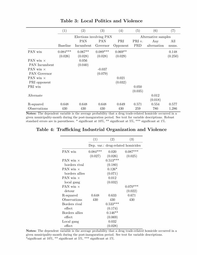
Table 3: Local Politics and Violence

(1) (2) (3) (4) (5) (6) (7)

Elections involving PAN Alternative samplesPAN PAN PRI PRI v. Any All

Baseline Incumbent Governor Opponent PRD alternation muns.

PAN win 0.084*** 0.067** 0.089*** 0.069** 0.148(0.026) (0.028) (0.028) (0.029) (0.250)

PAN win × 0.056PAN Incumbent (0.040)

PAN win × -0.037PAN Governor (0.079)

PAN win × 0.021PRI opponent (0.032)

PRI win 0.050(0.035)

Alternate 0.012(0.018)

R-squared 0.648 0.648 0.648 0.649 0.571 0.554 0.577Observations 430 430 430 430 259 780 1,286

Notes: The dependent variable is the average probability that a drug trade-related homicide occurred in agiven municipality-month during the post-inauguration period. See text for variable descriptions. Robuststandard errors are in parentheses. * significant at 10%, ** significant at 5%, *** significant at 1%.

Table 4: Trafficking Industrial Organization and Violence

(1) (2) (3)

Dep. var.: drug-related homicides

PAN win 0.084*** 0.020 0.087***(0.027) (0.026) (0.025)

PAN win × 0.513***borders rival (0.180)

PAN win × 0.126*borders allies (0.071)

PAN win × 0.012local gang (0.032)

PAN win × 0.070***detour (0.022)

R-squared 0.648 0.633 0.671Observations 430 430 430Borders rival 0.533***

effect (0.174)Borders allies 0.146**

effect (0.069)Local gang 0.032

effect (0.028)

Notes: The dependent variable is the average probability that a drug trade-related homicide occurred in agiven municipality-month during the post-inauguration period. See text for variable descriptions.*significant at 10%, ** significant at 5%, *** significant at 1%.

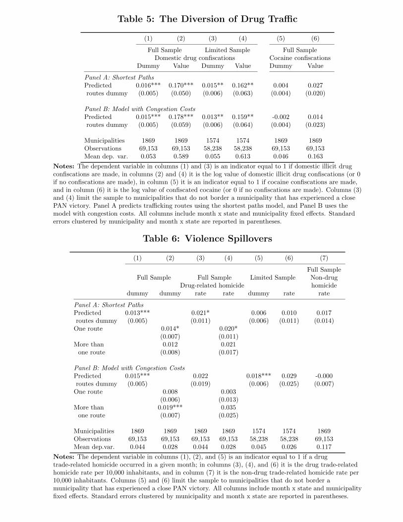
Table 5: The Diversion of Drug Traffic

(1) (2) (3) (4) (5) (6)

Full Sample Limited Sample Full SampleDomestic drug confiscations Cocaine confiscations

Dummy Value Dummy Value Dummy Value

Panel A: Shortest PathsPredicted 0.016*** 0.170*** 0.015** 0.162** 0.004 0.027routes dummy (0.005) (0.050) (0.006) (0.063) (0.004) (0.020)

Panel B: Model with Congestion CostsPredicted 0.015*** 0.178*** 0.013** 0.159** -0.002 0.014routes dummy (0.005) (0.059) (0.006) (0.064) (0.004) (0.023)

Municipalities 1869 1869 1574 1574 1869 1869Observations 69,153 69,153 58,238 58,238 69,153 69,153Mean dep. var. 0.053 0.589 0.055 0.613 0.046 0.163

Notes: The dependent variable in columns (1) and (3) is an indicator equal to 1 if domestic illicit drugconfiscations are made, in columns (2) and (4) it is the log value of domestic illicit drug confiscations (or 0if no confiscations are made), in column (5) it is an indicator equal to 1 if cocaine confiscations are made,and in column (6) it is the log value of confiscated cocaine (or 0 if no confiscations are made). Columns (3)and (4) limit the sample to municipalities that do not border a municipality that has experienced a closePAN victory. Panel A predicts trafficking routes using the shortest paths model, and Panel B uses themodel with congestion costs. All columns include month x state and municipality fixed effects. Standarderrors clustered by municipality and month x state are reported in parentheses.

Table 6: Violence Spillovers

(1) (2) (3) (4) (5) (6) (7)

Full SampleFull Sample Full Sample Limited Sample Non-drug

Drug-related homicide homicidedummy dummy rate rate dummy rate rate

Panel A: Shortest PathsPredicted 0.013*** 0.021* 0.006 0.010 0.017routes dummy (0.005) (0.011) (0.006) (0.011) (0.014)

One route 0.014* 0.020*(0.007) (0.011)

More than 0.012 0.021one route (0.008) (0.017)

Panel B: Model with Congestion CostsPredicted 0.015*** 0.022 0.018*** 0.029 -0.000routes dummy (0.005) (0.019) (0.006) (0.025) (0.007)

One route 0.008 0.003(0.006) (0.013)

More than 0.019*** 0.035one route (0.007) (0.025)

Municipalities 1869 1869 1869 1869 1574 1574 1869Observations 69,153 69,153 69,153 69,153 58,238 58,238 69,153Mean dep.var. 0.044 0.028 0.044 0.028 0.045 0.026 0.117

Notes: The dependent variable in columns (1), (2), and (5) is an indicator equal to 1 if a drugtrade-related homicide occurred in a given month; in columns (3), (4), and (6) it is the drug trade-relatedhomicide rate per 10,000 inhabitants, and in column (7) it is the non-drug trade-related homicide rate per10,000 inhabitants. Columns (5) and (6) limit the sample to municipalities that do not border amunicipality that has experienced a close PAN victory. All columns include month x state and municipalityfixed effects. Standard errors clustered by municipality and month x state are reported in parentheses.

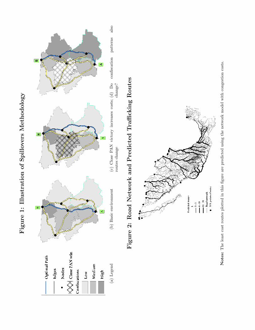
Fig

ure

1:

Illu

stra

tion

of

Sp

illo

vers

Meth

od

olo

gy

(a)

Leg

end

(b)

Bas

icen

vir

on

men

t(c

)C

lose

PA

Nvic

tory

incr

ease

sco

sts;

rou

tes

chan

ge

(d)

Do

con

fisc

ati

on

patt

ern

sals

och

an

ge?

Fig

ure

2:

Road

Netw

ork

an

dP

red

icte

dT

raffi

ckin

gR

ou

tes

Notes:

Th

ele

ast

cost

rou

tes

plo

tted

inth

isfi

gu

reare

pre

dic

ted

usi

ng

the

net

work

mod

elw

ith

con

ges

tion

cost

s.

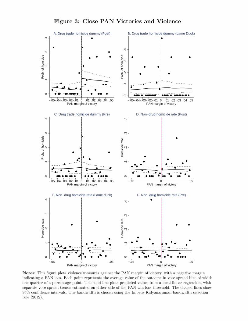
Figure 3: Close PAN Victories and Violence

0.1

.2.3

.4P

rob.

of h

omic

ide

−.05−.04−.03−.02−.01 0 .01 .02 .03 .04 .05PAN margin of victory

A. Drug trade homicide dummy (Post)

0.1

.2.3

.4P

rob.

of h

omic

ide

−.05−.04−.03−.02−.01 0 .01 .02 .03 .04 .05PAN margin of victory

B. Drug trade homicide dummy (Lame Duck)

0.1

.2.3

.4P

rob.

of h

omic

ide

−.05−.04−.03−.02−.01 0 .01 .02 .03 .04 .05PAN margin of victory

C. Drug trade homicide dummy (Pre)

0.1

.2.3

.4H

omic

ide

rate

−.05 0 .05PAN margin of victory

D. Non−drug homicide rate (Post)

0.1

.2.3

.4H

omic

ide

rate

−.05 0 .05PAN margin of victory

E. Non−drug homicide rate (Lame duck)

0.1

.2.3

.4H

omic

ide

rate

−.05 0 .05PAN margin of victory

F. Non−drug homicide rate (Pre)

Notes: This figure plots violence measures against the PAN margin of victory, with a negative marginindicating a PAN loss. Each point represents the average value of the outcome in vote spread bins of widthone quarter of a percentage point. The solid line plots predicted values from a local linear regression, withseparate vote spread trends estimated on either side of the PAN win-loss threshold. The dashed lines show95% confidence intervals. The bandwidth is chosen using the Imbens-Kalyanaraman bandwidth selectionrule (2012).

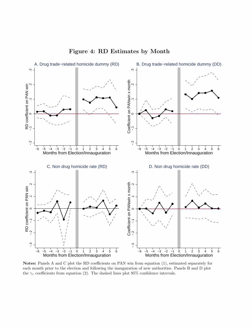
Figure 4: RD Estimates by Month

−.2

−.1

0.1

.2.3

RD

coe

ffici

ent o

n P

AN

win

−6 −5 −4 −3 −2 −1 0 1 2 3 4 5 6Months from Election/Innauguration

A. Drug trade−related homicide dummy (RD)

−.2

−.1

0.1

.2.3

Coe

ffici

ent o

n P

AN

win

x m

onth

−6 −5 −4 −3 −2 −1 0 1 2 3 4 5 6Months from Election/Innauguration

B. Drug trade−related homicide dummy (DD)

−.3

−.2

−.1

0.1

.2.3

RD

coe

ffici

ent o

n P

AN

win

−6 −5 −4 −3 −2 −1 0 1 2 3 4 5 6Months from Election/Innauguration

C. Non drug homicide rate (RD)

−.3

−.2

−.1

0.1

.2.3

Coe

ffici

ent o

n P

AN

win

x m

onth

−6 −5 −4 −3 −2 −1 0 1 2 3 4 5 6Months from Election/Innauguration

D. Non drug homicide rate (DD)

Notes: Panels A and C plot the RD coefficients on PAN win from equation (1), estimated separately foreach month prior to the election and following the inauguration of new authorities. Panels B and D plotthe γτ coefficients from equation (2). The dashed lines plot 95% confidence intervals.