Towards Using Tire-Road Contact Stresses in Pavement

Towards Using Tire-Road Contact Stresses in

Pavement Design and Analysis

M. De Beer*, J. W. Maina, Y. van Rensburg, J. M. Greben

[email protected]

CSIR Built Environment

P O Box 395

Pretoria

0001

South Africa

Presented at the

September 2011

Meeting of the Tire Society

*Presenter / Corresponding Author

2

M. De Beer et al

REFERENCE: M. De Beer, J. W. Maina, Y. van Rensburg and J. Greben "Towards Using Tire-

Road Contact Stresses in Pavement Design and Analysis," submitted for presentation at the 2011

Tire Society meeting, and for consideration for publication in the journal Tire Science and

Technology.

ABSTRACT: Optimization of road pavement design, especially towards the surface of the pavement,

requires a more rational approach to modeling of truck tire-road contact stresses. Various road surfacing

failures are given in this paper as examples, and it is shown that the traditional civil engineering tire model

represented by a single uniformly distributed vertical contact stress of circular shape is inadequate to

explain this type of surface failure. This paper therefore discusses the direct measurement of three-

dimensional (3D) tire pavement contact stresses using a flatbed sensor system referred to as the “Stress-In-

Motion” (SIM) system. The SIM system (or device) consists of multiple conically shaped steel pins, as well

as an array of instrumented sensors based on strain gauge technology. The test surface is textured with skid

resistance approaching that of a dry asphalt layer. Full-scale truck tires have been tested since the mid-

1990s and experience shows that 3D tire contact stresses are non-uniform and the footprint is often not of

circular shape. It was found that especially the vertical shape of contact stress distribution changes, mainly

as a function of tire loading. In overloaded/underinflated cases, vertical contact stresses maximize towards

the edges of the tire contact patch. Higher inflation pressures at lower loads, on the other hand, result in

maximum vertical stresses towards the center portion of the tire contact patch. These differences in shape

and magnitude need to be incorporated into modern road pavement design. Four different tire models were

used to represent a single tire type in order to demonstrate its effect on road pavement response of a typical

South African pavement structure. Only applied vertical stress was used for the analyses. It was found that

road surface layer life can reduce by as much as 94 percent as a result of simply using a different tire model

on the same pavement structure.

KEYWORDS: Tire, Contact, Tire-Road, Stress, Force, Measurement, Load, Patch, Pavement,

Design, Strain Energy of Distortion (SED).

3

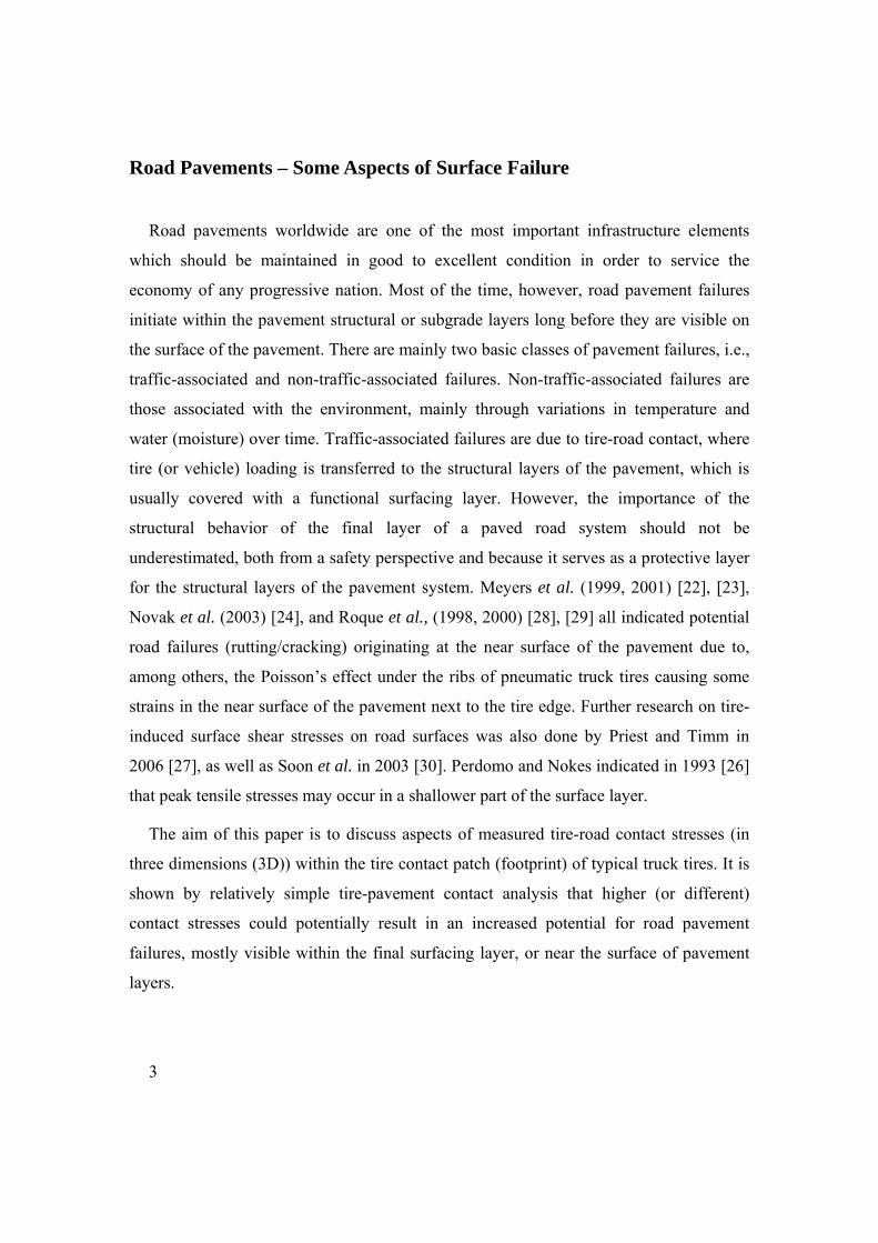
Road Pavements – Some Aspects of Surface Failure

Road pavements worldwide are one of the most important infrastructure elements

which should be maintained in good to excellent condition in order to service the

economy of any progressive nation. Most of the time, however, road pavement failures

initiate within the pavement structural or subgrade layers long before they are visible on

the surface of the pavement. There are mainly two basic classes of pavement failures, i.e.,

traffic-associated and non-traffic-associated failures. Non-traffic-associated failures are

those associated with the environment, mainly through variations in temperature and

water (moisture) over time. Traffic-associated failures are due to tire-road contact, where

tire (or vehicle) loading is transferred to the structural layers of the pavement, which is

usually covered with a functional surfacing layer. However, the importance of the

structural behavior of the final layer of a paved road system should not be

underestimated, both from a safety perspective and because it serves as a protective layer

for the structural layers of the pavement system. Meyers et al. (1999, 2001) [22], [23],

Novak et al. (2003) [24], and Roque et al., (1998, 2000) [28], [29] all indicated potential

road failures (rutting/cracking) originating at the near surface of the pavement due to,

among others, the Poisson’s effect under the ribs of pneumatic truck tires causing some

strains in the near surface of the pavement next to the tire edge. Further research on tire-

induced surface shear stresses on road surfaces was also done by Priest and Timm in

2006 [27], as well as Soon et al. in 2003 [30]. Perdomo and Nokes indicated in 1993 [26]

that peak tensile stresses may occur in a shallower part of the surface layer.

The aim of this paper is to discuss aspects of measured tire-road contact stresses (in

three dimensions (3D)) within the tire contact patch (footprint) of typical truck tires. It is

shown by relatively simple tire-pavement contact analysis that higher (or different)

contact stresses could potentially result in an increased potential for road pavement

failures, mostly visible within the final surfacing layer, or near the surface of pavement

layers.

4

Observations of Road Pavement Failures

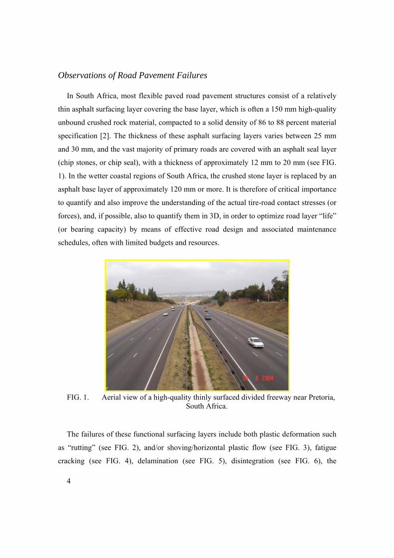
In South Africa, most flexible paved road pavement structures consist of a relatively

thin asphalt surfacing layer covering the base layer, which is often a 150 mm high-quality

unbound crushed rock material, compacted to a solid density of 86 to 88 percent material

specification [2]. The thickness of these asphalt surfacing layers varies between 25 mm

and 30 mm, and the vast majority of primary roads are covered with an asphalt seal layer

(chip stones, or chip seal), with a thickness of approximately 12 mm to 20 mm (see FIG.

1). In the wetter coastal regions of South Africa, the crushed stone layer is replaced by an

asphalt base layer of approximately 120 mm or more. It is therefore of critical importance

to quantify and also improve the understanding of the actual tire-road contact stresses (or

forces), and, if possible, also to quantify them in 3D, in order to optimize road layer “life”

(or bearing capacity) by means of effective road design and associated maintenance

schedules, often with limited budgets and resources.

FIG. 1. Aerial view of a high-quality thinly surfaced divided freeway near Pretoria, South Africa.

The failures of these functional surfacing layers include both plastic deformation such

as “rutting” (see FIG. 2), and/or shoving/horizontal plastic flow (see FIG. 3), fatigue

cracking (see FIG. 4), delamination (see FIG. 5), disintegration (see FIG. 6), the

5

formation of potholes (see FIG. 7), and subsurface rutting often with standing water in

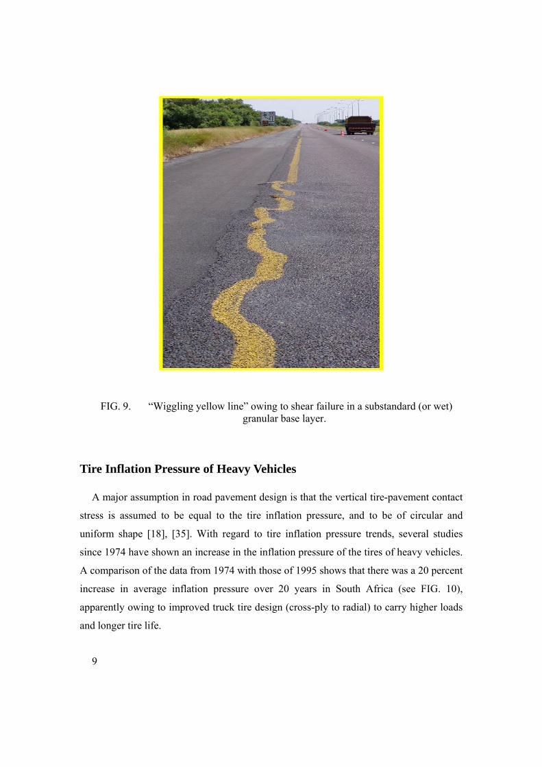
the wheel paths (see FIG. 8) during rain. FIG. 9 shows an example of a substandard base

layer, causing the typical ”wiggling yellow line” indicative of shear failure in the

unbound base layer. Most of these failures are related to tire-road interaction and are

therefore considered “traffic associated”. In this paper it is postulated that an improved

understanding of the 3D tire-road interaction forces (or contact stresses) could serve as a

sound platform for the formulation of improved pavement design rules. The traditional

assumption of one-dimensional (1D) uniformly distributed tire loading on a circular

shape for pavement design as discussed by Huang in 1993 [18], and Yoder and Witczak

in 1975 [35] is therefore questioned.

FIG. 2. Plastic deformation (or rutting/shoving) within the thin asphalt surfacing layer. Note the six lanes of rutting (left and right sides) owing to tire loading

combined with poor asphalt mix.

6

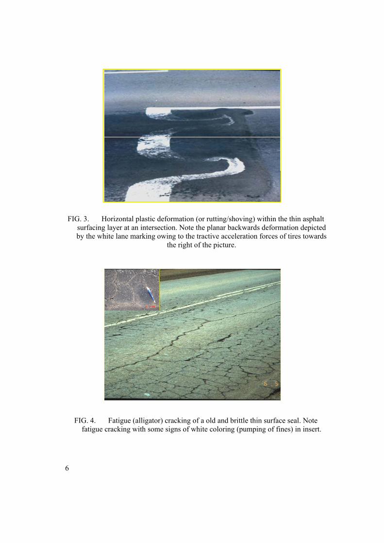
FIG. 3. Horizontal plastic deformation (or rutting/shoving) within the thin asphalt surfacing layer at an intersection. Note the planar backwards deformation depicted by the white lane marking owing to the tractive acceleration forces of tires towards

the right of the picture.

FIG. 4. Fatigue (alligator) cracking of a old and brittle thin surface seal. Note fatigue cracking with some signs of white coloring (pumping of fines) in insert.

7

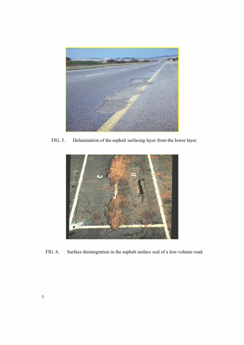
FIG. 5. Delamination of the asphalt surfacing layer from the lower layer.

FIG. 6. Surface disintegration in the asphalt surface seal of a low-volume road.

8

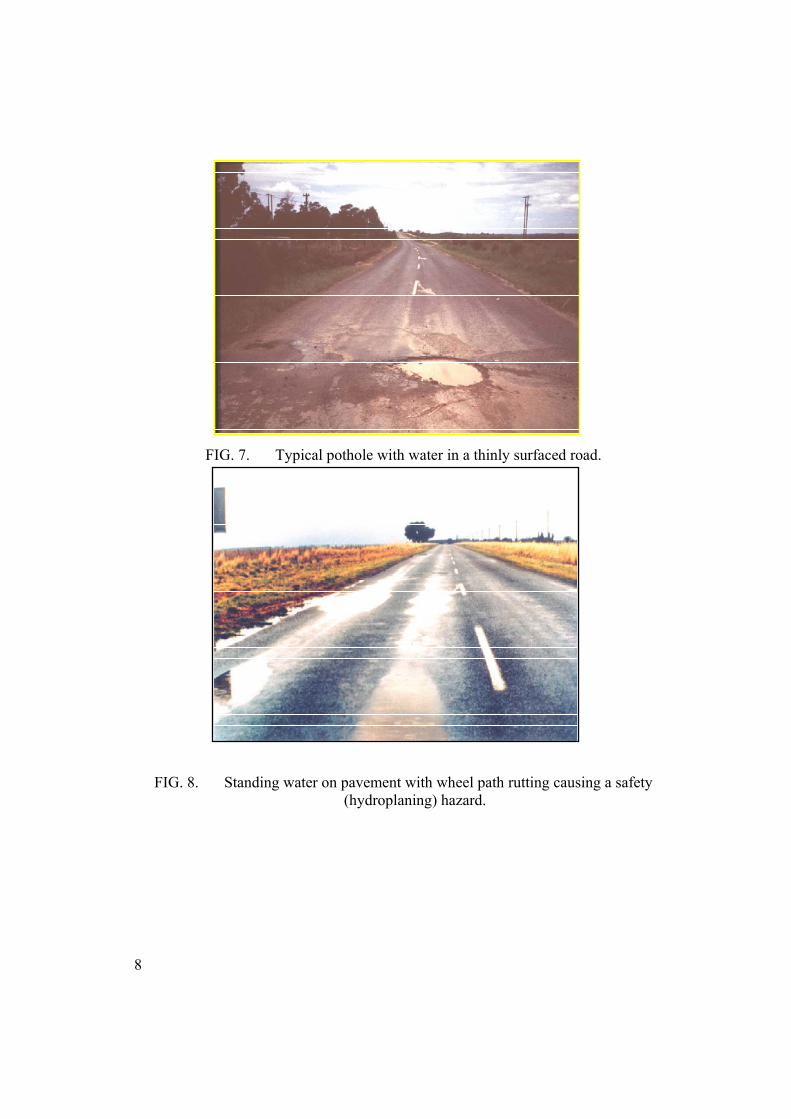
FIG. 7. Typical pothole with water in a thinly surfaced road.

FIG. 8. Standing water on pavement with wheel path rutting causing a safety (hydroplaning) hazard.

9

FIG. 9. “Wiggling yellow line” owing to shear failure in a substandard (or wet) granular base layer.

Tire Inflation Pressure of Heavy Vehicles

A major assumption in road pavement design is that the vertical tire-pavement contact

stress is assumed to be equal to the tire inflation pressure, and to be of circular and

uniform shape [18], [35]. With regard to tire inflation pressure trends, several studies

since 1974 have shown an increase in the inflation pressure of the tires of heavy vehicles.

A comparison of the data from 1974 with those of 1995 shows that there was a 20 percent

increase in average inflation pressure over 20 years in South Africa (see FIG. 10),

apparently owing to improved truck tire design (cross-ply to radial) to carry higher loads

and longer tire life.

10

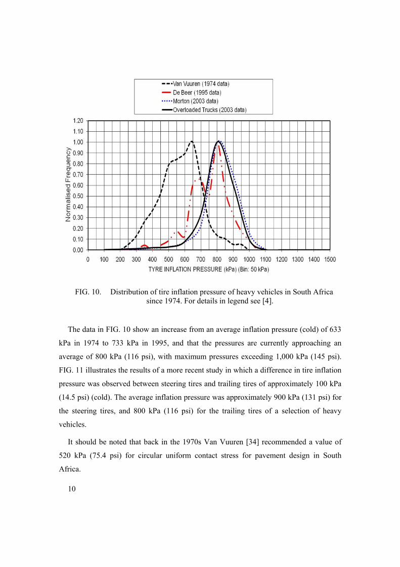
FIG. 10. Distribution of tire inflation pressure of heavy vehicles in South Africa

since 1974. For details in legend see [4].

The data in FIG. 10 show an increase from an average inflation pressure (cold) of 633

kPa in 1974 to 733 kPa in 1995, and that the pressures are currently approaching an

average of 800 kPa (116 psi), with maximum pressures exceeding 1,000 kPa (145 psi).

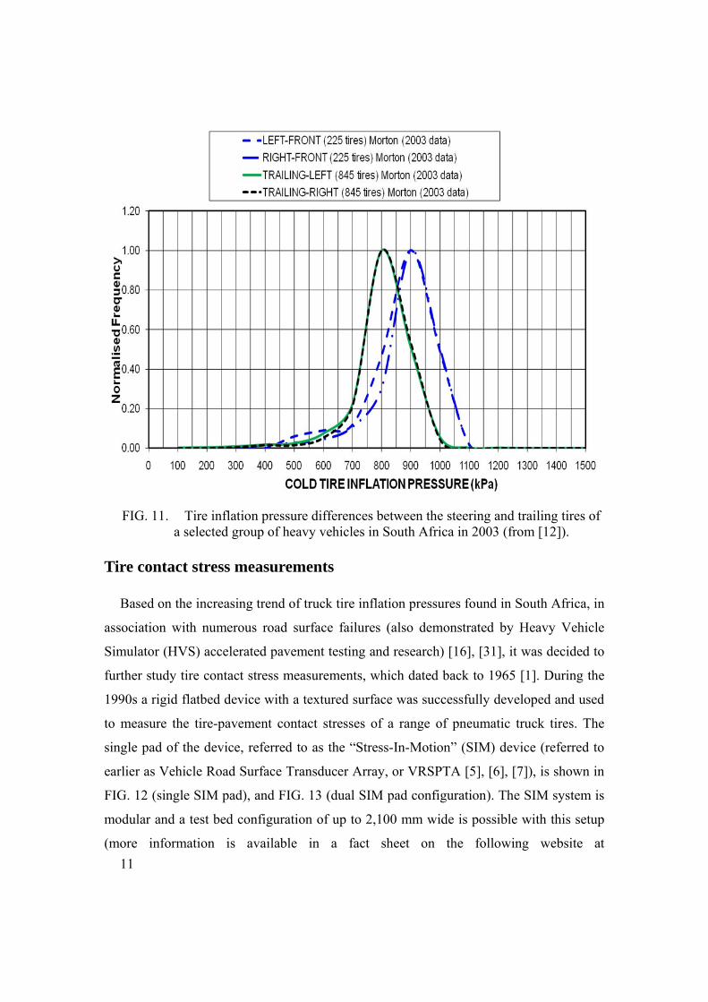
FIG. 11 illustrates the results of a more recent study in which a difference in tire inflation

pressure was observed between steering tires and trailing tires of approximately 100 kPa

(14.5 psi) (cold). The average inflation pressure was approximately 900 kPa (131 psi) for

the steering tires, and 800 kPa (116 psi) for the trailing tires of a selection of heavy

vehicles.

It should be noted that back in the 1970s Van Vuuren [34] recommended a value of

520 kPa (75.4 psi) for circular uniform contact stress for pavement design in South

Africa.

11

FIG. 11. Tire inflation pressure differences between the steering and trailing tires of

a selected group of heavy vehicles in South Africa in 2003 (from [12]).

Tire contact stress measurements

Based on the increasing trend of truck tire inflation pressures found in South Africa, in

association with numerous road surface failures (also demonstrated by Heavy Vehicle

Simulator (HVS) accelerated pavement testing and research) [16], [31], it was decided to

further study tire contact stress measurements, which dated back to 1965 [1]. During the

1990s a rigid flatbed device with a textured surface was successfully developed and used

to measure the tire-pavement contact stresses of a range of pneumatic truck tires. The

single pad of the device, referred to as the “Stress-In-Motion” (SIM) device (referred to

earlier as Vehicle Road Surface Transducer Array, or VRSPTA [5], [6], [7]), is shown in

FIG. 12 (single SIM pad), and FIG. 13 (dual SIM pad configuration). The SIM system is

modular and a test bed configuration of up to 2,100 mm wide is possible with this setup

(more information is available in a fact sheet on the following website at

12

http://www.csir.co.za/Built_environment/brochures.html [36]. For controlled tire loading

and tire inflation pressure the HVS was used for tire-pavement contact stress

measurements in association with the SIM device. The first typical SIM data were

published by De Beer in 1996 [5], and a comprehensive summary was presented in 1997

[7]. This was followed by several presentations relating SIM data with mechanistic

analyses of road pavements in 1999 [8], 2002 [9], 2004 [10], [11], 2006 [12], and 2008

[13].

FIG. 12. Flat bed Stress-In-Motion (SIM) device with Society of Automotive Engineering (SAE) coordinate system used in this study for the measurements of 3D tire contact force (or stress) conditions inside the tire contact patch of a slow-

rolling pneumatic tire (fitted on the Heavy Vehicle Simulator – HVS).

+X

+Z

Tyre Rotation

+/‐Y+/‐X

13

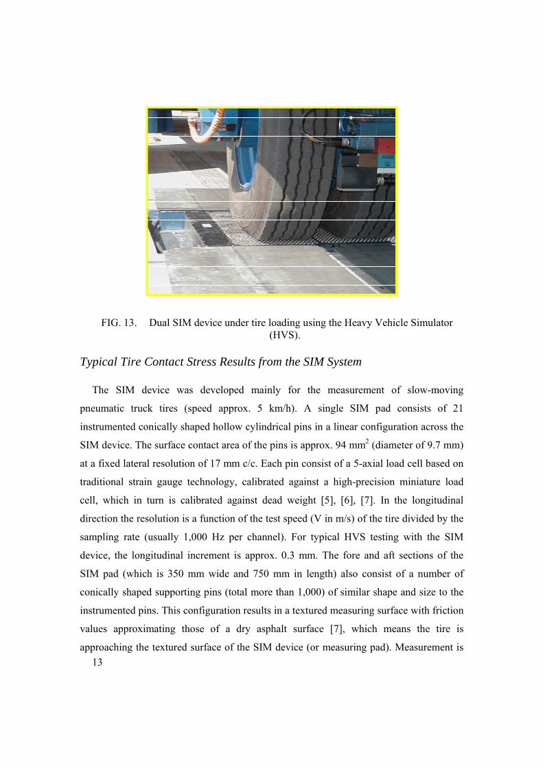
FIG. 13. Dual SIM device under tire loading using the Heavy Vehicle Simulator (HVS).

Typical Tire Contact Stress Results from the SIM System

The SIM device was developed mainly for the measurement of slow-moving

pneumatic truck tires (speed approx. 5 km/h). A single SIM pad consists of 21

instrumented conically shaped hollow cylindrical pins in a linear configuration across the

SIM device. The surface contact area of the pins is approx. 94 mm2 (diameter of 9.7 mm)

at a fixed lateral resolution of 17 mm c/c. Each pin consist of a 5-axial load cell based on

traditional strain gauge technology, calibrated against a high-precision miniature load

cell, which in turn is calibrated against dead weight [5], [6], [7]. In the longitudinal

direction the resolution is a function of the test speed (V in m/s) of the tire divided by the

sampling rate (usually 1,000 Hz per channel). For typical HVS testing with the SIM

device, the longitudinal increment is approx. 0.3 mm. The fore and aft sections of the

SIM pad (which is 350 mm wide and 750 mm in length) also consist of a number of

conically shaped supporting pins (total more than 1,000) of similar shape and size to the

instrumented pins. This configuration results in a textured measuring surface with friction

values approximating those of a dry asphalt surface [7], which means the tire is

approaching the textured surface of the SIM device (or measuring pad). Measurement is

14

made in the center portion of the SIM pad after the front part of the tire contact patch has

been “conditioned” by the textured surface, after which the aft part of the contact patch is

measured. A 3D contact stress pattern is obtained in one measurement cycle.

It should be noted that partial contact of instrumented SIM pins on rib or element

edges does occur with this system. The instrumented pins capture the components of a

vector force in the three directions (X, Y, Z) whenever there is contact with rubber,

instantaneously. In such a case, there is no specialized treatment of data necessary, but

additional passes could provide improvement of the definition of the forces/stresses at the

rib edges (where there is partial contact), especially when the tread pattern varies along

the tire patch. Further, non-ribbed tire designs (lug pattern) can be measured with the

SIM device. For this case, there can be a difference in the vertical pressure trace (leading

footprint edge to trailing footprint edge), depending on where the sensor (or

instrumented) pin contacts the individual tread lug (leading lug edge vs trailing lug edge).

Non-ribbed lug pattern tire design requires multiple passes in order to capture the

variation of contact forces/stresses along the length of the tire patch. In one example, a

sinusoidal pattern of total loading was observed, discussed in De Beer and Fisher in 1997

[6].

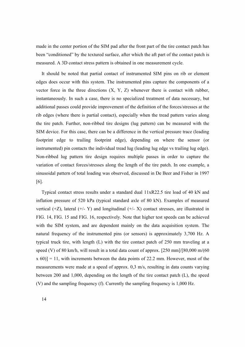
Typical contact stress results under a standard dual 11xR22.5 tire load of 40 kN and

inflation pressure of 520 kPa (typical standard axle of 80 kN). Examples of measured

vertical (+Z), lateral (+/- Y) and longitudinal (+/- X) contact stresses, are illustrated in

FIG. 14, FIG. 15 and FIG. 16, respectively. Note that higher test speeds can be achieved

with the SIM system, and are dependent mainly on the data acquisition system. The

natural frequency of the instrumented pins (or sensors) is approximately 3,700 Hz. A

typical truck tire, with length (L) with the tire contact patch of 250 mm traveling at a

speed (V) of 80 km/h, will result in a total data count of approx. [250 mm]/[80,000 m/(60

x 60)] = 11, with increments between the data points of 22.2 mm. However, most of the

measurements were made at a speed of approx. 0,3 m/s, resulting in data counts varying

between 200 and 1,000, depending on the length of the tire contact patch (L), the speed

(V) and the sampling frequency (f). Currently the sampling frequency is 1,000 Hz.

15

FIG. 14. Typical vertical (Z) contact stress pattern of a 11xR22.5 dual tire configuration with total tire load of 40 kN, and 520 kPa inflation pressure. Note

that a maximum contact stress of approx. 849 kPa was measured on the edge of the left tire in this illustration.

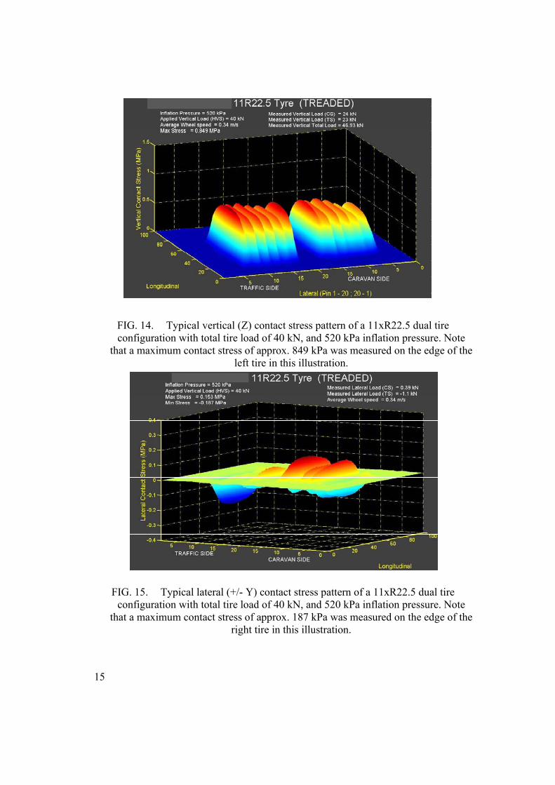
FIG. 15. Typical lateral (+/- Y) contact stress pattern of a 11xR22.5 dual tire configuration with total tire load of 40 kN, and 520 kPa inflation pressure. Note

that a maximum contact stress of approx. 187 kPa was measured on the edge of the right tire in this illustration.

16

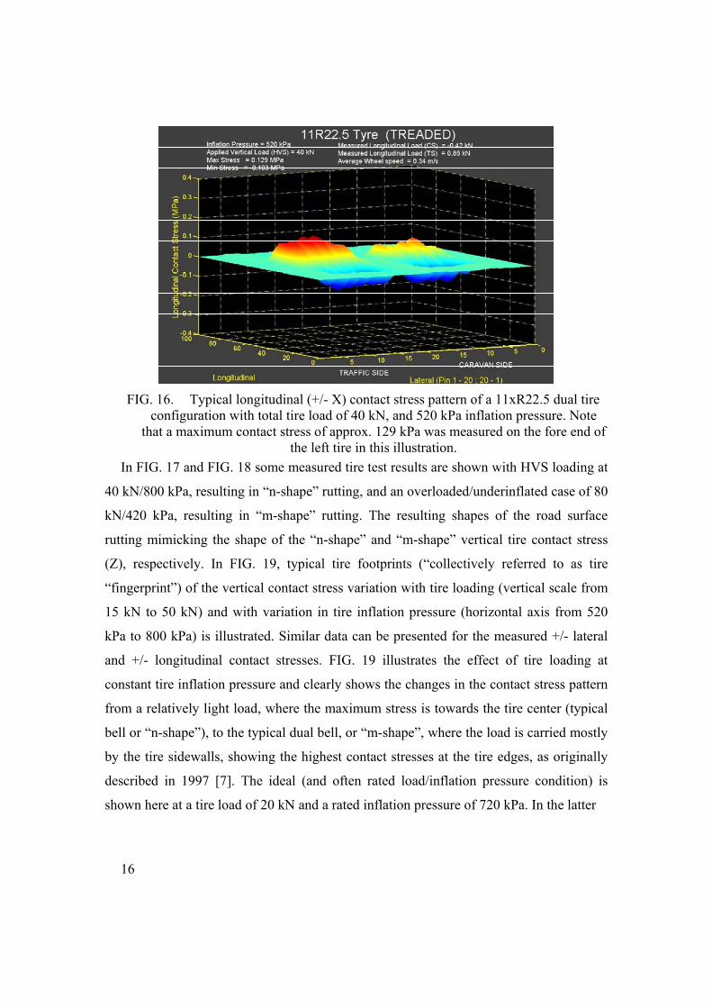
FIG. 16. Typical longitudinal (+/- X) contact stress pattern of a 11xR22.5 dual tire

configuration with total tire load of 40 kN, and 520 kPa inflation pressure. Note that a maximum contact stress of approx. 129 kPa was measured on the fore end of

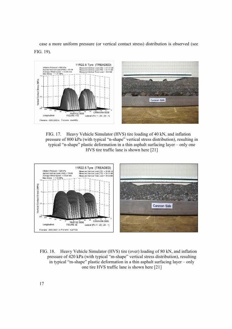
the left tire in this illustration. In FIG. 17 and FIG. 18 some measured tire test results are shown with HVS loading at

40 kN/800 kPa, resulting in “n-shape” rutting, and an overloaded/underinflated case of 80

kN/420 kPa, resulting in “m-shape” rutting. The resulting shapes of the road surface

rutting mimicking the shape of the “n-shape” and “m-shape” vertical tire contact stress

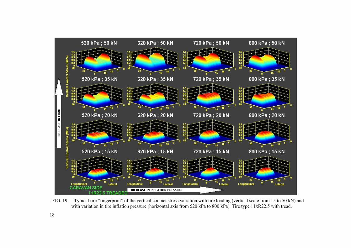
(Z), respectively. In FIG. 19, typical tire footprints (“collectively referred to as tire

“fingerprint”) of the vertical contact stress variation with tire loading (vertical scale from

15 kN to 50 kN) and with variation in tire inflation pressure (horizontal axis from 520

kPa to 800 kPa) is illustrated. Similar data can be presented for the measured +/- lateral

and +/- longitudinal contact stresses. FIG. 19 illustrates the effect of tire loading at

constant tire inflation pressure and clearly shows the changes in the contact stress pattern

from a relatively light load, where the maximum stress is towards the tire center (typical

bell or “n-shape”), to the typical dual bell, or “m-shape”, where the load is carried mostly

by the tire sidewalls, showing the highest contact stresses at the tire edges, as originally

described in 1997 [7]. The ideal (and often rated load/inflation pressure condition) is

shown here at a tire load of 20 kN and a rated inflation pressure of 720 kPa. In the latter

17

case a more uniform pressure (or vertical contact stress) distribution is observed (see

FIG. 19).

FIG. 17. Heavy Vehicle Simulator (HVS) tire loading of 40 kN, and inflation pressure of 800 kPa (with typical “n-shape” vertical stress distribution), resulting in

typical “n-shape” plastic deformation in a thin asphalt surfacing layer – only one HVS tire traffic lane is shown here [21]

FIG. 18. Heavy Vehicle Simulator (HVS) tire (over) loading of 80 kN, and inflation pressure of 420 kPa (with typical “m-shape” vertical stress distribution), resulting in typical “m-shape” plastic deformation in a thin asphalt surfacing layer – only

one tire HVS traffic lane is shown here [21]

18

FIG. 19. Typical tire “fingerprint” of the vertical contact stress variation with tire loading (vertical scale from 15 to 50 kN) and

with variation in tire inflation pressure (horizontal axis from 520 kPa to 800 kPa). Tire type 11xR22.5 with tread.

19

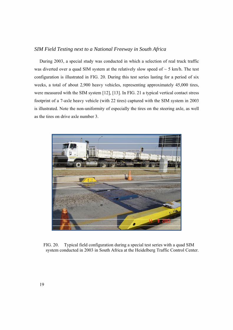
SIM Field Testing next to a National Freeway in South Africa

During 2003, a special study was conducted in which a selection of real truck traffic

was diverted over a quad SIM system at the relatively slow speed of ~ 5 km/h. The test

configuration is illustrated in FIG. 20. During this test series lasting for a period of six

weeks, a total of about 2,900 heavy vehicles, representing approximately 45,000 tires,

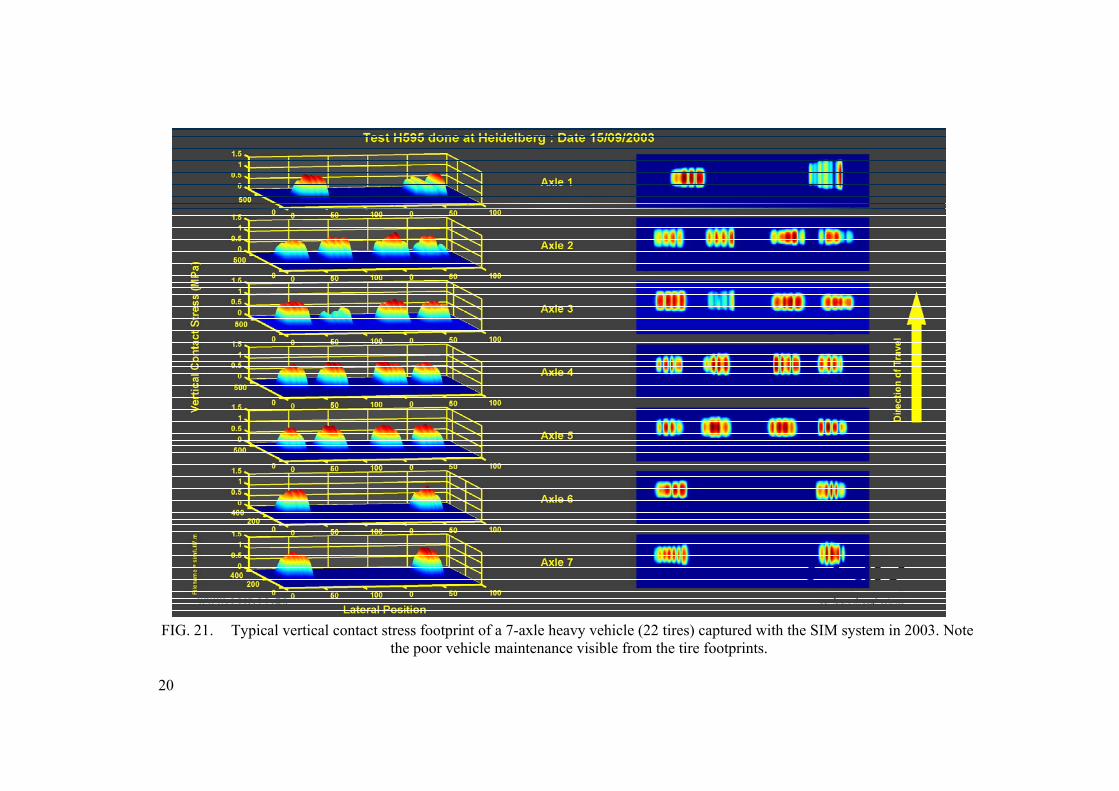
were measured with the SIM system [12], [13]. In FIG. 21 a typical vertical contact stress

footprint of a 7-axle heavy vehicle (with 22 tires) captured with the SIM system in 2003

is illustrated. Note the non-uniformity of especially the tires on the steering axle, as well

as the tires on drive axle number 3.

FIG. 20. Typical field configuration during a special test series with a quad SIM system conducted in 2003 in South Africa at the Heidelberg Traffic Control Center.

20

FIG. 21. Typical vertical contact stress footprint of a 7-axle heavy vehicle (22 tires) captured with the SIM system in 2003. Note the poor vehicle maintenance visible from the tire footprints.

21

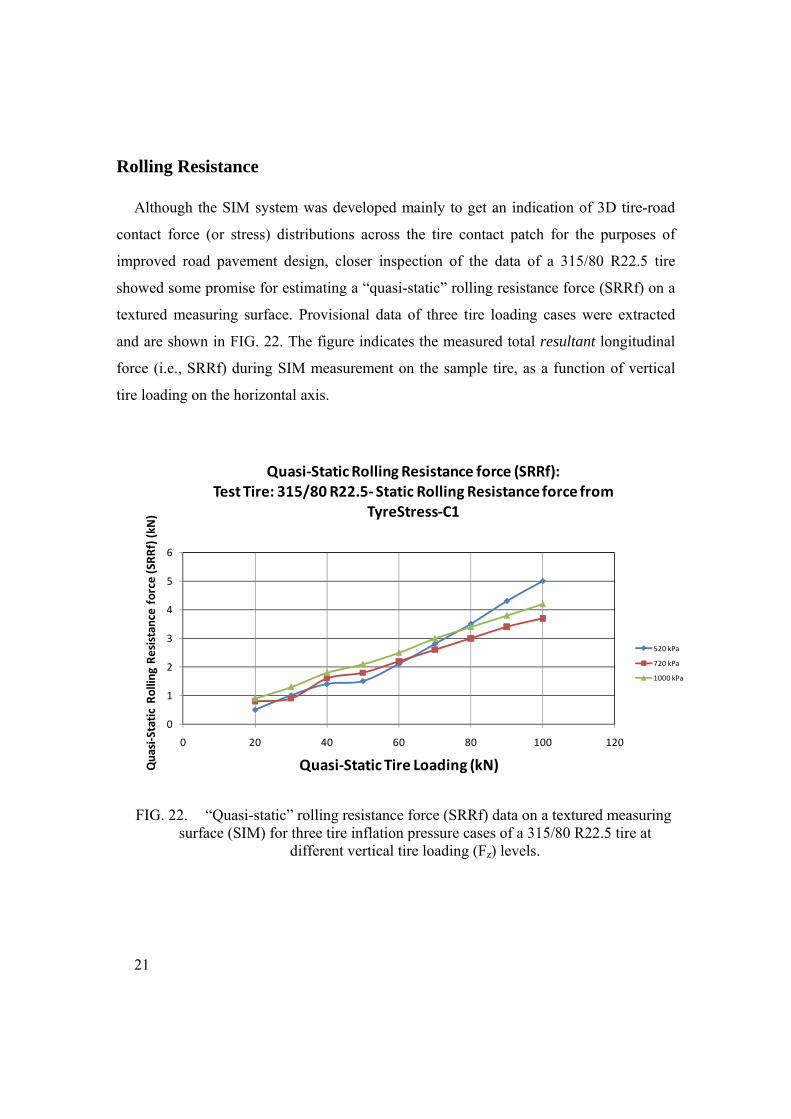
Rolling Resistance

Although the SIM system was developed mainly to get an indication of 3D tire-road

contact force (or stress) distributions across the tire contact patch for the purposes of

improved road pavement design, closer inspection of the data of a 315/80 R22.5 tire

showed some promise for estimating a “quasi-static” rolling resistance force (SRRf) on a

textured measuring surface. Provisional data of three tire loading cases were extracted

and are shown in FIG. 22. The figure indicates the measured total resultant longitudinal

force (i.e., SRRf) during SIM measurement on the sample tire, as a function of vertical

tire loading on the horizontal axis.

0

1

2

3

4

5

6

0 20 40 60 80 100 120

Quasi‐Static Rolling Resistance force (SRRf) (kN

)

Quasi‐Static Tire Loading (kN)

Quasi‐Static Rolling Resistance force (SRRf):Test Tire: 315/80 R22.5‐Static Rolling Resistance force from

TyreStress‐C1

520 kPa

720 kPa

1000 kPa

FIG. 22. “Quasi-static” rolling resistance force (SRRf) data on a textured measuring surface (SIM) for three tire inflation pressure cases of a 315/80 R22.5 tire at

different vertical tire loading (Fz) levels.

22

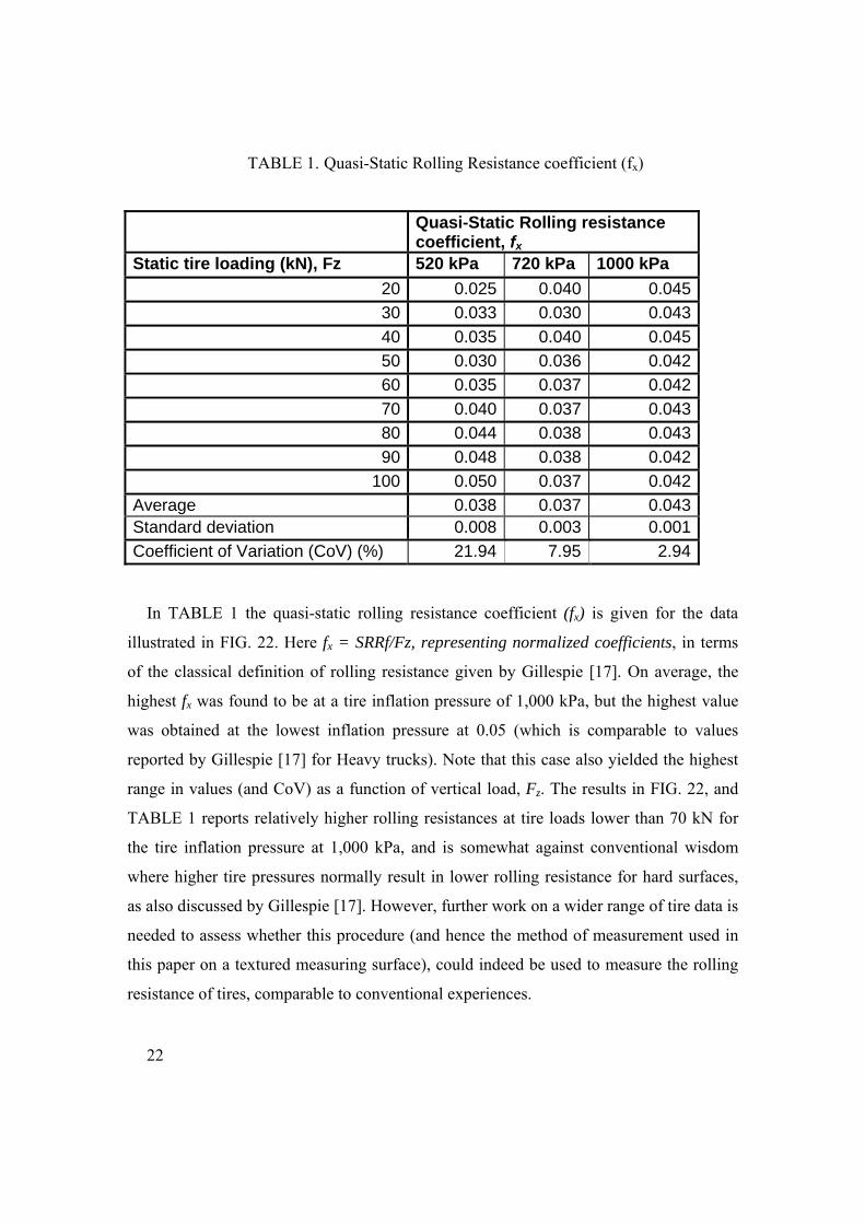
TABLE 1. Quasi-Static Rolling Resistance coefficient (fx)

Quasi-Static Rolling resistance coefficient, fx

Static tire loading (kN), Fz 520 kPa 720 kPa 1000 kPa 20 0.025 0.040 0.045 30 0.033 0.030 0.043 40 0.035 0.040 0.045 50 0.030 0.036 0.042 60 0.035 0.037 0.042 70 0.040 0.037 0.043 80 0.044 0.038 0.043 90 0.048 0.038 0.042

100 0.050 0.037 0.042 Average 0.038 0.037 0.043 Standard deviation 0.008 0.003 0.001 Coefficient of Variation (CoV) (%) 21.94 7.95 2.94

In TABLE 1 the quasi-static rolling resistance coefficient (fx) is given for the data

illustrated in FIG. 22. Here fx = SRRf/Fz, representing normalized coefficients, in terms

of the classical definition of rolling resistance given by Gillespie [17]. On average, the

highest fx was found to be at a tire inflation pressure of 1,000 kPa, but the highest value

was obtained at the lowest inflation pressure at 0.05 (which is comparable to values

reported by Gillespie [17] for Heavy trucks). Note that this case also yielded the highest

range in values (and CoV) as a function of vertical load, Fz. The results in FIG. 22, and

TABLE 1 reports relatively higher rolling resistances at tire loads lower than 70 kN for

the tire inflation pressure at 1,000 kPa, and is somewhat against conventional wisdom

where higher tire pressures normally result in lower rolling resistance for hard surfaces,

as also discussed by Gillespie [17]. However, further work on a wider range of tire data is

needed to assess whether this procedure (and hence the method of measurement used in

this paper on a textured measuring surface), could indeed be used to measure the rolling

resistance of tires, comparable to conventional experiences.

23

The preliminary findings for the SIM measured data on a 315/80 R22.5 tire for slow-

moving (< 10 km/h) free-rolling conditions include:

• There was a linear increase in SRRf with increased vertical tire loading at a

rate of:

o ~ 3 kN per 80 kN @ 750 kPa to 1,000 kPa to

o ~ 4 kN per 80 kN @ 520 kPa cold inflation pressure.

• There was an increase in SRRf with increased loading and decreased inflation

pressure (see 520 kPa result).

• The highest average rolling resistance coefficient (fx = 0.043) was obtained at

an inflation pressure of 1,000 kPa.

• The highest single value of the rolling resistance coefficient (fx = 0.050) was

obtained at the lowest inflation pressure (520 kPa) at the highest load

investigated here. This case also resulted in the highest range of coefficients (fx

= 0.025 to 0.050), compared with those at inflation pressures at 720 kPa and

1,000 kPa. See TABLE 1.

The above data should be confirmed through more research on a wider range of tires

and a wider range of operating conditions with the aid of the SIM system.

Road Pavement Analyses – A Simplistic Evaluation

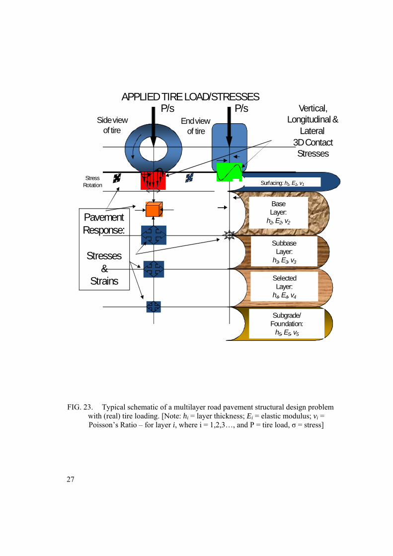
In FIG. 23 a schematic is shown defining a multilayer road pavement structural design

problem with “real” tire loading. The figure is self-explanatory. “Real tire loading” is

defined here as that measured with the SIM system, as opposed to the general civil

engineering assumption of a uniformly distributed vertical loading/stress of circular shape

for the tire loading. This problem was also addressed by the development of the first

worldwide tire/pavement contact-stress model based on artificial neural networks by El-

Gindy and Lewis in 2001 [14], as well as by a study by Fernando et al. in 2006 [15], also

based on SIM tire contact loading/stress measurements. For the present study, pavement

analyses were done using the normal linear elastic multilayer analysis (LEA) approach

24

[18], with measured vertical loading/stress as input, using four different tire models.

Note that since stresses are not required to be continuous in a displacement

assumed finite element analysis (FEA), it is difficult to compute stresses accurately in the

neighborhood of inter-element boundaries in FEA. Also in the case of FEA, the domain

of analysis is finite contrary to the multilayered elastic systems (LEA) which contain a

semi-infinite half space. Although analytical solution of multilayered elastic systems is

also known to lose computational accuracy close to the surface where the load acts, this

research has taken a special care to retain computational accuracy in the vicinity of load

boundaries. Here, double exponential quadrature, discussed by Ooura and Mori in 1991

[25], has been utilized together with Richardson’s extrapolation. Therefore, in this

research, LEA was used in order to accurately determine strain-energy-of-distortion

(SED) in the neighborhood of the tire (contact stress)-pavement interface.

Tire Models Used for Pavement Analyses in this Study

The four tire models used for pavement analyses in this study are:

• Tire Model 1: Assumed vertical loading of 20 kN and uniformly distributed

vertical contact stress of 520 kPa of circular shape (i.e., disk) without restriction

on the diameter of the disk (traditional method)

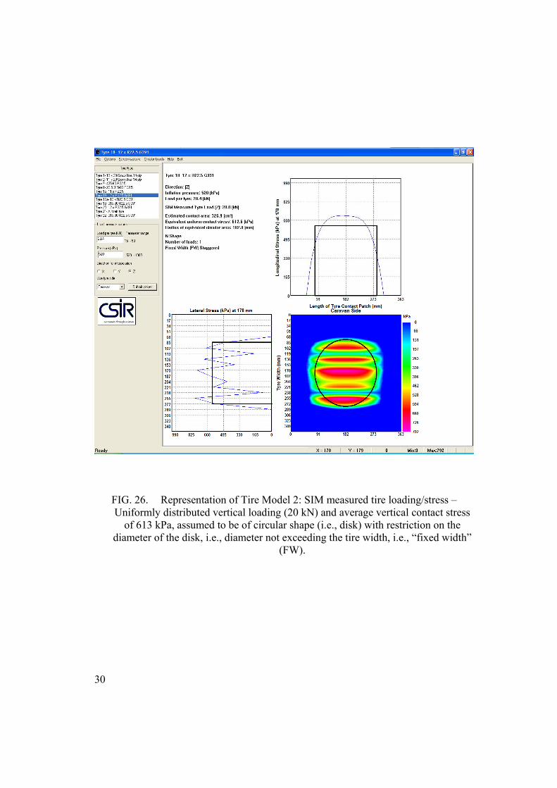
• Tire Model 2: SIM measured tire loading/stress – Uniformly distributed vertical

loading (20 kN) and average vertical contact stress of 613 kPa, assumed to be of

circular shape (i.e., disk) with restriction on the diameter of the disk, i.e., diameter

not exceeding the tire width.

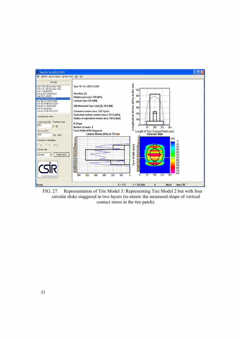
• Tire Model 3: Representing Tire Model 2 but with four circular disks staggered

in two layers (to mimic the measured shape of vertical contact stress in the tire

patch.

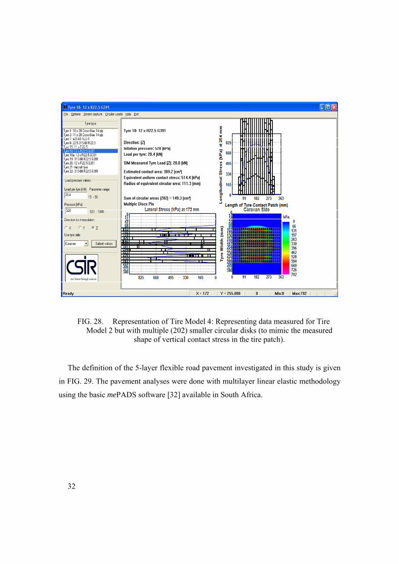
• Tire Model 4: Representing data measured for Tire Model 2 but with multiple

(202) smaller circular disks with a radius of 4.85 mm (to mimic the measured

shape of vertical contact stress in the tire patch).

25

The purpose of the various analyses that follow here is to demonstrate the effect of

different tire models on pavement responses, as obtained from (1) the vertical stress

reaction, and (2) the Strain Energy of Distortion (SED) [26], [33]. The SED discussed in

this paper is according to Timoshenko and Goodier [33], and is defined as the quantity of

strain energy stored per unit volume of the material that can be used as a basis for

determining the limiting stress at which failure occurs. For this, to be applied to isotropic

materials, it is important to separate this energy into two parts; one due to the change in

volume and the other due to the distortion, and consider only the second part in

determining the strength. Whatever the stress system, failure occurs when the strain

energy of distortion reaches a certain limit. Now, total strain energy per unit volume, V0,

can be expressed by using Hooke’s law as follows:

( ) ( ) ( )2222220 2

121

xzyzxyxzzyyxzyx GEEV τττσσσσσσνσσσ +++++−++= ……………(1)

where: iσ and ijτ are normal stress in the i-direction and shear stress on the i-face along

the j-direction, respectively. See also [21].

Whereas the component of strain energy due to distortion (SED), can then be

expressed as follows:

( )20 621

zyxEVSED σσσν

++−

−= ………………………………………………..…(2)

It is the notion in this paper that with this approach, points within the pavement

structural system that have higher values of strain energy of distortion (SED) (so-called

“hot-spots”) will potentially fail first before points with relatively lower values, as was

also indicated by Perdomo and Nokes [24] and De Beer et al [6]. Ideally, this should be

linked with the formation of traffic associated crack formation and potholes, and needs

further research to quantify, possible by way of appropriate empirical transfer functions.

26

Software dubbed “TyreStress” was developed to interpolate and also export the SIM

measured contact load/stress in the format of the above different tire models for the

purpose of pavement analyses (TyreStress is the so-called “delivery system” for tire

contact stress/load for pavement design). The mechanistic-empirical pavement analyses

were done using general (optimized) multilayer linear elastic methodology with the

possibility of multiple circular 3D tire loadings [19], [20], [21]. An example of the

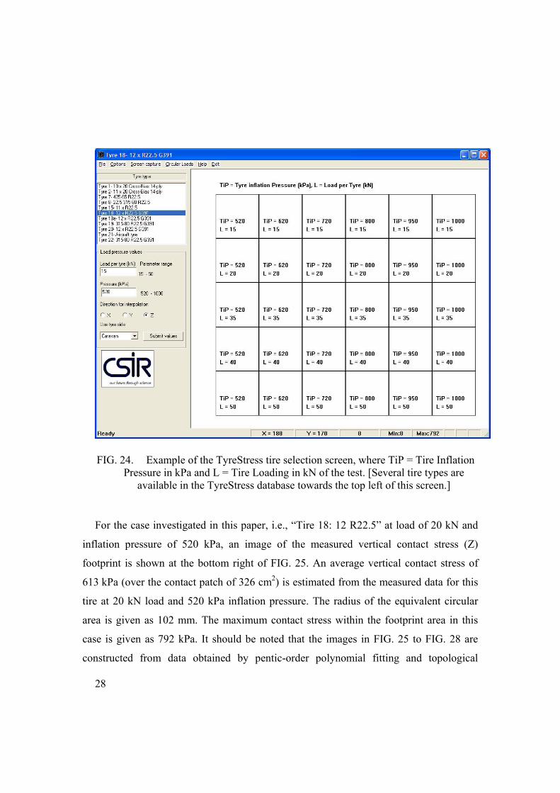
selection screen of TyreStress software is shown in FIG. 24.

27

P/s

Surfacing: h1, E1, v1

SelectedLayer:

h4, E4, v4

BaseLayer:

h2, E2, v2

Subgrade/Foundation:

h5, E5, v5

SubbaseLayer:

h3, E3, v3

APPLIED TIRE LOAD/STRESSESP/s

Pavement Response:

Stresses &

Strains

StressRotation

Vertical,Longitudinal &

Lateral 3D ContactStresses

Side view of tire

End viewof tire

FIG. 23. Typical schematic of a multilayer road pavement structural design problem with (real) tire loading. [Note: hi = layer thickness; Ei = elastic modulus; vi = Poisson’s Ratio – for layer i, where i = 1,2,3…, and P = tire load, σ = stress]

28

FIG. 24. Example of the TyreStress tire selection screen, where TiP = Tire Inflation Pressure in kPa and L = Tire Loading in kN of the test. [Several tire types are

available in the TyreStress database towards the top left of this screen.]

For the case investigated in this paper, i.e., “Tire 18: 12 R22.5” at load of 20 kN and

inflation pressure of 520 kPa, an image of the measured vertical contact stress (Z)

footprint is shown at the bottom right of FIG. 25. An average vertical contact stress of

613 kPa (over the contact patch of 326 cm2) is estimated from the measured data for this

tire at 20 kN load and 520 kPa inflation pressure. The radius of the equivalent circular

area is given as 102 mm. The maximum contact stress within the footprint area in this

case is given as 792 kPa. It should be noted that the images in FIG. 25 to FIG. 28 are

constructed from data obtained by pentic-order polynomial fitting and topological

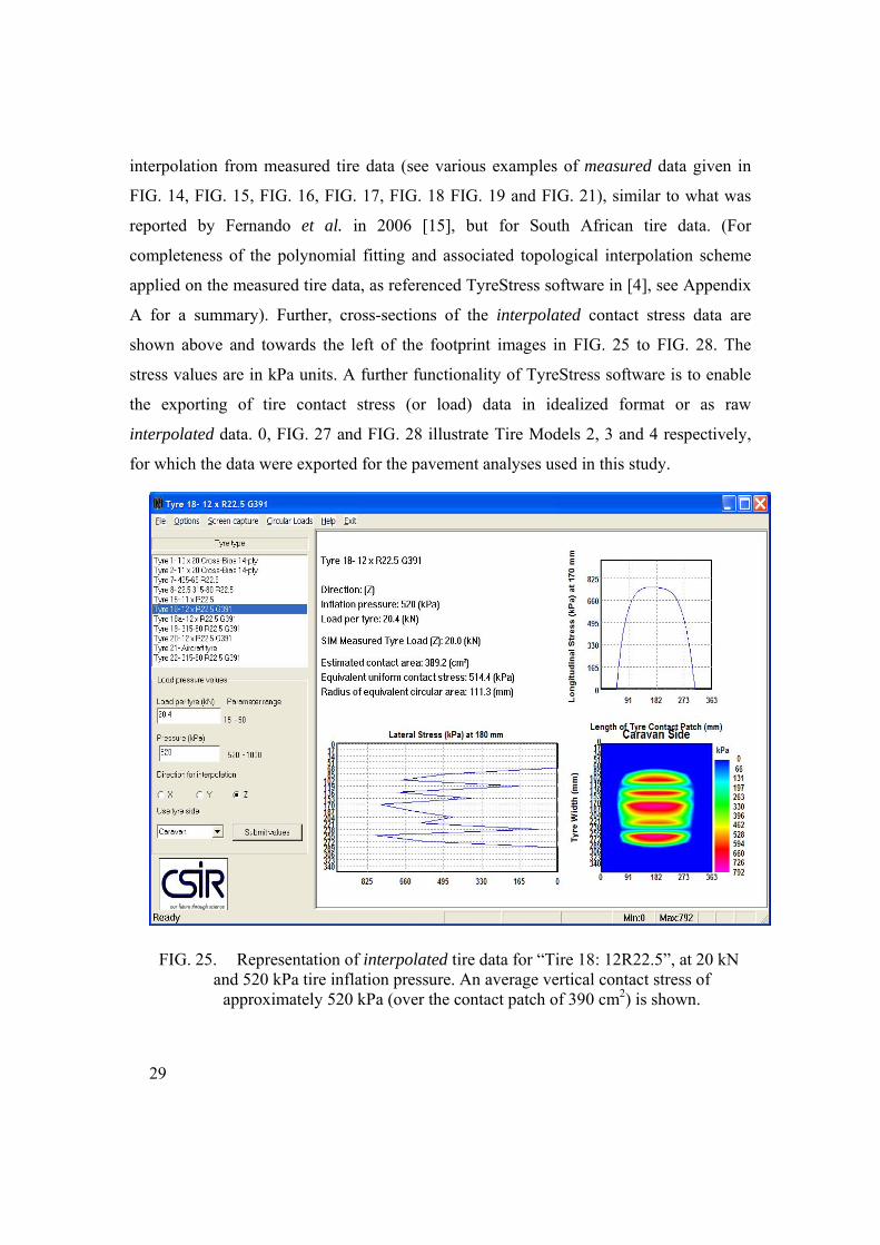
29

interpolation from measured tire data (see various examples of measured data given in

FIG. 14, FIG. 15, FIG. 16, FIG. 17, FIG. 18 FIG. 19 and FIG. 21), similar to what was

reported by Fernando et al. in 2006 [15], but for South African tire data. (For

completeness of the polynomial fitting and associated topological interpolation scheme

applied on the measured tire data, as referenced TyreStress software in [4], see Appendix

A for a summary). Further, cross-sections of the interpolated contact stress data are

shown above and towards the left of the footprint images in FIG. 25 to FIG. 28. The

stress values are in kPa units. A further functionality of TyreStress software is to enable

the exporting of tire contact stress (or load) data in idealized format or as raw

interpolated data. 0, FIG. 27 and FIG. 28 illustrate Tire Models 2, 3 and 4 respectively,

for which the data were exported for the pavement analyses used in this study.

FIG. 25. Representation of interpolated tire data for “Tire 18: 12R22.5”, at 20 kN and 520 kPa tire inflation pressure. An average vertical contact stress of

approximately 520 kPa (over the contact patch of 390 cm2) is shown.

30

FIG. 26. Representation of Tire Model 2: SIM measured tire loading/stress – Uniformly distributed vertical loading (20 kN) and average vertical contact stress

of 613 kPa, assumed to be of circular shape (i.e., disk) with restriction on the diameter of the disk, i.e., diameter not exceeding the tire width, i.e., “fixed width”

(FW).

31

FIG. 27. Representation of Tire Model 3: Representing Tire Model 2 but with four circular disks staggered in two layers (to mimic the measured shape of vertical

contact stress in the tire patch).

32

FIG. 28. Representation of Tire Model 4: Representing data measured for Tire Model 2 but with multiple (202) smaller circular disks (to mimic the measured

shape of vertical contact stress in the tire patch).

The definition of the 5-layer flexible road pavement investigated in this study is given

in FIG. 29. The pavement analyses were done with multilayer linear elastic methodology

using the basic mePADS software [32] available in South Africa.

33

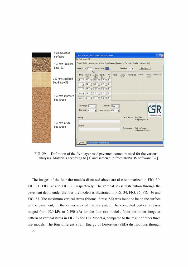
40 mm Asphalt Surfacing

150 mm Granular Base (G2)

150 mm Stabilized Sub‐Base (C4)

150 mm Improved Sub‐Grade

150 mm In‐SituSub‐Grade

FIG. 29. Definition of the five-layer road pavement structure used for the various analyses. Materials according to [3] and screen clip from mePADS software [32].

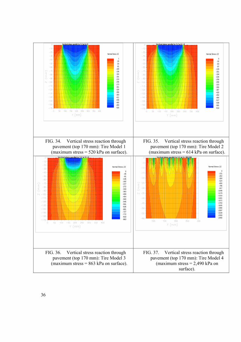
The images of the four tire models discussed above are also summarized in FIG. 30,

FIG. 31, FIG. 32 and FIG. 33, respectively. The vertical stress distribution through the

pavement depth under the four tire models is illustrated in FIG. 34, FIG. 35, FIG. 36 and

FIG. 37. The maximum vertical stress (Normal Stress ZZ) was found to be on the surface

of the pavement, in the center area of the tire patch. The computed vertical stresses

ranged from 520 kPa to 2,490 kPa for the four tire models. Note the rather irregular

pattern of vertical stress in FIG. 37 for Tire Model 4, compared to the result of other three

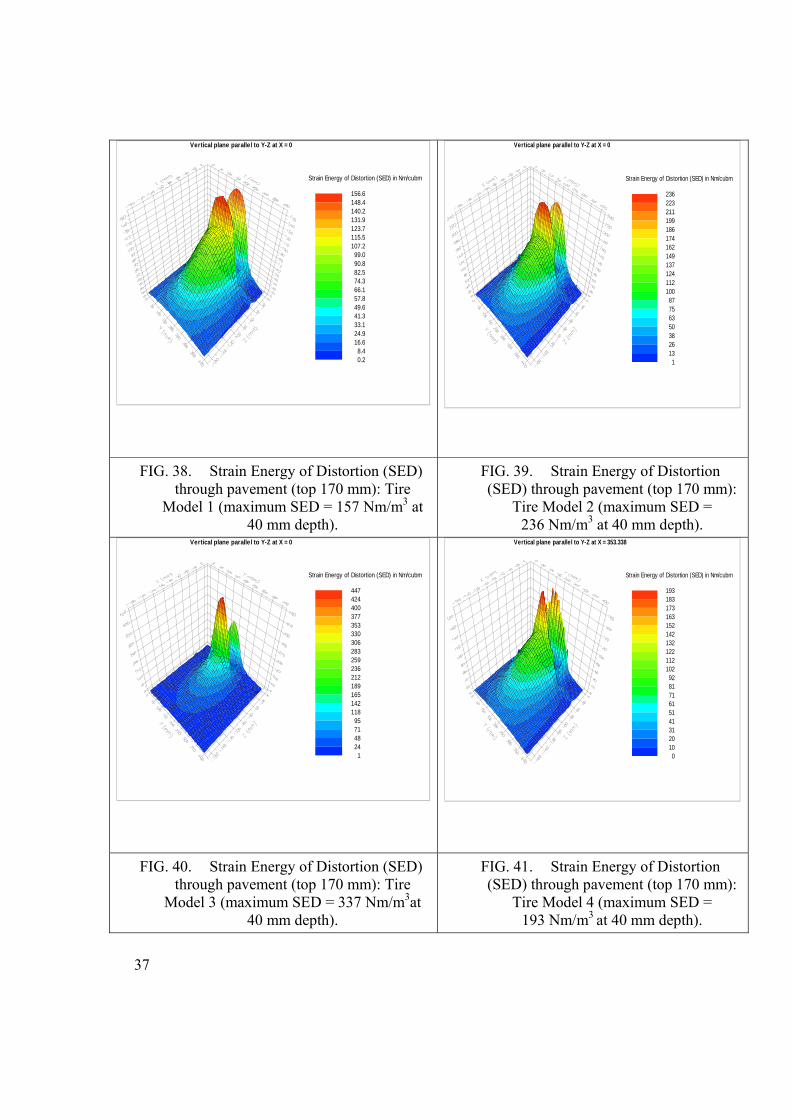
tire models. The four different Strain Energy of Distortion (SED) distributions through

34

the pavement are illustrated in FIG. 38, FIG. 39, FIG. 40 and FIG. 41. These figures

indicated two nominal peak values of SED through the pavement structure, one on the

surface of the 40 mm asphalt layer near the center of the tire patch, and the second at the

bottom of the asphalt layer at a depth of 40 mm, also near the center of the tire patch. The

maximum SED values at the bottom of the 40 mm asphalt layer ranged between 157

Nm/m3 and 337 Nm/m3. The positions of the peak SED values can be interpreted as “hot

spots” for potential road layer failure, as was discussed in by De Beer et al. in 1997 [7].

35

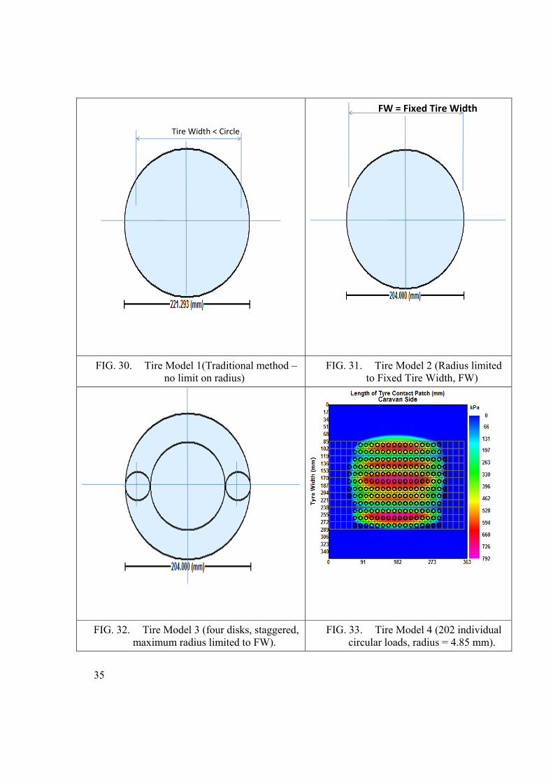
FIG. 30. Tire Model 1(Traditional method – no limit on radius)

FIG. 31. Tire Model 2 (Radius limited to Fixed Tire Width, FW)

FIG. 32. Tire Model 3 (four disks, staggered, maximum radius limited to FW).

FIG. 33. Tire Model 4 (202 individual circular loads, radius = 4.85 mm).

Tire Width < Circle

FW = Fixed Tire Width

36

Vertical plane parallel to Y-Z at X = 0

Normal Stress ZZ

1-26-54-81

-109-136-164-191-219-246-273-301-328-356-383-411-438-465-493-520


Normal Stress ZZ

0-32-64-97

-129-161-194-226-258-290-323-355-387-420-452-484-517-549-581-614

FIG. 34. Vertical stress reaction through pavement (top 170 mm): Tire Model 1

(maximum stress = 520 kPa on surface).


(maximum stress = 614 kPa on surface). Vertical plane parallel to Y-Z at X = 0

Normal Stress ZZ

0-45-91

-136-182-227-272-318-363-409-454-500-545-591-636-681-727-772-818-863

Vertical plane parallel to Y-Z at X = 353.338

Normal Stress ZZ

0-131-262-393-524-655-786-917

-1048-1179-1310-1441-1572-1703-1835-1966-2097-2228-2359-2490




(maximum stress = 2,490 kPa on surface).

37


Strain Energy of Distortion (SED) in Nm/cubm

156.6148.4140.2131.9123.7115.5107.299.090.882.574.366.157.849.641.333.124.916.68.40.2



236223211199186174162149137124112100877563503826131

FIG. 38. Strain Energy of Distortion (SED) through pavement (top 170 mm): Tire

Model 1 (maximum SED = 157 Nm/m3 at 40 mm depth).

FIG. 39. Strain Energy of Distortion (SED) through pavement (top 170 mm):

Tire Model 2 (maximum SED = 236 Nm/m3 at 40 mm depth).



447424400377353330306283259236212189165142118957148241

Vertical plane parallel to Y-Z at X = 353.338


1931831731631521421321221121029281716151413120100


Model 3 (maximum SED = 337 Nm/m3at 40 mm depth).

FIG. 41. Strain Energy of Distortion (SED) through pavement (top 170 mm):

Tire Model 4 (maximum SED = 193 Nm/m3 at 40 mm depth).

38

Discussion of Pavement Response

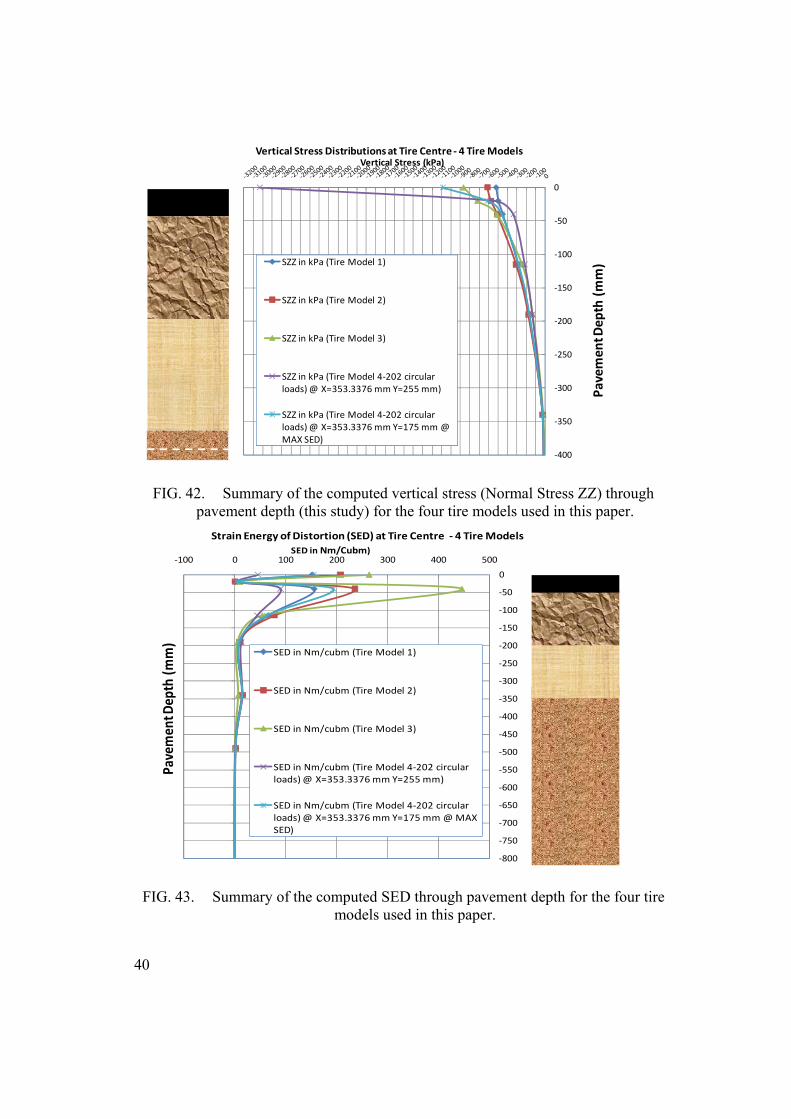
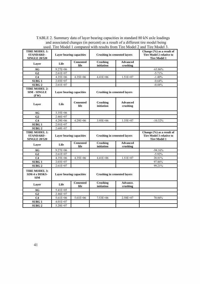
The two selected pavement response parameters, i.e., vertical stress through the

pavement as well as the SED, clearly indicate different maximum peak values, depending

on the tire model used. In this case a surface contact stress difference of up to 4.5 times

was computed between the standard assumption (Tire Model 1) and the case where the

tire was modeled as 202 multiple circular disks (Tire Model 4). Also, a change in SED

was obtained, peaking under Tire Model 3, and then reducing again in the case of Tire

Model 4. These peak SED values occurred both at zero depth (pavement surface) and at

the bottom of the 40 mm thin asphalt surfacing layer, with the maximum always at the

bottom of the asphalt surfacing layer. It is interesting to note that it seems that the SED

peaks at the bottom of this relatively stiffer asphalt layer (modeled with linear elastic

modulus (E1) of 3,000 kPa and Poisson’s Ratio v1 = 0.44). These peaks of SED are

believed to be indicative of the expected potential failure mechanism in this structure

(probably fatigue cracking to be initiated at the bottom of the asphalt layer). This is in

addition to potential rutting from the surface, indicated by the peak SED at z = 0 mm in

the center of the tire contact patch, under the various tire models (see summary of the

pavement response data (i.e., computed vertical stress and SED) shown in FIG. 42 and

FIG. 43). An attempt was also made to compute expected pavement “life” (or bearing

capacity in terms of standard 80 kN axle repetitions) for the pavement and the various tire

models investigated here. For the layer bearing capacities in terms of standard 80 kN

axles, existing fatigue and layer damage models available in the South Africa were used

[31] for the quantitative analyses. The results from Tire Model 1 were compared with

those from Tire Model 2, Tire Model 3 and Tire Model 4 for this purpose (see TABLE 2

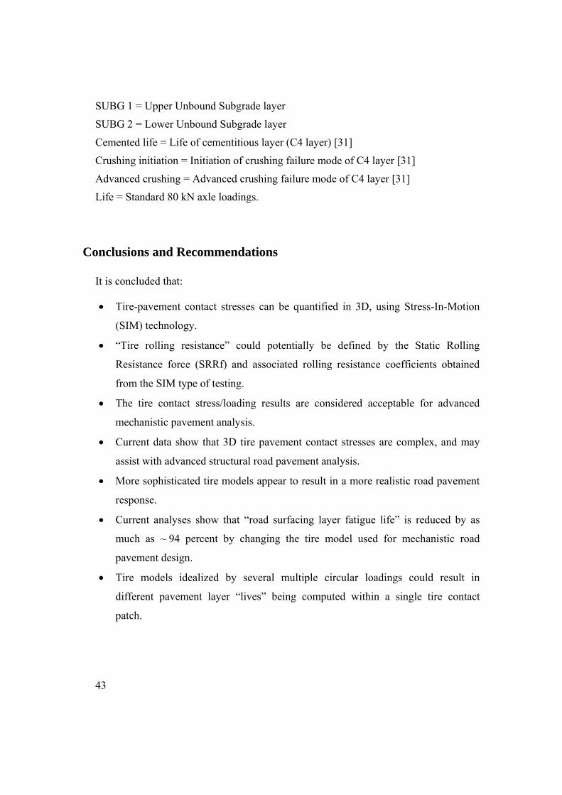
and TABLE 3). TABLE 2 indicates that the layer fatigue life (or bearing capacity) of the

40 mm asphalt layer (AG layer) is reduced by approximately 64 percent. The bearing

capacity of the unbound granular base (G2 layer) is reduced by approximately 6 percent,

and that of the lightly cementitious subbase layer (C4 layer) by 10 percent when the tire

model is changed from the traditional assumption (i.e., Tire Model 1) to Tire Model 2

(i.e., with SIM measured tire data and fixed width (FW) limitation). Similarly, the layer

39

“life” of the asphalt (AG layer) is reduced by approximately 94 percent, and that of the

unbound base (G2 layer) by approximately 6 percent when the results of Tire Model 1 are

compared with those found with Tire Model 3 (see results in TABLE 2). Interestingly,

according to Theyse et al. [31], the “life” or bearing capacity of the lightly cementitious

subbase layer (C4 layer) with regard to both fatigue and crushing failure associated with

these layers improved by approximately 70 percent owing to a slightly reduced vertical

stress on the top of this cementitious subbase (C4 layer). (See TABLE 2 and FIG. 42 at a

depth of 190 mm. TABLE 3 summarizes the effect on layer “life” on the same pavement,

comparing Tire Model 1 with two positions under Tire Model 4 (total of 202 circular

disks of 4.85 mm radius). The two positions (Position 1: X = 353.3376 mm, Y = 255 mm,

and Position 2: X = 353.3376 mm, Y = 175 mm, within Tire Model 4 contact patch – see

FIG. 42, FIG. 43 and TABLE 2) were selected to demonstrate that different pavement

layer “lives” are obtained under a single tire contact patch. The specific data from

TABLE 3 show that at Position 1 the asphalt layer (AG layer) life increased by 170

percent relative to Tire Model 1, and that of the lightly cementitious layer (C4 layer) by

60 percent. On the other hand, at Position 2 a reduction of 61 percent was computed for

the asphalt layer. Relatively minor effects were obtained for the other layers in this

pavement. The layer “life” discussed above is in accordance with layer damage laws for

mechanistic-empirical pavement analyses discussed in [31].

The above results are interpreted (as with the computed vertical stress) to be dictated

by the geometry and characteristics (i.e., tire contact stress patch and its contact shape) of

the tire model used for pavement modeling. The importance, therefore, of using a suitable

(and hopefully a more rational) tire model for pavement design cannot be

overemphasized. More research and analyses are, however, needed to validate the

theoretical behavior discussed here, and the results should be updated on the basis of

future appropriate research on a wider range of tires and road pavement types.

40

‐400

‐350

‐300

‐250

‐200

‐150

‐100

‐50

0

Pavemen

t Dep

th (mm)

Vertical Stress (kPa)Vertical Stress Distributions at Tire Centre ‐ 4 Tire Models

SZZ in kPa (Tire Model 1)



SZZ in kPa (Tire Model 4‐202 circular loads) @ X=353.3376 mm Y=255 mm)

SZZ in kPa (Tire Model 4‐202 circular loads) @ X=353.3376 mm Y=175 mm @ MAX SED)

FIG. 42. Summary of the computed vertical stress (Normal Stress ZZ) through pavement depth (this study) for the four tire models used in this paper.

‐800

‐750

‐700

‐650

‐600

‐550

‐500

‐450

‐400

‐350

‐300

‐250

‐200

‐150

‐100

‐50

0

‐100 0 100 200 300 400 500

Pavemen

t Dep

th (m

m)

SED in Nm/Cubm)

Strain Energy of Distortion (SED) at Tire Centre ‐ 4 Tire Models

SED in Nm/cubm (Tire Model 1)



SED in Nm/cubm (Tire Model 4‐202 circular loads) @ X=353.3376 mm Y=255 mm)

SED in Nm/cubm (Tire Model 4‐202 circular loads) @ X=353.3376 mm Y=175 mm @ MAX SED)

FIG. 43. Summary of the computed SED through pavement depth for the four tire models used in this paper.

41

TABLE 2. Summary data of layer bearing capacities in standard 80 kN axle loadings and associated changes (in percent) as a result of a different tire model being

used. Tire Model 1 compared with results from Tire Model 2 and Tire Model 3. TIRE MODEL 1:

STANDARD - SINGLE 20/520

Layer bearing capacities Crushing in cemented layers Change (%) as a result of Tire Model 2 relative to

Tire Model 1

Layer Life Cemented life

Crushing initiation

Advanced crushing

AG 9.27E+06 -63.86% G2 2.61E+07 -5.71% C4 4.35E+06 4.35E+06 4.41E+06 1.51E+07 -1.40%

SUBG 1 2.03E+07 -0.64% SUBG 2 2.61E+07 -0.44%

TIRE MODEL 2: SIM - SINGLE

(FW) Layer bearing capacities Crushing in cemented layers


Crushing initiation

Advanced crushing

AG 3.35E+06 G2 2.46E+07 C4 4.29E+06 4.29E+06 3.95E+06 1.35E+07 -10.32%

SUBG 1 2.01E+07 SUBG 2 2.60E+07

TIRE MODEL 1: STANDARD -

SINGLE 20/520 Layer bearing capacities Crushing in cemented layers

Change (%) as a result of Tire Model 3 relative to

Tire Model 1


Crushing initiation

Advanced crushing

AG 9.27E+06 -94.16% G2 2.61E+07 -5.92% C4 4.35E+06 4.35E+06 4.41E+06 1.51E+07 28.81%

SUBG 1 2.03E+07 97.86% SUBG 2 2.61E+07 99.21%

TIRE MODEL 3: SIM-4 x DISKS-

SIM Layer bearing capacities Crushing in cemented layers


Crushing initiation

Advance. crushing

AG 5.41E+05 G2 2.46E+07 C4 5.61E+06 5.61E+06 7.53E+06 2.58E+07 70.84%

SUBG 1 4.01E+07 SUBG 2 5.20E+07

42

TABLE 3. Summary data of layer bearing capacities in standard 80 kN axle loadings and associated changes (in percent) as a result of a different tire model being

used. Tire Model 1 compared with results from Tire Model 4 (both Positions 1 and 2 within tire patch)



Change (%) as a result of Tire Model 4 (Position 1) relative to Tire Model 1


Crushing initiation

Advanced crushing

AG 9.27E+06 170.43% G2 2.61E+07 5.44% C4 4.35E+06 4.35E+06 4.41E+06 1.51E+07 4.36%

SUBG 1 2.03E+07 2.73% SUBG 2 2.61E+07 1.57%

TIRE MODEL 4: SIM-ALL PINS

(202) - Position 1* Layer bearing capacities Crushing in cemented layers


Crushing initiation

Advanced crushing

AG 2.51E+07 G2 2.76E+07 C4 4.54E+06 4.54E+06 7.07E+06 2.42E+07 60.51%

SUBG 1 2.08E+07 SUBG 2 2.65E+07



Change (%) as a result of Tire Model 4 (Position 2) relative to Tire Model 1


Crushing initiation

Advanced crushing

AG 9.27E+06 -60.78% G2 2.61E+07 0.59% C4 4.35E+06 4.35E+06 4.41E+06 1.51E+07 0.48%

SUBG 1 2.03E+07 0.14% SUBG 2 2.61E+07 0.02%

TIRE MODEL 4: SIM-ALL PINS

(202) - Position 2* Layer bearing capacities Crushing in cemented layers


Crushing initiation

Advanced crushing

AG 3.63E+06 G2 2.63E+07 C4 4.37E+06 4.37E+06 4.62E+06 1.58E+07 4.76%

SUBG 1 2.03E+07 SUBG 2 2.61E+07

* Position 1 X=353.3376 mm Y=255 mm * Position 2 X=353.3376 mm Y=175 mm

Key:

AG = Asphalt surfacing layer, 40 mm thick

G2 = Unbound Granular Layer, 150 mm thick

C4 = Lightly Cemented Layer, 150 mm thick

43

SUBG 1 = Upper Unbound Subgrade layer

SUBG 2 = Lower Unbound Subgrade layer

Cemented life = Life of cementitious layer (C4 layer) [31]

Crushing initiation = Initiation of crushing failure mode of C4 layer [31]

Advanced crushing = Advanced crushing failure mode of C4 layer [31]

Life = Standard 80 kN axle loadings.

Conclusions and Recommendations

It is concluded that:

• Tire-pavement contact stresses can be quantified in 3D, using Stress-In-Motion

(SIM) technology.

• “Tire rolling resistance” could potentially be defined by the Static Rolling

Resistance force (SRRf) and associated rolling resistance coefficients obtained

from the SIM type of testing.

• The tire contact stress/loading results are considered acceptable for advanced

mechanistic pavement analysis.

• Current data show that 3D tire pavement contact stresses are complex, and may

assist with advanced structural road pavement analysis.

• More sophisticated tire models appear to result in a more realistic road pavement

response.

• Current analyses show that “road surfacing layer fatigue life” is reduced by as

much as ~ 94 percent by changing the tire model used for mechanistic road

pavement design.

• Tire models idealized by several multiple circular loadings could result in

different pavement layer “lives” being computed within a single tire contact

patch.

44

It is therefore postulated that “The better the representation of the “real/actual tire-

contact stress” regime, the better the road response and hence the design of road

pavements – especially near the road surface”. It is believed that an improved

understanding of the surface pavement failure mechanisms illustrated in this paper will be

possible with the incorporation of improved understanding and quantification of the tire-

road interaction mechanisms at the near road surface.

It is recommended that 3D tire road pavement contact stresses be quantified on a wider

range of tires, and their effect be incorporated into modern-day road pavement analyses.

Ideally, 3D tire pavement contact stresses should be used for the mechanistic-empirical

design of road pavement structures, as measured, with minimal idealization of shape and

magnitude.

Acknowledgements

The Executive Director of CSIR Built Environment is thanked for permission to

publish this paper.

References

[1] Bonse, R. P. H., Kuhn, S. H., Dynamic forces exerted by Moving Vehicles

on a Road Surface. Highway Research Board Bulletin, No. 233: Flexible

Pavement Design, 1959, pp. 9–32.

[2] Committee of State Road Authorities (CSRA), Structural Design of

Flexible Pavements for Interurban and Rural Roads. Technical

Recommendations for Highways No. 4 (Draft TRH 4), 1996. ISBN 1-

86844-218-7.

[3] Committee of State Road Authorities (CSRA), Guidelines for Road

Construction Materials. Technical Recommendations for Highways No. 14

(Draft TRH 14). 1985, 1996. ISBN 0-7988-3311-4.

45

[4] De Beer M., Fisher C., Van Rensburg Y., Greben J., Maina J. W.,

Framework for Tyre Contact Stress Information System (T-CSIS): Project

A-1. Report: SANRAL/SAPDM/A-1/2010-003, Revision of the South

African Pavement Design Method. Project Focus Area: Traffic Demand

Analysis, Version: 3rd Draft Report (Unpublished), March 2011.

[5] De Beer, M., Measurement of tyre/pavement interface stresses under

moving wheel loads. Proceedings of the Vehicle-Road and Vehicle-Bridge

Interaction Conference, June 5–10, 1994, Noordwijkerhout, The

Netherlands (DPVT 224), or Heavy Vehicles Systems, Special Series, Int.

J. Vehicle Design, Vol. 3, Nos 1–4, 1996, pp. 97–115. ISSN 01433369.

[6] De Beer M, and Fisher C., Contact Stresses of pneumatic tires measured

with the Vehicle-Road Surface Pressure Transducer Array (VRSPTA)

system for the University of California at Berkeley (UCB) and the Nevada

Automotive Test Center (NATC). Confidential Contract Research Report

CR-97/053, Volume 1 and Volume 2, June 1997.

[7] De Beer, M., Fisher, C., Jooste, F. J., Determination of pneumatic

tyre/pavement interface contact stresses under moving loads and some

effects on pavements with thin asphalt surfacing layers. Proceedings of the

8th International Conference on Asphalt Pavements (ICAP ‘97), Seattle,

Washington, August 10–14, 1997.

[8] De Beer M., Kannemeyer, L., Fisher, C., Towards improved mechanistic

design of thin asphalt layer surfacings based on actual tyre/pavement

contact Stress-In-Motion (SIM) data in South Africa. Proceedings of the

7th Conference on Asphalt Pavements for Southern Africa (CAPSA ’99),

Theme 5: Innovation in Asphalt Design, Victoria Falls, Zimbabwe, August

29 to September 2, 1999. ISBN 1874968268 (CD).

[9] De Beer, M., Fisher, C., Jooste, F. J., Evaluation of non-uniform tyre

contact stresses on thin asphalt pavements, Proceedings of the 9th

International Conference on Asphalt Pavements (ICAP 2002), Copenhagen,

46

2002. (Proceedings available on CD from conference organizers: The

Danish Road Directorate, Ministry of Transport, Denmark, and the

International Society of Asphalt Pavements (ISAP).

[10] De Beer, M., Fisher. C., Kannemeyer, L., Tyre-pavement interface contact

stresses on flexible pavements - quo vadis? Proceedings of the 8th

Conference on Asphalt Pavements for Southern Africa (Roads – The

Arteries of Africa), Sun City, North West Province, South Africa, 2004.

[11] De Beer, M., Fisher, C., Kannemeyer, L., Towards the application of

Stress-In-Motion (SIM). Results in pavement design and infrastructure

protection, Proceedings of the 8th International Symposium on Heavy

Vehicles, Weights and Dimensions (Loads, Roads and the Information

Highway), Misty Hills Conference Center, Muldersdrift, Gauteng, South

Africa, 2004.

[12] De Beer, M., Reconsideration of tyre-pavement input parameters for the

structural design of flexible pavements, Proceedings of the 10th

International Conference on Asphalt Pavements (10th ICAP), Quebec City,

Canada, 2006. ISBN: 978-2-550-49009-8 (CD); ISBN: 978-2-550-49008-1

(Printed).

[13] De Beer, M., Stress-In-Motion (SIM) – A new tool for road infrastructure

protection? Proceedings of the International Conference on Heavy Vehicles

(HV Paris 2008 – ICWIM5), WIM Session 7, May 19–22, 2008,

Paris/Marne-la-Vallée, France.

[14] El-Gindy, M., Lewis, H., Development of a Tire/Pavement Contact-Stress

Model Based on Artificial Neural Networks. Publication No. FHWA-RD-

99-041, January, FHWA, Research, Development, and Technology,

Turner-Fairbank Highway Research Center, McLean, VA, USA, 2001.

[15] Fernando, E. G., Musani, D., Park, D-W., Liu, W., Evaluation of effects of

tire size and inflation pressure on tire contact stresses and pavement

response, Report FHWA/TX-06/0-4361-1, August, Texas Transportation

47

Institute, The Texas A&M University System, College Station, Texas,

USA, 2006. See Pavement Responses to Loading Last visited on June 18,

2010 – URL: http://tti.tamu.edu/documents/0-4361-1.pdf. Date assessed

March 19, 2012.

[16] Freeme, C. R., De Beer, M., Viljoen, A. W., The behaviour and

mechanistic design of asphalt pavements. Proceedings of the 6th

International Conference on Structural Design of Asphalt Pavements, July

13–17, 1987, Ann Arbor, Michigan, USA, pp. 333–343.

[17] Gillespie, T. D., Fundamentals of Vehicle Dynamics. Society of

Automotive Engineers, Inc., Warrendale, PA, USA, 1992.

[18] Huang, Y. H., Pavement Analysis and Design, Prentice-Hall International,

Englewood Cliffs, NJ, USA, 1993. ISBN 0-13-655275-7.

[19] Maina, J. W., Matsui, K., Developing software for elastic analysis of

pavement structure responses to vertical and horizontal surface loadings,

Transportation Research Record, No. 1896, 2004, pp. 107–118.

[20] Maina, J. W., Denneman, E., De Beer, M., Introduction of new road

pavement response modelling software by means of benchmarking,

Proceedings of the 27th Annual Southern African Transport Conference,

South Africa, July 7–11, 2008. ISBN: 978-1-920017-34-7.

[21] Maina, J. W., De Beer, M., Improved performance evaluation of road

pavements by using measured tyre loading. Proceedings of the 2nd CSIR

Biennial Conference (Science Real and Relevant), November 17–18, 2008,

CSIR International Convention Centre, Pretoria, South Africa, p 13. ISBN:

978-1-920017-34-7.

[22] Myers, L. A., Roque, R., Ruth, B. E., Drakos, C., Measurement of contact

stresses for different truck tire types to evaluate their influence on near-

surface cracking and rutting, Transportation Research Record, No. 1655,

1999, pp 175–184.

48

[23] Myers, L. A., Roque, R., Birgisson, B., Propagation mechanisms for

surface-induced longitudinal wheel path cracks. Transportation Research

Record, No. 1778, 2001, pp 113–122.

[24] Novak, M., Birgisson, B., Roque, R., Three-dimensional finite element

analysis of measured tire contact stresses and their effects on instability

rutting of asphalt mixture pavements, Proceedings of the 82nd

Transportation Research Board Annual Meeting, Washington D.C., MD,

USA, January 12–16, 2003.

[25] Ooura,T. and Mori, M. “The Double Exponential Formula for Oscillatory

Functions over Half Infinity Integral”, Journal of Computational and

Applied Mathematics 38, 1991, pp.353-360.

[26] Perdomo, D., Nokes, B., Theoretical analysis of the effects of wide-base

tires on flexible pavements. In: Rigid and Flexible Pavement Design and

Rehabilitation (Pavement Design, Management, and Performance),

Transportation Research Record, No. 1388, 1993, pp. 60–69.

[27] Priest A. L., Timm, D. H., Mechanistic comparison of wide-base single

versus standard dual tire configurations. In: Pavement Rehabilitation,

Strength and Deformation Characteristics, and Surface Properties-Vehicle

Interaction, Transportation Research Record, No. 1949, 2006, pp 155–163.

[28] Roque, R., Myers, L. A., Ruth, B. E., Loading characteristics of modern

truck tires and their effects on surface cracking of asphalt pavements,

Proceedings of the 5th International Conference on the Bearing Capacity of

Roads and Airfields (BCRA ’98), July 6–8, Trondheim, Norway, Vol. 1,

1998, pp. 93–102.

[29] Roque R., Myers, L. A., Birgisson, B., Evaluation of measured tire contact

stress for the prediction of pavement response and performance.

Transportation Research Record, No. 1716, 2000, pp 73–81.

49

[30] Soon, S., Drescher, A., Stolarsky, H. K., Tire-induced surface stresses in

flexible pavements. Proceedings of the 82nd Transportation Research

Board Annual Meeting, Washington DC, MD, USA, January 12–16, 2003.

[31] Theyse, H. L., De Beer, M., Rust, F. C., Overview of the South African

Mechanistic Pavement Design Analysis Method. Proceedings of the 75th

Annual Transportation Research Board Meeting, January 7–11,

Washington, D.C., MD, USA, TRR 1539, 1996, pp. 6–17. ISBN

0309059127.

[32] Theyse, H. L., Muthen, M., Pavement Analysis And Design Software

(Pads) based on the South African Mechanistic-Empirical Design Method,

Proceedings of the 19th Annual South African Transport Conference

(SATC 2000), July, 2000, Pretoria, South Africa.

[33] Timoshenko, S., Goodier, J. N. Theory of Elasticity, 2nd Ed., New York,

McGraw-Hill, Inc., 1951.

[34] Van Vuuren, D. J., Tyre pressure and its effects on pavement design and

performance. National Institute for Road Research, Council for Scientific

and Industrial Research, Report RR 192, Pretoria, South Africa, 1974.

[35] Yoder, E. J., Witczack, K. M. W., Principles of Pavement Design, 2nd

Ed., New York, Wiley-Interscience, 1975. ISBN 0-471-97780-2.

[36] http://www.csir.co.za/Built_environment/brochures.html. Date assessed

March 19, 2012.

50

APPENDIX A

Polynomial fitting and data interpolation methodology for tire contact

stress/force measurements from SIM system

Topological interpolation in the TyreStress program

The TyreStress equipment gives data on the z , x or y – load (or stress if divided by area) for a

range of values of the tyre inflation pressure P and applied tyre loading L . Here z refers to the

downward pressure (so this load is always positive if z points downward), y refers to the lateral

movement (across the width of the tyre), and x refers to the longitudinal load in the direction of

the tyre. The measurements are done through an array of instrumented pins (or sensors) that are

arranged on a horizontal line in the lateral direction (perpendicular to the direction of the tyre).

When the tyre moves, different parts of the tyre touch the array of instrumented pins, or sensors

(the lateral position characterized by the variableλ ), and the position of the tyre is translated into

a longitudinal position via the linear relationship vt=ξ , where ( )xvv v= is the speed along the

positive x -axis. Measurements are done for different values of P and L and each ( )LP, pair

leads to a different load pattern in a different tyre domain (λ ,ξ ) where the loads are non-zero.

The set of measurements then leads to a grid of measured values. The TyreStress software was

developed for ease of tire stress/load data viewing and data exporting.

Since the user of the TyreStress software is generally interested in values other than the measured

( )LP, pairs, an interpolation scheme is developed to provide intermediate results. Since the tyre

domain (λ ,ξ ) changes its boundaries from one ( )LP, pair to another, the interpolation routine

has to recognize these topological properties and therefore interpolation is not straightforward. To

accommodate the changing boundaries, a topological interpolation routine is developed which

recognizes the boundaries and determines an appropriate set of loads corresponding to a desired

( )LP, set. Part of this interpolation procedure involves the definition of filters to decide which

small measured values represent noise and which ones are small but real.

The notation is defined first. The measured yx, and z loads are indicated by:

51

}1,,{ Nixii L=ξ , }1,,{ Niyii L=ξ and }1,,{ Nizii L=ξ (A1)

where the index i runs over the number of measurements per tyre, i.e., over different values of

vtii =ξ . Every pin (indicated by }1,{ λλλ Nii L=∈ ) has its own record. The surface of the

tire is mapped via the variables ( )λξ , . Measurements are made for a range of

}1,{ Pi NiPP L=∈ , and }1,{ Li NiLL L=∈ values. The idea is to provide interpolation

between these ( )ji LP , pairs. In the graphs of the TyreStress system the loads are shown in the

( )λξ , plane, by means of 3D plots. The topology of the tire implies that measurements in the

( )λξ , plane are correlated as they refer to the same physical object (the surface of the tire). This

translates into the demand for continuity of the loads/stresses in terms of these variables.

In practise, it is more important to enforce the continuity in ξ as there are lots of measurements

so that the results need to be smoothed to get a continuous representation. There are only 21 pins,

so at most there can be 21 significant λ measurements and these can best be treated as discrete

cases. If a polynomial is interpolated between too few points, one may get low-frequency

oscillations between the points, which is not desirable. Hence, λ is treated as another parameter,

which can be included in the ( )LP, set. This simplifies the interpolation procedure considerably

as one now only has continuity constraints in one variable. The measurements are now fitted as a

function of ξ with a polynomial of degree M (it is suggested that 7=M be used). Consider,

for example, the z load/stress:

}1,,{ Nizii L=ξ (A2)

Before one can fit a polynomial one has to identify the area where the values are non-zero, since

the inclusion of zeroes in the construction of the polynomial would invalidate the result. One

determines the first value of iξ where iz is larger than a cut-off value zε , and is not

immediately followed by a value lower than zε in the next two measurements. Formally, this

prescription can be defined as follows:

{ }NjzzzjN zjzjzj L1,,,min 21min =>>>= ++ εεε (A3)

{ }NjzzzjN zjzjzj L1;,,max 21max =>>>= −− εεε (A4)

52

with boundaries: minmin Nξξ = and

maxmax Nξξ = . The cut-off zε can be chosen to be a weighted

means of the measurement error and the maximum measurement value. The set of

1minmax +− NN pairs is now defined:

};,{ maxmin NNizii L=ξ (A5)

and fits a polynomial zF ≈)(ξ :

11;)( minmax10 +≥+−+++= MNNaaaF MMξξξ L (A6)

where the degree M must be smaller than the number of non-trivial measurements points -1. Fits

of datasets that have fewer than eight significant points if 7=M have to be disallowed. The

values of minξ and maxξ can be refined once one has constructed this polynomial by redefining

them as the values of ξ where the polynomial passes through zero. Due to the filtering

procedure, one normally should have minmin Nξξ < and

maxmax Nξξ > . However, in those cases

where a measurement point lies outside of this interval, it should be eliminated from the fitting

procedure. The ideal degree of the polynomial is about 7=M : low enough for it not to lead to

unphysical oscillations (overfitting) and high enough for it to be able to capture sufficient detail

in the tire profile. The parameters ia are fixed by an 2χ fitting procedure. Since this requires

sums over powers of ξ (up to a power of M2 ), it might be wise to renormalize the values to

avoid excessively large or small numbers. This problem also forewarns that polynomials of

higher degree ( 7>M ) may lead to numerical instabilities in the determination of the parameters

ia .

These polynomials are now interpolated between different sets of triplets ( )kji LP λ,, . One

problem is that in the lateral direction λ there will also be an upper and lower boundary beyond

which the values vanish. In the current representation this will mean that for those values of λ all

coefficients ia will be zero, and minξ and maxξ are thus undetermined. The coefficients ia

between different triplets ( )kji LP λ,, can now be interpolated. This would yield a complete

representation of the full polynomial in the ξ direction. However, there are various problems

with this method. By interpolating the values of the parameters ia one does not constrain oneself

to the ranges [ ]maxmin ,ξξ as the boundaries are imposed externally and are not implicit in the

53

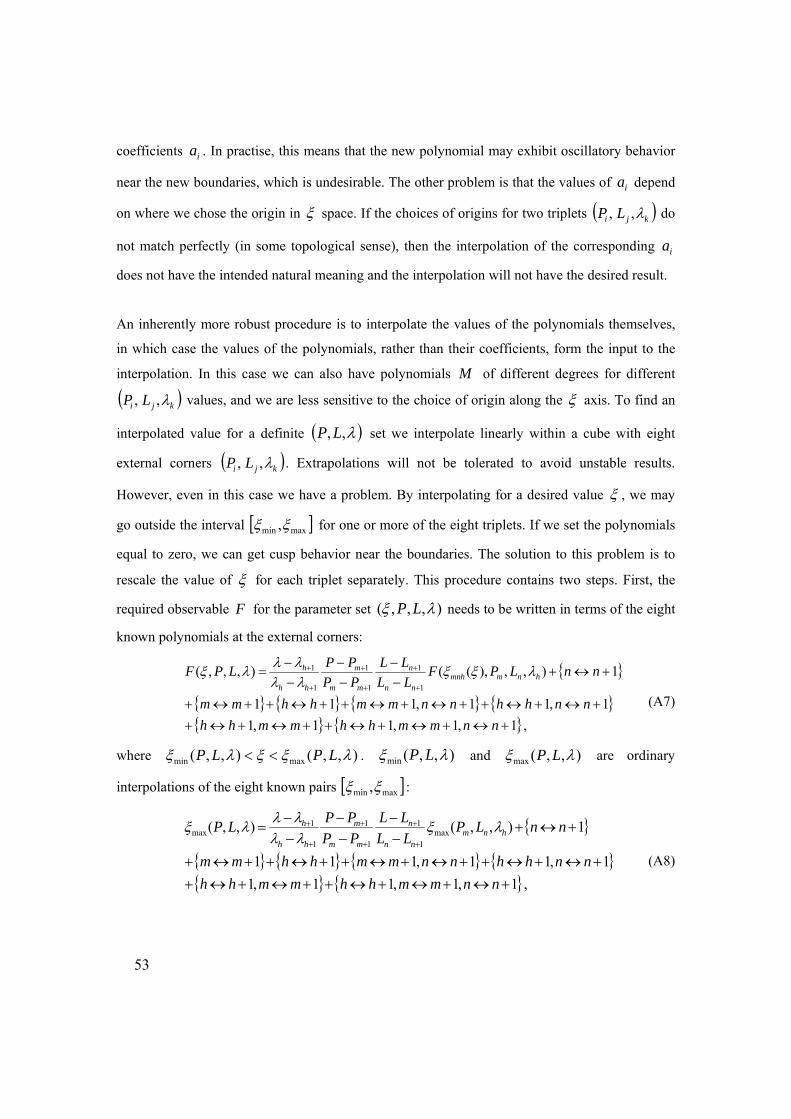
coefficients ia . In practise, this means that the new polynomial may exhibit oscillatory behavior

near the new boundaries, which is undesirable. The other problem is that the values of ia depend

on where we chose the origin in ξ space. If the choices of origins for two triplets ( )kji LP λ,, do

not match perfectly (in some topological sense), then the interpolation of the corresponding ia

does not have the intended natural meaning and the interpolation will not have the desired result.

An inherently more robust procedure is to interpolate the values of the polynomials themselves,

in which case the values of the polynomials, rather than their coefficients, form the input to the

interpolation. In this case we can also have polynomials M of different degrees for different

( )kji LP λ,, values, and we are less sensitive to the choice of origin along the ξ axis. To find an

interpolated value for a definite ( )λ,, LP set we interpolate linearly within a cube with eight

external corners ( )kji LP λ,, . Extrapolations will not be tolerated to avoid unstable results.

However, even in this case we have a problem. By interpolating for a desired value ξ , we may

go outside the interval [ ]maxmin ,ξξ for one or more of the eight triplets. If we set the polynomials

equal to zero, we can get cusp behavior near the boundaries. The solution to this problem is to

rescale the value of ξ for each triplet separately. This procedure contains two steps. First, the

required observable F for the parameter set ),,,( λξ LP needs to be written in terms of the eight

known polynomials at the external corners:

{ }

{ } { } { } { }{ } { },1,1,11,1

1,11,111

1),,),((),,,(1

1

1

1

1

1

+↔+↔+↔++↔+↔++↔+↔++↔+↔++↔++↔+

+↔+−−

−−

−−

=+

+

+

+

+

+

nnmmhhmmhhnnhhnnmmhhmm

nnLPFLLLL

PPPPLPF hnmmnh

nn

n

mm

m

hh

h λξξλλλλλξ

(A7)

where ),,(),,( maxmin λξξλξ LPLP << . ),,(min λξ LP and ),,(max λξ LP are ordinary

interpolations of the eight known pairs [ ]maxmin ,ξξ :

{ }

{ } { } { } { }{ } { },1,1,11,1

1,11,111

1),,(),,( max1

1

1

1

1

1max

+↔+↔+↔++↔+↔++↔+↔++↔+↔++↔++↔+

+↔+−−

−−

−−

=+

+

+

+

+

+

nnmmhhmmhhnnhhnnmmhhmm

nnLPLLLL

PPPPLP hnm

nn

n

mm

m

hh

h λξλλλλλξ

(A8)

54

and a similar expression for ),,(min λξ LP . The polynomials for discrete values of ( )hnm LP λ,,

were already defined before and were expressed in terms of the coefficients ia . Eq. (A7) would

be an ordinary interpolation between eight polynomials if ξξξ =)(mnh for each triplet ( )hnm ,, .

However, it should be ensured that )(ξξmnh lies in the relevant interval for the case ( )hnm ,, . To

accomplish this, )(ξξmnh is expressed in terms of the relevant boundaries:

{ } { }),,(),,(

),,(),,(),,(),,()(minmax

maxminminmax

λξλξξλξλξλξξλξξξ

LPLPLPLPLPLP hnmhnm

mnh −−+−

= (A9)

This definition is invariant for a shift in origin of the ξ -axis, even if this applies only to the case

),,( hnm LP λ . This shows that the rescaling procedure generates the desired symmetry and

invariances and embodies a robust procedure. Because of its internal interpolation )(,, ξξ hnm ,

which recognizes the boundaries of each tire examined, one can denote this procedure by the term

“topological interpolation”. In practise, this also appears to be a very robust formula which

minimizes the cut-off and cusps which can easily arise near the boundaries of the interpolation

region.

Instead of the polynomial fit to the individual cases, one could also have used cubic spline fitting.

With the new topological interpolation, which does not require an explicit polynomial fit, but just

a functional representation of intermediate values, this fitting procedure also becomes feasible.

Since satisfactory results are obtained with the current polynomial procedure, the spline option

was not further investigated. The presence of higher-order discontinuities in the cubic splines at

the matching points may represent a disadvantage of the spline option, but this property could

become an advantage if the splines can account for sudden changes in tire profiles that one wants

to reproduce. On the other hand, the freedom in splines may make it more difficult to fix the

external boundaries of the interval. Since the boundaries play a crucial role in the interpolation

routine, this property may represent a serious defect of spline fitting in this context. High-order

polynomials could be used to represent more details of the tire structure, but if the order of the

polynomial becomes too high, the fitting suffers from potential overfitting and unphysical high-

frequency oscillations result in the model representation. A more detailed explanation of the

above interpolation is given in the report by De Beer et al. (2011) [4].

55

List of table titles

TABLE 1. Quasi-Static Rolling Resistance coefficient (fx)

TABLE 2. Summary data of layer bearing capacities in standard 80 kN axle loadings

and associated changes (in percent) as a result of a different tire model being used.

Tire Model 1 compared with results from Tire Model 2 and Tire Model 3.

TABLE 3. Summary data of layer bearing capacities in standard 80 kN axle loadings

and associated changes (in percent) as a result of a different tire model being used.

Tire Model 1 compared with results from Tire Model 4 (both Positions 1 and 2

within tire patch)

List of figure captions

FIG. 1. Aerial view of a high-quality thinly surfaced divided freeway near Pretoria,

South Africa.

FIG. 2. Plastic deformation (or rutting/shoving) within the thin asphalt surfacing

layer. Note the six lanes of rutting (left and right sides) owing to tire loading

combined with poor asphalt mix.

FIG. 3. Horizontal plastic deformation (or rutting/shoving) within the thin asphalt

surfacing layer at an intersection. Note the planar backwards deformation depicted

by the white lane marking owing to the tractive acceleration forces of tires towards

the right of the picture.

FIG. 4. Fatigue (alligator) cracking of a old and brittle thin surface seal. Note fatigue

cracking with some signs of white coloring (pumping of fines) in insert.

FIG. 5. Delamination of the asphalt surfacing layer from the lower layer.

FIG. 6. Surface disintegration in the asphalt surface seal of a low-volume road.

FIG. 7. Typical pothole with water in a thinly surfaced road.

FIG. 8. Standing water on pavement with wheel path rutting causing a safety

(hydroplaning) hazard.

56

FIG. 9. “Wiggling yellow line” owing to shear failure in a substandard (or wet)

granular base layer.

FIG. 10. Distribution of tire inflation pressure of heavy vehicles in South Africa since

1974. For details in legend see [4].

FIG. 11. Tire inflation pressure differences between the steering and trailing tires of a

selected group of heavy vehicles in South Africa in 2003 (from [12]).

FIG. 12. Flat bed Stress-In-Motion (SIM) device with Society of Automotive

Engineering (SAE) coordinate system used in this study for the measurements of 3D

tire contact force (or stress) conditions inside the tire contact patch of a slow-rolling

pneumatic tire (fitted on the Heavy Vehicle Simulator – HVS).

FIG. 13. Dual SIM device under tire loading using the Heavy Vehicle Simulator

(HVS).

FIG. 14. Typical vertical (Z) contact stress pattern of a 11xR22.5 dual tire

configuration with total tire load of 40 kN, and 520 kPa inflation pressure. Note that

a maximum contact stress of approx. 849 kPa was measured on the edge of the left

tire in this illustration.

FIG. 15. Typical lateral (+/- Y) contact stress pattern of a 11xR22.5 dual tire


a maximum contact stress of approx. 187 kPa was measured on the edge of the right

tire in this illustration.

FIG. 16. Typical longitudinal (+/- X) contact stress pattern of a 11xR22.5 dual tire


a maximum contact stress of approx. 129 kPa was measured on the fore end of the

left tire in this illustration.

FIG. 17. Heavy Vehicle Simulator (HVS) tire loading of 40 kN, and inflation pressure

of 800 kPa (with typical “n-shape” vertical stress distribution), resulting in typical

“n-shape” plastic deformation in a thin asphalt surfacing layer – only one HVS tire

traffic lane is shown here [21]

57

FIG. 18. Heavy Vehicle Simulator (HVS) tire (over) loading of 80 kN, and inflation

pressure of 420 kPa (with typical “m-shape” vertical stress distribution), resulting in

typical “m-shape” plastic deformation in a thin asphalt surfacing layer – only one

tire HVS traffic lane is shown here [21]

FIG. 19. Typical tire “fingerprint” of the vertical contact stress variation with tire

loading (vertical scale from 15 to 50 kN) and with variation in tire inflation pressure

(horizontal axis from 520 kPa to 800 kPa). Tire type 11xR22.5 with tread.

FIG. 20. Typical field configuration during a special test series with a quad SIM

system conducted in 2003 in South Africa at the Heidelberg Traffic Control Center.

FIG. 21. Typical vertical contact stress footprint of a 7-axle heavy vehicle (22 tires)

captured with the SIM system in 2003. Note the poor vehicle maintenance visible

from the tire footprints.

FIG. 22. “Quasi-static” rolling resistance force (SRRf) data on a textured measuring

surface (SIM) for three tire inflation pressure cases of a 315/80 R22.5 tire at

different vertical tire loading (Fz) levels.

FIG. 23. Typical schematic of a multilayer road pavement structural design problem

with (real) tire loading. [Note: hi = layer thickness; Ei = elastic modulus; vi =

Poisson’s Ratio – for layer i, where i = 1,2,3…, and P = tire load, σ = stress]

FIG. 24. Example of the TyreStress tire selection screen, where TiP = Tire Inflation

Pressure in kPa and L = Tire Loading in kN of the test. [Several tire types are

available in the TyreStress database towards the top left of this screen.]

FIG. 25. Representation of interpolated tire data for “Tire 18: 12R22.5”, at 20 kN and

520 kPa tire inflation pressure. An average vertical contact stress of approximately

520 kPa (over the contact patch of 390 cm2) is shown.

FIG. 26. Representation of Tire Model 2: SIM measured tire loading/stress –

Uniformly distributed vertical loading (20 kN) and average vertical contact stress of

613 kPa, assumed to be of circular shape (i.e., disk) with restriction on the diameter

of the disk, i.e., diameter not exceeding the tire width, i.e., “fixed width” (FW).

58

FIG. 27. Representation of Tire Model 3: Representing Tire Model 2 but with four

circular disks staggered in two layers (to mimic the measured shape of vertical

contact stress in the tire patch).

FIG. 28. Representation of Tire Model 4: Representing data measured for Tire Model 2

but with multiple (202) smaller circular disks (to mimic the measured shape of

vertical contact stress in the tire patch).

FIG. 29. Definition of the five-layer road pavement structure used for the various

analyses. Materials according to [3] and screen clip from mePADS software [32].

FIG. 30. Tire Model 1(Traditional method – no limit on radius)

FIG. 31. Tire Model 2 (Radius limited to Fixed Tire Width, FW)

FIG. 32. Tire Model 3 (four disks, staggered, maximum radius limited to FW).

FIG. 33. Tire Model 4 (202 individual circular loads, radius = 4.85 mm).








(maximum stress = 2,490 kPa on surface).






Model 3 (maximum SED = 337 Nm/m3at 40 mm depth).

59



FIG. 42. Summary of the computed vertical stress (Normal Stress ZZ) through

pavement depth (this study) for the four tire models used in this paper.

FIG. 43. Summary of the computed SED through pavement depth for the four tire

models used in this paper.

Filename: Tirescience-SIM final paper 120316 De Beer et al March 20 2012.doc

Directory: I:\BE\IE\Transport Infra Struc Engineer\Morris De Beer\SIM-Tiresociety-US\Tiresociety-US\Tirescience USA

Template: C:\Documents and Settings\MBeer\Application Data\Microsoft\Templates\Normal.dotm

Title: Towards Tire-Road Contact Stresses and Pavement Design Subject: Tire-Road Interaction Author: Morris De Beer Keywords: Tire, Contact, Tire-Road, Stress, Force, Measurement, Load,

Patch, Pavement, Design, Strain Energy of Distortion (SED). Comments: Creation Date: 20/03/2012 16:01:00 Change Number: 2 Last Saved On: 20/03/2012 16:01:00 Last Saved By: De Beer Total Editing Time: 3 Minutes Last Printed On: 20/03/2012 16:01:00 As of Last Complete Printing Number of Pages: 59 Number of Words: 12 043 (approx.) Number of Characters: 68 651 (approx.)