Embed Size (px)
Citation preview
Topic 3: Data Analytics Using Ms. Excel (Conditional Aggregation functions, Array
Functions, 3D Functions, Financial Functions, Pivot Tables)
Conditional Aggregation functions
The powerful SUMIF function in Excel sums cells based on one criteria.
Numeric Criteria
Use the SUMIF function in Excel to sum cells based on numbers that meet specific criteria.
1. The SUMIF function below (two arguments) sums values in the range A1:A5 that are less than or equal
to 10.
2. The following SUMIF function gives the exact same result. The & operator joins the 'less than or equal
to' symbol and the value in cell C1.
3. The SUMIF function below (three arguments, last argument is the range to sum) sums values in the
range B1:B5 if the corresponding cells in the range A1:A5 contain the value 25.
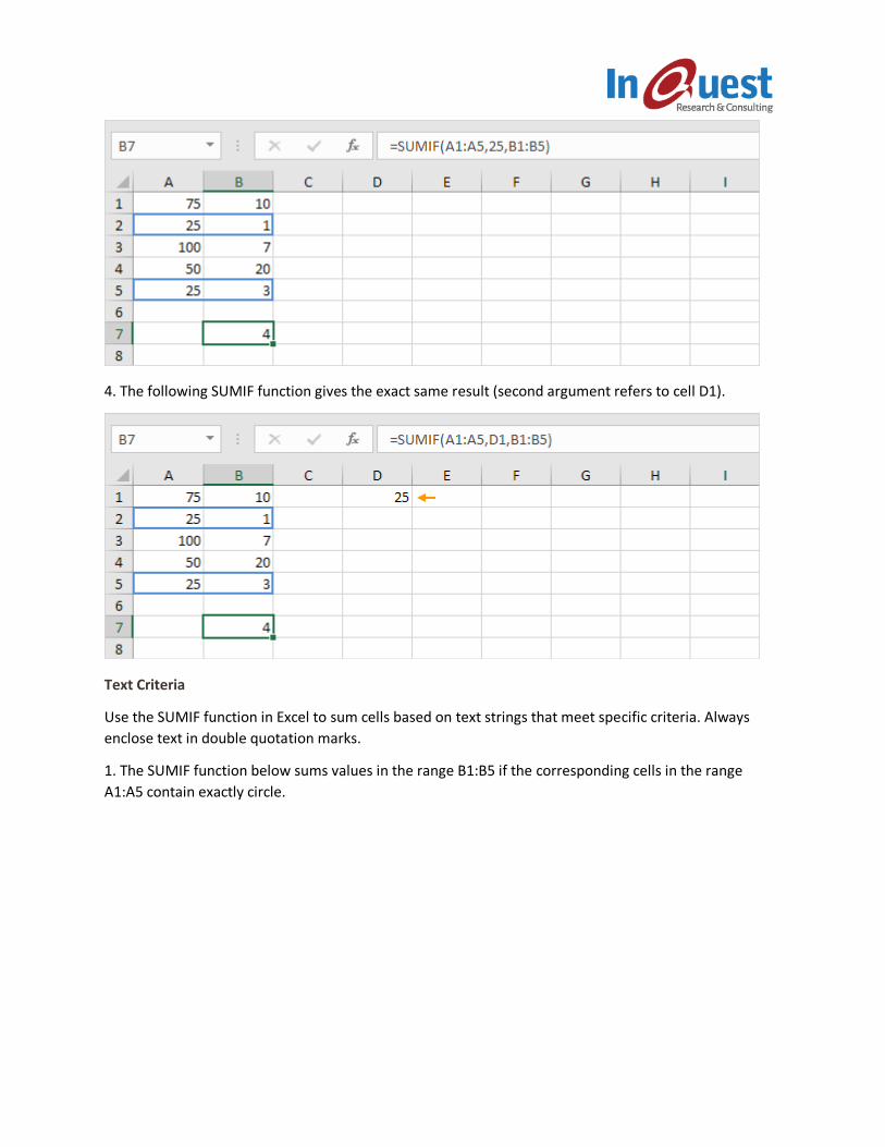
4. The following SUMIF function gives the exact same result (second argument refers to cell D1).
Text Criteria
Use the SUMIF function in Excel to sum cells based on text strings that meet specific criteria. Always
enclose text in double quotation marks.
1. The SUMIF function below sums values in the range B1:B5 if the corresponding cells in the range
A1:A5 contain exactly circle.
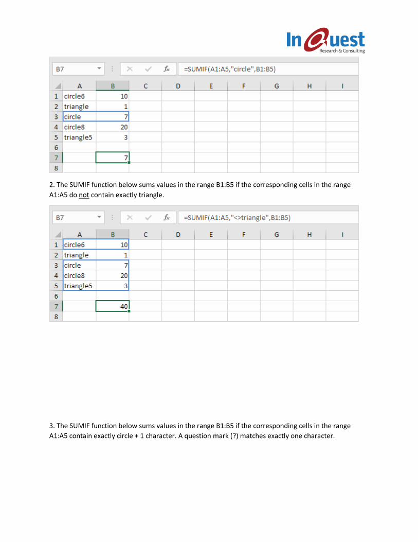
2. The SUMIF function below sums values in the range B1:B5 if the corresponding cells in the range
A1:A5 do not contain exactly triangle.
3. The SUMIF function below sums values in the range B1:B5 if the corresponding cells in the range
A1:A5 contain exactly circle + 1 character. A question mark (?) matches exactly one character.

4. The SUMIF function below sums values in the range B1:B5 if the corresponding cells in the range
A1:A5 contain a series of zero or more characters + le. An asterisk (*) matches a series of zero or more
characters.
5. The SUMIF functions below sum values in the range B1:B5 if the corresponding cells in the range
A1:A5 contain exactly triangle or circle8.
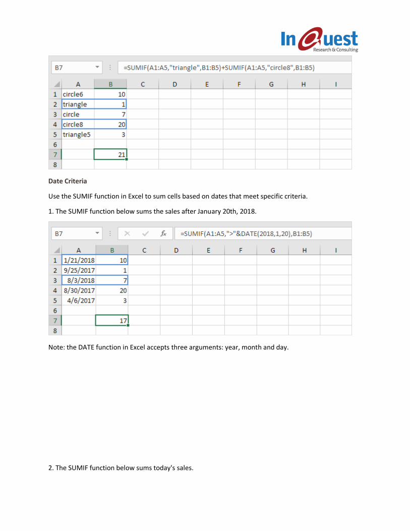
Date Criteria
Use the SUMIF function in Excel to sum cells based on dates that meet specific criteria.
1. The SUMIF function below sums the sales after January 20th, 2018.
Note: the DATE function in Excel accepts three arguments: year, month and day.
2. The SUMIF function below sums today's sales.
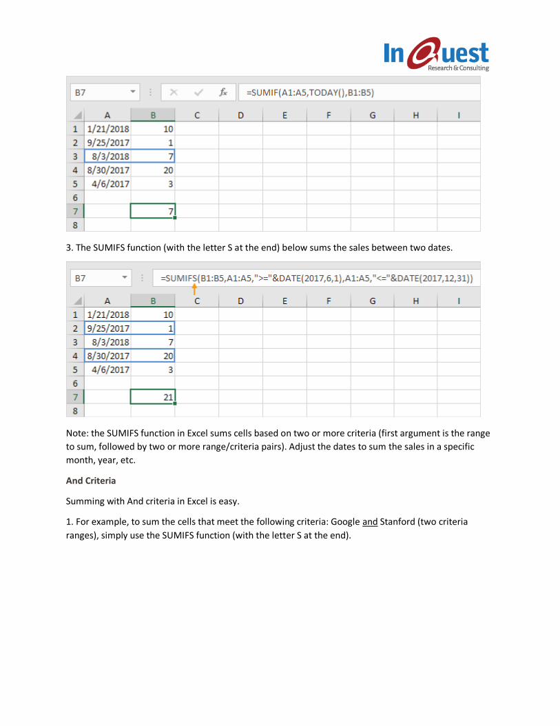
3. The SUMIFS function (with the letter S at the end) below sums the sales between two dates.
Note: the SUMIFS function in Excel sums cells based on two or more criteria (first argument is the range
to sum, followed by two or more range/criteria pairs). Adjust the dates to sum the sales in a specific
month, year, etc.
And Criteria
Summing with And criteria in Excel is easy.
1. For example, to sum the cells that meet the following criteria: Google and Stanford (two criteria
ranges), simply use the SUMIFS function (with the letter S at the end).
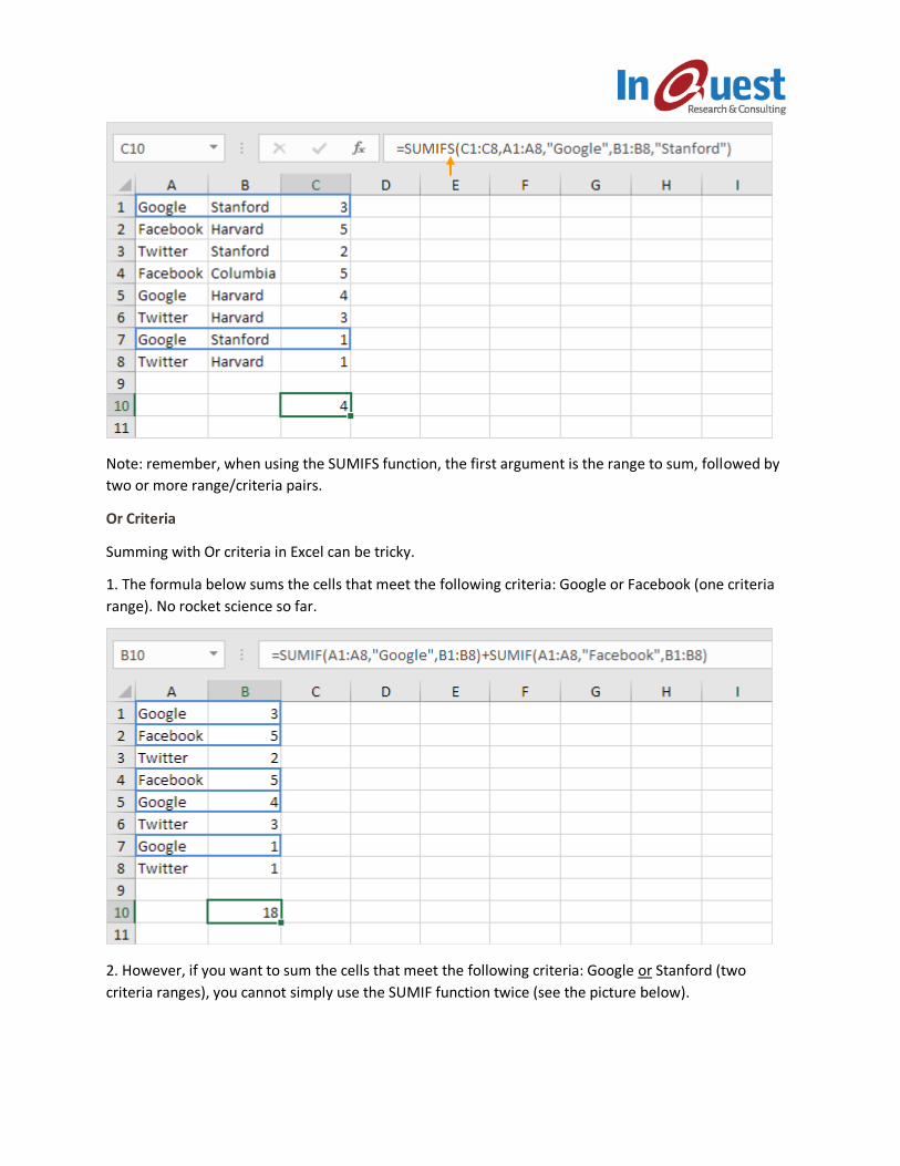
Note: remember, when using the SUMIFS function, the first argument is the range to sum, followed by
two or more range/criteria pairs.
Or Criteria
Summing with Or criteria in Excel can be tricky.
1. The formula below sums the cells that meet the following criteria: Google or Facebook (one criteria
range). No rocket science so far.
2. However, if you want to sum the cells that meet the following criteria: Google or Stanford (two
criteria ranges), you cannot simply use the SUMIF function twice (see the picture below).
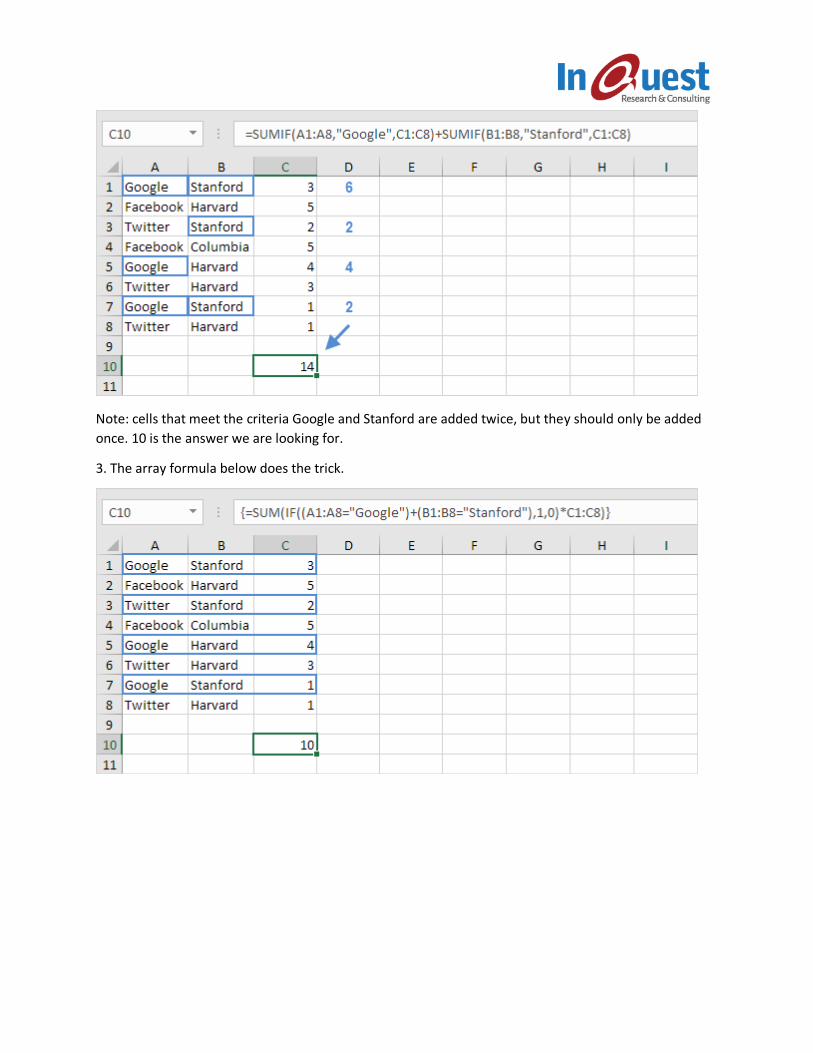
Note: cells that meet the criteria Google and Stanford are added twice, but they should only be added
once. 10 is the answer we are looking for.
3. The array formula below does the trick.
Countif
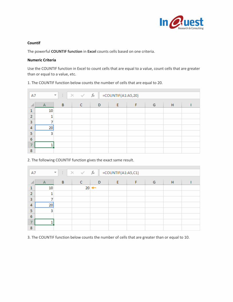
The powerful COUNTIF function in Excel counts cells based on one criteria.
Numeric Criteria
Use the COUNTIF function in Excel to count cells that are equal to a value, count cells that are greater
than or equal to a value, etc.
1. The COUNTIF function below counts the number of cells that are equal to 20.
2. The following COUNTIF function gives the exact same result.
3. The COUNTIF function below counts the number of cells that are greater than or equal to 10.
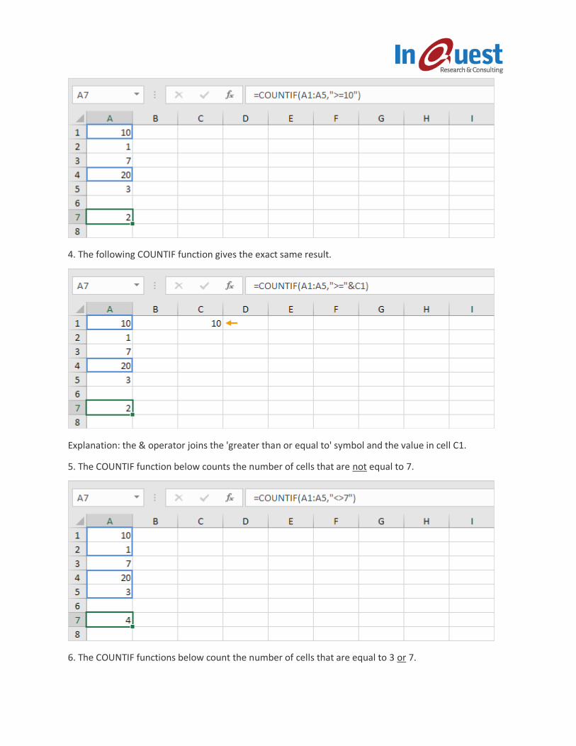
4. The following COUNTIF function gives the exact same result.
Explanation: the & operator joins the 'greater than or equal to' symbol and the value in cell C1.
5. The COUNTIF function below counts the number of cells that are not equal to 7.
6. The COUNTIF functions below count the number of cells that are equal to 3 or 7.
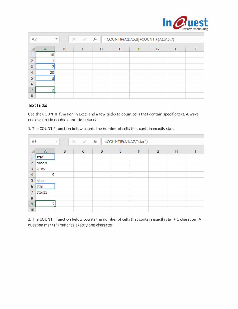
Text Tricks
Use the COUNTIF function in Excel and a few tricks to count cells that contain specific text. Always
enclose text in double quotation marks.
1. The COUNTIF function below counts the number of cells that contain exactly star.
2. The COUNTIF function below counts the number of cells that contain exactly star + 1 character. A
question mark (?) matches exactly one character.
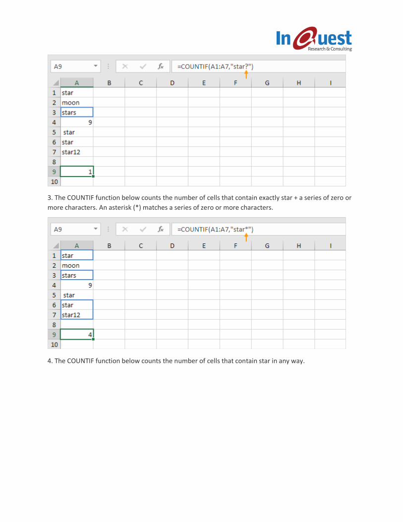
3. The COUNTIF function below counts the number of cells that contain exactly star + a series of zero or
more characters. An asterisk (*) matches a series of zero or more characters.
4. The COUNTIF function below counts the number of cells that contain star in any way.
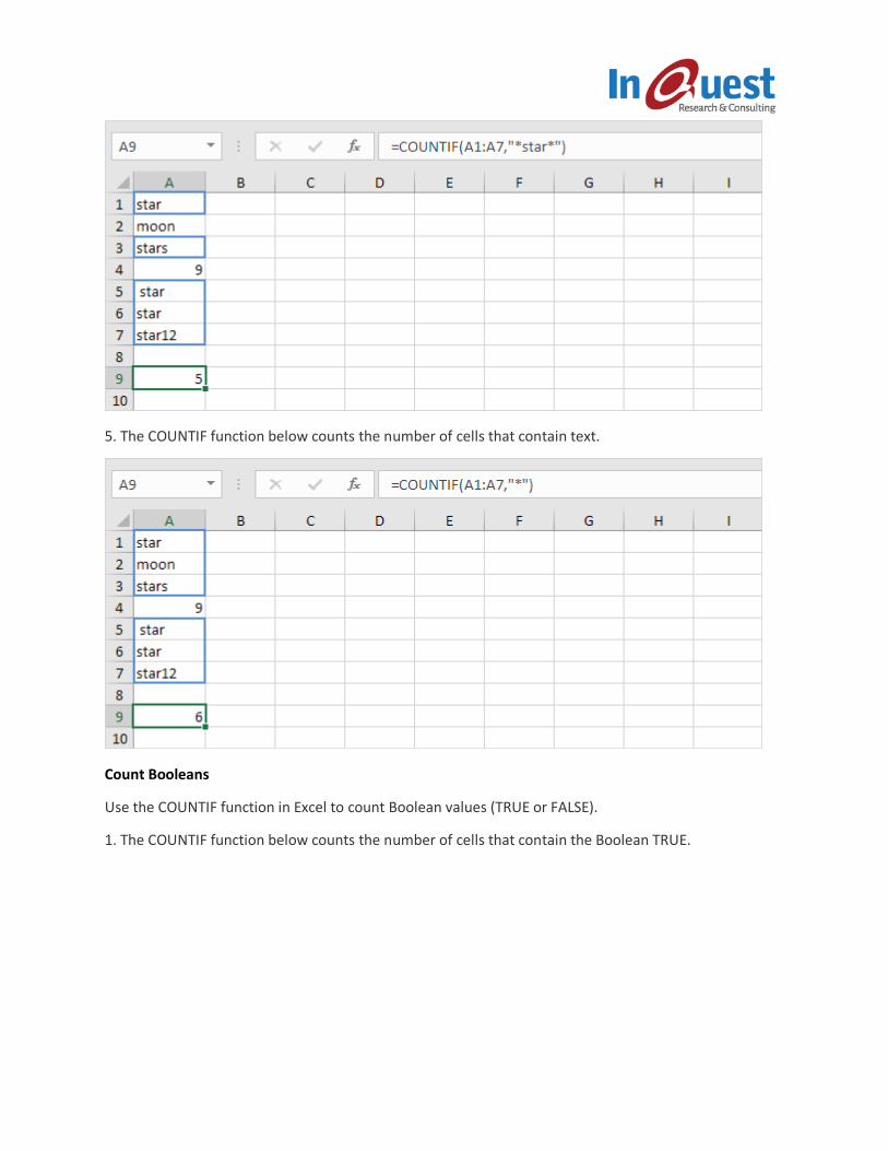
5. The COUNTIF function below counts the number of cells that contain text.
Count Booleans
Use the COUNTIF function in Excel to count Boolean values (TRUE or FALSE).
1. The COUNTIF function below counts the number of cells that contain the Boolean TRUE.
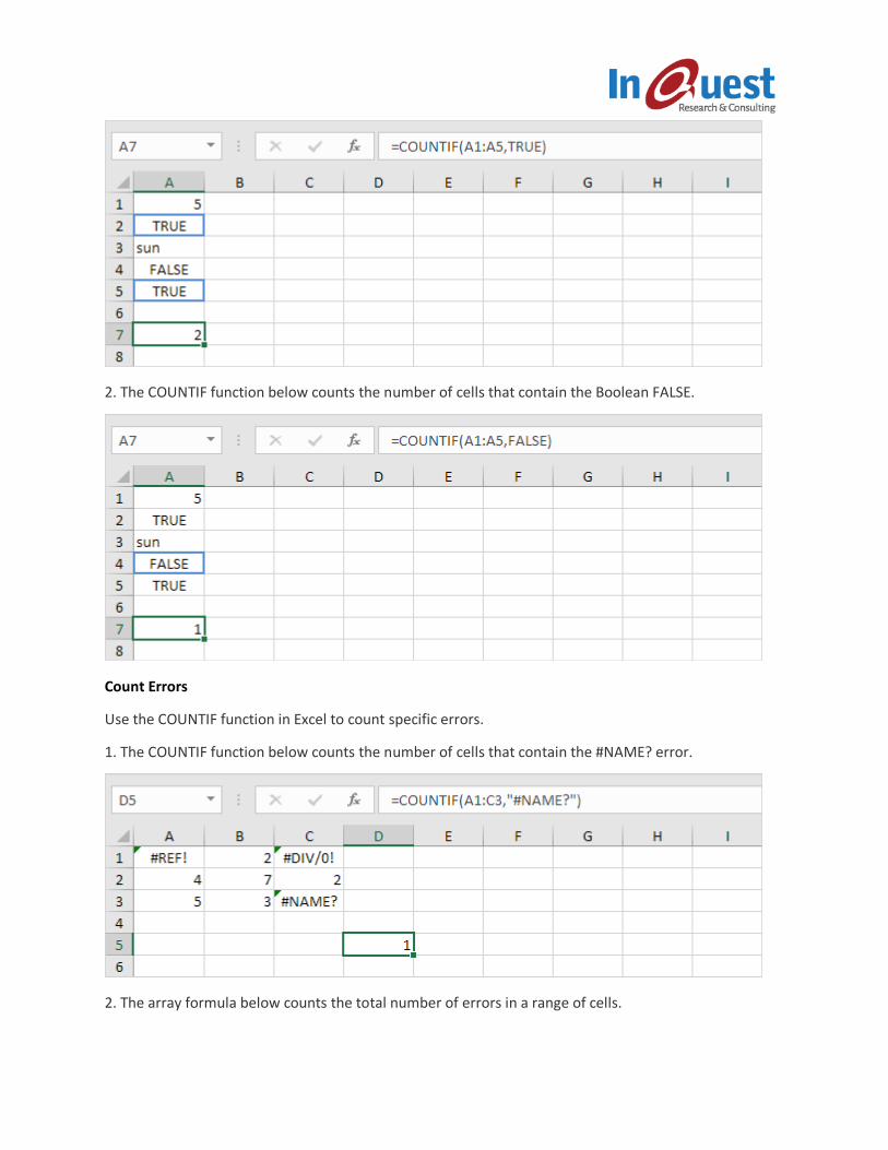
2. The COUNTIF function below counts the number of cells that contain the Boolean FALSE.
Count Errors
Use the COUNTIF function in Excel to count specific errors.
1. The COUNTIF function below counts the number of cells that contain the #NAME? error.
2. The array formula below counts the total number of errors in a range of cells.
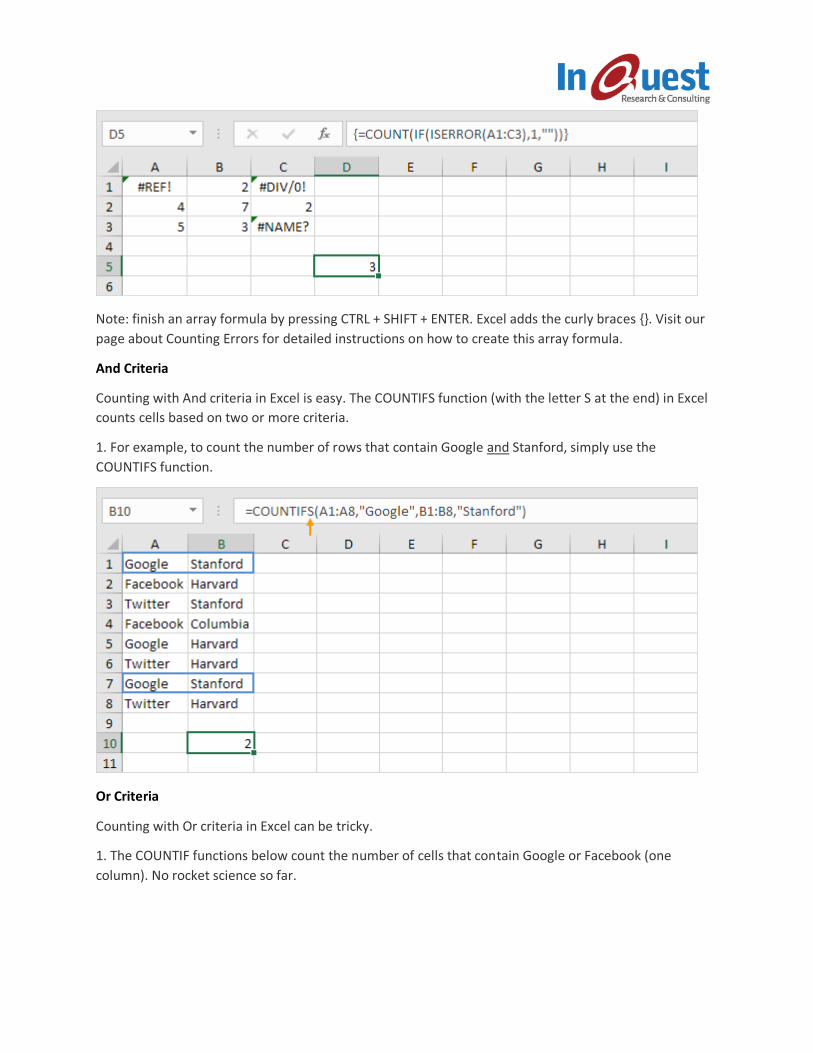
Note: finish an array formula by pressing CTRL + SHIFT + ENTER. Excel adds the curly braces {}. Visit our
page about Counting Errors for detailed instructions on how to create this array formula.
And Criteria
Counting with And criteria in Excel is easy. The COUNTIFS function (with the letter S at the end) in Excel
counts cells based on two or more criteria.
1. For example, to count the number of rows that contain Google and Stanford, simply use the
COUNTIFS function.
Or Criteria
Counting with Or criteria in Excel can be tricky.
1. The COUNTIF functions below count the number of cells that contain Google or Facebook (one
column). No rocket science so far.
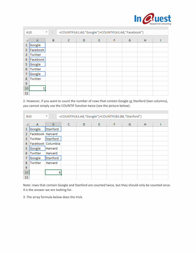
2. However, if you want to count the number of rows that contain Google or Stanford (two columns),
you cannot simply use the COUNTIF function twice (see the picture below).
Note: rows that contain Google and Stanford are counted twice, but they should only be counted once.
4 is the answer we are looking for.
3. The array formula below does the trick.
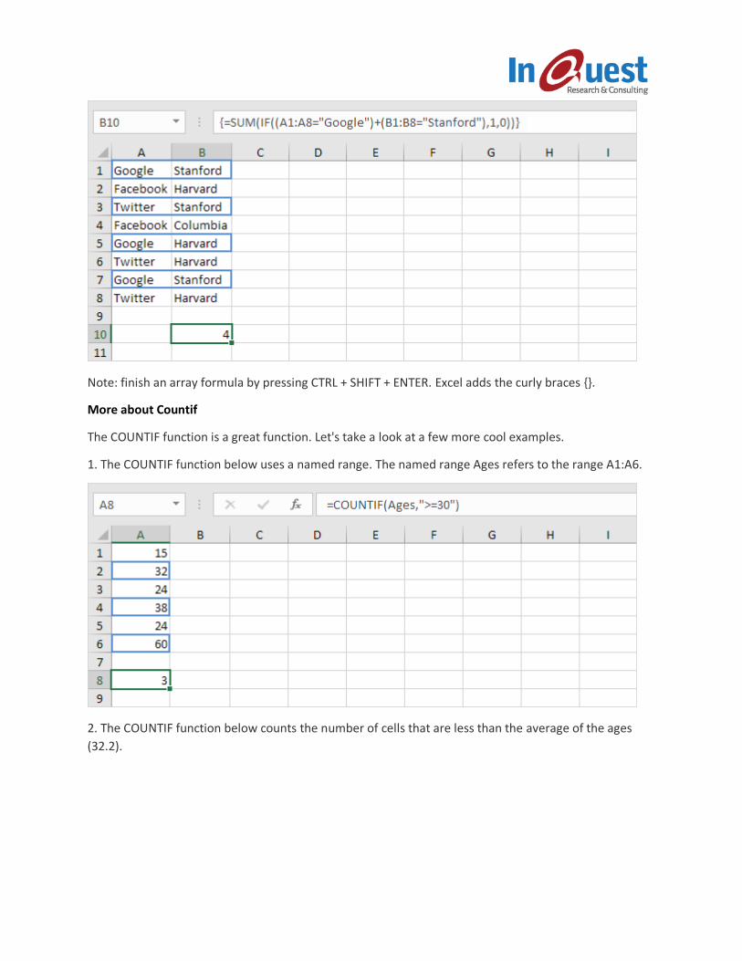
Note: finish an array formula by pressing CTRL + SHIFT + ENTER. Excel adds the curly braces {}.
More about Countif
The COUNTIF function is a great function. Let's take a look at a few more cool examples.
1. The COUNTIF function below uses a named range. The named range Ages refers to the range A1:A6.
2. The COUNTIF function below counts the number of cells that are less than the average of the ages
(32.2).
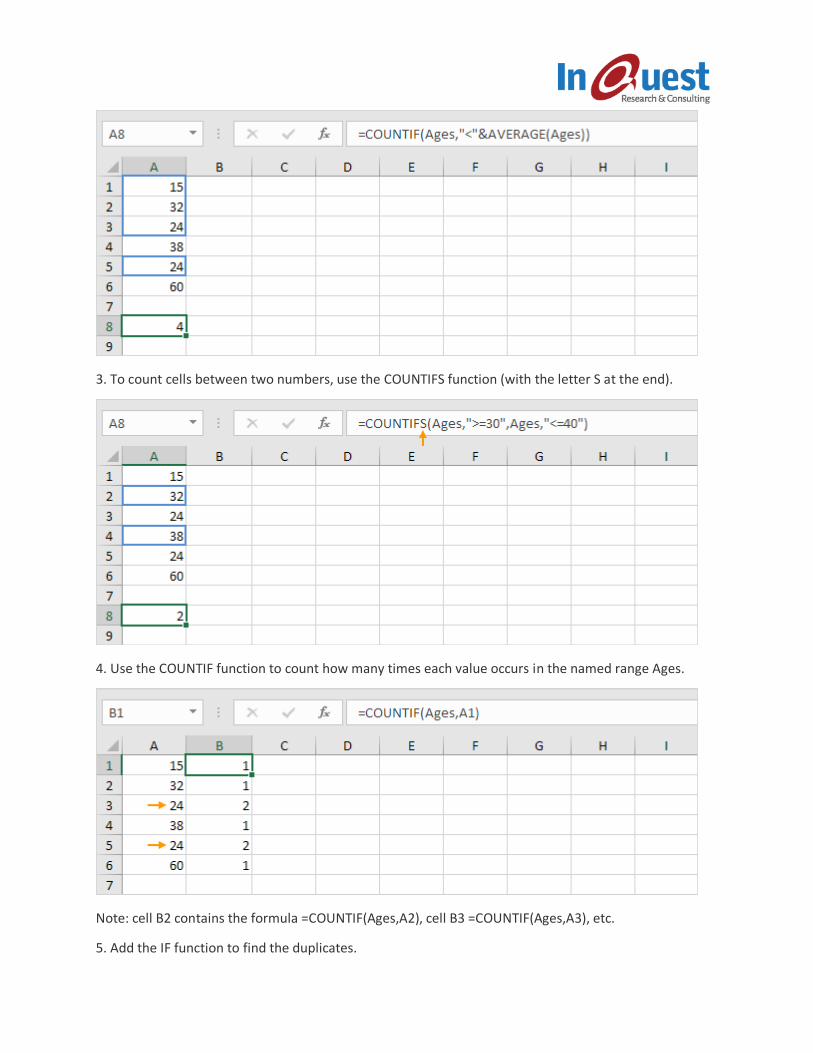
3. To count cells between two numbers, use the COUNTIFS function (with the letter S at the end).
4. Use the COUNTIF function to count how many times each value occurs in the named range Ages.
Note: cell B2 contains the formula =COUNTIF(Ages,A2), cell B3 =COUNTIF(Ages,A3), etc.
5. Add the IF function to find the duplicates.
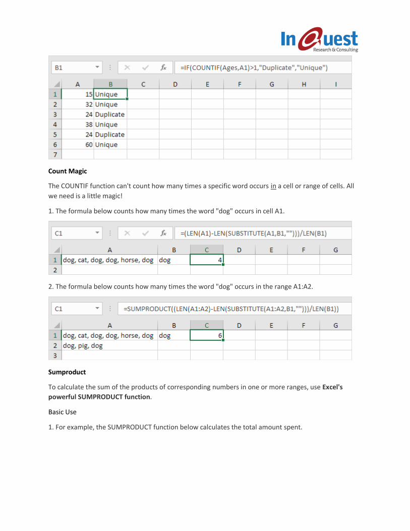
Count Magic
The COUNTIF function can't count how many times a specific word occurs in a cell or range of cells. All
we need is a little magic!
1. The formula below counts how many times the word "dog" occurs in cell A1.
2. The formula below counts how many times the word "dog" occurs in the range A1:A2.
Sumproduct
To calculate the sum of the products of corresponding numbers in one or more ranges, use Excel's
powerful SUMPRODUCT function.
Basic Use
1. For example, the SUMPRODUCT function below calculates the total amount spent.
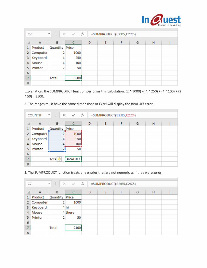
Explanation: the SUMPRODUCT function performs this calculation: (2 * 1000) + (4 * 250) + (4 * 100) + (2
* 50) = 3500.
2. The ranges must have the same dimensions or Excel will display the #VALUE! error.
3. The SUMPRODUCT function treats any entries that are not numeric as if they were zeros.
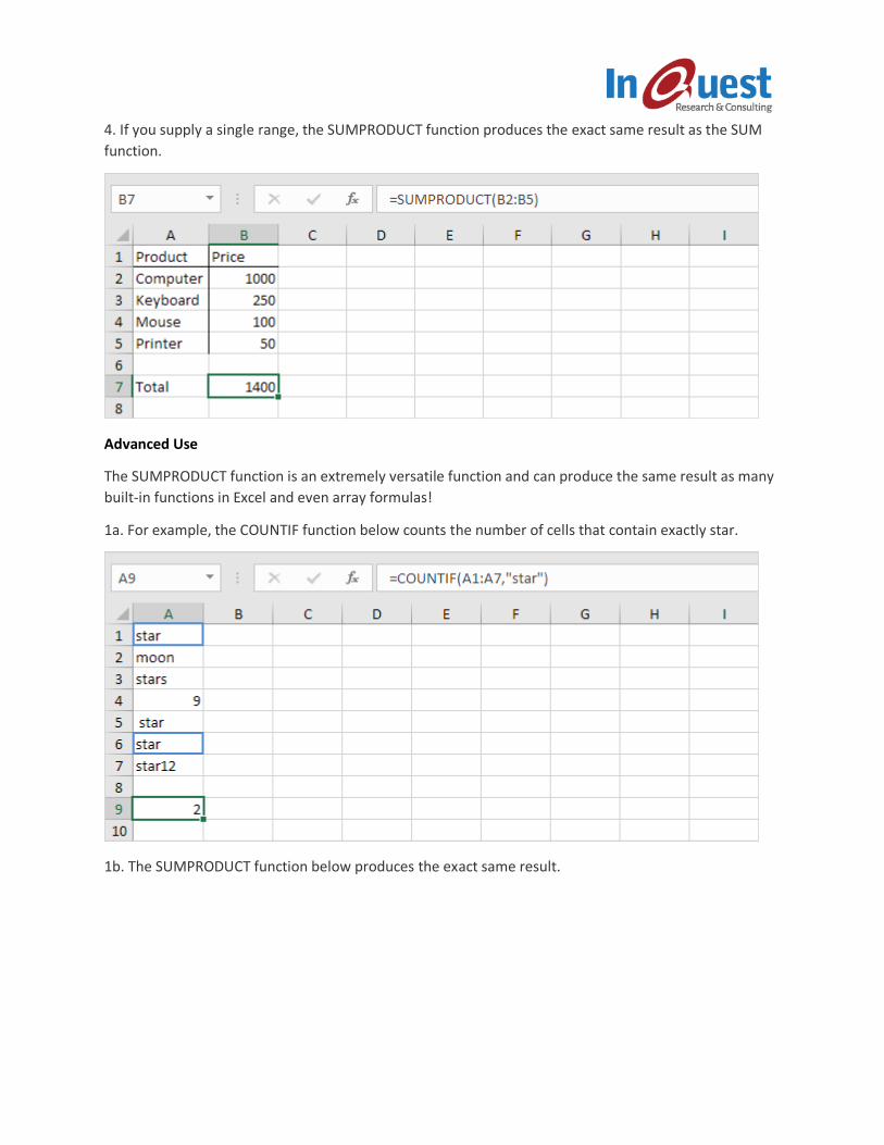
4. If you supply a single range, the SUMPRODUCT function produces the exact same result as the SUM
function.
Advanced Use
The SUMPRODUCT function is an extremely versatile function and can produce the same result as many
built-in functions in Excel and even array formulas!
1a. For example, the COUNTIF function below counts the number of cells that contain exactly star.
1b. The SUMPRODUCT function below produces the exact same result.
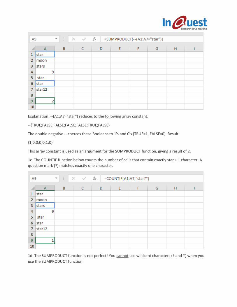
Explanation: --(A1:A7="star") reduces to the following array constant:
--{TRUE;FALSE;FALSE;FALSE;FALSE;TRUE;FALSE}
The double negative -- coerces these Booleans to 1's and 0's (TRUE=1, FALSE=0). Result:
{1;0;0;0;0;1;0}
This array constant is used as an argument for the SUMPRODUCT function, giving a result of 2.
1c. The COUNTIF function below counts the number of cells that contain exactly star + 1 character. A
question mark (?) matches exactly one character.
1d. The SUMPRODUCT function is not perfect! You cannot use wildcard characters (? and *) when you
use the SUMPRODUCT function.
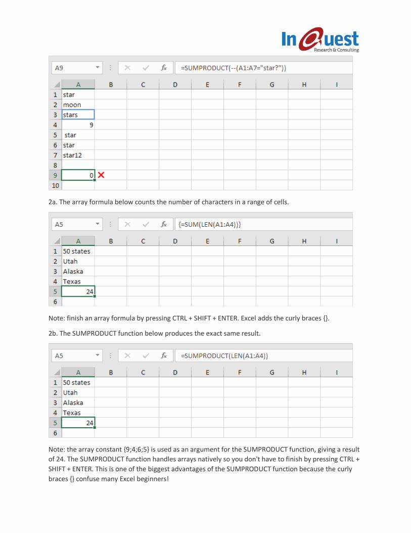
2a. The array formula below counts the number of characters in a range of cells.
Note: finish an array formula by pressing CTRL + SHIFT + ENTER. Excel adds the curly braces {}.
2b. The SUMPRODUCT function below produces the exact same result.
Note: the array constant {9;4;6;5} is used as an argument for the SUMPRODUCT function, giving a result
of 24. The SUMPRODUCT function handles arrays natively so you don't have to finish by pressing CTRL +
SHIFT + ENTER. This is one of the biggest advantages of the SUMPRODUCT function because the curly
braces {} confuse many Excel beginners!
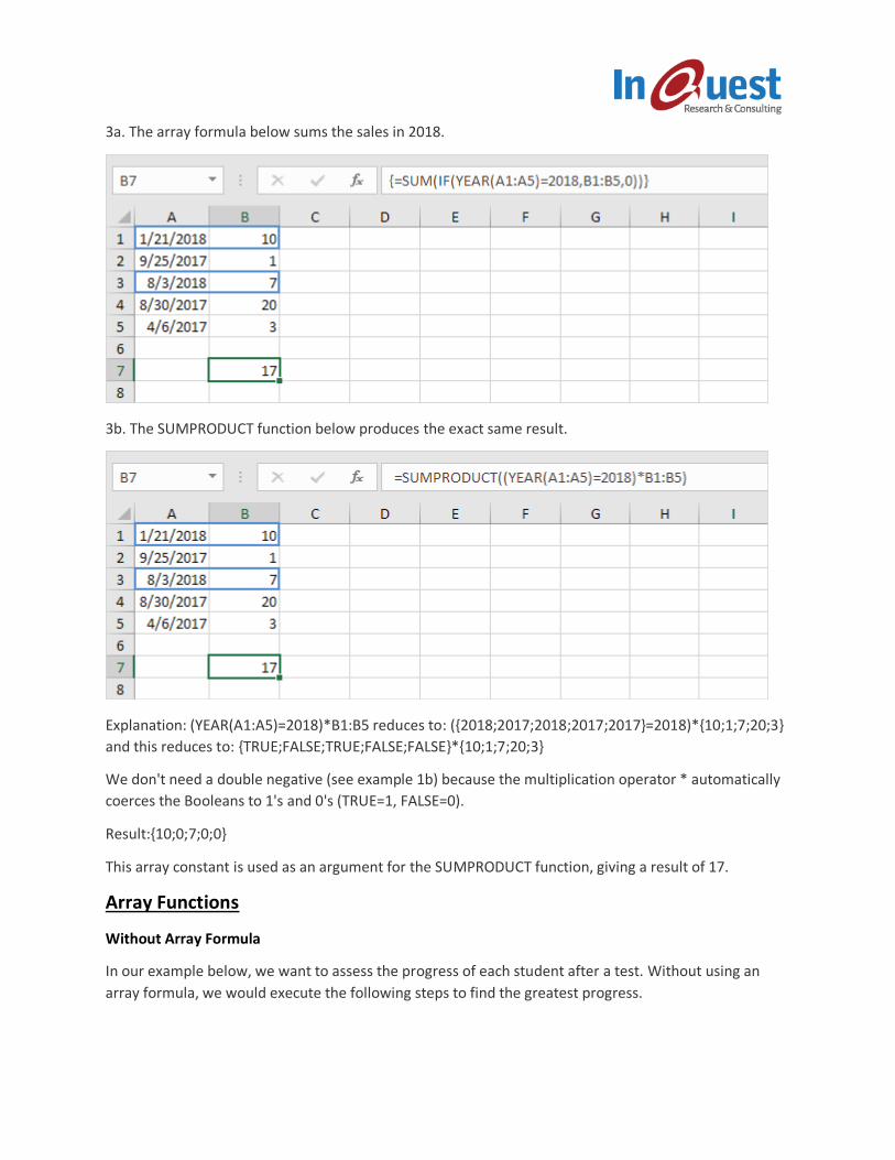
3a. The array formula below sums the sales in 2018.
3b. The SUMPRODUCT function below produces the exact same result.
Explanation: (YEAR(A1:A5)=2018)*B1:B5 reduces to: ({2018;2017;2018;2017;2017}=2018)*{10;1;7;20;3}
and this reduces to: {TRUE;FALSE;TRUE;FALSE;FALSE}*{10;1;7;20;3}
We don't need a double negative (see example 1b) because the multiplication operator * automatically
coerces the Booleans to 1's and 0's (TRUE=1, FALSE=0).
Result:{10;0;7;0;0}
This array constant is used as an argument for the SUMPRODUCT function, giving a result of 17.
Array Functions
Without Array Formula
In our example below, we want to assess the progress of each student after a test. Without using an
array formula, we would execute the following steps to find the greatest progress.
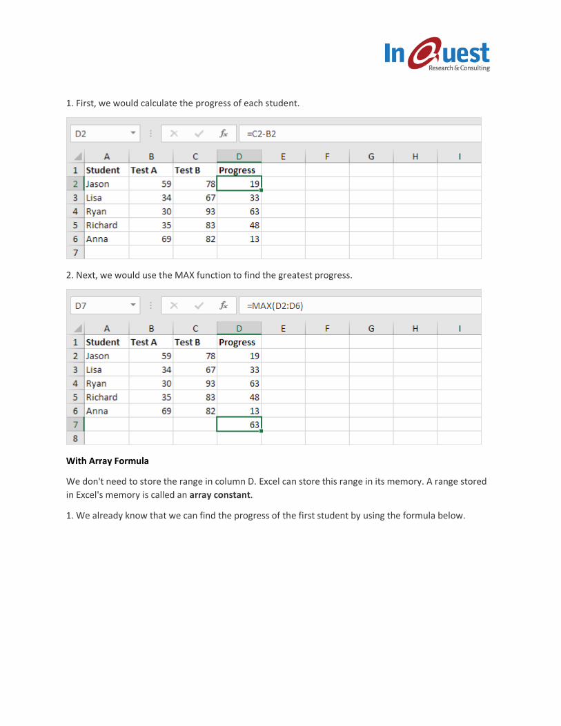
1. First, we would calculate the progress of each student.
2. Next, we would use the MAX function to find the greatest progress.
With Array Formula
We don't need to store the range in column D. Excel can store this range in its memory. A range stored
in Excel's memory is called an array constant.
1. We already know that we can find the progress of the first student by using the formula below.
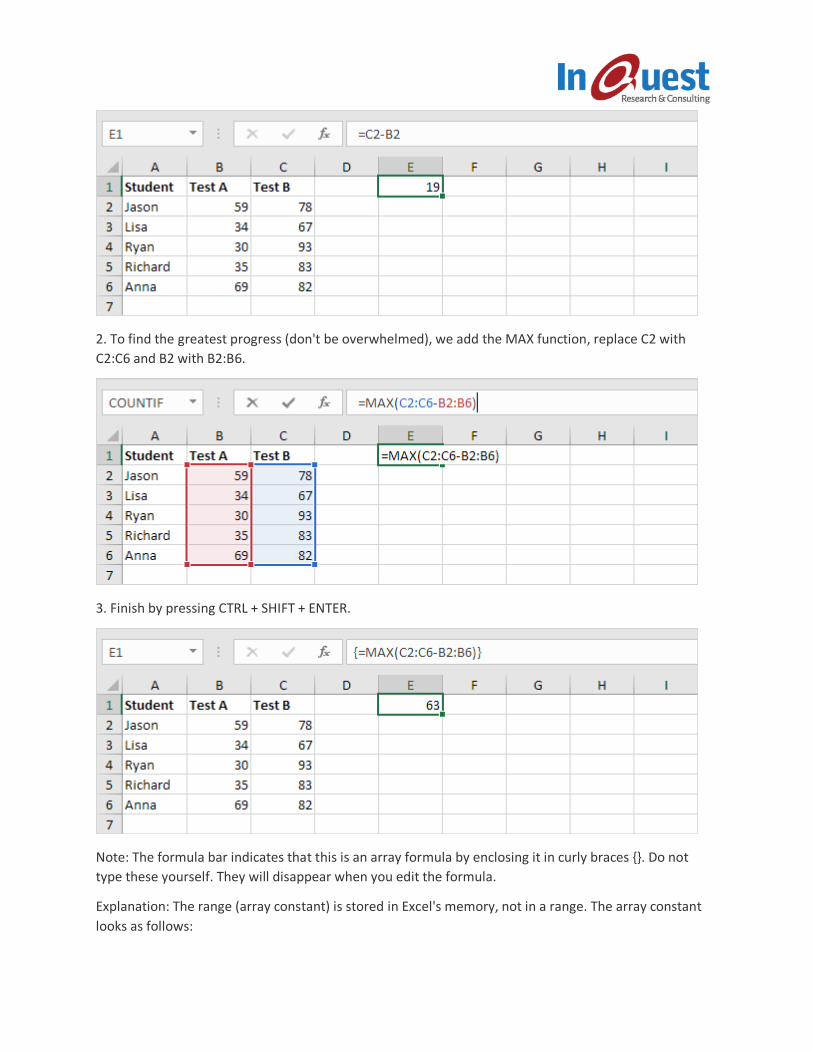
2. To find the greatest progress (don't be overwhelmed), we add the MAX function, replace C2 with
C2:C6 and B2 with B2:B6.
3. Finish by pressing CTRL + SHIFT + ENTER.
Note: The formula bar indicates that this is an array formula by enclosing it in curly braces {}. Do not
type these yourself. They will disappear when you edit the formula.
Explanation: The range (array constant) is stored in Excel's memory, not in a range. The array constant
looks as follows:
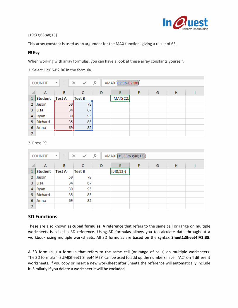
{19;33;63;48;13}
This array constant is used as an argument for the MAX function, giving a result of 63.
F9 Key
When working with array formulas, you can have a look at these array constants yourself.
1. Select C2:C6-B2:B6 in the formula.
2. Press F9.
3D Functions
These are also known as cubed formulas. A reference that refers to the same cell or range on multiple
worksheets is called a 3D reference. Using 3D formulas allows you to calculate data throughout a
workbook using multiple worksheets. All 3D formulas are based on the syntax: Sheet1:Sheet4!A2:B5.
A 3D formula is a formula that refers to the same cell (or range of cells) on multiple worksheets.
The 3D formula "=SUM(Sheet1:Sheet4!A2)" can be used to add up the numbers in cell "A2" on 4 different
worksheets. If you copy or insert a new worksheet after Sheet1 the reference will automatically include
it. Similarly if you delete a worksheet it will be excluded.
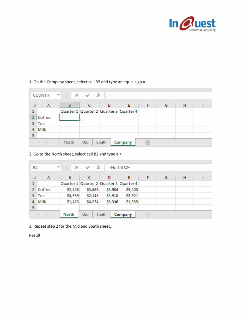
1. On the Company sheet, select cell B2 and type an equal sign =
2. Go to the North sheet, select cell B2 and type a +
3. Repeat step 2 for the Mid and South sheet.
Result.
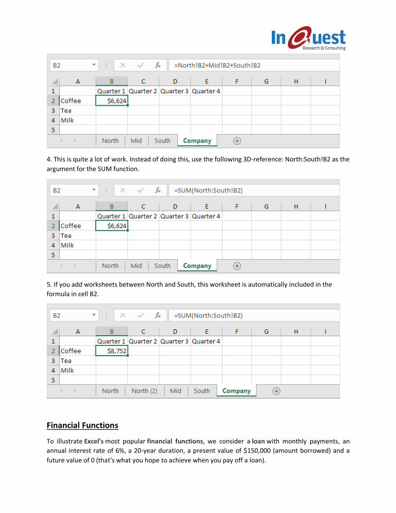
4. This is quite a lot of work. Instead of doing this, use the following 3D-reference: North:South!B2 as the
argument for the SUM function.
5. If you add worksheets between North and South, this worksheet is automatically included in the
formula in cell B2.
Financial Functions
To illustrate Excel's most popular financial functions, we consider a loan with monthly payments, an
annual interest rate of 6%, a 20-year duration, a present value of $150,000 (amount borrowed) and a
future value of 0 (that's what you hope to achieve when you pay off a loan).
We make monthly payments, so we use 6%/12 = 0.5% for Rate and 20*12 = 240 for Nper (total number
of periods). If we make annual payments on the same loan, we use 6% for Rate and 20 for Nper.
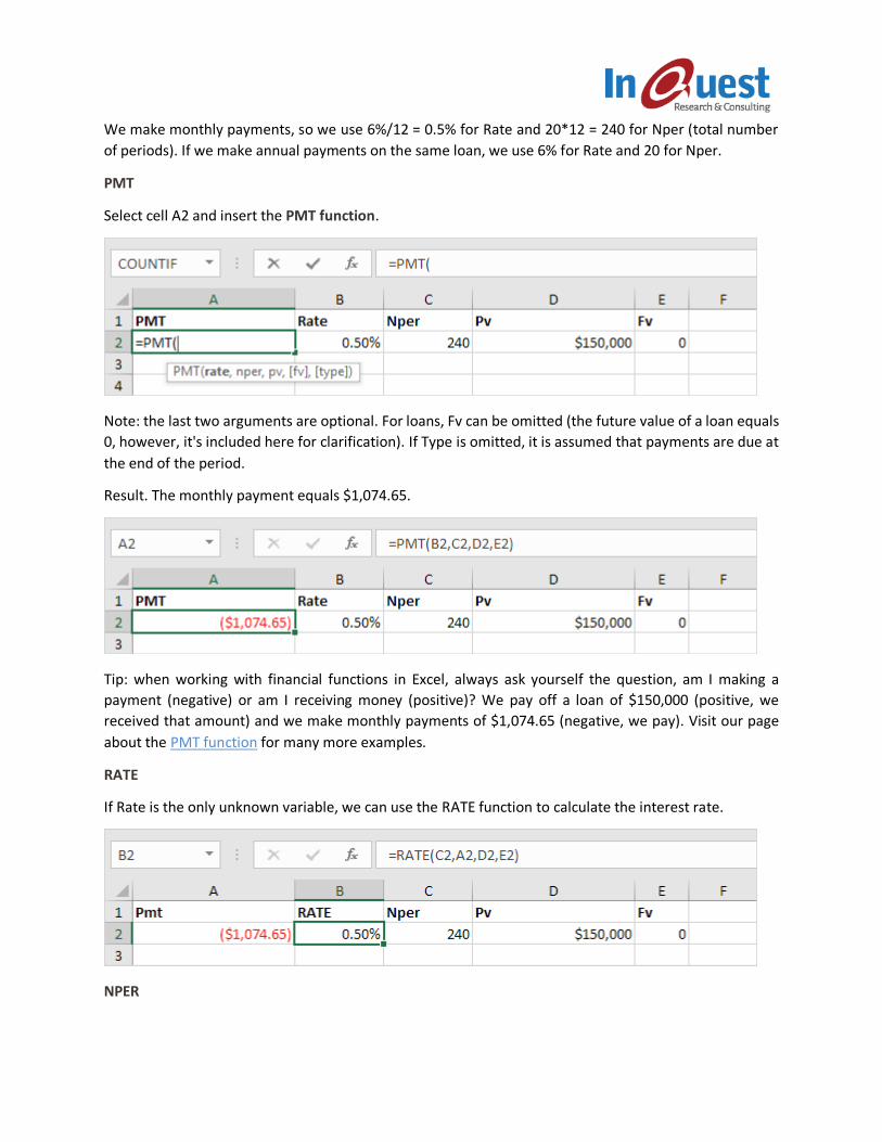
PMT
Select cell A2 and insert the PMT function.
Note: the last two arguments are optional. For loans, Fv can be omitted (the future value of a loan equals
0, however, it's included here for clarification). If Type is omitted, it is assumed that payments are due at
the end of the period.
Result. The monthly payment equals $1,074.65.
Tip: when working with financial functions in Excel, always ask yourself the question, am I making a
payment (negative) or am I receiving money (positive)? We pay off a loan of $150,000 (positive, we
received that amount) and we make monthly payments of $1,074.65 (negative, we pay). Visit our page
about the PMT function for many more examples.
RATE
If Rate is the only unknown variable, we can use the RATE function to calculate the interest rate.
NPER
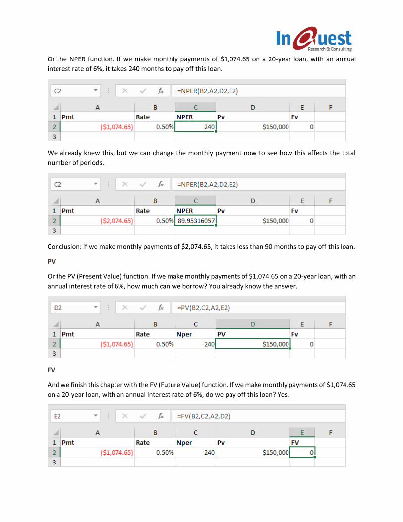
Or the NPER function. If we make monthly payments of $1,074.65 on a 20-year loan, with an annual
interest rate of 6%, it takes 240 months to pay off this loan.
We already knew this, but we can change the monthly payment now to see how this affects the total
number of periods.
Conclusion: if we make monthly payments of $2,074.65, it takes less than 90 months to pay off this loan.
PV
Or the PV (Present Value) function. If we make monthly payments of $1,074.65 on a 20-year loan, with an
annual interest rate of 6%, how much can we borrow? You already know the answer.
FV
And we finish this chapter with the FV (Future Value) function. If we make monthly payments of $1,074.65
on a 20-year loan, with an annual interest rate of 6%, do we pay off this loan? Yes.
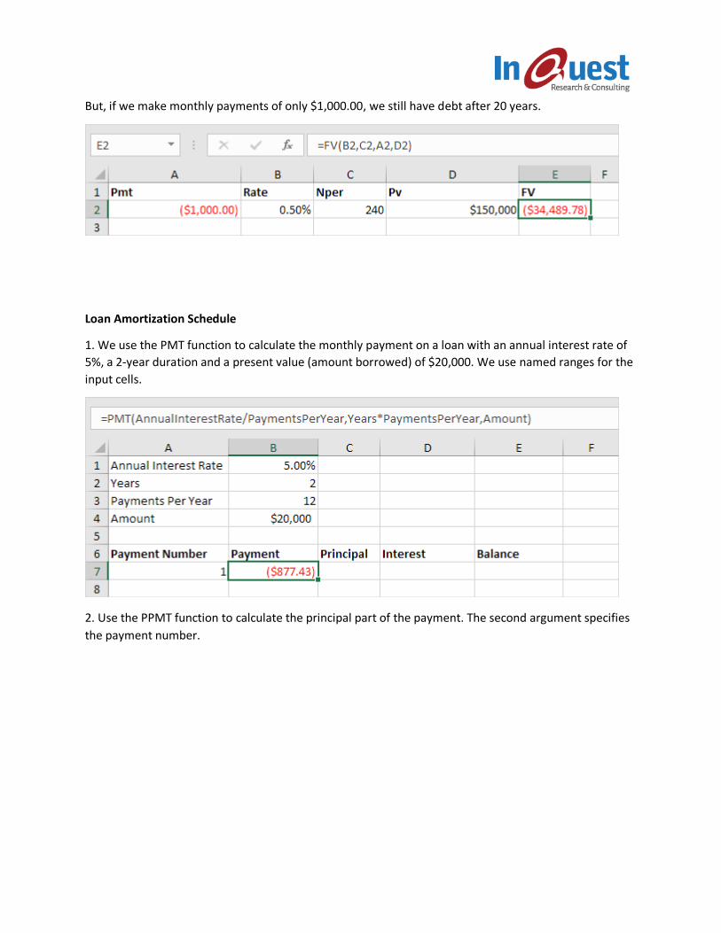
But, if we make monthly payments of only $1,000.00, we still have debt after 20 years.
Loan Amortization Schedule
1. We use the PMT function to calculate the monthly payment on a loan with an annual interest rate of
5%, a 2-year duration and a present value (amount borrowed) of $20,000. We use named ranges for the
input cells.
2. Use the PPMT function to calculate the principal part of the payment. The second argument specifies
the payment number.
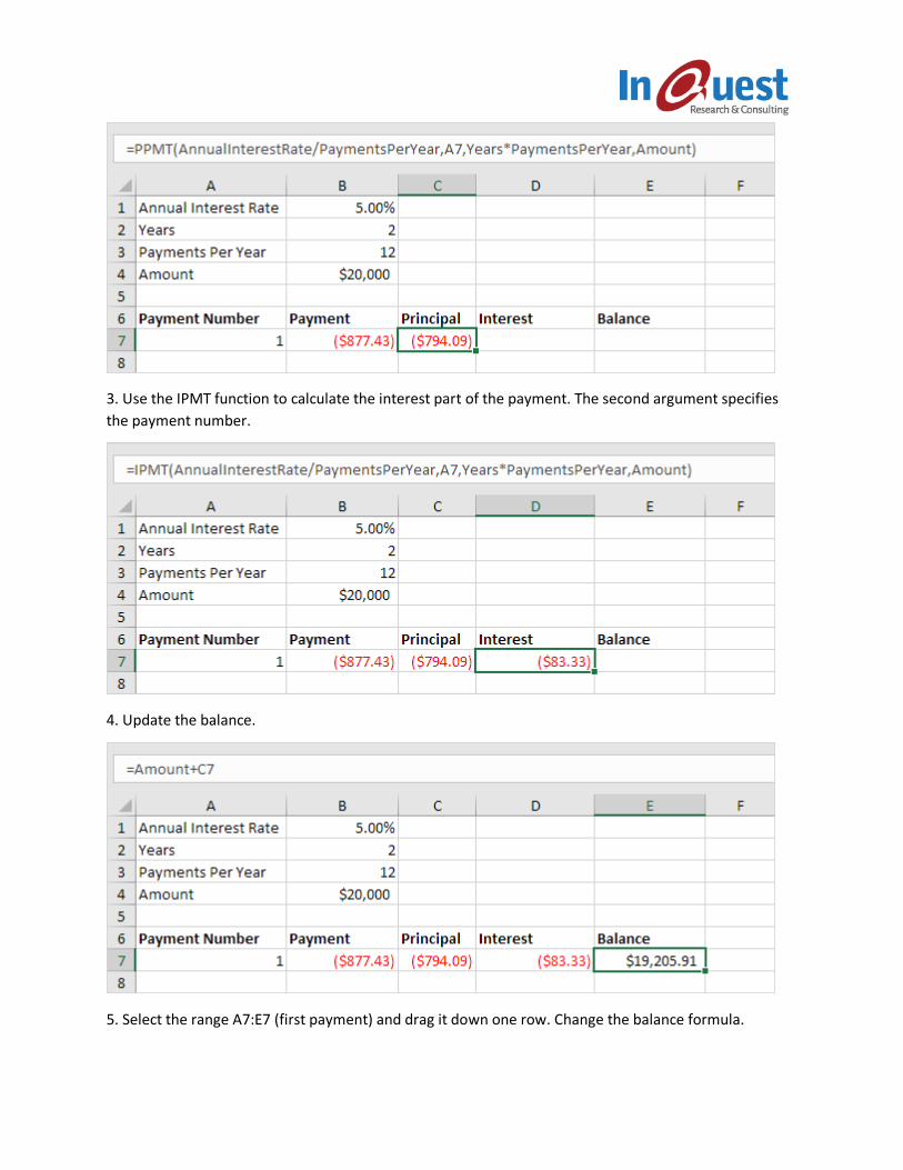
3. Use the IPMT function to calculate the interest part of the payment. The second argument specifies
the payment number.
4. Update the balance.
5. Select the range A7:E7 (first payment) and drag it down one row. Change the balance formula.
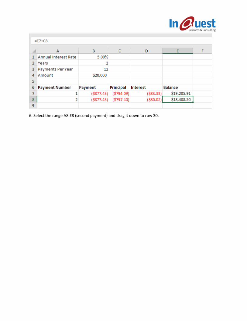
6. Select the range A8:E8 (second payment) and drag it down to row 30.
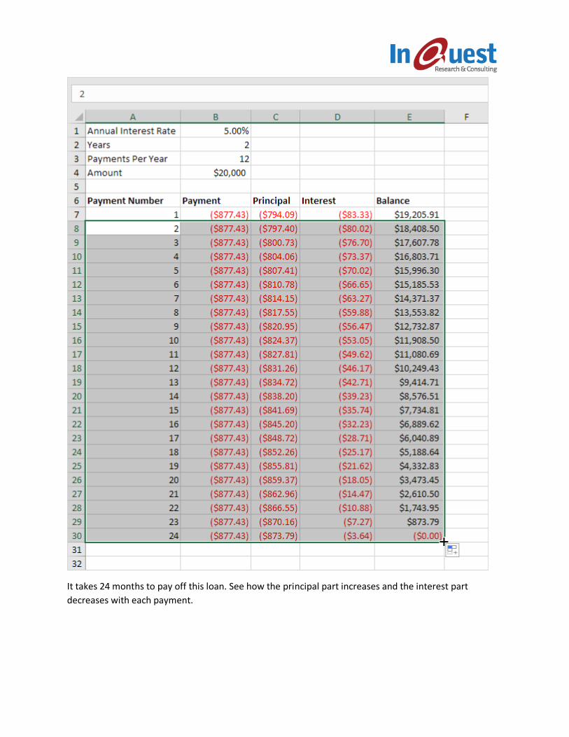
It takes 24 months to pay off this loan. See how the principal part increases and the interest part
decreases with each payment.
Pivot Tables
Pivot tables are one of Excel's most powerful features. A pivot table allows you to extract the significance
from a large, detailed data set.
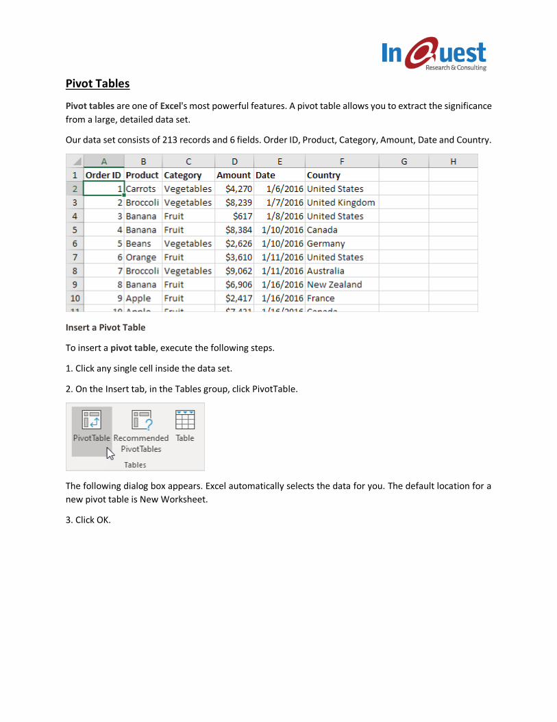
Our data set consists of 213 records and 6 fields. Order ID, Product, Category, Amount, Date and Country.
Insert a Pivot Table
To insert a pivot table, execute the following steps.
1. Click any single cell inside the data set.
2. On the Insert tab, in the Tables group, click PivotTable.
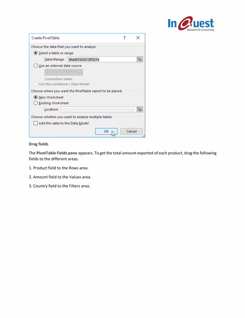
The following dialog box appears. Excel automatically selects the data for you. The default location for a
new pivot table is New Worksheet.
3. Click OK.
Drag fields
The PivotTable Fields pane appears. To get the total amount exported of each product, drag the following
fields to the different areas.
1. Product field to the Rows area.
2. Amount field to the Values area.
3. Country field to the Filters area.
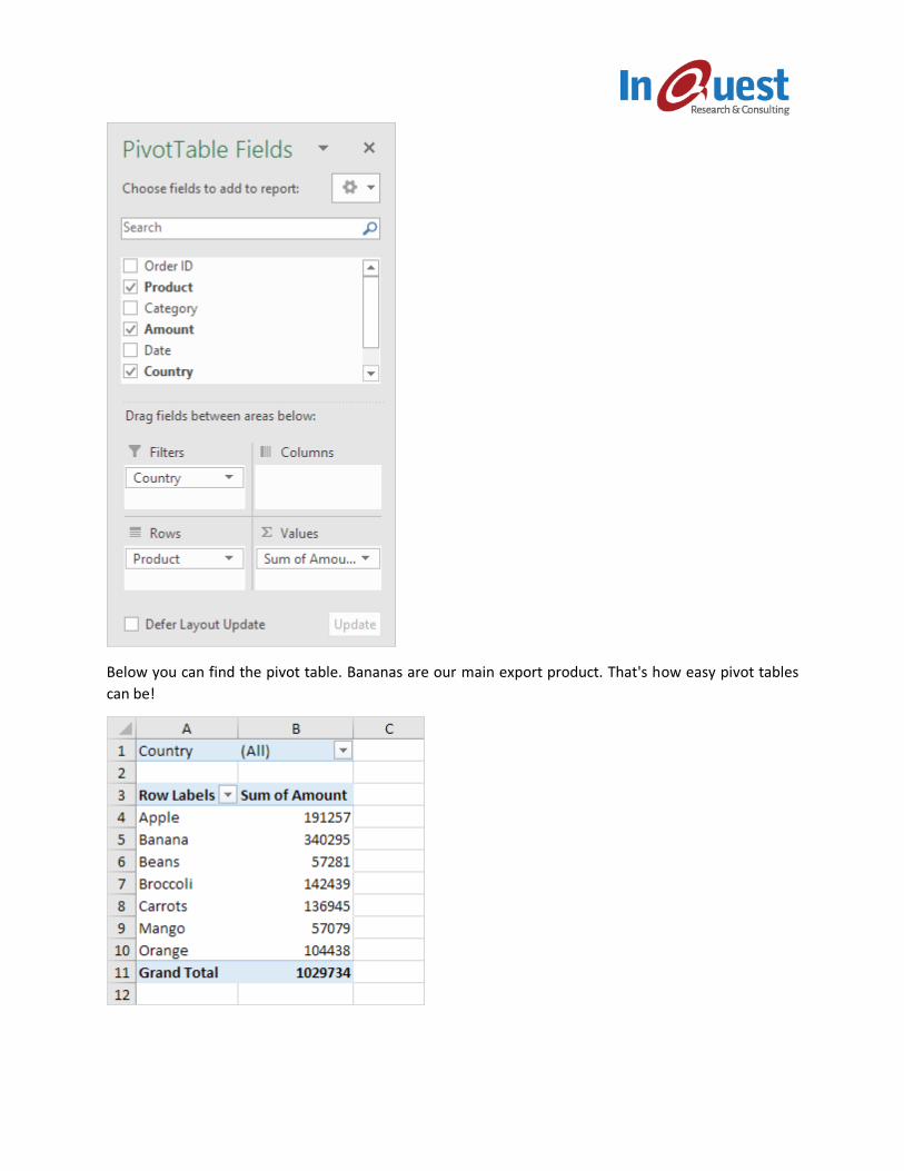
Below you can find the pivot table. Bananas are our main export product. That's how easy pivot tables
can be!
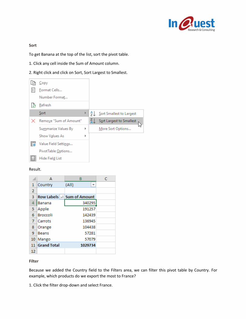
Sort
To get Banana at the top of the list, sort the pivot table.
1. Click any cell inside the Sum of Amount column.
2. Right click and click on Sort, Sort Largest to Smallest.
Result.
Filter
Because we added the Country field to the Filters area, we can filter this pivot table by Country. For
example, which products do we export the most to France?
1. Click the filter drop-down and select France.
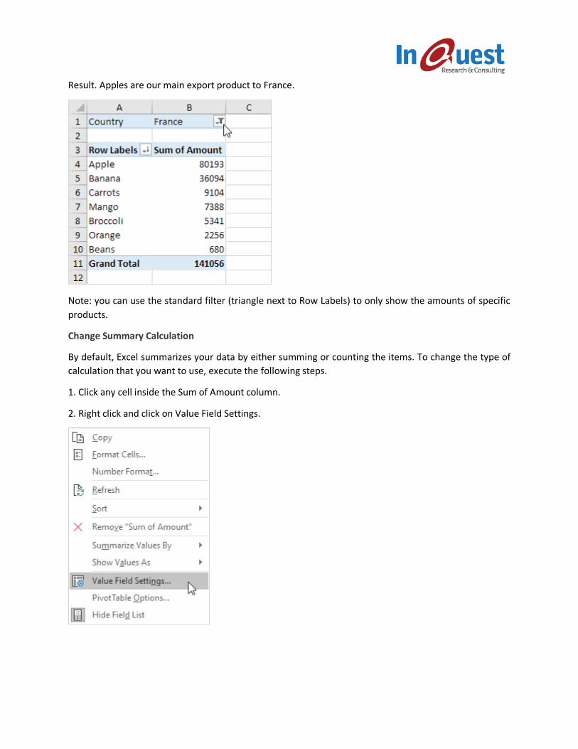
Result. Apples are our main export product to France.
Note: you can use the standard filter (triangle next to Row Labels) to only show the amounts of specific
products.
Change Summary Calculation
By default, Excel summarizes your data by either summing or counting the items. To change the type of
calculation that you want to use, execute the following steps.
1. Click any cell inside the Sum of Amount column.
2. Right click and click on Value Field Settings.
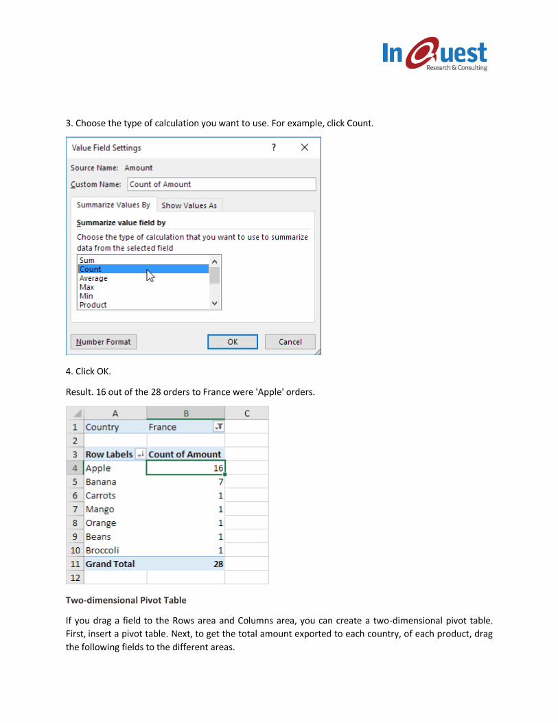
3. Choose the type of calculation you want to use. For example, click Count.
4. Click OK.
Result. 16 out of the 28 orders to France were 'Apple' orders.
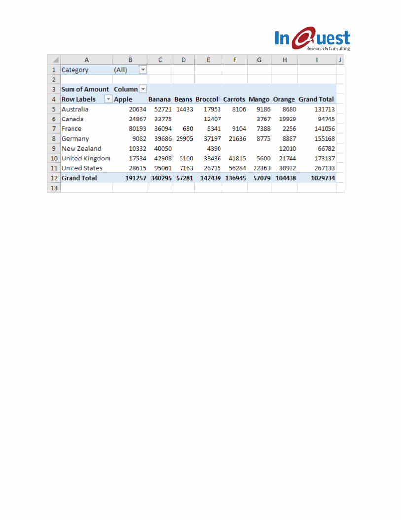
Two-dimensional Pivot Table
If you drag a field to the Rows area and Columns area, you can create a two-dimensional pivot table.
First, insert a pivot table. Next, to get the total amount exported to each country, of each product, drag
the following fields to the different areas.
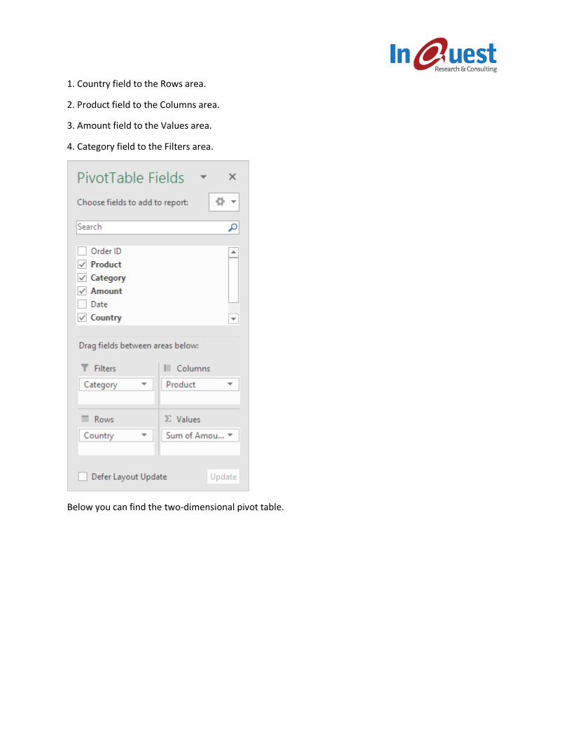
1. Country field to the Rows area.
2. Product field to the Columns area.
3. Amount field to the Values area.
4. Category field to the Filters area.
Below you can find the two-dimensional pivot table.