Embed Size (px)
Citation preview
Too Interconnected To Fail: Financial Contagion and Systemic Risk In Network Model of CDS and Other Credit Enhancement
Obligations of US Banks Sheri Markose1*, Simone Giansante*, Mateusz Gatkowski * and Ali Rais Shaghaghi*
*Centre for Computational Finance and Economic Agents (CCFEA) 1Economics Department, University of Essex, UK.
Prepared for Discussion at the ECB Workshop on "Recent advances in modelling systemic risk using network analysis", 5 October 2009
Abstract Credit default swaps (CDS) which constitute up to 98% of credit derivatives have had a unique, endemic and pernicious role to play in the current financial crisis. However, there are few in depth empirical studies of the financial network interconnections among banks and between banks and non-banks involved as CDS protection buyers and protection sellers. The ongoing problems related to technical insolvency of US commercial banks is not just confined to the so called legacy/toxic RMBS assets on balance sheets but also because of their credit risk exposures from SPVs (Special Purpose Vehicles) and the CDS markets. The dominance of a few big players in the chains of insurance and reinsurance for CDS credit risk mitigation in banks’ assets has led to the idea of “too interconnected to fail” resulting, as in the case of AIG, of having to maintain the fiction of non-failure in order to avert a credit event that can bring down the CDS pyramid and the financial system. This paper also includes a brief discussion of the complex system Agent-based Computational Economics (ACE) approach to financial network modeling for systemic risk assessment. Quantitative analysis is confined to the empirical reconstruction of the US CDS network based on the FDIC Quarter 4 data in order to conduct a series of stress tests that investigate the consequences of the fact that top 25 US banks account for $16 tn of the $34 tn gross notional value of CDS reported by the BIS and DTCC for the end of 2008.2 The May-Wigner stability condition for networks is considered for the hub like dominance of a few financial entities in the US CDS structures to understand the lack of robustness. We provide a Systemic Risk Ratio for major US banks for their CDS activity in terms of the loss of aggregate core capital. We also compare our stress test results with those provided by SCAP (Supervisory Capital Assessment Program.) A multi-agent simulator for the stress tests for CDS financial networks for US banks will be demonstrated. Keywords: Credit Default Swaps; Financial Networks; Systemic Risk; Agent Based Models; Complex Systems; Stress Testing JEL Classification : E17 , E44, E51, G21, G28 1Sheri Markose is the corresponding author and her email address is [email protected] . We acknowledge funding from the EC Marie Curie COMISEF project which pays for the Agent based Computational Economics modelling assistance from Dr. Simone Giansante and finances the PhD work of Mateusz Gatkowski and Ali Rais Shaghaghi. We are grateful for comments from Grazia Rapisarda (Credit Suisse), Surjit Kapadia (Bank of England), Russ Moro and Alistair Milne at the ESRC Money, Macro and Finance Workshop at Brunel University on 21 March 2009. The paper has benefited from respective inputs from Peter Spencer during talks given at York Economics Department; from Harbir Lamba, Rod Cross, Sheila Dow, Michael Kuchinski and John Kay at the Scottish Institute of Advanced Studies Workshop 2-3 July 09; Eric Girardin and Mathieu Gex at the Aix en Provence Summer School. All errors remain ours. 2 The ACE stress test results reported here will not include the operation of the iron clad law of deleverage and fire sales of assets to restore bank balance sheet equilibrium and also the short term obligations via the ABCP conduits.
2
Too Interconnected To Fail: Financial Networks of CDS and Other Credit Enhancement Obligations of US Banks
1. Introduction
1.1. Background The origins of the 2007 financial contagion, the trigger for which was the sub-prime crisis in the US, can be traced back to the development of financial products such as Residential Mortgage Backed Securities (RMBS)3, Collateralized Mortgage/Debt Obligations (CM/DOs) and Credit Default Swaps (CDS) which were subjected to little or no regulatory scrutiny for their systemic risk impact. These products have been dubbed ‘weapons of mass destruction’ (by Warren Buffet in 2002) as they led to multiple levels of debt/leverage with little contribution to returns from investment in the real economy4. They worked to bring about a system wide Ponzi scheme which collapsed, serially engulfing the Wall Street investment banks starting with Bear Stearns in March 2008 and followed by Lehman Brothers as the largest ever corporate failure5 in September 2008. The collapse of Freddie Mac and Fanny Mae and the severe mark downs on a global scale of the market value of retail banks, institutional investors and hedge funds which harboured sub-prime assets, has placed the financial system under unprecedented stress. As noted by Haldane (2009), the loss of 90% of market value of the top 23 US and European banks since 2007 when viewed as the decimation of a highly interconnected species in an ecosystem can only result in catastrophic consequences for the system as a whole, a matter which is averted with the use of $7.4 tn in the US and Euro 4 tn in UK and Europe of tax payer money for the bailout of financial system.
The global economic implications of the financial meltdown at this point have been noted to be greater than those for the Great Depression of 1929 at the same number of months into the crisis, Eichengreen and Rourke (2009). While all major crisis have generic features in terms of the macro-economic and monetary indicators of a boom and bust, every crisis has specific institutional ‘propagators’ unique to them. The 1929 crisis cannot be understood without knowledge of the workings of the Gold Standard, the return to it by the UK at an overvalued parity in 1925 and the attempts of the regulatory authorities of the day to ‘nobble’ the Gold Standard to avert the deflationary pressures in the UK with little recognition of the systemic risk consequences of this6. Likewise, it is the case that the 2007 financial meltdown and
3 Note, asset backed Securities, ABS, refers to the wider class of receivables from credit cards, car loans and other credit. If not specified, ABS can include MBS as well. 4 See, Brunnermeier (2008), Duffie (2007), Ashcroft and Schuermann (2008). They, respectively, cover the unfolding phases of the crisis, the specific characteristics of the credit derivatives and the features relevant to sub-prime securitization. 5The asset value of Lehman Brothers at time of filing was estimated at $691,063m. In contrast, the largest non-financial corporate that has filed to date is General Motors with $91,047m, Source Bankruptcydata.com 6 With regard to the 1929 crash and the Great Depression, at least four major studies including that of Keynes (1971), Robbins (1934), Rothbard (1963) and Friedman and Schwartz (F-S, for short,1963) have identified this crisis surrounding Gold Standard as the abiding factor behind the events that followed. However, as noted by Temin (1976), Keynesian, Austrian and Monetarist views differed considerably from this point onwards, especially on the cause of a drastic liquidity crunch in the system that took the form of a 33% fall in broad money from 1929-1933. This epitomized the
3
the on going economic crisis require analysis of the credit derivatives market and the Basel II micro-prudential ethos. The latter orchestrated the so called synthetic securitization within the ratings based assessment of risk which effectively substituted default risk of bank assets with counterparty risk of protection providers for these assets via the use of credit derivatives with little prior quantitative stress testing of consequences of the collective adoption of this credit protection scheme on the financial system as a whole.
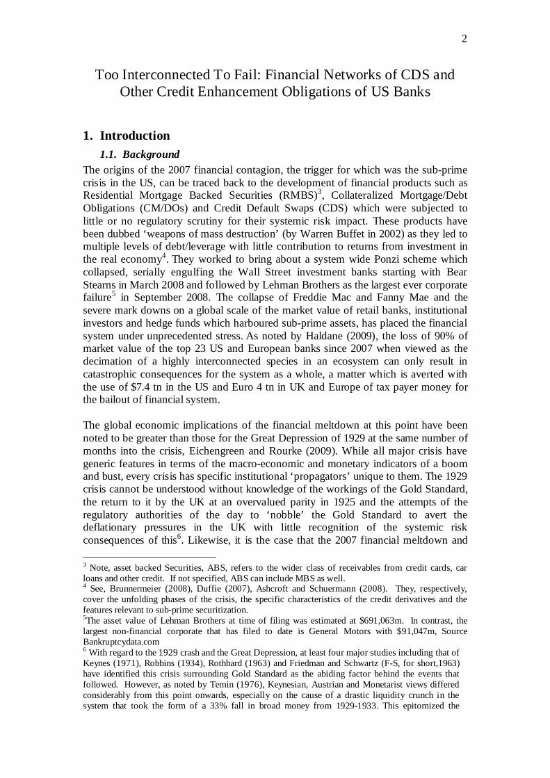
Figure 1. Credit Default Swaps Outstanding – Gross Notional
Source: BIS Dec 07, Jun 08 ; DTCC Other dates 90% CDS
The ongoing problems of bank solvency are not confined to the legacy/toxic RMBS assets on balance sheets but arise also because of their credit risk exposures from the Special Purpose Vehicles (SPV) and the CDS markets. In particular, we will analyse the FDIC data (See, Table A.1 in the Appendix 1) for top 25 US banks which are involved in CDS activity and account for $16 tn of the $34 tn gross notional value of CDS reported by the BIS (Bank of International Settlement) and DTCC (Depository Trust and Clearing Corporation) for the end of 2008. Figure 1 shows how by mid 2007 which coincided with the onset of the crisis, the gross notional value of the CDS market stood at an explosive level of about $58 tn. Post Lehman crisis, the gross notional value of CDS contracts has contracted with the amounts in multi-name index and tranche CDS shrinking faster than that for single name CDS. Pre Lehman crisis, some 20% of multi-name CDS was backed by RMBS CDOs. While these assets are included in the recovery plan of the TARP and TALF, the growth in these assets has
collapse of the banking sector and was accompanied by price deflation and economic contraction. Despite an increase of 15% of high powered money, Temin (1976, p.5) indicates that monetary authorities could do little to increase the stock of broad money as the latter depends on consumer confidence and lending activity of financial intermediaries who retained reserves rather than lent it. Nevertheless, the influential view propagated by F-S (ibid, pp 300-301,346) is that the Fed was responsible for the fall in broad money in the aftermath of the 1929 stock market crash.
17.1
Dec 07 Jun 08 31Oct 08 28 Nov 08 26 Dec 08 5 Mar 09
US $ Trillions
60
40
20
0
57
57.3
20.1
Indices & tranches
Single Name
37.2
34.5
18.1
16.4
32.5 30.5
16.5
15.9 14.3
16.2
4
virtually ceased marking the endemic nature of the credit crunch as these were main conduits by which banks raised funds for lending.
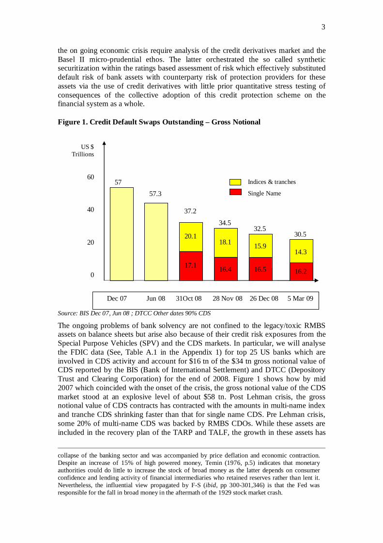
Data given below from British Bankers Association for 2006 gives a breakdown of the types of financial institutions involved globally as protection buyers and protection sellers in the CDS market. In the run up to the Basel II regime, while heavy micro prescriptions on capital adequacy of banks existed which also permitted them to use CDS credit mitigants in lieu of reserves, the same capital adequacy rules did not equally apply to all participants of the credit risk transfer system. Only banks were subject to capital regulation while about 50% (see Figure 2) of those institutions which were CDS sellers in the form of thinly capitalized hedge funds and Monolines7, were outside the regulatory boundary. This introduced significant weakness to the scheme leading to the criticism that the credit risk transfer, CRT, scheme was more akin to banks and other net beneficiaries of CDS purchasing insurance from passengers on the Titanic. As we will see, the benefits that accrued to banks fell far short of the intended default risk mitigation objectives and participants of the scheme were driven primarily by short term returns from the leveraged lending using CDS and CDOs as collateral in a carry trade.
Since the recent tax payer bailouts of large financial institutions such as AIG8, the dominance of a few big players in the CDS chains of insurance and reinsurance for credit risk mitigation has led to the idea of “too interconnected to fail”. Maintaining the fiction of non-failure of such a financial institution averts a key credit event that can trigger a chain of obligations with itself as the reference entity and also as guarantor of large swathes of balance sheet items of banks, the loss of which render these banks undercapitalized and threatened with insolvency. The failure to monitor and regulate the CDS market or to design enough controls to prevent the oversupply of cheap and inadequate bank credit insurance provided by financial entities such as the Monolines and hedge funds outside the so called ‘regulatory boundary’, has meant that the financial crisis not only could not be contained within the financial system, the clean up costs are impacting on tax payers in perpetuity.
7 At the end of 2007, AMBAC, MBIA and FSA account for 70% of the CDS contracts provided by Monolines with the first two accounting for $625 bn and $546 bn of this. The capital base of Monolines is approximately $20 bn and their insurance guarantees are to the tune of $2.3 tn, implying leverage of 115. 8 While the current cost to the US tax payer of the AIG bailout stands at $170 bn, the initial $85 bn payment to AIG was geared toward honouring its CDS obligations totalling over $66.2 bn. These include payouts to Goldman Sachs ($12.9 billion), Merrill Lynch ($6.8 billion), Bank of America ($5.2 billion), Citigroup ($2.3 billion) and Wachovia ($1.5 billion). Foreign banks were also beneficiaries, including Société Générale of France and Deutsche Bank of Germany, which each received nearly $12 billion; Barclays of Britain ($8.5 billion); and UBS of Switzerland ($5 billion).
5
Figure 2: Counterparties for CDS: Q4 2006. Threat to system comes from CDS sellers: 49% Hedge Funds and Monolines, which have wafer thin capital base
Source: British Bankers Association
This has manifested in an increase in the solvency risk of governments and also in a contraction of employment and growth. There is strong evidence that the imminent collapse of Lehman Brothers in 2008 led to meltdown level CDS spreads of other financial entities and the massive flight to safety that froze the short term money markets which started the credit crunch. The gross notional value of the CDS obligations of Lehman Brothers, ranked the 10th largest counterparty, is placed at between $5tn and $3.65tn9. The $400 bn CDS with Lehman Brothers itself as the reference entity on a face value of Lehman debt of only $150 bn resulted in CDS protections sellers on Lehman CDS potentially having to deliver as much as $365 bn as the recovery rate was about 8.625 cents per dollar. While the actual net payments on this was about $6 bn, the direct losses on Lehman bonds has been estimated at about $34 to $47 bn10. The simultaneous failure of Lehman and AIG with AIG as a credit event that triggers CDS payments would have corresponded to the so called Armageddon scenario considered in the stress tests we conduct.
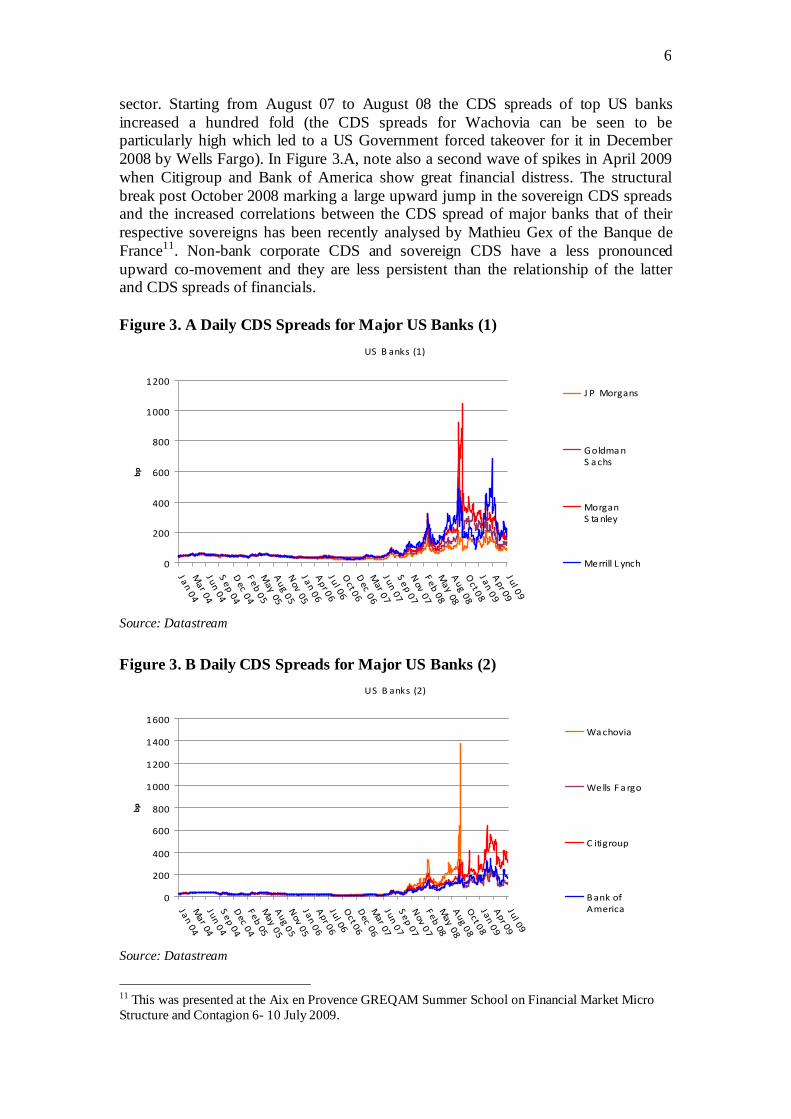
Figures 3.A, 3.B and 3.C on CDS spreads indicate how default risk on corporate debt and on bank assets which was first transmuted into counterparty risk within the banking and financial sector with the Basel II credit risk transfer process using CDS, has since the demise of Lehman Brothers also become the domain of growing and persistent sovereign risk due to the large size of tax payer bailouts of the financial
9 On the 15 September 2008, Financial Times estimated the size of Lehman’s largest CDS counterparties to be $473.33 bn (Société Générale), $383.99 bn (Credit Agricole), $729.56 bn (Barclays), $1138.09 bn (Deutsche Bank), $277.36 bn (Credit Suisse) and $652.97 (UBS). This totals about $3655bn. Losses arising from reassignments of CDS cover from Lehman as counterparty at much higher premia is estimated at about $20bn- $50bn. Satyajit Das is of the view that these estimated CDS related losses of about $100bn, which includes the direct loss from Lehman bonds due to inadequate cover, roughly corresponds to the recent recapitalization of US banks via SCAP. 10 This includes the bailout needed for Dexia which held $500m of Lehman bonds. Among the others with declared exposure: Swedbank $1.2bn; Freddie Mac $1.2bn; State Street $1bn; Allianz €400m; BNP Paribas €400m; AXA €300m; Intesa Sanpaolo €260m; Raffeissen Bank €252m; Unicredit €120m; ING €100m; Danske Bank $100m; Aviva £270m; Australia and New Zealand Bank $120m; Mistubishi $235m; China Citic Bank $76m; China Construction Bank $191m, Industrial Commercial Bank of China $152m and Bank of China $76m. For a fuller account of the losses on $1.84 bn Lehman minibonds and $8.76 bn of Lehman equity linked structured notes, see http://www.bloomberg.com/apps/news?pid=20601109&sid=aNFuVRL73wJc
CDS Buyers
Banks & Brokers39%
Securities Houses20%
Insurers /Reinsurers6%
Hedge Funds28%
Pension Funds2%
Mutual funds2%
Corporates2%
Other1%
CDS Sellers
Banks & Brokers33%
Securities Houses7%
Hedge Funds31%
Insurers/Reinsurers18%
Pension Funds5%
Mutual funds3%
Corporates2%
Other1%
6
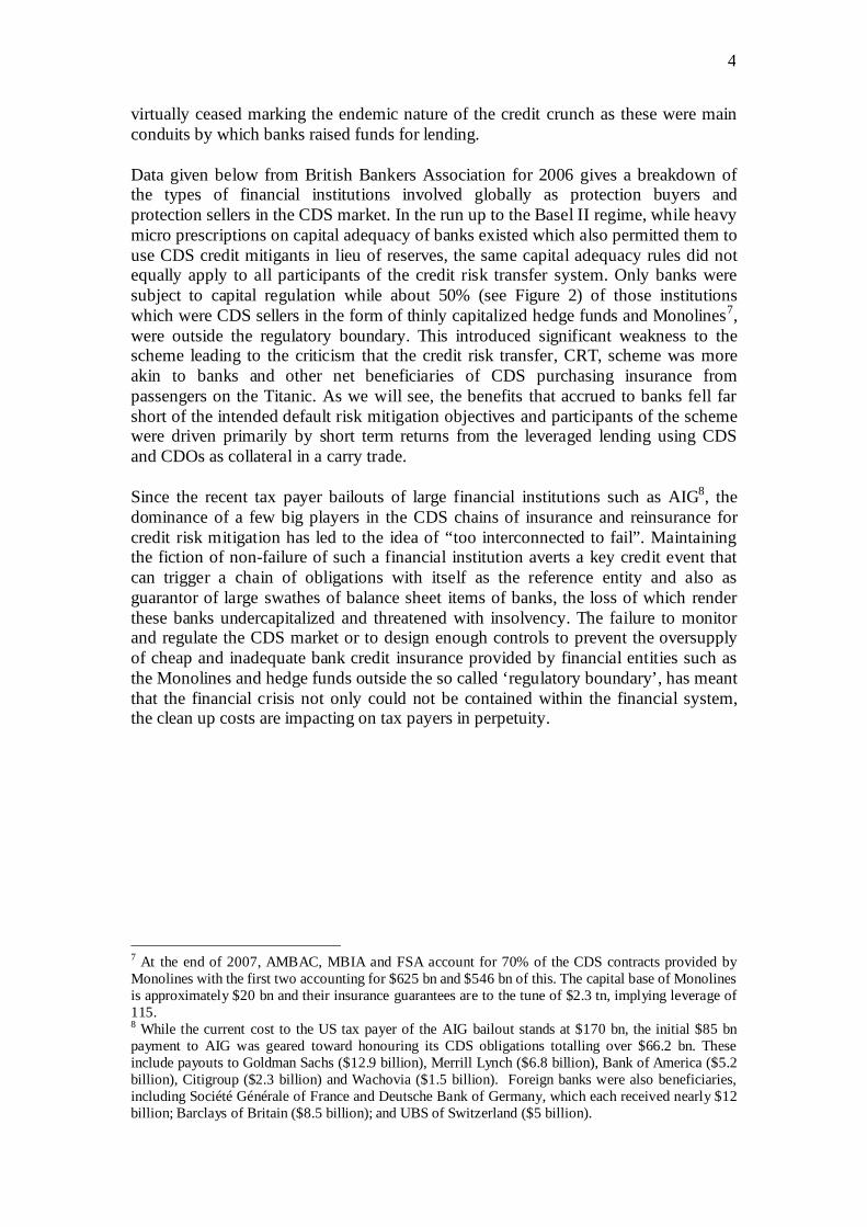
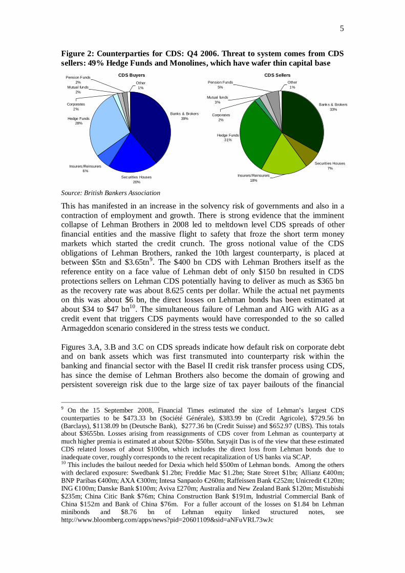
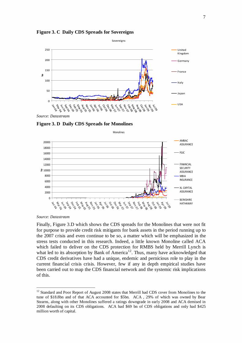
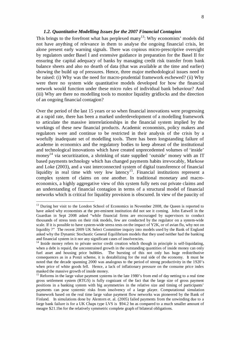
sector. Starting from August 07 to August 08 the CDS spreads of top US banks increased a hundred fold (the CDS spreads for Wachovia can be seen to be particularly high which led to a US Government forced takeover for it in December 2008 by Wells Fargo). In Figure 3.A, note also a second wave of spikes in April 2009 when Citigroup and Bank of America show great financial distress. The structural break post October 2008 marking a large upward jump in the sovereign CDS spreads and the increased correlations between the CDS spread of major banks that of their respective sovereigns has been recently analysed by Mathieu Gex of the Banque de France11. Non-bank corporate CDS and sovereign CDS have a less pronounced upward co-movement and they are less persistent than the relationship of the latter and CDS spreads of financials.
Figure 3. A Daily CDS Spreads for Major US Banks (1)
US B anks (1)
0
200
400
600
800
1000
1200
Ja
n 0
4M
ar 0
4Ju
n 0
4S
ep 0
4D
ec 0
4F
eb 0
5M
ay 0
5A
ug 0
5N
ov 0
5Ja
n 0
6A
pr 0
6Ju
l 06
Oct 0
6D
ec 0
6M
ar 0
7Ju
n 0
7S
ep 0
7N
ov 0
7F
eb 0
8M
ay 0
8A
ug 0
8O
ct 0
8Ja
n 0
9A
pr 0
9Ju
l 09
bp
J P Morgans
Goldma n
S a chs
Morgan
S ta nley
Merrill L ynch
Source: Datastream
Figure 3. B Daily CDS Spreads for Major US Banks (2)
US B anks (2)
0
200
400
600
800
1000
1200
1400
1600
J an
04
Mar 0
4J u
n 0
4S
ep 0
4D
ec 0
4F
eb 0
5M
ay 0
5A
ug 0
5N
ov 0
5J a
n 0
6A
pr 0
6J u
l 06
Oct 0
6D
ec 0
6M
ar 0
7J u
n 0
7S
ep 0
7N
ov 0
7F
eb 0
8M
ay 0
8A
ug 0
8O
ct 0
8J a
n 0
9A
pr 0
9J u
l 09
bp
Wa chovia
Wells F a rgo
C itigroup
B ank of
America
Source: Datastream
11 This was presented at the Aix en Provence GREQAM Summer School on Financial Market Micro Structure and Contagion 6- 10 July 2009.
7
Figure 3. C Daily CDS Spreads for Sovereigns
Sovereigns
0
50
100
150
200
250
Jan 0
4M
ar 04
Jun 0
4Sep
04
Dec 04
Feb 0
5M
ay 0
5Au
g 05N
ov 05
Jan 0
6Ap
r 06
Jul 0
6O
ct 06
Dec 06
Mar 0
7Ju
n 07
Sep 0
7N
ov 07
Feb 0
8M
ay 0
8Au
g 08O
ct 08
Jan 0
9Ap
r 09
Jul 0
9
bp
United
Kingdom
Germany
France
Italy
Japan
USA
Source: Datastream
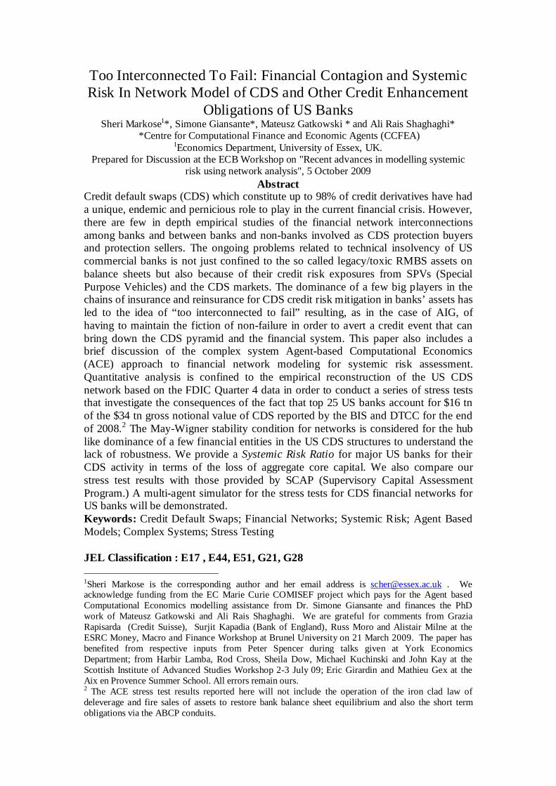
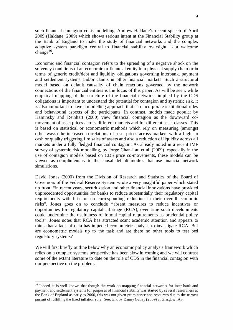
Figure 3. D Daily CDS Spreads for Monolines
Source: Datastream
Finally, Figure 3.D which shows the CDS spreads for the Monolines that were not fit for purpose to provide credit risk mitigants for bank assets in the period running up to the 2007 crisis and even continue to be so, a matter which will be emphasized in the stress tests conducted in this research. Indeed, a little known Monoline called ACA which failed to deliver on the CDS protection for RMBS held by Merrill Lynch is what led to its absorption by Bank of America12. Thus, many have acknowledged that CDS credit derivatives have had a unique, endemic and pernicious role to play in the current financial crisis crisis. However, few if any in depth empirical studies have been carried out to map the CDS financial network and the systemic risk implications of this.
12 Standard and Poor Report of August 2008 states that Merrill had CDS cover from Monolines to the tune of $18.8bn and of that ACA accounted for $5bn. ACA , 29% of which was owned by Bear Stearns, along with other Monolines suffered a ratings downgrade in early 2008 and ACA demised in 2008 defaulting on its CDS obligations. ACA had $69 bn of CDS obligations and only had $425 million worth of capital.
Monolines
0
2000
4000
6000
8000
10000
12000
14000
16000
18000
20000
Jan
04
Mar 0
4Ju
n 04
Sep
04D
ec 0
4Fe
b 05
May 05
Au
g 05
No
v 05
Jan
06
Ap
r 06Ju
l 06O
ct 06D
ec 0
6M
ar 07
Jun
07Se
p 07
No
v 07
Feb
08M
ay 08A
ug 0
8O
ct 08Ja
n 0
9A
pr 09
Jul 09
bp
AMBAC
ASSURANCE
FGIC
FINANCIAL
SECURITY
ASSURANCE
MBIA
INSURANCE
XL CAPITAL
ASSURANCE
BERKSHIRE
HATHAWAY
8
1.2. Quantitative Modelling Issues for the 2007 Financial Contagion This brings to the forefront what has perplexed many13: Why economists’ models did not have anything of relevance in them to analyse the ongoing financial crisis, let alone present early warning signals. There was copious micro-prescriptive oversight by regulators under Basel I and extensive guidance in preparation for the Basel II for ensuring the capital adequacy of banks by managing credit risk transfer from bank balance sheets and also no dearth of data (that was available at the time and earlier) showing the build up of pressures. Hence, three major methodological issues need to be raised: (i) Why was the need for macro-prudential framework eschewed? (ii) Why were there no system wide quantitative models developed for how the financial network would function under these micro rules of individual bank behaviour? And (iii) Why are there no modelling tools to monitor liquidity gridlocks and the direction of an ongoing financial contagion?
Over the period of the last 15 years or so when financial innovations were progressing at a rapid rate, there has been a marked underdevelopment of a modelling framework to articulate the massive interrelationships in the financial system implied by the workings of these new financial products. Academic economists, policy makers and regulators were and continue to be restricted in their analysis of the crisis by a woefully inadequate set of modelling tools. There has been longstanding failure of academe in economics and the regulatory bodies to keep abreast of the institutional and technological innovations which have created unprecedented volumes of ‘inside’ money14 via securitization, a shrinking of state supplied ‘outside’ money with an IT based payments technology which has changed payments habits irrevocably, Markose and Loke (2003), and a vast interconnected system of digital transference of financial liquidity in real time with very low latency15. Financial institutions represent a complex system of claims on one another. In traditional monetary and macro-economics, a highly aggregative view of this system fully nets out private claims and an understanding of financial contagion in terms of a structural model of financial networks which is critical for liquidity provision is obscured. In view of the paucity of 13 During her visit to the London School of Economics in November 2008, the Queen is reported to have asked why economists at the pre-eminent institution did not see it coming. John Eatwell in the Guardian in Sept 2008 asked “while financial firms are encouraged by supervisors to conduct thousands of stress tests on their risk models, few are conducted by the regulator on a system-wide scale. If it is possible to have system-wide stress tests on the impact of Y2K, or of avian flu, why not on liquidity ?” The recent 2009 UK Select Committee inquiry into models used by the Bank of England asked why the Dynamic Stochastic General Equilibrium models that they used neither had the banking and financial system in it nor any significant cases of insolvencies. 14 Inside money refers to private sector credit creation which though in principle is self-liquidating, when a debt is repaid, the unconstrained growth in the outstanding quantities of inside money can only fuel asset and housing price bubbles. The bursting of this not only has huge redistributive consequences as in a Ponzi scheme, it is destabilizing for the real side of the economy. It must be noted that the decade spanning 2000 was analogous to the period of strong productivity in the 1920’s when price of white goods fell. Hence, a lack of inflationary pressure on the consume price index masked the massive growth of inside money. 15 Reforms in the large value payment systems in the late 1980’s from end of day netting to a real time gross settlement system (RTGS) is fully cognizant of the fact that the large size of gross payment positions in a banking system with big asymmetries in the relative size and timing of participants’ payments can pose systemic risks from insolvency of a large player. Computational simulation framework based on the real time large value payment flow networks was pioneered by the Bank of Finland. In simulations done by Alentorn et. al. (2005) failed payments from the unwinding due to a large bank failure is for a UK Chaps type LVS is $94.2 bn as compared to a much smaller amount of meagre $21.1bn for the relatively symmetric complete graph of bilateral obligations.
9
such financial contagion crisis modelling, Andrew Haldane’s recent speech of April 2009 (Haldane, 2009) which shows serious intent at the Financial Stability group at the Bank of England to make the study of financial networks and the complex adaptive system paradigm central to financial stability oversight, is a welcome change16.
Economic and financial contagion refers to the spreading of a negative shock on the solvency conditions of an economic or financial entity in a physical supply chain or in terms of generic credit/debt and liquidity obligations governing interbank, payment and settlement systems and/or claims in other financial markets. Such a structural model based on default causality of chain reactions governed by the network connections of the financial entities is the focus of this paper. As will be seen, while empirical mapping of the structure of the financial networks implied by the CDS obligations is important to understand the potential for contagion and systemic risk, it is also important to have a modelling approach that can incorporate institutional rules and behavioural aspects of the participants. In contrast, models made popular by Kaminsky and Reinhart (2000) view financial contagion as the downward co-movement of asset prices across different markets and for different asset classes. This is based on statistical or econometric methods which rely on measuring (amongst other ways) the increased correlations of asset prices across markets with a flight to cash or quality triggering fire sales of assets and also a reduction of liquidity across all markets under a fully fledged financial contagion. As already noted in a recent IMF survey of systemic risk modelling, by Jorge Chan-Lau et al. (2009), especially in the use of contagion models based on CDS price co-movements, these models can be viewed as complimentary to the causal default models that use financial network simulations.
David Jones (2000) from the Division of Research and Statistics of the Board of Governors of the Federal Reserve System wrote a very insightful paper which stated up front: “in recent years, securitization and other financial innovations have provided unprecedented opportunities for banks to reduce substantially their regulatory capital requirements with little or no corresponding reduction in their overall economic risks”. Jones goes on to conclude “absent measures to reduce incentives or opportunities for regulatory capital arbitrage (RCA), over time such developments could undermine the usefulness of formal capital requirements as prudential policy tools”. Jones notes that RCA has attracted scant academic attention and appears to think that a lack of data has impeded econometric analysis to investigate RCA. But are econometric models up to the task and are there no other tools to test bed regulatory systems?
We will first briefly outline below why an economic policy analysis framework which relies on a complex systems perspective has been slow in coming and we will contrast some of the extant literature to date on the role of CDS in the financial contagion with our perspective on the problem.
16 Indeed, it is well known that though the work on mapping financial networks for inter-bank and payment and settlement systems for purposes of financial stability was started by several researchers at the Bank of England as early as 2000, this was not given prominence and resources due to the narrow pursuit of fulfilling the fixed inflation rule. See, talk by Danny Gabay (2009) at Glasgow IAS.
10
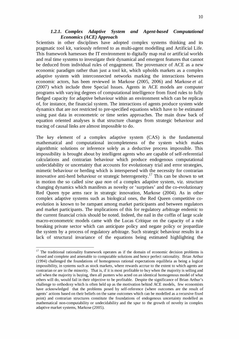
1.2.1. Complex Adaptive System and Agent-based Computational Economics (ACE) Approach
Scientists in other disciplines have adopted complex systems thinking and its pragmatic tool kit, variously referred to as multi-agent modelling and Artificial Life. This framework harnesses the IT environment to digitally map real or artificial worlds and real time systems to investigate their dynamical and emergent features that cannot be deduced from individual rules of engagement. The provenance of ACE as a new economic paradigm rather than just a tool kit, which upholds markets as a complex adaptive system with interconnected networks marking the interactions between economic actors, has been reviewed in Markose (2005, 2006) and Markose et al. (2007) which include three Special Issues. Agents in ACE models are computer programs with varying degrees of computational intelligence from fixed rules to fully fledged capacity for adaptive behaviour within an environment which can be replicas of, for instance, the financial system. The interactions of agents produce system wide dynamics that are not restricted to pre-specified equations which have to be estimated using past data in econometric or time series approaches. The main draw back of equation oriented analyses is that structure changes from strategic behaviour and tracing of causal links are almost impossible to do.
The key element of a complex adaptive system (CAS) is the fundamental mathematical and computational incompleteness of the system which makes algorithmic solutions or inference solely as a deductive process impossible. This impossibility is brought about by intelligent agents who are capable of self-referential calculations and contrarian behaviour which produce endogenous computational undecidability or uncertainty that accounts for evolutionary trial and error strategies, mimetic behaviour or herding which is interspersed with the necessity for contrarian innovative anti-herd behaviour or strategic heterogeneity.17 This can be shown to set in motion the so called sine qua non of a complex adaptive system, viz. structure changing dynamics which manifests as novelty or ‘surprises’ and the co-evolutionary Red Queen type arms race in strategic innovation, Markose (2004). As in other complex adaptive systems such as biological ones, the Red Queen competitive co-evolution is known to be rampant among market participants and between regulators and market participants. The implications of this for regulatory arbitrage endemic to the current financial crisis should be noted. Indeed, the nail in the coffin of large scale macro-econometric models came with the Lucas Critique on the capacity of a rule breaking private sector which can anticipate policy and negate policy or jeopardize the system by a process of regulatory arbitrage. Such strategic behaviour results in a lack of structural invariance of the equations being estimated highlighting the
17 The traditional rationality framework operates as if the domain of economic decision problems is closed and complete and amenable to computable solutions and hence perfect rationality. Brian Arthur (1994) challenged the foundations of homogenous rational expectations equilibria as being a logical impossibility, in systems such as stock markets, where rewards accrue to the extent to which agents are contrarian or are in the minority. That is, if it is most profitable to buy when the majority is selling and sell when the majority is buying, then all punters who acted on an identical homogenous model of what others will do, would fail in their objective to be profitable. Despite the significance of Brian Arthur’s challenge to orthodoxy which is often held up as the motivation behind ACE models, few economists have acknowledged that the problems posed by self-reference (where outcomes are the result of agents’ actions based on their beliefs on the same outcomes which can be modelled as a recursive fixed point) and contrarian structures constitute the foundations of endogenous uncertainty modelled as mathematical non-computability or undecidability and the spur to the growth of novelty in complex adaptive market systems, Markose (2005).
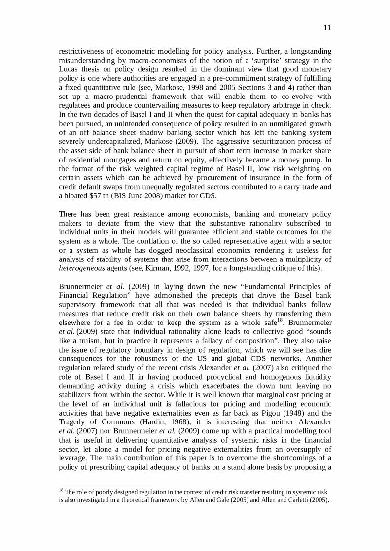
11
restrictiveness of econometric modelling for policy analysis. Further, a longstanding misunderstanding by macro-economists of the notion of a ‘surprise’ strategy in the Lucas thesis on policy design resulted in the dominant view that good monetary policy is one where authorities are engaged in a pre-commitment strategy of fulfilling a fixed quantitative rule (see, Markose, 1998 and 2005 Sections 3 and 4) rather than set up a macro-prudential framework that will enable them to co-evolve with regulatees and produce countervailing measures to keep regulatory arbitrage in check. In the two decades of Basel I and II when the quest for capital adequacy in banks has been pursued, an unintended consequence of policy resulted in an unmitigated growth of an off balance sheet shadow banking sector which has left the banking system severely undercapitalized, Markose (2009). The aggressive securitization process of the asset side of bank balance sheet in pursuit of short term increase in market share of residential mortgages and return on equity, effectively became a money pump. In the format of the risk weighted capital regime of Basel II, low risk weighting on certain assets which can be achieved by procurement of insurance in the form of credit default swaps from unequally regulated sectors contributed to a carry trade and a bloated $57 tn (BIS June 2008) market for CDS.
There has been great resistance among economists, banking and monetary policy makers to deviate from the view that the substantive rationality subscribed to individual units in their models will guarantee efficient and stable outcomes for the system as a whole. The conflation of the so called representative agent with a sector or a system as whole has dogged neoclassical economics rendering it useless for analysis of stability of systems that arise from interactions between a multiplicity of heterogeneous agents (see, Kirman, 1992, 1997, for a longstanding critique of this).
Brunnermeier et al. (2009) in laying down the new “Fundamental Principles of Financial Regulation” have admonished the precepts that drove the Basel bank supervisory framework that all that was needed is that individual banks follow measures that reduce credit risk on their own balance sheets by transferring them elsewhere for a fee in order to keep the system as a whole safe18. Brunnermeier et al. (2009) state that individual rationality alone leads to collective good “sounds like a truism, but in practice it represents a fallacy of composition”. They also raise the issue of regulatory boundary in design of regulation, which we will see has dire consequences for the robustness of the US and global CDS networks. Another regulation related study of the recent crisis Alexander et al. (2007) also critiqued the role of Basel I and II in having produced procyclical and homogenous liquidity demanding activity during a crisis which exacerbates the down turn leaving no stabilizers from within the sector. While it is well known that marginal cost pricing at the level of an individual unit is fallacious for pricing and modelling economic activities that have negative externalities even as far back as Pigou (1948) and the Tragedy of Commons (Hardin, 1968), it is interesting that neither Alexander et al. (2007) nor Brunnermeier et al. (2009) come up with a practical modelling tool that is useful in delivering quantitative analysis of systemic risks in the financial sector, let alone a model for pricing negative externalities from an oversupply of leverage. The main contribution of this paper is to overcome the shortcomings of a policy of prescribing capital adequacy of banks on a stand alone basis by proposing a
18 The role of poorly designed regulation in the context of credit risk transfer resulting in systemic risk is also investigated in a theoretical framework by Allen and Gale (2005) and Allen and Carletti (2005).
12
framework where the network connectivity and propensity to spread contagion from specific rather than generic properties of credit risk mitigants is considered. Our proposed systemic risk ratio for each bank solely for the CDS market is based on the proportionate loss of collective Tier 1 core capital of all the bank participants of this market from the demise of the trigger bank This will be done using an empirically reconstructed network structure of CDS obligations of US banks. Assumptions about netting of mutual obligations vis-à-vis the trigger bank and also various levels of exposure relative to core capital of banks will be made. The specific structural aspects of CDS obligations that have the potential to spread contagion that needs to be incorporated will be discussed.
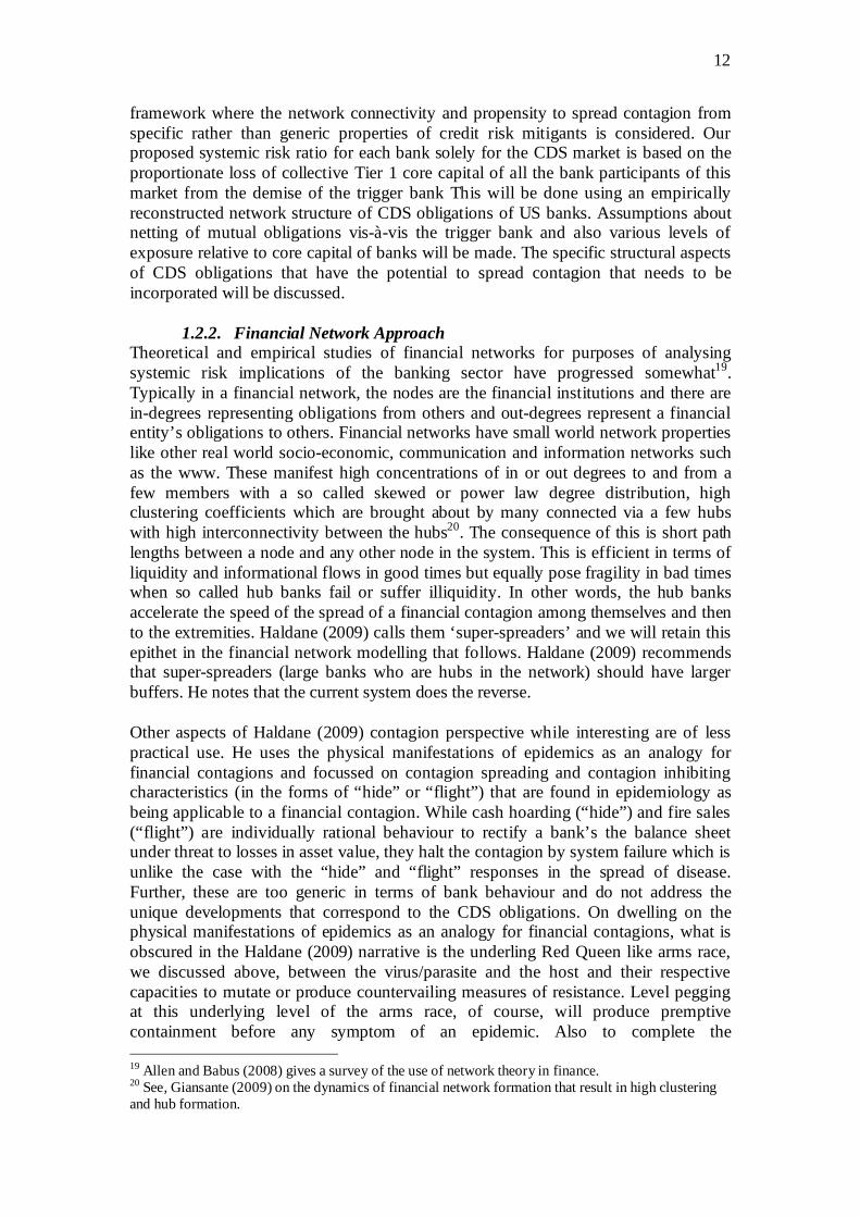
1.2.2. Financial Network Approach Theoretical and empirical studies of financial networks for purposes of analysing systemic risk implications of the banking sector have progressed somewhat19. Typically in a financial network, the nodes are the financial institutions and there are in-degrees representing obligations from others and out-degrees represent a financial entity’s obligations to others. Financial networks have small world network properties like other real world socio-economic, communication and information networks such as the www. These manifest high concentrations of in or out degrees to and from a few members with a so called skewed or power law degree distribution, high clustering coefficients which are brought about by many connected via a few hubs with high interconnectivity between the hubs20. The consequence of this is short path lengths between a node and any other node in the system. This is efficient in terms of liquidity and informational flows in good times but equally pose fragility in bad times when so called hub banks fail or suffer illiquidity. In other words, the hub banks accelerate the speed of the spread of a financial contagion among themselves and then to the extremities. Haldane (2009) calls them ‘super-spreaders’ and we will retain this epithet in the financial network modelling that follows. Haldane (2009) recommends that super-spreaders (large banks who are hubs in the network) should have larger buffers. He notes that the current system does the reverse.
Other aspects of Haldane (2009) contagion perspective while interesting are of less practical use. He uses the physical manifestations of epidemics as an analogy for financial contagions and focussed on contagion spreading and contagion inhibiting characteristics (in the forms of “hide” or “flight”) that are found in epidemiology as being applicable to a financial contagion. While cash hoarding (“hide”) and fire sales (“flight”) are individually rational behaviour to rectify a bank’s the balance sheet under threat to losses in asset value, they halt the contagion by system failure which is unlike the case with the “hide” and “flight” responses in the spread of disease. Further, these are too generic in terms of bank behaviour and do not address the unique developments that correspond to the CDS obligations. On dwelling on the physical manifestations of epidemics as an analogy for financial contagions, what is obscured in the Haldane (2009) narrative is the underling Red Queen like arms race, we discussed above, between the virus/parasite and the host and their respective capacities to mutate or produce countervailing measures of resistance. Level pegging at this underlying level of the arms race, of course, will produce premptive containment before any symptom of an epidemic. Also to complete the 19 Allen and Babus (2008) gives a survey of the use of network theory in finance. 20 See, Giansante (2009) on the dynamics of financial network formation that result in high clustering and hub formation.
13
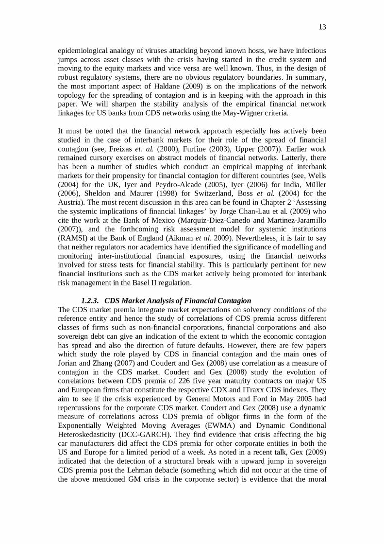
epidemiological analogy of viruses attacking beyond known hosts, we have infectious jumps across asset classes with the crisis having started in the credit system and moving to the equity markets and vice versa are well known. Thus, in the design of robust regulatory systems, there are no obvious regulatory boundaries. In summary, the most important aspect of Haldane (2009) is on the implications of the network topology for the spreading of contagion and is in keeping with the approach in this paper. We will sharpen the stability analysis of the empirical financial network linkages for US banks from CDS networks using the May-Wigner criteria.
It must be noted that the financial network approach especially has actively been studied in the case of interbank markets for their role of the spread of financial contagion (see, Freixas et. al. (2000), Furfine (2003), Upper (2007)). Earlier work remained cursory exercises on abstract models of financial networks. Latterly, there has been a number of studies which conduct an empirical mapping of interbank markets for their propensity for financial contagion for different countries (see, Wells (2004) for the UK, Iyer and Peydro-Alcade (2005), Iyer (2006) for India, Müller (2006), Sheldon and Maurer (1998) for Switzerland, Boss et al. (2004) for the Austria). The most recent discussion in this area can be found in Chapter 2 ‘Assessing the systemic implications of financial linkages’ by Jorge Chan-Lau et al. (2009) who cite the work at the Bank of Mexico (Marquiz-Diez-Canedo and Martinez-Jaramillo (2007)), and the forthcoming risk assessment model for systemic institutions (RAMSI) at the Bank of England (Aikman et al. 2009). Nevertheless, it is fair to say that neither regulators nor academics have identified the significance of modelling and monitoring inter-institutional financial exposures, using the financial networks involved for stress tests for financial stability. This is particularly pertinent for new financial institutions such as the CDS market actively being promoted for interbank risk management in the Basel II regulation.
1.2.3. CDS Market Analysis of Financial Contagion The CDS market premia integrate market expectations on solvency conditions of the reference entity and hence the study of correlations of CDS premia across different classes of firms such as non-financial corporations, financial corporations and also sovereign debt can give an indication of the extent to which the economic contagion has spread and also the direction of future defaults. However, there are few papers which study the role played by CDS in financial contagion and the main ones of Jorian and Zhang (2007) and Coudert and Gex (2008) use correlation as a measure of contagion in the CDS market. Coudert and Gex (2008) study the evolution of correlations between CDS premia of 226 five year maturity contracts on major US and European firms that constitute the respective CDX and ITraxx CDS indexes. They aim to see if the crisis experienced by General Motors and Ford in May 2005 had repercussions for the corporate CDS market. Coudert and Gex (2008) use a dynamic measure of correlations across CDS premia of obligor firms in the form of the Exponentially Weighted Moving Averages (EWMA) and Dynamic Conditional Heteroskedasticity (DCC-GARCH). They find evidence that crisis affecting the big car manufacturers did affect the CDS premia for other corporate entities in both the US and Europe for a limited period of a week. As noted in a recent talk, Gex (2009) indicated that the detection of a structural break with a upward jump in sovereign CDS premia post the Lehman debacle (something which did not occur at the time of the above mentioned GM crisis in the corporate sector) is evidence that the moral
14
hazard costs of tax payer bailouts of the financial sector has now transferred in a persistent way to sovereign risk.
The distress dependence approach (Chan-Lau et al (2009)) and the distress intensity matrix approach (Giesecke and Kim (2009)) are also noteworthy as important complimentary means of monitoring the direction in which a financial contagion is likely to spread.
Econometric model of CDS use by US banks by Minton et. al (2005) covers the period of 1999 to 2003. They regress CDS (buy/sell) on a number of bank balance sheet items. Econometric analysis is hampered by a lack of enough time series data. They conclude that banks that are net protection buyers are also likely to engage in asset securitization, originate foreign loans and have lower capital ratios. However, structural systemic risk implications are hard to assess within such econometric models.
The full structural mapping of the network interrelationships between banks in terms of their balance sheet and off balance sheet activities would need ACE type modelling especially to bring about the endogenous dynamic network link attachment and breaking that characterizes the different phases of boom and bust cycle. The dynamic changes in interlinkages signalling successful or failed payments and the dynamic matrix thereof is an essential part of estimating bank failure from contagion arising from an initial trigger event. Ball park figures of net core capital losses for each financial institution involved can be obtained for different scenarios. In contrast, the complementary approaches to assessing systemic risk discussed by Jorge Chan-Lau et al (2009) such as the co-risk model (Adrian and Bunnermeier (2008)), the distress dependence approach (Chan-Lau et al (2009)) and the distress intensity matrix approach (Giesecke and Kim (2009)) while useful in a diagnostic way have the disadvantages of reduced form models. That is, unravelling and changed behaviour of institutions under stress which set in motion non-linear negative feedback loops are impossible to track in frameworks other than an ACE one.
In the context of needing to monitor the financial sector for systemic risk implications on an on going basis, without a multi-agent simulation framework capable of digitally recording fine grained data bases of the different financial players involved and also mapping the links between sectors, we are condemned to sector by sector analysis or a simplistic modelling of interrelations between sectors often assumed for analytical tractability. The empirical mapping of the US CDS obligation in CDS banks undertaken in this paper is part of a larger EC COMISEF project which is concerned with developing a multi-agent based computational economics (ACE) framework that can articulate and demonstrate the interrelationships of the financial contagion with a view to aid policy analysis.
1.3. Structure of the paper The rest of the paper is organized as follows. In Sections 2.1, 2.2 and 2.3, the structure, scale and scope of the CDS market in the 2007/8 crisis will be discussed with the view to inform us of the challenges involved in the design of regulatory framework that can prevent system failure from credit risk transfer. In Section 2.4, some issues relating to the recent SCAP (Supervisory Capital Assessment Program) will be covered in order that some comparisons can be made between the stress tests
15
results specific to the CDS and CRT specific network topology driven contagion and other estimates of bank losses. Section 3.1 gives a short technical note on network statistics and contrast between small world networks and other graphs. The May-Wigner stability condition for networks is briefly discussed for the hub like dominance of a few financial entities in the US CDS structures to understand the lack of robustness. In Section 3.2, we set out the empirical reconstruction of the US CDS network based on the FDIC 2008 Quarter 4 data in order to conduct a series of stress tests to investigate the consequences of the fact that top 25 US banks account for $16 tn of the $34 tn gross notional value of CDS reported by the BIS and DTCC for the end of 2008. In Section 4 the financial stability implications of the financial network CDS linkages of banks are analyzed under different stress conditions. The trigger events include the demise of a US commercial bank (3 biggest, 1 medium sized and 1 small cap), and also of non-bank net protection sellers such as the Monolines. In addition to the normal weakness of bank balance sheets during times of recessions with growing charge offs on bank loans, explicit account of US bank exposure to credit enhancements of equity tranche of ABS CMOs and CDOs in less than bankruptcy remote SPVs and failed CDS protection arrangements will also be given. Section 5 gives concluding remarks and an outline for future work.
2. Challenges for Modelling a Regulatory Framework for CDS 2.1. CDS Structure, Obligations, Offset and Counterparty Risk
Here we give the salient structural aspects of the CDS market with the view to see how strategic aspects of participants in the market may jeopardize the objectives of the market in terms to providing protection against default risk of debt obligations in the system. Other objectives that has been claimed for CDS is the support it gives for raising capital and for economizing on capital. The latter role that CDS played in Basel II synthetic collateralized debt obligation (S-CDOs) based on receivables from pools of mortgages and their credit risk transfer from bank sheet to minimize capital requirements will be discussed to explain the increased involvement of top US banks in the CDO based CDS market.
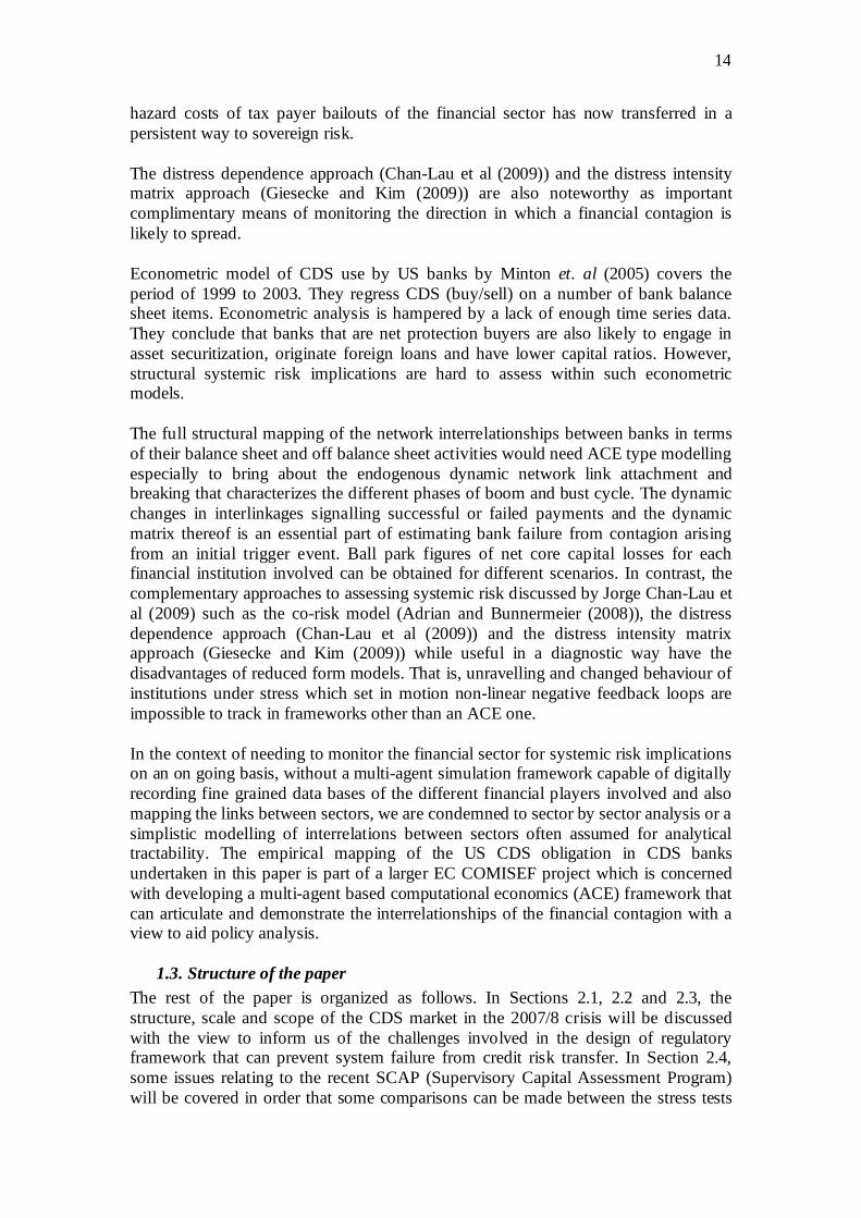
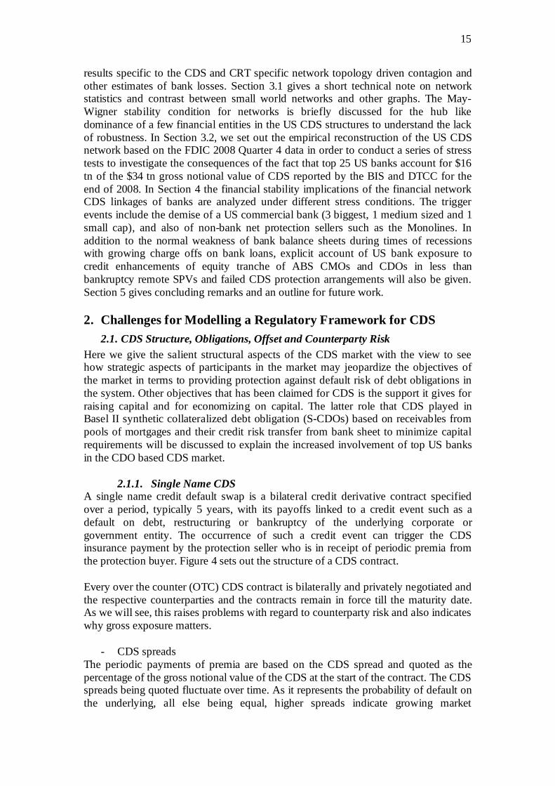
2.1.1. Single Name CDS A single name credit default swap is a bilateral credit derivative contract specified over a period, typically 5 years, with its payoffs linked to a credit event such as a default on debt, restructuring or bankruptcy of the underlying corporate or government entity. The occurrence of such a credit event can trigger the CDS insurance payment by the protection seller who is in receipt of periodic premia from the protection buyer. Figure 4 sets out the structure of a CDS contract.
Every over the counter (OTC) CDS contract is bilaterally and privately negotiated and the respective counterparties and the contracts remain in force till the maturity date. As we will see, this raises problems with regard to counterparty risk and also indicates why gross exposure matters.
- CDS spreads The periodic payments of premia are based on the CDS spread and quoted as the percentage of the gross notional value of the CDS at the start of the contract. The CDS spreads being quoted fluctuate over time. As it represents the probability of default on the underlying, all else being equal, higher spreads indicate growing market
16
expectations of the default on the debt with a jump to default spike at the time of the default event. The spreads are known to have strong self-reflexive properties in that they do not merely reflect the financial state of the underlying obligor, they can in turn accelerate the default event as ratings downgrade follow, cost of capital rises and stock market valuation falls for the obligor as the CDS spreads on them increase.
Figure 4 Credit Default Swap Structure (CDS) and Bear Raids
Note: Direction of CDS sale or cover is the unbroken arrow.
- The CDS Settlement Price
The default event can result in either a physical or cash settlement. For physical settlement, the protection buyer has to present the underlying debt and the protection seller has to pay at par (full face value). In cash settlement, the CDS buyer will receive face value of the debt of the reference entity less the market value for the recovery rate of the defaulted debt at the point of the credit event. A settlement auction is conducted by the International Swaps and Derivatives Association (ISDA) where participants submit bids and offers for the reference entity’s debt obligations and a final price is set for all cash and physical settlement. Note, the cost to the CDS seller to do a cash or physical settlement is the same per dollar of cover, i.e. 100(1-R), where R is the final settlement price given as a percentage of the par value of defaulted reference entity bonds.
2.1.2. Potential Perverse Incentives, Offset and Counterparty risk The controversial aspect about a CDS that makes the analogy with an insurance contract of limited use is that the buyer of a CDS need not own any underlying security or have any credit exposure to the reference entity that needs to be hedged. The so called naked CDS buy position is therefore a speculative one undertaken for
Default
Protection from
CDS Buyer, B
Default Protection
Seller, C
“INSURER”
(AIG)
Reference Entity
A (Bond Issuer)
or CDOs
Payment in case of Default of
X= 100 (1-R)
A “LENDS” to
Reference
Entity
Premium in bps
Recovery rate, R, is the ratio of
the value of the bond issued by
reference entity immediately
after default to the face value of
the bond
B sells CDS to D
Buyer D„Naked CDS” 3rd party D
receives
insurance when A
defaults; B still owns A’s
Bonds and D does not !
Default
Protection from
CDS Buyer, B
Default
Protection from
CDS Buyer, B
Default Protection
Seller, C
“INSURER”
(AIG)
Default Protection
Seller, C
“INSURER”
(AIG)
Reference Entity
A (Bond Issuer)
or CDOs
Payment in case of Default of
X= 100 (1-R)
A “LENDS” to
Reference
Entity
Premium in bps
Recovery rate, R, is the ratio of
the value of the bond issued by
reference entity immediately
after default to the face value of
the bond
B sells CDS to D
Buyer D„Naked CDS” 3rd party D
receives
insurance when A
defaults; B still owns A’s
Bonds and D does not !
Buyer D„Naked CDS” 3rd party D
receives
insurance when A
defaults; B still owns A’s
Bonds and D does not !
17
pecuniary gain from either the full cash settlement in the event of a default or a chance to offset the CDS purchase with a sale at an improved CDS spread. This implies that gross CDS notional values can be several (5-10) multiples of the underlying value of the debt obligations of the reference entity. It has been widely noted that naked CDS buyers with no insurable interest will gain considerably from the bankruptcy of the reference entity. Note the bear raid in Figure 4 refers to the possibility that when the CDS protection cover on a reference entity has been sold on to a third party, here D, who does not own the bonds of the reference entity, D has an incentive to short the stock of the reference entity to trigger its insolvency in order to collect the insurance to be paid up on the CDS. A short squeeze can be put on the bonds by naked CDS buyers so as to maximize payouts when the reference entity defaults. However, shorting bonds is harder to do than shorting stock of the reference entity. It is the case that even those CDS buyers who have exposure to the default risk on the debt of the reference entity may, after a point, find it more lucrative to cash in on the protection payment on the CDS with the bankruptcy of the reference entity rather than continue holding its debt21.
CDS protection sellers, if not part of the regulated banking sector, unlike the insurance market, need not have to hold reserves to make the pay offs in case of a credit event. Note, that there are capital requirements for banks that sell CDS. A CDS seller uses strategies relating to derivatives markets rather than standard insurance markets to make provision for potential payouts. Main CDS dealers have been known (as was the case with AIG) not to post initial collateral and only post mark to market variation margin which in a jump to default style dynamics for the CDS spread can imply abrupt jumps in additional collateral needed. Those CDS contracts operating on the ISDA (International Swaps and Derivatives Association) rules also have a provision of cross-default. If a counterparty cannot post collateral in a specified time frame, it can deem to have defaulted and if the shortfall of collateral exceeds a threshold, the counterparty is deemed to have defaulted across other ISDA CDS. These cross-defaults (a potential situation that AIG was in) can trigger a domino effect.
The other strategy adopted by CDS dealers and counterparties is a practice called “offsets” which though individually rational may collectively contribute to systemic risk as the chains of CDS obligations increase and also merge. Offsets can generate revenue for parties from premia as well as reduce their final payouts. In the above Figure 4, B having bought CDS cover from C, finds that the spreads have increased and may chose to eschew its hedge on the bonds of the reference entity A to earn the difference between the premia it pays to C and the higher premia it can now charge by an offset sale of CDS to D. This is marked by the brown arrows in Figure 4. In this system the ultimate beneficiary of CDS cover in case of default of reference entity A is the speculative party D. Note C has an absolute obligation to settle on $10 mn in order that B’s obligations net to zero.
21 Gillian Tett (FT, May 1 2009) suggests that the Morgan Stanley which has lent considerable sums to BTA, the largest bank in Kazakhstan, was keen to pull the plug on BTA for the reason that the CDS protection cover that it had taken out on BTA can then be triggered. Note Morgan Stanley was hedging its credit risk and the pure profiteering component of a naked CDS position is not involved here.
18
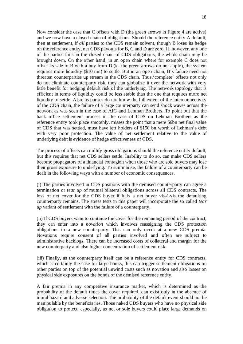
Now consider the case that C offsets with D (the green arrows in Figure 4 are active) and we now have a closed chain of obligations. Should the reference entity A default, then at settlement, if all parties to the CDS remain solvent, though B loses its hedge on the reference entity, net CDS payouts for B, C and D are zero. If, however, any one of the parties fails in the closed chain of CDS obligations, the whole chain may be brought down. On the other hand, in an open chain where for example C does not offset its sale to B with a buy from D (ie. the green arrows do not apply), the system requires more liquidity ($10 mn) to settle. But in an open chain, B’s failure need not threaten counterparties up stream in the CDS chain. Thus,‘complete’ offsets not only do not eliminate counterparty risk, they can globalize it over the network with very little benefit for hedging default risk of the underlying. The network topology that is efficient in terms of liquidity could be less stable than the one that requires more net liquidity to settle. Also, as parties do not know the full extent of the interconnectivity of the CDS chain, the failure of a large counterparty can send shock waves across the network as was seen in the case of AIG and Lehman Brothers. To point out that the back office settlement process in the case of CDS on Lehman Brothers as the reference entity took place smoothly, misses the point that a mere $6bn net final value of CDS that was settled, must have left holders of $150 bn worth of Lehman’s debt with very poor protection. The value of net settlement relative to the value of underlying debt is evidence of hedge effectiveness of CDS.
The process of offsets can nullify gross obligations should the reference entity default, but this requires that net CDS sellers settle. Inability to do so, can make CDS sellers become propagators of a financial contagion when those who are sole buyers may lose their gross exposure to underlying. To summarise, the failure of a counterparty can be dealt in the following ways with a number of economic consequences.
(i) The parties involved in CDS positions with the demised counterparty can agree a termination or tear up of mutual bilateral obligations across all CDS contracts. The loss of net cover for the CDS buyer if it is a net buyer vis-à-vis the defaulting counterparty remains. The stress tests in this paper will incorporate the so called tear up variant of settlement with the failure of a counterparty.
(ii) If CDS buyers want to continue the cover for the remaining period of the contract, they can enter into a novation which involves reassigning the CDS protection obligations to a new counterparty. This can only occur at a new CDS premia. Novations require consent of all parties involved and often are subject to administrative backlogs. There can be increased costs of collateral and margin for the new counterparty and also higher concentration of settlement risk.
(iii) Finally, as the counterparty itself can be a reference entity for CDS contracts, which is certainly the case for large banks, this can trigger settlement obligations on other parties on top of the potential unwind costs such as novation and also losses on physical side exposures on the bonds of the demised reference entity.
A fair premia in any competitive insurance market, which is determined as the probability of the default times the cover required, can exist only in the absence of moral hazard and adverse selection. The probability of the default event should not be manipulable by the beneficiaries. Those naked CDS buyers who have no physical side obligation to protect, especially, as net or sole buyers could place large demands on
19
the liquidity of the system at settlement. Adverse selection exists in an unregulated CDS market, if the net CDS sellers are those who have insufficient reserves to meet obligations at settlement. As we will see in the next section, due to low capital costs involved in the case of unregulated credit protection sellers, an oversupply of CDS insurance with low spreads put in place a carry trade which further increased the liquidity available to banks for bank lending and to securitize even poor quality subprime loans without the necessary capital either at an individual or collective level of the financial system.
2.2. The Basel II Risk Capital and Credit Risk Transfer (CRT)Rules Under Basel I since 1988, a standard 8% regulatory capital requirement applied to banks irrespective of the economic default risk of the debt instruments being held by banks. This led to two main outcomes. Firstly, remote SPV sale of RMBS mortgages and receivables from other loans which brought about the saving (of .08 x .5) of capital charge22 was primarily a regulatory arbitrage activity. The gains from additional loans made from the capital so released had to be offset against the cost of remote securitization. In retrospect, much of this aggressive lending from securitization far from being profitable turned out to be a financial disaster, something that can be seen only in a multi-period model, Markose and Dong (2004). They show that the very high percentage of RMBS (such as up to 50% in entities such as Washington Mutual) that was securitized could only have been possible due to the underpricing of the coupon on RMBS and the cost of credit enhancements. Secondly, there is also evidence of balance sheet asset quality deterioration, as it is cheaper to remotely securitize better quality assets and toxic assets began to be retained on the balance sheet (see Davidson et al., 2003: 294-297).
A combination of factors set in motion an extraordinary explosion of CDS activity by banks by 2004 in anticipation of the Ratings Based Assessment (RBA) of capital for banks. It is important to note that unlike remote SPV sales of RMBS, it is far from the case that synthetic securitization and CDS activity of banks was to escape capital regulation. Indeed, as seen from documents such as the Federal Reserve Board Basel II Capital Accord Notice of Proposed Rulemaking (NPR) and supporting Documents (2006)23, a step by step guide is given for permissibility of the ratings based assessment (RBA) for risk capital in banks. Part V Sections 7 and 43 on synthetic securitization holds up as best practice in banks on how to reduce risk based capital requirements encouraged the use of three features that mark this current crisis24. There was encouragement to use external ratings by so called Nationally
22 Capital charge is obtained by multiplying the risk weight with the 8% reserve requirement. Appendix 2 sets out the risk weights under Basel I and the more discriminating risk weights for different categories of rating for securitized assets under Basel II. 23 Fed Reserve Board Basel II Capital Accord Notice of Proposed Rulemaking (NPR) and Supporting Board Documents Draft Basel II NPR - Proposed Regulatory Text - Part V Risk-Weighted Assets for Securitization Exposures March 30, 2006 http://www.federalreserve.gov/GeneralInfo/basel2/DraftNPR/NPR/part_5.htm See also Federal Register Vol. 71, No. 247, Dec 2006, Proposed Rules and Basle Committee for Banking Supervision. Less prescriptive discussions on relationship between Basel II CRT and CDS and CDOs can be found in Anson et. al.(2004), Deacon (2003). 24 Another feature, viz. the use of VaR models to estimate risk capital to be held by banks will not be discussed here. The dangers of historically based simulations for VaR rather than the use of option market implied measures that have the capacity to pick up on extreme market events have been discussed in Markose and Alentorn (2007).
20
Recognized Statistical Rating Organization (NRSRO) agencies so that securitizations can be retained on the bank own balance sheet with reduced risk capital requirements. The mainstay of the ratings based assessment of risk in banks is to assign the risk weight for claims against a obligor or reference assets according to (i) the credit rating of obligors or the reference assets given by at least two external ratings given by NRSRO , or (ii) the credit ratings of the credit risk protection providers. The practice that bank balance sheet items can assume the risk weight of the rating of the protection provider brought about a complex system by which ratings replaced actual reserves of the system.
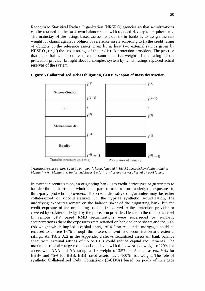
Figure 5 Collateralized Debt Obligation, CDO: Weapon of mass destruction
Tranche structure at time t0; at time t1, pool’s losses (shaded in black) absorbed by Equity tranche; Mezzanine Jr., Mezzanine, Senior and Super-Senior tranches are not yet affected by pool losses.
In synthetic securitization, an originating bank uses credit derivatives or guarantees to transfer the credit risk, in whole or in part, of one or more underlying exposures to third-party protection providers. The credit derivative or guarantee may be either collateralized or uncollateralized. In the typical synthetic securitization, the underlying exposures remain on the balance sheet of the originating bank, but the credit exposure of the originating bank is transferred to the protection provider or covered by collateral pledged by the protection provider. Hence, in the run up to Basel II, remote SPV based RMB securitizations were superseded by synthetic securitizations where the exposures were retained on bank balance sheets and the 50% risk weight which implied a capital charge of 4% on residential mortgages could be reduced to a mere 1.6% through the process of synthetic securitization and external ratings. As Table A.2 in the Appendix 2 shows securitized assets on bank balance sheet with external ratings of up to BBB could reduce capital requirements. The maximum capital charge reduction is achieved with the lowest risk weight of 20% for assets with AAA and AA rating, a risk weight of 35% for A rated assets, 50% for BBB+ and 75% for BBB. BBB- rated assets has a 100% risk weight. The role of synthetic Collateralized Debt Obligations (S-CDOs) based on pools of mortgage
21
backed securities as an underlying came about by the tie up with CDS cover for the tranche default of the CDO. Figure 5 gives the so called waterfall tranche structure of a CDO whereby junior tranches bear the brunt of or initial losses in the pool of underlying assets, leaving senior tranches with a much reduced default rate.
The Federal Reserve Board Basel II Capital Accord Notice of Proposed Rulemaking (NPR) and supporting Documents (2006) also gives encouragement as best practice of the use of multi-name CDO type securitizations which are prone to correlated risks rather than single name credit derivatives. This is evident in the so called effective N number of exposures: the risk weights for securitizations backed by exposures fewer than 6 are higher (at 20%) than for those that had 6 or more (at 7% - 12%).
Finally, the particular paragraphs below bear scrutiny as they encourage banks to maintain the fiction of no ex ante inclusion of provisions for an increase in bad state contingent cost of risk due to growth of counterparty risk or deterioration in the value of collateral which leads to increased costs in the use of credit derivatives.
Section 41 Paragraph (b) (2) of the NPR states that banks seeking risk capital reduction using third party risk cover should not have that the terms and conditions in the credit risk mitigants25 which imply the following:
(i) Allow for the termination of the credit protection due to deterioration in the credit quality of the underlying exposures;
(ii) Require the bank to alter or replace the underlying exposures to improve the credit quality of the pool of underlying exposures;
(iii) Increase the bank’s cost of credit protection in response to deterioration in the credit quality of the underlying exposures;
(iv) Increase the yield payable to parties other than the bank in response to a deterioration in the credit quality of the underlying exposures; or
(v) Provide for increases in a retained first loss position or credit enhancement provided by the bank after the inception of the securitization.
Not only is this premise of an unconditional guarantee a patently false one in theory, but also when such a bad state occurs, banks have to increase their risk capital after the event, in practice. A ratings down grade of the reference assets requires increased collateral from the CDS protection seller and possibly ratings downgrades on the CDS seller itself which leads to the CDS buyer having to make good the reserves to the tune of the ratings downgrade26. These increased demands for liquidity are highly
25 The credit risk mitigant is financial collateral, an eligible credit derivative from an eligible securitization guarantor, or an eligible guarantee from an eligible securitization guarantor. 26 Consider a down grade of an AAA rating to say BBB implies increased capital requirements of at least 4.4% is needed. This is determined by having to replace the low capital charge of 1.6% for the AAA rating (0.08x 0.2) with the new capital charge of 6% for the BBB (0.08 x 0.75). If the asset reaches junk status, the increased capital charge will be 6.4 %. The saga of how AIG was killed by collateral calls on its CDS guarantees (which included guarantees on $80 bn multi-sector loan backed CDOs) is given by Mollenkamp et. al. (2008). They also state how the Gary Gorton model of AIG
22
proclycical and is clearly an important ingredient of contagion producing propensity of the CDS financial network. It is conceivable that the unrealistic fiction to vitiate any conditionality of the credit risk mitigant provided by third parties, may be part of the reason why Basel II micro-regulators overlooked the need to subject their proposals to stress tests for their robustness.
In summary, the Basel II regulation is akin to gaolers who give prisoners the keys to the goal in order that they make a successful get away. Clear step by step guide has been given on the ‘best practice’ on how to reduce risk capital by using the services of credit risk protection issued by institutions not wholly within the regulated sector. A chronic underpricing of credit risk became endemic in the system as seemingly competitive low CDS spreads could be provided by the unregulated participants to the CDS based credit risk transfer scheme.
2.2.1 The mechanics of the CDS carry trade A fully fledged agent based model of bank behaviour following the above regulatory injunctions should incorporate the dynamics of a CDS carry trade that developed in 2004-2007. For sake of completeness this is discussed here, though it will not feature in the stress test results of this draft of the paper. Let ε and θi , respectively, denote the 8% regulatory capital requirement and the θi risk weight (see, Appendix 2) on the asset commensurate with its credit risk mitigant. The savings in risk capital is given by ε(1− θi) and if the credit risk mitigant is issued by an AAA rated company in the form of a CDS cover, which was the major instrument used, the maximum savings in risk capital that could be achieved is by reducing capital charge from 8% to 1.6%.
ε (1−θi) (FVtA) > λt FVt
A
FV: Face Value of the Asset. λt: CDS spread θi : Risk weight
In general, banks’ propensity to become CDS protection buyers in a carry trade is governed by the extent to which the saving in risk capital is greater than the cost of the credit risk mitigant which can be proxied by the CDS spread on the appropriately rated tranche. The CDS market due to mispricing presented banks with further incentives in the form of large leverage opportunities that has been called the negative basis carry trade from CDS.
In principle, a perfect hedge can be achieved between a bond of a given maturity and a CDS of the same maturity. Denoting the yield on the bond by yt and the CDS spread as λt, on purchasing a bond and its matching CDS, a hedger can lock in the risk free rate, rt . In the period, such as in 2006, when interest rates were low (3%), the S-CDO yields (about 10% for the mezzanine tranche) were high and the CDS spread low, we have :
yt - γt > rt .
exposures on their CDS positions failed to flag out the collateral calls that came thick and fast from AIG’s counterparties in 2008.
23
This fuelled a CDS carry trade. Consider a loan of a $1m at 3% interest which costs $30,000. This $1m loan is used to purchase a CDO which generates $100,000 gross return on $1m. The CDS spread at a low rate of 50 basis points (0.5 %) implies costs of $5000 per annum. Note the loan of $1m invested in CDO and a CDS nets a risk free ‘carry’ of $65,000 that is gained from the CDO yield of $100,000 less the interest rate and CDS spread costs which total $35,000. The $65,000 carry will enable further self-financed leverage where the CDO and CDS are used as collateral to borrow a further $2.16 m which in turn will cost approximately $75,600. The leveraged $2.16m if invested in more CDOs at a yield of 10%, we have another round of carry equal to $140,400 27which is obtained by the deducting the interest rate costs and CDS spread ($75,600) from the $216,000 yielded from the CDO. Such pyramiding of leverage from CDO/CDS activity characterized the height of the financial boom.
Equivalently, the above is referred to as the negative basis CDS carry trade as the CDS basis is defined as the difference between the CDS spread, γt, and the bond spread, sBt , on the bond less the risk free rate :
γt - sB
t < 0.
Note the bond spread is the difference between the yield on the bond and the interest rate, sBt = yt – rt. During the height of the carry trade it can be estimated that when S-CDO tranches on sub-prime yielded 15% and with low interest rates and CDS spreads that were underpriced by the likes of AIG, negative CDS basis on sub-prime was close to 1000 basis points. In contrast, the negative basis on say the CDX was about 150-300 basis points. The spikes in CDS spreads and the lack of market value on RMBS CDO, post Lehman, has more or less wiped out the negative carry trade and the money pump phenomena that it entailed.
2.3. The Scale and Scope of the US Bank Involvement in CDS Market As discussed above, the bloat in the CDS market with increased involvement of commercial banks in CDS protection buying and selling came about in the period after 2004 in anticipation of the Basel II risk weighted regime with lower risk weighting given to bank assets and pools of assets which can be shown to have CDS insurance from a AAA rated insurer.
We study the 25 US commercial banks as reported by the FDIC which are involved in the CDS market as protection buyers or sellers and other credit risk transfer activity from 2001 as the FDIC data starts at this point. Table A.1 in the Appendix reports the key data for 2008 Q4. In order to exclusively focus on the systemic risk from credit risk transfer to US banks from the new credit derivatives - the conventional aspects of bank balance sheet weakness arising from charge offs on different loan categories will not be directly included in the CDS orientated stress tests. Analysis will centre on the three following balance sheet and off balance sheet data:
(i) RMBS held as assets on bank balance sheets including CDOs which suffer mark to market losses,
27 Note the amount of leverage $2.16m that can be borrowed in a self-financing strategy when the carry is $65,000 is worked out by dividing $65,000 by the 3% interest rate. The interest rate cost on $2.16m at 3% is $64,800 and the CDS spread costs at 50 basis points is $10,800 which totals $75,600.
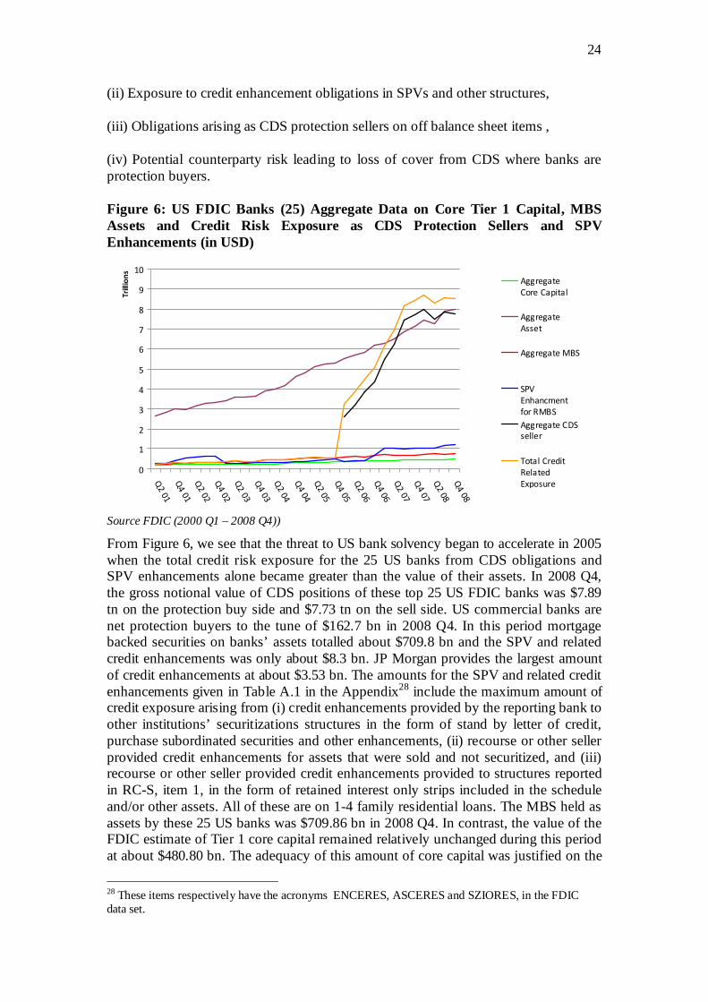
24
(ii) Exposure to credit enhancement obligations in SPVs and other structures,
(iii) Obligations arising as CDS protection sellers on off balance sheet items ,
(iv) Potential counterparty risk leading to loss of cover from CDS where banks are protection buyers.
Figure 6: US FDIC Banks (25) Aggregate Data on Core Tier 1 Capital, MBS Assets and Credit Risk Exposure as CDS Protection Sellers and SPV Enhancements (in USD)
0
1
2
3
4
5
6
7
8
9
10
Q2 01
Q4 01
Q2 02
Q4 02
Q2 03
Q4 03
Q2 04
Q4 04
Q2 05
Q4 05
Q2 06
Q4 06
Q2 07
Q4 07
Q2 08
Q4 08
Tri
llio
ns
Aggregate
Core Capital
Aggregate
Asset
Aggregate MBS
SPV
Enhancment
for RMBS
Aggregate CDS
seller
Total Credit
Related
Exposure
Source FDIC (2000 Q1 – 2008 Q4))
From Figure 6, we see that the threat to US bank solvency began to accelerate in 2005 when the total credit risk exposure for the 25 US banks from CDS obligations and SPV enhancements alone became greater than the value of their assets. In 2008 Q4, the gross notional value of CDS positions of these top 25 US FDIC banks was $7.89 tn on the protection buy side and $7.73 tn on the sell side. US commercial banks are net protection buyers to the tune of $162.7 bn in 2008 Q4. In this period mortgage backed securities on banks’ assets totalled about $709.8 bn and the SPV and related credit enhancements was only about $8.3 bn. JP Morgan provides the largest amount of credit enhancements at about $3.53 bn. The amounts for the SPV and related credit enhancements given in Table A.1 in the Appendix28 include the maximum amount of credit exposure arising from (i) credit enhancements provided by the reporting bank to other institutions’ securitizations structures in the form of stand by letter of credit, purchase subordinated securities and other enhancements, (ii) recourse or other seller provided credit enhancements for assets that were sold and not securitized, and (iii) recourse or other seller provided credit enhancements provided to structures reported in RC-S, item 1, in the form of retained interest only strips included in the schedule and/or other assets. All of these are on 1-4 family residential loans. The MBS held as assets by these 25 US banks was $709.86 bn in 2008 Q4. In contrast, the value of the FDIC estimate of Tier 1 core capital remained relatively unchanged during this period at about $480.80 bn. The adequacy of this amount of core capital was justified on the
28 These items respectively have the acronyms ENCERES, ASCERES and SZIORES, in the FDIC data set.
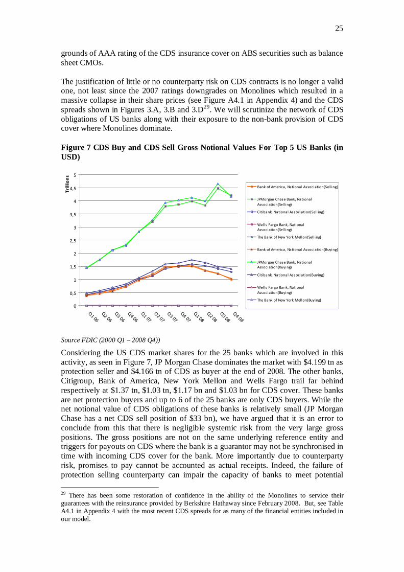
25
grounds of AAA rating of the CDS insurance cover on ABS securities such as balance sheet CMOs.
The justification of little or no counterparty risk on CDS contracts is no longer a valid one, not least since the 2007 ratings downgrades on Monolines which resulted in a massive collapse in their share prices (see Figure A4.1 in Appendix 4) and the CDS spreads shown in Figures 3.A, 3.B and 3.D29. We will scrutinize the network of CDS obligations of US banks along with their exposure to the non-bank provision of CDS cover where Monolines dominate.
Figure 7 CDS Buy and CDS Sell Gross Notional Values For Top 5 US Banks (in USD)
0
0,5
1
1,5
2
2,5
3
3,5
4
4,5
5
Q1 06
Q2 06
Q3 06
Q4 06
Q1 07
Q2 07
Q3 07
Q4 07
Q1 08
Q2 08
Q3 08
Q4 08
Tri
llio
ns
Bank of America, National Association(Sel l ing)
JPMorgan Chase Bank, National
Association(Sel l ing)
Citibank, National Association(Sel l ing)
Wells Fargo Bank, National
Association(Sel l ing)
The Bank of New York Mellon(Sel l ing)
Bank of America, National Association(Buying)
JPMorgan Chase Bank, National
Association(Buying)
Citibank, National Association(Buying)
Wells Fargo Bank, National
Association(Buying)
The Bank of New York Mellon(Buying)
Source FDIC (2000 Q1 – 2008 Q4))
Considering the US CDS market shares for the 25 banks which are involved in this activity, as seen in Figure 7, JP Morgan Chase dominates the market with $4.199 tn as protection seller and $4.166 tn of CDS as buyer at the end of 2008. The other banks, Citigroup, Bank of America, New York Mellon and Wells Fargo trail far behind respectively at $1.37 tn, $1.03 tn, $1.17 bn and $1.03 bn for CDS cover. These banks are net protection buyers and up to 6 of the 25 banks are only CDS buyers. While the net notional value of CDS obligations of these banks is relatively small (JP Morgan Chase has a net CDS sell position of $33 bn), we have argued that it is an error to conclude from this that there is negligible systemic risk from the very large gross positions. The gross positions are not on the same underlying reference entity and triggers for payouts on CDS where the bank is a guarantor may not be synchronised in time with incoming CDS cover for the bank. More importantly due to counterparty risk, promises to pay cannot be accounted as actual receipts. Indeed, the failure of protection selling counterparty can impair the capacity of banks to meet potential
29 There has been some restoration of confidence in the ability of the Monolines to service their guarantees with the reinsurance provided by Berkshire Hathaway since February 2008. But, see Table A4.1 in Appendix 4 with the most recent CDS spreads for as many of the financial entities included in our model.
26
CDS pay outs due to having to find new capital to make good the loss. Clearly, with many banks being only CDS buyers, the possibility of a zero or small bilaterally netted position with the failed counterparty is unlikely. Also, weakness in the markets for the collateral underpinning the tranched CDO products relating to the CDS or the failure of a reference entity can simultaneously trigger multiple payment obligations across the system.
In order to assess the potential systemic implications of the failure of a reference entity and/or of a protection selling counterparty to the banking sector as a whole, in Section 3 we construct the financial network interrelationships between the 25 banks and the external non-bank insurers. The dominance of some banks and the interrelated CDS links between banks as buyers and sellers of protection make it important to quantitatively model the contagion effect on the final loss of CDS cover and the threat to insolvency of other banks in due course.
2.4. Outline of Supervisory Capital Assessment Program (SCAP) On 7th of May 2009 Board of Governors of the Federal Reserve System announced results of stress test of US banking system under the rubric of SCAP (Supervisory Capital Assessment Program). SCAP has been conducted on 19 biggest US largest banks which account for in total two-thirds of all deposits. The assessment was aimed to measure how much additional capital is needed in the banking system in the view of recent financial crisis. Regulatory authorities aim to recapitalize banks that had been denuded of capital by loss of value on assets by default and increased collateral requirements due to failures in the credit risk mitigant scheme. From the announcement date financial institutions have one month in order to present a plan of acquiring additional capital, the plan is supposed to be in place by mid November 2009. Banks involved included: GMAC, Regions Financial, Bank of America, KeyCorp, SunTrust, Wells Fargo, Fifth Third Bancorp, Citigroup, Morgan Stanley, PNC Financial Services, Bank of New York Mellon, MetLife, BB&T, Capital One Financial, Goldman Sachs. Stress testing differed from usual sensitivity tests. The Fed gathered very detailed information on assets of banks and undertook tests based on two scenarios. The baseline scenario assumed that the economy would follow the path of consensus forecast and a more adverse scenario assumes non-positive developments in the economy and further deepening of financial crisis30. Banks were instructed to estimate potential losses on their portfolios in each of the scenarios and in two-year time horizon starting from beginning of 2009.
The SCAP results show that until end of 2010 there is a need for additional $185bn, which after developments of Q1 2009 translates into $75bn of capital that has to be raised by November 2009. It is worth underlining that this amount is shared by the 10 out of 19 institutions as the remaining 9 were, according to SCAP, in possession of adequate capital levels. Losses expected in the more adverse scenario amount to $600bn in the two year period. This combined with losses that banks have already suffered from since mid-2007 gives a very high amount of $950bn. The big share of it – around $455bn comes from losses on loan portfolios of banks, especially from
30 More information and details on the SCAP program can be found in Board of Governors of the Federal Reserve System (2009) “The Supervisory Capital Assessment Program: Design and Implementation” White Paper (Washington DC: Board of Governors, April 24). http://www.federalreserve.gov/newsevents/press/bcreg/20090424a.htm.

27
losses on residential mortgages and consumer related loans. The estimated cumulative loss on these assets is equal to 9.1%, which is historically a high number – higher than a peak loss during the Great Depression. Additionally, there is $135bn of estimated potential losses from trading-related exposures and securities. Firms trading with assets of $100bn or more, were asked to estimate potential trading-related and counterparty credit losses under a scenario based on market shocks similar to those that have occurred in 2008. The estimated losses were close to $100bn cumulated over the five companies that were asked to perform the test.
Table 1 : Supervisory Capital Assessment Program Aggregate Results for 19 Participating Bank Holding Companies for the More Adverse Scenario At December 31, 2008 $ Billions Tier 1 Capital 836,7 Tier 1 Common Capital 412,5 Risk Weighted Assets 7814,8 More Adverse Scenario Estimated for 2009 and 2010 for the More Adverse Scenario $ Billions As % of Loans Total Estimated Losses (Before purchase accounting adjustments) 599,2 First Lien Mortgages 102,3 8,80% Second/Junior Lien Mortgages 83,2 13,80% Commercial and Industrial Loans 60,1 6,10% Commercial Real Estate Loans 53 8,50% Credit Card Loans 82,4 22,50% Securities (AFS and HTM) 35,2 Na Trading & Counterparty 99,3 Na Other (1) 83,7 Na Memo: Purchase Accounting Adjustments 64,3 Resources Other Than Capital to Absorb Losses in the More Adverse Scenario (2) 362,9 SCAP Buffer Added for More Adverse Scenario (SCAP buffer is defined as additional Tier 1 Common/contingent Common) Indicated SCAP Buffer as of December 31, 2008 185 Less: Capital Actions and Effects of Q1 2009 Results (3) (4) 110,4 SCAP Buffer (5) 74,6
Notes: (1) Includes other consumer and non-consumer loans and miscellaneous commitments and obligations (2) Resources to absorb losses include pre-provision net revenue less the change in the allowance for loan and lease losses (3) Capital actions include completed or contracted transactions since Q4 2008 (4) Total includes only capital actions and effects of Q12009 results for firms that need to establish a SCAP buffer (5) There may be a need to establish an additional Tier 1capital buffer, but this would be satisfied by the additional Tier 1 Common capital buffer unless otherwise specified for a particular BHC
Source: Board of Governors of the Federal Reserve System, “The Supervisory Capital Assessment Program: Overview of Results”, 7 May 2009
28
In Section 4.5, the results of the SCAP stress tests will be compared with those from the ACE network model for CDS obligations.
3. Financial Networks: Theory and Empirics for the US CDS Obligations
The core thesis of the diversification claims for credit risk transfer of underlying default risk on bank loans by using CDS credit derivatives has been found practically not to have delivered. It is the purpose of this section to see to what extent this is due to the typical structures of real world financial networks which imply vulnerability of the system from hub like core banks and hence of highly correlated pathways emanating from them to the rest of the system. The term ‘too interconnected to fail’ has entered the lexicon of the recent crisis. We will briefly discuss the technical aspects of network topology and their stability conditions as studied by May-Wigner (May, 1972, 1973) and recently extended by Sinha (2005) and Sinha and Sinha (2006). A digital and empirical map of the highly interconnected links from CDS obligations among US banks is constructed to highlight issues relating to a structural model of financial contagion, systemic risk and the extent to which the delivery of promised protection via CDS and credit risk transfer is feasible.
3.1. Some Properties of Socio-Economic Networks Considerable empirical work has been done by physicists, econo-physicists and biologists on the network properties of the world wide web (www) (Watts and Strogatz (1998), Watts (1999), Newman (2003)), socio-economic networks on chains of influence and co-authorships (Jackson and Watts (2002), Jackson (2005)) and biological networks, Montoya and Sole (2001). These networks have been found to have so called “small world” network structures which though distinct from those for text book prototypes of random, regular and scale free networks, share important properties with them. Networks are mainly characterized by (a) the density of connectivity between nodes with high locally interconnectivity called clustering; (b) the links between nodes measured in terms of path lengths; and (c) when direction of links matter differentiated as in degrees and out degrees, the so called degree distribution in either direction represents distribution of links to and from nodes. Small world networks have dense local clusters as in regular networks but globally have properties of a random network with short path lengths between one node and any other node31.
Note in a random network and a small world one, the average shortest path between any two randomly chosen agents is found to be “small” and bounded by the logarithm of the total number of nodes in the system. In contrast, in regular networks while nodes are highly interconnected locally, the distance in terms of average links needed between a given node and another node randomly selected from the system is high.
Finally, small world networks are characterised by a highly skewed fat tailed or power law distribution in terms of large number of connections (in-degrees and out degrees) and payoffs to a relatively few individual nodes, Barabási and Albert (1999), which make them structurally different from the random and regular networks. In the latter 31 This is named after the work of the sociologist Stanley Milgram (1967) on the six degrees of separation in that everybody is linked to every body else in a communication type network by no more than six indirect links.
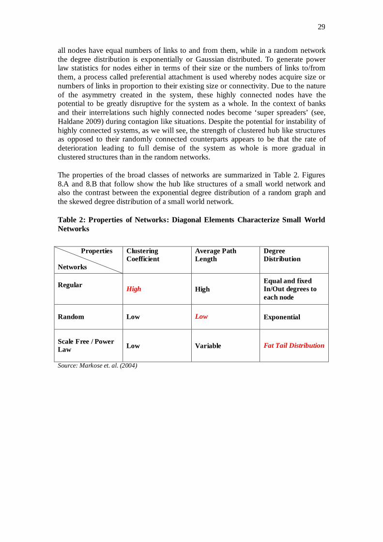
29
all nodes have equal numbers of links to and from them, while in a random network the degree distribution is exponentially or Gaussian distributed. To generate power law statistics for nodes either in terms of their size or the numbers of links to/from them, a process called preferential attachment is used whereby nodes acquire size or numbers of links in proportion to their existing size or connectivity. Due to the nature of the asymmetry created in the system, these highly connected nodes have the potential to be greatly disruptive for the system as a whole. In the context of banks and their interrelations such highly connected nodes become ‘super spreaders’ (see, Haldane 2009) during contagion like situations. Despite the potential for instability of highly connected systems, as we will see, the strength of clustered hub like structures as opposed to their randomly connected counterparts appears to be that the rate of deterioration leading to full demise of the system as whole is more gradual in clustered structures than in the random networks.
The properties of the broad classes of networks are summarized in Table 2. Figures 8.A and 8.B that follow show the hub like structures of a small world network and also the contrast between the exponential degree distribution of a random graph and the skewed degree distribution of a small world network.
Table 2: Properties of Networks: Diagonal Elements Characterize Small World Networks
Source: Markose et. al. (2004)
Properties Networks
Clustering Coefficient
Average Path Length
Degree Distribution
Regular High High
Equal and fixed In/Out degrees to each node
Random Low Low Exponential
Scale Free / Power Law Low Variable Fat Tail Distribution
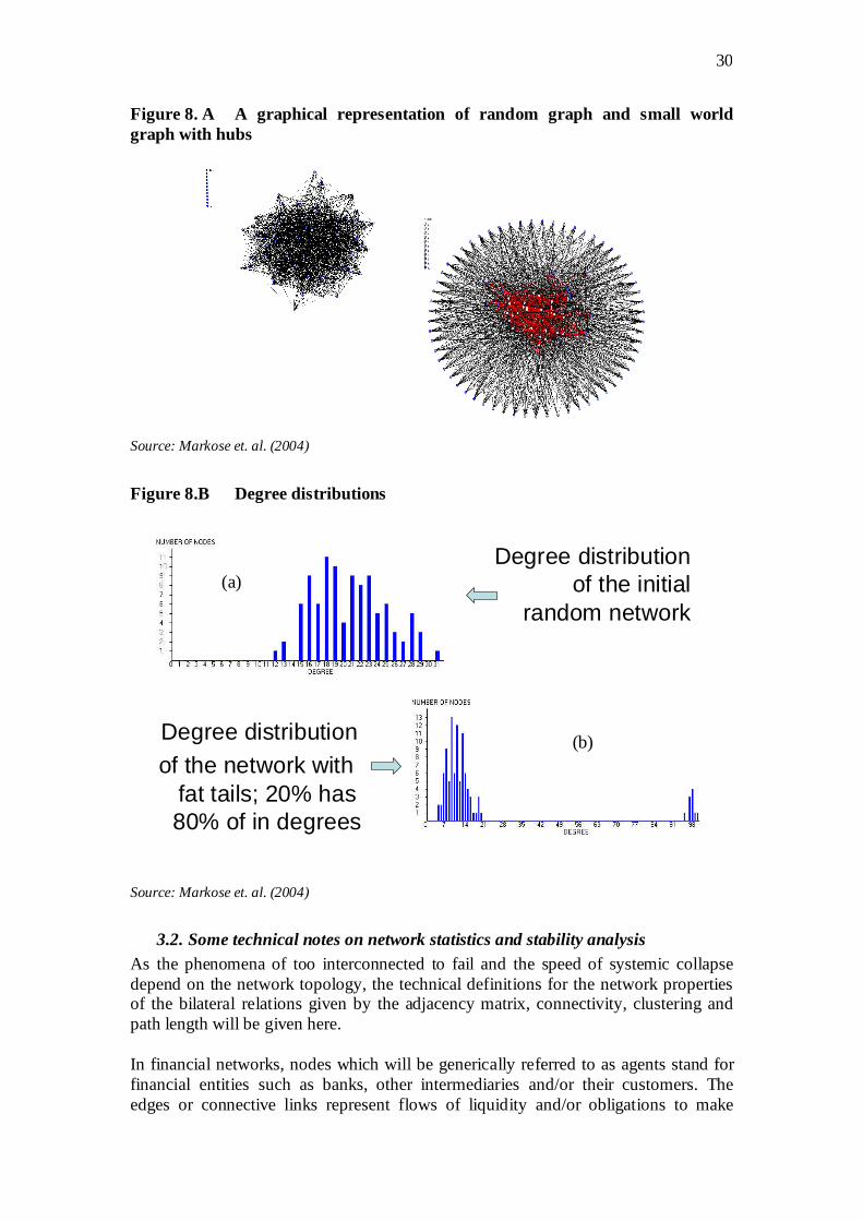
30
Figure 8. A A graphical representation of random graph and small world graph with hubs
Source: Markose et. al. (2004)
Figure 8.B Degree distributions
Degree distribution of the initial
random network
(a)
(b) Degree distributionof the network with
fat tails; 20% has 80% of in degrees
Source: Markose et. al. (2004)
3.2. Some technical notes on network statistics and stability analysis
As the phenomena of too interconnected to fail and the speed of systemic collapse depend on the network topology, the technical definitions for the network properties of the bilateral relations given by the adjacency matrix, connectivity, clustering and path length will be given here.
In financial networks, nodes which will be generically referred to as agents stand for financial entities such as banks, other intermediaries and/or their customers. The edges or connective links represent flows of liquidity and/or obligations to make
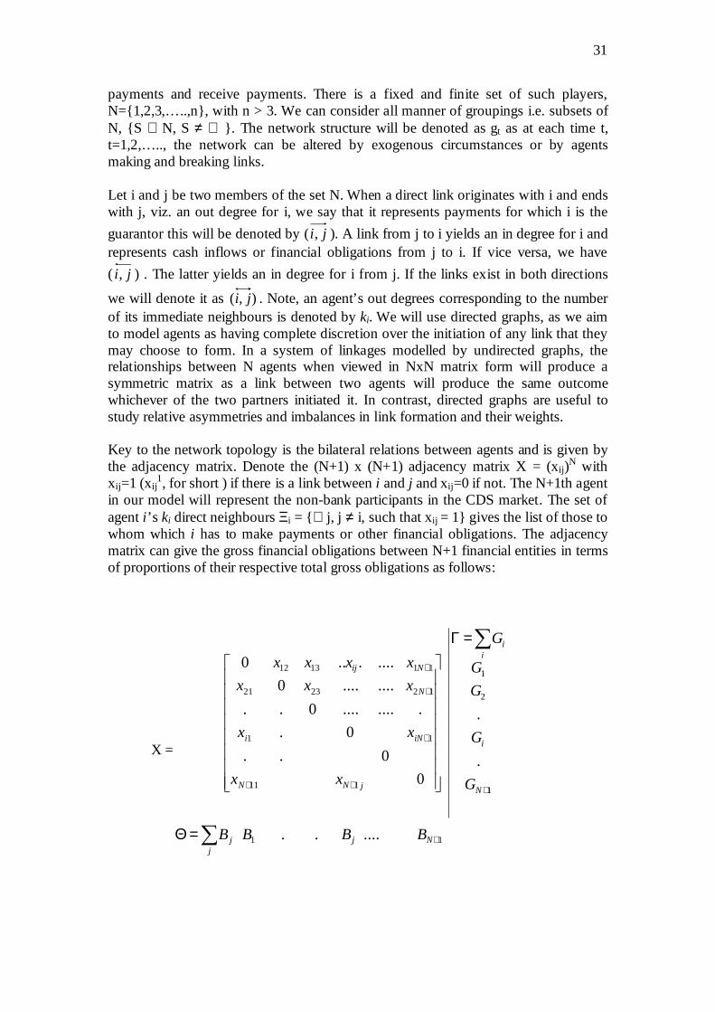
31
payments and receive payments. There is a fixed and finite set of such players, N={1,2,3,…..,n}, with n > 3. We can consider all manner of groupings i.e. subsets of N, {S ⊆ N, S ≠ ∅ }. The network structure will be denoted as gt as at each time t, t=1,2,….., the network can be altered by exogenous circumstances or by agents making and breaking links.
Let i and j be two members of the set N. When a direct link originates with i and ends with j, viz. an out degree for i, we say that it represents payments for which i is the
guarantor this will be denoted by (ji , ). A link from j to i yields an in degree for i and represents cash inflows or financial obligations from j to i. If vice versa, we have
( ji , ) . The latter yields an in degree for i from j. If the links exist in both directions
we will denote it as ),( ji . Note, an agent’s out degrees corresponding to the number of its immediate neighbours is denoted by ki. We will use directed graphs, as we aim to model agents as having complete discretion over the initiation of any link that they may choose to form. In a system of linkages modelled by undirected graphs, the relationships between N agents when viewed in NxN matrix form will produce a symmetric matrix as a link between two agents will produce the same outcome whichever of the two partners initiated it. In contrast, directed graphs are useful to study relative asymmetries and imbalances in link formation and their weights.
Key to the network topology is the bilateral relations between agents and is given by the adjacency matrix. Denote the (N+1) x (N+1) adjacency matrix X = (xij)N with xij=1 (xij
1, for short ) if there is a link between i and j and xij=0 if not. The N+1th agent in our model will represent the non-bank participants in the CDS market. The set of agent i ’s ki direct neighbours Ξi = {∀ j, j ≠ i, such that xij = 1} gives the list of those to whom which i has to make payments or other financial obligations. The adjacency matrix can give the gross financial obligations between N+1 financial entities in terms of proportions of their respective total gross obligations as follows:
X =
11
1
2
1
111
11
122321
111312
......
.
.
0
0..
0.
.........0..
........0
.......0
+
+++
+
+
+
∑
∑
=Θ
=Γ
Njj
j
N
i
ii
jNN
iNi
N
Nij
BBBB
G
G
G
G
G
xx
xx
xxx
xxxx
32
The summation for each row across the columns, Gi = ∑j
ijx , represents the gross
payment obligations that i is guarantor for. In the CDS market, Gi represents i’s obligations as a CDS protection seller. The summation of each column j across the row entries ∑=
iijj xB represents payments from i for which j is the beneficiary or j’s
exposure to all other i banks. In the CDS market, Bj, represents the CDS cover j is entitled to from others as a CDS buyer. The zeros along the diagonal imply that banks do not lend to themselves or self-insure (see, Upper, 2007). There can be asymmetry of entries such that for instance B1 need not equal G1. For example, in the case where bank 1 is only a CDS buyers, G1 is zero while B1 is not. Section 3.4 discusses how entries for matrix X is obtained for the CDS obligations of the 25 US banks.
Connectivity of a network: Connectivity is a statistic that measures the extent of links between nodes relative to all possible links in a complete graph. For a directed graph, denoting the total number
of out degrees to equal K = ∑=
N
iik
1
and N is the total number of nodes, connectivity of
a graph is given as )1( −NN
K.
Cluster Coefficient: Clustering in networks measures how interconnected each agent’s neighbours are and is considered to be the hallmark of social and species oriented networks. Specifically, there should be an increased probability that two of an agent’s neighbours are also neighbours of one another. For each agent with ki neighbours the total number of all possible directed links between them is given by ki (ki-1). Let Ei denote the actual number of links between agent i’s ki neighbours, viz. those of i’s ki neighbours who are also neighbours. The clustering coefficient Ci for agent i is given by
Ci = )1( −ii
i
kk
E. 32
The clustering coefficient of the network as a whole is the average of all Ci’s and is given by
C = N
CN
ii∑
=1 .
Note that the clustering coefficient for a random graph is
Crandom = p.
32 Numerically , Ei is calculated as follows. Using the NxN adjacency matrix X = (aij)
N with aij=1 (aij1
, for short) if there is a link between i and j and aij=0, if not. Agent i’s ki neighbours Ξi = { ∀ j , j ≠ i,
s.t aij = 1} , Ei for a directed graph is calculated as Ei = ∑∑Ξ∈ Ξ∈i ij m
jma 1 , j ≠ m.
33
This is because in a random graph the probability of node pairs being connected by edges are by definition independent, so there is no increase in the probability for two agents to being connected if they were neighbours of another agent than if they were not.
Average Path Length: A useful measure of the distance between two agents is given by the number of directed edges that separate them and this is referred to as their path length. In a random graph, the average shortest path length between all (i,j) pairs denoted by
randoml , is given by
Np
Nrandom
log
log=l .
If we keep the average number of degrees constant, i.e. Np = z, we see that the average path length increases logarithmically with the size N of the network. Random networks have quite a short path length which is due to the fact that many “shortcuts” between nodes arise from the random nature of the connections. In small world networks, the possibility of random reconnections enable two randomly chosen nodes in a network to have short path lengths. Regular networks miss these shortcuts and hence the average path length between an agent and a far flung one will be significantly longer. The exact path length depends crucially on the form of the network generated. Scale-free networks show an average path length which in most cases is also proportional to the logarithm of the network size, but the details depend on the way the preferential attachment is modelled.
3.3. May-Wigner Condition for Network Stability Here we will give a brief discussion of the May-Wigner condition for network stability in the context of small world networks. May (1972,1973) and Wigner (1957) derived the critical threshold below which any random network has a high probability of stability in terms of 3 parameters, N, the size of the network in terms of the total number of nodes, density of connections, D, and the strength of average interactions between nodes, σ. The network stability condition can be given equivalently as :
D < DMW = 2
1
σN ,
or:
.1<σND
The May-Wigner stability condition implies that on increasing the complexity of a network measured by its size (N), density of connections (D) and the strength of average interactions between nodes (σ) increases the instability of the network. This condition was originally shown in May (1972) to be true of a random graph. This created controversy as complexity is associated with diversity and the latter is understood to be tantamount to stability. Further, as the random graph construction in May (1972) does not have the high clustering that is associated with small world
34
networks which manifest the property that interactions between species and social interactions are not random, it became important to demonstrate what bearing the small world network properties of clustering and hub formations will have on the May-Wigner stability condition for networks. Sinha (2005) and Sinha and Sinha (2006) found that the transition point between stability and instability with respect to the given parameters (N, D and σ) does not differ between random and small world networks. However, they found that the speed and manner in which these different network systems transited into instability differed. An unstable clustered network system will disintegrate much less comprehensively than an unstable random network system. These aspects of network stability will be investigated for the US CDS network for banks. As far as the authors are aware, this may be the first analysis of the May-Wigner type stability properties of financial networks.
3.4. The Network Topology of US CDS Financial Interrelations The key to constructing the network interrelationships between the 25 US banks in their CDS activity is the relative CDS market shares of the banks involved. This reflects the notion of preferential attachment discussed earlier that Barabasi and Albert (1999) and others relate to power law outcomes in complex systems. From Table 3 we see that the top 3 banks ranked in terms of their dominance in this market (JP Morgan, Citibank and Bank of America) account for 83% of the total CDS purchases (and sales) for US banks. Note this also follows the same rank in terms of the value of their assets. Goldman Sachs is the 4 largest CDS player and with its inclusion,33 these 4 banks account for about 92% of CDS activity for US banks. The CDS network is a directed graph with inward links (in degrees) representing purchases and out going links (out degrees) representing the cover provided by the bank. As already discussed, the role of non-bank CDS providers in the form of the Monoline and other non-bank insurers is important in that not all of the $7. 89 tn CDS cover bought by US banks is from within the banking sector.
Our algorithm assigns in degrees and out degrees for a bank in terms of its respective market shares for CDS purchases and sales. Thus JP Morgan with a 53% share will have approximately direct links (in and out) with 14 banks and these are arranged assortatively, ie. 14 banks are chosen from the largest to the smallest. The following describes the algorithm that creates the CDS network and the CDS values being bought and sold between banks and the non-bank external entity. Here, N banks are indexed as i = 1, 2, … N. The N+1 agent is the ‘outside’ non-US and/or non-bank sector.
Gi : Gross Notional Amount of CDS for which Banki is guarantor
Bi : Gross Notional Amount of CDS for which Banki is beneficiary
SGi =
G
Gi Banki market share on the sell side of CDS
33 Note, in terms of assets, Goldman Sachs is ranked 11 and Wells Fargo which is the 4 th largest in terms of assets (now that Wachovia has been taken over), ranks only 13 in terms of CDS activity.
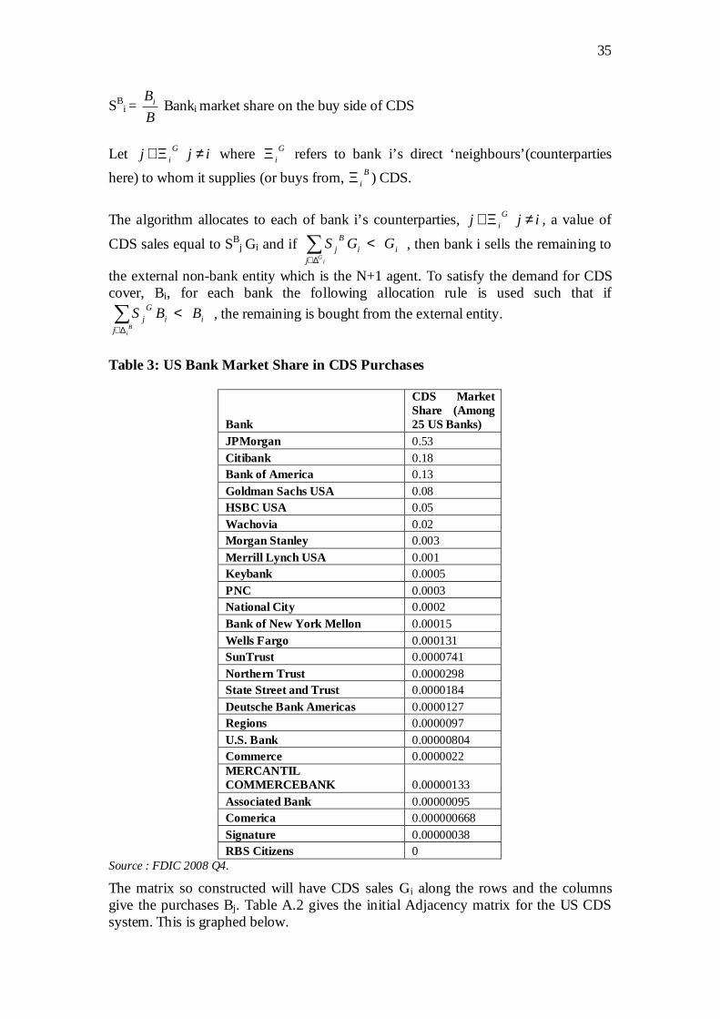
35
SBi =
B
Bi Banki market share on the buy side of CDS
Let ijj Gi ≠Ξ∈ where G
iΞ refers to bank i’s direct ‘neighbours’(counterparties
here) to whom it supplies (or buys from, BiΞ ) CDS.
The algorithm allocates to each of bank i’s counterparties, ijj Gi ≠Ξ∈ , a value of
CDS sales equal to SBj Gi and if ∑
∆∈
<i
Gjii
Bj GGS , then bank i sells the remaining to
the external non-bank entity which is the N+1 agent. To satisfy the demand for CDS cover, Bi, for each bank the following allocation rule is used such that if
∑∆∈
<B
ijii
Gj BBS , the remaining is bought from the external entity.
Table 3: US Bank Market Share in CDS Purchases
Bank
CDS Market Share (Among 25 US Banks)
JPMorgan 0.53 Citibank 0.18 Bank of America 0.13 Goldman Sachs USA 0.08 HSBC USA 0.05 Wachovia 0.02 Morgan Stanley 0.003 Merrill Lynch USA 0.001 Keybank 0.0005 PNC 0.0003 National City 0.0002 Bank of New York Mellon 0.00015 Wells Fargo 0.000131 SunTrust 0.0000741 Northern Trust 0.0000298 State Street and Trust 0.0000184 Deutsche Bank Americas 0.0000127 Regions 0.0000097 U.S. Bank 0.00000804 Commerce 0.0000022 MERCANTIL COMMERCEBANK 0.00000133 Associated Bank 0.00000095 Comerica 0.000000668 Signature 0.00000038 RBS Citizens 0
Source : FDIC 2008 Q4.
The matrix so constructed will have CDS sales Gi along the rows and the columns give the purchases Bj. Table A.2 gives the initial Adjacency matrix for the US CDS system. This is graphed below.
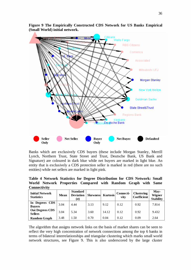
36
Figure 9 The Empirically Constructed CDS Network for US Banks Empirical (Small World) initial network.
Banks which are exclusively CDS buyers (these include Morgan Stanley, Merrill Lynch, Northern Trust, State Street and Trust, Deutsche Bank, US Bank and Signature) are coloured in dark blue while net buyers are marked in light blue. An entity that is exclusively a CDS protection seller is marked in red (there are no such entities) while net sellers are marked in light pink.
Table 4 Network Statistics for Degree Distribution for CDS Network: Small World Network Properties Compared with Random Graph with Same Connectivity
Initial Network Statistics Mean
Standard Deviation
(σ) Skewness Kurtosis Connecti-
vity Clustering Coefficient
May-WignerStability
In Degrees CDS Buyers 3.04 4.44 3.13 9.12 0.12 0.92 7.814
Out Degrees CDS Sellers 3.04 5.34 3.60 14.12 0.12 0.92 9.432
Random Graph 3.48 1.50 0.70 0.04 0.12 0.09 2.64
The algorithm that assigns network links on the basis of market shares can be seen to reflect the very high concentration of network connections among the top 6 banks in terms of bilateral interrelationships and triangular clustering which marks small world network structures, see Figure 9. This is also underscored by the large cluster
Seller Only
Defaulted Buyer Only
Net Seller Net Buyer
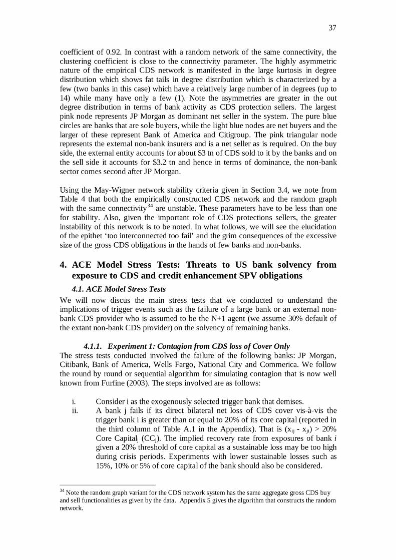
37
coefficient of 0.92. In contrast with a random network of the same connectivity, the clustering coefficient is close to the connectivity parameter. The highly asymmetric nature of the empirical CDS network is manifested in the large kurtosis in degree distribution which shows fat tails in degree distribution which is characterized by a few (two banks in this case) which have a relatively large number of in degrees (up to 14) while many have only a few (1). Note the asymmetries are greater in the out degree distribution in terms of bank activity as CDS protection sellers. The largest pink node represents JP Morgan as dominant net seller in the system. The pure blue circles are banks that are sole buyers, while the light blue nodes are net buyers and the larger of these represent Bank of America and Citigroup. The pink triangular node represents the external non-bank insurers and is a net seller as is required. On the buy side, the external entity accounts for about $3 tn of CDS sold to it by the banks and on the sell side it accounts for $3.2 tn and hence in terms of dominance, the non-bank sector comes second after JP Morgan.
Using the May-Wigner network stability criteria given in Section 3.4, we note from Table 4 that both the empirically constructed CDS network and the random graph with the same connectivity34 are unstable. These parameters have to be less than one for stability. Also, given the important role of CDS protections sellers, the greater instability of this network is to be noted. In what follows, we will see the elucidation of the epithet ‘too interconnected too fail’ and the grim consequences of the excessive size of the gross CDS obligations in the hands of few banks and non-banks.
4. ACE Model Stress Tests: Threats to US bank solvency from exposure to CDS and credit enhancement SPV obligations 4.1. ACE Model Stress Tests
We will now discus the main stress tests that we conducted to understand the implications of trigger events such as the failure of a large bank or an external non-bank CDS provider who is assumed to be the N+1 agent (we assume 30% default of the extant non-bank CDS provider) on the solvency of remaining banks.
4.1.1. Experiment 1: Contagion from CDS loss of Cover Only The stress tests conducted involved the failure of the following banks: JP Morgan, Citibank, Bank of America, Wells Fargo, National City and Commerica. We follow the round by round or sequential algorithm for simulating contagion that is now well known from Furfine (2003). The steps involved are as follows:
i. Consider i as the exogenously selected trigger bank that demises. ii. A bank j fails if its direct bilateral net loss of CDS cover vis-à-vis the
trigger bank i is greater than or equal to 20% of its core capital (reported in the third column of Table A.1 in the Appendix). That is (xij - xji) > 20% Core Capitalj (CCj). The implied recovery rate from exposures of bank i given a 20% threshold of core capital as a sustainable loss may be too high during crisis periods. Experiments with lower sustainable losses such as 15%, 10% or 5% of core capital of the bank should also be considered.
34 Note the random graph variant for the CDS network system has the same aggregate gross CDS buy and sell functionalities as given by the data. Appendix 5 gives the algorithm that constructs the random network.
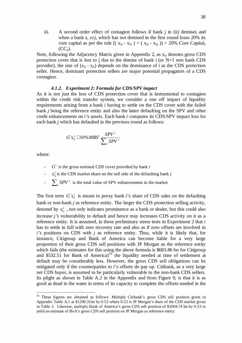
38
iii. A second order effect of contagion follows if bank j in (ii) demises and when a bank z, z≠j, which has not demised in the first round loses 20% its core capital as per the rule [( xiz - xzi ) + ( xjz - xzj )) > 20% Core Capitalz (CCz).
Note, following the Adjacency Matrix given in Appendix 2, as xij denotes gross CDS protection cover that is lost to j due to the demise of bank i (or N+1 non bank CDS provider), the size of (xij - xji) depends on the dominance of i as the CDS protection seller. Hence, dominant protection sellers are major potential propagators of a CDS contagion.
4.1.2. Experiment 2: Formula for CDS/SPV impact As it is not just the loss of CDS protection cover that is instrumental to contagion within the credit risk transfer system, we consider a one off impact of liquidity requirements arising from a bank i having to settle on the CDS cover with the failed bank j being the reference entity and also the latter defaulting on the SPV and other credit enhancements on i’s assets. Each bank i computes its CDS/SPV impact loss for each bank j which has defaulted in the previous round as follows:
∑+
z
z
jij
Gi
SPV
SPVMBSsG %10
where:
- iG is the gross notional CDS cover provided by bank i
- jGs is the CDS market share on the sell side of the defaulting bank j
- ∑z
zSPV is the total value of SPV enhancements in the market
The first term jG
isG is meant to proxy bank i ’s share of CDS sales on the defaulting bank or non-bank j as reference entity. The larger the CDS protection selling activity, denoted by j
Gs , not only indicates prominence as a bank or dealer, but this could also increase j’s vulnerability to default and hence may increases CDS activity on it as a reference entity. It is assumed, in these preliminary stress tests in Experiment 2 that i has to settle in full with zero recovery rate and also as if zero offsets are involved in i’s positions on CDS with j as reference entity. Thus, while it is likely that, for instance, Citigroup and Bank of America can become liable for a very large proportion of their gross CDS sell positions with JP Morgan as the reference entity which fails (the estimates for this using the above formula is $683.86 bn for Citigroup and $532.51 for Bank of America)35 the liquidity needed at time of settlement at default may be considerably less. However, the gross CDS sell obligations can be mitigated only if the counterparties to i’s offsets do pay up. Citibank, as a very large net CDS buyer, is assumed to be particularly vulnerable to the non-bank CDS sellers. Its plight as shown in Table A.2 in the Appendix and from Figure 9, is that it is as good as dead in the water in terms of its capacity to complete the offsets needed in the
35 These figures are obtained as follows: Multiply Citibank’s gross CDS sell position given in Appendix Table A.1 at $1290.31bn by 0.53 where 0.53 is JP Morgan’s share of the CDS market given in Table 3. Likewise, multiply Bank of America’s gross CDS sell position of $1004.74 bn by 0.53 to yield an estimate of BoA’s gross CDS sell position on JP Morgan as reference entity.
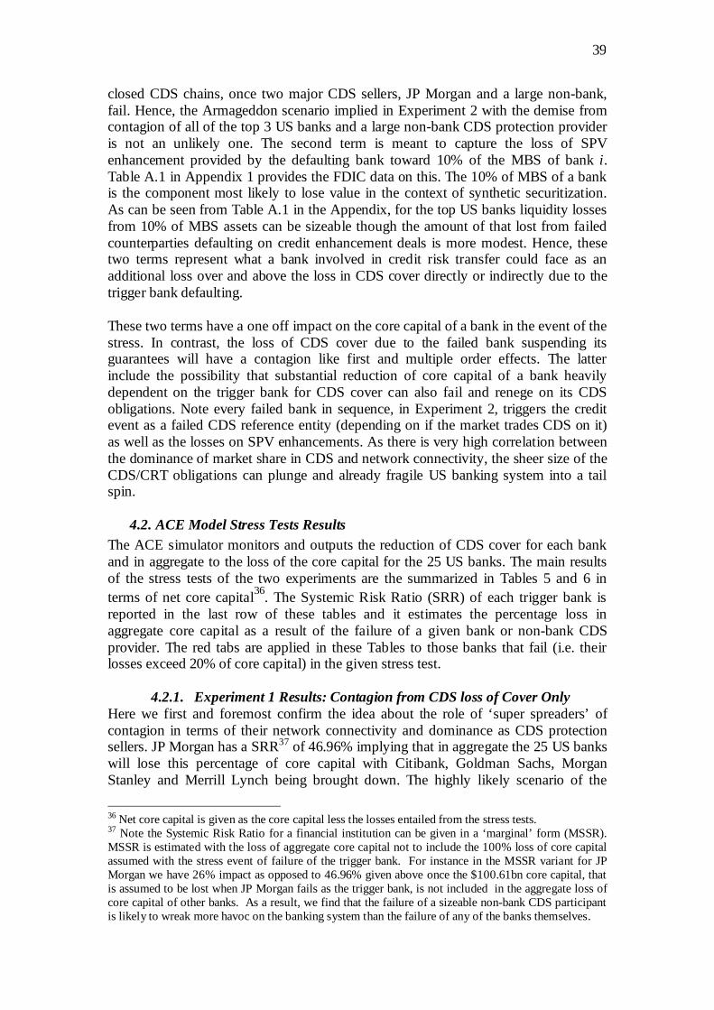
39
closed CDS chains, once two major CDS sellers, JP Morgan and a large non-bank, fail. Hence, the Armageddon scenario implied in Experiment 2 with the demise from contagion of all of the top 3 US banks and a large non-bank CDS protection provider is not an unlikely one. The second term is meant to capture the loss of SPV enhancement provided by the defaulting bank toward 10% of the MBS of bank i . Table A.1 in Appendix 1 provides the FDIC data on this. The 10% of MBS of a bank is the component most likely to lose value in the context of synthetic securitization. As can be seen from Table A.1 in the Appendix, for the top US banks liquidity losses from 10% of MBS assets can be sizeable though the amount of that lost from failed counterparties defaulting on credit enhancement deals is more modest. Hence, these two terms represent what a bank involved in credit risk transfer could face as an additional loss over and above the loss in CDS cover directly or indirectly due to the trigger bank defaulting.
These two terms have a one off impact on the core capital of a bank in the event of the stress. In contrast, the loss of CDS cover due to the failed bank suspending its guarantees will have a contagion like first and multiple order effects. The latter include the possibility that substantial reduction of core capital of a bank heavily dependent on the trigger bank for CDS cover can also fail and renege on its CDS obligations. Note every failed bank in sequence, in Experiment 2, triggers the credit event as a failed CDS reference entity (depending on if the market trades CDS on it) as well as the losses on SPV enhancements. As there is very high correlation between the dominance of market share in CDS and network connectivity, the sheer size of the CDS/CRT obligations can plunge and already fragile US banking system into a tail spin.
4.2. ACE Model Stress Tests Results The ACE simulator monitors and outputs the reduction of CDS cover for each bank and in aggregate to the loss of the core capital for the 25 US banks. The main results of the stress tests of the two experiments are the summarized in Tables 5 and 6 in terms of net core capital36. The Systemic Risk Ratio (SRR) of each trigger bank is reported in the last row of these tables and it estimates the percentage loss in aggregate core capital as a result of the failure of a given bank or non-bank CDS provider. The red tabs are applied in these Tables to those banks that fail (i.e. their losses exceed 20% of core capital) in the given stress test.
4.2.1. Experiment 1 Results: Contagion from CDS loss of Cover Only Here we first and foremost confirm the idea about the role of ‘super spreaders’ of contagion in terms of their network connectivity and dominance as CDS protection sellers. JP Morgan has a SRR37 of 46.96% implying that in aggregate the 25 US banks will lose this percentage of core capital with Citibank, Goldman Sachs, Morgan Stanley and Merrill Lynch being brought down. The highly likely scenario of the
36 Net core capital is given as the core capital less the losses entailed from the stress tests. 37 Note the Systemic Risk Ratio for a financial institution can be given in a ‘marginal’ form (MSSR). MSSR is estimated with the loss of aggregate core capital not to include the 100% loss of core capital assumed with the stress event of failure of the trigger bank. For instance in the MSSR variant for JP Morgan we have 26% impact as opposed to 46.96% given above once the $100.61bn core capital, that is assumed to be lost when JP Morgan fails as the trigger bank, is not included in the aggregate loss of core capital of other banks. As a result, we find that the failure of a sizeable non-bank CDS participant is likely to wreak more havoc on the banking system than the failure of any of the banks themselves.
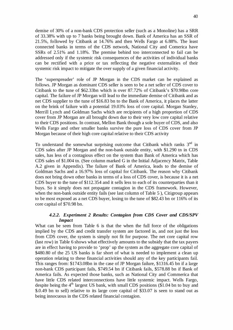
40
demise of 30% of a non-bank CDS protection seller (such as a Monoline) has a SRR of 33.38% with up to 7 banks being brought down. Bank of America has an SSR of 21.5%, followed by Citibank at 14.76% and then Wells Fargo at 6.88%. The least connected banks in terms of the CDS network, National City and Comerica have SSRs of 2.51% and 1.18%. The premise behind too interconnected to fail can be addressed only if the systemic risk consequences of the activities of individual banks can be rectified with a price or tax reflecting the negative externalities of their systemic risk impact to mitigate the over supply of a given financial activity.
The ‘superspreader’ role of JP Morgan in the CDS market can be explained as follows. JP Morgan as dominant CDS seller is seen to be a net seller of CDS cover to Citibank to the tune of $62.33bn which is over 87.72% of Citibank’s $70.98bn core capital. The failure of JP Morgan will lead to the immediate demise of Citibank and as net CDS supplier to the tune of $16.83 bn to the Bank of America, it places the latter on the brink of failure with a potential 19.03% loss of core capital. Morgan Stanley, Merrill Lynch and Goldman Sachs which are recipients of a high proportion of CDS cover from JP Morgan are all brought down due to their very low core capital relative to their CDS positions. In contrast, Mellon Bank though a sole buyer of CDS, and also Wells Fargo and other smaller banks survive the pure loss of CDS cover from JP Morgan because of their high core capital relative to their CDS activity
To understand the somewhat surprising outcome that Citibank which ranks 3nd in CDS sales after JP Morgan and the non-bank outside entity, with $1.290 tn in CDS sales, has less of a contagious effect on the system than Bank of America which has CDS sales of $1.004 tn. (See column marked G in the Initial Adjacency Matrix, Table A.2 given in Appendix). The failure of Bank of America, leads to the demise of Goldman Sachs and a 16.97% loss of capital for Citibank. The reason why Citibank does not bring down other banks in terms of a loss of CDS cover, is because it is a net CDS buyer to the tune of $112.354 and it sells less to each of its counterparties than it buys. So it simply does not propagate contagion in the CDS framework. However, when the non-bank outside entity fails (see last column of Table 5 ), Citigroup appears to be most exposed as a net CDS buyer, losing to the tune of $82.43 bn or 116% of its core capital of $70.98 bn.
4.2.2. Experiment 2 Results: Contagion from CDS Cover and CDS/SPV Impact
What can be seen from Table 6 is that the when the full force of the obligations implied by the CDS and credit transfer system are factored in, and not just the loss from CDS cover, the system is simply not fit for purpose. The net core capital row (last row) in Table 6 shows what effectively amounts to the subsidy that the tax payers are in effect having to provide to ‘prop’ up the system as the aggregate core capital of $480.80 of the 25 US banks is far short of what is needed to implement a clean up operation relating to these financial activities should any of the key participants fail. This ranges from: $1743.08bn in the case of JP Morgan failure, $1316.45 bn if a large non-bank CDS participant fails, $749.54 bn if Citibank fails, $578.88 bn if Bank of America fails. As expected those banks, such as National City and Commerica that have little CDS related interconnections have little systemic impact. Wells Fargo, despite being the 4th largest US bank, with small CDS positions ($1.04 bn to buy and $.0.49 bn to sell) relative to its large core capital of $33.07 is seen to stand out as being innocuous in the CDS related financial contagion.
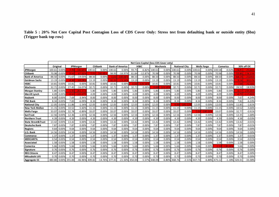
41
Table 5 : 20% Net Core Capital Post Contagion Loss of CDS Cover Only: Stress test from defaulting bank or outside entity ($bn) (Trigger bank top row)
JPMorgan 100.61 0.00% 0.00 -100.00% 100.61 0.00% 100.61 0.00% 93.75 -6.82% 100.61 0.00% 100.61 0.00% 100.61 0.00% 100.58 -0.02% 74.81 -25.64%
Citibank 70.98 0.00% 8.64 -87.82% 0.00 -100.00% 58.93 -16.97% 61.84 -12.87% 70.98 0.00% 70.98 0.00% 70.98 0.00% 70.98 0.00% -11.45 -116.13%
Bank of America 88.50 0.00% 71.67 -19.03% 88.50 0.00% 0.00 -100.00% 88.50 0.00% 88.50 0.00% 88.50 0.00% 88.50 0.00% 88.50 0.00% 68.14 -23.01%
Goldman Sachs 13.19 0.00% -8.98 -168.09% 13.19 0.00% 10.35 -21.54% 13.19 0.00% 13.19 0.00% 13.19 0.00% 13.19 0.00% 13.19 0.00% 9.16 -30.57%
HSBC 10.81 0.00% 10.81 0.00% 10.81 0.00% 10.81 0.00% 0.00 -100.00% 10.81 0.00% 10.81 0.00% 10.81 0.00% 10.81 0.00% 7.98 -26.18%
Wachovia 32.71 0.00% 27.45 -16.07% 32.71 0.00% 32.71 0.00% 32.71 0.00% 0.00 -100.00% 32.71 0.00% 32.71 0.00% 32.71 0.00% 26.52 -18.93%
Morgan Stanley 5.80 0.00% -5.93 -202.31% 5.80 0.00% 5.80 0.00% 5.80 0.00% 5.80 0.00% 5.80 0.00% 5.80 0.00% 5.80 0.00% -6.07 -204.66%
Merrill Lynch 4.09 0.00% -0.64 -115.67% 4.09 0.00% 4.09 0.00% 4.09 0.00% 4.09 0.00% 4.09 0.00% 4.09 0.00% 4.09 0.00% -0.70 -117.01%
Keybank 8.00 0.00% 7.69 -3.94% 8.00 0.00% 8.00 0.00% 8.00 0.00% 8.00 0.00% 8.00 0.00% 8.00 0.00% 8.00 0.00% 7.67 -4.24%
PNC Bank 8.34 0.00% 7.83 -6.09% 8.34 0.00% 8.34 0.00% 8.34 0.00% 8.34 0.00% 8.34 0.00% 8.34 0.00% 8.34 0.00% 7.82 -6.24%
National City 12.05 0.00% 11.86 -1.54% 12.05 0.00% 12.05 0.00% 12.05 0.00% 12.05 0.00% 0.00 -100.00% 12.05 0.00% 12.05 0.00% 11.85 -1.61%
New York Mellon 11.15 0.00% 10.52 -5.60% 11.15 0.00% 11.15 0.00% 11.15 0.00% 11.15 0.00% 11.15 0.00% 11.15 0.00% 11.15 0.00% 10.52 -5.66%
Wells Fargo 33.07 0.00% 32.78 -0.89% 33.07 0.00% 33.07 0.00% 33.07 0.00% 33.07 0.00% 33.07 0.00% 0.00 -100.00% 33.07 0.00% 32.77 -0.91%
SunTrust 12.56 0.00% 12.36 -1.65% 12.56 0.00% 12.56 0.00% 12.56 0.00% 12.56 0.00% 12.56 0.00% 12.56 0.00% 12.56 0.00% 12.35 -1.68%
Northern Trust 4.39 0.00% 4.39 0.00% 4.39 0.00% 4.39 0.00% 4.39 0.00% 4.39 0.00% 4.39 0.00% 4.39 0.00% 4.39 0.00% 4.38 -0.03%
State Street&Trust 13.42 0.00% 13.42 0.00% 13.42 0.00% 13.42 0.00% 13.42 0.00% 13.42 0.00% 13.42 0.00% 13.42 0.00% 13.42 0.00% 13.42 -0.01%
Deutsche Bank 7.87 0.00% 7.87 0.00% 7.87 0.00% 7.87 0.00% 7.87 0.00% 7.87 0.00% 7.87 0.00% 7.87 0.00% 7.87 0.00% 7.87 -0.01%
Regions 9.64 0.00% 9.64 0.00% 9.64 0.00% 9.64 0.00% 9.64 0.00% 9.64 0.00% 9.64 0.00% 9.64 0.00% 9.64 0.00% 9.64 0.00%
U.S. Bank 14.56 0.00% 14.56 0.00% 14.56 0.00% 14.56 0.00% 14.56 0.00% 14.56 0.00% 14.56 0.00% 14.56 0.00% 14.56 0.00% 14.56 0.00%
Commerce 1.37 0.00% 1.37 0.00% 1.37 0.00% 1.37 0.00% 1.37 0.00% 1.37 0.00% 1.37 0.00% 1.37 0.00% 1.37 0.00% 1.37 -0.01%
MERCANTIL 0.54 0.00% 0.54 0.00% 0.54 0.00% 0.54 0.00% 0.54 0.00% 0.54 0.00% 0.54 0.00% 0.54 0.00% 0.54 0.00% 0.54 -0.01%
Associated 1.58 0.00% 1.58 0.00% 1.58 0.00% 1.58 0.00% 1.58 0.00% 1.58 0.00% 1.58 0.00% 1.58 0.00% 1.58 0.00% 1.58 0.00%
Comerica 5.66 0.00% 5.66 0.00% 5.66 0.00% 5.66 0.00% 5.66 0.00% 5.66 0.00% 5.66 0.00% 5.66 0.00% 0.00 -100.00% 5.66 0.00%
Signature 0.76 0.00% 0.76 0.00% 0.76 0.00% 0.76 0.00% 0.76 0.00% 0.76 0.00% 0.76 0.00% 0.76 0.00% 0.76 0.00% 0.76 0.00%
RBS Citizens 8.47 0.00% 8.47 0.00% 8.47 0.00% 8.47 0.00% 8.47 0.00% 8.47 0.00% 8.47 0.00% 8.47 0.00% 8.47 0.00% 8.47 0.00%
Mitsubishi UFJ 0.70 0.00% 0.70 0.00% 0.70 0.00% 0.70 0.00% 0.70 0.00% 0.70 0.00% 0.70 0.00% 0.70 0.00% 0.70 0.00% 0.70 0.00%
Aggregate CC 480.80 0.00% 255.00 -46.96% 409.82 -14.76% 377.41 -21.50% 454.00 -5.57% 448.09 -6.80% 468.76 -2.51% 447.73 -6.88% 475.12 -1.18% 320.31 -33.38%
Net Core Capital (loss CDS Cover only)
JPMorgan Citibank Bank of America HSBC Wachovia National City Wells Fargo Comerica 30% off OEOriginal
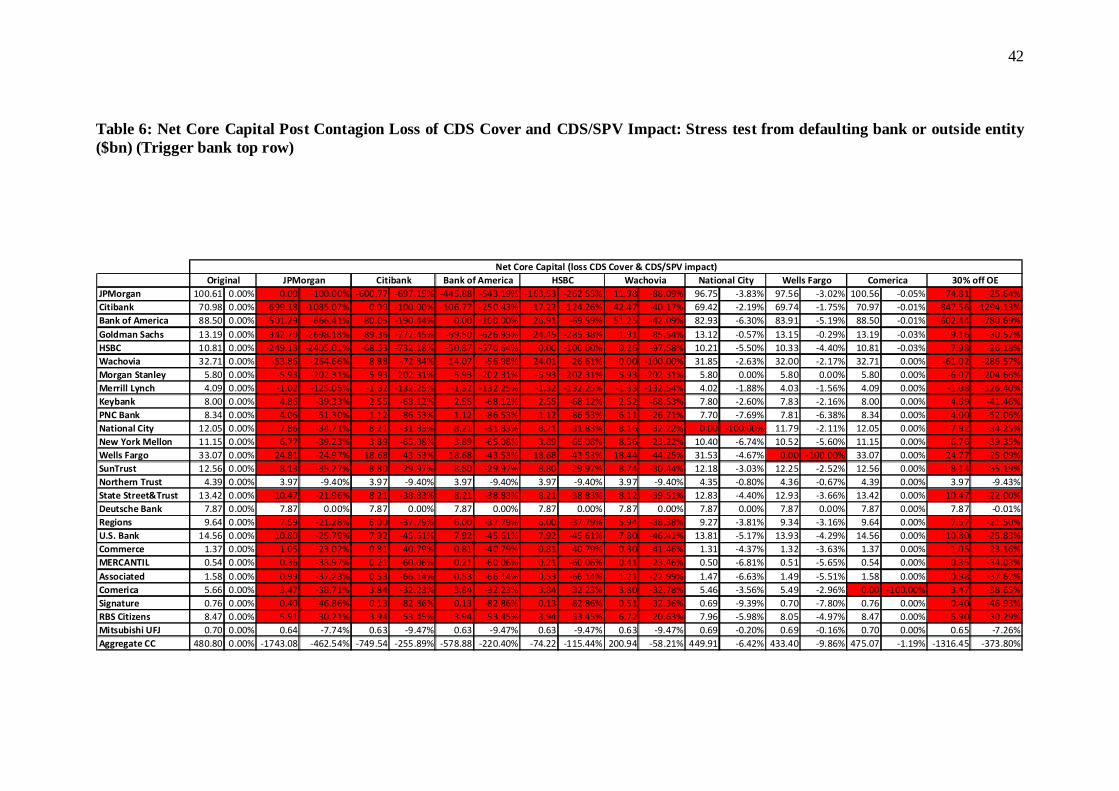
42
Table 6: Net Core Capital Post Contagion Loss of CDS Cover and CDS/SPV Impact: Stress test from defaulting bank or outside entity ($bn) (Trigger bank top row)
JPMorgan 100.61 0.00% 0.00 -100.00% -600.77 -697.15% -445.88 -543.19% -163.53 -262.55% 11.98 -88.09% 96.75 -3.83% 97.56 -3.02% 100.56 -0.05% 74.81 -25.64%
Citibank 70.98 0.00% -699.18 -1085.07% 0.00 -100.00% -106.77 -250.43% -17.22 -124.26% 42.47 -40.17% 69.42 -2.19% 69.74 -1.75% 70.97 -0.01% -847.56 -1294.13%
Bank of America 88.50 0.00% -501.29 -666.41% -80.05 -190.44% 0.00 -100.00% 26.91 -69.59% 51.25 -42.09% 82.93 -6.30% 83.91 -5.19% 88.50 -0.01% -602.44 -780.69%
Goldman Sachs 13.19 0.00% -342.70 -2698.18% -89.36 -777.45% -69.50 -626.93% -24.45 -285.38% 1.91 -85.54% 13.12 -0.57% 13.15 -0.29% 13.19 -0.03% 9.16 -30.57%
HSBC 10.81 0.00% -249.13 -2405.01% -68.33 -732.18% -50.87 -570.64% 0.00 -100.00% 0.26 -97.58% 10.21 -5.50% 10.33 -4.40% 10.81 -0.03% 7.98 -26.18%
Wachovia 32.71 0.00% -53.86 -264.66% 8.88 -72.84% 14.07 -56.98% 24.01 -26.61% 0.00 -100.00% 31.85 -2.63% 32.00 -2.17% 32.71 0.00% -61.02 -286.57%
Morgan Stanley 5.80 0.00% -5.93 -202.31% -5.93 -202.31% -5.93 -202.31% -5.93 -202.31% -5.93 -202.31% 5.80 0.00% 5.80 0.00% 5.80 0.00% -6.07 -204.66%
Merrill Lynch 4.09 0.00% -1.02 -125.05% -1.32 -132.25% -1.32 -132.25% -1.32 -132.25% -1.33 -132.54% 4.02 -1.88% 4.03 -1.56% 4.09 0.00% -1.08 -126.40%
Keybank 8.00 0.00% 4.86 -39.33% 2.55 -68.12% 2.55 -68.12% 2.55 -68.12% 2.52 -68.53% 7.80 -2.60% 7.83 -2.16% 8.00 0.00% 4.69 -41.46%
PNC Bank 8.34 0.00% 4.06 -51.30% 1.12 -86.53% 1.12 -86.53% 1.12 -86.53% 6.11 -26.71% 7.70 -7.69% 7.81 -6.38% 8.34 0.00% 4.00 -52.06%
National City 12.05 0.00% 7.86 -34.71% 8.21 -31.83% 8.21 -31.83% 8.21 -31.83% 8.16 -32.22% 0.00 -100.00% 11.79 -2.11% 12.05 0.00% 7.92 -34.25%
New York Mellon 11.15 0.00% 6.77 -39.23% 3.89 -65.08% 3.89 -65.08% 3.89 -65.08% 8.56 -23.22% 10.40 -6.74% 10.52 -5.60% 11.15 0.00% 6.76 -39.35%
Wells Fargo 33.07 0.00% 24.81 -24.97% 18.68 -43.53% 18.68 -43.53% 18.68 -43.53% 18.44 -44.25% 31.53 -4.67% 0.00 -100.00% 33.07 0.00% 24.77 -25.09%
SunTrust 12.56 0.00% 8.13 -35.27% 8.80 -29.97% 8.80 -29.97% 8.80 -29.97% 8.74 -30.44% 12.18 -3.03% 12.25 -2.52% 12.56 0.00% 8.14 -35.19%
Northern Trust 4.39 0.00% 3.97 -9.40% 3.97 -9.40% 3.97 -9.40% 3.97 -9.40% 3.97 -9.40% 4.35 -0.80% 4.36 -0.67% 4.39 0.00% 3.97 -9.43%
State Street&Trust 13.42 0.00% 10.47 -21.96% 8.21 -38.83% 8.21 -38.83% 8.21 -38.83% 8.12 -39.51% 12.83 -4.40% 12.93 -3.66% 13.42 0.00% 10.47 -22.00%
Deutsche Bank 7.87 0.00% 7.87 0.00% 7.87 0.00% 7.87 0.00% 7.87 0.00% 7.87 0.00% 7.87 0.00% 7.87 0.00% 7.87 0.00% 7.87 -0.01%
Regions 9.64 0.00% 7.59 -21.28% 6.00 -37.79% 6.00 -37.79% 6.00 -37.79% 5.94 -38.38% 9.27 -3.81% 9.34 -3.16% 9.64 0.00% 7.57 -21.50%
U.S. Bank 14.56 0.00% 10.80 -25.79% 7.92 -45.61% 7.92 -45.61% 7.92 -45.61% 7.80 -46.41% 13.81 -5.17% 13.93 -4.29% 14.56 0.00% 10.80 -25.83%
Commerce 1.37 0.00% 1.05 -23.02% 0.81 -40.79% 0.81 -40.79% 0.81 -40.79% 0.80 -41.46% 1.31 -4.37% 1.32 -3.63% 1.37 0.00% 1.05 -23.16%
MERCANTIL 0.54 0.00% 0.36 -33.97% 0.21 -60.06% 0.21 -60.06% 0.21 -60.06% 0.41 -23.46% 0.50 -6.81% 0.51 -5.65% 0.54 0.00% 0.35 -34.03%
Associated 1.58 0.00% 0.99 -37.23% 0.53 -66.14% 0.53 -66.14% 0.53 -66.14% 1.21 -22.99% 1.47 -6.63% 1.49 -5.51% 1.58 0.00% 0.98 -37.62%
Comerica 5.66 0.00% 3.47 -38.71% 3.84 -32.23% 3.84 -32.23% 3.84 -32.23% 3.80 -32.78% 5.46 -3.56% 5.49 -2.96% 0.00 -100.00% 3.47 -38.65%
Signature 0.76 0.00% 0.40 -46.86% 0.13 -82.86% 0.13 -82.86% 0.13 -82.86% 0.51 -32.36% 0.69 -9.39% 0.70 -7.80% 0.76 0.00% 0.40 -46.93%
RBS Citizens 8.47 0.00% 5.91 -30.21% 3.94 -53.45% 3.94 -53.45% 3.94 -53.45% 6.72 -20.63% 7.96 -5.98% 8.05 -4.97% 8.47 0.00% 5.90 -30.29%
Mitsubishi UFJ 0.70 0.00% 0.64 -7.74% 0.63 -9.47% 0.63 -9.47% 0.63 -9.47% 0.63 -9.47% 0.69 -0.20% 0.69 -0.16% 0.70 0.00% 0.65 -7.26%
Aggregate CC 480.80 0.00% -1743.08 -462.54% -749.54 -255.89% -578.88 -220.40% -74.22 -115.44% 200.94 -58.21% 449.91 -6.42% 433.40 -9.86% 475.07 -1.19% -1316.45 -373.80%
National City Wells Fargo Comerica 30% off OE
Net Core Capital (loss CDS Cover & CDS/SPV impact)
Original JPMorgan Citibank Bank of America HSBC Wachovia
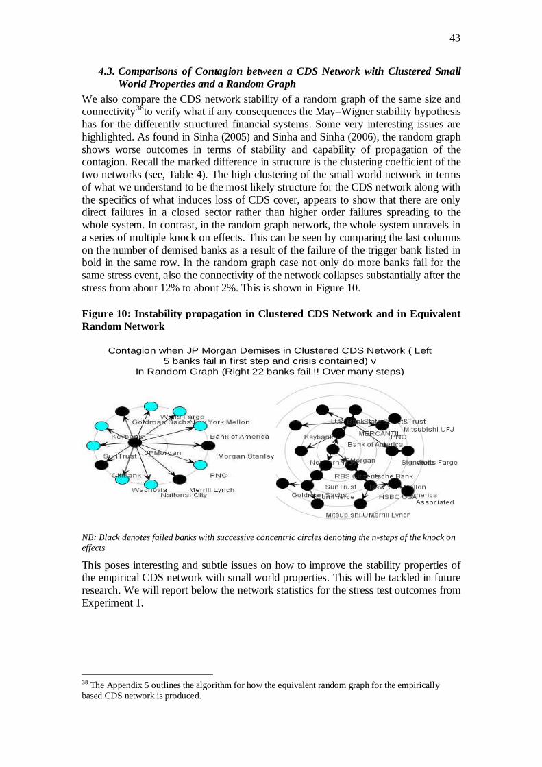
43
4.3. Comparisons of Contagion between a CDS Network with Clustered Small World Properties and a Random Graph
We also compare the CDS network stability of a random graph of the same size and connectivity38to verify what if any consequences the May–Wigner stability hypothesis has for the differently structured financial systems. Some very interesting issues are highlighted. As found in Sinha (2005) and Sinha and Sinha (2006), the random graph shows worse outcomes in terms of stability and capability of propagation of the contagion. Recall the marked difference in structure is the clustering coefficient of the two networks (see, Table 4). The high clustering of the small world network in terms of what we understand to be the most likely structure for the CDS network along with the specifics of what induces loss of CDS cover, appears to show that there are only direct failures in a closed sector rather than higher order failures spreading to the whole system. In contrast, in the random graph network, the whole system unravels in a series of multiple knock on effects. This can be seen by comparing the last columns on the number of demised banks as a result of the failure of the trigger bank listed in bold in the same row. In the random graph case not only do more banks fail for the same stress event, also the connectivity of the network collapses substantially after the stress from about 12% to about 2%. This is shown in Figure 10.
Figure 10: Instability propagation in Clustered CDS Network and in Equivalent Random Network
Contagion when JP Morgan Demises in Clustered CDS Network ( Left5 banks fail in first step and crisis contained) v
In Random Graph (Right 22 banks fail !! Over many steps)
NB: Black denotes failed banks with successive concentric circles denoting the n-steps of the knock on effects
This poses interesting and subtle issues on how to improve the stability properties of the empirical CDS network with small world properties. This will be tackled in future research. We will report below the network statistics for the stress test outcomes from Experiment 1.
38 The Appendix 5 outlines the algorithm for how the equivalent random graph for the empirically based CDS network is produced.
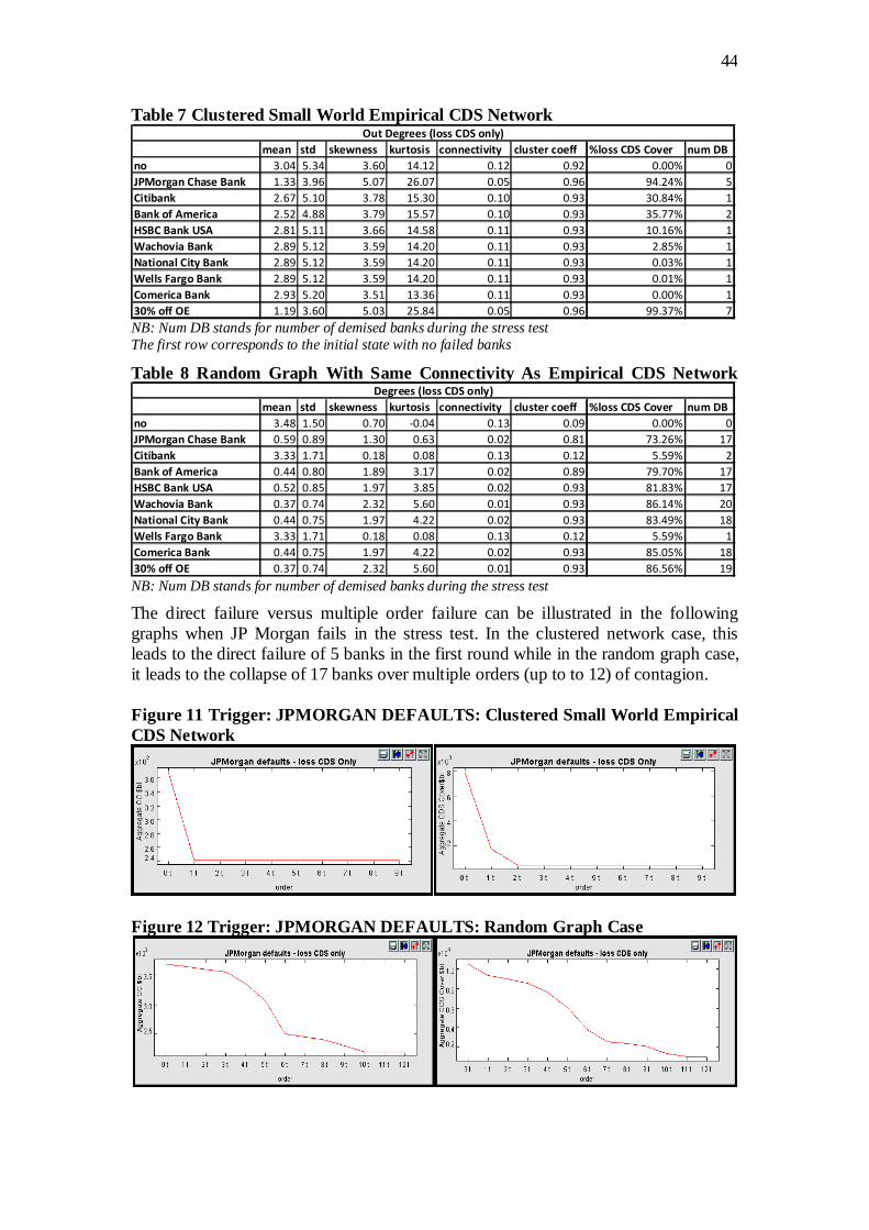
44
Table 7 Clustered Small World Empirical CDS Network
mean std skewness kurtosis connectivity cluster coeff %loss CDS Cover num DB
no 3.04 5.34 3.60 14.12 0.12 0.92 0.00% 0
JPMorgan Chase Bank 1.33 3.96 5.07 26.07 0.05 0.96 94.24% 5
Citibank 2.67 5.10 3.78 15.30 0.10 0.93 30.84% 1
Bank of America 2.52 4.88 3.79 15.57 0.10 0.93 35.77% 2
HSBC Bank USA 2.81 5.11 3.66 14.58 0.11 0.93 10.16% 1
Wachovia Bank 2.89 5.12 3.59 14.20 0.11 0.93 2.85% 1
National City Bank 2.89 5.12 3.59 14.20 0.11 0.93 0.03% 1
Wells Fargo Bank 2.89 5.12 3.59 14.20 0.11 0.93 0.01% 1
Comerica Bank 2.93 5.20 3.51 13.36 0.11 0.93 0.00% 1
30% off OE 1.19 3.60 5.03 25.84 0.05 0.96 99.37% 7
Out Degrees (loss CDS only)
NB: Num DB stands for number of demised banks during the stress test The first row corresponds to the initial state with no failed banks
Table 8 Random Graph With Same Connectivity As Empirical CDS Network
mean std skewness kurtosis connectivity cluster coeff %loss CDS Cover num DB
no 3.48 1.50 0.70 -0.04 0.13 0.09 0.00% 0
JPMorgan Chase Bank 0.59 0.89 1.30 0.63 0.02 0.81 73.26% 17
Citibank 3.33 1.71 0.18 0.08 0.13 0.12 5.59% 2
Bank of America 0.44 0.80 1.89 3.17 0.02 0.89 79.70% 17
HSBC Bank USA 0.52 0.85 1.97 3.85 0.02 0.93 81.83% 17
Wachovia Bank 0.37 0.74 2.32 5.60 0.01 0.93 86.14% 20
National City Bank 0.44 0.75 1.97 4.22 0.02 0.93 83.49% 18
Wells Fargo Bank 3.33 1.71 0.18 0.08 0.13 0.12 5.59% 1
Comerica Bank 0.44 0.75 1.97 4.22 0.02 0.93 85.05% 18
30% off OE 0.37 0.74 2.32 5.60 0.01 0.93 86.56% 19
Degrees (loss CDS only)
NB: Num DB stands for number of demised banks during the stress test
The direct failure versus multiple order failure can be illustrated in the following graphs when JP Morgan fails in the stress test. In the clustered network case, this leads to the direct failure of 5 banks in the first round while in the random graph case, it leads to the collapse of 17 banks over multiple orders (up to to 12) of contagion.
Figure 11 Trigger: JPMORGAN DEFAULTS: Clustered Small World Empirical CDS Network
Figure 12 Trigger: JPMORGAN DEFAULTS: Random Graph Case
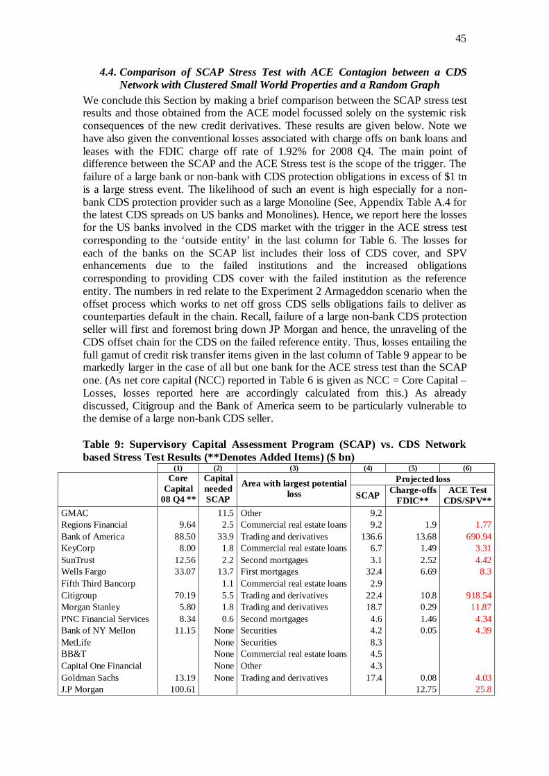
45
4.4. Comparison of SCAP Stress Test with ACE Contagion between a CDS Network with Clustered Small World Properties and a Random Graph
We conclude this Section by making a brief comparison between the SCAP stress test results and those obtained from the ACE model focussed solely on the systemic risk consequences of the new credit derivatives. These results are given below. Note we have also given the conventional losses associated with charge offs on bank loans and leases with the FDIC charge off rate of 1.92% for 2008 Q4. The main point of difference between the SCAP and the ACE Stress test is the scope of the trigger. The failure of a large bank or non-bank with CDS protection obligations in excess of $1 tn is a large stress event. The likelihood of such an event is high especially for a non-bank CDS protection provider such as a large Monoline (See, Appendix Table A.4 for the latest CDS spreads on US banks and Monolines). Hence, we report here the losses for the US banks involved in the CDS market with the trigger in the ACE stress test corresponding to the ‘outside entity’ in the last column for Table 6. The losses for each of the banks on the SCAP list includes their loss of CDS cover, and SPV enhancements due to the failed institutions and the increased obligations corresponding to providing CDS cover with the failed institution as the reference entity. The numbers in red relate to the Experiment 2 Armageddon scenario when the offset process which works to net off gross CDS sells obligations fails to deliver as counterparties default in the chain. Recall, failure of a large non-bank CDS protection seller will first and foremost bring down JP Morgan and hence, the unraveling of the CDS offset chain for the CDS on the failed reference entity. Thus, losses entailing the full gamut of credit risk transfer items given in the last column of Table 9 appear to be markedly larger in the case of all but one bank for the ACE stress test than the SCAP one. (As net core capital (NCC) reported in Table 6 is given as NCC = Core Capital – Losses, losses reported here are accordingly calculated from this.) As already discussed, Citigroup and the Bank of America seem to be particularly vulnerable to the demise of a large non-bank CDS seller.
Table 9: Supervisory Capital Assessment Program (SCAP) vs. CDS Network based Stress Test Results (**Denotes Added Items) ($ bn)
(1) (2) (3) (4) (5) (6)
Projected loss
Core Capital
08 Q4 **
Capital needed SCAP
Area with largest potential loss SCAP Charge-offs
FDIC** ACE Test
CDS/SPV** GMAC 11.5 Other 9.2 Regions Financial 9.64 2.5 Commercial real estate loans 9.2 1.9 1.77 Bank of America 88.50 33.9 Trading and derivatives 136.6 13.68 690.94 KeyCorp 8.00 1.8 Commercial real estate loans 6.7 1.49 3.31 SunTrust 12.56 2.2 Second mortgages 3.1 2.52 4.42 Wells Fargo 33.07 13.7 First mortgages 32.4 6.69 8.3 Fifth Third Bancorp 1.1 Commercial real estate loans 2.9 Citigroup 70.19 5.5 Trading and derivatives 22.4 10.8 918.54 Morgan Stanley 5.80 1.8 Trading and derivatives 18.7 0.29 11.87 PNC Financial Services 8.34 0.6 Second mortgages 4.6 1.46 4.34 Bank of NY Mellon 11.15 None Securities 4.2 0.05 4.39 MetLife None Securities 8.3 BB&T None Commercial real estate loans 4.5 Capital One Financial None Other 4.3 Goldman Sachs 13.19 None Trading and derivatives 17.4 0.08 4.03 J.P Morgan 100.61 12.75 25.8
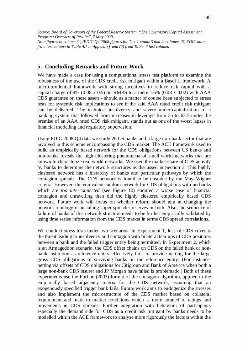
46
Source: Board of Governors of the Federal Reserve System, “The Supervisory Capital Assessment Program: Overview of Results”, 7 May 2009. Note figures in column (1) (FDIC Q4 2008 figures for Tier 1 capital) and in columns (5) FDIC data from last column in Table A.1 in Appendix) and (6) from Table 7 last column.
5. Concluding Remarks and Future Work We have made a case for using a computational stress test platform to examine the robustness of the use of the CDS credit risk mitigant within a Basel II framework. A micro-prudential framework with strong incentives to reduce risk capital with a capital charge of 4% (0.08 x 0.5) on RMBS to a mere 1.6% (0.08 x 0.02) with AAA CDS guarantee on these assets - should as a matter of course been subjected to stress tests for systemic risk implications to see if the said AAA rated credit risk mitigant can be delivered. The technical insolvency and severe under-capitalization of a banking system that followed from increases in leverage from 25 to 62.5 under the premise of an AAA rated CDS risk mitigant, stands out as one of the worst lapses in financial modelling and regulatory supervision.
Using FDIC 2008 Q4 data we study 26 US banks and a large non-bank sector that are involved in this scheme encompassing the CDS market. The ACE framework used to build an empirically based network for the CDS obligations between US banks and non-banks reveals the high clustering phenomena of small world networks that are known to characterize real world networks. We used the market share of CDS activity by banks to determine the network structures as discussed in Section 3. This highly clustered network has a hierarchy of banks and particular pathways by which the contagion spreads. The CDS network is found to be unstable by the May–Wigner criteria. However, the equivalent random network for CDS obligations with no banks which are too interconnected (see Figure 10) endured a worse case of financial contagion and unravelling than did the highly clustered empirically based CDS network. Future work will focus on whether reform should aim at changing the network topology or installing super-spreader reserves or both. Also, the sequence of failure of banks of this network structure needs to be further empirically validated by using time series information from the CDS market in terms CDS spread correlations.
We conduct stress tests under two scenarios. In Experiment 1, loss of CDS cover is the threat leading to insolvency and contagion with bilateral tear ups of CDS positions between a bank and the failed trigger entity being permitted. In Experiment 2, which is an Armageddon scenario, the CDS offset chains on CDS on the failed bank or non-bank institution as reference entity effectively fails to provide netting for the large gross CDS obligations of surviving banks on the reference entity. (For instance, netting via offsets of CDS obligations for Citigroup and Bank of America when both a large non-bank CDS insurer and JP Morgan have failed is problematic.) Both of these experiments use the Furfine (2003) format of the contagion algorithm, applied to the empirically based adjacency matrix for the CDS network, assuming that an exogenously specified trigger bank fails. Future work aims to endogenize the stresses and also implement the microstructure of the CDS market based on collateral requirement and mark to market conditions which is more attuned to ratings and movements in CDS spreads. Further integration with behaviour of participants especially the demand side for CDS as a credit risk mitigant by banks needs to be modelled within the ACE framework to analyse more rigorously the factors within the
47
CRT system of Basel II on whether it continues to set in force a system of perverse incentives or whether it can become a functional scheme capable of delivering policy objectives.
It must be noted that in Experiment 1, it is assumed that the loss of cover after tear ups translates into a full loss of capital rather than just an increase in liquidity needed for cover obtained by reassignment of counterparty from the failed entity to others. It is reasonable to assume that with the failure of any of the top three banks or a large non-bank CDS seller, given the very large gross size of the surviving banks’ guarantees on CDS on the failed bank as reference entity, further assumption of CDS cover from the latter will not find voluntary assignees. Fed compulsion and ‘sweeteners’ will be the order of the day. The resultant increase in concentration risk following reassignment is likely to jeopardize the system. A facility in the simulator will be built to implement CDS reassignments to quantify concentration risk.
The analysis shows that three top US banks and the non-bank net CDS protection sellers have become too interconnected to fail. The significance of this epithet lies in the fact that the CDS financial network is fundamentally unstable and the failure of any of the large players in it is likely to bring down a large chunk or the whole system down as in Experiment 2. The fiction of non-failure of major players and implied tax payer bailout is effectively what is propping up the system. The figures here (given in the bottom row of Table 6) ranges from: $1743.08 bn in the case of JP Morgan failure, $1316.45 bn if a large non-bank CDS participant fails, $749.54 bn if Citibank fails, $578.88 bn if Bank of America fails. Many will regard $1tn-$2tn as being the liquidity/capital deficit in the US financial system that is still explicitly or implicitly being financed by the tax payer not withstanding recent recapitalization and accelerated attempts of leading banks to repay the TARP loans. We identified so called ‘superspreaders’ (these include JP Morgan and large non-bank CDS protection sellers) in the CDS financial network and the systemic risk consequences of their failure is quantified in terms of a Systemic Risk Ratio which indicates how much core capital is lost collectively due to failure of the trigger entity. A strong case is made that such large CDS sellers who in the past have been exempt from initial collateral requirements should instead provide sufficient collateral in keeping with their superspreader status to mitigate the tax payer bailout costs. An urgent requirement of the continued activity of non-bank CDS protections sellers toward the credit risk mitigant scheme is that they increase their capital reserves by a minimum of 33% which should be sequestered in this superspreader fund. The proposal of a more transparent clearing house for CDS contracts is a way forward. However, there is no silver bullet regarding its success. The clearing house itself should have access to sufficient capital or liquidity to alleviate counterparty risk and we recommend that a super-spreader fund which reflects the systemic risk posed by network impacts of key participants in it. This fund can also add an egalitarian dimension to the mutualisation of losses that counterparties in the CDS settlement system may have to bear in the face of default by large players.
Our analysis shows that the CDS market in the context of the ratings based credit risk transfer system of Basel II as it stands with only reforms regarding clearing and settlement still poses serious systemic risk consequences. Clearly, the centralized multilateral clearing will overcome some of the ill effects of offsets which lead to long bilateral chains in the extant OTS setting which can pose liquidity issues from
48
needing to settle gross as counterparties fail simultaneously. However, the inherent dynamic for offsets in the CDS market will continue to pose the problem that it results in far too little being settled relative to the credit risk mitigant needed for the outstanding credit on the failed entity. Problems also relate to the strong adverse selection incentive especially to non-bank participants to the CDS based CRT scheme which is arguably what fuelled the dysfunctions due to the excessive carry trade with underpricing of CDS spreads. Finally, two problems relate to naked CDS buying. One is the additional liquidity requirements it imposes at time of settlement relative to needs of hedgers. The second problem which many practitioners, notably George Soros, have held up as its greatest danger is the ‘bear raid’ which relate to naked CDS buyers or those who have ‘overhedged’ with large long positions in a reference entity could short the stock of the company or simply block attempts at restructuring and so push healthy companies into bankruptcy. The CDS market may have a price discovery role to play on the probability of default of reference assets or entities. The analysis of this paper shows that it is highly doubtful that the CDS market can deliver at system level effective credit risk mitigation for bank assets and hence it is advisable to suspend the link in Basel II between the use of CDS cover and a reduction in capital charges. It will be interesting to see, in the ACE model, to what extent the CDS market will contract once this regulatory incentive is removed.
A major policy imperative for the fully fledged quantitative analysis at a fine grained disaggregated level using multi-agent models of the banking and financial sector in data based driven format requires that the all credit extensions should be electronically tagged so that their circulation in the system can be traced electronically within a publicly available repository. Model verité or full digital rebuilds is possible for many banking and financial systems and also of electronic markets. This ‘information gap’ on gross inter-institutional exposures, cross market, cross currency and cross country linkages has been highlighted in Chan-Lau et al. (2009).It has been argued that such digital mapping of institutional details with automatic updates from data feeds is essential as the starting point for stress tests of the systems. The development of state of the art simulators based on a digital mapping of actual financial systems is essential to understand their potential vulnerabilities and also to give quantitative analysis of contagion. Study of network connectivity of financial systems can illuminate potential areas of fragility. In contrast, current reliance on analytical or equation based models which have to make simplifying assumptions for purposes of tractability may often fail to high light the negative feedback loops that arise from network asymmetries over multi period runs. This ACE framework is both radically and subtly different from the extant macro-econometric modelling for purposes of policy analysis. Further, while multi-agent digital modelling of the financial, banking and payment and settlement systems and that of the macro-economy can subsume elements of extant macro-econometric and time series modelling, the latter cannot incorporate the heterogeneity at the level of actual individual agents be they mortgagees/households or banks. It is in tended as part of the larger project that the involvement of US banks in the CDS market will be integrated with other sectors of bank activity pertinent to the current contagion.
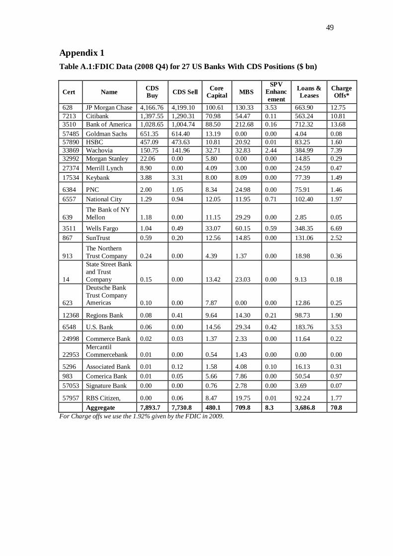
49
Appendix 1
Table A.1:FDIC Data (2008 Q4) for 27 US Banks With CDS Positions ($ bn)
Cert Name CDS Buy CDS Sell Core
Capital MBS SPV
Enhancement
Loans & Leases
Charge Offs*
628 JP Morgan Chase 4,166.76 4,199.10 100.61 130.33 3.53 663.90 12.75 7213 Citibank 1,397.55 1,290.31 70.98 54.47 0.11 563.24 10.81 3510 Bank of America 1,028.65 1,004.74 88.50 212.68 0.16 712.32 13.68
57485 Goldman Sachs 651.35 614.40 13.19 0.00 0.00 4.04 0.08 57890 HSBC 457.09 473.63 10.81 20.92 0.01 83.25 1.60 33869 Wachovia 150.75 141.96 32.71 32.83 2.44 384.99 7.39 32992 Morgan Stanley 22.06 0.00 5.80 0.00 0.00 14.85 0.29
27374 Merrill Lynch 8.90 0.00 4.09 3.00 0.00 24.59 0.47
17534 Keybank 3.88 3.31 8.00 8.09 0.00 77.39 1.49
6384 PNC 2.00 1.05 8.34 24.98 0.00 75.91 1.46
6557 National City 1.29 0.94 12.05 11.95 0.71 102.40 1.97
639 The Bank of NY Mellon 1.18 0.00 11.15 29.29 0.00 2.85 0.05
3511 Wells Fargo 1.04 0.49 33.07 60.15 0.59 348.35 6.69
867 SunTrust 0.59 0.20 12.56 14.85 0.00 131.06 2.52
913 The Northern Trust Company 0.24 0.00 4.39 1.37 0.00 18.98 0.36
14
State Street Bank and Trust Company 0.15 0.00 13.42 23.03 0.00 9.13 0.18
623
Deutsche Bank Trust Company Americas 0.10 0.00 7.87 0.00 0.00 12.86 0.25
12368 Regions Bank 0.08 0.41 9.64 14.30 0.21 98.73 1.90
6548 U.S. Bank 0.06 0.00 14.56 29.34 0.42 183.76 3.53
24998 Commerce Bank 0.02 0.03 1.37 2.33 0.00 11.64 0.22
22953 Mercantil Commercebank 0.01 0.00 0.54 1.43 0.00 0.00 0.00
5296 Associated Bank 0.01 0.12 1.58 4.08 0.10 16.13 0.31
983 Comerica Bank 0.01 0.05 5.66 7.86 0.00 50.54 0.97
57053 Signature Bank 0.00 0.00 0.76 2.78 0.00 3.69 0.07
57957 RBS Citizen, 0.00 0.06 8.47 19.75 0.01 92.24 1.77
Aggregate 7,893.7 7,730.8 480.1 709.8 8.3 3,686.8 70.8 For Charge offs we use the 1.92% given by the FDIC in 2009.
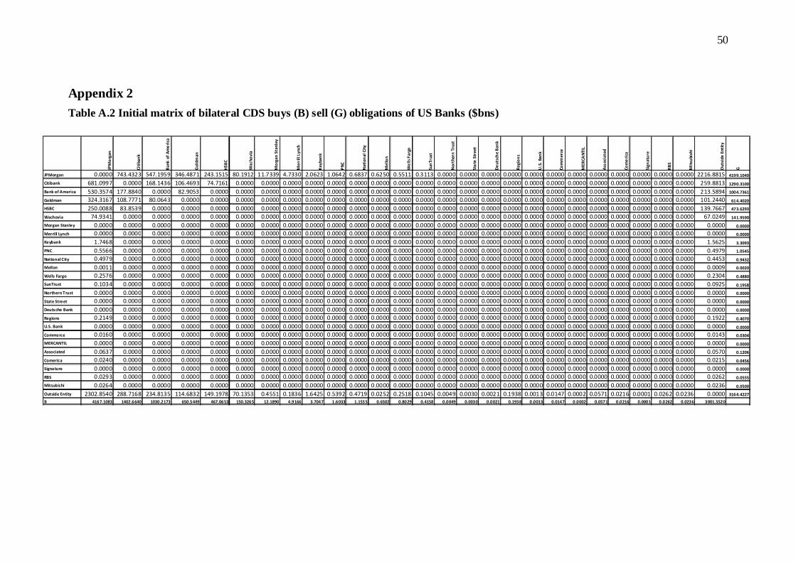
50
Appendix 2
Table A.2 Initial matrix of bilateral CDS buys (B) sell (G) obligations of US Banks ($bns) JP
Mo
rga
n
Cit
iba
nk
Ba
nk
of
Am
eri
ca
Go
ldm
an
HS
BC
Wa
ch
ov
ia
Mo
rga
n S
tan
ley
Me
rril
l Ly
nch
Ke
yb
an
k
PN
C
Na
tio
na
l C
ity
Me
llo
n
We
lls
Fa
rgo
Su
nT
rust
No
rth
ern
Tru
st
Sta
te S
tre
et
De
uts
che
Ba
nk
Re
gio
ns
U.S
. B
an
k
Co
mm
erc
e
ME
RC
AN
TIL
Ass
oci
ate
d
Co
me
rica
Sig
na
ture
RB
S
Mit
sub
ish
i
Ou
tsid
e E
nti
ty
G
JPMorgan 0.0000 743.4323 547.1959 346.4871 243.1515 80.1912 11.7339 4.7330 2.0623 1.0642 0.6837 0.6250 0.5511 0.3113 0.0000 0.0000 0.0000 0.0000 0.0000 0.0000 0.0000 0.0000 0.0000 0.0000 0.0000 0.0000 2216.8815 4199.1040
Citibank 681.0997 0.0000 168.1436 106.4693 74.7161 0.0000 0.0000 0.0000 0.0000 0.0000 0.0000 0.0000 0.0000 0.0000 0.0000 0.0000 0.0000 0.0000 0.0000 0.0000 0.0000 0.0000 0.0000 0.0000 0.0000 0.0000 259.8813 1290.3100
Bank of America 530.3574 177.8840 0.0000 82.9053 0.0000 0.0000 0.0000 0.0000 0.0000 0.0000 0.0000 0.0000 0.0000 0.0000 0.0000 0.0000 0.0000 0.0000 0.0000 0.0000 0.0000 0.0000 0.0000 0.0000 0.0000 0.0000 213.5894 1004.7361
Goldman 324.3167 108.7771 80.0643 0.0000 0.0000 0.0000 0.0000 0.0000 0.0000 0.0000 0.0000 0.0000 0.0000 0.0000 0.0000 0.0000 0.0000 0.0000 0.0000 0.0000 0.0000 0.0000 0.0000 0.0000 0.0000 0.0000 101.2440 614.4020
HSBC 250.0088 83.8539 0.0000 0.0000 0.0000 0.0000 0.0000 0.0000 0.0000 0.0000 0.0000 0.0000 0.0000 0.0000 0.0000 0.0000 0.0000 0.0000 0.0000 0.0000 0.0000 0.0000 0.0000 0.0000 0.0000 0.0000 139.7667 473.6293
Wachovia 74.9341 0.0000 0.0000 0.0000 0.0000 0.0000 0.0000 0.0000 0.0000 0.0000 0.0000 0.0000 0.0000 0.0000 0.0000 0.0000 0.0000 0.0000 0.0000 0.0000 0.0000 0.0000 0.0000 0.0000 0.0000 0.0000 67.0249 141.9590
Morgan Stanley 0.0000 0.0000 0.0000 0.0000 0.0000 0.0000 0.0000 0.0000 0.0000 0.0000 0.0000 0.0000 0.0000 0.0000 0.0000 0.0000 0.0000 0.0000 0.0000 0.0000 0.0000 0.0000 0.0000 0.0000 0.0000 0.0000 0.0000 0.0000
Merrill Lynch 0.0000 0.0000 0.0000 0.0000 0.0000 0.0000 0.0000 0.0000 0.0000 0.0000 0.0000 0.0000 0.0000 0.0000 0.0000 0.0000 0.0000 0.0000 0.0000 0.0000 0.0000 0.0000 0.0000 0.0000 0.0000 0.0000 0.0000 0.0000
Keybank 1.7468 0.0000 0.0000 0.0000 0.0000 0.0000 0.0000 0.0000 0.0000 0.0000 0.0000 0.0000 0.0000 0.0000 0.0000 0.0000 0.0000 0.0000 0.0000 0.0000 0.0000 0.0000 0.0000 0.0000 0.0000 0.0000 1.5625 3.3093
PNC 0.5566 0.0000 0.0000 0.0000 0.0000 0.0000 0.0000 0.0000 0.0000 0.0000 0.0000 0.0000 0.0000 0.0000 0.0000 0.0000 0.0000 0.0000 0.0000 0.0000 0.0000 0.0000 0.0000 0.0000 0.0000 0.0000 0.4979 1.0545
National City 0.4979 0.0000 0.0000 0.0000 0.0000 0.0000 0.0000 0.0000 0.0000 0.0000 0.0000 0.0000 0.0000 0.0000 0.0000 0.0000 0.0000 0.0000 0.0000 0.0000 0.0000 0.0000 0.0000 0.0000 0.0000 0.0000 0.4453 0.9432
Mellon 0.0011 0.0000 0.0000 0.0000 0.0000 0.0000 0.0000 0.0000 0.0000 0.0000 0.0000 0.0000 0.0000 0.0000 0.0000 0.0000 0.0000 0.0000 0.0000 0.0000 0.0000 0.0000 0.0000 0.0000 0.0000 0.0000 0.0009 0.0020
Wells Fargo 0.2576 0.0000 0.0000 0.0000 0.0000 0.0000 0.0000 0.0000 0.0000 0.0000 0.0000 0.0000 0.0000 0.0000 0.0000 0.0000 0.0000 0.0000 0.0000 0.0000 0.0000 0.0000 0.0000 0.0000 0.0000 0.0000 0.2304 0.4880
SunTrust 0.1034 0.0000 0.0000 0.0000 0.0000 0.0000 0.0000 0.0000 0.0000 0.0000 0.0000 0.0000 0.0000 0.0000 0.0000 0.0000 0.0000 0.0000 0.0000 0.0000 0.0000 0.0000 0.0000 0.0000 0.0000 0.0000 0.0925 0.1958
Northern Trust 0.0000 0.0000 0.0000 0.0000 0.0000 0.0000 0.0000 0.0000 0.0000 0.0000 0.0000 0.0000 0.0000 0.0000 0.0000 0.0000 0.0000 0.0000 0.0000 0.0000 0.0000 0.0000 0.0000 0.0000 0.0000 0.0000 0.0000 0.0000
State Street 0.0000 0.0000 0.0000 0.0000 0.0000 0.0000 0.0000 0.0000 0.0000 0.0000 0.0000 0.0000 0.0000 0.0000 0.0000 0.0000 0.0000 0.0000 0.0000 0.0000 0.0000 0.0000 0.0000 0.0000 0.0000 0.0000 0.0000 0.0000
Deutsche Bank 0.0000 0.0000 0.0000 0.0000 0.0000 0.0000 0.0000 0.0000 0.0000 0.0000 0.0000 0.0000 0.0000 0.0000 0.0000 0.0000 0.0000 0.0000 0.0000 0.0000 0.0000 0.0000 0.0000 0.0000 0.0000 0.0000 0.0000 0.0000
Regions 0.2149 0.0000 0.0000 0.0000 0.0000 0.0000 0.0000 0.0000 0.0000 0.0000 0.0000 0.0000 0.0000 0.0000 0.0000 0.0000 0.0000 0.0000 0.0000 0.0000 0.0000 0.0000 0.0000 0.0000 0.0000 0.0000 0.1922 0.4070
U.S. Bank 0.0000 0.0000 0.0000 0.0000 0.0000 0.0000 0.0000 0.0000 0.0000 0.0000 0.0000 0.0000 0.0000 0.0000 0.0000 0.0000 0.0000 0.0000 0.0000 0.0000 0.0000 0.0000 0.0000 0.0000 0.0000 0.0000 0.0000 0.0000
Commerce 0.0160 0.0000 0.0000 0.0000 0.0000 0.0000 0.0000 0.0000 0.0000 0.0000 0.0000 0.0000 0.0000 0.0000 0.0000 0.0000 0.0000 0.0000 0.0000 0.0000 0.0000 0.0000 0.0000 0.0000 0.0000 0.0000 0.0143 0.0304
MERCANTIL 0.0000 0.0000 0.0000 0.0000 0.0000 0.0000 0.0000 0.0000 0.0000 0.0000 0.0000 0.0000 0.0000 0.0000 0.0000 0.0000 0.0000 0.0000 0.0000 0.0000 0.0000 0.0000 0.0000 0.0000 0.0000 0.0000 0.0000 0.0000
Associated 0.0637 0.0000 0.0000 0.0000 0.0000 0.0000 0.0000 0.0000 0.0000 0.0000 0.0000 0.0000 0.0000 0.0000 0.0000 0.0000 0.0000 0.0000 0.0000 0.0000 0.0000 0.0000 0.0000 0.0000 0.0000 0.0000 0.0570 0.1206
Comerica 0.0240 0.0000 0.0000 0.0000 0.0000 0.0000 0.0000 0.0000 0.0000 0.0000 0.0000 0.0000 0.0000 0.0000 0.0000 0.0000 0.0000 0.0000 0.0000 0.0000 0.0000 0.0000 0.0000 0.0000 0.0000 0.0000 0.0215 0.0456
Signature 0.0000 0.0000 0.0000 0.0000 0.0000 0.0000 0.0000 0.0000 0.0000 0.0000 0.0000 0.0000 0.0000 0.0000 0.0000 0.0000 0.0000 0.0000 0.0000 0.0000 0.0000 0.0000 0.0000 0.0000 0.0000 0.0000 0.0000 0.0000
RBS 0.0293 0.0000 0.0000 0.0000 0.0000 0.0000 0.0000 0.0000 0.0000 0.0000 0.0000 0.0000 0.0000 0.0000 0.0000 0.0000 0.0000 0.0000 0.0000 0.0000 0.0000 0.0000 0.0000 0.0000 0.0000 0.0000 0.0262 0.0555
Mitsubishi 0.0264 0.0000 0.0000 0.0000 0.0000 0.0000 0.0000 0.0000 0.0000 0.0000 0.0000 0.0000 0.0000 0.0000 0.0000 0.0000 0.0000 0.0000 0.0000 0.0000 0.0000 0.0000 0.0000 0.0000 0.0000 0.0000 0.0236 0.0500
Outside Entity 2302.8540 288.7168 234.8135 114.6832 149.1978 70.1353 0.4551 0.1836 1.6425 0.5392 0.4719 0.0252 0.2518 0.1045 0.0049 0.0030 0.0021 0.1938 0.0013 0.0147 0.0002 0.0571 0.0216 0.0001 0.0262 0.0236 0.0000 3164.4227
B 4167.1083 1402.6640 1030.2173 650.5449 467.0653 150.3265 12.1890 4.9166 3.7047 1.6033 1.1555 0.6502 0.8029 0.4158 0.0049 0.0030 0.0021 0.1938 0.0013 0.0147 0.0002 0.0571 0.0216 0.0001 0.0262 0.0236 3001.5520
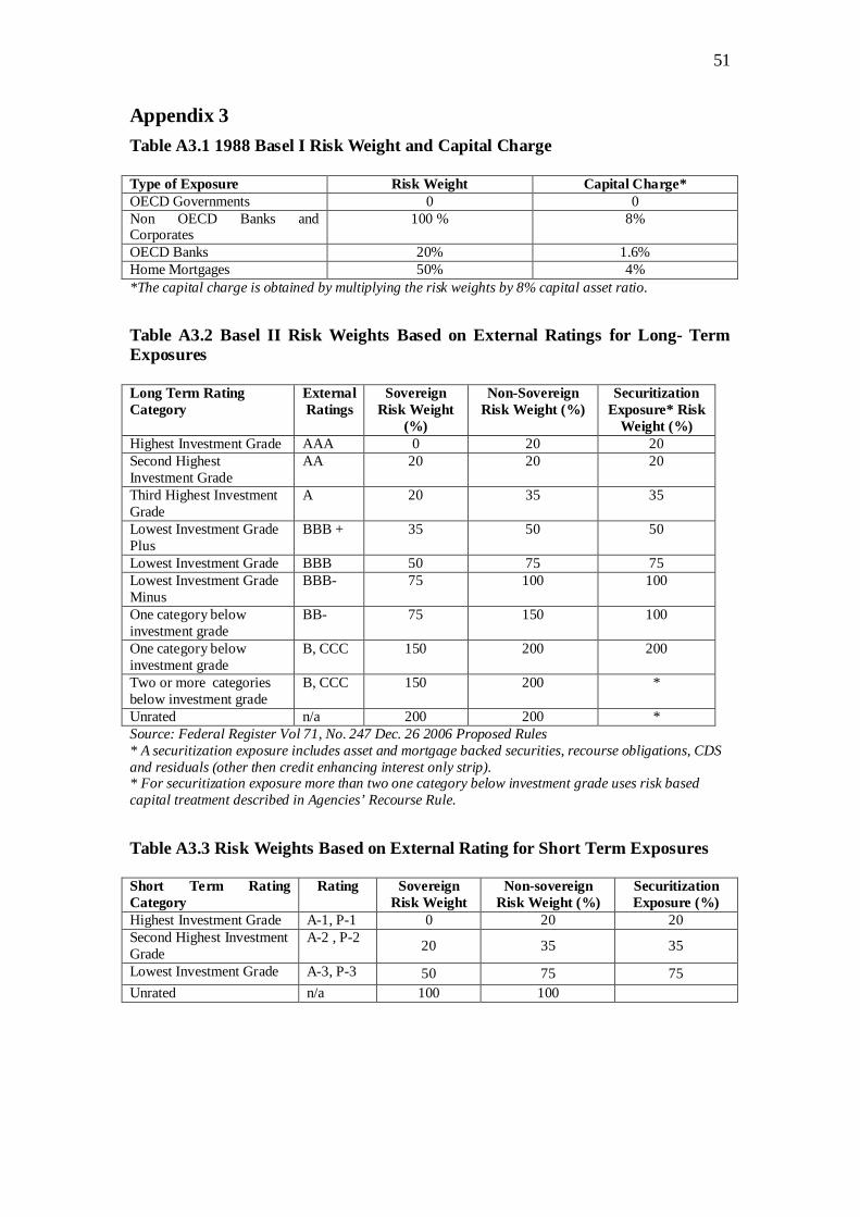
51
Appendix 3
Table A3.1 1988 Basel I Risk Weight and Capital Charge Type of Exposure Risk Weight Capital Charge* OECD Governments 0 0 Non OECD Banks and Corporates
100 % 8%
OECD Banks 20% 1.6% Home Mortgages 50% 4% *The capital charge is obtained by multiplying the risk weights by 8% capital asset ratio.
Table A3.2 Basel II Risk Weights Based on External Ratings for Long- Term Exposures Long Term Rating Category
External Ratings
Sovereign Risk Weight
(%)
Non-Sovereign Risk Weight (%)
Securitization Exposure* Risk
Weight (%) Highest Investment Grade AAA 0 20 20 Second Highest Investment Grade
AA 20 20 20
Third Highest Investment Grade
A 20 35 35
Lowest Investment Grade Plus
BBB + 35 50 50
Lowest Investment Grade BBB 50 75 75 Lowest Investment Grade Minus
BBB- 75 100 100
One category below investment grade
BB- 75 150 100
One category below investment grade
B, CCC 150 200 200
Two or more categories below investment grade
B, CCC 150 200 *
Unrated n/a 200 200 * Source: Federal Register Vol 71, No. 247 Dec. 26 2006 Proposed Rules * A securitization exposure includes asset and mortgage backed securities, recourse obligations, CDS and residuals (other then credit enhancing interest only strip). * For securitization exposure more than two one category below investment grade uses risk based capital treatment described in Agencies’ Recourse Rule.
Table A3.3 Risk Weights Based on External Rating for Short Term Exposures Short Term Rating Category
Rating Sovereign Risk Weight
Non-sovereign Risk Weight (%)
Securitization Exposure (%)
Highest Investment Grade A-1, P-1 0 20 20 Second Highest Investment Grade
A-2 , P-2 20 35 35
Lowest Investment Grade A-3, P-3 50 75 75 Unrated n/a 100 100
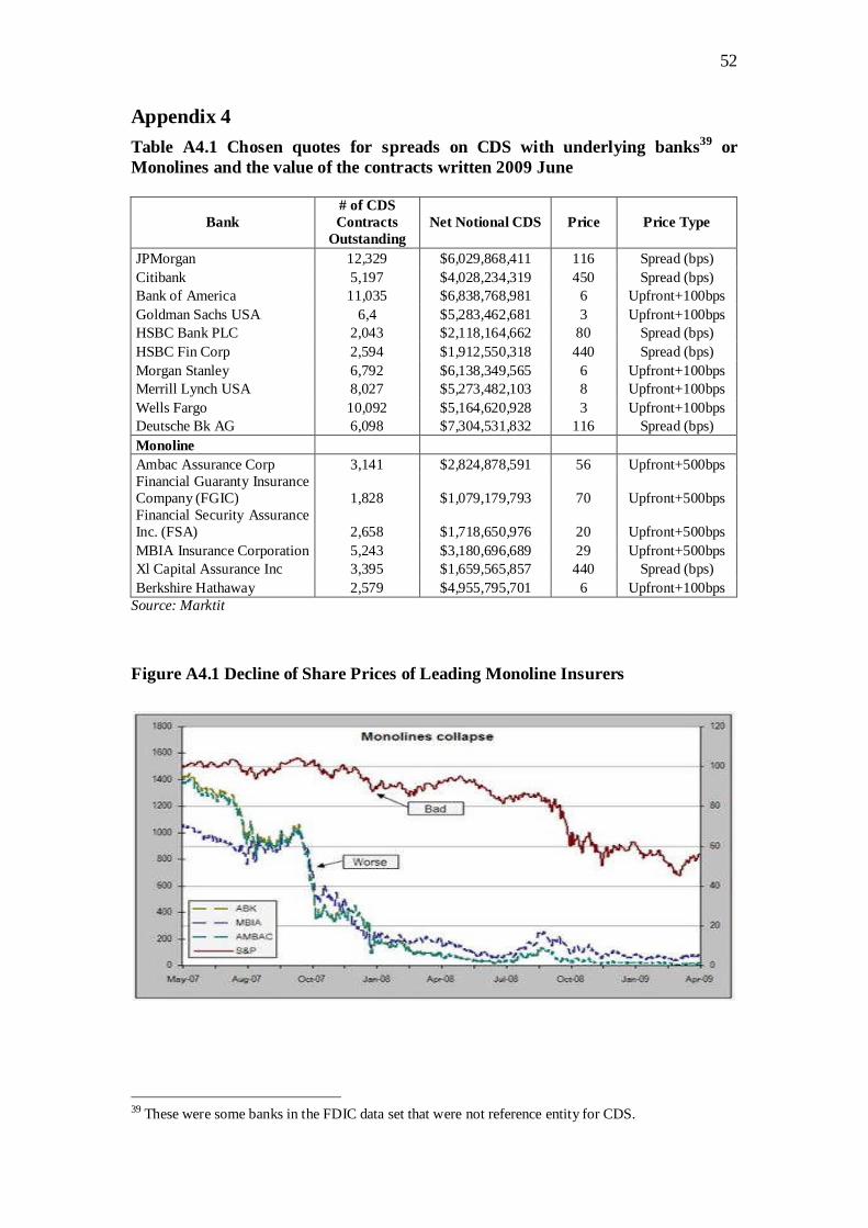
52
Appendix 4
Table A4.1 Chosen quotes for spreads on CDS with underlying banks39 or Monolines and the value of the contracts written 2009 June
Bank # of CDS Contracts
Outstanding Net Notional CDS Price Price Type
JPMorgan 12,329 $6,029,868,411 116 Spread (bps) Citibank 5,197 $4,028,234,319 450 Spread (bps) Bank of America 11,035 $6,838,768,981 6 Upfront+100bps Goldman Sachs USA 6,4 $5,283,462,681 3 Upfront+100bps HSBC Bank PLC 2,043 $2,118,164,662 80 Spread (bps) HSBC Fin Corp 2,594 $1,912,550,318 440 Spread (bps) Morgan Stanley 6,792 $6,138,349,565 6 Upfront+100bps Merrill Lynch USA 8,027 $5,273,482,103 8 Upfront+100bps Wells Fargo 10,092 $5,164,620,928 3 Upfront+100bps Deutsche Bk AG 6,098 $7,304,531,832 116 Spread (bps) Monoline Ambac Assurance Corp 3,141 $2,824,878,591 56 Upfront+500bps Financial Guaranty Insurance Company (FGIC) 1,828 $1,079,179,793 70 Upfront+500bps Financial Security Assurance Inc. (FSA) 2,658 $1,718,650,976 20 Upfront+500bps MBIA Insurance Corporation 5,243 $3,180,696,689 29 Upfront+500bps Xl Capital Assurance Inc 3,395 $1,659,565,857 440 Spread (bps) Berkshire Hathaway 2,579 $4,955,795,701 6 Upfront+100bps
Source: Marktit
Figure A4.1 Decline of Share Prices of Leading Monoline Insurers
39 These were some banks in the FDIC data set that were not reference entity for CDS.
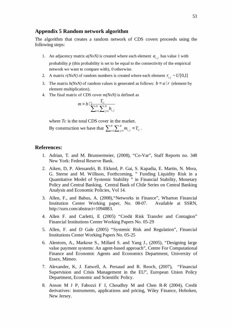
53
Appendix 5 Random network algorithm The algorithm that creates a random network of CDS covers proceeds using the following steps:
1. An adjacency matrix a(NxN) is created where each element jia , has value 1 with
probability p (this probability is set to be equal to the connectivity of the empirical network we want to compare with), 0 otherwise.
2. A matrix r(NxN) of random numbers is created where each element ]1,0[~, Ur ji
3. The matrix b(NxN) of random values is generated as follows: rab ⋅= (element by element multiplication).
4. The final matrix of CDS cover m(NxN) is defined as
∑ ∑= =
⋅=N
i
N
j ji
C
b
Tbm
1 1 ,
where Tc is the total CDS cover in the market.
By construction we have that C
N
i
N
j ji Tm =∑ ∑= =1 1 , .
References: 1. Adrian, T. and M. Brunnermeier, (2008), “Co-Var”, Staff Reports no. 348
New York: Federal Reserve Bank.
2. Aiken, D, P. Alessandri, B. Eklund, P. Gai, S. Kapadia, E. Martin, N. Mora, G. Sterne and M. Willison, Forthcoming, ” Funding Liquidity Risk in a Quantitative Model of Systemic Stability ” in Financial Stability, Monetary Policy and Central Banking, Central Bank of Chile Series on Central Banking Analysis and Economic Policies, Vol 14.
3. Allen, F., and Babus, A. (2008),“Networks in Finance”, Wharton Financial Institution Center Working paper, No. 08-07. Available at SSRN, http://ssrn.com/abstract=1094883.
4. Allen F. and Carletti, E (2005) “Credit Risk Transfer and Contagion” Financial Institutions Center Working Papers No. 05-29
5. Allen, F. and D Gale (2005) “Systemic Risk and Regulation”, Financial Institutions Center Working Papers No. 05-25
6. Alentorn, A., Markose S., Millard S. and Yang J., (2005), “Designing large value payment systems: An agent-based approach”, Centre For Computational Finance and Economic Agents and Economics Department, University of Essex, Mimeo.
7. Alexander, K, J. Eatwell, A. Persaud and R. Reoch, (2007), “Financial Supervision and Crisis Management in the EU”, European Union Policy Department, Economic and Scientific Policy.
8. Anson M J P, Fabozzi F J, Choudhry M and Chen R-R (2004), Credit derivatives: instruments, applications and pricing, Wiley Finance, Hoboken, New Jersey.
54
9. Ashcroft, A. and T. Schuermann (2008), “Understanding the Securitization of SubPrime Mortgage Credit ”, Federal Reserve Bank of New York Staff Report, no. 318.
10. Arthur,W.B.(1994).“Inductive behaviour and bounded rationality”, American Economic Review, 84, pp.406-411.
11. Barabási, A.-L.; R. Albert (1999). "Emergence of scaling in random networks". Science 286: 509–512.s
12. Basel Committee for Banking Supervision (2001), The New Basel Capital Accord. [Online]. Available: http://www.bis.org/publ/index.htm
13. Boss, M., H. Elsinger, M. Summer, S. Thurner. (2004), “An Empirical Analysis of the Network Structure of the Austrian Interbank Market”, Financial Stability Report, 7, Oestorreichesche Nationalbank.
14. Brunnermeier, M. (2008), “Deciphering the 2007-08 Liquidity and Credit Crunch”, Journal of Economic Perspectives,
15. Brunnermeier, M., A. Crockett, C. Goodhart, A. Persaud and H. Shin, (2009), “The Fundamental Principles of Financial Regulation”, Geneva Reports on the World Economy 11, International Center for Money and Banking Studies.
16. Chan-Lau, Jorge A., Espinosa-Vega, Marco A., Giesecke, Kay and Solé, Juan A. (April 2009) "Assessing the Systemic Implications of Financial Linkages," IMF Global Financial Stability Report, Vol. 2
17. Chan-Lau, Marco Espinosa, and Juan Solé, (2009a), "On the Use of Network Analysis to Assess Systemic Financial Linkages," IMF Working Paper, forthcoming.
18. Coudert, V., and Gex, M. (2008), “Contagion in the Credit Default Swap Market : The Case of the GM and Ford Crisis in 2005”, CEPII Working Paper No. 2008-14
19. Deacon, J (2003) “Global Securitization and CDOs”; John Wiley & Sons, Inc. The Atrium, Southern Gate, Chichester, West Sussex
20. Duffie, D. (2007), “Innovations in Credit Risk Transfer: Implications for Financial Stability”, Working Paper Stanford University.
21. Eichengreen, B. and Rourke, K.H. (2009), “A Tale of Two Depressions”, www.Voxeu.org
22. European Central Bank (2004), “Credit Risk Transfer by EU Banks: Activities, Risks and Risk Management”, Banking supervision Committee of the European System of Central Banks, May 2004, Frankfurt, Germany.
23. Fed Reserve Board Basel II Capital Accord Notice of Proposed Rulemaking (NPR) and Supporting Board Documents Draft Basel II NPR - Proposed Regulatory Text - Part V Risk-Weighted Assets for Securitization Exposures 30.03.2006 http://www.federalreserve.gov/GeneralInfo/basel2/DraftNPR/NPR/part_5.htm
24. Fender, Ingo and Scheicher, Martin (2008), “The ABX: How Do Markets Price Sub-Prime Mortgage Risk”, BIS Quarterly Review, September.
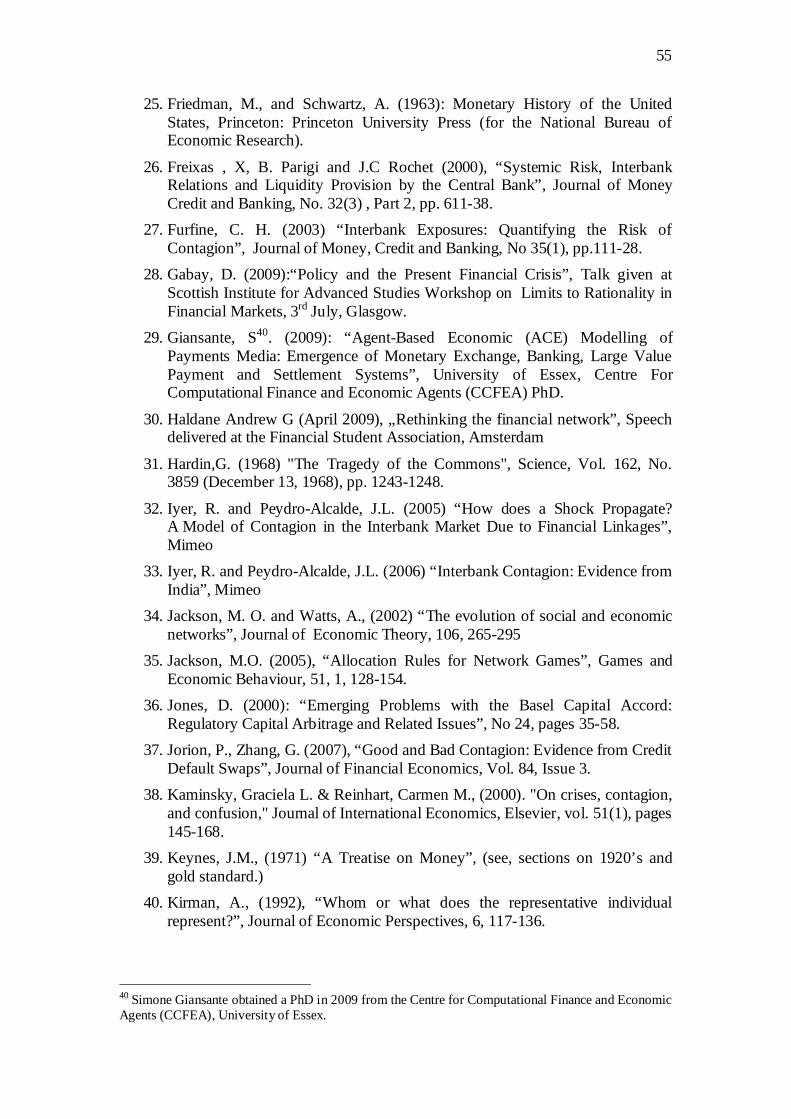
55
25. Friedman, M., and Schwartz, A. (1963): Monetary History of the United States, Princeton: Princeton University Press (for the National Bureau of Economic Research).
26. Freixas , X, B. Parigi and J.C Rochet (2000), “Systemic Risk, Interbank Relations and Liquidity Provision by the Central Bank”, Journal of Money Credit and Banking, No. 32(3) , Part 2, pp. 611-38.
27. Furfine, C. H. (2003) “Interbank Exposures: Quantifying the Risk of Contagion”, Journal of Money, Credit and Banking, No 35(1), pp.111-28.
28. Gabay, D. (2009):“Policy and the Present Financial Crisis”, Talk given at Scottish Institute for Advanced Studies Workshop on Limits to Rationality in Financial Markets, 3rd July, Glasgow.
29. Giansante, S40. (2009): “Agent-Based Economic (ACE) Modelling of Payments Media: Emergence of Monetary Exchange, Banking, Large Value Payment and Settlement Systems”, University of Essex, Centre For Computational Finance and Economic Agents (CCFEA) PhD.
30. Haldane Andrew G (April 2009), „Rethinking the financial network”, Speech delivered at the Financial Student Association, Amsterdam
31. Hardin,G. (1968) "The Tragedy of the Commons", Science, Vol. 162, No. 3859 (December 13, 1968), pp. 1243-1248.
32. Iyer, R. and Peydro-Alcalde, J.L. (2005) “How does a Shock Propagate? A Model of Contagion in the Interbank Market Due to Financial Linkages”, Mimeo
33. Iyer, R. and Peydro-Alcalde, J.L. (2006) “Interbank Contagion: Evidence from India”, Mimeo
34. Jackson, M. O. and Watts, A., (2002) “The evolution of social and economic networks”, Journal of Economic Theory, 106, 265-295
35. Jackson, M.O. (2005), “Allocation Rules for Network Games”, Games and Economic Behaviour, 51, 1, 128-154.
36. Jones, D. (2000): “Emerging Problems with the Basel Capital Accord: Regulatory Capital Arbitrage and Related Issues”, No 24, pages 35-58.
37. Jorion, P., Zhang, G. (2007), “Good and Bad Contagion: Evidence from Credit Default Swaps”, Journal of Financial Economics, Vol. 84, Issue 3.
38. Kaminsky, Graciela L. & Reinhart, Carmen M., (2000). "On crises, contagion, and confusion," Journal of International Economics, Elsevier, vol. 51(1), pages 145-168.
39. Keynes, J.M., (1971) “A Treatise on Money”, (see, sections on 1920’s and gold standard.)
40. Kirman, A., (1992), “Whom or what does the representative individual represent?”, Journal of Economic Perspectives, 6, 117-136.
40 Simone Giansante obtained a PhD in 2009 from the Centre for Computational Finance and Economic Agents (CCFEA), University of Essex.
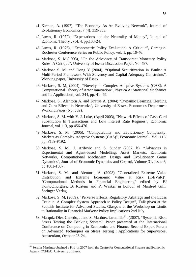
56
41. Kirman, A. (1997), “The Economy As An Evolving Network”, Journal of Evolutionary Economics, 7 (4): 339-353.
42. Lucas, R. (1972), “Expectations and the Neutrality of Money”, Journal of Economic Theory , vol. 4, pp.103-24.
43. Lucas, R. (1976), “Econometric Policy Evaluation: A Critique”, Carnegie-Rochester Conference Series on Public Policy, vol. 1, pp. 19-46.
44. Markose, S. M.(1998), “On the Advocacy of Transparent Monetary Policy Rules: A Critique”, University of Essex Discussion Paper, No. 487.
45. Markose S. M. and Dong Y (2004), “Optimal Securitization in Banks: A Multi-Period Framework With Solvency and Capital Adequacy Constraints”, Working paper, University of Essex.
46. Markose, S. M, (2004), “Novelty in Complex Adaptive Systems (CAS): A Computational Theory of Actor Innovation”, Physica A: Statistical Mechanics and Its Applications, vol. 344, pp. 41- 49.
47. Markose, S., Alentorn A. and Krause A. (2004) “Dynamic Learning, Herding and Guru Effects in Networks”, University of Essex, Economics Department Working Paper (No. 582).
48. Markose, S. M. with Y. J. Loke, (April 2003), “Network Effects of Cash-Card Substitution In Transactions and Low Interest Rate Regimes”, Economic Journal, vol.113, pp.456-476.
49. Markose, S. M. (2005), “Computability and Evolutionary Complexity: Markets as Complex Adaptive Systems (CAS)”, Economic Journal , Vol. 115, pp. F159-F192.
50. Markose, S. M., J. Arifovic and S. Sunder (2007, b), “Advances in Experimental and Agent-based Modelling: Asset Markets, Economic Networks, Computational Mechanism Design and Evolutionary Game Dynamics”, Journal of Economic Dynamics and Control, Volume 31, Issue 6, pp 1801-1807.
51. Markose, S. M., and Alentorn, A. (2008), "Generalized Extreme Value Distribution and Extreme Economic Value at Risk (E-EVaR)". "Computational Methods in Financial Engineering" edited by EJ Kontoghiorghes, B. Rustem and P. Winker in honour of Manfred Gilli, Springer Verlag.
52. Markose, S. M, (2009), “Perverse Effects, Regulatory Arbitrage and the Lucas Critique: A Complex System Approach to Policy Design”, Talk given at the Scottish Institute for Advanced Studies, Glasgow at the Workshop on Limits to Rationality in Financial Markets: Policy Implications 2nd July
53. Marquiz-Diez-Canedo, J. and S. Martinez-Jaramillo41, (2007), “Systemic Risk: Stress Testing the Banking System” Paper presented at the International Conference on Computing in Economics and Finance Second Expert Forum on Advanced Techniques on Stress Testing : Applications for Supervisors, Amsterdam, October 23-24.
41 Serafin Martinez obtained a Phd in 2007 from the Centre for Computational Finance and Economic Agents (CCFEA), University of Essex.
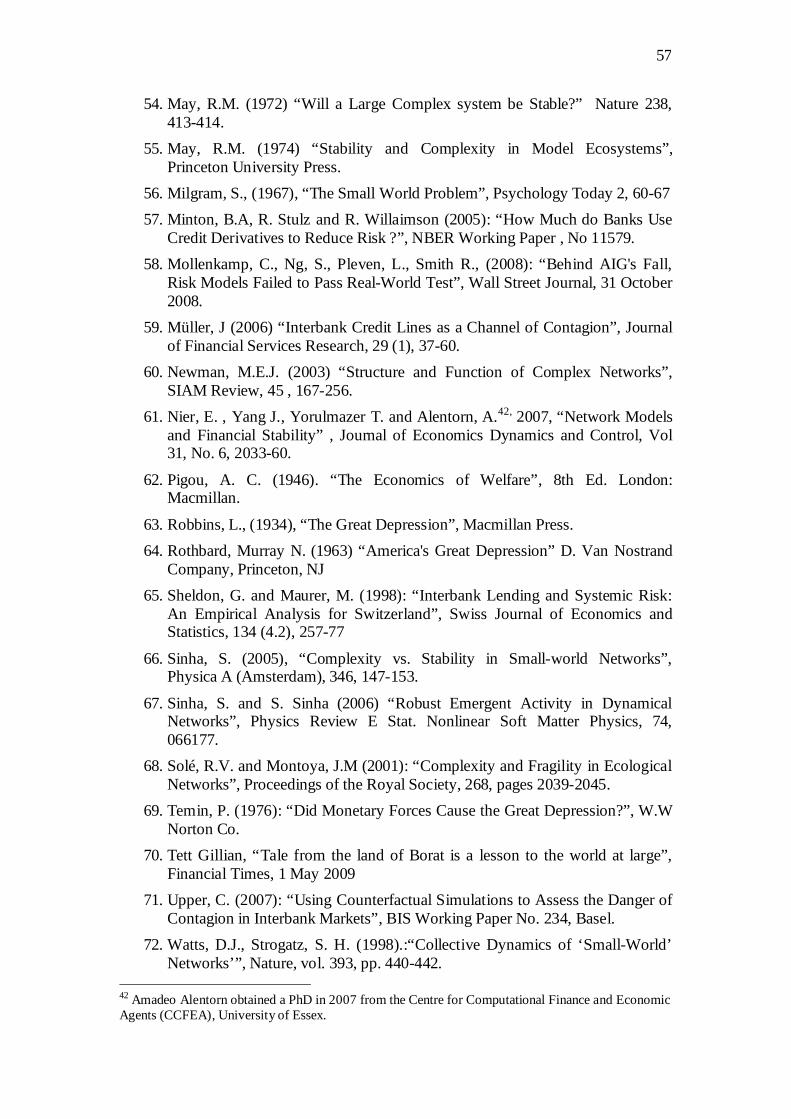
57
54. May, R.M. (1972) “Will a Large Complex system be Stable?” Nature 238, 413-414.
55. May, R.M. (1974) “Stability and Complexity in Model Ecosystems”, Princeton University Press.
56. Milgram, S., (1967), “The Small World Problem”, Psychology Today 2, 60-67
57. Minton, B.A, R. Stulz and R. Willaimson (2005): “How Much do Banks Use Credit Derivatives to Reduce Risk ?”, NBER Working Paper , No 11579.
58. Mollenkamp, C., Ng, S., Pleven, L., Smith R., (2008): “Behind AIG's Fall, Risk Models Failed to Pass Real-World Test”, Wall Street Journal, 31 October 2008.
59. Müller, J (2006) “Interbank Credit Lines as a Channel of Contagion”, Journal of Financial Services Research, 29 (1), 37-60.
60. Newman, M.E.J. (2003) “Structure and Function of Complex Networks”, SIAM Review, 45 , 167-256.
61. Nier, E. , Yang J., Yorulmazer T. and Alentorn, A.42, 2007, “Network Models and Financial Stability” , Journal of Economics Dynamics and Control, Vol 31, No. 6, 2033-60.
62. Pigou, A. C. (1946). “The Economics of Welfare”, 8th Ed. London: Macmillan.
63. Robbins, L., (1934), “The Great Depression”, Macmillan Press.
64. Rothbard, Murray N. (1963) “America's Great Depression” D. Van Nostrand Company, Princeton, NJ
65. Sheldon, G. and Maurer, M. (1998): “Interbank Lending and Systemic Risk: An Empirical Analysis for Switzerland”, Swiss Journal of Economics and Statistics, 134 (4.2), 257-77
66. Sinha, S. (2005), “Complexity vs. Stability in Small-world Networks”, Physica A (Amsterdam), 346, 147-153.
67. Sinha, S. and S. Sinha (2006) “Robust Emergent Activity in Dynamical Networks”, Physics Review E Stat. Nonlinear Soft Matter Physics, 74, 066177.
68. Solé, R.V. and Montoya, J.M (2001): “Complexity and Fragility in Ecological Networks”, Proceedings of the Royal Society, 268, pages 2039-2045.
69. Temin, P. (1976): “Did Monetary Forces Cause the Great Depression?”, W.W Norton Co.
70. Tett Gillian, “Tale from the land of Borat is a lesson to the world at large”, Financial Times, 1 May 2009
71. Upper, C. (2007): “Using Counterfactual Simulations to Assess the Danger of Contagion in Interbank Markets”, BIS Working Paper No. 234, Basel.
72. Watts, D.J., Strogatz, S. H. (1998).:“Collective Dynamics of ‘Small-World’ Networks’”, Nature, vol. 393, pp. 440-442.
42 Amadeo Alentorn obtained a PhD in 2007 from the Centre for Computational Finance and Economic Agents (CCFEA), University of Essex.

58
73. Watts, D. (1999), “Small Worlds”, Princeton University Press.
74. Wells, S. (2004): “Financial Interlinkages in the United Kingdom’s Interbank Market and the Risk of Contagion”, Bank of England, Working Paper No. 230.