1

Working Paper Series: 05-03

International Contagion in Emerging Markets

Dipinder S Randhawa* and Andreina Low Mei Lien

* Corresponding author Saw Centre for Financial Studies NUS Business School National University of Singapore Singapore 117592 bizdsr@nus.edu.sg Phone: (65) 6874 5835 Fax: (65) 6874 5834

2

International Contagion in Emerging Markets

Dipinder S Randhawa* and Andreina Low Mei Lien * Corresponding author Saw Centre for Financial Studies NUS Business School National University of Singapore Singapore 117592 bizdsr@nus.edu.sg Phone: (65) 6874 5835 Fax: (65) 6874 5834

3

1: Introduction Over the past three years investments in emerging market bonds have yielded

impressive returns. The JP Morgan EMBI posted an average annual return of 16.20% since 2001. According to the Institute of International Finance, gross issuance of bonds in emerging markets in 2004 exceeded $100 billion, the highest level since 1997. Lured by improved credit ratings in emerging markets, attractive returns and a proliferation in the type and numbers of issuers, the international investment community’s interest in both hard and local currency bonds is being sustained in 2005. Currently investors trade mainly foreign-currency denominated emerging market debt. Nonetheless with the steady growth and deepening in capital markets, specifically the rapid growth in the issue of fixed income securities over the past several years there has been increasing interest in local currency denominated bonds These bonds made up 75% of bonds issued by emerging market in 2003. This trend is expected to accelerate over the next five years.

There are growing fears however, that when US Federal interest rates rise further or if

the decline in the US dollar accelerates, investors may want to cash in on these profits leading to a sharp reversal into defensive and less risky markets. Furthermore backsliding on economic reforms by various governments and the tentative nature of the fundamentals underlying the American economy have been important risk factors to be reckoned with in recent times. In addition, given the history and relative high frequency of multiple financial crises since the 1990’s, and the possibility of credit contagion from other economies, there is a growing need to explore in greater depth, the risk-profiles of various emerging market bonds. Thus in the context of the growing importance of emerging credit markets, and the issues discussed above, this paper seeks to fill a gap in the existing literature on the risk-return characteristics of emerging market bond issues, an area that remain neglected relative to the research on emerging equity and currency markets

Specifically, this paper seeks to address the issue of whether contagion, i.e. spillover

effects from unanticipated idiosyncratic shocks from selected credit markets at the epicenter of financial upheaval, was transmitted to other emerging credit markets during the 1990s. In addition, it also studies if the channels of contagion change from one crisis to another. To do so, this paper adopts a precise working definition of contagion. This definition refers to the transmission of shocks resulting from a significant change in cross market linkages. This is distinct from shocks that would occur as a normal continuation of the same cross market linkages that existed in tranquil pre-crisis periods. To facilitate precise estimation we also use a latent factor model which estimates rather than implicitly assumes, the variance covariance structure of idiosyncratic shocks and common global shocks.

Contagion here is defined as the spillover effects from unanticipated country-specific shocks from one (or many) credit market(s) to another. Specifically, it measures the total volatility contributed by these unanticipated idiosyncratic shocks from another credit market that is in excess of what would usually be accounted for due to their normal relationships with each other. This is synonymous with the definition of shift-contagion used in recent literature. Such a definition of contagion provides a clear test of the effectiveness of international diversification in reducing portfolio risk in the event of a crisis. In addition, it also allows us to evaluate the role and potential effectiveness of international institutions, such as the

4

International Monetary Fund (IMF) or the World Bank, and bailout operations aiming to control contagion effects. This is of importance to the various national monetary authorities and policy-makers, as well as international institutions, such as the IMF or the World Bank. If shift-contagion exists, multi-lateral intervention and the use of capital controls used to mitigate the effects of contagion might be justified. However if shift-contagion does not exist and the increase in co-movements in asset markets are mainly due to long-term relationships between these markets, then these measures will only prolong, and not reduce the necessary adjustments that must be made to affected asset markets.

This definition of contagion is then employed to study daily returns measured by two independent data sets covering two distinct time periods. These are the daily returns on the JP Morgan Emerging Market Bond Indices (Global Diversified) (EMBI + GLB DIVERS) and of the JP Morgan Emerging Local Markets Indices (ELMI+). The first data set of EMBI+ GLB DIVERS1 covers five financial crises and the Mexican upgrade, occurred since March of 1994 to March of 2003. This includes; (i) the Mexican crisis in 1994, (ii) the Asian crisis in 1997, (iii) the Russian crisis in 1998, (iv) the Brazilian devaluation which followed in 1999, (v) Mexico’s credit rating upgrade in March of 2000 and (vi) the Argentina crisis beginning in October of 2000. The second data set of ELMI+2 of various Asian credit markets, and which covers the Asian economic crisis in 1997.

This paper then goes on to use factor models to decompose volatility of bond returns in various credit markets into a set of latent factors. These factors include (i) a world factor that encapsulates common shocks that affect all global economies to varying effects, (ii) unanticipated idiosyncratic factors which are unique to each credit market studied, and finally, (iiii) contagion factors arising from spillover effects of unanticipated contemporaneous shocks across countries. Contagion occurs if the factor loadings for the spillover effects across countries contribute significantly to total volatility in a country’s asset market returns. In order to correct for the GARCH (1,1) errors and the co-integrating relationships observed in the data collected, an indirect inference estimation technique is used.

The empirical results obtained indicate that the world factor or common global shocks play a dominant role in accounting for the total volatility experienced in different credit markets. The importance of country-specific shocks varies across countries as well as over the different sub-sample periods studied. Nonetheless, in general, country-specific shocks appear to contribute a significant amount of the volatility experienced in credit markets, particularly in the one that is accepted to be the ground-zero country dispersing contagion effects to others. More importantly, contagion from the spillover effects of unanticipated contemporaneous shocks across credit markets is found to exist in all the crisis periods studied. However, these spill-over effects are only significant for some, and not all the credit markets studied. The pool of affected credit markets does not remain the same across the different crisis periods studied. This implies not only that shift-contagion has occurred in the entire sample period studied, but that the nature of cross-market linkages also changes from

1 The bond indices included in the first data set of EMBI+ GLB DIVERS include that of Argentina, Brazil,

Mexico, Russia and Asia 2 The bond indices included in the second data set of ELMI+ include that of Hong Kong, Indonesia, Singapore

and Thailand

5

one crisis to another, and not just from periods of tranquility to periods of crisis. This finding distinguishes this paper from the existing credit contagion literature.

The rest of this paper is organized as follows: Section 2 provides a brief overview of recent contagion literature, while Section 3 elaborates on the background and stylized facts revolving round the five financial crises and the Mexican credit rating upgrade. This is followed in Section 4 by a detailed description of the data used and the descriptive statistics. Section 5 then explains and elaborates upon the latent model used in this paper, while Section 6 describes the indirect inference estimation technique used to correct for GARCH (1, 1) errors and the co-integrating relationships observed in the data series. Subsequently empirical results obtained from the indirect inference estimations are then presented in Section 7. Section 8 concludes.

2 Literature Review

Following the financial crises in the 1990’s3, there has been extensive research on transmission mechanisms facilitating contagion. However there is little agreement on the definition of contagion. In a broad overview of contagion literature, Pericoli and Sbracia (2003) describe five different contagion definitions. These can be subsumed into two broad definitions. The first definition differentiates a significant increase in cross-market linkages, contingent on a crisis, from increased co-movements in market returns due to their long-run relationships with each other. This is commonly known as shift-contagion. The second definition makes no such differentiation. There are strong advocates for both categories, and a brief overview of the literature employing the use of these definitions follows.

For simplicity, the second definition, which makes no differentiation between a

significant increase in cross-market linkages and a simultaneous increase in volatility due to normal interdependence between the affected credit markets, is discussed first. A popular approach to testing for contagion as specified by the second definition is the Generalized Autoregressive Conditional Heteroskedasticity (GARCH) framework. This is used to estimate the variance-covariance transmission mechanism, i.e. the transmission of shocks, across financial markets. Hamao, Masulis, and Ng (1990) were amongst the first to use the GARCH framework. They found evidence of significant volatility spillovers from the US and UK stock markets to the Japanese market during the 1987 US stock market crash. The authors also suggest that contagion did not occur evenly across markets, and was fairly stable over time.

Evidence of volatility spillovers during financial crises is also supported by Edwards (1998). He focuses on the transmission mechanism of volatility across Latin American bond markets after the Mexican peso crisis. Edwards estimates an augmented uni-variate GARCH model which shows that there were significant volatility spillovers from Mexico to Argentina, but not from Mexico to Chile. However, these tests do not indicate if the transmission mechanism changes during the crisis, i.e. if the cross-market linkages change significantly during the crisis.

3 This includes (i) the Exchange Rate Mechanism (ERM) currency attacks of 1992; (ii) the Mexican peso

devaluation of 1994; (iii) the Asian economic crisis of 1997; (iv) the Russian/LTCM collapse of 1998; (v) the Brazilian real collapse of 1999 and more recently (vi) the Turkey/Argentina crisis of 2000.

6

Another straightforward and widely used approach to the study of contagion, as

defined by the second definition is of significant changes in correlation-coefficients across markets. One of the most thorough studies done on contagion using this definition, is Baig and Goldfajn (1999). They test for contagion in stock market returns, currency prices, interest rates, and sovereign spreads in five Asian emerging markets during the Asian financial crisis of 1997. The authors find that correlation across the markets was significantly higher during the crisis period than in the period of tranquility preceding the Thai baht devaluation in 1997. Using a linear regression model, they conclude that the cross-market correlations increased significantly after the onset of the Asian crisis. In their paper, it is also found that bad news typically has a larger impact than good news on stock market and currency returns. Using the same correlation-coefficient analysis, Calvo and Reinhart (1996) analyze stock prices, Brady bond spreads and actual capital inflows and outflows to and from Asia and Latin America. They find that the correlation between the stock prices and the bond spreads, as well as across the emerging markets, increases after the 1994 Mexican peso crisis. They do not however explain if this is on account of a simultaneous increase in volatility due to normal interdependence between markets, or if the increase in correlations represents a significant change in cross-market linkages. Furthermore, Calvo and Reinhart (1996) do not test whether the changes in correlations are statistically significant.

In addition, these traditional tests based on cross-market correlation coefficients, have been recently challenged by several researchers. In particular, Forbes and Rigobon (2001a and 2001b), Boyer et al. (1999), Loretan and English (2000) and Corsetti et al. (2001) find strong evidence that the standard analysis employed by these traditional test is affected by sample selection bias problem. This occurs mainly because the correlation coefficients in ad hoc sub-samples (like periods of tranquility versus periods of crisis) tend to be biased by the presence of heteroskedasticity. Heteroskedasticity is common in financial market returns and is evident in the clustering of large and small forecast errors. This implies that there are sharp increases in volatility in financial markets, particularly during crisis periods. Therefore the correlation coefficients obtained are biased and have to be adjusted to be net of the effect of the increase in volatility. Correcting for this bias will allow us to differentiate between models of interdependence and models of contagion, as specified in the first definition of contagion. The papers that deal with this potential bias, and thus use shift-contagion as their main premise, are briefly discussed below.

Forbes and Rigobon (2001a and 2001b) analyze daily stock market returns during three major crisis periods; (i) the US stock market crash of October 1987; (ii) the Mexican peso collapse in 1994 and the (iii) Hong Kong financial crisis of October 1997). The authors filter the daily market returns using a VAR (Vector Auto-regressive) model and compute the cross-market correlations of the residuals obtained. By assuming a linear relationship between the filtered stock market returns, they correct for the bias due to the increase in volatility during the crises. The paper rejects the hypothesis of correlation breakdown in almost all cases, and concludes that interdependence rather than contagion effects account for the increased co-movements witnessed by various industrial and emerging countries. Using the same measure of interdependence as Forbes and Rigobon (2001a and 2001b), Boyer et al. and

7

Loretan and English (2000), also conclude that there is no evidence of structural change in the transmission mechanism across countries during the Mexican peso collapse.

However, using the same definition of shift-contagion, Corsetti et al. (2001) show that the frameworks used by Forbes and Rigobon (2001a and 2001b), Boyer et al. and Loretan and English (2000) implicitly fixed the value of the ratio between the variance of idiosyncratic shocks and the variance of the world factor, weighted by their factor loading (hereafter known as the λ-ratio). In doing so, these authors may select too low, or too high a value, for the λ-ratio. By selecting too low a value for the λ-ratio, (Forbes and Rigobon (2001a) and Boyer et al. (1999) set the λ-ratio to zero), the test results will erroneously favor the null hypothesis of interdependence, when one should reject in favor of contagion instead. The opposite is true in selecting too high a value for the λ-ratio. Using a latent factor model, Corsetti et al. (2001) estimate the λ-ratio for the Hong Kong stock market crisis in October 1997, and show that Forbes and Rigobon (2001a) and Boyer et al. (1999) had erroneously accepted the null hypothesis of no contagion.

However Corsetti et al. (2001) do not control for the GARCH (1, 1) and co-integrating relationships witnessed in various financial markets. These characteristics were observed in inflation figures (Coulson and Robins, 1985), term structure of interest rates (Engle, Hendry, and Trumbull, 1985), stock market returns (Engle, Lilien, and Robins, 1987) and foreign exchange markets (Domowitz and Hakkio 1985 and Bollerslev and Ghysels, 1996). This paper will use an augmented version of the latent factor model proposed by Corsetti et al. (2001) and Dungey et al.(2003) to measure shift-contagion (i.e. contagion reflected as spillover effects from unanticipated contemporaneous shocks across markets). The GARCH (1, 1) and co-integrating relationships witnessed in financial markets will be corrected for through an indirect estimation methodology as proposed by Dungey et al. (2002). As Dungey et al. (2002) only study the Russian/LTCM collapse; this paper significantly extends the use of the proposed methodology to a larger sample period, covering four other financial crises and the Mexican upgrade.

Pertinent to the issue of defining contagion, the definition used in this paper also allows for both multiple instantaneous equilibriums, and structural breaks in market behavior due to informational cascades and herding. Thus any evidence of contagion found in this paper may be explained by various transmission mechanisms (for example, Sachs, Tornell and Velasco 1996, Masson 1999, Kaminsky and Schmukler 1999 among many others).

Masson (1999) suggests that discontinuities in market returns could be directly

attributed to jumps between multiple equilibria, in which self-fulfilling prophecies could lead to contagion, if opinions are coordinated across markets. 4 The multiple equilibria theory of contagion is also consistent with other channels for contagion, such as wake-up calls (Goldstein 1998), or heightened investor awareness (Lowell, Neu and Tong 1998). These studies propose that a reappraisal of one country’s fundamentals may lead to a reappraisal of fundamentals in other similar countries, thereby resulting in contagion. As a result of these wake-up calls or heightened investor awareness, herd behavior across markets may also occur (Kaminsky and Schmukler 1999 and Calvo and Mendoza 2000). Krugman (1998) further 4 Loisel and Martin (2001)

8

proposes that herd behavior may lead to the bursting of asset bubbles created by moral hazard, or implied or explicit government guarantees.

Lastly, the definition of contagion used in this paper does not exclude the possibility of liquidity shocks based on market structure. Kyle and Tong (2001) suggest that during the Russia/LTCM crisis, when international investors trading in risky markets experience unanticipated shocks, they liquidate across their portfolios. Thus a shock in one market can lead to spillover effects in seemingly unconnected markets with similar market structures. Rigobon (2002) also propose that the change in investor universe, following Mexico’s credit rating upgrade to investment grade in March of 2000, has led to a change in the market structure for its external debts. The paper shows that there is a statistically significant change in the propagation of shocks following the announcement of the upgrade. Specifically, Mexico seems immune to the crises in other emerging markets, in particular to the Argentina crisis on October of 2000. 3 Background to Events & Stylized Facts 3.1 Mexican Crisis

The first financial crisis, covered in this paper, is the collapse of the Mexican peso on the 19th of December 1994. In the ensuing crisis, the value of the Mexican peso had halved, leading to soaring inflation and a severe economic recession. This can largely be viewed as an unanticipated shock, as just prior to the Mexican peso collapse, at the beginning of 1994, Mexico had entered into the North American Free Trade Agreement (hereafter known as NAFTA) with the United States (U.S.), its largest trading partner,. Furthermore, inflation had been largely tamed and foreign investment was rising in Mexico in the time preceding the crisis.

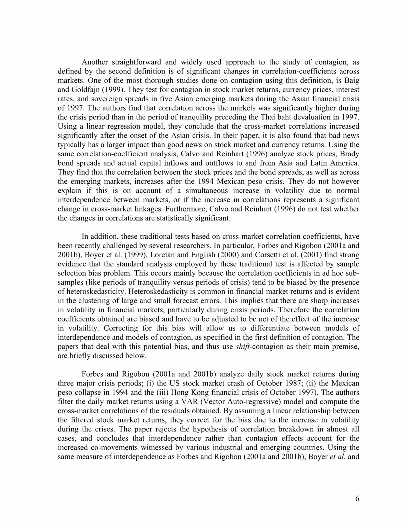
However there were also rising concerns regarding Mexico’s ballooning current

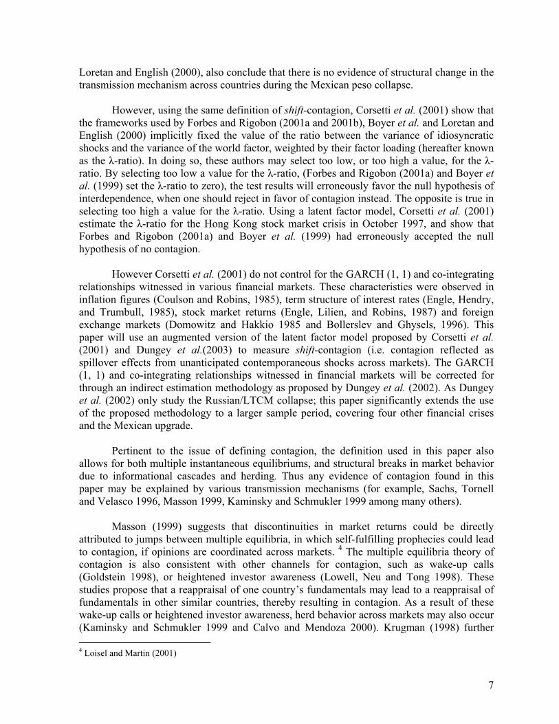
account deficit which increased from $6 billion in 1989 to more than $20 billion in 1992 and 1993.5 Figure 1 shows the rise in Mexico’s current account deficit from 1990 to the third quarter of 1994, the period preceding the crisis. Some analysts observed that the huge current account deficit meant that the quasi-pegged Mexican peso needed to be devalued. (Figures 1.) This coupled with internal political shocks and negative effects of higher interest rates on financial intermediaries and debtors are among the most oft-cited factors in triggering of the Mexican peso devaluation. (Figure 2)

In the weeks following the collapse of the Mexican peso, the Clinton administration made concerted efforts to help Mexico resolve the crisis. On the 31st of January of 1995, this culminated in a direct loan package consisting of $20 billion from the U.S., $18 billion from the IMF and about $13 billion from the Bank for International Settlements and other commercial banks6. Thereafter, after the implementation of a strict austerity package by the Mexican government, the Mexican peso continued to strengthen for the rest of 1995 and credit markets started to calm down.

5 Mexico’s current account deficit was roughly 8 percent, of gross national product (GNP), in 1992 and 7 percent

in 1993. Source : International Monetary Fund’s International Financial Statistics. 6 Peter Passell, “A Mexican Payoff”, New York Times, 12th October 1995

9

Figure 1 Mexico’s Current and Capital Account. 7 (Quarterly Data)

Figure 2. Interest rates (%)8

0

10

20

30

40

50

60

70

80

90

07/19

94

11/19

94

03/19

95

07/19

95

11/19

95

03/19

96

07/19

96

11/19

96

03/19

97

07/19

97

11/19

97

03/19

98

07/19

98

11/19

98

03/19

99

07/19

99

11/19

99

03/20

00

07/20

00

11/20

00

03/20

01

07/20

01

11/20

01

03/20

02

07/20

02

11/20

02

03/20

03

07/20

03

Time

Inte

rest

Rat

es (%

)

ArgentinaBrazilMexico

7 Source: A. Whitt, Jr., 1996, “The Mexican Peso Crisis”, Federal Reserve Bank of Atlanta. 8 The Economist Intelligence Unit – Country Indicators

10

3.2 East Asian Crisis In July 1997 the speculative attack on the Thai baht triggered the onset of a regional

and economic crisis that pushed several East Asian countries into deep recessions.9 A common feature, between the Mexican crisis in 1994 and the Asian economic crisis, is that against the backdrop of strong economic performance of the affected countries, these crises were unanticipated.

In the aftermath of the crisis, many factors were posited as the causes of the Asian

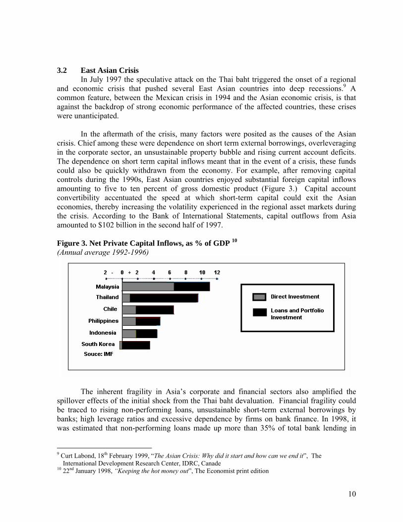
crisis. Chief among these were dependence on short term external borrowings, overleveraging in the corporate sector, an unsustainable property bubble and rising current account deficits. The dependence on short term capital inflows meant that in the event of a crisis, these funds could also be quickly withdrawn from the economy. For example, after removing capital controls during the 1990s, East Asian countries enjoyed substantial foreign capital inflows amounting to five to ten percent of gross domestic product (Figure 3.) Capital account convertibility accentuated the speed at which short-term capital could exit the Asian economies, thereby increasing the volatility experienced in the regional asset markets during the crisis. According to the Bank of International Statements, capital outflows from Asia amounted to $102 billion in the second half of 1997.

Figure 3. Net Private Capital Inflows, as % of GDP 10 (Annual average 1992-1996)

The inherent fragility in Asia’s corporate and financial sectors also amplified the spillover effects of the initial shock from the Thai baht devaluation. Financial fragility could be traced to rising non-performing loans, unsustainable short-term external borrowings by banks; high leverage ratios and excessive dependence by firms on bank finance. In 1998, it was estimated that non-performing loans made up more than 35% of total bank lending in

9 Curt Labond, 18th February 1999, “The Asian Crisis: Why did it start and how can we end it”, The

International Development Research Center, IDRC, Canade 10 22nd January 1998, “Keeping the hot money out”, The Economist print edition

11

Malaysia, Thailand, South Korea and Indonesia.11 In addition the public sector had also taken risky positions in short-term foreign-currency denominated debt markets. It was only following consolidation of data after the outbreak of the Asian crisis, that the larger international community discovered that South Korea and Indonesia had accumulated $150 billion in external debt, and Thailand had foreign exchange exposure to the tune of $100 billion.

Weak external economic conditions were also blamed for the rapid precipitation of the

financial crisis from Thailand to other parts of the region. While rapid export growth to the US brought Mexico out of its 1994-1995 recessions, Asian economies had experienced a sharp fall of about 25% in the value of their exports to Japan, one of their largest export markets.12 In addition the timing of the crisis also coincided with a cyclical downturn in the electronics industry and increased trade competition from China. Thus adverse external factors exacerbated recessionary conditions in Asia.

The International Monetary Fund (IMF) was eventually called in to co-ordinate rescue

packages for the most affected Southeast and East Asian economies, i.e. Thailand, Indonesia and South Korea. The rescue packages were of a considerable sum, as of July 1998 the combined value of the IMF rescue packages amounted to a total of $100 billion.13 Following a rapid turnaround in export markets and the imposition of stringent economic policies under the direction of the IMF, Asian economies with the exception of Indonesia, were finally back on the path to economic recovery. Markets generally calmed down after the end of the Korean crisis in October 1997. 3.3 Russian Crisis & the LTCM Collapse

The third financial shock to international credit markets came on 17th August 1998, when the Russian government announced the devaluation of the ruble. The ruble devaluation was soon followed by restructuring of all official Russian domestic-currency debt obligations falling due at the end of 1999. A 90-day moratorium was imposed on the repayment of private external debt. In the period preceding these announcements, the Russian credit market had already displayed signs of stress (Kharas, Pinto and Ulatove 2001)

It is now widely believed that the Russian credit crisis led to a reappraisal of credit and

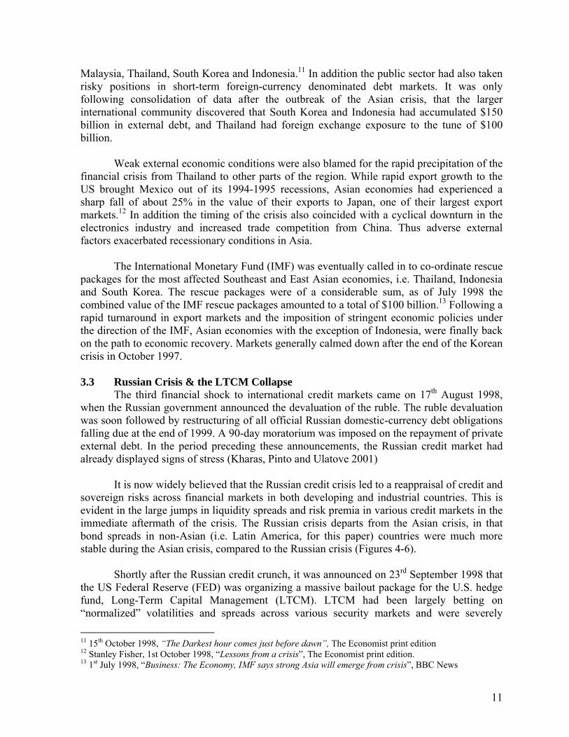
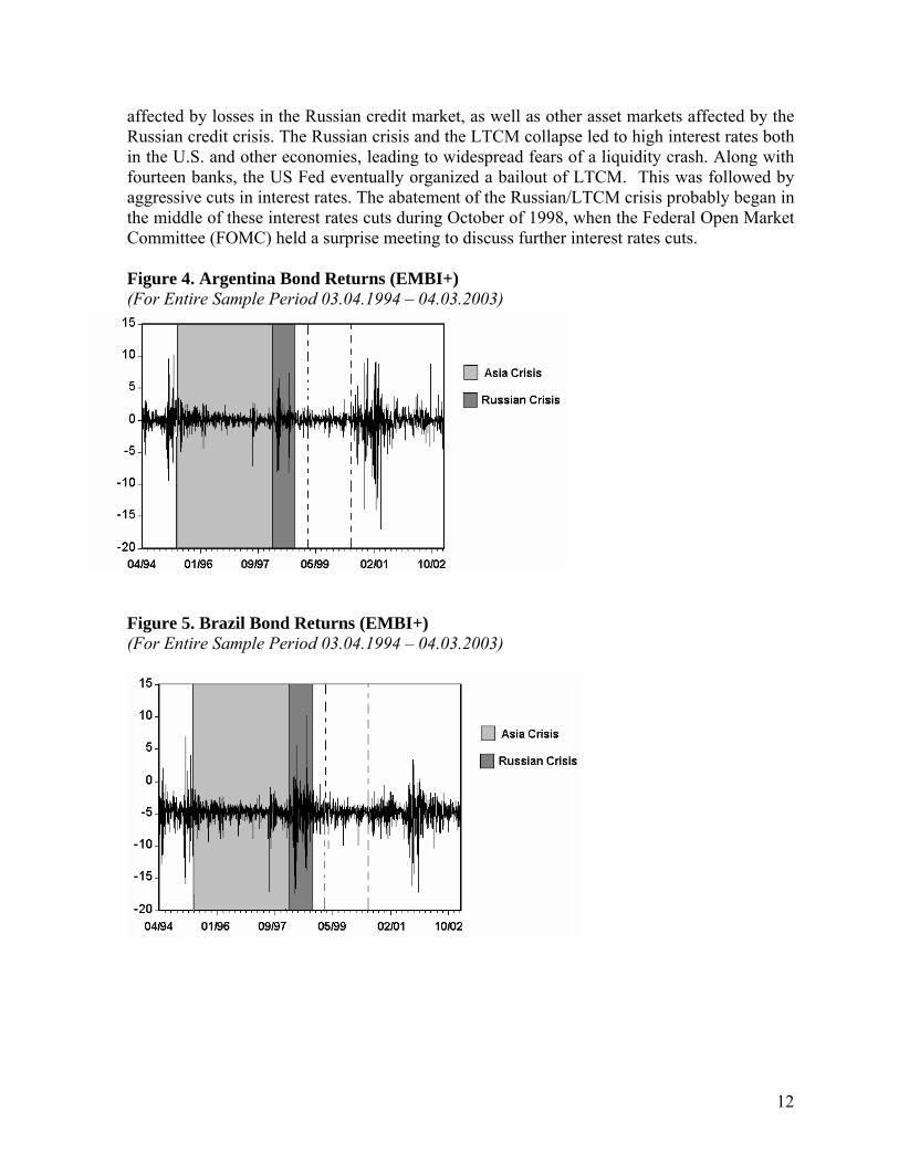
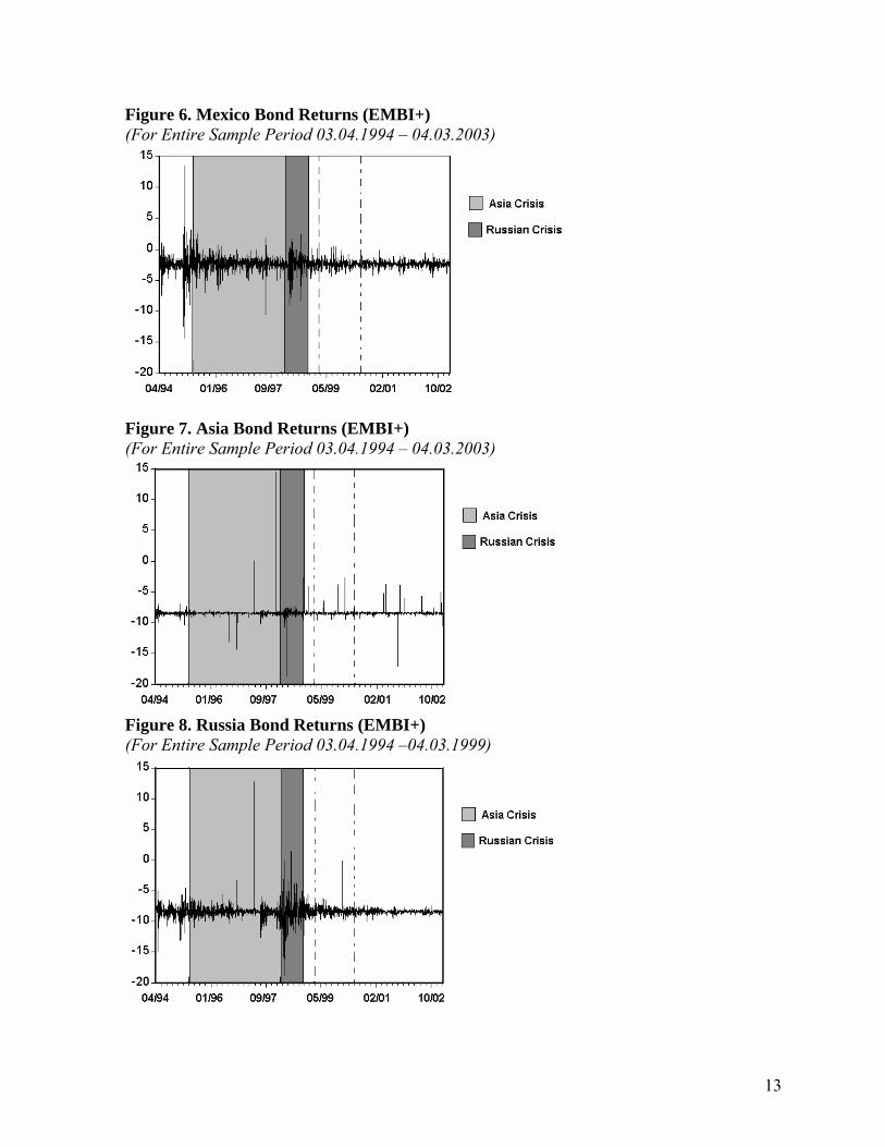
sovereign risks across financial markets in both developing and industrial countries. This is evident in the large jumps in liquidity spreads and risk premia in various credit markets in the immediate aftermath of the crisis. The Russian crisis departs from the Asian crisis, in that bond spreads in non-Asian (i.e. Latin America, for this paper) countries were much more stable during the Asian crisis, compared to the Russian crisis (Figures 4-6).

Shortly after the Russian credit crunch, it was announced on 23rd September 1998 that

the US Federal Reserve (FED) was organizing a massive bailout package for the U.S. hedge fund, Long-Term Capital Management (LTCM). LTCM had been largely betting on “normalized” volatilities and spreads across various security markets and were severely

11 15th October 1998, “The Darkest hour comes just before dawn”, The Economist print edition 12 Stanley Fisher, 1st October 1998, “Lessons from a crisis”, The Economist print edition. 13 1st July 1998, “Business: The Economy, IMF says strong Asia will emerge from crisis”, BBC News

12

affected by losses in the Russian credit market, as well as other asset markets affected by the Russian credit crisis. The Russian crisis and the LTCM collapse led to high interest rates both in the U.S. and other economies, leading to widespread fears of a liquidity crash. Along with fourteen banks, the US Fed eventually organized a bailout of LTCM. This was followed by aggressive cuts in interest rates. The abatement of the Russian/LTCM crisis probably began in the middle of these interest rates cuts during October of 1998, when the Federal Open Market Committee (FOMC) held a surprise meeting to discuss further interest rates cuts.

Figure 4. Argentina Bond Returns (EMBI+) (For Entire Sample Period 03.04.1994 – 04.03.2003)

Figure 5. Brazil Bond Returns (EMBI+) (For Entire Sample Period 03.04.1994 – 04.03.2003)

13

Figure 6. Mexico Bond Returns (EMBI+) (For Entire Sample Period 03.04.1994 – 04.03.2003)

Figure 7. Asia Bond Returns (EMBI+) (For Entire Sample Period 03.04.1994 – 04.03.2003)

Figure 8. Russia Bond Returns (EMBI+) (For Entire Sample Period 03.04.1994 –04.03.1999)

14

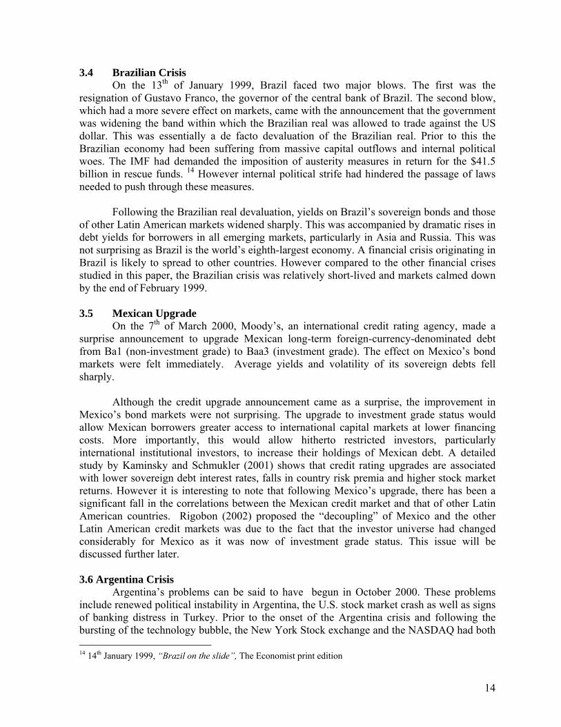
3.4 Brazilian Crisis On the 13th of January 1999, Brazil faced two major blows. The first was the

resignation of Gustavo Franco, the governor of the central bank of Brazil. The second blow, which had a more severe effect on markets, came with the announcement that the government was widening the band within which the Brazilian real was allowed to trade against the US dollar. This was essentially a de facto devaluation of the Brazilian real. Prior to this the Brazilian economy had been suffering from massive capital outflows and internal political woes. The IMF had demanded the imposition of austerity measures in return for the $41.5 billion in rescue funds. 14 However internal political strife had hindered the passage of laws needed to push through these measures.

Following the Brazilian real devaluation, yields on Brazil’s sovereign bonds and those of other Latin American markets widened sharply. This was accompanied by dramatic rises in debt yields for borrowers in all emerging markets, particularly in Asia and Russia. This was not surprising as Brazil is the world’s eighth-largest economy. A financial crisis originating in Brazil is likely to spread to other countries. However compared to the other financial crises studied in this paper, the Brazilian crisis was relatively short-lived and markets calmed down by the end of February 1999. 3.5 Mexican Upgrade

On the 7th of March 2000, Moody’s, an international credit rating agency, made a surprise announcement to upgrade Mexican long-term foreign-currency-denominated debt from Ba1 (non-investment grade) to Baa3 (investment grade). The effect on Mexico’s bond markets were felt immediately. Average yields and volatility of its sovereign debts fell sharply.

Although the credit upgrade announcement came as a surprise, the improvement in

Mexico’s bond markets were not surprising. The upgrade to investment grade status would allow Mexican borrowers greater access to international capital markets at lower financing costs. More importantly, this would allow hitherto restricted investors, particularly international institutional investors, to increase their holdings of Mexican debt. A detailed study by Kaminsky and Schmukler (2001) shows that credit rating upgrades are associated with lower sovereign debt interest rates, falls in country risk premia and higher stock market returns. However it is interesting to note that following Mexico’s upgrade, there has been a significant fall in the correlations between the Mexican credit market and that of other Latin American countries. Rigobon (2002) proposed the “decoupling” of Mexico and the other Latin American credit markets was due to the fact that the investor universe had changed considerably for Mexico as it was now of investment grade status. This issue will be discussed further later. 3.6 Argentina Crisis

Argentina’s problems can be said to have begun in October 2000. These problems include renewed political instability in Argentina, the U.S. stock market crash as well as signs of banking distress in Turkey. Prior to the onset of the Argentina crisis and following the bursting of the technology bubble, the New York Stock exchange and the NASDAQ had both 14 14th January 1999, “Brazil on the slide”, The Economist print edition

15

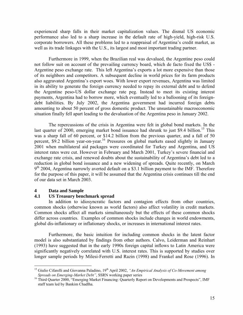
experienced sharp falls in their market capitalization values. The dismal US economic performance also led to a sharp increase in the default rate of high-yield, high-risk U.S. corporate borrowers. All these problems led to a reappraisal of Argentina’s credit market, as well as its trade linkages with the U.S., its largest and most important trading partner.

Furthermore in 1999, when the Brazilian real was devalued, the Argentine peso could

not follow suit on account of the prevailing currency board, which de facto fixed the US$ - Argentine peso exchange rate. This left Argentina’s exports a lot more expensive than those of its neighbors and competitors. A subsequent decline in world prices for its farm products also aggravated Argentina’s export woes. With lower export revenues, Argentina was limited in its ability to generate the foreign currency needed to repay its external debt and to defend the Argentine peso-US dollar exchange rate peg. Instead to meet its existing interest payments, Argentina had to borrow more, which eventually led to a ballooning of its foreign-debt liabilities. By July 2002, the Argentina government had incurred foreign debts amounting to about 50 percent of gross domestic product. The unsustainable macroeconomic situation finally fell apart leading to the devaluation of the Argentina peso in January 2002.

The repercussions of the crisis in Argentina were felt in global bond markets. In the

last quarter of 2000, emerging market bond issuance had shrunk to just $9.4 billion.15 This was a sharp fall of 60 percent, or $14.2 billion from the previous quarter, and a fall of 50 percent, $9.2 billion year-on-year.16 Pressures on global markets eased slightly in January 2001 when multilateral aid packages were coordinated for Turkey and Argentina, and US interest rates were cut. However in February and March 2001, Turkey’s severe financial and exchange rate crisis, and renewed doubts about the sustainability of Argentina’s debt led to a reduction in global bond issuance and a new widening of spreads. Quite recently, on March 9th 2004, Argentina narrowly averted default on a $3.1 billion payment to the IMF. Therefore for the purpose of this paper, it will be assumed that the Argentina crisis continues till the end of our data set in March 2003.

4 Data and Sample 4.1 US Treasury benchmark spread

In addition to idiosyncratic factors and contagion effects from other countries, common shocks (otherwise known as world factors) also affect volatility in credit markets. Common shocks affect all markets simultaneously but the effects of these common shocks differ across countries. Examples of common shocks include changes in world endowments, global dis-inflationary or inflationary shocks, or increases in international interest rates.

Furthermore, the basic intuition for including common shocks in the latent factor model is also substantiated by findings from other authors. Calvo, Leiderman and Reinhart (1993) have suggested that in the early 1990s foreign capital inflows to Latin America were significantly negatively correlated with U.S. interest rates. This is supported by studies over longer sample periods by Milesi-Ferretti and Razin (1998) and Frankel and Rose (1996). In

15 Giulio Cifarelli and Giovanna Paladino, 19th April 2002, “An Empirical Analysis of Co-Movement among

Spreads on Emerging-Market Debt”, SSRN working paper series 16 Third Quarter 2000, “Emerging Market Financing: Quarterly Report on Developments and Prospects”, IMF

staff team led by Bankim Chadlha.

16

the Asian context, Agénor and Hoffmaister (1998) find that world interest rates also have a significant impact on foreign capital inflows and the real exchange rate in South Korea, Philippines and Thailand.

Apart from the results of the studies above, the linkages between US interest rates and global variables is also supported by intuition and historical experience. As the nominal interest rate is determined both by the level of inflation in the economy, as well as the level of real interest rates, inflationary and deflationary shocks will also be reflected in movements in U.S. interest rates. Furthermore any major changes in world commodity markets will also tend to have a direct impact on the US economy, the largest consumer economy in the world, and thus reflected in movements in its interest rates. For example, the oil crises of 1973 and 1979 were a strong negative shock for the US economy, US interest rates were at historical highs in the ensuing period. As global variables have a high correlation with US interest rates, movements in U.S. interest rates can be assumed to provide a good representation of these global shocks.

Furthermore since the US Treasury 10-year bond is among the most liquid and highly

traded US debt instrument, and is the current benchmark for determining interest rate trends, it was included in our latent factor model as a proxy for common global shocks. Therefore the US Treasury benchmark spread for a 10 year bond is used as the world factor in the latent factor model, which will be specified and discussed later. Data on the US Treasury spread is obtained from DataStream. 4.2 JP Morgan bond indices

In addition data on various bond indices are also used in this paper. This data is derived from the DataStream data set. The data collected has been separated into two separate data sets, covering two distinct time periods. More specifically, the two data sets consist of the JP Morgan Emerging Market Bond Indices (Global Diversified) (hereafter EMBI+) and the JP Morgan Emerging Local Markets Indices (hereafter ELMI +). These indices are computed by simulating holding portfolios, whose weights are determined by risk, market capitalization, liquidity considerations, and collateral characteristics of the particular bonds. Data from these two indices are reported on a daily basis. 4.2.1 JP Morgan EMBI+ GLB. DIVERS

The first data set runs from the 4th of March 1994, to March 3rd 2003. The data covers a span of 9 years, encompassing the five financial crises and the Mexican upgrade mentioned. We study the first data set (or the first model of contagion) in seven time frames. The first timeframe gives a general overview of contagion for the entire sample period. Rigobon (2002) suggests that for the entire sample period studied, there were pronounced structural breaks in the linkages between the Latin American countries, particularly after Mexico’s credit rating status was upgraded from junk bond status to investment grade in March 2000. Thus, to examine the contagion effects in each period in greater detail as well as to investigate if there are significant changes in the transmission of contagion across time, we break down the entire sample period into six periods of high volatility and six periods of tranquility in financial markets.

17

The definitions of these sub-sample periods correspond to the description of the timing of the five financial crises and the Mexican upgrade mentioned above. The window definitions are similar to the ones used by Rigobon (2002). They are as follows: (i.) Mexican Crisis: (12.19.1994 - 03.31.199517) The first financial crisis began in

Mexico on the 19th of December 1994; when the fixed exchange rate system was abandoned and the Mexican peso was devalued. The crisis ended around the 31st of March 1995, when markets calmed down following the US-led bailout by the Clinton administration.

(ii.) Asian Economic Crisis: (06.01.1997 - 01.31.1998) The Asian economic crisis began

on the 1st of June 1997, when the Thai baht came under speculative attack. It is assumed that the Asian crisis ended at the end of January 1998, after the end of the South Korea crisis.

(iii.) Russian Crisis: (08.01.1998 - 10.31.998) The Russian crisis started with a sharp fall

in government securities’ prices in August of 1998. It ended after the Long-Term-Capital Management (LTCM) rescue by the U.S. Federal Reserve at the end of October of the same year.

(iv.) Brazilian Devaluation: (01.13.1999 - 02.28.1999) The devaluation of the Brazilian

real triggered the fourth financial crisis. This began in early January of 1999 and ended in February of the same year, after markets calmed down. It was relatively short-lived compared to the other financial crises studied.

(v.) Mexico Upgrade: (03.01.2000 - 05.31.2000) In March of 2000, Moody’s upgraded

Mexico’s external debt credit ratings from junk bond status to investment grade status. While this is not a ‘crisis’, the Mexican upgrade is included to reflect both positive and negative contagion effects. This period of ‘good news’ is assumed to have ended at the end of May, after market euphoria had diminished.

(vi.) Argentina Crisis: (10.01.2000 - 04.03.2003) Lastly, it can be claimed that the on-

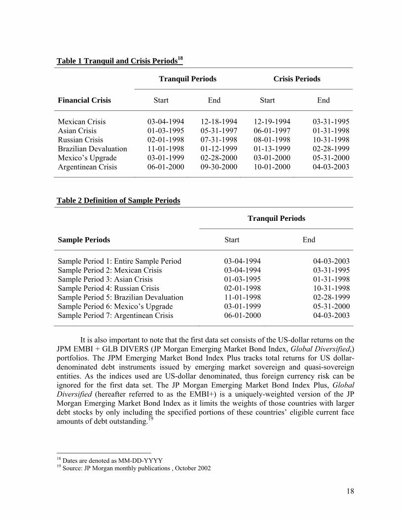
going Argentina crisis started in late 2000. This was precipitated by internal political shocks, beginning in October 2000, which led to general confusion over the economic policy and the currency board adopted by the ruling coalition. Thus this paper assumes that the crisis started in early October of 2000 until the end of the entire sample period. Each of these six periods of high volatility is then studied together with their corresponding pre-crisis period of tranquility. The six periods specified are as follows:

17 Dates are denoted as MM-DD-YYYY

18

Table 1 Tranquil and Crisis Periods18

Table 2 Definition of Sample Periods

It is also important to note that the first data set consists of the US-dollar returns on the

JPM EMBI + GLB DIVERS (JP Morgan Emerging Market Bond Index, Global Diversified,) portfolios. The JPM Emerging Market Bond Index Plus tracks total returns for US dollar-denominated debt instruments issued by emerging market sovereign and quasi-sovereign entities. As the indices used are US-dollar denominated, thus foreign currency risk can be ignored for the first data set. The JP Morgan Emerging Market Bond Index Plus, Global Diversified (hereafter referred to as the EMBI+) is a uniquely-weighted version of the JP Morgan Emerging Market Bond Index as it limits the weights of those countries with larger debt stocks by only including the specified portions of these countries’ eligible current face amounts of debt outstanding.19

18 Dates are denoted as MM-DD-YYYY 19 Source: JP Morgan monthly publications , October 2002

Tranquil Periods Crisis Periods

Financial Crisis Start End Start End Mexican Crisis 03-04-1994 12-18-1994 12-19-1994 03-31-1995Asian Crisis 01-03-1995 05-31-1997 06-01-1997 01-31-1998Russian Crisis 02-01-1998 07-31-1998 08-01-1998 10-31-1998Brazilian Devaluation 11-01-1998 01-12-1999 01-13-1999 02-28-1999Mexico’s Upgrade 03-01-1999 02-28-2000 03-01-2000 05-31-2000Argentinean Crisis 06-01-2000 09-30-2000 10-01-2000 04-03-2003

Tranquil Periods

Sample Periods Start End Sample Period 1: Entire Sample Period 03-04-1994 04-03-2003Sample Period 2: Mexican Crisis 03-04-1994 03-31-1995Sample Period 3: Asian Crisis 01-03-1995 01-31-1998Sample Period 4: Russian Crisis 02-01-1998 10-31-1998Sample Period 5: Brazilian Devaluation 11-01-1998 02-28-1999Sample Period 6: Mexico’s Upgrade 03-01-1999 05-31-2000Sample Period 7: Argentinean Crisis 06-01-2000 04-03-2003

19

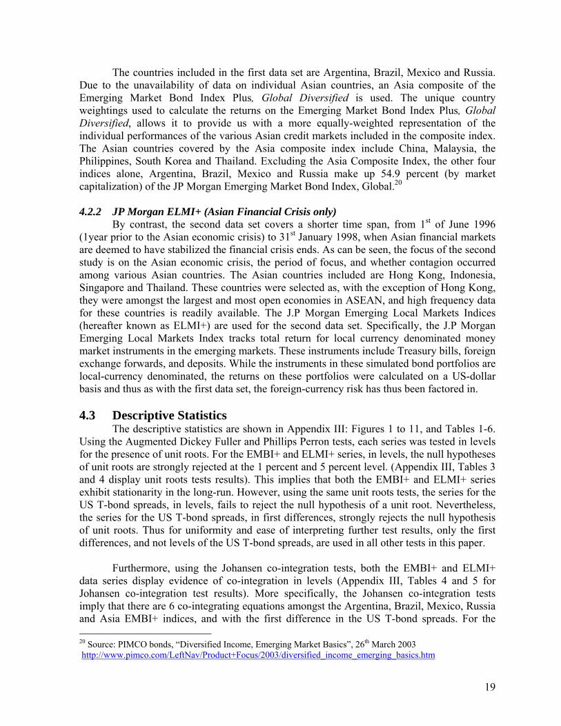
The countries included in the first data set are Argentina, Brazil, Mexico and Russia. Due to the unavailability of data on individual Asian countries, an Asia composite of the Emerging Market Bond Index Plus, Global Diversified is used. The unique country weightings used to calculate the returns on the Emerging Market Bond Index Plus, Global Diversified, allows it to provide us with a more equally-weighted representation of the individual performances of the various Asian credit markets included in the composite index. The Asian countries covered by the Asia composite index include China, Malaysia, the Philippines, South Korea and Thailand. Excluding the Asia Composite Index, the other four indices alone, Argentina, Brazil, Mexico and Russia make up 54.9 percent (by market capitalization) of the JP Morgan Emerging Market Bond Index, Global.20 4.2.2 JP Morgan ELMI+ (Asian Financial Crisis only)

By contrast, the second data set covers a shorter time span, from 1st of June 1996 (1year prior to the Asian economic crisis) to 31st January 1998, when Asian financial markets are deemed to have stabilized the financial crisis ends. As can be seen, the focus of the second study is on the Asian economic crisis, the period of focus, and whether contagion occurred among various Asian countries. The Asian countries included are Hong Kong, Indonesia, Singapore and Thailand. These countries were selected as, with the exception of Hong Kong, they were amongst the largest and most open economies in ASEAN, and high frequency data for these countries is readily available. The J.P Morgan Emerging Local Markets Indices (hereafter known as ELMI+) are used for the second data set. Specifically, the J.P Morgan Emerging Local Markets Index tracks total return for local currency denominated money market instruments in the emerging markets. These instruments include Treasury bills, foreign exchange forwards, and deposits. While the instruments in these simulated bond portfolios are local-currency denominated, the returns on these portfolios were calculated on a US-dollar basis and thus as with the first data set, the foreign-currency risk has thus been factored in. 4.3 Descriptive Statistics

The descriptive statistics are shown in Appendix III: Figures 1 to 11, and Tables 1-6. Using the Augmented Dickey Fuller and Phillips Perron tests, each series was tested in levels for the presence of unit roots. For the EMBI+ and ELMI+ series, in levels, the null hypotheses of unit roots are strongly rejected at the 1 percent and 5 percent level. (Appendix III, Tables 3 and 4 display unit roots tests results). This implies that both the EMBI+ and ELMI+ series exhibit stationarity in the long-run. However, using the same unit roots tests, the series for the US T-bond spreads, in levels, fails to reject the null hypothesis of a unit root. Nevertheless, the series for the US T-bond spreads, in first differences, strongly rejects the null hypothesis of unit roots. Thus for uniformity and ease of interpreting further test results, only the first differences, and not levels of the US T-bond spreads, are used in all other tests in this paper.

Furthermore, using the Johansen co-integration tests, both the EMBI+ and ELMI+

data series display evidence of co-integration in levels (Appendix III, Tables 4 and 5 for Johansen co-integration test results). More specifically, the Johansen co-integration tests imply that there are 6 co-integrating equations amongst the Argentina, Brazil, Mexico, Russia and Asia EMBI+ indices, and with the first difference in the US T-bond spreads. For the 20 Source: PIMCO bonds, “Diversified Income, Emerging Market Basics”, 26th March 2003 http://www.pimco.com/LeftNav/Product+Focus/2003/diversified_income_emerging_basics.htm

20

second data set, there are 5 co-integrating equations amongst the Hong Kong, Indonesia, Singapore and Thailand ELMI+ indices, and with the first difference in the US T-bond spread in the same corresponding time period. These results suggest that common factors are involved in the evolution of these two data sets. The Johansen co-integration tests suggest that there are commonalities between the various credit markets. These commonalities will be encapsulated in the latent factor model of interdependence discussed in the next section.

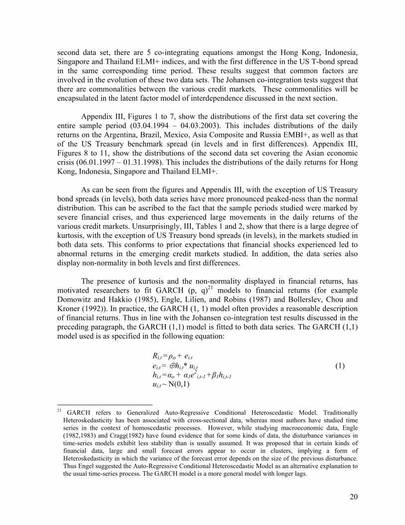
Appendix III, Figures 1 to 7, show the distributions of the first data set covering the entire sample period (03.04.1994 – 04.03.2003). This includes distributions of the daily returns on the Argentina, Brazil, Mexico, Asia Composite and Russia EMBI+, as well as that of the US Treasury benchmark spread (in levels and in first differences). Appendix III, Figures 8 to 11, show the distributions of the second data set covering the Asian economic crisis (06.01.1997 – 01.31.1998). This includes the distributions of the daily returns for Hong Kong, Indonesia, Singapore and Thailand ELMI+.

As can be seen from the figures and Appendix III, with the exception of US Treasury bond spreads (in levels), both data series have more pronounced peaked-ness than the normal distribution. This can be ascribed to the fact that the sample periods studied were marked by severe financial crises, and thus experienced large movements in the daily returns of the various credit markets. Unsurprisingly, III, Tables 1 and 2, show that there is a large degree of kurtosis, with the exception of US Treasury bond spreads (in levels), in the markets studied in both data sets. This conforms to prior expectations that financial shocks experienced led to abnormal returns in the emerging credit markets studied. In addition, the data series also display non-normality in both levels and first differences.

The presence of kurtosis and the non-normality displayed in financial returns, has motivated researchers to fit GARCH (p, q)21 models to financial returns (for example Domowitz and Hakkio (1985), Engle, Lilien, and Robins (1987) and Bollerslev, Chou and Kroner (1992)). In practice, the GARCH (1, 1) model often provides a reasonable description of financial returns. Thus in line with the Johansen co-integration test results discussed in the preceding paragraph, the GARCH (1,1) model is fitted to both data series. The GARCH (1,1) model used is as specified in the following equation:

Ri,t = ρo + ei,t ei,t = ⊕hi,t* ui,t (1) hi,t =αo + α1e2

i,t-1 +β1hi,t-1

ui,t ~ N(0,1) 21 GARCH refers to Generalized Auto-Regressive Conditional Heteroscedastic Model. Traditionally

Heteroskedasticity has been associated with cross-sectional data, whereas most authors have studied time series in the context of homoscedastic processes. However, while studying macroeconomic data, Engle (1982,1983) and Cragg(1982) have found evidence that for some kinds of data, the disturbance variances in time-series models exhibit less stability than is usually assumed. It was proposed that in certain kinds of financial data, large and small forecast errors appear to occur in clusters, implying a form of Heteroskedasticity in which the variance of the forecast error depends on the size of the previous disturbance. Thus Engel suggested the Auto-Regressive Conditional Heteroscedastic Model as an alternative explanation to the usual time-series process. The GARCH model is a more general model with longer lags.

21

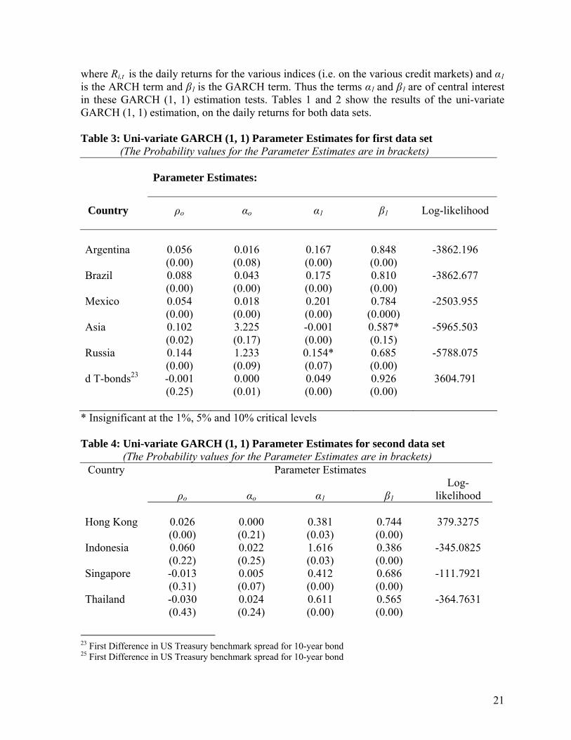
where Ri,t is the daily returns for the various indices (i.e. on the various credit markets) and α1 is the ARCH term and β1 is the GARCH term. Thus the terms α1 and β1 are of central interest in these GARCH (1, 1) estimation tests. Tables 1 and 2 show the results of the uni-variate GARCH (1, 1) estimation, on the daily returns for both data sets. Table 3: Uni-variate GARCH (1, 1) Parameter Estimates for first data set (The Probability values for the Parameter Estimates are in brackets) Parameter Estimates:

Country ρo αo α1 β1 Log-likelihood Argentina 0.056 0.016 0.167 0.848 -3862.196 (0.00) (0.08) (0.00) (0.00) Brazil 0.088 0.043 0.175 0.810 -3862.677 (0.00) (0.00) (0.00) (0.00) Mexico 0.054 0.018 0.201 0.784 -2503.955 (0.00) (0.00) (0.00) (0.000) Asia 0.102 3.225 -0.001 0.587* -5965.503 (0.02) (0.17) (0.00) (0.15) Russia 0.144 1.233 0.154* 0.685 -5788.075 (0.00) (0.09) (0.07) (0.00) d T-bonds23 -0.001 0.000 0.049 0.926 3604.791 (0.25) (0.01) (0.00) (0.00)

* Insignificant at the 1%, 5% and 10% critical levels Table 4: Uni-variate GARCH (1, 1) Parameter Estimates for second data set (The Probability values for the Parameter Estimates are in brackets) Country Parameter Estimates

ρo αo α1 β1 Log-

likelihood Hong Kong 0.026 0.000 0.381 0.744 379.3275 (0.00) (0.21) (0.03) (0.00) Indonesia 0.060 0.022 1.616 0.386 -345.0825 (0.22) (0.25) (0.03) (0.00) Singapore -0.013 0.005 0.412 0.686 -111.7921 (0.31) (0.07) (0.00) (0.00) Thailand -0.030 0.024 0.611 0.565 -364.7631 (0.43) (0.24) (0.00) (0.00)

23 First Difference in US Treasury benchmark spread for 10-year bond 25 First Difference in US Treasury benchmark spread for 10-year bond

22

d T-bonds25 -0.005 0.001 -0.072 0.833 429.4161 (0.06) (0.00) (0.00) (0.00)

A general examination of the estimation results shown above in tables 3 and 4, reveals

that there are some commonalities in the GARCH structures for both data series. α1, the ARCH term and β1, the GARCH term, is significant for all the daily returns of both the EMBI+ and the ELMI+, with the exception of the EMBI+ Asia composite index and the EMBI+ Russian index. However both indices still exhibit either significant ARCH or GARCH terms but not both. Thus the estimation results suggest that all the indices, including that of the Asia composite and the Russian index, display a form of heteroskedasticity in which the variance of the forecast error depends on the size of the previous disturbance. Therefore the GARCH effects will be encapsulated in the estimation methodology as described in the next section.

In summary, apart from the 10-year US Treasury benchmark spread, all the data series studied, do not exhibit unit root properties. In addition, the first difference of the 10-year US Treasury benchmark spread does not exhibit unit root properties. Furthermore, both data sets display non-normality, and fitting a uni-variate GARCH (1, 1) estimation model to both data series reveals that GARCH processes are predominant. Lastly, from the Johansen co-integration tests conducted, there is some evidence that there are common factors underlying both data sets. These common factors will be discussed in the latent factor model in the following section. 5. Model of Interdependence

We define a model of interdependence of credit markets during pre-crisis periods specified as a latent factor model. The framework is then extended to allow for an avenue for contagion during a crisis. The latent factor model used, originated from factor models based on the Arbitrage Pricing Theory, where market returns are specified by common factors and idiosyncratic factors representing non-diversifiable risk. It is widely accepted and used by several authors including Dungey and Matin (2001), Forbes and Rigobon (2002) and Bekaert, Harvey and Ng (2003). These factors include common global shocks (i.e. the world factor), country-specific shocks and transmission of contagion of across borders.

The major advantage of using the latent factor model is that it allows us to identify and quantify the various factors studied without having to resort to ad hoc identification of the pertinent fundamentals. (Eichengreen, Rose, Wyplosz 1996, Glick and Rose 1999, Forbes and Rigobon 1999) Details of the model are in Appendix 1. 6. Model of Contagion

The model of interdependence is augmented to allow for an avenue for contagion, where contagion is defined as the transmission of unanticipated idiosyncratic local shocks form one credit market to another. The definition of contagion used is similar to that of Masson (1999), where shocks are divided as either common shocks or spillover effects that result from some identifiable channel, and that of Forbes and Rigobon (2002), who defined

23

contagion as an increase in adjusted (unconditional) correlation during periods of financial crisis. The model used in this paper is adopted from that developed by Dungey, Fry, Gonzalez-Hermosillo and Martin (2003). For simplicity, a bi-variate model of contagion is first examined and subsequently augmented to form a multi-variate model of contagion. 6.1 Bi-variate model of contagion

To distinguish between bond returns in pre-crisis and crisis periods, yi,t represents the demeaned bond returns during the crisis periods, and xi,t, the return during the pre-crisis period. For simplicity, consider the case where contagion spreads from country 1 to country 2. Thus the latent factor model in equation (2) is now extended as follows y1,t = λ1ωt + δ1µ1,t,

y2,t = λ2ωt + δ2µ2,t, + γ1µ1,t, (10) where γ1 is the factor loading of contagion effect (i.e. unanticipated spillover shocks) from country 1 to country 2. Thus γ1 is zero when there are no contagion effects, and becomes significant only in the presence of contagion during crisis periods. Thus to test for the effects of contagion, this paper uses the volatility expression for y2,t , which is given by E[y2

i,t] = λ2i + δ2

i,t, + γj2

… i ≠ j (11) Thus the volatility of y2,t can be decomposed into the contributions of shocks from common global shocks, idiosyncratic factors or contagion as follows

(i) Contribution of the world factor26

(ii) Contribution of country-specific factor

(iii) Contribution of contagion from country j 6.2 Multi-variate Model of Contagion

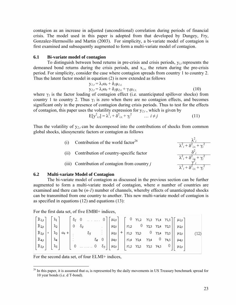
The bi-variate model of contagion as discussed in the previous section can be further augmented to form a multi-variate model of contagion, where n number of countries are examined and there can be (n-1) number of channels, whereby effects of unanticipated shocks can be transmitted from one country to another. This new multi-variate model of contagion is as specified in equations (12) and equations (13): For the first data set, of five EMBI+ indices,

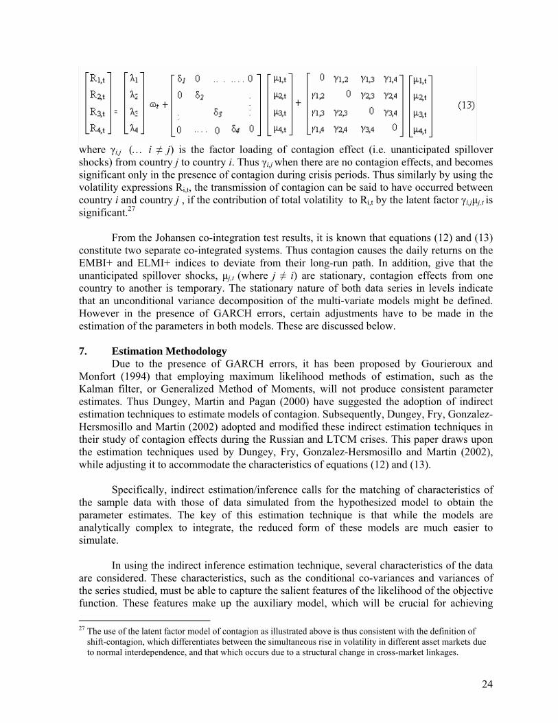
For the second data set, of four ELMI+ indices,

26 In this paper, it is assumed that ωt is represented by the daily movements in US Treasury benchmark spread for

10 year bonds (i.e. d T-bond).

λ2i

λ2i + δ2

i,t, + γj2

δ2i

λ2i + δ2

i,t, + γj2

γ2i

λ2i + δ2

i,t, + γj2

24

where γi,j (… i ≠ j) is the factor loading of contagion effect (i.e. unanticipated spillover shocks) from country j to country i. Thus γi,j when there are no contagion effects, and becomes significant only in the presence of contagion during crisis periods. Thus similarly by using the volatility expressions Ri,t, the transmission of contagion can be said to have occurred between country i and country j , if the contribution of total volatility to Ri,t by the latent factor γi,jµj,t is significant.27

From the Johansen co-integration test results, it is known that equations (12) and (13) constitute two separate co-integrated systems. Thus contagion causes the daily returns on the EMBI+ and ELMI+ indices to deviate from their long-run path. In addition, give that the unanticipated spillover shocks, µj,t (where j ≠ i) are stationary, contagion effects from one country to another is temporary. The stationary nature of both data series in levels indicate that an unconditional variance decomposition of the multi-variate models might be defined. However in the presence of GARCH errors, certain adjustments have to be made in the estimation of the parameters in both models. These are discussed below.

7. Estimation Methodology

Due to the presence of GARCH errors, it has been proposed by Gourieroux and Monfort (1994) that employing maximum likelihood methods of estimation, such as the Kalman filter, or Generalized Method of Moments, will not produce consistent parameter estimates. Thus Dungey, Martin and Pagan (2000) have suggested the adoption of indirect estimation techniques to estimate models of contagion. Subsequently, Dungey, Fry, Gonzalez-Hersmosillo and Martin (2002) adopted and modified these indirect estimation techniques in their study of contagion effects during the Russian and LTCM crises. This paper draws upon the estimation techniques used by Dungey, Fry, Gonzalez-Hersmosillo and Martin (2002), while adjusting it to accommodate the characteristics of equations (12) and (13).

Specifically, indirect estimation/inference calls for the matching of characteristics of the sample data with those of data simulated from the hypothesized model to obtain the parameter estimates. The key of this estimation technique is that while the models are analytically complex to integrate, the reduced form of these models are much easier to simulate.

In using the indirect inference estimation technique, several characteristics of the data

are considered. These characteristics, such as the conditional co-variances and variances of the series studied, must be able to capture the salient features of the likelihood of the objective function. These features make up the auxiliary model, which will be crucial for achieving 27 The use of the latent factor model of contagion as illustrated above is thus consistent with the definition of

shift-contagion, which differentiates between the simultaneous rise in volatility in different asset markets due to normal interdependence, and that which occurs due to a structural change in cross-market linkages.

25

efficient outcomes from the estimations. The details of the model that draws upon Dungey, Gonzalez-Hermosillo and Martin (2002) are laid out in Appendix II. 8. Empirical Results

This section presents the results from the indirect inference estimation of the two multi-variate models of contagion given in equations (12) and (13). This paper defines contagion, as the spillover effect from an unanticipated shock from one credit market to another. Thus contagion is said to exist if a significant proportion of the volatility in the daily returns of one credit market can be attributed to spillovers from other credit markets, apart from itself and the common world factor. 8.1 Empirical Results for First data set (JPM EMBI+ GLB DIVERS.)

The first model encompasses four emerging credit markets (i.e. Argentina, Brazil, Mexico and Russia), as well as an Asian composite that provides a broad representation of the Asian credit markets.

This paper studies the first model in seven time frames. The first timeframe gives a

general overview of contagion for the entire sample period from 4th of March 1994 to 3rd of March 2003. Subsequently, this sample period is broken down into six smaller sub-sample periods, as mentioned earlier. This enables us to examine in greater detail contagion effects during each of the six financial crises that occur during this period. Another reason for the breakdown of the entire sample period to six smaller sub-sample periods is to account for the possible structural breaks in the linkages among the credit markets studied. For brevity, only the most prominent features of each of these six sub-sample periods will be discussed. 8.1.1 Empirical Results for Entire Sample Period (JPM EMBI+ GLB DIVERS.)

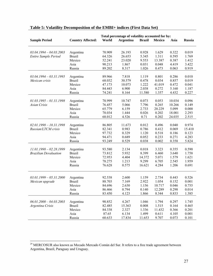
Table 5 presents the unconditional volatility decomposition of the daily returns on the five EMBI+ indices from the first data set for the entire sample period, as well as the six other sub-sample periods. The same information is also presented graphically in Appendix IV, Figures 1-7. Total volatility is broken down into the contribution due to the world factor, country-specific or idiosyncratic factors, and contagion from other countries.

To highlight the volatility decomposition in the tables presented, consider Argentina in Table 5. For the entire sample period (see Row beginning with 03.04.1994 – 04.03.2003 Entire Sample Period), the world factor is the dominant factor in the volatility decomposition of the daily returns in the Argentina credit market, and it contributes to 70.9 percent of total volatility in daily returns. This is due to the fact that external events, especially those affecting the US economy, play a large role in determining the global economic climate as well as local domestic interest rates. For example, U.S. monetary contractions were among the most important causes for the Mexican crisis in 1994. Argentina also has a relatively large idiosyncratic factor, and country-specific shocks from within its own credit market, contribute to 26.2 percent of total volatility in Argentina credit market returns. Contagion from Brazil, Asia and Russia is relatively insignificant, with credit market contributing to less than one percentage point of total volatility. In contrast, contagion from Mexico is relatively more significant, although not very substantial, as spillovers from Mexico accounts for 1.6 percent

26

of total volatility. This is largely due to the fact that improving economic conditions in Argentina, in the earlier part of the entire sample period, helped shield it from the earlier financial crisis. In addition, its adoption of fixed-exchange rate system also enabled it to be isolated from the spillover effects from the devaluation of the Brazilian real. More importantly, the Argentina crisis was compounded by internal political and economic troubles, and that the Argentina crisis accounts for about a third of the sample period studied. Therefore for the larger part of the entire sample period, Argentina tends to be largely affected only by country-specific shocks.

In general, for the entire sample period, as well as the other six sub-sample periods, the world factor dominates the volatility decomposition of the daily returns on various EMBI+ and ELMI+ indices. The world factor contributes to between 52 percent (Mexico) to 90 percent (Asia) of total volatility. This conforms to our a priori expectations, given the results of co-integration from the Johansen co-integration tests. It points strongly towards commonality in the movements of daily returns on the various credit market indices. More specifically, this result is also consistent with the view that increasing financial market integration has led to high and expected co-movements amongst credit markets around the world.

27

Table 5: Volatility Decomposition of the EMBI+ indices (First Data Set) Total percentage of volatility accounted for by: Sample Period Country Affected: World Argentina Brazil Mexico Asia Russia 03.04.1994 – 04.03.2003 Argentina 70.909 26.193 0.928 1.629 0.322 0.019 Entire Sample Period Brazil 64.326 26.653 5.345 1.311 0.595 1.769 Mexico 52.241 23.020 9.553 13.387 0.387 1.412 Asia 90.213 1.867 0.031 0.048 4.419 3.422 Russia 89.202 8.317 1.026 0.473 0.063 0.919 03.04.1994 – 03.31.1995 Argentina 89.966 7.818 1.119 0.801 0.286 0.010 Mexican crisis Brazil 68.032 30.579 0.478 0.034 0.857 0.019 Mexico 47.173 10.073 1.222 41.019 0.472 0.041 Asia 84.443 6.900 2.038 0.272 5.160 1.187 Russia 74.241 8.164 11.580 1.357 4.432 0.227 01.03.1995 – 01.31.1998 Argentina 78.999 10.747 0.073 0.053 10.034 0.096 Asian Crisis Brazil 76.457 5.066 7.796 0.265 10.266 0.149 Mexico 65.779 6.159 2.733 20.229 5.099 0.000 Asia 78.034 1.444 0.026 0.202 18.001 2.293 Russia 68.012 4.526 0.71 0.202 24.035 2.515 02.01.1998 – 10.31.1998 Argentina 86.805 11.673 0.012 0.496 0.040 0.974 Russian/LTCM crisis Brazil 82.341 0.983 0.786 0.412 0.069 15.410 Mexico 97.732 0.329 1.120 0.518 0.186 0.123 Asia 94.471 0.689 0.052 0.233 0.271 4.283 Russia 93.249 0.529 0.038 0.002 0.358 5.824 11.01.1998 – 02.28.1999 Argentina 93.580 2.134 0.018 3.323 0.355 0.590 Brazilian Devaluation Brazil 73.812 5.932 8.399 6.460 3.640 1.758 Mexico 72.953 4.404 14.372 5.071 1.579 1.621 Asia 78.275 1.213 9.299 6.705 2.545 1.959 Russia 76.628 0.575 16.621 4.284 1.206 0.691 03.01.1999 – 05.31.2000 Argentina 92.538 2.600 1.159 2.734 0.443 0.526 Mexican upgrade Brazil 88.703 7.169 2.922 1.054 0.152 0.001 Mexico 84.696 2.630 1.156 10.717 0.046 0.755 Asia 86.466 0.794 0.140 12.289 0.298 0.014 Russia 83.450 4.123 1.866 8.344 0.833 1.385 06.01.2000 – 04.03.2003 Argentina 90.852 4.267 1.046 1.794 0.297 1.745 Argentina Crisis Brazil 82.485 15.363 0.008 1.515 0.164 0.465 Mexico 84.338 2.327 1.336 11.432 0.366 0.201 Asia 87.65 6.134 1.499 0.611 4.105 0.001 Russia 60.633 17.834 11.653 9.707 0.073 0.101

29 MERCOSUR also known as Mecado Mercado Común del Sur. It refers to a free trade agreement between Argentina, Brazil, Paraguay and Uruguay.

28

Apart from Russia, country-specific factors are also relatively important for the EMBI+ indices. Idiosyncratic shocks account for between 4.4 percent (Asia) to 26.7 percent (Argentina) of total volatility. A possible explanation for the disparity could be that the Russian/LTCM crisis was relatively short-lived, compared to the financial turmoil that has afflicted the Asian and Latin American credit markets during the sample period.

Overall, contagion effects emanating from Argentina to the various Latin American credit markets seem to be the most pronounced. The transmission of contagion from Argentina contributes to 23 percent of the volatility in Mexico, and more than one quarter (26.7 percent) of the volatility in Brazil. This could be attributed to the fact that Argentina has stronger trade (through MERCOSUR with Brazil)29 and financial linkages with these two countries, and thus the channels for contagion from Argentina to them are well-defined, compared to those with Asia and Russia. 8.1.2 Empirical Results for the Mexican Crisis (JPM EMBI+ GLB DIVERS.)

Table 5, (see Row beginning with 03.04.1994 – 03.31.1995, Mexican crisis) presents the unconditional volatility decomposition of the returns on the EMBI+ indices during the Mexican crisis. A graphical representation of the same information is also presented in Appendix IV, Figure 2. It is interesting to note that while the country-specific factor account for 41 percent of total volatility for Mexico, the transmission of contagion from Mexico to other countries is relatively unsubstantial. Contribution of contagion from Mexico to Argentina, Brazil and Asia accounts for less than one percentage point of total volatility in these credit markets. In Russia, contagion from Mexico also only accounts for 1.4 percent of total volatility. In contrast, contagion emanating from Argentina contributes to between 6.9 percent (Asia) and 30.6 percent (Brazil) of total volatility in the various credit markets. With regards to this anomaly, one interesting explanation could be that the Mexican crisis affected the Argentina credit market more severely than the Mexican credit market itself.

8.1.3 Empirical Results for the Asian Crisis (JPM EMBI+ GLB DIVERS.)

In addition, Table 5 (see Row beginning with 01.03.1995 – 01.31.1998 Asian Crisis) also presents the unconditional volatility decomposition of the returns on the EMBI+ indices during the Asian crisis. Appendix IV, Figure 3 presents a graphical representation of the same information. Similarly, world factor accounts for a substantial amount, between 65.8 percent (Mexico) and 79 percent (Argentina), of total volatility experienced by various credit markets. This is due to the fact that as these countries have largely open economies with open capital accounts. Financial integration with the global economy at large has left them vulnerable to common external shocks. Indeed, the global easing of monetary policy (a “positive” common external shock), towards the end of 1998, was instrumental in bringing the Asian crisis to an end. Apart from Russia, the country-specific factors are relatively significant for all the credit markets, accounting for between 7.8 percent (Brazil) to 18 percent (Asia) for the EMBI+ indices studied. In addition, the transmission of contagion from Asia to the various credit markets is also high. Contagion from Asia, contributes to about 10 percent of total volatility in Argentina and Brazil, and 5.1 percent for Mexico. In particular, substantial amounts of volatility (24 percent) in the daily returns of the Russian EMBI+ are accounted for by spillover effects from Asia.

29

A likely explanation for the cross-country differences between the Latin American countries and Russia is that the Asian economies share closer trade ties with Russia, compared to their links with Latin American economies. World oil markets were traditionally influenced by economic developments in the industrialized countries. However over the past decade, developing countries, particularly in Asia, have been largely responsible for the increase in global oil consumption. Therefore the Asian economic crisis had produced a substantial decline in the demand for oil in Asia, and thus a sharp decline in oil prices. Thus Russia which is heavily reliant on oil and commodities for its export revenues, was especially vulnerable to contagion from Asia.30

8.1.4 Empirical Results for the Russian Crisis (JPM EMBI+ GLB DIVERS.)

Table 5 (see Row beginning with 02.01.1998 – 10.31.1998 Russian/LTCM crisis) presents the unconditional volatility decomposition of the returns on the EMBI+ indices during the Russian crisis. In addition Appendix IV, Figure 4 is a graphical representation of the same information. Interestingly, while contagion from Russia contributes to a substantial amount of volatility (15 percent) in Brazil, it does not seem to play an important role in determining the volatility in the other Latin American credit markets studied.

One possible explanation is that, both Brazil and Russia are primary commodity exporting economies. And thus the sharp fall in world commodity prices, in the aftermath of the Asian economic crisis, had badly affected both countries. Therefore compared to Argentina and Mexico, Brazil was already more vulnerable to contagion from Russia. 31

Baig and Goldfajn (2002) also proposed that the vulnerability of Brazil to contagion

may be a reflection of its fundamentals. Shortly before the onset of the Russian crisis, Brazil had just re-entered the global credit market as a sovereign issuer. Therefore the massive foreign-currency debts it had accumulated before and after re-entering global credit markets, led to doubts as to the health of the Brazilian financial markets, and thus to sharp capital outflows from Brazil, at the onset of the Russian crisis. (Appendix V, Figure 1 provides a graphical representation of the capital outflows experienced by Brazil during the Russian crisis)

In Asia, the transmission of contagion from Russia accounts for 4.3 percent of total volatility. This could also be attributed to trade linkages between Asia and Russia. For example, Thailand, one of the more active sovereign bond issuers in Asia, is the fourth largest exporter of sugar as of 1998. Similarly the Russian financial crisis, and thus the anticipated fall in Russia’s demand for commodity products, has a generally larger impact on these markets compared to that on Argentina and Mexico. 30 As of 1997, Russia was the world’s third largest oil producing country with an 8% share of global oil production. It is also the second largest natural gas producer with a 24% global market share. Source: IEA, BP, World Bureau of Metal Statistics (Production); Russian Economic Trends, Monthly update, April 1998 (Exports) 31 In August 1998, at the onset of the Russian crisis, world commodity prices, were 12% lower than at the start of the year, and was 25% lower as compared to June of 1997. Ironically, in anticipation of rich harvests of Brazilian coffee and sugar, the price of coffee and sugar had fallen considerably. Russia was also severely affected by depressed oil prices. This is especially so as of 1997, more than half of Russia’s export revenues were derived from the sale of oil, gas and metals.

30

8.1.5 Empirical Results for the Brazilian Devaluation (JPM EMBI+ GLB DIVERS.) Table 5 (see Row beginning with 11.01.1998 – 02.28.1999 Brazilian Devaluation)

also presents the unconditional volatility decomposition of returns on the EMBI+ indices during the Brazilian devaluation crisis. Appendix IV, Figure 3 presents a graphical representation of the same information. Surprisingly, despite the close trade and financial linkages between Argentina and Brazil, the Argentina credit market was little affected by the Brazil credit market during the Brazilian devaluation crisis. One possible explanation for Argentina’s seemingly invulnerability to contagion from Brazil could be the fact that Argentina’s problems were largely idiosyncratic because of its exchange rate arrangement. During the period preceding and immediately after the Brazilian devaluation, Argentina, unlike Brazil, was able to retain its fixed exchange-rate system, in which the Argentinean peso and the US-dollar were completely interchangeable at a one-to-one ratio.

In addition, at that point in time, Argentina’s overall level of bank deposits was relatively stable, therefore reducing the risk of capital flight. Furthermore, Argentina’s fixed exchange-rate system enabled it to maintain near-zero rates of inflation, and this helped to increase foreign investment flows to Argentina.32 More importantly, during the 1990s, Argentina also experienced higher productivity growth rates relative to Brazil (Appendix V, Table 1 provides details on productivity growth). This may have negated any immediate fears of contagion through trade linkages between both countries. Therefore notwithstanding possible doubts amongst the international investor community about the sustainability of the fixed exchange-rate system, the above-mentioned factors were probably the key reasons why Argentina was not as vulnerable to contagion from Brazil, as popular belief would have it. However while Argentina’s credit markets were not immediately affected by the Brazilian real devaluation, its export markets was severely affected by the resultant cheaper Brazilian exports. This was a key factor in Argentina’s problems in 2000.

By contrast Brazil accounts for substantial volatility, of between 9.3 percent (Asia) to 16.6 percent (Russia) in the other credit markets. As mentioned before in the discussion regarding the Russian crisis, Russia was more vulnerable to contagion, as its economy remained depressed by falling commodity prices, particularly global oil prices.

Trade linkages between Asia and Brazil probably accounts for Asia’s vulnerability to contagion from Brazil. Several Asian countries, such as Indonesia and Thailand, are direct competitors with Brazil in global export markets for many agricultural commodities. Therefore Brazil’s real devaluation could give it a competitive edge over several agricultural-based Asian economies. In addition, Brazil is a growing export market for Thailand, one of the key Asian sovereign debt issuers. Brazil alone accounts for half of all Thai export revenues for Latin America. Thus it could be anticipated that the Brazilian financial crisis would eventually lead to a fall in export revenues for Thailand, and therefore adversely affect its economy, and thus its credit market.

8.1.6 Empirical Results for the Mexican Upgrade (JPM EMBI+ GLB DIVERS.)

32 Source: The Wall Street Journal, 14th September 1998, “Argentina Confident Despite Ills in Brazil”, http://www.invertir.com/news/nr10851.html

31

Table 5 (see Row beginning with 03.01.1999 – 05.31.2000 Mexican upgrade) then continues to presents the unconditional volatility decomposition of the returns on the EMBI+ indices during the Mexican upgrade Appendix IV, Figure 5 presents a graphical representation of the same information. On the 7th of March of 2000, Moody’s announced the upgrading of Mexico’s long-term foreign currency credit rating from Ba1 (non-investment grade) to Baa3 (investment grade).

At first glance, it might be surprising to note that the transmission of spillover effects from Mexico to Argentina and Brazil seems to have fallen from the previous sub-sample period accounting for less than 3 percent of total volatility for both countries. However this is consistent with Rigobon (2002) where it is proposed that as Mexico is upgraded from non-investment to investment grade33, the set of investors that can hold its securities grows substantially, reducing the magnitude of liquidity shocks. Table 6 presents Moody’s credit ratings for long-term external debt of the various credit markets during the sub-sample period from 1st of March 1999 to 31st of May 2000. As can be seen from Table 10, both Argentina and Brazil were still rated as non-investment grade, in the sub-sample period studied. Thus the investor universe for Mexico and these two countries are quite different, and this could have substantially changed the channels of contagion from Mexico to Argentina and Brazil, and vice versa.

It is also interesting to note that the transmission of contagion from Mexico to Asia accounts for a relatively large proportion (12.3 percent) of total volatility in the Asian credit markets. This suggests that since emerging from the Asian financial crisis, a number of Asian countries experienced sharp gains in exports in 199934 allowing several of them to either gain, or maintain their investment-grade credit rating status. Therefore Mexico and Asia share a more similar investor pool and are thus more likely to experience stronger co-movements.

However while Russia is rated as non-investment grade by the various rating agencies, Mexico still accounts for a substantial amount of volatility (8.3 percent) of the Russian credit market. This could be due to the fact that along with Russia, Mexico is also one of the world’s largest oil producers (fifth-largest).35 The Mexican upgrade, coincided with rising oil prices. Between January 1999 and September 2000, oil prices had tripled due to strong global oil demand, OPEC oil production cutbacks, and various other factors.36 Thus the Mexican upgrade could have sent a strong signal to investors, that coupled with falling liquidity and default risk in the Russian credit markets, the strengthening of the Russian export market might eventually lead to a similar credit rating upgrade for Russia in the near future. Thus the Mexican upgrade could have led to positive co-movements in the Russian credit markets. Indeed in early October 2003, Moody’s became the first agency to raise Russia’s credit ratings on long-term foreign-currency debt to investment grade status (Baa3.)37 33 Moody’s upgraded Mexican external long-term debt from junk bond status to investment-grade status on the 7th of March of 2000.The credit rating upgrade was an exceptional boost of confidence to the Mexican economy. 34 Several Asian countries experienced a sharp rise in their export figures from 1998 to 1999. Export gains laid between 39.6% for China to 14.6% for India. 35 Mexico is also the world’s 10th largest oil exporter. Oil and gas revenues contribute to about a third of all Mexican Government revenues in 2002. Source: VirtualSources.com 36 Source: Energy Information Administration, “World Oil Market and Oil Price Chronologies: 1970-2002”. 37 Source: The Financial Times, Pyivi Munter, 13th October 2003, “Moody’s Russia upgrade highlights gulf”

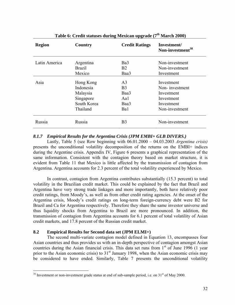
32

Table 6: Credit statuses during Mexican upgrade (7th March 2000)

Region Country Credit Ratings Investment/ Non-investment38

Latin America Argentina

Brazil Mexico

Ba3 B2 Baa3

Non-investment Non-investment Investment

Asia Hong Kong

Indonesia Malaysia Singapore South Korea Thailand

A3 B3 Baa3 Aa1 Baa3 Ba1

Investment Non- investment Investment Investment Investment Non-investment

Russia Russia B3 Non-investment

8.1.7 Empirical Results for the Argentina Crisis (JPM EMBI+ GLB DIVERS.)

Lastly, Table 5 (see Row beginning with 06.01.2000 – 04.03.2003 Argentina crisis) presents the unconditional volatility decomposition of the returns on the EMBI+ indices during the Argentine crisis. Appendix IV, Figure 6 presents a graphical representation of the same information. Consistent with the contagion theory based on market structure, it is evident from Table 11 that Mexico is little affected by the transmission of contagion from Argentina. Argentina accounts for 2.3 percent of the total volatility experienced by Mexico.

In contrast, contagion from Argentina contributes substantially (15.3 percent) to total volatility in the Brazilian credit market. This could be explained by the fact that Brazil and Argentina have very strong trade linkages and more importantly, both have relatively poor credit ratings, from Moody’s, as well as from other credit rating agencies. At the onset of the Argentina crisis, Moody’s credit ratings on long-term foreign-currency debt were B2 for Brazil and Ca for Argentina respectively. Therefore they share the same investor universe and thus liquidity shocks from Argentina to Brazil are more pronounced. In addition, the transmission of contagion from Argentina accounts for 6.1 percent of total volatility of Asian credit markets, and 17.8 percent of the Russian credit market. 8.2 Empirical Results for Second data set (JPM ELMI+)

The second multi-variate contagion model defined in Equation 13, encompasses four Asian countries and thus provides us with an in-depth perspective of contagion amongst Asian countries during the Asian financial crisis. This data set runs from 1st of June 1996 (1 year prior to the Asian economic crisis) to 31st January 1998, when the Asian economic crisis may be considered to have ended. Similarly, Table 7 presents the unconditional volatility

38 Investment or non-investment grade status at end of sub-sample period, i.e. on 31st of May 2000.

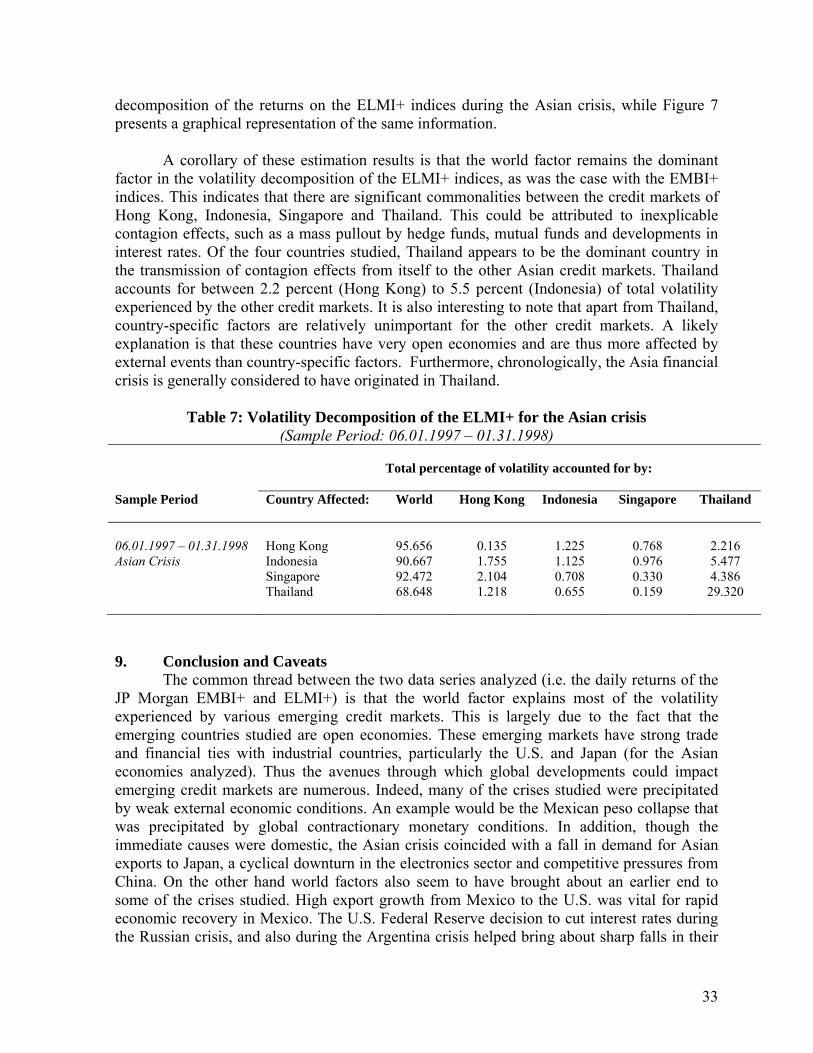
33

decomposition of the returns on the ELMI+ indices during the Asian crisis, while Figure 7 presents a graphical representation of the same information.

A corollary of these estimation results is that the world factor remains the dominant factor in the volatility decomposition of the ELMI+ indices, as was the case with the EMBI+ indices. This indicates that there are significant commonalities between the credit markets of Hong Kong, Indonesia, Singapore and Thailand. This could be attributed to inexplicable contagion effects, such as a mass pullout by hedge funds, mutual funds and developments in interest rates. Of the four countries studied, Thailand appears to be the dominant country in the transmission of contagion effects from itself to the other Asian credit markets. Thailand accounts for between 2.2 percent (Hong Kong) to 5.5 percent (Indonesia) of total volatility experienced by the other credit markets. It is also interesting to note that apart from Thailand, country-specific factors are relatively unimportant for the other credit markets. A likely explanation is that these countries have very open economies and are thus more affected by external events than country-specific factors. Furthermore, chronologically, the Asia financial crisis is generally considered to have originated in Thailand.

Table 7: Volatility Decomposition of the ELMI+ for the Asian crisis (Sample Period: 06.01.1997 – 01.31.1998)

Total percentage of volatility accounted for by: Sample Period Country Affected: World Hong Kong Indonesia Singapore Thailand 06.01.1997 – 01.31.1998 Hong Kong 95.656 0.135 1.225 0.768 2.216 Asian Crisis Indonesia 90.667 1.755 1.125 0.976 5.477 Singapore 92.472 2.104 0.708 0.330 4.386 Thailand 68.648 1.218 0.655 0.159 29.320 9. Conclusion and Caveats

The common thread between the two data series analyzed (i.e. the daily returns of the JP Morgan EMBI+ and ELMI+) is that the world factor explains most of the volatility experienced by various emerging credit markets. This is largely due to the fact that the emerging countries studied are open economies. These emerging markets have strong trade and financial ties with industrial countries, particularly the U.S. and Japan (for the Asian economies analyzed). Thus the avenues through which global developments could impact emerging credit markets are numerous. Indeed, many of the crises studied were precipitated by weak external economic conditions. An example would be the Mexican peso collapse that was precipitated by global contractionary monetary conditions. In addition, though the immediate causes were domestic, the Asian crisis coincided with a fall in demand for Asian exports to Japan, a cyclical downturn in the electronics sector and competitive pressures from China. On the other hand world factors also seem to have brought about an earlier end to some of the crises studied. High export growth from Mexico to the U.S. was vital for rapid economic recovery in Mexico. The U.S. Federal Reserve decision to cut interest rates during the Russian crisis, and also during the Argentina crisis helped bring about sharp falls in their

34

sovereign bond yield spreads. Thus given the strong influence of global factors, it is not surprising that the empirical results obtained in this paper show that the global factors contribute most to total volatility experienced by emerging credit markets.

However, evidence of the significance of country-specific or idiosyncratic shocks to

total volatility has been mixed. It varies greatly from country to country, as well as across different sub-sample periods studied. Nonetheless, an important result obtained from our estimates is that idiosyncratic factors for Argentina consistently explain a significant proportion of total volatility experienced by the Argentine credit market throughout the five financial crises and the Mexican upgrade. This could be largely attributed to Argentina’s fixed exchange rate policies, and higher than average export growth rates just prior to the onset of the Brazilian real devaluation. These factors could have shielded Argentina from the immediate spillover effects from Brazil. In addition, Argentina was affected little by the Mexican upgrade, as the investor universe for Argentina remained confined to investors willing and able to hold non-investment grade bonds. Therefore these factors could have isolated Argentina better from the various crises and thus most of the volatility experienced by Argentina are better explained by global shocks or shocks unique to the Argentina credit market itself.

The central focus of this paper, however, is to determine whether credit contagion

occurred during the various crises and the Mexican upgrade. From the empirical results obtained, it is evident that shift-contagion is present in every sub-sample period studied. Specifically it suggests that the total volatility of at least one of the credit markets studied can be explained by spillover effects from unanticipated contemporaneous idiosyncratic shocks in other credit markets. Using the specified definition of contagion, there is evidence of: (i) contagion from Mexico to Asia, during the Mexican peso collapse of 1994; (ii) contagion from Asia to the Latin American and Russian credit markets during the East Asian crisis of 1997; (iii) contagion from Russia to Brazil and Asia during the Russian/LTCM collapse of 1998; (iv) contagion from Brazil to Mexico, Asia and Russia during the Brazilian real devaluation of 1999 (v) “positive” contagion from Mexico to Asia and Russia after the Mexican upgrade of 2000 and (vi) from Argentina to Brazil, Russia and Asia in the ongoing Argentine crisis that began in 2000.

However, as can be seen from above, the contagion channels between countries vary

across credit markets, and over time. For example, the correlation between the Mexican credit market, and that of Argentina and Brazil, appears to have fallen sharply after the Mexican upgrade. Many explanations have been proposed both in this paper, and by other authors, for the differing contagion channels across credit markets and across times. Some of these theories include greater vulnerability to contagion due to fundamentals and trade ties, multi-equilibria theories of contagion, as well as liquidity theories based on market structure. This paper does not seek to statistically differentiate between the many explanations proposed. That issue is left to future research.

This paper has addressed issues of the existence of contagion, and the changes in

transmission mechanisms across time. It has augmented the model used by Dungey et al. (2002) to include the possibility of contagion across the Latin American, Asian and Russian

35

credit markets. In addition, it also extends the time period studied by Dungey et al. (2002), which deals only with the Russian/LTCM collapse, to one that studies all five financial crises that occurred since 1994 as well as the Mexican upgrade. Thus it adds to existing credit contagion literature, which will become increasing important as emerging countries, particularly in Asia, continue to expand their nascent bond markets.

Evidence of contagion during financial crises should serve as a cautionary warning to

institutional investors heavily invested in the credit markets of emerging economies. This is because the increase in volatility during financial crises are quite different from what maybe inferred from their normal interdependence relationships during more tranquil periods. Thus they may not be as widely diversified in their risk profiles as was initially believed. Given that pension fund, mutual fund and hedge funds from industrialized countries, make up a major proportion of these institutional investors, heavy losses in emerging credit markets in the event of a sharp reversal of market conditions, could mean that the contagion effects would not be just limited to emerging economies. Much caution would have to be practiced in investing in emerging market bonds, particularly in local-currency denominated bonds, where investors on top of liquidity and credit risks, are exposed to additional currency risk,.

On the other hand the findings from this paper also suggests that there are strong

reasons for multi-lateral organizations, such as the IMF and the World Bank, to step in early to try and rectify the situation in affected countries to mitigate the spillover effects from one market to another. However painful economic reforms would be unavoidable and any delays by governments in taking the necessary steps to establishing transparent and efficient banking and corporate sectors would only mean that they render becoming increasingly vulnerable to contagion in future financial crises.

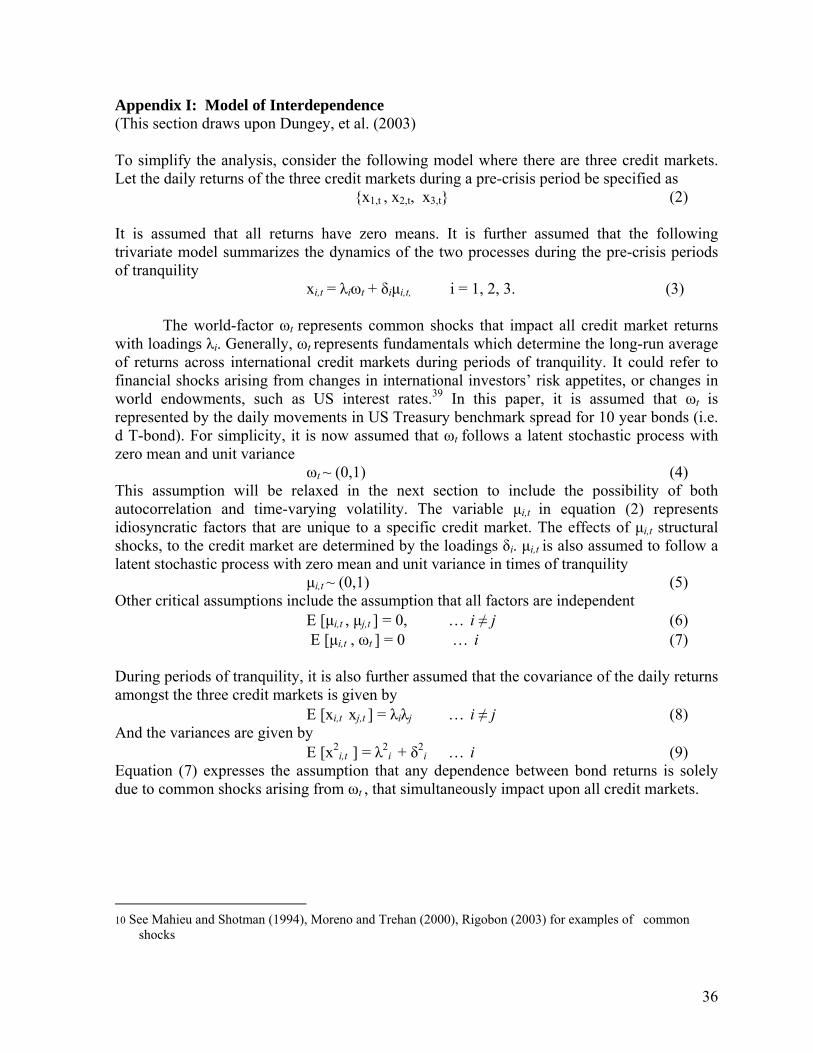
36

Appendix I: Model of Interdependence (This section draws upon Dungey, et al. (2003) To simplify the analysis, consider the following model where there are three credit markets. Let the daily returns of the three credit markets during a pre-crisis period be specified as

x1,t , x2,t, x3,t (2) It is assumed that all returns have zero means. It is further assumed that the following trivariate model summarizes the dynamics of the two processes during the pre-crisis periods of tranquility xi,t = λiωt + δiµi,t, i = 1, 2, 3. (3)

The world-factor ωt represents common shocks that impact all credit market returns with loadings λi. Generally, ωt represents fundamentals which determine the long-run average of returns across international credit markets during periods of tranquility. It could refer to financial shocks arising from changes in international investors’ risk appetites, or changes in world endowments, such as US interest rates.39 In this paper, it is assumed that ωt is represented by the daily movements in US Treasury benchmark spread for 10 year bonds (i.e. d T-bond). For simplicity, it is now assumed that ωt follows a latent stochastic process with zero mean and unit variance ωt ~ (0,1) (4) This assumption will be relaxed in the next section to include the possibility of both autocorrelation and time-varying volatility. The variable µi,t in equation (2) represents idiosyncratic factors that are unique to a specific credit market. The effects of µi,t structural shocks, to the credit market are determined by the loadings δi. µi,t is also assumed to follow a latent stochastic process with zero mean and unit variance in times of tranquility µi,t ~ (0,1) (5) Other critical assumptions include the assumption that all factors are independent E [µi,t , µj,t ] = 0, … i ≠ j (6) E [µi,t , ωt ] = 0 … i (7) During periods of tranquility, it is also further assumed that the covariance of the daily returns amongst the three credit markets is given by

E [xi,t xj,t ] = λiλj … i ≠ j (8) And the variances are given by

E [x2i,t ] = λ2

i + δ2i … i (9)

Equation (7) expresses the assumption that any dependence between bond returns is solely due to common shocks arising from ωt , that simultaneously impact upon all credit markets.

10 See Mahieu and Shotman (1994), Moreno and Trehan (2000), Rigobon (2003) for examples of common

shocks

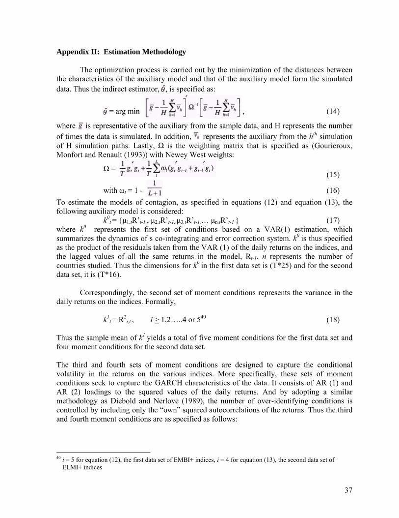
37

Appendix II: Estimation Methodology

The optimization process is carried out by the minimization of the distances between the characteristics of the auxiliary model and that of the auxiliary model form the simulated data. Thus the indirect estimator, , is specified as:

= arg min , (14)

where is representative of the auxiliary from the sample data, and H represents the number of times the data is simulated. In addition, represents the auxiliary from the hth simulation of H simulation paths. Lastly, Ω is the weighting matrix that is specified as (Gourieroux, Monfort and Renault (1993)) with Newey West weights:

Ω = (15)

with ωt = 1 - (16)

To estimate the models of contagion, as specified in equations (12) and equation (13), the following auxiliary model is considered: k0

t = µ1,tR’t-1 , µ2,tR’t-1, µ3,tR’t-1,… µn,tR’t-1 (17) where k0 represents the first set of conditions based on a VAR(1) estimation, which summarizes the dynamics of s co-integrating and error correction system. k0 is thus specified as the product of the residuals taken from the VAR (1) of the daily returns on the indices, and the lagged values of all the same returns in the model, Rt-1. n represents the number of countries studied. Thus the dimensions for k0 in the first data set is (T*25) and for the second data set, it is (T*16).

Correspondingly, the second set of moment conditions represents the variance in the daily returns on the indices. Formally, k1

t = R2i,t , i > 1,2…..4 or 540 (18)

Thus the sample mean of k1 yields a total of five moment conditions for the first data set and four moment conditions for the second data set. The third and fourth sets of moment conditions are designed to capture the conditional volatility in the returns on the various indices. More specifically, these sets of moment conditions seek to capture the GARCH characteristics of the data. It consists of AR (1) and AR (2) loadings to the squared values of the daily returns. And by adopting a similar methodology as Diebold and Nerlove (1989), the number of over-identifying conditions is controlled by including only the “own” squared autocorrelations of the returns. Thus the third and fourth moment conditions are as specified as follows:

40 i = 5 for equation (12), the first data set of EMBI+ indices, i = 4 for equation (13), the second data set of

ELMI+ indices

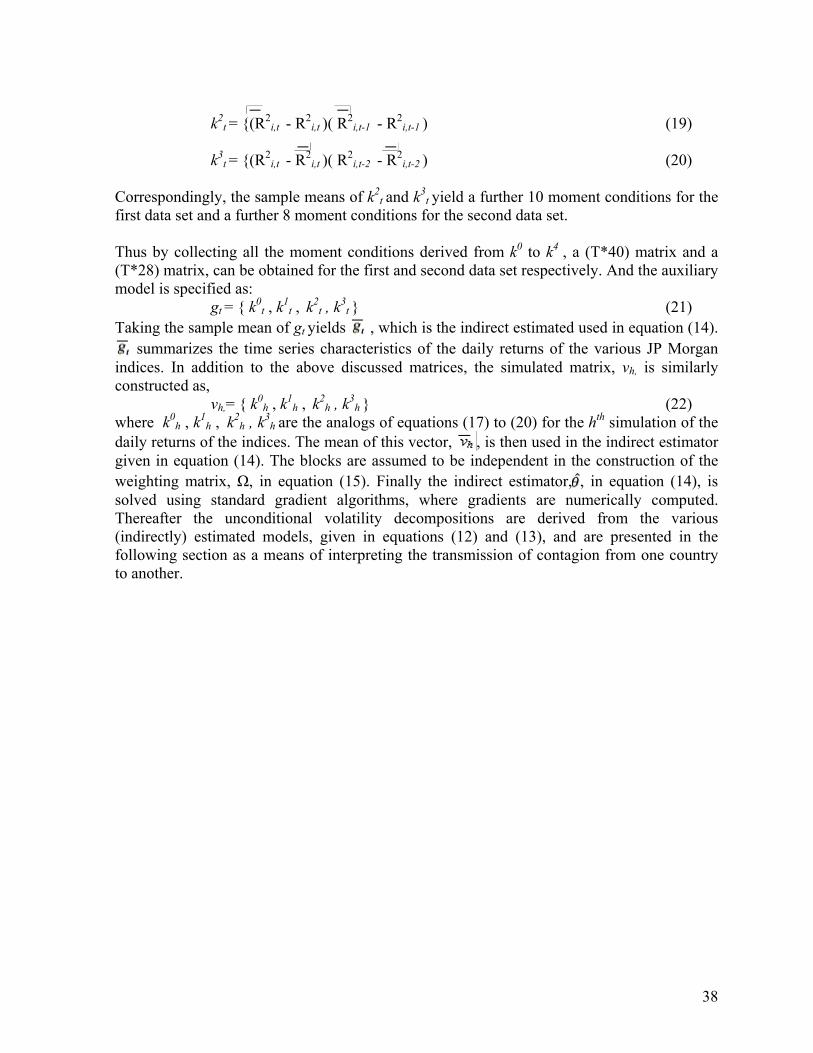
38

k2

t = (R2i,t - R2

i,t )( R2i,t-1 - R2

i,t-1 ) (19)

k3t = (R2

i,t - R2i,t )( R2

i,t-2 - R2i,t-2 ) (20)

Correspondingly, the sample means of k2

t and k3t yield a further 10 moment conditions for the

first data set and a further 8 moment conditions for the second data set. Thus by collecting all the moment conditions derived from k0 to k4 , a (T*40) matrix and a (T*28) matrix, can be obtained for the first and second data set respectively. And the auxiliary model is specified as: gt = k0

t , k1t , k2

t , k3t (21)

Taking the sample mean of gt yields , which is the indirect estimated used in equation (14). summarizes the time series characteristics of the daily returns of the various JP Morgan

indices. In addition to the above discussed matrices, the simulated matrix, vh, is similarly constructed as, vh,= k0

h , k1h , k2

h , k3h

(22) where k0

h , k1h , k2

h , k3h are the analogs of equations (17) to (20) for the hth simulation of the

daily returns of the indices. The mean of this vector, , is then used in the indirect estimator given in equation (14). The blocks are assumed to be independent in the construction of the weighting matrix, Ω, in equation (15). Finally the indirect estimator, , in equation (14), is solved using standard gradient algorithms, where gradients are numerically computed. Thereafter the unconditional volatility decompositions are derived from the various (indirectly) estimated models, given in equations (12) and (13), and are presented in the following section as a means of interpreting the transmission of contagion from one country to another.

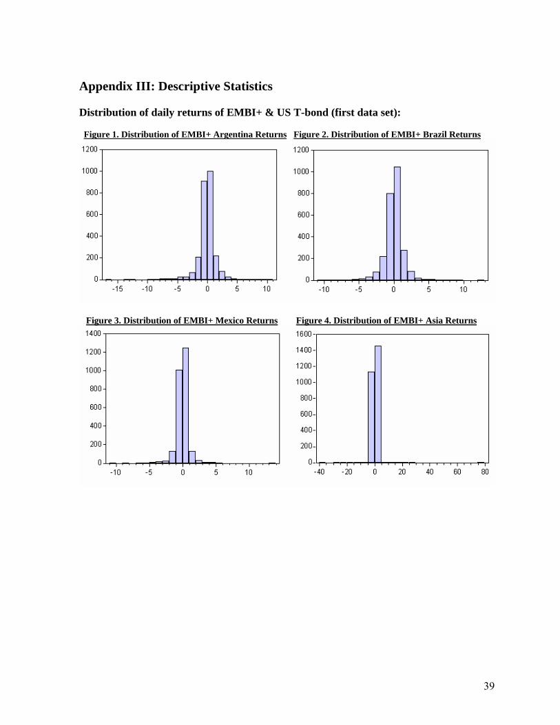
39

Appendix III: Descriptive Statistics Distribution of daily returns of EMBI+ & US T-bond (first data set): Figure 1. Distribution of EMBI+ Argentina Returns Figure 2. Distribution of EMBI+ Brazil Returns

Figure 3. Distribution of EMBI+ Mexico Returns Figure 4. Distribution of EMBI+ Asia Returns

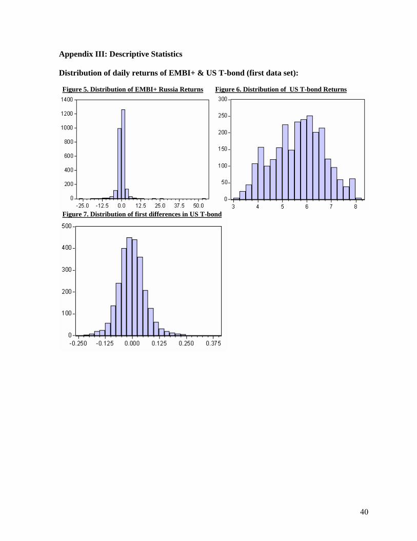
40

Appendix III: Descriptive Statistics Distribution of daily returns of EMBI+ & US T-bond (first data set): Figure 5. Distribution of EMBI+ Russia Returns Figure 6. Distribution of US T-bond Returns

Figure 7. Distribution of first differences in US T-bond

41

Appendix III: Descriptive Statistics Distribution of daily returns of ELMI+ (second data set): Figure 8. Distribution of ELMI+ H.K. Returns Figure 9. Distribution of ELMI+ Indonesia Returns

Figure 10. Distribution of ELMI+ Singapore Returns41 Figure 11. Distribution of ELMI+ Thailand Returns

41 Figure 10. Distribution of ELMI+ Singapore Returns

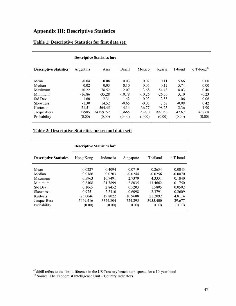
42

Appendix III: Descriptive Statistics Table 1: Descriptive Statistics for first data set:

Table 2: Descriptive Statistics for second data set:

42dtbill refers to the first difference in the US Treasury benchmark spread for a 10-year bond 44 Source: The Economist Intelligence Unit – Country Indicators

Descriptive Statistics for:

Descriptive Statistics Argentina Asia Brazil Mexico Russia T-bond d T-bond42

Mean -0.04 0.08 0.03 0.02 0.11 5.66 0.00 Median 0.02 0.05 0.10 0.05 0.12 5.74 0.00 Maximum 10.22 78.52 12.07 13.68 54.43 8.03 0.40 Minimum -16.86 -35.28 -10.78 -10.26 -26.50 3.10 -0.23 Std Dev. 1.60 2.31 1.42 0.92 2.55 1.06 0.06 Skewness -1.30 14.52 -0.65 -0.05 3.68 -0.08 0.42 Kurtosis 21.51 564.45 14.14 36.77 98.25 2.36 4.90 Jacque-Bera 37985 34359152 13665 123970 992056 47.67 468.68 Probability (0.00) (0.00) (0.00) (0.00) (0.00) (0.00) (0.00)

Descriptive Statistics for:

Descriptive Statistics Hong Kong Indonesia Singapore Thailand d T-bond

Mean 0.0227 -0.4094 -0.0719 -0.2634 -0.0043 Median 0.0186 0.0203 -0.0244 -0.0256 -0.0070 Maximum 0.5963 10.7491 2.7379 4.3331 0.1840 Minimum -0.8408 -21.7899 -2.8035 -13.4662 -0.1750 Std Dev. 0.1065 2.8452 0.5203 1.5805 0.0502 Skewness -0.9751 -2.2310 -0.6098 -2.3791 0.2609 Kurtosis 25.0046 19.8022 10.9608 21.2092 4.8114 Jacque-Bera 5449.416 3374.804 724.295 3955.400 39.677 Probability (0.00) (0.00) (0.00) (0.00) (0.00)

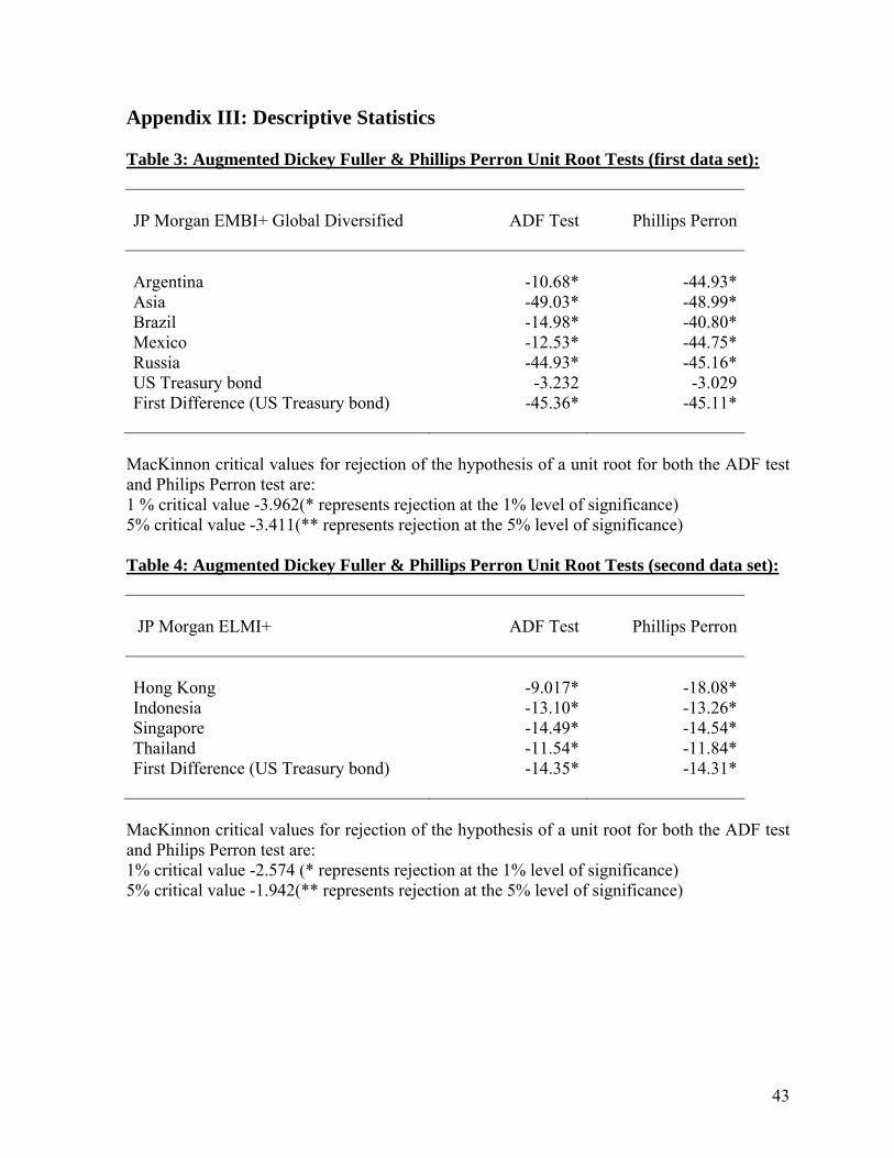
43

Appendix III: Descriptive Statistics Table 3: Augmented Dickey Fuller & Phillips Perron Unit Root Tests (first data set): JP Morgan EMBI+ Global Diversified ADF Test Phillips Perron

Argentina -10.68* -44.93*Asia -49.03* -48.99*Brazil -14.98* -40.80*Mexico -12.53* -44.75*Russia -44.93* -45.16*US Treasury bond -3.232 -3.029First Difference (US Treasury bond) -45.36* -45.11*

MacKinnon critical values for rejection of the hypothesis of a unit root for both the ADF test and Philips Perron test are: 1 % critical value -3.962(* represents rejection at the 1% level of significance) 5% critical value -3.411(** represents rejection at the 5% level of significance) Table 4: Augmented Dickey Fuller & Phillips Perron Unit Root Tests (second data set): JP Morgan ELMI+ ADF Test Phillips Perron Hong Kong -9.017* -18.08*Indonesia -13.10* -13.26*Singapore -14.49* -14.54*Thailand -11.54* -11.84*First Difference (US Treasury bond) -14.35* -14.31*

MacKinnon critical values for rejection of the hypothesis of a unit root for both the ADF test and Philips Perron test are: 1% critical value -2.574 (* represents rejection at the 1% level of significance) 5% critical value -1.942(** represents rejection at the 5% level of significance)

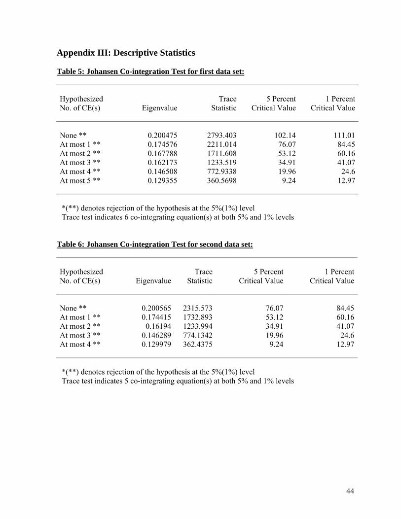
44

Appendix III: Descriptive Statistics Table 5: Johansen Co-integration Test for first data set: Hypothesized Trace 5 Percent 1 PercentNo. of CE(s) Eigenvalue Statistic Critical Value Critical Value None ** 0.200475 2793.403 102.14 111.01At most 1 ** 0.174576 2211.014 76.07 84.45At most 2 ** 0.167788 1711.608 53.12 60.16At most 3 ** 0.162173 1233.519 34.91 41.07At most 4 ** 0.146508 772.9338 19.96 24.6At most 5 ** 0.129355 360.5698 9.24 12.97 *(**) denotes rejection of the hypothesis at the 5%(1%) level Trace test indicates 6 co-integrating equation(s) at both 5% and 1% levels

Table 6: Johansen Co-integration Test for second data set: Hypothesized Trace 5 Percent 1 PercentNo. of CE(s) Eigenvalue Statistic Critical Value Critical Value None ** 0.200565 2315.573 76.07 84.45At most 1 ** 0.174415 1732.893 53.12 60.16At most 2 ** 0.16194 1233.994 34.91 41.07At most 3 ** 0.146289 774.1342 19.96 24.6At most 4 ** 0.129979 362.4375 9.24 12.97 *(**) denotes rejection of the hypothesis at the 5%(1%) level Trace test indicates 5 co-integrating equation(s) at both 5% and 1% levels

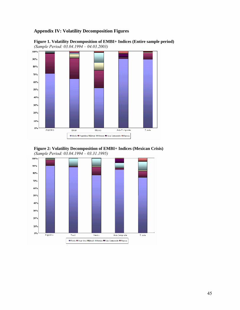
45

Appendix IV: Volatility Decomposition Figures Figure 1. Volatility Decomposition of EMBI+ Indices (Entire sample period) (Sample Period: 03.04.1994 – 04.03.2003)

Figure 2: Volatility Decomposition of EMBI+ Indices (Mexican Crisis) (Sample Period: 03.04.1994 – 03.31.1995)

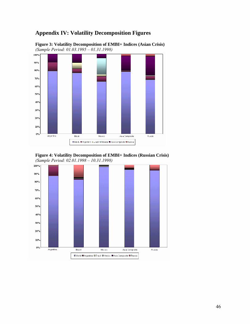
46

Appendix IV: Volatility Decomposition Figures Figure 3: Volatility Decomposition of EMBI+ Indices (Asian Crisis) (Sample Period: 01.03.1995 – 01.31.1998)

Figure 4: Volatility Decomposition of EMBI+ Indices (Russian Crisis) (Sample Period: 02.01.1998 – 10.31.1998)

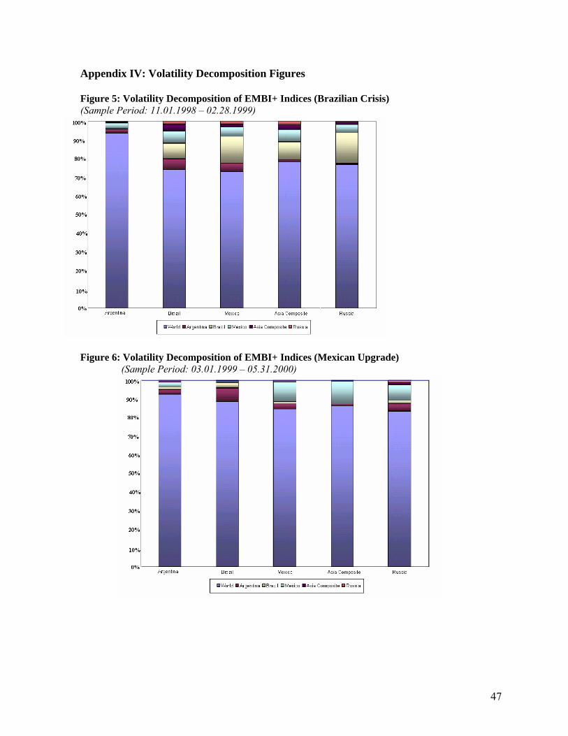
47

Appendix IV: Volatility Decomposition Figures Figure 5: Volatility Decomposition of EMBI+ Indices (Brazilian Crisis) (Sample Period: 11.01.1998 – 02.28.1999)

Figure 6: Volatility Decomposition of EMBI+ Indices (Mexican Upgrade) (Sample Period: 03.01.1999 – 05.31.2000)

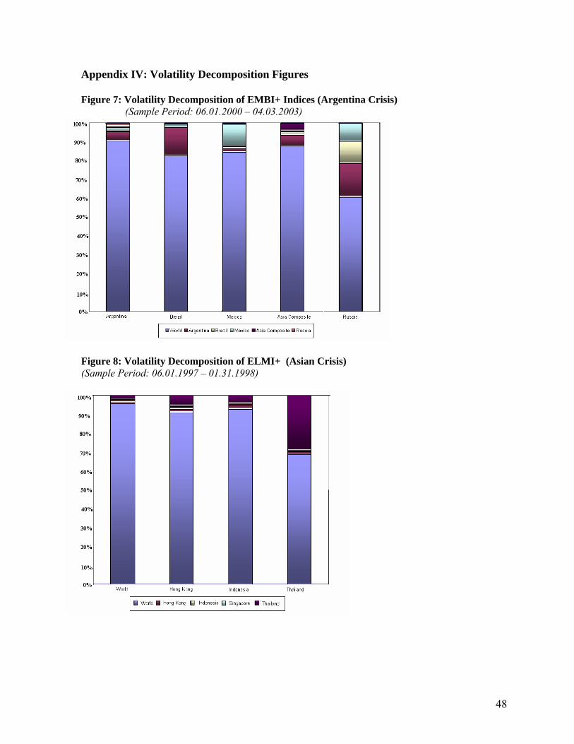
48

Appendix IV: Volatility Decomposition Figures

Figure 7: Volatility Decomposition of EMBI+ Indices (Argentina Crisis) (Sample Period: 06.01.2000 – 04.03.2003)

Figure 8: Volatility Decomposition of ELMI+ (Asian Crisis) (Sample Period: 06.01.1997 – 01.31.1998)

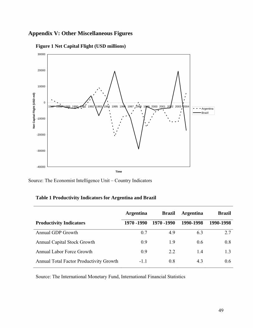
49

Appendix V: Other Miscellaneous Figures Figure 1 Net Capital Flight (USD millions)

-40000

-30000

-20000

-10000

0

10000

20000

30000

1987 1988 1989 1990 1991 1992 1993 1994 1995 1996 1997 1998 1999 2000 2001 2002 2003 2004

Time

Net

Cap

ital F

light

(USD

mil)

ArgentinaBrazil

Source: The Economist Intelligence Unit – Country Indicators

Table 1 Productivity Indicators for Argentina and Brazil Argentina Brazil Argentina Brazil

Productivity Indicators 1970 -1990 1970 -1990 1990-1998 1990-1998

Annual GDP Growth 0.7 4.9 6.3 2.7 Annual Capital Stock Growth 0.9 1.9 0.6 0.8 Annual Labor Force Growth 0.9 2.2 1.4 1.3 Annual Total Factor Productivity Growth -1.1 0.8 4.3 0.6

Source: The International Monetary Fund, International Financial Statistics

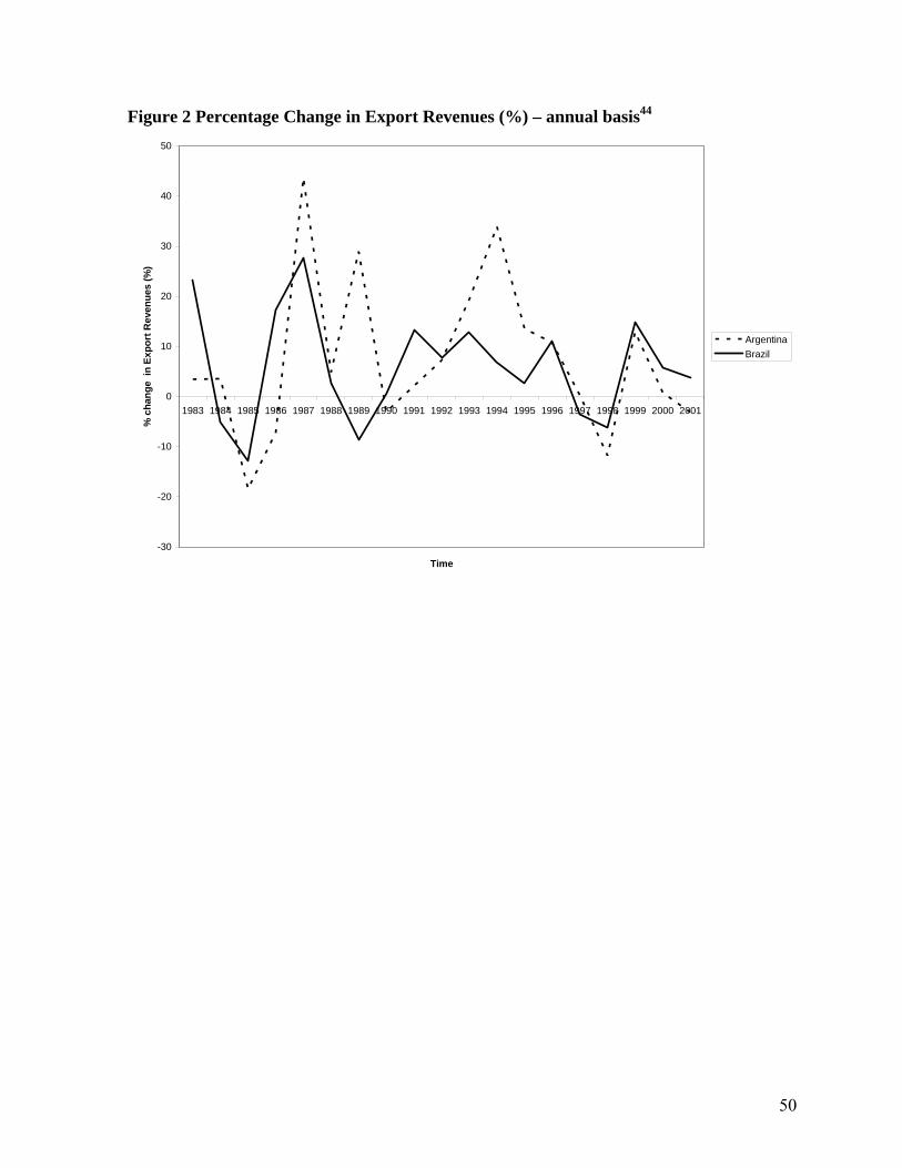
50

Figure 2 Percentage Change in Export Revenues (%) – annual basis44

-30

-20

-10

0

10

20

30

40

50

1983 1984 1985 1986 1987 1988 1989 1990 1991 1992 1993 1994 1995 1996 1997 1998 1999 2000 2001

Time

% c

hang

e in

Exp

ort R

even

ues

(%)

ArgentinaBrazil

51

References Agenor, Pierre-Richard, (1998) “The Surge in Capital Flows: Analysis of ‘Pull’ and ‘Push'

Factors”. International Journal of Finance & Economics, Vol. 3 (1) pp. 39-57. Arora, V., Cerisola, M., (2000), “How does U.S. Monetary Policy Influence Economic

Conditions in Emerging Markets?” IMF Working Paper 00/148 Baig, T. and Goldfajn, I. (1999), “Financial Market Contagion in the Asian Crisis”, IMF

Staff Papers, 46(2), pp 167-195 Bekaert, G., Harvey, C.R. and Ng, A. (2003), “Market Integration and Contagion”, Journal

of Business, forthcoming Bikchandani S. and Sharma S. (2000), “Herd Behavior in Financial Markets: A review” IMF

working paper WP/00/48 Bollerslev, T., R. Chou and K. Kroner (1992), “ARCH Modeling in Finance”, Journal of

Econometrics, 52, pp 5-59 Boyer, B. H., Gibson, M.S. and Loretan, M. (1999), “Pitfalls in test for changes in

correlations”, International Finance Discussion Paper, 597 Burton, F.N., Inoue, H., (1985), “The Influence of Country Risk Factors on Interest Rate

Differentials on International Bank Lending to Sovereign Borrowers”, Applied Economics 17, 491-507

Calvo, G.A., L. Leiderman, CM Reinhart (1993), "Capital Inflows and Real Exchange Rate

Appreciation in Latin America: The Role of External Factors," IMF Staff Papers, Vol. 40, No. 1, pp. 108-51.

Calvo, G.A. and E.G. Mendoza (2000), “Rational contagion and the Globalization of

Securities Markets”, Journal of International Econometrics, 51(1), pp 79-113 Calvo, S. and Reinhart, C. (1995), “Capital Inflows to Latin America: Is there Evidence of

Contagion Effects?”, World Bank and International Monetary Fund, mimeo. Cantor, R., Packer, F., (1996), “Determinants and Impact of Sovereign Credit Ratings”,

FRBNY, Economic Policy Review, 37-53 Corsetti, G., Pericoli, P. and Sbracia, M. (2001) “Correlation analysis of financial contagion:

what one should know before running a test” Termi di Discussione, Banca d’ Italia, No. 408

Coulson, N. and R. Robins, (1985) “Aggregate Economic Activity and the Variance of

Inflation: Another Look,” Economics Letters, 17, pp 71-75

52

Cragg, J. (1982), “Estimation and Testing in Testing in Time Series Regression Models with Heteroscedastic Disturbances”, Journal of Econometrics, 20, pp. 135- 157.

Diebold, F.X. and M. Nerlove (1989), “The Dynamics of Exchange Rate Volatility: A Multi-

variate Latent-Factor ARCH Model,” Journal of Applied Econometrics, 4, pp 1-22 Domowitz, I., and C. Hakkio (1985), “Conditional Variance and the Risk Premium in the

Foreign Exchange Market.”, Journal of International Economics 19, pp 47-66 Dornbush, R., Y.C. Park, and S. Classens (2000), “Contagion: Understanding How it

Spreads”, World Bank Research Observer, 15(2), pp 177-197 Dungey, M., V.L. Martin and A.R. Pagan (2000), “A Multivariate Latent Factor

Decomposition of International Bond Yield Spreads,” Journal of Applied Econometrics, 15(6), pp 697-715

Dungey, M. and Martin V.L. (2002), “Contagion across Financial Markets: An empirical

assessment”, New York Stock Exchange Conference Paper, February 16-17, Hawaii Dungey, M., Fry R., Gonzálex-Hermosillo B., and Martin V.L. (2002), “International

Contagion Effects from the Russian Crisis and the LTCM Near-Collapse”, IMF Working Paper WP/02/74

Dungey, M., Fry R., Gonzálex-Hermosillo B., and Martin V.L. (2003), “Empirical Modelling

of Contagion: A Review of Methodologies”, Quantitative Finance, under review Edwards, S., (1984), “LDC Foreign Borrowing and Default Risk: An Empirical Investigation

1976-1980”, American Economic Review 74, 726-734 Edwards S. (1986), “The Pricing of Bonds and bank Loans in International Markets. An

Empirical Analysis of Developing Countries’ Foreign Borrowing”, European Economic Review 30, 565-589

Edwards, S. (1998) “Interest Rate Volatility, capital controls and contagion” National

Bureau of Economic Research working paper, 6756 Edwards, S., Susmel, R., (2000), “Interest Rate Volatility and Contagion in Emerging

Markets. Evidence from the 1990s”, National Bureau of Economic Research Working Paper series number 7813

Eichengreen, B., A.K. Rose and C. Wyplosz (1996), “Contagion Currency Crises”, National

Bureau of Economic Research Working Paper, 5681 Engel, R. (1982) “Autoregressive Conditional Heteroskedasticity with Estimates of the

Variance of United Kingdom Inflations”, Econometrica, 50, pp 987-1008

53

Engel, R. (1983), “Estimates of the Variance of US Inflation based on the ARCH Model”, Journal of Money, Credit and Banking, 15, pp 286-301

Ebgel, R., D. Hendry, and D. Trumble (1985) “Small Sample Properties of ARCH Estimators

and Tests” Canadian Jornal of Economics, 18, pp 66-93 Engel, R., R. Lilen, and R. Robins (1987), “Estimating Time Varying Risk Premia in the Term

Structure: The ARCH-M Model”, Econometrica, 55, pp 391-407 Favero, C.A., and F. Giavazzi (2000), “Looking for Contagion: Evidence from the ERM”,

National Bureau of Economic Research Working Paper, 7797 Favero and Giavazzi (2002) “Is the International Propagation of Financial Shocks Non-

Linear? Evidence from the ERM,” Journal of International Economics, Volume 57,1 Jeffrey A. Frankel & Andrew K. Rose, (1996), “Currency Crashes in Emerging Marekts:

Empirircal Indicators” National Bureau of Economic Research Working Paper series number 5437

Frankel, Jeffrey A., Nouriel Roubini (2001) “The Role of Industrial Country Policies in

Emerging Market Crises”, National Bureau of Economic Research, Working Paper, Paper series number w8634, December 2001

Forbes K. and R. Rigobon (2000), “Measuring Contagion, Conceptual and Empirical Issues”

mimeo, MIT Forbes, K. and R. Rigobon (2002), “No Contagion, Only Interdependence: Measuring Stock

Market Comovements”, Journal of Finance, 57, 5, pp 2231- 2261 Glick, R. and A.K. Rose (1999), “Contagion and Trade: Why are currency crises regional?”,

Journal of International Money and Finance, 18 (4), 603-17 Goldstein M. (1998) “The Asian Financial Crisis: Causes, Cures and Systematic

Implications”, Policy Analysts in International Economics, 55, Institute for International Economics, Washington DC

Gourieroux, C., A. Monfort and E. Renault (1993) “Indirect Inference”, Journal of Applied

Econometrics, 8, S85-S118. Gourieroux, C. and A. Monfort (1994), Simulation Based Econometric Methods, CORE

Discussion Paper Hamao, Y., Masulis, R.W. and Ng. (1990) “Correlations in price changes and volatility

across international stock markets” Review of Financial Studies, 3, pp 281-307 International Monetary Fund, International Financial Statistics, various issues

54

Kamin, S.B., von Kleist, K., (1999), “The Evolution and Determination of Emerging Market

Credit Spreads in the 1990s”, Board of Governors of the Federal Reserve System, International Finance Discussion Papers, number 653

Kaminsky, G.L., and S.L. Schmuklet (1999), “What Triggers Market Jitters?” Journal of

International Money and Finance, 18, pp 537-560 Kaminsky Garciela, Richard K. Lyons, and Sergio L. Schmukler (2001), “Mutual Fund

Investment in Emerging Markets: An Overview”, The World Bank Economic Review, Volume 15, No. 2, P 315-340

Kaminsky Graciela, Sergio L. Schmukler (2001), “Emerging Markets Instability: Do

Sovereign Ratings Affect Country Risk and Stock Returns?” George Washington University, February 2001

King and Wadhwani (1990), “Transmission of Volatility between Stock Markets”, Review of

Financial Studies, Volume 3, Issue 1 Krugman, P. (1998), “What happened to Asia?” mimeo, MIT Kyle, A.S. and Wei X. (2001), “Contagion as a Wealth Effect”, The Journal of Finance,

LVI(4), pp 1401-1440 Loretan, M. and English W.B. (2000), “Evaluating ‘correlation breakdowns’ during periods

of market volatility”, In International Financial Markets and the implications for monetary and financial stability, Bank for International Settlements, Basel, Switzerland, pp 214-231

Lowell, J., C.R. Neu and D. Tong (1998), “Financial crises and contagion in emerging market

countries” RAND, MR-962 Matteo Ciccarelli, Alessandro Rebucci, (2003), “Measuring Contagion with a Bayesian,

Time-Varying Coefficient Model”, European Central Bank Working Paper number 263

Masson, P. (1999), “Contagion: Macroeconomic Models with Multiple Equilibria,” Journal

of International Money and Finance, 18, pp 587-602 Mauro, P., Sussman, N. Yafeh, Y., (2000), “Emerging Market Spreads: Then versus Now”,

IMF Working Paper 00/190 Milesi-Ferretti and Assaf Razin (1998), “Current Account Reversals and Currency Crises:

Empirical Regularities”, National Bureau of Economic Research, Working Papers 6620

55

Moreno Ramon, Baharat Trehan (2000), “Common Shocks and Currency Crises”, Federal Reserve Bank of San Francisco, April 28, 2000

Pericoli Marcello, Massimo Sbracia (2003), “A Primer on Financial Contagion”, Journal of

Economic Surveys Volume 17, Issue 4, September 2003 Pierre-Richard Agenor and Joshua Aizenman (1997), “Contagion and Volatility with

Imperfect Credit Markets”, International Monetary Fund, WP/97/127 Rigobon, R., (2001), “Contagion: How to measure it?” in Sebastian Edwards and Jeffrey

Frankel Edition, Currency Crises Prevention, National Bureau of Economic Research

Rigobon, R., (2002a), “On the Measurement of the International Propagation of shocks: Is it

stable?”, Journal of International Economics Sachs J., Tornell A. and Velasco A. (1996), “Financial Crises in Emerging Markets: The

Lessons from 1995”, National Bureau of Economic Research, Working paper W5576

Scherer, K.P, Avellaneda, M., (2000), “All for One… One for All?: A Principal Component

Analysis of the Latin American Brady Bond Debt from 1994 to 2000”, NYU Courant Institute of Mathematical Sciences Working Paper