Modeling Contagion and Systemic Risk · Modeling Contagion and Systemic Risk∗ Daniele Bianchi† Monica Billio‡ Roberto Casarin‡ Massimo Guidolin§ Abstract We model contagion

Modeling Contagion and Systemic Risk∗

Daniele Bianchi† Monica Billio‡ Roberto Casarin‡ Massimo Guidolin§

Abstract

We model contagion in financial markets as a shift in the strength of cross-firm network linkages, and

argue that this provide a natural and intuitive framework to measure systemic risk. We take an asset

pricing perspective and dynamically infer the network structure system-wide from the residuals of an

otherwise standard linear factor pricing model, where systematic and systemic risks are jointly consid-

ered. We apply the model to a large set of daily returns on blue chip companies, and find that high

systemic risk occurred across the period 2001/2002 (i.e. dot.com bubble, 9/11 attacks, financial scandals,

Iraq war), the great financial crisis, and the recent major Eurozone sovereign turmoil. Specifically, we

show that few financial firms are key for systemic risk measurement. Such network centrality holds also

at the industry level and does not depend on the relative market value of the financial sector. Finally,

we show that our network-implied systemic risk measure provides an early warning signal on aggregate

financial stress conditions.

Keywords: Financial Markets, Contagion, Networks, Systemic Risk, Asset Pricing

JEL codes: G12, G29

∗This version: January 8, 2015, Comments are welcome. We are grateful to Peter Kondor and NeilPearson for their helpful comments and suggestions. For financial supports, the authors thank the EuropeanUnion, Seventh Framework Programme FP7/2007-2013 under grant agreement SYRTO-SSH-2012-320270, bythe Institut Europlace de Finance, Systemic Risk grant, and by the Italian Ministry of Education, Universityand Research (MIUR) PRIN 2010-11 grant MISURA.

†University of Warwick - Finance Group, Coventry, CV4 7AL, UK. [email protected]‡Department of Economics, Universita Ca Foscari, Venezia, Italy§Department of Finance and IGIER, Bocconi University, Milan, Italy.

1

1 Introduction

Contagion appears central for systemic risk measurement and management in the aftermath

of the recent financial crisis. Dramatic shocks to a single institution can quickly affect others

operating in different markets, with different sizes and structures. Perhaps surprisingly, however,

contagion and systemic risk remain rather elusive concepts, in many respects incompletely

identified and poorly measured. In fact, anomalous patterns of cross-sectional dependence are

difficult even to identify, much less characterize empirically.1

In this paper, we address this situation by taking an asset pricing perspective and develop

a unified framework to empirically identify channels of contagion in large dimensional time se-

ries settings, where sources of systematic and systemic risks are not mutually exclusive. Our

methodology directly builds on the concept of network. Network analysis is omnipresent in

modern life, from Twitter to the study of the transmission of virus diseases. Broadly speaking,

a network represents the interconnections of a large multivariate system, and its graph represen-

tation can be used to study the properties of the transmission mechanism of exogenous shocks

(e.g. patient zero in a virus disease). We remain agnostic as to how contagion arises; rather, we

take it as given and seek how to capture it correctly for systemic risk measurement purposes.

For a given linear factor model, we measure contagion as a shift in the strength of the cross-

firm network linkages, which are inferred system-wide on the covariance structure of the model

residuals. This, not only allows disjoint sources of systematic and systemic risk coexist, but also

is consistent with the common wisdom that posits contagion representing a significant increase

in cross-sectional linkages across institutions/sectors/countries after a shock.2 In particular,

exposures of each firm to sources of systematic risk directly depends on the aggregate systemic

risk measured through network connectedness.

This paper builds on a recent literature advocating the use of network analysis in economics

and finance to make inference on the connectedness of institutions, sectors and countries, such

1See among others Forbes and Rigobon (2000), Forbes and Rigobon (2002) and Corsetti, Pericoli, and Sbra-cia (2005), Adrian and Brunnermeier (2010), Acharya, Pedersen, Phillippon, and Richardson (2011), Corsetti,Pericoli, and Sbracia (2011), Billio, Getmansky, Lo, and Pelizzon (2012), Barigozzi and Brownlees (2013), Dieboldand Yilmaz (2014), just to cite a few.

2See Forbes and Rigobon (2000) for a discussion of pros and cons of alternative definitions of contagion.

2

as Jackson (2008), Easley and Kleinberg (2010), Billio et al. (2012), Hautsch, Schaumburg,

and Schienle (2012), Barigozzi and Brownlees (2013), Diebold and Yilmaz (2014),Timmermann,

Blake, Tonks, and Rossi (2014) and Diebold and Yilmaz (2015). In particular, Billio et al. (2012)

and Diebold and Yilmaz (2014) show that the strength of connectedness of financial institutions

changed over time, substantially increasing across the recent great financial crisis. In the spirit

of Diebold and Yilmaz (2014), we provide a unified framework to empirically measure contagion

system-wide via Bayesian inference on cross-company linkages.

We take steps from this literature in several important directions. We propose a joint infer-

ence scheme on the network structure as a whole. Standard empirical methodologies are based

on pairwise correlation and Granger causality measures to build the financial network. Recent

evidence show that these pairwise measures can be biased making them of little value in a finan-

cial network context (see e.g. Forbes and Rigobon 2000, Ahelegbey, Billio, and Casarin 2014,

and Diebold and Yilmaz 2014). In this paper, we make system-wide inference on a large dimen-

sional network by simultaneously considering all of the possible linkages among institutions on

the basis of an underlying undirected graphical model.3

Also, we fully acknowledge the fact that parameters are uncertain. Existing methodologies

extract the network structure assuming the parameters of the model are constant in repeated

samples. As a result, the derived inference is thus to be read as contingent on the econome-

trician having full confidence in his parameters estimates, which is objectively rarely the case.

Moreover, alternative conceivable values of the parameters will typically lead to different net-

works. In this paper, we provide an exact finite-sample Bayesian estimation framework which

helps generate posterior distribution of virtually any function of the model parameters, as well

as posterior sufficient statistics for the underlying economic network. Such posterior estimates

allow to test hypothesis on the nature and structure of the network linkages in a unified setting,

which the earlier literature did not provide.

More prominently, we take into account the fact that contagion, and then systemic risk,

is more a shift concept than a steady state (e.g. Forbes and Rigobon 2000). Indeed, Billio

et al. (2012) and Diebold and Yilmaz (2014) provide evidence that connectedness of financial

3See Whittaker (1990); Dawid and Lauritzen (1993), Lauritzen (1996), Carvalho and West (2007), Wang andWest (2009) and Wang (2010) for more detailed discussions on graphical models and their applications.

3

institutions is stronger during financial turmoils. We take this evidence to suggest the presence of

two distinct unobserved states driving network connectedness, therefore contagion and systemic

risk. Consistently, we label the two latent states as “high” and “low” systemic risk, such that

when the economy is a state of contagion indicates a high risk that a shock to a single firm can

quickly affect the economic system as a whole.

Empirically, the paper focuses on a set of 100 blue-chip companies from the S&P100 Index.

We consider those institutions with more than 15 years of historical data. We are left with 83

firms. Returns are computed on a daily basis, dollar-valued and taken in excess of the risk-free

rate. The sample is 10/05/1996-31/10/2014 (4821 observations for each institution), for a total

of more than 400,000 firm-day observations. Our emphasis on stock returns is motivated by the

desire to incorporate the most current information for systemic risk measurement; stocks returns

reflect information more rapidly than non-trading-based measures such as accounting variables,

especially considering most of accounting information is not available on a daily frequency.

In the empirical analysis, we consider the impact of common sources of systematic risk

such as the excess return (in excess of the T-Bill rate) on aggregate financial wealth (i.e. the

CAPM). Defining a factor model does not mean that we take a stand on the mechanism that

transfer fundamentals into cross-sectional dependence. Of course, given its residual nature,

any statements on systemic risk will be conditional on a correct specification of the factor

model. Our methodology is rather general and can be easily applied to any linear factor pricing

model. To mitigate the model selection bias we consider other popular sources of systematic

risks such as size, value and shocks to macroeconomic factors. In particular we consider the

three-factor model initially proposed by Fama and French (1993), and an implementation of the

Merton (1973) intertemporal extension of the CAPM (I-CAPM) including shocks to aggregate

dividend yield and both default- and term-spreads as state variables, in addition to aggregate

wealth. Data are from the Center for Research in Security Prices (CRSP), the FredII database

of the St. Louis Federal Reserve Bank and Kenneth French’s website. The data for the 1-month

T-Bill are taken from Ibbotson Associates.

Our empirical findings show that high systemic risk characterized financial markets across

the period 2001/2002 (i.e. dot.com bubble, 9/11 attacks, Financial scandals, Iraq war), the

4

great financial crisis of 2008/2009, and the recent major Eurozone sovereign turmoil. Few

financial firms such as JP Morgan, Bank of America and Bank of New York Mellon turns out

to play a key role for systemic risk measurement, as they heavily outweigh other firms within

the economic network. This pattern holds also at the industry level, with industries classified

according to the Global Industry Classification Standard (GICS) developed by MSCI. In fact,

while the Energy sector is key within periods of low systemic risk, the financial sector plays a

crucial role globally when the probability of contagion across firms is high. This evidence is

in line with Barigozzi and Brownlees (2013) and Diebold and Yilmaz (2014). Interestingly, we

show that exposures to sources of systematic risk also change across firms when systemic risk

increases. For instance, exposure to both market and default risks tend to be higher in the

financial sector when systemic risk increases.

Building on these results, we show that the centrality feature of the financial sector can

not be reconciled with its relative market value. By using a Probit regression analysis we show

that systemic risk can be significantly predicted by increasing credit and default yield spread,

although such predictability power is low in magnitude. Also, we show that our model-implied

systemic risk indicator significantly predicts aggregate financial distress measured through the

St.Louis Fed Financial Stress Index. As such, our methodology can be thought of as an early

warning indicator to regulators and the public.

The remainder of the paper proceeds as follows. Section 2 lays out the model. Section

3 shows results from a simulation example. Section 4 discuss the data, the prior elicitation

and reports the main empirical results. The relationship between systemic risk, macroeconomic

variables and financial distress is investigated in Section 5. Section 6 concludes. We leave to

the Appendix derivations details and additional results.

2 Measuring Systemic Risk

We identify contagion as an increase in the strength of network connectedness. In general, any

network can be described by a p× p adjacency matrix, A, consisting of p unique “nodes” which

are connected through “edges”. Each entry in the adjacency matrix A, denoted aij , for row i

5

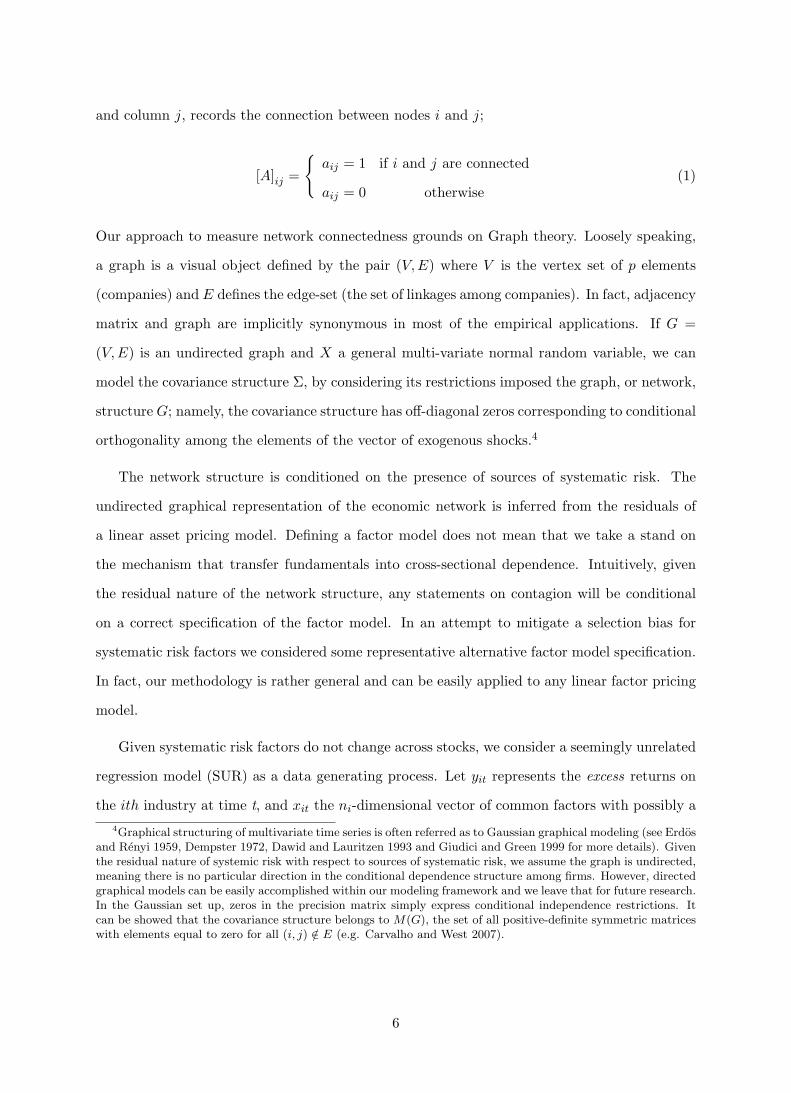
and column j, records the connection between nodes i and j;

[A]ij =

aij = 1 if i and j are connected

aij = 0 otherwise(1)

Our approach to measure network connectedness grounds on Graph theory. Loosely speaking,

a graph is a visual object defined by the pair (V,E) where V is the vertex set of p elements

(companies) and E defines the edge-set (the set of linkages among companies). In fact, adjacency

matrix and graph are implicitly synonymous in most of the empirical applications. If G =

(V,E) is an undirected graph and X a general multi-variate normal random variable, we can

model the covariance structure Σ, by considering its restrictions imposed the graph, or network,

structure G; namely, the covariance structure has off-diagonal zeros corresponding to conditional

orthogonality among the elements of the vector of exogenous shocks.4

The network structure is conditioned on the presence of sources of systematic risk. The

undirected graphical representation of the economic network is inferred from the residuals of

a linear asset pricing model. Defining a factor model does not mean that we take a stand on

the mechanism that transfer fundamentals into cross-sectional dependence. Intuitively, given

the residual nature of the network structure, any statements on contagion will be conditional

on a correct specification of the factor model. In an attempt to mitigate a selection bias for

systematic risk factors we considered some representative alternative factor model specification.

In fact, our methodology is rather general and can be easily applied to any linear factor pricing

model.

Given systematic risk factors do not change across stocks, we consider a seemingly unrelated

regression model (SUR) as a data generating process. Let yit represents the excess returns on

the ith industry at time t, and xit the ni-dimensional vector of common factors with possibly a

4Graphical structuring of multivariate time series is often referred as to Gaussian graphical modeling (see Erdosand Renyi 1959, Dempster 1972, Dawid and Lauritzen 1993 and Giudici and Green 1999 for more details). Giventhe residual nature of systemic risk with respect to sources of systematic risk, we assume the graph is undirected,meaning there is no particular direction in the conditional dependence structure among firms. However, directedgraphical models can be easily accomplished within our modeling framework and we leave that for future research.In the Gaussian set up, zeros in the precision matrix simply express conditional independence restrictions. Itcan be showed that the covariance structure belongs to M(G), the set of all positive-definite symmetric matriceswith elements equal to zero for all (i, j) /∈ E (e.g. Carvalho and West 2007).

6

constant term for individual i at time t ; the model dynamics can be summarized as

yt = X ′tβt + εt, εt ∼ Np (0,Σt (Gt)) (2)

t = 1, . . . , T , where yt = (y1t, . . . , ypt)′ is a p-dimensional vector of returns in excess of the risk-

free rate, Xt = diag(x1t, . . . , xpt) a n× p matrix of explanatory variables, with n =∑p

i=1 ni,

εt = (ε1t, . . . , εpt)′ a p-vector of normal random errors. The dynamics described in (2) is fairly

general since represents an approximation of a reduced-form stochastic discount factor where

the risk factors are assumed to capture investors’ beliefs on the business cycle (see Liew and

Vassalou 2000, Cochrane 2001, and Vassalou 2003).

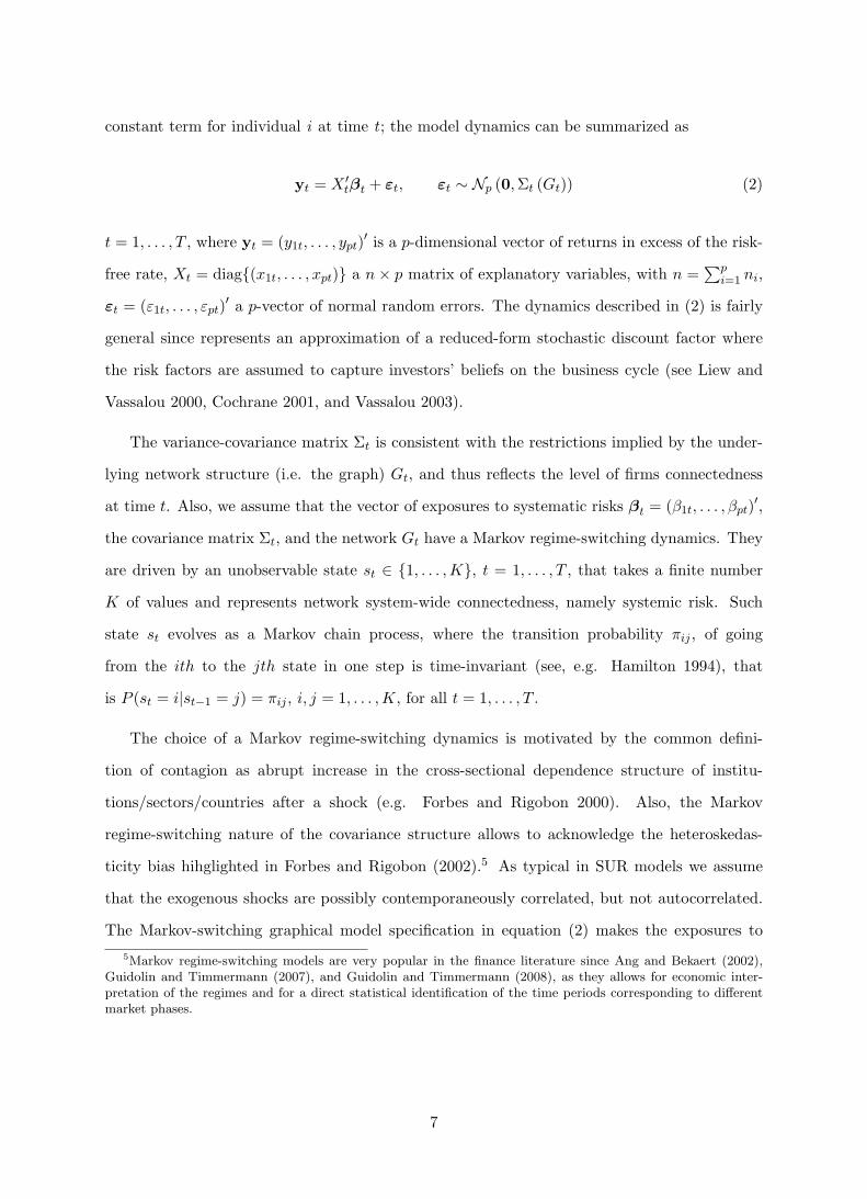
The variance-covariance matrix Σt is consistent with the restrictions implied by the under-

lying network structure (i.e. the graph) Gt, and thus reflects the level of firms connectedness

at time t. Also, we assume that the vector of exposures to systematic risks βt = (β1t, . . . , βpt)′,

the covariance matrix Σt, and the network Gt have a Markov regime-switching dynamics. They

are driven by an unobservable state st ∈ 1, . . . ,K, t = 1, . . . , T , that takes a finite number

K of values and represents network system-wide connectedness, namely systemic risk. Such

state st evolves as a Markov chain process, where the transition probability πij , of going

from the ith to the jth state in one step is time-invariant (see, e.g. Hamilton 1994), that

is P (st = i|st−1 = j) = πij , i, j = 1, . . . ,K, for all t = 1, . . . , T .

The choice of a Markov regime-switching dynamics is motivated by the common defini-

tion of contagion as abrupt increase in the cross-sectional dependence structure of institu-

tions/sectors/countries after a shock (e.g. Forbes and Rigobon 2000). Also, the Markov

regime-switching nature of the covariance structure allows to acknowledge the heteroskedas-

ticity bias hihglighted in Forbes and Rigobon (2002).5 As typical in SUR models we assume

that the exogenous shocks are possibly contemporaneously correlated, but not autocorrelated.

The Markov-switching graphical model specification in equation (2) makes the exposures to

5Markov regime-switching models are very popular in the finance literature since Ang and Bekaert (2002),Guidolin and Timmermann (2007), and Guidolin and Timmermann (2008), as they allows for economic inter-pretation of the regimes and for a direct statistical identification of the time periods corresponding to differentmarket phases.

7

sources of systematic risk time varying and directly depending on the regime of systemic risk;

βt =K∑

k=1

βkIk(st) (3)

with Ik (st) the indicator function which takes value one when the state st takes value k at time

t and zero otherwise. The state-specific covariance matrix Σk is constrained by a sate-specific

graph Gk, that is

Σt =K∑

k=1

Σk (Gk) Ik(st), Gt =K∑

k=1

GkIk(st) (4)

with Σk ∈ M(Gk) and M(Gk) the set of all positive-definite symmetric matrices with elements

equal to zero for all (i, j) /∈ E, given the state st = k. In the model, contagion is generated by

both the number of edges in Gt when st = k, and the magnitude of the dependence between

nodes measured by the correlation. Traditional connectedness measures do not distinguish

between these two sources and therefore may result in biased estimates. Also, the features of

the state-specific graph Gk play a crucial role in the estimation of our regime-switching model,

since they allow us to identify the regimes of low and high systemic risk exposure.

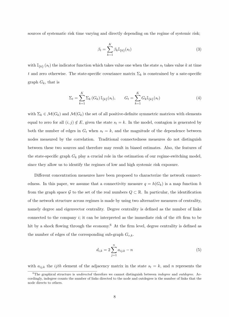
Different concentration measures have been proposed to characterize the network connect-

edness. In this paper, we assume that a connectivity measure q = h(Gk) is a map function h

from the graph space G to the set of the real numbers Q ⊂ R. In particular, the identification

of the network structure across regimes is made by using two alternative measures of centrality,

namely degree and eigenvector centrality. Degree centrality is defined as the number of links

connected to the company i; it can be interpreted as the immediate risk of the ith firm to be

hit by a shock flowing through the economy.6 At the firm level, degree centrality is defined as

the number of edges of the corresponding sub-graph Gv,k.

di,k = 2n∑

j=1

aij,k − n (5)

with aij,k the ijth element of the adjacency matrix in the state st = k, and n represents the

6The graphical structure is undirected therefore we cannot distinguish between indegree and outdegree. Ac-cordingly, indegree counts the number of links directed to the node and outdegree is the number of links that thenode directs to others.

8

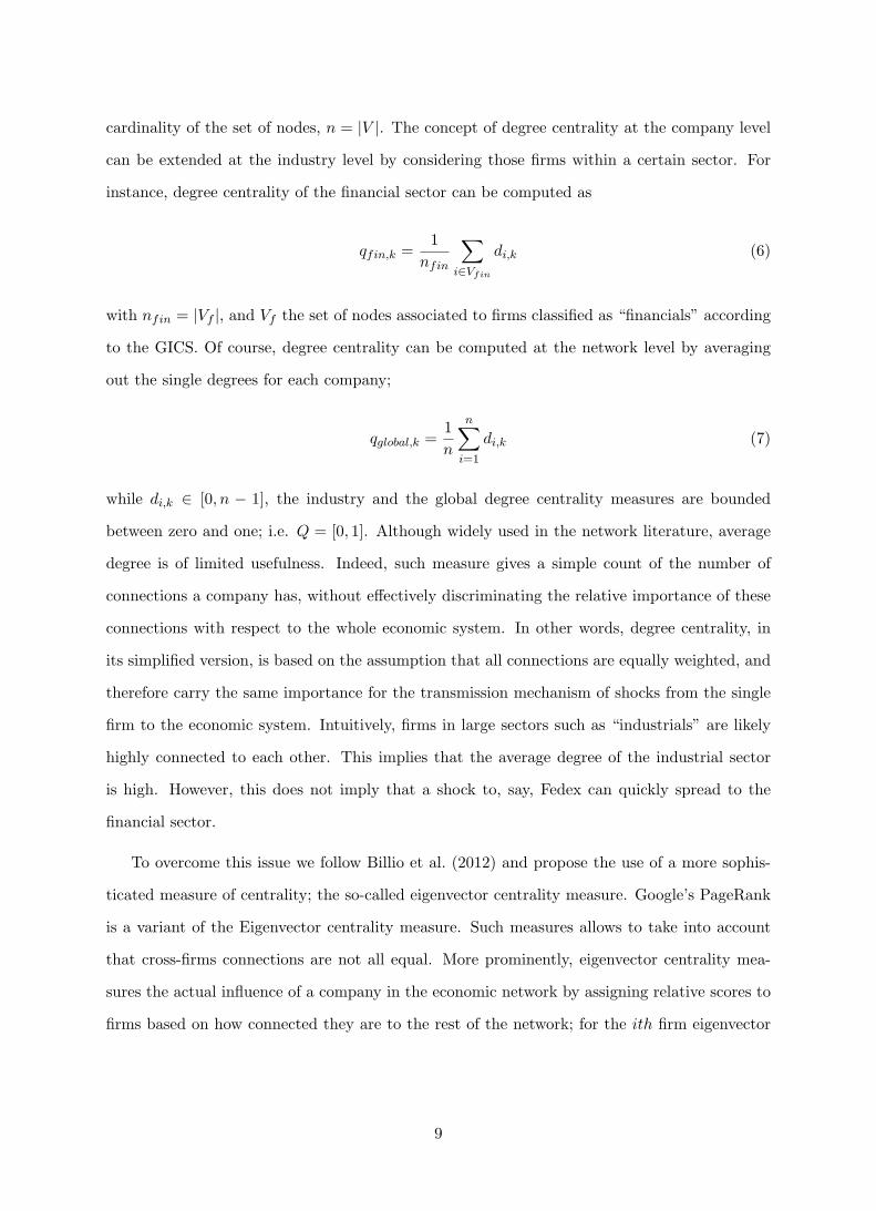
cardinality of the set of nodes, n = |V |. The concept of degree centrality at the company level

can be extended at the industry level by considering those firms within a certain sector. For

instance, degree centrality of the financial sector can be computed as

qfin,k =1

nfin

∑

i∈Vfin

di,k (6)

with nfin = |Vf |, and Vf the set of nodes associated to firms classified as “financials” according

to the GICS. Of course, degree centrality can be computed at the network level by averaging

out the single degrees for each company;

qglobal,k =1

n

n∑

i=1

di,k (7)

while di,k ∈ [0, n − 1], the industry and the global degree centrality measures are bounded

between zero and one; i.e. Q = [0, 1]. Although widely used in the network literature, average

degree is of limited usefulness. Indeed, such measure gives a simple count of the number of

connections a company has, without effectively discriminating the relative importance of these

connections with respect to the whole economic system. In other words, degree centrality, in

its simplified version, is based on the assumption that all connections are equally weighted, and

therefore carry the same importance for the transmission mechanism of shocks from the single

firm to the economic system. Intuitively, firms in large sectors such as “industrials” are likely

highly connected to each other. This implies that the average degree of the industrial sector

is high. However, this does not imply that a shock to, say, Fedex can quickly spread to the

financial sector.

To overcome this issue we follow Billio et al. (2012) and propose the use of a more sophis-

ticated measure of centrality; the so-called eigenvector centrality measure. Google’s PageRank

is a variant of the Eigenvector centrality measure. Such measures allows to take into account

that cross-firms connections are not all equal. More prominently, eigenvector centrality mea-

sures the actual influence of a company in the economic network by assigning relative scores to

firms based on how connected they are to the rest of the network; for the ith firm eigenvector

9

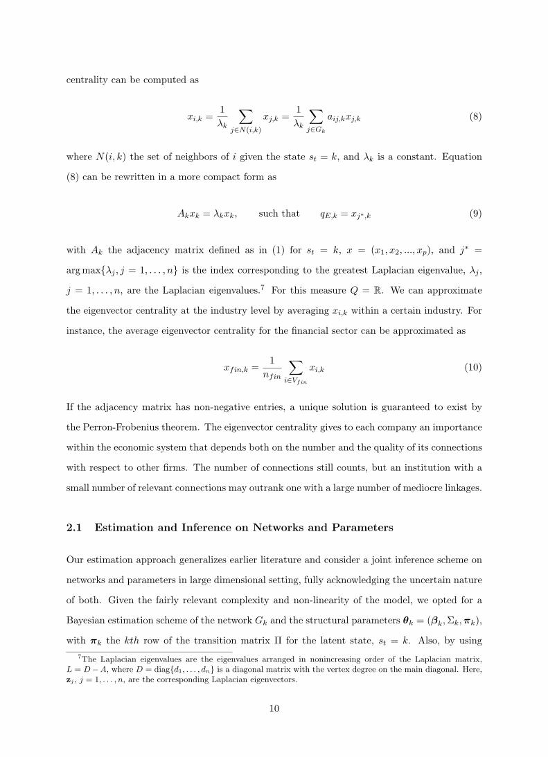
centrality can be computed as

xi,k =1

λk

∑

j∈N(i,k)

xj,k =1

λk

∑

j∈Gk

aij,kxj,k (8)

where N(i, k) the set of neighbors of i given the state st = k, and λk is a constant. Equation

(8) can be rewritten in a more compact form as

Akxk = λkxk, such that qE,k = xj∗,k (9)

with Ak the adjacency matrix defined as in (1) for st = k, x = (x1, x2, ..., xp), and j∗ =

argmaxλj , j = 1, . . . , n is the index corresponding to the greatest Laplacian eigenvalue, λj ,

j = 1, . . . , n, are the Laplacian eigenvalues.7 For this measure Q = R. We can approximate

the eigenvector centrality at the industry level by averaging xi,k within a certain industry. For

instance, the average eigenvector centrality for the financial sector can be approximated as

xfin,k =1

nfin

∑

i∈Vfin

xi,k (10)

If the adjacency matrix has non-negative entries, a unique solution is guaranteed to exist by

the Perron-Frobenius theorem. The eigenvector centrality gives to each company an importance

within the economic system that depends both on the number and the quality of its connections

with respect to other firms. The number of connections still counts, but an institution with a

small number of relevant connections may outrank one with a large number of mediocre linkages.

2.1 Estimation and Inference on Networks and Parameters

Our estimation approach generalizes earlier literature and consider a joint inference scheme on

networks and parameters in large dimensional setting, fully acknowledging the uncertain nature

of both. Given the fairly relevant complexity and non-linearity of the model, we opted for a

Bayesian estimation scheme of the network Gk and the structural parameters θk = (βk,Σk,πk),

with πk the kth row of the transition matrix Π for the latent state, st = k. Also, by using

7The Laplacian eigenvalues are the eigenvalues arranged in nonincreasing order of the Laplacian matrix,L = D−A, where D = diagd1, . . . , dn is a diagonal matrix with the vertex degree on the main diagonal. Here,zj , j = 1, . . . , n, are the corresponding Laplacian eigenvectors.

10

Bayesian tools we can generate posterior distributions of virtually any sufficient statistics for the

underlying network, as well as for any of the structural parameters of the linear factor pricing

model, something that earlier literature did not provide.

2.2 Prior Specification

For the Bayesian inference to work, we need to specify the prior distributions for the network

and the structural parameters. For a given graph Gk and state st = k the prior structure

is conjugate and the model dynamics (2) reduces to a standard SUR model (e.g., see Chib

and Greenberg 1995). This makes Bayesian updating straightforward and numerically feasible.

As far as the systemic risk state transition probabilities are concerned we choose a Dirichlet

distribution:

(πk1, ..., πkK) ∼ Dir (δk1, ..., δkL) (11)

with δki the concentration parameter for πki, and Πk = (πk1, ..., πkK) the kth row of the transi-

tion matrix Π. The role of the covariance structure Σk is one of the most important in the SUR

model specification. The non-diagonal structure of the residual covariance matrix improves

parameter estimation by exploiting shared features of the p−dimensional vector of excess re-

turns. However, an increasing p makes both the estimation error and complexity unfeasible to

be managed. In this context we take advantage of natural restrictions induced by graphical

model structuring (Carvalho and West 2007,Carvalho, West, and Massam 2007, and Wang and

West 2009).

The prior over the graph structure is defined as a Bernoulli distribution with parameter ψ

on each edge inclusion probability as an initial sparse inducing prior. That is, a p node graph

Gk = (Vk, Ek) with |Ek| edges has a prior probability

p(Gk) ∝∏

i,j

ψeij (1− ψ)(1−eij)

= ψ|Ek| (1− ψ)T−|Ek| (12)

with eij = 1 if (i, j) ∈ Ek. This prior has its peak at Tψ hedges, with T = p(p − 1)/2 , for

11

an unrestricted p node graph, providing a flexible way to directly control for the prior model

complexity. A uniform prior alternative might be used. However as pointed out in Jones,

Carvalho, Dobra, Hans, Carter, and West (2005), a uniform prior over the space of all graphs

is biased towards a graph with half of the total number of possible edges. As the number

of possible graphs for a p node structure is, for large p, the uniform prior gives priority to

those models where the number of edges is quite large. To induce sparsity and hence obtain

a parsimonious representation of the interdependence structure implied by a graph, we choose

ψ = 2/(p− 1) which would provide a prior mode at p edges. Conditional on a specified graph

Gk and state st = k, the joint posterior p (Σk, βk|Y ) has a conjugate prior structure;

Σk ∼ HIWGk(dk, Dk) (13)

with dk and Dk respectively the degrees of freedom and the scale hyper-parameters, and HIW

representing the Hyper Inverse-Wishart distribution (see Dawid and Lauritzen 1993) for the

structured covariance matrix Σk. The prior for the betas is independent on the covariance

structure,

βk ∼ Np (mk,Mk) (14)

with mk and Mk the location and scale hyper-parameters, respectively.8 The choice of the

prior hyper-parameters is discussed in Section 4. We also discuss extensively the sensitivity of

posteriors with respect to priors settings in a separate online appendix.

2.3 Posterior Approximation

In order to find a Bayesian estimation of the parameters, the graphs and the latent states we

follow a data augmentation principle (see Tanner and Wong 1987) which relies on the complete

likelihood function, that is the product of the data and state variable densities, given the

parameters and the graphs. Let us denote with zs:t = (zs, . . . , zt), s ≤ t, a collection of

vectors zu. The collections of graphs and parameters are defined as G = (G1, . . . , Gk) and

8Notice that the fact that priors for the covariance structure and the betas are independent does not mean theyrare sample independently in the Gibbs sampler. Indeed, in the sampling scheme they are sampled conditionallyon each other iteratively, and therefore can be thought as coming from the same joint distribution asymptotically.

12

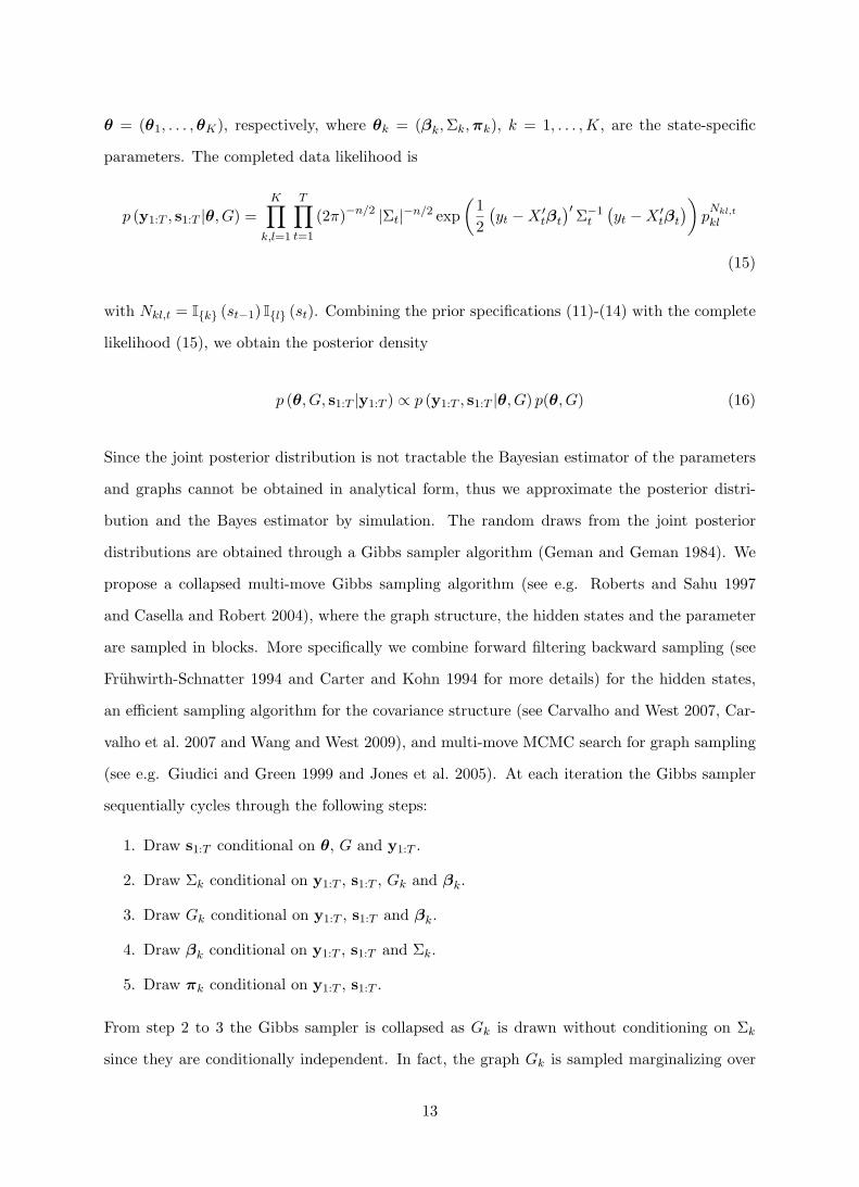
θ = (θ1, . . . ,θK), respectively, where θk = (βk,Σk,πk), k = 1, . . . ,K, are the state-specific

parameters. The completed data likelihood is

p (y1:T , s1:T |θ, G) =K∏

k,l=1

T∏

t=1

(2π)−n/2 |Σt|−n/2 exp

(

1

2

(

yt −X ′tβt

)′Σ−1t

(

yt −X ′tβt

)

)

pNkl,t

kl

(15)

with Nkl,t = Ik (st−1) Il (st). Combining the prior specifications (11)-(14) with the complete

likelihood (15), we obtain the posterior density

p (θ, G, s1:T |y1:T ) ∝ p (y1:T , s1:T |θ, G) p(θ, G) (16)

Since the joint posterior distribution is not tractable the Bayesian estimator of the parameters

and graphs cannot be obtained in analytical form, thus we approximate the posterior distri-

bution and the Bayes estimator by simulation. The random draws from the joint posterior

distributions are obtained through a Gibbs sampler algorithm (Geman and Geman 1984). We

propose a collapsed multi-move Gibbs sampling algorithm (see e.g. Roberts and Sahu 1997

and Casella and Robert 2004), where the graph structure, the hidden states and the parameter

are sampled in blocks. More specifically we combine forward filtering backward sampling (see

Fruhwirth-Schnatter 1994 and Carter and Kohn 1994 for more details) for the hidden states,

an efficient sampling algorithm for the covariance structure (see Carvalho and West 2007, Car-

valho et al. 2007 and Wang and West 2009), and multi-move MCMC search for graph sampling

(see e.g. Giudici and Green 1999 and Jones et al. 2005). At each iteration the Gibbs sampler

sequentially cycles through the following steps:

1. Draw s1:T conditional on θ, G and y1:T .

2. Draw Σk conditional on y1:T , s1:T , Gk and βk.

3. Draw Gk conditional on y1:T , s1:T and βk.

4. Draw βk conditional on y1:T , s1:T and Σk.

5. Draw πk conditional on y1:T , s1:T .

From step 2 to 3 the Gibbs sampler is collapsed as Gk is drawn without conditioning on Σk

since they are conditionally independent. In fact, the graph Gk is sampled marginalizing over

13

the covariance structure Σk (see Carvalho and West 2007, Carvalho et al. 2007 and Wang and

West 2009). A detailed description of the Gibbs sampler is given in the Appendix.

Inference on Markov-switching models, requires dealing with the identification issue aris-

ing from the invariance of the likelihood function to permutations of the hidden state vari-

ables. Different solutions to this problem have been proposed in the literature (see Fruhwirth-

Schnatter 2006 for a review). In this paper, we contribute to this stream of literature providing

a way to identify regimes through graphs. More specifically we suggest to identify the regimes

by imposing the following constraints on the state-specific graphs. We consider the following

identification constraints on the intercept: q(G1) < . . . < q(GK), where q is the average eigen-

vector centrality. This constraint allows us to interpret the first regime as the one associated

with the lowest systemic risk level and the last regime as the one associated with the highest

risk. In context where the eigenvector centrality is not sufficient to achieve a characterization

of the regimes, then a complexity measure (see, e.g. Newman 2003, Emmert-Streib and De-

hemer 2012), which combines information from different network measures, can be employed.

From a practical point of view, we find in our empirical applications that eigenvector centrality

ordering works as well as degree centrality constraint for the regime identification.

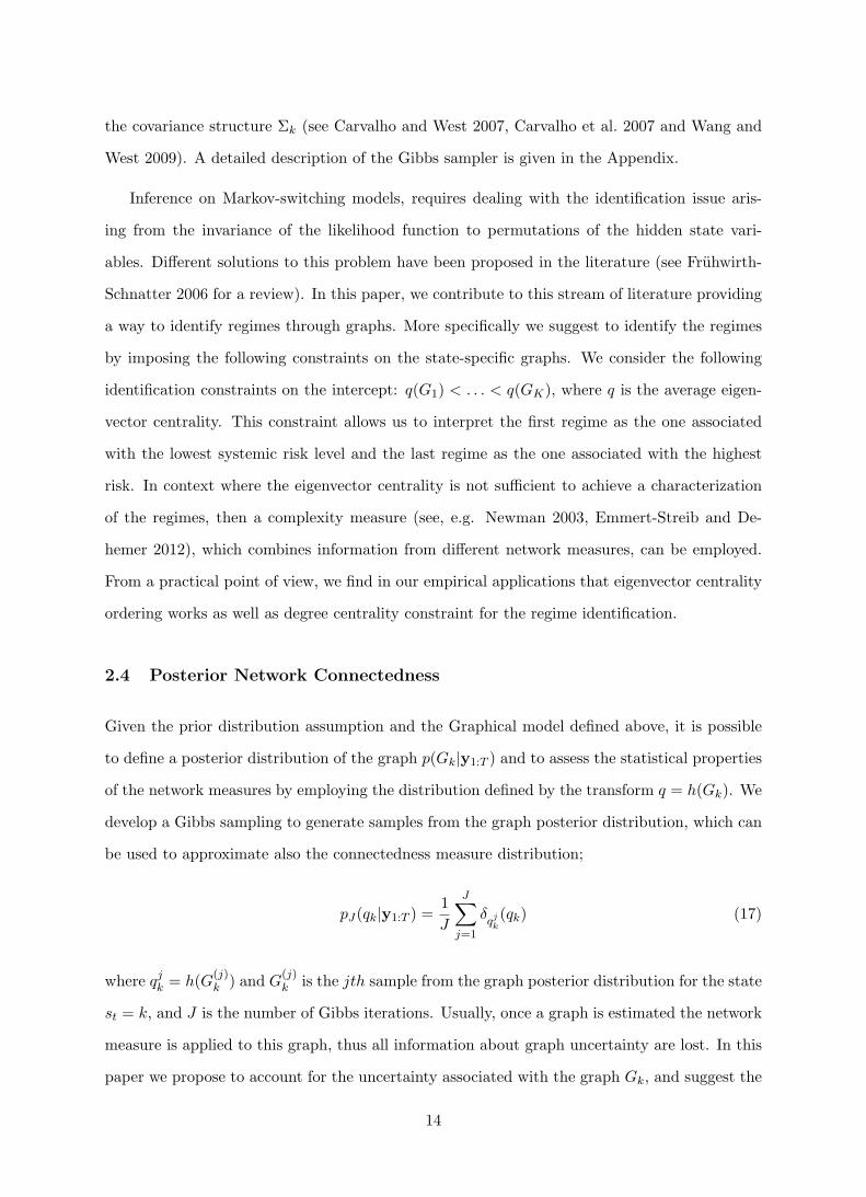
2.4 Posterior Network Connectedness

Given the prior distribution assumption and the Graphical model defined above, it is possible

to define a posterior distribution of the graph p(Gk|y1:T ) and to assess the statistical properties

of the network measures by employing the distribution defined by the transform q = h(Gk). We

develop a Gibbs sampling to generate samples from the graph posterior distribution, which can

be used to approximate also the connectedness measure distribution;

pJ(qk|y1:T ) =1

J

J∑

j=1

δqjk(qk) (17)

where qjk = h(G(j)k ) and G

(j)k is the jth sample from the graph posterior distribution for the state

st = k, and J is the number of Gibbs iterations. Usually, once a graph is estimated the network

measure is applied to this graph, thus all information about graph uncertainty are lost. In this

paper we propose to account for the uncertainty associated with the graph Gk, and suggest the

14

following integrated measure and its MCMC approximation

∫

Gk

h(Gk)p(Gk|y1:T )dGk ≈

∫

Qqk pJ(qk|y1:T )dqk

which is the empirical average of the sequence of measures qjk, j = 1, . . . , J , associated with the

MCMC graph sequence. As a whole, from the Bayesian scheme we can make robust hypothesis

testing on the network structure as we are able to approximate, at least numerically, the entire

distribution of networks conditioning on the state of contagion.

3 Simulation Example

Thus far we have introduced a tool for systemic risk measurement and emphasized its relation-

ship to conditional dependence properties in a large dimensional time series setting. Before put

this tool at work in a real financial markets context, we want to assess the reliability of the

estimation method through a simulation example. Specifically, we first investigate the ability

of our inference scheme to effectively capture network connectedness across states; then we

compare our proposed methodology against a standard Markov regime-switching SUR model.

The purpose of the these simulation exercise is to show the effectiveness and efficiency of our

systemic risk measurement scheme. Simulation results are based on a burn-in period of 2,000

draws out of 10,000 simulations storing every other of them.

First we simulate a sample of T = 1000 observations yt, for p = 20 assets and considering a

single factor xt ∼ i.i.d.N(0, 1). We assume the existence of two persistence states with π11 =

0.95 and π22 = 0.95. For simplicity we assume that the betas on the single factor are constant

across assets and are different across states, βi (st = 1) = 0.6 and βi (st = 2) = 1.2. The residual

covariance structure is also changes across regimes and is consistent with an underlying regime-

specific graph-based network Gk ∈ G. Network connectedness is set to be more concentrated

(i.e. higher aggregate eigenvector centrality) in state st = 2, which then represents high systemic

risk. To avoid any particular effect of prior elicitation we choose fairly vague priors with dk = 3

and Dk = 0.0001Ip for both states and ψ = 2/ (p− 1) for both states. We do not assume a

priori any clear difference in the network structure across states. Panel A of Figure 1 shows

15

the adjacency matrix that defines the true network against the estimated one for the contagion

state;

[Insert Figure 1 about here]

The figure makes clear that the model has a fairly good performance in identifying network

connectivity, namely, the adjacency matrix A. In fact, the estimated graphical structure is

short of two edges out of the nineteen in the original network.9

In the second simulation exercise we compare our model against a benchmark SUR without

network in the residual covariance matrix. To compare the utility from our method with respect

to the benchmark SUR, we compute the estimation risk for Σk using Stein’s loss function

Loss(

Σ,Σ)

= tr(

ΣΣ−1)

− log |ΣΣ−1| − p (18)

with Σ and Σ the estimated and true residuals covariance structure, respectively. We conduct

the experiment for different sample sizes, T = 50, 100, 200, with p = 20 assets and considering

a single factor xt ∼ i.i.d.N(0, 1). As above, we consider a persistence contagion state st = 2,

with π22 = 0.95. Betas are constant across assets and are different across states.

Panel B of Figure 1 shows box plots of the risk associated by different estimators across

different sample sizes. For the sake of exposition, we label our model as M1 and the classic

SSUR specification as M2. The figure makes clear that by fully acknowledging the network

structure underlying the idiosyncratic covariance structure Σ offers large gain over a standard

SUR model. Such gains, are particularly significant when the ratio between assets and the

sample size p/T increases. This is consistent with previous evidence on the efficiency of sparse

covariance estimates (see e.g. Carvalho et al. 2007 and Wang and West 2009, among others).

9Inference on the graphical structure is made using an add/delete Metropolis-Hastings-within-Gibbs algorithmas originally proposed in earlier literature such as George and McCulloch (1993), Madigan and York (1995),George and McCulloch (1997), Giudici and Green (1999), and Jones et al. (2005), among the others. Moredetails on the asymptotic properties of the estimation scheme and the sensitivity to different prior specificationsare discussed in a separate online Appendix.

16

4 Empirical Analysis

As empirical application we measure systemic risk for a large set of companies. Systemic risk

is jointly considered with sources of systematic risk which are assumed to capture investors’

beliefs on the business cycle (see Liew and Vassalou 2000, Cochrane 2001, Vassalou 2003, and

Campbell and Diebold 2009). In particular, while the exposure to sources of systematic risk (i.e.

betas) depends on the state of systemic risk, the latter directly depends on the betas given its

residual nature. As such, although conditionally independent, systematic and systemic risks are

not mutually exclusive. Although our methodology is rather general and can be easily applied

to any linear factor pricing model, we consider few popular sources of systematic risks such as

size, value and shocks to macroeconomic factors. This is mainly due to data availability at the

daily frequency.

4.1 Data and Factor Pricing Models

We focus on the 100 blue chip companies that compose the S&P100 Index. We consider those

institutions with more than 15 years of historical data, and then left with 83 companies. Table

1 summarize the firms in our dataset and the corresponding industry classification according to

the Global Industry Classification Standard (GICS), developed by MSCI. Returns are dollar-

valued and computed daily in excess of the risk-free rate. The sample period is 05/10/1996-

10/31/2014 (4821 observations for each company), for a total of more than 400,000 firm-day

observations. Our emphasis on stock returns is motivated by the desire to incorporate the most

current information in the network analysis; stocks returns reflect information more rapidly

than non-trading-based measures such as accounting variables.

[Insert Table 1 about here]

We analyze three representative asset pricing models starting from a conditional version of the

simple CAPM. Such model implies a unique risk factor which is represented by the excess return

(in excess of the 1-month T-Bill rate) on the aggregate value-weighted NYSE/AMEX/NASDAQ

index, taken from the Center for Research in Security Prices (CRSP). The return on the 1-month

17

T-Bill rate is taken from Ibbotson Associates, while returns on the market portfolio are taken

from the Kenneth French’s website. The CAPM performed well in initial tests (e.g. Fama and

MacBeth 1973), but has performed poorly since.

The second model considered is the well-known three-factor model initially proposed in Fama

and French (1993). This model includes two empirically motivated additional systematic risk

factors. In addition to excess return on aggregate wealth as for the simple CAPM, the model

consists of a second risk factor, SMB, which represents the return spread between portfolios of

stocks with small and large market capitalization. The third risk factor, HML, represents the

return difference between “value” and “growth” stocks, namely portfolios of stocks with high

and low book-to-market ratios.

Next, we consider one macroeconomic-based model. The third model is an empirical im-

plementation of the Merton (1973) intertemporal extension of the CAPM. Based on Camp-

bell (1996), who argues that innovations in state variables that forecasts changes in investment

opportunities should serve as risk factors, we use aggregate dividend yield and both default- and

term-spreads as state variables, in addition to aggregate wealth. Default spread is computed as

the difference between the yields of long-term corporate Baa bonds and long-term government

bonds. The term spread is measured the difference between the yields of 10- and 1-year govern-

ment bonds. Data on bonds and treasuries are taken from the FredII database of the Federal

Reserve Bank of St.Louis. The data for the 1-month T-Bill are taken from Ibbotson Associates.

We adopt the approach of Campbell (1996) and compute the changes in risk factors as the

innovations of a first order Vector Auto-Regressive (VAR(1)) process. To ensure that betas

are fully conditional and changes in risk factors satisfy the zero-conditional mean assumption,

Et−1Xt = 0, the VAR uses only historical data up to period t− 1. Thus, for each collection of

the CRSP aggregate value-weighted market portfolio and the candidate set of risk factors ht =

(rm,t, x′t)′, we estimate hτ = B0,t + B1,thτ−1 + et,τ for τ = 1, ..., t. Following Petkova (2006),

the innovations et,τ are orthogonalized from the excess return on the aggregate wealth and

scaled to have the same variance.

18

4.2 Prior Choices and Parameters Estimates

Realistic values for different prior distributions obviously depend on the problem at hand. For

the transition mechanism of systemic risk the prior hyper-parameters of the Dirichlet distribu-

tion are taken such that a priori systemic risk is persistent. Such prior belief is mainly based

on the common wisdom that increasing network connectedness is not a quickly mean-reverting

process (see e.g. Forbes and Rigobon 2002).

Given the large dimensional setting of the model, training the priors with firm-specific infor-

mation might be prohibitive. We take an agnostic perspective in setting the hyper-parameters

of the betas across institutions. The prior location parameter mk = 0 for each k = 1, ...,K.

The corresponding prior scale is set equal to Mk = 1000Ip across states. Notice we do not force

posterior estimates in any direction across states as the prior structure does not differ across

low vs high systemic risk states.

The prior degrees of freedom and scale of the Hyper-Inverse Wishart distribution for the

conditional covariance matrix are set to be dk = 3 and Dk = 0.0001Ip, respectively. This is

also a fairly vague, albeit proper, prior distribution. Finally, the prior for the graph space is

a Bernoulli distribution. We have chosen an hyper-parameter equal to ψ = 2/ (p− 1) which

would provide a prior mode at p edges. We could alternatively use a uniform prior over the

space of all graphs. However as pointed out in Jones et al. (2005), a uniform prior would be

biased towards a graph with half of the total number of possible edges. For large p, the uniform

prior gives priority to those models where the number of edges is quite large. In a separate

online appendix we show that posterior results are not very sensitive to the prior settings for

the hyper-parameters that govern the prior conditional betas and covariances.

In order to further reduce the sensitivity of posterior estimates to the prior specification, we

use a burn-in sample of 2,000 draws storing every other of the draws from the residuals 10,000

draws (see e.g. Primiceri 2005). The resulting auto-correlations of the draws are very low. A

convergence analysis in Section B of the online Appendix shows that this guarantees accurate

inference in our network based linear factor model.

Figure 2 shows the probability of high systemic risk in the economy over the testing sample.

19

The gray area represents the model-implied probability, while the red line shows the NBER

recession indicator for the period following the peak of the recession to through the through. The

figure makes clear that a wide state of contagion characterizes the period 2001/2002 (i.e. dot.com

bubble, 9/11 attacks, Financial scandals, Iraq war), the great financial crisis of 2008/2009, and

the recent major Eurozone sovereign turmoil.


Although there is mis-matching with respect to the business cycle indicator across the period

1998-2002, the NBER recession and high systemic risk tend to overlap across the recent great

financial crisis. The last period of high systemic risk can be linked to the European sovereign

debt crisis. As we would expect such period does not coincide with any recession period in the

United States.

Figure 3 shows the persistence parameters for systemic risk for each of the factor pricing

model considered. The first three boxplot report the probability of staying in a state of low

systemic risk. The last three boxplot show the persistence of high systemic risk in the economy.


Systemic risk persists with an average probability of πhh = 0.93, implying that the duration of a

period of high systemic risk is around 1/ (1− πhh) = 14 days, while the long run probability of

high systemic risk is equal to (1− πll) / (2− πhh − πll) = 0.33. This means that, in our sample

tend the economy tend to be affected by high systemic risk for about a third of trading days,

unconditionally.

Figure 4 shows changes in exposures to sources of systematic risks from low to high systemic

risk, computed from the Fama-French three-factor model. For the sake of exposition, results

are labeled according to the GISC industry classification. Top left panel shows the difference in

the intercepts across companies. The figure makes clear that the Jensen’s alphas do not change

across different regimes of systemic risk in a significant way. Indeed, the zero line never falls

outside the 95% confidence interval of the model estimates. Interestingly, the differences in

exposures to the aggregate wealth risk factor is significantly negative for financial firms. This

20

implies that the exposure to market risk of financial firms increases when systemic risk is higher.

The only exception within the financial sector is the Berkshire Hathaway Inc. of Warren Buffett.


Similarly, financial firms are more exposed to value risk when systemic risk is higher. Two

exceptions are again Berkshire Hathaway Inc., together with Morgan Stanley. Also Citigroup,

although has negative difference on the HML beta, it is not statistically significant. The Indus-

trial and Materials sectors also show an increasing exposure to value premium when systemic

risk is higher. Figure 5 shows changes to the conditional betas on shocks to macroeconomic

risk factors in the I-CAPM implementation. As we would expect, the behavior of the betas on

market risk is consistent with the Fama-French three-factor model. The only exception is again

Berkshire Hathaway Inc., although the difference in the beta is negative, on average.


Interestingly, the Energy sector shows the opposite path with respect to Financials. In fact, the

exposure to market risk of energy stocks tend to be lower when systemic risk is higher. Bottom

left panel shows the change of exposures to default risk from low vs. high systemic risk. On

average, exposure to default risk is higher when systemic risk is higher, although for a large

fraction of the sample such negative delta is not statistically significant. In the financial sector,

AIG, Morgan Stanley, Bank of America, and American Express tend to be more exposed to

default risk when systemic risk increases. In the technology sector Microsoft, IBM, Intel and

Oracle are more exposed to default risk during market turmoils. Bottom right panel shows

that both Energy and Financials tend to be less exposed to the aggregate dividend yield when

contagion is high.

4.3 Financial Networks

Thus far we have introduced tools to measure contagion and showed their efficiency and im-

plications for systematic and systemic risk measurement. We now put those tools at work and

investigate the evolution of networks connectedness over time. For the sake of completeness

21

we investigate network connectivity on the residuals covariance matrix under the CAPM, the

three-factor Fama-French model and the I-CAPM implementation. The amount of systemic

risk can be thought of as residual in nature with respect to sources of systematic risks, as it

strongly depends on how much of systematic risk is captured by the model.

Figure 6 shows the connectivity of firms inferred from the residuals of the SUR CAPM. The

size and the color of the nodes are proportional to their relevance in the network. More precisely,

size and color reflect the eigenvector centrality of each node as computed from equation (8). A

darker (bigger) blue color (node) means the corresponding firm is more systemically important

for the economy.


Top panel shows the network when systemic risk is low. Figure 6 makes clear that Energy

companies such as ConocoPhillips (COP), Apache (APA), Occidental Ptl. (OXY), and Exxon

(XOM) are central for the economic system (dark blue nodes). Interestingly, few consumer com-

panies such as Wal Mart (WMT), Costco (COST), Target (TGT), and Lowe’s Comp. (LOW)

are tightly link to each other, although completely disconnected from the rest of the economy.

The financial sector turns out to be relevant, although marginally less than the energy sector.

Indeed, big financial firms such as JP Morgan (JPM), AIG, Bank of America (BAC) and Wells

Fargo (WFC), although relevant, are not as central as, for instance, Exxon Mobile.

Bottom panel of Figure 6 shows that the situation changes when systemic risk is high.

Financials now are key in the transmission mechanism of exogenous shocks with firms such as

JP Morgan and Bank of America playing the major role. If we combine Figure 2 and Figure

6, we can intuitively confirm that in periods of market turmoils, the systemic importance of

banks and the financial sector substantially increases. In other words, a shock to, for instance,

Morgan Stanley, turns out to have a much bigger effect on the economy than an exogenous

shock on, say, Wal Mart. The marginal importance of each firm on the economic system as a

whole might be uniquely driven by their relative market size, or valuation. Figure 7 address this

issue by showing the network connectivity measured from the three-factor Fama-French model

residuals.


22

Top panel shows the network connectivity when systemic risk is low. Figure 7 confirms the key

role of the Energy sector when cross-firm contagion is modest. Exxon Mobil, ConocoPhillips,

Occidental Ptl., and Apache carry most of the systemic risk in the economic system. By

controlling for size and value, the role of the financial sector when systemic risk is low decreases.

Also, the economic network is now more sparse with lots of missing linkages. The energy and

the financial sectors seem to create a sub-network themselves. Consistent with Figure 6, bottom

panel of Figure 7 shows the key role of the financial sector in the network connectedness when

systemic risk increases. Also, the figure makes clear that the highest portion of systemic risk is

evidently carried on by the financial sector.

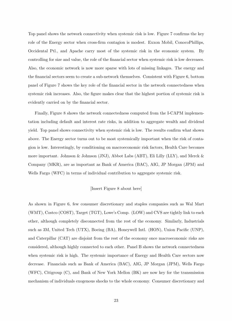
Finally, Figure 8 shows the network connectedness computed from the I-CAPM implemen-

tation including default and interest rate risks, in addition to aggregate wealth and dividend

yield. Top panel shows connectivity when systemic risk is low. The results confirm what shown

above. The Energy sector turns out to be most systemically important when the risk of conta-

gion is low. Interestingly, by conditioning on macroeconomic risk factors, Health Care becomes

more important. Johnson & Johnson (JNJ), Abbot Labs (ABT), Eli Lilly (LLY), and Merck &

Company (MKR), are as important as Bank of America (BAC), AIG, JP Morgan (JPM) and

Wells Fargo (WFC) in terms of individual contribution to aggregate systemic risk.


As shown in Figure 6, few consumer discretionary and staples companies such as Wal Mart

(WMT), Costco (COST), Target (TGT), Lowe’s Comp. (LOW) and CVS are tightly link to each

other, although completely disconnected from the rest of the economy. Similarly, Industrials

such as 3M, United Tech (UTX), Boeing (BA), Honeywell Intl. (HON), Union Pacific (UNP),

and Caterpillar (CAT) are disjoint from the rest of the economy once macroeconomic risks are

considered, although highly connected to each other. Panel B shows the network connectedness

when systemic risk is high. The systemic importance of Energy and Health Care sectors now

decrease. Financials such as Bank of America (BAC), AIG, JP Morgan (JPM), Wells Fargo

(WFC), Citigroup (C), and Bank of New York Mellon (BK) are now key for the transmission

mechanism of individuals exogenous shocks to the whole economy. Consumer discretionary and

23

staples are now connected to the rest of the economy through Procter & Gamble (PG). As a

whole, Figures 6-8, together with Figure 2 make clear that Financials are systemically important

across market turmoils, as an exogenous shocks on these institutions can quickly and heavily

affect the entire economic system.

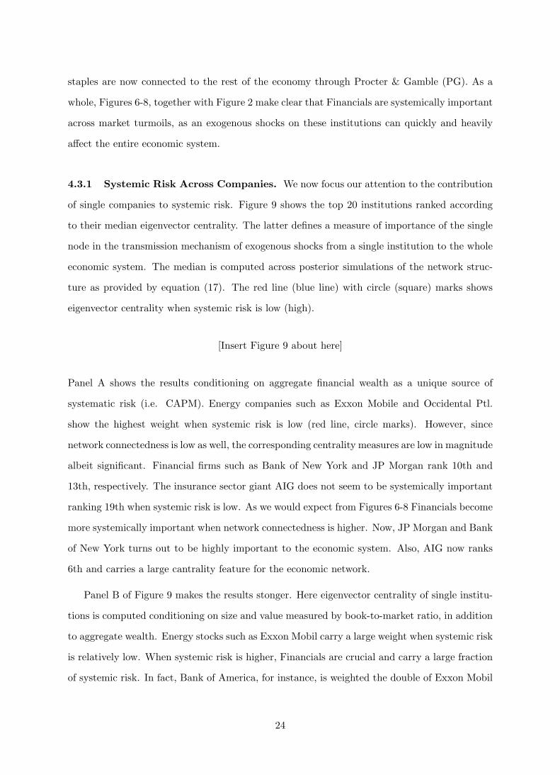
4.3.1 Systemic Risk Across Companies. We now focus our attention to the contribution

of single companies to systemic risk. Figure 9 shows the top 20 institutions ranked according

to their median eigenvector centrality. The latter defines a measure of importance of the single

node in the transmission mechanism of exogenous shocks from a single institution to the whole

economic system. The median is computed across posterior simulations of the network struc-

ture as provided by equation (17). The red line (blue line) with circle (square) marks shows

eigenvector centrality when systemic risk is low (high).


Panel A shows the results conditioning on aggregate financial wealth as a unique source of

systematic risk (i.e. CAPM). Energy companies such as Exxon Mobile and Occidental Ptl.

show the highest weight when systemic risk is low (red line, circle marks). However, since

network connectedness is low as well, the corresponding centrality measures are low in magnitude

albeit significant. Financial firms such as Bank of New York and JP Morgan rank 10th and

13th, respectively. The insurance sector giant AIG does not seem to be systemically important

ranking 19th when systemic risk is low. As we would expect from Figures 6-8 Financials become

more systemically important when network connectedness is higher. Now, JP Morgan and Bank

of New York turns out to be highly important to the economic system. Also, AIG now ranks

6th and carries a large cantrality feature for the economic network.

Panel B of Figure 9 makes the results stonger. Here eigenvector centrality of single institu-

tions is computed conditioning on size and value measured by book-to-market ratio, in addition

to aggregate wealth. Energy stocks such as Exxon Mobil carry a large weight when systemic risk

is relatively low. When systemic risk is higher, Financials are crucial and carry a large fraction

of systemic risk. In fact, Bank of America, for instance, is weighted the double of Exxon Mobil

24

and for times more than ConocoPhillips. Also, Panel B shows that network connectedness is

much more concentrated around financial firms when we condition on size and value in addition

to market risk. This is consistent with the idea that systemic risk (i.e. network connectedness)

and systematic risks, although are not directly depending on each other, are not mutually ex-

clusive. For instance, the average, median, eigenvector centrality under high systemic risk is

around 0.017 with the three-factor Fama-French model, against the modest 0.009 obtained from

the CAPM.

Bottom panel of Figure 9 shows median eigenvector centrality computed from the I-CAPM

implementation with shocks to macroeconomic risk factors. Again, Energy companies such as

Anadarko Ptl. (APC), ConocoPhillips (COP), Occidental Ptl. (OXY), Apache (APA), and

Schlumberger (SLB) carry the highest weights when systemic risk is low. The magnitude of the

median eigenvector centrality for other sectors is relatively low indicating a high concentration

around the Energy, and possibly the Health Care, sectors. When systemic risk is higher (blue

line), the weight of Financials tend to dominate other industries. Indeed, consistent with the

CAPM and the three-factor Fama-French model, financial companies such as JP Morgan (JPM),

Bank of America (BAC), Bank of New York Mellon (BK), AIG, Citigroup (C), and Wells Fargo

(WFC) are highly systemically important.

Figure 9 also makes clear a separation between states of high vs low systemic risks. In

fact, for instance for the three-factor model, the average eigenvector centrality of the top 20

institutions is 0.017 with high systemic risk, against an average median value of 0.0055 when

contagion is low. Interestingly, the separation of network connectedness across systemic risk

regimes is clearer once conditioning for macroeconomic risk (bottom panel).

We investigate the role of single companies for systemic risk by using also degree centrality

as proposed in Section 2. Degree centrality gives a simple count of the number of connections

a company has, without effectively discriminating the relative importance of these connections

with respect to the economic network. In fact, in its simplified version, degree centrality is

based on the assumption that all firms connections are equally weighted, and therefore carry

the same importance for the transmission mechanism of exogenous shocks. Table 2 reports the

top 10 companies ranked across median eigenvalue centrality and median degree. The median

25

is computed across posterior simulations of the network structure as provided by equation (17).

Column 2, 3 and 4 parallel the results of figure 9. Degree centrality is also computed conditioning

on different sources of systematic risks.


Panel A shows the top 10 institutions when systemic risk is low, and conditioning for aggregate

wealth as the unique source of systematic risk. Columns 5, 6 and 7 report the median degree

centrality. As far as the number of connections is concerned, different asset pricing models give

different rankings of systemically important companies. Residuals from the CAPM indicates

that Financials and Energy stocks are highly linked. Once we add size and value premia as

additional sources of systematic risk factors, consumer discretionary and staples companies

such as Home Depot (HD), Costco (COST), Lowe’s Comp. (LOW) and CVS ranks the highest.

Finally, Johnson & Johnson (JNJ) (Health Care), shows the highest number of linkages once

macroeconomic risks are considered.

These results show the limited usefulness of degree centrality as a measure of systemic risk

as the ranking is highly dependent on the factor asset pricing model used. This contradicts

columns 2,3, and 4 which reports the top 10 median eigenvector centralities. In fact, despite

the sources of systematic risk considered, Energy sector always ranks as the most important

for systemic risk measurement and management. Such contradiction is well understood in

network analysis. Indeed, eigenvector centrality gives to each company an importance within

the economic system that depends both on the number and the quality of its connections with

respect to other firms. The number of connections still counts, but an institution with a small

number of relevant connections may outrank one with a large number of mediocre linkages.

This is the case of consumer discretionary and staples firms.

Panel B of Table 2 shows that, when network connectivity is high, degree and eigenvector

centrality tend to converge. Financial companies such as JP Morgan, Bank of America, and

Bank of New York Mellon consistently rank within the most connected companies, as far as the

number of linkages is concerned. However, eigenvector centrality turns out to be more robust

for systemic risk measurement as it is less dependent on the factor pricing model.

26

Finally column 8 shows the average market value of each institution across low and high

systemic risk. The results makes evident that there is no clear cut one-to-one mapping between

the relevance of the nodes and their market value. Except for Exxon Mobile, which ranks high

across columns, General Electric (GE) and Microsoft (MSFT) have among the highest market

valuations but do not appear in centrality measures.

4.3.2 Systemic Risk Across Industries. One might argue that despite the clear role of

major financial companies such as JP Morgan, AIG and Bank of America, the financial sector

might not necessarily be central as a whole. The answer is partly given by figures 6-8. These

figures make clear the central role of the financial sector when systemic risk is high. For the

sake of completeness we compute both eigenvector centrality and degree for each sector defined

as in the GISC from MSCI. Degree and eigenvector measures are computed at the industry

level as indicated in equation (6) and (10), respectively. Table 3 shows the ranking of industries

according to posterior median eigenvector and degree centrality. Medians are computed across

posterior simulations of the network structure as provided by equation (17).


Panel A reports the results obtained considering aggregate wealth as the only source of sys-

tematic risk. Energy and financials are the sectors with the most important linkages with the

economic network. Again, looking at the average market value across industries there is no

clear-cut mapping with the corresponding connectivity ranking. When systemic risk is high

(Panel B), results are even clearer. The financial industry shows the higher system-wide eco-

nomic relevance, followed by the energy sector. Interestingly, last column shows that Telecomm

services and Technology have the highest average market valuation although they rank at the

bottom in terms of systemic risk relevance. Results are robust by including size, value and

macroeconomic factors as additional sources of systematic risk. Figure 10 finally shows that,

indeed, the disconnect between market value and systemic risk becomes clear by looking at the

time series of the relative market value of each sector with respect to the rest of the economy.


27

Top left panel, for instance, represents the market value of the financial sector over the rest of

the economy. The relative weight of the financial sector drops from 25% in 2006 to less than

10% across 2008. Figure 2 shows that across the crisis of 2008/2009 systemic risk is likely to be

high, which implies indeed an opposite relationship between contagion and market value. The

opposite is true for the Energy sector (top middle panel). In fact, the relative market value

of the energy sector increases when systemic risk is high across the period 2008/2009. Same

positive relationship might be drawn for Telecommunication Services as shown in the bottom

right panel. Industrials and Materials do not show a clear directional relationship with systemic

risk. Finally, the relative market value of the Tech industry spikes during late 90s and bounce

back beginning of 2000. This is the well known dot.com bubble.

5 Systemic Risk, Financial Distress and the Business Cycle

At the outset of the paper we clarify that we do not take any stake in any particular underlying

causal structure of an increasing network connectedness; rather, we take it as given and seek to

measure systemic risk from an agnostic point of view. However, understanding systemic risk is

of interest to understand financial crisis, and their relationship with the business cycle.

In this section we take a reduced form approach and investigate if variables which are

arguably related with investors’ belief on the business cycle are related to our measure of

systemic risk. Also, we investigate any early warning feature of our systemic risk indicator. We

use several macro financial variables to capture business cycle effects and investors’ expectations

on changes in the investment opportunity set. We consider the term-, default- and credit-yield

spreads, the aggregate dividend yield and price-earnings ratio, the VIX index, the Market

Uncertainty index proposed by Baker, Bloom, and Davis (2013), and the Financial Stress Index

held by the Federal Reserve Bank of St. Louis.10

Figure 11 shows the time series of the macro-financial predictors and the model-implied

10Although these macro-financial variables can not be exactly linked to the real side of the economy, earlyliterature showed that they can be sensibly assumed to capture investors’ beliefs on the business cycle as wellas changes in the investment opportunity set (see Campbell 1996, Liew and Vassalou 2000, Cochrane 2001, andVassalou 2003).

28

probability of high systemic risk.11


Top middle panel shows the Financial Stress Index, which is computed on a weekly basis and

greater than zero when the U.S. financial sector was in distress. The average value of the index is

normalized to be zero. Thus, zero is viewed as representing normal financial market conditions.

Values below zero suggest below-average financial market stress, while values above zero suggest

above-average financial market stress. Interestingly, a value higher than zero coincide to the

periods of high systemic risk according to out model. A similar relationship holds between

systemic risk and the VIX index (top right panel). Spikes in market uncertainty captured by

the VIX tend to be consistent with increasing systemic risk. Bottom left and right panels

show that also default spread and aggregate dividend yield can be potentially correlated with

systemic risk. For instance, an increasing default spread coincide with periods of high systemic

risk. Finally, the term spread does not show any evident relationship with systemic risk.

Building on this visual results, we formally investigate and lagged or contemporaneous re-

lationship between systemic risk and macro-financial variables. We estimate a Probit model

considering different combinations of the above macro-financial predictors as the set of inde-

pendent variables Zt. The dependent variable ct is a systemic risk indicator takes value one if

the probability of high systemic risk is higher than 0.5, and takes value zero otherwise. First,

we consider the contemporaneous relationship between state variables and systemic risk; we

estimate the model as

ct = γ0 + γ′1Zt + ǫt, ǫt ∼ N(

0, τ2)

(19)

Table 4 shows the estimates of the betas and the marginal effect of each independent variable.


11Default spread is computed as the difference between the yields of long-term corporate Baa bonds andlong-term government bonds. The term spread is measured the difference between the yields of 10- and 1-yeargovernment bonds. Credit spread is computed as the difference between the yields of long-term Baa corporatebonds and long-term Aaa corporate bonds. Data on bonds, treasuries and financial distress are taken fromthe FredII database of the Federal Reserve Bank of St.Louis. The data for the 1-month T-Bill are taken fromIbbotson Associates.

29

Panel A shows the estimated betas. Column 3 and 4 show evidence is in favor of a contempo-

raneous and positive relationship between systemic risk and credit and default spreads. Indeed,

the marginal effect of default (credit) risk reported in Panel is 0.38 (0.87), meaning that a one

unit increase in default (credit) risk implies an increasing probability of high systemic risk by

one percent. However, while the pseudo R2 by using default spread as unique predictor is 0.37,

the same drops to 0.07 when using the credit risk premium as the only independent variable.

The VIX index is also positive (beta is equal to 0.135) related to systemic risk and highly

statistical significant (p-value is equal to 0.000). Interestingly, column 8 shows that there is a

positive (beta equal to 1.842) contemporaneous relationship between systemic risk and financial

distress. The corresponding pseudo R2 is equal to 0.45.12

Figure 11 shows that some of the independent variables such as aggregate dividend yield

and default spread are not stationary. Using non-stationary variables as regressors in a Probit

model my generate a spurious regression problem, namely the betas of table 4 are signifi-

cant although there is no contemporaneous correlation in the data generating process between

systemic risk and the business cycle. Also, equation (19) does not tell anything about the

potential predictability of systemic risk. To investigate predictability of systemic risk and the

non-stationarity of predictors we estimate a Probit regression model as follows;

ct = γ0 + γ′1∆Zt + ǫt, ǫt ∼ N(

0, τ2)

(20)

using changes from time t to t−1 as independent variables, ∆Zt = Zt−Zt−1. Intuitively, we want

to investigate if an increase in, say, the credit yield spread is correlated with aggregate systemic

risk. Table 5 reports the estimates of the betas and the marginal effect of each independent

variable.


Interestingly, an increase in credit and default spreads is positively correlated with higher sys-

temic risk, with a pseudo R2 of 0.03 and 0,12, respectively. Other predictors such as aggregate

dividend yield and price-earning ratio loose their significance. As such, an increase in dividend

12Since the financial stress index is computed on a weekly basis, we transform the daily model-implied proba-bility of high systemic risk to weekly. We obtain that by taking the probability computed on friday of each weekor the last day of the week when friday is not an available trading day. This is consistent with the financial stressindex which is indeed computed on friday of each week.

30

yield does not lead to a higher systemic risk. Changes to aggregate financial distress are posi-

tively (0.424) and significantly (p-value= 0.001) correlated with systemic risk. Panel B shows

that a one unit increase in the financial stress index raises by 0.26% the probability of high sys-

temic risk. As a whole Table 5 shows that credit and default spreads have some predictability

power for systemic risk. Also, changes in aggregate conditions of financial distress are positively

correlated with systemic risk.

One important application of any systemic risk measure is to provide early warning signals

to regulators and the public. To argue that our systemic risk measures can effectively be

interpreted as early warning signal we have to investigate the predictability of financial distress

on the basis of the model-implied systemic risk indicator ct. We estimate a simple regression

with the financial stress index of the St.Louis Fed and current plus lagged values of the model-

implied high systemic risk indicator aggregated on a weekly basis. Panel A of Table 6 shows

the results.


Column 2 (M1) confirms the positive and significant contemporaneous relationship between

systemic risk and financial distress we found in Table 4. Column 3 (M3) shows that high

systemic risk can predict a higher financial distress one week ahead. Indeed, the beta on lagged

systemic risk is positive (1.331) and significant (p-value= 0.002), with and adjusted R2 equal to

0.35. As shown in Figure 11 top middle panel the financial stress index is rather persistence. In

order to mitigate any bias in the regression coefficient estimates we include lagged values of the

dependent variable as regressors. By including the lagged dependent variable the magnitude of

predictability sensibly decreases although remain significant.

For the sake of robustness we substitute the systemic risk indicator ct with the log of proba-

bility of systemic risk (LogProb). Panel B of Table 6 shows the results. The regression analysis

mainly confirms the results of Panel A. Our systemic risk measure helps predict aggregate con-

ditions of financial markets stress. Tables 4-6 lead us to conclude that changes in credit and

default spreads can help predict systemic risk, and that such model-implied systemic risk may

represents an early warning signal for aggregate financial markets stress conditions.

31

6 Conclusions

Contagion and systemic risk measurement have become overwhelmingly important over the

last few years. After the great financial crisis the main question has been to what extent the

economic system is robust to a shock to the financial sector. In the language of network analysis

this boils down to ask what is the connectedness of financial firms with the rest of the economic

network. We believe we contribute to answer this question by providing a useful and intuitive

model for contagion and systemic risk (system-wide connectivity) measurement.

We take an asset pricing perspective and infer the network structure system-wide from the

residuals of an otherwise standard linear factor pricing model. By conditioning on different

sources of systematic risk we implicitly recognize that systematic and systemic risk might be

independent but not mutually exclusive concepts. For the sake of completeness we consider

different sources of systematic risks such as aggregate financial wealth, size, value and shocks

to macroeconomic risk factors. For a given linear factor model, we measure contagion as a shift

in the strength of the cross-firm network linkages. This is consistent with the common wisdom

that posits contagion representing a significant increase in cross-sectional dependence across

institutions/sectors/countries after a shock.

We estimate the model by developing a Markov Chain Monte Carlo (MCMC) scheme, which

naturally embeds parameter uncertainty in the modeling framework. Unfortunately, parameter

uncertainty is not a minor issue. Indeed, in a full information framework any inference on

the economic network must be read as contingent on having full confidence in the parameters

point estimates. However, this is rarely the case, especially in high dimensional time series set-

tings. Moreover, alternative conceivable values of the parameters will typically lead to different

networks. We address this situation by providing an exact finite-sample Bayesian estimation

framework which helps generate posterior distribution of virtually any function of the linear

factor model parameters/statistics.

An empirical application on daily returns of a large dimensional set of blue chip stocks,

shows that financial firms and sector play indeed a crucial role in systemic risk measurement,

beyond their relative market values. Interestingly, our model-implied systemic risk measures can

32

be interpreted as an early warning signal as helps to predicts in the very near future conditions

of stress in financial markets.

By no means we argue that our model is a final result; but rather an initial step towards a

more careful modeling of contagion and systemic risk. More generally, we see our paper as part

of a vibrant emerging literature using network analysis in financial contexts, in which we have

the merit of introducing time variation, system-wide inference, and parameter uncertainty in

systemic risk measurement, which earlier literature did not provide.

33

References

Acharya, V., L. Pedersen, T. Phillippon, and M. Richardson. 2011. Measuring Systemic Risk. UnpublishedWorking Paper. New York University. .

Adrian, T., and M. Brunnermeier. 2010. CoVaR. Unpublished Working Paper. Princeton University and FederalResearve Bank of New York .

Ahelegbey, D., M. Billio, and R. Casarin. 2014. Bayesian Graphical Models for Structural Vector AutoregressiveProcesses. Journal of Applied Econometrics forthcoming.

Ang, A., and G. Bekaert. 2002. International asset allocation with regime shifts. Review of Financial Studies pp.1137–1187.

Baker, S., N. Bloom, and S. Davis. 2013. Measuring Economic Policy Uncertainty. Working Paper .

Barigozzi, M., and C. Brownlees. 2013. NETS: Network Estimation for Time Series. Working Paper .

Billio, M., M. Getmansky, A. Lo, and L. Pelizzon. 2012. Econometric Measures of Connectedness and SystematicRisk in the Finance and Insurance Sectors. Journal of Financial Economics 104:535–559.

Campbell, J. 1996. Understanding Risk and Return. Journal of Political Economy pp. 298–345.

Campbell, S., and F. Diebold. 2009. Stock returns and expected business conditions: Half a century of directevidence. Journal of Business and Economic Statistics pp. 266–278.

Carter, C., and R. Kohn. 1994. On Gibbs sampling for state-space models. Biometrika pp. 541–553.

Carvalho, C., and M. West. 2007. Dynamic Matrix-Variate Graphical Models. Bayesian Analysis pp. 69–98.

Carvalho, C., M. West, and H. Massam. 2007. Simulation of Hyper-Inverse Wishart Distributions on GraphicalModels. Biometrika p. 183.

Casella, G., and C. P. Robert. 2004. Monte Carlo Statistical Methods. New York: Springer Verlag.

Chib, S. 1995. Marginal Likelihood from the Gibbs Output. Journal of the American Statistical Association432:1313–1321.

Chib, S., and E. Greenberg. 1995. Hierarchical analysis of SUR models with extensions to correlated serial errorsand time-varying parameter models. Journal of Econometrics 68:339–360.

Cochrane, J. 2001. Asset Pricing. Princeton, NJ: Princeton University Press.

Corsetti, G., M. Pericoli, and M. Sbracia. 2005. Some Contagion, some Interdependence: More Pitfalls in Testsof Financial Contagion. Journal of International Money and Finance 24:1177 – 1199.

Corsetti, G., M. Pericoli, and M. Sbracia. 2011. Financial Contagion: The Viral Threat to the Wealth of Nations,chap. Correlation Analysis of Financial Contagion, pp. 11–20. John Wiley & Sons.

Dawid, A., and S. Lauritzen. 1993. Hyper-Markov Laws in the Statistical Analysis of Decomposable GraphicalModels. The Annals of Statistics pp. 1272–1317.

Dempster, A. 1972. Covariance Selection. Biometrics pp. 157–175.

Diebold, F., and K. Yilmaz. 2014. On the Network Topology of Variance Decompositions: Measuring theConnectedness of Financial Firms. Journal of Econometrics 182:119–134.

Diebold, F., and K. Yilmaz. 2015. Financial and Macroeconomic Connectedness: A Network Approach to Mea-surement and Monitoring. Oxford University Press.

Easley, D., and J. Kleinberg. 2010. Networks, Crowds and Markets. Cambridge University Press.

Emmert-Streib, F., and M. Dehemer. 2012. Exploring Statistical and Population Aspects of Network Complexity.PLoS ONE 7(5).

Erdos, P., and A. Renyi. 1959. On the Random Graphs. Publ. Math. pp. 290–297.

Fama, E., and K. French. 1993. Common Risk Factors in the Returns on Stocks and Bonds. Journal of FinancialEconomics 33:3–56.

Fama, E., and J. MacBeth. 1973. Risk, Return and Equilibrium. Journal of Political Economy pp. 607–636.

Forbes, K., and R. Rigobon. 2000. Measuring Contagion: Conceptual and Empirical Issues. International financialcontagion ed. Kluwer Academic Publisher.

34

Forbes, K., and R. Rigobon. 2002. No Contagion, Only Interdependence: Measuring Stock Market Comovements.Journal of Finance pp. 2223–2261.

Fruhwirth-Schnatter, S. 1994. Data Augmentation and Dynamic Linear Models. Journal of Time Series Analysis15:183–202.

Fruhwirth-Schnatter, S. 2006. Finite Mixture and Markov Switching Models. Berlin: Springer-Verlag.

Geman, S., and D. Geman. 1984. Stochastic Relaxation, Gibbs Distributions, and the Bayesian Restoration ofImages. IEEE Transactions 6:721–741.

George, E., and R. McCulloch. 1993. Variable Selection via Gibbs Sampling. Journal of the American StatisticalAssociation 88:881–889.

George, E., and R. McCulloch. 1997. Approaches for Bayesian Variable Selection. Statistica Sinica 7:339–379.

Giudici, P., and P. Green. 1999. Decomposable Graphical Gaussian Model Determination. Biometrika 86:758–801.

Guidolin, M., and A. Timmermann. 2007. Asset allocation under multivariate regime switching. Journal ofEconomic Dynamics and Control pp. 3502–3544.

Guidolin, M., and A. Timmermann. 2008. International asset allocation under regime switching, skew and kurtosispreferences. Review of Financial Studies pp. 889–935.

Hamilton, D., J. 1994. Time Series Analysis. Princeton University Press, Princeton.

Hautsch, N., J. Schaumburg, and M. Schienle. 2012. Financial Network Systemic Risk Contributions. DiscussionPaper 2012-053, CRC 649, Humboldt University Berlin .

Jackson, M. 2008. Social and Economic Networks. Princeton University Press.

Jones, B., C. Carvalho, A. Dobra, C. Hans, C. Carter, and M. West. 2005. Experiments in Stochastic Computationfor High-Dimensional Graphical Models. Statistical Science pp. 388–400.

Lauritzen, S. 1996. Graphical Models. Claredon Press, Oxford.

Liew, J., and M. Vassalou. 2000. Can book-to-market, size and momemtum be risk factors that predict economicgrowth? Journal of Financial Economics pp. 221–245.

Madigan, D., and J. York. 1995. Bayesian Graphical Models for Discrete Data. International Statistical Reviewpp. 215–232.

Merton, R. 1973. An Intertemporal Capital Asset Pricing Model. Econometrica 41:867–887.

Newman, M. 2003. The structure and function of complex networks. SIAM Review 45:167–256.

Petkova, R. 2006. Do the Fama-French Factors Proxy for Innovations in Predictive Variables? Journal of Financepp. 581–612.

Primiceri, G. 2005. Time Varying Structural Vector Autoregressions and Monetary Policy. Review of EconomicStudies 72:821–852.

Roberts, G., and S. Sahu. 1997. Updating schemes, covariance structure, blocking and parametrisation for theGibbs sampler. Journal of the Royal Statistical Society 59:291 – 318.

Tanner, A., and W. Wong. 1987. The Calculation of Posterior Distributions by Data Augmentation. Journal ofthe American Statistical Association 82:528–540.

Timmermann, A., D. Blake, I. Tonks, and A. Rossi. 2014. Network Centrality and Fund Performance. WorkingPaper .

Vassalou, M. 2003. News Related to future GDP growth as a risk factor in equity returns. Journal of FinancialEconomics pp. 47–73.

Wang, H. 2010. Sparse Seemingly Unrelated Regression Modelling: Applications in Finance and Econometrics.Computational Statistics and Data Analysis pp. 2866–2877.

Wang, H., and M. West. 2009. Bayesian Analysis of Matrix Normal Graphical Models. Biometrika pp. 821–834.

Whittaker, J. 1990. Graphical Models in Applied Multivariate Statistics. Chichester, UK: John Wiley and Sons.

35

Appendix

A The Gibbs Sampler

A.1 Sampling s1:T

In order to draw the unobservable state at each time and iteration we use a forward filtering backward sampling

(FFBS) algorithm (see Fruhwirth-Schnatter (1994) and Carter and Kohn (1994)). As the state st is discrete

valued the FFBS is applied in its Hamilton form. The Hamilton filter iterates in two steps, namely prediction

and updating. The prediction step at each time t is

p (st+1 = j|θ,y1:t) =K∑

k=1

pkjp (st = k|θ,y1:t) (A.21)

The updating step can be easily derived as

p(st+1 = j|θ,y1:t+1) =p(yt+1|st+1 = j,θ,y1:t)p(st+1 = j|y1:t,θ)

p (yt+1|y1:t,θ)(A.22)

where the normalizing constant is the marginal predictive likelihood defined as

p (yt+1|y1:t,θ) =

K∑

k=1

p (yt+1|st+1 = k,θ,y1:t) p (st+1 = k|θ,y1:t) (A.23)

The draw p(s1:T |y1:T ,θ) can then be obtained recursively and backward in time by using the smoothed proba-

bilities as

p(s1:T |y1:T ,θ) = p (sT |y1:T ,θ)×T−1∏

t=1

p (st|st+1,y1:t,θ) (A.24)

where for instance

p (st = k|st+1 = j,y1:t,θ) =pkjp (st = k|y1:t,θ)

p (st+1 = j|θ,y1:t)(A.25)

A.2 Sampling βk and Σk

Graphical structuring of multivariate normal distributions is often referred to covariance selection modelling

(Dempster 1972). In working with covariance selection models, Dawid and Lauritzen (1993) defined a family of

Markov probability distributions suitable for covariance matrices on decomposable graphs called Hyper-Inverse

Wishart. From a Bayesian perspective, for each state st = k and graphical structure Gk the hyper-inverse Wishart

turns out to be conjugate locally. Therefore, let Tk = t : st = k and Tk = Card(Tk), then the posterior for Σk

is

(Σk|y1:T ,θ, s1:T ,βk) ∼ HIWGk

dk + Tk, Dk +∑

t∈Tk

etke′tk

(A.26)

where etk = yt −X ′tβk. Conditional on s1:T and Σk, the posterior for the regime-dependent betas βk is

(βk|Σk,y1:T , s1:T ) ∼ Nn

M∗k

∑

t∈Tk

XtΩkyt +M−1

k mk

,M∗k

(A.27)

36

with M∗k =

(

∑

t∈TkXtΩkX

′

t +M−1

k

)−1

. Simulations from the hyper-inverse Wishart distribution is based on

Carvalho et al. (2007).

A.3 Sampling the Transition Matrix Π

As regards the transition probabilities πk = (πk1, . . . , πkK), for the state st = k, the conjugate Dirichlet prior

distribution (11) updates as

(πk1, . . . , πkK |y1:T , s1:T ) ∼ Dir (δk1 +Nk1, . . . , δkK +NkK) (A.28)

with Nkl =∑T

t=1Ik (st) Il (st−1) the empirical transition probabilities between the kth and the lth state.

A.4 Direct Graph Search within the Gibbs Algorithm

In order to learn the Graph structure Gk conditional on the state k we apply a Markov chain Monte Carlo

for multivariate graphical models (see, e.g. Giudici and Green 1999 and Jones et al. 2005). This relies on

the computation of the unnormalized posterior over graphs pk(Gk|y1:T , s1:T ) ∝ p(y1:T , s1:T |Gk)p(Gk), for any

specified state k. It is easy to check that due to the prior independence assumption of the parameters across

regimes,

pk (y1:T , s1:T |Gk) =

∫ ∫

∏

t∈Tk

(2π)−n/2 |Σk|−n/2 exp

(

1

2

(

yt −X ′tβk

)′Σ−1

k

(

yt −X ′tβk

)

)

p(βk)p(Σ|Gk)dβkdΣk

(A.29)

This integral cannot be evaluated analytically. We apply a Candidate’s formula along the line of Chib (1995) and

Wang (2010). Such an approximation gives the value of the marginal likelihood via the identity pk (y1:T , s1:T |Gk) =

pk (y1:T , s1:T , Gk,βk,Σk) /p(Σk,βk|y1:T , s1:T ). As pointed out in Wang (2010), two different approximations may

be viable by integrating over disjoint subsets of parameters (see the Appendix).

Following Jones et al. (2005) we apply a local-move Metropolis-Hastings based on the conditional posterior

pk(G|y1:T , s1:T ). A candidate G′

is sampled from a proposal distribution q(G′

|G) and accepted with probability

α = min

1,pk(G

′

|y1:T , s1:T )q(G|G′

)

pk(G|y1:T , s1:T )q(G′ |G)

= min

1,pk(G

′

|y1:T , s1:T )p(G′

)q(G|G′

)

pk(G|y1:T , s1:T )p(G)q(G′ |G)

This add/delete edge move proposal is accurate despite entails a substantial computational burden.

37

Table 1. Company List

This table summarize the companies in our dataset and the corresponding industry classification according tothe Global Industry Classification Standard (GICS), developed by MSCI. These companies represent the subsetof the blue chip stocks constitute the S&P100 for which we have at least 15 years of daily data. The S&P100composition listing is taken as of December 2014.

ID Ticker Company Name GICS Sector ID Ticker Company Name GICS Sector

1 MMM 3M Industrials 42 HAL Halliburton Energy

2 T AT&T Tel. Services 43 HPQ Hewlett-Packard Technology

3 ABT Abbot Labs Health Care 44 HD Home Depot Cons. Disc

4 ALL All State Financials 45 HON Honeywell Intl Industrials

5 MO Altria Group Cons. Stap. 46 INTC Intel Technology

6 AXP American Exp Financials 47 IBM International Bus Mchs Technology

7 AIG American Intl Gp. Financials 48 JPM JP Morgan Chase Financials

8 AMGN Amgen Health Care 49 JNJ Johnson & Johnson Health Care

9 APC Anadarko Petroleum Energy 50 LLY Eli Lilly Health Care

10 APA Apache Energy 51 LMT Lockheed Martin Industrials

11 AAPL Apple Technology 52 LOW Lowe’s Comp. Cons. Disc

12 BAC Bank of America Financials 53 MCD McDonald’s Cons. Disc

13 BAX Baxter Intl Health Care 54 MDT Medtronic Health Care

14 BRKB Berkshire Hathaway Financials 55 MKR Merck & Company Health Care

15 BIIB Biogen Idec Health Care 56 MSFT Microsoft Technology

16 BA Boeing Industrials 57 MS Morgan Stanley Financials

17 BMY Bristol Myers Squibb Health Care 58 NKE Nike Cons. Disc

18 CVS CVS Health Cons. Stap. 59 NSC Norfolk Southern Industrials

19 COF Capital One Finl. Financials 60 OXY Occidential Plt. Energy

20 CAT Caterpillar Industrials 61 ORCL Oracle Technology

21 CVX Chevron Energy 62 PEP PepsiCo Cons. Disc

22 CSCO Cisco System Technology 63 PFE Pfizer Health Care

23 C Citigroup Financials 64 PG Procter & Gamble Cons. Stap.

24 KO Coca Cola Cons. Stap. 65 QCOM Qualcomm Technology

25 CL Colgate-Palm. Cons. Stap. 66 RTN Raytheon Industrials

26 CMCSA Comcast Cons. Disc 67 SLB Schlumberger Energy

27 COP ConocoPhillips Energy 68 SPG Simon Property Grp. Financials

28 COST Costco Cons. Stap. 69 SO Southern Utilities

29 DVN Devon Energy Energy 70 SBUX Starbucks Cons. Disc

30 DOW Dow Chemical Materials 71 TGT Target Cons. Disc

31 DD DuPont Materials 72 TXN Texas Instruments Technology

32 EMC EMC Technology 73 BK Bank of New York Mellon Financials

33 EMR Emerson Elect. Industrials 74 TWX Time Warner Cons. Disc.

34 EXC Exelon Utilities 75 USB US Bancorp Financials

35 XOM Exxon Mobil Energy 76 UNP Union Pacific Industrials

36 FDX Fedex Industrials 77 UTX United Tech Industrials

37 F Ford Motor Cons. Disc 78 UNH UnitedHealth Grp Health Care

38 FCX Freeport-McMoran Materials 79 VZ Verizon Tel. Services

39 GD General Dynamics Industrials 80 WMT WalMart Cons. Stap.

40 GE General Electric Industrials 81 WAG Walgreen Cons. Stap.

41 GILD Gilead Sciences Health Care 82 DIS Walt Disney Cons. Disc.

83 WFC Wells Fargo Financials

38

Table 2. Systemic Risk Measurement Across Companies

Systemic risk across companies. This table report the top ten companies sorted by eigenvector centrality, degree centrality and market value. Eigenvector centralitymeasures the systemical importance of each company within the economic network. Degree centrality gives a simple count of the number of connections a companyhas. Market value is measured in million of dollars. The sample period is 05/10/1996-10/31/2014, daily. The network structure is computed conditioning on aggregatewealth (CAPM), then adding size and value risk fators (Fama-French), and conditioning on shocks to macro-finance state variables (I-CAPM).

Panel A: Low Systemic Risk

Eigenvector Centrality Degree Centrality Market Value

Ranking CAPM I-CAPM Fama-French CAPM I-CAPM Fama-French

1 Occidential Plt. Anadarko Ptl. Exxon Mobil Wells Fargo Johnson & Johnson Home Depot Exxon

2 Exxon ConocoPhillips Schlumberger Bank of America Anadarko Ptl. Costco General Electric

3 Schlumberger Schlumberger Bank of America Chevron ConocoPhillips Lowe’s Comp. Microsoft

4 ConocoPhillips Occidental Ptl. Apache Occidential Ptl. Wells Fargo CVS Health Wal Mart

5 Apache Apache Occidential Ptl. Intel United Tech Apple Pfizer

6 Chevron Johnson & Johnson ConocoPhillips Exxon Mobil Abbot Labs IBM Johnson & Johnson

7 Bank of America Eli Lilly Halliburton Bank of New York Apache Microsoft Apple

8 Halliburton Abbot Labs US Bancorp Schlumberger Occidental Ptl. Intel Citigroup

9 US Bancorp Wells Fargo Wells Fargo Colgate-Palm. Schlumberger WalMart IBM

10 Bank of New York JP Morgan Chase American Exp United Tech Caterpillar Target P&G

Panel B: High Systemic Risk



1 JP Morgan Chase JP Morgan Chase Bank of America JP Morgan Chase JP Morgan Chase Exxon Mobil General Electric

2 Bank of New York Bank of America Bank of New York Johnson & Johnson Johnson & Johnson Bank of America Microsoft

3 Bank of America Bank of New York JP Morgan Chase Wells Fargo Bank of America Bank of New York Exxon Mobil

4 Wells Fargo AIG Wells Fargo Bank of New York Schlumberger JP Morgan Chase Wal Mart

5 Citigroup Citigroup Exxon Mobil Exxon Mobil AIG Chevron Intel

6 AIG Wells Fargo US Bancorp Caterpillar Bank of New York Johnson & Johnson Cisco Systems

7 US Bancorp Chevron Citigroup Occidential Ptl. Intel Wells Fargo Pfizer

8 American Exp Capital One Finl. AIG Bank of America Citigroup Abbot Labs IBM

9 All State All State ConocoPhillips US Bancorp Anadarko Ptl. Apache Citigroup

10 Occidential Ptl. Exxon Mobil Chevron PepsiCo Cisco Anadarko Petroleum Johnson & Johnson

39

Table 3. Systemic Risk Measurement Across Industries

Systemic risk across industries. This table report the industries sorted by eigenvector centrality, degree centrality and market value. Eigenvector centrality measuresthe systemical importance of each industry within the economic network. Degree centrality gives a simple count of the number of connections an industry has. Marketvalue is measured in million of dollars and averaged across firms within the industry. Industry classification is based on the Global Industry Classification Standard(GICS) developed by MSCI. The sample period is 05/10/1996-10/31/2014, daily. The network structure is computed conditioning on aggregate wealth (CAPM),then adding size and value risk fators (Fama-French), and conditioning on shocks to macro-finance state variables (I-CAPM).

Panel A: Low Systemic Risk



1 Energy Energy Energy Energy Energy Cons. Stap. Tel. Services

2 Financials Financials Financials Materials Financials Technology Technology

3 Materials Health Care Utilities Financials Health Care Materials Cons. Stap.

4 Utilities Cons. Stap. Health Care Industrials Industrials Energy Energy

5 Industrials Utilities Cons. Stap. Cons. Stap. Cons. Stap. Utilities Health Care

6 Technology Industrials Technology Utilities Technology Health Care Financials

7 Cons. Stap. Technology Industrials Technology Utilities Financials Industrials

8 Health Care Materials Cons. Disc. Health Care Materials Industrials Materials

9 Cons. Disc Cons. Disc. Materials Cons. Disc. Cons. Disc. Cons. Disc. Utilities

10 Tel. Services Tel. Services Tel. Services Tel. Services Tel. Services Tel. Services Cons. Disc.

Panel B: High Systemic Risk



1 Financials Financials Financials Financials Energy Energy Technology

2 Materials Energy Energy Energy Financials Financials Tel. Services

3 Energy Health Care Utilities Materials Health Care Cons. Stap. Cons. Stap.

4 Industrials Materials Health Care Utilities Cons. Stap. Health Care Health Care

5 Utilities Utilities Cons. Stap. Cons. Stap. Technology Materials Energy

6 Cons. Stap. Technology Materials Industrials Materials Industrials Financials

7 Health Care Cons. Stap. Industrials Health Care Industrials Utilities Industrials

8 Technology Industrials Cons. Disc. Technology Utilities Technology Materials

9 Tel. Services Cons. Disc. Technology Cons. Disc. Tel. Services Cons. Disc. Cons. Disc.

10 Cons. Disc. Tel. Services Tel. Services Tel. Services Cons. Disc. Tel. Services Utilities

40

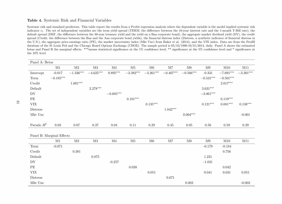
Table 4. Systemic Risk and Financial Variables

Systemic risk and standard predictors. This table report the results from a Probit regression analysis where the dependent variable is the model implied systemic riskindicator ct. The set of independent variables are the term yield spread (TERM, the difference between the 10-year interest rate and the 1-month T-Bill rate), thedefault spread (DEF, the difference between the 30-year treasury yield and the yield on a Baa corporate bond), the aggregate market dividend yield (DY), the creditspread (Credit, the difference between the Baa and the Aaa corporate bond yields), the financial distress index (Distress, a synthetic indicator of financial distress inthe U.S.), the aggregate price-earnings ratio (PE), the market uncertainty index (Mkt Unc) from Baker et al. (2014), and the VIX index. Data are from the FredIIdatabase of the St Louis Fed and the Chicago Board Options Exchange (CBOE). The sample period is 05/10/1996-10/31/2014, daily. Panel A shows the estimatedbetas and Panel B the marginal effects. ***means statistical significance at the 1% confidence level, ** significance at the 5% confidence level and * significance atthe 10% level.

Panel A: Betas

M1 M2 M3 M4 M5 M6 M7 M8 M9 M10 M11

Intercept -0.017 −1.336∗∗∗ −4.625∗∗∗ 0.895∗∗∗ −2.382∗∗∗ −3.261∗∗∗ −0.407∗∗∗ −0.566∗∗∗ -0.331 −7.691∗∗∗ −3.301∗∗∗

Term −0.185∗∗∗ −0.531∗∗∗ −0.501∗∗∗

Credit 1.001∗∗∗ 2.017∗∗∗

Default 2.278∗∗∗ 3.631∗∗∗

DY −0.685∗∗∗ −3.061∗∗∗

PE 0.101∗∗∗ 0.119∗∗∗

VIX 0.135∗∗∗ 0.121∗∗∗ 0.081∗∗∗ 0.138∗∗∗

Distress 1.842∗∗∗

Mkt Unc 0.004∗∗∗ -0.001

Pseudo R2 0.03 0.07 0.37 0.04 0.11 0.29 0.45 0.05 0.56 0.59 0.29

Panel B: Marginal Effects

M1 M2 M3 M4 M5 M6 M7 M8 M9 M10 M11

Term -0.071 -0.179 -0.184

Credit 0.381 0.756

Default 0.875 1.231

DY -0.257 -1.031

PE 0.038 0.042

VIX 0.051 0.041 0.031 0.051

Distress 0.671

Mkt Unc 0.002 -0.002

41

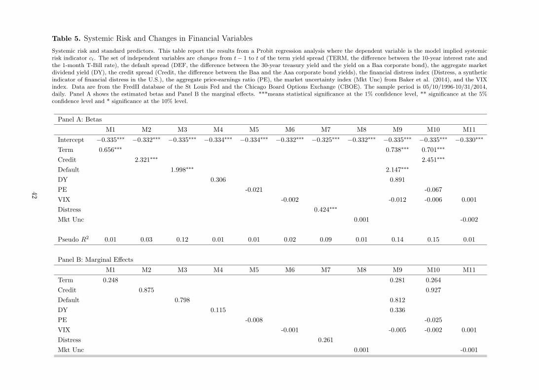
Table 5. Systemic Risk and Changes in Financial Variables

Systemic risk and standard predictors. This table report the results from a Probit regression analysis where the dependent variable is the model implied systemicrisk indicator ct. The set of independent variables are changes from t− 1 to t of the term yield spread (TERM, the difference between the 10-year interest rate andthe 1-month T-Bill rate), the default spread (DEF, the difference between the 30-year treasury yield and the yield on a Baa corporate bond), the aggregate marketdividend yield (DY), the credit spread (Credit, the difference between the Baa and the Aaa corporate bond yields), the financial distress index (Distress, a syntheticindicator of financial distress in the U.S.), the aggregate price-earnings ratio (PE), the market uncertainty index (Mkt Unc) from Baker et al. (2014), and the VIXindex. Data are from the FredII database of the St Louis Fed and the Chicago Board Options Exchange (CBOE). The sample period is 05/10/1996-10/31/2014,daily. Panel A shows the estimated betas and Panel B the marginal effects. ***means statistical significance at the 1% confidence level, ** significance at the 5%confidence level and * significance at the 10% level.

Panel A: Betas

M1 M2 M3 M4 M5 M6 M7 M8 M9 M10 M11

Intercept −0.335∗∗∗ −0.332∗∗∗ −0.335∗∗∗ −0.334∗∗∗ −0.334∗∗∗ −0.332∗∗∗ −0.325∗∗∗ −0.332∗∗∗ −0.335∗∗∗ −0.335∗∗∗ −0.330∗∗∗

Term 0.656∗∗∗ 0.738∗∗∗ 0.701∗∗∗

Credit 2.321∗∗∗ 2.451∗∗∗

Default 1.998∗∗∗ 2.147∗∗∗

DY 0.306 0.891

PE -0.021 -0.067

VIX -0.002 -0.012 -0.006 0.001

Distress 0.424∗∗∗

Mkt Unc 0.001 -0.002

Pseudo R2 0.01 0.03 0.12 0.01 0.01 0.02 0.09 0.01 0.14 0.15 0.01

Panel B: Marginal Effects

M1 M2 M3 M4 M5 M6 M7 M8 M9 M10 M11

Term 0.248 0.281 0.264

Credit 0.875 0.927

Default 0.798 0.812

DY 0.115 0.336

PE -0.008 -0.025

VIX -0.001 -0.005 -0.002 0.001

Distress 0.261

Mkt Unc 0.001 -0.001

42

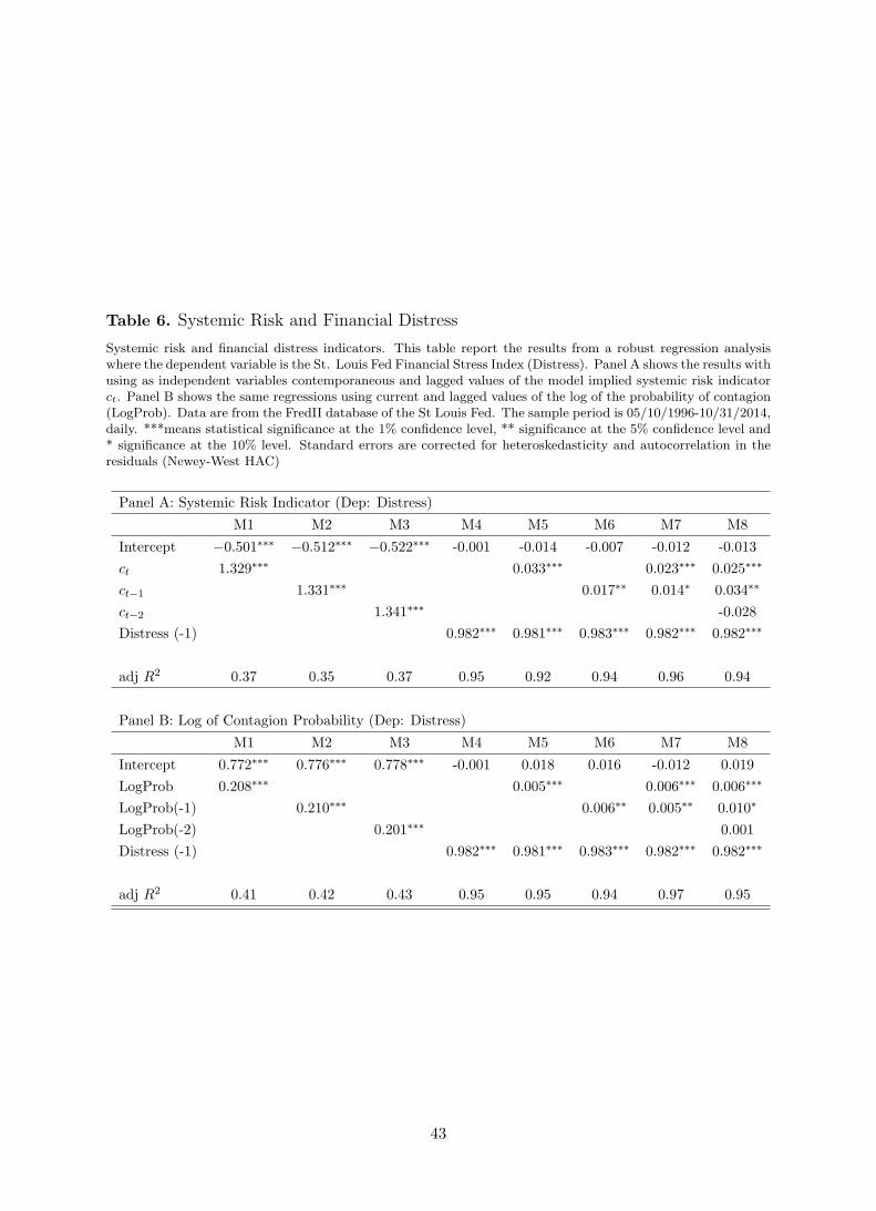
Table 6. Systemic Risk and Financial Distress

Systemic risk and financial distress indicators. This table report the results from a robust regression analysiswhere the dependent variable is the St. Louis Fed Financial Stress Index (Distress). Panel A shows the results withusing as independent variables contemporaneous and lagged values of the model implied systemic risk indicatorct. Panel B shows the same regressions using current and lagged values of the log of the probability of contagion(LogProb). Data are from the FredII database of the St Louis Fed. The sample period is 05/10/1996-10/31/2014,daily. ***means statistical significance at the 1% confidence level, ** significance at the 5% confidence level and* significance at the 10% level. Standard errors are corrected for heteroskedasticity and autocorrelation in theresiduals (Newey-West HAC)

Panel A: Systemic Risk Indicator (Dep: Distress)

M1 M2 M3 M4 M5 M6 M7 M8

Intercept −0.501∗∗∗ −0.512∗∗∗ −0.522∗∗∗ -0.001 -0.014 -0.007 -0.012 -0.013

ct 1.329∗∗∗ 0.033∗∗∗ 0.023∗∗∗ 0.025∗∗∗

ct−1 1.331∗∗∗ 0.017∗∗ 0.014∗ 0.034∗∗

ct−2 1.341∗∗∗ -0.028

Distress (-1) 0.982∗∗∗ 0.981∗∗∗ 0.983∗∗∗ 0.982∗∗∗ 0.982∗∗∗

adj R2 0.37 0.35 0.37 0.95 0.92 0.94 0.96 0.94

Panel B: Log of Contagion Probability (Dep: Distress)

M1 M2 M3 M4 M5 M6 M7 M8

Intercept 0.772∗∗∗ 0.776∗∗∗ 0.778∗∗∗ -0.001 0.018 0.016 -0.012 0.019

LogProb 0.208∗∗∗ 0.005∗∗∗ 0.006∗∗∗ 0.006∗∗∗

LogProb(-1) 0.210∗∗∗ 0.006∗∗ 0.005∗∗ 0.010∗

LogProb(-2) 0.201∗∗∗ 0.001

Distress (-1) 0.982∗∗∗ 0.981∗∗∗ 0.983∗∗∗ 0.982∗∗∗ 0.982∗∗∗

adj R2 0.41 0.42 0.43 0.95 0.95 0.94 0.97 0.95

43

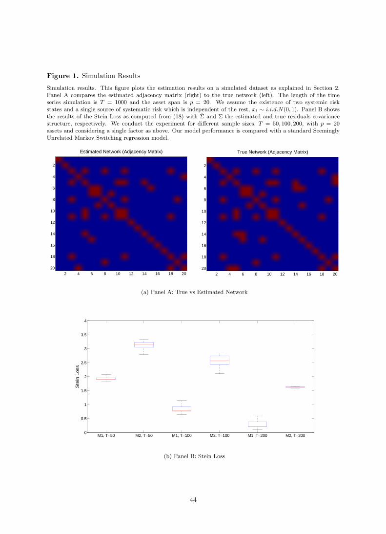
Figure 1. Simulation Results

Simulation results. This figure plots the estimation results on a simulated dataset as explained in Section 2.Panel A compares the estimated adjacency matrix (right) to the true network (left). The length of the timeseries simulation is T = 1000 and the asset span is p = 20. We assume the existence of two systemic riskstates and a single source of systematic risk which is independent of the rest, xt ∼ i.i.d.N(0, 1). Panel B showsthe results of the Stein Loss as computed from (18) with Σ and Σ the estimated and true residuals covariancestructure, respectively. We conduct the experiment for different sample sizes, T = 50, 100, 200, with p = 20assets and considering a single factor as above. Our model performance is compared with a standard SeeminglyUnrelated Markov Switching regression model.

Estimated Network (Adjacency Matrix)

2 4 6 8 10 12 14 16 18 20

2

4

6

8

10

12

14

16

18

20

True Network (Adjacency Matrix)

2 4 6 8 10 12 14 16 18 20

2

4

6

8

10

12

14

16

18

20

(a) Panel A: True vs Estimated Network

M1, T=50 M2, T=50 M1, T=100 M2, T=100 M1, T=200 M2, T=2000

0.5

1

1.5

2

2.5

3

3.5

4

Ste

in L

oss

(b) Panel B: Stein Loss

44

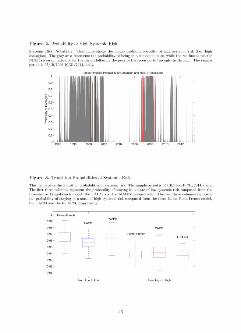
Figure 2. Probability of High Systemic Risk

Systemic Risk Probability. This figure shows the model-implied probability of high systemic risk (i.e. highcontagion). The gray area represents the probability of being in a contagion state, while the red line shows theNBER recession indicator for the period following the peak of the recession to through the through. The sampleperiod is 05/10/1996-10/31/2014, daily.

1996 1998 2000 2002 2004 2006 2008 2010 20120

0.1

0.2

0.3

0.4

0.5

0.6

0.7

0.8

0.9

1

Pro

babi

lity

of C

onta

gion

Model−Implied Probability of Contagion and NBER Recessions

Figure 3. Transition Probabilities of Systemic Risk

This figure plots the transition probabilities of systemic risk. The sample period is 05/10/1996-10/31/2014, daily.The first three columns represent the probability of staying in a state of low systemic risk computed from thethree-factor Fama-French model, the CAPM and the I-CAPM, respectively. The last three columns representthe probability of staying in a state of high systemic risk computed from the three-factor Fama-French model,the CAPM and the I-CAPM, respectively.

From Low to Low From High to High

0.91

0.92

0.93

0.94

0.95

0.96

0.97

0.98

0.99

1 Fama−French

Fama−French

CAPM

CAPM

I−CAPM

I−CAPM

45

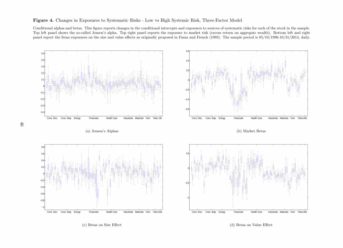
Figure 4. Changes in Exposures to Systematic Risks - Low vs High Systemic Risk, Three-Factor Model

Conditional alphas and betas. This figure reports changes in the conditional intercepts and exposures to sources of systematic risks for each of the stock in the sample.Top left panel shows the so-called Jensen’s alpha. Top right panel reports the exposure to market risk (excess return on aggregate wealth). Bottom left and rightpanel report the firms exposures on the size and value effects as originally proposed in Fama and French (1993). The sample period is 05/10/1996-10/31/2014, daily.

Cons. Disc. Cons. Stap. Energy Financials Health Care Industrials Materials Tech Telec Util

−0.4

−0.3

−0.2

−0.1

0

0.1

0.2

0.3

0.4

0.5

(a) Jensen’s Alphas

Cons. Disc. Cons. Stap. Energy Financials Health Care Industrials Materials Tech TelecUtils

−0.6

−0.4

−0.2

0

0.2

0.4

0.6

(b) Market Betas


−1

−0.8

−0.6

−0.4

−0.2

0

0.2

0.4

0.6

0.8

(c) Betas on Size Effect


−1

−0.5

0

0.5

(d) Betas on Value Effect

46

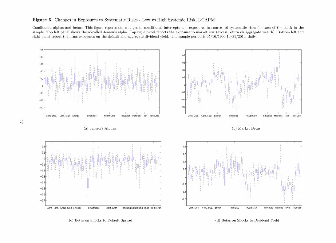
Figure 5. Changes in Exposures to Systematic Risks - Low vs High Systemic Risk, I-CAPM

Conditional alphas and betas. This figure reports the changes to conditional intercepts and exposures to sources of systematic risks for each of the stock in thesample. Top left panel shows the so-called Jensen’s alpha. Top right panel reports the exposure to market risk (excess return on aggregate wealth). Bottom left andright panel report the firms exposures on the default and aggregate dividend yield. The sample period is 05/10/1996-10/31/2014, daily.


−0.3

−0.2

−0.1

0

0.1

0.2

0.3

0.4

0.5

(a) Jensen’s Alphas


−0.6

−0.4

−0.2

0

0.2

0.4

0.6

0.8

(b) Market Betas


−0.7

−0.6

−0.5

−0.4

−0.3

−0.2

−0.1

0

0.1

0.2

(c) Betas on Shocks to Default Spread


−0.6

−0.4

−0.2

0

0.2

0.4

0.6

0.8

(d) Betas on Shocks to Dividend Yield

47

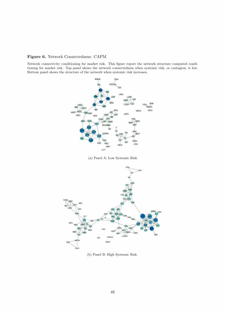
Figure 6. Network Connectedness: CAPM

Network connectivity conditioning for market risk. This figure report the network structure computed condi-tioning for market risk. Top panel shows the network connectedness when systemic risk, or contagion, is low.Bottom panel shows the structure of the network when systemic risk increases.

MMMDD

EMR

GE

UTX

T

VZ

ABT

BAX

BMYMKR

PFE

ALL

BAC

BRKB

MO

CL

AXPBK

USB

WFC

AIG

AMGN

BIIBFDX

GILD

XOM

APACVX

COP

HAL

OXY

SLB

AAPL

CJPM

TXN

JNJ

MDT

BA

GD

HON LMT

CVS

WAG

COF

CAT

FCX

EXC

FDX

QCOM

CSCO

INTC

ORCL

KO

MCD

PEPSO

PG

CMCSA

TWX

DIS

COST TGT

WMT

DVNAPCDOW

EMC

NSC

RTN

HPQ

HD

LOW

IBM

MSFT

LLY

MS

NKE

UNP

SPG

SBUX

UNH

(a) Panel A: Low Systemic Risk

MMM

DD

EMR

GE

UTX

TVZ

ABT

BAX

BMY MKR

PFE

ALL

BAC

BRKB

MO

CLAXP

BK

USB

WFC

AIG

AMGN

BIIB

FDX

GILD

APC

APACVX

COPHAL

OXY

SLB

AAPL

C

JPM

TXN

JNJ

MDT

BA

GD

HON

LMT

CVS

WAG

COF

CAT

FCX

EXC

FDX

QCOM

CSCO

INTC

ORCLKO

MCD

PEP

SO

PG

CMCSA

TWX

DIS

COST

TGT

WMT

DVN

XOM

DOW

EMC

NSC

RTN

HPQ

HD

LOW

IBM

MSFT

LLY

MS

NKE UNP

SPG

SBUX

UNH

(b) Panel B: High Systemic Risk

48

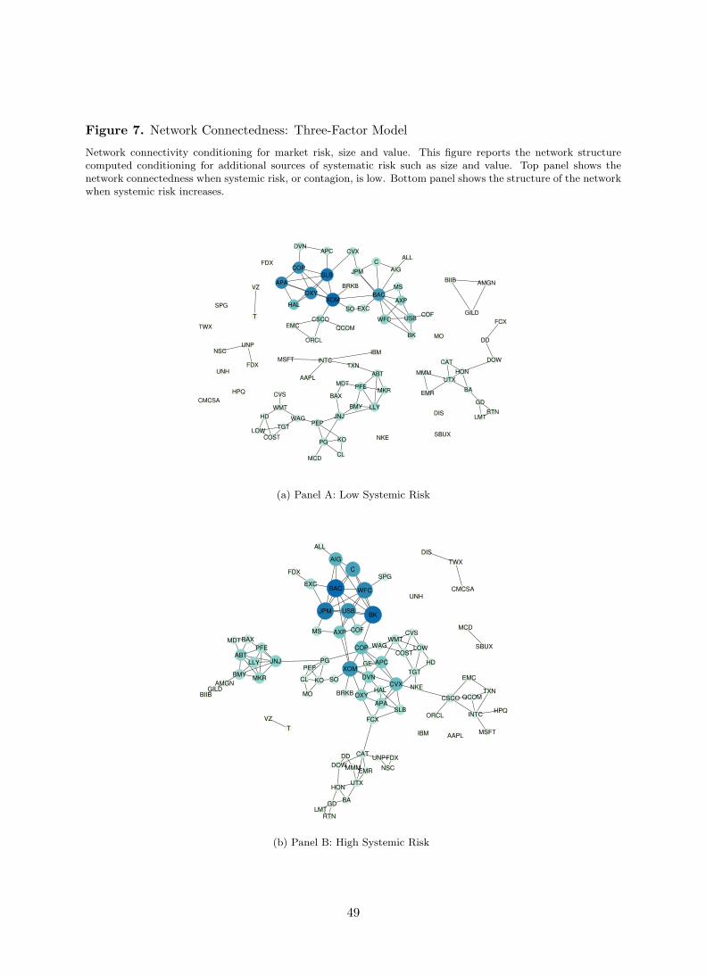
Figure 7. Network Connectedness: Three-Factor Model

Network connectivity conditioning for market risk, size and value. This figure reports the network structurecomputed conditioning for additional sources of systematic risk such as size and value. Top panel shows thenetwork connectedness when systemic risk, or contagion, is low. Bottom panel shows the structure of the networkwhen systemic risk increases.

MMM

DD

EMR

UTX

T

VZ

ABT

BAX

BMY

MKRPFE

ALL

BAC

BRKB

MO

CL

AXP

BK

USBWFC

AIG

AMGNBIIB

FDX

GILD

APC

APA

CVX

COP

HAL

OXY

SLB

AAPL

C

JPM

TXN

JNJ

MDT

BA

GD

HON

LMT

CVS

WAG

COF

CAT

FCX

EXC

FDX

QCOM

CSCO

INTC

ORCL

KO

MCD

PEP

SO

PG

CMCSA

TWX

DIS

COST

TGT

WMT

DVN

XOM

DOW

EMC

NSC

RTN

HPQ

HD

LOW

IBM

MSFT

LLY

MS

NKE

UNP

SPG

SBUX

UNH


MMM

DD

EMR

GE

UTX

T

VZ

ABT

BAX

BMYMKR

PFE

ALL

BAC

BRKBMO

CL

AXP

BKUSB

WFC

AIG

AMGN

BIIB

FDX

GILD

APC

APA

CVX

COP

HALOXY

SLB

AAPL

C

JPM

TXN

JNJ

MDT

BAGD

HON

LMT

CVS

WAG

COF

CAT

FCX

EXC

FDX

QCOMCSCO

INTCORCL

KO

MCD

PEP

SO

PG

CMCSA

TWX

DIS

COST

TGT

WMT

DVN

XOM

DOW

EMC

NSC

RTN

HPQ

HD

LOW

IBM MSFT

LLY

MS

NKE

UNP

SPG

SBUX

UNH


49

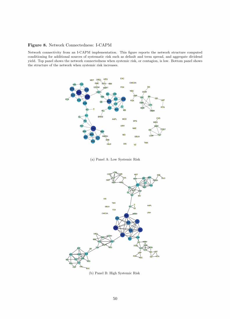
Figure 8. Network Connectedness: I-CAPM

Network connectivity from an I-CAPM implementation. This figure reports the network structure computedconditioning for additional sources of systematic risk such as default and term spread, and aggregate dividendyield. Top panel shows the network connectedness when systemic risk, or contagion, is low. Bottom panel showsthe structure of the network when systemic risk increases.

MMM

DD

EMRGE

UTX

T

VZ

ABT

BAX BMY

MKR

PFE

ALLBAC

BRKB

MO

CL

AXP

BK USB

WFC

AIG

AMGN

BIIB

FDX

GILD

APC

APA

CVX

COP

HAL

OXY

SLB

AAPL

C

JPM

TXN

JNJ

MDT

BAGD

HON

LMT

CVS

WAG

COF

CAT

FCX

EXC

FDX

QCOM

CSCO

INTC

ORCL

KO

MCD

PEP

SO

PG

CMCSA

TWXDIS

COST

TGT

WMT

DVN

XOM

DOW

EMC

NSC

RTN

HPQ

HD

LOW

IBM

MSFT

LLY

MS

NKE

UNP

SPG

SBUX

UNH


MMMDD

EMR

GEUTX

T

VZ

ABTBAXBMY

MKRPFE

HAL

FCX

EXC

MO

CL

AXP

OXYUSB

SLB

COP

AMGN

BIIB

FDX

GILD

JPM

C

CVX

AIG

ALL

BK

WFC

AAPL

APA

APC

TXN

JNJ

MDT

BA

GD

HON

LMT

CVS

WAG

DVN

CAT

XOM

BRKB

FDX

QCOM

CSCOINTC

ORCL

KO

MCD PEP

SO

PG

CMCSA

TWX

DIS

COST

TGT

WMT

COF

BAC

DOW

EMC

NSCRTN

HPQ

HD

LOW

IBM

MSFT

LLY

MS

NKE

UNP

SPG

SBUX

UNH


50

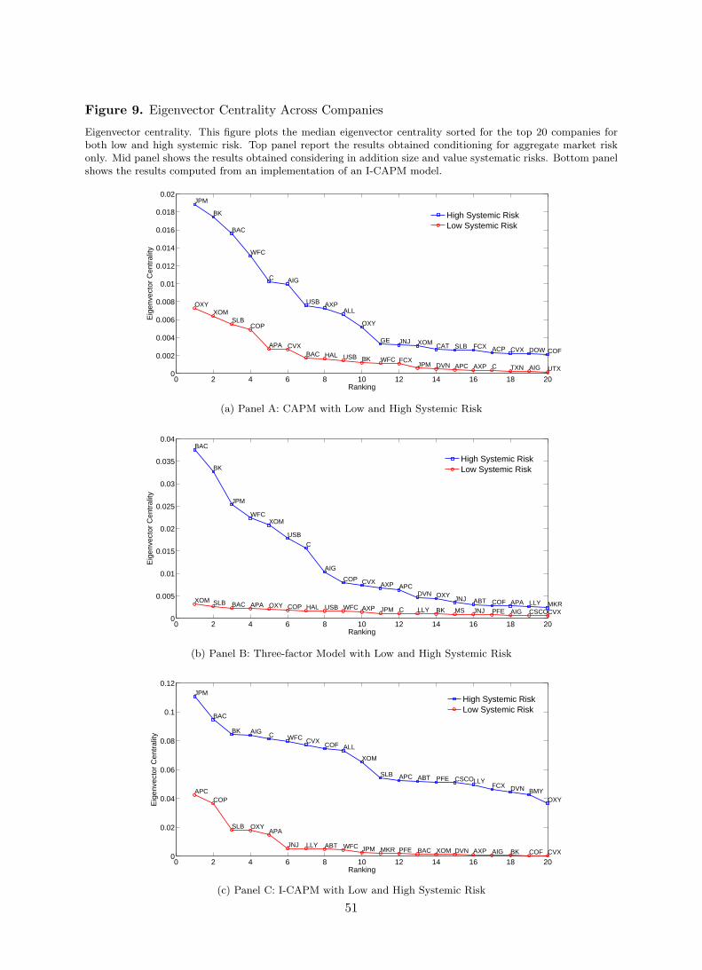
Figure 9. Eigenvector Centrality Across Companies

Eigenvector centrality. This figure plots the median eigenvector centrality sorted for the top 20 companies forboth low and high systemic risk. Top panel report the results obtained conditioning for aggregate market riskonly. Mid panel shows the results obtained considering in addition size and value systematic risks. Bottom panelshows the results computed from an implementation of an I-CAPM model.

0 2 4 6 8 10 12 14 16 18 200

0.002

0.004

0.006

0.008

0.01

0.012

0.014

0.016

0.018

0.02JPM

BK

BAC

WFC

C AIG

USB AXPALL

OXY

GE JNJ XOM CAT SLB FCX ACP CVX DOW COF

OXYXOM

SLBCOP

APA CVXBAC HAL USB BK WFC FCX

JPM DVN APC AXP C TXN AIG UTX

Ranking

Eig

enve

ctor

Cen

tral

ity

High Systemic RiskLow Systemic Risk

(a) Panel A: CAPM with Low and High Systemic Risk

0 2 4 6 8 10 12 14 16 18 200

0.005

0.01

0.015

0.02

0.025

0.03

0.035

0.04BAC

BK

JPM

WFCXOM

USB

C

AIG

COP CVX AXP APCDVN OXY

JNJ ABT COF APA LLY MKRXOM SLB BAC APA OXY COP HAL USB WFC AXP JPM C LLY BK MS JNJ PFE AIG CSCOCVX

Ranking

Eig

enve

ctor

Cen

tral

ity


(b) Panel B: Three-factor Model with Low and High Systemic Risk

0 2 4 6 8 10 12 14 16 18 200

0.02

0.04

0.06

0.08

0.1

0.12JPM

BAC

BK AIG C WFC CVXCOF ALL

XOM

SLB APC ABT PFE CSCOLLYFCX DVN BMY

OXYAPC

COP

SLB OXYAPA

JNJ LLY ABT WFC JPM MKR PFE BAC XOM DVN AXP AIG BK COF CVX

Eig

enve

ctor

Cen

tral

ity

Ranking


(c) Panel C: I-CAPM with Low and High Systemic Risk

51

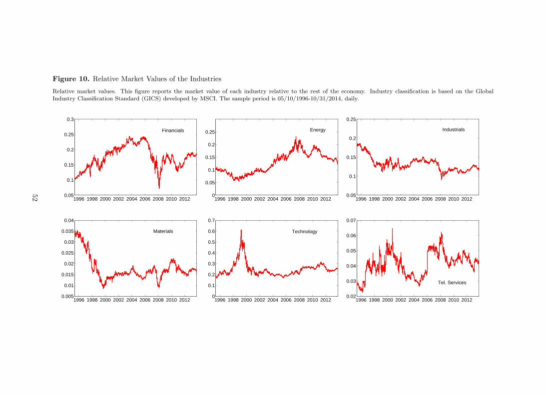
Figure 10. Relative Market Values of the Industries

Relative market values. This figure reports the market value of each industry relative to the rest of the economy. Industry classification is based on the GlobalIndustry Classification Standard (GICS) developed by MSCI. The sample period is 05/10/1996-10/31/2014, daily.

1996 1998 2000 2002 2004 2006 2008 2010 20120.05

0.1

0.15

0.2

0.25

0.3

1996 1998 2000 2002 2004 2006 2008 2010 20120

0.05

0.1

0.15

0.2

0.25

1996 1998 2000 2002 2004 2006 2008 2010 20120.05

0.1

0.15

0.2

0.25

1996 1998 2000 2002 2004 2006 2008 2010 20120.005

0.01

0.015

0.02

0.025

0.03

0.035

0.04

1996 1998 2000 2002 2004 2006 2008 2010 20120

0.1

0.2

0.3

0.4

0.5

0.6

0.7

1996 1998 2000 2002 2004 2006 2008 2010 20120.02

0.03

0.04

0.05

0.06

0.07

Financials Energy Industrials

Materials Technology

Tel. Services

52

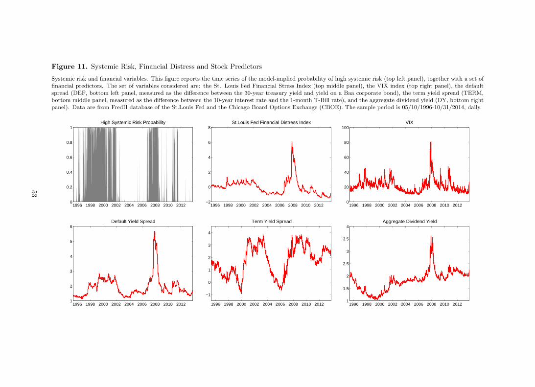
Figure 11. Systemic Risk, Financial Distress and Stock Predictors

Systemic risk and financial variables. This figure reports the time series of the model-implied probability of high systemic risk (top left panel), together with a set offinancial predictors. The set of variables considered are: the St. Louis Fed Financial Stress Index (top middle panel), the VIX index (top right panel), the defaultspread (DEF, bottom left panel, measured as the difference between the 30-year treasury yield and yield on a Baa corporate bond), the term yield spread (TERM,bottom middle panel, measured as the difference between the 10-year interest rate and the 1-month T-Bill rate), and the aggregate dividend yield (DY, bottom rightpanel). Data are from FredII database of the St.Louis Fed and the Chicago Board Options Exchange (CBOE). The sample period is 05/10/1996-10/31/2014, daily.

1996 1998 2000 2002 2004 2006 2008 2010 20120

0.2

0.4

0.6

0.8

1High Systemic Risk Probability

1996 1998 2000 2002 2004 2006 2008 2010 2012−2

0

2

4

6

8St.Louis Fed Financial Distress Index

1996 1998 2000 2002 2004 2006 2008 2010 20120

20

40

60

80

100VIX

1996 1998 2000 2002 2004 2006 2008 2010 20121

2

3

4

5

6Default Yield Spread

1996 1998 2000 2002 2004 2006 2008 2010 2012

−1

0

1

2

3

4

Term Yield Spread

1996 1998 2000 2002 2004 2006 2008 2010 20121

1.5

2

2.5

3

3.5

4Aggregate Dividend Yield

53

Documents

Modeling Contagion and Systemic Risk · Modeling Contagion and Systemic Risk∗ Daniele Bianchi† Monica Billio‡ Roberto Casarin‡ Massimo Guidolin§ Abstract We model contagion