Embed Size (px)
Citation preview

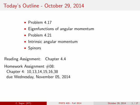
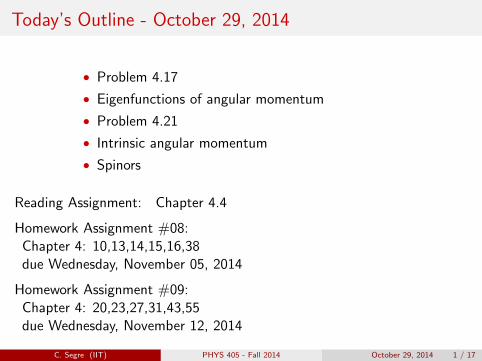
Today’s Outline - October 29, 2014
• Problem 4.17
• Eigenfunctions of angular momentum
• Problem 4.21
• Intrinsic angular momentum
• Spinors
Reading Assignment: Chapter 4.4
Homework Assignment #08:Chapter 4: 10,13,14,15,16,38due Wednesday, November 05, 2014
Homework Assignment #09:Chapter 4: 20,23,27,31,43,55due Wednesday, November 12, 2014
C. Segre (IIT) PHYS 405 - Fall 2014 October 29, 2014 1 / 17
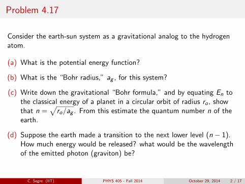
Problem 4.17
Consider the earth-sun system as a gravitational analog to the hydrogenatom.
(a) What is the potential energy function?
(b) What is the “Bohr radius,” ag , for this system?
(c) Write down the gravitational “Bohr formula,” and by equating En tothe classical energy of a planet in a circular orbit of radius ro , showthat n =
√ro/ag . From this estimate the quantum number n of the
earth.
(d) Suppose the earth made a transition to the next lower level (n − 1).How much energy would be released? what would be the wavelengthof the emitted photon (graviton) be?
C. Segre (IIT) PHYS 405 - Fall 2014 October 29, 2014 2 / 17
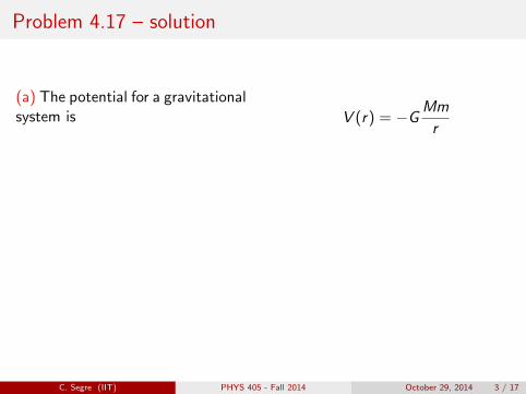
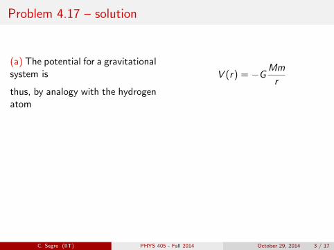
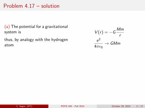
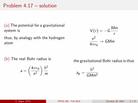
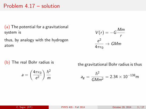
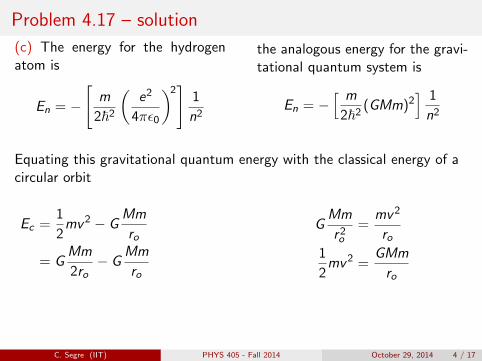
Problem 4.17 – solution
(a) The potential for a gravitationalsystem is
thus, by analogy with the hydrogenatom
(b) The real Bohr radius is
a =
(4πε0e2
)~2
m
V (r) = −GMm
re2
4πε0→ GMm
the gravitational Bohr radius is thus
ag =~2
GMm2= 2.34× 10−138m
C. Segre (IIT) PHYS 405 - Fall 2014 October 29, 2014 3 / 17
Problem 4.17 – solution
(a) The potential for a gravitationalsystem is
thus, by analogy with the hydrogenatom
(b) The real Bohr radius is
a =
(4πε0e2
)~2
m
V (r) = −GMm
r
e2
4πε0→ GMm
the gravitational Bohr radius is thus
ag =~2
GMm2= 2.34× 10−138m
C. Segre (IIT) PHYS 405 - Fall 2014 October 29, 2014 3 / 17
Problem 4.17 – solution
(a) The potential for a gravitationalsystem is
thus, by analogy with the hydrogenatom
(b) The real Bohr radius is
a =
(4πε0e2
)~2
m
V (r) = −GMm
re2
4πε0→ GMm
the gravitational Bohr radius is thus
ag =~2
GMm2= 2.34× 10−138m
C. Segre (IIT) PHYS 405 - Fall 2014 October 29, 2014 3 / 17
Problem 4.17 – solution
(a) The potential for a gravitationalsystem is
thus, by analogy with the hydrogenatom
(b) The real Bohr radius is
a =
(4πε0e2
)~2
m
V (r) = −GMm
re2
4πε0→ GMm
the gravitational Bohr radius is thus
ag =~2
GMm2
= 2.34× 10−138m
C. Segre (IIT) PHYS 405 - Fall 2014 October 29, 2014 3 / 17
Problem 4.17 – solution
(a) The potential for a gravitationalsystem is
thus, by analogy with the hydrogenatom
(b) The real Bohr radius is
a =
(4πε0e2
)~2
m
V (r) = −GMm
re2
4πε0→ GMm
the gravitational Bohr radius is thus
ag =~2
GMm2= 2.34× 10−138m
C. Segre (IIT) PHYS 405 - Fall 2014 October 29, 2014 3 / 17
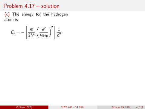
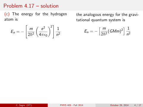
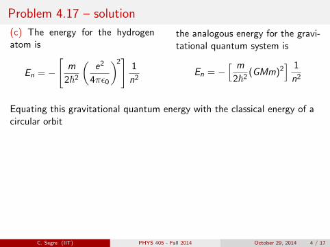
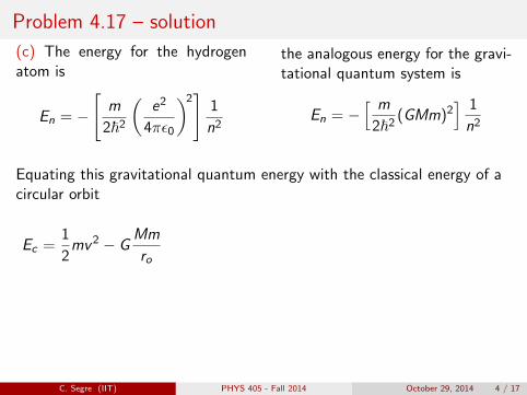
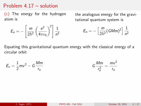
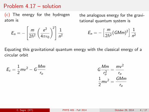
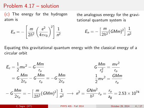
Problem 4.17 – solution
(c) The energy for the hydrogenatom is
En = −
[m
2~2
(e2
4πε0
)2]1
n2
the analogous energy for the gravi-tational quantum system is
En = −[ m
2~2(GMm)2
] 1
n2
Equating this gravitational quantum energy with the classical energy of acircular orbit
Ec =1
2mv2 − G
Mm
ro
= GMm
2ro− G
Mm
ro= −GMm
2ro
GMm
r2o=
mv2
ro1
2mv2 =
GMm
ro
− GMm
2ro= −
[ m
2~2(GMm)2
] 1
n2−→ n2 =
GNm2
~2ro =
roag
= 2.53× 1074
C. Segre (IIT) PHYS 405 - Fall 2014 October 29, 2014 4 / 17
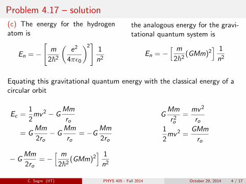
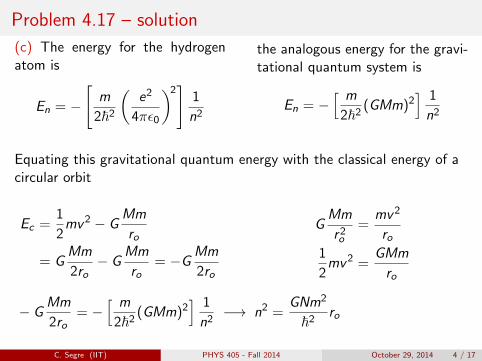
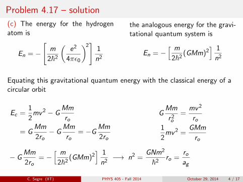
Problem 4.17 – solution
(c) The energy for the hydrogenatom is
En = −
[m
2~2
(e2
4πε0
)2]1
n2
the analogous energy for the gravi-tational quantum system is
En = −[ m
2~2(GMm)2
] 1
n2
Equating this gravitational quantum energy with the classical energy of acircular orbit
Ec =1
2mv2 − G
Mm
ro
= GMm
2ro− G
Mm
ro= −GMm
2ro
GMm
r2o=
mv2
ro
1
2mv2 =
GMm
ro
− GMm
2ro= −
[ m
2~2(GMm)2
] 1
n2−→ n2 =
GNm2
~2ro =
roag
= 2.53× 1074
C. Segre (IIT) PHYS 405 - Fall 2014 October 29, 2014 4 / 17
Problem 4.17 – solution
(c) The energy for the hydrogenatom is
En = −
[m
2~2
(e2
4πε0
)2]1
n2
the analogous energy for the gravi-tational quantum system is
En = −[ m
2~2(GMm)2
] 1
n2
Equating this gravitational quantum energy with the classical energy of acircular orbit
Ec =1
2mv2 − G
Mm
ro
= GMm
2ro− G
Mm
ro= −GMm
2ro
GMm
r2o=
mv2
ro1
2mv2 =
GMm
ro
− GMm
2ro= −
[ m
2~2(GMm)2
] 1
n2−→ n2 =
GNm2
~2ro =
roag
= 2.53× 1074
C. Segre (IIT) PHYS 405 - Fall 2014 October 29, 2014 4 / 17
Problem 4.17 – solution
(c) The energy for the hydrogenatom is
En = −
[m
2~2
(e2
4πε0
)2]1
n2
the analogous energy for the gravi-tational quantum system is
En = −[ m
2~2(GMm)2
] 1
n2
Equating this gravitational quantum energy with the classical energy of acircular orbit
Ec =1
2mv2 − G
Mm
ro
= GMm
2ro− G
Mm
ro
= −GMm
2ro
GMm
r2o=
mv2
ro1
2mv2 =
GMm
ro
− GMm
2ro= −
[ m
2~2(GMm)2
] 1
n2−→ n2 =
GNm2
~2ro =
roag
= 2.53× 1074
C. Segre (IIT) PHYS 405 - Fall 2014 October 29, 2014 4 / 17

Problem 4.17 – solution
(c) The energy for the hydrogenatom is
En = −
[m
2~2
(e2
4πε0
)2]1
n2
the analogous energy for the gravi-tational quantum system is
En = −[ m
2~2(GMm)2
] 1
n2
Equating this gravitational quantum energy with the classical energy of acircular orbit
Ec =1
2mv2 − G
Mm
ro
= GMm
2ro− G
Mm
ro= −GMm
2ro
GMm
r2o=
mv2
ro1
2mv2 =
GMm
ro
− GMm
2ro= −
[ m
2~2(GMm)2
] 1
n2−→ n2 =
GNm2
~2ro =
roag
= 2.53× 1074
C. Segre (IIT) PHYS 405 - Fall 2014 October 29, 2014 4 / 17
Problem 4.17 – solution
(c) The energy for the hydrogenatom is
En = −
[m
2~2
(e2
4πε0
)2]1
n2
the analogous energy for the gravi-tational quantum system is
En = −[ m
2~2(GMm)2
] 1
n2
Equating this gravitational quantum energy with the classical energy of acircular orbit
Ec =1
2mv2 − G
Mm
ro
= GMm
2ro− G
Mm
ro= −GMm
2ro
GMm
r2o=
mv2
ro1
2mv2 =
GMm
ro
− GMm
2ro= −
[ m
2~2(GMm)2
] 1
n2
−→ n2 =GNm2
~2ro =
roag
= 2.53× 1074
C. Segre (IIT) PHYS 405 - Fall 2014 October 29, 2014 4 / 17
Problem 4.17 – solution
(c) The energy for the hydrogenatom is
En = −
[m
2~2
(e2
4πε0
)2]1
n2
the analogous energy for the gravi-tational quantum system is
En = −[ m
2~2(GMm)2
] 1
n2
Equating this gravitational quantum energy with the classical energy of acircular orbit
Ec =1
2mv2 − G
Mm
ro
= GMm
2ro− G
Mm
ro= −GMm
2ro
GMm
r2o=
mv2
ro1
2mv2 =
GMm
ro
− GMm
2ro= −
[ m
2~2(GMm)2
] 1
n2−→ n2 =
GNm2
~2ro
=roag
= 2.53× 1074
C. Segre (IIT) PHYS 405 - Fall 2014 October 29, 2014 4 / 17
Problem 4.17 – solution
(c) The energy for the hydrogenatom is
En = −
[m
2~2
(e2
4πε0
)2]1
n2
the analogous energy for the gravi-tational quantum system is
En = −[ m
2~2(GMm)2
] 1
n2
Equating this gravitational quantum energy with the classical energy of acircular orbit
Ec =1
2mv2 − G
Mm
ro
= GMm
2ro− G
Mm
ro= −GMm
2ro
GMm
r2o=
mv2
ro1
2mv2 =
GMm
ro
− GMm
2ro= −
[ m
2~2(GMm)2
] 1
n2−→ n2 =
GNm2
~2ro =
roag
= 2.53× 1074
C. Segre (IIT) PHYS 405 - Fall 2014 October 29, 2014 4 / 17
Problem 4.17 – solution
(c) The energy for the hydrogenatom is
En = −
[m
2~2
(e2
4πε0
)2]1
n2
the analogous energy for the gravi-tational quantum system is
En = −[ m
2~2(GMm)2
] 1
n2
Equating this gravitational quantum energy with the classical energy of acircular orbit
Ec =1
2mv2 − G
Mm
ro
= GMm
2ro− G
Mm
ro= −GMm
2ro
GMm
r2o=
mv2
ro1
2mv2 =
GMm
ro
− GMm
2ro= −
[ m
2~2(GMm)2
] 1
n2−→ n2 =
GNm2
~2ro =
roag
= 2.53× 1074
C. Segre (IIT) PHYS 405 - Fall 2014 October 29, 2014 4 / 17
Problem 4.17 – solution
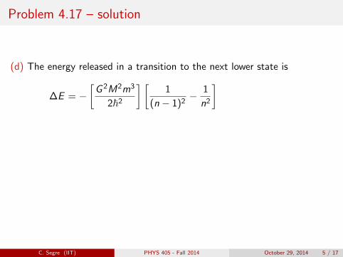
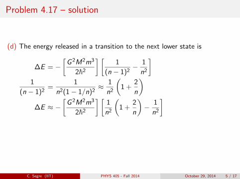
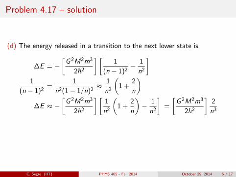
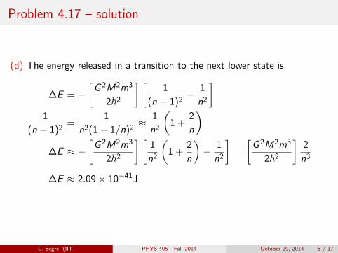
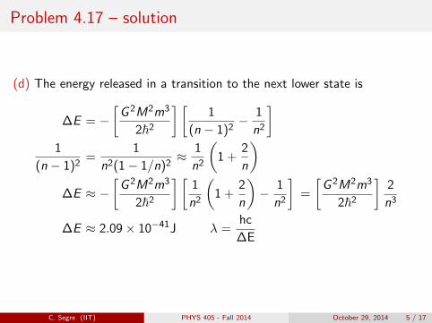
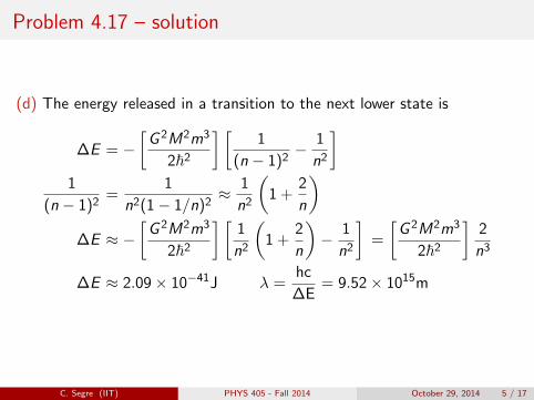
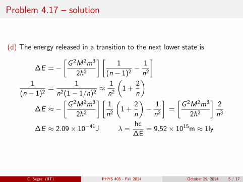
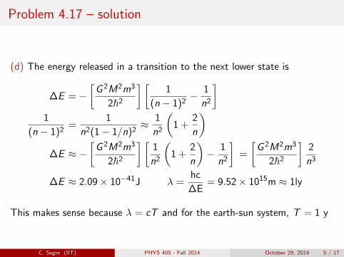
(d) The energy released in a transition to the next lower state is
∆E = −[G 2M2m3
2~2
] [1
(n − 1)2− 1
n2
]1
(n − 1)2=
1
n2(1− 1/n)2≈ 1
n2
(1 +
2
n
)∆E ≈ −
[G 2M2m3
2~2
] [1
n2
(1 +
2
n
)− 1
n2
]=
[G 2M2m3
2~2
]2
n3
∆E ≈ 2.09× 10−41J λ =hc
∆E= 9.52× 10¹⁵m ≈ 1ly
This makes sense because λ = cT and for the earth-sun system, T = 1 y
C. Segre (IIT) PHYS 405 - Fall 2014 October 29, 2014 5 / 17
Problem 4.17 – solution
(d) The energy released in a transition to the next lower state is
∆E = −[G 2M2m3
2~2
] [1
(n − 1)2− 1
n2
]
1
(n − 1)2=
1
n2(1− 1/n)2≈ 1
n2
(1 +
2
n
)∆E ≈ −
[G 2M2m3
2~2
] [1
n2
(1 +
2
n
)− 1
n2
]=
[G 2M2m3
2~2
]2
n3
∆E ≈ 2.09× 10−41J λ =hc
∆E= 9.52× 10¹⁵m ≈ 1ly
This makes sense because λ = cT and for the earth-sun system, T = 1 y
C. Segre (IIT) PHYS 405 - Fall 2014 October 29, 2014 5 / 17

Problem 4.17 – solution
(d) The energy released in a transition to the next lower state is
∆E = −[G 2M2m3
2~2
] [1
(n − 1)2− 1
n2
]1
(n − 1)2=
1
n2(1− 1/n)2
≈ 1
n2
(1 +
2
n
)∆E ≈ −
[G 2M2m3
2~2
] [1
n2
(1 +
2
n
)− 1
n2
]=
[G 2M2m3
2~2
]2
n3
∆E ≈ 2.09× 10−41J λ =hc
∆E= 9.52× 10¹⁵m ≈ 1ly
This makes sense because λ = cT and for the earth-sun system, T = 1 y
C. Segre (IIT) PHYS 405 - Fall 2014 October 29, 2014 5 / 17

Problem 4.17 – solution
(d) The energy released in a transition to the next lower state is
∆E = −[G 2M2m3
2~2
] [1
(n − 1)2− 1
n2
]1
(n − 1)2=
1
n2(1− 1/n)2≈ 1
n2
(1 +
2
n
)
∆E ≈ −[G 2M2m3
2~2
] [1
n2
(1 +
2
n
)− 1
n2
]=
[G 2M2m3
2~2
]2
n3
∆E ≈ 2.09× 10−41J λ =hc
∆E= 9.52× 10¹⁵m ≈ 1ly
This makes sense because λ = cT and for the earth-sun system, T = 1 y
C. Segre (IIT) PHYS 405 - Fall 2014 October 29, 2014 5 / 17
Problem 4.17 – solution
(d) The energy released in a transition to the next lower state is
∆E = −[G 2M2m3
2~2
] [1
(n − 1)2− 1
n2
]1
(n − 1)2=
1
n2(1− 1/n)2≈ 1
n2
(1 +
2
n
)∆E ≈ −
[G 2M2m3
2~2
] [1
n2
(1 +
2
n
)− 1
n2
]
=
[G 2M2m3
2~2
]2
n3
∆E ≈ 2.09× 10−41J λ =hc
∆E= 9.52× 10¹⁵m ≈ 1ly
This makes sense because λ = cT and for the earth-sun system, T = 1 y
C. Segre (IIT) PHYS 405 - Fall 2014 October 29, 2014 5 / 17
Problem 4.17 – solution
(d) The energy released in a transition to the next lower state is
∆E = −[G 2M2m3
2~2
] [1
(n − 1)2− 1
n2
]1
(n − 1)2=
1
n2(1− 1/n)2≈ 1
n2
(1 +
2
n
)∆E ≈ −
[G 2M2m3
2~2
] [1
n2
(1 +
2
n
)− 1
n2
]=
[G 2M2m3
2~2
]2
n3
∆E ≈ 2.09× 10−41J λ =hc
∆E= 9.52× 10¹⁵m ≈ 1ly
This makes sense because λ = cT and for the earth-sun system, T = 1 y
C. Segre (IIT) PHYS 405 - Fall 2014 October 29, 2014 5 / 17
Problem 4.17 – solution
(d) The energy released in a transition to the next lower state is
∆E = −[G 2M2m3
2~2
] [1
(n − 1)2− 1
n2
]1
(n − 1)2=
1
n2(1− 1/n)2≈ 1
n2
(1 +
2
n
)∆E ≈ −
[G 2M2m3
2~2
] [1
n2
(1 +
2
n
)− 1
n2
]=
[G 2M2m3
2~2
]2
n3
∆E ≈ 2.09× 10−41J
λ =hc
∆E= 9.52× 10¹⁵m ≈ 1ly
This makes sense because λ = cT and for the earth-sun system, T = 1 y
C. Segre (IIT) PHYS 405 - Fall 2014 October 29, 2014 5 / 17
Problem 4.17 – solution
(d) The energy released in a transition to the next lower state is
∆E = −[G 2M2m3
2~2
] [1
(n − 1)2− 1
n2
]1
(n − 1)2=
1
n2(1− 1/n)2≈ 1
n2
(1 +
2
n
)∆E ≈ −
[G 2M2m3
2~2
] [1
n2
(1 +
2
n
)− 1
n2
]=
[G 2M2m3
2~2
]2
n3
∆E ≈ 2.09× 10−41J λ =hc
∆E
= 9.52× 10¹⁵m ≈ 1ly
This makes sense because λ = cT and for the earth-sun system, T = 1 y
C. Segre (IIT) PHYS 405 - Fall 2014 October 29, 2014 5 / 17
Problem 4.17 – solution
(d) The energy released in a transition to the next lower state is
∆E = −[G 2M2m3
2~2
] [1
(n − 1)2− 1
n2
]1
(n − 1)2=
1
n2(1− 1/n)2≈ 1
n2
(1 +
2
n
)∆E ≈ −
[G 2M2m3
2~2
] [1
n2
(1 +
2
n
)− 1
n2
]=
[G 2M2m3
2~2
]2
n3
∆E ≈ 2.09× 10−41J λ =hc
∆E= 9.52× 10¹⁵m
≈ 1ly
This makes sense because λ = cT and for the earth-sun system, T = 1 y
C. Segre (IIT) PHYS 405 - Fall 2014 October 29, 2014 5 / 17
Problem 4.17 – solution
(d) The energy released in a transition to the next lower state is
∆E = −[G 2M2m3
2~2
] [1
(n − 1)2− 1
n2
]1
(n − 1)2=
1
n2(1− 1/n)2≈ 1
n2
(1 +
2
n
)∆E ≈ −
[G 2M2m3
2~2
] [1
n2
(1 +
2
n
)− 1
n2
]=
[G 2M2m3
2~2
]2
n3
∆E ≈ 2.09× 10−41J λ =hc
∆E= 9.52× 10¹⁵m ≈ 1ly
This makes sense because λ = cT and for the earth-sun system, T = 1 y
C. Segre (IIT) PHYS 405 - Fall 2014 October 29, 2014 5 / 17
Problem 4.17 – solution
(d) The energy released in a transition to the next lower state is
∆E = −[G 2M2m3
2~2
] [1
(n − 1)2− 1
n2
]1
(n − 1)2=
1
n2(1− 1/n)2≈ 1
n2
(1 +
2
n
)∆E ≈ −
[G 2M2m3
2~2
] [1
n2
(1 +
2
n
)− 1
n2
]=
[G 2M2m3
2~2
]2
n3
∆E ≈ 2.09× 10−41J λ =hc
∆E= 9.52× 10¹⁵m ≈ 1ly
This makes sense because λ = cT and for the earth-sun system, T = 1 y
C. Segre (IIT) PHYS 405 - Fall 2014 October 29, 2014 5 / 17

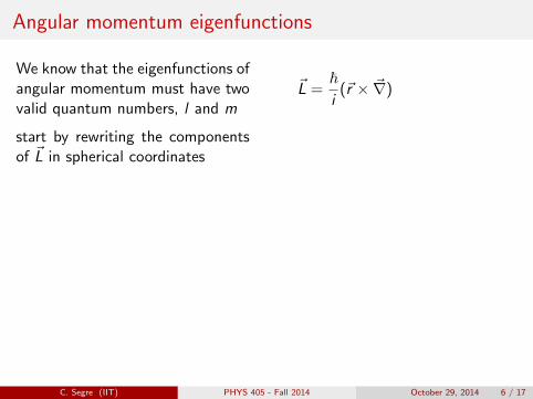
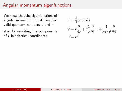
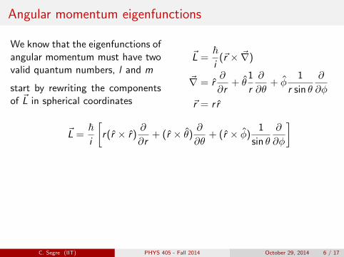
Angular momentum eigenfunctions
We know that the eigenfunctions ofangular momentum must have twovalid quantum numbers, l and m
start by rewriting the componentsof ~L in spherical coordinates
~L =~i
(~r × ~∇)
~∇ = r∂
∂r+ θ
1
r
∂
∂θ+ φ
1
r sin θ
∂
∂φ
~r = r r
~L =~i
[r(r × r)
∂
∂r+ (r × θ)
∂
∂θ+ (r × φ)
1
sin θ
∂
∂φ
]
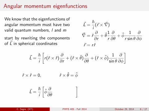
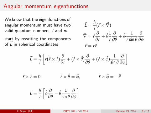
r × r = 0, r × θ = φ, r × φ = −θ
~L =~i
[
φ∂
∂θ− θ 1
sin θ
∂
∂φ
]
C. Segre (IIT) PHYS 405 - Fall 2014 October 29, 2014 6 / 17
Angular momentum eigenfunctions
We know that the eigenfunctions ofangular momentum must have twovalid quantum numbers, l and m
start by rewriting the componentsof ~L in spherical coordinates
~L =~i
(~r × ~∇)
~∇ = r∂
∂r+ θ
1
r
∂
∂θ+ φ
1
r sin θ
∂
∂φ
~r = r r
~L =~i
[r(r × r)
∂
∂r+ (r × θ)
∂
∂θ+ (r × φ)
1
sin θ
∂
∂φ
]
r × r = 0, r × θ = φ, r × φ = −θ
~L =~i
[
φ∂
∂θ− θ 1
sin θ
∂
∂φ
]
C. Segre (IIT) PHYS 405 - Fall 2014 October 29, 2014 6 / 17
Angular momentum eigenfunctions
We know that the eigenfunctions ofangular momentum must have twovalid quantum numbers, l and m
start by rewriting the componentsof ~L in spherical coordinates
~L =~i
(~r × ~∇)
~∇ = r∂
∂r+ θ
1
r
∂
∂θ+ φ
1
r sin θ
∂
∂φ
~r = r r
~L =~i
[r(r × r)
∂
∂r+ (r × θ)
∂
∂θ+ (r × φ)
1
sin θ
∂
∂φ
]
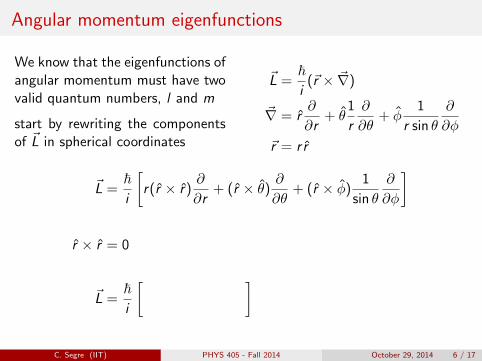
r × r = 0
, r × θ = φ, r × φ = −θ
~L =~i
[
φ∂
∂θ− θ 1
sin θ
∂
∂φ
]
C. Segre (IIT) PHYS 405 - Fall 2014 October 29, 2014 6 / 17
Angular momentum eigenfunctions
We know that the eigenfunctions ofangular momentum must have twovalid quantum numbers, l and m
start by rewriting the componentsof ~L in spherical coordinates
~L =~i
(~r × ~∇)
~∇ = r∂
∂r+ θ
1
r
∂
∂θ+ φ
1
r sin θ
∂
∂φ
~r = r r
~L =~i
[r(r × r)
∂
∂r+ (r × θ)
∂
∂θ+ (r × φ)
1
sin θ
∂
∂φ
]
r × r = 0, r × θ = φ
, r × φ = −θ
~L =~i
[φ∂
∂θ
− θ 1
sin θ
∂
∂φ
]
C. Segre (IIT) PHYS 405 - Fall 2014 October 29, 2014 6 / 17
Angular momentum eigenfunctions
We know that the eigenfunctions ofangular momentum must have twovalid quantum numbers, l and m
start by rewriting the componentsof ~L in spherical coordinates
~L =~i
(~r × ~∇)
~∇ = r∂
∂r+ θ
1
r
∂
∂θ+ φ
1
r sin θ
∂
∂φ
~r = r r
~L =~i
[r(r × r)
∂
∂r+ (r × θ)
∂
∂θ+ (r × φ)
1
sin θ
∂
∂φ
]
r × r = 0, r × θ = φ, r × φ = −θ
~L =~i
[φ∂
∂θ− θ 1
sin θ
∂
∂φ
]
C. Segre (IIT) PHYS 405 - Fall 2014 October 29, 2014 6 / 17
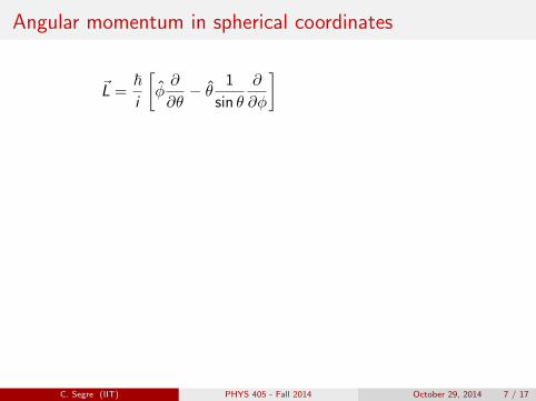
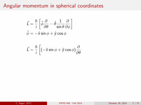
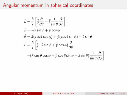
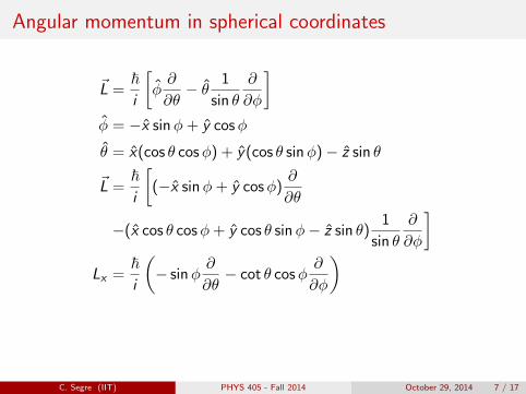
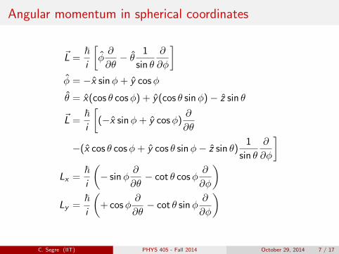
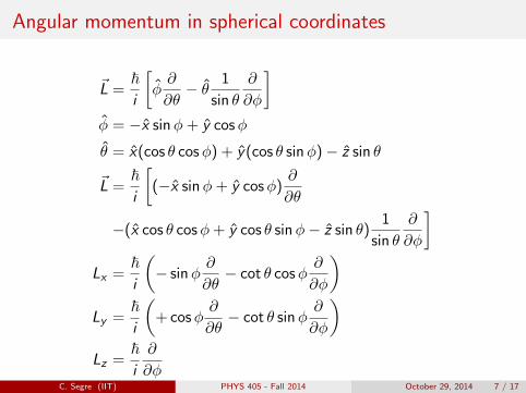
Angular momentum in spherical coordinates
~L =~i
[φ∂
∂θ− θ 1
sin θ
∂
∂φ
]
φ = −x sinφ+ y cosφ
θ = x(cos θ cosφ) + y(cos θ sinφ)− z sin θ
~L =~i
[(−x sinφ+ y cosφ)
∂
∂θ
−(x cos θ cosφ+ y cos θ sinφ− z sin θ)1
sin θ
∂
∂φ
]Lx =
~i
(− sinφ
∂
∂θ− cot θ cosφ
∂
∂φ
)Ly =
~i
(+ cosφ
∂
∂θ− cot θ sinφ
∂
∂φ
)Lz =
~i
∂
∂φ
C. Segre (IIT) PHYS 405 - Fall 2014 October 29, 2014 7 / 17
Angular momentum in spherical coordinates
~L =~i
[φ∂
∂θ− θ 1
sin θ
∂
∂φ
]φ = −x sinφ+ y cosφ
θ = x(cos θ cosφ) + y(cos θ sinφ)− z sin θ
~L =~i
[(−x sinφ+ y cosφ)
∂
∂θ
−(x cos θ cosφ+ y cos θ sinφ− z sin θ)1
sin θ
∂
∂φ
]
Lx =~i
(− sinφ
∂
∂θ− cot θ cosφ
∂
∂φ
)Ly =
~i
(+ cosφ
∂
∂θ− cot θ sinφ
∂
∂φ
)Lz =
~i
∂
∂φ
C. Segre (IIT) PHYS 405 - Fall 2014 October 29, 2014 7 / 17
Angular momentum in spherical coordinates
~L =~i
[φ∂
∂θ− θ 1
sin θ
∂
∂φ
]φ = −x sinφ+ y cosφ
θ = x(cos θ cosφ) + y(cos θ sinφ)− z sin θ
~L =~i
[(−x sinφ+ y cosφ)
∂
∂θ
−(x cos θ cosφ+ y cos θ sinφ− z sin θ)1
sin θ
∂
∂φ
]Lx =
~i
(− sinφ
∂
∂θ− cot θ cosφ
∂
∂φ
)
Ly =~i
(+ cosφ
∂
∂θ− cot θ sinφ
∂
∂φ
)Lz =
~i
∂
∂φ
C. Segre (IIT) PHYS 405 - Fall 2014 October 29, 2014 7 / 17
Angular momentum in spherical coordinates
~L =~i
[φ∂
∂θ− θ 1
sin θ
∂
∂φ
]φ = −x sinφ+ y cosφ
θ = x(cos θ cosφ) + y(cos θ sinφ)− z sin θ
~L =~i
[(−x sinφ+ y cosφ)
∂
∂θ
−(x cos θ cosφ+ y cos θ sinφ− z sin θ)1
sin θ
∂
∂φ
]Lx =
~i
(− sinφ
∂
∂θ− cot θ cosφ
∂
∂φ
)Ly =
~i
(+ cosφ
∂
∂θ− cot θ sinφ
∂
∂φ
)
Lz =~i
∂
∂φ
C. Segre (IIT) PHYS 405 - Fall 2014 October 29, 2014 7 / 17
Angular momentum in spherical coordinates
~L =~i
[φ∂
∂θ− θ 1
sin θ
∂
∂φ
]φ = −x sinφ+ y cosφ
θ = x(cos θ cosφ) + y(cos θ sinφ)− z sin θ
~L =~i
[(−x sinφ+ y cosφ)
∂
∂θ
−(x cos θ cosφ+ y cos θ sinφ− z sin θ)1
sin θ
∂
∂φ
]Lx =
~i
(− sinφ
∂
∂θ− cot θ cosφ
∂
∂φ
)Ly =
~i
(+ cosφ
∂
∂θ− cot θ sinφ
∂
∂φ
)Lz =
~i
∂
∂φC. Segre (IIT) PHYS 405 - Fall 2014 October 29, 2014 7 / 17
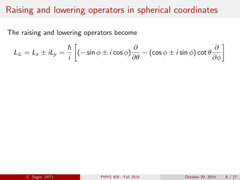
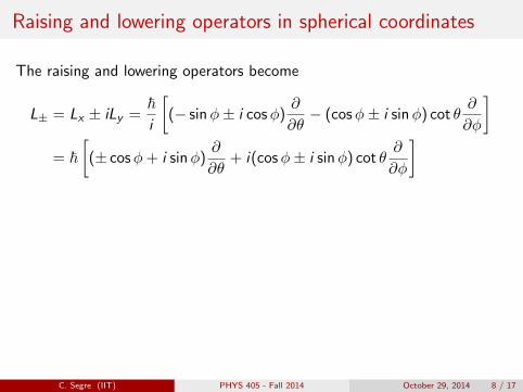
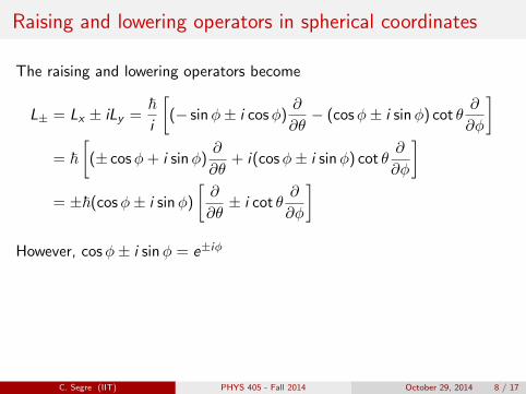
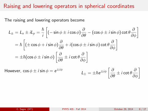
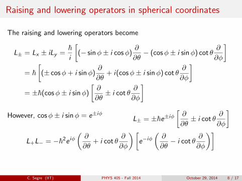
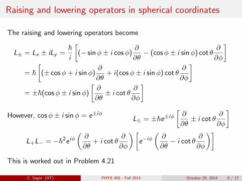
Raising and lowering operators in spherical coordinates
The raising and lowering operators become
L± = Lx ± iLy
=~i
[(− sinφ± i cosφ)
∂
∂θ− (cosφ± i sinφ) cot θ
∂
∂φ
]= ~
[(± cosφ+ i sinφ)
∂
∂θ+ i(cosφ± i sinφ) cot θ
∂
∂φ
]= ±~(cosφ± i sinφ)
[∂
∂θ± i cot θ
∂
∂φ
]
However, cosφ± i sinφ = e±iφL± = ±~e±iφ
[∂
∂θ± i cot θ
∂
∂φ
]L+L− = −~2e iφ
(∂
∂θ+ i cot θ
∂
∂φ
)[e−iφ
(∂
∂θ− i cot θ
∂
∂φ
)]This is worked out in Problem 4.21
C. Segre (IIT) PHYS 405 - Fall 2014 October 29, 2014 8 / 17

Raising and lowering operators in spherical coordinates
The raising and lowering operators become
L± = Lx ± iLy
=~i
[(− sinφ± i cosφ)
∂
∂θ− (cosφ± i sinφ) cot θ
∂
∂φ
]= ~
[(± cosφ+ i sinφ)
∂
∂θ+ i(cosφ± i sinφ) cot θ
∂
∂φ
]= ±~(cosφ± i sinφ)
[∂
∂θ± i cot θ
∂
∂φ
]However, cosφ± i sinφ = e±iφ
L± = ±~e±iφ
[∂
∂θ± i cot θ
∂
∂φ
]L+L− = −~2e iφ
(∂
∂θ+ i cot θ
∂
∂φ
)[e−iφ
(∂
∂θ− i cot θ
∂
∂φ
)]This is worked out in Problem 4.21
C. Segre (IIT) PHYS 405 - Fall 2014 October 29, 2014 8 / 17
Raising and lowering operators in spherical coordinates
The raising and lowering operators become
L± = Lx ± iLy =~i
[(− sinφ± i cosφ)
∂
∂θ− (cosφ± i sinφ) cot θ
∂
∂φ
]
= ~[
(± cosφ+ i sinφ)∂
∂θ+ i(cosφ± i sinφ) cot θ
∂
∂φ
]= ±~(cosφ± i sinφ)
[∂
∂θ± i cot θ
∂
∂φ
]However, cosφ± i sinφ = e±iφ
L± = ±~e±iφ
[∂
∂θ± i cot θ
∂
∂φ
]L+L− = −~2e iφ
(∂
∂θ+ i cot θ
∂
∂φ
)[e−iφ
(∂
∂θ− i cot θ
∂
∂φ
)]This is worked out in Problem 4.21
C. Segre (IIT) PHYS 405 - Fall 2014 October 29, 2014 8 / 17
Raising and lowering operators in spherical coordinates
The raising and lowering operators become
L± = Lx ± iLy =~i
[(− sinφ± i cosφ)
∂
∂θ− (cosφ± i sinφ) cot θ
∂
∂φ
]= ~
[(± cosφ+ i sinφ)
∂
∂θ+ i(cosφ± i sinφ) cot θ
∂
∂φ
]
= ±~(cosφ± i sinφ)
[∂
∂θ± i cot θ
∂
∂φ
]However, cosφ± i sinφ = e±iφ
L± = ±~e±iφ
[∂
∂θ± i cot θ
∂
∂φ
]L+L− = −~2e iφ
(∂
∂θ+ i cot θ
∂
∂φ
)[e−iφ
(∂
∂θ− i cot θ
∂
∂φ
)]This is worked out in Problem 4.21
C. Segre (IIT) PHYS 405 - Fall 2014 October 29, 2014 8 / 17

Raising and lowering operators in spherical coordinates
The raising and lowering operators become
L± = Lx ± iLy =~i
[(− sinφ± i cosφ)
∂
∂θ− (cosφ± i sinφ) cot θ
∂
∂φ
]= ~
[(± cosφ+ i sinφ)
∂
∂θ+ i(cosφ± i sinφ) cot θ
∂
∂φ
]= ±~(cosφ± i sinφ)
[∂
∂θ± i cot θ
∂
∂φ
]
However, cosφ± i sinφ = e±iφL± = ±~e±iφ
[∂
∂θ± i cot θ
∂
∂φ
]L+L− = −~2e iφ
(∂
∂θ+ i cot θ
∂
∂φ
)[e−iφ
(∂
∂θ− i cot θ
∂
∂φ
)]This is worked out in Problem 4.21
C. Segre (IIT) PHYS 405 - Fall 2014 October 29, 2014 8 / 17
Raising and lowering operators in spherical coordinates
The raising and lowering operators become
L± = Lx ± iLy =~i
[(− sinφ± i cosφ)
∂
∂θ− (cosφ± i sinφ) cot θ
∂
∂φ
]= ~
[(± cosφ+ i sinφ)
∂
∂θ+ i(cosφ± i sinφ) cot θ
∂
∂φ
]= ±~(cosφ± i sinφ)
[∂
∂θ± i cot θ
∂
∂φ
]However, cosφ± i sinφ = e±iφ
L± = ±~e±iφ
[∂
∂θ± i cot θ
∂
∂φ
]L+L− = −~2e iφ
(∂
∂θ+ i cot θ
∂
∂φ
)[e−iφ
(∂
∂θ− i cot θ
∂
∂φ
)]This is worked out in Problem 4.21
C. Segre (IIT) PHYS 405 - Fall 2014 October 29, 2014 8 / 17
Raising and lowering operators in spherical coordinates
The raising and lowering operators become
L± = Lx ± iLy =~i
[(− sinφ± i cosφ)
∂
∂θ− (cosφ± i sinφ) cot θ
∂
∂φ
]= ~
[(± cosφ+ i sinφ)
∂
∂θ+ i(cosφ± i sinφ) cot θ
∂
∂φ
]= ±~(cosφ± i sinφ)
[∂
∂θ± i cot θ
∂
∂φ
]However, cosφ± i sinφ = e±iφ
L± = ±~e±iφ
[∂
∂θ± i cot θ
∂
∂φ
]
L+L− = −~2e iφ(∂
∂θ+ i cot θ
∂
∂φ
)[e−iφ
(∂
∂θ− i cot θ
∂
∂φ
)]This is worked out in Problem 4.21
C. Segre (IIT) PHYS 405 - Fall 2014 October 29, 2014 8 / 17
Raising and lowering operators in spherical coordinates
The raising and lowering operators become
L± = Lx ± iLy =~i
[(− sinφ± i cosφ)
∂
∂θ− (cosφ± i sinφ) cot θ
∂
∂φ
]= ~
[(± cosφ+ i sinφ)
∂
∂θ+ i(cosφ± i sinφ) cot θ
∂
∂φ
]= ±~(cosφ± i sinφ)
[∂
∂θ± i cot θ
∂
∂φ
]However, cosφ± i sinφ = e±iφ
L± = ±~e±iφ
[∂
∂θ± i cot θ
∂
∂φ
]L+L− = −~2e iφ
(∂
∂θ+ i cot θ
∂
∂φ
)[e−iφ
(∂
∂θ− i cot θ
∂
∂φ
)]
This is worked out in Problem 4.21
C. Segre (IIT) PHYS 405 - Fall 2014 October 29, 2014 8 / 17
Raising and lowering operators in spherical coordinates
The raising and lowering operators become
L± = Lx ± iLy =~i
[(− sinφ± i cosφ)
∂
∂θ− (cosφ± i sinφ) cot θ
∂
∂φ
]= ~
[(± cosφ+ i sinφ)
∂
∂θ+ i(cosφ± i sinφ) cot θ
∂
∂φ
]= ±~(cosφ± i sinφ)
[∂
∂θ± i cot θ
∂
∂φ
]However, cosφ± i sinφ = e±iφ
L± = ±~e±iφ
[∂
∂θ± i cot θ
∂
∂φ
]L+L− = −~2e iφ
(∂
∂θ+ i cot θ
∂
∂φ
)[e−iφ
(∂
∂θ− i cot θ
∂
∂φ
)]This is worked out in Problem 4.21
C. Segre (IIT) PHYS 405 - Fall 2014 October 29, 2014 8 / 17
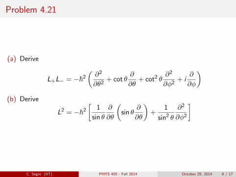
Problem 4.21
(a) Derive
L+L− = −~2(∂2
∂θ2+ cot θ
∂
∂θ+ cot2 θ
∂2
∂φ2+ i
∂
∂φ
)(b) Derive
L2 = −~2[
1
sin θ
∂
∂θ
(sin θ
∂
∂θ
)+
1
sin2 θ
∂2
∂φ2
]
C. Segre (IIT) PHYS 405 - Fall 2014 October 29, 2014 9 / 17

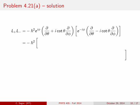
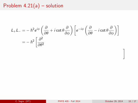
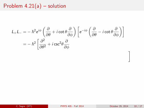
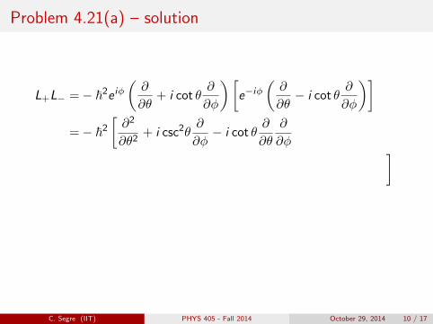
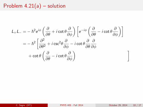
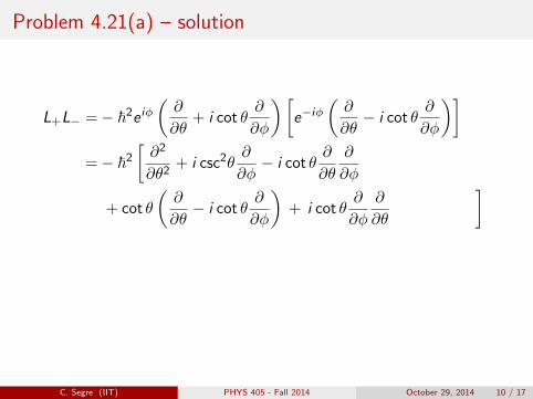
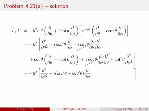
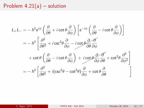
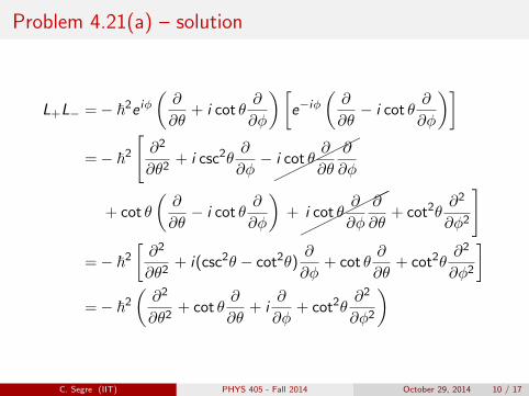
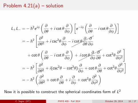
Problem 4.21(a) – solution
L+L− =− ~2e iφ(∂
∂θ+ i cot θ
∂
∂φ
)[e−iφ
(∂
∂θ− i cot θ
∂
∂φ
)]
=− ~2[
∂2
∂θ2+ i csc2θ
∂
∂φ− i cot θ
∂
∂θ
∂
∂φ
+ cot θ
(∂
∂θ− i cot θ
∂
∂φ
)+ i cot θ
∂
∂φ
∂
∂θ+ cot2θ
∂2
∂φ2
]=− ~2
[
∂2
∂θ2+ i(csc2θ − cot2θ)
∂
∂φ+ cot θ
∂
∂θ+ cot2θ
∂2
∂φ2
]=− ~2
(∂2
∂θ2+ cot θ
∂
∂θ+ i
∂
∂φ+ cot2θ
∂2
∂φ2
)Now it is possible to construct the spherical coordinates form of L2
C. Segre (IIT) PHYS 405 - Fall 2014 October 29, 2014 10 / 17
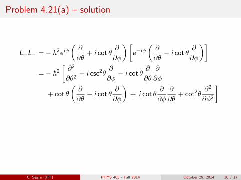
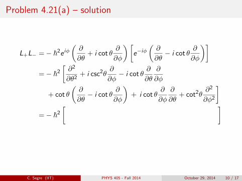
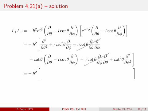
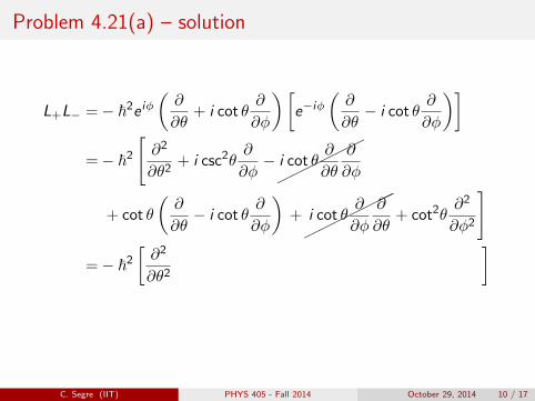
Problem 4.21(a) – solution
L+L− =− ~2e iφ(∂
∂θ+ i cot θ
∂
∂φ
)[e−iφ
(∂
∂θ− i cot θ
∂
∂φ
)]=− ~2
[
∂2
∂θ2+ i csc2θ
∂
∂φ− i cot θ
∂
∂θ
∂
∂φ
+ cot θ
(∂
∂θ− i cot θ
∂
∂φ
)+ i cot θ
∂
∂φ
∂
∂θ+ cot2θ
∂2
∂φ2
]
=− ~2[
∂2
∂θ2+ i(csc2θ − cot2θ)
∂
∂φ+ cot θ
∂
∂θ+ cot2θ
∂2
∂φ2
]=− ~2
(∂2
∂θ2+ cot θ
∂
∂θ+ i
∂
∂φ+ cot2θ
∂2
∂φ2
)Now it is possible to construct the spherical coordinates form of L2
C. Segre (IIT) PHYS 405 - Fall 2014 October 29, 2014 10 / 17
Problem 4.21(a) – solution
L+L− =− ~2e iφ(∂
∂θ+ i cot θ
∂
∂φ
)[e−iφ
(∂
∂θ− i cot θ
∂
∂φ
)]=− ~2
[∂2
∂θ2
+ i csc2θ∂
∂φ− i cot θ
∂
∂θ
∂
∂φ
+ cot θ
(∂
∂θ− i cot θ
∂
∂φ
)+ i cot θ
∂
∂φ
∂
∂θ+ cot2θ
∂2
∂φ2
]
=− ~2[
∂2
∂θ2+ i(csc2θ − cot2θ)
∂
∂φ+ cot θ
∂
∂θ+ cot2θ
∂2
∂φ2
]=− ~2
(∂2
∂θ2+ cot θ
∂
∂θ+ i
∂
∂φ+ cot2θ
∂2
∂φ2
)Now it is possible to construct the spherical coordinates form of L2
C. Segre (IIT) PHYS 405 - Fall 2014 October 29, 2014 10 / 17
Problem 4.21(a) – solution
L+L− =− ~2e iφ(∂
∂θ+ i cot θ
∂
∂φ
)[e−iφ
(∂
∂θ− i cot θ
∂
∂φ
)]=− ~2
[∂2
∂θ2+ i csc2θ
∂
∂φ
− i cot θ∂
∂θ
∂
∂φ
+ cot θ
(∂
∂θ− i cot θ
∂
∂φ
)+ i cot θ
∂
∂φ
∂
∂θ+ cot2θ
∂2
∂φ2
]
=− ~2[
∂2
∂θ2+ i(csc2θ − cot2θ)
∂
∂φ+ cot θ
∂
∂θ+ cot2θ
∂2
∂φ2
]=− ~2
(∂2
∂θ2+ cot θ
∂
∂θ+ i
∂
∂φ+ cot2θ
∂2
∂φ2
)Now it is possible to construct the spherical coordinates form of L2
C. Segre (IIT) PHYS 405 - Fall 2014 October 29, 2014 10 / 17
Problem 4.21(a) – solution
L+L− =− ~2e iφ(∂
∂θ+ i cot θ
∂
∂φ
)[e−iφ
(∂
∂θ− i cot θ
∂
∂φ
)]=− ~2
[∂2
∂θ2+ i csc2θ
∂
∂φ− i cot θ
∂
∂θ
∂
∂φ
+ cot θ
(∂
∂θ− i cot θ
∂
∂φ
)+ i cot θ
∂
∂φ
∂
∂θ+ cot2θ
∂2
∂φ2
]
=− ~2[
∂2
∂θ2+ i(csc2θ − cot2θ)
∂
∂φ+ cot θ
∂
∂θ+ cot2θ
∂2
∂φ2
]=− ~2
(∂2
∂θ2+ cot θ
∂
∂θ+ i
∂
∂φ+ cot2θ
∂2
∂φ2
)Now it is possible to construct the spherical coordinates form of L2
C. Segre (IIT) PHYS 405 - Fall 2014 October 29, 2014 10 / 17
Problem 4.21(a) – solution
L+L− =− ~2e iφ(∂
∂θ+ i cot θ
∂
∂φ
)[e−iφ
(∂
∂θ− i cot θ
∂
∂φ
)]=− ~2
[∂2
∂θ2+ i csc2θ
∂
∂φ− i cot θ
∂
∂θ
∂
∂φ
+ cot θ
(∂
∂θ− i cot θ
∂
∂φ
)
+ i cot θ∂
∂φ
∂
∂θ+ cot2θ
∂2
∂φ2
]
=− ~2[
∂2
∂θ2+ i(csc2θ − cot2θ)
∂
∂φ+ cot θ
∂
∂θ+ cot2θ
∂2
∂φ2
]=− ~2
(∂2
∂θ2+ cot θ
∂
∂θ+ i
∂
∂φ+ cot2θ
∂2
∂φ2
)Now it is possible to construct the spherical coordinates form of L2
C. Segre (IIT) PHYS 405 - Fall 2014 October 29, 2014 10 / 17
Problem 4.21(a) – solution
L+L− =− ~2e iφ(∂
∂θ+ i cot θ
∂
∂φ
)[e−iφ
(∂
∂θ− i cot θ
∂
∂φ
)]=− ~2
[∂2
∂θ2+ i csc2θ
∂
∂φ− i cot θ
∂
∂θ
∂
∂φ
+ cot θ
(∂
∂θ− i cot θ
∂
∂φ
)+ i cot θ
∂
∂φ
∂
∂θ
+ cot2θ∂2
∂φ2
]
=− ~2[
∂2
∂θ2+ i(csc2θ − cot2θ)
∂
∂φ+ cot θ
∂
∂θ+ cot2θ
∂2
∂φ2
]=− ~2
(∂2
∂θ2+ cot θ
∂
∂θ+ i
∂
∂φ+ cot2θ
∂2
∂φ2
)Now it is possible to construct the spherical coordinates form of L2
C. Segre (IIT) PHYS 405 - Fall 2014 October 29, 2014 10 / 17
Problem 4.21(a) – solution
L+L− =− ~2e iφ(∂
∂θ+ i cot θ
∂
∂φ
)[e−iφ
(∂
∂θ− i cot θ
∂
∂φ
)]=− ~2
[∂2
∂θ2+ i csc2θ
∂
∂φ− i cot θ
∂
∂θ
∂
∂φ
+ cot θ
(∂
∂θ− i cot θ
∂
∂φ
)+ i cot θ
∂
∂φ
∂
∂θ+ cot2θ
∂2
∂φ2
]=− ~2
[
∂2
∂θ2+ i(csc2θ − cot2θ)
∂
∂φ+ cot θ
∂
∂θ+ cot2θ
∂2
∂φ2
]
=− ~2(∂2
∂θ2+ cot θ
∂
∂θ+ i
∂
∂φ+ cot2θ
∂2
∂φ2
)Now it is possible to construct the spherical coordinates form of L2
C. Segre (IIT) PHYS 405 - Fall 2014 October 29, 2014 10 / 17
Problem 4.21(a) – solution
L+L− =− ~2e iφ(∂
∂θ+ i cot θ
∂
∂φ
)[e−iφ
(∂
∂θ− i cot θ
∂
∂φ
)]=− ~2
[∂2
∂θ2+ i csc2θ
∂
∂φ−����
��i cot θ
∂
∂θ
∂
∂φ
+ cot θ
(∂
∂θ− i cot θ
∂
∂φ
)+����
���
i cot θ∂
∂φ
∂
∂θ+ cot2θ
∂2
∂φ2
]
=− ~2[
∂2
∂θ2+ i(csc2θ − cot2θ)
∂
∂φ+ cot θ
∂
∂θ+ cot2θ
∂2
∂φ2
]
=− ~2(∂2
∂θ2+ cot θ
∂
∂θ+ i
∂
∂φ+ cot2θ
∂2
∂φ2
)Now it is possible to construct the spherical coordinates form of L2
C. Segre (IIT) PHYS 405 - Fall 2014 October 29, 2014 10 / 17
Problem 4.21(a) – solution
L+L− =− ~2e iφ(∂
∂θ+ i cot θ
∂
∂φ
)[e−iφ
(∂
∂θ− i cot θ
∂
∂φ
)]=− ~2
[∂2
∂θ2+ i csc2θ
∂
∂φ−����
��i cot θ
∂
∂θ
∂
∂φ
+ cot θ
(∂
∂θ− i cot θ
∂
∂φ
)+����
���
i cot θ∂
∂φ
∂
∂θ+ cot2θ
∂2
∂φ2
]
=− ~2[∂2
∂θ2
+ i(csc2θ − cot2θ)∂
∂φ+ cot θ
∂
∂θ+ cot2θ
∂2
∂φ2
]
=− ~2(∂2
∂θ2+ cot θ
∂
∂θ+ i
∂
∂φ+ cot2θ
∂2
∂φ2
)Now it is possible to construct the spherical coordinates form of L2
C. Segre (IIT) PHYS 405 - Fall 2014 October 29, 2014 10 / 17
Problem 4.21(a) – solution
L+L− =− ~2e iφ(∂
∂θ+ i cot θ
∂
∂φ
)[e−iφ
(∂
∂θ− i cot θ
∂
∂φ
)]=− ~2
[∂2
∂θ2+ i csc2θ
∂
∂φ−����
��i cot θ
∂
∂θ
∂
∂φ
+ cot θ
(∂
∂θ− i cot θ
∂
∂φ
)+����
���
i cot θ∂
∂φ
∂
∂θ+ cot2θ
∂2
∂φ2
]
=− ~2[∂2
∂θ2+ i(csc2θ − cot2θ)
∂
∂φ
+ cot θ∂
∂θ+ cot2θ
∂2
∂φ2
]
=− ~2(∂2
∂θ2+ cot θ
∂
∂θ+ i
∂
∂φ+ cot2θ
∂2
∂φ2
)Now it is possible to construct the spherical coordinates form of L2
C. Segre (IIT) PHYS 405 - Fall 2014 October 29, 2014 10 / 17
Problem 4.21(a) – solution
L+L− =− ~2e iφ(∂
∂θ+ i cot θ
∂
∂φ
)[e−iφ
(∂
∂θ− i cot θ
∂
∂φ
)]=− ~2
[∂2
∂θ2+ i csc2θ
∂
∂φ−����
��i cot θ
∂
∂θ
∂
∂φ
+ cot θ
(∂
∂θ− i cot θ
∂
∂φ
)+����
���
i cot θ∂
∂φ
∂
∂θ+ cot2θ
∂2
∂φ2
]
=− ~2[∂2
∂θ2+ i(csc2θ − cot2θ)
∂
∂φ+ cot θ
∂
∂θ
+ cot2θ∂2
∂φ2
]
=− ~2(∂2
∂θ2+ cot θ
∂
∂θ+ i
∂
∂φ+ cot2θ
∂2
∂φ2
)Now it is possible to construct the spherical coordinates form of L2
C. Segre (IIT) PHYS 405 - Fall 2014 October 29, 2014 10 / 17

Problem 4.21(a) – solution
L+L− =− ~2e iφ(∂
∂θ+ i cot θ
∂
∂φ
)[e−iφ
(∂
∂θ− i cot θ
∂
∂φ
)]=− ~2
[∂2
∂θ2+ i csc2θ
∂
∂φ−����
��i cot θ
∂
∂θ
∂
∂φ
+ cot θ
(∂
∂θ− i cot θ
∂
∂φ
)+����
���
i cot θ∂
∂φ
∂
∂θ+ cot2θ
∂2
∂φ2
]
=− ~2[∂2
∂θ2+ i(csc2θ − cot2θ)
∂
∂φ+ cot θ
∂
∂θ+ cot2θ
∂2
∂φ2
]
=− ~2(∂2
∂θ2+ cot θ
∂
∂θ+ i
∂
∂φ+ cot2θ
∂2
∂φ2
)Now it is possible to construct the spherical coordinates form of L2
C. Segre (IIT) PHYS 405 - Fall 2014 October 29, 2014 10 / 17
Problem 4.21(a) – solution
L+L− =− ~2e iφ(∂
∂θ+ i cot θ
∂
∂φ
)[e−iφ
(∂
∂θ− i cot θ
∂
∂φ
)]=− ~2
[∂2
∂θ2+ i csc2θ
∂
∂φ−����
��i cot θ
∂
∂θ
∂
∂φ
+ cot θ
(∂
∂θ− i cot θ
∂
∂φ
)+����
���
i cot θ∂
∂φ
∂
∂θ+ cot2θ
∂2
∂φ2
]
=− ~2[∂2
∂θ2+ i(csc2θ − cot2θ)
∂
∂φ+ cot θ
∂
∂θ+ cot2θ
∂2
∂φ2
]=− ~2
(∂2
∂θ2+ cot θ
∂
∂θ+ i
∂
∂φ+ cot2θ
∂2
∂φ2
)
Now it is possible to construct the spherical coordinates form of L2
C. Segre (IIT) PHYS 405 - Fall 2014 October 29, 2014 10 / 17
Problem 4.21(a) – solution
L+L− =− ~2e iφ(∂
∂θ+ i cot θ
∂
∂φ
)[e−iφ
(∂
∂θ− i cot θ
∂
∂φ
)]=− ~2
[∂2
∂θ2+ i csc2θ
∂
∂φ−����
��i cot θ
∂
∂θ
∂
∂φ
+ cot θ
(∂
∂θ− i cot θ
∂
∂φ
)+����
���
i cot θ∂
∂φ
∂
∂θ+ cot2θ
∂2
∂φ2
]
=− ~2[∂2
∂θ2+ i(csc2θ − cot2θ)
∂
∂φ+ cot θ
∂
∂θ+ cot2θ
∂2
∂φ2
]=− ~2
(∂2
∂θ2+ cot θ
∂
∂θ+ i
∂
∂φ+ cot2θ
∂2
∂φ2
)Now it is possible to construct the spherical coordinates form of L2
C. Segre (IIT) PHYS 405 - Fall 2014 October 29, 2014 10 / 17

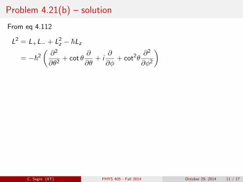
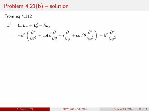
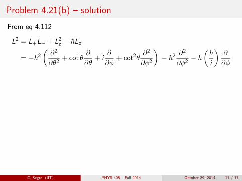
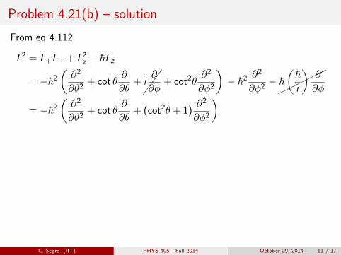
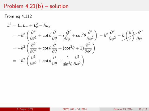
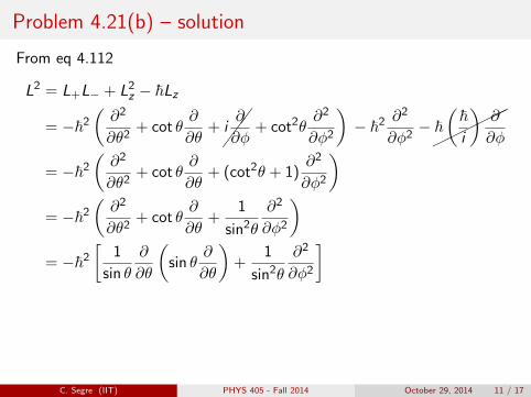
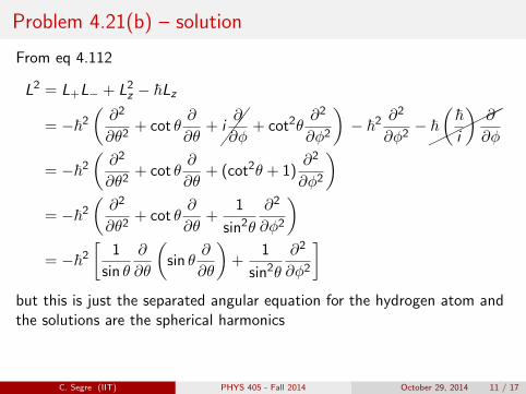
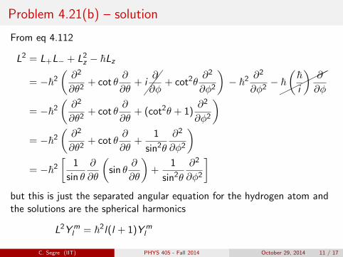
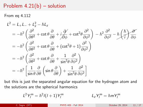
Problem 4.21(b) – solution
From eq 4.112
L2 = L+L− + L2z − ~Lz
= −~2(∂2
∂θ2+ cot θ
∂
∂θ+ i
∂
∂φ+ cot2θ
∂2
∂φ2
)
− ~2∂2
∂φ2− ~
(~i
)∂
∂φ
= −~2(∂2
∂θ2+ cot θ
∂
∂θ+ (cot2θ + 1)
∂2
∂φ2
)= −~2
(∂2
∂θ2+ cot θ
∂
∂θ+
1
sin2θ
∂2
∂φ2
)= −~2
[1
sin θ
∂
∂θ
(sin θ
∂
∂θ
)+
1
sin2θ
∂2
∂φ2
]but this is just the separated angular equation for the hydrogen atom andthe solutions are the spherical harmonics
L2Yml = ~2l(l + 1)Ym
l
LzYml = ~mYm
l
C. Segre (IIT) PHYS 405 - Fall 2014 October 29, 2014 11 / 17
Problem 4.21(b) – solution
From eq 4.112
L2 = L+L− + L2z − ~Lz
= −~2(∂2
∂θ2+ cot θ
∂
∂θ+ i
∂
∂φ+ cot2θ
∂2
∂φ2
)− ~2
∂2
∂φ2
− ~(~i
)∂
∂φ
= −~2(∂2
∂θ2+ cot θ
∂
∂θ+ (cot2θ + 1)
∂2
∂φ2
)= −~2
(∂2
∂θ2+ cot θ
∂
∂θ+
1
sin2θ
∂2
∂φ2
)= −~2
[1
sin θ
∂
∂θ
(sin θ
∂
∂θ
)+
1
sin2θ
∂2
∂φ2
]but this is just the separated angular equation for the hydrogen atom andthe solutions are the spherical harmonics
L2Yml = ~2l(l + 1)Ym
l
LzYml = ~mYm
l
C. Segre (IIT) PHYS 405 - Fall 2014 October 29, 2014 11 / 17
Problem 4.21(b) – solution
From eq 4.112
L2 = L+L− + L2z − ~Lz
= −~2(∂2
∂θ2+ cot θ
∂
∂θ+ i
∂
∂φ+ cot2θ
∂2
∂φ2
)− ~2
∂2
∂φ2− ~
(~i
)∂
∂φ
= −~2(∂2
∂θ2+ cot θ
∂
∂θ+ (cot2θ + 1)
∂2
∂φ2
)= −~2
(∂2
∂θ2+ cot θ
∂
∂θ+
1
sin2θ
∂2
∂φ2
)= −~2
[1
sin θ
∂
∂θ
(sin θ
∂
∂θ
)+
1
sin2θ
∂2
∂φ2
]but this is just the separated angular equation for the hydrogen atom andthe solutions are the spherical harmonics
L2Yml = ~2l(l + 1)Ym
l
LzYml = ~mYm
l
C. Segre (IIT) PHYS 405 - Fall 2014 October 29, 2014 11 / 17

Problem 4.21(b) – solution
From eq 4.112
L2 = L+L− + L2z − ~Lz
= −~2(∂2
∂θ2+ cot θ
∂
∂θ+
���
i∂
∂φ+ cot2θ
∂2
∂φ2
)− ~2
∂2
∂φ2−��
����~(~i
)∂
∂φ
= −~2(∂2
∂θ2+ cot θ
∂
∂θ+ (cot2θ + 1)
∂2
∂φ2
)= −~2
(∂2
∂θ2+ cot θ
∂
∂θ+
1
sin2θ
∂2
∂φ2
)= −~2
[1
sin θ
∂
∂θ
(sin θ
∂
∂θ
)+
1
sin2θ
∂2
∂φ2
]but this is just the separated angular equation for the hydrogen atom andthe solutions are the spherical harmonics
L2Yml = ~2l(l + 1)Ym
l
LzYml = ~mYm
l
C. Segre (IIT) PHYS 405 - Fall 2014 October 29, 2014 11 / 17
Problem 4.21(b) – solution
From eq 4.112
L2 = L+L− + L2z − ~Lz
= −~2(∂2
∂θ2+ cot θ
∂
∂θ+
���
i∂
∂φ+ cot2θ
∂2
∂φ2
)− ~2
∂2
∂φ2−��
����~(~i
)∂
∂φ
= −~2(∂2
∂θ2+ cot θ
∂
∂θ+ (cot2θ + 1)
∂2
∂φ2
)
= −~2(∂2
∂θ2+ cot θ
∂
∂θ+
1
sin2θ
∂2
∂φ2
)= −~2
[1
sin θ
∂
∂θ
(sin θ
∂
∂θ
)+
1
sin2θ
∂2
∂φ2
]but this is just the separated angular equation for the hydrogen atom andthe solutions are the spherical harmonics
L2Yml = ~2l(l + 1)Ym
l
LzYml = ~mYm
l
C. Segre (IIT) PHYS 405 - Fall 2014 October 29, 2014 11 / 17
Problem 4.21(b) – solution
From eq 4.112
L2 = L+L− + L2z − ~Lz
= −~2(∂2
∂θ2+ cot θ
∂
∂θ+
���
i∂
∂φ+ cot2θ
∂2
∂φ2
)− ~2
∂2
∂φ2−��
����~(~i
)∂
∂φ
= −~2(∂2
∂θ2+ cot θ
∂
∂θ+ (cot2θ + 1)
∂2
∂φ2
)= −~2
(∂2
∂θ2+ cot θ
∂
∂θ+
1
sin2θ
∂2
∂φ2
)
= −~2[
1
sin θ
∂
∂θ
(sin θ
∂
∂θ
)+
1
sin2θ
∂2
∂φ2
]but this is just the separated angular equation for the hydrogen atom andthe solutions are the spherical harmonics
L2Yml = ~2l(l + 1)Ym
l
LzYml = ~mYm
l
C. Segre (IIT) PHYS 405 - Fall 2014 October 29, 2014 11 / 17
Problem 4.21(b) – solution
From eq 4.112
L2 = L+L− + L2z − ~Lz
= −~2(∂2
∂θ2+ cot θ
∂
∂θ+
���
i∂
∂φ+ cot2θ
∂2
∂φ2
)− ~2
∂2
∂φ2−��
����~(~i
)∂
∂φ
= −~2(∂2
∂θ2+ cot θ
∂
∂θ+ (cot2θ + 1)
∂2
∂φ2
)= −~2
(∂2
∂θ2+ cot θ
∂
∂θ+
1
sin2θ
∂2
∂φ2
)= −~2
[1
sin θ
∂
∂θ
(sin θ
∂
∂θ
)+
1
sin2θ
∂2
∂φ2
]
but this is just the separated angular equation for the hydrogen atom andthe solutions are the spherical harmonics
L2Yml = ~2l(l + 1)Ym
l
LzYml = ~mYm
l
C. Segre (IIT) PHYS 405 - Fall 2014 October 29, 2014 11 / 17
Problem 4.21(b) – solution
From eq 4.112
L2 = L+L− + L2z − ~Lz
= −~2(∂2
∂θ2+ cot θ
∂
∂θ+
���
i∂
∂φ+ cot2θ
∂2
∂φ2
)− ~2
∂2
∂φ2−��
����~(~i
)∂
∂φ
= −~2(∂2
∂θ2+ cot θ
∂
∂θ+ (cot2θ + 1)
∂2
∂φ2
)= −~2
(∂2
∂θ2+ cot θ
∂
∂θ+
1
sin2θ
∂2
∂φ2
)= −~2
[1
sin θ
∂
∂θ
(sin θ
∂
∂θ
)+
1
sin2θ
∂2
∂φ2
]but this is just the separated angular equation for the hydrogen atom andthe solutions are the spherical harmonics
L2Yml = ~2l(l + 1)Ym
l
LzYml = ~mYm
l
C. Segre (IIT) PHYS 405 - Fall 2014 October 29, 2014 11 / 17
Problem 4.21(b) – solution
From eq 4.112
L2 = L+L− + L2z − ~Lz
= −~2(∂2
∂θ2+ cot θ
∂
∂θ+
���
i∂
∂φ+ cot2θ
∂2
∂φ2
)− ~2
∂2
∂φ2−��
����~(~i
)∂
∂φ
= −~2(∂2
∂θ2+ cot θ
∂
∂θ+ (cot2θ + 1)
∂2
∂φ2
)= −~2
(∂2
∂θ2+ cot θ
∂
∂θ+
1
sin2θ
∂2
∂φ2
)= −~2
[1
sin θ
∂
∂θ
(sin θ
∂
∂θ
)+
1
sin2θ
∂2
∂φ2
]but this is just the separated angular equation for the hydrogen atom andthe solutions are the spherical harmonics
L2Yml = ~2l(l + 1)Ym
l LzYml = ~mYm
l
C. Segre (IIT) PHYS 405 - Fall 2014 October 29, 2014 11 / 17
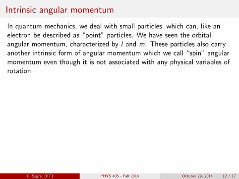
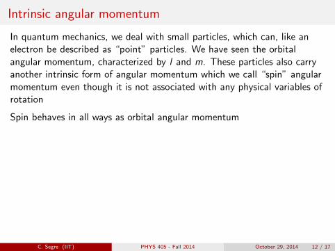
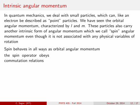
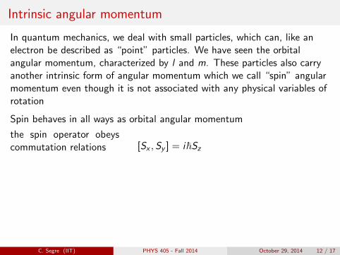
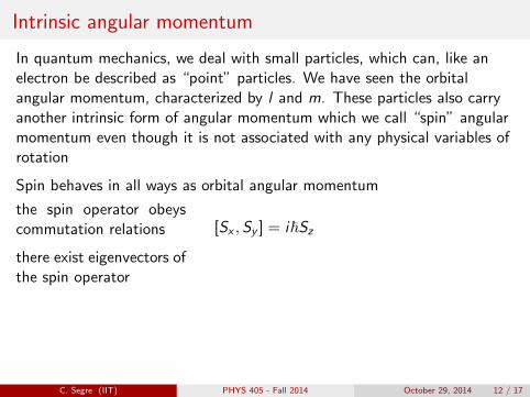
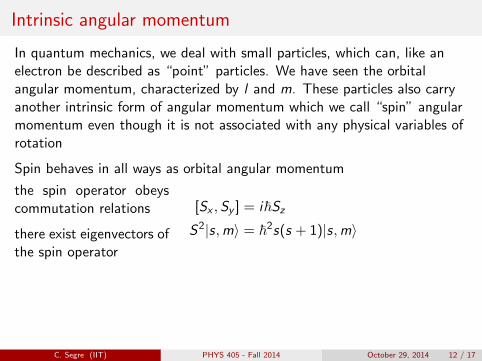
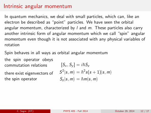
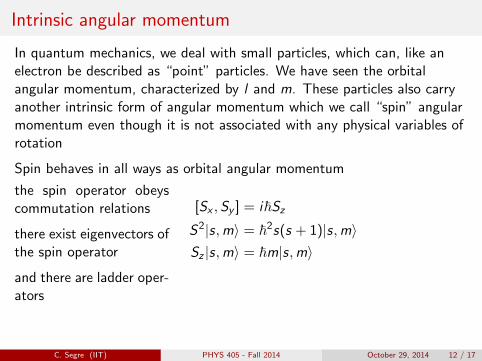
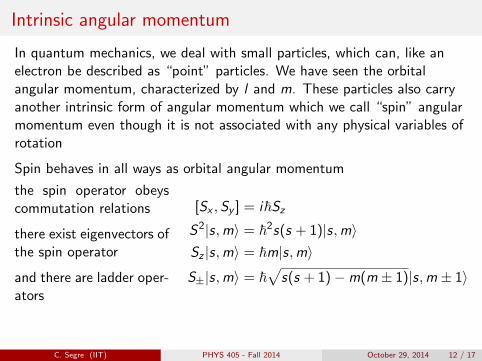
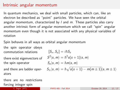
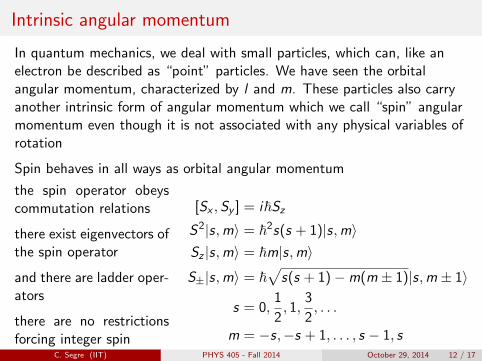
Intrinsic angular momentum
In quantum mechanics, we deal with small particles, which can, like anelectron be described as “point” particles. We have seen the orbitalangular momentum, characterized by l and m. These particles also carryanother intrinsic form of angular momentum which we call “spin” angularmomentum even though it is not associated with any physical variables ofrotation
Spin behaves in all ways as orbital angular momentum
the spin operator obeyscommutation relations
there exist eigenvectors ofthe spin operator
and there are ladder oper-ators
there are no restrictionsforcing integer spin
[Sx ,Sy ] = i~SzS2|s,m〉 = ~2s(s + 1)|s,m〉Sz |s,m〉 = ~m|s,m〉
S±|s,m〉 = ~√
s(s + 1)−m(m ± 1)|s,m ± 1〉
s = 0,1
2, 1,
3
2, . . .
m = −s,−s + 1, . . . , s − 1, s
C. Segre (IIT) PHYS 405 - Fall 2014 October 29, 2014 12 / 17
Intrinsic angular momentum
In quantum mechanics, we deal with small particles, which can, like anelectron be described as “point” particles. We have seen the orbitalangular momentum, characterized by l and m. These particles also carryanother intrinsic form of angular momentum which we call “spin” angularmomentum even though it is not associated with any physical variables ofrotation
Spin behaves in all ways as orbital angular momentum
the spin operator obeyscommutation relations
there exist eigenvectors ofthe spin operator
and there are ladder oper-ators
there are no restrictionsforcing integer spin
[Sx ,Sy ] = i~Sz
S2|s,m〉 = ~2s(s + 1)|s,m〉Sz |s,m〉 = ~m|s,m〉
S±|s,m〉 = ~√
s(s + 1)−m(m ± 1)|s,m ± 1〉
s = 0,1
2, 1,
3
2, . . .
m = −s,−s + 1, . . . , s − 1, s
C. Segre (IIT) PHYS 405 - Fall 2014 October 29, 2014 12 / 17
Intrinsic angular momentum
In quantum mechanics, we deal with small particles, which can, like anelectron be described as “point” particles. We have seen the orbitalangular momentum, characterized by l and m. These particles also carryanother intrinsic form of angular momentum which we call “spin” angularmomentum even though it is not associated with any physical variables ofrotation
Spin behaves in all ways as orbital angular momentum
the spin operator obeyscommutation relations
there exist eigenvectors ofthe spin operator
and there are ladder oper-ators
there are no restrictionsforcing integer spin
[Sx ,Sy ] = i~SzS2|s,m〉 = ~2s(s + 1)|s,m〉
Sz |s,m〉 = ~m|s,m〉
S±|s,m〉 = ~√
s(s + 1)−m(m ± 1)|s,m ± 1〉
s = 0,1
2, 1,
3
2, . . .
m = −s,−s + 1, . . . , s − 1, s
C. Segre (IIT) PHYS 405 - Fall 2014 October 29, 2014 12 / 17
Intrinsic angular momentum
In quantum mechanics, we deal with small particles, which can, like anelectron be described as “point” particles. We have seen the orbitalangular momentum, characterized by l and m. These particles also carryanother intrinsic form of angular momentum which we call “spin” angularmomentum even though it is not associated with any physical variables ofrotation
Spin behaves in all ways as orbital angular momentum
the spin operator obeyscommutation relations
there exist eigenvectors ofthe spin operator
and there are ladder oper-ators
there are no restrictionsforcing integer spin
[Sx ,Sy ] = i~SzS2|s,m〉 = ~2s(s + 1)|s,m〉Sz |s,m〉 = ~m|s,m〉
S±|s,m〉 = ~√
s(s + 1)−m(m ± 1)|s,m ± 1〉
s = 0,1
2, 1,
3
2, . . .
m = −s,−s + 1, . . . , s − 1, s
C. Segre (IIT) PHYS 405 - Fall 2014 October 29, 2014 12 / 17
Intrinsic angular momentum
In quantum mechanics, we deal with small particles, which can, like anelectron be described as “point” particles. We have seen the orbitalangular momentum, characterized by l and m. These particles also carryanother intrinsic form of angular momentum which we call “spin” angularmomentum even though it is not associated with any physical variables ofrotation
Spin behaves in all ways as orbital angular momentum
the spin operator obeyscommutation relations
there exist eigenvectors ofthe spin operator
and there are ladder oper-ators
there are no restrictionsforcing integer spin
[Sx ,Sy ] = i~SzS2|s,m〉 = ~2s(s + 1)|s,m〉Sz |s,m〉 = ~m|s,m〉
S±|s,m〉 = ~√
s(s + 1)−m(m ± 1)|s,m ± 1〉
s = 0,1
2, 1,
3
2, . . .
m = −s,−s + 1, . . . , s − 1, sC. Segre (IIT) PHYS 405 - Fall 2014 October 29, 2014 12 / 17
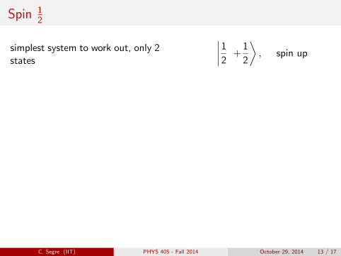
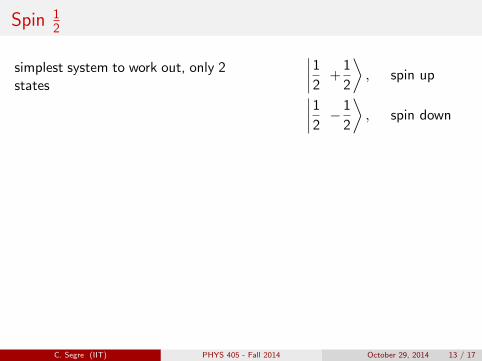
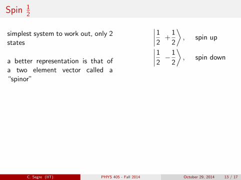
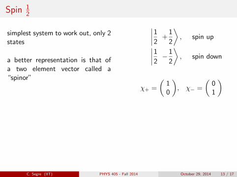
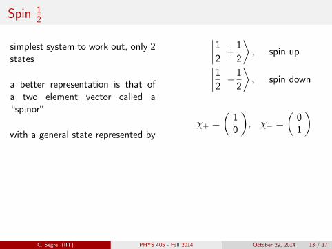
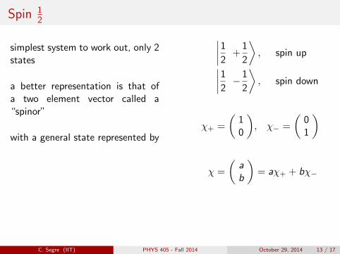
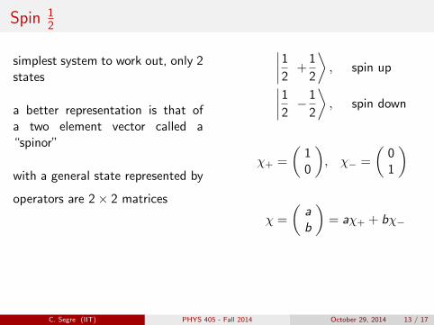
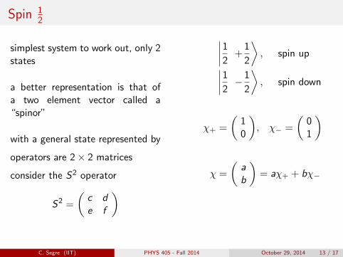
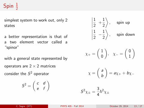
Spin 12
simplest system to work out, only 2states
a better representation is that ofa two element vector called a“spinor”
with a general state represented by
operators are 2× 2 matrices
consider the S2 operator
S2 =
(c de f
)
∣∣∣∣12 +1
2
⟩, spin up∣∣∣∣12 − 1
2
⟩, spin down
χ+ =
(10
), χ− =
(01
)
χ =
(ab
)= aχ+ + bχ−
S2χ± =3
4~2χ±
C. Segre (IIT) PHYS 405 - Fall 2014 October 29, 2014 13 / 17
Spin 12
simplest system to work out, only 2states
a better representation is that ofa two element vector called a“spinor”
with a general state represented by
operators are 2× 2 matrices
consider the S2 operator
S2 =
(c de f
)
∣∣∣∣12 +1
2
⟩, spin up
∣∣∣∣12 − 1
2
⟩, spin down
χ+ =
(10
), χ− =
(01
)
χ =
(ab
)= aχ+ + bχ−
S2χ± =3
4~2χ±
C. Segre (IIT) PHYS 405 - Fall 2014 October 29, 2014 13 / 17
Spin 12
simplest system to work out, only 2states
a better representation is that ofa two element vector called a“spinor”
with a general state represented by
operators are 2× 2 matrices
consider the S2 operator
S2 =
(c de f
)
∣∣∣∣12 +1
2
⟩, spin up∣∣∣∣12 − 1
2
⟩, spin down
χ+ =
(10
), χ− =
(01
)
χ =
(ab
)= aχ+ + bχ−
S2χ± =3
4~2χ±
C. Segre (IIT) PHYS 405 - Fall 2014 October 29, 2014 13 / 17
Spin 12
simplest system to work out, only 2states
a better representation is that ofa two element vector called a“spinor”
with a general state represented by
operators are 2× 2 matrices
consider the S2 operator
S2 =
(c de f
)
∣∣∣∣12 +1
2
⟩, spin up∣∣∣∣12 − 1
2
⟩, spin down
χ+ =
(10
), χ− =
(01
)
χ =
(ab
)= aχ+ + bχ−
S2χ± =3
4~2χ±
C. Segre (IIT) PHYS 405 - Fall 2014 October 29, 2014 13 / 17

Spin 12
simplest system to work out, only 2states
a better representation is that ofa two element vector called a“spinor”
with a general state represented by
operators are 2× 2 matrices
consider the S2 operator
S2 =
(c de f
)
∣∣∣∣12 +1
2
⟩, spin up∣∣∣∣12 − 1
2
⟩, spin down
χ+ =
(10
)
, χ− =
(01
)
χ =
(ab
)= aχ+ + bχ−
S2χ± =3
4~2χ±
C. Segre (IIT) PHYS 405 - Fall 2014 October 29, 2014 13 / 17
Spin 12
simplest system to work out, only 2states
a better representation is that ofa two element vector called a“spinor”
with a general state represented by
operators are 2× 2 matrices
consider the S2 operator
S2 =
(c de f
)
∣∣∣∣12 +1
2
⟩, spin up∣∣∣∣12 − 1
2
⟩, spin down
χ+ =
(10
), χ− =
(01
)
χ =
(ab
)= aχ+ + bχ−
S2χ± =3
4~2χ±
C. Segre (IIT) PHYS 405 - Fall 2014 October 29, 2014 13 / 17
S2 matrix
S2χ+ =3
4~2χ+
(c de f
)(10
)=
3
4~2(
10
)(
ce
)=
(34~
2
0
)c =
3
4~2, e = 0
S2χ− =3
4~2χ−
(c de f
)(01
)=
3
4~2(
01
)(
df
)=
(0
34~
2
)d = 0, f =
3
4~2
S2 =3
4~2(
1 00 1
)
C. Segre (IIT) PHYS 405 - Fall 2014 October 29, 2014 14 / 17

S2 matrix
S2χ+ =3
4~2χ+
(c de f
)(10
)=
3
4~2(
10
)
(ce
)=
(34~
2
0
)c =
3
4~2, e = 0
S2χ− =3
4~2χ−
(c de f
)(01
)=
3
4~2(
01
)(
df
)=
(0
34~
2
)d = 0, f =
3
4~2
S2 =3
4~2(
1 00 1
)
C. Segre (IIT) PHYS 405 - Fall 2014 October 29, 2014 14 / 17
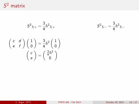
S2 matrix
S2χ+ =3
4~2χ+
(c de f
)(10
)=
3
4~2(
10
)(
ce
)=
(34~
2
0
)
c =3
4~2, e = 0
S2χ− =3
4~2χ−
(c de f
)(01
)=
3
4~2(
01
)(
df
)=
(0
34~
2
)d = 0, f =
3
4~2
S2 =3
4~2(
1 00 1
)
C. Segre (IIT) PHYS 405 - Fall 2014 October 29, 2014 14 / 17

S2 matrix
S2χ+ =3
4~2χ+
(c de f
)(10
)=
3
4~2(
10
)(
ce
)=
(34~
2
0
)c =
3
4~2, e = 0
S2χ− =3
4~2χ−
(c de f
)(01
)=
3
4~2(
01
)(
df
)=
(0
34~
2
)d = 0, f =
3
4~2
S2 =3
4~2(
1 00 1
)
C. Segre (IIT) PHYS 405 - Fall 2014 October 29, 2014 14 / 17

S2 matrix
S2χ+ =3
4~2χ+
(c de f
)(10
)=
3
4~2(
10
)(
ce
)=
(34~
2
0
)c =
3
4~2, e = 0
S2χ− =3
4~2χ−
(c de f
)(01
)=
3
4~2(
01
)
(df
)=
(0
34~
2
)d = 0, f =
3
4~2
S2 =3
4~2(
1 00 1
)
C. Segre (IIT) PHYS 405 - Fall 2014 October 29, 2014 14 / 17
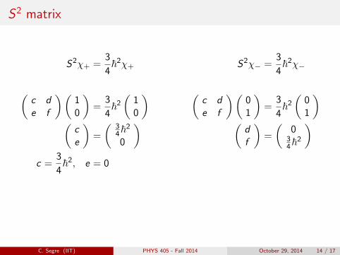
S2 matrix
S2χ+ =3
4~2χ+
(c de f
)(10
)=
3
4~2(
10
)(
ce
)=
(34~
2
0
)c =
3
4~2, e = 0
S2χ− =3
4~2χ−
(c de f
)(01
)=
3
4~2(
01
)(
df
)=
(0
34~
2
)
d = 0, f =3
4~2
S2 =3
4~2(
1 00 1
)
C. Segre (IIT) PHYS 405 - Fall 2014 October 29, 2014 14 / 17
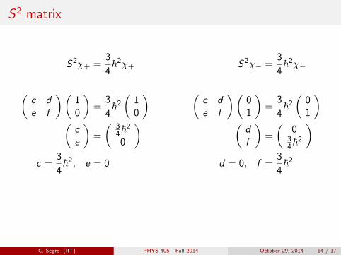
S2 matrix
S2χ+ =3
4~2χ+
(c de f
)(10
)=
3
4~2(
10
)(
ce
)=
(34~
2
0
)c =
3
4~2, e = 0
S2χ− =3
4~2χ−
(c de f
)(01
)=
3
4~2(
01
)(
df
)=
(0
34~
2
)d = 0, f =
3
4~2
S2 =3
4~2(
1 00 1
)
C. Segre (IIT) PHYS 405 - Fall 2014 October 29, 2014 14 / 17
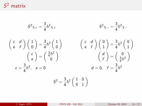
S2 matrix
S2χ+ =3
4~2χ+
(c de f
)(10
)=
3
4~2(
10
)(
ce
)=
(34~
2
0
)c =
3
4~2, e = 0
S2χ− =3
4~2χ−
(c de f
)(01
)=
3
4~2(
01
)(
df
)=
(0
34~
2
)d = 0, f =
3
4~2
S2 =3
4~2(
1 00 1
)
C. Segre (IIT) PHYS 405 - Fall 2014 October 29, 2014 14 / 17
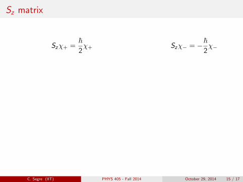
Sz matrix
Szχ+ =~2χ+
(c de f
)(10
)=
~2
(10
)(
ce
)=
( ~20
)c =
~2, e = 0
Szχ− = −~2χ−
(c de f
)(01
)= −~
2
(01
)(
df
)=
(0
−~2
)d = 0, f = −~
2
Sx =~2
(1 00 −1
)
C. Segre (IIT) PHYS 405 - Fall 2014 October 29, 2014 15 / 17
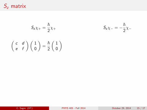
Sz matrix
Szχ+ =~2χ+
(c de f
)(10
)=
~2
(10
)
(ce
)=
( ~20
)c =
~2, e = 0
Szχ− = −~2χ−
(c de f
)(01
)= −~
2
(01
)(
df
)=
(0
−~2
)d = 0, f = −~
2
Sx =~2
(1 00 −1
)
C. Segre (IIT) PHYS 405 - Fall 2014 October 29, 2014 15 / 17

Sz matrix
Szχ+ =~2χ+
(c de f
)(10
)=
~2
(10
)(
ce
)=
( ~20
)
c =~2, e = 0
Szχ− = −~2χ−
(c de f
)(01
)= −~
2
(01
)(
df
)=
(0
−~2
)d = 0, f = −~
2
Sx =~2
(1 00 −1
)
C. Segre (IIT) PHYS 405 - Fall 2014 October 29, 2014 15 / 17
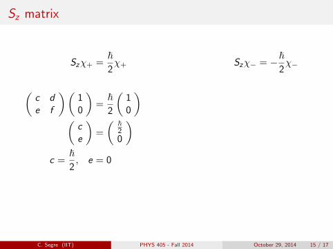
Sz matrix
Szχ+ =~2χ+
(c de f
)(10
)=
~2
(10
)(
ce
)=
( ~20
)c =
~2, e = 0
Szχ− = −~2χ−
(c de f
)(01
)= −~
2
(01
)(
df
)=
(0
−~2
)d = 0, f = −~
2
Sx =~2
(1 00 −1
)
C. Segre (IIT) PHYS 405 - Fall 2014 October 29, 2014 15 / 17
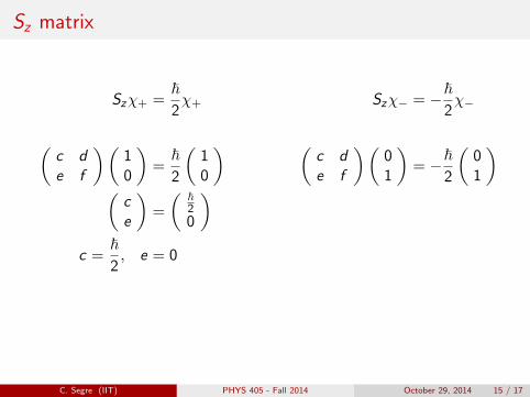
Sz matrix
Szχ+ =~2χ+
(c de f
)(10
)=
~2
(10
)(
ce
)=
( ~20
)c =
~2, e = 0
Szχ− = −~2χ−
(c de f
)(01
)= −~
2
(01
)
(df
)=
(0
−~2
)d = 0, f = −~
2
Sx =~2
(1 00 −1
)
C. Segre (IIT) PHYS 405 - Fall 2014 October 29, 2014 15 / 17
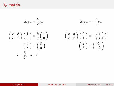
Sz matrix
Szχ+ =~2χ+
(c de f
)(10
)=
~2
(10
)(
ce
)=
( ~20
)c =
~2, e = 0
Szχ− = −~2χ−
(c de f
)(01
)= −~
2
(01
)(
df
)=
(0
−~2
)
d = 0, f = −~2
Sx =~2
(1 00 −1
)
C. Segre (IIT) PHYS 405 - Fall 2014 October 29, 2014 15 / 17
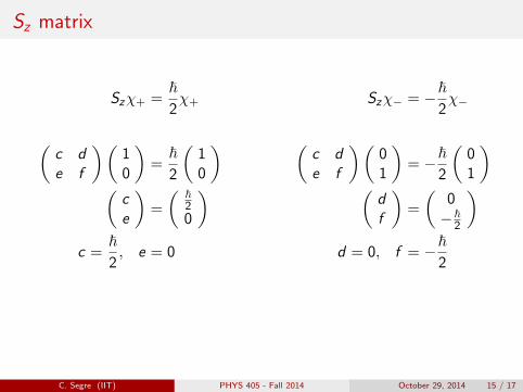
Sz matrix
Szχ+ =~2χ+
(c de f
)(10
)=
~2
(10
)(
ce
)=
( ~20
)c =
~2, e = 0
Szχ− = −~2χ−
(c de f
)(01
)= −~
2
(01
)(
df
)=
(0
−~2
)d = 0, f = −~
2
Sx =~2
(1 00 −1
)
C. Segre (IIT) PHYS 405 - Fall 2014 October 29, 2014 15 / 17
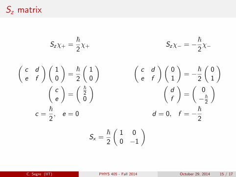
Sz matrix
Szχ+ =~2χ+
(c de f
)(10
)=
~2
(10
)(
ce
)=
( ~20
)c =
~2, e = 0
Szχ− = −~2χ−
(c de f
)(01
)= −~
2
(01
)(
df
)=
(0
−~2
)d = 0, f = −~
2
Sx =~2
(1 00 −1
)
C. Segre (IIT) PHYS 405 - Fall 2014 October 29, 2014 15 / 17
Spin ladder matrices
We can now proceed to find the matrix representation of the spin raisingand lowering operators. We take the general definition and apply it to thecase where S = 1
2
S±|s,m〉 = ~√s(s + 1)−m(m ± 1)|s,m ± 1〉
S+χ− = ~
√1
2
(1
2+ 1
)−(−1
2
)(−1
2+ 1
)χ+
= ~√
3
4+
1
4
χ+
= ~χ+
S−χ+ = ~
√1
2
(1
2+ 1
)−(
1
2
)(1
2− 1
)χ−
= ~√
3
4+
1
4χ− = ~χ−
(c de f
)(01
)= ~
(10
)(
c de f
)(10
)= ~
(00
)d = ~, c , e, f = 0
thus the two operators become
S+ = ~(
0 10 0
), S− = ~
(0 01 0
)
C. Segre (IIT) PHYS 405 - Fall 2014 October 29, 2014 16 / 17
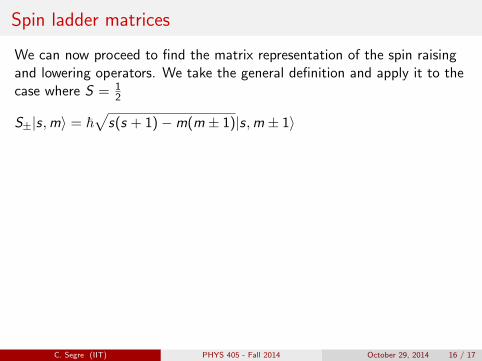
Spin ladder matrices
We can now proceed to find the matrix representation of the spin raisingand lowering operators. We take the general definition and apply it to thecase where S = 1
2
S±|s,m〉 = ~√
s(s + 1)−m(m ± 1)|s,m ± 1〉
S+χ− = ~
√1
2
(1
2+ 1
)−(−1
2
)(−1
2+ 1
)χ+ = ~
√3
4+
1
4χ+
= ~χ+
S−χ+ = ~
√1
2
(1
2+ 1
)−(
1
2
)(1
2− 1
)χ−
= ~√
3
4+
1
4χ− = ~χ−
(c de f
)(01
)= ~
(10
)(
c de f
)(10
)= ~
(00
)d = ~, c , e, f = 0
thus the two operators become
S+ = ~(
0 10 0
), S− = ~
(0 01 0
)
C. Segre (IIT) PHYS 405 - Fall 2014 October 29, 2014 16 / 17

Spin ladder matrices
We can now proceed to find the matrix representation of the spin raisingand lowering operators. We take the general definition and apply it to thecase where S = 1
2
S±|s,m〉 = ~√
s(s + 1)−m(m ± 1)|s,m ± 1〉
S+χ− = ~
√1
2
(1
2+ 1
)−(−1
2
)(−1
2+ 1
)χ+ = ~
√3
4+
1
4χ+ = ~χ+
S−χ+ = ~
√1
2
(1
2+ 1
)−(
1
2
)(1
2− 1
)χ−
= ~√
3
4+
1
4χ− = ~χ−
(c de f
)(01
)= ~
(10
)(
c de f
)(10
)= ~
(00
)d = ~, c , e, f = 0
thus the two operators become
S+ = ~(
0 10 0
), S− = ~
(0 01 0
)
C. Segre (IIT) PHYS 405 - Fall 2014 October 29, 2014 16 / 17
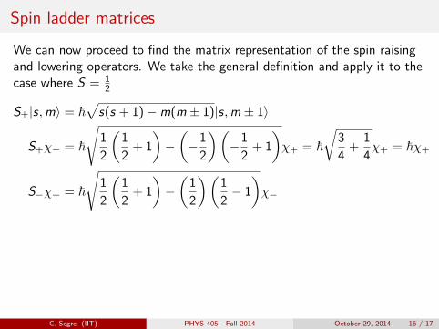
Spin ladder matrices
We can now proceed to find the matrix representation of the spin raisingand lowering operators. We take the general definition and apply it to thecase where S = 1
2
S±|s,m〉 = ~√
s(s + 1)−m(m ± 1)|s,m ± 1〉
S+χ− = ~
√1
2
(1
2+ 1
)−(−1
2
)(−1
2+ 1
)χ+ = ~
√3
4+
1
4χ+ = ~χ+
S−χ+ = ~
√1
2
(1
2+ 1
)−(
1
2
)(1
2− 1
)χ−
= ~√
3
4+
1
4χ− = ~χ−(
c de f
)(01
)= ~
(10
)(
c de f
)(10
)= ~
(00
)d = ~, c , e, f = 0
thus the two operators become
S+ = ~(
0 10 0
), S− = ~
(0 01 0
)
C. Segre (IIT) PHYS 405 - Fall 2014 October 29, 2014 16 / 17

Spin ladder matrices
We can now proceed to find the matrix representation of the spin raisingand lowering operators. We take the general definition and apply it to thecase where S = 1
2
S±|s,m〉 = ~√
s(s + 1)−m(m ± 1)|s,m ± 1〉
S+χ− = ~
√1
2
(1
2+ 1
)−(−1
2
)(−1
2+ 1
)χ+ = ~
√3
4+
1
4χ+ = ~χ+
S−χ+ = ~
√1
2
(1
2+ 1
)−(
1
2
)(1
2− 1
)χ− = ~
√3
4+
1
4χ−
= ~χ−(c de f
)(01
)= ~
(10
)(
c de f
)(10
)= ~
(00
)d = ~, c , e, f = 0
thus the two operators become
S+ = ~(
0 10 0
), S− = ~
(0 01 0
)
C. Segre (IIT) PHYS 405 - Fall 2014 October 29, 2014 16 / 17
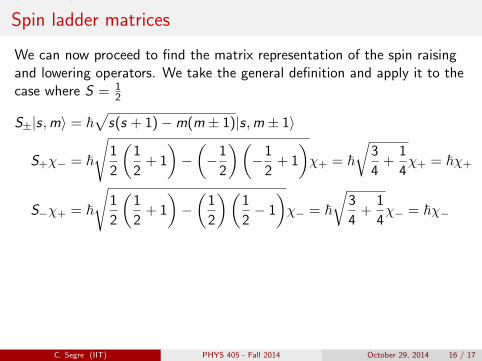
Spin ladder matrices
We can now proceed to find the matrix representation of the spin raisingand lowering operators. We take the general definition and apply it to thecase where S = 1
2
S±|s,m〉 = ~√
s(s + 1)−m(m ± 1)|s,m ± 1〉
S+χ− = ~
√1
2
(1
2+ 1
)−(−1
2
)(−1
2+ 1
)χ+ = ~
√3
4+
1
4χ+ = ~χ+
S−χ+ = ~
√1
2
(1
2+ 1
)−(
1
2
)(1
2− 1
)χ− = ~
√3
4+
1
4χ− = ~χ−
(c de f
)(01
)= ~
(10
)(
c de f
)(10
)= ~
(00
)d = ~, c , e, f = 0
thus the two operators become
S+ = ~(
0 10 0
), S− = ~
(0 01 0
)
C. Segre (IIT) PHYS 405 - Fall 2014 October 29, 2014 16 / 17
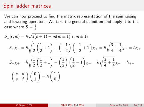
Spin ladder matrices
We can now proceed to find the matrix representation of the spin raisingand lowering operators. We take the general definition and apply it to thecase where S = 1
2
S±|s,m〉 = ~√
s(s + 1)−m(m ± 1)|s,m ± 1〉
S+χ− = ~
√1
2
(1
2+ 1
)−(−1
2
)(−1
2+ 1
)χ+ = ~
√3
4+
1
4χ+ = ~χ+
S−χ+ = ~
√1
2
(1
2+ 1
)−(
1
2
)(1
2− 1
)χ− = ~
√3
4+
1
4χ− = ~χ−(
c de f
)(01
)= ~
(10
)
(c de f
)(10
)= ~
(00
)d = ~, c , e, f = 0
thus the two operators become
S+ = ~(
0 10 0
), S− = ~
(0 01 0
)
C. Segre (IIT) PHYS 405 - Fall 2014 October 29, 2014 16 / 17

Spin ladder matrices
We can now proceed to find the matrix representation of the spin raisingand lowering operators. We take the general definition and apply it to thecase where S = 1
2
S±|s,m〉 = ~√
s(s + 1)−m(m ± 1)|s,m ± 1〉
S+χ− = ~
√1
2
(1
2+ 1
)−(−1
2
)(−1
2+ 1
)χ+ = ~
√3
4+
1
4χ+ = ~χ+
S−χ+ = ~
√1
2
(1
2+ 1
)−(
1
2
)(1
2− 1
)χ− = ~
√3
4+
1
4χ− = ~χ−(
c de f
)(01
)= ~
(10
)(
c de f
)(10
)= ~
(00
)
d = ~, c , e, f = 0
thus the two operators become
S+ = ~(
0 10 0
), S− = ~
(0 01 0
)
C. Segre (IIT) PHYS 405 - Fall 2014 October 29, 2014 16 / 17
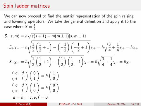
Spin ladder matrices
We can now proceed to find the matrix representation of the spin raisingand lowering operators. We take the general definition and apply it to thecase where S = 1
2
S±|s,m〉 = ~√
s(s + 1)−m(m ± 1)|s,m ± 1〉
S+χ− = ~
√1
2
(1
2+ 1
)−(−1
2
)(−1
2+ 1
)χ+ = ~
√3
4+
1
4χ+ = ~χ+
S−χ+ = ~
√1
2
(1
2+ 1
)−(
1
2
)(1
2− 1
)χ− = ~
√3
4+
1
4χ− = ~χ−(
c de f
)(01
)= ~
(10
)(
c de f
)(10
)= ~
(00
)d = ~, c , e, f = 0
thus the two operators become
S+ = ~(
0 10 0
), S− = ~
(0 01 0
)
C. Segre (IIT) PHYS 405 - Fall 2014 October 29, 2014 16 / 17
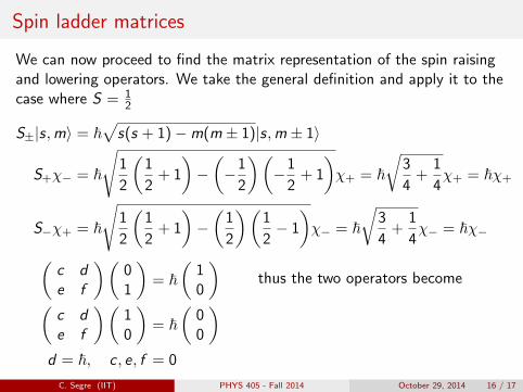
Spin ladder matrices
We can now proceed to find the matrix representation of the spin raisingand lowering operators. We take the general definition and apply it to thecase where S = 1
2
S±|s,m〉 = ~√
s(s + 1)−m(m ± 1)|s,m ± 1〉
S+χ− = ~
√1
2
(1
2+ 1
)−(−1
2
)(−1
2+ 1
)χ+ = ~
√3
4+
1
4χ+ = ~χ+
S−χ+ = ~
√1
2
(1
2+ 1
)−(
1
2
)(1
2− 1
)χ− = ~
√3
4+
1
4χ− = ~χ−(
c de f
)(01
)= ~
(10
)(
c de f
)(10
)= ~
(00
)d = ~, c , e, f = 0
thus the two operators become
S+ = ~(
0 10 0
), S− = ~
(0 01 0
)
C. Segre (IIT) PHYS 405 - Fall 2014 October 29, 2014 16 / 17
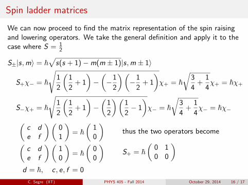
Spin ladder matrices
We can now proceed to find the matrix representation of the spin raisingand lowering operators. We take the general definition and apply it to thecase where S = 1
2
S±|s,m〉 = ~√
s(s + 1)−m(m ± 1)|s,m ± 1〉
S+χ− = ~
√1
2
(1
2+ 1
)−(−1
2
)(−1
2+ 1
)χ+ = ~
√3
4+
1
4χ+ = ~χ+
S−χ+ = ~
√1
2
(1
2+ 1
)−(
1
2
)(1
2− 1
)χ− = ~
√3
4+
1
4χ− = ~χ−(
c de f
)(01
)= ~
(10
)(
c de f
)(10
)= ~
(00
)d = ~, c , e, f = 0
thus the two operators become
S+ = ~(
0 10 0
)
, S− = ~(
0 01 0
)
C. Segre (IIT) PHYS 405 - Fall 2014 October 29, 2014 16 / 17
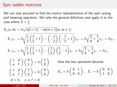
Spin ladder matrices
We can now proceed to find the matrix representation of the spin raisingand lowering operators. We take the general definition and apply it to thecase where S = 1
2
S±|s,m〉 = ~√
s(s + 1)−m(m ± 1)|s,m ± 1〉
S+χ− = ~
√1
2
(1
2+ 1
)−(−1
2
)(−1
2+ 1
)χ+ = ~
√3
4+
1
4χ+ = ~χ+
S−χ+ = ~
√1
2
(1
2+ 1
)−(
1
2
)(1
2− 1
)χ− = ~
√3
4+
1
4χ− = ~χ−(
c de f
)(01
)= ~
(10
)(
c de f
)(10
)= ~
(00
)d = ~, c , e, f = 0
thus the two operators become
S+ = ~(
0 10 0
), S− = ~
(0 01 0
)
C. Segre (IIT) PHYS 405 - Fall 2014 October 29, 2014 16 / 17

Pauli matrices
Recall that the raising and lower-ing operators were related to the x-and y-components of angular mo-mentum. This is the same for spin.
the matrix representations are thus
Since each component of ~S has aprefactor of ~/2, it is more commonto write the components of the spinusing the Pauli spin matrices
S± = Sx ± iSy
Sx =1
2(S+ + S−)
=~2
(0 11 0
)
Sy =1
2i(S+ − S−)
=~2
(0 −ii 0
)
~S =~2~σ
σx ≡(
0 11 0
)σy ≡
(0 −ii 0
)σz ≡
(1 00 −1
)
C. Segre (IIT) PHYS 405 - Fall 2014 October 29, 2014 17 / 17
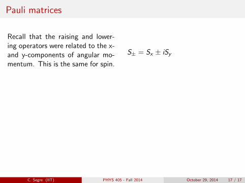
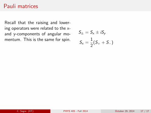
Pauli matrices
Recall that the raising and lower-ing operators were related to the x-and y-components of angular mo-mentum. This is the same for spin.
the matrix representations are thus
Since each component of ~S has aprefactor of ~/2, it is more commonto write the components of the spinusing the Pauli spin matrices
S± = Sx ± iSy
Sx =1
2(S+ + S−)
=~2
(0 11 0
)Sy =
1
2i(S+ − S−)
=~2
(0 −ii 0
)
~S =~2~σ
σx ≡(
0 11 0
)σy ≡
(0 −ii 0
)σz ≡
(1 00 −1
)
C. Segre (IIT) PHYS 405 - Fall 2014 October 29, 2014 17 / 17
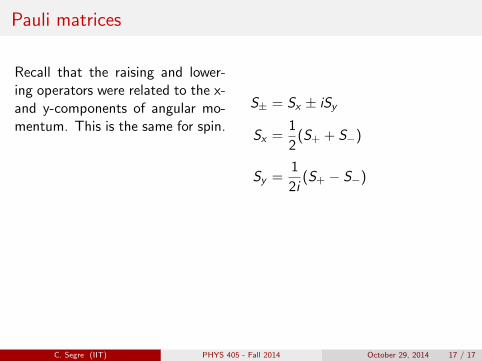
Pauli matrices
Recall that the raising and lower-ing operators were related to the x-and y-components of angular mo-mentum. This is the same for spin.
the matrix representations are thus
Since each component of ~S has aprefactor of ~/2, it is more commonto write the components of the spinusing the Pauli spin matrices
S± = Sx ± iSy
Sx =1
2(S+ + S−)
=~2
(0 11 0
)
Sy =1
2i(S+ − S−)
=~2
(0 −ii 0
)~S =
~2~σ
σx ≡(
0 11 0
)σy ≡
(0 −ii 0
)σz ≡
(1 00 −1
)
C. Segre (IIT) PHYS 405 - Fall 2014 October 29, 2014 17 / 17
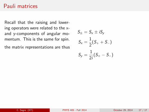
Pauli matrices
Recall that the raising and lower-ing operators were related to the x-and y-components of angular mo-mentum. This is the same for spin.
the matrix representations are thus
Since each component of ~S has aprefactor of ~/2, it is more commonto write the components of the spinusing the Pauli spin matrices
S± = Sx ± iSy
Sx =1
2(S+ + S−)
=~2
(0 11 0
)
Sy =1
2i(S+ − S−)
=~2
(0 −ii 0
)~S =
~2~σ
σx ≡(
0 11 0
)σy ≡
(0 −ii 0
)σz ≡
(1 00 −1
)
C. Segre (IIT) PHYS 405 - Fall 2014 October 29, 2014 17 / 17
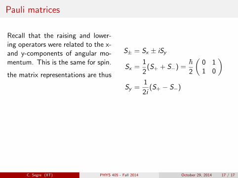
Pauli matrices
Recall that the raising and lower-ing operators were related to the x-and y-components of angular mo-mentum. This is the same for spin.
the matrix representations are thus
Since each component of ~S has aprefactor of ~/2, it is more commonto write the components of the spinusing the Pauli spin matrices
S± = Sx ± iSy
Sx =1
2(S+ + S−) =
~2
(0 11 0
)Sy =
1
2i(S+ − S−)
=~2
(0 −ii 0
)~S =
~2~σ
σx ≡(
0 11 0
)σy ≡
(0 −ii 0
)σz ≡
(1 00 −1
)
C. Segre (IIT) PHYS 405 - Fall 2014 October 29, 2014 17 / 17
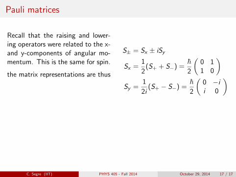
Pauli matrices
Recall that the raising and lower-ing operators were related to the x-and y-components of angular mo-mentum. This is the same for spin.
the matrix representations are thus
Since each component of ~S has aprefactor of ~/2, it is more commonto write the components of the spinusing the Pauli spin matrices
S± = Sx ± iSy
Sx =1
2(S+ + S−) =
~2
(0 11 0
)Sy =
1
2i(S+ − S−) =
~2
(0 −ii 0
)
~S =~2~σ
σx ≡(
0 11 0
)σy ≡
(0 −ii 0
)σz ≡
(1 00 −1
)
C. Segre (IIT) PHYS 405 - Fall 2014 October 29, 2014 17 / 17
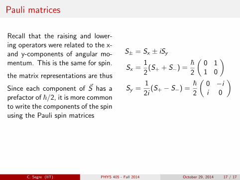
Pauli matrices
Recall that the raising and lower-ing operators were related to the x-and y-components of angular mo-mentum. This is the same for spin.
the matrix representations are thus
Since each component of ~S has aprefactor of ~/2, it is more commonto write the components of the spinusing the Pauli spin matrices
S± = Sx ± iSy
Sx =1
2(S+ + S−) =
~2
(0 11 0
)Sy =
1
2i(S+ − S−) =
~2
(0 −ii 0
)
~S =~2~σ
σx ≡(
0 11 0
)σy ≡
(0 −ii 0
)σz ≡
(1 00 −1
)
C. Segre (IIT) PHYS 405 - Fall 2014 October 29, 2014 17 / 17
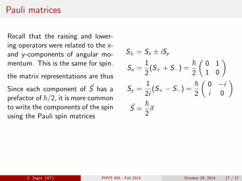
Pauli matrices
Recall that the raising and lower-ing operators were related to the x-and y-components of angular mo-mentum. This is the same for spin.
the matrix representations are thus
Since each component of ~S has aprefactor of ~/2, it is more commonto write the components of the spinusing the Pauli spin matrices
S± = Sx ± iSy
Sx =1
2(S+ + S−) =
~2
(0 11 0
)Sy =
1
2i(S+ − S−) =
~2
(0 −ii 0
)~S =
~2~σ
σx ≡(
0 11 0
)σy ≡
(0 −ii 0
)σz ≡
(1 00 −1
)
C. Segre (IIT) PHYS 405 - Fall 2014 October 29, 2014 17 / 17
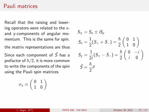
Pauli matrices
Recall that the raising and lower-ing operators were related to the x-and y-components of angular mo-mentum. This is the same for spin.
the matrix representations are thus
Since each component of ~S has aprefactor of ~/2, it is more commonto write the components of the spinusing the Pauli spin matrices
S± = Sx ± iSy
Sx =1
2(S+ + S−) =
~2
(0 11 0
)Sy =
1
2i(S+ − S−) =
~2
(0 −ii 0
)~S =
~2~σ
σx ≡(
0 11 0
)
σy ≡(
0 −ii 0
)σz ≡
(1 00 −1
)
C. Segre (IIT) PHYS 405 - Fall 2014 October 29, 2014 17 / 17
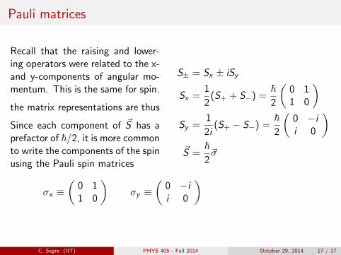
Pauli matrices
Recall that the raising and lower-ing operators were related to the x-and y-components of angular mo-mentum. This is the same for spin.
the matrix representations are thus
Since each component of ~S has aprefactor of ~/2, it is more commonto write the components of the spinusing the Pauli spin matrices
S± = Sx ± iSy
Sx =1
2(S+ + S−) =
~2
(0 11 0
)Sy =
1
2i(S+ − S−) =
~2
(0 −ii 0
)~S =
~2~σ
σx ≡(
0 11 0
)σy ≡
(0 −ii 0
)
σz ≡(
1 00 −1
)
C. Segre (IIT) PHYS 405 - Fall 2014 October 29, 2014 17 / 17
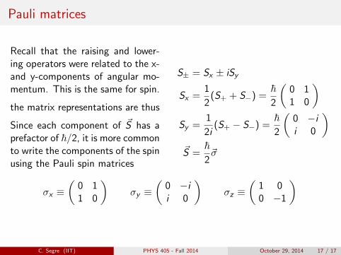
Pauli matrices
Recall that the raising and lower-ing operators were related to the x-and y-components of angular mo-mentum. This is the same for spin.
the matrix representations are thus
Since each component of ~S has aprefactor of ~/2, it is more commonto write the components of the spinusing the Pauli spin matrices
S± = Sx ± iSy
Sx =1
2(S+ + S−) =
~2
(0 11 0
)Sy =
1
2i(S+ − S−) =
~2
(0 −ii 0
)~S =
~2~σ
σx ≡(
0 11 0
)σy ≡
(0 −ii 0
)σz ≡
(1 00 −1
)
C. Segre (IIT) PHYS 405 - Fall 2014 October 29, 2014 17 / 17