Embed Size (px)
Citation preview

Thèse de Doctorat
é c o l e d o c t o r a l e s c i e n c e s p o u r l ’ i n g é n i e u r e t m i c r o t e c h n i q u e s
U N I V E R S I T É D E F R A N C H E - C O M T É
■
A Robust & Reliable Data-drivenPrognostics Approach Based onExtreme Learning Machine andFuzzy Clustering
Kamran JAVED


Thèse de Doctorat
é c o l e d o c t o r a l e s c i e n c e s p o u r l ’ i n g é n i e u r e t m i c r o t e c h n i q u e s
U N I V E R S I T É D E F R A N C H E - C O M T É
THESE presentee par
Kamran JAVED
pour obtenir le
Grade de Docteur de
l’Universite de Franche-Comte
Specialite : Automatique
A Robust & Reliable Data-driven PrognosticsApproach Based on
Extreme Learning Machine and Fuzzy Clustering
Unite de Recherche : FEMTO-ST, UMR CNRS 6174
Soutenue le 9 Avril, 2014 devant le Jury :
Louise TRAVE-MASSUYES Presidente Directeur de Recherche, LAAS CNRS, Toulouse (Fr)
Said RECHAK Rapporteur Prof., Ecole Nationale Polytechnique d’Alger, Algerie
Enrico ZIO Rapporteur Prof., Politecnico di Milano, Italie
Antoine GRALL Examinateur Prof., Universite de Technologie de Troyes (Fr)
Janan ZAYTOON Examinateur Prof., Universite de Reims (Fr)
Rafael GOURIVEAU Co-Directeur de these Maitre de Conferences, ENSMM, Besancon (Fr)
Noureddine ZERHOUNI Co-Directeur de these Prof., ENSMM, Besancon (Fr)


To my loving parents Javed and Shaheen, for everything I am now.To my respectable uncle Qazi Mohammad Farooq for his support, who hasbeen a constant source of inspiration.

Abstract
Prognostics and Health Management (PHM) aims at extending the life cycle of en-gineering assets, while reducing exploitation and maintenance costs. For this reason,prognostics is considered as a key process with future capabilities. Indeed, accurateestimates of the Remaining Useful Life (RUL) of an equipment enable defining furtherplan of actions to increase safety, minimize downtime, ensure mission completion andefficient production.Recent advances show that data-driven approaches (mainly based on machine learningmethods) are increasingly applied for fault prognostics. They can be seen as black-boxmodels that learn system behavior directly from Condition Monitoring (CM) data, usethat knowledge to infer its current state and predict future progression of failure. How-ever, approximating the behavior of critical machinery is a challenging task that canresult in poor prognostics. As for understanding, some issues of data-driven prognos-tics modeling are highlighted as follows. 1) How to effectively process raw monitoringdata to obtain suitable features that clearly reflect evolution of degradation? 2) Howto discriminate degradation states and define failure criteria (that can vary from caseto case)? 3) How to be sure that learned-models will be robust enough to show steadyperformance over uncertain inputs that deviate from learned experiences, and to bereliable enough to encounter unknown data (i.e., operating conditions, engineering vari-ations, etc.)? 4) How to achieve ease of application under industrial constraints andrequirements? Such issues constitute the problems addressed in this thesis and have ledto develop a novel approach beyond conventional methods of data-driven prognostics.The main contributions are as follows.
• The data-processing step is improved by introducing a new approach for featuresextraction using trigonometric and cumulative functions, where features selectionis based on three characteristics, i.e., monotonicity, trendability and predictability.The main idea of this development is to transform raw data into features thatimprove accuracy of long-term predictions.
• To account for robustness, reliability and applicability issues, a new predictionalgorithm is proposed: the Summation Wavelet-Extreme Learning Machine (SW-ELM). SW-ELM ensures good prediction performances while reducing the learning
iii

time. An ensemble of SW-ELM is also proposed to quantify uncertainty andimprove accuracy of estimates.
• Prognostics performances are also enhanced thanks to the proposition of a newhealth assessment algorithm: the Subtractive-Maximum Entropy Fuzzy Clustering(S-MEFC). S-MEFC is an unsupervised classification approach which uses max-imum entropy inference to represent uncertainty of unlabeled multidimensionaldata and can automatically determine the number of states (clusters), i.e., with-out human assumption.
• The final prognostics model is achieved by integrating SW-ELM and S-MEFC toshow evolution of machine degradation with simultaneous predictions and discretestate estimation. This scheme also enables to dynamically set failure thresholdsand estimate RUL of monitored machinery.
Developments are validated on real data from three experimental platforms: PRONOS-TIA FEMTO-ST (bearings test-bed), CNC SIMTech (machining cutters), C-MAPSSNASA (turbofan engines) and other benchmark data. Due to realistic nature of theproposed RUL estimation strategy, quite promising results are achieved. However, reli-ability of the prognostics model still needs to be improved which is the main perspectiveof this work.
Keywords: Prognostics, Data-driven, Extreme learning Machine, Fuzzy Clustering, RUL

Acknowledgements
Special thanks to Almighty for the wisdom & perseverance, that he bestowed upon methroughout my Ph.D.
I am thankful to FEMTO-ST Institute & Universite de Franche-Comte Besancon (France)for the Ph.D. position & a unique research environment.
I would like to express my respect & gratitude to my supervisors Assoc. Prof. RafaelGouriveau & Prof. Noureddine Zerhouni, for their continuous guidance, & valuable in-puts to my research.
I would like to thank my thesis reporters: Prof. Said Rechak, Prof. Enrico Zio, &the examiners: Prof. Louise Trave-Massuyes, Prof. Antoine Grall, Prof. Janan Zay-toon for taking time to review my thesis.
I would like to acknowledge for the helpful suggestions from Assoc. Prof. EmmanuelRamasso, Assoc. Prof. Kamal Medjaher & Dr. Tarak Benkedjouh. I also want to thankmy other colleagues, without particular order: Syed Zill-e-Hussnain, Bilal Komati, Bap-tiste Veron, Nathalie Herr, Ahmed Mosallam, Haithem Skima & many others for thefriendly environment & fruitful discussions.
Many thanks to my wife Momna for her support, & my little angel Musa who neverlet me go bored of my work.
I am grateful to my parents, my uncle, my brothers & other family members who sup-ported me over the years.
Finally, I won’t forget my friend Salik, who encouraged me to pursue my research careerwith this opportunity.
Kamran Javed
v


Contents
Acronyms & Notations xix
General introduction 1
1 Enhancing data-driven prognostics 51.1 Prognostics and Health Management (PHM) . . . . . . . . . . . . . . . 5
1.1.1 PHM as an enabling discipline . . . . . . . . . . . . . . . . . . . 51.1.2 Prognostics and the Remaining Useful Life . . . . . . . . . . . . 81.1.3 Prognostics and uncertainty . . . . . . . . . . . . . . . . . . . . . 9
1.2 Prognostics approaches . . . . . . . . . . . . . . . . . . . . . . . . . . . . 121.2.1 Physics based prognostics . . . . . . . . . . . . . . . . . . . . . . 121.2.2 Data-driven prognostics . . . . . . . . . . . . . . . . . . . . . . . 131.2.3 Hybrid prognostics . . . . . . . . . . . . . . . . . . . . . . . . . . 161.2.4 Synthesis and discussions . . . . . . . . . . . . . . . . . . . . . . 19
1.3 Frame of data-driven prognostics . . . . . . . . . . . . . . . . . . . . . . 221.3.1 Data acquisition . . . . . . . . . . . . . . . . . . . . . . . . . . . 221.3.2 Data pre-processing . . . . . . . . . . . . . . . . . . . . . . . . . 231.3.3 Prognostics modeling strategies for RUL estimation . . . . . . . 23
1.4 Open issues & problem statement for the thesis . . . . . . . . . . . . . . 251.4.1 Defining challenges of prognostics modeling . . . . . . . . . . . . 251.4.2 Toward enhanced data-driven prognostics . . . . . . . . . . . . . 27
1.5 Summary . . . . . . . . . . . . . . . . . . . . . . . . . . . . . . . . . . . 30
2 From raw data to suitable features 312.1 Problem addressed . . . . . . . . . . . . . . . . . . . . . . . . . . . . . . 31
2.1.1 Importance of features for prognostics . . . . . . . . . . . . . . . 312.1.2 Toward monotonic, trendable and predictable features . . . . . . 33
2.2 Data processing . . . . . . . . . . . . . . . . . . . . . . . . . . . . . . . . 342.2.1 Feature extraction approaches . . . . . . . . . . . . . . . . . . . . 342.2.2 Feature selection approaches . . . . . . . . . . . . . . . . . . . . 36
2.3 Proposition of a new data pre-treatment procedure . . . . . . . . . . . . 36
vii
2.3.1 Outline . . . . . . . . . . . . . . . . . . . . . . . . . . . . . . . . 362.3.2 Steps for feature extraction / selection . . . . . . . . . . . . . . . 38
2.4 First PHM case study on real data . . . . . . . . . . . . . . . . . . . . . 432.4.1 Bearings datasets of IEEE PHM Challenge 2012 . . . . . . . . . 432.4.2 Feature extraction and selection results . . . . . . . . . . . . . . 44
2.5 Predictability based prognostics: underlying concepts . . . . . . . . . . . 492.5.1 Proposition of a new data post-treatment procedure . . . . . . . 492.5.2 Predictability based feature selection procedure . . . . . . . . . . 51
2.6 Second PHM case study on real data . . . . . . . . . . . . . . . . . . . . 522.6.1 Outline . . . . . . . . . . . . . . . . . . . . . . . . . . . . . . . . 522.6.2 Building a prognostics model . . . . . . . . . . . . . . . . . . . . 542.6.3 Prognostics results and impact of predictability . . . . . . . . . . 602.6.4 Observations . . . . . . . . . . . . . . . . . . . . . . . . . . . . . 62
2.7 Summary . . . . . . . . . . . . . . . . . . . . . . . . . . . . . . . . . . . 62
3 From features to predictions 653.1 Long-term predictions for prognostics . . . . . . . . . . . . . . . . . . . 653.2 ELM as a potential prediction tool . . . . . . . . . . . . . . . . . . . . . 67
3.2.1 From ANN to ELM . . . . . . . . . . . . . . . . . . . . . . . . . 673.2.2 ELM for SLFN: learning principle and mathematical perspective 683.2.3 Discussions: ELM for prognostics . . . . . . . . . . . . . . . . . . 70
3.3 SW-ELM and Ensemble models for prognostics . . . . . . . . . . . . . . 713.3.1 Wavelet neural network . . . . . . . . . . . . . . . . . . . . . . . 713.3.2 Summation Wavelet-Extreme Learning Machine for SLFN . . . . 733.3.3 SW-ELM Ensemble for uncertainty estimation . . . . . . . . . . 77
3.4 Benchmarking SW-ELM on time series issues . . . . . . . . . . . . . . . 783.4.1 Outline: aim of tests and performance evaluation . . . . . . . . . 783.4.2 First issue: approximation problems . . . . . . . . . . . . . . . . 793.4.3 Second issue: one-step ahead prediction problems . . . . . . . . . 813.4.4 Third issue: multi-steps ahead prediction (msp) problems . . . . 83
3.5 PHM case studies on real data . . . . . . . . . . . . . . . . . . . . . . . 853.5.1 First case study: cutters datasets & simulation settings . . . . . 853.5.2 Second case study: bearings datasets of PHM Challenge 2012 . . 96
3.6 Summary . . . . . . . . . . . . . . . . . . . . . . . . . . . . . . . . . . . 98
4 From predictions to RUL estimates 994.1 Problem addressed: dynamic threshold assignment . . . . . . . . . . . . 99
4.1.1 Failure threshold: univariate approach and limits . . . . . . . . . 994.1.2 Failure threshold: multivariate approach and limits . . . . . . . . 1004.1.3 Toward dynamic failure threshold . . . . . . . . . . . . . . . . . . 101
4.2 Clustering for health assessment: outline & problems . . . . . . . . . . . 1014.2.1 Categories of classification methods . . . . . . . . . . . . . . . . 1014.2.2 Clustering and discrete state estimation . . . . . . . . . . . . . . 1024.2.3 Issues and requirement . . . . . . . . . . . . . . . . . . . . . . . . 103

4.3 Discrete state estimation: the S-MEFC Algorithm . . . . . . . . . . . . 1044.3.1 Background . . . . . . . . . . . . . . . . . . . . . . . . . . . . . . 1044.3.2 S-MEFC for discrete state estimation . . . . . . . . . . . . . . . 108
4.4 Enhanced multivariate degradation based modeling . . . . . . . . . . . . 1104.4.1 Outline: dynamic FTs assignment procedure . . . . . . . . . . . 1104.4.2 Off-line phase: learn predictors and classifiers . . . . . . . . . . . 1114.4.3 On-line phase: simultaneous predictions & discrete estimation . . 112
4.5 PHM case study on real data . . . . . . . . . . . . . . . . . . . . . . . . 1134.5.1 Turbofan Engines datasets of IEEE PHM Challenge 2008 . . . . 1134.5.2 Performance evaluation and simulation setting . . . . . . . . . . 1144.5.3 Prognostics results on complete test data . . . . . . . . . . . . . 1154.5.4 Benefits of the proposed approach . . . . . . . . . . . . . . . . . 120
4.6 Summary . . . . . . . . . . . . . . . . . . . . . . . . . . . . . . . . . . . 120
5 Conclusion and future works 121
Bibliography 125
A Appendix A 145A.1 Taxonomy of maintenance policies . . . . . . . . . . . . . . . . . . . . . 145
A.1.1 Corrective maintenance . . . . . . . . . . . . . . . . . . . . . . . 146A.1.2 Preventive maintenance . . . . . . . . . . . . . . . . . . . . . . . 146
A.2 Relation between diagnostics and prognostics . . . . . . . . . . . . . . . 147A.3 FCM algorithm . . . . . . . . . . . . . . . . . . . . . . . . . . . . . . . . 149A.4 Metrics for model accuracy . . . . . . . . . . . . . . . . . . . . . . . . . 149A.5 Benchmark datasets . . . . . . . . . . . . . . . . . . . . . . . . . . . . . 150
A.5.1 Carnallite surge tank dataset . . . . . . . . . . . . . . . . . . . . 150A.5.2 Industrial dryer dataset . . . . . . . . . . . . . . . . . . . . . . . 152A.5.3 Mechanical hair dryer dataset . . . . . . . . . . . . . . . . . . . . 153A.5.4 NN3 forecasting data . . . . . . . . . . . . . . . . . . . . . . . . . 153
Publications (February 2011 - January 2014) 155


List of Figures
1.1 PHM cycle (adapted from [119]) . . . . . . . . . . . . . . . . . . . . . . 71.2 Illustration of prognostics and RUL estimates . . . . . . . . . . . . . . . 91.3 Component health evolution curves (adapted from [178]) . . . . . . . . . 101.4 Uncertainty bands associated with RUL estimations (adapted from [191]) 111.5 Series approach for hybrid prognostics model (adapted from [71]) . . . . 161.6 Battery capacity predictions and new pdf of RUL [169] . . . . . . . . . . 171.7 Parallel approach for hybrid prognostics model (adapted from [71]) . . . 181.8 Classification of prognostics approaches . . . . . . . . . . . . . . . . . . 191.9 Prognostics approaches: applicability vs. performance . . . . . . . . . . 221.10 Univariate degradation based modeling strategy . . . . . . . . . . . . . . 241.11 Direct RUL prediction strategy . . . . . . . . . . . . . . . . . . . . . . . 241.12 Multivariate degradation based modeling strategy . . . . . . . . . . . . . 251.13 Illustration of challenge: robustness . . . . . . . . . . . . . . . . . . . . . 261.14 Illustration of challenge: reliability . . . . . . . . . . . . . . . . . . . . . 271.15 Thesis key points scheme - toward robust, reliable & applicable prognostics 29
2.1 From data to RUL . . . . . . . . . . . . . . . . . . . . . . . . . . . . . . 322.2 Effects of features on prognostics . . . . . . . . . . . . . . . . . . . . . . 332.3 Feature extraction approaches (adapted from [211]) . . . . . . . . . . . . 352.4 Proposed approach to obtain monotonic and trendable features . . . . . 372.5 WT and DWT . . . . . . . . . . . . . . . . . . . . . . . . . . . . . . . . 382.6 Classical features extracted from a degraded bearing . . . . . . . . . . . 392.7 Trigonometric features extracted from a degraded bearing . . . . . . . . 412.8 PRONOSTIA testbed - FEMTO-ST Institute, AS2M department . . . . 432.9 Bearing degradation: run-to-failure vibration signal . . . . . . . . . . . . 442.10 Trigonometric features and classical features . . . . . . . . . . . . . . . . 452.11 Extracted features and their respective cumulative features (good case) 462.12 Extracted features and their respective cumulative features (bad case) . 462.13 Fitness plots . . . . . . . . . . . . . . . . . . . . . . . . . . . . . . . . . 472.14 Comparison of classical and cumulative features on 17 bearings . . . . . 482.15 Compounds of predictability concept . . . . . . . . . . . . . . . . . . . . 50
xi
2.16 Illustration of predictability measure . . . . . . . . . . . . . . . . . . . . 512.17 Selection procedure based on predictability . . . . . . . . . . . . . . . . 522.18 Engine diagram [72] . . . . . . . . . . . . . . . . . . . . . . . . . . . . . 532.19 Filtered feature from engine dataset . . . . . . . . . . . . . . . . . . . . 532.20 Procedure to analyze the impact of predictability . . . . . . . . . . . . . 542.21 Iterative model for multi-steps predictions [76] . . . . . . . . . . . . . . 552.22 Predictability of features for H = tc+ 134 . . . . . . . . . . . . . . . . . 572.23 Example of degrading feature prediction . . . . . . . . . . . . . . . . . . 582.24 Visualization of classes from multidimensional data of 40 engines . . . . 602.25 ED results (test− 1): a),b) All features and c),d) Predictable features . 602.26 Classification with all features . . . . . . . . . . . . . . . . . . . . . . . . 612.27 Classification with predictable features . . . . . . . . . . . . . . . . . . . 61
3.1 Discrete state estmation and RUL estimation [76] . . . . . . . . . . . . . 673.2 Structure of FFNN and RNN [102] . . . . . . . . . . . . . . . . . . . . . 683.3 Single layer feed forward neural network . . . . . . . . . . . . . . . . . . 693.4 Mother and daughter wavelet from Morlet function . . . . . . . . . . . . 723.5 Structure and learning view of proposed SW-ELM . . . . . . . . . . . . 753.6 SW-ELME and confidence limit interval (CI) . . . . . . . . . . . . . . . 783.7 Fault code approximations and corresponding errors . . . . . . . . . . . 803.8 Tool wear estimation and corresponding errors . . . . . . . . . . . . . . 813.9 One-step ahead prediction of bulb temperature and corresponding errors 823.10 One-step ahead prediction of Air temperature and corresponding errors 823.11 msp of time series 61 (NN3) . . . . . . . . . . . . . . . . . . . . . . . . . 843.12 msp of sensor 2 (Engine 5) . . . . . . . . . . . . . . . . . . . . . . . . . 843.13 Accuracy of: a) msp for 8 NN3 series, b) msp for 5 Turbofan engines . . 843.14 Cutting force signals in three axes (Fx, Fy, Fz) [223] . . . . . . . . . . . 853.15 Cutting tool wear estimation - methodology . . . . . . . . . . . . . . . . 873.16 Force features extracted from 315 cuts . . . . . . . . . . . . . . . . . . . 873.17 Robustness: learning and testing with one cutter . . . . . . . . . . . . . 883.18 Robustness analysis: partially unknown data for a “single cutter” model 893.19 Reliability: learning and testing with three cutters . . . . . . . . . . . . 903.20 Reliability analysis: partially unknown data for “multi-cutter” model . . 913.21 Reliability: learning and testing with unknown data . . . . . . . . . . . 923.22 Reliability analysis with totally unknown data . . . . . . . . . . . . . . . 933.23 Estimation with multi-cutter model on unknown data . . . . . . . . . . 933.24 Tool wear evolution and precise wear limit . . . . . . . . . . . . . . . . . 953.25 Cutting tools wear estimation and CI construction . . . . . . . . . . . . 963.26 Examples of multi-step ahead predictions (Classical vs. Proposed) . . . 98
4.1 Transition from healthy to degrading state [75] . . . . . . . . . . . . . . 1014.2 Usefulness and limits of classification methods in PHM (adapted from [75])1024.3 Discrete state estimation from multidimensional data . . . . . . . . . . . 1034.4 Entropy contour plot . . . . . . . . . . . . . . . . . . . . . . . . . . . . . 105

4.5 Density measurement for each data point [4] . . . . . . . . . . . . . . . . 1074.6 Revised density measuring procedure [4] . . . . . . . . . . . . . . . . . . 1084.7 Example of clustering with DSE (left) and ED (right) metrics [3] . . . . 1094.8 Enhanced multivariate degradation based modeling strategy . . . . . . . 1114.9 off-line phase . . . . . . . . . . . . . . . . . . . . . . . . . . . . . . . . . 1124.10 Simultaneous predictions and state estimation . . . . . . . . . . . . . . . 1134.11 Sensor measurement from 100 engines (training data) and life spans . . 1134.12 Prediction interval [166] . . . . . . . . . . . . . . . . . . . . . . . . . . . 1144.13 RUL estimation - Test 1 . . . . . . . . . . . . . . . . . . . . . . . . . . . 1154.14 Visualization of classes and data point membership functions . . . . . . 1164.15 Dynamic threshold assignment results (for discrete states) . . . . . . . . 1174.16 Actual RUL vs. estimated RUL (100 Tests) . . . . . . . . . . . . . . . . 1184.17 RUL error distribution a) proposed approach and b) by [166] . . . . . . 1194.18 Scores for 100 tests (enhanced multivariate degradation based modeling) 119
A.1 Classification of maintenance policies in industry . . . . . . . . . . . . . 145A.2 Steps to obtain prognostics results & relationship to diagnostics [178] . . 148A.3 Input data: RMS and variance . . . . . . . . . . . . . . . . . . . . . . . 151A.4 Output targets . . . . . . . . . . . . . . . . . . . . . . . . . . . . . . . . 151A.5 Input data . . . . . . . . . . . . . . . . . . . . . . . . . . . . . . . . . . . 152A.6 Output: dry bulb temperature . . . . . . . . . . . . . . . . . . . . . . . 152A.7 Voltage of heading device and air temperature . . . . . . . . . . . . . . 153A.8 Time series from NN3 datasets for multi-steps predictions . . . . . . . . 154


List of Tables
1.1 7 layers of PHM cycle . . . . . . . . . . . . . . . . . . . . . . . . . . . . 71.2 Prognostics approach selection . . . . . . . . . . . . . . . . . . . . . . . 22
2.1 Features extracted from 4th level Approximation . . . . . . . . . . . . . 402.2 Datasets of IEEE PHM 2012 Prognostics challenge . . . . . . . . . . . . 442.3 Features fitness analysis . . . . . . . . . . . . . . . . . . . . . . . . . . . 472.4 Comparing features fitness (mean performances on 17 bearings) . . . . . 482.5 C-MPASS output features . . . . . . . . . . . . . . . . . . . . . . . . . . 532.6 Prediction models - Settings . . . . . . . . . . . . . . . . . . . . . . . . . 562.7 Predictability results on a single test . . . . . . . . . . . . . . . . . . . . 572.8 RUL percentage error with ANFIS . . . . . . . . . . . . . . . . . . . . . 62
3.1 Datasets to benchmark performances for time series application . . . . . 793.2 Approximation problems: results comparison . . . . . . . . . . . . . . . 803.3 One step-ahead prediction problems: results comparison . . . . . . . . . 823.4 Multi-setp ahead prediction problems: results comparison . . . . . . . . 843.5 Type of cutting tools used during experiments . . . . . . . . . . . . . . . 863.6 Robustness and applicability for a single cutter model . . . . . . . . . . 893.7 Reliability and applicability for 3 cutters models . . . . . . . . . . . . . 903.8 Reliability and applicability for unknown data . . . . . . . . . . . . . . . 923.9 Tool wear estimation with SW-ELME - Settings . . . . . . . . . . . . . 943.10 Reliability and applicability for unknown data with SW-ELME . . . . . 953.11 Long term prediction results for 5 test bearings . . . . . . . . . . . . . . 97
4.1 Prognostics model results comparison for 100 test engines . . . . . . . . 117
xv


List of Algorithms
1 Learning scheme of an ELM . . . . . . . . . . . . . . . . . . . . . . . . . 702 Learning scheme of the SW-ELM . . . . . . . . . . . . . . . . . . . . . . 763 S-MEFC . . . . . . . . . . . . . . . . . . . . . . . . . . . . . . . . . . . . 1104 Key steps of FCM algorithm . . . . . . . . . . . . . . . . . . . . . . . . 149
xvii


Acronyms & Notations
ANFIS Adaptive Neuro-Fuzzy Inference SystemANN Artificial Neural NetworksCBM Condition Based MaintenanceCI Confidence IntervalsCM Condition MonitoringCNC Computer Numerical Control machineCV RMSE Coefficient of Variation of the Root Mean Square ErrorCWT Continuous Wavelet TransformDD Data-driven approachDWT Discrete Wavelet TransformDSE Standardized Euclidean DistanceED Euclidean DistanceELM Extreme Learning MachineEOL End Of LifeFCM Fuzzy C-MeansFFNN Feed Forward Neural NetworkFT Failure ThresholdHyb Hybrid approachM Models of predictionMAPE Mean Average Percent ErrorMEFC Maximum Entropy based Fuzzy ClusteringMEI Maximum entropy inferenceMFE Mean Forecast ErrorMRA Multi-Resolution Analysismsp Multi-steps ahead predictionsNFS Neuro-Fuzzy SystemNW Nguyen Widrow procedurePHM Prognostics and Health ManagementPOF Physics of failure
xix

R Correlation coefficientRMS Root Mean SquareRUL Remaining Useful LifeSC Subtractive ClusteringSLFN Single Layer Feed Forward Neural NetworkSW-ELM Summation Wavelet-Extreme Learning MachineSW-ELME Summation Wavelet-Extreme Learning Machine EnsembleS-MEFC Subtractive-Maximum Entropy Fuzzy ClusteringWT Wavelet transform
b Hidden node bias (i.e., SLFN)c Number of clustersC Constant
CF Cumulative Featured Dilate (or scale) daughter waveletf Activation function for hidden nodesf Average output from two different activation functions
F or F FeatureH Hidden layer output matrixH† Moore-Penrose generalized inverseHavg Average of two hidden layer output matrixℓD Learning data for prognostics model
M Monotonicity
N Number of hidden nodesomj Predicted output of mth model against the jth input sample
o Prediction model output (i.e., SLFN)
O Averaged output from multiple prediction modelsR2 Coefficient of determinations Translate (or shifts) daughter wavelett Outputs samplestc Current timetD Time of degradationtf Time at which prediction passes the FTU Fuzzy partition matrixv Cluster centerV Cluster centers matrixw Input-hidden neuron weightsx Inputs samplesβ Output weight matrixΨ Mother waveletµij Membership of the ith data point to the jth centroidσ2oj Variance
σ Standard deviation

General introduction
Any machine during its service life is prone to degrade with the passage of time. How-ever, the failure of engineering assets or their critical machinery can not only be a lossin the manufacturing process or timely services to the customers, but can also havemajor negative outcomes. In some cases, machinery malfunctioning can even result inirreversible damages to the environment or in safety problems, for example, jet crashdue to engine failure, rail accident due to bearing failure, etc. This highlights the needto maintain critical machinery before a failure could happen.Generally, maintenance can be defined as, “the combination of all technical and associ-ated administrative actions intended to retain a system in a state at which it can performthe required function” [66]. With recent advances in modern technology, industrials andresearchers are progressing toward enhanced maintenance support systems that aim atimproving reliability and availability of critical engineering assets while reducing over-all costs. Therefore, the role of maintenance has changed from a “necessary evil” to a“profit contributor” [194]. Also, the trends have grown rapidly and shifted from fail-fixmaintenance to predict-prevent maintenance. In this context, one should speak aboutthe evolution in maintenance policies [66], that began from unplanned corrective main-tenance practices for non-critical machinery, and then shifted to a planned preventivemaintenance (PM). More precisely, the PM is performed by either pre-defined scheduleor by performing Condition-Based Maintenance (CBM) on the basis of current stateof the machinery. Further, the CBM evolved to predictive maintenance strategy, thatis based on forecasts of future evolution of machine degradation. Therefore, upon de-tection of failure precursors, prognostics 1 becomes a necessary step to anticipate (andpredict) the failure of degrading equipment at future times to estimate the RemainingUseful Life (RUL) [226]. Indeed, it is assumed that adequate actions (either maintenancetasks, either load profile changes) must be performed in a timely manner, such that, crit-ical failures that could lead to major breakdowns or huge wastes can be avoided, whichenables optimizing machinery service delivery potential during its lifetime. To fulfillsuch time critical needs, an enhanced application of CBM is through prognostics, andtherefore, CBM has evolved into the concept of Prognostics and Health Management.
1Note: In literature keywords prognosis, prognostic or prognostics are used, but for the thesis theword “prognostics” is considered.
2 Introduction
For modern industry, PHM appears to be a key enabler for improving availability of crit-ical engineering assets while reducing inopportune spending and security risks. Withinthe framework of PHM, prognostics is considered as a core process for deploying aneffective predictive maintenance scheme. Prognostics is also called as the “predictionof a system’s lifetime”, as its primary objective is to intelligently use the monitoringinformation of an in-service machinery, and to predict its RUL before a failure occurs,given the current machine condition and its past operation profile [105].Machinery operates in a dynamic environment, where its behavior is often non-linear dueto different factors like environmental and operating conditions, temperature, pressure,noise, engineering variance, etc. As a result, the condition monitoring data gatheredfrom machinery are subject to high levels of uncertainty and unpredictability. Also,with lack of knowledge and understanding about complex deterioration processes, pre-dicting behavior of an in-service machinery can be a complicated challenge. Althoughin the past decade there are several efforts around the world, real prognostics systems tomeet industrial challenges are still scarce. This can be due to a highly complex and non-linear operational environment of industrial systems, which makes it hard to establisheffective prognostics approaches that are: robust enough to tolerate uncertainty, reliableenough to show acceptable performance under diverse conditions, and applicable enoughto fit industrial constraints. As a result, the need for an enhanced prognostics approachcan be pointed out.In this thesis, the developments are achieved following a thorough literature review onthree different approaches for prognostics, i.e., physics based, data-driven, and hybridapproaches. This enables identifying the key challenges related to implementation ofa prognostics model, i.e., robustness, reliability and applicability. To account for suchchallenges, a novel approach for prognostics is introduced by applying advanced tech-niques from data-driven category of prognostics approaches. The overall performances ofdata-driven prognostics framework are enhanced by focusing on data-processing, healthassessment, and behavior prediction steps. Most importantly, as compared to conven-tional approaches of data-driven prognostics, RUL estimation is achieved by integratingtwo newly developed rapid machine learning algorithms. The proposed developmentsalso give a new direction to perform prognostics with a data-driven approach.
The structure of the thesis manuscript is organized as follows.
Chapter 1 gives an overview of PHM, and the role of prognostics. Following thata thorough survey on the classification of prognostics approaches is presented includingtheir pros and cons. Different RUL estimation strategies with data-driven approachesare also reviewed, and the challenges of prognostics modeling are defined.
Chapter 2 discusses the importance of data-processing, its impact on prognostics mod-eling, and on the accuracy of RUL estimates. Therefore, developments are focused onfeatures extraction and selection steps, and aim at obtaining features that clearly reflectmachine degradation, and can be easily predicted. In order, to validate the propositions,two PHM case studies are considered: real data of turbofan engines from PHM challenge

Introduction 3
2008, and real data of bearings from PHM challenge 2012.
Chapter 3 presents a new rapid learning algorithm, the Summation Wavelet-ExtremeLearning Machine (SW-ELM) that enables performing “long-term predictions”. Forissues related to time series (i.e., approximation, one step-ahead prediction, multi-stepahead prediction) and challenges of prognostics modeling, the performances of SW-ELMare benchmarked with different approaches to show its improvements. An ensemble ofSW-ELM is also proposed to quantify uncertainty of the data / modeling phase, andto improve accuracy of estimates. In order, to further validate the proposed predictionalgorithm, two PHM case studies are considered: real data of a CNC machine, and realdata of bearings from PHM challenge 2012.
Chapter 4 is dedicated to the complete implementation of prognostics model, andits validation. Firstly, a new unsupervised classification algorithm is proposed namely,the Subtractive-Maximum Entropy Fuzzy Clustering (S-MEFC), that enables estimat-ing the health state of the system. Secondly, a novel strategy for RUL estimation ispresented by integrating SW-ELM and S-MEFC as a prognostics model. The proposedapproach allows tracking the evolution of machine degradation, with simultaneous pre-dictions and discrete state estimation and can dynamically set the failure thresholds.Lastly, to investigate the efficiency of the proposed prognostics approach, a case studyon the real data of turbofan engines from PHM challenge 2008 is presented, and thecomparison with results from recent publications is also given.
Chapter 5 concludes this research work by summarizing the developments, improve-ments and limitations. A discussion on the future perspectives is also laid out.


Chapter 1Enhancing data-driven prognostics
This chapter presents a thorough survey on Prognostics and Health Manage-ment literature, importance of prognostics, its issues and uncertainty. Also, adetailed classification of prognostics approaches is presented. All categoriesof prognostics approaches are assessed upon different criteria to point outtheir importance. Thereby, recent strategies of RUL estimation are reviewedand the challenges of prognostics modeling are defined. Thanks to that, theproblem statement and objectives of this thesis are finally given at the end ofthe chapter.
1.1 Prognostics and Health Management (PHM)
1.1.1 PHM as an enabling discipline
With aging, machinery or its components are more vulnerable to failures. Availabilityand maintainability of such machinery are of great concern to ensure smooth functioningand to avoid unwanted situations. Also, the optimization of service and the minimiza-tion of life cycle costs / risks require continuous monitoring of deterioration process,and reliable prediction of life time at which machinery will be unable to perform de-sired functionality. According to [87], for such requirements, the barriers of traditionalCondition-Based Maintenance (CBM) for widespread application, identified during a2002 workshop organized by National Institute of Standards and Technology (USA),are as follows:
1. inability to continually monitor a machine;
2. inability to accurately and reliably predict the Remaining Useful Life (RUL);
6 Chapter 1
3. inability of maintenance systems to learn and identify impending failures andrecommend what action should be taken.
These barriers can be further redefined as deficiencies in sensing, prognostics and rea-soning. Also, over the last decade, CBM has evolved into the concept of Prognostics andHealth Management (PHM) [87], due to its broader scope. Basically, PHM is an emerg-ing engineering discipline which links studies of failure mechanisms (corrosion, fatigue,overload, etc.) and life cycle management [191]. It aims at extending service cycle of anengineering asset, while reducing exploitation and maintenance costs. Mainly, acronymPHM consists of two elements [85, 87, 226].
1. Prognostics refers to a prediction / forecasting / extrapolation process by mod-eling fault progression, based on current state assessment and future operatingconditions;
2. Health Management refers to a decision making capability to intelligently per-form maintenance and logistics activities on the basis of diagnostics / prognosticsinformation.
PHM has by and large been accepted by the engineering systems community in general,and the aerospace industry in particular, as the future direction [172]. Among differentstrategies of maintenance (Appendix A.1), PHM is contemporary maintenance strategythat can facilitate equipment vendors, integrators or operators to dynamically maintaintheir critical engineering assets. According to [191], in U.S military two significantweapon platforms were designed with a prognostics capability: Joint Strike FighterProgram [85], and the Future Combat Systems Program [22]. As technology is maturing,PHM is also and active research at NASA for their launch vehicles and spacecrafts [149].In other words, PHM is a key enabler to facilitate different industries to meet theirdesired goals e.g. process industry, power energy, manufacturing, aviation, automotive,defence, etc. Some of the key benefits of PHM can be highlighted as follows:
• increase availability and reduce operational costs to optimized maintenance;
• improve system safety (predict to prevent negative outcomes);
• improve decision making to prolong life time of a machinery.
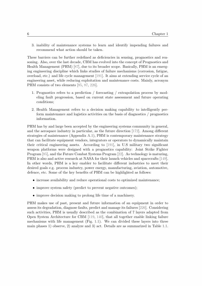
PHM makes use of past, present and future information of an equipment in order toassess its degradation, diagnose faults, predict and manage its failures [226]. Consideringsuch activities, PHM is usually described as the combination of 7 layers adapted fromOpen System Architecture for CBM [119, 140], that all together enable linking failuremechanisms with life management (Fig. 1.1). We can divided these layers into threemain phases 1) observe, 2) analyze and 3) act. Details are as summarized in Table 1.1.
1.1 Prognostics and Health Management (PHM) 7
Table 1.1: 7 layers of PHM cycle
Observe1. Data acquisition: gather useful condition monitoring (CM) data records using
digitized sensors.2. Data processing : perform data cleaning, denoising, relevant features extraction
and selection.
Analyze3. Condition assessment : assess current condition of monitored machinery,
and degradation level.4. Daignostics: perform diagnostics to detect, isolate and identify faults (see
Appendix A.2).5. Prognostics: perform prognostics to project current health of degrading mach-
inery onto future to estimate RUL and associate a confidence interval.
Act6. Decision support : (off-line) recommend actions for maintenance / logistic
(e.g. service quality), and (on-line) system configuration (safety actions).7. Human Machine Interface: interact with different layers, e.g. prognostics,
decision support and display warnings etc.
641 641.5 642 642.5 643 643.5 6442387.9
2387.95
2388
2388.05
2388.1
2388.15
2388.2
2388.25
2388.3
2388.35
0 2000 4000 6000 8000 10000 1200012
13
14
U (V
)
0 1000 2000 3000 4000 5000 600017
18
19
20
Niv
ea
u 1
0 1000 2000 3000 4000 5000 6000-0.1
0
0.1
Temps (min)
PHM
Condition
Assessment
Diagnostic
Prognostics
Data
Acquisition
Data
Processing
Decision
Support
Human Machine
Interface
Figure 1.1: PHM cycle (adapted from [119])
Within analysis phase, prognostics is considered as a key task with future capabilities,which should be performed efficiently for successful decision support to recommendactions for maintenance [13], or system configuration [14]. Therefore, prognostics is acore process in PHM cycle, to decide plan of actions, increase safety, minimize downtime,ensure mission completion and efficient production [49].

8 Chapter 1
1.1.2 Prognostics and the Remaining Useful Life
The concept of prognostics was initially introduced in the medical domain. Medicalprognostics is defined as “the prediction of the future course and the outcome of diseaseprocess” [8]. In engineering, prognostics is generally understood as the process of moni-toring health of an engineering asset, and of predicting the life time at which it will notperform the required function. According to literature, there are several definitions ofprognostics [178], but, few interesting ones are given as follows:
1. the capability to provide early detecting of the precursor and / or incipient faultcondition of a component, and to have the technology and means to manage andpredict the progression of this fault condition to component failure [67];
2. predictive diagnostics, which includes determining the remaining life or time spanof proper operation of a component [86];
3. the prediction of future health states based on current health assessment, historicaltrends and projected usage loads on the equipment and / or process [207];
4. failure prognostics involves forecasting of system degradation based on observedsystem condition [133];
5. the forecast of an asset’s remaining operational life, future condition, or risk tocompletion [83].
A common acceptance can be dressed from above definitions: prognostics can be seen asthe “prediction of a system’s lifetime” as it is a process whose objective is to predict theRemaining Useful Life before a failure occurs. Also, let retain the definition proposedby the International Organization for Standardization [99]:“prognostics is the estimation of time to failure and risk for one or more existing andfuture failure modes”.Note that, the implementation of prognostics for a particular application can be madeat different levels of abstraction like: critical components, sub-system or entire system.Also, RUL is expressed by considering units corresponding to the primary measurementof use for overall system. For example, in case of commercial aircrafts the unit is cycles(i.e., related to number of take-offs), for aircraft engines it is hours of operation, for au-tomobiles it is kilometers (or miles). Having said that, whatever the level of abstractionand the unit to define that, prognostics facilitate decision makers with information, thatenables them to change operating conditions (e.g. load). Consequently, it may prolongservice life of the machinery. In addition, it also benefits the planners to manage up-coming maintenance and to initiate a logistics process, that enables a smooth transitionfrom faulty machinery to fully functional [175].The main capability of prognostics is to help maintenance staff with insight of futurehealth states of a monitored system. This task is mainly composed of two differentsteps. The first step is related to the assessment of current health state (i.e., severity ordegradation detection), which can also be considered under detection and diagnostics.
1.1 Prognostics and Health Management (PHM) 9
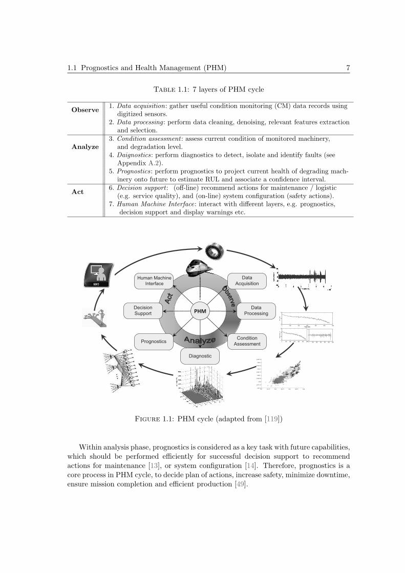
Different pattern recognition techniques can be applied to this phase. The second stepaims at predicting (or forecasting) degradation trends to estimate the RUL, where timeseries techniques can be applied [63].As for illustration of RUL estimation task, consider left part of Fig. 1.2, where for sakeof simplicity the degradation is considered as a one-dimensional signal. In such case,the RUL can be computed between current time tc after degradation has been detectedtD, and the time at which predicted signal passes the failure threshold (FT) (assumedor precisely set by an expert), i.e., time tf, with some confidence to the prediction. TheFT does not necessarily indicate complete failure of the machinery, but a faulty statebeyond which there is a risk of functionality loss [171], and end of life (EOL). Therefore,RUL can be defined by Eq. (1.1):
RUL = tf − tc (1.1)
where tf is a random variable of time to failure, and tc is the current time.
Degradation detected
Time (t)
RU
L
Actual RUL
EOL
Estimated RUL &
confidence
Time (t)
Estimated RUL
tD tc
(end of life - EOL) Complete Failure
Failure threshold (FT)
De
gra
din
g s
tate
Un
cert
ain
(F
T)
tf tc
Actual RUL
Figure 1.2: Illustration of prognostics and RUL estimates
Providing a confidence to predictions is essential for prognostics due to inherent un-certainties of deterioration phenomena, unclear future operating conditions and errorsassociated to the prognostics model. Therefore, decision making should be based onthe bounds of RUL confidence interval rather than single value [178]. Also, narrowconfidence intervals represent high precision / accuracy and are preferred over wide con-fidence intervals that indicate large uncertainty, thus risky decisions should be avoided.Therefore, the combined uncertainty of RUL estimate is not only due to prediction butdue to the FT as well (which should be precise).The right part of Fig. 1.2 shows a situation, where estimated RUL value is updated whennew data arrives at each time interval. In this manner, different RULs are estimated withsome confidence according to availability of data from monitored machinery. Obviously,accuracy of RUL estimates should increase with time, as more data are available.
1.1.3 Prognostics and uncertainty
Aging of machinery in a dynamic environment is a complex phenomena, and it is oftennon-linear function of usage, time, and environmental conditions [191]. Following that,
10 Chapter 1
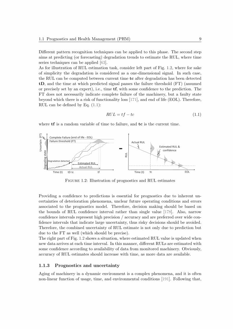
real monitoring data from machinery condition (vibration, temperature, humidity, pres-sure, etc.,) are usually noisy and open to high variability due to direct or indirect impactof usage and environmental conditions related to the degradation of failing machinery.In other words, real-life machinery prognostics is subject to high levels of uncertainty,either due to gathered data or either due to degradation mechanisms. As for example,consider a process, where a component degrades from a healthy state to failure state(see Fig. 1.3). The same component can have different degrading curves due to differentfailure modes (e.g. in case of bearings inner race, outer race, cage crack), even exposedto same operating conditions. Although, failure modes can be for a same bearing, butstill each mode can result different states of degradation that result different RULs. Insuch situations, RUL estimation becomes a complicated challenge for the prognosticsmodel, that requires timely predicting the future unknown and intelligently assessingthe faulty state.
Novel event Novel event
Degraded but operable state
Functional failure
Failure mode 1
Failure mode 2
Failure mode 3
Co
mp
on
en
t H
ea
lth
Time
Bearing
Inner race Balls in cageOuter race
Figure 1.3: Component health evolution curves (adapted from [178])
From the above discussions, some key issues of prognostics can be pointed out.
• How to tackle inherent uncertainties of data?
• How to represent uncertainty of machine deterioration process (i.e., from good tofaulty state)?
• How to avoid uncertainty of FTs, to enable accurate RUL estimates?
Such issues can be related to different sources of uncertainty [40].
1. Input uncertainties that can be due to initial damage, material properties, manu-facturing variability, etc.
1.1 Prognostics and Health Management (PHM) 11
2. Model uncertainties that can be due to modeling error related to inaccurate pre-dictions (for data-driven prognostic approaches it can be related to incompletecoverage of data model training [71]). However, such uncertainties can be reducedby improved modeling methods.
3. Measurement uncertainties that are related to data collection, data processing,etc., and can be managed to a better level. For example sensor noise, loss ofinformation due to data processing, etc.
4. Operating environment uncertainties like unforeseen future loads or environments.
Whatever the type of uncertainties in prognostics, they can impact the accuracy ofRUL estimates which prevents to recommend timely actions for decision making processor system configuration. In brief, for prognostics system development, three differentprocesses are essential to handle uncertainty [40].
• To represent uncertainty of data, which include common theories like fuzzy settheory, probability theory, etc.;
• To quantify uncertainty related to different sources as correctly as possible;
• To manage the uncertainty by processing the data in an effective manner.
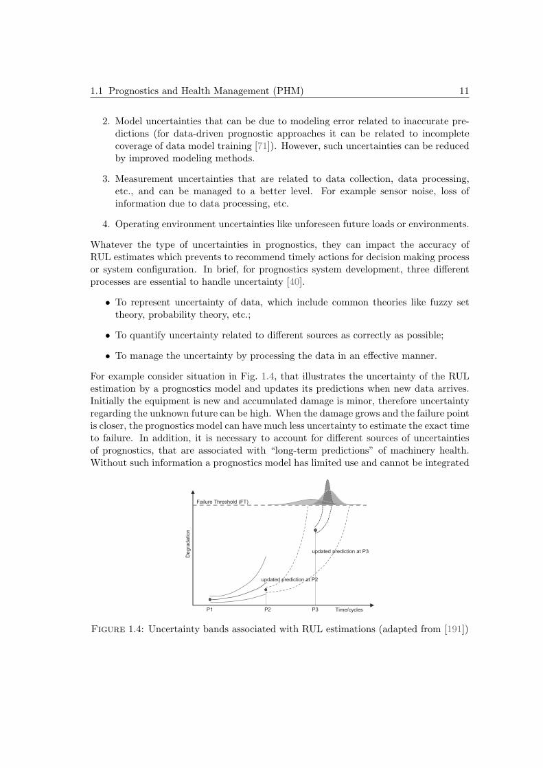
For example consider situation in Fig. 1.4, that illustrates the uncertainty of the RULestimation by a prognostics model and updates its predictions when new data arrives.Initially the equipment is new and accumulated damage is minor, therefore uncertaintyregarding the unknown future can be high. When the damage grows and the failure pointis closer, the prognostics model can have much less uncertainty to estimate the exact timeto failure. In addition, it is necessary to account for different sources of uncertaintiesof prognostics, that are associated with “long-term predictions” of machinery health.Without such information a prognostics model has limited use and cannot be integrated
Failure Threshold (FT)
Degra
datio
n
Time/cycles P1 P2 P3
updated prediction at P2
updated prediction at P3
Figure 1.4: Uncertainty bands associated with RUL estimations (adapted from [191])
12 Chapter 1
for critical applications. Therefore, in this thesis, uncertainty of prognostics is dealt by:quantifying uncertainty due to data and modeling phase, representing uncertainty usingfuzzy set theory, and managing uncertainty by processing data.
1.2 Prognostics approaches
The core process of prognostics is to estimate the RUL of machinery by predicting thefuture evolution at an early stages of degradation. An accurate RUL estimation enablesto run the equipment safely as long as it is healthy, which benefits in terms of additionaltime to opportunely plan and prepare maintenance interventions for most convenientand inexpensive times [105]. Due to the significance of such aspects, study on PHMhas grown rapidly in recent years, where different prognostics approaches are beingdeveloped. Several review papers on the classification of prognostics approaches havebeen published [60, 74, 105, 115, 153, 156, 177, 178, 192, 193]. In spite of divergence inliterature, we bring discussions on common grounds, where prognostics approaches areclassified into three types: 1) physics based prognostics, 2) data-driven prognostics and3) hybrid prognostics. But still, these classes are not well addressed in literature, whichrequires a detailed survey.
1.2.1 Physics based prognostics
1.2.1.1 Overview
The physics based or model based approaches for prognostics use explicit mathematicalrepresentation (or white-box model) to formalize physical understanding of a degradingsystem [155]. RUL estimates with such approaches are achieved on the basis of acquiredknowledge of the process that affects normal machine operation and can cause failure.They are based on the principle that failure occurs from fundamental processes: me-chanical, electrical, chemical, thermal, radiation [154]. Common approaches of physicsbased modeling include material level models like spall progression models, crack-growthmodels or gas path models for turbine engines [84, 178, 191]. To identify potential failuremechanisms, such methods utilize knowledge like loading conditions, geometry, and ma-terial properties of a system [153]. To predict the behavior of the system, such methodsrequire detailed knowledge and through understanding of the process and mechanismsthat cause failure. In other words, failure criteria are created by using physics of failure(POF) analysis and historic data information about failed equipment [88]. Implementa-tion of physics based approach has to go through number of steps that include, failuremodes and effects analysis (FMEA), feature extraction, and RUL estimation [153].It should be noted that in literature, different works categorize physics based (or model-based) prognostics as POF and system modeling approach [155, 158]. However, theyshould be limited to POF [192, 197], because system modeling approaches are depen-dent on data-driven methods to tune parameters of physics based model and should beclassified as hybrid approach for prognostics (see section 1.2.3).

1.2 Prognostics approaches 13
1.2.1.2 Application point of view
In general, physics based approaches are application specific. They assume that sys-tem behavior can be described analytically and accurately. Physics based methods aresuitable for a situation where accuracy outweighs other factors, such as the case of airvehicles [168]. POF models are usually applied at component or material level [197].However, for most industrial applications physics based methods might not be a properchoice, because fault types can vary from one component to another and are difficultto identify without interrupting operating machinery [84]. In addition, system spe-cific knowledge like material composition, geometry may not be always available [155].Besides that, future loading conditions also affect fault propagation. Therefore in adynamic operating environment, the model may not be accurate due to assumptions,errors and uncertainty in the application [197]. In such cases POF models are combinedwith data-driven methods to update model parameters in an on-line manner, whichturns into a hybrid approach (and is discussed in section 1.2.3).
1.2.2 Data-driven prognostics
Data-driven (DD) prognostics approaches can be seen as black box models that learnsystems behavior directly from collected condition monitoring (CM) data (e.g. vibration,acoustic signal, force, pressure, temperature, current, voltage, etc). They rely on theassumption that the statistical characteristics of system data are relatively unchangedunless a malfunctioning occurs. Such methods transform raw monitoring data into rel-evant information and behavioral models (including the degradation) of the system.Therefore, data-driven methods can be low cost models with an advantage of betterapplicability, as they only require data instead of prior knowledge or human experts[110, 111, 155].According to literature, several studies are performed to categorize data-driven prog-nostics approaches. [63, 220] classified data-driven methods into machine learning andstatistical approaches. [60, 156] classified data-driven approaches as artificial intelligence(AI) techniques and Statistical techniques. A survey on AI approaches for prognosticswas presented by [176], where data-driven approaches were categorized as conventionalnumerical methods and machine learning methods. [158] classified data-driven prognos-tics methods as, evolutionary, machine learning / AI and state estimation techniques.However, we classify data-driven approaches for prognostics into two categories. 1)machine learning approaches and 2) statistical approaches.
1.2.2.1 Machine learning approaches
Machine learning approaches are branch of AI that attempt to learn by examples and arecapable to capture complex relationships among collected data that are hard to describe.Obviously, such methods are suitable for situations where physics based modeling arenot favorable to replicate behavior model [111]. Depending on the type of availabledata, learning can be performed in different ways. Supervised learning can be applied

14 Chapter 1
to labeled data, i.e., data are composed of input and the desired output is known. Un-supervised learning is applied to unlabeled data, i.e., learning data are only composedof input and desired output is unknown. Semi-supervised learning that involves bothlabeled (few data points) and unlabeled data. A partially supervised learning is per-formed when data have imprecise and / or uncertain soft labels, (i.e., learning data arecomposed of input and desired outputs are known with soft labels or belief mass [50]).Machine learning is a rapidly growing field in PHM domain, and vast numbers of algo-rithms are being developed. In brief, machine learning approaches for prognostics canbe categorized with some examples as follows.
Connectionist methods - Flexible methods that use examples to learn and infercomplex relations among data e.g.:
• Artificial neural networks (ANN) [9, 107, 134];
• Combination of ANN and Fuzzy rules, e.g. Neuro-Fuzzy systems [59, 107].
Bayesian methods - Probabilistic graphical methods mostly used in presence ofuncertainty, particularly dynamic Bayesian approaches e.g.:
• Markov Models and variants, e.g. Hidden Markov Models (HMM) [138, 165];
• State estimation approaches, e.g. Kalman Filter, Particle Filter and variants [20,174, 178].
Instance Based Learning methods (IBL) - Obtain knowledge from stored ex-amples that were presented for learning and utilize this knowledge to find similaritybetween learned examples and new objects:
• K-nearest neighbor algorithm [142];
• Case-based reasoning for advanced IBL [197].
Combination methods - Can be an effective combination of supervised, unsuper-vised methods, semi-supervised and partially supervised methods or other possible com-binations to overcome drawbacks of an individual data-driven approach, for e.g.:
• Connectionist approach and state estimation techniques [18];
• Connectionist approach and clustering methods [108, 164];
• Ensemble of different approaches to quantify uncertainty and to achieve robustmodels [17, 20, 89].
Note that, some of the above mentioned categories can also include supervised, unsu-pervised, semi-supervised learning or partially supervised approaches, however we avoidany strict classification.

1.2 Prognostics approaches 15
1.2.2.2 Statistical approaches
They estimate the RUL by fitting the probabilistic model to the collected data and ex-trapolate the fitted curve to failure criteria. Statistical approaches are simple to conduct.Like machine learning approaches, statistical methods also require sufficient conditionmonitoring (CM) data to learn behavior of degrading machinery. However, they canhave large errors in case of incomplete data, and the nature of data has therefore itsown importance in this category.[177] presented a state-of-the-art review of statistical approaches, where the taxonomywas mainly based on nature of CM data. From this systematic review, some commonlyknown prognostics approaches can be: regression based methods, stochastic filteringor state estimation methods like Kalman Filters Particle Filters and variants, HiddenMarkov models and variants etc. Further details about this taxonomy are describedin [177]. It should be noted that, Bayesian techniques cited just above can also beaddressed as machine learning approaches. Other methods in this category can be clas-sical time series prediction methods like Auto-Regressive Moving Average and variantsor proportional hazards models [178].
1.2.2.3 Application point of view
In general, the strength of data-driven approaches is their ability to transform high-dimensional noisy data into low-dimensional information for prognostics decisions [60].However, data-driven methods encounter common criticism that they require more dataas compared to physics based approach, which is not surprising. Obviously sufficientquantities of run-to-failure data are necessary for data-driven models to learn and cap-ture complex relations among data. In this context, sufficient quantity means that datahas been observed for all fault-modes of interest [191]. However, some industrial systemscan not be allowed to run until failure due to their consequences.Beside that, quantity and quality of data are also important. Indeed, real machinery op-erates in highly non-linear environment and monitored data could be of high variability,sensor noise, which can impact on performance of data-driven methods. Therefore, it isessential to properly process acquired data in order to obtain good features to reducemodeling complexity, and increase accuracy of RUL estimates.Machine learning approaches have the advantage that, they can be deployed rapidly andwith low implementation cost as compared to physics based methods. In addition, theycan provide system-wide scope, where scope of physics based approaches can be limited.Machine learning approach for prognostics could be performed with a connectionist feedforward neural network [107] to predict continuous state of degradation recursively, untilit reaches FT. However, such methods provide point predictions and do not furnish anyconfidence [111]. In comparison, Bayesian methods can be applied to manage uncer-tainty of prognostics [40], but, again RUL estimates rely on FT. Instance based learningmethods do not need FT and can directly estimate the RUL by matching similarityamong stored examples and new test instances [142]. They can also be called as expe-rience based approaches [197]. Combination of different machine learning approaches
16 Chapter 1
can be a suitable choice to overcome drawbacks of an individual method [164]. But,whatever the approach considered for building a prognostics model, it is important toinvolve operating conditions and actual usage environment.Lastly, statistical approaches for prognostics also require large amount of failure data toimplement models. These approaches are economical and require fewer computationsas compared to machine learning approaches. For e.g. methods like classical regressionare simpler to build. However, they do not consider operating conditions, actual usageenvironments and failure mechanism [220].
1.2.3 Hybrid prognostics
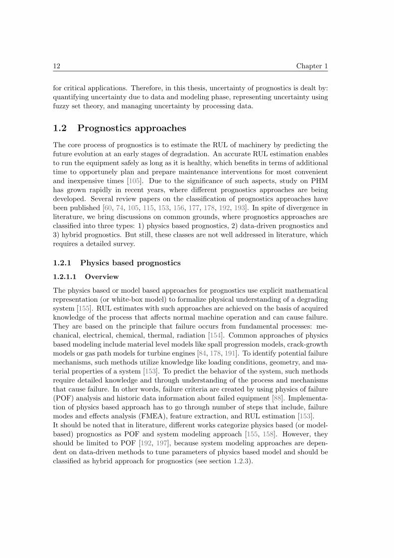
A hybrid (Hyb) approach is an integration of physics based and data-driven prognosticsapproaches, that attempts to leverage the strengths from both categories. The main ideais to benefit from both approaches to achieve finely tuned prognostics models that havebetter capability to manage uncertainty, and can result in more accurate RUL estimates.According to literature, hybrid modeling can be performed in two ways [157]: 1) seriesapproach, and 2) parallel approach.
1.2.3.1 Series approach
In PHM discipline, series approach is also known as system modeling approach thatcombines physics based approach having prior knowledge about the process being mod-eled, and a data-driven approach that serves as a state estimator of unmeasured processparameters which are hard to model by first principles [160]. Several works in recentliterature address series approach as model based prognostics [19, 155, 158, 174]. How-ever it cannot be regarded as model based, because, physics based model is dependanton a data-driven approach to tune its parameters (see Fig. 1.5).
Figure 1.5: Series approach for hybrid prognostics model (adapted from [71])
In brief, the representation (or modeling) of an engineering asset is made with mathe-matical functions or mappings, like differential equations. Statistical estimation methodsbased on residuals and parity relations (i.e., difference of predictions from a model andsystem observations) are applied to detect, isolate and predict degradation to estimatethe RUL [130, 192]. Practically, even if the model of process is known, RUL estimates
1.2 Prognostics approaches 17
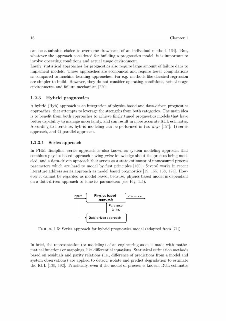
might be hard to achieve, where the state of the degrading machinery may not be observ-able directly or measurements may be affected by noise [71]. In this case, a mathematicalmodel is integrated with on-line parameter estimation methods to infer degrading stateand furnish reliable quantification of uncertainty. State estimation techniques can beBayesian methods like Kalman filter, Particle filter and variant [178], that update theprediction upon collection of new data [57, 58] (see Fig. 1.6).
Figure 1.6: Battery capacity predictions and new pdf of RUL [169]
As for example from recent literature, [16] developed a physics based model relying onparticle filtering to predict the RUL of turbine blades. An approach to RUL estimationof power MOSFETs (metal oxide field effect transistor) was presented by [41], whichused an extended Kalman filter and a particle filter to accomplish prognostics mod-els. An unscented Kalman filter based approach was applied for prognostics of PEMFC(polymer electrolyte membrane fuel cell) [221]. Recently, another interesting applica-tion on prognostics PEMFC was presented by [112], using particle filter that enabled toinclude non-observable states into physical models. [33] proposed a particle filter basedapproach to track spall propagation rate and to update predictions. [10, 11] presenteda Matlab based tutorial that combines physical model for crack growth and particlefilter, which uses the observed data to identify model parameters. [17] proposed a seriesapproach concerning the prediction of the RUL of a creeping turbine blade.
1.2.3.2 Parallel approach
Physics based approaches make use of system specific knowledge, while data-driven ap-proaches utilize in situ monitoring data for prognostics. Both approaches can have theirown limitations and advantages. A parallel combination can benefit from advantagesof physics based and data-driven approach, such that the output from resulting hybridmodel is more accurate (see Fig. 1.7). According to literature, with parallel approach,the data-driven models are trained to predict the residuals not explained by the firstprinciple model [71, 185].In PHM discipline still different terminologies are being used for such modeling. [21]
18 Chapter 1
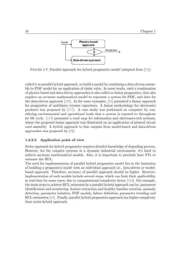
Figure 1.7: Parallel approach for hybrid prognostics model (adapted from [71])
called it as parallel hybrid approach, to build a model by combining a data-driven ensem-ble to POF model for an application of choke valve. In some works, such a combinationof physics based and data-driven approaches is also called as fusion prognostics, that alsorequires an accurate mathematical model to represent a system for POF, and data forthe data-driven approach [182]. As for some examples, [44] presented a fusion approachfor prognostics of multilayer ceramic capacitors. A fusion methodology for electronicsproducts was proposed by [117]. A case study was performed on computer by con-sidering environmental and operational loads that a system is exposed to throughoutits life cycle. [155] presented a road map for information and electronics-rich systems,where the proposed fusion approach was illustrated on an application of printed circuitcard assembly. A hybrid approach to fuse outputs from model-based and data-drivenapproaches was proposed by [82].
1.2.3.3 Application point of view
Series approach for hybrid prognostics requires detailed knowledge of degrading process.However, for the complex systems in a dynamic industrial environment, it’s hard toachieve accurate mathematical models. Also, it is important to precisely have FTs toestimate the RUL.The need for implementation of parallel hybrid prognostics model lies in the limitationof building a prognostics model with an individual approach i.e., data-driven or model-based approach. Therefore, accuracy of parallel approach should be higher. However,implementation of such models include several steps, which can limit their applicabilityin real-time for some cases, due to computational complexity factor [182]. For example,the main steps to achieve RUL estimates by a parallel hybrid approach can be, parameteridentification and monitoring, feature extraction and healthy baseline creation, anomalydetection, parameter isolation, POF models, failure definition, parameter trending andRUL estimation [44]. Finally, parallel hybrid prognostics approach has higher complexitythan series hybrid approach.
1.2 Prognostics approaches 19
1.2.4 Synthesis and discussions
1.2.4.1 Proposed classification of prognostics approaches
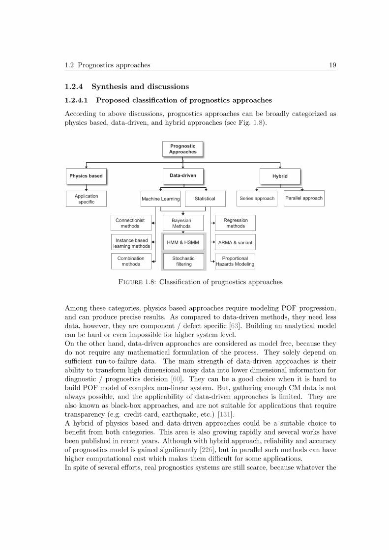
According to above discussions, prognostics approaches can be broadly categorized asphysics based, data-driven, and hybrid approaches (see Fig. 1.8).
Physics based
Application
specific
Hybrid
Series approach
Parallel approach
Data-driven
Machine Learning Statistical
Connectionist
methods
Regression
methods
Combination
methods
Instance based
learning methods ARMA & variant
Proportional
Hazards Modeling
HMM & HSMM
Stochastic
filtering
Prognostic
Approaches
Bayesian
Methods
Figure 1.8: Classification of prognostics approaches
Among these categories, physics based approaches require modeling POF progression,and can produce precise results. As compared to data-driven methods, they need lessdata, however, they are component / defect specific [63]. Building an analytical modelcan be hard or even impossible for higher system level.On the other hand, data-driven approaches are considered as model free, because theydo not require any mathematical formulation of the process. They solely depend onsufficient run-to-failure data. The main strength of data-driven approaches is theirability to transform high dimensional noisy data into lower dimensional information fordiagnostic / prognostics decision [60]. They can be a good choice when it is hard tobuild POF model of complex non-linear system. But, gathering enough CM data is notalways possible, and the applicability of data-driven approaches is limited. They arealso known as black-box approaches, and are not suitable for applications that requiretransparency (e.g. credit card, earthquake, etc.) [131].A hybrid of physics based and data-driven approaches could be a suitable choice tobenefit from both categories. This area is also growing rapidly and several works havebeen published in recent years. Although with hybrid approach, reliability and accuracyof prognostics model is gained significantly [226], but in parallel such methods can havehigher computational cost which makes them difficult for some applications.In spite of several efforts, real prognostics systems are still scarce, because whatever the
20 Chapter 1
prognostics approach either physics based, data-driven or hybrid, they are subject toparticular assumptions [178]. In addition, each approach has its own advantages anddisadvantages, which limits their applicability. Thereby, for a particular application(either for system level or for component level) a prognostics approach should be selectedby considering two important factors: 1) performance and 2) applicability.
1.2.4.2 Usefulness evaluation - criteria
In general, prognostics domain lacks in standardized concepts, and is still evolving toattain certain level of maturity for real industrial applications. To approve a prognosticsmodel for a critical machinery, it is required to evaluate its performances a priori, againstcertain issues that are inherent to uncertainty from various sources. However, there areno universally accepted methods to quantify the benefit of a prognostics method [191],where, the desired set of prognostics metrics is not explicit and less understood. Methodsto evaluate the performances of prognostics have acquired significant attention in recentyears. From a survey, [171, 173] provided a functional classification of performancemetrics, and categorize them into four classes.
1. Algorithm performance: metrics in this category evaluate prognostics model per-formance by errors obtained from actual and estimated RUL. Selection amongcompetitive models is performed by considering different accuracy and precisioncriteria, e.g. Mean Absolute Percentage Error (MAPE), standard deviations, etc.
2. Computational performance: metrics in this category highlight the importanceof computational performance of prognostics models, especially in case of criti-cal systems that require less computational time for decision making. Therefore,for a particular prognostics approach computational performance can be easilymeasured by CPU time or elapsed time (or wall-clock time).
3. Cost Benefit Risk: metrics in this category are related to cost benefits that areinfluenced by accuracy of RUL estimates. Obviously, operational costs can bereduced if RUL estimates are accurate. Because, this will result in replacementof fewer components before the need and also potentially fewer costly failures[171]. For example, metrics in this class can be the ratio of mean time betweenfailure (MTBF) and mean time between unit replacement (MTBUR), return oninvestment (ROI), etc.
4. Ease of algorithm Certification: metrics in this category are related to the assur-ance of an algorithm for a particular application (see [171] for details).
From the above classification, Cost Benefit Risk metrics have a broad scope, and obvi-ously it is hard to quantify probable risks that are to be avoided. The Ease of algorithmCertification metrics are related to algorithm performance class, because if the prognos-tics model error / confidence is not mastered, it can not be certified.In addition to above classification, a list of off-line metrics is also proposed by [171, 173]to assess prognostics models before they are applied to a real situation. For example,
1.2 Prognostics approaches 21
this includes metrics of: accuracy and precision, prognostics horizon, prediction spread,horizon / prediction ratio, which are again related to algorithm performance class.Therefore, finally this thesis focuses only on metrics from algorithm and computationalperformance classes for prognostics model evaluation (i.e., class 1 and 2).
As far as applicability of the prognostics approach is concerned, thanks to the discus-sions on the application point of view for each prognostics approach (in sections 1.2.1.2,1.2.2.3, 1.2.3.3) one can point out important criteria for applicability assessment:
• requirement of degradation process model;
• failure thresholds;
• generality or scope of the approach;
• learning experience, i.e., run-to-failure data;
• transparency or openness.
• modeling complexity and computation time.
1.2.4.3 Prognostics approach selection
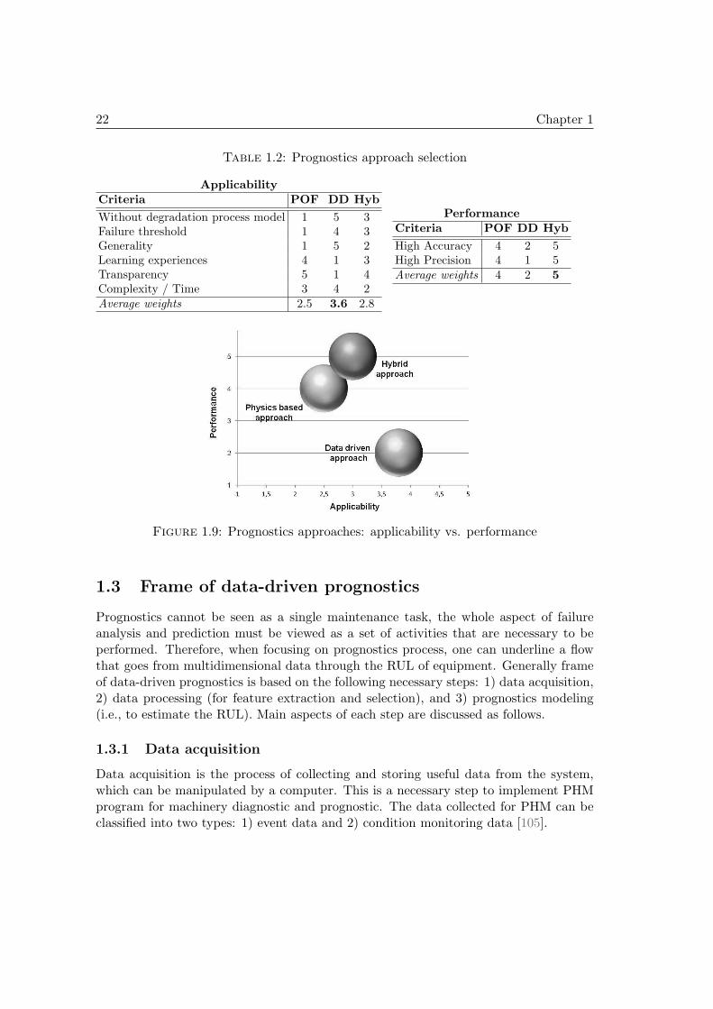
According to above discussions, in order to select a prognostics approach, performanceand applicability factors are assessed upon different criteria (based on previous survey).An interval I = [1, 5] is considered to assign weights for each approach according to thegiven criteria, where 1 represents min weight and 5 represents max weight. For examplein Table 1.2, consider the first entry “without degradation process model” (applicabil-ity factor). For this criteria, data-driven approach has max weight (i.e., 5), because itdoes not require any explicit model of degradation process for prognostics. Similarly,physics based approach has been assigned min weight (i.e., 1), as it is dependent onmathematical model of degradation process. In this manner, weights for each criteriaare carefully given for both factors (i.e., applicability and performance) in Table 1.2,and are further averaged to finally select a particular prognostics approach. For moreclarity, a plot of averaged weights in terms of applicability vs. performance is alsoshown in Fig. 1.9. The assessment clearly shows that data-driven methods have higherapplicability as compared to other approaches, but performances need further improve-ment. Considering the importance of such broader aspects, following topics focus ondata-driven approaches, particularly combination methods from machine learning cat-egory (section 1.2.2.1). Data-driven prognostics with combination of machine learningmethods is a less explored area, but apparently growing rapidly due to its good poten-tial to overcome drawbacks of conventional data-driven approaches. Like other machinelearning methods, combination methods can be deployed quickly and cheaply, and canprovide system wide coverage. Finally, combination approach can also be suitable tomeet most of the criteria related to performance and applicability factors, which areconsidered in this thesis (i.e., Table 1.2).
22 Chapter 1
Table 1.2: Prognostics approach selection
ApplicabilityCriteria POF DD Hyb
Without degradation process model 1 5 3Failure threshold 1 4 3Generality 1 5 2Learning experiences 4 1 3Transparency 5 1 4Complexity / Time 3 4 2Average weights 2.5 3.6 2.8
PerformanceCriteria POF DD Hyb
High Accuracy 4 2 5High Precision 4 1 5Average weights 4 2 5
Figure 1.9: Prognostics approaches: applicability vs. performance
1.3 Frame of data-driven prognostics
Prognostics cannot be seen as a single maintenance task, the whole aspect of failureanalysis and prediction must be viewed as a set of activities that are necessary to beperformed. Therefore, when focusing on prognostics process, one can underline a flowthat goes from multidimensional data through the RUL of equipment. Generally frameof data-driven prognostics is based on the following necessary steps: 1) data acquisition,2) data processing (for feature extraction and selection), and 3) prognostics modeling(i.e., to estimate the RUL). Main aspects of each step are discussed as follows.
1.3.1 Data acquisition
Data acquisition is the process of collecting and storing useful data from the system,which can be manipulated by a computer. This is a necessary step to implement PHMprogram for machinery diagnostic and prognostic. The data collected for PHM can beclassified into two types: 1) event data and 2) condition monitoring data [105].
1.3 Frame of data-driven prognostics 23
1. Event data: event data records are combination of information on what actuallyhappened (e.g. breakdown, installation, overhaul, etc) and what were the causesand / or and what was done (e.g. preventive maintenance, minor repairs, etc.) forthe targeted engineering asset.
2. Condition monitoring (CM) data: CM data are collected thorough a procedure ofmonitoring parameters of health condition / state of the machinery, in order toclearly identify the changes that can develop faults or can even lead to failures.Such parameters can be vibration, force, temperature, voltage, acoustic, humidity,etc., where various sensors can be applied to collect data for such parameters likeaccelerometers to measure vibration, dynamometers to measure force, etc.
1.3.2 Data pre-processing
Raw data acquired from the machinery are normally redundant and noisy and cannotbe used directly by a prognostics model. In other words, relevant information relatedto degrading machinery is often hidden in raw data, and should be processed to ex-tract / select features. Also, the effectiveness of a prognostics model is closely relatedto the quality of features, that can impact uncertainty of prognostics. Besides that, itis also important to identify features that are sensitive to machine condition and clearlyreflect failure progression to serve need of modeling task [38, 211]. Feature selection orvariable selection is an important process to obtain a subset of useful features that canbe used for prognostics model construction.
1.3.3 Prognostics modeling strategies for RUL estimation
The primary objective of prognostics is to build an effective model that is capable ofpredicting the evolution of degrading features (or variables) under anticipated operatingconditions, and can provide RUL of the machinery. However, estimation of RUL is usu-ally hard to perform. In recent years, research to build accurate prognostics models hasgained popularity, and there are rapid advances especially with data-driven approaches.According to the discussions, we classify the RUL estimation strategies with a data-driven approach into three groups, 1) univariate degradation based modeling, 2) directRUL prediction and 3) multivariate degradation based modeling.
1.3.3.1 Univariate degradation based modeling
The univariate degradation based prognostics modeling rely on the prediction of con-tinuous degrading state followed by a failure criteria, where RUL estimate is obtainedwhen degrading signal intersects a pre-defined FT (see Fig. 1.10). In this case, the data-driven approaches learn the model of degradation from time series observations throughregression, trending or stochastic process modeling [36, 219]. The main difficulty withthis method is to define FTs, which is often very hard to achieve and can restrict the ap-plicability of univariate degradation based approach. Due to this problem, some worksin literature assume FTs to estimate the RUL [28, 186]. However, such assumptions are

24 Chapter 1
less realistic for prognostics application and should be avoided, because, the uncertaintyof FT can lead to poor prognostics and negative outcomes.
Data pre-processing
Features
extraction
Features
selection
Data
acquisition
Physical system
Prognostics model
Features prediction
tc tf
RUL
EOL
Failure threshold (FT)
Time (t)
Degra
dation
Figure 1.10: Univariate degradation based modeling strategy
1.3.3.2 Direct RUL prediction (or similarity based prognostics)
Direct RUL prediction approach learns from the data directly, the relation betweenobserved trends and equipment EOL time to obtain RUL. Therefore, the RUL is derivedfrom data-driven model by applying a pattern matching process (or finding similarity)between the current observation and the knowledge of equipment RUL [71, 199, 227](see Fig. 1.11). This method does not require definition of failure criteria, but rely onsmooth and monotonic trends to facilitate pattern matching [142]. However, even asmall deviation from matched history case, either due to uncertain operating conditionsor non-linearity due to noise phenomena can lead to large RUL errors. In addition,it is also necessary to have sufficient knowledge on RULs available in training dataset.Lastly, the similarity search procedure can be costly as well [197].
Prognostics model Data pre-processing
Features
extraction
Features
selection
Data
acquisition
Library of models
RUL
Similarity
Physical system
Figure 1.11: Direct RUL prediction strategy
1.3.3.3 Multivariate degradation based modeling
With univariate degradation based approach, failure definitions could be a difficult taskto achieve. To resolve that issue, a new idea for RUL estimation was proposed by [61].According to this proposition, prognostics modeling is performed by using a predictionmodel and a health assessment model to estimate the RUL. The complete illustration ofthis method was given in [164]. Later, this approach was further developed and namedas joint approach for RUL estimation [166]. Mainly, the aim of multivariate degradation
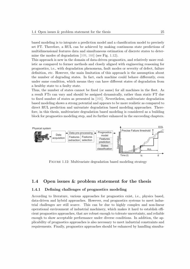
1.4 Open issues & problem statement for the thesis 25
based modeling is to integrate a prediction model and a classification model to preciselyset FT. Therefore, a RUL can be achieved by making continuous state predictions ofmultidimensional features data and simultaneous estimation of discrete states to deter-mine the modes of degradation [109, 166] (see Fig. 1.12).This approach is new in the domain of data-driven prognostics, and relatively more real-istic as compared to former methods and closely aligned with engineering reasoning forprognostics, i.e., with degradation phenomena, fault modes or severity of defect, failuredefinition, etc. However, the main limitation of this approach is the assumption aboutthe number of degrading states. In fact, each machine could behave differently, evenunder same condition, which means they can have different states of degradation froma healthy state to a faulty state.Thus, the number of states cannot be fixed (or same) for all machines in the fleet. Asa result FTs can vary and should be assigned dynamically, rather than static FT dueto fixed number of states as presented in [166]. Nevertheless, multivariate degradationbased modeling shows a strong potential and appears to be more realistic as compared todirect RUL prediction and univariate degradation based modeling approaches. There-fore, in this thesis, multivariate degradation based modeling is considered as a buildingblock for prognostics modeling step, and its further enhanced in the succeeding chapters.
Data pre-processing
Features
extraction
Features
selection
Data
acquisition
Prognostics
model
RUL
tc tf Time (t)
De
gra
datio
n
EOL
Precise Failure threshold Physical system
Features
prediction
States
classification
Figure 1.12: Multivariate degradation based modeling strategy
1.4 Open issues & problem statement for the thesis
1.4.1 Defining challenges of prognostics modeling
According to literature, various approaches for prognostics exist, i.e., physics based,data-driven and hybrid approaches. However, real prognostics systems to meet indus-trial challenges are still scarce. This can be due to highly complex and non-linearoperational environment of industrial machinery, which makes it hard to establish effi-cient prognostics approaches, that are robust enough to tolerate uncertainty, and reliableenough to show acceptable performance under diverse conditions. In addition, the ap-plicability of prognostics approaches is also necessary to meet industrial constraints andrequirements. Finally, prognostics approaches should be enhanced by handling simulta-
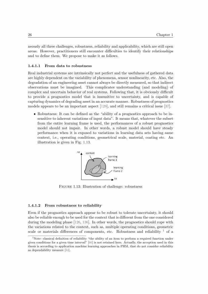
26 Chapter 1
neously all three challenges, robustness, reliability and applicability, which are still openareas. However, practitioners still encounter difficulties to identify their relationshipsand to define them. We propose to make it as follows.
1.4.1.1 From data to robustness
Real industrial systems are intrinsically not perfect and the usefulness of gathered dataare highly dependent on the variability of phenomena, sensor nonlinearity, etc. Also, thedegradation of an engineering asset cannot always be directly measured, so that indirectobservations must be imagined. This complicates understanding (and modeling) ofcomplex and uncertain behavior of real systems. Following that, it is obviously difficultto provide a prognostics model that is insensitive to uncertainty, and is capable ofcapturing dynamics of degrading asset in an accurate manner. Robustness of prognosticsmodels appears to be an important aspect [128], and still remains a critical issue [37].
• Robustness: It can be defined as the “ability of a prognostics approach to be in-sensitive to inherent variations of input data”. It means that, whatever the subsetfrom the entire learning frame is used, the performances of a robust prognosticsmodel should not impair. In other words, a robust model should have steadyperformance when it is exposed to variations in learning data sets having samecontext, i.e., operating conditions, geometrical scale, material, coating etc. Anillustration is given in Fig. 1.13.
Figure 1.13: Illustration of challenge: robustness
1.4.1.2 From robustness to reliability
Even if the prognostics approach appear to be robust to tolerate uncertainty, it shouldalso be reliable enough to be used for the context that is different from the one consideredduring the modeling phase [126, 136]. In other words, the prognostics should cope withthe variations related to the context, such as, multiple operating conditions, geometricscale or materials differences of components, etc. Robustness and reliability 1 of a
1Note: classical definition of reliability “the ability of an item to perform a required function undergiven conditions for a given time interval” [66] is not retained here. Actually, the acception used in thisthesis is according to application machine learning approaches in PHM, that do not consider reliabilityas dependability measure [34].
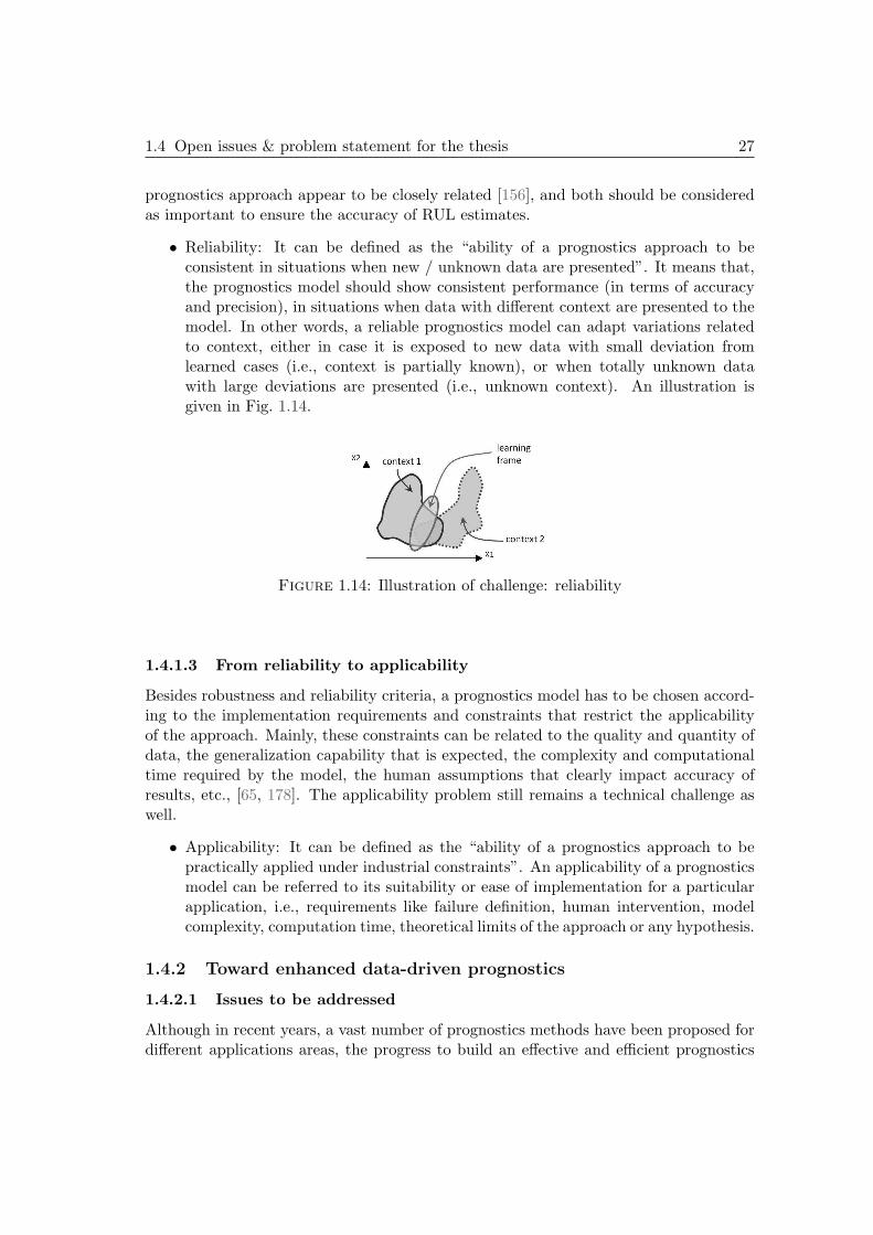
1.4 Open issues & problem statement for the thesis 27
prognostics approach appear to be closely related [156], and both should be consideredas important to ensure the accuracy of RUL estimates.
• Reliability: It can be defined as the “ability of a prognostics approach to beconsistent in situations when new / unknown data are presented”. It means that,the prognostics model should show consistent performance (in terms of accuracyand precision), in situations when data with different context are presented to themodel. In other words, a reliable prognostics model can adapt variations relatedto context, either in case it is exposed to new data with small deviation fromlearned cases (i.e., context is partially known), or when totally unknown datawith large deviations are presented (i.e., unknown context). An illustration isgiven in Fig. 1.14.
Figure 1.14: Illustration of challenge: reliability
1.4.1.3 From reliability to applicability
Besides robustness and reliability criteria, a prognostics model has to be chosen accord-ing to the implementation requirements and constraints that restrict the applicabilityof the approach. Mainly, these constraints can be related to the quality and quantity ofdata, the generalization capability that is expected, the complexity and computationaltime required by the model, the human assumptions that clearly impact accuracy ofresults, etc., [65, 178]. The applicability problem still remains a technical challenge aswell.
• Applicability: It can be defined as the “ability of a prognostics approach to bepractically applied under industrial constraints”. An applicability of a prognosticsmodel can be referred to its suitability or ease of implementation for a particularapplication, i.e., requirements like failure definition, human intervention, modelcomplexity, computation time, theoretical limits of the approach or any hypothesis.
1.4.2 Toward enhanced data-driven prognostics
1.4.2.1 Issues to be addressed
Although in recent years, a vast number of prognostics methods have been proposed fordifferent applications areas, the progress to build an effective and efficient prognostics
28 Chapter 1
approach is still limited. Usually, lack of understating about complex and non-linearbehavior of degrading machinery under dynamic operating environment prevents prac-titioners to develop precise mathematical models for prognostics. In such situationsdata-driven prognostics approaches can be a good alternate to learn behavior of de-grading machinery directly from the data, without any physical understanding aboutthe degradation process. However, performances of prognostics model can suffer duedifferent factors like: inherent uncertainties associated to deterioration process, lack ofsufficient quantities of run-to-failure data, sensor noise, unknown environmental andoperating conditions, and engineering variations. Obviously in such situations it couldbe quite hard to precisely infer the exact state of degrading machinery, and to furtherpredict the evolution of degradation from the collected data. In this context, inherentuncertainty of data (e.g. due to variability of phenomena, sensor non-linearity, etc,) canaffect robustness of the prognostics model in the learning frame, and also small or largedeviations from learned experiences (e.g. due to different context) can affect reliabilityof the prognostics model in the testing frame. Moreover, the applicability of the prog-nostics model is equally important from engineering point of view, to meet real-timeconstraints and requirements for a particular industrial application. According to thesediscussions, key issues of data-driven prognostics can be summarized as follows.
• How to obtain right information in the form of features that clearly reflect deteri-oration phenomena?
• How to improve robustness and reliability of prognostics model to handle uncertaininputs and deviations from learned experiences?
• How to improve the applicability of the prognostics model to meet constraints andrequirements of a real application?
• How to validate the performances of a prognostics model?
The issues highlighted above confirm that, the need to enhanced data-driven prognosticsis inevitable. Therefore, the main assumptions, objective and contributions of this thesisare provided in the following sections.
1.4.2.2 Assumptions
To address identified problems, following assumptions have been made for the proposedprognostics approach.
1. There is at least one way to extract features that are representative of machineryconditions.
2. Collected data should consist of historical run-to-failure observation sequences.
3. It is assumed that degradation has been already detected (see Fig. 1.2).
4. Degrading machinery can not go under self healing.
5. It is assumed that prognostics is achieved at component level.
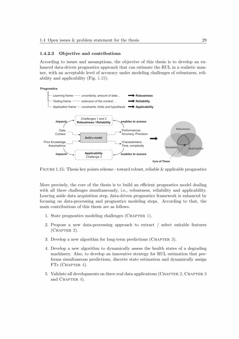
1.4 Open issues & problem statement for the thesis 29
1.4.2.3 Objective and contributions
According to issues and assumptions, the objective of this thesis is to develop an en-hanced data-driven prognostics approach that can estimate the RUL in a realistic man-ner, with an acceptable level of accuracy under modeling challenges of robustness, reli-ability and applicability (Fig. 1.15).
Prognostics
Robustness Learning frame uncertainty, amount of data…
Reliability Testing frame extension of the context…
Applicability Application frame constraints, limits and hypothesis
Data
Context
Prior Knowledge
Assumptions
Performances:
Accuracy, Precision
Characteristics:
Time, complexity
impacts
impacts
enables to assess
enables to assess
Build a model
Challenges 1 and 2
Robustness / Reliability
Applicability
Challenge 3
Robustness
Reliability Applicability
Core of Thesis
Figure 1.15: Thesis key points scheme - toward robust, reliable & applicable prognostics
More precisely, the core of the thesis is to build an efficient prognostics model dealingwith all three challenges simultaneously, i.e., robustness, reliability and applicability.Leaving aside data acquisition step, data-driven prognostics framework is enhanced byfocusing on data-processing and prognostics modeling steps. According to that, themain contributions of this thesis are as follows.
1. State prognostics modeling challenges (Chapter 1).
2. Propose a new data-processing approach to extract / select suitable features(Chapter 2).
3. Develop a new algorithm for long-term predictions (Chapter 3).
4. Develop a new algorithm to dynamically assess the health states of a degradingmachinery. Also, to develop an innovative strategy for RUL estimation that per-forms simultaneous predictions, discrete state estimation and dynamically assignFTs (Chapter 4).
5. Validate all developments on three real data applications (Chapter 2, Chapter 3and Chapter 4).

30 Chapter 1
1.5 Summary
This chapter presents a thorough survey on PHM literature and its growing importanceas a modern strategy to maintain and manage life cycle of critical machinery. Also prog-nostics process is pointed out as a key enabler to ensure mission achievement of systemswhile reducing costs and risks. According to that, a detailed classification of prognosticsapproaches is presented. Data-driven prognostics appear to have better applicability ascompared to other approaches, but still lacks in accuracy performances. Following that,open challenges of robustness, reliability and applicability are defined, and the mainissues / requirements for data-driven approach are discussed. This enabled to highlightthe objective of thesis. Following chapters are the building blocks toward enhanceddata-driven prognostics, and focus on “data-processing” step to extract / select suitablefeatures, and on “prognostics modeling” step to improve multivariate degradation basedmodeling strategy for RUL estimation.
Chapter 2From raw data to suitable features
This chapter presents data-processing approaches to obtain suitable features,that reduce the uncertainty of prognostics and result in accurate RUL esti-mates. Following a survey on features extraction and selection, the data pre-treatment approach is presented to extract features having monotonic trends,that clearly reflect evolution of machine degradation. To perform feature se-lection, recent metrics for feature fitness are considered from the literature.Moreover, a data post-treatment approach is introduced, which emphasize tofurther reduce multidimensional features data by assessing predictability offeatures. The underlying idea is that, prognostics should take into account theability of a practitioner (or its models) to perform “long-term predictions”.Thus, proposed method emphasizes on the post selection phase, and aims atshowing that it should be performed according to the predictability of features:as there is no interest in retaining features that are hard to be predicted. Theproposed developments are validated on real data of turbofan engines fromPHM data challenge 2008 and bearings from PHM data challenge 2012.
2.1 Problem addressed
2.1.1 Importance of features for prognostics
According to literature, prognostics may encounter various situations regarding collectedinformation and data from past, present or future behavior. Among different approachesfor prognostics (physics based, data-driven, hybrid approaches [84, 105, 178]), data-driven techniques are easier to deploy when its hard to understand first principles ofa complex machinery to build a diagnostics or prognostics model [109, 213]. Theyare black-box models that learn system behavior directly from CM data and use thatknowledge to infer its current state and to predict failure progression to estimate RUL.
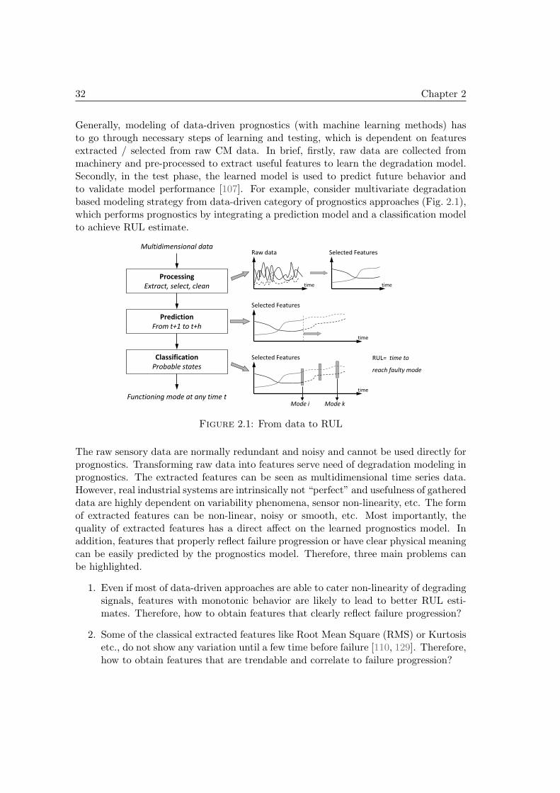
32 Chapter 2
Generally, modeling of data-driven prognostics (with machine learning methods) hasto go through necessary steps of learning and testing, which is dependent on featuresextracted / selected from raw CM data. In brief, firstly, raw data are collected frommachinery and pre-processed to extract useful features to learn the degradation model.Secondly, in the test phase, the learned model is used to predict future behavior andto validate model performance [107]. For example, consider multivariate degradationbased modeling strategy from data-driven category of prognostics approaches (Fig. 2.1),which performs prognostics by integrating a prediction model and a classification modelto achieve RUL estimate.
Processing
Extract, select, clean
Prediction
From t+1 to t+h
Classification
Probable states
Multidimensional data
Functioning mode at any time t time
Mode i
Selected Features
Mode k
time
Selected Features
time
Selected Features
time
Raw data
RUL= time to
reach faulty mode
Figure 2.1: From data to RUL
The raw sensory data are normally redundant and noisy and cannot be used directly forprognostics. Transforming raw data into features serve need of degradation modeling inprognostics. The extracted features can be seen as multidimensional time series data.However, real industrial systems are intrinsically not “perfect” and usefulness of gathereddata are highly dependent on variability phenomena, sensor non-linearity, etc. The formof extracted features can be non-linear, noisy or smooth, etc. Most importantly, thequality of extracted features has a direct affect on the learned prognostics model. Inaddition, features that properly reflect failure progression or have clear physical meaningcan be easily predicted by the prognostics model. Therefore, three main problems canbe highlighted.
1. Even if most of data-driven approaches are able to cater non-linearity of degradingsignals, features with monotonic behavior are likely to lead to better RUL esti-mates. Therefore, how to obtain features that clearly reflect failure progression?
2. Some of the classical extracted features like Root Mean Square (RMS) or Kurtosisetc., do not show any variation until a few time before failure [110, 129]. Therefore,how to obtain features that are trendable and correlate to failure progression?
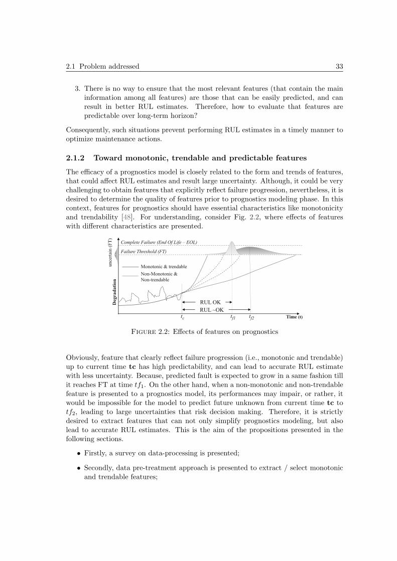
2.1 Problem addressed 33
3. There is no way to ensure that the most relevant features (that contain the maininformation among all features) are those that can be easily predicted, and canresult in better RUL estimates. Therefore, how to evaluate that features arepredictable over long-term horizon?
Consequently, such situations prevent performing RUL estimates in a timely manner tooptimize maintenance actions.
2.1.2 Toward monotonic, trendable and predictable features
The efficacy of a prognostics model is closely related to the form and trends of features,that could affect RUL estimates and result large uncertainty. Although, it could be verychallenging to obtain features that explicitly reflect failure progression, nevertheless, it isdesired to determine the quality of features prior to prognostics modeling phase. In thiscontext, features for prognostics should have essential characteristics like monotonicityand trendability [48]. For understanding, consider Fig. 2.2, where effects of featureswith different characteristics are presented.
RUL ~OK
Time (t) tc
Complete Failure (End Of Life – EOL)
Failure Threshold (FT)
Deg
rad
ati
on
unce
rtai
n (
FT
)
tf1 tf2
RUL OK
Monotonic & trendable
Non-Monotonic &
Non-trendable
Figure 2.2: Effects of features on prognostics
Obviously, feature that clearly reflect failure progression (i.e., monotonic and trendable)up to current time tc has high predictability, and can lead to accurate RUL estimatewith less uncertainty. Because, predicted fault is expected to grow in a same fashion tillit reaches FT at time tf1. On the other hand, when a non-monotonic and non-trendablefeature is presented to a prognostics model, its performances may impair, or rather, itwould be impossible for the model to predict future unknown from current time tc totf2, leading to large uncertainties that risk decision making. Therefore, it is strictlydesired to extract features that can not only simplify prognostics modeling, but alsolead to accurate RUL estimates. This is the aim of the propositions presented in thefollowing sections.
• Firstly, a survey on data-processing is presented;
• Secondly, data pre-treatment approach is presented to extract / select monotonicand trendable features;
34 Chapter 2
• Lastly, data post-treatment approach is introduced to further reduce multidimen-sional features data by assessing their predictability.
2.2 Data processing
2.2.1 Feature extraction approaches
Feature extraction is of great importance for machinery diagnostics / prognostics. Inliterature, a large number of signal processing techniques (or feature extraction methods)have been proposed. Prior to any selection among different possibilities, it is required toinvestigate an appropriate method for a specific application [105, 211]. However, thereis huge literature on this topic, which is beyond the scope of the thesis. Let’s highlightthe three main categories of signal processing techniques which are shown in Fig. 2.3.
2.2.1.1 Time domain
Time-domain feature extraction is directly performed on the sensed waveforms (e.g.acoustic emissions, vibration signal) to identify signatures. In a classical manner time-domain approach extracts characteristic features using statistics like mean, variance,root mean square (RMS), standard deviation, etc. These are suitable in case of station-ary signals. Otherwise extracted features may show sensitivity to variation in data andinherit non-linearity which can complicate prognostics modeling and may prevent RULprediction in a timely manner. Apart from statistical approaches, time-domain anal-ysis can be further categorized into model-based methods, like autoregressive movingaverage, or signal processing methods like synchronous averaging or correlation [211].
2.2.1.2 Frequency domain
Features extracted from time domain techniques are considered to be suitable for faultdetection. However, frequency-domain techniques are considered more effective for faultdiagnostic, because, they have good ability to identify and isolate frequency components.The most widely applied technique in this category is Fast Fourier Transform (FFT).Other methods that belong to this category are cepstrum, spectral analysis, higher-orderspectra and envelop analysis [105, 211, 214]. The main limitation of frequency-domaintechniques is their inability to deal with non-stationary signals, unfortunately which isthe case in degrading machinery.
2.2.1.3 Time-frequency
Time-frequency techniques aim at investigating signals in both time and frequency do-mains. They are considered to be powerful tools to analyze non-stationary signals. Someof the popular time-frequency techniques proposed in literature are: Short Time FourierTransform (STFT), Wigner-Ville Distribution [32], Wavelet Transform (WT) [47], Em-pirical Mode Decomposition (EMD) [97], Hilbert-Huang Transform based on EMD andHilbert spectral analysis [96], spectral kurtosis [12] and cyclostationary analysis [73]. A
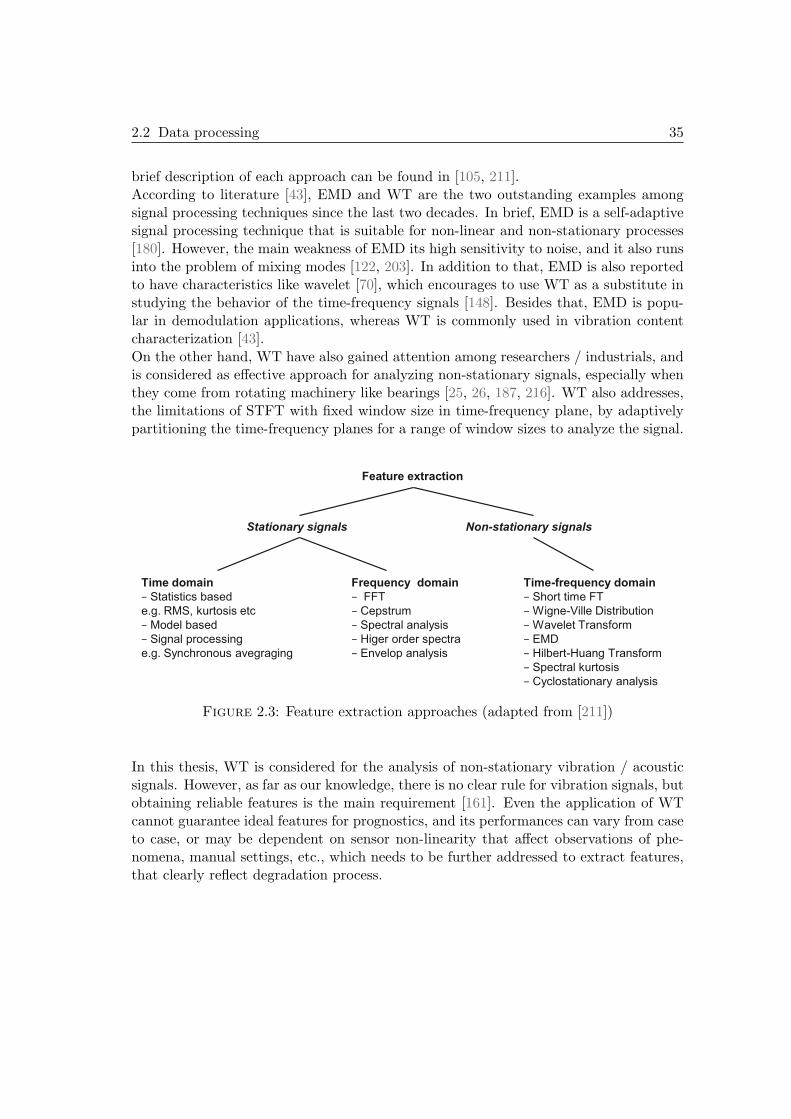
2.2 Data processing 35
brief description of each approach can be found in [105, 211].According to literature [43], EMD and WT are the two outstanding examples amongsignal processing techniques since the last two decades. In brief, EMD is a self-adaptivesignal processing technique that is suitable for non-linear and non-stationary processes[180]. However, the main weakness of EMD its high sensitivity to noise, and it also runsinto the problem of mixing modes [122, 203]. In addition to that, EMD is also reportedto have characteristics like wavelet [70], which encourages to use WT as a substitute instudying the behavior of the time-frequency signals [148]. Besides that, EMD is popu-lar in demodulation applications, whereas WT is commonly used in vibration contentcharacterization [43].On the other hand, WT have also gained attention among researchers / industrials, andis considered as effective approach for analyzing non-stationary signals, especially whenthey come from rotating machinery like bearings [25, 26, 187, 216]. WT also addresses,the limitations of STFT with fixed window size in time-frequency plane, by adaptivelypartitioning the time-frequency planes for a range of window sizes to analyze the signal.
Time-frequency domain
− Short time FT
− Wigne-Ville Distribution
− Wavelet Transform
− EMD
− Hilbert-Huang Transform
− Spectral kurtosis
− Cyclostationary analysis
Frequency domain
− FFT
− Cepstrum
− Spectral analysis
− Higer order spectra
− Envelop analysis
Time domain
− Statistics based
e.g. RMS, kurtosis etc
− Model based
− Signal processing
e.g. Synchronous avegraging
Feature extraction
Stationary signals Non-stationary signals
Figure 2.3: Feature extraction approaches (adapted from [211])
In this thesis, WT is considered for the analysis of non-stationary vibration / acousticsignals. However, as far as our knowledge, there is no clear rule for vibration signals, butobtaining reliable features is the main requirement [161]. Even the application of WTcannot guarantee ideal features for prognostics, and its performances can vary from caseto case, or may be dependent on sensor non-linearity that affect observations of phe-nomena, manual settings, etc., which needs to be further addressed to extract features,that clearly reflect degradation process.
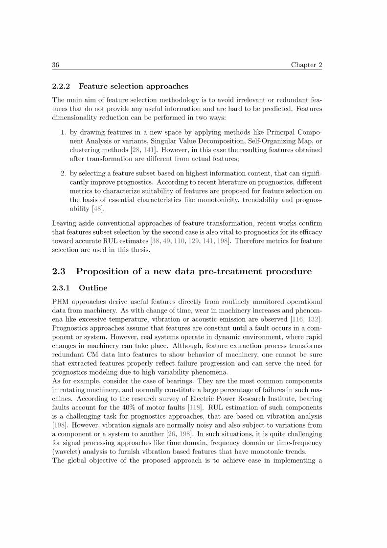
36 Chapter 2
2.2.2 Feature selection approaches
The main aim of feature selection methodology is to avoid irrelevant or redundant fea-tures that do not provide any useful information and are hard to be predicted. Featuresdimensionality reduction can be performed in two ways:
1. by drawing features in a new space by applying methods like Principal Compo-nent Analysis or variants, Singular Value Decomposition, Self-Organizing Map, orclustering methods [28, 141]. However, in this case the resulting features obtainedafter transformation are different from actual features;
2. by selecting a feature subset based on highest information content, that can signifi-cantly improve prognostics. According to recent literature on prognostics, differentmetrics to characterize suitability of features are proposed for feature selection onthe basis of essential characteristics like monotonicity, trendability and prognos-ability [48].
Leaving aside conventional approaches of feature transformation, recent works confirmthat features subset selection by the second case is also vital to prognostics for its efficacytoward accurate RUL estimates [38, 49, 110, 129, 141, 198]. Therefore metrics for featureselection are used in this thesis.
2.3 Proposition of a new data pre-treatment procedure
2.3.1 Outline
PHM approaches derive useful features directly from routinely monitored operationaldata from machinery. As with change of time, wear in machinery increases and phenom-ena like excessive temperature, vibration or acoustic emission are observed [116, 132].Prognostics approaches assume that features are constant until a fault occurs in a com-ponent or system. However, real systems operate in dynamic environment, where rapidchanges in machinery can take place. Although, feature extraction process transformsredundant CM data into features to show behavior of machinery, one cannot be surethat extracted features properly reflect failure progression and can serve the need forprognostics modeling due to high variability phenomena.As for example, consider the case of bearings. They are the most common componentsin rotating machinery, and normally constitute a large percentage of failures in such ma-chines. According to the research survey of Electric Power Research Institute, bearingfaults account for the 40% of motor faults [118]. RUL estimation of such componentsis a challenging task for prognostics approaches, that are based on vibration analysis[198]. However, vibration signals are normally noisy and also subject to variations froma component or a system to another [26, 198]. In such situations, it is quite challengingfor signal processing approaches like time domain, frequency domain or time-frequency(wavelet) analysis to furnish vibration based features that have monotonic trends.The global objective of the proposed approach is to achieve ease in implementing a
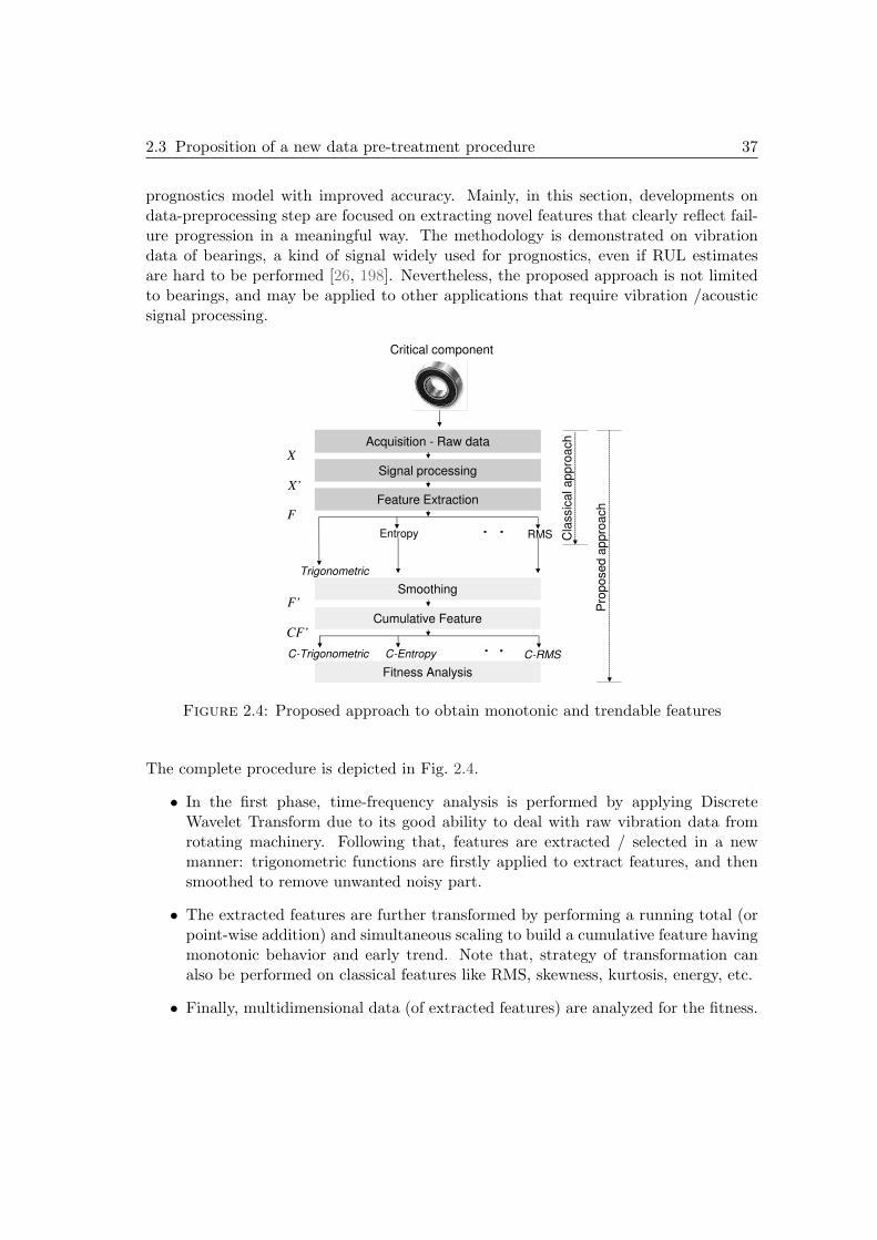
2.3 Proposition of a new data pre-treatment procedure 37
prognostics model with improved accuracy. Mainly, in this section, developments ondata-preprocessing step are focused on extracting novel features that clearly reflect fail-ure progression in a meaningful way. The methodology is demonstrated on vibrationdata of bearings, a kind of signal widely used for prognostics, even if RUL estimatesare hard to be performed [26, 198]. Nevertheless, the proposed approach is not limitedto bearings, and may be applied to other applications that require vibration /acousticsignal processing.
Critical component
Acquisition - Raw data X
X’Signal processing
l appro
ach
F’
CF’
X’
F
Fitness Analysis
Trigonometric
. .Entropy RMS
C-Trigonometric . .C-Entropy C-RMS
Cumulative Feature
Smoothing
Feature Extraction
Cla
ssic
al ap
Pro
posed
appro
ach
Figure 2.4: Proposed approach to obtain monotonic and trendable features
The complete procedure is depicted in Fig. 2.4.
• In the first phase, time-frequency analysis is performed by applying DiscreteWavelet Transform due to its good ability to deal with raw vibration data fromrotating machinery. Following that, features are extracted / selected in a newmanner: trigonometric functions are firstly applied to extract features, and thensmoothed to remove unwanted noisy part.
• The extracted features are further transformed by performing a running total (orpoint-wise addition) and simultaneous scaling to build a cumulative feature havingmonotonic behavior and early trend. Note that, strategy of transformation canalso be performed on classical features like RMS, skewness, kurtosis, energy, etc.
• Finally, multidimensional data (of extracted features) are analyzed for the fitness.
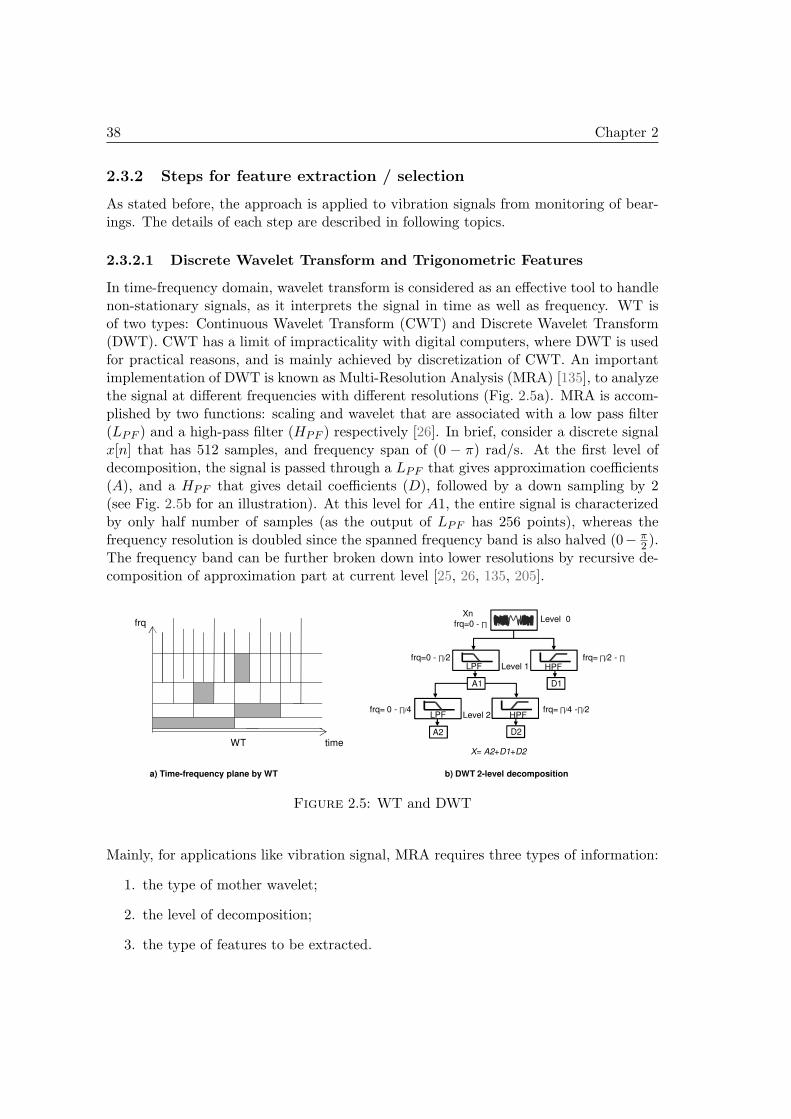
38 Chapter 2
2.3.2 Steps for feature extraction / selection
As stated before, the approach is applied to vibration signals from monitoring of bear-ings. The details of each step are described in following topics.
2.3.2.1 Discrete Wavelet Transform and Trigonometric Features
In time-frequency domain, wavelet transform is considered as an effective tool to handlenon-stationary signals, as it interprets the signal in time as well as frequency. WT isof two types: Continuous Wavelet Transform (CWT) and Discrete Wavelet Transform(DWT). CWT has a limit of impracticality with digital computers, where DWT is usedfor practical reasons, and is mainly achieved by discretization of CWT. An importantimplementation of DWT is known as Multi-Resolution Analysis (MRA) [135], to analyzethe signal at different frequencies with different resolutions (Fig. 2.5a). MRA is accom-plished by two functions: scaling and wavelet that are associated with a low pass filter(LPF ) and a high-pass filter (HPF ) respectively [26]. In brief, consider a discrete signalx[n] that has 512 samples, and frequency span of (0 − π) rad/s. At the first level ofdecomposition, the signal is passed through a LPF that gives approximation coefficients(A), and a HPF that gives detail coefficients (D), followed by a down sampling by 2(see Fig. 2.5b for an illustration). At this level for A1, the entire signal is characterizedby only half number of samples (as the output of LPF has 256 points), whereas thefrequency resolution is doubled since the spanned frequency band is also halved (0− π
2 ).The frequency band can be further broken down into lower resolutions by recursive de-composition of approximation part at current level [25, 26, 135, 205].
frq
LPF HPF
A1 D1
Level 1
Level 0Xn
frq=0 - �
frq=0 - �/2 frq= �/2 - �
timeWT
LPF HPF
A1
D2
D1
A2
Level 2frq= 0 - �/4 frq= �/4 -�/2
a) Time-frequency plane by WT
X= A2+D1+D2
b) DWT 2-level decomposition
Figure 2.5: WT and DWT
Mainly, for applications like vibration signal, MRA requires three types of information:
1. the type of mother wavelet;
2. the level of decomposition;
3. the type of features to be extracted.
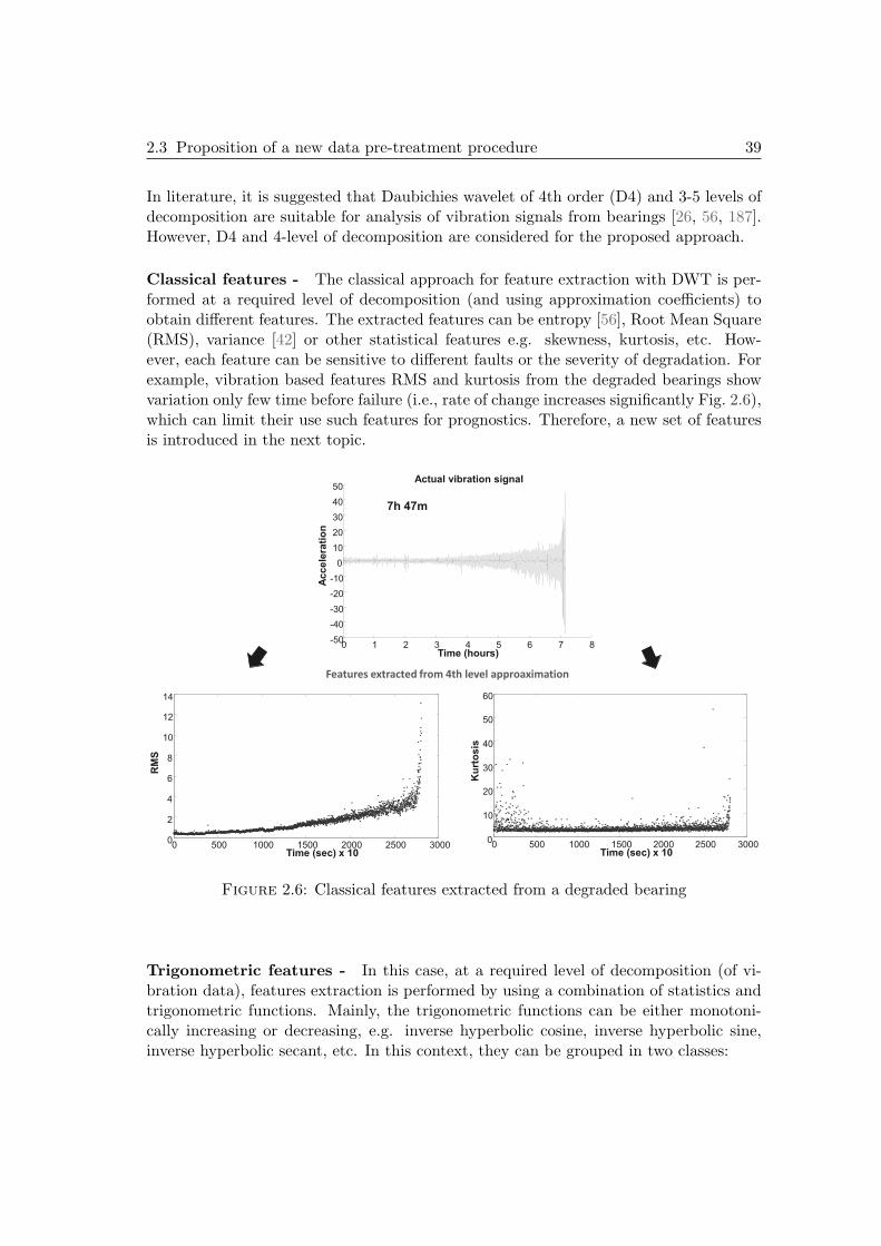
2.3 Proposition of a new data pre-treatment procedure 39
In literature, it is suggested that Daubichies wavelet of 4th order (D4) and 3-5 levels ofdecomposition are suitable for analysis of vibration signals from bearings [26, 56, 187].However, D4 and 4-level of decomposition are considered for the proposed approach.
Classical features - The classical approach for feature extraction with DWT is per-formed at a required level of decomposition (and using approximation coefficients) toobtain different features. The extracted features can be entropy [56], Root Mean Square(RMS), variance [42] or other statistical features e.g. skewness, kurtosis, etc. How-ever, each feature can be sensitive to different faults or the severity of degradation. Forexample, vibration based features RMS and kurtosis from the degraded bearings showvariation only few time before failure (i.e., rate of change increases significantly Fig. 2.6),which can limit their use such features for prognostics. Therefore, a new set of featuresis introduced in the next topic.
0 500 1000 1500 2000 2500 30000
10
20
30
40
50
60
Time (sec) x 10
Ku
rto
sis
Features extracted from 4th level approaximation
0 500 1000 1500 2000 2500 3000 0
2
4
6
8
10
12
14
Time (sec) x 10
RM
S
0 1 2 3 4 5 6 7 8 -50
-40
-30
-20
-10
0
10
20
30
40
50
Time (hours)
Ac
ce
lera
tio
n
Actual vibration signal
7h 47m
Figure 2.6: Classical features extracted from a degraded bearing
Trigonometric features - In this case, at a required level of decomposition (of vi-bration data), features extraction is performed by using a combination of statistics andtrigonometric functions. Mainly, the trigonometric functions can be either monotoni-cally increasing or decreasing, e.g. inverse hyperbolic cosine, inverse hyperbolic sine,inverse hyperbolic secant, etc. In this context, they can be grouped in two classes:

40 Chapter 2
• functions that have domain (−∞,∞), e.g. inverse hyperbolic sine (asinh), inversetangent (atan), etc;
• functions that have different domain value but not (−∞,∞), e.g. inverse hyper-bolic cosine (acosh), inverse hyperbolic secant (asech), hyperbolic tangent (tanh).
For the second class, input values outside the domain are transformed to complex outputs(i.e., complex numbers), which can be further explored. However, the first class appearsto be more relevant to a real data, as it allows domain values from (−∞,∞). Therefore,we limit the study to the first class only.The main benefit of using trigonometric functions is that: such function transform theinput data to different scale such that, resulting features have better trends and low scaleas compared to classical features. To achieve that, a trigonometric function operateson array (X) element-wise (xj , j = 1,2,..,n) to scale, and a standard deviation (SD)applied to the scaled array for extracting feature value: 1) standard deviation of inversehyperbolic sin Eq. 2.1, 2) standard deviation of inverse tangent Eq. 2.2.
σ(
log[
xj + (x2j + 1)1/2])
(2.1)
σ
(
i
2log
(
i+ xji− xj
))
(2.2)
For illustration, an example of features extracted with classical approach from a de-graded bearing are presented in Fig. 2.6, and features extracted using Eq. 2.1 andEq. 2.2 are show in Fig. 2.7. The results clearly depict that, trigonometric features haveearlier trends and monotonic behavior, thanks to scaling by trigonometric functions.Finally, different features extracted from 4th level approximation (i.e., terminal nodes,Fig. 2.5b) of the decomposed vibration signal are listed in Table 2.1.
Table 2.1: Features extracted from 4th level Approximation
Trigonometric Features (proposed)
Standard Deviation of inverse hyperbolic sine σ(
log[
xj + (x2j + 1)1/2])
Standard Deviation of inverse tangent σ(
i2 log
(
i+xj
i−xj
))
Classical FeaturesEntropy (threshold) E(x) =
∑
j E(xj)
Energy e =∑n
j=0 x2j
Root mean square RMS =√
1n (x
21 + ...+ x2n)
Skewness∑n
j=1(xj−X)3
(n−1)σ3
Kurtosis∑n
j=1(xj−X)4
(n−1)σ4
Upper bound max(x) + 12max(X)−min(X)
n−1
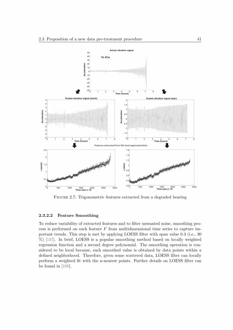
2.3 Proposition of a new data pre-treatment procedure 41
Features extracted from 4th level approaximation
0 1 2 3 4 5 6 7 8 -50
-40
-30
-20
-10
0
10
20
30
40
50
Time (hours)
Ac
ce
lera
tio
n
Actual vibration signal
7h 47m
0 1 2 3 4 5 6 7 8 -5
-4
-3
-2
-1
0
1
2
3
4
5
Time (hours)
Ac
ce
lera
tio
n
Scaled vibration signal (asinh)
0 1 2 3 4 5 6 7 8 -2
-1.5
-1
-0.5
0
0.5
1
1.5
2
Time (hours)
Ac
ce
lera
tio
n
Scaled vibration signal (atan)
0 500 1000 1500 2000 2500 3000 0
0.5
1
1.5
2
2.5
Time (sec) x 10
s (a
sin
h)
0 500 1000 1500 2000 2500 3000 0.2
0.4
0.6
0.8
1
1.2
1.4
1.6
Time (sec) x 10
s (a
tan
)
Figure 2.7: Trigonometric features extracted from a degraded bearing
2.3.2.2 Feature Smoothing
To reduce variability of extracted features and to filter unwanted noise, smoothing pro-cess is performed on each feature F from multidimensional time series to capture im-portant trends. This step is met by applying LOESS filter with span value 0.3 (i.e., 30%) [137]. In brief, LOESS is a popular smoothing method based on locally weightedregression function and a second degree polynomial. The smoothing operation is con-sidered to be local because, each smoothed value is obtained by data points within adefined neighborhood. Therefore, given some scattered data, LOESS filter can locallyperform a weighted fit with the n-nearest points. Further details on LOESS filter canbe found in [100].

42 Chapter 2
2.3.2.3 Cumulative features
Any machine is bound to degrade as time grows. In this context, the main idea of thisstep is obtain features that can clearly reflect failure progression and satisfy requirementsmentioned in section 2.1.2. In fact, features with non-linear behavior don’t clearly in-dicate state of the machinery under operation i.e., they don’t distinguish among good,degrading or failure states. Note that such non-linearity can also represent self-healingas well. Here we assume that it is not possible to undergo self-recovery, which is thecase for components like bearings, gears, or cutting tools. However, this assumptiondoes not hold for batteries that may undergo self-recovery during non-use [49].Therefore, we propose a straightforward but effective strategy to build features, whichaims at transforming an extracted feature into its cumulative form to have monotonicityand trendability characteristics. The transformation task is achieved by applying a cu-mulative function on a time series, to perform a (point-wise) running total and a scalingoperation simultaneously. This procedure results features that can clearly distinguishamong different states of degrading machinery.
CFv =
N∑
i=1
´Fv(i)
∣
∣
∣
∣
(
N∑
i=1
´Fv(i)
)∣
∣
∣
∣
1/2, v = 1,2....,k (2.3)
where,N∑
i=1Fv(i) represents running total of a “smoothed vth” feature Fv(i) up to “N”
points, and CFv represents transformed cumulative feature. It should be noted that,the cumulation of a feature can be sensitive to noise, therefore, features smoothing mustbe performed a priori (section 2.3.2.2).
2.3.2.4 Analyzing fitness of features
This step aims at identifying subset of features that have better fitness for furtherprognostics modeling. The central assumption is that, monotonic and trendable featurescan lead to more accurate RUL estimates, as compared to features that have contrarybehavior. Therefore two simple metrics are considered to assess suitability (or fitness)of a feature: 1) Monotonicity (from literature) 2) Trendability (proposed).
• “Monotonicity” characterizes underlying increasing or decreasing trend [48]:
M =
∣
∣
∣
∣
no. of d/dx > 0
n− 1− no. of d/dx < 0
n− 1
∣
∣
∣
∣
(2.4)
where “n” is for number of observations in a particular feature. Monotonicity M ismeasured by absolute difference of “positive” and “negative” derivatives for eachfeature. The value of M can be from 0 to 1: highly monotonic features will haveM=1 and for non-monotonic features M=0.

2.4 First PHM case study on real data 43
• “Trendability” is related to the functional form of an extracted feature and its cor-relation to time. That is, how the state of an engineering asset varies with time.Surely, a constant function (of feature) will have zero correlation with time, wherea linear function will have strong correlation. In similar way, correlation can varywith increase in non-linearity (i.e., a non-linear feature will result low correlation).To measure trendability a straight forward formula is given in Eq. (2.5).
R =n (
∑
xy)− (∑
x) (∑
y)√
[
n∑
x2 − (∑
x)2][
n∑
y2 − (∑
y)2]
(2.5)
where R is the correlation coefficient between two variables x and y. Correlationcan be positive, negative, perfect or no correlation. Thus, R ∈ [−1; 1] is thecorrelation coefficient between feature x and time index y.
2.4 First PHM case study on real data
2.4.1 Bearings datasets of IEEE PHM Challenge 2012
To demonstrate the effectiveness of our contributions, developments are applied tothe dataset from IEEE PHM 2012 Data Challenge. Data are mainly composed ofrun-to-failure vibration signals related to ball bearings from an experimental platformPRONOSTIA [5, 144]. In brief, PRONOSTIA is dedicated to test and validate faultdetection, diagnosis and prognostics methods on ball bearings (Fig. 2.8).
PROGNOSTICS
R
U
L
?
Rotation module
Data acquisition
Accelerometer
Bearing
Figure 2.8: PRONOSTIA testbed - FEMTO-ST Institute, AS2M department
This platform has been designed and realized at AS2M department of FEMTO-ST Insti-
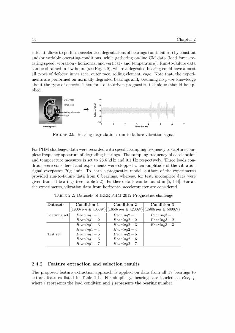
44 Chapter 2
tute. It allows to perform accelerated degradations of bearings (until failure) by constantand/or variable operating-conditions, while gathering on-line CM data (load force, ro-tating speed, vibration - horizontal and vertical - and temperature). Run-to-failure datacan be obtained in few hours (see Fig. 2.9), where a degraded bearing could have almostall types of defects: inner race, outer race, rolling element, cage. Note that, the experi-ments are performed on normally degraded bearings and, assuming no prior knowledgeabout the type of defects. Therefore, data-driven prognostics techniques should be ap-plied.
Run-to-failure vibration data
0 1 2 3 4 5 6 7 -10
-5
0
5
10
Time (hours)
Ac
ce
lera
tio
n
Outer race
Inner race
Rolling elements
Cage
Bearing Parts
Figure 2.9: Bearing degradation: run-to-failure vibration signal
For PHM challenge, data were recorded with specific sampling frequency to capture com-plete frequency spectrum of degrading bearings. The sampling frequency of accelerationand temperature measures is set to 25.6 kHz and 0.1 Hz respectively. Three loads con-dition were considered and experiments were stopped when amplitude of the vibrationsignal overpasses 20g limit. To learn a prognostics model, authors of the experimentsprovided run-to-failure data from 6 bearings, whereas, for test, incomplete data weregiven from 11 bearings (see Table 2.2). Further details can be found in [5, 144]. For allthe experiments, vibration data from horizontal accelerometer are considered.
Table 2.2: Datasets of IEEE PHM 2012 Prognostics challenge
Datasets Condition 1 Condition 2 Condition 3(1800rpm & 4000N) (1650rpm & 4200N) (1500rpm & 5000N)
Learning set Bearing1− 1 Bearing2− 1 Bearing3− 1Bearing1− 2 Bearing2− 2 Bearing3− 2Bearing1− 3 Bearing2− 3 Bearing3− 3Bearing1− 4 Bearing2− 4
Test set Bearing1− 5 Bearing2− 5Bearing1− 6 Bearing2− 6Bearing1− 7 Bearing2− 7
2.4.2 Feature extraction and selection results
The proposed feature extraction approach is applied on data from all 17 bearings toextract features listed in Table 2.1. For simplicity, bearings are labeled as Beri−j ,where i represents the load condition and j represents the bearing number.
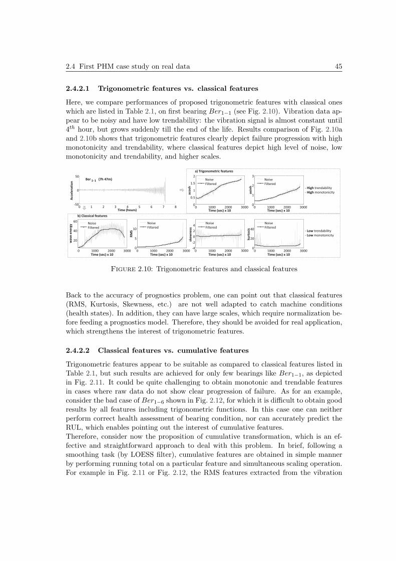
2.4 First PHM case study on real data 45
2.4.2.1 Trigonometric features vs. classical features
Here, we compare performances of proposed trigonometric features with classical oneswhich are listed in Table 2.1, on first bearing Ber1−1 (see Fig. 2.10). Vibration data ap-pear to be noisy and have low trendability: the vibration signal is almost constant until4th hour, but grows suddenly till the end of the life. Results comparison of Fig. 2.10aand 2.10b shows that trigonometric features clearly depict failure progression with highmonotonicity and trendability, where classical features depict high level of noise, lowmonotonicity and trendability, and higher scales.
0 1000 2000 3000 0
0.5
1
1.5
2
Time (sec) x 10
aco
sh
0 1000 2000 3000 0
1
2
3
Time (sec) x 10
asi
nh
0 1000 2000
20
40
60
Time (sec) x 10
wa
ve
en
erg
y
0 1000 2000 3000 0
5
10
Time (sec) x 10
RM
S
0 1000 2000 -4
-2
0
2
4
Time (sec) x 10
ske
wn
ess
0 1000 2000 3000 0
20
40
Time (sec) x 10
ku
rto
sis
Noise
Filtered
Noise
Filtered
Noise
Filtered
Noise
Filtered
Noise
Filtered
Noise
Filtered
0 1 2 3 4 5 6 7 8 -50
0
50
Time (hours)
Acc
ele
rati
on
Ber 1 - 1 (7h 47m)
- Low trendability
- Low monotonicity
- High trendability
- High monotonicity
a) Trigonometric features
b) Classical features
3000 3000
Figure 2.10: Trigonometric features and classical features
Back to the accuracy of prognostics problem, one can point out that classical features(RMS, Kurtosis, Skewness, etc.) are not well adapted to catch machine conditions(health states). In addition, they can have large scales, which require normalization be-fore feeding a prognostics model. Therefore, they should be avoided for real application,which strengthens the interest of trigonometric features.
2.4.2.2 Classical features vs. cumulative features
Trigonometric features appear to be suitable as compared to classical features listed inTable 2.1, but such results are achieved for only few bearings like Ber1−1, as depictedin Fig. 2.11. It could be quite challenging to obtain monotonic and trendable featuresin cases where raw data do not show clear progression of failure. As for an example,consider the bad case of Ber1−6 shown in Fig. 2.12, for which it is difficult to obtain goodresults by all features including trigonometric functions. In this case one can neitherperform correct health assessment of bearing condition, nor can accurately predict theRUL, which enables pointing out the interest of cumulative features.Therefore, consider now the proposition of cumulative transformation, which is an ef-fective and straightforward approach to deal with this problem. In brief, following asmoothing task (by LOESS filter), cumulative features are obtained in simple mannerby performing running total on a particular feature and simultaneous scaling operation.For example in Fig. 2.11 or Fig. 2.12, the RMS features extracted from the vibration
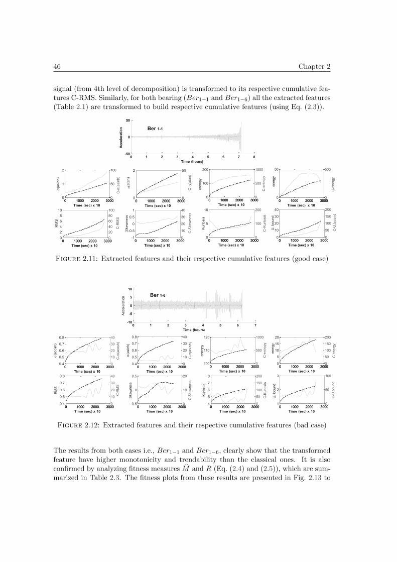
46 Chapter 2
signal (from 4th level of decomposition) is transformed to its respective cumulative fea-tures C-RMS. Similarly, for both bearing (Ber1−1 and Ber1−6) all the extracted features(Table 2.1) are transformed to build respective cumulative features (using Eq. (2.3)).
0 1000 2000 30000
100
200
Time (sec) x 10
entr
opy
0 1000 2000 30000
500
1000
C-e
ntr
opy
0 1000 2000 30000
50
Time (sec) x 10
W.e
nerg
y
0 1000 2000 30000
500
C-W
.energ
y
0 1 2 3 4 5 6 7 8
x 106
-50
0
50
Time (hours)
Accele
rati
on
0 1000 2000 30000
1
2
Time (sec) x 10
s(a
sin
h)
0 1000 2000 30000
50
100
C-s
(asin
h)
0 1000 2000 3000 0
2
4
6
8
10
Time (sec) x 10
RM
S
0 1000 2000 3000 0
20
40
60
80
100
C-R
MS
0 1000 2000 3000 -1
-0.5
0
0.5
1
Time (sec) x 10
Skew
ness
0 1000 2000 3000 0
10
20
30
40
C-S
kew
ness
0 1000 2000 3000 0
5
10
Time (sec) x 10
Kurt
osis
0 1000 2000 3000 0
100
200
C-K
urt
osis
0 1000 2000 3000 0
10
20
30
40
Time (sec) x 10
U. bound
0 1000 2000 3000 0
50
100
150
200
C-U
.bound
Ber 1-1
0 1000 2000 3000 0
2
Time (sec) x 10
s (a
tan)
0 1000 2000 3000 0
50
C- s
(ata
n)
0
0
C-W
.energ
yC
-W
Figure 2.11: Extracted features and their respective cumulative features (good case)
0 1 2 3 4 5 6 7
x 106
-10
-5
0
5
10
Time (hours)
Accele
ration Ber 1-6
0 1000 2000 30000.4
0.5
0.6
0.7
0.8
Time (sec) x 10
s(a
cosh)
0 1000 2000 30000
10
20
30
40
C-s
(acosh)
0 1000 2000 30000.4
0.5
0.6
0.7
0.8
Time (sec) x 10
s(a
sin
h)
0 1000 2000 30000
10
20
30
40
C-s
(asin
h)
0 1000 2000 3000100
110
120
Time (sec) x 10
entr
opy
0 1000 2000 30000
500
1000
C-e
ntr
opy
0 1000 2000 30000
5
10
15
20
Time (sec) x 10
W.e
nerg
y
0 1000 2000 30000
50
100
150
200C
-W.e
nerg
y
0 1000 2000 30000.4
0.5
0.6
0.7
0.8
Time (sec) x 10
RM
S
0 1000 2000 30000
10
20
30
40
C-R
MS
0 1000 2000 3000-0.5
0
0.5
Time (sec) x 10
Skew
ness
0 1000 2000 30000
10
20
C-S
kew
ness
0 1000 2000 30004
5
6
7
8
Time (sec) x 10
Kurt
osis
0 1000 2000 30000
50
100
150
200
C-K
urt
osis
0 1000 2000 30001
2
3
Time (sec) x 10
W.e
nerg
y
0 1000 2000 30000
50
100
C-U
.bound
0
0
C-W
.energ
yC
-W
U. bound
Figure 2.12: Extracted features and their respective cumulative features (bad case)
The results from both cases i.e., Ber1−1 and Ber1−6, clearly show that the transformedfeature have higher monotonicity and trendability than the classical ones. It is alsoconfirmed by analyzing fitness measures M and R (Eq. (2.4) and (2.5)), which are sum-marized in Table 2.3. The fitness plots from these results are presented in Fig. 2.13 to
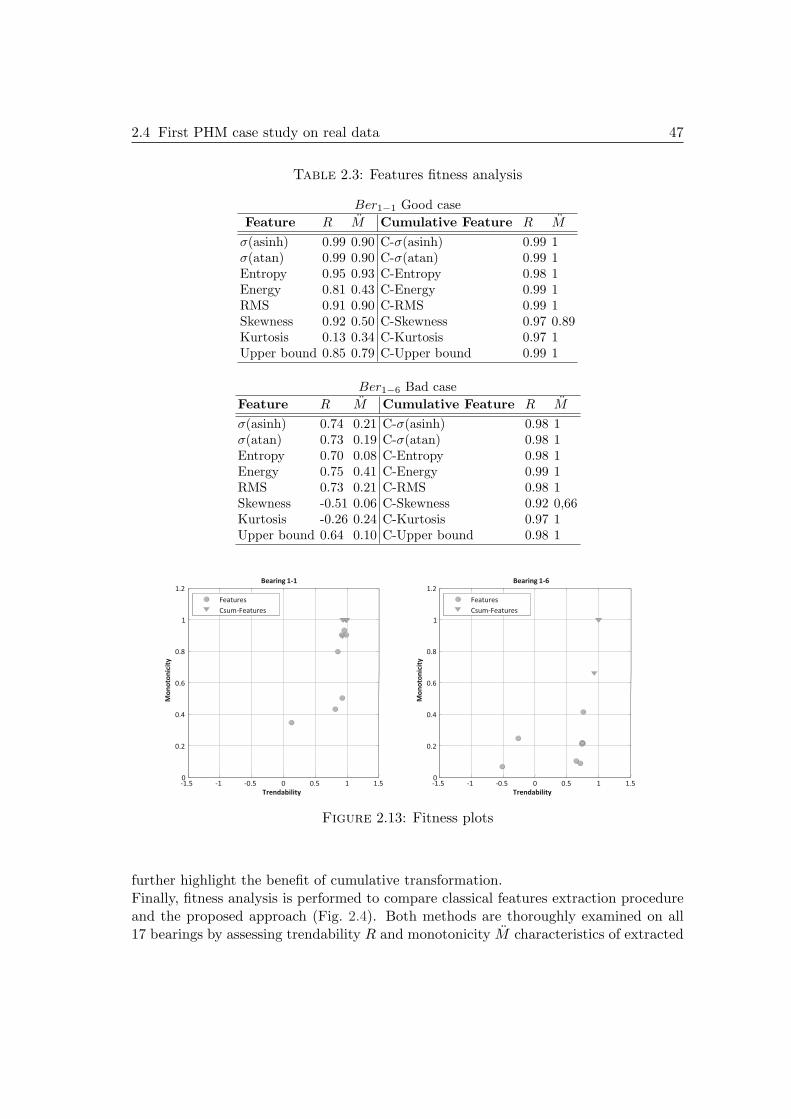
2.4 First PHM case study on real data 47
Table 2.3: Features fitness analysis
Ber1−1 Good case
Feature R M Cumulative Feature R M
σ(asinh) 0.99 0.90 C-σ(asinh) 0.99 1σ(atan) 0.99 0.90 C-σ(atan) 0.99 1Entropy 0.95 0.93 C-Entropy 0.98 1Energy 0.81 0.43 C-Energy 0.99 1RMS 0.91 0.90 C-RMS 0.99 1Skewness 0.92 0.50 C-Skewness 0.97 0.89Kurtosis 0.13 0.34 C-Kurtosis 0.97 1Upper bound 0.85 0.79 C-Upper bound 0.99 1
Ber1−6 Bad case
Feature R M Cumulative Feature R M
σ(asinh) 0.74 0.21 C-σ(asinh) 0.98 1σ(atan) 0.73 0.19 C-σ(atan) 0.98 1Entropy 0.70 0.08 C-Entropy 0.98 1Energy 0.75 0.41 C-Energy 0.99 1RMS 0.73 0.21 C-RMS 0.98 1Skewness -0.51 0.06 C-Skewness 0.92 0,66Kurtosis -0.26 0.24 C-Kurtosis 0.97 1Upper bound 0.64 0.10 C-Upper bound 0.98 1
-1.5 -1 -0.5 0 0.5 1 1.5 0
0.2
0.4
0.6
0.8
1
1.2
Trendability
Mo
no
ton
icit
y
Bearing 1-1
-1.5 -1 -0.5 0 0.5 1 1.5 0
0.2
0.4
0.6
0.8
1
1.2
Trendability
Mo
no
ton
icit
y
Bearing 1-6
Features
Csum-Features
Features
Csum-Features
Figure 2.13: Fitness plots
further highlight the benefit of cumulative transformation.Finally, fitness analysis is performed to compare classical features extraction procedureand the proposed approach (Fig. 2.4). Both methods are thoroughly examined on all17 bearings by assessing trendability R and monotonicity M characteristics of extracted
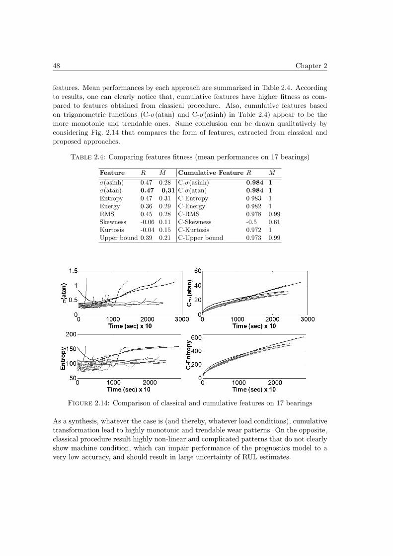
48 Chapter 2
features. Mean performances by each approach are summarized in Table 2.4. Accordingto results, one can clearly notice that, cumulative features have higher fitness as com-pared to features obtained from classical procedure. Also, cumulative features basedon trigonometric functions (C-σ(atan) and C-σ(asinh) in Table 2.4) appear to be themore monotonic and trendable ones. Same conclusion can be drawn qualitatively byconsidering Fig. 2.14 that compares the form of features, extracted from classical andproposed approaches.
Table 2.4: Comparing features fitness (mean performances on 17 bearings)
Feature R M Cumulative Feature R M
σ(asinh) 0.47 0.28 C-σ(asinh) 0.984 1σ(atan) 0.47 0,31 C-σ(atan) 0.984 1Entropy 0.47 0.31 C-Entropy 0.983 1Energy 0.36 0.29 C-Energy 0.982 1RMS 0.45 0.28 C-RMS 0.978 0.99Skewness -0.06 0.11 C-Skewness -0.5 0.61Kurtosis -0.04 0.15 C-Kurtosis 0.972 1Upper bound 0.39 0.21 C-Upper bound 0.973 0.99
Figure 2.14: Comparison of classical and cumulative features on 17 bearings
As a synthesis, whatever the case is (and thereby, whatever load conditions), cumulativetransformation lead to highly monotonic and trendable wear patterns. On the opposite,classical procedure result highly non-linear and complicated patterns that do not clearlyshow machine condition, which can impair performance of the prognostics model to avery low accuracy, and should result in large uncertainty of RUL estimates.
2.5 Predictability based prognostics: underlying concepts 49
2.5 Predictability based prognostics: underlying concepts
2.5.1 Proposition of a new data post-treatment procedure
As discussed earlier, the standard of machine learning approaches for prognostics is di-vided into two phases, i.e., learning phase and testing phase section. In classical wayprognostics model is learned by set of features that are acquired from a sensor signal.The model must be retrained upon these features, until significant performance levelis achieved. This approach can be time expensive because some of the features can bevery hard to be predicted. In other words, there is no use in retaining such featuresthat are not predictable. According to existing procedure of data-driven prognostics,critical phase of prediction should be met in appropriate manner for further classifica-tion and RUL estimation (see Fig. 2.1), where learning phase of prognostics modelingshould consider the important steps of “feature selection” and “prediction modeling” ina simultaneous manner in order to retain or reject features on the basis of predictability.From aforesaid procedure, two issues can be pointed out. Firstly, there is no uniqueway to select most relevant features that are predictable and contribute for better RULestimation. Secondly, the predictability should be assessed according to a predictionmodel as well as the horizon of prediction. The main purpose of this method is to recon-sider the learning phase of data-driven approaches by considering both steps “featureselection” and “prognostics modeling” as complementary and closely related.
2.5.1.1 Time series models and accuracy over horizon
In fact, predictability is not a well defined concept. Generally, predictability attributesto the capability in making predictions of future occurrence on the basis of past infor-mation. It should depict a goodness of predictions, so that undesirable events can beavoided by making accurate forecasts in a timely manner. Predictions can be incorrect,therefore, it is important to understand their quality in a framework that is dependenton the considered time series. Also, predictability can be affected by different factorsthat vary from event to event and make modeling process more complicated [201].According to literature, predictability states for the degree of correctness in forecast-ing or shows the usefulness of a forecasting method [7]. In this context, it must beconsidered that up to what extent accurate predictions of a given time series can beprovided by an applied modeling approach. Therefore, metrics are required in orderto show significance of accurate prediction modeling. Remarkably, there are few worksthat focus on the predictability aspect by considering modeling accuracy. [201] used sea-sonally adjusted coefficient of efficiency to evaluate predictability of univariate streamflow process. However, in this study need of a suitable forecasting approach as wellas model performance measure is highlighted for a particular domain. [113] presenteda quantitative metric to measure time series predictability using genetic programming.[62] provided an improvement of those developments. [183] defined metrics to determinesuitable predictors for genomic sequence: quantitative metrics that depict the abilityof time series to be predicted by a particular approach. However, they were useful forsingle step-ahead forecasting methods.
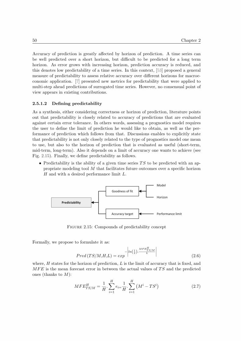
50 Chapter 2
Accuracy of prediction is greatly affected by horizon of prediction. A time series canbe well predicted over a short horizon, but difficult to be predicted for a long termhorizon. As error grows with increasing horizon, prediction accuracy is reduced, andthis denotes low predictability of a time series. In this context, [53] proposed a generalmeasure of predictability to assess relative accuracy over different horizons for macroe-conomic application. [7] presented new metrics for predictability that were applied tomulti-step ahead predictions of surrogated time series. However, no consensual point ofview appears in existing contributions.
2.5.1.2 Defining predictability
As a synthesis, either considering correctness or horizon of prediction, literature pointsout that predictability is closely related to accuracy of predictions that are evaluatedagainst certain error tolerance. In others words, assessing a prognostics model requiresthe user to define the limit of prediction he would like to obtain, as well as the per-formance of prediction which follows from that. Discussions enables to explicitly statethat predictability is not only closely related to the type of prognostics model one meanto use, but also to the horizon of prediction that is evaluated as useful (short-term,mid-term, long-term). Also it depends on a limit of accuracy one wants to achieve (seeFig. 2.15). Finally, we define predictability as follows.
• Predictability is the ability of a given time series TS to be predicted with an ap-propriate modeling tool M that facilitates future outcomes over a specific horizonH and with a desired performance limit L.
Predictability
Accuracy target
Goodness of fit
Model
Horizon
Performance limit
Figure 2.15: Compounds of predictability concept
Formally, we propose to formulate it as:
Pred (TS/M,H,L) = exp−
∣
∣
∣
∣
∣
ln( 1
2).
MFEHTS/ML
∣
∣
∣
∣
∣
(2.6)
where, H states for the horizon of prediction, L is the limit of accuracy that is fixed, andMFE is the mean forecast error in between the actual values of TS and the predictedones (thanks to M):
MFEHTS/M =
1
H.
H∑
i=1
ei=1
H.
H∑
i=1
(
M i − TSi)
(2.7)
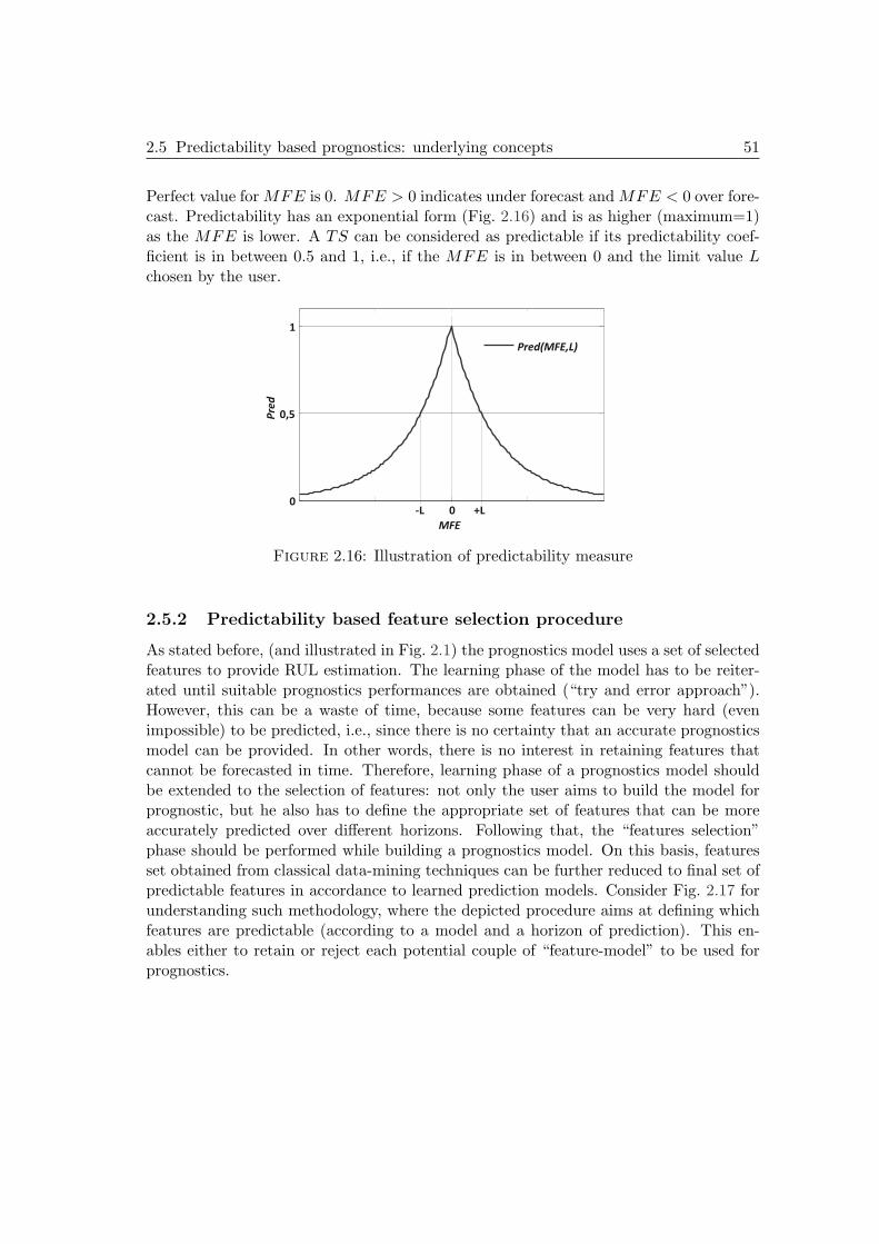
2.5 Predictability based prognostics: underlying concepts 51
Perfect value forMFE is 0. MFE > 0 indicates under forecast andMFE < 0 over fore-cast. Predictability has an exponential form (Fig. 2.16) and is as higher (maximum=1)as the MFE is lower. A TS can be considered as predictable if its predictability coef-ficient is in between 0.5 and 1, i.e., if the MFE is in between 0 and the limit value Lchosen by the user.
+L 0
0,5
1
MFE
Pre
d
Pred(MFE,L)
-L 0
Figure 2.16: Illustration of predictability measure
2.5.2 Predictability based feature selection procedure
As stated before, (and illustrated in Fig. 2.1) the prognostics model uses a set of selectedfeatures to provide RUL estimation. The learning phase of the model has to be reiter-ated until suitable prognostics performances are obtained (“try and error approach”).However, this can be a waste of time, because some features can be very hard (evenimpossible) to be predicted, i.e., since there is no certainty that an accurate prognosticsmodel can be provided. In other words, there is no interest in retaining features thatcannot be forecasted in time. Therefore, learning phase of a prognostics model shouldbe extended to the selection of features: not only the user aims to build the model forprognostic, but he also has to define the appropriate set of features that can be moreaccurately predicted over different horizons. Following that, the “features selection”phase should be performed while building a prognostics model. On this basis, featuresset obtained from classical data-mining techniques can be further reduced to final set ofpredictable features in accordance to learned prediction models. Consider Fig. 2.17 forunderstanding such methodology, where the depicted procedure aims at defining whichfeatures are predictable (according to a model and a horizon of prediction). This en-ables either to retain or reject each potential couple of “feature-model” to be used forprognostics.
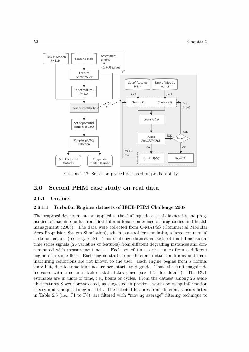
52 Chapter 2
Feature
extract/select
Couples {Fi/Mj}
selection
Bank of Models
j = 1..M
Assessment
criteria
- H
- L: MFE target
Sensor signals
Set of features
i = 1..n
Set of potential
couples {Fi/Mj}
Test predictability
Set of selected
features
Prognostic
models learned
Bank of Models
j=1..M
Set of features
i=1..n
Learn Fi/Mj
Asses
Pred(Fi/Mj,H,L)
Reject Fi
j = M?
j = 1 i = 1
OK
!OK
Choose Fi Choose Mj
OK
!OK
i = i
j = j+1
i = i + 1
j = 1
Retain Fi/Mj
Figure 2.17: Selection procedure based on predictability
2.6 Second PHM case study on real data
2.6.1 Outline
2.6.1.1 Turbofan Engines datasets of IEEE PHM Challenge 2008
The proposed developments are applied to the challenge dataset of diagnostics and prog-nostics of machine faults from first international conference of prognostics and healthmanagement (2008). The data were collected from C-MAPSS (Commercial ModularAero-Propulsion System Simulation), which is a tool for simulating a large commercialturbofan engine (see Fig. 2.18). This challenge dataset consists of multidimensionaltime series signals (26 variables or features) from different degrading instances and con-taminated with measurement noise. Each set of time series comes from a differentengine of a same fleet. Each engine starts from different initial conditions and man-ufacturing conditions are not known to the user. Each engine begins from a normalstate but, due to some fault occurrence, starts to degrade. Thus, the fault magnitudeincreases with time until failure state takes place (see [175] for details). The RULestimates are in units of time, i.e., hours or cycles. From the dataset among 26 avail-able features 8 were pre-selected, as suggested in previous works by using informationtheory and Choquet Integral [164]. The selected features from different sensors listedin Table 2.5 (i.e., F1 to F8), are filtered with “moving average” filtering technique to
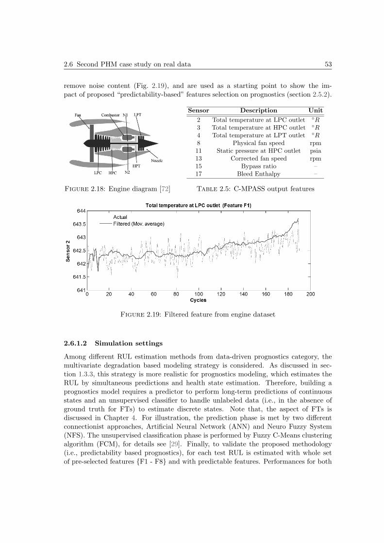
2.6 Second PHM case study on real data 53
remove noise content (Fig. 2.19), and are used as a starting point to show the im-pact of proposed “predictability-based” features selection on prognostics (section 2.5.2).
Figure 2.18: Engine diagram [72]
Sensor Description Unit
2 Total temperature at LPC outlet ◦R3 Total temperature at HPC outlet ◦R4 Total temperature at LPT outlet ◦R8 Physical fan speed rpm11 Static pressure at HPC outlet psia13 Corrected fan speed rpm15 Bypass ratio –17 Bleed Enthalpy –
Table 2.5: C-MPASS output features
Figure 2.19: Filtered feature from engine dataset
2.6.1.2 Simulation settings
Among different RUL estimation methods from data-driven prognostics category, themultivariate degradation based modeling strategy is considered. As discussed in sec-tion 1.3.3, this strategy is more realistic for prognostics modeling, which estimates theRUL by simultaneous predictions and health state estimation. Therefore, building aprognostics model requires a predictor to perform long-term predictions of continuousstates and an unsupervised classifier to handle unlabeled data (i.e., in the absence ofground truth for FTs) to estimate discrete states. Note that, the aspect of FTs isdiscussed in Chapter 4. For illustration, the prediction phase is met by two differentconnectionist approaches, Artificial Neural Network (ANN) and Neuro Fuzzy System(NFS). The unsupervised classification phase is performed by Fuzzy C-Means clusteringalgorithm (FCM), for details see [29]. Finally, to validate the proposed methodology(i.e., predictability based prognostics), for each test RUL is estimated with whole setof pre-selected features {F1 - F8} and with predictable features. Performances for both
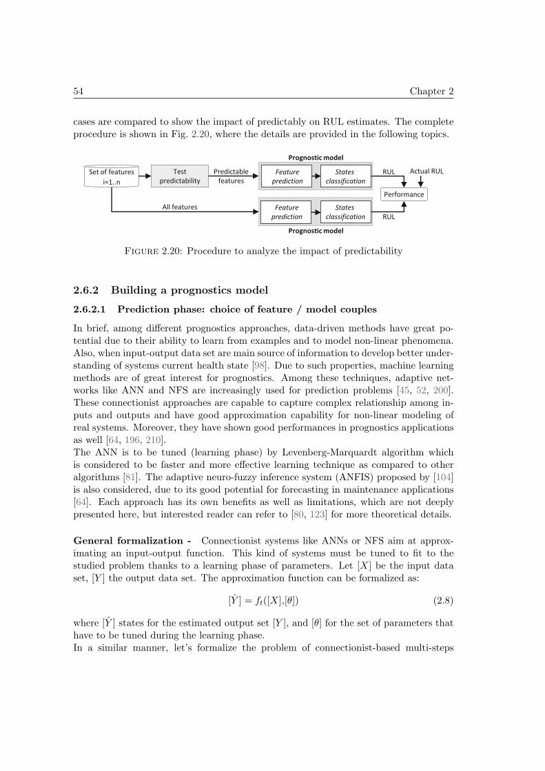
54 Chapter 2
cases are compared to show the impact of predictably on RUL estimates. The completeprocedure is shown in Fig. 2.20, where the details are provided in the following topics.
Test
predictability
Set of features
i=1..n
Performance
Feature
prediction
Feature
prediction
States
classification
States
classification
Actual RUL RUL
RUL
Prognostic model
Prognostic model
Predictable
features
All features
Figure 2.20: Procedure to analyze the impact of predictability
2.6.2 Building a prognostics model
2.6.2.1 Prediction phase: choice of feature / model couples
In brief, among different prognostics approaches, data-driven methods have great po-tential due to their ability to learn from examples and to model non-linear phenomena.Also, when input-output data set are main source of information to develop better under-standing of systems current health state [98]. Due to such properties, machine learningmethods are of great interest for prognostics. Among these techniques, adaptive net-works like ANN and NFS are increasingly used for prediction problems [45, 52, 200].These connectionist approaches are capable to capture complex relationship among in-puts and outputs and have good approximation capability for non-linear modeling ofreal systems. Moreover, they have shown good performances in prognostics applicationsas well [64, 196, 210].The ANN is to be tuned (learning phase) by Levenberg-Marquardt algorithm whichis considered to be faster and more effective learning technique as compared to otheralgorithms [81]. The adaptive neuro-fuzzy inference system (ANFIS) proposed by [104]is also considered, due to its good potential for forecasting in maintenance applications[64]. Each approach has its own benefits as well as limitations, which are not deeplypresented here, but interested reader can refer to [80, 123] for more theoretical details.
General formalization - Connectionist systems like ANNs or NFS aim at approx-imating an input-output function. This kind of systems must be tuned to fit to thestudied problem thanks to a learning phase of parameters. Let [X] be the input dataset, [Y ] the output data set. The approximation function can be formalized as:
[Y ] = ft([X],[θ]) (2.8)
where [Y ] states for the estimated output set [Y ], and [θ] for the set of parameters thathave to be tuned during the learning phase.In a similar manner, let’s formalize the problem of connectionist-based multi-steps
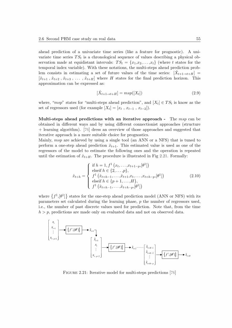
2.6 Second PHM case study on real data 55
ahead prediction of a univariate time series (like a feature for prognostic). A uni-variate time series TSt is a chronological sequence of values describing a physical ob-servation made at equidistant intervals: TSt = {x1,x2, . . . ,xt} (where t states for thetemporal index variable). With these notations, the multi-steps ahead prediction prob-lem consists in estimating a set of future values of the time series: [Xt+1→t+H ] =[xt+1 , xt+2 , xt+3 , . . . , xt+H ] where H states for the final prediction horizon. Thisapproximation can be expressed as:
[Xt+1→t+H ] = msp([Xt]) (2.9)
where, “msp” states for “multi-steps ahead prediction”, and [Xt] ∈ TSt is know as theset of regressors used (for example [Xt] = [xt , xt−1 , xt−2]).
Multi-steps ahead predictions with an iterative approach - The msp can beobtained in different ways and by using different connectionist approaches (structure+ learning algorithm). [76] dress an overview of those approaches and suggested thatiterative approach is a more suitable choice for prognostics.Mainly, msp are achieved by using a single tool (an ANN or a NFS) that is tuned toperform a one-step ahead prediction xt+1. This estimated value is used as one of theregressors of the model to estimate the following ones and the operation is repeateduntil the estimation of xt+H . The procedure is illustrated in Fig 2.21. Formally:
xt+h =
if h = 1, f1(
xt, . . . ,xt+1−p,[θ1])
elseif h ∈ {2, . . . ,p},f1
(
xt+h−1, . . . ,xt+1,xt, . . . ,xt+h−p,[θ1])
elseif h ∈ {p+ 1, . . . ,H},f1
(
xt+h−1, . . . ,xt+h−p,[θ1])
(2.10)
where{
f1,[θ1]}
states for the one-step ahead prediction model (ANN or NFS) with itsparameters set calculated during the learning phase, p the number of regressors used,i.e., the number of past discrete values used for prediction. Note that, from the timeh > p, predictions are made only on evaluated data and not on observed data.
1
1
t
t
t p
x
x
x
−
− +
� �� �� �� �� �� �� �
�{ }1 1
,[ ]f θ1
ˆt
x+
1
2
ˆt
t
t p
x
x
x
+
− +
� �� �� �� �� �� �� �
�{ }1 1
,[ ]f θ2
ˆt
x+ 1
2
ˆ
ˆ
ˆ
t H
t H
t H p
x
x
x
+ −
+ −
+ −
� �� �� �� �� �� �� �
�ˆ
t Hx
+{ }1 1,[ ]f θ
Figure 2.21: Iterative model for multi-steps predictions [76]

56 Chapter 2
Application - The msp technique has been used to forecast features in time to illus-trate the procedure of feature selection based on predictability concept. Experimentsare performed by using an ANN and a NFS as potential models for feature predic-tions, where each model is tuned according to parameters shown in Table 2.6. Thetraining of each model is met by multidimensional time series data of 40 turbofan en-gines from the challenge data record file “train− FD001.txt” (downloaded from [143]),where 5 engines data from the same file are used to perform tests. It should be notedthat for both off-line training and on-line testing tasks, the challenge data record file“train− FD001.txt” is considered. The msp are performed from time tc = 50 till thedefined prediction horizon (tc + 134), using an iterative approach. According to thedimension of feature space, “M” univariate prediction models (either ANN or NFS) arelearned in the off-line phase, i.e., feature-model couple. In the on-line phase, the learnedmodels are tested on data from 5 different engines. Prediction results obtained from eachtest are thoroughly investigated on predictability criteria to retain or reject each coupleof potential “feature-model” to be used for prognostics, where limit of predictability Lis set to 0.5 (see Fig. 2.17).
Table 2.6: Prediction models - Settings
ANN-Parameters Settings
Input / Hidden / Output layer neurons 3 / 5 / 1Hidden / Output layer Activation function sigmoidal / linear
Training Algorithm Levenberg-Marquardt
ANFIS-Parameters Settings
Input / Output layer neurons 3 / 1Number / type of input membership function 3 / Pi-shaped
Rules / Fuzzy Inference System 27 / First order SugenoDefuzzification method Weighted AverageTraining Algorithm Hybrid Method
2.6.2.2 Predictability results from prediction phase
As stated before, in order to exclude unpredictable features, predictability analysis isperformed on each test. For illustration, simulation results from a single test are reportedin Table 2.7 over different indexes of prediction horizon for a better understanding. Theobtained results show that features F2 and F3 do not satisfy predictability criteria,neither by ANN nor by ANFIS, as it is clearly indicated by their lower values of pre-dictability (i.e., Pred < 0.5). Similar findings about F2 and F3 are obtained from othertest cases as well, by applying both connectionist tools.This behavior is shown in Fig. 2.22, that presents a global picture of features pre-dictability over prediction horizon (tc + 134) steps ahead. Note that, ANFIS showedbetter performance with higher predictability values as compared to ANN for most ofthe simulations. Also results show that predictability is highly dependent on the horizon
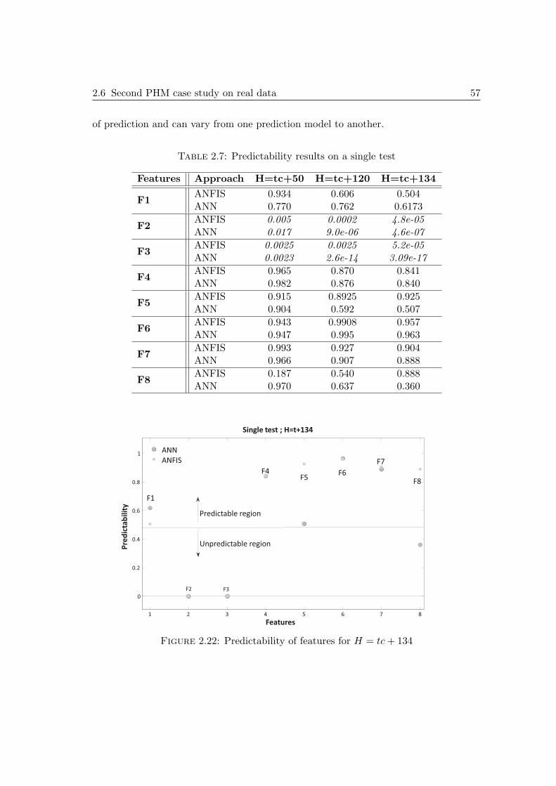
2.6 Second PHM case study on real data 57
of prediction and can vary from one prediction model to another.
Table 2.7: Predictability results on a single test
Features Approach H=tc+50 H=tc+120 H=tc+134
F1ANFIS 0.934 0.606 0.504ANN 0.770 0.762 0.6173
F2ANFIS 0.005 0.0002 4.8e-05ANN 0.017 9.0e-06 4.6e-07
F3ANFIS 0.0025 0.0025 5.2e-05ANN 0.0023 2.6e-14 3.09e-17
F4ANFIS 0.965 0.870 0.841ANN 0.982 0.876 0.840
F5ANFIS 0.915 0.8925 0.925ANN 0.904 0.592 0.507
F6ANFIS 0.943 0.9908 0.957ANN 0.947 0.995 0.963
F7ANFIS 0.993 0.927 0.904ANN 0.966 0.907 0.888
F8ANFIS 0.187 0.540 0.888ANN 0.970 0.637 0.360
1 2 3 4 5 6 7 8
0
0.2
0.4
0.6
0.8
1
Features
Pre
dic
tab
ilit
y
Single test ; H=t+134
ANN
ANFIS
F3 F2
F1
Predictable region
F4 F5
F6
F7
F8
Unpredictable region
Figure 2.22: Predictability of features for H = tc+ 134
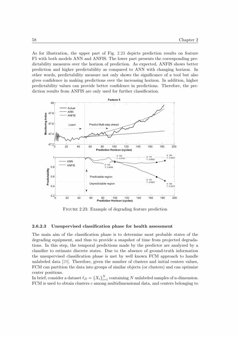
58 Chapter 2
As for illustration, the upper part of Fig. 2.23 depicts prediction results on featureF5 with both models ANN and ANFIS. The lower part presents the corresponding pre-dictability measures over the horizon of prediction. As expected, ANFIS shows betterprediction and higher predictability as compared to ANN with changing horizon. Inother words, predictability measure not only shows the significance of a tool but alsogives confidence in making predictions over the increasing horizon. In addition, higherpredictability values can provide better confidence in predictions. Therefore, the pre-diction results from ANFIS are only used for further classification.
0 20 40 60 80 100 120 140 160 180 20047.2
47.4
47.6
47.8
48
Prediction Horizon (cycles)
Mo
nit
ori
ng
In
de
x
Feature 5
Actual
ANN
ANFIS
0 20 40 60 80 100 120 140 160 180 2000.2
0.4
0.6
0.8
1
X: 184
Y: 0.9253
Pre
dic
tab
ilit
y
Prediction Horizon (cycles)
X: 184
Y: 0.5075
X: 170
Y: 0.5922
X: 170
Y: 0.8925
X: 100
Y: 0.9155
X: 100
Y: 0.9048
ANN
ANFIS
Learn Predict Multi-step ahead
Predictable region
Unpredictable region
Figure 2.23: Example of degrading feature prediction
2.6.2.3 Unsupervised classification phase for health assessment
The main aim of the classification phase is to determine most probable states of thedegrading equipment, and thus to provide a snapshot of time from projected degrada-tions. In this step, the temporal predictions made by the predictor are analyzed by aclassifier to estimate discrete states. Due to the absence of ground-truth informationthe unsupervised classification phase is met by well known FCM approach to handleunlabeled data [29]. Therefore, given the number of clusters and initial centers values,FCM can partition the data into groups of similar objects (or clusters) and can optimizecenter positions.In brief, consider a dataset ℓD = {Xi}Ni=1 containingN unlabeled samples of n-dimension.FCM is used to obtain clusters c among multidimensional data, and centers belonging to
2.6 Second PHM case study on real data 59
each cluster V = {vj}cj=1. Formally, the FCM clustering is attained by assigning mem-bership grade (µij) between [0, 1] to every data point that corresponds to each clustercenter (or in other words belong to various groups), based on the measured distancebetween a data point and center of the cluster. If a data point is closer to a particularcluster center, a greater membership value is assigned. The summation of membershipgrades from all data points correspond to a membership equal to ’1’. FCM aims tooperate in an iterative manner, assuming the number of clusters is known it reducesfollowing objective function:
J =N∑
i=1
c∑
j=1
(µij)m.‖xi − vj‖2 (2.11)
where, ‖xi − vj‖2 represents the Euclidean Distance (ED) (to measure similarity be-tween) between the ith data point and the jth cluster center v (Eq. 2.12), fuzzy partitionmatrix can be represented as U = [µij ]c×N , where µij describes the membership of the
ith data point to the jth centroid, and m > 1 is a weighting exponent. The key steps ofFCM algorithm are summarize in Appendix A.3.
ED =
√
√
√
√
n∑
i=1
(xi − vj)2 (2.12)
2.6.2.4 Health assessment
Briefly, in the learning phase, a classifier is built to identify states of degrading equip-ment. For this purpose, different functioning modes have to be considered. In this case,four states of degradation are assumed, namely: steady state, degrading state, transitionstate and critical state. FCM is used to assign temporal predictions to different classesbased on fuzzy partitioning (to cluster) multidimensional data. The number of clustersis preset to 4 for the FCM algorithm. Accordingly, the multidimensional training dataof 40 engines are partitioned into four groups, where each group represents a particularstate of degradation. It should be noted that, each engine has different life span ornumber of cycles. For illustration purpose, 2D visualizations from clustering phase areshown in Fig. 2.24.In the on-line test phase, discrete states are assigned to continuous state predictions (ormsp) by measuring the ED between predictions (of multidimensional data) and clusterscenters (Eq. 2.12). Following that, class labels can be given by looking at the closestmatch. For more clarity, measured distances for the case of all features and predictablefeatures are shown in Fig. 2.25. Finally, RUL estimate is obtained, when transition fromdegrading state (d) at time tc to faulty state (f) at time tf occurs (see Eq. (2.13)).
transition dState→ f ⇒ RUL = Sd→f − tc (2.13)
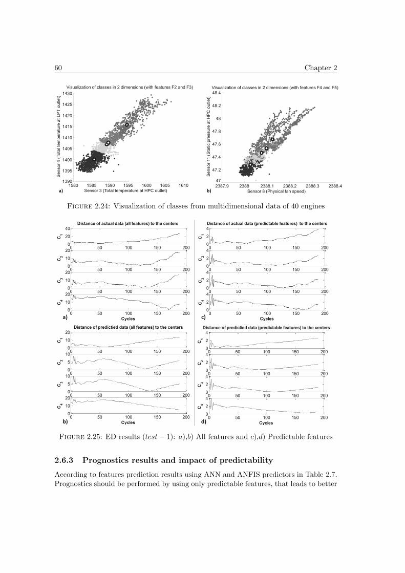
60 Chapter 2
a) b) 1580 1585 1590 1595 1600 1605 1610
1390
1395
1400
1405
1410
1415
1420
1425
1430
Visualization of classes in 2 dimensions (with features F2 and F3)
Sensor 3 (Total temperature at HPC outlet)
Se
nso
r 4
(To
tal te
mp
era
ture
at L
PT
ou
tle
t)
2387.9 2388 2388.1 2388.2 2388.3 2388.4
47
47.2
47.4
47.6
47.8
48
48.2
48.4
Visualization of classes in 2 dimensions (with features F4 and F5)
Sensor 8 (Physical fan speed)
Se
nso
r 11
(S
tatic p
ressu
re a
t H
PC
ou
tle
t)
Figure 2.24: Visualization of classes from multidimensional data of 40 engines
0 50 100 150 2000
20
40
Distance of actual data (all features) to the centers
C1
0 50 100 150 2000
10
20
C2
0 50 100 150 2000
10
20
C3
0 50 100 150 2000
10
20
Cycles
C4
0 50 100 150 2000
10
20
Distance of predictied data (all features) to the centers
C1
0 50 100 150 2000
5
10
C2
0 50 100 150 2000
5
10
C3
0 50 100 150 2000
10
20
Cycles
C4
0 50 100 150 2000
2
4
Distance of predictied data (predictable features) to the centers
C1
0 50 100 150 2000
2
4
C2
0 50 100 150 2000
2
4
C3
0 50 100 150 2000
2
4
Cycles
C4
a)
b) d)
0 50 100 150 2000
2
4
Distance of actual data (predictable features) to the centers
C1
0 50 100 150 2000
2
4
C2
0 50 100 150 2000
2
4
C3
0 50 100 150 2000
2
4
Cycles
C4
c)
Figure 2.25: ED results (test− 1): a),b) All features and c),d) Predictable features
2.6.3 Prognostics results and impact of predictability
According to features prediction results using ANN and ANFIS predictors in Table 2.7.Prognostics should be performed by using only predictable features, that leads to better
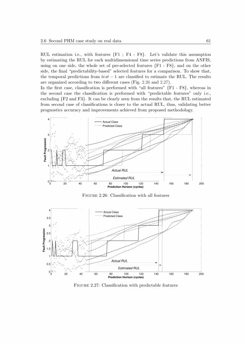
2.6 Second PHM case study on real data 61
RUL estimation i.e., with features {F1 ; F4 - F8}. Let’s validate this assumptionby estimating the RUL for each multidimensional time series predictions from ANFIS,using on one side, the whole set of pre-selected features {F1 - F8}, and on the otherside, the final “predictability-based” selected features for a comparison. To show that,the temporal predictions from test − 1 are classified to estimate the RUL. The resultsare organized according to two different cases (Fig. 2.26 and 2.27).In the first case, classification is performed with “all features” {F1 - F8}, whereas inthe second case the classification is performed with “predictable features” only i.e.,excluding {F2 and F3}. It can be clearly seen from the results that, the RUL estimatedfrom second case of classifications is closer to the actual RUL, thus, validating betterprognostics accuracy and improvements achieved from proposed methodology.
3
4
og
res
sio
n
Actual Class
Predicted Class
0 20 40 60 80 100 120 140 160 180 2000
1
2
Prediction Horizon (cycles)
Fa
ult
Pro
g
Actual RUL
Estimated RUL
Figure 2.26: Classification with all features
3
3.5
4Actual Class
Predicted Class
0 20 40 60 80 100 120 140 160 180 2000
0.5
1
1.5
2
2.5
3
Prediction Horizon (cycles)
Fa
ult
Pro
gre
ss
ion
Actual RUL
Estimated RUL
Figure 2.27: Classification with predictable features
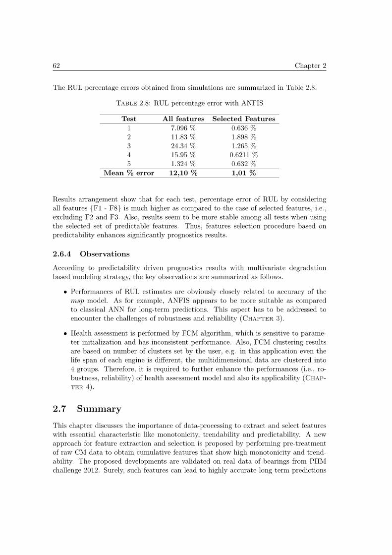
62 Chapter 2
The RUL percentage errors obtained from simulations are summarized in Table 2.8.
Table 2.8: RUL percentage error with ANFIS
Test All features Selected Features
1 7.096 % 0.636 %2 11.83 % 1.898 %3 24.34 % 1.265 %4 15.95 % 0.6211 %5 1.324 % 0.632 %
Mean % error 12,10 % 1,01 %
Results arrangement show that for each test, percentage error of RUL by consideringall features {F1 - F8} is much higher as compared to the case of selected features, i.e.,excluding F2 and F3. Also, results seem to be more stable among all tests when usingthe selected set of predictable features. Thus, features selection procedure based onpredictability enhances significantly prognostics results.
2.6.4 Observations
According to predictability driven prognostics results with multivariate degradationbased modeling strategy, the key observations are summarized as follows.
• Performances of RUL estimates are obviously closely related to accuracy of themsp model. As for example, ANFIS appears to be more suitable as comparedto classical ANN for long-term predictions. This aspect has to be addressed toencounter the challenges of robustness and reliability (Chapter 3).
• Health assessment is performed by FCM algorithm, which is sensitive to parame-ter initialization and has inconsistent performance. Also, FCM clustering resultsare based on number of clusters set by the user, e.g. in this application even thelife span of each engine is different, the multidimensional data are clustered into4 groups. Therefore, it is required to further enhance the performances (i.e., ro-bustness, reliability) of health assessment model and also its applicability (Chap-
ter 4).
2.7 Summary
This chapter discusses the importance of data-processing to extract and select featureswith essential characteristic like monotonicity, trendability and predictability. A newapproach for feature extraction and selection is proposed by performing pre-treatmentof raw CM data to obtain cumulative features that show high monotonicity and trend-ability. The proposed developments are validated on real data of bearings from PHMchallenge 2012. Surely, such features can lead to highly accurate long term predictions

2.7 Summary 63
and ease in implementation of prognostics model. This aspect is validated in Chapter 3.Secondly, another concept of predictability driven prognostics is presented to performpost-treatment of features subset for further reduction. Indeed, there is no use of fea-tures that are hard to be predicted. The proposed developments are validated on realdata of turbofan engines from PHM challenge 2008. Prognostics modeling is achievedby multivariate degradation based modeling strategy. For the sake of illustration ANNand ANFIS are used as prediction models and FCM algorithm is used for unsuper-vised classification phase. Besides that, some weaknesses of multivariate degradationbased modeling are also highlighted in section 2.6.4. To further enhance this strategy,and according to the objective of this thesis (section 1.4.2.3). Chapter 3 presents anew approach for “long-term predictions”, and Chapter 4 presents a new approach forunsupervised classification.

Chapter 3From features to predictions
This chapter presents a new connectionist approach to perform “long-termpredictions” for prognostics. More precisely, a Summation Wavelet-ExtremeLearning Machine algorithm is proposed to address issues related to prognos-tics modeling challenges, i.e., robustness, reliability, applicability. Moreover,an ensemble of SW-ELM models is proposed to quantify the uncertainty dueto data and modeling phase.Firstly, for issues related to time-series, i.e., approximation, one step-aheadprediction, and multi-steps ahead prediction, SW-ELM is benchmarked withExtreme Learning Machine, Levenberg Marquardt and ELMAN algorithmson six industrial data sets. Secondly, to validate the efficiency of SW-ELMwith respect to challenges, a real case of Computer Numerical Control (CNC)machine is considered for tool wear monitoring task. Thorough comparisonswith ELM algorithm are given to show enhanced robustness and reliability ofSW-ELM on different data sets.Finally, to validate the concept of cumulative features (Chapter 2), SW-ELM is used as a potential model to perform “long-term predictions” withcumulative features. For this case study, SW-ELM is applied to real data ofbearings from PHM challenge 2012.
3.1 Long-term predictions for prognostics
According to multivariate degradation based modeling strategy (Chapter 1), the prog-nostics phase is composed of two complementary modules: a prediction engine that fore-casts observations in time, and a classifier which provides the most probable states ofthe machinery. The RUL is obtained from the estimated time to reach the faulty state(see Fig. 1.12). Obviously, for prognostics part, the prediction phase is critical and must
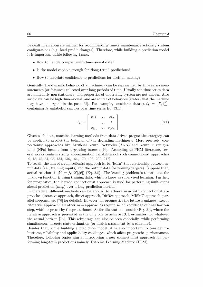
66 Chapter 3
be dealt in an accurate manner for recommending timely maintenance actions / systemconfigurations (e.g. load profile changes). Therefore, while building a prediction modelit is important tackle following issues.
• How to handle complex multidimensional data?
• Is the model capable enough for “long-term” predictions?
• How to associate confidence to predictions for decision making?
Generally, the dynamic behavior of a machinery can be represented by time series mea-surements (or features) collected over long periods of time. Usually the time series dataare inherently non-stationary, and properties of underlying system are not known. Alsosuch data can be high dimensional, and are source of behaviors (states) that the machinemay have undergone in the past [55]. For example, consider a dataset ℓD = {Xi}Ni=1
containing N unlabeled samples of n time series Eq. (3.1).
ℓD =
x11 . . . x1n... · · · ...
xN1 . . . xNn
(3.1)
Given such data, machine learning methods from data-driven prognostics category canbe applied to predict the behavior of the degrading machinery. More precisely, con-nectionist approaches like Artificial Neural Networks (ANN) and Neuro Fuzzy sys-tems (NFs) benefit from a growing interest [76]. According to PHM literature, sev-eral works confirm strong approximation capabilities of such connectionist approaches[9, 18, 45, 64, 98, 134, 136, 164, 170, 196, 202, 217].To recall, the aim of a connectionist approach is, to “learn” the relationship between in-put data (i.e., training inputs) and the output data (or training targets). Suppose that,actual relations is [Y ] = ft([X],[θ]) (Eq. 2.8). The learning problem is to estimate theunknown function ft using training data, which is know as supervised learning. Further,for prognostics, the learned connectionist approach is used for performing multi-stepsahead prediction (msp) over a long prediction horizon.In literature, different methods can be applied to achieve msp with connectionist ap-proaches (iterative approach, direct approach, DirRec approach, MISMO approach, par-allel approach, see [76] for details). However, for prognostics the future is unknow, except“iterative approach” all other msp approaches require prior knowledge of final horizonstep, which is preset by the practitioner. As for illustration, consider Fig. 3.1, where theiterative approach is presented as the only one to achieve RUL estimates, for whateverthe actual horizon [76]. This advantage can also be seen especially, while performingsimultaneous discrete state estimation (or health assessment by a classifier).Besides that, while building a prediction model, it is also important to consider ro-bustness, reliability and applicability challenges, which affect prognostics performances.Therefore, following topics aim at introducing a new connectionist approach for per-forming long-term predictions namely, Extreme Learning Machine (ELM).
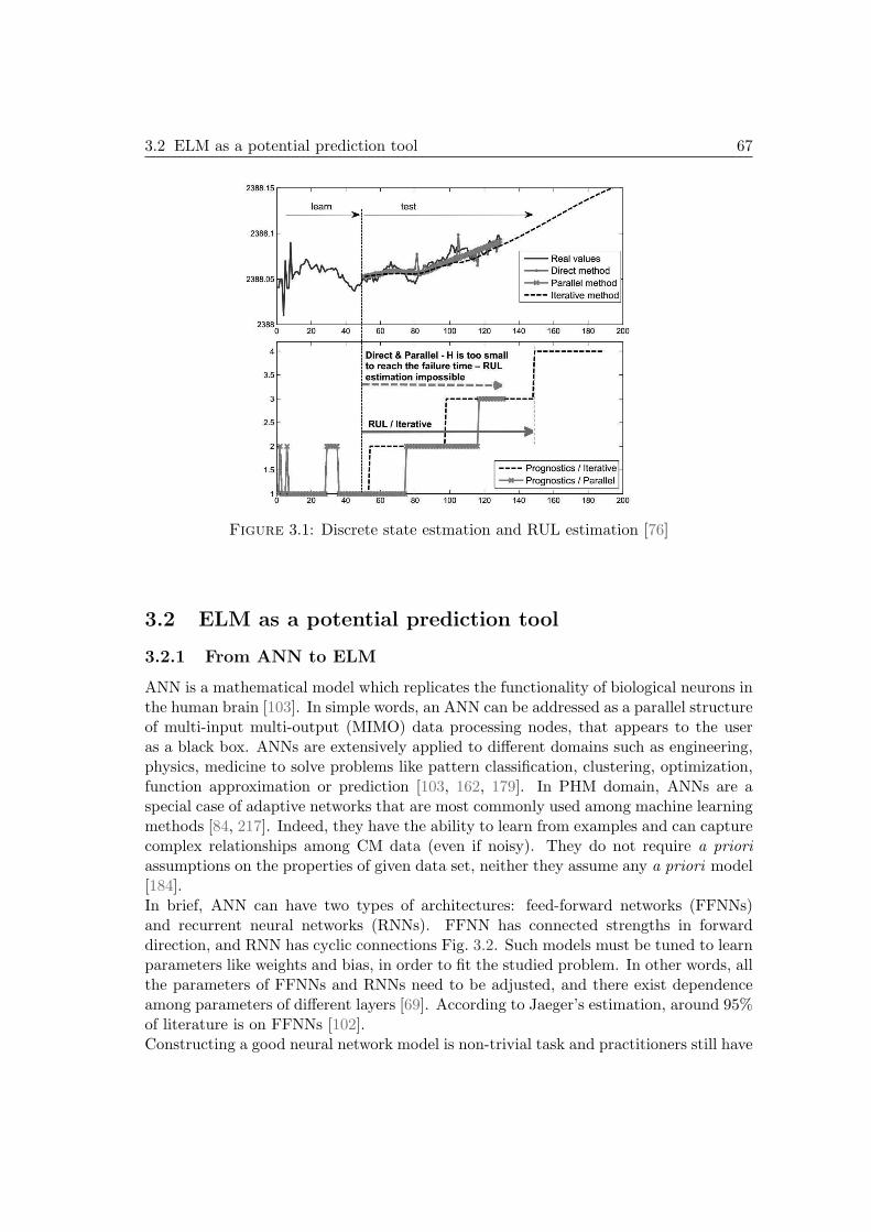
3.2 ELM as a potential prediction tool 67
Figure 3.1: Discrete state estmation and RUL estimation [76]
3.2 ELM as a potential prediction tool
3.2.1 From ANN to ELM
ANN is a mathematical model which replicates the functionality of biological neurons inthe human brain [103]. In simple words, an ANN can be addressed as a parallel structureof multi-input multi-output (MIMO) data processing nodes, that appears to the useras a black box. ANNs are extensively applied to different domains such as engineering,physics, medicine to solve problems like pattern classification, clustering, optimization,function approximation or prediction [103, 162, 179]. In PHM domain, ANNs are aspecial case of adaptive networks that are most commonly used among machine learningmethods [84, 217]. Indeed, they have the ability to learn from examples and can capturecomplex relationships among CM data (even if noisy). They do not require a prioriassumptions on the properties of given data set, neither they assume any a priori model[184].In brief, ANN can have two types of architectures: feed-forward networks (FFNNs)and recurrent neural networks (RNNs). FFNN has connected strengths in forwarddirection, and RNN has cyclic connections Fig. 3.2. Such models must be tuned to learnparameters like weights and bias, in order to fit the studied problem. In other words, allthe parameters of FFNNs and RNNs need to be adjusted, and there exist dependenceamong parameters of different layers [69]. According to Jaeger’s estimation, around 95%of literature is on FFNNs [102].Constructing a good neural network model is non-trivial task and practitioners still have
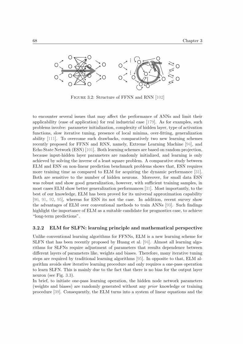
68 Chapter 3
Figure 3.2: Structure of FFNN and RNN [102]
to encounter several issues that may affect the performance of ANNs and limit theirapplicability (ease of application) for real industrial case [179]. As for examples, suchproblems involve: parameter initialization, complexity of hidden layer, type of activationfunctions, slow iterative tuning, presence of local minima, over-fitting, generalizationability [111]. To overcome such drawbacks, comparatively two new learning schemesrecently proposed for FFNN and RNN, namely, Extreme Learning Machine [94], andEcho State Network (ESN) [101]. Both learning schemes are based on random projection,because input-hidden layer parameters are randomly initialized, and learning is onlyachieved by solving the inverse of a least square problem. A comparative study betweenELM and ESN on non-linear prediction benchmark problems shows that, ESN requiresmore training time as compared to ELM for acquiring the dynamic performance [31].Both are sensitive to the number of hidden neurons. Moreover, for small data ESNwas robust and show good generalization, however, with sufficient training samples, inmost cases ELM show better generalization performances [31]. Most importantly, to thebest of our knowledge, ELM has been proved for its universal approximation capability[90, 91, 92, 95], whereas for ESN its not the case. In addition, recent survey showthe advantages of ELM over conventional methods to train ANNs [93]. Such findingshighlight the importance of ELM as a suitable candidate for prognostics case, to achieve“long-term predictions”.
3.2.2 ELM for SLFN: learning principle and mathematical perspective
Unlike conventional learning algorithms for FFNNs, ELM is a new learning scheme forSLFN that has been recently proposed by Huang et al. [94]. Almost all learning algo-rithms for SLFNs require adjustment of parameters that results dependence betweendifferent layers of parameters like, weights and biases. Therefore, many iterative tuningsteps are required by traditional learning algorithms [95]. In opposite to that, ELM al-gorithm avoids slow iterative learning procedure and only requires a one-pass operationto learn SLFN. This is mainly due to the fact that there is no bias for the output layerneuron (see Fig. 3.3).In brief, to initiate one-pass learning operation, the hidden node network parameters(weights and biases) are randomly generated without any prior knowledge or trainingprocedure [39]. Consequently, the ELM turns into a system of linear equations and the
3.2 ELM as a potential prediction tool 69
x1
(bk)
1
Ñ
k
(wk, bk)
Input layer
Hidden layer
Output layer
x2
xn
O
S
-5 -4 -3 -2 -1 0 1 2 3 4 50
0.1
0.2
0.3
0.4
0.5
0.6
0.7
0.8
0.9
1Log-sigmoid transfer function
Activation ftn.
Figure 3.3: Single layer feed forward neural network
unknown weights between the hidden and output layer nodes can be obtained analyti-cally by only applying Moore-Penrose generalized inverse procedure [124, 167].Let note n and m the numbers of inputs and outputs (i.e., targets), N the numberof learning data samples (xi,ti), where i ∈ [1 . . . N ], xi = [xi1,xi2,...,xin]
T ∈ ℜn andti = [ti1,ti2,...,tim]T ∈ ℜm, and N the number of hidden nodes, each one with an ac-tivation function f(x). For each sample j, the output oj is mathematically expressedas:
N∑
k=1
βk.f(wk.xj + bk) = oj , j = 1,2,...., N (3.2)
where wk = [wk1,wk2,...,wkn]T ∈ ℜn, is an input weight vector connecting the kth hidden
neuron to the input layer neurons, (wk ·xj) is the inner product of weights and inputs,and bk ∈ ℜ is the bias of kth neuron of hidden layer. Also, βk = [βk1,βk2,...,βkm]T ∈ ℜm,is the weight vector to connect the kth neuron of hidden layer and output neurons.Therefore, in order to minimize the difference between network output oj and given
target tj ,∑N
j=1 ‖oj − tj‖ = 0, there exist βk, wk and bk such that:
N∑
k=1
βk.f(wk.xj + bk) = tj , j = 1,2,...., N (3.3)
which can be expressed in matrix form as,
Hβ = T (3.4)
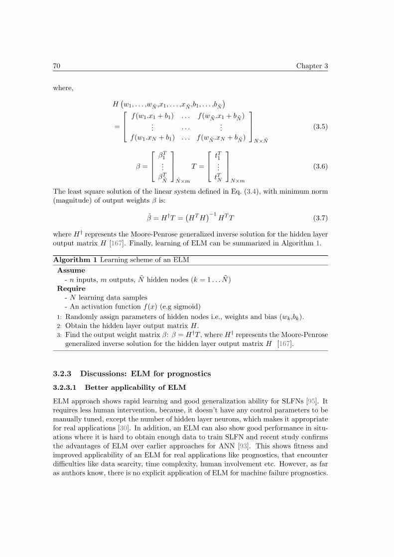
70 Chapter 3
where,
H(
w1, . . . ,wN ,x1, . . . ,xN ,b1, . . . ,bN)
=
f(w1.x1 + b1) . . . f(wN .x1 + bN )... · · · ...
f(w1.xN + b1) . . . f(wN .xN + bN )
N×N
(3.5)
β =
βT1...βTN
N×m
T =
tT1...tTN
N×m
(3.6)
The least square solution of the linear system defined in Eq. (3.4), with minimum norm(magnitude) of output weights β is:
β = H†T =(
HTH)−1
HTT (3.7)
where H† represents the Moore-Penrose generalized inverse solution for the hidden layeroutput matrix H [167]. Finally, learning of ELM can be summarized in Algorithm 1.
Algorithm 1 Learning scheme of an ELM
Assume
- n inputs, m outputs, N hidden nodes (k = 1 . . . N)Require
- N learning data samples- An activation function f(x) (e.g sigmoid)
1: Randomly assign parameters of hidden nodes i.e., weights and bias (wk,bk).2: Obtain the hidden layer output matrix H.3: Find the output weight matrix β: β = H†T , where H† represents the Moore-Penrose
generalized inverse solution for the hidden layer output matrix H [167].
3.2.3 Discussions: ELM for prognostics
3.2.3.1 Better applicability of ELM
ELM approach shows rapid learning and good generalization ability for SLFNs [95]. Itrequires less human intervention, because, it doesn’t have any control parameters to bemanually tuned, except the number of hidden layer neurons, which makes it appropriatefor real applications [30]. In addition, an ELM can also show good performance in situ-ations where it is hard to obtain enough data to train SLFN and recent study confirmsthe advantages of ELM over earlier approaches for ANN [93]. This shows fitness andimproved applicability of an ELM for real applications like prognostics, that encounterdifficulties like data scarcity, time complexity, human involvement etc. However, as faras authors know, there is no explicit application of ELM for machine failure prognostics.

3.3 SW-ELM and Ensemble models for prognostics 71
3.2.3.2 Issues and requirements
ELM method has two parameters that are set by the user, number of hidden layer neu-rons and variance of the hidden layer weights [151]. The interaction between improperinitialization of weights and neurons of the hidden layer may impair performance of theELM model [30]. In view of expected performances of a prognostics model highlightedin section 1.4, practical considerations related to model accuracy and implementationissues should be addressed for real applications.
• Due to random initialization of parameters (weights and biases), ELM modelmay require high complexity of hidden layer [162]. This may cause ill-condition,and reduce robustness of ELM to encounter variations in the input data, and theexpected output of the model may not be close to the real output [77]. Also therandomly initialized weights can affect model generalization ability which shouldalso be considered.
• It is required to carefully choose hidden neuron activation functions that canparticipate in better convergence of the algorithm, show good ability to transformnon-linear inputs, and also result in a compact structure of network (i.e, hiddenneurons) for a suitable level of accuracy [91, 103, 111].
• Finally, ELM can perform estimates after learning phase, however, it does notquantify uncertainty of modeling phase like any ANN. Therefore, it is necessary tobracket unknown future with confidence intervals to show reliability of estimatesand also to facilitate decision making step for prognostics applications.
Therefore, to address these issues and requirements, the next section presents a newlearning scheme for SLFN, which is an improved variant of ELM, namely, the SummationWavelet- Extreme Learning Machine (SW-ELM).
3.3 SW-ELM and Ensemble models for prognostics
Combining neural networks and wavelet theory as an approximation or prediction modelsappears to be an effective solution in many applicative areas. However, when buildingsuch systems, one has to face parsimony problem, i.e., to look for a compromise betweenthe complexity of the learning phase and accuracy performances. Following topics focuson building a new structure of connectionist network, the SW-ELM that enables goodaccuracy and generalization performances, while limiting the learning time and reducingthe impact of random initialization procedure.
3.3.1 Wavelet neural network
3.3.1.1 Concept and structure
Wavelet theory is an outcome of multidisciplinary struggles, that brought together en-gineers, mathematicians and physicists [159]. The term wavelet means a “little wave”.
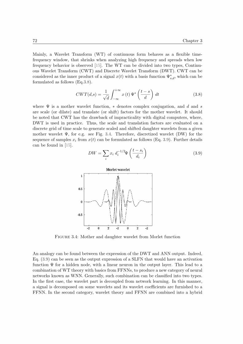
72 Chapter 3
Mainly, a Wavelet Transform (WT) of continuous form behaves as a flexible time-frequency window, that shrinks when analyzing high frequency and spreads when lowfrequency behavior is observed [15]. The WT can be divided into two types, Continu-ous Wavelet Transform (CWT) and Discrete Wavelet Transform (DWT). CWT can beconsidered as the inner product of a signal x(t) with a basis function Ψ∗
s,d, which can beformulated as follows (Eq.3.8).
CWT (d,s) =1√d
∫ +∞
−∞x (t)Ψ∗
(
t− s
d
)
dt (3.8)
where Ψ is a mother wavelet function, ∗ denotes complex conjugation, and d and sare scale (or dilate) and translate (or shift) factors for the mother wavelet. It shouldbe noted that CWT has the drawback of impracticality with digital computers, where,DWT is used in practice. Thus, the scale and translation factors are evaluated on adiscrete grid of time scale to generate scaled and shifted daughter wavelets from a givenmother wavelet Ψ, for e.g. see Fig. 3.4. Therefore, discretized wavelet (DW) for thesequence of samples xi from x(t) can be formulated as follows (Eq. 3.9). Further detailscan be found in [15].
DW =∑
i
xi d−1/2i Ψ
(
t− sidi
)
(3.9)
Figure 3.4: Mother and daughter wavelet from Morlet function
An analogy can be found between the expression of the DWT and ANN output. Indeed,Eq. (3.9) can be seen as the output expression of a SLFN that would have an activationfunction Ψ for a hidden node, with a linear neuron in the output layer. This lead to acombination of WT theory with basics from FFNNs, to produce a new category of neuralnetworks known as WNN. Generally, such combination can be classified into two types.In the first case, the wavelet part is decoupled from network learning. In this manner,a signal is decomposed on some wavelets and its wavelet coefficients are furnished to aFFNN. In the second category, wavelet theory and FFNN are combined into a hybrid

3.3 SW-ELM and Ensemble models for prognostics 73
structure. The scope of following topics cover the latter category.Let note n the number of inputs of a WNN, and N the number of hidden nodes withwavelet functions (eg. Morlet, see Fig. 3.3). According to this, the output of a WNNcan be formulated as:
y =N∑
k=1
vkΨk
n∑
j=1
wkjxj
(3.10)
Ψk (x) = |dk|−1/2Ψ
(
x− skdk
)
(3.11)
where x = x1,x2,...,xn depicts the input values, Ψk represents the family of daughterwavelets that are scaled and translated from a single mother wavelet function Ψ, dk andsk are the corresponding scale (dilate) and translation factors. Lastly, wk = [wk1,wk2,...,wkn]
T ∈ ℜn is an input weight vector connecting the kth hidden neuron to the inputlayer neurons, and vk is the weight to connect the kth neuron of hidden layer and theoutput.
3.3.1.2 Issues and requirements
According to literature, the initialization of dilation and translation factors (dk and sk inEq. (3.11)) is considered as a critical phase. Indeed, it is necessary to properly initializethese parameters for fast convergence of algorithm [39, 150]. As wavelets functionsvanish rapidly, improper initialization may lead to the following issues:
• a wavelet can be too local for a very small dilation;
• improper translation may be out of interest domain.
Therefore, the random tuning of dilation and translation factors of wavelets is inadvis-able, and parameters initialization should be based on the input domain. This aspect istaken into account in the proposed model (section 3.3.2).
3.3.2 Summation Wavelet-Extreme Learning Machine for SLFN
3.3.2.1 Structure and mathematical perspective
As mentioned in previous section, ELM is quiet efficient as compared to traditionalmethods to learn SLFNs. However, issues like parameters initialization, model com-plexity and choice of activation functions have to be carefully addressed for improvedperformance. Since structure and proper choice of activation functions enhances thecapability of the SLFN network to encounter low and high frequency signals simulta-neously. The number of neurons required for hidden layer decreases and a compactstructure is achieved [15, 103, 124]. Therefore, we propose the Summation Wavelet-Extreme Learning (SW-ELM) algorithm. The proposed structure of SW-ELM takesadvantages of WT and SLFN (see Fig. 3.5), for which two significant modifications areperformed in the hidden layer.

74 Chapter 3
• Structure - Non-linear transformations are dealt in a better manner by using aconjunction of two distinct activation functions (f1 and f2) in each hidden noderather than a single activation function. The output from a hidden node is the aver-age value after performing transformation from dual activations (f = (f1 + f2) /2).
• Activation functions - To improve convergence of algorithm, an inverse hyper-bolic sine ([124], Eq. (3.12)) and a Morlet wavelet ([39, 159], Eq. (3.13)) are usedas dual activation functions.
f1 = θ (X) = log[
x+ (x2 + 1)1/2]
(3.12)
f2 = ψ (X) = cos (5x) e(−0.5x2) (3.13)
Such a combination of activation functions makes the network more adequate to dealwith dynamic systems.According to modifications mentioned above, for each sample j Eq. 3.2 can be adaptedand the output oj is mathematically expressed as:
N∑
k=1
βk.f [(θ,ψ) (wk.xj + bk)] = oj ,j = 1,2,...,N (3.14)
where wk = [wk1,wk2,...,wkn]T ∈ ℜn, is an input weight vector connecting the kth hidden
neuron to the input layer neurons, (wk.xj) is the inner product of weights and inputs,and bk ∈ ℜ is the bias of kth neuron of hidden layer. Also, βk = [βk1,βk2,...,βkm]T ∈ ℜm,is the weight vector to connect the kth neuron of hidden layer and output neurons.Finally, f shows the average output from two different activation functions i.e., aninverse hyperbolic sine activation function θ and a Morlet wavelet activation functionψ. In order to minimize the difference between network output oj and given target tj ,∑N
j=1 ‖oj − tj‖ = 0, there exist βk, wk and bk such that:
N∑
k=1
βk.f [(θ,ψ) (wk.xj + bk)] = tj , j = 1,2,...,N (3.15)
which can be expressed in matrix form as,
Havgβ = T (3.16)
where Havg is a[
N × N]
matrix expressed as,
Havg
(
w1, . . . ,wN ,x1, . . . ,xN ,b1, . . . ,bN)
=
f (θ,ψ)
(w1.x1 + b1) . . .(
wN .x1 + bN)
... · · · ...(w1.xN + b1) . . .
(
wN .xN + bN)
(3.17)
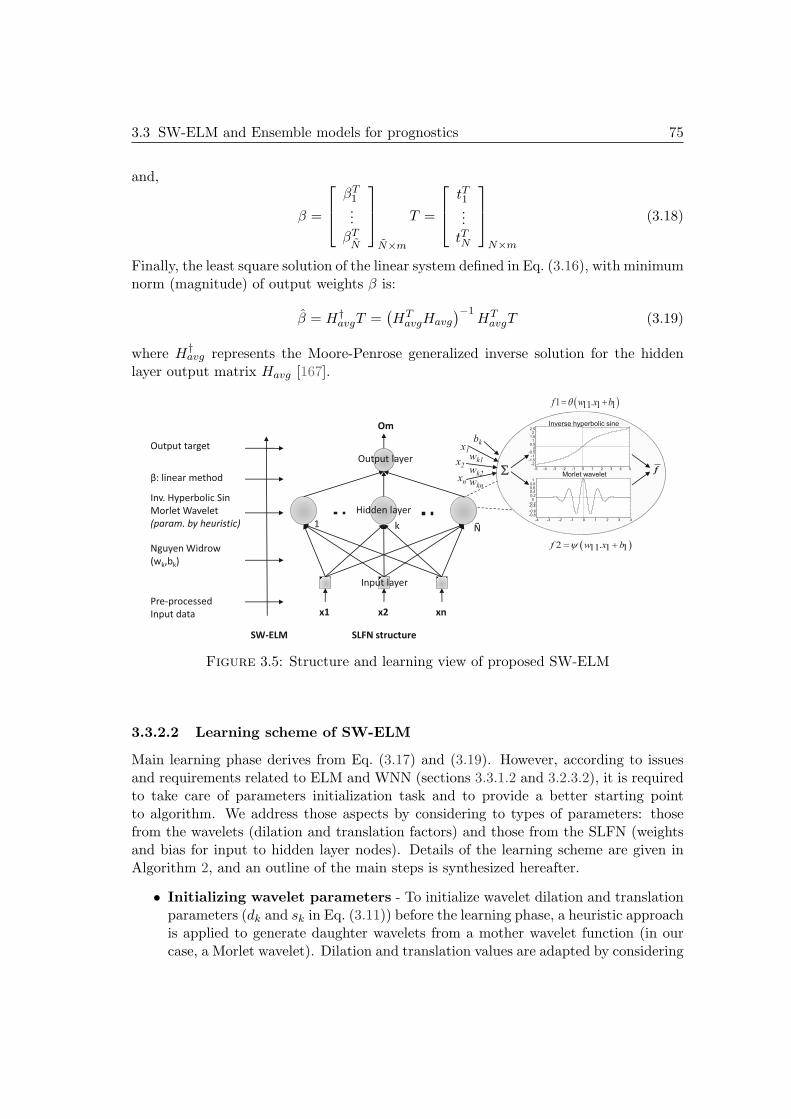
3.3 SW-ELM and Ensemble models for prognostics 75
and,
β =
βT1...βTN
N×m
T =
tT1...tTN
N×m
(3.18)
Finally, the least square solution of the linear system defined in Eq. (3.16), with minimumnorm (magnitude) of output weights β is:
β = H†avgT =
(
HTavgHavg
)−1HT
avgT (3.19)
where H†avg represents the Moore-Penrose generalized inverse solution for the hidden
layer output matrix Havg [167].
x1 xn x2
1 Ñ k
Om
Hidden layer
SW-ELM SLFN structure
Output layer
Input layer
S
f xn
x1
x2
bk
wk1
wk2 wkn
Nguyen Widrow (wk,bk)
Pre-processed Input data
Inv. Hyperbolic Sin Morlet Wavelet (param. by heuristic)
β: linear method
Output target
( )1 .11 1 1f w x bq= +
( )2 .11 1 1f w x by= +
-5 -4 -3 -2 -1 0 1 2 3 4 5
-2 -1.5
-1 -0.5
0 0.5 1
1.5 2
2.5 Inverse hyperbolic sine
-4 -3 -2 -1 0 1 2 3 4
-0.8 -0.6
-0.2 0
0.2 0.4 0.6 0.8 1
Morlet wavelet
-0.4
Figure 3.5: Structure and learning view of proposed SW-ELM
3.3.2.2 Learning scheme of SW-ELM
Main learning phase derives from Eq. (3.17) and (3.19). However, according to issuesand requirements related to ELM and WNN (sections 3.3.1.2 and 3.2.3.2), it is requiredto take care of parameters initialization task and to provide a better starting pointto algorithm. We address those aspects by considering to types of parameters: thosefrom the wavelets (dilation and translation factors) and those from the SLFN (weightsand bias for input to hidden layer nodes). Details of the learning scheme are given inAlgorithm 2, and an outline of the main steps is synthesized hereafter.
• Initializing wavelet parameters - To initialize wavelet dilation and translationparameters (dk and sk in Eq. (3.11)) before the learning phase, a heuristic approachis applied to generate daughter wavelets from a mother wavelet function (in ourcase, a Morlet wavelet). Dilation and translation values are adapted by considering

76 Chapter 3
the domain of the input space where wavelet functions are not equal to zero [150].This procedure is detailed in Algorithm 2. Besides that, wavelet function witha small dilation value are low frequency filters, whereas with increasing dilationfactors the wavelet behave as high frequency filter [15]. Finally, the effects ofrandom initialization of wavelet parameters are avoided, and the initializationguarantees that wavelet function stretches over the whole input domain [150].
• Initializing weights and bias - The hard random parameters initialization stepis substituted by well known Nguyen Widrow (NW) procedure to initialize weightsand bias [145]. The intent is to provide a better starting point for learning. NWmethod is a simple alteration of hard random initialization that aims at adjustinginput weights intervals and hidden bias according to the input-hidden layer topol-ogy. It has been argued that NW method has shown improved performances overothers methods for random parameters initialization of ANNs [152].
Algorithm 2 Learning scheme of the SW-ELM
Require - N learning data samples (xi,ti), n inputs (j = 1 . . . n)
- N hidden nodes (k = 1 . . . N)- An inverse hyperbolic sine and a Morlet wavelet activation functions
Ensure - Initialize weights and bias from SLFN, initialize Morlet parameters- Find hidden to output weights matrix β
SW-ELM learning procedure
1: Initialization of wavelet parameters [150]2: - Define the input space domain intervals3: - Compute [xjmin ; xjmax]: {domain containing the input xj in all observed samp.}4: - Define dilation and translation parameters per domain5: -Compute Dkj = 0,2× [xjmax −xjmin]: {temporal dilatation parameter for input xj}6: - Compute Mkj = [xjmin + xjmax]/2: {temporal translation parameter for input xj}7: - Initialize Morlet parameters (dk and sk)8: - Compute dk = mean(Dkj)j=1...n: {dilatation factor}9: - Compute sk = mean(Mkj)j=1...n: {translation factor}
10: Initialization of weights and bias parameters by Nguyen Widrow approach [145]11: - Initialize small (random) input weights wk(old) in [−0.5 ; +0.5]: {weights from input
nodes to hidden nodes}12: - Adjust weights parameters by applying NW approach13: - Compute βfactor = C × N
1n : {C is a constant ≤ 0.7}
14: - Compute wk(new) = βfactor × wk(old)
‖wk(old)‖ : {normalized weights}15: - Initialize bias values bk16: - bk = random number between −βfactor and +βfactor17: Adjust linear parameters: those from the hidden to the output layers18: - Obtain hidden layer output matrix Havg using Eq. (3.17)
19: - Find the output weight matrix β in Eq. (3.19) by applying Moore-Penrose generalizedinverse procedure
3.3 SW-ELM and Ensemble models for prognostics 77
3.3.3 SW-ELM Ensemble for uncertainty estimation
Despite the fact that ELM based algorithms have several advantages over traditionalmethods to learn SLFN, one of the main shortcoming can be, that their solution varyfor each run due to random initialization of learning parameters (weights and biases).Thus unsatisfactory or low performances can occur. This is also a common existing issueof classical ANNs, that parameters are randomly initialized without prior informationof final parameters (from hidden to output layer) [139, 181]. Also, such models do notfurnish any indication about the quality of outcomes in order to facilitate practitionerwith decision making. That is, considering the uncertainties which arise either due tomodel misspecification or either due to variations of input data by probabilistic events[114]. Although there is no single algorithm or model for prognostics that works forall sorts of situations, the integration (ensemble) of multiple models appears to be lesslikely to be in error than an individual model [89, 114]. Due to such issues, in literatureit is preferred to apply an ensemble strategy of multiple models to improve robustnessand to show reliability of estimates [89].Mainly, the ensemble strategy is achieved by integrating several SW-ELM models, whereeach individual model is initialized with different parameters (Fig. 3.6). This strategyenables building confidence intervals (CI) that indicate the presence of uncertainty andcan facilitate in decision making (e.g. to perform further maintenance actions). Fol-lowing that, the desired output O can be obtained by averaging outputs from multipleSW-ELM models.
Oj =1
M
M∑
m=1
omj (3.20)
where omj is the predicted output of mth model against the jth input sample.
Assuming that SW-ELM models are unbiased, variance σ2oj due to random initializationof parameters and input variations can be estimated via variance ofM models outcomes[114].
V ar(Oj) = σ2oj =1
M − 1
M∑
m=1
(
omj −Oj
)2(3.21)
Thanks to variance σ2oj , the final estimated output can be constructed according to a
confidence limit interval (CI):
CI =[
Oj ± z∗ ×√
σ2oj
]
(3.22)
where z∗ is the critical value for CI up to desired level, i.e. the 100(1− α)% quantile ofa normal distribution. In our case, confidence level is 95%, where z∗ = 1.96 accordingto standard Gaussian distribution table.
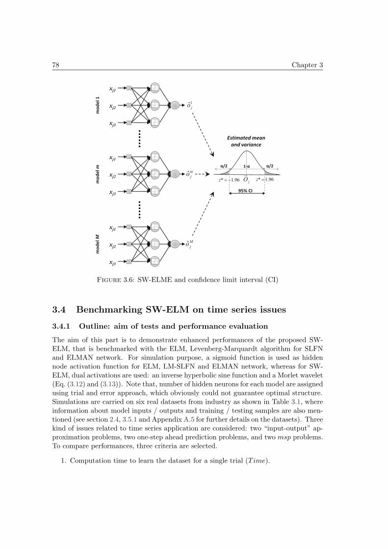
78 Chapter 3
xj1 -5 -4 -3 -2 -1 0 1 2 3 4 5-2.5
-2
-1.5
-1
-0.5
0
0.5
1
1.5
2
2.5Inverse hyperbolic sine
xj3 -5 -4 -3 -2 -1 0 1 2 3 4 5-2.5
-2
-1.5
-1
-0.5
0
0.5
1
1.5
2
2.5Inverse hyperbolic sine
xj2 -5 -4 -3 -2 -1 0 1 2 3 4 5-2.5
-2
-1.5
-1
-0.5
0
0.5
1
1.5
2
2.5
1ˆ jo
xj1 -5 -4 -3 -2 -1 0 1 2 3 4 5-2.5
-2
-1.5
-1
-0.5
0
0.5
1
1.5
2
2.5
xj3 -5 -4 -3 -2 -1 0 1 2 3 4 5-2.5
-2
-1.5
-1
-0.5
0
0.5
1
1.5
2
2.5
xj2 -5 -4 -3 -2 -1 0 1 2 3 4 5-2.5
-2
-1.5
-1
-0.5
0
0.5
1
1.5
2
2.5
ˆmjo
xj1 -5 -4 -3 -2 -1 0 1 2 3 4 5-2.5
-2
-1.5
-1
-0.5
0
0.5
1
1.5
2
2.5
xj3 -5 -4 -3 -2 -1 0 1 2 3 4 5-2.5
-2
-1.5
-1
-0.5
0
0.5
1
1.5
2
2.5
xj2 -5 -4 -3 -2 -1 0 1 2 3 4 5-2.5
-2
-1.5
-1
-0.5
0
0.5
1
1.5
2
2.5
ˆMjo
mo
de
l 1
m
od
el
m
mo
de
l M
95% CI
Estimated mean
and variance
1-α α/2 α/2
jO * 1.96z =* 1.96z = -
Figure 3.6: SW-ELME and confidence limit interval (CI)
3.4 Benchmarking SW-ELM on time series issues
3.4.1 Outline: aim of tests and performance evaluation
The aim of this part is to demonstrate enhanced performances of the proposed SW-ELM, that is benchmarked with the ELM, Levenberg-Marquardt algorithm for SLFNand ELMAN network. For simulation purpose, a sigmoid function is used as hiddennode activation function for ELM, LM-SLFN and ELMAN network, whereas for SW-ELM, dual activations are used: an inverse hyperbolic sine function and a Morlet wavelet(Eq. (3.12) and (3.13)). Note that, number of hidden neurons for each model are assignedusing trial and error approach, which obviously could not guarantee optimal structure.Simulations are carried on six real datasets from industry as shown in Table 3.1, whereinformation about model inputs / outputs and training / testing samples are also men-tioned (see section 2.4, 3.5.1 and Appendix A.5 for further details on the datasets). Threekind of issues related to time series application are considered: two “input-output” ap-proximation problems, two one-step ahead prediction problems, and two msp problems.To compare performances, three criteria are selected.
1. Computation time to learn the dataset for a single trial (T ime).

3.4 Benchmarking SW-ELM on time series issues 79
2. Model fitting accuracy is evaluated by the coefficient of determination (R2) thatshould be close to 1 and coefficient of variation of the Root Mean Squared Error(CV RMSE) that should be as low as possible (close to 0 - it is often expressedin percentage) (see Appendix A.4).
3. Network complexity is reflected by the number of hidden neurons (Hid− nodes).
With each approach (i.e., ELM, SWELM, LM-SLFN, ELMAN), 50 simulations areperformed on a particular dataset and the best results are summarized.
Table 3.1: Datasets to benchmark performances for time series application
Approximation problemsData Description Input Output Train Test
Pump [170] Condition Root mean square, Fault code 73 (samp.) 19 (samp.)Appendix A.5 monitoring VarianceCNC [222] Condition Max force, Cutting amp. Tool wear C33, C09, C18 C18section 3.5.1 monitoring Amp. Ratio, Avg. force (450 samp.) (165 samp.)
One step-ahead prediction problems
Ind. Dryer [1] Predict Fuel flow, Fan speed Bulb temp. 500 (samp.) 367 (samp.)Appendix A.5 temperature Flow raw material yt+1
Bulb temp. ytHair dryer [2] Predict Voltage of device xt Air temp. 500 (samp.) 500 (samp.)Appendix A.5 temperature Air temp. yt yt+1
Multi-step ahead prediction problems
NN3 [6] Time series Time series (4 reg.) Same series 51, 54, 56, 58, All seriesAppendix A.5 forecast (xt, xt−1, xt−2, xt−3) xt+1→t+18 60, 61, 92, 106 (18 samp.)Turbofan [175] Predict Degradation series Same series 90 engines 5 enginessection 2.6.1.1 degradation 3 reg. (xt, xt−1, xt−2) xt+1→t+H H ∈ [103, 283]
3.4.2 First issue: approximation problems
In case of approximation or estimation problems, real datasets from two different de-grading machineries are used for condition monitoring task. The first dataset is from aCarnallite surge tank pump, which is used to approximate fault codes, where the seconddataset is from a CNC milling machine to estimate wear of degrading cutting tools (Ta-ble 3.1). Results in Table 3.2 show that SW-ELM for both test datasets performs bestapproximations, with a compact structure, and it requires less learning time.
1. ELM has clear superiority of fast learning times (5.8e−004 and 5.0e−004 sec) for bothdatasets. In addition, SW-ELM and ELM can learn much rapidly as compared toLM-SLFN or ELMAN network. This is mainly due to the advantages of single-steplearning phase of ELM based models, whereas LM-SLFN and ELMAN networkrequired additional 50 epochs for the Pump dataset and 10 epochs for CNCdataset to achieve better accuracy performances.
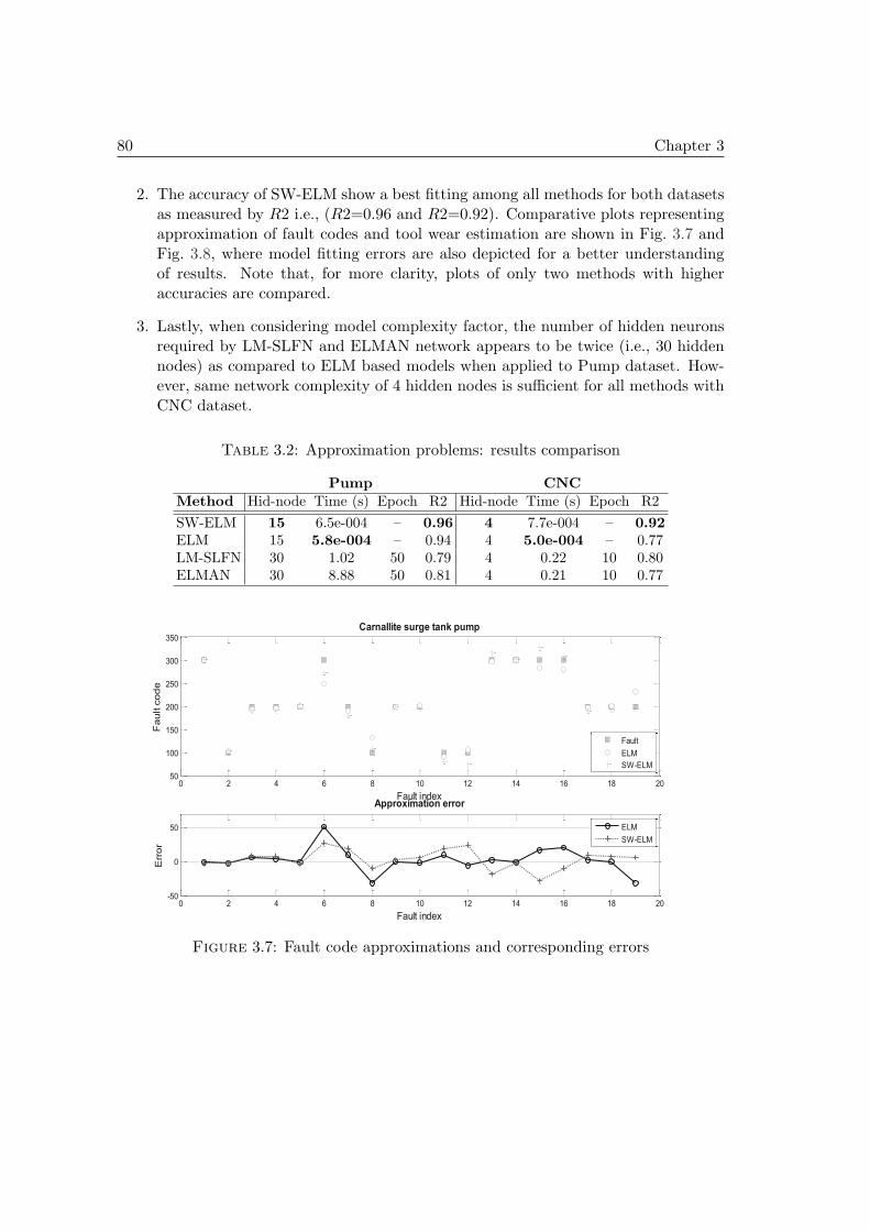
80 Chapter 3
2. The accuracy of SW-ELM show a best fitting among all methods for both datasetsas measured by R2 i.e., (R2=0.96 and R2=0.92). Comparative plots representingapproximation of fault codes and tool wear estimation are shown in Fig. 3.7 andFig. 3.8, where model fitting errors are also depicted for a better understandingof results. Note that, for more clarity, plots of only two methods with higheraccuracies are compared.
3. Lastly, when considering model complexity factor, the number of hidden neuronsrequired by LM-SLFN and ELMAN network appears to be twice (i.e., 30 hiddennodes) as compared to ELM based models when applied to Pump dataset. How-ever, same network complexity of 4 hidden nodes is sufficient for all methods withCNC dataset.
Table 3.2: Approximation problems: results comparison
Pump CNCMethod Hid-node Time (s) Epoch R2 Hid-node Time (s) Epoch R2
SW-ELM 15 6.5e-004 – 0.96 4 7.7e-004 – 0.92ELM 15 5.8e-004 – 0.94 4 5.0e-004 – 0.77LM-SLFN 30 1.02 50 0.79 4 0.22 10 0.80ELMAN 30 8.88 50 0.81 4 0.21 10 0.77
0 2 4 6 8 10 12 14 16 18 2050
100
150
200
250
300
350
Fault index
Fa
ult c
od
e
Carnallite surge tank pump
0 2 4 6 8 10 12 14 16 18 20-50
0
50
Fault index
Err
or
Approximation error
ELM
SW-ELM
Fault
ELM
SW-ELM
Figure 3.7: Fault code approximations and corresponding errors
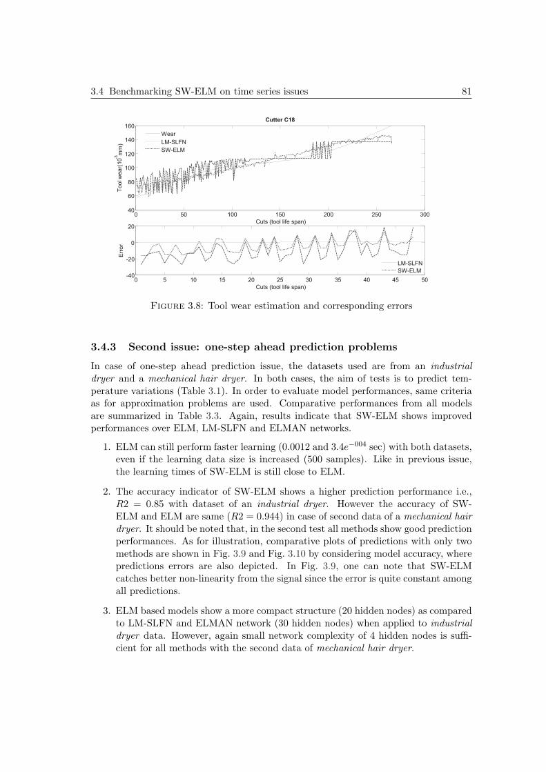
3.4 Benchmarking SW-ELM on time series issues 81
0 5 10 15 20 25 30 35 40 45 50 -40
-20
0
20
Cuts (tool life span)
Err
or
0 50 100 150 200 250 300 40
60
80
100
120
140
160
Cuts (tool life span)
Tool w
ear(
10 -3
mm
) Cutter C18
Wear
LM-SLFN
SW-ELM
LM-SLFN
SW-ELM
Figure 3.8: Tool wear estimation and corresponding errors
3.4.3 Second issue: one-step ahead prediction problems
In case of one-step ahead prediction issue, the datasets used are from an industrialdryer and a mechanical hair dryer. In both cases, the aim of tests is to predict tem-perature variations (Table 3.1). In order to evaluate model performances, same criteriaas for approximation problems are used. Comparative performances from all modelsare summarized in Table 3.3. Again, results indicate that SW-ELM shows improvedperformances over ELM, LM-SLFN and ELMAN networks.
1. ELM can still perform faster learning (0.0012 and 3.4e−004 sec) with both datasets,even if the learning data size is increased (500 samples). Like in previous issue,the learning times of SW-ELM is still close to ELM.
2. The accuracy indicator of SW-ELM shows a higher prediction performance i.e.,R2 = 0.85 with dataset of an industrial dryer. However the accuracy of SW-ELM and ELM are same (R2 = 0.944) in case of second data of a mechanical hairdryer. It should be noted that, in the second test all methods show good predictionperformances. As for illustration, comparative plots of predictions with only twomethods are shown in Fig. 3.9 and Fig. 3.10 by considering model accuracy, wherepredictions errors are also depicted. In Fig. 3.9, one can note that SW-ELMcatches better non-linearity from the signal since the error is quite constant amongall predictions.
3. ELM based models show a more compact structure (20 hidden nodes) as comparedto LM-SLFN and ELMAN network (30 hidden nodes) when applied to industrialdryer data. However, again small network complexity of 4 hidden nodes is suffi-cient for all methods with the second data of mechanical hair dryer.
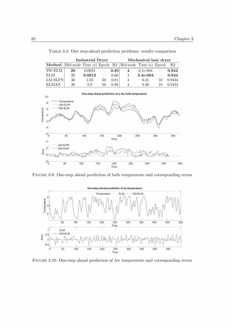
82 Chapter 3
Table 3.3: One step-ahead prediction problems: results comparison
Industrial Dryer Mechanical hair dryerMethod Hid-node Time (s) Epoch R2 Hid-node Time (s) Epoch R2
SW-ELM 20 0.0024 – 0.85 4 6.1e-004 – 0.944ELM 20 0.0012 – 0.66 4 3.4e-004 – 0.944LM-SLFN 30 1.03 50 0.81 4 0.21 10 0.9434ELMAN 30 8.9 50 0.80 4 0.20 10 0.9434
0 50 100 150 200 250 300 350 -2
0
2
4
6
8
10
Time
Tem
pera
ture
One-step ahead prediction of a dry bulb temperature
Temperature
LM-SLFN
SW-ELM
0 50 100 150 200 250 300 350 400 -2
0
2
4
Time
Err
or
LM-SLFN
SW-ELM
Figure 3.9: One-step ahead prediction of bulb temperature and corresponding errors
50 100 150 200 250 300 350 400 450 500
4
5
6
Time
Te
mp
era
ture
One-step ahead prediction of air temperature
0 50 100 150 200 250 300 350 400 450
-0.5
0
0.5
1
Time
Err
or
Temperature ELM SW-ELM
ELM
SW-ELM
Figure 3.10: One-step ahead prediction of Air temperature and corresponding errors

3.4 Benchmarking SW-ELM on time series issues 83
3.4.4 Third issue: multi-steps ahead prediction (msp) problems
In case of msp problems, again two data sets are used to test models performancesusing iterative approach (section 2.6.2.1). The first test data, are from NN3 competition,where horizon of prediction is defined as last 18 values of each time series for test. Thesecond dataset are from NASA data repository, and is composed of run to failure sensormeasurements from degrading Turbofan engines, where the horizon of prediction is froma current time tc up to end of degradation (see Table 3.1 data record train−FD001.txtis used to train and test the models). Similarly, like in previous issues, 50 trials areperformed and best results are presented. Themsp accuracy of each model is assessed bycomputing CV RMSE, that enables evaluating relative closeness of predictions, whichshould be as low as possible. Whereas, computational time (for a single trial) andnetwork complexity are evaluated similarly as in previous cases. Models performancesare summarized in Table 3.4.A comparative plot is shown in Fig. 3.11 with two models having higher accuracies ofmsp with NN3 competition data for time series 61. Averaged performances of predictionmodels for all randomly selected time series (51, 54, 56, 58, 60, 61, 92, 106) are given inTable 3.4.In case of Turbofan engines dataset, the comparative plot of two models on test-engine5 is shown in Fig. 3.12, where SW-ELM explicitly shows good prediction capabilityover long horizon. Averaged performances of prediction models for all tests are given inTable 3.4.
1. Among all methods, ELM requires less computation time for learning with bothdatasets (i.e., 5.5e−004 and 0.004 sec), where SW-ELM also shows rapid learningbehavior closer to ELM. As explained before, this is mainly due to the one-passlearning phase.
2. Most importantly, accuracy indicator (CV RMSE) of SW-ELM is highest in com-parison to others models for both datasets (i.e., NN3 competition and Turbofanengines). A synthetic but explicit view of that is given in Fig. 3.13. Note that suchperformances of SW-ELM are obtained with a same structure like other methods(see point 3).
3. The network complexity of all models is same with both datasets (i.e., 30 hiddennodes and 3 hidden nodes). Note that for all test on 5 Turbofan engines even withmore complex models of ELM, LM-SLFN and ELMAN network poor predictionperformances where obtained, therefore the only complexity of 3 hidden nodes iscompatible with the data.
Finally, again SW-ELM enables a good compromise among model accuracy, learningtime and network complexity.
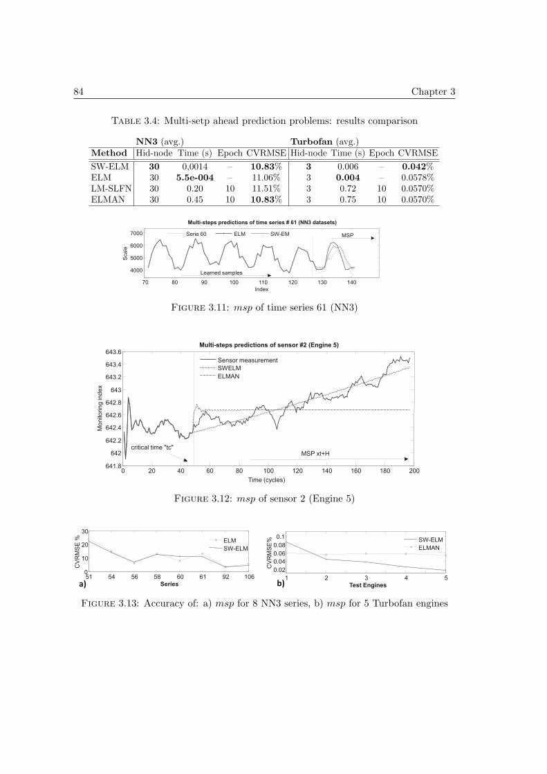
84 Chapter 3
Table 3.4: Multi-setp ahead prediction problems: results comparison
NN3 (avg.) Turbofan (avg.)Method Hid-node Time (s) Epoch CVRMSE Hid-node Time (s) Epoch CVRMSE
SW-ELM 30 0,0014 – 10.83% 3 0.006 – 0.042%ELM 30 5.5e-004 – 11.06% 3 0.004 – 0.0578%LM-SLFN 30 0.20 10 11.51% 3 0.72 10 0.0570%ELMAN 30 0.45 10 10.83% 3 0.75 10 0.0570%
70 80 90 100 110 120 130 140
4000
5000
6000
7000
Index
Sca
le
Multi-steps predictions of time series # 61 (NN3 datasets)
Serie 60 ELM SW-EM MSP
Learned samples
Figure 3.11: msp of time series 61 (NN3)
Current time tc msp (test phase)
Time (cycles)
0 20 40 60 80 100 120 140 160 180 200 641.8
642
642.2
642.4
642.6
642.8
643
643.2
643.4
643.6
Mo
nito
rin
g ind
ex
Multi-steps predictions of sensor #2 (Engine 5)
Sensor measurement
SWELM
ELMAN
MSP xt+H critical time "tc"
Figure 3.12: msp of sensor 2 (Engine 5)
a) b) 51 54 56 58 60 61 92 106 0
10
20
30
Series
CV
RM
SE
%
ELM
SW-ELM
1 2 3 4 5
0.02
0.04
0.06
0.08
0.1
Test Engines
CV
RM
SE
%
SW-ELM
ELMAN
Figure 3.13: Accuracy of: a) msp for 8 NN3 series, b) msp for 5 Turbofan engines
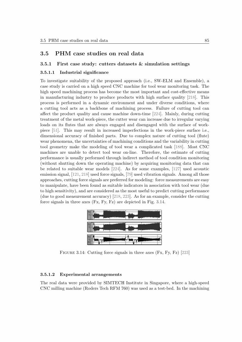
3.5 PHM case studies on real data 85
3.5 PHM case studies on real data
3.5.1 First case study: cutters datasets & simulation settings
3.5.1.1 Industrial significance
To investigate suitability of the proposed approach (i.e., SW-ELM and Ensemble), acase study is carried on a high speed CNC machine for tool wear monitoring task. Thehigh speed machining process has become the most important and cost-effective meansin manufacturing industry to produce products with high surface quality [218]. Thisprocess is performed in a dynamic environment and under diverse conditions, wherea cutting tool acts as a backbone of machining process. Failure of cutting tool canaffect the product quality and cause machine down-time [224]. Mainly, during cuttingtreatment of the metal work-piece, the cutter wear can increase due to irregular varyingloads on its flutes that are always engaged and disengaged with the surface of work-piece [51]. This may result in increased imperfections in the work-piece surface i.e.,dimensional accuracy of finished parts. Due to complex nature of cutting tool (flute)wear phenomena, the uncertainties of machining conditions and the variability in cuttingtool geometry make the modeling of tool wear a complicated task [188]. Most CNCmachines are unable to detect tool wear on-line. Therefore, the estimate of cuttingperformance is usually performed through indirect method of tool condition monitoring(without shutting down the operating machine) by acquiring monitoring data that canbe related to suitable wear models [224]. As for some examples, [127] used acousticemission signal, [121, 218] used force signals, [79] used vibration signals. Among all thoseapproaches, cutting force signals are preferred for modeling: force measurements are easyto manipulate, have been found as suitable indicators in association with tool wear (dueto high sensitivity), and are considered as the most useful to predict cutting performance(due to good measurement accuracy) [218, 223]. As for an example, consider the cuttingforce signals in three axes (Fx, Fy, Fz) are depicted in Fig. 3.14.
Figure 3.14: Cutting force signals in three axes (Fx, Fy, Fz) [223]
3.5.1.2 Experimental arrangements
The real data were provided by SIMTECH Institute in Singapore, where a high-speedCNC milling machine (Roders Tech RFM 760) was used as a test-bed. In the machining
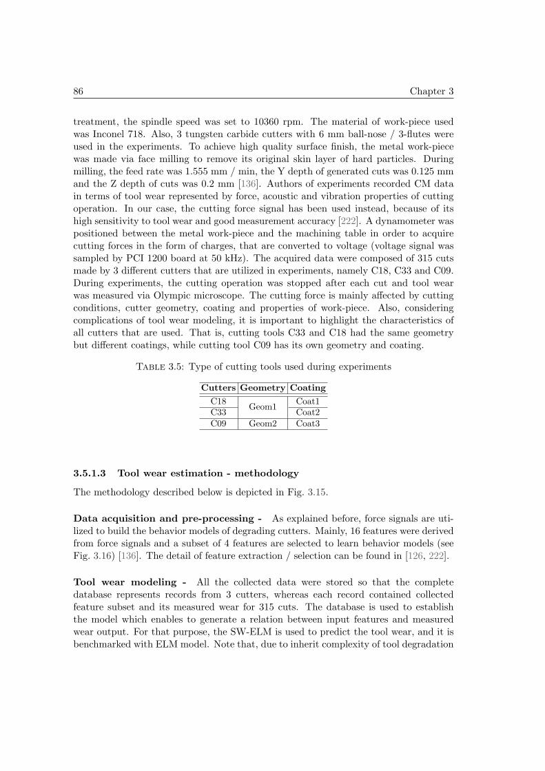
86 Chapter 3
treatment, the spindle speed was set to 10360 rpm. The material of work-piece usedwas Inconel 718. Also, 3 tungsten carbide cutters with 6 mm ball-nose / 3-flutes wereused in the experiments. To achieve high quality surface finish, the metal work-piecewas made via face milling to remove its original skin layer of hard particles. Duringmilling, the feed rate was 1.555 mm / min, the Y depth of generated cuts was 0.125 mmand the Z depth of cuts was 0.2 mm [136]. Authors of experiments recorded CM datain terms of tool wear represented by force, acoustic and vibration properties of cuttingoperation. In our case, the cutting force signal has been used instead, because of itshigh sensitivity to tool wear and good measurement accuracy [222]. A dynamometer waspositioned between the metal work-piece and the machining table in order to acquirecutting forces in the form of charges, that are converted to voltage (voltage signal wassampled by PCI 1200 board at 50 kHz). The acquired data were composed of 315 cutsmade by 3 different cutters that are utilized in experiments, namely C18, C33 and C09.During experiments, the cutting operation was stopped after each cut and tool wearwas measured via Olympic microscope. The cutting force is mainly affected by cuttingconditions, cutter geometry, coating and properties of work-piece. Also, consideringcomplications of tool wear modeling, it is important to highlight the characteristics ofall cutters that are used. That is, cutting tools C33 and C18 had the same geometrybut different coatings, while cutting tool C09 has its own geometry and coating.
Table 3.5: Type of cutting tools used during experiments
Cutters Geometry Coating
C18Geom1
Coat1C33 Coat2C09 Geom2 Coat3
3.5.1.3 Tool wear estimation - methodology
The methodology described below is depicted in Fig. 3.15.
Data acquisition and pre-processing - As explained before, force signals are uti-lized to build the behavior models of degrading cutters. Mainly, 16 features were derivedfrom force signals and a subset of 4 features are selected to learn behavior models (seeFig. 3.16) [136]. The detail of feature extraction / selection can be found in [126, 222].
Tool wear modeling - All the collected data were stored so that the completedatabase represents records from 3 cutters, whereas each record contained collectedfeature subset and its measured wear for 315 cuts. The database is used to establishthe model which enables to generate a relation between input features and measuredwear output. For that purpose, the SW-ELM is used to predict the tool wear, and it isbenchmarked with ELM model. Note that, due to inherit complexity of tool degradation
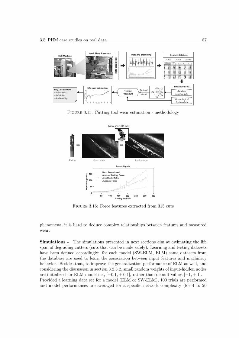
3.5 PHM case studies on real data 87
Perf. Assessment
- Robustness
- Reliability
- Applicability
CNC Machine
Da
ta a
cqu
isit
ion
Work Piece & sensors Data pre-processing
0 50 100 150 200 250 300 3500
10
20
30
40
50
60
70
80
90
Cuts
Mon
itorin
g ind
ex
Force features
Cut. #33
Feature database
Cut. #18 Cut. #09
Testing
Procedure
Trained
Model
Chronological
Testing data
Random
training data
Simulation Sets Life span estimation
160 180 200 220 240 260 280 300 3200
20
40
60
80
100
120
140
160
Cuts (tool life)
To
ol
wear
(10
- 3m
m)
Figure 3.15: Cutting tool wear estimation - methodology
50 100 150 200 250 300 350
0
50
100
150
Cutting tool life
Mo
nit
ori
ng
In
dex
Force Signals
Max. Force Level
Amp. of Cutiing Force
Amplitude Ratio
Average Force
Good state Faulty state
(view after 315 cuts)
Cutter
Figure 3.16: Force features extracted from 315 cuts
phenomena, it is hard to deduce complex relationships between features and measuredwear.
Simulations - The simulations presented in next sections aim at estimating the lifespan of degrading cutters (cuts that can be made safely). Learning and testing datasetshave been defined accordingly: for each model (SW-ELM, ELM) same datasets fromthe database are used to learn the association between input features and machinerybehavior. Besides that, to improve the generalization performance of ELM as well, andconsidering the discussion in section 3.2.3.2, small random weights of input-hidden nodesare initialized for ELM model i.e., [−0.1,+ 0.1], rather than default values [−1,+ 1].Provided a learning data set for a model (ELM or SW-ELM), 100 trials are performedand model performances are averaged for a specific network complexity (for 4 to 20

88 Chapter 3
hidden nodes). It should be noted that model performance for a single trial is equal toan accumulated performance from 10 different simulations: for which data subsets (ofcutting tools) are learned after random permutation (to introduce variation in data),while test are performed on remaining data in chronological order (see Fig. 3.15). Forclarity, detailed results are furnished with different model complexity (hidden neuron),data variability / model steadiness and related tool wear estimation.
Performance criteria - To discuss the robustness, reliability, and applicability of themodels (and according to the analysis scheme proposed in Fig. 1.15), performances ofthe models are assessed in terms of accuracy and network complexity. More precisely,3 criteria are computed: the Mean Average Percent Error of prediction (MAPE) thatshould be as low as possible, the coefficient of determination (R2) that should be closerto 1 (see Appendix A.4), and the learning time (T ime). The obtained results are dividedinto two different cases for better understanding (section 3.5.1.4 and 3.5.1.5).
3.5.1.4 Results discussion: robustness and applicability
This case aims at evaluating the prediction accuracy of each model by assessing itsrobust performance with a single cutting tool (with data of same attributes) to establisha model i.e., C18, C33 and C09. For learning, data set from a particular cutting toolis created by randomly selecting 150 data samples, while rest of the data (165 datasamples) are presented in chronological order to test the accuracy of the learned model(Fig. 3.17). This procedure is repeated 10 times for each model-cutting tool couple andis considered as a “single trial”. Comparative analysis on robust tool wear predictionperformances from all model-cutting tool couples are shown in Table 3.6. Among allmodel-cutting tool couples with varying learning data, SW-ELM model has more robustperformance on tests as compared to ELM, even when small learning data are presentedto both models. However, the average learning time of ELM is slightly faster than SW-ELM. The detailed simulations from the obtained results are presented in Fig. 3.18. Inbrief, Fig. 3.18a, shows an average accuracy (R2) performance for 5 different networkcomplexities, where best results are achieved by SW-ELM for tests on cutter C09 andC18 (with no. hidden nodes 16 and 12). Considering these results, Fig. 3.18b comparesthe steadiness of both models (SW-ELM and ELM) for 100 trials. One can see thatSW-ELM is more robust to input variations as its test accuracy (R2) is steady for 100trials with tests on both cutters i.e., C09 and C18. In addition, Fig. 3.18c depicts acomparison on average results of tool wear estimation on cutter C09.
Figure 3.17: Robustness: learning and testing with one cutter
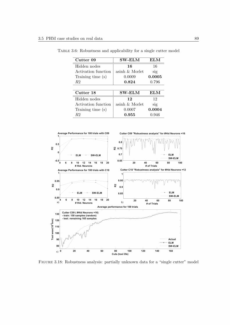
3.5 PHM case studies on real data 89
Table 3.6: Robustness and applicability for a single cutter model
Cutter 09 SW-ELM ELM
Hidden nodes 16 16Activation function asinh & Morlet sigTraining time (s) 0.0009 0.0005R2 0.824 0.796
Cutter 18 SW-ELM ELM
Hidden nodes 12 12Activation function asinh & Morlet sigTraining time (s) 0.0007 0.0004R2 0.955 0.946
20 40 60 80 100 0.65
0.7
0.75
0.8
# of Trials
R2
Cutter C09 "Robustness analysis" for #Hid Neurons =16
20 40 60 80 100
0.85
0.9
0.95
1
# of Trials
R2
Cutter C18 "Robustness analysis" for #Hid Neurons =12
4 6 8 10 12 14 16 18 20 -0.5
0
0.5
1
# Hid. Neurons
R2
Average Performance for 100 trials with C09
4 6 8 10 12 14 16 18 20 0.85
0.9
0.95
1
# Hid. Neurons
R2
Average Performance for 100 trials with C18
0 20 40 60 80 100 120 140 160
80
90
100
110
120
130
Cuts (tool life)
To
ol w
ear(
10
-3 m
m)
Average performance for 100 trials
ELM SW-ELM
ELM SW-ELM
ELM
SW-ELM
Actual
ELM
SW-ELM
ELM
SW-ELM
a) b)
Cutter C09 ( #Hid Neurons =16)
- train: 150 samples (random)
- test: remaining 165 samples
c)
Figure 3.18: Robustness analysis: partially unknown data for a “single cutter” model
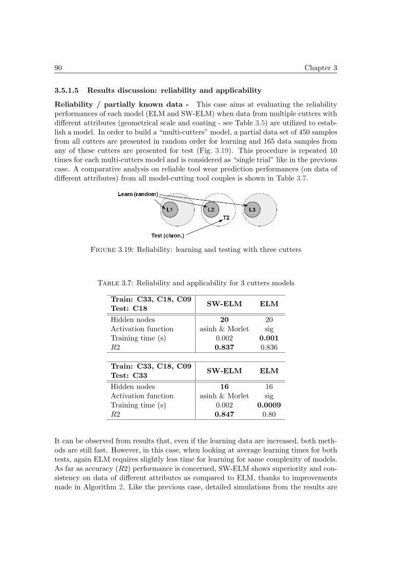
90 Chapter 3
3.5.1.5 Results discussion: reliability and applicability
Reliability / partially known data - This case aims at evaluating the reliabilityperformances of each model (ELM and SW-ELM) when data from multiple cutters withdifferent attributes (geometrical scale and coating - see Table 3.5) are utilized to estab-lish a model. In order to build a “multi-cutters” model, a partial data set of 450 samplesfrom all cutters are presented in random order for learning and 165 data samples fromany of these cutters are presented for test (Fig. 3.19). This procedure is repeated 10times for each multi-cutters model and is considered as “single trial” like in the previouscase. A comparative analysis on reliable tool wear prediction performances (on data ofdifferent attributes) from all model-cutting tool couples is shown in Table 3.7.
Figure 3.19: Reliability: learning and testing with three cutters
Table 3.7: Reliability and applicability for 3 cutters models
Train: C33, C18, C09SW-ELM ELM
Test: C18
Hidden nodes 20 20Activation function asinh & Morlet sigTraining time (s) 0.002 0.001R2 0.837 0.836
Train: C33, C18, C09SW-ELM ELM
Test: C33
Hidden nodes 16 16Activation function asinh & Morlet sigTraining time (s) 0.002 0.0009R2 0.847 0.80
It can be observed from results that, even if the learning data are increased, both meth-ods are still fast. However, in this case, when looking at average learning times for bothtests, again ELM requires slightly less time for learning for same complexity of models.As far as accuracy (R2) performance is concerned, SW-ELM shows superiority and con-sistency on data of different attributes as compared to ELM, thanks to improvementsmade in Algorithm 2. Like the previous case, detailed simulations from the results are
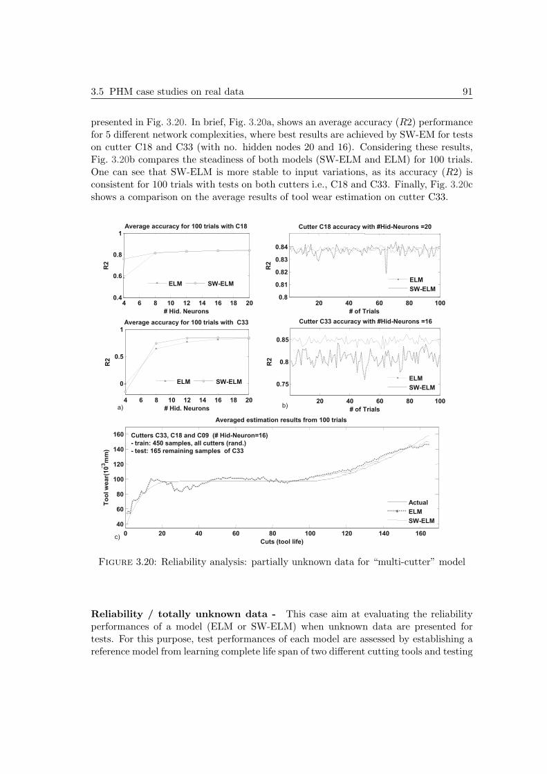
3.5 PHM case studies on real data 91
presented in Fig. 3.20. In brief, Fig. 3.20a, shows an average accuracy (R2) performancefor 5 different network complexities, where best results are achieved by SW-EM for testson cutter C18 and C33 (with no. hidden nodes 20 and 16). Considering these results,Fig. 3.20b compares the steadiness of both models (SW-ELM and ELM) for 100 trials.One can see that SW-ELM is more stable to input variations, as its accuracy (R2) isconsistent for 100 trials with tests on both cutters i.e., C18 and C33. Finally, Fig. 3.20cshows a comparison on the average results of tool wear estimation on cutter C33.
-
4 6 8 10 12 14 16 18 20
0
0.5
1
# Hid. Neurons
R2
Average accuracy for 100 trials with C33
4 6 8 10 12 14 16 18 20 0.4
0.6
0.8
1
# Hid. Neurons
R2
Average accuracy for 100 trials with C18
0 20 40 60 80 100 120 140 160
40
60
80
100
120
140
160
Cuts (tool life)
To
ol w
ear(
10
3 m
m)
Averaged estimation results from 100 trials
20 40 60 80 100 0.8
0.81
0.82
0.83
0.84
# of Trials
R2
Cutter C18 accuracy with #Hid-Neurons =20
20 40 60 80 100
0.75
0.8
0.85
# of Trials
R2
Cutter C33 accuracy with #Hid-Neurons =16
ELM SW-ELM
ELM SW-ELM
ELM
SW-ELM
ELM
SW-ELM
Actual
ELM
SW-ELM
a) b)
c)
Cutters C33, C18 and C09 (# Hid-Neuron=16)
- train: 450 samples, all cutters (rand.)
- test: 165 remaining samples of C33
Figure 3.20: Reliability analysis: partially unknown data for “multi-cutter” model
Reliability / totally unknown data - This case aim at evaluating the reliabilityperformances of a model (ELM or SW-ELM) when unknown data are presented fortests. For this purpose, test performances of each model are assessed by establishing areference model from learning complete life span of two different cutting tools and testing
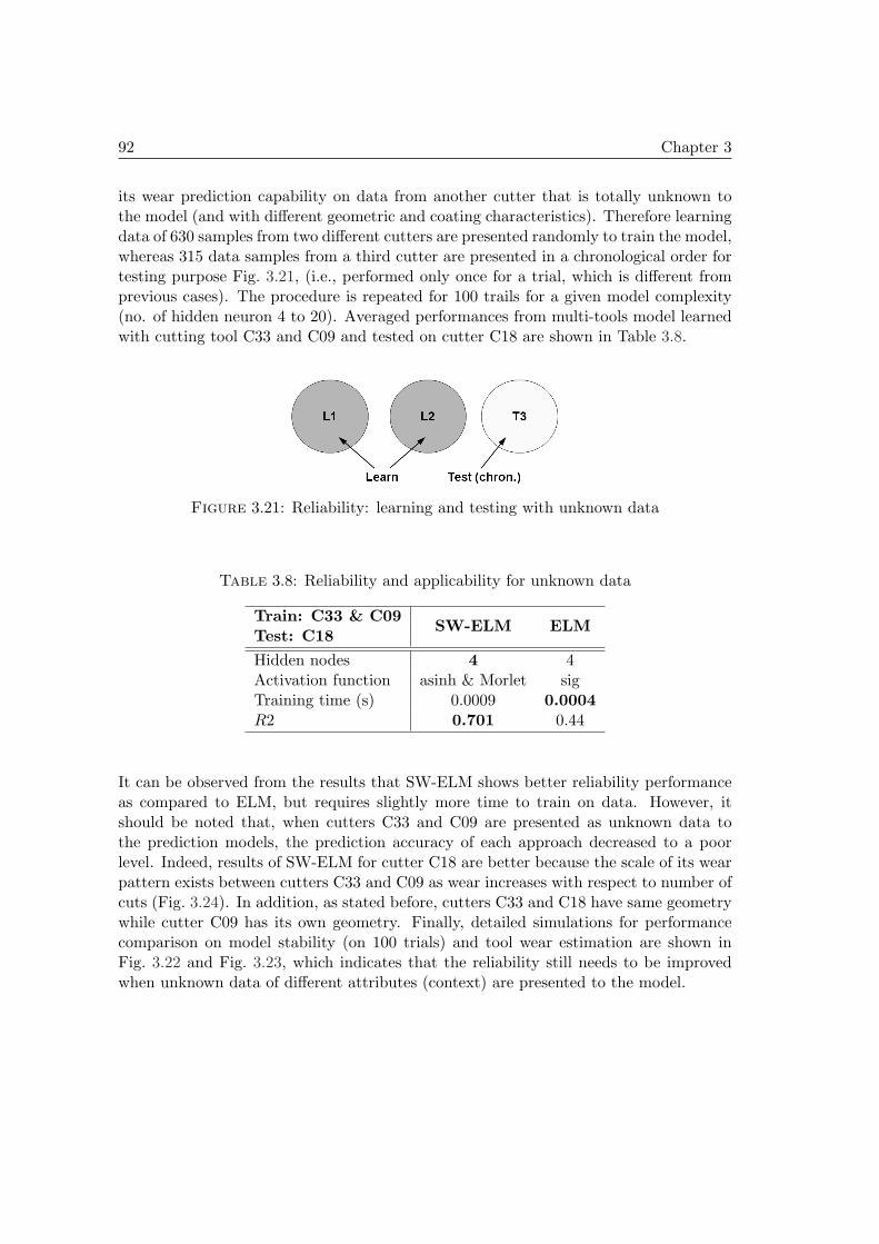
92 Chapter 3
its wear prediction capability on data from another cutter that is totally unknown tothe model (and with different geometric and coating characteristics). Therefore learningdata of 630 samples from two different cutters are presented randomly to train the model,whereas 315 data samples from a third cutter are presented in a chronological order fortesting purpose Fig. 3.21, (i.e., performed only once for a trial, which is different fromprevious cases). The procedure is repeated for 100 trails for a given model complexity(no. of hidden neuron 4 to 20). Averaged performances from multi-tools model learnedwith cutting tool C33 and C09 and tested on cutter C18 are shown in Table 3.8.
Figure 3.21: Reliability: learning and testing with unknown data
Table 3.8: Reliability and applicability for unknown data
Train: C33 & C09SW-ELM ELM
Test: C18
Hidden nodes 4 4Activation function asinh & Morlet sigTraining time (s) 0.0009 0.0004R2 0.701 0.44
It can be observed from the results that SW-ELM shows better reliability performanceas compared to ELM, but requires slightly more time to train on data. However, itshould be noted that, when cutters C33 and C09 are presented as unknown data tothe prediction models, the prediction accuracy of each approach decreased to a poorlevel. Indeed, results of SW-ELM for cutter C18 are better because the scale of its wearpattern exists between cutters C33 and C09 as wear increases with respect to number ofcuts (Fig. 3.24). In addition, as stated before, cutters C33 and C18 have same geometrywhile cutter C09 has its own geometry. Finally, detailed simulations for performancecomparison on model stability (on 100 trials) and tool wear estimation are shown inFig. 3.22 and Fig. 3.23, which indicates that the reliability still needs to be improvedwhen unknown data of different attributes (context) are presented to the model.
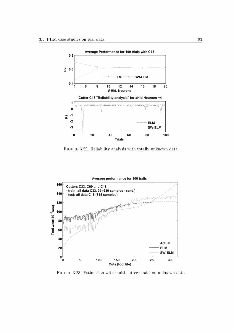
3.5 PHM case studies on real data 93
4 6 8 10 12 14 16 18 20 0.4
0.6
0.8
# Hid. Neurons
R2
Average Performance for 100 trials with C18
0 20 40 60 80 100
-3
-2
-1
0
1
Trials
R2
Cutter C18 "Reliability analysis" for #Hid Neurons =4
ELM SW-ELM
ELM
SW-ELM
Figure 3.22: Reliability analysis with totally unknown data
0 50 100 150 200 250 300 0
20
40
60
80
100
120
140
160
Cuts (tool life)
To
ol w
ear(
10
-3 m
m)
Average performance for 100 trails
Actual
ELM
SW-ELM
Cutters C33, C09 and C18
- train: all data C33, 09 (630 samples - rand.)
- test: all data C18 (315 samples)
Figure 3.23: Estimation with multi-cutter model on unknown data

94 Chapter 3
3.5.1.6 SW-ELME and its reliability performance
Simulation settings - Considering the superiority of SW-ELM over ELM, the en-semble strategy is only performed with SW-ELM approach. In this strategy, the initialstep is to determine structure of a single SW-ELM model. That is, a structure of modelwhich results satisfactory performances with minimum possible complexity. Followingthat, multiple SW-ELM models of same complexity are integrated to produce averagedoutput and to improve accuracy of estimates (Table 3.9). However, to be more expliciton that, each individual model is learned with same dataset, but initialized with differ-ent parameters, i.e., weights and biases.Tests are performed on three different cutters i.e., C18, C33 and C09, where each indi-vidual SW-ELM model is learned with 680 samples and tested on unknown data of 265samples. For example, learning set includes cutter data C18, C33 and C09 (up to 50samples) and testing set is composed of remaining 265 samples from C09 (starting fromcurrent time tc=50 till the last cut 315) that are totally unknown to the model.
Table 3.9: Tool wear estimation with SW-ELME - Settings
SW-ELME Settings
No. of models in ensemble 100Hidden neuron per model 10Actv. functions asinh & MorletCurrent time tc 50
Wear limit - Setting a precise wear limit is vital to any prognostics approach. Anyassumptions should be avoided for practical reasons. Therefore, it should be precisely as-signed for a particular application. For CNC application, tool wear evolution is classifiedin 5 wear states, “initial wear, slight wear, moderate wear, severe wear and worn-out”[68]. As for all cutters tool life span are same, we use a simple partition based clus-tering approach, namely, K-means algorithm to cluster their wear patterns (see [208]for clustering details). The benefit of this step is to identify worn-out state for all cut-ters. Therefore, threshold can be set when tool degrades from severe wear to worn-outstate (see Fig. 3.24 where max wear is common limit for tests i.e., wear limit is set to130 10−3mm). However, the aspect of wear limits or thresholds is addressed in Chapter4 with details.
Results and discussion - Results from all cases i.e., C18, C33 and C09 with SW-ELME model are summarized in Table 3.10. The cutting tool life span or remaining lifeis estimated by setting a common wear limit among all cutters. That is, the number ofcuts that can be successfully made until defined wear limit. Finally, 95% CI intervalsindicating lower and upper confidence bounds of estimates with an SW-ELME modelare furnished for each test case (see Fig. 3.25).
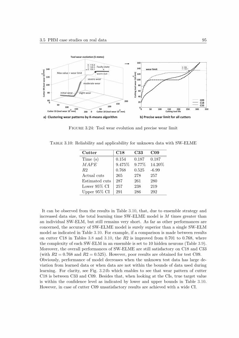
3.5 PHM case studies on real data 95
a) Clustering wear patterns by K-means algorithm b) Precise wear limit for all cutters
0 50
100 150
200 0 50
100
150 200 60
80
100
120
140
Cutter 18 (tool wear 10 -3
mm)
X: 118.8 Y: 126.3 Z: 130.1
Tool wear evolution (5 states)
Cutter 33 (tool wear 10 -3 mm)
Cu
tte
r 0
9 (
too
l w
ea
r 1
0 -3
m
m)
initial wear
moderate wear
severe wear
worn-out
Faulty state
Max value = wear limit
slight wear
0 50 100 150 200 250 300 350 0
20
40
60
80
100
120
140
160
X: 256 Y: 130.1
Cutting tool life
Cu
ttin
g t
oo
l w
ea
r (1
0 -3
m
m)
C09 C18 C33
wear limit
Figure 3.24: Tool wear evolution and precise wear limit
Table 3.10: Reliability and applicability for unknown data with SW-ELME
Cutter C18 C33 C09
Time (s) 0.154 0.187 0.187MAPE 9.475% 9.77% 14.20%R2 0.768 0.525 -6.99Actual cuts 265 278 257Estimated cuts 287 261 280Lower 95% CI 257 238 219Upper 95% CI 291 286 292
It can be observed from the results in Table 3.10, that, due to ensemble strategy andincreased data size, the total learning time SW-ELME model is M times greater thanan individual SW-ELM, but still remains very short. As far as other performances areconcerned, the accuracy of SW-ELME model is surely superior than a single SW-ELMmodel as indicated in Table 3.10. For example, if a comparison is made between resultson cutter C18 in Tables 3.8 and 3.10, the R2 is improved from 0.701 to 0.768, wherethe complexity of each SW-ELM in an ensemble is set to 10 hidden neurons (Table 3.9).Moreover, the overall performances of SW-ELME are still satisfactory on C18 and C33(with R2 = 0.768 and R2 = 0.525). However, poor results are obtained for test C09.Obviously, performance of model decreases when the unknown test data has large de-viation from learned data or when data are not within the bounds of data used duringlearning. For clarity, see Fig. 3.24b which enables to see that wear pattern of cutterC18 is between C33 and C09. Besides that, when looking at the CIs, true target valueis within the confidence level as indicated by lower and upper bounds in Table 3.10.However, in case of cutter C09 unsatisfactory results are achieved with a wide CI.
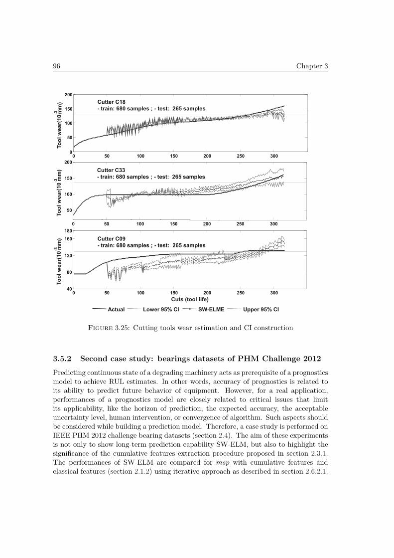
96 Chapter 3
0 50 100 150 200 250 300 0
50
100
150
200
To
ol
we
ar(
10
-3
mm
) Cutter C18
- train: 680 samples ; - test: 265 samples
0 50 100 150 200 250 300
50
100
150
200
To
ol
we
ar(
10 -3
m
m) Cutter C33
- train: 680 samples ; - test: 265 samples
0 50 100 150 200 250 300 40
80
120
160
180
Cuts (tool life)
To
ol
we
ar(
10
-3
mm
) Cutter C09
- train: 680 samples ; - test: 265 samples
Actual Lower 95% CI SW-ELME Upper 95% CI
Figure 3.25: Cutting tools wear estimation and CI construction
3.5.2 Second case study: bearings datasets of PHM Challenge 2012
Predicting continuous state of a degrading machinery acts as prerequisite of a prognosticsmodel to achieve RUL estimates. In other words, accuracy of prognostics is related toits ability to predict future behavior of equipment. However, for a real application,performances of a prognostics model are closely related to critical issues that limitits applicability, like the horizon of prediction, the expected accuracy, the acceptableuncertainty level, human intervention, or convergence of algorithm. Such aspects shouldbe considered while building a prediction model. Therefore, a case study is performed onIEEE PHM 2012 challenge bearing datasets (section 2.4). The aim of these experimentsis not only to show long-term prediction capability SW-ELM, but also to highlight thesignificance of the cumulative features extraction procedure proposed in section 2.3.1.The performances of SW-ELM are compared for msp with cumulative features andclassical features (section 2.1.2) using iterative approach as described in section 2.6.2.1.
3.5 PHM case studies on real data 97
3.5.2.1 Learning and testing schemes
To perform msp, a compact structure SW-ELM with topology 3 inputs, 4 hidden and1 output nodes is used. Note that, 3 inputs represent regressors from a particularfeature (xt, xt−1, xt−2), where output represents msp (xt+1→t+H), H∈ msp horizon. Tominimize the impact of random parameters on learning and testing tasks, small normsof input-hidden weights and bias are initialized by setting C = 0.001 (i.e., for beta valuein NW procedure see Algorithm 2). Learning of SW-ELM model is performed on run-tofailure data sets from bearings Ber1−1 and Ber1−2 under operating conditions 1800 rpmand 4000 N [5, 144]. In test phase, incomplete data sets from 5 bearings under sameoperating conditions (i.e., Ber1−3 to Ber1−7) are used to predict the RUL (see detailsabout data in section 2.4). In other words, predictions are performed from a currenttime (of test data) to the end of the bearings life. Assuming that a single model cannotguarantee accuracy of predictions for all tests, 100 SW-ELM models (with differentparameters) are learned, and the best model with minimum learning error is selected fortesting phase. Note that, the learning of a single model is achieved in a rapid mannerin just 0.0063 sec, due to one-step learning phase (section 3.3.2).
3.5.2.2 Results and discussion
For illustration, predictions results with classical and proposed feature extraction ap-proaches are compared for test bearings Ber1−3 and Ber1−7 in Fig. 3.26. One canqualitatively note the accuracy of predictions with proposed methodology: the figuredepicts very minor difference between the actual and predicted trends, where predic-tions with classical feature show poor results. This conclusion can be extended for alltested bearings (see Table 3.11 for all results): predictions with cumulative features areachieved with high accuracy and generalization even for long prediction horizons likeBer1− 7 (“757 steps”) with MAPE = 0.46%. Such results are of good omen for prog-nostics: since predictions follow trending behavior of features in an accurate manner (asillustrated in Fig. 2.2). The complete approach (cumulative features with SW-ELM)should lead to low uncertainty of RUL estimates.
Table 3.11: Long term prediction results for 5 test bearings
Bearing Predicted steps MAPE (classical) MAPE (proposed)
1− 3 573 2.09 % 1.32 %1− 4 289 32.14 % 1.89 %1− 5 161 0.38 % 0.186 %1− 6 146 0.68 % 0.184 %1− 7 757 16.92 % 0.46 %
MAPE: Mean Absolute Percent Error - [0,∞[, Perfect score = 0
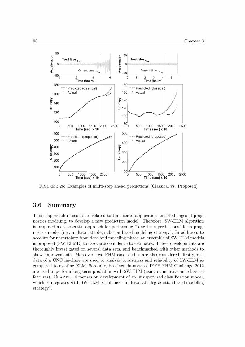
98 Chapter 3
0 500 1000 1500 2000 2500
100
120
140
160
180
Time (sec) x 10
En
tro
py
Predicted (classical)
Actual
0 500 1000 1500 2000 2500 80
100
120
140
160
180
Time (sec) x 10
En
tro
py
Actual
Predicted (classical)
0 500 1000 1500 2000 2500 100
200
300
400
500
Time (sec) x 10
C-E
ntr
op
y
Predicted (proposed)
Actual
0 500 1000 1500 2000
100
200
300
400
500
600
Time (sec) x 10
C-E
ntr
op
y
Predicted (proposed)
Actual
0 1 2 3 4 5
-20
0
20
Time (hours)
Accele
rati
on
Test Ber 1-7
0 2 4 6 -50
0
50
Time (hours)
Accele
rati
on
Test Ber 1-3
Current time Current time
Figure 3.26: Examples of multi-step ahead predictions (Classical vs. Proposed)
3.6 Summary
This chapter addresses issues related to time series application and challenges of prog-nostics modeling, to develop a new prediction model. Therefore, SW-ELM algorithmis proposed as a potential approach for performing “long-term predictions” for a prog-nostics model (i.e., multivariate degradation based modeling strategy). In addition, toaccount for uncertainty from data and modeling phase, an ensemble of SW-ELM modelsis proposed (SW-ELME) to associate confidence to estimates. These, developments arethoroughly investigated on several data sets, and benchmarked with other methods toshow improvements. Moreover, two PHM case studies are also considered: firstly, realdata of a CNC machine are used to analyze robustness and reliability of SW-ELM ascompared to existing ELM. Secondly, bearings datasets of IEEE PHM Challenge 2012are used to perform long-term prediction with SW-ELM (using cumulative and classicalfeatures). Chapter 4 focuses on development of an unsupervised classification model,which is integrated with SW-ELM to enhance “multivariate degradation based modelingstrategy”.
Chapter 4From predictions to RUL estimates
This chapter presents an enhanced multivariate degradation based modelingstrategy for data-driven prognostics. To estimate the RUL of a machinery,prognostics modeling phase requires precise knowledge about failure thresh-olds (FTs). However, prognostics can have large uncertainty, when there isabsence of prior knowledge about actual states of degrading machinery (i.e.,unlabeled data).To address this issue, and also to further improve prognostics performances(i.e., robustness, reliability, applicability), firstly, a new clustering algorithmis proposed to handle unlabeled data and to represent the uncertainty of degra-dation process namely, Subtractive-Maximum Entropy Fuzzy Clustering (S-MEFC). Following that, a novel approach for prognostics is presented to en-hance “multivariate degradation based modeling strategy” to avoid uncertainFTs. In brief, the proposed prognostics model integrates two new algorithms,namely, the SW-ELM (introduced in Chapter 3) and the S-MEFC, in or-der to predict the behavior of degrading machinery, to dynamically assign theFTs, and to automatically determine different states of degradation. Indeed,for practical reasons there is no interest in assuming FT for RUL estimation.The effectiveness of the approach is evaluated by applying it to real datasetof turbofan engines from PHM challenge 2008.
4.1 Problem addressed: dynamic threshold assignment
4.1.1 Failure threshold: univariate approach and limits
Forecasting future of complex machinery is a complicated task, which is encountered inmany PHM applications for industry [166]. Mainly, for PHM applications, prognostics
100 Chapter 4
models are applied to perform “long-term predictions” of continuous observations fol-lowed by a failure thresholds (FT) to detect faulty state, and to estimate the RUL of thedegrading machinery. The FT does not necessarily indicate complete failure of the ma-chinery, but beyond which risk of functionality loss [171]. As discussed in section 1.1.2,in a classical manner the RUL estimate is based on the study of one-dimensional sig-nal: RUL is computed between a current time to initiate prediction and the time atwhich degrading signal passes the FT or a limit on damage level. The assessment ofsystem’s health requires the threshold to be tuned precisely which can be a practicallimitation especially in situations when the signal does not represent any physical mean-ing [166]. Therefore, uncertainty of RUL estimates is not only due to prediction, butto FTs as well. The uncertainty of FT can lead to large RUL errors. According to[166], to ensure reliability of RUL estimates, the use of multidimensional degradationsignals is preferred rather than one-dimension signal. Practically, this restricts the use ofclassical thresholding techniques, where specification of FT is a critical issue and thereis lack of standard approaches for this purpose [116, 155]. In other words, the use ofmultidimensional degrading signals makes thresholding techniques more complicated.
4.1.2 Failure threshold: multivariate approach and limits
With multivariate degradation based modeling strategy for RUL estimates, machinedegradation can be represented by continuous and discrete states (section 1.3.3.3), wherecontinuous state shows value of degrading signal, while discrete states depict fault mode.Therefore, to perform prognostics with multivariate degradation based modeling, it isrequired to build an efficient tool to predict continuous states of signals (that repre-sent features) and a classifier to estimate discrete states reflecting the probable statesof degradation. Most importantly with this approach, it is not only the question ofperforming good predictions, but also to stop prediction process at right time, which isthe task of a classifier that sets FTs. Describing the problem of prognostics by meansof continuous states and discrete states, is new in PHM community and it’s only ad-dressed in few publications [108, 164, 166]. The use of discrete states not only avoidsclassical way of assuming thresholds, but can also benefit in reducing uncertainty ofRUL estimates. However, works presented in [108, 164, 166] have a common drawbackthat the number of discrete states are pre-assumed for continuous observations and theRUL estimates are achieved accordingly. This assumptions is not realistic in case ofdegrading machinery, because, the behavior of each machine can differ according to op-erational environment. Even if two identical machines are exposed to similar operatingconditions, most probably, their degrading behavior would be different, and each couldrepresent different level of degradation. In such situations, it can be quite challenging oreven impossible for previous approaches (that pre-assume fault modes or discrete states)to assign FTs, which limits their applicability.
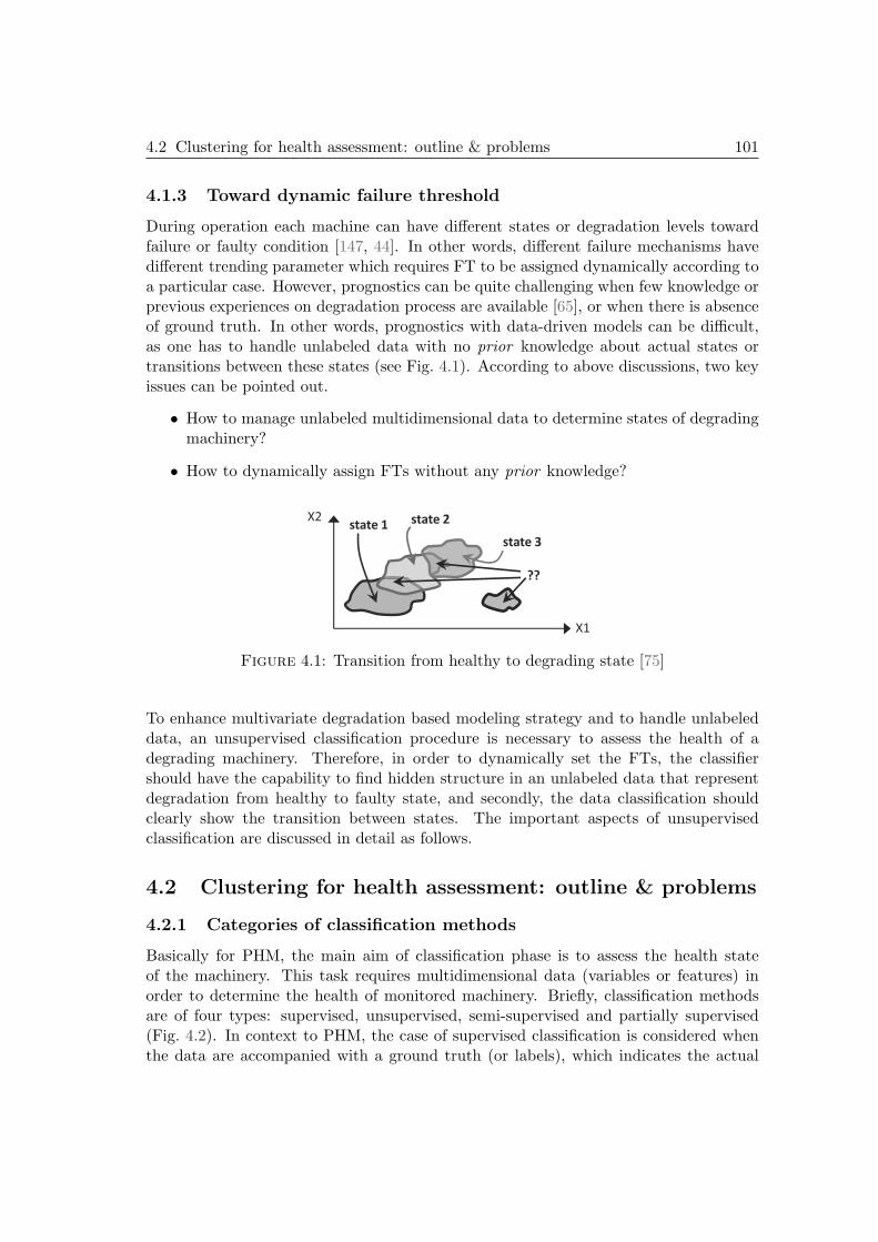
4.2 Clustering for health assessment: outline & problems 101
4.1.3 Toward dynamic failure threshold
During operation each machine can have different states or degradation levels towardfailure or faulty condition [147, 44]. In other words, different failure mechanisms havedifferent trending parameter which requires FT to be assigned dynamically according toa particular case. However, prognostics can be quite challenging when few knowledge orprevious experiences on degradation process are available [65], or when there is absenceof ground truth. In other words, prognostics with data-driven models can be difficult,as one has to handle unlabeled data with no prior knowledge about actual states ortransitions between these states (see Fig. 4.1). According to above discussions, two keyissues can be pointed out.
• How to manage unlabeled multidimensional data to determine states of degradingmachinery?
• How to dynamically assign FTs without any prior knowledge?
state 1
X1
X2 state 2
state 3
??
Figure 4.1: Transition from healthy to degrading state [75]
To enhance multivariate degradation based modeling strategy and to handle unlabeleddata, an unsupervised classification procedure is necessary to assess the health of adegrading machinery. Therefore, in order to dynamically set the FTs, the classifiershould have the capability to find hidden structure in an unlabeled data that representdegradation from healthy to faulty state, and secondly, the data classification shouldclearly show the transition between states. The important aspects of unsupervisedclassification are discussed in detail as follows.
4.2 Clustering for health assessment: outline & problems
4.2.1 Categories of classification methods
Basically for PHM, the main aim of classification phase is to assess the health stateof the machinery. This task requires multidimensional data (variables or features) inorder to determine the health of monitored machinery. Briefly, classification methodsare of four types: supervised, unsupervised, semi-supervised and partially supervised(Fig. 4.2). In context to PHM, the case of supervised classification is considered whenthe data are accompanied with a ground truth (or labels), which indicates the actual
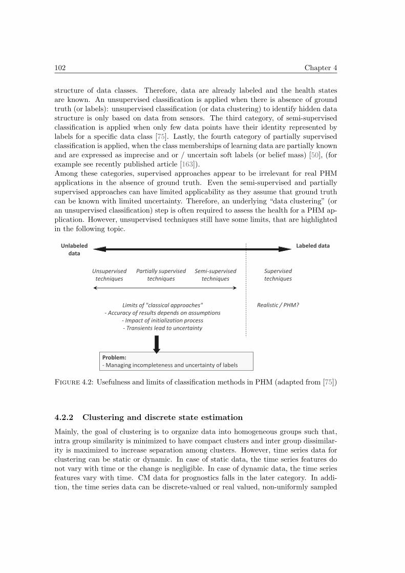
102 Chapter 4
structure of data classes. Therefore, data are already labeled and the health statesare known. An unsupervised classification is applied when there is absence of groundtruth (or labels): unsupervised classification (or data clustering) to identify hidden datastructure is only based on data from sensors. The third category, of semi-supervisedclassification is applied when only few data points have their identity represented bylabels for a specific data class [75]. Lastly, the fourth category of partially supervisedclassification is applied, when the class memberships of learning data are partially knownand are expressed as imprecise and or / uncertain soft labels (or belief mass) [50], (forexample see recently published article [163]).Among these categories, supervised approaches appear to be irrelevant for real PHMapplications in the absence of ground truth. Even the semi-supervised and partiallysupervised approaches can have limited applicability as they assume that ground truthcan be known with limited uncertainty. Therefore, an underlying “data clustering” (oran unsupervised classification) step is often required to assess the health for a PHM ap-plication. However, unsupervised techniques still have some limits, that are highlightedin the following topic.
Problem:
- Managing incompleteness and uncertainty of labels
Unlabeled
data
Labeled data
Unsupervised
techniques
Supervised
techniques
Realistic / PHM? Limits of "classical approaches"
- Accuracy of results depends on assumptions
- Impact of initialization process
- Transients lead to uncertainty
Partially supervised
techniques
Semi-supervised
techniques
Figure 4.2: Usefulness and limits of classification methods in PHM (adapted from [75])
4.2.2 Clustering and discrete state estimation
Mainly, the goal of clustering is to organize data into homogeneous groups such that,intra group similarity is minimized to have compact clusters and inter group dissimilar-ity is maximized to increase separation among clusters. However, time series data forclustering can be static or dynamic. In case of static data, the time series features donot vary with time or the change is negligible. In case of dynamic data, the time seriesfeatures vary with time. CM data for prognostics falls in the later category. In addi-tion, the time series data can be discrete-valued or real valued, non-uniformly sampled
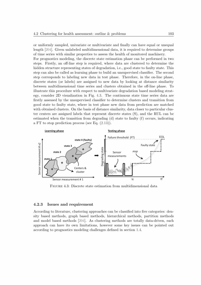
4.2 Clustering for health assessment: outline & problems 103
or uniformly sampled, univariate or multivariate and finally can have equal or unequallength [204]. Given unlabeled multidimensional data, it is required to determine groupsof time series with similar properties to assess the health of monitored machinery.For prognostics modeling, the discrete state estimation phase can be performed in twosteps. Firstly, an off-line step is required, where data are clustered to determine thehidden structure representing states of degradation, i.e., good state to faulty state. Thisstep can also be called as learning phase to build an unsupervised classifier. The secondstep corresponds to labeling new data in test phase. Therefore, in the on-line phase,discrete states (or labels) are assigned to new data by looking at distance similaritybetween multidimensional time series and clusters obtained in the off-line phase. Toillustrate this procedure with respect to multivariate degradation based modeling strat-egy, consider 2D visualization in Fig. 4.3. The continuous state time series data arefirstly assessed by the unsupervised classifier to determine clusters and transition fromgood state to faulty state, where in test phase new data from prediction are matchedwith obtained clusters. On the basis of distance similarity, data closer to particular clus-ter centers are assigned labels that represent discrete states (S), and the RUL can beestimated when the transition from degrading (d) state to faulty (f) occurs, indicatinga FT to stop prediction process (see Eq. (2.13)).
Learning phase
Se
nso
r m
ea
sure
me
nt
# x
2
Centers &
cluster
state 1
state 2
state 3
state 4 (faulty) Failure threshold (FT)
Sensor
measurements
Testing phase
tf
De
gra
din
g s
tate
tc
EOL
msp
Faulty state
Sensor measurement # 1
Figure 4.3: Discrete state estimation from multidimensional data
4.2.3 Issues and requirement
According to literature, clustering approaches can be classified into five categories: den-sity based methods, graph based methods, hierarchical methods, partition methodsand model based methods [204]. As clustering methods are totally data-driven, eachapproach can have its own limitations, however some key issues can be pointed outaccording to prognostics modeling challenges defined in section 1.4.

104 Chapter 4
• Clustering algorithms can be sensitive to noise and outliers, which can influencecluster centers and distort clusters. As a result, the robustness of a prognosticsmodel is affected.
• Clustering algorithms can have inconsistent performance, such that each run givesdifferent results, which can affect robustness and reliability of a prognostics model.
• Clustering algorithms can be time consuming, dependent on human involvementto initialize parameters (i.e., number of clusters and initial centers values), limitedto specific data types (e.g. time series with equal lengths). Such issues reduce theapplicability of the clustering approach for a prognostics model.
As for real prognostics application where machinery operates in a dynamic environmentand data are affected by inherent non-linearities, with the absence of prior knowledge ofground truth, clustering of an unlabeled data could be quite hard. In this case, it is alsoimportant to represent uncertainty of unlabeled multidimensional data like, transitionsamong different states, which can be performed by theories like fuzzy sets, probability,etc. Therefore, to achieve the goal of dynamic FTs, it is required to propose a newalgorithm that accounts for issues mentioned above and can improve the efficiency ofthe prognostics model.
4.3 Discrete state estimation: the S-MEFC Algorithm
4.3.1 Background
4.3.1.1 Maximum Entropy Fuzzy Clustering (MEFC)
The clustering algorithms attempt to find an inherent structure for a given set of unla-beled data points by partitioning data into subgroups or clusters (representing similarobjects). Typically, the partition based clustering algorithm (either hard or fuzzy) runas follows: assuming the initial positions of cluster center (or centroids) a membershipfunction generates partition, which is measured by a cost function for fitness analysis.An iterative approach is implemented until the membership function create a partitionthat reduces the cost function [27]. Most importantly, whatever the clustering algorithm,it should provide compact clusters by minimizing the distance between similar objects(or data points) and separate dissimilar objects objects by maximizing their distances.In other words, intra-cluster distances should be minimized and inter-cluster distancesshould be maximized to obtain boundaries of clusters.According to literature, to handle the issue of vague (imprecise) boundaries of clusters,fuzzy logic is considered as an effective tool [23]. Also, there are several approachesfor fuzzy clustering, but, such techniques may induce biases in the choice of member-ship function [27]. Thereby, [125] proposed an algorithm namely, the maximum entropybased fuzzy clustering algorithm (MEFC), that ensures a maximum fairness to handleimprecise data and minimize such choice of bias of membership function via maximumentropy principle. In addition, MEFC algorithm is considered to be robust as compared
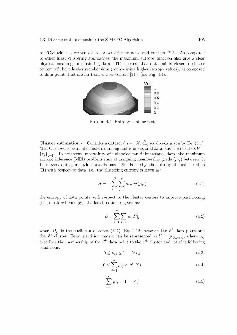
4.3 Discrete state estimation: the S-MEFC Algorithm 105
to FCM which is recognized to be sensitive to noise and outliers [215]. As comparedto other fuzzy clustering approaches, the maximum entropy function also give a clearphysical meaning for clustering data. This means, that data points closer to clustercenters will have higher memberships (representing higher entropy values), as comparedto data points that are far from cluster centers [215] (see Fig. 4.4).
Figure 4.4: Entropy contour plot
Cluster estimation - Consider a dataset ℓD = {Xi}Ni=1 as already given by Eq. (3.1).MEFC is used to estimate clusters c among multidimensional data, and their centers V ={vj}cj=1. To represent uncertainty of unlabeled multidimensional data, the maximumentropy inference (MEI) problem aims at assigning membership grade (µij) between [0,1] to every data point which avoids bias [125]. Formally, the entropy of cluster centers(H) with respect to data, i.e., the clustering entropy is given as:
H = −N∑
i=1
c∑
j=1
µijlog (µij) (4.1)
the entropy of data points with respect to the cluster centers to improve partitioning(i.e., clustered entropy), the loss function is given as:
L =
N∑
i=1
c∑
j=1
µijD2ij (4.2)
where Dij is the euclidean distance (ED) (Eq. 2.12) between the ith data point andthe jth cluster. Fuzzy partition matrix can be represented as U = [µij ]c×N , where µijdescribes the membership of the ith data point to the jth cluster and satisfies followingconditions.
0 ≤ µij ≤ 1 ∀ i,j (4.3)
0 ≤N∑
j=1
µij < N ∀ i (4.4)
c∑
i=1
µij = 1 ∀ j (4.5)
106 Chapter 4
A fuzzy clustering based on MEI aims at obtaining data points that minimize Eq. (4.2)and the membership assignments that meet Eq. (4.3-4.5). Further, to maximize Eq. (4.1)subject to Eq. (4.2) and constraints by Eq. (4.3-4.5), a Langrangian multiplier approachis used which gives following solutions [125]:
µij =e−D2
ij/2σ2∑c
k=1 e−D2
ik/2σ2∀ i,j (4.6)
where σ represents the fuzziness parameter, and 2σ2 is “temperature” in statisticalphysics. When σ = 0, the clustering becomes hard, when σ → ∞ each pattern is equallyassigned to all clusters [125]. Therefore, σ has similar properties like fuzziness parameter“m” in FCM clustering, however it has more clear physical meaning. In should be notedthat the resulting Eq. (4.6) satisfies (4.2) only when centers vj are fixed. Similarly, whenµij are fixed, the centers are updated with a following solution achieved from a proofsimilar to [29] for FCM:
vj =
∑Ni=1 µij ·xi∑N
i=1 µij∀ j (4.7)
which means that vj is the center of jth cluster.
Issues and requirements - According to [215], the performance of MEFC algorithmis dependent on the choice of the number of clusters and their initial centers. Therefore,it is required to properly initialize such parameters, to achieve an optimized solutionsand avoid issues like inconsistency due to parameter initialization, which gives differentresults for different parameter inputs.
4.3.1.2 Subtractive Clustering
According to literature, to overcome issues of parameter initialization and to achievethe global optimum solution, methods like genetic algorithm and particle swarm op-timization were applied [225]. However, such methods are computationally expensivewhich limits their applicability, for real prognostics applications. A simple and effectivealgorithm has been proposed by Yager and Filev [209], to estimate number of clustersand their initial centers, namely mountain clustering. But again, the algorithm wascomputationally expensive, because the computations grow exponentially according tothe dimensions of the problem [46]. Finally, an extension of Mountain Clustering wasproposed by Chiu [46], called as Subtractive Clustering (SC) which has an additionaladvantage to handle high dimensional data.Briefly, SC is a one pass approach to estimate cluster centers among numeric data (basedon the density function), that does not require any iterative optimization. Therefore,this method can be used to provide number of clusters and initial centers for algorithmslike FCM or its other variants [125]. According to [54], SC is robust clustering algo-rithm could (a) remove outliers (robust to outliers that can impact clusters centers), (b)resolve conflicting data and (c) discard unnecessary patterns. In addition, it does not
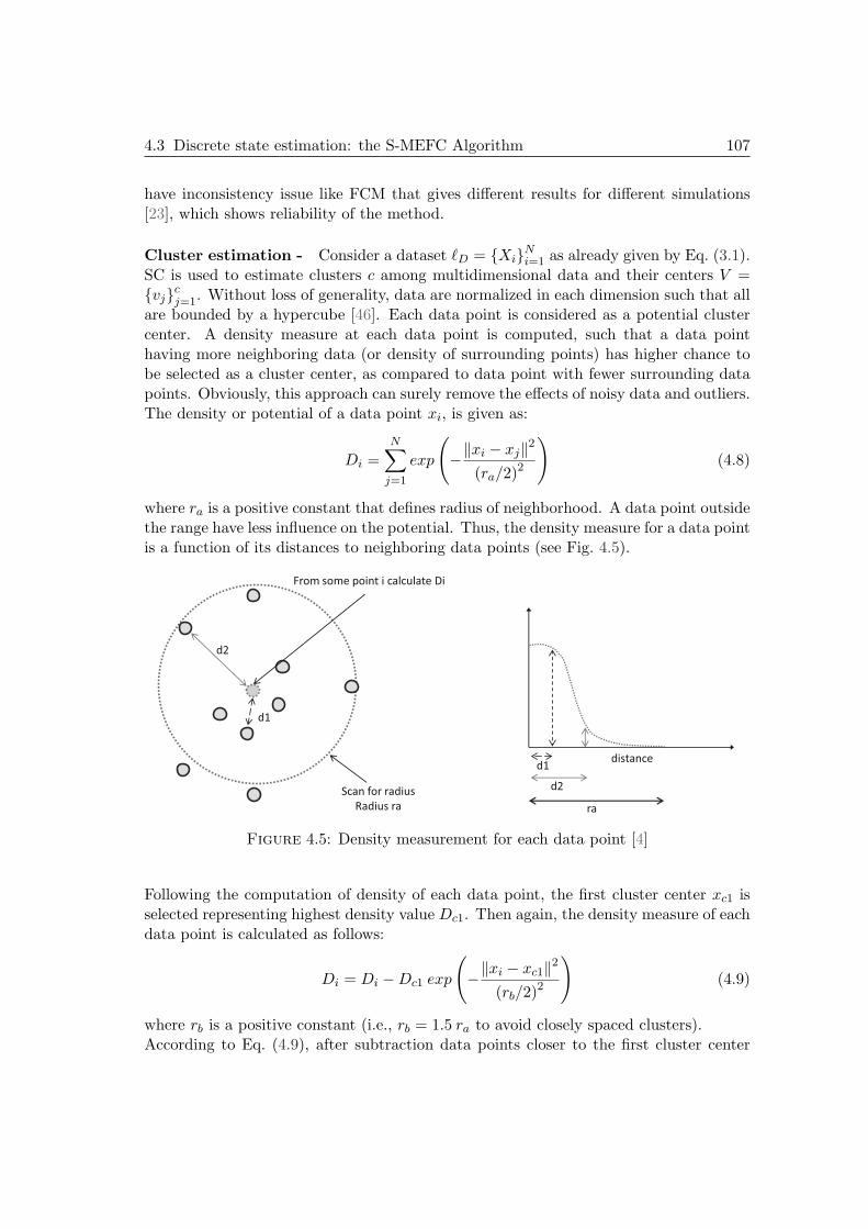
4.3 Discrete state estimation: the S-MEFC Algorithm 107
have inconsistency issue like FCM that gives different results for different simulations[23], which shows reliability of the method.
Cluster estimation - Consider a dataset ℓD = {Xi}Ni=1 as already given by Eq. (3.1).SC is used to estimate clusters c among multidimensional data and their centers V ={vj}cj=1. Without loss of generality, data are normalized in each dimension such that allare bounded by a hypercube [46]. Each data point is considered as a potential clustercenter. A density measure at each data point is computed, such that a data pointhaving more neighboring data (or density of surrounding points) has higher chance tobe selected as a cluster center, as compared to data point with fewer surrounding datapoints. Obviously, this approach can surely remove the effects of noisy data and outliers.The density or potential of a data point xi, is given as:
Di =N∑
j=1
exp
(
−‖xi − xj‖2
(ra/2)2
)
(4.8)
where ra is a positive constant that defines radius of neighborhood. A data point outsidethe range have less influence on the potential. Thus, the density measure for a data pointis a function of its distances to neighboring data points (see Fig. 4.5).
d1 distance
d2
ra
Scan for radius
Radius ra
d1
d2
From some point i calculate Di
Figure 4.5: Density measurement for each data point [4]
Following the computation of density of each data point, the first cluster center xc1 isselected representing highest density value Dc1. Then again, the density measure of eachdata point is calculated as follows:
Di = Di −Dc1 exp
(
−‖xi − xc1‖2
(rb/2)2
)
(4.9)
where rb is a positive constant (i.e., rb = 1.5 ra to avoid closely spaced clusters).According to Eq. (4.9), after subtraction data points closer to the first cluster center
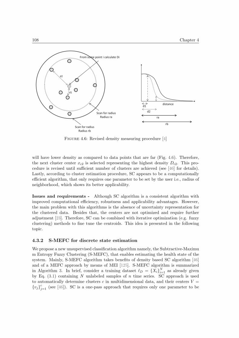
108 Chapter 4
d1 distance
d2
ra
rb
Scan for radius
Radius ra
Scan for radius
Radius rb
d1
d2
From some point i calculate Di
Figure 4.6: Revised density measuring procedure [4]
will have lower density as compared to data points that are far (Fig. 4.6). Therefore,the next cluster center xc2 is selected representing the highest density Dc2. This pro-cedure is revised until sufficient number of clusters are achieved (see [46] for details).Lastly, according to cluster estimation procedure, SC appears to be a computationallyefficient algorithm, that only requires one parameter to be set by the user i.e., radius ofneighborhood, which shows its better applicability.
Issues and requirements - Although SC algorithm is a consistent algorithm withimproved computational efficiency, robustness and applicability advantages. However,the main problem with this algorithms is the absence of uncertainty representation forthe clustered data. Besides that, the centers are not optimized and require furtheradjustment [23]. Therefore, SC can be combined with iterative optimization (e.g. fuzzyclustering) methods to fine tune the centroids. This idea is presented in the followingtopic.
4.3.2 S-MEFC for discrete state estimation
We propose a new unsupervised classification algorithm namely, the Subtractive-Maximum Entropy Fuzzy Clustering (S-MEFC), that enables estimating the health state of thesystem. Mainly, S-MEFC algorithm takes benefits of density based SC algorithm [46]and of a MEFC approach by means of MEI [125]. S-MEFC algorithm is summarizedin Algorithm 3. In brief, consider a training dataset ℓD = {Xi}Ni=1 as already givenby Eq. (3.1) containing N unlabeled samples of n time series. SC approach is usedto automatically determine clusters c in multidimensional data, and their centers V ={vj}cj=1 (see [46]). SC is a one-pass approach that requires only one parameter to be
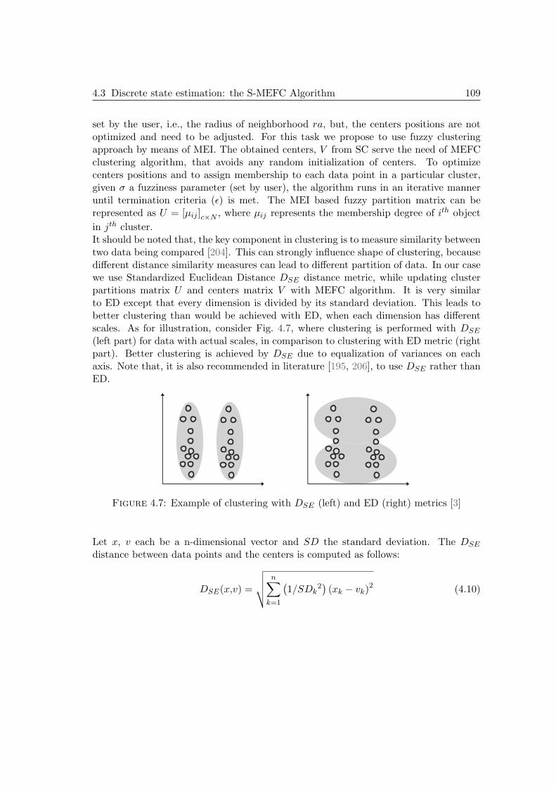
4.3 Discrete state estimation: the S-MEFC Algorithm 109
set by the user, i.e., the radius of neighborhood ra, but, the centers positions are notoptimized and need to be adjusted. For this task we propose to use fuzzy clusteringapproach by means of MEI. The obtained centers, V from SC serve the need of MEFCclustering algorithm, that avoids any random initialization of centers. To optimizecenters positions and to assign membership to each data point in a particular cluster,given σ a fuzziness parameter (set by user), the algorithm runs in an iterative manneruntil termination criteria (ǫ) is met. The MEI based fuzzy partition matrix can berepresented as U = [µij ]c×N , where µij represents the membership degree of ith object
in jth cluster.It should be noted that, the key component in clustering is to measure similarity betweentwo data being compared [204]. This can strongly influence shape of clustering, becausedifferent distance similarity measures can lead to different partition of data. In our casewe use Standardized Euclidean Distance DSE distance metric, while updating clusterpartitions matrix U and centers matrix V with MEFC algorithm. It is very similarto ED except that every dimension is divided by its standard deviation. This leads tobetter clustering than would be achieved with ED, when each dimension has differentscales. As for illustration, consider Fig. 4.7, where clustering is performed with DSE
(left part) for data with actual scales, in comparison to clustering with ED metric (rightpart). Better clustering is achieved by DSE due to equalization of variances on eachaxis. Note that, it is also recommended in literature [195, 206], to use DSE rather thanED.
Figure 4.7: Example of clustering with DSE (left) and ED (right) metrics [3]
Let x, v each be a n-dimensional vector and SD the standard deviation. The DSE
distance between data points and the centers is computed as follows:
DSE(x,v) =
√
√
√
√
n∑
k=1
(
1/SDk2)
(xk − vk)2 (4.10)
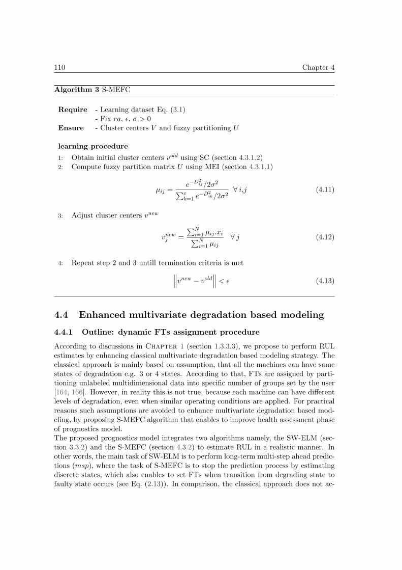
110 Chapter 4
Algorithm 3 S-MEFC
Require - Learning dataset Eq. (3.1)- Fix ra, ǫ, σ > 0
Ensure - Cluster centers V and fuzzy partitioning U
learning procedure
1: Obtain initial cluster centers vold using SC (section 4.3.1.2)2: Compute fuzzy partition matrix U using MEI (section 4.3.1.1)
µij =e−D2
ij/2σ2∑c
k=1 e−D2
ik/2σ2∀ i,j (4.11)
3: Adjust cluster centers vnew
vnewj =
∑Ni=1 µij .xi
∑Ni=1 µij
∀ j (4.12)
4: Repeat step 2 and 3 untill termination criteria is met
∥
∥
∥vnew − vold
∥
∥
∥< ǫ (4.13)
4.4 Enhanced multivariate degradation based modeling
4.4.1 Outline: dynamic FTs assignment procedure
According to discussions in Chapter 1 (section 1.3.3.3), we propose to perform RULestimates by enhancing classical multivariate degradation based modeling strategy. Theclassical approach is mainly based on assumption, that all the machines can have samestates of degradation e.g. 3 or 4 states. According to that, FTs are assigned by parti-tioning unlabeled multidimensional data into specific number of groups set by the user[164, 166]. However, in reality this is not true, because each machine can have differentlevels of degradation, even when similar operating conditions are applied. For practicalreasons such assumptions are avoided to enhance multivariate degradation based mod-eling, by proposing S-MEFC algorithm that enables to improve health assessment phaseof prognostics model.The proposed prognostics model integrates two algorithms namely, the SW-ELM (sec-tion 3.3.2) and the S-MEFC (section 4.3.2) to estimate RUL in a realistic manner. Inother words, the main task of SW-ELM is to perform long-term multi-step ahead predic-tions (msp), where the task of S-MEFC is to stop the prediction process by estimatingdiscrete states, which also enables to set FTs when transition from degrading state tofaulty state occurs (see Eq. (2.13)). In comparison, the classical approach does not ac-
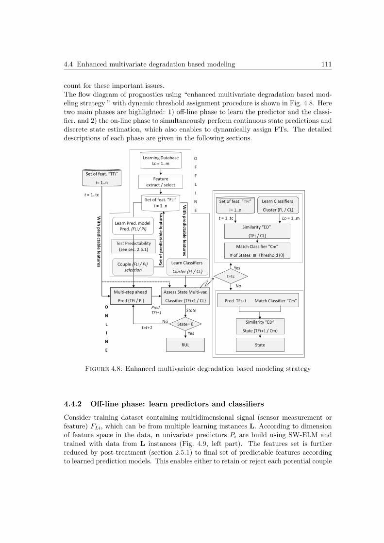
4.4 Enhanced multivariate degradation based modeling 111
count for these important issues.The flow diagram of prognostics using “enhanced multivariate degradation based mod-eling strategy ” with dynamic threshold assignment procedure is shown in Fig. 4.8. Heretwo main phases are highlighted: 1) off-line phase to learn the predictor and the classi-fier, and 2) the on-line phase to simultaneously perform continuous state predictions anddiscrete state estimation, which also enables to dynamically assign FTs. The detaileddescriptions of each phase are given in the following sections.
Feature
extract / select
Learning Database
LD = 1..m
Set of feat. “FLi”
i = 1..n
Learn Pred. model
Pred. {FLi / Pi}
Learn Classifiers
Cluster {FL / CL} t=tc
Set of feat. “TFi”
i= 1..n
Similarity “ED”
{TFt / CL}
Similarity “ED”
State {TFt+1 / Cm}
Learn Classifiers
Cluster {FL / CL}
LD = 1..m t = 1..tc
Match Classifier ”Cm”
# of States Threshold (q)
Pred. TFt+1 Match Classifier “Cm”
Yes
No
State
Assess State Multi-var.
Classifier {TFt+1 / CL}
State= q
Set of feat. “TFi”
i= 1..n
RUL
Multi-step ahead
Pred {TFi / Pi}
Yes
No
Pred.
TFt+1 State
t = 1..tc
O
F
F
L
I
N
E
O
N
L
I
N
E
Test Predictability
(see sec. 2.5.1)
Couple {FLi / Pi}
selection
Se
t o
f p
red
icta
ble
fe
atu
res
With
pre
dicta
ble
fea
ture
s
t=t+1
With
pre
dicta
ble
fea
ture
s
Figure 4.8: Enhanced multivariate degradation based modeling strategy
4.4.2 Off-line phase: learn predictors and classifiers
Consider training dataset containing multidimensional signal (sensor measurement orfeature) FLi, which can be from multiple learning instances L. According to dimensionof feature space in the data, n univariate predictors Pi are build using SW-ELM andtrained with data from L instances (Fig. 4.9, left part). The features set is furtherreduced by post-treatment (section 2.5.1) to final set of predictable features accordingto learned prediction models. This enables either to retain or reject each potential couple
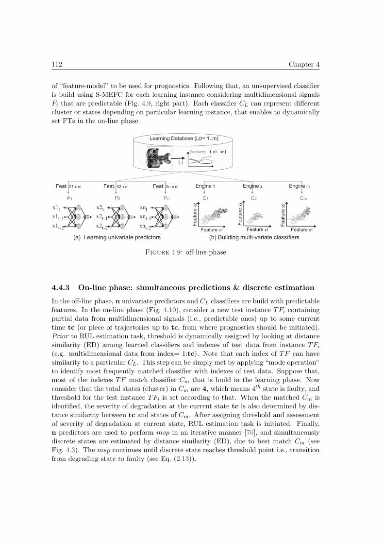
112 Chapter 4
of “feature-model” to be used for prognostics. Following that, an unsupervised classifieris build using S-MEFC for each learning instance considering multidimensional signalsFi that are predictable (Fig. 4.9, right part). Each classifier CL can represent differentcluster or states depending on particular learning instance, that enables to dynamicallyset FTs in the on-line phase.
(a) Learning univariate predictors (b) Building multi-variate classifiers
x1t
x1t-2
x1t-1
x2t
x2t-2
x2t-1
xnt
xnt-2
xnt-1
Fe
atu
re x
2
Feature x1 Feature x1
Fe
atu
re x
2
Feature x1
Fe
atu
re x
2
C2 Cm C1 P1 P2 Pn
Feat. Xn x m Feat. X1 x m Feat. X2 x m Engine 1 Engine m Engine 2
Learning Database (LD= 1..m)
Features ( x1.. xn)
L1
Figure 4.9: off-line phase
4.4.3 On-line phase: simultaneous predictions & discrete estimation
In the off-line phase, n univariate predictors and CL classifiers are build with predictablefeatures. In the on-line phase (Fig. 4.10), consider a new test instance TFi containingpartial data from multidimensional signals (i.e., predictable ones) up to some currenttime tc (or piece of trajectories up to tc, from where prognostics should be initiated).Prior to RUL estimation task, threshold is dynamically assigned by looking at distancesimilarity (ED) among learned classifiers and indexes of test data from instance TFi
(e.g. multidimensional data from index= 1:tc). Note that each index of TF can havesimilarity to a particular CL. This step can be simply met by applying “mode operation”to identify most frequently matched classifier with indexes of test data. Suppose that,most of the indexes TF match classifier Cm that is build in the learning phase. Nowconsider that the total states (cluster) in Cm are 4, which means 4th state is faulty, andthreshold for the test instance TFi is set according to that. When the matched Cm isidentified, the severity of degradation at the current state tc is also determined by dis-tance similarity between tc and states of Cm. After assigning threshold and assessmentof severity of degradation at current state, RUL estimation task is initiated. Finally,n predictors are used to perform msp in an iterative manner [76], and simultaneouslydiscrete states are estimated by distance similarity (ED), due to best match Cm (seeFig. 4.3). The msp continues until discrete state reaches threshold point i.e., transitionfrom degrading state to faulty (see Eq. (2.13)).
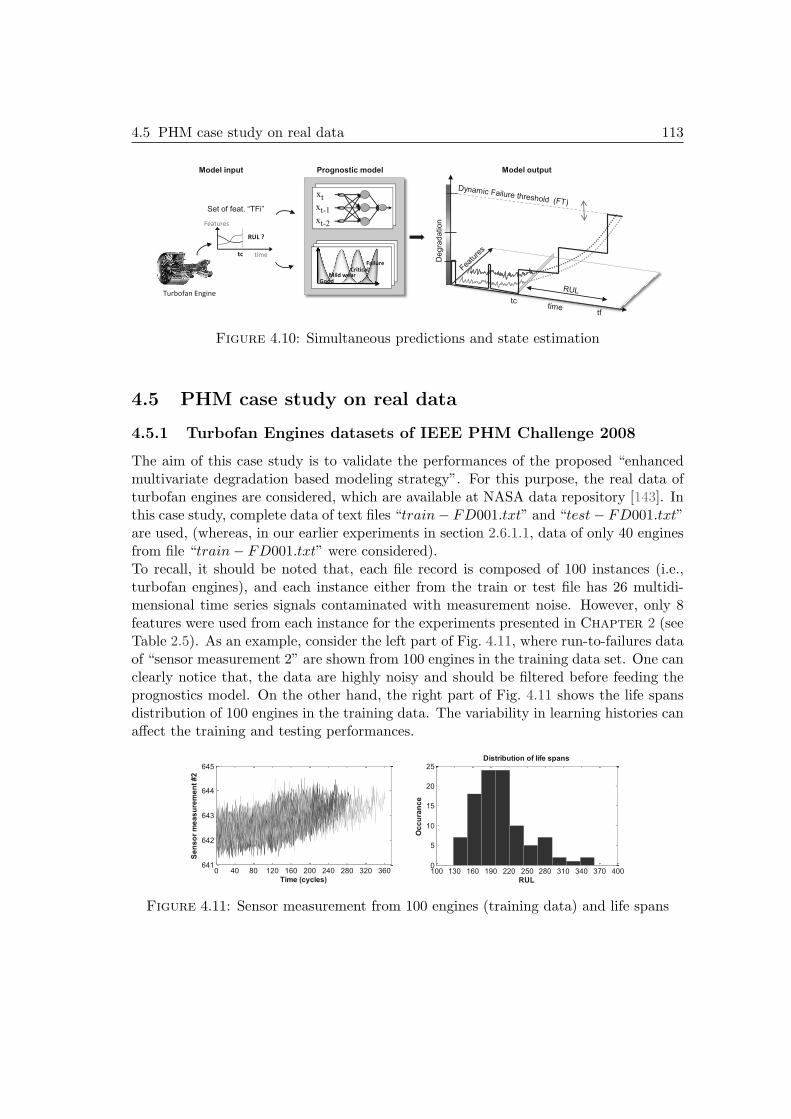
4.5 PHM case study on real data 113
time
Features
tc
Set of feat. “TFi”
Good Mild wear
Critical Failure
Model output
De
gra
datio
n
tc
tf
RUL ?
Prognostic modelModel input
Turbofan Engine
xt
xt-2
xt-1
Figure 4.10: Simultaneous predictions and state estimation
4.5 PHM case study on real data
4.5.1 Turbofan Engines datasets of IEEE PHM Challenge 2008
The aim of this case study is to validate the performances of the proposed “enhancedmultivariate degradation based modeling strategy”. For this purpose, the real data ofturbofan engines are considered, which are available at NASA data repository [143]. Inthis case study, complete data of text files “train− FD001.txt” and “test− FD001.txt”are used, (whereas, in our earlier experiments in section 2.6.1.1, data of only 40 enginesfrom file “train− FD001.txt” were considered).To recall, it should be noted that, each file record is composed of 100 instances (i.e.,turbofan engines), and each instance either from the train or test file has 26 multidi-mensional time series signals contaminated with measurement noise. However, only 8features were used from each instance for the experiments presented in Chapter 2 (seeTable 2.5). As an example, consider the left part of Fig. 4.11, where run-to-failures dataof “sensor measurement 2” are shown from 100 engines in the training data set. One canclearly notice that, the data are highly noisy and should be filtered before feeding theprognostics model. On the other hand, the right part of Fig. 4.11 shows the life spansdistribution of 100 engines in the training data. The variability in learning histories canaffect the training and testing performances.
100 130 160 190 220 250 280 310 340 370 4000
5
10
15
20
25
RUL
Oc
cu
ran
ce
Distribution of life spans
0 40 80 120 160 200 240 280 320 360641
642
643
644
645
Time (cycles)
Se
ns
or
me
as
ure
me
nt
#2
Figure 4.11: Sensor measurement from 100 engines (training data) and life spans
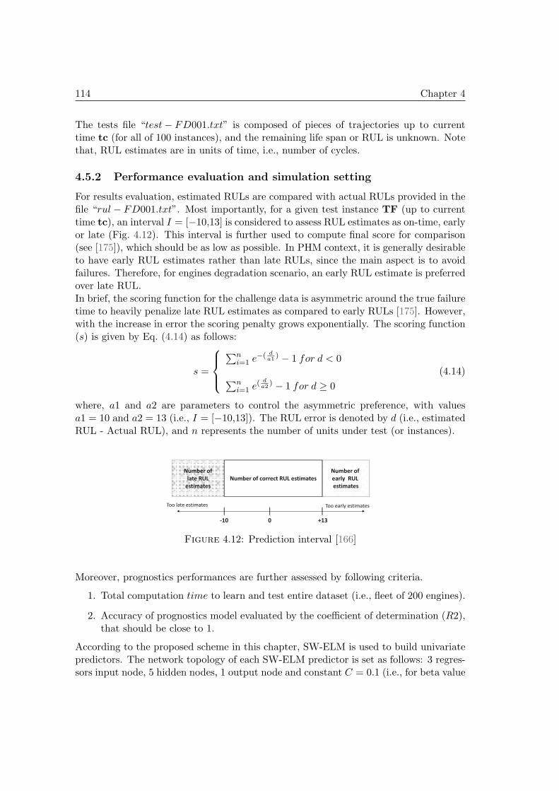
114 Chapter 4
The tests file “test− FD001.txt” is composed of pieces of trajectories up to currenttime tc (for all of 100 instances), and the remaining life span or RUL is unknown. Notethat, RUL estimates are in units of time, i.e., number of cycles.
4.5.2 Performance evaluation and simulation setting
For results evaluation, estimated RULs are compared with actual RULs provided in thefile “rul − FD001.txt”. Most importantly, for a given test instance TF (up to currenttime tc), an interval I = [−10,13] is considered to assess RUL estimates as on-time, earlyor late (Fig. 4.12). This interval is further used to compute final score for comparison(see [175]), which should be as low as possible. In PHM context, it is generally desirableto have early RUL estimates rather than late RULs, since the main aspect is to avoidfailures. Therefore, for engines degradation scenario, an early RUL estimate is preferredover late RUL.In brief, the scoring function for the challenge data is asymmetric around the true failuretime to heavily penalize late RUL estimates as compared to early RULs [175]. However,with the increase in error the scoring penalty grows exponentially. The scoring function(s) is given by Eq. (4.14) as follows:
s =
∑ni=1 e
−( da1
) − 1 for d < 0
∑ni=1 e
( da2
) − 1 for d ≥ 0
(4.14)
where, a1 and a2 are parameters to control the asymmetric preference, with valuesa1 = 10 and a2 = 13 (i.e., I = [−10,13]). The RUL error is denoted by d (i.e., estimatedRUL - Actual RUL), and n represents the number of units under test (or instances).
������ ��
��� ��
���������
������ ��
���� ��
���������
������ ��������� �����������
��� ���
��� ����� ��������� ��� ������
�
Figure 4.12: Prediction interval [166]
Moreover, prognostics performances are further assessed by following criteria.
1. Total computation time to learn and test entire dataset (i.e., fleet of 200 engines).
2. Accuracy of prognostics model evaluated by the coefficient of determination (R2),that should be close to 1.
According to the proposed scheme in this chapter, SW-ELM is used to build univariatepredictors. The network topology of each SW-ELM predictor is set as follows: 3 regres-sors input node, 5 hidden nodes, 1 output node and constant C = 0.1 (i.e., for beta value
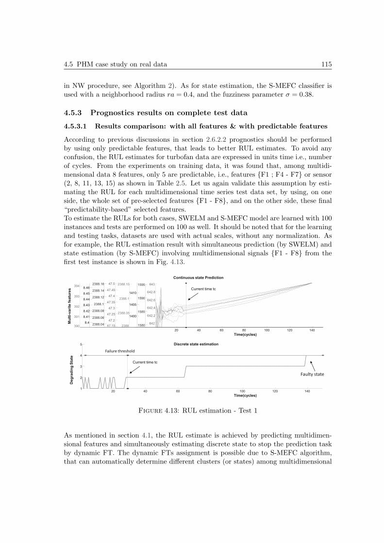
4.5 PHM case study on real data 115
in NW procedure, see Algorithm 2). As for state estimation, the S-MEFC classifier isused with a neighborhood radius ra = 0.4, and the fuzziness parameter σ = 0.38.
4.5.3 Prognostics results on complete test data
4.5.3.1 Results comparison: with all features & with predictable features
According to previous discussions in section 2.6.2.2 prognostics should be performedby using only predictable features, that leads to better RUL estimates. To avoid anyconfusion, the RUL estimates for turbofan data are expressed in units time i.e., numberof cycles. From the experiments on training data, it was found that, among multidi-mensional data 8 features, only 5 are predictable, i.e., features {F1 ; F4 - F7} or sensor(2, 8, 11, 13, 15) as shown in Table 2.5. Let us again validate this assumption by esti-mating the RUL for each multidimensional time series test data set, by using, on oneside, the whole set of pre-selected features {F1 - F8}, and on the other side, these final“predictability-based” selected features.To estimate the RULs for both cases, SWELM and S-MEFC model are learned with 100instances and tests are performed on 100 as well. It should be noted that for the learningand testing tasks, datasets are used with actual scales, without any normalization. Asfor example, the RUL estimation result with simultaneous prediction (by SWELM) andstate estimation (by S-MEFC) involving multidimensional signals {F1 - F8} from thefirst test instance is shown in Fig. 4.13.
20 40 60 80 100 120 140
642
642.2
642.4
642.6
642.8
643
Continuous state Prediction
Time(cycles)
1580
1585
1590
1595
1400
1405
1410
2388
2388.05
2388.1
2388.15
47.15
47.2
47.25
47.3
47.35
47.4
47.45
47.5
2388.04
2388.06
2388.08
2388.1
2388.12
2388.14
2388.16
8.4
8.41
8.42
8.43
8.44
8.45
8.46
391
392
393
394
Mu
lti-
vari
te f
eatu
res
Failure threshold θ
20 40 60 80 100 120 140 1
2
3
4
5 Discrete state estimation
Time(cycles)
Deg
rad
ing
Sta
te
Faulty state
Current time tc
Current time tc
390
Failure threshold
Figure 4.13: RUL estimation - Test 1
As mentioned in section 4.1, the RUL estimate is achieved by predicting multidimen-sional features and simultaneously estimating discrete state to stop the prediction taskby dynamic FT. The dynamic FTs assignment is possible due to S-MEFC algorithm,that can automatically determine different clusters (or states) among multidimensional
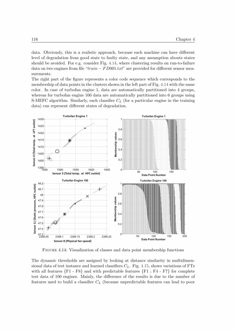
116 Chapter 4
data. Obviously, this is a realistic approach, because each machine can have differentlevel of degradation from good state to faulty state, and any assumption abouts statesshould be avoided. For e.g. consider Fig. 4.14, where clustering results on run-to-failuredata on two engines from file “train− FD001.txt” are provided for different sensor mea-surements.The right part of the figure represents a color code sequence which corresponds to themembership of data points in the clusters shown in the left part of Fig. 4.14 with the samecolor. In case of turbofan engine 1, data are automatically partitioned into 4 groups,whereas for turbofan engine 100 data are automatically partitioned into 6 groups usingS-MEFC algorithm. Similarly, each classifier CL (for a particular engine in the trainingdata) can represent different states of degradation.
1585 1590 1595 1600 16051395
1400
1405
1410
1415
1420
1425
1430
Turbofan Engine 1
50 100 150 2000
0.2
0.4
0.6
0.8
1
Me
mb
ers
hip
va
lue
s
Data Point Number
Turbofan Engine 100
2388.05 2388.1 2388.15 2388.2 2388.2547.3
47.4
47.5
47.6
47.7
47.8
47.9
48
48.1
48.2
Turbofan Engine 100
Se
nso
r 4
(To
tal
tem
p.
at
LP
T o
utl
et)
50 100 1500
0.2
0.4
0.6
0.8
1
Me
mb
ers
hip
va
lue
s
Data Point Number
Turbofan Engine 1
Sensor 3 (Total temp. at HPC outlet)
Sensor 8 (Physical fan speed)
Se
nso
r 1
1 (
Sta
tic
pre
ssu
re,
HP
C o
utl
et)
Figure 4.14: Visualization of classes and data point membership functions
The dynamic thresholds are assigned by looking at distance similarity in multidimen-sional data of test instance and learned classifiers CL. Fig. 4.15, shows variations of FTswith all features {F1 - F8} and with predictable features {F1 ; F4 - F7} for completetest data of 100 engines. Mainly, the difference of the results is due to the number offeatures used to build a classifier CL (because unpredictable features can lead to poor
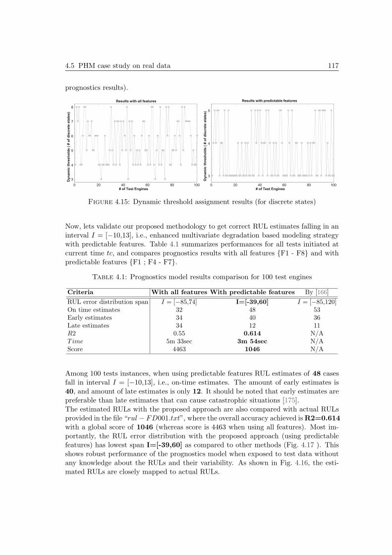
4.5 PHM case study on real data 117
prognostics results).
0 20 40 60 80 100
3
4
5
6
7
8
# of Test Engines
Dyn
am
ic t
hre
sh
old
s (
# o
f d
isc
rete
sta
tes)
Results with all features
0 20 40 60 80 100
3
4
5
Results with predictable features
# of Test Engines
Dyn
am
ic t
hre
sh
old
s (
# o
f d
isc
rete
sta
tes)
Figure 4.15: Dynamic threshold assignment results (for discrete states)
Now, lets validate our proposed methodology to get correct RUL estimates falling in aninterval I = [−10,13], i.e., enhanced multivariate degradation based modeling strategywith predictable features. Table 4.1 summarizes performances for all tests initiated atcurrent time tc, and compares prognostics results with all features {F1 - F8} and withpredictable features {F1 ; F4 - F7}.
Table 4.1: Prognostics model results comparison for 100 test engines
Criteria With all features With predictable features By [166]
RUL error distribution span I = [−85,74] I=[-39,60] I = [−85,120]On time estimates 32 48 53Early estimates 34 40 36Late estimates 34 12 11R2 0.55 0.614 N/AT ime 5m 33sec 3m 54sec N/AScore 4463 1046 N/A
Among 100 tests instances, when using predictable features RUL estimates of 48 casesfall in interval I = [−10,13], i.e., on-time estimates. The amount of early estimates is40, and amount of late estimates is only 12. It should be noted that early estimates arepreferable than late estimates that can cause catastrophic situations [175].The estimated RULs with the proposed approach are also compared with actual RULsprovided in the file “rul − FD001.txt”, where the overall accuracy achieved isR2=0.614with a global score of 1046 (whereas score is 4463 when using all features). Most im-portantly, the RUL error distribution with the proposed approach (using predictablefeatures) has lowest span I=[-39,60] as compared to other methods (Fig. 4.17 ). Thisshows robust performance of the prognostics model when exposed to test data withoutany knowledge about the RULs and their variability. As shown in Fig. 4.16, the esti-mated RULs are closely mapped to actual RULs.
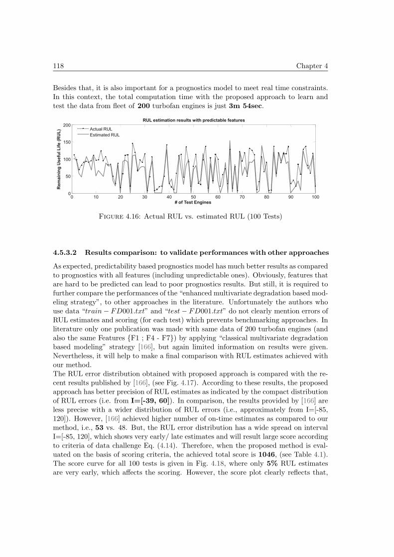
118 Chapter 4
Besides that, it is also important for a prognostics model to meet real time constraints.In this context, the total computation time with the proposed approach to learn andtest the data from fleet of 200 turbofan engines is just 3m 54sec.
0 10 20 30 40 50 60 70 80 90 100 0
50
100
150
200
# of Test Engines
Re
ma
inin
g U
se
ful L
ife
(R
UL
)
RUL estimation results with predictable features
Actual RUL
Estimated RUL
Figure 4.16: Actual RUL vs. estimated RUL (100 Tests)
4.5.3.2 Results comparison: to validate performances with other approaches
As expected, predictability based prognostics model has much better results as comparedto prognostics with all features (including unpredictable ones). Obviously, features thatare hard to be predicted can lead to poor prognostics results. But still, it is required tofurther compare the performances of the “enhanced multivariate degradation based mod-eling strategy”, to other approaches in the literature. Unfortunately the authors whouse data “train− FD001.txt” and “test− FD001.txt” do not clearly mention errors ofRUL estimates and scoring (for each test) which prevents benchmarking approaches. Inliterature only one publication was made with same data of 200 turbofan engines (andalso the same Features {F1 ; F4 - F7}) by applying “classical multivariate degradationbased modeling” strategy [166], but again limited information on results were given.Nevertheless, it will help to make a final comparison with RUL estimates achieved withour method.The RUL error distribution obtained with proposed approach is compared with the re-cent results published by [166], (see Fig. 4.17). According to these results, the proposedapproach has better precision of RUL estimates as indicated by the compact distributionof RUL errors (i.e. from I=[-39, 60]). In comparison, the results provided by [166] areless precise with a wider distribution of RUL errors (i.e., approximately from I=[-85,120]). However, [166] achieved higher number of on-time estimates as compared to ourmethod, i.e., 53 vs. 48. But, the RUL error distribution has a wide spread on intervalI=[-85, 120], which shows very early/ late estimates and will result large score accordingto criteria of data challenge Eq. (4.14). Therefore, when the proposed method is eval-uated on the basis of scoring criteria, the achieved total score is 1046, (see Table 4.1).The score curve for all 100 tests is given in Fig. 4.18, where only 5% RUL estimatesare very early, which affects the scoring. However, the score plot clearly reflects that,
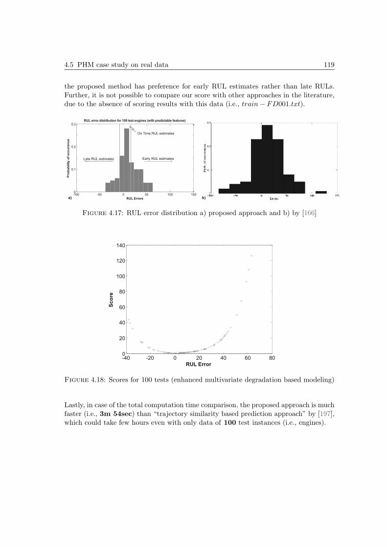
4.5 PHM case study on real data 119
the proposed method has preference for early RUL estimates rather than late RULs.Further, it is not possible to compare our score with other approaches in the literature,due to the absence of scoring results with this data (i.e., train− FD001.txt).
-100 -50 0 50 100 1500
0.1
0.2
0.3
RUL Errors
Pro
ba
bilit
y o
f o
cc
ura
nc
e
RUL error distribution for 100 test engines (with predictable features)
Early RUL estimates Late RUL estimates
On Time RUL estimates
a) b)
Figure 4.17: RUL error distribution a) proposed approach and b) by [166]
-40 -20 0 20 40 60 80 0
20
40
60
80
100
120
140
RUL Error
Sc
ore
Figure 4.18: Scores for 100 tests (enhanced multivariate degradation based modeling)
Lastly, in case of the total computation time comparison, the proposed approach is muchfaster (i.e., 3m 54sec) than “trajectory similarity based prediction approach” by [197],which could take few hours even with only data of 100 test instances (i.e., engines).
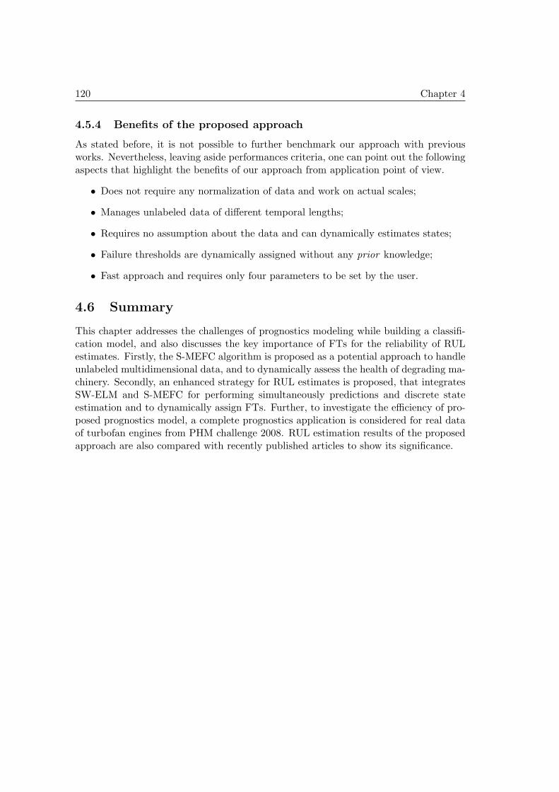
120 Chapter 4
4.5.4 Benefits of the proposed approach
As stated before, it is not possible to further benchmark our approach with previousworks. Nevertheless, leaving aside performances criteria, one can point out the followingaspects that highlight the benefits of our approach from application point of view.
• Does not require any normalization of data and work on actual scales;
• Manages unlabeled data of different temporal lengths;
• Requires no assumption about the data and can dynamically estimates states;
• Failure thresholds are dynamically assigned without any prior knowledge;
• Fast approach and requires only four parameters to be set by the user.
4.6 Summary
This chapter addresses the challenges of prognostics modeling while building a classifi-cation model, and also discusses the key importance of FTs for the reliability of RULestimates. Firstly, the S-MEFC algorithm is proposed as a potential approach to handleunlabeled multidimensional data, and to dynamically assess the health of degrading ma-chinery. Secondly, an enhanced strategy for RUL estimates is proposed, that integratesSW-ELM and S-MEFC for performing simultaneously predictions and discrete stateestimation and to dynamically assign FTs. Further, to investigate the efficiency of pro-posed prognostics model, a complete prognostics application is considered for real dataof turbofan engines from PHM challenge 2008. RUL estimation results of the proposedapproach are also compared with recently published articles to show its significance.
Chapter 5Conclusion and future works
This chapter concludes the research work by summarizing issues addressedin the thesis, developments and contributions. A discussion on limits of theapproach is also laid out to address future perspectives.
Conclusion
To optimize machinery service delivery potential during its lifetime, the main goal ofprognostics is to intelligently use condition monitoring data from an in-service machin-ery, and estimate the Remaining Useful Life (RUL) before a failure. Therefore, it is a coreprocess of Prognostics and Health Management (PHM) discipline that links the studiesof failure mechanism and life cycle management of critical engineering assets. However,in a dynamic operational environment, the deterioration process of a machinery can beaffected by different factors like engineering variances, failure modes, environmental andoperating conditions. The data acquired from such machinery are usually noisy andsubject to high level of uncertainty / unpredictability, and estimation of RUL is usuallya hard task. To perform an accurate prognostics, one has to address the challenges ofmodeling phase i.e., robustness to encounter uncertain inputs, reliability to encounterunknown data operating conditions, engineering variations, etc., and applicability tomeet industrial constraints and requirements. According to this, data-driven prognos-tics approaches appear to be a valuable alternative to deal with uncertainty of availabledata, in applications where a deep understanding of system physics is not available.In this thesis, a novel prognostics approach is developed that aims at enhancing data-driven prognostics in a realistic manner, with an acceptable level of accuracy undermodeling challenges of robustness, reliability and applicability. For this purpose, mainlytwo aspects are considered: data processing and prognostics modeling.In Chapter 1, the literature on PHM and classification of prognostics approaches isextensively reviewed. Prognostics approaches, (i.e., physics based, data-driven, and hy-brid) are assessed upon different criteria that are related to two important factors: 1)
122 Chapter 5
applicability and 2) performances. The assessment shows that data-driven methods havehigher applicability as compared to physics based and hybrid approaches, but their per-formances require further improvement that can be linked with robustness and reliabilityof the approach. Different strategies for data-driven prognostics are further reviewedwhich enables us to point out that the “multivariate degradation based modeling strat-egy” for RUL estimation has a strong potential, and is more realistic as compared todirect RUL prediction and to univariate degradation based modeling. Therefore, it isconsidered as a building block for prognostics modeling step. Besides that, for openchallenges of prognostics modeling, i.e., robustness, reliability and applicability, newdefinitions are also proposed, which are not clearly defined in the literature.Whatever the prognostics approach is, it requires suitable time series features or variablesthat are sensitive to machine degradation, reflect failure progression, and can be pre-dicted easily. In Chapter 2 we propose the data pre-treatment and data post-treatmentmethods for feature extraction and selection. In brief, for data pre-treatment firstly, rawdata are analyzed by applying discrete wavelet transform. Secondly feature extractionis performed in a new manner by using trigonometric functions and cumulative trans-formation. Finally, feature selection is performed by assessing their fitness in terms ofmonotonicity and trendability characteristics. Experiments on real data bearings fromPHM challenge 2012 show significant improvements by the proposed data pre-treatmentprocedure, as compared to classical way of feature extraction and selection. The datapost-treatment phase emphasize to further reduce multidimensional features data byassessing their predictability, as there is no interest in retaining features that are hardto be predicted. To show the impact of data post-treatment procedure, the multivariatedegradation based modeling strategy is applied to estimate the RUL by simultaneouspredictions and discrete state estimation. Experiments on real data of turbofan enginesfrom PHM data challenge 2008 show that, the use of multidimensional data with pre-dictable features is beneficial in improving accuracy of RUL estimates. In addition, someweaknesses of multivariate degradation based modeling strategy are also identified, tobe addressed in succeeding chapters.To account for issues related to time series prediction and the challenges of prognos-tics modeling (i.e., robustness, reliability and applicability), a new prediction algorithmis proposed in Chapter 3: the Summation Wavelet-Extreme Learning Machine (SW-ELM). SW-ELM is a supervised approach that does not require any iterative learninglike classical neural network and has only two parameters to be set by user. For timeseries prediction issues, the performances of SW-ELM are benchmarked with existingExtreme Learning Machine (ELM), Levenberg-Marquardt algorithm for SLFN and EL-MAN network on six different data sets. Results show improved performances achievedby SW-ELM in terms of computation time, model complexity and prediction accuracy.To validate the efficiency of SW-ELM with respect to robustness and reliability chal-lenges, a real case of Computer Numerical Control (CNC) machine is considered fortool wear monitoring task. Moreover, it is observed that, lower magnitude (or norm)of weights and bias of SW-ELM during learning phase can play a significant role inimproving testing accuracy. Although, performances of SW-ELM are of great interestbut, such rapid learning methods should be used as ensemble of multiple models to
123
achieve more robust and accurate performances rather than a single model. Therefore,an ensemble of SW-ELM is also proposed to quantify uncertainty and improve accuracyof estimates. Note that, during experiments the reliability of SW-ELM is assessed onunknown data of cutting tools with engineering variations like geometry and coating.Moreover, SW-ELM is further used to perform “long-term predictions” with real data ofdegraded bearings from PHM challenge 2012, with constant operating conditions. Themulti-step ahead prediction (msp) results with cumulative features are also comparedby msp using classical features.In Chapter 4 prognostics performances are further enhanced by a new health assessmentalgorithm: the Subtractive-Maximum Entropy Fuzzy Clustering (S-MEFC). S-MEFC isan unsupervised classification approach that can automatically determine the numberof states (clusters) from multidimensional data, i.e., without human assumption andhas consistent performance for each run. S-MEFC uses Maximum Entropy Inferenceto represent uncertainty of data rather than traditional fuzzy memberships. Moreover,a novel strategy for RUL estimation is also presented by integrating SW-ELM and S-MEFC as prognostics model. Both models are run simultaneously in order to perform“long-term predictions” and discrete state estimation, and to dynamically set failurethresholds (FTs). Lastly, the efficiency of the proposed “enhanced multivariate degra-dation based modeling strategy”, is investigated on a case study of turbofan enginesfrom PHM challenge 2008, and the results are thoroughly compared with recent pub-lications. From results analysis we find that, the proposed RUL estimation strategyis more realistic as compared to existing methods in terms of applicability criteria likecomputational time, model complexity and parameters, human assumptions and do-main knowledge. In addition, the accuracy of RUL estimates show better robustness ofthe proposed approach over fleet of test engines with different life spans. Besides that,the reliability of the prognostics approach is also improved by avoiding uncertain FTsbased on assumptions and are assigned dynamically in precise manner for each test case.
Obviously no model is perfect, however, the proposed developments on data-processingand prognostics modeling show good potential and improved performances as comparedto traditional methods. In addition, they also fulfill four main conditions of data-drivenprognostics, as mentioned in [24], 1) ability to extract features related to damage, 2)to set FTs, 3) fault propagation model to project fault growth up to the FT and 4)associate confidence. The main limits of proposed data-driven approach are as follows.
1. How to automate the initialization of two important parameters of the prognosticsmodel, which are to be set by the user, i.e., number of neurons in the hidden layerof SW-ELM, and the radius of neighborhood of a cluster in S-MEFC?
2. How to further manage the uncertainty related to data and prognostics modeling?
3. How to integrate variable operating conditions to enhance learning / testing per-formances of the prognostics model?
Nevertheless, this research work is a step ahead in PHM domain toward maturity ofprognostics.

124 Chapter 5
Future works
In general, inherent uncertainty in the machinery is a major hurdle while developingprognostics models, and indeed one of the factors that add to uncertainty is variableoperating conditions. Such issue can greatly affect reliability of the prognostics model.Indeed, the variations of operating conditions can affect the behavior of degrading ma-chinery, for e.g. increase in load can speedup the deterioration process and reduceRUL of machinery, while decrease in load results opposite behavior. Thus, operatingconditions should be used as inputs of the prognostics model, and this topic needs tobe further explored. Also, another problem could be the absence of future operatingconditions, which demands to intelligently manage the learning phase of data-drivenprognostics model, to avoid large uncertainty of predictions phase.Among different limits highlighted above, the key areas for future focus are uncertaintymanagement and integration of variable operating conditions. Therefore, current devel-opments of this thesis will be further extended as follows.
1. To manage and quantify uncertainty related to data and prognostics modeling;
2. To investigate the effects of variable operating conditions on the proposition ofcumulative features;
3. To integrate variable operating conditions as inputs of the prognostics model;
4. To extend the development to higher level rather than a component level.

Bibliography
[1] Industrial dryer datasetftp://ftp.esat.kuleuven.ac.be/sista/data/process industry.
[2] Mechanical hair dryer datasetftp://ftp.esat.kuleuven.ac.be/sista/data/mechanical.
[3] Microarray cluster analysis and applicationshttp://www.science.co.il/enuka/essays/microarray-review.pdf.
[4] Subtractive clustering densityhttp://www.spikingneurons.com/.
[5] IEEE PHM 2012 prognostic challengewww.femto-st.fr/f/d/ieeephm2012-challenge-details.pdf.
[6] NN3 forecasting competitionhttp://www.neural-forecasting-competition.com/nn3/index.htm.
[7] Abbas, S. R., and Arif, M. New time series predictability metrics for nearestneighbor based forecasting. In Multitopic Conference, 2006. INMIC’06. IEEE(2006), IEEE, pp. 100–105.
[8] Abu-Hanna, A., and Lucas, P. Prognostic models in medicine. Methods ofInformation in Medicine 40, 1 (2001), 1–5.
[9] Aka, R., Lia, Y.-F., Vitellia, V., and Zio, E. A genetic algorithm andneural network technique for predicting wind power under uncertainty. ChemicalEngineering 33 (2013), 1–6.
[10] An, D., Choi, J.-H., and Kim, N. H. A tutorial for model-based prognosticsalgorithms based on matlab code. In Annual Conference of the Prognostics andHealth Management Society, Mineapolis, Sept. 23-27 (2012).
126 BIBLIOGRAPHY
[11] An, D., Choi, J.-H., and Kim, N. H. Prognostics 101: A tutorial for particlefilter-based prognostics algorithm using matlab. Reliability Engineering & SystemSafety 115, 0 (2013), 161–169.
[12] Antoni, J. The spectral kurtosis: a useful tool for characterising non-stationarysignals. Mechanical Systems and Signal Processing 20, 2 (2006), 282–307.
[13] Asmai, S. A., Hussin, B., and Yusof, M. M. A framework of an intelligentmaintenance prognosis tool. In Computer Research and Development, 2010 SecondInternational Conference on (2010), IEEE, pp. 241–245.
[14] Balaban, E., and Alonso, J. J. An approach to prognostic decision makingin the aerospace domain. In Annual Conference of the Prognostics and HealthManagement Society, Mineapolis, Sept. 23-27 (2012).
[15] Banakar, A., and Azeem, M. F. Artificial wavelet neural network and itsapplication in neuro-fuzzy models. Applied Soft Computing 8, 4 (2008), 1463–1485.
[16] Baraldi, P., Cadini, F., Mangili, F., and Zio, E. Model-based and data-driven prognostics under different available information. Probabilistic EngineeringMechanics 32, 0 (2013), 66–79.
[17] Baraldi, P., Cadinia, F., Mangilia, F., and Zioa, E. Prognostics underdifferent available information. Chemical Engineering 33 (2013), 163–168.
[18] Baraldi, P., Compare, M., Sauco, S., and Zio, E. Ensemble neural network-based particle filtering for prognostics. Mechanical Systems and Signal Processing41, 1-2 (2013), 288–300.
[19] Baraldi, P., Mangili, F., and Zio, E. Investigation of uncertainty treatmentcapability of model-based and data-driven prognostic methods using simulateddata. Reliability Engineering & System Safety 112, 0 (2013), 94–108.
[20] Baraldi, P., Mangili, F., Zio, E., et al. A kalman filter-based ensembleapproach with application to turbine creep prognostics. IEEE Transactions onReliability 61, 4 (2012), 966–977.
[21] Baraldi, P., Zio, E., Mangili, F., Gola, G., Nystad, B. H., et al. Anhybrid ensemble based approach for process parameter estimation in offshore oilplatforms. In Proceedings of EHPG Meeting (2011), pp. 1–11.
[22] Barton, P. H. Prognostics for combat systems of the future. In Autotestcon,2006 IEEE (2006), IEEE, pp. 599–604.
[23] Bataineh, K., Naji, M., and Saqer, M. A comparison study between variousfuzzy clustering algorithms. Editorial Board 5, 4 (2011), 335.
BIBLIOGRAPHY 127
[24] Bechhoefer, E. Data Driven Prognostics for Rotating Machinery. Ed. SeifedineKadry. Hershey: IGI Global, 2013.
[25] Bellini, A., Filippetti, F., Tassoni, C., and Capolino, G.-A. Advancesin diagnostic techniques for induction machines. Industrial Electronics, IEEETransactions on 55, 12 (2008), 4109–4126.
[26] Bendjama, H., Bouhouche, S., and Boucherit, M. S. Application of wavelettransform for fault diagnosis in rotating machinery. International Journal of Ma-chine Learning and Computing 2, 1 (2012), 82–87.
[27] Beni, G., and Liu, X. A least biased fuzzy clustering method. Pattern Analysisand Machine Intelligence, IEEE Transactions on 16, 9 (1994), 954–960.
[28] Benkedjouh, T., Medjaher, K., Zerhouni, N., and Rechak, S. Healthassessment and life prediction of cutting tools based on support vector regression.Journal of Intelligent Manufacturing (2013), 1–11.
[29] Bezdek, J.-C. Pattern Recognition with Fuzzy Objective Function Algorithm.Plenum New York, 1981.
[30] Bhat, A. U., Merchant, S., and Bhagwat, S. S. Prediction of melting pointof organic compounds using extreme learning machines. Industrial and Engineer-ing Chemistry Research 47, 3 (2008), 920–925.
[31] Bin, L., Yibin, L., and Xuewen, R. Comparison of echo state network andextreme learning machine on nonlinear prediction. Journal of Computational In-formation Systems 7, 6 (2011), 1863–1870.
[32] Boashash, B., and Black, P. An efficient real-time implementation of thewigner-ville distribution. Acoustics, Speech and Signal Processing, IEEE Transac-tions on 35, 11 (1987), 1611–1618.
[33] Bolander, N., Qiu, H., Eklund, N., Hindle, E., and Taylor, R. Physics-based remaining useful life prediction for aircraft engine bearing prognosis. InAnnual Conference of the Prognostics and Health Management Society (2009).
[34] Bosnic, Z., and Kononenko, I. An overview of advances in reliability estima-tion of individual predictions in machine learning. Intelligent Data Analysis 13, 2(2009), 385–401.
[35] Butler, S. Prognostic Algorithms for Condition Monitoring and Remaining Use-ful Life Estimation. PhD thesis, National University of Ireland Maynooth, 2012.
[36] Caesarendra, W., Widodo, A., Pham, H., and Yang, B.-S. Machine degra-dation prognostic based on rvm and arma/garch model for bearing fault simulateddata. In Prognostics and Health Management Conference, PHM’10 (2010), IEEE,pp. 1–6.
128 BIBLIOGRAPHY
[37] Camci, F., and Chinnam, R. B. Health-state estimation and prognostics inmachining processes. Automation Science and Engineering, IEEE Transactionson 7, 3 (2010), 581–597.
[38] Camci, F., Medjaher, K., Zerhouni, N., and Nectoux, P. Feature evalu-ation for effective bearing prognostics. Quality and Reliability Engineering Inter-national 29, 4 (2013), 477–486.
[39] Cao, J., Lin, Z., and Huang, G.-B. Composite function wavelet neural net-works with extreme learning machine. Neurocomputing 73, 7-9 (2010), 1405–1416.
[40] Celaya, J. R., Saxena, A., and Goebel, K. Uncertainty representationand interpretation in model-based prognostics algorithms based on kalman filterestimation. In Annual Conference of the Prognostics and Health ManagementSociety (2012).
[41] Celaya, J. R., Saxena, A., Saha, S., and Goebel, K. F. Prognosticsof power mosfets under thermal stress accelerated aging using data-driven andmodel-based methodologies. In Annual Conference of the Prognostics and HealthManagement Society, Montreal (2011).
[42] Chebil, J., Noel, G., Mesbah, M., and Deriche, M. Wavelet decompositionfor the detection and diagnosis of faults in rolling element bearings. Jordan Journalof Mechanical & Industrial Engineering 4, 5 (2010), 260–266.
[43] Chen, B., Zhang, Z., Sun, C., Li, B., Zi, Y., and He, Z. Fault feature extrac-tion of gearbox by using overcomplete rational dilation discrete wavelet transformon signals measured from vibration sensors. Mechanical Systems and Signal Pro-cessing 33 (2012), 275–298.
[44] Cheng, S., and Pecht, M. A fusion prognostics method for remaining usefullife prediction of electronic products. In Automation Science and Engineering,CASE 2009. IEEE International Conference on (2009), IEEE, pp. 102–107.
[45] Chinnam, R. B., and Baruah, P. A neuro-fuzzy approach for estimating meanresidual life in condition-based maintenance systems. International Journal ofMaterials and Product Technology 20, 1 (2004), 166–179.
[46] Chiu, S. L. Fuzzy model identification based on cluster estimation. Journal ofintelligent and Fuzzy systems 2, 3 (1994), 267–278.
[47] Chui, C. K. An introduction to wavelets, vol. 1. Academic press, 1992.
[48] Coble, J., and Hines, J. W. Identifying optimal prognostics parameters fromdata: A genetic algorithms approach. In Annual Conference of the Prognosticsand Health Management Society (2009).
BIBLIOGRAPHY 129
[49] Coble, J., and Hines, J. W. Applying the general path model to estimation ofremaining useful life. International Journal of Prognostics and Health Management2, 1 (2011), 74–84.
[50] Come, E., Oukhellou, L., Denoeux, T., and Aknin, P. Learning from par-tially supervised data using mixture models and belief functions. Pattern recogni-tion 42, 3 (2009), 334–348.
[51] Das, S., Hall, R., Herzog, S., Harrison, G., and Bodkin, M. Essentialsteps in prognostic health management. In Prognostics and Health Management(PHM), 2011 IEEE Conference on (2011), IEEE, pp. 1–9.
[52] De Freitas, J. G., MacLeod, I., and Maltz, J. Neural networks for pneu-matic actuator fault detection. Transaction-South African Institute of ElectricalEngineers 90 (1999), 28–34.
[53] Diebold, F. X., and Kilian, L. Measuring predictability: theory and macroe-conomic applications. Journal of Applied Econometrics 16, 6 (2001), 657–669.
[54] Doan, C., Liong, S., and Karunasinghe, D. Derivation of effective and effi-cient data set with subtractive clustering method and genetic algorithm. Journalof Hydroinformatics 7 (2005), 219–233.
[55] Dong, M. A tutorial on nonlinear time-series data mining in engineering assethealth and reliability prediction: concepts, models, and algorithms. MathematicalProblems in Engineering (2010).
[56] Dong, S., Tang, B., and Chen, R. Bearing running state recognition basedon non-extensive wavelet feature scale entropy and support vector machine. Mea-surement 46, 10 (2013), 4189–4199.
[57] Doucet, A., De Freitas, N., Gordon, N., et al. Sequential Monte Carlomethods in practice., ISBN: 978-1-4757-3437-9, vol. 1. Springer, 2001.
[58] Doucet, A., Godsill, S., and Andrieu, C. On sequential simulation-basedmethods for Bayesian filtering. Department of Engineering, University of Cam-bridge UK, 1998.
[59] Dragomir, O. E., Dragomir, F., Gouriveau, R., and Minca, E. Mediumterm load forecasting using anfis predictor. In Control & Automation (MED),2010 18th Mediterranean Conference on (2010), IEEE, pp. 551–556.
[60] Dragomir, O. E., Gouriveau, R., Dragomir, F., Minca, E., Zerhouni,
N., et al. Review of prognostic problem in condition-based maintenance. InEuropean Control Conference, ECC’09 (2009), pp. 1585–1592.

130 BIBLIOGRAPHY
[61] Dragomir, O. E., Gouriveau, R., Zerhouni, N., Dragomir, F., et al.
Framework for a distributed and hybrid prognostic system. In 4th IFAC Con-ference on Management and Control of Production and Logistics, MCPL’2007(2007), vol. 3, pp. 431–436.
[62] Duan, M. Time Series Predictability. Graduate School Milwaukee: MarquetteUniversity, 2002.
[63] Eker, O., Camci, F., and Jennions, I. Major challenges in prognostics: Studyon benchmarking prognostics datasets. PHM Europe, 6th–8th July (2012).
[64] El-Koujok, M., Gouriveau, R., and Zerhouni, N. Towards a neuro-fuzzysystem for time series forecasting in maintenance applications. In IFAC WorldCongress, Korea (2008).
[65] El-Koujok, M., Gouriveau, R., and Zerhouni, N. Reducing arbitrarychoices in model building for prognostics: An approach by applying parsimonyprinciple on an evolving neuro-fuzzy system. Microelectronics Reliability 51 (2011),310–320.
[66] EN, N. 13306. Terminologie de la maintenance (2001).
[67] Engel, S. J., Gilmartin, B. J., Bongort, K., and Hess, A. Prognostics,the real issues involved with predicting life remaining. In Aerospace ConferenceProceedings, 2000 IEEE (2000), vol. 6, IEEE, pp. 457–469.
[68] Ertunc, H. M., and Oysu, C. Drill wear monitoring using cutting force signals.Mechatronics 14, 5 (2004), 533–548.
[69] Feng, G., Huang, G.-B., Lin, Q., and Gay, R. Error minimized extremelearning machine with growth of hidden nodes and incremental learning. NeuralNetworks, IEEE Transactions on 20, 8 (2009), 1352–1357.
[70] Flandrin, P., Rilling, G., and Goncalves, P. Empirical mode decomposi-tion as a filter bank. Signal Processing Letters, IEEE 11, 2 (2004), 112–114.
[71] Francesca, M. Development of advanced computational methods for Prognosticsand Health Management in energy components and systems. PhD thesis, Politec-nico di Milano, 2013.
[72] Frederick, D. K., DeCastro, J. A., and Litt, J. S. User’s guide for thecommercial modular aero-propulsion system simulation (c-mapss).
[73] Gardner, W. A., Napolitano, A., and Paura, L. Cyclostationarity: Half acentury of research. Signal processing 86, 4 (2006), 639–697.
[74] Gorjian, N., Ma, L., Mittinty, M., Yarlagadda, P., and Sun, Y. A reviewon reliability models with covariates. In Engineering Asset Lifecycle Management.Springer, 2010, pp. 385–397.
BIBLIOGRAPHY 131
[75] Gouriveau, R., Ramasso, E., Zerhouni, N., et al. Strategies to face imbal-anced and unlabelled data in phm applications. Chemical Engineering Transac-tions 33 (2013), 115–120.
[76] Gouriveau, R., and Zerhouni, N. Connexionist-systems-based long term pre-diction approaches for prognostics. Reliability, IEEE Transactions on 61, 4 (2012),909–920.
[77] Guopeng, Z., Zhiqi, S., Chunyan, M., and Zhihong, M. On improvingthe conditioning of extreme learning machine: a linear case. In Information,Communications and Signal Processing. ICICS 09. 7th International Conferenceon (Piscataway, NJ, USA, 2009).
[78] Gupta, J. S., Trinquier, C., Lorton, A., and Feuillard, V. Characteri-zation of prognosis methods: an industrial approach. In European Conference ofthe Prognostics and Health Management Society (2012).
[79] Haddadi, E., M. R Shabghard, and M. M Ettefagh. Effect of differenttool edge conditions on wear detection by vibration spectrum analysis in turningoperation. Journal of Applied Sciences 8, 21 (2008), 3879–3886.
[80] Hagan, M.-T., Demuth, H.-B., and Beale, M.-H. Neural Network Design.Boston, MA: PWS Publishing, 1996.
[81] Hagan, M. T., and Menhaj, M. B. Training feedforward networks with themarquardt algorithm. Neural Networks, IEEE Transactions on 5, 6 (1994), 989–993.
[82] Hansen, R. J., Hall, D. L., and Kurtz, S. K. A new approach to thechallenge of machinery prognostics. Journal of engineering for gas turbines andpower 117, 2 (1995), 320–325.
[83] Heng, A., Tan, A. C., Mathew, J., Montgomery, N., Banjevic, D., and
Jardine, A. K. Intelligent condition-based prediction of machinery reliability.Mechanical Systems and Signal Processing 23, 5 (2009), 1600–1614.
[84] Heng, A., Zhang, S., Tan, A. C., and Mathew, J. Rotating machineryprognostics: State of the art, challenges and opportunities. Mechanical Systemsand Signal Processing 23, 3 (2009), 724–739.
[85] Hess, A., Calvello, G., and Dabney, T. Phm a key enabler for the jsfautonomic logistics support concept. In Aerospace Conference, 2004. Proceedings.2004 IEEE (2004), vol. 6, IEEE, pp. 3543–3550.
[86] Hess, A., Calvello, G., and Frith, P. Challenges, issues, and lessons learnedchasing the. In Aerospace Conference, 2005 IEEE (2005), IEEE, pp. 3610–3619.
132 BIBLIOGRAPHY
[87] Hess, A., Stecki, J. S., and Rudov-Clark, S. D. The maintenance awaredesign environment: Development of an aerospace phm software tool. In Proc.PHM08 (2008).
[88] Hong, S., Zhou, Z., and Lv, C. Storage lifetime prognosis of an intermediatefrequency (if) amplifier based on physics of failure method. Chemical Engineering33 (2013).
[89] Hu, C., Youn, B. D., Wang, P., and Taek Yoon, J. Ensemble of data-drivenprognostic algorithms for robust prediction of remaining useful life. ReliabilityEngineering & System Safety 103 (2012), 120–135.
[90] Huang, G.-B., and Chen, L. Convex incremental extreme learning machine.Neurocomputing 70, 16 (2007), 3056–3062.
[91] Huang, G.-B., and Chen, L. Enhanced random search based incremental ex-treme learning machine. Neurocomputing 71, 16 (2008), 3460–3468.
[92] Huang, G.-B., Chen, L., and Siew, C.-K. Universal approximation usingincremental constructive feedforward networks with random hidden nodes. NeuralNetworks, IEEE Transactions on 17, 4 (2006), 879–892.
[93] Huang, G.-B., Wang, D. H., and Lan, Y. Extreme learning machines: asurvey. International Journal of Machine Learning and Cybernetics 2, 2 (2011),107–122.
[94] Huang, G.-B., Zhu, Q.-Y., and Siew, C.-K. Extreme learning machine: a newlearning scheme of feedforward neural networks. In Neural Networks, Proceedings.2004 IEEE International Joint Conference on (2004), vol. 2, IEEE, pp. 985–990.
[95] Huang, G.-B., Zhu, Q.-Y., and Siew, C.-K. Extreme learning machine: the-ory and applications. Neurocomputing 70, 1 (2006), 489–501.
[96] Huang, N. E., and Shen, S. S. Hilbert-Huang transform and its applications,vol. 5. World Scientific, 2005.
[97] Huang, N. E., Shen, Z., Long, S. R., Wu, M. C., Shih, H. H., Zheng, Q.,
Yen, N.-C., Tung, C. C., and Liu, H. H. The empirical mode decompositionand the hilbert spectrum for nonlinear and non-stationary time series analysis.Proceedings of the Royal Society of London. Series A: Mathematical, Physical andEngineering Sciences 454, 1971 (1998), 903–995.
[98] Huang, R., Xi, L., Li, X., Richard Liu, C., Qiu, H., and Lee, J. Residuallife predictions for ball bearings based on self-organizing map and back propagationneural network methods. Mechanical Systems and Signal Processing 21, 1 (2007),193–207.
[99] ISO13381-1. Condition monitoring and diagnostics of machines prognosticsPart1: General guidelines. International Standard, ISO, 2004.

BIBLIOGRAPHY 133
[100] Iwaniec, J., Lisowski, W., and Uhl, T. Nonparametric approach to im-provement of quality of modal parameters estimation. Journal of Theoretical andApplied Mechanics 43 (2005), 327–344.
[101] Jaeger, H. The echo state approach to analyzing and training recurrent neuralnetworks-with an erratum note. Bonn, Germany: German National ResearchCenter for Information Technology GMD Technical Report 148 (2001).
[102] Jaeger, H. Tutorial on training recurrent neural networks, covering BPPT,RTRL, EKF and the echo state network approach. GMD-Forschungszentrum In-formationstechnik, 2002.
[103] Jalab, H. A., and Ibrahim, R. W. New activation functions for complex-valued neural network. International Journal of the Physical Sciences 6, 7 (2011),1766–1772.
[104] Jang, J.-S., and Sun, C.-T. Neuro-fuzzy modeling and control. Proceedings ofthe IEEE 83, 3 (1995), 378–406.
[105] Jardine, A. K., Lin, D., and Banjevic, D. A review on machinery diagnosticsand prognostics implementing condition-based maintenance. Mechanical systemsand signal processing 20, 7 (2006), 1483–1510.
[106] Jarrell, D. B., SISK, D. R., and Bond, L. J. Prognostics and condition-based maintenance: A new approach to precursive metrics. Nuclear technology145, 3 (2004), 275–286.
[107] Javed, K., Gouriveau, R., Zemouri, R., Zerhouni, N., et al. Improvingdata-driven prognostics by assessing predictability of features. Prognostics andHealth Management Society 2011 (2011), 555–560.
[108] Javed, K., Gouriveau, R., Zemouri, R., Zerhouni, N., et al. Featuresselection procedure for prognostics: An approach based on predictability. 8th IFACInt. Symp. On Fault Dectection, Supervision and Safety of Technical Processes(2012), 25–30.
[109] Javed, K., Gouriveau, R., and Zerhouni, N. Novel failure prognosticsapproach with dynamic thresholds for machine degradation. In IECON 2013-39th Annual Conference on IEEE Industrial Electronics Society, Vienna, Austria,IEEE, pp. 4402–4407.
[110] Javed, K., Gouriveau, R., Zerhouni, N., and Nectoux, P. A featureextraction procedure based on trigonometric functions and cumulative descriptorsto enhance prognostics modeling. In Prognostics and Health Management (PHM),2013 IEEE Conference on (2013), IEEE, pp. 1–7.
[111] Javed, K., Gouriveau, R., Zerhouni, N., Zemouri, R., and Li, X. Robust,reliable and applicable tool wear monitoring and prognostic: approach based on
134 BIBLIOGRAPHY
an improved-extreme learning machine. In IEEE Conf. on Prognostics and HealthManagement (Denver, CO, USA, 2012).
[112] Jouin, M., Gouriveau, R., Hissel, D., Pra, M.-C., and Zerhouni, N.
Prognostics of {PEM} fuel cell in a particle filtering framework. InternationalJournal of Hydrogen Energy 39, 1 (2014), 481–494.
[113] Kaboudan, M. Ameasure of time series predictability using genetic programmingapplied to stock returns. Journal of Forecasting 18, 5 (1999), 345–357.
[114] Khosravi, A., Nahavandi, S., Creighton, D., and Atiya, A. F. Com-prehensive review of neural network-based prediction intervals and new advances.Neural Networks, IEEE Transactions on 22, 9 (2011), 1341–1356.
[115] Kothamasu, R., Huang, S. H., and VerDuin, W. H. System health monitor-ing and prognostics-a review of current paradigms and practices. The InternationalJournal of Advanced Manufacturing Technology 28, 9-10 (2006), 1012–1024.
[116] Kumar, S., and Pecht, M. Modeling approaches for prognostics and healthmanagement of electronics. International Journal of Performability Engineering6, 5 (2010), 467–476.
[117] Kumar, S., Torres, M., Chan, Y., and Pecht, M. A hybrid prognosticsmethodology for electronic products. In Neural Networks. IJCNN 2008.(IEEEWorld Congress on Computational Intelligence). IEEE International Joint Con-ference on (2008), IEEE, pp. 3479–3485.
[118] Lau, E. C., and Ngan, H. Detection of motor bearing outer raceway defectby wavelet packet transformed motor current signature analysis. Instrumentationand Measurement, IEEE Transactions on 59, 10 (2010), 2683–2690.
[119] Lebold, M., and Thurston, M. Open standards for condition-based mainte-nance and prognostic systems. In 5th Annual Maintenance and Reliability Con-ference (2001).
[120] Lee, J., Wu, F., Zhao, W., Ghaffari, M., Liao, L., and Siegel, D.
Prognostics and health management design for rotary machinery systemsreviews,methodology and applications. Mechanical Systems and Signal Processing 42, 1(2014), 314–334.
[121] Leem, C. S., Dornfeld, D., and Dreyfus, S. A customized neural networkfor sensor fusion in on-line monitoring of cutting tool wear. Journal of engineeringfor industry 117, 2 (1995), 152–159.
[122] Lei, Y., Lin, J., He, Z., and Zuo, M. J. A review on empirical mode decom-position in fault diagnosis of rotating machinery. Mechanical Systems and SignalProcessing 35, 1 (2013), 108–126.
BIBLIOGRAPHY 135
[123] Li, C., and Cheng, K.-H. Recurrent neuro-fuzzy hybrid-learning approach toaccurate system modeling. Fuzzy Sets and Systems 158, 2 (2007), 194–212.
[124] Li, M.-B., Huang, G.-B., Saratchandran, P., and Sundararajan, N.
Fully complex extreme learning machine. Neurocomputing 68 (2005), 306–314.
[125] Li, R.-P., and Mukaidono, M. A maximum-entropy approach to fuzzy cluster-ing. In Fuzzy Systems, 1995. International Joint Conference of the Fourth IEEEInternational Conference on Fuzzy Systems and The Second International FuzzyEngineering Symposium., Proceedings of 1995 IEEE International Conference on(1995), vol. 4, IEEE, pp. 2227–2232.
[126] Li, X., Lim, B., Zhou, J., Huang, S., Phua, S., Shaw, K., and Er, M.
Fuzzy neural network modelling for tool wear estimation in dry milling operation.In Annual Conference of the Prognostics and Health Management Society (2009).
[127] Li, X., and Yao, X. Multi-scale statistical process monitoring in machining.Industrial Electronics, IEEE Transactions on 52, 3 (2005), 924–927.
[128] Liao, L. An adaptive modeling for robust prognostics on a reconfigurable platform.PhD thesis, University of Cincinnati, 2010.
[129] Liao, L. Discovering prognostic features using genetic programming in remaininguseful life prediction. Industrial Electronics, IEEE Transactions on 61, 5 (2014),2464–2472.
[130] Liu, J., Djurdjanovic, D., Marko, K. A., and Ni, J. A divide and conquerapproach to anomaly detection, localization and diagnosis. Mechanical Systemsand Signal Processing 23, 8 (2009), 2488–2499.
[131] Liu, J., Wang, W., Ma, F., Yang, Y., and Yang, C. A data-model-fusionprognostic framework for dynamic system state forecasting. Engineering Applica-tions of Artificial Intelligence 25, 4 (2012), 814–823.
[132] Loutas, T., and Kostopoulos, V. Utilising the Wavelet Transform inCondition-Based Maintenance: A Review with Applications. 2012.
[133] Luo, J., Namburu, M., Pattipati, K., Qiao, L., Kawamoto, M., and Chi-
gusa, S. Model-based prognostic techniques [maintenance applications]. In AU-TOTESTCON 2003. IEEE Systems Readiness Technology Conference. Proceed-ings (2003), IEEE, pp. 330–340.
[134] Mahamad, A. K., Saon, S., and Hiyama, T. Predicting remaining useful lifeof rotating machinery based artificial neural network. Computers & Mathematicswith Applications 60, 4 (2010), 1078–1087.
[135] Mallat, S. G. A theory for multiresolution signal decomposition: the waveletrepresentation. Pattern Analysis and Machine Intelligence, IEEE Transactions on11, 7 (1989), 674–693.

136 BIBLIOGRAPHY
[136] Massol, O., Li, X., Gouriveau, R., Zhou, J., and Gan, O. P. An exts basedneuro-fuzzy algorithm for prognostics and tool condition monitoring. In ControlAutomation Robotics & Vision (ICARCV), 2010 11th International Conferenceon (2010), IEEE, pp. 1329–1334.
[137] MATLAB. curve fitting toolbox. The MathWorks Inc., Natick, Massachusetts,2010.
[138] Medjaher, K., Tobon-Mejia, D. A., and Zerhouni, N. Remaining usefullife estimation of critical components with application to bearings. Reliability,IEEE Transactions on 61, 2 (2012), 292–302.
[139] Meireles, M. R., Almeida, P. E., and Simoes, M. G. A comprehensive re-view for industrial applicability of artificial neural networks. Industrial Electronics,IEEE Transactions on 50, 3 (2003), 585–601.
[140] MIMOSA-CBM. Condition-based maintenancehttp://www.mimosa.org/?q=wiki/mimosa-osa-cbm.
[141] Mosallam, A., Medjaher, K., and Zerhouni, N. Nonparametric time seriesmodelling for industrial prognostics and health management. The InternationalJournal of Advanced Manufacturing Technology 69, 5-8 (2013), 1685–1699.
[142] Mosallam, A., Medjaher, K., Zerhouni, N., et al. Bayesian approach forremaining useful life prediction. Chemical Engineering Transactions 33 (2013),139–144.
[143] NASA. Prognostic data repositoryhttp://ti.arc.nasa.gov/tech/dash/pcoe/prognostic-data-repository/.
[144] Nectoux, P., Gouriveau, R., Medjaher, K., Ramasso, E., Morello,
B., Zerhouni, N., and Varnier, C. Pronostia: An experimental platform forbearings accelerated life test. In IEEE International Conference on Prognosticsand Health Management, Denver, CO, USA (2012).
[145] Nguyen, D., and Widrow, B. Improving the learning speed of 2-layer neuralnetworks by choosing initial values of the adaptive weights. In Neural Networks,1990., 1990 IJCNN International Joint Conference on (1990), IEEE, pp. 21–26.
[146] Niu, G., Yang, B.-S., and Pecht, M. Development of an optimized condition-based maintenance system by data fusion and reliability-centered maintenance.Reliability Engineering & System Safety 95, 7 (2010), 786–796.
[147] Nystad, B. H., Gola, G., and Hulsund, J. E. Lifetime models for remaininguseful life estimation with randomly distributed failure thresholds. In First euro-pean conference of the prognostics and health management society (2012), vol. 3.
BIBLIOGRAPHY 137
[148] Olhede, S., and Walden, A. The hilbert spectrum via wavelet projections.Proceedings of the Royal Society of London. Series A: Mathematical, Physical andEngineering Sciences 460, 2044 (2004), 955–975.
[149] Osipov, V., Luchinsky, D., Smelyanskiy, V., and et al. In-flight fail-ure decision and prognostics for the solid rocket booster. In AIAA 43rdAIAA/ASME/SAE/ ASEE Joint Propulsion Conference and Exhibit, Cincinnati,OH, July 8-11 (2007).
[150] Oussar, Y., and Dreyfus, G. Initialization by selection for wavelet networktraining. Neurocomputing 34, 1 (2000), 131–143.
[151] Parviainen, E., Riihimaki, J., Miche, Y., and Lendasse, A. Interpretingextreme learning machine as an approximation to an infinite neural network. InIn KDIR (2010), pp. 65–73.
[152] Pavelka, A., and Prochazka, A. Algorithms for initialization of neural net-work weights. In In Proceedings of the 12th Annual Conference, MATLAB 2004(2004), vol. 2, pp. 453–459.
[153] Pecht, M. Prognostics and health management of electronics. Wiley OnlineLibrary, 2008.
[154] Pecht, M., and Gu, J. Physics-of-failure-based prognostics for electronic prod-ucts. Transactions of the Institute of Measurement and Control 31, 3-4 (2009),309–322.
[155] Pecht, M., and Jaai, R. A prognostics and health management roadmap forinformation and electronics-rich systems. Microelectronics Reliability 50, 3 (2010),317–323.
[156] Peng, Y., Dong, M., and Zuo, M. J. Current status of machine prognosticsin condition-based maintenance: a review. The International Journal of AdvancedManufacturing Technology 50, 1-4 (2010), 297–313.
[157] Penha, R.L., t. H., and B.R. Upadhyaya. Application of hybrid modeling formonitoring heat exchangers. In 3rd Meeting of the Americas - America’s NuclearEnergy Symposium, (Miami, FL, October 16-18, 2002).
[158] Peysson, F., Ouladsine, M., Noura, H., Leger, J.-B., and Allemand,
C. New approach to prognostic systems failures. In Proceedings of the 17th IFACWorld Congress (2007).
[159] Pourtaghi, A., and Lotfollahi-Yaghin, M. Wavenet ability assessment incomparison to ann for predicting the maximum surface settlement caused by tun-neling. Tunnelling and Underground Space Technology 28 (2012), 257–271.
[160] Psichogios, D. C., and Ungar, L. H. A hybrid neural network-first principlesapproach to process modeling. AIChE Journal 38, 10 (1992), 1499–1511.
138 BIBLIOGRAPHY
[161] Rafiee, J., Rafiee, M., and Tse, P. Application of mother wavelet functionsfor automatic gear and bearing fault diagnosis. Expert Systems with Applications37, 6 (2010), 4568–4579.
[162] Rajesh, R., and Prakash, J. S. Extreme learning machines-a review and state-of-the-art. International journal of wisdom based computing 1 (2011), 35–49.
[163] Ramasso, E., and Denoeux, T. Making use of partial knowledge about hiddenstates in hmms: an approach based on belief functions. IEEE Transactions onFuzzy Systems (submitted) (2013).
[164] Ramasso, E., and Gouriveau, R. Prognostics in switching systems: Evidentialmarkovian classification of real-time neuro-fuzzy predictions. In Prognostics andHealth Management Conference, 2010. PHM’10 (2010), IEEE, pp. 1–10.
[165] Ramasso, E., Placet, V., Gouriveau, R., Boubakar, L., Zerhouni, N.,
et al. Health assessment of composite structures in unconstrained environmentsusing partially supervised pattern recognition tools. Prognostics and Health Man-agement Society (2012), 1–11.
[166] Ramasso, E., Rombaut, M., and Zerhouni, N. Joint prediction of continuousand discrete states in time-series based on belief functions. Cybernetics, IEEETran. on 43, 1 (2013), 37–50.
[167] Rao, C. R., and Mitra, S. K. Generalized Inverse of Matrices and its Appli-cations. John Wiley and Sons, New York, 1971.
[168] Roemer, M. J., Nwadiogbu, E., and Bloor, G. Development of diagnosticand prognostic technologies for aerospace health management applications. InAerospace Conference, 2001, IEEE Proceedings (2001), vol. 6, IEEE, pp. 3139–3147.
[169] Saha, B., and Goebel, K. Modeling li-ion battery capacity depletion in a parti-cle filtering framework. In Proceedings of the annual conference of the prognosticsand health management society (2009).
[170] Samhouri, M., Al-Ghandoor, A., Ali, S. A., Hinti, I., and Massad, W.
An intelligent machine condition monitoring system using time-based analysis:neuro-fuzzy versus neural network. Jordan Journal of Mechanical and IndustrialEngineering 3, 4 (2009), 294–305.
[171] Saxena, A., Celaya, J., Balaban, E., Goebel, K., Saha, B., Saha, S.,
and Schwabacher, M. Metrics for evaluating performance of prognostic tech-niques. In Prognostics and Health Management, 2008. PHM 2008. InternationalConference on (2008), IEEE, pp. 1–17.
[172] Saxena, A., Celaya, J., Saha, B., Saha, S., and Goebel, K. Evaluatingprognostics performance for algorithms incorporating uncertainty estimates. InAerospace Conference, 2010 (2010), IEEE, pp. 1–11.
BIBLIOGRAPHY 139
[173] Saxena, A., Celaya, J., Saha, B., Saha, S., and Goebel, K. Metrics foroffline evaluation of prognostic performance. International Journal of Prognosticsand Health Management 1, 1 (2010), 20.
[174] Saxena, A., Celaya, J. R., Roychoudhury, I., Saha, S., Saha, B., and
Goebel, K. Designing data-driven battery prognostic approaches for variableloading profiles: Some lessons learned. In European Conference of Prognosticsand Health Management Society (2012).
[175] Saxena, A., Goebel, K., Simon, D., and Eklund, N. Damage propagationmodeling for aircraft engine run-to-failure simulation. In Prognostics and HealthManagement, 2008. PHM 2008. International Conference on (2008), IEEE, pp. 1–9.
[176] Schwabacher, M., and Goebel, K. A survey of artificial intelligence forprognostics. In AAAI Fall Symposium (2007), pp. 107–114.
[177] Si, X.-S., Wang, W., Hu, C.-H., and Zhou, D.-H. Remaining useful lifeestimation–a review on the statistical data driven approaches. European Journalof Operational Research 213, 1 (2011), 1–14.
[178] Sikorska, J., Hodkiewicz, M., and Ma, L. Prognostic modelling optionsfor remaining useful life estimation by industry. Mechanical Systems and SignalProcessing 25, 5 (2011), 1803–1836.
[179] Singh, R., and Balasundaram, S. Application of extreme learning machinemethod for time series analysis. International Journal of Intelligent Technology 2,4 (2007), 256–262.
[180] Sun, H., He, Z., Zi, Y., Yuan, J., Wang, X., Chen, J., and He, S. Mul-tiwavelet transform and its applications in mechanical fault diagnosis a review.Mechanical Systems and Signal Processing 43, 1-2 (2014), 1–24.
[181] Sun, Z.-L., Choi, T.-M., Au, K.-F., and Yu, Y. Sales forecasting usingextreme learning machine with applications in fashion retailing. Decision SupportSystems 46, 1 (2008), 411–419.
[182] Sutharssan, T., Stoyanov, S., Bailey, C., and Rosunally, Y. Prognosticsand health monitoring of high power led. Micromachines 3, 1 (2012), 78–100.
[183] Teodorescu, H.-N., and Fira, L.-I. Analysis of the predictability of timeseries obtained from genomic sequences by using several predictors. Journal ofIntelligent and Fuzzy Systems 19, 1 (2008), 51–63.
[184] C.M. Bishop. Neural Networks for Pattern Recognition. Oxford University Press,Walton Street, Oxford OX2 6DP, 1995.
[185] Thompson, M. L., and Kramer, M. A. Modeling chemical processes usingprior knowledge and neural networks. AIChE Journal 40, 8 (1994), 1328–1340.
140 BIBLIOGRAPHY
[186] Tobon-Mejia, D., Medjaher, K., and Zerhouni, N. Cnc machine tool’swear diagnostic and prognostic by using dynamic bayesian networks. MechanicalSystems and Signal Processing 28 (2012), 167–182.
[187] Tobon-Mejia, D. A., Medjaher, K., Zerhouni, N., and Tripot, G. A data-driven failure prognostics method based on mixture of gaussians hidden markovmodels. Reliability, IEEE Transactions on 61, 2 (2012), 491–503.
[188] Torabi, A. J., Joo, E. M., Xiang, L., Siong, L. B., Lianyin, Z., Jie,
P. S., Junhong, Z., Lin, S., Sheng, H., and Tijo, J. T. T. A survey on arti-ficial intelligence technologies in modeling of high speed end-milling processes. InAdvanced Intelligent Mechatronics, 2009. AIM 2009. IEEE/ASME InternationalConference on (2009), IEEE, pp. 320–325.
[189] Tran, V. T., and Yang, B.-S. Machine fault diagnosis and prognosis: The stateof the art. The International Journal of Fluid Machinery and Systems (IJFMS)2, 1 (2009), 61–71.
[190] Tran, V. T., and Yang, B.-S. An intelligent condition-based maintenanceplatform for rotating machinery. Expert Systems with Applications 39, 3 (2012),2977–2988.
[191] Uckun, S., Goebel, K., and Lucas, P. Standardizing research methods forprognostics. In PHM Int. Conf. on (2008), pp. 1–10.
[192] Vachtsevanos, G., Lewis, F.-L., Roemer, M., and Hess, A. IntelligentFault Diagnosis and Prognosis for Engineering Systems. New Jersey, Hoboken:Wiley & Sons, 2006.
[193] Van Noortwijk, J. A survey of the application of gamma processes in mainte-nance. Reliability Engineering & System Safety 94, 1 (2009), 2–21.
[194] Waeyenbergh, G., and Pintelon, L. A framework for maintenance conceptdevelopment. International Journal of Production Economics 77, 3 (2002), 299–313.
[195] Wang, J.-c., Hu, J., Huang, X.-x., and Xu, S.-c. Assessment of differentgenetic distances in constructing cotton core subset by genotypic values. Journalof Zhejiang University SCIENCE B 9, 5 (2008), 356–362.
[196] Wang, P., and Vachtsevanos, G. Fault prognostic using dynamic waveletneural networks. Artificial Intelligence for Engineering Design Analysis and Man-ufacturing 15, 04 (2001), 349–365.
[197] Wang, T. Trajectory similarity based prediction for remaining useful life estima-tion. PhD thesis, University of Cincinnati, 2010.
BIBLIOGRAPHY 141
[198] Wang, T. Bearing life prediction based on vibration signals: A case study andlessons learned. In Prognostics and Health Management, IEEE Conference on(USA, 2012).
[199] Wang, T., Yu, J., Siegel, D., and Lee, J. A similarity-based prognostics ap-proach for remaining useful life estimation of engineered systems. In InternationalConference on Prognostics and Health Management (2008), IEEE, pp. 1–6.
[200] Wang, W. An adaptive predictor for dynamic system forecasting. MechanicalSystems and Signal Processing 21, 2 (2007), 809–823.
[201] Wang, W., Gelder, P. V., and J.K Vrijling, title = Measuring pre-
dictability of Daily Streamflow Processes Based on Univariate Time
Series Model, b. . i. y. . . v. . . p. . .
[202] Wang, W. Q., Golnaraghi, M. F., and Ismail, F. Prognosis of machinehealth condition using neuro-fuzzy systems. Mechanical Systems and Signal Pro-cessing 18, 4 (2004), 813–831.
[203] Wang, Y., He, Z., and Zi, Y. A comparative study on the local mean de-composition and empirical mode decomposition and their applications to rotatingmachinery health diagnosis. Journal of Vibration and Acoustics 132, 2 (2010),021010.
[204] Warren Liao, T. Clustering of time series dataa survey. Pattern Recognition38, 11 (2005), 1857–1874.
[205] Wave-Tutorial. Tutorial on wavelets.
[206] Wu, T.-J., Hsieh, Y.-C., and Li, L.-A. Statistical measures of dna sequencedissimilarity under markov chain models of base composition. Biometrics 57, 2(2001), 441–448.
[207] Wu, W., Hu, J., and Zhang, J. Prognostics of machine health condition usingan improved arima-based prediction method. In Industrial Electronics and Ap-plications, 2007. ICIEA 2007. 2nd IEEE Conference on (2007), IEEE, pp. 1062–1067.
[208] Xu, R., Wunsch, D., et al. Survey of clustering algorithms. Neural Networks,IEEE Transactions on 16, 3 (2005), 645–678.
[209] Yager, R. R., and Filev, D. P. Approximate clustering via the mountainmethod. Systems, Man and Cybernetics, IEEE Transactions on 24, 8 (1994),1279–1284.
[210] Yam, R., Tse, P., Li, L., and Tu, P. Intelligent predictive decision supportsystem for condition-based maintenance. The International Journal of AdvancedManufacturing Technology 17, 5 (2001), 383–391.

142 BIBLIOGRAPHY
[211] Yan, W., Qiu, H., and Iyer, N. Feature extraction for bearing prognosticsand health management (phm)-a survey (preprint). Tech. rep., DTIC Document,2008.
[212] Yang, Q. Model-based and data driven fault diagnosis methods with applicationsto process monitoring. PhD thesis, Case Western Reserve University, 2004.
[213] Yin, S., Luo, H., and Ding, S. Real-time implementation of fault-tolerant con-trol systems with performance optimization. Industrial Electronics, IEEE Trans-actions on 61, 5 (2014), 2402–2411.
[214] Yu, J. A hybrid feature selection scheme and self-organizing map model formachine health assessment. Applied Soft Computing 11, 5 (2011), 4041–4054.
[215] Zaidi, H., Diaz-Gomez, M., Boudraa, A., and Slosman, D. Fuzzyclustering-based segmented attenuation correction in whole-body pet imaging.Physics in Medicine and Biology 47, 7 (2002), 1143–1160.
[216] Zarei, J., and Poshtan, J. Bearing fault detection using wavelet packet trans-form of induction motor stator current. Tribology International 40, 5 (2007),763–769.
[217] Zemouri, R., Gouriveau, R., and Zerhouni, N. Improving the predictionaccuracy of recurrent neural network by a pid controller. International Journal ofSystems Applications, Engineering & Development 4, 2 (2010), 19–34.
[218] Zhai, L., Er, M., Li, X., Gan, O., Phua, S., Huang, S., Zhou, J., San, L.,
and Torabi, A. Intelligent monitoring of surface integrity and cutter degradationin high-speed milling processes. In Annual Conference of the Prognostics andHealth Management Society (2010).
[219] Zhang, G. P. Time series forecasting using a hybrid arima and neural networkmodel. Neurocomputing 50 (2003), 159–175.
[220] Zhang, H., Kang, R., and Pecht, M. A hybrid prognostics and health man-agement approach for condition-based maintenance. In Industrial Engineering andEngineering Management, 2009. IEEM 2009. IEEE International Conference on(2009), IEEE, pp. 1165–1169.
[221] Zhang, X., and Pisu, P. An unscented kalman filter based approach for thehealth-monitoring and prognostics of a polymer electrolyte membrane fuel cell. InAnnual Conference of the Prognostics and Health Management Society (2012).
[222] Zhou, J., Li, X., Gan, O. P., Han, S., and Ng, W. K. Genetic algorithmsfor feature subset selection in equipment fault diagnosis. In Engineering AssetManagement. Springer, 2006, pp. 1104–1113.

BIBLIOGRAPHY 143
[223] Zhou, J.-H., Pang, C. K., Lewis, F. L., and Zhong, Z.-W. Intelligent diag-nosis and prognosis of tool wear using dominant feature identification. IndustrialInformatics, IEEE Transactions on 5, 4 (2009), 454–464.
[224] Zhou, J.-H., Pang, C. K., Zhong, Z.-W., and Lewis, F. L. Tool wearmonitoring using acoustic emissions by dominant-feature identification. Instru-mentation and Measurement, IEEE Transactions on 60, 2 (2011), 547–559.
[225] Zhu, J.-H., and Li, H.-G. Subtractive fuzzy c-means clustering approach withapplications to fuzzy predictive control. WSEAS Transactions on Systems andControl 6, 2 (2011), 33–43.
[226] Zio, E. Prognostics and health management of industrial equipment. Diagnosticsand Prognostics of Engineering Systems: Methods and Techniques (2012), 333–356.
[227] Zio, E., and Di Maio, F. A data-driven fuzzy approach for predicting theremaining useful life in dynamic failure scenarios of a nuclear system. ReliabilityEngineering & System Safety 95, 1 (2010), 49–57.

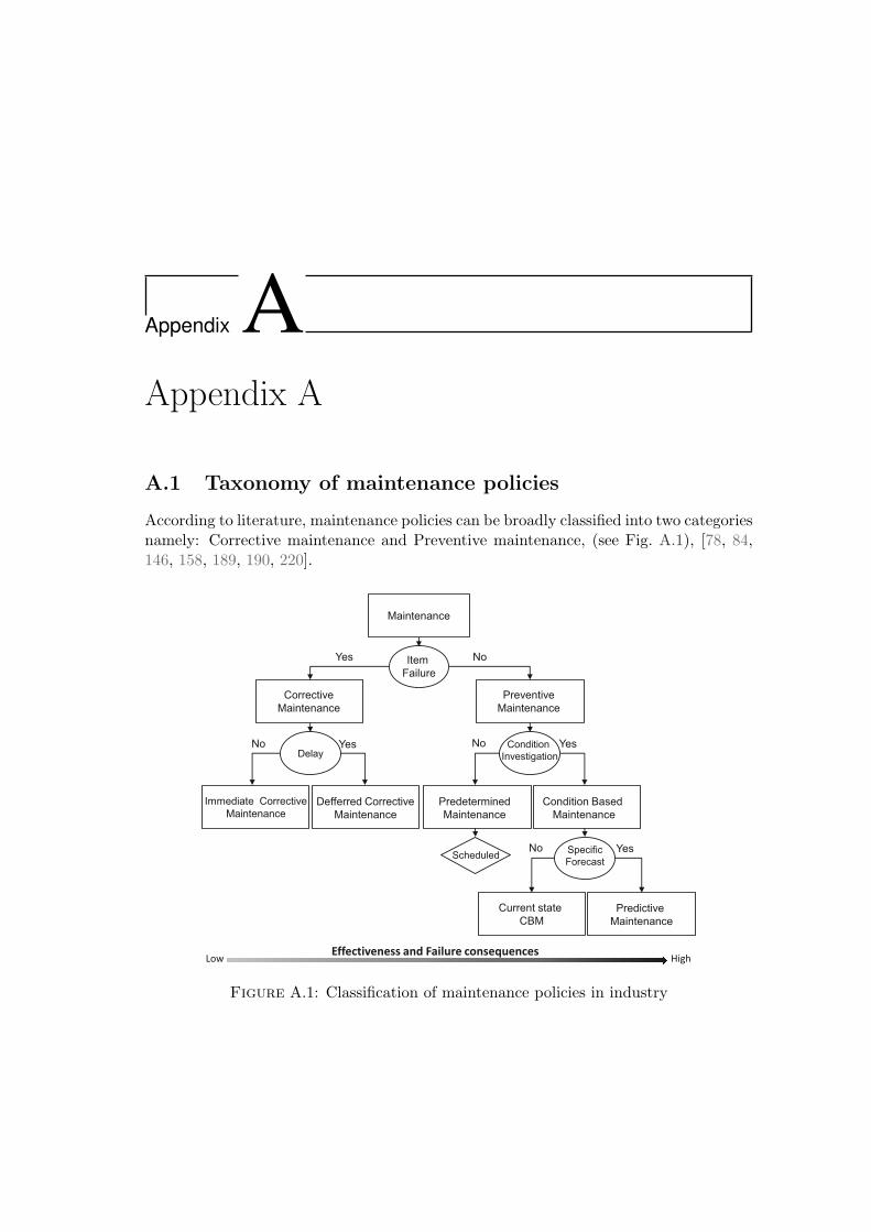
Appendix AAppendix A
A.1 Taxonomy of maintenance policies
According to literature, maintenance policies can be broadly classified into two categoriesnamely: Corrective maintenance and Preventive maintenance, (see Fig. A.1), [78, 84,146, 158, 189, 190, 220].
Maintenance
Corrective
Maintenance
Preventive
Maintenance
Item
Failure
Defferred Corrective
Maintenance
Immediate Corrective
Maintenance Condition Based
Maintenance
Predetermined
Maintenance
Condition
Investigation Delay
Specific
Forecast Scheduled
Effectiveness and Failure consequences Low High
Yes No
YesNo Yes No
Yes No
Predictive
Maintenance
Current state
CBM
Figure A.1: Classification of maintenance policies in industry

146 Appendix A
A.1.1 Corrective maintenance
Corrective maintenance is an earliest form of maintenance that is unplanned (or reactive)and is undertaken after machinery breakdown. A failed item is repaired or replacedwith a new one to store functional capabilities. This type of maintenance can be furthercategorized as immediate corrective maintenance or deferred corrective maintenance [78].However, such maintenance is suitable for non-critical engineering assets, where failureconsequences are slight and no immediate safety risks are involved. In other words, itshould be used when there are no serious consequences of unscheduled downtime.
A.1.2 Preventive maintenance
Preventive maintenance is a planned (or proactive) strategy for maintaining machinery,that was introduced in 1950s [189]. The main objective was to increase availability of ma-chinery as compared to corrective maintenance. Preventive maintenance can be furtherclassified as predetermined maintenance and Condition Based Maintenance (CBM).
A.1.2.1 Predetermined maintenance
With predetermined maintenance repairs are performed on the basis of pre-definedschedule (or fixed intervals). Maintenance tasks are carried periodically (like lubri-cation, calibration, refurbishing, checking and inspecting machinery) after fixed timeintervals to decrease the deterioration phenomena [190]. However, the maintenance pro-cedures do not involve evaluation of current state in particular. Although predeterminedmaintenance can be a simple approach to maintain equipment, it can be costly due tounnecessary stoppages or replacements of operating machinery. Another problem of thisapproach is that failures are assumed to occur in well defined intervals [115].
A.1.2.2 Condition-Based Maintenance (CBM)
CBM strategy is a step forward from predetermined maintenance, as it utilizes real-timecondition monitoring data to maintain machinery, and repair only when need arises[63, 158]. Therefore, unnecessary maintenance procedures are avoided and maintenancecosts are reduced significantly. A CBM program has three main stages that are discussedin [105]: 1) data-acquisition, 2) data pre-processing and 3) decision making. The firststage is a building block for CBM procedure, where monitored information is gatheredand stored. In the second stage feature extraction and selection tasks are performed.Lastly, the third stage of decision making recommends maintenance actions throughdiagnostics (for fault detection, isolation and identification) and prognostics of degradingequipment. Having knowledge of the current state of the equipment, and predicting itsfuture behavior are the basis of CBM [106]. Therefore, in industrial context CBMapproach can be of two types.
Current state CBM: in this case CBM is based only on the current-state of theequipment and do not include prediction / forecasting of future states of the degrading

A.2 Relation between diagnostics and prognostics 147
equipment. Therefore, maintenance decisions are based on the estimation of current-state only and equipment is run as long as it is healthy [78, 158].
Predictive maintenance: it is an innovative maintenance approach that is foundedon assessment of current health state of equipment and on the prediction of future evo-lution (i.e., prognostics) using specific future conditions. It means, the same item couldhave different service life, when different future conditions are applied [18, 78, 105]. Iden-tification of problems at early stages and estimation of remaining operating life enablesthe machinery to run till healthy state, and provide time to opportunely plan / sched-uled necessary maintenance actions prior to break down.
A.2 Relation between diagnostics and prognostics
Like prognostics, diagnostic is also an important element of PHM cycle (section 1.1.1).In literature, there is a little disagreement, that prognostics is related to and highlydependent upon diagnostics. Mainly, diagnostics involves fault / failure detection, isola-tion and identification of damage that has occurred, while prognostics is concerned withRUL estimation and associated confidence interval (see Fig. A.2).Therefore, in terms of relation between diagnostics and prognostics, diagnostics processdetects and identifies a fault / failure that has caused degradation, where prognosticsprocess generates a rational estimation of RUL until complete failure [178]. However,in general, diagnostics is a reactive process that is performed after the occurrence offault / failure and cannot stop machine downtime in, where a prognostics is a predict-to-prevent behavior [120]. It should be noted that there is a difference between “faultdiagnostics” and “failure diagnosis”. The terminology of fault diagnostics implies that,the machinery under observation is still operational, however, cannot continue oper-ating indefinitely without any maintenance intervention. Where, failure diagnostics isperformed on machinery that has ceased to perform its functionality [35].As compared to prognostic, diagnostics domain is well developed and has several ap-plications in industry. The main approaches for diagnostics can be model based ordata-driven, however these topics are not covered in the thesis (see [212]).
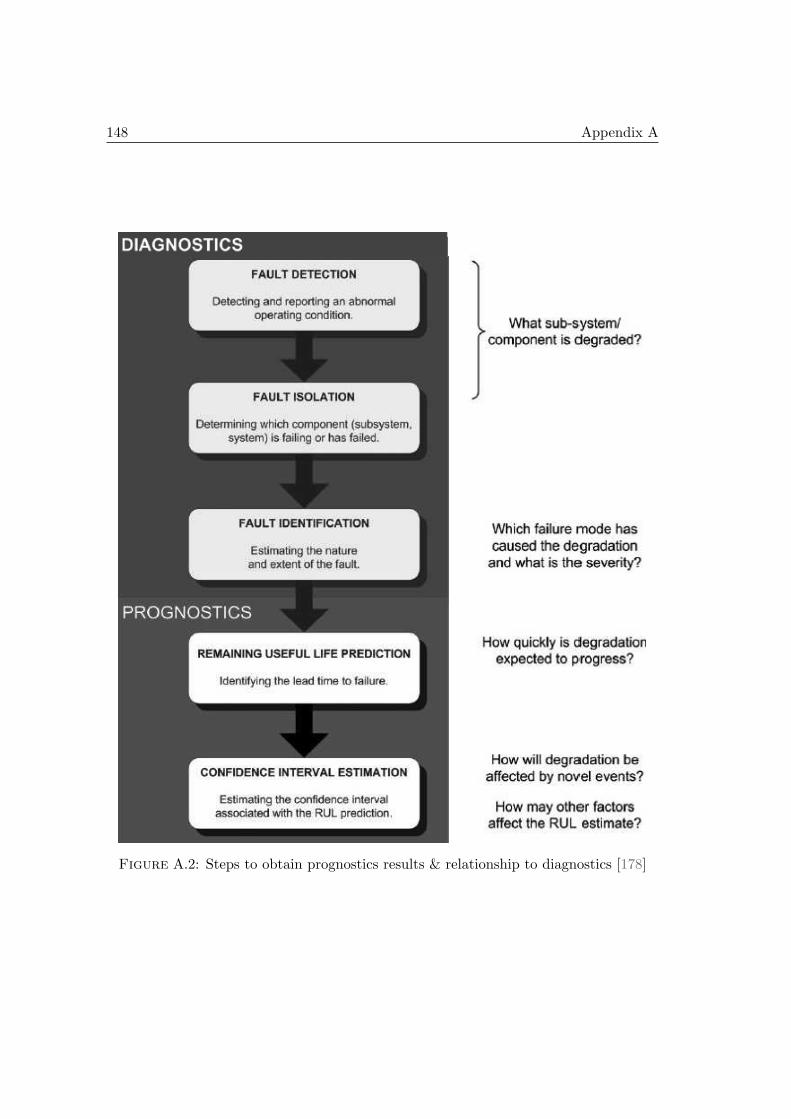
148 Appendix A
Figure A.2: Steps to obtain prognostics results & relationship to diagnostics [178]

A.3 FCM algorithm 149
A.3 FCM algorithm
According to [29], the main steps of FCM algorithms are summarized as follows.
Algorithm 4 Key steps of FCM algorithm
Require - Learning dataset Eq. (3.1)- No. of clusters c, initial Cluster centers V , Fuzziness parameter m
Ensure - Cluster centers V and fuzzy partitioning U
learning procedure
1: Compute fuzzy partition matrix U
µij =1
∑ck=1
(
‖xi−vj‖‖xi−vk‖
) 2
m−1
∀ i,j (A.1)
2: Adjust cluster centers vnew
vnewj =
∑Ni=1 µ
mij .xi
∑Ni=1 µ
mij
∀ j (A.2)
3: Repeat step 1 and 2 untill termination criteria is met
∥
∥
∥vnew − vold∥
∥
∥ < ǫ (A.3)
A.4 Metrics for model accuracy
• MAPE: the mean absolute percentage error, or known as mean absolute percentagedeviation (MAPD). MAPE usually expresses accuracy as a percentage and can beformulated as follows,
MAPE =100
n
n∑
i=1
∣
∣
∣
∣
yi − yiyi
∣
∣
∣
∣
(A.4)
where yi indicates the actual value and yi indicates the predicted value.
• R2: evaluates the variability in the actual values explained by the model and canbe computed by dividing explained variation by total variation:
R2 = 1− SSE
SSyy(A.5)

150 Appendix A
where SSE is the measure of deviation of observations from the predicted values,i.e., SSE =
∑
i (yi − yi)2, and SSyy is the measure of observation from the mean
value, i.e., SSyy =∑
i (yi − y)2.
• CVRMSE: Coefficient of Variation of the Root Mean Squared Error evaluates therelative closeness of the predictions to the actual values and can be formulated as,
CV RMSE = 100× RMSE
y(A.6)
where RMSE is the root mean square error i.e.,
RMSE =
√
∑ni=1 (yi − yi)
2
n(A.7)
It should be noted that, all metrics are unit less.
A.5 Benchmark datasets
A.5.1 Carnallite surge tank dataset
The dataset was provided by Arab Potash company [170]. Mainly, the data were ac-quired from a critical component called as Carnallite surge tank pump to perform condi-tion monitoring task in an intelligent manner. The main objective was to replace visualinspection (human) for condition monitoring with an automated system to detect faultsand avoid breakdowns.Data were collected from component item 13, and were further divided into three bins,each containing two different time signal features, namely the root mean square (RMS)and the variance (σ2) Fig. A.3, and their corresponding fault code Fig. A.4. The testsaim at approximating the output “fault codes” by feeding neural networks with twoinputs (RMS and σ2). The whole dataset consists of 92 samples, from which 73 sampleswere used to learn the models, whereas the remaining 19 were used for testing purpose.
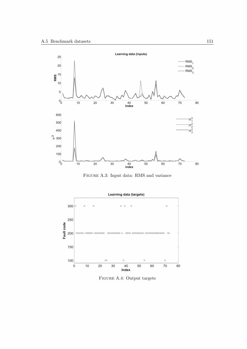
A.5 Benchmark datasets 151
0 10 20 30 40 50 60 70 80 0
100
200
300
400
500
600
index
s 2
0 10 20 30 40 50 60 70 80 0
5
10
15
20
25
Index
RM
S
Learning data (inputs)
RMS 1
RMS 2
RMS 3
s 2
1
s 2
2
s 2
3
Figure A.3: Input data: RMS and variance
0 10 20 30 40 50 60 70 80
100
150
200
250
300
Index
Fau
lt c
od
e
Learning data (targets)
Figure A.4: Output targets
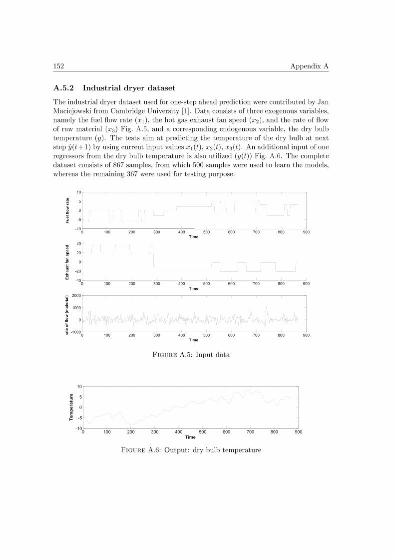
152 Appendix A
A.5.2 Industrial dryer dataset
The industrial dryer dataset used for one-step ahead prediction were contributed by JanMaciejowski from Cambridge University [1]. Data consists of three exogenous variables,namely the fuel flow rate (x1), the hot gas exhaust fan speed (x2), and the rate of flowof raw material (x3) Fig. A.5, and a corresponding endogenous variable, the dry bulbtemperature (y). The tests aim at predicting the temperature of the dry bulb at nextstep y(t+1) by using current input values x1(t), x2(t), x3(t). An additional input of oneregressors from the dry bulb temperature is also utilized (y(t)) Fig. A.6. The completedataset consists of 867 samples, from which 500 samples were used to learn the models,whereas the remaining 367 were used for testing purpose.
0 100 200 300 400 500 600 700 800 900 -10
-5
0
5
10
Time
Fu
el fl
ow
rate
0 100 200 300 400 500 600 700 800 900 -40
-20
0
20
40
Time
Ex
ha
us
t fa
n s
pe
ed
0 100 200 300 400 500 600 700 800 900 -1000
0
1000
2000
Time
rate
of
flo
w (
ma
teri
al)
Figure A.5: Input data
0 100 200 300 400 500 600 700 800 900 -10
-5
0
5
10
Time
Te
mp
era
ture
Figure A.6: Output: dry bulb temperature
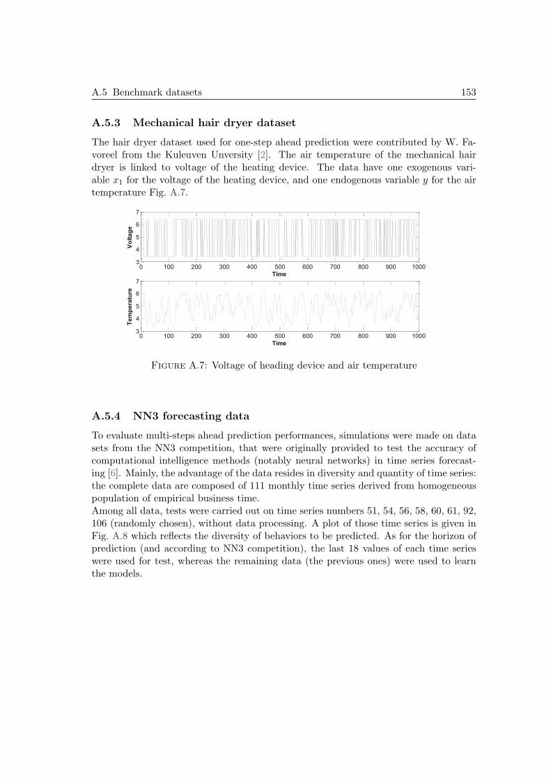
A.5 Benchmark datasets 153
A.5.3 Mechanical hair dryer dataset
The hair dryer dataset used for one-step ahead prediction were contributed by W. Fa-voreel from the Kuleuven Unversity [2]. The air temperature of the mechanical hairdryer is linked to voltage of the heating device. The data have one exogenous vari-able x1 for the voltage of the heating device, and one endogenous variable y for the airtemperature Fig. A.7.
0 100 200 300 400 500 600 700 800 900 10003
4
5
6
7
Time
Vo
lta
ge
0 100 200 300 400 500 600 700 800 900 10003
4
5
6
7
Time
Te
mp
era
ture
Figure A.7: Voltage of heading device and air temperature
A.5.4 NN3 forecasting data
To evaluate multi-steps ahead prediction performances, simulations were made on datasets from the NN3 competition, that were originally provided to test the accuracy ofcomputational intelligence methods (notably neural networks) in time series forecast-ing [6]. Mainly, the advantage of the data resides in diversity and quantity of time series:the complete data are composed of 111 monthly time series derived from homogeneouspopulation of empirical business time.Among all data, tests were carried out on time series numbers 51, 54, 56, 58, 60, 61, 92,106 (randomly chosen), without data processing. A plot of those time series is given inFig. A.8 which reflects the diversity of behaviors to be predicted. As for the horizon ofprediction (and according to NN3 competition), the last 18 values of each time serieswere used for test, whereas the remaining data (the previous ones) were used to learnthe models.
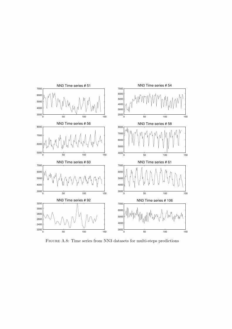
0 50 100 1503000
4000
5000
6000
7000NN3 Time series # 51
0 50 100 1502000
3000
4000
5000
6000
7000
NN3 Time series # 54
0 50 100 1505000
6000
7000
8000
NN3 Time series # 56
0 50 100 1504000
5000
6000
7000
8000
NN3 Time series # 58
0 50 100 1503000
4000
5000
6000
7000
NN3 Time series # 60
0 50 100 1503000
4000
5000
6000
7000
NN3 Time series # 61
0 50 100 1502200
2400
2600
2800
3000
3200
NN3 Time series # 92
0 50 100 1503000
4000
5000
6000
7000
NN3 Time series # 106
Figure A.8: Time series from NN3 datasets for multi-steps predictions

Publications (February 2011 - January 2014)
Journal Articles
• Javed K., Gouriveau R., Zerhouni N, SW-ELM: A summation wavelet extremelearning machine algorithm with a priori parameter initialization, Neurocomput-ing, Vol. 123, pp. 299-307, January 2014.
• Javed K., Gouriveau R., Zerhouni N, Enabling health monitoring approach basedon vibration data for accurate prognostics, IEEE Transactions on Industrial Elec-tronics, Accepted.
• Javed K., Gouriveau R., Zerhouni N, , Li X., Improving Robustness and Relia-bility of Tool Wear Monitoring and Prognostics: A Summation Wavelet-ExtremeLearning Machine Approach, Engineering Applications of Artificial Intelligence,Revised Manuscript Under Review.
In progress
• Javed K., Gouriveau R., Zerhouni N, A new multivariate approach for prognosticsbased on Extreme Learning Machine & Fuzzy clustering.
• Javed K., Gouriveau R., Zerhouni N, A survey and taxonomy of prognostics ap-proaches.
Conferences
• Javed K., Gouriveau R., Zerhouni N, Novel failure prognostics approach with dy-namic thresholds for machine degradation, In: Proceedings of the 39th AnnualConference of the IEEE Industrial Electronics Society, IECON 2013, Vienna, Aus-tria, 10-13 November 2013.
• Javed K., Gouriveau R., Zerhouni N, A feature extraction procedure based ontrigonometric functions and cumulative descriptors to enhance prognostics mod-eling and estimates, In: Proceedings of the IEEE International Conference onPrognostics and Health Management, IEEE PHM 2013, Gaithersburg, MD, USA,24-27 June 2013.
• Javed K., Gouriveau R., Zemouri R., Zerhouni N, Features Selection Procedurefor Prognostics: An Approach Based on Predictability, In: Proceedings of the 8thIFAC International Symposium on Fault Detection, Supervision and Safety forTechnical Processes, SAFEPROCESS 2012, Mexico, 29-31 August 2012.

• Javed K., Gouriveau R., Zerhouni N., Zemouri R., Li X., Robust, reliable andapplicable tool wear monitoring and prognostic: approach based on an Improved-Extreme Learning Machine, In: Proceedings of the IEEE International Conferenceon Prognostics and Health Management, IEEE PHM 2012, Denver, CO, USA, 18-21 June 2012.
• Javed K., Gouriveau R., Zemouri R., Zerhouni N, Improving data-driven prognos-tics by assessing predictability of features, In: Proceedings of the Annual Confer-ence of the Prognostics and Health Management Society, PHM 2011, Montreal,QC, Canada, 25-29 September 2011.


Resume :
Le pronostic industriel vise a etendre le cycle de vie d’un dispositif physique, tout en reduisant les couts d’ex-
ploitation et de maintenance. Pour cette raison, le pronostic est considere comme un processus cle avec
des capacites de prediction. En effet, des estimations precises de la duree de vie avant defaillance d’un
equipement, Remaining Useful Life (RUL), permettent de mieux definir un plan d’action visant a accroıtre
la securite, reduire les temps d’arret, assurer l’achevement de la mission et l’efficacite de la production.
Des etudes recentes montrent que les approches guidees par les donnees sont de plus en plus appliquees
pour le pronostic de defaillance. Elles peuvent etre considerees comme des modeles de type boite noire pour
l’etude du comportement du systeme directement a partir des donnees de surveillance d’etat, pour definir l’etat
actuel du system et predire la progression future de defauts. Cependant, l’approximation du comportement des
machines critiques est une tache difficile qui peut entraıner des mauvais pronostic. Pour la comprehension
de la modelisation du pronostic guide par les donnees, on considere les points suivants. 1) Comment trai-
ter les donnees brutes de surveillance pour obtenir des caracteristiques appropriees refletant l’evolution de la
degradation? 2) Comment distinguer les etats de degradation et definir des criteres de defaillance (qui peuvent
varier d’un cas a un autre)? 3) Comment etre sur que les modeles definis seront assez robustes pour montrer
une performance stable avec des entrees incertaines s’ecartant des experiences acquises, et seront suffisam-
ment fiables pour integrer des donnees inconnues (c’est a dire les conditions de fonctionnement, les variations
de l’ingenierie, etc.)? 4) Comment realiser facilement une integration sous des contraintes et des exigences
industrielles? Ces questions sont des problemes abordes dans cette these. Elles ont conduit a developper une
nouvelle approche allant au-dela des limites des methodes classiques de pronostic guide par les donnees. Les
principales contributions sont les suivantes.
– L’etape de traitement des donnees est amelioree par l’introduction d’une nouvelle approche d’extraction
des caracteristiques a l’aide de fonctions trigonometriques et cumulatives qui sont basees sur trois ca-
racteristiques : la monotonie, la “trendability” et la previsibilite. L’idee principale de ce developpement est de
transformer les donnees brutes en indicateurs qui ameliorent la precision des previsions a long terme.
– Pour tenir compte de la robustesse, de la fiabilite et de l’applicabilite, un nouvel algorithme de prediction
est propose: Summation Wavelet-Extreme Learning Machine (SW-ELM). Le SW-ELM assure de bonnes
performances de prediction, tout en reduisant le temps d’apprentissage. Un ensemble de SW-ELM est
egalement propose pour quantifier l’incertitude et ameliorer la precision des estimations.
– Les performances du pronostic sont egalement renforcees grace a la proposition d’un nouvel algorithme
d’evaluation de la sante du system: Subtractive-Maximum Entropy Fuzzy Clustering (S-MEFC). S-MEFC est
une approche de classification non supervisee qui utilise l’inference de l’entropie maximale pour representer
l’incertitude de donnees multidimensionnelles. Elle peut automatiquement determiner le nombre d’etats,
sans intervention humaine.
– Le modele de pronostic final est obtenu en integrant le SW-ELM et le S-MEFC pour montrer l’evolution de la
degradation de la machine avec des predictions simultanees et l’estimation d’etats discrets. Ce programme
permet egalement de definir dynamiquement les seuils de defaillance et d’estimer le RUL des machines
surveillees.
Les developpements sont valides sur des donnees reelles a partir de trois plates-formes experimentales: PRO-
NOSTIA FEMTO-ST (banc d’essai des roulements), CNC SIMTech (fraises d’usinage), C-MAPSS NASA (tur-
boreacteurs) et d’autres donnees de reference. Toutefois, la perspective principale de ce travail est d’ameliorer
la fiabilite du modele de pronostic.
Mots-cles : Prognostics, Data-driven, Extreme learning Machine, Fuzzy Clustering, RUL