THREE EMPRICAL ESSAYS ON MERGERS AND REGULATION IN

THREE EMPRICAL ESSAYS ON MERGERS AND REGULATION IN THE TELECOMMUNICATIONS INDUSTRY

by

DAIGYO SEO

B.A., Hanyang University, 1996 M.S., Hanyang University, 1998

M.A., University of Pittsburgh, 2002

AN ABSTRACT OF A DISSERTATION

submitted in partial fulfillment of the requirements for the degree

DOCTOR OF PHILOSOPHY

Department Of Economics College of Arts and Science

KANSAS STATE UNIVERSITY Manhattan, Kansas

2007

brought to you by COREView metadata, citation and similar papers at core.ac.uk

provided by K-State Research Exchange

https://core.ac.uk/display/5164574?utm_source=pdf&utm_medium=banner&utm_campaign=pdf-decoration-v1

Abstract

This empirical dissertation consists of three essays on mergers and regulation in the U.S.

telecommunications industry. An abstract for each of the three essays follows.

Essay 1: This study has attempted to measure the productivity growth associated with 25

incumbent local exchange carriers (ILECs) over the period 1996-2005 using a Malmquist

productivity index. The average efficiency scores for our sample companies have not changed

significantly between 1996 and 2005, which indicates that the average ILECs shows no

measurable improvement in terms of optimizing their input-output combinations over time. We

find some empirical evidence of a positive merger effect, although this effect diminishes over

time. In addition, we find that non-merged firms underperform in terms of average productivity

growth.

Essay 2: This study analyzes the merger effects for 25 ILECs over the period 1996-2005

using stochastic frontier analysis with a time-varying inefficiency model. In addition, we conduct

a comparison of indices between the stochastic frontier analysis and the Malmquist index method.

The empirical results indicate that the sample of telecommunications firms has experienced

deterioration in average productivity growth following the mergers. In addition, both approaches

suggest that firms that do not merge underperform in terms of average productivity growth.

Essay 3: This essay investigates whether the substitution of price cap regulation (PCR), along

with other regulatory regimes, for traditional rate of return regulation (RRR) has had a

measurable effect on productivity growth in the U.S. telecommunications industry. A stochastic

frontier approach, which differs from previous studies, is employed to compute efficiency

change, technological progress, and productivity growth for 25 LECs over the period 1988-1998.

By examining the relationship between the change in productivity growth and regulatory regime

variables, while controlling for other effects, we find that PCR and other regulatory regimes have

a positive effect on productivity growth. However, only PCR has a significant and positive

effect in both contemporaneous and lagged model specifications.

THREE EMPIRICAL ESSAYS ON MERGERS AND REGULATION IN THE U.S. TELECOMMUNICATIONS INDUSTRY

by

DAIGYO SEO

B.A., Hanyang University, 1996 M.S., Hanyang University, 1998

M.A., University of Pittsburgh, 2002

A DISSERTATION

submitted in partial fulfillment of the requirements for the degree

DOCTOR OF PHILOSOPHY

Department of Economics College of Arts and Science

KANSAS STATE UNIVERSITY Manhattan, Kansas

2007

Approved by:

Major Professor Dennis L. Weisman

Abstract

This empirical dissertation consists of three essays on mergers and regulation in the U.S.

telecommunications industry. An abstract for each of the three essays follows.

Essay 1: This study has attempted to measure the productivity growth associated with 25

incumbent local exchange carriers (ILECs) over the period 1996-2005 using a Malmquist

productivity index. The average efficiency scores for our sample companies have not changed

significantly between 1996 and 2005, which indicates that the average ILECs shows no

measurable improvement in terms of optimizing their input-output combinations over time. We

find some empirical evidence of a positive merger effect, although this effect diminishes over

time. In addition, we find that non-merged firms underperform in terms of average productivity

growth.

Essay 2: This study analyzes the merger effects for 25 ILECs over the period 1996-2005

using stochastic frontier analysis with a time-varying inefficiency model. In addition, we conduct

a comparison of indices between the stochastic frontier analysis and the Malmquist index method.

The empirical results indicate that the sample of telecommunications firms has experienced

deterioration in average productivity growth following the mergers. In addition, both approaches

suggest that firms that do not merge underperform in terms of average productivity growth.

Essay 3: This essay investigates whether the substitution of price cap regulation (PCR),

along with other regulatory regimes, for traditional rate of return regulation (RRR) has had a

measurable effect on productivity growth in the U.S. telecommunications industry. A stochastic

frontier approach, which differs from previous studies, is employed to compute efficiency

change, technological progress, and productivity growth for 25 LECs over the period 1988-1998.

By examining the relationship between the change in productivity growth and regulatory regime

variables, while controlling for other effects, we find that PCR and other regulatory regimes have

a positive effect on productivity growth. However, only PCR has a significant and positive

effect in both contemporaneous and lagged model specifications.

vii

Table of Contents

List of Figures ............................................................................................................................... ix

List of Tables ................................................................................................................................. x

Acknowledgements...................................................................................................................... xii

Dedication ................................................................................................................................... xiii

Chapter 1 - Introduction................................................................................................................. 1

Chapter 2 - Productivity Growth and Merger Efficiencies in the U.S. Telecommunications

Industry ................................................................................................................................... 6

INTRODUCTION ...................................................................................................................... 6

METHODLOGY ...................................................................................................................... 10

DATA ....................................................................................................................................... 17

EMPIRICAL RESULTS........................................................................................................... 18

CONCLUSION......................................................................................................................... 21

Figures and Tables .................................................................................................................... 23

Chapter 3 - Market Consolidation and Productivity Growth in U.S. Telecommunications:

Stochastic Frontier analysis vs. Malmquist index......................................................................... 32

INTRODUCTION .................................................................................................................... 32

METHODOLOGY ................................................................................................................... 36

Distance Functions................................................................................................................ 36

Stochastic Frontier Model..................................................................................................... 37

A Malmquist Index Approach .............................................................................................. 41

DATA ....................................................................................................................................... 43

EMPIRICAL RESULTS........................................................................................................... 45

CONCLUSION......................................................................................................................... 48


Chapter 4 - The Impact of Incentive Regulation on the U.S. Telecommunications Industry:

A Stochastic Frontier Approach ............................................................................................ 59

INTRODUCTION .................................................................................................................... 59

viii

THEORY OF STOCHASTIC FRONTIER ANALYSIS ......................................................... 62

Distance Function ................................................................................................................. 62

Stochastic Frontier Analysis ................................................................................................. 63

Data and Productivity Growth .............................................................................................. 66

THE EFFECTS OF PCR ON THE PRODUCTIVITY GROWTH CHANGE........................ 70

Regulatory Regime Variables ............................................................................................... 70

Control Variables .................................................................................................................. 70

Econometric Specification .................................................................................................... 72

CONCLUSION......................................................................................................................... 74


Chapter 5 - Conclusion ................................................................................................................. 82

References..................................................................................................................................... 84

ix

List of Figures

Figure 2.1 Output-Oriented DEA ................................................................................................. 23

Figure 2.2 Output Distance Function............................................................................................ 24

Figure 3.1 Output Distance Function............................................................................................ 50

x

List of Tables

Table 2.1 History of Mergers among RBOCs .............................................................................. 25

Table 2.2 Summary Statistics ....................................................................................................... 26

Table 2.3 Technical Efficiency Scores, 1996-2005 ...................................................................... 27

Table 2.4 Peers from DEA, 1996-2005 ........................................................................................ 28

Table 2.5 Mean Technical Efficiency change, Technological change and Productivity change,

1996-2005 ............................................................................................................................. 29

Table 2.6 Mean Technical Efficiency Change, Technological Change, and Productivity Growth

Change, 3 years before and 3 years after merger.................................................................. 30


Change, Pre-merger and Post-merger ................................................................................... 31

Table 3.1 Summary Statistics ....................................................................................................... 51

Table 3.2 LR Tests of hypotheses for parameters of stochastic production frontier model ......... 52

Table 3.3 Estimated parameters for stochastic production frontier model ................................... 53

Table 3.4 Mean Technical Efficiency change, Technological change and Productivity change for

SFM, 1996-2005 ................................................................................................................... 54

Table 3.5 Technological Change for SFM, 1996-2005 ................................................................ 55


Change for SFM, Pre-merger and Post-merger .................................................................... 56

Table 3.7 Mean Efficiency Change and Technological Change between Stochastic Frontier

Model and Malmquist Index, Pre-merger and Post-merger.................................................. 57

Table 3.8 Comparison of Mean Productivity Growth Change between Stochastic Frontier Model

and Malmquist Index, Pre-merger and Post-merger ............................................................. 58

Table 4.1 LR Tests of hypotheses for parameters of stochastic production frontier model ......... 76

Table 4.2 Estimated parameters for stochastic production frontier model ................................... 77

Table 4.3 Sample Mean of Technical Efficiency Change, Technological Change, and

Productivity Growth Change Using a Stochastic Frontier Approach................................... 78

xi


Change, 1988-1990 and 1991-1998...................................................................................... 79

Table 4.5 Summary Statistics for Explanatory Variables............................................................. 80

Table 4.6 Factors Explaining Productivity Growth Change......................................................... 81

xii

Acknowledgements

The deepest appreciation goes to my major advisor, Dr. Dennis L. Weisman, who has

been my “American father” for many years. Throughout my Ph.D. program, he has constantly

guided and encouraged me to challenge the toughest issues in the field of microeconomics. In

addition to his academic guidance, his thoughtful consideration and kindness in the way he lives

his daily life served as an exceptional lesson to me. I truly believe that having him as my main

advisor was one of the luckiest things in my entire life.

Special thanks go to Dr. Allen Featherstone. He has given me the opportunity to learn

production economics, which, in fact, turned out to be a significant contribution to my

dissertation. I would like to thank Dr. Tracy M. Turner for giving me the opportunity to join her

research project, which I very much enjoyed. I would also like to thank my dissertation

committee members, Dr. Dong Li, Dr. Philip G. Gayle, and Dr. John M. McCulloh, for their

invaluable help and guidance. Finally, I would like to thank my fellow Korean graduate student,

Shin-Jae Kang.

xiii

Dedication

This dissertation is dedicated to my beloved family, especially to my parents and my wife,

Yeonkyung Ha, for endless encouragement, support, and patience.

1

CHAPTER 1 - Introduction

This dissertation is comprised of three empirical essays that investigate mergers and regulation in

the U.S. telecommunications industry. The first two essays address the effect of a series of

mergers in the telecommunications industry after the passage of the 1996 Telecommunications

Act (1996 Act). The third essay analyzes the effect of implementation of incentive regulation in

telecommunications industry.

The primary objective of Chapter 2 is to investigate whether productivity growth has

increased among incumbent local exchange carriers (ILECs) that have merged since the 1996

Telecommunications Act and whether the merged firms performed better than firms that did not

merge in terms of productivity growth during the period 1996-2005 .

Mergers can be either a pro-competitive or anti-competitive in terms of their effect on

industry performance, including productive efficiency. The horizontal merger guidelines (HMG)

of the U.S. Department of Justice (DOJ) rely, in part, upon market concentration in evaluating

whether particular mergers raise anticompetitive concerns. In addition to market concentration,

the HMG also take into account potential adverse competitive effects and entry analysis in

evaluating proposed mergers. Specifically, Section 4 of the HMG (revised April 8, 1997)

describes the significance of merger efficiencies. When the efficiency gains from a merger,

which may result in lower prices or quality improvements, are expected to outweigh the other

effects of the merger that may serve to lessen competition, the agency will consider approving

the proposed merger. These observations notwithstanding, it is difficult in practice to verify and

quantify these merger efficiencies.

A Malmquist productivity growth index introduced by Caves et al. (1982) and further

developed by Färe et al. (1994) is employed to compute productivity growth, which is comprised

2

of technical efficiency change and technological change. In addition, this essay measures firm-

level technical efficiencies using dynamic data envelope analysis (DEA) to evaluate the ILECs’

ability to optimize output over time.

The main findings of this essay indicate that mergers positively affect average

productivity growth, but that this effect decreases over time. In addition, firms that have not

merged under-perform firms that have merged in terms of average productivity growth.

The primary objective of Chapter 3 is to evaluate the effectiveness of mergers that

occurred between 1996 and 2005 using stochastic frontier analysis (SFA). This essay

investigates whether productivity growth has increased among ILECs that have merged since the

1996 Act and whether the merged firms performed better than those firms that did not merge.

The second objective is to compare the results on productivity growth between the SFA and the

Malmquist index approach. This comparison provides useful information on the robustness of

the efficiency findings across different approaches.

One of the methods that may be used to examine efficiencies is to measure productivity

growth, inclusive of its underlying components--technological progress and changes in technical

efficiency. From a policy perspective, the decomposition of productivity growth into these

components provides important information for analysis. For example, if policymakers are able

to determine the key drivers of productivity growth, they may adopt policies that can

significantly improve the performance of firms in the industry and hence the overall economy.

Suppose, for example, that a lack of technological progress is the source of low productivity

growth. It would then be possible to adopt various policies that serve to stimulate technological

innovation and move the technology frontier outward over time. If high rates of technological

3

change associated with low rates of efficiency change are measured, then policy makers may

focus on the policy that increases the efficiency of the individual firms.

Chapter 3 finds that the firm sample has experienced deterioration in average productivity

growth following the merger. This empirical finding is attributed to technological regression, a

finding that may lead policymakers to consider implementing policies that serve to shift out the

production frontier over time. In terms of average growth in productivity, the only firm in the

sample not to have merged ranks third lowest among the 25 ILECs.

Another component of this chapter is a comparison of indices for the stochastic frontier

analysis and the Malmquist index method. This comparison provides useful information on

robustness. With the exception of one firm using the Malmquist index method, both methods

indicate that every firm in the sample has experienced negative annual growth in technological

change. Indices of productivity growth suggest that most of the firms experience negative

growth in annual productivity growth following the merger across both methods. However, in

terms of productivity growth, it is noteworthy that the only firm not to have merged

underperforms relative to the firms that have merged during the post-merger periods. In SFA,

annual productivity growth for BellSouth is the third lowest in the sample and the fourth lowest

using the Malmquist index method.

The primary objective of Chapter 4 is to measure productivity growth associated with

technological progress and changes in technical efficiency in order to examine the improvement

in the local exchange carriers’ (LECs’) productivity growth. In addition, this essay analyzes the

effects associated with the adoption of incentive regulation on the LECs’ productivity growth

rate.

4

A large volume of research has examined the effects of the implementation of incentive

regulation regimes. Schmalensee and Rohlfs (1992) examined the effect of price cap regulation

(PCR) on productivity gains. They found that the cumulative productivity gains increased $1.8

billion over the period of price cap regulation (PCR) relative to the pre price-cap period.

Majumdar (1997) employed a non-parametric approach, commonly referred to as data

envelopment analysis (DEA), to examine the effect of incentive regulation on the productive

performance of 45 local exchange carriers (LECs) over the period 1988-1993. He showed that

PCR has a positive but lagged effect on technical efficiency. Uri (2001) used a Malmquist index

to measure the change in productivity growth following the implementation of incentive

regulation. He found that productivity growth increased by approximately 5 percent per year for

the 19 LECs over the period 1988-1999.

Although a number of empirical studies have found that the effect of incentive regulation

on productivity growth in the U.S. telecommunications industry is substantially positive, some

have concluded that the effect of incentive regulation is ambiguous. For example, Resende

(1999) estimated a translog cost function combined with a total factor productivity (TFP) growth

decomposition for the period 1989-1994. He found that incentive regulation did not enhance the

level of productive efficiency. Uri (2002) employed a corrected ordinary least squares (COLS)

approach to measure the efficiency gains associated with the implementation of incentive

regulation in the U.S. telecommunications industry. Using data from 19 LECs over the 1988-

1999 period, he found no empirical evidence that incentive regulation had enhanced technical

efficiency.

The results of Chapter 4 broadly indicate that the adoption of PCR and incentive

regulation (IR), more generally, has had a positive impact on operating performance in the U.S.

5

telecommunications industry. By examining the relationship between productivity growth and

regulatory regime variables, while controlling for all other effects, we find that PCR and other

forms of incentive regulation have a positive effect on productivity growth. It is noteworthy,

however, that only PCR has a significant and positive effect on productivity growth in both

contemporaneous and lagged model specifications.

6

CHAPTER 2 - Productivity Growth and Merger Efficiencies in the

U.S. Telecommunications Industry

INTRODUCTION

In 1974, the U.S. Department of Justice (DOJ) initiated an anti-trust suit against AT&T that was

ultimately settled on January 8, 1982.1 On January 1, 1984, AT&T’s local operating companies

were divested into seven independent Regional Holding Companies known as the Regional Bell

Operating Companies (RBOCs). 2, 3 Following this divestiture, AT&T provided long distance

service and the seven RBOCs provided primarily local telephone service and intraLATA long-

distance service.4 The RBOCs were prohibited from providing interLATA long-distance service.

This de facto quarantine imposed on the RBOCs was designed to spur competition in long-

distance and telecommunications equipment markets. The expectation was that the gains from

the ensuing competition would outweigh the loss of economies of scope that derive from the

joint provision of local and long distance telecommunications (Baxter, 1991, p.30).

The passage of the 1996 Telecommunications Act (1996 Act) was the next significant

event designed to further stimulate competition in telecommunications markets.5 This statute

required local exchange carriers (LECs) to unbundle their networks and share the component

1 See Chapter 2 in Sappington and Weisman (1996) for a detailed history of these industry developments. 2 The seven RBOCs were Ameritech Corporation, Bell Atlantic Corporation, BellSouth Corporation, NYNEX Corporation, Pacific Telesis Group, Southwestern Bell Corporation and U S West, Inc. 3 In addition to the seven RBOCs, two smaller companies, Cincinnati Bell and Southern New England Telephone (SNET), became stand-alone companies after the settlement. There were also several operating companies such as GTE, United, Continental and Central telephone system that are known as independent telephone companies because they were never part of the Bell System. 4 As part of the break-up of AT&T, the U.S. was partitioned into approximately 161 local access transport areas or LATAs. The RBOCs were restricted to providing intraLATA long distance service. This essentially meant that the RBOCs could not provide long distance service across area code boundaries. 5 The Telecommunications Act of 1996 is divided into seven Sections. Obligations of Incumbent Local Exchange Carriers (ILECs) were in Title I. Additional duties of ILECs include negotiation, interconnection, unbundled access, resale, notice of changes and collocation.

7

inputs, or “unbundled network elements” (UNEs), with rivals at regulatory prescribed rates if

“the failure to provide access to such network elements would impair the ability of the

telecommunications carrier seeking access to provide the services that it seeks to offer” (Section

251(d)(2)(B)). 6 Consequently, the 1996 Act gave rise to a new group of communications

carriers known as competitive local exchange carriers (CLECs) that compete directly with

incumbent local exchange carriers (ILECs). 7 Section 271 of the 1996 Act also provided a

mechanism through which the RBOCs could re-enter the interLATA long-distance market.

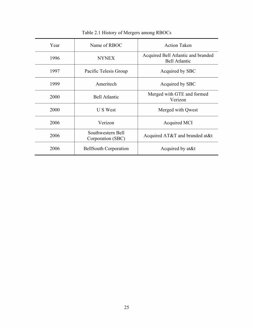
A significant amount of industry consolidation followed in the aftermath of the passage

of the 1996 Act.8 This consolidation was primarily directed at increasing economies of scale in

the provision of local telephone service and also re-capturing the economies of scope that had

been sacrificed as part of the AT&T divestiture. Southwestern Bell Corporation (SBC, now

at&t) was perhaps the most aggressive RBOC in this consolidation campaign.

SBC acquired Pacific Telesis Group, Southern New England Telephone and Ameritech in

1997, 1998 and 1999, respectively. A merger between Bell Atlantic and GTE formed Verizon in

2000. U.S. West agreed to merge with QWEST Communications in 1999 and this merger was

approved by state and federal regulators in 2000. In 2005, AT&T was acquired by SBC

communications. Shortly after this merger, the company was renamed at&t Inc. Finally,

Verizon acquired MCI in January 2006, followed by at&t’s December 2006 acquisition of

6 CLECs can lease UNEs and combine them with their own facilities to provide the retail telecommunications product. UNE-L, or the unbundled network loop, is example of this type of network element. The UNE-L entails leasing the loop, which is the connection from the telephone exchange’s central office to the customer premises. UNE-P, or the unbundled network element platform, is a special type of resale in which the network inputs are combined for the entrant by the incumbent provider. The price for UNE-P is lower than that of pure resale because it is based on TELRIC (total element long-run incremental cost) rather than avoided cost, but the two are functionally indistinguishable otherwise. The Federal Communications Commission began phasing out UNE-P in 2005 because it believed the availability of UNE-P was having an adverse effect on investment in network infrastructure. See FCC (2005). 7 At the time of the 1996 Act, the ILECs were comprised of local telephone companies, including the Regional Bell Operating Companies (RBOCs). 8 The history of ILEC mergers from 1996 onward is shown in Table 1.

8

BellSouth Corporation—the last of the RBOCs to have retained its original corporate name

following the 1984 AT&T divestiture.9, 10

In general, mergers can be either pro-competitive or anti-competitive in terms of their

effect on industry performance, including productive efficiency. The horizontal merger

guidelines (HMG) of the U.S. Department of Justice (DOJ) rely, in part, upon market

concentration in evaluating whether particular mergers raise anticompetitive concerns. In

addition to market concentration, the HMG also take into account potential adverse competitive

effects and entry analysis in evaluating proposed mergers. Specifically, Section 4 of the HMG

(revised April 8, 1997) describes the significance of merger efficiencies. When efficiency gains

from a merger, which may result in lower prices or quality improvements, are expected to

dominate the other effects of the merger that may serve to lessen competition, the agency would

consider approving the proposed merger. These observations notwithstanding, it is difficult in

practice to verify and quantify these merger efficiencies.11

A number of empirical studies have computed efficiency scores for the U.S.

telecommunications industry, including Majumdar (1995, 1997), Resende (2000) and Resende

and Facanha (2005). And yet, most of the studies that examine efficiency in the

telecommunications industry have concentrated on either the effects of different regulatory

regimes or the impact of the AT&T divestiture.12 The measurement of efficiency gains with

respect to mergers has heretofore been given surprisingly little attention in the literature.

9 Cincinnati Bell, which is not part of AT&T break-up, retains its brand name and continues to use the Bell logo. 10 This trend continues in the wireless industry as well as the wireline industry. For instance, in 2004, AT&T and Cingular Wireless merged and became the largest provider in the wireless industry. Sprint PCS also merged with Nextel and adopted the brand Sprint-Nextel in 2005. See Weisman (2007) for further discussion of these mergers and the economic factors driving them. 11 The HMG of the DOJ introduced cognizable efficiencies that are merger-specific. The HMG (p. 31) indicate that “Cognizable efficiencies are assessed net of costs produced by the merger or incurred in achieving those efficiencies.” 12 See Shin et al. (1992) and Krouse et al. (1999) for research on the effects of the AT&T divestiture.

9

In this essay, a Malmquist productivity growth index introduced by Caves et al. (1982)

and further developed by Färe et al. (1994) is employed to compute productivity growth, which

is comprised of technical efficiency change and technological change.13 A large number of

papers employ the Malmquist index to measure productivity growth for a cross-section of

industries.14 With specific reference to the telecommunications sector in the U.S., Uri (2001,

2002) used a Malmquist index to measure the change in productivity growth following the

implementation of incentive regulation. He found that productivity growth increased by

approximately 5 percent per year for the 19 LECs over the period 1988-1999.

This study differs from Uri in three critical respects. First, we investigate the

effectiveness of mergers over the 1996 to 2005 time period. We seek to determine whether

productivity growth has increased for ILECs that have merged since the 1996 Act and whether

the merged firms perform better than a firm that did not merge in terms of productivity growth.

Employing a Malmquist index, we find that the change in productivity growth for merged firms

is higher than that of firms that did not merge, ceteris paribus. In contrast to Uri, our findings

indicate that productivity growth decreased for most firms in the sample. Second, our sample

includes 25 LECs and therefore provides for a more robust analysis. Third, we measure firm-

level technical efficiencies using dynamic DEA to evaluate the ILECs’ ability to optimize output

over time.

13 Kwoka (1993) analyzed the impact of different regulatory policies on productivity growth for both AT&T and British Telecom (BT). He found empirical evidence that both the privatization of BT and the divestiture of AT&T had a significant effect on productivity growth. Resende (1999) found no statistically significant relationship between incentive regulation and increased productivity growth. Stranczak et al. (1994) investigated whether privatization and competition affect productivity growth in the telecommunications industry. They found no empirical evidence of a statistically significant relationship between long distance competition and productivity growth. 14 For example, Färe et al. (1994) examined productivity growth in 17 OECD countries for the 1979-1988 period using the Malmquist index. They found that the country that has the highest productivity growth rate is Japan while that of the U.S. is slightly higher than average. Lall et al. (2002) also used the Malmquist index to measure productivity growth in over 30 countries in the Western Hemisphere over the 1978-1994 period. They found that civil, economic, and political liberty played a significant role in productivity growth for Caribbean countries.

10

The remainder of this essay is organized as follows. The analytical framework and

theory used to measure productivity growth and the decomposition of the Malmquist index are

described in Section 2. In Section 3, the data used in this essay are discussed. Section 4

provides the empirical results for the DEA scores and changes in productivity growth. We

compare the pre-merger and post-merger productivity growth and technical efficiency change

among ILECs that have merged since the 1996 Act relative to the ILEC that did not merge.15

Finally, Section 5 contains a brief summary of the results and a conclusion.

METHODLOGY

There are two principal approaches to the estimation of production frontiers, the parametric

method and the non-parametric method. The Malmquist index approach employed in this essay

is of the latter type. One of the important advantages of using this index is the ability to

decompose productivity growth rates into technical efficiency change and technological change.

In addition, no explicit functional form for the frontier is required since the DEA approach uses

linear programming. DEA also allows for multiple inputs and multiple outputs that are not as

easily estimated using parametric methods. Another distinct advantage of using the DEA

method in measuring productivity growth is that it does not require any price data. Before

turning to a discussion of the specific properties of the Malmquist index, we provide an overview

of the DEA technique.16

DEA is a linear programming method that uses data on the multiple input and output

quantities to construct a hypersurface over the data points. This hypersurface is constructed by

the solution to a series of linear programming problems. There are input-oriented and output-

oriented DEA methods. The former is conducted by reducing the amount of all inputs

15 BellSouth Corporation is the only ILEC that had not merged prior to 2005. 16 The first influential DEA model was developed by Charnes et al. (1978).

11

proportionally without a reduction in output. The latter is conducted by determining the

maximum proportional increase in output for any given level of input.

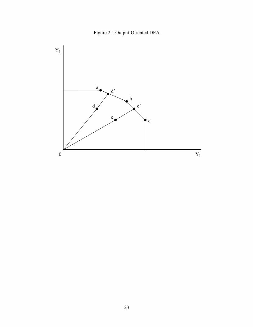
Output-oriented DEA is depicted in Figure 1. There are two outputs ( )1 2,Y Y and five

firms ( ), , , ,a b c d e . Firms a , b and c are efficient since they lie on the production frontier.

Calculating the technical efficiency score of firm d is equivalent to:

'

00

ddTEd

= . (1)

In similar fashion, the technical efficiency score for firm e is equal to:

'

00

eeTEe

= . (2)

Therefore, the value of the efficiency score lies between 0 and 1.

For firm d , the efficient target is 'd which lies on the line segment joining points a andb .

Firms a andb are typically referred to as the peers of firm d . In similar fashion, firm e ’s peers

are firms b and c . Note that the value of technical efficiency for firms a , b and c are assigned

the value of one and each firm is its own peer.

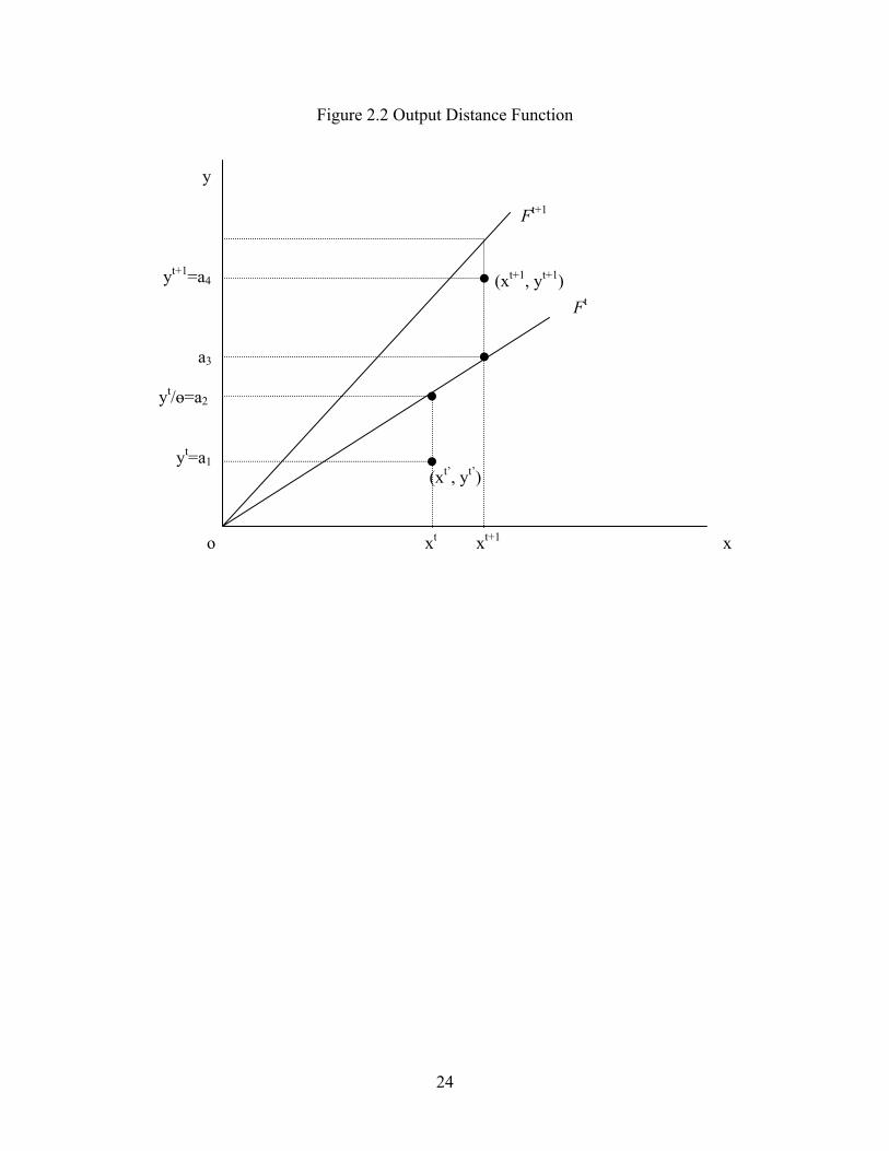
We turn now to discuss the distance function that is required to construct a Malmquist

index. Based on Caves et al. (1982), we assume that for each time period 1, , ,t T= … the

production technology tF maps input vectors, t nx +∈R into output vectors, t my +∈R ,17

( ){ }, : can produce t t t t tF x y x y= , (3)

17 The production technology is assumed to satisfy the following axioms in order to be a meaningful model of production: i) the possibility of inaction; ii) monotonicity of the output correspondence; iii) disposability of output; iv) the output set is closed; and v) irreversibility (Färe and Grosskopf, 1994).

12

where R is the set of real numbers. The production technology tF is homogeneous of degree 1

in output. Following Shepard (1970), the output distance function is defined at time t as:

( ) ( ){ }( ) 1, inf : , sup : ,

tt t t t t t t tO

yD x y x F x y Fθ θ θθ

−⎧ ⎫⎛ ⎞⎪ ⎪= ∈ = ∈⎨ ⎬⎜ ⎟⎪ ⎪⎝ ⎠⎩ ⎭

.18 (4)

The distance function ( ),t t tOD x y is homogeneous of degree 1 in output. Note that input-output

vectors lie below the production technology set, which implies that ( ), 1t t tOD x y ≤ if and only if

( ),t t tx y F∈ . Moreover, ( ), 1t t tOD x y = if and only if input-output combinations lie on the

boundary of the production technology set that is illustrated in Figure 2.19 The value of the

distance function evaluated at ( ),t tx y is 2

2

1oaoa

= , while the value of the distance function

evaluated at ( )' ',t tx y is 1

2

1oaoa

< .20 In order to construct a Malmquist index, another distance

function from a different time period is required. This distance function is expressed as:

( )1

1 1 1, inf : ,t

t t t t tO

yD x y x Fθθ

++ + +⎧ ⎫⎛ ⎞⎪ ⎪= ∈⎨ ⎬⎜ ⎟

⎪ ⎪⎝ ⎠⎩ ⎭

( ){ }( ) 11 1sup : ,t t tx y Fθ θ

−+ += ∈ . (5)

This distance function measures the maximal proportional change in output required to make

( )1 1,t tx y+ + feasible in relation to the technology at time t . In Figure 2, production ( )1 1,t tx y+ +

18 The input distance function can be defined as follows:

( ), su p : , .t

t t t t tI

xD x y y Fδδ

⎧ ⎫⎛ ⎞⎪ ⎪= ∈⎨ ⎬⎜ ⎟⎪ ⎪⎝ ⎠⎩ ⎭

19 Farrell (1957) referred to a firm as “technically efficient” when ( ), 1t t t

OD x y = . 20 Refer to Färe and Grosskopf (2000) for additional discussion of distance functions.

13

occurs outside the production possibility set at time t . The value of the distance function for

observation ( )1 1,t tx y+ + relative to technology tF is 4

3

1oaoa

> .

A Malmquist index is the ratio of two distance functions and is constructed as follows:

( )( )

1 1,

,

t t tOt

c t t tO

D x yM

D x y

+ +

= .21 (6)

Färe et al. (1994) suggest using the output-based Malmquist index in order to avoid the use of an

arbitrary benchmark:

( ) ( )( )

( )( )

1 1 1 1 11 1

1

, ,, , ,

, ,

t t t t t tO Ot t t t

O t t t t t tO O

D x y D x yM x y x y

D x y D x y

+ + + + ++ +

+

⎛ ⎞⎛ ⎞⎜ ⎟⎜ ⎟=⎜ ⎟⎜ ⎟⎝ ⎠⎝ ⎠

. (7)

From the production frontier perspective, technical efficiency measures how far below

the production frontier a particular firm’s technology resides. Technological change implies

technological innovation and it measures the extent to which that frontier moves outward/inward

over time. In order to decompose a Malmquist index into a technical efficiency change and

technological change, (7) can be represented as:

( ) ( )( )

( )( )

( )( )

1 1 1 1 11 1

1 1 1 1

, , ,, , ,

, , ,

t t t t t t t t tO O Ot t t t

O t t t t t t t t tO O O

D x y D x y D x yM x y x y

D x y D x y D x y

+ + + + ++ +

+ + + +

⎛ ⎞⎛ ⎞⎜ ⎟⎜ ⎟= ×⎜ ⎟⎜ ⎟⎝ ⎠⎝ ⎠

, (8)

where ( )( )

1 1 1,

,

t t tO

t t tO

D x y

D x y

+ + +

measures the change in relative efficiency (i.e., whether the production

technology is moving closer to or farther away from the production frontier) between periods t

21 Technology in period t is treated as the base-case technology.

14

and 1t + . ( )( )

( )( )

1 1

1 1 1 1

, ,

, ,

t t t t t tO O

t t t t t tO O

D x y D x y

D x y D x y

+ +

+ + + +

⎛ ⎞⎛ ⎞⎜ ⎟⎜ ⎟⎜ ⎟⎜ ⎟⎝ ⎠⎝ ⎠

measures the shift in the technology frontier between

the two periods evaluated at tx and 1tx + .

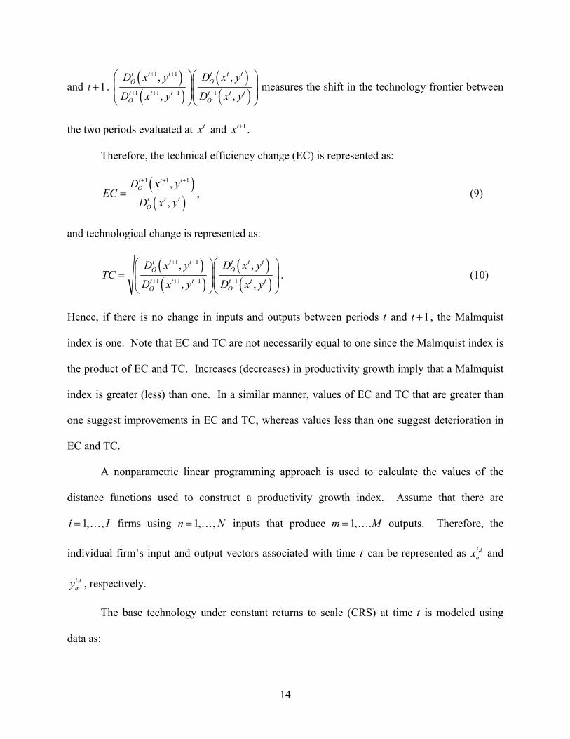
Therefore, the technical efficiency change (EC) is represented as:

( )( )

1 1 1,

,

t t tO

t t tO

D x yEC

D x y

+ + +

= , (9)

and technological change is represented as:

( )( )

( )( )

1 1

1 1 1 1

, ,

, ,

t t t t t tO O

t t t t t tO O

D x y D x yTC

D x y D x y

+ +

+ + + +

⎛ ⎞⎛ ⎞⎜ ⎟⎜ ⎟=⎜ ⎟⎜ ⎟⎝ ⎠⎝ ⎠

. (10)

Hence, if there is no change in inputs and outputs between periods t and 1t + , the Malmquist

index is one. Note that EC and TC are not necessarily equal to one since the Malmquist index is

the product of EC and TC. Increases (decreases) in productivity growth imply that a Malmquist

index is greater (less) than one. In a similar manner, values of EC and TC that are greater than

one suggest improvements in EC and TC, whereas values less than one suggest deterioration in

EC and TC.

A nonparametric linear programming approach is used to calculate the values of the

distance functions used to construct a productivity growth index. Assume that there are

1, ,i I= … firms using 1, ,n N= … inputs that produce 1, .m M= … outputs. Therefore, the

individual firm’s input and output vectors associated with time t can be represented as ,i tnx and

,i tmy , respectively.

The base technology under constant returns to scale (CRS) at time t is modeled using

data as:

15

( ) , ,

1 1

, such that , , 0I I

t t t t i i t i i t t im m n n

i i

F x y y z y z x x z= =

⎧ ⎫= ≤ ≤ ≥⎨ ⎬⎩ ⎭

∑ ∑ , (11)

where iz is the intensity of use of the thi firm’s technology. By adding the following convexity

condition based on Afriat (1972), the constant returns to scale assumption can be modified to

allow for variable returns to scale (VRS):

1

1I

i

iz

=

=∑ . (12)

One may obtain technical efficiency change under constant returns to scale technology and then

decompose it into two components–the pure efficiency component and the residual scale

component. The former is due to pure technical inefficiency and the latter is due to scale

inefficiency.22

In order to calculate a Malmquist index in (8), four different linear programming

problems are used to solve for the values of four distance functions. These are given by

( ),t t tOD x y , ( )1 1,t t t

OD x y+ + , ( )1 ,t t tOD x y+ ( )1 1 1, ,t t t

OD x y+ + + . For firm 'i ,

( )( ) 1', ', ',, maxt i t i t i

O zD x y θ θ−=

s. t. ' ', ,

1

Ii i t i i t

m mi

y z yθ=

≤∑

, ',

1

Ii i t i t

n ni

z x x=

≤∑ (13)

0iz ≥ .

22 The decomposition can be expressed as:

( )1 1, , ,

,

t t t tOM x y x y TEC H EFC H

TEC H PEFC H SC H

+ + = ×

= × ×

where TECH represents technological change, EFCH represents technical efficiency change, PEFCH represents pure efficiency change and SCH represents scale change. EFCH is computed under CRS while PEFCH is computed under VRS.

16

and ( )( ) 11 ', 1 ', 1 ',, maxt i t i t i

O zD x y θ θ−

+ + + =

s. t. ' ', 1 , 1 , 1

1

Ii i t i t i t

m mi

y z yθ + + +

=

≤∑ (14)

, 1 , 1 ', 1

1

Ii t i t i t

n ni

z x x+ + +

=

≤∑

0iz ≥ .

Two additional distance functions are required to calculate a Malmquist index for the two

periods t and 1t + . The first of these is calculated for firm 'i as

( )( ) 1', 1 ', 1 ',, maxt i t i t i

O zD x y θ θ−

+ + =

s. t. ' ', 1 ,

1

Ii i t i i t

m mi

y z yθ +

=

≤∑ (15)

, ', 1

1

Ii i t i t

n ni

z x x +

=

≤∑

0iz ≥ .

Note that the value of θ in (15) need not be greater than or equal to unity. For example, the

observation could lie above the feasible production possibility set since a production

combination from period 1t + is compared to technology in period t. The last linear

programming problem entails the same calculations as in (15) with transposed superscripts, t

and 1t + , and stated as

( )( ) 11 ', ', ',, maxt i t i t i

O zD x y θ θ−

+ =

s. t. ' ', , 1

1

Ii i t i i t

m mi

y z yθ +

=

≤∑ (16)

, 1 ',

1

Ii i t i t

n ni

z x x+

=

≤∑

17

0iz ≥ .

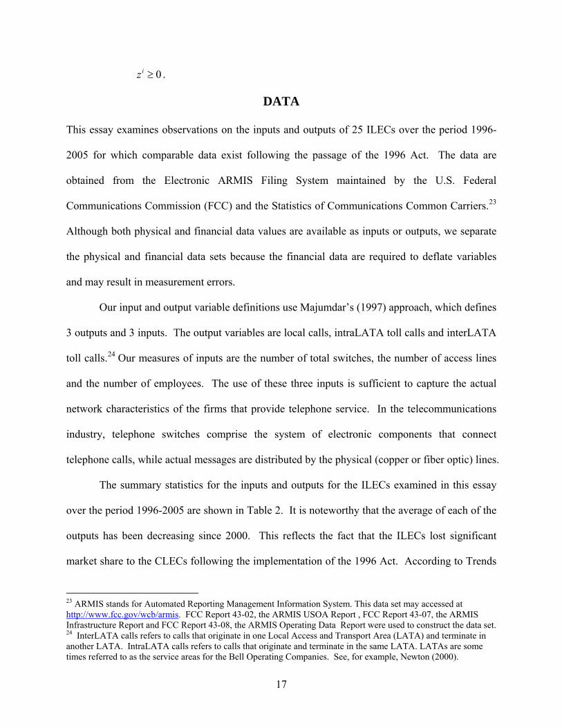
DATA

This essay examines observations on the inputs and outputs of 25 ILECs over the period 1996-

2005 for which comparable data exist following the passage of the 1996 Act. The data are

obtained from the Electronic ARMIS Filing System maintained by the U.S. Federal

Communications Commission (FCC) and the Statistics of Communications Common Carriers.23

Although both physical and financial data values are available as inputs or outputs, we separate

the physical and financial data sets because the financial data are required to deflate variables

and may result in measurement errors.

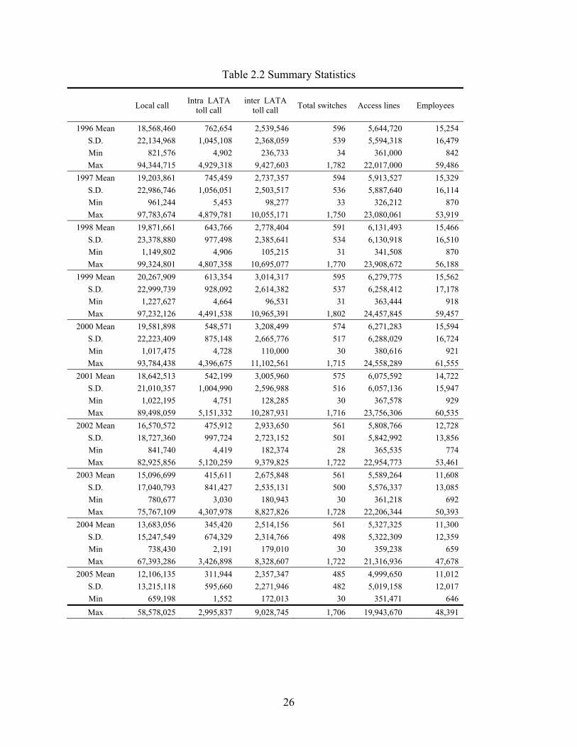
Our input and output variable definitions use Majumdar’s (1997) approach, which defines

3 outputs and 3 inputs. The output variables are local calls, intraLATA toll calls and interLATA

toll calls.24 Our measures of inputs are the number of total switches, the number of access lines

and the number of employees. The use of these three inputs is sufficient to capture the actual

network characteristics of the firms that provide telephone service. In the telecommunications

industry, telephone switches comprise the system of electronic components that connect

telephone calls, while actual messages are distributed by the physical (copper or fiber optic) lines.

The summary statistics for the inputs and outputs for the ILECs examined in this essay

over the period 1996-2005 are shown in Table 2. It is noteworthy that the average of each of the

outputs has been decreasing since 2000. This reflects the fact that the ILECs lost significant

market share to the CLECs following the implementation of the 1996 Act. According to Trends

23 ARMIS stands for Automated Reporting Management Information System. This data set may accessed at http://www.fcc.gov/wcb/armis. FCC Report 43-02, the ARMIS USOA Report , FCC Report 43-07, the ARMIS Infrastructure Report and FCC Report 43-08, the ARMIS Operating Data Report were used to construct the data set. 24 InterLATA calls refers to calls that originate in one Local Access and Transport Area (LATA) and terminate in another LATA. IntraLATA calls refers to calls that originate and terminate in the same LATA. LATAs are some times referred to as the service areas for the Bell Operating Companies. See, for example, Newton (2000).

18

in Telephone Service (2007), the CLEC share of end-user switched access lines increased from

4.3 percent in 1999 to 17.9 percent in 2005. In addition, significant growth in the number of

wireless subscribers and usage has caused the traditional wireline companies to experience

significant erosion in their long distance telephone volumes.25

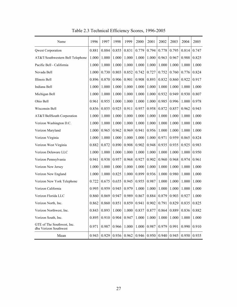
EMPIRICAL RESULTS

Results for the efficiency scores and productivity growth indices are reviewed in this section. In

Table 3, we provide the technical efficiency scores for all merged and non-merged firms from

1996 through 2005. Note that a firm that lies on the production frontier has a value of one for its

efficiency score for each year regardless of improvement or deterioration in its performance. As

a result, we are not able to examine the real efficiency change of the frontier firms over the

sample period. Despite this complexity, this approach does provide information as to how the

efficiency measures for the non-frontier firms are changing over time. When the efficiency score

is closer to one, the efficiency of the non-frontier firm is catching up to that of the frontier firms.

For example, in Table 3, a technical efficiency score for Qwest of 0.881 in 1996 indicates that

Qwest could produce approximately 11.9 percent more output with the same level of inputs if it

moved up on to the production frontier.

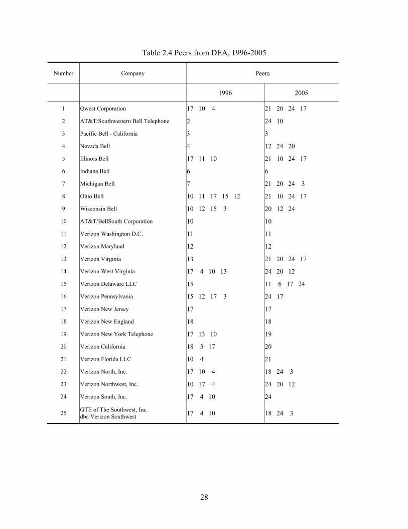
In Table 4, we identify those firms that define the frontier technology for the first year

(1996) and the final year (2005) adjacent to their observed combination of inputs and outputs. In

1996, 12 firms lie on the production frontier, while 11 firms lie on the production frontier in

2005. Table 4 indicates that Southwestern Bell, Nevada Bell, Michigan Bell, Verizon Virginia

and Verizon Delaware were all on the production frontier in 1996, and yet all became non-

production frontier firms in 2005. In addition, there are changes in the groups of peer firms over 25 The Cellular Telecommunications and Internet Association (CTIA)’s survey data (2006) reveals a rapid increase in the number of wireless telephone subscribers, from 44,042,992 in 1996 to 207,896,198 in 2005, or an increase of 372%.

19

the two periods. For example, the peers for Qwest Corporation were Nevada Bell, BellSouth

Corporation and Verizon New Jersey in 1996. However, only Verizon New Jersey remained in

the same peer group for Qwest Corporation in 2005. Efficient firms on the frontier that do not

appear as a peer for inefficient firms may be considered to be on the frontier as a result of their

distinct characteristics in terms of input/output combinations. For Example, Indiana Bell and

Michigan Bell do not appear as a peer for any firm in 1996 while Verizon New Jersey appears as

a peer for 12 firms.

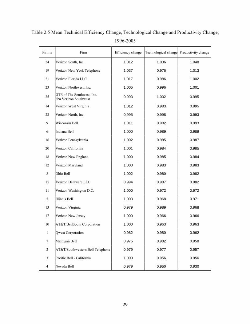
Table 5 provides the mean values of technical efficiency change, technological change

and productivity growth change for the 25 ILECs over the period 1996 to 2005.26 The firms in

the table are presented in descending order of the magnitude of their average productivity growth

over the sample period. Verizon South shows a 4.8 percent average growth in productivity,

which is due to a 1.2 percent growth in technical efficiency change and a 3.6 percent growth in

technological change. It is useful to note the number of companies that improved their

performance over the sample period. Only 4 out of 25 companies, Verizon South, Verizon New

York, Verizon Florida and Verizon Northwest, realized positive productivity growth over the

sample period. For example, Verizon South experienced a 4.8 percent annual growth in

productivity over the sample period.

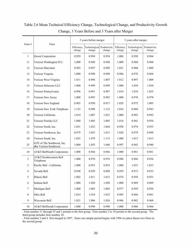
Table 6 reports the average of technical efficiency change, technological change and

productivity growth 3 years before and 3 years after the merger. The sample companies are

classified by 3 groups. The first group includes firm 1 and firms 11 through 25 for mergers that

occurred in 2000. The second group includes firms 2 through 9 for mergers that occurred in

26 In this paper, the mean is the geometric mean. Let tM denote the Malmquist index, where t stands for time and t

= 1, 2, . . . , 10. The geometric mean is computed as 10

101

.ttM

=Π

20

1999.27 The last group contains only BellSouth Corporation as it is the only the non-merged

firm in the sample. The reason we examine the periods 3 years before and 3 years after the

merger is to identify the merger effect for the same time interval.28

Seven companies, comprised of firms 1, 11, 12, 14, 15, 16 and 18 from the first group,

and two companies, firms 3 and 4 from the second group, have experienced increases in

productivity growth. However, the control company, BellSouth Corporation, experienced

decreased productivity growth. Five companies, firms 3, 12, 15, 16, and 18, were able to reverse

their performance from deterioration 3 years before the merger to improvement for 3 years after

their merger. For example, Pacific Bell-California experienced a 3.3 percent average growth in

productivity for the 3 years after the merger, but a -4.7 percent average growth in productivity

for the 3 years prior to the merger.

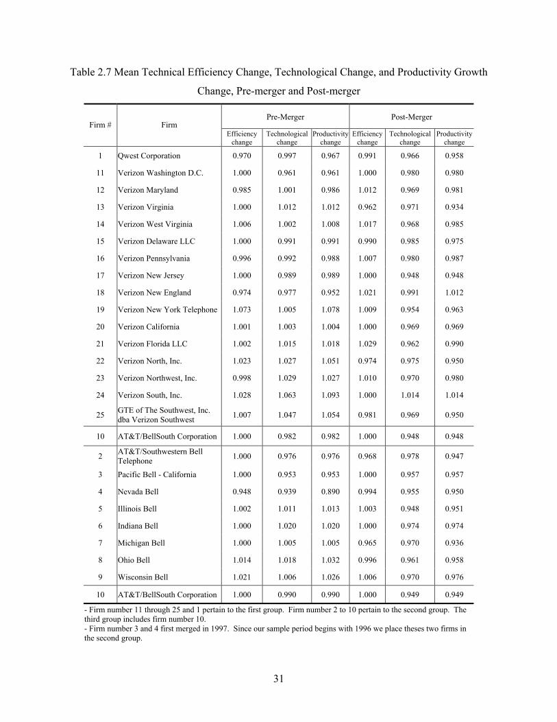
Table 7 reports the mean of technical efficiency change, technological change, and

productivity growth between the pre-merger and post-merger periods. The mergers occurred in

2000 and 1999 for the first and second groups, respectively. Therefore, in order to compare

every firm in each group with a non-merged firm, we compute two measures for BellSouth

Corporation. One measure is conducted from 2000 and the other measure is conducted from

1999. When comparing the measures in Table 6, the number of companies that experienced

increased productivity growth decreased from 9 to 4. This suggests that the merger effect of

increased productivity growth diminishes over time.

It is noteworthy that 3 companies, Verizon Virginia, Southwestern Bell and Michigan

Bell, experienced lower average productivity growth after the merger than that of BellSouth

27 In fact, Pacific Telesis Group which has Pacific Bell and Nevada Bell operating companies first merged in 1997. Since our sample period begins with 1996 we place theses two companies in the second group. 28 The maximum number of indexes before the merger for the second group is 3 (i.e., 1997, 1998, and 1999). The 1997 index refers to the change between 1996 and 1997. Therefore, in order to compare the same period, we must use a 3-year data span before and after the merger.

21

Corporation. The mean productivity growth for BellSouth Corporation was computed for two

different time periods. One is computed over 5 years and yields an annual growth rate of -5.2

percent. The other is computed over 6 years and yields an annual growth rate of -5.1 percent. It

should be noted that BellSouth Corporation, the only firm that was not part of a merger in our

sample, is one of the worst performing ILECs in terms of average productivity growth.

Conclusion

The passage of the 1996 Telecommunications Act ushered in a period of increased consolidation

in the U.S. telecommunications industry. Of the seven RBOCs created as a result of the AT&T

divestiture, only 3 remain, Qwest, Verizon and AT&T (formerly SBC). In order to examine the

efficiencies associated with these mergers, this study attempts to measure the productivity

growth associated with 25 ILECs over the period 1996-2005 using a Malmquist productivity

index. We also compute technical efficiency scores, which enable us to capture the relative

efficiency effects and explain how the efficiency for the non-efficient firm is changing over time.

The average efficiency scores for our sample companies have not changed significantly between

1996 and 2005. This implies that the average ILEC shows no measurable improvement in terms

of optimizing their input-output combinations over time.

The results of computing a Malmquist productivity index reveal that 9 out of 25

individual firms are shown to have increased their average productivity growth for the 3-year

period after the merger. When we partition these firms into pre-merger and post-merger

categories, the number of firms that increase productivity growth is reduced to 4 firms. This

suggests that the impact on average productivity growth resulting from the mergers decreases

over time. In addition, the measure of the Malmquist productivity index for the non-merged firm,

BellSouth Corporation, is one of the lowest firms in the sample. The index for BellSouth

22

Corporation shows about a -5 percent decline in annual productivity growth. These results

therefore provide some evidence of a positive merger effect, although this effect appears to

diminish over time.

23

Figure 2.1 Output-Oriented DEA

Y2

0 Y1

a d’

e’

e

db

c

24

Figure 2.2 Output Distance Function

y yt+1=a4 a3 yt/ө=a2 yt=a1

o xt xt+1 x

Ft+1

Ft

(xt’, yt’)

(xt+1, yt+1)

25

Table 2.1 History of Mergers among RBOCs

Year Name of RBOC Action Taken

1996 NYNEX Acquired Bell Atlantic and branded Bell Atlantic

1997 Pacific Telesis Group Acquired by SBC

1999 Ameritech Acquired by SBC

2000 Bell Atlantic Merged with GTE and formed Verizon

2000 U S West Merged with Qwest

2006 Verizon Acquired MCI

2006 Southwestern Bell Corporation (SBC) Acquired AT&T and branded at&t

2006 BellSouth Corporation Acquired by at&t

26

Table 2.2 Summary Statistics

Local call Intra LATA toll call

inter LATA toll call Total switches Access lines Employees

1996 Mean 18,568,460 762,654 2,539,546 596 5,644,720 15,254 S.D. 22,134,968 1,045,108 2,368,059 539 5,594,318 16,479 Min 821,576 4,902 236,733 34 361,000 842 Max 94,344,715 4,929,318 9,427,603 1,782 22,017,000 59,486

1997 Mean 19,203,861 745,459 2,737,357 594 5,913,527 15,329 S.D. 22,986,746 1,056,051 2,503,517 536 5,887,640 16,114 Min 961,244 5,453 98,277 33 326,212 870 Max 97,783,674 4,879,781 10,055,171 1,750 23,080,061 53,919

1998 Mean 19,871,661 643,766 2,778,404 591 6,131,493 15,466 S.D. 23,378,880 977,498 2,385,641 534 6,130,918 16,510 Min 1,149,802 4,906 105,215 31 341,508 870 Max 99,324,801 4,807,358 10,695,077 1,770 23,908,672 56,188

1999 Mean 20,267,909 613,354 3,014,317 595 6,279,775 15,562 S.D. 22,999,739 928,092 2,614,382 537 6,258,412 17,178 Min 1,227,627 4,664 96,531 31 363,444 918 Max 97,232,126 4,491,538 10,965,391 1,802 24,457,845 59,457

2000 Mean 19,581,898 548,571 3,208,499 574 6,271,283 15,594 S.D. 22,223,409 875,148 2,665,776 517 6,288,029 16,724 Min 1,017,475 4,728 110,000 30 380,616 921 Max 93,784,438 4,396,675 11,102,561 1,715 24,558,289 61,555

2001 Mean 18,642,513 542,199 3,005,960 575 6,075,592 14,722 S.D. 21,010,357 1,004,990 2,596,988 516 6,057,136 15,947 Min 1,022,195 4,751 128,285 30 367,578 929 Max 89,498,059 5,151,332 10,287,931 1,716 23,756,306 60,535

2002 Mean 16,570,572 475,912 2,933,650 561 5,808,766 12,728 S.D. 18,727,360 997,724 2,723,152 501 5,842,992 13,856 Min 841,740 4,419 182,374 28 365,535 774 Max 82,925,856 5,120,259 9,379,825 1,722 22,954,773 53,461

2003 Mean 15,096,699 415,611 2,675,848 561 5,589,264 11,608 S.D. 17,040,793 841,427 2,535,131 500 5,576,337 13,085 Min 780,677 3,030 180,943 30 361,218 692 Max 75,767,109 4,307,978 8,827,826 1,728 22,206,344 50,393

2004 Mean 13,683,056 345,420 2,514,156 561 5,327,325 11,300 S.D. 15,247,549 674,329 2,314,766 498 5,322,309 12,359 Min 738,430 2,191 179,010 30 359,238 659 Max 67,393,286 3,426,898 8,328,607 1,722 21,316,936 47,678

2005 Mean 12,106,135 311,944 2,357,347 485 4,999,650 11,012 S.D. 13,215,118 595,660 2,271,946 482 5,019,158 12,017 Min 659,198 1,552 172,013 30 351,471 646 Max 58,578,025 2,995,837 9,028,745 1,706 19,943,670 48,391

27

Table 2.3 Technical Efficiency Scores, 1996-2005

Name 1996 1997 1998 1999 2000 2001 2002 2003 2004 2005

Qwest Corporation 0.881 0.884 0.855 0.831 0.779 0.794 0.778 0.795 0.814 0.747

AT&T/Southwestern Bell Telephone 1.000 1.000 1.000 1.000 1.000 1.000 0.963 0.967 0.988 0.825

Pacific Bell - California 1.000 1.000 1.000 1.000 1.000 1.000 1.000 1.000 1.000 1.000

Nevada Bell 1.000 0.730 0.803 0.852 0.742 0.727 0.752 0.760 0.776 0.824

Illinois Bell 0.896 0.870 0.906 0.901 0.908 0.893 0.832 0.860 0.922 0.917

Indiana Bell 1.000 1.000 1.000 1.000 1.000 1.000 1.000 1.000 1.000 1.000

Michigan Bell 1.000 1.000 1.000 1.000 1.000 1.000 0.932 0.949 0.930 0.807

Ohio Bell 0.961 0.955 1.000 1.000 1.000 1.000 0.985 0.996 1.000 0.978

Wisconsin Bell 0.856 0.855 0.925 0.911 0.957 0.958 0.872 0.857 0.962 0.943

AT&T/BellSouth Corporation 1.000 1.000 1.000 1.000 1.000 1.000 1.000 1.000 1.000 1.000

Verizon Washington D.C. 1.000 1.000 1.000 1.000 1.000 1.000 1.000 1.000 1.000 1.000

Verizon Maryland 1.000 0.965 0.962 0.969 0.941 0.956 1.000 1.000 1.000 1.000

Verizon Virginia 1.000 1.000 1.000 1.000 1.000 1.000 0.971 0.959 0.865 0.824

Verizon West Virginia 0.882 0.872 0.890 0.908 0.902 0.948 0.935 0.935 0.925 0.983

Verizon Delaware LLC 1.000 1.000 1.000 1.000 1.000 1.000 1.000 1.000 1.000 0.950

Verizon Pennsylvania 0.941 0.938 0.957 0.968 0.927 0.902 0.960 0.968 0.974 0.961

Verizon New Jersey 1.000 1.000 1.000 1.000 1.000 1.000 1.000 1.000 1.000 1.000

Verizon New England 1.000 1.000 0.825 1.000 0.899 0.936 1.000 0.980 1.000 1.000

Verizon New York Telephone 0.722 0.675 0.655 0.945 0.955 0.987 1.000 1.000 1.000 1.000

Verizon California 0.995 0.959 0.945 0.979 1.000 1.000 1.000 1.000 1.000 1.000

Verizon Florida LLC 0.860 0.869 0.947 0.989 0.867 0.884 0.879 0.903 0.927 1.000

Verizon North, Inc. 0.862 0.860 0.851 0.859 0.941 0.902 0.791 0.829 0.835 0.825

Verizon Northwest, Inc. 0.843 0.893 1.000 1.000 0.837 0.877 0.864 0.889 0.836 0.882

Verizon South, Inc. 0.895 0.910 0.904 0.947 1.000 1.000 1.000 1.000 1.000 1.000

GTE of The Southwest, Inc. dba Verizon Southwest 0.971 0.987 0.966 1.000 1.000 0.987 0.979 0.991 0.990 0.910

Mean 0.943 0.929 0.936 0.962 0.946 0.950 0.940 0.945 0.950 0.935

28

Table 2.4 Peers from DEA, 1996-2005

Number Company Peers

1996 2005

1 Qwest Corporation 17 10 4 21 20 24 17

2 AT&T/Southwestern Bell Telephone 2 24 10

3 Pacific Bell - California 3 3

4 Nevada Bell 4 12 24 20

5 Illinois Bell 17 11 10 21 10 24 17

6 Indiana Bell 6 6

7 Michigan Bell 7 21 20 24 3

8 Ohio Bell 10 11 17 15 12 21 10 24 17

9 Wisconsin Bell 10 12 15 3 20 12 24

10 AT&T/BellSouth Corporation 10 10

11 Verizon Washington D.C. 11 11

12 Verizon Maryland 12 12

13 Verizon Virginia 13 21 20 24 17

14 Verizon West Virginia 17 4 10 13 24 20 12

15 Verizon Delaware LLC 15 11 6 17 24

16 Verizon Pennsylvania 15 12 17 3 24 17

17 Verizon New Jersey 17 17

18 Verizon New England 18 18

19 Verizon New York Telephone 17 13 10 19

20 Verizon California 18 3 17 20

21 Verizon Florida LLC 10 4 21

22 Verizon North, Inc. 17 10 4 18 24 3

23 Verizon Northwest, Inc. 10 17 4 24 20 12

24 Verizon South, Inc. 17 4 10 24

25 GTE of The Southwest, Inc. dba Verizon Southwest 17 4 10 18 24 3

29

Table 2.5 Mean Technical Efficiency Change, Technological Change and Productivity Change,

1996-2005

Firm # Firm Efficiency change Technological change Productivity change

24 Verizon South, Inc. 1.012 1.036 1.048

19 Verizon New York Telephone 1.037 0.976 1.013

21 Verizon Florida LLC 1.017 0.986 1.002

23 Verizon Northwest, Inc. 1.005 0.996 1.001

25 GTE of The Southwest, Inc. dba Verizon Southwest 0.993 1.002 0.995

14 Verizon West Virginia 1.012 0.983 0.995

22 Verizon North, Inc. 0.995 0.998 0.993

9 Wisconsin Bell 1.011 0.982 0.993

6 Indiana Bell 1.000 0.989 0.989

16 Verizon Pennsylvania 1.002 0.985 0.987

20 Verizon California 1.001 0.984 0.985

18 Verizon New England 1.000 0.985 0.984

12 Verizon Maryland 1.000 0.983 0.983

8 Ohio Bell 1.002 0.980 0.982

15 Verizon Delaware LLC 0.994 0.987 0.982

11 Verizon Washington D.C. 1.000 0.972 0.972

5 Illinois Bell 1.003 0.968 0.971

13 Verizon Virginia 0.979 0.989 0.968

17 Verizon New Jersey 1.000 0.966 0.966

10 AT&T/BellSouth Corporation 1.000 0.963 0.963

1 Qwest Corporation 0.982 0.980 0.962

7 Michigan Bell 0.976 0.982 0.958

2 AT&T/Southwestern Bell Telephone 0.979 0.977 0.957

3 Pacific Bell - California 1.000 0.956 0.956

4 Nevada Bell 0.979 0.950 0.930

30


Change, 3 Years Before and 3 Years after Merger

3 years before merger 3 years after merger Firm # Firm

Efficiency change

Technological change

Productivity change

Efficiency change


Productivity change

1 Qwest Corporation 0.959 0.994 0.954 1.006 0.958 0.964

11 Verizon Washington D.C. 1.000 0.948 0.948 1.000 0.960 0.960

12 Verizon Maryland 0.992 0.997 0.989 1.021 0.988 1.009

13 Verizon Virginia 1.000 0.998 0.998 0.986 0.978 0.964

14 Verizon West Virginia 1.011 0.996 1.007 1.012 0.997 1.009

15 Verizon Delaware LLC 1.000 0.999 0.999 1.000 1.034 1.034

16 Verizon Pennsylvania 0.996 0.991 0.987 1.014 1.010 1.025

17 Verizon New Jersey 1.000 0.993 0.993 1.000 0.978 0.978

18 Verizon New England 0.965 0.950 0.917 1.029 0.975 1.003

19 Verizon New York Telephone 1.123 0.990 1.112 1.016 0.968 0.983

20 Verizon California 1.014 1.007 1.021 1.000 0.993 0.993

21 Verizon Florida LLC 1.000 1.005 1.005 1.014 0.941 0.954

22 Verizon North, Inc. 1.031 1.032 1.064 0.958 0.974 0.933

23 Verizon Northwest, Inc. 0.979 1.035 1.013 1.020 0.979 0.999

24 Verizon South, Inc. 1.032 1.078 1.112 1.000 1.013 1.013

25 GTE of The Southwest, Inc. dba Verizon Southwest 1.004 1.055 1.060 0.997 0.943 0.940

10 AT&T/BellSouth Corporation 1.000 0.966 0.966 1.000 0.961 0.961

2 AT&T/Southwestern Bell Telephone 1.000 0.976 0.976 0.988 0.966 0.954

3 Pacific Bell - California 1.000 0.953 0.953 1.000 1.033 1.033

4 Nevada Bell 0.948 0.939 0.890 0.959 0.973 0.933

5 Illinois Bell 1.002 1.011 1.013 0.974 0.958 0.933

6 Indiana Bell 1.000 1.020 1.020 1.000 0.969 0.969

7 Michigan Bell 1.000 1.005 1.005 0.977 0.959 0.936

8 Ohio Bell 1.014 1.018 1.032 0.995 0.966 0.961

9 Wisconsin Bell 1.021 1.006 1.026 0.986 0.982 0.968


- Firm number 11 through 25 and 1 pertain to the first group. Firm number 2 to 10 pertain to the second group. The third group includes firm number 10. - Firm number 3 and 4 first merged in 1997. Since our sample period begins with 1996 we place theses two firms in the second group.

31


Change, Pre-merger and Post-merger

Pre-Merger Post-Merger Firm # Firm

Efficiency change


Productivity change

Efficiency change


Productivity change




















4 Nevada Bell 0.948 0.939 0.890 0.994 0.955 0.950

5 Illinois Bell 1.002 1.011 1.013 1.003 0.948 0.951

6 Indiana Bell 1.000 1.020 1.020 1.000 0.974 0.974

7 Michigan Bell 1.000 1.005 1.005 0.965 0.970 0.936

8 Ohio Bell 1.014 1.018 1.032 0.996 0.961 0.958

9 Wisconsin Bell 1.021 1.006 1.026 1.006 0.970 0.976


- Firm number 11 through 25 and 1 pertain to the first group. Firm number 2 to 10 pertain to the second group. The third group includes firm number 10. - Firm number 3 and 4 first merged in 1997. Since our sample period begins with 1996 we place theses two firms in the second group.

32

CHAPTER 3 - Market Consolidation and Productivity Growth in

U.S. Telecommunications: Stochastic Frontier analysis vs.

Malmquist index

INTRODUCTION

In 1996, the Telecommunications Act of 1996 (1996 Act) substantially amended the

Communications Act of 1934 (1934 Act)29. The primary purpose of the 1996 Act was to

stimulate competition in both local and long distance telecommunications markets. Incumbent

Local Exchange Carriers (ILECs) were required to open up local exchange telecommunications

markets to competition by unbundling their networks and providing the component inputs,

known as unbundled network elements (UNEs), to competitive local exchange carriers (CLECs)

at prices set by state regulators.30 As the quid pro quo for such network sharing, the 1996 Act

allowed the Regional Bell Operating Companies’ (RBOCs) to gain entry into the interLATA

long distance market once they satisfied the so-called “Competitive Checklist contained in

Section 271 of the Act.31, 32

29 The 1934 Act empowered Federal Communications Commission (FCC) to regulate the telecommunications industry in the U.S. 30 CLECs can lease the individual unbundled network elements and combine them with their own facilities to provide the retail telecommunications product. UNE-L, or the unbundled network loop, is example of this type of network element. The UNE-L entails leasing the loop, which is the connection from the telephone exchange’s central office to the customer premises equipment. UNE-P, or the unbundled network element platform, is a special type of resale in which the network inputs are combined for the entrant by the incumbent provider. The price for UNE-P is lower than that of pure resale because it is based on TELRIC (total element long-run incremental cost) rather than avoided cost, but the two are functionally indistinguishable otherwise. The Federal Communications Commission began phasing out UNE-P in 2005 because it came to believe that the availability of UNE-P was having an adverse effect on investment in network infrastructure. See FCC (2005). 31 At the time of the divestiture, 1984, there were seven RBOCs: Ameritech Corporation, Bell Atlantic Corporation, BellSouth Corporation, NYNEX Corporation, Pacific Telesis Group, Southwestern Bell Corporation and U.S. West, Inc. 32 InterLATA long distance calls refers to calls that originate in one Local Access and Transport Area (LATA), cross over and terminate in another LATA. IntraLATA long distance calls refers to calls that originate and terminate in the same LATA. LATAs are some times referred to as the service areas for the Bell Operating Companies. See Newton (2000).

33

One of the key trends in the telecommunications industry following the passage of the

1996 Act was a series of business consolidations among ILECs that policy makers did not fully

anticipate.33 Southwestern Bell Corporation (SBC, now at&t) was a leader in this trend. SBC

acquired Pacific Telesis Group, Southern New England Telephone and Ameritech in 1997, 1998

and 1999, respectively. U.S. West merged with QWEST Communications in 1999. A merger

between Bell Atlantic and GTE formed Verizon in 2000. In 2005, AT&T was acquired by SBC

communications and branded at&t Inc. In December 2006, at&t acquired BellSouth Corporation,

which is the last of the RBOCs to have retained its original corporate name following the 1984

AT&T divestiture.

The Department of Justice (DOJ) and the Federal Trade Commission (FTC) use the

Horizontal Merger Guidelines (HMG) to evaluate horizontal mergers. The HMG take into

account a number of factors including market concentration, entry barriers, and merger

efficiencies.34 As long as competition remains vigorous following the merger, measured in terms

of little or no discernible increase in market power, the merger is likely to be approved by the

DOJ/FTC. Nonetheless, from an operational standpoint, these prospective efficiency gains are

difficult to verify and quantify.

One of the methods that may be used to examine efficiencies is to measure productivity

growth, inclusive of its underlying components--technological progress and changes in technical

efficiency. From a policy perspective, the decomposition of productivity growth into these

components provides important information for analysis. For example, if policymakers are able

to determine the key drivers of productivity growth, they may adopt policies that can

33 Another important trend in the telecommunications industry is vertical integration. See, for example, Weisman (2000). 34 In order to measure efficiencies, the HMG introduced the “cognizable efficiency” concept which “are assessed net of costs produced by the merger or incurred in achieving those efficiencies.” See HMG (p. 31)

34

significantly improve the performance of firms and the overall economy. Suppose, for example,

that the lack of technological progress is the source of low productivity growth. It would then be

possible to put in place various policies that stimulate technological innovation and move the

technology frontier outwards over time. If high rates of technological change associated with

low rates of efficiency change are measured, then policy makers may focus on the policy that

increases the efficiency of firms.

To measure the production frontier, we use an output distance function approach

introduced by Shepard (1970). The main advantage of the distance function approach is that it

allows for a multiple-input and multiple-output technology without requiring price data. The

distance function can be estimated in several ways. These include data envelopment analysis

(DEA), parametric deterministic linear programming (PLP), corrected ordinary least squares

(COLS), and stochastic frontier analysis (SFA).

There are a number of empirical studies that measure productivity growth using SFA

across different industries.35 Kim and Han (2001) measured productivity growth associated with

technological change and efficiency changes in Korean manufacturing industries. They found

that technological change was the main factor contributing to productivity growth. Coelli et al.

(2003) employed SFA to investigate productivity growth in Bangladesh crop agriculture over the

period 1961-1992. Using 16 regional data points, they found that productivity growth is affected

by the green revolution and agricultural research expenditures. Recently, Resende (2006)

conducted an analysis that examined parametric and non-parametric efficiency measures

resulting from the implementation of incentive regulation in the U.S. telecommunications

industry. He compared efficiency scores obtained from DEA, COLS, and SFA (with time-

35 Uri (2002) employed a COLS approach to measure the efficiency gains associated with the implementation of incentive regulation in the U.S. telecommunications industry. Using data from 19 LECs over the 1988-1999 time period, Uri found no empirical evidence that incentive regulation had enhanced technical efficiency.

35

invariant and time-varying inefficiency effects). He found no significant consistency across the

different methods.

Despite a voluminous literature on productivity growth using SFA, the measurement of

productivity growth associated with mergers has received surprisingly little attention.

Specifically, in the telecommunications industry, no study to date has attempted to measure

productivity growth and proceeded to decompose it into its component parts, technological

change and efficiency change, using a stochastic frontier model.36 Therefore, this study provides

productivity growth measures associated with the decomposition analysis, which differs from

Resende (2006) who examines efficiency scores. In addition, this study compares both the SFA

approach and the Malmquist index approach for mergers in the U.S. telecommunications

industry.37

This study has two principal objectives. The first objective is to evaluate the

effectiveness of mergers that occurred between 1996 and 2005 using SFA. We investigate

whether productivity growth has increased among ILECs that have merged since the 1996 Act

and whether the merged firms performed better than those firms that did not merge. The second

objective is to compare productivity growth results between SFA and a Malmquist index

approach. This comparison provides useful information on the robustness of the efficiency

findings across different approaches.

The remainder of this essay is organized as follows. Section 2 discusses the multiple

output distance function and presents the models used in the study. In Section 3, we discuss the

data. The empirical results are presented and compared in Section 4. Section 5 contains a brief

summary and conclusion.

36 Seo and Weisman (2007) investigated the same issue with a non-parametric approach. 37 There are number of empirical studies that compare parametric and non-parametric methods in various industries. See, for example, Aigner and Chu (1968), and Kopp and Smith (1980).

36

Methodology

Distance Function

In order to define the output distance function, we first introduce the production technology. We

assume that for each time period 1, , ,t T= … the production technology tF maps input

vectors, ntx +∈R , into output vectors, m

ty +∈R ,

( ){ }, : can produce tt t t tF x y x y= , (1)

whereR is the set of real numbers.38 The production technology tF is homogeneous of degree

one in output. Following Shepard (1970), the output distance function is defined at time t as:

( ) ( ){ }( ) 1, inf : , sup : ,t tt

Ot t t t t tyD x y x F x y Fθ θ θθ

−⎧ ⎫⎛ ⎞= ∈ = ∈⎨ ⎬⎜ ⎟⎝ ⎠⎩ ⎭

. (2)

According to Lovell et al. (1994), the output distance function ( ),Ot t tD x y is non-

decreasing, positively linearly homogeneous39 and convex in y and decreasing in x .40 Note that

input-output vectors lie below the production technology set. This implies that ( ), 1Ot t tD x y ≤ if

and only if ( ), tt tx y F∈ . Moreover, ( ), 1Ot t tD x y = if and only if input-output combinations lie on

the boundary of the production technology set, which is illustrated in Figure 1. The value of the

38 The production technology must satisfy the following axioms in order to be a meaningful model of production: i) the possibility of inaction. ii) monotonicity of the output correspondence iii) disposability of output iv) the output set is closed v) irreversibility (Färe, R., and S. Grosskopf. 1994). 39 In Section 2.2, we assume homogeneity of degree one in y. 40 One can define the input distance function as follows: ( ), s u p : , .tt

I t t t txD x y y Fδδ

⎧ ⎫⎛ ⎞= ∈⎨ ⎬⎜ ⎟⎝ ⎠⎩ ⎭

37

distance function evaluated at ( ),t tx y is 2

2

1oaoa

= , whereas the value of the distance function

evaluated at ( )' ',t tx y is 1

2

1oaoa

< .41

Stochastic Frontier Model

Aigner et al. (1977) and Meeusen and van den Broeck (1977) simultaneously published

an analysis of the Stochastic Frontier Model (SFM) in different outlets. Technical efficiency, as

well as random shocks, is considered and specified in this model. The main advantage of SFM is

that it accounts for the possible influence of noise on the shape and positioning of the frontier,

something that deterministic frontier models are unable to do. In other words, issues such as

measurement error and other random factors can be separated from the sources of variation in

technical efficiency. SFM posits a production function with an error term associated with two

components. These two components consist of a symmetric error term accounting for noise and

an asymmetric error term accounting for technical inefficiency.

In order to estimate the stochastic frontier, a distance function must be specified. Based

on Coelli and Perelman (2000), the multiple output distance function is specified in translog

functional form and is given by42:

01 1 1 1

1ln( ) ln ln ln ln2

J L J J

Oi j ij l il jk ij ikj l j k

D y x y yα α β α= = = =

= + + +∑ ∑ ∑∑

1 1 1 1

1 1ln ln ln ln , 1, 2, ,2 2

L L J L

lm il im jl ij ill m j l

x x y x i Iβ δ= = = =

+ + =∑∑ ∑∑ … (3)

where J is the number of outputs, L is the number of inputs, and i denotes the i th firm in the

sample. The restrictions required for homogeneity of degree one in outputs are

41 Refer to Coelli et al. (1998) and Kumbhakar and Lovell (2000) for further discussion of distance functions. 42 In this study, we use 3 outputs and 3 inputs.

38

1

1J

jj

α=

=∑ (4)

and

1

0, 1, 2, ,J

jkk

j Jα=

= = …∑ and 1

0, 1, 2, ,L

jll

l Lδ=

= = …∑ . (5)

The restrictions required for symmetry are

, , 1, 2, ,jk kj j k Jα α= = … and , , 1, 2, ,lm ml l m Lβ β= = … . (6)

Lovell et al. (1994) proposed a convenient method for imposing the homogeneity

restriction in (3). Homogeneity implies that

( ) ( ), , ,O OD x y D x yλ λ= for any 0λ > . (7)

Hence, we arbitrarily choose one of the outputs, the J th output, and normalize on it. This, in

turn, allows us to obtain

( ),, O

OJ J

D x yyD xy y

⎛ ⎞=⎜ ⎟

⎝ ⎠. (8)

The translog function can be written as:

1 1 1* * *

01 1 1 1

1ln( ) ln ln ln ln2ij

J L J Joi

j l il jk ij ikj l j kiJ

D y x y yy

α α β α− − −

= = = =

= + + +∑ ∑ ∑∑

1

*

1 1 1 1

1 1ln ln ln ln , 1, 2, ,2 2

L L J L


x x y x i Iβ δ−

= = = =

+ + =∑∑ ∑∑ … , (9)

where * ijij

iJ

yy

y= .43 Equation (9) can be rewritten in the following functional form

( ) ( )*ln( ) , , , lniJ Oiy TL y x Dα β− = − 44 (10)

43 Note that the value of Jth output, ln iJ

iJ

yy

⎛ ⎞⎜ ⎟⎝ ⎠

, is 0. This implies that the summations involving outputs are

comprised of J-1 terms.

39

SFM has two error components that are comprised of a two-sided noise component and a

non-negative technical inefficient component. We append the noise term iv and change the

notation from ( )ln OiD to iu− . This transformation yields the stochastic frontier function

associated with the time trend for panel data and is expressed as follows:

1* 2

01 1

1ln( ) ln ln2

J L

it T j ijt l ilt TTj l

Y t y x tα α α β α−

= =

− = + + + +∑ ∑

1 1 2* * *

1 1 1 1 1

1 1 1ln ln ln ln ln2 2 2

J J L L

jk ijt ikt lm ilt imt Tj ijtj k l m j

y y x x t yα β α− −

= = = = =

+ + +∑∑ ∑∑ ∑

1*

1 1 1

1 1ln ln ln2 2

L J L

Tl ilt jl ijt ilt it itl j l

t x y x v uβ δ−

= = =

+ + + +∑ ∑∑ .45 (11)

where 1,2, ,t T= … is a time trend. itY and *ijty are the output and arbitrarily normalized output

for firm i , respectively. Subscripts ,j k index outputs; , ,α β δ are parameters to be estimated; x

variables are inputs. Subscripts ,l m index inputs; the itv s are the error components and are

assumed to be independently and identically distributed as ( )20, vN σ . The itu ’s are the technical

inefficiency components.

Following Battese and Coelli (1992), the technical inefficiency error term is defined by

( )exp , 1, 2, , ; 1, 2, ,it iu u t T i I t Tη= − − = =⎡ ⎤⎣ ⎦ … … , (12)

where the iu s are assumed to be a non-negative truncation of the normal distribution ( )2,N μμ σ

associated with technical inefficiency in production.46 iu is the technical inefficiency effect for

44 Note that Doi = 1 implies that the boundary of the frontier. 45 Note that as suggested by Morrison-Paul et al. (2000), one can change the sign of dependent variable. This change allows for interpreting estimates that conform to the standard SFA framework. 46 There are other distributional assumptions imposed on the inefficiency error term, such as half-normal, exponential, and gamma-halton. See, for example, Kumbhakar and Lovell (2000).

40

firm i for the last period of the sample;47 η is an unknown parameter to be estimated and

represents the rate of change in technical inefficiency. Therefore, a positive value, 0η > , implies

that the technical inefficiency effects are decreasing over time.48 One of the advantages of using

the error term in (12) is that any technical inefficiency changes over time can be separated from

technical change. In this essay, the maximum likelihood estimates of the unknown parameters

and the technical inefficiency, defined by (11) and (12), are obtained using the FRONTIER 4.1

computer program.49

Following Coelli et al. (1998) and given estimates for (11) and (12), the technical

efficiencies of production for each firm in the t th year can be predicted as:

( )expit itTE u= − .50 (13)

Therefore, the technical efficiency change between periods t and 1t − is calculated as:

1

itit

it

TEECTE −

= . (14)

With the estimates of the parameters in (11) and (12), the index of the technological

change for firm i is calculated by evaluating the partial derivative of the production function

with respect to time. The calculation of technological change is computed according to:

( ) ( )* * * * * *, , , , , , , ,1 1is is it it

it

f y x t f y x tTC

s tα β α β⎡ ⎤ ⎡ ⎤∂ ∂

⎢ ⎥ ⎢ ⎥= + × +∂ ∂⎢ ⎥ ⎢ ⎥⎣ ⎦ ⎣ ⎦

.51 (15)

47 In the last period, T, the value of the exponential function is 1 which implies that iT iu u= . 48 If η > 0 then –η(t – T) ≡ –η(t – T) and it iu u> . However, the value of the exponential function is decreasing monotonically towards the value of the last period in the sample. If η = 0, the translog specification in (11) becomes a time-invariant inefficiency model. 49 See Coelli (1996a). 50 The predicted values of technical efficiency lie between zero and one. The value of one implies that the firm lies on the boundary of the production possibility set.

41

Finally, the TFP index can be obtained by the product of the index of technical efficiency

change and the index of technological change calculated from (14) and (15):

it it itTFP EC TC= × . (16)

A Malmquist Index Approach

A Malmquist index approach is a non-parametric method for measuring productivity growth that

allows for a decomposition in terms of technological progress and efficiency change. One of the

important advantages of using this index is that no explicit functional form for the frontier is

required since the DEA approach uses linear programming. In addition, the DEA method does

not require any price data.52

Following Caves et al. (1982), a Malmquist index, which is computed as the ratio of two

output distance functions, is constructed as:

( )( )

,,

Ot t tS

Os s s

D x yM

D x y= ,53 (17)

where t and s are adjacent periods. Färe et al. (1994) suggested using the output-based

Malmquist index in order to avoid the use of an arbitrary benchmark:

( ) ( )( )

( )( )

, ,, , ,

, ,Os t t Ot t t

O t t s sOs s s Ot s s

D x y D x yM x y x y

D x y D x y⎛ ⎞⎛ ⎞

= ⎜ ⎟⎜ ⎟⎜ ⎟⎜ ⎟⎝ ⎠⎝ ⎠

. (18)

In order to decompose a Malmquist index into technical efficiency change and

technological change, (18) can be rearranged as:

51 Equation (15) differs from Nishimizu and Page (1982) in two respects. First, the former uses a stochastic frontier approach to estimate the technology, while the latter uses deterministic model. Second, the former uses a geometric mean whereas the latter uses an arithmetic mean. 52 Although a distance production approach does not require price data for both parametric and non-parametric methods, revenue, cost, and profit approaches which employ parametric estimation do require price data. 53 Technology in period t is treated as the base-case technology.

42

( ) ( )( )

( )( )

( )( )

, , ,, , ,

, , ,Ot t t Os t t Os s s

O t t s sOs s s Ot t t Ot s s

D x y D x y D x yM x y x y

D x y D x y D x y⎛ ⎞⎛ ⎞

= × ⎜ ⎟⎜ ⎟⎜ ⎟⎜ ⎟⎝ ⎠⎝ ⎠

, (19)

where ( )( )

,,

Ot t t

Os s s

D x yD x y

measures whether the production technology is getting closer to or farther

away from the production frontier between adjacent periods s and t .

( )( )

( )( )

, ,, ,

Os t t Os s s

Ot t t Ot s s

D x y D x yD x y D x y

⎛ ⎞⎛ ⎞⎜ ⎟⎜ ⎟⎜ ⎟⎜ ⎟⎝ ⎠⎝ ⎠

measures the move of the technology frontier between the two

periods evaluated at sx and tx .

Therefore, the technical efficiency change (EC) is expressed as:

( )( )

,,

Ot t t

Os s s

D x yEC

D x y= , (20)

and technological change is expressed as:

( )( )

( )( )

, ,, ,

Os t t Os s s

Ot t t Ot s s

D x y D x yTC

D x y D x y⎛ ⎞⎛ ⎞

= ⎜ ⎟⎜ ⎟⎜ ⎟⎜ ⎟⎝ ⎠⎝ ⎠

. (21)

A Malmquist index of one indicates that there is no change in inputs and outputs between

adjacent periods s and t . It should be noted, however, that, EC and TC are not necessarily equal

to one because the Malmquist index is the product of EC and TC. A value for the Malmquist

index greater than one indicates that productivity growth is positive, whereas a Malmquist index

value less than one implies that productivity growth is negative.

In this study, linear programming is used to calculate values of the distance functions

which, in turn, determine the productivity growth index. The DEA procedures used here follow

Färe et al. (1994). In order to calculate a Malmquist index in (19), four different linear

programming problems are used to solve for the values of four distance functions. These

43

distance functions are given by ( ),Os s sD x y , ( ),Os t tD x y , ( ),Ot t tD x y and ( ),Ot s sD x y . The

computations for the linear programming are carried out using the DEAP 2.1 computer

program.54

DATA

The data used in this analysis represents a balanced panel that consists of annual data for 25

ILECs over the 1996-2005 time period. The sample period starts with 1996 because this essay

focuses on mergers among ILECs following the 1996 Act. The year 2005 is chosen as the

ending period as it was necessary to exclude two merger cases where data were limited or

unavailable.55 The primary sources of data are obtained from the Electronic ARMIS Filing

System and the Statistics of Communications Common Carriers maintained by the U.S. Federal

Communications Commission (FCC).56

Local calls, intraLATA toll calls and interLATA toll calls are the output variables since

these are the core services provided by ILECs. The measures of inputs are the number of total

switches, the number of access lines, and the number of employees.57 The use of these three

inputs captures the actual industry characteristic for providing telephone service. In the

telecommunications industry, telephone switches, represent the system of electronic components

that connect telephone calls, while actual messages are distributed by the telephone lines,

sometimes referred to as local loops.

54 See Coelli (1996b). 55 Those two mergers occurred in December 2005 and 2006. 56 ARMIS is the acronym for Automated Reporting Management Information System. One may refer to http://www.fcc.gov/wcb/armis to access the data set. FCC Report 43-02, the ARMIS USOA Report, FCC Report 43-07, the ARMIS Infrastructure Report and FCC Report 43-08, the ARMIS Operating Data Report were used to populate the data set. 57 Majumdar (1997) also introduced the same classification for outputs and inputs.

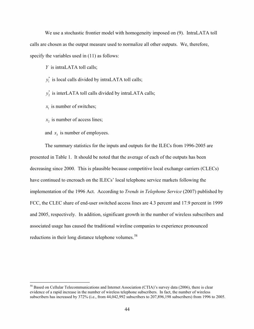
44

We use a stochastic frontier model with homogeneity imposed on (9). IntraLATA toll

calls are chosen as the output measure used to normalize all other outputs. We, therefore,

specify the variables used in (11) as follows:

Y is intraLATA toll calls;

*1y is local calls divided by intraLATA toll calls;

*2y is interLATA toll calls divided by intraLATA calls;

1x is number of switches;

2x is number of access lines;

and 3x is number of employees.

The summary statistics for the inputs and outputs for the ILECs from 1996-2005 are

presented in Table 1. It should be noted that the average of each of the outputs has been

decreasing since 2000. This is plausible because competitive local exchange carriers (CLECs)

have continued to encroach on the ILECs’ local telephone service markets following the

implementation of the 1996 Act. According to Trends in Telephone Service (2007) published by

FCC, the CLEC share of end-user switched access lines are 4.3 percent and 17.9 percent in 1999

and 2005, respectively. In addition, significant growth in the number of wireless subscribers and

associated usage has caused the traditional wireline companies to experience pronounced

reductions in their long distance telephone volumes.58

58 Based on Cellular Telecommunications and Internet Association (CTIA)’s survey data (2006), there is clear evidence of a rapid increase in the number of wireless telephone subscribers. In fact, the number of wireless subscribers has increased by 372% (i.e., from 44,042,992 subscribers to 207,896,198 subscribers) from 1996 to 2005.

45

EMPIRICAL RESULTS

The test results for various null hypotheses presented in Table 2 are conducted using log-

likelihood ratio (LR) tests. The LR test statistic is calculated by ( ) ( )02 AL H L H− × −⎡ ⎤⎣ ⎦ , where

( )0L H and ( )AL H are the log-likelihood values under the null and alternative hypotheses,

respectively. Given the stochastic frontier specification, we first test for changes in technical

inefficiency. The null hypothesis ( )0γ μ η= = = is rejected at the 1% significance level. This

implies technical inefficiency effects are statistically significant. The second null hypothesis,

that there is no technological change, is strongly rejected at the 1% significance level. This

result suggests that technological change exists in the model. The third hypothesis, testing that

technical inefficiency effects have a half-normal distribution is not rejected, indicating that the

technical inefficiency effects can be represented by a half normal distribution. The last set of

hypothesis tests focuses on whether technical inefficiency is time-invariant. This hypothesis is

rejected at the 1% statistical significance level, implying that technical inefficiency varies over

time. In addition, the estimate of η is statistically significant.

The maximum likelihood estimates (MLE) of the parameters in the translog stochastic

frontier production function defined by (11) and (12) are presented in Table 3. Note that the

parameter γ2

2 2μ

μ ν

σγ

σ σ⎛ ⎞

=⎜ ⎟⎜ ⎟+⎝ ⎠ is the ratio of the error variances from (11). Therefore, the value of

γ must lie between zero and one. If 0γ = , no technical inefficiency is present, while 1γ =

indicates that there exists no random noise. Thus, our estimate of γ = 0.872 implies that the

technical inefficiency component dominates the random noise component. The significant and

positive estimate of the time varying inefficiency effect, 0.0964η = , indicates that the technical

46

inefficiency effects are decreasing monotonically over time. These results further substantiate

the claim that there are time variant technical inefficiency effects in the error term that are

decreasing over time.

The indices for average productivity growth, efficiency, and technological change for the

period 1996-2005 are shown in table 4. The average efficiency change for all firms is greater

than one. The estimates of the inefficiency error term indicate that technical efficiency has

occurred at a positive rate while the rate of growth decreased continuously during the sample

period. However, indices of average productivity growth for each firm indicate negative growth

in productivity. For example, Qwest Corporation exhibits a -3.5 percent growth in annual

productivity. It is noteworthy that BellSouth (firm 10), the only firm that has not merged in the

sample, experienced the second lowest average productivity growth.

Table 5 provides technological change estimates for each firm across each time period.

Only three companies, Qwest Corporation, Southwestern Bell, and BellSouth have shown

persistent declines in technological change. All of the indices of technological change are less

than one indicating technological regression over time. One way of interpreting technological

regression in this study is that it may be the result of structural changes in the

telecommunications industry. Production in the conventional sectors, which is our main focus,

reveals no improvement, while the shift into new business models associated with new products

such as satellite TV, broadband, and voice over internet protocol (VoIP) that require high

technology grows rapidly.59

Table 6 presents the average productivity, efficiency, and technological change for each

individual firm during the pre-merger and post-merger periods. The duration of the post-merger

59 See Neuchterlein and Weiser (2005) for a comprehensive analysis of the technological dynamics of the telecommunications industry and its economic implications.

47

period is 5 and 6 years for the first and second group, respectively. Therefore, in order to

compare every firm in each group with a firm that has not merged, we compute two measures for

BellSouth Corporation. One is calculated from 2000 and the other is calculated from 1999.

When examining the indices in Table 6, it is noteworthy that every company experienced a

decline in every index after a merger. Specifically, BellSouth experienced a -5.2 percent annual

growth in productivity after the merger. Only firms 11 and 20 experience lower annual growth

in productivity than that of BellSouth during the post-merger periods.

We examine the robustness of these results by comparing the SFA and the Malmquist

index. These results are presented in Table 7 and Table 8. Table 7 compares the mean

efficiency change and the mean technological change between the SFM and the Malmquist index

method during the pre-merger and post-merger periods. There is a common trend in indices of

mean technological change. Using the Malmquist index method, only Verizon South has shown

positive (1.4 percent per year) growth in technological change after the merger. Otherwise, both

methods indicate negative growth in technological change over the post-merger period. There

are some inconsistent results for the mean efficiency change between the two methods. Using

the SFM, each firm experiences positive growth in annual efficiency change over the post-

merger period. However, the Malmquist index method indicates that 9 out of 25 individual firms

exhibit negative growth in annual efficiency change. The differences between two methods are

likely attributable to the particular specification of the inefficiency error term in SFM.

In Table 8, the Malmquist index method indicates that 4 out of 25 individual firms have

experienced increases in average productivity growth. In contrast, the stochastic frontier

estimation approach indicates that every firm has experienced decreases in average productivity

growth after the merger. Only firms 18 and 24 measured by the Malmquist index method exhibit

48

a 1.2 percent and 1.4 percent average growth in productivity, respectively. The remainder of the

firms has experienced negative growth in productivity. These results imply that most of the

firms experience deterioration in productivity following their mergers. Another interesting result

concerns the number of companies that experience productivity performance worse than

BellSouth, which is a non-merged control company. In terms of productivity growth, only 2

companies perform worse than BellSouth using the SFM approach, while 3 companies perform

worse than BellSouth using the Malmquist index.

CONCLUSION

This study analyzes the merger effects for 25 ILECs over the period 1996-2005 using stochastic

frontier analysis with a time varying inefficiency model. We find that our sample has

experienced deterioration in average productivity growth following the merger. This empirical

finding is attributed to technological regression, a finding that may lead policymakers to consider

implementing policies that serve to shift out the production frontier over time. In terms of

average growth in productivity, the performance of BellSouth, the only firm in the sample not to

have merged, ranks third lowest among the 25 ILECs.

Another component of this study is a comparison of indices for the stochastic frontier

analysis and the Malmquist index method. This comparison provides useful information on

robustness. With the exception of one firm using the Malmquist index method, both methods

indicate that every firm in the sample has experienced negative annual growth in technological

change. Indices of productivity growth suggest that most of the firms experience negative

growth in annual productivity after the merger according to both methods. However, in terms of

productivity growth, it is noteworthy that the only firm not to have merged underperforms during

49

post-merger periods. In SFM, annual productivity growth for BellSouth is the third lowest

company in the sample and the fourth lowest using the Malmquist index method.

In the telecommunications industry, the traditional wireline telecommunications sector

has experienced a shift toward a new business model involving satellite TV, Voice over Internet

Protocol (VoIP) and broadband internet. This study is not able to fully examine the far-reaching

effects of these phenomena. Hence, further research is necessary to investigate the impact of

these structural changes on the performance of the U.S telecommunications industry.

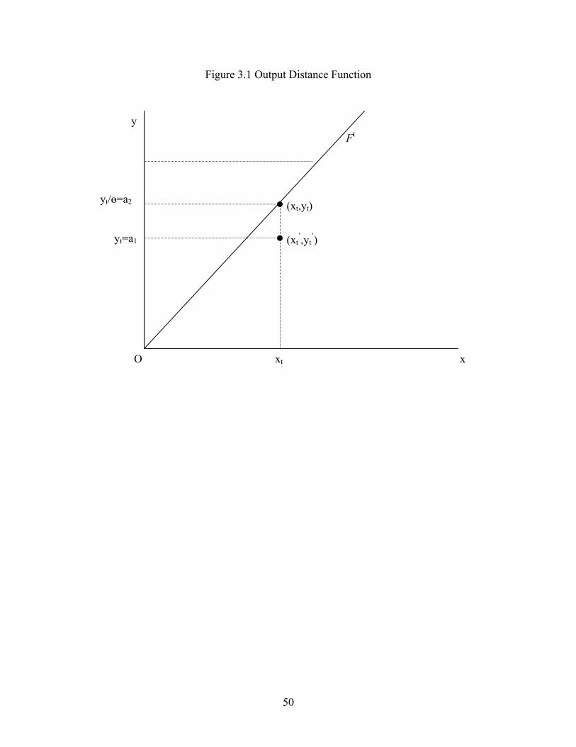
50

Figure 3.1 Output Distance Function

y yt/ө=a2 yt=a1

O xt x

Ft

(xt’,yt

’)

(xt,yt)

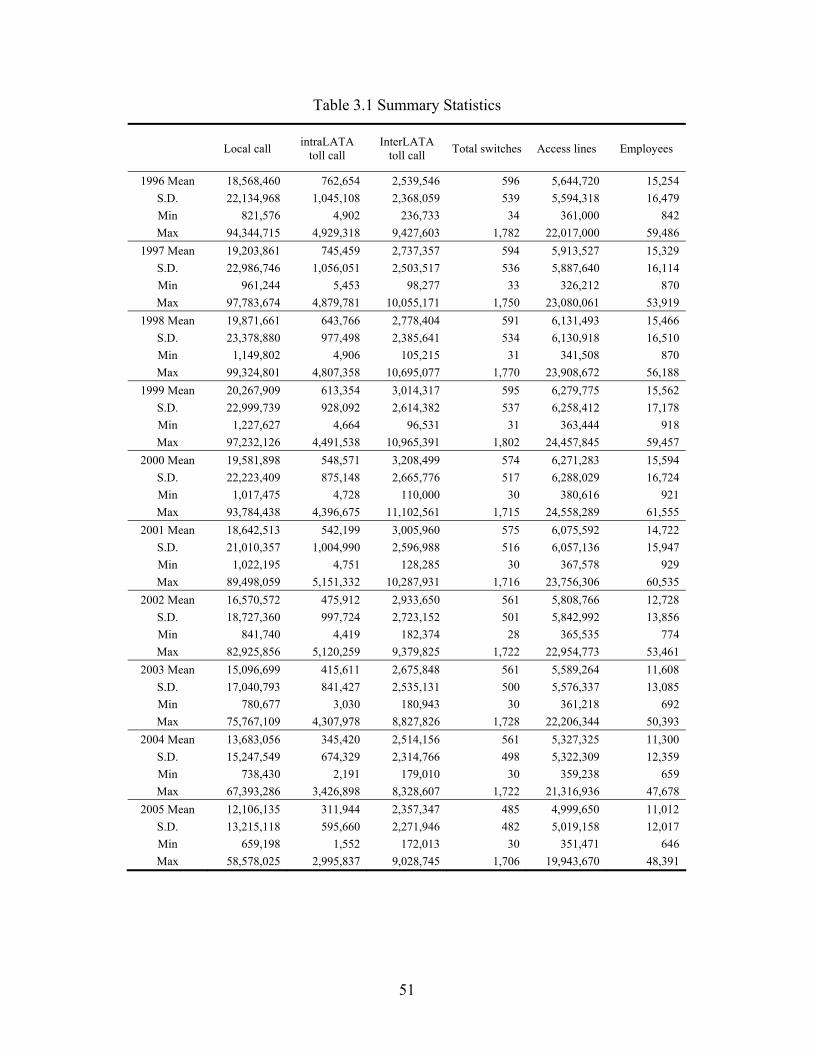
51

Table 3.1 Summary Statistics

Local call intraLATA toll call

InterLATA toll call Total switches Access lines Employees

1996 Mean 18,568,460 762,654 2,539,546 596 5,644,720 15,254 S.D. 22,134,968 1,045,108 2,368,059 539 5,594,318 16,479 Min 821,576 4,902 236,733 34 361,000 842 Max 94,344,715 4,929,318 9,427,603 1,782 22,017,000 59,486

1997 Mean 19,203,861 745,459 2,737,357 594 5,913,527 15,329 S.D. 22,986,746 1,056,051 2,503,517 536 5,887,640 16,114 Min 961,244 5,453 98,277 33 326,212 870 Max 97,783,674 4,879,781 10,055,171 1,750 23,080,061 53,919

1998 Mean 19,871,661 643,766 2,778,404 591 6,131,493 15,466 S.D. 23,378,880 977,498 2,385,641 534 6,130,918 16,510 Min 1,149,802 4,906 105,215 31 341,508 870 Max 99,324,801 4,807,358 10,695,077 1,770 23,908,672 56,188

1999 Mean 20,267,909 613,354 3,014,317 595 6,279,775 15,562 S.D. 22,999,739 928,092 2,614,382 537 6,258,412 17,178 Min 1,227,627 4,664 96,531 31 363,444 918 Max 97,232,126 4,491,538 10,965,391 1,802 24,457,845 59,457

2000 Mean 19,581,898 548,571 3,208,499 574 6,271,283 15,594 S.D. 22,223,409 875,148 2,665,776 517 6,288,029 16,724 Min 1,017,475 4,728 110,000 30 380,616 921 Max 93,784,438 4,396,675 11,102,561 1,715 24,558,289 61,555

2001 Mean 18,642,513 542,199 3,005,960 575 6,075,592 14,722 S.D. 21,010,357 1,004,990 2,596,988 516 6,057,136 15,947 Min 1,022,195 4,751 128,285 30 367,578 929 Max 89,498,059 5,151,332 10,287,931 1,716 23,756,306 60,535

2002 Mean 16,570,572 475,912 2,933,650 561 5,808,766 12,728 S.D. 18,727,360 997,724 2,723,152 501 5,842,992 13,856 Min 841,740 4,419 182,374 28 365,535 774 Max 82,925,856 5,120,259 9,379,825 1,722 22,954,773 53,461

2003 Mean 15,096,699 415,611 2,675,848 561 5,589,264 11,608 S.D. 17,040,793 841,427 2,535,131 500 5,576,337 13,085 Min 780,677 3,030 180,943 30 361,218 692 Max 75,767,109 4,307,978 8,827,826 1,728 22,206,344 50,393

2004 Mean 13,683,056 345,420 2,514,156 561 5,327,325 11,300 S.D. 15,247,549 674,329 2,314,766 498 5,322,309 12,359 Min 738,430 2,191 179,010 30 359,238 659 Max 67,393,286 3,426,898 8,328,607 1,722 21,316,936 47,678

2005 Mean 12,106,135 311,944 2,357,347 485 4,999,650 11,012 S.D. 13,215,118 595,660 2,271,946 482 5,019,158 12,017 Min 659,198 1,552 172,013 30 351,471 646 Max 58,578,025 2,995,837 9,028,745 1,706 19,943,670 48,391

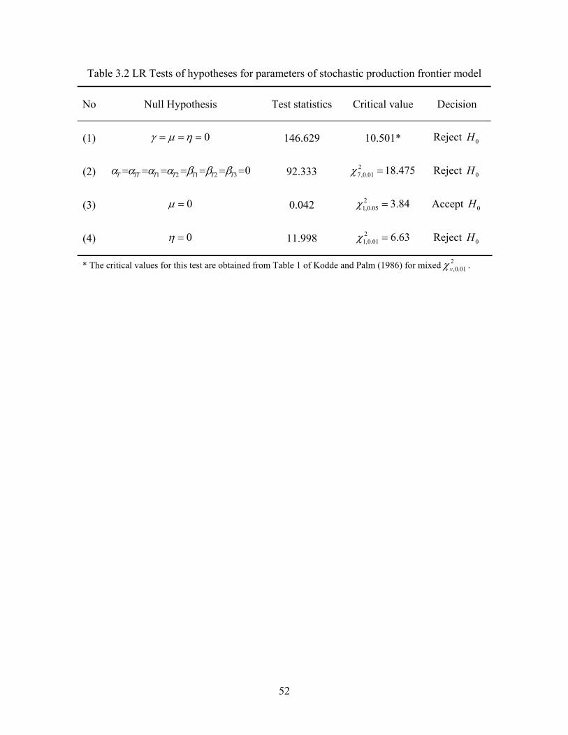
52

Table 3.2 LR Tests of hypotheses for parameters of stochastic production frontier model

No Null Hypothesis Test statistics Critical value Decision

(1) 0γ μ η= = = 146.629 10.501* Reject 0H

(2) 1 2 1 2 3 0T TT T T T T Tα α α α β β β= = = = = = = 92.333 27,0.01 18.475χ = Reject 0H

(3) 0μ = 0.042 21,0.05 3.84χ = Accept 0H

(4) 0η = 11.998 21,0.01 6.63χ = Reject 0H

* The critical values for this test are obtained from Table 1 of Kodde and Palm (1986) for mixed 2,0.01vχ .

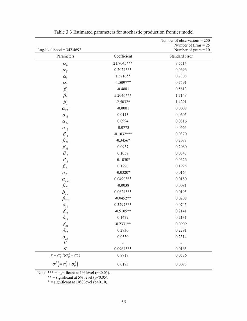
53

Table 3.3 Estimated parameters for stochastic production frontier model

Log-likelihood = 342.4692

Number of observations = 250 Number of firms = 25 Number of years = 10

Parameters Coefficient Standard error

0α 21.7045*** 7.5514

Tα 0.2024*** 0.0696

1α 1.5716** 0.7308

2α -1.5097** 0.7591

1β -0.4881 0.5813

2β 5.2046*** 1.7148

3β -2.5032* 1.4291

TTα -0.0001 0.0008

11α 0.0113 0.0605

22α 0.0994 0.0816

12α -0.0773 0.0665

11β -0.1032*** 0.0370

22β -0.3456* 0.2073

33β 0.0937 0.2060

12β 0.1057 0.0747

13β -0.1030* 0.0626

23β 0.1290 0.1928

1Tα -0.0320* 0.0164

2Tα 0.0490*** 0.0180

1Tβ -0.0038 0.0081

2Tβ 0.0624*** 0.0195

3Tβ -0.0452** 0.0208

11δ 0.3297*** 0.0745

12δ -0.5105** 0.2141

13δ 0.1479 0.2131

21δ -0.2331** 0.0909

22δ 0.2730 0.2291

23δ 0.0330 0.2314 μ - - η 0.0964*** 0.0163

2 2 2/( )μ μ νγ σ σ σ= + 0.8719 0.0536

( )2 2 2μ νσ σ σ= + 0.0183 0.0073

Note: *** = significant at 1% level (p<0.01). ** = significant at 5% level (p<0.05).

* = significant at 10% level (p<0.10).

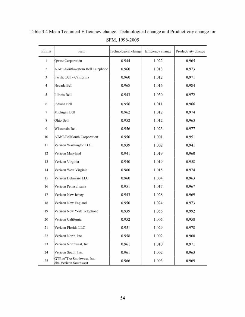
54

Table 3.4 Mean Technical Efficiency change, Technological change and Productivity change for

SFM, 1996-2005

Firm # Firm Technological change Efficiency change Productivity change

1 Qwest Corporation 0.944 1.022 0.965

2 AT&T/Southwestern Bell Telephone 0.960 1.013 0.973

3 Pacific Bell - California 0.960 1.012 0.971

4 Nevada Bell 0.968 1.016 0.984

5 Illinois Bell 0.943 1.030 0.972

6 Indiana Bell 0.956 1.011 0.966

7 Michigan Bell 0.962 1.012 0.974

8 Ohio Bell 0.952 1.012 0.963

9 Wisconsin Bell 0.956 1.023 0.977

10 AT&T/BellSouth Corporation 0.950 1.001 0.951

11 Verizon Washington D.C. 0.939 1.002 0.941

12 Verizon Maryland 0.941 1.019 0.960

13 Verizon Virginia 0.940 1.019 0.958

14 Verizon West Virginia 0.960 1.015 0.974

15 Verizon Delaware LLC 0.960 1.004 0.963

16 Verizon Pennsylvania 0.951 1.017 0.967

17 Verizon New Jersey 0.943 1.028 0.969

18 Verizon New England 0.950 1.024 0.973

19 Verizon New York Telephone 0.939 1.056 0.992

20 Verizon California 0.952 1.005 0.958

21 Verizon Florida LLC 0.951 1.029 0.978

22 Verizon North, Inc. 0.958 1.002 0.960

23 Verizon Northwest, Inc. 0.961 1.010 0.971

24 Verizon South, Inc. 0.961 1.002 0.963

25 GTE of The Southwest, Inc. dba Verizon Southwest 0.966 1.003 0.969

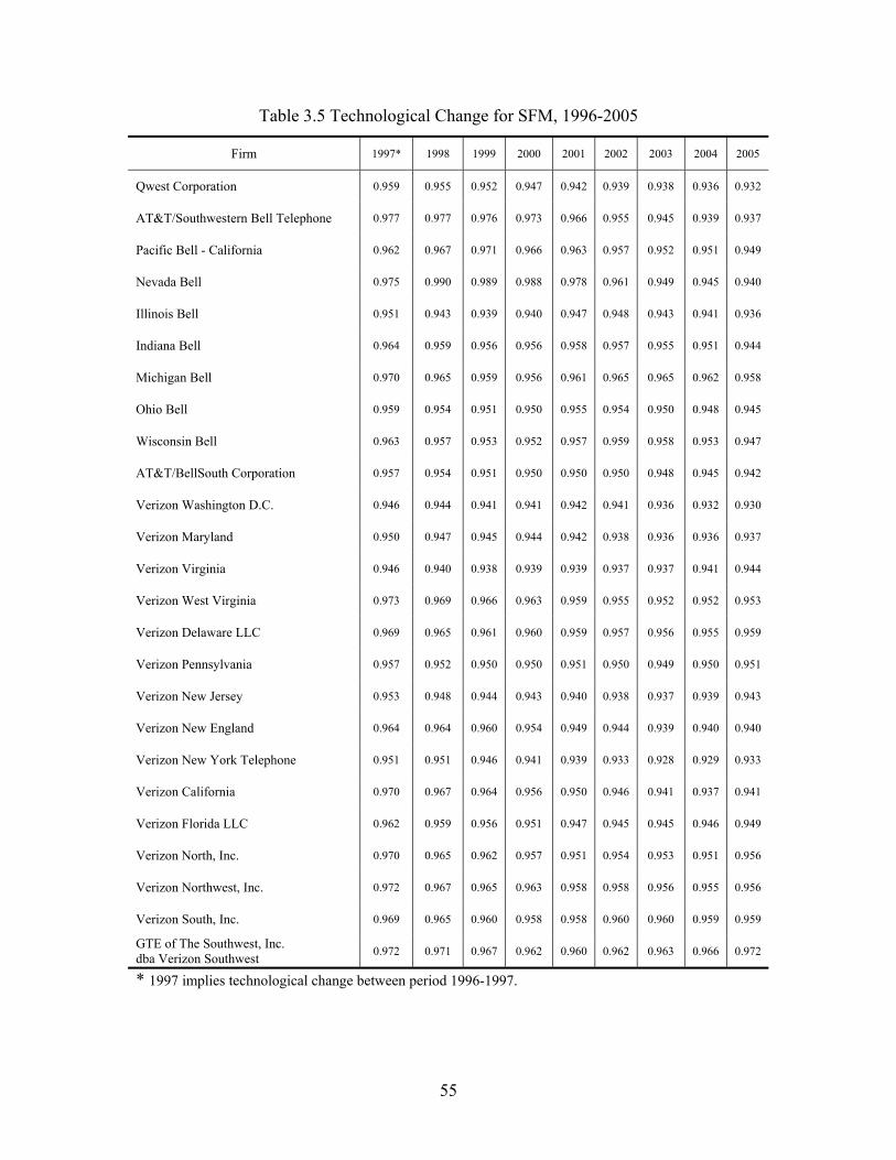
55

Table 3.5 Technological Change for SFM, 1996-2005

Firm 1997* 1998 1999 2000 2001 2002 2003 2004 2005

Qwest Corporation 0.959 0.955 0.952 0.947 0.942 0.939 0.938 0.936 0.932

AT&T/Southwestern Bell Telephone 0.977 0.977 0.976 0.973 0.966 0.955 0.945 0.939 0.937

Pacific Bell - California 0.962 0.967 0.971 0.966 0.963 0.957 0.952 0.951 0.949

Nevada Bell 0.975 0.990 0.989 0.988 0.978 0.961 0.949 0.945 0.940

Illinois Bell 0.951 0.943 0.939 0.940 0.947 0.948 0.943 0.941 0.936

Indiana Bell 0.964 0.959 0.956 0.956 0.958 0.957 0.955 0.951 0.944

Michigan Bell 0.970 0.965 0.959 0.956 0.961 0.965 0.965 0.962 0.958

Ohio Bell 0.959 0.954 0.951 0.950 0.955 0.954 0.950 0.948 0.945

Wisconsin Bell 0.963 0.957 0.953 0.952 0.957 0.959 0.958 0.953 0.947

AT&T/BellSouth Corporation 0.957 0.954 0.951 0.950 0.950 0.950 0.948 0.945 0.942

Verizon Washington D.C. 0.946 0.944 0.941 0.941 0.942 0.941 0.936 0.932 0.930

Verizon Maryland 0.950 0.947 0.945 0.944 0.942 0.938 0.936 0.936 0.937

Verizon Virginia 0.946 0.940 0.938 0.939 0.939 0.937 0.937 0.941 0.944

Verizon West Virginia 0.973 0.969 0.966 0.963 0.959 0.955 0.952 0.952 0.953

Verizon Delaware LLC 0.969 0.965 0.961 0.960 0.959 0.957 0.956 0.955 0.959

Verizon Pennsylvania 0.957 0.952 0.950 0.950 0.951 0.950 0.949 0.950 0.951

Verizon New Jersey 0.953 0.948 0.944 0.943 0.940 0.938 0.937 0.939 0.943

Verizon New England 0.964 0.964 0.960 0.954 0.949 0.944 0.939 0.940 0.940

Verizon New York Telephone 0.951 0.951 0.946 0.941 0.939 0.933 0.928 0.929 0.933

Verizon California 0.970 0.967 0.964 0.956 0.950 0.946 0.941 0.937 0.941

Verizon Florida LLC 0.962 0.959 0.956 0.951 0.947 0.945 0.945 0.946 0.949

Verizon North, Inc. 0.970 0.965 0.962 0.957 0.951 0.954 0.953 0.951 0.956

Verizon Northwest, Inc. 0.972 0.967 0.965 0.963 0.958 0.958 0.956 0.955 0.956

Verizon South, Inc. 0.969 0.965 0.960 0.958 0.958 0.960 0.960 0.959 0.959

GTE of The Southwest, Inc. dba Verizon Southwest 0.972 0.971 0.967 0.962 0.960 0.962 0.963 0.966 0.972

* 1997 implies technological change between period 1996-1997.

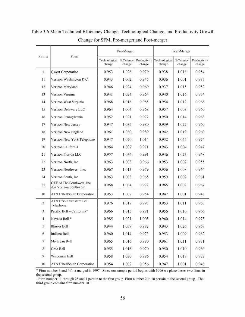
56


Change for SFM, Pre-merger and Post-merger

Pre-Merger Post-Merger Firm # Firm


Efficiency change

Productivity change


Efficiency change

Productivity change



















3 Pacific Bell – California* 0.966 1.015 0.981 0.956 1.010 0.966

4 Nevada Bell * 0.985 1.021 1.005 0.960 1.014 0.973

5 Illinois Bell 0.944 1.039 0.982 0.943 1.026 0.967

6 Indiana Bell 0.960 1.014 0.973 0.953 1.009 0.962

7 Michigan Bell 0.965 1.016 0.980 0.961 1.011 0.971

8 Ohio Bell 0.955 1.016 0.970 0.950 1.010 0.960

9 Wisconsin Bell 0.958 1.030 0.986 0.954 1.019 0.973

10 AT&T/BellSouth Corporation 0.954 1.002 0.956 0.947 1.001 0.948 * Firm number 3 and 4 first merged in 1997. Since our sample period begins with 1996 we place theses two firms in the second group. - Firm number 11 through 25 and 1 pertain to the first group. Firm number 2 to 10 pertain to the second group. The third group contains firm number 10.

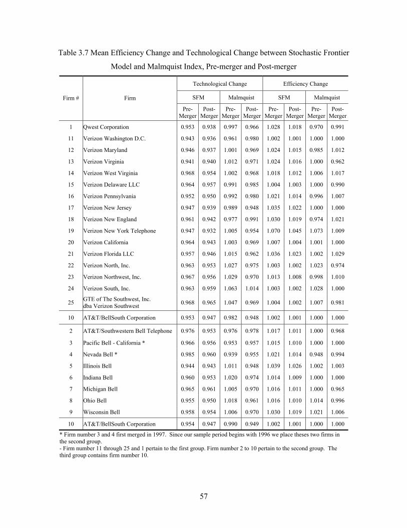
57

Table 3.7 Mean Efficiency Change and Technological Change between Stochastic Frontier

Model and Malmquist Index, Pre-merger and Post-merger

Technological Change Efficiency Change

SFM Malmquist SFM Malmquist Firm # Firm

Pre-Merger

Post-Merger

Pre-Merger

Post-Merger

Pre-Merger

Post-Merger

Pre-Merger

Post-Merger

1 Qwest Corporation 0.953 0.938 0.997 0.966 1.028 1.018 0.970 0.991

11 Verizon Washington D.C. 0.943 0.936 0.961 0.980 1.002 1.001 1.000 1.000

12 Verizon Maryland 0.946 0.937 1.001 0.969 1.024 1.015 0.985 1.012

13 Verizon Virginia 0.941 0.940 1.012 0.971 1.024 1.016 1.000 0.962

14 Verizon West Virginia 0.968 0.954 1.002 0.968 1.018 1.012 1.006 1.017

15 Verizon Delaware LLC 0.964 0.957 0.991 0.985 1.004 1.003 1.000 0.990

16 Verizon Pennsylvania 0.952 0.950 0.992 0.980 1.021 1.014 0.996 1.007

17 Verizon New Jersey 0.947 0.939 0.989 0.948 1.035 1.022 1.000 1.000

18 Verizon New England 0.961 0.942 0.977 0.991 1.030 1.019 0.974 1.021

19 Verizon New York Telephone 0.947 0.932 1.005 0.954 1.070 1.045 1.073 1.009

20 Verizon California 0.964 0.943 1.003 0.969 1.007 1.004 1.001 1.000

21 Verizon Florida LLC 0.957 0.946 1.015 0.962 1.036 1.023 1.002 1.029

22 Verizon North, Inc. 0.963 0.953 1.027 0.975 1.003 1.002 1.023 0.974

23 Verizon Northwest, Inc. 0.967 0.956 1.029 0.970 1.013 1.008 0.998 1.010

24 Verizon South, Inc. 0.963 0.959 1.063 1.014 1.003 1.002 1.028 1.000

25 GTE of The Southwest, Inc. dba Verizon Southwest 0.968 0.965 1.047 0.969 1.004 1.002 1.007 0.981

10 AT&T/BellSouth Corporation 0.953 0.947 0.982 0.948 1.002 1.001 1.000 1.000

2 AT&T/Southwestern Bell Telephone 0.976 0.953 0.976 0.978 1.017 1.011 1.000 0.968

3 Pacific Bell - California * 0.966 0.956 0.953 0.957 1.015 1.010 1.000 1.000

4 Nevada Bell * 0.985 0.960 0.939 0.955 1.021 1.014 0.948 0.994

5 Illinois Bell 0.944 0.943 1.011 0.948 1.039 1.026 1.002 1.003

6 Indiana Bell 0.960 0.953 1.020 0.974 1.014 1.009 1.000 1.000

7 Michigan Bell 0.965 0.961 1.005 0.970 1.016 1.011 1.000 0.965

8 Ohio Bell 0.955 0.950 1.018 0.961 1.016 1.010 1.014 0.996

9 Wisconsin Bell 0.958 0.954 1.006 0.970 1.030 1.019 1.021 1.006

10 AT&T/BellSouth Corporation 0.954 0.947 0.990 0.949 1.002 1.001 1.000 1.000

* Firm number 3 and 4 first merged in 1997. Since our sample period begins with 1996 we place theses two firms in the second group. - Firm number 11 through 25 and 1 pertain to the first group. Firm number 2 to 10 pertain to the second group. The third group contains firm number 10.

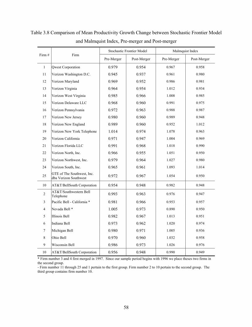
58

Table 3.8 Comparison of Mean Productivity Growth Change between Stochastic Frontier Model

and Malmquist Index, Pre-merger and Post-merger

Stochastic Frontier Model Malmquist Index Firm # Firm

Pre-Merger Post-Merger Pre-Merger Post-Merger

1 Qwest Corporation 0.979 0.954 0.967 0.958

11 Verizon Washington D.C. 0.945 0.937 0.961 0.980

12 Verizon Maryland 0.969 0.952 0.986 0.981

13 Verizon Virginia 0.964 0.954 1.012 0.934

14 Verizon West Virginia 0.985 0.966 1.008 0.985

15 Verizon Delaware LLC 0.968 0.960 0.991 0.975

16 Verizon Pennsylvania 0.972 0.963 0.988 0.987

17 Verizon New Jersey 0.980 0.960 0.989 0.948

18 Verizon New England 0.989 0.960 0.952 1.012

19 Verizon New York Telephone 1.014 0.974 1.078 0.963

20 Verizon California 0.971 0.947 1.004 0.969

21 Verizon Florida LLC 0.991 0.968 1.018 0.990

22 Verizon North, Inc. 0.966 0.955 1.051 0.950

23 Verizon Northwest, Inc. 0.979 0.964 1.027 0.980

24 Verizon South, Inc. 0.965 0.961 1.093 1.014

25 GTE of The Southwest, Inc. dba Verizon Southwest 0.972 0.967 1.054 0.950

10 AT&T/BellSouth Corporation 0.954 0.948 0.982 0.948

2 AT&T/Southwestern Bell Telephone 0.993 0.963 0.976 0.947

3 Pacific Bell - California * 0.981 0.966 0.953 0.957

4 Nevada Bell * 1.005 0.973 0.890 0.950

5 Illinois Bell 0.982 0.967 1.013 0.951

6 Indiana Bell 0.973 0.962 1.020 0.974

7 Michigan Bell 0.980 0.971 1.005 0.936

8 Ohio Bell 0.970 0.960 1.032 0.958

9 Wisconsin Bell 0.986 0.973 1.026 0.976

10 AT&T/BellSouth Corporation 0.956 0.948 0.990 0.949

* Firm number 3 and 4 first merged in 1997. Since our sample period begins with 1996 we place theses two firms in the second group. - Firm number 11 through 25 and 1 pertain to the first group. Firm number 2 to 10 pertain to the second group. The third group contains firm number 10.

59

Chapter 4 - The Impact of Incentive Regulation on the U.S.

Telecommunications Industry: A Stochastic Frontier Approach

INTRODUCTION

Since the late 1980s, one of the most important trends in regulatory policy in the U.S.

telecommunications industry has been the transition from traditional rate-of-return regulation

(RRR) to alternative forms of regulation, so called incentive regulation (IR).60,61 Regulators in

the telecommunications industry anticipated that the adoption of incentive regulation would

lower prices, enhance technical innovation, encourage firms to operate with efficient technology

and reduce the administrative costs of regulation.

A large volume of research has examined the effects associated with the implementation

of incentive regulations.62 Schmalensee and Rohlfs (1992) examined the effect of price cap

regulation (PCR)63 on productivity gains. They compared AT&T’s productivity gains on

switched services in the period prior to the implementation of PCR (1986-1988) with the period

following the implementation of PCR (1989-1991). Schmalensee and Rholfs found that the

60 Economists have long criticized the incentive properties of RRR. For example, Braeutigam and Panzar (1989) describe potential problems of RRR, including: (1) incentives to misreport cost allocations; (2) choose an inefficient technology mix; (3) underinvestment in cost-reducing innovation; (4) underproduce in the non-core market; (5) inefficient diversification. Sappington (2001) has analyzed potential flaws in RRR to include: (1) firms are not likely to perform fully in terms of incentives for innovation and cost minimization; (2) over capitalization; (3) regulatory cost are high; (4) consumers bear excessive risk; (5) cost shifting; (6) distortion of diversification and innovation; (7) operate with inefficient technology; and (8) insufficient pricing flexibility. See also Weisman (1996) for a discussion of similar drawback associated with price cap regulation with earnings sharing. 61 In this essay, we examine 4 different types of IR. These are Earnings Sharing, Hybrid Price Caps, Price Caps, and Other Forms of IR. See Sappington and Weisman (1996) for a discussion of incentive regulation in the telecommunications industry. 62 Empirical analyses of the effects of incentive regulation have focused on performance metrics such as services prices, production costs, productivity, investment in infrastructure, service quality, company profits, service penetration rates and new services in the telecommunications industry. See Kridel et al. (1996) for further review. 63 PCR is the dominant regulatory regime among incentive regulation regimes. Substituting PCR for RRR provides for Pareto-superior change for all primary economic entities: the regulator, consumers, and competitors. See Weisman (2000b).

60

cumulative productivity gains were $1.8 billion higher during the PCR period relative to the

RRR period.64

Majumdar (1997) employed a non-parametric approach, commonly referred to as data

envelopment analysis (DEA), to examine the effect of incentive regulation on the productive

performance of 45 local exchange carriers (LECs) over the period 1988-1993. He showed that

PCR has a positive but lagged effect on technical efficiency.65 Uri (2001) used a Malmquist

index to measure the change in productivity growth following the implementation of incentive

regulation. He found that productivity growth increased by approximately 5 percent per year for

the 19 LECs over the period 1988-1999.

Although a number of empirical studies have concluded that the effect of incentive

regulation on productivity growth in the U.S. telecommunications industry is substantially

positive, some studies find that the effect of incentive regulation is ambiguous. For example,

Resende (1999)66 estimated a translog cost function combined with total factor productivity

(TFP) growth decomposition for the period 1989-1994. He found that incentive regulation did

not enhance the level of productive efficiency. Uri (2002) employed a corrected ordinary least

64 Kwoka (1993) analyzed the impact of different regulatory policies on productivity growth of British Telecom (BT). He found empirical evidence that the combination of privatization and price cap regulation for BT substantially affected productivity increases from 1984 to 1987. Tardiff and Taylor (1993) examined the effects of the implementation of incentive regulation on the local telecommunications firms in the U.S. They found that firms operating incentive regulation improved their annual total factor productivity (TFP) growth rate by 2.8 percentage points. This increase is attributed to the gains in output productivity and reduction in the growth rate of input under incentive regulation. Ai and Sappington (2002) used a fixed-effects estimation to examine the effect of incentive regulation on the U.S. telecommunications industry. They find that the incentive regulation improves network modernization and lowered costs. 65 Kang (2000) introduced both static and dynamic DEA to investigate the effects of the implementation of incentive regulatory regimes at the state level for 28 local exchange carriers (LECs) over the period 1988 and 1998. He found that state level PCR had a positive effect on pure technical efficiency—an estimated improvement on average of 4 % in terms of the LECs’ technical efficiency. Jung (2005) also employed both static and dynamic DEA to examine the effects of the implementation of incentive regulatory regimes for the period 1988-2000. His empirical findings, including various efficiency scores, indicated that only pure price cap regulation has a positive influence on improving efficiency scores. 66 Resende (2000) used DEA to analyze the impact of alternative forms of regulation in the U.S. telecommunications industry. He found no empirical evidence in support of the claim that price cap regulation had a positive effect on technical efficiency.

61

squares (COLS) approach to measure the efficiency gains associated with the implementation of

incentive regulation in the U.S. telecommunications industry. Using data from 19 LECs over the

1988-1999 time period, he found no empirical evidence that incentive regulation had enhanced

technical efficiency.

In an attempt to resolve the extant ambiguity in the literature concerning the effect of

incentive regulation on productivity growth, this essay investigates whether the substitution of

PCR along with other incentive regulatory regimes for RRR enhanced the productive efficiency

in the U.S. telecommunications industry using a stochastic frontier analysis (SFA). Specifically,

we measure the productivity growth for 25 local exchange carriers’ (LECs), inclusive of its

underlying components -- technological progress and changes in technical efficiency over the

period 1988 to 1998.

This study has two principal objectives. First, using SFA, this essay measures

productivity growth associated with technological progress and changes in technical efficiency to

examine the improvement in the LECs’ productivity growth. Although previous studies provide

some useful results in terms of productivity growth, employing the SFA approach differs from

previous studies in material ways. Second, this essay analyzes the effects associated with the

adoption of incentive regulation on the LECs’ productivity growth rate.

The remainder of this essay is organized as follows. Section 2 discusses the multiple

output distance function and presents the models used in the study. In Section 3, we discuss the

data set, hypothesis tests and productivity growth changes. The estimates of the factors,

including various regulatory regime variables, that explain changes in productivity growth are

presented and discussed in Section 4. Section 5 provides a brief summary and conclusion.

62

THEORY OF STOCHASTIC FRONTIER ANALYSIS

Distance Function

To measure the production frontier, an output distance function is employed. The main

advantage of the distance function approach is that it allows for a multiple-input and multiple-

output technology without requiring price data, which is typically a constraint in working with

telecommunications industry data.67

In order to define the output distance function, we first introduce the production

technology. We assume that for each time period 1, , ,t T= … the production technology tF maps

input vectors, ntx +∈R , into output vectors, m

ty +∈R ,

( ){ }, : can produce tt t t tF x y x y= , (1)

whereR is the set of real numbers.68 The production technology tF is homogeneous of degree

one in output. Following Shepard (1970), the output distance function is defined at time t as:

( ) ( ){ }( ) 1, inf : , sup : ,t tt

Ot t t t t tyD x y x F x y Fθ θ θθ

−⎧ ⎫⎛ ⎞= ∈ = ∈⎨ ⎬⎜ ⎟⎝ ⎠⎩ ⎭

. (2)

According to Lovell et al. (1994), the output distance function ( ),Ot t tD x y is non-

decreasing, positively linearly homogeneous and convex in y and decreasing in x .69 Note that

the input-output vectors lie below the production technology set. This implies that

67 The distance function can be estimated in several ways. These include data envelopment analysis (DEA), parametric deterministic linear programming (PLP), corrected ordinary least squares (COLS), and stochastic frontier analysis (SFA). 68 The production technology must satisfy following axioms in order to be a meaningful model of production: i) the possibility of inaction; ii) monotonicity of the output correspondence; iii) disposability of output iv); the output set is closed v); irreversibility (Färe, R., and S. Grosskopf. 1994). 69 Refer to Coelli et al. (1998) for further discussion of distance functions.

63

( ), 1Ot t tD x y ≤ if and only if ( ), tt tx y F∈ . Moreover, ( ), 1Ot t tD x y = if and only if ( ),t tx y lie on

the boundary of the production technology set.

Stochastic Frontier Analysis

There are two main approaches employed in efficiency analysis: econometric methods and the

non-parametric DEA method. Depending upon the assumed property of the error term, the

econometric method is categorized by a deterministic approach or a stochastic approach. The

main advantage of stochastic frontier analysis (SFA) is that it accounts for the possible influence

of noise on the shape and positioning of the frontier, something that deterministic frontier models

are unable to do. In other words, issues such as measurement error and other random factors can

be separated from the sources of variation in technical efficiency. SFA posits a production

function with an error term associated with two components. These two components consist of a

symmetric error term accounting for noise and an asymmetric error term accounting for technical

inefficiency.

Based on Coelli and Perelman (2000), the multiple output distance function is specified

in translog functional form and is given by:

01 1 1 1

1ln( ) ln ln ln ln2

J L J J

Oi j ij l il jk ij ikj l j k

D y x y yα α β α= = = =

= + + +∑ ∑ ∑∑

1 1 1 1

1 1ln ln ln ln , 1, 2, ,2 2

L L J L


x x y x i Iβ δ= = = =

+ + =∑∑ ∑∑ … (3)

where J is the number of outputs, L is the number of inputs, and i denotes the i th firm in the

sample. The restrictions required for homogeneity of degree one in outputs are

1

1J

jjα

=

=∑ , (4)

and

64

1

0, 1, 2, ,J

jkk

j Jα=

= = …∑ and 1

0, 1, 2, ,L

jll

l Lδ=

= = …∑ . (5)

The restrictions required for symmetry are

, , 1, 2, ,jk kj j k Jα α= = … and , , 1, 2, ,lm ml l m Lβ β= = … . (6)

Lovell et al. (1994) proposed a convenient method for imposing the homogeneity

restriction in (3). Homogeneity implies that

( ) ( ), , ,O OD x y D x yλ λ= for any 0λ > . (7)

Hence, we arbitrarily choose one of the outputs, and set 1

Jyλ = , which allows us to obtain

( ),, O

OJ J

D x yyD xy y

⎛ ⎞=⎜ ⎟

⎝ ⎠. (8)

The translog function can be written as:

1 1 1* * *

01 1 1 1

1ln( ) ln ln ln ln2ij

J L J Joi

j l il jk ij ikj l j kiJ

D y x y yy

α α β α− − −

= = = =

= + + +∑ ∑ ∑∑

1

*

1 1 1 1

1 1ln ln ln ln , 1, 2, ,2 2

L L J L


x x y x i Iβ δ−

= = = =

+ + =∑∑ ∑∑ … , (9)

where * ijij

iJ

yy

y= . Equation (9) can be rewritten in the following functional form

( ) ( )*ln( ) , , , lniJ Oiy TL y x Dα β− = − 70 (10)

We append the noise term iv and change the notation from ( )ln OiD to iu− . This

transformation yields the stochastic frontier function associated with the time trend for the panel

data and is expressed as follows:

70 Note that Doi =1 implies that the firm lies on the boundary of the frontier.

65

1* 2

01 1

1ln( ) ln ln2

J L

it T j ijt l ilt TTj l

Y t y x tα α α β α−

= =

− = + + + +∑ ∑

1 1 2* * *

1 1 1 1 1

1 1 1ln ln ln ln ln2 2 2

J J L L

jk ijt ikt lm ilt imt Tj ijtj k l m j

y y x x t yα β α− −

= = = = =

+ + +∑∑ ∑∑ ∑

1*

1 1 1

1 1ln ln ln2 2

L J L

Tl ilt jl ijt ilt it itl j l

t x y x v uβ δ−

= = =

+ + + +∑ ∑∑ ,71 (11)

where 1,2, ,t T= … is a time trend. itY and *ijty are the output and arbitrarily normalized output

for firm i , respectively. Subscripts ,j k index outputs; , ,α β δ are parameters to be estimated; x

variables are inputs. Subscripts ,l m index inputs; the itv s are the error components and are

assumed to be independently and identically distributed as ( )20, vN σ . The itu ’s are the technical

inefficiency components.

Following Battese and Coelli (1992), the technical inefficiency error term is defined by

( )exp , 1, 2, , ; 1, 2, ,it iu u t T i I t Tη= − − = =⎡ ⎤⎣ ⎦ … … , (12)

where the iu s are assumed to be a non-negative truncation of the normal distribution ( )2,N μμ σ

associated with technical inefficiency in production. iu is the technical inefficiency effect for

firm i for the last period of the sample; η is an unknown parameter to be estimated and

represents the rate of change in technical inefficiency. Therefore, a positive value, 0η > , implies

that the technical inefficiency effects are decreasing over time.72 One of the advantages of using

71 Note that as suggested by Morrison-Paul et al. (2000), one can change the sign of dependent variable. This change allows for interpreting estimates that conform to the standard SFA framework. 72 If η > 0 then - η (t-T) ≡ η(T-t) and it iu u> . However, the value of the exponential function is decreasing monotonically towards the value of the last period in the sample. If η = 0, the translog specification in (11) becomes a time-invariant inefficiency model.

66

the error term in (12) is that any technical inefficiency changes over time can be separated from

technical change.

Following Coelli et al. (1998) and given the estimates for (11) and (12), the technical

efficiencies of production for each firm in the t th year can be predicted as:

( )expit itTE u= − .73 (13)

Therefore, the technical efficiency change between adjacent periods t and s is calculated as:

itit

is

TEECTE

= . (14)

With the estimates of the parameters in (11) and (12), the index of the technological

change for firm i is calculated by evaluating the partial derivative of the production function

with respect to time. The calculation of technological change is computed according to:

( ) ( )* * * * * *, , , , , , , ,1 1is is it it

it

f y x t f y x tTC

s tα β α β⎡ ⎤ ⎡ ⎤∂ ∂

⎢ ⎥ ⎢ ⎥= + × +∂ ∂⎢ ⎥ ⎢ ⎥⎣ ⎦ ⎣ ⎦

. (15)

Finally, the TFP index can be obtained by the product of the index of technical efficiency

change and the index of technological change calculated from (14) and (15):

it it itTFP EC TC= × . (16)

Data and Productivity Growth

The data used in this analysis represent a balanced panel that consists of annual data for 25

ILECs over the 1988-1998 period.74 The primary sources of data are obtained from the

73 The predicted values of technical efficiency lie between zero and one. A value of one implies that the firm lies on the boundary of the production possibility set. 74 Starting with the year 1988, the accounting system that tracks these data was changed.

67

Electronic ARMIS Filing System and the Statistics of Communications Common Carriers

maintained by the U.S. Federal Communications Commission (FCC).75

Local calls, intraLATA toll calls, and interLATA toll calls are the output variables since

these are the core services provided by ILECs. 76 The measures of inputs are the total number of

switches, the number of access lines, and the number of employees.77 The use of these three

inputs captures the actual industry characteristics for producing telephone service.

We use a stochastic frontier model with homogeneity imposed on (9). IntraLATA toll

calls are chosen as the output measure used to normalize all other outputs. We therefore specify

the variables used in (11) as follows:

Y is intraLATA toll calls;

*1y is local calls divided by intraLATA toll calls;

*2y is interLATA toll calls divided by intraLATA calls;

1x is number of switches;

2x is number of access lines;

and 3x is number of employees.

The test results for various null hypotheses presented in Table 1 are conducted using log-

likelihood ratio (LR) tests.78 Given the stochastic frontier specification, we first test for changes

75 ARMIS is the acronym for Automated Reporting Management Information System. One may refer to http://www.fcc.gov/wcb/armis to access the data set. FCC Report 43-02, the ARMIS USOA Report, FCC Report 43-07, the ARMIS Infrastructure Report and FCC Report 43-08, the ARMIS Operating Data Report were used to populate the data set. 76 As part of the break up of AT&T in 1984, the U.S. was partitioned into approximately 161 local access transport areas or LATAs. The RBOCs were restricted to providing intraLATA long distance service which essentially meant that they could not provide long distance service across area code boundaries. Section 271 of the 1996 Telecommunications Act specified the terms and conditions that would enable the RBOCs to re-enter the interLATA long distance market. 77 Majumdar (1997) also introduced the same classification for outputs and inputs. 78 The LR test statistic is calculated by -2x[L(H0) - L(HA)], where L(H0) and L(HA) are the log-likelihood values under the null and alternative hypotheses, respectively.

68

in technical inefficiency. The null hypothesis ( )0γ μ η= = = is rejected at the 1% significance

level. This implies that OLS does not fit the actual frontier well due to the technical inefficiency

effects. The second null hypothesis, that there is no technological change, is strongly rejected.

This result suggests that technological change exists in the model. The third hypothesis test that

technical inefficiency effects have a half-normal distribution is also rejected. The last set of

hypothesis tests focuses on whether technical inefficiency is time-invariant. This hypothesis is

rejected at the 1% level of statistical significance, implying that there is no time-invariance in

technical inefficiency.

Table 2 reports the maximum likelihood estimates (MLE) of the parameters in the

translog stochastic frontier production function defined by (11) and (12). Note that the

parameter γ2

2 2μ

μ ν

σγ

σ σ⎛ ⎞

=⎜ ⎟⎜ ⎟+⎝ ⎠ is the ratio of the error variances from (11). Therefore, the value of

γ must lie between zero and one. If 0γ = , no technical inefficiency is present, while 1γ =

indicates that there exists no random noise. Thus, our estimate of γ =0.853 implies that the

technical inefficiency component dominates the random noise component. The significant and

positive estimate of the time varying inefficiency effect, 0.0292η = , indicates that the technical

inefficiency effects are monotonically decreasing over time. These results further substantiate

the claim that there are time variant technical inefficiency effects in the error term that are

decreasing over time.

Table 3 reports the indices for the sample mean of technical efficiency, technological

change, and productivity growth changes for the period from 1988 to 1998. The index of

efficiency change is greater than one over this time period. The estimates of the inefficiency

error term indicate that technical efficiency has occurred at a positive rate while the rate of

69

growth decreased continuously during the sample period. The index for technological change

decreases until 1991 and then reflects an overall improvement in technology. In addition,

technological change is a dominant factor in the decomposition. Thus, the sample mean for the

productivity growth change, which declined initially, is increasing from 1991. This may be

attributed to the change in the regulatory regime since price cap regulation for interstate access

went into effect in 1991.

Table 4 presents the measures for average productivity, efficiency, and technological

change for each individual firm during the 1988-1990 and 1991-1998 periods. Since price caps

for interstate access went into effect in 1991, it is important to determine whether the adoption of

this new regulatory regime affects productivity growth over the 1991-1998 time period.

Each LEC in the sample, with the exception of Qwest, experienced increases in mean

technological change following the implementation of the incentive regulatory regime. This

result implies that there was improvement in technology. In addition, with the exception of

Qwest and Illinois Bell, each individual firm experienced an increase in annual productivity

growth. For example, Pacific Bell-California experienced a 4.1 percent average growth in

productivity over the period 1991-1998, but only a 1.4 percent average growth in productivity

prior to 1991. It is noteworthy that only Verizon Hawaii experienced negative growth in

productivity in both sample periods, although Verizon Hawaii improved its performance over the

sample periods. These empirical findings strongly suggest that the substitution of incentive

regulation for traditional RRR enhanced performance in the U.S. telecommunications industry

over the sample periods. In the next section, we discuss the relationship between productivity

growth change and selected independent variables.

70

THE EFFECTS OF PCR ON THE PRODUCTIVITY GROWTH CHANGE

Regulatory Regime Variables

In this essay, the various regulatory regimes are classified into five groups: rate of return (RRR),

earnings sharing (ESHARE), hybrid price caps (HPCR), pure price caps (PCR), and other

incentive regulations (OIR). RRR includes only traditional RRR. ESHARE contains all forms

of earnings sharing such as banded rate of return with earnings sharing. Price caps with earnings

sharing and revenue sharing are categorized by HPCR. Price caps with pricing flexibility and

indexed price caps are classified as PCR. OIR contains banded RRR, rate freeze (with pricing

flexibility) and all other hybrid types of incentive regulation.79

It should be noted that there is a measurement issue associated with matching each firm

with a particular regulatory regime. That is, LECs that operates across different states may be

subject to disparate regulatory regimes. For example, in 1988, Qwest, then-US West, operated

15 local companies over 14 different states. Qwest in Colorado was under RRR with pricing

flexibility while Qwest in Idaho was under traditional RRR. To solve this problem, we use the

percentage ratio of a firm’s total loops in a specific state to that firm’s total number of loops in

different states as a proxy.80

Control Variables

In addition to the regulatory regime variables, we introduce 8 explanatory variables: FIBER,

TOLLC, BSLINE, SIZE, BELL, HUMCAP, CORCO, and COCS.81

FIBER is used to control for the effects of network modernization. There are two

principal technology types in the development of telecommunications networks: transmission

79 We follow Kang (2000)’s classification. The data source is based on Abel and Clements (1998). 80 Based on Kang (2000) and Resende (2000), we employ these regulatory variables. 81 Control variables used in this essay are based on Majumdar (1997) and Kang (2000) with a few exceptions as noted.

71

facilities and switching facilities. Due to data limitations, we compute the ratio of sheath

kilometers of fiber deployed in the cable to sheath kilometers of total cable as a measure of

network modernization.

TOLLC is computed as the percentage ratio of number of toll calls to total number of

calls. TOLLC is used to control for the effects of competition in long distance service.

BSLINE is used to control for the effects of competition in the exchange access service

market. Bypass is a form of competition in local exchange access markets which can lead to

pronounced losses in LEC revenues without corresponding reductions in LEC costs.82 Business

customers tend to have greater opportunities to bypass the local network because of their location

in the urban cores with high teledensity (local loops per square mile). Thus, this measure is

computed as the percentage ratio of business access lines to total access lines.

SIZE is employed as an explanatory variable to control for scale effects among LECs.

SIZE is computed as the log of deflated total revenue.83

BELL is used to distinguish regional bell operating company (RBOC) and independent

LECs. BELL is a dummy variable which takes on the value 1 if the LEC is an RBOC and the

value of 0 otherwise.

HUMCAP is used to capture the difference in worker quality among the LECs. In theory,

high-quality employees are likely to receive a higher rate of compensation, whereas low quality

82 The nature of the telecommunications production process is that the vast majority of costs are incurred in providing for the option of use rather than actual use. This implies, of course, that reductions in demand and revenues do not translate into comparable reduction in LEC costs. As Mitchell and Vogelsang (1997, p. 9) observe:

In telecommunications networks, production facilities have well-determined capacities, and the costs of operation are nearly independent of the flow of services through those facilities . . . Consequently, . . . variable costs are very small.

83 Total revenues are deflated by the CPI for overall telephone services (base year = 1984).

72

employees are likely to receive a somewhat lower rate of compensation. Thus, as a proxy for

worker quality, we use average real compensation per employee.84

CORCO is used to control for the effects of differences in the firm’s long-run business

investment. This variable is computed as the percentage ratio of planning, human resources, and

research and development expenses to total operating expenses.

COCS is used to explain the effects of differences in the LEC’s level of customer service.

The higher the quality of service the firm provides the higher the demand for its services, ceteris

paribus. As a proxy for the firm’s level of customer service, we use the percentage ratio of

customer operating expenses to total operating expenses.85

Econometric specification

In the previous section, we defined the regulatory regime variables along with seven explanatory

variables. In this section, we turn to investigate the relationship between productivity growth

change and the regulatory regime variables. In addition, it is interesting to ascertain whether the

lagged values of the regulatory variables have substantially influenced the firm’s performance in

the near term since the change in regulatory policy and the individual firm’s reaction to the new

policy may occur over time. Thus, our model includes two-period lagged regulatory variables

and is specified as follows:

4 2 8

, , , ,1 0 1

it j t l j i t l k k it itj l k

TFP R Xα β δ ε− −= = =

= + + +∑∑ ∑ (17)

2~ (0, )it N εε σ

84 To obtain real compensation of labor, total compensation of labor was deflated by the employment cost indexes in communications obtained from the U.S. Department of Labor, Bureau of Labor Statistics 85 Summary statistics for the explanatory variables are reported in Table 5.

73

where the subscript i indexes the individual firm. itTFP is the total factor productivity index in

the t th year, and , ,j i t lR − represents a dummy variable for the j th regulatory regime in the t-k th

year. ,k itX represents the kth control variable, as defined in the previous section, in the t-k th

year. , ,α β δ are parameters to be estimated. itε is the error term.

Generally speaking, our a priori expectation is that FIBER, TOLLC, BELL, HUMCAP,

CORCO, and COCS will have positive effects, while BSLINE will have negative effects. The

OLS estimates of these regulatory variables along with the control variables are reported in Table

6. Model 1 includes no time lags, while Model 2 and Model 3 include a one-period time lag and

a two-period time lag, respectively.

Except ESHRE, all estimates of the incentive regulation regime variables in Model 1 are

positive and statistically significant. This implies that the adoption of incentive regulation has a

positive effect on productivity growth. It is noteworthy that the coefficient on PCR indicates a

substantially positive relationship with TFP growth. Moreover, only PCR is positively related to

productivity growth at the 1% significance level in all three models. That is PCR shows a

consistent result across the various specification of the time lag. This result implies that there is

a pronounced positive effect of PCR on productivity growth. In practice, PCR plays an

instrumental role in enhancing productivity growth relative to the other regulatory regimes.

FIBER is positively related to the productivity growth change at the 1% significance

level in all three models. This indicates that network modernization in the form of investment in

fiber optic cables positively enhanced productivity growth.

The contribution of toll call (TOLLC) to productivity growth has a positive impact and is

significant at the 1% significance level in all three models. Since toll markets are more lucrative

than local markets, increasing competition in the toll service market induces more entry in the

74

market. Thus, firms operating with a high proportion of toll services are likely to encounter

intense competition that, in turn, drives them to be more productive.

Business line (BSLINE) is negatively related to productivity growth. Business markets

are more susceptible to bypass competition due to high measures of teledensity. This can lead to

a large loss of LEC revenues without a corresponding reduction in LEC costs.

Baby Bells (BELL) variable is positively related to the change in productivity growth.

This implies that regional bell operating companies (RBOCs) performed better in terms of

productivity growth change relative to non-RBOCs.

On the other hand, corporate cost (CORCO) is negatively related to the change in

productivity growth at the 1% significance level in all three models. This result implies that

increasing levels of investment in human capital and research has no measurable, positive impact

on productivity growth. Rather, physical (capital) investment may be the dominant factor in

terms of enhancing production performance in the telecommunications industry.

The human capital (HUMCAP), customer cost (COCS) and SIZE are negatively related

to productivity growth. However, with the lone exception of model 3, these estimates are not

statistically significant.

CONCLUSION

The pervasive adoption of PCR and IR is one of the outstanding achievements of

regulatory economics in the United States and throughout the western world. In theory, PCR is

superior to RRR in that it provides stronger incentives for operating efficiency. The theoretical

literature notwithstanding, the empirical evidence concerning the effect of incentive regulation

on productivity growth has been mixed. Hence, the primary objective of this essay is to

investigate whether the implementation of PCR along with other regulatory regime variables has

75

had a positive effect on productivity growth in the U.S. telecommunications industry. In

addition, this essay employs a stochastic frontier approach, which differs from previous studies,

to compute efficiency change, technological progress, and productivity growth for 25 LECs over

the 1988-1998 sample periods.

Every LEC in the sample, with the exception of Qwest, experienced an increase in mean

technological change following the implementation of incentive regulation. Furthermore, with

the exception of Qwest and Illinois Bell, each firm in the sample experienced an increase in

annual productivity growth following the implementation of incentive regulation. This may

imply that the adoption of PCR and IR, more generally, has had positive impact on operating

performance in the U.S. telecommunications industry.

By examining the relationship between productivity growth, regulatory regime variables

and a set of control variables, we find that PCR and other regulatory regimes have a positive

effect on productivity growth. However, only PCR has a significant and positive effect on

productivity growth in both contemporaneous and lagged model specifications.

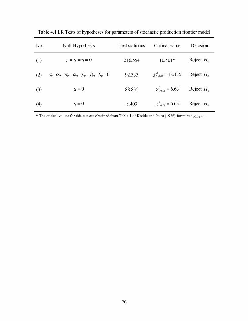
76

Table 4.1 LR Tests of hypotheses for parameters of stochastic production frontier model

No Null Hypothesis Test statistics Critical value Decision

(1) 0γ μ η= = = 216.554 10.501* Reject 0H

(2) 1 2 1 2 3 0T TT T T T T Tα α α α β β β= = = = = = = 92.333 27,0.01 18.475χ = Reject 0H

(3) 0μ = 88.835 21,0.01 6.63χ = Reject 0H

(4) 0η = 8.403 21,0.01 6.63χ = Reject 0H

* The critical values for this test are obtained from Table 1 of Kodde and Palm (1986) for mixed 2,0.01vχ .

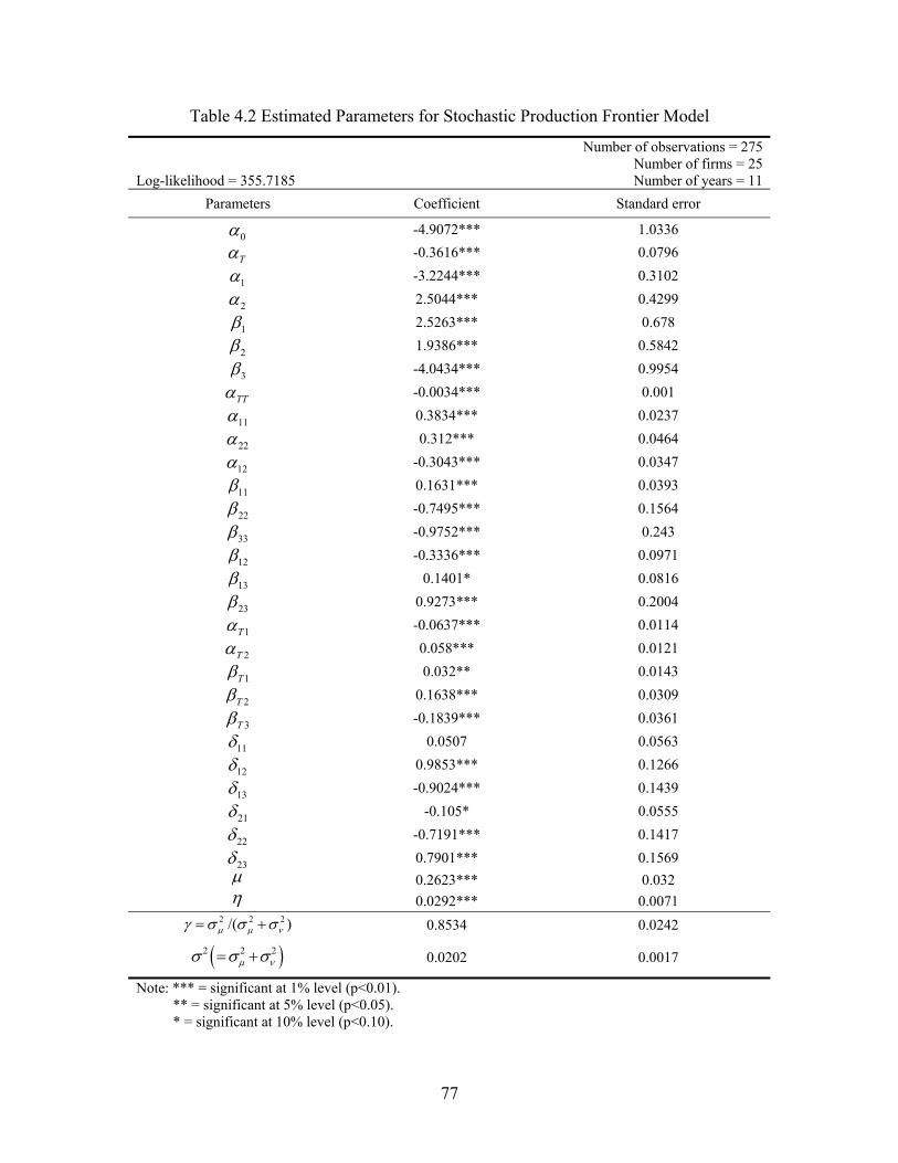
77

Table 4.2 Estimated Parameters for Stochastic Production Frontier Model

Log-likelihood = 355.7185

Number of observations = 275 Number of firms = 25 Number of years = 11

Parameters Coefficient Standard error

0α -4.9072*** 1.0336

Tα -0.3616*** 0.0796

1α -3.2244*** 0.3102

2α 2.5044*** 0.4299

1β 2.5263*** 0.678

2β 1.9386*** 0.5842

3β -4.0434*** 0.9954

TTα -0.0034*** 0.001

11α 0.3834*** 0.0237

22α 0.312*** 0.0464

12α -0.3043*** 0.0347

11β 0.1631*** 0.0393

22β -0.7495*** 0.1564

33β -0.9752*** 0.243

12β -0.3336*** 0.0971

13β 0.1401* 0.0816

23β 0.9273*** 0.2004

1Tα -0.0637*** 0.0114

2Tα 0.058*** 0.0121

1Tβ 0.032** 0.0143

2Tβ 0.1638*** 0.0309

3Tβ -0.1839*** 0.0361

11δ 0.0507 0.0563

12δ 0.9853*** 0.1266

13δ -0.9024*** 0.1439

21δ -0.105* 0.0555

22δ -0.7191*** 0.1417

23δ 0.7901*** 0.1569 μ 0.2623*** 0.032 η 0.0292*** 0.0071

2 2 2/( )μ μ νγ σ σ σ= + 0.8534 0.0242

( )2 2 2μ νσ σ σ= + 0.0202 0.0017

Note: *** = significant at 1% level (p<0.01). ** = significant at 5% level (p<0.05). * = significant at 10% level (p<0.10).

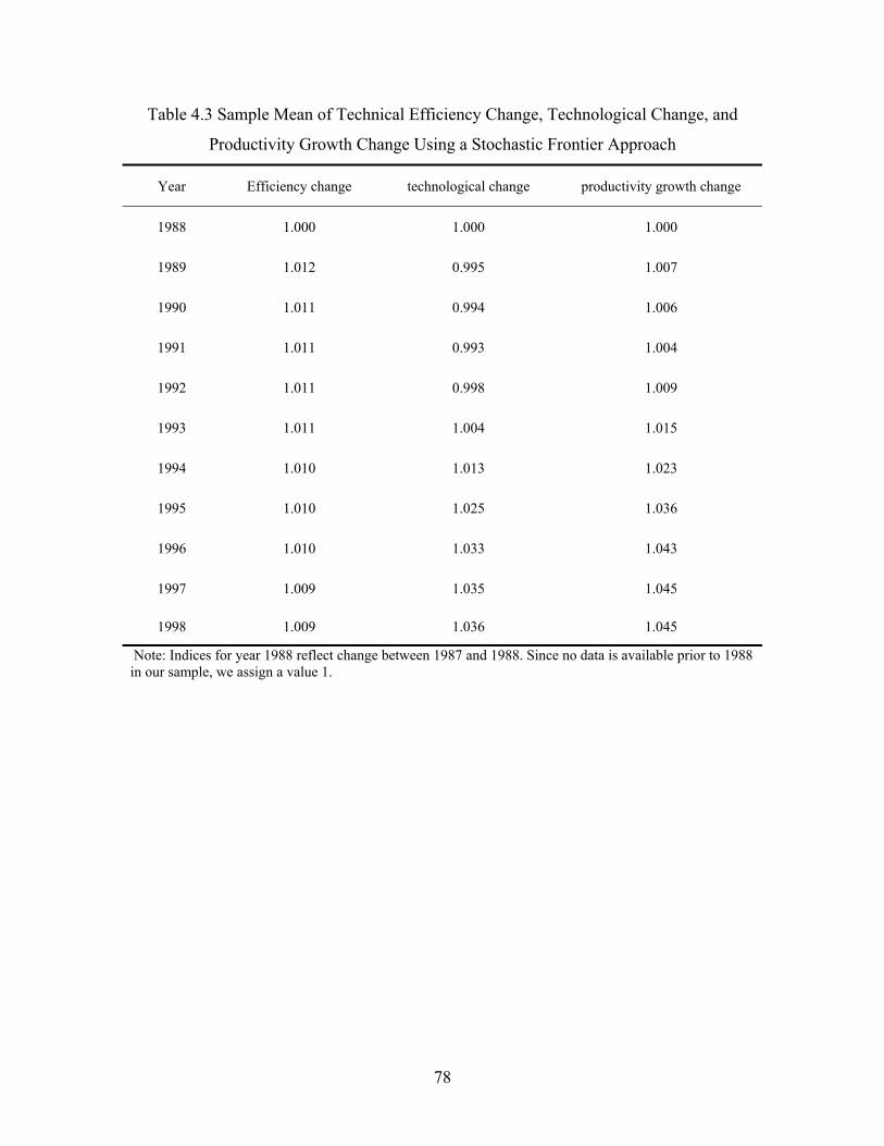
78

Table 4.3 Sample Mean of Technical Efficiency Change, Technological Change, and

Productivity Growth Change Using a Stochastic Frontier Approach

Year Efficiency change technological change productivity growth change

1988 1.000 1.000 1.000

1989 1.012 0.995 1.007

1990 1.011 0.994 1.006

1991 1.011 0.993 1.004

1992 1.011 0.998 1.009

1993 1.011 1.004 1.015

1994 1.010 1.013 1.023

1995 1.010 1.025 1.036

1996 1.010 1.033 1.043

1997 1.009 1.035 1.045

1998 1.009 1.036 1.045

Note: Indices for year 1988 reflect change between 1987 and 1988. Since no data is available prior to 1988 in our sample, we assign a value 1.

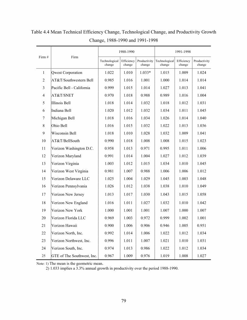
79


Change, 1988-1990 and 1991-1998

1988-1990 1991-1998 Firm # Firm


Efficiency change

Productivity change


Efficiency change

Productivity change

1 Qwest Corporation 1.022 1.010 1.033* 1.015 1.009 1.024

2 AT&T/Southwestern Bell 0.985 1.016 1.001 1.000 1.014 1.014


4 AT&T/SNET 0.970 1.018 0.988 0.989 1.016 1.004

5 Illinois Bell 1.018 1.014 1.032 1.018 1.012 1.031

6 Indiana Bell 1.020 1.012 1.032 1.034 1.011 1.045

7 Michigan Bell 1.018 1.016 1.034 1.026 1.014 1.040

8 Ohio Bell 1.016 1.015 1.032 1.022 1.013 1.036

9 Wisconsin Bell 1.018 1.010 1.028 1.032 1.009 1.041

10 AT&T/BellSouth 0.990 1.018 1.008 1.008 1.015 1.023









19 Verizon New York 1.000 1.001 1.001 1.007 1.000 1.007


21 Verizon Hawaii 0.900 1.006 0.906 0.946 1.005 0.951




25 GTE of The Southwest, Inc. 0.967 1.009 0.976 1.019 1.008 1.027

Note: 1) The mean is the geometric mean. 2) 1.033 implies a 3.3% annual growth in productivity over the period 1988-1990.

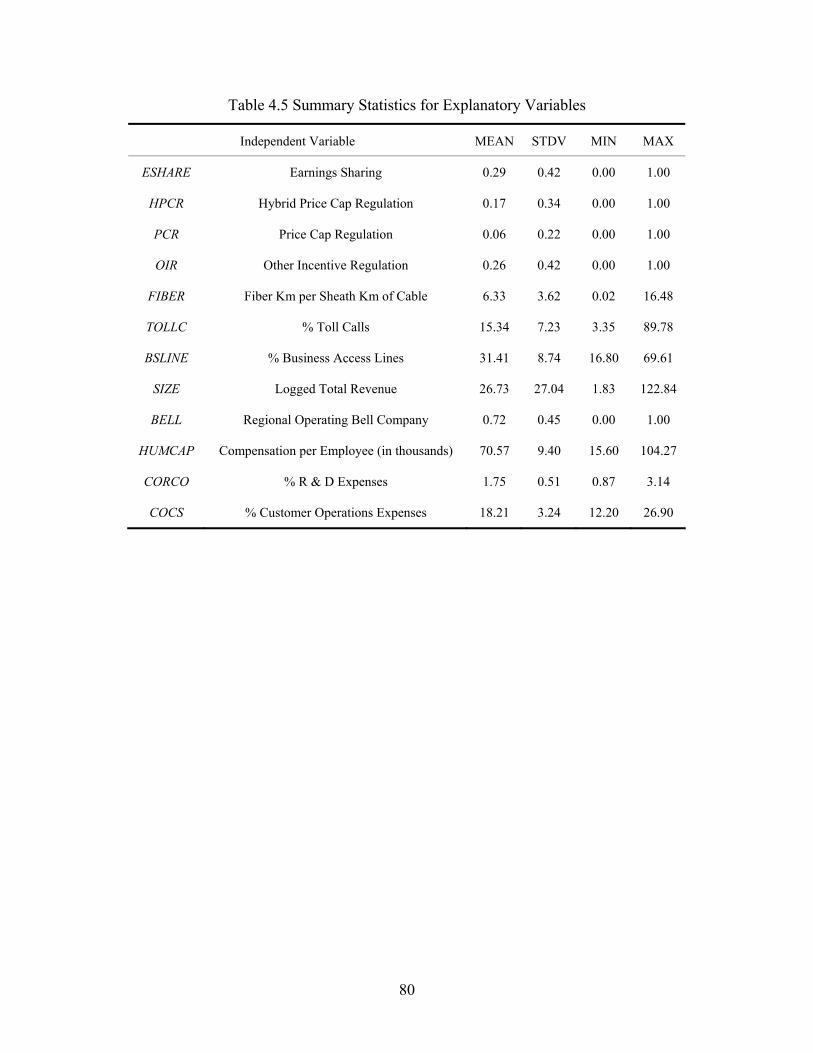
80

Table 4.5 Summary Statistics for Explanatory Variables

Independent Variable MEAN STDV MIN MAX

ESHARE Earnings Sharing 0.29 0.42 0.00 1.00

HPCR Hybrid Price Cap Regulation 0.17 0.34 0.00 1.00

PCR Price Cap Regulation 0.06 0.22 0.00 1.00

OIR Other Incentive Regulation 0.26 0.42 0.00 1.00

FIBER Fiber Km per Sheath Km of Cable 6.33 3.62 0.02 16.48

TOLLC % Toll Calls 15.34 7.23 3.35 89.78

BSLINE % Business Access Lines 31.41 8.74 16.80 69.61

SIZE Logged Total Revenue 26.73 27.04 1.83 122.84

BELL Regional Operating Bell Company 0.72 0.45 0.00 1.00

HUMCAP Compensation per Employee (in thousands) 70.57 9.40 15.60 104.27

CORCO % R & D Expenses 1.75 0.51 0.87 3.14

COCS % Customer Operations Expenses 18.21 3.24 12.20 26.90

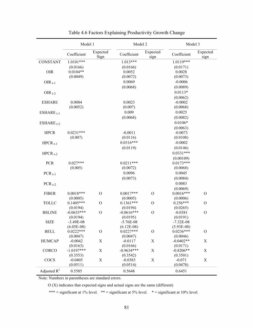
81

Table 4.6 Factors Explaining Productivity Growth Change

Model 1

Model 2

Model 3

Coefficient Expected Sign

Coefficient Expected sign

Coefficient Expected sign

CONSTANT 1.0101*** 1.013*** 1.0119*** (0.0166) (0.0166) (0.0171)

OIR 0.0104** 0.0052 0.0028 (0.0049) (0.0072) (0.0073)

OIR t-1 0.0069 -0.0006 (0.0068) (0.0089)

OIR t-2 0.0113* (0.0062)

ESHARE 0.0084 0.0023 -0.0002 (0.0052) (0.007) (0.0068)

ESHARE t-1 0.009 0.0025 (0.0068) (0.0082)

ESHARE t-2 0.0106* (0.0063)

HPCR 0.0231*** -0.0011 -0.0073 (0.007) (0.0116) (0.0108)

HPCR t-1 0.0316*** -0.0002 (0.0119) (0.0146)

HPCR t-2 0.0331*** (0.00109)

PCR 0.027*** 0.0211*** 0.0173*** (0.005) (0.0072) (0.0068)

PCR t-1 0.0096 0.0045 (0.0073) (0.0084)

PCR t-2 0.0083 (0.0069)

FIBER 0.0018*** O 0.0017*** O 0.0016*** O (0.0005) (0.0005) (0.0006)

TOLLC 0.1405*** O 0.1361*** O 0.256*** O (0.0194) (0.0194) (0.0265)

BSLINE -0.0635*** O -0.0616*** O -0.0381 O (0.0194) (0.0195) (0.0191)

SIZE -3.49E-08 -5.76E-08 -7.32E-08 (6.05E-08) (6.12E-08) (5.93E-08)

BELL 0.0222*** O 0.0227*** O 0.0236*** O (0.0047) (0.0047) (0.0046)

HUMCAP -0.0042 X -0.0117 X -0.0402** X (0.0163) (0.0166) (0.0171)

CORCO -1.0197*** X -0.9634*** X -0.8206** X (0.3553) (0.3542) (0.3501)

COCS -0.0405 X -0.0383 X -0.071 X (0.0511) (0.0514) (0.0478)

Adjusted R2 0.5585 0.5648 0.6451

Note: Numbers in parentheses are standard errors.

O (X) indicates that expected signs and actual signs are the same (different)

*** = significant at 1% level. ** = significant at 5% level. * = significant at 10% level.

82

CHAPTER 5 - Conclusion

This dissertation is comprised of three empirical essays that investigate the effect of

mergers and regulation in the U.S. telecommunications industry. The first two essays, chapters 2

and 3, respectively, address the effect of a series of mergers in the telecommunications industry

following the passage of the 1996 Telecommunications Act (1996 Act). The third essay, chapter

4, investigates the effect of the implementation of incentive regulation in the telecommunications

industry.

The primary objective of chapter 2 is to determine whether productivity growth has

increased among ILECs that have merged since the 1996 Telecommunications Act and whether

the merged firms performed better than firms that did not merge in terms of productivity growth

during the period 1996-2005. The empirical results of this chapter suggest that mergers

positively affected average productivity growth over the sample period.

The primary objective of Chapter 3 is to evaluate the effectiveness of mergers that

occurred between 1996 and 2005 using SFA. This chapter also compares productivity growth

results between the SFA and the Malmquist index approach. Both methods indicate that every

firm in the sample has experienced negative annual growth in technological change.

Furthermore, both methods indicate that most of the firms in the sample experience negative

annual productivity growth following the merger.

Chapters 2 and 3 suggest that consolidation reduces deterioration in productivity growth.

This result is of potential value to both government and industry as further consolidation may be

in the offing.

The primary objective of Chapter 4 is to measure productivity growth associated with

technological progress and changes in technical efficiency in order to examine the improvement

83

in the LECs’ productivity growth following the adoption of incentive regulation. The results of

Chapter 4 indicate that the adoption of PCR and IR, more generally, has had positive impact on

operating performance in the U.S. telecommunications industry. In addition, PCR has a

significant and positive effect on productivity growth in both contemporaneous and lagged

model specifications.

Chapter 4, in contrast to the other literature, provides strong empirical evidence in

support of the theoretical literature concerning the superiority of price cap over traditional rate-of

-return regulation.

Broadly speaking, the contributions of this dissertation are two fold. First, measuring the

efficiency gains associated with consolidation in the U.S. telecommunications industry has been

given relatively little attention in the literature heretofore. Two of the essays address whether the

efficiency gains expected from these mergers were, in fact, realized. Second, the stochastic

frontier analysis employed in this dissertation has not been applied pervasively in the analysis of

the telecommunications sector. Therefore, these three empirical essays collectively provide a

rigorous analysis of timely issues that may be employed by regulators charged with

implementing public policy in the telecommunications sector—a sector of the economy that is

responsible for a significant and increasing share of gross domestic product.86

86 According to Bureau of Economic Analysis, the broadcasting and telecommunications sector in the U.S. generated $304.1 billion dollars of GDP in 2005.

84

References Abel, J. R. and M. E. Clements. 1998. “A Time Series and Cross-sectional Classification of State

Regulatory Policy Adopted for Local Exchange Carriers.” The National Regulatory

Research Institute NRRI 98-25.

Ai, C. and D. E. M. Sappington. 2002. “The Impact of Incentive Regulation on the U.S.

Telecommunications Industry.” Journal of Regulatory Economics 22(2): 133-160.

Aigner, D. J., and S. F. Chu. 1968. “On estimating the industry production function” American

Economic Review 58: 826-839.

Aigner, D. J., and C. A. K. Lovell, and P. Schmidt. 1977. “Formulation and Estimation of

Stochastic Frontier Production Function Models” Journal of Econometrics 6(1): 21-37.

Afriat, A. N. 1972. “Efficiency Estimation of Production Functions.” International Economic

Review, 13(3): 568-598.

Battese, G.E., and T. J. Coelli. 1992. “Frontier production functions, technical efficiency and

panel data: with application to paddy farmers in India” Journal of Productivity Analysis

3: 153-169.

Braeutigam, R. and J. C. Panzar. 1989. “Diversification Incentives Under ‘Price-based’ and

‘Cost-based’ Regulation.” RAND Journal of Economics 20(3): 373-391.

Caves, D. W., L. R. Christensen, and E. W. Diewert. 1982. “Multilateral Comparisons of Output,

Input, and Productivity Using Superlative Index Numbers.” Economic Journal 92(365):

73-86.

Cellular Telecommunications and Internet Association (CTIA). “Semi-Annual Wireless Industry

Survey” http://files.ctia.org/pdf/CTIAEndYear2005Survey_update.pdf (2006).

http://files.ctia.org/pdf/CTIAEndYear2005Survey_update.pdf

85

Charnes, A., W. W. Cooper, and E. Rhodes. 1978. “Measuring the efficiency of decision making

units.” European Journal of Operational Research 2(6): 429-444.

Coelli, T. J.1996a. “A guide to FRONTIER Version 4.1: A Computer Program for Stochastic

Frontier production and Cost Function Estimation” CEPA Working Papers, No. 7/96,

School of Economics, University of New England, Armidale.

Coelli, T. J.1996b. “A guide to DEAP Version 2.1: A Data Envelopment Analysis (Computer)

Program” CEPA Working Papers, No. 8/96, School of Economics, University of New

England, Armidale.

Coelli, T. J., and S. Perelman, 2000. “Technical efficiency of European railways: a distance

function approach” Applied Economics 32: 1967-1976.

Coelli, T. J., D. S. Prasada Rao and G. E. Battese, 1998. An Introduction to Efficiency and

Productivity Analysis. Norwell, MA: Kluwer Academic Publishers.

Coelli, T. J., S. Rahman, and C. Thirtle. 2003. “A stochastic frontier approach to total factor

productivity measurement in Bangladeshi crop agriculture, 1961-92” Journal of

International Development 15: 321-333.

Department of Justice and the Federal Trade Commission. 1992. Horizontal Merger Guidelines,

[Inclusive of April 8, 1997 Revisions]

Evans, D. 1983. Breaking Up Bell: Essays on Industrial Organization and Regulation. New

York, NY: Elsevier Science Publishing Co., Inc.

Färe, R., and S. Grosskopf. 1994. Cost and Revenue Constrained Production. New York, NY:

Springer-Verlag.

86

Färe, R., and S. Grosskopf. 2000. “Theory and Application of Directional Distance Functions.”

Journal of Productivity Analysis 13: 93-103.

Färe, R., S. Grosskopf, M. Norris and Z. Zhang. 1994. “Productivity Growth, Technical Progress,

and Efficiency Change in Industrialized Countries.” American Economic Review 84(1):

66-83.

Farrell, M. J. 1954. “The Measurement of Productivity Efficiency.” Journal of Royal Statistical

Society 120(3): 11-29.

Federal Communications Commission. Annual (1993, 1995, 1998). Monitoring Report.

Washington D.C. http://www.fcc.gov/wcb/iatd/stats.html

Federal Communications Commission. Telecommunications of Act 1996. Washington D.C.

http://www.fcc.gov/Reports/tcom1996.pdf

Federal Communications Commission. Annual. Statistics of Communications Common Carriers.

Washington D.C. http://www.fcc.gov/wcb/iatd/stats.html

Federal Communications Commission. 2005. In the Matter of Review of the Section 251

Unbundling Obligations of Incumbent Local Exchange Carriers (CC Docket No. 01-338),

(Triennial Review Order on Remand).

Federal Communications Commission. 2006. 11th Commercial Mobile Radio Services

Competition Report. Washington D.C. http://wireless.fcc.gov/cmrsreports.html

Federal Communications Commission. January 2007. Local Telephone Competition. Washington

D.C. http://www.fcc.gov/wcb/iatd/stats.html

Federal Communications Commission. February 2007. Trends in Telephone Service. Washington

D.C. http://www.fcc.gov/wcb/trend.html

http://www.fcc.gov/wcb/iatd/stats.html

http://www.fcc.gov/Reports/tcom1996.pdf


http://wireless.fcc.gov/cmrsreports.html


http://www.fcc.gov/wcb/trend.html

87

Jung, I. 2005. “Incentive Regulation and the Technical Efficiency of U.S. Telecommunications

Carriers: A DEA Approach.” Ph.D. thesis, Kansas State University.

Kang, J. 2000. “State Level Price Cap Regulation and Technical Efficiency: U.S. Local

Exchange Carriers.” Ph.D. thesis, Kansas State University.

Kim, S. and G. Han. 2001. “A Decomposition of Total Factor Productivity Growth in Korean

Manufacturing Industries: A Stochastic Frontier Approach” Journal of Productivity

Analysis 16: 269-281.

Kodde, D. A., and F. Palm. 1986. “Wald criteria for jointly testing equality and inequality

restrictions” Econometrica 54(5): 1243-1248.

Kopp, R., and V. Smith. 1980. “Frontier production function estimates for steam electric

generation: A comparative analysis” Southern Economic Journal 46: 1049-1059.

Kwoka, J. E. 1993. “The Effects of Divestiture, Privatization, and Competition on Productivity

in U.S. and U.K. Telecommunications.” Review of Industrial Organization 8: 49-61.

Kridel, D., D. E. M. Sappington, and D. L. Weisman. 1996. “ The Effects of Incentive

Regulation in the Telecommunications Industry: A Survey.” Journal of Regulatory

Economics 9: 269-306.

Krouse, C., K. Danger, C. Cabolis, T. Carter, J. Riddle, and D. Ryan. 1999. “The Bell System

Divestiture and The Efficiency of The Operating Companies.” Journal of Law and

Economics 42:61-87.

Kumbhakar, S. C. and C. A. K. Lovell. 2000. Stochastic Frontier Analysis. New York, NY:

Cambridge University Press.

88

Lall, P., A. M. Featherstone and D. W. Norman. 2002. “Productivity Growth in the Western

Hemisphere (1978-94): The Caribbean in Perspective.” Journal of Productivity Analysis

17: 213-231.

Lehman, D. E., and D. L. Weisman. 2000. THE TELECOMMUNICATIONS ACT OF 1996: THE

“COSTS” OF MANAGED COMPETITION. NY: Springer.

Lovell, C. A. K., S. Richardson, P. Travers, and L.L Wood, 1994. “ Resources and Functionings:

A New View of Inequality in Australia.” Wolfgang Eichhon, eds., Models and

Measurement of Welfare and Inequality, Heidelberg: Springer-Verlag.

Majumdar, S. K. 1995. “X-efficiency in Emerging Competitive Markets: The Case of U.S.

Telecommunications.” Journal of Economic Behavior and Organization 26:129-144.

Majumdar, S. K. 1997. “Incentive Regulation and Productive Efficiency in the U.S.

Telecommunications Industry.” The Journal of Business 70(4): 547-576.

Meeusen, W., and J. van den Broeck. 1977. “Efficiency Estimation from Cobb-Douglas

Production Functions with Composed Error” International Economic Review 18(2): 435-

444.

Mitchell, B. and Vogelsang, I. 1991. Telecommunications Pricing: Theory and Evidence. New

York: Cambridge University Press

Morrison Paul, C. J., W. E. Johnston, and G. A. G. Frengley. 2000. “Efficiency in New Zealand

Sheep and Beep Farming: The Impact of Regulatory Reform” Review of Economics and

Statistics 82(2): 325-337.

Neuchterlein J, and P. Weiser. Digital Crossroads, American Telecommunications Policy in the

Internet Age. Cambridge MA: The MIT Press, 2005.

89

Newton, H. 2000. Newton’s Telecom Dictionary. New York, NY: Telecom Books.

Nishimizu, M. and J.M. Page. 1982. “Total Factor Productivity Growth, Technical Progress and

Technical Efficiency Change: Dimensions of Productivity Change in Yugoslavia, 1965-

78” The Economic Journal 92: 929-936.

Resende, M. 1999. “Productivity Growth and Regulation in U.S. Local Telephony.” Information

Economics and Policy 11: 23-44.

Resende, M. 2000. “Regulatory Regimes and Efficiency in U.S. Local Telephony.” Oxford

Economic Papers 52:447-470.

Resende, M. 2006. “Efficiency Measurement and Regulation in U.S. Telecommunications: A

Robustness Analysis” EUI Working Papers, No. 2006/15, Department of Economics,

European University Institute, Italy.

Resende, M., and L. O. Façanha. 2005. “Price-cap regulation and service-quality in

telecommunications: an empirical study” Information Economics and Policy 17: 1-12.

Sappington, D. E. M. , and D. L. Weisman. 1996. Designing Incentive Regulation For The

Telecommunications Industry. Cambridge MA.: MIT Press and Washington D.C.: AEI

Press.

Sappington, D. E. M. 2001. “ Price Regulation and Incentives.” In Handbook of

Telecommunications Economics, eds. By Martin Cave, Sumit Majumdar, and Vogelsang.

Amsterdam: North-Holland

Sappington, D. E. M. and Weisman, D. L. 1996. Designing Incentive Regulation for the

Telecommunications Industry. Cambridge MA: MIT Press and Washington D.C.: AEI

Press

90

Schmalensee, R. and J. Rohlfs. 1992. “Productivity Gains resulting from Interstate Price Caps for

AT&T.” National Economic Research Associates.

Seo, D., and D. L. Weisman. 2007. “Productivity Growth and Merger Efficiencies in the U.S.

Telecommunications Industry” Kansas State University, Working paper.

Seo, D., and A. Featherstone. 2007. “Market Consolidation and Productivity Growth in U.S.

Telecommunications: Stochastic Frontier analysis vs. Malmquist index” Kansas State

University, Working paper.

Shelanski, H. 2007. “Adjusting regulation to competition: Toward a new model for U.S.

telecommunications policy” Yale Journal of Regulation 24(1): 55-105.

Shepard, R. W. 1970. Theory of cost and production functions. Princeton, NJ: Princeton

University Press.

Shin, R., and J. Ying. 1992. “Unnatural monopolies in local telephone.” RAND Journal of

Economics 23: 171-183.

Staranczak, G. A., E. R. Sepulveda, P. A. Dilworth and S. A. Shaikh. 1994. “Industry structure,

productivity and international competitiveness: the case of telecommunications.”

Information Economics and Policy 6: 121-142.

Tardiff, J. and W.E. Taylor. 1993. “Telephone Company Performance Under Alternative Forms

of Regulation in the U.S.” National Economic Research Associates.

Uri, N. D. 2002. “Measuring the change in productive efficiency in telecommunications in the

USA” Journal of Economic Studies 29(2): 150-167.

Uri, N. D., 2001. “Productivity Change, Technical Progress, and Efficiency Improvement in

Telecommunications.” Review of Industrial Organization 18: 283-300.

91

Uri, N. D., 2002. “Assessing the Effect of Incentive Regulation on Productive Efficiency in

Telecommunications in the United States.” European Journal of Law and Economics 13:

113-127.

Uri, N. D. 2002. “Measuring the change in productive efficiency in telecommunications in the

USA” Journal of Economic Studies 29(2): 150-167.

U. S. Department of Labor. Bureau of Labor Statistics. http://www.bls.gov/ncs/

U. S. Department of Commerce. NAICS DATA. http://www.bea.gov/industry/

Weisman, Dennis L. 1993. “Superior Regulatory Regimes in Theory and Practice.” Journal of

Regulatory Economics 5: 355-366.

Weisman, D. L. 2000a. “Vertical Integration in Telecommunications.” Gary Madden, eds.,

Traditional Telecommunications Economics: The International Handbook of

Telecommunications Economics, V. 1. Northampton, MA: Edward Elgar Publishing.

Weisman, Dennis L. 2000b. “Regulatory Moral Hazard: Price Caps and Endogenous Entry

Under the 1996 Telecommunications Act.” In Expanding Competition in Regulated

Industries, ed. by Michael A. Crew. Boston, MA: Kluwer Academic Publishers, pp. 1-21.

Weisman, Dennis L. 2002a. “Is There ‘Hope’ For Price Cap Regulation?” Information

Economics and Policy, 14(3): 349-370.

Weisman, Dennis L. 2002b. “Strategic Sharing In Regulatory Regimes.” Economics Letters,

75(3): 361-367.

Zimmerman, P. R. 2007. “Recent Development in U.S. Wireline Telecommunications.”

Telecommunications Policy, 31: 419-437.

http://www.bls.gov/ncs/

Documents

THREE EMPRICAL ESSAYS ON MERGERS AND REGULATION IN