Embed Size (px)
Citation preview

UC MercedUC Merced Electronic Theses and Dissertations
TitleOptimizing HVAC Systems using Occupant Detection and User Thermal Preferences
Permalinkhttps://escholarship.org/uc/item/903009qq
AuthorBeltran, Alex
Publication Date2017 Peer reviewed|Thesis/dissertation
eScholarship.org Powered by the California Digital LibraryUniversity of California

University of California
Merced
Optimizing HVAC Systems using Occupant
Detection and User Thermal Preferences
A thesis submitted in partial satisfaction
of the requirements for the degree
Master of Science in Electrical Engineering and Computer Science
by
Alex Beltran
2017

c© Copyright by
Alex Beltran
2017
The thesis of Alex Beltran is approved.
Shawn Newsam
Miguel A. Carreira-Perpinan
Alberto E. Cerpa, Committee Chair
University of California, Merced
2017
iii

Dedicated to my mother, father, and all three of my big brothers.
iv
Table of Contents
1 Introduction . . . . . . . . . . . . . . . . . . . . . . . . . . . . . . . . 1
2 Related Work . . . . . . . . . . . . . . . . . . . . . . . . . . . . . . . 3
2.1 Occupancy Detection . . . . . . . . . . . . . . . . . . . . . . . . . 3
2.2 Occupant Comfort . . . . . . . . . . . . . . . . . . . . . . . . . . 5
2.3 Building Modeling . . . . . . . . . . . . . . . . . . . . . . . . . . 8
3 ThermoSense: Occupancy Sensing for HVAC Control . . . . . . 10
3.1 ThermoSense . . . . . . . . . . . . . . . . . . . . . . . . . . . . . 12
3.1.1 Hardware . . . . . . . . . . . . . . . . . . . . . . . . . . . 14
3.1.2 Power Consumption . . . . . . . . . . . . . . . . . . . . . 15
3.2 Occupancy Regression . . . . . . . . . . . . . . . . . . . . . . . . 16
3.2.1 PIR Sensor Input . . . . . . . . . . . . . . . . . . . . . . . 18
3.2.2 Thermal Background . . . . . . . . . . . . . . . . . . . . . 18
3.2.3 Feature Vectors . . . . . . . . . . . . . . . . . . . . . . . . 19
3.2.4 K-Nearest Neighbors . . . . . . . . . . . . . . . . . . . . . 23
3.2.5 Linear Regression . . . . . . . . . . . . . . . . . . . . . . . 24
3.2.6 Artificial Neural Network . . . . . . . . . . . . . . . . . . . 25
3.2.7 Filter . . . . . . . . . . . . . . . . . . . . . . . . . . . . . . 25
3.2.8 ThermoSense Performance . . . . . . . . . . . . . . . . . . 26
3.2.9 Model Discussion . . . . . . . . . . . . . . . . . . . . . . . 27
3.3 Energy Analysis . . . . . . . . . . . . . . . . . . . . . . . . . . . . 29
v
3.4 Conditioning Effectiveness . . . . . . . . . . . . . . . . . . . . . . 31
3.5 Summary . . . . . . . . . . . . . . . . . . . . . . . . . . . . . . . 33
4 FORCES: Feedback & control for Occupants . . . . . . . . . . . 35
4.1 System Design Overview . . . . . . . . . . . . . . . . . . . . . . . 38
4.1.1 System Architecture . . . . . . . . . . . . . . . . . . . . . 38
4.1.2 Application and Feedback Design . . . . . . . . . . . . . . 41
4.2 Experimental Setup . . . . . . . . . . . . . . . . . . . . . . . . . . 46
4.2.1 Population Description . . . . . . . . . . . . . . . . . . . . 46
4.2.2 Recruitment Process . . . . . . . . . . . . . . . . . . . . . 47
4.2.3 Feedback Assignment . . . . . . . . . . . . . . . . . . . . . 47
4.2.4 Building Description . . . . . . . . . . . . . . . . . . . . . 48
4.2.5 Energy Calculation . . . . . . . . . . . . . . . . . . . . . . 49
4.3 Results . . . . . . . . . . . . . . . . . . . . . . . . . . . . . . . . . 51
4.3.1 Preliminary Study . . . . . . . . . . . . . . . . . . . . . . 51
4.3.2 Primary Study . . . . . . . . . . . . . . . . . . . . . . . . 55
4.4 Discussion . . . . . . . . . . . . . . . . . . . . . . . . . . . . . . . 63
4.5 Summary . . . . . . . . . . . . . . . . . . . . . . . . . . . . . . . 65
5 Control Using Optimization, Occupancy, & Local User Sensing 66
5.1 System Overview . . . . . . . . . . . . . . . . . . . . . . . . . . . 67
5.2 Model Predictive Control . . . . . . . . . . . . . . . . . . . . . . . 68
5.2.1 HVAC System Description . . . . . . . . . . . . . . . . . . 68
5.2.2 Objective Function . . . . . . . . . . . . . . . . . . . . . . 71
vi

5.2.3 Constraints . . . . . . . . . . . . . . . . . . . . . . . . . . 75
5.2.4 Given/Precalculated Constants . . . . . . . . . . . . . . . 77
5.3 Implementation Details . . . . . . . . . . . . . . . . . . . . . . . . 79
5.4 Evaluation . . . . . . . . . . . . . . . . . . . . . . . . . . . . . . . 81
5.4.1 Model Evaluation . . . . . . . . . . . . . . . . . . . . . . . 81
5.4.2 Energy Usage . . . . . . . . . . . . . . . . . . . . . . . . . 86
5.5 Summary . . . . . . . . . . . . . . . . . . . . . . . . . . . . . . . 88
6 Conclusion . . . . . . . . . . . . . . . . . . . . . . . . . . . . . . . . . 89
References . . . . . . . . . . . . . . . . . . . . . . . . . . . . . . . . . . . 91
vii
List of Figures
3.1 Occupancy Hardware . . . . . . . . . . . . . . . . . . . . . . . . . 13
3.2 8x8 thermal array sensing an occupant. . . . . . . . . . . . . . . . 14
3.3 Energy usage for different duty cyles. . . . . . . . . . . . . . . . . 16
3.4 Occupancy Regression Process . . . . . . . . . . . . . . . . . . . . 17
3.5 PIR compared to ground truth. . . . . . . . . . . . . . . . . . . . 20
3.6 PIR evaluation of all three rooms . . . . . . . . . . . . . . . . . . 20
3.7 Plot of residual distribution . . . . . . . . . . . . . . . . . . . . . 26
3.8 Model raw and filtered outputs. . . . . . . . . . . . . . . . . . . . 27
3.9 NRMSE of a ThermoSense node in a zone. . . . . . . . . . . . . . 28
3.10 Strategy Comparision . . . . . . . . . . . . . . . . . . . . . . . . . 29
3.11 RMSE of Sensor . . . . . . . . . . . . . . . . . . . . . . . . . . . . 30
3.12 Ventilation effectiveness of the strategies. . . . . . . . . . . . . . . 32
4.1 Comfort Application Screenshots . . . . . . . . . . . . . . . . . . 38
4.2 FORCES System Architecture . . . . . . . . . . . . . . . . . . . . 40
4.3 Drift strategy set-points to save energy . . . . . . . . . . . . . . . 44
4.4 PMV vote distribution for each feedback type . . . . . . . . . . . 51
4.5 Perceived and Actual Temperature Preference . . . . . . . . . . . 53
4.6 Vote volume for each day of study . . . . . . . . . . . . . . . . . . 55
4.7 Example fault detection usage . . . . . . . . . . . . . . . . . . . . 56
4.8 Reiterated votes . . . . . . . . . . . . . . . . . . . . . . . . . . . . 59
viii
5.1 CoolUs Architecture Overview . . . . . . . . . . . . . . . . . . . . 67
5.2 HVAC Single Duct VAV Terminal Reheat Layout . . . . . . . . . 68
5.3 3-D Model of building . . . . . . . . . . . . . . . . . . . . . . . . 81
5.4 Non-Linear Thermal Model . . . . . . . . . . . . . . . . . . . . . 82
5.5 Linear Thermal Model . . . . . . . . . . . . . . . . . . . . . . . . 83
5.6 Zone 2: Predicted vs. Measured Zone Temperature Results . . . . 84
5.7 Zone 1: Predicted vs. Measured Zone Temperature Results . . . . 84
5.8 Fan quadratic regression . . . . . . . . . . . . . . . . . . . . . . . 85
5.9 Energy comparison between baseline and CoolUs . . . . . . . . . 86
5.10 Baseline and CoolUs Mass Flow Patterns . . . . . . . . . . . . . . 87
5.11 CoolUs Occupancy . . . . . . . . . . . . . . . . . . . . . . . . . . 88
ix

List of Tables
3.1 Energy Usage for independent components. . . . . . . . . . . . . . 15
3.2 Parameters of linear model and fit metrics. . . . . . . . . . . . . . 25
3.3 Evaluation of the models used. . . . . . . . . . . . . . . . . . . . . 28
4.1 PMV Constants . . . . . . . . . . . . . . . . . . . . . . . . . . . . 39
4.2 Demographics of Study Population . . . . . . . . . . . . . . . . . 46
4.3 Energy Cost per Feedback - Preliminary . . . . . . . . . . . . . . 48
4.4 Survey: Did the user find the app useful? . . . . . . . . . . . . . . 54
4.5 Satisfaction and comfort . . . . . . . . . . . . . . . . . . . . . . . 57
4.6 Reiterated votes for (Non-)Physical feedbacks . . . . . . . . . . . 61
4.7 Satisfaction of Primary Study Feedbacks . . . . . . . . . . . . . . 62
4.8 Energy Cost per Feedback - Primary Study . . . . . . . . . . . . . 62
5.1 MPC variables and descriptions . . . . . . . . . . . . . . . . . . . 70
5.2 Parameters used for PMV . . . . . . . . . . . . . . . . . . . . . . 78
5.3 Energy Usage . . . . . . . . . . . . . . . . . . . . . . . . . . . . . 87
x
Acknowledgments
First, I would like to thank my advisor Alberto E. Cerpa who provided me guid-
ance, feedback, and motivated me. I would also like to thank my master comittee
members Shawn Newsam and Miguel A. Carreira-Perpinan who provided useful
feedback and advice.
Thank you to my peers Niloufar P. Esfahani and Daniel A. Winkler. They
both helped me tremendously in making progress in my research and were great
friends. I would also like to thank Tao Liu and Varick L. Erickson who demon-
strated to me what an excellent graduate student is suppose to be.
Specifically, I would like to acknowledge the work included in this thesis which
were co-authored by myself, my peers, and a few Professors. Chapter 3 is based
on the publication, ThermoSense [BEC13], with co-primary author Varick L.
Erickson who did all of the building energy simulation and helped significantly
with the writing. Chapter 4 is based on the publication, FORCES [WBE16], with
co-primary author Daniel Winkler who created the iOS application for voting,
analyzed the physical feedback, and helped with the majority of the writing.
Niloufar P. Esfahani wrote the android application, helped write the related works
section, and help analyze general voting patterns. Professor Paul P. Maglio also
provided invaluable feedback for this publication. Parts of Chapter 5 and Related
Work about Model Predictive Control was first published in SenSys [BC14].And
once again, Professor Cerpa who helped make all the above possible with guidance
and editing.
xi

Vita
2008-2012 Bachelor of Science, Computer Science
Teaching Assistant, Electrical Engineering and Computer Sci-
ence, Department, University of California–Merced.
2013–2017 Research Assistant, Electrical Engineering and Computer Sci-
ence, University of California–Merced.
Publications
Alex Beltran, Varick Erickson (Co-primary Author), Alberto E. Cerpa, Ther-
moSense: Occupancy Thermal Based Sensing for HVAC Control, In Proceedings
of the Fifth ACM Workshop on Embedded Sensing Systems for Energy-Efficient
Buildings (Buildsys 2013), November, 2013.
Varick L. Erickson, Alex Beltran, Daniel A. Winkler, Niloufar P. Esfahani,
John R. Lusby, Alberto E. Cerpa, ”TOSS: Thermal Occupancy Sensing Sys-
tem”, Proceedings of the Fifth ACM Workshop on Embedded Sensing Systems
for Energy-Efficient Buildings (BuildSys 2013), pp. 35:1–35:2, ACM,Rome, Italy,
2013.
xii
Varick L. Erickson, Alex Beltran, Daniel A. Winkler, Niloufar P. Esfahani,
John R. Lusby, Alberto E. Cerpa, ”ThermoSense: Thermal Array Sensor Net-
works in Building Management”, Proceedings of the Eleventh ACM Conference
on Embedded Network Sensor Systems (SenSys 2013), pp. 87:1–87:2, ACM,
Rome, Province of Rome, Italy, November, 2013.
Alex Beltran and Alberto E. Cerpa. 2014. Optimal HVAC building control
with occupancy prediction. In Proceedings of the 1st ACM Conference on Em-
bedded Systems for Energy-Efficient Buildings (BuildSys ’14). ACM, New York,
NY, USA, 168-171. DOI=http://dx.doi.org/10.1145/2674061.2674072
Alex Beltran and Alberto E. Cerpa. 2015. Poster: Model Predictive Control
with Real-time Occupancy Detection. In Proceedings of the 13th ACM Confer-
ence on Embedded Networked Sensor Systems (SenSys ’15). ACM, New York,
NY, USA, 437-438. DOI: http://dx.doi.org/10.1145/2809695.2817902
Grigore Stamatescu, Alex Beltran, and Alberto Cerpa. 2016. Data-driven
Comfort Models for User-centric Predictive Control in Smart Buildings: Poster
Abstract. In Proceedings of the 3rd ACM International Conference on Systems
for Energy-Efficient Built Environments (BuildSys ’16). ACM, New York, NY,
USA, 221-222. DOI: https://doi.org/10.1145/2993422.2996394
xiii

Daniel A. Winkler, Alex Beltran (Co-primary Author), Niloufar P. Esfa-
hani, Paul P. Maglio, and Alberto E. Cerpa. 2016. FORCES: feedback and
control for occupants to refine comfort and energy savings. In Proceedings
of the 2016 ACM International Joint Conference on Pervasive and Ubiquitous
Computing (UbiComp ’16). ACM, New York, NY, USA, 1188-1199. DOI:
http://dx.doi.org/10.1145/2971648.2971700
xiv
Abstract of the Thesis
Optimizing HVAC Systems using Occupant
Detection and User Thermal Preferences
by
Alex Beltran
Master of Science in Electrical Engineering and Computer Science
University of California, Merced, 2017
Professor Alberto E. Cerpa, Chair
Buildings are a crucial part of our daily lives and people spend 87% of their time
inside buildings. To maintain thermal comfort in buildings a significant amount
of energy is used to condition these spaces. In the US buildings account for 40%
of energy usage and of that 50% of energy goes to heating, ventilation, and air
conditioning (HVAC). Often this energy is wasted by conditioning empty rooms
or by leaving building occupants unsatisfied with the temperature of their room.
In this thesis we present several ways to reduce energy usage while improv-
ing user comfort. First, we reduce energy consumption by incorporating a new
thermal-based occupancy sensor. Energy can be saved by using these thermal
based sensors to detect occupancy and predict movements between rooms and
only conditioning rooms which are occupied. Second, we focus on improving oc-
cupant’s thermal comfort by giving them a method of participatory voting and
influencing how they vote by using several feedback mechanisms which can in-
crease user engagement and reduce HVAC energy usage. And finally, we combine
the previous concepts into an optimization problem that finds the optimal control
sequences based on occupancy, user voting, and several other inputs.
xv
CHAPTER 1
Introduction
Internet of Things (IoT) has become ubiquitous at home and in offices both in
academia and commercially. Wireless sensor mesh networks can be established
to gather sensor data which is sent to a gateway node and sent to a server. Users
then interact with these devices and their environment using IoT.
According to the US Department of Energy, buildings account for 40% of
energy usage in the U.S. and, of that 40%, 50% of this energy is used for heat-
ing, ventilation, and air conditioning (HVAC) [bed]. Conditioning buildings is
important since people spend 87% of their time inside a building [KNO01]. The
goal of conditioning office spaces is largely missed since 35% of occupants report
that they are dissatisfied with their thermal comfort [EC]. In addition to uncom-
fortable occupants, a common issue is that spaces are conditioned when they are
unoccupied.
In this thesis, we contribute the following:
• A novel occupancy detection method using low power thermal array sensors
in a wireless sensor network
• Develop a voting application to allow users to vote on their thermal pref-
erence
• Evaluate 5 different voting feedback systems and their influences on how
1

users vote and the changes in energy usage
• Develop and evaluate the combination of occupancy detection, occupancy
prediction, and thermal comfort into a thermal model to calculate optimal
control sequences
This thesis begins at Chapter 2 with related work for all of the topics. After
Chapter 2, this thesis can be broken into three core chapters: Chapter 3 covers
occupancy detection, Chapter 4 covers participatory sensing, and Chapter 5 com-
bines the previous two technologies to create a model using occupancy detection
and comfort. The final chapter is left for closing remarks and conclusions.
2
CHAPTER 2
Related Work
2.1 Occupancy Detection
The authors of [KJD09] test the use of cameras as optical turnstiles to estimate
occupancy. However, they fail to address how cumulative error can impact occu-
pancy estimates. As previously mentioned, even a single error will cause error to
propagate forward. The total ground truth was also limited to 4 hours total for
different times of the day.
The authors of [EAC] also use cameras as optical turnstiles. They mount
multiple strategically placed cameras in hallways to measure occupancy for sev-
eral areas. In addition, they also have a PIR sensor network in order to better
distinguish empty rooms. Again, the major drawback to this approach is the
cumulative error that will occur. However, unlike [KJD09], they discuss strate-
gies for reducing cumulative error. They impose maximum occupancy limits and
use a particle filter with an occupancy model with live data to estimate the er-
ror. However, since their approach uses a model, their approach also requires
a non-trivial amount of ground truth occupancy data (2 weeks), collected using
webcams. The occupancy RMSE achieved was 1.83 persons, more than 5 times
the ThermoSense’s error.
In [BLT10], elderly people are tracked using Imote2 motes with Enalab cam-
eras and utilizing a motion histogram for a period of 1 week. Occupant counts are
3

achieved by counting peaks within the histograms. Their system also includes
PIR sensors in order to detect occupancy for certain areas. There are several
drawbacks to this approach. Since the camera must continually poll the room in
order to generate the motion histograms, the power consumption during periods
of occupancy will be high. The problem of privacy also exists for this system;
cameras must be placed directly in the room.
The papers [LSS10, ABD11] describe methods that uses door sensors with
PIR sensors to obtain a binary measurement of occupancy. Ground truth data
was collected using surveys and manual annotations, and the experiments were
run for 1-4 weeks and 4 days respectively. By adding door sensors, they minimize
instances where overly still occupants become invisible to the PIR sensor. While
this technique improves the binary measurement of occupancy, these systems do
not provide a precise occupancy estimate.
Rather than rely on PIR sensors alone, the authors of [SBK11] also utilize
active radio frequency identification (RFID) tags to determine occupancy. By
deploying multiple antennas with the occupied space, the RFID tags were able to
broadcast their presence every 5 seconds. The limitation to this strategy is that
every occupant must possess a RFID tag, and that tag must always be co-located
with the occupant.
The papers [LHD09,MMC11] estimates occupancy by measuring a variety of
parameters. They collected ground truth data for 5 and 1 weeks deployments,
using video camera and a user voluntary electronic tally counter to measure
room occupancy respectively. In these deployments, they utilize multiple sensors
to estimate occupancy; CO2, CO, lighting, temperature, humidity, motion, and
acoustics. For each parameter, they define multiple feature vectors, which are
then used with several models to estimate occupancy. While this multi-sensor
4
approach works well for the sole purpose of occupancy estimates, this approach
will not work well if combined with a ventilation strategy. They assume that
ventilation will not affect occupancy estimates of the room. However, since ven-
tilation will affect CO2 and humidity levels and thus occupancy estimates, it is
likely that ventilation rates based on occupancy estimates from this system will
lead to wild fluctuations in ventilation actuation and periods of under-ventilation.
In this case, ventilation is better controlled by CO2 sensors directly even with
the known calibration and response time issues [FFS06]. In essence, if CO2 or
humidity is used as sensory input, you can either control ventilation or estimate
occupancy, not do both at once.
2.2 Occupant Comfort
Previous work has used building occupants as participatory sensors [RES10]. By
bringing humans into the loop [EC,BTG13, JB12,Bur14,Rob14], these systems
collect thermal comfort information from building occupants, and then use PMV
to determine temperature setpoints to improve comfort. These works conclude
that gathering sensation data such as “Feeling Too Hot” improves usability, as
users are unable to determine their ideal temperature. All studies resulted in
energy savings and improved satisfaction. Besides PMV, a multi-armed bandit
framework [MJK13] and an optimization model [HW13] have been used to find
improved temperature setpoints based on voting patterns. Although these sys-
tems provide alternative methods to translating human input to HVAC control
strategy, they do not determine how data presentation and environmental feed-
back can be used to promote certain voting application behavior, which is the
focus of our study.
[Rob14] describes operation of a comfort voting application with features sim-
5
ilar to our Physical and Drift mechanisms. Although algorithmic details of their
control strategies are unavailable, the case study concludes that these features
reduce energy consumption by 22.95%. However, due to the age of the building,
and the combination of the Physical and Drift mechanisms, it is difficult to dis-
tinguish which feature led to energy savings, and how they would generalize to
other buildings.
[Sch77] found that a person will act in an altruistic manner if they are shown
the consequences of their actions. [PSJ07] shows that a 32% energy reduction
can be achieved among dormitory residents by presenting energy usage infor-
mation. However, the participants were incentivized with rewards, and 22% of
participants admitted that they would not continue using the strategies after the
study. [BTG13] describes the design of a metering system that presents energy
consumption data and zone temperature to occupants, and energy traces over a
10 day period show that a 5% energy savings was gained when the users were
given control. Providing additional energy-saving tips caused a negligible change
in energy consumption. [HHP00] finds that informing people of their energy usage
influences their behavior, but not always predictably. Similar results are achieved
in residential electricity consumption feedback systems [ELK13,PKS14]. These
studies make it clear that providing this information to participants can cause a
change in behavior, but none suggest how this information might be used in an
application where the improvement in energy efficiency also presents a trade-off
with the voter’s satisfaction and comfort. In our work, we wish to determine this
relationship, and find how it can be used to create purpose-built applications for
either energy efficiency or occupant comfort.
In [GCG08], social norms techniques were used to increase participation in a
program at a hotel for towel reuse. They found that telling hotel guests about the
6
percentage of hotel visitors that had also participated in the program led to in-
creased participation. They concluded that reporting building-level participation
in the displayed statistic is ideal to draw new users into the study. In [NSC08],
it is shown that although people may not believe that the actions of others will
motivate them to save energy, the opposite holds true. The behavior of peers was
seen to cause a large amount of savings among those users. In our study, we see
if this effect holds true in a thermal comfort application when we inform the user
about application usage by their peers.
Work done in [SBK11] allows homes to be efficiently heated using occupancy
sensing and prediction, replacing user-programmed thermostats. Similarly, the
authors of [YNF14] inform the design of future heating and cooling systems by
investigating users’ experiences with the Nest learning Thermostat, a commer-
cially available smart home device. They create a set of design implications for
Eco-Interaction, the design of features and human-system interactions with the
goal of saving energy.
In [CFH14], a drift control strategy was deployed in the campus housing of
8 University undergraduates for a period of ∼18 days. The authors learned that
some occupants will learn to adopt new thermal regulation strategies (i.e. clothing
changes, heating the room in advance) while others will struggle to maintain
comfort. Changes in activation of the zones’ radiators suggest energy savings up
to 42.2%. Despite the similarity in the drift control mechanism, it is difficult to
relate the results found in this study to ours, largely due to environmental/study
conditions. For instance, the University students’ schedules were not known,
making it difficult to know what savings were due to the room being empty. In
comparison, the participants of our study have very structured hours, and rely on
comfort in their space to remain productive. In our work, we wish to determine
7
if this drift strategy can be used in a commercial building to save energy while
still maintaining high occupant satisfaction.
Research done in [YAL14] investigates the use of different feedback mecha-
nisms to improve the energy efficiency of an occupant’s office space by remind-
ing/enabling the occupant to disable unnecessary equipment (lights, computer,
etc.) when the user is not in the office. In our work, we wish to reduce the energy
consumption of the HVAC system while it conditions the user’s space. For this
reason, we must leverage energy savings against occupant comfort. Additional
work [ZYL13] claims that occupant activity prediction based on real-time plug
energy load data can be used to control plug load devices and HVAC system, but
no evidence or experimental results are presented to support these claims.
2.3 Building Modeling
[KMB13] explores the use of MPC in a multi-zone building. In this paper a
model is developed and evaluated by simulation over a 24 hour period. This
paper has flexible temperature bounds set for a 6am to 6pm workday with no
consideration of occupancy. [BC14] uses simulation in order to demonstrate that
real-time occupancy can provide additional savings. In our paper, predicted
occupancy is used in a building to show that it savings can be achieved. Further
work is done in a longer period by [MKD12] which includes load balancing based
on the chiller system used in their building. This paper does not take occupancy
prediction into consideration.
Work has also been done to a small extent to use occupancy prediction with
MPC in [GIB12]. This paper’s occupancy prediction has two main methods, the
first being a reactive method where there is no occupancy prediction and the cur-
8
rent occupancy is said to be constant. The second method has the ground truth
for the entirety of the MPC. The reactive method assumes whatever occupancy
is true at the moment will hold true for the remainder the model. Our paper
takes into consideration of occupancy patterns to allow for preconditioning and
minimize conflicts with comfort constraints while saving energy.
In addition to traditional MPC models, work has been done in [MB] [PVR13]
[PMV13] to build a Stochastic Model Predictive Control (SMPC). These efforts
focus on uncertainty of occupancy and thermal load predictions and minimizes
the amount the temperature falls outside the comfort constraints while optimizing
the system as a whole. None of the systems do occupancy detection and only
consider them as part of the load of the system. With the addition of occupancy
detection, greater savings can be achieved with flexible minimum ventilation.
Work has also been done to predict a buildings occupancy through out the day.
[MCM12] uses different machine learning strategies and evaluates the accuracy of
each method. Based on this information they are able turn off the HVAC when
it is not in use. The control strategy is not specified and there is no discussion
on the comfort of the occupants used in their strategy. [ECC] uses a Markov
Chain to predict occupancy of the day and the result of their savings are from
lowering ventilation due to occupancy and changing the set point bounds in the
building. Their system switches from occupied to unoccupied strategies if a zone
is predicted to be occupied for a threshold value. This scheme is naive in that
it does not use the dynamics of the room in order to ensure that the room is
properly condition when an occupant enters. In our system we use MPC to find
an optimal solution that can occur with any occupant patterns.
9

CHAPTER 3
ThermoSense: Occupancy Thermal
Based Sensing for HVAC Control
The primary goal of every HVAC system is to keep occupants comfortable with
the secondary goal of minimizing energy consumption. In this chapter, we will
focus on reducing energy consumption in a buildings by intelligently controlling
the HVAC using the knowledge of the number of occupants within each room.
We also take into consideration how our models affect the ability to keep each
zone’s temperature within the zone’s target temperature range when a room is
occupied. One method of reducing consumption is to condition based on actual
usage. Rooms are often conditioned assuming constant maximum occupancy.
This leads to heating or cooling empty rooms. In addition, spaces only partially
occupied are over-ventilated leading to loss of conditioned air and thus thermal
energy.
There are two different parts of HVAC systems usage that are affected by
occupancy; temperature and ventilation. Temperature control is dependent on
whether a space is occupied. In this case, a passive infrared (PIR) or ultra-
sonic sensor is sufficient to have a binary indication if a space is occupied. Bi-
nary sensing is common for lighting control and has also been used for tem-
perature control [ABD11, LSS10] applications. However, ventilation, used to
control CO2 levels and indoor pollutants, depends on the number of people oc-
10
cupying a space. One method is to simply regulate CO2 levels directly with
a CO2 sensors. However, these systems are slow to respond and are prone to
calibration errors [FFS06]. Since standards exist for ventilating based on room
occupancy [ASH07], sensors that measure occupancy can be used to regulate
ventilation. Cameras have been used for measuring occupancy [TS, EAC] but
have several drawbacks. They are sensitive to sudden lighting and background
changes. Camera placement is also an issue. Cameras placed in office spaces raise
privacy concerns. While cameras can be placed in public hallways and function
as an “optical” turnstile, this strategy is prone to cumulative error [EAC]. If an
optical turnstile misses even a single person entering/exiting a space, this error is
propagated until another offsetting error occurs or some other mechanism, such
as assuming the room is empty at 4am, is used to remove the cumulative error.
For example, if the last person in an office leaves at 6pm and this transition is
missed, then the occupancy will remain erroneously at one.
In this chapter, we develop ThermoSense, an occupancy monitoring system
that utilizes thermal based sensing and PIR sensors. We develop a novel low-
power multi-sensor node for measuring occupancy utilizing a thermal sensor array
combined with a PIR sensor. The thermal sensor array used is able to measure
temperatures in an 8x8 grid pattern within an 2.5mx2.5m area. We show it is
possible to use these temperature readings in order to determine how many peo-
ple are within the space. Unlike the CO2 sensor, the thermal array can measure
occupancy in near real-time. The thermal array is also not sensitive to optical
issues, such as lighting or background changes. By adding a PIR sensor, we
increase accuracy of detecting empty spaces and the overall accuracy of the plat-
form. The PIR sensor is also used to reduce the node’s power consumption by
triggering the mote and thermal array only when someone is present. We test
this new platform with a 17-node deployment covering 10 building areas totaling
11
2,100 sq. ft. for a period of three weeks. Using this data, we tested four differ-
ent usage based conditioning strategies and analyze the energy usage; we show
that 25% annual energy savings are possible with occupant based conditioning
strategies. In this chapter, we contribute the following:
• We developed a novel multi-sensor platform for estimating occupancy uti-
lizing a thermal sensor array and a PIR sensor. We performed a full system
power consumption analysis and tested a 17-node deployment over a 3 weeks, in
10 HVAC conditioning areas, covering 2,100 sq.ft.
• We developed a new occupancy regression process using the sensor data,
which includes thermal map background update, feature extraction, occupancy
regression and post-processing filtering. We tested three regression, including
K-Nearest Neighbors (KNN), Artificial Neural Networks (ANN), and linear re-
gression (LR). Using this process, we showed that these types of sensors are
capable of estimating occupancy with an RMSE of only ≈0.35 persons.
• We tested four different strategies for HVAC conditioning and show how
different sensing and actuation strategies affect energy consumption and occupant
comfort. We showed that by using this system for conditioning usage based
control of temperature and ventilation we can save 25% energy annually while
maintaining occupant comfort.
3.1 ThermoSense
In this section we discuss ThermoSense, a wireless sensor network of nodes that
can measure occupancy using a combination of thermal readings and PIR. Fig-
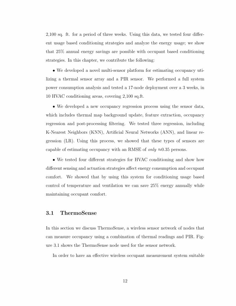
ure 3.1 shows the ThermoSense node used for the sensor network.
In order to have an effective wireless occupant measurement system suitable
12
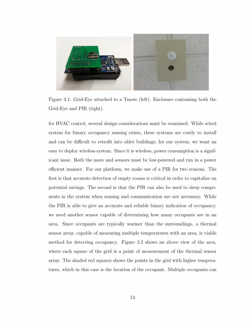
Figure 3.1: Grid-Eye attached to a Tmote (left). Enclosure containing both the
Grid-Eye and PIR (right).
for HVAC control, several design considerations must be examined. While wired
system for binary occupancy sensing exists, these systems are costly to install
and can be difficult to retrofit into older buildings; for our system, we want an
easy to deploy wireless system. Since it is wireless, power consumption is a signif-
icant issue. Both the mote and sensors must be low-powered and run in a power
efficient manner. For our platform, we make use of a PIR for two reasons. The
first is that accurate detection of empty rooms is critical in order to capitalize on
potential savings. The second is that the PIR can also be used to sleep compo-
nents in the system when sensing and communication are not necessary. While
the PIR is able to give an accurate and reliable binary indication of occupancy,
we need another sensor capable of determining how many occupants are in an
area. Since occupants are typically warmer than the surroundings, a thermal
sensor array, capable of measuring multiple temperatures with an area, is viable
method for detecting occupancy. Figure 3.2 shows an above view of the area,
where each square of the grid is a point of measurement of the thermal sensor
array. The shaded red squares shows the points in the grid with higher tempera-
tures, which in this case is the location of the occupant. Multiple occupants can
13

Figure 3.2: 8x8 thermal array sensing an occupant.
be distinguished by higher density of warmer temperatures.
3.1.1 Hardware
Each ThermoSense node contains a Tmote Sky, PIR, and Grid-Eye Sensor. The
Tmote Sky [tmo], produced by MoteIV, has a 8MHz TI-MSP430 micro-controller
with 48k Flash storage and 10k RAM. The Tmote communicates using a Chipcon
CC2420 radio. The PIR sensor is connected to the Tmote’s digital input/output
pin while the Grid-Eye is connected to the I2C clock and data pins. We developed
a board in order to connect both the Grid-Eye and PIR sensor with the Tmote.
The PIR used in the nodes is the PaPIR EKMB VZ series developed by
Panasonic. The PIR is able to detect motion up to 12m with a detection a
viewing angle of 102◦x92◦ horizontal by vertically respectively [PaP]. The infrared
thermal array used to detect actual occupancy is the Grid-Eye sensor made by
Panasonic [Gri], priced at $31. This sensor measures 64 temperatures in an
8x8 grid where the physical size of this grid is determined by the distance the
14

Components Used Energy Usage.
Mote Only 4.72 mA
Mote + PIR 4.73 mA
Mote + PIR + Grid-Eye 4.76 mA
Mote + PIR + Grid-Eye + Radio 4.82 mA
Table 3.1: Energy Usage for independent components.
sensor is to the target surface. We found the Grid-Eye to be able to sense within
a 2.5mx2.5m square when placed at a height of 3m. The Grid-Eye measures
temperatures from -20Co to 80Co with an accuracy of ±2.5Co and can sample 10
times per second (each sample contains 64 temperature values).
3.1.2 Power Consumption
We used two 3000 mAh lithium batteries for each node in our deployment. We
found battery life of ThermoSense node to be over three weeks sampling once
every five seconds. For a more detail analysis of the consumption, we measure
each component of the platform separately using an oscilloscope. Table 3.1 sum-
marizes the results. The difference in energy between using PIR and Grid-Eye
together as compared to the PIR only is small (0.03 mA). Adding the radio with
the Grid-Eye and PIR only increases the current use by 0.06 mA. Since the sam-
ples were only sent once every 5 seconds, the energy use of the radio is small.
Figure 3.3 shows the lifetime of the system at different duty cycles for different
battery capacities. Since we have access to 80 Ah batteries that fit in our en-
closure, we can estimate how long this system would last with larger capacity
batteries. We can see even in the worse case, an 80 Ah battery would last longer
than 1 year. If we were to sleep various components of the mote and if we were
15

10 20 30 40 50 60 70 80 90 1000
5
10
15
20
25
30
Tim
e (
mo
nth
s)
Battery Capacity (Ah)
Power Consumption
0%
0.2sps − 50%
0.2sps − 100%
3sps − 50%
3sps − 100%
Duty Cycles
Figure 3.3: Energy usage for different duty cyles.
to do smart local data processing to transmit only deviations from a model, we
could even further reduce power consumption and extend system lifetime. These
optimizations are left for future work.
3.2 Occupancy Regression
In this section, we develop the process for occupancy regression in order to esti-
mate occupancy from the ThermoSense node. Figure 3.4 shows an overview of
this process. Information from the PIR and thermal sensors is used to update
and maintain background levels of the thermal map. The current values along
with the current background are used to create features vectors. These feature
vectors are inputed into a regression model, which produces a “raw” occupancy
estimate. A filter is then applied to the “raw” occupancy along with past occu-
pancy estimates to produce the final occupancy estimate.
16
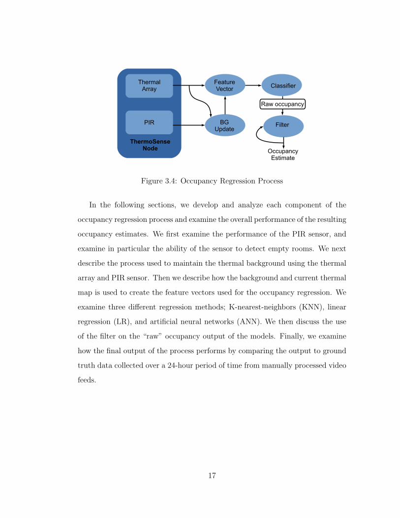
Figure 3.4: Occupancy Regression Process
In the following sections, we develop and analyze each component of the
occupancy regression process and examine the overall performance of the resulting
occupancy estimates. We first examine the performance of the PIR sensor, and
examine in particular the ability of the sensor to detect empty rooms. We next
describe the process used to maintain the thermal background using the thermal
array and PIR sensor. Then we describe how the background and current thermal
map is used to create the feature vectors used for the occupancy regression. We
examine three different regression methods; K-nearest-neighbors (KNN), linear
regression (LR), and artificial neural networks (ANN). We then discuss the use
of the filter on the “raw” occupancy output of the models. Finally, we examine
how the final output of the process performs by comparing the output to ground
truth data collected over a 24-hour period of time from manually processed video
feeds.
17

3.2.1 PIR Sensor Input
In our ThermoSense nodes, the PIR is used to detect if a room is currently
occupied or unoccupied. The nature of the PIRs only allows motion detection,
but people are not constantly moving when they are occupying a room. The
PIR signal constantly fluctuates when motion is detected, and this requires a
smoothing method to process it. Therefore, we smooth the raw PIR values over
a period of 8 minutes. This period was found by evaluating multiple differnt time
windows and it is sufficient time to allow someone to remain inactive for a short
time while still being able to detect that the room is being used. An 8 minute
period was also found to return the least number of false positives. These false
positives can occur when a person momentarily enters a room (e.g. a janitor) or
positives that continue to be returned after a person has left a room (e.g. motion
activity before leaving). This smoothing compared to ground truth can be seen
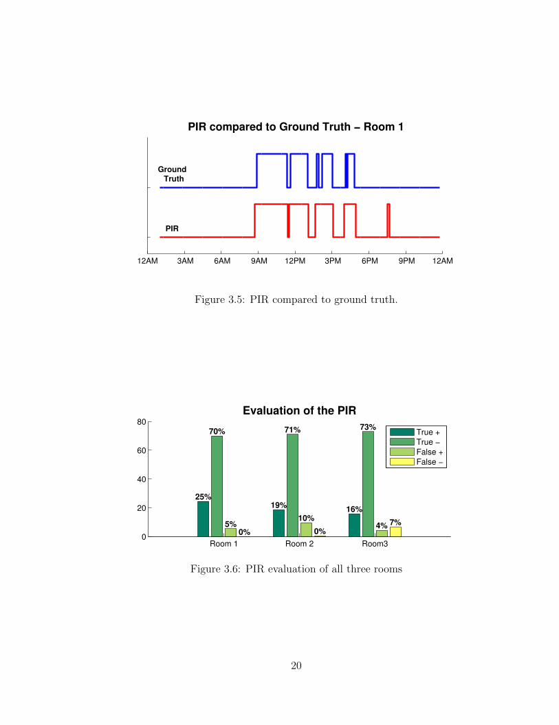
in Figure 3.5.
Due to low number of false negatives, seen in Figure 3.6, the PIR can be used
reliably as an unoccupied indicator. This can be used to override any predictions
that would normally be made by our thermal array sensor. Once a room has been
established as occupied by the PIR, additional models can be used to further
evaluate the actual occupancy of a room.
3.2.2 Thermal Background
Since occupants are typically by far the warmest objects in a conditioned room,
the thermal array can be used to detect occupants within a space. However, in
order to distinguish between passive warm objects such as computers or refrig-
erators and humans, we maintain a thermal background map. If the PIR sensor
indicates the room is empty, then this information can be used to determine the
18
thermal background of the space. As the background can change over time, this
background is continuously updated. In addition to maintaining the background,
the standard deviation of each grid position is also saved; this standard deviation
is used in the following section as a thresholding parameter for distinguishing
significantly warm grid components. Algorithm 1 defines how our current back-
ground and standard deviation for each pixel for this background is maintained.
a If the PIR has detected no movement for the 15 previous minutes, the back-
ground is updated using an exponential weighted moving average (EWMA) and
the standard deviation is updated for each grid component. We found 15 minutes
worked best, as it is unlikely an occupant remains motionless for 15 minutes. This
threshold is also commonly used for PIR based lighting control [NLP98]. How-
ever, if an occupant occupies a space for a significant period, it is possible that
the background changes during this period. To adjust the background while the
space is occupied, we chose a few grid points with the lowest temperatures as
our scaling components. The points with the lowest temperatures are most likely
unoccupied and can be used to update the old background. We divide these
scale points with the old background and average them to find a multiplier we
can use to update our previous background. We then multiply the scale to the
old background to find out a new background. The new background is smoothed
into our old background by using an EWMA but with a significantly lower weight
applied.
3.2.3 Feature Vectors
We next define feature vectors that we will use as input for the regression models.
While it is possible utilize all 64 values of the thermal array along with the PIR
sensor, we found that this approach did not generalize well; the models would
19
12AM 3AM 6AM 9AM 12PM 3PM 6PM 9PM 12AM
PIR compared to Ground Truth − Room 1
Ground Truth
PIR
Figure 3.5: PIR compared to ground truth.
Room 1 Room 2 Room30
20
40
60
80
Evaluation of the PIR
25%
70%
5%0%
19%
71%
10%
0%
16%
73%
4% 7%
True +
True −
False +
False −
Figure 3.6: PIR evaluation of all three rooms
20
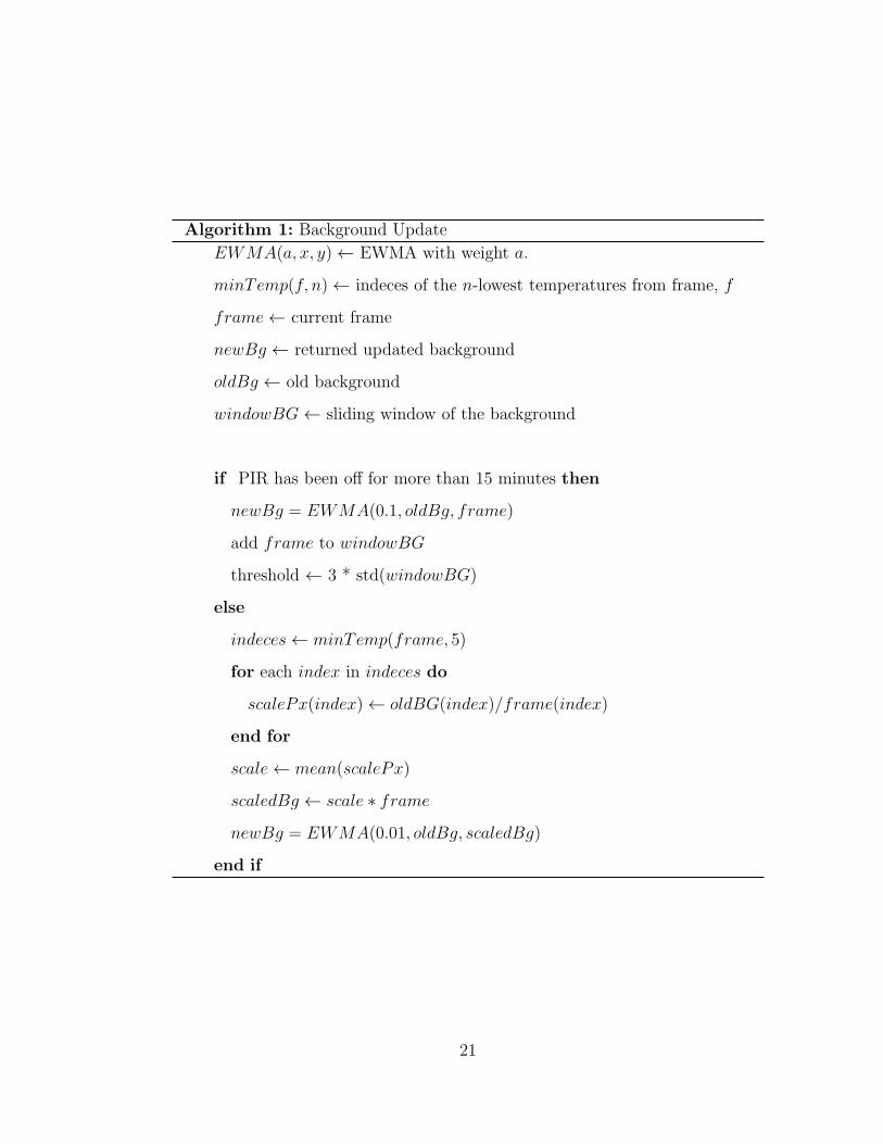
Algorithm 1: Background Update
EWMA(a, x, y)← EWMA with weight a.
minTemp(f, n)← indeces of the n-lowest temperatures from frame, f
frame← current frame
newBg ← returned updated background
oldBg ← old background
windowBG← sliding window of the background
if PIR has been off for more than 15 minutes then
newBg = EWMA(0.1, oldBg, frame)
add frame to windowBG
threshold ← 3 * std(windowBG)
else
indeces← minTemp(frame, 5)
for each index in indeces do
scalePx(index)← oldBG(index)/frame(index)
end for
scale← mean(scalePx)
scaledBg ← scale ∗ frame
newBg = EWMA(0.01, oldBg, scaledBg)
end if
21
not work well when applied to different areas. Instead, we use the following
three features for our models; the total number of significantly warm points, the
number of grouped points that are warm, and the size of the largest group of warm
points. The following subsections formally defines how we extract these features.
We tried a significant number of other less successful feature vectors, e.g. 64 raw
values, 64 thresholded-binary values, size of all connected components, different
permuations of the feature vectors, etc., but cannot discuss these due to space
limitations.
All three feature vectors are based on identifying the significantly warm points
on the grid. As our first step, we first create a 8x8 binary matrix representing
the significantly warm points from the thermal map. This is done by taking
the difference between the background and the current thermal map and apply-
ing a standard deviation based threshold to this difference. We define current
thermal values, background, and standard deviation as Mij = (m0,0...m7,7),
Bij = (b0,0...b7,7), Sij = (s0,0...s7,7), respectively. An active point is defined as
being three standard deviations away from the background,
f(i, j) =
True, if Mi,j − Bi,j > 3 ∗ Si,j
False, if Mi,j − Bi,j < 3 ∗ Si,j
Feature 1: Total Active Points - For our first feature, we use the total number
of active points. A larger total is correlated with higher number of occupants.
Feature 2: Number of Connected Components - Our second feature is based on
connected components [HT73]. Connected components is a method of identifying
groups of points within a matrix that are connected to each other. A point is
considered connected if it is the same value as the point diagonal or directly
adjacent. A component is a group of connected points. The number of the
22
components, which are number of grouped warm points in our application, is
correlated to the number of people occupying the area.
Feature 3: Size of Largest Component - The third feature is the size of the
largest component with the grid. Multiple occupants standing close together
will create one large component rather than several separate components which
would results in a lower occupancy count. The size of the largest component
is positively correlated with occupancy and can be used to get a more accurate
count.
3.2.4 K-Nearest Neighbors
The first model we consider is K-Nearest Neighbors. Let X = (x0...xn) be the
the components of the feature vector of the current frame. Y = (y0...yn) is each
individual feature components found inside the entire training set, Z = (Y0...Ym).
We use euclidean distance to calculate the distance between feature vectors,
d(X,Zj) =
√
√
√
√
n∑
i=0
(xi − Zji)2
We then find the minimum k distances from the training set of Z and collect
the distances as D = (d0...dk) with it’s corresponding occupancy labels as
L = (l0...lk). Weight is applied depending on the distance to each labels to get
the final predicted occupancy, P .
P =k
∑
i=0
wili, where wi = 1− di/(k
∑
j=0
dj)
When calculating KNN, we find the 5 nearest neighbors and the distances
associated with each. The predicted occupancy is averaged with the labels asso-
23

ciated with the 5 closest values, with the largest weight given to values with the
smallest distance.
3.2.5 Linear Regression
The next model we examine is a linear regression model. We define a linear model
y = βAA+ βSS + β
where y is the estimated occupancy (predicted variable), A is the number of
active pixels and S is the size of the largest component (indicator variables). βi
is the corresponding coefficient for the indicator variable i and β is a constant.
While the other models also included the number of components as a parameter,
for the linear model, we chose A and S by testing permutations of the feature
vectors that minimized root mean squared error (RMSE) and had significant
coefficients (p < 0.05). We also found that the model fit best when estimating
positive occupancy. Thus, we train the linear model with data for the 1, 2, and
3 person cases and rely on the PIR sensor to determine if a space is empty.
Table 3.2 shows the fitted model parameters along with p values of each
parameter and the F-test of the overall model. Using a p < 0.05 threshold, we
see the p-values for each of the indicator variables is significant. We see also find
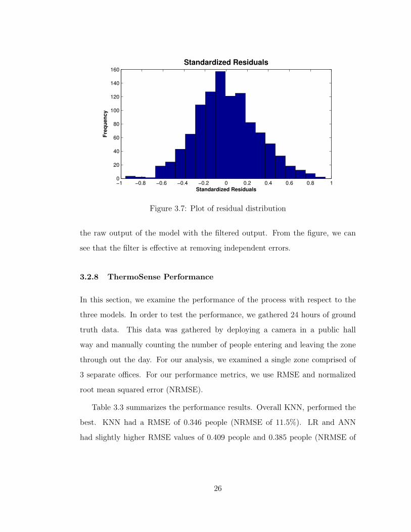
that p ≈ 0 from the F-test and R2 = 0.858, indicating a good fit. Figure 3.7,
shows the distribution of the residuals. The normal distribution verifies that the
independent error assumption has not been violated.
24
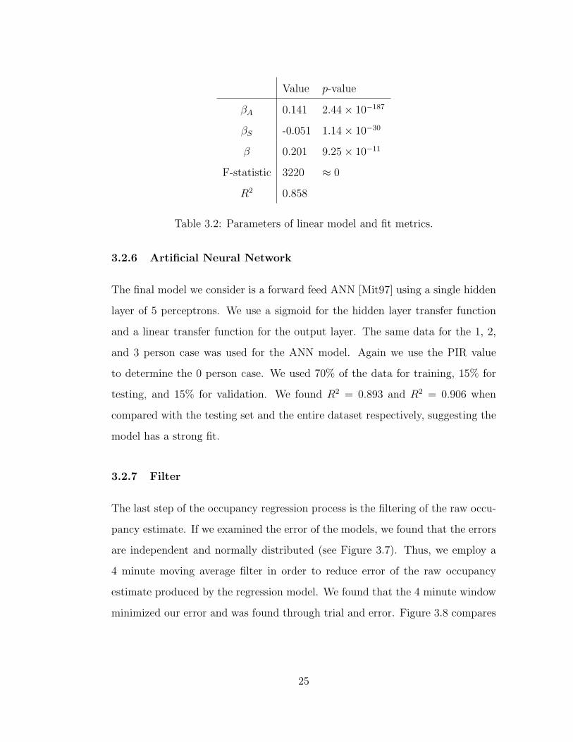
Value p-value
βA 0.141 2.44× 10−187
βS -0.051 1.14× 10⁻³⁰
β 0.201 9.25× 10⁻¹¹
F-statistic 3220 ≈ 0
R2 0.858
Table 3.2: Parameters of linear model and fit metrics.
3.2.6 Artificial Neural Network
The final model we consider is a forward feed ANN [Mit97] using a single hidden
layer of 5 perceptrons. We use a sigmoid for the hidden layer transfer function
and a linear transfer function for the output layer. The same data for the 1, 2,
and 3 person case was used for the ANN model. Again we use the PIR value
to determine the 0 person case. We used 70% of the data for training, 15% for
testing, and 15% for validation. We found R2 = 0.893 and R2 = 0.906 when
compared with the testing set and the entire dataset respectively, suggesting the
model has a strong fit.
3.2.7 Filter
The last step of the occupancy regression process is the filtering of the raw occu-
pancy estimate. If we examined the error of the models, we found that the errors
are independent and normally distributed (see Figure 3.7). Thus, we employ a
4 minute moving average filter in order to reduce error of the raw occupancy
estimate produced by the regression model. We found that the 4 minute window
minimized our error and was found through trial and error. Figure 3.8 compares
25
−1 −0.8 −0.6 −0.4 −0.2 0 0.2 0.4 0.6 0.8 10
20
40
60
80
100
120
140
160
Standardized Residuals
Standardized Residuals
Fre
qu
en
cy
Figure 3.7: Plot of residual distribution
the raw output of the model with the filtered output. From the figure, we can
see that the filter is effective at removing independent errors.
3.2.8 ThermoSense Performance
In this section, we examine the performance of the process with respect to the
three models. In order to test the performance, we gathered 24 hours of ground
truth data. This data was gathered by deploying a camera in a public hall
way and manually counting the number of people entering and leaving the zone
through out the day. For our analysis, we examined a single zone comprised of
3 separate offices. For our performance metrics, we use RMSE and normalized
root mean squared error (NRMSE).
Table 3.3 summarizes the performance results. Overall KNN, performed the
best. KNN had a RMSE of 0.346 people (NRMSE of 11.5%). LR and ANN
had slightly higher RMSE values of 0.409 people and 0.385 people (NRMSE of
26
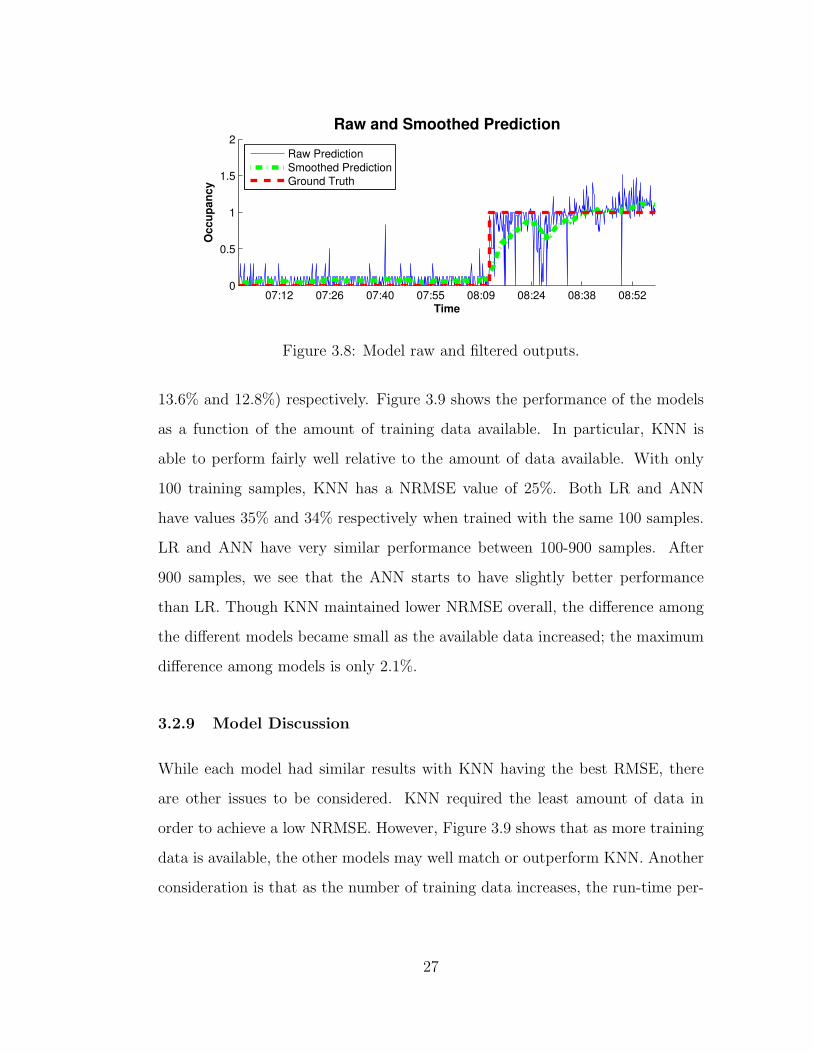
07:12 07:26 07:40 07:55 08:09 08:24 08:38 08:520
0.5
1
1.5
2
Raw and Smoothed Prediction
Time
Oc
cu
pa
nc
y
Raw Prediction
Smoothed Prediction
Ground Truth
Figure 3.8: Model raw and filtered outputs.
13.6% and 12.8%) respectively. Figure 3.9 shows the performance of the models
as a function of the amount of training data available. In particular, KNN is
able to perform fairly well relative to the amount of data available. With only
100 training samples, KNN has a NRMSE value of 25%. Both LR and ANN
have values 35% and 34% respectively when trained with the same 100 samples.
LR and ANN have very similar performance between 100-900 samples. After
900 samples, we see that the ANN starts to have slightly better performance
than LR. Though KNN maintained lower NRMSE overall, the difference among
the different models became small as the available data increased; the maximum
difference among models is only 2.1%.
3.2.9 Model Discussion
While each model had similar results with KNN having the best RMSE, there
are other issues to be considered. KNN required the least amount of data in
order to achieve a low NRMSE. However, Figure 3.9 shows that as more training
data is available, the other models may well match or outperform KNN. Another
consideration is that as the number of training data increases, the run-time per-
27
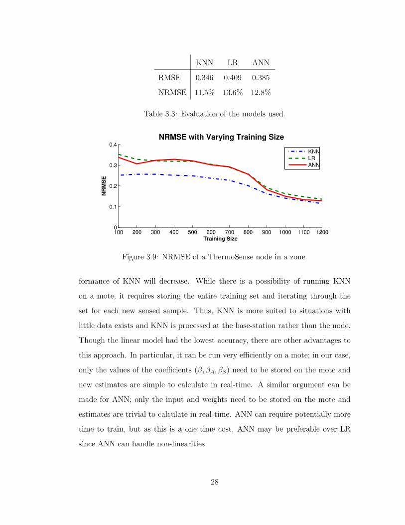
KNN LR ANN
RMSE 0.346 0.409 0.385
NRMSE 11.5% 13.6% 12.8%
Table 3.3: Evaluation of the models used.
100 200 300 400 500 600 700 800 900 1000 1100 12000
0.1
0.2
0.3
0.4
NRMSE with Varying Training Size
Training Size
NR
MS
E
KNN
LR
ANN
Figure 3.9: NRMSE of a ThermoSense node in a zone.
formance of KNN will decrease. While there is a possibility of running KNN
on a mote, it requires storing the entire training set and iterating through the
set for each new sensed sample. Thus, KNN is more suited to situations with
little data exists and KNN is processed at the base-station rather than the node.
Though the linear model had the lowest accuracy, there are other advantages to
this approach. In particular, it can be run very efficiently on a mote; in our case,
only the values of the coefficients (β, βA, βS) need to be stored on the mote and
new estimates are simple to calculate in real-time. A similar argument can be
made for ANN; only the input and weights need to be stored on the mote and
estimates are trivial to calculate in real-time. ANN can require potentially more
time to train, but as this is a one time cost, ANN may be preferable over LR
since ANN can handle non-linearities.
28
Jan Feb Mar Apr May Jun Jul Aug Sep Oct Nov Dec0
100000
200000
300000
400000
B → Baseline
I → ThermoSense Binary
T → ThermoSense
R → Reactive
38%
44%
51%
B I T R
39%
42%
49%
B I T R
29%
32%
38%
B I T R
18%
22%
28%
B I T R
11%
16%
21%
B I T R
9%14
%
19%
B I T R
9%
15%
18%
B I T R
11%
17%
19%
B I T R
12%
17%
20%
B I T R
19%
23%
27%
B I T R
36%
39%
46%
B I T R
39%
44%
52%
B I T R
Monthly HVAC Consumption
Month
kw
h
Heating
Cooling
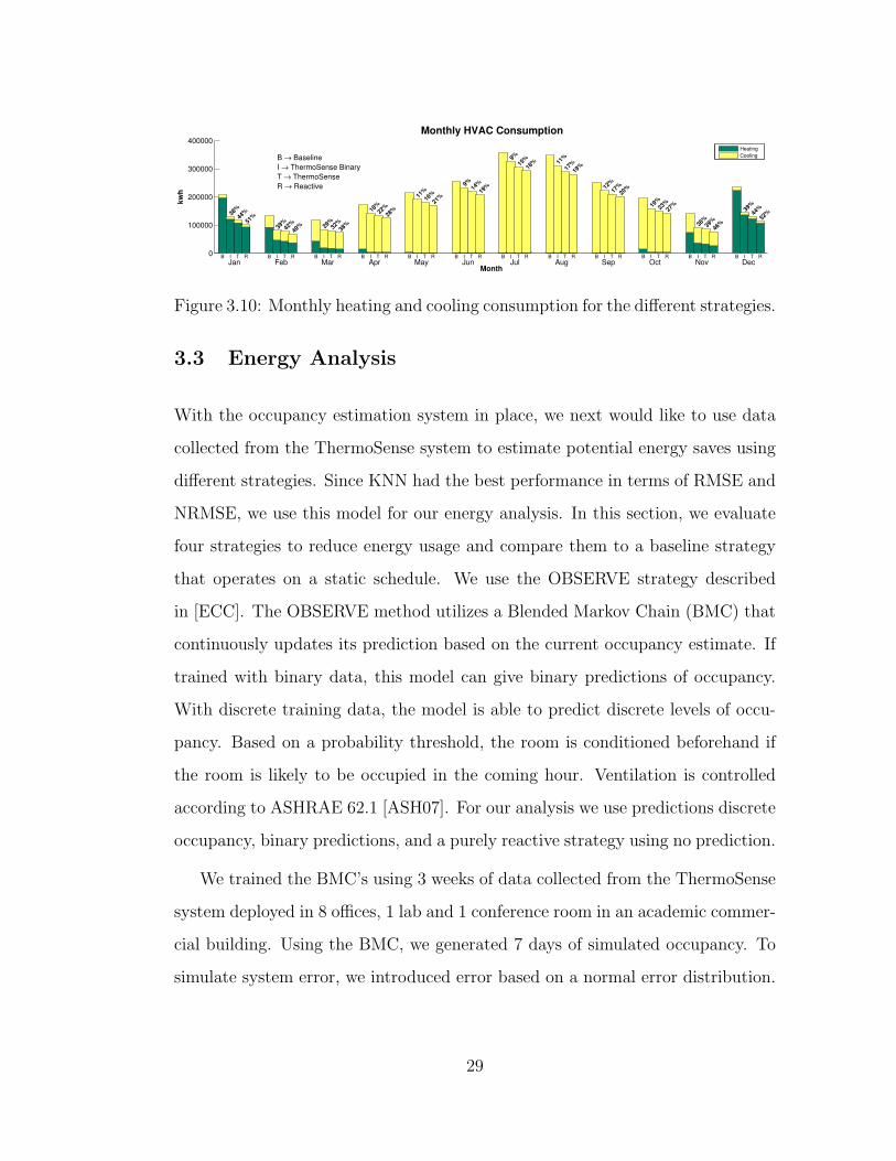
Figure 3.10: Monthly heating and cooling consumption for the different strategies.
3.3 Energy Analysis
With the occupancy estimation system in place, we next would like to use data
collected from the ThermoSense system to estimate potential energy saves using
different strategies. Since KNN had the best performance in terms of RMSE and
NRMSE, we use this model for our energy analysis. In this section, we evaluate
four strategies to reduce energy usage and compare them to a baseline strategy
that operates on a static schedule. We use the OBSERVE strategy described
in [ECC]. The OBSERVE method utilizes a Blended Markov Chain (BMC) that
continuously updates its prediction based on the current occupancy estimate. If
trained with binary data, this model can give binary predictions of occupancy.
With discrete training data, the model is able to predict discrete levels of occu-
pancy. Based on a probability threshold, the room is conditioned beforehand if
the room is likely to be occupied in the coming hour. Ventilation is controlled
according to ASHRAE 62.1 [ASH07]. For our analysis we use predictions discrete
occupancy, binary predictions, and a purely reactive strategy using no prediction.
We trained the BMC’s using 3 weeks of data collected from the ThermoSense
system deployed in 8 offices, 1 lab and 1 conference room in an academic commer-
cial building. Using the BMC, we generated 7 days of simulated occupancy. To
simulate system error, we introduced error based on a normal error distribution.
29
12am 6am 12pm 6pm0
0.2
0.4
0.6
0.8
1
1.2
1.4
Hour
RM
SE
(C
o)
RMSE: Summer Room Temperature
Reactive
Predicted
Binary Prediction
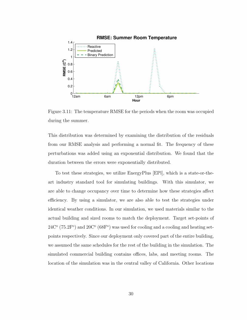
Figure 3.11: The temperature RMSE for the periods when the room was occupied
during the summer.
This distribution was determined by examining the distribution of the residuals
from our RMSE analysis and performing a normal fit. The frequency of these
perturbations was added using an exponential distribution. We found that the
duration between the errors were exponentially distributed.
To test these strategies, we utilize EnergyPlus [EPl], which is a state-or-the-
art industry standard tool for simulating buildings. With this simulator, we
are able to change occupancy over time to determine how these strategies affect
efficiency. By using a simulator, we are also able to test the strategies under
identical weather conditions. In our simulation, we used materials similar to the
actual building and sized rooms to match the deployment. Target set-points of
24Co (75.2Fo) and 20Co (68Fo) was used for cooling and a cooling and heating set-
points respectively. Since our deployment only covered part of the entire building,
we assumed the same schedules for the rest of the building in the simulation. The
simulated commercial building contains offices, labs, and meeting rooms. The
location of the simulation was in the central valley of California. Other locations
30
were not evaluated in the interest of space.
Figure 3.10 shows the monthly breakdown of the heating and cooling. All
three strategies had significant energy savings over the baseline strategy. Over-
all, the reactive strategy had the lowest energy consumption. This strategy con-
sumed 29.6% less than the baseline strategy annually. It saves additional energy
since it does not pre-condition rooms ahead of time. However, we will see that
this savings in energy comes at the cost of comfort (Section 3.4). In general, all
the strategies had the largest percentage of savings during winter months (Nov
- Feb) and the lowest percentage of savings during the warmer months (May -
Sep). ThermoSense and ThermoSense Binary had 24.8% and 19.7% savings re-
spectively. The binary approach consumed more energy since this strategy has a
tendency to over-ventilate. Over-ventilation reduces efficiency since it increases
the amount of outside air that needs to be conditioned. The greatest differences
between the ThermoSense and ThermoSense Binary approaches occur during the
warmest and coldest months (Jan, Dec, Jul, Aug) where ThermoSense consumed
5-6% less than ThermoSense Binary. Increased ventilation of ThermoSense bi-
nary during these months has a greater impact on efficiency than during milder
shoulder seasons.
3.4 Conditioning Effectiveness
In the previous section, we show that occupant based conditioning saves a sig-
nificant amount of energy. However, conditioning effectiveness also needs to be
considered.
For the temperature effectiveness, we examine a room that is only occupied
at 8am, 3pm, and 4pm on Mondays and focus our analysis to the warm months
31
0:00 4:00 8:00 12:00 16:00 20:00 24:000
100
200
300
400
500
Hour
CF
M
Total Building Ventilation Rate
Baseline ASHRAE
Reactive/ThermoSense Binary
ThermoSense
Required
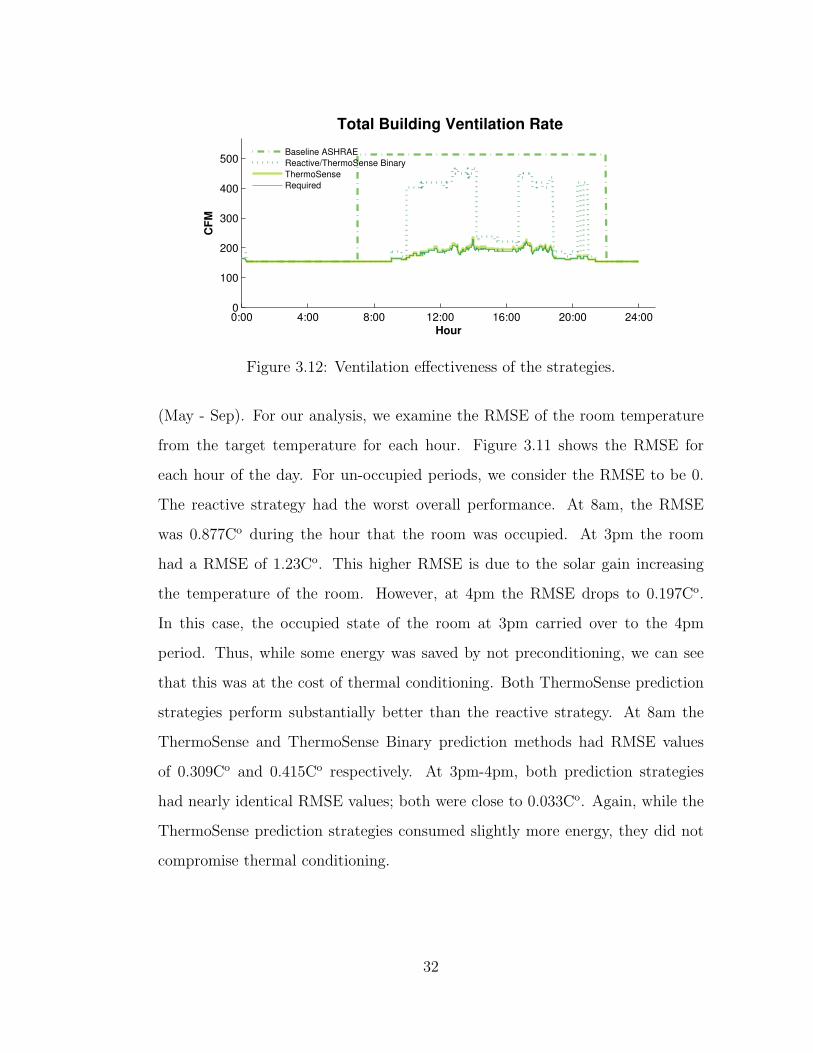
Figure 3.12: Ventilation effectiveness of the strategies.
(May - Sep). For our analysis, we examine the RMSE of the room temperature
from the target temperature for each hour. Figure 3.11 shows the RMSE for
each hour of the day. For un-occupied periods, we consider the RMSE to be 0.
The reactive strategy had the worst overall performance. At 8am, the RMSE
was 0.877Co during the hour that the room was occupied. At 3pm the room
had a RMSE of 1.23Co. This higher RMSE is due to the solar gain increasing
the temperature of the room. However, at 4pm the RMSE drops to 0.197Co.
In this case, the occupied state of the room at 3pm carried over to the 4pm
period. Thus, while some energy was saved by not preconditioning, we can see
that this was at the cost of thermal conditioning. Both ThermoSense prediction
strategies perform substantially better than the reactive strategy. At 8am the
ThermoSense and ThermoSense Binary prediction methods had RMSE values
of 0.309Co and 0.415Co respectively. At 3pm-4pm, both prediction strategies
had nearly identical RMSE values; both were close to 0.033Co. Again, while the
ThermoSense prediction strategies consumed slightly more energy, they did not
compromise thermal conditioning.
32

Next we examine the ventilation effectiveness of the system. For our analysis,
we evaluate the ventilation of the spaces for one particular day. As previously
mentioned, we use the ASHRAE 62.1 standard to determine the ventilation ac-
cording to occupancy. As ventilation is regulated in real-time, the binary based
strategies (reactive and ThermoSense binary prediction) have the same ventila-
tion rates. As we cannot determine the precise occupancy with a binary occu-
pancy estimate, we assume maximum occupancy for rooms that are occupied for
ventilation. The baseline strategy assumes maximum occupancy from 7am to
10pm. Figure 3.12 shows the baseline, ThermoSense binary, and ThermoSense
based strategies. We can see that the baseline strategy greatly over-ventilates.
However, there is also a short period at the beginning where the baseline strategy
under-ventilates; this illustrates the shortcomings of a static schedule. Both the
ThermoSense binary and ThermoSense strategies were able to meet the required
ventilation level. However, we can see that the ThermoSense binary strategy still
over-ventilates the area a great deal; overall, this strategy over-ventilated the area
by 170%. The ThermoSense binary strategy performed best when multiple rooms
were empty, which can be seen during the period between 2pm and 5pm. Since
only a few rooms were occupied, only a few rooms were over-ventilated. The
ThermoSense based ventilation performed the best. We can see that the ventila-
tion rate is only 3.25% more than the required rate. This is due mainly to a 10%
occupancy increase added by design in order to protect against under-ventilation
that could be caused by sensor errors [ECC].
3.5 Summary
In this chapter, we developed ThermoSense, an occupancy monitoring system
that utilizes thermal based sensing and PIR sensors. We developed a novel low-
33
power multi-sensor node for measuring occupancy using a thermal sensor array
combined with a PIR sensor. We showed it is possible to use these temperature
readings in order to determine how many people are within the space using a
novel occupancy regression process. Unlike the CO2 sensor, the thermal array
can measure occupancy in near real-time. The thermal array is also not sensitive
to optical issues, such as lighting or background changes. By adding a PIR sensor,
we increased accuracy of detecting empty spaces and the overall accuracy of the
platform. The PIR sensor is also used to reduce the node’s power consumption by
triggering the mote and thermal array only when someone is present. We tested
this new platform with a 17-node deployment covering 10 building conditioning
areas totaling 2,100 sq. ft. for a period of three weeks and showed that Ther-
moSense is able to detect occupancy with a RMSE of only ≈0.35 persons. Using
this data, we tested four different usage based conditioning strategies and ana-
lyzed the energy usage; we showed that 25% annual energy savings are possible
with occupant based conditioning strategies.
34
CHAPTER 4
FORCES: Feedback and control for Occupants
to Refine Comfort and Energy Savings
In the previous chapter, we addressed the issue of reducing energy cost using
an occupancy regression. This however does not take into consideration if the
occupants within the building are comfortable. In this chapter, we introduce a
participatory voting system to allow occupants to vote based on their thermal
preferences and for these votes to change the thermal conditions of their spaces.
Unlike the previous chapter, this body of work’s goal is to increase user satisfac-
tion with a building’s thermal condition while reducing energy consumption.
Although comfortable temperatures in commercial work environments make
employees happier and more productive [FR97,SF05], maintaining ideal temper-
ature for occupants is difficult to do correctly. Building managers are responsible
for setting temperatures for spaces within buildings, but the chosen temperature
setpoints are general estimates for the building and do not necessarily suit the
thermal preferences of the individual occupants. A pre-study survey we con-
ducted, completed by 61 occupants in 3 University buildings, indicated that 96%
of those surveyed have had to take individual action to improve their comfort in
their work space by using a personal heater or fan, adjusting clothing or using
a blanket, adjusting their thermostat (only 18% of those surveyed reported an
effective thermostat), relocating, etc. Importantly, 33% of those surveyed indi-
35
cated that they have had to avoid their work environment due to discomfort,
45% reporting that the thermal conditions of their work environment inhibits
their ability to work efficiently.
This occupant discomfort is caused by imperfect temperature setpoint selec-
tion. The state-of-the-art method for choosing temperature setpoints is taken
from the American Society of Heating, Refrigeration, Air-Conditioning Engi-
neering (ASHRAE) Standard 55 [ASH04], which relies on Predicted Mean Vote
(PMV). PMV uses parameters such as temperature and humidity to calculate an
expected comfort level for an individual from -3 (“Too Cold”) to 3 (“Too Hot”).
A key limitation of using PMV is the difficulty of ascertaining other parameter
values, such as clothing level and metabolic rate. Our pre-study survey indicates
that occupants prefer temperatures as low as 63◦F and as high as 85◦F, and
so even with perfect PMV factor estimation, variation in occupant temperature
preference makes PMV prone to error.
At home, an occupant can adjust a thermostat to suit his or her preference.
However, as thermostats often aren’t available to employees in commercial build-
ings, most who want to modify the temperature in their space must contact the
building manager and request an adjustment. According to our pre-study survey,
only 13% of participants had contacted the building manager with satisfactory
results, and they did so no more than twice a month. As only 34% of those sur-
veyed reported satisfaction with the building HVAC system, this indicates that
occupants are deterred by the adjustment process, and would prefer to bear the
discomfort rather than repeatedly contact the building manager.
Work done in [EC,BTG13, JB12, Bur14, Rob14, RDS14] develop methods of
collecting thermal comfort data. [EC,Rob14] continue by using this data to man-
age the thermal characteristics of the space to fit occupant preferences by adap-
36

tively conditioning the user’s zone. In general, the occupants are found to be
significantly more satisfied once given the ability to control building tempera-
tures.
Although these comfort voting applications improve upon standard methods
of building interaction, there is still work to be done. A comfort voting application
in a commercial building must aim to achieve the primary goals of the building
manager, typically either reduction of energy consumption, or maximization of
occupant comfort. Our main contributions are the following:
• We develop FORCES, Feedback and control for Occupants to Refine Comfort
and Energy Savings, a multi-platform application that a building occupant can
use to vote on thermal comfort within a space. The application uses this informa-
tion to adjust the HVAC system using two different control strategies to improve
occupant comfort while trying to minimize energy use.
• We propose 5 application feedback types that use various methods of data
presentation and environmental stimuli to promote specific behavior in using
FORCES. In a 1-month preliminary study, we analyze how these feedback types
affect user behavior for thermal comfort and show that green and physical feed-
back provide the best energy savings and user comfort satisfaction.
• In a longer 40-week study, these two feedback types coupled with two different
control strategies are implemented across 61 participants in 3 different buildings
to understand how their use affects HVAC system energy consumption and user
satisfaction. We show an increased user satisfaction from 33.9% to 93.3% and a
reduced energy consumption by as much as 18.99%. In addition, we find that by
including a drifting control strategy, savings up to 37% can be realized without
a significant reduction of occupant satisfaction.
To our knowledge, this is the first work that investigates how different feed-
37

Figure 4.1: From left to right, iOS, Android, Web version
back mechanisms and control strategies can influence human decisions in a ther-
mal comfort application controlling an HVAC system in production buildings to
balance the energy/comfort tradeoff.
4.1 System Design Overview
4.1.1 System Architecture
FORCES is a comfort voting application that allows occupants to vote for their
thermal preference. Based on this vote, the room’s thermal conditioning is
changed to better suit this preference. To facilitate user interaction with FORCES,
we developed iOS, Android and Web interfaces as shown in Figure 4.1. Using
strategies from [EC] we receive votes from users describing how they feel, from
Cold (-3) to Hot (3). These values are defined as the Actual Mean Vote (AMV),
38

Name Value
Air Speed 0.1m/s
Mean Radiant Temperature 25◦C
Humidity 30%
Metabolic rate 70W/m2
Clothing Level 0.5clo
Table 4.1: PMV Constants
and are used to find the ideal temperature for the room by setting it equal to
Fanger’s formulation of PMV [Fan70]. PMV uses parameters such as the clothing
coefficient and metabolic rate that are difficult to obtain for each participant, so
we use estimated parameter values obtained from [CBE] that are appropriate for
an office worker adjusted by season, as shown in Table 4.1. A temperature found
to be suitable according to ASHRAE Standard 55 [ASH04] is one with a PMV
value between 0.5 and -0.5, where the occupant is neither too hot or cold. We
can therefore solve for this comfortable temperature and set it for the room.
Figure 4.2 shows an overview of the FORCES system. When a user submits a
vote for their comfort, it is sent to the FORCES API, and feedback information
is sent back to the user. The collected AMVs are tallied every 5 minutes and
averaged in zones with multiple users. The AMV is used by the PMV model to
determine the next room temperature setpoint, which is given to the Building
Management System (BMS) for actuation. The building makes the necessary
adjustments to condition the room to the desired temperature. As the thermal
conditions are monitored by the user and votes are used to further modify the
temperature, FORCES creates a closed loop feedback system with the human as
a sensor.
Setpoints are handled by the BMS, which achieves the setpoint. WebC-
39
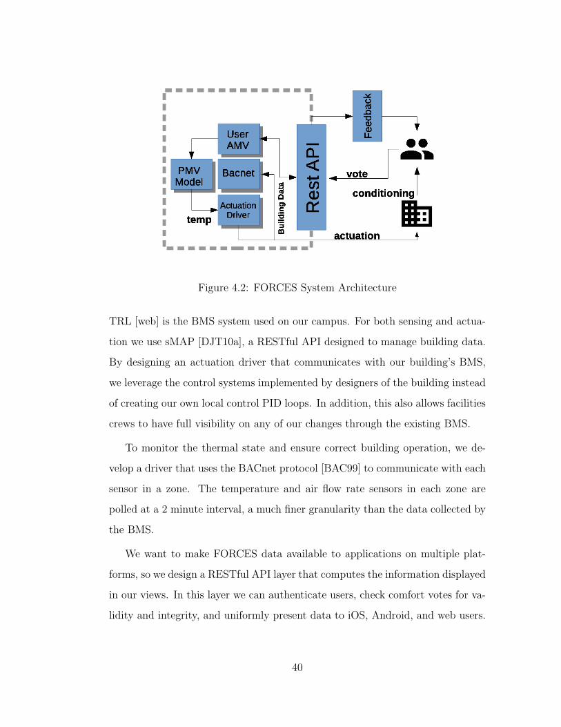
Figure 4.2: FORCES System Architecture
TRL [web] is the BMS system used on our campus. For both sensing and actua-
tion we use sMAP [DJT10a], a RESTful API designed to manage building data.
By designing an actuation driver that communicates with our building’s BMS,
we leverage the control systems implemented by designers of the building instead
of creating our own local control PID loops. In addition, this also allows facilities
crews to have full visibility on any of our changes through the existing BMS.
To monitor the thermal state and ensure correct building operation, we de-
velop a driver that uses the BACnet protocol [BAC99] to communicate with each
sensor in a zone. The temperature and air flow rate sensors in each zone are
polled at a 2 minute interval, a much finer granularity than the data collected by
the BMS.
We want to make FORCES data available to applications on multiple plat-
forms, so we design a RESTful API layer that computes the information displayed
in our views. In this layer we can authenticate users, check comfort votes for va-
lidity and integrity, and uniformly present data to iOS, Android, and web users.
40
4.1.2 Application and Feedback Design
Application design affects user interaction in various ways. For instance, im-
provement of a mobile application’s user interface can improve user enjoyment.
Additionally, we hypothesize that in control applications like ours where the hu-
man is in the loop, feedback provided to the user can also influence their voting
patterns. Based on research discussed in Related Work, we choose 5 feedback
mechanisms for our comfort voting application, described below in detail.
4.1.2.1 Physical Feedback
By design, the vote collection system architecture defines periods of time for
votes to be collected from users before a control decision is made and actuation
begins. The period chosen between actuations is typically several minutes, as the
amount of time required to condition a room to temperature is large. However,
with several minutes between a user casting a vote about thermal comfort and
the building’s response, a user may become dissatisfied with the quality of the
HVAC control.
To minimize this effect, we propose a “physical” feedback that immediately
triggers a long burst of air from the HVAC system when a vote is received. This
“instant gratification” provides sensory stimulation in the form of sound from the
vents and an increase of air movement that assures the user that the system is
changing in response to a vote. The additional activation when a vote is received
may create wear and tear on the HVAC system; for this reason, we limit the
feedback to just one burst per system actuation period. In our experiment, this
period was set to 5 minutes. Long-term experiments are required to measure any
impact of this feedback on HVAC equipment, so we leave this for future work.
41
4.1.2.2 Expected Action Feedback
In commercial buildings, multiple occupants are commonly required to share the
same thermal zone and HVAC infrastructure due to system design. To a thermal
comfort control application, this causes complications as there is no longer a one-
to-one relationship between an occupant and a space. In particular, previous
work [EC] showed that a shared thermal zone encourages users to exaggerate
votes in order to “bias” the system towards their own preferences. One likely
cause for this bias is that a user may not know what votes are being cast by
other users in the shared space.
Once a user casts a vote, the expected action feedback takes a tally of all votes
that have been cast in the last voting period, and then reports back to the user
exactly what action the system is expected to take. To a user, this confirms that
the system has received the user’s vote, and implies what votes are being made
by other users in the same space. This feedback can reduce the bias observed in
previous works if the system intends to react as the user wants, or could enhance
the bias if the system’s planned actions conflict with the user’s vote.
4.1.2.3 Social Feedback
By informing a user about their peers’ activity, also known as the descriptive
norm, it is possible to encourage a particular behavioral pattern. In [GCG08],
hotel guests were found to be more willing to participate in an environmental
conservation program when told that a large percentage of other hotel guests
participated. Similarly, our social feedback notifies a user of the recent voting
patterns of their peers, to encourage interaction with FORCES. To calculate
peer participation, voting activity is determined across the entire building. The
number of active users in the last week is found, and the percentage of those who
42
have voted in the last 24 hours is reported to the user. We calculate activity
based only on active users to keep the percentage relatively high even during
periods of inactivity.
4.1.2.4 Leaderboard Feedback
Another feedback type that operates on social stimuli is the leaderboard, a com-
mon form of gamification [DDK11]. The leaderboard reports a user’s “score”, and
shows the user’s rank among all users with respect to this score. In our study,
vote volume (i.e. total number of votes) was chosen as the score, but other met-
rics may be used as well. The advantage of the leaderboard is the introduction of
competition into the voting platform. Users that are high on the leaderboard will
be motivated to continue voting to maintain their high position, and users that
are low on the leaderboard can clearly see how they compare to the top leaders.
We suspect that leaderboard use helps maintain interest by inspiring competition
among voters.
4.1.2.5 Green Feedback
The primary objective of a building’s HVAC system is to make occupants com-
fortable, so a user of an app like FORCES may vote with no thought to system
energy efficiency. However, if a control change will significantly improve the
building’s efficiency but minimally affect occupant comfort, the occupant may be
willing to make the more sustainable vote. Green feedback informs users of the
environmental implications of their voting pattern to encourage votes that are
more energy-aware.
By comparing a zone’s default temperature setpoints to those used by FORCES
and considering the outside temperature, we can determine how much more or
43
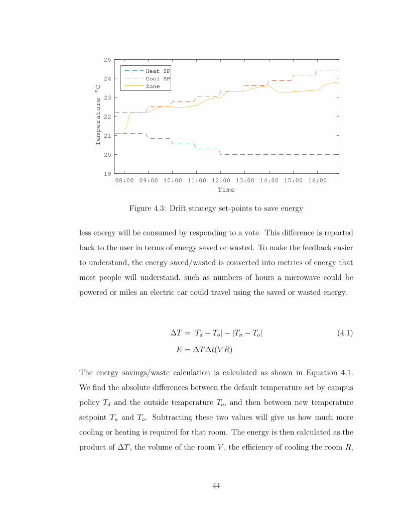
08:00 09:00 10:00 11:00 12:00 13:00 14:00 15:00 16:00
Time
19
20
21
22
23
24
25
Temperature °C
Heat SP
Cool SP
Zone
Figure 4.3: Drift strategy set-points to save energy
less energy will be consumed by responding to a vote. This difference is reported
back to the user in terms of energy saved or wasted. To make the feedback easier
to understand, the energy saved/wasted is converted into metrics of energy that
most people will understand, such as numbers of hours a microwave could be
powered or miles an electric car could travel using the saved or wasted energy.
∆T = |Td − To| − |Tn − To| (4.1)
E = ∆T∆t(V R)
The energy savings/waste calculation is calculated as shown in Equation 4.1.
We find the absolute differences between the default temperature set by campus
policy Td and the outside temperature To, and then between new temperature
setpoint Tn and To. Subtracting these two values will give us how much more
cooling or heating is required for that room. The energy is then calculated as the
product of ∆T , the volume of the room V , the efficiency of cooling the room R,
44
and time ∆t. Before reporting to the user, we convert the energy savings/waste
into more intuitive units by multiplying it by appropriate conversion factors.
Examples of units presented to the users are: “You have saved/wasted enough
energy to cook gp pizzas”, “drive an electric car gc miles”, etc.
4.1.2.6 Drift Control
Previous work in building control strategies [Hor99, PSP10] dictates that it is
difficult to maintain user interest in a comfort voting application once thermal
comfort is achieved. Similarly to [CFH14], we introduce a control strategy that
allows heating/cooling setpoints of a room to drift apart. This allows temperature
to “float” within these expanding bounds, allowing energy savings. Example use
of such a drift strategy can be seen in Figure 4.3.
In normal usage, heating/cooling setpoints are chosen based on occupant vot-
ing patterns. However, if these bounds are held unnecessarily tightly, extra energy
will be consumed. We imagine drift providing the most benefit in two situations.
The first is when outside temperature is comfortable, so minimal ventilation will
be sufficient to maintain thermal comfort. The second is when occupants only
need temporary conditioning, for example while they are cooling off from walking
inside on a hot day, or if they come in and out of the office and don’t need their
room conditioned the whole time.
In our experiments, we allow the bounds to start drifting apart 30 minutes
after the occupants’ last vote, and the drift moves each bound apart by 1/2 ◦F
every 30 minutes. In practice, the bounds are reset to ±1◦F from the last voted
temperature each morning, and unless votes occur will be allowed to float to the
farthest possible bounds of 66◦F and 76◦F, as chosen by the building managers.
45

Male Female Declined
Gender 30.5% 66.1% 3.4%
18-29 30-39 40-49 50+ Declined
Age 33.9% 22.0% 28.8% 13.6% 1.7%
Table 4.2: Demographics of Study Population
4.2 Experimental Setup
In this section we explain the participant recruitment process, the demographics
of the recruited participants, the buildings used in the study, and their installed
HVAC systems. Our preliminary study examines the effect of the 5 proposed
feedback systems on participant satisfaction and energy consumption across a 4-
week period. The results are then used to narrow down on the two most promising
feedbacks for a long-term study. In total, our studies include 61 participants over
a span of 40 weeks, with more than 1300 comfort votes collected.
4.2.1 Population Description
To discern differences in voting patterns due to feedback modification, FORCES
was deployed across a diverse population. The majority of the FORCES par-
ticipants are full-time employees in administrative offices or research labs, with
76% working 30+ hours/week. 71% of those included in the study share their
work space with one or more people. Interestingly, our study is predominantly fe-
male, aligned with the current population that occupies the building. Additional
population demographics can be found in Table 4.2.
46

4.2.2 Recruitment Process
The study begins for each participant upon completion of a skill session with
one of the project’s researchers. The skill session allows us to complete four
objectives:
1) The participant reviews and signs the Institutional Review Board (IRB) con-
sent form.
2) The participant completes a pre-study survey, providing demographics, workspace
information, and initial comfort in the space. The participant will complete a
post-study survey later for comparison.
3) The researcher helpes install the application on iOS, android, or bookmark
the web-voting page based on the participant’s preference. Application use is
explained to the participant, describing feedback in a neutral way.
4) The participant was provided login credentials as well as contact information
for the researchers, in case an issue was encountered.
The FORCES system operates autonymously, with manual intervention re-
quired only if a fault in the HVAC system were to occur. Building managers love
the FORCES system as it reduces the need for frequent requests for temperature
adjustment, reducing their workload and keeping building users more satisfied.
4.2.3 Feedback Assignment
In the preliminary study, we sequentially assigned feedback types as we recruited
participants with the exception of physical feedback. As the physical feedback of
one user’s vote would alter the thermal sensation of another, we chose to specif-
ically assign physical feedback only to participants that had their own thermal
zones. As the remaining feedback methods were assigned semi-randomly, partic-
47

Feedback Type Baseline Energy Feedback Energy Percentage Incr. Projected Cost Incr.
(KWH/day) (KWH/day) (USD)
Social 83.38 89.23 7.01 % $17,584.74
Green 28.93 30.06 3.90 % $9,782.48
Physical 13.36 14.26 6.76 % $16,973.22
Expected 81.03 87.29 7.73 % $19,393.60
Leaderboard 19.05 20.98 10.12 % $25,389.26
Table 4.3: Energy Cost per Feedback - Preliminary
ipants that shared a thermal zone often received different feedback types. In this
manner, we get a nearly-equal number of participants in each feedback type, and
a fairly random spatial distribution.
At the end of the preliminary study, we found that having different feedback
methods within a single HVAC zone makes energy analysis of the feedback types
difficult. In the primary study, we corrected this by assigning feedback randomly
across the HVAC zones, but assigning all users within a zone to the same feedback
condition.
4.2.4 Building Description
FORCES was activated across three buildings, covering a total of 2 open recep-
tionist areas, 33 offices, 8 research labs, and 14 cubicles. Most of the offices house
one or two participants, while the cubicle areas and research labs can hold as
many as 6 and 10, respectively. In BLD2, a terminal reheat system is present
with thermafusers, allowing zones with a shared variable air volume (VAV) box
to receive individual control (excluding cubicle areas, which must share control).
In BLD1 and BLD3, thermafusers are not available, so in some cases individual
control is not possible, even in offices.
48

4.2.5 Energy Calculation
Our campus has a central cooling/heating plant which stores chilled/heated water
that is distributed to our buildings, which use single duct terminal reheat HVAC
systems. We use a model of energy usage from [KB11], which calculates energy
usage based on air temperature differentials through the cooling/heating coils and
the fan electricity used to move the air. Here we describe how we follow [KB11]
for use in our buildings.
The outside and circulated inside air are mixed in the economizer to Tm, the
“mixed air temperature”. The Air Handler Unit (AHU) cooling coil them cools
Tm to the supplied temperature Ts, to be pushed to each room for conditioning.
The cost of cooling for a particular zone is computed as the mass flow of air to
the zone mz (A fraction of the total mz from the AHU) multiplied by the change
of temperature. A massive fan in the AHU provides air for the a group of zones.
A cooling coefficient, ηc, is applied to the result as shown in Equation 4.2
Pc = ηc(Tm − Ts)mz (4.2)
Once past the cooling coil, the temperature is increased by the zone’s heating coil
from Ts to the discharge temperature, Td. The power for heating is therefore the
increase in temperature times the mass flow for the zone and a heating coefficient,
ηh as shown in Equation 4.3.
Ph = ηh(Ts − Td)mz (4.3)
The final addition to total power use is that of the air supply fan. The power is
the square of the total mass flow, mt, multiplied by fan efficiency coefficient κ.
∆Pf = κmt2 (4.4)
49
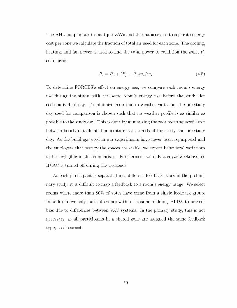
The AHU supplies air to multiple VAVs and thermafusers, so to separate energy
cost per zone we calculate the fraction of total air used for each zone. The cooling,
heating, and fan power is used to find the total power to condition the zone, Pz
as follows:
Pz = Ph + (Pf + Pc)mz/mt (4.5)
To determine FORCES’s effect on energy use, we compare each room’s energy
use during the study with the same room’s energy use before the study, for
each individual day. To minimize error due to weather variation, the pre-study
day used for comparison is chosen such that its weather profile is as similar as
possible to the study day. This is done by minimizing the root mean squared error
between hourly outside-air temperature data trends of the study and pre-study
day. As the buildings used in our experiments have never been repurposed and
the employees that occupy the spaces are stable, we expect behavioral variations
to be negligible in this comparison. Furthermore we only analyze weekdays, as
HVAC is turned off during the weekends.
As each participant is separated into different feedback types in the prelimi-
nary study, it is difficult to map a feedback to a room’s energy usage. We select
rooms where more than 80% of votes have come from a single feedback group.
In addition, we only look into zones within the same building, BLD2, to prevent
bias due to differences between VAV systems. In the primary study, this is not
necessary, as all participants in a shared zone are assigned the same feedback
type, as discussed.
50

Probability Density
0
0.05
0.1
0.15
0.2
0.25
0.3
0.35
0.4
Cold Cool Slightly
Cool
Neutral Slightly
Warm
Warm Hot
Green
Social
Leaderboard
Physical
Expected
Figure 4.4: PMV vote distribution for each feedback type
4.3 Results
4.3.1 Preliminary Study
The preliminary study deployed all 5 feedback types to narrow down the ones that
showed the most promise with respect to energy efficiency and user satisfaction.
As this experiment was to compare feedback types only, the drift control strategy
is not evaluated here.
In Figure 4.4 we see the distribution of votes along the PMV scale for each
feedback tested in our preliminary study. On the x axis, the PMV range is shown
from “Too Cold” (-3) to “Too Hot” (3). On the y axis, the fraction of votes
with that value is shown, such that the sum of a feedback type across all comfort
levels is equal to 1. The distribution of votes gives intuition into the goal of the
51
users. For instance, leaderboard and physical have the majority of votes on the
right of the scale, indicating a preference for cooler temperatures. Due to the hot
weather during the study, providing cooler temperatures will result in increased
energy usage. However, the vote distribution of users with the green feedback is
greater on the lower end of the scale, with 47.41% of participants voting below
neutral, 35.56% above neutral, and 17.04% voting for neutral comfort. As each
vote below neutral is a request for warmer air, it shows that users were willing
to increase the temperature, decreasing energy usage.
Interesting artifacts can be found in other feedback vote distributions, as well.
Leaderboard users, for instance, generate 1.61x more neutral votes than the feed-
back with the second highest neutral votes (green). This indicates a strategy for
users to inflate their rank on the leaderboard using votes that don’t greatly affect
the temperature. As the Leaderboard’s “gamified” interface encourages its users
to provide more votes (even neutral ones), the FORCES system will have explicit
affirmation that the user is comfortable (neutral), helping FORCES to establish
and maintain comfortable temperatures. In contrast, with other feedback meth-
ods, FORCES must make an implicit assumption that the user is comfortable
based on the absence of votes. Physical feedback is designed to provide an im-
mediate impression to the user that the HVAC system is working. However, the
application provides no incentives to reduce energy consumption. This is shown
in the figure, as 61.97% of the votes submitted by users with physical feedback
are above neutral, requesting cooler air at the cost of more energy. Both social
and expected feedback can be seen to have a higher concentration of votes on
the extremes and a reduction near neutral. This is expected, as somebody in a
comfortable zone feels less need to vote.
Using the procedure discussed in Calculating Energy, we analyzed the energy
52
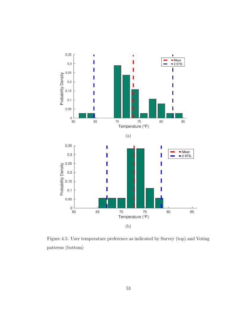
(a)
(b)
Figure 4.5: User temperature preference as indicated by Survey (top) and Voting
patterns (bottom)
53

Feedback Useful Neutral Not Useful
Green 33.33 33.33 33.33
Social 60.00 20.00 20.00
Leaderboard 50.00 50.00 0.00
Physical 100.00 0.00 0.00
Expected 100.00 0.00 0.00
Table 4.4: Survey: Did the user find the app useful?
efficiency of the 5 deployed feedback types over the one-month study. Table 4.3
reports the energy usage, as well as the projected cost if FORCES were installed
on an entire building. As shown, the energy consumption of all feedback types
increased over the baseline comparison point. The variations in baseline energy
shown in Table 4.3 are caused by the differences in square footage of the spaces,
number of occupants, thermal load, solar gain, and other factors. Although many
of these variations are unavoidable, we don’t compare these rooms to each other,
but to themselves with and without the FORCES system. In this way, we can
use the feedbacks’ relative performance to choose the ones that performed most
efficiently. In particular, these results show that Green feedback led to the least
energy usage by a fair margin, with Physical and Social as runners-up.
In addition to the energy analysis performed on the 5 feedback types, we also
investigate what the building occupants thought of the app’s usefulness by having
them complete a survey at the end of the study. As shown in Table 4.4, both
Physical and Expected feedback methods were found to be useful by unanimous
vote. Due to the relatively low energy usage of Green and Physical feedbacks
and the usefulness of Physical feedback, we think these two are best suited for
the long-term study.
54
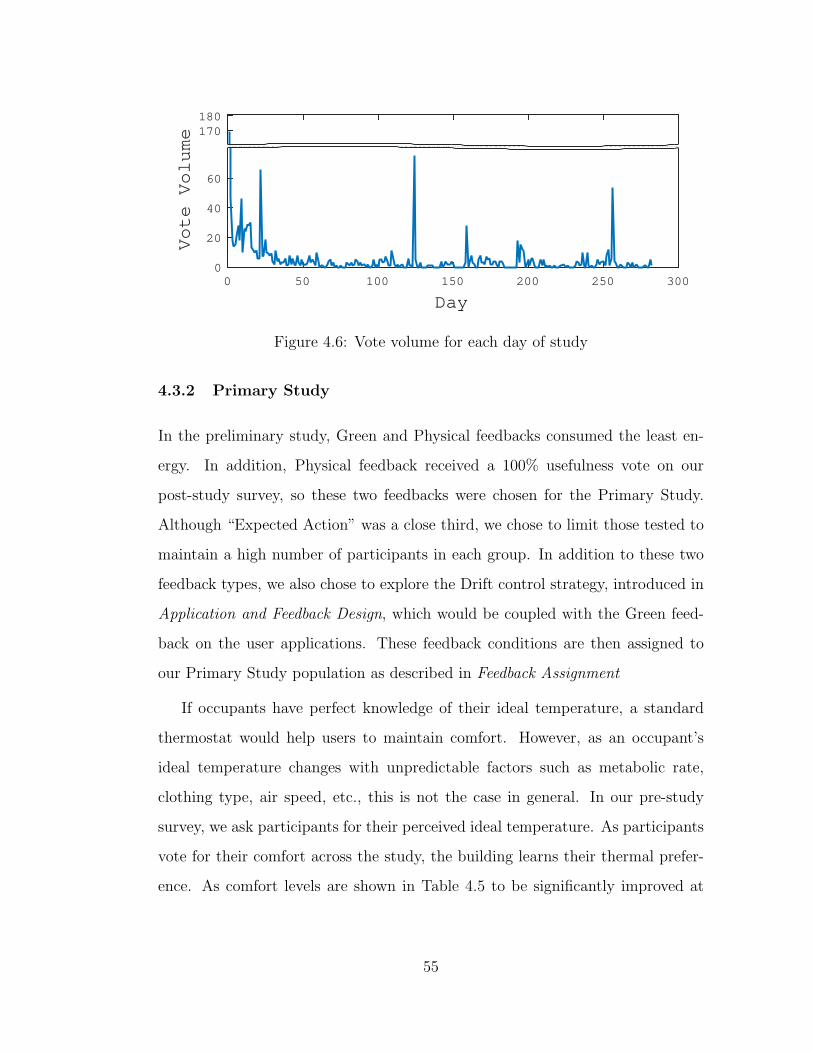
Day
0 50 100 150 200 250 300
Vote Volume
0
20
40
60
170
180
Figure 4.6: Vote volume for each day of study
4.3.2 Primary Study
In the preliminary study, Green and Physical feedbacks consumed the least en-
ergy. In addition, Physical feedback received a 100% usefulness vote on our
post-study survey, so these two feedbacks were chosen for the Primary Study.
Although “Expected Action” was a close third, we chose to limit those tested to
maintain a high number of participants in each group. In addition to these two
feedback types, we also chose to explore the Drift control strategy, introduced in
Application and Feedback Design, which would be coupled with the Green feed-
back on the user applications. These feedback conditions are then assigned to
our Primary Study population as described in Feedback Assignment
If occupants have perfect knowledge of their ideal temperature, a standard
thermostat would help users to maintain comfort. However, as an occupant’s
ideal temperature changes with unpredictable factors such as metabolic rate,
clothing type, air speed, etc., this is not the case in general. In our pre-study
survey, we ask participants for their perceived ideal temperature. As participants
vote for their comfort across the study, the building learns their thermal prefer-
ence. As comfort levels are shown in Table 4.5 to be significantly improved at
55
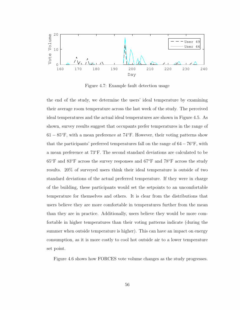
Day
160 170 180 190 200 210 220 230 240
Vote Volume
0
10
20
User 49
User 44
Figure 4.7: Example fault detection usage
the end of the study, we determine the users’ ideal temperature by examining
their average room temperature across the last week of the study. The perceived
ideal temperatures and the actual ideal temperatures are shown in Figure 4.5. As
shown, survey results suggest that occupants prefer temperatures in the range of
61− 85◦F, with a mean preference at 74◦F. However, their voting patterns show
that the participants’ preferred temperatures fall on the range of 64− 76◦F, with
a mean preference at 73◦F. The second standard deviations are calculated to be
65◦F and 83◦F across the survey responses and 67◦F and 78◦F across the study
results. 20% of surveyed users think their ideal temperature is outside of two
standard deviations of the actual preferred temperature. If they were in charge
of the building, these participants would set the setpoints to an uncomfortable
temperature for themselves and others. It is clear from the distributions that
users believe they are more comfortable in temperatures further from the mean
than they are in practice. Additionally, users believe they would be more com-
fortable in higher temperatures than their voting patterns indicate (during the
summer when outside temperature is higher). This can have an impact on energy
consumption, as it is more costly to cool hot outside air to a lower temperature
set point.
Figure 4.6 shows how FORCES vote volume changes as the study progresses.
56

Satisfaction Level Pre-Survey Post-Survey
Satisfied 11.9% 66.67%
Somewhat Satisfied 22.0% 26.67%
Neutral 18.6% 6.67%
Somewhat Dissatisfied 28.8% 0.0%
Dissatisfied 18.6% 0.0%
Thermal Comfort First Vote Post-Survey
Cold 22.0% 0.0%
Cool 6.0% 0.0%
Slightly Cool 20.0% 12.0%
Neutral 8.0% 60.0%
Slightly Warm 18.0% 12.0%
Warm 6.0% 8.0%
Hot 20.0% 8.0%
Table 4.5: Satisfaction and comfort
57
As not all participants could be recruited on the same day, we have shifted the
vote timeline so that the day of the study session aligns with “Day 0” in the
figure. This also means that votes on the final days represent only votes from
users that started using the system the earliest. We can see that application
usage during the first month is relatively high. As the novelty period wears off
and the buildings learn the occupants’ preference, the amount the users vote tends
to diminish. Despite the novelty wearing off, we see that FORCES application
usage continues into the long-term as users periodically provide corrections to
the temperature of their zone. In addition, as usage settles into a background
voting pattern, spikes in occupant voting patterns often signify faults in the
HVAC system, and can be easily used for fault detection and diagnostics (FDD).
One example is shown in Figure 4.7, where spikes in voting patterns for users
44 and 49, who work in separate cubicles in the same office, are correctly time-
aligned. Inspecting the data, we found that these peaks correspond to BLD2
HVAC maintenance, where the system was being intermittently disabled.
In previous data, we often see patterns where users vote for their comfort,
wait a short period of time, and then cast the same vote again. We refer to these
duplicate votes as “reiterated votes”, an indication that the user is not yet able to
feel the effects of the requested conditioning, and is submitting additional votes
to reiterate their request. Three examples of reiterated votes in voting patterns of
users with various feedback types can be seen in Figure 4.8. The amount of time
required for a room to be conditioned to temperature following a vote depends on
the size of the room, amount of ventilation, and other factors. Vote reiteration
occurs because it can often take on the order of 15 minutes for an office to reach a
desired temperature setpoint, even to perform only a few degrees of temperature
change.
58

15:00 15:15 15:30 15:45 16:00 16:15 16:30 16:45 17:00 17:15
-2
0
2 2 votes 2 votes
(a)
08:00 08:15 08:30 08:45 09:00 09:15 09:30 09:45
-2
0
2 2 votes 3 votes
(b)
14:36 14:39 14:42 14:45 14:48 14:51 14:54 14:57 15:00
-2
0
2
4 votes
(c)
Figure 4.8: Reiterated votes
59
The benefit of physical feedback is the immediate HVAC action in the voter’s
space. Although physical feedback does not necessarily help the room reach its
desired setpoint significantly faster, the actuation will make clear to the voter
that the vote has been received, and the space is being conditioned. If this
feedback makes clear to voters that the room is quickly responding to a vote,
our data should show fewer reiterated votes from users with physical feedback
than with any of the non-physical feedbacks. To determine this, we separate the
voting patterns of each individual voter, and find all occurrences of two votes
being submitted within some ∆t of each other. This ∆t is chosen to be twice the
system actuation period, or 10 minutes in our experiments. This is because in
the worst case, the user votes at the very beginning of a voting period, waits 5
minutes for the vote tally and beginning of the next actuation period, and then
waits another entire system actuation period for the room to change to the user’s
liking. If a user feels the need to re-vote within this period, we consider it a
reiterated vote, caused by the slow response of the system. The results of this
analysis can be seen in Table 4.6, where our 23 users with physical feedback are
shown to reiterate their votes in 80 clusters, and the remaining 38 users with non-
physical feedback cast 377 reiterated votes. Across the 40-week study, users with
non-physical feedback cast, on average, 2.9× more reiterated votes than users
with physical feedback, supporting the hypothesis that the effects of physical
feedback provide immediate feedback that help to quickly satisfy the occupants.
The pre-study survey allowed us to see the initial conditions of the users and
their space. At the conclusion of the study, we note what changes the application
has made with the comfort and satisfaction of the users.
The thermal comfort at the beginning of the study as shown in Table 4.5
was distributed; 48% of participants were cold to some degree, 44% were hot to
60
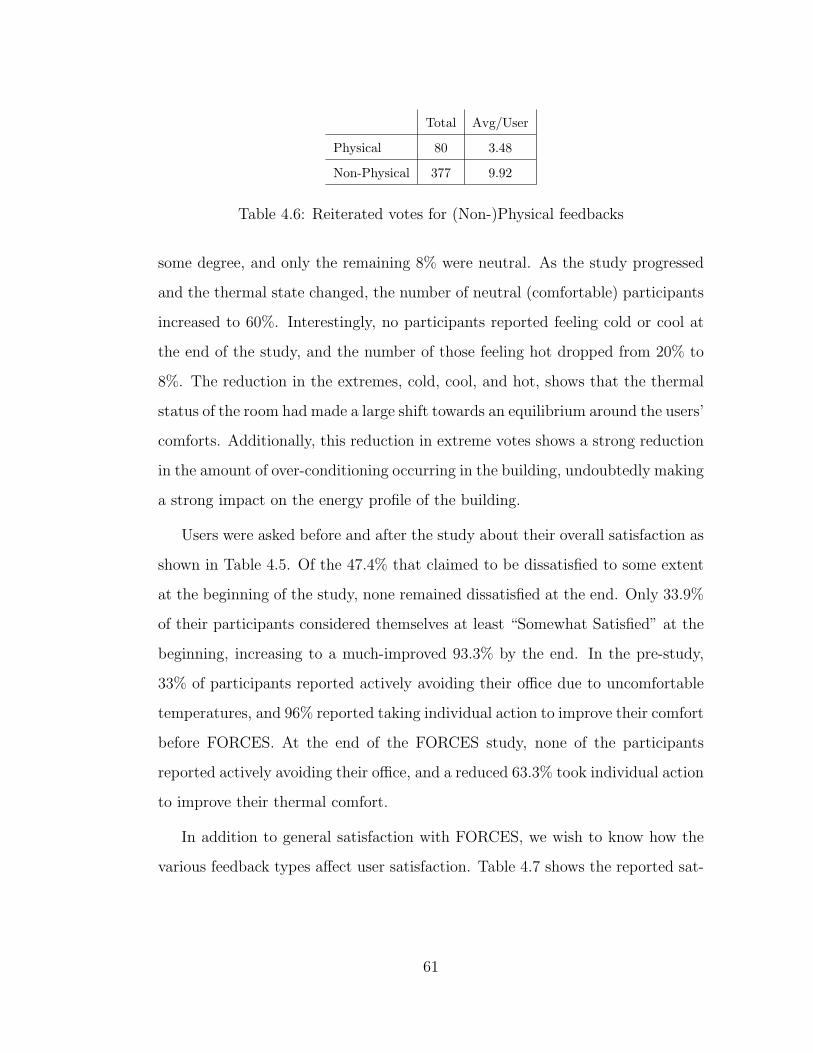
Total Avg/User
Physical 80 3.48
Non-Physical 377 9.92
Table 4.6: Reiterated votes for (Non-)Physical feedbacks
some degree, and only the remaining 8% were neutral. As the study progressed
and the thermal state changed, the number of neutral (comfortable) participants
increased to 60%. Interestingly, no participants reported feeling cold or cool at
the end of the study, and the number of those feeling hot dropped from 20% to
8%. The reduction in the extremes, cold, cool, and hot, shows that the thermal
status of the room had made a large shift towards an equilibrium around the users’
comforts. Additionally, this reduction in extreme votes shows a strong reduction
in the amount of over-conditioning occurring in the building, undoubtedly making
a strong impact on the energy profile of the building.
Users were asked before and after the study about their overall satisfaction as
shown in Table 4.5. Of the 47.4% that claimed to be dissatisfied to some extent
at the beginning of the study, none remained dissatisfied at the end. Only 33.9%
of their participants considered themselves at least “Somewhat Satisfied” at the
beginning, increasing to a much-improved 93.3% by the end. In the pre-study,
33% of participants reported actively avoiding their office due to uncomfortable
temperatures, and 96% reported taking individual action to improve their comfort
before FORCES. At the end of the FORCES study, none of the participants
reported actively avoiding their office, and a reduced 63.3% took individual action
to improve their thermal comfort.
In addition to general satisfaction with FORCES, we wish to know how the
various feedback types affect user satisfaction. Table 4.7 shows the reported sat-
61

Satisfaction Level Green Physical Green+Drift
Satisfied 66.67 75.00 62.50
Somewhat Satisfied 0.00 25.00 37.50
Neutral 33.33 0.00 0.00
Somewhat Dissatisfied 0.00 0.00 0.00
Dissatisfied 0.00 0.00 0.00
Table 4.7: Satisfaction of Primary Study Feedbacks
Feedback Type Baseline Energy Feedback Energy Percentage Decr. Projected Cost Decr.
(KWH/day) (KWH/day) (USD)
Green+Drift 95.83 60.27 37.11% $93,113.80
Green 54.70 52.31 4.38% $10,984.34
Physical 88.65 71.81 18.99% $47,663.29
Table 4.8: Energy Cost per Feedback - Primary Study
isfaction after the primary study was complete. Physical feedback resulted in
the highest user satisfaction, likely caused by the instant thermal gratification
experienced by the user. The Green+Drift feedback resulted in the lowest sat-
isfaction, but all users were still at least “Somewhat Satisfied”, much improved
from the pre-study conditions.
As explained in Feedback Assignment, each participant in a zone shared the
same feedback type for our primary study. Following the procedure described in
Calculating Energy, the change in energy consumption is computed for each zone,
which is then averaged for each feedback type. As shown in Table 4.8, FORCES
operation caused a decrease in energy usage for all feedback types, with Green
feedback using the most energy at just a 4.4% reduction, and Green+Drift strat-
egy obtaining a 37.1% decrease in energy usage. Although Physical feedback was
found to consume more energy than Green feedback in the short-term preliminary
62
study, analysis of the long-term study data found Physical to result in significant
energy savings over Green feedback alone.
To show how the energy savings found in the Primary study would affect a
building’s energy bill, we project the energy reduction computed for each feed-
back types onto an example building on our campus, Building 0 (BLD0). BLD0
used 1,091,429 ton-hr for cooling and 124,860.76 therms for heating in 2014. As
our campus pays $0.175(USD)/ ton-hr for cooling and $0.14(USD)/ therm for
heating, $250,933.24 was spent to condition BLD0 for 1 year. The projected
change in cost is reported in the last column of Table 4.8.
4.4 Discussion
The energy model used for energy analysis does not take into consideration the
additional wear on the machinery that may occur in the system, potentially
increasing overall capital costs. Changes in the fan speed and damper position
occur over large periods of time and causing a burst of air to be provided to
a room may cause a reduction in the life of the system. This additional cost
may be considered negligible but further research should be done to confirm this
assertion.
In the baseline energy consumption used for comparison, we did not include
the energy used by occupants using their own personal electrical resistive heaters
or fans to improve their personal comfort (a significant number of users based on
our pre-study survey data), so the energy savings results reported are conserva-
tive.
In our preliminary study, all feedback types showed an increase in energy
consumption with respect to the baseline. We believe this was an artifact of the
63
very few zones that could be analyzed due to the random feedback assignments
strategy used in the preliminary study, as it was explained in Energy Calculation.
Furthermore, the results shown in Fig. 4.4 using all user data would indicate that
at least Green feedback should have produced a decrease in energy consumption
from baseline. Nevertheless, the results allow us to establish a relative comparison
among the different feedback types. In the primary study, every zone was used in
the energy calculation, since each zone was assigned just one feedback type. We
believe the feedback assignment in the primary study combined with the longer
experimental time allowed us to get more meaningful results.
In the primary study, all feedback types decreased energy consumption while
improving user satisfaction. Physical feedback saved more energy than Green, but
less than Green+Drift. We hypothesize that this may be the result of the human
perception of control, as psychological studies have also shown that direct control
can lead to greater satisfaction [Pac90]. Users may be willing to vote and/or
allow the system to drift to a slight discomfort area, but still be satisfied with the
system since they are in control. Although Green+Drift led to significant energy
savings, satisfaction was only slightly lower than that of Green and Physical, and
higher than baseline.
We believe the results in this work open new potentially exciting interdisci-
plinary research avenues. By including the human-in-the-loop, we need to further
investigate the intersection of human incentives structures (behavioral economists
and cognitive scientists) together with control of large cyberphysical systems (en-
gineers) to further understand the inter-relationships between human behavior
and system control.
64
4.5 Summary
Comfort voting applications are becoming more prevalent, but work has not been
done to examine how application feedback can affect HVAC energy consumption
and occupant satisfaction. In this work, we developed a multi-platform comfort
voting application with 5 different methods of feedback. Through a 1-month
preliminary study, we investigate how these feedback types affect the satisfaction
of the users and the energy consumption of the building. We then use the results
to narrow down on the two most promising feedbacks, for evaluation for a long-
term study. Across a 40-week study covering 3 buildings and 61 participants, we
find that using feedback systems can improve satisfaction from 33.9% to 93.3%,
and reduce energy consumption by 18.99%. Furthermore, with the inclusion
of a drifting control strategy, a 37% energy reduction can be realized without
significantly reducing occupant comfort.
65

CHAPTER 5
Building CoolUs: Control using Optimization,
Occupancy, and Local User Sensing
The previous two chapters were focused on comfort and occupancy as two in-
dependent concepts, but using a model predictive control (MPC) scheme these
two techniques can be combined into a larger problem. By using both occu-
pant and comfort data, we can use the data as in an MPC problem and develop
an optimization problem. With an optimization based solution based on the
entire HVAC system and occupancy patterns we can minimize monetary cost
through out the building while constrained to occupant comfort. In this chap-
ter we present a model predictive control (MPC) framework for smart building
control. The framework has several components, including (a) occupancy sens-
ing in real-time, (b) occupancy prediction models based on historical occupancy
data, (c) thermodynamic building models, participatory sensing model and (e)
a model predictive control optimization that minimizes monetary costs in energy
use while maintaining quality comfort bounds for the building’s users. The occu-
pancy sensing information is based on the methods developed in Chapter 3 and
the participatory sensing method as explained in Chapter 4
The main contributions offered in this chapter are:
• A Model Predictive Control (MPC) framework that considers both occu-
pancy prediction and participatory sensing
66
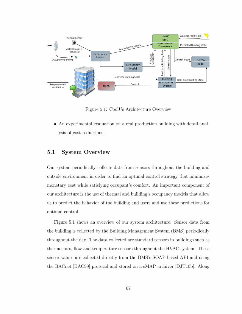
Control
Real�time Building StateReal�time Building State
Predicted Building State
Real�time Occupancy
Weather Prediction
Control Inputs
Co
ntr
ol I
np
uts
Thermal Sensor
Active/PassiveIR Sensor
Re
al�
tim
e B
uild
ing
Sta
te
Occupancy Sensing
Temperature &Ventilation
Pre
dic
ted
Occ
up
an
cy
Figure 5.1: CoolUs Architecture Overview
• An experimental evaluation on a real production building with detail anal-
ysis of cost reductions
5.1 System Overview
Our system periodically collects data from sensors throughout the building and
outside environment in order to find an optimal control strategy that minimizes
monetary cost while satisfying occupant’s comfort. An important component of
our architecture is the use of thermal and building’s occupancy models that allow
us to predict the behavior of the building and users and use these predictions for
optimal control.
Figure 5.1 shows an overview of our system architecture. Sensor data from
the building is collected by the Building Management System (BMS) periodically
throughout the day. The data collected are standard sensors in buildings such as
thermostats, flow and temperature sensors throughout the HVAC system. These
sensor values are collected directly from the BMS’s SOAP based API and using
the BACnet [BAC99] protocol and stored on a sMAP archiver [DJT10b]. Along
67
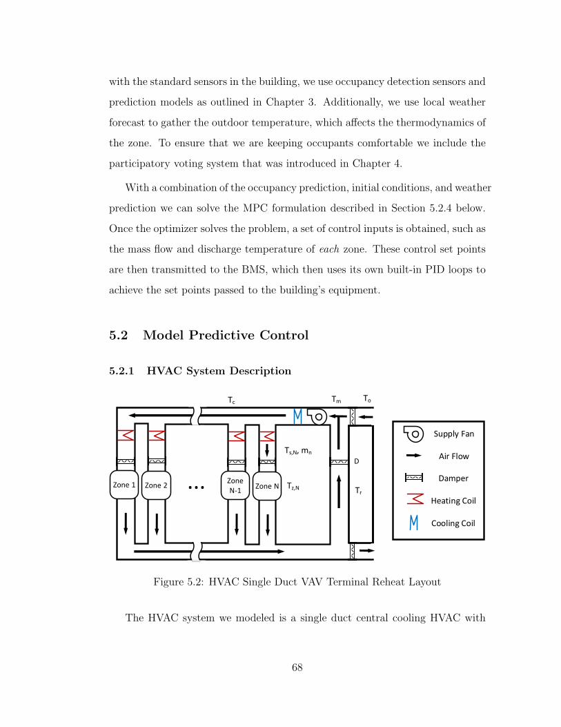
with the standard sensors in the building, we use occupancy detection sensors and
prediction models as outlined in Chapter 3. Additionally, we use local weather
forecast to gather the outdoor temperature, which affects the thermodynamics of
the zone. To ensure that we are keeping occupants comfortable we include the
participatory voting system that was introduced in Chapter 4.
With a combination of the occupancy prediction, initial conditions, and weather
prediction we can solve the MPC formulation described in Section 5.2.4 below.
Once the optimizer solves the problem, a set of control inputs is obtained, such as
the mass flow and discharge temperature of each zone. These control set points
are then transmitted to the BMS, which then uses its own built-in PID loops to
achieve the set points passed to the building’s equipment.
5.2 Model Predictive Control
5.2.1 HVAC System Description
...Zone 1 Zone 2Zone
N-1Zone N
Supply Fan
Air Flow
Damper
Heating Coil
Cooling Coil
D
TcTo
Ts,N, mn
Tm
Tz,N Tr
Figure 5.2: HVAC Single Duct VAV Terminal Reheat Layout
The HVAC system we modeled is a single duct central cooling HVAC with
68
terminal reheat as shown in Figure 5.2. The process begins at the supply fan in
the air handler unit (AHU), which supplies air for all of the zones. The supply
fan’s air first goes through a cooling coil, which cools the air to the minimum
required temperature needed for all of the zones. Before air enters a zone, the
air passes through a variable air volume (VAV) unit that regulates the amount
of air that flows into a zone. Terminal reheat occurs when the heating coil
increases the temperature before discharging air into a zone. A discharge setpoint
temperature is selected for each zone and the VAV ensures that the air is heated
to this temperature for each zone. The air supplied to the zone is mixed with the
current zone air, and some of the air is exhausted out of the zone to maintain a
constant static pressure. The return air from each zone is mixed in the return
duct, and then portions of it may enter the economizer.
The economizer unit contains several dampers to regulate the amount of air
that is recirculated in the system and the amount of fresh air that is brought into
the system from the outside. At certain times of the year, it is viable to use all
outside air if the outside air temperature is close to the desired set point. It is
also possible that the outside air temperature is significantly higher or lower then
the desired temperature at which point most of the air is recirculated inside the
building to save energy. Although it may be desirable to recirculate all possible air
in the system to reduce cooling and heating costs, there is a necessary minimum
amount of outside air required for a zone due to carbon dioxide and other gases
generated by furniture, appliances and occupants of the zone. Once the air is
mixed, it returns back to the air handling unit and the cycle begins again.
69

Type Symbol Description
Constants Mn Capacity of a zone
cp Heat capacity of air
Rn,i Resistance between zone i and zone n
Rn,o Resistance between zone n and the outside
ηc, ηh Cooling and heating efficiency
rg Monetary cost of gas per kwh
re Monetary cost of electricity per kwh
τ , N Number of time steps and zones
Tc,min(t) Min cooling temperature
Ts,max(t) Max heating temperature
Ro Required ventilation per occupant
RanRequired ventilation for an area
An Area of a zone
Variable Tzn(t) Zone Temperature
Tsn(t) Supply air temperature to a zone
Tc(t) Cooled air temperature supplied by the AHU
Tm(t) Mixed Air Temperature
D(t) Damper position for outside air
Tr(t) Return temperature
mzn(t) Mass flow into a zone
ms(t) Total mass flow of all zones
ρu,n(t), ρl,n(t) Upper and lower comfort penalty parameters
φp Penalty coefficient
t, n Time, Zone
Given or To(t) Outside air temperature
Pre-calculated Q Thermal load
On(t) Occupancy
Vmin,n(t) Minimum ventilation required for a zone
T+zn(t), T−
zn(t) Upper and lower comfort bounds
Table 5.1: MPC variables and descriptions
70

5.2.2 Objective Function
Our optimization problem, at a high level, can be seen as the minimization of
HVAC operation’s monetary cost subject to occupant comfort, regulatory con-
straints, and hardware constraints. For MPC, we need to insert our initial state
of the building, and model the changes in thermodynamics of the room over a
set period to ensure we conform to the constraints of the system. Time is a
crucial part of our formulation due to changes in occupancy, which require pre-
conditioning a zone in time for an occupant who we predict is about to enter a
zone. Overall we attempt to find the best control sequences while minimizing
monetary cost due to energy usage. In our formulation of the system, we aim to
keep the system convex by making our objective function quadratic with respect
to the optimization variables and only use linear constraints. A convex prob-
lem is computationally easier to solve and has no local optima. Our end result,
however, is a nonconvex quadratic problem with linear constraints.
In the next sections, several variables and constants will be introduced, which
are listed in Table 5.1. In this table, variables labeled as Given may vary across
time, but can be pre-calculated or fetched before the optimization problem starts.
An example of a Given function is the outside temperature, To(t), which can be
acquired via weather forecasting sources. See Section 5.2.4 for further explana-
tion.
The monetary cost of the HVAC system used in our objective function is the
sum of the power used to cool air, Pc, the power used to heat the air, Ph, and the
power used to move the air via the supply fan, Pf . These different power usages
are converted to a common unit such as monetary value since each component
may draw its power from different energy sources such as gas or electricity , which
costs typically vary. We use the conversion constants re and rg to convert power
71
obtained from electricity and power obtained from gas into a monetary amount,
respectively.
First, the cost of cooling is the change in temperature from the mixed air
(Tm) to the supplied air (Tc). The efficiency of decreasing the temperature is ηc
shown in Equation 5.2
ms(t) =N∑
n=1
mzn(t) (5.1)
Pc =cpηc
τ∑
t=1
ms(t)(Tm(t)− Tc(t)) (5.2)
The mixed air temperature Tm is a mixture of the return temperature Tr and
the outside temperature (To). The return temperature is based on the contribu-
tion of the temperature that comes from each zone. The return air is written
as:
Tr(t) =
N∑
n=1
mzn(t)Tzn(t)
ms(t)(5.3)
Once the air returns and arrives at the economizer section of the AHU, part
of it is exhausted and part is recirculated. The amount recirculated is based on
the damper position, D(t), which has a value between 0 and 1. D(t) = 1 is when
the recirculating damper is fully opened and D(t) = 0 when the system is using
all outside air.
Tm(t) = D(t)Tr(t) + (1−D(t))To(t) (5.4)
If we substitute values back to the original Pc, the division of ms is removed
from Tr, but we are still left with a cubic polynomial of optimization variables
72
in the objective function with D(t)N∑
n=1
mzn(t)Tzn(t) which increases the com-
plexity of the problem. To reduce the order of this polynomial, we linearize
f(Tzn(t),mzn(t)) = Tzn(t)mzn(t). Equation 5.3 can therefore be re-written as:
Tr(t) =
N∑
n=1
−Tznmzn + mznTzn(t) +mzn(t)Tzn
ms(t)(5.5)
By linearizing this term, we keep our objective function quadratic. We mini-
mize the error of this model simplification by choosing sensible values of mzn and
Tzn , as explained in Section 5.4.1.
Similarly the cost of heating is the change in temperature from the cool air
supplied by the AHU to the supplied air temperature. The supplied temperature
is different per VAV box so the mass flow into each zone is separated to find the
cost per zone. The efficiency of heating this air, ηh, is then applied to the sum
of all the zones.
Ph =cpηh
N∑
i=1
τ∑
t=1
mzi(t)(Tsi(t)− Tc(t)) (5.6)
The cost of the fan is shown to be a squared increase with respect to mass
flow in [KMB13] and is written in Equation 5.7 with an efficiency factor of ηf .
Pf =τ
∑
t=1
ηfms(t)2 (5.7)
Due to changes in occupancy, there may be periods of time when a single
time step is not enough time for our zone temperature to fall within the feasible
range. This can occur due to an incorrect occupancy prediction which may leave
the room in a very warm/cold state when an occupant enters the room. To
relax our comfort constraint we include a penalty function ρunand ρun
. These
73
penalty function are included into our cost function and also included in our
comfort constraint as discussed in Section 5.2.3.1. This penalty is added to
our formulation as shown in Equation 5.8. We multiply this constraint by a
coefficient, φp, to denote how strict we want the bounds to be.
Cs = φp
N∑
n=1
τ∑
t=1
ρun(t) + ρln(t) (5.8)
Simply summing the power terms does not capture the difference of pricing
between different forms of energy, specifically the differences between using gas
and electricity. In our location, gas is significantly cheaper than electricity. We
therefore have a conversion to a monetary cost with conversion factors re and
rg for electricity and gas, respectively. The heating element is based on gas and
both the fan and cooling are based on electricity. Along with the monetary cost,
we add our comfort penalty, Cs. The final objective function is therefore:
minmn(t),Tzn (t),Tsn (t),Tc(t),D(t)
t∈1...τ,n∈1...N
re(Pc + Pf ) + rg(Ph) + Cs
subject to: Constraints 1-12
(5.9)
At this point, we have a quadratic nonconvex objective function. Our problem
is non-convex due to the formulation of Pc and Ph. Both have a term that are
similar in structure (x−y)z which makes the problem nonconvex even though our
constraints are x−y ≥ 0. Specifically for equation 5.2 we havems(t)(Tm(t)−Tc(t))
In the following section, we will introduce linear constraints to our problem.
74
5.2.3 Constraints
5.2.3.1 Thermal Model Constraint
The following thermal model proposed is heavily influenced by [KMB13] with
modifications to make the constraint linear. In order to model the thermody-
namics of a zone, we use a resistor-capacitor model where each zone is considered
a capacitor and interactions between zones are resistors. Some of the variables in
our formulation are overlayed on Figure 5.2 to help show the physical relationship
these variables have with the AHU loop. Each zone n has a capacity of Mn and,
between zone n and zone j, a resistance Rn,j. The resistance between a zone and
the outside temperature is considered a special case noted as Rn,o
To model the change in a zone n’s current temperature, Tzn , we break apart
the problem into a few core components include the displacement of air and the
heat transfer of zones. Each zone is supplied air, mzn , at a supply temperature
of Tsn . If mzn air is put into a zone, an equal amount of air within the zone must
exit the system to maintain a constant static pressure. This transfer of air can
be represented as (Ts − Tz)cpmz where cp is the air capacity. The heat transfer
that occurs between a zone and an outside wall is (To − Tzn)Rn,o where To is
the outside temperature. In our model, the heat transfer that occurs between
adjacent zones is∑N
i=0(Tzi − Tzn)/Rn,i. Along with this, there is a thermal load
Qn in the zone. This load can be attributed to occupancy, appliances, machinery,
and objects that increase/decrease the temperature. The general thermal model,
based on [KMB13], for this system for a single zone n is:
Mn
d
dtTzn = (Tsn−Tzn)cpmzn+Qn+(To−Tzn)/Rn,o+
N∑
i=0,i 6=n
(Tzi−Tzn)/Rn,i (5.10)
75

We only considered the outside temperature due to the larger temperature
differential between a conditioned zone and outside weather, which causes a larger
change in temperature in a zone which leads the term (Tzi−Tzn)/Rn,i to approach
0. Our equation can therefore be simplified to:
Mn
d
dtTzn = (Tsn − Tzn)cpmzn +Qn + (To − Tzn) /Rn,o (5.11)
Due to mzn , Tsn , and Tzn being optimization variables, the first term in Equa-
tion 5.11 causes the constraint to be non-linear. These constraints can be made
linear using Taylor’s theorem as in Equation 5.12 where Tsn , Tzn , and mzn are
initial conditions for Tsn , Tzn and mzn , respectively, for all values of t. Selection
of good Tsn , Tzn , and mzn is discussed in Section 5.4.1.
Mn
d
dtTzn = cp(−Tsnmzn + mznTsn +mznTsn + Tznmzn − mznTzn −mznTzn)
+Qn + (To − Tzn)/Rn,o
(5.12)
Equation 5.12 can be discretized with respect to time as follows:
Tzn(t+ 1) = Tzn(t) +∆t
Mn
(
cp(−Tsnmzn + mznTsn(t) +mzn(t)Tsn + Tznmzn
− mznTzn(t)−mzn(t)Tzn) +Qn + (To(t)− Tzn(t))/Rn,o
)
(5.13)
This Equation will be considered as our first constraint of the system.
Constraint 1: Equation 5.13 – Thermal Model
The remaining constraints are based on the physical properties of the system,
building regulations that the HVAC system must follow, and comfort constraints.
76
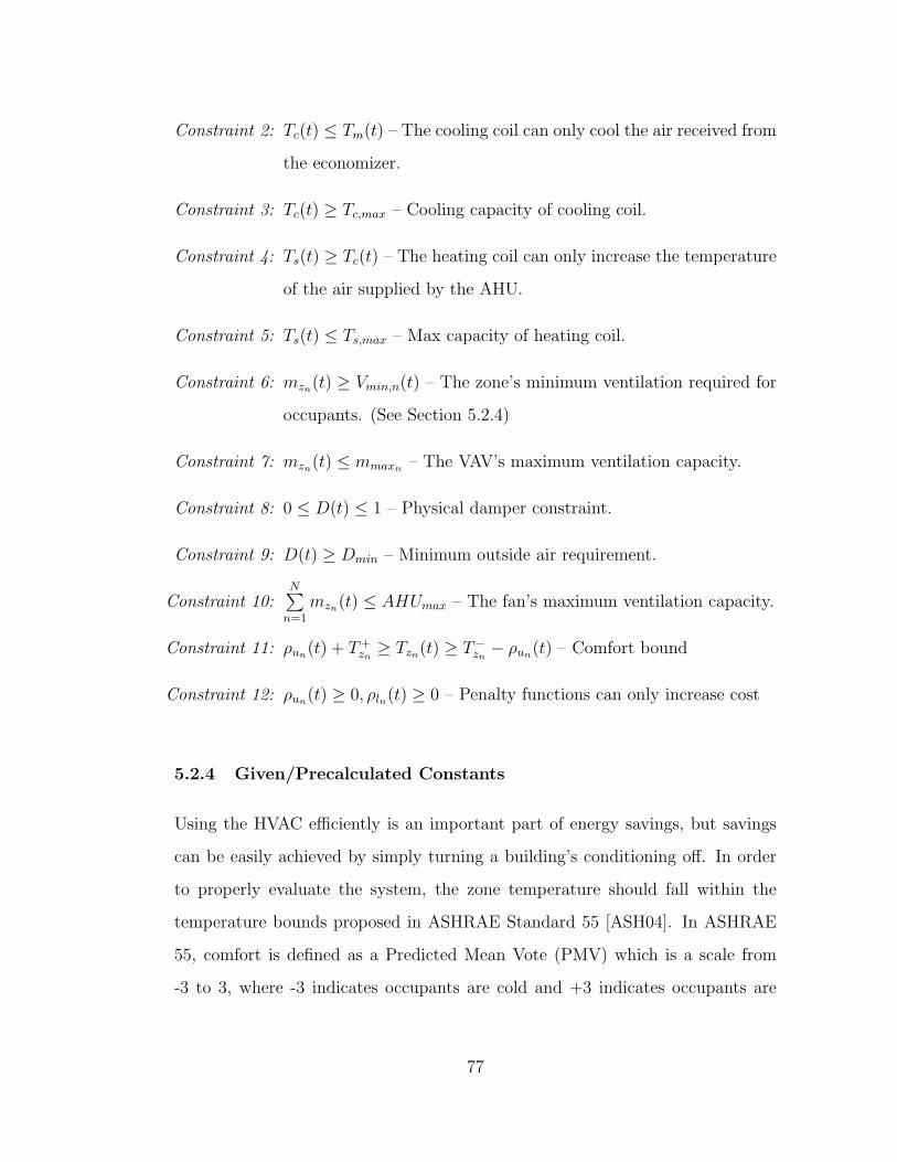
Constraint 2: Tc(t) ≤ Tm(t) – The cooling coil can only cool the air received from
the economizer.
Constraint 3: Tc(t) ≥ Tc,max – Cooling capacity of cooling coil.
Constraint 4: Ts(t) ≥ Tc(t) – The heating coil can only increase the temperature
of the air supplied by the AHU.
Constraint 5: Ts(t) ≤ Ts,max – Max capacity of heating coil.
Constraint 6: mzn(t) ≥ Vmin,n(t) – The zone’s minimum ventilation required for
occupants. (See Section 5.2.4)
Constraint 7: mzn(t) ≤ mmaxn– The VAV’s maximum ventilation capacity.
Constraint 8: 0 ≤ D(t) ≤ 1 – Physical damper constraint.
Constraint 9: D(t) ≥ Dmin – Minimum outside air requirement.
Constraint 10:N∑
n=1
mzn(t) ≤ AHUmax – The fan’s maximum ventilation capacity.
Constraint 11: ρun(t) + T+
zn≥ Tzn(t) ≥ T−
zn− ρun
(t) – Comfort bound
Constraint 12: ρun(t) ≥ 0, ρln(t) ≥ 0 – Penalty functions can only increase cost
5.2.4 Given/Precalculated Constants
Using the HVAC efficiently is an important part of energy savings, but savings
can be easily achieved by simply turning a building’s conditioning off. In order
to properly evaluate the system, the zone temperature should fall within the
temperature bounds proposed in ASHRAE Standard 55 [ASH04]. In ASHRAE
55, comfort is defined as a Predicted Mean Vote (PMV) which is a scale from
-3 to 3, where -3 indicates occupants are cold and +3 indicates occupants are
77
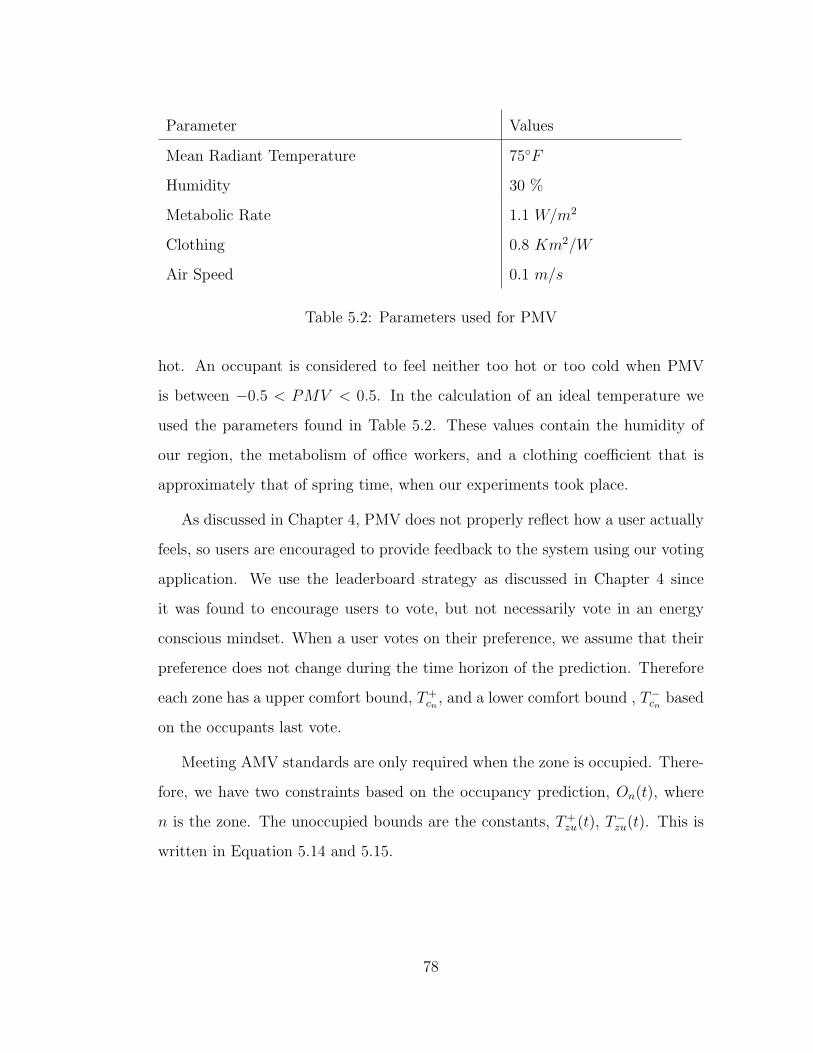
Parameter Values
Mean Radiant Temperature 75◦F
Humidity 30 %
Metabolic Rate 1.1 W/m2
Clothing 0.8 Km2/W
Air Speed 0.1 m/s
Table 5.2: Parameters used for PMV
hot. An occupant is considered to feel neither too hot or too cold when PMV
is between −0.5 < PMV < 0.5. In the calculation of an ideal temperature we
used the parameters found in Table 5.2. These values contain the humidity of
our region, the metabolism of office workers, and a clothing coefficient that is
approximately that of spring time, when our experiments took place.
As discussed in Chapter 4, PMV does not properly reflect how a user actually
feels, so users are encouraged to provide feedback to the system using our voting
application. We use the leaderboard strategy as discussed in Chapter 4 since
it was found to encourage users to vote, but not necessarily vote in an energy
conscious mindset. When a user votes on their preference, we assume that their
preference does not change during the time horizon of the prediction. Therefore
each zone has a upper comfort bound, T+cn, and a lower comfort bound , T−
cnbased
on the occupants last vote.
Meeting AMV standards are only required when the zone is occupied. There-
fore, we have two constraints based on the occupancy prediction, On(t), where
n is the zone. The unoccupied bounds are the constants, T+zu(t), T
−zu(t). This is
written in Equation 5.14 and 5.15.
78
T+zn
=
T+cn
if On(t) > 0
T+zu if On(t) = 0
(5.14)
T−zn
=
T−cn
if On(t) > 0
T−zu if On(t) = 0
(5.15)
Alongside comfort requirements, there are also ventilation requirements to re-
duce gases that build up in a room. To fall within ASHRAE Standard 62.1 [ASH07]
the zone must be properly ventilated. By knowing the number of occupants we
can find the exact minimum required cubic feet per minute (CFM) for each zone.
The amount of CFM required is shown in Equation 5.16, whereRp is the minimum
CFM per person, Ra is CFM per ft2, Pz is the number of occupants and Az is the
zone’s area. For an office the Rp = 5CFM/person and Rp = 0.6cfm/ft2. The
square footage of each zone is [275, 725, 725, 400, 300, 700, 400, 400], respectively.
A conversion from CFM, which is a unit of volume, to kgps is approximated by
using air pressure at sea level at 70◦F .
Vmin,n(t) = RpOn(t) +RaAn (5.16)
The final precalculated value in our system that is retrieved is weather fore-
casting used for To. Forecasts are retrieved from the OpenWeatherMap API [Ope].
5.3 Implementation Details
In order to solve the model described in the previous sections we used the pro-
gramming language Julia [BEK17] using the optimization library JuMP [DHL17].
JuMP allows for different solvers to be interchanged with relative ease. To solve
our quadratic objective problem with linear constraints, we use an Interior Point
79
Optimizer (Ipopt) [WB06], which is standard solver and capable of solving non-
linear optimization problems. To solve a problem which models a building of size
N = 9 and time steps τ = 6 takes on average 0.2 seconds. As building actuation
is done on the scale of minutes, the time it takes to solve for a single optimization
problem is well within what is considered acceptable.
Every 5 minutes, we solve the optimization problem and gather the solved
variables to be actuated. Within the buildings management system (BMS), we
can set our desired points for each variable through out the building and allow
the normal building control routines to take control. An example of how we
control would be setting the point for the mass flow. For each zone, our solution
contains the flow for each zone which can then be set as required mass flow can
be set via the BMS. We only adjust the setpoint, and the building is capable
of changing the supply fan’s speed and damper position for each zone to meet
the needs of all the zones. Another possible way of control, is to include the
damper position and fan speed within our model, however this adds additional
complications on the number of setpoints required to control the building and
requires to add additional complexity to the model. It is also possible that these
lower level setpoints are not available to be controlled by the BMS interface.
Because of these reasons we chose to use the high level set point method. The
points we set every actuation period include all zones’ mass flow (mzn), zones’
supply temperature(Tsi), and cooling temperature (Tc). In order to avoid issues
with static pressure, we do not modify the outside air damper position and allow
the BMS to use it’s standard econmizer control routines.
80

Figure 5.3: 3-D Model of building
5.4 Evaluation
Evaluation of this model was conducted at the University of California, Merced
campus during the summer. Experiments were run during the summer where the
temperature were at lows of 61◦F to highs 96◦F . We chose a single floor office
space with a square footage of 5750ft2, as depicted in Figure 5.3. This building
contains 40 workers that occupy the building between 6:00am and 2:00am.
5.4.1 Model Evaluation
In Section 5.2.3.1, a non-linear thermal model and linear thermal model was
established. In this section we confirm that both models are accurate to what
occurs in an actual building.
The unknowns in a building would be the capacitance, Mn, the resistance,
and the thermal load, Q, of each zone. Based on the thermal model alone, each
zone’s constants are independent to each other, which makes solving these values
81
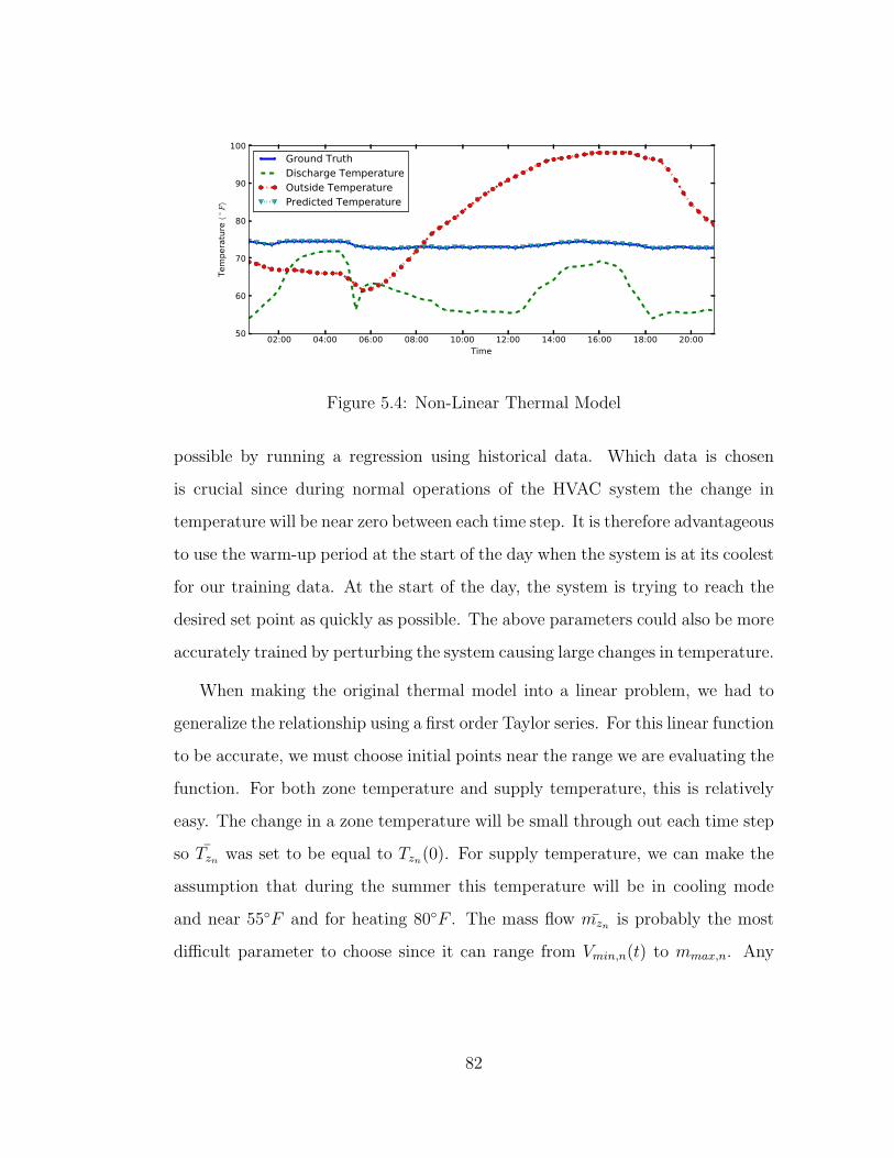
02:00 04:00 06:00 08:00 10:00 12:00 14:00 16:00 18:00 20:00Time
50
60
70
80
90
100
Tempe
rature (
◦ F)
Ground TruthDischarge TemperatureOutside TemperaturePredicted Temperature
Figure 5.4: Non-Linear Thermal Model
possible by running a regression using historical data. Which data is chosen
is crucial since during normal operations of the HVAC system the change in
temperature will be near zero between each time step. It is therefore advantageous
to use the warm-up period at the start of the day when the system is at its coolest
for our training data. At the start of the day, the system is trying to reach the
desired set point as quickly as possible. The above parameters could also be more
accurately trained by perturbing the system causing large changes in temperature.
When making the original thermal model into a linear problem, we had to
generalize the relationship using a first order Taylor series. For this linear function
to be accurate, we must choose initial points near the range we are evaluating the
function. For both zone temperature and supply temperature, this is relatively
easy. The change in a zone temperature will be small through out each time step
so Tzn was set to be equal to Tzn(0). For supply temperature, we can make the
assumption that during the summer this temperature will be in cooling mode
and near 55◦F and for heating 80◦F . The mass flow mzn is probably the most
difficult parameter to choose since it can range from Vmin,n(t) to mmax,n. Any
82
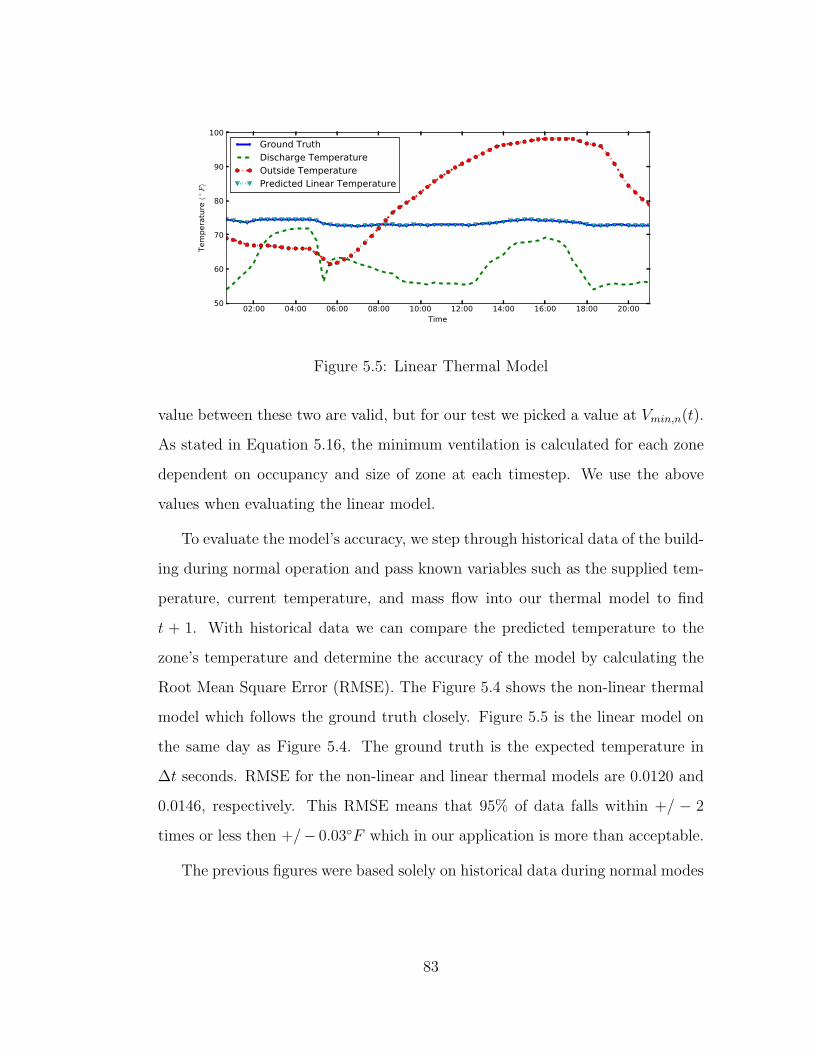
02:00 04:00 06:00 08:00 10:00 12:00 14:00 16:00 18:00 20:00Time
50
60
70
80
90
100
Tempe
rature (
◦ F)
Ground TruthDischarge TemperatureOutside TemperaturePredicted Linear Temperature
Figure 5.5: Linear Thermal Model
value between these two are valid, but for our test we picked a value at Vmin,n(t).
As stated in Equation 5.16, the minimum ventilation is calculated for each zone
dependent on occupancy and size of zone at each timestep. We use the above
values when evaluating the linear model.
To evaluate the model’s accuracy, we step through historical data of the build-
ing during normal operation and pass known variables such as the supplied tem-
perature, current temperature, and mass flow into our thermal model to find
t + 1. With historical data we can compare the predicted temperature to the
zone’s temperature and determine the accuracy of the model by calculating the
Root Mean Square Error (RMSE). The Figure 5.4 shows the non-linear thermal
model which follows the ground truth closely. Figure 5.5 is the linear model on
the same day as Figure 5.4. The ground truth is the expected temperature in
∆t seconds. RMSE for the non-linear and linear thermal models are 0.0120 and
0.0146, respectively. This RMSE means that 95% of data falls within +/ − 2
times or less then +/− 0.03◦F which in our application is more than acceptable.
The previous figures were based solely on historical data during normal modes
83

00:00 02:00 04:00 06:00 08:00 10:00 12:00 14:00 16:00 18:00 20:00 22:00Time
55
60
65
70
75
80
85
90
95Te
mpe
rature (
◦ F)
Actual (Tz)Discharge TemperatureOutside TemperaturePredicted (Tz)
Figure 5.6: Zone 2: Predicted vs. Measured Zone Temperature Results
00:00 02:00 04:00 06:00 08:00 10:00 12:00 14:00 16:00 18:00 20:00 22:00Time
55
60
65
70
75
80
85
90
95
Tempe
rature (
◦ F)
Actual (Tz)Discharge TemperatureOutside TemperaturePredicted (Tz)
Figure 5.7: Zone 1: Predicted vs. Measured Zone Temperature Results
84
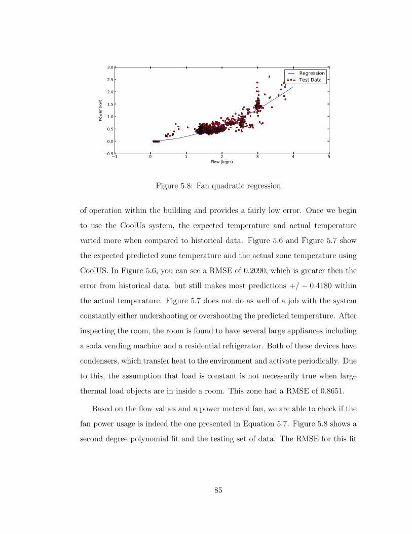
−1 0 1 2 3 4 5Flow (kgps)
−0.5
0.0
0.5
1.0
1.5
2.0
2.5
3.0
Powe
r (kw
)
RegressionTest Data
Figure 5.8: Fan quadratic regression
of operation within the building and provides a fairly low error. Once we begin
to use the CoolUs system, the expected temperature and actual temperature
varied more when compared to historical data. Figure 5.6 and Figure 5.7 show
the expected predicted zone temperature and the actual zone temperature using
CoolUS. In Figure 5.6, you can see a RMSE of 0.2090, which is greater then the
error from historical data, but still makes most predictions +/ − 0.4180 within
the actual temperature. Figure 5.7 does not do as well of a job with the system
constantly either undershooting or overshooting the predicted temperature. After
inspecting the room, the room is found to have several large appliances including
a soda vending machine and a residential refrigerator. Both of these devices have
condensers, which transfer heat to the environment and activate periodically. Due
to this, the assumption that load is constant is not necessarily true when large
thermal load objects are in inside a room. This zone had a RMSE of 0.8651.
Based on the flow values and a power metered fan, we are able to check if the
fan power usage is indeed the one presented in Equation 5.7. Figure 5.8 shows a
second degree polynomial fit and the testing set of data. The RMSE for this fit
85
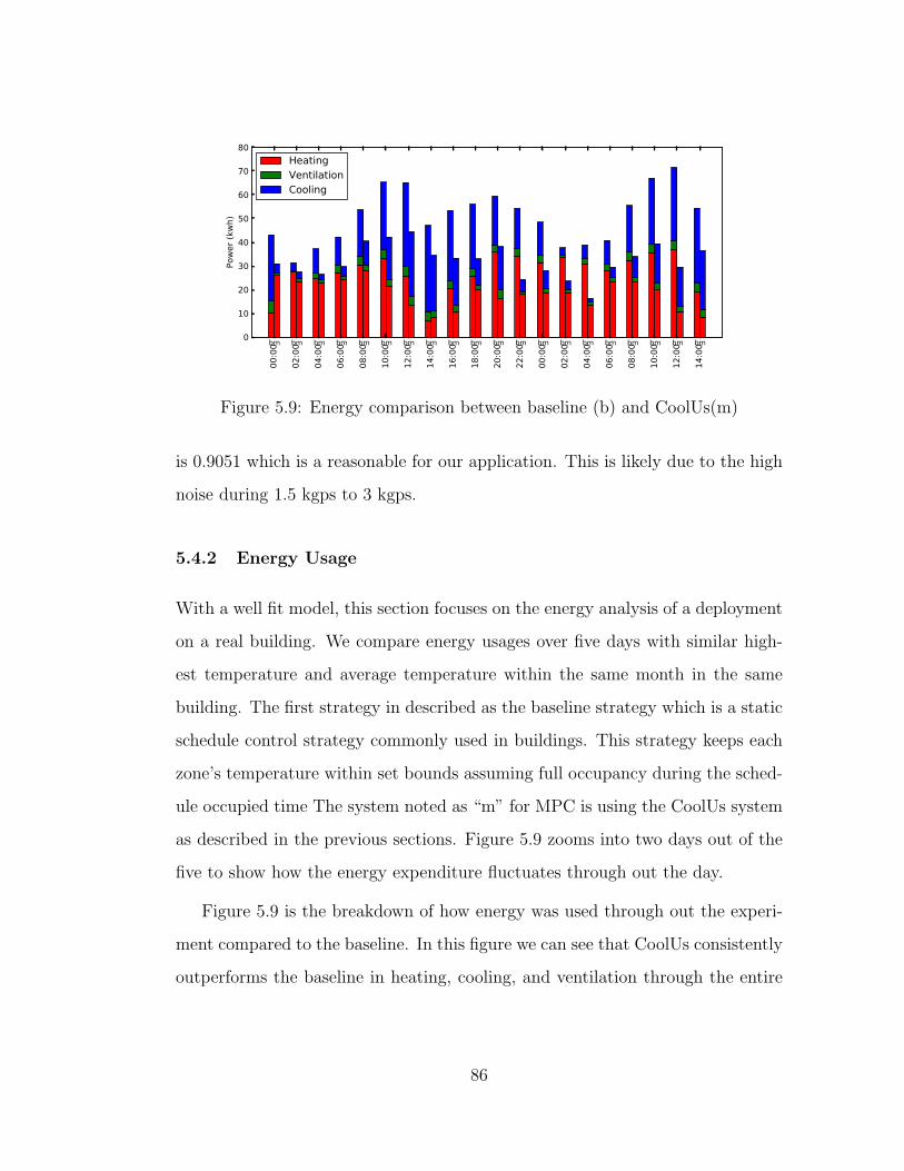
00:00
02:00
04:00
06:00
08:00
10:00
12:00
14:00
16:00
18:00
20:00
22:00
00:00
02:00
04:00
06:00
08:00
10:00
12:00
14:00
0
10
20
30
40
50
60
70
80
Powe
r (kw
h)
bm bm bm bm bm bm bm bm bm bm bm bm bm bm bm bm bm bm bm bm
HeatingVentilationCooling
Figure 5.9: Energy comparison between baseline (b) and CoolUs(m)
is 0.9051 which is a reasonable for our application. This is likely due to the high
noise during 1.5 kgps to 3 kgps.
5.4.2 Energy Usage
With a well fit model, this section focuses on the energy analysis of a deployment
on a real building. We compare energy usages over five days with similar high-
est temperature and average temperature within the same month in the same
building. The first strategy in described as the baseline strategy which is a static
schedule control strategy commonly used in buildings. This strategy keeps each
zone’s temperature within set bounds assuming full occupancy during the sched-
ule occupied time The system noted as “m” for MPC is using the CoolUs system
as described in the previous sections. Figure 5.9 zooms into two days out of the
five to show how the energy expenditure fluctuates through out the day.
Figure 5.9 is the breakdown of how energy was used through out the experi-
ment compared to the baseline. In this figure we can see that CoolUs consistently
outperforms the baseline in heating, cooling, and ventilation through the entire
86
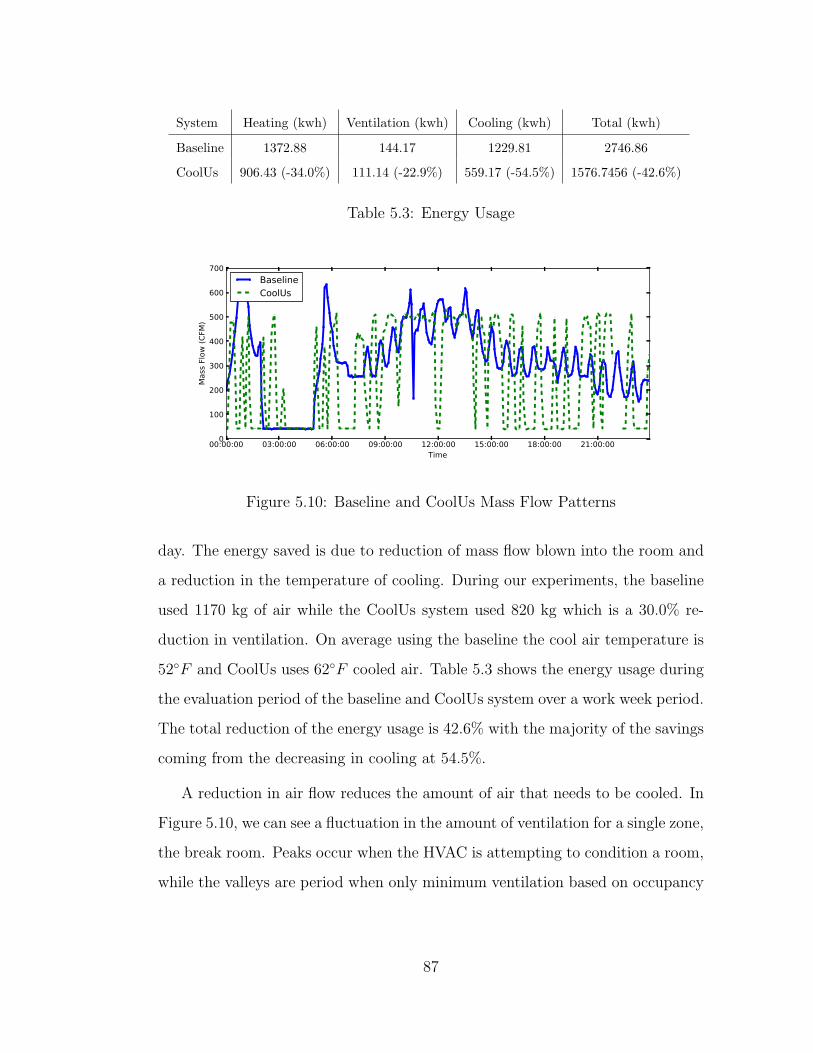
System Heating (kwh) Ventilation (kwh) Cooling (kwh) Total (kwh)
Baseline 1372.88 144.17 1229.81 2746.86
CoolUs 906.43 (-34.0%) 111.14 (-22.9%) 559.17 (-54.5%) 1576.7456 (-42.6%)
Table 5.3: Energy Usage
00:00:00 03:00:00 06:00:00 09:00:00 12:00:00 15:00:00 18:00:00 21:00:00Time
0
100
200
300
400
500
600
700
Mass F
low (CFM
)
BaselineCoolUs
Figure 5.10: Baseline and CoolUs Mass Flow Patterns
day. The energy saved is due to reduction of mass flow blown into the room and
a reduction in the temperature of cooling. During our experiments, the baseline
used 1170 kg of air while the CoolUs system used 820 kg which is a 30.0% re-
duction in ventilation. On average using the baseline the cool air temperature is
52◦F and CoolUs uses 62◦F cooled air. Table 5.3 shows the energy usage during
the evaluation period of the baseline and CoolUs system over a work week period.
The total reduction of the energy usage is 42.6% with the majority of the savings
coming from the decreasing in cooling at 54.5%.
A reduction in air flow reduces the amount of air that needs to be cooled. In
Figure 5.10, we can see a fluctuation in the amount of ventilation for a single zone,
the break room. Peaks occur when the HVAC is attempting to condition a room,
while the valleys are period when only minimum ventilation based on occupancy
87

00:00 02:00 04:00 06:00 08:00 10:00 12:00 14:00 16:00 18:00 20:00 22:000.0
0.2
0.4
0.6
0.8
1.0
1.2
1.4103
Figure 5.11: CoolUs Occupancy
is used. Figure 5.11 shows the occupancy for the break room and by comparing
these two figures side by side, we can see some overlap during extended periods of
occupancy such as 2:00am until 6:00am, but the room is being ventilated during
unoccupied periods such as 6:00am to 7:00am. This is due our system using a
predicted occupancy to precondition a zone. The baseline does preconditioning
also, but based on a rule which begins to precondition an hour before occupants
are schedule to enter a zone.
5.5 Summary
In this chapter we show that an accurate model can be developed for a build-
ing’s thermodynamics. This model has a root mean square error of 0.0146 and
0.2090 when compared to historical data and when actually used in a zone with
a constant load, respectively. A five day study controlling a building showed that
our system can decrease HVAC energy usage by 42.6% using a combination of
occupancy detection, comfort voting, and a model predictive control framework.
88

CHAPTER 6
Conclusion
In this thesis, we covered several topics in the smart building domain. We first
started by focusing on energy savings that can be achieved by detecting occupancy
using a novel sensing technique. Using this new sensor and our regression pipeline
we obtain a root mean square error of 0.35 when evaluated in 10 building zones
over three weeks. After discussing occupancy sensing, we focused on thermal
comfort of participants and how to influence how occupants participate in thermal
voting systems. Several feedback types were evaluated to see which feedback
mechanisms can reduce energy cost while maintaining thermal comfort. Using the
occupancy sensing and participatory sensing, we combined these two techniques
to create a model based approach to reduce monetary expenditure in buildings.
The occupancy detection technique was used to ensure the zones within a building
were only conditioned when occupied and pre-condition before occupants enter a
space. The comfort data we used was capable of adapting the thermal constraints
of a zone depending on how they voted on their thermal comfort. By combining
these two methods, we were able to reduce energy expenditure by 42.6% during
our week long evaluation using our model predictive approach.
Based on this work, there are many avenues for future work to be taken.
The optimization problem developed in the end can be further expanded to take
additional elements into consideration such as non-constant thermal load. There
are also stochastic model prediction methods that can be explored to take the
89

probabilistic nature of changes in occupancy and comfort. This stochastic model
would also require work towards a probability model of human comfort.
90
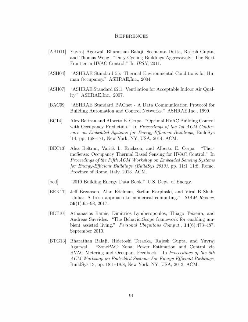
References
[ABD11] Yuvraj Agarwal, Bharathan Balaji, Seemanta Dutta, Rajesh Gupta,and Thomas Weng. “Duty-Cycling Buildings Aggressively: The NextFrontier in HVAC Control.” In IPSN, 2011.
[ASH04] “ASHRAE Standard 55: Thermal Environmental Conditions for Hu-man Occupancy.” ASHRAE,Inc., 2004.
[ASH07] “ASHRAE Standard 62.1: Ventilation for Acceptable Indoor Air Qual-ity.” ASHRAE,Inc., 2007.
[BAC99] “ASHRAE Standard BACnet - A Data Communication Protocol forBuilding Automation and Control Networks.” ASHRAE,Inc., 1999.
[BC14] Alex Beltran and Alberto E. Cerpa. “Optimal HVAC Building Controlwith Occupancy Prediction.” In Proceedings of the 1st ACM Confer-ence on Embedded Systems for Energy-Efficient Buildings, BuildSys’14, pp. 168–171, New York, NY, USA, 2014. ACM.
[BEC13] Alex Beltran, Varick L. Erickson, and Alberto E. Cerpa. “Ther-moSense: Occupancy Thermal Based Sensing for HVAC Control.” InProceedings of the Fifth ACM Workshop on Embedded Sensing Systemsfor Energy-Efficient Buildings (BuildSys 2013), pp. 11:1–11:8, Rome,Province of Rome, Italy, 2013. ACM.
[bed] “2010 Building Energy Data Book.” U.S. Dept. of Energy.
[BEK17] Jeff Bezanson, Alan Edelman, Stefan Karpinski, and Viral B Shah.“Julia: A fresh approach to numerical computing.” SIAM Review,59(1):65–98, 2017.
[BLT10] Athanasios Bamis, Dimitrios Lymberopoulos, Thiago Teixeira, andAndreas Savvides. “The BehaviorScope framework for enabling am-bient assisted living.” Personal Ubiquitous Comput., 14(6):473–487,September 2010.
[BTG13] Bharathan Balaji, Hidetoshi Teraoka, Rajesh Gupta, and YuvrajAgarwal. “ZonePAC: Zonal Power Estimation and Control viaHVAC Metering and Occupant Feedback.” In Proceedings of the 5thACM Workshop on Embedded Systems For Energy-Efficient Buildings,BuildSys’13, pp. 18:1–18:8, New York, NY, USA, 2013. ACM.
91
[Bur14] “Human-Building Interaction Framework for Personalized ThermalComfort-Driven Systems in Office Buildings.” Journal of Computingin Civil Engineering, 28(1):2–16, 2014.
[CBE] “CBE Thermal Comfort Tool.” http://cbe.berkeley.edu/comforttool/.Accessed: 2016-3-02.
[CFH14] Adrian Clear, Adrian Friday, Mike Hazas, and Carolynne Lord. “Catchmy drift?: achieving comfort more sustainably in conventionally heatedbuildings.” In Proceedings of the 2014 conference on Designing inter-active systems, pp. 1015–1024. ACM, 2014.
[DDK11] Sebastian Deterding, Dan Dixon, Rilla Khaled, and Lennart Nacke.“From Game Design Elements to Gamefulness: Defining ”Gamifica-tion”.” In Proceedings of the 15th International Academic MindTrekConference: Envisioning Future Media Environments, MindTrek ’11,pp. 9–15, New York, NY, USA, 2011. ACM.
[DHL17] Iain Dunning, Joey Huchette, and Miles Lubin. “JuMP: A modelinglanguage for mathematical optimization.” SIAM Review, 59(2):295–320, 2017.
[DJT10a] Stephen Dawson-Haggerty, Xiaofan Jiang, Gilman Tolle, Jorge Or-tiz, and David Culler. “sMAP: A Simple Measurement and Actua-tion Profile for Physical Information.” In Proceedings of the 8th ACMConference on Embedded Networked Sensor Systems, SenSys ’10, pp.197–210, New York, NY, USA, 2010. ACM.
[DJT10b] Stephen Dawson-Haggerty, Xiaofan Jiang, Gilman Tolle, Jorge Ortiz,and David Culler. “sMAP: a simple measurement and actuation profilefor physical information.” In Proceedings of the 8th ACM Conferenceon Embedded Networked Sensor Systems, pp. 197–210. ACM, 2010.
[EAC] V. L. Erickson, S. Achleitner, and A. E. Cerpa. “Poem: Power-efficientOccupancy-based Energy Management System.” In IPSN’13.
[EC] Varick Erickson and Alberto E. Cerpa. “Thermovote: ParticipatorySensing for Efficient Building HVAC Conditioning.” In Proceedings ofthe Fourth ACM Workshop on Embedded Sensing Systems for Energy-Efficiency in Buildings (BuildSys 2012).
[ECC] Varick L Erickson, Miguel A Carreira-Perpinan, and Alberto E Cerpa.“OBSERVE: Occupancy-based system for efficient reduction of HVACenergy.” In IPSN’11.
92

[ELK13] Thomas Erickson, Ming Li, Younghun Kim, Ajay Deshpande, Sam-bit Sahu, Tian Chao, Piyawadee Sukaviriya, and Milind Naphade.“The Dubuque Electricity Portal: Evaluation of a City-scale Residen-tial Electricity Consumption Feedback System.” In CHI 2013, pp.1203–1212, New York, NY, USA, 2013. ACM.
[EPl] “EnergyPlus - Building Energy Analysis Tool.”http://apps1.eere.energy.gov/buildings/energyplus/.
[Fan70] Poul O Fanger et al. “Thermal comfort. Analysis and applications inenvironmental engineering.” Thermal comfort. Analysis and applica-tions in environmental engineering., 1970.
[FFS06] William Fisk, David Faulkner, and Douglas Sullivan. “Accuracy ofCO2 sensors in commercial buildings: a pilot study.” Technical report,LBNL, 2006.
[FR97] William J. Fisk and Arthur H. Rosenfeld. “Estimates of ImprovedProductivity and Health from Better Indoor Environments.” IndoorAir, 7(3):158–172, 1997.
[GCG08] Noah J. Goldstein, Robert B. Cialdini, and Vladas Griskevicius. “ARoom with a Viewpoint: Using Social Norms to Motivate Envi-ronmental Conservation in Hotels.” Journal of Consumer Research,35(3):472–482, 2008.
[GIB12] S. Goyal, H.A. Ingley, and P. Barooah. “Zone-level control algorithmsbased on occupancy information for energy efficient buildings.” InAmerican Control Conference (ACC), 2012, pp. 3063–3068, June 2012.
[Gri] “Grid-Eye.” http://pewa.panasonic.com/downloads/grid-eye/.
[HHP00] Jessica Henryson, Teresa Hkansson, and Jurek Pyrko. “Energy effi-ciency in buildings through information Swedish perspective.” EnergyPolicy, 28(3):169 – 180, 2000.
[Hor99] Eric Horvitz. “Principles of Mixed-initiative User Interfaces.” In Pro-ceedings of the SIGCHI Conference on Human Factors in ComputingSystems, CHI ’99, pp. 159–166, New York, NY, USA, 1999. ACM.
[HT73] John Hopcroft and Robert Tarjan. “Algorithm 447: efficient algo-rithms for graph manipulation.” Commun. ACM, 16(6):372–378, June1973.
93
[HW13] Lam Abraham Hang-yat and Dan Wang. “Carrying My Environ-ment with Me: A Participatory-sensing Approach to Enhance ThermalComfort.” In Proceedings of the 5th ACM Workshop on Embedded Sys-tems For Energy-Efficient Buildings, BuildSys’13, pp. 21:1–21:8, NewYork, NY, USA, 2013. ACM.
[JB12] Farrokh Jazizadeh and Burcin Becerik-Gerber. “Toward AdaptiveComfort Management in Office Buildings Using Participatory Sens-ing for End User Driven Control.” In Proceedings of the FourthACM Workshop on Embedded Sensing Systems for Energy-Efficiencyin Buildings, BuildSys ’12, pp. 1–8, New York, NY, USA, 2012. ACM.
[KB11] Anthony Kelman and Francesco Borrelli. “Bilinear model predictivecontrol of a HVAC system using sequential quadratic programming.”In IFAC World Congress, 2011.
[KJD09] Ankur Kamthe, Lun Jiang, Matt Dudys, and Alberto Cerpa.“SCOPES: Smart Cameras Object Position Estimation System.” InEWSN, 2009.
[KMB13] Anthony Kelman, Yudong Ma, and Francesco Borrelli. “Analysis of lo-cal optima in predictive control for energy efficient buildings.” Journalof Building Performance Simulation, 6(3):236–255, 2013.
[KNO01] Neil E Klepeis, William C Nelson, Wayne R Ott, John P Robinson,Andy M Tsang, Paul Switzer, Joseph V Behar, Stephen C Hern, andWilliam H Engelmann. “The National Human Activity Pattern Survey(NHAPS): a resource for assessing exposure to environmental pollu-tants.” Journal of Exposure Science and Environmental Epidemiology,11(3):231, 2001.
[LHD09] Khee Poh Lam, Michael Hoynck, Bing Dong, Burton Andrews, Yun-Shang Chiou, Rui Chang, Diego Benitez, and Joonho Choi. “Occu-pancy Detection Through an Extensive Environmental Sensor Networkin an Open-Plan Office Building.” In International Building Perfor-mace Simulation Association, 2009.
[LSS10] Jiakang Lu, Tamim Sookoor, Vijay Srinivasan, Ge Gao, Brian Holben,John Stankovic, Eric Field, and Kamin Whitehouse. “The smart ther-mostat: using occupancy sensors to save energy in homes.” In SenSys,2010.
[MB] Yu Ma and Francesco Borrelli. “Fast Stochastic Predictive Control forBuilding Temperature Regulation.” In ACC’12.
94

[MCM12] Sunil Mamidi, Yu-Han Chang, and Rajiv Maheswaran. “Improvingbuilding energy efficiency with a network of sensing, learning and pre-diction agents.” In Proceedings of the 11th International Conferenceon Autonomous Agents and Multiagent Systems-Volume 1, pp. 45–52.International Foundation for Autonomous Agents and Multiagent Sys-tems, 2012.
[Mit97] Tom M. Mitchell. Machine Learning. McGraw-Hill, New York, 1997.
[MJK13] Parisa Mansourifard, Farrokh Jazizadeh, Bhaskar Krishnamachari,and Burcin Becerik-Gerber. “Online Learning for Personalized Room-Level Thermal Control: A Multi-Armed Bandit Framework.” In Pro-ceedings of the 5th ACM Workshop on Embedded Systems For Energy-Efficient Buildings, BuildSys’13, pp. 20:1–20:8, New York, NY, USA,2013. ACM.
[MKD12] Yudong Ma, Anthony Kelman, Allan Daly, and Francesco Borrelli.“Predictive control for energy efficient buildings with thermal storage.”IEEE control systems magazine, 32(1):44–64, 2012.
[MMC11] S. Mamidi, R. Maheswaran, and Y. Chang. “Smart Sensing, Estima-tion, and Prediction for Efficient Building Energy Management.” InMulti-agent Smart Computing Workshop, 2011.
[NLP98] “Occupancy Sensors, Motion-sensing devices for lighting control.”Lighting Research Center, 1998.
[NSC08] Jessica M. Nolan, P. Wesley Schultz, Robert B. Cialdini, Noah J. Gold-stein, and Vladas Griskevicius. “Normative Social Influence is Under-detected.” Personality and Social Psychology Bulletin, 34(7):913–923,2008.
[Ope] “OpenWeatherMap.” https://openweathermap.org/. Accessed: 2017-06-24.
[Pac90] Monica Paciuk. The Role of Personal Control of the Environment inThermal Comfort and Satisfaction at the Workplace. EnvironmentalDesign Research Association, 1990.
[PaP] “Panasonic PIR.” http://pewa.panasonic.com/downloads/papirs-ekmb/.
[PKS14] Jeni Paay, Jesper Kjeldskov, Mikael B. Skov, Dennis Lund, Tue Mad-sen, and Michael Nielsen. “Design of an Appliance Level Eco-feedback
95

Display for Domestic Electricity Consumption.” In OzCHI 2014, pp.332–341, New York, NY, USA, 2014. ACM.
[PMV13] Alessandra Parisio, Marco Molinari, Damiano Varagnolo, andKarl Henrik Johansson. “A scenario-based predictive control approachto building HVAC management systems.” In Automation Science andEngineering (CASE), 2013 IEEE International Conference on, pp.428–435. IEEE, 2013.
[PSJ07] John E. Petersen, Vladislav Shunturov, Kathryn Janda, Gavin Platt,and Kate Weinberger. “Dormitory residents reduce electricity con-sumption when exposed to realtime visual feedback and incentives.”International Journal of Sustainability in Higher Education, 8(1):16–33, 2007.
[PSP10] James Pierce, Diane J. Schiano, and Eric Paulos. “Home, Habits, andEnergy: Examining Domestic Interactions and Energy Consumption.”In Proceedings of the SIGCHI Conference on Human Factors in Com-puting Systems, CHI ’10, pp. 1985–1994, New York, NY, USA, 2010.ACM.
[PVR13] Alessandra Parisio, Damiano Varagnolo, Daniel Risberg, GiorgioPattarello, Marco Molinari, and Karl H. Johansson. “RandomizedModel Predictive Control for HVAC Systems.” In Proceedings of the5th ACM Workshop on Embedded Systems For Energy-Efficient Build-ings, BuildSys’13, pp. 19:1–19:8, New York, NY, USA, 2013. ACM.
[RDS14] Markus Rittenbruch, Jared Donovan, and Yasu Santo. “Evaluatingthe Use of Ambient and Tangible Interaction Approaches for PersonalIndoor Climate Preferences.” In Proceedings of the 2014 ACM Inter-national Joint Conference on Pervasive and Ubiquitous Computing:Adjunct Publication, UbiComp ’14 Adjunct, pp. 159–162, New York,NY, USA, 2014. ACM.
[RES10] Sasank Reddy, Deborah Estrin, and Mani Srivastava. “RecruitmentFramework for Participatory Sensing Data Collections.” In Proceed-ings of the 8th International Conference on Pervasive Computing, Per-vasive’10, pp. 138–155, Berlin, Heidelberg, 2010. Springer-Verlag.
[Rob14] Building Robotics. “Case Study: Johnson Controls Inc.” Technicalreport, 300 Frank H Ogawa Plaza #614 — Oakland, CA, January2014.
96

[SBK11] James Scott, A.J. Bernheim Brush, John Krumm, Brian Meyers, MikeHazas, Steve Hodges, and Nicolas Villar. “PreHeat: Controlling HomeHeating Using Occupancy Prediction.” In Proceedings of UbiComp2011. ACM, September 2011.
[Sch77] Shalom H Schwartz. “Normative Influences on Altruism1.” Advancesin experimental social psychology, 10:221–279, 1977.
[SF05] Olli Seppanen and William J. Fisk. “Control of temperature for healthand productivity in offices.” ASHRAE Transactions, 111(2):680–686,2005.
[tmo] “Tmote Sky.” http://www.snm.ethz.ch/Projects/TmoteSky.
[TS] Thiago Teixeira and Andreas Savvides. “Lightweight People Countingand Localization in Indoor Spaces Using Camera Sensor Nodes.” InICDSC’07.
[WB06] Andreas Wachter and Lorenz T Biegler. “On the implementation ofan interior-point filter line-search algorithm for large-scale nonlinearprogramming.” Mathematical programming, 106(1):25–57, 2006.
[WBE16] Daniel A. Winkler, Alex Beltran, Niloufar P. Esfahani, Paul P. Maglio,and Alberto E. Cerpa. “FORCES: Feedback and Control for Occu-pants to Refine Comfort and Energy Savings.” In Proceedings of the2016 ACM International Joint Conference on Pervasive and Ubiqui-tous Computing, UbiComp ’16, pp. 1188–1199, New York, NY, USA,2016. ACM.
[web] “Automated Logic - WebCTRL.” http://www.automatedlogic.com/product/webctrl/.Accessed: 2016-3-02.
[YAL14] Ray Yun, Azizan Aziz, Bertrand Lasternas, Chenlu Zhang, VivianLoftness, Peter Scupelli, Yunjeong Mo, Jie Zhao, and Nana Wilber-force. “The design and evaluation of intelligent energy dashboard forsustainability in the workplace.” In International Conference of De-sign, User Experience, and Usability, pp. 605–615. Springer Interna-tional Publishing, 2014.
[YNF14] Rayoung Yang, Mark W. Newman, and Jodi Forlizzi. “Making Sus-tainability Sustainable: Challenges in the Design of Eco-interactionTechnologies.” In Proceedings of the SIGCHI Conference on HumanFactors in Computing Systems, CHI ’14, pp. 823–832, New York, NY,USA, 2014. ACM.
97

[ZYL13] Jie Zhao, Ray Yun, Bertrand Lasternas, Haopeng Wang, Khee PohLam, Azizan Aziz, and Vivian Loftness. “Occupant behavior andschedule prediction based on office appliance energy consumption datamining.” CISBAT 2013 Conference-Clean Technology for Smart Citiesand Buildings, pp. 549–554, 2013.
98