Calhoun: The NPS Institutional Archive

Theses and Dissertations Thesis Collection

1991-09

A single-commodity mine transshipment problem.

Glaser, Tammy L.

Monterey, California. Naval Postgraduate School

http://hdl.handle.net/10945/28540

NAVAL POSTGRADUATE SCHOOL

Monterey, California

A SINGLE-COMMODITYMINE TRANSSHIPMENT PROBLEM

by

Tammy L. Glaser

September 1991

Thesis Advisor R. Kevin Wood

Approved for public release; distribution is unlimited.

T260305

Jnclassified

cunty classification of this page

report documentation page

la Report Security Classification Unclassified lb Restrictive Markings

2a Security Classification Authority

2b Declassification Downgrading Schedule

3 Distribution 'Availability of Report

Approved for public release; distribution is unlimited.

14 Performing Organization Report Number(s) 5 Monitoring Organization Report Number(s)

6a Name of Performing Organization

Naval Posteraduate School

6b Office Symbol

(if applicable) OR7a Name of Monitoring Oiganization

Naval Postgraduate School

6c Address (city, state, and ZIP code;

Monterey, CA 93943-5000

7b Address (dry, state, and ZIP code)

Monterey, CA 93943-5000

8a Name of Funding Sponsoring Organization 8b Office Symbol(if applicable)

9 Procurement Instrument Identification Number

8c Address (city, slate, and ZIP code) 10 Source of Funding Numbers

Program Element No Project No Task No Work L'nit Accession No

11 Title (Include security classification) A SINGLE-COMMODITY MINE TRANSSHIPMENT PROBLEM12 Personal Authorfs) Tanimv L. Glaser

13a Type of Report

Master's Thesis

13b Time CoveredFrom To

14 Date of Report (year, month, day)

September 1991

15 Page Count

84

16 Supplementary Notation The views expressed in this thesis are those of the author and do not reflect the official policy or po-

sition of the Department of Defense or the U.S. Government.

7 Cosati Codes

Field Group Subgroup

18 Subject Terms (continue on reveise if necessary and identify by block number)

Single-commodity transshipment, time-expanded networks

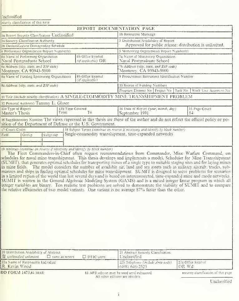
19 Abstract (continue on reverse if necessary and identify by block number)

The Fleet Commanders-in-Chief often request recommendations from Commander, Mine Warfare Command, onschedules for naval mine transshipment. Tliis thesis develops and implements a model, Scheduler for Mine Transsliipment

(SUMIT), that generates optimal schedules for transporting mines of a single type to suitable staging sites and for laying minesin mine fields. The model considers the number of available air, land and sea assets such as military' aircraft, trucks, sub-

marines and ships in finding optimal schedules for mine transslupment. SUMIT is designed to solve problems for scenarios

in a limited region of the world that last several days and is based on interconnected, time-expanded mine and mode networks.

SUMIT is written in the General Algebraic Modeling System (GAMS) and is a mixed integer linear program in which all

integer variables are binary. Ten realistic test problems are solved to demonstrate the viability of SUMIT and to comparethe relative efficiencies of two model variants. One variant is on average 87% faster than the other.

20 Distribution. Availability of Abstract

B unclassified unlimited D same as report D DT1C users

21 Abstract Security Classification

Unclassified

22a Name of Responsible Individual

R. Kevin Wood22b Telephone (include Area code)

(408) 646-2523

22c Office Symbol

OR WdDD FORM 1473.84 MAR 83 APR edition may be used until exhausted

All other editions are obsolete

security classification of this page

Unclassified

Approved for public release; distribution is unlimited.

A Single-Commodity

Mine Transshipment Problem

by

Tammy L. Glaser

Lieutenant, United States Navy

B.S., United States Naval Academy, 1985

Submitted in partial fulfillment of the

requirements for the degree of

MASTER OF SCIENCE IN OPERATIONS RESEARCH

from the

NAVAL POSTGRADUATE SCHOOLSeptember 1991

Peter Purdue, Chairman,

Department of Operations Research

u

ABSTRACT

The Fleet Commanders-in-Chief often request recommendations from Commander,

Mine Warfare Command, on schedules for naval mine transshipment. This thesis de-

velops and implements a model, Scheduler for Mine Transshipment (SUM IT), that

generates optimal schedules for transporting mines of a single type to suitable staging

sites and for laying mines in mine fields. The model considers the number of available

air, land and sea assets such as military aircraft, trucks, submarines and ships in finding

optimal schedules for mine transshipment. SUM IT is designed to solve problems for

scenarios in a limited region of the world that last several days and is based on inter-

connected, time-expanded mine and mode networks. SUMIT is written in the General

Algebraic Modeling System (GAMS) and is a mixed integer linear program in which all

integer variables are binary. Ten realistic test problems are solved to demonstrate the

viability of SUMIT and to compare the relative efficiencies of two model variants. One

variant is on average 87% faster than the other.

111

THESIS DISCLAIMER

The reader is cautioned that computer programs developed in this research may not

have been exercised for all cases of interest. While every effort has been made, within

the time available, to ensure that the programs are free of computational and logic er-

rors, they cannot be considered validated. Any application of these programs without

additional verification is at the risk of the user.

IV

TABLE OF CONTENTS

I. INTRODUCTION 1

A. PURPOSE 1

B. BACKGROUND 1

1. Node Description 2

2. Mode Description 3

3. Arc Description 4

C. SCOPE 4

D. OUTLINE 5

II. MODEL FORMULATION 6

A. GENERAL DESCRIPTION 6

B. ASSUMPTIONS 8

C. FORMULATION 10

1. Indices 10

2. Data 12

3. Decision Variables 14

4. Model A 16

5. Comments about Model A 17

6. Model B 18

7. Comments about Model B 19

8. Detailed Data Description for Both Models 19

9. Network Generation Rules for Both Models 26

10. Generation of Incompatible Arc Groups 27

11. Flow Existence Rules 30

III. COMPUTATIONAL RESULTS 32

A. COMPUTER IMPLEMENTATION OF PROPOSED MODELS 32

B. COMPARISON OF MODELS 32

C. GAMS IMPLEMENTATION OF SUM IT 35

D. REDUCTION OF MINE FLOW AND INVENTORY IN BOTH MOD-

ELS 36

IV. CONCLUSIONS 39

APPENDIX A. SAMPLE PROGRAM, FIRST RUN 41

APPENDIX B. SAMPLE OUTPUT, FIRST RUN 58

APPENDIX C. SAMPLE PROGRAM, SECOND RUN 62

APPENDIX D. SAMPLE OUTPUT, SECOND RUN 68

APPENDIX E. GAMS IMPLEMENTATION OF SUMIT 71

A. SUMIT OUTPUT 71

B. END TIME AND TIME PERIOD LENGTH 71

C. OBTAINING NEARLY OPTIMAL SOLUTIONS 72

LIST OF REFERENCES 73

INITIAL DISTRIBUTION LIST 75

VI

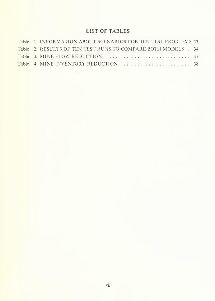
LIST OF TABLES

Table 1. INFORMATION ABOUT SCENARIOS FOR TEN TEST PROBLEMS 33

Table 2. RESULTS OF TEN TEST RUNS TO COMPARE BOTH MODELS . . 34

Table 3. MINE FLOW REDUCTION 37

Table 4. MINE INVENTORY REDUCTION 38

vn

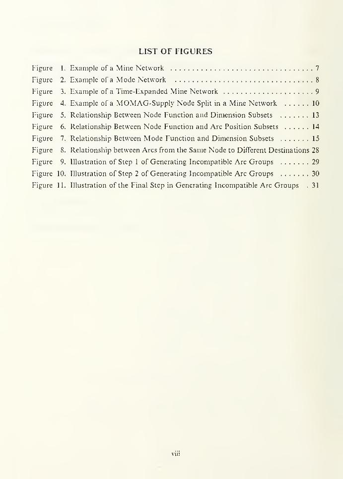
LIST OF FIGURES

Figure 1. Example of a Mine Network 7

Figure 2. Example of a Mode Network 8

Figure 3. Example of a Time-Expanded Mine Network 9

Figure 4. Example of a MOMAG-Supply Node Split in a Mine Network 10

Figure 5. Relationship Between Node Function and Dimension Subsets 13

Figure 6. Relationship Between Node Function and Arc Position Subsets 14

Figure 7. Relationship Between Mode Function and Dimension Subsets 15

Figure 8. Relationship between Arcs from the Same Node to Different Destinations 28

Figure 9. Illustration of Step 1 of Generating Incompatible Arc Groups 29

Figure 10. Illustration of Step 2 of Generating Incompatible Arc Groups 30

Figure 11. Illustration of the Final Step in Generating Incompatible Arc Groups .31

VUl

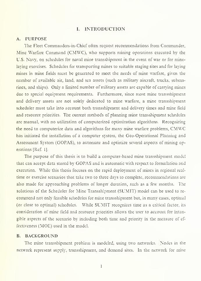
I. INTRODUCTION

A. PURPOSE

The Fleet Commanders-in-Chief often request recommendations from Commander,

Mine Warfare Command (CMW'C), who supports mining operations executed by the

U.S. Navy, on schedules for naval mine transshipment in the event of war or for mine-

laying exercises. Schedules for transporting mines to suitable staging sites and for laying

mines in mine fields must be generated to meet the needs of mine warfare, given the

number of available air, land, and sea assets (such as military aircraft, trucks, subma-

rines, and ships). Only a limited number of military' assets are capable of carrying mines

due to special equipment requirements. Furthermore, since most mine transshipment

and delivery assets are not solely dedicated to mine warfare, a mine transshipment

scheduler must take into account both transshipment and delivery times and mine field

and resource priorities. The current methods of planning mine transshipment schedules

are manual, with no utilization of computerized optimization algorithms. Recognizing

the need to computerize data and algorithms for many mine warfare problems, CMWChas initiated the installation of a computer system, the Geo-Operational Planning and

Assessment System (GOPAS), to automate and optimize several aspects of mining op-

erations [Ref. 1].

The purpose of this thesis is to build a computer-based mine transshipment model

that can accept data stored by GOPAS and is automatic with respect to formulation and

execution. While this thesis focuses on the rapid deployment of mines in regional real-

time or exercise scenarios that take two to three days to complete, recommendations are

also made for approaching problems of longer duration, such as a few months. The

solutions of the Scheduler for Mine Transshipment (SUM IT) model can be used to re-

commend not only feasible schedules for mine transshipment but, in many cases, optimal

(or close to optimal) schedules. While SUM IT recognizes time as a critical factor, its

consideration of mine field and resource priorities allows the user to account for intan-

gible aspects of the scenario by including both time and priority in the measure of ef-

fectiveness (MOE) used in the model.

B. BACKGROUNDThe mine transshipment problem is modeled, using two networks. Nodes in the

network represent supply, transshipment, and demand sites. In the network for mine

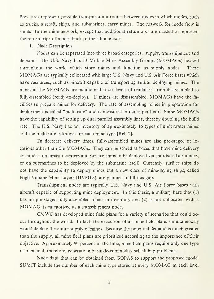
flow, arcs represent possible transportation routes between nodes in which modes, such

as trucks, aircraft, ships, and submarines, carry mines. The network for mode flow is

similar to the mine network, except that additional return arcs are needed to represent

the return trips of modes back to their home base.

1. Node Description

Nodes can be separated into three broad categories: supply, transshipment and

demand. The U.S. Navy has 13 Mobile iMine Assembly Groups (MOMAGs) located

throughout the world which store mines and function as supply nodes. These

MOMAGs are typically collocated with large U.S. Navy and U.S. Air Force bases which

have resources, such as aircraft capable of transporting and/or deploying mines. The

mines at the MOMAGs are maintained at six levels of readiness, from disassembled to

fully-assembled (ready-to-deploy). If mines are disassembled, MOMAGs have the fa-

cilities to prepare mines for delivery. The rate of assembling mines in preparation for

deployment is called "build rate" and is measured in mines per hour. Some MOMAGshave the capability of setting up dual parallel assembly lines, thereby doubling the build

rate. The U.S. Navy has an inventory of approximately 16 types of underwater mines

and the build rate is known for each mine type [Ref. 2].

To decrease delivery times, fully-assembled mines are also pre-staged at lo-

cations other than the MOMAGs. They can be stored at bases that have mine delivery

air modes, on aircraft carriers and surface ships to be deployed via ship-based air modes,

or on submarines to be deployed by the submarine itself. Currently, surface ships do

not have the capability to deploy mines but a new class of mine-laying ships, called

High-Volume Mine Layers (HVMLs), are planned to fill this gap.

Transshipment nodes are typically U.S. Navy and U.S. Air Force bases with

aircraft capable of supporting mine deployment. In this thesis, a military base that (1)

has no pre-staged fully-assembled mines in inventory and (2) is not collocated with a

MOMAG, is categorized as a transshipment node.

CMWC has developed mine field plans for a variety of scenarios that could oc-

cur throughout the world. In fact, the execution of all mine field plans simultaneously

would deplete the entire supply of mines. Because the potential demand is much greater

than the supply, all mine field plans are prioritized according to the importance of their

objective. Approximately 90 percent of the time, mine field plans require only one type

of mine and, therefore, generate only single-commodity scheduling problems.

Node data that can be obtained from GOPAS to support the proposed model

SUMIT include the number of each mine type stored at every MOMAG at each level

of readiness, the number of each mine type pre-staged at given bases, the number of each

mine type demanded at every mine field, the build rate of every MOMAG for each mine

type, the capability for a double assembly line, the priority of the mine field, and the type

of node (land or sea).

2. Mode Description

Modes can be separated into two broad categories: transportation modes and

delivery modes. Modes that cannot deploy mines in a mine field are categorized as

transportation modes. These modes include land modes, such as trucks, and air modes,

such as U.S. Air Force C-141 and C-130 cargo aircraft. Delivery modes can deploy

mines and include air modes, such as U.S. Navy and U.S. Marine Corps shore-based and

ship-based aircraft and U.S. Air Force B-52 bombers, and sea modes, such as subma-

rines. Due to weight and size constraints, most air modes and all land modes can only

carry one mine type per trip. Sea modes, which will include HVMLs in the future, are

able to carry more than one mine type aboard. Because modes have multiple capabili-

ties, they may also be critical to the success of other missions and can be prioritized ac-

cording to the scenario. For example, if Anti-Submarine Warfare (ASW) plays a vital

role in the scenario, a higher priority should be placed on non-ASW modes to deploy the

mines.

Since the mine transshipment problem includes mobile supply sites (aircraft

carriers, ships, and submarines), differences arise in how mobile supply sites are incor-

porated into the network. For this thesis, resources normally classified as modes are

treated as nodes if they function as supply nodes and can only store mines. For example,

aircraft carriers and surface ships, which store mines but are not capable of laying them,

are classified as fixed nodes in the model. The aircraft stationed aboard the vessel

function as modes that lay mines. To maintain consistency in the structure of the net-

work, submarines and HVMLs, which are able to deploy mines, are treated as fixed

nodes that have dummy modes stationed aboard to deliver mines. In addition, because

aircraft carriers and ships may not be located at the on-station point for launch of air-

craft at the beginning of the problem, SUM IT allows the transit of aircraft carriers and

ships at the beginning and end of the problem. This exception is not required for sub-

marines which travel directly to the mine fields.

Mode data supported by GOPAS include category (transshipment or delivery);

dimension (land, air or sea); speed (nautical miles per hour); capacity for each mine type

(mines per unit mode); time to load mines (hours); time to unload or deliver mines

(hours); total time to refuel, change crews, and conduct routine maintenance or repairs

to prepare modes for their next trip (hours); maximum range (nautical miles); the num-

ber of each mode available at each supply and transshipment node; and mode priority.

3. Arc Description

Because the flow of mines between nodes in the network is very structured, the

only arc data that require support from GOPAS is the distance between nodes (nautical

miles). Arc capacity (mines per trip) and length (time peiiods) can be calculated from

the node data. Based on the data input by the user, SUM IT only forms arcs for mine

networks that are directed from supply nodes to supply nodes, supply nodes to trans-

shipment nodes, supply nodes to demand nodes, and transshipment nodes to demand

nodes. SUM IT generates the same arcs for mode networks, except the return arcs are

also included and are directed back to the home base. In Chapter II, the section entitled

"Network Generation Rules" explains in detail other rules used to generate the net-

works.

C. SCOPE

Other researchers have studied the multi-commodity transshipment problem for

mine warfare and for other military applications. Wingate and Zakary [Ref. 3] proposed

a continuous variable model for multi-commodity transshipment problems, that could

be applied to mine transshipment. However, their model was too general and did not

address characteristics unique to the mine transshipment problem, such as the existence

of modes (i.e., aircraft carriers and submarines) that also function as supply nodes.

Collier, Lally, and Puntenney [Refs. 4, 5 , 6] developed continuous variable models

for military deployment problems from the U.S. Transportation Command

(TRANSCOM) using sea and air assets. The mine transshipment problem is smaller

with potential supply sites limited to the 13 MOMAGs plus the bases and sea assets at

which mines are pre-staged. The proposed model SUM IT is designed for regional

problems spanning a time window of two to three days in which the total number of

nodes can be about ten, while the TRANSCOM model developed by Puntenney covers

movement requests among as many as 22 ports, planning general schedules lasting up

to three months. Due to the importance of time in a short-duration mine transshipment

problem, sea assets are limited to U.S. Navy vessels, located near the mine fields at the

beginning of the problem, that either have the capability to deploy mines or have air

assets aboard that are able to lay mines, while sea assets play a prominent role in ship-

ping material in the TRANSCOM problem. Since the mine transshipment problem re-

quires mines to be deployed as soon as possible, it does not include opportune delivery

times, which were used to generate costs for the objective function in the TRANSCOMproblem. Finally, data concerning limits on the mine loading and unloading capacities

at non-MOMAG supply sites and restrictions on the number of aircraft allowed at

transshipment sites at one time is not available in GOPAS.

The scope of this thesis could encompass a multi-commodity transshipment model

that optimizes schedules for deploying different mine types in a global scenario. Multi-

commodity problems usually involve mixed-integer programs that use extensive amounts

of computer resources to find optimal solutions for large networks. Because only one

mine type can be transported by a mode for each trip, the complexity of the mine

transshipment problem increases. Since very little preliminary groundwork has been laid

which specifically addresses schedule optimization for the mine transshipment problem,

the scope of this thesis has been narrowed to a single-commodity approach. Because

this thesis focuses on regional scenarios that require mine deployment to a couple of

mine fields over a period of several days, the use of a single-commodity model is justified

by the fact that (1) most mine fields require only one type of mine and (2) the majority

of MOMAGs do not supply all 16 types of mines. Furthermore, the transshipment of

mines over long distances may take more time than is allotted for the scenario, which

then restricts mine supply to sites in the same region of the world as the mine fields.

Thus, a global problem could conceivably be divided into several regional subproblems,

which could be solved separately, if nodes contained in one regional subproblem were

not contained in the other regional subproblems.

D. OUTLINE

This thesis is divided into four chapters. Chapter I is the introduction. Chapter II

proposes and describes in detail two model formulations. Chapter III discusses the re-

sults often test problems that compare the size and speed of the two model formulations

and recommends procedures for executing SUMIT in the General Algebraic Modeling

System (GAMS) [Ref. 7], a software package. Chapter IV contains conclusions about

the methodology described in this thesis, discusses the weaknesses of SUMIT, and re-

commends future enhancements of SUMIT.

II. MODEL FORMULATION

A. GENERAL DESCRIPTION

Both proposed mine transshipment models contain two separate networks: one for

the mines and another for the modes. The mine network is represented by a set of bal-

ance equations that controls the flow of mines through all nodes. Two types of variables

are contained in the balance equations for the mine network: one variable type repres-

ents the shipment of mines from origin nodes to destination nodes via modes and the

other represents the inventory of mines at nodes. The mode network is represented by

another set of balance equations that controls the flow of modes to and from all nodes.

The mine and mode networks are linked by a set of equations that relate the flow vari-

ables in the two sets of balance equations. In the linking equations, sending mines via

an arc contained in the mine network, forces flow on the corresponding arc in the mode

network. In other words, mines cannot flow through the mine network unless there is

a mode to carry them. Furthermore, the number of mines flowing through the network

is limited by the capacities of the associated modes.

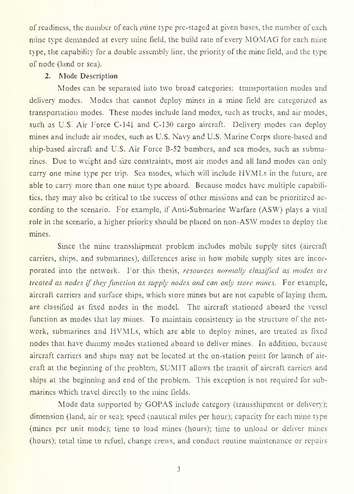
The mine network is directed, meaning that arcs are ordered pairs of nodes. All

paths must start at supply nodes, possibly flow through other supply nodes and trans-

shipment nodes, and must arrive at demand nodes. Circuits, which are paths that start

and end at the same node, are limited to transfers between supply nodes. Figure 1 il-

lustrates a mine network, where s„ t„ and d, respectively represent supply, transshipment,

and demand at node /. Notice that the path from s2 to /, contains two arcs, which indi-

cates that two different types of modes are available to transport the mines. [Ref. 8]

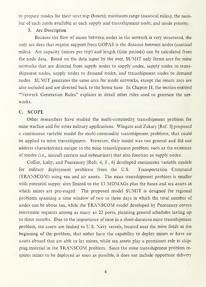
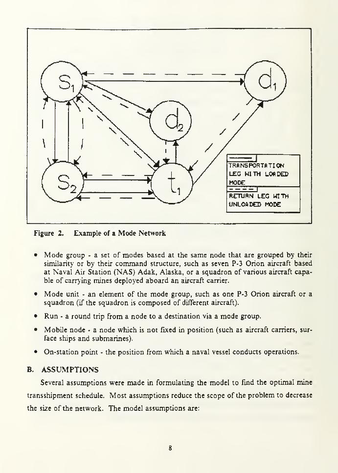
The structure of the mode network is an expansion of the mine network, which has

additional arcs returning empty modes back to their origin node. The return arcs are

critical because they prevent arcs that represent the same mode leaving at a different

time period from being used before the mode has returned from its previous run. Figure

2 depicts a mode network, associated with the mine network of Figure 2.

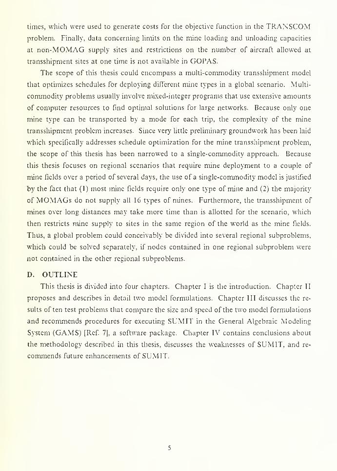
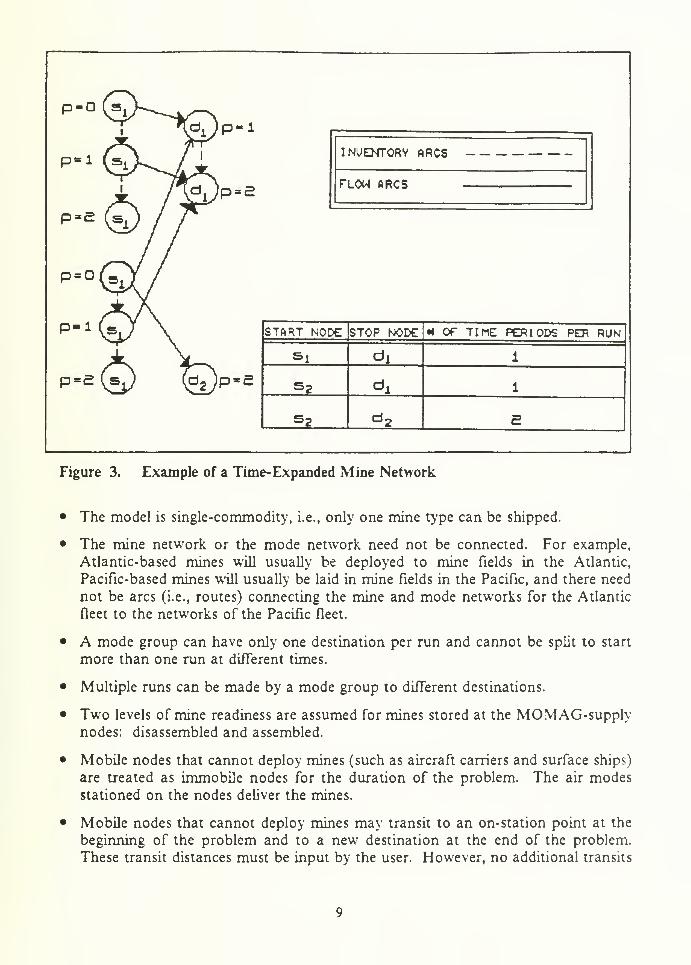
Time-expansion of nodes in the two networks and in the linking equations is re-

quired to allow modes to make multiple sequential trips in either transporting or laying

mines. Different arc lengths (which are measured in time periods) also make time-

expansion desirable. In essence, time-expansion expands every node over several periods

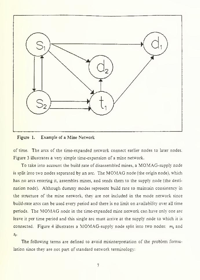
Figure 1. Example of a Mine Network

of time. The arcs of the time-expanded network connect earlier nodes to later nodes.

Figure 3 illustrates a very simple time-expansion of a mine network.

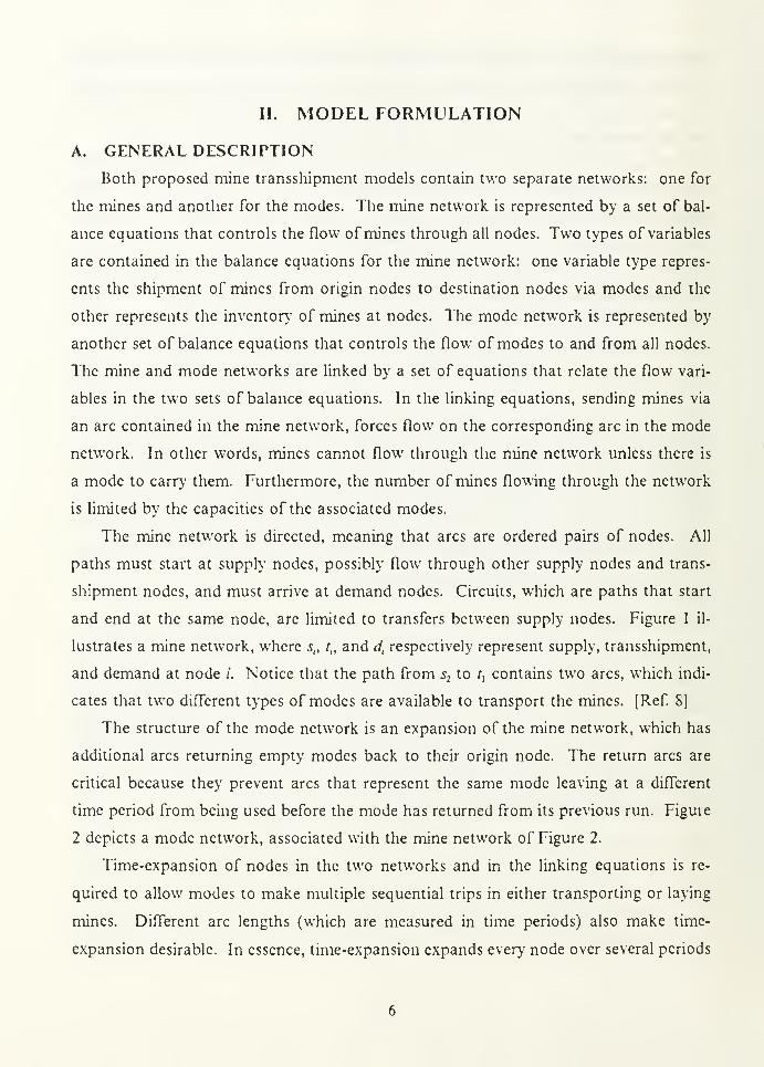
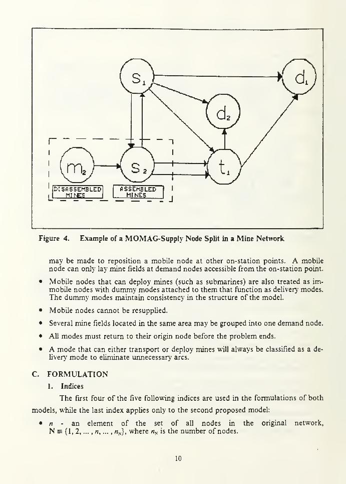
To take into account the build rate of disassembled mines, a MOMAG-supply node

is split into two nodes separated by an arc. The MOMAG node (the origin node), which

has no arcs entering it, assembles mines, and sends them to the supply node (the desti-

nation node). Although dummy modes represent build rate to maintain consistency in

the structure of the mine network, they are not included in the mode network since

build-rate arcs can be used every period and there is no limit on availability over all time

periods. The MOMAG node in the time-expanded mine network can have only one arc

leave it per time period and this single arc must arrive at the supply node to which it is

connected. Figure 4 illustrates a MOMAG-supply node split into two nodes: m^ and

The following terms are defined to avoid misinterpretation of the problem formu-

lation since they are not part of standard network terminology:

TRANSPORTATIONLEG WITH LOADEDMODE

RETURN LEG WITHUNLOADED MODE

Figure 2. Example of a Mode Network

• Mode group - a set of modes based at the same node that are grouped by their

similarity or by their command structure, such as seven P-3 Orion aircraft based

at Naval Air Station (NAS) Adak, Alaska, or a squadron of various aircraft capa-

ble of carrying mines deployed aboard an aircraft carrier.

• Mode unit - an element of the mode group, such as one P-3 Orion aircraft or a

squadron (if the squadron is composed of different aircraft).

• Run - a round trip from a node to a destination via a mode group.

• Mobile node - a node which is not fixed in position (such as aircraft carriers, sur-

face ships and submarines).

• On-station point - the position from which a naval vessel conducts operations.

B. ASSUMPTIONS

Several assumptions were made in formulating the model to find the optimal mine

transshipment schedule. Most assumptions reduce the scope of the problem to decrease

the size of the network. The model assumptions are:

p-0 (W)^

1

p=£(J)y

p=d(Sa /

"^T)p-i

/^JP'5

INUENTORV ARCS

FLOW ARCS

(d^)p-e

START NODE STOP NODE # OF TIME PERIODS PEP RUN

Si di 1

s 2 *i 1

s2 *2 E

Figure 3. Example of a Time-Expanded Mine Network

• The model is single-commodity, i.e., only one mine type can be shipped.

• The mine network or the mode network need not be connected. For example,

Atlantic-based mines will usually be deployed to mine fields in the Atlantic,

Pacific-based mines will usually be laid in mine fields in the Pacific, and there need

not be arcs (i.e., routes) connecting the mine and mode networks for the Atlantic

fleet to the networks of the Pacific fleet.

• A mode group can have only one destination per run and cannot be split to start

more than one run at different times.

• Multiple runs can be made by a mode group to different destinations.

• Two levels of mine readiness are assumed for mines stored at the MOMAG-supplynodes: disassembled and assembled.

• Mobile nodes that cannot deploy mines (such as aircraft carriers and surface ships)

are treated as immobile nodes for the duration of the problem. The air modesstationed on the nodes deliver the mines.

• Mobile nodes that cannot deploy mines may transit to an on-station point at the

beginning of the problem and to a new destination at the end of the problem.

These transit distances must be input by the user. However, no additional transits

r

DISASSEMBLED

[JJ11IO_

Figure 4. Example of a MOMAG-Supply Node Split in a Mine Network

may be made to reposition a mobile node at other on-station points. A mobile

node can only lay mine fields at demand nodes accessible from the on-station point.

• Mobile nodes that can deploy mines (such as submarines) are also treated as im-

mobile nodes with dummy modes attached to them that function as delivery modes.The dummy modes maintain consistency in the structure of the model.

• Mobile nodes cannot be resupplied.

• Several mine fields located in the same area may be grouped into one demand node.

• All modes must return to their origin node before the problem ends.

• A mode that can either transport or deploy mines will always be classified as a de-

livery mode to eliminate unnecessary arcs.

C. FORMULATION1. Indices

The first four of the five following indices are used in the formulations of both

models, while the last index applies only to the second proposed model:

• n - an element of the set of all nodes in the original network,

N = {1, 2, ... , n, ... , «N}, where ns is the number of nodes.

10

• n - an element of the set of all modes in the original networkM = {1, 2, ...

,[i, ... , nM), where «M is the number of modes.

• p - an element of the set of all time periods used for the time-expansion,

P = {0, 1, 2, ..., p, ... , Up}, where nv is the number of time periods plus one.

• / - an element of the set of integers used for iterative loops, 1 = {1,2 i, ... ,nl),

where n, = nj,.

• g - an element of the set of incompatible arc groups, G = {1, 2, ... ,g, ... , nG ] , wherenG is the highest total number of groups, where nc = n?

— 1.

The elements in the set P actually represent the start and end points of time periods

considered by the model. For example, the first period starts at p equals and ends at

p equals 1. The extra period starting at nr— 1 and ending at nv is needed to calculate

constants for mine inventory after the last period of the problem. The procedure for

determining incompatible arc groups is described in the section under "Generation of

Incompatible Arc Groups."

The node and mode indices can be categorized by several subset indices repres-

enting the function, dimension or arc position of the node or mode. For example,

MOMAG nodes, which are always origin nodes, can only be positioned on land and

transshipment modes travel on land or by air. This information is critical in constructing

a network that has realistic arcs and meets the assumptions of the model. The following

subindices are subsets of the node set N:

• m - an element of the set of all MOMAG nodes MN , where m e MNcN,

• 5 - an element of the set of all supply nodes SN , where 5 e SNcN.

• / - an element of the set of all transshipment nodes TN , where / e TNcN.

• d - an element of the set of all demand nodes DN , where d e DNc=N.

• / - an element of the set of all nodes positioned on land LN, where/ e LNs(MN U SN U TN).

• c - an element of the set of all nodes located on or under the sea CN, wherec e CNs(SN (J DN).

• / - an element of the set of all origin nodes IN for arcs in the original network,where i e IN s (MN U SN U TN).

• j - an element of the set of all destination nodes JN for arcs in the original network,

where j e JN = (SN U TN U DN) .

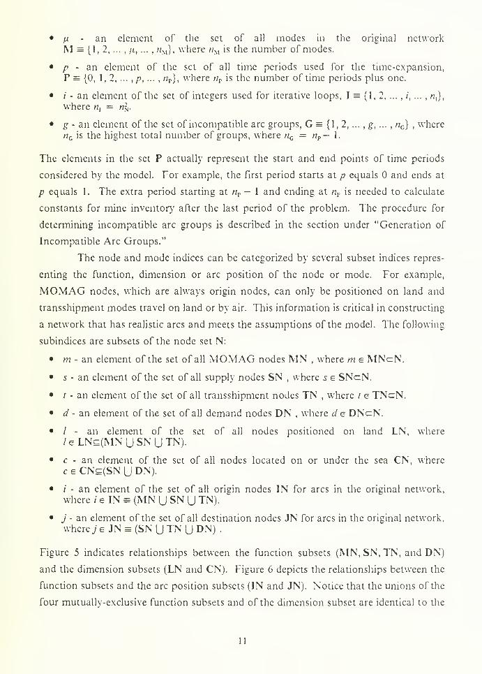
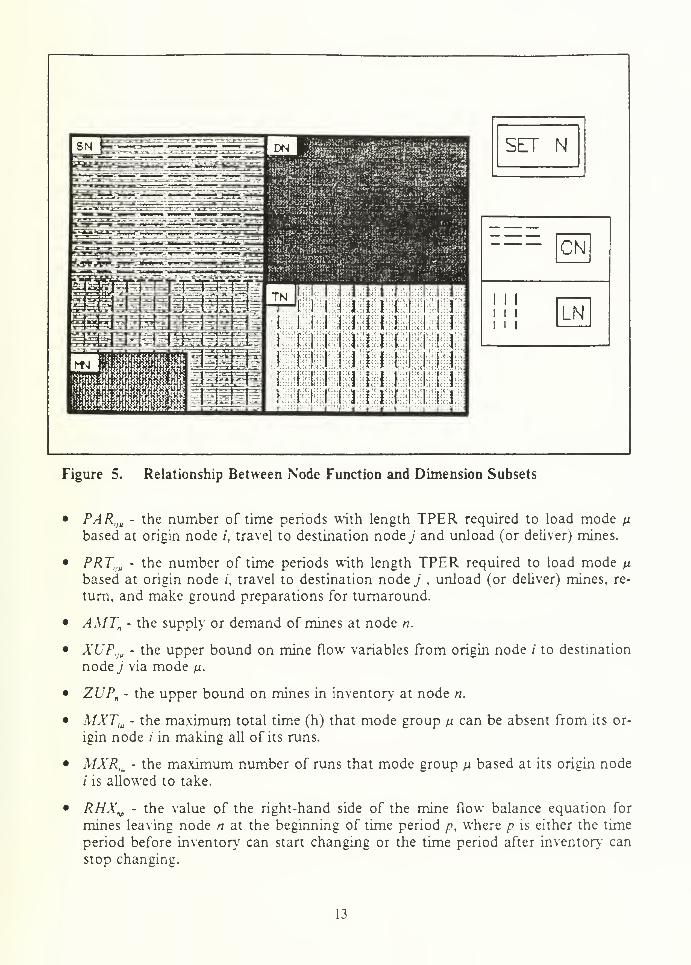
Figure 5 indicates relationships between the function subsets (MN, SN, TN, and DN)

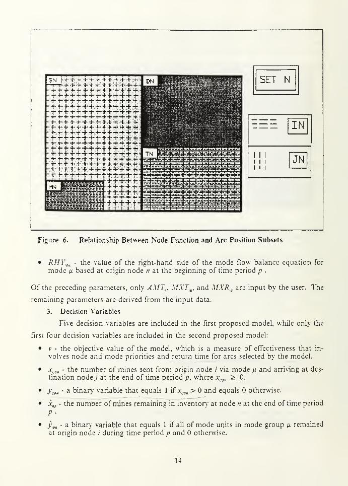
and the dimension subsets (LN and CN). Figure 6 depicts the relationships between the

function subsets and the arc position subsets (IN and JN). Notice that the unions of the

four mutually-exclusive function subsets and of the dimension subset are identical to the

11

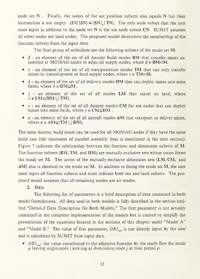
node set N . Finally, the union of the arc position subsets also equals N but their

intersection is not empty: (INf]JN) = (SN \J TN). The only node subset that the user

must input in addition to the node set N is the sea node subset CN. SUMIT assumes

all other nodes are land nodes. The proposed model determines the membership of the

function subsets from the input data.

The final group of subindices arc the following subsets of the mode set M:

/? - an element of the set of all dummy build modes BM that transfer mines as-

sembled at MOMAG nodes to adjacent supply nodes, where /? e BMcM.

t - an element of the set of all transportation modes TM that can only transfer

mines to transshipment or land supply nodes, where t e TMcM.

S - an element of the set of all delivery modes DM that can deploy mines into minefields, where S e DMsM .

k - an element of the set of all modes LM that travel on land, whereX e LMc(BM (J TM).

y - an element of the set of all dummy modes CM for sea nodes that can deploymines into mine fields, where y e CMsDM .

a - an element of the set of all aircraft modes AM that transport or deliver mines,

where a e AMs(TM U DM).

The same dummy build mode can be used for all MOMAG nodes if they have the same

build rate (the treatment of parallel assembly lines is mentioned in the next section).

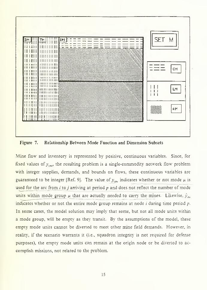
Figure 7 indicates the relationship between the function and dimension subsets of M.

The function subsets (BM, TM, and DM) are mutually-exclusive sets whose union forms

the mode set M. The union of the mutually-exclusive dimension sets (LM, CM, and

AM) also is identical to the mode set M. In addition to listing the mode set M, the user

must input all function subsets and must indicate both sea and land subsets. The pro-

posed model assumes that all remaining modes are air modes.

2. Data

The following list of parameters is a brief description of data contained in both

model formulations. All data used in both models is fully described in the section enti-

tled "Detailed Data Description for Both Models." The first parameter is not actually

contained in the computer implementation of the models but is created to simplify the

presentation of the equations located in the sections of this chapter under "Model A"

and "Model B." The value of first parameter, OBJ,JPU

is not directly input by the user

and is calculated by SUMIT from input data.

• OBJi;pil

- the value contributed to the objective function by the mode flow for modeH leaving origin node / arriving at destination node j at time period p.

12

SET N

CN

1 1

1

1 1 1

1 1 1

LN

Figure 5. Relationship Between Node Function and Dimension Subsets

PAR,JU

- the number of time periods with length TPER required to load mode nbased at origin node /, travel to destination node j and unload (or deliver) mines.

PRT„U

• the number of time periods with length TPER required to load mode /x

based at origin node /, travel to destination nodey , unload (or deliver) mines, re-

turn, and make ground preparations for turnaround.

AMTn- the supply or demand of mines at node n.

XUPIJU

- the upper bound on mine flow variables from origin node i to destination

node j via mode /i.

ZUP„ - the upper bound on mines in inventory" at node n.

MXTtu• the maximum total time (h) that mode group \x can be absent from its or-

igin node i in making all of its runs.

MXRiu- the maximum number of runs that mode group n based at its origin node

/ is allowed to take.

RHXV - the value of the right-hand side of the mine flow balance equation for

mines leaving node n at the beginning of time period p, where p is either the time

period before inventory can start changing or the time period after inventory' can

stop changing.

13

SN ''+•& .*.*:*: *.**.*;**aii-T—ti-+ *--»- + + + -H-f-t-+-f1 +-+* + + + + +• **• #i:#£jte!Jfc!HKi

:

«HI•4- 4- 4- 4-4- -4- 4-4- 4- 4--+4=+'• 4- 4- 4-4-4-4-4-4-4- 4- -4-f-f-+• 4-4- 4444 4-444;444;lf1'T :

l(!:'i':

'f!J

!J!:

!J!.'!jll?l-!j|:jl,

;!i!-!t*y

-H 4- +- -*- -4- HE- -I- •+- HK+ +-*•Hh

:

*t+- 4-4--*-4--*--t-4-4-44-4;4:*-44* 4 4*44 44 + 4- 44:Hk;.¥4- +" if 4-4j* 4-4- 4- 4-4-4-W44-4-4 4-4--44-4-4-44-44H*-** 4-4- 4*444 4-4*44;*4v4-4- *i4 4** jSHK+444 44444444444*** :H?

444444 4*4- + *44 * iHNi4- +- 4- 4- -4 -f- 4- 4- 4- 4> 4- 4/ •*•

:

4-

4>4-+4-%:'

SET N

IN

1 1

1

I I I

I II

JN

Figure 6. Relationship Between Node Function and Arc Position Subsets

• RHYIPU- the value of the right-hand side of the mode flow balance equation for

mode (j. based at origin node n at the beginning of time period p .

Of the preceding parameters, only AMTn , MXTitl

, and MXR,Uare input by the user. The

remaining parameters are derived from the input data.

3. Decision Variables

Five decision variables are included in the first proposed model, while only the

first four decision variables are included in the second proposed model:

• v - the objective value of the model, which is a measure of effectiveness that in-

volves node and mode priorities and return time for arcs selected by the model.

• xIJPU

- the number of mines sent from origin node / via mode n and arriving at des-

tination node j at the end of time period p, where xm > 0.

• ylJPU- a binary variable that equals l if jc,,pu > and equals otherwise.

• x„p

- the number of mines remaining in inventory at node n at the end of time period

P

•Pipu

' a binary variable that equals l if all of mode units in mode group \i remained

at origin node / during time period p and otherwise.

14

SET M

CM

1 1

1

1 1 1

1 1 1

LM

AM

Figure 7. Relationship Between Mode Function and Dimension Subsets

Mine flow and inventory is represented by positive, continuous variables. Since, for

fixed values o£yiJpll ,

the resulting problem is a single-commodity network flow problem

with integer supplies, demands, and bounds on flows, these continuous variables are

guaranteed to be integer [Ref. 9). The value ofy,Jptl

indicates whether or not mode \x is

used for the arc from / toy arriving at period p and does not reflect the number of mode

units within mode group \x that are actually needed to cam' the mines. Likewise, ypu

indicates whether or not the entire mode group remains at node / during time period p.

In some cases, the model solution may imply that some, but not all mode units within

a mode group, will be empty as they transit. By the assumptions of the model, these

empty mode units cannot be diverted to meet other mine field demands. However, in

reality, if the scenario warrants it (i.e., squadron integrity is not required for defense

purposes), the empty mode units can remain at the origin node or be diverted to ac-

complish missions, not related to the problem.

15

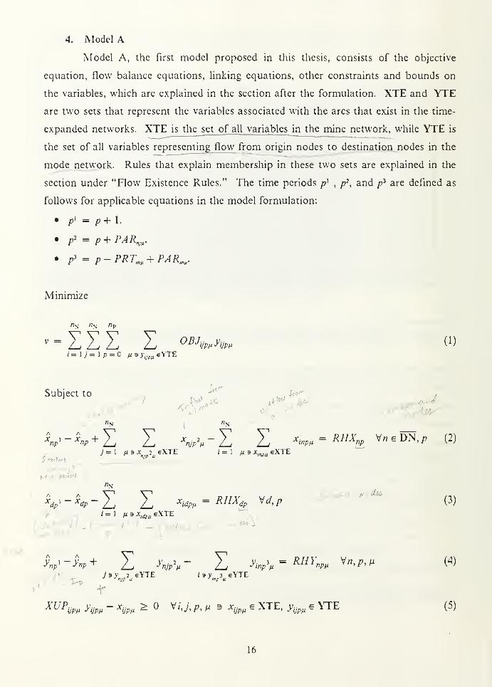
4. Model A

Model A, the first model proposed in this thesis, consists of the objective

equation, flow balance equations, linking equations, other constraints and bounds on

the variables, which are explained in the section after the formulation. XTE and YTE

are two sets that represent the variables associated with the arcs that exist in the time-

expanded networks. XTE is the set of all variables in the mine network, while YTE is

the set of all variables representing flow from origin nodes to destination nodes in the

mode network. Rules that explain membership in these two sets are explained in the

section under "Flow Existence Rules." The time periods px

, p7

, and p3 arc defined as

follows for applicable equations in the model formulation:

• p1 = p+ 1.

• f - p + PAR^

• ? = p-PRTmtl + PAR

mil.

Minimize

fly; ri\; Tip

i= i j = l p = fi9 >' sYTE- Z Z Z Z °*wjw <"

' 'jpf

Subject to

A A

Z Z V*~E Z *m-*H*B. V« €DN.ji (2)

y = 1 /i3j: 2 eXTE / = 1 /u 9 * eXTE

fW

V-%-Z Z **-*«%. W,p «*—'

"'*"(3)

1=1 ^^eXTE1

?

/sv 2 €YTE /9V 3 eYTE

^^/w, J'lteii- -^M ^ ° V/,y, /?, m s *«»« e XTE, y«pu e \TE (5)

16

«N

Z Z PRTij,y^ * A/A^> v'^ <6)

y=i p9>WM eYTE

Z Z >w* MA v/»" (7 >

7=1 p.j^.YTE

< xijpM

< XVPijti

Vi,j,p,n (8)

yijptie{0, 1} V/,;,aai (9)

< j?np < Z[//>„ Vn,p (10)

j)^e{0,l} V/,p,#i (11)

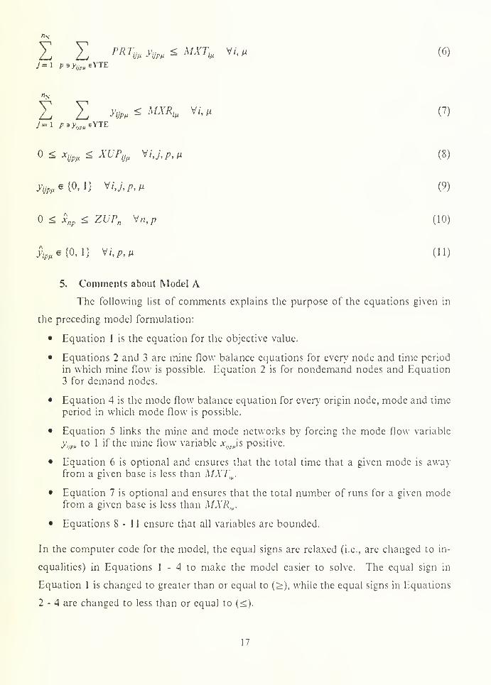
5. Comments about Model A

The following list of comments explains the purpose of the equations given in

the preceding model formulation:

• Equation 1 is the equation for the objective value.

• Equations 2 and 3 are mine flow balance equations for every node and time period

in which mine flow is possible. Equation 2 is for nondcmand nodes and Equation

3 for demand nodes.

• Equation 4 is the mode flow balance equation for ever}' origin node, mode and time

period in which mode flow is possible.

• Equation 5 links the mine and mode networks by forcing the mode flow variable

yiJfllto 1 if the mine flow variable x

ljpu\s positive.

• Equation 6 is optional and ensures that the total time that a given mode is awayfrom a given base is less than MXT

itl.

• Equation 7 is optional and ensures that the total number of runs for a given modefrom a given base is less than MXR

IU.

• Equations 8-11 ensure that all variables are bounded.

In the computer code for the model, the equal signs are relaxed (i.e., are changed to in-

equalities) in Equations 1 - 4 to make the model easier to solve. The equal sign in

Equation 1 is changed to greater than or equal to (>), while the equal signs in Equations

2 - 4 are changed to less than or equal to (<).

17

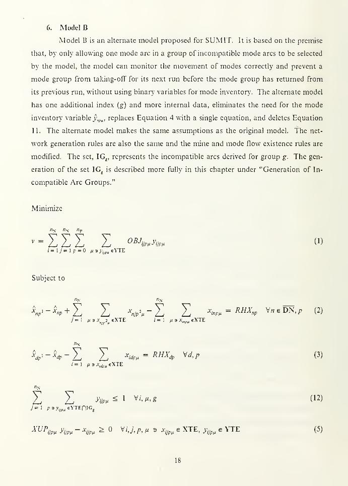
6. Model B

Model B is an alternate model proposed for SUM IT. It is based on the premise

that, by only allowing one mode arc in a group of incompatible mode arcs to be selected

by the model, the model can monitor the movement of modes correctly and prevent a

mode group from taking-ofF for its next run before the mode group has returned from

its previous run, without using binary variables for mode inventor}'. The alternate model

has one additional index (g) and more internal data, eliminates the need for the mode

inventor}' variable ynpil , replaces Equation 4 with a single equation, and deletes Equation

11. The alternate model makes the same assumptions as the original model. The net-

work generation rules are also the same and the mine and mode flow existence rules are

modified. The set, IG^, represents the incompatible arcs derived for group g. The gen-

eration of the set IG4

is described more fully in this chapter under "Generation of In-

compatible Arc Groups."

Minimize

n^ riy- n-f

' - Z Z Z Z 0BJw»y<m mi=\j=lp = ^ 3 > WM eVTE

Subject to

"NA Av -V

+

Z Z V.-Z Z 'I*-*!*** V—DKP (2)

j ~ 1 n*> x 2 eXTE (' = 1 ^3 x-... eXTE

"N

v - ** - Z Z **» = rhx*p

v^ p ^' = 1 H* \dfU

eXTE

Z Z jw* l v/.".« ( 12 ^

7=1 p»yVpil eYTEniGg

XUPijPlx yiJPM

- xijPM ^ ° V/,y, p, n 3 x

iJpMe XTE, yiJpM

e YTE (5)

18

"N

y=l p.ty^tYTE

Z E -^ * M^ v/-

"

(7)

^ *^ < XUPUfl

Vi,j,p,n (8)

^€'{0,1} Vi,j.p,li (9)

^ Jrv ^ Zt//>„ V/i,/> (10)

7. Comments about Model B

All comments from Model A also apply to Model B, except for those that per-

tain to Equations 4 and 11. The purpose of Equation 12, which replaces Equation 4 in

Model A, is to ensure that only one arc in a group of incompatible arcs is selected.

8. Detailed Data Description for Both Models

The data discussed in the next five paragraphs is input by the user and must be

manipulated by both models to generate the networks, calculate the data describing the

networks, time-expand the nodes to form the time-expanded networks, and develop data

for the objective and constraint equations. The input data in the following list is scalar.

The first three scalars are required input and the last three are optional (default values

will be assumed if no input is given):

• TEND - the time (in hours, h) by which all modes transport or deliver mines,

meeting all demand, and return to their origin nodes, where TEND > 0.

• TPER - the length of the time period (h) used in the time expansion, where

< TPER ^ TEND.

• REET - the value of the zero tolerance for comparing real data, where

< RELT <> 0.001. I.e, tf\x-y\ < REET, then x = y is assumed.

• MNLA • the minimum distance (in nautical miles, nm) that air modes can transport

mines to prevent air modes from shipping mines over short routes intended for land

modes, where MNLA ^ . The default is 0.

• MXSS - the maximum distance (nm) allowed for supply to supply transfers, where

MXSS > 0. The default is the maximum distance between nodes.

19

• DISC - a binary parameter in which 1 means to run the model without checking

for disconnected networks and means to check for disconnected networks and to

run the model for the first connected network found. The default is 0.

The model converts TEND into \_TESDjTPER~\ time periods since it time-expands the

network over time periods of length TPER. If TPER is relatively small, the round-off

error is less when converting times to time periods. However, a smaller time period

length also yields more time periods for the problem, which expands the size of the

model. Since a large model is harder to solve, a balance must be struck between TPER

and the number of periods that will be formed. The user must also make TEND large

enough to result in a feasible solution while making it small enough to cut down the size

of the time-expansion.

The data presented in the following list pertains to the node index n or any of

its subindices. For all data pertaining to priorities in this thesis, a lower value implies a

higher priority, e.g., a demand node with a priority of 1 is more important than a node

with priority 2. The purpose of the third parameter MXDn is to allow the user to group

mine fields that are close together into one node and to account for transit time needed

to travel between mine fields. Since a mode group can only have one destination node

per run, MXDd permits the mode group to travel to all mine fields within a demand node

if it has the capacity to carry enough mines. The first parameter is required as input and

the last five are optional:

• AMTn- the supply or demand at node n (mines), where, by convention, assembled

supply and MOMAG disassembled supply amounts are positive and demandamounts are negative. The default is 0.

• PRN„ - the priority of node n, where PRNn > . The default is the maximum nodepriority (or 1 if none are input).

• MXDd - the maximum distance (nm) between mine fields within a demand node d,

where MXDd > . The default is 0.

• BGDC

- the distance (nm) that must be transited by the sea node c to reach its on-

station point before launching aircraft to lay mines, where BGDC;> 0. The default

value is 0.

• EDDC

- the distance (nm) that must be transited by the sea node c to reach a newdestination by the last period of the problem after it completes its last run, whereEDD

C ^ 0. The default value is 0.

• SPXe- the transit speed (nm/h) of the sea node, where SPXC > 0. If DGD

C >or EDDC > 0, SPXC

is no longer optional.

The optional parameters BGDC , EDDC , and SPXC

are not intended to be used for sub-

marines and HVMLs since these modes transit directly to the mine field.

20

The following list of input parameters describes mode characteristics indexed

by mode n or any of its subindices. The first seven parameters are required and the last

one is optional:

• CAPU

- the capacity of one mode unit of mode \i (mines), where CAP > 0. CAP,,

is required for all modes except dummy build modes, whose capacities are com-puted by the model.

• MXL„ - the maximum distance (nm) that mode n can travel from its origin nodeand be able to return, where MXL^ > 0. MXL^ is required for all modes except the

dummy build modes.

• SPD„ - the average transit speed (nm'h) of mode n , where SPDU> 0. SPD

Vis re-

quired for all modes, where the speed of a dummy build mode /? is its build rate.

• TLDU

- the average amount of time (h) needed to load a mode group and take-off,

where TLD„ > 0. The default is 0.

• TULU

- the average amount of time (h) needed to unload a mode group for trans-

portation modes or deploy the mines for deliver}' mode groups, where TULM> 0.

The default is 0.

• TGD„ - the average amount of time (h) needed to spend on the ground after a runbefore reloading and taking off, where TGD„ > 0. The default is 0.

• PRMV

- the priority of mode n, where PRMU> . The default is the maximum

mode priority (or 1 if none are input).

The parameter CAP„ can be used in two different ways. If a mode group is composed

of the same type of mode unit, the capacity of a mode unit can be input as CAPM

. But,

if the mode group is composed of variety of modes, CAPUshould be the total number

of mines that the mode group can carry. The user must take this distinction into ac-

count when inputting the number of modes stationed at node. For example, if the mode

group at a give node is composed of seven P3 Orion aircraft and the user inputs CAP„

as the capacity of a mode unit, the number of modes at that node should be seven.

However, if the mode group based at a given node is a tactical air squadron and the user

inputs CAPU as the total capacity, the number of modes at that node should be one.

For dummy sea modes based at mobile sea nodes that can deploy mines, CAPyshould

equal the supply of the node in which the dummy sea mode is stationed. The three

time-related parameters, TLDP , TULP , and TGD

P , are assumed to equal for dummy

build modes.

The next list of parameters involves the mode groups based at their origin

nodes. The first parameter is required and the last four parameters are optional:

• NUM,„ - the number of mode units \x in the mode group based at origin node /,

where NUMIU> 0. NUM

IV> 1 for at least one mode group containing mode units

n at every origin node /'. The default is 0.

21

• BGTlu

- the earliest time (h) in which mode group n is available for loading at its

origin node / for its first run, where < BGTllt< TEND . The default is 0.

• EDTtu

- the latest time (h) by which mode group n must return to its origin node /'

after completing its last run, where < EDTllt< TEND . The default is TEND.

• MXTlu

- the maximum total time (h) that mode group n can be absent from its or-

igin node i in making all of its runs, where < MXTiu< TEND. The default is

TEND.

• MXR,U

- the maximum number of runs that mode group \x based at its origin node/ is allowed to take, where ^ MXR

llt<, [TEND / TPER]. The default is

[TEND I TPERl

For dummy build modes, NUMmP should equal 2 if the MOMAG node m has dual par-

allel assembly lines and 1 otherwise. This convention will double the build rate for par-

allel assembly lines. If the number of parallel assembly lines at MOMAGs are increased

in the future, then the user can account for this growth by setting NUMmP equal to the

number of parallel assembly lines. For dummy sea modes stationed on mobile sea nodes

that can deploy mines, NUM^ should equal 1.

The following optional input parameter pertains to arcs in the mine and mode

networks. It allows the user to rule out arcs in the networks that will be selected by the

model:

• XMP,JU

- a binary parameter in which 1 implies that no arc from origin node / to

destination nodej via mode group n shall be allowed in the network. The default

value is 0.

Thus, by including XMPIJtl

if necessary, the user can eliminate arcs that are not allowed

because of obscure rules not accounted for in the model.

The final input parameter is required and defines the distance between nodes:

• DISU- the distance (nm) between origin node / and destination nodej. The default

value is 0.

Distances may be given in a table containing all distances between points. Distances

may also be listed separately for arcs that will probably be used in the network. If the

distance from node / to nodej is input, then the model assumes that it also equals the

distance from nodey to node /. The former method of input ensures that the model will

consider all possible node combinations for the networks, while the latter method is less

tedious to enter if the user thinks only a few arcs are needed.

Two important conventions must be followed to ensure the successful generation

of the correct mine and mode networks. Entering "negative" distances allows the user to

describe two properties of the networks without creating additional input parameters.

22

First, all distances between nodes that are on the same land mass must be less than

-0.5 to indicate arcs that have potential land routes: DIS,r < -0.5, where lj* I'. Sec-

ond, to identify a MOMAG node and its adjacent supply node, the distance between a

MOMAG node and its adjacent supply node must be equal to -0.5: DISm ,= —0.5.

This convention ensures that the iMOMAG node is connected only to its adjacent supply

node.

The next list of parameters is computed by the model, given the input data to

describe the original and the time-expanded networks for mode flow and mine flow.

These parameters assume that the network has already been generated. (Generation

rules will be given in the next section of this chapter under "Network Generation

Rules"). The model takes a conservative approach to rounding time periods up or down.

For example, when converting time data to time periods, the model rounds up begin

times input by the user (BGTlu) but rounds down end times (EDTJ. Rounding data in

this way ensures that the time periods fall within time bounds input by the user. Like-

wise, calculations of arrival time periods for one-way trips and return time periods for

round trips are rounded up to be on the safe side.

• NRLT - the value of the negative zero tolerance allowed when comparing real data,

where NRLT = - KELT.

• SUMA - the number of arcs in the mine network.

• ARC,JU

- the set that indicates whether or not the arc from node i to node J via modep belongs in the mine and modes networks.

• ARTlJ)t

- a temporary set that is identical to ARCtJll

.

• DNOn- a temporary parameter that serves two different purposes in the model: (1)

to indicate when node n has already been checked for calculating MXM„ in one

loop and for calculating MXSn in another loop and (2) to indicate that node n is

included in the first connected network found.

• NFC„ - the set of nodes that does not form a component with at least one supply

node and one demand node.

• XTEIJPU

- the set that indicates whether or not the mine arc leaving node / and ar-

riving at j at the end of time period p via mode p., belongs in the time-expanded

network.

• YTEl]pu

- the set that indicates whether or not the mode arc leaving node i and ar-

riving at j at the end of time period p via mode p, belongs in the time-expanded

network.

• MNUV - the set of all mine flow balance equations in which at least one arc leaves

node n at the beginning of time period p or one arc arrives at node n at the end of

time period p.

23

•

•

MDUipik

- the set of all mode flow balance equations in which at least one arc leaves

node i at the beginning of time period p via mode p or one arc arrives at node / at

the end of time period p via mode p.

RHX^ - the value of the right-hand side of the mine flow balance equation for

mines leaving node n at the beginning of time period p, where p is either the time

period before inventory can start changing or the time period after inventory canstop changing and

VT t Y $ min{\AMTn \,ZUPn } if p is before.KtiAnp -

| [[p is after

RHYlpil

- the value of the right-hand side of the mode flow balance equation for

mode p based at origin node n at the beginning of time period p , where RHYipil

equals 1 if/? is the time period before mode p can start its first run, equals — 1 ifpis the time period after it can finish its last run, and equals otherwise. Notice

that, since mode flow and inventory variables are binary, 1 represents the presence

of the supply of mode p. at n when the problem starts and —1 represents the final

return of the mode supply at the end of the problem.

PARtJll

- the number of time periods with length TPER required to load mode pbased at origin node /, travel to destination node,/ and unload (or deliver) mines,

Wher£TLD„ + TUL

PARijM

= TPER

+1 k>eBM.( | DISij I

+ MXDt) I (SPD^ TPER) otherwise.

PRT,JU

• the number of time periods with length TPER required to load mode pbased at origin node /, travel to destination node j , unload (or deliver) mines, re-

turn, and make ground preparations for turnaround, where

TLD^ + TUEM+ TGD

M

PRTiJfl

= TPER

Jl if/xeBM.+

|(2 | DISij | + MXDt) I (SPD^ TPER) otherwise.

INDn- the indegree of (or the number of arcs directed into) node n.

OTDn- the outdegree of (or the number of arcs directed out of) node n.

BGP,)U

- the earliest time period in which a run can start at origin node i and arrive

at its destination node,/ via mode p., where BGPtJli;> BGT

lti j TPER.

EDP,JU

- the latest time period in which a run can start at origin node i and arrive

at its destination node j via mode p, where EDPIJU< EDT

tu / TPER.

MXMn- the maximum number of mines that could be sent through node n if all

demand on paths containing node n were filled.

MXS„ - the maximum number of mines that could be sent through node n if all

supply on paths containing node n were sent.

OBJ„pu- the value contributed to the objective function by the mode flow for mode

M leaving origin node i arriving at destination node j at time period p, where

24

•

•

OBJim = [PRNtPRNj PRM^ {p + PRT

ijfl)f .

ZUPn- the upper bound (mines) on mine inventory for node n, where

ZUPn = rmn{MXMn , MXSn ).

XUPfju

- the upper bound on mine flow variables from origin node i to destination

nodey via mode /i, where

XUPlJlx

= imniZUPuZUPj^APpNUMtJ.

The parameters BGP,Jti

and EDP,jlk

are the keys to eliminating unnecessary arcs. For

example, if the origin node / is a transshipment node, the model starts creating outgoing

arcs after the earliest period in which mines could have arrived at node /. Likewise, the

model does not create arcs that send mines to an origin node in periods after the last

possible run could have left the origin node. This requirement cuts down on the number

of continuous and binary variables, which increases the speed of model execution.

The parameter OBJtJpil

is composed of two parts: the priority parameters and the

time parameter. The priority parameters, PRN„ PRNj, and PRMU , enable the model to

consider the relative priorities of nodes and modes during optimization. Because scaling

problems may occur if the objective value grows too large, the user should only input

relative priorities and the maximum priority should be less than five. Since the model is

a minimization, the model tends to select mode flow across arcs for which the priority

portion of the objective value is smaller (implying that the priority is higher). The sec-

ond part of the objective value is the time parameter, p + PRTi]lt

. The model will again

tend to select mode flow for which the time portion is smaller. Thus, mode flow that

starts sooner and has a faster round trip time will be considered more optimal. Because

it is the product of the priority parameters and time parameters, the objective value of

SUM IT incorporates both priority and time into a measure of effectiveness.

Model B generates nine extra internal parameters and deletes one internal pa-

rameter (MDU,ru ) from the original model. These additional parameters are needed to

delineate the set of incompatible arcs lGr Additional parameters generated by Model

B are:

• IBEO - a scalar which is incremented by one in the loop that computes GBGIJPI1

andGED,m for arcs in the incompatible arc groups \GV where

IBEG > MNBifi

.

• MRNitl

- the minimum return period PRTIJU

over all arcs from node / directed to

node,/ via mode jx.

25

• MRXIU

- the maximum return period PRTljM

over all arcs from node / directed to

node j via mode /j.

• MNA iv- the minimum arrival period PAR0u over all arcs from node / directed to

node j via mode y. for which PRT0tl= MNAW .

• MNB,„ - the minimum begin period BGPljM

over all arcs from node i directed to nodej via mode it.

• MXEtll

- the maximum end period EDPijtl

over all arcs from node / directed to nodej via mode fi.

• LSGiu

- the number of incompatible arc groups leaving / via mode n, whereEDG'

l]tlis EDG

IJtlfor which PAR,

Jtl= MNA

itland PRT,

JU= MRA,

Vin the equation

LSGiM= mm{EDG'

Ufl) + 2 - MNB

ifJ- MRN

i/x.

• GBGIJPU

- the group number g of the first incompatible arc grouping IG4in which

the arc from / via mode n toy arriving at time period p appears.

• GEDiJPU

- the group number g of the last incompatible arc grouping IG^ in whichthe arc from / via mode \x toj arriving at time period p appears.

9. Network Generation Rules for Both Models

Before discussing the mine and mode flow existence sets XTE and YTE, rules

for generating the original network are given since membership in the mine or mode

networks is a criteria for membership in the flow existence sets. Initially, the set of eli-

gible arcs is assumed to be the power set N x N x M. Arcs that do not meet the rules

for network generation are eliminated from the power set. The following list describes

the existence requirements for arcs from origin node i to destination node j via mode n

that belong to the original network:

• An arc must leave oricin node / and arrive at destination node j via mode n if

NUMlff> 0,/ + j,DIS

u + 0, and MXLU< \DISV \ .

• Any arc from / to j via n is eliminated if XMP,Jti= 1

.

• Any arc between two supply nodes on land, i,j e SNHLN , via a land transporta-

tion mode, fi e TMflLM , is eliminated if DISQ£ or | DIStj \ £ MXSS. .

• Any arc between two supply nodes on land, i,j e SNflLN , via an air transporta-

tion mode n e TMflAM is eliminated if DJSU< and one of the following state-

ments are true: | DIS, \ ^ MNLA or | DIS 1 ^ MXSS.

Any arc between two supply nodes, i,j e SN, via mode \x is eliminated if

iJ4LN or n4TM.

Anv arc is eliminated between two nodes i,j via land transportation modeax e TMflLM ifDISy > 0.

Any arc is eliminated between two land nodes ij e LN via air transportation modeH e TMflAM if DlS

tJ< Oand \D1S,j\ > MNLA.

26

Any arc from sea node c is eliminated if it does not arrive at demand node d.

Any arc directed to cither supply node s or transshipment node / is eliminated if the

mode is a delivery mode <5.

Any arc arriving at a demand node d via a nondelivery mode is eliminated.

Any arc leaving a MOMAG node m and arriving at any node j for whichDISmJ # —0.5 is eliminated.

Any arc entering a MOMAG node m is eliminated.

Any arc leaving a transshipment node / and arriving at a supply node s is elimi-

nated.

Any arc from / to j via n is eliminated if its round trip time TPER x PRTlJU

is

greater than the total time allowed MXTm or the time difference betweenEDT

IUand BGTm .

Eliminate all arcs directed from node / if node / has no mines in inventory at the

beginning of the problem and no arcs are directed into node i.

Any arc from / toy via n is eliminated if BGPIJtl> EDP

iJu.

Any arc whose origin node i and destination node j is not contained in the first

connected component found.

10. Generation of Incompatible Arc Groups

The procedure for determining incompatible arc groups for Model B sets up in-

compatible arc groups around an arc that has a return period equal to MRNiltand has

an arrival period equal to MNAm . Because such an arc has the minimum return period

and the minimum arrival period for mode n leaving node /, the first run associated with

this arc has the earliest arrival time period. The number of potential runs for this arc is

also greater than (or equal to) the number of potential runs for other arcs that do not

meet this criteria because arcs with greater return periods are forced to make fewer runs

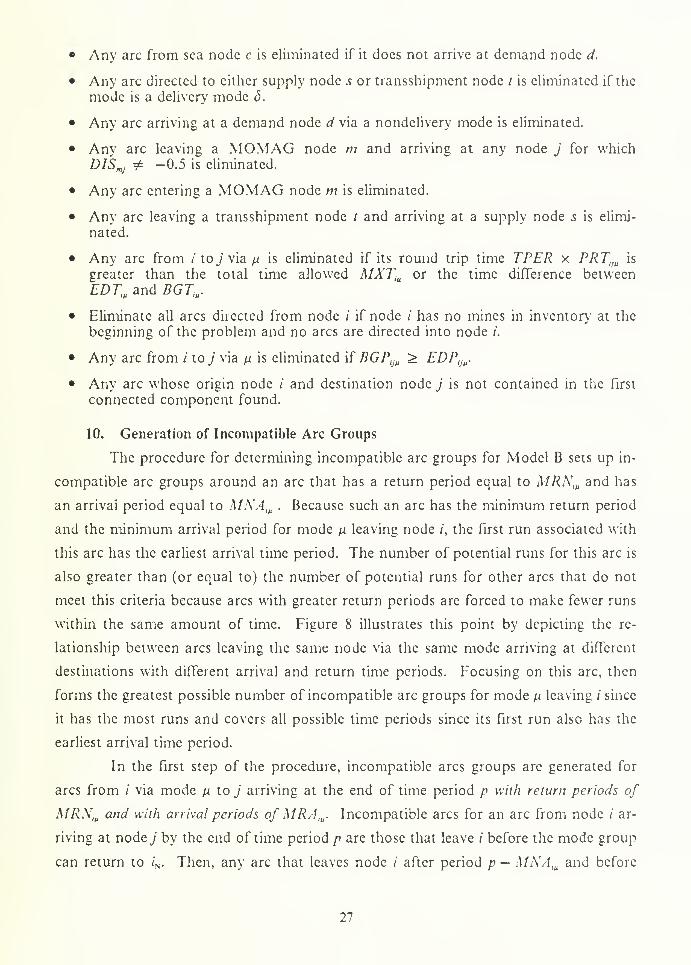
within the same amount of time. Figure 8 illustrates this point by depicting the re-

lationship between arcs leaving the same node via the same mode arriving at different

destinations with different arrival and return time periods. Focusing on this arc, then

forms the greatest possible number of incompatible arc groups for mode \x leaving / since

it has the most runs and covers all possible time periods since its first run also has the

earliest arrival time period.

In the first step of the procedure, incompatible arcs groups are generated for

arcs from / via mode \i to j arriving at the end of time period p with return periods of

MRN,Uand with arrival periods ofMRAm . Incompatible arcs for an arc from node i ar-

riving at nodey by the end of time period p are those that leave / before the mode group

can return to /N . Then, any arc that leaves node / after period p — MNA iltand before

27

i 2 3 4

MNA = 1 MRN = 2

From. To PAR PRT

y. _f

. — i— --i 1

Si ^ 1 2

Si d 2 1 3

Figure 8. Relationship between Arcs from the Same Node to Different Destinations

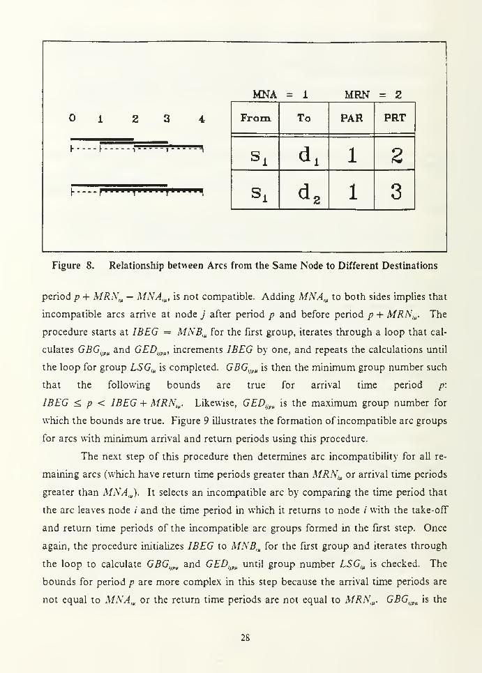
period p + MRNm — MNAm , is not compatible. Adding MNAm to both sides implies that

incompatible arcs arrive at node j after period p and before period p + MRNiu. The

procedure starts at IBEG = MNBIU

for the first group, iterates through a loop that cal-

culates GBGIJPU

and GED,JPU , increments IBEG by one, and repeats the calculations until

the loop for group LSGm is completed. GBG,JPU

is then the minimum group number such

that the following bounds are true for arrival time period p:

IBEG <, p < IBEG + MRNllt

. Likewise, GED,]PU

is the maximum group number for

which the bounds are true. Figure 9 illustrates the formation of incompatible arc groups

for arcs with minimum arrival and return periods using this procedure.

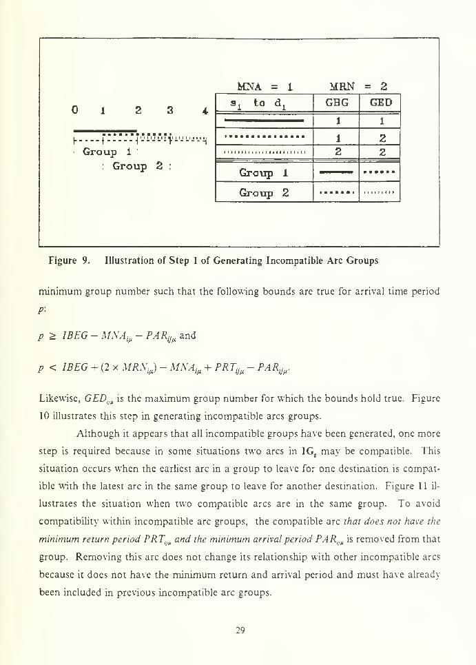
The next step of this procedure then determines arc incompatibility for all re-

maining arcs (which have return time periods greater than MRNlMor arrival time periods

greater than MNAIU). It selects an incompatible arc by comparing the time period that

the arc leaves node / and the time period in which it returns to node / with the take-off

and return time periods of the incompatible arc groups formed in the first step. Once

again, the procedure initializes IBEG to MNB,U for the first group and iterates through

the loop to calculate GBGIJPU

and GEDIJPU

until group number LSG1U

is checked. The

bounds for period p are more complex in this step because the arrival time periods are

not equal to MNAm or the return time periods are not equal to MRNm . GBGIJPIi

is the

28

12 3 4

MNA = 1 MRN = 2

a, to d. GBG GED

1 1

r \4-

Group 1

: Group 2 :

'-'-'H

i i i • i • i i i i i i i 1 1 i i i i i t i

1

22

2

Group 1

Group 2 < i i i t i i i

Figure 9. Illustration of Step 1 of Generating Incompatible Arc Groups

minimum group number such that the following bounds are true for arrival time period

P-

p ^ IBEG - MNAiu- PAR

iiuand

p < IBEO + (2 x MRN¥)- MNA

ifl+ PRT

ijfl- PAR

!JfX.

Likewise, GED„U

is the maximum group number for which the bounds hold true. Figure

10 illustrates this step in generating incompatible arcs groups.

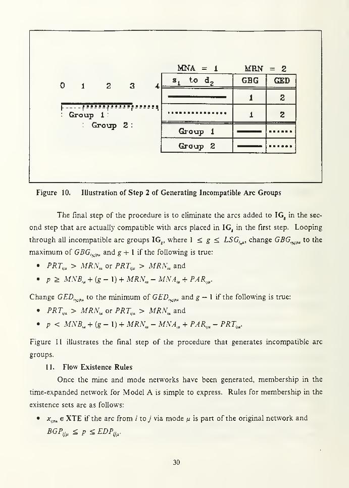
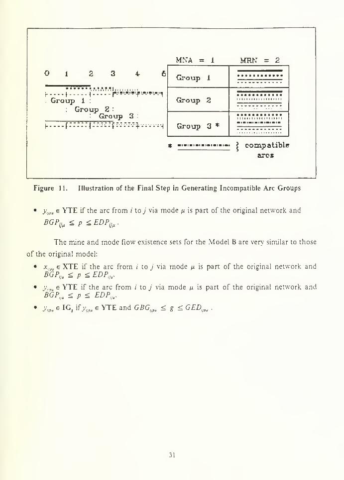
Although it appears that all incompatible groups have been generated, one more

step is required because in some situations two arcs in \Ggmay be compatible. This

situation occurs when the earliest arc in a group to leave for one destination is compat-

ible with the latest arc in the same group to leave for another destination. Figure 11 il-

lustrates the situation when two compatible arcs are in the same group. To avoid

compatibility within incompatible arc groups, the compatible arc that does not have the

minimum return period PRTIJUand the minimum arrival period PAR

lJUis removed from that

group. Removing this arc does not change its relationship with other incompatible arcs

because it does not have the minimum return and arrival period and must have already

been included in previous incompatible arc groups.

29

MNA = 1 MRN = 2

I-fiii«|«Jii

: Group 1

Group 2

-"-"!

aL

to d2 GBG GED

1 2

1 2

Group 1

Group 2

Figure 10. Illustration of Step 2 of Generating Incompatible Arc Groups

The final step of the procedure is to eliminate the arcs added to IG, in the sec-

ond step that are actually compatible with arcs placed in IG, in the first step. Looping

through all incompatible arc groups IG4 , where 1 <, g <, LSG

lnll , change GBGlfi/f)Uto the

maximum of GBGIS!PU

and g + 1 if the following is true:

• PRTyM> MRN

IUor PRTUu > MRNlu

and

• p > MNBm + (g - 1) + MRNm - MNAm + PARW .

Change GED,^pu to the minimum of GEDISIPU

and g — 1 if the following is true:

• PRTIJU> MRN

luor PRT

iJlt> MRN

IUand

• p < MNBm + (g - 1) + MRNm - MNA iH+ PARW - PRTIJtt

.

Figure 1 1 illustrates the final step of the procedure that generates incompatible arc

groups.

11. Flow Existence Rules

Once the mine and mode networks have been generated, membership in the

time-expanded network for Model A is simple to express. Rules for membership in the

existence sets are as follows:

• xIJPU

€ XTE if the arc from / toj via mode ^ is part of the original network and

BGPfr <; p < EDPijfX

.

30

MNA = 1 MUN = 2

i 2 3 4 6

•••r.i ftm i

r 1 1 r™w™FtfWW1Group 1 :

Group 2 :

Group 3

K ....f:::::f:::::f:-:r:-:^.- i,,H

Group 1

Group 2 lllllllllllltllllll

Group 3 *1 l l 1 1 i l i l 1 1 i i l i 1 1 i i

* I compatible

arcs

Figure 11. Illustration of the Final Step in Generating Incompatible Arc Groups

• yIJPIIe YTE if the arc from i loj via mode [i is part of the original network and

BGPyMz p < EDP

iJfi.

The mine and mode flow existence sets for the Model B are very similar to those

of the original model:

• x„pu e XTE if the arc from / to j via mode n is part of the original network andBGP

IJU< p < EDP,

JU.

• y,.pu e YTE if the arc from i to j via mode (i is part of the original network andBGP

IJU< p < EDP

IJU.

• ym e IG, ifj^ e YTE and GBGIJPti

< g < GEDIJPU

.

31

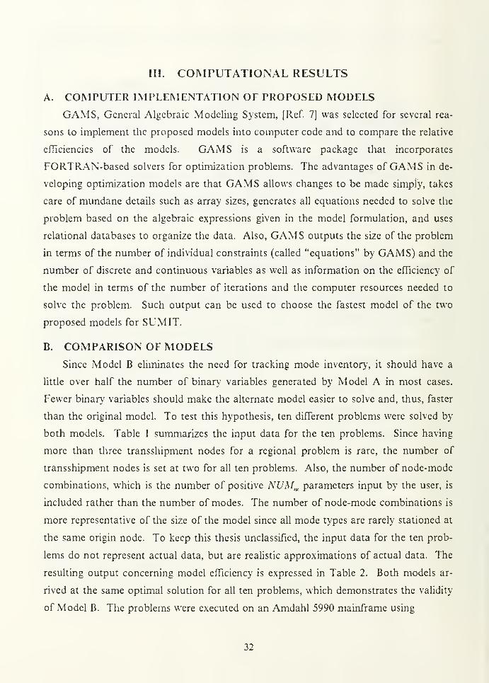
III. COMPUTATIONAL RESULTS

A. COMPUTER IMPLEMENTATION OF PROPOSED MODELS

GAMS, General Algebraic Modeling System, [Ref. 7] was selected for several rea-

sons to implement the proposed models into computer code and to compare the relative

efTiciencies of the models. GAMS is a software package that incorporates

FORTRAN-based solvers for optimization problems. The advantages of GAMS in de-

veloping optimization models are that GAMS allows changes to be made simply, takes

care of mundane details such as array sizes, generates all equations needed to solve the

problem based on the algebraic expressions given in the model formulation, and uses

relational databases to organize the data. Also, GAMS outputs the size of the problem

in terms of the number of individual constraints (called "equations" by GAMS) and the

number of discrete and continuous variables as well as information on the efficiency of

the model in terms of the number of iterations and the computer resources needed to

solve the problem. Such output can be used to choose the fastest model of the two

proposed models for SUMIT.

B. COMPARISON OF MODELSSince Model B eliminates the need for tracking mode inventory, it should have a

little over half the number of binary variables generated by Model A in most cases.

Fewer binary variables should make the alternate model easier to solve and, thus, faster

than the original model. To test this hypothesis, ten different problems were solved by

both models. Table 1 summarizes the input data for the ten problems. Since having

more than three transshipment nodes for a regional problem is rare, the number of

transshipment nodes is set at two for all ten problems. Also, the number of node-mode

combinations, which is the number of positive NUMivparameters input by the user, is

included rather than the number of modes. The number of node-mode combinations is

more representative of the size of the model since all mode types are rarely stationed at

the same origin node. To keep this thesis unclassified, the input data for the ten prob-

lems do not represent actual data, but are realistic approximations of actual data. The

resulting output concerning model efficiency is expressed in Table 2. Both models ar-

rived at the same optimal solution for all ten problems, which demonstrates the validity

of Model B. The problems were executed on an Amdahl 5990 mainframe using

32

GAMS/ZOOM, where is ZOOM is one of the packages available with GAMS for mixed

integer programs.

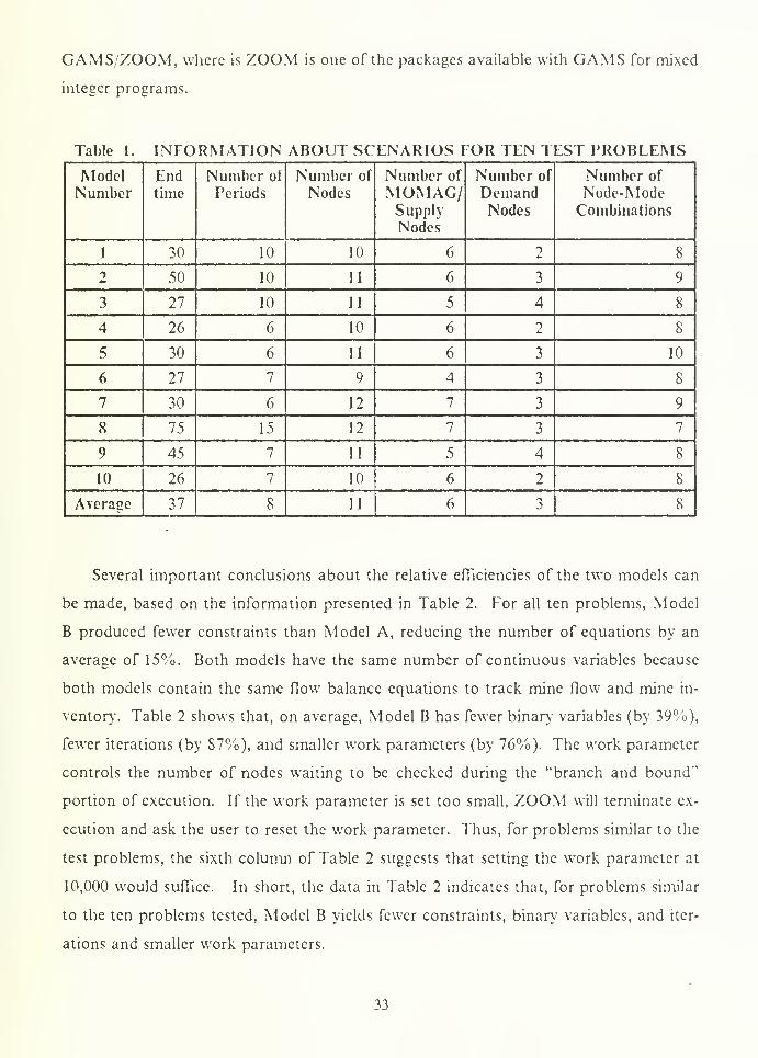
Table 1. INFORMATION ABOUT SCENARIOS FOR TEN TEST PROBLEMSModelNumber

Endtime

Number of

Periods

Number of

NodesNumber of

MOMAG/SupplyNodes

Number of

DemandNodes

Number of

Node-ModeCombinations

1 30 10 10 6 2 8

2 50 10 11 6 3 9

3 27 10 11 5 4 8

4 26 6 10 6 2 8

5 30 6 11 6 3 10

6 27 7 9 4 3 8

7 30 6 12 7 3 9

8 75 15 12 7 3 7

9 45 7 11 5 4 8

10 26 7 10 6 2 8

Average 37 8 11 6 3 8

Several important conclusions about the relative efficiencies of the two models can

be made, based on the information presented in Table 2. For all ten problems, Model

B produced fewer constraints than Model A, reducing the number of equations by an

average of 15%. Both models have the same number of continuous variables because

both models contain the same flow balance equations to track mine flow and mine in-

ventory. Table 2 shows that, on average, Model B has fewer binary variables (by 39%),

fewer iterations (by 87%), and smaller work parameters (by 76%). The work parameter

controls the number of nodes waiting to be checked during the "branch and bound"

portion of execution. If the work parameter is set too small, ZOOM will terminate ex-

ecution and ask the user to reset the work parameter. Thus, for problems similar to the

test problems, the sixth column of Table 2 suggests that setting the work parameter at

10,000 would suffice. In short, the data in Table 2 indicates that, for problems similar

to the ten problems tested, Model B yields fewer constraints, binary variables, and iter-

ations and smaller work parameters.

33

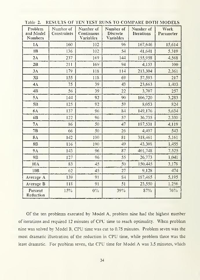
Table 2. RESULTS OF TEN TEST RUNS TO COMPARE BOTH MODELSProblem

and ModelNumbers

Number of

Constraints

Number of

ContinuousVariables

Number of

Discrete

Variables

Number of

Iterations

WorkParameter

1A 160 102 96 167,646 15,614

IB 136 102 54 41,641 5.319

2A 237 169 144 155,958 4.568

2B 211 169 94 4,153 100

3A 179 118 114 213,304 2,361

3B 155 118 69 57.593 217

4A 75 39 43 23,663 1,403

4B 56 39 22 3,707 257

5A 144 92 90 106,720 3,283

5B 125 92 59 8,053 824

6A 137 96 84 149.176 5,634

6B 122 96 57 36.735 2,330

7A 86 50 47 187,531 4,119

7B 66 50 26 4,407 543

8A 142 100 81 318,461 5,161

8B 116 100 49 43,308 1 ,455

9A 143 96 87 401,748 7.525

9B 127 96 55 26,773 1,041

10A 83 45 50 150.445 3,178

10B 62 45 27 9,128 474

Average A 139 91 84 187,465 5,195

Average B 118 91 51 23.550 1.256

Percent

Reduction15% 0% 39% 87% 76%

Of the ten problems executed by Model A, problem nine had the highest number

of iterations and required 12 minutes of CPU time to reach optimality. When problem

nine was solved by Model B, CPU time was cut to 0.75 minutes. Problem seven was the

most dramatic illustration of the reduction in CPU time, while problem three was the

least dramatic. For problem seven, the CPU time for Model A was 3.5 minutes, which

34

was reduced to only 0.1 minutes when solved by Model B. The CPU time taken by

Model A and by Model B to solve problem three was 7.5 minutes and two minutes re-

spectively. The fact that Model B produces fewer constraints and fewer binary variables

means that it requires fewer iterations and a smaller work parameter to reach optimality.

This reduction in size and increase in speed, cut the CPU time by two-thirds in the

worst-case situation of the ten problems tested.

C. GAMS IMPLEMENTATION OF SUMIT

The implementation of SUMIT and a sample problem in GAMS is given in Ap-

pendix A. The output from the first run of the problem in Appendix A is contained in

Appendix B. The input for and the output from the second, and final run, are contained

in Appendices C and D respectively. Appendix E discusses several aspects of the GAMSimplementation of SUMIT, including a description of SUMIT's output.

Because large mixed integer problems are hard to solve, the user should limit the

number of time periods to ten if the problem has more than ten nodes. However, since

it is difficult to judge the end time and time period length for a new problem, the user

should follow the recommendations given in Appendix E to find appropriate values for

the end time and time period length. Notice that the efficiency data in Table 2 does not

include the initial runs discussed in Appendix E because these runs are very' quick.

Other mixed integer program solvers are also available with GAMS. The solver,

XA, solved the first run of sample problem in Appendix A in only 18,859 iterations,

while, as shown in Appendix B, ZOOM required 76,589 iterations. Thus, XA seems to

be superior to ZOOM in solving mine transshipment problems using the SUMIT model.

A way to attack large problems is to allow SUMIT to divide the large problem into

several subproblems. SUMIT does not require that the mine or the mode network be

connected. In other words, a path need not exist between all nodes in each network.

If the network can be divided into multiple connected components, then SUMIT can

split the problem into separate subproblems, one for each component. For networks

that are large enough to tax the computer's disk space, running SUMIT for each con-

nected component may solve a problem that could not otherwise be solved. By setting

the scalar DISC equal to 0, SUMIT will run the optimization on the first connected

component of the network that it finds and will notify the user of the nodes not con-

tained in the first component. The user must then rerun SUMIT for the nodes that were

not in the first connected component.

35

The sample program given in Appendix A is an example of a large problem that was

divided into subproblems by SUMIT. Appendix B contains the first solution output by

SUM IT. SUMIT tells the user to rerun the program for nodes not included in the first

component found. If there are at least one supply node and one demand node in this

list that have not already been included in components already solved, the user should

rerun SUMIT for the nodes indicated. The user may rerun SUMIT without deleting

excessive amounts of input data by setting (1) NUMm equal to for every node and

mode combination that was included in the mine network for the first run of SUMIT

and (2) AMTd equal to for all demand already filled by the first run. Appendix C

contains the input portion of SUMIT for the second run and illustrates this simple

change. Notice that, since the second problem was smaller, the end time TEND and

time period length TPER could be decreased.

In many cases, finding the proven optimal solution is very expensive in computer

time and memory, so GAMS provides an option that allows the user to specify an ac-

ceptable "optimality gap." During the branch and bound portion of execution, ZOOMfinds an upper bound and a lower bound on the objective value for the optimal solution.

ZOOM terminates execution and reports an "INTEGER SOLUTION" if it has found

a feasible integer solution in which the absolute distance between these two bounds di-

vided by the lower bound is less than the optimality gap, called OPTCR. The integer

solution reported when ZOOMS halts execution for this reason is not a proven optimal

solution. In fact, when running the ten test problems using Model B, the solver found

the optimal solution, without proving optimality, by using the GAMS default value of

OPTCR (0.1) in six cases. Optimal solutions were also found, but not proven, for three

of the remaining four problems by using an OPTCR of 0.01. Appendix E contains rec-

ommendations for setting an appropriate OPTCR.

D. REDUCTION OF MINE FLOW AND INVENTORY IN BOTH MODELSAs stated previously, both models have the same number of continuous variables

since they both contain the same flow balance equations for mine flow. Creating "rea-

sonable" mine flow and inventory variables decreases the number of continuous vari-

ables needed in the model. In the computer implementation of SUMIT, applying the

network generation and flow existence rules ensures that only "reasonable" variables for

mine flow and inventory are used. In the first portion of the "Pre-Model

Manipulation" section of the program (see Appendix A), the set parameter ARCiJU

indi-

cates the arcs that make sense for mine flow in the mine network. In the part of this

36

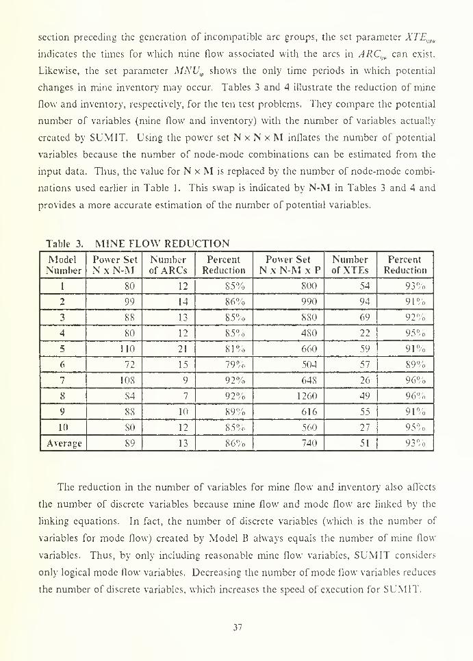
section preceding the generation of incompatible arc groups, the set parameter XTEtJflt

indicates the times for which mine flow associated with the arcs in ARC,JU

can exist.

Likewise, the set parameter MNUipshows the only time periods in which potential

changes in mine inventory may occur. Tables 3 and 4 illustrate the reduction of mine

flow and inventory, respectively, for the ten test problems. They compare the potential

number of variables (mine flow and inventory) with the number of variables actually

created by SUM IT. Using the power set N x N x M inflates the number of potential

variables because the number of node-mode combinations can be estimated from the

input data. Thus, the value for N x M is replaced by the number of node-mode combi-

nations used earlier in Table 1. This swap is indicated by N-M in Tables 3 and 4 and

provides a more accurate estimation of the number of potential variables.

Table 3. MINE FLOW REDUCTION

ModelNumber

Power Set

N x N-MNumberof ARCs

Percent

Reduction

Power Set

N x N-M x PNumberof XTEs

Percent

Reduction

1 80 12 85% 800 54 93%

2 99 14 86% 990 94 91%

3 88 13 S5% 880 69 92%

4 80 12 85% 4 SO 22 95%

5 110 21 81% 660 59 91%

6 72 15 79% 504 57 89%

7 10S 9 92% 64 S 26 96%

8 84 7 92% 1260 49 96%

9 8S 10 89% 616 55 91%

10 80 12 85% 560 27 95%

Average 89 13 86% 740 51 93%

The reduction in the number of variables for mine flow and inventory also affects

the number of discrete variables because mine flow and mode flow are linked by the

linking equations. In fact, the number of discrete variables (which is the number of

variables for mode flow) created by Model B always equals the number of mine flow

variables. Thus, by only including reasonable mine flow variables, SUM IT considers

only logical mode flow variables. Decreasing the number of mode flow variables reduces

the number of discrete variables, which increases the speed of execution for SUMIT.

37

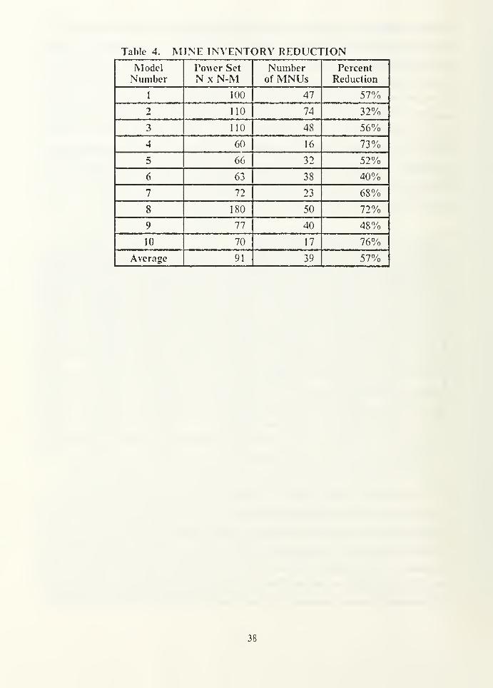
Table 4. MINE INVENTORY REDUCTIONModelNumber

Po>ver Set

N x N-MNumberof MNUs

Percent

Reduction

I 100 47 57%

2 110 74 32%

3 110 48 56%

4 60 16 73%

5 66 32 52%

6 63 38 40%

7 72 23 6S%

8 180 50 72%

9 77 40 48%

10 70 17 76%

Average 91 39 57%

38

IV. CONCLUSIONS

This thesis developed a single-commodity mine transshipment model, called

SUM IT, for the rapid deployment of mines in a region of the world over a time window

of two to three days. It considered two possible versions of SUMIT for computer im-

plementation into GAMS. For ten problems tested, Model A and Model B arrived at

the same optimal solution, but differed in relative efficiencies. For the size of the

problems tested, Model B appeared to be faster and is, therefore, the model of choice for

the implementation of SUMIT into GAMS.

Transshipment models involving integer programs tend to be difficult to solve, even

for small problems. When limited to a region of the world spanning a few days, the

mine transshipment problem is small enough to attempt integer programming. This

thesis explored a viable approach for solving small mine transshipment problems using

integer programs by replacing the binary mode networks, which was done in Model A,

with sets of incompatible arc groups for every mode, which was done in Model B. The

results of the ten test problems in this thesis demonstrate the superiority of using in-

compatible arc groups in the size and speed of the model for problem comparable to the

test problems.

In addition to providing optimal or nearly optimal schedules for mine transship-

ment, SUMIT can be used as one of many tools for making decisions concerning mine

warfare. SUMIT can give insight to logistical planners at CMWC in deciding the

quantity and location of pre-staged mines, the quantity of mines that should be fully

assembled at MOMAGs, and the MOMAGs that should receive resources for dual as-

sembly lines to decrease the amount of time needed to deploy sets of mine fields for the

most likely scenarios. In preparation for mine deployment, SUMIT can be run for dif-

ferent combinations of nodes and modes to indicate where modes should be based to

decrease deployment time. Finally, SUMIT can be used to demonstrate the advantages

of building new mine laying platforms, such as the HVMLs, by not only illustrating the

time that could be saved in mine deployment for short-term regional scenarios, but also

indicating which non-mine warfare platforms would be allowed to perform other critical

missions.

Several enhancements could be made to SUMIT to improve its user friendliness and

expand the size of the problems that it can manage:

39

• Develop a "front end" program in another language to read user input from a data

file and printout the GAMS program for execution. The front end program wouldread data from GOPAS and allow users to use SUM IT without directly interfacing

with GAMS.

• Develop a program in another language to read the GAMS output file and con-struct schedules that are more readable.

• Allow a mode group from a given node to be split between destinations when ap-

propriate.

• Determine whether or not allowing more than two levels of mine readiness wouldbe practical. This could be accomplished by splitting the MOMAG nodes so that

each level of readiness for disassembled mines is represented by a MOMAG nodeand by putting one arc between MOMAG nodes for each level of readiness for

disassembled mines and the associated supply node for assembled mines.

• Include constraints that take into account the limits placed on mine loading andunloading capacities at non-MOMAG supply sites and the restrictions on the

number of aircraft allowed at transshipment sites at one time. Currently, this data

is not available in GOPAS.

Finally, the problem discussed in this thesis could be expanded for follow-on re-

search in two ways:

• Develop a model that encompasses world-wide scenarios of longer durations. This

problem could be approached by adapting the integer rounding technique devel-

oped by Puntenney to SUM IT [Ref. 6].

• Develop a multi-commodity transshipment model by applying the work of Collier,

Lally, and Puntenney [Refs. 4, 5 , 6].

40

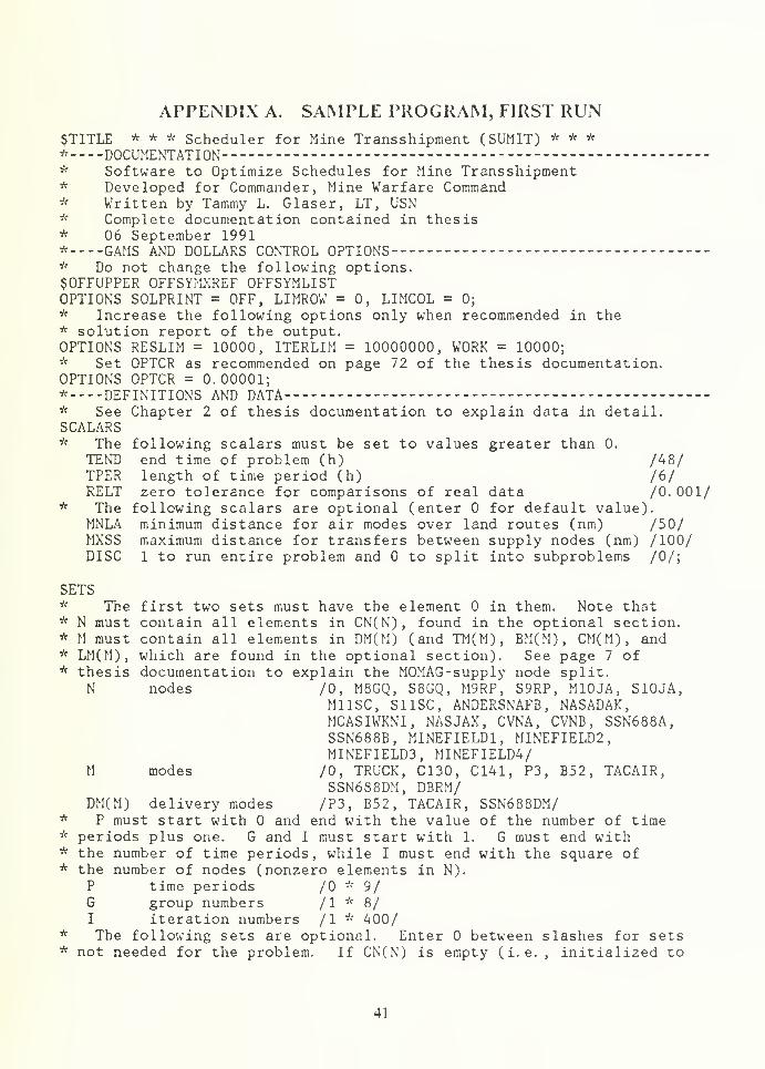
APPENDIX A. SAMPLE PROGRAM, FIRST RUN$TITLE * * * Scheduler for Mine Transshipment (SUMIT) * * ** DOCUMENTATION ---

* Software to Optimize Schedules for Mine Transshipment* Developed for Commander, Mine Warfare Command* Written by Tammy L. Glaser, LT, USN* Complete documentation contained in thesis* 06 September 1991* GAMS AND DOLLARS CONTROL OPTIONS* Do not change the following options.$0FFUPPER OFFSYMXREF OFFSYMLISTOPTIONS SOLPRINT = OFF, LIMROW = 0, LIMCOL = 0;

* Increase the following options only when recommended in the* solution report of the output.OPTIONS RESLIM = 10000, ITERLIM = 10000000, WORK = 10000;* Set OPTCR as recommended on page 72 of the thesis documentation.OPTIONS OPTCR = 0. 00001;* DEFINITIONS AND DATA* See Chapter 2 of thesis documentation to explain data in detail.SCALARS* The following scalars must be set to values greater than 0.

TEND end time of problem (h) /48/TPER length of time period (h) /6/RELT zero tolerance for comparisons of real data /0. 001/

* The following scalars are optional (enter for default value).MNLA minimum distance for air modes over land routes (nm) /50/MXSS maximum distance for transfers between supply nodes (nm) /100/DISC 1 to run entire problem and to split into subproblems /0/;

SETS* The first two sets must have the element in them. Note that* N must contain all elements in CN(N), found in the optional section.* M must contain all elements in DM(M) (and TM(M), BM(M), CM(M), and* LM(M), which are found in the optional section). See page 7 of* thesis documentation to explain the MOMAG-supply node split.

N nodes /0, M8GQ, S8GQ, M9RP, S9RP, M10JA, S10JA,Ml ISC, SI ISC, ANDERSNAFB, NASADAK,MCASIWKNI, NASJAX, CVNA, CVND , SSN688A,SSN688B, MINEFIELD1, MINEFIELD2,MINEFIELD3, MINEFIELD4/

M modes /0, TRUCK, C130, C141, P3, B52, TACAIR,SSN688DM, DBRM/

DM(M) delivery modes /P3, B52, TACAIR, SSN688DM/* P must start with and end with the value of the number of time,v periods plus one. G and I must start with 1. G must end with* the number of time periods, while I must end with the square of* the number of nodes (nonzero elements in N).

P time periods /0 * 9/G group numbers /l * 8/I iteration numbers /l Vf 400/

* The following sets are optional. Enter between slashes for sets* not needed for the problem. If CN(N) is empty (i.e. , initialized to

41

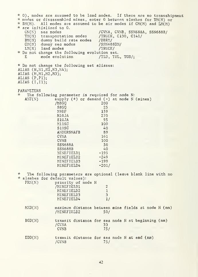
* 0), nodes are assumed to be land nodes. If there are no transshipment* modes or disassembled mines, enter between slashes for TM(M) or* BM(M). All modes are assumed to be air modes if CM(M) and LM(M)* are initialized to 0.

CN(N) sea nodes /CVNA, CVNB , SSN688A, SSN688B/TM(M) transportation modes /TRUCK, C130, C141/BM(M) dummy build rate modes /DBRM/CM(M) dummy sea modes /SSN688DM/LM(M) land modes /TRUCK/

* Do not change the following evolution set.

E mode evolution /TLD, TUL, TGD/;

* Do not change the following set aliases:ALIAS (N,N1,N2,N3,N4);ALIAS (M,M1,M2,M3);ALIAS (P,P1);ALIAS (1,11);

PARAMETERS,v The following parameter is required for node N:

AMT(N) supply ( + ) or demand (-) at node N (mines)/M8GQ 200S8GQ 25M9RP 159M10JA 270S10JA 95M11SC 100S11SC 40ANDERSNAFB 89CVNA 161CVNB 100SSN688A 50SSN688B 40MINEFIELD

1

-195MINEFIELD2 -249M1NEFIELD3 -199MINEFIELD4 -201/

* The following parameters are optional (leave blank line with no* slashes for default values):

PRN(N) priority of node N/MINEFIELD1 2

MINEFIELD2 1

MINEFIELD3 3

MINEFIELD4 1/

MXD(N) maximum distance between mine fields at node N (nm)/MINEFIELD2 50/

BGD(N) transit distance for sea node N at beginning (nm)/CVNA 33CVNB 75/

EDD(N) transit distance for sea node N at end (nm)

/CVNB 75/

42

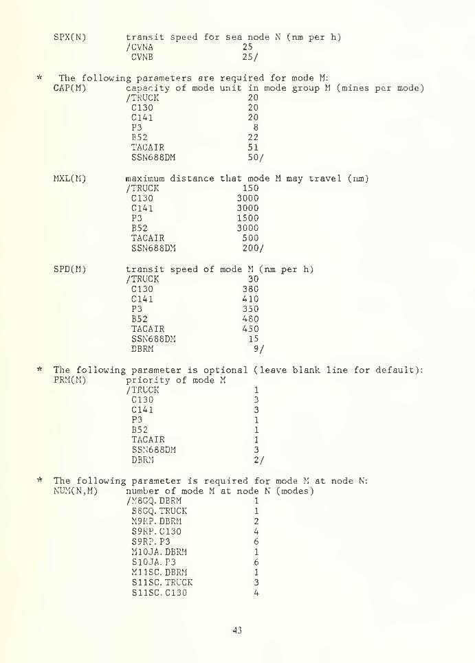
SPX(N) transit speed for sea node N (nra per h)/CVNA 25CVNB 25/

* The following parameters are required for mode M:

CAP(M) capacity of mode unit in mode group M (mines per mode)/TRUCK

'

20C130 20C141 20P3 8

E52 22TACAIR 51SSN688DM 50/

MXL(M) maximum distance that mode M may travel (nm)/TRUCK 150C130 3000C141 3000P3 1500B52 3000TACAIR 500SSN688DM 200/

SPD(M) transit speed of mode M (nm per h)/TRUCK 30C130 380C141 410P3 350B52 480TACAIR 450SSN688DM 15

DBRM 9/

* The following parameter is optional (leave blank line for default):PRM(M) priority of mode M

/TRUCK"

1

C130 3

C141 3

P3 1

B52 1

TACAIR 1

SSN688DM 3

DBRM 2/

The following parameter is required for mode M at node N:

NUM(N,M) number of mode M at node N (modes)M8GQ.DBRM 1

S8GQ. TRUCK 1

M9RP. DBRM 2

S9RP.C130 4

S9RP. P3 6

M10JA. DBRM 1

S10JA. P3 6

M11SC.DBRM 1

S11SC. TRUCK 3

S11SC.C130 4

43

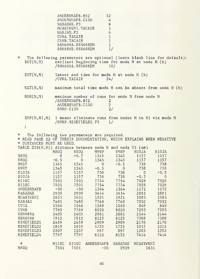
ANDERSNAFB. B52 12ANDERSNAFB.C130 4NASADAK. P3 6

MCASIWKNI.TACAIR 1

NASJAX. P3 6

CVNA. TACAIR 1

CVNB.TACAIR 1

SSN688A. SSN688DM 1

SSN688B. SSN688DM 1/

The following parameters are optional (leave blank line for default):BGT(N,M) earliest beginning time for mode M at node N (h)

/SSN688A. SSN688DM 10/

EDT(N,M) latest end time for mode M at node N (h)/CVNA. TACAIR 24/

MXT(N,M) maximum total time mode M can be absent from node N (h)

MXR(N,M) maximum number of runs for mode M from node N/ANDERSNAFB. B52 2

ANDERSNAFB. C130 2

S9RP. C130 2/

XMP(N,N1,M) 1 means eliminate runs from nodes N to Nl via mode M/S9RP. MINEFIELD2. P3 1/

* The following two parameters are required.* READ PAGE 22 OF THESIS DOCUMENTATION, WHICH EXPLAINS WHEN NEGA* DISTANCES MUST BE USED.TABLE DIS(N

:,N1) distance between node N and node Nl (nm)

M8GQ S8GQ M9RP S9RP M10JA !S10JAM8GQ -0.5 1345 1345 1157 1157S8GQ -0.5 1345 1345 1157 1157M9RP 1345 1345 -0.5 738 738S9RP 1345 1345 -0.5 738 738M10JA 1157 1157 738 738 -0.5S10JA 1157 1157 738 738 -0.5M11SC 7501 7501 7754 7754 7028 7028S11SC 7501 7501 7754 7754 7028 7028ANDERSNAFB -30 -30 1364 1364 1172 1172NASADAK 2939 2939 3614 3614 2881 2881MCASIWKNI 1631 1631 1821 1821 1083 1083NASJAX 7485 7485 7768 7768 7032 7032CVNA 1566 1566 1580 1580 849 849CVNB 7789 7789 8020 8020 7293 7293SSN688A 2405 2405 2881 2881 2144 2144SSN688B 7812 7812 8125 8125 7388 7388MINEF1ELD1 2459 2459 2909 2909 2170 2170MINEFIELD2 1819 1819 1725 1725 1015 1015MINEFIELD3 2207 2207 897 897 1203 1203MINEFIELD4 7797 7797 8152 8152 7414 7414

+ M11SC SI ISC ANDERSNAFB NASADAK MCASIWKNIM8GQ 7501 7501 -30 2939 1631

44

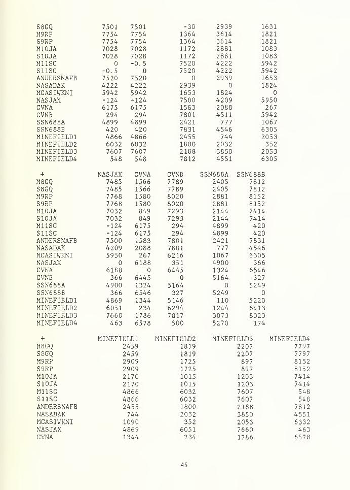
S8GQ 7501 7501 -30 2939 1631M9RP 7754 7754 1364 3614 1821S9RP 7754 7754 1364 3614 1821M10JA 7028 7028 1172 2881 1083SIOJA 7028 7028 1172 2881 1083M11SC -0.5 7520 4222 5942S11SC -0.5 7520 4222 5942ANDERSNAFB 7520 7520 2939 1653NASADAK 4222 4222 2939 1824MCASIWKNI 5942 5942 1653 1824NASJAX -124 -124 7500 4209 5950CVNA 6175 6175 1583 2088 267CVNB 294 294 7801 4511 5942SSN688A 4899 4899 2421 777 1067SSN688B 420 420 7831 4546 6305M1NEFIELD1 4866 4866 2455 744 2053MINEFIELD2 6032 6032 1800 2032 352MINEFIELD3 7607 7607 2188 3850 2053MINEFIELD4 548 548 7812 4551 6305

+ NASJAX CVNA CVNB SSN688A SSN688BM8GQ 7485 1566 7789 2405 7812S8GQ 7485 1566 7789 2405 7812M9RP 7768 1580 8020 2881 8152S9RP 7768 1580 8020 2881 8152MIOJA 7032 849 7293 2144 7414SIOJA 7032 849 7293 2144 7414M11SC -124 6175 294 4899 420S11SC -124 6175 294 4899 4>20

ANDERSNAFB 7500 1583 7801 2421 7831NASADAK 4209 2088 7801 777 4546MCASIWKNI 5950 267 6216 1067 6305NASJAX 6188 351 4900 366CVNA 6188 6445 1324 6546CVNB 366 6445 5164 327SSN688A 4900 1324 5164 5249SSN688B 366 6546 327 5249MINEFIELD1 4869 1344 5146 110 5220MINEFIELD2 6051 234 6294 1244 6413MINEF1ELD3 7660 1786 7817 3073 8023MINEFIELD4 463 6578 500 5270 174

+ MINEFIELD1 MINEFIELD2 MINEFIELD3 MINEFIELD4M8GQ :2459 1819 2207 7797S8GQ :2459 1819 2207 7797M9RP :2909 1725 897 8152S9RP ;2909 1725 897 8152MIOJA :2170 1015 1203 7414SIOJA :2170 1015 1203 7414M11SC (^866 6032 7607 548S11SC i^866 6032 7607 548ANDERSNAFB :2455 1800 2188 7812NASADAK 744 2032 3850 4551MCASIWKNI 1090 352 2053 6332NASJAX i^869 6051 7660 463CVNA 1344 234 1786 6578

45

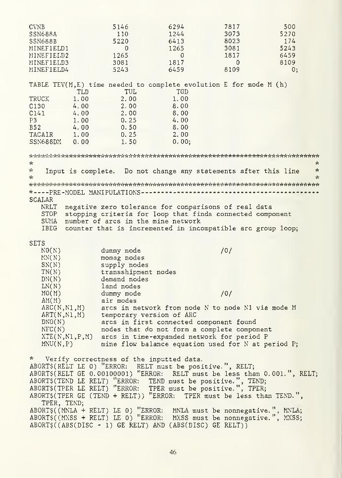
CVNB 5146 6294 7817 500SSN688A 110 1244 3073 5270SSN688B 5220 6413 8023 174MINEFIELD1 1265 3081 5243MINEFIELD2 1265 1817 6459MINEFIELD3 3081 1817 8109MINEFIELD4 5243 6459 8109 0;

TABLE TEV(M,E) time needed to complete evolution E for mode M (h)TLD TUL TGD

2.00 1.002.00 8.00

TRUCK 1.00C130 4.00C141 4.00P3 1.00B52 4.00TACAIR 1.00SSN688DM 0.00

0025502550

8. 004.008.002.000.00;

,v Input is complete. Do not change any statements after this line *Vr ***iW«Y}Y}Y}V}Y*tfcik?Y*:MMYiV*?YyMWcyc***iV?Y^

* PRE-MODEL MANIPULATIONSSCALAR

NRLT negative zero tolerance for comparisons of real dataSTOP stopping criteria for loop that finds connected componentSUMA number of arcs in the mine networkIBEG counter that is incremented in incompatible arc group loop;

SETSN0(N)MN(N)SN(N)TN(N)DN(N)LN(N)M0(M)AM(M)ARC(N,N1,M)ART(N,N1,M)DN0(N)NFC(N)XTE(N,N1,P,M)MNU(N,P)

dummy node /0/momag nodessupply nodestransshipment nodesdemand nodesland nodesdummy mode /0/air modesarcs in network from node N to node Nl via mode Mtemporary version of ARCarcs in first connected component foundnodes that do not form a complete componentarcs in time-expanded network for period Pmine flow balance equation used for N at period P;

* Verify correctness of the inputted data.AB0RT$(RELT LE 0) "ERROR: RELT must be positive.", RELT;AB0RT$(RELT GE 0.00100001) "ERROR: RELT must be less than 0.001.", RELT;AB0RT$(TEND LE RELT) "ERROR: TEND must be positive.", TEND;AB0RT$(TPER LE RELT) "ERROR: TPER must be positive.", TPER;AB0RT$(TPER GE (TEND + RELT)) "ERROR: TPER must be less than TEND.",

TPER, TEND;AB0RT$((MNLA + RELT) LE 0) "ERROR: MNLA must be nonnegative. " , MNLA;AB0RT$((MXSS + RELT) LE 0) "ERROR: MXSS must be nonnegative.", hDCSS;

AB0RT$((ABS(DISC - 1) GE RELT) AND (ABS(DISC) GE RELT))

46

"ERROR: DISC must be equal to or 1. ", DISC;

* Initialize or set default values for certain parameters.TEND = FLOOR(TEND / TPER);NRLT = -1 * RELT;MXSS$(MXSS LE NRLT) = SMAX((N,N1), ABS(DIS(N,N1) ) ) + (2 * RELT);AMT(N) = FLOOR(AMT(N) )$(AMT(N) GE 0.5) + CEIL( AMT(N) )$( AMT(N) LE -0.5);MXL(M)$BM(M) = -0.5;NUM(N,M) = FL00R(NUM(N,M));XMP(N,N1,M)$(N0(N) * N0(N) * M0(M)) = 0;

DIS(N,N1)$(N0(N) * N0(N1)) = 0;

DIS(N,N1)$(ABS(DIS(N,N1)) LE RELT) = DIS(N1,N);TM(M)$M0(M) = NO;

BM(M)$M0(M) = NO;

CN(N)$N0(N) = NO;

CM(M)$M0(M) = NO;

LM(M)$M0(M) = NO;

* Verify the correctness of the inputted data.ABORT$(SUM(M$DM(M), 1) LE 0.5) "ERROR: No delivery modes entered", DM;

AB0RT$(SUM(N$(AMT(N) GE 0.5), AMT(N)) LE 0.5)"ERROR: No supply amounts (+) entered.", AMT;

AB0RT$(SUM(N$(AMT(N) LE -0.5), ABS( AMT(N) ) ) LE 0.5)"ERROR: No demand amounts (-) entered.", AMT;

AB0RT$(SUM(N, AMT(N)) LE -0.5)"ERROR: Total demand (-) exceeds total supply ( + ).", AMT;

AB0RT$(SMIN(M$(N0T (M0(M) + BM(M))), MXL(M)) LE RELT)"ERROR: All MXL(M) must be positive. "

"Did you forget the maximum range for dummy sea modes?", MXL, CM;

AB0RT$(SMIN(M$(N0T (M0(M) + BM(M))), SPD(M)) LE RELT)"ERROR: All SPD(M) must be positive. "

"Did you forget the maximum range for dummy sea modes?", SPD, CM;

AB0RT$(SMIN((N,M), NUM(N,M)) LE -0.5)"ERROR: NUM(N,M) must all be nonnegative. " , NUM;

AB0RT$(SUM((N,N1), ABS(DIS(N,N1) ) ) LE RELT)"ERROR: No distances (DIS(N,N1)) inputted", DIS;

AB0RT$(SUM((N,N1,M)$((ABS(XMP(N,N1,M) - 1) GE RELT) AND(ABS(XMP(N,N1,M)) GE RELT)), 1) GE 0.5)"ERROR: All XMP(N,N1,M) must be equal to or 1.", XMP;

* Categorize nodes and modes into appropriate subsets.MN(N) = YES$((AMT(N) GE 0.5) AND ( SUM(M$BM(M) , NUM(N,M)) GE 0.5));SN(N) = YES$((N0T (N0(N) + MN(N) ) )$( ( AMT(N) GE 0.5)

OR ((ABS(AMT(N)) LE 0.5) AND (SUM(N1$MN(N1)

,

1$(ABS(DIS(N,N1) + 0.5) LE RELT)) GE 0.5))));TN(N) = YES$((N0T (N0(N) + SN(N) ) )$( ABS(AMT(N) ) LE 0.5));DN(N) = YES$(AMT(N) LE -0.5);CN(N) = YES$(CN(N) + DN(N));LN(N) = YES$(N0T (CN(N) + N0(N)));AM(M) = YES$(N0T (LM(M) + CM(M) + BM(M) + M0(M)));

* Include all logical arcs in network.ARC(N,N1,M)$(((MN(N) + SN(N) + TN(N)) * (SN(N1) + TN(N1) + DN(N1)))

$((NUM(N,M) GE 0.5) AND (ABS(0RD(N) - ORD(Nl)) GE 0.5)AND ((ABS(MXL(M)) - ABS(DIS(N,N1) ) ) GE NRLT)

4"

AND (ABS(DIS(N,N1)) GE RELT))) = YES;* Eliminate all arcs as indicated by user.ARC(N,N1,M)$(ABS(XMP(N,N1,M) - 1) LE RELT) = NO;* Eliminate all arcs between supply nodes on land via land modes* that have nonnegative distances or have distances greater than MXSS.ARC(N,N1,M)$((SN(N) * SN(N1) * LN(N) * LN(N1) * TM(M) * LM(M))

$((DIS(N,N1) GE NRLT) OR ((MXSS - ABS(DIS(N,N1) ) ) LE RELT))) = NO;* Eliminate all arcs between supply nodes on land via air trans-* portation when the arcs are over land and absolute distances are* less than MNLA or their absolute distances are greater than MXSS.ARC(N,N1,M)$((SN(N) * SN(N1) * LN(N) * LN(N1) * TM(M) * AM(M))

$((((MNLA - ABS(DIS(N,N1))) GE RELT) AND (DIS(N,N1) LE NRLT))OR ((MXSS - ABS(DIS(N,N1))) LE RELT))) = NO;

* Eliminate all arcs between two supply nodes in which at least* one node is on land or that use nontransportation modes.ARC(N,N1,M)$(SN(N) * SN(N1) * (NOT (LN(N) * LN(N1) * TM(M)))) = NO;,v Eliminate all arcs between nodes via land transportation modes* for which the distance is nonnegative.ARC(N,N1,M)$((TM(M) * LM(M))$(DIS(N,N1) GE NRLT)) = NO;,v Eliminate all arcs between land nodes via air transportation* modes when the arcs are over land and absolute distances are* less than MNLA.ARC(N,N1,M)$((LN(N) * LN(N1) * TM(M) * AM(M))

$(((MNLA - ABS(DIS(N,N1))) GE RELT) AMD (DIS(N,N1) LE NRLT))) = NO;* Eliminate all arcs from sea nodes to nondemand nodes.ARC(N,N1,M)$(CN(N) * (NOT DN(N1))) = NO;* Eliminate all arcs to either supply or transshipment nodes* via delivery modes.ARC(N,N1,M)$((SN(N1) + TN(N1)) * DM(M)) = NO;,v Eliminate all arcs to demand nodes via nondelivery modes.ARC(N,N1,M)$(DN(N1) * (NOT DM(M))) = NO;lV Eliminate all arcs leaving MOMAG nodes to nodes for which* the distance is not equal to -0. 5.

ARC(N,N1,M)$(MN(N)$(ABS(DIS(N,N1) + 0.5) GE RELT)) = NO;,v Eliminate all arcs arriving at MOMAG nodes.ARC(N,N1,M)$MN(N1) = NO;,v Eliminate all arcs from transshipment nodes to supply nodes.ARC(N,N1,M)$(TN(N) * SN(N1)) = NO;

,v Verify that only one arc leaves each MOMAG node.AB0RT$ (SMAX(N$MN(N), SUM( (Nl ,M)$ARC(N,N1 ,M) , 1)) GE 1.5)

"ERROR: At least one MOMAG node has more than one arc leaving it.

"MOMAG nodes and the current network is listed as follows:", MN, ARC;

PARAMETERSPAR(N,N1,M) time periods to travel from N to Nl via M one-wayPRT(N,N1,M) time periods to travel from N to Nl via M round tripIND(N) in degree of (number of arcs entering) node NOTD(N) out degree of (number of arcs leaving) node NBGP(N,N1,M) earliest time to include arc from N to Nl via MEDP(N,N1,M) latest time to include arc from N to Nl via MMXM(N) maximum number of mines through N to fill demandsMXS(N) maximum number of mines through N from supply nodesZUP(N) upper bound on mine inventory at NXUP(N,N1,M) upper bound on mine flow from N to Nl via MRHX(N,P) fixed value on mine inventory at N at period P

48

MRN(N,M) minimum return period PRT from N via MMRX(N,M) maximum return period PRT from N via MMNA(N.M) minimum arrival period PAR from N via M if PRT=MRNMNB(N,M) minimum begin period BGP from N via MMXE(N,M) maximum end period EDP from N via MLSG(N,M) last group number needed from N via MGBG(N,N1,P,M) first group number from N to Nl via M at P

GED(N,N1,P,M) last group number from N to Nl via M at P;

* In* ConvCAP(M)PRN(N)PRM(M)PRN(N)PRM(M)MXD(N)BGD(N)EDB(N)SPX(N)BGT(N,EDT(N,SUMA =

MXT(N,MXR(N,GBG(N,GED(N,MXR(N,MXT(N,MXT(N,

$((EDT(N,

$((

RELT)) = MAX(1,RELT)) = MAX(1,

SMAX(N1,SMAX(M1,

itialize or set default values for certain parameters,ert times to time periods.= FL00R(CAP(M));$N0(N) = 0;

$M0(M) = 0;

$((N0T N0(N))$(PRN(N) LE$((N0T M0(M))$(PRM(M) LE$(N0T DN(N)) = 0;

$N0(N) = 0;

$N0(N) = 0;

$N0(N) = 0;

M)$(N0(N)*M0(M)) = 0;

M)$(N0(N)*M0(M)) = 0;

0;

M)$(N0(N)*M0(M))M)$(N0(N)*M0(M))N1,P,M)$(N0(N) *

N1,P,M)$(N0(N) *

M)$(MXR(N,M) GE

PRN(Nl)));PRM(Ml)));

= 0;

= 0;

N0(N1)N0(N1)

RELT) =

= 0;

= 0;

* M0(M))* M0(M))FL00R(MXR(N,M));

M)$(MXT(N,M) GE RELT) = FL00R(MXT(N,M) / TPER);M)$((N0T (N0(N) + M0(M)))MXT(N,M) LE RELT) AND (NUM(N,M) GE 0.5))) = TEND;M)$((N0T (N0(N) + M0(M)))EDT(N,M) LE RELT) AND (NUM(N.M) GE 0.5))) = TPER * TEND;

* Calculate capacity for dummy build rate modes.CAP(M)$BM(M) = FL00R(SPD(M) * TPER);

* Verify the correctness of the inputted data.STOP = TEND + 1;

AB0RT$((ABS(CARD(P) - 2 - TEND)) GE RELT)"ERROR: The set P must contain integers from to 'STOP'"(see the next line for the value of 'STOP').", STOP, P;

ABORT$(ABS(CARD(G) - TEND) GE RELT)"ERROR: The set G must contain integers from 1 to 'TEND'

STOP = (CARD(N) - 1) ** 2;

AB0RT$(ABS(CARD(I) - STOP) GE RELT)"ERROR: The set I must contain integers from 1 to 'STOP'"(see the next line for the value of 'STOP').", STOP, I;

AB0RT$((SMIN(N, PRN(N)) + RELT) LE 0)"ERROR: PRN(N) must all be nonnegative. ", PRN

AB0RT$((SMIN(N, MXD(N)) + RELT) LE 0)"ERROR: MXD(N) must all be nonnegative.", J-DCD

ABORT$((SMIN(N, BGD(N)) + RELT) LE 0)

"ERROR: BGD(N) must all be nonnegative.", BGDAB0RT$((SMIN(N, EDD(N)) + RELT) LE 0)

TEND, G;

49

"ERROR: EDD(N) must all be nonnegative. " , EDD;ABORT$((SMIN(N, SPX(N)) + RELT) LE 0)

"ERROR: SFX(N) must all be nonnegative.", SPX;ABORT$(SUM(N$(((BGD(N) GE RELT) OR (EDD(N) GE RELT))

AND (SPX(N) LE RELT)), 1) GE 0.5)"ERROR: If BGD(N) or EDD(N) is inputted, SPX(N) must be positive."BGD, EDD, SPX;

ABORT? (SMIN(M$(NOT M0(M)), CAP(M)) LE 0.5)"ERROR: CAP(M) must all be positive. ",

"Did you forget the capacity for dummy sea modes?", CAP, CM;ABORT$((SMIN(M, PRM(M)) + RELT) LE 0)

"ERROR: PRM(M) must all be nonnegative.", PRM;ABORT$((SMIN((N,M), BGT(N,M)) + RELT) LE 0)

"ERROR: BGT(N,M) must all be nonnegative.", BGT;ABORT$((SMIN((N,M), EDT(N,M)) + RELT) LE 0)

"ERROR: EDT(N,M) must all be nonnegative.", EDT;ABORT$((SMIN((N,M), MXT(N,M)) + RELT) LE 0)

"ERROR: MXT(N,M) must all be nonnegative.", MXT;AB0RT$((SMIN((N,M), MXR(N,M)) + RELT) LE 0)

"ERROR: MXR(N,M) must all be nonnegative.", MXR;AB0RT$((SMIN(N, SPX(N)) + RELT) LE 0)

"ERROR: SPX(N) must all be nonnegative.", SPX;AB0RT$((SMIN((M,E), TEV(M,E)) + RELT) LE 0)

"ERROR: TEV(M,E) must all be nonnegative.", TEV;

* Adjust BGT and EDT if nonzero BGD and EDD is inputted. Convert* BGT and EDT to time periods.BGT(N,M)$(N0T (N0(N) + M0(M)))

= CEIL(((BGD(N) / SPX(N))$((SPX(N) GE RELT) AND (NUM(N,M) GE 0.5))+ BGT(N,M)) / TPER);

EDT(N,M)$(N0T (N0(N) + M0(M)))= FL00R(((EDD(N) / SPX(N) )$( (SPX(N) GE RELT) AND (NUM(N,M) GE 0.5))+ EDT(N,M)) / TPER);

* Calculate PAR taking into account load, travel, and unload/* delivery times. Calculate PRT taking into account load,* travel, unload/delivery, return travel, and ground times.PAR(N,N1,M)$(ARC(N.N1,M)$(SPD(M) GE RELT))

= CEIL(((TEV(M,'TLD') + TEV(M,'TUL')) / TPER) + 1$BM(M)+ ((ABS(DIS(N,N1)) + MXD(Nl)) / (TPER * SPD(M) ) )$(N0T BM(M)));

PRT(N,N1,M)$(ARC(N,N1,M)$(SPD(M) GE RELT))= CEIL(((TEV(M,'TLD') + TEV(M,'TUL') + TEV(M, 'TGD

1

)) / TPER)+ (((2 * ABS(DIS(N,N1))) + MXD(Nl)) / (TPER * SPD(M) ))$(N0T BM(M))+ 1$BM(M));

* Eliminate all arcs from N to Nl via M if PRT is greater than* MXT or (EDT - BGT). If node N has no supply and no incoming arcs,* eliminate all arcs directed from node N.

ARC(N,N1,M)$(ARC(N,N1,M)$(((MXT(N,M) - PRT(N,N1,M)) LE NRLT)OR ((PRT(N,N1,M) - (EDT(N,M) - BGT(N,M))) GE RELT))) = NO;

ARC(N,N1,M)$((SUM((N2,M1)$ARC(N2,N,M1), 1) LE 0.5)AND (ABS(AMT(N)) LE 0.5)) = NO;

ART(N,N1,M) = ARC(N,N1,M);

* In a loop, take the following steps until a loop in which* no arcs are deleted from the mine network is made:

50

* Calculate SUMA, IND, and OTD. Initialize DNO and MXM.* Calculate EDP and MXM by checking all possible paths* in the network. Reinitialize DNO and MXS. Calculate* BGP and MXS by checking all possible paths in the network.* (In these loops, DNO indicates whether or not MXM or MXS* has already been updated for origin node of the arc being* checked. ) Calculate EDP for arcs leaving MOMAG nodes.* Eliminate arcs from N to Nl via M for which PRT is* greater than (EDP - BGP).* If node N has no supply and no incoming arcs from* other nodes, eliminate all arcs directed from node N.

* If DISC equals 0, then set* DNO to 'yes' for all nodes in the first connected* component found. If DISC equals 1, then set DNO to 'yes'* for all nodes (except dummy node 0). Eliminate arcs whose* nodes are not contained in the first component found.L00P(I1$(ABS(SUMA - SUM( (N,N1 ,M)$ART(N,N1 ,M) , 1)) GE RELT)

,

SUMA = SUM((N,N1,M)$ART(N,N1,M), 1):

IND(N) = SUM((N1,M)$ART(N1,N,M), 1):

OTD(N) = SUM((N1,M)$ART(N,N1,M), 1):

DNO(N) = YES;MXM(N) = 0;

L00P(N$(DN(N)$((IND(N) + OTD(N)) GE 0.5)),DNO(N) = NO;

L00P((N1,M)$ART(N1,N,M),EDP(N1,N,M) = MIN(EDT(N1,M), TEND) - PRT(N1,N,M) + PAR(N1,N,M);MXM(N1)$(DN0(N1) + DNO(N)) = ABS(AMT(N)) + MXM(Nl);DNO(Nl) = NO;

L00P((N2,M1)$ART(N2,N1,M1)

,

EDP(N2,N1,M1) = MAX(EDP(N2,N1,M1),MIN(EDP(N1,N,M) - PAR(N1,N,M), MIN(EDT(N2,M1) ,TEND)- PRT(N2,N1,M1) + PAR(N2,N1,M1)));

MXM(N2)$(DNO(N2) + DNO(N)) = ABS(AMT(N)) + MXM(N2);DN0(N2) = NO;

L00P((N3,M2)$ART(N3,N2,M2),EDP(N3,N2,M2) = MAX(EDP(N3 ,N2 ,M2)

,

MIN(EDP(N2,N1,M1) - PAR(N2 ,N1 ,M1)

,

MIN(EDT(N3,M2), TEND)- PRT(N3,N2,M2) + PAR(N3 ,N2,M2) ) );

MXM(N3)$(DN0(N3) + DNO(N)) = ABS(AMT(N)) + MXM(N3);DN0(N3) = NO;

LOOP((N4,M3)$ART(N4,N3,M3),EDP(N4,N3,M3) = MAX(EDP(N4,N3,M3)

,

MIN(EDP(N3,N2,M2) - PAR(N3 ,N2 ,M2)

,

MIN(EDT(N4,M3), TEND)- PRT(N4,N3,M3) + PAR(N4,N3 ,M3) ) );

MXM(N4)$(DN0(N4) + DNO(N)) = ABS(AMT(N)) + MXM(N4);DN0(N4) = NO))));

DN0(N1)$(N0T DN(N1)) = YES);BGP(N,N1,M)$ART(N,N1,M)

= PAR(N,N1,M)$(IND(N) L£ 0.5) + TEND$(IND(N) GE 0.5)+ BGT(N,M);

DN0(N) = YES;MXS(N) = 0;

L00P(N$((IND(N) LE 0.5) AND (0TD(N) GE 0.5)),MXS(N)$DN0(N) = AMT(N);

51

DNO(N) = NO;LOOP((Nl,M)$ART(N,Nl,M),

MXS(Nl)$(DNO(N) + DNO(Nl)) = MXS(Nl) + AMT(N)+ AMT(Nl)$(NOT DN(N1));

DNO(Nl) = NO;LOOP((N2,Ml)$ART(Nl,N2,Ml),

BGP(N1,N2,M1) = MIN(BGP(N1,N2,M1), PAR(N1 ,N2 ,M1)+ BGP(N,N1,M)$(AHT(N1) LE 0.5) + BGT(N1,M1));

NXS(N2)$(DN0(N) + DN0(N2)) = MXS(N2) + AMT(N)+ AMT(N1)$(N0T DN(N1)) + AMT(N2)$(N0T DN(N2));

DN0(N2) = NO;LOOP( (N3 ,M2 ) $ART(N2 ,N3 ,M2)

,

BGP(N2,N3,M2) = MIN(BGP(N2,N3,M2) , PAR(N2,N3,M2)+ BGP(N1,N2,M1)$(AMT(N2) LE 0.5) + BGT(N2,M2));

MXS(N3)$(DN0(N) + DN0(N3)) = MXS(N3) + AMT(N)+ ANT(N1)$(N0T DN(N1)) + AMT(N2)$(N0T DN(N2))+ AMT(N3)$(N0T DN(N3));

DN0(N3) = NO;

L00P((N4,M3)$ART(N3,N4,M3),BGP(N3,N4,M3) = MIN(BGP(N3,N4,M3) , PAR(N3,N4,M3)

+ BGP(N2,N3,M2)$(AMT(N3) LE 0.5) + BGT(N3,M3));MXS(N4)$(DN0(N) + DN0(N4)) = MXS(N4) + AMT(N)

+ AMT(N1)$(N0T DN(N1)) + AMT(N2)$(N0T DN(N2))+ AMT(N3)$(N0T DN(N3)) + AMT(N4)$(N0T DN(N4));

DN0(N4) = NO))));DN0(N1)$(IND(N1) GE 0.5) = YES);

EDP(N,N1,M)$(MN(N)$((CAP(M) * NUM(N,M)) GE RELT)) = MIN(EDP(N,N1,M)

,

CEIL(MIN(MXS(N),MXM(N)) / (CAP(M) * NUM(N,M))));ART(N,N1,M)$(ART(N,N1,M)$((EDP(N,N1,M) - BGP(N,N1,M)) LE NRLT)) = NO;

ART(N,N1,M)$((SUM((N2,M1)$ART(N2,N,M1), 1) LE 0.5)AND (ABS(AMT(N)) LE 0.5)) = NO;

* Initialize DIS, DNO and STOP if DISC equals 0.

DIS(N,N1)$(DISC LE 0.5) = 0;

LOOP(M$(DISC LE 0.5),DIS(N,N1)$ART(N,N1,M) = 1);

DNO(N)$(DISC LE 0.5)= YES$(ABS(SMIN((N1,N2,M)$((N0T N0(N1)) * ART(N1 ,N2,M) ) , ORD(Nl))- ORD(N)) LE RELT);

STOP$(DISC LE 0.5) = SUM( (N,N1)$DN0(N) , DIS(N,N1) + DIS(N1,N));* Starting with the first nondummy node in network found, set* DNO to 'yes' for any node which (1) is on a path with the first* node found or (2) is on a backtrack path from other nodes on a* path with the first node found. Stop when all arcs in the network* have been checked.

L00P(I$((ST0P GE 0.5) AND (DISC LE 0.5)),L00P(N$DN0(N),

L00P(N1$((DIS(N,N1) GE 0.5) OR (DIS(N1,N) GE 0.5)),DNO(Nl) = YES;DIS(N,N1)$(DIS(N,N1) GE 0.5) = 0;

DIS(N1,N)$(DIS(N1,N) GE 0.5) = 0));STOP = SUM((N,N1)$DN0(N), DIS(N,N1) + DIS(N1,N)));

DN0(N)$((N0T N0(N))$(ABS(DISC - 1) LE RELT)) = YES;ART(N,N1,M)$(N0T (DNO(N) * DN0(N1))) = NO;

* Ensure that the first component found contains both supply and* demand. If not, repeat the process for the next component.

SUMA$(((SUM(N$(DNO(N) * DN(N)), ABS(AMT(N))) LE 0.5)

52

OR (SUM(N$(DNO(N) * SN(N)), AMT(N)) LE 0. 5))$(DISC LE 0.5)) = 0;

NFC(N)$(DN0(N)$((SUM(N1$(DN0(N1) * SN(N1)), AMT(Nl)) LE 0.5)OR (SUM(N2$(DNO(N2) * DN(N2)), ABS( AMT(N2) ) ) LE 0.5))) = YES;

ART(N,N1,M)$((N0T (NFC(N) * NFC(Nl))) * ARC(N,N1,M)) = YES);

* Ensure that total supply is greater than total demand* in generated network.AB0RT$((SUM(N$(DN0(N) * DN(N)), ABS(AMT(N)))

- SUM(N$(DN0(N) * (MN(N) + SN(N))), AMT(N))) GE 0.5)"ERROR: Total demand (-) exceeds total supply (+) ",

"in generated network.", DNO, AMT;

* Reset the following parameters if N is not in the first connected* component found.ART(N,N1,M) = ARC(N,N1,M);ARC(N,N1,M)$(N0T (DN0(N) * DNO(Nl))) = NO;

MXT(N,M)$(N0T DN0(N)) = 0;

MXR(N,M)$(N0T DNO(N)) = 0;

BGT(N,M)$(N0T DNO(N)) = 0;

EDT(N,M)$(N0T DN0(N)) = 0;

PAR(N,N1,M)$(N0T ARC(N,N1,M)) = 0;

PRT(N,N1,M)$(N0T ARC(N,N1,M)) = 0;

BGP(N,N1,M)$(N0T ARC(N,N1,M)) = 0;

EDP(N,N1,M)$(N0T ARC(N,N1,M)) = 0;

NUN(N,M)$(SUM(N1$PRT(N,N1,M), 1) LE 0.5) = -1 * NUM(N,M);

* Set XTE equal to 'yes ' f° r flH arcs from N to Nl via M that* are part of the mine network if P is less than or equal to EDP* and greater than or equal to BGP. Set MNU to 'yes' if at least* one arc exists from N to Nl (or from Nl to N) via mode M at time* period P.

XTE(N,N1,P,M) = YES$(ARC(N,N1,M)$(((0RD(P) - (EDP(N,N1,M) + 1)) LE RELT)AND ((ORD(P) - BGP(N,N1,M)) GE RELT)));

MNU(N,P)$(N0T N0(N)) = YES$(SUM((N1,M), 1$(XTE(N1,N,P,M) + XTE(N,N1,P + PAR(N,N1 ,M) ,M) ) ) GE 0.5);

* Calculate ZUP, XUP, and RHX using AMT, MXS and MXM.ZUP(N)$(N0T N0(N)) = ABS(AMT(N))$DN(N) + MIN(MXS(N), MXM(N))$(N0T DN(N));XUP(N,N1,M)$ARC(N,N1,M) = MIN(ZUP(N), ZUP(Nl), CAP(M) * NUM(N,M));RHX(N,P)$(DNO(N)$(ABS(ORD(P) - SMIN(P1$MNU(N,P1) , ORD(Pl))) LE RELT))

= ABS(AMT(N)) - 2$(ABS(AIfT(N)) LE RELT);RHX(N,P)$(DNO(N)

$(ABS(0RD(P) - 1 - SMAX(P1$MNU(N,P1), ORD(Pl))) LE RELT)) = -1;

RHX(N,P)$(DNO(N)$(RHX(N,P) GE RELT)) = MIN(RHX(N,P) , ZUP(N));

* Calculate the following parameters in preparation for forming* incompatible arc groups.MRN(N,M)$(DNO(N)$(NUM(N,M) GE 0.5)) = SMIN(N1$ARC(N,N1 ,M) , PRT(N,N1 ,M));

MRX(N,M)$(DNO(N)$(NUM(N,M) GE 0.5)) = SMAX(N1$ARC(N,N1,M) , PRT(N,N1,M) );

MNA(N,M)$(DNO(N)$(NUM(N,M) GE 0.5)) = SMIN(N1$(ARC(N,N1 ,M)

$(ABS(PRT(N,N1,M) - MRN(N,M)) LE RELT)), PAR(N,N1 ,M) );

MNB(N,M)$(DNO(N)$(NUM(N,M) GE 0.5)) = SMIN(N1$ARC(N,N1 ,M) , BGP(N,N1 ,M) );

MXE(N,M)$(DNO(N)$(NUM(N,M) GE 0.5)) = SMAX(N1$ARC(N,N1 ,M) , EDP(N,N1,M));LSG(N,M)$(DNO(N)$(NUM(N,M) GE 0.5)) = SMAX(N1$(ARC(N,N1 ,M)

$((ABS(PRT(N,N1,M) - MRN(N,N)) LE RELT)

53

AND (ADS(PAR(N,N1,M) - MNA(N.M)) LE RELT))), EDP(N,N1 ,M) );

LSG(N,M)$(DNO(N)$(LSG(N,M) GE RELT)) = 2 + LSG(N.M) - MND(N.M) - MRN(N,M);LSG(N,M)$(DNO(N)$(((MRN(N,M) - (MXE(N.M) - MNB(N,M))) GE RELT)

AND (SUM(N1$ARC(N,N1,M), 1) GE 1.5))) = 1;

* Calculate GBG and GED. This loop is explained in depth on page* 27 of the thesis documentation.L00P((N,N1,M)$((DN0(N) * (NOT MN(N) ) )$( (NUM(N,M) GE 0.5)

AND ((MRX(N.M) - 1 GE RELT) OR ( ( ABS(MRX(N,M) - 1) LE RELT)AND (SUM(N2$ARC(N,N2,M), 1) GE 1.5))))),L00P(P$XTE(N,N1,P,M),

IBEG = MNB(N,M);L00P(G$((LSG(N,M) - ORD(G)) GE NRLT)

,

GBG(N,N1,P,M)$((GBG(N,N1,P,M) LE RELT)AND (ABS(PRT(N,N1,M) - MRN(N,M)) LE RELT)AND (ABS(PAR(N,N1,M) - MNA(N.M)) LE RELT))= ORD(G)$(((ORD(P) - 1 - IBEG) GE NRLT)AND ((IBEG + MRN(N.M) - ORD(P) + 1) GE RELT));

GED(N,N1,P,M)$((ABS(PRT(N,N1,M) - MRN(N.M)) LE RELT)AND (ABS(PAR(N,N1,M) - MNA(N,M)) LE RELT))= MAX(ORD(G)$((ABS(IBEG + MRN(N,M) - ORD(P) + 1) GE RELT)AND ((ORD(P) - 1 - IBEG) GE NRLT)), GED(N,N1 ,P,M) );

GBG(N,N1,P,M)$((GBG(N,N1,P,M) LE RELT)AND ((ABS(PRT(N,N1,M) - MRN(N,M)) GE RELT)OR (ABS(PAR(N,N1,M) - MNA(N.M)) GE RELT)))= ORD(G)$(((IBEG + 2 * MRN(N,M) - MNA(N,M)- ORD(P) + PRT(N,N1,M) - PAR(N,N1,M)) GE NRLT)AND ((ORD(P) - 1 + PAR(N,N1,M)- IBEG + MNA(N,M)) GE NRLT));

GED(N,N1,P,M)$((ABS(PRT(N,N1,M) - MRN(N,M)) GE RELT)OR (ABS(PAR(N,N1,M) - MNA(N,M)) GE RELT))= MAX(ORD(G)$(((IBEG + 2 * MRN(N,M) - MNA(N,M)- ORD(P) + PRT(N,N1,M) - PAR(N,N1,M)) GE NRLT)AND ((ORD(P) - 1 + PAR(N,N1,M)- IBEG + MNA(N,M)) GE NRLT)), GED(N,N1,P,M) );

IBEG = IBEG + 1)));

LOOP((G,N,M)$((LSG(N,M) - ORD(G)) GE NRLT),L00P((N1,P)$((GBG(N,N1,P,M) GE RELT) AND ( ( ABS(PRT(N,N1 ,M)

- MRN(N,M)) GE RELT) OR ( ABS(PAR(N,N1 ,N) - MNA(N,M)) GE RELT))AND ((ORD(P) - PAR(N,N1,M) - MNB(N,M) - ORD(G) - MRK(N,M)+ MNA(N,M)) GE NRLT)),GBG(N,N1,P,M) = MAX(GBG(N,N1,P,M), ORD(G) + 1)));

LOOP((G,N,M)$((LSG(N,M >

)- ORD(G)) GE NRLT),

L00P((N1,P)$((GED(N,N1,P,M) GE RELT) AND ( ( ABS(PRT(N,N1 ,M)- MRN(N,M)) GE RELT) OR (ABS(PAR(N,N1 ,M) - MNA(N,M)) GE RELT))AND ((MNB(N,M) + ORD(G) + MRN(N,M) - MNA(N,M)- ORD(P)- PRT(N,N1,M) + PAR(N,N1,M)) GE RELT)),GED(N,N1,P,M) = MIN(GED(N,N1,P,M), ORD(G) - 1)));

* MODEL FOR SUMITPOSITIVE VARIABLES

X(N,N1,P,M) flow of mines from N to Nl via mode M at time period P

Z(N,P) mines inventory at N at time period P;

54

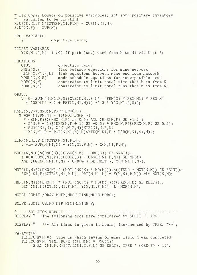
* fix upper bounds on positive variables; set some positive inventory* variables to be constantX.UP(N,N1,P,M)$XTE(N,N1,P,M) = XUF(N,N1,M);Z.UP(N.P) = ZUP(N);

FREE VARIABLEV objective value;

BINARY VARIABLEY(N,N1,P,M) 1 (0) if path (not) used from N to Nl via M at P;

EQUATIONSOBJV objective valueMNFB(N,P) flow balance equations for mine networkLINK(N,N1 ,P,M) link equations between mine and mode networksMDSK(N,M,G) mode schedule equations for incompatible arcsMDPG(N,M) constraint to limit total time that M is from NMDRG(N,M) constraint to limit total runs that M is from N;

OBJV. .

V =G= SUM((N,N1,P,M)$XTE(N,N1,P,M), (PRN(N) * PRN(Nl) * PRM(M)* (ORD(P) - 1 + PRT(N,N1,M))) ** 2 * Y(N,N1 ,P,M) );

MNFB(N,P)$(MNU(N,P) * DNO(N))..=G= (1$DN(N) - 1$(N0T DN(N)))* (Z(N,P)$((RHX(N,P) LE 0.5) AND (RHX(N,P) GE -1.5))- Z(N,P + 1)$(RHX(N,P + 1) GE -0.5) + RHX(N,P)$(RHX(N,P) GE 0.5))- SUM((N1,M), X(N1,N,P,M)$XTE(N1,N,P,M)- X(N,N1,P + PAR(N,N1,M),M)$XTE(N,N1,P + PAR(N,N1 ,M) ,M) );

LINK(N,N1,P,M)$XTE(N,N1,P,M). .

=L= XUP(N,N1,M) * Y(N,N1,P,M) - X(N,N1,P,M);

MDSK(N,M,G)$(DNO(N)$((LSG(N,M) - ORD(G)) GE NRLT))..1 =G= SUM((N1,P)$(((0RD(G) - GBG(N,N1 ,P,M) ) GE NRLT)AND ((GED(N,N1,P,M) - ORD(G)) GE NRLT)), Y(N,N1 ,P,M) );

MDPG(N,M)$((DNO(N) * (NOT (N0(N) * M0(M) ) ) )$( (TEND - MXT(N.M)) GE RELT)),SUM((N1,P)$XTE(N,N1,P,M), PRT(N,N1,M) * Y(N,N1,P,M)) =L= MXT(N,M);

MDRG(N,M)$((DNO(N) * (NOT (N0(N) * M0(M) ) ) )$(MXR(N,M) GE RELT))..SUM((N1,P)$XTE(N,N1,P

S M), Y(N,N1 S P,M)) =L= MXR(N,M);

MODEL SUMIT /OBJV ,MNFB,MDSK, LINK, MDPG.MDRG/;

SOLVE SUMIT USING MIP MINIMIZING V;

* SOLUTION REPORTDISPLAY " The following arcs were considered by SUMIT.", ARC;

DISPLAY " *** All times in given in hours, incremented by TPER. ***";

PARAMETERTIMECOMP(N,*) Time in which laying of mine field N was completed;TIMECOMP(N,*TIME.DONE')$(DN(N) * DNO(N))

= SMAX((N1,P,M)$(Y. L(N1,N,P,M) GE RELT), TPER * (ORD(P) - 1));

55

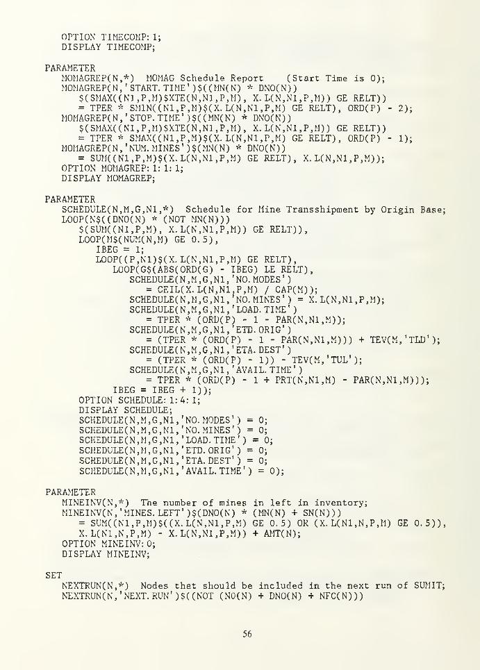
OPTION TIMECOMP: 1;

DISPLAY TIMECOMP;

PARAMETERMOMAGREP(N,*) MOMAG Schedule Report (Start Time is 0);MOMAGREP(N, ' START. TIME* )$((MN(N) * DNO(N))

$(SMAX((N1,P,M)$XTE(N,N1,P,M), X. L(N,N1 ,P,M) ) GE RELT))= TPER * SMIN((N1,P,M)$(X. L(N,N1,P,M) GE RELT), ORD(P) - 2);

MOMAGREP(N,' STOP. TIME') $((MN(N) * DNO(N))$(SMAX((N1,P,M)$XTE(N,N1,P,M), X. L(N,N1 ,P,M) ) GE RELT))= TPER * SMAX((N1,P,M)$(X. L(N,N1,F,M) GE RELT), ORD(P) - 1);

MOMAGREP(N, 'NUM. MINES' )$(MN(N) * DNO(N))= SUM((N1,P,M)$(X.L(N,N1,P,M) GE RELT), X. L(N,N1,P,M) );

OPTION MOMAGREP: 1: 1: 1;

DISPLAY MOMAGREP;

PARAMETERSCHEDULE(N,M,G,N1,*) Schedule for Mine Transshipment by Origin Base;L00P(N$((DN0(N) * (NOT MN(N)))

$(SUM((N1,P,M), X. L(N,N1,P,M)) GE RELT)),LOOP(M$(NUM(N,M) GE 0.5),

IBEG = 1;

L00P((P,N1)$(X. L(N,N1,P,M) GE RELT),LOOP(G$(ABS(ORD(G) - IBEG) LE RELT),

SCHEDULE(N,M,G,N1, 'NO. MODES'

)

= CEIL(X. L(N,N1,P,M1 / CAP(M));SCHEDULE(N,M,G,Nl, f

NO. MINES') = X. L(N,N1 ,P,M);SCHEDULE (N,M,G,N1 ,

'LOAD. TIME'

)

= TPER * (ORD(P) - 1 - PAR(N,N1,M));SCHEDULER, M,G,N1, 'ETD. ORIG' )

= (TPER * (0RD(P1 - 1 - PAR(N,N1,M))) + TEV(M, 'TLD' );

SCHEDULE(N,M,G,N1, 'ETA. DEST'

)

= (TPER * (ORD(F) - 1)) - TEV(M,'TUL');SCH£DULE(N,M,G,N1, 'AVAIL. TIME'

)

= TPER * (ORD(P) - 1 + PRT(N,N1,M) - PAR(N,N1 ,M) ));IBEG = IBEG + 1));

OPTION SCHEDULE: 1:4: 1;

DISPLAY SCHEDULE;SCHEDULE(N,M,G,N1,' NO. MODES') = 0;

SCHEDULE(N,M,G,N1, 'NO. MINES') = 0;

SCHEDULE(N,M,G,N1, 'LOAD. TIME') = 0;

SCHEDULE(N,M,G,N1,*ETD. ORIG') = 0;

SCHEDULE(N,M,G,N1, 'ETA. DEST') = 0;

SCHEDULE(N,M,G,N1,' AVAIL. TIME') = 0);

PARAMETERMINEINV(N,*) The number of mines in left in inventory;MINEINV(N, 'MINES. LEFT' )$(DNO(N) * (MN(N) + SN(N)))

= SUM((N1,P,M)$((X.L(N,N1,P,M) GE 0.5) OR (X. L(N1,N,P,M) GE 0.5)),X.L(N1,N,P,M) - X.L(N,N1,P,M)) + AMT(N);

OPTION MINEINV: 0;

DISPLAY MINEINV;

SETNEXTRUN(N,*) Nodes that should be included in the next run of SUMIT;NEXTRUN(N, 'NEXT. RUN') $( (NOT (N0(N) + DNO(N) + NFC(N)))

56

$((SMAX((N1,M)$ART(N,N1,M), ABS(NUM(N,M) ) ) GE 0.5)OR (AMT(N) LE -0.5))) = YES;

LOOP(I$((ABS(ORD(I) - 1) LE 0.5)AND (SUM(N$(NEXTRUN(N 'NEXT. RUN') * DN(N)), AMT(N)) LE -0.5)AND (SUM(N$NEXTRUN(N, 'NEXT. RUN'), 1) GE 0.5)),DISPLAY " Change NUM(N,M) and DN(N) to for all nodes not in ",

" NEXTRUN(N) and rerun SUMIT to finish the solution.", NEXTRUN;L00P(I1$((ABS(0RD(I1) - 1) LE 0.5)

AND (SUM(N$NEXTRUN(N, 'NEXT. RUN'), AMT(N)) LE -0.5)),AMT(N) = AMT(N)$NEXTRUN(N,' NEXT. RUN 1

);

OTTION AMT.-0;

DISPLAY "WARNING: There is not enough supply to meet demand ",

"for the next run of SUMIT.", AMT));

57

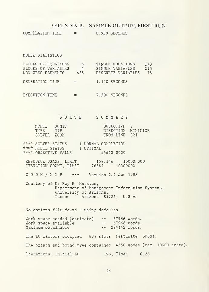
APPENDIX B. SAMPLE OUTPUT, FIRST RUNCOMPILATION TIME = 0. 950 SECONDS

MODEL STATISTICS

BLOCKS OF EQUATIONSBLOCKS OF VARIABLESNON ZERO ELEMENTS

GENERATION TIME

6 SINGLE EQUATIONS 1734 SINGLE VARIABLES 213

625 DISCRETE VARIABLES 78

1. 190 SECONDS

EXECUTION TIME 7.500 SECONDS

SOLVEMODEL SUMITTYPE MIPSOLVER ZOOM

**** SOLVER STATUS**** MODEL STATUS**** OBJECTIVE VALUE

RESOURCE USAGE, LIMITITERATION COUNT, LIMIT

SUMMARYOBJECTIVE VDIRECTION MINIMIZEFROM LINE 821

ZOOM/XMP

1 NORMAL COMPLETION1 OPTIMAL

45612. 0000

158. 146 10000. 00076589 10000000

Version 2. 1 Jun 1988

Courtesy of Dr Roy E. Marsten,Department of Management Information Systems,University of Arizona,Tucson Arizona 85721, U.S.A.

No options file found - using defaults.

Work space needed (estimate)Work space availableMaximum obtainable

67966 words.67966 words.

294142 words.

The LU factors occupied 804 slots (estimate 3068).

The branch and bound tree contained 4550 nodes (max. 10000 nodes).

Iterations: Initial LP 193, Time: 0.26

5S

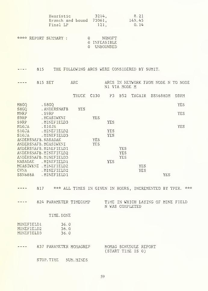
Heuristic 3214,Branch and bound 73061,Final LP 121,

8. 21149.45

0. 14

**** REPORT SUMMARY : NONOPTINFEASIBLEUNBOUNDED

815 THE FOLLOWING ARCS WERE CONSIDERED BY SUMIT.

815 SET ARC ARCS IN NETWORK FNl VIA MODE M

TRUCK C130 P3 B52 TACAIR

M8GQ . S8GQS8GQ . ANDERSNAFB YESM9RP . S9RPS9RP . MCASIWKNI YESS9RP . MINEFIELD3 YESM10JA .S10JAS10JA .MINEFIELD2 YESS10JA . MINEFIELD3 YESANDERSNAFB. NASADAK YESANDERSNAFB. MCASIWKNI YESANDERSNAFB. MINEFIELD1 YESANDERSNAFB. MINEFIELD2 YESANDERSNAFB. MINEFIELD3 YESNASADAK .MINEFIELD1 YESMCASIWKNI .MINEFIELD2 YESCVNA . MINEFIELD2 YESSSN688A .MINEFIELDl

YES

YES

YES

YES

817 *** ALL TIMES IN GIVEN IN HOURS, INCREMENTED BY TPER. ***

824 PARAMETER TIMECOMP TIME IN WHICH LAYING OF MINE FIELDN WAS COMPLETED

TIME. DONE

MINEFIELDlMINEFIELD2MINEFIELD3

36.036.

36.0

837 PARAMETER MOMAGREP

STOP. TIME NUM. MINES

MOMAG SCHEDULE REPORT(START TIME IS 0)

59

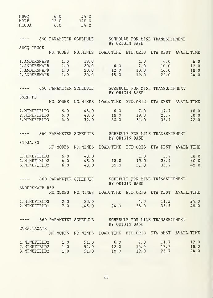
M8GQ 6.0 54.0M9RP 12.0 128.

M10JA 6.0 54.0

860 PARAMETER SCHEDULE

S8GQ. TRUCKNO. MODES NO. MINES

l.ANDERSNAFB 1.02.ANDERSNAFB 1.03.ANDERSNAFB 1.04. ANDERSNAFB 1.

SCHEDULE FOR MINE TRANSSHIPMENTBY ORIGIN BASE

INES LOAD. TIME ETD. ORIG ETA. DEST AVAIL. TIME

19.0 1.0 4.0 6.020.0 6.0 7.0 10.0 12.020.0 12.0 13.0 16.0 18.020. 18.0 19.0 22.0 24.0

S9RP. P3

860 PARAMETER SCHEDULE

NO. MODES NO. MINES

1.MINEFIELD3 6.02. MINEFIELD3 6.

3.MINEFIELD3 4.0

SCHEDULE FOR MINE TRANSSHIPMENTBY ORIGIN BASE

INES LOAD. TIME ETD. ORIG ETA. DEST AVAIL. TIME

48.0 6.0 7.0 11. 7 18.048. 18.0 19. 23. 7 30.032.0 30.0 31.0 35. 7 42.0

860 PARAMETER SCHEDULE

S10JA. P3

SCHEDULE FOR MINE TRANSSHIPMENTBY ORIGIN BASE

NO. MODES NO. MINES LOAD. TIME ETD. ORIG ETA. DEST AVAIL. TIME

1.MINEFIELD3 6.0 48.02.MINEFIELD2 6.0 48.03.MINEFIELD2 6.0 48.0

18.

30.0

1.019.031.0

5. 7

23.735. 7

18.030.042.0

860 PARAMETER SCHEDULE

ANDERSNAFB. B52NO. MODES NO. MINES

1.MINEFIELD3 2.0 23.02.MINEFIELD1 7.0 145.0

SCHEDULE FOR MINE TRANSSHIPMENTBY ORIGIN BASE

LOAD. TIME ETD. ORIG ETA. DEST AVAIL. TIME

24.0 28.011.535.5

24.048.

860 PARAMETER SCHEDULE

CVNA. TACAIR

SCHEDULE FOR MINE TRANSSHIPMENTBY ORIGIN BASE

NO. MODES NO. MINES LOAD. TIME ETD. ORIG ETA. DEST AVAIL. TIME

1.MINEFIELD2 1.0 51.0 6.0 7.0 11. 7 12.02.MINEFIELD2 1.0 51. 12.0 13. 17. 7 18.03.MINEFIELD2 1.0 51.0 18.0 19.0 23. 7 24.0

60

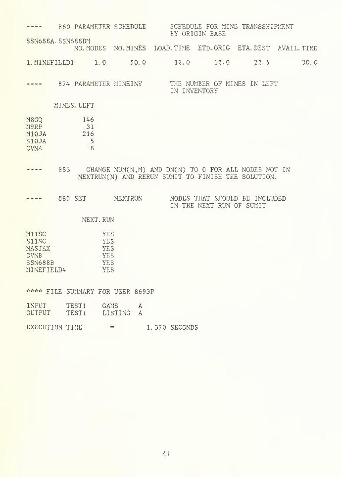
860 PARAMETER SCHEDULE SCHEDULE FOR MINE TRANSSHIPMENTBY ORIGIN BASE

SSN688A. SSN688DMNO. MODES NO. MINES LOAD. TIME ETD. ORIG ETA. DEST AVAIL. TIME

1.MINEFIELD1 1.0 50.0 12. 12.0 22. 5 30.

874 PARAMETER MINEINV THE NUMBER OF MINES IN LEFTIN INVENTORY

MINES. LEFT

M8GQ 146M9RP 31M10JA 216S10JA 5

CVNA 8

883 CHANGE NUM(N,M) AND DN(N) TO FOR ALL NODES NOT INNEXTRUN(N) AND RERUN SUMIT TO FINISH THE SOLUTION.

» mm m m 883 SET NEXTRUN

NEXT. RUN

M11SC YESS11SC YESNASJAX YESCVNB YESSSN688B YESMINEFIELD4 YES

NODES THAT SHOULD BE INCLUDEDIN THE NEXT RUN OF SUMIT

***ft FILE SUMMARY FOR USER 8693P

INPUTOUTPUT

TEST1TEST1

GAMS ALISTING A

EXECUTION TIME 1. 370 SECONDS

61

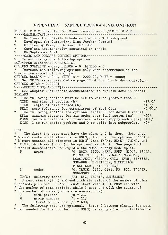
APPENDIX C. SAMPLE PROGRAM, SECOND RUN$TITLE * * * Scheduler for Mine Transshipment (SUMIT) * * ** DOCUMENTATION -

* Software to Optimize Schedules for Mine Transshipment* Developed for Commander, Mine Warfare Command* Written by Tammy L. Glaser, LT, USN* Complete documentation contained in thesis* 06 September 1991* GAMS AND DOLLARS CONTROL OPTIONS* Do not change the following options.$0FFUPPER OFFSYMXREF OFFSYMLISTOPTIONS SOLPRINT = OFF, LIMROW = 0, LIMCOL = 0;* Increase the following options only when recommended in the* solution report of the output.OPTIONS RESLIM = 10000, ITERLIM = 10000000, WORK = 10000;* Set OPTCR as recommended on page 72 of the thesis documentation.OPTIONS OPTCR = 0. 00001;* DEFINITIONS AND DATA* See Chapter 2 of thesis documentation to explain data in detail.SCALARS* The following scalars must be set to values greater than 0.

TEND end time of problem (h) /27. 0/TPER length of time period (h) /l. 2/RELT zero tolerance for comparisons of real data /0. 001/

* The following scalars are optional (enter for default value).MNLA minimum distance for air modes over land routes (run) /50/MXSS maximum distance for transfers between supply nodes (nm) /100/DISC 1 to run entire problem and to split into subproblems /0/;

SETS* The first two sets must have the element in them. Note that* N must contain all elements in CN(N), found in the optional section.* M must contain all elements in DM(M) (and TM(M), BM(M), CM(M), and* LM(M), which are found in the optional section). See page 7 of* thesis documentation to explain the MOMAG-supply node split.

N nodes /0, MSGQ, S8GQ, M9RP, S9RP, M10JA, S10JA,Ml ISC, SI ISC, ANDERSNAFB, NASADAK,MCASIWKNI, NASJAX, CVNA, CVNB , SSN688A,SSN688B, MINEFIELD1, MINEFIELD2,MINEFIELD3, MINEFIELD4/

M modes /0, TRUCK, C130, C141, P3, B52, TACAIR,SSN688DM, DBRM/

DM(M) delivery modes /P3, B52, TACAIR, SSN688DM/* P must start with and end with the value of the number of time* periods plus one. G and I must start with 1. G must end with* the number of time periods, while I must end with the square of* the number of nodes (nonzero elements in N).

P time periods /0 * 23/G group numbers /l * 22/I iteration numbers /l * 400/

* The following sets are optional. Enter between slashes for sets* not needed for the problem. If CN(N) is empty (i.e. , initialized to

62

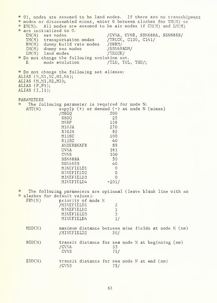
* 0), nodes are assumed to be land nodes. If there are no transshipment* modes or disassembled mines, enter between slashes for TM(M) or* BM(M). All modes are assumed to be air modes if CM(M) and LM(M)* are initialized to 0.

CN(N) sea nodes /CVNA, CVNB, SSN688A, SSN688B/TM(M) transportation modes /TRUCK, C130, C141/BM(M) dummy build rate modes /DBRM/CM(M) dummy sea modes /SSN688DM/LM(M) land modes /TRUCK/

* Do not change the following evolution set.

E mode evolution /TLD, TUL, TGD/;

* Do not change the following set aliases:ALIAS (N,N1,N2,N3,N4);ALIAS (M,M1,M2,M3);ALIAS (P,P1);ALIAS (1,11);

PARAMETERS* The following parameter is required for node N:

AMT(N) supply (+) or demand (-) at node N (mines)/M8GQ 200S8GQ 25M9RP 159M10JA 270S10JA 95M11SC 100S11SC 40ANDERSNAFB 89

CVNA 161CVNB 100SSN688A 50SSN688B 40MINEFIELD1MINEFIELD2MINEFIELD3MINEFIELD4 -201/

* The following parameters are optional (leave blank line with no,v slashes for default values):

PRN(N) priority of node N/MINEF1ELD1 2

MINEFIELD2 1

MINEF1ELD3 3

MINEFIELD4 1/

MXD(N) maximum distance between mine fields at node N (run)

/MINEFIELD2 50/

BGD(N) transit distance for sea node N at beginning (nm)/CVNA 33CVNB 75/

EDD(N) transit distance for sea node N at end (nm)/CVNB 75/

63

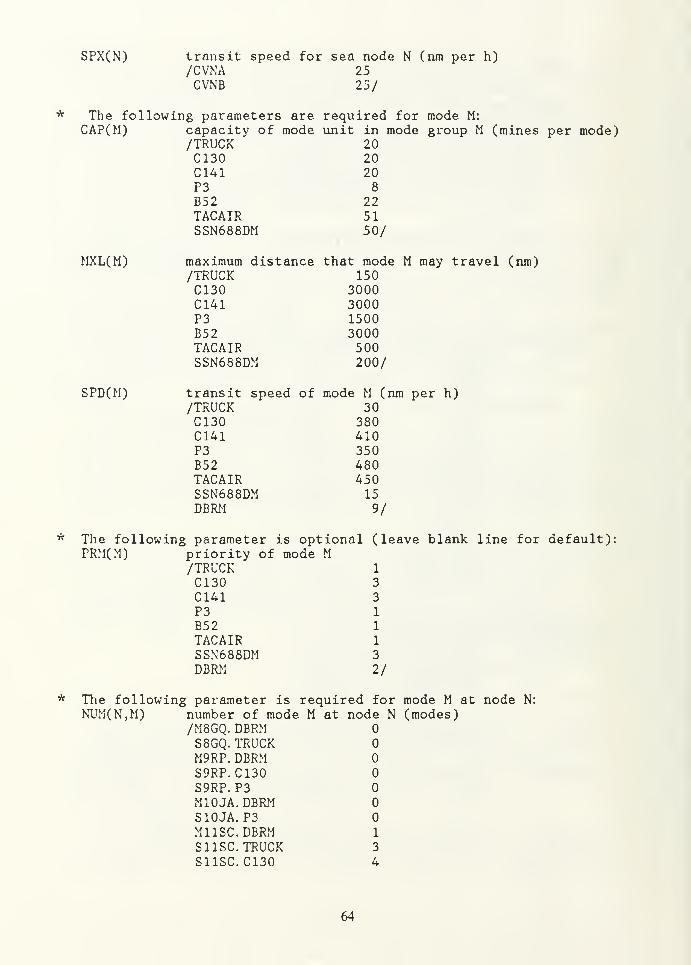
SPX(N) transit speed for sea node N (run per h)/CVNA 25CVNB 25/

* The following parameters are required for mode M:

CAP(M) capacity of mode unit in mode group M (mines per mode)/TRUCK

'

20C130 20C141 20P3 8

B52 22TACAIR 51SSN688DM 50/

MXL(M) maximum distance that mode M may travel (nm)/TRUCK 150C130 3000C141 3000P3 1500B52 3000TACAIR 500SSN688DM 200/

SPD(M) transit speed of mode M (nm per h)/TRUCK 30C130 380C141 410P3 350B52 480TACAIR 450SSN688DM 15

DBRM 9/

* The following parameter is optional (leave blank line for default):TRM(M)

NUM(N,M)

priority of mode M/TRUCK

'

1

C130 3

C141 3

P3 1

B52 1

TACAIR 1

SSN688DM 3

DBRM 2/

;parameter is required for mode M at node

number of mode M at node N (modes)/M8GQ. DBRMS8GQ. TRUCKM9RP. DBRMS9RP.C130S9RP. P3M10JA. DBRMS10JA. P3Ml ISC. DBRM 1

S11SC. TRUCK 3

S11SC.C130 4

64

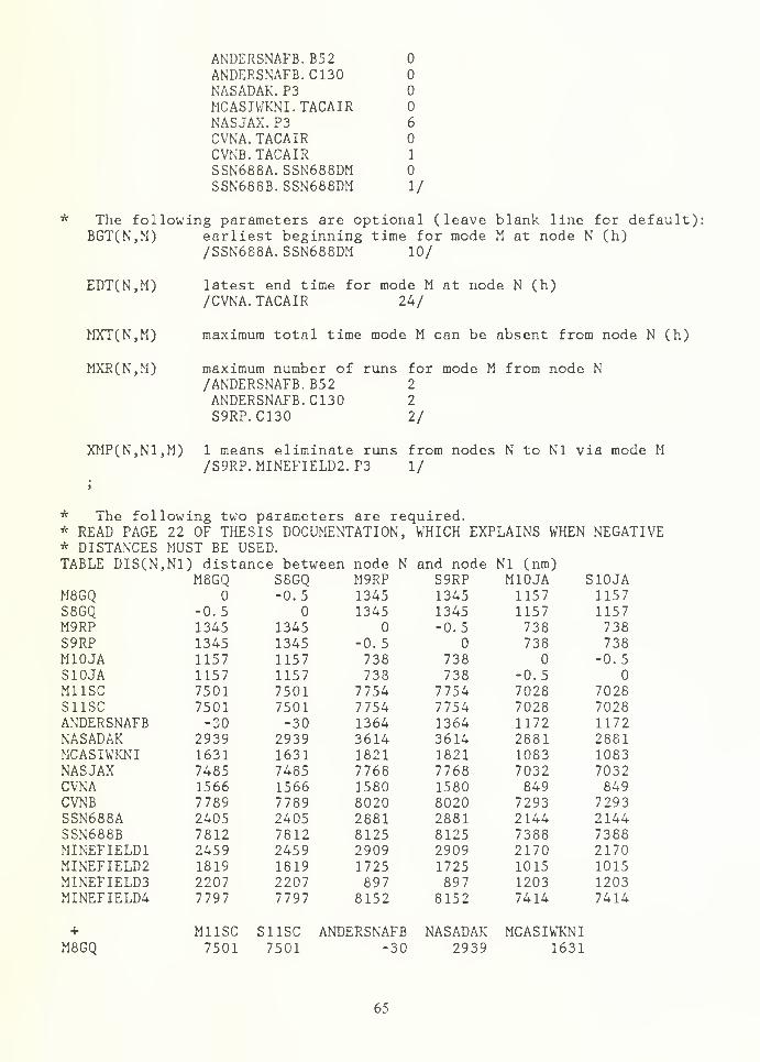
ANDERSNAFB. B52ANDERSNAFB. C130KASADAK. P3MCASIWKNI.TACAIRNASJAX. P3 6

CVNA. TACAIRCVNB. TACAIR 1

SSN688A. SSN688DMSSN688B. SSN688DM 1/

The following parameters are optional (leave blank line for default):BGT(N,M) earliest beginning time for mode M at node N (h)

/SSN688A. SSN688DM 10/

EDT(N.M) latest end time for mode M at node N (h)/CVNA. TACAIR 24/

MXT(N,M) maximum total time mode M can be absent from node N (h)

MXR(N,M) maximum number of runs for mode M from node N/ANDERSNAFB. B52 2

ANDERSNAFB. C 130 2

S9RP. C130 2/

XMP(N,N1,M) 1 means eliminate runs from nodes N to Nl via mode M/S9RP. MINEFIELD2.P3 1/

* The following two parameters are required.* READ PAGE 22 OF THESIS DOCUMENTATION, WHICH EXPLAINS WHEN NEGA* DISTANCES MUST BE USED.TABLE DIS(N,,N1) distance between node N and node Nl (nra)

M8GQ S8GQ M9RP S9RP M10JA 1510JAM8GQ -0.5 1345 1345 1157 1157S8GQ -0.5 1345 1345 1157 1157M9RP 1345 1345 -0.5 738 738S9RP 1345 1345 -0.5 738 738M10JA 1157 1157 738 738 -0.5S10JA 1157 1157 738 738 -0.5M11SC 7501 7501 7754 7754 7028 7028S11SC 7501 7501 7754 7754 7028 7028ANDERSNAFB -30 -30 1364 1364 1172 1172NASADAK 2939 2939 3614 3614 2881 2881MCASIWKNI 1631 1631 1821 1821 1083 1083NASJAX 7485 7485 7768 7768 7032 7032CVNA 1566 1566 1580 1580 849 849CVNB 7789 7789 8020 8020 7293 7293SSN688A 2405 2405 2881 2881 2144 2144SSN688B 7812 7812 8125 8125 7388 7388MINEFIELD1 2459 2459 2909 2909 2170 2170MINEFIELD2 1819 1819 1725 1725 1015 1015MINEFIELD3 2207 2207 897 897 1203 1203MINEFIELD4 7797 7797 8152 8152 7414 7414

+ M11SC SI ISC ANDERSNAFB NASADAK MCASIWKNIM8GQ 7501 7501 -30 2939 1631

65

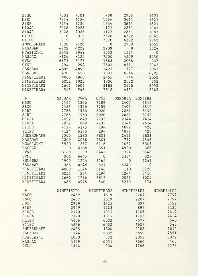
S8GQ 7501 7501 -30 2939 1631M9RP 7754 7754 1364 3614 1821S9RP 7754 7754 1364 3614 1821N10JA 7028 7028 1172 2881 1083SIOJA 7028 7028 1172 2881 1083M11SC -0.5 7520 4222 5942S11SC -0.5 7520 4222 5942ANDERSNAFB 7520 7520 2939 1653NASADAK 4222 4222 2939 1824MCASIWKNI 5942 5942 1653 1824NASJAX -124 -124 7500 4209 5950CVNA 6175 6175 1583 2088 267CVNB 294 294 7801 4511 5942SSN688A 4899 4899 2421 777 1067SSN688B 420 420 7831 4546 6305MINEFIELD1 4866 4866 2455 744 2053MINEFIELD2 6032 6032 1800 2032 352MINEFIELD3 7607 7607 2188 3850 2053MINEFIELD4 548 548 7812 4551 6305

+ NASJAX CVNA CVNB SSN688A SSN688BM8GQ 7485 1566 7789 2405 7812S8GQ 7485 1566 7789 2405 7812M9RP 7768 1580 8020 2881 8152S9RP 7768 1580 8020 2881 8152MIOJA 7032 849 7293 2144 7414SIOJA 7032 849 7293 2144 7414M11SC -124 6175 294 4899 420S11SC -124 6175 294 4899 420ANDERSNAFB 7500 1583 7801 2421 7831NASADAK 4209 2088 7801 777 4546MCASIWKNI 5950 267 6216 1067 6305NASJAX 6188 351 4900 366CVNA 6188 6445 1324 6546CVNB 366 6445 5164 327SSN688A 4900 1324 5164 5249SSN688B 366 6546 327 5249MINEFIELD1 4869 1344 5146 110 5220MINEFIELD2 6051 234 6294 1244 6413MINEFIELD3 7660 1786 7817 3073 8023MINEFIELD4 463 6578 500 5270 174

+ MINEFIELD1 MINEFIELD2 MINEFIELD3 MINEFIELD4M8GQ 2459 1819 2207 7797S8GQ 2459 1819 2207 7797M9RP 2909 1725 897 8152S9RP ;>909 1725 897 8152MIOJA 2170 1015 1203 7414SIOJA \>170 1015 1203 7414M11SC 4866 6032 7607 548S11SC 4866 6032 7607 548ANDERSNAFB 2455 1800 2188 7812NASADAK 744 2032 3850 4551MCASIWKNI :L090 352 2053 6332NASJAX 4869 6051 7660 463CVNA ;L344 234 1786 6578

66

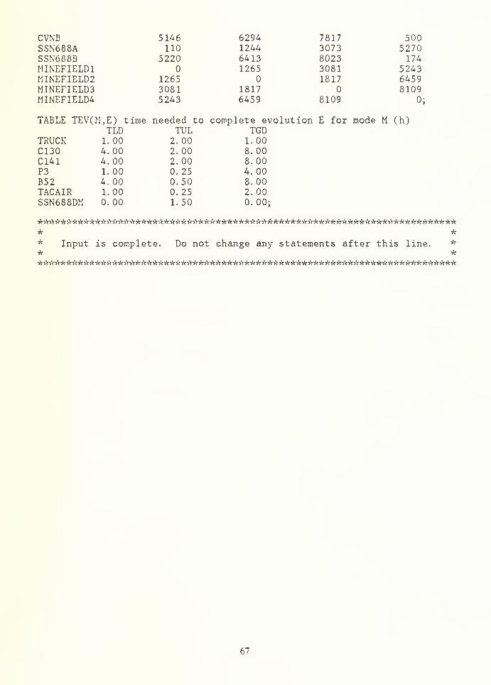
CVNB 5146 6294 7817 500SSN688A 110 1244 3073 5270SSN688B 5220 6413 8023 174MINEFIELD1 1265 3081 5243MINEFIELD2 1265 1817 6459MINEFIELD3 3081 1817 8109MINEFIELD4 5243 6459 8109 0;

TABLE TEV(M,E) time needed to complete evolution E for mode M (h)TLD TUL TGD

TRUCK 1. 00 2.00 1. 00C130 4.00 2.00 8.00C141 4.00 2.00 8.00P3 1.00 0.25 4. 00B52 4.00 0.50 8.00TACAIR 1.00 0.25 2. 00SSN688DM 0.00 1.50 0. 00;

* Input is complete. Do not change any statements after this line. *

*iYVoYyciYyc*yoY*}YyoY*iYVc*}YiYyrVc**yr*>Y**VcA:Y***iY***yo

67

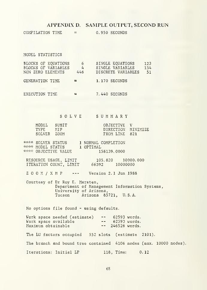
APPENDIX D. SAMPLE OUTPUT, SECOND RUNCOMPILATION TIME = 0. 950 SECONDS

MODEL STATISTICS

BLOCKS OF EQUATIONSBLOCKS OF VARIABLESNON ZERO ELEMENTS

GENERATION TIME

6 SINGLE EQUATIONS 1234 SINGLE VARIABLES 154

446 DISCRETE VARIABLES 51

1. 170 SECONDS

EXECUTION TIME 7.440 SECONDS

SOLVEMODEL SUMITTYPE MIPSOLVER ZOOM

**** SOLVER STATUS**** MODEL STATUS**** OBJECTIVE VALUE

RESOURCE USAGE, LIMITITERATION COUNT, LIMIT

SUMMARYOBJECTIVE VDIRECTION MINIMIZEFROM LINE 821

ZOOM/XMP

1 NORMAL COMPLETION1 OPTIMAL

158139. 0000

105.820 10000.00066392 10000000

Version 2. 1 Jun 1988

Courtesy of Dr Roy E. Marsten,Department of Management Information Systems,University of Arizona,Tucson Arizona 85721, U.S.A.

No options file found - using defaults.

Work space needed (estimate)Work space availableMaximum obtainable

62593 words.62593 words.

246526 words.

The LU factors occupied 552 slots (estimate 2101).

The branch and bound tree contained 4106 nodes (max. 10000 nodes),

Iterations: Initial LP 118, Time: 0.12

6S

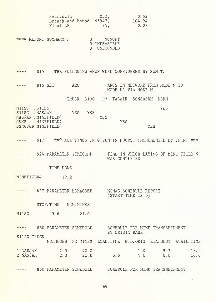
Heuristic 253, 0.62Branch and bound 65947, 104.94Final LP 74, 0.07

**** REPORT SUMMARY : N0N0PTINFEASIBLEUNBOUNDED

815 THE FOLLOWING ARCS WERE CONSIDERED BY SUMIT.

815 SET ARC ARCS IN NETWORK FROM NODE N TONODE Nl VIA MODE M

TRUCK C130 P3 TACAIR SSN688DM DBRM

M11SC .S11SC YESSI ISC .NASJAX YES YESNASJAX .MINEFIELD4 YESCVNB . MINEFIELD4 YESSSN688B.MINEFIELD4 YES

817 *** ALL TIMES IN GIVEN IN HOURS, INCREMENTED BY TPER. ***

824 PARAMETER TIMECOMP TIME IN WHICH LAYING OF MINE FIELD NWAS COMPLETED

TIME. DONE

MINEFIELD4 19. 2

837 PARAMETER MOMAGREP MOMAG SCHEDULE REPORT(START TIME IS 0)

STOP. TIME NUM. MINES

M11SC 3.6 21.0

860 PARAMETER SCHEDULE SCHEDULE FOR MINE TRANSSHIPMENTBY ORIGIN BASE

SI ISC. TRUCKNO. MODES NO. MINES LOAD. TIME ETD. ORIG ETA. DEST AVAIL. TIME

1. NASJAX 2.0 40.0 1.0 5.2 13.22. NASJAX 2.0 21.0 3.6 4.6 8.8 16.8

860 PARAMETER SCHEDULE SCHEDULE FOR MINE TRANSSHIPMENT

6')

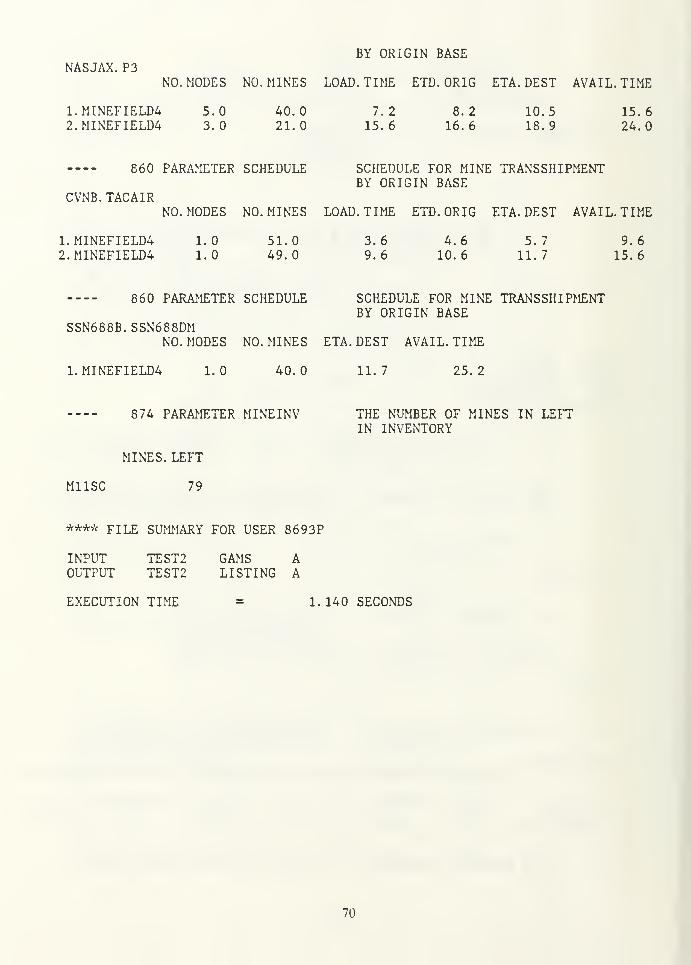
BY ORIGIN BASENASJAX. P3

NO. MODES NO. MINES LOAD. TIME ETD. ORIG ETA. DEST AVAIL. TIME

1.MINEFIELD4 5.0 40.0 7.2 8.2 10.5 15.62.MINEFIELD4 3.0 21.0 15.6 16.6 18.9 24.0

860 PARAMETER SCHEDULE SCHEDULE FOR MINE TRANSSHIPMENTBY ORIGIN BASE

CVNB. TACAIRNO. MODES NO. MINES LOAD. TIME ETD. ORIG ETA. DEST AVAIL. TIME

1.MINEFIELD4 1.0 51.0 3.6 4.6 5.7 9.62.MINEFIELD4 1.0 49.0 9.6 10.6 11.7 15.6

860 PARAMETER SCHEDULE SCHEDULE FOR MINE TRANSSHIPMENTBY ORIGIN BASE

SSN688B. SSN688DMNO. MODES NO. MINES ETA. DEST AVAIL. TIME

1.MINEFIELD4 1.0 40.0 11.7 25.2

874 PARAMETER MINEINV THE NUMBER OF MINES IN LEFTIN INVENTORY

MINES. LEFT

M11SC 79

**** file SUMMARY FOR USER 8693P

INPUT TEST2 GAMS AOUTPUT TEST2 LISTING A

EXECUTION TIME = 1. 140 SECONDS

70

APPENDIX E. GAMS IMPLEMENTATION OF SUMIT

A. SUMIT OUTPUTThe output of SUMIT is composed of standard GAMS reports and of data dis-

played by the program. The standard GAMS reports include an echo print of the pro-

gram, compilation time, model statistics (i.e., number of constraints and continuous and

discrete variables), and solve summary. The echo print of the program was deleted from

Appendix B since the program is given in Appendix A. The data output by SUMIT was

also edited to make Appendix B fit within the page margins. The data displayed by the

program include the arcs generated for the mine network (which has the same arcs as the

mode network), the time in which the mine field deployment was complete, the

MOMAG schedule report, the schedules for mine transshipment, the mine inventory at

the end of the problem, and the nodes that should be included in the next run of

SUMIT. SUMIT prints out the mine network to allow the user to verify that all arcs

in the mine and mode networks are appropriate. The MOMAG schedule report con-

tains the times in which each MOMAG must start and stop assembling mines and the

number of mines that each MOMAG must build. SUMIT then prints out separate mine

transshipment schedules for each origin node that reports the following information:

origin node, mode group, run number for the node-mode combination, destination node,

total number of mines carried by the mode group, number of mode units needed, the

time to start loading the mode group, estimated time of departure from the origin node,

estimated time of arrival at the destination node, and the time in which the mode is

available for loading for its next flight. It also warns the user if total supply is less than

total demand for nodes recommended in the next run.

B. END TIME AND TIME PERIOD LENGTH

To find appropriate values for the end time and time period length for a new prob-

lem, the user should take the following steps: the user should initially execute GAMSusing the relaxed version of ZOOM, which is faster since it allows binary variables as-

sume any values between zero and one. To indicate the relaxed version of ZOOM, the

user must change the problem identifier "MIP" to "RMIP" in the "SOLVE" statement,

which is found on line 821 of the program (see Appendix A, page 55). The goal of

making these quick runs is to identify the latest end time with an appropriate number

of periods in which the solver reports an infeasible solution ("INFEASIBLE") in the

71

section of the output labeled "SOLUTION REPORT." Then, the user should run

SUM IT using an end time equal to the latest infcasible end time plus one extra time

period with binary requirements enforced (replacing "RMIP" with "MIP" in the

"SOLVE" statement). In most cases, adding an extra time period will make the solution

feasible. If the problem is not feasible when the binary variables are enforced, the

"SOLUTION REPORT" portion of the output will contain the phrase "INTEGER

INFEAS1BLE". If the solution is integer infeasible, the user should first verify that

there is enough supply to meet the demand for the mine network output by the SUM IT.

If the supply is sufficient, then the user should rerun the "MIP" version ofZOOM after

increasing the end time by one extra time period until a feasible solution is found. Since

the purpose of these final runs is to find the first integer feasible solution, the user may

set the OPTCR at 1.0 to find the solution as quickly as possible.

C. OBTAINING NEARLY OPTIMAL SOLUTIONS

A general rule of thumb is recommended to obtain nearly optimal solutions for

SUM IT. When the user makes the first run of the "MIP" version of ZOOM, the user

should set OPTCR equal to 0.10 in line 16 of the program, rerun SUMIT, and verify that

the reported solution is satisfactory. If the number of iterations is less than 10,000,

which is given in the "SOLUTION REPORT" portion of the output indicated by "IT-

ERATION COUNT", rerunning SUMIT with a very small OPTCR, such as 0.01, will

probably yield an optimal solution within a reasonable number of iterations, but will not

usually prove it. If the number of iterations is greater than 10,000, the user may rerun

SUMIT at an OPTCR between 0.01 and 0.1 to find a solution that is optimal or close

to optimal, but not proven. Proving optimality by using an OPTCR less than 0.01 is

not recommended since this may result in an excessive solution time and excessive disk

storage requirements.

72

LIST OF REFERENCES

1. Bevins, M. J., "System Specification and Design for the Geo-operational Planning

and Assessment System (GOPAS)", Commander, Mine Warfare Command, Naval

Base Charleston, SC 24908, 01 March 1990 (Revision 1).

2. NA VSEA Mine Familiarizer, Naval Mine Warfare Engineering Activity, Yorktown,

VA 23691, 1985.

3. Wingate, J. W. and Zakary, C. W., Network Modeling and Linear Programming

Methods for Mine Field Logistic Planning, NSWC TR 87-214, Research and Tech-

nology Department, Naval Surface Warfare Center, Dahlgren, VA 22448, 29 Feb-

ruary 1988.

4. Collier, K. S., Deployment Planning: A Linear Programming Model with Variable

Reduction, M.S. Thesis in Operations Research, Naval Postgraduate School,

Monterey, CA 93943, September 1987.

5. Lally, M. J., Strategic Allocation of Sealift: A GAMS-based Integer Programming

Approach, M.S. Thesis in Operations Research, Naval Postgraduate School,

Monterey, CA 93943, September 1987.

6. Puntenney, M. C, Optimization Models for Military Aircraft Deployment, M.S.

Thesis in Operations Research, Naval Postgraduate School, Monterey, CA 93943,

March 1989.

7. Brooke, A., Kendrick, D., and Meeraus, A., GAMS, A User's Guide, The Scientific

Press, 1988.

8. Bazaraa, M. S., Jarvis, J. J., and Sherali, H. D., Linear Programming and Network

Flows, second edition, John Wiley & Sons, Inc., 1990.

73

9. Lawler, E., Combinatorial Optimization: Networks and Matroids, Holt, Rinehart,

and Winston, 1976.

74

INITIAL DISTRIBUTION LIST

No. Copies

1. Defense Technical Information Center 2

Cameron Station

Alexandria, VA 22304-6145

2. Library, Code 52 2

Naval Postgraduate SchoolMonterey, CA 93943-5002

3. Commander, Mine Warfare Command 3

ATTN: N3Naval Base Charleston, SC 29408

4. Tammy L. Glaser, LT, USN 2

Navy Recruiting District New Orleans440 bauphine Street

New Orleans, LA 70146

5. Professor R. Kevin Wood, Code OR/Wd 4Department of Operations ResearchNaval Postgraduate SchoolMonterey, CA 93943

6. Professor Robert F. Dell, Code OR/De 1

Department of Operations ResearchNaval Postgraduate SchoolMonterey, CA 93943

7. Professor Richard E. Rosenthal, Code OR/Ri 1

Department of Operations ResearchNaval Postgraduate SchoolMonterev, CA 93943

75

ThesisG45655 Glaser

c.l A single-commodity minetransshipment problem.