Embed Size (px)
Citation preview
Université de Franche-Comté
École Doctorale Carnot-Pasteur(ED CP n 554)
PhD Thesis
presented by
Ashok Kumar VERMA
Improvement of the planetary
ephemerides using spacecraft
navigation data and its application to
fundamental physics
directed by Agnes Fienga
19th September 2013
Jury :
Président : Veronique Dehant ROB, Belgium
Rapporteurs : Gilles Metris OCA, France
Richard Biancale CNES, France
Examinateurs : Jacques Laskar IMCCE, France
Luciano Iess University of Rome, Italy
Veronique Dehant ROB, Belgium
Jose Lages UFC, France
Directeur: Agnes Fienga OCA, France

2
3
Acknowledgements
Foremost, I would like to express my sincere gratitude to my advisor Dr. Agnes Fienga for thecontinuous support of my Ph.D study and research, for her patience, motivation, enthusiasm,and immense knowledge. Her guidance helped me in all the time of research, and writing ofscientific papers and this thesis. I could not have imagined having a better advisor and mentorfor my Ph.D study.
I would like to acknowledge the financial support of the French Space Agency (CNES) andRegion Franche-Comte. Part of this thesis was made using the GINS software; I would like toacknowledge CNES, who provided us access to this software. I am also grateful to J.C Marty(CNES) and P. Rosenbatt (Royal Observatory of Belgium) for their support in handling theGINS software.
I would also like to thanks Observatoire de Besancon, UTINAM for providing me a libraryand computer facilities of the lab to pursue this study. I am grateful to all respective faculties,staff and colleagues of the lab for their direct and indirect contributions to made my stay fruitfuland pleasant.
Needless to say, my Besancon years would not have been as much fun without the companyof my friends, Arvind Rajpurohit, Eric Grux and Andre Martins. Without their support and love,I could not have imagined my successful stay at Besancon. And at last but not least, I am happythat the distance to my family and my friends back home has remained purely geographical. Iwish to thank my family for their love and support which provided my inspiration and was mydriving force. I owe them everything and wish I could show them just how much I love andappreciate them.

4 Acknowledgements
5
Abstract
The planetary ephemerides play a crucial role for spacecraft navigation, mission planning, re-duction and analysis of the most precise astronomical observations. The construction of suchephemerides is highly constrained by the tracking observations, in particular range, of the spaceprobes collected by the tracking stations on the Earth. The present planetary ephemerides (DE,INPOP, EPM) are mainly based on such observations. However, the data used by the planetaryephemerides are not the direct raw tracking data, but measurements deduced after the analysisof raw data made by the space agencies and the access to such processed measurements remainsdifficult in terms of availability.
The goal of the thesis is to use archives of past and present space missions data indepen-dently from the space agencies, and to provide data analysis tools for the improvement of theplanetary ephemerides INPOP, as well as to use improved ephemerides to perform tests ofphysics such as general relativity, solar corona studies, etc.
The first part of the study deals with the analysis of the Mars Global Surveyor (MGS)tracking data as an academic case for understanding. The CNES orbit determination softwareGINS was used for such analysis. The tracking observations containing one-, two-, and three-way Doppler and two-way range are then used to reconstruct MGS orbit precisely and obtainedresults are consistent with those published in the literature. As a supplementary exploitationof MGS, we derived the solar corona model and estimated the average electron density alongthe line of sight separately for slow and fast wind regions. Estimated electron densities arecomparable with the one found in the literature. Fitting the planetary ephemerides, includingadditional data which were corrected for the solar corona perturbations, noticeably improves theextrapolation capability of the planetary ephemerides and the estimation of the asteroid masses(Verma et al., 2013a).
The second part of the thesis deals with the complete analysis of the MESSENGER trackingdata. This analysis improved the Mercury ephemeris up to two order of magnitude comparedto any latest ephemerides. Such high precision ephemeris, INPOP13a, is then used to performgeneral relativity tests of PPN-formalism. Our estimations of PPN parameters (β and γ) are themost stringent than previous results (Verma et al., 2013b).

6 Abstract
7
Résumé
Les éphémérides planétaires jouent un role crucial pour la navigation des missions spatialesactuelles et la mise en place des missions futures ainsi que la réduction et l’analyse des ob-servations astronomiques les plus précises. La construction de ces éphémérides est fortementcontrainte par les observations de suivi des sondes spatiales collectées par les stations de suivisur la Terre. Les éphémérides planétaires actuelles (DE, INPOP, EPM) sont principalementbasées sur ces observations. Toutefois, les données utilisées par les éphémérides planétairesne sont pas issues directement des données brutes du suivi, mais elles dépendent de mesuresdéduites après l’ analyse des données brutes. Ces analyses sont faites par les agences spatialeset leur accès demeure difficile en terme de disponibilité.
L’objectif de la thèse est d’utiliser des archives de données de missions spatiales passéeset présentes et de fournir des outils d’analyse de données pour l’amélioration de l’éphémérideplanétaire INPOP, ainsi que pour une meilleure utilisation des éphémérides pour effectuer destests de la physique tels que la relativité générale, les études de la couronne solaire, etc.
La première partie de l’étude porte sur l’analyse des données de suivi de la sonde MarsGlobal Surveyor (MGS) prise comme un cas d’école pour la compéhension de l’observable.Le logiciel du CNES pour la détermination d’orbite GINS a été utilisé pour une cette analyse.Les résultats obtenus sont cohérents avec ceux publiés dans la littérature. Comme exploitationsupplémentaire des données MGS, nous avons étudié des modèles de couronne solaire et estiméla densité moyenne d’électrons le long de la ligne de visée séparément pour les zones de ventssolaires lents et rapides. Les densités électroniques estimées sont comparables à celles que l’ontrouve dans la littérature par d’autres techniques. L’ajout dans l’ajustement des éphéméridesplanétaires des données qui ont été corrigées pour les perturbations de plasma solaire, amélioresensiblement la capacité d’extrapolation des éphémérides planétaires et l’estimation des massesd’astéroides (Verma et al., 2013a).
La deuxième partie de la thèse traite de l’analyse complète des données de suivi d’une sondeactuellement en orbite autour de Mercure, Messenger. Cette analyse a amélioré les éphéméridesde Mercure jusqu’à deux ordres de grandeur par rapport à toutes les dernières éphémérides. Lanouvelle éphéméride de haute précision, INPOP13a, est ensuite utilisée pour effectuer des testsde la relativité générale via le formalisme PPN. Nos estimations des paramètres PPN (γ et β)donnent de plus fortes contraintes que les résultats antérieurs (Verma et al., 2013b).

8 Resume
9
Contents
Contents 9
List of figures 13
List of tables 17
Acronyms 19
1. Introduction 1
1.1. Introduction to planetary ephemerides . . . . . . . . . . . . . . . . . . . . . . 11.2. INPOP . . . . . . . . . . . . . . . . . . . . . . . . . . . . . . . . . . . . . . . 3
1.2.1. INPOP construction . . . . . . . . . . . . . . . . . . . . . . . . . . . 31.2.2. INPOP evolution . . . . . . . . . . . . . . . . . . . . . . . . . . . . . 5
1.3. Importances of the direct analysis of radioscience data for INPOP . . . . . . . 8
2. The radioscience observables and their computation 13
2.1. Introduction . . . . . . . . . . . . . . . . . . . . . . . . . . . . . . . . . . . . 132.2. The radioscience experiments . . . . . . . . . . . . . . . . . . . . . . . . . . . 14
2.2.1. Planetary atmosphere . . . . . . . . . . . . . . . . . . . . . . . . . . . 152.2.2. Planetary gravity . . . . . . . . . . . . . . . . . . . . . . . . . . . . . 152.2.3. Solar corona . . . . . . . . . . . . . . . . . . . . . . . . . . . . . . . 162.2.4. Celestial mechanics . . . . . . . . . . . . . . . . . . . . . . . . . . . . 17
2.3. Radiometric data . . . . . . . . . . . . . . . . . . . . . . . . . . . . . . . . . 182.3.1. ODF contents . . . . . . . . . . . . . . . . . . . . . . . . . . . . . . . 18
2.3.1.1. Group 1 . . . . . . . . . . . . . . . . . . . . . . . . . . . . 182.3.1.2. Group 2 . . . . . . . . . . . . . . . . . . . . . . . . . . . . 192.3.1.3. Group 3 . . . . . . . . . . . . . . . . . . . . . . . . . . . . 19
2.3.1.3.1. Time-tags . . . . . . . . . . . . . . . . . . . . . . 192.3.1.3.2. Format IDs . . . . . . . . . . . . . . . . . . . . . 192.3.1.3.3. Observables . . . . . . . . . . . . . . . . . . . . . 20
2.3.1.4. Group 4 . . . . . . . . . . . . . . . . . . . . . . . . . . . . 232.3.1.4.1. Ramp tables . . . . . . . . . . . . . . . . . . . . . 24
2.3.1.5. Group 5 . . . . . . . . . . . . . . . . . . . . . . . . . . . . 252.3.1.6. Group 6 . . . . . . . . . . . . . . . . . . . . . . . . . . . . 252.3.1.7. Group 7 . . . . . . . . . . . . . . . . . . . . . . . . . . . . 25
2.4. Observation Model . . . . . . . . . . . . . . . . . . . . . . . . . . . . . . . . 25

10 Contents
2.4.1. Time scales . . . . . . . . . . . . . . . . . . . . . . . . . . . . . . . . 262.4.1.1. Universal Time (UT or UT1) . . . . . . . . . . . . . . . . . 262.4.1.2. Coordinated Universal Time (UTC) . . . . . . . . . . . . . . 262.4.1.3. International Atomic Time (TAI) . . . . . . . . . . . . . . . 272.4.1.4. Terrestrial Time (TT) . . . . . . . . . . . . . . . . . . . . . 282.4.1.5. Barycentric Dynamical Time (TDB) . . . . . . . . . . . . . 28
2.4.2. Light time solution . . . . . . . . . . . . . . . . . . . . . . . . . . . . 302.4.2.1. Time conversion . . . . . . . . . . . . . . . . . . . . . . . . 312.4.2.2. Down-leg τU computation . . . . . . . . . . . . . . . . . . . 312.4.2.3. Up-leg τU computation . . . . . . . . . . . . . . . . . . . . 332.4.2.4. Light time corrections, δτD and δτU . . . . . . . . . . . . . . 33
2.4.2.4.1. Relativistic correction δτRC . . . . . . . . . . . . . 332.4.2.4.2. Solar Corona correction δτS C . . . . . . . . . . . . 342.4.2.4.3. Media corrections δτMC . . . . . . . . . . . . . . . 34
2.4.2.5. Total light time delay . . . . . . . . . . . . . . . . . . . . . 352.4.2.5.1. Round-trip delay . . . . . . . . . . . . . . . . . . 352.4.2.5.2. One-way delay . . . . . . . . . . . . . . . . . . . 35
2.4.3. Doppler and range observables . . . . . . . . . . . . . . . . . . . . . . 362.4.3.1. Two-way (F2) and Three-way (F3) Doppler . . . . . . . . . . 37
2.4.3.1.1. Ramped . . . . . . . . . . . . . . . . . . . . . . . 372.4.3.1.2. Unramped . . . . . . . . . . . . . . . . . . . . . . 39
2.4.3.2. One-way (F1) Doppler . . . . . . . . . . . . . . . . . . . . . 402.4.3.3. Two-way (ρ2,3) Range . . . . . . . . . . . . . . . . . . . . . 41
2.5. GINS: orbit determination software . . . . . . . . . . . . . . . . . . . . . . . 432.5.1. Dynamic model . . . . . . . . . . . . . . . . . . . . . . . . . . . . . . 44
2.5.1.1. Gravitational forces . . . . . . . . . . . . . . . . . . . . . . 442.5.1.1.1. Gravitational potential . . . . . . . . . . . . . . . 452.5.1.1.2. Solid planetary tides . . . . . . . . . . . . . . . . . 462.5.1.1.3. Sun, Moon and planets perturbation . . . . . . . . 472.5.1.1.4. General relativity . . . . . . . . . . . . . . . . . . 48
2.5.1.2. Non-Gravitational forces . . . . . . . . . . . . . . . . . . . 492.5.1.2.1. Solar radiation pressure . . . . . . . . . . . . . . . 502.5.1.2.2. Atmospheric drag and lift . . . . . . . . . . . . . . 512.5.1.2.3. Thermal radiation . . . . . . . . . . . . . . . . . . 532.5.1.2.4. Albedo and infrared radiation . . . . . . . . . . . 542.5.1.2.5. Motor burn . . . . . . . . . . . . . . . . . . . . . 55
2.5.2. Variational equations . . . . . . . . . . . . . . . . . . . . . . . . . . . 562.5.3. Parameter estimation . . . . . . . . . . . . . . . . . . . . . . . . . . . 57
3. Mars Global Surveyor: Radioscience data analysis 61
3.1. Introduction . . . . . . . . . . . . . . . . . . . . . . . . . . . . . . . . . . . . 613.2. Mission overview . . . . . . . . . . . . . . . . . . . . . . . . . . . . . . . . . 62
3.2.1. Mission design . . . . . . . . . . . . . . . . . . . . . . . . . . . . . . 623.2.2. Spacecraft geometry . . . . . . . . . . . . . . . . . . . . . . . . . . . 633.2.3. Radioscience data . . . . . . . . . . . . . . . . . . . . . . . . . . . . . 65
Contents 11
3.3. Orbit determination . . . . . . . . . . . . . . . . . . . . . . . . . . . . . . . . 663.3.1. Data processing and dynamic modeling . . . . . . . . . . . . . . . . . 673.3.2. Solve-for parameters . . . . . . . . . . . . . . . . . . . . . . . . . . . 68
3.4. Orbit computation results . . . . . . . . . . . . . . . . . . . . . . . . . . . . . 693.4.1. Acceleration budget . . . . . . . . . . . . . . . . . . . . . . . . . . . 693.4.2. Doppler and range postfit residuals . . . . . . . . . . . . . . . . . . . . 713.4.3. Orbit overlap . . . . . . . . . . . . . . . . . . . . . . . . . . . . . . . 733.4.4. Estimated parameters . . . . . . . . . . . . . . . . . . . . . . . . . . . 74
3.4.4.1. FS and FD scale factors . . . . . . . . . . . . . . . . . . . . 743.4.4.2. DSN station position and ephemeris bias . . . . . . . . . . . 75
3.5. Supplementary investigations . . . . . . . . . . . . . . . . . . . . . . . . . . . 773.5.1. GINS solution vs JPL Light time solutions . . . . . . . . . . . . . . . 773.5.2. Box-Wing macro-model vs Spherical macro-model . . . . . . . . . . . 79
3.6. Conclusion and prospectives . . . . . . . . . . . . . . . . . . . . . . . . . . . 82
4. Solar corona correction of radio signals and its application to planetary ephemeris 85
4.1. Introduction . . . . . . . . . . . . . . . . . . . . . . . . . . . . . . . . . . . . 854.2. The solar cycle . . . . . . . . . . . . . . . . . . . . . . . . . . . . . . . . . . 86
4.2.1. Magnetic field of the Sun . . . . . . . . . . . . . . . . . . . . . . . . . 864.2.2. Sunspots . . . . . . . . . . . . . . . . . . . . . . . . . . . . . . . . . 884.2.3. Solar maxima . . . . . . . . . . . . . . . . . . . . . . . . . . . . . . . 884.2.4. Solar minima . . . . . . . . . . . . . . . . . . . . . . . . . . . . . . . 88
4.3. The solar wind . . . . . . . . . . . . . . . . . . . . . . . . . . . . . . . . . . 894.3.1. Fast solar wind . . . . . . . . . . . . . . . . . . . . . . . . . . . . . . 894.3.2. Slow solar wind . . . . . . . . . . . . . . . . . . . . . . . . . . . . . . 90
4.4. Radio signal perturbation . . . . . . . . . . . . . . . . . . . . . . . . . . . . . 914.5. Solar corona correction of radio signals and its application to planetary ephemeris 924.6. Conclusion . . . . . . . . . . . . . . . . . . . . . . . . . . . . . . . . . . . . 984.7. Verma et al. (2013a) . . . . . . . . . . . . . . . . . . . . . . . . . . . . . . . . 98
5. Improvement of the planetary ephemeris and test of general relativity with MES-
SENGER 117
5.1. Introduction . . . . . . . . . . . . . . . . . . . . . . . . . . . . . . . . . . . . 1175.2. MESSENGER data analysis . . . . . . . . . . . . . . . . . . . . . . . . . . . 119
5.2.1. Mission design . . . . . . . . . . . . . . . . . . . . . . . . . . . . . . 1195.2.2. Spacecraft geometry . . . . . . . . . . . . . . . . . . . . . . . . . . . 1205.2.3. Radioscience data . . . . . . . . . . . . . . . . . . . . . . . . . . . . . 1225.2.4. Dynamical modeling and orbit determination processes . . . . . . . . . 122
5.3. Orbit determination . . . . . . . . . . . . . . . . . . . . . . . . . . . . . . . . 1245.3.1. Acceleration budget . . . . . . . . . . . . . . . . . . . . . . . . . . . 1245.3.2. Significance of MESSENGER observation for INPOP . . . . . . . . . 1265.3.3. Evolution of INPOP with the accuracy of MESSENGER orbit . . . . . 128
5.3.3.1. Case I: First guess orbit for Messenger and INPOP12a . . . . 1295.3.3.1.1. Description . . . . . . . . . . . . . . . . . . . . . 1295.3.3.1.2. Results . . . . . . . . . . . . . . . . . . . . . . . . 130

12 Contents
5.3.3.2. Case II: New Mercury orientation model and INPOP12b . . . 1305.3.3.2.1. Description . . . . . . . . . . . . . . . . . . . . . 1305.3.3.2.2. Results . . . . . . . . . . . . . . . . . . . . . . . . 132
5.3.3.3. Case III: Group delay and INPOP12c . . . . . . . . . . . . . 1345.3.3.3.1. Description . . . . . . . . . . . . . . . . . . . . . 1345.3.3.3.2. Results . . . . . . . . . . . . . . . . . . . . . . . . 135
5.3.3.4. Case IV: New gravity field HgM002 and INPOP12d . . . . . 1355.3.3.4.1. Description . . . . . . . . . . . . . . . . . . . . . 1355.3.3.4.2. Results . . . . . . . . . . . . . . . . . . . . . . . . 136
5.3.3.5. Case V: Extension of the mission and INPOP13a . . . . . . . 1385.3.3.5.1. Description . . . . . . . . . . . . . . . . . . . . . 1385.3.3.5.2. Results . . . . . . . . . . . . . . . . . . . . . . . . 1385.3.3.5.3. Comparisons . . . . . . . . . . . . . . . . . . . . 1405.3.3.5.4. INPOP13a ephemeris . . . . . . . . . . . . . . . . 141
5.4. Verma et al. (2013b) . . . . . . . . . . . . . . . . . . . . . . . . . . . . . . . 142
6. General conclusions 157
Publications 161
Bibliographie 163

13
List of Figures
1.1. Schematic diagram for the procedure of the INPOP construction. . . . . . . . . 41.2. Percentage contribution of the data in the INPOP construction. . . . . . . . . . 51.3. Percentage contribution of each data type used in the construction INPOP series
(Fienga, 2011). . . . . . . . . . . . . . . . . . . . . . . . . . . . . . . . . . . 61.4. Extrapolation capability of the planetary ephemerides: INPOP08 (Fienga et al.,
2008), INPOP10a (Fienga et al., 2011a), and INPOP10b (Fienga et al., 2011b). 8
2.1. Two- or three-way radio wave propagation between a spacecraft and Deep SpaceNetwork (DSN) station. . . . . . . . . . . . . . . . . . . . . . . . . . . . . . . 14
2.2. Radio wave bending when the spacecraft is occulted by the planet and the signalpropagates through the atmosphere and ionosphere of the planet. . . . . . . . . 15
2.3. Mars gravity field derived from Mariner 9, Viking 1&2 and Mars Global Sur-veyor (MGS) spacecraft (Pätzold et al., 2004). . . . . . . . . . . . . . . . . . . 16
2.4. Electron density distribution with respect to minimum distance of the line ofsight (MDLOS) from Sun (Verma et al., 2013a). Black: profile derived fromBird et al. (1996); and Red: profile derived from Guhathakurta et al. (1996) . . 17
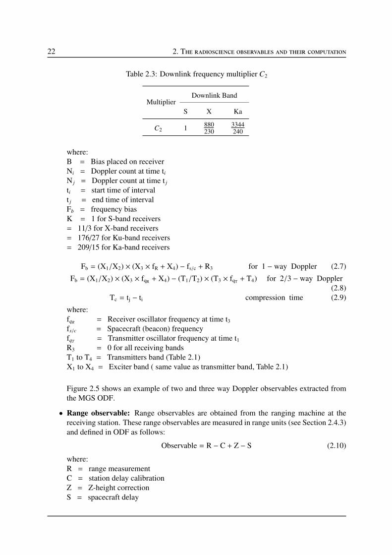
2.5. One- ,Two-, and three-way Doppler observables of the MGS spacecraft. . . . . 232.6. Two way range observables of the MGS spacecraft. . . . . . . . . . . . . . . . 232.7. Ramped frequency fo and frequency rate f measured for MGS spacecraft. . . . 242.8. Transformation between the time scales. . . . . . . . . . . . . . . . . . . . . . 262.9. Time history of the UT1 since 1962. These values of UT1 are extracted from
EOP file. . . . . . . . . . . . . . . . . . . . . . . . . . . . . . . . . . . . . . . 272.10. Time history of the TAI since 1973. . . . . . . . . . . . . . . . . . . . . . . . 282.11. Panels: (a) transformations of various coordinate time scales, (b) time history
of TT - TDB. . . . . . . . . . . . . . . . . . . . . . . . . . . . . . . . . . . . 292.12. Geometric sketch of the vectors involved in the computation of the light time
solution, where C is the solar system barycentric; E is the Earth geocenter; andB is the center of the central body. . . . . . . . . . . . . . . . . . . . . . . . . 32
2.13. Relativistic and solar corona corrections to light time solution (expressed inseconds): (a) for MGS, (b) for MESSENGER. . . . . . . . . . . . . . . . . . . 35
2.14. Round-trip light time solution of MGS (panel a) and MESSENGER (panel b)spacecraft, computed from the Eq. 2.33. . . . . . . . . . . . . . . . . . . . . . 36
2.15. The technique used for computing the integration of Eq. 2.40. W is the precisionwidth of the interval of the integration, and tstart and tend is the start and end timesof the ramp table (see Section 2.4.3.1). . . . . . . . . . . . . . . . . . . . . . . 39

14 List of Figures
2.16. The process of the spacecraft orbit determination. . . . . . . . . . . . . . . . . 43
2.17. A simple geometric macro-model of the spacecraft. . . . . . . . . . . . . . . . 50
3.1. Summary of MGS mission phases from launch to mapping period (Albee et al.,2001). . . . . . . . . . . . . . . . . . . . . . . . . . . . . . . . . . . . . . . . 63
3.2. View of the MGS spacecraft (Albee et al., 2001). . . . . . . . . . . . . . . . . 64
3.3. Pole-to-Pole tracking of the MGS spacecraft during mapping period (Tyleret al., 2001). . . . . . . . . . . . . . . . . . . . . . . . . . . . . . . . . . . . . 66
3.4. Gravitational and non-gravitational accelerations acting on the MGS spacecraft.See text for the explanation of each column. . . . . . . . . . . . . . . . . . . . 70
3.5. Quality of the MGS orbit in terms of rms values of the postfit residuals foreach one-day data-arc: (a) one-way Doppler given in millihertz (1-way: 1 mHz= 0.035 mm/s = speed of light / X-band frequency); (b) two- and three-wayDoppler given in millihertz (2/3-way: 1 mHz = 0.0178 mm/s = 0.5×speed oflight / X-band frequency); and (c) two-way range given in meter. The peaks andgaps in residuals correspond to solar conjunction periods of MGS. . . . . . . . 71
3.6. Orbit overlap differences for the entire mapping period of MGS mission for the(a) radial direction, (b) along-track direction, and (c) cross-track or normal tothe orbit plane. . . . . . . . . . . . . . . . . . . . . . . . . . . . . . . . . . . 73
3.7. Scale factors: a) atmospheric drag and b) solar radiation pressure. . . . . . . . 74
3.8. The continental map of DSN stations. Image credit: NASA . . . . . . . . . . . 75
3.9. Distance bias estimated for each data-arc and for each participating station: a)station position bias and b) range bias corrections to the INPOP10b ephemeris. 76
3.10. Range bias comparison between GINS solution and Light time solution usingINPOP10b ephemeris: (a) range bias computed from the JPL light time solu-tion, (b) range bias corresponding to the GINS solution, (c) difference betweenthe GINS and JPL light time solutions. . . . . . . . . . . . . . . . . . . . . . . 78
3.11. Evolution of the orbit change with respect to number of days in the data -arcand with the number of iterations. Panels of the figure are corresponding to a)Iteration-01 and b) Iterations-10. The green, red, and black colors in the figureare corresponding to 2-, 8-, and 15-days data-arc respectively. . . . . . . . . . 79
3.12. Difference between Box-Wing and Spherical macro-models: (a) Doppler rootmean square (rms) residuals, (b) range rms residuals, and (c) range bias. . . . . 80
3.13. Non-gravitational accelerations and scale factors estimated using Box-Wing macro-model (Black) and Spherical macro-model (Red). . . . . . . . . . . . . . . . . 81
4.1. Approximated global coronal magnetic field structure for the beginnings ofyears correspond to solar maximum: (a) 1992 and (b) 2002. The photosphericradial field strength is represented by the greyscale, with white/black indicatingpositive/negative polarity. Green/red field lines represent open fields of posi-tive/negative polarity and blue lines represent closed fields. These figures havebeen extracted from Petrie (2013). . . . . . . . . . . . . . . . . . . . . . . . . 87
4.2. The solar sunspot cycle2, since 1955 to present. Figure shows the variation ofan average monthly sunspot numbers with time. . . . . . . . . . . . . . . . . . 87
List of Figures 15
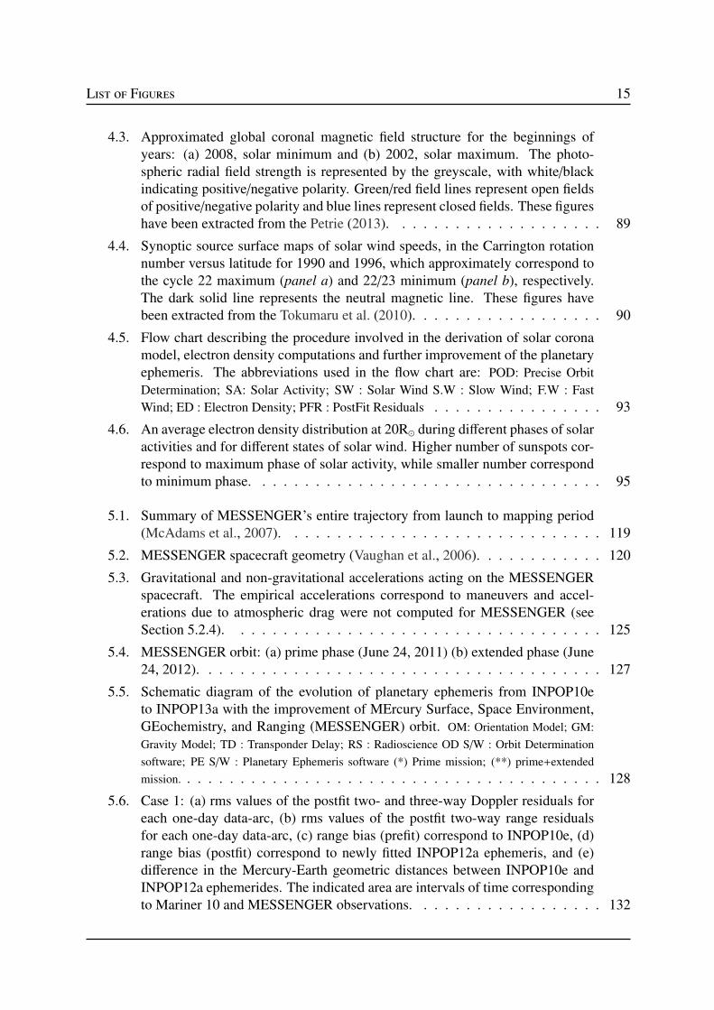
4.3. Approximated global coronal magnetic field structure for the beginnings ofyears: (a) 2008, solar minimum and (b) 2002, solar maximum. The photo-spheric radial field strength is represented by the greyscale, with white/blackindicating positive/negative polarity. Green/red field lines represent open fieldsof positive/negative polarity and blue lines represent closed fields. These figureshave been extracted from the Petrie (2013). . . . . . . . . . . . . . . . . . . . 89
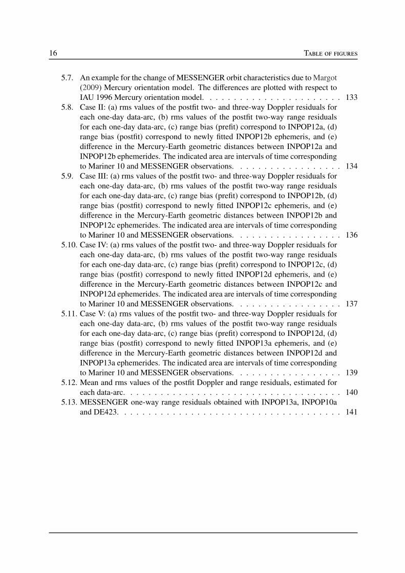
4.4. Synoptic source surface maps of solar wind speeds, in the Carrington rotationnumber versus latitude for 1990 and 1996, which approximately correspond tothe cycle 22 maximum (panel a) and 22/23 minimum (panel b), respectively.The dark solid line represents the neutral magnetic line. These figures havebeen extracted from the Tokumaru et al. (2010). . . . . . . . . . . . . . . . . . 90
4.5. Flow chart describing the procedure involved in the derivation of solar coronamodel, electron density computations and further improvement of the planetaryephemeris. The abbreviations used in the flow chart are: POD: Precise Orbit
Determination; SA: Solar Activity; SW : Solar Wind S.W : Slow Wind; F.W : Fast
Wind; ED : Electron Density; PFR : PostFit Residuals . . . . . . . . . . . . . . . . 93
4.6. An average electron density distribution at 20R⊙ during different phases of solaractivities and for different states of solar wind. Higher number of sunspots cor-respond to maximum phase of solar activity, while smaller number correspondto minimum phase. . . . . . . . . . . . . . . . . . . . . . . . . . . . . . . . . 95
5.1. Summary of MESSENGER’s entire trajectory from launch to mapping period(McAdams et al., 2007). . . . . . . . . . . . . . . . . . . . . . . . . . . . . . 119
5.2. MESSENGER spacecraft geometry (Vaughan et al., 2006). . . . . . . . . . . . 120
5.3. Gravitational and non-gravitational accelerations acting on the MESSENGERspacecraft. The empirical accelerations correspond to maneuvers and accel-erations due to atmospheric drag were not computed for MESSENGER (seeSection 5.2.4). . . . . . . . . . . . . . . . . . . . . . . . . . . . . . . . . . . 125
5.4. MESSENGER orbit: (a) prime phase (June 24, 2011) (b) extended phase (June24, 2012). . . . . . . . . . . . . . . . . . . . . . . . . . . . . . . . . . . . . . 127
5.5. Schematic diagram of the evolution of planetary ephemeris from INPOP10eto INPOP13a with the improvement of MErcury Surface, Space Environment,GEochemistry, and Ranging (MESSENGER) orbit. OM: Orientation Model; GM:
Gravity Model; TD : Transponder Delay; RS : Radioscience OD S/W : Orbit Determination
software; PE S/W : Planetary Ephemeris software (*) Prime mission; (**) prime+extended
mission. . . . . . . . . . . . . . . . . . . . . . . . . . . . . . . . . . . . . . . . 128
5.6. Case 1: (a) rms values of the postfit two- and three-way Doppler residuals foreach one-day data-arc, (b) rms values of the postfit two-way range residualsfor each one-day data-arc, (c) range bias (prefit) correspond to INPOP10e, (d)range bias (postfit) correspond to newly fitted INPOP12a ephemeris, and (e)difference in the Mercury-Earth geometric distances between INPOP10e andINPOP12a ephemerides. The indicated area are intervals of time correspondingto Mariner 10 and MESSENGER observations. . . . . . . . . . . . . . . . . . 132
16 Table of figures
5.7. An example for the change of MESSENGER orbit characteristics due to Margot(2009) Mercury orientation model. The differences are plotted with respect toIAU 1996 Mercury orientation model. . . . . . . . . . . . . . . . . . . . . . . 133
5.8. Case II: (a) rms values of the postfit two- and three-way Doppler residuals foreach one-day data-arc, (b) rms values of the postfit two-way range residualsfor each one-day data-arc, (c) range bias (prefit) correspond to INPOP12a, (d)range bias (postfit) correspond to newly fitted INPOP12b ephemeris, and (e)difference in the Mercury-Earth geometric distances between INPOP12a andINPOP12b ephemerides. The indicated area are intervals of time correspondingto Mariner 10 and MESSENGER observations. . . . . . . . . . . . . . . . . . 134
5.9. Case III: (a) rms values of the postfit two- and three-way Doppler residuals foreach one-day data-arc, (b) rms values of the postfit two-way range residualsfor each one-day data-arc, (c) range bias (prefit) correspond to INPOP12b, (d)range bias (postfit) correspond to newly fitted INPOP12c ephemeris, and (e)difference in the Mercury-Earth geometric distances between INPOP12b andINPOP12c ephemerides. The indicated area are intervals of time correspondingto Mariner 10 and MESSENGER observations. . . . . . . . . . . . . . . . . . 136
5.10. Case IV: (a) rms values of the postfit two- and three-way Doppler residuals foreach one-day data-arc, (b) rms values of the postfit two-way range residualsfor each one-day data-arc, (c) range bias (prefit) correspond to INPOP12c, (d)range bias (postfit) correspond to newly fitted INPOP12d ephemeris, and (e)difference in the Mercury-Earth geometric distances between INPOP12c andINPOP12d ephemerides. The indicated area are intervals of time correspondingto Mariner 10 and MESSENGER observations. . . . . . . . . . . . . . . . . . 137
5.11. Case V: (a) rms values of the postfit two- and three-way Doppler residuals foreach one-day data-arc, (b) rms values of the postfit two-way range residualsfor each one-day data-arc, (c) range bias (prefit) correspond to INPOP12d, (d)range bias (postfit) correspond to newly fitted INPOP13a ephemeris, and (e)difference in the Mercury-Earth geometric distances between INPOP12d andINPOP13a ephemerides. The indicated area are intervals of time correspondingto Mariner 10 and MESSENGER observations. . . . . . . . . . . . . . . . . . 139
5.12. Mean and rms values of the postfit Doppler and range residuals, estimated foreach data-arc. . . . . . . . . . . . . . . . . . . . . . . . . . . . . . . . . . . . 140
5.13. MESSENGER one-way range residuals obtained with INPOP13a, INPOP10aand DE423. . . . . . . . . . . . . . . . . . . . . . . . . . . . . . . . . . . . . 141
17
List of Tables
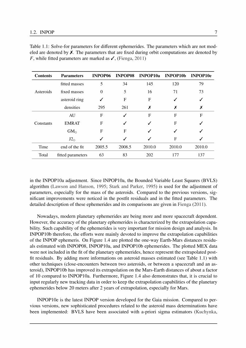
1.1. Solve-for parameters for different ephemerides. The parameters which are notmodeled are denoted by . The parameters that are fixed during orbit com-putations are denoted by F, while fitted parameters are marked as , (Fienga,2011) . . . . . . . . . . . . . . . . . . . . . . . . . . . . . . . . . . . . . . . 7
1.2. Sources for the processed spacecraft and lander missions data sets, used for theconstruction of INPOP. . . . . . . . . . . . . . . . . . . . . . . . . . . . . . . 9
2.1. Constants dependent upon transmitter or exciter band . . . . . . . . . . . . . . 202.2. Spacecraft transponder ratio M2 (M2R
) . . . . . . . . . . . . . . . . . . . . . . 212.3. Downlink frequency multiplier C2 . . . . . . . . . . . . . . . . . . . . . . . . 222.4. Constant Crange requried for converting second to range units. . . . . . . . . . . 42
3.1. MGS spacecraft macro-model characteristics (Marty, 2011) . . . . . . . . . . . 653.2. Year wise summary of the Doppler and range tracking data used for orbit solution. 663.3. Comparison of postfit Doppler and range residuals, and overlapped periods,
between different authors. . . . . . . . . . . . . . . . . . . . . . . . . . . . . . 72
4.1. Electron densities estimated from different models at 20R⊙ and at 215R⊙ (1AU). 964.2. Statistics of the range bias before and after solar corona corrections. . . . . . . 97
5.1. MESSENGER spacecraft macro-model characteristics (Vaughan et al., 2002). . 1225.2. Summary of the Doppler and range tracking data used for orbit determination. . 1245.3. An average magnitude of MESSENGER accelerations estimated during prime
and extended phase of the mission. . . . . . . . . . . . . . . . . . . . . . . . . 1275.4. Recommended values for the direction of the north pole of rotation and the
prime meridian of the Mercury, 1996 (Davies et al., 1996). . . . . . . . . . . . 1295.5. Statistics of the residuals obtained for Case I, i) postfit Doppler and range resid-
uals, ii) prefit (INPOP10e) and postfit (INPOP12a) range bias. . . . . . . . . . 1315.6. Recommended model for the orientation of Mercury (Margot, 2009). . . . . . . 1315.7. Statistics of the residuals obtained for Case II, i) postfit Doppler and range resid-
uals, ii) prefit (INPOP12a) and postfit (INPOP12b) range bias. . . . . . . . . . 1335.8. Statistics of the residuals obtained for Case III, i) postfit Doppler and range
residuals, ii) prefit (INPOP12b) and postfit (INPOP12c) range bias. . . . . . . 1355.9. Statistics of the residuals obtained for Case IV, i) postfit Doppler and range
residuals, ii) prefit (INPOP12c) and postfit (INPOP12d) range bias. . . . . . . 137

18 List of tables
5.10. Statistics of the residuals obtained for Case V , i) postfit Doppler and rangeresiduals, ii) prefit (INPOP12d) and postfit (INPOP13a) range bias. . . . . . . 139
5.11. Comparisons of postfit residuals between different authors. . . . . . . . . . . . 141
19
Acronyms
AMD . . . . . . . . . . angular momentum wheel desaturation
BVE . . . . . . . . . . . block 5 exciter
BVLS . . . . . . . . . .Bounded Variable Least Squares
BWmm . . . . . . . . . .Box-Wing macro-model
CME . . . . . . . . . . coronal mass ejections
CNES . . . . . . . . . .Centre National d’Etudes Spatiales
COI . . . . . . . . . . . center of integration
DSMs . . . . . . . . . . deep-space maneuvers
DSN . . . . . . . . . . .Deep Space Network
EOP . . . . . . . . . . .Earth Orientation Parameters
EPM . . . . . . . . . . .Ephemerides of Planets and the Moon
ESA . . . . . . . . . . .European Space Agency
Gaia . . . . . . . . . . .Global Astrometric Interferometer for Astrophysics
GINS . . . . . . . . . . “Géodésie par Intégrations Numériques Simultanées”
GR . . . . . . . . . . . general relativity
HEF . . . . . . . . . . . high efficiency
HGA . . . . . . . . . . high gain antenna
IAU . . . . . . . . . . . International Astronomical Union
IERS . . . . . . . . . . International Earth Rotation and Reference Systems Service
IMF . . . . . . . . . . . Interplanetary Magnetic Field

20 Acronyms
INPOP . . . . . . . . . “Intégrateur Numérique Planétaire de l’Observatoire de Paris”
ITRF . . . . . . . . . . International Terrestrial Reference Frame
JPL . . . . . . . . . . . Jet Propulsion Laboratory
LLR . . . . . . . . . . .Lunar Laser Ranging
LOS . . . . . . . . . . . line of sight
MDLOS . . . . . . . .minimum distance of the line of sight
MDM . . . . . . . . . .Momentum Dump Maneuver
MESSENGER . . . . .MErcury Surface, Space Environment, GEochemistry, and Ranging
MEX . . . . . . . . . .Mars Express
MGS . . . . . . . . . .Mars Global Surveyor
MMNAV . . . . . . . .Multimission Navigation
MNL . . . . . . . . . .Magnetic Neutral Line
MOI . . . . . . . . . . .Mars orbit insertion
NAIF . . . . . . . . . .Navigation and Ancillary Information Facility
NASA . . . . . . . . . .National Aeronautics and Space Administration
OCM . . . . . . . . . .Orbit Correction Maneuver
ODF . . . . . . . . . . .Orbit Data File
ODP . . . . . . . . . . .Orbit Determination Program
ODY . . . . . . . . . .Odyssey
PDS . . . . . . . . . . . Planetary Data System
PPN . . . . . . . . . . . Parameterized Post-Newtonian
RMDCT . . . . . . . .Radio Metric Data Conditioning Team
rms . . . . . . . . . . . root mean square
SEP . . . . . . . . . . . Sun-Earth-Probe
SPmm . . . . . . . . . . Spherical macro-model

Acronyms 21
TAI . . . . . . . . . . . International Atomic Time
TCB . . . . . . . . . . .Barycentric Coordinate Time
TCG . . . . . . . . . . .Geocentric Coordinate Time
TCMs . . . . . . . . . . trajectory-correction maneuvers
TDB . . . . . . . . . . .Barycentric Dynamical Time
TT . . . . . . . . . . . .Terrestrial Time
UT1 . . . . . . . . . . .Universal Time
UTC . . . . . . . . . . .Coordinated Universal Time
VEX . . . . . . . . . . .Venus Express
WSO . . . . . . . . . .Wilcox Solar Observatory

22 Acronyms

1
Chapter 1
Introduction
1.1 Introduction to planetary ephemerides
The word ephemeris originated from the Greek language “εϕηµǫρoς ”. The planetary ephemerisgives the positions and velocities of major bodies of the solar system at a given epoch. Histor-ically, positions (right ascension and declination) were given as printed tables of values, atregular intervals of date and time. Nowadays, the modern ephemerides are often computedelectronically from mathematical models of the motion.
Before 1960’s, analytical models were used for describing the state of the solar systembodies as a function of time. At that time only optical angular measurements of solar systembodies were available. In 1964 radar measurements of the terrestrial planets have been mea-sured. These measurements significantly improved the knowledge of the position of the objectsin space. The first laser ranges to the lunar corner cube retroreflectors were then obtained in1969 (Newhall et al., 1983). With the developments of these techniques, a group at MIT, hadinitiated such an ephemeris program as a support of solar system observations and resulting sci-entific analyses. The first modern ephemerides, deduced from radar and optical observations,were then developed at MIT (Ash et al., 1967). The achieved precision in the measurements,and the improvement in the dynamics of the solar system objects, gave an opportunities to teststhe theory of general relativity (GR) (Shapiro, 1964).
In the late 1970’s, the first numerically integrated planetary ephemerides were built by JetPropulsion Laboratory (JPL), so called DE96 (Standish et al., 1976). There have been manyversions of the JPL DE ephemerides, from the 1960s through the present. With the beginningof the Space Age, space probes began their journeys resulting in a revolution in knowledgethat is still continuing. These ephemerides have then served for spacecraft navigation, missionplanning, reduction and analysis of the most precise of astronomical observations. Number ofefforts were then also devoted for testing the GR using astrometric and radiometric observations(Anderson et al., 1976, 1978).
2 1. Introduction
Improvements in the planetary ephemerides occurred simultaneously with the evolution ofthe space missions and the navigation of the probes. Navigation observations were included forthe first time in the construction of DE102 ephemeris (Newhall et al., 1983). In this ephemeris,planet orbit were constrained by the Viking range measurements along with entire historicalastronomical observations. Such addition of the Viking range measurements improved the Marsposition by more than 4 order of magnitude and JPL becomes the only source of developmentof high precision planetary ephemerides. In the 1970’s and early 1980’s, a lot of work wasdone in the astronomical community to update the astronomical almanacs all around the word.Four major types of observations (optical measurements, radar ranging, spacecraft ranging, andlunar laser ranging) were then included in the adjustment of the ephemeris DE200 (Standish,1990). This ephemeris becomes a worldwide standard for several decades. In the late 1990s,a new series of the JPL ephemerides were introduced. In particular, DE405 (Standish, 1998),which covers the period between 1600 to 2200, was widely used for the spacecraft navigationand data analysis. DE423 (Folkner, 2010) is the most recent documented ephemeris producedby the JPL.
However, almost from a decade, the European Space Agency (ESA) is very active in the de-velopment of interplanetary missions in collaboration with the National Aeronautics and SpaceAdministration (NASA). These missions include: Giotto for the study of the comets Halley;Ulysses for charting the poles of the Sun; Huygens for Titan; Rosetta for comet; Mars Express(MEX) for Mars; Venus Express (VEX) for Venus; Global Astrometric Interferometer for As-trophysics (Gaia) for space astrometry; BebiColombo for Mercury (future mission); JUICE forJupiter (future mission); etc. With the new era of European interplanetary missions, the “In-tégrateur Numérique Planétaire de l’Observatoire de Paris” (INPOP) project was initiated in2003 to built the first European planetary ephemerides independently from the JPL. INPOP hasthen evolved over the years and the first official release was made on 2008, so-called INPOP06(Fienga et al., 2008). Currently several versions of INPOP are available to the users: INPOP06(Fienga et al., 2008); INPOP08 (Fienga et al., 2009); INPOP10a (Fienga et al., 2011a); IN-POP10b (Fienga et al., 2011b); and INPOP10e (Fienga et al., 2013). INPOP10a was the firstplanetary ephemerides solving for the mass of the Sun (GM⊙) for a given fixed value of As-tronomical Unit (AU). Since INPOP10a, new estimations of the Sun mass together with theoblateness of the Sun (J2⊙) are regularly obtained. With the website www.imcce.fr/inpop,these ephemerides are freely distributed to the users. With this users can have access to positionsand velocities of the major planets of our solar system and of the moon, the libration angles ofthe moon but also to the differences between the terrestrial time TT (time scale used to datethe observations) and the barycentric times TDB or TCB (time scale used in the equations ofmotion).
With such gradual improvement, INPOP has become an international reference for spacenavigation. INPOP is the official ephemerides used for the Gaia mission navigation and theanalysis of the Gaia observations. INPOP10e (Fienga et al., 2013) is the latest ephemerides de-livered by the INPOP team to support this mission. Moreover, the INPOP team is also involvedin the preparation of the Bepi-Colombo and the JUICE missions. The brief description of theINPOP construction and its evolution are given in Section 1.2.
1.2. INPOP 3
Moreover, in addition to DE and INPOP ephemerides, there is one more numerical ephemerideswhich were developed at the Institute of Applied Astronomy of the Russian Academy of Sci-ences, called Ephemerides of Planets and the Moon (EPM). These ephemerides are based uponthe same modeling as the JPL DE ephemeris. Their of the EPM ephemerides, the most recentare EPM2004 (Pitjeva, 2005), EPM2008 (Pitjeva, 2010), and EPM2011 (Pitjeva and Pitjev,2013). The EPM2004 ephemerides were constructed over the 1880-2020 time interval in theTDB time scale. In this ephemerides GM of all planets, the Sun, the Moon and value of Earth-Moon mass ratio correspond to DE405 (Standish, 1998), while for EPM2008 these values areclose to DE421 (Folkner et al., 2008).
1.2 INPOP
The construction of independent planetary ephemerides is a crucial point for the strategy ofspace development in Europe. As mentioned before, JPL ephemerides were used as a referencefor spacecraft navigation of the US and the European missions. With the delivery of INPOP thesituation has changed. Since 2006, a completely autonomous planetary ephemerides has beenbuilt in Europe and became an international reference for space navigation and for scientificresearch in the dynamics of the Solar System objects and in fundamental physics.
1.2.1 INPOP construction
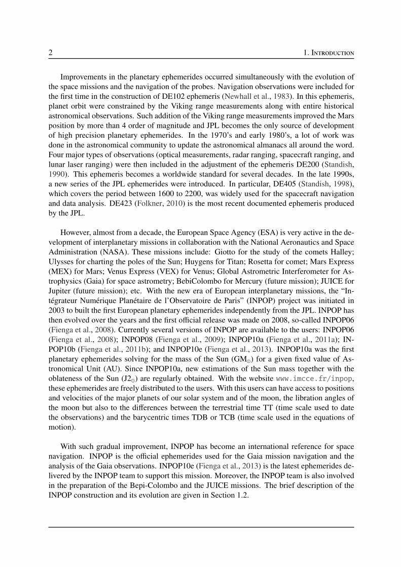
INPOP numerically integrates the equations of motion of the major bodies of our solar systemincluding about 300 asteroids about the solar system barycenter and of the motion and rotationof the Moon about the Earth. Figure 1.1 shows the systematic diagram for the procedure of theINPOP construction. The brief descriptions of this procedure is described as follows:
• The dynamic model of INPOP follows the recommendations of the International Astro-nomical Union (IAU) in terms of compatibility between time scales, Terrestrial Time (TT)and Barycentric Dynamical Time (TDB), and metric in the relativistic equations of mo-tion. It is developed in the Parameterized Post-Newtonian (PPN) framework, and includesthe solar oblateness, the perturbations induced by the major asteroids (about 300) as wellas the tidal effects of the Earth and Moon. The trajectories of the major bodies are ob-tained by the numerical integration of a differential equation of first order, Y ′ = F(t,Y(t)),where Y is the parameter that describes the state vectors of the system (position/velocityof the bodies, their orientations) (Manche, 2011). Prior knowledge of these parameters atepoch zero (t0, usually J2000) are then used to initiate the integrations with the method ofAdams (Hairer et al., 1987). Detailed descriptions of the INPOP dynamic modeling aregiven in the Fienga et al. (2008) and Manche (2011).
• The numerical integration produces a file of positions and velocities (state vectors) of the
4 1. Introduction
Figure 1.1: Schematic diagram for the procedure of the INPOP construction.
solar system bodies at each time step of the integration. The step size of 0.055 days isusually chosen to minimize the roundoff error. Each component of the state vectors of thesolar system bodies relative to the solar system barycenter and the Moon relative to theEarth are then represented by an Nth-degree expansion in Chebyshev polynomials (seeNewhall (1989) for more details). Interpolation of these polynomials gives the access ofthe state vectors at any given epoch.
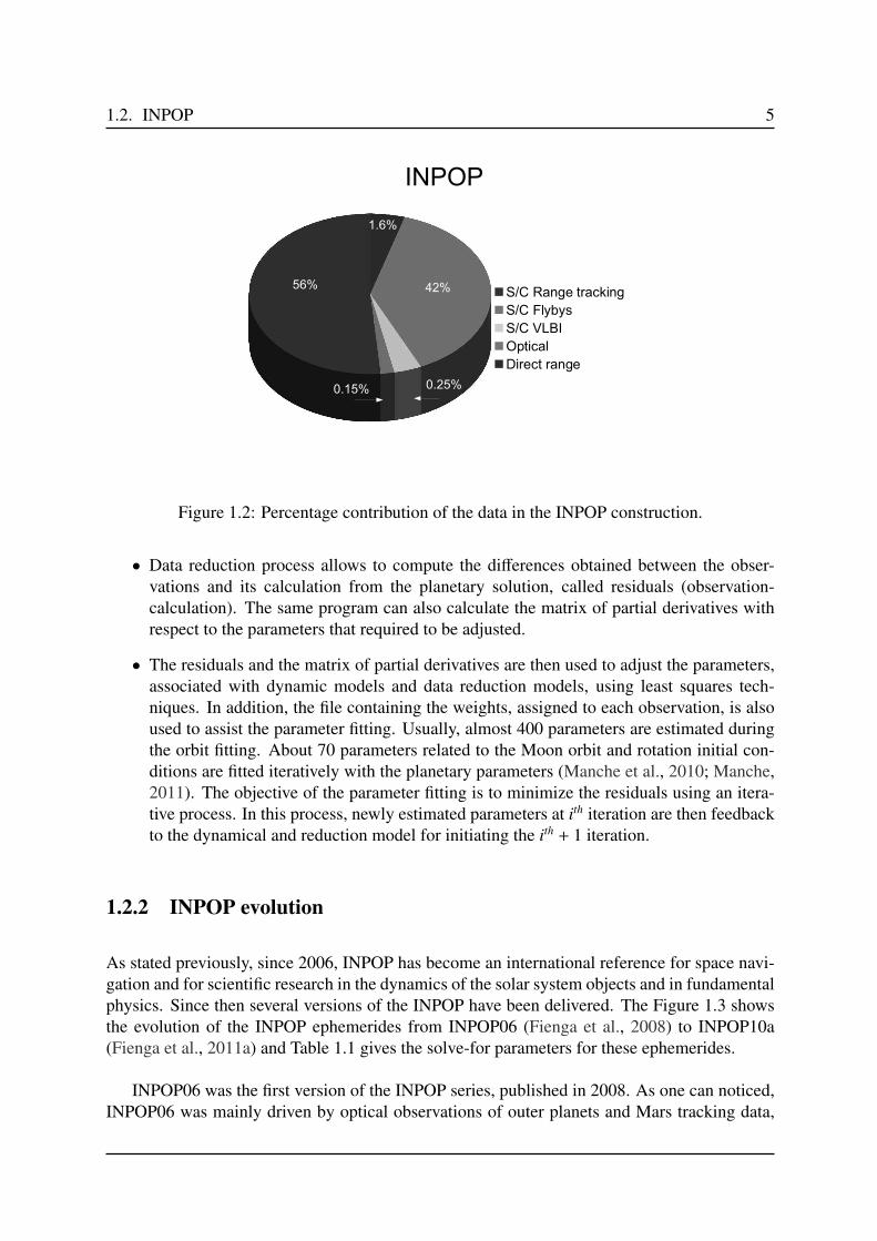
• Interpolated solutions of the state vectors are then used to reduce the observations. Thereare several types of observations that are used for the construction of planetary ephemerides(Fienga et al., 2008): direct radar observations of the planet surface (Venus, Mercury andMars), spacecraft tracking data (radar ranging, ranging and VLBI), optical observations(transit, photographic plates and CCD observations for outer planets), and Lunar LaserRanging (LLR) for Moon. The observations and the parameters associated with the datareduction are then induced in the data reduction models (see Figure 1.1). Descriptionof such models can be found in Fienga et al. (2008). Figure 1.2 shows the contribu-tions in percentage of the different types of data used for constraining the recent seriesof INPOP. More than 136,000 planetary observations are involved in this process. FromFigure 1.2 one can noticed that, nowadays, planetary ephemerides are mainly driven bythe spacecraft data. However, old astrometric data are still important especially for a bet-ter knowledge of outer planet orbits for which few or no spacecraft data are available (seeSection 1.2.2 for more details).
1.2. INPOP 5
!
"!"!
#$$
Figure 1.2: Percentage contribution of the data in the INPOP construction.
• Data reduction process allows to compute the differences obtained between the obser-vations and its calculation from the planetary solution, called residuals (observation-calculation). The same program can also calculate the matrix of partial derivatives withrespect to the parameters that required to be adjusted.
• The residuals and the matrix of partial derivatives are then used to adjust the parameters,associated with dynamic models and data reduction models, using least squares tech-niques. In addition, the file containing the weights, assigned to each observation, is alsoused to assist the parameter fitting. Usually, almost 400 parameters are estimated duringthe orbit fitting. About 70 parameters related to the Moon orbit and rotation initial con-ditions are fitted iteratively with the planetary parameters (Manche et al., 2010; Manche,2011). The objective of the parameter fitting is to minimize the residuals using an itera-tive process. In this process, newly estimated parameters at ith iteration are then feedbackto the dynamical and reduction model for initiating the ith + 1 iteration.
1.2.2 INPOP evolution
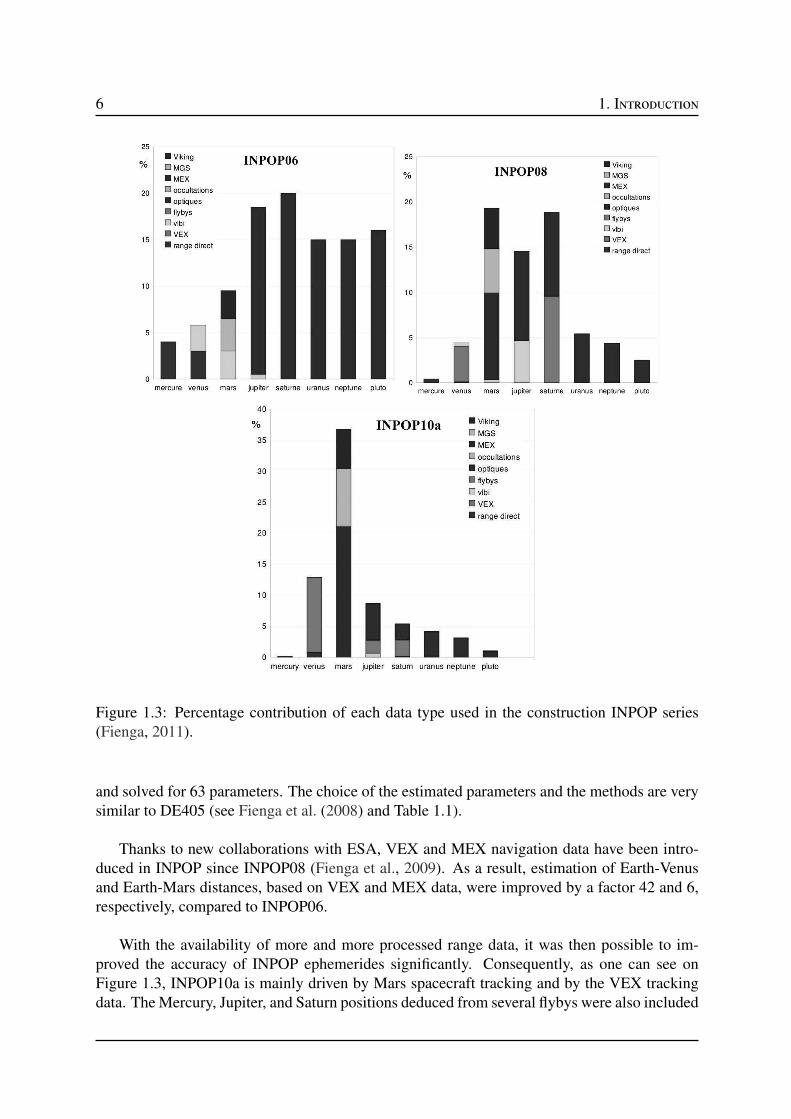
As stated previously, since 2006, INPOP has become an international reference for space navi-gation and for scientific research in the dynamics of the solar system objects and in fundamentalphysics. Since then several versions of the INPOP have been delivered. The Figure 1.3 showsthe evolution of the INPOP ephemerides from INPOP06 (Fienga et al., 2008) to INPOP10a(Fienga et al., 2011a) and Table 1.1 gives the solve-for parameters for these ephemerides.
INPOP06 was the first version of the INPOP series, published in 2008. As one can noticed,INPOP06 was mainly driven by optical observations of outer planets and Mars tracking data,
6 1. Introduction
Figure 1.3: Percentage contribution of each data type used in the construction INPOP series(Fienga, 2011).
and solved for 63 parameters. The choice of the estimated parameters and the methods are verysimilar to DE405 (see Fienga et al. (2008) and Table 1.1).
Thanks to new collaborations with ESA, VEX and MEX navigation data have been intro-duced in INPOP since INPOP08 (Fienga et al., 2009). As a result, estimation of Earth-Venusand Earth-Mars distances, based on VEX and MEX data, were improved by a factor 42 and 6,respectively, compared to INPOP06.
With the availability of more and more processed range data, it was then possible to im-proved the accuracy of INPOP ephemerides significantly. Consequently, as one can see onFigure 1.3, INPOP10a is mainly driven by Mars spacecraft tracking and by the VEX trackingdata. The Mercury, Jupiter, and Saturn positions deduced from several flybys were also included
1.2. INPOP 7
Table 1.1: Solve-for parameters for different ephemerides. The parameters which are not mod-eled are denoted by . The parameters that are fixed during orbit computations are denoted byF, while fitted parameters are marked as , (Fienga, 2011)
Contents Parameters INPOP06 INPOP08 INPOP10a INPOP10b INPOP10e
fitted masses 5 34 145 120 79
Asteroids fixed masses 0 5 16 71 73
asteroid ring F F
densities 295 261
AU F F F F
Constants EMRAT F F
GM⊙ F F
J2⊙ F
Time end of the fit 2005.5 2008.5 2010.0 2010.0 2010.0
Total fitted parameters 63 83 202 177 137
in the INPOP10a adjustment. Since INPOP10a, the Bounded Variable Least Squares (BVLS)algorithm (Lawson and Hanson, 1995; Stark and Parker, 1995) is used for the adjustment ofparameters, especially for the mass of the asteroids. Compared to the previous versions, sig-nificant improvements were noticed in the postfit residuals and in the fitted parameters. Thedetailed description of these ephemerides and its comparisons are given in Fienga (2011).
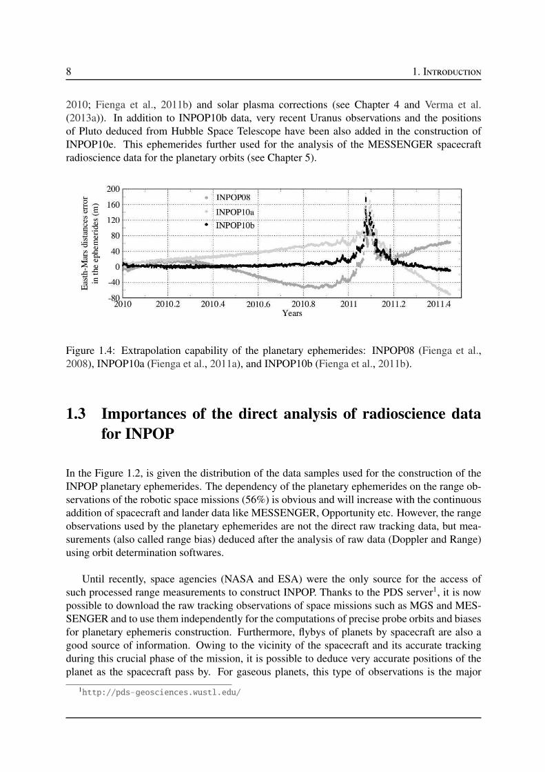
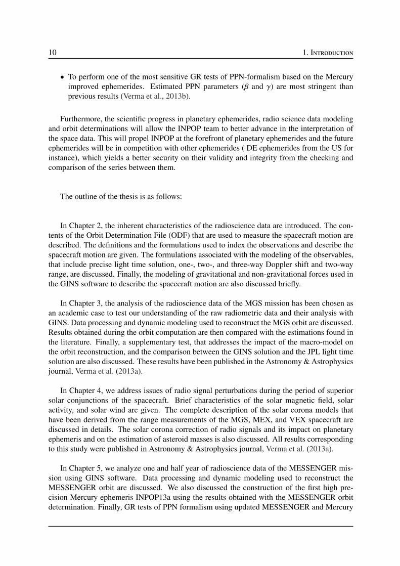
Nowadays, modern planetary ephemerides are being more and more spacecraft dependent.However, the accuracy of the planetary ephemerides is characterized by the extrapolation capa-bility. Such capability of the ephemerides is very important for mission design and analysis. InINPOP10b therefore, the efforts were mainly devoted to improve the extrapolation capabilitiesof the INPOP ephemeris. On Figure 1.4 are plotted the one-way Earth-Mars distances residu-als estimated with INPOP08, INPOP10a, and INPOP10b ephemerides. The plotted MEX datawere not included in the fit of the planetary ephemerides, hence represent the extrapolated post-fit residuals. By adding more informations on asteroid masses estimated (see Table 1.1) withother techniques (close-encounters between two asteroids, or between a spacecraft and an as-teroid), INPOP10b has improved its extrapolation on the Mars-Earth distances of about a factorof 10 compared to INPOP10a. Furthermore, Figure 1.4 also demonstrates that, it is crucial toinput regularly new tracking data in order to keep the extrapolation capabilities of the planetaryephemerides below 20 meters after 2 years of extrapolation, especially for Mars.
INPOP10e is the latest INPOP version developed for the Gaia mission. Compared to per-vious versions, new sophisticated procedures related to the asteroid mass determinations havebeen implemented: BVLS have been associated with a-priori sigma estimators (Kuchynka,
8 1. Introduction
2010; Fienga et al., 2011b) and solar plasma corrections (see Chapter 4 and Verma et al.(2013a)). In addition to INPOP10b data, very recent Uranus observations and the positionsof Pluto deduced from Hubble Space Telescope have been also added in the construction ofINPOP10e. This ephemerides further used for the analysis of the MESSENGER spacecraftradioscience data for the planetary orbits (see Chapter 5).
Figure 1.4: Extrapolation capability of the planetary ephemerides: INPOP08 (Fienga et al.,2008), INPOP10a (Fienga et al., 2011a), and INPOP10b (Fienga et al., 2011b).
1.3 Importances of the direct analysis of radioscience data
for INPOP
In the Figure 1.2, is given the distribution of the data samples used for the construction of theINPOP planetary ephemerides. The dependency of the planetary ephemerides on the range ob-servations of the robotic space missions (56%) is obvious and will increase with the continuousaddition of spacecraft and lander data like MESSENGER, Opportunity etc. However, the rangeobservations used by the planetary ephemerides are not the direct raw tracking data, but mea-surements (also called range bias) deduced after the analysis of raw data (Doppler and Range)using orbit determination softwares.
Until recently, space agencies (NASA and ESA) were the only source for the access ofsuch processed range measurements to construct INPOP. Thanks to the PDS server1, it is nowpossible to download the raw tracking observations of space missions such as MGS and MES-SENGER and to use them independently for the computations of precise probe orbits and biasesfor planetary ephemeris construction. Furthermore, flybys of planets by spacecraft are also agood source of information. Owing to the vicinity of the spacecraft and its accurate trackingduring this crucial phase of the mission, it is possible to deduce very accurate positions of theplanet as the spacecraft pass by. For gaseous planets, this type of observations is the major
1http://pds-geosciences.wustl.edu/

1.3. Importances of the direct analysis of radioscience data for INPOP 9
constraint on their orbits (flybys of Jupiter, Neptune, and Saturn, mainly). Even if they are notnumerous (less than 0.5% of the data sample), they provide 50% of the constraints brought toouter planet orbits.
Table 1.2: Sources for the processed spacecraft and lander missions data sets, used for theconstruction of INPOP.
Type Mission Planet Data source
VEX Venus ESA
Orbiter MGS Mars JPL/CNES/PDS
MEX Mars ESA/ROB
ODY Mars JPL
Mariner 10 Mercury JPL
MESSENGER Mercury JPL/PDS
Pioneer 10 & 11 Jupiter JPL
Flyby Voyager 1 & 2 Jupiter JPL
Ulysses Jupiter JPL
Cassini Jupiter JPL
Voyager 2 Uranus JPL
Voyager 2 Neptune JPL
Lander Viking Mars JPL
pathfinder Mars JPL
The goal of the thesis is therefore to analyze the radioscience data independently (see Chap-ter 2) and then to improve INPOP. High precision ephemerides are then used for performingtests of physics such as solar corona studies (see Chapter 4) and tests of GR through the PPNformalism (see Chapter 5). In this thesis, such analysis has been performed with entire MarsGlobal Surveyor (MGS) (see Chapter 3) and MESSENGER (see Chapter 5) radioscience datausing Centre National d’Etudes Spatiales (CNES) orbit determination software “Géodésie parIntégrations Numériques Simultanées” (GINS). Key aspects of this thesis are:
• To make INPOP independent from the space agencies and to deliver most up-to-date highaccurate ephemerides to the users.
• To maintain consistency between spacecraft orbit and planet orbit constructions.
• To perform for the first time studies of the solar corona with the ephemerides. The so-lar corona model derived from the range bias are then used to correct the solar coronaperturbations and for the construction of INPOP ephemerides (Verma et al., 2013a).
• To analyze the entire MESSENGER radioscience data corresponding to the mappingphase, make INPOP the first ephemerides in the world with the high precision Mercuryorbit INPOP13a of about -0.4±8.4 meters (Verma et al., 2013b).
10 1. Introduction
• To perform one of the most sensitive GR tests of PPN-formalism based on the Mercuryimproved ephemerides. Estimated PPN parameters (β and γ) are most stringent thanprevious results (Verma et al., 2013b).
Furthermore, the scientific progress in planetary ephemerides, radio science data modelingand orbit determinations will allow the INPOP team to better advance in the interpretation ofthe space data. This will propel INPOP at the forefront of planetary ephemerides and the futureephemerides will be in competition with other ephemerides ( DE ephemerides from the US forinstance), which yields a better security on their validity and integrity from the checking andcomparison of the series between them.
The outline of the thesis is as follows:
In Chapter 2, the inherent characteristics of the radioscience data are introduced. The con-tents of the Orbit Determination File (ODF) that are used to measure the spacecraft motion aredescribed. The definitions and the formulations used to index the observations and describe thespacecraft motion are given. The formulations associated with the modeling of the observables,that include precise light time solution, one-, two-, and three-way Doppler shift and two-wayrange, are discussed. Finally, the modeling of gravitational and non-gravitational forces used inthe GINS software to describe the spacecraft motion are also discussed briefly.
In Chapter 3, the analysis of the radioscience data of the MGS mission has been chosen asan academic case to test our understanding of the raw radiometric data and their analysis withGINS. Data processing and dynamic modeling used to reconstruct the MGS orbit are discussed.Results obtained during the orbit computation are then compared with the estimations found inthe literature. Finally, a supplementary test, that addresses the impact of the macro-model onthe orbit reconstruction, and the comparison between the GINS solution and the JPL light timesolution are also discussed. These results have been published in the Astronomy & Astrophysicsjournal, Verma et al. (2013a).
In Chapter 4, we address issues of radio signal perturbations during the period of superiorsolar conjunctions of the spacecraft. Brief characteristics of the solar magnetic field, solaractivity, and solar wind are given. The complete description of the solar corona models thathave been derived from the range measurements of the MGS, MEX, and VEX spacecraft arediscussed in details. The solar corona correction of radio signals and its impact on planetaryephemeris and on the estimation of asteroid masses is also discussed. All results correspondingto this study were published in Astronomy & Astrophysics journal, Verma et al. (2013a).
In Chapter 5, we analyze one and half year of radioscience data of the MESSENGER mis-sion using GINS software. Data processing and dynamic modeling used to reconstruct theMESSENGER orbit are discussed. We also discussed the construction of the first high pre-cision Mercury ephemeris INPOP13a using the results obtained with the MESSENGER orbitdetermination. Finally, GR tests of PPN formalism using updated MESSENGER and Mercury

1.3. Importances of the direct analysis of radioscience data for INPOP 11
ephemerides are discussed. All these results are submitted for publication in Astronomy &Astrophysics journal, Verma et al. (2013b).
In Chapter 6, we summarize the achieved goal followed by the conclusions and prospectivesof the thesis.

12 1. Introduction
13
Chapter 2
The radioscience observables and their
computation
2.1 Introduction
The radioscience study is the branch of science which usually consider the phenomenas as-sociate with radio wave generation and propagation. In space, these radio signals could beoriginated from natural sources (for example: pulsars) or from artificial sources such as space-craft. If the source of these signals is natural, then study is referred to radio astronomy. Usuallythe objective of radio astronomy is to perform a study of the generation and of the process ofpropagation of the signal.
However, if the source of the radio signals is artificial satellite, then the radioscience exper-iment are usually related to the phenomena that occurred along the line of sight (LOS) whichaffect the radio waves propagation. Small changes in phase or amplitude (or both) of the ra-dio signals, when propagating between spacecraft and the Deep Space Network (DSN) stationon Earth, allow us to study, celestial mechanics, planetary atmosphere, solar corona, planetaryephemeris, planetary gravity field, test of GR, etc.
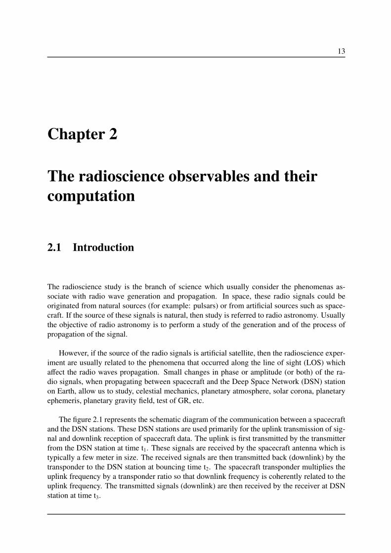
The figure 2.1 represents the schematic diagram of the communication between a spacecraftand the DSN stations. These DSN stations are used primarily for the uplink transmission of sig-nal and downlink reception of spacecraft data. The uplink is first transmitted by the transmitterfrom the DSN station at time t1. These signals are received by the spacecraft antenna which istypically a few meter in size. The received signals are then transmitted back (downlink) by thetransponder to the DSN station at bouncing time t2. The spacecraft transponder multiplies theuplink frequency by a transponder ratio so that downlink frequency is coherently related to theuplink frequency. The transmitted signals (downlink) are then received by the receiver at DSNstation at time t3.
14 2. The radioscience observables and their computation
Receiver
UPLINK
DOWNLINK
DSN Station
S/C Antenna
Solar Panel
Bus
Transmitter
Figure 2.1: Two- or three-way radio wave propagation between a spacecraft and Deep SpaceNetwork (DSN) station.
While tracking the spacecraft, the Doppler shift is routinely measured in the frequency ofthe signal at the receiving DSN station. The Doppler shift, which represents the change in thereceived signal frequency from the transmitted signal, may be caused by the spacecraft orbitaround the planet, Earth revolution around the Sun, Earth rotation, atmospheric perturbationsetc. Doppler observables, which are collected at the receiving station, are the average valuesof this Doppler shift over a period of time called count interval. These collected radiometricdata could be one-, two-, or three-way Doppler and range observations. Time delay in terms ofdistance is represented by range observable and rate of change of this distance is called Dopplerobservables. When the DSN stations on Earth only receive a downlink signal from a spacecraft,the communication is called one-way. The observables are called two-way if the transmitted andreceived antennas are the same, and three-way observables if they are different. An example oftwo- or three-way communication is shown in Figure 2.1).
2.2 The radioscience experiments
The radioscience experiments are used for study the planetary environment and its physicalstate. Such experiments already have been performed and tested with early flight planetarymissions. For example, Voyager (Eshleman et al., 1977; Tyler et al., 1981, 1986) ,Ulysses (Birdet al., 1994; Pätzold et al., 1995), Marine 10 (Howard et al., 1974), Mars Global Surveyor (Tyleret al., 2001; Konopliv et al., 2006; Marty et al., 2009), Mars Express (Pätzold et al., 2004). Briefdescription of these investigation are discussed below.

2.2. The radioscience experiments 15
Atmosphere and Ionosphere
α
aa
Spacecraft
Earth Antenna
Planet
Figure 2.2: Radio wave bending when the spacecraft is occulted by the planet and the signalpropagates through the atmosphere and ionosphere of the planet.
2.2.1 Planetary atmosphere
In order to study planetary environment, the spacecraft orbit can be arrange such that, the space-craft passes behind the orbiting planet as seen from the DSN stations. This phenomena knownas occultation. Just before, the spacecraft is hidden by the planetary disc, signals sent betweenthe spacecraft and the ground station will travel through the atmosphere and ionosphere of theplanet. The refraction in the atmosphere and ionosphere bends the LOS, as shown in Figure2.2. This bending will produce a phase and frequency shift in the received signal. Analysis ofthis shift can be then account for investigating the atmospheric and ionospheric properties ofthe planet.
Measurements of the Doppler shift on a spacecraft coherent downlink determine the LOScomponent of the spacecraft velocity. These Doppler and range measurements are then alsouseful to compute the precise orbit of the spacecraft. The geometry between the spacecraft andthe Earth station are then useful to determine the refraction or bending angle, α, as shown inFigure 2.2. The ray asymptotes, a (see Figure 2.2), and the bending angle, α, can be used toestimate the refraction profile of the atmosphere and ionosphere (Fjeldbo et al., 1971). Thisrefractivity could be then interpreted in terms of pressure and temperature by assuming thehydrostatic equilibrium (Pätzold et al., 2004).
2.2.2 Planetary gravity
The accurate determination of the spacecraft orbit requires a precise knowledge of the gravityfield and its temporal variations of the planet. Such variations in the gravity field are associatedwith the high and low concentration of the mass below and at the surface of the planet. Theycause the slight change in the speed of the spacecraft relative to the ground station on Earth and

16 2. The radioscience observables and their computation
induced small shift in the receiving frequency. After removing the Doppler shift induced by theplanetary motion, spacecraft orbital motion, atmospheric friction, solar wind, it is then possibleto compute the spacecraft acceleration or deceleration induced by the gravity field of the planet.
Figure 2.3: Mars gravity field derived from Mariner 9, Viking 1&2 and Mars Global Surveyor(MGS) spacecraft (Pätzold et al., 2004).
Gravity field mapping require the spacecraft downlink carries signal coherent with a highlystable uplink from the Earth station. The two-way radio tracking of these signals provides anaccurate measurement of spacecraft velocity along the LOS to the tracking station on Earth.Figure 2.3 represents an example of the gravity field mapping of the Mars surface using suchradio tracking signals of Mariner 9, Viking 1&2 and Mars Global Surveyor (MGS) spacecraft(Pätzold et al., 2004). This mapping was derived from the gravity field model (Kaula, 1966),developed upto degree and order 75. The strong positive anomalies shown in Figure 2.3 cor-respond to the regions of highest elevation on the Mars surface. The low circular orbiter, suchas MGS, allows to mapping an accurate and complete gravity field of the planet. However, thehighly eccentric orbiter, such as Mars Express (MEX) or MESSENGER, is not best suitable forinvestigating the global map of the gravity field of orbiting planet.
2.2.3 Solar corona
When the LOS passes close to the sun as seen from the Earth and all three bodies (Planet, Sunand Earth) approximately lies in the straight line, then such geometric configuration is calledsolar conjunction. During conjunction periods, strong turbulent and ionized gases of coronaregion severely degrade the radio wave signals when propagating between spacecraft and Earthtracking stations. Such degradations cause a delay and a greater dispersion of the radio signals.The group and phase delays induced by the Sun activity are directly proportional to the totalelectron contents along the LOS and inversely with the square of carrier radio wave frequency.
By analyzing spacecraft radio waves which are directly intercepted by solar plasma, it isthen possible to study the corona density distribution, the solar wind region and the corona
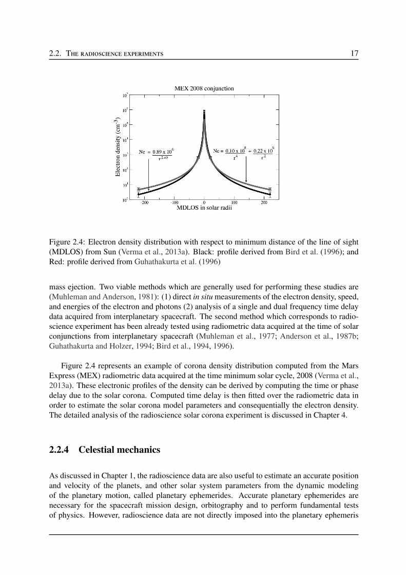
2.2. The radioscience experiments 17
Figure 2.4: Electron density distribution with respect to minimum distance of the line of sight(MDLOS) from Sun (Verma et al., 2013a). Black: profile derived from Bird et al. (1996); andRed: profile derived from Guhathakurta et al. (1996)
mass ejection. Two viable methods which are generally used for performing these studies are(Muhleman and Anderson, 1981): (1) direct in situ measurements of the electron density, speed,and energies of the electron and photons (2) analysis of a single and dual frequency time delaydata acquired from interplanetary spacecraft. The second method which corresponds to radio-science experiment has been already tested using radiometric data acquired at the time of solarconjunctions from interplanetary spacecraft (Muhleman et al., 1977; Anderson et al., 1987b;Guhathakurta and Holzer, 1994; Bird et al., 1994, 1996).
Figure 2.4 represents an example of corona density distribution computed from the MarsExpress (MEX) radiometric data acquired at the time minimum solar cycle, 2008 (Verma et al.,2013a). These electronic profiles of the density can be derived by computing the time or phasedelay due to the solar corona. Computed time delay is then fitted over the radiometric data inorder to estimate the solar corona model parameters and consequentially the electron density.The detailed analysis of the radioscience solar corona experiment is discussed in Chapter 4.
2.2.4 Celestial mechanics
As discussed in Chapter 1, the radioscience data are also useful to estimate an accurate positionand velocity of the planets, and other solar system parameters from the dynamic modelingof the planetary motion, called planetary ephemerides. Accurate planetary ephemerides arenecessary for the spacecraft mission design, orbitography and to perform fundamental testsof physics. However, radioscience data are not directly imposed into the planetary ephemeris

18 2. The radioscience observables and their computation
software, they are instead first analyzed by the spacecraft orbit determination software. Rangebias, which present the systematic error in the geometric position of the planet as seen from theEarth, can be estimated while computing the orbit of the spacecraft. These rang bias imposestrong constraints on the orbits of the planet, as well as on other solar system parameters. Inconsequence, such data not only allow the construction of an accurate planetary ephemeris,they also contribute significantly to our knowledge of parameters such as asteroid masses. Adetailed description of such analysis using MGS, and MESSENGER spacecraft radiometricdata is discussed in Chapters 3, and 5, respectively.
2.3 Radiometric data
The radiometric data which are produced by the NASA DSN Multimission Navigation (MM-NAV) Radio Metric Data Conditioning Team (RMDCT) is called Orbit Data File (ODF)1. TheseODF are used to determine the spacecraft trajectories, gravity field affecting them, and radiopropagation conditions. Each ODF is in standard JPL binary format and consists of many36-byte logical records, which falls into 7 primary groups. In this work, we have developed anindependent software to extract the contents of these ODFs. This software reads the binary ODFand writes the contents in specific format, called GINS format. GINS is the orbit determinationsoftware, independently developed at the CNES (see Section 2.5).
2.3.1 ODF contents
The ODF contains several groups of informations. An ODF usually contains most groups, butmay not have all. The format of such groups are given in Kwok (2000). The brief descriptionof the contents of these groups is given below.
2.3.1.1 Group 1
• This group is usually a first group among the several records. It identifies the spacecraftID, the file creation time, the hardware, and the software associated with the ODF. Thisgroup also provides the information about the reference date and time for ODF time-tags.Currently the ODF data time-tags are referenced to Earth Mean Equatorial equinox of1950 (EME-50).
1http://geo.pds.nasa.gov/

2.3. Radiometric data 19
2.3.1.2 Group 2
• This group is usually a second group among the several groups records. It contains thestring character that some time used to identify the contents of the data record, such as,TIMETAG, OBSRVBL, FREQ, ANCILLARY-DATA.
2.3.1.3 Group 3
• This is the third group that usually contains majority of the data included in the ODF.According to the data categories, the description of this group is given below.
2.3.1.3.1 Time-tags
• Observable time: First in this category is the Doppler and range observable time TT
measured at the receiving station. Observable time TT corresponds to the time at themidpoint of the count interval, Tc. The integer and the fractional part of this time-tag(TT ) is given separately in ODF. The integer part is measured from 0 hours UTC on 1January 1950, whereas the fractional part is given in milliseconds.
• Count interval: Doppler observables are derived from the change in the Doppler cyclecount. The time period on which these counts are accumulated is called count intervalor compression time Tc. Typically count times have a duration of tens of seconds to afew thousand of seconds. For example, count time could be between 1-10 s when thespacecraft is near a planet or roughly 1000 s for interplanetary cruise.
• Station delay: This gives the information corresponding to the downlink and uplink delayat the receiving and at the transmitting station respectively. It is given in nanosecond inthe ODF.
2.3.1.3.2 Format IDs
• Spacecraft ID: It identities the spacecraft ID which corresponds to ODF data. For exam-ple: 94 for MGS
• Data type ID: As mentioned before, the radiometric data could be one-, two-, and three-way Doppler and two-way range. The ODF provides a specific ID associated with thesedata set. For example: 11, 12, and 13 integers give in ODF correspond to one-, two-, andthree-way Doppler respectively, whereas 37 stands for two-way range.

20 2. The radioscience observables and their computation
• Station ID: This is an integer that gives the receiving and transmitting stations ID thatare associated with the time period covered by the ODF. The transmitting station ID isset to zero, if the date type is one-way Doppler.
• Band ID: It identifies the uplink (at transmitting station), downlink (at receiving station),and exciter band (at receiving station) ID. The ID of these bands are set to 1, 2, and 3 forS, X, and Ka band.
• Date Validity ID: It is the quality indicator of the data. It set to zero for a good qualityof data and set to one for a bad data.
2.3.1.3.3 Observables
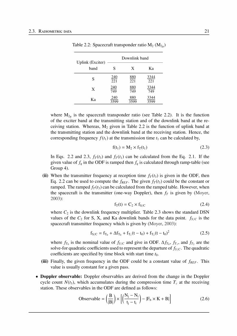
• Reference frequency: It is the frequency measured at the reception time t3 at the receiv-ing station in UTC (see Section 2.4.1). This frequency can be constant or ramped. How-ever, the given reference frequency in the ODF could be a reference oscillator frequencyfq, or a transmitter frequency fT , or a Doppler reference frequency fREF . The computedvalues of Doppler observables are directly affected by the fREF . Hence, the computationof the fREF from the reference oscillator frequency fq, or from the transmitter frequencyfT is discussed below.
(i) When the given frequency in the ODF is fq, then it is needed to first compute thetransmitter frequency, which is given by (Moyer, 2003):
fT(t) = T3 × fq(t) + T4 (2.1)
where T3 and T4 are the transmitter-band dependent constants as given in Table 2.1.From Eq. 2.1, one can compute the transmitter frequency at the receiving stationand at the transmitting station by replacing the time t to t3 and t1 respectively. Thus,the fREF at reception time can calculated by multiplying the spacecraft transponderratio with fT :
fREF(t3) = M2R × fT(t3) (2.2)
Table 2.1: Constants dependent upon transmitter or exciter band
BandTransmitter Band
T1 T2 T3 T4 (Hz)
S 240 221 96 0
X 240 749 32 6.5×10⁹
Ku 142 153 1000 -7.0×10⁹
Ka 14 15 1000 1.0×10¹⁰
2.3. Radiometric data 21
Table 2.2: Spacecraft transponder ratio M2 (M2R)
Uplink (Exciter)Downlink band
band S X Ka
S 240221
880221
3344221
X 240749
880749
3344749
Ka 2403599
8803599
33443599
where M2Ris the spacecraft transponder ratio (see Table 2.2). It is the function
of the exciter band at the transmitting station and of the downlink band at the re-ceiving station. Whereas, M2 given in Table 2.2 is the function of uplink band atthe transmitting station and the downlink band at the receiving station. Hence, thecorresponding frequency f (t1) at the transmission time t1 can be calculated by,
f(t1) = M2 × fT(t1) (2.3)
In Eqs. 2.2 and 2.3, fT (t3) and fT (t1) can be calculated from the Eq. 2.1. If thegiven value of fq in the ODF is ramped then fq is calculated through ramp-table (seeGroup 4).
(ii) When the transmitter frequency at reception time fT (t3) is given in the ODF, thenEq. 2.2 can be used to compute the fREF . The given fT (t3) could be the constant orramped. The ramped fT (t3) can be calculated from the ramped table. However, whenthe spacecraft is the transmitter (one-way Doppler), then fT is given by (Moyer,2003):
fT(t) = C2 × fS/C (2.4)
where C2 is the downlink frequency multiplier. Table 2.3 shows the standard DSNvalues of the C2 for S, X, and Ka downlink bands for the data point. fS/C is thespacecraft transmitter frequency which is given by (Moyer, 2003):
fS/C = fT0 + ∆fT0 + fT1(t − t0) + fT2(t − t0)2 (2.5)
where fT0 is the nominal value of fS/C and give in ODF. ∆ fT0 , fT1 , and fT2 are thesolve-for quadratic coefficients used to represent the departure of fS/C. The quadraticcoefficients are specified by time block with start time t0.
(iii) Finally, the given frequency in the ODF could be a constant value of fREF . Thisvalue is usually constant for a given pass.
• Doppler observable: Doppler observables are derived from the change in the Dopplercycle count N(t3), which accumulates during the compression time Tc at the receivingstation. These observables in the ODF are defined as follows:
Observable =( B
|B|
)
×
[(Nj − Ni
tj − ti
)
− |Fb × K + B|]
(2.6)
22 2. The radioscience observables and their computation
Table 2.3: Downlink frequency multiplier C2
MultiplierDownlink Band
S X Ka
C2 1 880230
3344240
where:B = Bias placed on receiverNi = Doppler count at time ti
N j = Doppler count at time t j
ti = start time of intervalt j = end time of intervalFb = frequency biasK = 1 for S-band receivers= 11/3 for X-band receivers= 176/27 for Ku-band receivers= 209/15 for Ka-band receivers
Fb = (X1/X2) × (X3 × fR + X4) − fs/c + R3 for 1 − way Doppler (2.7)
Fb = (X1/X2) × (X3 × fqR + X4) − (T1/T2) × (T3 × fqT + T4) for 2/3 − way Doppler(2.8)
Tc = tj − ti compression time (2.9)
where:fqR
= Receiver oscillator frequency at time t3
fs/c = Spacecraft (beacon) frequencyfqT
= Transmitter oscillator frequency at time t1
R3 = 0 for all receiving bandsT1 to T4 = Transmitters band (Table 2.1)X1 to X4 = Exciter band ( same value as transmitter band, Table 2.1)
Figure 2.5 shows an example of two and three way Doppler observables extracted fromthe MGS ODF.
• Range observable: Range observables are obtained from the ranging machine at thereceiving station. These range observables are measured in range units (see Section 2.4.3)and defined in ODF as follows:
Observable = R − C + Z − S (2.10)
where:R = range measurementC = station delay calibrationZ = Z-height correctionS = spacecraft delay
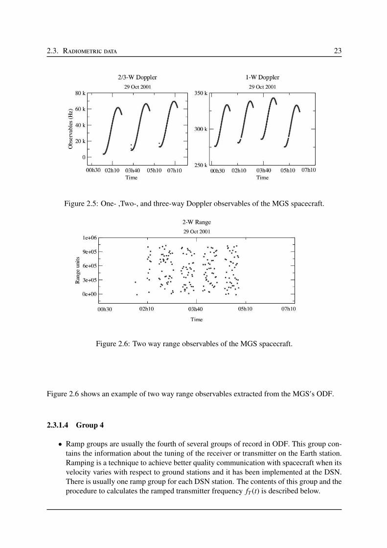
2.3. Radiometric data 23
Figure 2.5: One- ,Two-, and three-way Doppler observables of the MGS spacecraft.
Figure 2.6: Two way range observables of the MGS spacecraft.
Figure 2.6 shows an example of two way range observables extracted from the MGS′s ODF.
2.3.1.4 Group 4
• Ramp groups are usually the fourth of several groups of record in ODF. This group con-tains the information about the tuning of the receiver or transmitter on the Earth station.Ramping is a technique to achieve better quality communication with spacecraft when itsvelocity varies with respect to ground stations and it has been implemented at the DSN.There is usually one ramp group for each DSN station. The contents of this group and theprocedure to calculates the ramped transmitter frequency fT (t) is described below.
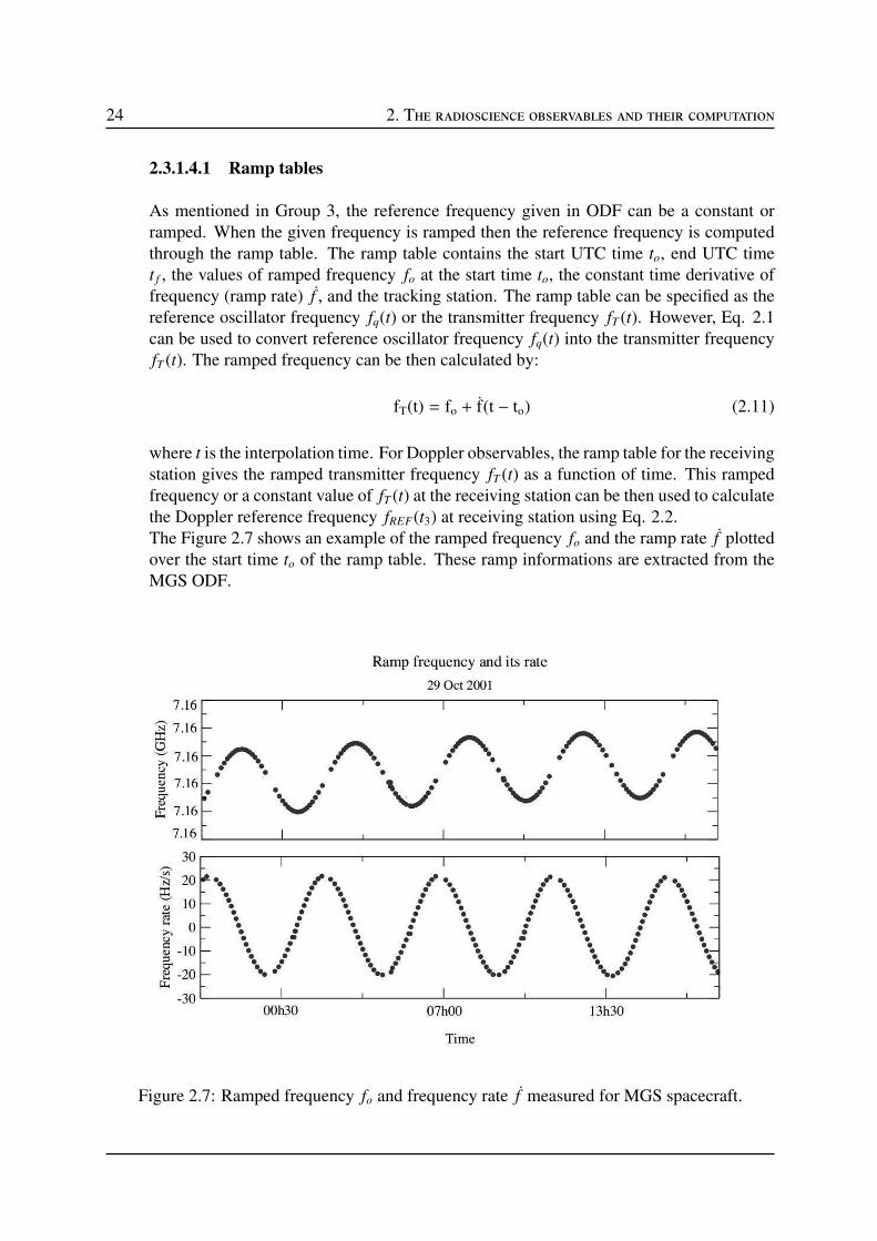
24 2. The radioscience observables and their computation
2.3.1.4.1 Ramp tables
As mentioned in Group 3, the reference frequency given in ODF can be a constant orramped. When the given frequency is ramped then the reference frequency is computedthrough the ramp table. The ramp table contains the start UTC time to, end UTC timet f , the values of ramped frequency fo at the start time to, the constant time derivative offrequency (ramp rate) f , and the tracking station. The ramp table can be specified as thereference oscillator frequency fq(t) or the transmitter frequency fT (t). However, Eq. 2.1can be used to convert reference oscillator frequency fq(t) into the transmitter frequencyfT (t). The ramped frequency can be then calculated by:
fT(t) = fo + f(t − to) (2.11)
where t is the interpolation time. For Doppler observables, the ramp table for the receivingstation gives the ramped transmitter frequency fT (t) as a function of time. This rampedfrequency or a constant value of fT (t) at the receiving station can be then used to calculatethe Doppler reference frequency fREF(t3) at receiving station using Eq. 2.2.The Figure 2.7 shows an example of the ramped frequency fo and the ramp rate f plottedover the start time to of the ramp table. These ramp informations are extracted from theMGS ODF.
Figure 2.7: Ramped frequency fo and frequency rate f measured for MGS spacecraft.
2.4. ObservationModel 25
2.3.1.5 Group 5
• This is a clock offset group. It is usually the fifth of several groups of record in ODF.It contains information on clock offsets at DSN stations contributing to the ODF. Thisgroup may be omitted from the ODF and used only with VLBI data. It contains the startand end time of the clock offset which is measured from 0 hours UTC on 1 January 1950.It also includes the DSN station ID and the correspond clock offset given in nanoseconds.The informations of this group are generally not useful for the radioscience studies.
2.3.1.6 Group 6
• This group is usually not include in the ODF and omitted all the time.
2.3.1.7 Group 7
• It is a data summary group which contains summary information on contents of the ODF,such as, the first and last date of the data sample, total number of samples, used trans-mitting and receiving stations, band ID, and the type of data available in the ODF. Thisgroup is optional and may be omitted from the ODF.
2.4 Observation Model
For given spacecraft radiometric data obtained by the DSN are described in Section 2.3. Thesedata record for each data point contains ID information which is necessary to unambiguouslyidentify the data point and the observed value of the observable (see Group 3 of Section 2.3.1).In order to better understand these radiometric data and to estimate the precise orbit of thespacecraft, it is then necessary to compute the observables.
The computation of the observables requires the time and frequency information of thetransmitted frequencies at the transmitter. The various time scales and their transformationsused for these computation are described in Section 2.4.1. Using the time scale transformations,the reception time t3 and the transmission time t1 can be then derived from the light-time delaydescribed in the Section 2.4.2. Using these informations it is then possible to compute theDoppler and range observables as described in Section 2.4.3.
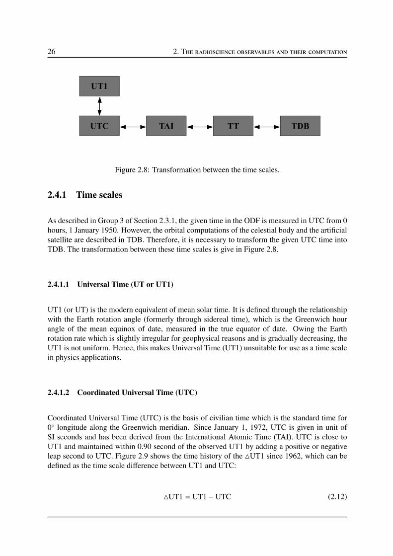
26 2. The radioscience observables and their computation
Figure 2.8: Transformation between the time scales.
2.4.1 Time scales
As described in Group 3 of Section 2.3.1, the given time in the ODF is measured in UTC from 0hours, 1 January 1950. However, the orbital computations of the celestial body and the artificialsatellite are described in TDB. Therefore, it is necessary to transform the given UTC time intoTDB. The transformation between these time scales is give in Figure 2.8.
2.4.1.1 Universal Time (UT or UT1)
UT1 (or UT) is the modern equivalent of mean solar time. It is defined through the relationshipwith the Earth rotation angle (formerly through sidereal time), which is the Greenwich hourangle of the mean equinox of date, measured in the true equator of date. Owing the Earthrotation rate which is slightly irregular for geophysical reasons and is gradually decreasing, theUT1 is not uniform. Hence, this makes Universal Time (UT1) unsuitable for use as a time scalein physics applications.
2.4.1.2 Coordinated Universal Time (UTC)
Coordinated Universal Time (UTC) is the basis of civilian time which is the standard time for0 longitude along the Greenwich meridian. Since January 1, 1972, UTC is given in unit ofSI seconds and has been derived from the International Atomic Time (TAI). UTC is close toUT1 and maintained within 0.90 second of the observed UT1 by adding a positive or negativeleap second to UTC. Figure 2.9 shows the time history of the UT1 since 1962, which can bedefined as the time scale difference between UT1 and UTC:
UT1 = UT1 − UTC (2.12)
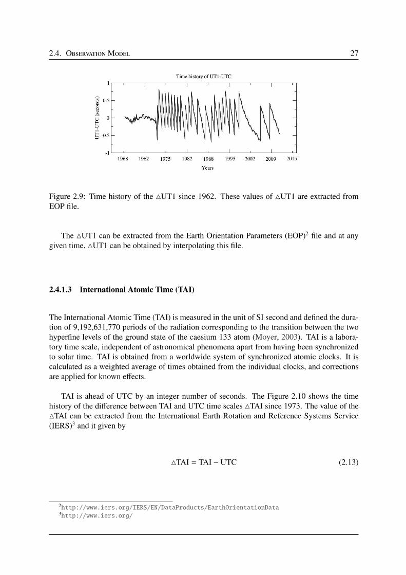
2.4. ObservationModel 27
Figure 2.9: Time history of the UT1 since 1962. These values of UT1 are extracted fromEOP file.
The UT1 can be extracted from the Earth Orientation Parameters (EOP)2 file and at anygiven time, UT1 can be obtained by interpolating this file.
2.4.1.3 International Atomic Time (TAI)
The International Atomic Time (TAI) is measured in the unit of SI second and defined the dura-tion of 9,192,631,770 periods of the radiation corresponding to the transition between the twohyperfine levels of the ground state of the caesium 133 atom (Moyer, 2003). TAI is a labora-tory time scale, independent of astronomical phenomena apart from having been synchronizedto solar time. TAI is obtained from a worldwide system of synchronized atomic clocks. It iscalculated as a weighted average of times obtained from the individual clocks, and correctionsare applied for known effects.
TAI is ahead of UTC by an integer number of seconds. The Figure 2.10 shows the timehistory of the difference between TAI and UTC time scales TAI since 1973. The value of theTAI can be extracted from the International Earth Rotation and Reference Systems Service(IERS)3 and it given by
TAI = TAI − UTC (2.13)
2http://www.iers.org/IERS/EN/DataProducts/EarthOrientationData3http://www.iers.org/
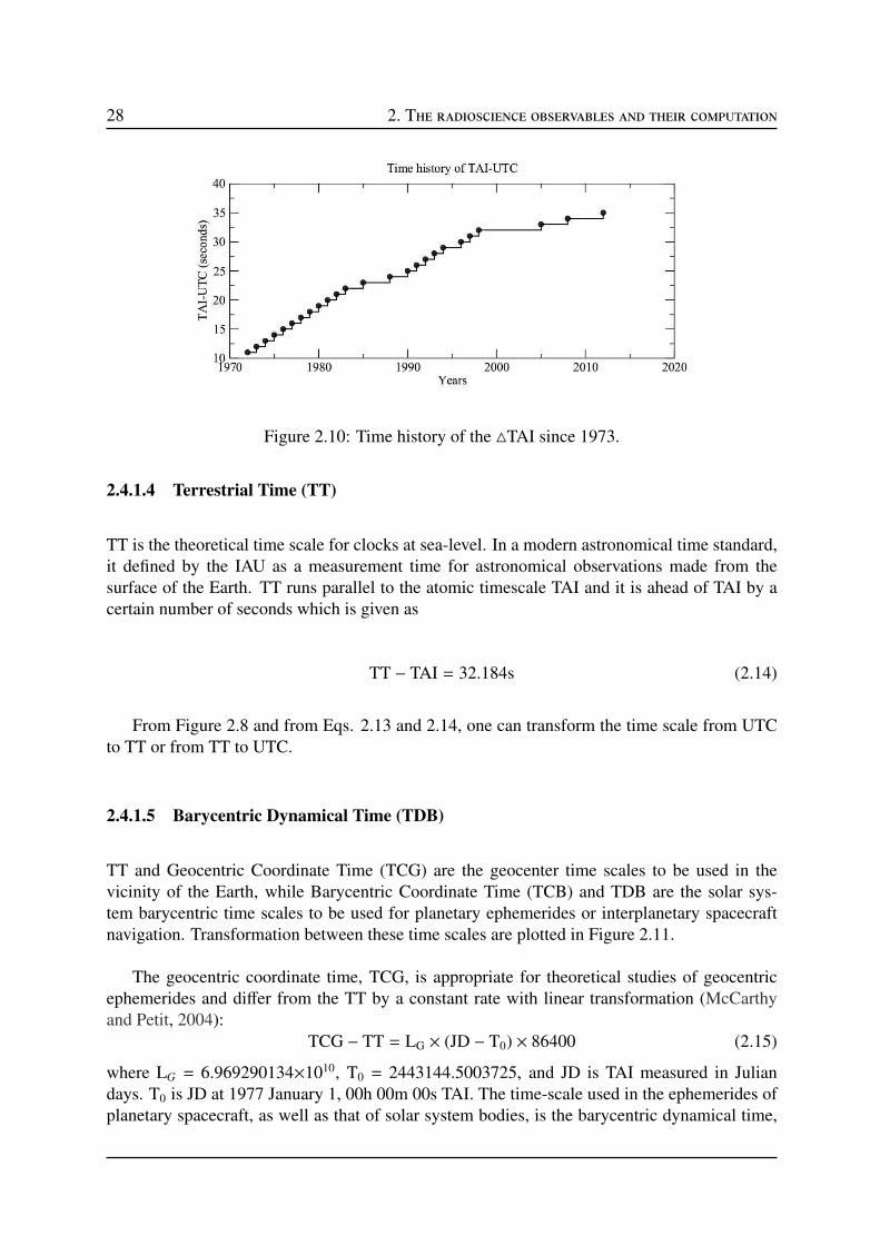
28 2. The radioscience observables and their computation
Figure 2.10: Time history of the TAI since 1973.
2.4.1.4 Terrestrial Time (TT)
TT is the theoretical time scale for clocks at sea-level. In a modern astronomical time standard,it defined by the IAU as a measurement time for astronomical observations made from thesurface of the Earth. TT runs parallel to the atomic timescale TAI and it is ahead of TAI by acertain number of seconds which is given as
TT − TAI = 32.184s (2.14)
From Figure 2.8 and from Eqs. 2.13 and 2.14, one can transform the time scale from UTCto TT or from TT to UTC.
2.4.1.5 Barycentric Dynamical Time (TDB)
TT and Geocentric Coordinate Time (TCG) are the geocenter time scales to be used in thevicinity of the Earth, while Barycentric Coordinate Time (TCB) and TDB are the solar sys-tem barycentric time scales to be used for planetary ephemerides or interplanetary spacecraftnavigation. Transformation between these time scales are plotted in Figure 2.11.
The geocentric coordinate time, TCG, is appropriate for theoretical studies of geocentricephemerides and differ from the TT by a constant rate with linear transformation (McCarthyand Petit, 2004):
TCG − TT = LG × (JD − T0) × 86400 (2.15)
where LG = 6.969290134×10¹⁰, T0 = 2443144.5003725, and JD is TAI measured in Juliandays. T0 is JD at 1977 January 1, 00h 00m 00s TAI. The time-scale used in the ephemerides ofplanetary spacecraft, as well as that of solar system bodies, is the barycentric dynamical time,
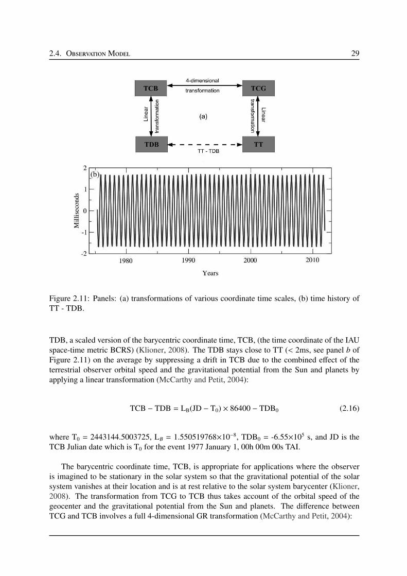
2.4. ObservationModel 29
Figure 2.11: Panels: (a) transformations of various coordinate time scales, (b) time history ofTT - TDB.
TDB, a scaled version of the barycentric coordinate time, TCB, (the time coordinate of the IAUspace-time metric BCRS) (Klioner, 2008). The TDB stays close to TT (< 2ms, see panel b ofFigure 2.11) on the average by suppressing a drift in TCB due to the combined effect of theterrestrial observer orbital speed and the gravitational potential from the Sun and planets byapplying a linear transformation (McCarthy and Petit, 2004):
TCB − TDB = LB(JD − T0) × 86400 − TDB0 (2.16)
where T0 = 2443144.5003725, LB = 1.550519768×10⁻⁸, TDB0 = -6.55×10⁵ s, and JD is theTCB Julian date which is T0 for the event 1977 January 1, 00h 00m 00s TAI.
The barycentric coordinate time, TCB, is appropriate for applications where the observeris imagined to be stationary in the solar system so that the gravitational potential of the solarsystem vanishes at their location and is at rest relative to the solar system barycenter (Klioner,2008). The transformation from TCG to TCB thus takes account of the orbital speed of thegeocenter and the gravitational potential from the Sun and planets. The difference betweenTCG and TCB involves a full 4-dimensional GR transformation (McCarthy and Petit, 2004):
30 2. The radioscience observables and their computation
TCB − TCG = c−2
∫ t
t0
[v2e
2+ Uext ( #„x e)
]
dt + #„v e.(#„x − #„x e)
+ O(c−4) (2.17)
where #„x e and #„v e are the barycentric position and velocity of the geocenter, the #„x is thebarycentric position of the observer and Uext is the Newtonian potential of all of the solar systembodies apart from the Earth, evaluated at the geocenter. In this formula, t is TCB and t0 is chosento be consistent with 1977 January 1, 00h 00m 00s TAI. The neglected terms, O(c−4), are oforder 10−16 in rate for terrestrial observers. Uext ( #„x e) and #„v e are all ephemeris-dependent, andso the resulting TCB belongs to that particular ephemeris, and the term #„v e.(
#„x - #„x e) is zero atthe geocenter.
The all above set of Equations 2.15-2.17 are precisely modeled in INPOP. The numericalintegration has been performed to obtain a realization of Equation 2.17 with a nanosecondaccuracy (Fienga et al., 2009). The difference between TT-TDB therefore can be extracted atany time from the INPOP planetary ephemeris using the tool called calceph4. The spacecraftorbit determination software GINS (see Section 2.5), integrates the equations of motion in thespecific coordinate time called, ephemeris time (ET). In GINS, this time is also referred to asTDB, as defined by Moyer (2003). As discrepancies between TT and TDB or ET are smallerthan 2 ms (see panel b of Figure 2.11), the transformation between the time scales defined eitherin INPOP or GINS are analogous and show consistency between both software.
2.4.2 Light time solution
The light time solution is used to compute the one-way or round-trip light time of the signalpropagating between the tracking station on the Earth and the spacecraft. In order to computethe Doppler and range observables, the first step is to obtain the light time solution. This solutioncan be modeled by computing the positions and velocities of the transmitter at the transmittingtime t1(T DB), spacecraft at the bouncing time t2(T DB) (for round-trip) or transmitting timet2(T DB) (for one-way), and receiver at the receiving time t3(T DB).
For round-trip light time, spacecraft observations involve two tracking stations, a transmit-ter, and a receiver which may not be at the same location. Therefore, two light time solutionsmust be computed, one for up-leg of the signal (transmitter to spacecraft) and one for down-leg(spacecraft to receiver). However, one-way light time requires only single solution because thesignal is transmitting by the spacecraft to the receiver. These solutions can be obtained in theSolar system barycenter space-time reference frame for a spacecraft located anywhere in theSolar system.
Since spacecraft observations are usually given at receiver time UTC (see section 2.3.1),the computation sequence therefore works backward in time: given the receiver time t3(UTC),
4http://www.imcce.fr/inpop/calceph/
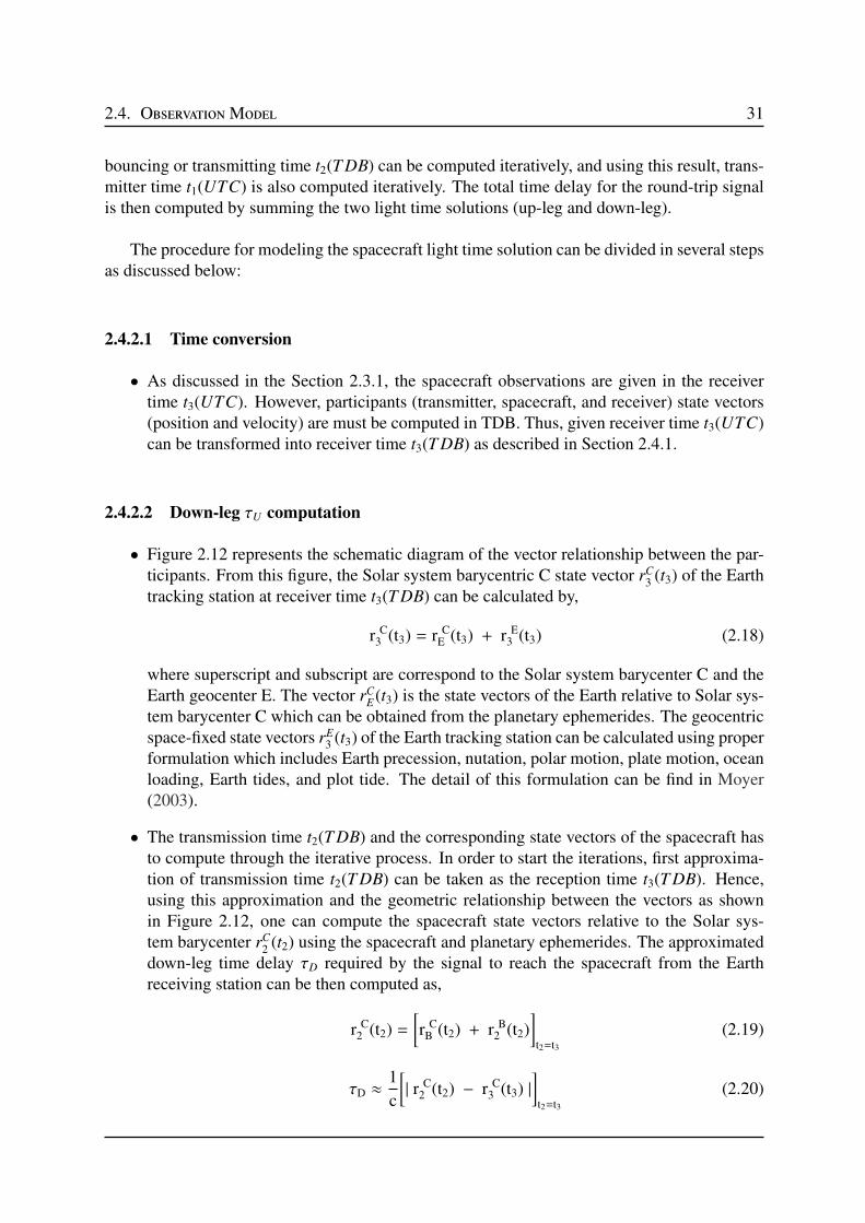
2.4. ObservationModel 31
bouncing or transmitting time t2(T DB) can be computed iteratively, and using this result, trans-mitter time t1(UTC) is also computed iteratively. The total time delay for the round-trip signalis then computed by summing the two light time solutions (up-leg and down-leg).
The procedure for modeling the spacecraft light time solution can be divided in several stepsas discussed below:
2.4.2.1 Time conversion
• As discussed in the Section 2.3.1, the spacecraft observations are given in the receivertime t3(UTC). However, participants (transmitter, spacecraft, and receiver) state vectors(position and velocity) are must be computed in TDB. Thus, given receiver time t3(UTC)can be transformed into receiver time t3(T DB) as described in Section 2.4.1.
2.4.2.2 Down-leg τU computation
• Figure 2.12 represents the schematic diagram of the vector relationship between the par-ticipants. From this figure, the Solar system barycentric C state vector rC
3 (t3) of the Earthtracking station at receiver time t3(T DB) can be calculated by,
r C3 (t3) = r C
E (t3) + r E3 (t3) (2.18)
where superscript and subscript are correspond to the Solar system barycenter C and theEarth geocenter E. The vector rC
E(t3) is the state vectors of the Earth relative to Solar sys-
tem barycenter C which can be obtained from the planetary ephemerides. The geocentricspace-fixed state vectors rE
3 (t3) of the Earth tracking station can be calculated using properformulation which includes Earth precession, nutation, polar motion, plate motion, oceanloading, Earth tides, and plot tide. The detail of this formulation can be find in Moyer(2003).
• The transmission time t2(T DB) and the corresponding state vectors of the spacecraft hasto compute through the iterative process. In order to start the iterations, first approxima-tion of transmission time t2(T DB) can be taken as the reception time t3(T DB). Hence,using this approximation and the geometric relationship between the vectors as shownin Figure 2.12, one can compute the spacecraft state vectors relative to the Solar sys-tem barycenter rC
2 (t2) using the spacecraft and planetary ephemerides. The approximateddown-leg time delay τD required by the signal to reach the spacecraft from the Earthreceiving station can be then computed as,
r C2 (t2) =
[
r CB (t2) + r B
2 (t2)]
t2=t3
(2.19)
τD ≈1
c
[
| r C2 (t2) − r C
3 (t3) |]
t2=t3
(2.20)

32 2. The radioscience observables and their computation
Figure 2.12: Geometric sketch of the vectors involved in the computation of the light timesolution, where C is the solar system barycentric; E is the Earth geocenter; and B is the centerof the central body.
where superscript B represents the central body of the orbiting spacecraft. The vectorrC
B(t2) given in Eq. 2.19 is the state vector of the central body relative to the Solar system
barycenter obtained from the planetary ephemerides. While, rB2 (t2) is the spacecraft state
vectors relative to center of the central body computed from the spacecraft ephemerides.In Eq. 2.20, c is the speed of light and τD is the down-leg time delay which can becomputed through the Eqs. 2.19 and 2.18. An estimated value of the bouncing time t2
can be then computed as,t2 = t3 − τD (2.21)
• Now using this result, we can then estimate the barycentric position of the spacecraft atbouncing time t2. Hence, the down-leg vector ρD as shown in Figure 2.12 can be thenobtained as,
ρD = r C2 (t2) − r C
3 (t3) (2.22)
The improved value of the down-leg time delay τD, in seconds, can be then estimated as,
τD =1
c(| ρD |) + δτD (2.23)
where δτD is a down-leg light time corrections which includes the relativistic, solarcorona, and media contributions to the propagation delay. Furthermore, Eqs. 2.21 to
2.4. ObservationModel 33
2.23 need to iterate until the latest estimate of τD differs from the previous estimate bysome define value such as 0.05µ.
2.4.2.3 Up-leg τU computation
• For round-trip light time solution, next is to compute the up-leg time delay. A similar iter-ative procedure as used for down-leg solution can be used the up-leg solution. Up-leg timedelay τU which represents the time required for signal to travel between the spacecraft andthe Earth transmitting station. In order to begin the iterations, first approximation can beassumed as,
τU ≈ τD (2.24)
Therefore, while using Eq. 2.24, approximated transmitting time t1(T DB) can be thencomputed as,
t1 = t2 − τU (2.25)
• The barycentric state vectors of the transmitting station rC1 (t1) at transmitted time t1(T DB)
as shown in Figure 2.12 can be computed from Eq. 2.18 by replacing the 3 with 1, that is,
r C1 (t1) = r C
E (t1) + r E1 (t1) (2.26)
Now, using Eq. 2.26, one can compute the up-leg state vector as give by,
ρU = r C2 (t2) − r C
1 (t1) (2.27)
where rC2 (t2) is the barycentric position of the spacecraft at bouncing time t2(T DB) and
can be calculated from Eq. 2.19. Finally, the new estimation of the up-leg time delay τU ,in seconds, is given by,
τU =1
c(| ρU |) + δτU (2.28)
where δτU is the up-leg light time correction analogous to δτD of Eq. 2.23. Eqs. 2.25 to2.28 are then need to iterative until the convergence is achieved.
2.4.2.4 Light time corrections, δτD and δτU
2.4.2.4.1 Relativistic correction δτRC
Electromagnetic signals that are traveling between the spacecraft and the Earth tracking en-counters light time delay when it passes close to the massive celestial bodies. This effects isknown as S hapiro delay or gravitational time delay (Shapiro, 1964). Such time delays arecaused by the bending of the light path which increase the travailing path of the signal. Hence,

34 2. The radioscience observables and their computation
relativistic time delays caused by the gravitational attraction of the bodies can be expressed, inseconds, as (Shapiro, 1964; Moyer, 2003),
δτRCU =(1 + γ) µS
c3ln
r S1 + r S
2 + r S12 +
(1+γ) µS
c2
r S1 + r S
2 − r S12 +
(1+γ) µS
c2
+
10∑
B=1
(1 + γ) µB
c3ln
[
r B1 + r B
2 + r B12
r S1 + r S
2 − r S12
]
(2.29)
where superscript S and B correspond to the Sun and the celestial body. r1, r2, and r12 arethe distance between the spacecraft and the Sun S (or celestial body B), the Earth station andthe Sun S (or celestial body B), and the spacecraft and the Earth station, respectively. The µS
and µB are the gravitational constant of the Sun and the celestial body, respectively.
For round-trip signal, Eq. 2.29 represents the relativistic time delay δτRCUrelative to the
up-leg of the signal. The corresponding down-leg relativistic time delay δτRCDcan be calculate
using the same equation by replacing the 1 with 2 and 2 with 3. Hence, the total relativistic timedelay, in seconds, during the round-trip of the signal can be given as,
δτRC = δτRCU + δτRCD (2.30)
2.4.2.4.2 Solar Corona correction δτS C
As mentioned in Section 2.2.3, solar corona severely degrades the radio wave signals whenpropagating between spacecraft and Earth tracking stations. The delay owing to the solar coronaare directly proportional to the total electron contents along the LOS and inversely with thesquare of carrier radio wave frequency. Solar corona model for computing such delays for eachlegs are described in Chapter 3. The total round-trip solar corona delay, in seconds, can bewritten as,
δτSC = δτSCU + δτSCD (2.31)
2.4.2.4.3 Media corrections δτMC
The media corrections consist of Earth′s troposphere correction and the correction due to thecharge particles of the Earth ionosphere. Such delays however relatively lesser compare to therelativistic and solar corona delays. The tropospheric model used for computing these correc-tions for each legs are discussed in Chao (1971); Moyer (2003). The total round-trip mediacorrection, in seconds, can be written as,
δτMC = δτMCU + δτMCD (2.32)
Figure 2.13 shows an example of relativistic correction and solar corona correction to lighttime solution for MGS and MESSENGER spacecraft.

2.4. ObservationModel 35
Figure 2.13: Relativistic and solar corona corrections to light time solution (expressed in sec-onds): (a) for MGS, (b) for MESSENGER.
2.4.2.5 Total light time delay
2.4.2.5.1 Round-trip delay
The total round-trip delay is the sum of number of terms, that includes,
ρ = ( τD + τU ) − (TDB − TAI)t3 + (TDB − TAI)t1
−(TAI − UTC)t3 + (TAI − UTC)t1
+δρU + δρD (2.33)
where quantities δρD and δρU are the downlink delay at receiver and uplink delay at trans-mitter (see Group 3 of Section 2.3.1), respectively. The time differences given in Eq. 2.33 canbe obtained as described in Section 2.4.1, while τD and τU can be obtained from Eqs. 2.23 and2.28 respectively. Figure 2.14 illustrates an example for the total round-trip time that requiredby the signal to travel from the transmitter to the spacecraft (up-leg) and then from the space-craft to the receiver (down-leg). This time solution shown in Figure 2.14 corresponds to MGS(panel a) and MESSENGER (panel b) spacecraft.
2.4.2.5.2 One-way delay

36 2. The radioscience observables and their computation
Figure 2.14: Round-trip light time solution of MGS (panel a) and MESSENGER (panel b)spacecraft, computed from the Eq. 2.33.
One-way light, in seconds, which is used to calculate the one-way Doppler observables canbe calculated as,
ρ1 = ρ1 + (TDB − TAI)t2 (2.34)
where ρ1 is the difference between reception time t3(UTC) and the spacecraft transmitter timet2(T DB).
2.4.3 Doppler and range observables
The radiometric data obtained by the Earth tracking station (DSN) usually consists of three kindof measurements (one-way Doppler, two/three-way Doppler, and two-way range). The detaildescription of these measurements and other contents of the ODF that are useful for recognizethe data are described in Section 2.3.1. Observation model which computes the observationsrequires the time history of the transmitted frequency at the transmitter. Such time history whichcontains transmitter time t1(UTC) and receiver time t3(UTC), can be obtained as describedin Section 2.4.2. The corresponding transmitter frequency which can be obtained from thedifferent forms of given frequency in ODF is described in Group 3 of Section 2.3.1.
One of the most important aspect of precise orbit determination of the spacecraft is to com-pute the observables. These observables require spacecraft ephemerides which can be con-structed from the dynamic modeling (see Section 2.5). An observation model accounts thepropagation of signal and allows to compute the frequency change between received and trans-mitted signal, also called Doppler shi f t. The difference between observed (given in ODF) and

2.4. ObservationModel 37
computed values, also called residuals, are then used to adjust the dynamic model along withobservation model for accounting the discrepancy in the models.
This section contains the formulations for computing the one-way Doppler, two/three-wayDoppler, and two-way range observables. These formulations are based on Moyer (2003).The motivation for developing an observation model is to have a better understanding of theradiometric data. However, for precise computation, such as for MGS (see Chapter 3) and forMESSENGER (see Chapter 5), GINS orbit determination model (see Section 2.5) has beenused. Moreover, GINS observation model is also based on Moyer (2003) formulations and thebrief overview of the GINS dynamic model is described in Section 2.5.
2.4.3.1 Two-way (F2) and Three-way (F3) Doppler
2.4.3.1.1 Ramped
Doppler observable can be derived from the difference between the number of cycles receivedby a receiving station and the number of cycles produced by a fixed or ramped known referencefrequency fREF , during a specific count interval Tc. The given observables time-tag TT in theODF is the mid-point of the count interval Tc (see Group 3 of Section 2.3.1). To compute theseobservables (Eq. 2.40), it is thus necessary to obtain the starting time t3s
(UTC) and the endingtime t3e
(UTC) of the count interval, which is given in seconds by
t3s(UTC) = TT −1
2Tc (2.35)
t3e(UTC) = TT +1
2Tc (2.36)
where TT and Tc can be extracted from the ODF. Using Eqs. 2.35 and 2.36 the correspond-ing transmitting starting time t1s
(UTC) and ending time t1e(UTC), in seconds, can be obtained
from light time solution (see Section 2.4.2), that is,
t1s(UTC) = t3s(UTC) − ρs (2.37)
t1e(UTC) = t3e(UTC) − ρe (2.38)
where ρs and ρe is the round-trip light time computed from Eq. 2.33. Similarly, the corre-sponding start and end TDB at the receiving station and at the transmission station, which arerequired for the light time solution, can be computed as described in Section 2.4.1.
Using the time recorded history of the transmitters, the two-way Doppler F2 and three-wayDoppler F3 can be computed as the difference in the total accumulation of the Doppler cycles,which is given as, in Hz,
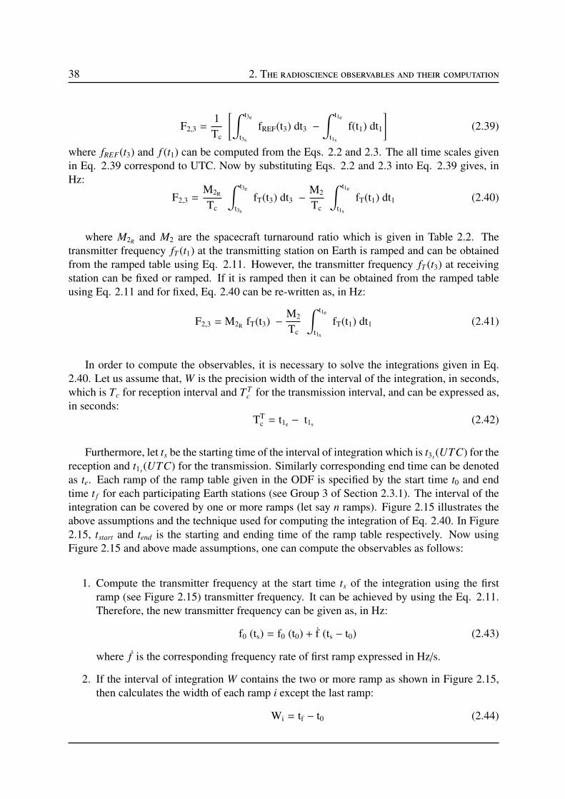
38 2. The radioscience observables and their computation
F2,3 =1
Tc
[∫ t3e
t3s
fREF(t3) dt3 −
∫ t1e
t1s
f(t1) dt1
]
(2.39)
where fREF(t3) and f (t1) can be computed from the Eqs. 2.2 and 2.3. The all time scales givenin Eq. 2.39 correspond to UTC. Now by substituting Eqs. 2.2 and 2.3 into Eq. 2.39 gives, inHz:
F2,3 =M2R
Tc
∫ t3e
t3s
fT(t3) dt3 −M2
Tc
∫ t1e
t1s
fT(t1) dt1 (2.40)
where M2Rand M2 are the spacecraft turnaround ratio which is given in Table 2.2. The
transmitter frequency fT (t1) at the transmitting station on Earth is ramped and can be obtainedfrom the ramped table using Eq. 2.11. However, the transmitter frequency fT (t3) at receivingstation can be fixed or ramped. If it is ramped then it can be obtained from the ramped tableusing Eq. 2.11 and for fixed, Eq. 2.40 can be re-written as, in Hz:
F2,3 = M2R fT(t3) −M2
Tc
∫ t1e
t1s
fT(t1) dt1 (2.41)
In order to compute the observables, it is necessary to solve the integrations given in Eq.2.40. Let us assume that, W is the precision width of the interval of the integration, in seconds,which is Tc for reception interval and T T
c for the transmission interval, and can be expressed as,in seconds:
TTc = t1e − t1s (2.42)
Furthermore, let ts be the starting time of the interval of integration which is t3s(UTC) for the
reception and t1s(UTC) for the transmission. Similarly corresponding end time can be denoted
as te. Each ramp of the ramp table given in the ODF is specified by the start time t0 and endtime t f for each participating Earth stations (see Group 3 of Section 2.3.1). The interval of theintegration can be covered by one or more ramps (let say n ramps). Figure 2.15 illustrates theabove assumptions and the technique used for computing the integration of Eq. 2.40. In Figure2.15, tstart and tend is the starting and ending time of the ramp table respectively. Now usingFigure 2.15 and above made assumptions, one can compute the observables as follows:
1. Compute the transmitter frequency at the start time ts of the integration using the firstramp (see Figure 2.15) transmitter frequency. It can be achieved by using the Eq. 2.11.Therefore, the new transmitter frequency can be given as, in Hz:
f0 (ts) = f0 (t0) + f (ts − t0) (2.43)
where f is the corresponding frequency rate of first ramp expressed in Hz/s.
2. If the interval of integration W contains the two or more ramp as shown in Figure 2.15,then calculates the width of each ramp i except the last ramp:
Wi = tf − t0 (2.44)
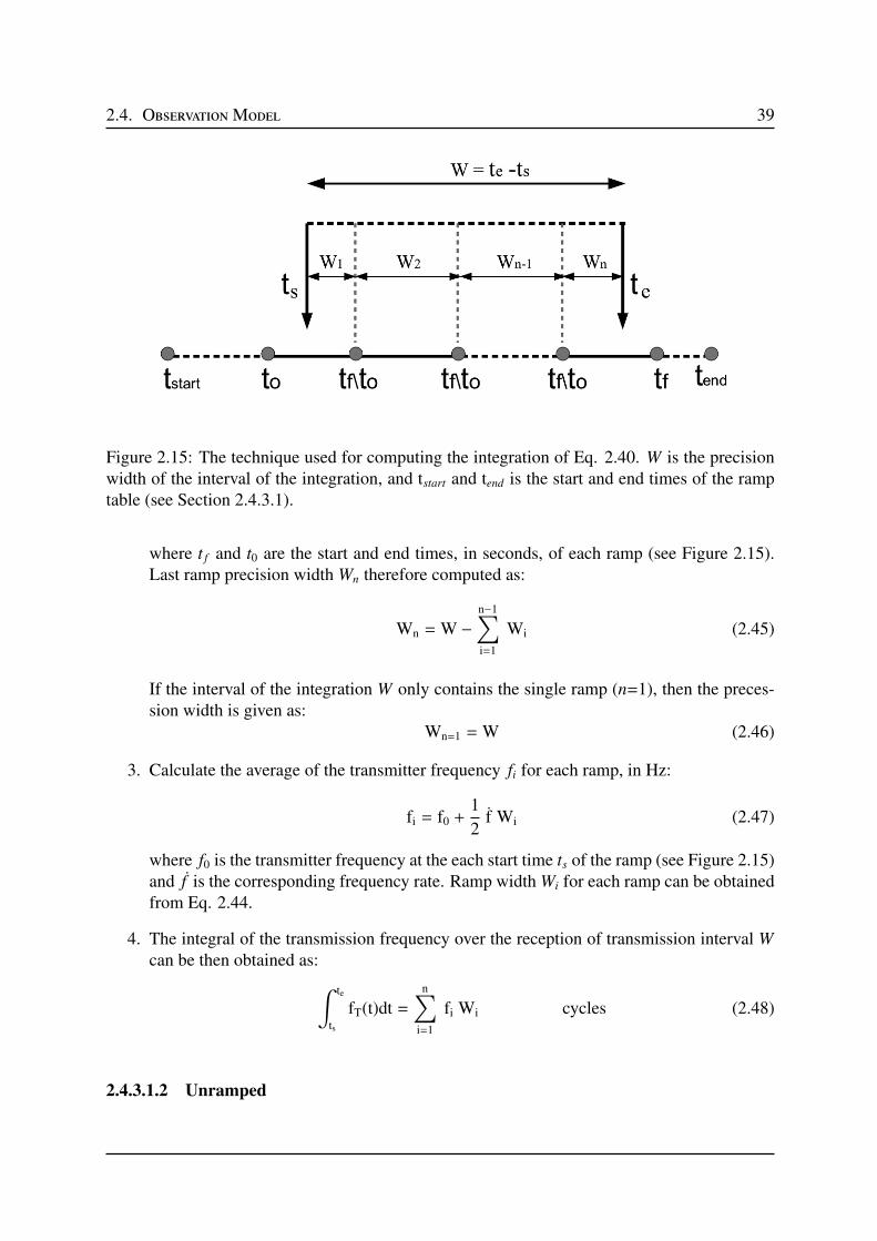
2.4. ObservationModel 39
Figure 2.15: The technique used for computing the integration of Eq. 2.40. W is the precisionwidth of the interval of the integration, and tstart and tend is the start and end times of the ramptable (see Section 2.4.3.1).
where t f and t0 are the start and end times, in seconds, of each ramp (see Figure 2.15).Last ramp precision width Wn therefore computed as:
Wn =W −n−1∑
i=1
Wi (2.45)
If the interval of the integration W only contains the single ramp (n=1), then the preces-sion width is given as:
Wn=1 =W (2.46)
3. Calculate the average of the transmitter frequency fi for each ramp, in Hz:
fi = f0 +1
2f Wi (2.47)
where f0 is the transmitter frequency at the each start time ts of the ramp (see Figure 2.15)and f is the corresponding frequency rate. Ramp width Wi for each ramp can be obtainedfrom Eq. 2.44.
4. The integral of the transmission frequency over the reception of transmission interval W
can be then obtained as:
∫ te
ts
fT(t)dt =n
∑
i=1
fi Wi cycles (2.48)
2.4.3.1.2 Unramped
40 2. The radioscience observables and their computation
As mentioned earlier, the given transmitter frequency can be constant or ramped. If it is con-stant, then it corresponds to the unramped transmitter frequency. Let us consider that, during aninterval dt1, dn cycles of the constant transmitter frequency fT (t1) are transmitted. During thecorresponding reception interval dt3, receiving station on Earth received M2dn cycles, whereM2 is the spacecraft turnaround ration (see Table 2.2). Therefore, the total accumulation of theconstant Doppler cycles is given as, in Hz:
F2,3 =M2 fT(t1)
Tc
[∫ t3e
t3s
dt3 −
∫ t1e
t1s
dt1
]
(2.49)
where t3sand t3e
are the start and end times of the reception time-tag TT which can be computedfrom Eqs. 2.35 and 2.36 respectively. Similarly t1s
and t1eare the corresponding transmitting
times which can be computed from Eqs. 2.37 and 2.38 respectively. All the time given in Eq.2.49 are in UTC.
Now evaluating Eq. 2.49:
F2,3 =M2 fT(t1)
Tc
[t3e − t1e] − [t3s − t1s]
(2.50)
Eq. 2.50 can be used to calculate the computed values of unramped two-way F2 and three-way F3 Doppler observables, in Hz.
2.4.3.2 One-way (F1) Doppler
When the radio signal is continuously transmitted from the spacecraft and received by the DSNstation on Earth, then the observables are referred to one-way. These observations are alwaysunramped and can be modeled as, in Hz, (Moyer, 2003):
F1 = C2 fT0 −1
Tc
∫ t2e (TAI)
t2s (TAI)
[
fT(t2)]
dt2(TAI) (2.51)
where C2 is the downlink frequency multiplier given in Table 2.3. fT0 is the nominal valueof spacecraft transmitter frequency fS/C (Eq. 2.5). fT (t2) is the transmitter frequency at thespacecraft at transmission time t2(T AI), given by Eq. 2.4.
Now by substituting Eqs. 2.4 and 2.5 in Eq. 2.51, the one-way Doppler observables can bewritten as, in Hz:
F1 = C2 fT0 −C2
Tc
∫ t2e (TAI)
t2s (TAI)
[
fT0 + ∆fT0 + fT1(t2 − t0) + fT2(t2 − t0)2]
dt2(TAI) (2.52)

2.4. ObservationModel 41
As one can see in Eq. 2.52, the terms containing the coefficients fT1 and fT2 are functionsof the spacecraft transmission time t2(T AI). Hence, the upper limit t2e
(T AI) and lower limitt2s
(T AI) of the integration are only required to evaluate these terms. Since these terms (<2ms) are small, the limits of the integration can be replaced with the corresponding values incoordinate time TDB (Moyer, 2003). These coordinate times, t2e
(T DB) and t2s(T DB), can be
obtained from the light time solution (see down-leg computation of Section 2.4.2).
Now by evaluating the integral of Eq. 2.52 using the above approximation it comes (Moyer,2003), in Hz:
F1 = C2 fT0
(ρ1e − ρ1s + ∆)
Tc
−C2
∆fT0 + fT1(t2m − t0) + fT2(t2m − t0)2 +fT2
12
(
T′
c
)2 T′
c
Tc(2.53)
where ρ1eand ρ1s
are the one-way light times at the end and at the start of the Doppler countinterval Tc at the receiver. These one-way light times and the time bias ∆, expressed in seconds,are given by:
ρ1e = t3e(UTC) − t2e(TDB) (2.54)
ρ1s = t3s(UTC) − t2s(TDB) (2.55)
∆ = (TDB − TAI)t2e− (TDB − TAI)t2s
(2.56)
The quadratic coefficients ∆ fT0 , fT1 , and fT2 given in Eq. 2.53 are specified by time blockwith start a time t0. In Eq. 2.53, T
′
c is the transmission interval at the spacecraft and t2mis the
average of the TDB values of the epochs at the start and end of the transmission interval at thespacecraft. These can expressed as, in seconds:
T′
c = Tc − (ρ1e − ρ1s + ∆) (2.57)
t2m =t2e(TDB) + t2s(TDB)
2(2.58)
2.4.3.3 Two-way (ρ2,3) Range
In addition to Doppler data, ODF also contains the range data as described in section 2.3.1.These data sets usually are not included in the orbit determination process. However, processingof range data along with orbit determination are extremely useful for the improvement of theplanetary ephemerides. This section will give the formulation for computing the two-way ramprange observables.
The range observables given in ODF are uniquely given in the range units. The conversionfactor F required to convert seconds into range units is a function of the transmitter signal

42 2. The radioscience observables and their computation
Table 2.4: Constant Crange requried for converting second to range units.
Type Crange
S-Band 12
X-Banda, HEF 1175
X-Bandb, BVE 2211496
a: for uplink X-band at a 34-m mount high efficiency (HEF)antenna.b: for uplink X-band at anytracking station that as a block5 exciter (BVE).
frequency fT and a constant fraction depending on the uplink band (Moyer, 2003). The integralof Fdt at the transmitting station gives the change in the phase of the transmitted ranging pulse(uniquely coded in range units) at its transmission time. When the spacecraft receives theranging pulse, it returns the pulse on its downlink. The time needed by the spacecraft to turnthe pulse around within its electronics is called transponder delay which is different for eachspacecraft. When the pulse is received at the Earth station, the actual light time is determinedincluding the light time delay corrections described in section 2.4.2. In addition it also includesthe delays due to the transmitter and receiver electronics at the Earth station and the delay in thespacecraft transponder.
The equation for calculating the conversion factor F at the transmitting or receiving stationon Earth is a function of the uplink band at the station. For S-, and X-band transmitter frequencyfT , is in range units/second:
F = Crange fT (2.59)
where, Crange is the band based constant given in Table 2.4. The classification of uplinkX-band antennas, which may either be mounted as high efficiency (HEF) or as block 5 exciter(BVE), can be obtained from the ODF. The equation for calculating the computed value of2-way ramped range observable is given by (Moyer, 2003), in modulo M expressed range units,
ρ2 =
∫ t3(UTC)
t1(UTC)
F(t) dt (2.60)
where t3(UTC) is the reception time at the receiving station and t1(UTC) is the transmissiontime at the transmitting station. The conversion factor F(t) can be calculated from Eq. 2.59 forthe corresponding band. Modulo M is the length of the ranging pulse in range units and it iscalculated from:
M = 2n+6 (2.61)
where n is the component number of the lowest frequency ranging component. The numbern can be obtained from the ODF. The integral of Eq. 2.60 can be evaluated using the sametechnique as described for two- and three-way ramped Doppler.
The transmitting time t1(UTC) given in Eq. 2.60 can be obtained from the light time solutionas described in Section 2.4.2. Now by substituting Eq. 2.59 in Eq. 2.60, it will give the time
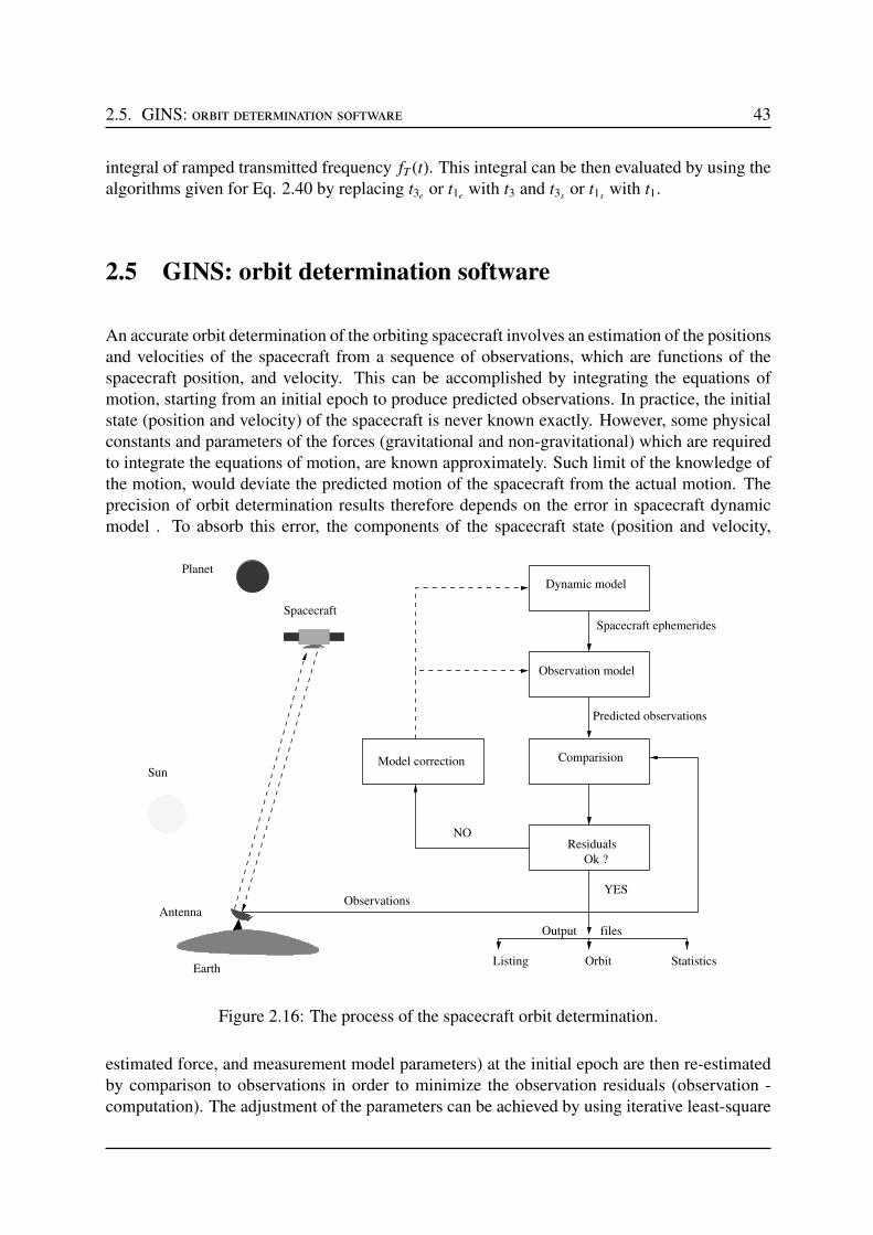
2.5. GINS: orbit determination software 43
integral of ramped transmitted frequency fT (t). This integral can be then evaluated by using thealgorithms given for Eq. 2.40 by replacing t3e
or t1ewith t3 and t3s
or t1swith t1.
2.5 GINS: orbit determination software
An accurate orbit determination of the orbiting spacecraft involves an estimation of the positionsand velocities of the spacecraft from a sequence of observations, which are functions of thespacecraft position, and velocity. This can be accomplished by integrating the equations ofmotion, starting from an initial epoch to produce predicted observations. In practice, the initialstate (position and velocity) of the spacecraft is never known exactly. However, some physicalconstants and parameters of the forces (gravitational and non-gravitational) which are requiredto integrate the equations of motion, are known approximately. Such limit of the knowledge ofthe motion, would deviate the predicted motion of the spacecraft from the actual motion. Theprecision of orbit determination results therefore depends on the error in spacecraft dynamicmodel . To absorb this error, the components of the spacecraft state (position and velocity,
files
Spacecraft ephemerides
Predicted observations
NO
YESObservations
Planet
Sun
Spacecraft
Earth
Antenna
Dynamic model
Observation model
Comparision
Residuals
Ok ?
Model correction
Listing Orbit Statistics
Output
Figure 2.16: The process of the spacecraft orbit determination.
estimated force, and measurement model parameters) at the initial epoch are then re-estimatedby comparison to observations in order to minimize the observation residuals (observation -computation). The adjustment of the parameters can be achieved by using iterative least-square
44 2. The radioscience observables and their computation
techniques. Hence, it can be summarized that, for the precise orbit determination, one needsa dynamic model which describes the forces acting on the spacecraft, a observational modelwhich is a function of observed parameters and spacecraft state vector, and a least-squaresestimation algorithm used to obtain the estimates.
The flow chart of orbit determination based on dynamic model in the frame of GINS soft-ware is given Figure 2.16. GINS is an orbit determination software developed by the CNES.This software was initially developed for the Earth orbiting spacecraft and then further devel-oped for the interplanetary spacecraft. GINS numerically integrates the equations of motionand the associated variational equations, and simultaneously retrieves the physical parametersof the force model using an iterative least-squares technique. From Figure 2.16, one can seethat, the first step of the orbit determination is to compute the spacecraft ephemerides fromthe dynamic model of the spacecraft motion. The section 2.5.1 gives a brief description ofsuch dynamic model used in the GINS software for planetary spacecraft. After computing thespacecraft ephemerides, the next step is to predict the observations from the observation model.The formulation associated with the observation model, which may consist to one-, two-, andthree-way Doppler and range observables, is described in Section 2.4.3. Finally, the differencebetween observed and computed observables gives the residuals, which describe the precision inthe computations. These residuals are then used to adjust the dynamic and observation modelsby computing the solve-for parameters using least square techniques described in Section 2.5.3.If the residuals meet the convergence criteria then it produce a three files output: a listing con-taining the estimated solve-for parameters, an ephemeris of the orbit containing the spacecraftstate vectors and its acceleration at each time step of the numerical integration, and statistics ofthe residuals. The detailed description of GINS software algorithms are given in the igsac-cneswebpage5.
2.5.1 Dynamic model
The dynamic model which consists of equations of motion can be described in an inertial frameas follows:
#„r = #„a g +#„a ng (2.62)
where #„r is the position vector between the center of mass of the spacecraft and the planet,#„a g is the sum of gravitational forces acting on the spacecraft, and #„a ng is the sum of non-gravitational forces acting on the spacecraft.
2.5.1.1 Gravitational forces
When the spacecraft is orbiting the planet then the primary force acting of the spacecraft is theforce of gravity, specifically, the gravitational attraction of the orbiting planet. However, there
5http://igsac-cnes.cls.fr/documents/gins/GINS_Doc_Algo_V4.html
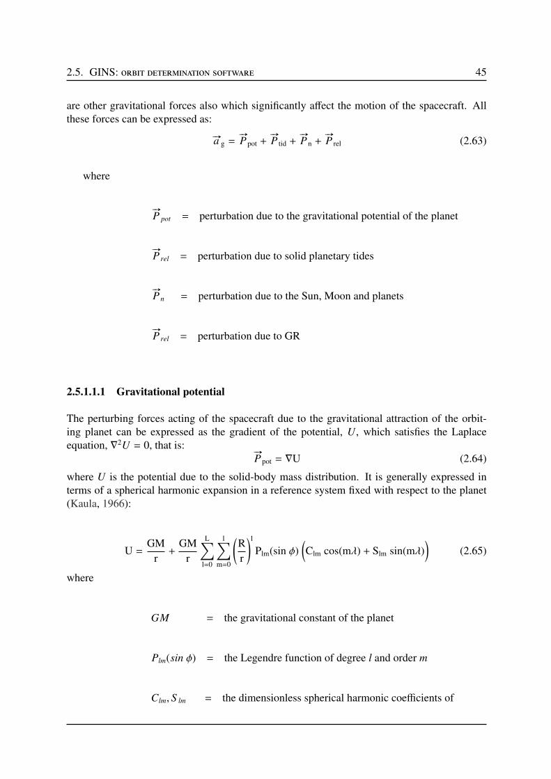
2.5. GINS: orbit determination software 45
are other gravitational forces also which significantly affect the motion of the spacecraft. Allthese forces can be expressed as:
#„a g =#„
Ppot +#„
P tid +#„
Pn +#„
P rel (2.63)
where
#„
P pot = perturbation due to the gravitational potential of the planet
#„
P rel = perturbation due to solid planetary tides
#„
Pn = perturbation due to the Sun, Moon and planets
#„
P rel = perturbation due to GR
2.5.1.1.1 Gravitational potential
The perturbing forces acting of the spacecraft due to the gravitational attraction of the orbit-ing planet can be expressed as the gradient of the potential, U, which satisfies the Laplaceequation, ∇2U = 0, that is:
#„
Ppot = ∇U (2.64)
where U is the potential due to the solid-body mass distribution. It is generally expressed interms of a spherical harmonic expansion in a reference system fixed with respect to the planet(Kaula, 1966):
U =GM
r+
GM
r
L∑
l=0
l∑
m=0
(
R
r
)l
Plm(sin φ)(
Clm cos(mλ) + Slm sin(mλ))
(2.65)
where
GM = the gravitational constant of the planet
Plm(sin φ) = the Legendre function of degree l and order m
Clm, S lm = the dimensionless spherical harmonic coefficients of
46 2. The radioscience observables and their computation
degree l and order m
R = the mean equatorial radius of the planet
r, φ, λ = the spherical coordinates of the spacecraft in a reference
system fixed with respect to the planet
L = the maximum number of degree and order
In practice, Eq. 2.65 is usually represented by the normalized spherical harmonic coeffi-cients (Clm, S lm) and normalized Legendre function Plm. The normalized coefficients are muchmore uniform in magnitude than the unnormalized coefficients. These normalized coefficientsare defined by:
Clm
S lm
=
√
(l + m)!
(2 − δ0m)(2l + 1)(l − m)!
Clm
S lm
(2.66)
and
Plm =
√
(2 − δ0m)(2l + 1)(l − m)!
(l + m)!Plm (2.67)
If one assumes that the reference system origin coincides with center of mass of the planet, thensummation of Eq. 2.65 starts from degree (l) 2 or C10 = C11 = S 10 = 0.
2.5.1.1.2 Solid planetary tides
Since the planet is a non-rigid elastic body, its mass distribution and the shape will be changedunder the gravitational attraction of the perturbing bodies. Tides deformations of a planet ornatural satellite caused by periodic variations of the local gravity acceleration as the planet orsatellite rotates and revolves in the gravity field of a perturbing bodies. Tidal disturbances of aplanet are primarily caused by the sun and by its satellites. The temporal variation of the freespace geopotential induced from solid planet tides can be expressed as a change in the externalgeopotential by the following expression (Wahr, 1981; Dow, 1988)
#„a tid = ∇(∆Utid) (2.68)
where,
∆Utid =GM
R2
3∑
l=2
l∑
m=0
∑
k(l,m)
Hk ei(Θk+χk) k0k
[(R
r
)l+1
Ylm(φ, λ) + k+k
(R
r
)l+3
Yl+2m (φ, λ)
]
(2.69)
2.5. GINS: orbit determination software 47
Ylm(φ, λ) = (−1)m
√
(2l + 1)(l − m)!
4π (l + m)!Plm(sin φ) eimλ (2.70)
Plm(sin φ) = the unnormalized associated Legendre function of
degree l and order m
Hk = the frequency dependent tidal amplitude in meters
Θk , χk = Doodson argument and phase correction for constituent k
( χk = 0, if l − m is even; χk = π/2, if l − m is odd
k0k, k+
k= Love numbers for tidal constituent k
r, φ, λ = geocentric body-fixed coordinates of the satellite
k(l,m) = each combination of l,m has a unique list of
tidal frequencies, k, to sum over
2.5.1.1.3 Sun, Moon and planets perturbation
The gravitational perturbations of the Sun, Moon and other planets can be modeled with suffi-cient accuracy using point mass approximations. In the inertial coordinate system of the centerof integration (COI) , the N-body accelerations can be expressed as:
#„
Pn =∑
i
GMi
[
#„r ic
ric3−
#„r ip
rip3
]
(2.71)
where
GMi = gravitational constant of body i
48 2. The radioscience observables and their computation
ric = position of body i relative to COI
rip = position of spacecraft relative of body i
The gravitational constant GM and the position of body i can be obtained from the planetaryephemerides (Standish, 1998; Fienga et al., 2009, 2011a).
2.5.1.1.4 General relativity
When the massless particle moves in the field of one massive body then relativistic perturbativeacceleration can be given as:
#„
P rel =GMc
c2r3
[(
(2β + 2γ)GMc
r− γ( #„r . #„r )
)
#„r + (2 + 2γ) ( #„r . #„r ) #„r
]
+2(#„
Ω × #„r )
+L(1 + γ)GMc
c2r3
[
3
r2( #„r × #„r ) ( #„r .
#„
J ) + ( #„r ×#„
J )
]
(2.72)
where
#„
Ω ≈
(
1 + γ
2
)
#„
R cs ×
−GMs#„
R cs
c2R3cs
GMc = gravitational constant of the COI
GMs = gravitational constant of Sun
#„r , #„r = position and velocity vectors of the spacecraft relative
to the COI
#„
R cs,#„
R cs = position and velocity vectors of the Sun relative
to the COI

2.5. GINS: orbit determination software 49
#„
J = the COI angular momentum per unit mass
L = the Lense-Thirring parameter
γ, β = the parameterized post-Newtonian (PPN) parameters
The first term of Eq. 2.72 is the Schwarzschild motion (Huang et al., 1990) and describesthe main effect on the spacecraft orbit with the precession of perigee. The second term of Eq.2.72 is the effect of geodesic precession, which results in a precession of the orbit plane (Bertottiet al., 1987). The last term of Eq. 2.72 is the Lense-Thirring precession (Ciufolini, 1986).
2.5.1.2 Non-Gravitational forces
Computation of the spacecraft trajectory which relies on radio tracking is limited by the un-certainty on the spacecraft non-gravitational acceleration. There are several non-gravitationalforces acting on a spacecraft, many of which must be taken into account in order to achievehigh accuracy in the orbit determination. Such non-gravitational forces acting on the spacecraftcan be expressed as:
#„a ng =#„
P sr +#„
P cd +#„
P th +#„
P rad +#„
Pmb (2.73)
where
#„
P sr = perturbations due to the solar radiation pressure
#„
P cd = perturbations due to the atmospheric drag
#„
P th = perturbations due to the thermal radiation
#„
P rad = perturbations due to the albedo and infrared radiation
#„
Pmb = perturbations due to the motor burn
Since the surface forces depend on the shape and orientation of the spacecraft, the forcemodels are therefore spacecraft dependent. The Box −Wing model of the spacecraft so-called
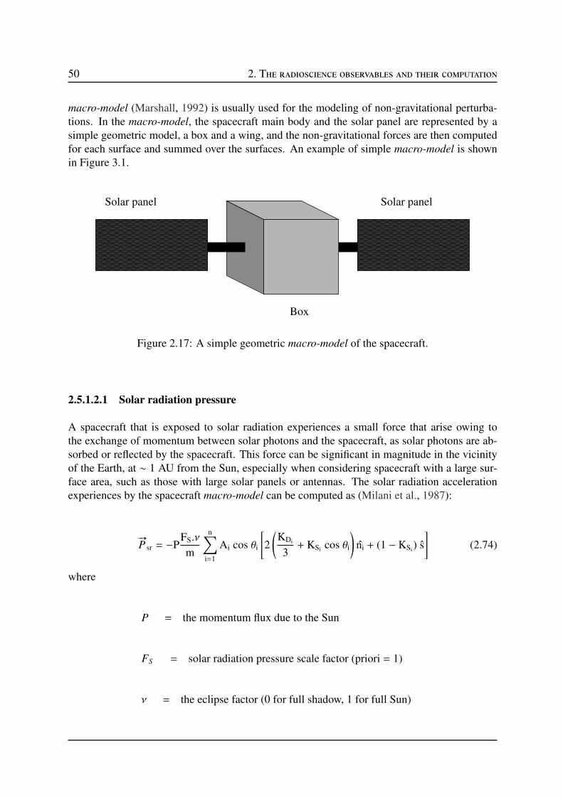
50 2. The radioscience observables and their computation
macro-model (Marshall, 1992) is usually used for the modeling of non-gravitational perturba-tions. In the macro-model, the spacecraft main body and the solar panel are represented by asimple geometric model, a box and a wing, and the non-gravitational forces are then computedfor each surface and summed over the surfaces. An example of simple macro-model is shownin Figure 3.1.
Box
Solar panel Solar panel
Figure 2.17: A simple geometric macro-model of the spacecraft.
2.5.1.2.1 Solar radiation pressure
A spacecraft that is exposed to solar radiation experiences a small force that arise owing tothe exchange of momentum between solar photons and the spacecraft, as solar photons are ab-sorbed or reflected by the spacecraft. This force can be significant in magnitude in the vicinityof the Earth, at ∼ 1 AU from the Sun, especially when considering spacecraft with a large sur-face area, such as those with large solar panels or antennas. The solar radiation accelerationexperiences by the spacecraft macro-model can be computed as (Milani et al., 1987):
#„
P sr = −PFS.ν
m
n∑
i=1
Ai cos θi
[
2
(
KDi
3+ KSi cos θi
)
ni + (1 − KSi) s
]
(2.74)
where
P = the momentum flux due to the Sun
FS = solar radiation pressure scale factor (priori = 1)
ν = the eclipse factor (0 for full shadow, 1 for full Sun)
2.5. GINS: orbit determination software 51
m = mass of the spacecraft
Ai = surface area of the i-th plate
θi = angle between surface normal and spacecraft-Sun vector for i-th plate
ni = surface normal unit vector for i-th plate
s = spacecraft-Sun unit vector
KDi= specular reflectivity for i-th plate
KS i= diffusive reflectivity for i-th plate
n = total number of plates in the model
Typically materials used for the construction of the spacecraft, specular reflectivity KD anddiffusive reflectivity KS coefficients lies in the range from 0.2 to 0.9 (van der Ha and Modi,1977).
2.5.1.2.2 Atmospheric drag and lift
When a spacecraft is in the vicinity of a planetary body then low altitude spacecraft mayexperience non-gravitational perturbation due to the atmosphere of planet. This atmosphericperturbation on the spacecraft is negligible if the planet does contain an atmosphere ( for ex-ample, the Mercury and the Moon). The accurate modeling of this aerodynamic force requiresthe knowledge of the physical properties of the atmosphere, especially the density of the upperatmosphere.
A spacecraft of arbitrary shape moving with velocity #„v in an atmosphere of density ρ willexperience both lift and drag forces. However, the lift forces are very small as compared to thedrag forces. These drag forces are directed opposite to the velocity of the spacecraft motionwith respect to the atmospheric flux, hence decelerating the spacecraft. The drag and lift forcecan be model as:
#„
P cd = −1
2ρ
[
FD
n∑
i=1
CDi
Ai
m( #„v r .
#„ni).#„v r

52 2. The radioscience observables and their computation
+FL
n∑
i=1
CLi
Ai
m( #„v r .
#„ni).#„v r
]
(2.75)
where
ρ = the atmospheric density
#„v r = the spacecraft velocity relative to the atmosphere
m = mass of the spacecraft
n = total number of spacecraft faces directly expose to atmosphere
#„ni = the unit vector normal to the face i
Ai = the cross-sectional area of the i-th face
CDi= the aerodynamic drag coefficient of the i-th face
CLi= the aerodynamic lift coefficient of the i-th face
FD = drag force scale factor (priori = 1)
Density models for the upper atmosphere are partly empirical and based on the laws of staticequilibrium distribution. There are a number of empirical atmospheric density models used forcomputing the atmospheric density. These include the Jacchia 71 (Jacchia, 1977), the DragTemperature Model (DTM) (Barlier et al., 1978), NRLMSISE-00 (Hedin et al., 1996).
The relative velocity #„v r of the spacecraft with respect to the atmosphere depends on thecomplex atmospheric dynamics. However, a reasonable approximation of the relative velocityis obtained with the assumption that the atmosphere co-rotates with the planet. Therefore, usingthis assumption relative velocity can be expressed as:
#„v r =#„v − #„ω × #„r (2.76)

2.5. GINS: orbit determination software 53
where, #„v is the spacecraft velocity, #„r is the spacecraft position from the COI, and #„ω is theangular velocity of the planet.
2.5.1.2.3 Thermal radiation
The surface temperature of a spacecraft is affected by exterior flows received from the Sunand the planet. Since the temperatures of the spacecraft surface are not uniform, there existsa force due to a net thermal radiation imbalance. This perturbation depends on the shape, thethermal property, the pattern of thermal dumping, the orbit characteristics, and the thermal en-vironment of the spacecraft as a whole. The perturbation due to thermal radiation can be modelas (Afonso et al., 1989):
#„
P th = −2
3
σ
c
n∑
i=1
Ai
mεi T4
i#„ni (2.77)
where
σ = the Stefan-Boltzmann constant
c = the speed of light
m = mass of the spacecraft
n = total number of spacecraft faces
#„ni = the unit vector normal to the i-th face
Ai = the cross-sectional area of the i-th face
Ti = the temperature of the i-th face
εi = the emissivity coefficient of the i-th face

54 2. The radioscience observables and their computation
2.5.1.2.4 Albedo and infrared radiation
In addition to the direct solar radiation pressure, the radiation emitted by the planet leads toa small pressure on the spacecraft. Such radiations can have two components, that is short-wave albedo and longwave infrared. In both cased the acceleration on the spacecraft decreaseslightly with the altitude due to the inverse square law of the emitted radiation pressure. Thisperturbation can be model as:
(i) Albedo radiation
#„
P rad =P
π
n∑
i=1
Ai
m
n∑
i=1
ρa( #„s .
# „
dS )( #„u .# „
dS )
D2
#„
βi (2.78)
(ii) Infrared radiation
#„
P rad =P
π
n∑
i=1
Ai
m
n∑
i=1
e
4
( #„u .# „
dS )
D2
#„
β′
i (2.79)
where
P = the momentum flux due to the Sun (4,5605 × 10⁻⁶
#„s = the unit vector in the direction COI-Sun
# „
dS = the unit vector normal to the surface element of the orbiting planet
#„n = the planet-spacecraft unit vector in the direction of surface element
D = distance between the surface element of planet and the spacecraft
ρa = albedo relative to the surface element
e = emissivity relative to the surface element
m = mass of the spacecraft
2.5. GINS: orbit determination software 55
n = total number of spacecraft faces
#„ni = the unit vector normal to the i-th face
Ai = the cross-sectional area of the i-th face
#„
βi = reflectivity vector of the i-th face
#„
β′
i = reflectivity infrared vector of the i-th face
2.5.1.2.5 Motor burn
The acceleration of the spacecraft due to a motor burn can be represented by (Moyer, 1971):
#„
Pmb = aU[
u(t − T0) + u(t − Tf)]
(2.80)
where,
a = magnitude of#„
Pmb
U = unit vector in direction of#„
Pmb
T0 = effective start time of motor
T f = effective end time of motor
T f = epoch in TDB
u(t − T0) = 1 for t ≥ T0 and 0 for t < T0, when T0 → T f
The acceleration magnitude a is given by (Moyer, 1971):
a =F(t)
m(t)C =
F0 + F1 t + F2t2 + F3t3 + +F4 t4
m0 + M0t + 12M1t2 + 1
3M2t3 + 14M3 t4
C (2.81)
56 2. The radioscience observables and their computation
where,
F(t) = magnitude of thrust at time t. The polynomial coefficients
of F(t) is solve-for paramerts
t = t - T0
m(t) = spacecraft mass at time t
Mn = polynomial coefficients of propellant mass flow rate at time t
C = 0.001 for F in newtons and m in kg
2.5.2 Variational equations
Variational equations are the way to describe the variations in the spacecraft state with respectto the solve-for parameters. These equations are always linear and solved simultaneously withthe equations of motion. Let the differential equations of motion is given by:
d2 #„r
dt2=
#„
F ( #„r , #„r , t, #„ε ) (2.82)
where #„r and #„r are the state vector of the spacecraft relative to COI. #„ε is the vector of solve-for parameter (such as, initial conditions, drag coefficient, solar radiation pressure coefficient,gravity harmonics, etc). The variational equations can be then written as:
d2
dt2
(
∂ #„r
∂ #„ε
)
=∂
#„
F
∂ #„r.∂ #„r
∂ #„ε+∂
#„
F
∂ #„r.∂ #„r
∂ #„ε+∂
#„
F
∂ #„ε(2.83)
with, at t = t0
• if #„ε is the parameter of the dynamical equations ( #„ε d), then:
∂ #„r
∂ #„ε d=∂ #„r
∂ #„ε d= 0 (2.84)
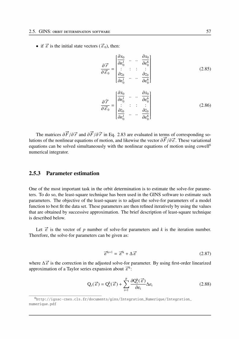
2.5. GINS: orbit determination software 57
• if #„ε is the initial state vectors ( #„ε 0), then:
∂ #„r
∂ #„ε 0=
∂x0
∂ε10
.. ..∂x0
∂ε60
: : : :∂z0
∂ε10
.. ..∂z0
∂ε60
(2.85)
∂ #„r
∂ #„ε 0=
∂x0
∂ε10
.. ..∂x0
∂ε60
: : : :∂z0
∂ε10
.. ..∂z0
∂ε60
(2.86)
The matrices ∂#„
F/∂ #„r and ∂#„
F/∂ #„r in Eq. 2.83 are evaluated in terms of corresponding so-lutions of the nonlinear equations of motion, and likewise the vector ∂
#„
F/∂ #„ε . These variationalequations can be solved simultaneously with the nonlinear equations of motion using cowell6
numerical integrator.
2.5.3 Parameter estimation
One of the most important task in the orbit determination is to estimate the solve-for parame-ters. To do so, the least-square technique has been used in the GINS software to estimate suchparameters. The objective of the least-square is to adjust the solve-for parameters of a modelfunction to best fit the data set. These parameters are then refined iteratively by using the valuesthat are obtained by successive approximation. The brief description of least-square techniqueis described below.
Let #„ε is the vector of p number of solve-for parameters and k is the iteration number.Therefore, the solve-for parameters can be given as:
#„ε k+1 = #„ε k + ∆ #„ε (2.87)
where ∆ #„ε is the correction in the adjusted solve-for parameter. By using first-order linearizedapproximation of a Taylor series expansion about #„ε k:
Qc(#„ε ) = Qk
c( #„ε ) +p
∑
i=1
∂Qkc( #„ε )
∂εi∆εi (2.88)
6http://igsac-cnes.cls.fr/documents/gins/Integration_Numerique/Integration_
numerique.pdf
58 2. The radioscience observables and their computation
where Qc is the theoretical values computed from the models which is a function of solve-forparameters #„ε . If, Qo defines the real observations, then the residuals (observation - computa-tion) can be given as:
r = Qo − Qc
= Qo − Qkc( #„ε ) +
p∑
i=1
∂Qkc( #„ε )
∂εi∆εi
= ∆Q −p
∑
i=1
∂Qkc( #„ε )
∂εi∆εi (2.89)
If m be the number of observations, then first and second terms Eq. 2.89 can be written as:
# „
∆Q =
∆Q1
::∆Qm
= B (2.90)
∂#„
Qkc
∂ #„ε∆ #„ε =
∂Qkc1
∂ε1.. ..
∂Qkc1
∂εp
: .. .. :: .. .. :∂Qk
cm
∂ε1.. ..
∂Qkcm
∂εp
.
∆ε1
::
∆εp
= A.∆ #„ε (2.91)
In order to estimate the best solve-for parameters, according to least-square technique, sumS of the square of the residuals should be minimum. Where sum S is given by:
S =m
∑
j=1
(
Bj − Aj . ∆#„ε
)2
(2.92)
where B j is the jth value of B and A j is the jth row of matrix A. For weighted least-square, theexpression of sum S is given as:
S =m
∑
j=1
Wj .
(
Bj − Aj . ∆#„ε
)2
(2.93)
where W j is the jth value of diagonal weight matrix W, which is given by:
W =
W1 0.
.
0 Wm
(2.94)
2.5. GINS: orbit determination software 59
In order to achieve the minimum square of the sum S of the residuals, the gradient of S withrespect of solve-for parameter should equal to zero. Which is given as:
AT .W .(
B − A . ∆ε)
= 0
AT .W . A . ∆ε = AT .W . B (2.95)
For example, if W is the identity matrix and number of solve-for parameters P equal to 2,then Eq. 2.95 can be written as:
∑mj=1
(∂Qc j
∂ε1
)2∑m
j=1
(∂Qc j
∂ε1
)
.
(∂Qc j
∂ε2
)
∑mj=1
(∂Qc j
∂ε1
)
.
(∂Qc j
∂ε2
)
∑mj=1
(∂Qc j
∂ε2
)2
.
∆ε1
∆ε2
=
∑mj=1 ∆Q .
(∂Qc j
∂ε1
)
∑mj=1 ∆Q .
(∂Qc j
∂ε2
)
(2.96)
The computed value of the observations Qc can be calculated from the state vectors of thespacecraft and the position of the stations at time of measurement (see Section 2.4.3). Thegradient of the Qc with respect to the solve-for parameters ε given in Eq. 2.96 can be writtenas:
∂#„
Qcj
∂ #„ε=∂
#„
Qcj
∂ #„r.∂ #„r
∂ #„ε+∂
#„
Qcj
∂ #„r.∂ #„r
∂ #„ε(2.97)
In Eq. 2.97, #„r and #„r , and ∂ #„r /∂ #„ε and ∂ #„r /∂ #„ε , can be computed from the numerical in-tegration of equations of motion and variational equations (Eqs. 2.85 and 2.86) respectively.Whereas, ∂
#„
Qc j/∂ #„r and ∂
#„
Qc j/∂ #„r can be computed analytically.
The steps used for estimating the solve-for parameters are (see Figure 2.16):
• to provide initial conditions and planetary ephemerides to the dynamical model,
• integrate numerically the equations of motion (Eq. 2.62) along with the variational equa-tions (Eq. 2.83) in order to calculate the state vectors of the spacecraft and the partialderivative of the state vector with respect to solve-for parameters (Eqs. 2.85 and 2.86),
• to calculate the theoretical observations Qc using the formulation given in section 2.4.3,
• to calculate the partial derivative of the theoretical observations with respect to solve-forparameters and then to compute the residuals (Eq. 2.89),
• to calculate the normal matrix and its inverse and then to calculate the corrections in thesolve-for parameters (Eq. 2.95),

60 2. The radioscience observables and their computation
• these correction are then used to refine the parameters using iterative processes (Eq. 2.87)until the residuals have met the specified convergence criterion.

61
Chapter 3
Mars Global Surveyor: Radioscience data
analysis
3.1 Introduction
Mars is the most explored terrestrial planet in the solar system. Many space missions havebeen attempted to Mars than to any other place in the solar system except the Moon. Thesemissions include flyby missions (Mariner, Rosetta), orbiter missions (Mars Global Surveyor,Mars Odyssey, Mars Express, Mars Reconnaissance Orbiter ), and lander missions (Viking,Mars Exploration Rovers, Mars Science Laboratory). Obtaining scientific information is theprimary reason for launching and operating such deep-space missions. Usually, science ob-jectives of such missions involve: high resolution imaging of the planet surface, studies of thegravity and topography, studies of the atmosphere and the interior of the Mars, studies of bio-logical, geological, and geochemical processes, etc. To achieve the mission objectives, some ofthese investigations are performed by using a dedicate science instrument aboard the spacecraft,which measure a particular physical phenomenon, for example:
• The thermal emission spectrometer: is used to measure the infrared spectrum of energyemitted by the planet. This information is used to study the composition of rock, soil,atmospheric dust, clouds, etc.
• The orbital laser altimeter: is used to measure the time, takes for a transmitted laser beamto reach the surface, reflect, and return. This information provides the topographic mapsof Mars.
• The magnetometer: is used to determine a magnetic field, and its strength and orientation.
On the other hand, some objectives are undertaken as opportunities arise to take advantage of aspacecraft special capabilities or unique location or other circumstance. For example:

62 3. Mars Global Surveyor: Radioscience data analysis
• With the radioscience experiment, which measures the Doppler shift of radio signals, itis then possible to determine the gravity field by computing the change in the speed ofthe spacecraft, associated with the high and low concentration of the mass below and atthe surface of the Mars. Moreover, unique location such as spacecraft occultation allowsthe radio signals pass through the Martian atmosphere on their way to Earth. Hence,perturbations in the signals induced by the atmosphere allows to derive the atmosphericand ionospheric characteristics of the Mars. Brief description of such investigations arediscussed in Chapter 2.
This chapter deals with the radioscience data analyses to precisely construct the MGS or-bit. Such analyses has been already performed by several authors, such as Yuan et al. (2001);Lemoine et al. (2001); Konopliv et al. (2006); Marty et al. (2009). We have therefore cho-sen MGS as an academic case to test our understanding of the raw radiometric data (ODF, seeChapter 2) and their analysis with GINS by comparing our results with the one found in theabove literature. Moreover, these analyses also allowed us to derive solar corona model andto perform corona physic studies. Derivation of such models and their application to planetaryephemerides are discussed in Chapter 4 and in Verma et al. (2013a).
The outline of this chapter is as follows: in the Section 3.2 an overview of the MGS missionis discussed. Data processing and dynamic modeling used for the orbit construction is describedin the Section 3.3. Results obtained during the orbit computation and their comparison with theestimations found in the literature are discussed in the Section 3.4. The supplementary tests,which include: (a) comparison between the GINS solution and the JPL light time solution, and(b) the impact of the macro-model on the orbit reconstruction, are discussed in Section 3.5.Conclusion and prospectives of these results are reported in Section 3.6.
3.2 Mission overview
3.2.1 Mission design
MGS was a NASA’s space mission to Mars. It was launched from the Cape Canaveral AirStation in Florida on 7th November 1996 aboard a Delta II rocket. The MGS began its Marsorbit insertion on 12th September 1997. Figure 3.1 illustrates the summary of the MGS missionfrom launch to the Mars orbit insertion (MOI) in an elliptical orbit, the initial areobrakingperiod, the science-phase period, the aerobraking resumption, and mapping in the circular orbit(Albee et al., 2001).
The MOI represents an extremely crucial maneuver, because any failure would result ina fly-by mission. The MOI slows down the spacecraft and allows Mars to capture the probeinto an elliptical orbit. Near the point of closest approach on spacecraft in-bound trajectory,the main engines fired for approximately 20 to 25 minutes to slow down the spacecraft. This
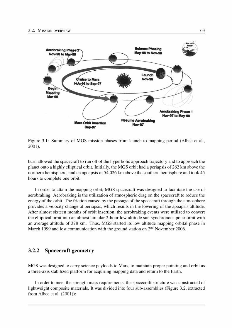
3.2. Mission overview 63
Figure 3.1: Summary of MGS mission phases from launch to mapping period (Albee et al.,2001).
burn allowed the spacecraft to run off of the hyperbolic approach trajectory and to approach theplanet onto a highly elliptical orbit. Initially, the MGS orbit had a periapsis of 262 km above thenorthern hemisphere, and an apoapsis of 54,026 km above the southern hemisphere and took 45hours to complete one orbit.
In order to attain the mapping orbit, MGS spacecraft was designed to facilitate the use ofaerobraking. Aerobraking is the utilization of atmospheric drag on the spacecraft to reduce theenergy of the orbit. The friction caused by the passage of the spacecraft through the atmosphereprovides a velocity change at periapsis, which results in the lowering of the apoapsis altitude.After almost sixteen months of orbit insertion, the aerobraking events were utilized to convertthe elliptical orbit into an almost circular 2-hour low altitude sun synchronous polar orbit withan average altitude of 378 km. Thus, MGS started its low altitude mapping orbital phase inMarch 1999 and lost communication with the ground station on 2nd November 2006.
3.2.2 Spacecraft geometry
MGS was designed to carry science payloads to Mars, to maintain proper pointing and orbit asa three-axis stabilized platform for acquiring mapping data and return to the Earth.
In order to meet the strength mass requirements, the spacecraft structure was constructed oflightweight composite materials. It was divided into four sub-assemblies (Figure 3.2, extractedfrom Albee et al. (2001)):
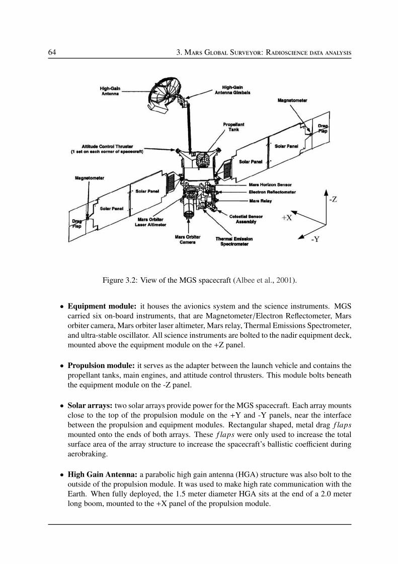
64 3. Mars Global Surveyor: Radioscience data analysis
Figure 3.2: View of the MGS spacecraft (Albee et al., 2001).
• Equipment module: it houses the avionics system and the science instruments. MGScarried six on-board instruments, that are Magnetometer/Electron Reflectometer, Marsorbiter camera, Mars orbiter laser altimeter, Mars relay, Thermal Emissions Spectrometer,and ultra-stable oscillator. All science instruments are bolted to the nadir equipment deck,mounted above the equipment module on the +Z panel.
• Propulsion module: it serves as the adapter between the launch vehicle and contains thepropellant tanks, main engines, and attitude control thrusters. This module bolts beneaththe equipment module on the -Z panel.
• Solar arrays: two solar arrays provide power for the MGS spacecraft. Each array mountsclose to the top of the propulsion module on the +Y and -Y panels, near the interfacebetween the propulsion and equipment modules. Rectangular shaped, metal drag f laps
mounted onto the ends of both arrays. These f laps were only used to increase the totalsurface area of the array structure to increase the spacecraft’s ballistic coefficient duringaerobraking.
• High Gain Antenna: a parabolic high gain antenna (HGA) structure was also bolt to theoutside of the propulsion module. It was used to make high rate communication with theEarth. When fully deployed, the 1.5 meter diameter HGA sits at the end of a 2.0 meterlong boom, mounted to the +X panel of the propulsion module.
3.2. Mission overview 65
Table 3.1: MGS spacecraft macro-model characteristics (Marty, 2011)
Spacecraft body Components Area (m2) Diffuse ref Specular ref.
Solar Arrays Composite (front) 7.85 0.049 0.198
Composite (back) 7.85 0.079 0.282
+X, -X 3.30 0.130 0.520
Spacecraft Bus +Y, -Y 3.56 0.130 0.520
+Z, -Z 2.31 0.130 0.520
HGA +X 1.94 0.100 0.400
As described in Chapter 2 (Section 2.5.1), the precise computation of the spacecraft tra-jectory relies on the non-gravitational accelerations that are acting in the spacecraft. Thesenon-gravitational forces depend on the shape, size, surface properties, and orientations of thespacecraft. Thus, an accurate spacecraft geometry is an essential information for modeling suchforces precisely. The characteristics of the MGS macro-model are given in Table 3.1 (Lemoineet al., 1999).
3.2.3 Radioscience data
MGS is the first operational planetary mission to employ exclusively X-band technology forradioscience observations, tracking, and spacecraft command and communication (Tyler et al.,2001). The radioscience instrument used for this purpose is the spacecraft telecommunicationssubsystem, augmented by an ultra-stable oscillator, and the normal MGS transmitter and re-ceiver. The ultra-stable oscillator typically have frequency stabilities on the order of 1×10⁻¹³
for time intervals of 1 to 100 seconds (Cash et al., 2008). The oscillator provides the refer-ence frequency for the radioscience experiments and operates on the X-band 7164.624 MHzuplink and 8416.368 MHz downlink frequency. The radioscience data are then collected by theDSN and consist of one-way Doppler, two- and three-way ramped Doppler, and two-way rangeobservations (see Chapter 2 for full details of radioscience data).
Figure 5.2.3 illustrates the MGS tracking strategy during the mapping period for sharing theorbit between: i) the occultation studies when MGS was near the limb of the planet, and ii) thegravity studies during the MGS Earth side pass (Tyler et al., 2001). Pole-to-Pole two- and three-way Doppler observations provide the primary information of Mars gravity field. Whereas, one-way Doppler observations obtained during the occultation period provide an information aboutthe Martian atmosphere and ionosphere. Table 3.2 gives the summary of the data coverageobtained during the mapping period and used to construct the MGS orbit.
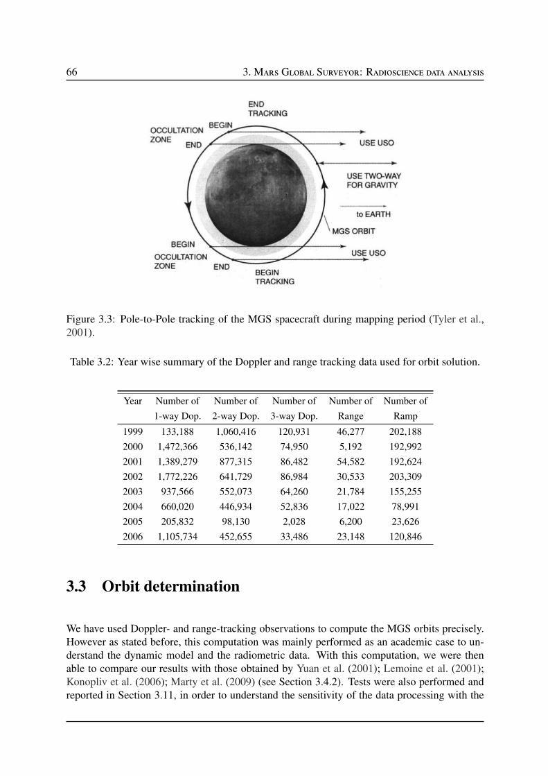
66 3. Mars Global Surveyor: Radioscience data analysis
Figure 3.3: Pole-to-Pole tracking of the MGS spacecraft during mapping period (Tyler et al.,2001).
Table 3.2: Year wise summary of the Doppler and range tracking data used for orbit solution.
Year Number of Number of Number of Number of Number of
1-way Dop. 2-way Dop. 3-way Dop. Range Ramp
1999 133,188 1,060,416 120,931 46,277 202,188
2000 1,472,366 536,142 74,950 5,192 192,992
2001 1,389,279 877,315 86,482 54,582 192,624
2002 1,772,226 641,729 86,984 30,533 203,309
2003 937,566 552,073 64,260 21,784 155,255
2004 660,020 446,934 52,836 17,022 78,991
2005 205,832 98,130 2,028 6,200 23,626
2006 1,105,734 452,655 33,486 23,148 120,846
3.3 Orbit determination
We have used Doppler- and range-tracking observations to compute the MGS orbits precisely.However as stated before, this computation was mainly performed as an academic case to un-derstand the dynamic model and the radiometric data. With this computation, we were thenable to compare our results with those obtained by Yuan et al. (2001); Lemoine et al. (2001);Konopliv et al. (2006); Marty et al. (2009) (see Section 3.4.2). Tests were also performed andreported in Section 3.11, in order to understand the sensitivity of the data processing with the
3.3. Orbit determination 67
accuracy of non-gravitational forces by assuming different shapes of MGS macro-model.
3.3.1 Data processing and dynamic modeling
The radioscience observations, used for computing the MGS orbit, are available on the NASAPlanetary Data System (PDS) Geoscience website1. These observations are analyzed with thehelp of the GINS software. As described in Section 2.5 of Chapter 2, GINS numerically inte-grates the equations of motion (Eqs. 2.62) and the associated variational equations (Eqs. 2.83).It simultaneously retrieves the physical parameters of the force model using an iterative least-squares technique (see Section 2.5.3). The modeling of the MGS orbit includes gravitationaland non-gravitational forces that are acting on the spacecraft (see Section 2.5.1). In addition tothese forces, third body perturbations due to Phobos and Deimos are also included.
The data processing and the dynamic modeling are done as follows:
• In order to have access to the planet positions and velocities, planetary ephemeris hasbeen used for both measurements and force models (e.g, DE405, INPOP10b).
• The Mars geopotential is modeled in terms of spherical harmonic. This model is given byEq. 2.65 as described in section 2.5.1. Fully normalized spherical harmonic coefficientsof MGS95J solution2 has been used. MGS95J is a 95x95 spherical harmonics modelwhich was derived from 6 years of MGS tracking data plus 3 years of measurements onthe Mars Odyssey (ODY) spacecraft (Konopliv et al., 2006).
• The rotation model which defines the orientation of the Mars is taken from the Konoplivet al. (2006).
• Earth kinematics and polar motion effects are taken according to the IERS standards(McCarthy and Petit, 2003).
• The Phobos and Deimos ephemerides are taken as developed by Lainey et al. (2007).
• The complex geometry of the spacecraft is treated as a combination of flat plates arrangein the shape of box, with attached solar arrays and drag flaps, and attached HGA. ThisBox-Wing model includes six plates for the spacecraft bus, four plates to represent thefront and back side of the +Y and -Y solar arrays, and a parabolic HGA. The surface areaand reflectivity of this macro-model are given in Table 3.1. Moreover, in addition to thismacro-model, a Spherical macro-model has been also used to reconstruct the MGS orbitand to understand the impact of macro-model over the orbit reconstruction (see Section3.5).
1http://geo.pds.nasa.gov/missions/mgs/rsraw.html2http://pds-geosciences.wustl.edu/mgs/mgs-m-rss-5-sdp-v1/mors_1033/sha/
68 3. Mars Global Surveyor: Radioscience data analysis
• Using such configurations of the MGS macro-models, solar radiation pressure (Eq. 2.74),atmospheric drag (Eq. 2.75), and Mars radiation pressure (Eqs. 2.78 and 2.79) forces arecomputed separately for each plate and HGA. Vectorial sum of all these components arethen compute to calculate the total force acting on the spacecraft.
• In addition to the macro-model characteristics, orientations of the spacecraft are alsotaken in account. The attitude of spacecraft, and of its articulated panels and antenna ininertial frame are defined in terms of quaternions. These quaternions are extracted fromthe SPICE Navigation and Ancillary Information Facility (NAIF) C-Kernels3.
• MGS periodically fires its thruster to desaturate the reactions wheels, which absorb an-gular momentum from disturbance torque acting on the spacecraft. Thus, empirical ac-celerations are modeled over the duration of each angular momentum wheel desaturation(AMD) event (Marty, 2011). Constant radial, along-track, and cross-track accelerationsare applied over the duration of each AMD event, and are estimated as part of each orbitdetermination solution.
• The relativistic effects on the measurements and on the spacecraft dynamics are modeledbased on the PPN formulation as described in Sections 2.4 and 2.5.1 of Chapter 2.
• The tropospheric delay corrections to the measurements are also included. Computationof this delay uses meteorological data (pressure, temperature and humidity) collectedevery half-hour at the DSN sites.
3.3.2 Solve-for parameters
For the orbit computation and for the parameter estimation, a multi-arc approach is used to getindependent estimates of the MGS accelerations. In this method, orbital fits are obtained fromshort data-arcs of two days with two hours (approx. one orbital period of MGS) of overlappingperiod. The short day data-arcs are used to accounting the model imperfections (see Section3.5) and overlapping period are used to estimate the quality of the spacecraft orbit determina-tion by taking orbit overlap differences between two successive data-arcs (see Section 3.4). Inorder to account the effect of shortest wavelengths of Mars gravity field on the MGS motion,we integrate the equations of motion using the time-step of 20s. An iterative least-squares fit isthen performed on the complete set of Doppler- and range-tracking data-arcs.
Solve-for parameters which have been estimated during the MGS orbit determination are:
• The initial state vector components at the epoch for each arc. Prior values of these vectorsare taken from the SPICE NAIF kernels.
3http://naif.jpl.nasa.gov/naif/
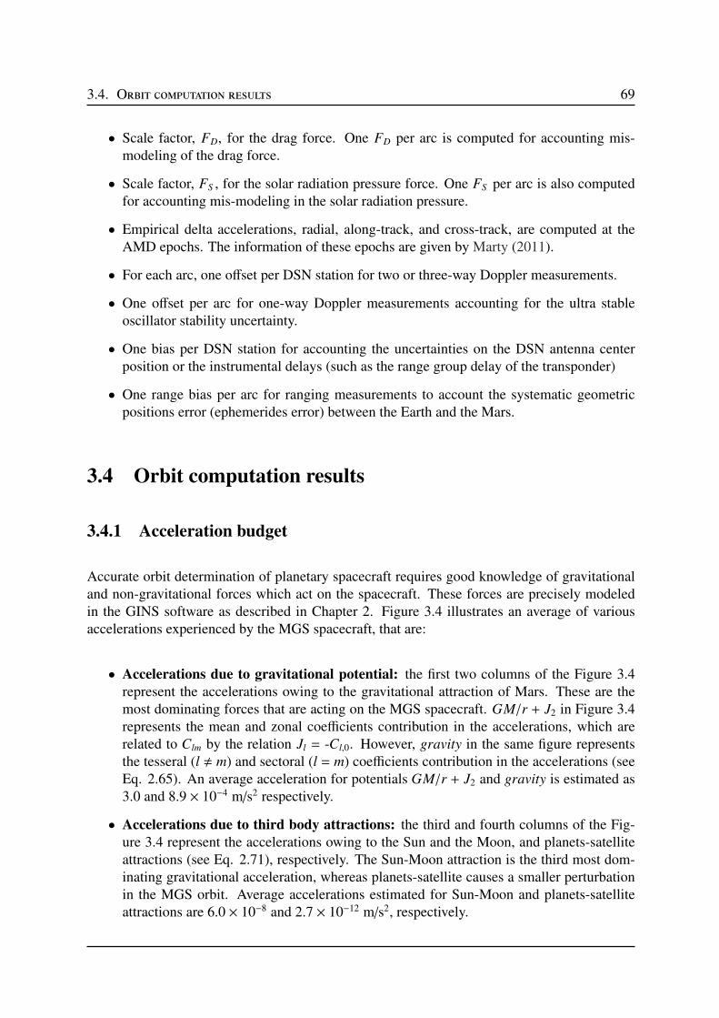
3.4. Orbit computation results 69
• Scale factor, FD, for the drag force. One FD per arc is computed for accounting mis-modeling of the drag force.
• Scale factor, FS , for the solar radiation pressure force. One FS per arc is also computedfor accounting mis-modeling in the solar radiation pressure.
• Empirical delta accelerations, radial, along-track, and cross-track, are computed at theAMD epochs. The information of these epochs are given by Marty (2011).
• For each arc, one offset per DSN station for two or three-way Doppler measurements.
• One offset per arc for one-way Doppler measurements accounting for the ultra stableoscillator stability uncertainty.
• One bias per DSN station for accounting the uncertainties on the DSN antenna centerposition or the instrumental delays (such as the range group delay of the transponder)
• One range bias per arc for ranging measurements to account the systematic geometricpositions error (ephemerides error) between the Earth and the Mars.
3.4 Orbit computation results
3.4.1 Acceleration budget
Accurate orbit determination of planetary spacecraft requires good knowledge of gravitationaland non-gravitational forces which act on the spacecraft. These forces are precisely modeledin the GINS software as described in Chapter 2. Figure 3.4 illustrates an average of variousaccelerations experienced by the MGS spacecraft, that are:
• Accelerations due to gravitational potential: the first two columns of the Figure 3.4represent the accelerations owing to the gravitational attraction of Mars. These are themost dominating forces that are acting on the MGS spacecraft. GM/r + J2 in Figure 3.4represents the mean and zonal coefficients contribution in the accelerations, which arerelated to Clm by the relation Jl = -Cl,0. However, gravity in the same figure representsthe tesseral (l , m) and sectoral (l = m) coefficients contribution in the accelerations (seeEq. 2.65). An average acceleration for potentials GM/r + J2 and gravity is estimated as3.0 and 8.9 × 10⁻⁴ m/s2 respectively.
• Accelerations due to third body attractions: the third and fourth columns of the Fig-ure 3.4 represent the accelerations owing to the Sun and the Moon, and planets-satelliteattractions (see Eq. 2.71), respectively. The Sun-Moon attraction is the third most dom-inating gravitational acceleration, whereas planets-satellite causes a smaller perturbationin the MGS orbit. Average accelerations estimated for Sun-Moon and planets-satelliteattractions are 6.0 × 10⁻⁸ and 2.7 × 10⁻¹² m/s2, respectively.

70 3. Mars Global Surveyor: Radioscience data analysis
Acceleration type
10-14
10-12
10-10
10-8
10-6
10-4
10-2
100
Acc
eler
atio
n
MGS acceleration budget
GM/r + J2 gravite Moon-Sun planets relativity x-stoc y-stoc z-stoc atmospher press.sol albedoemiss. ir
(m/s
)
2
1
2
3
4
5
6 7 8
9
10
1112
13
tides
Figure 3.4: Gravitational and non-gravitational accelerations acting on the MGS spacecraft. Seetext for the explanation of each column.
• Accelerations due to general relativity: the fifth column of the Figure 3.4 represents theaccelerations owing to the contribution of general relativity (see Eq. 2.72). An averagevalue of this acceleration is estimated as 1.1 × 10⁻⁹ m/s2.
• Accelerations due to maneuvers: the sixth, seventh, and eighth columns of the Figure3.4 represent empirical accelerations that are estimated over the duration of each AMD(see Eq. 2.80). Average value of radial (x-stoc), along-track (y-stoc), and cross-track (z-stoc) accelerations are estimated as 1.0×10⁻⁴, 1.2×10⁻⁴, and 1.8×10⁻⁴ m/s2 respectively.
• Accelerations due to atmospheric drag: the ninth column of the Figure 3.4 representsthe acceleration owing to the resistance of the Mars atmosphere (see Eq. 2.75). It is oneof the largest non-gravitational accelerations acting on the low altitude spacecraft. ForMGS, an average value of this acceleration is estimated as 4.8 × 10⁻⁹ m/s2.
• Accelerations due to solar radiation pressure: the tenth column of the Figure 3.4 rep-resents the acceleration due to the solar radiation pressure (see Eq. 2.74). It is the largestnon-gravitational acceleration acting on the MGS spacecraft with an average value of4.5 × 10−8 m/s2.

3.4. Orbit computation results 71
• Accelerations due to Mars radiation: the eleventh and twelfth columns represent theaccelerations due to the Infra-Red radiation (see Eq. 2.79) and Albedo (see Eq. 2.78)of the Mars. These are the smallest non-gravitational accelerations acting on the MGSspacecraft with average values of 1.1 × 10⁻⁹ and 3.0 × 10⁻⁹ m/s2 respectively.
• Accelerations due to solid planetary tides: the thirteen column represents the accelera-tions owing to the contribution of solid planetary tides (see Eq. 2.69). An average valueof this acceleration is estimated as 4.18 × 10⁻⁹ m/s2.
3.4.2 Doppler and range postfit residuals
Figure 3.5: Quality of the MGS orbit in terms of rms values of the postfit residuals for each one-day data-arc: (a) one-way Doppler given in millihertz (1-way: 1 mHz = 0.035 mm/s = speedof light / X-band frequency); (b) two- and three-way Doppler given in millihertz (2/3-way: 1mHz = 0.0178 mm/s = 0.5×speed of light / X-band frequency); and (c) two-way range given inmeter. The peaks and gaps in residuals correspond to solar conjunction periods of MGS.
In general, the Doppler data are mainly used for the computation of spacecraft orbit. Theyare sensitive to the modeling of the spacecraft dynamics and provide strong constraints on the

72 3. Mars Global Surveyor: Radioscience data analysis
orbit construction. However, range data are also used to assist the orbit computation. UnlikeDoppler data, range data are more sensitive to the positions of the planet in the solar system andprovide strong constraints to the planetary ephemerides.
Figure 3.5 illustrates the rms values of the Doppler- and range postfit residuals estimatedfor each data-arc. Doppler residuals represent the accuracy in the computation of Doppler shiftand in the dynamic modeling of the MGS spacecraft, whereas range residuals represents theaccuracy in the computation of range measurements. To plot, we did not consider 19% of thedata-arcs during which: i) the Sun-Earth-Probe (SEP) angle <12 and rms value of the postfitDoppler and range residuals are above 15mHz and 7 m respectively, and ii) the drag coefficientsand solar radiation pressures have unrealistic values.
In Figure 3.5, the peaks and the gaps in the postfit residuals correspond to solar conjunctionperiods. Excluding these periods, the rms value of the postfit Doppler- and two- way rangeresiduals for each data-arc is varying from1.8 to 5.8 mHz4,5 and 0.4 to 1.2m, respectively. Theseestimations are comparable with Yuan et al. (2001); Lemoine et al. (2001); Marty et al. (2009),see Table 3.3. The mean value of the estimated Doppler offset for each DSN station trackingpass is of the order of a few tenths of mHz, which is lower than the Doppler postfit residualsfor each data-arc. This implies that there is no large offset in the modeling of the Doppler shiftmeasurements at each tracking DSN station.
Table 3.3: Comparison of postfit Doppler and range residuals, and overlapped periods, betweendifferent authors.
AuthorsResidualsa Overlapb
Doppler (mHz) Range (m) R (m) T (m) N (m) 3D (m)
Yuan et al. (2001)c 3.4-4.9 - 1.6 2.5 10.6 -
Lemoine et al. (2001)c 3.4-5.6 - 1.5 2.55 8.75 -
Konopliv et al. (2006) - - 0.15 1.5 1.6 -
Marty et al. (2009) 2-5 0.5-1 - - - 2.1
This chapter 1.8-5.8 0.4-1.2 0.33±0.27* 2.5±2.1* 3.0±2* 2.7±2.0*
a range of the mean values estimated for each data-arc.b mean value estimated for entire data.c authors gave the values in mm/s, we therefore divided the values by a factor 0.0178 to obtain approxi-
mate values in mHz.* mean±1-σ dispersion of the rms values
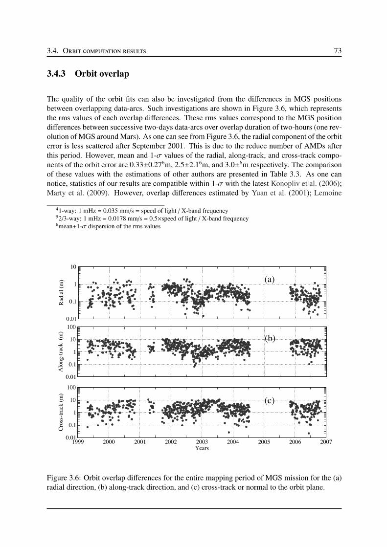
3.4. Orbit computation results 73
3.4.3 Orbit overlap
The quality of the orbit fits can also be investigated from the differences in MGS positionsbetween overlapping data-arcs. Such investigations are shown in Figure 3.6, which representsthe rms values of each overlap differences. These rms values correspond to the MGS positiondifferences between successive two-days data-arcs over overlap duration of two-hours (one rev-olution of MGS around Mars). As one can see from Figure 3.6, the radial component of the orbiterror is less scattered after September 2001. This is due to the reduce number of AMDs afterthis period. However, mean and 1-σ values of the radial, along-track, and cross-track compo-nents of the orbit error are 0.33±0.276m, 2.5±2.16m, and 3.0±6m respectively. The comparisonof these values with the estimations of other authors are presented in Table 3.3. As one cannotice, statistics of our results are compatible within 1-σ with the latest Konopliv et al. (2006);Marty et al. (2009). However, overlap differences estimated by Yuan et al. (2001); Lemoine
41-way: 1 mHz = 0.035 mm/s = speed of light / X-band frequency52/3-way: 1 mHz = 0.0178 mm/s = 0.5×speed of light / X-band frequency6mean±1-σ dispersion of the rms values
0.01
0.1
1
10
Rad
ial
(m)
0.01
0.1
1
10
100
Alo
ng-t
rack
(m
)
1999 2000 2001 2002 2003 2004 2005 2006 2007Years
0.01
0.1
1
10
100
Cro
ss-t
rack
(m
)
(a)
(b)
(c)
Figure 3.6: Orbit overlap differences for the entire mapping period of MGS mission for the (a)radial direction, (b) along-track direction, and (c) cross-track or normal to the orbit plane.

74 3. Mars Global Surveyor: Radioscience data analysis
et al. (2001) are approximately ∼3 times higher in the normal direction and approximately ∼5times higher in the radial-direction. It can be explained by the different gravity fields whichwere used for the computations. For example, Yuan et al. (2001) had used a spherical harmon-ics model developed upto degree and order 75, while Lemoine et al. (2001) updated the modelupto degree and order 80. Moreover, both authors used only one year of mapping data for theircomputations. On the other hand, Konopliv et al. (2006); Marty et al. (2009) and on this chapter,the entire mapping period data since 1999 to the end of mission (late 2006) has been analyzedwith 95×95 spherical harmonics model. Because of the short circular orbit of the MGS, suchhigh order tesseral (l , m) and sectoral (l = m) coefficients are important to model gravitationforces precisely.
3.4.4 Estimated parameters
3.4.4.1 FS and FD scale factors
The Solar radiation pressure (Eqs. 2.74) and the atmospheric drag (Eqs. 2.75) are the most dom-inating non-gravitational forces that are acting on the MGS spacecraft. As mentioned earlier,these non-gravitational forces depend upon the characteristic of the spacecraft model (macro-model) and its orientation. Thus, in order to accounting the inaccuracy in the spacecraft mod-eling and its orientations, an overall scale factors (FS and FD) are estimated for each data-arc.However, for an accurate modeling, one can expect these values approximately equal to one.
0.5
1
1.5
Scale
facto
r F
1999 2000 2001 2002 2003 2004 2005 2006 2007Years
0
1
2
3
Scale
facto
r F D
s
(a)
(b)
Figure 3.7: Scale factors: a) atmospheric drag and b) solar radiation pressure.
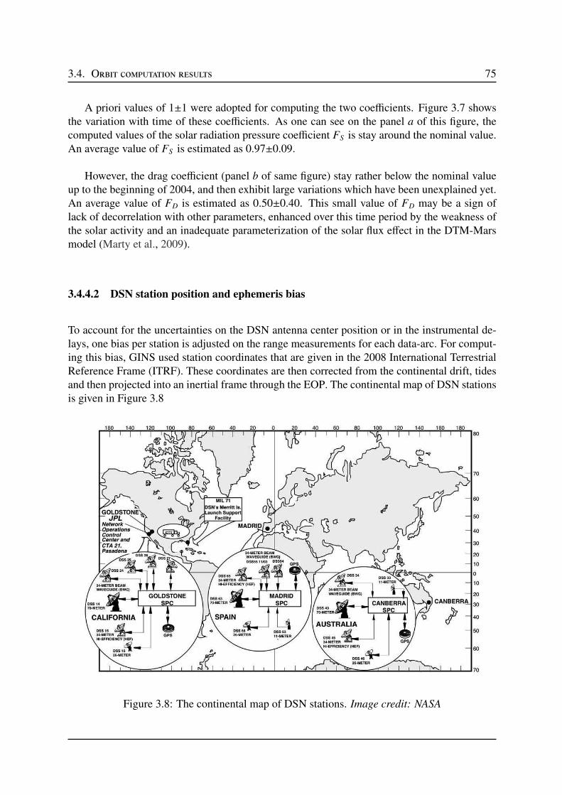
3.4. Orbit computation results 75
A priori values of 1±1 were adopted for computing the two coefficients. Figure 3.7 showsthe variation with time of these coefficients. As one can see on the panel a of this figure, thecomputed values of the solar radiation pressure coefficient FS is stay around the nominal value.An average value of FS is estimated as 0.97±0.09.
However, the drag coefficient (panel b of same figure) stay rather below the nominal valueup to the beginning of 2004, and then exhibit large variations which have been unexplained yet.An average value of FD is estimated as 0.50±0.40. This small value of FD may be a sign oflack of decorrelation with other parameters, enhanced over this time period by the weakness ofthe solar activity and an inadequate parameterization of the solar flux effect in the DTM-Marsmodel (Marty et al., 2009).
3.4.4.2 DSN station position and ephemeris bias
To account for the uncertainties on the DSN antenna center position or in the instrumental de-lays, one bias per station is adjusted on the range measurements for each data-arc. For comput-ing this bias, GINS used station coordinates that are given in the 2008 International TerrestrialReference Frame (ITRF). These coordinates are then corrected from the continental drift, tidesand then projected into an inertial frame through the EOP. The continental map of DSN stationsis given in Figure 3.8
Figure 3.8: The continental map of DSN stations. Image credit: NASA
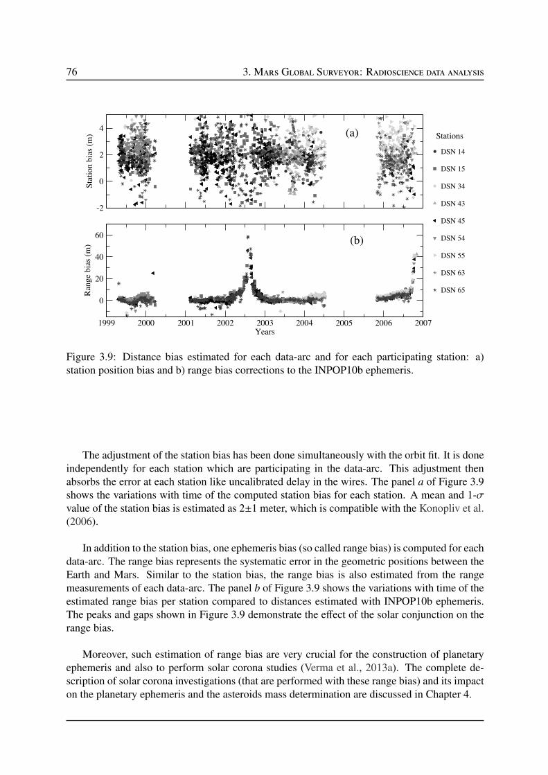
76 3. Mars Global Surveyor: Radioscience data analysis
-2
0
2
4
Sta
tion b
ias
(m)
DSN 14
DSN 15
DSN 34
DSN 43
DSN 45
DSN 54
DSN 55
DSN 63
DSN 65
1999 2000 2001 2002 2003 2004 2005 2006 2007Years
0
20
40
60
Ran
ge
bia
s (m
)
(a)
(b)
Stations
Figure 3.9: Distance bias estimated for each data-arc and for each participating station: a)station position bias and b) range bias corrections to the INPOP10b ephemeris.
The adjustment of the station bias has been done simultaneously with the orbit fit. It is doneindependently for each station which are participating in the data-arc. This adjustment thenabsorbs the error at each station like uncalibrated delay in the wires. The panel a of Figure 3.9shows the variations with time of the computed station bias for each station. A mean and 1-σvalue of the station bias is estimated as 2±1 meter, which is compatible with the Konopliv et al.(2006).
In addition to the station bias, one ephemeris bias (so called range bias) is computed for eachdata-arc. The range bias represents the systematic error in the geometric positions between theEarth and Mars. Similar to the station bias, the range bias is also estimated from the rangemeasurements of each data-arc. The panel b of Figure 3.9 shows the variations with time of theestimated range bias per station compared to distances estimated with INPOP10b ephemeris.The peaks and gaps shown in Figure 3.9 demonstrate the effect of the solar conjunction on therange bias.
Moreover, such estimation of range bias are very crucial for the construction of planetaryephemeris and also to perform solar corona studies (Verma et al., 2013a). The complete de-scription of solar corona investigations (that are performed with these range bias) and its impacton the planetary ephemeris and the asteroids mass determination are discussed in Chapter 4.
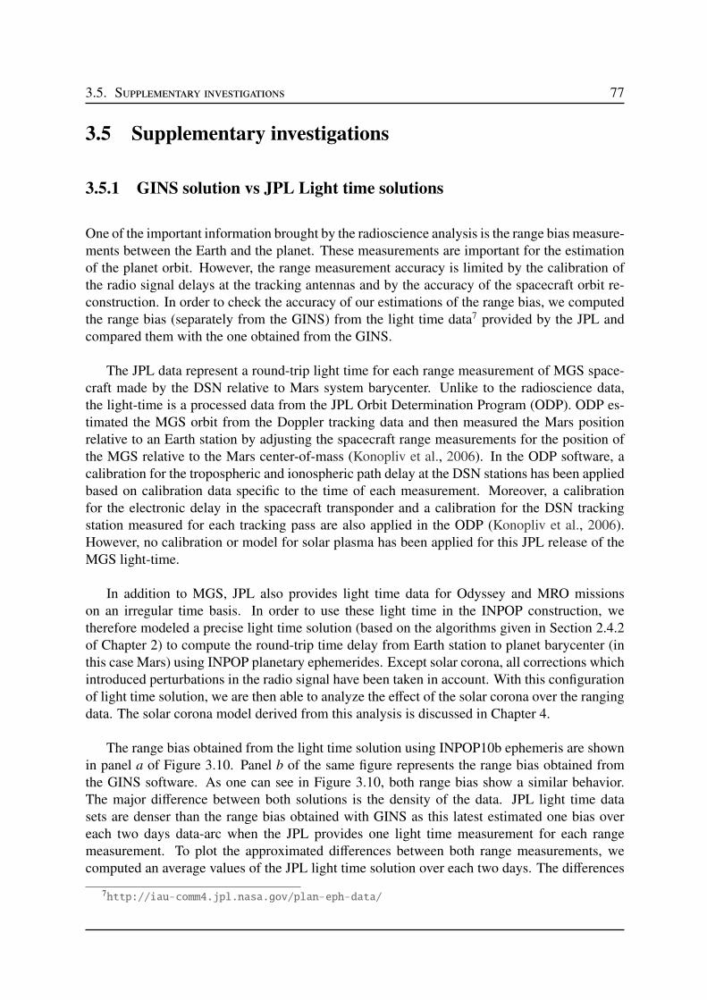
3.5. Supplementary investigations 77
3.5 Supplementary investigations
3.5.1 GINS solution vs JPL Light time solutions
One of the important information brought by the radioscience analysis is the range bias measure-ments between the Earth and the planet. These measurements are important for the estimationof the planet orbit. However, the range measurement accuracy is limited by the calibration ofthe radio signal delays at the tracking antennas and by the accuracy of the spacecraft orbit re-construction. In order to check the accuracy of our estimations of the range bias, we computedthe range bias (separately from the GINS) from the light time data7 provided by the JPL andcompared them with the one obtained from the GINS.
The JPL data represent a round-trip light time for each range measurement of MGS space-craft made by the DSN relative to Mars system barycenter. Unlike to the radioscience data,the light-time is a processed data from the JPL Orbit Determination Program (ODP). ODP es-timated the MGS orbit from the Doppler tracking data and then measured the Mars positionrelative to an Earth station by adjusting the spacecraft range measurements for the position ofthe MGS relative to the Mars center-of-mass (Konopliv et al., 2006). In the ODP software, acalibration for the tropospheric and ionospheric path delay at the DSN stations has been appliedbased on calibration data specific to the time of each measurement. Moreover, a calibrationfor the electronic delay in the spacecraft transponder and a calibration for the DSN trackingstation measured for each tracking pass are also applied in the ODP (Konopliv et al., 2006).However, no calibration or model for solar plasma has been applied for this JPL release of theMGS light-time.
In addition to MGS, JPL also provides light time data for Odyssey and MRO missionson an irregular time basis. In order to use these light time in the INPOP construction, wetherefore modeled a precise light time solution (based on the algorithms given in Section 2.4.2of Chapter 2) to compute the round-trip time delay from Earth station to planet barycenter (inthis case Mars) using INPOP planetary ephemerides. Except solar corona, all corrections whichintroduced perturbations in the radio signal have been taken in account. With this configurationof light time solution, we are then able to analyze the effect of the solar corona over the rangingdata. The solar corona model derived from this analysis is discussed in Chapter 4.
The range bias obtained from the light time solution using INPOP10b ephemeris are shownin panel a of Figure 3.10. Panel b of the same figure represents the range bias obtained fromthe GINS software. As one can see in Figure 3.10, both range bias show a similar behavior.The major difference between both solutions is the density of the data. JPL light time datasets are denser than the range bias obtained with GINS as this latest estimated one bias overeach two days data-arc when the JPL provides one light time measurement for each rangemeasurement. To plot the approximated differences between both range measurements, wecomputed an average values of the JPL light time solution over each two days. The differences
7http://iau-comm4.jpl.nasa.gov/plan-eph-data/
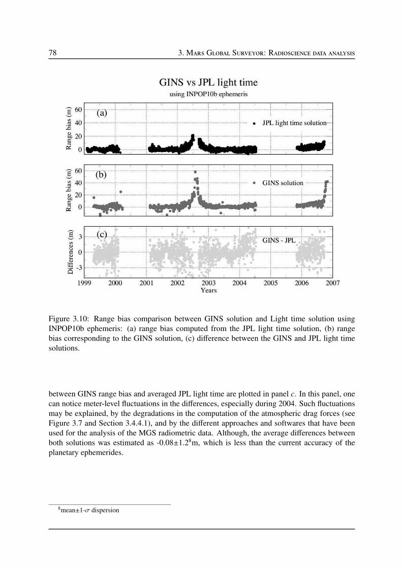
78 3. Mars Global Surveyor: Radioscience data analysis
Figure 3.10: Range bias comparison between GINS solution and Light time solution usingINPOP10b ephemeris: (a) range bias computed from the JPL light time solution, (b) rangebias corresponding to the GINS solution, (c) difference between the GINS and JPL light timesolutions.
between GINS range bias and averaged JPL light time are plotted in panel c. In this panel, onecan notice meter-level fluctuations in the differences, especially during 2004. Such fluctuationsmay be explained, by the degradations in the computation of the atmospheric drag forces (seeFigure 3.7 and Section 3.4.4.1), and by the different approaches and softwares that have beenused for the analysis of the MGS radiometric data. Although, the average differences betweenboth solutions was estimated as -0.08±1.28m, which is less than the current accuracy of theplanetary ephemerides.
8mean±1-σ dispersion
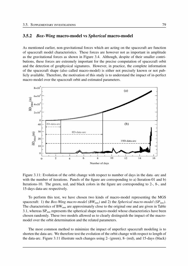
3.5. Supplementary investigations 79
3.5.2 Box-Wing macro-model vs Spherical macro-model
As mentioned earlier, non-gravitational forces which are acting on the spacecraft are functionof spacecraft model characteristics. These forces are however not as important in amplitudeas the gravitational forces as shown in Figure 3.4. Although, despite of their smaller contri-butions, these forces are extremely important for the precise computation of spacecraft orbitand the detection of geophysical signatures. However, in practice, the complete informationof the spacecraft shape (also called macro-model) is either not precisely known or not pub-licly available. Therefore, the motivation of this study is to understand the impact of in-perfectmacro-model over the spacecraft orbit and estimated parameters.
Figure 3.11: Evolution of the orbit change with respect to number of days in the data -arc andwith the number of iterations. Panels of the figure are corresponding to a) Iteration-01 and b)Iterations-10. The green, red, and black colors in the figure are corresponding to 2-, 8-, and15-days data-arc respectively.
To perform this test, we have chosen two kinds of macro-model representing the MGSspacecraft: 1) the Box-Wing macro-model (BWmm) and 2) the Spherical macro-model (SPmm).The characteristics of BWmm are approximately close to the original one and are given in Table3.1, whereas SPmm represents the spherical shape macro-model whose characteristics have beenchosen randomly. These two models allowed us to clearly distinguish the impact of the macro-model over the orbit determination and the related parameters.
The most common method to minimize the impact of unperfect spacecraft modeling is toshorten the data-arc. We therefore test the evolution of the orbit change with respect to length ofthe data-arc. Figure 3.11 illustrate such changes using 2- (green), 8- (red), and 15-days (black)
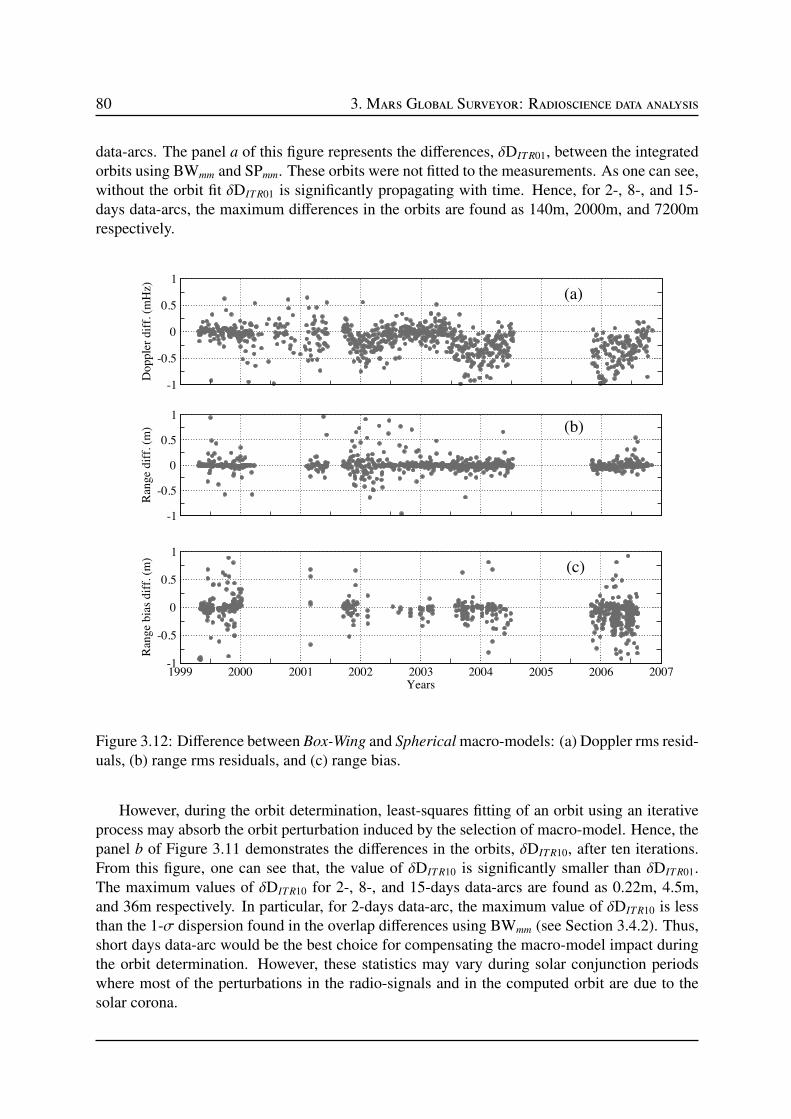
80 3. Mars Global Surveyor: Radioscience data analysis
data-arcs. The panel a of this figure represents the differences, δDITR01, between the integratedorbits using BWmm and SPmm. These orbits were not fitted to the measurements. As one can see,without the orbit fit δDITR01 is significantly propagating with time. Hence, for 2-, 8-, and 15-days data-arcs, the maximum differences in the orbits are found as 140m, 2000m, and 7200mrespectively.
-1
-0.5
0
0.5
1
Dopple
r dif
f. (
mH
z)
-1
-0.5
0
0.5
1
Ran
ge
dif
f. (
m)
1999 2000 2001 2002 2003 2004 2005 2006 2007Years
-1
-0.5
0
0.5
1
Ran
ge
bia
s dif
f. (
m)
(a)
(b)
(c)
Figure 3.12: Difference between Box-Wing and Spherical macro-models: (a) Doppler rms resid-uals, (b) range rms residuals, and (c) range bias.
However, during the orbit determination, least-squares fitting of an orbit using an iterativeprocess may absorb the orbit perturbation induced by the selection of macro-model. Hence, thepanel b of Figure 3.11 demonstrates the differences in the orbits, δDITR10, after ten iterations.From this figure, one can see that, the value of δDITR10 is significantly smaller than δDITR01.The maximum values of δDITR10 for 2-, 8-, and 15-days data-arcs are found as 0.22m, 4.5m,and 36m respectively. In particular, for 2-days data-arc, the maximum value of δDITR10 is lessthan the 1-σ dispersion found in the overlap differences using BWmm (see Section 3.4.2). Thus,short days data-arc would be the best choice for compensating the macro-model impact duringthe orbit determination. However, these statistics may vary during solar conjunction periodswhere most of the perturbations in the radio-signals and in the computed orbit are due to thesolar corona.
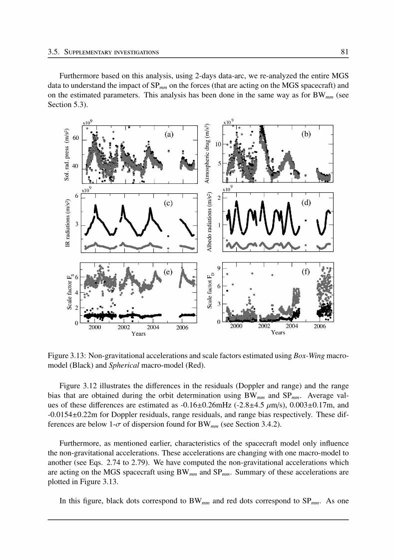
3.5. Supplementary investigations 81
Furthermore based on this analysis, using 2-days data-arc, we re-analyzed the entire MGSdata to understand the impact of SPmm on the forces (that are acting on the MGS spacecraft) andon the estimated parameters. This analysis has been done in the same way as for BWmm (seeSection 5.3).
Figure 3.13: Non-gravitational accelerations and scale factors estimated using Box-Wing macro-model (Black) and Spherical macro-model (Red).
Figure 3.12 illustrates the differences in the residuals (Doppler and range) and the rangebias that are obtained during the orbit determination using BWmm and SPmm. Average val-ues of these differences are estimated as -0.16±0.26mHz (-2.8±4.5 µm/s), 0.003±0.17m, and-0.0154±0.22m for Doppler residuals, range residuals, and range bias respectively. These dif-ferences are below 1-σ of dispersion found for BWmm (see Section 3.4.2).
Furthermore, as mentioned earlier, characteristics of the spacecraft model only influencethe non-gravitational accelerations. These accelerations are changing with one macro-model toanother (see Eqs. 2.74 to 2.79). We have computed the non-gravitational accelerations whichare acting on the MGS spacecraft using BWmm and SPmm. Summary of these accelerations areplotted in Figure 3.13.
In this figure, black dots correspond to BWmm and red dots correspond to SPmm. As one
82 3. Mars Global Surveyor: Radioscience data analysis
can see that, scale factor estimations for the solar radiation pressure FS (panel e) and for theatmospheric drag FD (panel f ) are much higher for SPmm than BWmm. These scale-factors areestimated to account the mis-modeling in the corresponding accelerations. As a result, bothBWmm and SPmm experienced approximately a similar accelerations due to the solar radiationpressure (panel a) and the atmospheric drag (panel b).
However, such scale factors have not been estimated for accelerations due to the Mars ra-diations (Infra-Red radiation (panel c) and Albedo (panel d)). Owing to the different physicalproperties of both macro-models, as expected, BWmm experienced approximately five timesgreater Mars radiation accelerations than SPmm. Due to the small contribution of these accelera-tions over the spacecraft motion, they did not bring much perturbations in the overall spacecraftorbit (Figure 3.11) and postfit residuals (Figure 3.12).
3.6 Conclusion and prospectives
The radioscience data analysis of the MGS spacecraft was chosen as an academic case to testour understanding of the raw radiometric data and their analysis with GINS by comparing ourresults with the literature. In this chapter, we have analyzed the entire radioscience data of MarsGlobal Surveyor since 1999 to 2006. This analysis has been done independently by using GINSorbit determination software. For accounting the non-gravitational forces precisely, a ten-platewith parabolic high gain antenna Box-Wing macro-model was used. In addition, orientationsof the spacecraft and its articulated panels were also taken in account and modeled in termsof quaternions. Two-day data-arcs have been used to perform the numerical integration usingupdated 95×95 MGS95J Mars gravity model.
The estimated accuracy of the orbit and the parameters are consistent with the results foundin the literature (Yuan et al. (2001); Lemoine et al. (2001); Konopliv et al. (2006); Marty et al.(2009), see Table 3.3). Moreover, we also compared range bias that were computed from ouranalysis with reduced light time data provided by JPL. An independent light time solutionsoftware has been developed to treat the JPL light time data. The range bias computed fromboth softwares are consistent with each other, and hence confirm the validity of our analysiswith respect to JPL ODP software.
To understand the impact of the macro-model over the orbit perturbations and estimatedparameters, we developed a new Spherical macro-model. We then re-analyzed the entire ra-dioscience data and compared the outcomes with the one obtained from the Box-Wing macro-model. With this comparison, we confirmed that, in the absence of precise knowledge of thespacecraft characteristics, short data-arc can be preferable to accounting the mis-modeling inthe spacecraft model without costing the orbit accuracy. However, this analysis may be notpreferable for extracting an accurate geophysical signals from the Doppler measurements, suchas the estimation of gravity field coefficients. In that case, an accurate modeling of the non-gravitational forces which depend upon the quality of macro-model are highly essential.
3.6. Conclusion and prospectives 83
The part of these analysis, which consists of an accurate orbit determination of the MGSwith Box-Wing macro-model, is published in Verma et al. (2013a). Moreover as a prospectiveof these analysis, we performed solar physics studies using data acquired at the time of solarconjunction periods. The Chapter 4 deals with the deduction of a solar corona model fromthe range bias that are computed at the time of the solar conjunctions. This model is thenused to correct the range bias from the solar corona perturbations and also to estimate thecorresponding averaged electron densities. The corrected or improved range bias are then usedfor the construction of planetary ephemerides (Verma et al., 2013a).
Furthermore, the hypothesis based on the supplementary tests of macro-model and thechoice of data-arc, have been successfully used in Chapter 5 for the analysis of MESSENGERradioscience data and for the precise computations of MESSENGER orbit.

84 3. Mars Global Surveyor: Radioscience data analysis
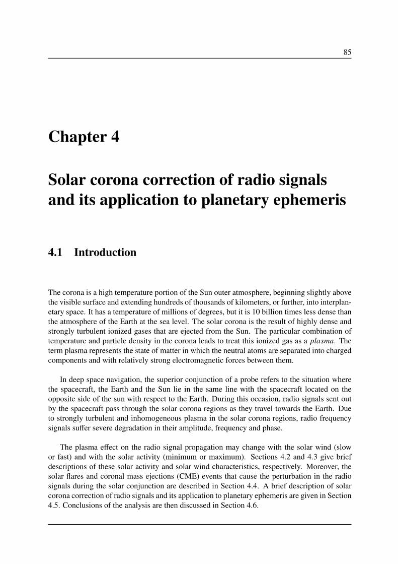
85
Chapter 4
Solar corona correction of radio signals
and its application to planetary ephemeris
4.1 Introduction
The corona is a high temperature portion of the Sun outer atmosphere, beginning slightly abovethe visible surface and extending hundreds of thousands of kilometers, or further, into interplan-etary space. It has a temperature of millions of degrees, but it is 10 billion times less dense thanthe atmosphere of the Earth at the sea level. The solar corona is the result of highly dense andstrongly turbulent ionized gases that are ejected from the Sun. The particular combination oftemperature and particle density in the corona leads to treat this ionized gas as a plasma. Theterm plasma represents the state of matter in which the neutral atoms are separated into chargedcomponents and with relatively strong electromagnetic forces between them.
In deep space navigation, the superior conjunction of a probe refers to the situation wherethe spacecraft, the Earth and the Sun lie in the same line with the spacecraft located on theopposite side of the sun with respect to the Earth. During this occasion, radio signals sent outby the spacecraft pass through the solar corona regions as they travel towards the Earth. Dueto strongly turbulent and inhomogeneous plasma in the solar corona regions, radio frequencysignals suffer severe degradation in their amplitude, frequency and phase.
The plasma effect on the radio signal propagation may change with the solar wind (slowor fast) and with the solar activity (minimum or maximum). Sections 4.2 and 4.3 give briefdescriptions of these solar activity and solar wind characteristics, respectively. Moreover, thesolar flares and coronal mass ejections (CME) events that cause the perturbation in the radiosignals during the solar conjunction are described in Section 4.4. A brief description of solarcorona correction of radio signals and its application to planetary ephemeris are given in Section4.5. Conclusions of the analysis are then discussed in Section 4.6.

86 4. Solar corona correction of radio signals and its application to planetary ephemeris
All results described in this chapter are published in the Astronomy & Astrophysics journal.We therefore represent Section 4.7 by Verma et al. (2013a). This section gives the completedescription of the solar corona model that has been derived from the range measurements ofthe MGS, MEX, and VEX, spacecraft. The improvement in the extrapolation capability of theplanetary ephemeris and the estimation of the asteroid masses are also discussed in the samesection.
4.2 The solar cycle
The amount of magnetic flux that rises up to the Sun surface varies with time in a cycle calledthe solar cycle, which also correspond to the periodic change in the Sun’s activity (includingchanges in the levels of solar radiation and ejection of solar material) and appearance (sunspots,flares, etc). This cycle is sometimes referred to as the sunspot cycle which is associated withstrong magnetic fields. According to the Sun activity and the appearance of sunspots, the ex-treme of the solar cycles can be defined as solar maximum or solar minimum. A brief descrip-tion of these terminology are given below.
4.2.1 Magnetic field of the Sun
The Sun magnetic field is generated by the motion of conductive plasma inside the Sun. Thismotion is created through convection. The high temperatures of the Sun cause the positivelycharged ions and negatively charged electrons that make up its plasma to move around. Suchmovement of the plasma creates many complicated magnetic fields. Moreover, due to the un-equal rotation of the Sun around its axis, the plasma near the poles rotates slower than theplasma at the equator causing twisting and stretching of magnetic fields. The twisted magneticfields lead to the formation of Sunspots (see Section 4.2.2), prominences, and an active corona.
The Sun magnetic field is stronger near the poles and weaker at the equator. In addition tobeing complex, the magnetic lines actually extend far out into space and this distant extensionof the magnetic field is called the Interplanetary Magnetic Field (IMF). Indeed, most of thestructure of the Sun corona is shaped by the magnetic field which traps and contains the hotgases. As shown in Figure1 4.1, the basic shape of the Sun magnetic field is like the field ofa simple bar magnet that connect opposite polarities. However, this basic field (also called adipole field) is a much more complex series of local fields that vary over time, scattered allover the surface, and constantly changing their positions and strengths (closed field presentedby blue lines on the same figure).
On Figure 4.1 one can notice that, the Sun magnetic field has flipped (open field presentedby green and red lines) around the time of solar maximum (see Section 4.2.3). Eventually
1This figure has been extracted from the Petrie (2013) only for the demonstration purpose.

4.2. The solar cycle 87
Figure 4.1: Approximated global coronal magnetic field structure for the beginnings of yearscorrespond to solar maximum: (a) 1992 and (b) 2002. The photospheric radial field strength isrepresented by the greyscale, with white/black indicating positive/negative polarity. Green/redfield lines represent open fields of positive/negative polarity and blue lines represent closedfields. These figures have been extracted from Petrie (2013).
after ∼11 years, at the peak of the sunspot cycle the magnetic poles exchange places, calledpolarity reversal. The winding process then starts over leading to another cycle of ∼11 yearswith another polarity reversal to return to the Sun to its original state. Thus, the solar magneticfield has a ∼22 years cycle to return to its original state.
Figure 4.2: The solar sunspot cycle2, since 1955 to present. Figure shows the variation of anaverage monthly sunspot numbers with time.
88 4. Solar corona correction of radio signals and its application to planetary ephemeris
4.2.2 Sunspots
Sunspots are regions where the solar magnetic fields are very strong and twisted. They are tem-porary phenomena on the photosphere of the Sun that appear visibly as dark spots and typicallylast for several days, although very large ones may live for several weeks (see Ringnes (1964)for age-frequency distribution of sunspot groups). In visible light, sunspots appear darker thantheir surroundings as they are relatively thousands of degrees cooler than an average temper-ature of solar surface. The quantity that measures the number of sunspots and the groups ofsunspots present on the Sun surface is refereed as sunspot number. The number and locationof sunspots change over time. An average monthly distribution of sunspot numbers2 are plot-ted with respect to time in Figure 4.2. The peaks in this figure correspond to the highest solaractivities and the cycle of these activities last approximately for 11 years on average.
4.2.3 Solar maxima
The solar maxima is the period of greatest solar activity in the ∼11 years solar cycle (Figure 4.2).During a solar maximum, the solar surface is covered by relatively large active regions (Leonand Jay, 2010) and large numbers of sunspots appear on the Sun surface. At solar maximum,the Sun magnetic field lines are the most distorted due to the magnetic field on the solar equatorrotating at a slightly faster than at the solar poles and causing more solar activity (see Figure4.3). The magnetic field of the Sun approximates that of a dipole at high solar latitudes andreverse polarity during the peak of the sunspot cycle (see Figure 4.1).
4.2.4 Solar minima
In contrast to solar maximum, the solar minimum is the period of least solar activity in the ∼11year solar cycle (Figure 4.2). During this time the Sun is in line with its magnetic poles asit has completed an 180 degree reversal and then have less solar activity. Typically, the activeregions that are present during this time, occur at high solar latitude (far from the equator) (Leonand Jay, 2010). During a solar minimum the Sun magnetic field, resembles that of an iron barmagnet, with great closed loops near the equator and open field lines near the poles (see Figure4.3).
2http://www.sidc.be/sunspot-data/
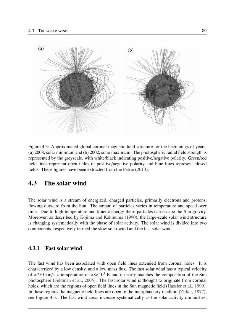
4.3. The solar wind 89
Figure 4.3: Approximated global coronal magnetic field structure for the beginnings of years:(a) 2008, solar minimum and (b) 2002, solar maximum. The photospheric radial field strength isrepresented by the greyscale, with white/black indicating positive/negative polarity. Green/redfield lines represent open fields of positive/negative polarity and blue lines represent closedfields. These figures have been extracted from the Petrie (2013).
4.3 The solar wind
The solar wind is a stream of energized, charged particles, primarily electrons and protons,flowing outward from the Sun. The stream of particles varies in temperature and speed overtime. Due to high temperature and kinetic energy these particles can escape the Sun gravity.Moreover, as described by Kojima and Kakinuma (1990), the large-scale solar wind structureis changing systematically with the phase of solar activity. The solar wind is divided into twocomponents, respectively termed the slow solar wind and the fast solar wind.
4.3.1 Fast solar wind
The fast wind has been associated with open field lines extended from coronal holes. It ischaracterized by a low density, and a low mass flux. The fast solar wind has a typical velocityof ≃750 km/s, a temperature of ≃8×10⁵ K and it nearly matches the composition of the Sunphotosphere (Feldman et al., 2005). The fast solar wind is thought to originate from coronalholes, which are the regions of open field lines in the Sun magnetic field (Hassler et al., 1999).In these regions the magnetic field lines are open to the interplanetary medium (Zirker, 1977),see Figure 4.3. The fast wind areas increase systematically as the solar activity diminishes,
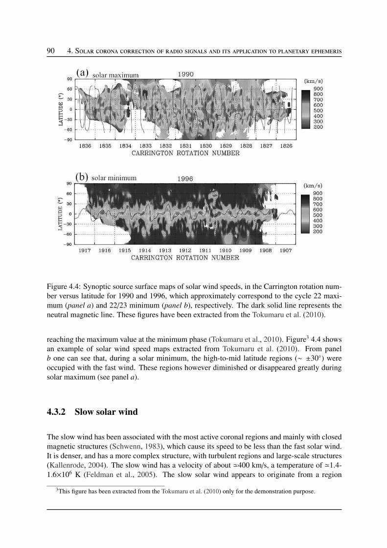
90 4. Solar corona correction of radio signals and its application to planetary ephemeris
Figure 4.4: Synoptic source surface maps of solar wind speeds, in the Carrington rotation num-ber versus latitude for 1990 and 1996, which approximately correspond to the cycle 22 maxi-mum (panel a) and 22/23 minimum (panel b), respectively. The dark solid line represents theneutral magnetic line. These figures have been extracted from the Tokumaru et al. (2010).
reaching the maximum value at the minimum phase (Tokumaru et al., 2010). Figure3 4.4 showsan example of solar wind speed maps extracted from Tokumaru et al. (2010). From panelb one can see that, during a solar minimum, the high-to-mid latitude regions (∼ ±30) wereoccupied with the fast wind. These regions however diminished or disappeared greatly duringsolar maximum (see panel a).
4.3.2 Slow solar wind
The slow wind has been associated with the most active coronal regions and mainly with closedmagnetic structures (Schwenn, 1983), which cause its speed to be less than the fast solar wind.It is denser, and has a more complex structure, with turbulent regions and large-scale structures(Kallenrode, 2004). The slow wind has a velocity of about ≃400 km/s, a temperature of ≃1.4-1.6×10⁶ K (Feldman et al., 2005). The slow solar wind appears to originate from a region
3This figure has been extracted from the Tokumaru et al. (2010) only for the demonstration purpose.
4.4. Radio signal perturbation 91
around the Sun equatorial belt that is known as the streamer belt. Coronal streamers extendoutward from this region, carrying plasma from the interior along closed magnetic loops (Lang,2000). However Bravo and Stewart (1997) suggest that coronal holes may also be the sourcesof slow winds, which could be emerging from the bordering. During solar maximum, theslow wind area increase systematically over the solar latitude and decrease as solar activitydiminishes (Tokumaru et al., 2010). Figure 4.4 shows that, during solar minimum, the lowlatitude regions were dominated by the slow wind and became ubiquitous at all latitudes duringthe maximum.
4.4 Radio signal perturbation
The perturbation in the radio signals is one of the consequences of the solar corona. For adeep space probe, when the Sun directly intercepts the radio signals between the spacecraftand the Earth, it induces perturbations in the signals and degrades them enormously. However,such degradations give an opportunity to compute time delay induced by the solar plasma andto study its physical characteristics with the plasma parameter. The time delay indicates theextra time due to the presence of an ionized medium in the propagation path, and the plasmaparameter is a measure of the number of particles in a volume (so called electron density) alongthe line of sight (LOS).
There could be a number of causes which degrade the radio signal during solar conjunctions.The solar flares and CME could be the most important events that occur in the solar corona andcause the degradation of signal. These events are often associated with the solar activity and canoccur during both phases of Sun activity, solar maximum and solar minimum. During the lowperiods of the solar cycle, events are less frequent and generally confined to the Sun equatorialregion, when during periods of high solar activity, events are much more frequent and mayoccur at any place on the Sun surface (see Figure 4.4). The brief characteristics of these eventsare given below:
• Solar flare: Sudden energy release in the solar atmosphere is called solar flare (Hudsonet al., 1995). The enormous explosions of the Sun surface typically last for a few minutesand can release enormous amount of energy. The solar flares are known to be associatedwith the magnetic field structure of the Sun around the sunspots (Parker, 1963). If thisstructure becomes twisted and sheared then magnetic field lines can cross and reconnectwith an explosive release of energy. This causes an eruption of gases on the solar surface,and extends hundreds of thousands of kilometers out from the surface of the Sun follow-ing the magnetic lines to form a solar flare. During the first stages of the solar flare, highvelocity protons are ejected and travel at around a third the speed of light. The ejectedmaterial follows the arc of the magnetic lines and then returns to the Sun, although somematerial is ejected into outer space especially during the larger flares.
• Coronal mass ejections: They are another form of disturbance that can affect radio com-

92 4. Solar corona correction of radio signals and its application to planetary ephemeris
munications. CME are the explosions in the Sun corona that cause huge bubbles of gasthat are threaded with magnetic field lines, and the bubbles are ejected over the spaceduring several hours. During the CME, the fluctuations of the Sun magnetic fields causea release of huge quantities of matter and electromagnetic radiation into space above theSun surface, either near the corona, or farther into the solar system, or even beyond. Suchrelease of matter disrupts the steady flow of the solar wind producing a large increase inthe flow. Unlike a solar flare, a CME doesn’t produce intense light. But it does produce amagnetic shockwave which may interact with the Earth magnetic field.
Both events increase the level of solar radiation in the solar corona regions. During su-perior solar conjunctions, when radio signals interact with these radiations, then the signalssuffer severe degradation and cause a time delay on ranging measurements and a phase advanceon Doppler measurements. The magnitudes of these effects are inversely proportional to thesquare of the signal frequency and the radial distance (outward from the Sun) (Muhleman et al.,1977; Schwenn and Marsch, 1990, 1991; Guhathakurta and Holzer, 1994; Bird et al., 1994;Guhathakurta et al., 1996). Thus, solar corona effects on the radio signals are decreasing withincrease in frequency and with distance from the Sun. Peaks in the Figures 3.5 and 3.9 (panelb) of Chapter 3 show an example of solar corona effects on Doppler and range measurements.The solar corona model deduce from the range measurements acquired at the time of solar con-junctions allowed us to compute time delay due to the presence of an ionized medium in thepropagation path. One can then also estimate an average electron density along the line of sight(LOS).
4.5 Solar corona correction of radio signals and its applica-
tion to planetary ephemeris
As described in sections 4.2 and 4.3, solar wind area and solar events are frequently changingwith the solar activity. Hence, one can expect different distributions of charged particles in slowand fast wind regions (Schwenn, 2006). Therefore, it is necessary to identify if the region ofthe radio signal propagation is either affected by the slow wind or by the fast wind. In thissection we investigated these regions and derived the characteristics of solar corona modelsand associated electron density distribution at different phases of solar activity (maximum andminimum) and at different solar wind states (slow and fast). The processed range data obtainedafter orbit determination have been used to derive the models and to estimate the time delaydue to the solar corona. These estimations lead us to remove the solar corona perturbationsfrom the range data. The corrected range data are then used for the construction of planetaryephemeris. This complementary range data noticeably improve the extrapolation capability ofthe planetary ephemeris and the estimation of the asteroid masses. All results corresponding tothis study are published in the Astronomy & Astrophysics journal. In this section we gave thebrief description of the steps used to derive the solar corona models. The outcomes of this studyare given in Section 4.7 and followed by Verma et al. (2013a).
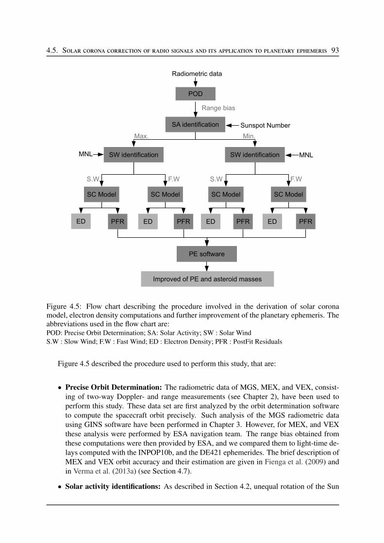
4.5. Solar corona correction of radio signals and its application to planetary ephemeris 93
!" "
" " " "
#$
Figure 4.5: Flow chart describing the procedure involved in the derivation of solar coronamodel, electron density computations and further improvement of the planetary ephemeris. Theabbreviations used in the flow chart are:POD: Precise Orbit Determination; SA: Solar Activity; SW : Solar WindS.W : Slow Wind; F.W : Fast Wind; ED : Electron Density; PFR : PostFit Residuals
Figure 4.5 described the procedure used to perform this study, that are:
• Precise Orbit Determination: The radiometric data of MGS, MEX, and VEX, consist-ing of two-way Doppler- and range measurements (see Chapter 2), have been used toperform this study. These data set are first analyzed by the orbit determination softwareto compute the spacecraft orbit precisely. Such analysis of the MGS radiometric datausing GINS software have been performed in Chapter 3. However, for MEX, and VEXthese analysis were performed by ESA navigation team. The range bias obtained fromthese computations were then provided by ESA, and we compared them to light-time de-lays computed with the INPOP10b, and the DE421 ephemerides. The brief description ofMEX and VEX orbit accuracy and their estimation are given in Fienga et al. (2009) andin Verma et al. (2013a) (see Section 4.7).
• Solar activity identifications: As described in Section 4.2, unequal rotation of the Sun
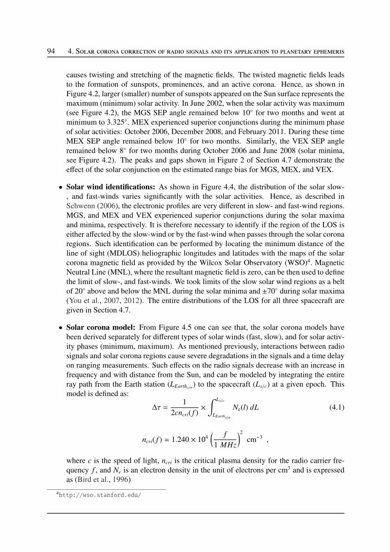
94 4. Solar corona correction of radio signals and its application to planetary ephemeris
causes twisting and stretching of the magnetic fields. The twisted magnetic fields leadsto the formation of sunspots, prominences, and an active corona. Hence, as shown inFigure 4.2, larger (smaller) number of sunspots appeared on the Sun surface represents themaximum (minimum) solar activity. In June 2002, when the solar activity was maximum(see Figure 4.2), the MGS SEP angle remained below 10 for two months and went atminimum to 3.325. MEX experienced superior conjunctions during the minimum phaseof solar activities: October 2006, December 2008, and February 2011. During these timeMEX SEP angle remained below 10 for two months. Similarly, the VEX SEP angleremained below 8 for two months during October 2006 and June 2008 (solar minima,see Figure 4.2). The peaks and gaps shown in Figure 2 of Section 4.7 demonstrate theeffect of the solar conjunction on the estimated range bias for MGS, MEX, and VEX.
• Solar wind identifications: As shown in Figure 4.4, the distribution of the solar slow-, and fast-winds varies significantly with the solar activities. Hence, as described inSchwenn (2006), the electronic profiles are very different in slow- and fast-wind regions.MGS, and MEX and VEX experienced superior conjunctions during the solar maximaand minima, respectively. It is therefore necessary to identify if the region of the LOS iseither affected by the slow-wind or by the fast-wind when passes through the solar coronaregions. Such identification can be performed by locating the minimum distance of theline of sight (MDLOS) heliographic longitudes and latitudes with the maps of the solarcorona magnetic field as provided by the Wilcox Solar Observatory (WSO)4. MagneticNeutral Line (MNL), where the resultant magnetic field is zero, can be then used to definethe limit of slow-, and fast-winds. We took limits of the slow solar wind regions as a beltof 20 above and below the MNL during the solar minima and ±70 during solar maxima(You et al., 2007, 2012). The entire distributions of the LOS for all three spacecraft aregiven in Section 4.7.
• Solar corona model: From Figure 4.5 one can see that, the solar corona models havebeen derived separately for different types of solar winds (fast, slow), and for solar activ-ity phases (minimum, maximum). As mentioned previously, interactions between radiosignals and solar corona regions cause severe degradations in the signals and a time delayon ranging measurements. Such effects on the radio signals decrease with an increase infrequency and with distance from the Sun, and can be modeled by integrating the entireray path from the Earth station (LEarths/n
) to the spacecraft (Ls/c) at a given epoch. Thismodel is defined as:
∆τ =1
2cncri( f )×
∫ Ls/c
LEarths/n
Ne(l) dL (4.1)
ncri( f ) = 1.240 × 10⁴(
f
1 MHz
)2
cm−3 ,
where c is the speed of light, ncri is the critical plasma density for the radio carrier fre-quency f , and Ne is an electron density in the unit of electrons per cm3 and is expressedas (Bird et al., 1996)
4http://wso.stanford.edu/
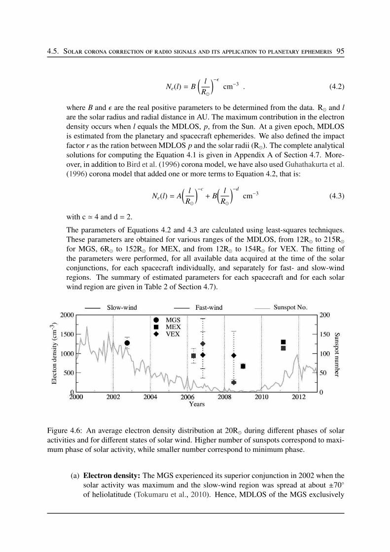
4.5. Solar corona correction of radio signals and its application to planetary ephemeris 95
Ne(l) = B
(
l
R⊙
)−ǫ
cm−3 . (4.2)
where B and ǫ are the real positive parameters to be determined from the data. R⊙ and l
are the solar radius and radial distance in AU. The maximum contribution in the electrondensity occurs when l equals the MDLOS, p, from the Sun. At a given epoch, MDLOSis estimated from the planetary and spacecraft ephemerides. We also defined the impactfactor r as the ration between MDLOS p and the solar radii (R⊙). The complete analyticalsolutions for computing the Equation 4.1 is given in Appendix A of Section 4.7. More-over, in addition to Bird et al. (1996) corona model, we have also used Guhathakurta et al.(1996) corona model that added one or more terms to Equation 4.2, that is:
Ne(l) = A
(
l
R⊙
)−c
+ B
(
l
R⊙
)−d
cm−3 (4.3)
with c ≃ 4 and d = 2.
The parameters of Equations 4.2 and 4.3 are calculated using least-squares techniques.These parameters are obtained for various ranges of the MDLOS, from 12R⊙ to 215R⊙for MGS, 6R⊙ to 152R⊙ for MEX, and from 12R⊙ to 154R⊙ for VEX. The fitting ofthe parameters were performed, for all available data acquired at the time of the solarconjunctions, for each spacecraft individually, and separately for fast- and slow-windregions. The summary of estimated parameters for each spacecraft and for each solarwind region are given in Table 2 of Section 4.7).
Figure 4.6: An average electron density distribution at 20R⊙ during different phases of solaractivities and for different states of solar wind. Higher number of sunspots correspond to maxi-mum phase of solar activity, while smaller number correspond to minimum phase.
(a) Electron density: The MGS experienced its superior conjunction in 2002 when thesolar activity was maximum and the slow-wind region was spread at about ±70
of heliolatitude (Tokumaru et al., 2010). Hence, MDLOS of the MGS exclusively
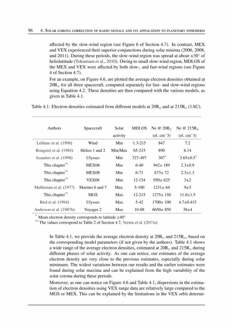
96 4. Solar corona correction of radio signals and its application to planetary ephemeris
affected by the slow-wind region (see Figure 6 of Section 4.7). In contrast, MEXand VEX experienced their superior conjunctions during solar minima (2006, 2008,and 2011). During these periods, the slow-wind region was spread at about ±30 ofheliolatitude (Tokumaru et al., 2010). Owing to small slow-wind region, MDLOS ofthe MEX and VEX were affected by both slow-, and fast-wind regions (see Figure4 of Section 4.7).
For an example, on Figure 4.6, are plotted the average electron densities obtained at20R⊙ for all three spacecraft, computed separately for fast- and slow-wind regionsusing Equation 4.2. These densities are then compared with the various models, asgiven in Table 4.1.
Table 4.1: Electron densities estimated from different models at 20R⊙ and at 215R⊙ (1AU).
Authors Spacecraft Solar MDLOS Ne @ 20R⊙ Ne @ 215R⊙
activity (el. cm−3) (el. cm−3)
Leblanc et al. (1998) Wind Min 1.3-215 847 7.2
Bougeret et al. (1984) Helios 1 and 2 Min/Max 65-215 890 6.14
Issautier et al. (1998) Ulysses Min 327-497 307* 2.65±0.5*
This chapter** MEX06 Min 6-40 942± 189 2.3±0.9
This chapter** MEX08 Min 6-71 673± 72 2.3±1.3
This chapter** VEX08 Min 12-154 950± 625 3±2
Muhleman et al. (1977) Mariner 6 and 7 Max. 5-100 1231± 64 9±3
This chapter** MGS Max 12-215 1275± 150 11.0±1.5
Bird et al. (1994) Ulysses Max 5-42 1700± 100 4.7±0.415
Anderson et al. (1987b) Voyager 2 Max 10-88 6650± 850 38±4
* Mean electron density corresponds to latitude ≥40** The values correspond to Table 2 of Section 4.7, Verma et al. (2013a)
In Table 4.1, we provide the average electron density at 20R⊙ and 215R⊙, based onthe corresponding model parameters (if not given by the authors). Table 4.1 showsa wide range of the average electron densities, estimated at 20R⊙ and 215R⊙ duringdifferent phases of solar activity. As one can notice, our estimates of the averageelectron density are very close to the previous estimates, especially during solarminimum. The widest variations between our results and the earlier estimates werefound during solar maxima and can be explained from the high variability of thesolar corona during these periods.
Moreover, as one can notice on Figure 4.6 and Table 4.1, dispersions in the estima-tion of electron densities using VEX range data are relatively large compared to theMGS or MEX. This can be explained by the limitations in the VEX orbit determi-
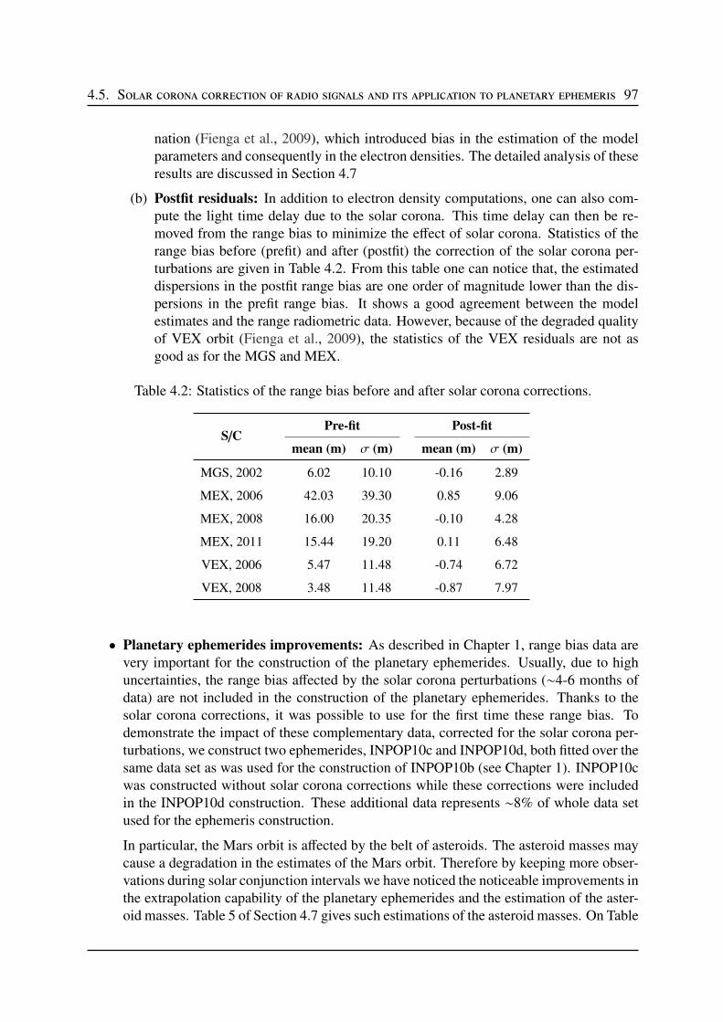
4.5. Solar corona correction of radio signals and its application to planetary ephemeris 97
nation (Fienga et al., 2009), which introduced bias in the estimation of the modelparameters and consequently in the electron densities. The detailed analysis of theseresults are discussed in Section 4.7
(b) Postfit residuals: In addition to electron density computations, one can also com-pute the light time delay due to the solar corona. This time delay can then be re-moved from the range bias to minimize the effect of solar corona. Statistics of therange bias before (prefit) and after (postfit) the correction of the solar corona per-turbations are given in Table 4.2. From this table one can notice that, the estimateddispersions in the postfit range bias are one order of magnitude lower than the dis-persions in the prefit range bias. It shows a good agreement between the modelestimates and the range radiometric data. However, because of the degraded qualityof VEX orbit (Fienga et al., 2009), the statistics of the VEX residuals are not asgood as for the MGS and MEX.
Table 4.2: Statistics of the range bias before and after solar corona corrections.
S/CPre-fit Post-fit
mean (m) σ (m) mean (m) σ (m)
MGS, 2002 6.02 10.10 -0.16 2.89
MEX, 2006 42.03 39.30 0.85 9.06
MEX, 2008 16.00 20.35 -0.10 4.28
MEX, 2011 15.44 19.20 0.11 6.48
VEX, 2006 5.47 11.48 -0.74 6.72
VEX, 2008 3.48 11.48 -0.87 7.97
• Planetary ephemerides improvements: As described in Chapter 1, range bias data arevery important for the construction of the planetary ephemerides. Usually, due to highuncertainties, the range bias affected by the solar corona perturbations (∼4-6 months ofdata) are not included in the construction of the planetary ephemerides. Thanks to thesolar corona corrections, it was possible to use for the first time these range bias. Todemonstrate the impact of these complementary data, corrected for the solar corona per-turbations, we construct two ephemerides, INPOP10c and INPOP10d, both fitted over thesame data set as was used for the construction of INPOP10b (see Chapter 1). INPOP10cwas constructed without solar corona corrections while these corrections were includedin the INPOP10d construction. These additional data represents ∼8% of whole data setused for the ephemeris construction.
In particular, the Mars orbit is affected by the belt of asteroids. The asteroid masses maycause a degradation in the estimates of the Mars orbit. Therefore by keeping more obser-vations during solar conjunction intervals we have noticed the noticeable improvements inthe extrapolation capability of the planetary ephemerides and the estimation of the aster-oid masses. Table 5 of Section 4.7 gives such estimations of the asteroid masses. On Table

98 4. Solar corona correction of radio signals and its application to planetary ephemeris
6 of Section 4.7, significantly improved masses, estimated with INPOP10d, are then com-pared with the one found in the literature and showed 80% better consistency with respectto INPOP10c. Moreover, MEX extrapolated residuals computed with INPOP10d showa better long-term behavior compared with INPOP10c with 30% less degraded residualsafter two years of extrapolation. The complete analysis of these results are discussed inSection 4.7.
4.6 Conclusion
We have analyzed the large-scale structure of the corona electron density, since 2001 to 2011.This analysis has been done with the range bias data of the MGS, MEX, and VEX spacecraftacquired during solar conjunction periods. The parameters of the solar corona models are thendeduced from these data. These parameters were estimated separately for each spacecraft atdifferent phases of solar activity (maximum and minimum) and at different solar wind states(slow and fast). We compared our results with the previous estimations that were based ondifferent techniques and different data sets. Our results are consistent, especially during solarminima, with estimations obtained by these different techniques. However, during the solarmaxima, electron densities obtained with different methods or different spacecraft show weakerconsistencies.
We have also demonstrated the impact of solar corona correction on the construction ofplanetary ephemerides. The supplementary data, corrected from the solar corona perturbations,allowed us to gain ∼8% of whole data set. Such corrected data are then used for the firsttime in the construction of INPOP and induce a noticeable improvement in the estimation ofthe asteroid masses and a better long-term behavior of the ephemerides. In addition to theseimprovements, recent Uranus observations and positions of Pluto have beed added to constructthe latest INPOP10e ephemerides (Fienga et al., 2013). For the further improvement, INPOP10eis then used for the analysis of MESSENGER radioscience data (see Chapter 5).
As stated previously, all results described in this chapter are published in the Astronomy &Astrophysics journal. The Section 4.7 therefore represented by the Verma et al. (2013a), whichdescribed the complete analysis of these results.
4.7 Verma et al. (2013a)
A&A 550, A124 (2013)DOI: 10.1051/0004-6361/201219883c© ESO 2013
Astronomy&
Astrophysics
Electron density distribution and solar plasma correction
of radio signals using MGS, MEX, and VEX spacecraft navigation
data and its application to planetary ephemerides⋆
A. K. Verma1,2, A. Fienga1,3, J. Laskar3, K. Issautier4 , H. Manche3, and M. Gastineau3
1 Observatoire de Besançon, CNRS UMR6213, 41bis Av. de l’Observatoire, 25000 Besançon, France2 CNES, Toulouse, France
e-mail: [email protected] Astronomie et Systèmes Dynamiques, IMCCE-CNRS UMR 8028, 77 Av. Denfert-Rochereau, 75014 Paris, France4 LESIA, Observatoire de Paris, CNRS, UPMC, Université Paris Diderot, 5 place Jules Janssen, 92195 Meudon, France
Received 25 June 2012 / Accepted 19 December 2012
ABSTRACT
The Mars Global Surveyor (MGS), Mars Express (MEX), and Venus Express (VEX) experienced several superior solar conjunctions.These conjunctions cause severe degradations of radio signals when the line of sight between the Earth and the spacecraft passes nearto the solar corona region. The primary objective of this work is to deduce a solar corona model from the spacecraft navigation dataacquired at the time of solar conjunctions and to estimate its average electron density. The corrected or improved data are then usedto fit the dynamical modeling of the planet motions, called planetary ephemerides. We analyzed the radio science raw data of theMGS spacecraft using the orbit determination software GINS. The range bias, obtained from GINS and provided by ESA for MEXand VEX, are then used to derive the electron density profile. These profiles are obtained for different intervals of solar distances:from 12 R⊙ to 215 R⊙ for MGS, 6 R⊙ to 152 R⊙ for MEX, and from 12 R⊙ to 154 R⊙ for VEX. They are acquired for each spacecraftindividually, for ingress and egress phases separately and both phases together, for different types of solar winds (fast, slow), andfor solar activity phases (minimum, maximum). We compared our results with the previous estimations that were based on in situmeasurements, and on solar type III radio and radio science studies made at different phases of solar activity and at different solar windstates. Our results are consistent with estimations obtained by these different methods. Moreover, fitting the planetary ephemeridesincluding complementary data that were corrected for the solar corona perturbations, noticeably improves the extrapolation capabilityof the planetary ephemerides and the estimation of the asteroids masses.
Key words. celestial mechanics – ephemerides – Sun: corona
1. Introduction
The solar corona and the solar wind contain primarily ionizedhydrogen ions, helium ions, and electrons. These ionized parti-cles are ejected radially from the Sun. The solar wind param-eters, the velocity, and the electron density are changing withtime, radial distances (outward from Sun), and the solar cycles(Schwenn & Marsch 1990, 1991). The strongly turbulent andionized gases within the corona severely degrade the radio wavesignals that propagate between spacecraft and Earth tracking sta-tions. These degradations cause a delay and a greater dispersionof the radio signals. The group and phase delays induced by theSun activity are directly proportional to the total electron con-tents along the line of sight (LOS) and inversely proportionalwith the square of carrier radio wave frequency.
By analyzing spacecraft radio waves facing a solar conjunc-tion (when the Sun directly intercepts the radio signals betweenthe spacecraft and the Earth), it is possible to study the electroncontent and to better understand the Sun. An accurate determi-nation of the electron density profile in the solar corona and inthe solar wind is indeed essential for understanding the energytransport in collision-less plasma, which is still an open ques-tion (Cranmer 2002). Nowadays, mainly radio scintillation and
⋆ Tables 5, 6 and Appendix A are available in electronic form athttp://www.aanda.org
Table 1. Previous models based on in situ and radio science measure-ments (see text for detailed descriptions).
Spacecraft Data type AuthorMariner 6 and 7 radio science Muhleman et al. (1977)Voyager 2 radio science Anderson et al. (1987)Ulysses radio science Bird et al. (1994)Helios land 2 in situ Bougeret et al. (1984)Ulysses in situ Issautier et al. (1998)Skylab Coronagraph Guhathakurta et al. (1996)Wind solar radio Leblanc et al. (1998)
burst III
white-light coronagraph measurements can provide an estima-tion of the electron density profile in the corona (Guhathakurta& Holzer 1994; Bird et al. 1994; Guhathakurta et al. 1996, 1999;Woo & Habbal 1999). However, the solar wind acceleration andthe corona heating take place between 1 to 10 R⊙ where in situobservations are not possible. Several density profiles of solarcorona model based on different types of data are described inthe literature (Table 1). The two viable methods that are gen-erally used to derive these profiles are (Muhleman & Anderson1981) (1) direct in situ measurements of the electron density,speed, and energies of the electron and photons, and (2) an
Article published by EDP Sciences A124, page 1 of 17
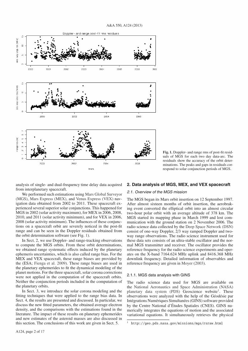
A&A 550, A124 (2013)
Fig. 1. Doppler- and range rms of post-fit resid-uals of MGS for each two day data-arc. Theresiduals show the accuracy of the orbit deter-minations. The peaks and gaps in residuals cor-respond to solar conjunction periods of MGS.
analysis of single- and dual-frequency time delay data acquiredfrom interplanetary spacecraft.
We performed such estimations using Mars Global Surveyor(MGS), Mars Express (MEX), and Venus Express (VEX) nav-igation data obtained from 2002 to 2011. These spacecraft ex-perienced several superior solar conjunctions. This happened forMGS in 2002 (solar activity maximum), for MEX in 2006, 2008,2010, and 2011 (solar activity minimum), and for VEX in 2006,2008 (solar activity minimum). The influences of these conjunc-tions on a spacecraft orbit are severely noticed in the post-fitrange and can be seen in the Doppler residuals obtained fromthe orbit determination software (see Fig. 1).
In Sect. 2, we use Doppler- and range-tracking observationsto compute the MGS orbits. From these orbit determinations,we obtained range systematic effects induced by the planetaryephemeris uncertainties, which is also called range bias. For theMEX and VEX spacecraft, these range biases are provided bythe (ESA; Fienga et al. 2009). These range biases are used inthe planetary ephemerides to fit the dynamical modeling of theplanet motions. For the three spacecraft, solar corona correctionswere not applied in the computation of the spacecraft orbits.Neither the conjunction periods included in the computation ofthe planetary orbits.
In Sect. 3, we introduce the solar corona modeling and thefitting techniques that were applied to the range bias data. InSect. 4, the results are presented and discussed. In particular, wediscuss the new fitted parameters, the obtained average electrondensity, and the comparisons with the estimations found in theliterature. The impact of these results on planetary ephemeridesand new estimates of the asteroid masses are also discussed inthis section. The conclusions of this work are given in Sect. 5.
2. Data analysis of MGS, MEX, and VEX spacecraft
2.1. Overview of the MGS mission
The MGS began its Mars orbit insertion on 12 September 1997.After almost sixteen months of orbit insertion, the aerobrak-ing event converted the elliptical orbit into an almost circulartwo-hour polar orbit with an average altitude of 378 km. TheMGS started its mapping phase in March 1999 and lost com-munication with the ground station on 2 November 2006. Theradio science data collected by the Deep Space Network (DSN)consist of one-way Doppler, 2/3 way ramped Doppler and two-way range observations. The radio science instrument used forthese data sets consists of an ultra-stable oscillator and the nor-mal MGS transmitter and receiver. The oscillator provides thereference frequency for the radio science experiments and oper-ates on the X-band 7164.624 MHz uplink and 8416.368 MHzdownlink frequency. Detailed information of observables andreference frequency are given in Moyer (2003).
2.1.1. MGS data analysis with GINS
The radio science data used for MGS are available onthe National Aeronautics and Space Administration (NASA)planetary data system (PDS) Geoscience website1. Theseobservations were analyzed with the help of the Géodésie parIntégrations Numériques Simultanées (GINS) software providedby the Centre National d’Études Spatiales (CNES). GINS nu-merically integrates the equations of motion and the associatedvariational equations. It simultaneously retrieves the physical
1 http://geo.pds.nasa.gov/missions/mgs/rsraw.html
A124, page 2 of 17
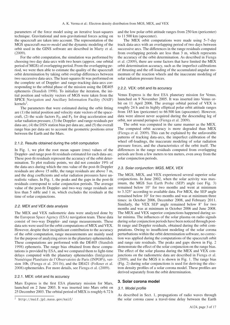
A. K. Verma et al.: Electron density distribution from MGS, MEX, and VEX
parameters of the force model using an iterative least-squarestechnique. Gravitational and non-gravitational forces acting onthe spacecraft are taken into account. The representation of theMGS spacecraft macro-model and the dynamic modeling of theorbit used in the GINS software are described in Marty et al.(2009).
For the orbit computation, the simulation was performed bychoosing two day data-arcs with two hours (approx. one orbitalperiod of MGS) of overlapping period. From the overlapping pe-riod, we were then able to estimate the quality of the spacecraftorbit determination by taking orbit overlap differences betweentwo successive data-arcs. The least-squares fit was performed onthe complete set of Doppler- and range-tracking data-arcs cor-responding to the orbital phase of the mission using the DE405ephemeris (Standish 1998). To initialize the iteration, the ini-tial position and velocity vectors of MGS were taken from theSPICE Navigation and Ancillary Information Facility (NAIF)kernels2.
The parameters that were estimated during the orbit fittingare (1) the initial position and velocity state vectors of the space-craft, (2) the scale factors FD and FS for drag acceleration andsolar radiation pressure, (3) the Doppler- and range residuals perdata-arc, (4) the DSN station bias per data arc, and (5) the overallrange bias per data-arc to account the geometric positions errorbetween the Earth and the Mars.
2.1.2. Results obtained during the orbit computation
In Fig. 1, we plot the root mean square (rms) values of theDoppler- and range post-fit residuals estimated for each data-arc.These post-fit residuals represent the accuracy of the orbit deter-mination. To plot realistic points, we did not consider 19% ofthe data-arcs during which the rms value of the post-fit Dopplerresiduals are above 15 mHz, the range residuals are above 7 m,and the drag coefficients and solar radiation pressures have un-realistic values. In Fig. 1, the peaks and the gaps in the post-fitresiduals correspond to solar conjunction periods. The averagevalue of the post-fit Doppler- and two-way range residuals areless than 5 mHz and 1 m, which excludes the residuals at thetime of solar conjunctions.
2.2. MEX and VEX data analysis
The MEX and VEX radiometric data were analyzed done bythe European Space Agency (ESA) navigation team. These dataconsist of two-way Doppler- and range measurements. Thesedata sets were used for the orbit computations of MEX and VEX.However, despite their insignificant contribution to the accuracyof the orbit computation, range measurements are mainly usedfor the purpose of analyzing errors in the planetary ephemerides.These computations are performed with the DE405 (Standish1998) ephemeris. The range bias obtained from these compu-tations is provided by ESA, and we compared them to light-timedelays computed with the planetary ephemerides (IntégrateurNumérique Planétaire de l’Observatoire de Paris (INPOP)), ver-sion 10b, (Fienga et al. 2011b), and the DE421 (Folkner et al.2008) ephemerides. For more details, see Fienga et al. (2009).
2.2.1. MEX: orbit and its accuracy
Mars Express is the first ESA planetary mission for Mars,launched on 2 June 2003. It was inserted into Mars orbit on25 December 2003. The orbital period of MEX is roughly 6.72 h
2 http://naif.jpl.nasa.gov/naif/
and the low polar orbit attitude ranges from 250 km (pericenter)to 11 500 km (apocenter).
The MEX orbit computations were made using 5–7-daytrack data-arcs with an overlapping period of two days betweensuccessive arcs. The differences in the range residuals computedfrom overlapping periods are less than 3 m, which representsthe accuracy of the orbit determination. As described in Fiengaet al. (2009), there are some factors that have limited the MEXorbit determination accuracy, such as the imperfect calibrationsof thrusting and the off-loading of the accumulated angular mo-mentum of the reaction wheels and the inaccurate modeling ofsolar radiation pressure forces.
2.2.2. VEX: orbit and its accuracy
Venus Express is the first ESA planetary mission for Venus,launched on 9 November 2005. It was inserted into Venus or-bit on 11 April 2006. The average orbital period of VEX isroughly 24 h and its highly elliptical polar orbit attitude rangesfrom 185 km (pericenter) to 66 500 km (apocenter). However,data were almost never acquired during the descending leg oforbit, nor around periapsis (Fienga et al. 2009).
The orbit was computed in the same manner as the MEX.The computed orbit accuracy is more degraded than MEX(Fienga et al. 2009). This can be explained by the unfavorablepatterns of tracking data-arcs, the imperfect calibration of thewheel off-loadings, the inaccurate modeling of solar radiationpressure forces, and the characteristics of the orbit itself. Thedifferences in the range residuals computed from overlappingperiods are from a few meters to ten meters, even away from thesolar conjunction periods.
2.3. Solar conjunction: MGS, MEX, VEX
The MGS, MEX, and VEX experienced several superior solarconjunctions. In June 2002, when the solar activity was max-imum, the MGS Sun Earth Probe (SEP) angle (see Fig. 3)remained below 10 for two months and went at minimumto 3.325 according to available data. For MEX, the SEP angleremained below 10 for two months and was at minimum threetimes: in October 2006, December 2008, and February 2011.Similarly, the VEX SEP angle remained below 8 for twomonths and was at minimum in October 2006 and June 2008.The MEX and VEX superior conjunctions happened during so-lar minima. The influences of the solar plasma on radio signalsduring solar conjunction periods have been noticed through post-fit range and Doppler residuals, obtained during the orbit com-putations. Owing to insufficient modeling of the solar coronaperturbations within the orbit determination software, no correc-tion was applied during the computations of the spacecraft orbitand range rate residuals. The peaks and gaps shown in Fig. 2demonstrate the effect of the solar conjunction on the range bias.The effect of the solar plasma during the MEX and VEX con-junctions on the radiometric data are described in Fienga et al.(2009), and for the MGS it is shown in Fig. 1. The range bias(Fig. 2) during solar conjunctions is used for deriving the elec-tron density profiles of a solar corona model. These profiles arederived separately from the orbit determination.
3. Solar corona model
3.1. Model profile
As described in Sect. 1, propagations of radio waves throughthe solar corona cause a travel-time delay between the Earth
A124, page 3 of 17
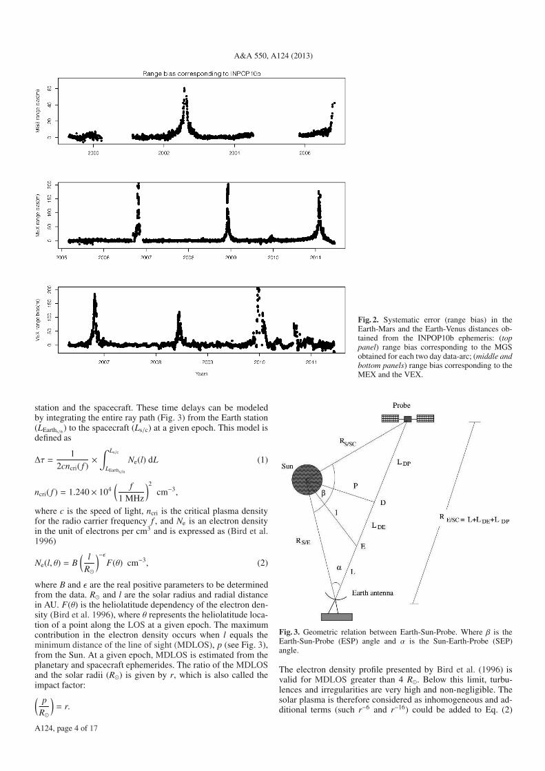
A&A 550, A124 (2013)
Fig. 2. Systematic error (range bias) in theEarth-Mars and the Earth-Venus distances ob-tained from the INPOP10b ephemeris: (toppanel) range bias corresponding to the MGSobtained for each two day data-arc; (middle andbottom panels) range bias corresponding to theMEX and the VEX.
station and the spacecraft. These time delays can be modeledby integrating the entire ray path (Fig. 3) from the Earth station(LEarths/n ) to the spacecraft (Ls/c) at a given epoch. This model isdefined as
∆τ =1
2cncri( f )×
∫ Ls/c
LEarths/n
Ne(l) dL (1)
ncri( f ) = 1.240 × 10⁴(
f
1 MHz
)2
cm−3,
where c is the speed of light, ncri is the critical plasma densityfor the radio carrier frequency f , and Ne is an electron densityin the unit of electrons per cm3 and is expressed as (Bird et al.1996)
Ne(l, θ) = B
(
l
R⊙
)−ǫ
F(θ) cm−3, (2)
where B and ǫ are the real positive parameters to be determinedfrom the data. R⊙ and l are the solar radius and radial distancein AU. F(θ) is the heliolatitude dependency of the electron den-sity (Bird et al. 1996), where θ represents the heliolatitude loca-tion of a point along the LOS at a given epoch. The maximumcontribution in the electron density occurs when l equals theminimum distance of the line of sight (MDLOS), p (see Fig. 3),from the Sun. At a given epoch, MDLOS is estimated from theplanetary and spacecraft ephemerides. The ratio of the MDLOSand the solar radii (R⊙) is given by r, which is also called theimpact factor:(
p
R⊙
)
= r.
Fig. 3. Geometric relation between Earth-Sun-Probe. Where β is theEarth-Sun-Probe (ESP) angle and α is the Sun-Earth-Probe (SEP)angle.
The electron density profile presented by Bird et al. (1996) isvalid for MDLOS greater than 4 R⊙. Below this limit, turbu-lences and irregularities are very high and non-negligible. Thesolar plasma is therefore considered as inhomogeneous and ad-ditional terms (such r−6 and r−16) could be added to Eq. (2)
A124, page 4 of 17

A. K. Verma et al.: Electron density distribution from MGS, MEX, and VEX
(Muhleman et al. 1977; Bird et al. 1994). However, because ofthe very high uncertainties in the spacecraft orbit and range biasmeasurements within these inner regions, we did not includethese terms in our solar corona corrections.
At a given epoch, the MGS, MEX, and VEX MDLOS al-ways remain in the ecliptic plane. The latitudinal variations inthe coverage of data are hence negligible compared to the varia-tion in the MDLOS. These data sets are thus less appropriate forthe analysis of the electron density as a function of heliolatitude(Bird et al. 1996). Equation (2) can therefore be expressed as afunction of the single-power-law (ǫ) of radial distance only andbe reduced to
Ne(l) = B
(
l
R⊙
)−ǫ
cm−3. (3)
On the other hand, at a given interval of the MDLOS in the eclip-tic plane, Guhathakurta et al. (1996) and Leblanc et al. (1998)added one or more terms to Eq. (3), that is
Ne(l) = A
(
l
R⊙
)−c
+ B
(
l
R⊙
)−d
cm−3 (4)
with c ≃ 4 and d = 2.To estimate the travel-time delay, we analytically integrated
the LOS (Eq. (1)) from the Earth station to the spacecraft, usingEq. (3) and Eq. (4) individually. The analytical solutions of theseintegrations are given in Appendix A.
In general, the parameters of the electron density profiles dif-fer from one model to another. These parameters may vary withthe type of observations, with the solar activity, or with the so-lar wind state. In contrast, the primary difference between theseveral models postulated for the electron density (r > 4) is theparameter ǫ (Eq. (3)), which can vary from 2.0 to 3.0.
For example, the density profile parameters obtained byMuhleman et al. (1977) using the Mariner-7 radio science datafor the range of the MDLOS from 5 R⊙ to 100 R⊙ at the time ofmaximum solar cycle phase are
Ne =(1.3 ± 0.9) × 108
r6+
(0.66 ± 0.53) × 106
r2.08 ± 0.23cm−3.
The electron density profile derived by Leblanc et al. (1998)using the data obtained by the Wind radio and plasma waveinvestigation instrument, for the range of the MDLOS fromabout 1.3 R⊙ to 215 R⊙ at the solar cycle minimum is
Ne =0.8 × 10⁸
r6+
0.41 × 10⁷
r4+
0.33 × 10⁶
r2cm−3.
Furthermore, based on in situ measurements, such as thoseobtained with the Helios 1 and 2 spacecraft, Bougeret et al.(1984) gave an electronic profile as a function of the MDLOSfrom 64.5 R⊙ to 215 R⊙ as follows
Ne =6.14p2.10
cm−3.
Similarly, Issautier et al. (1998) analyzed in situ measurementsof the solar wind electron density as a function of heliolatitudeduring a solar minimum. The deduced electron density profile athigh latitude (>40) is given as
Ne =2.65
p2.003 ± 0.015cm−3.
This Ulysses high-latitude data set is a representative sample ofthe stationary high-speed wind. This offered the opportunity to
study the in situ solar wind structure during the minimal varia-tions in the solar activity. As presented in Issautier et al. (1998),electronic profiles deduced from other observations in numerousstudies were obtained either during different phases of solar ac-tivity (minimum or maximum), different solar wind states (fastor slow-wind), using data in the ecliptic plane (low latitudes).These conditions may introduce some bias in the estimation ofelectronic profiles of density.
Comparisons of the described profiles with the results ob-tained in this study are presented in Sect. 4.2 and are plotted inFig. 9.
3.2. Solar wind identification of LOS and data fitting
As described in Schwenn (2006), the electronic profiles are verydifferent in slow- and fast-wind regions. In slow-wind regions,one expects a higher electronic density close to the MNL of thesolar corona magnetic field at low latitudes (You et al. 2007).It is then necessary to identify if the region of the LOS is eitheraffected by the slow-wind or by the fast-wind. To investigate thatquestion, we computed the projection of the MDLOS on the Sunsurface. We then located the MDLOS heliographic longitudesand latitudes with the maps of the solar corona magnetic field asprovided by the WSO3. This magnetic field is calculated fromphotospheric field observations with a potential field model4.
However, zones of slow-wind are variable and not preciselydetermined (Mancuso & Spangler 2000; Tokumaru et al. 2010).As proposed in You et al. (2007, 2012), we took limits of theslow solar wind regions as a belt of 20 above and below theMNL during the solar minima. For the 2002 solar maximum,this hypothesis is not valid, the slow-wind region being widerthan during solar minima. Tokumaru et al. (2010) showed thedominating role of the slow-wind for this entire period and forlatitudes lower than ±70 degrees.
An example of the MDLOS projection on the Sun’s surfacewith the maps of solar corona magnetic field is shown in Fig. 4.These magnetic field maps correspond to the mean epoch of theingress and egress phases of the solar conjunction at 20 R⊙. Thedark solid line represents the MNL and the belt of the slow-wind region is presented by dashed lines. The two marked pointsgive the projected locations of the MDLOS, ingress (N) andegress () at 20 R⊙. For the entire MDLOS, this distribution ofthe slow- or fast-wind regions in the ingress and egress phasesof solar conjunctions are shown in Fig. 5. The black (white) barsin Fig. 5 present the count of data sets distributed in the slow-(fast-) wind region.
After separating the MDLOS into slow- and fast-wind re-gions as defined in Fig. 5, the parameters of Eqs. (3) and (4) arethen calculated using least-squares techniques. These parame-ters are obtained for various ranges of the MDLOS, from 12 R⊙to 215 R⊙ for MGS, 6 R⊙ to 152 R⊙ for MEX, and from 12 R⊙to 154 R⊙ for VEX. The adjustments were performed, for allavailable data acquired at the time of the solar conjunctions, foreach spacecraft individually, and separately for fast- and slow-wind regions (see Table 2).
To estimate the robustness of the electronic profile de-terminations, adjustments on ingress and egress phases wereperformed separately. The differences between these two esti-mations and the one obtained on the whole data set give thesensitivity of the profile fit to the distribution of the data, butalso to the solar wind states. These differences are thus taken as
3 http://wso.stanford.edu/4 http://wso.stanford.edu/synsourcel.html
A124, page 5 of 17
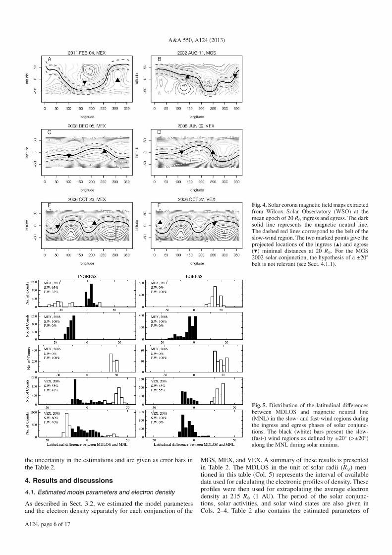
A&A 550, A124 (2013)
Fig. 4. Solar corona magnetic field maps extractedfrom Wilcox Solar Observatory (WSO) at themean epoch of 20 R⊙ ingress and egress. The darksolid line represents the magnetic neutral line.The dashed red lines correspond to the belt of theslow-wind region. The two marked points give theprojected locations of the ingress (N) and egress() minimal distances at 20 R⊙. For the MGS2002 solar conjunction, the hypothesis of a ±20
belt is not relevant (see Sect. 4.1.1).
Fig. 5. Distribution of the latitudinal differencesbetween MDLOS and magnetic neutral line(MNL) in the slow- and fast-wind regions duringthe ingress and egress phases of solar conjunc-tions. The black (white) bars present the slow-(fast-) wind regions as defined by ±20 (>±20)along the MNL during solar minima.
the uncertainty in the estimations and are given as error bars inthe Table 2.
4. Results and discussions
4.1. Estimated model parameters and electron density
As described in Sect. 3.2, we estimated the model parametersand the electron density separately for each conjunction of the
MGS, MEX, and VEX. A summary of these results is presentedin Table 2. The MDLOS in the unit of solar radii (R⊙) men-tioned in this table (Col. 5) represents the interval of availabledata used for calculating the electronic profiles of density. Theseprofiles were then used for extrapolating the average electrondensity at 215 R⊙ (1 AU). The period of the solar conjunc-tions, solar activities, and solar wind states are also given inCols. 2–4. Table 2 also contains the estimated parameters of
A124, page 6 of 17
A. K. Verma et al.: Electron density distribution from MGS, MEX, and VEXT
ab
le2.
Sol
arco
rona
mod
elpa
ram
eter
san
del
ectr
onde
nsit
ies
esti
mat
edfr
omtw
odiff
eren
tmod
els
usin
gth
eM
GS
,ME
X,a
ndV
EX
rang
ebi
as.
S/C
Yea
rS
.C1
S.W
.S2
MD
LO
S3
Ne=
Br−ǫ
Ne=
Ar−
4+
Br−
2
B(×
106)
ǫN
e@20
R⊙
Ne@
215
R⊙∗
B(×
106)
A(×
108)
Ne@
20R⊙
Ne@
215
R⊙∗
MG
SA
ug.2
002
Max
S.W
12–2
150.
51±
0.06
2.00±
0.01
1275±
150
11±
1.5
0.52±
0.04
013
00±
100
11±
1F.
W–
––
––
––
––
ME
XO
ct.2
006
Min
S.W
––
––
––
––
–F.
W6–
401.
90±
0.50
2.54±
0.07
942±
189
2.3±
0.9
0.30±
0.10
0.16±
0.02
850±
263
6±
1
ME
XD
ec.2
008
Min
S.W
6–71
0.89±
0.42
2.40±
0.16
673±
722.
3±
1.3
0.22±
0.04
0.10±
0.02
615±
905±
1F.
W–
––
––
––
––
ME
XF
eb.2
011
Min
S.W
40–1
520.
52±
0.10
2∗∗
1300±
25∗
11±
10.
52±
0.10
013
00±
25∗
11±
1F.
W6–
601.
70±
0.10
2.44±
0.01
1138±
313.
5±
0.5
0.33±
0.02
0.24±
0.04
975±
607±
1
VE
XO
ct.2
006
Min
S.W
12–1
540.
52±
0.30
2.10±
0.10
964±
600
7±
40.
40±
0.28
010
00±
600
9±
6F.
W12
–130
1.35±
1.10
2.33±
0.30
1256±
649
5±
20.
44±
0.15
010
87±
480
9±
4
VE
XJu
n.20
08M
inS
.W12
–154
1.70±
1.50
2.50±
0.50
950±
625
3±
20.
31±
0.20
077
5±
450
7±
4F.
W41
–96
0.10±
0.01
2∗∗
250±
25∗
2±
10.
10±
0.01
025
0±
25∗
2±
1
Note
s.T
heel
ectr
onde
nsit
you
tfro
mth
ein
terv
alof
the
MD
LO
Sis
extr
apol
ated
from
the
give
nm
odel
para
met
ers.
(1)
S.C
:sol
arcy
cle;
(2)
S.W
.S:s
olar
win
dst
ate
(F.W
:fas
t-w
ind,
S.W
:slo
w-w
ind)
;(3
)M
DL
OS
:min
imum
dist
ance
ofth
eli
neof
sigh
tin
the
unit
ofso
lar
radi
i(R⊙);
(∗)
extr
apol
ated
valu
e;(∗∗)
fixe
d.
two different models: the first model from Bird et al. (1996)corresponds to Eq. (3), whereas the second model is based onGuhathakurta et al. (1996) and Leblanc et al. (1998) and followsEq. (4) with c = 4. Estimated model parameters for the slow-and fast-wind regions are presented in Cols. 6 and 7.
4.1.1. Mars superior conjunction
The MGS experienced its superior conjunction in 2002 whenthe solar activity was maximum and the slow-wind region wasspread at about ±70 of heliolatitude (Tokumaru et al. 2010).Figure 6 represents the projection of the MGS MDLOS on thesolar surface (black dots) superimposed with the 2002 synop-tic source surface map of solar wind speeds derived from STELIPS observations extracted from Tokumaru et al. (2010). It sug-gests that, the MDLOS of the MGS exclusively remains in theslow-wind region. Respective estimates of the model parametersand of the electron densities are given in Table 2. From this ta-ble one can see that the estimates of the electron density fromboth models are very similar. Parameter ǫ of Eq. (3) is then es-timated as 2.00 ± 0.01, which represents a radially symmetricalbehavior of the solar wind and hence validates the assumptionof a spherically symmetrical behavior of the slow-wind duringsolar maxima (Guhathakurta et al. 1996). Whereas for Eq. (4),the contribution of the r−4 term at large heliocentric distances(r > 12 R⊙) is negligible compared to the r−2 term. Thus, theparameter A for these large heliocentric distances is fixed to zeroand consequently gave similar results to Eq. (3), as shown inTable 2.
In contrast, MEX experienced its superior conjunctionsin 2006, 2008, and 2011 during solar minima. The distributionof data during these conjunctions with respect to MDLOS areshown in Fig. 7. From this figure, one can see that the MEX 2006(2008) conjunction corresponds to the fast- (slow-) wind re-gion, whereas 2011 conjunction is a mixture of slow- and fast-winds. The estimated parameters of these conjunctions are givenin Table 2. An example of the comparison between two mod-els (Eqs. (3) and (4)) is shown in Fig. 8. This figure comparesthe electron density profiles obtained from the two models dur-ing the MEX 2008 conjunction. These profiles are extrapolatedfrom 1 R⊙ to 6 R⊙ and from 71 R⊙ to 215 R⊙. The upper trianglesin Fig. 8 indicate electronic densities obtained at 20 R⊙ and at theextrapolated distance of 215 R⊙ (1 AU) with error bars obtainedas described in Sect. 3.2. As one sees in that figure, electronicprofiles are quite similar over the computation interval till 71 R⊙and become significantly different after this limit. This suggeststhat the estimated parameters for both models are valid for therange of MDLOS given in Table 2. Finally, for the MEX 2011conjunction, as shown in Figs. 5 and 7, the data are mainly dis-tributed in the slow-wind (63%) during ingress phase and in thefast-wind (100%) during egress phase. Owing to the unavailabil-ity of slow-wind data near the Sun (MDLOS< 40 R⊙), we fixed ǫto 2 for Eq. (3) (see Table 2). Moreover, the average electron den-sity estimated for this conjunction is higher for the slow-windthan for the fast-wind and it is consistent with Tokumaru et al.(2010), which suggests that near the MNL, the electron contentis higher than in the fast-wind regions.
4.1.2. Venus superior conjunction
The VEX 2006 and 2008 conjunctions exhibit a mixture ofslow- and fast-wind (Fig. 7). These conjunctions occurred ap-proximately at the same time as the MEX superior conjunctions.
A124, page 7 of 17

A&A 550, A124 (2013)
Fig. 6. 2002 synoptic source surface map of solar wind speeds derived from STEL IPS observations extracted from Tokumaru et al. (2010). Theblack dots represent the MGS MDLOS during the 2002 conjunction period for the range of 12 R⊙ to 120 R⊙.
Fig. 7. Distribution of the MGS, MEX, andVEX data in the slow (black) and fast (white)wind with respect to MDLOS in units of so-lar radii (R⊙). Negative (positive) MDLOS rep-resents the distribution in the ingress (egress)phase.
Table 3. Electron densities estimated from different models at 20 R⊙ and at 215 R⊙ (1 AU).
Authors Spacecraft Solar MDLOS Ne @ 20 R⊙ Ne @ 215 R⊙activity (el. cm−3) (el. cm−3)
Leblanc et al. (1998) Wind Min 1.3–215 847 7.2Bougeret et al. (1984) Helios 1 and 2 Min/Max 65–215 890 6.14Issautier et al. (1998) Ulysses Min 327–497 307∗ 2.65 ± 0.5∗
Muhleman et al. (1977) Mariner 6 and 7 Max. 5–100 1231 ± 64 9 ± 3Bird et al. (1994) Ulysses Max 5–42 1700 ± 100 4.7 ± 0.415Anderson et al. (1987) Voyager 2 Max 10–88 6650 ± 850 38 ± 4
Notes. (∗) Mean electron density corresponds to latitude ≥40.
However, the limitations in the VEX orbit determination intro-duced bias in the estimation of the model parameters and theelectron densities. This can be verified from the discrepanciespresented in Table 2 for the VEX 2006 and 2008 conjunctions.Despite these high uncertainties, post-fit range bias corrected forthe solar corona allows one to add complementary data in theconstruction of the planetary ephemerides (see Sect. 4.5).
4.2. Comparison with other models
Table 3 represents the estimated electron densities at 20 R⊙and 215 R⊙ (1 AU) from the various models. These models arerepresentative of radio science measurements (Muhleman et al.1977; Anderson et al. 1987; Bird et al. 1994, 1996), in situmeasurements (Bougeret et al. 1984; Issautier et al. 1997), and
A124, page 8 of 17
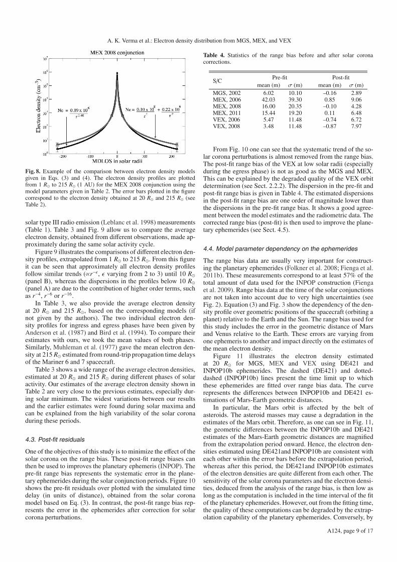
A. K. Verma et al.: Electron density distribution from MGS, MEX, and VEX
Fig. 8. Example of the comparison between electron density modelsgiven in Eqs. (3) and (4). The electron density profiles are plottedfrom 1 R⊙ to 215 R⊙ (1 AU) for the MEX 2008 conjunction using themodel parameters given in Table 2. The error bars plotted in the figurecorrespond to the electron density obtained at 20 R⊙ and 215 R⊙ (seeTable 2).
solar type III radio emission (Leblanc et al. 1998) measurements(Table 1). Table 3 and Fig. 9 allow us to compare the averageelectron density, obtained from different observations, made ap-proximately during the same solar activity cycle.
Figure 9 illustrates the comparisons of different electron den-sity profiles, extrapolated from 1 R⊙ to 215 R⊙. From this figureit can be seen that approximately all electron density profilesfollow similar trends (∝r−ǫ , ǫ varying from 2 to 3) until 10 R⊙(panel B), whereas the dispersions in the profiles below 10 R⊙(panel A) are due to the contribution of higher order terms, suchas r−4, r−6 or r−16.
In Table 3, we also provide the average electron densityat 20 R⊙ and 215 R⊙, based on the corresponding models (ifnot given by the authors). The two individual electron den-sity profiles for ingress and egress phases have been given byAnderson et al. (1987) and Bird et al. (1994). To compare theirestimates with ours, we took the mean values of both phases.Similarly, Muhleman et al. (1977) gave the mean electron den-sity at 215 R⊙ estimated from round-trip propagation time delaysof the Mariner 6 and 7 spacecraft.
Table 3 shows a wide range of the average electron densities,estimated at 20 R⊙ and 215 R⊙ during different phases of solaractivity. Our estimates of the average electron density shown inTable 2 are very close to the previous estimates, especially dur-ing solar minimum. The widest variations between our resultsand the earlier estimates were found during solar maxima andcan be explained from the high variability of the solar coronaduring these periods.
4.3. Post-fit residuals
One of the objectives of this study is to minimize the effect of thesolar corona on the range bias. These post-fit range biases canthen be used to improves the planetary ephemeris (INPOP). Thepre-fit range bias represents the systematic error in the plane-tary ephemerides during the solar conjunction periods. Figure 10shows the pre-fit residuals over plotted with the simulated timedelay (in units of distance), obtained from the solar coronamodel based on Eq. (3). In contrast, the post-fit range bias rep-resents the error in the ephemerides after correction for solarcorona perturbations.
Table 4. Statistics of the range bias before and after solar coronacorrections.
S/CPre-fit Post-fit
mean (m) σ (m) mean (m) σ (m)MGS, 2002 6.02 10.10 –0.16 2.89MEX, 2006 42.03 39.30 0.85 9.06MEX, 2008 16.00 20.35 –0.10 4.28MEX, 2011 15.44 19.20 0.11 6.48VEX, 2006 5.47 11.48 –0.74 6.72VEX, 2008 3.48 11.48 –0.87 7.97
From Fig. 10 one can see that the systematic trend of the so-lar corona perturbations is almost removed from the range bias.The post-fit range bias of the VEX at low solar radii (especiallyduring the egress phase) is not as good as the MGS and MEX.This can be explained by the degraded quality of the VEX orbitdetermination (see Sect. 2.2.2). The dispersion in the pre-fit andpost-fit range bias is given in Table 4. The estimated dispersionsin the post-fit range bias are one order of magnitude lower thanthe dispersions in the pre-fit range bias. It shows a good agree-ment between the model estimates and the radiometric data. Thecorrected range bias (post-fit) is then used to improve the plane-tary ephemerides (see Sect. 4.5).
4.4. Model parameter dependency on the ephemerides
The range bias data are usually very important for construct-ing the planetary ephemerides (Folkner et al. 2008; Fienga et al.2011b). These measurements correspond to at least 57% of thetotal amount of data used for the INPOP construction (Fiengaet al. 2009). Range bias data at the time of the solar conjunctionsare not taken into account due to very high uncertainties (seeFig. 2). Equation (3) and Fig. 3 show the dependency of the den-sity profile over geometric positions of the spacecraft (orbiting aplanet) relative to the Earth and the Sun. The range bias used forthis study includes the error in the geometric distance of Marsand Venus relative to the Earth. These errors are varying fromone ephemeris to another and impact directly on the estimates ofthe mean electron density.
Figure 11 illustrates the electron density estimatedat 20 R⊙ for MGS, MEX and VEX using DE421 andINPOP10b ephemerides. The dashed (DE421) and dotted-dashed (INPOP10b) lines present the time limit up to whichthese ephemerides are fitted over range bias data. The curverepresents the differences between INPOP10b and DE421 es-timations of Mars-Earth geometric distances.
In particular, the Mars orbit is affected by the belt ofasteroids. The asteroid masses may cause a degradation in theestimates of the Mars orbit. Therefore, as one can see in Fig. 11,the geometric differences between the INPOP10b and DE421estimates of the Mars-Earth geometric distances are magnifiedfrom the extrapolation period onward. Hence, the electron den-sities estimated using DE421and INPOP10b are consistent witheach other within the error bars before the extrapolation period,whereas after this period, the DE421and INPOP10b estimatesof the electron densities are quite different from each other. Thesensitivity of the solar corona parameters and the electron densi-ties, deduced from the analysis of the range bias, is then low aslong as the computation is included in the time interval of the fitof the planetary ephemerides. However, out from the fitting time,the quality of these computations can be degraded by the extrap-olation capability of the planetary ephemerides. Conversely, by
A124, page 9 of 17

A&A 550, A124 (2013)
Fig. 9. Comparison of different electron densityprofiles at different phases of the solar cyclefrom 1 R⊙ to 215 R⊙ (1 AU).
fitting the planetary ephemerides (INPOP) including data cor-rected for the solar corona perturbations, some noticeable im-provement can appear in the extrapolation capability of the plan-etary ephemerides and in the estimates of the asteroid masses(see Sect. 4.5).
4.5. Impact on planetary ephemerides
As one can see in Fig. 10, correct the effects induced by the so-lar corona on the observed Mars-Earth distances is significantover some specific periods of time (during solar conjunctions).We aim to estimate the impact of this important but time-limitedimprovement of the measurements of interplanetary distanceson the construction of the planetary ephemerides. To evalu-ate any possible improvement, we produced two ephemerides,INPOP10c and INPOP10d, both fitted over the same data setas was used for the construction of INPOP10b (Fienga et al.2011b). This data set contains all planetary observations com-monly used for INPOP (see Fienga et al. 2009, 2011a), includingthe MGS data obtained in section 2.1.1 and the MEX and VEXrange bias provided by ESA. These newly built ephemerides arebased on the same dynamical modeling as described in Fiengaet al. (2009, 2011a). However, INPOP10c is estimated withoutany solar corona corrections on the MGS, MEX and VEX rangebias, and INPOP10d includes the solar corona corrections evalu-ated in the previous sections. The selection of the fitted asteroidmasses and the adjustment method (bounded value least-squaresassociated with a priori sigmas) are the same for the two cases.The weighting schema are also identical. The differences remainin the quality and the quantity of the range bias used for the fit(one corrected for solar plasma and one not) and in the procedureselecting the data actually used in the fit.
For INPOP10c, about 119901 observations were selected. Ofthese, 57% are MGS, MEX, and VEX range bias data that arenot corrected for solar corona effects. Based on a very conser-vative procedure, observations obtained two months before andafter the conjunctions were removed from the fitted data sam-ple. This strategy leads to removal of about 7% of the whole
data set, which represents 14% of the MGS, MEX, and VEXobservations. For INPOP10d, thanks to the solar corona correc-tions, only observations of SEP smaller than 1.8 degrees wereremoved from the data sample. This represents less than 1% ofthe whole data sample. The estimated accuracy of the measure-ments corrected for the solar plasma is 2.4 meters when obser-vations not affected by the solar conjunctions have an accuracyof about 1.7 m. By keeping more observations during solar con-junction intervals, the number of data with a good accuracy isthen significantly increased.
Adjustments of planet initial conditions, mass of the sun, sunoblateness, mass of an asteroid ring, and the masses of 289 as-teroids were then performed in the same fitting conditions asINPOP10b.
No significant differences were noted for the evaluated pa-rameters except for the asteroid masses.
For the masses estimated both in INPOP10c and INPOP10d,20% induce perturbations bigger than 5 m on the Earth-Mars dis-tances during the observation period. The masses of these 59 ob-jects are presented in Table 5. Within the 1-σ uncertainties de-duced from the fit, we notice 10 (17%) significant differencesin masses obtained with INPOP10c and INPOP10d, quoted witha “*” in Col. 5 of the Table, 7 (12%) new estimates made withINPOP10d, noted N in Cols. 5, and 6 (10%) masses put to 0 inINPOP10d when estimated in INPOP10c, marked with 0 in thefifth column.
Table 6 lists masses found in the literature compared with thequoted values of Table 5. In this Table, 80% of the INPOP10destimates have a better consistency with the values obtainedby close encounters than the one obtained with INPOP10c. Ofthese, the new estimates obtained with INPOP10d for (20), (139)and (27) agree well with the values found in the literature. For(45) Eugenia, the INPOP10c value is closer to the mass deducedfrom the motion of its satellite (Marchis et al. 2008) even if theINPOP10d value is still compatible at 2-σ. For (130) Elektra,the INPOP10c and INPOP10d estimated values are certainlyunder evaluated. Finally, one can note the systematic bigger
A124, page 10 of 17

A. K. Verma et al.: Electron density distribution from MGS, MEX, and VEX
Fig. 10. Left panel: model-estimated solar corona over-plotted on the pre-fit residuals. Right panel: post-fit residuals after corona corrections. Top,middle, and bottom panels correspond to the MGS 2002, MEX 2008, and VEX 2006 conjunctions.
uncertainties of the INPOP10d estimates. The supplementarydata sample collected during the solar conjunctions that has 30%more noise than the data collected beyond the conjunction canexplain the degradation of the uncertainties for the INPOP10ddeterminations compared to INPOP10c.
By correcting the range bias for the solar corona effects, weadded more informations related to the perturbations induced bythe asteroids during the conjunction intervals.
In principal, during the least-squares estimation of the as-teroid masses, the general trend of the gravitational perturba-tion induced by the asteroid on the planet orbits should be de-scribed the most completely by the observable (the Earth-Marsdistances) without any lack of information. In particular, for anoptimized estimation, the data sets used for the fit should includelocal maxima of the perturbation.
However, it could happen that some of the local maxima oc-cur during the solar conjunction intervals. One can then expect adegradation of the least-squares estimation of the perturber massif no solar corrections are applied or if these intervals are not
taken into account during the fit. To estimate which mass de-termination can be more degraded than another by this windoweffect, we estimated L, the percentage of local maxima rejectedfrom the INPOP10c fit in comparison with the INPOP10d ad-justment including all data sets corrected for solar plasma. L willgive the loss of information induced by the rejection of the solarconjunction intervals in terms of highest perturbations.
The L criteria are given in Col. 7 of Table 5. As an exam-ple, for (24) Themis one notes in Table 6 the good agreementbetween the close encounter estimates and the INPOP10d massdetermination compared with INPOP10c. On the other hand,based on the L criteria, 36% of the local maxima happen nearsolar conjunctions. By neglecting the solar conjunction intervals,more than a third of the biggest perturbations are missing in theadjustment. This can explain the more realistic INPOP10d esti-mates compared with INPOP10c.
We also indicate in Table 5 if important constraints wereadded in the fit (Col. 8). In these cases, even if new observa-tions are added to the fit (during the solar conjunction periods),
A124, page 11 of 17
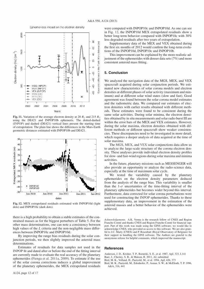
A&A 550, A124 (2013)
Fig. 11. Variation of the average electron density at 20 R⊙ and 215 R⊙using the DE421 and INPOP10b ephemeris. The dotted-dashed(INPOP) and dashed (DE421) vertical lines present the starting timeof extrapolation. The plain line shows the differences in the Mars-Earthgeometric distances estimated with INPOP10b and DE421.
Fig. 12. MEX extrapolated residuals estimated with INPOP10d (lightdots) and INPOP10c (dark dots).
there is a high probability to obtain a stable estimates of the con-strained masses as for the biggest perturbers of Table 5. For theother mass determinations, one can note a consistency betweenhigh values of the L criteria and the non-negligible mass differ-ences between INPOP10c and INPOP10d.
By improving the range bias residuals during the solar con-junction periods, we then slightly improved the asteroid massdeterminations.
Estimates of residuals for data samples not used in theINPOP fit and dated after or before the end of the fitting intervalare currently made to evaluate the real accuracy of the planetaryephemerides (Fienga et al. 2011a, 2009). To estimate if the useof the solar corona corrections induces a global improvementof the planetary ephemerides, the MEX extrapolated residuals
were computed with INPOP10c and INPOP10d. As one can seein Fig. 12, the INPOP10d MEX extrapolated residuals show abetter long-term behavior compared with INPOP10c with 30%less degraded residuals after two years of extrapolation.
Supplementary data of the MEX and VEX obtained duringthe first six months of 2012 would confirm the long-term evolu-tions of the INPOP10d, INPOP10c and INPOP10b.
This improvement can be explained by the more realistic ad-justment of the ephemerides with denser data sets (7%) and moreconsistent asteroid mass fitting.
5. Conclusion
We analyzed the navigation data of the MGS, MEX, and VEXspacecraft acquired during solar conjunction periods. We esti-mated new characteristics of solar corona models and electrondensities at different phases of solar activity (maximum and min-imum) and at different solar wind states (slow and fast). Goodagreement was found between the solar corona model estimatesand the radiometric data. We compared our estimates of elec-tron densities with earlier results obtained with different meth-ods. These estimates were found to be consistent during thesame solar activities. During solar minima, the electron densi-ties obtained by in situ measurements and solar radio burst III arewithin the error bars of the MEX and VEX estimates. However,during the solar maxima, electron densities obtained with dif-ferent methods or different spacecraft show weaker consisten-cies. These discrepancies need to be investigated in more detail,which requires a deeper analysis of data acquired at the time ofsolar maxima.
The MGS, MEX, and VEX solar conjunctions data allow usto analyze the large-scale structure of the corona electron den-sity. These analyses provide individual electron density profilesfor slow- and fast-wind regions during solar maxima and minimaactivities.
In the future, planetary missions such as MESSENGER willalso provide an opportunity to analyze the radio-science data,especially at the time of maximum solar cycle.
We tested the variability caused by the planetaryephemerides on the electron density parameters deducedfrom the analysis of the range bias. This variability is smallerthan the 1-σ uncertainties of the time-fitting interval of theplanetary ephemerides but becomes wider beyond this interval.Furthermore, data corrected for solar corona perturbations wereused for constructing the INPOP ephemerides. Thanks to thesesupplementary data, an improvement in the estimation of theasteroid masses and a better behavior of the ephemerides wereachieved.
Acknowledgements. A.K. Verma is the research fellow of CNES and RegionFranche-Comté and thanks CNES and Region Franche-Comté for financial sup-port. Part of this work was made using the GINS software; we would like toacknowledge CNES, who provided us access to this software. We are also grate-ful to J.C. Marty (CNES) and P. Rosenbatt (Royal Observatory of Belgium) fortheir support in handling the GINS software. The Authors are grateful to theanonymous referee for helpful comments, which improved the manuscript.
References
Anderson, J. D., Krisher, T. P., Borutzki, S. E., et al. 1987, ApJ, 323, L141Baer, J., Chesley, S. R., & Matson, R. 2011, AJ, submittedBird, M. K., Volland, H., Paetzold, M., et al. 1994, ApJ, 426, 373Bird, M. K., Paetzold, M., Edenhofer, P., Asmar, S. W., & McElrath, T. P. 1996,
A&A, 316, 441
A124, page 12 of 17
A. K. Verma et al.: Electron density distribution from MGS, MEX, and VEX
Bougeret, J.-L., King, J. H., & Schwenn, R. 1984, Sol. Phys., 90, 401Cranmer, S. R. 2002, Space Sci. Rev., 101, 229Fienga, A., Laskar, J., Morley, T., et al. 2009, A&A, 507, 1675Fienga, A., Laskar, J., Manche, H., et al. 2011a, Celestial Mechanics and
Dynamical AstronomyFienga, A., Kuchynka, P., Laskar, J., et al. 2011b, in EPSC-DPS Join Meeting
2011, 1879Folkner, W. M., Williams, J. G., & Boggs, D. H. 2008, IOM 343R-08-003Guhathakurta, M., & Holzer, T. E. 1994, ApJ, 426, 782Guhathakurta, M., Holzer, T. E., & MacQueen, R. M. 1996, ApJ, 458, 817Guhathakurta, M., Fludra, A., Gibson, S. E., Biesecker, D., & Fisher, R. 1999,
J. Geophys. Res., 104, 9801Issautier, K., Meyer-Vernet, N., Moncuquet, M., & Hoang, S. 1997, Sol. Phys.,
172, 335Issautier, K., Meyer-Vernet, N., Moncuquet, M., & Hoang, S. 1998,
J. Geophys. Res., 103, 1969Kuchynka, P., Laskar, J., Fienga, A., & Manche, H. 2010, A&A, 514, A96Leblanc, Y., Dulk, G. A., & Bougeret, J.-L. 1998, Sol. Phys., 183, 165Mancuso, S., & Spangler, S. R. 2000, ApJ, 539, 480Marchis, F., Descamps, P., Baek, M., et al. 2008, Icarus, 196, 97
Marty, J. C., Balmino, G., Duron, J., et al. 2009, Planet. Space Sci., 57,350
Moyer, T. D. 2003, Formulation for Observed and Computed Values of DeepSpace Network Data Types for Navigation (John Wiley & Sons), 2
Muhleman, D. O., & Anderson, J. D. 1981, ApJ, 247, 1093Muhleman, D. O., Esposito, P. B., & Anderson, J. D. 1977, ApJ, 211, 943Schwenn, R. 2006, Space Sci. Rev., 124, 51Schwenn, R., & Marsch, E. 1990, Physics of the Inner Heliosphere, I Large-Scale
Phenomena (Springer), Phys. Chem. Space, 20Schwenn, R., & Marsch, E. 1991, Physics of the Inner Heliosphere, II Particles,
Waves and Turbulence (Springer), Phys. Chem. Space, 21Standish, E. M. 1998, IOM 312F-98-483Tokumaru, M., Kojima, M., & Fujiki, K. 2010, J. Geophys. Res. (Space Physics),
115, 4102Woo, R., & Habbal, S. R. 1999, Geophys. Res. Lett., 26, 1793You, X. P., Hobbs, G. B., Coles, W. A., Manchester, R. N., & Han, J. L. 2007,
ApJ, 671, 907You, X. P., Coles, W. A., Hobbs, G. B., & Manchester, R. N. 2012, MNRAS,
422, 1160Zielenbach, W. 2011, ApJ, 142, 120
Pages 14 to 17 are available in the electronic edition of the journal at http://www.aanda.org
A124, page 13 of 17
A&A 550, A124 (2013)
Table 5. Masses of the 59 asteroids that induce perturbations greater than 5 m on the Earth-Mars distances during the period of observations(Kuchynka et al. 2010).
IAU designation INPOP10c INPOP10d Diff S Impact L
number 1012 × M⊙ 1012 × M⊙ 1012 × M⊙ m %
4 130.109 ± 0.716 130.109 ± 0.983 0.000 1198.953 20.5 S1 467.267 ± 2.047 467.267 ± 2.437 0.000 793.741 17.3 S2 103.843 ± 1.689 102.654 ± 1.933 1.189 146.270 11.8 S324 5.723 ± 0.531 5.723 ± 0.611 0.000 93.536 1.0 S10 43.513 ± 3.300 43.513 ± 3.877 0.000 77.003 15.9 S19 3.884 ± 0.447 3.450 ± 0.526 0.435 59.069 13.8 N3 11.793 ± 0.714 11.793 ± 0.803 0.000 55.639 0.6 S704 19.217 ± 2.315 19.217 ± 2.869 0.000 34.492 7.4 S532 2.895 ± 1.043 2.895 ± 1.093 0.000 32.714 2.3 S9 3.864 ± 0.613 3.063 ± 0.665 0.801 29.606 20.6 N7 5.671 ± 0.512 5.367 ± 0.591 0.305 27.822 13.9 S29 7.629 ± 1.067 7.227 ± 1.225 0.402 26.673 2.9 S24 7.641 ± 1.596 2.194 ± 1.775 5.447 * 26.131 36.0 N31 3.256 ± 2.034 4.411 ± 2.050 1.155 23.466 24.1 S15 13.576 ± 0.939 13.576 ± 1.264 0.000 21.555 20.6 S6 7.084 ± 0.822 7.084 ± 1.048 0.000 21.150 7.4 S11 3.771 ± 0.976 3.771 ± 1.110 0.000 17.301 31.9 S139 0.000 ± 0.000 3.579 ± 0.595 3.579 N 16.687 32.0 N747 4.129 ± 0.841 6.805 ± 1.089 2.676 * 15.937 31.6 N105 3.111 ± 0.556 3.111 ± 0.745 0.000 15.196 4.5 N20 0.000 ± 0.000 1.921 ± 0.661 1.921 N 14.763 39.9 N372 12.365 ± 2.676 12.365 ± 2.990 0.000 13.796 19.0 S8 3.165 ± 0.353 3.325 ± 0.365 0.159 12.664 17.7 S45 3.523 ± 0.819 1.518 ± 0.962 2.005 * 11.790 21.0 N41 3.836 ± 0.721 2.773 ± 0.977 1.063 11.568 15.2 N405 0.005 ± 0.003 0.006 ± 0.003 0.001 11.378 21.2 N511 9.125 ± 2.796 9.125 ± 3.138 0.000 10.248 20.5 S52 8.990 ± 2.781 8.990 ± 3.231 0.000 9.841 3.0 S16 12.613 ± 2.286 12.613 ± 2.746 0.000 9.701 8.9 S419 1.185 ± 0.461 0.425 ± 0.398 0.760 9.585 10.2 N78 0.026 ± 0.016 0.024 ± 0.016 0.002 9.389 9.8 N259 0.092 ± 0.002 0.006 ± 0.003 0.086 9.222 31.4 N27 0.000 ± 0.000 1.511 ± 0.982 1.511 N 9.146 29.5 N23 0.000 ± 0.000 0.093 ± 0.156 0.093 N 9.067 31.1 N488 3.338 ± 1.850 0.000 ± 0.000 3.338 0 8.614 2.8 N230 0.000 ± 0.000 0.263 ± 0.169 0.263 N 7.620 27.0 N409 0.002 ± 0.001 0.002 ± 0.001 0.000 0 7.574 2.2 N94 1.572 ± 1.097 7.631 ± 2.488 6.058 * 7.466 28.5 N344 2.701 ± 0.497 2.088 ± 0.515 0.613 7.465 15.3 N130 0.099 ± 0.047 0.221 ± 0.069 0.122 * 7.054 31.7 N111 1.002 ± 0.323 0.000 ± 0.000 1.002 0 6.985 11.4 N109 0.495 ± 0.322 1.318 ± 0.852 0.823 6.865 18.7 N42 1.144 ± 0.362 0.083 ± 0.389 1.061 * 6.829 0.6 N63 0.000 ± 0.000 0.424 ± 0.143 0.424 N 6.451 17.4 N12 2.297 ± 0.319 1.505 ± 0.331 0.792 * 6.159 21.7 N469 0.088 ± 0.073 0.000 ± 0.000 0.088 0 6.107 18.1 N144 0.176 ± 0.297 0.751 ± 0.361 0.575 6.087 22.8 N
Notes. Columns 2 and 3 give the values of the masses with the 1-σ uncertainties obtained with INPOP10c and INPOP10d. The differences betweenINPOP10c and INPOP10d values are given in Col. 4. Column 5 indicates if the INPOP10d masses are newly determined (quoted N), set equal to 0when estimated by INPOP10c (quoted 0), significantly different from INPOP10c determinations (*). The maximum impacts of the perturbationsare given in Col. 5. In Col. 7 is given the L criteria, the rate of local maxima rejected from the INPOP10c fit but included in the INPOP10d. In thelast column we provide the status of the imposed constraints: S for strong and N for normal.
A124, page 14 of 17
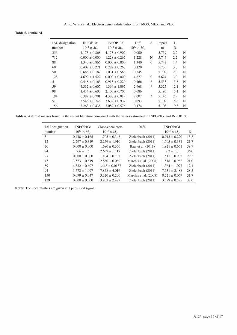
A. K. Verma et al.: Electron density distribution from MGS, MEX, and VEX
Table 5. continued.
IAU designation INPOP10c INPOP10d Diff S Impact Lnumber 1012 × M⊙ 1012 × M⊙ 1012 × M⊙ m %
356 4.173 ± 0.868 4.173 ± 0.902 0.000 5.759 2.2 N712 0.000 ± 0.000 1.228 ± 0.267 1.228 N 5.745 2.2 N88 1.340 ± 0.866 0.000 ± 0.000 1.340 0 5.742 1.4 N60 0.402 ± 0.221 0.282 ± 0.268 0.120 5.733 3.8 N50 0.686 ± 0.187 1.031 ± 0.566 0.345 5.702 2.0 N128 4.699 ± 1.522 0.000 ± 0.000 4.677 0 5.624 3.0 N5 0.448 ± 0.165 0.913 ± 0.220 0.466 * 5.533 15.8 N59 4.332 ± 0.607 1.364 ± 1.097 2.968 * 5.325 12.1 N98 1.414 ± 0.603 2.100 ± 0.705 0.686 5.195 15.1 N194 6.387 ± 0.701 4.380 ± 0.819 2.007 * 5.145 2.9 N51 3.546 ± 0.748 3.639 ± 0.937 0.093 5.109 15.6 N156 3.263 ± 0.438 3.089 ± 0.576 0.174 5.103 19.3 N
Table 6. Asteroid masses found in the recent literature compared with the values estimated in INPOP10c and INPOP10d.
IAU designation INPOP10c Close-encounters Refs. INPOP10dnumber 1012 × M⊙ 1012 × M⊙ 1012 × M⊙ %
5 0.448 ± 0.165 1.705 ± 0.348 Zielenbach (2011) 0.913 ± 0.220 15.812 2.297 ± 0.319 2.256 ± 1.910 Zielenbach (2011) 1.505 ± 0.331 21.720 0.000 ± 0.000 1.680 ± 0.350 Baer et al. (2011) 1.921 ± 0.661 39.924 7.6 ± 1.6 2.639 ± 1.117 Zielenbach (2011) 2.2 ± 1.7 36.027 0.000 ± 0.000 1.104 ± 0.732 Zielenbach (2011) 1.511 ± 0.982 29.545 3.523 ± 0.819 2.860 ± 0.060 Marchis et al. (2008) 1.518 ± 0.962 21.059 4.332 ± 0.607 1.448 ± 0.0187 Zielenbach (2011) 1.364 ± 1.097 12.194 1.572 ± 1.097 7.878 ± 4.016 Zielenbach (2011) 7.631 ± 2.488 28.5130 0.099 ± 0.047 3.320 ± 0.200 Marchis et al. (2008) 0.221 ± 0.069 31.7139 0.000 ± 0.000 3.953 ± 2.429 Zielenbach (2011) 3.579 ± 0.595 32.0
Notes. The uncertainties are given at 1 published sigma.
A124, page 15 of 17

A&A 550, A124 (2013)
Appendix A: Analytical solution
This section presents the analytical solutions of Eq. (1). Let, I1and I2 be the integral solutions of Eq. (1) using Eqs. (3) and (4)i.e.,
I1 =
∫ Ls/c
LEarths/n
B
(
l
R⊙
)−ǫ
dL (A.1)
and
I2 =
∫ Ls/c
LEarths/n
[
A
(
l
R⊙
)−4
+ B
(
l
R⊙
)−2]
dL. (A.2)
From the geometry (Fig. 3) we define
P = RS/E sinα,
LDC = RE/SC − RS/E cos α,
L2DE = l2 − P2,
l2 = L2 + R2S/E − 2 L RS/E cos α,
where α and β are the angle between the Sun-Earth-Probe (SEP)and the Earth-Sun-Probe (ESP). P is the MDLOS from the Sun.With these expressions, I1 can be written as
I1 =
∫ Ls/c
LEarths/n
B Rǫ⊙
( dL
(L2 + R2S/E − 2 L RS/E cos α)ǫ/2
)
= B Rǫ⊙
∫ Ls/c
LEarths/n
( dL
([L − RS/E cos α]2 + R2S/E sin2 α)ǫ/2
)
·
Assuming,
x = L − RS/E cos α,
a = RS/E sin α,
dx = dL,
with L = 0 at the Earth station (LEarths/n ) and L = RE/SC at thespacecraft (Ls/c). Then the integral I1 can be written as
I1 = B Rǫ⊙
∫ RE/SC−RS/E cos α
−RS/E cos α
dx
(x2 + a2)ǫ/2
=B Rǫ⊙
aǫ
∫ RE/SC−RS/E cos α
−RS/E cos α
dx
(1 + x2
a2 )ǫ/2·
Now letx
a= tan θ,
and
dx = a sec2 θ dθ.
Therefore,
I1 =B Rǫ⊙
aǫ
∫ arctan(
(RE/SC−RS/E cos α)
a
)
arctan(
(−RS/E cos α)
a
)
a sec2 θ
(tan2 θ + 1)ǫ/2dθ. (A.3)
From the geometry of Fig. 3, the lower limit of Eq. (A.3) can bewritten as
arctan(
−RS/E cos α
a
)
= arctan(
−RS/E cos α
RS/E sin α
)
,
with
cot α = tan(
π
2− α
)
·
Hence,
arctan(
−RS/E cos α
a
)
= α −π
2·
Similarly, the upper limit of Eq. (A.3) can be written as
arctan(
RE/SC − RS/E cos α
a
)
= arctan(
RE/SC − RS/E cos α
RS/E sin α
)
,
with
RE/SC − RS/E cos α = RS/E sin α[
tan(
β −
π
2− α
) ]
.
Hence,
arctan(
RE/SC − RS/E cos α
a
)
= β + α −π
2·
Now Eq. (A.3) is given by
I1 =B Rǫ⊙
aǫ
∫ β+α− π2
α− π2
a sec2 θ
(tan2 θ + 1)ǫ/2dθ.
with
sec2 θ = tan2 θ + 1,
and
cos θ =1
sec θ·
Therefore, the integral I1 can be written as
I1 =B Rǫ⊙
aǫ−1
∫ β+α− π2
α− π2
(cos θ)ǫ−2 dθ. (A.4)
The maximum contribution of the integral occurs at θ = 0. Tosolve this integral, Taylor series expansion was used and for θnear zero, it can be given as
f (θ) = f (0) + θ(d f
dθ
)
+θ2
2!
(d2 f
dθ2
)
+θ3
3!
(
d3 f
dθ3
)
+θ4
4!
(d4 f
dθ4
)
. . . + θ(θn), (A.5)
with
f (θ) = (cos θ)ǫ−2.
Then
f (0) = 1(d f
dθ
)
= −(ǫ − 2) (sin θ) (cos θ)(ǫ−3),
(d f
dθ
)
θ=0= 0,
(d2 f
dθ2
)
= (ǫ − 2) (ǫ − 3) (sin2 θ) (cos θ)(ǫ−4)
−(ǫ − 2) (cos θ)(ǫ−2),
A124, page 16 of 17

A. K. Verma et al.: Electron density distribution from MGS, MEX, and VEX
(d2 f
dθ2
)
θ=0= −(ǫ − 2),
(d3 f
dθ3
)
= −(ǫ − 2) (ǫ − 3) (ǫ − 4) (sin3 θ) (cos θ)(ǫ−5)
+(ǫ − 2) (3ǫ − 8) (sin θ) (cos θ)(ǫ−3),
(d3 f
dθ3
)
θ=0= 0,
(d4 f
dθ4
)
= (ǫ − 2) (ǫ − 3) (ǫ − 4) (ǫ − 5) (sin4 θ) (cos θ)(ǫ−6)
−(ǫ − 2) (ǫ − 3) (6ǫ − 20) (sin2 θ) (cos θ)(ǫ−4)
+(ǫ − 2) (3ǫ − 8) (cos θ)(ǫ−2),
(d4 f
dθ4
)
θ=0= (ǫ − 2) (3ǫ − 8).
Now, Eq. (A.5) can be written as
(cos θ)(ǫ−2) = 1 − (ǫ − 2)θ2
2!+ (ǫ − 2) (3ǫ − 8)
θ4
4!+ . . . θ (θn)
= 1 −ǫ − 2
2θ2 +
3ǫ2 − 14ǫ + 1624
θ4 + . . . θ (θn).
By neglecting the higher order terms, the integral (Eq. (A.4)) canbe written as
I1 =B Rǫ⊙
aǫ−1
∫ β+α− π2
α− π2
(
1 −ǫ − 2
2θ2 +
3ǫ2 − 14ǫ + 1624
θ4)
dθ
=B Rǫ⊙
aǫ−1
[
θ −ǫ − 2
6θ3 +
3ǫ2 − 14ǫ + 16120
θ5]β+α− π2
α− π2
=B Rǫ⊙
aǫ−1
[
β −ǫ − 2
6
(
(β + α − π/2)3 − (α − π/2)3)
+3ǫ2 − 14ǫ + 16
120
(
(β + α − π/2)5 − (α − π/2)5)
]
·
By substituting the value of a, we can write the integral I1 as
I1 =B Rǫ⊙
(RS/E sinα)ǫ−1
[
β −ǫ − 2
6
(
(β + α − π/2)3 − (α − π/2)3)
+3ǫ2 − 14ǫ + 16
120
(
(β + α − π/2)5 − (α − π/2)5)
]
. (A.6)
Now, Eq. (A.2) can be written as I2 = I2a + I2b where,
I2a =
∫ Ls/c
LEarths/n
A
(
l
R⊙
)−4
dL, (A.7)
and
I2b =
∫ Ls/c
LEarths/n
B
(
l
R⊙
)−2
dL. (A.8)
Using a similar approach to the previous integral, one canwrite
I2a =A R4
⊙
a3
∫ β+α− π2
α− π2
cos2 θ dθ
=A R4
⊙
a3
[
14
(2 θ + sin 2θ)
]β+α− π2
α− π2
=A R4
⊙
4 a3
[
(2 β − sin 2(α + β) + sin 2α)]
=A R4
⊙
4 R3S/E sin3 α
[
(2 β − sin 2(α + β) + sin 2α)]
·
Similarly, Eq. (A.8) can be written as
I2b =B R2
⊙
a
∫ β+α− π2
α− π2
dθ
=B R2
⊙
a
[
θ
]β+α− π2
α− π2
=B R2
⊙
RS/E sin αβ.
Now by using I2a and I2b, expression I2 can be written as
I2 =A R4
⊙
4 R3S/E sin3 α
[
(2 β − sin 2(α + β) + sin 2α)]
+B R2
⊙
RS/E sin αβ. (A.9)
A124, page 17 of 17

116 4. Solar corona correction of radio signals and its application to planetary ephemeris
117
Chapter 5
Improvement of the planetary ephemeris
and test of general relativity with
MESSENGER
5.1 Introduction
Mercury is the smallest and least explored terrestrial planet of the solar system. Mariner 10was the first spacecraft which made three close encounters (two in 1974 and one in 1975) tothis planet and provided most of our current knowledge of the planet until early 2008 (Smithet al., 2010). In addition to Mariner 10 flyby observations, ground based radar measurementswere the only observations which were used to study the gravity field of Mercury and its phys-ical structure (spherical body with slightly flattened at the poles and mildly elongated equator)(Anderson et al., 1987a, 1996). In 2004, NASA launched a dedicate mission, MESSENGER, tolearn more about this planet. MESSENGER made three close encounters (two in 2008 and onein 2009) to Mercury and became the first spacecraft which observed Mercury from its orbit.
Till now, MESSENGER has completed more than two years on orbit at Mercury. Duringthe orbital period, radio tracking of MESSENGER routinely measured the Doppler and rangeobservables at DSN stations. These observables are important to estimate the spacecraft statevectors (position and velocity) and to improve the knowledge of Mercury’s gravity field andits geophysical properties (Srinivasan et al., 2007). Using the first six months of radiosciencedata during the orbital period, Smith et al. (2012) computed the gravity field and gave betterconstraints on the internal structure (density distribution) of Mercury. This updated gravityfield becomes crucial for the present computation of MESSENGER orbit and to perform preciserelativistic tests.
The primary objectives of this work is to determine the precise orbit of the MESSENGERspacecraft around Mercury using radioscience data and then improve the planetary ephemeris
1185. Improvement of the planetary ephemeris and test of general relativity with
MESSENGER
INPOP (see Chapter 1). The updated spacecraft and planetary ephemerides are then used toperform sensitive relativistic tests of the PPN parameters (γ and β).
As described in Chapter 1, spacecraft range measurements are used for the construction ofplanetary ephemerides. These measurements approximately cover 56% of whole INPOP dataand impose strong constraints on the planet orbits and on the other solar system parametersincluding asteroid masses. However, until now, only five flybys (two from Mariner 10 and threefrom MESSENGER) range measurements were available for imposing strong constraints to theMercury’s orbit (Fienga et al., 2011a). Therefore, range measurements obtained by MESSEN-GER spacecraft during its mapping period are important to improve our knowledge of the orbitof Mercury.
Moreover, high precision radioscience observations also gave an opportunity to performsensitive relativistic tests by estimating possible violation of GR of the two relativistic parame-ters (γ and β) of the PPN formalism of general relativity (Will, 1993). The previous estimationsof these parameters, using different techniques and different data set, can be found in Bertottiet al. (2003); Müller et al. (2008); Pitjeva (2009); Williams et al. (2009); Manche et al. (2010);Konopliv et al. (2011); Fienga et al. (2011a). However, because of Mercury relatively largeeccentricity and close proximity to the Sun, its orbital motion provides one of the best solar sys-tem tests of general relativity (Anderson et al., 1997). In addition, Fienga et al. (2010, 2011a)also demonstrated that, Mercury observations are far more sensitive to PPN modification of GRthan other data used in the planetary ephemerides construction. We therefore, also performedsuch tests with the latest MESSENGER observations to obtain one of the best value for PPNparameters.
In this chapter, we introduce the updated planetary ephemeris INPOP13a and summarizethe technique used for the estimation of the PPN parameters. The outline of the chapter is asfollow: The section 5.2 gives an overview of the MESSENGER mission. The radioscience dataanalysis and the dynamical modeling of MESSENGER are also discussed in the same section.In section 5.3, we present the results obtained during the orbit determination. The evolution ofINPOP with the accuracy of MESSENGER orbit, and the brief description of tests performedwith the INPOP13a are also discussed in this section.
The results presented in this chapter are gathered in an article submitted for publication inAstronomy & Astrophysics. The Section 5.4 is therefore stated as Verma et al. (2013b). Thissection deals with the detailed analysis of the tests performed with the high precision Mercuryephemeris INPOP13a.

5.2. MESSENGER data analysis 119
Figure 5.1: Summary of MESSENGER’s entire trajectory from launch to mapping period(McAdams et al., 2007).
5.2 MESSENGER data analysis
5.2.1 Mission design
Under the NASA’s Discovery program, the MErcury Surface, Space ENvironment, GEochem-istry, and Ranging (MESSENGER) spacecraft is the first probe to orbit the planet Mercury.It launched in August 3, 2004, from Pad B of Space Launch Complex 17 at Cape CanaveralAir Force Station, Florida, aboard a three-stage Boeing Delta II rocket. On March 18, 2011,MESSENGER successfully entered Mercury’s orbit after completing three flybys of Mercuryfollowing two flybys of Venus and one of Earth.
The 6.6-year trip from launch to Mercury orbit insertion is one of the longest interplanetarycruise phase options considered for MESSENGER. The spacecraft system design lifetime ac-counted for a seven-year journey to Mercury followed by a prime (one-year) and extended (one-or more-year) Mercury orbit phases. MESSENGER used gravity assists from Earth, Venus andMercury to lower its speed relative to Mercury at orbit insertion. Several trajectory-correctionmaneuvers (TCMs), including five large deep-space maneuvers (DSMs) were also used to ad-just its path to Mercury (McAdams et al., 2007). As a summary of the entire trajectory fromlaunch to mapping period is shown in Fig. 5.1.

1205. Improvement of the planetary ephemeris and test of general relativity with
MESSENGER
Figure 5.2: MESSENGER spacecraft geometry (Vaughan et al., 2006).
As shown in this figure, approximately one year after launch, MESSENGER made its firstflyby of Earth on August 2, 2005 and then headed toward the Venus flybys using largest DSM.The MESSENGER made two Venus flybys, first occurred on October 24, 2006 and second onJune 5, 2007. These flybys headed MESSENGER towards Mercury by additionally using theDSM performed after second flyby of Venus. In January 14, 2008 MESSENGER became firstspacecraft which provided first close-up look of Mercury in more than 30 years. The Mercuryflyby 1-to-Mercury orbit insertion transfer trajectory, shown in Fig. 5.1, includes three Mercuryflyby-DSM segments that lower the spacecraft speed relative to Mercury and on March 18,2011, MESSENGER successfully entered Mercury’s orbit.
The MESSENGER spacecraft was initially inserted into a ∼12-hour, near-polar orbit aroundMercury, with an initial periapsis altitude of 200 km, initial periapsis longitude of 60°N, andapoapsis at ∼15,200 km altitude in the southern hemisphere. After successful first year flight inthe orbit, mission was extended to one or more year which began on 18 March 2012. Duringfirst extended mission, two orbit-correction maneuvers were executed, four days apart, in April2012 to reduce MESSENGER’s orbital period from ∼12 to ∼8 hours (Flanigan et al., 2013)
5.2.2 Spacecraft geometry
The MESSENGER spacecraft was designed and constructed to withstand the harsh environ-ments associated with achieving and operating in Mercury orbit. The spacecraft structure isconstructed primarily of lightweight composite material housing a complex dual-mode propul-sion system. Figure 5.2 shows the complex geometry of the MESSENGER spacecraft, where,panel (a) shows the spacecraft components, and panel (b) represents the coordinate system. Ta-ble 5.1 gives the approximated characteristics of the spacecraft components, extracted from theVaughan et al. (2002).
5.2. MESSENGER data analysis 121
The whole system of the MESSENGER spacecraft can be divided into eight subsystems.The briefly introduction of these subsystems is given below and detailed information can befound in Leary et al. (2007):
• Structures and mechanisms: the primary spacecraft structures are the core, the adapterring, the sunshade, the solar panels, and the magnetometer boom. The core of the space-craft tightly integrates support panels with the propulsion system. Three mechanical as-semblies were deployed during operation, the two solar panels and the 3.6-m magne-tometer boom. The solar array hinges are located at each end of the arms connectingthe panels to the core structure. Whereas, the magnetometer boom is separated into twosegments with one hinge between the spacecraft structure and the first segment and theother between the two segments.
• Propulsion: the MESSENGER propulsion system is a pressurized bipropellant dual-mode system. As shown in Figure 5.2, they are three main propellant tanks, a refillableauxiliary fuel tank, and a helium pressurant tank provide propellant and pressurant stor-age. MESSENGER carries seventeen thrusters. Three thruster types, arranged in five dif-ferent thruster module configurations, provide the required spacecraft forces and torques.
• Thermal: the thermal design of the MESSENGER spacecraft relies upon a ceramic-clothsunshade to protect the vehicle from the intense solar environment. Sunshade can expe-rienced maximum temperature of 350°C at Mercury but creates a benign thermal envi-ronment for the main spacecraft bus, allowing the use of essentially standard electronics,components, and thermal blanketing materials.
• Power: the power system is designed to support about 390 W of load power near Earthand 640 W during Mercury orbit. The power is primarily provided by two solar panelsthat are mounted on small booms extendable beyond the sunshade and rotating to trackthe Sun.
• Avionics: MESSENGER is equipped with redundant integrated electronics modules (IEM).The IEM implements command and data handling, guidance and control, and fault pro-tection functions. A primary driver of the IEM architecture was to simplify spacecraftfault protection.
• Software: it provides the main processor-supported code that performs commanding,data handling, and spacecraft control.
• Guidance and control: this subsystem maintains spacecraft attitude and executes propul-sive maneuvers for spacecraft trajectory control. It also controls the solar panel orienta-tion to maintain a Sun offset angle providing sufficient power at moderate panel temper-atures. It is also responsible for keeping the sunshade pointed towards the Sun to protectthe spacecraft bus from extreme heat and radiation.
• Radio frequency telecommunications: this subsystem consists of small deep spacetransponders, solid-state power amplifiers, phased-array antennas, and medium- and low-gain antennas. The goals of this subsystem is, to provide the highest quality and quantity
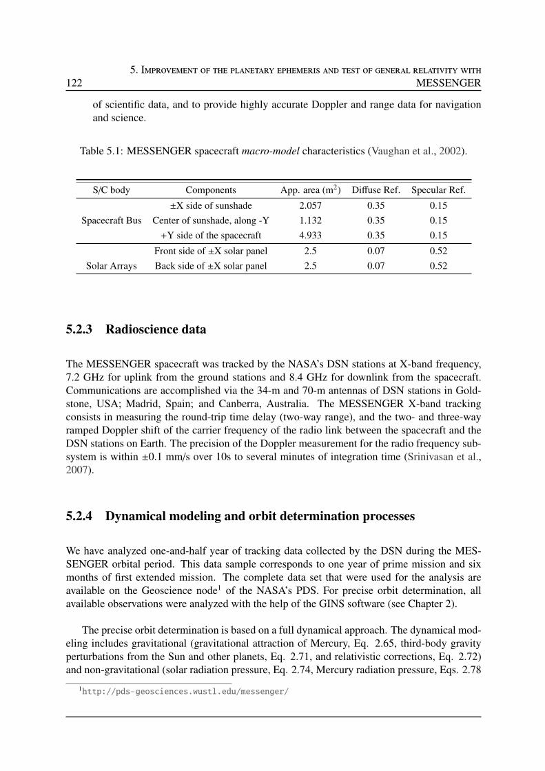
1225. Improvement of the planetary ephemeris and test of general relativity with
MESSENGER
of scientific data, and to provide highly accurate Doppler and range data for navigationand science.
Table 5.1: MESSENGER spacecraft macro-model characteristics (Vaughan et al., 2002).
S/C body Components App. area (m2) Diffuse Ref. Specular Ref.
±X side of sunshade 2.057 0.35 0.15
Spacecraft Bus Center of sunshade, along -Y 1.132 0.35 0.15
+Y side of the spacecraft 4.933 0.35 0.15
Front side of ±X solar panel 2.5 0.07 0.52
Solar Arrays Back side of ±X solar panel 2.5 0.07 0.52
5.2.3 Radioscience data
The MESSENGER spacecraft was tracked by the NASA’s DSN stations at X-band frequency,7.2 GHz for uplink from the ground stations and 8.4 GHz for downlink from the spacecraft.Communications are accomplished via the 34-m and 70-m antennas of DSN stations in Gold-stone, USA; Madrid, Spain; and Canberra, Australia. The MESSENGER X-band trackingconsists in measuring the round-trip time delay (two-way range), and the two- and three-wayramped Doppler shift of the carrier frequency of the radio link between the spacecraft and theDSN stations on Earth. The precision of the Doppler measurement for the radio frequency sub-system is within ±0.1 mm/s over 10s to several minutes of integration time (Srinivasan et al.,2007).
5.2.4 Dynamical modeling and orbit determination processes
We have analyzed one-and-half year of tracking data collected by the DSN during the MES-SENGER orbital period. This data sample corresponds to one year of prime mission and sixmonths of first extended mission. The complete data set that were used for the analysis areavailable on the Geoscience node1 of the NASA’s PDS. For precise orbit determination, allavailable observations were analyzed with the help of the GINS software (see Chapter 2).
The precise orbit determination is based on a full dynamical approach. The dynamical mod-eling includes gravitational (gravitational attraction of Mercury, Eq. 2.65, third-body gravityperturbations from the Sun and other planets, Eq. 2.71, and relativistic corrections, Eq. 2.72)and non-gravitational (solar radiation pressure, Eq. 2.74, Mercury radiation pressure, Eqs. 2.78
1http://pds-geosciences.wustl.edu/messenger/
5.2. MESSENGER data analysis 123
and 2.79) forces that are acting on the spacecraft. These forces have been taken into accountin the force budget of MESSENGER. Because of the thin atmosphere of Mercury, we haveassumed that MESSENGER experienced negligible resistance due to the atmosphere, henceatmospheric drag force was not included in the force budget. Moreover, MESSENGER firessmall thrusters (nominally on each Tuesday) to perform Momentum Dump Maneuver (MDM)2
for reducing the spacecraft angular momentum to a safe level. In addition to MDM, MESSEN-GER also performed Orbit Correction Maneuver (OCM)2 typically once every Mercury year(∼88 Earth days) to maintain minimum altitude below 500 kilometers. Due to insufficient in-formation of these maneuvers, we therefore did not include the epoch of each maneuver duringthe orbit computation. Hence, empirical delta accelerations, radial, along-track, and cross-track,at the epoch of maneuvers were not included in the force budget.
The measurement (Doppler and range) models (see Sec. 2.4.3) and the light time corrections(see Sec. 2.4.2), that are modeled in GINS, are described in chapter 2. During the computations,DSN station coordinates were corrected from the Earth’s polar motion, solid-Earth tides, andfrom the ocean loading, based on the formulation given in Moyer (2003). In addition to thesecorrections, radiometric data also have been corrected from tropospheric propagation throughthe meteorological data2 (pressure, temperature and humidity) of the stations.
The complex geometry of the MESSENGER spacecraft was treated as a combination of flatplates arranged in the shape of box, with attached solar arrays, so called Box-Wing macro-model.The approximated characteristics of this macro-model, which includes cross-section area andspecular and diffuse reflectivity coefficients of the components, extracted from Vaughan et al.(2002) and are given in Table 5.1. In addition to the macro-model characteristics, orientationsof the spacecraft were also taken in account. The attitude of the spacecraft, and of its articulatedpanels in an inertial frame are usually defined in terms of quaternions. The approximate valueof these quaternions were extracted from the SPICE NAIF software. The macro-model and itsorientation have allowed to calculate the non-gravitational accelerations that are acting on theMESSENGER spacecraft due to the radiation pressure from the Sun and Mercury (albedo andthermal infra-red emission).
For orbit computations and for parameters estimations, a multi-arc approach was used toget an independent estimate of the MESSENGER accelerations. In this method, we integratedthe equations of motion using the time-step of 50s and then, orbital fits were obtained fromshort data-arcs fitted over the observations span of one-day using an iterative process. The shortdata-arcs of one-day have been chosen to account for the model imperfections (see section 3.5of Chapter 3).
An iterative least-square fit was performed on the complete set of Doppler- and range-tracking data-arcs corresponding to the orbital phase of the mission. The summary of thesetracking data are given in Table 5.2. Several parameters have been estimated during the or-bit computation. They are similar to the one estimated for MGS spacecraft (see Sec. 3.3.2 ofChapter 3) except scale factor for atmospheric drag and empirical delta accelerations.
2http://pds-geosciences.wustl.edu/messenger/mess-v_h-rss-1-edr-rawdata-v1/messrs_
0xxx/ancillary/
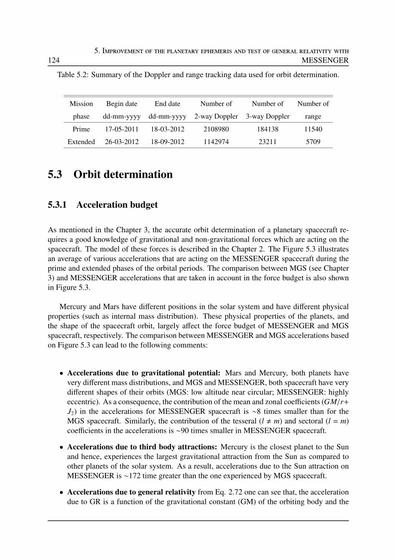
1245. Improvement of the planetary ephemeris and test of general relativity with
MESSENGER
Table 5.2: Summary of the Doppler and range tracking data used for orbit determination.
Mission Begin date End date Number of Number of Number of
phase dd-mm-yyyy dd-mm-yyyy 2-way Doppler 3-way Doppler range
Prime 17-05-2011 18-03-2012 2108980 184138 11540
Extended 26-03-2012 18-09-2012 1142974 23211 5709
5.3 Orbit determination
5.3.1 Acceleration budget
As mentioned in the Chapter 3, the accurate orbit determination of a planetary spacecraft re-quires a good knowledge of gravitational and non-gravitational forces which are acting on thespacecraft. The model of these forces is described in the Chapter 2. The Figure 5.3 illustratesan average of various accelerations that are acting on the MESSENGER spacecraft during theprime and extended phases of the orbital periods. The comparison between MGS (see Chapter3) and MESSENGER accelerations that are taken in account in the force budget is also shownin Figure 5.3.
Mercury and Mars have different positions in the solar system and have different physicalproperties (such as internal mass distribution). These physical properties of the planets, andthe shape of the spacecraft orbit, largely affect the force budget of MESSENGER and MGSspacecraft, respectively. The comparison between MESSENGER and MGS accelerations basedon Figure 5.3 can lead to the following comments:
• Accelerations due to gravitational potential: Mars and Mercury, both planets havevery different mass distributions, and MGS and MESSENGER, both spacecraft have verydifferent shapes of their orbits (MGS: low altitude near circular; MESSENGER: highlyeccentric). As a consequence, the contribution of the mean and zonal coefficients (GM/r+
J2) in the accelerations for MESSENGER spacecraft is ∼8 times smaller than for theMGS spacecraft. Similarly, the contribution of the tesseral (l , m) and sectoral (l = m)coefficients in the accelerations is ∼90 times smaller in MESSENGER spacecraft.
• Accelerations due to third body attractions: Mercury is the closest planet to the Sunand hence, experiences the largest gravitational attraction from the Sun as compared toother planets of the solar system. As a result, accelerations due to the Sun attraction onMESSENGER is ∼172 time greater than the one experienced by MGS spacecraft.
• Accelerations due to general relativity from Eq. 2.72 one can see that, the accelerationdue to GR is a function of the gravitational constant (GM) of the orbiting body and the
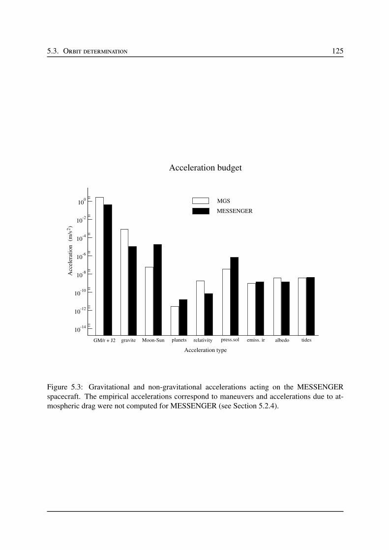
5.3. Orbit determination 125
Acceleration type
10-14
10-12
10-10
10-8
10-6
10-4
10-2
100
Acc
eler
atio
n
Acceleration budget
GM/r + J2 gravite Moon-Sun planets relativity press.sol albedoemiss. ir
(m/s
)
2
MGS
MESSENGER
tides
Figure 5.3: Gravitational and non-gravitational accelerations acting on the MESSENGERspacecraft. The empirical accelerations correspond to maneuvers and accelerations due to at-mospheric drag were not computed for MESSENGER (see Section 5.2.4).
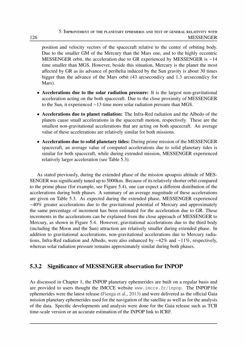
1265. Improvement of the planetary ephemeris and test of general relativity with
MESSENGER
position and velocity vectors of the spacecraft relative to the center of orbiting body.Due to the smaller GM of the Mercury than the Mars one, and to the highly eccentricMESSENGER orbit, the acceleration due to GR experienced by MESSENGER is ∼14time smaller than MGS. However, beside this situation, Mercury is the planet the mostaffected by GR as its advance of perihelia induced by the Sun gravity is about 30 timesbigger than the advance of the Mars orbit (43 arcsecond/cy and 1.3 arcsecond/cy forMars).
• Accelerations due to the solar radiation pressure: It is the largest non-gravitationalacceleration acting on the both spacecraft. Due to the close proximity of MESSENGERto the Sun, it experienced ∼13 time more solar radiation pressure than MGS.
• Accelerations due to planet radiation: The Infra-Red radiation and the Albedo of theplanets cause small accelerations in the spacecraft motion, respectively. These are thesmallest non-gravitational accelerations that are acting on both spacecraft. An averagevalue of these accelerations are relatively similar for both missions.
• Accelerations due to solid planetary tides: During prime mission of the MESSENGERspacecraft, an average value of computed accelerations due to solid planetary tides issimilar for both spacecraft, while during extended mission, MESSENGER experiencedrelatively larger acceleration (see Table 5.3).
As stated previously, during the extended phase of the mission apoapsis altitude of MES-SENGER was significantly tuned up to 5000km. Because of its relatively shorter orbit comparedto the prime phase (for example, see Figure 5.4), one can expect a different distribution of theaccelerations during both phases. A summary of an average magnitude of these accelerationsare given on Table 5.3. As expected during the extended phase, MESSENGER experienced∼40% greater accelerations due to the gravitational potential of Mercury and approximatelythe same percentage of increment has been estimated for the acceleration due to GR. Theseincrements in the accelerations can be explained from the close approach of MESSENGER toMercury, as shown in Figure 5.4. However, gravitational accelerations due to the third body(including the Moon and the Sun) attraction are relatively smaller during extended phase. Inaddition to gravitational accelerations, non-gravitational accelerations due to Mercury radia-tions, Infra-Red radiation and Albedo, were also enhanced by ∼42% and ∼11%, respectively,whereas solar radiation pressure remains approximately similar during both phases.
5.3.2 Significance of MESSENGER observation for INPOP
As discussed in Chapter 1, the INPOP planetary ephemerides are built on a regular basis andare provided to users thought the IMCCE website www.imcce.fr/inpop. The INPOP10eephemerides were the latest release (Fienga et al., 2013) and were delivered as the official Gaiamission planetary ephemerides used for the navigation of the satellite as well as for the analysisof the data. Specific developments and analysis were done for the Gaia release such as TCBtime-scale version or an accurate estimation of the INPOP link to ICRF.
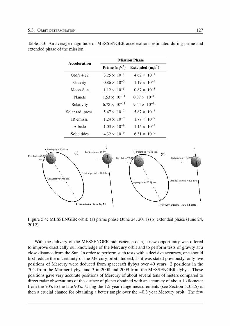
5.3. Orbit determination 127
Table 5.3: An average magnitude of MESSENGER accelerations estimated during prime andextended phase of the mission.
AccelerationMission Phase
Prime (m/s2) Extended (m/s2)
GM/r + J2 3.25 × 10⁻¹ 4.62 × 10⁻¹
Gravity 0.86 × 10⁻⁵ 1.19 × 10⁻⁵
Moon-Sun 1.12 × 10⁻⁵ 0.87 × 10⁻⁵
Planets 1.53 × 10⁻¹¹ 0.87 × 10⁻¹¹
Relativity 6.78 × 10⁻¹¹ 9.44 × 10⁻¹¹
Solar rad. press. 5.47 × 10⁻⁷ 5.87 × 10⁻⁷
IR emissi. 1.24 × 10⁻⁹ 1.77 × 10⁻⁹
Albedo 1.03 × 10⁻⁹ 1.15 × 10⁻⁹
Solid tides 4.32 × 10⁻⁹ 6.31 × 10⁻⁹
Figure 5.4: MESSENGER orbit: (a) prime phase (June 24, 2011) (b) extended phase (June 24,2012).
With the delivery of the MESSENGER radioscience data, a new opportunity was offeredto improve drastically our knowledge of the Mercury orbit and to perform tests of gravity at aclose distance from the Sun. In order to perform such tests with a decisive accuracy, one shouldfirst reduce the uncertainty of the Mercury orbit. Indeed, as it was stated previously, only fivepositions of Mercury were deduced from spacecraft flybys over 40 years: 2 positions in the70’s from the Mariner flybys and 3 in 2008 and 2009 from the MESSENGER flybys. Thesepositions gave very accurate positions of Mercury of about several tens of meters compared todirect radar observations of the surface of planet obtained with an accuracy of about 1 kilometerfrom the 70’s to the late 90’s. Using the 1.5 year range measurements (see Section 5.3.3.5) isthen a crucial chance for obtaining a better tangle over the ∼0.3 year Mercury orbit. The few
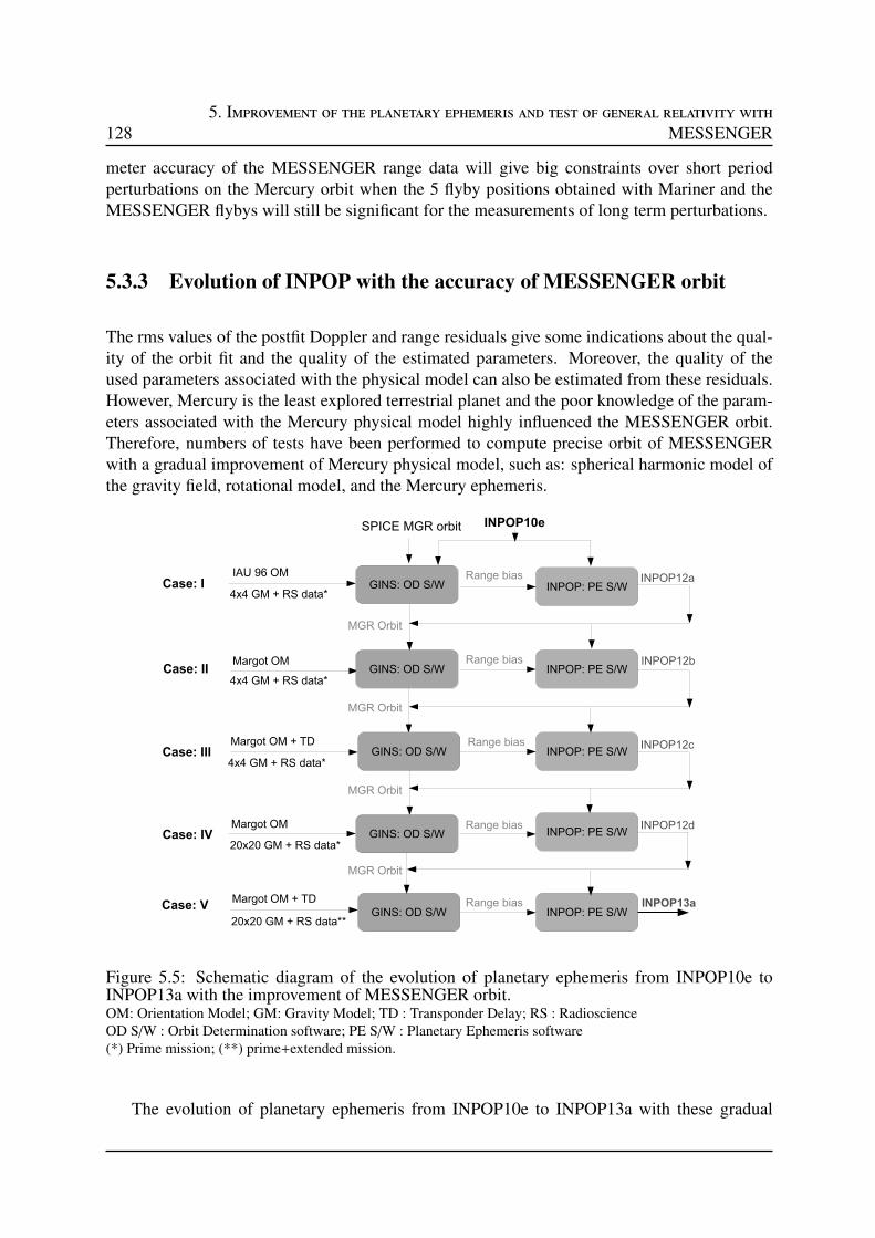
1285. Improvement of the planetary ephemeris and test of general relativity with
MESSENGER
meter accuracy of the MESSENGER range data will give big constraints over short periodperturbations on the Mercury orbit when the 5 flyby positions obtained with Mariner and theMESSENGER flybys will still be significant for the measurements of long term perturbations.
5.3.3 Evolution of INPOP with the accuracy of MESSENGER orbit
The rms values of the postfit Doppler and range residuals give some indications about the qual-ity of the orbit fit and the quality of the estimated parameters. Moreover, the quality of theused parameters associated with the physical model can also be estimated from these residuals.However, Mercury is the least explored terrestrial planet and the poor knowledge of the param-eters associated with the Mercury physical model highly influenced the MESSENGER orbit.Therefore, numbers of tests have been performed to compute precise orbit of MESSENGERwith a gradual improvement of Mercury physical model, such as: spherical harmonic model ofthe gravity field, rotational model, and the Mercury ephemeris.
! "#
$
%$
!
!
!
!
"#
"#&
"#
#'#'
#'#'
%$
$
$
$
$
Figure 5.5: Schematic diagram of the evolution of planetary ephemeris from INPOP10e toINPOP13a with the improvement of MESSENGER orbit.OM: Orientation Model; GM: Gravity Model; TD : Transponder Delay; RS : RadioscienceOD S/W : Orbit Determination software; PE S/W : Planetary Ephemeris software(*) Prime mission; (**) prime+extended mission.
The evolution of planetary ephemeris from INPOP10e to INPOP13a with these gradual
5.3. Orbit determination 129
improvements is shown in Figure 5.5. From this figure one can see that, improved inputs havebeen implemented to GINS software in the subsequent tests. Using these inputs and the onedescribed in Sections 5.2.4, GINS constructs the MESSENGER orbit precisely. The estimatedrange bias from GINS are then used to built the new planetary ephemeris. The constants anddynamical modeling used for the construction of the new ephemerides are similar to INPOP10e(see Chapter 1). A global adjustment of the planet initial conditions including Pluto, the massof the Sun, the oblateness of the Sun, the ratio between the mass of the Moon and 140 asteroidmasses. The improved ephemeris and the MESSENGER orbit are then used as a input forsubsequent tests to reconstruct the MESSENGER orbit and planetary ephemeris. The detailedanalysis of these tests are given in the following sections:
5.3.3.1 Case I: First guess orbit for Messenger and INPOP12a
5.3.3.1.1 Description
Before the MESSENGER mission, Mariner 10 flybys observations and ground based radarmeasurements were the only observations which were used to study the gravity field of Mer-cury and its physical structure (spherical body with slightly flattened at the poles and mildlyelongated equator) (Anderson et al., 1987a, 1996). Later, using the altimetric and radio trackingobservations from MESSENGER first two flybys of Mercury Smith et al. (2010) derived thespherical harmonic model of Mercury gravity field HgM001 developed up to degree and order4. In this test, we have analyzed radioscience data of the MESSENGER spacecraft acquiredat the time of prime phase of the mission (see Table 5.2) using HgM001 gravity model. TheMESSENGER orbital fits were obtained from one-day data-arcs using an iterative process (seeSection 5.2.4 for more details). To initialize the iteration, initial position and velocity vectorsof MESSENGER were taken from the SPICE NAIF kernels3. The positions and velocities ofthe planets were accessed through the latest INPOP10e planetary ephemeris. Moreover, theorientation of Mercury was defined as recommended by the IAU4 (see Table 5.4).
Table 5.4: Recommended values for the direction of the north pole of rotation and the primemeridian of the Mercury, 1996 (Davies et al., 1996).
Parameter value
α0 = 281.01 - 0.033T
δ0 = 61.45 - 0.005T
W = 329.68 + 6.1385025d
α0, δ0: are right ascension and declination respectively, whichdefine the spin axis with equinox J2000 at epoch J2000.W: is the rotational phaseT: is the interval in Julian centuries (of 36525 days) from thestandard epochd: is the interval in days (of 86400 SI seconds) from thestandard epoch, with epochs defined in TDB
3ftp://naif.jpl.nasa.gov/pub/naif/pds/data/mess-e_v_h-spice-6-v1.0/4It is a default orientation of Mercury defined in the GINS software
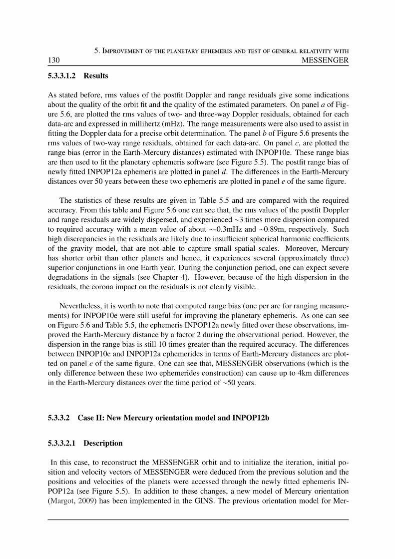
1305. Improvement of the planetary ephemeris and test of general relativity with
MESSENGER
5.3.3.1.2 Results
As stated before, rms values of the postfit Doppler and range residuals give some indicationsabout the quality of the orbit fit and the quality of the estimated parameters. On panel a of Fig-ure 5.6, are plotted the rms values of two- and three-way Doppler residuals, obtained for eachdata-arc and expressed in millihertz (mHz). The range measurements were also used to assist infitting the Doppler data for a precise orbit determination. The panel b of Figure 5.6 presents therms values of two-way range residuals, obtained for each data-arc. On panel c, are plotted therange bias (error in the Earth-Mercury distances) estimated with INPOP10e. These range biasare then used to fit the planetary ephemeris software (see Figure 5.5). The postfit range bias ofnewly fitted INPOP12a ephemeris are plotted in panel d. The differences in the Earth-Mercurydistances over 50 years between these two ephemeris are plotted in panel e of the same figure.
The statistics of these results are given in Table 5.5 and are compared with the requiredaccuracy. From this table and Figure 5.6 one can see that, the rms values of the postfit Dopplerand range residuals are widely dispersed, and experienced ∼3 times more dispersion comparedto required accuracy with a mean value of about ∼-0.3mHz and ∼0.89m, respectively. Suchhigh discrepancies in the residuals are likely due to insufficient spherical harmonic coefficientsof the gravity model, that are not able to capture small spatial scales. Moreover, Mercuryhas shorter orbit than other planets and hence, it experiences several (approximately three)superior conjunctions in one Earth year. During the conjunction period, one can expect severedegradations in the signals (see Chapter 4). However, because of the high dispersion in theresiduals, the corona impact on the residuals is not clearly visible.
Nevertheless, it is worth to note that computed range bias (one per arc for ranging measure-ments) for INPOP10e were still useful for improving the planetary ephemeris. As one can seeon Figure 5.6 and Table 5.5, the ephemeris INPOP12a newly fitted over these observations, im-proved the Earth-Mercury distance by a factor 2 during the observational period. However, thedispersion in the range bias is still 10 times greater than the required accuracy. The differencesbetween INPOP10e and INPOP12a ephemerides in terms of Earth-Mercury distances are plot-ted on panel e of the same figure. One can see that, MESSENGER observations (which is theonly difference between these two ephemerides construction) can cause up to 4km differencesin the Earth-Mercury distances over the time period of ∼50 years.
5.3.3.2 Case II: New Mercury orientation model and INPOP12b
5.3.3.2.1 Description
In this case, to reconstruct the MESSENGER orbit and to initialize the iteration, initial po-sition and velocity vectors of MESSENGER were deduced from the previous solution and thepositions and velocities of the planets were accessed through the newly fitted ephemeris IN-POP12a (see Figure 5.5). In addition to these changes, a new model of Mercury orientation(Margot, 2009) has been implemented in the GINS. The previous orientation model for Mer-

5.3. Orbit determination 131
Table 5.5: Statistics of the residuals obtained for Case I, i) postfit Doppler and range residuals,ii) prefit (INPOP10e) and postfit (INPOP12a) range bias.
Residuals Value** Required accuracy
type (Srinivasan et al., 2007)
2-, and 3-way Doppler -0.3±16.3 mHz < 0.1 mm/s (∼5.7 mHz* )
2-way Range -0.002±8 m < 3 m
1-way range bias, INPOP10e 161±249 m < 10 m
1-way range bias, INPOP12a 181±102 m < 10 m
* 2/3-way: 1 mHz = 0.0178 mm/s = 0.5×speed of light / X-band frequency.** mean±1-σ dispersion of the rms values
Table 5.6: Recommended model for the orientation of Mercury (Margot, 2009).
Parameter value
α0 = 281.0097 - 0.0328T
δ0 = 61.4143 - 0.0049T
W = 329.75 + 6.1385025d
+ 0.00993822 sin(M1)
-0.00104581 sin(M2)
-0.00010280 sin(M3)
-0.00002364 sin(M4)
-0.00000532 sin(M5)
where
M1 = 174.791086 + 4.092335d
M2 = 349.582171 + 8.184670d
M3 = 164.373257 + 12.277005d
M4 = 339.164343 + 16.369340d
M5 = 153.955429 + 20.461675d
Angles are expressed in degrees, and Tand d are defined as in Table 5.4.
cury was inadequate because it uses an obsolete spin orientation, neglects oscillations in thespin rate called longitude librations, and relies on a prime meridian that no longer reflects itsintended dynamical significance (Margot, 2009). These effects induce positional errors on thesurface of ∼2.5 km in latitude and up to several km in longitude (e.g, see Figure 5.7). TheMargot (2009) updated orientation model incorporates modern values of the spin orientation,includes non-zero obliquity and librations, and restores the dynamical significance to the primemeridian. The characteristics of this model is given in Table 5.6. The gravity model used forthis computations is the one used for previous solution (i.e, HgM001).
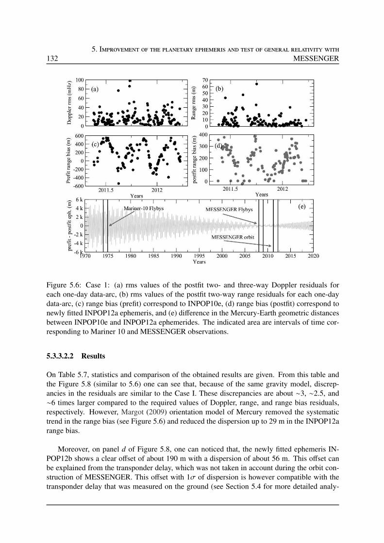
1325. Improvement of the planetary ephemeris and test of general relativity with
MESSENGER
Figure 5.6: Case 1: (a) rms values of the postfit two- and three-way Doppler residuals foreach one-day data-arc, (b) rms values of the postfit two-way range residuals for each one-daydata-arc, (c) range bias (prefit) correspond to INPOP10e, (d) range bias (postfit) correspond tonewly fitted INPOP12a ephemeris, and (e) difference in the Mercury-Earth geometric distancesbetween INPOP10e and INPOP12a ephemerides. The indicated area are intervals of time cor-responding to Mariner 10 and MESSENGER observations.
5.3.3.2.2 Results
On Table 5.7, statistics and comparison of the obtained results are given. From this table andthe Figure 5.8 (similar to 5.6) one can see that, because of the same gravity model, discrep-ancies in the residuals are similar to the Case I. These discrepancies are about ∼3, ∼2.5, and∼6 times larger compared to the required values of Doppler, range, and range bias residuals,respectively. However, Margot (2009) orientation model of Mercury removed the systematictrend in the range bias (see Figure 5.6) and reduced the dispersion up to 29 m in the INPOP12arange bias.
Moreover, on panel d of Figure 5.8, one can noticed that, the newly fitted ephemeris IN-POP12b shows a clear offset of about 190 m with a dispersion of about 56 m. This offset canbe explained from the transponder delay, which was not taken in account during the orbit con-struction of MESSENGER. This offset with 1σ of dispersion is however compatible with thetransponder delay that was measured on the ground (see Section 5.4 for more detailed analy-
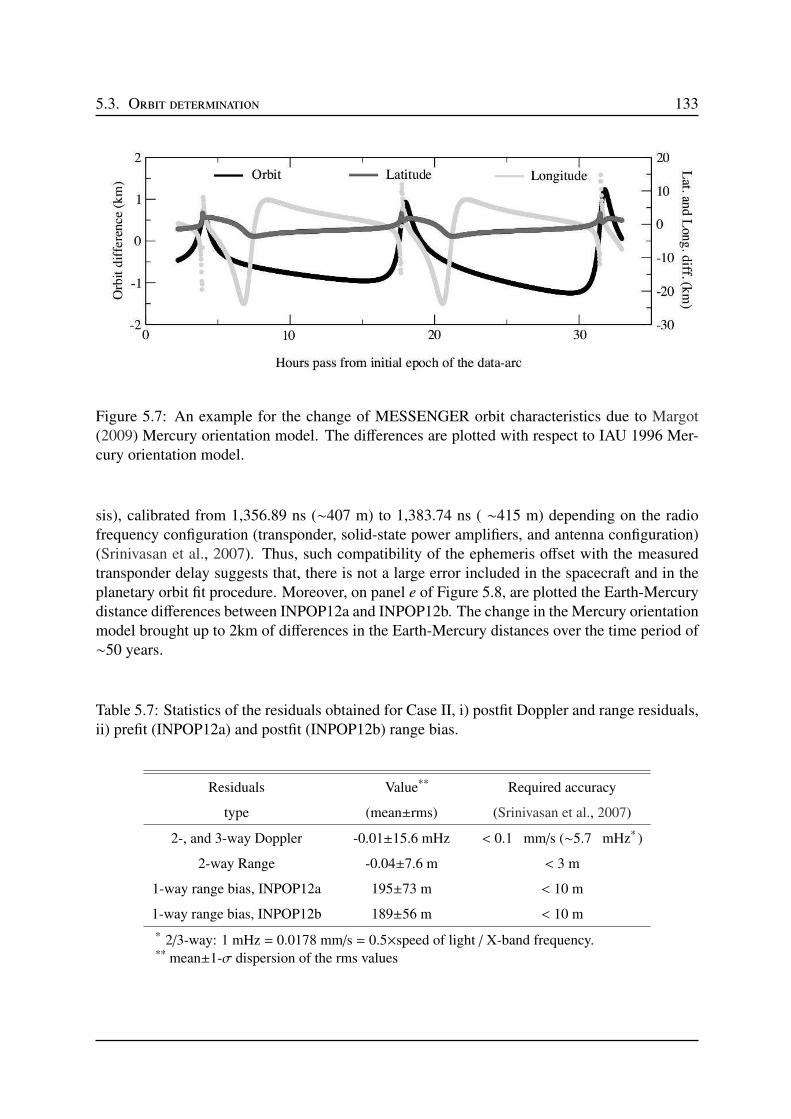
5.3. Orbit determination 133
Figure 5.7: An example for the change of MESSENGER orbit characteristics due to Margot(2009) Mercury orientation model. The differences are plotted with respect to IAU 1996 Mer-cury orientation model.
sis), calibrated from 1,356.89 ns (∼407 m) to 1,383.74 ns ( ∼415 m) depending on the radiofrequency configuration (transponder, solid-state power amplifiers, and antenna configuration)(Srinivasan et al., 2007). Thus, such compatibility of the ephemeris offset with the measuredtransponder delay suggests that, there is not a large error included in the spacecraft and in theplanetary orbit fit procedure. Moreover, on panel e of Figure 5.8, are plotted the Earth-Mercurydistance differences between INPOP12a and INPOP12b. The change in the Mercury orientationmodel brought up to 2km of differences in the Earth-Mercury distances over the time period of∼50 years.
Table 5.7: Statistics of the residuals obtained for Case II, i) postfit Doppler and range residuals,ii) prefit (INPOP12a) and postfit (INPOP12b) range bias.
Residuals Value** Required accuracy
type (mean±rms) (Srinivasan et al., 2007)
2-, and 3-way Doppler -0.01±15.6 mHz < 0.1 mm/s (∼5.7 mHz* )
2-way Range -0.04±7.6 m < 3 m
1-way range bias, INPOP12a 195±73 m < 10 m
1-way range bias, INPOP12b 189±56 m < 10 m
* 2/3-way: 1 mHz = 0.0178 mm/s = 0.5×speed of light / X-band frequency.** mean±1-σ dispersion of the rms values
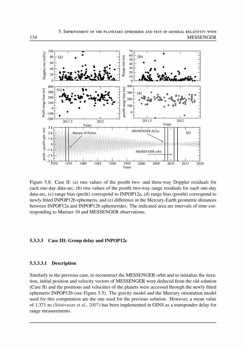
1345. Improvement of the planetary ephemeris and test of general relativity with
MESSENGER
Figure 5.8: Case II: (a) rms values of the postfit two- and three-way Doppler residuals foreach one-day data-arc, (b) rms values of the postfit two-way range residuals for each one-daydata-arc, (c) range bias (prefit) correspond to INPOP12a, (d) range bias (postfit) correspond tonewly fitted INPOP12b ephemeris, and (e) difference in the Mercury-Earth geometric distancesbetween INPOP12a and INPOP12b ephemerides. The indicated area are intervals of time cor-responding to Mariner 10 and MESSENGER observations.
5.3.3.3 Case III: Group delay and INPOP12c
5.3.3.3.1 Description
Similarly to the previous case, to reconstruct the MESSENGER orbit and to initialize the itera-tion, initial position and velocity vectors of MESSENGER were deduced from the old solution(Case II) and the positions and velocities of the planets were accessed through the newly fittedephemeris INPOP12b (see Figure 5.5). The gravity model and the Mercury orientation modelused for this computation are the one used for the previous solution. However, a mean valueof 1,371 ns (Srinivasan et al., 2007) has been implemented in GINS as a transponder delay forrange measurements.
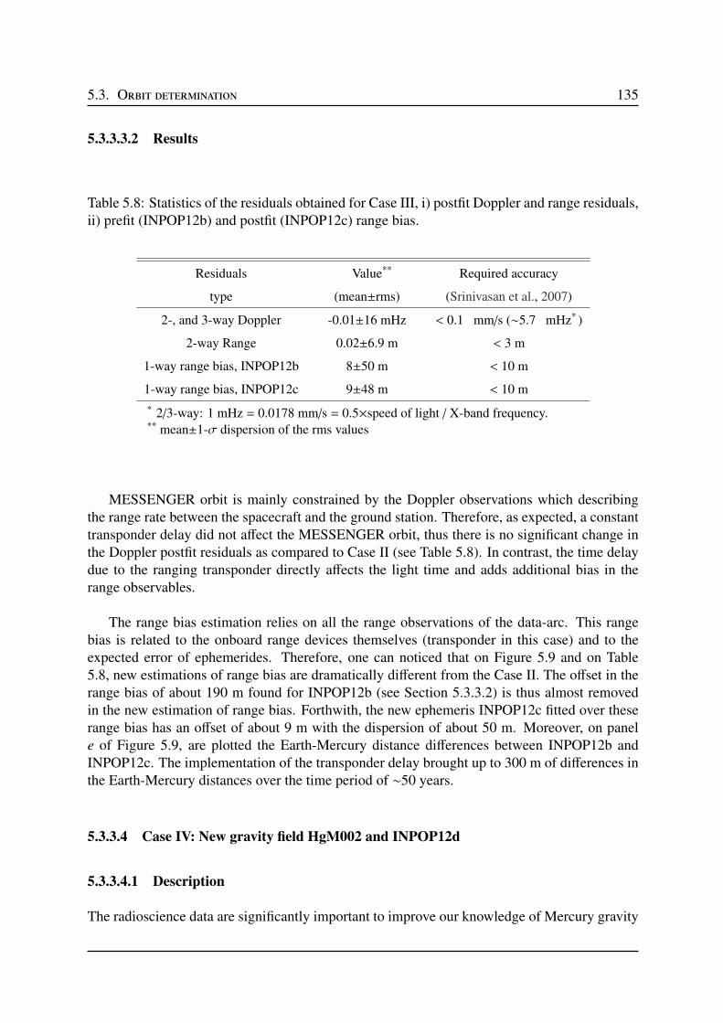
5.3. Orbit determination 135
5.3.3.3.2 Results
Table 5.8: Statistics of the residuals obtained for Case III, i) postfit Doppler and range residuals,ii) prefit (INPOP12b) and postfit (INPOP12c) range bias.
Residuals Value** Required accuracy
type (mean±rms) (Srinivasan et al., 2007)
2-, and 3-way Doppler -0.01±16 mHz < 0.1 mm/s (∼5.7 mHz* )
2-way Range 0.02±6.9 m < 3 m
1-way range bias, INPOP12b 8±50 m < 10 m
1-way range bias, INPOP12c 9±48 m < 10 m
* 2/3-way: 1 mHz = 0.0178 mm/s = 0.5×speed of light / X-band frequency.** mean±1-σ dispersion of the rms values
MESSENGER orbit is mainly constrained by the Doppler observations which describingthe range rate between the spacecraft and the ground station. Therefore, as expected, a constanttransponder delay did not affect the MESSENGER orbit, thus there is no significant change inthe Doppler postfit residuals as compared to Case II (see Table 5.8). In contrast, the time delaydue to the ranging transponder directly affects the light time and adds additional bias in therange observables.
The range bias estimation relies on all the range observations of the data-arc. This rangebias is related to the onboard range devices themselves (transponder in this case) and to theexpected error of ephemerides. Therefore, one can noticed that on Figure 5.9 and on Table5.8, new estimations of range bias are dramatically different from the Case II. The offset in therange bias of about 190 m found for INPOP12b (see Section 5.3.3.2) is thus almost removedin the new estimation of range bias. Forthwith, the new ephemeris INPOP12c fitted over theserange bias has an offset of about 9 m with the dispersion of about 50 m. Moreover, on panele of Figure 5.9, are plotted the Earth-Mercury distance differences between INPOP12b andINPOP12c. The implementation of the transponder delay brought up to 300 m of differences inthe Earth-Mercury distances over the time period of ∼50 years.
5.3.3.4 Case IV: New gravity field HgM002 and INPOP12d
5.3.3.4.1 Description
The radioscience data are significantly important to improve our knowledge of Mercury gravity
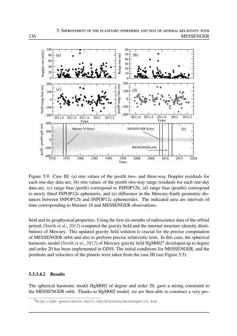
1365. Improvement of the planetary ephemeris and test of general relativity with
MESSENGER
Figure 5.9: Case III: (a) rms values of the postfit two- and three-way Doppler residuals foreach one-day data-arc, (b) rms values of the postfit two-way range residuals for each one-daydata-arc, (c) range bias (prefit) correspond to INPOP12b, (d) range bias (postfit) correspondto newly fitted INPOP12c ephemeris, and (e) difference in the Mercury-Earth geometric dis-tances between INPOP12b and INPOP12c ephemerides. The indicated area are intervals oftime corresponding to Mariner 10 and MESSENGER observations.
field and its geophysical properties. Using the first six months of radioscience data of the orbitalperiod, (Smith et al., 2012) computed the gravity field and the internal structure (density distri-bution) of Mercury. This updated gravity field solution is crucial for the precise computationof MESSENGER orbit and also to perform precise relativistic tests. In this case, the sphericalharmonic model (Smith et al., 2012) of Mercury gravity field HgM0025 developed up to degreeand order 20 has been implemented in GINS. The initial conditions for MESSENGER, and thepositions and velocities of the planets were taken from the case III (see Figure 5.5).
5.3.3.4.2 Results
The spherical harmonic model HgM002 of degree and order 20, gave a strong constraint tothe MESSENGER orbit. Thanks to HgM002 model, we are then able to construct a very pre-
5http://pds-geosciences.wustl.edu/missions/messenger/rs.htm
5.3. Orbit determination 137
Table 5.9: Statistics of the residuals obtained for Case IV, i) postfit Doppler and range residuals,ii) prefit (INPOP12c) and postfit (INPOP12d) range bias.
Residuals Value** Required accuracy
type (mean±rms) (Srinivasan et al., 2007)
2-, and 3-way Doppler -0.002±5.0 mHz < 0.1 mm/s (∼5.7 mHz* )
2-way Range -0.002±1.7 m < 3 m
1-way range bias, INPOP12c 1.8±17 m < 10 m
1-way range bias, INPOP12d 0.7±7.5 m < 10 m
* 2/3-way: 1 mHz = 0.0178 mm/s = 0.5×speed of light / X-band frequency.** mean±1-σ dispersion of the rms values, excluding solar corona
Figure 5.10: Case IV: (a) rms values of the postfit two- and three-way Doppler residuals foreach one-day data-arc, (b) rms values of the postfit two-way range residuals for each one-daydata-arc, (c) range bias (prefit) correspond to INPOP12c, (d) range bias (postfit) correspond tonewly fitted INPOP12d ephemeris, and (e) difference in the Mercury-Earth geometric distancesbetween INPOP12c and INPOP12d ephemerides. The indicated area are intervals of time cor-responding to Mariner 10 and MESSENGER observations.

1385. Improvement of the planetary ephemeris and test of general relativity with
MESSENGER
cise orbit of MESSENGER and then of Mercury. As one can see on Figure 5.10 and Table5.9, the rms values of postfit Doppler and range residuals are ∼3 times smaller with almost zeromean values compared to the one found with HgM001 gravity model. Because of such accuracyin the orbit computation, one can easily disentangle the impact of the solar corona on the obser-vations (peaks on Figure 5.10). As one can noticed from Table 5.9, the estimated rms values ofthe Doppler and range residuals, excluding superior solar conjunction periods, are compatiblewith the required accuracy of about 0.1 mm/s and 3 m, respectively (Srinivasan et al., 2007).Moreover, we have also adjusted Doppler offsets per arc and per DSN station (participatingin the data-arc) accounting for the systematic errors generated by the devices at each trackingstation. As expected, the fitted values for each DSN station tracking pass is of the order of afew tenths of mHz, which is lower than the Doppler postfit residuals for each data-arc. No largeoffset was then detected in the modeling of the Doppler shift measurements at each trackingstation.
As a consequence of the precise MESSENGER orbit, the dispersion in the range bias es-timated for INPOP12c is almost 30 m less than the one found with previous estimations (seeFigure 5.10 and Table 5.9). The new ephemeris INPOP12d fitted over these range bias has anoffset of about 7.5 m with a mean value less than meter. Such accuracy in the range bias alsoshows the compatibility with the required accuracy of about 10 m. Further improvements inthe range bias however may be limited by the uncalibrated transponder time delays due to ei-ther temperature variations or electronic perturbations from other devices. On panel e of Figure5.10, are plotted the Earth-Mercury distance differences between INPOP12c and INPOP12d.The improvement of the MESSENGER orbit can lead up to 500 m of changes in the Earth-Mercury distances. The accuracy of Mercury orbit depends then upon the quality of the rangebias.
5.3.3.5 Case V: Extension of the mission and INPOP13a
5.3.3.5.1 Description
As stated before, on March 2012, the MESSENGER mission was extended to one or moreyears. Therefore, in the construction of the latest INPOP13a ephemeris, we have analyzed allavailable MESSENGER radioscience data, including one year of prime phase and six monthsof extended phase. The analysis was performed in the same manner as for previous cases.
5.3.3.5.2 Results
During the extended phase of the mission, MESSENGER was placed in an ∼8-hour orbit toconduct further scans of Mercury by significantly tuned the apoapsis altitude of MESSENGER(e.g, see Figure 5.4). As described in Section 5.3.1, this change in the orbit significantly alteredthe acceleration budget of the MESSENGER spacecraft (see Table 5.3). On figure 5.11, areplotted the rms values of the postfit Doppler and range residuals for both phases. Statistics of
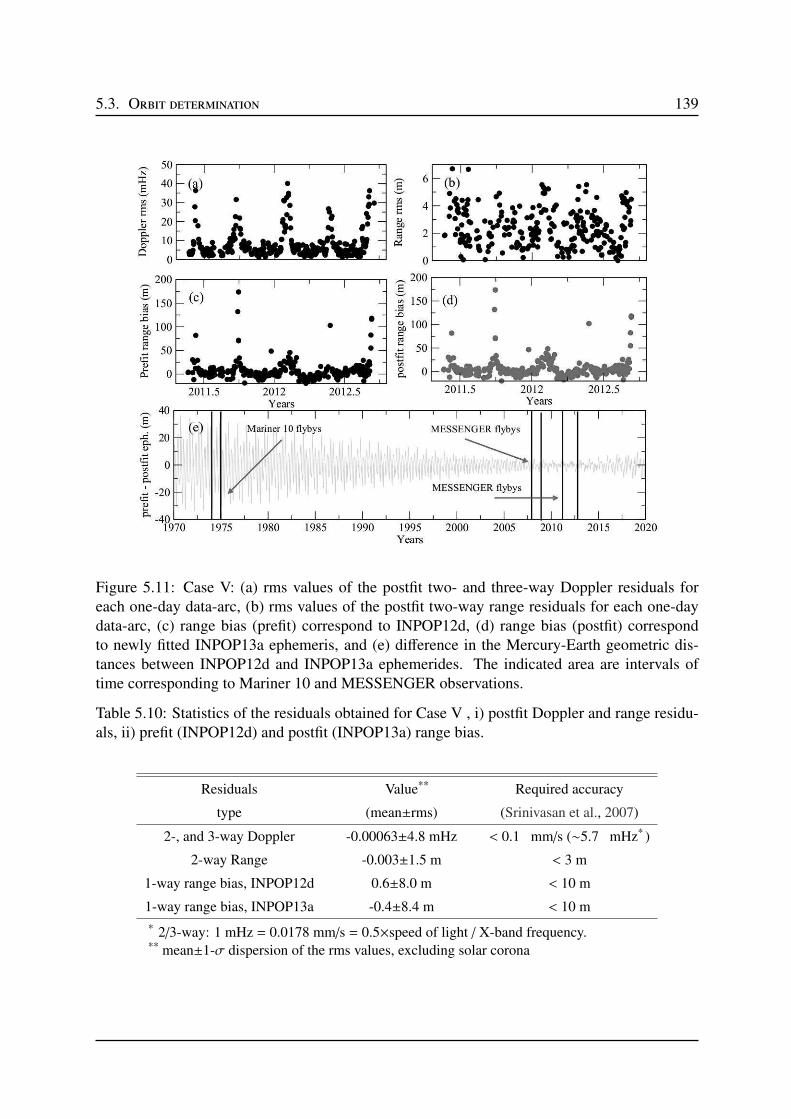
5.3. Orbit determination 139
Figure 5.11: Case V: (a) rms values of the postfit two- and three-way Doppler residuals foreach one-day data-arc, (b) rms values of the postfit two-way range residuals for each one-daydata-arc, (c) range bias (prefit) correspond to INPOP12d, (d) range bias (postfit) correspondto newly fitted INPOP13a ephemeris, and (e) difference in the Mercury-Earth geometric dis-tances between INPOP12d and INPOP13a ephemerides. The indicated area are intervals oftime corresponding to Mariner 10 and MESSENGER observations.
Table 5.10: Statistics of the residuals obtained for Case V , i) postfit Doppler and range residu-als, ii) prefit (INPOP12d) and postfit (INPOP13a) range bias.
Residuals Value** Required accuracy
type (mean±rms) (Srinivasan et al., 2007)
2-, and 3-way Doppler -0.00063±4.8 mHz < 0.1 mm/s (∼5.7 mHz* )
2-way Range -0.003±1.5 m < 3 m
1-way range bias, INPOP12d 0.6±8.0 m < 10 m
1-way range bias, INPOP13a -0.4±8.4 m < 10 m
* 2/3-way: 1 mHz = 0.0178 mm/s = 0.5×speed of light / X-band frequency.** mean±1-σ dispersion of the rms values, excluding solar corona
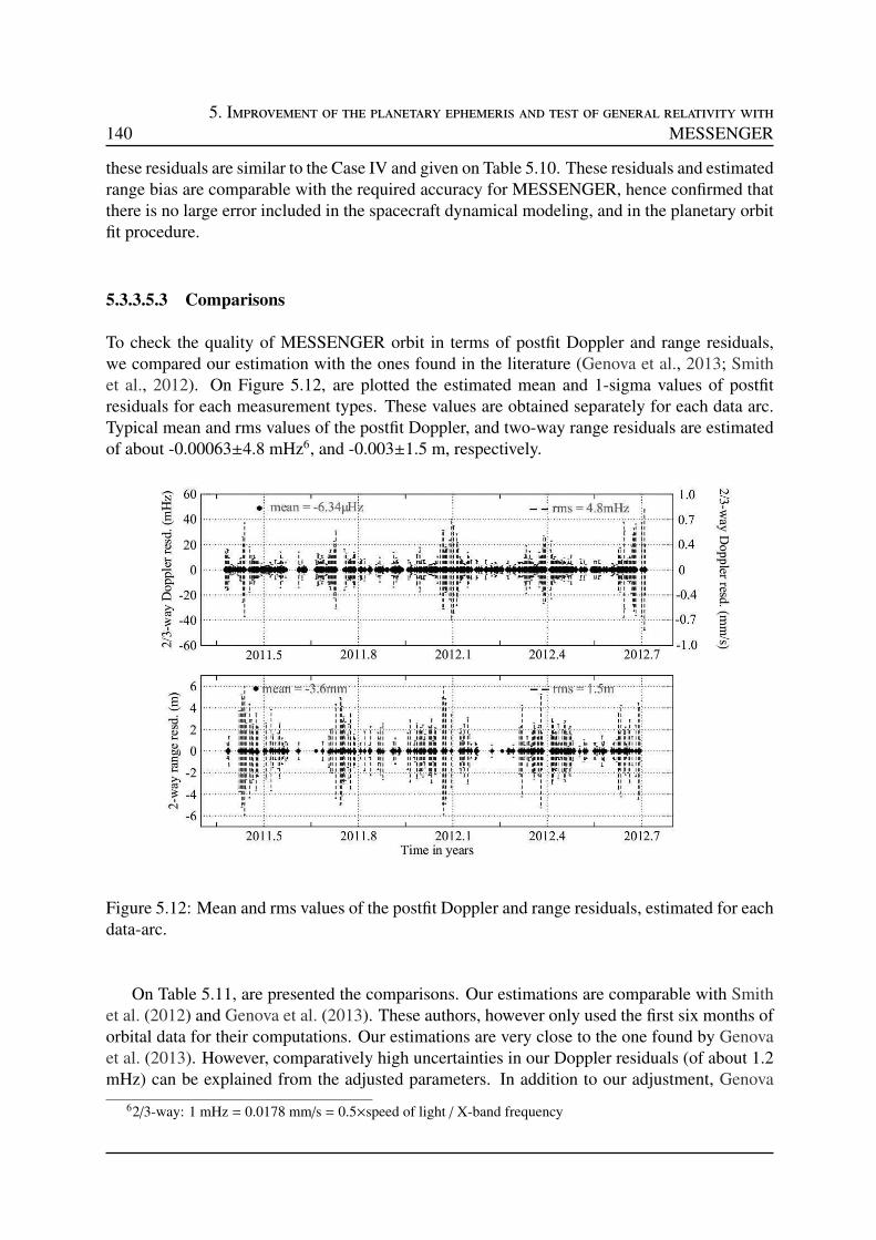
1405. Improvement of the planetary ephemeris and test of general relativity with
MESSENGER
these residuals are similar to the Case IV and given on Table 5.10. These residuals and estimatedrange bias are comparable with the required accuracy for MESSENGER, hence confirmed thatthere is no large error included in the spacecraft dynamical modeling, and in the planetary orbitfit procedure.
5.3.3.5.3 Comparisons
To check the quality of MESSENGER orbit in terms of postfit Doppler and range residuals,we compared our estimation with the ones found in the literature (Genova et al., 2013; Smithet al., 2012). On Figure 5.12, are plotted the estimated mean and 1-sigma values of postfitresiduals for each measurement types. These values are obtained separately for each data arc.Typical mean and rms values of the postfit Doppler, and two-way range residuals are estimatedof about -0.00063±4.8 mHz6, and -0.003±1.5 m, respectively.
Figure 5.12: Mean and rms values of the postfit Doppler and range residuals, estimated for eachdata-arc.
On Table 5.11, are presented the comparisons. Our estimations are comparable with Smithet al. (2012) and Genova et al. (2013). These authors, however only used the first six months oforbital data for their computations. Our estimations are very close to the one found by Genovaet al. (2013). However, comparatively high uncertainties in our Doppler residuals (of about 1.2mHz) can be explained from the adjusted parameters. In addition to our adjustment, Genova
62/3-way: 1 mHz = 0.0178 mm/s = 0.5×speed of light / X-band frequency
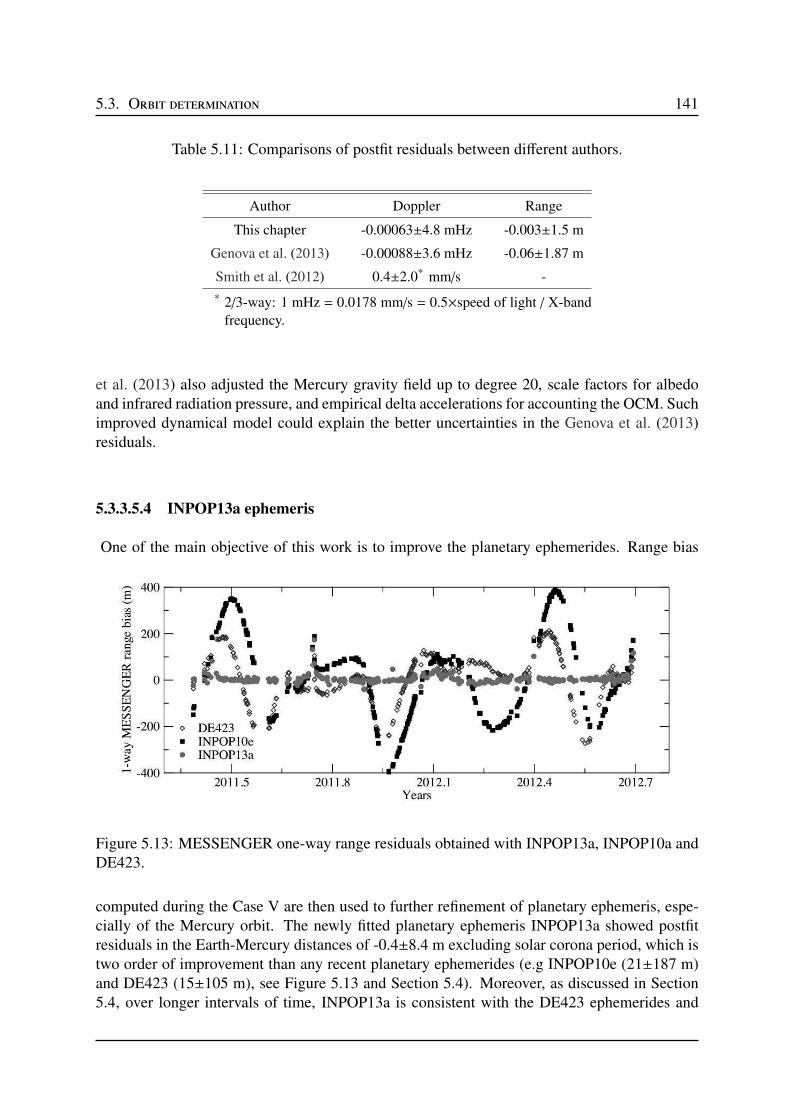
5.3. Orbit determination 141
Table 5.11: Comparisons of postfit residuals between different authors.
Author Doppler Range
This chapter -0.00063±4.8 mHz -0.003±1.5 m
Genova et al. (2013) -0.00088±3.6 mHz -0.06±1.87 m
Smith et al. (2012) 0.4±2.0* mm/s -
* 2/3-way: 1 mHz = 0.0178 mm/s = 0.5×speed of light / X-bandfrequency.
et al. (2013) also adjusted the Mercury gravity field up to degree 20, scale factors for albedoand infrared radiation pressure, and empirical delta accelerations for accounting the OCM. Suchimproved dynamical model could explain the better uncertainties in the Genova et al. (2013)residuals.
5.3.3.5.4 INPOP13a ephemeris
One of the main objective of this work is to improve the planetary ephemerides. Range bias
Figure 5.13: MESSENGER one-way range residuals obtained with INPOP13a, INPOP10a andDE423.
computed during the Case V are then used to further refinement of planetary ephemeris, espe-cially of the Mercury orbit. The newly fitted planetary ephemeris INPOP13a showed postfitresiduals in the Earth-Mercury distances of -0.4±8.4 m excluding solar corona period, which istwo order of improvement than any recent planetary ephemerides (e.g INPOP10e (21±187 m)and DE423 (15±105 m), see Figure 5.13 and Section 5.4). Moreover, as discussed in Section5.4, over longer intervals of time, INPOP13a is consistent with the DE423 ephemerides and
1425. Improvement of the planetary ephemeris and test of general relativity with
MESSENGER
improved the internal accuracy of INPOP by a factor two on the geocentric distances. Further-more, to understand the impact of six months complementary data of the extended phase overthe Mercury orbit, on panel e of Figure 5.11, are plotted the Earth-Mercury distance differencesbetween INPOP12d and INPOP13a ephemerides. The additional data of the extended phaseindeed gave small constraints to ∼0.3 Earth year of Mercury orbit, and brought up to 20 m ofdifferences in the Earth-Mercury distances over the time period of ∼50 years.
As a scientific exploitation of these results, such high precision planetary ephemeris IN-POP13a allowed us to perform several tests. The detailed analysis of these tests are describedin the Section 5.4. An example of such tests are: (a) Impact of planetary ephemeris over theMESSENGER orbit, and (b) GR tests of PPN-formalism and its impact over the MESSENGERorbit.
(a) The geometric distances between the Earth and Mercury are ∼16 times ameliorated in IN-POP13a compared to INPOP10e. To analyze the impact of the improvement of the plan-etary ephemeris over the spacecraft orbit, we reanalyzed the entire one and half year ofradioscience data using INPOP10e ephemeris. The dynamical modeling and the orbit de-termination process accounted for performing this analysis are the same as used for CaseV. The improvement in the Mercury ephemeris however brought negligible variations inthe MESSENGER orbit. The differences between the two solutions, one obtained withINPOP10e and other with INPOP13a, in the rms postfit Doppler and range residuals wereestimated as 0.008±0.04 mHz, and 0.05±0.3 m, respectively. These values are however farbelow compared to the estimated accuracy of 4.8 mHz, and 1.5 m respectively.
(b) GR tests of PPN-formalism were also performed with INPOP13a. Because of the highprecision Mercury ephemeris, our estimations of the PPN parameters are most stringentthan previous results. We considered the 5, 10 and 25% of changes in the postfit residualscompared to INPOP13a. These changes in the postfit residuals are then used to estimate thepossible violation of two relativistic parameters (γ and β) of the PPN formalism of GR. Thisanalysis shows ten times smaller uncertainty in the estimation of β and γ than our previousresults with INPOP10a or INPOP08. Moreover, one of the best estimation of the parameterγ by Bertotti et al. (2003) is compatible with our 25% of estimation.
5.4 Verma et al. (2013b)
Astronomy & Astrophysics manuscript no. messenger September 26, 2013(DOI: will be inserted by hand later)
Use of MESSENGER radioscience data to improve planetary
ephemeris and to test general relativity.
A. K. Verma1,2, A. Fienga3,4, J. Laskar4, H. Manche4, and M. Gastineau4
1 Observatoire de Besancon, UTINAM-CNRS UMR6213, 41bis avenue de l’Observatoire, 25000 Besancon, France2 Centre National d’Etudes Spatiales, 18 avenue Edouard Belin, 31400 Toulouse, France3 Observatoire de la Cote d'Azur, GeoAzur-CNRS UMR7329, 250 avenue Albert Einstein, 06560 Valbonne, France4 Astronomie et Systemes Dynamiques, IMCCE-CNRS UMR8028, 77 Av. Denfert-Rochereau, 75014 Paris, France
September 26, 2013
Abstract. Current knowledge of Mercury orbit is mainly brought by the direct radar ranging obtained from the 60s to 1998and five Mercury flybys made by Mariner 10 in the 70s, and MESSENGER made in 2008 and 2009. On March 18, 2011,MESSENGER became the first spacecraft orbiting Mercury. The radioscience observations acquired during the orbital phaseof MESSENGER drastically improved our knowledge of the orbit of Mercury. An accurate MESSENGER orbit is obtained byfitting one-and-half years of tracking data using GINS orbit determination software. The systematic error in the Earth-Mercurygeometric positions, also called range bias, obtained from GINS are then used to fit the INPOP dynamical modeling of theplanet motions. An improved ephemeris of the planets is then obtained, INPOP13a, and used to perform general relativity testof PPN-formalism. Our estimations of PPN parameters are most stringent than previous results.
Key words. messenger - celestial mechanics - ephemerides - general relativity
1. Introduction
Mercury is the smallest and least explored terrestrial planet ofthe solar system. Mariner 10 was the first spacecraft whichmade three close encounters (two in 1974 and one in 1975) tothis mysterious planet and provided most of our current knowl-edge of the planet until early 2008 (Smith et al. 2010). In ad-dition to Mariner 10 flyby observations, ground based radarmeasurements were the only observations which were used tostudy Mercury’s gravity field and its physical structure (spher-ical body with slightly flattened at the poles and mildly elon-gated equator) (Anderson et al. 1987, 1996). In 2004, NationalAeronautics and Space Administration (NASA) launched adedicated mission, MErcury Surface, Space Environment,GEochemistry, and Ranging (MESSENGER), to learn moreabout this planet. MESSENGER made three close encounters(two in 2008 and one in 2009) to Mercury and became the firstspacecraft which observed Mercury from its orbit.
Till now, MESSENGER has completed more than twoyears on orbit at Mercury. During the orbital period, radiotracking of MESSENGER routinely measured the Dopplerand range observables at Deep Space Network (DSN) sta-tions. These observables are important to estimate the space-craft state vectors (position and velocity) and to improve theknowledge of Mercury’s gravity field and its geophysical prop-erties (Srinivasan et al. 2007). Using the first six months of
Send offprint requests to: A. Verma, [email protected]
radioscience data during the orbital period, Smith et al. (2012)computed the gravity field and gave better constraints on the in-ternal structure (density distribution) of Mercury. This updatedgravity field becomes crucial for the present computation ofMESSENGER orbit and to perform precise relativistic tests.
The primary objectives of this work are to determinethe precise orbit of the MESSENGER spacecraft aroundMercury using radioscience data and then improve the plan-etary ephemeris INPOP (Fienga et al. 2008, 2009, 2011a). Theupdated spacecraft and planetary ephemerides are then usedto perform sensitive relativistic tests of the Parametrized PostNewtonian (PPN) parameters (γ and β).
Nowadays, spacecraft range measurements are the most ac-curate measurements that have been used for the constructionof planetary ephemerides. These measurements approximatelycover 56% of whole INPOP data (Fienga et al. 2011a) and im-pose strong constraints on the planet orbits and on the othersolar system parameters including asteroid masses. However,until now, only five flybys (two from Mariner 10 and three fromMESSENGER) range measurements were available for impos-ing strong constraints to Mercury’s orbit (Fienga et al. 2011a).Therefore, range measurements obtained by MESSENGERspacecraft during its mapping period are important to improveour knowledge of the Mercury’s orbit.
Moreover, high precision radioscience observations alsogave an opportunity to perform sensitive relativistic tests byestimating possible violation of the two relativistic parame-
2 Verma et al.: Planetary ephemeris construction and test of relativity with MESSENGER
ters (γ and β) of the PPN formalism of general relativity (GR)(Will 1993). The previous estimations of these parameters us-ing different techniques and different data set, can be found in(Bertotti et al. 2003; Muller et al. 2008; Pitjeva 2009; Williamset al. 2009; Manche et al. 2010; Konopliv et al. 2011; Fiengaet al. 2011a). However, because of Mercury relatively large ec-centricity and close proximity to the Sun, its orbital motion pro-vides one of the best solar system tests of GR (Anderson et al.1997). In addition, Fienga et al. (2010, 2011a) also demon-strated that, Mercury observations are far more sensitive toPPN modification of GR than other data used in the planetaryephemerides. We, therefore, also performed the test of GR withthe latest MESSENGER observations to obtained one of thebest value for PPN parameters.
In this paper, we introduce the updated planetary ephemerisINPOP13a and summarize the technique used for the esti-mation of the PPN parameters. The outline of the paper isas follows: Section 2 discussed the radioscience data analy-sis of the MESSENGER spacecraft. The dynamic modeling ofMESSENGER and the results obtained during orbit computa-tion are also discussed in the same section. In section 3, wediscussed the construction of INPOP13a using the results ob-tained in section 2. In section 4, we discussed the gravitationaltests using updated MESSENGER and Mercury ephemerides.Section 5 follows with conclusions and perspectives of the re-sults.
2. MESSENGER data analysis
2.1. Mission overview and tracking data
Under the NASA’s Discovery program, the MErcurySurface, Space ENvironment, GEochemistry, and Ranging(MESSENGER) spacecraft is the first probe to orbit the planetMercury. It launched in August 3, 2004, from Pad B of SpaceLaunch Complex 17 at Cape Canaveral Air Force Station,Florida, aboard a three-stage Boeing Delta II rocket. On March18, 2011, MESSENGER successfully entered Mercury’s orbitafter completing three flybys of Mercury following two flybysof Venus and one of Earth (Solomon et al. 2007).
The MESSENGER spacecraft was initially inserted into a∼12-hour, near-polar orbit around Mercury, with an initial pe-riapsis altitude of 200 km, initial periapsis latitude of 60°N,and apoapsis at ∼15,200 km altitude in the southern hemi-sphere. After successful first year flight in the orbit, missionwas extended to one or more year which began on 18 March2012. During first extended mission, two orbit-correction ma-neuvers were executed, four days apart, in April 2012 to reduceMESSENGER’s orbital period from ∼12 to ∼8 hours (Flaniganet al. 2013)
The MESSENGER spacecraft was tracked by the NASA’sDSN stations at X-band frequency, 7.2 GHz for a uplink fromthe ground stations and 8.4 GHz for a downlink from thespacecraft. Communications are accomplished via the 34-mand 70-m antennas of DSN stations in Goldstone, CA; Madrid,Spain; and Canberra, Australia. MESSENGER’s X-band track-ing consists in measuring the round-trip time delay (two-wayrange), and the two- and three-way ramped Doppler shift of
the carrier frequency of the radio link between the space-craft and the DSN stations on Earth. The precision of theDoppler measurement for the radio frequency subsystem iswithin ±0.1 mm/s over 10s to several minutes of integrationtime (Srinivasan et al. 2007).
2.2. Data analysis and dynamic modeling
We have analyzed one-and-half years of tracking data collectedby the DSN during MESSENGER orbital period. These databelongs to one year of the prime mission and six months offirst extended mission (see Table 1). The complete data setthat were used for the analysis are available on the Geosciencenode1 of the NASA’s Planetary Data System (PDS). For pre-cise orbit determination, all available observations were ana-lyzed with the help of the Godsie par Intgrations NumriquesSimultanes (GINS) software, which is developed by the CentreNational d’Etudes Spatiales (CNES) in collaboration withRoyal Observatory of Belgium (ROB). GINS numerically in-tegrates the equations of motion and the associated variationalequations. It simultaneously retrieves the physical parametersof the force model using an iterative least-squares technique.
2.2.1. Dynamic modeling and orbit determination
processes.
The precise orbit determination is based on a full dynamicalapproach. The dynamic modeling includes gravitational (grav-itational attraction of Mercury, third-body gravity perturbationsfrom the Sun and other planets, and relativistic corrections)and nongravitational (solar radiation pressure; Mercury radia-tion pressure) forces that are acting on the spacecraft. Theseforces have been taken into account in the force budget ofMESSENGER. The latest spherical harmonic model (Smithet al. 2012) of Mercury’s gravity field, HgM0022 developedup to degree and order 20, and the associated Mercury’s orien-tation model (Margot 2009) have been considered for precisecomputation.
The measurement (Doppler and range) models and thelight time corrections that are modeled in GINS, correspondto the formulation given by Moyer (2003). During computa-tions, DSN station coordinates were corrected from the Earth’spolar motion, solid-Earth tides, and from the ocean loading. Inaddition to these corrections, radiometric data also have beencorrected from tropospheric propagation through the meteoro-logical data3 (pressure, temperature and humidity) of the sta-tions.
The complex geometry of the MESSENGER spacecraftwas treated as a combination of flat plates arrange in the shapeof a box, with attached solar arrays, so called Box-Wing macro-model. The approximated characteristics of this macro-model,
1 http://pds-geosciences.wustl.edu/messenger/2 http://pds-geosciences.wustl.edu/missions/
messenger/rs.htm3 http://pds-geosciences.wustl.edu/messenger/
mess-v_h-rss-1-edr-rawdata-v1/messrs_0xxx/ancillary/
wea/

Verma et al.: Planetary ephemeris construction and test of relativity with MESSENGER 3
which includes cross-sectional area and specular and diffusereflectivity coefficients of the components, were taken from(Vaughan et al. 2002). In addition to the macro-model char-acteristics, orientations of the spacecraft were also taken inaccount. The attitude of spacecraft, and of its articulated pan-els in inertial space were defined in terms of quaternions. Theapproximate value of these quaternions was extracted fromthe C-kernel4 system of the SPICE Navigation and AncillaryInformation Facility (NAIF) software. The macro-model andits orientation have allowed to calculate the nongravitationalaccelerations that are acting on the MESSENGER spacecraftdue to the radiation pressure from Sun and Mercury (albedoand thermal infrared emission).
For orbit computation and parameters estimation, a multi-arc approach was used to get independent estimates of theMESSENGER accelerations. In this method, we integrated theequations of motion using the time-step of 50s and then, or-bital fits were obtained from short data-arcs fitted over the ob-servations span of one-day using an iterative process. The shortdata-arcs of one-day have chosen to account the model imper-fections. To initialize the iteration, the initial position and ve-locity vectors of MESSENGER were taken from the SPICENAIF spk-kernels5.
2.2.2. Solve-for parameters
An iterative least-squares fit was performed on the completeset of Doppler- and range-tracking data-arcs corresponding tothe orbital phase of the mission using an INPOP10e (Fiengaet al. 2013) planetary ephemeris6. We have processed datafrom 17 May 2011 to 18 September 2012 excluding maneu-vers epoch. Summary of these tracking data are given in Table1. MESSENGER fires small thrusters to perform MomentumDump Maneuver (MDM) for reducing the spacecraft angularmomentum to a safe level. Normal operations (during orbitalperiods) includes only one commanded momentum dump ev-ery two weeks. In addition, Orbit Correction Maneuver (OCM)were also performed (typically once every Mercury year (88Earth days)) to maintain the minimum altitude below 500 kilo-meters. Such large intervals between the MESSENGER ma-neuvers facilitate the orbit determination. The data-arcs corre-spond to the maneuvers epoch thus not included in the analysis.The total one-day data-arcs of about 440 were then used for theanalysis.
Several parameters have been estimated during orbit com-putation. These parameters are: spacecraft state vectors at thestart epoch of each data-arc, for a total of 440×6=2640 param-eters; one scale factor per data-arc for solar radiation force foraccounting inaccuracy in the force model (total of 440 param-eters); one Doppler bias per arc for each DSN station for ac-counting the systematic errors generated by the devices at eachtracking station (total of
∑4401 1×n parameters, where n is the
4 ftp://naif.jpl.nasa.gov/pub/naif/pds/data/mess-e_
v_h-spice-6-v1.0/messsp_1000/data/ck/5 ftp://naif.jpl.nasa.gov/pub/naif/pds/data/mess-e_
v_h-spice-6-v1.0/messsp_1000/data/spk/6 http://www.imcce.fr/inpop/
number of stations participating in the data-arc); one stationbias per arc for each DSN station for accounting the uncertain-ties on the DSN antenna center position or the instrumental de-lays (total of
∑4401 1×n parameters); and one range bias per arc
for ranging measurements to account the systematic geometricpositions error (ephemerides bias) between the Earth and theMercury (total of 440 parameters).
2.3. Orbit Determination
2.3.1. Postfit residuals
The root mean square (rms) values of the post-fitted Dopplerand range residuals give some indication about the quality ofthe orbit fit and the estimated parameters. Moreover, quality ofthe used parameters associated the physical model can also bejudged from these residuals. Fig. 1 illustrates the time historyof the residuals estimated for each measurement type. In thisfigure, panel a represents the rms values of two- and three-wayDoppler residuals that were obtained for each data-arc and ex-pressed in millihertz (mHz). As Mercury has shorter orbit thanother planets, it experiences 5 superior conjunctions (when theEarth, the Sun and the spacecraft lie on the same line, withthe spacecraft located on the opposite side of the Sun with re-spect to Earth) during the time interval covered by the analysis.Due to insufficient modeling of the solar corona perturbationswithin the GINS software, no model of solar plasma has beenapplied during the computations of the MESSENGER orbit.The peaks shown in Fig. 1, therefore, demonstrates the cleareffect of the solar conjunctions on the typical fit to the Dopplerand range data residuals.
Excluding the solar conjunction periods, when Sun-Earth-Probe angle remained below 10, an average value ofDoppler residuals has been found approximately 4.8±2.2 mHz(∼0.09±0.04 mm/s), which is comparable with (Smith et al.2012; Stanbridge et al. 2011; Srinivasan et al. 2007). The meanvalue of the estimated Doppler bias for each DSN station track-ing pass has been found very small (few tenths of mHz), whichis lower than the Doppler post-fit residuals for each data-arc. Itdemonstrated that we have no large bias in the modeling of theDoppler shift measurements at each tracking station.
The range measurements were also used to assist in fittingthe Doppler data for a precise orbit determination. The panelb of Fig. 1 represents the rms values of two-way range resid-uals that were obtained for each data-arc. An average value ofthese range residuals has been found approximately 1.9±1.4 m,which is comparable with (Srinivasan et al. 2007).
2.3.2. Scale factor and range bias
We have fitted one scale factor per data-arc for solar radia-tion force to account the inaccuracy in the force model. Panela of Fig. 2 represents the time history of such scale factors.These scale factors are over plotted with the beta-angle, whichis the angle between MESSENGER orbital plane and the vec-tor from the Sun direction. The variation in the MESSENGERorbital plane (beta-angle) relative to the Sun occurs as Mercurymoves around the Sun. For example, at 10, 100, and 180 of
4 Verma et al.: Planetary ephemeris construction and test of relativity with MESSENGER
Table 1: Summary of the Doppler and range tracking data used for orbit determination.
Mission Begin date End date Number of Number of Number of
phase dd-mm-yyyy dd-mm-yyyy 2-way Doppler 3-way Doppler range
Prime 17-05-2011 18-03-2012 2108980 184138 11540
Extended 26-03-2012 18-09-2012 1142974 23211 5709
Fig. 1: Quality of the MESSENGER orbit in terms of rms values of the post-fit residuals for each one-day data-arc: (a) two- andthree-way Doppler given in millihertz (multiply by 0.0178 to obtain residuals in mm/s), and (b) two-way range given in meter.
Mercury true anomaly, the corresponding beta-angles are 83,0, and -78, respectively (Ercol et al. 2012). At 0 beta-angle,the spacecraft travels directly between the Sun and the planet,while, at 90, the spacecraft experienced maximum of sunlight.As one can see from panel a of Fig. 2, the solar pressure coeffi-cients have variations which approximately follow those of thebeta-angle. This implies that, whenever MESSENGER orbitalplane approaches the maximum beta-angle, it experiences largesunlight. The automatic orientation of the solar panels to bal-ances the need for power and the temperature of the surface ofthe panel is then taken care by the scale factor to reduce themodeling error. The fitted scale factor for solar radiation pres-sure is, therefore, typically in the range of about 2.1±0.5. Thisvalue is nearly twice the a priori value and reflect imperfectionin the force model due to the approximate representation of themacro-model.
The panel b of Fig. 2 illustrates the one-way range bias es-timated for the ranging measurements for each data-arc. Thesebias are the representation of the systematic uncertainties in theEarth-Mercury geometric positions. The black (•) and red (N)dots in the figure correspond to INPOP10e (Fienga et al. 2013)
and DE423 (Folkner 2010), respectively. An average value ofthese range bias for INPOP10e and DE423 was 21±187 mand 15±105 m, respectively. Such range bias are then usedin the planetary ephemerides to fit the dynamical modeling ofthe planet motions. (see Sec. 3). Thus, MESSENGER rang-ing measurements have been used to reconstruct the orbit ofMercury around the Sun. The improved planetary ephemeris,INPOP13a (see Sec. 3.2), was then used to re-analyzed theMESSENGER radiometric data, in order to study the impactof planetary ephemeris over the computation of MESSENGERorbit and associated parameters (see Sec. 3.3).
2.3.3. Spacecraft transponder group delay calibration
Planetary ephemerides are a good tool to test gravity model andGR (Fienga et al. 2011a) and to perform solar corona studies(Verma et al. 2013). Moreover, it is also possible to calibratethe transponder group delay from the planetary ephemeris. Thespacecraft receives and transmits the signal to the Earth sta-tion through the on-board transponder, which causes the timedelay in the range measurements. This delay varies from one

Verma et al.: Planetary ephemeris construction and test of relativity with MESSENGER 5
Fig. 2: History of the fitted scale factor and estimated range bias: (a) scale factor (for solar radiation acceleration) fitted overeach one-day data-arc to account inaccuracy in the force model, and (b) one-way range bias, represent the systematic error in theEarth-Mercury positions, estimated for each one-day arc using INPOP10e (•) and DE423 (N) planetary ephemerides.
spacecraft to an other depending on the radio frequency con-figuration. Usually an average value of this delay is measuredat different occasions on the ground before launch. However,the group delay is not perfectly stable and can fluctuate by afew ns, depending upon variations in a number of parameterssuch as temperature and signal strength.
For MESSENGER, we estimated this group delay withthe planetary ephemeris. This procedure becomes an alternatemethod to test the procedure and quality of the orbit fit bycomparing estimated group delay with the delay tested on theground. As the transponder delay does not affect the Dopplermeasurements, we were, therefore, able to compute the pre-cise orbit of the spacecraft without considering the transponderdelay in the range measurements. With this configuration, wehave then reanalyzed the entire radio tracking data (see Table1). To check the precision on the knowledge of the space-craft orbit, we compared the radial, along-track, and cross-track components of the orbit for each data arc with the so-lution obtained in Section 2.3.1. An average rms value of ra-dial, along-track, and cross-track difference is 0.015m, 0.16m,and 0.19m, respectively. Less than meter level of differences inthe orbit implies that, transponder delay has negligible impacton the orbit, as spacecraft orbit is mostly constrained by theDoppler tracking data. However, there are a dramatic changein the estimation of range bias, which now include ephemerisbias plus the bias due to the transponder delay. Using theserange bias as a measurement to fit the planetary ephemeris,we found a clear off-set in the Earth-Mercury geocentric dis-tances of about 410±20 m (two-way) during orbital period
of the MESSENGER. This estimation of transponder delay iscompatible with the one found during ground testing, whichranged from 1,356.89 ns (∼ 407 m) to 1,383.74 ns (∼ 415 m)(Srinivasan et al. 2007). Thus these results also suggested, thereis not a large error in the spacecraft and the planetary orbit fitprocedure.
3. Improvement of planetary ephemeris, INPOP
3.1. General presentation
Since 2003, INPOP planetary ephemerides are built on a reg-ular basis and provided to users thought the IMCCE websitewww.imcce.fr/inpop. The INPOP10e ephemeris was the lat-est release (Fienga et al. 2013) and delivered as the official Gaiamission planetary ephemerides used for the navigation of thesatellite as well as for the analysis of the data. Specific develop-ments and analysis were done for the Gaia release such as TCBtime-scale version or an accurate estimation of the INPOP linkto ICRF.
With the delivery of the MESSENGER radio science data, anew opportunity was offered to improve drastically our knowl-edge of the orbit of Mercury and to perform tests of gravity ata close distance from the Sun.
The use of the 1.5 year range measurements deduced fromthe previous analysis ( see section 2) is then a crucial chancefor obtaining a better knowledge over the ∼0.3 year Mercuryorbit. The few meter accuracy of the MESSENGER range datawill give big constraints over short period perturbations onMercury’s orbit. The 5 flyby positions obtained with Mariner
6 Verma et al.: Planetary ephemeris construction and test of relativity with MESSENGER
and the MESSENGER flybys will still be significant for themeasurements of long term perturbations. Only the addition ofthe Bepi-Colombo range data will be able to disentangle suchlong term effects.
3.2. INPOP13a
The constants and dynamical modeling used for the con-struction of the new ephemerides, INPOP13a, are similar toINPOP10e. A global adjustment of the planet initial conditions(including Pluto and the Moon), the mass of the Sun, the oblate-ness of the Sun, the ratio between the mass of the Earth and theMoon, and 62 asteroid masses. Values of the obtained parame-ters are given in Tables 2 and 3. Even if Mercury is not directlyaffected by the main belt asteroids, the use of the range mea-surements between MESSENGER and the Earth does have animpact on the Earth orbit and then could bring some informa-tion on asteroid masses perturbing the Earth orbit. On Table 3,we only gave the masses that are significantly different fromthose obtained with INPOP10e and inducing detectable signa-tures below 5 meters. These masses are also compared withthe Konopliv et al. (2011) on the same table. The masses ofthe biggest objects differ from the two ephemerides inside their2-sigmas error bars, and one can notice the new determinationof the mass of (51) Nemausa inducing slightly bigger perturba-tions on Mercury (7 meters) and Venus (8 meters) geocentricdistances than on Mars (5 meters).
On Table 4 are given the postfit residuals obtained withINPOP13a and compared with those obtained with INPOP10e.One can see a noticeable improvement of the Mercury orbitover all the periods of the fit including direct radar observa-tions. The result is of course more striking for MESSENGERrange measurements which were deduced from the section 2,and not used for the fit of INPOP10e. In this particular case,the improvement reaches a factor almost 16 on the estimationof the distance between Mercury and the Earth (see Figure 3).The extrapolated residuals given in Table 4 are not really sig-nificant as INPOP10e was fitted over a very similar interval oftime ending at about 2010.4 when INPOP13a was fitted up to2011.4.
On Figures 4 are plotted the differences betweenINPOP13a, INPOP10e and DE423 for Mercury geocentricright ascension, declination and distances, and the Earth-Moon barycenter longitudes, latitudes and distances in theBCRS. These differences give estimations of the internal ac-curacy of INPOP13a. By comparisons, the same differencesbetween INPOP10a and DE421 are also plotted. They presentthe improvements reached since INPOP10a, clearly notice-able for the Mercury geocentric distances (a factor two be-tween INPOP13a-DE423 and INPOP10a-DE421). They areless impressive for the EMB, however, one can notice thatthe clear systematic trend in the INPOP10a-DE423 barycentricdistances of the EMB is removed in INPOP13a-DE423. Thefact that the differences between INPOP13a and INPOP10e aresmaller than the differences to DE ephemerides is mainly dis-cussed in Fienga et al. (2011a) and Fienga et al. (2013) by adifferent method of computing the orbit of the Sun relative to
the solar system barycenter, as well as a different distributionof planetary and asteroid masses.
In conclusion, INPOP13a shows an important improvementin the Mercury orbit especially during the MESSENGER or-bital and flyby phases of the mission. Over longer intervals oftime, INPOP13a is consistent with the DE423 ephemerides im-proving the internal accuracy of these ephemerides by a fac-tor two on the geocentric distances. The improvement over theEMB orbit in the BCRS is less important but still a systematictrend noticeable in the EMB barycentric distance differencesbetween INPOP10a and DE421 seems to be removed in thenew comparisons.
3.3. Reconstruction of MESSENGER orbit with
INPOP13a
As given in Table 4, geometric distances between Earth andMercury are ∼16 times ameliorated in INPOP13a than theINPOP10e. To analyze the impact of the improvement of theplanetary ephemeris over the spacecraft orbit, we reanalyzedthe entire one and half year of radioscience data (see Table 1)using INPOP13a ephemeris. The dynamical modeling and or-bit determination process accounted to perform this analysisare the same as discussed in section 2.2. To compare the re-sults of this analysis with the one obtained from INPOP10e(see Section 2.3.1), the differences in the Doppler and rangepostfit residuals along with the changes occurred in periapsisand apoapsis altitude of MESSENGER are plotted in Fig. 5.
An average value of these differences and its 1σ mean dis-persion for Doppler, and range postfit residuals was estimatedas 0.008±0.04 mHz, and 0.05±0.3 m, respectively. These val-ues are far below the estimated accuracy of 4.8±2.2 mHz,and 1.9±1.4 m (see Section 2.3.1) for Doppler, and rangepostfit residuals, respectively. In addition to these residuals,we also compared the orbit of MESSENGER computed withINPOP13a and INPOP10e ephemerides. The differences in theperiapsis δp and apoapsis δa altitudes of MESSENGER due tothe change of planetary ephemeris are plotted in panel c and d
of Fig. 5. An average and 1σ dispersion of δp, and δa was foundas 0.05±1.2 m, and 0.03±1.2 m, respectively. These values arealso far below the required accuracy of 10 m (Srinivasan et al.2007) for MESSENGER orbit. Hence, this analysis is consis-tent with the fact that, change in the planetary ephemeris duringthe construction of the spacecraft orbit does not alter the radio-science analysis significantly.
4. Test of general relativity
4.1. General presentation
INPOP13a was built in the frame of GR in using theParametrized Post-Newtonian formalism (PPN). A detailed de-scription of the modeling used for the INPOP ephemerides isgiven in (Fienga et al. (2011a)). Specific relativistic timescaleshave been set up and integrated in INPOP (TCB, TDB) andmainly two parameters characterized the relativistic formalismin modern planetary ephemerides: the parameter β, measuringthe non linearity of gravity and γ, measuring the deflexion of
Verma et al.: Planetary ephemeris construction and test of relativity with MESSENGER 7
Fig. 3: MESSENGER one-way range residuals obtained with INPOP13a, INPOP10a and DE423.
Table 2: Values of parameters obtained in the fit of INPOP13a, INPOP10e to observations. Comparisons to DE423 are also given.
INPOP13a INPOP10e DE423± 1σ ± 1σ ± 1σ
(EMRAT-81.3000)× 10−4 (5.770 ± 0.020) (5.700 ± 0.020) (5.694 ± 0.015)J2⊙ × 10−7 (2.40 ± 0.20) (1.80 ± 0.25) 1.80
GM⊙ - 132712440000 [km3. s−2] (48.063 ± 0.4) (50.16 ± 1.3) 40.944AU - 1.49597870700 × 10¹¹ [m] 9.0 9.0 (-0.3738 ± 3 )
Table 3: Asteroid masses obtained with INPOP13a, significantly different from values found in INPOP10e, and inducing a changein the Earth-planets distances smaller than 5 meters over the fitting interval. The uncertainties are given at 1 published sigma andcompared with Konopliv et al. (2011).
IAU designation INPOP13a INPOP10e Konopliv et al. (2011)number 1012 x M⊙ 1012 x M⊙ 1012 x M⊙
1 468.430 ± 1.184 467.267 ± 1.855 467.90 ± 3.252 103.843 ± 0.982 102.654 ± 1.600 103.44 ± 2.559 3.637 ± 0.400 4.202 ± 0.670 3.28 ± 1.0815 14.163 ± 0.555 15.839 ± 0.950 14.18 ±1.4916 11.212 ± 1.373 12.613 ± 2.208 12.41 ± 3.4419 5.182 ± 0.342 4.892 ± 0.513 3.20 ± 0.5346 3.076 ± 0.446 3.525 ± 0.743 –51 3.287 ± 0.485 0.009 ± 0.004 –65 8.789 ± 2.266 4.210 ± 0.863 –78 1.486 ± 0.504 2.562 ± 0.574 –
105 2.070 ± 0.365 3.046 ± 0.635 –106 3.369 ± 0.408 3.870 ± 0.411 –134 3.451 ± 0.595 1.014 ± 0.368 –194 4.872 ± 0.452 5.601 ± 0.636 –324 5.087 ± 0.189 4.769 ± 0.435 5.34 ± 0.99
light. In GR, both are supposed to be equal to 1 and were fixedto 1 for the INPOP13a construction. The GINS software usedfor the analysis of the radio science data and the reconstructionof the MESSENGER orbit is also coded in the PPN framework,including both β and γ PPN parameters.
Up to now, general relativity theory (GRT) successfully de-scribed all available observations and no clear observational ev-idence against GR were identified. However, the discovery ofDark Energy that challenges GRT as a complete model for themacroscopic universe and the continuing failure to merge GRT
and quantum physics indicate that new physical ideas should besearched for. To streamline this search it is indispensable to testGRT in all accessible regimes and to highest possible accuracy.
Among all possibilities to test GRT, the tests of the mo-tion and light propagation in the solar system were histori-cally the first ones and are still very important since they givehighest accuracies since the dynamics of the solar system iswell understood and supported by a long history of observa-tional data. Concerning the Einstein field equations, the mostimportant framework used for the tests in the solar system is
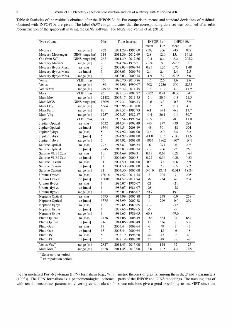
8 Verma et al.: Planetary ephemeris construction and test of relativity with MESSENGER
Table 4: Statistics of the residuals obtained after the INPOP13a fit. For comparison, means and standard deviations of residualsobtained with INPOP10e are given. The label GINS range indicates that the corresponding data set was obtained after orbitreconstruction of the spacecraft in using the GINS software. For MGS, see Verma et al. (2013).
Type of data Nbr Time Interval INPOP13a INPOP10emean 1-σ mean 1-σ
Mercury range [m] 462 1971.29 - 1997.60 -108 866 -45 872Mercury Messenger GINS range [m] 314 2011.39 - 2012.69 2.8 12.0 15.4 191.8Out from SC* GINS range [m] 267 2011.39 - 2012.66 -0.4 8.4 6.2 205.2Mercury Mariner range [m] 2 1974.24 - 1976.21 -124 56 -52.5 113Mercury flybys Mess ra [mas] 3 2008.03 - 2009.74 0.85 1.35 0.73 1.48Mercury flybys Mess de [mas] 3 2008.03 - 2009.74 2.4 2.4 2.4 2.5Mercury flybys Mess range [m] 3 2008.03 - 2009.74 -1.9 7.7 -5.05 5.8Venus VLBI [mas] 46 1990.70 - 2010.86 1.6 2.6 1.6 2.6Venus range [m] 489 1965.96 - 1990.07 502 2236 500 2235Venus Vex range [m] 24970 2006.32 - 2011.45 1.3 11.9 1.1 11.9Mars VLBI [mas] 96 1989.13 - 2007.97 -0.02 0.41 -0.00 0.41Mars Mex range [m] 21482 2005.17 - 2011.45 -2.1 20.6 -1.3 21.5Mars MGS GINS range [m] 13091 1999.31 - 2006.83 -0.6 3.3 -0.3 3.9Mars Ody range [m] 5664 2006.95 - 2010.00 1.6 2.3 0.3 4.1Mars Path range [m] 90 1997.51 - 1997.73 6.1 14.1 -6.3 13.7Mars Vkg range [m] 1257 1976.55 - 1982.87 -0.4 36.1 -1.4 39.7Jupiter VLBI [mas] 24 1996.54 - 1997.94 -0.5 11.0 -0.3 11.0Jupiter Optical ra [mas] 6532 1914.54 - 2008.49 -40 297 -39 297Jupiter Optical de [mas] 6394 1914.54 - 2008.49 -48 301 -48 301Jupiter flybys ra [mas] 5 1974.92 - 2001.00 2.6 2.9 2.4 3.2Jupiter flybys de [mas] 5 1974.92 - 2001.00 -11.0 11.5 -10.8 11.5Jupiter flybys range [m] 5 1974.92 - 2001.00 -1065 1862 -907 1646Saturne Optical ra [mas] 7971 1913.87 - 2008.34 -6 293 -6 293Saturne Optical de [mas] 7945 1913.87 - 2008.34 -12 266 -2 266Saturne VLBI Cass ra [mas] 10 2004.69 - 2009.31 0.19 0.63 0.21 0.64Saturne VLBI Cass de [mas] 10 2004.69 - 2009.31 0.27 0.34 0.28 0.33Saturne Cassini ra [mas] 31 2004.50 - 2007.00 0.8 3.4 0.8 3.9Saturne Cassini de [mas] 31 2004.50 - 2007.00 6.5 7.2 6.5 7.2Saturne Cassini range [m] 31 2004.50 - 2007.00 -0.010 18.44 -0.013 18.84Uranus Optical ra [mas] 13016 1914.52 - 2011.74 7 205 7 205Uranus Optical de [mas] 13008 1914.52 - 2011.74 -6 234 -6 234Uranus flybys ra [mas] 1 1986.07 - 1986.07 -21 -21Uranus flybys de [mas] 1 1986.07 - 1986.07 -28 -28Uranus flybys range [m] 1 1986.07 - 1986.07 20.7 19.7Neptune Optical ra [mas] 5395 1913.99 - 2007.88 2 258 0.0 258Neptune Optical de [mas] 5375 1913.99 - 2007.88 -1 299 -0.0 299Neptune flybys ra [mas] 1 1989.65 - 1989.65 -12 -12Neptune flybys de [mas] 1 1989.65 - 1989.65 -5 -5Neptune flybys range [m] 1 1989.65 - 1989.65 66.8 69.6Pluto Optical ra [mas] 2438 1914.06 - 2008.49 -186 664 34 654Pluto Optical de [mas] 2461 1914.06 - 2008.49 11 536 7 539Pluto Occ ra [mas] 13 2005.44 - 2009.64 6 49 3 47Pluto Occ de [mas] 13 2005.44 - 2009.64 -7 18 -6 18Pluto HST ra [mas] 5 1998.19 - 1998.20 -42 43 33 43Pluto HST de [mas] 5 1998.19 - 1998.20 31 48 28 48
Venus Vex** range [m] 2827 2011.45 - 2013.00 51 124 52 125Mars Mex** range [m] 4628 2011.45 - 2013.00 -3.0 11.5 4.2 27.5* Solar corona period** Extrapolation period
the Parametrized Post-Newtonian (PPN) formalism (e.g., Will(1993)). The PPN formalism is a phenomenological schemewith ten dimensionless parameters covering certain class of
metric theories of gravity, among them the β and γ parametersparts of the INPOP and GINS modelings. The tracking data ofspace missions give a good possibility to test GRT since the
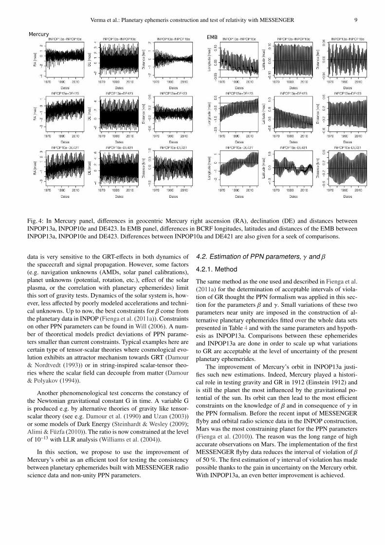
Verma et al.: Planetary ephemeris construction and test of relativity with MESSENGER 9
Fig. 4: In Mercury panel, differences in geocentric Mercury right ascension (RA), declination (DE) and distances betweenINPOP13a, INPOP10e and DE423. In EMB panel, differences in BCRF longitudes, latitudes and distances of the EMB betweenINPOP13a, INPOP10e and DE423. Differences between INPOP10a and DE421 are also given for a seek of comparisons.
data is very sensitive to the GRT-effects in both dynamics ofthe spacecraft and signal propagation. However, some factors(e.g. navigation unknowns (AMDs, solar panel calibrations),planet unknowns (potential, rotation, etc.), effect of the solarplasma, or the correlation with planetary ephemerides) limitthis sort of gravity tests. Dynamics of the solar system is, how-ever, less affected by poorly modeled accelerations and techni-cal unknowns. Up to now, the best constraints for β come fromthe planetary data in INPOP (Fienga et al. (2011a)). Constraintson other PPN parameters can be found in Will (2006). A num-ber of theoretical models predict deviations of PPN parame-ters smaller than current constraints. Typical examples here arecertain type of tensor-scalar theories where cosmological evo-lution exhibits an attractor mechanism towards GRT (Damour& Nordtvedt (1993)) or in string-inspired scalar-tensor theo-ries where the scalar field can decouple from matter (Damour& Polyakov (1994)).
Another phenomenological test concerns the constancy ofthe Newtonian gravitational constant G in time. A variable Gis produced e.g. by alternative theories of gravity like tensor-scalar theory (see e.g. Damour et al. (1990) and Uzan (2003))or some models of Dark Energy (Steinhardt & Wesley (2009);Alimi & Fuzfa (2010)). The ratio is now constrained at the levelof 10−13 with LLR analysis (Williams et al. (2004)).
In this section, we propose to use the improvement ofMercury’s orbit as an efficient tool for testing the consistencybetween planetary ephemerides built with MESSENGER radioscience data and non-unity PPN parameters.
4.2. Estimation of PPN parameters, γ and β
4.2.1. Method
The same method as the one used and described in Fienga et al.(2011a) for the determination of acceptable intervals of viola-tion of GR thought the PPN formalism was applied in this sec-tion for the parameters β and γ. Small variations of these twoparameters near unity are imposed in the construction of al-ternative planetary ephemerides fitted over the whole data setspresented in Table 4 and with the same parameters and hypoth-esis as INPOP13a. Comparisons between these ephemeridesand INPOP13a are done in order to scale up what variationsto GR are acceptable at the level of uncertainty of the presentplanetary ephemerides.
The improvement of Mercury’s orbit in INPOP13a justi-fies such new estimations. Indeed, Mercury played a histori-cal role in testing gravity and GR in 1912 (Einstein 1912) andis still the planet the most influenced by the gravitational po-tential of the sun. Its orbit can then lead to the most efficientconstraints on the knowledge of β and in consequence of γ inthe PPN formalism. Before the recent input of MESSENGERflyby and orbital radio science data in the INPOP construction,Mars was the most constraining planet for the PPN parameters(Fienga et al. (2010)). The reason was the long range of highaccurate observations on Mars. The implementation of the firstMESSENGER flyby data reduces the interval of violation of βof 50 %. The first estimation of γ interval of violation has madepossible thanks to the gain in uncertainty on the Mercury orbit.With INPOP13a, an even better improvement is achieved.

10 Verma et al.: Planetary ephemeris construction and test of relativity with MESSENGER
Fig. 5: Comparison between INPOP13a and INPOP10e estimations of MESSENGER orbit: (a) differences in the postfit Dopplerresiduals; (b) differences in the postfit range residuals; (c) differences in the periapsis altitude δp; (d) differences in the apoapsisaltitude δa.
Table 5: Intervals of violation for PPN parameters β and γ deduced from Figure 6 panel (a) labelled INPOP13a and Figure 6panel (b) labelled INPOP13aWF. Values from INPOP08 and INPOP10a are extracted from Fienga et al. (2010) and Fienga et al.(2011a) with a threshold for the variations of the postfit residuals of 5% given in Column 4. K11 stands for Konopliv et al.(2011), M08 for Muller et al. (2008), W09 for Williams et al. (2009), B03 for Bertotti et al. (2003) and L11 for Lambert & LePoncin-Lafitte (2011).
Fixed PPN Estimated PPN Limit [%] × 105
γ = 1 (β -1) INPOP08 5 (7.5 ± 12.5)INPOP10a 5 (-6.2 ± 8.1)INPOP13a 5 (-0.02 ± 0.12)INPOP13a 10 (-0.15 ± 0.70)INPOP13a 25 (0.2 ± 2.5)
γ = γB03 (β -1) INPOP10a 5 (-4.1 ± 7.80)INPOP13a 25 (-1.1 ± 1.1)
INPOP13aWF 5 (-0.25 ± 1.25)K11 (4± 24)
M08-LLR-SEP (15 ± 18)W09-LLR-SEP (12 ± 11)
β = 1 (γ -1) INPOP10a 5 (4.5 ± 7.5)INPOP13a 5 (0.0 ± 0.18)INPOP13a 10 (0.0 ± 1.1)INPOP13a 25 (-0.3 ± 2.5)
INPOP13aWF 5 (-0.1 ± 2.6)K11 (18 ± 26)
B03-CASS (2.1 ± 2.3)L11-VLB (-8 ± 12 )

Verma et al.: Planetary ephemeris construction and test of relativity with MESSENGER 11
Fig. 6: Variations of postfit residuals obtained for different values of PPN β (x-axis) and γ (y-axis). The panels (a) and (c) areobtained in considering the variations of the whole data sets when for the panels (b) and (d), variations of the Mercury flybydata (from Mariner and MESSENGER missions) are excluded from the analysis. The dash line indicates the limit in γ given byBertotti et al. (2003).
4.2.2. Results
Results obtained in term of percentages of variations of postfitresiduals between a planetary ephemeris fitted and built up withPPN parameters different from one and INPOP13a are given inFigure 6. The panel (a) of the Figure 6 gives the map of thevariations in % of the full dataset postfit residuals. The panel(b) of the Figure 6 gives the same map but without taking intoaccount the variations of the Mercury flyby data. Note that, forthe panel (b), the Mercury flybys data are indeed used in theephemerides fit but not in the analysis of the postfit residualsfor testing GR. The map of panels (a) and (b) is then dramati-cally different : where for the map including the Mariner data
the limits for β and γ are stringent, the constraints are greatlyenlarged for these two parameters. These phenomena were ex-pected as the variations of PPN parameters induce long termperturbations in the geocentric distances of Mercury as one cansee on Figure 7. The panels (c) and (d) are similar to (a) and(b), respectively, but obtained with ephemeris INPOP10a. Inthis ephemeris, MESSENGER flyby data were included its fitsbut not the orbital data. By comparing panels (a) and (c), onecan see that the use of the MESSENGER orbital data reducesignificantly the intervals of violation for both PPN parametersby a factor 10. In a same manner, in the most pessimistic case,without considering the Mercury flybys in the analysis of the
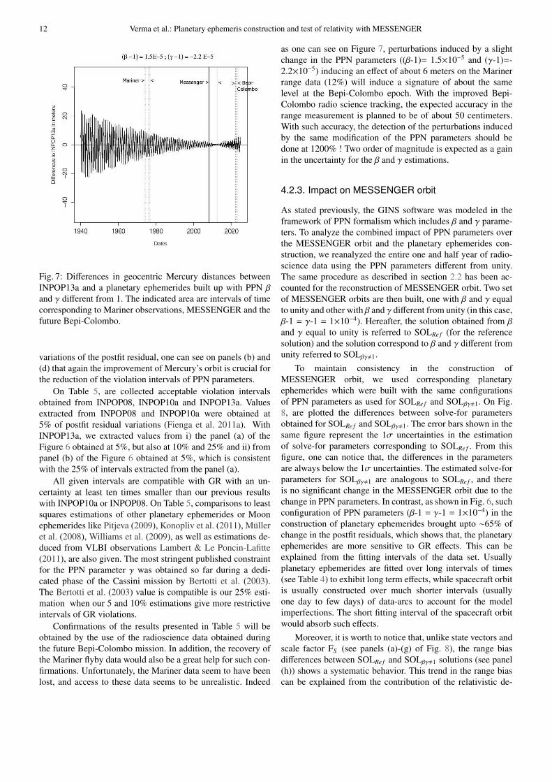
12 Verma et al.: Planetary ephemeris construction and test of relativity with MESSENGER
Fig. 7: Differences in geocentric Mercury distances betweenINPOP13a and a planetary ephemerides built up with PPN βand γ different from 1. The indicated area are intervals of timecorresponding to Mariner observations, MESSENGER and thefuture Bepi-Colombo.
variations of the postfit residual, one can see on panels (b) and(d) that again the improvement of Mercury’s orbit is crucial forthe reduction of the violation intervals of PPN parameters.
On Table 5, are collected acceptable violation intervalsobtained from INPOP08, INPOP10a and INPOP13a. Valuesextracted from INPOP08 and INPOP10a were obtained at5% of postfit residual variations (Fienga et al. 2011a). WithINPOP13a, we extracted values from i) the panel (a) of theFigure 6 obtained at 5%, but also at 10% and 25% and ii) frompanel (b) of the Figure 6 obtained at 5%, which is consistentwith the 25% of intervals extracted from the panel (a).
All given intervals are compatible with GR with an un-certainty at least ten times smaller than our previous resultswith INPOP10a or INPOP08. On Table 5, comparisons to leastsquares estimations of other planetary ephemerides or Moonephemerides like Pitjeva (2009), Konopliv et al. (2011), Mulleret al. (2008), Williams et al. (2009), as well as estimations de-duced from VLBI observations Lambert & Le Poncin-Lafitte(2011), are also given. The most stringent published constraintfor the PPN parameter γ was obtained so far during a dedi-cated phase of the Cassini mission by Bertotti et al. (2003).The Bertotti et al. (2003) value is compatible is our 25% esti-mation when our 5 and 10% estimations give more restrictiveintervals of GR violations.
Confirmations of the results presented in Table 5 will beobtained by the use of the radioscience data obtained duringthe future Bepi-Colombo mission. In addition, the recovery ofthe Mariner flyby data would also be a great help for such con-firmations. Unfortunately, the Mariner data seem to have beenlost, and access to these data seems to be unrealistic. Indeed
as one can see on Figure 7, perturbations induced by a slightchange in the PPN parameters ((β-1)= 1.5×10⁻⁵ and (γ-1)=-2.2×10⁻⁵) inducing an effect of about 6 meters on the Marinerrange data (12%) will induce a signature of about the samelevel at the Bepi-Colombo epoch. With the improved Bepi-Colombo radio science tracking, the expected accuracy in therange measurement is planned to be of about 50 centimeters.With such accuracy, the detection of the perturbations inducedby the same modification of the PPN parameters should bedone at 1200% ! Two order of magnitude is expected as a gainin the uncertainty for the β and γ estimations.
4.2.3. Impact on MESSENGER orbit
As stated previously, the GINS software was modeled in theframework of PPN formalism which includes β and γ parame-ters. To analyze the combined impact of PPN parameters overthe MESSENGER orbit and the planetary ephemerides con-struction, we reanalyzed the entire one and half year of radio-science data using the PPN parameters different from unity.The same procedure as described in section 2.2 has been ac-counted for the reconstruction of MESSENGER orbit. Two setof MESSENGER orbits are then built, one with β and γ equalto unity and other with β and γ different from unity (in this case,β-1 = γ-1 = 1×10⁻⁴). Hereafter, the solution obtained from βand γ equal to unity is referred to SOLRe f (for the referencesolution) and the solution correspond to β and γ different fromunity referred to SOLβγ,1.
To maintain consistency in the construction ofMESSENGER orbit, we used corresponding planetaryephemerides which were built with the same configurationsof PPN parameters as used for SOLRe f and SOLβγ,1. On Fig.8, are plotted the differences between solve-for parametersobtained for SOLRe f and SOLβγ,1. The error bars shown in thesame figure represent the 1σ uncertainties in the estimationof solve-for parameters corresponding to SOLRe f . From thisfigure, one can notice that, the differences in the parametersare always below the 1σ uncertainties. The estimated solve-forparameters for SOLβγ,1 are analogous to SOLRe f , and thereis no significant change in the MESSENGER orbit due to thechange in PPN parameters. In contrast, as shown in Fig. 6, suchconfiguration of PPN parameters (β-1 = γ-1 = 1×10⁻⁴) in theconstruction of planetary ephemerides brought upto ∼65% ofchange in the postfit residuals, which shows that, the planetaryephemerides are more sensitive to GR effects. This can beexplained from the fitting intervals of the data set. Usuallyplanetary ephemerides are fitted over long intervals of times(see Table 4) to exhibit long term effects, while spacecraft orbitis usually constructed over much shorter intervals (usuallyone day to few days) of data-arcs to account for the modelimperfections. The short fitting interval of the spacecraft orbitwould absorb such effects.
Moreover, it is worth to notice that, unlike state vectors andscale factor FS (see panels (a)-(g) of Fig. 8), the range biasdifferences between SOLRe f and SOLβγ,1 solutions (see panel(h)) shows a systematic behavior. This trend in the range biascan be explained from the contribution of the relativistic de-
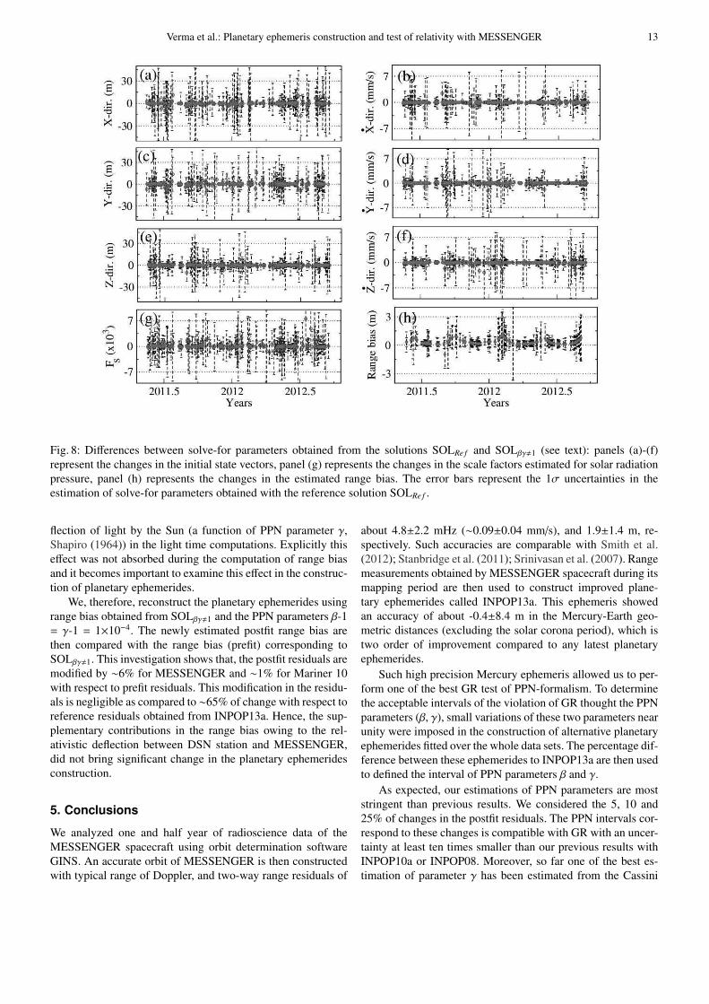
Verma et al.: Planetary ephemeris construction and test of relativity with MESSENGER 13
Fig. 8: Differences between solve-for parameters obtained from the solutions SOLRe f and SOLβγ,1 (see text): panels (a)-(f)represent the changes in the initial state vectors, panel (g) represents the changes in the scale factors estimated for solar radiationpressure, panel (h) represents the changes in the estimated range bias. The error bars represent the 1σ uncertainties in theestimation of solve-for parameters obtained with the reference solution SOLRe f .
flection of light by the Sun (a function of PPN parameter γ,Shapiro (1964)) in the light time computations. Explicitly thiseffect was not absorbed during the computation of range biasand it becomes important to examine this effect in the construc-tion of planetary ephemerides.
We, therefore, reconstruct the planetary ephemerides usingrange bias obtained from SOLβγ,1 and the PPN parameters β-1= γ-1 = 1×10⁻⁴. The newly estimated postfit range bias arethen compared with the range bias (prefit) corresponding toSOLβγ,1. This investigation shows that, the postfit residuals aremodified by ∼6% for MESSENGER and ∼1% for Mariner 10with respect to prefit residuals. This modification in the residu-als is negligible as compared to ∼65% of change with respect toreference residuals obtained from INPOP13a. Hence, the sup-plementary contributions in the range bias owing to the rel-ativistic deflection between DSN station and MESSENGER,did not bring significant change in the planetary ephemeridesconstruction.
5. Conclusions
We analyzed one and half year of radioscience data of theMESSENGER spacecraft using orbit determination softwareGINS. An accurate orbit of MESSENGER is then constructedwith typical range of Doppler, and two-way range residuals of
about 4.8±2.2 mHz (∼0.09±0.04 mm/s), and 1.9±1.4 m, re-spectively. Such accuracies are comparable with Smith et al.(2012); Stanbridge et al. (2011); Srinivasan et al. (2007). Rangemeasurements obtained by MESSENGER spacecraft during itsmapping period are then used to construct improved plane-tary ephemerides called INPOP13a. This ephemeris showedan accuracy of about -0.4±8.4 m in the Mercury-Earth geo-metric distances (excluding the solar corona period), which istwo order of improvement compared to any latest planetaryephemerides.
Such high precision Mercury ephemeris allowed us to per-form one of the best GR test of PPN-formalism. To determinethe acceptable intervals of the violation of GR thought the PPNparameters (β, γ), small variations of these two parameters nearunity were imposed in the construction of alternative planetaryephemerides fitted over the whole data sets. The percentage dif-ference between these ephemerides to INPOP13a are then usedto defined the interval of PPN parameters β and γ.
As expected, our estimations of PPN parameters are moststringent than previous results. We considered the 5, 10 and25% of changes in the postfit residuals. The PPN intervals cor-respond to these changes is compatible with GR with an uncer-tainty at least ten times smaller than our previous results withINPOP10a or INPOP08. Moreover, so far one of the best es-timation of parameter γ has been estimated from the Cassini
14 Verma et al.: Planetary ephemeris construction and test of relativity with MESSENGER
observations by Bertotti et al. (2003), which is compatible withour 25% of estimation.
Moreover, to further improve the accuracy of the PPN pa-rameters, and to confirmed the results given in Table 5, oneneeds to analysis the radioscience data of the future Bepi-Colombo mission.
6. Acknowledgments
We are very thankful to CNES and Region Franche-Comte,who gave us finical support for pursuing these studies. The partof this work is done using GINS software, we would like to ac-knowledge CNES who provided us access to this software. A.K. Verma is thankful to P. Rosenbatt and S. Le Maistre for thefruitful discussion. We are also thankful to G.Esposito-Faresefor his constructive remarks and comments.
References
Alimi, J.-M. & Fuzfa, A. 2010, in American Institute of PhysicsConference Series, Vol. 1241, American Institute of PhysicsConference Series, ed. J.-M. Alimi & A. Fuozfa, 690–699
Anderson, J. D., Colombo, G., Espsitio, P. B., Lau, E. L., &Trager, G. B. 1987, Icarus, 71, 337
Anderson, J. D., Jurgens, R. F., Lau, E. L., Slade, III, M. A., &Schubert, G. 1996, Icarus, 124, 690
Anderson, J. D., Turyshev, S. G., Asmar, S. W., et al. 1997,Planet. Space Sci., 45, 21
Bertotti, B., Iess, L., & Tortora, P. 2003, Nature, 425, 374Damour, T., Gibbons, G. W., & Gundlach, C. 1990, Physical
Review Letters, 64, 123Damour, T. & Nordtvedt, K. 1993, Phys. Rev. D, 48, 3436Damour, T. & Polyakov, A. M. 1994, General Relativity and
Gravitation, 26, 1171Ercol, C. J., M., B. S., & Holtzman, G. A. 2012, in Thermal
and Fluids Analysis Workshop, TFAWS2012-PT-03Fienga, A., Laskar, J., Kuchynka, P., et al. 2010, in IAU
Symposium, Vol. 261, IAU Symposium, ed. S. A. Klioner,P. K. Seidelmann, & M. H. Soffel, 159–169
Fienga, A., Laskar, J., Manche, H., et al. 2011a, CelestialMechanics and Dynamical Astronomy
Fienga, A., Laskar, J., Morley, T., et al. 2009, Astronomy &Astrophysics, 507, 1675
Fienga, A., Manche, H., a. L. J., & Gastineau, M. 2008,Astronomy & Astrophysics, 477, 315
Fienga, A., Manche, H., Laskar, J., Gastineau, M., & Verma,A. 2013, ArXiv e-prints
Flanigan, S. H., OShaughnessy, D. J., Wilson, M. N., &Hill, T. A. 2013, in 23rd Space Flight Mechanics Meeting,American Astronomical Society, 13–382
Folkner, W. M. 2010, JPL, interoffice memorandum, IOM343R-10-001
Konopliv, A. S., Asmar, S. W., Folkner, W. M., et al. 2011,icarus, 211, 401
Lambert, S. B. & Le Poncin-Lafitte, C. 2011, A&A, 529, A70
Manche, H., Fienga, A., Laskar, J., et al. 2010, in JourneesSystemes de Reference Spatio-temporels 2010, JourneesSystemes de references
Margot, J.-L. 2009, Celestial Mechanics and DynamicalAstronomy, 105, 329
Moyer, T. D. 2003, Formulation for Observed and ComputedValues of Deep Space Network Data Types for Navigation,Vol. 2 (John Wiley & Sons)
Muller, J., Soffel, M., & Klioner, S. A. 2008, Journal ofGeodesy, 82, 133
Pitjeva, E. V. 2009, in IAU Symposium, AmericanAstronomical Society, Vol. 261, 603
Shapiro, I. I. 1964, Physical Review Letters, 13, 789Smith, D. E., Zuber, M. T., Phillips, R. J., et al. 2012, Science,
336, 214Smith, D. E., Zuber, M. T., Phillips, R. J., et al. 2010, icarus,
209, 88Solomon, S. C., McNutt, R. L., Gold, R. E., & Domingue, D. L.
2007, Space Sci. Rev., 131, 3Srinivasan, D. K., Perry, M. E., Fielhauer, K. B., Smith, D. E.,
& Zuber, M. T. 2007, Space Science Reviews, 131, 557Stanbridge, D. R., Williams, K. E., Taylor, A. H., et al. 2011,
in AAS/AIAA Astrodynamics Specialist Conference, AAS11-548
Steinhardt, P. J. & Wesley, D. 2009, Phys. Rev. D, 79, 104026Uzan, J.-P. 2003, Annales Henri Poincare, 4, 347Vaughan, R. M., Haley, D. R., OShaughnessy, D. J., & Shapiro,
H. S. 2002, Advances in the Astronautical Sciences, 109,1139
Verma, A. K., Fienga, A., Laskar, J., et al. 2013, Astronomy &Astrophysics, 550, A124
Will, C. M., ed. 1993, pp. 396. ISBN 0521439736, Theory andExperiment in Gravitational Physics (Cambridge UniversityPress)
Will, C. M. 2006, Living Reviews in Relativity, 9, 3Williams, J. G., Turyshev, S. G., & Boggs, D. H. 2004, Physical
Review Letters, 93, 261101Williams, J. G., Turyshev, S. G., & Boggs, D. H. 2009,
International Journal of Modern Physics D, 18, 1129
157
Chapter 6
General conclusions
This thesis has been essentially motivated by the independent analysis of the past and presentspace mission radiometric data, and to provide data analysis tools for the improvement of theplanetary ephemerides INPOP, as well as to use improved ephemerides to perform tests ofphysics such as general relativity, solar corona studies, etc.
The thesis has presented the research results obtained from the direct analysis of the MGSand MESSENGER radiometric raw data. To start the analysis, we have first developed anindependent software to extract the contents of the Orbit Data Files (ODFs). These contentsare then used to reconstruct the precise orbits of the MGS and MESSENGER spacecraft usingGINS software developed by CNES. In addition, based on the algorithms given in Chapter 2,we have also developed an independent light time solution software in order to treat the JPLlight time data.
The first part of the thesis deals with the analysis of the MGS radiometric data as an aca-demic case to test our understanding of the raw radiometric data and their analysis with GINS bycomparing our results with the literature. We have analyzed the entire radioscience data of MGSsince 1999 to 2006 using Box-Wing macro-model consisting ten-plate and a parabolic high gainantenna. On average, an estimated root mean square (rms) value of the post-fit Doppler- andtwo-way range residuals are less than 5 mHz and 1 m respectively, excluding the residuals atthe time of solar conjunctions. Such accuracy of the orbit and of the estimated parameters (seeChapter 3) are consistent with the results found in the literature (Yuan et al. (2001); Lemoineet al. (2001); Konopliv et al. (2006); Marty et al. (2009), see Table 3.3). Moreover, we alsocompared range bias that were computed from GINS with the reduced light time data providedby JPL. These range bias are consistent with each other, and hence confirm the validity of ouranalysis with respect to JPL ODP software.
Furthermore, the study has been also performed to understand the impact of the macro-model over the orbit perturbations and the estimated parameters. Instead to a Box-Wing macro-model, a Spherical macro-model was used for a new analysis of the entire radiometric data. By
158 6. General conclusions
comparing the outcomes of these models (see Chapter 3), we confirmed that, in the absence ofprecise knowledge of the spacecraft characteristics, short data-arc can be preferable to accountfor the mis-modeling in the spacecraft model without costing the orbit accuracy. However, thisanalysis may be not preferable for extracting an accurate geophysical signals from the Dopplermeasurements, such as the estimation of gravity field coefficients.
As a supplementary exploitation of MGS, we also performed solar physic studies for thefirst time using range bias data acquired at the time of solar conjunction periods. In additionto MGS, range bias data of MEX and VEX missions were also used and allowed us to analyzethe large-scale structure of the electron density of the solar corona since 2001 to 2011. The pa-rameters of the solar corona models, estimated separately for each spacecraft at different phasesof solar activity (maximum and minimum) and at different solar wind states (slow and fast),are then deduced from these data using least square techniques. We compared our estimateswith earlier results obtained with different methods. These estimates were found to be consis-tent during the same solar activities, especially during solar minima. However, during the solarmaxima, electron densities obtained with different methods or different spacecraft show weakerconsistencies.
We have also demonstrated the impact of solar corona correction on the construction ofplanetary ephemerides. Data acquired during the period of solar conjunctions show a severedegradation in the radio signals and consequently in the range bias. The observations obtainedtwo months before and after the conjunctions were therefore usually removed from the fitteddata sample of planetary ephemerides. The supplementary data, corrected from the solar coronaperturbations, allowed us to gain ∼8% of whole data set. Such corrected data are then usedfor the first time in the construction of INPOP and induce a noticeable improvement in theestimation of the asteroid masses and a better long-term behavior of the ephemerides. Theseresults are published in the Astronomy & Astrophysics journal, Verma et al. (2013a).
After the successful analysis of the MGS radiometric data, the second part of the thesis dealswith the complete analysis of the MESSENGER tracking data. MESSENGER is the first space-craft orbiting Mercury. It therefore gives an ample opportunity to improve our knowledge of theMercury orbit and also to perform one of the most sensitive GR tests of PPN-formalism. Weanalyzed one and half year of radioscience data using GINS software. The Box-Wing macro-model of the MESSENGER spacecraft was seen as a combination of flat plates arranged in theshape of a box, with attached solar arrays. For orbit computation and for parameters estimation,a multi-arc approach was used to get an independent estimate of the MESSENGER accelera-tions. In this method, we integrated the equations of motion using the time step of 50s and then,orbital fits were obtained from short data-arcs fitted over the observation span of one-day usingan iterative process. Excluding solar corona period, the estimated typical mean and rms valueof postfit Doppler, and two-way range residuals of about -0.00063±4.8 mHz, and -0.003±1.5m respectively. Such accuracies are comparable with Genova et al. (2013); Smith et al. (2012);Stanbridge et al. (2011); Srinivasan et al. (2007).
The range bias computed from the GINS are then used for further refinement in the Mer-cury ephemeris. Using these range bias, we built the planetary ephemerides INPOP13a. This
6. General conclusions 159
ephemeris showed an accuracy of -0.4±8.4 m in the geocentric Mercury residuals excludingsolar corona period, which is two order of improvement than any latest planetary ephemerides(e.g INPOP10e (21±187 m) and DE423 (15±105 m)). The GR tests of PPN-formalism werethen performed with such high precision Mercury ephemerides. To determine the acceptable in-tervals of the violation of GR thought the PPN parameters (β, γ), small variations of these twoparameters near unity were imposed in the construction of alternative planetary ephemeridesfitted over the whole data sets. The percentage difference between these ephemerides to IN-POP13a are then used to define the intervals of PPN parameters β and γ.
As expected, our estimations of PPN parameters are most stringent than previous results. Weconsidered 5, 10 and 25% of changes in the postfit residuals. The PPN intervals correspondingto these changes are compatible with GR with an uncertainty at least ten times smaller than ourprevious results with INPOP10a or INPOP08. Moreover, so far one of the best estimation ofparameter γ has been estimated from the Cassini observations by Bertotti et al. (2003), whichis compatible with our 25% of estimation. Furthermore, our 5 and 10% estimations give noindication of possible asymmetry. We also demonstrated that, despite the less quantity andquality of the Mariner 10 data, these latest are very important to consider for long term effectsof the PPN parameters. The results of this study are submitted for publication in Astronomy &Astrophysics, Verma et al. (2013b).
In 2015, the BepiColombo mission, a joint mission of the European Space Agency (ESA)and the Japan Aerospace and eXploration Agency (JAXA) to the planet Mercury, will be launch.The main future work will be therefore to analyze the radioscience data obtained from thismission to further improvement in the accuracy of the PPN parameters. Moreover, the toolsdeveloped during these thesis will also be useful for the analysis of past, present, and fu-ture space missions, such as Odyssey, MRO etc..., and to deliver most up-to-date high accu-rate ephemerides to the users. This will definitely propel INPOP at the forefront of planetaryephemerides and will make team INPOP independent from the navigation team of the spaceagencies.

160 6. General conclusions
161
Publications
• Verma, A. K., Fienga, A., Laskar, J., Manche, H., Gastineau, M., 2013b. Use of MES-SENGER radioscience data to improve planetary ephemeris and to test general relativity.Astronomy & Astrophysics, submitted.
• Verma, A. K., Fienga, A., Laskar, J., Issautier, K., Manche, H., Gastineau, M., Feb.2013a. Electron density distribution and solar plasma correction of radio signals us-ing MGS, MEX, and VEX spacecraft navigation data and its application to planetaryephemerides. Astronomy & Astrophysics 550, A124.
• Fienga, A.; Manche, H.; Laskar, J.; Gastineau, M.; Verma, A. INPOP new release: IN-POP10e. eprint arXiv:1301.1510, 2013.
• Fienga, A.; Laskar, J.; Verma, A.; Manche, H.; Gastineau, M. INPOP: Evolution, appli-cations, and perspective. SF2A-2012: Proceedings of the Annual meeting of the FrenchSociety of Astronomy and Astrophysics. Eds.: S. Boissier, P. de Laverny, N. Nardetto, R.Samadi, D. Valls-Gabaud and H. Wozniak, pp.25-33, 2012.
• Verma, A.K., Fienga, A. New developments in spacecraft raw data direct analysis for theINPOP planetary ephemerides. IAU Joint Discussion 7: Space-Time Reference Systemsfor Future Research at IAU General Assembly-Beijing, id.39, August 2012.
• Verma, A.K., Fienga. INPOP: The planetary ephemerides and its applications. 39thCOSPAR Scientific Assembly, 14-22 July 2012, Mysore, India. Abstract C5.1- 15-12,p.2082.
• Verma, A.K., Fienga, A. Electron density distribution and solar plasma correction of ra-dio signals using MGS, MEX and VEX spacecraft navigation data and its application toplanetary ephemerides. 39th COSPAR Scientific Assembly, 14-22 July 2012, Mysore,India. Abstract D3.5-5-12, p.2081.
• Verma, A.K., Fienga, A. Re-Estimation of Solar Corona Coefficients (a, b, c) by UsingMGS & Mex Spacecraft Data. EPSC-DPS Joint Meeting 2011, 2-7 October 2011, Nantes,France, 2011epsc.conf.1828V.

162 Publications
163
Bibliography
Afonso, G., Barlier, F., Mignard, F., Carpino, M., Farinella, P., Oct. 1989. Orbital effects ofLAGEOS seasons and eclipses. Annales Geophysicae 7, 501–514.
Albee, A. L., Arvidson, R. E., Palluconi, F., Thorpe, T., Oct. 2001. Overview of the Mars GlobalSurveyor mission. Journal of Geophysical Research 106, 23291–23316.
Anderson, J. D., Colombo, G., Espsitio, P. B., Lau, E. L., Trager, G. B., Sep. 1987a. The mass,gravity field, and ephemeris of Mercury. Icarus71, 337–349.
Anderson, J. D., Jurgens, R. F., Lau, E. L., Slade, III, M. A., Schubert, G., Dec. 1996. Shapeand Orientation of Mercury from Radar Ranging Data. Icarus124, 690–697.
Anderson, J. D., Keesey, M. S. W., Lau, E. L., Standish, Jr., E. M., Newhall, X. X., 1978.Tests of general relativity using astrometric and radio metric observations of the planets.Acta Astronautica 5, 43.
Anderson, J. D., Keesey, M. S. W., Lau, E. L., Standish, Jr., E. M., Newhall, X. X.,V. N. Novikov & D. N. Cheverov (Eds.), Oct. 1976. Tests of general relativity using as-trometric and radiometric observations of the planets.
Anderson, J. D., Krisher, T. P., Borutzki, S. E., Connally, M. J., Eshe, P. M., Hotz, H. B.,Kinslow, S., Kursinski, E. R., Light, L. B., Matousek, S. E., Moyd, K. I., Roth, D. C., Sweet-nam, D. N., Taylor, A. H., Tyler, G. L., Gresh, D. L., Rosen, P. A., Dec. 1987b. Radio rangemeasurements of coronal electron densities at 13 and 3.6 centimeter wavelengths during the1985 solar conjunction of Voyager 2. The Astrophysical Journal 323, L141–L143.
Anderson, J. D., Turyshev, S. G., Asmar, S. W., Bird, M. K., Konopliv, A. S., Krisher, T. P.,Lau, E. L., Schubert, G., Sjogren, W. L., Jan. 1997. Radio-science investigation on a MercuryOrbiter mission. Planet. Space Sci.45, 21–29.
Ash, M. E., Shapiro, I. I., Smith, W. B., Apr. 1967. Astronomical constants and planetaryephemerides deduced from radar and optical observations. AJ72, 338–+.
Barlier, F., Berger, C., Falin, J. L., Kockarts, G., Thuillier, G., Mar. 1978. A thermosphericmodel based on satellite drag data. Annales de Geophysique 34, 9–24.
Bertotti, B., Ciufolini, I., Bender, P. L., Mar. 1987. New test of general relativity - Measurementof de Sitter geodetic precession rate for lunar perigee. Physical Review Letters 58, 1062–1065.
164 BIBLIOGRAPHY
Bertotti, B., Iess, L., Tortora, P., Sep. 2003. A test of general relativity using radio links withthe Cassini spacecraft. Nature425, 374–376.
Bird, M. K., Paetzold, M., Edenhofer, P., Asmar, S. W., McElrath, T. P., Dec. 1996. Coro-nal radio sounding with Ulysses: solar wind electron density near 0.1AU during the 1995conjunction. Astronomy & Astrophysics 316, 441–448.
Bird, M. K., Volland, H., Paetzold, M., Edenhofer, P., Asmar, S. W., Brenkle, J. P., May 1994.The coronal electron density distribution determined from dual-frequency ranging measure-ments during the 1991 solar conjunction of the ULYSSES spacecraft. The AstrophysicalJournal 426, 373–381.
Bougeret, J.-L., King, J. H., Schwenn, R., Feb. 1984. Solar radio burst and in situ determinationof interplanetary electron density. Solar Physics 90, 401–412.
Bravo, S., Stewart, G. A., Nov. 1997. Fast and Slow Wind from Solar Coronal Holes. ApJ489,992.
Cash, P., Emmons, D., Welgemoed, J., Dec. 2008. Ultra-stable oscillators for space application.In: 40th Annual Precise Time and Time Interval (PTTI) Meeting. pp. 51–56.
Chao, C. C., Oct. 1971. New Tropospheric Range Corrections with Seasonal Adjustment. NewTropospheric Range Corrections with Seasonal Adjustment, Deep Space Network ProgressReport, 31-1526, VI, 67-82 31.
Ciufolini, I., Jan. 1986. Measurement of the Lense-Thirring drag on high-altitude, laser-rangedartificial satellites. Physical Review Letters 56, 278–281.
Davies, M. E., Abalakin, V. K., Bursa, M., Lieske, J. H., Morando, B., Morrison, D.,Seidelmann, P. K., Sinclair, A. T., Yallop, B., Tjuflin, Y. S., Jan. 1996. Report of theIAU/IAG/COSPAR Working Group on Cartographic Coordinates and Rotational Elementsof the Planets and Satellites: 1994. Celestial Mechanics and Dynamical Astronomy 63, 127–148.
Dow, J. M., 1988. An improved tidal model for high accuracy satellite orbit determination. In:16th International Symposium on Space Technology and Science, Vol. 1. Vol. 1. pp. 701–705.
Eshleman, V. R., Tyler, G. L., Anderson, J. D., Fjeldbo, G., Levy, G. S., Wood, G. E., Croft,T. A., Nov. 1977. Radio science investigations with Voyager. Space Science Reviews 21,207–232.
Feldman, U., Landi, E., Schwadron, N. A., Jul. 2005. On the sources of fast and slow solarwind. Journal of Geophysical Research (Space Physics) 110, 7109.
Fienga, A., May 2011. Ephemerides planetaires et systemes de reference. Habilitation a Dirigerdes Recherches, Universeite de Franche-Comte - Observatoire de Besancon, in French.
Fienga, A., Kuchynka, P., Laskar, J., Manche, H., , Gastineau, M., Oct. 2011b. Asteroid massdeterminations with the inpop planetary ephemerides. EPSC-DPS Join Meeting 2011. p.1879.
BIBLIOGRAPHY 165
Fienga, A., Laskar, J., Kuchynka, P., Le Poncin-Lafitte, C., Manche, H., Gastineau, M., Jan.2010. Gravity tests with INPOP planetary ephemerides. In: Klioner, S. A., Seidelmann, P. K.,Soffel, M. H. (Eds.), IAU Symposium. Vol. 261 of IAU Symposium. pp. 159–169.
Fienga, A., Laskar, J., Manche, H., Kuchynka, P., Desvignes, G., Gastineau, M, ., Cognard,I., a. G., 2011a. The planetary ephemerides inpop10a and its applications in fundamentalphysics. Celestial Mechanics and Dynamical Astronomy.
Fienga, A., Laskar, J., Morley, T., Manche, H., Kuchynka, P., Le Poncin-Lafitte, C., Budnik,F., Gastineau, M., Somenzi, L., Dec. 2009. INPOP08, a 4-D planetary ephemeris: fromasteroid and time-scale computations to ESA Mars Express and Venus Express contributions.Astronomy & Astrophysics 507, 1675–1686.
Fienga, A., Manche, H., a. L. J., Gastineau, M., 2008. Inpop06: a new numerical planetaryephemeris. Astronomy & Astrophysics 477, 315–327.
Fienga, A., Manche, H., Laskar, J., Gastineau, M., Verma, A., Jan. 2013. INPOP new release:INPOP10e. ArXiv e-prints.
Fjeldbo, G., Kliore, A. J., Eshleman, V. R., Mar. 1971. The Neutral Atmosphere of Venus asStudied with the Mariner V Radio Occultation Experiments. Astronomical Journal 76, 123.
Flanigan, S. H., OShaughnessy, D. J., Wilson, M. N., Hill, T. A., 2013. MESSENGER ma-neuvers to reduce orbital period during the extended mission: Ensuring maximum use ofthe bi-propellant propulsion system. In: 23rd Space Flight Mechanics Meeting, AmericanAstronomical Society. pp. 13–382.
Folkner, W. M., Feb. 2010. Planetary ephemeris DE423 fit to Messenger encounters with Mer-cury. JPL, interoffice memorandum IOM 343R-10-001.
Folkner, W. M., Williams, J. G., Boggs, D. H., Mar. 2008. JPL planetary and lunar ephemeridesDE421, IOM 343R-08-003.
Genova, A., Iess, L., Marabucci, M., Jun. 2013. Mercury’s gravity field from the first six monthsof MESSENGER data. Planet. Space Sci.81, 55–64.
Guhathakurta, M., Holzer, T. E., May 1994. Density structure inside a polar coronal hole. TheAstrophysical Journal 426, 782–786.
Guhathakurta, M., Holzer, T. E., MacQueen, R. M., Feb. 1996. The Large-Scale Density Struc-ture of the Solar Corona and the Heliospheric Current Sheet. The Astrophysical Journal 458,817.
Hairer, E., Norsett, S. P., Wanner, G. (Eds.), 1987. Solving Ordinary Differential Equations I:Nonstiff Problems. Springer series in Computational Mathematics. Springer.
Hassler, D. M., Dammasch, I. E., Lemaire, P., Brekke, P., Curdt, W., Mason, H. E., Vial, J.-C., Wilhelm, K., Feb. 1999. Solar Wind Outflow and the Chromospheric Magnetic Network.Science 283, 810.
166 BIBLIOGRAPHY
Hedin, A. E., Fleming, E. L., Manson, A. H., Schmidlin, F. J., Avery, S. K., Clark, R. R., Franke,S. J., Fraser, G. J., Tsuda, T., Vial, F., Vincent, R. A., Sep. 1996. Empirical wind model forthe upper, middle and lower atmosphere. Journal of Atmospheric and Terrestrial Physics 58,1421–1447.
Howard, H. T., Tyler, G. L., Fjeldbo, G., Kliore, A. J., Levy, G. S., Brunn, D. L., Dickin-son, R., Edelson, R. E., Martin, W. L., Postal, R. B., Seidel, B., Sesplaukis, T. T., Shirley,D. L., Stelzried, C. T., Sweetnam, D. N., Zygielbaum, A. I., Esposito, P. B., Anderson, J. D.,Shapiro, I. I., Reasenberg, R. D., Mar. 1974. Venus: Mass, Gravity Field, Atmosphere, andIonosphere as Measured by the Mariner 10 Dual-Frequency Radio System. Science 183,1297–1301.
Huang, C., Ries, J. C., Tapley, B. D., Watkins, M. M., Jun. 1990. Relativistic effects for near-earth satellite orbit determination. Celestial Mechanics and Dynamical Astronomy 48, 167–185.
Hudson, H., Haisch, B., Strong, K. T., Mar. 1995. Comment on ’The solar flare myth’ by J. T.Gosling. J. Geophys. Res.100, 3473–3477.
Issautier, K., Meyer-Vernet, N., Moncuquet, M., Hoang, S., Feb. 1998. Solar wind radial andlatitudinal structure - Electron density and core temperature from ULYSSES thermal noisespectroscopy. Journal of Geophysical Research 103, 1969.
Jacchia, L. G., Mar. 1977. Thermospheric Temperature, Density, and Composition: New Mod-els. SAO Special Report 375.
Kallenrode, M.-B., 2004. Space physics : an introduction to plasmas and particles in the helio-sphere and magnetospheres.
Kaula, W. M. (Ed.), 1966. Theory of satellite geodesy: Applications of satellites to geodesy.Dover Publications.
Klioner, S. A., Feb. 2008. Relativistic scaling of astronomical quantities and the system ofastronomical units. A&A478, 951–958.
Kojima, M., Kakinuma, T., Aug. 1990. Solar cycle dependence of global distribution of solarwind speed. Space Sci Rev, 53, 173–222.
Konopliv, A. S., Asmar, S. W., Folkner, W. M., Karatekin, Ö., Nunes, D. C., Smrekar, S. E.,Yoder, C. F., Zuber, M. T., Jan. 2011. Mars high resolution gravity fields from MRO, Marsseasonal gravity, and other dynamical parameters. icarus 211, 401–428.
Konopliv, A. S., Yoder, C. F., Standish, E. M., Yuan, D.-N., Sjogren, W. L., May 2006. Aglobal solution for the Mars static and seasonal gravity, Mars orientation, Phobos and Deimosmasses, and Mars ephemeris. Icarus 182, 23–50.
Kuchynka, P., 2010. Etude des perturbations induites par les asteroides sur les mouvements desplanetes et des sondes spatiales autour du point de lagrange l2. PhD in astronomy, Observa-toire de Paris.
BIBLIOGRAPHY 167
Kwok, A., 2000. TRK-2-18 Tracking System Interfaces Orbit Data File Interface. TRK-2-18Tracking System Interfaces Orbit Data File Interface, Deep Space Mission System, JPL D-16765, 820-013.
Lainey, V., Dehant, V., Pätzold, M., Apr. 2007. First numerical ephemerides of the Martianmoons. Astronomy and Astrophysics 465, 1075–1084.
Lang, K. R., Sep. 2000. The Sun From Space. Ap&SS273, 1–6.
Lawson, C. L., Hanson, R. J., 1995. Solving Least Squares Problems. SIAM, Philadelphia, PA.
Leary, J. C., Conde, R. F., Dakermanji, G., Engelbrecht, C. S., Ercol, C. J., Fielhauer, K. B.,Grant, D. G., Hartka, T. J., Hill, T. A., Jaskulek, S. E., Mirantes, M. A., Mosher, L. E., Paul,M. V., Persons, D. F., Rodberg, E. H., Srinivasan, D. K., Vaughan, R. M., Wiley, S. R., Aug.2007. The MESSENGER Spacecraft. Space Sci Rev, 131, 187–217.
Leblanc, Y., Dulk, G. A., Bougeret, J.-L., Nov. 1998. Tracing the Electron Density from theCorona to 1au. Solar Physics 183, 165–180.
Lemoine, F. G., Rowlands, D. D., Smith, D. E., Chinn, D. S., Pavlis, D. E., Luthcke, S. B.,Neumann, G. A., Zuber, M. T., Aug. 1999. Orbit determination for Mars Global Surveyorduring mapping. In: AAS/AIAA Astrodynamics Specialist Conference, 16-19 August. pp.99–328.
Lemoine, F. G., Smith, D. E., Rowlands, D. D., Zuber, M. T., Neumann, G. A., Chinn, D. S.,Pavlis, D. E., Oct. 2001. An improved solution of the gravity field of Mars (GMM-2B) fromMars Global Surveyor. J. Geophys. Res.106, 23359–23376.
Leon, G., Jay, M. P., 2010. The solar corona; 2nd ed. Cambridge Univ. Press.
Manche, H., 2011. Elaboration des ephemeride inpop : modele dynamique et ajustements auxdonnees de telemetrie laser lune. Ph.D. thesis, in french, Observatoire de Paris.
Manche, H., Fienga, A., Laskar, J., Gastineau, M., Bouquillon, S., Francou, G., Kuchynka, P.,Nov. 2010. LLR residuals of the latest INPOP solution and constraints on post-Newtonianparameters. In: Journées Systèmes de Référence Spatio-temporels 2010. Journees Systemesde references.
Margot, J.-L., Dec. 2009. A Mercury orientation model including non-zero obliquity and libra-tions. Celestial Mechanics and Dynamical Astronomy 105, 329–336.
Marshall, J. A., 1992. Modeling radiation forces acting on TOPEX/Poseidon for precision orbitdetermination.
Marty, J. C., 2011. Characteristics of the MGS macro-model. Private communication.
Marty, J. C., Balmino, G., Duron, J., Rosenblatt, P., Le Maistre, S., Rivoldini, A., Dehant, V.,van Hoolst, T., Mar. 2009. Martian gravity field model and its time variations from MGS andOdyssey data. Planetary and Space Science 57, 350–363.
168 BIBLIOGRAPHY
McAdams, J. V., Farquhar, R. W., Taylor, A. H., Williams, B. G., Aug. 2007. MESSENGERMission Design and Navigation. Space Sci Rev, 131, 219–246.
McCarthy, D. D., Petit, G., 2003. IERS technical note no 32. Tech. rep., IERS ConventionCentre, http://www.iers.org/iers/publications/tn/tn32/.URL http://www.iers.org/iers/publications/tn/tn32/
McCarthy, D. D., Petit, G., 2004. IERS Conventions (2003). IERS Technical Note 32, 1.
Milani, A., Nobili, A. M., Farinella, P., 1987. Non-gravitational perturbations and satellitegeodesy.
Moyer, T., 1971. Dpodp manual. IOM 3215-37, JPL.
Moyer, T. D., 2003. Formulation for Observed and Computed Values of Deep Space NetworkData Types for Navigation. Vol. 2. John Wiley & Sons.
Muhleman, D. O., Anderson, J. D., Aug. 1981. Solar wind electron densities from Viking dual-frequency radio measurements. The Astrophysical Journal 247, 1093–1101.
Muhleman, D. O., Esposito, P. B., Anderson, J. D., Feb. 1977. The electron density profile ofthe outer corona and the interplanetary medium from Mariner-6 and Mariner-7 time-delaymeasurements. Astrophysics Journal 211, 943–957.
Müller, J., Soffel, M., Klioner, S. A., Mar. 2008. Geodesy and relativity. Journal of Geodesy82, 133–145.
Newhall, X. X., 1989. Numerical Representation of Planetary Ephemerides. Celestial Mechan-ics 45, 305.
Newhall, X. X., Standish, E. M., Williams, J. G., Aug. 1983. DE 102 - A numerically integratedephemeris of the moon and planets spanning forty-four centuries. Astronomy & Astrophysics125, 150–167.
Parker, E. N., Jul. 1963. The Solar-Flare Phenomenon and the Theory of Reconnection andAnnihiliation of Magnetic Fields. ApJS8, 177.
Pätzold, M., Bird, M. K., Edenhofer, P., Asmar, S. W., McElrath, T. P., 1995. Dual-frequencyradio sounding of the solar corona during the 1995 conjunction of the Ulysses spacecraft.Geographical research letters 22, 3313–3316.
Pätzold, M., Neubauer, F. M., Carone, L., Hagermann, A., Stanzel, C., Häusler, B., Remus, S.,Selle, J., Hagl, D., Hinson, D. P., Simpson, R. A., Tyler, G. L., Asmar, S. W., Axford, W. I.,Hagfors, T., Barriot, J.-P., Cerisier, J.-C., Imamura, T., Oyama, K.-I., Janle, P., Kirchengast,G., Dehant, V., Aug. 2004. MaRS: Mars Express Orbiter Radio Science. In: Wilson, A., Chi-carro, A. (Eds.), Mars Express: the Scientific Payload. Vol. 1240 of ESA Special Publication.pp. 141–163.
Petrie, G. J. D., May 2013. Solar Magnetic Activity Cycles, Coronal Potential Field Models andEruption Rates. ApJ768, 162.
BIBLIOGRAPHY 169
Pitjeva, E. V., May 2005. High-Precision Ephemerides of Planets-EPM and Determination ofSome Astronomical Constants. Solar System Research 39, 176–186.
Pitjeva, E. V., May 2009. EPM Ephemerides and Relativity. In: IAU Symposium, AmericanAstronomical Society. Vol. 261. p. 603.
Pitjeva, E. V., Jan. 2010. EPM ephemerides and relativity. In: Klioner, S. A., Seidelmann, P. K.,Soffel, M. H. (Eds.), IAU Symposium. Vol. 261 of IAU Symposium. pp. 170–178.
Pitjeva, E. V., Pitjev, N. P., Jul. 2013. Relativistic effects and dark matter in the Solar systemfrom observations of planets and spacecraft. MNRAS432, 3431–3437.
Ringnes, T. S., 1964. On the lifetime of sunspot groups. Astrophysica Norvegica 9, 95.
Schwenn, R., Nov. 1983. The average solar wind in the inner heliosphere: Structures and slowvariations. In: NASA Conference Publication. Vol. 228 of NASA Conference Publication.pp. 489–507.
Schwenn, R., Jun. 2006. Solar Wind Sources and Their Variations Over the Solar Cycle. SpaceScience Reviews 124, 51–76.
Schwenn, R., Marsch, E. (Eds.), 1990. Physics of the Inner Heliosphere, Vol. I: Large-ScalePhenomena. Vol. 20 of Physics and Chemistry in Space. Springer.
Schwenn, R., Marsch, E. (Eds.), 1991. Physics of the Inner Heliosphere, Vol. II: Particles,Waves and Turbulence. Vol. 21 of Physics and Chemistry in Space. Springer.
Shapiro, I. I., Dec. 1964. Fourth Test of General Relativity. Physical Review Letters 13, 789–791.
Smith, D. E., Zuber, M. T., Phillips, R. J., Solomon, S. C., Hauck, S. A., Lemoine, F. G.,Mazarico, E., Neumann, G. A., Peale, S. J., Margot, J.-L., Johnson, C. L., Torrence, M. H.,Perry, M. E., Rowlands, D. D., Goossens, S., Head, J. W., Taylor, A. H., Apr. 2012. GravityField and Internal Structure of Mercury from MESSENGER. Science 336, 214–.
Smith, D. E., Zuber, M. T., Phillips, R. J., Solomon, S. C., Neumann, G. A., Lemoine, F. G.,Peale, S. J., Margot, J., Torrence, M. H., Talpe, M. J., Head, J. W., Hauck, S. A., Johnson,C. L., Perry, M. E., Barnouin, O. S., McNutt, R. L., Oberst, J., Sep. 2010. The equatorialshape and gravity field of Mercury from MESSENGER flybys 1 and 2. icarus 209, 88–100.
Srinivasan, D. K., Perry, M. E., Fielhauer, K. B., Smith, D. E., Zuber, M. T., Aug. 2007.The Radio Frequency Subsystem and Radio Science on the MESSENGER Mission. SpaceScience Reviews 131, 557–571.
Stanbridge, D. R., Williams, K. E., Taylor, A. H., Page, B. R., Bryan, C. G., Dunham, D. W.,Wolff, P., Williams, B. G., Aug. 2011. Achievable force model accuracies for messenger inmercury orbit. In: AAS/AIAA Astrodynamics Specialist Conference. AAS 11-548.
Standish, E. M., Aug. 1998. JPL planetary and lunar ephemerides, DE405/LE405, IOM 312F-98-483.
170 BIBLIOGRAPHY
Standish, Jr., E. M., Keesey, M. S. W., Newhall, X. X., Feb. 1976. JPL Development Ephemerisnumber 96.
Standish, E. M., J., Jul. 1990. The observational basis for JPL’s DE 200, the planetaryephemerides of the Astronomical Almanac. Astronomy & Astrophysics 233, 252–271.
Stark, P., Parker, R., 1995. Bounded-variable least-squares: an algorithm and applications.Computational Statistics 10, 1292013141.
Tokumaru, M., Kojima, M., Fujiki, K., Apr. 2010. Solar cycle evolution of the solar wind speeddistribution from 1985 to 2008. Journal of Geophysical Research (Space Physics) 115, 4102.
Tyler, G. L., Balmino, G., Hinson, D. P., Sjogren, W. L., Smith, D. E., Simpson, R. A., Asmar,S. W., Priest, P., Twicken, J. D., Oct. 2001. Radio science observations with Mars GlobalSurveyor: Orbit insertion through one Mars year in mapping orbit. Journal of geophysicalresearch 106, 23327–23348.
Tyler, G. L., Eshleman, V. R., Anderson, J. D., Levy, G. S., Lindal, G. F., Wood, G. E., Croft,T. A., Apr. 1981. Radio science investigations of the Saturn system with Voyager 1 - Prelim-inary results. Science 212, 201–206.
Tyler, G. L., Eshleman, V. R., Hinson, D. P., Marouf, E. A., Simpson, R. A., Sweetnam, D. N.,Anderson, J. D., Campbell, J. K., Levy, G. S., Lindal, G. F., Jul. 1986. Voyager 2 radioscience observations of the Uranian system Atmosphere, rings, and satellites. Science 233,79–84.
van der Ha, J. C., Modi, V. J., Dec. 1977. Analytical evaluation of solar radiation induced orbitalperturbations of space structures. Journal of the Astronautical Sciences 25, 283–306.
Vaughan, R. M., Haley, D. R., OShaughnessy, D. J., Shapiro, H. S., 2002. Momentum man-agement for the MESSENGER mission. Advances in the Astronautical Sciences 109, 1139–1158.
Vaughan, R. M., Leary, J. C., Conde, R. F., Dakermanji, G., Ercol, C. J., Fielhauer, K. B., Grant,D. G., Hartka, T. J., Hill, T. A., Jaskulek, S. E., McAdams, J. V., Mirantes, M. A., Persons,D. F., Srinivasan, D. K., Jan. 2006. Return to Mercury: The MESSENGER spacecraft andmission. In: Institute of Electrical and Electronics Engineers (IEEE) Aerospace Conference.IEEEAC paper 1562,15 pp., 2006.
Verma, A. K., Fienga, A., Laskar, J., Issautier, K., Manche, H., Gastineau, M., Feb. 2013a.Electron density distribution and solar plasma correction of radio signals using MGS, MEX,and VEX spacecraft navigation data and its application to planetary ephemerides. Astronomy& Astrophysics 550, A124.
Verma, A. K., Fienga, A., Laskar, J., Manche, H., Gastineau, M., 2013b. Use of MESSENGERradioscience data to improve planetary ephemeris and to test general relativity. Astronomy &Astrophysics, submitted.

BIBLIOGRAPHY 171
Wahr, J. M., Mar. 1981. Body tides on an elliptical, rotating, elastic and oceanless earth. Geo-physical Journal International 64, 677–703.
Will, C. M. (Ed.), 1993. pp. 396. ISBN 0521439736. Theory and Experiment in GravitationalPhysics. Cambridge University Press.
Williams, J. G., Turyshev, S. G., Boggs, D. H., 2009. Lunar Laser Ranging Tests of the Equiv-alence Principle with the Earth and Moon. International Journal of Modern Physics D 18,1129–1175.
You, X. P., Coles, W. A., Hobbs, G. B., Manchester, R. N., May 2012. Measurement of theelectron density and magnetic field of the solar wind using millisecond pulsars. MNRAS422,1160–1165.
You, X. P., Hobbs, G. B., Coles, W. A., Manchester, R. N., Han, J. L., Dec. 2007. An ImprovedSolar Wind Electron Density Model for Pulsar Timing. The Astrophysical Journal 671, 907–911.
Yuan, D.-N., Sjogren, W. L., Konopliv, A. S., Kucinskas, A. B., Oct. 2001. Gravity field ofMars: A 75th Degree and Order Model. J. Geophys. Res.106, 23377–23402.
Zirker, J. B., Aug. 1977. Coronal holes and high-speed wind streams. Reviews of Geophysicsand Space Physics 15, 257–269.

172 BIBLIOGRAPHY


![NOTICE - Chhattisgarh High Courtcghighcourt.nic.in/causelists/090514.pdf · singh,sumit verma,raghvendra verma,mala verma,anuradha verma / a.g. [ for further hearing ] [along with](https://img.pdfslide.us/doc/110x75/5fbf4f4afbfa7a76fb42cccf/notice-chhattisgarh-high-singhsumit-vermaraghvendra-vermamala-vermaanuradha.jpg)