A Comparison of GPS Broadcast and DMA Precise Ephemerides

Marc A. Weiss Time and Frequency Division

National Institute of Standards and Technology Gerard Petit Steve Shattil Time Section T Tauri Research 6

International Bureau of Weights and Measures

Abstract

We compare the brwdcast ephemerides from G&M Positioning Sdellites (GPS) to the post- processed ephemerides from the Defense Mapping Agency (DMA). We find signifimt energy in the spectrum ofthe residwls ai 1 qclelday and higher multiples. We estimcrte the time variance of the resid& and show that the short term residuals, from IS min, exhibit power h w processes with greater low frequency perturbations thun white phase modulation. We discuss the signiJicance of these results for the perfotmance of the GPS Kahun filter which estimutes the broadcast orbits.

Introduction

We study here the accuracy and stability of the ephemerides broidcast from Global Positioning System satellites. We refer to them as the operational ephemerides (OE). We use as a reference, ephemerides computed in post-processed mode by the Defense Mapping Agency (DMA), called precise ephemerides (PE), and made available about 2-4 weeks after the fact. The OE are computed by the GPS operational control segment (OCS) based on data from their five tracking stations, four located near the equator nearly equispaced around the globe, and the station in Colorado Springs, Colorado, USA. The OCS uses a Kalman filter and data received from monitor stations in near-real time to update estimates of position every 15 min. The DMA ephemeris is computed based on data from the same five stations supplemented by their five tracking sites, four located at sites in the mid-latitudes of the northern and southern hemispheres. Part of the improvement in the PE is due to the improved geometry gained by having the extra stations. Other improvements inaccuracy come from estimating positions after the fact. The PES are estimated once a week for the previous 8 d, thus providing the advantage of hindsight as well as the overlap of 1 d to maintain continuity.

The PE data are in the form of the estimates of x,y,z coordinates of each satellite referenced to each 15 minute of the day. The OE are Keplerian elements of the satellite orbit as estimated in real time by the Kalman filter in the GPS control segment at Falcon Air Force Base, Colorado

I

293

Springs, Colorado. For each satellite, we evaluate the OE at each 15 minute of the day and subtract the resultant OE vector of the satellite position from the PE position for that time. We then cast the difference vector into components radial to the earth, along the satellite track, or on-track, and perpendicular to the satellite path, or cross track (r,o,c). We then analyze the resultant data. Such studies have been done before at different periods in the history of GPSl21.

The GPS is used as a source of precise time and time comparison in two modes, either by directly receiving the time from satellites or by using the common-view methodl'J: measuring the time offset as received from a satellite at remote locations and transferring time between ground station clocks by differencing the measurements. Time transfer accuracies of 50 ns-1 s are available from direct measurement of GPS time in the presence of selective availability (S/A), for averaging times from 10 min to 1 day, depending on the algorithm used. S/A is the name for the deliberate degradation of the signals from GPS satellites to deny the full possible -accuracy to the unauthorized user. Common-view time transfer accuracies vary from 30 ns to 1 ns with measurements once per day, depending on the baseline between sites and the use of corrections to transmitted data, assuming the local coordinates are appropriately accurate. International Atomic Time ("AI) is computed using mostly GPS common-view measurements to compare remote clocks. On intercontinental links measurements are corrected for the difference between broadcast and precise ephemerides. Both methods depend on the accuracy of broadcast ephemerides to compute the slant range to the satellite, hence the transmission delay.

Broadcast Ephemerides

The GPS broadcast ephemerides are computed by the Air Force Operational Control Segment (OCS). The OCS has global tracking and monitor stations located at:

0 Falcon (longitude= 255.5" E, latitude= 38.5" N), 0 Diego Garcia Island (longitude= 722"E, latitude= G.3"S), 0 Kwajalein Island (longitude= 167.3"E, latitude= 9.l0N), 0 Hawaii (longitude= 201.8"E, latitude = 21.6"N). 0 Ascension Island (longitude= 345.8"E7 latitude= 7.6"S),

The stations measure pseudo-range to all satellites in view, correcting for S/A. The data are brought together at the Falcon site where they are processed in the OCS Kalman filter. This filter concurrently estimates states for monitor station clocks, satellite clocks, and satellite ephemerides. Operational ephemerides are estimated Keplerian elements of the satellite motion. The satellite ephemerides and clock predictions are uploaded to the satellites usually once per day, though more frequently if needed to maintain appropriate user range errors. we obtained the OE's for this paper from the International GPS Geodynamics Service (IGS).

In June 1992 the International Association of Geodesy set up the IGS to support geodetic and geophysical research activitied31. Through a number of observatories equipped with

294

GPS receivers, archiving data centers and analysis centers, it collects GPS data and derives such products as ephemerides or earth orientation parameters. Three distribution centers (at NASNGoddard Space Flight Center (NASNGSFC), Greenbelt MD, University of California at San Diego (UCSD), Institut Geographique National Paris) are reachable by the INTERNET network for users to have access to data and products.

More than 30 receivers continuously operating throughout the world collect data and transmit it in a common format (RINEX) to regional data centers. Among the collected data are the broadcast ephemerides which are decoded from the navigation message. The Crustal Dynamics Data Information Service (CDDIS) at NASNGSFC serves as a global collection center to gather all the data, check the uniqueness and consistency, then transfer them to the 3 distribution centers. We obtained our OE data from the CDDIS and from the center at UCSD.

Among the products, GPS precise ephemerides camputed by seven analysis centers are available on a regular basis with a delay of about one week. They are the Center for Orbit Determination in Europe, University of Bern (CODE), the Geodetic Survey of Canada, Ottawa (EMR), the European Space Agency, Darmstadt (ESA), the GeoForschungsZentrum, Potsdam (GFZ), the Jet Propulsion Laboratory, Pasadena, California (JPL), the National Geodetic Survey, Rockville, Maryland (NGS), the Scripps Institution of Oceanography, La Jolla, California (SIO). The procedures of orbit determination are described in [4] and in messages available on the IGS computers Is]. The ephemerides represent an Earth-centered, Earth-fixed trajectory using GPS time as the time scale. While both the DMA PE and the GPS OE are expressed in the WGS-84 coordinate system, these ephemerides available from the IGS are referenced to the more accurate coordinate system defined by the International Earth Rotation Service's (IERS) Terrestrial Reference Frame (ITRF). IGS also plans to combine the results of the analysis centers to make available IGS combined precise ephemerides, with a delay of about two weeks.

Precise Ephemerides

The post-processed ephemerides used for this study were produced by the Defense Mapping Agency (DMA). These GPS precise ephemerides and clocks were computed at the Naval Surface Warfare Center (NSWC) starting from August of 1987. They were transferred to the DMA in July 1989 for Block I satellites and in January of 1990 for block 11. Orbits, satellite clocks, station clocks, and Earth orientation are estimated simultaneously. Until recently, computations were broken into partitions of no more than seven satellites. Now all satellites are estimated in one partition. Details of these PE's are published elsewherd61.

The pseudo-range measurements used for the computations of precise ephemerides are per- formed at ten tracking stations. Five of the stations are the Air Force's OCS monitoring stations mentioned in the previous paragraph. The other five stations are operated by DMA and are located in:

Australia (longitude= 138.7' E, latitude= 34.7" S), Argentina (longitude= 301.5' E, latitude= 34.6" S), England (longitude= 358.7' E, latitude= 51.5' N),

1

295

0 Bahrain (longitude= 50.6" E, latitude= 26.2" N), 0 Ecuador (longitude= 281.5" E, latitude= 0.2" S).

The DMA provides both the x,y,z positions at every 15 minute of the day, as well as the satellite clock offsets from GPS time at each hour of the day.

Results

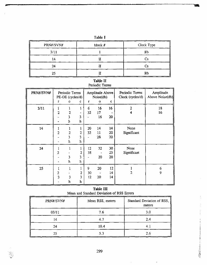
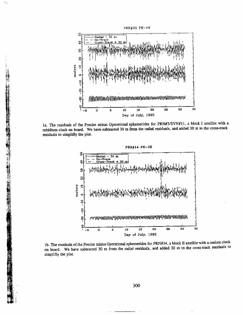
While we analyzed data for 22 satellites, for brevity we focus here on 4 satellites. These are fairly representative of the effects we found. We use one satellite from the early development phase of GPS, called block I. This one uses a rubidium clock with no base-plate temperature control. The other three are block I1 satellites, two with cesium clocks, and one with rubidium and with baseplate temperature control to 0.1 "C. These are descnied in Table I. There are two numbers for each satellite, though for most of the block I1 satellites they are the same. The PRN number is the pseudo-random code number (PRJY) that the satellite t;ansmits and is the number by which users know it. The satellite vehicle number (SVN) is a unique number associated with the particular satellite and is the number by which the operators know it. When a satellite becomes inoperable, its PRN number can be given to another satellite vehicle (SV). Each of the four satellites PRN's 3, 14, 24, and 25 appear in plots labeled a, b, c, and d, respectively. We present three plots of the differenced ephemerides: 1) the r,o,c differences PE-OE plotted only for PRN's 3 and 14, plots l a and lb, respectively, 2) the modulus of the FFI' of PE-OE data (using a cosine squared windowing function), Figures 2a-2d, and 3) the Time Deviationr7J of the PE-OE data in Figures 3a-3d. We also present the modulus Fast Fourier Transform (FFT) of the DMA estimates of satellite clock offsets from GPS time in 4 a 4 . In plots l a and lb and 2a-2d we have offset some of the values to make the plot easier to view. In l a and l b we have subtracted 30 m from the radial residuals, and added 30 m to the cross-track residuals. In the log-log plots 2a-2d we have divided the radial errors by 100 and multiplied the cross-track errors by 100.

We consider the residuals in the PE-OE data to be dominated by errors in the OE. The accuracy of the PE is expected to be of the order of 1.5 m in each of the radial, on-track and cross-track components. In particular, the PE has a known radial error due to using the WGS-84 value of GM, the universal gravitational constant times the mass of the earth, for the earth. This produces an error of the order of 1.3 m. Since the OE uses the same value, this effect should cancel.

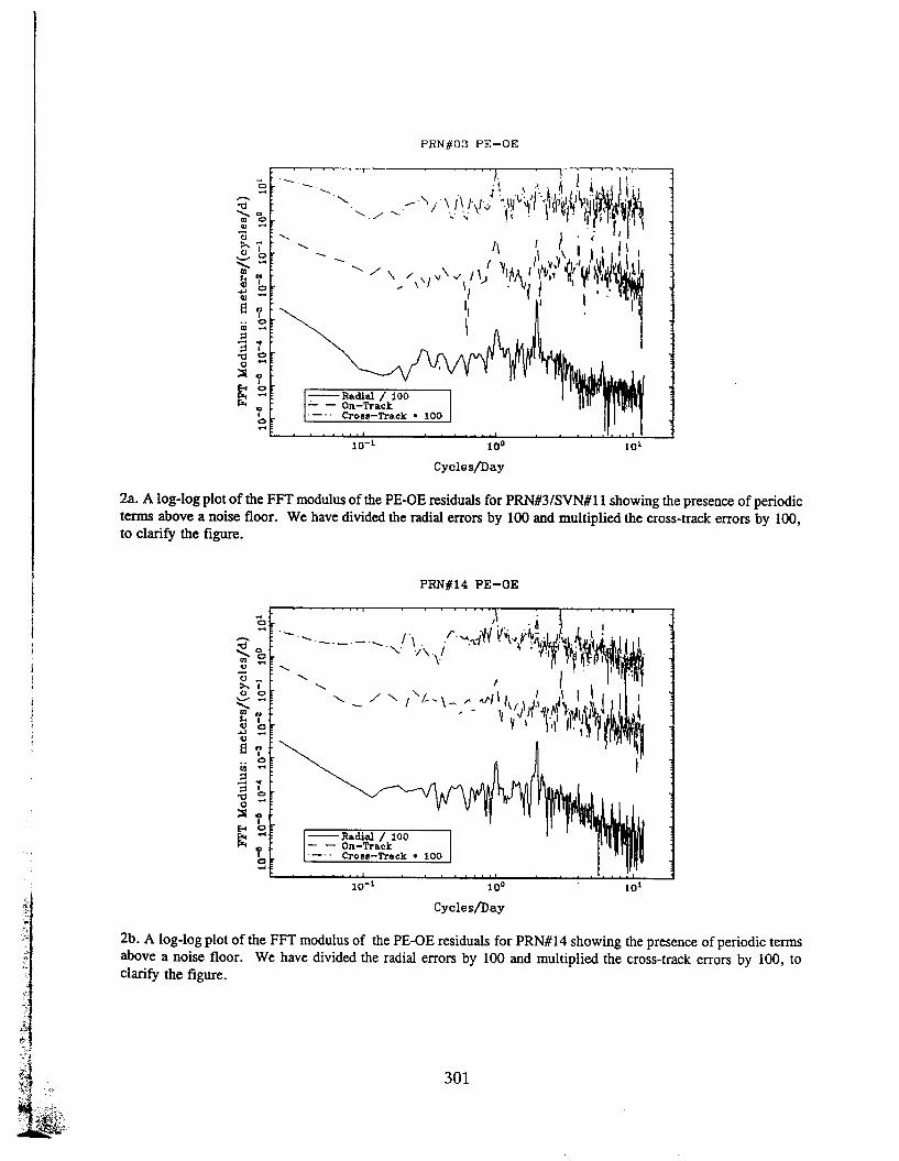
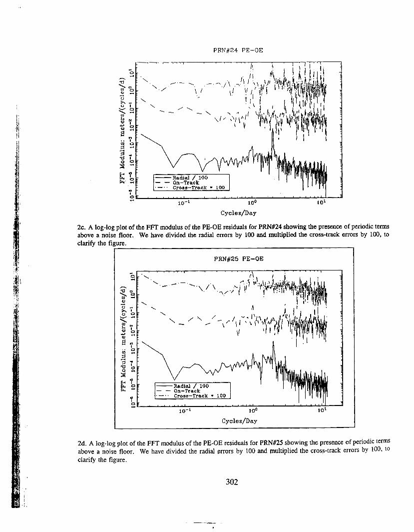
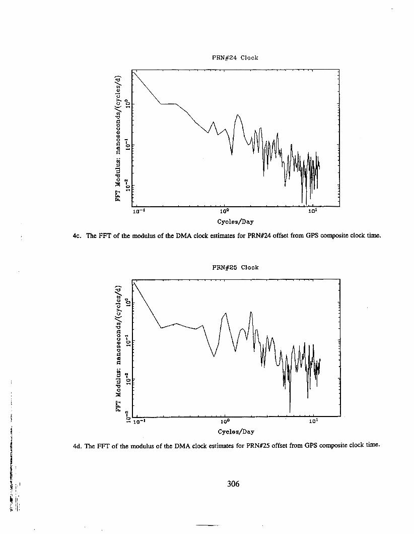
We consider two effects: periodic terms and underlying noise types. From Figures 2a-2d, we see significant energy in periodic terms with periods of 1, 2 and 3 cycles/day. There are often higher multiples of these as well. We plot the FFT of the clocks versus GPS time to look for correlation in Figures 4a4d, considering the possibility that the cause of the variations are unmodelled clock variations being driven into forced error by the OCS Kalman filter. The filter has no model for periodicity in the clocks, hence could pass a periodic clock offset into positioning errors. We summa'rize the periodic terms in table 11.

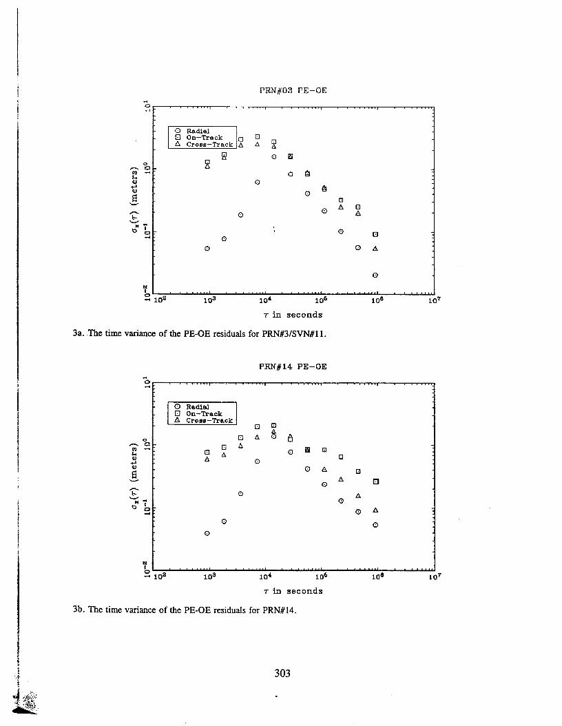
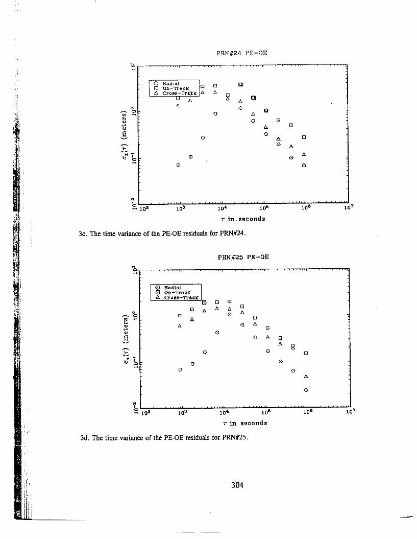
Figures 3a-3d show there are two underlying noise types present in the data beneath the

296

periodic effects. The radial noise is much smaller than on- and cross-track noise for all satellites. The periodic terms bias the oY() plots at half the period of the cycle, which generally occurs at 2 4 h. The slope for the short term data, before the effect of the periodic terms, typically varies from 0 to f on the log-log plot. This indicates dominant noise types of flicker and random walk in position respectively, appearing significantly in at least intervals of 15-30 min. After that the values are biased by the periodic effects. For periods longer than 8 h of integration the dominant noise type is white noise in position, indicated by a f1/2 slope. The random walk process has impulses of about 20 cm at 15 min, and then increases by the square root of the averaging time to about 1 m at 4 h. At that point the white process takes over with an equivalent standard deviation of 1 m at 4 h.

Since the noise type in long term is white modulation of position we are justified in computing the mean and standard deviation of the root-sum-square (RSS) error of the r, o and c errors. These are listed in table 111.

I

Conclusions

We conclude first that the periodic ephemeris error terms are not generally correlated with satellite clock offsets. There are some periodic terms in the rubidium clocks, notably with the block I satellites. Since the block I rubidium clocks have no base-plate temperature control, and since rubidium clocks in general have significant temperature coefficients it is not unexpected that these SV clocks have periodic behavior coherent with the period of the orbits. These terms are not evident in the block I1 clocks, where we see only a white FM noise process with any confidence.

Assuming the PE errors are less than 1.5 m, the periodic terms in the PE-OE computation are residual errors in the OCS Kalman estimates of position. It is not surprising to find periodic terms coherent with the period of the Earth-satellite system, and higher multiples. The filters which estimate the PE and OE estimate Keplerian elements whose differences must produce periodic terms. However, the magnitude and persistence of some of the stronger terms suggest the possibility for improvement. Simply a consistent error in the orbit eccentricity could produce the sinusoid we see.

Periodicities in orbit errors can produce positioning error biases for users. It is common to try to improve a position fix by averaging. Qpically navigation or positioning receivers use the best available satellites at a given time. Since this geometry repeats day to day, receivers will often repeat satellite configurations day to day used for positioning. Each such positioning may be biased by periodic errors in broadcast satellite coordinates. This suggests a strategy of randomizing the sequence of satellites used from day to day to improve the effects of averaging.

The residuals of an optimal filter should behave according to white noise modulation with no periodic behavior. One implication is that the periodicities could perhaps be removed. If the OCS had access to a post-processed ephemeris with a 2-3 day delay, they could use the periodic residuals to estimate corrections to Keplerian elements. The broadening of some of the spectral lines in the data suggests limits to this idea. The short term noise type of random walk in position indicates instability in the Kalman estimates.

t

I

297

Bibliography

[l] W. Lewandowski, G. Petit, C. Thomas, Common-view time transfer “Precision and

[2] W. Lewandowski, M. A. Weiss, “Precise Ephemerides for GPS Time Transfer,” Proc.

[3] Mueller I.I., Beu tler G., “The International GPS Service for Geodynamics: Develop- ment and Current Structure, ” Proc. 6th International Geodetic Symposium on Satellite Positioning, Columbus, p.823, 1992.

accuracy of GPS time transfer, ” IEEE Trans IM, Vol 42, NO 2, p 474, 1993.

21st PTTI, 1989.

[4] To appear in Proc. of the IGS analysis workshop, Ottawa, October 1993. [5] IGS reports, computer files, Internet address 130.92.4.10. [6] E.R. Swift, “GPS Orbit/Clock Estimation Based on Smoothed Pseudorange Data fmm

a IO Station Global Network”, Roc. of IAG Symp 109, p.151 G.L. Mader ed., Springer Verlag, 1993.

[‘7l D. W. Allan, M. Weiss, J. L. Jespersen, “A Fkquency-Domain View of Time-Domain Characterization of Clocks and Time and h q u e n c y Distribution Systems, ” Proc. 45th Annual Symposium on Frequency Control, 1991.

298

PRN#/SVN#

311 1

14

24

25

Table In Mean and Standard Deviation of RSS Errors

PFW#/SVN# Mean RSS, meters Standard Deviation of RSS, meters

0311 1 7.6 3 .O

14 4.7 2.4

24 10.4 4.1

25 5.3 2.6

299

block # Clock Type

I Rb

I1 cs II cs I1 Rb

PRN#03 PE-OE 0 (D 1

0 N -

I 0 m - I

0 d-’

7 1 1 0 1 5 10 16 20 25 30 35 d

I -5 0

Day of July. 1993

la. The residuals of the Precise minus Operational ephemerides for PRN#3/SVN#11, a block I satellite with a rubidium clock on board. We have subtracted 30 m from the radial residuals, and added 30 m to the cross-track residuals to simplifiy the plot.

4 I I t ,

PRNHl4 PE-OE

ft

300

PRN#03 PE-OE

2a. A log-log plot of the FFT modulus of the PE-OE residuals for PRN#3/SVN#ll showing the presence of periodic terms above a noise floor. We have divided the radial errors by 100 and multiplied the cross-track errors by 100, to clarify the figure.

PRN#14 PE-OE

2b. A log-log plot of the FFT modulus of the PE-OE residuals for PRN#14 showing the presence of periodic terms above a noise floor. We have divided the radial errors by 100 and multiplied the cross-track errors by 100, to clarify the figure.

301

PRN#24 PE-OE

clarify the f

I 0 4 101 100

Cycles/Day 10-1

2c. A log-log plot of the FFT modulus of the PE-OE residuals for PRN#24 showing the presence of periodic terms above a noise floor. We have divided the radial errors by 100 and multiplied the cross-track errors by 100, to

'e.

PRN#25 PE-OE

2d. A log-log plot of the FFT modulus of the PE-OE residuals for PRN#25 showing the presence of periodic terms above a noise floor. We have divided the radial errors by 100 and multiplied the cross-track errors by 1003 to clarify the figure.

302

PRN#O3 PE-OE

in seconds

3a. The time variance of the PE-OE residuals for PRN#3/SVN#ll.

N b .-I

t

0

0

0

O h 0 A

0

A 0

O A

0

lOa 103 104 1 06 106 107

in seconds

3b. The time variance of the PE-OE residuals for PRN#14.

303

B

0

0

A ' A

0 0 A

0 El

0 a I3

B A

O A

Q A

Q

r i n seconds

3c. The time variance of the PE-OE residuals for .PRN#24.

0 On-Track

a b

A a A

0

N

0 I I I I . , . . . , * 3 1 . - . , *

io3 10' 106 106 107 4 102

r i n seconds

3d. The time variance of the PE-OE residuals for PRN#25.

304

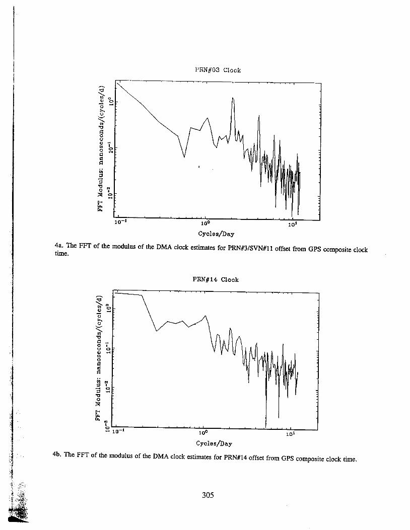
4a. The FFT of the modulus of the DMA clock estimates for PRN#3/SVN#11 offset from GPS composite clock time.

PRN#l4 Clock

Cycle s/Day 4b. The FFT of the modulus of the DMA clock estimates for PRN#14 offset from GPS composite clock time.

305

PRN#24 Clack

Cycles/Day

4c. The FFT of the modulus of the DMA clock estimates for PRN#24 offset from GPS composite clock time.

PRN#25 Clack

Cycles/Day

4d. The FFT of the modulus of the DMA clock estimates for PRN#25 offset from GPS composite clock time.

306